Papers - Open Knowledge Repository - World Bank Group

FIRST INTERNATIONAL CONFERENCE ON CARBON PRICING World Bank Working Paper Series November 2019

Pub

lic D

iscl

osur

e A

utho

rized

Pub

lic D

iscl

osur

e A

utho

rized

Pub

lic D

iscl

osur

e A

utho

rized

Pub

lic D

iscl

osur

e A

utho

rized

Background The Carbon Pricing Leadership Coalition (CPLC) and the World Bank Group hosted the world's first International Research Conference on Carbon Pricing on February 14-15, 2019 in New Delhi, India. With the goal of strengthening the carbon pricing knowledge base and fostering an improved understanding of the evolving challenges to its successful application, the Carbon Pricing Leadership Coalition convened researchers, practitioners, and interested stakeholders for the CPLC Research Conference. The event brought together over 30 researchers from across the globe to present papers on various carbon pricing themes. These papers were selected through a review process by an international scientific committee comprising of academics, researchers, and policymakers. The two-day Conference hosted over 170 participants and were centered around six central themes: (1) Learning from Experience, (2) Carbon Pricing Design, (3) Concepts and Methods, (4) Political Economy, (5) Decarbonizing the Economy, and (6) Emerging Frontiers. Each day featured plenary sessions with leading experts, followed by concurrent sessions covering the six themes. After the research conference, researchers were invited to submit their working papers in this Working Paper Series publication. The following is a compilation of the papers submitted as part of this process.

Table of Contents Lobbying, relocation risk, and allocation of free allowances in the EU ETS by Kerstin Burghaus, Nicolas Koch, Julian Bauer, Ottmar Edenhofer A Proposal for a Carbon Fee and Dividend in New Jersey by William Atkinson, Stav Bejerano, Victor Hua, Jonathan Lu, Samuel Moore, Jivahn Moradian, Hamza Nishtar, Aileen Wu Australia-EU ETS linking: lessons for the post-Paris world by Stuart Evans and Aaron Wu Blockchain, Double Counting, and the Paris Agreement by Henrique Schneider Business responses to climate policy uncertainty: Theoretical analysis of a twin deferral strategy and the risk-adjusted price of carbon by Alexander A. Golub, Ruben Lubowski, Pedro Piris-Cabezas Cooperative Carbon Taxes Under the Paris Agreement that Even Fuel Exporters Could Like by Grzegorz Peszko, Alexander Golub, Dominique van der Mensbrugghe Creating a Climate for Change? Carbon Pricing and Long-Term Policy Reform in Mexico by Arjuna Dibley and Rolando Garcia-Miron Estimating Effective Carbon Prices: Accounting for Fossil Fuel Subsidies by Vivid Economics and the Overseas Development Institute Estimating the Power of International Carbon Markets to Increase Global Climate Ambition by Pedro Piris-Cabezas, Ruben Lubowski, Gabriela Leslie, Environmental Defense Fund Global Carbon Pricing System As A Mechanism to Strengthen Competitiveness and Reduce CO2 Emissions In Energy-Intensive Trade-Exposed Sectors, Such as Primary Aluminum Production by Sergey Chestnoy and Dinara Gershinkova Global carbon pricing: When and What flexibilities revisited in a second-best framework by Meriem Hamdi-Cherif

5 39 77 100 115 131 156 179 200 233 245

Interaction between the carbon tax and renewable energy support schemes in Colombia: Complementary or overlapping? by Daniela Gutiérrez Torres Internal Corporate Carbon Pricing: An Analysis of Carbon Emission Reductions for U.S. Companies by John W. Byrd and Elizabeth S. Cooperman Leveraging Private Sector Investment in Energy Efficiency: Pilot Case Studies of Selected Sub-Saharan African Countries by Martin Burian, Joachim Schnurr, Grant A. Kirkman, Janak Shrestha Preparing India for Future Carbon Markets Building on India’s PAT and REC Schemse for the Post 2020 Markets by Tamiksha Singh and Karan Mangotra Pricing Carbon to Contain Violence by Shiran Victoria Shen The Environmental Effectiveness of Carbon Taxes: A comparative Case Study of the Nordic Experience by Sachintha Sarasi Fernando What if the Biggest EU Member States had Emulated Sweden’s Outstanding Carbon Tax? by Eoin Ó Broin, Jens Ewald, Franck Naduad, Érika Mata, Magnus Hennlock, Louis-Gaëtan Girdaudet, Thoman Sterner

265 284 303 318 331 349 369

Lobbying, relocation risk and allocation of freeallowances in the EU ETS

24th April 2019

Kerstin Burghaus1, Nicolas Koch2, Julian Bauer3, Ottmar Edenhofer4

Abstract

We study the nexus between permit allocation, lobbying and reloca-tion risk. Using new data from the EU Transparency Register and theEuropean Union Transaction Log (EUTL), we start with an empiricalanalysis of how the number of free emission allowances under the EUEmissions Trading System (EU ETS) is linked to lobbying activity. Al-though registration is voluntary and data limitations remain, the registerconstitutes a considerable improvement over previous data on lobbyingin terms of reliability and coverage. With the data, we establish a robustpositive link between lobbying and the number of free allowances. Tooffer an explanation for our empirical findings, we then develop an an-alytical model of a signaling game with asymmetric information aboutrelocation cost. We examine under which conditions sectors have an in-centive to systematically understate their cost of relocating to a countrywithout emissions regulations, thus exaggerating relocation risk. Further,we analyze when this strategy indeed leads to an overallocation of freeemissions allowances compared to a benchmark allocation without lob-bying.

Keyword(s): EU ETS, overallocation, lobbying, relocation risk, sig-naling games

JEL classification: C72, D72, Q52, Q53, Q54, Q58

1Mercator Research Institute on Global Commons and Climate Change (MCC), Torgauer Str. 12 - 15, 10829 Berlin- Germany. Email: [email protected]



4Mercator Research Institute on Global Commons and Climate Change (MCC), Potsdam Institute for Climate ImpactResearch (PIK), and Technische Universität Berlin (TU-Berlin). Email: [email protected].

1

2 RELATED LITERATURE

1 Introduction

In giving out free emissions allowances, the EU aims to minimize relocation risk toavoid carbon leakage and job loss. The actual share of free permit allocation in theEU Emissions Trading System (EU ETS) is, however, significantly higher than theoptimal allocation share that would minimize relocation risk (Martin et al. (2014)).A possible explanation for this observation is that firms and sectors successfullylobby for more permits by threatening to relocate to countries which are not underthe EU ETS. Understanding whether this indeed drives permit allocation is a crucialfirst step on the way to a more efficient allocation in the future.

Although intuitive, the link between permit allocation, lobbying and relocationrisk has so far not been properly analyzed. The representation of lobbying activ-ity in existing empirical models is rather weak due to lack of reliable data. Onthe theoretical side, lobbying through relocation threats as described above wouldrequire to model a signaling game with asymmetric information about actual re-location cost. The information asymmetry may allow lobbyists to understate theirtrue relocation cost, thus exaggerating their relocation risk to obtain more permits.However, existing models use a principal-agent approach where decision-makerscare for (monetary) contributions made by lobbies in return for political favors (e.g.Anger et al. (2016)). While highly relevant in US election campaigns, for exam-ple, this approach does not seem to adequately describe lobbying in the EU ETS.5We explicitly model a signaling game with asymmetric information between lob-bies and a policymaker and use new data from the EU Transparency Register andthe European Union Transaction Log (EUTL) to verify and explain the influence oflobbying on permit allocation in the EU ETS.

In the next section, we give an overview over related theoretical and empiricalliterature. In section 3, we explain our data sources and empirical approach anddescribe and discuss the results derived from the empirical model. Afterwards, weoffer an explanation for the empirical findings through a theoretical model of strate-gic information transmission in section 4. Section 5 concludes and offers tentativepolicy recommendations.

2 Related Literature

Our work is related to previous literature on the effects of lobbying on emissionstrading schemes. Hanoteau (2005) and Lai (2008) consider a framework where lob-

5See also Skodvin et al. (2010).

2


bying can influence the policy process at two stages: first, when the proportion ofgrandfathered permits in the allocation is determined and second, when the cap sizeis set. Both models show that with lobbying, the decisions in both stages are inter-related. Lobbying may lead to grandfathering of permits rather than auctioning. Bygiving out a greater share of permits for free, the government may be able to achievea more stringent emissions cap. Anger et al. (2016) study the sectoral allocation offree allowances for a given cap size and show that the allocation is biased towardssectors with stronger lobbies (the ETS sectors) and the regulatory burden is shiftedto sectors outside the ETS. As the emission tax on the latter sectors becomes inef-ficiently high, lobbying also leads to efficiency losses. The strength of lobbies ismeasured here by the size of political contributions. All models described so far as-sume a common-agency approach in the line of Grossman and Helpman (1994)6 inwhich the government cares for these political contributions along with social wel-fare. In this type of models, how far policies under lobbying deviate from the firstbest in general depends on how much the government values political contributionsrelative to social welfare and on the strength of lobby groups. Common-agencymodels have been employed in the wider context of environmental and energy pol-icy for example by Frederiksson (1997) and Aidt (1998) to analyze the effect oflobbying on environmental taxes or more recently by Anger et al. (2015) in thecontext of energy taxes.

How should such political contributions be interpreted? A straightforward in-terpretation would be to understand them as financial contributions, like campaignspending, or simply bribes. Anger et al. (2015) point out that contributions couldalso be information provided to the government. As indicated above, there is evi-dence that in the EU ETS, informational lobbying is indeed the more relevant formof lobbying. However, if we want to understand lobbying as taking place throughinformation transmission, then we have to account for questions regarding strategicbehavior and the truthfulness and credibility of information submitted. These ques-tions cannot be answered in a common-agency approach, without explicitly mod-eling the mechanism of information transmission. Potters and van Winden (1992)have done this by setting up a signaling game between the government and onelobby group. They assume an exogenous fixed cost of lobbying and substantial dif-ference in the preferences of the lobby group and the government. Lobbying leadsto a gain for the government and the lobby group in some cases, while it is a sociallywasteful activity in others. The inclusion of endogenous signaling costs or mech-

6The common-agency approach initially goes back to Bernheim and Whinston (1986).

3


anisms to evaluate the truthfulness of a signal increases the scope for informationtransmission and may be beneficial to both government and lobby group. Pottersand van Winden build on the seminal paper by Crawford and Sobel (1982), whomodel strategic information transmission when signaling is costless.7In an environ-mental context, informational lobbying has been studied by Naevdal and Brazee(2000). They show that a government which would like to choose policy optimallyaccording to an unknown state of nature is always at least as well off when lobbiedby an environmental pressure group which has certainty about the state of nature.Also, they derive conditions under which lobbying will result in truthful informa-tion transmission. None of the papers has considered the effect of informationallobbying on the allocation of permits in an emissions trading scheme.

The empirical literature on the influence of lobbying on emissons trading schemesis rather scarce. Markussen and Svendsen (2005) compare a Green Paper for thedirective to establish the EU ETS with the final directive. They conclude that thedominant interest groups indeed influenced the final design of the EU ETS. Notably,it led to grandfathering rather than auctioning of permits. Also Rode (2014) studiesa particular event in policy-making. He compares the final allocation of permits inthe U.K. in trading phase I of the EU ETS to an allocation suggested in a provisionalallocation plan published one year before the actual plan. Rode finds evidence foran effect of lobbying, in particular that a firm’s financial connections to members ofparliament have a positive impact on the amount of free permits received. This find-ing is supported by Anger et al. (2016) who suggest that the allocation of permitsfor trading phase one favors sectors with stronger lobbying activity. Even thoughAnger et al. (2016) also link their empirical study to an analytical model, how ex-actly lobbying influences permit allocation remains a black box in their model aswell as the previously cited ones. An explanation for the missing link is offered inthe form of relocation risk in the paper by Martin et al. (2014) mentioned in theintroduction: They explicitly account for the EU’s objective to prevent firms fromrelocating to non-regulated countries. Their analysis shows that permit allocationin EU ETS is inefficient. Leakage risk overcompensated and the efficient alloca-tion reduces job risk substantially without increasing the number of freely allocatedpermits.

Anger et al. (2016) construct their lobbying index from voluntarily disclosed sur-vey data. Obviously, the representation of lobbying in the empirical studies suffersfrom the extreme difficulty of obtaining suitable data on lobbying activity. While

7Further work building on this paper includes Ainsworth (1992), Austen-Smith and Wright (1992) and Austen-Smith(1994). A good overview over models on informational lobbying can be found in Grossman and Helpman (2001).

4

3 EMPIRICAL ANALYSIS

registration in the Transparency Register is still voluntary, the data derived from theregister still constitutes a considerable improvement both in terms of reliability andcoverage. We describe this new data source as well as our empirical approach in thenext section.

3 Empirical analysis

To motivate our analytical model, we bring together two administrative data sources,heretofore not used to study the link between permit allocation and lobbying inthe EU ETS. Using a panel regression that controls for various fixed unobservablecharacteristics at the firm and country level, we then show that lobbying activity ispositively linked to the number of free allowances received.

3.1 Data

The primary data source used to measure lobbying is the EU Transparency Register.The register shall cover every activity that has the objective to directly or indirectlyinfluence the policy-making process of the EU institutions (EP 2014). Registeredentities agree to a code of conduct and guarantee that their provided information iscorrect. The European Parliament (EP) has made registration on the TransparencyRegister a precondition for access to its facilities since 2011. Since 2014, membersof the European Commission (EC) only meet with lobbyists who are listed in theTransparency Register. Efforts to make registration mandatory including the Euro-pean Council, however, failed in 2018. We still believe that the current register is afairly comprehensive dataset of lobby organizations since access to the premises ofthe EP and EC is arguably crucial to the work of lobby groups. The current registerconsists of 11.837 entries (as of July 27, 2018). Although registration is voluntaryand data limitations remain, the register constitutes a considerable improvementover previous data on lobbying (e.g. Anger et al. 2016) in terms of reliability andcoverage.

The registered entries on the Transparency Register provide information aboutthe legislation they are monitoring, their financial expenses, number of employees,as well their number of badges for the EU parliament (see Figure 1). Yet, they donot indicate a sector affiliation. In order to establish which sector registered enti-ties lobby, we use text mining techniques to match lobby organizations and indus-trial sectors. To this end, we exploit the information provided on the lobby name,self-proclaimed goals, covered EU initiatives and expert groups. Our approach is

5


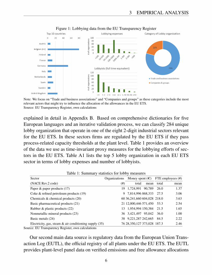
Figure 1: Lobbying data from the EU Transparency Register

Note: We focus on “Trade and business associations” and “Companies and groups” as these categories include the mostrelevant actors that might try to influence the allocation of the allowances in the EU ETS.Source: EU Transparency Register, own calculations

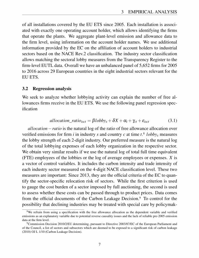
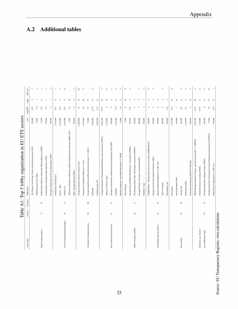
explained in detail in Appendix B. Based on comprehensive dictionaries for fiveEuropean languages and an iterative validation process, we can classify 284 uniquelobby organization that operate in one of the eight 2-digit industrial sectors relevantfor the EU ETS. In these sectors firms are regulated by the EU ETS if they passprocess-related capacity thresholds at the plant level. Table 1 provides an overviewof the data we use as time-invariant proxy measures for the lobbying efforts of sec-tors in the EU ETS. Table A1 lists the top 5 lobby organization in each EU ETSsector in terms of lobby expenses and number of lobbyists.

Table 1: Summary statistics for lobby measuresSector Organizations Money spent (C) FTE employees (#)(NACE Rev.2 code) (#) total mean total meanPaper & paper products (17) 19 1,724,991 90,789 26.0 1.37Coke & refined petroleum products (19) 9 7,814,996 868,333 27.5 3.06Chemicals & chemical products (20) 60 36,241,660 604,028 218.0 3.63Basic pharmaceutical products (21) 21 12,000,446 571,450 53.3 2.54Rubber & plastic products (22) 13 1,954,994 150,384 21.5 1.65Nonmetallic mineral products (23) 36 3,421,497 95,042 36.0 1.00Basic metals (24) 38 9,221,287 242,665 84.5 2.22Electricity, gas, steam & air conditioning supply (35) 76 28,350,127 373,028 187.3 2.46

Source: EU Transparency Register, own calculations

Our second main data source is regulatory data from the European Union Trans-action Log (EUTL), the official registry of all plants under the EU ETS. The EUTLprovides plant-level panel data on verified emissions and free allowance allocations

6


of all installations covered by the EU ETS since 2005. Each installation is associ-ated with exactly one operating account holder, which allows identifying the firmsthat operate the plants. We aggregate plant-level emission and allowance data tothe firm level, using information on the account holder names. We use additionalinformation provided by the EC on the affiliation of account holders to industrialsectors based on the NACE Rev.2 classification. The industry sector classificationallows matching the sectoral lobby measures from the Transparency Register to thefirm-level EUTL data. Overall we have an unbalanced panel of 5,652 firms for 2005to 2016 across 29 European countries in the eight industrial sectors relevant for theEU ETS.

3.2 Regression analysis

We seek to analyze whether lobbying activity can explain the number of free al-lowances firms receive in the EU ETS. We use the following panel regression spec-ification

allocation_ratioisct = b lobbys +dX +ai + gct + eisct (3.1)

allocation� ratio is the natural log of the ratio of free allowance allocation oververified emissions for firm i in industry s and country c at time t.8 lobbys measuresthe lobby strength of each 2-digit industry. Our preferred measure is the natural logof the total lobbying expenses of each lobby organization in the respective sector.We obtain very similar results if we use the natural log of total full time equivalent(FTE) employees of the lobbies or the log of average employees or expenses. X isa vector of control variables. It includes the carbon intensity and trade intensity ofeach industry sector measured on the 4-digit NACE classification level. These twomeasures are important: Since 2013, they are the official criteria of the EC to quan-tify the sector-specific relocation risk of sectors. While the first criterion is usedto gauge the cost burden of a sector imposed by full auctioning, the second is usedto assess whether these costs can be passed through to product prices. Data comesfrom the official documents of the Carbon Leakage Decision.9 To control for thepossibility that declining industries may be treated with special care by policymak-

8We refrain from using a specification with the free allowance allocation as the dependent variable and verifiedemissions as an explanatory variable due to potential reverse causality issues and the lack of reliable pre-2005 emissiondata at the firm level.

9Commission Decision 2010/2/EU determining, pursuant to Directive 2003/87/EC of the European Parliament andof the Council, a list of sectors and subsectors which are deemed to be exposed to a significant risk of carbon leakage(2010) OJ L 1/10 (Carbon Leakage Decision).

7


ers (which may explain success of lobbying for free allocation), we also control foremployment growth between 2000 and 2003 for each sector and country. Data istaken from Eurostat.10 All our regressions are conditional on firm fixed effects, ai.They absorb all time invariant unobservable firm characteristics. Additionally, weinclude year fixed effects that vary by country, gct , to capture country-specific timetrends and macroeconomic shocks.

Given that the allowance allocation is determined at the beginning of each ofthe three compliance periods (Phase I: 2005-2007, Phase II: 2008-2012, Phase III:2013-2020), all following years of each compliance period are dependent on initialperiodic allocation schedule. Therefore, we only include the observations from thefirst year of each compliance phase in our regression (i.e. t = 2005, 2008, or 2013).This leaves us with 13,648 observations if we include the electricity sector in oursample and 6,548 observations if we focus exclusively on manufacturing firms inthe EU ETS.

3.3 Results

Estimation results are shown in Table 2. They are structured around two panels: thefirst panel reports results only for Phase I and II of the EU ETS while the secondpanel relates to results based on a sample that also includes Phase III. Each panelcontains three estimations: the first is based on a sample that includes the electricitysector, the second focuses exclusively on manufacturing firms, and the third addsfurther control variables.

We start the discussion with findings for Phase I and II of the EU ETS. In thesetwo trading periods, at least 95% and 90% of allowances had to be allocated for free,respectively. Allocation rules in Phase I and II were highly decentralized (each EUMember State had its own National Allocation Plan) and based on historical emis-sions (grandfathering). Prior reaseach has shown that industrial emitters receivedfairly generous allocations of free permits in these trading periods (Ellerman et al.2016), making this time frame particularly interesting to study the effects of lobby-ing.

All specifications for Phase I and II yield a positive and statistically significantcoefficient estimate for lobbying efforts. This finding supports the hypothesis thatthere is a positive relationship between lobbying and allocation of free emission al-lowances in the EU ETS. Because we report results generated using log transformeddata, the coefficient estimates can be interpreted as elasticities. For instance, spec-

10http://ec.europa.eu/eurostat/web/lfs/data/database taken on 04.05.2018.

8


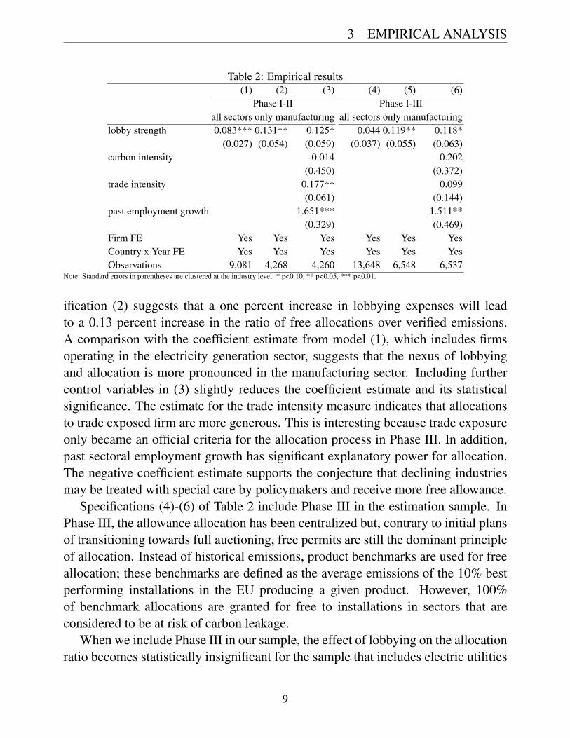
Table 2: Empirical results(1) (2) (3) (4) (5) (6)

Phase I-II Phase I-IIIall sectors only manufacturing all sectors only manufacturing

lobby strength 0.083*** 0.131** 0.125* 0.044 0.119** 0.118*(0.027) (0.054) (0.059) (0.037) (0.055) (0.063)

carbon intensity -0.014 0.202(0.450) (0.372)

trade intensity 0.177** 0.099(0.061) (0.144)

past employment growth -1.651*** -1.511**(0.329) (0.469)

Firm FE Yes Yes Yes Yes Yes YesCountry x Year FE Yes Yes Yes Yes Yes YesObservations 9,081 4,268 4,260 13,648 6,548 6,537

Note: Standard errors in parentheses are clustered at the industry level. * p<0.10, ** p<0.05, *** p<0.01.

ification (2) suggests that a one percent increase in lobbying expenses will leadto a 0.13 percent increase in the ratio of free allocations over verified emissions.A comparison with the coefficient estimate from model (1), which includes firmsoperating in the electricity generation sector, suggests that the nexus of lobbyingand allocation is more pronounced in the manufacturing sector. Including furthercontrol variables in (3) slightly reduces the coefficient estimate and its statisticalsignificance. The estimate for the trade intensity measure indicates that allocationsto trade exposed firm are more generous. This is interesting because trade exposureonly became an official criteria for the allocation process in Phase III. In addition,past sectoral employment growth has significant explanatory power for allocation.The negative coefficient estimate supports the conjecture that declining industriesmay be treated with special care by policymakers and receive more free allowance.

Specifications (4)-(6) of Table 2 include Phase III in the estimation sample. InPhase III, the allowance allocation has been centralized but, contrary to initial plansof transitioning towards full auctioning, free permits are still the dominant principleof allocation. Instead of historical emissions, product benchmarks are used for freeallocation; these benchmarks are defined as the average emissions of the 10% bestperforming installations in the EU producing a given product. However, 100%of benchmark allocations are granted for free to installations in sectors that areconsidered to be at risk of carbon leakage.

When we include Phase III in our sample, the effect of lobbying on the allocationratio becomes statistically insignificant for the sample that includes electric utilities

9


(4). This finding is likely driven by the fact that operators in the power generationsector no longer received any free allowances in Phase III. If we focus in (5) and (6)on manufacturing firms only, we find very similar effects of lobbying as in PhaseI and II, both in terms of magnitude and statistical significance. Notably, the coef-ficients on carbon intensity and trade intensity have the expected positive sign butthey remain statistically insignificant.

3.4 Discussion

The principal value of the investigation is to corroborate widespread beliefs11 thatlobbying is positively linked to the amount of emissions allowances received in theEU ETS. Newly available data from the EU Transparency Register indeed points tothe relevance of lobbying in the European cap-and-trade program. However, datalimitations imply that our empirical investigation can only provide associationalestimates for relationship between lobbying and permit allocation.

While our firm panel offers an econometrically efficient way of controlling forunobservable characteristics and trends, we cannot control for time-varying andtime-invariant industry characteristics. This is because the data on lobbying activityis only available at the industry level (subject to measurement error from our textmining) for a single point in time. In this respect, our investigation may sufferfrom omitted variable bias. Therefore, we caution against an over-interpretation ofour results as estimates of the cause and effect relationship between lobbying andpermit allocation.

Further, we cannot offer an explanation for the link between lobbying and permitallocation from our empirical analysis. As indicated in the introduction, such anexplanation could be provided by including relocation risk into the analysis. To doso, we would need reliable information on the firm level on the costs and benefitsof shifting business abroad. Given the lack of such data, we cannot take a stanceeither on whether there is overallocation of permits to lobbying firms relative to theallocation that would achieve the stated EU objective of minimizing relocation risk.Based on the presented correlational evidence, we therefore subsequently appeal totheory to identify the conditions under which lobbying might lead to overallocationof free allowances in cap-and-trade systems and to explain the effect.

11For instance, The Economist (2006) argues: “...what should have been an exercise in setting rules for a new marketbecame a matter of horsetrading about pollution limits, with powerful companies lobbying for the largest possibleallowances.”

10

4 A MODEL OF LOBBYING WITH ASYMMETRIC INFORMATION

4 A model of lobbying with asymmetric information

In this and the next section, we develop an analytical model to offer an explanationfor the empirical link between lobbying and permit allocation via relocation risk.The setup of the model partly builds on Martin et al. (2014), using, for example,a simplified version of the authors’ representation of relocation risk and the objec-tive of the policymaker. However, Martin et al. (2014) do not explicitly considerlobbying.

4.1 Setup4.1.1 General Setup

We set up a model of a signaling game with asymmetric information about relo-cation cost between lobbies and a policymaker. We consider the following generalsetup: In the domestic economy, there are N firms i = 1, ..,N, each representing oneeconomic sector. Firms differ solely in the cost they would incur if they decidedto relocate business to another country. We assume that there are K different cost

types [e1, ...,eK]. Every cost type is shared by Nk firms, withKÂ

k=1Nk = N. Firm i will

relocate whenever its net cost of doing so, ei, made up of the gross cost of movingless of profits abroad, is smaller than the profit pi = p(qi) it loses at home. In otherwords: Firm i relocates if and only if ei < �p(qi). For simplification, we assumethat profits depend only on the number of free permits received, are zero if a firmdoes not receive any permits and are monotonously increasing in the amount of freeallowances received, i.e. p(0) = 0,p 0(qi)> 0. Note that if a firm is making positiveprofits in its home country, the net cost of relocation will have to be negative for itto consider relocating.

Free allowances are allocated among firms by a policymaker who seeks to min-imize a weighed sum of aggregate relocation risk and the number of permits dis-tributed, given a fixed cap Q of allowances. The objective function of the policy-maker can thus be specified as

min{qi}

Ob j :=N

Âi=1

prob(ei <�p(qi))+qN

Âi=1

qi (4.1)

s.t.N

Âi=1

qi Q

where prob(ei <�p(qi)) denotes the probability of firm i moving abroad, given that

11


it receives qi free allowances and {qi}= {q1, ..,qN} is the set of free allowances foreach of the N firms.12 We will assume in our analysis that the weight q on thepermit number is positive but small (see assumption 2), so that the policymaker hasa focus on risk minimization and only considers the number of permits allocatedwhen indifferent between several risk-minimizing allocations.

Relocation costs ei are assigned to firms randomly, by nature, and are private in-formation to each company. The policymaker only knows that there are K differentcost types and knows their true probability distribution. He does not know, however,the actual mapping of cost types to firms. He can only infer a belief about the costtype of a specific firm from the probability distribution. Firms can try to influencethis prior belief via lobbying, by spending resources to convince the policymakerthat their relocation costs are lower (or higher) than they actually are, i.e. that costsare ei < ei (ei > ei). Contrary to ei, the signal ei e[e1, ...,eK] is observable by thepolicymaker. We assume that lobbying costs Ci(ei,ei) depend on the cost ei of afirm and the signal ei sent. The exact functional relation is private information ofthe firm, so that even if costs are disclosed by the lobby, the policymaker cannotinfer the true relocation cost from this number. This may for example be explainedby signaling costs being just one component of lobbying expenditures (others beingfixed costs of employing lobbyists, access costs, ...) and the policymaker observingonly aggregate expenditures. Costs are zero if a sector decides to signal its true cost:Ci(ei = ei) = 0 8i. We discuss functional specifications and alternative assumptionsin appendix B.3. Firm i chooses ei so as to maximize the difference

E [p(q(ei,{e�i}))]�Ci(ei,ei) (4.2)

of the expected profits obtained when lobbying and lobbying costs. The func-tion q(ei, e�i) indicates that firm i anticipates the dependency of freely allocatedallowances on its own signal as well as the signals sent by the other firms. We as-sume that the latter are not known by firm i when deciding about ei. We thereforeuse the expectation operator E in (4.2).

The timing of events is as follows: (1) Nature assigns a cost type to each firm.(2) Each firm i learns its cost type. (3) Every firm i decides whether to engage inlobbying or not and chooses a signal. (4) The policymaker observes the signals.(5) The policymaker decides about the allocation of free allowances. (6) The firmdecides whether to relocate or not. We solve the model backwards starting from the

12Martin et al. (2014) assume that the policymaker attaches different weights to the firms, dependent on their emis-sions and number of employees. As firms in our model differ only in relocation cost, we set the weights to one inequation (4.1).

12


last stage.

4.1.2 Specification with two cost types

To keep the model simple, we consider a version where there are only two differentcost types, so that ei e {eL,eH} with eH < eL < 0. Indices refer to low and highabsolute value (�ek) of relocation cost respectively and correlate with a low- and ahigh-relocation risk type. To see this, note that the absolute value of relocation costsis equivalent to the net gain from going abroad. With only two cost types, there arealso only two possible signals. This case is indeed a good proxy for the actualsituation in the EU ETS, where firms are sorted in either a high relocation risk orlow relocation risk group as reflected by the carbon leakage list. We assume in thefollowing that there are N = 3 firms and that each firm i has the same probability ofbeing a certain cost type k, i.e. prob(ei = ek) = 1/2 8k. This simplistic setup greatlyreduces the set of sensible policy options, so that the model can be solved manually:For each cost type, we can identify what we henceforth call the ’reservation numberof permits’. It is the number of permits qk, which is just sufficient to keep a firm ofcost type k from relocating:

qk := q Q | ek =�p(q) (4.3)

Allocating more than this number of permits to a firm of cost type k does not alterrelocation risk. The policymaker will therefore choose a permit allocation which issome combination of the reservation number of permits for the different cost typesand zero. In other words, the policymaker will choose from the set Q=

�0,qL,qH

,

taking into account the cap Q on total free allowances.The allocation of permits in the following subsections depends on the stringency

of the cap Q on free allowances and also on the relative size of qL and qH . In thisrespect, we make the following assumption:

Assumption 1. The cap and the reservation number of permits for the L- and the H-type satisfy thefollowing conditions:

a) Q = 2qH

b) qL < 12qH

The first part of assumption 1 implies that only two firms can be served if thepolicymaker allocates qH to the other two. It is thus not possible to set relocationrisk to zero by simply allocating qH to each of the three firms. This is essential fora meaningful allocation problem. We will see later that the inequality qL < 1

2qH

13


in the second part of the assumption is crucial to make the return to lobbying suf-ficiently large to support a Nash equilibrium with exaggeration of relocation costsand overallocation of permits.

4.2 Benchmark permit allocation without lobbying

How would the policymaker allocate permits if there was no lobbying? If he allo-cates a number of permits qi to a firm i, this firm will stay if its reservation numberof permits qi is qi or smaller, i.e. qi qi, and relocate otherwise. Trivially, by as-sumption, if a firm receives zero free permits, it will relocate whatever cost type itis, so that prob(ei <�p(0)) = prob(ei < 0) = 1. Not every possible combination ofreservation permits qk will exhaust the number of free permits Q completely. Per-mits which are left over after serving each of the three firms will not be distributed aslong as it is in the interest of the policymaker to keep the number of freely allocatedpermits as small as possible (q > 0). We can now solve the allocation problem:

Lemma 1. Under assumption 1, in an equilibrium without lobbying, G chooses thepermit allocation (qH ,qL,qL) or a permutation thereof if besides relocation risk, Gseeks to minimize the number of permits given out freely (q > 0).

Proof. Ignoring order, the policy vector Q =�

0,qL,qH

yields ten possible alloca-tions of permits to the three firms. Knowing that both cost types are equally likely,we can compute relocation risk for each allocation. It is simply the sum over theprobabilities for each firm i that the number of permits qi allocated to firm i issmaller than that firm’s reservation number of permits qi. Let relocation risk be ¬.We find that the allocations (0,qH ,qH) and (qL,qL,qH) both yield a relocation riskof 1:

¬(0,qH ,qH) =3

Âi=1

prob(ei <�p(qi))|(0,qH ,qH) =3

Âi=1

prob(qi < qi)|(0,qH ,qH) = 1+0+0 = 1

¬(qL,qL,qH) =3

Âi=1

prob(ei <�p(qi))|(qL,qL,qH) =3

Âi=1

prob(qi < qi)|(qL,qL,qH) = 2 · 12+0 = 1

Here, assumption 1b) ensures that 2qH > qH+2qL, so that the allocation (qL,qL,qH)uses less permits and thus minimizes the government’s objective function.

4.3 Permit allocation with lobbying

We now define the strategies for the firms and the policymaker when there is lob-

14


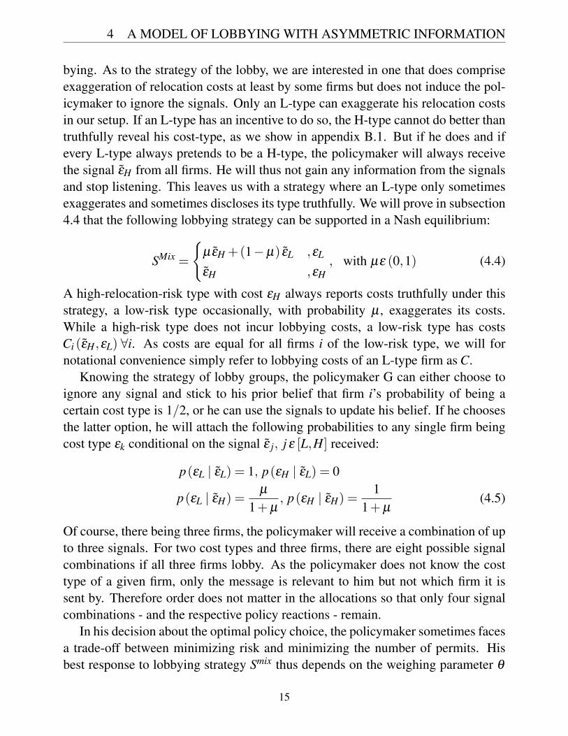
bying. As to the strategy of the lobby, we are interested in one that does compriseexaggeration of relocation costs at least by some firms but does not induce the pol-icymaker to ignore the signals. Only an L-type can exaggerate his relocation costsin our setup. If an L-type has an incentive to do so, the H-type cannot do better thantruthfully reveal his cost-type, as we show in appendix B.1. But if he does and ifevery L-type always pretends to be a H-type, the policymaker will always receivethe signal eH from all firms. He will thus not gain any information from the signalsand stop listening. This leaves us with a strategy where an L-type only sometimesexaggerates and sometimes discloses its type truthfully. We will prove in subsection4.4 that the following lobbying strategy can be supported in a Nash equilibrium:

SMix =

(µ eH +(1�µ) eL ,eL

eH ,eH, with µe (0,1) (4.4)

A high-relocation-risk type with cost eH always reports costs truthfully under thisstrategy, a low-risk type occasionally, with probability µ , exaggerates its costs.While a high-risk type does not incur lobbying costs, a low-risk type has costsCi (eH ,eL) 8i. As costs are equal for all firms i of the low-risk type, we will fornotational convenience simply refer to lobbying costs of an L-type firm as C.

Knowing the strategy of lobby groups, the policymaker G can either choose toignore any signal and stick to his prior belief that firm i’s probability of being acertain cost type is 1/2, or he can use the signals to update his belief. If he choosesthe latter option, he will attach the following probabilities to any single firm beingcost type ek conditional on the signal e j, j e [L,H] received:

p(eL | eL) = 1, p(eH | eL) = 0

p(eL | eH) =µ

1+µ, p(eH | eH) =

11+µ

(4.5)

Of course, there being three firms, the policymaker will receive a combination of upto three signals. For two cost types and three firms, there are eight possible signalcombinations if all three firms lobby. As the policymaker does not know the costtype of a given firm, only the message is relevant to him but not which firm it issent by. Therefore order does not matter in the allocations so that only four signalcombinations - and the respective policy reactions - remain.

In his decision about the optimal policy choice, the policymaker sometimes facesa trade-off between minimizing risk and minimizing the number of permits. Hisbest response to lobbying strategy Smix thus depends on the weighing parameter q

15


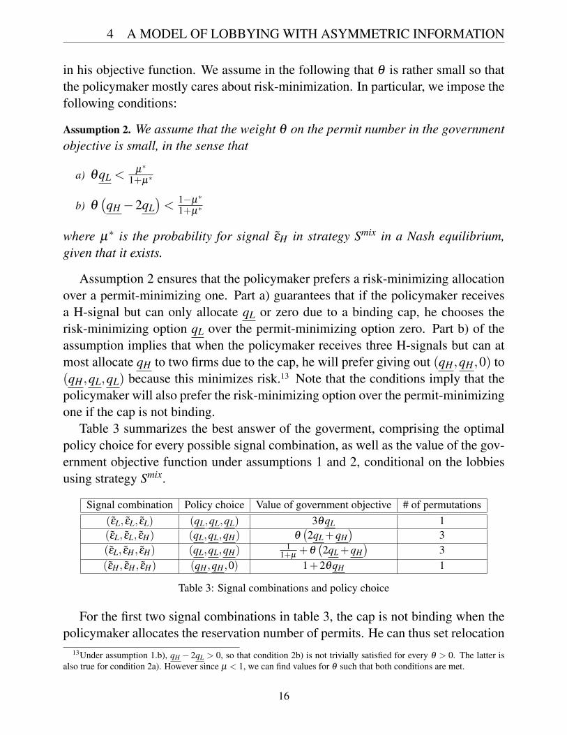
in his objective function. We assume in the following that q is rather small so thatthe policymaker mostly cares about risk-minimization. In particular, we impose thefollowing conditions:

Assumption 2. We assume that the weight q on the permit number in the governmentobjective is small, in the sense that

a) qqL < µ⇤

1+µ⇤

b) q�qH �2qL

�< 1�µ⇤

1+µ⇤

where µ⇤ is the probability for signal eH in strategy Smix in a Nash equilibrium,given that it exists.

Assumption 2 ensures that the policymaker prefers a risk-minimizing allocationover a permit-minimizing one. Part a) guarantees that if the policymaker receivesa H-signal but can only allocate qL or zero due to a binding cap, he chooses therisk-minimizing option qL over the permit-minimizing option zero. Part b) of theassumption implies that when the policymaker receives three H-signals but can atmost allocate qH to two firms due to the cap, he will prefer giving out (qH ,qH ,0) to(qH ,qL,qL) because this minimizes risk.13 Note that the conditions imply that thepolicymaker will also prefer the risk-minimizing option over the permit-minimizingone if the cap is not binding.

Table 3 summarizes the best answer of the goverment, comprising the optimalpolicy choice for every possible signal combination, as well as the value of the gov-ernment objective function under assumptions 1 and 2, conditional on the lobbiesusing strategy Smix.

Signal combination Policy choice Value of government objective # of permutations(eL, eL, eL) (qL,qL,qL) 3qqL 1(eL, eL, eH) (qL,qL,qH) q

�2qL +qH

�3

(eL, eH , eH) (qL,qL,qH)1

1+µ +q�2qL +qH

�3

(eH , eH , eH) (qH ,qH ,0) 1+2qqH 1

Table 3: Signal combinations and policy choice

For the first two signal combinations in table 3, the cap is not binding when thepolicymaker allocates the reservation number of permits. He can thus set relocation

13Under assumption 1.b), qH � 2qL > 0, so that condition 2b) is not trivially satisfied for every q > 0. The latter isalso true for condition 2a). However since µ < 1, we can find values for q such that both conditions are met.

16


risk to zero and will choose the permit allocation which matches the signal. Forthe third and fourth combination on the other hand, the policymaker has to comparerelocation risk of the policy options. We summarize the policymaker’s best answerto lobbying strategy Smix in the lemma below:

Lemma 2. Under assumptions 1 and 2, the best answer of the policymaker to lobby-ing strategy Smix is as given in table 3.

Proof. In can be verified straightforwardly, using the conditional probabilities fromequation (4.5) and proceeding otherwise as in the proof of lemma 1, that the alloca-tions in table 3 are indeed the best answers.

While the permit allocation in the second and third row of table 3 is the sameas in the benchmark case without lobbying, it is different if the policymaker ei-ther receives three L-, or three H-signals. In the former case, he benefits from thesignals in the sense that he can set relocation risk to zero and at the same time al-locate less permits than in the benchmark allocation. In the latter case, he allocatesmore permits than in the benchmark case, thereby acting in favor of the lobbyingfirms. If this case occurs sufficiently often (if µ is sufficiently large), there will beoverallocation of permits, as we show in section 4.5.

4.4 Existence of a Nash equilibrium with lobbying

In this subsection, we prove that with policy chosen as in table 3, conditions canbe found such that strategy Smix satisfies firms’ incentive constraints and can thusbe sustained in a Nash equilibrium for some 0 < µ⇤ < 1. A prerequisite is that theprofit from being assigned the large number of permits, p(qH), is sufficiently largerelative to p(qL). This is guaranteed by assumption 1b) together with the followingassumption:

Assumption 3. ∂p(qk)∂qk

> 0 and p(qk) is homogeneous of degree s � 1, 8k.

We have already assumed earlier that profits are increasing in the number of per-mits. The new part is the homogeneity assumption. It is a sufficient condition toensure that if qH is sufficiently large relative to qL (in line with assumption 1b)), asimilar relation holds for profits. We are now ready to prove the following proposi-tion:

Proposition 1. Under assumptions 1, 2 and 3 and with the government strategy de-scribed in table 3, there exists a cost interval

�C,C

�,C > 0, such that there is at

17


least one Nash-equilibrium where every firm plays strategy SMix if lobbying costsare within the interval

�C,C

�. In such a Nash equilibrium, every H-type reveals its

type truthfully, while every L-type mixes between truth-telling and pretending to bethe H-type with some probability µ⇤ with 0 < µ⇤ < 1.

Proof. See appendix B.1.

Proposition 1 states the conditions under which lobbies have no incentive todeviate from strategy Smix, given that the best response of the government is asdescribed in table 3. The crucial part of the proof is to show when an L-type willindeed mix signals with a probability 0 < µ⇤ < 1. Intuitively, if the costs of sendinga H-signal as an L-type are too low, i.e. C < C, an L-type would always want toplay H with probability µ = 1. If, on the other hand, costs are too high, i.e. C �C,then even if the probability µ with which the H-signal is sent tends to zero, expectedprofits from sending it net of costs C are lower than the profit p(qL) from sending atruthful signal. An L-type would therefore want to choose µ = 0. If C e

�C,C

�, there

exists at least one interior solution for µ . There may be two, as expected profits fromsending a H-signal are quadratic, first de- and then increasing with higher µ: On theone hand, a higher µ makes the policymaker think that there is a higher probabilityof a firm being a H-type, which leads him to mix in qH more often. On the otherhand, with all firms chosing a higher µ , there is a larger probability of a signalcombination with more than one H-signal. In this case, the cap becomes bindingand there is a chance of receiving nothing or qL despite sending the H-signal. Forlow µ , the latter effect dominates, so that expected profits fall when µ increases.For large µ , the former effect dominates and expected profits rise again.

4.5 Overallocation of permits in a Nash equilibrium with lobbying

In the previous subsection, we have shown under which conditions lobbying affectsthe allocation of emission permits, even though a government may not expect everymessage sent by lobby groups to be truthful. A question still to be answered iswhether lobbying leads to an overallocation of permits. We will in the followingdistinguish two kinds of overallocation: aggregate and conditional.

Definition 1. There is aggregate overallocation if the total expected number of per-mits given out to all firms when there is lobbying exceeds the number given outwhen there is no lobbying. There is conditional overallocation if the expected num-

18


ber of permits for a firm sending the H-signal exceeds that firm’s expected numberof permits when no firm lobbies.

The reason why lobbying may in fact not lead to overallocation in the aggregateis that an L-type sometimes reveals his cost-type truthfully. If so, the policymakercan allocate the low reservation number of permits. This leads to less permits beingallocated in total if the policymaker sees three L-signals, as we explained belowtable 3. Whether there is aggregate overallocation or not depends on the size ofthe equilibrium µ⇤, which in turn depends crucially on lobbying costs. One mightbe tempted to presume that there will always be conditional overallocation, sincereceiving more permits is the sole goal of lobbying for a firm. However, because ofthe cap on permits and the competition with other lobbying firms, there is the riskof ending up with zero permits in a lobbying equilibrium if the government receivesH-signals from all three firms. The following proposition states the conditions foraggregate and conditional overallocation conditional under strategy SMix.

Proposition 2. Overallocation under strategy SMix

1. Under assumptions 1 and 2, there is conditional overallocation for any µ⇤

with 0 < µ⇤ < 1.

2. (i) Under assumptions 1 and 2, there exists a µoe (0,1), such that there isaggregate overallocation for any µ > µo. (ii) Further, there exists an interval�C,Co� ✓

�C,C

�for lobbying costs such that if Ce

�C,Co�, there is at least

one equilibrium probability µ⇤ for a H-signal that satisfies µo < µ⇤ < 1.

Proof. See appendix B.2.

In the proof of proposition 2, we show that there always exists a cost intervalsuch that there is at least one Nash equilibrium probability µ⇤ for a H-signal whichleads to overallocation of free allowances. This cost interval depends on the equilib-rium permit allocation and expected profits and thus, ultimately, on the distributionof cost types. The same is true for lobbying costs, which we have assumed to bea function of the signal sent by and the true cost type of a firm. We should there-fore briefly comment on whether reasonable specifications of the cost function cangenerate lobbying costs within the interval for any given distribution of cost typesin line with our assumptions. To avoid tedious math in the main text, we discussthis issue in more detail in appendix B.3. Not surprisingly, we find that the upper

19

5 CONCLUSION AND WORK IN PROGRESS

boundary for costs is more easily met if costs are linear rather than quadratic (or afunction of even higher order) in the the distance of the signal from the true costtype.

5 Conclusion and work in progress

In this paper, we developed a consistent explanation of the nexus between lobby-ing, overcompensation and relocation risk. Our paper hereby provides a basis fordiscussing policy reform options to achieve a more efficient allocation of emissionallowances in the future.

First, we have shown that there is a robust empirical correlation between lobby-ing and the allocation of free emissions allowances in the EU ETS. We have thendeveloped an analytical model which offers an explanation for the empirical link viainformation asymmetries between a policymaker and regulated firms concerning re-location costs. We have proven for a model specification with three firms and twocost types that depending on lobbying costs, firms with high relocation costs mayhave an incentive to signal that costs are lower than they actually are. Even thoughthe policymaker knows this, he will find it beneficial not to ignore lobbying becausehe gains from occasional true information. Systematic exaggeration of relocationrisk by low risk firms may however lead to overallocation of free allowances relativeto an equilibrium without lobbying.

How could lobbies induced to reveal their cost types truthfully? Two options nat-urally come to mind: On the one hand stricter regulations, like transparency laws,could be established to reduce the information asymmetry between policymakersand lobby groups. In the context of the EU ETS, stricter regulation might includemaking registration in the Transparency Register mandatory, or laws to disclose truerelocation cost. Indeed, negotiations to make the Transparency Register Mandatoryhave started in April 2018. However, such regulation is likely to be difficult to im-pose on firms. First, stricter transparency requirements might meet legal barriers.Second, there have to be mechanisms to verify the information given which is notalways possible. A second option to induce truth-telling would therefore be to raisethe costs of lobbying, for example by increasing the costs of access to policymak-ers.14 In our model, sufficiently high lobbying costs will make giving a misleadingsignal not worthwile. Firms with high relocation costs would be induced to revealthem truthfully if costs exceeded the upper limit in proposition 1.

14See also Ainsworth (1992), for a discussion of the options to achieve truthful information transmission.

20

REFERENCES

The insights from the specification with only two cost types and three firms arepromising. The next step in the analytical analysis is to examine to which extentresults carry over to the general discrete case with N firms and K cost types. Thisextension is under way.

ReferencesAidt, T. S. (1998). Political internalization of economic externalities and environmental policy.Journal of Public Economics 69(1), 1–16.

Ainsworth, S. (1993). Regulating lobbyists and interest group influence. The Journal of Poli-tics 55(1), 41–56.

Anger, N., E. Asane-Otoo, C. Böhringer, and U. Oberndorfer (2016). Public interest versus inter-est groups: a political economy analysis of allowance allocation under the EU emissions tradingscheme. International Environmental Agreements: Politics, Law and Economics 16(5), 621–638.

Anger, N., C. Böhringer, and A. Lange (2015). The political economy of energy tax differentiationacross industries: theory and empirical evidence. Journal of Regulatory Economics 47(1), 78–98.

Austen-Smith, D. (1994). Strategic transmission of costly information. Econometrica: Journal ofthe Econometric Society, 955–963.

Austen-Smith, D. and J. R. Wright (1992). Competitive lobbying for a legislator’s vote. SocialChoice and Welfare 9(3), 229–257.

Bernheim, B. D. and M. D. Whinston (1986). Menu auctions, resource allocation, and economicinfluence. The quarterly journal of economics 101(1), 1–31.

Crawford, V. P. and J. Sobel (1982). Strategic information transmission. Econometrica: Journal ofthe Econometric Society, 1431–1451.

Economist, T. (2006, November). Soot, smoke and mirrors. The Economist.

Ellerman, A. D., C. Marcantonini, and A. Zaklan (2016, January). The European Union EmissionsTrading System: Ten Years and Counting. Review of Environmental Economics and Policy 10(1),89–107.

European Parliament, C. (2014, September). Interinstitutional Agreement between the EuropeanParliament and the European Commission of 19 September 2014 on the transparency register fororganisations and self-employed individuals engaged in EU policy-making and policy implemen-tation. Official Journal of the European Union L 277/11.

Fredriksson, P. G. (1997). The political economy of pollution taxes in a small open economy.Journal of environmental economics and management 33(1), 44–58.

Grossman, G. M. and E. Helpman (1994). Protection for sale. American Economic Review 84(4),833–850.

21

REFERENCES

Grossman, G. M. and E. Helpman (2001). Special interest politics. MIT press.

Hanoteau, J. (2005). The political economy of tradable emissions permits allocation. PoliticalEconomy of Environment Policy, pp1-20, March2003.

Jaraite, J., T. Jong, A. Kazukauskas, A. Zaklan, and A. Zeitlberger (2013). Matching EU ETSaccounts to historical parent companies: a technical note. European University Institute, Florence.Retrieved June 18, 2014.

Lai, Y.-B. (2008). Auctions or grandfathering: the political economy of tradable emission permits.Public Choice 136(1-2), 181–200.

Markussen, P. and G. T. Svendsen (2005). Industry lobbying and the political economy of ghgtrade in the european union. Energy Policy 33(2), 245–255.

Martin, R., M. Muûls, L. B. De Preux, and U. J. Wagner (2014). Industry compensation underrelocation risk: A firm-level analysis of the eu emissions trading scheme. American EconomicReview 104(8), 2482–2508.

Nævdal, E. and R. J. Brazee (2000). A guide to extracting information from environmental pressuregroups. Environmental and Resource Economics 16(1), 105–119.

Potters, J. and F. Van Winden (1992). Lobbying and asymmetric information. Public choice 74(3),269–292.

Rode, A. (2014). Rent-seeking over tradable emission permits: Theory and evidence. In AEAConference Proceedings 2015 and Working Paper. Citeseer.

Skodvin, T., A. T. Gullberg, and S. Aakre (2010). Target-group influence and political feasibility:the case of climate policy design in europe. Journal of European Public Policy 17(6), 854–873.

22

Appendix

A Appendix

A.1 Text mining to match lobby organizations and industrial sectors

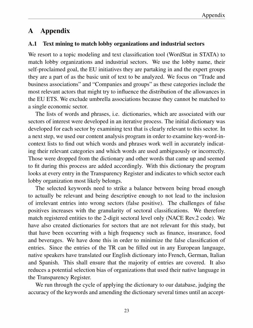
We resort to a topic modeling and text classification tool (WordStat in STATA) tomatch lobby organizations and industrial sectors. We use the lobby name, theirself-proclaimed goal, the EU initiatives they are partaking in and the expert groupsthey are a part of as the basic unit of text to be analyzed. We focus on “Trade andbusiness associations” and “Companies and groups” as these categories include themost relevant actors that might try to influence the distribution of the allowances inthe EU ETS. We exclude umbrella associations because they cannot be matched toa single economic sector.

The lists of words and phrases, i.e. dictionaries, which are associated with oursectors of interest were developed in an iterative process. The initial dictionary wasdeveloped for each sector by examining text that is clearly relevant to this sector. Ina next step, we used our content analysis program in order to examine key-word-in-context lists to find out which words and phrases work well in accurately indicat-ing their relevant categories and which words are used ambiguously or incorrectly.Those were dropped from the dictionary and other words that came up and seemedto fit during this process are added accordingly. With this dictionary the programlooks at every entry in the Transparency Register and indicates to which sector eachlobby organization most likely belongs.

The selected keywords need to strike a balance between being broad enoughto actually be relevant and being descriptive enough to not lead to the inclusionof irrelevant entries into wrong sectors (false positive). The challenges of falsepositives increases with the granularity of sectoral classifications. We thereforematch registered entities to the 2-digit sectoral level only (NACE Rev.2 code). Wehave also created dictionaries for sectors that are not relevant for this study, butthat have been occurring with a high frequency such as finance, insurance, foodand beverages. We have done this in order to minimize the false classification ofentries. Since the entries of the TR can be filled out in any European language,native speakers have translated our English dictionary into French, German, Italianand Spanish. This shall ensure that the majority of entries are covered. It alsoreduces a potential selection bias of organizations that used their native language inthe Transparency Register.

We run through the cycle of applying the dictionary to our database, judging theaccuracy of the keywords and amending the dictionary several times until an accept-

23

Appendix

able level of validity is reached. We define this level as 95 percent of classificationsbeing accurate of a random 10 percent sample. We also double check the matchingof the 200 lobbies with the highest expenditures in order to avoid sorting errors witha high impact on the results. The full dictionary is available upon request.

To identify EU ETS firms in the category "Companies and Groups” of the Trans-parency Register, we resort to the Ownership Links and Enhanced EUTL DatasetProject, which links accounts in the EUTL with the ultimate owners of these ac-counts (Jaraite et al. 2013).

24

Appendix

A.2 Additional tablesTa

ble

A1:

Top

5lo

bby

orga

niza

tion

inEU

ETS

sect

ors

sect

orna

me

sect

or#

#of

firm

slo

bbyN

ame

cost

sem

plFT

Eem

pl#E

Pac

cr

Pape

r&pa

perp

rodu

cts

1719

The

Alli

ance

forB

ever

age

Car

tons

and

the

Envi

ronm

ent(

AC

E)15

0,00

04.

755

3

UPM

-Kym

men

eO

yj(U

PM)

75,0

004.

57

2

Finn

ish

Fore

stIn

dust

ries

Fede

ratio

n(M

etsä

teol

lisuu

sry

)(FF

IF)

75,0

003.

7511

1

Con

fede

ratio

nof

Euro

pean

Pape

rInd

ustri

es(C

EPI)

550,

000

2.5

73

Euro

pean

Org

anis

atio

nof

the

Saw

mill

indu

stry

(EO

S)35

0,00

02

22

Cok

e&

refin

edpe

trole

umpr

oduc

ts19

9

Fuel

sEur

ope

(Fue

lsEu

rope

)2,

375,

000

10.5

157

BP

p.l.c

.(B

P)2,

875,

000

5.25

94

TOTA

LS.

A.

1,87

5,00

05.

256

6

Tech

nica

lCom

mitt

eeof

Petro

leum

Add

itive

Man

ufac

ture

rsin

Euro

peA

ISB

L(A

TC)

5,00

02.

510

OM

VA

ktie

nges

ells

chaf

t(O

MV

)55

0,00

02

21

Che

mic

als

&ch

emic

alpr

oduc

ts20

60

Euro

pean

Che

mic

alIn

dust

ryC

ounc

il(C

efic)

12,3

00,0

0047

7629

Verb

and

derC

hem

isch

enIn

dust

riee.

V.(V

CI)

4,37

5,00

027

849

Ges

amtv

erba

ndK

unst

stof

fver

arbe

itend

eIn

dust

riee.

V.(G

KV

)75

,000

2727

BASF

SE3,

300,

000

11.7

519

9

Cob

altI

nstit

ute

(CI)

2,87

5,00

011

.512

Bas

icph

arm

aceu

tical

prod

ucts

2121

Euro

pean

Fede

ratio

nof

Phar

mac

eutic

alIn

dust

ries

and

Ass

ocia

tions

(EFP

IA)

5,50

3,20

615

.75

305

John

son

&Jo

hnso

n(J

&J)

1,12

5,00

05

1515

Euro

pean

Con

fede

ratio

nof

Phar

mac

eutic

alEn

trepr

eneu

rs(E

UC

OPE

)25

0,00

04

41

SAN

OFI

1,12

5,00

03.

7511

4

Bun

desv

erba

ndde

rArz

neim

ittel

-Her

stel

lere

.V.(

BAH

)75

,000

3.5

61

Rub

ber&

plas

ticpr

oduc

ts22

13

Plas

ticsE

urop

e5,

000

816

9

Euro

pean

Tyre

&R

ubbe

rMan

ufac

ture

rs’A

ssoc

iatio

n(E

TRM

A)

750,

000

3.25

55

The

Euro

pean

Plas

ticPi

pes

and

Fitti

ngs

Ass

ocia

tion

(TEP

PFA

)15

0,00

03

4

Euro

pean

Plas

tics

Con

verte

rsA

ssoc

iatio

n(E

uPC

)40

0,00

02

32

Pire

lli&

C.S

pA25

0,00

02

32

Non

met

allic

min

eral

prod

ucts

2336

CEM

BU

REA

U-T

heEu

rope

anC

emen

tAss

ocia

tion

(CEM

BU

REA

U)

450,

000

49

9

Euro

pean

Con

stru

ctio

nIn

dust

ryFe

dera

tion

(FIE

C)

450,

000

44

2

Bun

desv

erba

ndG

lasi

ndus

trie

e.V.

(BV

Gla

s)15

0,00

03

6

Gla

ssfo

rEur

ope

300,

000

24

3

Wie

nerb

erge

rAG

360,

000

1.75

4

Bas

icm

etal

s24

38

Euro

met

aux

1,37

5,00

014

.515

8

Roy

alM

etaa

luni

e(M

U)

150,

000

716

Aur

ubis

AG

550,

000

6.5

144

EURO

ALL

IAG

ES1,

125,

000

5.5

64

Wirt

scha

ftsVe

rein

igun

gM

etal

le(W

VM

etal

le)

600,

000

412

1

3576

BD

EWB

unde

sver

band

derE

nerg

ie-u

ndW

asse

rwirt

scha

fte.

V.(B

DEW

)2,

875,

000

13.7

524

6

Elec

trici

ty,g

as,s

team

&Po

lish

Elec

trici

tyA

ssoc

iatio

n(P

KEE

)1,

125,

000

10.7

511

4

airc

ondi

tioni

ngsu

pply

Euro

pean

Fede

ratio

nof

Ener

gyTr

ader

s(E

FET)

450,

000

811

7

Euro

pean

Net

wor

kof

Tran

smis

sion

Syst

emO

pera

tors

forE

lect

ricity

(EN

TSO

-E)

75,0

007.

515

10

Publ

icPo

wer

Cor

pora

tion

S.A

.(PP

CS.

A.)

350,

000

6.75

211

Sour

ce:E

UTr

ansp

aren

cyR

egis

ter,

own

calc

ulat

ions

25

B APPENDIX

B Appendix

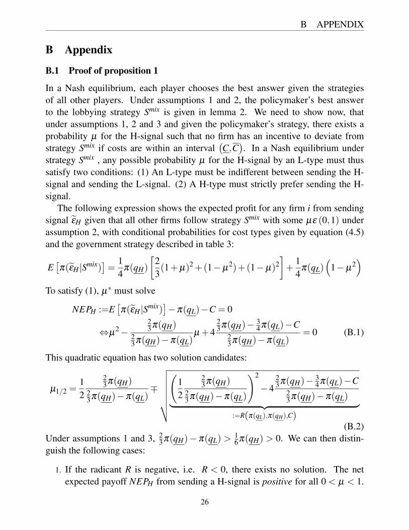
B.1 Proof of proposition 1

In a Nash equilibrium, each player chooses the best answer given the strategiesof all other players. Under assumptions 1 and 2, the policymaker’s best answerto the lobbying strategy Smix is given in lemma 2. We need to show now, thatunder assumptions 1, 2 and 3 and given the policymaker’s strategy, there exists aprobability µ for the H-signal such that no firm has an incentive to deviate fromstrategy Smix if costs are within an interval

�C,C

�. In a Nash equilibrium under

strategy Smix , any possible probability µ for the H-signal by an L-type must thussatisfy two conditions: (1) An L-type must be indifferent between sending the H-signal and sending the L-signal. (2) A H-type must strictly prefer sending the H-signal.

The following expression shows the expected profit for any firm i from sendingsignal eeH given that all other firms follow strategy Smix with some µe (0,1) underassumption 2, with conditional probabilities for cost types given by equation (4.5)and the government strategy described in table 3:

E⇥p(eeH |Smix)

⇤=

14

p(qH)

23(1+µ)2 +(1�µ2)+(1�µ)2

�+

14

p(qL)⇣

1�µ2⌘

To satisfy (1), µ⇤ must solve

NEPH :=E⇥p(eeH |Smix)

⇤�p(qL)�C = 0

,µ2 �23p(qH)

23p(qH)�p(qL)

µ +423p(qH)� 3

4p(qL)�C23p(qH)�p(qL)

= 0 (B.1)

This quadratic equation has two solution candidates:

µ1/2 =12

23p(qH)

23p(qH)�p(qL)

⌥

vuuuuut

12

23p(qH)

23p(qH)�p(qL)

!2

�423p(qH)� 3

4p(qL)�C23p(qH)�p(qL)

| {z }:=R(p(qL),p(qH),C)

(B.2)Under assumptions 1 and 3, 2

3p(qH)�p(qL) >16p(qH) > 0. We can then distin-

guish the following cases:

1. If the radicant R is negative, i.e. R < 0, there exists no solution. The netexpected payoff NEPH from sending a H-signal is positive for all 0 < µ < 1.

26

B APPENDIX

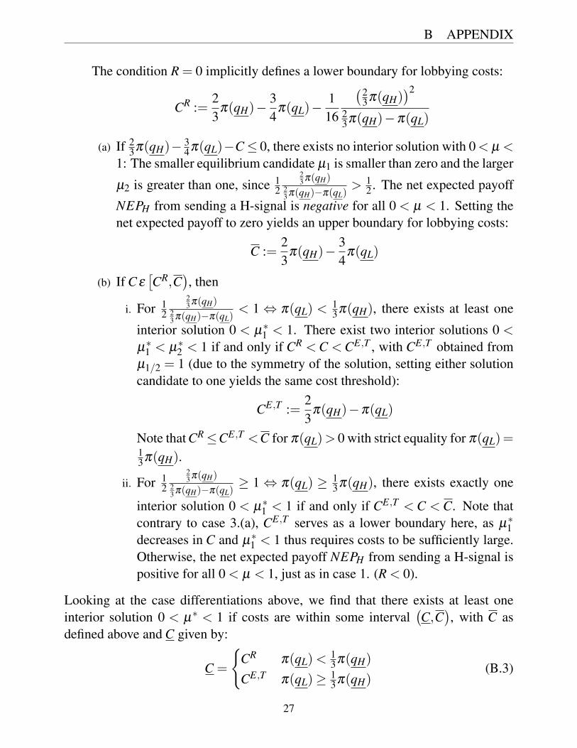
The condition R = 0 implicitly defines a lower boundary for lobbying costs:

CR :=23

p(qH)�34

p(qL)�116

�23p(qH)

�2

23p(qH)�p(qL)

(a) If 23p(qH)� 3

4p(qL)�C 0, there exists no interior solution with 0< µ <1: The smaller equilibrium candidate µ1 is smaller than zero and the larger

µ2 is greater than one, since 12

23 p(qH)

23 p(qH)�p(qL)

> 12. The net expected payoff

NEPH from sending a H-signal is negative for all 0 < µ < 1. Setting thenet expected payoff to zero yields an upper boundary for lobbying costs:

C :=23

p(qH)�34

p(qL)

(b) If C e⇥CR,C

�, then

i. For 12

23 p(qH)

23 p(qH)�p(qL)

< 1 , p(qL) <13p(qH), there exists at least one

interior solution 0 < µ⇤1 < 1. There exist two interior solutions 0 <

µ⇤1 < µ⇤

2 < 1 if and only if CR < C < CE,T , with CE,T obtained fromµ1/2 = 1 (due to the symmetry of the solution, setting either solutioncandidate to one yields the same cost threshold):

CE,T :=23

p(qH)�p(qL)

Note that CR CE,T <C for p(qL)> 0 with strict equality for p(qL)=13p(qH).

ii. For 12

23 p(qH)

23 p(qH)�p(qL)

� 1 , p(qL) � 13p(qH), there exists exactly one

interior solution 0 < µ⇤1 < 1 if and only if CE,T < C < C. Note that

contrary to case 3.(a), CE,T serves as a lower boundary here, as µ⇤1

decreases in C and µ⇤1 < 1 thus requires costs to be sufficiently large.

Otherwise, the net expected payoff NEPH from sending a H-signal ispositive for all 0 < µ < 1, just as in case 1. (R < 0).

Looking at the case differentiations above, we find that there exists at least oneinterior solution 0 < µ⇤ < 1 if costs are within some interval

�C,C

�, with C as

defined above and C given by:

C =

(CR p(qL)<

13p(qH)

CE,T p(qL)� 13p(qH)

(B.3)

27

B APPENDIX

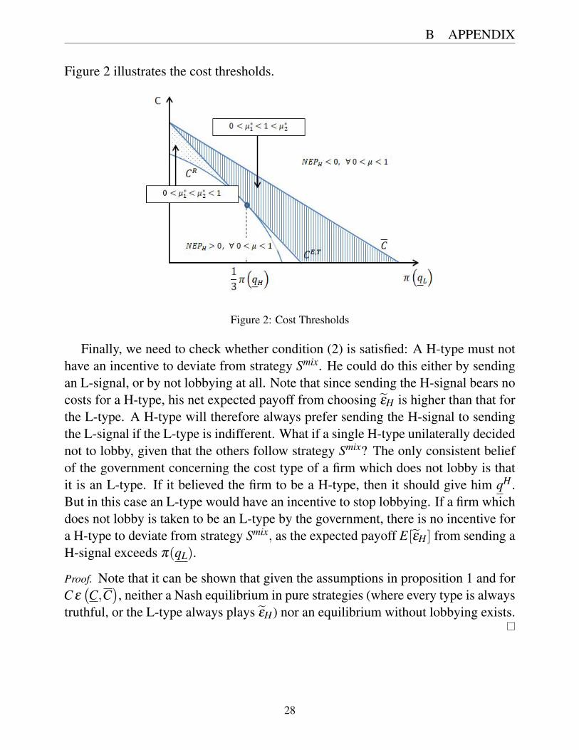
Figure 2 illustrates the cost thresholds.

Figure 2: Cost Thresholds

Finally, we need to check whether condition (2) is satisfied: A H-type must nothave an incentive to deviate from strategy Smix. He could do this either by sendingan L-signal, or by not lobbying at all. Note that since sending the H-signal bears nocosts for a H-type, his net expected payoff from choosing eeH is higher than that forthe L-type. A H-type will therefore always prefer sending the H-signal to sendingthe L-signal if the L-type is indifferent. What if a single H-type unilaterally decidednot to lobby, given that the others follow strategy Smix? The only consistent beliefof the government concerning the cost type of a firm which does not lobby is thatit is an L-type. If it believed the firm to be a H-type, then it should give him qH .But in this case an L-type would have an incentive to stop lobbying. If a firm whichdoes not lobby is taken to be an L-type by the government, there is no incentive fora H-type to deviate from strategy Smix, as the expected payoff E[eeH ] from sending aH-signal exceeds p(qL).

Proof. Note that it can be shown that given the assumptions in proposition 1 and forC e�C,C

�, neither a Nash equilibrium in pure strategies (where every type is always

truthful, or the L-type always plays eeH) nor an equilibrium without lobbying exists.

28

B APPENDIX

B.2 Proof of proposition 2

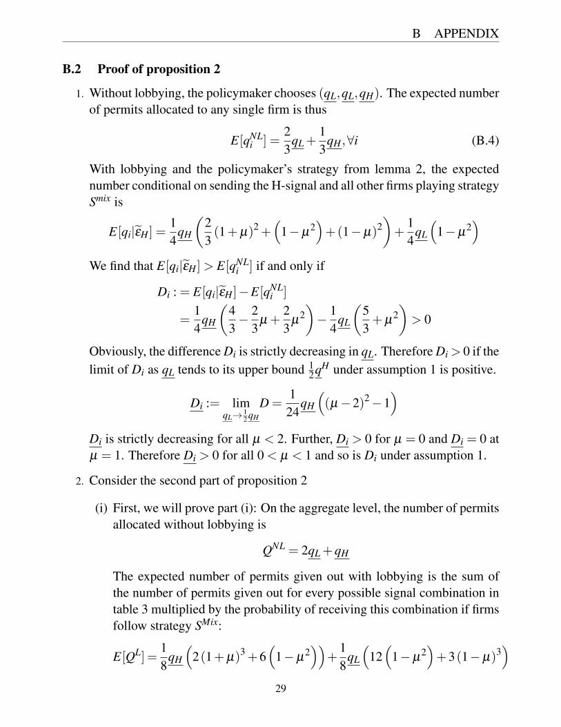
1. Without lobbying, the policymaker chooses (qL,qL,qH). The expected numberof permits allocated to any single firm is thus

E[qNLi ] =

23

qL +13

qH ,8i (B.4)

With lobbying and the policymaker’s strategy from lemma 2, the expectednumber conditional on sending the H-signal and all other firms playing strategySmix is

E[qi|eeH ] =14

qH

✓23(1+µ)2 +

⇣1�µ2

⌘+(1�µ)2

◆+

14

qL

⇣1�µ2

⌘

We find that E[qi|eeH ]> E[qNLi ] if and only if

Di : = E[qi|eeH ]�E[qNLi ]

=14

qH

✓43� 2

3µ +

23

µ2◆� 1

4qL

✓53+µ2

◆> 0

Obviously, the difference Di is strictly decreasing in qL. Therefore Di > 0 if thelimit of Di as qL tends to its upper bound 1

2qH under assumption 1 is positive.

Di := limqL! 1

2 qH

D =124

qH

⇣(µ �2)2 �1

⌘

Di is strictly decreasing for all µ < 2. Further, Di > 0 for µ = 0 and Di = 0 atµ = 1. Therefore Di > 0 for all 0 < µ < 1 and so is Di under assumption 1.

2. Consider the second part of proposition 2

(i) First, we will prove part (i): On the aggregate level, the number of permitsallocated without lobbying is

QNL = 2qL +qH

The expected number of permits given out with lobbying is the sum ofthe number of permits given out for every possible signal combination intable 3 multiplied by the probability of receiving this combination if firmsfollow strategy SMix:

E[QL] =18

qH

⇣2(1+µ)3 +6

⇣1�µ2

⌘⌘+

18

qL

⇣12⇣

1�µ2⌘+3(1�µ)3

⌘

29

B APPENDIX

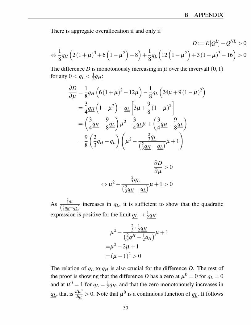
There is aggregate overallocation if and only if

D := E[QL]�QNL > 0

, 18

qH

⇣2(1+µ)3 +6

⇣1�µ2

⌘�8⌘+

18

qL

⇣12⇣

1�µ2⌘+3(1�µ)3 �16

⌘> 0

The difference D is monotonously increasing in µ over the invervall (0,1)for any 0 < qL < 1

2qH :

∂D∂ µ

=18

qH

⇣6(1+µ)2 �12µ

⌘� 1

8qL

⇣24µ +9(1�µ)2

⌘

=34

qH

⇣1+µ2

⌘�qL

3µ +

98(1�µ)2

�

=

✓34

qH � 98

qL

◆µ2 � 3

4qLµ +

✓34

qH � 98

qL

◆

=98

✓23

qH �qL

◆ µ2 �

23qL�2

3qH �qL�µ +1

!

∂D∂ µ

> 0

, µ2 �23qL�2

3qH �qL�µ +1 > 0

As23 qL

(23 qH�qL)

increases in qL, it is sufficient to show that the quadratic

expression is positive for the limit qL ! 12qH :

µ2 �23 ·

12qH�2

3qH � 12qH

�µ +1

=µ2 �2µ +1

=(µ �1)2 > 0

The relation of qL to qH is also crucial for the difference D. The rest ofthe proof is showing that the difference D has a zero at µ0 = 0 for qL = 0and at µ0 = 1 for qL = 1

2qH , and that the zero monotonously increases in

qL, that is dµ0

dqL> 0. Note that µ0 is a continuous function of qL. It follows

30

B APPENDIX

then that under assumption 2 with 0 < qL < 12qH , there exists a µ0 with

0 < µ0 < 1 such that there is overallocation whenever µ > µ0. As to thefirst step, substitute qL = 0 to find that

D|qL=0 =18

qH

⇣2(1+µ)3 +6

⇣1�µ2

⌘�8⌘

=18

qH

⇣2µ3 +6µ

⌘� 0, 8µe[0,1]

with strict equality at µ0 = 0. Then substitute the upper limit qL = 12qH :

limqL! 1

2 qH

D =18

qH

✓2(1+µ)3 +12

⇣1�µ2

⌘+

32(1�µ)3 �16

◆

=� 116

qH (1�µ)3 0, 8µe [0,1]

This time, there is strict equality for µ0 = 1. Finally, we prove that dµ0

dqL> 0

. Totally differentiating D = 0 yields:

18

qH

✓6⇣

1+µ0⌘2

�12µ0◆� 1

8qL

✓24µ0 +9

⇣1�µ0

⌘2◆�

dµ0

+18

✓12✓

1�⇣

µ0⌘2◆+3⇣

1�µ0⌘3

�16◆

dqL = 0

Solve for dµ0

dqL:

dµ0

dqL=�

12⇣

1��µ0�2

⌘+3�1�µ0�3 �16

qH

⇣6(1+µ0)2 �12µ0

⌘�qL

⇣24µ0 +9(1�µ0)2

⌘ > 0

The denominator is proportional by a positive constant to the derivative∂D∂ µ at µ = µ0, which we have proven to be positive. The numerator onthe other hand is negative for any µ e [0,1] This can easily be checked bynoting that it is decreasing in µ and substituting µ = 0.

(ii) Now we prove part 2.(ii) of proposition 2: Consider the two solutioncandidates for a Nash equilibrium probability for signal eH in equation(B.2) in the proof of proposition 1: We want to show that we can alwaysfind an intervall

⇣C,C0

⌘for lobbying costs such that at least one of the

31

B APPENDIX

two solution candidates in equation (B.2) satisfies µ0 < µ < 1 whenever

C e⇣

C,C0⌘

. In other words, we want to show that for some⇣

C,C0⌘

,

there exists an interior solution µ⇤ which satisfies µ⇤ > µ0 whenever

Ce⇣

C,C0⌘

.It is easy to see from equation (B.2) that both solution candidates are con-tinuous in lobbying costs C. Given R � 0, µ1 monotonously decreases

from 12

23 p(qH)

23 p(qH)�p(qL)

to zero and µ2 monotonously increases from 12

23 p(qH)

23 p(qH)�p(qL)

to23 p(qH)

23 p(qH)�p(qL)

� 1 as C increases towards C. It can be verified that

µ0 < 1/2 whenever p(qL) <13p(qH) so that 1

2

23 p(qH)

23 p(qH)�p(qL)

< 1. Since

12

23 p(qH)

23 p(qH)�p(qL)

� 12, there is always overallocation at µ2 if it is an interior

solution for the equilibrium probability for a H-signal (if µ2 < 1). Defineas Co,T the C that solves µ1 = µ0. It is given by

Co,T =23

0

@1�µ0⇣

1�µ0⌘

4

1

Ap(qH)�3+⇣

µ0⌘2

4p(qL) (B.5)

We can distinguish two cases:

(a) 12

23 p(qH)

23 p(qH)�p(qL)

< 1 , p(qL)<13p(qH): µ1 satisfies µ0 < µ1 < 1 if and only

if C < C < Co,T . Both equilibrium probabilities are linked to over-allocation, that isµ1 and µ2 satisfy µ0 < µ1 < µ2 < 1, if and only ifC <C <CE,T (<Co,T ).

(b) 12

23 p(qH)

23 p(qH)�p(qL)

� 1 , p(qL)� 13p(qH): µ1 satisfies µ0 < µ1 < 1 if and only

if CE,T < C < Co,T . The larger solution candidate µ2 is greater thanone.

Looking at the case differentiation, there is at least one interior solutionµ⇤ which satisfies µ⇤ > µ0 if and only if Ce

⇣C,C0

⌘, with C as defined in

(B.3)and C0 :=Co,T .

B.3 Specifications for the cost function

A reasonable assumption for lobbying costs is that they are in some way increasingin the distance of the signal ei from the actual relocation cost ei. A quite general

32

B APPENDIX

specification of lobbying costs in line with this assumption is the following:

Ci (ei,ei) = ke

q(ei � ei)2

v, ke e (0,•) (B.6)

It seems reasonable to assume that costs are non-concave, i.e. C00i (·) � 0, or v � 1,

such that marginal costs of sending a false signal are non-decreasing in the distanceof the signal from the true cost type. For v = 1, costs are linear in the distance ofthe signal from the true cost type, while for v = 2, costs are quadratic.

Alternatively, costs might depend on the signal and the cost type indirectly,through the signaled and true reservation number of permits:

Ci (ei,ei) = kq

q(q(ei)�qi(ei))2

v, kq e (0,•) (B.7)

where q(ei) andqi(ei) depend on the signal ei and the cost type ei of firm i respec-tively via (4.3).In the former case, costs depend only on the exogenous distributionof cost types. In the latter case, the reservation number of permits depend also onthe functional specification of the profit function. With both specifications, we canalways find an interval for k such that costs fall within the critical interval.

However, with the specification (B.6), the upper boundary for ke quickly ap-proaches zero as �eH becomes large if marginal costs are increasing (v > 1). Thisis because for any given relation between �eH and �eL, costs increase quadraticallyin �eH , while the expected profit from lobbying only increases linearly due to thelinear relation (4.3) between profits and cost types. Define the upper boundary forke such that C <C0 as ke . With specification (B.6), we derive ke from C =C0 as

ke =C0

p(eH � eL)2v

With C0 given by Co,T in (B.5) and using the relation (4.3), we obtain

ke =

3+(µ0)2

4 eL � 23

✓1� µ0(1�µ0)

4

◆eH

p(eH � eL)2v

Consider some given ratio 0 < eL/eH < 1 and some given 0 < µ0 < 1. The upperboundary ke converges to zero as �eH becomes large if v > 1:

lim�eH!•

ke = lim�eH!•

(�eH)1�v

23

✓1� µ0(1�µ0)

4

◆� 3+(µ0)

2

4eLeH

q( eL

eH�1)2

v = 0 v > 1

33

B APPENDIX

The alternative specification (B.7) is more flexible here, because the number ofreservation permits rises less strongly if marginal profits are increasing in the permitnumber. Define the upper boundary as kq, then

kq =

23

✓1� µ0(1�µ0)

4

◆p(qH)�

3+(µ0)2

4 p(qL)

q(qH �qL)2

v

Further, assume the following specification for profits:

p(qi) = g (qi)r g > 0, r � 1 (B.8)

With the specification (B.8) for profits and the relation (4.3), we can determine thereservation numbers of permits qH and qL as

qH =

✓�eH

g

◆1/r

qL =

✓�eL

g

◆1/r

The upper boundary can then be expressed in terms of the exogenously given relo-cation cost as:

kq =

3+(µ0)2

4 eL � 23

✓1� µ0(1�µ0)

4

◆eH

s✓⇣�eH

g

⌘1/r�⇣�eL

g

⌘1/r◆2

v

The limit is

lim�eH!•

kq = lim�eH!•

(�eH)1�v/r (g)v/r

23

✓1� µ0(1�µ0)

4

◆� 3+(µ0)

2

4eLeH

s✓1�⇣

eLeH

⌘1/r◆2

v

This limit is zero if and only if v > r, as in this case, lobbying costs increase fasterwhen �eH increases than profits for the H-type do.

34

6

A Proposal for a Carbon Fee and Dividend in New Jersey Authors (listed alphabetically): William Atkinson, Stav Bejerano, Victor Hua, Jonathan Lu, Samuel Moore, Jivahn Moradian*, Hamza Nishtar, Aileen Wu. *Corresponding author: [email protected]

1. Abstract

We describe a comprehensive, politically feasible proposal for a Carbon Fee and Dividend (CF&D) policy in the state of New Jersey (USA). This proposal is informed by conversations with over 80 state stakeholders, including legislators, academics, and representatives from environmental, labor, and business groups. We propose a rising fee beginning at $30/ton of carbon dioxide (CO2), with 70% to a household dividend and 30% to energy-intensive/trade-exposed (EITE) businesses, vulnerable communities, climate change adaptation, and low-carbon technology investments. We analyze the potential economic effects of this policy, including the positive effect on NJ renewables, changes in energy prices, impacts on households by size and income level, impacts on vulnerable economic sectors, and overall macroeconomic effects. We suggest avenues for sustainable investment, and address potential legal barriers including the Motor Fuels Tax Act. Finally, we discuss the political feasibility of the policy, including public opinion and the results of our stakeholder conversations. We conclude that a statewide CF&D policy is a politically feasible way to reduce emissions without significantly harming New Jersey’s economy.

2. Introduction

2.1 Motivation for a Carbon Fee and Dividend Policy

A strong causal relationship has been established between greenhouse gas (GHG) emissions and climate change (Stips et al. 2016), which poses a major threat to New Jersey. Sea-level rise is projected to place 174,000 - 482,000 state residents at risk of inundation by 2100, and factoring in population growth increases this figure substantially (Hauer et al. 2016). The economic and social costs associated with climate change include increased extreme weather, damages to fisheries, decreased crop yields, more severe droughts and floods, heat-related illnesses, and increased insect-borne disease rates (EPA 2016). Even an individual state’s actions to fight carbon emissions can yield effects; in the US and Western Europe, each ton of reduced CO2 emissions is associated with health co-benefits of $30-600 (West et al. 2013). Effective solutions should ensure that costs are fairly allocated, and must not harm New Jersey’s economy. We propose a CF&D policy as a simple, efficient method for reducing carbon emissions, establishing New Jersey as a leading state for US climate policy while promoting the economic welfare of most citizens and businesses.

7

2.2 Existing CF&D or Carbon Tax Programs

National carbon taxes currently exist in Chile, Costa Rica, Denmark, Finland, France,

Iceland, Ireland, Japan, Mexico, Norway, Sweden, Switzerland and the UK (World Bank 2014). Carbon taxes have also been implemented at the sub-national level, for instance in British Columbia. We examine the policies in Denmark, Ireland, and British Columbia because they are well-documented and share similarities with our proposal.

2.2.1 Denmark

The tax was introduced in 1992 and is currently DKr ~170/tCO2e (~$27/tCO2e1), with 60% percent of the revenue dedicated to industry and 40% to environmental programs. From 1990-2012, Denmark’s CO2 emissions fell by 14% (World Bank 2017).

2.2.2 Ireland

The tax was implemented in 2010 on oil and gas consumption to increase revenues and reduce GHG emissions. This rate was increased in stages to €20/tCO2e (~$23.50/tCO2e) in 2012, and the tax has been extended to all fossil fuels. Tax revenues flow to the government’s budget (World Bank 2017).

2.2.3 British Columbia (BC)

A revenue-neutral carbon tax was introduced in 2008 on emissions-generating fuels, covering the sources of about 70% of BC’s total GHG emissions. The tax rose by C$5 per year from its initial rate of C$10/tCO2e to reach C$30/tCO2e (~$23/tCO2e) in 2012, which remains the current rate. All of the revenue generated by the tax is returned to businesses and households through tax deductions and credits (World Bank 2017).

2.3 Our Policy Proposal

This paper describes the mechanics and feasibility of a state-level New Jersey CF&D policy. Although a nation-wide fee would have greater impact and fewer opportunities for leakage, statewide options should be investigated in case a national consensus cannot be reached. New Jersey has the potential to be a climate policy leader, given its strong incentives for solar and offshore wind energy, its ambitious Renewable Portfolio Standard, its lack of fossil fuel infrastructure, and its vulnerability to climate impacts which could spur the motivation to act. Moreover, a CF&D policy appeals to both the progressive priority of protecting low-income households and the conservative preference for market-based policy. Considerable economic

1 Currency conversions performed on 9/25/2018.

8

simulations and research, along with case studies of similar implementations in other locations, find that this policy can reduce emissions without economic blowback.

3. Methods

3.1 Economic Analyses (Section 6)

To assess the economic effects of our proposed CF&D policy, we study the economic effects of previous CF&D implementations, as well as models of similar policies in other US states. Because limited economic studies were available specifically for NJ, we assume that New Jersey would be sufficiently similar to these other cases. We provide more specific descriptions of individual analyses in Section 6. Note that for the purposes of this paper, all dollar values are given in nominal terms.

3.2 Conversations with Stakeholders (Section 7)

To gauge political feasibility, we presented our proposal to 83 stakeholders between December 2017 and June 2018. These stakeholders typically held key leadership roles within relevant interest groups, including environmental groups, research groups, government officials, and business/trade/energy companies or coalitions. Our conversations helped us form relationships with stakeholders and exchange ideas and resources, in order to develop and strengthen our eventual policy proposal.

We attempted a quantitative analysis of the stakeholders’ responses to our proposal. A thorough analysis of our notes generated three main categories of data for each stakeholder (whenever possible):

1) A “rating” between -2, denoting strong opposition, and 2, denoting strong support, of the stakeholder’s overall views on the proposal.

2) A “rating” between -2 and 2 of the stakeholder’s preference for how to use the revenue generated by our proposal (2 denotes strong preference for a revenue-neutral policy in which all revenue is used for the “dividend”; -2 denotes strong preference for greater investment in additional environmental priorities).

3) A categorization (42 categories) and record of the concerns, then-unanswered questions, objections, and any additional considerations, legislative preferences, ideas, and suggestions raised by each stakeholder. We strove to conduct an impartial, objective, and honest analysis. However, there are

imperfections: the ratings and the categorization rely on an extrapolation of the stakeholder’s stance from our notes, and the stakeholders who were willing to meet might not accurately represent broader stakeholder opinions in NJ. We classify stakeholders into 5 categories:

● “Environmental groups”: any organized group with an explicit environmental activism orientation, including student groups, faith groups, environmental justice groups, and miscellaneous advocacy groups for which environment-related activism work is either at the core of or a branch of the organization’s work. This is a particularly diverse stakeholder category, composing over half of our total stakeholder sample size.

● “Academia”: professors and researchers employed by a university.

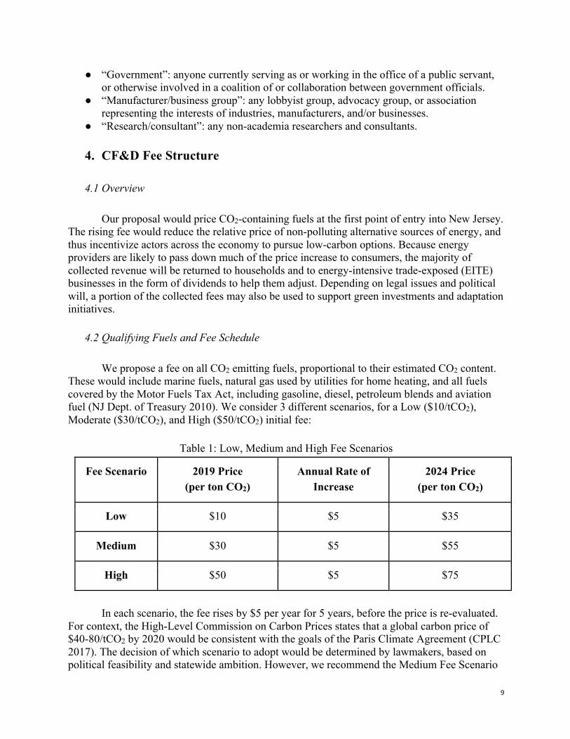
9

● “Government”: anyone currently serving as or working in the office of a public servant, or otherwise involved in a coalition of or collaboration between government officials.

● “Manufacturer/business group”: any lobbyist group, advocacy group, or association representing the interests of industries, manufacturers, and/or businesses.

● “Research/consultant”: any non-academia researchers and consultants.

4. CF&D Fee Structure

4.1 Overview

Our proposal would price CO2-containing fuels at the first point of entry into New Jersey. The rising fee would reduce the relative price of non-polluting alternative sources of energy, and thus incentivize actors across the economy to pursue low-carbon options. Because energy providers are likely to pass down much of the price increase to consumers, the majority of collected revenue will be returned to households and to energy-intensive trade-exposed (EITE) businesses in the form of dividends to help them adjust. Depending on legal issues and political will, a portion of the collected fees may also be used to support green investments and adaptation initiatives.

4.2 Qualifying Fuels and Fee Schedule

We propose a fee on all CO2 emitting fuels, proportional to their estimated CO2 content. These would include marine fuels, natural gas used by utilities for home heating, and all fuels covered by the Motor Fuels Tax Act, including gasoline, diesel, petroleum blends and aviation fuel (NJ Dept. of Treasury 2010). We consider 3 different scenarios, for a Low ($10/tCO2), Moderate ($30/tCO2), and High ($50/tCO2) initial fee:

Table 1: Low, Medium and High Fee Scenarios

Fee Scenario 2019 Price (per ton CO2)

Annual Rate of Increase

2024 Price (per ton CO2)

Low $10 $5 $35

Medium $30 $5 $55

High $50 $5 $75

In each scenario, the fee rises by $5 per year for 5 years, before the price is re-evaluated.

For context, the High-Level Commission on Carbon Prices states that a global carbon price of $40-80/tCO2 by 2020 would be consistent with the goals of the Paris Climate Agreement (CPLC 2017). The decision of which scenario to adopt would be determined by lawmakers, based on political feasibility and statewide ambition. However, we recommend the Medium Fee Scenario

10

because it is more ambitious than the Low Scenario, yet more politically feasible than the High Scenario. For the sake of simplicity in this proposal, our calculations are based on the Medium Fee Scenario unless otherwise specified.

4.3 Relationship to RGGI: Fees for Electric Power

This CF&D policy should complement the Regional Greenhouse Gas Initiative (RGGI), which New Jersey will be re-joining as per Governor Phil Murphy’s 2018 Executive Order (NJ DEP 2018). RGGI places a carbon cap-and-trade system on electric power plants that use fossil fuels with a capacity of over 25 MW, with the aim of reducing the power sector’s GHG emissions (Ramseur 2017). Our proposed policy can optionally apply to electricity; specifically, to imported electricity and to fossil fuels used for producing electricity. Evidently, applying the fee to the electric sector without any adjustments for power plants that are already targeted by RGGI would lead to them being double taxed. We define two main options for applying our policy to electricity and, consequently, our policy’s relationship with RGGI:

1. Apply the fee to all sectors, and rebate the electric sector for RGGI prices. The downside of this option is that rebating all concerned electric power plants for their carbon allowances, which are dependent on the new RGGI price, makes this option complex to implement. In addition, this would essentially negate New Jersey’s RGGI participation since the effective carbon price is the one our policy sets.

2. Apply the fee to all sectors other than the electric sector. This option would work with RGGI by preserving RGGI’s electricity price and imposing our fee on the remaining sectors. The downside of this option is that it will require diligent monitoring of imported fuels to verify whether or not they are being used to generate electric power.

We recommend pursuing the first option (impose the fee on companies affected by RGGI and rebate their RGGI fees), because it will have a higher effective carbon price for companies involved. RGGI’s price has historically remained well under $10/tCO2 (RGGI, 2018), which is much lower (and therefore less impactful on emissions) than our $30/tCO2 scenario. This option does increase the risk of emissions leakage, as external power will be relatively cheaper.

4.4 Point of Assessment & Collection Mechanism

The carbon fee would be applied to entities purchasing fuel for electricity production or electricity for household distribution, and at the first point of in-state transfer of motor fuels. This criterion is important for the fee’s application to electricity, since three of New Jersey’s four investor-owned utility companies have parent companies headquartered out-of-state (the exception being PSE&G). The fee on imports of fuels for electricity generation (including coal, natural gas and crude oil), wholesale electricity, and natural gas would be charged upon their first entry into New Jersey.

According to current protocols, the fee on fuels unrelated to electricity production, electricity distribution or natural gas distribution, should be charged upon entry into the terminal transfer system, defined as “the fuel distribution system consisting of refineries, pipelines, vessels and terminals” by the New Jersey tax code §54:39-102.

For New Jersey, a small state with many terminals just outside of state lines, provision §54:39-118 allows importing motor fuels suppliers to treat the removal of fuels from

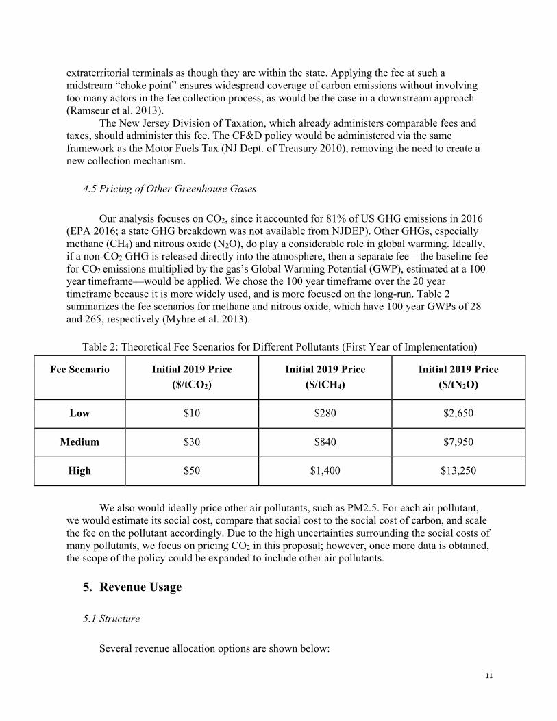
11

extraterritorial terminals as though they are within the state. Applying the fee at such a midstream “choke point” ensures widespread coverage of carbon emissions without involving too many actors in the fee collection process, as would be the case in a downstream approach

(Ramseur et al. 2013). The New Jersey Division of Taxation, which already administers comparable fees and

taxes, should administer this fee. The CF&D policy would be administered via the same framework as the Motor Fuels Tax (NJ Dept. of Treasury 2010), removing the need to create a new collection mechanism.

4.5 Pricing of Other Greenhouse Gases

Our analysis focuses on CO2, since it accounted for 81% of US GHG emissions in 2016 (EPA 2016; a state GHG breakdown was not available from NJDEP). Other GHGs, especially methane (CH4) and nitrous oxide (N2O), do play a considerable role in global warming. Ideally, if a non-CO2 GHG is released directly into the atmosphere, then a separate fee—the baseline fee for CO2 emissions multiplied by the gas’s Global Warming Potential (GWP), estimated at a 100 year timeframe—would be applied. We chose the 100 year timeframe over the 20 year timeframe because it is more widely used, and is more focused on the long-run. Table 2 summarizes the fee scenarios for methane and nitrous oxide, which have 100 year GWPs of 28 and 265, respectively (Myhre et al. 2013).

Table 2: Theoretical Fee Scenarios for Different Pollutants (First Year of Implementation)

Fee Scenario Initial 2019 Price ($/tCO2)

Initial 2019 Price ($/tCH4)

Initial 2019 Price ($/tN2O)

Low $10 $280 $2,650

Medium $30 $840 $7,950

High $50 $1,400 $13,250

We also would ideally price other air pollutants, such as PM2.5. For each air pollutant,

we would estimate its social cost, compare that social cost to the social cost of carbon, and scale the fee on the pollutant accordingly. Due to the high uncertainties surrounding the social costs of many pollutants, we focus on pricing CO2 in this proposal; however, once more data is obtained, the scope of the policy could be expanded to include other air pollutants.

5. Revenue Usage

5.1 Structure

Several revenue allocation options are shown below:

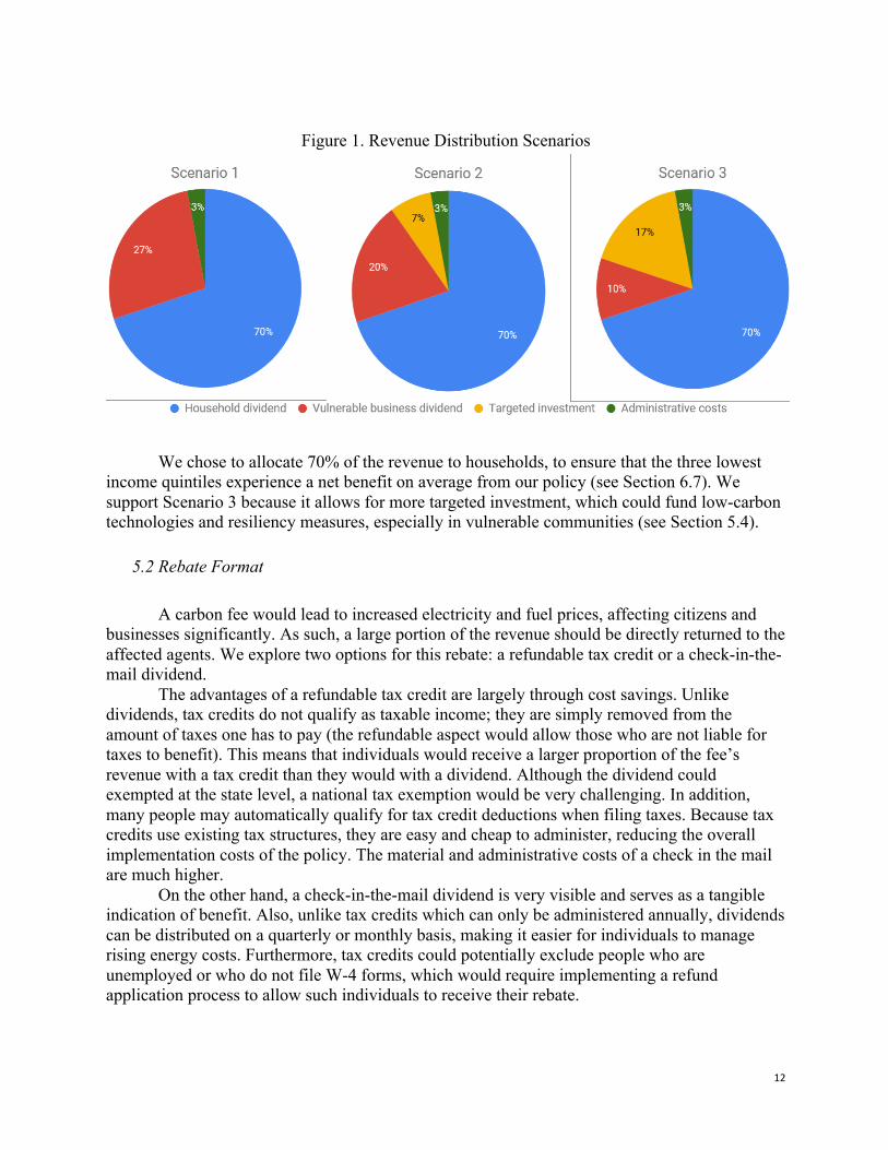
12

Figure 1. Revenue Distribution Scenarios

We chose to allocate 70% of the revenue to households, to ensure that the three lowest income quintiles experience a net benefit on average from our policy (see Section 6.7). We support Scenario 3 because it allows for more targeted investment, which could fund low-carbon technologies and resiliency measures, especially in vulnerable communities (see Section 5.4).

5.2 Rebate Format

A carbon fee would lead to increased electricity and fuel prices, affecting citizens and businesses significantly. As such, a large portion of the revenue should be directly returned to the affected agents. We explore two options for this rebate: a refundable tax credit or a check-in-the-mail dividend.

The advantages of a refundable tax credit are largely through cost savings. Unlike dividends, tax credits do not qualify as taxable income; they are simply removed from the amount of taxes one has to pay (the refundable aspect would allow those who are not liable for taxes to benefit). This means that individuals would receive a larger proportion of the fee’s revenue with a tax credit than they would with a dividend. Although the dividend could exempted at the state level, a national tax exemption would be very challenging. In addition, many people may automatically qualify for tax credit deductions when filing taxes. Because tax credits use existing tax structures, they are easy and cheap to administer, reducing the overall implementation costs of the policy. The material and administrative costs of a check in the mail are much higher.

On the other hand, a check-in-the-mail dividend is very visible and serves as a tangible indication of benefit. Also, unlike tax credits which can only be administered annually, dividends can be distributed on a quarterly or monthly basis, making it easier for individuals to manage rising energy costs. Furthermore, tax credits could potentially exclude people who are unemployed or who do not file W-4 forms, which would require implementing a refund application process to allow such individuals to receive their rebate.

13

5.3 Business Rebates

The portion of the fee that is redistributed to EITE businesses should be designed to help them to deal with increased costs in the short-term, while incentivizing them to improve energy efficiency in the long run. We would identify businesses that are

a) Energy intensive: energy and transportation make up a significant part of costs. This is the case for many construction, manufacturing, and mining companies (see Sections 6.3 and 6.4). This would not apply to companies directly involved in the production or distribution of fossil fuels.

b) Face significant out-of-state competition with which a pollution fee would put them at a considerable cost disadvantage. This would mainly apply to small and medium-sized businesses; according to the New Jersey Business and Industry Association, 86% of businesses that are vulnerable to tax increases earned less than $10 million in net allocated income (NJBIA 2018). As the fee increases each year, we would simultaneously decrease the dividend for these

EITE businesses, to encourage the adoption of low-carbon energy sources. It is important to ensure that the rebate does not disincentivize energy-intensive businesses from shifting to more efficient systems.

5.4 Targeted Investment

Many stakeholders have suggested that investment should be made to fund sustainability initiatives that decrease emissions and help vulnerable communities adapt to climate change impacts. This section explores some potential investment avenues.

Some sectors still lack committed state action in support of adaptation to climate change. The New Jersey Climate Adaptation Alliance (NJCAA) identifies several areas where state action remains insufficient, including developing cost-effective methods to control weeds and vectors, improving stormwater runoff management, and creating “incentive programs to preserve, increase, or improve climate-resilient agricultural land” (NJCAA 2014a). In addition, the NJCAA recommends educating healthcare professionals about how the field of public health is changing due to the negative consequences of climate change, and increasing studies of flood impacts on the spread of contaminated soil (NJCAA 2014b).

Electric vehicles are another investment option that are becoming an increasingly viable solution to reducing transportation emissions, which account for over half of NJ’s total carbon emissions (EIA 2018a). Electric vehicle use can be incentivized through higher gas prices, which increase their competitiveness relative to other vehicles, and by installing charging stations. The latter strategy was tested through the 2016 Workplace Charging Grant Program, which funded employers to install charging stations in their parking lots; however, this project ran out of funding as of January 2017, and applications are currently being waitlisted (Smart Solution, 2018).

Due to the abundance of investment options, we suggest that policymakers and their staff decide where to allot the revenue. Regardless, we recommend that the revenue distribution be publicly accessible if possible, since transparency would increase public support of this policy. Although we do not advise against rewarding firms for reducing emissions, politicians should

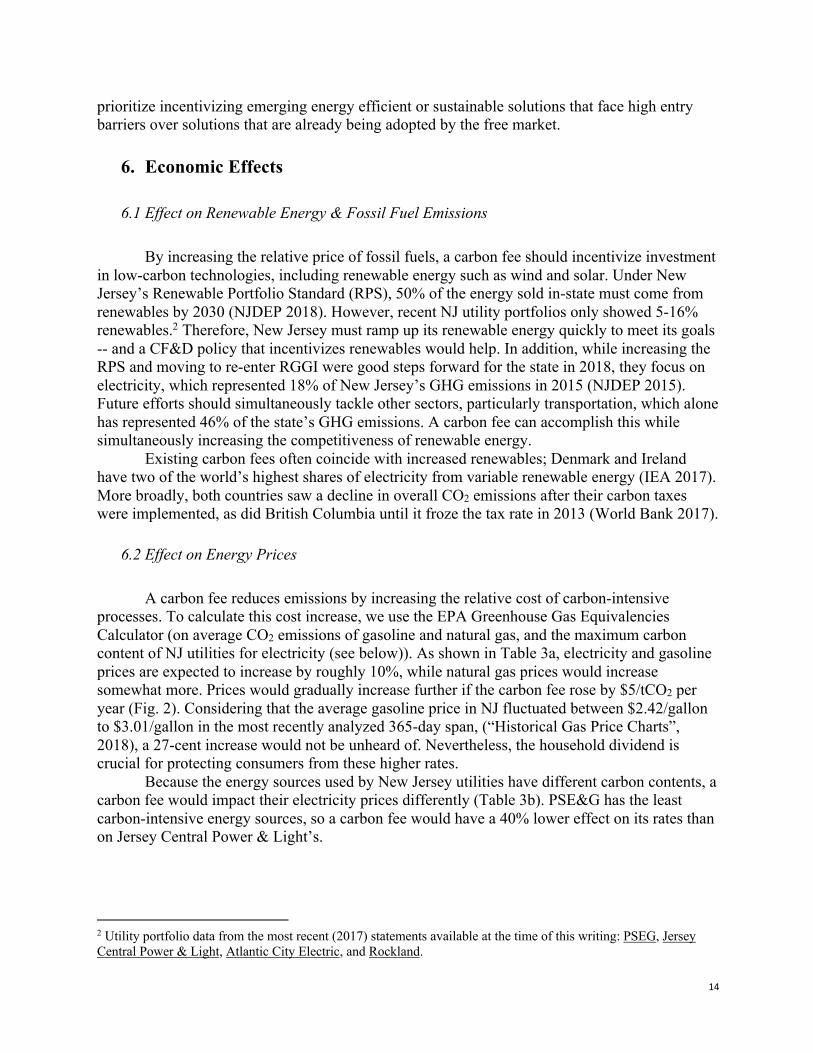
14

prioritize incentivizing emerging energy efficient or sustainable solutions that face high entry barriers over solutions that are already being adopted by the free market.

6. Economic Effects

6.1 Effect on Renewable Energy & Fossil Fuel Emissions

By increasing the relative price of fossil fuels, a carbon fee should incentivize investment in low-carbon technologies, including renewable energy such as wind and solar. Under New Jersey’s Renewable Portfolio Standard (RPS), 50% of the energy sold in-state must come from renewables by 2030 (NJDEP 2018). However, recent NJ utility portfolios only showed 5-16% renewables.2 Therefore, New Jersey must ramp up its renewable energy quickly to meet its goals -- and a CF&D policy that incentivizes renewables would help. In addition, while increasing the RPS and moving to re-enter RGGI were good steps forward for the state in 2018, they focus on electricity, which represented 18% of New Jersey’s GHG emissions in 2015 (NJDEP 2015). Future efforts should simultaneously tackle other sectors, particularly transportation, which alone has represented 46% of the state’s GHG emissions. A carbon fee can accomplish this while simultaneously increasing the competitiveness of renewable energy.

Existing carbon fees often coincide with increased renewables; Denmark and Ireland have two of the world’s highest shares of electricity from variable renewable energy (IEA 2017). More broadly, both countries saw a decline in overall CO2 emissions after their carbon taxes were implemented, as did British Columbia until it froze the tax rate in 2013 (World Bank 2017).

6.2 Effect on Energy Prices

A carbon fee reduces emissions by increasing the relative cost of carbon-intensive processes. To calculate this cost increase, we use the EPA Greenhouse Gas Equivalencies Calculator (on average CO2 emissions of gasoline and natural gas, and the maximum carbon content of NJ utilities for electricity (see below)). As shown in Table 3a, electricity and gasoline prices are expected to increase by roughly 10%, while natural gas prices would increase somewhat more. Prices would gradually increase further if the carbon fee rose by $5/tCO2 per year (Fig. 2). Considering that the average gasoline price in NJ fluctuated between $2.42/gallon to $3.01/gallon in the most recently analyzed 365-day span, (“Historical Gas Price Charts”, 2018), a 27-cent increase would not be unheard of. Nevertheless, the household dividend is crucial for protecting consumers from these higher rates.

Because the energy sources used by New Jersey utilities have different carbon contents, a carbon fee would impact their electricity prices differently (Table 3b). PSE&G has the least carbon-intensive energy sources, so a carbon fee would have a 40% lower effect on its rates than on Jersey Central Power & Light’s.

2 Utility portfolio data from the most recent (2017) statements available at the time of this writing: PSEG, Jersey Central Power & Light, Atlantic City Electric, and Rockland.

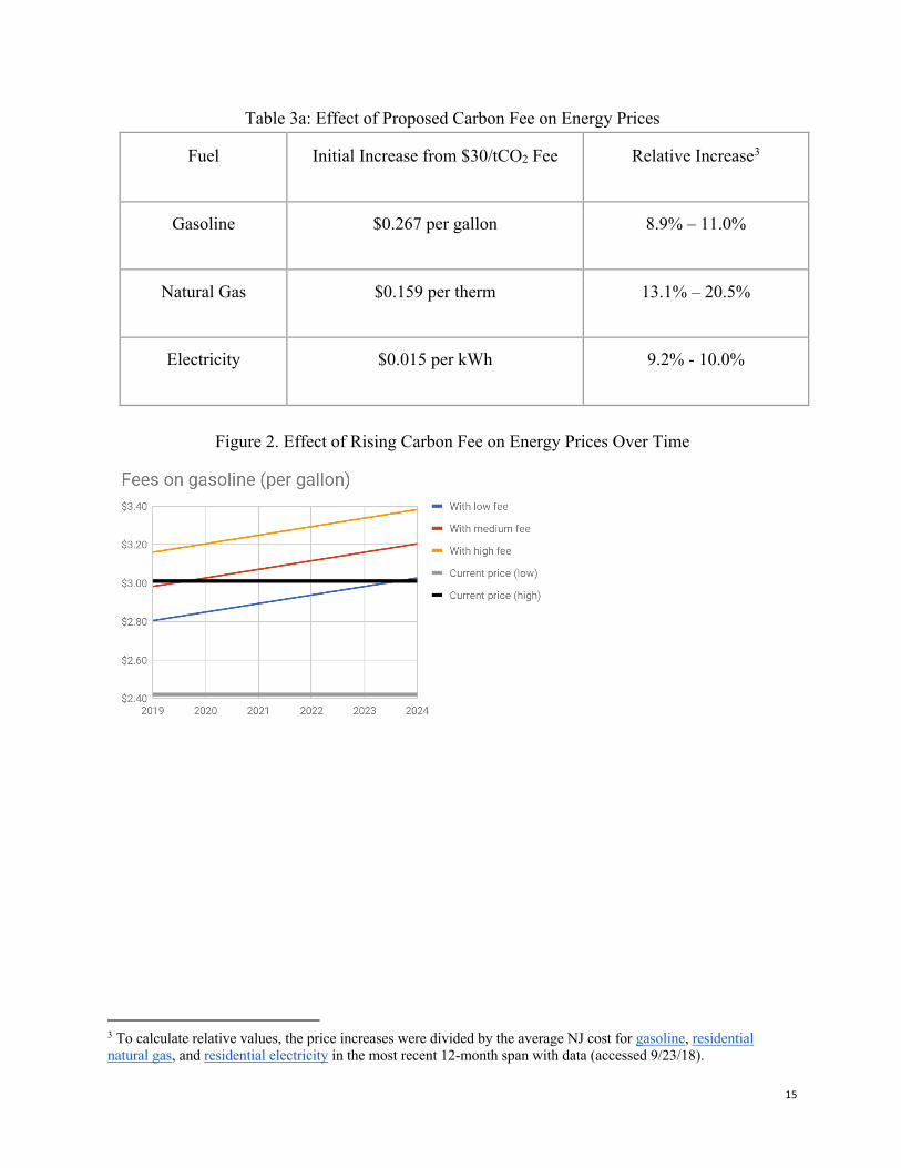
15

Table 3a: Effect of Proposed Carbon Fee on Energy Prices

Fuel Initial Increase from $30/tCO2 Fee Relative Increase3

Gasoline $0.267 per gallon 8.9% – 11.0%

Natural Gas $0.159 per therm 13.1% – 20.5%

Electricity $0.015 per kWh 9.2% - 10.0%

Figure 2. Effect of Rising Carbon Fee on Energy Prices Over Time

3 To calculate relative values, the price increases were divided by the average NJ cost for gasoline, residential natural gas, and residential electricity in the most recent 12-month span with data (accessed 9/23/18).

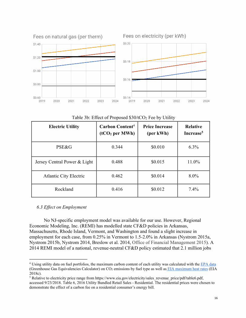
16

Table 3b: Effect of Proposed $30/tCO2 Fee by Utility

Electric Utility

Carbon Content4 (tCO2 per MWh)

Price Increase (per kWh)

Relative Increase5

PSE&G 0.344 $0.010 6.3%

Jersey Central Power & Light 0.488 $0.015 11.0%

Atlantic City Electric 0.462 $0.014 8.0%

Rockland 0.416 $0.012 7.4%

6.3 Effect on Employment

No NJ-specific employment model was available for our use. However, Regional

Economic Modeling, Inc. (REMI) has modelled state CF&D policies in Arkansas, Massachusetts, Rhode Island, Vermont, and Washington and found a slight increase in employment for each case, from 0.25% in Vermont to 1.5-2.0% in Arkansas (Nystrom 2015a, Nystrom 2015b, Nystrom 2014, Breslow et al. 2014, Office of Financial Management 2015). A 2014 REMI model of a national, revenue-neutral CF&D policy estimated that 2.1 million jobs

4 Using utility data on fuel portfolios, the maximum carbon content of each utility was calculated with the EPA data (Greenhouse Gas Equivalencies Calculator) on CO2 emissions by fuel type as well as EIA maximum heat rates (EIA 2018c). 5 Relative to electricity price range from https://www.eia.gov/electricity/sales_revenue_price/pdf/table6.pdf, accessed 9/23/2018. Table 6, 2016 Utility Bundled Retail Sales - Residential. The residential prices were chosen to demonstrate the effect of a carbon fee on a residential consumer’s energy bill.

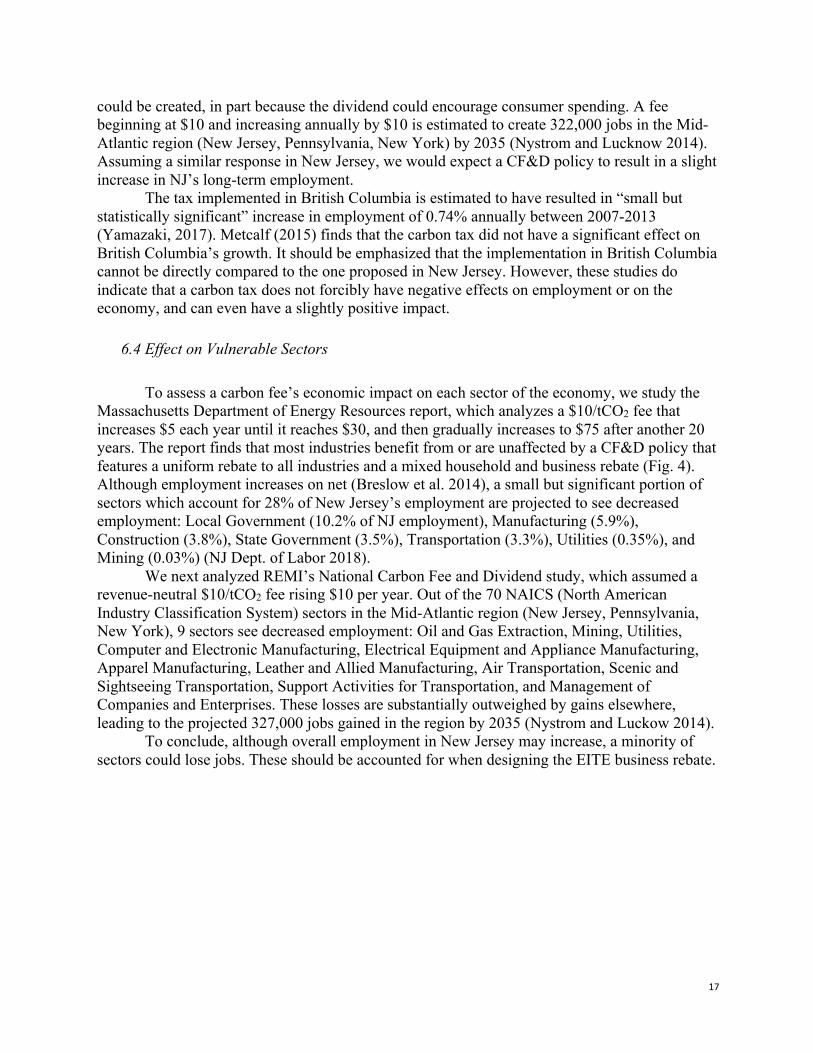
17

could be created, in part because the dividend could encourage consumer spending. A fee beginning at $10 and increasing annually by $10 is estimated to create 322,000 jobs in the Mid-Atlantic region (New Jersey, Pennsylvania, New York) by 2035 (Nystrom and Lucknow 2014). Assuming a similar response in New Jersey, we would expect a CF&D policy to result in a slight increase in NJ’s long-term employment.

The tax implemented in British Columbia is estimated to have resulted in “small but statistically significant” increase in employment of 0.74% annually between 2007-2013 (Yamazaki, 2017). Metcalf (2015) finds that the carbon tax did not have a significant effect on British Columbia’s growth. It should be emphasized that the implementation in British Columbia cannot be directly compared to the one proposed in New Jersey. However, these studies do indicate that a carbon tax does not forcibly have negative effects on employment or on the economy, and can even have a slightly positive impact.

6.4 Effect on Vulnerable Sectors

To assess a carbon fee’s economic impact on each sector of the economy, we study the Massachusetts Department of Energy Resources report, which analyzes a $10/tCO2 fee that increases $5 each year until it reaches $30, and then gradually increases to $75 after another 20 years. The report finds that most industries benefit from or are unaffected by a CF&D policy that features a uniform rebate to all industries and a mixed household and business rebate (Fig. 4). Although employment increases on net (Breslow et al. 2014), a small but significant portion of sectors which account for 28% of New Jersey’s employment are projected to see decreased employment: Local Government (10.2% of NJ employment), Manufacturing (5.9%), Construction (3.8%), State Government (3.5%), Transportation (3.3%), Utilities (0.35%), and Mining (0.03%) (NJ Dept. of Labor 2018).

We next analyzed REMI’s National Carbon Fee and Dividend study, which assumed a revenue-neutral $10/tCO2 fee rising $10 per year. Out of the 70 NAICS (North American Industry Classification System) sectors in the Mid-Atlantic region (New Jersey, Pennsylvania, New York), 9 sectors see decreased employment: Oil and Gas Extraction, Mining, Utilities, Computer and Electronic Manufacturing, Electrical Equipment and Appliance Manufacturing, Apparel Manufacturing, Leather and Allied Manufacturing, Air Transportation, Scenic and Sightseeing Transportation, Support Activities for Transportation, and Management of Companies and Enterprises. These losses are substantially outweighed by gains elsewhere, leading to the projected 327,000 jobs gained in the region by 2035 (Nystrom and Luckow 2014).

To conclude, although overall employment in New Jersey may increase, a minority of sectors could lose jobs. These should be accounted for when designing the EITE business rebate.

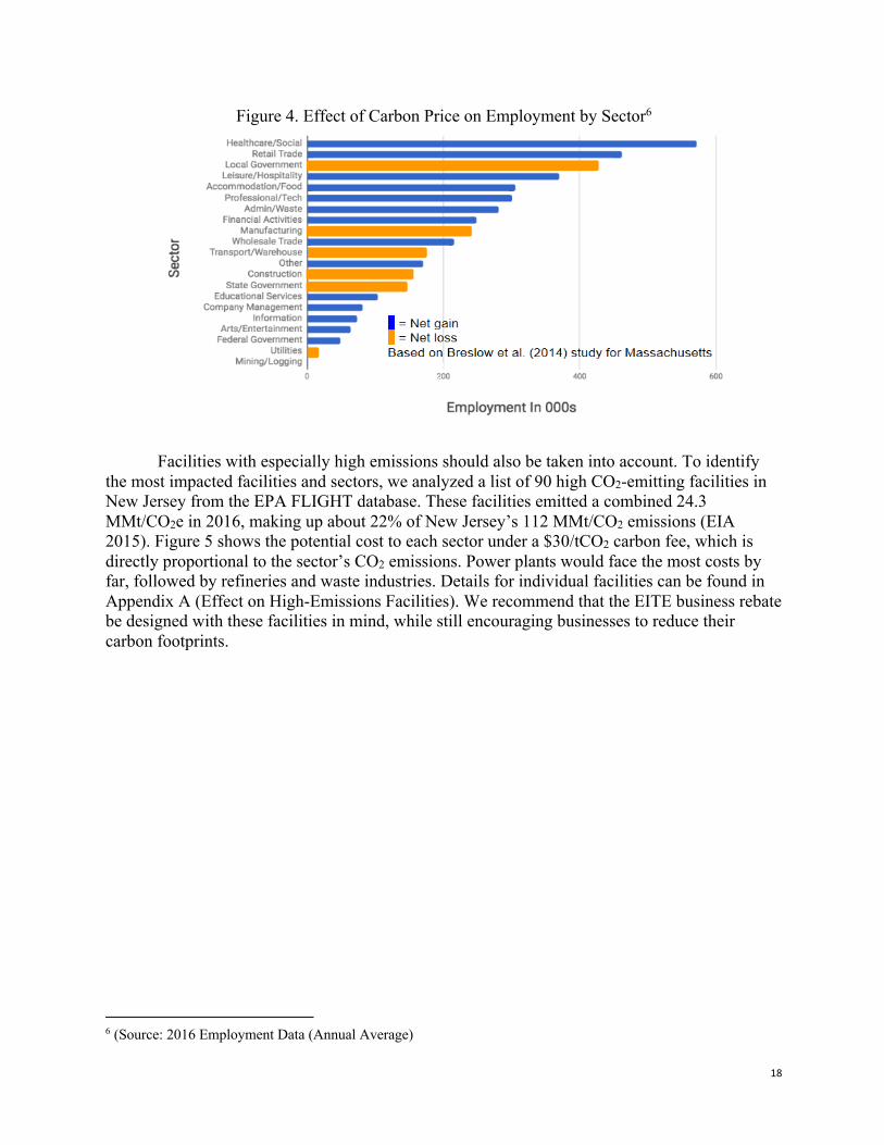
18

Figure 4. Effect of Carbon Price on Employment by Sector6

Facilities with especially high emissions should also be taken into account. To identify the most impacted facilities and sectors, we analyzed a list of 90 high CO2-emitting facilities in New Jersey from the EPA FLIGHT database. These facilities emitted a combined 24.3 MMt/CO2e in 2016, making up about 22% of New Jersey’s 112 MMt/CO2 emissions (EIA 2015). Figure 5 shows the potential cost to each sector under a $30/tCO2 carbon fee, which is directly proportional to the sector’s CO2 emissions. Power plants would face the most costs by far, followed by refineries and waste industries. Details for individual facilities can be found in Appendix A (Effect on High-Emissions Facilities). We recommend that the EITE business rebate be designed with these facilities in mind, while still encouraging businesses to reduce their carbon footprints.

6 (Source: 2016 Employment Data (Annual Average)

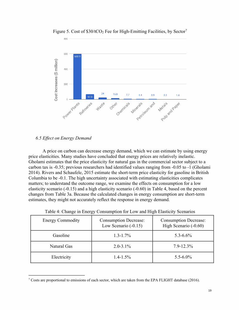
19

Figure 5. Cost of $30/tCO2 Fee for High-Emitting Facilities, by Sector7

6.5 Effect on Energy Demand

A price on carbon can decrease energy demand, which we can estimate by using energy price elasticities. Many studies have concluded that energy prices are relatively inelastic. Gholami estimates that the price elasticity for natural gas in the commercial sector subject to a carbon tax is -0.35; previous researchers had identified values ranging from -0.05 to -1 (Gholami 2014). Rivers and Schaufele, 2015 estimate the short-term price elasticity for gasoline in British Columbia to be -0.1. The high uncertainty associated with estimating elasticities complicates matters; to understand the outcome range, we examine the effects on consumption for a low elasticity scenario (-0.15) and a high elasticity scenario (-0.60) in Table 4, based on the percent changes from Table 3a. Because the calculated changes in energy consumption are short-term estimates, they might not accurately reflect the response in energy demand.

Table 4: Change in Energy Consumption for Low and High Elasticity Scenarios

Energy Commodity Consumption Decrease: Low Scenario (-0.15)

Consumption Decrease: High Scenario (-0.60)

Gasoline 1.3-1.7% 5.3-6.6%

Natural Gas 2.0-3.1% 7.9-12.3%

Electricity 1.4-1.5% 5.5-6.0%

7 Costs are proportional to emissions of each sector, which are taken from the EPA FLIGHT database (2016).

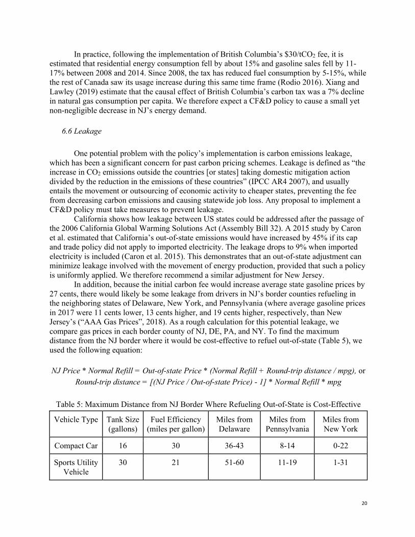
20

In practice, following the implementation of British Columbia’s $30/tCO2 fee, it is estimated that residential energy consumption fell by about 15% and gasoline sales fell by 11-17% between 2008 and 2014. Since 2008, the tax has reduced fuel consumption by 5-15%, while the rest of Canada saw its usage increase during this same time frame (Rodio 2016). Xiang and Lawley (2019) estimate that the causal effect of British Columbia’s carbon tax was a 7% decline in natural gas consumption per capita. We therefore expect a CF&D policy to cause a small yet non-negligible decrease in NJ’s energy demand.

6.6 Leakage

One potential problem with the policy’s implementation is carbon emissions leakage, which has been a significant concern for past carbon pricing schemes. Leakage is defined as “the increase in CO2 emissions outside the countries [or states] taking domestic mitigation action divided by the reduction in the emissions of these countries” (IPCC AR4 2007), and usually entails the movement or outsourcing of economic activity to cheaper states, preventing the fee from decreasing carbon emissions and causing statewide job loss. Any proposal to implement a CF&D policy must take measures to prevent leakage.

California shows how leakage between US states could be addressed after the passage of the 2006 California Global Warming Solutions Act (Assembly Bill 32). A 2015 study by Caron et al. estimated that California’s out-of-state emissions would have increased by 45% if its cap and trade policy did not apply to imported electricity. The leakage drops to 9% when imported electricity is included (Caron et al. 2015). This demonstrates that an out-of-state adjustment can minimize leakage involved with the movement of energy production, provided that such a policy is uniformly applied. We therefore recommend a similar adjustment for New Jersey.

In addition, because the initial carbon fee would increase average state gasoline prices by 27 cents, there would likely be some leakage from drivers in NJ’s border counties refueling in the neighboring states of Delaware, New York, and Pennsylvania (where average gasoline prices in 2017 were 11 cents lower, 13 cents higher, and 19 cents higher, respectively, than New Jersey’s (“AAA Gas Prices”, 2018). As a rough calculation for this potential leakage, we compare gas prices in each border county of NJ, DE, PA, and NY. To find the maximum distance from the NJ border where it would be cost-effective to refuel out-of-state (Table 5), we used the following equation: NJ Price * Normal Refill = Out-of-state Price * (Normal Refill + Round-trip distance / mpg), or

Round-trip distance = [(NJ Price / Out-of-state Price) - 1] * Normal Refill * mpg

Table 5: Maximum Distance from NJ Border Where Refueling Out-of-State is Cost-Effective

Vehicle Type Tank Size (gallons)

Fuel Efficiency (miles per gallon)

Miles from Delaware

Miles from Pennsylvania

Miles from New York

Compact Car 16 30 36-43 8-14 0-22

Sports Utility Vehicle

30 21 51-60 11-19 1-31

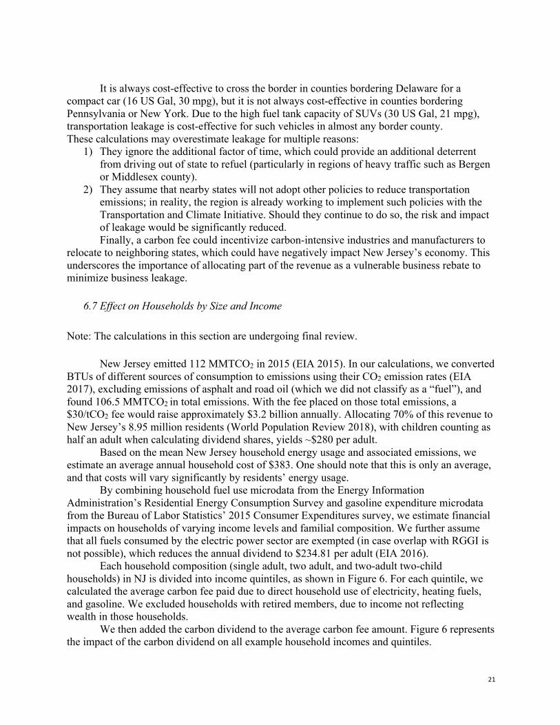
21

It is always cost-effective to cross the border in counties bordering Delaware for a

compact car (16 US Gal, 30 mpg), but it is not always cost-effective in counties bordering Pennsylvania or New York. Due to the high fuel tank capacity of SUVs (30 US Gal, 21 mpg), transportation leakage is cost-effective for such vehicles in almost any border county. These calculations may overestimate leakage for multiple reasons:

1) They ignore the additional factor of time, which could provide an additional deterrent from driving out of state to refuel (particularly in regions of heavy traffic such as Bergen or Middlesex county).

2) They assume that nearby states will not adopt other policies to reduce transportation emissions; in reality, the region is already working to implement such policies with the Transportation and Climate Initiative. Should they continue to do so, the risk and impact of leakage would be significantly reduced.

Finally, a carbon fee could incentivize carbon-intensive industries and manufacturers to relocate to neighboring states, which could have negatively impact New Jersey’s economy. This underscores the importance of allocating part of the revenue as a vulnerable business rebate to minimize business leakage.

6.7 Effect on Households by Size and Income Note: The calculations in this section are undergoing final review. New Jersey emitted 112 MMTCO2 in 2015 (EIA 2015). In our calculations, we converted BTUs of different sources of consumption to emissions using their CO2 emission rates (EIA 2017), excluding emissions of asphalt and road oil (which we did not classify as a “fuel”), and found 106.5 MMTCO2 in total emissions. With the fee placed on those total emissions, a $30/tCO2 fee would raise approximately $3.2 billion annually. Allocating 70% of this revenue to New Jersey’s 8.95 million residents (World Population Review 2018), with children counting as half an adult when calculating dividend shares, yields ~$280 per adult.

Based on the mean New Jersey household energy usage and associated emissions, we estimate an average annual household cost of $383. One should note that this is only an average, and that costs will vary significantly by residents’ energy usage.

By combining household fuel use microdata from the Energy Information Administration’s Residential Energy Consumption Survey and gasoline expenditure microdata from the Bureau of Labor Statistics’ 2015 Consumer Expenditures survey, we estimate financial impacts on households of varying income levels and familial composition. We further assume that all fuels consumed by the electric power sector are exempted (in case overlap with RGGI is not possible), which reduces the annual dividend to $234.81 per adult (EIA 2016).

Each household composition (single adult, two adult, and two-adult two-child households) in NJ is divided into income quintiles, as shown in Figure 6. For each quintile, we calculated the average carbon fee paid due to direct household use of electricity, heating fuels, and gasoline. We excluded households with retired members, due to income not reflecting wealth in those households.

We then added the carbon dividend to the average carbon fee amount. Figure 6 represents the impact of the carbon dividend on all example household incomes and quintiles.

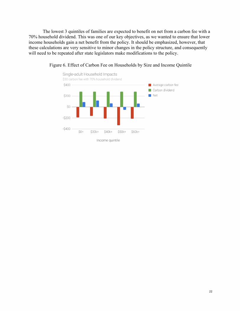
22

The lowest 3 quintiles of families are expected to benefit on net from a carbon fee with a 70% household dividend. This was one of our key objectives, as we wanted to ensure that lower income households gain a net benefit from the policy. It should be emphasized, however, that these calculations are very sensitive to minor changes in the policy structure, and consequently will need to be repeated after state legislators make modifications to the policy.

Figure 6. Effect of Carbon Fee on Households by Size and Income Quintile

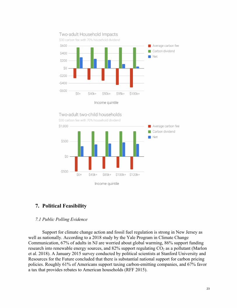
23

7. Political Feasibility

7.1 Public Polling Evidence

Support for climate change action and fossil fuel regulation is strong in New Jersey as well as nationally. According to a 2018 study by the Yale Program in Climate Change Communication, 67% of adults in NJ are worried about global warming, 86% support funding research into renewable energy sources, and 82% support regulating CO2 as a pollutant (Marlon et al. 2018). A January 2015 survey conducted by political scientists at Stanford University and Resources for the Future concluded that there is substantial national support for carbon pricing policies. Roughly 61% of Americans support taxing carbon-emitting companies, and 67% favor a tax that provides rebates to American households (RFF 2015).

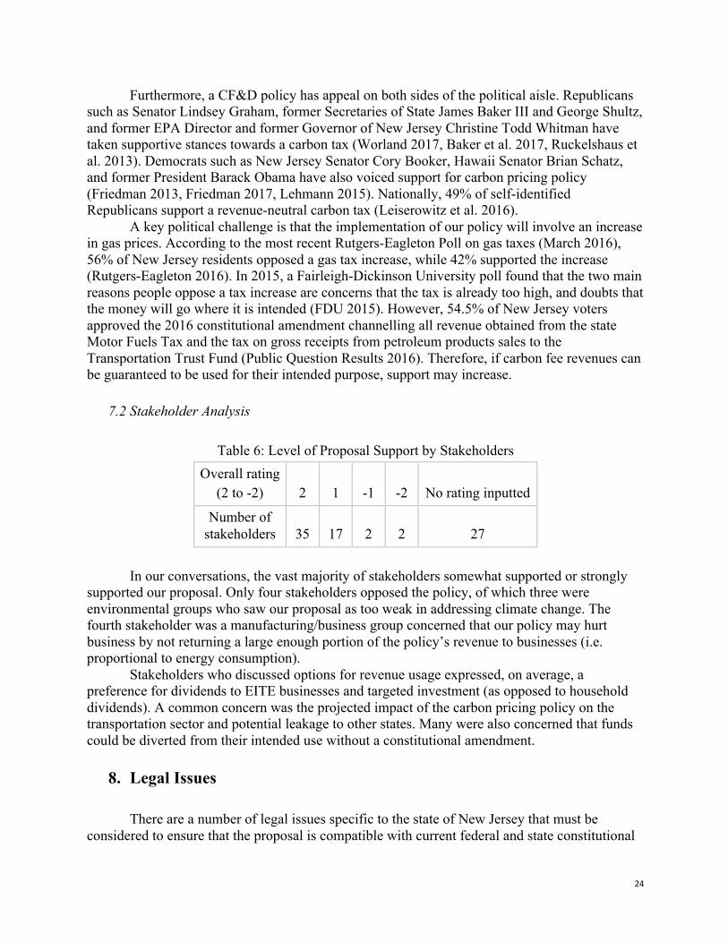
24

Furthermore, a CF&D policy has appeal on both sides of the political aisle. Republicans such as Senator Lindsey Graham, former Secretaries of State James Baker III and George Shultz, and former EPA Director and former Governor of New Jersey Christine Todd Whitman have taken supportive stances towards a carbon tax (Worland 2017, Baker et al. 2017, Ruckelshaus et al. 2013). Democrats such as New Jersey Senator Cory Booker, Hawaii Senator Brian Schatz, and former President Barack Obama have also voiced support for carbon pricing policy (Friedman 2013, Friedman 2017, Lehmann 2015). Nationally, 49% of self-identified Republicans support a revenue-neutral carbon tax (Leiserowitz et al. 2016).

A key political challenge is that the implementation of our policy will involve an increase in gas prices. According to the most recent Rutgers-Eagleton Poll on gas taxes (March 2016), 56% of New Jersey residents opposed a gas tax increase, while 42% supported the increase (Rutgers-Eagleton 2016). In 2015, a Fairleigh-Dickinson University poll found that the two main reasons people oppose a tax increase are concerns that the tax is already too high, and doubts that the money will go where it is intended (FDU 2015). However, 54.5% of New Jersey voters approved the 2016 constitutional amendment channelling all revenue obtained from the state Motor Fuels Tax and the tax on gross receipts from petroleum products sales to the Transportation Trust Fund (Public Question Results 2016). Therefore, if carbon fee revenues can be guaranteed to be used for their intended purpose, support may increase.

7.2 Stakeholder Analysis

Table 6: Level of Proposal Support by Stakeholders Overall rating

(2 to -2) 2 1 -1 -2 No rating inputted

Number of stakeholders 35 17 2 2 27

In our conversations, the vast majority of stakeholders somewhat supported or strongly

supported our proposal. Only four stakeholders opposed the policy, of which three were environmental groups who saw our proposal as too weak in addressing climate change. The fourth stakeholder was a manufacturing/business group concerned that our policy may hurt business by not returning a large enough portion of the policy’s revenue to businesses (i.e. proportional to energy consumption).

Stakeholders who discussed options for revenue usage expressed, on average, a preference for dividends to EITE businesses and targeted investment (as opposed to household dividends). A common concern was the projected impact of the carbon pricing policy on the transportation sector and potential leakage to other states. Many were also concerned that funds could be diverted from their intended use without a constitutional amendment.

8. Legal Issues

There are a number of legal issues specific to the state of New Jersey that must be considered to ensure that the proposal is compatible with current federal and state constitutional

25

law. In addition, it is necessary to consider the potential legal safeguards that can be implemented to prevent the CF&D revenue from being reallocated to other areas.

8.1 Interstate Commerce Clause:

The Dormant Commerce Clause is an implicit part of the US Constitution which prevents states from regulating commerce in favor of in-state businesses (U.S. Const. art. I, § 8). The potential for legal conflict arises upon consideration of how New Jersey obtains its energy supply. New Jersey imports its crude oil, natural gas and coal from neighboring states (particularly New York and Pennsylvania) because it does not produce any of these fuels (EIA 2018b). Consequently, the carbon fee will almost exclusively apply on imported fossil fuels.

The carbon fee, however, does not violate the Dormant Commerce Clause because it is applied at the first point of in-state sale. This practice is no different, from a legal standpoint, from the common practice of placing a sales tax on goods sold in-state but produced out-of-state. The legal interstate commerce issue is avoided because the fee is not applied at the interstate level; however it could not be applied to fuels being transported through New Jersey (Morris et al. 2016).

If the CF&D policy were to be challenged under the terms of the Dormant Commerce Clause, it would meet the legal requirements for waiving the clause. In Pike v. Bruce Church, Inc. (1970), the Supreme Court ruled that “Where the statute regulates evenhandedly to effectuate a legitimate local public interest, and its effects on interstate commerce are only incidental, it will be upheld unless the burden imposed on such commerce is clearly excessive in relation to the putative local benefits” (Justicia, 1970). The magnitude of the carbon fee depends on the fuel’s carbon content, not the location of energy production, so our policy treats in-state and out-of-state entities the same. The intention of the CF&D is to improve public health and environmental outcomes, both of which are in the “local public interest.” Assuming that one considers that said benefits outweigh the strain on interstate commerce, our proposed CF&D policy stands up to legal tests established by the U.S. Supreme Court and meets the requirements of the Dormant Commerce Clause.

8.2 Motor Fuels Tax Amendment:

A public referendum in 2016 approved a state constitutional amendment to dedicate all revenue from the Motor Fuels Tax and the Petroleum Products Gross Receipts Tax to the Transportation Trust Fund (TTF), whose capital is used to maintain and develop the state’s transportation system. This poses a challenge for our proposal because it would prevent us from using much of the revenue as a household dividend.

Although carbon fee revenues could be directed to the TTF for green transportation projects such as NJ Transit improvements, the scope of said projects would be limited by the agencies’ decisions, and the loss of dividend revenue could have regressive effects on consumers. Exempting CF&D from the TTF requirement would be preferable, allowing the fee revenue to go towards household dividends. According to correspondence with Professor Robert Williams from Rutgers University’s Center for State Constitutional Studies, this distinction could potentially be accomplished if the carbon fee were legally classified as a regulatory fee and not as a tax. New Jersey has judicial precedent stating that a specific fee can be classified as a

26

regulatory fee, provided that its primary purpose is not to raise general revenue, and that it is proportional to the cost of the action it prohibits. Several New Jersey court cases, including Bellington v. Township of East Windsor, Holmdel Builders Ass’n v. Township of Holmdel, and Resolution Trust Corp. v. Lanzaro, have upheld this standard. Provided that its primary objective is to tackle health and environmental concerns instead of raising government revenue, and that it is accurately priced to offset the harmful effects of carbon emissions, a carbon fee can satisfy both classification requirements (Henchman 2013).

8.3 Annual Appropriations Bill:

The New Jersey Supreme Court ruled in Burgos v. New Jersey that “each year's appropriations act will reflect the present legislative and executive judgment as to the budgetary priority” and therefore can supersede statutory legislation. This means that annual appropriations bills in New Jersey can reallocate funds away from their original purpose. In effect, during Chris Christie’s tenure, approximately $1.5 billion was diverted from the Clean Energy Fund to balance the budget, appropriating revenue initially intended for energy efficiency programs (Johnson 2017). Fund appropriation was the most commonly expressed concern among the stakeholders we talked with, as seven groups voiced this as their primary concern.

It is likely that a constitutional amendment to dedicate funds to a specific purpose would need to be passed alongside a CF&D policy, to protect funds destined for rebates or sustainable investment from appropriations raiding. Although such amendments require substantial political will and public support, there exists recent precedent: the 2017 amendment dedicating settlement funds from environmental contamination lawsuits to either the case’s costs or conservation and cleanup projects, as well as the 2016 Motor Fuels Tax amendment, are both good examples (NJ TTF 2018).

9. Conclusion

9.1 Lessons for Carbon Pricing Advocacy

Our stakeholder outreach has established that engagement with existing political and advocacy groups is critical. A robust discussion process that incorporates the priorities of state stakeholders can solve this issue. Based on our conversations, our proposal has changed from a 100% dividend to a 70% dividend and 30% investment model. In addition, policymakers’ main concerns are the household impacts, so a core point of our research is that low- and moderate-income households benefit on average. It is advisable to supplement carbon pricing with low-emissions alternatives, such as public transportation or electric vehicles. Government assistance may be needed to assist low-income households that cannot cope with the large upfront cost of many alternatives.

9.2 CF&D Policy Viability

We conclude that a CF&D policy is a politically feasible method of reducing carbon emissions in NJ without harming the state’s economy. It is important to note that many of the

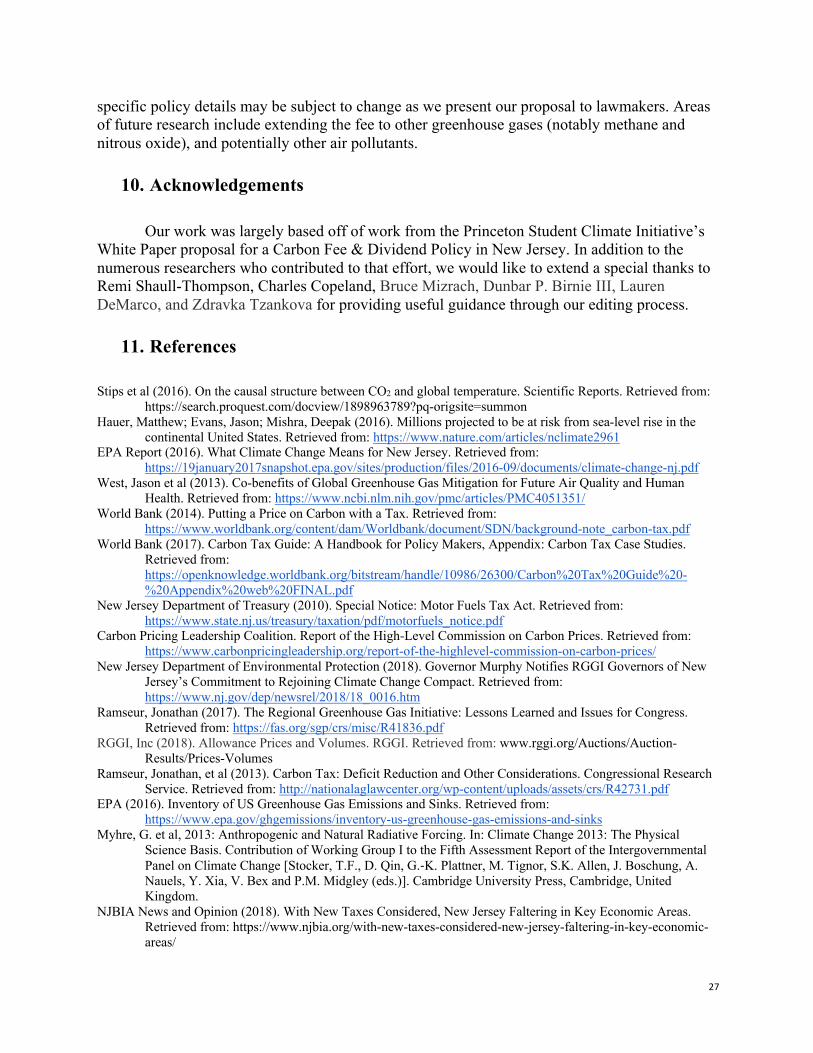
27

specific policy details may be subject to change as we present our proposal to lawmakers. Areas of future research include extending the fee to other greenhouse gases (notably methane and nitrous oxide), and potentially other air pollutants.

10. Acknowledgements

Our work was largely based off of work from the Princeton Student Climate Initiative’s White Paper proposal for a Carbon Fee & Dividend Policy in New Jersey. In addition to the numerous researchers who contributed to that effort, we would like to extend a special thanks to Remi Shaull-Thompson, Charles Copeland, Bruce Mizrach, Dunbar P. Birnie III, Lauren DeMarco, and Zdravka Tzankova for providing useful guidance through our editing process.

11. References Stips et al (2016). On the causal structure between CO2 and global temperature. Scientific Reports. Retrieved from:

https://search.proquest.com/docview/1898963789?pq-origsite=summon Hauer, Matthew; Evans, Jason; Mishra, Deepak (2016). Millions projected to be at risk from sea-level rise in the

continental United States. Retrieved from: https://www.nature.com/articles/nclimate2961 EPA Report (2016). What Climate Change Means for New Jersey. Retrieved from:

https://19january2017snapshot.epa.gov/sites/production/files/2016-09/documents/climate-change-nj.pdf West, Jason et al (2013). Co-benefits of Global Greenhouse Gas Mitigation for Future Air Quality and Human

Health. Retrieved from: https://www.ncbi.nlm.nih.gov/pmc/articles/PMC4051351/ World Bank (2014). Putting a Price on Carbon with a Tax. Retrieved from:

https://www.worldbank.org/content/dam/Worldbank/document/SDN/background-note_carbon-tax.pdf World Bank (2017). Carbon Tax Guide: A Handbook for Policy Makers, Appendix: Carbon Tax Case Studies.

Retrieved from: https://openknowledge.worldbank.org/bitstream/handle/10986/26300/Carbon%20Tax%20Guide%20-%20Appendix%20web%20FINAL.pdf

New Jersey Department of Treasury (2010). Special Notice: Motor Fuels Tax Act. Retrieved from: https://www.state.nj.us/treasury/taxation/pdf/motorfuels_notice.pdf

Carbon Pricing Leadership Coalition. Report of the High-Level Commission on Carbon Prices. Retrieved from: https://www.carbonpricingleadership.org/report-of-the-highlevel-commission-on-carbon-prices/

New Jersey Department of Environmental Protection (2018). Governor Murphy Notifies RGGI Governors of New Jersey’s Commitment to Rejoining Climate Change Compact. Retrieved from: https://www.nj.gov/dep/newsrel/2018/18_0016.htm

Ramseur, Jonathan (2017). The Regional Greenhouse Gas Initiative: Lessons Learned and Issues for Congress. Retrieved from: https://fas.org/sgp/crs/misc/R41836.pdf

RGGI, Inc (2018). Allowance Prices and Volumes. RGGI. Retrieved from: www.rggi.org/Auctions/Auction-Results/Prices-Volumes

Ramseur, Jonathan, et al (2013). Carbon Tax: Deficit Reduction and Other Considerations. Congressional Research Service. Retrieved from: http://nationalaglawcenter.org/wp-content/uploads/assets/crs/R42731.pdf

EPA (2016). Inventory of US Greenhouse Gas Emissions and Sinks. Retrieved from: https://www.epa.gov/ghgemissions/inventory-us-greenhouse-gas-emissions-and-sinks

Myhre, G. et al, 2013: Anthropogenic and Natural Radiative Forcing. In: Climate Change 2013: The Physical Science Basis. Contribution of Working Group I to the Fifth Assessment Report of the Intergovernmental Panel on Climate Change [Stocker, T.F., D. Qin, G.-K. Plattner, M. Tignor, S.K. Allen, J. Boschung, A. Nauels, Y. Xia, V. Bex and P.M. Midgley (eds.)]. Cambridge University Press, Cambridge, United Kingdom.

NJBIA News and Opinion (2018). With New Taxes Considered, New Jersey Faltering in Key Economic Areas. Retrieved from: https://www.njbia.org/with-new-taxes-considered-new-jersey-faltering-in-key-economic-areas/

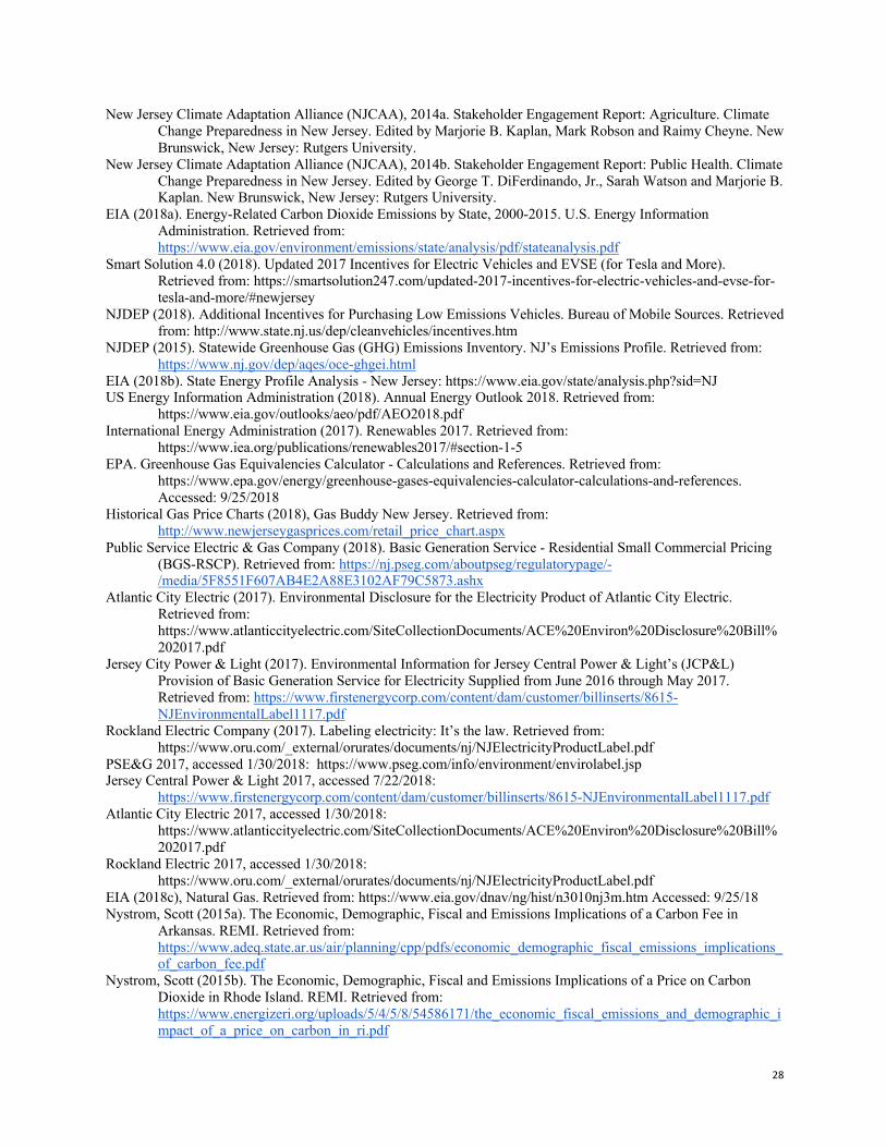
28

New Jersey Climate Adaptation Alliance (NJCAA), 2014a. Stakeholder Engagement Report: Agriculture. Climate Change Preparedness in New Jersey. Edited by Marjorie B. Kaplan, Mark Robson and Raimy Cheyne. New Brunswick, New Jersey: Rutgers University.

New Jersey Climate Adaptation Alliance (NJCAA), 2014b. Stakeholder Engagement Report: Public Health. Climate Change Preparedness in New Jersey. Edited by George T. DiFerdinando, Jr., Sarah Watson and Marjorie B. Kaplan. New Brunswick, New Jersey: Rutgers University.

EIA (2018a). Energy-Related Carbon Dioxide Emissions by State, 2000-2015. U.S. Energy Information Administration. Retrieved from: https://www.eia.gov/environment/emissions/state/analysis/pdf/stateanalysis.pdf

Smart Solution 4.0 (2018). Updated 2017 Incentives for Electric Vehicles and EVSE (for Tesla and More). Retrieved from: https://smartsolution247.com/updated-2017-incentives-for-electric-vehicles-and-evse-for-tesla-and-more/#newjersey

NJDEP (2018). Additional Incentives for Purchasing Low Emissions Vehicles. Bureau of Mobile Sources. Retrieved from: http://www.state.nj.us/dep/cleanvehicles/incentives.htm

NJDEP (2015). Statewide Greenhouse Gas (GHG) Emissions Inventory. NJ’s Emissions Profile. Retrieved from: https://www.nj.gov/dep/aqes/oce-ghgei.html

EIA (2018b). State Energy Profile Analysis - New Jersey: https://www.eia.gov/state/analysis.php?sid=NJ US Energy Information Administration (2018). Annual Energy Outlook 2018. Retrieved from:

https://www.eia.gov/outlooks/aeo/pdf/AEO2018.pdf International Energy Administration (2017). Renewables 2017. Retrieved from:

https://www.iea.org/publications/renewables2017/#section-1-5 EPA. Greenhouse Gas Equivalencies Calculator - Calculations and References. Retrieved from:

https://www.epa.gov/energy/greenhouse-gases-equivalencies-calculator-calculations-and-references. Accessed: 9/25/2018

Historical Gas Price Charts (2018), Gas Buddy New Jersey. Retrieved from: http://www.newjerseygasprices.com/retail_price_chart.aspx

Public Service Electric & Gas Company (2018). Basic Generation Service - Residential Small Commercial Pricing (BGS-RSCP). Retrieved from: https://nj.pseg.com/aboutpseg/regulatorypage/-/media/5F8551F607AB4E2A88E3102AF79C5873.ashx

Atlantic City Electric (2017). Environmental Disclosure for the Electricity Product of Atlantic City Electric. Retrieved from: https://www.atlanticcityelectric.com/SiteCollectionDocuments/ACE%20Environ%20Disclosure%20Bill%202017.pdf

Jersey City Power & Light (2017). Environmental Information for Jersey Central Power & Light’s (JCP&L) Provision of Basic Generation Service for Electricity Supplied from June 2016 through May 2017. Retrieved from: https://www.firstenergycorp.com/content/dam/customer/billinserts/8615-NJEnvironmentalLabel1117.pdf

Rockland Electric Company (2017). Labeling electricity: It’s the law. Retrieved from: https://www.oru.com/_external/orurates/documents/nj/NJElectricityProductLabel.pdf

PSE&G 2017, accessed 1/30/2018: https://www.pseg.com/info/environment/envirolabel.jsp Jersey Central Power & Light 2017, accessed 7/22/2018:

https://www.firstenergycorp.com/content/dam/customer/billinserts/8615-NJEnvironmentalLabel1117.pdf Atlantic City Electric 2017, accessed 1/30/2018:

https://www.atlanticcityelectric.com/SiteCollectionDocuments/ACE%20Environ%20Disclosure%20Bill%202017.pdf

Rockland Electric 2017, accessed 1/30/2018: https://www.oru.com/_external/orurates/documents/nj/NJElectricityProductLabel.pdf

EIA (2018c), Natural Gas. Retrieved from: https://www.eia.gov/dnav/ng/hist/n3010nj3m.htm Accessed: 9/25/18 Nystrom, Scott (2015a). The Economic, Demographic, Fiscal and Emissions Implications of a Carbon Fee in

Arkansas. REMI. Retrieved from: https://www.adeq.state.ar.us/air/planning/cpp/pdfs/economic_demographic_fiscal_emissions_implications_of_carbon_fee.pdf

Nystrom, Scott (2015b). The Economic, Demographic, Fiscal and Emissions Implications of a Price on Carbon Dioxide in Rhode Island. REMI. Retrieved from: https://www.energizeri.org/uploads/5/4/5/8/54586171/the_economic_fiscal_emissions_and_demographic_impact_of_a_price_on_carbon_in_ri.pdf

29

Nystrom, Scott (2014). The Economic, Demographic, Fiscal and Emissions Implications from a Carbon Price Policy in Vermont. REMI. Retrieved from: https://www.energyindependentvt.org/wp-content/uploads/2015/04/REMI_Final.pdf

Breslow et al (2014). Analysis of a Carbon Fee or Tax as a Mechanism to Reduce GHG Emissions in Massachusetts. Retrieved from: https://www.mass.gov/files/documents/2016/08/pg/mass-carbon-tax-study.pdf

Forecasting and Research Division, Office of Financial Management (2015). Washington State, Economic Modeling of Greenhouse Gas Emission Reductions. Retrieved from: https://www.governor.wa.gov/sites/default/files/documents/WhitePaper_CarbonEmissionReductionsMarch2015.pdf

Nystrom, Scott; Luckow, Patrick (2014). The Economic, Climate, Fiscal, Power and Demographic Implications of a National Fee-and-Dividend Carbon Tax. REMI, Synapse. Retrieved from: http://citizensclimatelobby.org/wp-content/uploads/2014/06/REMI-carbon-tax-report-62141.pdf

2016 Employment Data (Annual Average). http://lwd.state.nj.us/labor/lpa/employ/ces/ces_index.html Downloaded 1/25/2018.

Statista (2018). GDP of British Columbia, Canada 2000-2017. Retrieved from: https://www.statista.com/statistics/577563/gdp-of-british-columbia-canada/

NJ Department of Labor and Workforce Development (2018). Current Employment Statistics. Retrieved from: https://www.nj.gov/labor/lpa/employ/ces/ces_index.html

EPA FLIGHT Database (2016). 2016 Greenhouse Gas Emissions from Large Facilities. Retrieved from: https://ghgdata.epa.gov/ghgp/main.do, accessed 1/30/2018. We first select the state “New Jersey”, then select the "All Fuel Combustion" option under "Emissions by Fuel Type", and finally only select the "CO2" option under "Greenhouse Gas Emissions".

EIA (2015). New Jersey Rankings: Total Carbon Dioxide Emissions, 2015. Retrieved from: https://www.eia.gov/state/rankings/?sid=NJ#series/226

Gholami, Zahra (2014). Case Study on the Effectiveness of Carbon Pricing Estimating the Impact of Carbon Tax on Natural Gas Demand on British Columbia. Retrieved from: https://open.library.ubc.ca/cIRcle/collections/ubctheses/24/items/1.0166938

Rivers, Nicholas and Schaufele, Brandon (2015). Salience of carbon taxes in the gasoline market. Journal of Environmental Economics and Management. Retrieved from: https://www.sciencedirect.com/science/article/pii/S0095069615000613

Rodio, Brian (2016). Analyzing British Columbia’s Carbon Tax. Retrieved from: https://publicpolicy.wharton.upenn.edu/live/news/1520-analyzing-british-columbias-carbon-tax

IPCC 4th Assessment Report (2007). Carbon Leakage. Retrieved from: https://www.ipcc.ch/publications_and_data/ar4/wg3/en/ch11s11-7-2.html

Caron, Justin et al (2014). Leakage from sub-national climate policy: The case of California’s cap-and-trade program. Retrieved from: https://www.researchgate.net/profile/Justin_Caron/publication/267508014_Leakage_from_Sub-national_Climate_Policy_The_Case_of_California's_Cap-and-Trade_Program/links/5451001a0cf249aa53dc8dd5/Leakage-from-Sub-national-Climate-Policy-The-Case-of-Californias-Cap-and-Trade-Program.pdf

AAANY Gas Prices (accessed 2/16/2018). Retrieved from: https://gasprices.aaa.com/state-gas-price-averages/ EIA (2017). Carbon Dioxide Emissions Coefficients. Retrieved from:

https://www.eia.gov/environment/emissions/co2_vol_mass.php World Population Review (2018). New Jersey Population 2018. Retrieved from:

http://worldpopulationreview.com/states/new-jersey-population/ EIA (2009). 2009 Residential Energy Consumption Survey Data. Retrieved from:

https://www.eia.gov/consumption/residential/data/2009/ Bureau of Labor Statistics (2015). Consumer Expenditures in 2015. Retrieved from:

https://www.bls.gov/opub/reports/consumer-expenditures/2015/home.htm EIA (2016). Table CT8. Electric Power Sector Consumption Estimates, 1960-2016, New Jersey. Retrieved from:

https://www.eia.gov/state/seds/data.php?incfile=/state/seds/sep_use/eu/use_eu_NJ.html&sid=NJ Marlon et al (2018). Yale Climate Opinion Maps - U.S. 2018. Yale Program on Climate Change Communication.

Retrieved from: http://climatecommunication.yale.edu/visualizations-data/ycom-us-2018/ Resources for the Future (2015). Global Warming National Poll. Retrieved from:

http://www.rff.org/files/sharepoint/Documents/RFF-NYTimes-Stanford-global-warming-poll-Jan-2015-topline-part-3.pdf

30

Worland, Justin (2017). Republican Senator Endorses ‘Price on Carbon’ to Fight Climate Change. Time. Retrieved from: http://time.com/4947960/lindsay-graham-climate-change-carbon-tax/

Baker et al. (2017). Climate Leadership Council: The Conservative Case for Carbon Dividends. Retrieved from: https://www.clcouncil.org/media/TheConservativeCaseforCarbonDividends.pdf

Ruckelshaus et. al. (2013). A Republican Case for Climate Action. New York Times. Retrieved from: https://www.nytimes.com/2013/08/02/opinion/a-republican-case-for-climate-action.html

Friedman, Matt (2013). Where Cory Booker and Steve Lonegan Stand on the Issues. NJ.com. Retrieved from: https://www.nj.com/politics/index.ssf/2013/10/where_cory_booker_and_steve_lonegan_stand_on_the_issues.html

Friedman, Lisa (2017). Some Democrats See Tax Overhaul as a Path to Taxing Carbon. New York Times. Retrieved from: https://www.nytimes.com/2017/08/17/climate/carbon-tax-reform-climate-change.html

Lehmann, Evan (2015). Obama Calls Carbon Price Better Than Regulations. Scientific American. Retrieved from: https://www.scientificamerican.com/article/obama-calls-carbon-price-better-than-regulations/

Leiserowitz et. al. (2016). Politics & Global Warming, November 2016. Yale Program on Climate Change Communication. Retrieved from: http://climatecommunication.yale.edu/publications/politics-global-warming-november-2016/2/

Rutgers-Eagleton Poll (2016). New Jerseyans Continue to Oppose Gas Tax Hike; Possible Estate Tax Trade-Off Does Little to Boost Support. Gas Tax Archives - Center for Public Interest Polling. Retrieved from: http://eagletonpoll.rutgers.edu/category/gas-tax/

Fairleigh-Dickinson University Poll (2015). Policymakers Face a Bumpy Road with Taxpayers Over the Gas Tax. Retrieved from: http://view2.fdu.edu/publicmind/2015/151119/

Public Question Results (2016). Retrieved from: http://www.njelections.org/2016-results/2016-official-general-results-question2.pdf

National Archives. The Constitution of the United States: A Transcription. Retrieved from: https://www.archives.gov/founding-docs/constitution-transcript

Morris et al. (2016). State-Level Carbon Taxes: Options and Opportunities for Policymakers. Retrieved from: https://www.brookings.edu/wp-content/uploads/2016/07/State-level-carbon-taxes-Options-and-opportunities-for-policymakers.pdf

Justicia (1970). Pike v. Bruce Church, Inc., 397 U.S. 137 (1970). Retrieved from: https://supreme.justia.com/cases/federal/us/397/137/

NJ Transportation Trust Fund Authority (2018). Appropriation Revenies. Retrieved from: https://www.state.nj.us/ttfa/financing/apprevenues.shtm

Henchman, Joseph (2013). How Is The Money Used? Federal and State Cases Distinguishing Taxes and Fees. Tax Foundation. Retrieved from: https://files.taxfoundation.org/legacy/docs/TaxesandFeesBook.pdf

Justia US Law. Burgos v. New Jersey. Retrieved from: https://law.justia.com/cases/new-jersey/supreme-court/2015/a-55-04.html

Johnson, Tom (2017). Clean Energy Fund Raided (Again) to Plug Last Hole in State Budget. NJ Spotlight. Retrieved from: http://www.njspotlight.com/stories/17/06/26/clean-energy-fund-raided-again-to-plug-last-hole-in-state-budget/

NJ Transportation Trust Fund Authority (2018). Frequently Asked Questions. Retrieved from: https://www.nj.gov/ttfa/faq/

Justicia US Supreme Court (1970). Pike v. Bruce Church, Inc., 397 U.S. 137 (1970). Retrieved from: https://supreme.justia.com/cases/federal/us/397/137/

Xiang, Di; Lawley, Chad (2018). The Impact of British Columbia’s Carbon Tax on Residential Natural Gas Consumption. Energy Economics, Vol. 80. Retrieved from: https://doi.org/10.1016/j.eneco.2018.12.004

Yamazaki, Akio (2017). Jobs and Climate Policy: Evidence from British Columbia’s Revenue Neutral Carbon Tax. Journal of Environmental Economics and Management, Vol. 83. Retrieved from: https://doi.org/10.1016/j.jeem.2017.03.003

Metcalf, Gilbert (2015). A Conceptual Framework for Measuring the Effectiveness of Green Fiscal Reforms. Green Growth Knowledge Platform. Retrieved from: http://www.greengrowthknowledge.org/sites/default/files/Metcalf_A_Conceptual_Framework_for_Measuring_the_Effectiveness_of_Green_Fiscal.pdf

Murray, Brian; Rivers, Nicholas (2015). British Columbia’s Revenue Neutral Carbon Tax: A Review of the Latest “Grand Experiment” in Environmental Policy. Energy Policy, Vol. 86. Retrieved from: https://doi.org/10.1016/j.enpol.2015.08.011

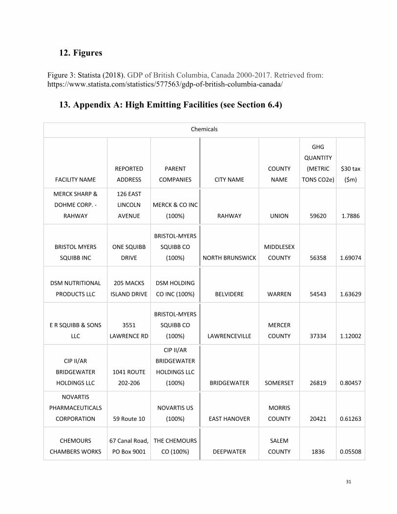
31

12. Figures

Figure 3: Statista (2018). GDP of British Columbia, Canada 2000-2017. Retrieved from: https://www.statista.com/statistics/577563/gdp-of-british-columbia-canada/

13. Appendix A: High Emitting Facilities (see Section 6.4)

Chemicals

FACILITY NAME

REPORTED

ADDRESS

PARENT

COMPANIES CITY NAME

COUNTY

NAME

GHG

QUANTITY

(METRIC

TONS CO2e)

$30 tax

($m)

MERCK SHARP &

DOHME CORP. -

RAHWAY

126 EAST

LINCOLN

AVENUE

MERCK & CO INC

(100%) RAHWAY UNION 59620 1.7886

BRISTOL MYERS

SQUIBB INC

ONE SQUIBB

DRIVE

BRISTOL-MYERS

SQUIBB CO

(100%) NORTH BRUNSWICK

MIDDLESEX

COUNTY 56358 1.69074

DSM NUTRITIONAL

PRODUCTS LLC

205 MACKS

ISLAND DRIVE

DSM HOLDING

CO INC (100%) BELVIDERE WARREN 54543 1.63629

E R SQUIBB & SONS

LLC

3551

LAWRENCE RD

BRISTOL-MYERS

SQUIBB CO

(100%) LAWRENCEVILLE

MERCER

COUNTY 37334 1.12002

CIP II/AR

BRIDGEWATER

HOLDINGS LLC

1041 ROUTE

202-206

CIP II/AR

BRIDGEWATER

HOLDINGS LLC

(100%) BRIDGEWATER SOMERSET 26819 0.80457

NOVARTIS

PHARMACEUTICALS

CORPORATION 59 Route 10

NOVARTIS US

(100%) EAST HANOVER

MORRIS

COUNTY 20421 0.61263

CHEMOURS

CHAMBERS WORKS

67 Canal Road,

PO Box 9001

THE CHEMOURS

CO (100%) DEEPWATER

SALEM

COUNTY 1836 0.05508

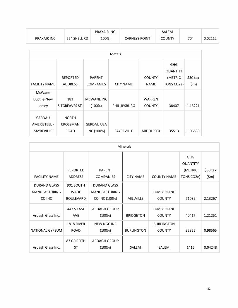
32

PRAXAIR INC 554 SHELL RD

PRAXAIR INC

(100%) CARNEYS POINT

SALEM

COUNTY 704 0.02112

Metals

FACILITY NAME

REPORTED

ADDRESS

PARENT

COMPANIES CITY NAME

COUNTY

NAME

GHG

QUANTITY

(METRIC

TONS CO2e)

$30 tax

($m)

McWane

Ductile-New

Jersey

183

SITGREAVES ST.

MCWANE INC

(100%) PHILLIPSBURG

WARREN

COUNTY 38407 1.15221

GERDAU

AMERISTEEL -

SAYREVILLE

NORTH

CROSSMAN

ROAD

GERDAU USA

INC (100%) SAYREVILLE MIDDLESEX 35513 1.06539

Minerals

FACILITY NAME

REPORTED

ADDRESS

PARENT

COMPANIES CITY NAME COUNTY NAME

GHG

QUANTITY

(METRIC

TONS CO2e)

$30 tax

($m)

DURAND GLASS

MANUFACTURING

CO INC

901 SOUTH

WADE

BOULEVARD

DURAND GLASS

MANUFACTURING

CO INC (100%) MILLVILLE

CUMBERLAND

COUNTY 71089 2.13267

Ardagh Glass Inc.

443 S EAST

AVE

ARDAGH GROUP

(100%) BRIDGETON

CUMBERLAND

COUNTY 40417 1.21251

NATIONAL GYPSUM

1818 RIVER

ROAD

NEW NGC INC

(100%) BURLINGTON

BURLINGTON

COUNTY 32855 0.98565

Ardagh Glass Inc.

83 GRIFFITH

ST

ARDAGH GROUP

(100%) SALEM SALEM 1416 0.04248

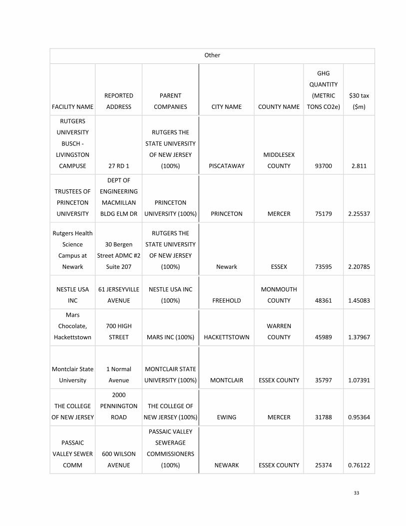
33

Other

FACILITY NAME

REPORTED

ADDRESS

PARENT


GHG

QUANTITY

(METRIC

TONS CO2e)

$30 tax

($m)

RUTGERS

UNIVERSITY

BUSCH -

LIVINGSTON

CAMPUSE 27 RD 1

RUTGERS THE

STATE UNIVERSITY

OF NEW JERSEY

(100%) PISCATAWAY

MIDDLESEX

COUNTY 93700 2.811

TRUSTEES OF

PRINCETON

UNIVERSITY

DEPT OF

ENGINEERING

MACMILLAN

BLDG ELM DR

PRINCETON

UNIVERSITY (100%) PRINCETON MERCER 75179 2.25537

Rutgers Health

Science

Campus at

Newark

30 Bergen

Street ADMC #2

Suite 207

RUTGERS THE

STATE UNIVERSITY

OF NEW JERSEY

(100%) Newark ESSEX 73595 2.20785

NESTLE USA

INC

61 JERSEYVILLE

AVENUE

NESTLE USA INC

(100%) FREEHOLD

MONMOUTH

COUNTY 48361 1.45083

Mars

Chocolate,

Hackettstown

700 HIGH

STREET MARS INC (100%) HACKETTSTOWN

WARREN

COUNTY 45989 1.37967

Montclair State

University

1 Normal

Avenue

MONTCLAIR STATE

UNIVERSITY (100%) MONTCLAIR ESSEX COUNTY 35797 1.07391

THE COLLEGE

OF NEW JERSEY

2000

PENNINGTON

ROAD

THE COLLEGE OF

NEW JERSEY (100%) EWING MERCER 31788 0.95364

PASSAIC

VALLEY SEWER

COMM

600 WILSON

AVENUE

PASSAIC VALLEY

SEWERAGE

COMMISSIONERS

(100%) NEWARK ESSEX COUNTY 25374 0.76122

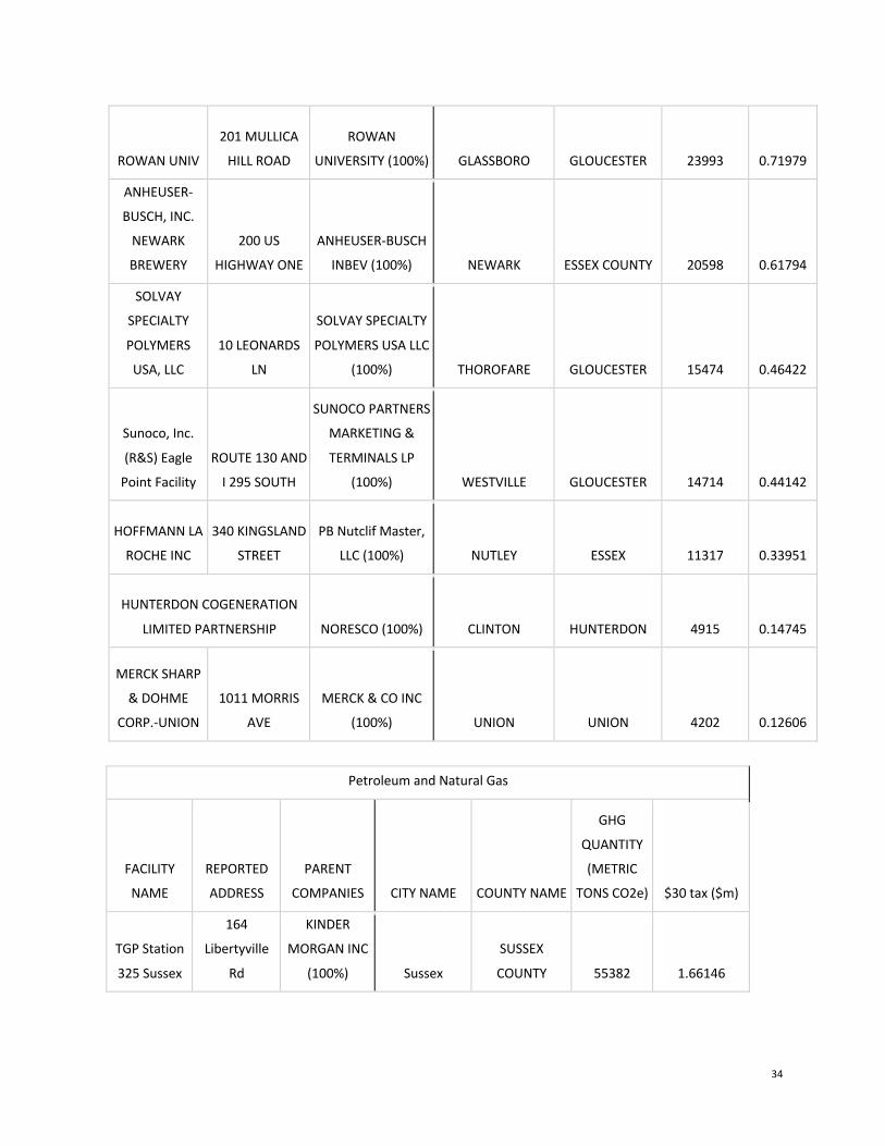
34

ROWAN UNIV

201 MULLICA

HILL ROAD

ROWAN

UNIVERSITY (100%) GLASSBORO GLOUCESTER 23993 0.71979

ANHEUSER-

BUSCH, INC.

NEWARK

BREWERY

200 US

HIGHWAY ONE

ANHEUSER-BUSCH

INBEV (100%) NEWARK ESSEX COUNTY 20598 0.61794

SOLVAY

SPECIALTY

POLYMERS

USA, LLC

10 LEONARDS

LN

SOLVAY SPECIALTY

POLYMERS USA LLC

(100%) THOROFARE GLOUCESTER 15474 0.46422

Sunoco, Inc.

(R&S) Eagle

Point Facility

ROUTE 130 AND

I 295 SOUTH

SUNOCO PARTNERS

MARKETING &

TERMINALS LP

(100%) WESTVILLE GLOUCESTER 14714 0.44142

HOFFMANN LA

ROCHE INC

340 KINGSLAND

STREET

PB Nutclif Master,

LLC (100%) NUTLEY ESSEX 11317 0.33951

HUNTERDON COGENERATION

LIMITED PARTNERSHIP NORESCO (100%) CLINTON HUNTERDON 4915 0.14745

MERCK SHARP

& DOHME

CORP.-UNION

1011 MORRIS

AVE

MERCK & CO INC

(100%) UNION UNION 4202 0.12606

Petroleum and Natural Gas

FACILITY

NAME

REPORTED

ADDRESS

PARENT


GHG

QUANTITY

(METRIC

TONS CO2e) $30 tax ($m)

TGP Station

325 Sussex

164

Libertyville

Rd

KINDER

MORGAN INC

(100%) Sussex

SUSSEX

COUNTY 55382 1.66146

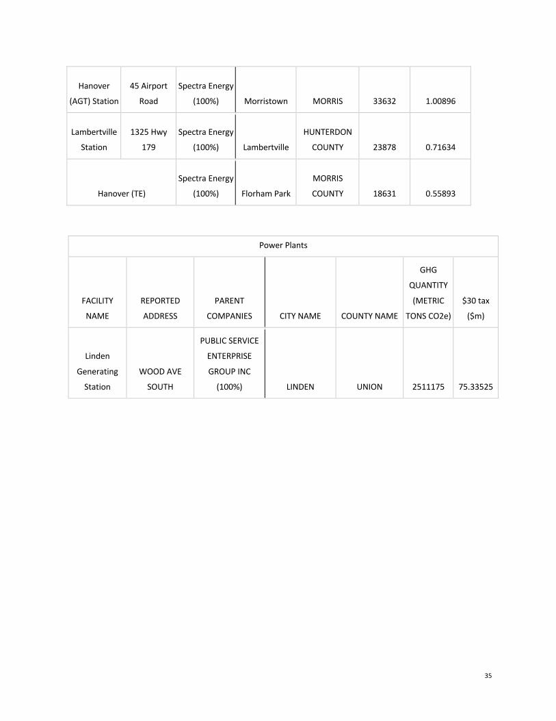
35

Hanover

(AGT) Station

45 Airport

Road

Spectra Energy

(100%) Morristown MORRIS 33632 1.00896

Lambertville

Station

1325 Hwy

179

Spectra Energy

(100%) Lambertville

HUNTERDON

COUNTY 23878 0.71634

Hanover (TE)

Spectra Energy

(100%) Florham Park

MORRIS

COUNTY 18631 0.55893

Power Plants

FACILITY

NAME

REPORTED

ADDRESS

PARENT


GHG

QUANTITY

(METRIC

TONS CO2e)

$30 tax

($m)

Linden

Generating

Station

WOOD AVE

SOUTH

PUBLIC SERVICE

ENTERPRISE

GROUP INC

(100%) LINDEN UNION 2511175 75.33525

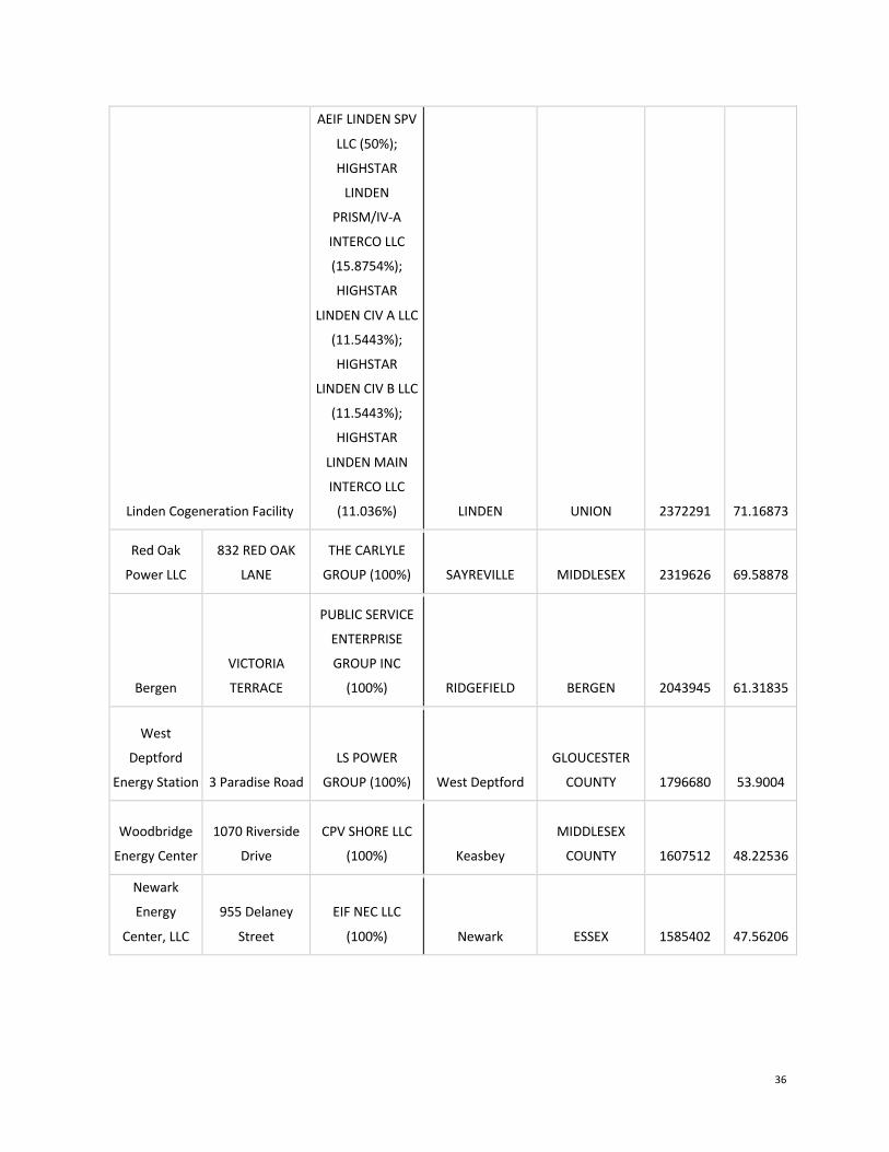
36

Linden Cogeneration Facility

AEIF LINDEN SPV

LLC (50%);

HIGHSTAR

LINDEN

PRISM/IV-A

INTERCO LLC

(15.8754%);

HIGHSTAR

LINDEN CIV A LLC

(11.5443%);

HIGHSTAR

LINDEN CIV B LLC

(11.5443%);

HIGHSTAR

LINDEN MAIN

INTERCO LLC

(11.036%) LINDEN UNION 2372291 71.16873

Red Oak

Power LLC

832 RED OAK

LANE

THE CARLYLE

GROUP (100%) SAYREVILLE MIDDLESEX 2319626 69.58878

Bergen

VICTORIA

TERRACE

PUBLIC SERVICE

ENTERPRISE

GROUP INC

(100%) RIDGEFIELD BERGEN 2043945 61.31835

West

Deptford

Energy Station 3 Paradise Road

LS POWER

GROUP (100%) West Deptford

GLOUCESTER

COUNTY 1796680 53.9004

Woodbridge

Energy Center

1070 Riverside

Drive

CPV SHORE LLC

(100%) Keasbey

MIDDLESEX

COUNTY 1607512 48.22536

Newark

Energy

Center, LLC

955 Delaney

Street

EIF NEC LLC

(100%) Newark ESSEX 1585402 47.56206

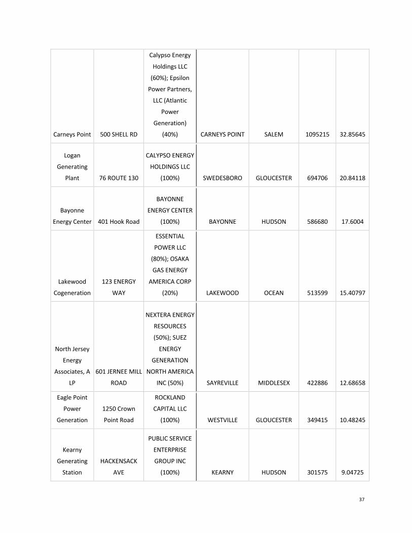
37

Carneys Point 500 SHELL RD

Calypso Energy

Holdings LLC

(60%); Epsilon

Power Partners,

LLC (Atlantic

Power

Generation)

(40%) CARNEYS POINT SALEM 1095215 32.85645

Logan

Generating

Plant 76 ROUTE 130

CALYPSO ENERGY

HOLDINGS LLC

(100%) SWEDESBORO GLOUCESTER 694706 20.84118

Bayonne

Energy Center 401 Hook Road

BAYONNE

ENERGY CENTER

(100%) BAYONNE HUDSON 586680 17.6004

Lakewood

Cogeneration

123 ENERGY

WAY

ESSENTIAL

POWER LLC

(80%); OSAKA

GAS ENERGY

AMERICA CORP

(20%) LAKEWOOD OCEAN 513599 15.40797

North Jersey

Energy

Associates, A

LP

601 JERNEE MILL

ROAD

NEXTERA ENERGY

RESOURCES

(50%); SUEZ

ENERGY

GENERATION

NORTH AMERICA

INC (50%) SAYREVILLE MIDDLESEX 422886 12.68658

Eagle Point

Power

Generation

1250 Crown

Point Road

ROCKLAND

CAPITAL LLC

(100%) WESTVILLE GLOUCESTER 349415 10.48245

Kearny

Generating

Station

HACKENSACK

AVE

PUBLIC SERVICE

ENTERPRISE

GROUP INC

(100%) KEARNY HUDSON 301575 9.04725

38

Hudson

Generating

Station

DUFFIELD AND

VAN KEUREN

AVE

PUBLIC SERVICE

ENTERPRISE

GROUP INC

(100%) JERSEY CITY HUDSON 224991 6.74973

Bayonne Plant

Holding, LLC 10 HOOK ROAD

TALEN ENERGY

CORP (100%) BAYONNE HUDSON 215907 6.47721

Ocean

Peaking

Power, LP

123 ENERGY

WAY

ESSENTIAL

POWER LLC

(100%) LAKEWOOD OCEAN 195044 5.85132

Newark Bay

Cogen 414 462 AVE P

TALEN ENERGY

CORP (100%) NEWARK ESSEX 174543 5.23629

Camden Plant

Holding, LLC

570 CHELTON

AVE

TALEN ENERGY

CORP (100%) CAMDEN CAMDEN 144775 4.34325

B L England

900 NORTH

SHORE ROAD

ROCKLAND

CAPITAL LLC

(100%) MARMORA Cape May 94456 2.83368

Pedricktown

Cogeneration

Plant

143 HIGHWAY

130

TALEN ENERGY

CORP (100%) PEDRICKTOWN SALEM 80340 2.4102

Howard M

Down 211 N WEST AVE

CITY OF

VINELAND (100%) VINELAND Cumberland 76050 2.2815

E F

Kenilworth,

Inc.

2000 GALLOPING

HILL RD BLDG K-

14

ATLANTIC POWER

CORP (100%) KENILWORTH UNION 75741 2.27223

Clayville

4087 S. Lincoln

Ave.

CITY OF

VINELAND (100%) Vineland

CUMBERLAND

COUNTY 67943 2.03829

Cumberland

Energy Center

4001 EAST MAIN

ST

CALPINE CORP

(100%) MILLVILLE Cumberland 60182 1.80546

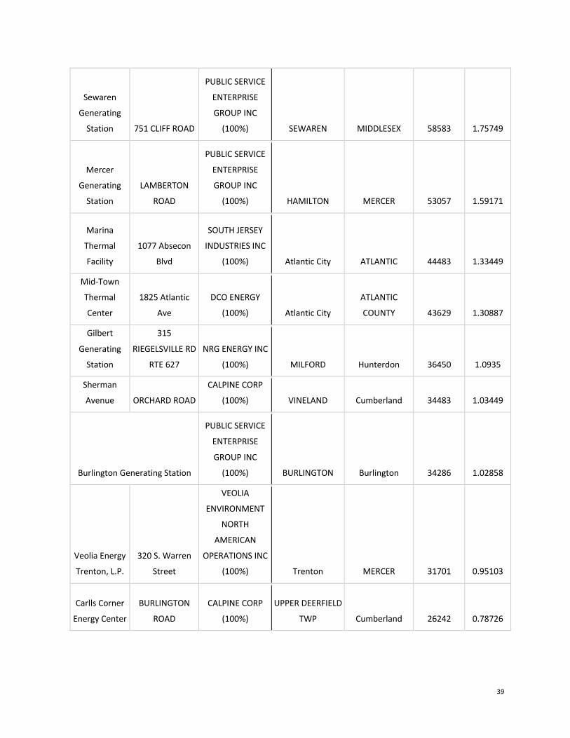
39

Sewaren

Generating

Station 751 CLIFF ROAD

PUBLIC SERVICE

ENTERPRISE

GROUP INC

(100%) SEWAREN MIDDLESEX 58583 1.75749

Mercer

Generating

Station

LAMBERTON

ROAD

PUBLIC SERVICE

ENTERPRISE

GROUP INC

(100%) HAMILTON MERCER 53057 1.59171

Marina

Thermal

Facility

1077 Absecon

Blvd

SOUTH JERSEY

INDUSTRIES INC

(100%) Atlantic City ATLANTIC 44483 1.33449

Mid-Town

Thermal

Center

1825 Atlantic

Ave

DCO ENERGY

(100%) Atlantic City

ATLANTIC

COUNTY 43629 1.30887

Gilbert

Generating

Station

315

RIEGELSVILLE RD

RTE 627

NRG ENERGY INC

(100%) MILFORD Hunterdon 36450 1.0935

Sherman

Avenue ORCHARD ROAD

CALPINE CORP

(100%) VINELAND Cumberland 34483 1.03449

Burlington Generating Station

PUBLIC SERVICE

ENTERPRISE

GROUP INC

(100%) BURLINGTON Burlington 34286 1.02858

Veolia Energy

Trenton, L.P.

320 S. Warren

Street

VEOLIA

ENVIRONMENT

NORTH

AMERICAN

OPERATIONS INC

(100%) Trenton MERCER 31701 0.95103

Carlls Corner

Energy Center

BURLINGTON

ROAD

CALPINE CORP

(100%)

UPPER DEERFIELD

TWP Cumberland 26242 0.78726

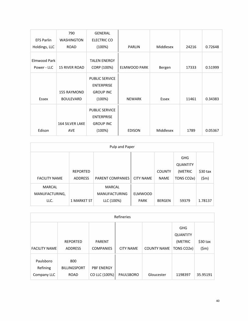
40

EFS Parlin

Holdings, LLC

790

WASHINGTON

ROAD

GENERAL

ELECTRIC CO

(100%) PARLIN Middlesex 24216 0.72648

Elmwood Park

Power - LLC 15 RIVER ROAD

TALEN ENERGY

CORP (100%) ELMWOOD PARK Bergen 17333 0.51999

Essex

155 RAYMOND

BOULEVARD

PUBLIC SERVICE

ENTERPRISE

GROUP INC

(100%) NEWARK Essex 11461 0.34383

Edison

164 SILVER LAKE

AVE

PUBLIC SERVICE

ENTERPRISE

GROUP INC

(100%) EDISON Middlesex 1789 0.05367

Pulp and Paper

FACILITY NAME

REPORTED

ADDRESS PARENT COMPANIES CITY NAME

COUNTY

NAME

GHG

QUANTITY

(METRIC

TONS CO2e)

$30 tax

($m)

MARCAL

MANUFACTURING,

LLC. 1 MARKET ST

MARCAL

MANUFACTURING

LLC (100%)

ELMWOOD

PARK BERGEN 59379 1.78137

Refineries

FACILITY NAME

REPORTED

ADDRESS

PARENT


GHG

QUANTITY

(METRIC

TONS CO2e)

$30 tax

($m)

Paulsboro

Refining

Company LLC

800

BILLINGSPORT

ROAD

PBF ENERGY

CO LLC (100%) PAULSBORO Gloucester 1198397 35.95191

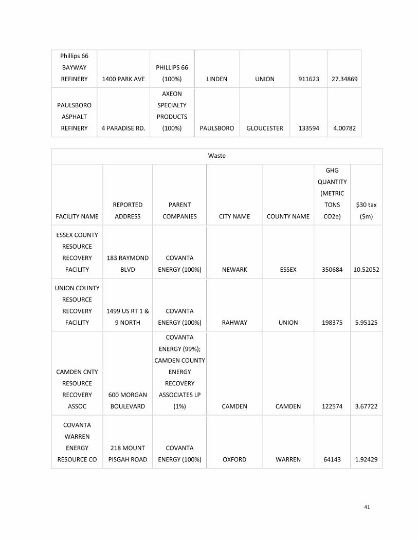
41

Phillips 66

BAYWAY

REFINERY 1400 PARK AVE

PHILLIPS 66

(100%) LINDEN UNION 911623 27.34869

PAULSBORO

ASPHALT

REFINERY 4 PARADISE RD.

AXEON

SPECIALTY

PRODUCTS

(100%) PAULSBORO GLOUCESTER 133594 4.00782

Waste

FACILITY NAME

REPORTED

ADDRESS

PARENT


GHG

QUANTITY

(METRIC

TONS

CO2e)

$30 tax

($m)

ESSEX COUNTY

RESOURCE

RECOVERY

FACILITY

183 RAYMOND

BLVD

COVANTA

ENERGY (100%) NEWARK ESSEX 350684 10.52052

UNION COUNTY

RESOURCE

RECOVERY

FACILITY

1499 US RT 1 &

9 NORTH

COVANTA

ENERGY (100%) RAHWAY UNION 198375 5.95125

CAMDEN CNTY

RESOURCE

RECOVERY

ASSOC

600 MORGAN

BOULEVARD

COVANTA

ENERGY (99%);

CAMDEN COUNTY

ENERGY

RECOVERY

ASSOCIATES LP

(1%) CAMDEN CAMDEN 122574 3.67722

COVANTA

WARREN

ENERGY

RESOURCE CO

218 MOUNT

PISGAH ROAD

COVANTA

ENERGY (100%) OXFORD WARREN 64143 1.92429

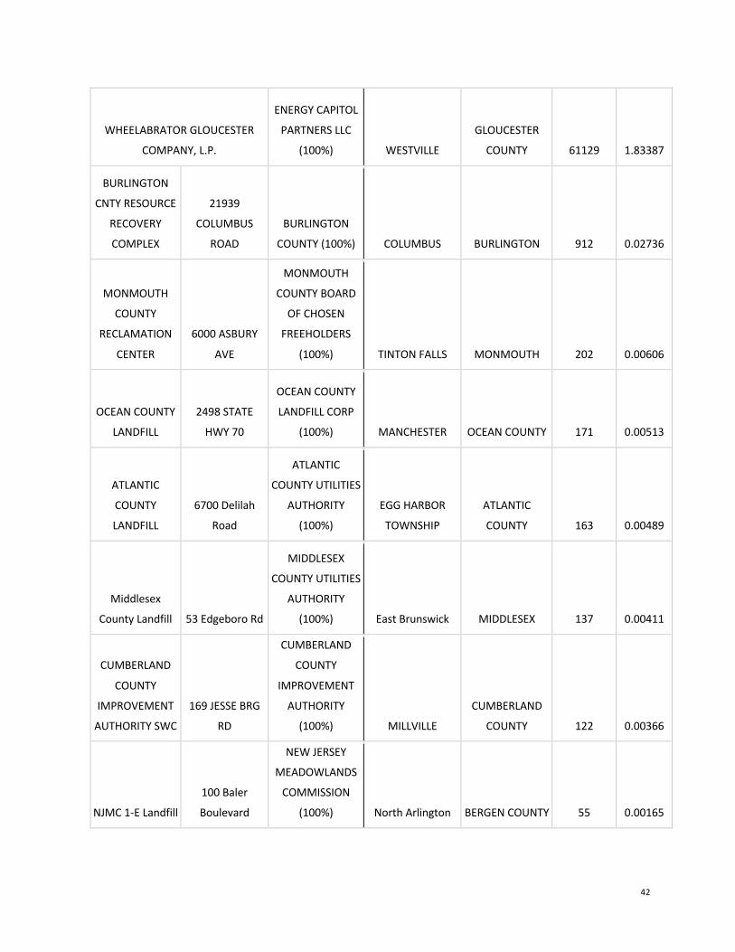
42

WHEELABRATOR GLOUCESTER

COMPANY, L.P.

ENERGY CAPITOL

PARTNERS LLC

(100%) WESTVILLE

GLOUCESTER

COUNTY 61129 1.83387

BURLINGTON

CNTY RESOURCE

RECOVERY

COMPLEX

21939

COLUMBUS

ROAD

BURLINGTON

COUNTY (100%) COLUMBUS BURLINGTON 912 0.02736

MONMOUTH

COUNTY

RECLAMATION

CENTER

6000 ASBURY

AVE

MONMOUTH

COUNTY BOARD

OF CHOSEN

FREEHOLDERS

(100%) TINTON FALLS MONMOUTH 202 0.00606

OCEAN COUNTY

LANDFILL

2498 STATE

HWY 70

OCEAN COUNTY

LANDFILL CORP

(100%) MANCHESTER OCEAN COUNTY 171 0.00513

ATLANTIC

COUNTY

LANDFILL

6700 Delilah

Road

ATLANTIC

COUNTY UTILITIES

AUTHORITY

(100%)

EGG HARBOR

TOWNSHIP

ATLANTIC

COUNTY 163 0.00489

Middlesex

County Landfill 53 Edgeboro Rd

MIDDLESEX

COUNTY UTILITIES

AUTHORITY

(100%) East Brunswick MIDDLESEX 137 0.00411

CUMBERLAND

COUNTY

IMPROVEMENT

AUTHORITY SWC

169 JESSE BRG

RD

CUMBERLAND

COUNTY

IMPROVEMENT

AUTHORITY

(100%) MILLVILLE

CUMBERLAND

COUNTY 122 0.00366

NJMC 1-E Landfill

100 Baler

Boulevard

NEW JERSEY

MEADOWLANDS

COMMISSION

(100%) North Arlington BERGEN COUNTY 55 0.00165

43

GLOUCESTER

COUNTY SOLID

WASTE

COMPLEX

493

MONROEVILLE

ROAD (C.R. 694)

GLOUCESTER

COUNTY

IMPROVEMENT

AUTHORITY

(GCIA) (100%) SWEDESBORO

GLOUCESTER

COUNTY 53 0.00159

INTERSTATE

WASTE

REMOVAL

PARKLANDS

RECLM SLF 1070 ROUTE 206

WASTE

MANAGEMENT

INC (100%) BORDENTOWN BURLINGTON 37 0.00111

Pennsauken

Sanitary Landfill

9600 RIVER

ROAD

POLLUTION

CONTROL

FINANCING

AUTHORITY

(100%) PENNSAUKEN CAMDEN 26 0.00078

44

Australia–EU ETS linking: lessons for the post–Paris world Stuart Evans and Aaron Wu

Abstract

The Australia–EU ETS linking negotiations were the first attempt to link emissions trading systems (ETS) with substantively different designs. While negotiations were cut short by the subsequent repeal of Australia’s carbon price, the progress made toward developing the link brings lessons for bottom up cooperation, as envisioned under the Paris Agreement. This paper draws on the authors’ first–hand experience negotiating the link, and interviews with key players in the negotiations to draw lessons regarding the drivers of, and barriers to cooperation. Moreover, it considers several unanswered questions regarding the practical design of international linking agreements. In doing so, the paper addresses the broader implications of linking for the political economy of carbon markets and climate clubs, to assess how linking policy design interacts with domestic and international political processes.

42

1. Introduction

Over the last two decades, international climate negotiations under the UNFCCC have seen the hope of Kyoto, the collapse in Copenhagen, and the recent breakthrough of Paris. Throughout these vacillations, a common theme has remained, that to avoid dangerous levels of climate change requires broad–based, internationally–linked carbon markets. Yet despite this agreement progress on developing and linking carbon markets has been remarkably slow. While the annual spectacle of the UNFCCC negotiations captures much of the policy makers attention, in this paper we argue that they should examine a less prominent set of negotiations which holds substantial insights into the potential future nature of a global carbon market.

The Australia–EU ETS Linking Arrangements were an ambitious attempt to set the standard for the future integration of carbon markets. Negotiated over a 12–month period, these arrangements would link what was then the world’s two largest functioning emissions trading systems (ETS’) to create the world’s first inter–continental carbon market.1 In doing so the link was also to be the first example of ‘heterogeneous linking’, with each ETSs retaining the bulk of their underlying policy design.

While a change in government in Australia spelled the end of this arrangement in September 2013, these linking arrangements bring important lessons for international climate policy. This paper seeks to bring these lessons to light, by answering the following questions: — how was this agreement forged; — what were the driving forces and key barriers; — what techniques and approaches were used to achieve this collaboration; and, — what lessons might this hold for future international cooperation on climate change?

These questions were explored in interviews with key parties to the negotiations: former Australian Minister for Climate Change, Greg Combet; former European Commissioner for Climate Action, Connie Hedegaard; and multiple senior officials from Australia and Europe that were actively involved in the negotiations.

The remainder of the paper is structured as follows. — the first section offers an abridged history of the Australia–EU linking negotiations. — the second explores the economic, political, and institutional factors that enabled the link. — the third draws out key implications of the Australia–EU linking negotiations for

international climate policy cooperation in a post–Paris world.

2. Link details and negotiating history

Late 2011 was a time of change for the Australian and EU ETSs. While Australia prepared for the implementation of its hard–fought policy, for the EU it was a period of consolidation following several rocky years caused by the global recession. As each jurisdiction looked to the future, to outside observers there was little indication that these vastly different ETS would soon be looking to link.

On 10 July 2011, the Australian government announced details of its Clean Energy Future package, the culmination of a multi–year policy process to introduce an economy–wide

1 The Australian Carbon Pricing Mechanism was a fixed price ETS (essentially a carbon tax) from 2012–15, with linking scheduled to begin from the floating price ETS phase commencing in 2015.

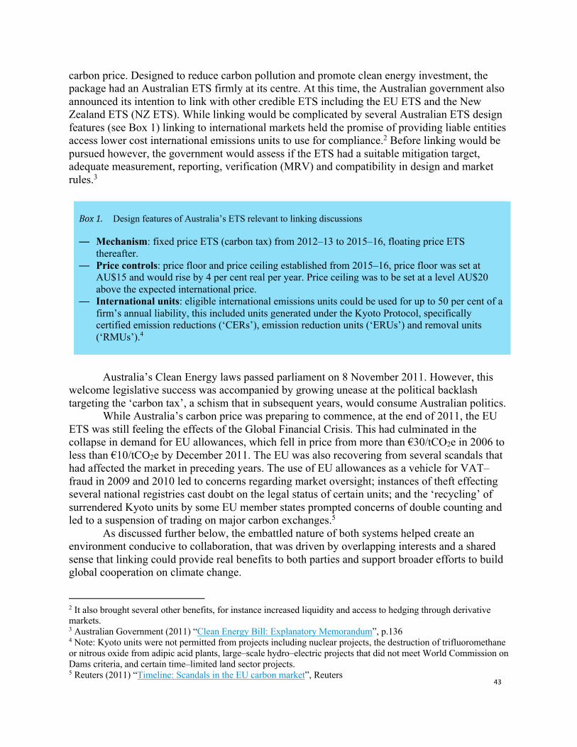
43

carbon price. Designed to reduce carbon pollution and promote clean energy investment, the package had an Australian ETS firmly at its centre. At this time, the Australian government also announced its intention to link with other credible ETS including the EU ETS and the New Zealand ETS (NZ ETS). While linking would be complicated by several Australian ETS design features (see Box 1) linking to international markets held the promise of providing liable entities access lower cost international emissions units to use for compliance.2 Before linking would be pursued however, the government would assess if the ETS had a suitable mitigation target, adequate measurement, reporting, verification (MRV) and compatibility in design and market rules.3

Box1. Design features of Australia’s ETS relevant to linking discussions

— Mechanism: fixed price ETS (carbon tax) from 2012–13 to 2015–16, floating price ETS thereafter.

— Price controls: price floor and price ceiling established from 2015–16, price floor was set at AU$15 and would rise by 4 per cent real per year. Price ceiling was to be set at a level AU$20 above the expected international price.

— International units: eligible international emissions units could be used for up to 50 per cent of a firm’s annual liability, this included units generated under the Kyoto Protocol, specifically certified emission reductions (‘CERs’), emission reduction units (‘ERUs’) and removal units (‘RMUs’).4

Australia’s Clean Energy laws passed parliament on 8 November 2011. However, this welcome legislative success was accompanied by growing unease at the political backlash targeting the ‘carbon tax’, a schism that in subsequent years, would consume Australian politics.

While Australia’s carbon price was preparing to commence, at the end of 2011, the EU ETS was still feeling the effects of the Global Financial Crisis. This had culminated in the collapse in demand for EU allowances, which fell in price from more than €30/tCO2e in 2006 to less than €10/tCO2e by December 2011. The EU was also recovering from several scandals that had affected the market in preceding years. The use of EU allowances as a vehicle for VAT–fraud in 2009 and 2010 led to concerns regarding market oversight; instances of theft effecting several national registries cast doubt on the legal status of certain units; and the ‘recycling’ of surrendered Kyoto units by some EU member states prompted concerns of double counting and led to a suspension of trading on major carbon exchanges.5

As discussed further below, the embattled nature of both systems helped create an environment conducive to collaboration, that was driven by overlapping interests and a shared sense that linking could provide real benefits to both parties and support broader efforts to build global cooperation on climate change.

2 It also brought several other benefits, for instance increased liquidity and access to hedging through derivative markets. 3 Australian Government (2011) “Clean Energy Bill: Explanatory Memorandum”, p.136 4 Note: Kyoto units were not permitted from projects including nuclear projects, the destruction of trifluoromethane or nitrous oxide from adipic acid plants, large–scale hydro–electric projects that did not meet World Commission on Dams criteria, and certain time–limited land sector projects. 5 Reuters (2011) “Timeline: Scandals in the EU carbon market”, Reuters

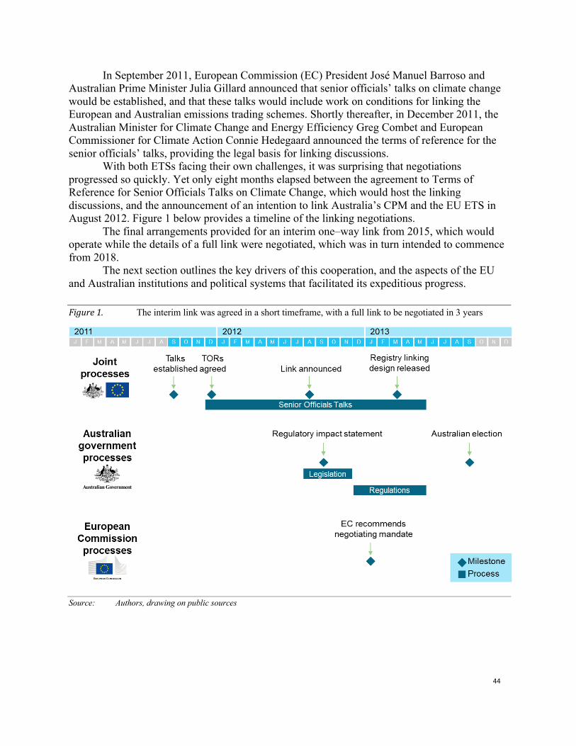
44

In September 2011, European Commission (EC) President José Manuel Barroso and Australian Prime Minister Julia Gillard announced that senior officials’ talks on climate change would be established, and that these talks would include work on conditions for linking the European and Australian emissions trading schemes. Shortly thereafter, in December 2011, the Australian Minister for Climate Change and Energy Efficiency Greg Combet and European Commissioner for Climate Action Connie Hedegaard announced the terms of reference for the senior officials’ talks, providing the legal basis for linking discussions.

With both ETSs facing their own challenges, it was surprising that negotiations progressed so quickly. Yet only eight months elapsed between the agreement to Terms of Reference for Senior Officials Talks on Climate Change, which would host the linking discussions, and the announcement of an intention to link Australia’s CPM and the EU ETS in August 2012. Figure 1 below provides a timeline of the linking negotiations.

The final arrangements provided for an interim one–way link from 2015, which would operate while the details of a full link were negotiated, which was in turn intended to commence from 2018.

The next section outlines the key drivers of this cooperation, and the aspects of the EU and Australian institutions and political systems that facilitated its expeditious progress. Figure1. The interim link was agreed in a short timeframe, with a full link to be negotiated in 3 years

Source: Authors, drawing on public sources

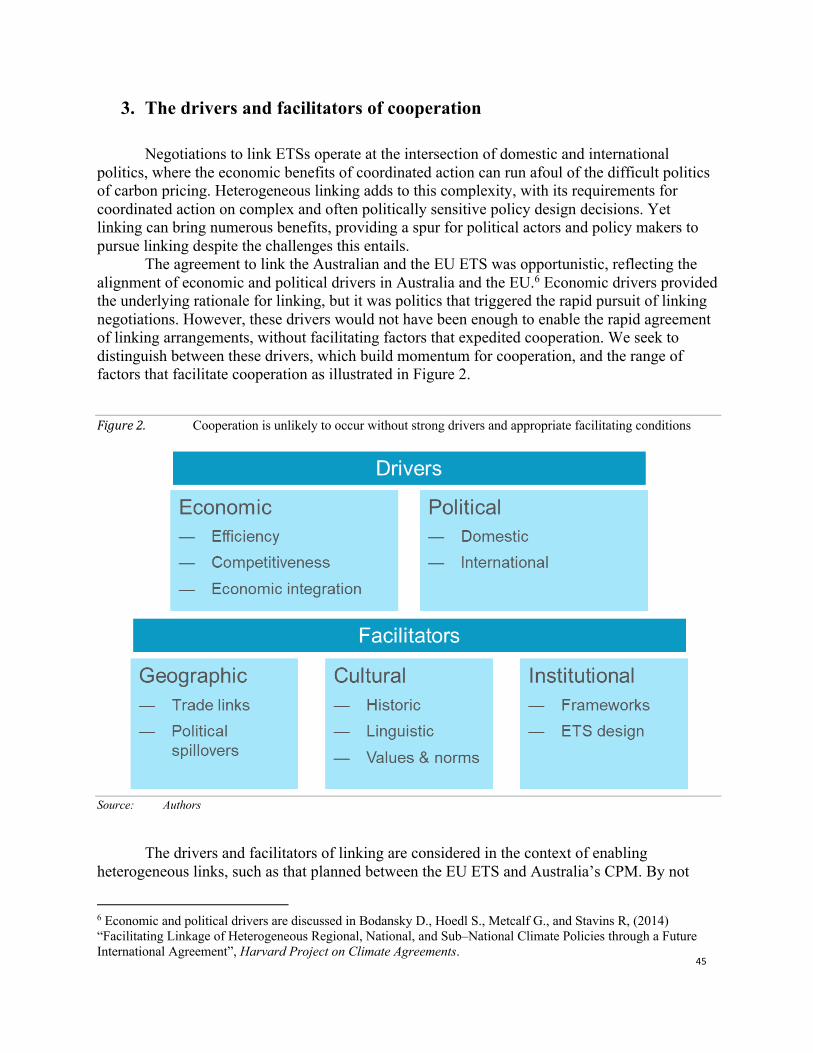
45

3. The drivers and facilitators of cooperation

Negotiations to link ETSs operate at the intersection of domestic and international politics, where the economic benefits of coordinated action can run afoul of the difficult politics of carbon pricing. Heterogeneous linking adds to this complexity, with its requirements for coordinated action on complex and often politically sensitive policy design decisions. Yet linking can bring numerous benefits, providing a spur for political actors and policy makers to pursue linking despite the challenges this entails.

The agreement to link the Australian and the EU ETS was opportunistic, reflecting the alignment of economic and political drivers in Australia and the EU.6 Economic drivers provided the underlying rationale for linking, but it was politics that triggered the rapid pursuit of linking negotiations. However, these drivers would not have been enough to enable the rapid agreement of linking arrangements, without facilitating factors that expedited cooperation. We seek to distinguish between these drivers, which build momentum for cooperation, and the range of factors that facilitate cooperation as illustrated in Figure 2.

Figure2. Cooperation is unlikely to occur without strong drivers and appropriate facilitating conditions

Source: Authors

The drivers and facilitators of linking are considered in the context of enabling heterogeneous links, such as that planned between the EU ETS and Australia’s CPM. By not

6 Economic and political drivers are discussed in Bodansky D., Hoedl S., Metcalf G., and Stavins R, (2014) “Facilitating Linkage of Heterogeneous Regional, National, and Sub–National Climate Policies through a Future International Agreement”, Harvard Project on Climate Agreements.

46

requiring policy alignment, heterogenous links can broaden the scope of possible agreement for instance, by allowing jurisdictions to maintain or introduce policy designs that may be unacceptable if imposed on the other party. As such, heterogenous linking can generate larger economic and political benefits for a jurisdiction by enabling policies to be nuanced to account for jurisdiction–specific circumstances.7,8 Differences between the EU ETS and Australian CPM design included coverage, cap setting arrangements, allocation of allowances, price controls, and access to domestic offsets and international units. Such differences respond to real, and relevant, differences in domestic circumstances, but also introduce greater complexity for managing the interactions of bespoke systems. The sections below outline these drivers and facilitators of cooperation and discuss where and how these played a role in the linking process.

3.1 Economic drivers of cooperation

Direct economic gains provide the central theoretical justification for trade and are prominent in the linking literature.9 Alongside the political benefits that can be delivered by linking, these form the dual–motivators for international linking of carbon markets.

The economic drivers for linking can be grouped into three categories, the significant efficiency gains that are generated by linking markets, reductions in competitiveness impacts and resulting carbon leakage, and the potential for ETS–linking as a component of broader economic integration. In the subsections below, we examine the potential role that economic drivers can play in mobilising support for linking in general and consider their specific role in the Australia–EU ETS linking negotiations.

3.1.1 Gains from trade and market efficiency

In the linking literature, potentially large gains from trade provide the economic basis for cooperation and a key metric for prioritising linking partners.10 Emissions reductions in low–cost jurisdictions avoid the need to cut pollution in higher–cost jurisdictions, which in turn pay for the privilege. These gains from trade could be substantial, with global emissions trading potentially reducing the 2030 costs of meeting the Paris Agreement National Determined Commitments (NDCs) by one–third and more than halving the 2050 costs of limiting global warming to less than 2oC.11

7 Metcalf G. and Weisbach D. (2012) “Linking Policies When Tastes Differ: Global Climate Policy in a Heterogeneous World”, Review of Environmental Economics and Policy, 6:1, 110–129 8 An example of this would be Australia’s Carbon Farming Initiative (CFI), which was an important policy for Australia but one that the EU would not been ready to emulate in the EU ETS. Heterogenous linking allowed the CFI to continue to operate in Australia which meant the potential for mobilising greater gains from trade as more mitigation sources were covered and providing domestic political benefits for the Australian system. 9 For an early example see Manne A., Richels S., (1996) “The Berlin Mandate: The Costs of Meeting Post 2000 Targets and Timetables”, Energy Policy 24:3, 205–210. 10 A recent analysis of the economics of prioritising jurisdictions is in Doda B., Taschini L. (2016) “Carbon dating: When is it beneficial to link ETSs?” Grantham Institute Grantham Research Institute on Climate Change and the Environment Working Paper, 208 11 World Bank, Ecofys, Vivid Economics (2016) “State and Trends of Carbon Pricing, 2016”, World Bank, Washington DC

47

The potential gains from trade underpinned the case for linking Australia and the EU’s carbon markets. However, on both sides these potential benefits were tempered by concerns regarding the need to protect the integrity of their respective ETS. In considering linking partners, European officials wanted ‘more than pure gains from trade’ but to have ‘meaningful partners’ who would not see linking as ‘an export project’.12 These motivations were mirrored in Australian officials who ‘had always imagined international linking to be a crucial part of emissions trading’ providing ‘a very efficient way to meet your target as long as you had confidence in the units you were going to use’.13 This requirement for confidence in the integrity of a linking partner’s ETS is one that will be revisited several times in subsequent sections of this paper.

Another commonly discussed benefit of linking is the efficiency gains that come from the increased market liquidity and the ability to spread compliance costs across multiple jurisdictions. As a small market, Australian firms would benefit from access a well–established liquid market for allowances, offering a wide range of derivative products and risk management services. Efficiency would be further enhanced by an increased market size that would reduce risks of abuse of market power. Further many of Australia’s largest emitters also had liabilities under the EU ETS and linking was expected to bring benefits by enabling them to manage liabilities across markets. On the other hand, as the larger partner efficiency gains for the EU were expected to be marginal.

While these economic impacts are often the focus of linking literature, for the Australia–EU link they were simply context, a welcome feature that was related – but subsidiary – to the key drivers that shifted linking from a possibility to a shared objective.14 Further, the clear caveats introduced by officials on both sides stressing that gains from trade are insufficient without ‘meaningful partners’ and ‘confidence in the units’ point to a more complex story.15

3.1.2 Competitiveness and carbon leakage

That linking provides aggregate economic benefits is uncontroversial, however these benefits are often unevenly distributed. One manifestation of this, is the potential for differential carbon prices to create competitive distortions. In all interviews conducted, it was clear that these potential competitiveness impacts were a key concern.

When carbon prices differ across jurisdictions, this creates the risk of ‘carbon leakage’, where industrial production and emissions move to another jurisdiction due to its lower effective carbon price. The risks of leakage are largest when carbon prices differ between jurisdictions that compete in emissions intensive product markets. When there is a lack of direct competition, leakage is less likely, however the perceived impacts of having a higher carbon price than trading partners can still prove a sensitive political issue, as is further discussed in Section 3.2 below.

12 Interview with European Official, September 2018 13 Interview with Australian Official, October 2018 14 This low priority is further evidence by the fact that no modelling of expected gains from trade was performed by the Australian government, nor, to the authors’ knowledge, by the EC. 15 For the EU the motivations of pursuing linking were primarily political as discussed in section 3.2 below. The EU’s pursuit of ETS linking is discussed in Jevnaker T., Wettestad J. (2016) “Linked Carbon Markets: Silver Bullet, or Castle in the Air?”, Climate Law 6 (2016) 142–151

48

Australia’s ETS was designed with an initial fixed price period that was roughly calibrated to the expected European price, starting at AU$23/tCO2e in 2012.16 Within months of its legislation however, the collapsing European price meant that Australia’s fixed price looked likely to be significantly higher than the price of EU allowances, and one of the highest explicit carbon prices in the world. This created a clear motivator for linking, that nicely with the EU’s interest in stemming declining prices:

From our perspective showing that you were consistent with an international price was really important, as the fixed price ended up being quite a bit higher than were the international price…

…It just suited both of us really – we were happy to take their low price, and they were happy to take our demand.

Interview with Australian Official, October 2018

The risk of carbon leakage was only a minor consideration for the EU–Australia link,

however, the desire to align prices to address perceived competitiveness impacts was a clear political priority. While a minor driver in this case, the potential for linking to reduce the risk of carbon leakage provides a clear example of the economic benefits that can flow from regulatory alignment. The benefits from greater regulatory alignment are not unique to ETS–linking, and the section below discusses how broader processes of economic integration can contribute to the proliferation of ETS links.

3.1.3 Economic integration

In some cases, linking may be pursued as part of a broader package of economic integration, where carbon pricing is one of many policies to be aligned. The rapid expansion of the EU ETS is the most compelling example of this. The EU was the first jurisdiction to introduce a broad and harmonised carbon price in 2005, and with the EU enlargements in 2007 and 2013 increased its scope to include 31 countries.17 This expansion process meant that carbon pricing was included as part of a wider set of arrangements to enhance economic and political cooperation. With carbon pricing tied to this broader set of outcomes, the EU was able to expand its ETS to jurisdictions like Poland, that are unlikely to have otherwise implemented a carbon price. More recently this approach featured as part of the Ukraine–European Union Association Agreement, which has spurred Ukraine’s ongoing efforts to develop an ETS.

While greater economic integration was not a direct consideration for the EU–Australia linking negotiations, the EU viewed the expansion of emissions trading as in its clear interests. the EU’s recent position to refuse trade agreements with countries that fail to ratify the Paris

16 See Australian Government (2012) “Budget 2012–13: The Clean Energy Future Plan” 17 Excluding Switzerland, which is now a linked system, but including EEA members Iceland, Norway and Liechtenstein.

49

Agreement, suggests climate cooperation will remain a clear objective of the EU’s economic diplomacy.18

3.2 Political drivers of cooperation

The economic gains from linking are potentially large but can be unevenly distributed across society. These uneven impacts and the political contests and compromise they generate, shape domestic climate politics. These domestic drivers in turn influence and react to international political drivers, with cooperation on international carbon markets effecting domestic policy and domestic politics acting as a driver of international cooperation. Below we identify a range of political motivations for linking, and how these were pursued by the Australian government and European Commission through ETS linking.

3.2.1 Domestic political drivers

A clear message across all interviews was that domestic political considerations are the first hurdle that needed to be surmounted before linking can be considered. Domestic politics drives differences in ETS design that can complicate linking and create barriers to aligning incompatible ETS. However, the potential political benefits associated with linking can also be a key driver, conferring political legitimacy, redistributing rents, and altering the costs of domestic policy reversal.

Each ETS has design peculiarities, that reflect the politics of its jurisdiction and the process required to create the coalition necessary to establish carbon pricing.19 For Australia, this meant that while it could learn from the EU ETS, it also faced specific drivers that necessitated a different approach:

the politics in Australia was different, the economy and emissions profile was different… and therefore we needed particular flexibilities and to have a different sort of an ETS than the European one.

Interview with Greg Combet, August 2018

Some of these differences would complicate the task of linking. At the same time, the

political drivers that created these differences would mean that altering ETS design to better align policy could be challenging. EU officials felt that ‘with our heavy systems, with the European Parliament and 28 members states’, their room for manoeuvre on linking was ‘very

18 Stone J. (2018) “EU to refuse to sign trade deals with countries that don't ratify Paris climate change accord”, the Independent 19 The role of domestic political factors in mediating design and diffusion of ETS policies is discussed in detail in Wettestad J. and Gulbrandsen L. (2018) “The Evolution of Carbon Markets: Design and Diffusion”

50

limited’.20 Australia was not as constrained and remained ‘open’ to looking at various design aspects including the price floor.21

Once it was clear that there was scope for reaching an agreement, the political benefits of linking shone through. Central to this was the value of cooperation in addressing the perceived competitiveness impacts of carbon pricing. While neither side felt that there was a real threat of carbon leakage, there was a concern that ‘if either of us were seen to be treating our industries better or worse, than that was used in the respective domestic context’.22 By demonstrating cooperative action, linking was a potential inoculant to the narrative of perceived competitive disadvantage:

We are talking about the economic crisis years, as you can imagine European industry would say “why are we going to pay for this when nobody else is?” … whatever the government that would say “we are going to do this”, then that helped in showing that Europe was not alone in doing this.

Interview with Connie Hedegaard, September 2018

We needed to neutralise the alleged competitiveness impacts on an economy going alone with carbon pricing, and for me I was able to say our second largest trading partner, which is the EU in aggregate, we would have the same carbon price, and ultimately, I wanted the same carbon price as in China, our largest trading partner… so there was an active discussion about the importance of linkage from a political point of view, not just the integrity of it all but the politics of it, to say that “this is a growing international position and our trading partners will have the same carbon price”.


This is not to say that the linking arrangements did not have real effects on businesses

compliance costs. For Australia, linking was expected to alter prices in a way that shifted rents to emissions–intensive industries. As a small market, linking would mean that the price of Australian carbon units would track those of EU allowances. However, because under the agreement Australian firms could meet up to 12.5 percent of liabilities (reduced from 50 percent as initially legislated) with lower cost Kyoto units,23 this resulted in an increase in the effective rate of assistance for entities receiving free Australian carbon units under the Jobs and Competitiveness Program.24

20 Interview with European Official, September 2018 21 Interview with Australian Official, October 2018 22 Interview with Australian Official, October 2018 23 Eligible Kyoto units include Certified Emissions Reductions (CERs) and Emissions Reductions Units (ERUs) 24 As Kyoto units traded at a lower price than EU allowances, and because Australia units were expected to track the EU allowance price, there was expected to be arbitrage by liable entities, which would sell some of the free allowances received and meet liabilities with cheaper Kyoto units. This increased the effective rate of assistance. This is described in more detail in Australian Government (2012) “Regulatory Impact Statement: Interim Partial

51

Linking also had the benefit as a tool to reduce the risk of policy reversal. Combet was clear in the view that ‘if we linked it would improve the chances of the sustainability of the system’,25 his officials ‘strongly agreed… that if we had negotiated an international link and we had a system with integrity, it wouldn’t make it impossible, but it would be somewhat harder to walk back away from’.26 These incentives proved insufficient however, with the linking arrangements one of many casualties of Australia’s fractious politics. The implications of this still reverberate – Australia's climate wars remain in full swing, and it has relapsed to its global bad actor status on climate change. These potential implications for international politics are discussed below.

3.2.2 International political drivers

International political drivers can include prestige from taking leadership positions, and benefits from design and influence over institutions governing carbon markets. For the last two decades the EU, and many of its member states, have viewed climate change as a clear domain of European leadership – aligning with its support for the liberal international order and citizen’s preferences for environmental leadership.27 28 This was reflected in the significant diplomatic efforts it made to generate support for the Paris Agreement, and in acting to protect it. In recent years, China’s collaborative approach to climate change has been seen in part as a response aimed at building status as a responsible actor in the international system.29

For Europe ‘it was a political wish to have the ETS family growing… for a very long time’. Internationally, Australia was viewed as a laggard facing particularly pernicious politics. Referring to Australia, Hedegaard recognised that ‘there are not many other countries that have had such a hard time to get a political majority behind a more consistent climate policy’,30 and the opportunity to turn the tables, therefore proved a powerful motivator:

...from our perspective if we could do anything to ensure that Australia finally would get some way of pricing emissions and get some kind of emissions trading system running, then for obvious reasons that was very much in our interest.


(One–Way) Link between the Australian Emissions Trading Scheme (ETS) and the European Union Emissions Trading System (EU ETS)” 25 Interview with Greg Combet, August 2018 26 Interview with Australian Official, October 2018 27 Oberthür S., Roche C. (2008) “EU Leadership in International Climate Policy: Achievements and Challenges” The International Spectator: Italian Journal of International Affairs, 43:3, 35–50, 28 Schreurs M., Tiberghien Y. (2007) “Multi–level Reinforcement: Explaining European Union Leadership in Climate Change Mitigation” Global Environmental Politics, 7:4, 19–46 29 Wu, F. (2016) “Shaping China’s Climate Diplomacy: Wealth, Status, and Asymmetric Interdependence”, Journal of Chinese Political Science, 21(2) 30 Interview with Connie Hedegaard, September 2018

52

The benefits from greater action in Australia, however, were on their own potentially less consequential than the powerful role that a linking proof of concept could provide in spurring greater action. For this, Australia fit the bill:

you cannot start as the first thing you do to link with a potential Chinese scheme, you have to gradually find out how you would actually do that, and in that sense Australia, given the size of it, was manageable.


But it wasn’t just the size of Australia’s market that appealed, there was also an

alignment of approaches, with the European Commission coming to the view ‘that there was a serious interest in building a strong carbon market' and that the ETS would be used ‘for the purpose that we also decided we wanted to use the carbon market for’.31 Therefore, for Europe the link provided a demonstration–case. Something to iron out the wrinkles, show the benefits of emissions trading, and provide a clear set of standards to inform the action of other parties.32 The European Commission support for what it considers credible ETS is well documented and helps act as an anchor for expectation amongst jurisdictions pursuing ETS with an eye to future linking.

As the first attempt to link ETS featuring heterogeneous designs the EU–Australia link was seen as ‘pioneering work’, with the potential to set standards for those who followed:

an EU–Australia linking treaty could also offer a kind of platform for further partners to engage with our two connected markets… If a third or a fourth country would like to participate we would sit together with them and say “these are the conditions we’ve agreed, this is what we are prepared to talk to you about, we will also integrate you into our market on the basis of these conditions, and we negotiate around the margins” – we don’t need to reinvent the wheel every time.

Interview with European Official, September 2018

The importance of setting these rules becomes clear, when considering the large flows of

economic activity that would be mobilised by international emissions trading of the scale needed to achieve the objectives of the Paris Agreement. In turn this means that linking requires deep integration of markets and regulatory regimes, which is near impossible to deliver through the consensus–based mechanisms of the UNFCCC. The Kyoto Protocol provided a detailed architecture to facilitate trade, yet each jurisdiction that utilised Kyoto units within domestic

31 Interview with European Official, September 2018 32 Note that in this case the EU showed a specific interest in establishing standards, norms and learning that would be instructive for jurisdictions pursuing heterogeneous linking, rather than other aspects of ETS policy design. There is an extensive literature on policy diffusion in domestic ETS design, see for instance Gulbrandsen L., Wettestad J., Victor D. and Underdal A. (2019) “The political roots of divergence in carbon market design: implications for linking”, Climate Policy 19:4 427–438; and Biedenkopf K. (2016) “The EU in Transnational Climate Networks: the Case for the Partnership for Market Readiness”, chapter in the European Union’s Engagement with Transnational Policy Networks, 2016, 102–123, Cambridge University Press, Cambridge.

53

carbon markets added additional rules and restrictions to their use and trade. Further the Kyoto architecture saw minimal trade in Assigned Amount Units (AAUs) which were developed to enable linking of domestic carbon markets.

The rules established under Article 6 of the Paris Agreement will be less detailed, less stringent, and open to a greater degree of interpretation, which will require jurisdictions pursuing ETS linking to develop supplementary rules. These rules will be developed outside the UNFCCC, potentially through linking agreements amongst a club of carbon markets, this is discussed further in section 4.33 As international institutions tend to rigidity, this means that

jurisdictions that engage early, may craft the rules of the global carbon market in line with their interests and preferences.34 Being an early rule–maker therefore brings potentially significant power and influence, that offer a clear potential driver of cooperation.

3.3 Facilitators of linking

The Australia–EU ETS linking negotiations also shed light on the attributes of policies or jurisdictions that are relevant not because they increase the benefits of linking, but for making the process easier, and greasing the wheels to enable linking to occur when the circumstances align. These facilitators can be grouped into three broad categories geographic links, institutional compatibility and cultural factors.

3.3.1 Geographic links

Geography appears to facilitate ETS linking, as can be seen through the Western Climate Initiative and Regional Greenhouse Gas Initiative in North America, and the link between Switzerland’s ETS and the EU ETS. Close geographic links are often associated with greater trade and business links which can increase the economic and political gains from linking, and can facilitate linking by example, with the introduction of carbon pricing in neighbouring jurisdictions far more salient.35 Further, greater links between society and business can enable the exchange of information between jurisdictions that accelerate the development of business and regulatory readiness for the introduction of carbon markets.

The EU–Australia link upended this trend, by featuring carbon markets on opposite sides of the globe. At the same time, it differed from previous experience by pursuing compatible ETS rather than harmonisation. Here though, geographic distance facilitated linking, with little competition between emissions intensive industries in Australia and the EU which often supplied different regional markets. This lack of competition meant that there was less political imperative for alignment of industry assistance arrangements, which could have proved an insurmountable challenge in both jurisdictions:

33 For an introduction to these clubs see Keohane R., Petsonk A., Hanafi A. (2017) “Toward a club of carbon markets” Climatic Change, 144:1, 81–95 34 As examples of rigidity, take for instance the unchanging membership of the UN Security Council, and the failure of the World Bank and IMF to adopt voting reforms to reflect changing geopolitical circumstances. 35 Görlach B., Mehling M. and Roberts E. (2015) “Designing Institutions, Structures and Mechanisms to Facilitate the Linking of Emissions Trading Schemes”, publication for the German Emissions Trading Authority (DEHSt)

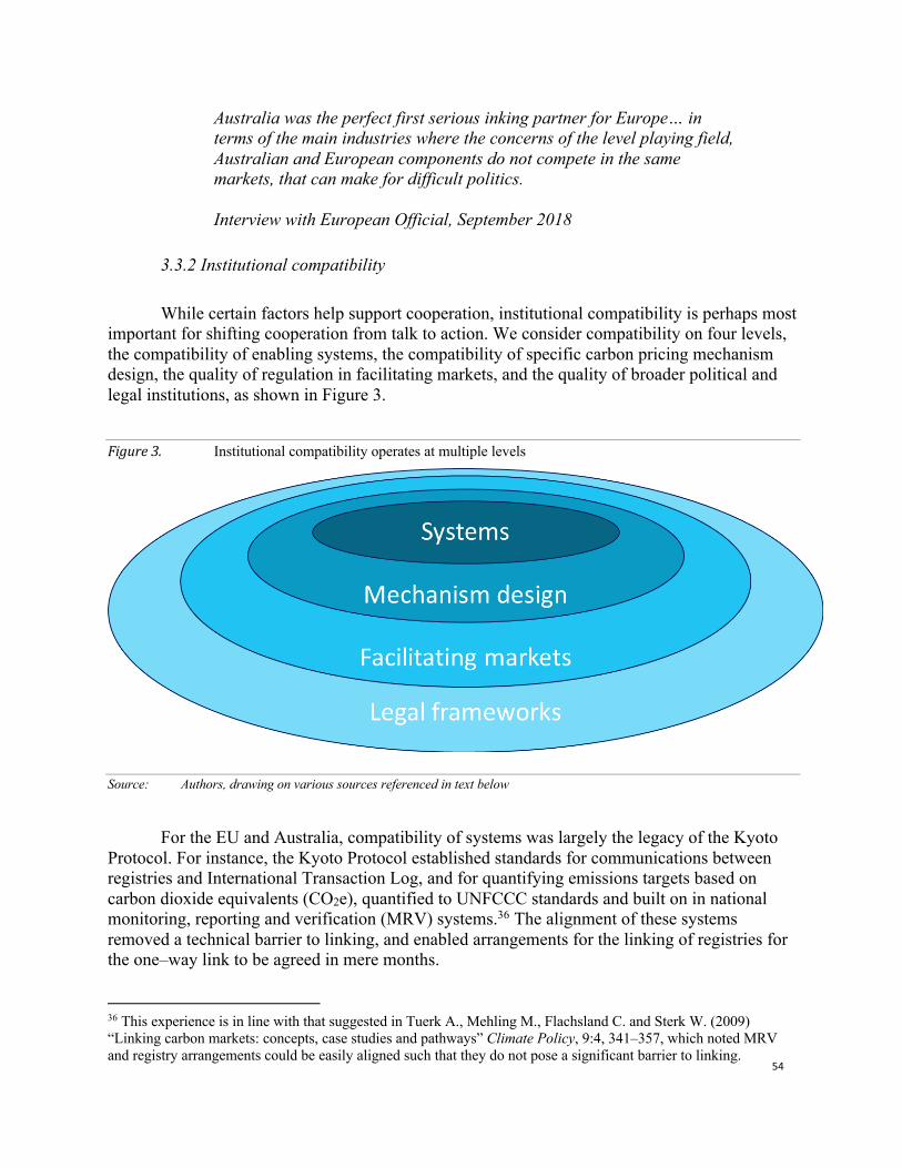
54

Australia was the perfect first serious inking partner for Europe… in terms of the main industries where the concerns of the level playing field, Australian and European components do not compete in the same markets, that can make for difficult politics.


3.3.2 Institutional compatibility

While certain factors help support cooperation, institutional compatibility is perhaps most

important for shifting cooperation from talk to action. We consider compatibility on four levels, the compatibility of enabling systems, the compatibility of specific carbon pricing mechanism design, the quality of regulation in facilitating markets, and the quality of broader political and legal institutions, as shown in Figure 3.

Figure3. Institutional compatibility operates at multiple levels

Source: Authors, drawing on various sources referenced in text below

For the EU and Australia, compatibility of systems was largely the legacy of the Kyoto Protocol. For instance, the Kyoto Protocol established standards for communications between registries and International Transaction Log, and for quantifying emissions targets based on carbon dioxide equivalents (CO2e), quantified to UNFCCC standards and built on in national monitoring, reporting and verification (MRV) systems.36 The alignment of these systems removed a technical barrier to linking, and enabled arrangements for the linking of registries for the one–way link to be agreed in mere months.

36 This experience is in line with that suggested in Tuerk A., Mehling M., Flachsland C. and Sterk W. (2009) “Linking carbon markets: concepts, case studies and pathways” Climate Policy, 9:4, 341–357, which noted MRV and registry arrangements could be easily aligned such that they do not pose a significant barrier to linking.

55

This compatibility extended to the design of the emissions trading mechanisms, which meant that only minor changes were required to enable the initial one–way link, specifically altering Australia’s price controls and introducing a more stringent limit on use of Kyoto Protocol units.37 It also meant that potential barriers to ETS–linking were more easily fixed, for instance, changes to the Australian system to enable trade during the one–way linking period using ‘shadow units’, built on the existing architecture.

As part of the linking arrangements, Australia also agreed to remove its price floor. Australian officials emphasise that this was crucial to the negotiations, however this is at odds with the recollection of European officials, who suggest that the negotiations ‘were used… as a political opportunity to make some limited changes’.38 The price floor was indeed a matter of ongoing debate among Australian policy makers, suggesting that the truth is likely that removing of the price floor did simplify linking, but that this represented an opportunity as much as sacrifice for Australian policy makers. The need for policy flexibility however was not equal. Given the EU’s size, Australia was ‘hardly an equal party’ in the link, which meant that if EU member states wanted to change the EU ETS, it would ‘just have to cop [accept] it’.39

Moving beyond mechanism specific considerations, a focus of early discussions was regulation of markets facilitating emissions trading to ensure the efficient interaction of secondary markets.40 Large markets create an attractive target for unscrupulous actors, with the challenge facing carbon markets amplified by having assets (allowances) that are tradeable across multiple markets:

I think the neglected area of really integrating carbon markets is the issue of market oversight... if you take a Daimler share traded in Frankfurt and a Daimler share trading in Shanghai, you cannot buy a Daimler share in Frankfurt and then sell it on to Shanghai. Allowances are completely different, you click a button and they go from a Portuguese company, to a Finnish company and the next moment they can go to Romania, they can go anywhere… [In Europe] we have financial market rules that we have created together, but there is nothing like this on the international side… for all practical purposes a carbon allowance is more like a share or a bond than a barrel of oil… so you could create for yourself quite some trouble, in terms of fraud and with market oversight.


Given these risks, confidence in broader market regulation is required. These market

regulations play an important role, for instance defining accounting requirements, financial

37 Further discussion of technical and policy issues effecting linking can be found in Santikarn M., L. Li, S. La Hoz Theuer, Haug C. (2018) “A Guide to Linking Emissions Trading Systems”, ICAP: Berlin. 38 Interview with European Official, September 2018 39 Interview with Greg Combet, August 2018 40 A discussion of the need for consistent oversight and legal treatment of units is provided in Betz R., Stafford A. (2008) “The Policy Issues Arising with the Linking of International Emissions Trading Schemes” Australian Resources and Energy Law Journal, 27:1, 86–104.

56

market rules and regulation of exchanges and insurance products.41 Following instances of fraud in the early years of the EU ETS, reforms tightened governance, including by defining allowances as financial products. Australia had also learned from the EU’s experiences and introduced regulatory settings that the EU were ‘quite comfortable’ could address issues of fraud, market misconduct and registry–issues.42

Related to this is the broader legal frameworks that govern markets and in which policy decisions are made. This can include the degree of confidence in the rule of law, protection of property rights, and provision of avenues for input and recourse for parties effected by regulatory change. The regulatory systems established to govern climate policy in Australia ensured there would be ‘stability in the way decisions would be made’,43 with a reciprocated view that the EU’s well–established political and legal systems would ensure the quality of policy design and implementation:

we had worked with the EU, and they know we are a democracy with strong law making and enforcement and that’s enormously valuable… Confidence in the quality of the regulatory regime with which you will be linking is obviously critical. Absolutely fundamental.


Overall this existing institutional compatibility enabled negotiations to proceed apace,

moving from commencement of Senior Officials Talks in December 2011 to the announced link in August 2012.

3.3.3 Cultural factors

Culture operates through several channels to facilitate (or impede) cooperation.44 Shared heritage can strengthen ties and increases the likelihood of ongoing engagement between governments, shared language simplifies negotiations and supports the formation of relationships, while shared norms and values help align the objectives that parties pursue through cooperation. These factors often play out on a national level, but they are also important for engagement at an individual or group level.45

The linking negotiations brought together like–minded groups from the European and Australian civil service, who could relate to each other’s experiences in trying to implement effective climate policy. The decision to structure linking negotiations as a dialogue between technical experts altered the dynamics of the negotiation from the outset:

41 Mehling M. (2016) “Legal Frameworks for Linking National Emissions Trading Systems”, ed. Carlarne, Gray, Tarasofsky, Oxford University Press, Oxford 42 Interview with Australian Official, October 2018 43 Interview with Australian Official, October 2018 44 Caporaso J. (1992) “International relations theory and multilateralism: the search for foundations”, International Organization, 46, pp 599–632 45 Hofstede G. (1980) “Culture’s Consequences: International Differences in Work–Related Values”, Beverly Hills: Sage.

57

The negotiation on this link was done between technical people, the emissions trading people, not the international negotiators. It was sort of a little strategy, we kept the negotiations between the people who were deep technically on our two schemes, and we negotiated in that way rather than in the typical international negotiators’ way.

Interview with Australian Official, October 2018

In structuring negotiations in this way, the negotiations created an informal cross–

national network of ETS experts, that could cooperate effectively to advance the objective of linking.46 This meant that the negotiations took the form of ‘an open engagement of technical people… who had similar policy initiatives in mind and understood their respective domestic constraints’. In many cases these experts had been working on the carbon pricing for years, with ‘very longstanding links between the policy advisors in Australia and in Europe’. The negotiators long–term involvement in carbon pricing and deep understanding of the associated challenges, meant that they ‘had real empathy for the struggles that each other had within our systems, which we could talk about openly’.47

The mutual respect between negotiators in turn provide European negotiators with the surety they needed that Australia had a shared vision of a global carbon market:

We were impressed by the intellectual rigor and the seriousness of the Australian administration and how much brain power they put into this, so we judged that there was a serious interest in building a strong carbon market.


This long history and sense that both sides were working against potentially volatile

political headwinds to reach a shared objective, galvanised efforts to reach a tractable deal. These efforts extended to officials working across national boundaries to smooth the way for an agreement. At Hedegaard’s request, Combet and Australian officials met with key players within the EU. As one official described, they ‘went on a charm offensive’ giving presentations to several member states and meeting with OECD officials.48 Much of Combet’s focus was on Germany, recalling advice from Hedegaard that if he could ‘go over to Berlin and convince the Germans, than this is going to get over the line’.49 This cooperation was reciprocated, with European officials paving the way for Australia to drop its price floor:

46 Slaughter outlines in detail how such informal and semi–formal networks have acted across borders to advance shared policy objectives, see Slaughter A., (2005), “A New World Order”, Princeton University Press, NJ. The role of networks in policy cooperation and diffusion on emissions trading is discussed in more detail in Paterson M., Hoffmann M., Betsill M., and Bernstein S. (2014), “The Micro Foundations of Policy Diffusion Toward Complex Global Governance: An Analysis of the Transnational Carbon Emission Trading Network”, Comparative Political Studies. 47(3) 420–449 47 Interview with Australian Official, October 2018 48 Interview with Australian Official, October 2018 49 Interview with Greg Combet, August 2018

58

The Greens were not keen on getting rid of the price floor, but of course the EU was not keen on the price floor itself and I think that was the persuasive thing. I got the senior public servants in the European Commission who advised Connie Hedegaard on the phone, and they explained why they didn’t like the price floor concept and how it would impact their ETS. And I think that was the final thing. I didn’t have to say much; the European Union people convinced the Greens to drop it.

Greg Combet, former Australian Minister for Climate Change

In these ways, officials were not just technocrats but also political actors. As leaders in

the development of the Australian and EU ETSs respectively, they were aware of the political trade–offs that would be required to facilitate a link. In a noticeable shift from the traditional approaches to climate negotiations, officials worked not as opponents seeking advantage, but partners, pursuing shared objectives and assisting each other in navigating respective domestic politics.

4. Implications for cooperation on carbon markets

The sections above show how difficult it can be disentangle the ‘economy’ from the realm of ‘politics’ in the interplay of market and social relations.50 This complexity is reflected in the influence of economic structure on ETS design; the interplay of drivers in seeking to protect the Australian ETS and develop a test case for linking; the role of officials working across political boundaries to mobilise the link in pursuit of their objectives; and the role of institutions and trust as cornerstones of cooperation. This in turn suggests a far more complex picture than is usually considered when discussing linking. This complexity, however, can help us draw several conclusions regarding the value of domestic policy flexibility under heterogeneous links and its limitations, the nature of international law applying to these links, and what this implies for future cooperation on carbon markets.

4.1 Policy flexibility in integrated carbon markets

As discussed in Section 2, ETSs are designed in a specific political and economic context, this context also bounds the scope of negotiations. Fundamental then, for linking heterogenous ETS is identifying where flexibility is possible, and where alignment or agreed limits are necessary. These inflexible elements combine considerations of policy with political feasibility to identify minimum criteria for ETS to link:

No matter what the different design or the coverage of the scheme, if you have confidence in the emissions units that were being traded, then it was possible to link them together. It would be imperfect, but it would be

50 As outlined in Polanyi (1944) “The Great Transformation”, Polanyi’s seminal work suggested that the modern market economy remained tethered to social and political relations and that a ‘self–regulating’ market was a social construction, that was never fully achievable.

59

possible. And I think in an international environment you’ve got to be willing to except that... You’ve really got to have enough flexibility to bring it off because it’s quite a complex challenge.


It is those two things that you need… that you have a genuine belief that you are not losing on environmental ambition – you need to be increasing the environmental ambition – but that you are not economically disadvantaging yourself in doing that.

Interview with European Official, September2018

These considerations were reflected in the scope of the full linking negotiations, which

were to include MRV, the use of third–party units and domestic offsets, competitiveness and carbon leakage, and market oversight.51 Some of these attributes, notably MRV, competitiveness and market oversight have been discussed previously. The addition of domestic offsets and third–party units to this list demonstrates that potential future links were a key consideration:

Obviously if you’ve got an ETS and you’re linking the major thing is to maintain the integrity of the linked markets and not allow dodgy units to be coming into it… The way to deal with that was to say “well in these combined markets, through this linking process, neither of us will admit any offsets or credits unless both of us agree what they are” … It was all discussed, but never ultimately settled, because of politics in Australia. It would have had to be settled. We agreed that we’d have to agree.


Linking with third parties has flow on effects to all members of a link, which creates a

clear risk that needs to be managed.52 There is still scope for some differences between parties, as was the case with the EU and Australia’s treatment on Kyoto units, however clear rules would need to be agreed to govern their use. As such, the decision to link influences not just interactions with the immediate partner, but also the set of future links that might be made. This means that linking with one jurisdiction may preclude, or at least make more difficult, linking with an alternative jurisdiction at a future date.

51 See Australian Government, European Commission (2012) “Joint press release: Australia and European Commission agree on pathway towards fully linking Emissions Trading systems”. These areas for agreement broadly align with the broader literature on heterogeneous linking, which finds that rules may be needed to deliver sufficient ambition, ensure environmental integrity and protect the functioning of markets, see for instance, Kansy T., 2016, Making the links between carbon markets in a post–Paris world 52 The risk of arbitrage trading from differential treatment of domestic offsets is discussed in Tuerk A., Mehling M., Flachsland C. and Sterk W., 2009, “Linking carbon markets: concepts, case studies and pathways”, Climate Policy, 9:4, 341–357.

60

4.2 International law and carbon market governance

Carbon markets generate significant rents and large amounts of economic activity. This means that negotiations looking to link these markets differ significantly from traditional environmental negotiations, instead being ‘more like two tax systems talking to each other to get a tax treaty’ which aimed ‘having confidence in the reciprocal treatment of each other’.53

This is a fundamental insight for negotiators developing the Paris Rulebook for the utilisation of carbon markets. The Paris Agreement provides welcome flexibility which enables parties to adopt market mechanisms in line with their domestic circumstances, and the rules established through the ongoing Article 6 negotiations can establish standards and practices that facilitate linking of carbon pricing mechanisms.54 However, the integration of carbon markets requires tendrils that reach deep into the structure of domestic economies, which no agreement formed under the consensus–based procedures of the UNFCCC can hope to provide.

Linking treaties can form the basis of deeper cooperation, and as discussed above, this link was a potential test case to inform future links. While the negotiations did not discuss these issues in detail, the need for an additional treaty or treaties, negotiated outside of the UNFCCC, raises clear questions of international law. This includes whether new institutions are required to manage linking arrangements and their potential structure, accession arrangements, rules, decision making criteria, and powers. However, as shown by Australia’s subsequent politics, ‘you can write down something in terms of contracts, but contracts can also be broken’.55 This means that treaties much be accompanied by credible legislation and governance:

You need to have a very strong legal underpinning domestically, and I think even this linking agreement – and that’s part of this confidence building exercise – even building an international treaty cannot supersede or replace the need for having a very strong legal underpinning on the domestic side… that, for me, is always the core in terms of this integration of carbon markets, it’s the only way ahead.


Reflecting this basis in domestic law, the arrangement reached between Australia and the

EU was not a treaty, but ‘a political commitment to link, effectively done through press releases’.56 It was clear to the negotiators that linking was a process of cooperation and confidence building, underpinned by domestic action. This focus on trust over process, has important implications for choice of linking partners.

53 Interview with Australian Official, October 2018 54 Importantly, accounting rules to ensure against double counting and clarify treatment of uncovered sectors should establish a set of standards that provide some confidence in the credibility of traded mitigation outcomes. 55 Interview with European Official, September 2018 56 Interview with Australian Official, October 2018. Note a full linking agreement would have required a treaty as specified in Article 25(1a) of the EU ETS Directive, see European Commission, 2019, Directive 2003/87/EC of the European Parliament and of the Council (Consolidated).

61

4.3 Finding the right linking partner

Linking is sometimes seen as a kind of dating market, with jurisdictions comparing attributes to identify the partner with the most favourable set of attributes that provide the greatest economics gains.57 However, what the discussion above has shown is that this transactional approach can miss the broader set of drivers and facilitating factors that must be considered before committing to a link.58 When we account for the multiple political drivers of linking and the institutions and rules required, a prioritisation of linking partners may focus more on the intent of the potential partner and their willingness to engage in cooperation for the longer–term:

The way I think about linking, is that it’s a bit like the analogy of marriage, when you’ve decided to get married you don’t write a contract… you know the other partner and the other partner knows you, and you know the upsides and downsides and decide whether to engage or not. You don’t go into conditional marriage where you only go into marriage if you change X, Y or Z…this comes to the crunch in this debate, to say “is there enough confidence respectively that you take the step and engage?”


This approach sees linking as a relationship based on shared objectives and credibility,

which implies a very different approach to prioritising potential partners. This means that the direct economic benefits from linking may receive less weight than a jurisdiction’s political alignment, or their value in creating coalitions to embed markets and generate self–enforcing political support. Further, the high bar for establishing institutions and domestic laws to implement linking, suggests that integration of carbon markets to the level foreseen in the Australia–EU negotiations is likely to be limited to developed countries with established and stable governance. Further expansions of ETS–linking beyond this small group will require ongoing engagement to build capacity of governments in not just ETS design and implementation, but also in broader issues of market governance.

5. Conclusions

This paper has discussed the lessons that can be drawn from negotiations to link the Australian and EU ETSs. It draws out a complex web of considerations, linking the economic and political drivers of cooperation with a set of facilitating factors that smooth the way.

It finds that domestic political factors played a dominant role in determining the scope of the negotiations and their prospects for success. Indeed, it was the alignment of political drivers, at the domestic and international level, that drove cooperation and created the momentum to

57 See Doda B. and Taschini L., 2016, “Carbon dating: When is it beneficial to link ETSs?” Grantham Institute Grantham Research Institute on Climate Change and the Environment Working Paper No. 208 58 Mehling, M., 2016, “Legal Frameworks for Linking National Emissions Trading Systems”, in “The Oxford Handbook of International Climate Change Law”, ed. Carlarne, Gray, Tarasofsky, Oxford University Press, Oxford

62

agree a link in such a short period. However, these drivers alone would not have been enough, without facilitating factors such as the shared experience and objectives of officials, and robust institutions in each jurisdiction. The need for deep integration of markets sets a high bar for institutional compatibility which may mean that full links may be predominantly the domain of developed countries for some time.

Overall Australia and the EU’s experience with linking points to the high potential for these agreements to support cooperation by bringing together diverse markets. In turn, linking agreements have the potential to close some of the gaps in the international legal architecture that will be needed to give linking effect. However, it also suggests that in the near–term jurisdiction’s considering linking may struggle to find a partner with a credible market and well aligned objectives. Despite the challenges this poses for the vision of developing a truly integrated global markets, the rapid progress of the linking negotiations should give pause for hope that rapid progress is possible when circumstances align.

References Australian Government, 2011, “Clean Energy Bill: Explanatory Memorandum”, p.136

www.legislation.gov.au/Details/C2011B00166/Download Australian Government, 2012, “Regulatory Impact Statement: Interim Partial (One–Way) Link between the

Australian Emissions Trading Scheme (ETS) and the European Union Emissions Trading System (EU ETS)”

Australian Government, 2012, “Budget 2012–13: The Clean Energy Future Plan”, https://www.budget.gov.au/2012–13/content/ministerial_statements/climate/html/climate_change–02.htm

Australian Government, European Commission, 2012, “Joint press release: Australia and European Commission agree on pathway towards fully linking Emissions Trading systems”

Betz R. and Stafford A., 2008, “The Policy Issues Arising with the Linking of International Emissions Trading Schemes”, Australian Resources and Energy Law Journal, 27:1, 86–104.

Biedenkopf K., 2016, “The EU in Transnational Climate Networks: the Case for the Partnership for Market Readiness”, chapter in the European Union’s Engagement with Transnational Policy Networks, 2016, 102–123, Cambridge University Press, Cambridge.

Bodansky D., Hoedl S., Metcalf G., and Stavins R., 2014, “Facilitating Linkage of Heterogeneous Regional, National, and Sub–National Climate Policies through a Future International Agreement”, Harvard Project on Climate Agreements.

Caporaso J., 1992, “International relations theory and multilateralism: the search for foundations”. International Organization, 46, pp 599–632

Doda B. and Taschini L., 2016, “Carbon dating: When is it beneficial to link ETSs?” Grantham Institute Grantham Research Institute on Climate Change and the Environment Working Paper, 208

European Commission, 2019, Directive 2003/87/EC of the European Parliament and of the Council (Consolidated), https://eur–lex.europa.eu/legal–content/EN/TXT/PDF/?uri=CELEX:02003L0087–20140430&from=EN

Görlach B., Mehling M., and Roberts E., 2015, “Designing Institutions, Structures and Mechanisms to Facilitate the Linking of Emissions Trading Schemes”, publication for the German Emissions Trading Authority (DEHSt)

Gulbrandsen L., Wettestad J., Victor D. and Underdal A., 2019, The political roots of divergence in carbon market design: implications for linking, Climate Policy 19:4 427–438

Hofstede G., 1980, “Culture’s Consequences: International Differences in Work–Related Values”, Beverly Hills: Sage.

Jevnaker T., Wettestad J., 2016, “Linked Carbon Markets: Silver Bullet, or Castle in the Air?”, Climate Law 6 (2016) 142–151

Kansy T., 2016, “Making the links between carbon markets in a post–Paris world”, http://blogs.worldbank.org/climatechange/making–links–between–carbon–markets–post–paris–world

Keohane R., Petsonk A., Hanafi A., 2017, “Toward a club of carbon markets”, Climatic Change, 144:1, 81–95

63

Manne A., Richels S., 1996, “The Berlin Mandate: The Costs of Meeting Post 2000 Targets and Timetables”, Energy Policy 24:3, 205–210.

Mehling, M., 2016, “Legal Frameworks for Linking National Emissions Trading Systems”, in “The Oxford Handbook of International Climate Change Law”, ed. Carlarne, Gray, Tarasofsky, Oxford University Press, Oxford

Metcalf G. and Weisbach D., 2012, “Linking Policies When Tastes Differ: Global Climate Policy in a Heterogeneous World”, Review of Environmental Economics and Policy, 6:1, 110–129

Oberthür S., Roche C., 2008, “EU Leadership in International Climate Policy: Achievements and Challenges”, The International Spectator: Italian Journal of International Affairs, 43:3, 35–50,

Paterson M., Hoffmann M., Betsill M., and Bernstein S., 2014, “The Micro Foundations of Policy Diffusion Toward Complex Global Governance: An Analysis of the Transnational Carbon Emission Trading Network”, Comparative Political Studies. 47(3) 420–449

Polanyi, 1944, “The Great Transformation”, Farrar & Rinehart, NY, USA. Reuters, 20 January 2011, “Timeline: Scandals in the EU carbon market” https://www.reuters.com/article/us-carbon-

scandals/timeline-scandals-in-the-eu-carbon-market-idUSTRE70J4M120110120 Santikarn M., L. Li, S. La Hoz Theuer, and Haug C., 2018, “A Guide to Linking Emissions Trading Systems”.

ICAP: Berlin. Schreurs M., Tiberghien Y., 2007, “Multi–level Reinforcement: Explaining European Union Leadership in Climate

Change Mitigation”, Global Environmental Politics, 7:4, 19–46 Slaughter A., 2005, “A New World Order”, Princeton University Press, NJ. Stone J., 12 February 2018, “EU to refuse to sign trade deals with countries that don't ratify Paris climate change

accord”, the Independent, https://www.independent.co.uk/news/world/europe/eu-trade-deal-paris-climate-change-accord-agreement-cecilia-malmstr-m-a8206806.html

Tuerk A., Mehling M., Flachsland C. and Sterk W., 2009, “Linking carbon markets: concepts, case studies and pathways”, Climate Policy, 9:4, 341–357.

Wettestad J., Gulbrandsen L., 2018, “The Evolution of Carbon Markets: Design and Diffusion”, London/New York, Routledge, 262 p.

World Bank, Ecofys, Vivid Economics, 2016, “State and Trends of Carbon Pricing, 2016”, World Bank, Washington DC

Wu, F., 2016, “Shaping China’s Climate Diplomacy: Wealth, Status, and Asymmetric Interdependence”, Journal of Chinese Political Science, 21(2)

64

Blockchain, Double Counting, and the Paris Agreement Henrique Schneider

Abstract

This essay explores possibilities and limitations of applying blockchain distributed ledger technology to select aspects of the Paris Agreement, especially to issues under Article 6 (and, where relevant, Articles 4, and 13). Through the application of blockchain, double counting (and similar concerns) can be mitigated while making reporting, tracking and managing corresponding adjustments efficient. Blockchain enables accounting for nationally determined contributions (NDCs) and increases the transparency in the implementation of the Paris Agreement. This, on the other hand, depends on a careful institutional set–up. This essay lays out the requirements for a blockchain system (or a set of blockchain) under Article 6. At the same time, it considers the limitations of applying blockchain. These limitations arise due to the distributed ledger technology itself, but also due to the nature of international negotiations in connection with the Paris Agreement. Keywords Blockchain, Distributed Ledger Technology, Paris Agreement, Carbon Markets, Cooperative Approaches, Corresponding Adjustments, Double Counting

This essay explores possibilities and limitations of applying blockchain distributed ledger technology (DLT) to select aspects of the Paris Agreement (PA, or, Agreement), especially to issues under Article 6 (and, where relevant, Articles 4, and 13). While this essay identifies several areas in which blockchain DLT could ease the implementation of the articles just mentioned, it will also highlight limitations to this approach.

Some limits to blockchain are imposed by the technology itself. The most important, however, arise from the context in which it could be employed. Blockchain cannot substitute negotiations by Sovereign Subjects (in the language of the United Nations: Parties), which determine the set–up of a system to which blockchain DLT, be it one blockchain of a set of blockchain, could be applied.

Blockchain DLT is a form of implementation, and not an institutional set–up. It is quite the inverse: blockchain can only implement a pre–arranged institutional set–up. On the other hand, the decision for using blockchain has implications for the institutional set up.

While there is increasing literature (of different quality) on applying blockchain to the Paris Agreement (compare, for example, Baynham–Herd, Z. (2017), Marke (2018), or Macinante, J. (2018)), the specific interaction between Article 6 and distributed ledgers remains unexplored. In addition, climate summits subsequent to Paris do not mention blockchain in the decision tests. Not even at the climate conference held in Katowice in 2018, tasked with

65

developing the so–called “Paris Rulebook”, did blockchain become a consideration by Parties in conjunction with article 6, or any other Article.1

From this background, this paper advances an idea of how to apply blockchain DLT to the Article 6 of the Paris Agreement. The main thesis of this essay is: through the application of blockchain distributed ledger technology, double counting (and similar concerns) can be mitigated while making reporting, tracking and managing corresponding adjustments efficient. Blockchain enables accounting for nationally determined contributions (NDCs) and increases the transparency in the implementation of the Paris Agreement. This, on the other hand, depends on a careful institutional set–up.

In a first section, this paper explains the idea of blockchain and its core, the distributed ledger. The second section explains how blockchain relates to issues of the Article 6, and subsequently 4 and 13, of the Paris Agreement. The third discusses the limitations of this approach. A brief conclusion ends the paper.

1. Blockchain Distributed Ledger Technology

Blockchain is a digital, public, permanent, append–only distributed ledger (Idelberger et al. 2016). A ledger is a list of transactions. This list is chronologically structured, i.e. every new transaction is added to the list immediately after the one before it. It is not possible to change earlier entries as it is not possible to switch their place or delete them, therefore permanent and append–only.

While these attributes are common to most or all types of ledgers, blockchain’s ledger has further characteristics. It is digital, existing as a mathematical structure. It is distributed, i.e. it is not centrally managed, but maintained by a group of dispersed managers, or, nodes. The mathematical structure of the ledger exists in all nodes at the same time and in the same form. The management principle of blockchain does not allow for the nodes to split the ledger nor for division of labor. Every node performs the exact same task and every ledger in all nodes of a system is identical. System stands for a group of nodes and agents using a specific algorithm based on blockchain.

The ledgers can change by adding an entry to them (all). This occurs, when a majority – over 50% – of the nodes of that system agree to add an entry to the ledger. Once they do so, all nodes add the entry to their respective ledgers creating isomorphism among the ledgers in the nodes. The blockchain–system relies on all nodes being isomorphic as a sign of robustness. The ledger as a mathematical structure exists at the same time in a potentially unlimited number of nodes. A transaction can only be added if most nodes process the exact same transaction, validating it.

At regular intervals, the program creates a block that contains all of the transactions in that period. There is a group of nodes called “miners” who compete to validate the transactions in the block. Once a block is validated, it gets connected to the previous block to create a chain of validated blocks. If a block cannot be validated, it does not become part of the chain and all transactions therein are lost. (In cryptocurrencies, the mining nodes compete against each other for validating the block. The first to succeed, receives a unit of cryptocurrency.) Records cannot

1 Refer to the decisions; the penultimate, non–consensus, texts provide more insight into the technical topics that were negotiated; they can be found under: https://unfccc.int/sites/default/files/resource/Katowice%20text%2C%2014%20Dec2018_1015AM.pdf

66

be altered retroactively without the alteration of all subsequent blocks and the collusion of the network. Therefore, to hack a validated block an agent would need to hack the entire chain simultaneously.

In addition to these requirements, the isomorphic ledgers distributed among nodes are public. Any interested entity – even a non–node–running–entity or not–transaction–party–entity – is able to view them and identify the transactions as well as the agents of the transactions. Often, blockchain is wrongly understood as an anonymous system. It allows anonymity and it allows full transparency. By default, however, it is a pseudonymous system.

While the previous paragraphs sketch the core of the logic behind blockchain, additional background could foster its understanding. One important issue, for example, is establishing the relationship of blockchain to Bitcoin. While the cryptocurrency Bitcoin is the first application of blockchain, not all blockchain is necessarily Bitcoin – nor cryptocurrency. Blockchain is a technology applicable to all matters of governance, for example to smart contracts, to record keeping, or to bookkeeping (Catalini & Gans 2016).

Satoshi Nakamoto, the pseudonymous creator of blockchain and Bitcoin, wrote in a message sent to a cryptography–focused mailing list in October 2008. “I’ve been working on a new electronic cash system that’s fully peer–to–peer, with no trusted third party.” As he wrote these words about Bitcoin, he attached a white paper in which he developed blockchain. Nakamoto thought blockchain as a new way of answering an old question: how there can be enough trust between peers to exchange something of value.

His answer: neither through force nor through central institutions but through networks. Combining established cryptography tools with computer science research, blockchain operationalizes trust in tying it to the transactions. Peers might continue to distrust each other, but they will trust a transaction if it is robust, verified, unique (i.e. without a possibility for double counting), shown transparently and isomorphic on all data points, or nodes. In other words, Nakamoto (2008) intended to create a system in which it is costly to create value but cheap to guarantee property as well as costly to rig the system but cheap to verify the transactions of that system.

How does a transaction in blockchain work? Let it be explained using Bitcoin as an example. In Bitcoin, a transaction is the transfer of cryptocurrency from one person to another. One person can send cryptocurrency to the other person. To do so, the first person creates a transaction on her computer that must reference a past transaction on blockchain in which she received enough funds, as well as her private key to the funds and the other person’s address. That transaction is then sent out to the nodes in the network. The nodes will validate the transaction as long as it has followed the appropriate rules. If most nodes accept the transaction, i.e. the deduction from the first person, the authentication of the key, and the addition to the second person, all nodes will add the entry into a data–block and the transaction is completed.

In Bitcoin and other cryptocurrencies, a subset of nodes, called miners, organize valid transactions into lists called blocks. A block in progress contains a list of recent valid transactions and a cryptographic reference to the previous block. In blockchain–based cryptocurrency–systems like Bitcoin and Ethereum, miners race to complete new blocks, a process that requires solving a labor–intensive mathematical puzzle, which is unique to each new block. The first miner to solve the puzzle will earn some cryptocurrency as a reward. The mathematical puzzle involves randomly guessing at a number called a nonce. The nonce is combined with the other data in the block to create an encrypted digital fingerprint, called a hash.

67

The hash must meet certain conditions; if it does not; the miner tries another random nonce and calculates the hash again. It takes an enormous number of tries to find a valid hash. This process deters hackers by making it hard to modify the ledger. While some blockchain entities use other systems to secure their chains, this approach, called “proof of work”, is the most thoroughly tested.

This is the final step in securing the ledger. When a mining node becomes the first to maintain a block, it sends the block to the rest of the network for approval, earning digital tokens in reward. Mining difficulty is encoded in blockchain’s protocol; Bitcoin and Ethereum are designed to make it increasingly hard to solve a block over time. Since each block also contains a reference to the previous one, the blocks are mathematically chained together. Tampering with an earlier block would require repeating the proof of work for all the subsequent blocks in the chain.

Which of these attributes of blockchain are important when using it to implement or operationalize the Paris Agreement? First, blockchain is a system among peers. Second, it creates trust by identifying trust with transactional clarity. Third, it has no central institutions but allocates responsibility to all peers at the same time. Fourth, different specific systems can emerge while adopting the same blockchain principle. Fifth, blockchain is public; in other words, transactions are transparent.

Trust is a risk judgement between different parties. In blockchain, determining trust is a function of proving identity (authentication) and proving permissions (authorization). Put more simply, the blockchain wants to know, “Are you who you say you are?” and “Should you be able to do what you are trying to do?”

In the case of blockchain, private key cryptography provides a powerful ownership tool that fulfills authentication requirements. Possession of a private key is ownership. In the context of the Paris Agreement, each agent or party to a transaction would be required to have its own key, giving them ownership but also identifying them to the system. Authentication, however, is not enough.

Authorization – having enough money, broadcasting the correct transaction type, etc. – needs a distributed, peer–to–peer network as a starting point. A distributed network reduces the risk of centralized corruption or failure. This distributed network must also be committed to the transaction network’s recordkeeping and security. Authorizing transactions is a result of the entire network applying the rules upon which it was designed (the blockchain's protocol).

There is plenty of research on applying blockchain to matters of governance, especially accounting. Sarkar (2018) provides a broad overview on blockchain, governance and the management of accounting processes. Faning & Centers (2016) as well as Kokina et al. (2017) show how accounting has increasingly been incorporating blockchain in order to keep records, clear transactions, and consolidate reports. Kiviat (2015) explores risks and limitations of applying blockchain to accounting and smart contracts. If blockchain is thought of as a system of governance, it can be used for governance purposes in connection with the Paris Agreement.

2. The Paris Agreement and Blockchain

This section operationalizes the former by identifying select topics of the Paris

Agreement that could profit from blockchain. Here, the focus is Article 6 (and, where relevant, article 4 and 13), especially aspects of this article that are important in relation with blockchain, for example double counting and corresponding adjustments. This section is going to explain,

68

first, the general issues concerning the topic; second, to summarize the system requirements for blockchain; and finally, to discuss its application to Article 6.

Article 6 of the Paris Agreement allows countries to use international carbon markets to achieve their mitigation targets communicated in Nationally Determined Contributions (NDC). Article 6.2 allows countries to use “internationally transferred mitigation outcomes (ITMOs)”, i.e. climate change mitigation achieved in one country but claimed by another, to achieve their NDC targets. Article 6.4 establishes a new crediting mechanism under international supervision that could be used for similar purposes.

Theuer, Schneider, & Broekhoff (2018, 1) briefly expose the idea of carbon markets and its challenge (slightly edited by the author of this essay): “Carbon markets are considered a key tool to reduce greenhouse gas emissions. They can reduce the cost of achieving mitigation targets by providing flexibility in how and where emissions are reduced and could thereby facilitate the adoption of more ambitious mitigation targets. Yet international carbon markets involve a number of environmental integrity risks if not designed and implemented appropriately, they could result in greater greenhouse gas emissions than if they were not employed. The Paris Agreement therefore requires Parties to ensure environmental integrity when engaging in international transfers of mitigation outcomes. A key risk to environmental integrity concerns international transfers from countries with weak mitigation targets.”

The application blockchain to Article 6 faces similar challenges. They occur at the conceptual and at the implementation level.

2.1 Technical Issues of the Paris Agreement

While there are many areas in which blockchain could be applied to the implementation of the Paris Agreement, focusing on one, Article 6, makes its possibilities and limitations as well as its interactions with the institutional set–up clearer. By directing its attention to Article 6.1–7, this section will also discuss direct implications for Articles 4 and 13 as well as for the relevant paragraphs in Decision 1/CP.21 (Decision) and subsequent decisions. This section will be following the outline of expert discussions and negotiations as in Schneider, Kollmuss, & Lazarus (2015), Theuer et al. (2017), Schneider et al. (2017), OECD/IEA (2017), and Marcu et al. (2017) as well as in the numerous presentations made in preparation for the COP 24 (2018).

The Paris Agreement contains principled provisions on counting, accounting and accounting for a NDC. At a general level, they are (Schneider et al. 2017): — Definition of targets, methods and accounting approaches in Article 4.8 PA and para 28

Decision (Formulating NDC), Article 4.10 PA (timeframe for NDC), Article 4.12 and para 29 Decision (public registration of NDC), as well as Article 4.13 PA and para 31 Decision (accounting for NDC).

— Tracking progress in Article 13.7 PA and para 91–98 Decision. — Accounting for international transfers in Article 6.2 PA and para 33 Decision (corresponding

adjustments), as well as Article 6.5 PA and para 37–38 Decision (emission reductions). — Final assessment in Article 4.13 PA and para 31 Decision (accounting for NDCs). — Review and compliance in Article 13.11 PA and para 91–98 Decision (technical

expectations), as well as Article 15 PA and para 104 Decision (mechanism to promote compliance).

These provisions, however, need operationalization. With operationalization comes interpretation, which leads to many still unanswered questions, even in the already specialized

69

realm of accounting. Examples of such questions with consequences for counting and accounting, and therefore for the application of blockchain, are: — How to deal with differently formulated NDCs – intensity goals, CO2–equivalents, NDCs

based on target, NDCs based on investments, etc.? — How to deal with NDCs formulated on different basis – emissions, budget, target, intensity,

measures, etc.? — How to handle multi–year versus single–year NDCs? — How to differentiate NDCs covering whole economies, some sectors of an economy,

subsectors, and programs of activities or projects? — What does count as a reduction in the sense of a climate–action unit, i.e. mitigation outcome,

as stipulated in 6.2, or an emission reduction, as stipulated in 6.4? Factual reductions of CO2 equivalents, removals, sinks, avoidance, or even capacity building?

— How to change a NDC? With which consequences to already recorded or transferred reductions?

— How to count and account for domestic transfers? — How to generate climate–action units and relate them to NDCs? For example, by quantifying

mitigation targets and progress, quantifying mitigation outcomes, avoiding double counting (and similar concerns), accommodating different metrics, dealing with different vintages, adjusting for additionality and non–permanence.

— In addition, some Parties think that units, especially internationally transferable mitigation outcomes ITMOs, should bear a serial number to be clearly identifiable. This would help identifying their vintage, the history of their transferences, and their use or cancellation. More robust suggestions want ITMOs to be identifiable by what, when, by whom, to what extent, and in which quality they attest. For one of the most robust information on ITMOs, refer to Schneider et al. (2017, 62–63).

This set of open questions bear relevance to the application of blockchain to Article 6. The answers to these questions will affect the three building blocks of a blockchain: unit, transaction, and log. As negotiations regarding the operationalization of Article 6 PA have not reached a conclusion yet, the questions remain unanswered. This section will address them, in as far as they need to be responded in order to generate a “systems requirement” for a blockchain under Article 6.

In addition to these conceptual questions, there are two technical problems with the implementation of Article 6 bearing systemic relevance: How to adjust correspondingly when transacting climate–action units – as long as the relationship between the units under 6.2 and those under 6.4 is not clear, “climate action units” will be used here as a neutral term referring, potentially, to both – and how to avoid double counting (and issuing, crediting, claiming, using, etc.) when engaging in cooperative approaches under Article 6 PA?

A corresponding adjustment is the method by which transferring Parties and acquiring Parties participating in cooperative approaches (help) avoid double counting. From the accounting point of view, adjusting correspondingly seems to denote a method for settling accounts. The Paris Agreement and related decisions do not specify (yet) the technical rules for settling accounts. They also leave open whether the settlement occurs at a given point of time, typically the end of a pre–defined period, or continuously, i.e. immediately after or even as the transaction occurs. In addition, the official documents do not explain what constitutes double counting. Instead, they often refer to the statement of Article 4.13 of the Paris Agreement, “Parties shall avoid double counting in accounting for their NDCs”. In expert panels, a consensus

70

seems to emerge understanding double counting as arising, when the same unit is used by more than one Party or for more than one purpose, e.g. achieving an NDC and achieving some other aim.

So far, two different approaches for operationalizing the corresponding adjustments and the subsequent usage or cancellation of units seem to have emerged. The first is the introduction of a buffer registry. This buffer registry records transactions between Parties and, at the end of a pre–determined period, allows for clearing and balancing the respective Parties’ accounts for use and cancellation. The second approach counts and accounts with a greenhouse–gas (GHG) inventory and a balance sheet. Departing from a Party’s GHG inventory, acquired units would be subtracted from and transferred units would be added to a balance sheet. At the end of a pre–determined period, the initial inventory as well as a balance sheet are reported and balanced. What is adjusted is the balance sheet, and not the inventory. Netting them is at the same time a report as well as the proof of work whether a Party has achieved its aims under the Agreement. While the first approach is more flexible allowing for differently formulated NDCs, the second approach is clearer in the sense of accounting but presupposes metricized GHG inventories in each Party.

In the penultimate versions of the negotiation texts version of the Katowice negotiating texts (December 13th, 2018), the second approach seems to have emerged as a possible consensus. Regarding Article 6.2 PA, the draft reads: “10. For ITMOs measured in a metric determined by participating Parties, each participating Party shall consistently apply its corresponding adjustments by effecting an addition or subtraction from a starting point of a zero balance, with a resulting balance that reflects net transfers and acquisitions and is applied to the NDC … .” And “11. For ITMOs measured in tonnes of CO2e, each participating Party shall consistently apply its corresponding adjustments by effecting an addition or subtraction to the emissions and removals covered by its NDC, as derived from its national inventory report, and reported pursuant to paragraph VII.B.26(a), resulting in an adjusted balance. The corresponding adjustment shall be effected through [either]: (a) [An addition of the quantity of ITMOs first transferred and a subtraction of the quantity of ITMOs used;] (b) [An addition of the quantity of ITMOs transferred and a subtraction of the quantity of ITMOs acquired].”2 Regarding Article 6.4, the parallel, non–consensus text refers to the here quoted text in its paragraphs 60, 62–64.3 However, in the final decision taken in Katowice, all text relevant to Article 6 was omitted; formulating its operational rules was deferred to 2019.

After having reviewed the (numerous) open questions regarding to challenges to conception and implementation of Article 6 PA, the system–requirements for the application of blockchain can nonetheless be formulated. Indeed, formulating them could help answering or addressing at least some of the challenges.

2 Refer to https://unfccc.int/sites/default/files/resource/Ministerial%20consultations_Art.%206.2_Second%20Iteration_13dec_18hrs_clean.pdf; texts in brackets denotes the lack of consensus. 3 Refer to https://unfccc.int/sites/default/files/resource/Ministerial%20consultations_Art.%206.4_Second%20Iteration_13dec_18hrs_clean.pdf

71

2.2 Desiderata for a System of Accounting

From the point of view of accounting strictly speaking, three system–requirements are necessary: the unit, the transaction, and its logging.

Within a system of accounting, the accounting unit must be measurable, clear, and stable. Formulating the unit in a mathematical structure leads to measurability and clarity. When the mathematical structure for measuring the unit remains unchanged and is unchangeable by single agents, the unit becomes stable. If more than one unit coexist at the same time, the accounting system needs to define one as a base–unit into which the others are transformed, at least for reporting reasons.

For example, most accounting systems choose the currency of the sovereign entity as base–unit of accounting. It may incorporate transactions in other currencies, but at some point, it transforms these other currencies into its default currency, or, unit. This has a threefold consequence for its application to the Paris Agreement. First, every Party needs to define its respective measurable, clear and stable base–unit, supposedly, the unit in which the NDC is formulated, ideally, a ton–equivalent of CO2. Second, it is possible for Parties to entertain different units as long as they define their respective the base–unit. Third, each Party that entertains different units will have to convert all units to its respective base–unit – at least at some point.

It bears noting that many NDCs do not necessarily identify a defined amount that could be easily included in a ledger because the NDC target is defined against a moving and unknowable future fact (e.g. intensity–based targets). Accounting is still possible, but that much harder than where a defined, limited budget can be identified. On the other hand, blockchain does not include the NDC in the ledger, but a unit, since only units can be held, transferred, cancelled, or used. The accounting problem imposed by e.g. intensity–based targets is not necessarily a blockchain problem. The problem will be how to relate the units to the target. On the other hand, if the units have a unitary metric or can be converted into a unitary metric, the system requirement of blockchain is fulfilled.

In yet another way of putting it: blockchain needs a measurable, clear and stable unit. Without it, the cooperative system will have either to set up conversion rules to accounting units that are fit for blockchain or it cannot use blockchain.

A transaction denotes an exchange. Independently from the context of the exchanged goods, a transaction leads to changes in the ledgers of the parties involved in the transaction. Taking the simplest transaction there is, a one–to–one exchange, as an example: this transaction leads to two changes in each of the two ledgers. The first party notes what is subtracted from its ledger and what is added to it. The second party notes what is subtracted from its ledger and what is added to it.

If party one sells chocolate to party two at 5 GBP, the changes to the ledger are as follows: Party one, minus chocolate, plus 5 GBP. Party two, minus 5 GBP, plus chocolate. The correspondingly adjusted ledgers, in accounting, are maintained separately, each party maintaining its own. While parties could, after each transaction, consolidate the ledger by compiling the balance sheet, usually they only do so after a pre–determined amount of time elapses, for example, a quarter or a year. This has a twofold consequence for its application to the Paris Agreement. First, if there is exchange of units among Parties, the exchange should be accounted for in the manner of a set of subtraction and addition for each party involved in a transaction. Second, there is need to clarify how often the ledger is consolidated and reported to

72

those entities not involved in this transaction. The possibilities are immediately or after a pre–determined period.

An aspect of transaction, negotiations usually ask how to treat the use of a climate–action unit against the fulfillment of an NDC or its voluntary cancellation. From the point of view of accounting, the solution to both is not different from the system explained above. The use for NDC or cancellation of a unit is a transaction. On one side, on the account of how many units a Party has, the unit is subtracted. On the other side, a use for NDC or cancellation account, the used or cancelled unit is added. The two accounts balance each other, and the ledger is thus settled.

In accounting, each accounting party logs all its transactions in a log. Usually, this log is permanent, append–only, central and private. Permanent means that entries cannot be changed and deleted but by new entries which are recorded as new entries at the bottom of the old ledger, therefore appendant. Central logs are those that exist only in one instantiation; therefore, whoever maintains the log controls it and its entries. Outsiders or unauthorized parties cannot view the private log. The conversion of centrality of management and privacy of the log is especially valuable for private entities, such as companies.

This has a twofold consequence for its application to the Paris Agreement. First, there is the question whether the log is central or not. Note that from the point of view of accounting, a private log maintained by one or each Party and a central log maintained by the UNFCCC, for example, are both examples of central logs. They are central because the log exists in one instantiation only, i.e. there is just one log or one main log. Maintaining isomorphic logs at the same time is the contrary to central, thus, decentral. The second question is whether the log (or the logs) are private or open to public or other–Party viewing.

One overarching theme concerns whether corresponding adjustments only apply to instruments under 6.2 or also under 6.4. While the discussion must remain open in this paper, it is worthwhile noting that from the point of view of accounting, nothing prevents applying the logic discussed here to 6.2 as well as 6.4. In any case, blockchain can equally be applied to both.

2.3 Applying Blockchain to Accounting in the Paris Agreement

When exploring how and to what extend to apply blockchain to select aspects of the Paris Agreement, there is need to differentiate two sets of questions. The first is how the system should be set–up in order for blockchain to work. The second is, once the system has been set–up and blockchain applied to it, what consequences it bears. The first questions will be discussed using the three elements identified above: unit, transaction, and log. The second questions will then lead to a more general review.

For the blockchain technology to be applicable to some aspects of Article 6 of the Paris Agreement, climate–action units, emission reductions or ITMOs, need a metric. From the point of view of blockchain, it is not important how the metric is generated; whether by actual emissions reductions, co–benefit, adaptation plans, economic diversification, etc.; it matters that the metric and the generation of units is a rule–following procedure that can be expressed by a mathematical structure. This mathematical structure would, then, be the primary algorithm for a blockchain system under Paris. Each Party can have an algorithm of their own, or there could be different Parties adopting or subscribing to a common algorithm. Under Paris, a potential unlimited number of algorithms can be established. A system denotes here a specific algorithm. Each system needs to have a base–unit.

73

It especially matters that the metric of the unit does not change. The base–unit for a blockchain should be clear and stable. This, however, does not mean that there cannot be different types of units, or that a Party cannot entertain different types of units at the same type. On the other hand, a different algorithm would govern each type. If tokens of different types are traded and exchanged, a separate algorithm might determine their “exchange rate”. Therefore, blockchain would establish different sets of blockchain–algorithms with each a different unit, and it could also establish a methodology of conversion.

It is probable that Parties will agree on the conditions of some transfers bilaterally and tailored to each transfer; others could be more automatic and e.g. involve a defined, open–ended link between cap–and–trade systems or other domestic policies. Either way, it is highly unlikely that conversion factors or other comparability metrics will be agreed at a central level for all Parties. Again, this is not a necessary requirement for applying blockchain to Article 6, for different systems of cooperation can apply different versions of blockchain, tailored to their needs and specifications.

Let, for the simplicity of the argument, assume that there is one blockchain with one algorithm. How would the management and maintenance of such a blockchain work, notably regarding the no–double–counting–rule and adjusting correspondingly for transactions?

As for the transactions, the same algorithm that manages the units would manage the transactions. As mentioned above, the algorithm is the determinant in a system of blockchain. It connects the nodes, generates the time–interval in which blocks must be maintained, and serves as an objective anchor for the creation of units. In principle, there are two variants of how far–reaching the algorithm should be:

The first (“thin”) variant is establishing one or more algorithms clearing either each Party’s balance sheet or buffer account. This algorithm would, at the same time, track and settle transactions as well as adjust additions and subtractions to the balance sheet or buffer account correspondingly. While this kind of algorithm can be used in both cases, it would work better with the balance sheet approach, since by adding or subtracting units to a ledger its logic is already subscribed to the balance sheet. Note, however, that this application of blockchain, even if relying on the balance–sheet–approach, does not presuppose a GHG inventory. The results the algorithm produces, i.e. the up–to–date–ledger, can also be used to account for transfers under any other type of base and NDC, if appropriate mathematical conversions are made.

The first variant does not use the algorithm to its full extent. A possible second (“thick”) variant is more ambitious in applying blockchain to Article 6 PA. It presupposes that Parties exchanging units adopt the same algorithm. This can best be explained using an example. Imagine that there is a central mechanism managed by the UNFCCC and imagine there is a multilateral mechanism between some Parties. In this more ambitious variant, there would be one single algorithm for all Parties engaged in the central mechanism managed by the UNFCCC and there would be one single algorithm used by all Parties to the multilateral mechanism. If one Party used both, it will use both algorithm and a third–one, a conversion algorithm; maybe, this conversion algorithm can even be global, a central facility of the UNFCCC.

At a first glance, this might seem complicated and prone to double counting (and similar concerns). But it is not. The algorithms cannot transact without the nodes; it is the nodes that “certify” a transaction. There is no transaction without “proof of work” and there is no addition without subtraction. The algorithms can also be programmed to only allow into their systems units created in that system. E.g. even if a Party uses the conversion algorithm to convert units from the UNFCCC managed mechanism into those of the multilateral mechanism, the

74

multilateral mechanism’s algorithm can be programmed not to allow converted units to be further transferred. With blockchain, a Party can be part of multiple algorithm, without risking double counting (and similar) or losing a unit. Furthermore, the blockchain’s algorithm(s) can ensure an identification of each unit, if so programmed.

Independently from either variant, blockchain has the additional advantage that its users can always know the state of transactions and the whereabouts of units. This, by the way, seems to imply that there isn’t need for a pre–determined timeframe in which to report and consolidate adjustments, balance sheets or buffer accounts, since the algorithm itself always establishes each Party’s and the system’s balance. In addition, it is worthwhile recalling that blockchain system, by default, is a system of transparency. The state of transactions and whereabouts of units are in principle known to all, Parties and non–Parties.

This means that the algorithm does not only fulfill the role as technical standard for a transaction. As it manages transactions, it also is a log. By the definition of blockchain, this log is decentralized and public. In this context, it would make sense to turn each participating Party of a system of crediting and transferring, i.e. of a blockchain or of an algorithm, into a node. Each Party should have its own authorization and identification code. Even if not only 200 country Parties but also unlimited agents had a code, it would not make it more difficult for blockchain the work. Contemporary banking transactions are effectuated with a potentially unlimited number of keys and codes.

This dual structure of Parties as nodes and users of the system corresponds with certain set–up requirements: As nodes, Parties are active in the governance of the system validating each transaction – a transaction can only be added to the general ledger if more than 50% of nodes clear it. This also means that Parties always have access to the ledger and to the logs, leading, thus, to more transparency and accountability. As users, Parties to a system can use the system’s blockchain in counting their climate–action units, their engagement in international cooperation, accounting for their own NDCs as well as multi–Party benchmarking. As users, Parties can rely on blockchain as a fast, clear, secure, and cheap technology.

This outline shows that applying blockchain to Article 6 of the Paris Agreement, with obvious consequences for Articles 4 and 13, has not only technical but more importantly systemic consequences. On the one hand, it can mitigate and even eliminate the problem of double counting (and similar issues) while solving the problem of adjusting correspondingly. This is a feature of Blockchain sharing the logical pre–requisites of any accounting system, unit, transaction, and log, while relying on the decentral management of isomorphic ledgers and on nodal verification. These aspects are clear desiderata of the Paris Agreement.

On the other hand, applying blockchain leads to other consequences that are not expressly foreseen in the Agreement. Among these consequences are transparency, instantaneous clearing and settling of accounts, instantaneous reporting, and constant verification (in the accounting sense – importantly different from physical verifications). These consequences arise because of the features of blockchain as a distributed ledger. They are not necessarily unavoidable. An algorithm can be programmed to mask the Parties’ identity as it can be programed to not to settle accounts or only to reveal the results after a certain time or on pre–determined timeframes. The algorithm can accommodate non–consolidation of blocks until a defined point in time; it would keep record of all transactions but neither disclose nor verify them (in the accounting sense) until the adequate command is given. While blockchain can accommodate as such, it would seem inefficient to curb so many of the advantages of that technology. There are some aspects that

75

cannot be changed. These are: decentralization, distribution of ledgers, append–only ledgers, and nodal verification.

3. Limitations of Blockchain

After the review of the technical set–up and its consequences when applying Blockchain to Article 6 PA, it seems important to discuss its limitations. There are technical limitations lying in the conception of blockchain as a technology itself. Then, there are limitations given the nature of the Paris Agreement. Finally, blockchain cannot do some things on its own.

3.1 Limitations due to technology

Blockchain is a remarkably robust system. As per current knowledge, among all its different applications that have been running since 2008, not once has a system with a properly programmed algorithm broken down. On the other hand, the algorithm has not only to be properly programmed, it must remain unchanged. A change of rules would probably lead to a new algorithm. This raises the issue of how to treat or incorporate units of different algorithms. While the systemic security of a system of blockchain seems not to be an issue, there is the problem of physical security of hacking. Many party–agents and nodes of blockchain have been targeted by cybercrime. While the attacks, even if successful, could not influence the system per se due to its multi–nodal nature, they could successfully harm the attacked party–agents and nodes.

In a system in which the total amount of nodes is limited, there is the risk of collusion. If more than half of all nodes agree to set prices, divide markets, or on any other form of detrimental coordination, the whole system is affected. This, on the other hand, diminishes the potential gains from collusion. In a system with potentially unlimited number of nodes, this threat is mitigated by the rate of creation of new nodes being higher than the incentives to collude. In a system with a limited number of nodes, however, the incentives to collude are not counter–balanced by the increase of nodes.

Finally, the application of blockchain can be complex. While the management of the system as well as its use are simple, its setting–up and especially the programming of the algorithm presupposes knowledge and commitment.

3.2 Limitations due to the Nature of PA

Some limitations in the application of blockchain to Article 6 – the focus of this essay – arise due to the nature of the Paris Agreement as a fruit of negotiation between sovereign Parties. These limitations are not absolute; Parties can address them. In minimum, however, negotiations do not become easier by having to treat more technical issues in a more definite way.

The application of blockchain presupposes a pre–defined institutional set–up, i.e. stable rules, modalities, and procedures. This potentially burdens negotiations in two ways. First, experience has shown that the more rules, modalities, and procedures are negotiated, the more time–intensive and difficult negotiations become. Second, defining an overarching system in the sense of blockchain means setting–up this system in its entirety, i.e. negotiations cannot settle

76

some issues while leaving others open. Once the system is set–up and the algorithm programmed, changing it is almost impossible; at least, it is strongly discouraged. Foreseeing all the necessary details is, generally and in Party–negotiations, a difficult task. In addition, it should be mentioned that blockchain needs some infrastructure, for example specialized computers and electrical power.

While blockchain eases the implementation of technical aspects of the Paris Agreement as well as compliance and reporting, its technical specificities might impose a higher entry–barrier to some Parties and non–Party entities interested in the select Articles of the Agreement to which it is applied. Examples of these barriers are the understanding of blockchain, programming of a specific algorithm, hardware and software requirements to run a node, especially a mining node, or software requirements to use the system, to mention some.

From a negotiations point of view, blockchain’s limitations arise because the application of blockchain pre–judges negotiations’ outcomes. For example, applying blockchain necessitates the definition of unit, transactions, and logs. While addressing these issues is not controversial per se, they ought to be addressed because of the Agreement and the Parties’ decision and not because they must be addressed to implement a technology. Similarly, the implementation of blockchain combines otherwise separate layers of the Paris Agreement. The example of this essay being Article 6, 4, and 13. Again: while it is not controversial to harmonize the requirements of these articles, it is controversial to do it because of a technology in their implementation.

3.3 Final caveats

In addition to the limitations to blockchain due to its technology or due to the nature of the Paris Agreement, there are decisions that cannot be delegated to the implementation phase or to the implementation with blockchain as wells as there are processes that cannot be implemented by blockchain itself. Among the first are decisions relating to the unit and its metric of to units and their metrics as well as to rules, modalities, and procedures. Furthermore, the criteria for qualification and participation in the instrument(s) or mechanism(s) under Article 6.2 and 6.4 are not part of blockchain. While the technology can accommodate for either, both, and different instantiations of them, it is a question of principle whether the technology should do so.

Examples of processes that cannot be delegated to the blockchain are real verification and how to deal with the share of proceeds. While blockchain robustly verifies the accounting side of each transaction, the real, or climate–impact, side still needs “on the ground” verification. While blockchain eases transactions in climate–unit between Parties, the monetary transactions are outside its scope.

4. Conclusions

This essay has shown that through the application of blockchain, double counting (and similar concerns) can be mitigated while making reporting, tracking and managing corresponding adjustments in transacting climate–action units efficient. Blockchain enables accounting for nationally determined contributions (NDCs) and increases the transparency of Paris Agreement’s implementation. This, on the other hand, depends on a careful institutional set–up.

77

The application of blockchain to select aspects of the Paris Agreement – this essay focused on Article 6 (, 4, and 13) – faces, however, limitations. The careful institutional set–up it presupposes is one of its most important limitations because it burdens negotiations. In addition, there are technical limitations to what a blockchain can deliver.

In lieu of an overall conclusion, a practical suggestion is to apply blockchain to a pilot program under Article 6.4 of the Paris Agreement, to establish learnings, and to decide whether to scale it at a later point in time.

As Asian Development Bank ADB (2018) puts it: “Pilot activities are essential to develop an attractive and credible international post–2020 carbon market. This includes preparing countries to participate in cooperative approaches and the new mechanism under Article 6.4, while also feeding knowledge, experience, and the results of testing of different approaches into the negotiations and post–2020 implementation of Article 6. As shown by the development of the rules for the Clean Development Mechanism (CDM), a successful mechanism is built on a long process of trial and error. Functional approaches can only be developed in a rapid fashion if pilot activities test the key issues related to international market mechanisms, including the contentious issues. This requires engagement by all stakeholders and a transparent process of documenting the results of these pilot activities.”

References ADB. 2018. Article 6 of the Paris Agreement: Piloting for Enhanced Readiness. Discussion Paper Baynham–Herd, Zachary. 2017. “Technology: Enlist blockchain to boost conservation.” Nature, 548: 523. Catalini, Christian, and Joshua Gans. 2016. “Some simple economics of the blockchain.” National Bureau of

Economic Research. White Paper No. w22952. Idelberger, Florian, Guido Governatori, Regis Riveret, and Giovanni Sartor. 2016. “Evaluation of logic–based smart

contracts for blockchain systems.” In International Symposium on Rules and Rule Markup Languages for the Semantic Web edited by Alferes Jose Julio et al., 167–83. Cham: Springer.

Fanning, Kurt, and David P. Centers. 2016. “Blockchain and its coming impact on financial services.” Journal of Corporate Accounting & Finance 27 (5): 53–57.

Kiviat, Trevor. 2015. “Beyond bitcoin: Issues in regulating blockchain transactions.” Duke Law Joural 65: 569–611. Kokina, Julia, Ruben Mancha, and Dessislava Pachamanova. 2017. Blockchain: Emergent industry adoption and

implications for accounting. Journal of Emerging Technologies in Accounting 14 (2): 91–100. Macinante, Justin. 2018. “Operationalizing Cooperative Approaches Under the Paris Agreement by Valuing

Mitigation Outcomes.” Edinburgh School of Law Research Paper No. 2018/25. Marcu, Andrei et al. 2017. “Paris Agreement Issues and Options: Elements for Text under Article 6.” ICTSD

Working Paper. Marcu, Andrei and Peter Zaman. 2018. “Paris Agreement 'Straw Man': Guidance on Cooperative Approaches

Referred to in Article 6, Paragraph 2 of the Paris Agreement.” ICTSD Brief. Marke, Alastair, ed. 2018. Transforming Climate Finance and Green Investment with Blockchains. Orlando:

Academic Press. Nakamoto, S. 2008. Bitcoin: A peer–to–peer electronic cash system. OECD/IEA Project for the Climate Change Expert Group. 2017. Workshop Summary Workshop on “Corresponding

Adjustment” as part of Article 6 accounting. Ottawa, Canada. Sarkar, Swapan. 2018. “Blockchain Accounting, The Disruption Ahead.” The Management Accountant Journal 53

(6): 73–78. Schneider, Lambert, Anja Kollmuss, and Michael Lazarus. 2015. “Addressing the risk of double counting emission

reductions under the UNFCCC.” Climatic Change 131 (4): 473–86. Schneider, Lambert et al. 2017. “Robust accounting of international transfers under article 6 of the Paris

Agreement.” German Emissions Trading Authority (DEHSt). Theuer, Stephanie La Hoz et at. 2017. “International transfers under Article 6 in the context of diverse ambition of

NDCs.” Stockholm Environment Institute Working Paper 2017,10.

78

Theuer, Stephanie La Hoz et al. 2019. “When less is more: limits to international transfers under article 6 of the Paris Agreement.” Climate Policy 19 (4): 1–13.

UNFCCC (2015). Paris Agreement. FCCC/CP/2015/10/Add.1 UNFCCC (2015). Decision 1/CP21. FCCC/CP/2015/10/Add.1

79

Business responses to climate policy uncertainty: Theoretical analysis of a twin deferral strategy and the risk-adjusted price of carbon Alexander A. Golub 1,*, Ruben Lubowski 2, Pedro Piris-Cabezas.2 1American University Washington, Washington, D.C., USA 2Environmental Defense Fund, New York (US), Madrid (Spain) *Corresponding author ([email protected])

Abstract

There is currently a mismatch between politically declared climate goals and the current level of action in progress worldwide to cut greenhouse gas emissions. Adjustments of climate policy will inevitably result in carbon markets corrections. We use a theoretical analysis of the relative riskiness of different abatement strategies to explain business behavior with respect of abatement. By delaying investment into low-carbon technologies, corporations are building up a net short position on abatement that is subject to risk, as reductions in policy uncertainty could drive carbon prices upward. Given the potential for a number of sequential adjustments to climate policy, we estimate a stepwise rising function to describe the shape of the future price pathway across emerging global carbon markets. We develop a feasible hedging strategy for corporations potentially exposed to future carbon liabilities. In particular, options on low-cost abatement options, such as from reducing emissions from deforestation (REDD+), could play an essential role in helping firms to engineer the future payoffs from their abatement strategies. Policies to facilitate the use of REDD+ will help make it part of solutions for business and environment in the face of continued uncertainty and policy delays. Research and development into new low carbon technologies is a complementary hedging approach that corporations may use to mitigate risks of future carbon liabilities. Key words: Climate policy uncertainty; risk adjusted carbon price; Foster-Hart risk metrics; real options; REDD+

1. Introduction

Most of actions to decarbonize the global economy will ultimately rely on private business investment and management choices. But in absence of a clear and long-term climate policy, businesses are not ready to commit sufficient resources into lower carbon approaches, recognizing that the risk of premature decarbonization may erode an existing comparative advantage and reduce a long-term returns. At the same time many corporations have become aware of the risks associated with investment into traditional fossil fuel technologies. Many corporations are reluctant to invest into carbon intensive assets realizing the potential future exposure to an emerging price of carbon. A growing number of corporations are adopting internal carbon pricing that establishes a “shadow carbon price” to guide company decisions (CDP 2017). This carbon price is mostly used for evaluating new investments, but not for the

80

proactive management of already installed capacities. As long as operating profits exceed operating costs, these assets will remain in business, not yielding production space to lower carbon assets.

In this paper, we study the interaction of an uncertain future carbon price and current demand for abatement or carbon allowances that in turn determine the spot carbon price. We develop a conceptual model of firm behavior that predicts a step-wise, rising trajectory for the evolution of future carbon prices. We also demonstrate a strong relation between the magnitude of policy uncertainty and the degree of suppression of a spot carbon price.

We consider climate policy uncertainty attributed to a mismatch between politically declared goals (keeping the global temperature increase below 2C) and the current level of action in progress worldwide to cut greenhouse gas emissions. Then, applying a theoretical analysis of the relative riskiness of different abatement strategies, we explain business behavior with respect of abatement. We argue that climate policy uncertainty suppresses near-term demand for abatement, offset credits and other carbon emissions units. We explain a mechanism of demand suppression and highlight the risk exposure created by a ‘short’ position on abatement. This suggests a stepwise dynamic for future carbon prices. We finally explain a feasible hedging strategy for corporations potentially exposed to future carbon liabilities.

The next section summarizes our theoretical findings. Section 3 applies these findings to discuss the carbon price dynamics of regional and global carbon markets. Section 4 explains how near-term investment into low-cost abatement opportunities, notably from Reducing Emissions from Deforestation and forest Degradation (REDD+) could be a hedging tool to mitigate risks attributed to climate policy uncertainties. Section 5 presents conclusions.

2. Policy uncertainty and firms’ abatement strategies

This section provides a conceptual analysis of a carbon dependent firm’s response to climate policy uncertainties. We consider a stylized partial equilibrium problem for a firm that heavily depends on use of fossil fuels and has to decide how to handle the probability of an eventual transition cost of adjusting to climate policy in the future. A firm has several abatement alternatives but all of them are associated with significant upfront investments, which are at risk of becoming stranded or “troubled” assets.

Understanding riskiness of compliance strategies: a formal analysis

Consider the following stylized situation: A firm produces a carbon-intensive product, such as electric power, and has expected carbon emissions𝑉$. In the future carbon emissions regulations are anticipated to be in place. These regulations will necessitate an anticipated abatement level of 𝑋, denoting required emissions reduction below business-as-usual (BAU) emissions. While the anticipated value of abatement target is𝑋$, there is still uncertainty about the stringency of forthcoming climate policy, such that the firm is uncertain actual level of future required abatement. This target could be in an interval&𝑋'; 𝑋)*. Carbon 𝑃price is likely a convex function of an abatement target. Let 𝑃$ = 𝑃(𝑋$) be the anticipated carbon price. Given this price, the anticipated profit of the firm is a function of anticipated carbon price: 𝜋$ = 𝜋(𝑃$) =𝜋(𝑃(𝑋$)).

81

The firm has an alternative technology that could be deployed to reduce carbon emissions. The firm breaks even with the new technology if carbon price is𝑃$. However, at present a carbon price is much lower and premature deployment may not be in the best interest of the firm. In a policy uncertainty environment, the firm has a “deferral option” to delay the deployment on a new technology until more information is available (see Golub et al., (2017)). If the value of this deferral option is high enough, the firm should wait until at least some of the policy uncertainty is resolved before making a final investment decision in the new technology.

Deployment of a new technology may also take some time. For the period of deployment, the firm may be short on abatement. The firm then has two choices to cover its carbon liability: (1) buy and bank a required number of emissions allowances prior to the compliance period to cover its potential shortfall; and (2) simply wait to buy a required number of emissions allowances on a spot market during the compliance period1.

If there is no uncertainty regarding carbon price during compliance period, then either option works well for the firm yielding the same expected profit such that the firm is indifferent as long as the spot price during pre-compliance period 𝑃$1 satisfies the following equality: 𝑃$1 = 𝑃$(1 + 𝑟)56 (1) Where 𝑟 denotes risk-free interest rate on capital and 𝑡 is a time interval until the compliance period. That is, in case of no policy uncertainty, the firm will be willing to pay a slightly discounted price for carbon allowances during pre-compliance period and bank them.2

However, in case of policy uncertainty, actual abatement target and consequentially an actual price of carbon allowances is uncertain, meaning that therefore profit 𝜋 is uncertain too.

In case the firm has a long position on abatement (banked number of allowances), 𝜋(𝑃) is an increasing function in𝑃. In case the firm is short on abatement, 𝜋(𝑃) is a decreasing function in𝑃 (see Figure 1).

Let 𝜋8denotes profits in the case the firm has a short position on abatement, while 𝜋9 denotes profits in the case the firm has created a long position on abatement (bought allowances prior compliance period and banked them). If the actual realized abatement requirement is equal to the anticipated target, then the spot price during the compliance period is assumed to equal the anticipated price, i.e.: 𝑋 = 𝑋$ => 𝑃$ = 𝑃(𝑋$). As mentioned above, in this case the firm gains the same profit implementing either strategy (being long or being short on abatement), i.e. 𝜋9;𝑃(𝑋$)< = 𝜋8(𝑃(𝑋$)).

1 Of course, the firm also may deploy an abatement technology and reduce its abatement liability. We consider this option later when considering a multi-period decision process. 2 We assume allowances available before compliance period are “compliance grade” allowances. In reality it may not be the case. We also assume this transaction does not increase cost of capital for the firm. In this “no risk” case, we assume the cost of capital of the firm is equal to the risk-free rate.

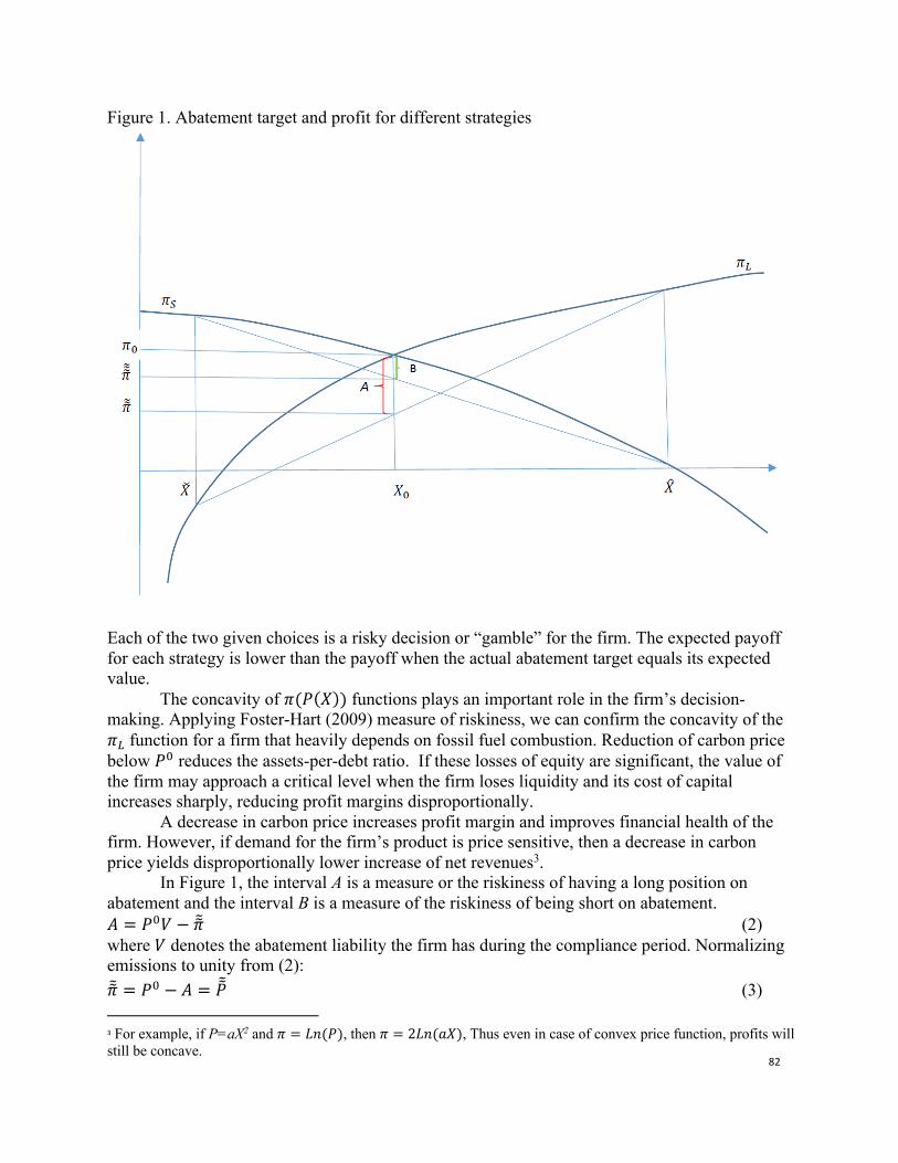
82

Figure 1. Abatement target and profit for different strategies

Each of the two given choices is a risky decision or “gamble” for the firm. The expected payoff for each strategy is lower than the payoff when the actual abatement target equals its expected value.

The concavity of 𝜋(𝑃(𝑋)) functions plays an important role in the firm’s decision-making. Applying Foster-Hart (2009) measure of riskiness, we can confirm the concavity of the 𝜋9function for a firm that heavily depends on fossil fuel combustion. Reduction of carbon price below 𝑃$ reduces the assets-per-debt ratio. If these losses of equity are significant, the value of the firm may approach a critical level when the firm loses liquidity and its cost of capital increases sharply, reducing profit margins disproportionally.

A decrease in carbon price increases profit margin and improves financial health of the firm. However, if demand for the firm’s product is price sensitive, then a decrease in carbon price yields disproportionally lower increase of net revenues3.

In Figure 1, the interval A is a measure or the riskiness of having a long position on abatement and the interval B is a measure of the riskiness of being short on abatement. 𝐴 = 𝑃$𝑉 − 𝜋?@ (2) where 𝑉 denotes the abatement liability the firm has during the compliance period. Normalizing emissions to unity from (2): 𝜋?@ = 𝑃$ − 𝐴 = 𝑃@@ (3)

3 For example, if P=aX2 and 𝜋 = 𝐿𝑛(𝑃), then 𝜋 = 2𝐿𝑛(𝑎𝑋), Thus even in case of convex price function, profits will still be concave.

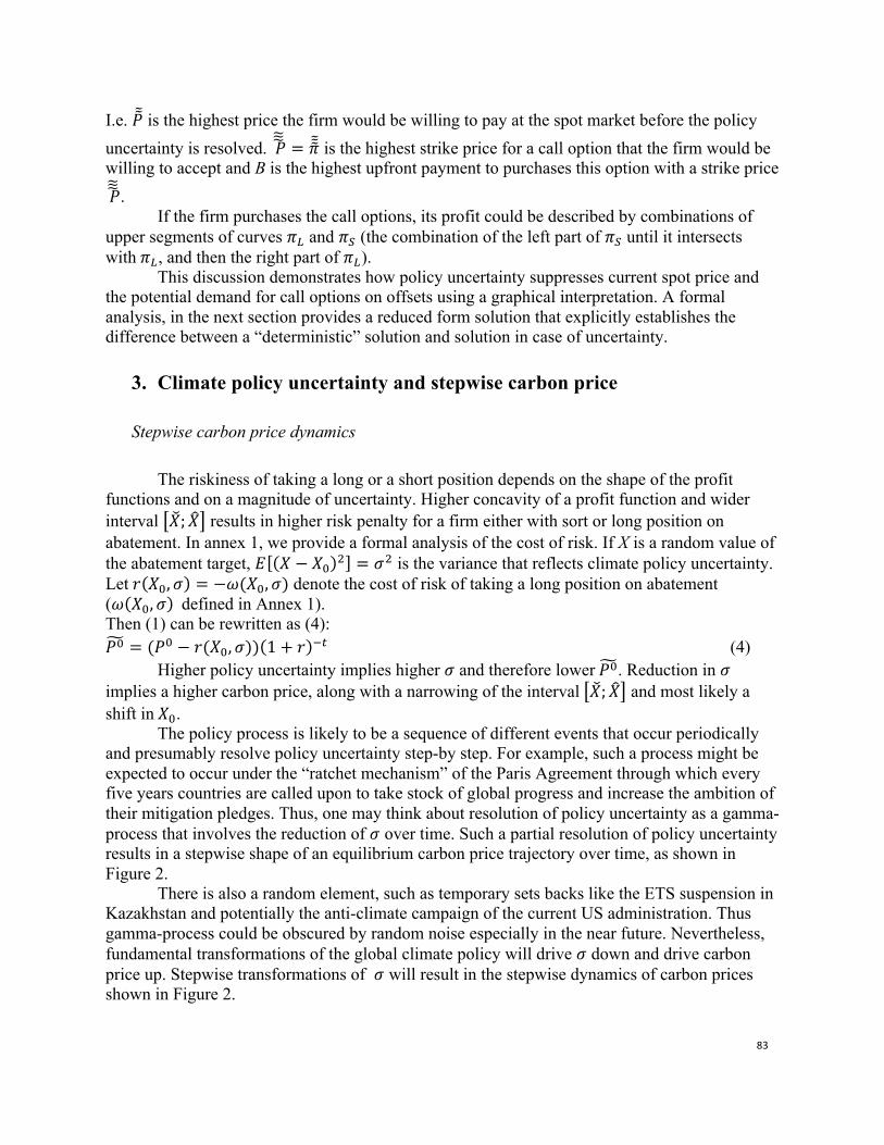
83

I.e. 𝑃@@ is the highest price the firm would be willing to pay at the spot market before the policy uncertainty is resolved. 𝑃EEE = 𝜋?@@ is the highest strike price for a call option that the firm would be willing to accept and B is the highest upfront payment to purchases this option with a strike price 𝑃EEE .

If the firm purchases the call options, its profit could be described by combinations of upper segments of curves 𝜋9 and 𝜋8 (the combination of the left part of 𝜋8 until it intersects with𝜋9, and then the right part of 𝜋9).

This discussion demonstrates how policy uncertainty suppresses current spot price and the potential demand for call options on offsets using a graphical interpretation. A formal analysis, in the next section provides a reduced form solution that explicitly establishes the difference between a “deterministic” solution and solution in case of uncertainty.

3. Climate policy uncertainty and stepwise carbon price

Stepwise carbon price dynamics

The riskiness of taking a long or a short position depends on the shape of the profit functions and on a magnitude of uncertainty. Higher concavity of a profit function and wider interval &𝑋'; 𝑋)* results in higher risk penalty for a firm either with sort or long position on abatement. In annex 1, we provide a formal analysis of the cost of risk. If X is a random value of the abatement target, 𝐸[(𝑋 − 𝑋$)H] = 𝜎H is the variance that reflects climate policy uncertainty. Let𝑟(𝑋$, 𝜎) = −𝜔(𝑋$, 𝜎) denote the cost of risk of taking a long position on abatement (𝜔(𝑋$, 𝜎)defined in Annex 1). Then (1) can be rewritten as (4): 𝑃$1 = (𝑃$ − 𝑟(𝑋$, 𝜎))(1 + 𝑟)56 (4)

Higher policy uncertainty implies higher 𝜎 and therefore lower𝑃$1 . Reduction in 𝜎 implies a higher carbon price, along with a narrowing of the interval&𝑋'; 𝑋)* and most likely a shift in𝑋$.

The policy process is likely to be a sequence of different events that occur periodically and presumably resolve policy uncertainty step-by step. For example, such a process might be expected to occur under the “ratchet mechanism” of the Paris Agreement through which every five years countries are called upon to take stock of global progress and increase the ambition of their mitigation pledges. Thus, one may think about resolution of policy uncertainty as a gamma-process that involves the reduction of 𝜎 over time. Such a partial resolution of policy uncertainty results in a stepwise shape of an equilibrium carbon price trajectory over time, as shown in Figure 2.

There is also a random element, such as temporary sets backs like the ETS suspension in Kazakhstan and potentially the anti-climate campaign of the current US administration. Thus gamma-process could be obscured by random noise especially in the near future. Nevertheless, fundamental transformations of the global climate policy will drive 𝜎 down and drive carbon price up. Stepwise transformations of 𝜎 will result in the stepwise dynamics of carbon prices shown in Figure 2.

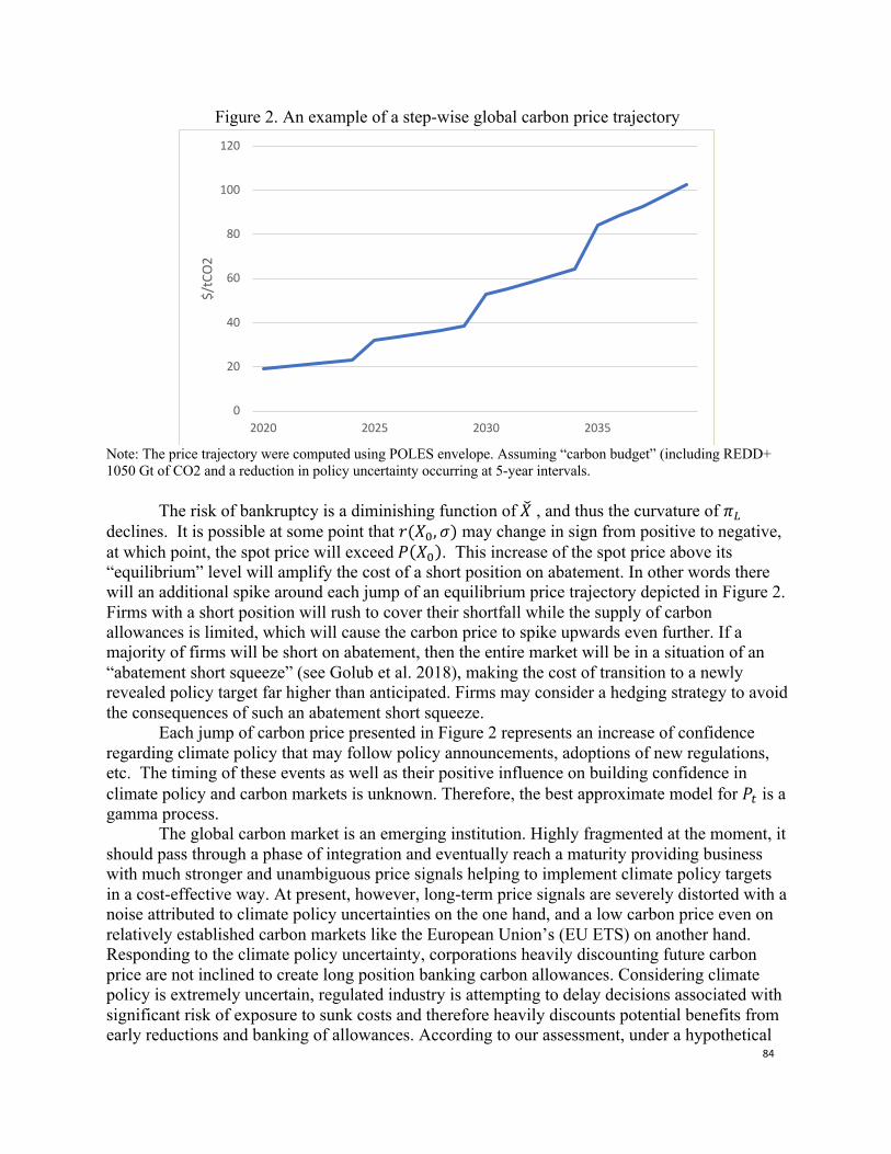
84

Figure 2. An example of a step-wise global carbon price trajectory

Note: The price trajectory were computed using POLES envelope. Assuming “carbon budget” (including REDD+ 1050 Gt of CO2 and a reduction in policy uncertainty occurring at 5-year intervals.

The risk of bankruptcy is a diminishing function of𝑋' , and thus the curvature of 𝜋9 declines. It is possible at some point that 𝑟(𝑋$, 𝜎) may change in sign from positive to negative, at which point, the spot price will exceed𝑃(𝑋$). This increase of the spot price above its “equilibrium” level will amplify the cost of a short position on abatement. In other words there will an additional spike around each jump of an equilibrium price trajectory depicted in Figure 2. Firms with a short position will rush to cover their shortfall while the supply of carbon allowances is limited, which will cause the carbon price to spike upwards even further. If a majority of firms will be short on abatement, then the entire market will be in a situation of an “abatement short squeeze” (see Golub et al. 2018), making the cost of transition to a newly revealed policy target far higher than anticipated. Firms may consider a hedging strategy to avoid the consequences of such an abatement short squeeze.

Each jump of carbon price presented in Figure 2 represents an increase of confidence regarding climate policy that may follow policy announcements, adoptions of new regulations, etc. The timing of these events as well as their positive influence on building confidence in climate policy and carbon markets is unknown. Therefore, the best approximate model for 𝑃6 is a gamma process.

The global carbon market is an emerging institution. Highly fragmented at the moment, it should pass through a phase of integration and eventually reach a maturity providing business with much stronger and unambiguous price signals helping to implement climate policy targets in a cost-effective way. At present, however, long-term price signals are severely distorted with a noise attributed to climate policy uncertainties on the one hand, and a low carbon price even on relatively established carbon markets like the European Union’s (EU ETS) on another hand. Responding to the climate policy uncertainty, corporations heavily discounting future carbon price are not inclined to create long position banking carbon allowances. Considering climate policy is extremely uncertain, regulated industry is attempting to delay decisions associated with significant risk of exposure to sunk costs and therefore heavily discounts potential benefits from early reductions and banking of allowances. According to our assessment, under a hypothetical

0

20

40

60

80

100

120

2020 2025 2030 2035

$/tC

O2

85

case of perfect certainty over announced future targets, a forward-looking analysis of the EU-ETS would imply a spot price for EUAsin a range $25-30/tCO2 in the early 2017. The actual price was about $5/tCO2. However, over last 2 years, the price increased nearly 5 times.4 There are several factors that could explain such an increase. Resolution of policy uncertainty and increased confidence by European corporations in the longevity of the climate policy is one the most important factors behind the recent price dynamics.

There are several studies on global climate policy and corresponding price of carbon that give us un understanding of magnitude of carbon price needed in the future to comply with announced and to large extend agreed climate policy goals. For example, according to Nordhaus (2013, 2015)5 in 2030 carbon price that corresponds to 2 C stabilization target should be in a range of $90-180/tCO2.6 We estimate that such myopic pricing of carbon corresponds to about 20% implicit discount rate on EU market and about 25-23% at the global market.

Climate policy is likely to evolve in an iterative manner in response to new scientific discoveries, economic development, and continually changing political environment. Such adjustments of climate policy will inevitably result in carbon markets corrections. Given the disconnect between the ambitious agreed-on climate policy target to keep increase of the global temperature below 2 C, on one hand, and weak and fragmented current climate policy that produces low prices of carbon on another hand, we anticipate strengthening of carbon emissions regulations to align with long term environmental targets. Corporations will receive stronger and clearer signals from regulators. This development will result in building business confidence in carbon markets and consequential increase of carbon price.

Quantitative assessment of the global carbon price

We developed a projection of international carbon prices under a gradually evolving international policy environment consistent with the implementation of the Paris Agreement and measures to neutralize new emissions from civil aviation after 2020 (under negotiation in the International Civil Aviation Organization). We assume the implementation of the Paris Agreement involves a carbon market that gradually expands in terms of its coverage and the tightness of the emissions limits. Information about future climate policy is only incrementally revealed to market actors at 5-year intervals, in line with the ratchet mechanism of the Paris Agreement. Our projection of carbon prices is shown in Figure 3.

4 EUA price increased in the beginning of 2018 (http://markets.businessinsider.com/commodities/co2-emissionsrechte) 5 Nordhaus, William D. The climate casino: Risk, uncertainty, and economics for a warming world. Yale University Press, 2013. Nordhaus, William. "Climate clubs: overcoming free-riding in international climate policy." The American Economic Review 105.4 (2015): 1339-1370. 6 This price range corresponds to cumulative total emissions limit 930-1330 Gt of CO2.

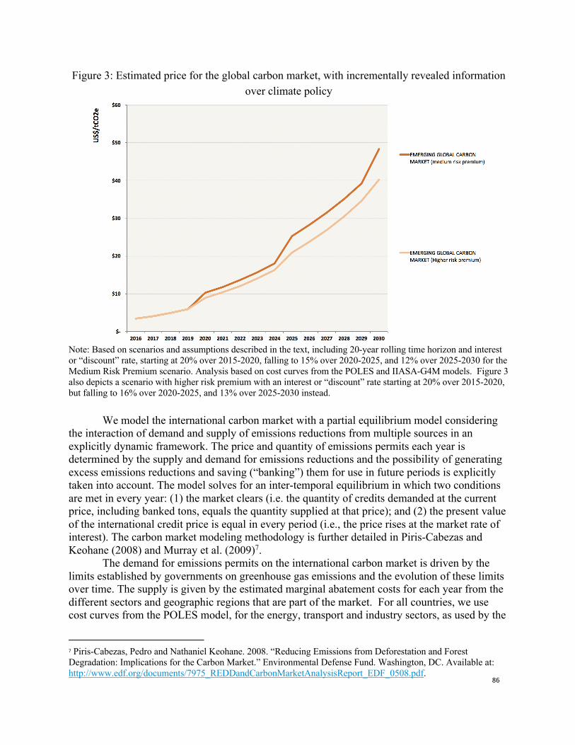
86

Figure 3: Estimated price for the global carbon market, with incrementally revealed information over climate policy

Note: Based on scenarios and assumptions described in the text, including 20-year rolling time horizon and interest or “discount” rate, starting at 20% over 2015-2020, falling to 15% over 2020-2025, and 12% over 2025-2030 for the Medium Risk Premium scenario. Analysis based on cost curves from the POLES and IIASA-G4M models. Figure 3 also depicts a scenario with higher risk premium with an interest or “discount” rate starting at 20% over 2015-2020, but falling to 16% over 2020-2025, and 13% over 2025-2030 instead.

We model the international carbon market with a partial equilibrium model considering the interaction of demand and supply of emissions reductions from multiple sources in an explicitly dynamic framework. The price and quantity of emissions permits each year is determined by the supply and demand for emissions reductions and the possibility of generating excess emissions reductions and saving (“banking”) them for use in future periods is explicitly taken into account. The model solves for an inter-temporal equilibrium in which two conditions are met in every year: (1) the market clears (i.e. the quantity of credits demanded at the current price, including banked tons, equals the quantity supplied at that price); and (2) the present value of the international credit price is equal in every period (i.e., the price rises at the market rate of interest). The carbon market modeling methodology is further detailed in Piris-Cabezas and Keohane (2008) and Murray et al. (2009)7.

The demand for emissions permits on the international carbon market is driven by the limits established by governments on greenhouse gas emissions and the evolution of these limits over time. The supply is given by the estimated marginal abatement costs for each year from the different sectors and geographic regions that are part of the market. For all countries, we use cost curves from the POLES model, for the energy, transport and industry sectors, as used by the

7 Piris-Cabezas, Pedro and Nathaniel Keohane. 2008. “Reducing Emissions from Deforestation and Forest Degradation: Implications for the Carbon Market.” Environmental Defense Fund. Washington, DC. Available at: http://www.edf.org/documents/7975_REDDandCarbonMarketAnalysisReport_EDF_0508.pdf.

87

European Commission for its international carbon market modeling8,9. We add cost curves for reducing deforestation from the rest of the world based on the global land-use modeling cluster of the International Institute of Applied Systems Analysis (IIASA), assuming a gradual phase-in through 2030.10

In addition to periodical corrections of carbon price illustrated in Figure 1, there will be residual volatility and mid-term deviations from equilibrium pathway attributed to various factors that may temporarily influence carbon price.

Global market segmentation and multiple carbon price

Between 2016 and 2019, the modelled international market includes California, and Canadian provinces (British Columbia, Manitoba, Ontario, Quebec). In 2020, the EU, Norway, Switzerland, South Korea and international aviation sector join the global market. At the same time, we assume the rest of the world gradually phases into the market at the rate of 10% a year starting in 2020 to achieve a full global market by 2030. The gradual phase-in includes both potential buyers and sellers of reduced emissions from deforestation and forest degradation (REDD+) and other emission reductions from other developing countries.

With respect to the long-term stringency of international policy, we consider a scenario with global reductions for 2050 in line with the goal established by the G8 leaders at the July 9, 2009 Major Economies Forum. This calls for the G8 to reduce emissions by 80% or more by 2050 as part of a global reduction of 50% by 2050 relative to 2005 levels, with the aim of limiting warming to no more than two degrees Celsius above preindustrial levels. However, to model a gradual ramp-up of global policy, we assume a less ambitious global reduction trajectory up through 2030, which is on a straight-line path between 2015 levels and a 25% reduction by 2050. The trajectory of the global cap then becomes steeper over 2030-2050. This global reduction scenario falls short of the long-term goals adopted in the Paris Agreement and results in conservative carbon price estimates.

When banking is allowed, rational expectations mean that allowance prices will increase at a constant rate of interest reflecting the real rate of return in the market. In our analysis, this interest rate is an exogenous parameter that must be chosen. If prices were expected to rise at any rate other than the market rate of return, this would provide systematic opportunities for investors to profit from buying or selling carbon permits. These profit opportunities would be

8 In particular, for this analysis we used updated cost curves released in October 2012 by ENERDATA. The POLES model generates worldwide MACCs broken down at the level of the main countries and regions (54 consuming countries + 12 regions) for the energy, industry, and transport sectors. The marginal abatement cost (MAC) curves and business-as-usual (BAU) emissions estimates for California are based on ARB’s estimates scaled down proportionally to reflect the latest changes to BAU emissions from Bailey et al. (2013), which incorporates the impact of the last economic recession. Staff at the California Air Resources Board (CARB) provided estimates of BAU emissions and the MAC curves for capped sectors (Onda and Fine, 2012). For Quebec we use MAC curves and BAU estimates based on the POLES model for Canada, scaled down to reflect the heterogeneity in sectoral emission composition of the Canadian provinces. 9 The BAU estimates for energy consumption in Brazil is in line with the COPPE INDC no regrets scenario described in chapter 2.6 authored by researcher from COPPE UFRJ for the MILES report (see citation in footnote 5). 10 For a detailed description of IIASA’s global land-use modeling cluster see Gusty M., P. Havlik and M. Obersteiner. 2008. “Technical description of the IIASA model cluster”, International Institute for Applied Systems Analysis, Laxenburg, Austria. Available at:http://www.obt.inpe.br/prodes/index.php

88

expected to induce buying or selling until the arbitrage opportunities were eliminated. These assumptions are common practice in economic modeling of carbon markets.

We adjust the standard modeling framework described above so as to provide more realistic analysis of how the carbon market is evolving and may continue to develop over the coming decades. As discussed theoretically, uncertainties create incentives to defer purchases and banking of emissions units and other investments that could result in sunk costs. This is consistent with empirical evidence that policy risk is depressing carbon prices in existing carbon markets, such as the European Union (e.g. Koch et al. 2014, 2016)11.

To account for policy uncertainty, we limit the typical assumption of perfect foresight by modeling a global carbon policy that is only incrementally revealed to market actors. This step-wise learning about policy means market actors face uncertainty about the future and cannot select their most cost-effective mitigation strategy and levels of banking once and for all but, rather, need to adjust to new information as it arrives. Market actors face the risk of significant adjustment costs if prices go higher (or lower) than anticipated and thus have incentives to manage the potential risks through instruments such as option contracts, rather than direct purchases of credits.

To model this stepwise pattern of learning, we introduce a risk premium on top of the modeled interest rate, which is a key input into the model and assume it decreases in 5-year intervals matching the ratchet mechanism of the Paris Agreement, as greater certainty over the future emerges.

We assume a risk-free (real) interest rate of 5% and a risk-adjusted interest or “discount” rate, including a risk-premium, that starts at 20% over 2016-2020, falling to 15% over 2020-2025, and 10% over 2025-2030. The 20% risk-adjusted interest rate is chosen to be consistent with estimation of the risk premium embedded due to policy uncertainty under the current European Emissions Trading System (ETS)12. For the sake of realism, we also limit the foresight of market actors by assuming a planning horizon that is limited at 20 years. Thus, market actors in 2016 look ahead to 2035 and market actors in 2020 and 2025 look ahead to 2039 and 2044, respectively.

To model the effect of learning, we then run our model iteratively at 5-year steps. We first solve the model starting in 2016 with a 20% interest rate to estimate prices and banking in each year. This provides the conditions we estimate through 2020, which we then use to re-run the analysis with a 15% interest rate, starting in 2020. This then provides the conditions through 2025, which we then use to re-run the analysis with a 12% interest rate, starting in 2025. The result of this analysis is an estimated price path that rises in a step-wise fashion over time, as shown in Figure 1, with an estimated carbon price is $3.4 in 2016 rising to $49/tCO2e by 2030 (and $78/t by 2035) as carbon markets grow and policies become less uncertain. While prices are initially depressed due to the modelled uncertainties, prices eventually have to rise higher and faster under this scenario to compensate for the lost mitigation opportunities that are not undertaken in the early years due to the excessive risk. The price path also exhibits periodic jumps as the market adjusts to greater information that provides more certainty over future

11 Pedro Piris-Cabezas and Ruben Lubowski. 2013. “Increasing Demand by Raising Long Term Expectations: the Importance of a 2030 Target for the European Union’s Climate Policy.” Environmental Defense Fund. Washington, DC. 12 Pedro Piris-Cabezas and Ruben Lubowski. 2013. “Increasing Demand by Raising Long Term Expectations: the Importance of a 2030 Target for the European Union’s Climate Policy.” Environmental Defense Fund. Washington, DC.

89

climate policies. As a sensitivity analysis, Figure 1 also depicts a scenario with higher risk premium with an interest or “discount” rate starting at 20% over 2015-2020, but falling to 16% over 2020-2025, and 13% over 2025-2030 instead, which results in lower forecasted carbon prices.

4. Engineering payoff: How REDD+ specific risks modify carbon price?

The high degree of policy uncertainty and high riskiness of banking carbon allowances implies most firms are likely to remain short on abatement. The maximum price the firm is willing to pay to hedge an entire short position is B in Figure 1 (see also the annex): 𝐵 = 𝜙(𝑋$, 𝜎) (5)

The firms should be willing to pay up to −𝜙(𝑋$, 𝜎) to hedge their short position buying a call options with strike price(𝜋8;𝑃(𝑋$)< + 𝜙(𝑋$, 𝜎))/𝑉. However within polluting industries it may be difficult to find enough candidates willing to wright call options since𝜙(𝑋$, 𝜎) >𝜔(𝑋$, 𝜎)13 In other words, the premium a firm is ready to pay is lower than the price a similar firm would be willing to accept for an option contract (this price should be sufficient to compensate for risk of creation of a long position). However, there could be a different situation with options on low-cost abatement from other sectors, such as Reducing Emissions from Deforestation and Forest Degradation (REDD+), as described by Golub et al. (2017). In order to establish a long position on REDD+, the cost to REDD+ credit producers would just be the temporally forgone revenues (as the decision to defer deforestation could be reversed in any time). As long as this revenue is less than −𝜙(𝑋$, 𝜎) and as long as strike price is high enough, REDD+ producers are able to write call options and slow down deforestation to accumulate offsets to cover sold options. A carbon intensive firm may create an options portfolio and rebalance it dynamically as new information regarding climate policy revealed.

The main requirement for a hedging tool is an absence of correlation with return on a risky position. Ideally one should look for a negative correlation, but such hedge is usually expensive (for example long position on Exxon-Mobil could be perfectly hedged by a put option, but in theory return of this portfolio will be zero minus transaction cost). REDD+ provides a hedging opportunity with a positive return for all participants in the transaction:

Return of REDD+ has a negative correlation with short abatement position: if carbon price goes high, REDD+ yields returns while a short position on abatement generated losses (and vice versa). As described further in Golub et al. (2017), the cost of REDD+ production (including monetized risk) will likely be determined by factors not directly related with factors that drive carbon prices. As result there is an arbitrage between value of long position on abatement (value of a call option on REDD+) for a business looking for a hedge (that value could be derived from a distribution of the future carbon price) on one hand, and cost of REDD+ call option “production” on another hand. As result the global society has a net benefit from using REDD+ to hedge short position on abatement. Indeed, the global benefits could be even greater if society would be net long on abatement right away implementing immediately strict policy to cut carbon emissions. But there are well known political barriers that prevent such a policy and instead generate climate policy uncertainties. Thus REDD+ should not be blamed for

13 According to our preliminary analysis of heterogeneous firms, some of them could be well position to cut emissions earlier and then sell call options, but on average polluting industries as a whole will be net short.

90

delay in abatement, but should be treated as a “first aid” to compensate for political indecisions and delays.

Research and Development (R&D) into new low carbon technologies is another hedging instrument that corporations may use to mitigate the cost of an abatement short squeeze. This kind of R&D creates a real option (call option) to deploy a low-carbon technology. This instrument can lower costs in response to both explicit and implicit carbon prices. However, the call option on low-carbon technology would not provide immediate relief, since some time will be necessary to mobilize the required capital and to deploy the technology. The best result for a carbon intensive firm and for society would be obtained when both call options are available. An option on REDD+ provides an immediate relief for the firm exposed to climate policy and the call option on low-carbon technologies guarantees timely adjustment of emissions pathway and creates the foundation for long-term emissions reductions. Cap and trade creates an adequate institutional environment to build incentives for corporations to be long on both options REDD+ and R&D. In other words, cap and trade is a better policy environment compare to carbon tax (or technology standards) for dynamic hedging of abatement interventions and the emissions pathway.

Thus, options on REDD+ will reduce magnitude of abatement short squeeze and partiality mitigate the carbon price jump. Options on low carbon technologies will create opportunities for transition to a low emissions pathway and in general reduce the long-term equilibrium carbon price.

Conclusions

Climate policy uncertainty creates incentives to defer investment into both carbon intensive and low-carbon technologies. There is thus a net reduction in both investment and production efficiency. In this paper, we presented a conceptual analysis of the driving forces behind these disincentives and established a relationship between the magnitude of policy uncertainty and the risks of premature investments into both high and low-carbon strategies. We demonstrate that the value of the deferral option is an increasing function of uncertainty represented in the model by the standard deviation of return on investment.

By delaying investment into low-carbon technologies, corporations are building up a net short position on abatement that is subject to risk. Current climate policy is weak and inconsistent with the target of limiting warming to 2°C or below and policy. Market uncertainties suppress demand for banking allowances for the longer term, contributing to low carbon prices in the current spot market for carbon emission units. Over time, a strengthening of climate policy should resolve uncertainties and reduce the riskiness of mitigation investments (including, depending on strength of the policy, investments into lower-emitting fossil fuel technologies).

We anticipate a number of sequential adjustments to climate policy, indicating greater stringency over time, and derive a stepwise rising function to describe the anticipated dynamics of the future carbon price pathway across international markets. Of course, radical innovations in energy production and consumption may change the profile of the global carbon price pathway, but even in this case carbon prices are likely to increase before declining.

Options on low-cost abatement options, notably REDD+, could play an essential role in helping firms to engineer the future payoffs from their abatement strategies (Golub et al. 2018). Such call options offer the potential to dramatically change the shape of a firm’s profit function,

91

allowing the firm will avoid the least desirable outcomes including bankruptcy. Similarly, research and development into low-carbon technologies creates valuable optionality to deploy cost-effective mitigation in the future. Investments into REDD+ and other low-carbon strategies, however, are yet a largely unknown and ambiguous instrument for business. Policies to legitimize investments in near-term opportunities such as REDD+, including creating consensus on high quality standards, and to facilitate corporate ability to access to high-quality REDD+ units at large scales will also help make it part of solutions for business and environment in the face of continued uncertainty and policy delays. Policies to provide a minimum price for emissions reductions, including through auctions of tradable price guarantees (i.e. ‘put’ options; Bodnar et al. 2017) or other price guarantee mechanisms, could incentivize supply of REDD+ and other near-term sources of abatement, as well as R&D into low-carbon technologies, in the face of continuing policy and market uncertainties.

References Bodnar, P, Otta, C, Edwards, R, Hoch, S, McGlynn, E.F. and Wagner, G. (2017). Underwriting 1.5°C: competitive

approaches to financing accelerated climate change mitigation. Climate Policy 1-15. Bosetti, V, Lubowski, R., Golub, A., Markandya, A. (2011). “Linking Reduced Deforestation and a Global Carbon

Market: Implications for Clean Energy Technology and Policy Flexibility.” Environment and Development Economics 16(4): 479-505.

Brockhaus, M., Korhonen-Kurki, K., Sehring, J., Di Gregorio, M., Assembe-Mvondo, S., Babon, A., Bekele, M., Gebara, M.F., Khatri, D.B., Kambire, H. and Kengoum, F. (2017). “REDD+, transformational change and the promise of performance-based payments: a qualitative comparative analysis.” Climate Policy 17(6): 708-730.

CDP (2016). Out of the starting blocks: Tracking progress on corporate climate action. London, UK. Environmental Defense Fund (EDF) and Climate and Forest Capital (CFC) (2018, forthcoming). The REDD+

Acceleration Fund: Mobilizing Private Capital to Reduce Emissions from Tropical Deforestation. An Investment Blueprint. Washington, DC.

Environmental Defense Fund (EDF). (2016). “ICAO’s Market-Based Measure: An interactive tool to see how additional countries’ support for the MBM can boost coverage of international aviation emissions.“ Available at: https://www.edf.org/climate/icaos-market-based-measure

Environmental Defense Fund (EDF) and International Emissions Trading Association (IETA). (2016). Carbon Pricing: The Paris Agreement’s Key Ingredient. Washington, DC.

Foster, D.P., Hart,S. (2009). “An Operational Measure of Riskiness.” Journal of Political Economy 117(5): 785–814.

Fuss, S., Szolgayová, J., Golub, A., Obersteiner, M. (2011). “Options on low-cost abatement and investment in the energy sector: new perspectives on REDD+.” Environment and Development Economics 16(4): 507-525.

Golub, A., Lubowski, R. and Piris-Cabezas, P. (2017). “Balancing Risks from Climate Policy Uncertainties: The Role of Options and Reduced Emissions from Deforestation and Forest Degradation.” Ecological Economics 138: 90-98.

Golub, A.A., Fuss, S., Lubowski, R., Hiller, J., Khabarov, N., Koch, N., Krasovskii, A., Kraxner, F., Laing, T., Obersteiner, M. and Palmer, C. (2018). Escaping the climate policy uncertainty trap: options contracts for REDD+. Climate Policy, pp.1-8.

Hamrick, K. and M. Gallant. (2017). Unlocking Potential: State of the Voluntary Carbon Markets 2017. Ecosystem Marketplace, Forest Trends, Washington, DC.

Koch, N.T., Fuss, S., Grosjean, G., Edenhofer, O. (2014). “Causes of the EU ETS price drop: Recession, CDM, renewable policies or a bit of everything?—New evidence.” Energy Policy 73: 676-685.

Koch, N., Grosjean, G., Fuss, S., Edenhofer, O. (2016). “Politics matters: Regulatory events as catalysts for price formation under cap-and-trade.” Journal of Environmental Economics and Management 8: 121–139.

Lubowski, R., Golub, A., Taschini, L. and Parkhouse, R. (2014). “Bridging the REDD+ Finance Gap.” 2014. In Greenhouse Gas Market Report 2014. International Emissions Trading Association (IETA), Washington, DC.

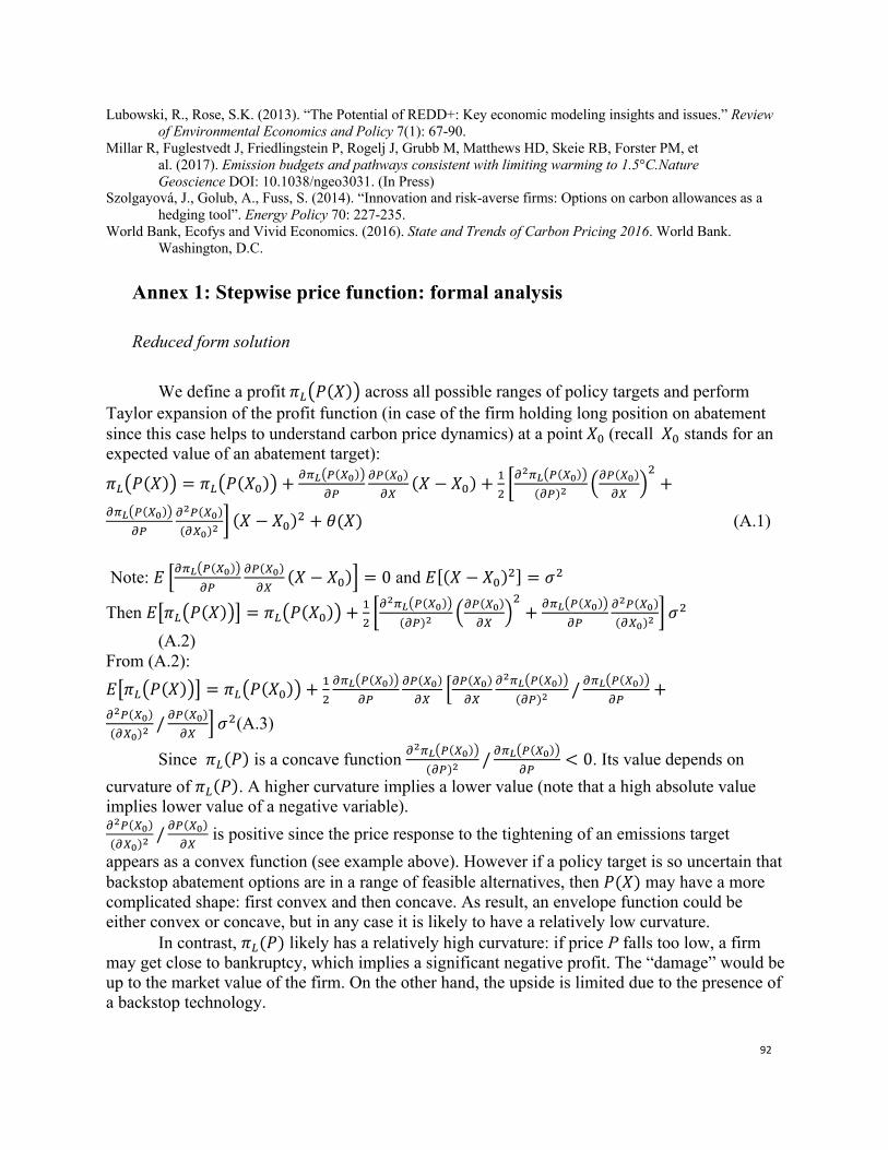
92

Lubowski, R., Rose, S.K. (2013). “The Potential of REDD+: Key economic modeling insights and issues.” Review of Environmental Economics and Policy 7(1): 67-90.

Millar R, Fuglestvedt J, Friedlingstein P, Rogelj J, Grubb M, Matthews HD, Skeie RB, Forster PM, et al. (2017). Emission budgets and pathways consistent with limiting warming to 1.5°C.Nature Geoscience DOI: 10.1038/ngeo3031. (In Press)

Szolgayová, J., Golub, A., Fuss, S. (2014). “Innovation and risk-averse firms: Options on carbon allowances as a hedging tool”. Energy Policy 70: 227-235.

World Bank, Ecofys and Vivid Economics. (2016). State and Trends of Carbon Pricing 2016. World Bank. Washington, D.C.

Annex 1: Stepwise price function: formal analysis

Reduced form solution

We define a profit𝜋9;𝑃(𝑋)< across all possible ranges of policy targets and perform

Taylor expansion of the profit function (in case of the firm holding long position on abatement since this case helps to understand carbon price dynamics) at a point𝑋$(recall 𝑋$ stands for an expected value of an abatement target):

𝜋9;𝑃(𝑋)< = 𝜋9;𝑃(𝑋$)< +PQR;S(TU)<

PSPS(TU)PT

(𝑋 − 𝑋$) +VHWP

XQR;S(TU)<(PS)X

YPS(TU)PT

ZH+

PQR;S(TU)<PS

PXS(TU)(PTU)X

[ (𝑋 − 𝑋$)H + 𝜃(𝑋) (A.1) Note: 𝐸 ]PQR;S(TU)<

PSPS(TU)PT

(𝑋 − 𝑋$)^ = 0 and 𝐸[(𝑋 − 𝑋$)H] = 𝜎H

Then 𝐸&𝜋9;𝑃(𝑋)<* = 𝜋9;𝑃(𝑋$)< +VHWP

XQR;S(TU)<(PS)X

YPS(TU)PT

ZH+ PQR;S(TU)<

PSPXS(TU)(PTU)X

[ 𝜎H (A.2) From (A.2): 𝐸&𝜋9;𝑃(𝑋)<* = 𝜋9;𝑃(𝑋$)< +

VHPQR;S(TU)<

PSPS(TU)PT

]PS(TU)PT

PXQR;S(TU)<(PS)X

/ PQR;S(TU)<PS

+PXS(TU)(PTU)X

/ PS(TU)PT

^ 𝜎H(A.3)

Since 𝜋9(𝑃) is a concave function PXQR;S(TU)<(PS)X

/ PQR;S(TU)<PS

< 0. Its value depends on curvature of 𝜋9(𝑃). A higher curvature implies a lower value (note that a high absolute value implies lower value of a negative variable). PXS(TU)(PTU)X

/ PS(TU)PT

is positive since the price response to the tightening of an emissions target appears as a convex function (see example above). However if a policy target is so uncertain that backstop abatement options are in a range of feasible alternatives, then 𝑃(𝑋) may have a more complicated shape: first convex and then concave. As result, an envelope function could be either convex or concave, but in any case it is likely to have a relatively low curvature.

In contrast, 𝜋9(𝑃) likely has a relatively high curvature: if price P falls too low, a firm may get close to bankruptcy, which implies a significant negative profit. The “damage” would be up to the market value of the firm. On the other hand, the upside is limited due to the presence of a backstop technology.

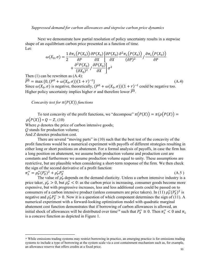
93

Suppressed demand for carbon allowances and stepwise carbon price dynamics

Next we demonstrate how partial resolution of policy uncertainty results in a stepwise shape of an equilibrium carbon price presented as a function of time. Let:

𝜔(𝑋$, 𝜎) =12𝜕𝜋9;𝑃(𝑋$)<

𝜕𝑃𝜕𝑃(𝑋$)𝜕𝑋 b

𝜕𝑃(𝑋$)𝜕𝑋

𝜕H𝜋9;𝑃(𝑋$)<(𝜕𝑃)H /

𝜕𝜋9;𝑃(𝑋$)<𝜕𝑃

+𝜕H𝑃(𝑋$)(𝜕𝑋$)H

/𝜕𝑃(𝑋$)𝜕𝑋 c 𝜎H

Then (1) can be rewritten as (A.4): 𝑃$1 = max{0, (𝑃$ + 𝜔(𝑋$, 𝜎))(1 + 𝑟)56} (A.4) Since 𝜔(𝑋$, 𝜎) is negative, theoretically, (𝑃$ + 𝜔(𝑋$, 𝜎))(1 + 𝑟)56 could be negative too. Higher policy uncertainty implies higher 𝜎 and therefore lower𝑃$1 .

Concavity test for 𝜋(𝑃(𝑋)) functions

To test concavity of the profit functions, we “decompose” 𝜋;𝑃(𝑋)< = 𝜋(𝜌;𝑃(𝑋)< =𝜌;𝑃(𝑋)< ∗ 𝑄 − 𝑍, (10) Where 𝜌 denotes the price of carbon intensive goods; Q stands for production volume; And Z denotes production cost.

There are several “moving parts” in (10) such that the best test of the concavity of the profit functions would be a numerical experiment with payoffs of different strategies resulting in either long or short positions on abatement. For a formal analysis of payoffs, in case the firm has a long position on abatement, we assume both production volume and production cost are constants and furthermore we assume production volume equal to unity. These assumptions are restrictive, but are plausible when considering a short-term response of thefirm. We then check the sign of the second derivative of a profit function: 𝜋9mm = 𝜌Smm(𝑃Tm )H + 𝜌Sm 𝑃Tmm (A.5 )

The value of 𝜌Sm depends on the demand elasticity. Unless a carbon intensive industry is a price taker, 𝜌Sm > 0, but 𝜌Smm < 0: as the carbon price is increasing, consumer goods become more expensive, but with progressive increases, less and less additional costs could be passed on to consumers of a carbon intensive product (unless consumers are price takers). In (11) 𝜌Smm(𝑃Tm )H is negative and 𝜌Sm 𝑃Tmm > 0. Now it is a question of which component determines the sign of (11). A numerical experiment with a forward-looking optimization model with quadratic marginal abatement cost function demonstrates that if borrowing of carbon allowances is allowed, an initial shock of allowances will be distributed over time14 such that 𝑃Tmm ≅ 0. Then𝜋9mm < 0 and 𝜋9 is a concave function as depicted in Figure 1.

14 While emissions trading systems may restrict borrowing in practice, an emerging practice is for emissions trading systems to include a type of borrowing at the system scale via a cost containment mechanism such as, for example, an allowance reserve that offers credits at a fixed price.

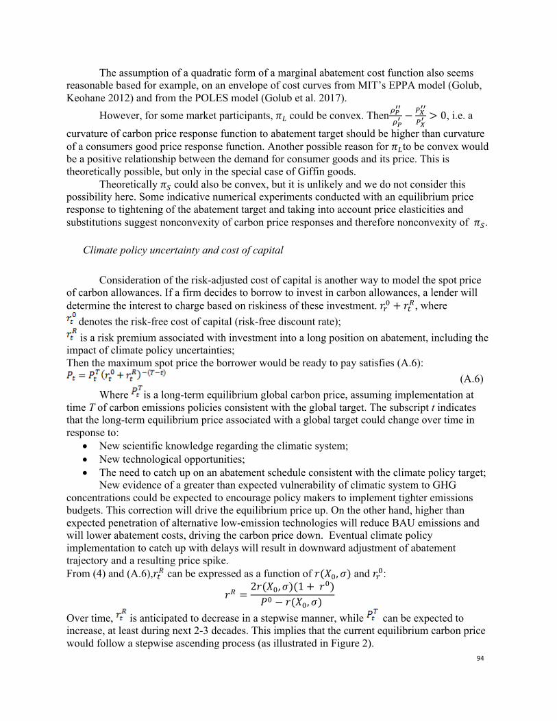
94

The assumption of a quadratic form of a marginal abatement cost function also seems reasonable based for example, on an envelope of cost curves from MIT’s EPPA model (Golub, Keohane 2012) and from the POLES model (Golub et al. 2017).

However, for some market participants, 𝜋9could be convex. Thenopqq

opq −

Srqq

Srq > 0, i.e. a

curvature of carbon price response function to abatement target should be higher than curvature of a consumers good price response function. Another possible reason for 𝜋9to be convex would be a positive relationship between the demand for consumer goods and its price. This is theoretically possible, but only in the special case of Giffin goods.

Theoretically 𝜋8 could also be convex, but it is unlikely and we do not consider this possibility here. Some indicative numerical experiments conducted with an equilibrium price response to tightening of the abatement target and taking into account price elasticities and substitutions suggest nonconvexity of carbon price responses and therefore nonconvexity of 𝜋8.

Climate policy uncertainty and cost of capital

Consideration of the risk-adjusted cost of capital is another way to model the spot price of carbon allowances. If a firm decides to borrow to invest in carbon allowances, a lender will determine the interest to charge based on riskiness of these investment. 𝑟s$ + 𝑟6t, where

denotes the risk-free cost of capital (risk-free discount rate); is a risk premium associated with investment into a long position on abatement, including the

impact of climate policy uncertainties; Then the maximum spot price the borrower would be ready to pay satisfies (A.6):

(A.6) Where is a long-term equilibrium global carbon price, assuming implementation at

time T of carbon emissions policies consistent with the global target. The subscript t indicates that the long-term equilibrium price associated with a global target could change over time in response to:

• New scientific knowledge regarding the climatic system; • New technological opportunities; • The need to catch up on an abatement schedule consistent with the climate policy target;

New evidence of a greater than expected vulnerability of climatic system to GHG concentrations could be expected to encourage policy makers to implement tighter emissions budgets. This correction will drive the equilibrium price up. On the other hand, higher than expected penetration of alternative low-emission technologies will reduce BAU emissions and will lower abatement costs, driving the carbon price down. Eventual climate policy implementation to catch up with delays will result in downward adjustment of abatement trajectory and a resulting price spike. From (4) and (A.6),𝑟6t can be expressed as a function of 𝑟(𝑋$, 𝜎) and 𝑟s$:

𝑟t =2𝑟(𝑋$, 𝜎)(1 +𝑟$)𝑃$ − 𝑟(𝑋$, 𝜎)

Over time, is anticipated to decrease in a stepwise manner, while can be expected to increase, at least during next 2-3 decades. This implies that the current equilibrium carbon price would follow a stepwise ascending process (as illustrated in Figure 2).

95

Cooperative Carbon Taxes Under the Paris Agreement that Even Fuel Exporters Could Like Grzegorz Peszko (World Bank), Alexander Golub (American University), Dominique van der Mensbrugghe (Purdue University)

Abstract

Economists often argue that the Paris Agreement will deliver on its 2° goal when the self-interests between a “club” of primary movers on climate action and more reluctant parties are aligned. A joint and reciprocal commitment to minimum domestic carbon prices and international transfers is often identified as an efficient instrument of this alignment. The climate policy leaders have not mobilized the political will to form such a club yet, let alone mobilizing adequate transfers to induce comprehensive cooperation. Even if they do, they will face several fossil fuel producers and exporters who are particularly reluctant to cooperate through traditional carbon prices, which extract their resource rents and transfer them to fuel importers. This paper argues that one way to align incentives for increased climate policy ambition is to shift the base of carbon taxes upstream to where fossil fuels are first extracted from the ground. This could be implemented through cooperative wellhead carbon tax treaties between fuel exporters and importers with revenue sharing agreements. Producers’ carbon tax would cover domestic emissions in fossil-fuel dependent countries but allow them to retain (a portion of) revenues otherwise collected abroad. This proposition is first illustrated in a partial equilibrium welfare economic framework and then quantified with a global, dynamic, recursive general equilibrium model integrated with global partial equilibrium fuel extraction models. Design, implementation and political economy issues are discussed. Key words: Carbon tax; climate cooperation, fossil-fuel dependent countries; border adjustment; supply side climate policies, ENVISAGE.

1. Introduction: Policy challenge to achieve Paris goal

The Paris Agreement adopted a goal to keep a global temperature rise this century below 2 degrees Celsius above pre-industrial levels and to pursue efforts to limit the temperature increase even further to 1.5 degrees Celsius. But this long-term global goal does not translate into incentives for each country to cooperate in achieving it. Several studies showed that the individual country goals embedded in their nationally determined contributions (NDCs) combined exceed this global aspiration. In particular, the fossil fuel-dependent countries (FFDCs) have been reluctant to implement ambitious climate policies amid concerns that the low-carbon transition will lead to a global decline in fossil fuel industries and related value chains currently vital to their economies.

Free riding incentives broke the coalition of climate action leaders under Annex I of the Kyoto Protocol and undercut their ability to attract developing countries to collectively determined mitigation commitments. The Paris Agreement achieved universal participation (at least initially) but at the cost of abandoning binding emission targets and allowing each country

96

to set its individually determined level of ambition for climate change mitigation and adaptation (NDCs). These voluntary pledges are to be reviewed internationally every 5 years, in the hope that global ambition will be increased by ‘naming and shaming’ (Falkner 2016) and moral pressure (Figueres 2016) supported by financial and technology transfers through climate finance and carbon markets from developed to developing countries (Cramton et al. 2012; Jakob et al. 2014; 2016; Carraro 2016).

Economists are often skeptical as to whether global ambition of climate action can indeed be increased mainly through moral suasion (Ostrom 2009, Stiglitz 2015, Barrett and Dannenberg 2016). Economic theory suggests that in the absence of a global government with coercive powers an effective and stable international environmental agreement need to be bound by aligning self-interests of the participants, hence self-enforcing (Barrett 1994; Diamantoudi and Sartzetakis 2006; Hoel and Schneider 1997).

The Paris Agreement explicitly acknowledged the primacy of domestic self-interest in climate policy and does not provide for any legally binding minimum levels of ambition of NDCs or enforcement instruments. But the open, bottom-up architecture of the Paris Agreement explicitly permits a group of parties under Article 6.1 to form a club (Nordhaus 2015) and pursue voluntary cooperation to allow for higher ambition in their mitigation and adaptation actions. Articles 6.2, 6.4 and 6.8 identify market and non-market approaches that could operationalize cooperation within and between climate clubs.

To make a climate club stable, its members should enjoy exclusive benefits and privileges that prevent them from defecting or free-riding on the efforts of other members. More recent literature argues that the Paris Agreement will become effective when the nationally determined contributions (NDCs) are complemented with collectively determined (but individually binding) contributions adopted by such a club of the willing parties (Gollier and Tirole 2015; MacKay 2015). They suggest this would enable trust building and effective enforcement based on reciprocity (“I will if you will” as suggested by Ostrom 2009) to keep the club stable (Cramton et al. 2017). Weitzman (2014) and many others argue that such collectively determined contributions could be built around the minimum levels of national carbon prices.

Once internally stable, a club of climate action leaders could start playing a multi-stage Stackelberg game and use a combination of “nudges”—such as financial and technology transfers (Steckel, et al 2017), carbon markets and border adjustment taxes (Böhringer et al., 2012; Cosbey et al., 2012; Nordhaus 2015; Kortum and Weisbach 2016), or other punishments (Dannenberg 2016)—to entice more ‘reluctant’ non-members to join the club. At some phase of this game a critical mass of participants could make a comprehensive global cooperative coalition stable (Barrett 2003; Cramton 2017). Many other economic and political issues can also be linked to cooperative behavior in international climate games (Carraro and Marchoiori 2004; Barrett and Dannenberg 2016). So far, the climate policy leaders have not been able to mobilize political will to agree on collective commitment, let alone mobilizing adequate side-payments to nudge cooperation by others.

Several countries and regions have revealed self-interest in pursuing some aspects of a low-carbon transition (LCT) independently of efforts to achieve the goals of the Paris Agreement. Most EU member states, California and a few other U.S. states, British Columbia and Quebec in Canada, and among developing countries Korea, China, India, New Zealand, Chile or more recently Morocco have invested in exploiting their first movers’ advantage in low-carbon, knowledge intensive technologies and products and establish their presence in international economic geography. What all these countries and regions have in common is that

97

they are net importers of fossil fuels and have already accumulated capital, skills and capabilities in knowledge-intensive rather than energy-intensive economic activities.

The literature on incentives for climate cooperation is dominated by the old developed-developing countries divide and the assumption that the level of ambition of mitigation action is inversely related to income. Recently, however, several low-income countries that are vulnerable to climate change (such as the Alliance of Small Island States (AOSIS group) are becoming global leaders of climate mitigation without waiting for massive foreign financial transfers, although their ability to act is constrained by lack of resources. It proves that the willingness to cooperate on climate action is no longer determined primarily by income level.

Instead, the most reluctant countries to cooperate include those whose economies depend on fossil fuel revenues and energy-intensive power and manufacturing sectors (FFDCs). Many FFDCs—whether low-, or high-income, have been reluctant to implement domestic climate mitigation actions amid concerns that it would disrupt their (often narrow) revenue sources and established comparative advantage. These concerns were duly recognized in the original United Nations Framework Convention on Climate Change adopted in 1992, Kyoto Protocol and in the Paris Agreement. Without addressing these concerns, an international coalition may not be comprehensive and stable enough to achieve the 2°C goal.

The perspective of fossil fuel exporters on demand-side climate policies is not new to the economic literature. Already in 1982 Bergstrom showed that if the main oil consuming nations cooperated with each other they can extract significant rents from oil producing nations through national excise taxes, counterbalancing the OPEC cartel goals. Liski and Tahvonen (2004), Jonansson et al. (2009) or Dong and Whalley (2009) confirmed that standard demand-side climate policies of OECD countries would capture OPEC oil rents. Bauer et al. (2016) applied the REMIND model to show that carbon prices introduced by importers of fossil fuels capture a portion of the resource rent from fuel exporters, while Strand (2008; 2013) and Karp et al (2015) found with the theoretical model that a carbon tax extracts higher rents from exporters than a cap-and-trade scheme. Franks et al. (2015) and Edenhofer and Ockenfels (2015) moved the debate further by demonstrating with a theoretical model that for fuel importers carbon taxes are superior alternative to capital taxes because the former capture part of the resource rent that is held initially by the owners and exporters of fossil fuels. They showed that this result holds regardless of whether fuel importers cooperate, and that fuel exporters loose even if they can influence price strategically with an export tax. Erickson et al. 2015; Erickson and Lazarus 2015; Elliott et al 2010 and Seto et al. 2016 explored further why carbon lock-in makes fossil fuel producers reluctant to undertake climate action. Therefore, Stiglitz (2015) noted that fossil fuel exporters may not have the incentive to implement traditional demand-side domestic carbon pricing just under the pressure of moral suasion.

Wirl (1995) found that best strategy for oil exporters is to pre-empt importers’ carbon tax at the wellhead. Dullieux et al 2014 suggested that in anticipation of consumers’ carbon tax the the OPEC could respond by increasing the producer price to postpone extraction and reduce consumption, rendering the carbon tax useless. In this way, they argue - OPEC can reap (a part of) the ”climate rent”. Similarly, Bohringer et al (2013) and Böhringer (2018) argued that OPEC may want to retain resource rents by increasing the oil price as a response to EU climate policy, thereby reversing leakage, but the coalition or cartel size critically affect the scope for rent seeking and leakage reduction.

There is a particular stream of literature proposing supply-side climate policies for the major fossil fuel producers (mainly coal) as a way to solve the “green paradox” challenge (Sinn

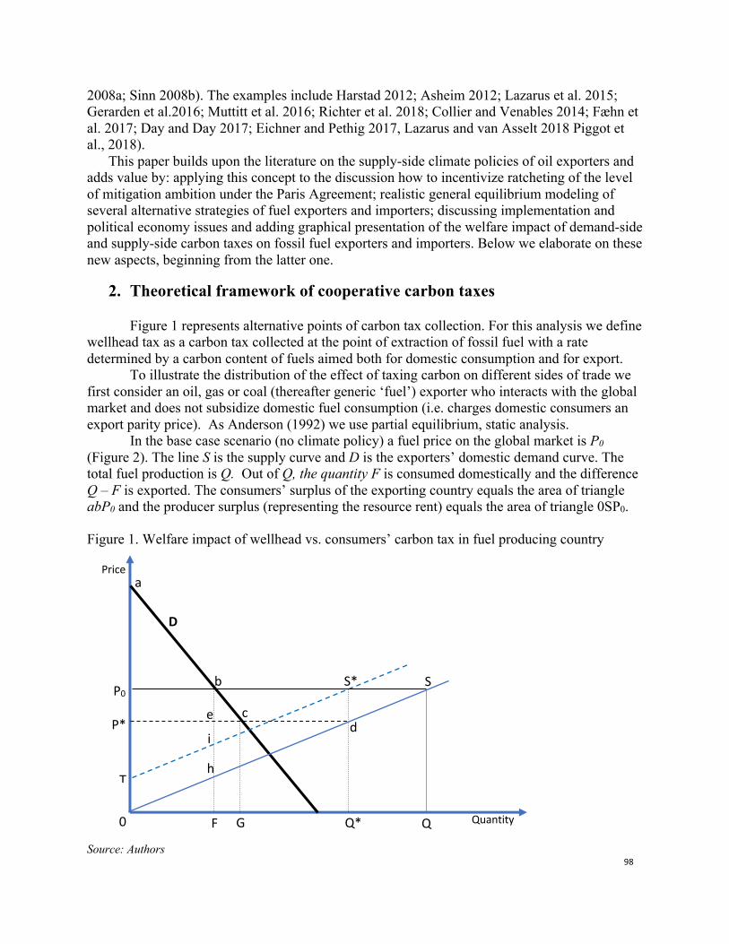
98

2008a; Sinn 2008b). The examples include Harstad 2012; Asheim 2012; Lazarus et al. 2015; Gerarden et al.2016; Muttitt et al. 2016; Richter et al. 2018; Collier and Venables 2014; Fæhn et al. 2017; Day and Day 2017; Eichner and Pethig 2017, Lazarus and van Asselt 2018 Piggot et al., 2018).

This paper builds upon the literature on the supply-side climate policies of oil exporters and adds value by: applying this concept to the discussion how to incentivize ratcheting of the level of mitigation ambition under the Paris Agreement; realistic general equilibrium modeling of several alternative strategies of fuel exporters and importers; discussing implementation and political economy issues and adding graphical presentation of the welfare impact of demand-side and supply-side carbon taxes on fossil fuel exporters and importers. Below we elaborate on these new aspects, beginning from the latter one.

2. Theoretical framework of cooperative carbon taxes

Figure 1 represents alternative points of carbon tax collection. For this analysis we define wellhead tax as a carbon tax collected at the point of extraction of fossil fuel with a rate determined by a carbon content of fuels aimed both for domestic consumption and for export.

To illustrate the distribution of the effect of taxing carbon on different sides of trade we first consider an oil, gas or coal (thereafter generic ‘fuel’) exporter who interacts with the global market and does not subsidize domestic fuel consumption (i.e. charges domestic consumers an export parity price). As Anderson (1992) we use partial equilibrium, static analysis.

In the base case scenario (no climate policy) a fuel price on the global market is P0 (Figure 2). The line S is the supply curve and D is the exporters’ domestic demand curve. The total fuel production is Q. Out of Q, the quantity F is consumed domestically and the difference Q – F is exported. The consumers’ surplus of the exporting country equals the area of triangle abP0 and the producer surplus (representing the resource rent) equals the area of triangle 0SP0. Figure 1. Welfare impact of wellhead vs. consumers’ carbon tax in fuel producing country

Source: Authors

S* S

D

Q* Q 0

P*

P0

h

e

b

a

c

Price

Quantity

d

G F

i

T

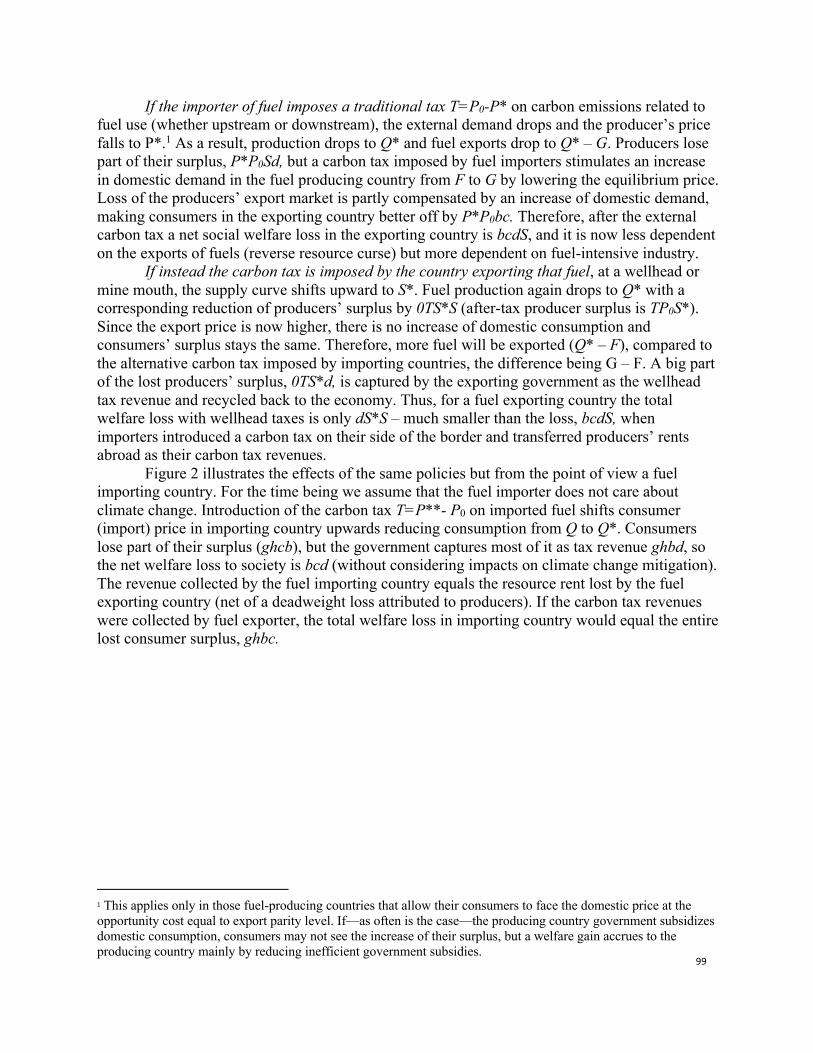
99

If the importer of fuel imposes a traditional tax T=P0-P* on carbon emissions related to fuel use (whether upstream or downstream), the external demand drops and the producer’s price falls to P*.1 As a result, production drops to Q* and fuel exports drop to Q* – G. Producers lose part of their surplus, P*P0Sd, but a carbon tax imposed by fuel importers stimulates an increase in domestic demand in the fuel producing country from F to G by lowering the equilibrium price. Loss of the producers’ export market is partly compensated by an increase of domestic demand, making consumers in the exporting country better off by P*P0bc. Therefore, after the external carbon tax a net social welfare loss in the exporting country is bcdS, and it is now less dependent on the exports of fuels (reverse resource curse) but more dependent on fuel-intensive industry.

If instead the carbon tax is imposed by the country exporting that fuel, at a wellhead or mine mouth, the supply curve shifts upward to S*. Fuel production again drops to Q* with a corresponding reduction of producers’ surplus by 0TS*S (after-tax producer surplus is TP0S*). Since the export price is now higher, there is no increase of domestic consumption and consumers’ surplus stays the same. Therefore, more fuel will be exported (Q* – F), compared to the alternative carbon tax imposed by importing countries, the difference being G – F. A big part of the lost producers’ surplus, 0TS*d, is captured by the exporting government as the wellhead tax revenue and recycled back to the economy. Thus, for a fuel exporting country the total welfare loss with wellhead taxes is only dS*S – much smaller than the loss, bcdS, when importers introduced a carbon tax on their side of the border and transferred producers’ rents abroad as their carbon tax revenues.

Figure 2 illustrates the effects of the same policies but from the point of view a fuel importing country. For the time being we assume that the fuel importer does not care about climate change. Introduction of the carbon tax T=P**- P0 on imported fuel shifts consumer (import) price in importing country upwards reducing consumption from Q to Q*. Consumers lose part of their surplus (ghcb), but the government captures most of it as tax revenue ghbd, so the net welfare loss to society is bcd (without considering impacts on climate change mitigation). The revenue collected by the fuel importing country equals the resource rent lost by the fuel exporting country (net of a deadweight loss attributed to producers). If the carbon tax revenues were collected by fuel exporter, the total welfare loss in importing country would equal the entire lost consumer surplus, ghbc.

1 This applies only in those fuel-producing countries that allow their consumers to face the domestic price at the opportunity cost equal to export parity level. If—as often is the case—the producing country government subsidizes domestic consumption, consumers may not see the increase of their surplus, but a welfare gain accrues to the producing country mainly by reducing inefficient government subsidies.

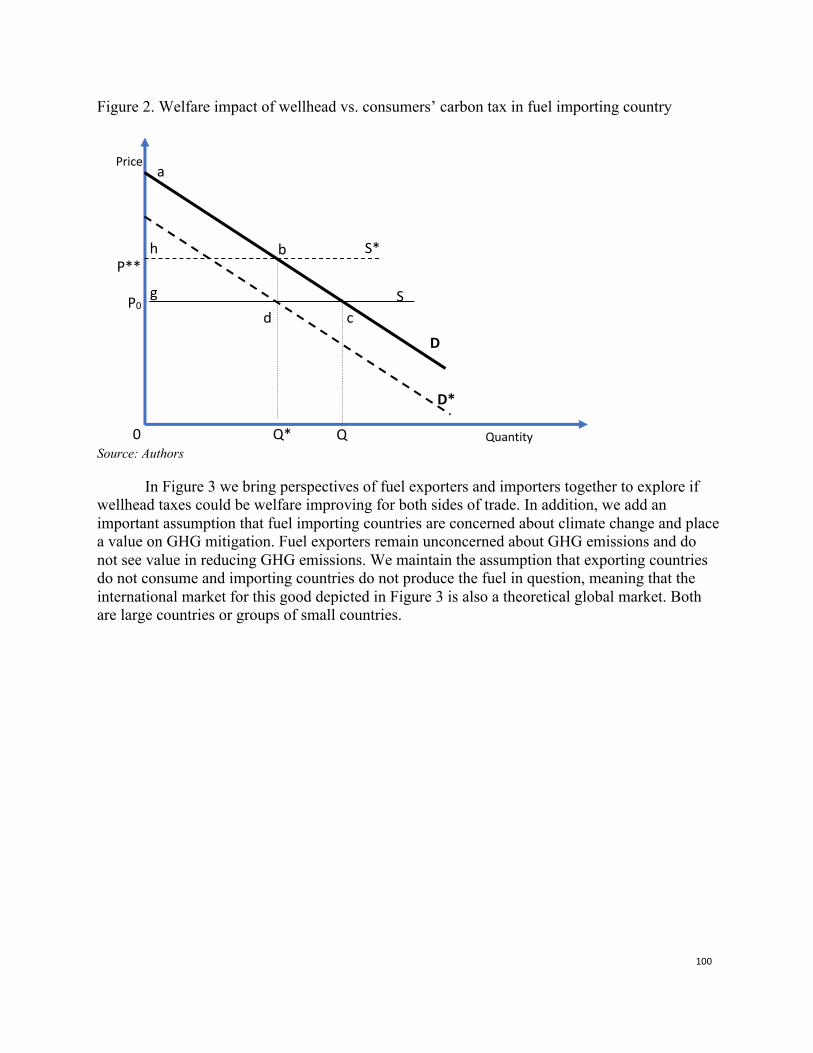
100

Figure 2. Welfare impact of wellhead vs. consumers’ carbon tax in fuel importing country

Source: Authors

In Figure 3 we bring perspectives of fuel exporters and importers together to explore if wellhead taxes could be welfare improving for both sides of trade. In addition, we add an important assumption that fuel importing countries are concerned about climate change and place a value on GHG mitigation. Fuel exporters remain unconcerned about GHG emissions and do not see value in reducing GHG emissions. We maintain the assumption that exporting countries do not consume and importing countries do not produce the fuel in question, meaning that the international market for this good depicted in Figure 3 is also a theoretical global market. Both are large countries or groups of small countries.

S*

S

D

Q* Q 0

P0

P**’

h

g

b

a

c

Price

Quantity

D*

d

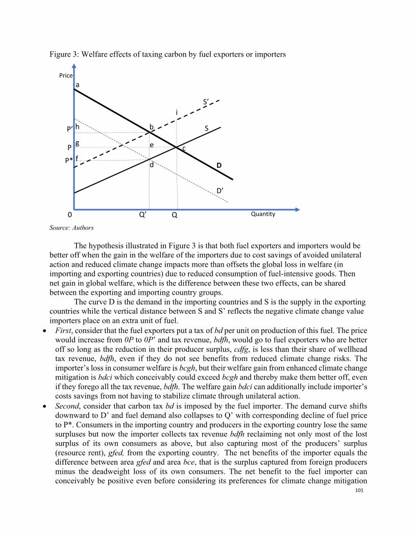
101

Figure 3: Welfare effects of taxing carbon by fuel exporters or importers

Source: Authors

The hypothesis illustrated in Figure 3 is that both fuel exporters and importers would be better off when the gain in the welfare of the importers due to cost savings of avoided unilateral action and reduced climate change impacts more than offsets the global loss in welfare (in importing and exporting countries) due to reduced consumption of fuel-intensive goods. Then net gain in global welfare, which is the difference between these two effects, can be shared between the exporting and importing country groups.

The curve D is the demand in the importing countries and S is the supply in the exporting countries while the vertical distance between S and S’ reflects the negative climate change value importers place on an extra unit of fuel.

• First, consider that the fuel exporters put a tax of bd per unit on production of this fuel. The price would increase from 0P to 0P’ and tax revenue, bdfh, would go to fuel exporters who are better off so long as the reduction in their producer surplus, cdfg, is less than their share of wellhead tax revenue, bdfh, even if they do not see benefits from reduced climate change risks. The importer’s loss in consumer welfare is bcgh, but their welfare gain from enhanced climate change mitigation is bdci which conceivably could exceed bcgh and thereby make them better off, even if they forego all the tax revenue, bdfh. The welfare gain bdci can additionally include importer’s costs savings from not having to stabilize climate through unilateral action.

• Second, consider that carbon tax bd is imposed by the fuel importer. The demand curve shifts downward to D’ and fuel demand also collapses to Q’ with corresponding decline of fuel price to P*. Consumers in the importing country and producers in the exporting country lose the same surpluses but now the importer collects tax revenue bdfh reclaiming not only most of the lost surplus of its own consumers as above, but also capturing most of the producers’ surplus (resource rent), gfed, from the exporting country. The net benefits of the importer equals the difference between area gfed and area bce, that is the surplus captured from foreign producers minus the deadweight loss of its own consumers. The net benefit to the fuel importer can conceivably be positive even before considering its preferences for climate change mitigation

S’

S

D

Q’ Q 0

P

P’ h

g

f

b

a

i

c

d

Price

Quantity

D’

P*

e

102

and cost-saving from avoided unilateral action. Fuel exporters would have to absorb the full loss of resource rent, cdfg.

• Third, if both sides impose a smaller carbon tax which together summed to bd, the tax revenue would be shared between the two country groups in proportion to their tax rates. Their net welfare gains or losses would depend on the difference between each country’s share of tax revenue and their respective loss of consumer and producer surplus. Fuel importers can enjoy additional gains if they attach value to climate mitigation and are prepared to achieve climate goals through ambitious unilateral mitigation action. In any case the global gain, bci, could be shared between the two groups of countries without explicit, climate finance foreign transfers. Fuel importing countries alternatively or additionally could tax carbon on the consuming side of the border and thereby possibly improve their own and global welfare, but at the expense of the exporters in this situation. (Snape 1992)

In this section we have made a graphical presentation of a theoretical proposition that large fuel exporting and importing countries (or respective groups of smaller countries) can negotiate a carbon tax with revenue sharing that could be welfare improving for both trading partners, providing that a large share of carbon tax revenues is collected by fuel producers. In the next section we test this proposition with a global CGE model.

3. Quantitative analysis of cooperative carbon taxes The model

ENVISAGE is a global, dynamic, recursive Computable General Equilibrium (CGE)

model built for and used by the World Bank (van der Mensbrugghe 2008). This version of ENVISAGE and the scenarios were designed for the World Bank’s forthcoming report (Peszko et al. 2018) The core of ENVISAGE is based on detailed economic structures of 141 countries and regions derived from the Global Trade Analysis Project (GTAP) database (version 9 calibrated to a 2011 reference year). For this analysis ENVISAGE was integrated with extractive sector models for oil & gas (Rystad U-Cube), and coal (Wood Mackenzie). This extractive extension of ENVISAGE covers detailed data on all oil and gas fields and coal mines in the world and endogenously converts unknown reserves into proven reserves and brings proven reserves to production, responding to resource prices determined endogenously in ENVISAGE.2 Some key distinctive features of the modelling framework include: • The recursive nature of the model reflects myopic policy makers’ perspective on decision

making under uncertainty and surprises based on forward induction strategies. Several alternative plausible futures are explored, without making any judgment about their likelihood. Exploratory scenario analysis better represents conditions for decision making about climate policies than constrained optimization back-casting often used in the economic literature on low-carbon transition pathways (Clarke et al. 2014; IPCC 2018). For example, it allows accumulation of vulnerable capital stock before the policy or technology shocks occur. The models with perfect rational foresight, on the other hand, assume near instantaneous reaction to any policy announcement and expectation, which is overly optimistic.

2 The detailed model documentation is available in supplementary materials (van der Mensbrugghe 2008).

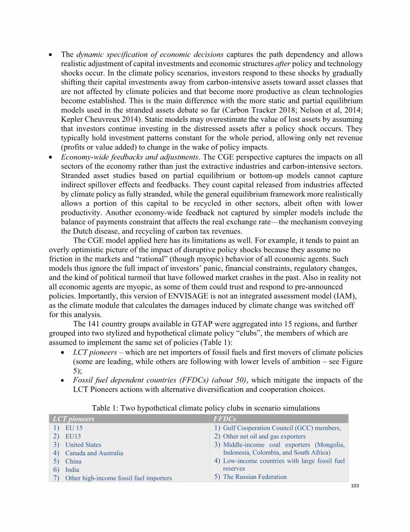
103

• The dynamic specification of economic decisions captures the path dependency and allows realistic adjustment of capital investments and economic structures after policy and technology shocks occur. In the climate policy scenarios, investors respond to these shocks by gradually shifting their capital investments away from carbon-intensive assets toward asset classes that are not affected by climate policies and that become more productive as clean technologies become established. This is the main difference with the more static and partial equilibrium models used in the stranded assets debate so far (Carbon Tracker 2018; Nelson et al, 2014; Kepler Cheuvreux 2014). Static models may overestimate the value of lost assets by assuming that investors continue investing in the distressed assets after a policy shock occurs. They typically hold investment patterns constant for the whole period, allowing only net revenue (profits or value added) to change in the wake of policy impacts.

• Economy-wide feedbacks and adjustments. The CGE perspective captures the impacts on all sectors of the economy rather than just the extractive industries and carbon-intensive sectors. Stranded asset studies based on partial equilibrium or bottom-up models cannot capture indirect spillover effects and feedbacks. They count capital released from industries affected by climate policy as fully stranded, while the general equilibrium framework more realistically allows a portion of this capital to be recycled in other sectors, albeit often with lower productivity. Another economy-wide feedback not captured by simpler models include the balance of payments constraint that affects the real exchange rate—the mechanism conveying the Dutch disease, and recycling of carbon tax revenues.

The CGE model applied here has its limitations as well. For example, it tends to paint an overly optimistic picture of the impact of disruptive policy shocks because they assume no friction in the markets and “rational” (though myopic) behavior of all economic agents. Such models thus ignore the full impact of investors’ panic, financial constraints, regulatory changes, and the kind of political turmoil that have followed market crashes in the past. Also in reality not all economic agents are myopic, as some of them could trust and respond to pre-announced policies. Importantly, this version of ENVISAGE is not an integrated assessment model (IAM), as the climate module that calculates the damages induced by climate change was switched off for this analysis.

The 141 country groups available in GTAP were aggregated into 15 regions, and further grouped into two stylized and hypothetical climate policy “clubs”, the members of which are assumed to implement the same set of policies (Table 1):

• LCT pioneers – which are net importers of fossil fuels and first movers of climate policies (some are leading, while others are following with lower levels of ambition – see Figure 5);

• Fossil fuel dependent countries (FFDCs) (about 50), which mitigate the impacts of the LCT Pioneers actions with alternative diversification and cooperation choices.

Table 1: Two hypothetical climate policy clubs in scenario simulations

LCT pioneers FFDCs 1) EU 15 2) EU13 3) United States 4) Canada and Australia 5) China 6) India 7) Other high-income fossil fuel importers

1) Gulf Cooperation Council (GCC) members, 2) Other net oil and gas exporters 3) Middle-income coal exporters (Mongolia,

Indonesia, Colombia, and South Africa) 4) Low-income countries with large fossil fuel

reserves 5) The Russian Federation

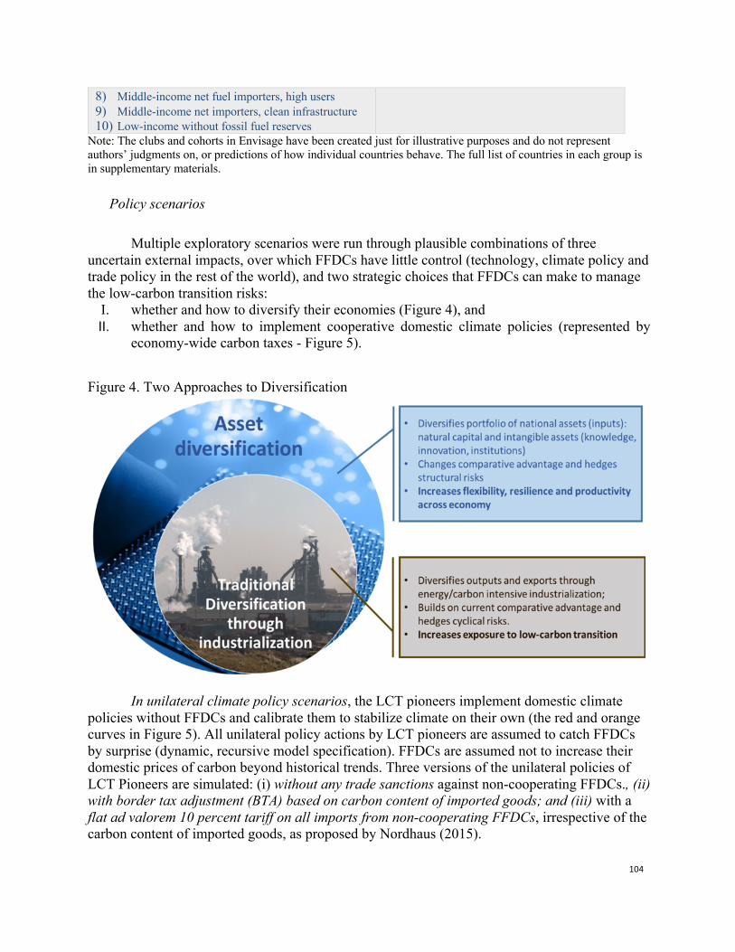
104

8) Middle-income net fuel importers, high users 9) Middle-income net importers, clean infrastructure 10) Low-income without fossil fuel reserves

Note: The clubs and cohorts in Envisage have been created just for illustrative purposes and do not represent authors’ judgments on, or predictions of how individual countries behave. The full list of countries in each group is in supplementary materials.

Policy scenarios

Multiple exploratory scenarios were run through plausible combinations of three uncertain external impacts, over which FFDCs have little control (technology, climate policy and trade policy in the rest of the world), and two strategic choices that FFDCs can make to manage the low-carbon transition risks:

I. whether and how to diversify their economies (Figure 4), and II. whether and how to implement cooperative domestic climate policies (represented by

economy-wide carbon taxes - Figure 5).

Figure 4. Two Approaches to Diversification

In unilateral climate policy scenarios, the LCT pioneers implement domestic climate policies without FFDCs and calibrate them to stabilize climate on their own (the red and orange curves in Figure 5). All unilateral policy actions by LCT pioneers are assumed to catch FFDCs by surprise (dynamic, recursive model specification). FFDCs are assumed not to increase their domestic prices of carbon beyond historical trends. Three versions of the unilateral policies of LCT Pioneers are simulated: (i) without any trade sanctions against non-cooperating FFDCs., (ii) with border tax adjustment (BTA) based on carbon content of imported goods; and (iii) with a flat ad valorem 10 percent tariff on all imports from non-cooperating FFDCs, irrespective of the carbon content of imported goods, as proposed by Nordhaus (2015).

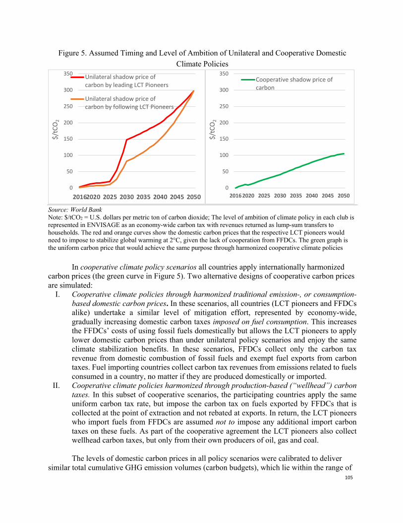
105

Figure 5. Assumed Timing and Level of Ambition of Unilateral and Cooperative Domestic Climate Policies

Source: World Bank Note: $/tCO2 = U.S. dollars per metric ton of carbon dioxide; The level of ambition of climate policy in each club is represented in ENVISAGE as an economy-wide carbon tax with revenues returned as lump-sum transfers to households. The red and orange curves show the domestic carbon prices that the respective LCT pioneers would need to impose to stabilize global warming at 2°C, given the lack of cooperation from FFDCs. The green graph is the uniform carbon price that would achieve the same purpose through harmonized cooperative climate policies

In cooperative climate policy scenarios all countries apply internationally harmonized carbon prices (the green curve in Figure 5). Two alternative designs of cooperative carbon prices are simulated:

I. Cooperative climate policies through harmonized traditional emission-, or consumption-based domestic carbon prices. In these scenarios, all countries (LCT pioneers and FFDCs alike) undertake a similar level of mitigation effort, represented by economy-wide, gradually increasing domestic carbon taxes imposed on fuel consumption. This increases the FFDCs’ costs of using fossil fuels domestically but allows the LCT pioneers to apply lower domestic carbon prices than under unilateral policy scenarios and enjoy the same climate stabilization benefits. In these scenarios, FFDCs collect only the carbon tax revenue from domestic combustion of fossil fuels and exempt fuel exports from carbon taxes. Fuel importing countries collect carbon tax revenues from emissions related to fuels consumed in a country, no matter if they are produced domestically or imported.

II. Cooperative climate policies harmonized through production-based (“wellhead”) carbon taxes. In this subset of cooperative scenarios, the participating countries apply the same uniform carbon tax rate, but impose the carbon tax on fuels exported by FFDCs that is collected at the point of extraction and not rebated at exports. In return, the LCT pioneers who import fuels from FFDCs are assumed not to impose any additional import carbon taxes on these fuels. As part of the cooperative agreement the LCT pioneers also collect wellhead carbon taxes, but only from their own producers of oil, gas and coal.

The levels of domestic carbon prices in all policy scenarios were calibrated to deliver

similar total cumulative GHG emission volumes (carbon budgets), which lie within the range of

0

50

100

150

200

250

300

350

20162020 2025 2030 2035 2040 2045 2050

$/tC

O2

Unilateral shadow price ofcarbon by leading LCT Pioneers

Unilateral shadow price ofcarbon by following LCT Pioneers

0

50

100

150

200

250

300

350

20162020 2025 2030 2035 2040 2045 2050

$/tC

O2

Cooperative shadow price ofcarbon

106

the IPCC AR5 estimates of equal probability of achieving the 2°C stabilization objectives. The cooperative carbon prices lie within the lower range of shadow carbon prices extrapolated by the World Bank from the report of the High-Level Commission on Carbon Prices, which found those prices consistent with the core objective of the Paris Agreement of keeping temperature rise below 2°C, provided supportive policies are in place (Carbon Pricing Leadership Coalition 2017). The scenario structure is summarized in Box 1.

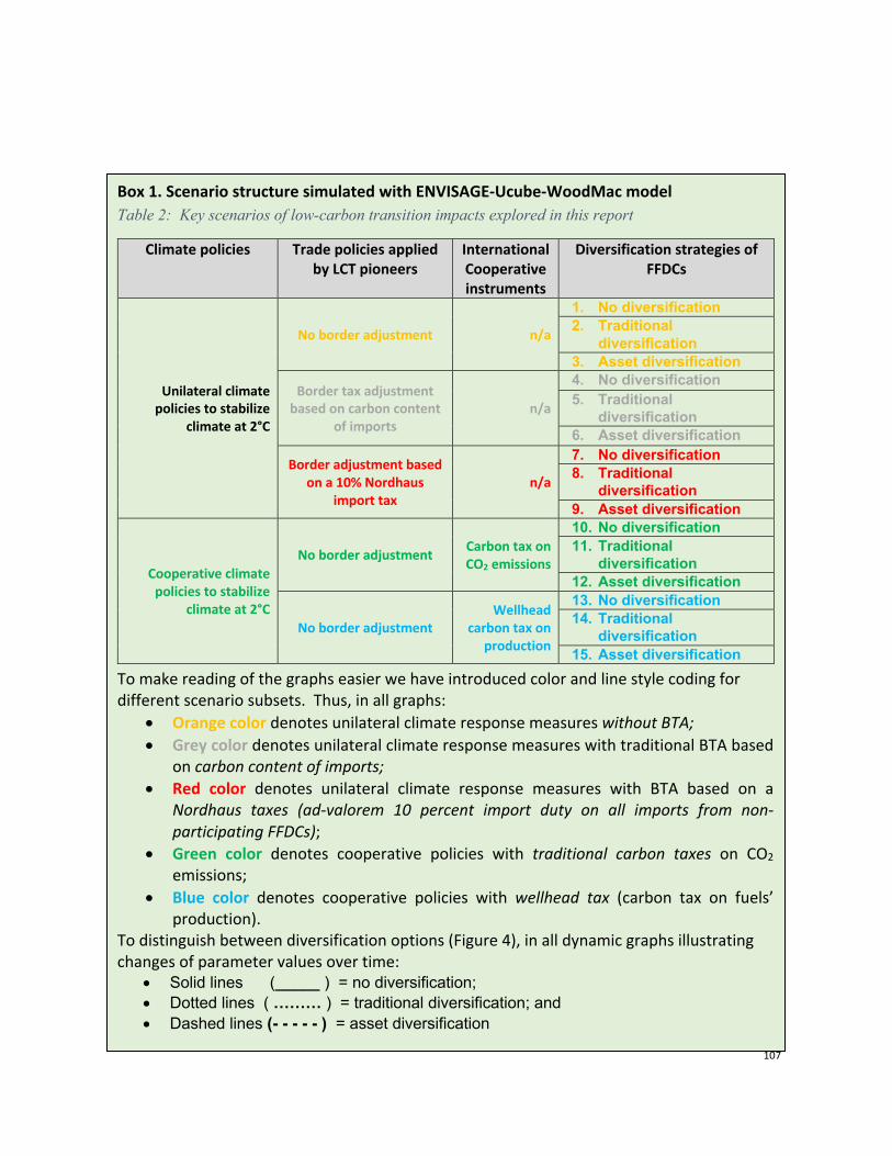
107

Box 1. Scenario structure simulated with ENVISAGE-Ucube-WoodMac model

Table 2: Key scenarios of low-carbon transition impacts explored in this report

Climate policies Trade policies applied by LCT pioneers

International Cooperative instruments

Diversification strategies of FFDCs

Unilateral climate policies to stabilize

climate at 2°C

No border adjustment n/a

1. No diversification 2. Traditional

diversification 3. Asset diversification

Border tax adjustment based on carbon content

of imports n/a



Border adjustment based on a 10% Nordhaus

import tax n/a



Cooperative climate policies to stabilize

climate at 2°C

No border adjustment Carbon tax on CO2 emissions



No border adjustment Wellhead

carbon tax on production



To make reading of the graphs easier we have introduced color and line style coding for different scenario subsets. Thus, in all graphs:

• Orange color denotes unilateral climate response measures without BTA; • Grey color denotes unilateral climate response measures with traditional BTA based

on carbon content of imports; • Red color denotes unilateral climate response measures with BTA based on a

Nordhaus taxes (ad-valorem 10 percent import duty on all imports from non-participating FFDCs);

• Green color denotes cooperative policies with traditional carbon taxes on CO2 emissions;

• Blue color denotes cooperative policies with wellhead tax (carbon tax on fuels’ production).

To distinguish between diversification options (Figure 4), in all dynamic graphs illustrating changes of parameter values over time:

• Solid lines (_____ ) = no diversification; • Dotted lines ( ……… ) = traditional diversification; and • Dashed lines (- - - - - ) = asset diversification

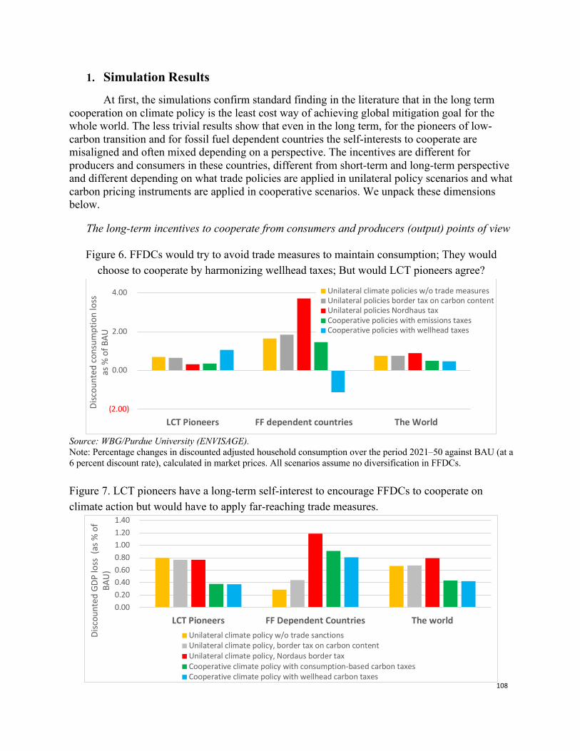
108

1. Simulation Results At first, the simulations confirm standard finding in the literature that in the long term

cooperation on climate policy is the least cost way of achieving global mitigation goal for the whole world. The less trivial results show that even in the long term, for the pioneers of low-carbon transition and for fossil fuel dependent countries the self-interests to cooperate are misaligned and often mixed depending on a perspective. The incentives are different for producers and consumers in these countries, different from short-term and long-term perspective and different depending on what trade policies are applied in unilateral policy scenarios and what carbon pricing instruments are applied in cooperative scenarios. We unpack these dimensions below.

The long-term incentives to cooperate from consumers and producers (output) points of view

Figure 6. FFDCs would try to avoid trade measures to maintain consumption; They would choose to cooperate by harmonizing wellhead taxes; But would LCT pioneers agree?

Source: WBG/Purdue University (ENVISAGE). Note: Percentage changes in discounted adjusted household consumption over the period 2021–50 against BAU (at a 6 percent discount rate), calculated in market prices. All scenarios assume no diversification in FFDCs. Figure 7. LCT pioneers have a long-term self-interest to encourage FFDCs to cooperate on climate action but would have to apply far-reaching trade measures.

(2.00)

0.00

2.00

4.00

LCT Pioneers FF dependent countries The World

Disc

ount

ed c

onsu

mpt

ion

loss

as

% o

f BAU

Unilateral climate policies w/o trade measuresUnilateral policies border tax on carbon contentUnilateral policies Nordhaus taxCooperative policies with emissions taxesCooperative policies with wellhead taxes

0.000.200.400.600.801.001.201.40

LCT Pioneers FF Dependent Countries The world

Disc

ount

ed G

DP lo

ss (

as %

of

BAU

)

Unilateral climate policy w/o trade sanctionsUnilateral climate policy, border tax on carbon contentUnilateral climate policy, Nordaus border taxCooperative climate policy with consumption-based carbon taxesCooperative climate policy with wellhead carbon taxes

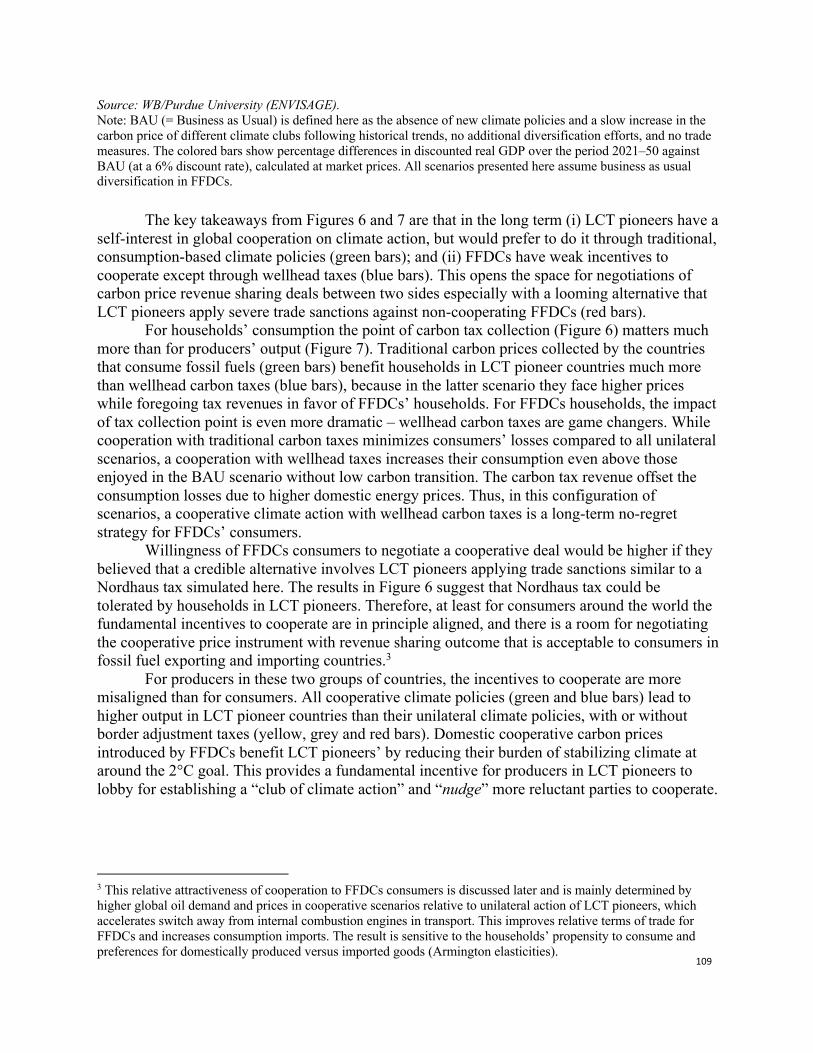
109

Source: WB/Purdue University (ENVISAGE). Note: BAU (= Business as Usual) is defined here as the absence of new climate policies and a slow increase in the carbon price of different climate clubs following historical trends, no additional diversification efforts, and no trade measures. The colored bars show percentage differences in discounted real GDP over the period 2021–50 against BAU (at a 6% discount rate), calculated at market prices. All scenarios presented here assume business as usual diversification in FFDCs.

The key takeaways from Figures 6 and 7 are that in the long term (i) LCT pioneers have a self-interest in global cooperation on climate action, but would prefer to do it through traditional, consumption-based climate policies (green bars); and (ii) FFDCs have weak incentives to cooperate except through wellhead taxes (blue bars). This opens the space for negotiations of carbon price revenue sharing deals between two sides especially with a looming alternative that LCT pioneers apply severe trade sanctions against non-cooperating FFDCs (red bars).

For households’ consumption the point of carbon tax collection (Figure 6) matters much more than for producers’ output (Figure 7). Traditional carbon prices collected by the countries that consume fossil fuels (green bars) benefit households in LCT pioneer countries much more than wellhead carbon taxes (blue bars), because in the latter scenario they face higher prices while foregoing tax revenues in favor of FFDCs’ households. For FFDCs households, the impact of tax collection point is even more dramatic – wellhead carbon taxes are game changers. While cooperation with traditional carbon taxes minimizes consumers’ losses compared to all unilateral scenarios, a cooperation with wellhead taxes increases their consumption even above those enjoyed in the BAU scenario without low carbon transition. The carbon tax revenue offset the consumption losses due to higher domestic energy prices. Thus, in this configuration of scenarios, a cooperative climate action with wellhead carbon taxes is a long-term no-regret strategy for FFDCs’ consumers.

Willingness of FFDCs consumers to negotiate a cooperative deal would be higher if they believed that a credible alternative involves LCT pioneers applying trade sanctions similar to a Nordhaus tax simulated here. The results in Figure 6 suggest that Nordhaus tax could be tolerated by households in LCT pioneers. Therefore, at least for consumers around the world the fundamental incentives to cooperate are in principle aligned, and there is a room for negotiating the cooperative price instrument with revenue sharing outcome that is acceptable to consumers in fossil fuel exporting and importing countries.3

For producers in these two groups of countries, the incentives to cooperate are more misaligned than for consumers. All cooperative climate policies (green and blue bars) lead to higher output in LCT pioneer countries than their unilateral climate policies, with or without border adjustment taxes (yellow, grey and red bars). Domestic cooperative carbon prices introduced by FFDCs benefit LCT pioneers’ by reducing their burden of stabilizing climate at around the 2°C goal. This provides a fundamental incentive for producers in LCT pioneers to lobby for establishing a “club of climate action” and “nudge” more reluctant parties to cooperate.

3 This relative attractiveness of cooperation to FFDCs consumers is discussed later and is mainly determined by higher global oil demand and prices in cooperative scenarios relative to unilateral action of LCT pioneers, which accelerates switch away from internal combustion engines in transport. This improves relative terms of trade for FFDCs and increases consumption imports. The result is sensitive to the households’ propensity to consume and preferences for domestically produced versus imported goods (Armington elasticities).

110

The menu of nudges simulated here include two forms of border adjustment taxes and a cooperative wellhead tax.4

The incentives to cooperate on climate action are weaker for FFDCs producers. The output loss (against BAU) in cooperative scenarios is higher than in unilateral policy scenario without any trade measures even when cooperation is facilitated by wellhead taxes. Traditional BTAs based on the carbon content of imported goods (grey bars) may not be sufficient incentive to encourage most producers in FFDCs to cooperate, even in the long run (Figure 7). This border policy increases cost for FFDCs but makes only modest difference relative to unilateral policy without trade measures, which has already reduced FFDCs exports dominated by oil and gas. The credible threat of Nordhaus tax, on the other hand, would provide a much stronger incentive for the FFDCs producers to participate in the global climate policy and accept domestic carbon taxes if it helped to prevent trade sanctions. The cooperative scenarios reduce discounted GDP loss in FFDCs by 0.9% with traditional carbon taxes and 0.8 percent with producer taxes vs. 1.2 percent in unilateral scenario with Nordhaus border taxes.

In both groups of countries, the impact on production does not differ too much depending on where the tax revenues are collected (green and blue bars are of similar size in Figure 7). Foregone revenues of wellhead taxes do not affect GDP and investments in LCT pioneer countries relative to traditional cooperative carbon taxes and make little difference to GDP in FFDCs (Figure 7). In both cooperative scenarios, carbon taxes decrease producers’ surplus by the same amount. This is because by scenario design, carbon tax revenues are returned as lump-sum transfers to households which divide additional revenue between consumption of domestically produced and imported goods, while the rest goes to savings and investments. Producers in LCT pioneers are not affected by forgone carbon tax revenues in their countries, because with wellhead taxes consumers in FFDCs have higher income which they use to purchase imported consumer goods also from LCT pioneers. Producers in FFDCs benefit (although not much) from higher carbon tax revenues collected in their countries, because their domestic consumers do not spend all extra income on current consumption but save a portion of it to support domestic investments and localization of production, while part of increased domestic consumption budget goes to purchase domestically produced goods as well. Distribution of producers’ benefits of wellhead taxes across borders depends households’ propensity to save and their Armington elasticities of substitution between products of fuel importing and exporting countries. It is worth noting that in percentage terms the impact of low carbon transition is stronger on consumption of FFDCs households than on their GDP in all climate policy scenarios. This is because the structural transformation of FFDCs’ economies takes time and requires investments from increased domestic saving which supports GDP but temporarily crowds-out households’ consumption. Wellhead taxes allow FFDCs to capture a significant portion of resource rents as domestic tax revenue and to transfer them to households, immediately boosting their consumption above BAU5 and trickling down to boost output only after a time-lag and depending

4 Note that the value that LCT Pioneers place on avoided costs of climate change is not included in their welfare metrics simulated with the CGE model. We assume that this shadow value of a stable climate for LCT pioneers is higher than their costs of unilateral climate policies without trade sanctions (yellow bars) and that they will aim at minimizing their costs by a combination of trade policies and cooperative deals. 5 Alternative revenue recycling schemes are possible but not applied here.

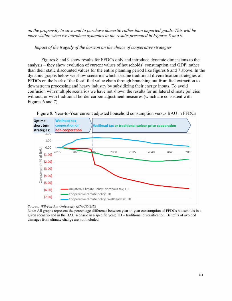
111

on the propensity to save and to purchase domestic rather than imported goods. This will be more visible when we introduce dynamics to the results presented in Figures 8 and 9.

Impact of the tragedy of the horizon on the choice of cooperative strategies

Figures 8 and 9 show results for FFDCs only and introduce dynamic dimensions to the

analysis – they show evolution of current values of households’ consumption and GDP, rather than their static discounted values for the entire planning period like figures 6 and 7 above. In the dynamic graphs below we show scenarios which assume traditional diversification strategies of FFDCs on the back of the fossil fuel value chain through branching out from fuel extraction to downstream processing and heavy industry by subsidizing their energy inputs. To avoid confusion with multiple scenarios we have not shown the results for unilateral climate policies without, or with traditional border carbon adjustment measures (which are consistent with Figures 6 and 7).

Figure 8. Year-to-Year current adjusted household consumption versus BAU in FFDCs

Source: WB/Purdue University (ENVISAGE) Note: All graphs represent the percentage difference between year-to-year consumption of FFDCs households in a given scenario and in the BAU scenario in a specific year; TD = traditional diversification. Benefits of avoided damages from climate change are not included.

(7.00)

(6.00)

(5.00)

(4.00)

(3.00)

(2.00)

(1.00)

0.00

1.00

2.00

2015 2020 2025 2030 2035 2040 2045 2050

Cons

umpt

ion

% o

f BAU

Unilateral Climate Policy; Nordhaus tax; TDCooperative climate policy; TDCooperative climate policy; Wellhead tax; TD

Optimal short term strategies:

Wellhead tax cooperation or non-cooperation or

Wellhead tax or traditional carbon price cooperation

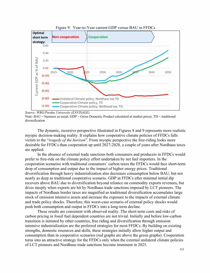
112

Figure 9: Year-to-Year current GDP versus BAU in FFDCs

Source: WBG/Purdue University (ENVISAGE). Note: BAU = business as usual; GDP = Gross Domestic Product calculated at market prices; TD = traditional diversification

The dynamic, recursive perspective illustrated in Figures 8 and 9 represents more realistic myopic decision-making reality. It explains how cooperative climate policies of FFDCs falls victim to the “tragedy of the horizon”. From myopic perspective the free-riding looks more desirable for FFDCs than cooperation up until 2027-2028, a couple of years after Nordhaus taxes are applied.

In the absence of external trade sanctions both consumers and producers in FFDCs would prefer to free-ride on the climate policy effort undertaken by net fuel importers. In the cooperation scenarios with traditional consumers’ carbon taxes the FFDCs would face short-term drop of consumption and output due to the impact of higher energy prices. Traditional diversification through heavy industrialization also decreases consumption below BAU, but not nearly as deep as traditional cooperative scenario. GDP in FFDCs after minimal initial dip recovers above BAU due to diversification beyond reliance on commodity exports revenues, but dives steeply when exports are hit by Nordhaus trade sanctions imposed by LCT pioneers. The impacts of Nordhaus border taxes are magnified as traditional diversification accumulates large stock of emission intensive assets and increase the exposure to the impacts of external climate and trade policy shocks. Therefore, this worst-case scenario of external policy shocks would push both consumption and output in FFDCs into a long-term decline.

These results are consistent with observed reality. The short-term costs and risks of carbon pricing in fossil fuel dependent countries are not trivial. Initially and before low-carbon transition is initiated by other countries, free riding and diversification through emission intensive industrialization are the preferred strategies for most FFDCs. By building on existing strengths, domestic resources and skills, these strategies initially allow higher output and consumption than in cooperative scenarios (red graphs are above the green graphs). Cooperation turns into an attractive strategy for the FFDCs only when the external unilateral climate policies of LCT pioneers and Nordhaus trade sanctions become imminent in 2025.

(1.00)

(0.80)

(0.60)

(0.40)

(0.20)

0.00

0.20

0.40

0.60

2015 2020 2025 2030 2035 2040 2045 2050

Curr

ent G

DP a

s % o

f BAU

Unilateral Climate policy, Nordhaus tax TDCooperative Climate policy, TDCooperative Climate policy, Wellhead tax, TD

Optimal short term strategy:

Non-cooperation Cooperation

113

Wellhead carbon taxes give an additional consumption (Figure 8) and output (Figure 9) boost in FFDCs because they retain significant additional tax revenue that in traditional cooperative scenarios are collected abroad. Wellhead carbon taxes not only ensure the highest long-term growth and consumption for FFDCs, but also represent the only cooperative strategy that aligns short- and long-term incentives for FFDC consumers on a continuous basis. Wellhead taxes alleviate short-term regrets of low-carbon transition to households by preventing their consumption from ever falling below the BAU level throughout the period until 2050, irrespective of the diversification strategy chosen by the FFDCs.

The simulations with CGE model confirm the proposition made with the theoretical model in the previous section that under certain conditions well-head taxes can be the first-best and even no-regret climate action strategies for FFDCs, and that there is a scope for net fuel importers and exporters to negotiate cooperative carbon tax agreements with revenue sharing provisions. Sharing carbon tax revenue between fossil fuel exporters and importers may be vitally important for FFDCs as it would help them alleviate the short-term negative social impacts of low-carbon transition. The wellhead tax makes a significant difference in terms of mitigating consumption losses from implementing domestic carbon pricing (figure 9). It is also important to incentivize and enable deeper diversification in FFDCs – not only beyond oil and gas, but also beyond fossil-fuel dependent manufacturing industries. Deeper diversification requires significant upfront investment in human capital and R&D, with returns that are long-term and appear elusive to current policy makers and business leaders in FFDCs. Wellhead taxes would also partly offset the revenue lost due to the lower global demand for fossil fuels.

It is in mutual interest, first to have FFDCs participate in the global climate policy from the very beginning, and second to decrease their dependency of fossil fuels6. This motivation would justify a compromise on wellhead tax at least for the period until 2030 on condition that FFDCs make efforts to diversify their economies away from the fossil fuel product space. This compromise would allow more space to negotiate an even tighter climate policy with a higher carbon price than in the cooperation scenario if needed.7 Thus, the wellhead tax in combination with deeper and faster diversification creates a structural foundation to engrain FFDCs in global climate policy efforts in line with their self-interest and long-term development aspirations.

So, what this analysis so far tells us about the strategies to induce cooperation under the Paris Agreement? The first-best strategy for LCT Pioneers is cooperation on climate action through traditional carbon prices, while for FFDCs the first-best strategy is free riding even with traditional border carbon adjustments or cooperation through well-head carbon taxes. Consumers in LCT pioneers may not be willing to accept international wellhead carbon taxes but would not mind imposing Nordhaus trade sanctions against non-participating FFDCs. FFDCs would try to avoid Nordhaus taxes, hence would be prompted to negotiate the carbon tax revenue sharing agreements and embark in cooperative climate action that produces economic outcomes somewhere between the green and blue graphs. 5. Discussion and conclusions: Design and political economy issues

6 We also should mention that cooperative scenario is the only one when FFDC significantly reduce its carbon emissions. 7 We did sensitivity runs with higher carbon taxes and alternative diversification strategies, that are not included due to the space limitations.

114

Wellhead carbon taxes could be an effective way to price carbon in a way that reduces

domestic emissions in FFDCs and also enables them to retain (an agreed portion of) resource rents that with traditional carbon prices are collected abroad. Wellhead taxes would have the same effect on fossil fuel demand as traditional cooperative carbon pricing but would limit the wealth transfer from fuel exporters to importers.

Wellhead taxes could align incentives to ramp-up the level of climate policy ambition between climate policy leaders and the most reluctant countries and between current and future consumers in the fossil fuel-depended countries. They would reduce emissions in the latter and increase resources available for enhancing climate co-benefits of diversification and for managing the social and political impacts of major structural changes. Wellhead carbon taxes can effectively overcome the tragedy of the horizon and social resistance to low-carbon transition in FFDCs. They could offer them a continuous and sustainable rise in welfare, while fully engaging them in the international efforts to stabilize the climate.

Both theoretical analysis and model simulations confirm that wellhead taxes can make both parties better off when the gain in the welfare of the importers due to cost savings of avoided unilateral action and reduced climate change impacts more than offsets the global loss in welfare (in importing and exporting countries) due to reduced consumption of fuel-intensive goods. The net welfare gain, which is the difference between these two effects, can be shared between the participating countries through the terms of well-head carbon tax agreements.

Wellhead carbon taxes represent a new variation of cooperative carbon pricing proposed in the economic literature (Cooper 2004, Crampton et al. 2017; Flannery et al. 2018), and can be designed as common and contingent commitments needed to operationalize the incentive structure under the Paris Agreement (MacKay et al. 2017). Administratively, they are similar in structure to extraction/severance taxes applied in the U.S. or excise taxes, so tax administration would be simple and familiar to treasuries. There are not dissimilar from fuel export taxes, which many FFDCs already apply, except that a wellhead tax also covers domestic fuel consumption, so are less distortionary.

The political economy challenge for fuel importing countries would be to convince their consumers to bear the burden of higher prices and forego a portion of the tax revenue for the benefit of fuel exporters. By sharing the carbon tax revenue with exporters, fuel importers could gain cooperation of FFDCs in climate policy, mitigate competitiveness and leakage effects of unilateral carbon pricing, and enjoy cost savings of not having to stabilize climate through extremely ambitious unilateral action. Under the cooperative tax agreement, the fuel exporters and importers could agree on carbon tax rates on both sides of a trade that would determine the share of tax revenue each would collect. These non-cash financial transfers (revenue sharing) between countries can be negotiated bilaterally or multilaterally. Fuel importing countries may not like that in a way wellhead carbon taxes would achieve what OPEC could not – expand producers’ revenues by decreasing output and increasing fuel prices. But the toll to pay by FFDCs for this benefit is domestic carbon prices and mitigation of their GHG emissions, which should have some value to LCT pioneers. Contrary to OPEC BAU expectations cooperation through revenue sharing carbon taxes facilitates structural decline of fossil fuel value chain. Acceptability of the wellhead carbon taxes to fuel importers could increase if FFDCs agreed to transfer a portion of tax revenue to a Green Climate Fund to assist the lowest-income and most vulnerable countries in meeting the challenges of adaptation to climate change.

115

Political economy issues in the fuel exporting countries would be not less challenging, especially for the first movers. In the absence of comprehensive cooperative club putting a carbon price on fuels destined for domestic consumption and exports would trigger at least two legitimate concerns. First, the potential loss of their current comparative advantage in energy intensive products. It could be addressed with wellhead carbon tax design when in return for taxing domestic emissions FFDCs would retain most of the revenue that alternatively would have been collected abroad. Yet, this argument holds only when the alternative of high carbon prices in fuel importing countries to unilaterally stabilize climate becomes credible. The second concern is about tax competition. First movers can lose market share to other fuel exporters whose exports do not carry a carbon price tag. Addressing this concern would require fuel importers to refrain from additional carbon tax on the emissions embedded in the fuel imported from fuel exporters with wellhead carbon taxes, while keeping carbon prices on fuels imported from countries without a wellhead carbon tax agreement. This could be agreed through bilateral or multilateral tax treaties between the members of a climate action club.

The political economy and administration challenges of any new cooperative carbon price should always be seen against alternative and equivalent forms of cooperative carbon pricing. Emissions trading systems have been linked between a few homogenous advanced economies, such as the EU or sub-national jurisdictions in the U.S., Canada and China. But linking heterogeneous distant countries is bound to be burdened with administrative complexity and political economy issues, and thus has not moved beyond early conceptual ideas and some short-lived political declarations. Even the most advanced OECD countries have not been able to align their consumption-based carbon taxes, let alone mobilizing significant international financial transfers. The pursuits of scaling up climate finance and carbon markets encounter persistent difficulties (OECD 2016; Westphal et al. 2015). Strategic financial transfers designed as conditional incentives for results-based cooperative policy efforts (Steckel et al. 2017) remain in the realm of innovative academic ideas rather than politics of climate finance which remain scattered by uncoordinated minute project-by-project financing deals with high transaction costs and weak incentive effect. Trade sanctions pose a host of other challenges and risks. International negotiations of cooperative wellhead taxes could be easier than consumption-based carbon prices because the latter includes two issues, pricing and financial transfers, to be negotiated at the same time, while negotiations of wellhead taxes can be focused on a single issue: domestic carbon tax rates.

New unconventional policy instruments are needed to induce international cooperation for increased climate policy ambition under the Paris Agreement taking into consideration sustainable development aspirations of all countries. This paper does not propose cooperative wellhead carbon tax treaties between fuel exporters and importers with revenue sharing agreements as a silver bullet to solve climate cooperation puzzle. It identifies this novel cooperative instrument as one of the options worth further research and policy debate. References Ackerman, F. and E.A. Stanton, 2012: Climate Risks and Carbon Prices: Revising the Social Cost of Carbon.

Economics: The Open-Access, Open-Assessment E-Journal, 6(2012-10), doi:10.5018/economics-ejournal.ja.2012-10.

Anda, J., Golub, A. and Strukova, E., 2009. Economics of climate change under uncertainty: Benefits of flexibility. Energy Policy, 37(4), pp.1345-1355.

116

Anderson, K., 1992. The standard welfare economics of policies affecting trade and the environment. The Greening of World Trade Issues, pp.25-48.

Asheim GB (2012) A distributional argument for supply-side climate policies. Environ Resour Econ 56:239– 254. https://doi.org/10.1007/s10640-012-9590-2

Barrett, Scott. 1994. “Self-Enforcing International Environmental Agreements.” Oxford Economic Paper 46. Faculty of Economics, London Business School, Centre for Social and Economic Research on the Global Environment.

Barrett S (2003) Environment and statecraft: the strategy of environmental treaty-making. Oxford University Press, Oxford

Barrett, Scott, Astrid Dannenberg. 2016. An experimental investigation into ‘pledge and review’ in climate negotiations. Climatic Change September 2016, Volume 138, Issue 1–2, pp 339–351

Bauer, Nico, Ioanna Mouratiadou Gunnar Luderer Lavinia Baumstark Robert J. Brecha Ottmar Edenhofer Elmar Kriegler. 2016. Global fossil energy markets and climate change mitigation – an analysis with REMIND. Climatic Change May 2016, Volume 136, Issue 1, pp 69–82 | Cite as

Bergstrom, Theodore. 1982. "On capturing oil rents with a national excise tax" American Economic Review Vol. 72 Issue 1

Böhringer, Christoph & Rosendahl, Knut Einar & Schneider, Jan, 2018. "Unilateral Emission Pricing and OPEC's Behaviour," Strategic Behavior and the Environment, now publishers, vol. 7(3–-4), pages 225-280.

Böhringer C., E. J. Balistreri, and T. F. Rutherford (2012). The role of border carbon adjustment in unilateral climate policy: Overview of an Energy Modeling Forum study (EMF 29). Energy Economics 34, Supplement 2, 97 – 110. doi: 10.1016 / j.eneco.2012.10.003, ISSN: 0140-9883.

Carbon Tracker. 2018. 2 Degrees of Separation: Company-level transition risk July 2018 update. https://www.carbontracker.org/reports/2-degrees-of-separation-update/

Carraro, Carlo and Carmen Marchiori (2004), “Endogenous Strategic Issue Linkage in International Negotiations,” in Carlo Carraro and Vito Fragnelli (eds), Game Practice and the Environment, Edward Elgar Publishing Limited, chapter 3: 65 — 86.

Carraro, Carlo. 2016. “Clubs, R&D, and Climate Finance: Incentives for Ambitious GHG Emission Reductions.” In: The Paris Agreement and Beyond: International Climate Change Policy Post-2020,” edited by R.N. Stavins and R. C. Stowe. Cambridge, Mass.: Harvard Project on Climate Agreements.

Clarke, L. et al., 2014: Assessing transformation pathways. In: Climate Change 2014: Mitigation of Climate Change. Contribution of Working Group III to the Fifth Assessment Report of the Intergovernmental Panel on Climate Change [Edenhofer, O., R. Pichs-Madruga, Y. Sokona, E. Farahani, S. Kadner, K. Seyboth, A. Adler, I. Baum, S. Brunner, P. Eickemeier, B. Kriemann, J. Savolainen, S. Schlömer, C. von Stechow, T. Zwickel, and J.C. Minx (eds.)]. Cambridge University Press, Cambridge, United Kingdom and New York, NY, USA, pp. 413510

Collier P, Venables A. J. 2014. Closing coal: economic and moral incentives. Ox Rev Econ Policy 30:492–512. https://doi.org/10.1093/oxrep/gru024

Cooper, R.N. 2004. “A Global Carbon Tax?” Council on Foreign Relations, Commissioned Briefing Notes for the CIGI/CFGS L20 Project

Cosbey, A., Droege, S., Fischer, C., Reinaud, J., Stephenson, J., Weischer, L., and P. Wooders. 2012. “A Guide for the Concerned: Guidance on the Elaboration and Implementation of Border Carbon Adjustment,” Entwined Policy Report No. 3 (http://www.iisd.org/pdf/2012/bca_guidance.pdf).

Cramton, Peter and S. Stoft. 2012. “Global Climate Games: How Pricing and a Green Fund Foster Cooperation,” Economics of Energy & Environmental Policy, 1:2. http://dx.doi.org/10.5547/2160-5890.1.2.9.

Cramton, Peter, MacKay, D.J., Ockenfels, A., and S. Stoft. 2017. Global Carbon Pricing: The Path to Climate Cooperation. MIT Press.

Dannenberg, Astrid. 2016. Non-binding agreements in public goods experiments. Oxford Economic Papers, Volume 68, Issue 1, 1 January 2016, Pages 279–300, https://doi.org/10.1093/oep/gpv048

Day. C, Day G (2017) Climate change, fossil fuel prices and depletion: the rationale for a falling export tax. Econ Model 63:153–160. https://doi.org/10.1016/j.econmod.2017.01.006

Diamantoudi, E. and E. Sartzetakis. 2006. “Stable International Environmental Agreements: An fffnalytical Approach.” Journal of Public Economic Theory 8 (2): 247–263.

Dong Yan, John Whalley. 2009. A Third Benefit of Joint Non-OPEC Carbon Taxes: Transferring OPEC Monopoly Rent CESIFO WORKING PAPER NO. 2741

117

Dullieux, Rémy, Lionel Ragot and Katheline Schubert. 2011. Carbon Tax and OPEC's Rents Under a Ceiling Constraint. The Scandinavian Journal of Economics Vol. 113, No. 4, Climate Change and Distribution (December 2011), pp. 798-824

Edenhofer, Ottmar and Axel Ockenfels. 2015. Climate Policy at an Impasse. In: Cramton, Peter, MacKay, D.J., Ockenfels, A., and S. Stoft. 2017. Global Carbon Pricing: The Path to Climate Cooperation. MIT Press.

Eichner T, Pethig R (2017) Self-enforcing environmental agreements and trade in fossil energy deposits. J Environmental Economic Management 85:1–20. https://doi.org/10.1016/j.jeem.2017.04.004

Elliott, J., Foster, I., Kortum, S., Munson, T., Perez Cervantes, F. and Weisbach, D., 2010. Trade and carbon taxes. American Economic Review, 100(2), pp.465-69.

Erickson P, Lazarus M, Tempest K. 2015. Carbon lock-in from fossil fuel supply infrastructure. Stockholm Environment Institute, Seattle

Falkner Robert. 2016. The Paris Agreement and the new logic of international climate politics. International Affairs 92(5) 2016, pp. 1107-1125

Figueres, Christiana. 2016. The Power of Policy: Reinforcing the Paris Trajectory. Global Policy Volume 7 . Issue 3. September 2016

Flannery, Brian P., Jennifer Hillman, Jan Mares, Matthew Porterfield. 2018. Framework Proposal for a US Upstream Greenhouse Gas Tax with WTO-Compliant Border Adjustments. Resource for the Future Working Paper. http://www.rff.org/research/publications/framework-proposal-us-upstream-greenhouse-gas-tax-wto-compliant-border

Franks, Max; Edenhofer, Ottmar; Lessmann, Kai (2015): Why finance ministers favor carbon taxes, even if they do not take climate change into account. In Environmental and Resource Economics. DOI: 10.1007/s10640-015-9982-1.

Fæhn T, Hagem C, Lindholt L et al (2017) Climate policies in a fossil fuel producing country: demand versus supply side policies. Energy J 38:77–102. https://doi.org/10.5547/01956574.38.1.tfae

Gerarden T, Reeder WS, Stock JH (2016) Federal coal program reform, the clean power plan, and the interaction of upstream and downstream climate policies. National Bureau of Economic Research

Gollier Christian, G., and Tirole, T. 2015. “Negotiating Effective Institutions against Climate Change.” The Harvard Project on Climate Agreements, Discussion Paper 15–72. Harvard Kennedy School. https://www.belfercenter.org/sites/default/files/legacy/files/dp72_gollier-tirole.pdf.

Harstad B. 2012. Buy coal! A case for supply-side environmental policy. J Polit Econ 120:77–115. https://doi. org/10.1086/665405

Hoel, M. and K. Schneider. 1997. Incentives to Participate in an International Environmental Agreement. Environmental and Resource Economics 9 (2): 153–170.

International Panel on Climate Change (IPPC). 2018. Global Warming of 1.5 °C. http://www.ipcc.ch/report/sr15/ Jakob, Michael, Jan Christoph Steckel, and Ottmar Edenhofer. 2014. Consumption- versus Production-Based

Emission Policies. Annual Review of Resource Economics 6: 297–318. Johansson, D., Azar, C., Lindgren, K., & Persson, T. (2009). OPEC Strategies and Oil Rent in a Climate Conscious

World. The Energy Journal, 30(3), 23-50. Retrieved from http://www.jstor.org/stable/41323366 Karp, L., S. Siddiqui and J. Strand. 2015. Dynamic Climate Policy With Both Strategic and Non-Strategic Agents:

Taxes Versus Quantities. Environmental and Resource Economics, 65, 135-158. Kepler Cheuvreux. 2014. ‘Stranded Assets, Fossilised Revenues.

https://www.keplercheuvreux.com/pdf/research/EG_EG_253208.pdf Kortum, Sam and David Weisbach (2016), Border Adjustments for Carbon Emissions: Basic Concepts and Design.

http://www.rff.org/files/document/file/RFF-DP-16-09.pdf Lazarus M, Erickson P, Tempest K (2015) Supply-side climate policy: the road less taken. Stockholm Environment

Institute, Seattle Lazarus, Michael, Harro van Asselt. 2018. Fossil fuel supply and climate policy: exploring the road less taken.

Climatic Change. September 2018, Volume 150, Issue 1–2, pp 1–13 Liski, Matti, Olli Tahvonen. 2004. Can carbon tax eat OPEC's rents? Journal of Environmental Economics and

Management. Volume 47, Issue 1, January 2004, Pages 1-12 MacKay, David J. C., Peter Cramton, Axel Ockenfels and Steven Stoft. 2015). Price Carbon — I Will If You Will.

Nature. 315. VOL 526. 15 October 2015. Moore, F.C. and D.B. Diaz, 2015: Temperature impacts on economic growth warrant stringent mitigation policy.

Nature Climate Change, 5(January), 127-132, doi:10.1038/nclimate2481. Muttitt G, McKinnon H, Stockman Letal (2016) The Sky’s limit: why the Paris climate goals require a managed

decline of fossil fuel production. Oil Change International, Washington, DC

118

Nelson, David, Morgan Hervé-Mignucci, Andrew Goggins, Sarah Jo Szambelan, Julia Zuckerman. 2014. Moving to a Low-Carbon Economy: The Financial Impact of the Low-Carbon Transition. Climate Policy Initiative.

Nordhaus, W.D., 2013. The climate casino: Risk, uncertainty, and economics for a warming world. Yale University Press.

Nordhaus, W.D., 2014: Estimates of the Social Cost of Carbon: Concepts and Results from the DICE-2013R Model and Alternative Approaches. Journal of the Association of Environmental and Resource Economists, 1(1-2), 273-312, doi:10.1086/676035

Nordhaus, William. 2015. "Climate Clubs: Overcoming Free-Riding in International Climate Policy." American Economic Review, 105 (4): 1339-70.

OECD. 2015. Climate Finance in 2013-14 and the USD 100 billion Goal: A Report by the OECD in Collaboration with Climate Policy Initiative, OECD Publishing, Paris, https://doi.org/10.1787/9789264249424-en.

Ostrom, E. 2009. “A Polycentric Approach for Coping with Climate Change.” World Bank Policy Research Working Papers WPS5095.

Peszko Grzegorz, Dominique van der Mensbrugghe, Alexander Golub, John Ward, Dimitri Zenghelis, Cor Marijs, Anne Schopp, John Rogers, Amelia Midgley. 2018. “At a Crossroads: Climate Strategies of Fossil Fuel Dependent Countries.” World Bank (forthcoming)

Piggot, Georgia, Peter Erickson, Harro van Asselt & Michael Lazarus. 2018. Swimming upstream: addressing fossil fuel supply under the UNFCCC, Climate Policy, 18:9, 1189-1202, DOI: 10.1080/14693062.2018.1494535

Pizer, William, Matthew Adler, Joseph Aldy, David Anthoff, Maureen Cropper, Kenneth Gillingham, Michael Greenstone, Brian Murray, Richard Newell, Richard Richels, Arden Rowell, Stephanie Waldhoff, Jonathan Wiene. et al., 2014: Using and improving the social cost of carbon. Science, 346(6214), 1189-1190, doi:10.1126/science.1259774.

Revesz, R. et al., 2014: Global warming: Improve economic models of climate change. Nature, 508(7495), 173-175, doi:10.1038/508173a.

Philipp M. Richter & Roman Mendelevitch & Frank Jotzo. 2018. Coal taxes as supply-side climate policy: a rationale for major exporters? Climatic Change, Springer, vol. 150(1), pages 43-56, September

Rose, S.K., D.B. Diza, and G.J. Blanford, 2017a: Undesterstanding the Social Cost of Carbon: A Model diagnostic and Inter-comparison Study. Climate Change Economics, 08(02),

Seto KC, Davis SJ, Mitchell RB et al (2016) Carbon lock-in: types, causes, and policy implications. Annu Rev Environ Resour 41:425–452. https://doi.org/10.1146/annurev-environ-110615-085934

Sinn, H.-W. 2008a. “Das grüne Paradoxon: Warum man das Angebot bei der Klimapolitik nicht vergessen darf”, Perspektiven der Wirtschaftspolitik 9, 2008, p. 109–142

Sinn, H-W. 2008b. Public policies against global warming: a supply side approach. International Tax Public Finance 15(4): 360–394

Steckel, Jan Christoph, Michael Jakob, Christian Flachsland,Ulrike Kornek, Kai Lessmann and Ottmar Edenhofer. 2017. From climate finance toward sustainable development finance. WIREs Clim Change 2017, 8:e437. doi: 10.1002/wcc.437

Stern, N., 2016: Current climate models are grossly misleading. Nature, 530, 407-409, doi:10.1038/530407a. Stiglitz, Joseph. 2015. Overcoming the Copenhagen Failure with Flexible Commitments. Economics of Energy &

Environmental Policy, Vol. 4, No. 2. Strand, Jon. 2008. Importer and Producer Petroleum Taxation: A Geo-Political Model. IMF Working Paper. Fiscal

Affairs Department. © 2008 International Monetary Fund Strand, Jon. 2013. Strategic Climate Policy with Offsets and Incomplete Abatement: Carbon Taxes Versus Cap-and-

Trade. Journal of Environmental Economics and Management, 66, 202-218 Tahvonen, Olli. 1995. International CO2 Taxation and the Dynamics of Fossil Fuel Markets. International Tax and

Public Finance, 2:261-278. Kluwer Academic Publishers Vrontisi, Z., Luderer, G., Saveyn, B., Keramidas, K., Reisa, L.A., Baumstark, L., Bertram, C., De Boer, H.S.,

Drouet, L., Fragkiadakis, K. and Fricko, O., 2018. Enhancing global climate policy ambition towards a 1.5° C stabilization: a short-term multi-model assessment. Environmental Research Letters, 13(4), p.044039.

Weitzman, M.L., 2011. Fat-tailed uncertainty in the economics of catastrophic climate change. Review of Environmental Economics and Policy, 5(2), pp.275-292.

Weitzman, M.L. 2014. “Can Negotiating a Uniform Carbon Price Help to Internalize the Global Warming Externality?” Journal of the Association of Environmental and Resource Economists 1 (1): 29–49.

Westphal, M.I., Canfin, P., Ballesteros, A., and J. Morgan. 2015. “Getting to $100 Billion: Climate Finance Scenarios and Projections to 2020.” World Resources Institute Working Paper.

119

Wirl, Franz. 1995. The exploitation of fossil fuels under the threat of global warming and carbon taxes: A dynamic game approach. Environmental and Resource Economics. Volume 5, Issue 4, pp 333–352. https://doi.org/10.1007/BF00691573

120

Creating a Climate for Change? Carbon Pricing and Long-Term Policy Reform in Mexico Arjuna Dibley1 and Rolando Garcia-Miron2

Abstract

Since 2013 Mexico has been celebrated as an international leader in carbon pricing policy, having introduced both a carbon tax and an emissions trading scheme (ETS). These carbon pricing policies present an interesting puzzle: democratic governments often struggle to make long term policy ‘investments’, where they seek to impose short term costs on specific groups for long term gains. Indeed, this dynamic has beleaguered carbon pricing policies in democracies around the world. How is it that the Mexican government has overcome these problems to impose two carbon pricing laws? In this paper, we argue that the Mexican government introduced its carbon pricing policies without making a long-term policy ‘investment’ in either the carbon tax or the ETS. Both policies are designed structurally to impose only minimal costs upon the industrial sectors they purport to regulate. Nonetheless, the policies allow the Mexican government to obtain meaningful short-term 'returns’; both from the revenue raised from them, and from the international status, aid, and technical assistance they attract. These short-term returns mean that the government has limited incentives to impose the costly reforms needed to achieve the benefits of carbon pricing over the long-term. We conclude offering some policy reform suggestions to change the interests among cost-burdened groups and the government. Deploying international and domestic policy efforts that better orient the private and public sector towards the long-term, may better enable the Mexican government to truly ‘invest’ in carbon pricing reform.

1 JSD Candidate, Stanford Law School. Graduate Fellow, Steyer-Taylor Center for Energy Policy and Finance, Stanford University. 2 JSD Candidate, Stanford Law School. The authors are grateful for financial support to carry out this research from the Tinker Foundation, the Center for Latin American Studies and the Freeman Spogli Institute at Stanford University.

121

Introduction

In November 2013, the Mexican Congress passed a remarkable tax reform bill, the details of which went largely unnoticed domestically and abroad. Buried within the bill was the first national carbon tax in North America, imposing a levy on fossil fuels produced and imported into Mexico.3 Among others, the tax is applied to the supply of petroleum, a widely used industrial and transport fuel in the country. The tax thus impacts industry groups and individuals alike. In its more than five years of operation the tax has collected billions of pesos per annum on affected industry groups and has at times contributed to an increase in gas prices for all consumers and industry. Furthermore, in 2018 the Mexican Congress also amended the country’s national General Law on Climate Change (Ley General de Cambio Climático, LGCC)4 to mandate the creation of a national emissions trading scheme (ETS) to sit alongside the carbon tax. Capturing the electricity and industrial sectors, the ETS will impose further compliance and emission reduction burdens on a set of concentrated industrial groups.

Where many other jurisdictions have tried and failed to adopt carbon pricing policies, the Mexican government has seemingly introduced two concurrent pricing mechanisms in just five years. The country thus presents an interesting puzzle for those interested in the political economy of climate change law and policy adoption. What conditions have enabled carbon pricing policies to be introduced in this important and high-emitting middle-income country (MIC)?

Economists have argued for over four decades that the most efficient way for decoupling economic growth and emissions production is through policies which allow for the pricing of this negative externality (e.g. Nordhaus, 2013). The argument goes, that by introducing a tax on emissions or introducing emissions caps and trading markets, countries can – relative to other policy choices – most efficiently internalize the cost of emissions across the whole of an economy (e.g. Aldy & Stavins, 2012; M. A. Mehling, Metcalf, & Stavins, 2018). Despite the decades of economic analysis in support of carbon pricing policy, only a handful of jurisdictions around the world have been successful at introducing enduring and effective carbon pricing laws and policies. While the number of jurisdictions enacting such policies is growing, scholars have argued that the numbers are low because introducing such reforms presents challenging political economy dynamics (Rabe, 2018). Such reforms impose short-term costs on concentrated economic interest groups, to deliver public benefits which accrue to dispersed groups over the long-term. Furthermore, unlike green industrial policies – like feed-in-tariffs or other renewable subsidies – the benefits of carbon pricing (namely, reduced emissions) are largely invisible. As such, there are few obvious incentives for politicians to introduce carbon pricing policies, and potentially high political costs for doing so. However, a few jurisdictions, like Mexico, have been able to introduce such policies, which has led to a literature that examines what conditions enable carbon pricing policy.

3 The carbon tax was one of several measures that were included in an amendment package to the Law on the Special Tax on Production and Services (Ley del Impuesto Especial Sobre Producción y Servicios, LIEPS). The LIEPS is a framework tax law that contains several taxes unconnected between them, including additional and different taxes on gasoline, sugar in carbonated drinks, and others. Further details below. 4 We have translated all Spanish language names, terms, and quotes in this paper to English. Where possible we have included the original Spanish language directly in the paper. For longer quotes, we have included pinpoint references to the original sources.

122

The existing literature on carbon pricing policy adoption has tended to consider how actors (Fielding, Head, Laffan, Western, & Hoegh-Guldberg, 2012; Harrison & Sundstrom, 2010), institutions (Bättig & Bernauer, 2009; Fredriksson & Neumayer, 2016; Hughes & Lipscy, 2013; Lipscy, 2019) and interests (Meckling, 2011) shape the distributional elements of climate mitigation policy reform. That is, the literature analyzes how policy structures impact interest groups today, and what this means for the survival of the policy. In focusing on the distributional implications of policies, these existing theories have tended not to consider temporal elements of policy adoption. That is, they do not consider whether a policy structure creates the conditions for that policy to survive over the long-term. There is an emerging literature which does consider the temporal elements of mitigation policy, but it has not taken account of the way political economic structures of MICs shape these long-term policy outcomes.

In this paper we use the emerging literature on the temporal dimensions of climate policy adoption, to ask why and how Mexico – an important MIC – has introduced its carbon pricing laws and policies, and whether the political and economic conditions in the country can enable these policies to last over the long-term. By tracing the historical context and development of the carbon tax and the ETS in Mexico, we map out political and economic constituents important to the reform process in that country. We show through our interview data and content analysis, that the policymaking process has not created the conditions to allow the government to impose costs on industrial groups for the long-term gain of reducing emissions.5 Instead, existing policy has allowed the government to obtain short-term benefits which distract from achieving long-term gains. Thus, we offer some policy suggestions which may better align interest groups to support carbon pricing reform over the long-term. We start making this argument by considering the literature on long-term policymaking.

A Framework for Evaluating Long-Term Policymaking in Middle-Income Countries

Political scientists and policy scholars have recently started to argue for scholarship

evaluating the temporal – and not just distributional – dimensions of policy problems. This literature argues that long-term policy problems, such as climate mitigation, face challenges in how short-term benefits are traded off against long-term costs. These problems make it particularly challenging for policymakers in democracies to make policy ‘investments’, imposing short-term costs on voters and other cost burdened groups for a future public ‘return’. As such, scholars argue that long-term policymaking is hard because it is structurally difficult to overcome the short-term interests of politicians and policymakers, including their desire to maintain office and not impose costs on the public, and overcoming opposition from cost-bearing organized groups who also tend to focus on protecting their short-term interests (Finnegan, 2019; Jacobs, 2016; MacKenzie, 2016).

With respect to climate policy specifically, a small number of scholars have started to consider how institutions can be designed to make these policy ‘investments’ easier. For

5 Drawing on a case study design (Yin, 2014), we mapped out the political economy of Mexico’s carbon pricing policy and conducted in-depth semi-structured interviews with fifteen high-level actors from institutions relevant to that policy process. Our list of interviewees includes current and former high-level government officials, technical experts working for the Mexican government, specialists at consulting agencies, members of domestic and international environmental NGO’s, researchers at think-tanks, and academics, among others.

123

instance, Meckling et al. (2018), studying the US and EU, argue that those countries that introduced incentive schemes for renewable energy before introducing carbon pricing policies, have been able to sustain such schemes longer. These scholars argue that such green industrial policies created financial incentives for some companies to operate within the context of a decarbonizing economy, and thus created an interest group to support the government to introduce carbon pricing policies. This existing literature is in a nascent stage, and as such, focuses almost exclusively on industrialized democracies.6

There are good reasons to think that MIC democracies, like Mexico, face a considerably different set of political and economic conditions which make the long-term adoption of climate mitigation policies more difficult.7 This includes that MICs are under immense short-term pressure to grow their economies quickly to address domestic poverty. At the same time, these economies are often export oriented, and thus are particularly weary of policy reforms which will impact their international competitiveness.8 Indeed, Mexico derives as much as 34 percent of its GDP from industry (compared to an OECD average of 24 percent). Furthermore, 73 percent of its GDP is derived from trade related activities (compared to an OECD average of 56 percent). As such, policymakers in Mexico, like other MICs, have a particularly strong short-term incentive not to disrupt its industrial sectors or energy systems.

Additionally, throughout international climate change negotiations, MICs argued that they should not bear equivalent responsibility to developed countries for climate mitigation because their relative historical and per-capita contribution has been low. Mexico’s overall emissions of 730Mt CO2e, for instance, represents a little over 1 percent of global emissions. Given the historically low rate of MICs’ emissions, domestic political interest groups in such countries tend to be focused more on adaptation efforts, rather than mitigation efforts (Fisher, 2012; Keohane & Victor, 2016). As such, the domestic political costs for short-term action on mitigation is conceivably higher in MICs than it is for industrialized countries, where there may be more local political constituents who support mitigation policy.

Finally, as they were formerly excluded from international climate change mitigation commitments, many MICs have until recently never sought to introduce or implement policies to reduce emissions. Indeed, prior to 2012, Mexico had no law on the books addressing climate change. Introducing and implementing new policy frameworks, such as carbon pricing, requires technical administrative capacity which is time consuming, costly to develop, and – importantly – is often supported by international aid (Dibley & Wilder, 2016; Meckling & Nahm, 2018; Victor, 2011).

In sum, in order to evaluate Mexico’s carbon pricing schemes from this temporal dimension, this paper considers the way that local institutions shape the short- and long-term

6 The literature on carbon pricing policy adoption in Mexico, for instance, remains limited. Scholars and policymakers have written about the carbon tax regulatory settings in Mexico (Dahan, Rittenhouse, Sopher, & Kouchakji, 2015; IETA, 2018; M. Mehling & Dimantchev, 2017; Never & Betz, 2014; Romero-Lankao, Hughes, Rosas-Huerta, Borquez, & Gnatz, 2013; Rong, 2010; Veysey et al., 2016), but there has been very limited analysis of why these carbon pricing policies have come into place (cf. Torres-Ramírez, 2014). In addition, while studies have considered the carbon tax, there has not been any scholarly analysis on the carbon pricing policies together. 7 While some scholars have argued that the political economy of climate policy should be thought of differently in developing countries, they have not considered the way in which these differences impact the temporal dimensions of policy (Gupta, 2016; Never & Betz, 2014; Tanner & Allouche, 2011). 8 As we describe in more detail below, our interviews and the analysis of legislative documents reveal that the potential negative effect that carbon pricing could have on the international competitiveness of the Mexican industry was a major concern of legislators and industrial groups when these policies were being debated.

124

interests of policymakers and cost-burdened industry groups in the policymaking process. It also considers the way that domestic and international actors have shaped the country’s institutions, and the effect this has for carbon pricing policy over the long-term.

Institutional Background to Carbon Pricing Reform in Mexico

Foundations for the LGCC and ETS: Environmental and Energy Reform and International Climate Negotiations

The threads of Mexico’s current carbon pricing mechanisms extend back several years.

Although there was some discussion about the introduction of an ETS within Mexico during the last years of President Ernesto Zedillo’s (1994-2000) administration, it was not until the Vicente Fox (2000-2006) administration that institutional changes started to be made to this end. In particular, Fox made changes to the Secretariat of Environment and Natural Resources (Secretaría de Medio Ambiente y Recursos Naturales, SEMARNAT), Mexico’s main federal environmental regulatory agency, by introducing an economic policy analysis group into that agency. This change gave SEMARNAT some of the frameworks to start to analyze the costs of climate change and start proposing market-based solutions to this environmental problem.

Although the discussion about carbon pricing policies had commenced during Zedillo’s and Fox’s administrations, this issue came closer to the center of the national policy during the administration of President Felipe Calderón (2006-2012). One of Calderón’s ambitions as President was to introduce energy reform to the country, to break the stranglehold of the state- dominated sector.9 In the context of this broader energy reform, Calderón also introduced laws on energy efficiency and renewable energy.10 Both laws created incentive structures, new institutions, and a financial vehicle for the deployment of a clean energy transition.11 Importantly for the purposes of this paper, the Calderón administration also introduced the LGCC as part of this broader energy reform process.

Calderón’s decision to extend the energy reform process to include climate change was curious. At the stage of that reform, it was not clear that the parties meeting under the UN Framework Convention on Climate Change (UNFCCC) would be able to find consensus around a new international agreement (as they eventually did in 2015), nor that Mexico would eventually have mitigation obligations under any such agreement (Bodansky, Brunnee, & Rajamani, 2017). Writing about the history of Mexico’s climate policy, Torres-Ramírez (2014) argues that Calderón introduced the LGCC because he had personal interests in climate change and ambitions to use the agenda as a way of securing a position in an international organization following his presidency.12 Others have argued that his administration was motivated by raising international finance from what was already, in 2012, a significant pool of international

9 During his administration, Vicente Fox also attempted to reform the energy sector in Mexico but was not able to obtain enough political support for his projects in Congress. 10 The Law for the Sustainable Use of Energy (Ley para el Aprovechamiento Sustentable de la Energía, LASE) and the Law for the Use of Renewable Energy and the Financing of Energy Transition (Ley para el Aprovechamiento de Energías Renovables y el Financiamiento de la Transición Energética, LAERFTE). 11 Recent scholarship has examined the political economy which enabled these laws and their effects (Valenzuela & Studer, 2017). 12 Indeed, following his presidency Calderón became the honorary chair of the international climate change research and advocacy group, the New Climate Economy.

125

development finance for climate mitigation purposes (Valenzuela & Studer, 2017). Indeed, at the time the LGCC was proposed, the UNFCCC negotiations were firmly focused on the issue of climate finance and raising the $100 billion Green Climate Fund. This pattern, of using climate change to obtain benefits from the international community, is a theme which has been a persistent motivator for climate mitigation policy in the country, as we discuss further below. Lastly, during our interviews, several respondents mentioned that Calderón’s administration also wanted to present Mexico as a global leader on climate change issues to combat the negative effect that Mexico’s rising violence levels were having on the country’s international reputation.

The Calderón administration passed the LGCC on June 2012, only a few months before they handed power to President Enrique Peña Nieto. The LGCC distributes powers, duties, and responsibilities for climate policymaking across the Mexican government. Importantly, the law orders the creation of the National Registry of Emissions (Registro Nacional de Emisiones, RENE),13 mandates the creation of various intergovernmental groups to coordinate government action, and establishes the Fund for Climate Change (Fondo para el Cambio Climático, FCC) to cover the costs of actions to combat climate change.14 This law became one of President Calderón’s most important legacies and reinforced the international image of Mexico as a country deeply committed to the fight against climate change. Indeed, with the LGCC, Mexico became only the second country in the world to enact a comprehensive climate change law (Averchenkova, Fankhauser, & Nachmany, 2017).15

The transition from the Calderón to the Peña Nieto administration (2012-2018) brought an important change in the political approach to climate mitigation policy. With the completion of negotiations of the Paris Agreement in 2015, it became clear that MICs, including Mexico, would be subject to compliance obligations under the new scheme. Under the Agreement, countries’ domestic policy would also be scrutinized by the UNFCCC and civil society groups. Indeed, Mexico’s nationally determined contribution under the Paris Agreement, pledges the country for an emission mitigation target of a 36 percent GHG and 70 percent soot emission reductions by 2030 compared to business as usual. Given this focus on domestic emission reductions, under Peña Nieto’s administration, SEMARNAT expanded the regulatory basis of the LGCC.

One area where the Peña Nieto’s administration expanded the regulatory basis of the LGCC was in relation to provisions of the LGCC which allow the government to enforce economic mechanisms (fiscal, financial or market-based) that provide incentives to achieve the objectives of the national policy on climate change.16 The LGCC provided several examples of the types of policies that each of these categories would cover, but in no case made the adoption

13 As we will explain further below, one of the most relevant elements included in the 2012 version of the LGCC was that it mandated the creation of the RENE, which would be part of the responsibilities of SEMARNAT. As several of our interviewees highlighted, the existence of the RENE was essential when the Peña Nieto administration decided to introduce an ETS in Mexico. 14 Several respondents explained that the LGCC didn’t face relevant opposition from the private sector when it was being discussed in Congress because basically it only imposed responsibilities and costs on the government and not on the private sector. The only duty that the 2012 version of the LGCC established for the private sector was the duty to report emissions to the RENE in those cases mandated by the RENE rules. In fact, to this day the only sanctions for the private sector contained in the LGCC are those for failing to report or providing false or inaccurate information to the RENE. 15 The United Kingdom, which was the first country to pass a comprehensive law, passed the Climate Change Act in 2008. 16 Articles 91 and 92, LGCC.

126

of any of these mechanisms mandatory for the authorities.17 These articles of the LGCC eventually became the basis for the ETS, which we discuss further below.

Pacto por México: The Basis for the Carbon Tax

When President Enrique Peña Nieto took office in December 2012, he did so with the promise of modernizing Mexico’s legal institutions to promote the economic development that had been stopped by an outdated constitutional and regulatory framework. The reform agenda of the incoming President, outlined in the Agreement for Mexico (Pacto por México), was organized around 14 structural reforms that would transform central areas of Mexico’s economy and political system. One of those reforms was the fiscal reform, which sought to modernize Mexico’s fiscal system by simplifying the process, expanding the base of those covered, and preventing tax evasion and fraud. A second area of reform contained in the Agreement for Mexico was in relation to energy.

The tax reform was enacted in the last months of 2013. Among the changes introduced by the major fiscal reform was the addition of new taxes within the LIEPS. The LIEPS is a framework tax law that contains a broad variety of special taxes, which are not connected among them. For example, the LIEPS contains taxes on a wide-ranging variety of products and services such as alcoholic beverages, tobacco, energy drinks, and gambling. Importantly, before the 2013 amendment, the LIEPS already included a tax on fuels for vehicles, which was maintained after the reform and still exists to this day.18 The president’s proposal to modify the LIEPS, which had a clear revenue raising objective, suggested the adjustment of the taxes on alcoholic beverages and the temporary import of vehicles. Additionally, the project proposed the creation of new taxes on beverages with added sugar, pesticides, and fossil fuels (Mexico’s carbon tax). As we discuss in further detail below, it was within the scope of the LIEPS and this revenue raising effort, that Mexico’s carbon tax is situated.

A second of the Peña Nieto administration’s reform areas, also enacted towards the end of 2013, was energy. By allowing private investment in the oil and electricity sector and granting more independence and autonomy to the country’s state-owned oil company (PEMEX) and electricity company (CFE), the administration sought to ‘modernize’ Mexico’s energy sector. The reform transformed these two state-owned companies into ‘state productive enterprises’.19 The rationale behind granting more autonomy to PEMEX and CFE was that in the past both companies had been under the direct control of the president, which meant that the operations of the companies were subject to greater political burdens, making them, at times, economically inefficient (Stojanovski, 2011). In essence, the reform privatized the corporate structure of the

17 For example, the original 2012 version of article 94 of the LGCC established, as an option of a market-based economic mechanism, that SEMARNAT, with the participation of the Commission on Climate Change and the Council on Climate Change, could establish a voluntary ETS with the objective to reduce emissions. Importantly, the LGCC made it clear that the creation of an ETS was not mandatory for SEMARNAT and that, if created, participation in the system would have to be voluntary for the private sector. As we will explain below, this article was reformed in 2018 to establish the mandatory ETS in Mexico. 18 Today, in addition to the carbon tax (which covers a variety of fuels that produce carbon emissions), the LIEPS contains two more taxes on vehicle fuels. 19 The concept of state productive enterprise was introduced to the Mexican legal system with president Peña’s structural reforms. In essence, the goal was to create the regulatory and corporate framework that would allow the companies owned by the Mexican government to operate like private companies, in an attempt to increase their productivity.

127

enterprises, reduced their tax burden, and changed the regulatory framework, transferring responsibilities that were previously in the Secretariat of Energy (Secretaría de Energía, SENER) and assigning them to independent bodies such as the National Hydrocarbon Commission (Comisión Nacional de Hidrocarburos, CNH) and the Energy Regulatory Commission (Comisión Reguladora de Energía, CRE). As we describe below, this broader context of energy reform played a significant role in the passage of the carbon tax.

As this short historical overview demonstrates, the institutional factors which led to the development of the carbon tax and the ETS differed. The ETS was enabled by the LGCC, a law enacted by President Calderón who was eager to build Mexico’s international reputation and raise international climate finance. On the other hand, the carbon tax was driven primarily because of the domestic energy and tax reforms of the Peña Nieto administration. In the next section we consider how these broader institutional dynamics shaped actor behavior and interests in respect of each policy.

Actors and Interests Motivating Carbon Pricing Adoption

Raising Revenue Through the Carbon Tax

The passage of Peña Nieto’s energy reform created a problem for Mexico’s federal government. The government had traditionally relied on its power over PEMEX to extract financial resources from it during periods of fiscal distress. Using variable (and high) tax rates, the federal government was able to extract financial resources from the company – to use it as a ‘cash machine’, as one of our respondents described it. The 2013 energy reform reduced the tax burden on PEMEX and limited the flexibility of the executive to vary the rate collected depending on the needs of the moment. The objective of this part of the reform was to leave PEMEX enough financial resources to operate as a productive enterprise, but the side-effect of this reform was that it sapped a critical source of revenue from the government.20 This financial situation set the foundations for the carbon tax.

Despite this setting, the idea of a carbon tax was not created in direct response to this fiscal hole. According to our respondents, the notion that Mexico could enact a carbon tax developed earlier at the Centro Mario Molina (CMM), a private research institution in Mexico City. There, Carlos Muñoz Piña, a researcher at the economic research unit with extensive governmental experience, had been working on the possibility of implementing a carbon tax in Mexico.21 We were told that knowing of the fiscal hole that the energy reform would create, the government was eager to find – defensible – fiscal mechanisms to redress this situation. According to our interviewees, at the beginning of the Peña Nieto administration, officials at the Secretariat of Finance and Public Credit (Secretaría de Hacienda y Crédito Público, SHCP) contacted the CMM and requested them to create a proposal of a ‘green tax reform package’ that had a revenue raising focus. This ‘green tax reform package’ would be part of the broader fiscal reform that President Peña Nieto was going to present to Congress. In response to this request,

20 Stojanovski’s (2011) study on PEMEX supports these comments about the institution’s financial performance and relationship to the government. 21 In 2015, when the carbon tax was already being collected in Mexico, Muñoz Piña moved from the CMM to the federal government, where he was in charge for the remainder of the Peña Nieto administration of the area overseeing the implementation of the carbon tax, among other taxes.

128

the economic research unit of the CMM prepared a reform proposal that included four new ‘green taxes’, with the carbon tax being the most important of them.22

The carbon tax provided the perfect solution for the fiscal problem that the government was facing. A solution that would “hit two targets with one stone”, as an interviewee expressed. Because of the way the tax was designed (which we discuss further below), PEMEX was one of the most important contributors to this source of revenue. In effect, the government continued to be able to raise revenue through PEMEX, while maintaining its more independent corporate structure.

Given these benefits, the SHCP and others in the executive branch pushed for the tax to pass through Congress, a necessary pre-condition for its enactment. The original plan presented by the SHCP to Congress justified the need of this tax presenting environmental reasons. As we mentioned before, since its creation at the CMM this tax had been labeled as a ‘green tax’. Interestingly, the proposal that President Peña submitted to Congress argued that within the two available carbon pricing mechanisms (carbon tax and ETS), the carbon tax was a better alternative for Mexico because of its flexibility and the fact that it would be easier to implement and collect. This important piece of information confirms what several of our respondents told us, that the carbon tax and the ETS developed as independent policies, pursued by different policymakers, with essentially no coordination between them.23

The carbon tax project submitted by the Executive proposed a carbon price per ton of CO2 of 70.68 MXN (approximately 5.30 USD at that time) and would cover a wide variety of fuels. However, when this price proposal hit Congress, it was subject to substantial lobbying from affected industry groups.24 According to respondents, the arguments of the industry focused around two issues. Firstly, that such a significant increase in the price of fuels would affect the ‘international competitiveness’ of the Mexican industry. If there had to be a carbon tax, the industry claimed, the rate had to be significantly lower than the one proposed by the Executive.

Secondly, the industry argued that natural gas should be excluded from the tax because it was a cleaner ‘transition fuel’. At that point natural gas was already one of the most important fuels used in the production of electricity in Mexico. Several respondents noted that during the last years of President Calderón’s administration, the ‘shale-gas revolution’ in the US market and the attendant fall in natural gas prices, led Mexican authorities to rely increasingly on this fuel in electricity production. The government had entered into several long-term commercial agreements to purchase natural gas from the US and invested in infrastructure to use this fuel for electricity production. We were told that affected industrial groups spread the view among legislators that, given these energy market dynamics, including natural gas in the carbon tax would significantly rise electricity household prices. This increase in electricity prices would obviously be widely unpopular and politically costly for elected officials.

After intense negotiations in Congress, a ‘decaffeinated’ version of the tax – to borrow a phrase from one of our respondents – was approved. The rate per ton of CO2 was reduced to

22 In the reform proposal that was presented to Congress, the SHCP removed two of the ‘green taxes’ originally proposed by the CMM and left only the tax on pesticides and the carbon tax. 23 The carbon tax was promoted, implemented, and managed by officials at the SHCP while the ETS was promoted, implemented, and managed by officials at SEMARNAT. 24 At the request of the SHCP, the CMM prepared several reports explaining the economic and environmental benefits of the carbon tax. The government circulated these reports among legislators in an attempt to counteract the lobbying efforts of affected industry groups and convince them to support the proposal as presented by the Executive.

129

39.80 MXN (around 3.00 USD at the time), making it one of the lowest carbon prices in the world.25 Additionally, natural gas was completely excluded from the tax.26

Since its enactment in 2013, the carbon tax has remained on the books and is collected by Mexico’s tax agency. However, reflecting some of the empirical environmental economics work that has been done on the tax, our respondents almost unanimously noted that the carbon tax – with its extremely low rate – has failed to change industry behavior or to send a signal to the market.27 Essentially, if the tax sent any message to the industry, it was that it should move towards the use of natural gas, which has led to an increase in the use of that fuel in the country.28 While Mexican authorities claim that the carbon tax is one of the few currently in place in the world and is supporting the reduction of emissions, in reality the tax does little other than act as a tool for raising revenue to fill a financial hole left by the energy market reform process. Furthermore, revenue raised by this tax is collected in the general funds of the federal treasury and mixed with all the other resources collected from federal taxes, and not ‘recycled’ for other purposes which may create conditions for increasing its rate, an issue we return to later in this paper.

The story of Mexico’s carbon tax is a classic demonstration of why long-term oriented policymaking is difficult in democracies. Short-term private sector and political time-horizons coalesced to create strong incentives to abandon the long-term environmental benefits of this policy mechanism. Rather than imposing a cost on industry for the long-term environmental benefits of reduced emissions, the government opted to protect its short-term interests and avoid the potentially politically costly consequences of imposing costs on industry and the public (through increasing electricity prices).29 As we demonstrate in the following section, these short-term interests also dominated the process in relation to the ETS.

ETS Reform: Incrementalism, Individual Interests, and International Incentives

Both the carbon tax and the ETS were possible policy options available to Mexican policymakers under the existing legal framework. As distinct to the carbon tax, which was passed largely because of the political window of opportunity created by the major energy and fiscal reforms enacted at the beginning of Peña Nieto’s administration, Mexico’s ETS required a

25 The price per ton of CO2 is set in Mexican Pesos. Although the price per ton has been increased in the LIEPS to reflect inflation, the Mexican currency has significantly devalued in relation to the USD since 2013. This devaluation has meant an even lower price per ton when converted to USD. As of the time of writing, the price per ton established in the LIEPS is 48.87 MXN (around 2.50 USD). 26 Jet fuel is covered by the carbon tax in the LIEPS but in practice it is excluded from the tax by executive decree. The Executive argued that Mexico’s international aviation commitments made it impossible for the country to charge a carbon tax on jet fuel. 27 At the time of writing, the carbon tax adds approximately 0.1274 MXN (0.0067 USD) to each liter of gasoline purchased by a consumer. 28 Additionally, it has protected the decision of the government to rely heavily on natural gas as a fuel for the production of electricity, with the emissions that come with its use. 29 The arrival of Andrés Manuel López Obrador to the presidency in December of 2018 led to speculation about the future of the various fuel taxes contained in the LIEPS (including the carbon tax) since as a candidate he had criticized previous administrations for the increase in fuel prices and promised that, if elected, fuel prices would decrease. Nonetheless, the budget and tax package passed by his administration maintained the carbon tax for the year 2019 and only slightly increased the price per ton of CO2 to reflect inflation. The other two fuel taxes that are part of the LIEPS were also kept for the year 2019. Below we further elaborate on the possible implications that the arrival of López Obrador to the presidency could have for Mexico’s carbon tax and ETS.

130

long process of political work at the domestic and international level, as well as the development of important technical capacities before it was eventually adopted in 2018. In this section we explain how the ETS came to be adopted under the LGCC. We argue that there were three motivating factors which led to the enactment of the ETS and, as we will explain, to the predominance of short-term over long-term interests; we discuss each below.

Incrementalism to Preserve Private Sector Engagement

Similar to the case of the carbon tax, the conceptual origins of Mexico’s ETS can be traced back to the CMM, the non-government research institute. The respondents with whom we spoke indicated that in this institution Rodolfo Lacy Tamayo, who served as its technical director (2005-2012), developed the framework for what would become Mexico’s ETS. In 2012, with the beginning of Peña Nieto’s administration, Lacy Tamayo was appointed Undersecretary of Planning and Environmental Policy at SEMARNAT. According to respondents, once he was in this position Lacy Tamayo made one of his top political priorities to achieve the implementation of an ETS in Mexico.30

Lacy Tamayo was focused on ensuring that the process for ETS adoption avoided some of the criticism that the carbon tax implementation had faced. There was a view within SEMARNAT, that the enactment of Mexico’s carbon tax damaged the willingness of the private sector in Mexico to accept any new carbon pricing mechanism. In their view, the tax was an example of government taxation through the ‘back door’; that is, it was an industry tax dressed up as a ‘green tax’ and hidden in a broader reform agenda. There were many in the private sector who argued that they had to lobby to change the carbon tax because they had not been consulted sufficiently during its design and implementation process. Accordingly, the Undersecretary of Planning and Environmental Policy at SEMARNAT and his staff knew that it was necessary to ‘engage’ the private sector from the earliest stages of the design of the policy. This was particularly the case given the technical complexity of an ETS as opposed to a tax.

To ensure that the private sector31 understood and were bought-in to the ETS idea, Lacy Tamayo and the rest of his team at SEMARNAT started a dialogue with industry groups before making any regulatory change. Our respondents mentioned that Juan Carlos Arredondo Brun, who served under Lacy Tamayo as the General Director of Policies for Climate Change in SEMARNAT from 2016 to early 2019, was the person in charge of maintaining this dialogue with the private sector. We were also told that the main point of contact between the secretariat and the private sector was coordinated through the Business Council for Sustainable Development (Consejo Empresarial para el Desarrollo Sostenible, CESPEDES). This organization coordinates and organizes the voice of the private sector in their negotiations with environmental authorities.32 Some respondents indicated that CESPEDES represented the ‘mainstream’ view of the private sector and that when a particular industry group wanted to pursue a more confrontational position with the government, it would do so through the specific chamber of that industry.

30 Lacy Tamayo left his position as undersecretary in SEMARNAT in mid-2018 to become the Director for the Environment Directorate of the Organization for Economic Cooperation and Development. 31 In this section, references to the ‘private sector’ refer to those industry groups which were proposed to be covered by the scheme, namely electricity and industry groups. 32 In addition to their role as business representatives, CESPEDES also releases documents with policy recommendations and organizes forums and workshops on issues related to business and the environment.

131

Interestingly, several respondents with whom we spoke said that while the private sector initially were disinterested and threatened SEMARNAT to block the ETS altogether, they were eventually convinced to remain in the discussion and eventually became active in the process. For instance, we were told that CESPEDES’ initial argument to SEMARNAT was that Mexico should not have to contribute to the international climate mitigation effort because it represented such a small amount of global emissions. However, after some time, the private sector became convinced that the government would pass some kind of regulation, given Mexico’s commitments internationally, and that of all the regulatory approaches an ETS was the ‘least-worst’ option among potential carbon regulatory options.33

We were told that SEMARNAT kept the private sector engaged by involving them in frequent meetings and workshops. Some of our interviewees reported that over a long period, officials from SEMARNAT held weekly meetings with representatives of the private sector. We do not have data on the exact issues discussed in these meetings but based on some of the agendas of such meetings and our respondent interviews, we know that, at least in part, the purpose of these meetings was to ‘educate’ the private sector about the benefits of the ETS as a policy mechanism, and to explain the economic theory underpinning it. To this end, international experts from leading US universities, the International Energy Trading Association (IETA), the Environmental Defense Fund (EDF), and international aid agencies (particularly the German GIZ, and USAID) helped to provide financial and technical resources into supporting these meetings.34

In addition to ‘education’, SEMARNAT also invited the private sector to provide feedback into the regulatory reform needed to underpin the ETS. SEMARNAT did involve civil society groups as well as private sector participants into this discussion. However, based on our interviews with some civil society groups and observers, the consultation process became “less inclusive of non-commercial participants over time”. Indeed, some civil society representatives with whom we spoke expressed concern that the private sector had ‘captured’ the law-making process, in much the same way as the carbon tax process when it got to Congress. While it is not possible to assess whether this was simply the view of a narrow group of individual respondents, the extent of private sector control over the law-making process is possible to discern by closely examining the language inserted into the LGCC to enable the ETS.

As discussed elsewhere in this paper, the 2012 version of the LGCC included powers for SEMARNAT to create a voluntary ETS in Mexico at its discretion. As SEMARNAT began to move towards regulating the ETS, the institution commissioned several studies to understand what regulations could be introduced under the 2012 version of the law, including whether the available options would be sufficient to create an enduring ETS. After reviewing the options, the decision in SEMARNAT was that in order to establish an effective ETS it would be necessary to reform the LGCC to make the creation of the ETS mandatory for SEMARNAT and participation in the system mandatory for the private sector.

The legislative process to reform the LGCC began in 2017 and produced intense debate among the interested groups. Respondents indicated that, similar to the strategy deployed during the legislative negotiations of the carbon tax, the private sector structured their central arguments

33 A sentiment that was bolstered with the election of Andrés Manuel López Obrador in 2018 as Mexico’s next president. 34 We were told that in many cases these financial and technical resources not only supported these meetings but also benefited directly the private sector, helping them acquire the expertise and technology required to participate in the ETS.

132

around the notion of maintaining Mexican industries’ ‘international competitiveness’. In essence, their view was that any new legislation should not impose excessive burdens to industry and should give them enough time to adjust to any new regulatory framework. This view proved to be a persuasive position. In its final version, the amended LGCC includes changes throughout the law that use the language of maintaining competitiveness and minimizing impacts on industry.35 Below we have detailed some of the changes between the 2012 and 2018 versions of the LGCC to the main provision enabling the ETS, article 94 (our emphasis added): LGCC (2012) LGCC (2018 amendment) Article 94.- The Secretariat, with the participation of the Commission and the Council, can establish a voluntary emissions trading scheme with the objective to promote reductions in emissions that can be achieved with the minimum possible cost, in a measurable, reportable and verifiable manner.

Article 94.- The Secretariat, with the participation and consensus of the Commission, the Council and the representation of the participating sectors, must establish in a progressive and gradual manner an emissions trading scheme with the objective to promote reductions in emissions that can be achieved with the minimum possible cost, in a measurable, reportable and verifiable manner, without affecting the competitiveness of the participating sectors in relation to the international markets.

The effect of these legislative changes to Mexico’s main climate change law is to

enshrine the short-term interests of the private sector into law. The LGCC amendments establish that SEMARNAT must be extremely careful not to affect the ‘competitiveness’ of the Mexican industry with the ETS. Some further detail of what this ‘competitiveness’ limitation includes, is outlined in the Second Transitory Article of the amendment which states (our emphasis added):

The rules [for the emissions trading scheme] must consider the circumstances of competitiveness of the national industry in the global context, particularly in those sectors where their economic activity is exposed to international competition, making sure that their competitiveness is not affected.

Additionally, the private sector was able to convince the legislators to design the

implementation of the ETS in a way that, in practice, delays for several years any real effects of the system. Specifically, the transitory provisions of the reform of 2018 establish that before the ETS fully enters into force, there will be a three-year pilot period. According to the text of the Second Transitory Article of the amendment, during this pilot stage, SEMARNAT cannot impose any ‘economic effects’ on industry (our emphasis added):

Before the implementation of the emissions trading scheme mentioned in Article 94, [the Secretariat] will establish the preliminary rules for a pilot

35 The first versions of the reform project presented to Congress did not include this language. These elements were added when the law was being discussed in Congress.

133

phase without economic effects for the participants, which will last thirty six months.

Respondents mentioned that SEMARNAT is interpreting the phrase “without economic

effects” as mandating that in the pilot phase the allowances will be distributed without cost and that it cannot impose any sanctions or penalties to those private actors that choose not to participate in the pilot of the ETS.

The incorporation of these legislative changes to the framework of the ETS in practice means that the private sector has substantial negotiating power to ensure that the ETS rules do not impose costs on industry (at least not until other countries impose similar trading schemes). Additionally, and importantly, the private sector was able to build into the ETS, what appears to be a veto over the ETS. The law establishes that SEMARNAT ‘must’ develop the ETS with the ‘consensus’ of the ‘participating sectors’. Taken together, the private sector has been highly effective at protecting their short-term interests in much the same way as in relation to the carbon tax.

Individual Interests of Bureaucratic Elite

Although private sector participants may have had significant influence over the ETS lawmaking process, our respondents went to lengths to highlight that there was nothing sinister about the policy reform process. Most respondents suggested that the policymakers involved in the ETS reform process demonstrated a considerable commitment to environmental policy. The most common response we heard from respondents about the policy reform process, was that individual policymakers involved in the ETS reform were pragmatically pursuing the only ‘open window’ in which to achieve environmental reform in the short-term.

Some respondents mentioned that individual interests supporting the ETS were also shaped by the concentration of such policymakers. These respondents noted that the ETS had been pushed by a concentrated number of actors located largely in elite parts of the bureaucracy and supported by local and international civil society organizations and foreign governments (as we discuss further below). In practice, this situation makes the entire process highly susceptible to changes in the short-term political cycle. Respondents mentioned that the arrival of the administration of President López Obrador, which started on December 1, 2018 brings enormous uncertainty to the future of the ETS in Mexico.36 The change of administration already brought with it new appointments at the secretary, undersecretary, and general director levels in SEMARNAT and will likely bring even more adjustments.37 These changes will probably mean

36 In the summer of 2018 Mexico held a general election in which Andrés Manuel López Obrador – a former mayor of Mexico City – was elected the president to replace Peña Nieto. López Obrador’s campaign did not mention climate and environmental issues extensively. However, he issued a policy document during the campaign – ‘NATURAMLO’ – in which he presented general principles underpinning his future environmental policy. The document indicates ongoing support for the existing ETS, stating that: “Mexico will have an emissions market that promotes local development and reduces economic inequality.” Additionally, it explains that the next administration will “adjust public policy on climate change to comply with the Paris Agreement.” Importantly, the document is silent on the carbon tax. Authors have a copy of the document, available on request. 37 Traditionally, in Mexico the arrival of a new presidential administration means that most of the high-level bureaucrats are substituted (secretaries, undersecretaries, and most general directors). This renovation is even stronger when there is a change in the political party holding the presidency (as is the case with the arrival of López Obrador). Additionally, the plans of the López Obrador administration to significantly cut salaries of public

134

that most, or almost all, of the technical experts that developed the ETS during the Peña Nieto administration will be removed or resign in the first months of the López Obrador presidency.38

Importantly, the LGCC mandates that for the pilot stage of the ETS to begin operating, SEMARNAT must issue the market rules, which is the administrative regulation that establishes the details of the functioning of the ETS. Respondents told us that during the last months of President Peña Nieto’s administration, officials at SEMARNAT were in the final stages of the administrative process necessary to issue the market rules. According to these interviewees, the plan of these officials was to publish the rules during the last months of 2018 so that the pilot of the ETS could begin in January of 2019. Nonetheless, before the change of administration, the transition team of the incoming López Obrador administration asked the outgoing officials at SEMARNAT to suspend the publication of the market rules until they have had enough time to review them. The delay in the publication of the market rules meant, among other things, that the pilot phase of the ETS did not start on January of 2019, as it was originally planned.39

In sum, a small group of personally motivated individuals concentrated within the bureaucracy played a key role in advancing the ETS process. This group responded to short-term incentives built into the Mexican political system. They pushed against the only open window available to them to pursue an ETS; and they were also impacted by the short-term structure of Mexico’s political system.

International Incentives

The final set of explanations we heard in relation to the ETS implementation were about the international incentives which drove the policy adoption process. For our respondents it was clear that the international setting provides two types of incentives for domestic policymakers, international status and resources.

As we explained when we described the process that led to the enactment of the LGCC, respondents frequently mentioned that high-level Mexican government officials pay considerable attention to the international image of the country. As it did for President Calderón, the allure of international status and finance seemed to have influenced the process that led to the enactment of the ETS in Mexico. In particular, we were told by several respondents that after SEMARNAT realized that a legal reform was necessary to create Mexico’s ETS, they began conversations with legislators. The legislators were not receptive of this proposal and the project never passed the committees in Congress. According to many interviewees, it was an international event what provided the political incentive to move this project forward in Congress.

On December 2017 President Peña traveled to Paris to participate in the One Planet Summit. According to respondents, to be able to show that his administration was committed to maintaining Mexico as a global leader in the adoption of policies to fight climate change he used

employees, reduce non-essential government positions, and move federal offices outside of Mexico City have increased the expectation that a higher proportion of federal employees will leave the government within the first months of the new administration. 38 An interviewee commenting on the number of high-level bureaucrats that left the federal government in the first months of the López Obrador administration expressed concerns about the fact that “there is almost no one left at SEMARNAT that understands the technical complexities of operating an ETS”. This interviewee added that this situation not only affects SEMARNAT but also SENER and other relevant areas of the federal government. 39 As of March of 2019, SEMARNAT has not published the market rules. According to respondents, there is great uncertainty in the sector because SEMARNAT has not indicated when it will publish the market rules.

135

his political power to move forward the ETS reform in Congress. This interpretation of the political impulse behind the reform of the LGCC is reinforced by the fact that in his speech in Paris the president listed all the actions his administration had promoted to combat climate change and he highlighted that Mexico would soon become the first country in Latin America to have an ETS, thus pushing Congress to make the changes needed to the LGCC.

Nonetheless, the One Planet Summit was not the first time that international status had motivated high-level officials to promote the implementation of an ETS in Mexico. Before President Peña’s visit to Paris, his administration had already demonstrated that Mexico wanted to signal its commitment to combating climate change through carbon pricing policies by signing several agreements on this issue. For example, on April 2014, Mexico signed a Memorandum of Understanding with California for a voluntary market and on December 2017 Mexico signed the Carbon Pricing for the Americas. Commenting on why Mexico’s government was generally so active on the international level, one respondent mentioned “Mexico signs everything” and then explained that for government officials it is very important to maintain the image of the country as a global leader on international issues, especially environmental ones.40

Our respondents made it clear that foreign policy status was not the only way in which the international realm incentivized action by domestic policymakers. International agencies and foreign governments contributed significant financial and technical resources to support SEMARNAT’s efforts to develop an ETS. For example, in 2017 the World Bank’s Partnership for Market Readiness gave a 3 million USD grant to Mexico to develop the ETS.41 Additionally, respondents mentioned that reports, workshops, and trainings were frequently financed by international organizations or international assistance agencies. This international support is evidenced by the vast number of the reports, studies, and agendas of workshops on this topic supported by international organizations working with SEMARNAT. Furthermore, our interviewees mentioned that international assistance also provides technical support to Mexican institutions. For example, we were told that a large staff of the German aid and development agency (GIZ) had been seconded to SEMARNAT to assist with the implementation of the ETS. In our conversations we were told that among international aid agencies, the United States aid agency (USAID) and GIZ traditionally have been the two largest donors working on this issue but that in the last few years GIZ has become the most important one.42

When questioned about how relevant the international support has been to the process, respondents consistently mentioned that it had been ‘indispensable’. Although there was political will in some areas in SEMARNAT to create the ETS, without international financial and technical assistance the institution would not be able to develop and operate the program. While not in and of themselves problematic, these international incentives feed into and reward the short-term nature of the policymaking process. They create rewards for the Mexican government’s achievement of short-term policy processes on carbon pricing – such as rewarding the President who will only be in office for a number of years – without necessarily incentivizing policy reform for the long-term. To be clear, our argument is not that short-term policy efforts are without effect. To the contrary, we think that such incentives are important, but our view is

40 This respondent further explained that finding the political will to sign international documents that made the country look good was easy but finding the political will to implement them in the country was a different story. 41 Further details available at: 42 Several respondents mentioned that the decision of the López Obrador administration to suspend, until further notice, the publication of the market rules (and with it suspend the beginning of the pilot phase of the ETS), created enormous uncertainty within the international organizations and international assistance agencies that had been closely cooperating with SEMARNAT during the Peña Nieto government.

136

that more effort should be directed towards achieving carbon pricing reform over the long-term. In the section that follows, we evaluate how international and domestic policymakers may be better directed to supporting carbon pricing over the long-term.

Reframing Carbon Pricing as a Long-Term Policy Issue

In this section of the paper, we propose three reform approaches to better align the incentives of important public and private sector constituents for long-term carbon pricing policy reform in Mexico.

Regulatory Change to Allow Revenue Recycling

The existing regulatory settings do not clarify the way in which the carbon tax will interact with the ETS once it is established. Respondents with whom we spoke suggested that both the tax and ETS would run concurrently. Regardless whether the carbon tax remains in force or not, the ETS is projected to raise revenue for the government through the auctioning of allowances. Mehling and Dimantchev (2017) estimate that under a 26 percent below business as usual scenario in which tax and ETS operate concurrently, carbon pricing could raise up to 2 trillion pesos in total for the period between 2017 and 2030. Even under more conservative estimates, it is likely that carbon pricing will generate substantial revenue for the government. As such, it is worth considering how best to deploy, or ‘recycle’, such revenue to support carbon pricing policies.

Economists have paid considerable attention to the issue of how best to recycle carbon pricing revenues. This literature has considered the way in which different tax and trading schemes increases household costs and has shown that the distributional impact of these carbon pricing policies varies depending on the sources of household income and household expenditure patterns. In some instances, carbon pricing policies can be regressive, and thus there is a substantial discussion among economists on how best to recycle carbon revenues in a way that minimizes the distributional impact of these policies (Dissou & Siddiqui, 2014; L. H. Goulder & Parry, 2008; Pezzey & Jotzo, 2012).

Some scholars argue that the best way to redress the distributional impacts of carbon pricing are by using carbon revenues to reduce distortionary taxes on labor, profits, or consumption, which discourage desirable economic activity – particularly among low income households. In this way, carefully designed and revenue neutral revenue recycling can result in higher economic output on top of emissions abatement, thus resulting in a “double dividend” (Lawrence H. Goulder, 1995). Others have argued for making direct payments to households or offering tax incentives for low income households to directly offset price increases for carbon pricing. There are a number of distributional activities to which the Mexican administration could direct carbon revenues. This might include the provision of payments to low-income households to offset (or provide additional stimulus) with existing revenues, or fund larger scale poverty-alleviation measures, such as public infrastructure.

Ensuring that revenues are used for specific distributional purposes in Mexico would require some changes to the law. The existing law establishing both the carbon tax and ETS are silent on revenue recycling. The carbon tax, as is the general rule for all federal taxes in Mexico,

137

is collected by the SHCP and placed in the general revenue fund of the federal government.43 And, as the full ETS regulation on this issue has not yet been released at the time of writing, we are not sure how revenue from allowances would be dealt with under that scheme. Nonetheless, legal amendments of this nature may be possible. The change could be affected by changing article 2, section I, subsection H (which contains the carbon tax), of the LIEPS, to specify a particular destination for the revenue collected from this tax. Indeed, there is relevant precedent of tax revenue being distributed in this way for other taxes also established by the LIEPS. As we mentioned before, the LIEPS (a framework law containing several different and unconnected taxes) contains three different taxes on vehicle fuels (the carbon tax being one of them). For one of these vehicle fuel taxes, the LIEPS details how the amounts collected from this tax will be distributed among the states and municipalities.44 A similar change could also be made within the legislative framework of the new ETS.

The literature on revenue recycling also includes an alternative approach to the use of these finances – that is using collected revenue for environmental purposes such as pollution control measures or climate change adaptation activities. For instance, revenue collected from the carbon tax or the ETS might be placed in the Climate Change Fund, which is already established by the LGCC and has a mandate to be spent on adaptation (or mitigation) activities. To realize this approach, the government would need to make the same legislative changes discussed above to direct revenues to the Fund. As the Fund already has a specific purpose to finance the implementation of actions related to climate change, revenues would then be required to be used for that purpose.

Our interviews in Mexico suggest that revenue recycling could play an important role in building private sector support for carbon pricing. Several respondents with whom we spoke mentioned that a revenue recycling policy would help to build support from the private sector for the carbon pricing policies, because they currently viewed such policies as an additional tax, rather than as a policy to effect environmental outcomes. In particular, our respondents argued that specific and targeted spending – particularly for environmental purposes – would help private participants understand the link between the carbon pricing policies and their intended environmental outcome. If the revenue raised from carbon pricing is used for climate adaptation, for instance, the government could claim that carbon pricing is being used as a way of protecting the private sector from its underlying long-term climate risks (discussed further below). Indeed, the political and psychological benefits which our respondents noted, is reflective of broader findings on revenue recycling within some experimental studies on this issue (Baranzini & Carattini, 2017; Carattini, Carvalho, & Fankhauser, 2018; Klenert et al., 2018).

Using Carbon Pricing Revenue to Build Long-Term Political Constituencies

As we described above, the main group of policymakers who have been engaged in the carbon pricing process are policymaking elites who are subject to the short-term nature of Mexico’s election cycles. This places the carbon pricing policies at greater risk of being replaced during presidential transitions within Mexico and with political transitions in the countries which are providing support to the Mexican government. Indeed, as we described previously, key

43 Article 12 of the Revenue Law of the Federation for the Fiscal Year 2019 (Ley de Ingresos de la Federación para el Ejercicio Fiscal de 2019 – LIFEF19) and article 22 of the Federal Treasury Law (Ley de Tesorería de la Federación – LTF). 44 Article 2-A of the LIEPS, which contains a tax on gasoline and diesel.

138

decision makers within the Mexican bureaucracy have already been replaced and many more could be substituted in the near future as a consequence of the changes arising from the López Obrador administration.

To manage this transition risk issue, policymakers and others should try and coral long-term political advocates of carbon pricing. To this end, recycled revenue provided to households may build some electoral support for these policies among voters. However, as previous efforts at using recycled revenue have shown, it is important that such revenue recycling is communicated effectively, and that revenue provision is widely dispersed (Bowen, 2015). This type of socially-oriented spending of carbon revenues may be particularly well-suited to build support for carbon pricing among left-leaning leaders like López Obrador. In addition, connecting revenue spending to broader household level social programs could help to raise the interest of other parts of the Mexican bureaucracy to become engaged and invested in the carbon pricing process.

Similarly, it may be useful to tie carbon pricing revenue into the federal public financing structure in Mexico. Although Mexico’s 32 federal entities (31 states and Mexico City) are able to raise revenue themselves, they receive substantial financing from the federal government.45 This has become an increasing proportion of federal funding in recent years. If carbon pricing revenues were used to provide financial resources to states this would create an incentive for states and state politicians to maintain these policies. Such an approach would also create an incentive for political parties (who have constituents at national and state level) to support carbon pricing over the longer term. By tying carbon revenue into the federal system, a reform of this nature would diversify the stakeholders interested in supporting the pricing schemes.46

Corporate Governance Reform to Create Long-Term Incentives

As we discussed above, the motivator for the private sector to participate in the ETS process is that it is the ‘least-worst’ climate regulatory option available to the government.47 In other words, the private sector in Mexico is participating in the carbon pricing discussions because of the threat of external regulation and not because of an intrinsic motivation to avoid climate outcomes or their direct and indirect financial costs. Accordingly, as was demonstrated in relation to the carbon tax and ETS negotiation, the private sector has maintained an incentive to minimize its short-term costs of compliance with any regulatory regime that the Mexican government introduces.

One approach which policymakers could take to ensure that the private sector is more oriented to thinking long-term is to introduce corporate governance reform to encourage industry to better account for long-term risks posed by climate change. Specifically, our legal analysis

45 Despite being a federal country, Mexico’s fiscal system is highly centralized. As a result of the political conditions that prevailed during most of the last century in the country, a fiscal system emerged in which most of the resources are collected at the federal level and then distributed to the federal entities to be spent at the local level. Although there have been attempts by some states to make more use of their power to raise revenues, these efforts have generally failed as they clashed with political opposition and absence of technical capabilities. 46 The tax on vehicle fuel contained in article 2-A of the LIEPS that we described earlier is a clear example of this mechanism. In that case all the resources collected by the tax are transferred to local entities, which means there is enormous support at the local level of government for this tax. 47 The acquiescence of emissions trading by the private sector is a pattern of behavior which is consistent with studies of private sector behavior vis-a-vis carbon pricing in the US and EU (Meckling, 2011).

139

suggests that it may be possible to make relatively minor changes to the existing General Law of Commercial Companies (Ley General de Sociedades Mercantiles – LGSM) and the Securities Market Law (Ley del Mercado de Valores – LMV) to this end. These two laws (LGSM and LMV) create the corporate governance framework for publicly traded stock corporations (sociedad anónima bursátil), the most significant privately held corporate entities in Mexico. Under the LMV, all directors of publicly traded companies must comply diligently with the duties imposed by the LMV and the company’s bylaws.48 They must always act in good faith and in the best interest of the company and the companies it controls. To comply with this duty of care, directors can and should request from the company and its controlled entities any information reasonably necessary to make informed decisions. Additionally, they can and must request the presence of company directors and other relevant individuals that could contribute or provide information to make informed decisions. Furthermore, the LMV lists, as one of the duties of the board of directors, to track the main risks that the company and its controlled entities faces. These risks should be identified based on the information presented by the committees, the general director, and the internal and external auditing entities.49

In 2019, given the veracity and volume of scientific information about climate change, it is possible for private sector directors to now access detailed and accurate information on the effect that climate change will have on their physical assets (‘physical risks’) over a fixed period of time, and to foreshadow potential social, legal and economic consequences because of such changes (so called ‘transition risks’). Given this, policymakers or advocates may seek to amend, or simply clarify to corporate regulators that, the LMV explicitly requires that directors consider and manage climate risk. The purpose of a reform of this nature would be to compel firms to forecast their own individual long-term risks arising as a consequence of climate change and factor these into their internal decision making.

The effect of a corporate governance reform of this nature would be to incentivize the private sector toward trying to avoid long-term climate risks which could affect their financial position. In this way, the government would be incentivizing the private sector to also try and avoid the long-term effects of climate change, rather than just trying to avoid the short-term costs imposed by government regulation. This might be particularly true if the carbon pricing policies better incorporate revenue recycling approaches too.

Conclusions

In this paper we have argued that the carbon pricing reform process in Mexico has been captured by the short-term incentives of policymakers and the industry groups that they are seeking to regulate. Rather than seeking to ‘invest’ – or impose costs on industry today for gains tomorrow – we showed how the Mexican government was motivated to introduce the carbon tax by an immediate desire to address a fiscal hole left by the energy reform in the country. Rather than trading off the short-term costs of the carbon tax on industry for long-term benefits (emission reductions), the trade-off was between the short-term costs and the short-term budgetary gains. The government had no incentive to lift the tax price to secure the long-term emissions benefit, because it was receiving enough short-term benefits.

48 Article 30, LMV. 49 Article 28 (V), LMV.

140

With respect to the ETS we highlighted how a series of short-term interests also skewed the long-term policymaking process. As we described, through a sophisticated lobbying effort, industry groups have been able to enshrine their short-term cost-avoidance interests in the main law on climate change – the LGCC. In an attempt to achieve their interests of achieving some climate reform through any ‘open-policy window’, senior bureaucrats have minimized the extent to which they impose costs on the private sector. Well-meaning international incentives have offered benefits to the Mexican government, without necessarily requiring changes which will enable long-term carbon pricing reform. In this way, international incentives have offered the Mexican government short-term benefits for them imposing some modest short-term costs on industry. Again, the long-term costs have not been sufficiently included in this calculation.

In mapping out this short-term oriented policy process, we have urged scholars, policymakers, donors and others to rethink carbon pricing in Mexico as a problem of long-term policymaking. We have urged those working on carbon pricing to reposition the temporal dimensions of the policymaking process as a main priority. To this end, we have proposed some mechanisms to better align the interests of policymakers and the industrial groups they are seeking to regulate towards the long-term. This includes changing incentives for the private sector to help them internalize climate risk and to build incentives for them to support carbon pricing, such as recycling revenue for carbon pricing to offset such risks. We also recommended engagement of long-term political actors in Mexico, such as states, voters, other parts of the bureaucracy and political parties so that they might continue to push for carbon pricing beyond presidential political cycles.

Political and economic differences notwithstanding, our observations about the short-termism of the carbon pricing policy reform process in Mexico is relevant for other countries. Because carbon pricing has largely been considered as a redistribution problem, many of the political and economic analysis of these policies have focused on how to effectively and fairly reallocate the costs for it within a polity. However, in this paper we have sought to argue that carbon pricing is a problem both of redistribution and of long-term policymaking. The implication for scholars and policymakers studying or advocating for carbon pricing in other jurisdictions, is that they should not just be asking whether a carbon pricing policy is fair and is thus structured in a way to build the right constituencies for change today; they should also be asking whether the policy is structured in a way that will enable it to persist longer-term. This might include asking whether a diverse array of political constituents – beyond elected officials – have been engaged in the process? And whether the policies have been embedded in laws which are more likely to persist beyond political cycles?

A further implication of this study is in relation to the role of international support for carbon pricing from international donors, NGOs, and other groups. Such international support can be positive, encouraging engagement and action, as it did in Mexico. However, international support itself may create short-term incentives for signaling that reforms have been made, without changing the underlying long-term dimensions of this reform. To this end, policymakers who are supporting carbon pricing policies should consider how they can diversify support to a broad group of political constituents in a country, not just in senior members of government in environmental bureaucracies. This may involve considering how to support political actors who continue, beyond short-term political cycles, such as decision makers within different layers of government and different line ministries, political parties, private sector actors, and voters. Carbon pricing policies will only reduce emissions if they remain in place over the long-term;

141

thus, the ability of such policies to persist, should be central to how we think about these instruments.

References Aldy, J. E., & Stavins, R. N. (2012). The Promise and Problems of Pricing Carbon: Theory and Experience. Journal

of Environment & Development, 21(2), 152–180. https://doi.org/10.1177/1070496512442508 Averchenkova, A., Fankhauser, S., & Nachmany, M. (2017). Trends in Climate Change Legislation. London:

Edward Elgar. Baranzini, A., & Carattini, S. (2017). Effectiveness, earmarking and labeling: testing the acceptability of carbon

taxes with survey data. Environmental Economics and Policy Studies, 19(1), 197–227. https://doi.org/10.1007/s10018-016-0144-7

Bättig, M. B., & Bernauer, T. (2009). National Institutions and Global Public Goods : Are Democracies More Cooperative in Climate Change Policy ? National Institutions and Global Public Goods : Are Democracies More Cooperative in Climate Change Policy ? International Organization, 63(02), 281–308. https://doi.org/10.1017/S0020818309090092

Bodansky, D., Brunnee, J., & Rajamani, L. (2017). International Climate Change Law. Retrieved from https://global.oup.com/academic/product/international-climate-change-law-9780199664290?cc=us&lang=en&

Bowen, A. (2015). Carbon pricing : how best to use the revenue ? Policy brief. Grantham Reasearch Institute on Climate Change and the Environment. Retrieved from http://www.lse.ac.uk/grantham/

Carattini, S., Carvalho, M., & Fankhauser, S. (2018, September 1). Overcoming public resistance to carbon taxes. Wiley Interdisciplinary Reviews: Climate Change. John Wiley & Sons, Ltd. https://doi.org/10.1002/wcc.531

Dahan, L., Rittenhouse, K., Sopher, P., & Kouchakji, K. (2015). Mexico: An Emissions Trading Case Study. Dibley, A., & Wilder, M. A. M. (2016). Forest Carbon Rights: Lessons Learned from Australia and New Zealand.

Carbon & Climate Law Review : CCLR. Dissou, Y., & Siddiqui, M. S. (2014). Can carbon taxes be progressive? Energy Economics, 42, 88–100.

https://doi.org/10.1016/J.ENECO.2013.11.010 Fielding, K. S., Head, B. W., Laffan, W., Western, M., & Hoegh-Guldberg, O. (2012). Australian politicians’ beliefs

about climate change: Political partisanship and political ideology. Environmental Politics, 21(5), 712–733. https://doi.org/10.1080/09644016.2012.698887

Finnegan, J. (2019). Institutions, climate change, and the foundations of long-term policymaking (Centre for Climate Change Economics and Policy Working Paper No. 353). London. Retreived from www.cccep.ac.uk

Fisher, S. (2012). Policy storylines in Indian climate politics: opening new political spaces? Environment and Planning C: Government and Policy, 30(1), 109–127. https://doi.org/10.1068/c10186

Fredriksson, P. G., & Neumayer, E. (2016). Corruption and Climate Change Policies: Do the Bad Old Days Matter? Environmental and Resource Economics, 63(2), 451–469. https://doi.org/10.1007/s10640-014-9869-6

Goulder, L. H. (1995). Environmental taxation and the double dividend: A reader’s guide. International Tax and Public Finance, 2(2), 157–183. https://doi.org/10.1007/BF00877495

Goulder, L. H., & Parry, I. W. H. (2008). Instrument Choice in Environmental Policy. Review of Environmental Economics and Policy, 2(2), 152–174. https://doi.org/10.1093/reep/ren005

Gupta, J. (2016). Climate change governance: History, future, and triple-loop learning? Wiley Interdisciplinary Reviews: Climate Change, 7(2), 192–210. https://doi.org/10.1002/wcc.388

Harrison, K., & Sundstrom, L. M. (2010). Global Commons, Domestic Decisions: the Comparative Politics of Climate Change. Cambridge, UNITED STATES: MIT Press. Retrieved from http://ebookcentral.proquest.com/lib/stanford-ebooks/detail.action?docID=3339449

Hughes, L., & Lipscy, P. Y. (2013). The Politics of Energy. Annual Review of Political Science, 16(1), 449–469. https://doi.org/10.1146/annurev-polisci-072211-143240

IETA. (2018). MEXICO: A Market Based Climate Policy Case Study. Washington D.C. Retrieved from www.ieta.org

Jacobs, A. M. (2016). Policy Making for the Long Term in Advanced Democracies. Annu. Rev. Polit. Sci, 19, 433–454. https://doi.org/10.1146/annurev-polisci-110813-034103

142

Keohane, R. O., & Victor, D. G. (2016). Cooperation and discord in global climate policy. Nature Climate Change, 6(6), 570–575. https://doi.org/10.1038/nclimate2937

Klenert, D., Mattauch, L., Combet, E., Edenhofer, O., Hepburn, C., Rafaty, R., & Stern, N. (2018). Making carbon pricing work for citizens. Nature Climate Change, 8(8), 669–677. https://doi.org/10.1038/s41558-018-0201-2

Lipscy, P. P. (2019). The Institutional Politics of Energy and Climate Change. Stanford. Retrieved from http://www.lipscy.org/Introduction_lipscyenergyweb.pdf

MacKenzie, M. K. (2016). Institutional Design and Sources of Short-Termism. In Institutions For Future Generations (pp. 24–46). Oxford University Press. https://doi.org/10.1093/acprof:oso/9780198746959.003.0002

Meckling, J. (2011). The Globalization of Carbon Trading: Transnational Business Coalitions in Climate Politics The Globalization of Carbon Trading The Globalization of Carbon Trading: Transnational Business Coalitions in Climate Politics. Global Environmental Politics, 11(2), 26–50. Retrieved from https://muse.jhu.edu/article/428887

Meckling, J., & Nahm, J. (2018, February 6). The power of process: State capacity and climate policy. Governance. https://doi.org/10.1111/gove.12338

Meckling, J., Sterner, T., & Wagner, G. (2018, December 13). Policy sequencing toward decarbonization. Nature Energy, pp. 918–922. https://doi.org/10.1038/s41560-018-0089-0

Mehling, M. A., Metcalf, G. E., & Stavins, R. N. (2018, March 2). Linking climate policies to advance global mitigation. Science. American Association for the Advancement of Science. https://doi.org/10.1126/science.aar5988

Mehling, M., & Dimantchev, E. (2017). Achieving the Mexican Mitigation Targets: Options for an Effective Carbon Pricing Policy Mix. Retrieved from http://climate.blue/es/

Never, B., & Betz, J. (2014). Comparing the Climate Policy Performance of Emerging Economies. World Development, 59, 1–15. https://doi.org/10.1016/j.worlddev.2014.01.016

Nordhaus, W. D. (2013). The Climate casino : risk, uncertainty, and economics for a warming world. Yale University Press. Retrieved from https://www.jstor.org/stable/j.ctt5vkrpp

Pezzey, J. C. V., & Jotzo, F. (2012). Tax-versus-trading and efficient revenue recycling as issues for greenhouse gas abatement. Journal of Environmental Economics and Management, 64(2), 230–236. https://doi.org/10.1016/J.JEEM.2012.02.006

Rabe, B. G. (2018). Can we price carbon? Cambridge, MA: MIT Press. Romero-Lankao, P., Hughes, S., Rosas-Huerta, A., Borquez, R., & Gnatz, D. M. (2013). Institutional capacity for

climate change responses: an examination of construction and pathways in Mexico City and Santiago. Environment and Planning C: Government and Policy, 31, 785–805. https://doi.org/10.1068/c12173

Rong, F. (2010). Understanding developing country stances on post-2012 climate change negotiations: Comparative analysis of Brazil, China, India, Mexico, and South Africa. Energy Policy, 38(8), 4582–4591. https://doi.org/10.1016/J.ENPOL.2010.04.014

Stojanovski, O. (2011). Handcuffed: an assessment of Pemex’s performance and strategy. In D. G. Victor, D. Hults, & M. Thurber (Eds.), Oil and Governance: State-Owned Enterprises and the World Energy Supply2 (pp. 280–333). Cambridge: Cambridge University Press.

Tanner, T., & Allouche, J. (2011). Towards a New Political Economy of Climate Change and Development. IDS Bulletin, 42(3), 1–14. https://doi.org/10.1111/j.1759-5436.2011.00217.x

Torres-Ramírez, B. (2014). Mexico and Climate Change: Was the Country a Multilateral Leader? Global Governance, 147–162. Retrieved from http://journals.rienner.com/doi/pdf/10.5555/1075-2846-20.1.147?code=lrpi-site

Valenzuela, J. M., & Studer, I. (2017). Climate Change Policy and Power Sector Reform in Mexico under the Golden Age of Gas. In D. Arent, C. Arndt, M. Miller, F. Tarp, & O. Zinaman (Eds.), The Political Economy of Clean Energy Transitions (Vol. 1). Oxford: Oxford University Press. https://doi.org/10.1093/oso/9780198802242.001.0001

Veysey, J., Octaviano, C., Calvin, K., Martinez, S. H., Kitous, A., McFarland, J., & van der Zwaan, B. (2016). Pathways to Mexico’s climate change mitigation targets: A multi-model analysis. Energy Economics, 56, 587–599. https://doi.org/10.1016/J.ENECO.2015.04.011

Victor, D. G. (2011). Global Warming Gridlock : Creating More Effective Strategies for Protecting the Planet. Cambridge, UK : Cambridge University Press. Retrieved from https://searchworks.stanford.edu/view/9103208

Yin, R. K. (2014). Case study research: Design and methods. Los Angeles: SAGE.

143

Estimating Effective Carbon Prices: Accounting for Fossil Fuel Subsidies Vivid Economics and the Overseas Development Institute

1. Introduction Fossil fuel subsidies create a negative carbon price. The recent report of the High-Level

Commission on Carbon Prices emphasises that “reducing fossil fuel subsidies is another essential step toward carbon pricing—in effect, these subsidies are similar to a negative emissions price.”1 Without fossil fuel subsidy reform, carbon pricing is significantly undermined, and low-carbon technologies are made inefficiently more expensive. Consistent with this, a key recommendation of the 2018 report of the Global Commission on the Economy and Climate was that all developed and emerging economies, and others where possible, commit to introducing or strengthening carbon pricing by 2020, and phase out fossil fuel subsidies.2 The report found that subsidy reform and carbon pricing alone could generate an estimated US$2.8 trillion in government revenues per year in 2030 – resources that can be used to invest in public priorities.

As such, there is a need to provide clear metrics that link the phasing out of fossil fuel subsidies with carbon pricing to strengthen policy action and accountability. Although there have been calls to incorporate subsidies into the analysis of effective carbon prices, to date, this analysis has been limited.

These linkages have been echoed by key investor and business groups. The ‘Investor Agenda’ representing almost 400 investors with over $32 trillion in assets under management has called for governments to “put a meaningful price on carbon, and phase–out fossil fuel subsidies by set deadlines”.3 The ‘We Mean Business’ coalition, representing over 800 companies, developed definitions for five carbon pricing bands to provide a common language to talk about pricing levels. This includes negative carbon prices/fossil fuel subsidies (see Figure 1 over page). They highlighted that this negative price on carbon is one way that governments boost fossil fuel consumption and render low–carbon alternatives economically less viable.4

The aim of this analysis is to develop two complementary approaches for determining and reporting on both carbon prices and fossil fuel subsidies in conjunction with each other. We label these the ‘revenue’ and ‘price’ approach and apply each to the United Kingdom (UK) as a first case study, to test how this analysis might be replicated for all the G–7 countries. If taken up by key governments and international institutions, these metrics would significantly increase transparency around fossil fuel subsidies and support fiscal policy coherence through more robust carbon pricing combined with wider fiscal tools to implement climate policy. This, in

1 Carbon Pricing Leadership Coalition (2017). Report of the High-Level Commission on Carbon Prices. 2 New Climate Economy (2018) Unlocking the Inclusive Growth Story of the 21st Century. 3 Investor Agenda (2018). 2018 Global Investor Statement to Governments on Climate Change. 4 CDP and the We Mean Business Coalition (2015) Carbon Pricing Pathways.

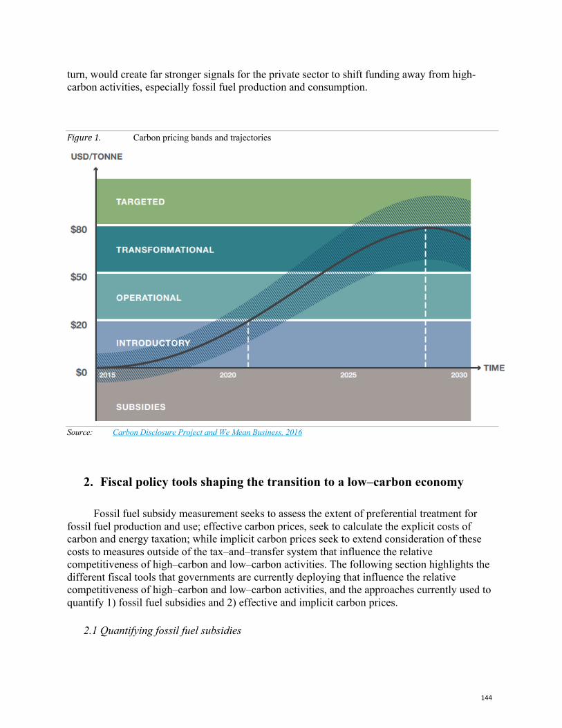
144

turn, would create far stronger signals for the private sector to shift funding away from high-carbon activities, especially fossil fuel production and consumption.

Figure1. Carbon pricing bands and trajectories

Source: Carbon Disclosure Project and We Mean Business, 2016

2. Fiscal policy tools shaping the transition to a low–carbon economy

Fossil fuel subsidy measurement seeks to assess the extent of preferential treatment for

fossil fuel production and use; effective carbon prices, seek to calculate the explicit costs of carbon and energy taxation; while implicit carbon prices seek to extend consideration of these costs to measures outside of the tax–and–transfer system that influence the relative competitiveness of high–carbon and low–carbon activities. The following section highlights the different fiscal tools that governments are currently deploying that influence the relative competitiveness of high–carbon and low–carbon activities, and the approaches currently used to quantify 1) fossil fuel subsidies and 2) effective and implicit carbon prices.

2.1 Quantifying fossil fuel subsidies

145

In recent years there has been increased pressure for the reduction or removal of fossil fuel subsidies as part of an integrated policy response to climate change. Reflecting this, there have been several efforts to define, identify and quantify the level of fossil fuel subsidies.

In its Agreement on Subsidies and Countervailing Measures, the World Trade Organization (WTO) defines a subsidy to include financials contribution by a government, or agent of a government, that is recipient-specific and confers a benefit on its recipients in comparison to other market participants.5

This definition has been accepted by the 164 World Trade Organisation (WTO) Member States, including all G–7 countries, and includes the following subsidy categories: 1. direct transfer of funds (e.g. budgetary transfers, grants, loans and equity infusion), and

potential direct transfers of funds or liabilities (e.g. loan guarantees), below market value 2. government revenue that is otherwise due, foregone or not collected (e.g. fiscal

incentives such as tax expenditures) 3. government provision of goods or services other than general infrastructure, or purchase

of goods, below market value 4. income or price support.

The WTO does not, however, quantify energy subsidies. Rather, the three most prominent approaches adopted by international organisations are: — The Organisation for Economic Cooperation and Development’s (OECD) inventory

approach which quantifies the value of the policies and measures introduced by governments that support the production or consumption of fossil fuels.

— The International Energy Agency’s (IEA) price-gap approach which identifies the impact of policies supporting fossil fuels by measuring the difference between final consumer prices and a representative non-subsidised price (adjusted for transport and distribution costs).

— The International Monetary Fund’s (IMF) efficient-tax approach identifies the price-gap between the actual cost of consuming a fossil fuel and the efficient price, that would prevail if the externalities associated with that consumption were efficiently priced.

These measures have different attributes that make them appropriate for different uses. The OECD’s inventory approach provides a clear definition of the specific policies that support fossil fuel consumption, and draws links between fiscal and energy policy, but does not capture the impact of policies, such as renewable energy mandates, that impact prices and consumption but do not directly affect a government’s fiscal balance.6 The IEA’s price–gap approach identifies the net impacts of policies on prices, however the value of producer support estimates must be calculated separately (using the inventory approach). In this approach, the effects of specific consumption subsidies are also unclear and the impact of policies that have a countervailing impact on prices may be missed. Although focussed on consumption subsidies the IMF’s efficient tax approach provides the broadest measure. It references the data of the OECD and IEA to establish a price–gap measure of consumption subsidies, and then calculates the difference between actual tax treatment and the efficient tax level for a fuel and/or sector to estimate ‘pre-tax subsidies’. It then calculates the additional Value Added Tax (VAT) revenue that is foregone by not pricing the energy sector at efficient prices, so-called ‘post–tax subsidies’. Externalities considered by the IMF include climate change, local air pollution, congestion and

5 WTO (1994) Agreement on Subsidies and Countervailing Measures. 6 This includes accounting for transfers to producers that compensate them for selling fossil fuel products for below-market prices. An explicit measures approach is also used by the Global Subsidies Initiative, which uses the World Trade Organisation’s definition of a subsidy as its basis for definition and quantification.

146

road accidents and damage. However, identifying and quantifying these externalities is often deeply uncertain.7

The approaches above are methodologically distinct, but complementary. For instance, in 2018, an OECD and IEA review combined estimates from the inventory and price–gap approaches to estimate fossil fuel subsidies in 76 countries8 (responsible for 94 per cent of global CO2 emissions). This analysis includes country by country estimates of budget transfers and tax expenditures for the production and consumption of oil, gas and coal but does not include subsidies provided through public finance (government grants, concessional loans, equity, guarantees and insurance), nor direct government provision of goods and services (such as investments in state-owned enterprise) or income and price support (such as through capacity mechanisms). The studies found that support to fossil fuels reached US$373 billion in 2015.9 While significant, these subsidies are small when compared to the post–tax subsidies provided by not pricing the externalities, such as unpriced pollution or traffic congestion, associated with fossil fuel consumption. The IMF’s estimates suggest that in 2015, this broader set of subsidies were likely to be more than US$5 trillion.10

With the work of these organisations, alongside research organisations and civil society groups, there has been significant improvement in our understanding of the magnitude and distribution of fossil fuel subsidies. Further, several countries have taken up fossil fuel subsidy reforms in the past few years, as shown in Figure 2. Nonetheless, substantial gaps remain due to limited transparency at the national level, and a full accounting of global energy subsidies (to fossil fuels and renewables) has never been completed. As a result, it is likely that global estimates are well below current levels of support.

7 The IMF’s measure of post-tax subsidies accounts for the social cost of carbon (SCC), which links this estimate of subsidies with the discussion on carbon pricing below. For estimates of the SCC see: US IAWG (2013) Technical Update of the Social Cost of Carbon. 8 OECD (2018) Companion to the Inventory of Support Measures to Fossil Fuels. 9 Parallel research by the IEA found that subsidies for renewables in power generation amounted to $140 billion in 2016 (IEA, 2017). 10 IMF (2015) How Large are Global Energy Subsidies?.

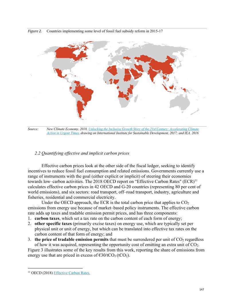
147

Figure2. Countries implementing some level of fossil fuel subsidy reform in 2015-17

Source: New Climate Economy, 2018, Unlocking the Inclusive Growth Story of the 21st Century: Accelerating Climate Action in Urgent Times, drawing on International Institute for Sustainable Development, 2017; and IEA, 2016

2.2 Quantifying effective and implicit carbon prices

Effective carbon prices look at the other side of the fiscal ledger, seeking to identify

incentives to reduce fossil fuel consumption and related emissions. Governments currently use a range of instruments with the goal (either explicit or implicit) of steering their economies towards low–carbon activities. The 2018 OECD report on “Effective Carbon Rates" (ECR)11 calculates effective carbon prices in 42 OECD and G-20 countries (representing 80 per cent of world emissions), and six sectors: road transport, off–road transport, industry, agriculture and fisheries, residential and commercial electricity.

Under the OECD approach, the ECR is the total carbon price that applies to CO2 emissions from energy use because of market–based policy instruments. The effective carbon rate adds up taxes and tradable emission permit prices, and has three components: 1. carbon taxes, which set a tax rate on the carbon content of each form of energy; 2. other specific taxes (primarily excise taxes) on energy use, which are typically set per

physical unit or unit of energy, but which can be translated into effective tax rates on the carbon content of that form of energy; and

3. the price of tradable emission permits that must be surrendered per unit of CO2 regardless of how it was acquired, representing the opportunity cost of emitting an extra unit of CO2.

Figure 3 illustrates some of the key results from this work, reporting the share of emissions from energy use that are priced in excess of €30/tCO2 (tCO2).

11 OECD (2018) Effective Carbon Rates.

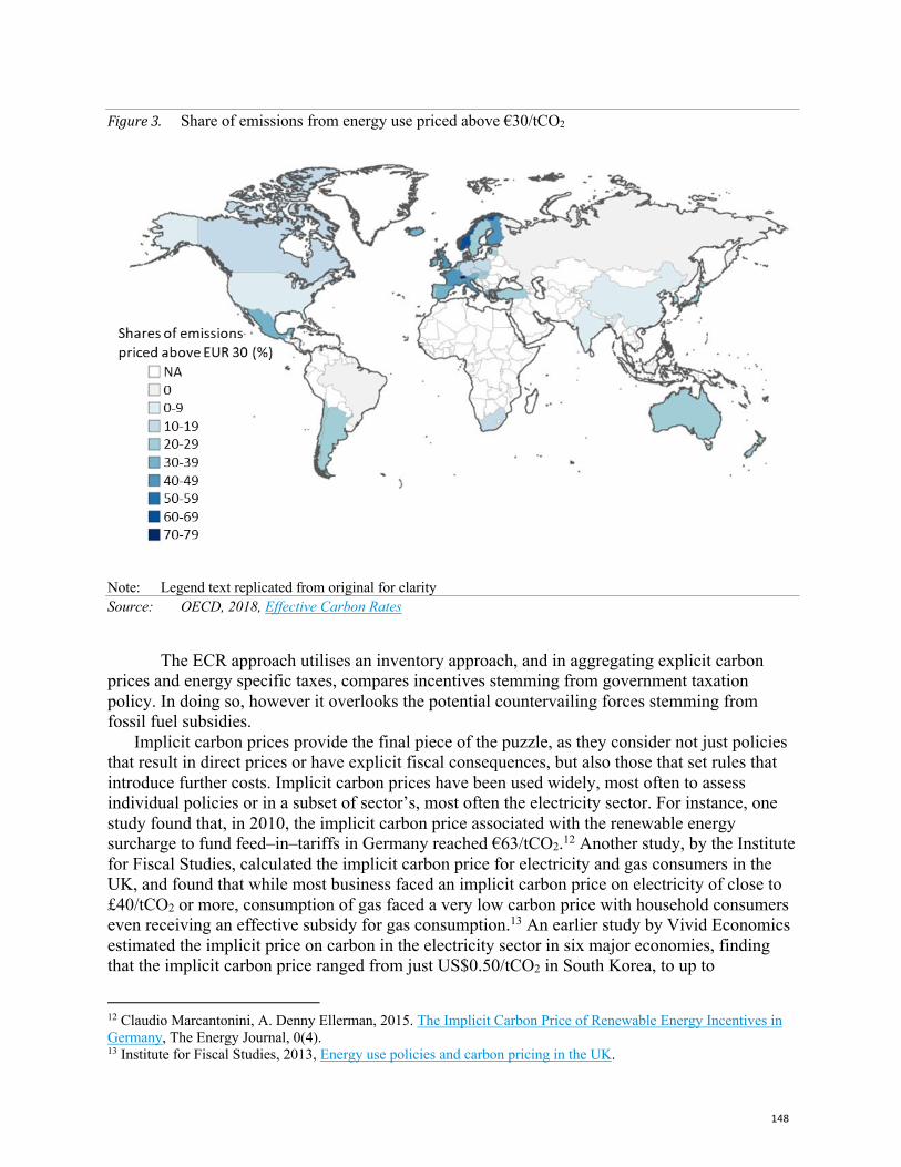
148

Figure3. Share of emissions from energy use priced above €30/tCO2

Note: Legend text replicated from original for clarity Source: OECD, 2018, Effective Carbon Rates

The ECR approach utilises an inventory approach, and in aggregating explicit carbon prices and energy specific taxes, compares incentives stemming from government taxation policy. In doing so, however it overlooks the potential countervailing forces stemming from fossil fuel subsidies.

Implicit carbon prices provide the final piece of the puzzle, as they consider not just policies that result in direct prices or have explicit fiscal consequences, but also those that set rules that introduce further costs. Implicit carbon prices have been used widely, most often to assess individual policies or in a subset of sector’s, most often the electricity sector. For instance, one study found that, in 2010, the implicit carbon price associated with the renewable energy surcharge to fund feed–in–tariffs in Germany reached €63/tCO2.12 Another study, by the Institute for Fiscal Studies, calculated the implicit carbon price for electricity and gas consumers in the UK, and found that while most business faced an implicit carbon price on electricity of close to £40/tCO2 or more, consumption of gas faced a very low carbon price with household consumers even receiving an effective subsidy for gas consumption.13 An earlier study by Vivid Economics estimated the implicit price on carbon in the electricity sector in six major economies, finding that the implicit carbon price ranged from just US$0.50/tCO2 in South Korea, to up to

12 Claudio Marcantonini, A. Denny Ellerman, 2015. The Implicit Carbon Price of Renewable Energy Incentives in Germany, The Energy Journal, 0(4). 13 Institute for Fiscal Studies, 2013, Energy use policies and carbon pricing in the UK.

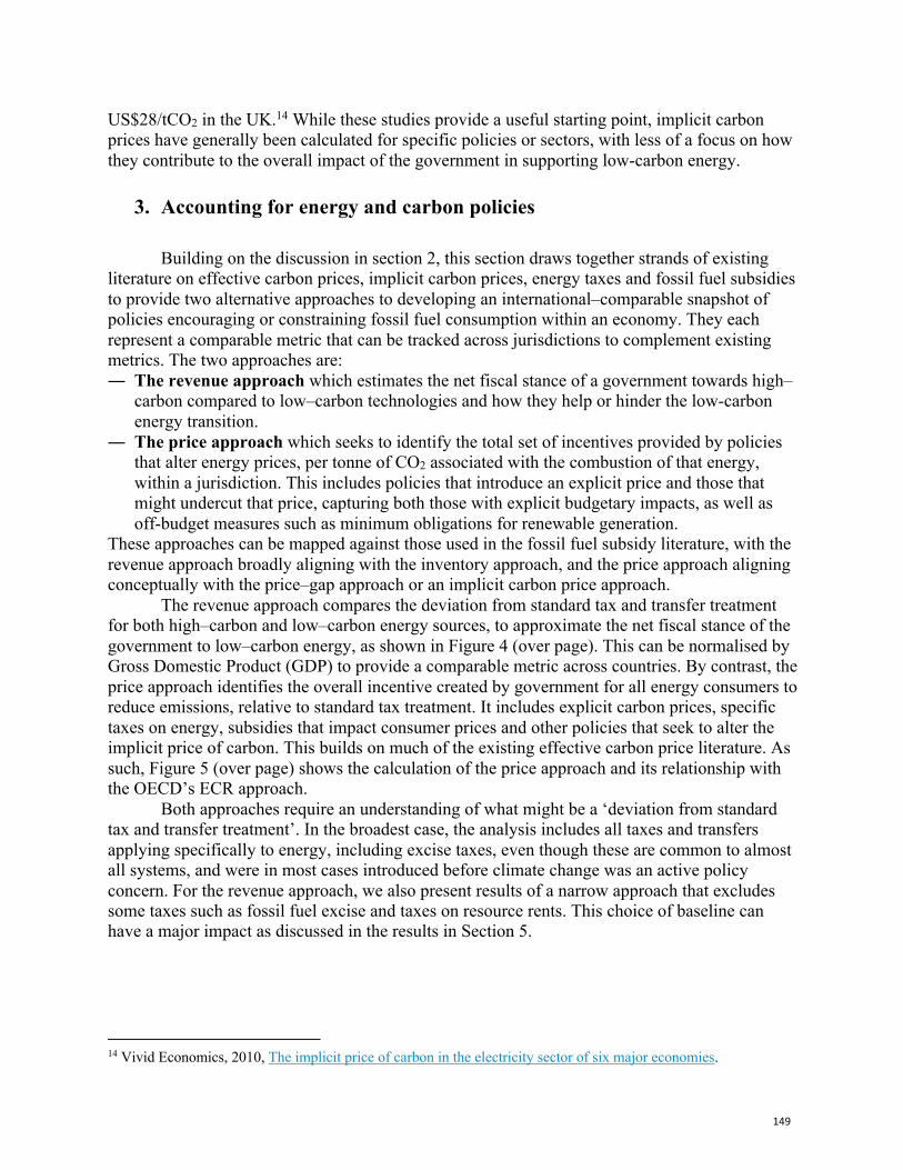
149

US$28/tCO2 in the UK.14 While these studies provide a useful starting point, implicit carbon prices have generally been calculated for specific policies or sectors, with less of a focus on how they contribute to the overall impact of the government in supporting low-carbon energy.

3. Accounting for energy and carbon policies

Building on the discussion in section 2, this section draws together strands of existing literature on effective carbon prices, implicit carbon prices, energy taxes and fossil fuel subsidies to provide two alternative approaches to developing an international–comparable snapshot of policies encouraging or constraining fossil fuel consumption within an economy. They each represent a comparable metric that can be tracked across jurisdictions to complement existing metrics. The two approaches are: ― The revenue approach which estimates the net fiscal stance of a government towards high–

carbon compared to low–carbon technologies and how they help or hinder the low-carbon energy transition.

― The price approach which seeks to identify the total set of incentives provided by policies that alter energy prices, per tonne of CO2 associated with the combustion of that energy, within a jurisdiction. This includes policies that introduce an explicit price and those that might undercut that price, capturing both those with explicit budgetary impacts, as well as off-budget measures such as minimum obligations for renewable generation.

These approaches can be mapped against those used in the fossil fuel subsidy literature, with the revenue approach broadly aligning with the inventory approach, and the price approach aligning conceptually with the price–gap approach or an implicit carbon price approach.

The revenue approach compares the deviation from standard tax and transfer treatment for both high–carbon and low–carbon energy sources, to approximate the net fiscal stance of the government to low–carbon energy, as shown in Figure 4 (over page). This can be normalised by Gross Domestic Product (GDP) to provide a comparable metric across countries. By contrast, the price approach identifies the overall incentive created by government for all energy consumers to reduce emissions, relative to standard tax treatment. It includes explicit carbon prices, specific taxes on energy, subsidies that impact consumer prices and other policies that seek to alter the implicit price of carbon. This builds on much of the existing effective carbon price literature. As such, Figure 5 (over page) shows the calculation of the price approach and its relationship with the OECD’s ECR approach.

Both approaches require an understanding of what might be a ‘deviation from standard tax and transfer treatment’. In the broadest case, the analysis includes all taxes and transfers applying specifically to energy, including excise taxes, even though these are common to almost all systems, and were in most cases introduced before climate change was an active policy concern. For the revenue approach, we also present results of a narrow approach that excludes some taxes such as fossil fuel excise and taxes on resource rents. This choice of baseline can have a major impact as discussed in the results in Section 5.

14 Vivid Economics, 2010, The implicit price of carbon in the electricity sector of six major economies.

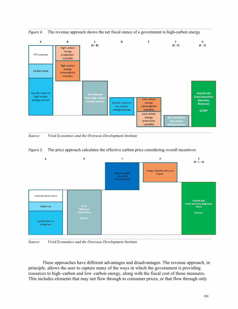
150

Figure4. The revenue approach shows the net fiscal stance of a government to high-carbon energy

Source: Vivid Economics and the Overseas Development Institute

Figure5. The price approach calculates the effective carbon price considering overall incentives


These approaches have different advantages and disadvantages. The revenue approach, in

principle, allows the user to capture many of the ways in which the government is providing resources to high–carbon and low–carbon energy, along with the fiscal cost of those measures. This includes elements that may not flow through to consumer prices, or that flow through only

151

indirectly, such as production subsidies. On the other hand, it does not capture induced transfers from policies that operate outside of the tax and transfer system. For instance, the revenue approach would not account for the impact of mandatory renewable energy targets, that provide transfers from consumers (through higher prices) to renewable energy generators. The revenue approach also requires a definition of what constitutes high–carbon and low–carbon energy that, in cases such as gas generation, may be debatable. In contrast, the price approach has the advantage of capturing the effect of policies on prices, including those that place an implicit price on carbon, such as renewables mandates. The price approach, however, fails to capture the impact of subsidies that only affect prices indirectly or not at all, such as fossil fuel production subsidies, or free allowances/rebates provided under a carbon price that may not be directly reflected in marginal incentives.

Consistent with these differing advantages and disadvantages, the approaches may be relevant for different audiences. For those focused on fiscal policy, the revenue approach provides a better indication of the fiscal opportunity costs associated with net subsidising fossil fuels and it can allow one to identify where contradictory incentives exist in the tax and transfer system due to countervailing policies supporting high–carbon and low–carbon energy. In contrast, the price approach is more relevant for those with a focus on the incentives created by energy fiscal policy, as it shows where incentives for decarbonisation are the strongest and where incentives may be inadequate to support the energy transition.

4. Methodology and assumptions

To demonstrate proof of concept, we have applied both the price approach and the revenue approach to the UK and tested the potential for replicating this analysis for all G-7 countries in the future. Below we outline our methodology in applying the conceptual approach outlined above, to demonstrate that these approaches can provide a tractable tool for policy makers seeking to understand the channels through which the tax and transfer system effect policy, and one that could be rolled out to other jurisdictions to better understand effective carbon prices in operation in an economy.

4.1 Revenue approach

The revenue approach focuses on quantifying, at the aggregate level, how the fiscal system supports or constrains the production and use of fossil fuel and low–carbon energy sources. By comparing the treatment of fossil fuels and their low-carbon alternatives, we identify the government’s net fiscal stance towards these energy options. In applying the revenue approach, we seek to identify where the treatment of fossil fuels and low-carbon energy is different from the treatment of other economic activities under the fiscal system.15 As such a key challenge for this approach, is the method of categorising policies supporting or constraining fossil fuel or low-carbon energy.

We present two variants on the treatment of government revenues in this approach, to account for the multiple objectives that a fiscal system may attempt to achieve:

15 That is, where a fiscal measure specifically targets energy, for instance a specific fuel tax would be counted whereas a broad-based value added tax would not.

152

― The broad approach includes a wide set of taxes as potentially targeting fossil fuels, this includes the Climate Change Levy (CCL) and Carbon Price Support (CPS); European Union (EU) Emission Trading Scheme (ETS) auctions; environmental levies; petroleum resource taxes; and revenues from fuel duties.

― The narrow approach includes a narrower set of taxes, which are focussed on carbon emissions or environmental outcomes more specifically, and therefore excludes revenues from fuel duties and petroleum resource taxes.

The exclusion of revenues from fuel duties and petroleum resource taxes under the narrow approach, reflects the fact that these taxes were established for purposes wholly separate from addressing carbon emissions from fossil fuels. For instance, fuel duties have been charged for decades well before addressing climate change was considered a serious policy objective. The popularity of fuel duties reflects both their stability (in the near term) as a revenue source and their role in internalising – to an extent – a range of externalities associated with fuel consumption, such as local air pollution and congestion. As such this taxation treatment is somewhat or wholly divorced from the carbon emissions associated with the fuel use. Similarly, the purpose of the petroleum resource tax (up to now) has been as a mechanism to achieve a return to the state for the value of the extraction of a scarce resource, rather than as a tax treatment applied to a carbon intensive fuel.

In calculating the revenue approach (both broad and narrow), we have used public data that is easily accessible. The data on revenues have been collected from the OBR’s March 2018 Economic and Fiscal Outlook – supplementary fiscal tables on receipts16. The data on expenditure measures have been sourced from the OBR’s March 2018 Economic and Fiscal Outlook – supplementary fiscal tables on expenditure.17

We have categorised the following expenditure as support for low–carbon energy: energy efficiency measures and incentives in the households and public sector; warm homes discount; feed–in–tariffs; renewables obligation; contracts for difference; capacity market; expenditure on renewable heat incentive.18

UK governments’ support for fossil fuels include VAT exemptions for electricity and natural gas use in the residential sector and an additional winter fuel and cold weather payments made to the households. The data for these is taken from the review of the OECD’s 2018 inventory of subsidies and the OBR’s March 2018 Economic and fiscal outlook.

4.2 Price approach

The price approach requires the mapping of emissions and energy use against energy taxation and subsidies to calculate the net tax burden for each activity (e.g. use of electricity in the residential sector) for which final energy use and emissions are available.

16 OBR 2018 March 2018 Economic and Fiscal Outlook – supplementary fiscal tables: receipts and other. 17 OBR 2018 March 2018 Economic and Fiscal Outlook – supplementary fiscal tables: expenditure. 18 Some of these policies, for instance the renewables obligation and feed-in-tariffs are revenue neutral, as the tax collected is equal to expenditure provided under the measure. These are nonetheless included given their inclusion in national accounts.

153

Given data availability across multiple sources, we calculate the effective carbon price (£/tCO2) for the year 2016. Energy use and emissions data are gathered from the IEA’s Extended World Energy Balances 201819 and the IEA’s CO2 Emissions from Fuel Combustion 201820.

Effective carbon prices are calculated for the sectors corresponding to the following IEA sectors: Iron and steel; Chemical and Petrochemicals; Non-ferrous metals; Non-metallic minerals; Transport equipment; Machinery; Mining and quarrying; Food and tobacco; Paper, pulp and printing; Wood and wood products; Construction; Textile and leather; Non-specified industry; Transport; Domestic aviation; Residential; Commercial and public services; Agriculture/forestry; Fishing. We provide estimates of effective carbon prices for each of the sectors noted above for the following fuels (corresponding to the sum of IEA fuels): Coal (cooking coal, other bituminous coal, patent fuel, coke oven coke, coke oven gas and blast furnace gas), Natural gas, Oil (crude/NLG/feedstocks, refinery gas, kerosene type jet fuels, other kerosene, fuel oil, naphtha and petroleum coke), LPG, Motor gasoline, and Gas/diesel oil. To calculate each aspect of the price approach the following data sources were used: ― Specific taxes on energy use; For the UK, this category comprises the excise that is levied

on energy use, predominantly on the use of liquid fuels in transport. Data on excise rates was compiled from the European Commission’s Excise Duty Tables.21

― Carbon taxes; The UK has carbon taxes that partially overlap with the covered sectors of an emissions trading system. These include the Climate Change Levy (CCL) charged on energy use in non–domestic sectors and the Carbon Price Support that levies an additional charge on electricity generators. For these policies, tax rates were drawn from the HM Revenues & Customs Guidance.22

― Emissions Permit Price; The European Union Emissions Trading System (EU ETS) has been treated as equivalent in its incentive effects to a marginal tax on emissions, based on data sourced from the Intercontinental Exchange.23

― Price uplift from other energy policies; The price uplift from energy policies is only identified to have a material impact in the electricity sector. The data for electricity price components from energy policies was gathered from the Committee on Climate Change’s Energy Prices and Bills 2017.24

― Energy subsidies with a price impact; Energy subsidy data is drawn from various sources including UK government publications and the OECD’s Inventory of Support Measures for Fossil Fuels (2018).25

Further detailed description of assumptions for each element is provided in the Annex.

19 IEA (2018) World Energy Balances 2018. 20 IEA (2018) CO2 Emissions from Fuel Combustion 2018. 21 European Commission (2016) EXCISE DUTY TABLES Part II – Energy and Electricity. 22 HM Revenues & Custom Guidance (2018) Climate Change Levy Rates. 23 Intercontinental Exchange (via Quandl), 2016, EUA futures (December delivery). 24 Committee on Climate Change (2017) Energy Prices and Bills – impacts of meeting carbon budgets. 25 Further details provided in the Annex, see OECD (2018); Ofgem (2016); HMRC (2017b); HM Treasury (2014); HMRC (2016); HMRC (2015); HMRC (2014).

154

4.3 Replicability of approaches

Both the revenue approach and price approach applied in this paper are replicable across the G-7 countries.

The data for fossil fuel tax revenues and fossil fuel and low–carbon subsidies used in the revenue approach is derived from government reported figures on annual receipts and expenditures. We expect this data to also be publicly reported by the other G-7 countries.

For the price approach most of the energy consumption, emissions and taxes data are available from global sources. As shown in Table 1, energy consumption and emissions data are gathered from the IEA databases, which reports these for all countries. Similarly, data on excise rates and EU ETS prices is compiled from the EU databases, which covers all the EU countries. For non–EU countries in the G-7 – Canada, Japan and the US – excise and ETS data (where applicable) will be easily available from government sources. In addition, the ODI maintains a database on fossil fuel subsidies for all major economies.

The UK specific data utilized in this approach is expected to be replicable using administrative data in other G-7 countries. The carbon taxes (apart from the ETS), breakdown of price components from different policies and some energy subsidies data are available from government sources. As the G-7 make up the seven largest advanced economies of the world, similar data will be collected and reported by respective national regulators and should be accessible from their government data agencies and data portals.

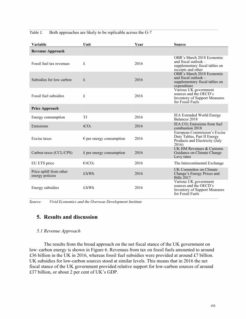
155

Table1. Both approaches are likely to be replicable across the G-7

Variable Unit Year Source Revenue Approach

Fossil fuel tax revenues £ 2016 OBR’s March 2018 Economic and fiscal outlook – supplementary fiscal tables on receipts and other

Subsidies for low carbon £ 2016 OBR’s March 2018 Economic and fiscal outlook – supplementary fiscal tables on expenditure

Fossil fuel subsidies £ 2016 Various UK government sources and the OECD’s Inventory of Support Measures for Fossil Fuels

Price Approach

Energy consumption TJ 2016 IEA Extended World Energy Balances 2018

Emissions tCO2 2016 IEA CO2 Emissions from fuel combustion 2018

Excise taxes € per energy consumption 2016 European Commission’s Excise Duty Tables, Part II Energy Products and Electricity (July 2016)

Carbon taxes (CCL/CPS) £ per energy consumption 2016 UK HM Revenues & Customs Guidance on Climate Change Levy rates

EU ETS price €/tCO2 2016 The Intercontinental Exchange

Price uplift from other energy policies £/kWh 2016

UK Committee on Climate Change’s Energy Prices and Bills 2017

Energy subsidies £/kWh 2016 Various UK government sources and the OECD’s Inventory of Support Measures for Fossil Fuels


5. Results and discussion

5.1 Revenue Approach

The results from the broad approach on the net fiscal stance of the UK government on low–carbon energy is shown in Figure 6. Revenues from tax on fossil fuels amounted to around £36 billion in the UK in 2016, whereas fossil fuel subsidies were provided at around £7 billion. UK subsidies for low-carbon sources stood at similar levels. This means that in 2016 the net fiscal stance of the UK government provided relative support for low-carbon sources of around £37 billion, or about 2 per cent of UK’s GDP.

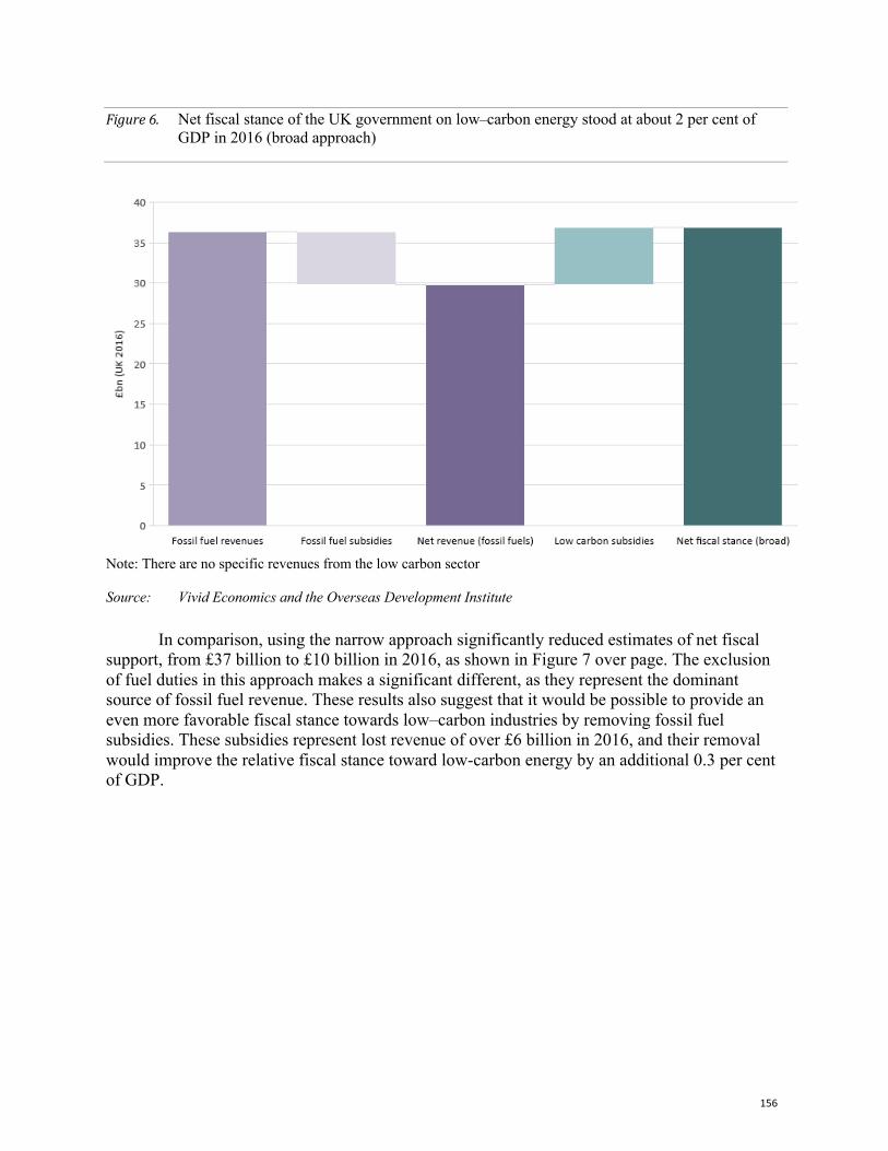
156

Figure6. Net fiscal stance of the UK government on low–carbon energy stood at about 2 per cent of GDP in 2016 (broad approach)

Note: There are no specific revenues from the low carbon sector Source: Vivid Economics and the Overseas Development Institute

In comparison, using the narrow approach significantly reduced estimates of net fiscal support, from £37 billion to £10 billion in 2016, as shown in Figure 7 over page. The exclusion of fuel duties in this approach makes a significant different, as they represent the dominant source of fossil fuel revenue. These results also suggest that it would be possible to provide an even more favorable fiscal stance towards low–carbon industries by removing fossil fuel subsidies. These subsidies represent lost revenue of over £6 billion in 2016, and their removal would improve the relative fiscal stance toward low-carbon energy by an additional 0.3 per cent of GDP.

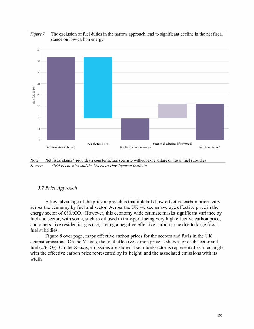
157

Figure7. The exclusion of fuel duties in the narrow approach lead to significant decline in the net fiscal stance on low-carbon energy

Note: Net fiscal stance* provides a counterfactual scenario without expenditure on fossil fuel subsidies. Source: Vivid Economics and the Overseas Development Institute

5.2 Price Approach

A key advantage of the price approach is that it details how effective carbon prices vary

across the economy by fuel and sector. Across the UK we see an average effective price in the energy sector of £80/tCO2. However, this economy wide estimate masks significant variance by fuel and sector, with some, such as oil used in transport facing very high effective carbon price, and others, like residential gas use, having a negative effective carbon price due to large fossil fuel subsidies.

Figure 8 over page, maps effective carbon prices for the sectors and fuels in the UK against emissions. On the Y–axis, the total effective carbon price is shown for each sector and fuel (£/tCO2). On the X–axis, emissions are shown. Each fuel/sector is represented as a rectangle, with the effective carbon price represented by its height, and the associated emissions with its width.

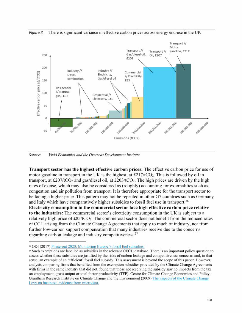
158

Figure8. There is significant variance in effective carbon prices across energy end-use in the UK


Transport sector has the highest effective carbon prices: The effective carbon price for use of motor gasoline in transport in the UK is the highest, at £217/tCO2. This is followed by oil in transport, at £207/tCO2 and gas/diesel oil, at £203/tCO2. The high prices are driven by the high rates of excise, which may also be considered as (roughly) accounting for externalities such as congestion and air pollution from transport. It is therefore appropriate for the transport sector to be facing a higher price. This pattern may not be repeated in other G7 countries such as Germany and Italy which have comparatively higher subsidies to fossil fuel use in transport.26 Electricity consumption in the commercial sector face high effective carbon price relative to the industries: The commercial sector’s electricity consumption in the UK is subject to a relatively high price of £85/tCO2. The commercial sector does not benefit from the reduced rates of CCL arising from the Climate Change Agreements that apply to much of industry, nor from further low-carbon support compensation that many industries receive due to the concerns regarding carbon leakage and industry competitiveness.27

26 ODI (2017) Phase-out 2020: Monitoring Europe’s fossil fuel subsidies. 27 Such exemptions are labelled as subsidies in the relevant OECD database. There is an important policy question to assess whether these subsidies are justified by the risks of carbon leakage and competitiveness concerns and, in that sense, an example of an ‘efficient’ fossil fuel subsidy. This assessment is beyond the scope of this paper. However, analysis comparing firms that benefited from the exemption subsidies provided by the Climate Change Agreements with firms in the same industry that did not, found that those not receiving the subsidy saw no impacts from the tax on employment, gross output or total factor productivity (TFP). Centre for Climate Change Economics and Policy, Grantham Research Institute on Climate Change and the Environment (2009) The impacts of the Climate Change Levy on business: evidence from microdata.

159

Most direct combustion in industries face a low effective carbon price which would increase if fossil fuel subsidies were eliminated: Energy consumption including coal, natural gas and oil products in the industrial sector pay a small positive effective carbon price, ranging from £2/tCO2 to £14/tCO2. As noted above, industries are lightly taxed and benefit from subsidies in the form of carbon tax exemptions and rate reductions. Natural gas consumption in the residential sector faces a negative effective carbon price, however energy policies drive up the price faced by electricity consumption: VAT subsidies on natural gas use in households give an effective carbon price of -£32/tCO2. Electricity consumption is subjected to the same VAT subsidy, however energy policies such as support for low–carbon and energy efficiency schemes bring the effective carbon price on electricity use to a positive figure of £31/tCO2.

6. Conclusions

To demonstrate proof of concept, this study builds on existing literature on effective carbon prices, implicit carbon prices, energy taxes and fossil fuel subsidies to provide two alternative approaches to developing an international–comparable snapshot of the total set of incentives encouraging or constraining fossil fuel consumption within an economy. By applying both the revenue and price approaches developed in this study to the UK, and testing their replicability across the G-7, we find each approach represents a comparable metric that can be tracked across jurisdictions and complement existing metrics.

Applying the revenue approach to the UK shows that in 2016 the net fiscal stance of the UK government to low–carbon energy provided net support of around £37 billion, or about 2 per cent of UK’s GDP. However, this figure drops significantly, to £10 billion, when fossil fuel duties and resource rents are excluded from this calculation. The removal of the approximately £6 billion of fossil fuel subsidies presents an opportunity to further enhance the government’s positive fiscal stance to low–carbon energy.

Applying the price approach to the UK reveals high effective carbon prices for electricity consumption in the commercial sector and for fuel use in transport (£85/tCO2 and £207/tCO2 respectively), the impact of fossil fuel subsidies results in negligible effective carbon prices for industry (£2/tCO2 to £14/tCO2). In the case of gas use in households, significant subsidies through VAT tax breaks results in a negative effective carbon price (-£32/tCO2).

Applying these approaches to a broader set of countries (including the G-7 in the first instance) would provide additional evidence to support far more joined up efforts at the international and national level initiatives to tackle fossil fuel subsidies and implement carbon pricing. The G-7 (including the EU) is a key group for engagement as they have committed to ending fossil fuel subsidies by 2025 (2020 for the EU) and already have a range of carbon pricing instruments in place. There are also wider opportunities to support these activities under the Sustainable Development Goals (SDGs) and the United Nations Framework Convention on Climate Change (UNFCCC) Paris Agreement, including within nationally determined contributions (NDCs). A 2015 study of intended NDCs (INDCs) found 67 countries had included references to fiscal instruments (carbon pricing, subsidy reform etc.).28

Analysis by the Carbon Pricing Leadership Coalition shows that effective energy fiscal reform packages include both a revenue component (lower subsidy costs or higher revenues

28 IISD (2015) Fiscal Instruments in INDCs.

160

through a taxes or carbon pricing) and a spending component (such as a reduction in other taxes; increased spending on social protection, cash transfers, or public services).29 By linking revenue from subsidy reform and carbon pricing to spending on wider public priorities, fiscal reform has a higher probability of success. The approaches set out in this paper provide improved metrics regarding the nature and interactions of fossil fuel subsidies, carbon pricing and energy policies. This can help policy makers target energy policy reforms in a manner that results in better outcomes for the climate, the economy and society.

Annex: Assumptions in calculating the price approach

Specific taxes on energy use

For the UK, this category comprises the excise that is levied on energy use in the UK, predominantly on the use of liquid fuels in transport. Data on excise rates was compiled from the European Commission’s Excise Duty Tables. To align this data with the energy and emissions data from the IEA, we assume: ― ‘Business use’ corresponds to the following IEA sectors: Iron and steel; Chemical and

Petrochemicals; Non-ferrous metals; Non-metallic minerals; Transport equipment; Machinery; Food and tobacco; Paper, pulp and printing; Wood and wood products; Textile and leather; Non–specified industry; Commercial and public services (partly, see below).

― ‘Non–business use’ relates to the IEA sectors of Commercial & public services (in part, see below) and residential.

― Energy used in the Commercial and Public Services category was allocated to business and non-business use based on Eurostat input–output tables, where the allocation was 100 per cent and 0 per cent for coal, 21 per cent and 79 per cent for refined products and 38 per cent and 62 per cent for electricity and natural gas, for business and non–business use respectively.

― ‘Industrial and Commercial Usage’ corresponds to the IEA sector categories of Construction & Mining and Quarrying.

― ‘Agriculture, horticulture, pisciculture, forestry’ and ‘Agriculture’ correspond to the IEA sector of agriculture/forestry.

― ‘Gas Oil’, ‘Heavy fuel oil’, ‘Kerosene’, ‘Petroleum’ and ‘Gasoline’ are assumed to correspond to the IEA fuels gas/diesel oil, fuel oil, other kerosene and motor gasoline respectively.

Carbon taxes

The UK has carbon taxes that overlap with covered sector in an emissions trading system.

This includes the Climate Change Levy (CCL) charged on energy use in non–domestic sectors and the CPS that levies an additional charge on electricity generators. For these policies, tax rates were drawn from HM Revenues & Customs Guidance, with the following specific assumptions:

29 Carbon Pricing Leadership Coalition (2017) Report of the High-Level Commission on Carbon Prices.

161

― The CCL is assumed to be charged on energy use in the following IEA sectors: Iron & steel; Chemical & Petrochemicals; Non–ferrous metals; Non–metallic minerals; Transport equipment; Machinery; Mining & quarrying; Food & tobacco; Paper, pulp & printing; Wood & wood products; Construction; Textile & leather; Non–specified industry; Commercial & public services; Agriculture/forestry; Fishing.

― The CCL is charged on the following fuels: Natural gas; LPG; Coking coal; Other bituminous coal; Petroleum coke; Coke oven coke; Electricity; Coke oven gas; Blast furnace gas; Refinery gas.

― The proportion of energy use liable to pay the reduced rate of CCL is calculated as the proportion of emissions under the Climate Change Agreements (CCA)30 in each sector.

― We assume that electricity generators fully pass through the costs of the CPS, hence all electricity use is assumed to be subject to an implicit carbon price equivalent to the average effective carbon price for electricity generation from the CPS, in proportion with each sector’s electricity consumption.

Emissions Permit Price

The EU ETS has been treated as equivalent in its incentive effects to a marginal tax on

emissions. The data is drawn from the Intercontinental Exchange, with the EU ETS allowance price calculated as the average spot price in July 2016, amounting to 4.04 £/tCO2 (4.65 €/tCO2 converted with an exchange rate of €1 = £0.87). Other assumptions include: ― All emissions from the following IEA sectors are covered: Iron & steel; Chemical &

Petrochemicals; Non–ferrous metals; Non–metallic minerals; Paper, pulp & printing; Domestic aviation.

― 70 per cent of emissions in the IEA sector of Food & tobacco and 12 per cent of emissions in Commercial & public services are covered EU ETS. This is based on the comparison of emissions data for the sector, and historic data from the UK’s National Allocation Plan, giving EU-ETS covered emissions.

― Electricity producers pass on 100 per cent of costs, so that usage of electricity is assumed to be subject to an implicit carbon tax equivalent to the average effective carbon price in electricity generation, in proportion with each sector’s electricity consumption.

Price uplift from other energy policies

The price uplift from energy policies is only identified for the electricity usage in the UK.

The data for electricity price components from energy policies was gathered from Committee on Climate Change’s Energy Prices and Bills 2017. These price components were mapped to the electricity consumption in end–use sectors and attributed to their respective end–use electricity emissions, to arrive at £/tCO2 figures. The following assumptions were made: ― For the ‘residential’ sector, the following policies are assumed applicable: Support for low-

carbon; Energy efficiency (low–carbon); Capacity market; System integration costs

30 Environment Agency (2017) Climate Change Agreements – Target Unit Performance Data.

162

(transmission and intermittency); Additional distribution costs; Merit order effect; Warm Homes Discount; Energy efficiency (other); Smart meters.

― For the ‘commercial’ and ‘manufacturing’ sectors, the policies identified include: Support for Low–carbon; Carbon Reduction Commitment (CRC); Capacity market; System integration costs (transmission and intermittency); Additional distribution costs; Merit Order effect.

― ‘Small commercial’ and ‘Medium commercial’ correspond to the proportions of the IEA sector category of commercial and public services, in accordance with the electricity consumed that were liable to pay the CRC scheme, which amounted to be 71 per cent of the commercial and public services sector.

― ‘Large manufacturing’ is the following IEA sectors: Transport equipment; Mining & quarrying; Food & tobacco; Machinery; Wood & wood products; Construction; Textile & leather; Non–specified industry.

― ‘Large manufacturing (low–carbon support compensation)’ correspond to the following IEA sectors: Iron & steel; Chemical & petrochemicals; Non–ferrous metals; Non–metallic minerals; Paper, pulp & printing.

― ‘Extra–large manufacturing (low–carbon support & carbon price compensation)’ is excluded from the analysis to avoid double counting, as CPS is already considered under the carbon tax element.

Energy subsidies with a price impact

Energy subsidy data is drawn from Various UK government sources and the OECD’s

Inventory of Support Measures for Fossil Fuels, compiled by the Overseas Development Institute and Vivid Economics. In addition to the policy exemptions considered above, subsidies that are deemed to have a price impact include the reduced rate of VAT for electricity and natural gas consumed in the residential sector. This subsidy is calculated based on the average VAT rate per household from the Committee on Climate Change’s Energy Prices and Bills 2017. Other subsidies, such as reduced rate of excise for red diesel and rural fuel duty relief were also identified, but not included due to a lack of data availability.

References Carbon Pricing Leadership Coalition. 2017. “Report of the High-Level Commission on Carbon Prices.” Committee on Climate Change. 2017. “Energy Prices and Bills – impacts of meeting carbon budgets.”

https://www.theccc.org.uk/wp-content/uploads/2017/03/Energy-Prices-and-Bills-Committee-on-Climate-Change-March-2017.pdf.

CDP and the We Mean Business Coalition. 2015. “Carbon Pricing Pathways.” https://b8f65cb373b1b7b15febc70d8ead6ced550b4d987d7c03fcdd1d.ssl.cf3.rackcdn.com/cms/reports/documents/000/000/800/original/carbon-pricing-pathways-2015.pdf?1471963999

Environment Agency. 2017. “Climate Change Agreements – Target Unit Performance Data.” https://data.gov.uk/dataset/10e1339c- 50d5-4ca4-a5df-6ed4528f6367/climate-change-agreements-target-unit-performance-data.

European Commission. 2016. “Excise Duty Tables Part II – Energy and Electricity.” HM Revenues & Custom Guidance. 2018. “Climate Change Levy Rates.” IEA. 2018. “CO2 Emissions from Fuel Combustion 2018.” IEA. 2018. “World Energy Balances 2018.”

163

Anika Terton, Philip Gass, Laura Merrill, Armin Wagner and Eike Meyer. 2015. “Fiscal Instruments in INDCs: How countries are looking to fiscal policies to support INDC implementation.” IISD. https://www.iisd.org/sites/default/files/publications/fiscal- instruments-indcs.pdf.

David Coady, Ian Parry, Louis Sears and Baoping Shang. 2015. “How Large are Global Energy Subsidies?” IMF. https://www.imf.org/external/pubs/ft/wp/2015/wp15105.pdf.

Institute for Fiscal Studies. 2013. “Energy use policies and carbon pricing in the UK.” https://www.ifs.org.uk/comms/r84.pdf.

Intercontinental Exchange. 2016. “EUA futures (December delivery).” Investor Agenda. 2018. “2018 Global Investor Statement to Governments on Climate Change.”

http://theinvestoragenda.org/wp-content/uploads/2018/10/GISGCC-FINAL-post-GCAS-with-signatories_-update-5-Oct.pdf.

Claudio Marcantonini, Claudio and Denny Ellerman. 2015. “The Implicit Carbon Price of Renewable Energy Incentives in Germany”, The Energy Journal, 0(4).

New Climate Economy. 2018. “Unlocking the Inclusive Growth Story of the 21st Century.” https://newclimateeconomy.report/2018/wpcontent/uploads/sites/6/2018/09/NCE_2018_FULL-REPORT.pdf.

Ipek Gencsu, Maeve McLynn, Matthias Runkel, Markus Trilling, Laurie van der Burg, LeahWorrall, Shelagh Whitley and Florian Zerzawy. 2017. “Phase-out 2020: Monitoring Europe’s fossil fuel subsidies.”ODI. https://www.odi.org/sites/odi.org.uk/files/resource-documents/11762.pdf.

OBR. 2018. “March 2018 Economic and Fiscal Outlook – supplementary fiscal tables: expenditure.” OBR. 2018. “March 2018 Economic and Fiscal Outlook – supplementary fiscal tables: receipts and other.” OECD. 2018. “Companion to the Inventory of Support Measures to Fossil Fuels.” OECD Publishing, Paris.

https://dx.doi.org/10.1787/9789264286061-en. OECD. 2018. “Effective Carbon Rates 2018.” https://doi.org/10.1787/9789264305304-en. US IAWG. 2013. “Technical Update of the Social Cost of Carbon.” Vivid Economics. 2010. “The implicit price of carbon in the electricity sector of six major economies.” Report

prepared for The Climate Institute, October 2010. http://www.vivideconomics.com/wpcontent/uploads/2015/03/Vivid_Econ_Implicit_Carbon_Prices.pdf.

WTO. 1994. Agreement on Subsidies and Countervailing Measures.

164

Estimating the Power of International Carbon Markets to Increase Global Climate Ambition Pedro Piris-Cabezas, Ruben Lubowski, and Gabriela Leslie Environmental Defense Fund January 30, 2019

Abstract

By helping achieve emissions targets more inexpensively than expected, emissions trading systems can lower political resistance to more ambitious targets, enabling deeper and faster cuts in climate pollution over time. Using a dynamic global partial-equilibrium carbon market model, we quantify cost savings under scenarios for emissions trading both within and across countries, as well as the corresponding potential to escalate reductions if those cost savings were translated into greater mitigation. We examine the potential for emissions trading to allocate reductions cost-effectively over time and also assess the possible impact of including emissions reductions from avoided deforestation within international carbon markets. Finally, given that substantial political and implementation hurdles remain to full international trading, we evaluate scenarios in which future policy developments are uncertain as well as scenarios in which only partial subsets of the nations participate in international market cooperation. We find the global use of carbon markets could allow the world to nearly double climate ambition relative to current Paris pledges (NDCs) over 2020–2035, without increasing total global costs compared to a base case without international markets. Since avoided deforestation is such a large source of low-cost mitigation, linking reduced deforestation to an international carbon market is a key driver of the potential ambition gains. Significant ambition gains remain under partial coverage scenarios with less than half of global emissions linked via markets, based on a “heat map” analysis of countries’ market readiness, and scenarios with policy uncertainty that causes market actors to delay mitigation.

1. Introduction

It is widely understood that expanding the scope of carbon markets both subnationally and internationally can lower the costs of achieving global emissions targets, by enabling businesses and individuals to tap the lowest cost sources of emissions reduction available (e.g. Nordhaus and Boyer 1999; Böhringer 2000; Fujimori et al. 2016; Hof et al. 2017; Ranson and Stavins 2013; Doda and Taschini 2017; Liu et al. 2019; Parry et al. 2018). What is less commonly emphasized—but potentially more important for the health of the climate and the future of the planet over the longer term—is how cost savings from emissions trading could translate into deeper cuts in greenhouse gases. By lowering total abatement costs and creating economic opportunities for firms and governments to benefit from climate policies, carbon markets offer the potential to boost climate ambition.

165

Although climate goals are typically established on the basis of emissions targets, rather than expenditure targets per se, implementation costs are a key consideration for industry and other stakeholders that hold political sway. Moreover, climate policies are established iteratively over time. Carbon markets thus have the potential to lower the political resistance to setting more ambitious targets in the future by spurring innovation and helping to achieve initial targets more easily and at lower cost than expected. This conjecture is consistent with practical experience. Under every Emissions Trading System (ETS) to date, emissions have fallen faster and at lower cost than expected (Haites 2018). While multiple factors have contributed to this phenomenon, periods of low prices and large “surpluses” (banks) of allowances have been generally followed by decisions to adopt more ambitious long-term targets under the European Union Emissions Trading System (EU ETS), the Regional Greenhouse Gas Initiative (RGGI) and California’s cap-and-trade program. This contrasts with the typical experience with carbon taxes which are usually low but rarely adjusted (Haites 2018).

While a number of studies have analyzed countries’ current pledges under the Paris Agreement (their Nationally Determined Contributions; NDCs) and found that, if successfully implemented, they would significantly reduce global emissions below a 2030 baseline, a significant ambition gap between current pledges and a pathway consistent with 2°C temperature rise remains (Akimoto et al. 2017; Kaya et al. 2016; Kitous and Keramidas 2015; Liu et al. 2019; Rogelj et al. 2016; Vandyck et al. 2016). Even if NDC implementation would significantly reduce the chances of global temperature increases greater than 4°C, their chances of stabilizing temperatures below 2°C are estimated to remain below 10% if current ambition levels persist (Fawcett et al. 2015). The recent Intergovernmental Panel on Climate Change (IPCC) (2018) report on the benefits of limiting global temperature rise to 1.5°C versus 2.0°C starkly reveals the urgency of increasing global climate ambition. Our analysis explores the potential contribution of alternative scenarios for international emissions trading to help close the “emissions gap” to increase the chances of stabilizing temperatures below 2ºC (e.g. UNEP 2017).

In this paper, we apply a partial-equilibrium carbon market model to analyze the potential global cost savings under a set of scenarios for the development of global and regional linked carbon markets over 2020–2035. Total cost reductions are evaluated relative to a base case of current policies and measures under which the European Union (EU) and other individual nations achieve their current NDCs in a close to cost-effective manner (similar to what would be achieved under a comprehensive domestic emissions trading system). We then examine the potential to “reinvest” the corresponding savings into raising global mitigation ambition, while breaking even on overall costs.

Other studies have estimated the potential cost savings from international carbon market linkages under the Paris Agreement (World Bank, Ecofys and Vivid Economics 2016; Fujimori et al. 2016; Rose et al. 2018; Hof et al. 2017). Our study differs in several respects from these past studies. First, our study focuses on the potential cost savings to contribute to greater ambition, examining the cumulative period from 2020 to 2035.1 Second, in order to more comprehensively evaluate the potential of expanding carbon markets to contribute to greater ambition, we consider the potential of the energy (including transport), industry, and avoided deforestation and the six major greenhouse gases (carbon dioxide, methane, nitrous oxide, SF6, HFC and PFC) to contribute to emissions reductions. We thus expand the scope of analysis beyond just fossil carbon emissions and energy, which have been the focus of most other

1 The World Bank, Ecofys, and Vivid Economics (2016) study also estimated the additional reductions that could be secured with the cost savings from linkage, albeit for only one year (2030), rather than cumulatively over time.

166

analyses, with the notable exception of Fujimori et al. (2016). Other studies, such as Hof et al. (2017), have included land use emissions in baseline reference scenarios, as well as NDC emissions targets, but do not explicitly model the cost of reducing emissions from the land sector. Our analysis is the first to examine the major role of avoiding tropical deforestation (i.e. Reducing Emissions from Tropical Deforestation and forest Degradation; REDD+) to contribute to cost savings via international market linkages under the Paris Agreement.

Third, we consider not only greater “where” flexibility, by adding additional sectors and gases, but additional “when” flexibility as well. Our analysis is the first to evaluate the benefits of linking markets under the Paris Agreement with an explicitly dynamic model, taking into account the possibility to carry forward (“bank”) emissions permits over the 2020–2035 period to minimize costs in an intertemporal context according to expectations of future emissions limits. Such intertemporal flexibility is a key attribute of the cost-effectiveness of emissions trading systems (PMR-ICAP 2016; Schmalensee and Stavins 2017). While many parties currently do not consider banking to be an acceptable arrangement for meeting current NDCs, the power of markets to drive earlier and faster emissions reductions via banking could play a critical role in facilitating the ratcheting down of emissions targets over time.

Finally, we analyze an idealized global market scenario as a benchmark, but also evaluate more limited carbon market scenarios with constrained geographic and sectoral scope and where market actors do not have perfect foresight. We base our scenarios on a “heat map” analysis that identifies which countries are most prepared and inclined to implement carbon markets in the near term. As part of our intertemporal optimization, we also examine the impact of limited market certainty over future carbon market developments, which serves to delay mitigation and hamper cost-effectiveness. By considering these real-world constraints, we compare the idealized market case with potentially more realistic carbon market scenarios based on limited geographic coverage and ongoing policy uncertainty.

Assuming well-designed policies with accurate accounting rules and clear policy signals, we find the global use of carbon markets could allow the world to nearly double climate ambition, measured in terms of cumulative global mitigation over 2020–2035, in comparison to a pathway based on current Paris Agreement pledges (NDCs). Significant ambition gains remain under scenarios with less than half of global emissions linked via markets as well as with policy uncertainty that leads to delayed mitigation relative to the least-cost scenarios. Because avoided deforestation is a large source of low-cost mitigation, linking reduced deforestation to carbon markets is a major estimated driver of the potential ambition gains.

Section 2 below describes our methods, covering the modeling framework, associated assumptions, data and scenario construction. Section 3 presents our results. Section 4 provides discussion and we then conclude with a discussion of policy implications.

2. Methods

We develop and apply a partial equilibrium model of potential future carbon markets to examine emissions trends and abatement opportunities from 2020 through 2035 across the 28 EU countries and 34 other countries/regions, encompassing the energy (including transportation) and industry sectors, as well as avoided tropical deforestation. The model balances demand and supply for emissions abatement across multiple sources and sectors in a dynamic framework. The market demand for emissions reductions derives from the annual greenhouse gas (GHG) emissions (considering carbon dioxide, methane, nitrous oxide, SF6, HFC and PFC) under an

167

estimated emissions trajectory, assumed to establish a “cap” for each country (and sector within each country) consistent with meeting the NDC. These trajectories determine each country and subsector’s yearly and cumulative need for abatement under its NDC relative to a business-as-usual (BAU) trajectory from 2020 through 2035. The demand for abatement in each year (exclusive of banking, as discussed below) is the aggregation of these abatement requirements across the participating countries (and sectors within them), as well as from the international aviation sector based on commitments under the International Civil Aviation Organization (ICAO). In turn, the supply of abatement is an aggregation of the estimated marginal abatement costs (MACs) for each year from the different sectors and geographic regions included in a particular market scenario.

In the case of international markets, demand and supply are aggregated across the participating regions and all countries (including international aviation) are assumed to meet their international mitigation commitments. Only surplus emissions reductions over and beyond what is needed to achieve an NDC can be exported. This is consistent with an international market scenario in which there is fully transparent accounting, with appropriate “corresponding adjustments” to ensure that emissions reductions traded internationally only count towards one international commitment, either of a country or of ICAO.

The model solves for an inter-temporal equilibrium under alternative hypothetical markets for emissions units in in which two conditions are met in every year: (1) the market clears (i.e., the quantity of emissions reductions demanded at the current price, including banked tons, equals the quantity supplied at that price); and (2) the present value of the international unit price is equal in every period (i.e., the price rises at the market rate of interest). A real interest rate of 5% was assumed as the starting point for this analysis, but additional analyses were conducted to examine the sensitivity to this assumption. Furthermore, the model is solved using a mid-term 2035 time-horizon to capture in a limited fashion the impact that future compliance periods might have in the near-term, based on the degree of market foresight.

Table 1. Key assumptions for modelled scenarios

• Mitigation potentials include energy (including transport) and industry sectors, as well as avoided tropical deforestation, and the six major greenhouse gases (carbon dioxide, methane, nitrous oxide, SF6, HFC and PFC).

• Nations achieve their NDC emissions reductions targets based on an annual trajectory that establishes an absolute limit on emissions for each sector; similarly international aviation meets its international mitigation commitments under ICAO.

• Trading occurs based on a least-cost approach across participating nations and sectors based on marginal abatement cost curves.

• Full accounting transparency is in place for all trades of emissions reductions such that all traded units represent real mitigation and there is no double counting of reductions towards more than one international commitment.

• Banking (carry forward) of emissions units (based on emissions below the annualized target trajectory of NDCs) is permitted and occurs to the point where banked units appreciate at the rate of interest (plus a risk premium in the case of policy uncertainty).

Our analysis is grounded in the emissions projections and estimated marginal abatement

cost curves from the Prospective Outlook on Long-term Energy Systems (POLES) model, a

168

global energy-economic simulation model widely used by the European Commission, which examines the energy, transport and industry sectors, including CO2 as well as non-CO2 gases (e.g. Kitous et al. 2016). These data were obtained from Enerdata, which updates and commercializes these estimates. We supplemented the data from POLES with estimates for the costs of REDD+, based on the global land-use modeling cluster of the International Institute of Applied Systems Analysis (IIASA), as described in Gusti, Khabarov and Forsell (2015). Emissions from the global agricultural sector were added into the estimate of global BAU emissions based on projections from the Food and Agriculture Organization (FAO) of the United Nations,2 but mitigation potential from agriculture was not included in this analysis.

We explore the impact of using international markets to meet NDC goals by comparing compliance costs under a range of market scenarios relative to a “base case” where all the nations in a particular market scenario meet their current NDCs through 2035 through domestic action alone. For each scenario, we calculate the amount of emissions reductions that are economically feasible without increasing costs relative to a base case of sector-specific strategies, without the use of trading to take advantage of cost differentials among either countries or sectors.

For the base case, we first estimate total global costs for meeting countries’ Paris Agreement pledges given their existing use of markets and estimates of current sectoral plans and policies. Next, we quantify the cost savings under different scenarios for market coverage and integration, where market actors can lower their costs of meeting emissions limits by taking advantage of cost differentials across sectors, countries, and over time, both within and across countries. We consider a set of idealized global market coverage scenarios where market actors have perfect information and estimate the potential cost savings and associated potential to increase climate ambition relative to the base case. We then compare those estimates to cases of more limited market participation across countries and where market actors have incomplete market information. All scenarios are assessed with and without the inclusion of emission reductions from tropical forests (known as REDD+). Our assumptions and scenarios are further detailed below.

Estimating NDC Ambition Targets

The starting point of our analysis is a projection of BAU emissions and an estimate of current mitigation ambition under each nation’s current NDC pledges under the Paris Agreement. This follows the “Enerblue” scenario from Enerdata, which reflects the current NDC pledges under Paris Agreement. For the forestry and land-use sector, we follow the estimated BAU projections for each country developed by IIASA. We then estimate the contribution of the sector to each country’s NDC based on the country and global estimates from Forsell et al. (2016). Demand from the implementation of the Carbon Offsetting and Reduction Scheme for International Aviation (CORSIA) under ICAO was incorporated based on estimates from an interactive tool developed by the Environmental Defense Fund (EDF) that estimates overall coverage and demand from CORSIA, according to current levels of participation.3

The black line in Figure 1 below shows global BAU emissions across all sectors, while the blue line shows emissions if countries achieve the current level of mitigation ambition from

2 Data available at: http://www.fao.org/faostat/en/#data/GT/visualize 3 The tool is available at: https://www.edf.org/climate/icaos-market-based-measure

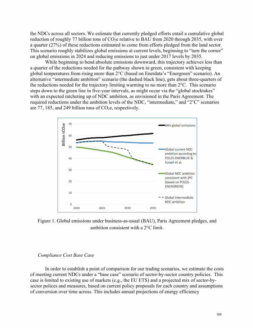
169

the NDCs across all sectors. We estimate that currently pledged efforts entail a cumulative global reduction of roughly 77 billion tons of CO2e relative to BAU from 2020 through 2035, with over a quarter (27%) of these reductions estimated to come from efforts pledged from the land sector. This scenario roughly stabilizes global emissions at current levels, beginning to “turn the corner” on global emissions in 2024 and reducing emissions to just under 2017 levels by 2035.

While beginning to bend absolute emissions downward, this trajectory achieves less than a quarter of the reductions needed for the pathway shown in green, consistent with keeping global temperatures from rising more than 2°C (based on Enerdata’s “Energreen” scenario). An alternative “intermediate ambition” scenario (the dashed black line), gets about three-quarters of the reductions needed for the trajectory limiting warming to no more than 2°C. This scenario steps down to the green line in five-year intervals, as might occur via the “global stocktakes” with an expected ratcheting up of NDC ambition, as envisioned in the Paris Agreement. The required reductions under the ambition levels of the NDC, “intermediate,” and “2°C” scenarios are 77, 185, and 249 billion tons of CO2e, respectively.

Figure 1. Global emissions under business-as-usual (BAU), Paris Agreement pledges, and ambition consistent with a 2°C limit.

Compliance Cost Base Case

In order to establish a point of comparison for our trading scenarios, we estimate the costs of meeting current NDCs under a “base case” scenario of sector-by-sector country policies. This case is limited to existing use of markets (e.g., the EU ETS) and a projected mix of sector-by-sector polices and measures, based on current policy proposals for each country and assumptions of conversion over time across. This includes annual projections of energy efficiency

170

requirements, renewable energy mandates, and transport-, industry-, and land-use-specific regulations varying across each country.4

Domestic Markets Scenario

We then consider the case where each country can meet the cumulative reductions required by their NDCs at least-cost domestically via a carbon market or other carbon pricing approach that achieves their target at least cost. Our model ensures marginal abatement costs are equalized across sectors and also that market actors can optimally select the timing of their emissions reductions to achieve cumulative reductions at least-cost, assuming a discount rate of 5% to account for the cost of capital. This captures the ability of market actors to “bank” emissions units and save them for use in later periods when caps may be tighter and corresponding mitigation costs higher. This type of “when” flexibility is typically allowed in carbon markets and generally important for enabling cost effectiveness.

Full Global Markets Scenarios, with and without REDD+

We then analyze costs under a fully global market where market actors can trade across all countries and regions, as well as cost-effectively select the timing of mitigation over time. To isolate the potential importance of including market-based approaches to REDD+, which has been left out of compliance carbon markets to date, we consider a case where market actors can use emissions reductions from land-use for their own NDCs but can only trade emissions internationally across the energy, transport, and industry sectors. We then examine the added benefit of allowing further trading of reductions from REDD+.

Robustness test

We then test the robustness of cost saving estimates under the full global market scenario using a sensitivity analysis in which market actors are uncertain about the future and therefore delay emissions reductions relative to the least-cost scenario. Regulatory and policy uncertainty will tend to induce market actors to adopt a wait-and-see attitude to mitigation investments, which will depress near-term market demand. We model such a case based on the inclusion of a risk premium, which gradually declines over time but lowers the benefit of banking emissions reductions for use in future periods compared to the case with full market certainty. Following the scenario of Golub, Lubowski, Piris-Cabezas (2017, work of the author), we assume the risk premium falls at five-year intervals, to reflect greater information that increases certainty over future policy. In particular, we assume an interest or “discount” rate, starting at 20% in 2020, falling to 15% in 2025 and 10% in 2030. We solve the model iteratively over 2020–2035, 2025–2035 and 2030–2035, carrying over the amount of emissions reductions banked for future compliance periods from the previous runs.

4 This scenario is based on Enerdata’s “Enerblue” scenario for the energy, transport and industry sectors complemented with our own estimates for the forest and land-use sectors calibrated to match global estimates from IIASA.

171

Partial Markets Coverage

We consider three cases for partial market development, building from the “heat map” analysis discussed in Appendix below, ranking countries by their societal readiness and strategic value with respect to carbon market pricing advocacy. Notably, the heat map analysis ranks countries based on their readiness and importance in terms of emissions (both directly and via links to other important countries), rather than in terms of their ability to maximize gains from trade in a market system. All countries continue to be engaged in meeting their NDCs, but partial carbon market development only enables certain countries to take advantage of potential cost reductions. All scenarios also include implementation of CORSIA under ICAO based on current levels of participation. Given the pivotal role of REDD+, for each partial markets scenario, we also model scenarios where the limited global markets open up additional REDD+ from the rest of the world.5

Global ‘Heat Map’ Scenario

This scenario involves a global market based on the economy-wide coverage of the EU, United States, and China and the next 25 highest-ranking countries from our heat map analysis (see Appendix). This results in an estimated 79% coverage of current global emissions. This percentage declines slightly over time as the emissions from some of the countries not included in the heat map are growing relative fast, including in terms of emissions from deforestation.

Asia-Pacific Scenario

This scenario envisions the regional evolution of a carbon market in Asia (as could emerge around China and South Korea), bringing in the highest-ranking countries from the heat map analysis in the Asia-Pacific region, as well as linking with Kazakhstan (but excluding South Asia). This includes economy-wide coverage of China, Thailand, Vietnam, Indonesia, Malaysia, South Korea, Japan, Singapore, Philippines, Kazakhstan, Australia, and New Zealand. This regional market development is assumed to catalyze coverage of all sectors in China. The scenario also includes participation from the EU as well as the U.S., but with their coverage limited to the power and industrial sectors (as per the current coverage of the EU ETS). This scenario results in estimated coverage of 42% of current emissions.

Americas Scenario

This scenario explores the potential impact of the Western Climate Initiative and the Pacific Alliance leading to a greater coverage throughout the Americas, bringing in all the highest-ranking countries from the heat map analysis across the Americas, including both the United States and Brazil. This scenario includes 100% coverage of the U.S., Canada, Mexico, Colombia, Peru, Chile, Argentina, and Brazil. The scenario also includes participation from the

5 In the Asia-Pacific case, described below, we consider additional REDD+ net of NDC from Brazil, Mexico, Colombia, Peru and 50% of the rest of the world. In the Americas case, described below, we consider additional REDD+ net of NDC from Indonesia, Thailand and Malaysia and 50% of the rest of the world.

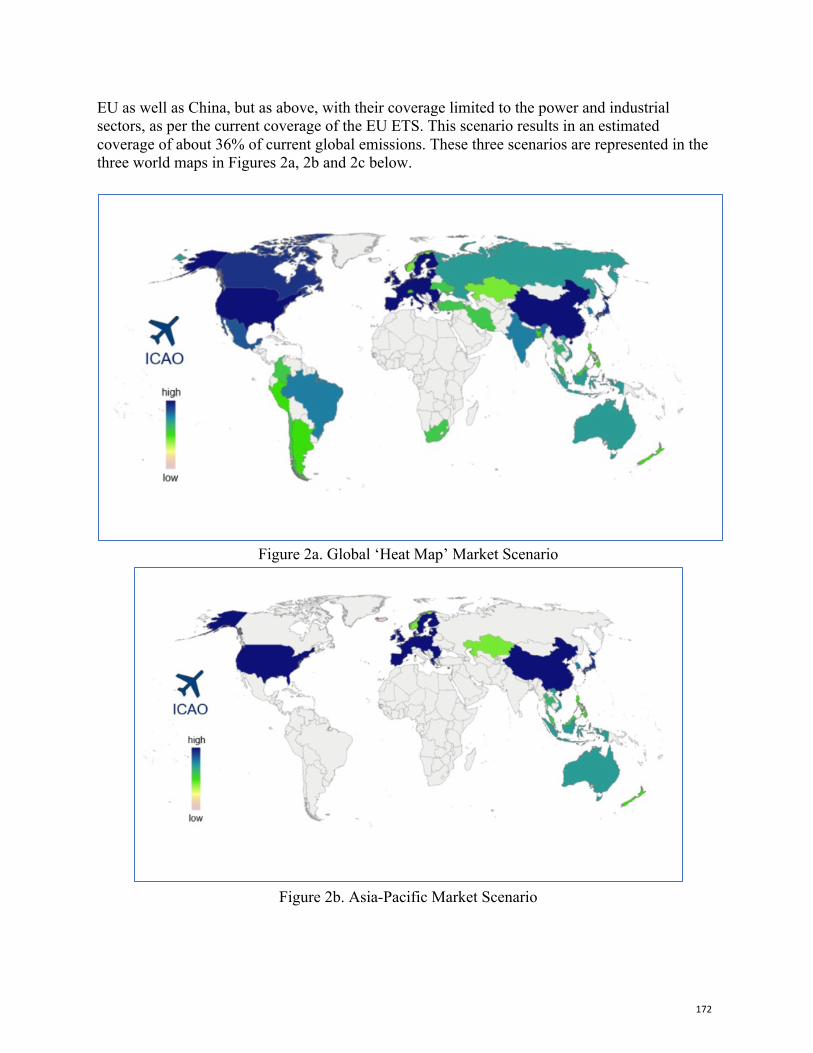
172

EU as well as China, but as above, with their coverage limited to the power and industrial sectors, as per the current coverage of the EU ETS. This scenario results in an estimated coverage of about 36% of current global emissions. These three scenarios are represented in the three world maps in Figures 2a, 2b and 2c below.

Figure 2a. Global ‘Heat Map’ Market Scenario

Figure 2b. Asia-Pacific Market Scenario

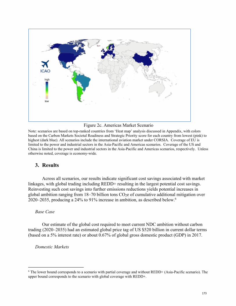
173

Figure 2c. Americas Market Scenario

Note: scenarios are based on top-ranked countries from ‘Heat map’ analysis discussed in Appendix, with colors based on the Carbon Markets Societal Readiness and Strategic Priority score for each country from lowest (pink) to highest (dark blue). All scenarios include the international aviation market under CORSIA. Coverage of EU is limited to the power and industrial sectors in the Asia-Pacific and Americas scenarios. Coverage of the US and China is limited to the power and industrial sectors in the Asia-Pacific and Americas scenarios, respectively. Unless otherwise noted, coverage is economy-wide.

3. Results

Across all scenarios, our results indicate significant cost savings associated with market linkages, with global trading including REDD+ resulting in the largest potential cost savings. Reinvesting such cost savings into further emissions reductions yields potential increases in global ambition ranging from 18–70 billion tons CO2e of cumulative additional mitigation over 2020–2035, producing a 24% to 91% increase in ambition, as described below.6

Base Case

Our estimate of the global cost required to meet current NDC ambition without carbon trading (2020–2035) had an estimated global price tag of US $520 billion in current dollar terms (based on a 5% interest rate) or about 0.67% of global gross domestic product (GDP) in 2017.

Domestic Markets

6 The lower bound corresponds to a scenario with partial coverage and without REDD+ (Asia-Pacific scenario). The upper bound corresponds to the scenario with global coverage with REDD+.

174

Our estimates of the total cost savings from implementing domestic carbon markets in all nations yield 4% reduction in total mitigation costs relative to the base case. These cost savings are limited given that mitigation ambition is relatively low and the NDC base case scenario already includes contributions across all sectors, including a large contribution from the land-use sector and cost-effective achievement of NDCs within, if not across, each of the modelled sectors. Given these assumptions, the base case is therefore already akin to the result achieved under use of carbon pricing. If we were to develop a model with greater granularity for non-market policies within each country and sector, the cost savings from implementing domestic markets would likely be substantially larger.

Full Global Markets Scenarios, with and without REDD+ Our scenario modelling a fully global carbon market that channels the same total global resources in the most cost-effective fashion lowers total costs by an estimated 62%—from over half a trillion to $197 billion current dollar terms—in the case of a global market for energy, transport, and industry sectors (but where REDD+ is restricted to domestic use only). Costs fall an additional 43% from $197 to $111 billion, such that overall cost savings are 79% relative to the base case, when the global market al.so includes REDD+. These costs savings occur because there is a large spread in ambition across countries (and in some cases across sectors at the country level), resulting in lack of cost-effectiveness globally. Figure 3 shows the wide spread in modelled carbon prices under the base case.

Figure 3: Spread in ambition across countries, as shown by estimated carbon price in 2020, assuming domestic trading across energy and industry. ($/tCO2e)

Robustness test

Modelling information uncertainty with a “risk premium” increases costs by 18% to $131

billion (in current dollar terms) in the case of a full global market with REDD+. Even so, this still achieves 95% of the cost savings as under the case of full certainty and thus enabling equivalent increases in the level of mitigation ambition.

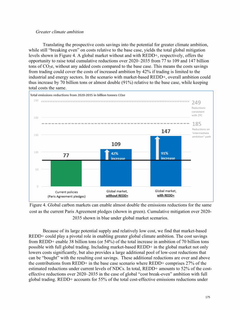
175

Greater climate ambition

Translating the prospective costs savings into the potential for greater climate ambition, while still “breaking even” on costs relative to the base case, yields the total global mitigation levels shown in Figure 4. A global market without and with REDD+, respectively, offers the opportunity to raise total cumulative reductions over 2020–2035 from 77 to 109 and 147 billion tons of CO2e, without any added costs compared to the base case. This means the costs savings from trading could cover the costs of increased ambition by 42% if trading is limited to the industrial and energy sectors. In the scenario with market-based REDD+, overall ambition could thus increase by 70 billion tons or almost double (91%) relative to the base case, while keeping total costs the same.

Figure 4. Global carbon markets can enable almost double the emissions reductions for the same cost as the current Paris Agreement pledges (shown in green). Cumulative mitigation over 2020-

2035 shown in blue under global market scenarios.

Because of its large potential supply and relatively low cost, we find that market-based REDD+ could play a pivotal role in enabling greater global climate ambition. The cost savings from REDD+ enable 38 billion tons (or 54%) of the total increase in ambition of 70 billion tons possible with full global trading. Including market-based REDD+ in the global market not only lowers costs significantly, but also provides a large additional pool of low-cost reductions that can be “bought” with the resulting cost savings. These additional reductions are over and above the contributions from REDD+ in the base case scenario where REDD+ comprises 27% of the estimated reductions under current levels of NDCs. In total, REDD+ amounts to 52% of the cost-effective reductions over 2020–2035 in the case of global “cost break-even” ambition with full global trading. REDD+ accounts for 55% of the total cost-effective emissions reductions under

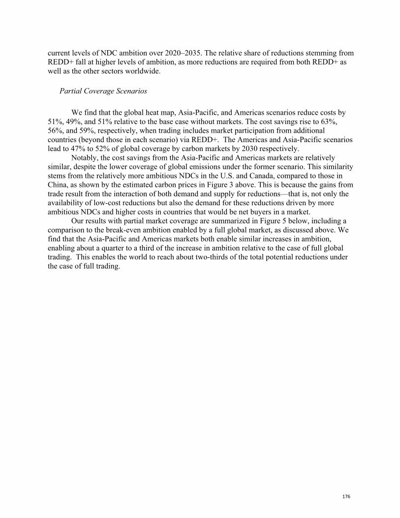
176

current levels of NDC ambition over 2020–2035. The relative share of reductions stemming from REDD+ fall at higher levels of ambition, as more reductions are required from both REDD+ as well as the other sectors worldwide.

Partial Coverage Scenarios

We find that the global heat map, Asia-Pacific, and Americas scenarios reduce costs by 51%, 49%, and 51% relative to the base case without markets. The cost savings rise to 63%, 56%, and 59%, respectively, when trading includes market participation from additional countries (beyond those in each scenario) via REDD+. The Americas and Asia-Pacific scenarios lead to 47% to 52% of global coverage by carbon markets by 2030 respectively.

Notably, the cost savings from the Asia-Pacific and Americas markets are relatively similar, despite the lower coverage of global emissions under the former scenario. This similarity stems from the relatively more ambitious NDCs in the U.S. and Canada, compared to those in China, as shown by the estimated carbon prices in Figure 3 above. This is because the gains from trade result from the interaction of both demand and supply for reductions—that is, not only the availability of low-cost reductions but also the demand for these reductions driven by more ambitious NDCs and higher costs in countries that would be net buyers in a market.

Our results with partial market coverage are summarized in Figure 5 below, including a comparison to the break-even ambition enabled by a full global market, as discussed above. We find that the Asia-Pacific and Americas markets both enable similar increases in ambition, enabling about a quarter to a third of the increase in ambition relative to the case of full global trading. This enables the world to reach about two-thirds of the total potential reductions under the case of full trading.

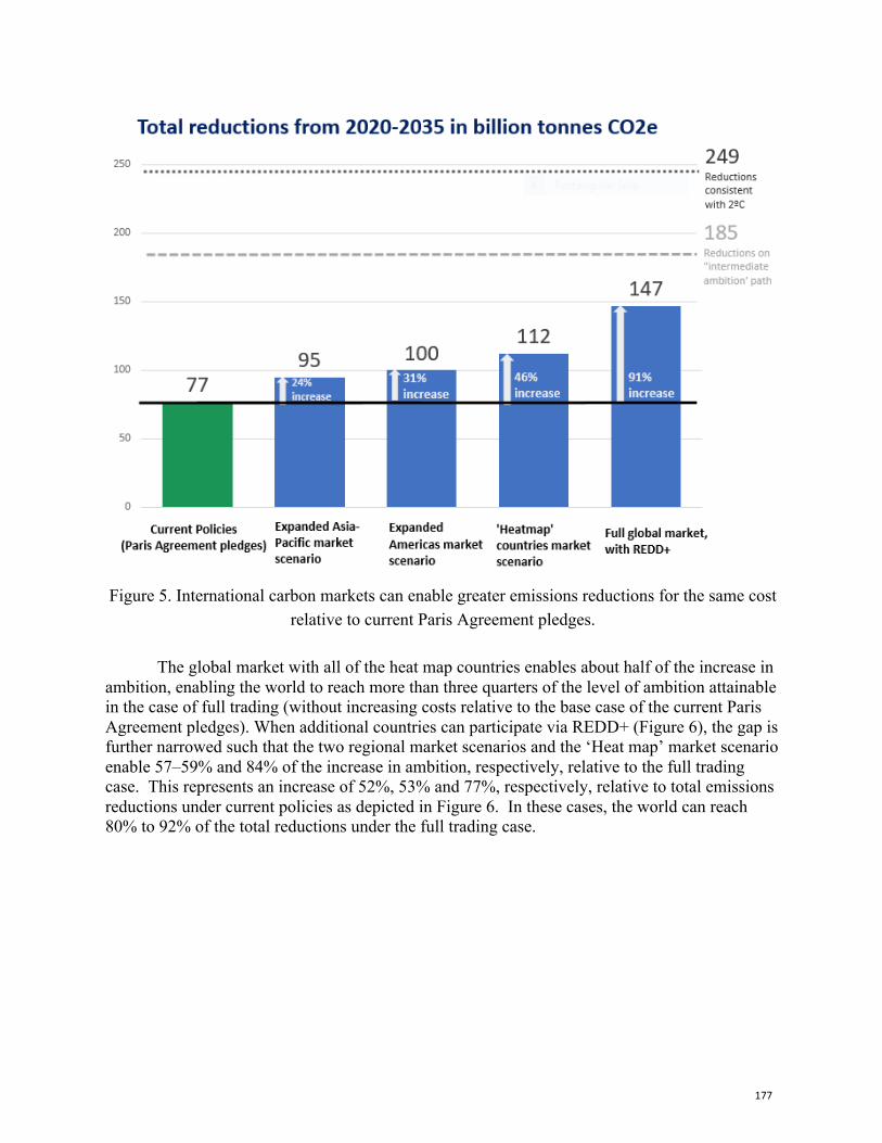
177

Figure 5. International carbon markets can enable greater emissions reductions for the same cost

relative to current Paris Agreement pledges.

The global market with all of the heat map countries enables about half of the increase in ambition, enabling the world to reach more than three quarters of the level of ambition attainable in the case of full trading (without increasing costs relative to the base case of the current Paris Agreement pledges). When additional countries can participate via REDD+ (Figure 6), the gap is further narrowed such that the two regional market scenarios and the ‘Heat map’ market scenario enable 57–59% and 84% of the increase in ambition, respectively, relative to the full trading case. This represents an increase of 52%, 53% and 77%, respectively, relative to total emissions reductions under current policies as depicted in Figure 6. In these cases, the world can reach 80% to 92% of the total reductions under the full trading case.

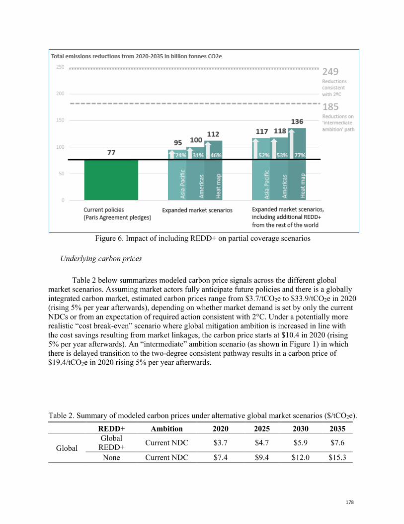
178

Figure 6. Impact of including REDD+ on partial coverage scenarios

Underlying carbon prices

Table 2 below summarizes modeled carbon price signals across the different global

market scenarios. Assuming market actors fully anticipate future policies and there is a globally integrated carbon market, estimated carbon prices range from $3.7/tCO2e to $33.9/tCO2e in 2020 (rising 5% per year afterwards), depending on whether market demand is set by only the current NDCs or from an expectation of required action consistent with 2°C. Under a potentially more realistic “cost break-even” scenario where global mitigation ambition is increased in line with the cost savings resulting from market linkages, the carbon price starts at $10.4 in 2020 (rising 5% per year afterwards). An “intermediate” ambition scenario (as shown in Figure 1) in which there is delayed transition to the two-degree consistent pathway results in a carbon price of $19.4/tCO2e in 2020 rising 5% per year afterwards. Table 2. Summary of modeled carbon prices under alternative global market scenarios ($/tCO2e).

REDD+ Ambition 2020 2025 2030 2035

Global Global

REDD+ Current NDC $3.7 $4.7 $5.9 $7.6

None Current NDC $7.4 $9.4 $12.0 $15.3

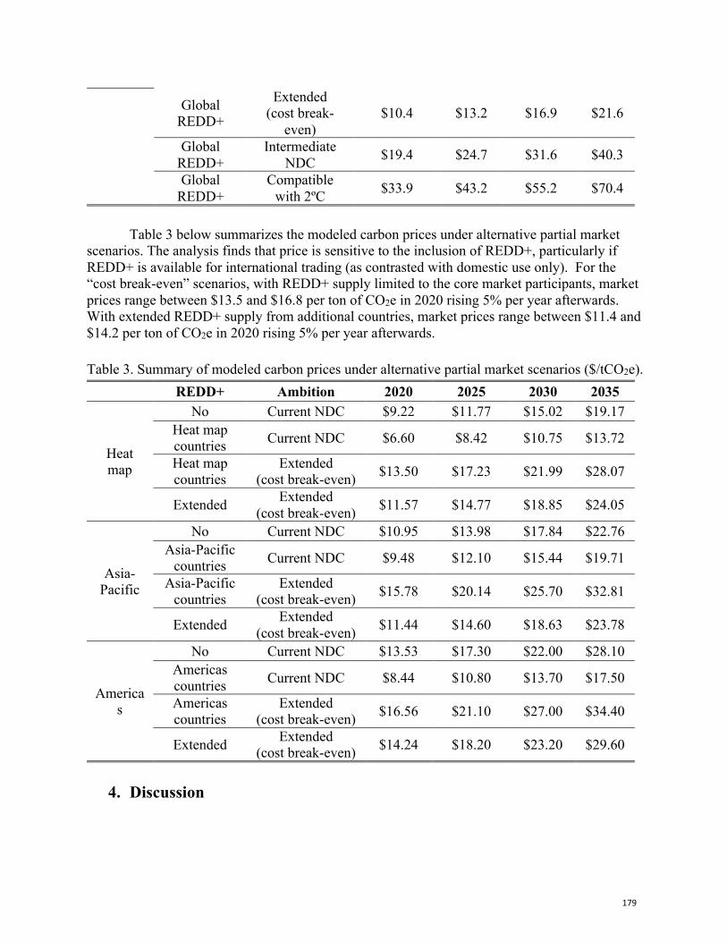
179

Global REDD+

Extended (cost break-

even) $10.4 $13.2 $16.9 $21.6

Global REDD+

Intermediate NDC $19.4 $24.7 $31.6 $40.3

Global REDD+

Compatible with 2ºC $33.9 $43.2 $55.2 $70.4

Table 3 below summarizes the modeled carbon prices under alternative partial market

scenarios. The analysis finds that price is sensitive to the inclusion of REDD+, particularly if REDD+ is available for international trading (as contrasted with domestic use only). For the “cost break-even” scenarios, with REDD+ supply limited to the core market participants, market prices range between $13.5 and $16.8 per ton of CO2e in 2020 rising 5% per year afterwards. With extended REDD+ supply from additional countries, market prices range between $11.4 and $14.2 per ton of CO2e in 2020 rising 5% per year afterwards. Table 3. Summary of modeled carbon prices under alternative partial market scenarios ($/tCO2e).

REDD+ Ambition 2020 2025 2030 2035

Heat map

No Current NDC $9.22 $11.77 $15.02 $19.17 Heat map countries Current NDC $6.60 $8.42 $10.75 $13.72

Heat map countries

Extended (cost break-even) $13.50 $17.23 $21.99 $28.07

Extended Extended (cost break-even) $11.57 $14.77 $18.85 $24.05

Asia-Pacific

No Current NDC $10.95 $13.98 $17.84 $22.76 Asia-Pacific

countries Current NDC $9.48 $12.10 $15.44 $19.71

Asia-Pacific countries



Americas

No Current NDC $13.53 $17.30 $22.00 $28.10 Americas countries Current NDC $8.44 $10.80 $13.70 $17.50

Americas countries



4. Discussion

180

Our results of the potential cost savings from a fully global market range from 62–79%, depending on the inclusion of REDD+, are consistent with other studies, notably Fujimori et al. (2016), despite their different methodology which was not explicitly intertemporal. Fujimori et al.’s study is based on Asia-Pacific Integrated Model/Computable General Equilibrium (AIM/CGE) and estimates that a global market, inclusive of land use, based on current NDCs would reduce global welfare loss by 75% and produce a price of around $9/tCO2 in 2030, also comparable with our estimates.

Our estimated percentage savings are also in line with Rose et al.’s (2018) analysis of a global carbon market for power and industry sectors that evolves in a stepwise manner to help meet NDCs. They estimate cost savings ranging from 59%, 75% and 72%, as markets progressively integrate by 2020, 2025 and 2030, up to the point where 50% of global emissions are covered. Nevertheless, Rose et al.’s study generates significantly higher prices compared to our idealized case, perhaps as their analysis considers a market with more restricted scope and is not intertemporal in nature.

Hof et al.’s analysis (2017) similarly finds that allowing for global emissions trading under their mid-range scenario of baseline emissions reduces the costs of NDC implementation by 56% for unconditional NDC targets and by 44% for conditional NDC targets. These estimated cost reductions are more modest than our findings and the findings in the above studies, but they also note that their assumed implementation costs are found to be quite sensitive to underlying assumptions about socioeconomic developments. In addition, their study does not include reductions from LULUCF, which have significantly contributed to the cost savings from allowing global trading in our model.

In terms of the potential to use cost savings to increase ambition, we estimate greater potential savings from markets—and correspondingly greater potential to help finance additional emissions reductions—compared to a report by the World Bank, Ecofys and Vivid Economics (2016). That report estimates that international emission trading could reduce the total abatement costs of achieving current Paris pledges by about a third by 2030, while cutting total mitigation costs in half by 2050 in a 2°C consistent scenario. Our analysis (along with Fujimori’s) considers a broader range of mitigation activities. While the World Bank considers CO2 emissions from the energy and industrial sectors, we consider all GHGs and the potential role of REDD+ in an international market. We also consider a longer time period (2020–2035, versus 2030 only).

Our analysis reported in this paper still potentially underestimates the benefits of markets, as we did not consider opportunities for trading of non-CO2 emissions from agricultural activities and we limited our consideration of forestry to reducing deforestation and degradation, without including the potential of reforestation and improved forest management. Furthermore, our analysis only considers cost savings from an equalization of expected marginal abatement costs across countries, without consideration of the potential benefits from ongoing buffering idiosyncratic market or policy shocks across countries, which Doda and Taschini (2017) estimate can produce significant added savings.

Moreover, our estimated increase in ambition is due mostly to the gains from international trade, and not the increase in use of domestic markets to meet national targets. Expanding the use of markets from the base case to the “full trading” scenario can be divided into two steps: first, broadening the use of emission trading as an instrument of domestic policy, with the “full trading” scenario assuming that every country in the world uses an internal carbon market to meet its NDC; second, linking those markets through international trading. Both steps

181

yield cost savings, and thus potential increases in ambition. Our modeling suggests that the lion’s share of the gains from global markets are due to international linking, with a much smaller share coming from increased use of domestic carbon markets. While this conclusion needs further analysis, it has potentially striking implications, suggesting that carbon pricing policies that encourage international cooperation—such as carbon markets—may be able to capture significantly more cost savings, and thus increased ambition, than carbon pricing policies that are less prone to linkage.

This finding comes with an important qualification due to the nature of our model. While the model is fairly disaggregated among countries, it is relatively coarse within countries, because only four sectors are modeled: energy, transport, industry, and forestry and land-use. Because our model assumes least-cost abatement in each sector within each country (including within the EU-region aggregate), it effectively assumes the use of within-sector emission trading or other market-based policies, rather than more costly command-and-control measures. More fine-grained sectoral coverage would yield greater estimated cost savings due to greater within-country trading. Nonetheless, a striking conclusion from our analysis is that virtually the entire cost savings (96 percent) are due to international linking, with just 4 percent of estimated cost savings coming from increased use of domestic trading. At the very least, this suggests that the potential for gains from international trade are significantly greater than the gains from intersectoral trade within each country.

5. Conclusion

Experience with several Emissions Trading Systems (ETS) to date suggests that by helping to achieve initial targets more easily and economically than expected, carbon markets can lower political resistance to setting more ambitious targets in the future. Our analysis explores this potential with respect to Paris Agreement targets. We consider cumulative mitigation over 2020–2035, rather than single-year targets alone, and also examine a broader set of sectors and gases, compared to other studies of post-Paris international carbon markets. In particular, we provide the first evaluation of the extent to which including avoided deforestation (REDD+) in international carbon markets can enable greater climate ambition under the Paris Agreement.

We find that the global use of emissions trading, based on well-designed accounting rules and the banking (carry-forward) of emissions units over 2020–2035 could allow the world to nearly double climate ambition relative to current NDCs without increasing aggregate costs. In particular, we estimate that holding total discounted abatement cost constant, cumulative emissions reductions over the period 2020–2035 would increase from 77 Gt CO2e in the base case to 147 Gt CO2e in a scenario with full global emission trading—an increase of 91 percent. A large share of the gains come from the inclusion of REDD+. This suggests that the development of well-designed and high-integrity approaches for international market cooperation, as envisioned under Article 6 of the Paris Agreement, as well as the inclusion of REDD+, merit significant policy attention as a means of closing the global emissions gap.

The large boost in ambition possible as a result of international emissions trading is promising. However, even in the case with REDD+ in a full global market, the cost savings from carbon markets in the “break-even” scenarios do not yield enough ambition relative to what is necessary to avoid dangerous warming, as shown by the 2°C scenario. On the one hand, breaking even on costs compared to current levels of ambition could be seen as a relatively low

182

bar for increasing total commitments. Yet, just based on this requirement, global trading gets 80% of the way to the intermediate scenario and 60% of the way to the 2°C scenario.

A fully global carbon market is likely unrealistic in the medium term, given differences in country readiness as well as political hurdles to linking markets, particularly when these could entail large financial resource transfers among countries. Even so, our partial sector coverage models indicate that even limited trading conditions evolving around regional lines—potentially consistent with ongoing cooperation on trade, environmental quality, migration and other regional strategic issues—can boost climate ambition measurably. Thus, our results give support to the continued promotion of carbon markets worldwide as a valuable tool in the global effort to reduce emissions at scale.

In addition, total ambition could be further increased by expanding global carbon market coverage through allowing additional cost-effective emissions reductions from sectors not contemplated in this modeling exercise—namely, agriculture and other forest-based measures such as reforestation and sustainable forest management. Furthermore, if forward-looking market actors can anticipate this eventual ratcheting-up of ambition, they would have incentives to act early to take advantage of lower cost abatement opportunities in order to avoid future cost increases. This has the potential to activate a virtuous circle that could further help close the near-term ambition gap and get the world on track towards meeting the Paris Agreement goal.

References Akimoto, Keigo, Fuminori Sano, Bianka Shoai Tehrani. “The Analyses on the Economic Costs for Achieving the

Nationally Determined Contributions and the Expected Global Emission Pathhways.” Evolutionay and Institutional Economics Review 14, no. 1 (2017). 193–206. doi: 10.1007/s40844-016-0049-y

Böhringer, Christophe. “Cooling down hot air: a global CGE analysis of post-Kyoto carbon abatement strategies.” Energy Policy 28, no. 11 (2000). 779–89. doi:10.1016/S0301-4215(00)00060-4

Doda, Baran and Luca Taschini. “Carbon dating: When is it beneficial to link ETSs?” Journal of the Association of Environmental and Resource Economists 4, no. 3 (2017). 701–30. doi:10.1086/691975

Forsell, Nicklas, Olga Turkovska, Mykola Gusti, Michael Obersteiner, Michel den Elzen, Petr Havlik. “Assessing the INDCs’ land use. land use change. and forest emission projections.” Carbon Balance and Management 11, no. 26 (2016). doi:10.1186/s13021-016-0068-3.

Fujimori, Shinichiro, Izumi Kubota, Hancheng Dai, Kiyoshi Takahashi, Tomoko Hasegawa, Jing-Yu Liu, Yasuaki Hijioka, Toshihiko Masui, and Maho Takimi. “Will international emissions trading help achieve the objectives of the Paris Agreement?” Environmental Research Letters 11 (2016). doi:10.1088/1748-9326/11/10/104001

Golub, Alexander, Ruben Lubowski, and Pedro Piris-Cabezas. “Balancing Risks from Climate Policy Uncertainties: The Role of Options on Reduced Emissions from Deforestation and Forest Degradation.” Ecological Economics 138C (2017). 90–98. doi:10.1016/j.ecolecon.2017.03.013

Gusti, Mikola, Nikolay Khabarov, and Nicklas Forsell. “Sensitivity of marginal abatement cost curves to variation of G4M parameters.” In: Proceedings. 4th International Workshop on Uncertainty in Atmospheric Emissions. 7–9 October 2015. Krakow. Poland. 152–158. Systems Research Institute. Polish Academy of Sciences. Warsaw, Poland (2015). ISBN 83-894-7557-X.

Haites, Erik. “Carbon taxes and greenhouse gas emissions trading systems: What have we learned?” Climate Policy 18, no. 8 (2018). 955–966. doi:10.1080/14693062.2018.1492897

Hof, Andries F., Michel G. J. den Elzen, Annemiek Admiraal, Mark Roelfsema, David E. H. J. Gernaat, Detlef P. van Vuuren. “Global and Regional Abatement Costs of Nationally Determined Contributions (NDCs) and of Enhanced Action to Levels Well Below 2°C and 1.5°C.” Environmental Science & Policy 71 (2017). 30–40. doi:10.1016/j.envsci.2017.02.008

Kaya, Yoichi, Mitsutsune Yamaguchi, Keigo Akimoto. “The uncertainty of climate sensitivity and its implication for the Paris negotiation.” Sustainability Science 11, no. 3 (2016). 515–518. doi: 10.1007/s11625-015-0339-z

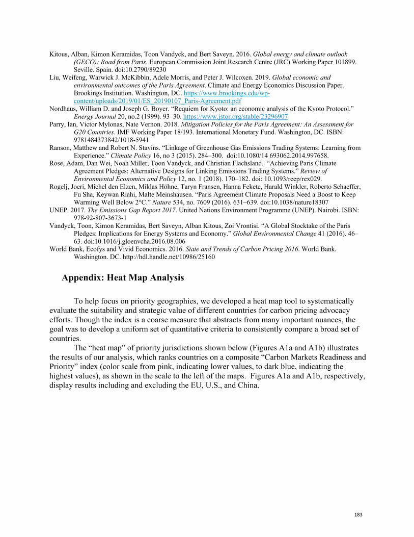
183

Kitous, Alban, Kimon Keramidas, Toon Vandyck, and Bert Saveyn. 2016. Global energy and climate outlook (GECO): Road from Paris. European Commission Joint Research Centre (JRC) Working Paper 101899. Seville. Spain. doi:10.2790/89230

Liu, Weifeng, Warwick J. McKibbin, Adele Morris, and Peter J. Wilcoxen. 2019. Global economic and environmental outcomes of the Paris Agreement. Climate and Energy Economics Discussion Paper. Brookings Institution. Washington, DC. https://www.brookings.edu/wp-content/uploads/2019/01/ES_20190107_Paris-Agreement.pdf

Nordhaus, William D. and Joseph G. Boyer. “Requiem for Kyoto: an economic analysis of the Kyoto Protocol.” Energy Journal 20, no.2 (1999). 93–30. https://www.jstor.org/stable/23296907

Parry, Ian, Victor Mylonas, Nate Vernon. 2018. Mitigation Policies for the Paris Agreement: An Assessment for G20 Countries. IMF Working Paper 18/193. International Monetary Fund. Washington, DC. ISBN: 9781484373842/1018-5941

Ranson, Matthew and Robert N. Stavins. “Linkage of Greenhouse Gas Emissions Trading Systems: Learning from Experience.” Climate Policy 16, no 3 (2015). 284–300. doi:10.1080/14 693062.2014.997658.

Rose, Adam, Dan Wei, Noah Miller, Toon Vandyck, and Christian Flachsland. “Achieving Paris Climate Agreement Pledges: Alternative Designs for Linking Emissions Trading Systems.” Review of Environmental Economics and Policy 12, no. 1 (2018). 170–182. doi: 10.1093/reep/rex029.

Rogelj, Joeri, Michel den Elzen, Miklas Höhne, Taryn Fransen, Hanna Fekete, Harald Winkler, Roberto Schaeffer, Fu Sha, Keywan Riahi, Malte Meinshausen. “Paris Agreement Climate Proposals Need a Boost to Keep Warming Well Below 2°C.” Nature 534, no. 7609 (2016). 631–639. doi:10.1038/nature18307

UNEP. 2017. The Emissions Gap Report 2017. United Nations Environment Programme (UNEP). Nairobi. ISBN: 978-92-807-3673-1

Vandyck, Toon, Kimon Keramidas, Bert Saveyn, Alban Kitous, Zoi Vrontisi. “A Global Stocktake of the Paris Pledges: Implications for Energy Systems and Economy.” Global Environmental Change 41 (2016). 46–63. doi:10.1016/j.gloenvcha.2016.08.006

World Bank, Ecofys and Vivid Economics. 2016. State and Trends of Carbon Pricing 2016. World Bank. Washington. DC. http://hdl.handle.net/10986/25160

Appendix: Heat Map Analysis

To help focus on priority geographies, we developed a heat map tool to systematically

evaluate the suitability and strategic value of different countries for carbon pricing advocacy efforts. Though the index is a coarse measure that abstracts from many important nuances, the goal was to develop a uniform set of quantitative criteria to consistently compare a broad set of countries.

The “heat map” of priority jurisdictions shown below (Figures A1a and A1b) illustrates the results of our analysis, which ranks countries on a composite “Carbon Markets Readiness and Priority” index (color scale from pink, indicating lower values, to dark blue, indicating the highest values), as shown in the scale to the left of the maps. Figures A1a and A1b, respectively, display results including and excluding the EU, U.S., and China.

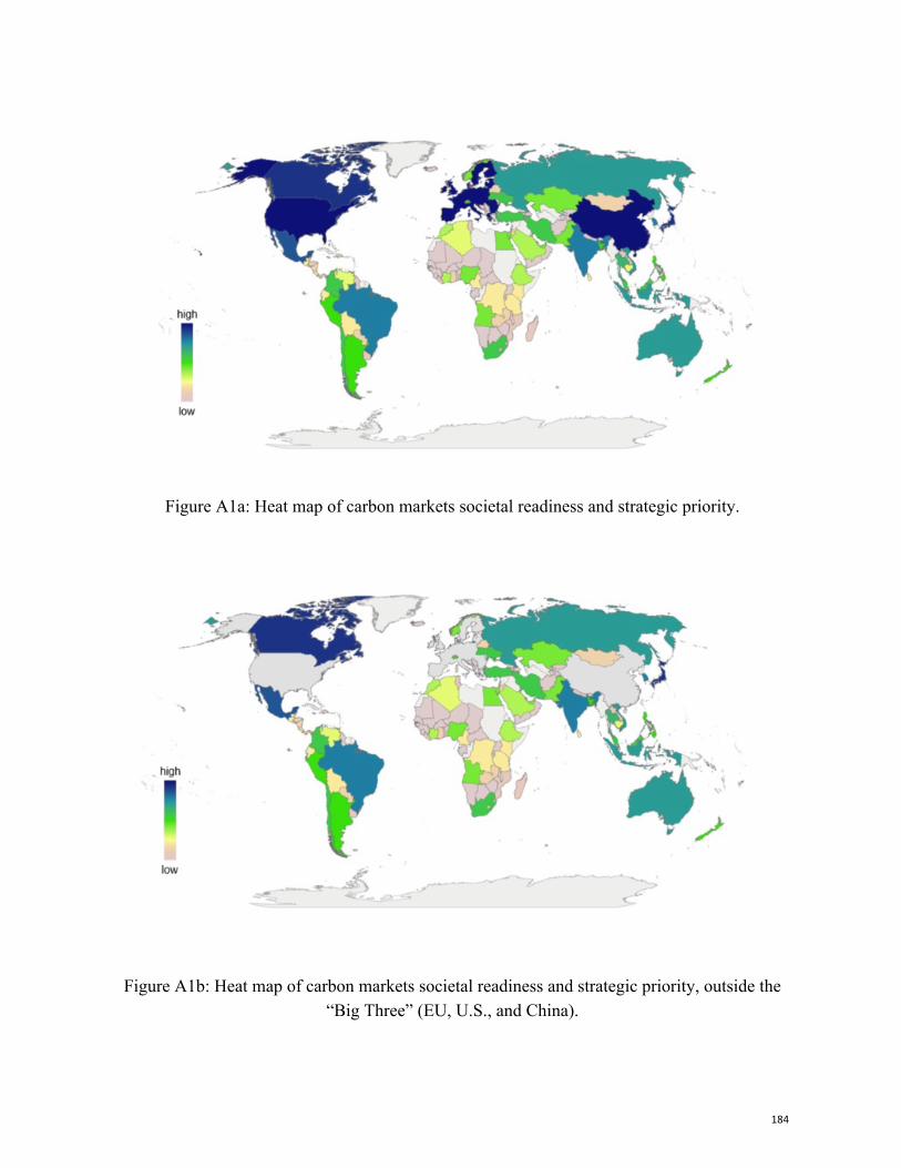
184

Figure A1a: Heat map of carbon markets societal readiness and strategic priority.

Figure A1b: Heat map of carbon markets societal readiness and strategic priority, outside the “Big Three” (EU, U.S., and China).

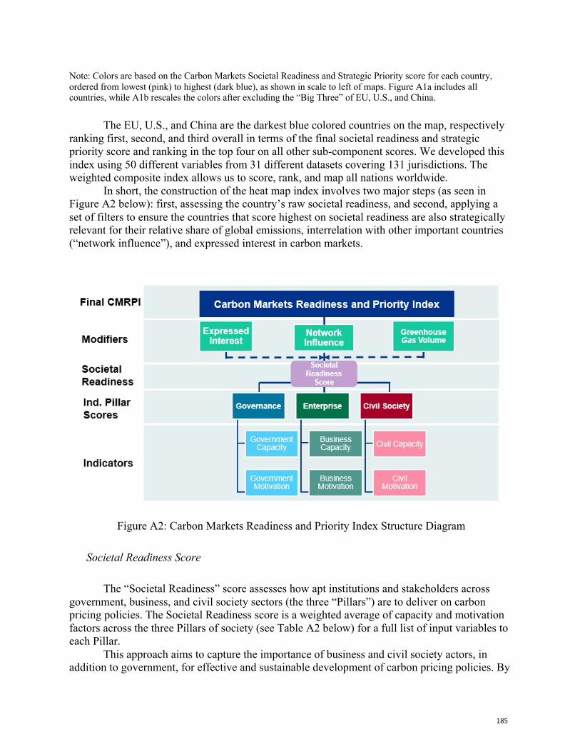
185

Note: Colors are based on the Carbon Markets Societal Readiness and Strategic Priority score for each country, ordered from lowest (pink) to highest (dark blue), as shown in scale to left of maps. Figure A1a includes all countries, while A1b rescales the colors after excluding the “Big Three” of EU, U.S., and China.

The EU, U.S., and China are the darkest blue colored countries on the map, respectively ranking first, second, and third overall in terms of the final societal readiness and strategic priority score and ranking in the top four on all other sub-component scores. We developed this index using 50 different variables from 31 different datasets covering 131 jurisdictions. The weighted composite index allows us to score, rank, and map all nations worldwide.

In short, the construction of the heat map index involves two major steps (as seen in Figure A2 below): first, assessing the country’s raw societal readiness, and second, applying a set of filters to ensure the countries that score highest on societal readiness are also strategically relevant for their relative share of global emissions, interrelation with other important countries (“network influence”), and expressed interest in carbon markets.

Figure A2: Carbon Markets Readiness and Priority Index Structure Diagram

Societal Readiness Score

The “Societal Readiness” score assesses how apt institutions and stakeholders across government, business, and civil society sectors (the three “Pillars”) are to deliver on carbon pricing policies. The Societal Readiness score is a weighted average of capacity and motivation factors across the three Pillars of society (see Table A2 below) for a full list of input variables to each Pillar.

This approach aims to capture the importance of business and civil society actors, in addition to government, for effective and sustainable development of carbon pricing policies. By

186

dividing each Pillar into its capacity and motivation scores, the approach further seeks to capture that successful implementation of carbon pricing policies should require the confluence of both “demand” drivers for these policies, given the underlying interests of different stakeholders, and the capacity to “supply” such policies via relevant institutions, legal frameworks, and politically salient constituencies.

Strategic Relevance Filter

In addition to the raw “societal readiness” score, we apply three score modifiers that rescale the values to reflect the strategic relevance of each country for achieving global climate goals, which could also affect the propensity of that country to participate in carbon pricing initiatives due to internal and external pressures:

Greenhouse Gas Volume Modifier: Captures the current GHG emissions from each country, including from the land-use sector, to reflect the strategic value of targeting high–total emission countries;

Expressed Interest Modifier: Captures interest demonstrated by political leaders in market-based mechanisms to control carbon emissions. This approach includes various indications of interest, such as mention of markets in the country’s NDC and its participation in the World Bank–managed Partnership for Market Readiness (PMR). As this measure is intended to capture potential for future adoption of a market-based system, it does not include current adoption of a carbon market nationally or sub-nationally (e.g., in the U.S., China, Japan, Canada, and South Korea) as part of the score. However, it does include considerations or adoption of a carbon tax and whether this tax includes an offsetting approach (e.g., in Colombia), given the potential role of a tax as a stepping stone toward a broader market-based system.

Network Influence Modifier: Captures the degree of connectedness to other priority countries. This modifier recognizes that countries may be of strategic importance due to their ability to exert influence and catalyze action in other priority countries. A country’s network of relationships is proxied in terms of trade relations (as captured by absolute volume of trade in goods) with the priority countries under consideration. Alternative measures of network influence were calculated, taking into account the expressed interest considerations both individually and jointly.

More details on the individual components of the score and how each modifier was calculated are provide in the Methodological Notes below.

Table A1 below provides a “dashboard” that breaks down the heat map results for the top 25 countries, excluding the “Big Three” (EU, U.S., and China). The score magnitude and overall ranking of each layer of the final Index can be individually assessed in the columns titled “Societal Readiness” (Total Pillar Score), “Expressed Interest,” “Total GHGs,” and “Network Influence.”

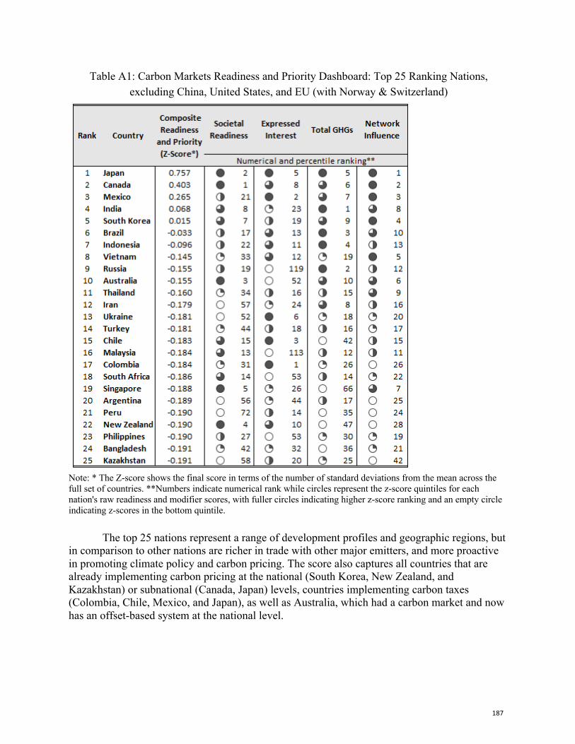
187

Table A1: Carbon Markets Readiness and Priority Dashboard: Top 25 Ranking Nations, excluding China, United States, and EU (with Norway & Switzerland)

Note: * The Z-score shows the final score in terms of the number of standard deviations from the mean across the full set of countries. **Numbers indicate numerical rank while circles represent the z-score quintiles for each nation's raw readiness and modifier scores, with fuller circles indicating higher z-score ranking and an empty circle indicating z-scores in the bottom quintile.

The top 25 nations represent a range of development profiles and geographic regions, but in comparison to other nations are richer in trade with other major emitters, and more proactive in promoting climate policy and carbon pricing. The score also captures all countries that are already implementing carbon pricing at the national (South Korea, New Zealand, and Kazakhstan) or subnational (Canada, Japan) levels, countries implementing carbon taxes (Colombia, Chile, Mexico, and Japan), as well as Australia, which had a carbon market and now has an offset-based system at the national level.

188

Heat Map Results

As the map shows, the EU, United States, and China are the highest priorities, respectively ranking first, second, and third overall in terms of the final societal readiness and strategic priority score and ranking in the top four on all other sub-component scores. Among the rest of the world, the top ranking countries are Japan, Canada, Mexico, India, and South Korea, with a relatively high confluence of all factors, Brazil and Indonesia follow after, with particularly high GHG emissions from deforestation. The next highest ranking countries are Vietnam, Russia, Australia, Thailand, Iran, Ukraine, Turkey, Chile, Malaysia, and Colombia, respectively, with countries in italics likely being more challenging due to comparatively low values for societal readiness and (for Russia and Malaysia) expressed interest.

Additional insights are provided by the component rankings (see Table A1 above). Though relatively low in GHG emissions in itself, Vietnam stands out for its network influence with large emitters (US, China, and Japan), South Africa follows next, notable as the sole candidate from Africa and for its relatively high societal readiness value. In terms of societal readiness, Japan, Canada, Australia, Singapore, and South Korea are highest, but the other modifiers affect the relative rankings. Kazakhstan is notable as a country with a relatively low societal readiness index value that is nonetheless implementing a carbon market (after a period of suspension). Finally. some regional groupings emerge, as discussed below.

The Americas. Based on high levels of by expressed interest compared to other nations, Mexico, followed by Chile and Colombia, stand out as potential near-term prospects for developing new carbon markets. Chile is particularly notable, making the list due to high scores on expressed interest and other dimensions, despite relatively low GHG emissions. Brazil is one of the world’s largest emitters and a country with a large economy deeply enmeshed in global trade networks, while Argentina and Peru also make the top 25. Highly-ranked Canada is a potential priority to help expand and consolidate these systems.

Southeast and East Asia. Japan, Indonesia, Vietnam, and Thailand stand out as leading candidates. South Korea, also highly ranked, has already implemented a carbon market and could be an important regional catalyst, while China, as it develops its own market, can present a long-term anchor for the region. Singapore is much lower down the list (#19), largely given its low emissions, but stands out as a potentially nearer-term prospect given its very high societal readiness and network influence factors.

Methodological Details

Below, we provide additional methodological details on the heat map analysis. The Carbon Markets Readiness and Priority index scores and ranks 132 nations on the potential for and payoff of implementing a carbon market in the near and medium term. Our index model is comprised of two main components: The Societal Readiness Score, which evaluates core institutional readiness across three Pillars (Governance, Enterprise, and Civil Society); and a strategic relevance filter incorporating three Modifiers, which assess regional influence via trade networks, demonstrated political interest, and overall climate impact via GHG emissions volumes.

We used a weighted composite index approach to score and rank nations worldwide in accordance with their estimated “Carbon Markets Readiness and Priority.” Indices were

189

aggregated using 50 different variables from 31 different datasets covering 131 jurisdictions worldwide (see Table 2 for a list of variables and data sources). Rather than treat EU member nations individually, we constructed a composite score for the European Union using GDP-weighted averages (for indices and non-additive variables) and weighted sums (for additive variables) for all of the EU-28 member nations.

All input data was adjusted using min-max normalization to reach a common zero-to-one scale prior to aggregation: X = the set of all country scores for a given variable xi = the score from variable X for a given country i

is the normalized score of variable X for country i We chose this method for all steps in our model for which normalization is used, as it

eradicates negative values from the data—thus allowing us to multiply in Modifiers (as noted below) without the sign of the score unintentionally cancelling out.

The Three Pillars of Societal Readiness: Governance, Enterprise, Civil

The Societal Readiness Score is a composite of three Pillars, representing a core societal group relevant to carbon pricing: Governance, Enterprise, and Civil Society. Each Pillar is comprised of two aggregated “Indicators” representing the Capacity and Motivation of each. The input data to each Indicator are listed in Table A2 below. Each Indicator is a simple average of all normalized input data. If a nation is missing data for all inputs to an indicator, that nation is dropped. In turn, each of the three Pillar scores is a weighted average of its corresponding Capacity and Motivation scores—in this context, both Indicators are given an equal weight.

The rationale behind including and equally weighting both Capacity and Motivation is that while a nation may have all the structural requirements to successfully implement and govern a carbon market, insufficient political or civil will—or pressure from major enterprises—can present roadblocks to the establishment of carbon pricing mechanisms. Similarly, strong political will, or large economic benefits to carbon pricing, can lead to important steps taken toward a carbon market, even in a nation that ranks lower in terms of political and economic sophistication and development.

Together, and across all three Pillars, these scores create what we call the “raw readiness” of a given country—represented by the Societal Readiness Score. The Societal Readiness Score is a weighted average of the final scores of each Pillar, with the Governance Pillar given a higher weight (50%) than the Enterprise and Civil scores (25% each).

Strategic Relevance Filter

In addition to the raw Societal Readiness Score, we include a strategic relevance filter based on three score Modifiers that capture market readiness propensity beyond institutional capacity alone.

The Expressed Interest modifier captures the interest demonstrated by policymakers toward implementing a market-based mechanism to control carbon emissions. This is a simple average of five normalized variables: participation in the Carbon Pricing Leadership Coalition; Participation and extent of progress within the World Bank’s PMR; the extent of domestic

)min()max()min(XX

Xxn ii

--

=

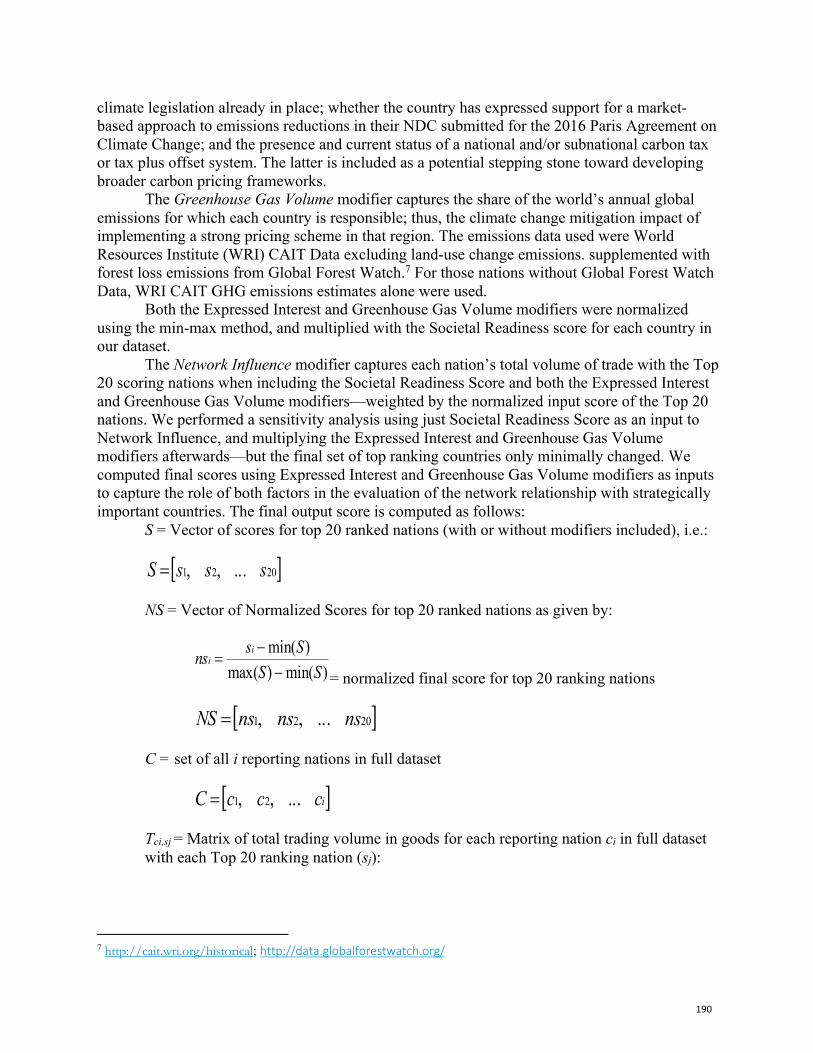
190

climate legislation already in place; whether the country has expressed support for a market-based approach to emissions reductions in their NDC submitted for the 2016 Paris Agreement on Climate Change; and the presence and current status of a national and/or subnational carbon tax or tax plus offset system. The latter is included as a potential stepping stone toward developing broader carbon pricing frameworks.

The Greenhouse Gas Volume modifier captures the share of the world’s annual global emissions for which each country is responsible; thus, the climate change mitigation impact of implementing a strong pricing scheme in that region. The emissions data used were World Resources Institute (WRI) CAIT Data excluding land-use change emissions. supplemented with forest loss emissions from Global Forest Watch.7 For those nations without Global Forest Watch Data, WRI CAIT GHG emissions estimates alone were used.

Both the Expressed Interest and Greenhouse Gas Volume modifiers were normalized using the min-max method, and multiplied with the Societal Readiness score for each country in our dataset.

The Network Influence modifier captures each nation’s total volume of trade with the Top 20 scoring nations when including the Societal Readiness Score and both the Expressed Interest and Greenhouse Gas Volume modifiers—weighted by the normalized input score of the Top 20 nations. We performed a sensitivity analysis using just Societal Readiness Score as an input to Network Influence, and multiplying the Expressed Interest and Greenhouse Gas Volume modifiers afterwards—but the final set of top ranking countries only minimally changed. We computed final scores using Expressed Interest and Greenhouse Gas Volume modifiers as inputs to capture the role of both factors in the evaluation of the network relationship with strategically important countries. The final output score is computed as follows:

S = Vector of scores for top 20 ranked nations (with or without modifiers included), i.e.:

NS = Vector of Normalized Scores for top 20 ranked nations as given by:

= normalized final score for top 20 ranking nations

C = set of all i reporting nations in full dataset

Tci,sj = Matrix of total trading volume in goods for each reporting nation ci in full dataset with each Top 20 ranking nation (sj):

7 http://cait.wri.org/historical; http://data.globalforestwatch.org/

[ ]2021 ...,, sssS =

)min()max()min(SS

Ssns ii

--

=

[ ]2021 ...,, nsnsnsNS =

[ ]icccC ...,, 21=

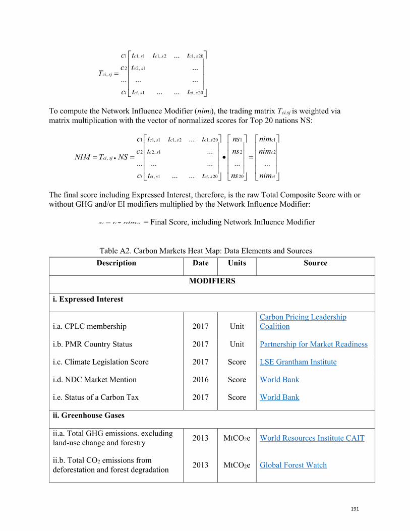
191

To compute the Network Influence Modifier (nimi), the trading matrix Tci,sj is weighted via matrix multiplication with the vector of normalized scores for Top 20 nations NS:

The final score including Expressed Interest, therefore, is the raw Total Composite Score with or without GHG and/or EI modifiers multiplied by the Network Influence Modifier:

= Final Score, including Network Influence Modifier

Table A2. Carbon Markets Heat Map: Data Elements and Sources

Description Date Units Source

MODIFIERS

i. Expressed Interest

i.a. CPLC membership 2017 Unit Carbon Pricing Leadership Coalition

i.b. PMR Country Status 2017 Unit Partnership for Market Readiness

i.c. Climate Legislation Score 2017 Score LSE Grantham Institute

i.d. NDC Market Mention 2016 Score World Bank

i.e. Status of a Carbon Tax 2017 Score World Bank

ii. Greenhouse Gases

ii.a. Total GHG emissions. excluding land-use change and forestry 2013 MtCO2e World Resources Institute CAIT

ii.b. Total CO2 emissions from deforestation and forest degradation 2013 MtCO2e Global Forest Watch

úúúú

û

ù

êêêê

ë

é

=

20,1,

1,2

20,12,11,1

2

1

,

...............

...

...scisci

sc

scscsc

i

sjci

tt

tttt

c

cc

T

úúúú

û

ù

êêêê

ë

é

=

úúúú

û

ù

êêêê

ë

é

•

úúúú

û

ù

êêêê

ë

é

== •

ci

c

c

scisci

sc

scscsc

i

sjci

nim

nimnim

ns

nsns

tt

tttt

c

cc

NSTNIM......

...............

...

...2

1

20

2

1

20,1,

1,2

20,12,11,1

2

1

,

ciii nimts *=

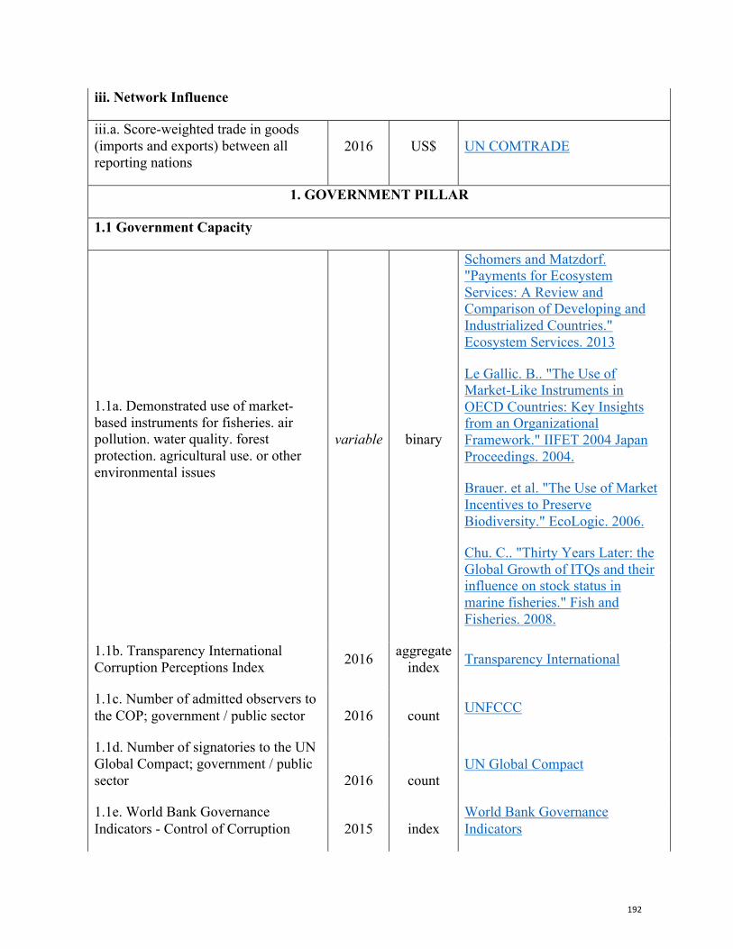
192

iii. Network Influence

iii.a. Score-weighted trade in goods (imports and exports) between all reporting nations

2016 US$ UN COMTRADE

1. GOVERNMENT PILLAR

1.1 Government Capacity

1.1a. Demonstrated use of market-based instruments for fisheries. air pollution. water quality. forest protection. agricultural use. or other environmental issues

variable binary

Schomers and Matzdorf. "Payments for Ecosystem Services: A Review and Comparison of Developing and Industrialized Countries." Ecosystem Services. 2013

Le Gallic. B.. "The Use of Market-Like Instruments in OECD Countries: Key Insights from an Organizational Framework." IIFET 2004 Japan Proceedings. 2004.

Brauer. et al. "The Use of Market Incentives to Preserve Biodiversity." EcoLogic. 2006.

Chu. C.. "Thirty Years Later: the Global Growth of ITQs and their influence on stock status in marine fisheries." Fish and Fisheries. 2008.

1.1b. Transparency International Corruption Perceptions Index 2016 aggregate

index Transparency International

1.1c. Number of admitted observers to the COP; government / public sector 2016 count UNFCCC

1.1d. Number of signatories to the UN Global Compact; government / public sector 2016 count

UN Global Compact

1.1e. World Bank Governance Indicators - Control of Corruption 2015 index

World Bank Governance Indicators

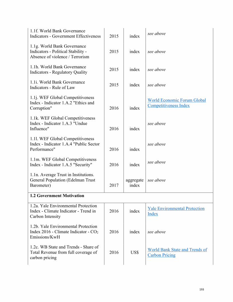
193

1.1f. World Bank Governance Indicators - Government Effectiveness 2015 index see above

1.1g. World Bank Governance Indicators - Political Stability - Absence of violence / Terrorism

2015 index see above

1.1h. World Bank Governance Indicators - Regulatory Quality 2015 index see above

1.1i. World Bank Governance Indicators - Rule of Law 2015 index see above

1.1j. WEF Global Competitiveness Index - Indicator 1.A.2 "Ethics and Corruption" 2016 index

World Economic Forum Global Competitiveness Index

1.1k. WEF Global Competitiveness Index - Indicator 1.A.3 "Undue Influence" 2016 index

see above

1.1l. WEF Global Competitiveness Index - Indicator 1.A.4 "Public Sector Performance" 2016 index

see above

1.1m. WEF Global Competitiveness Index - Indicator 1.A.5 "Security" 2016 index see above

1.1n. Average Trust in Institutions. General Population (Edelman Trust Barometer) 2017

aggregate index

see above

1.2 Government Motivation

1.2a. Yale Environmental Protection Index - Climate Indicator - Trend in Carbon Intensity

2016 index Yale Environmental Protection Index

1.2b. Yale Environmental Protection Index 2016 - Climate Indicator - CO2 Emissions/KwH

2016 index see above

1.2c. WB State and Trends - Share of Total Revenue from full coverage of carbon pricing

2016 US$ World Bank State and Trends of Carbon Pricing

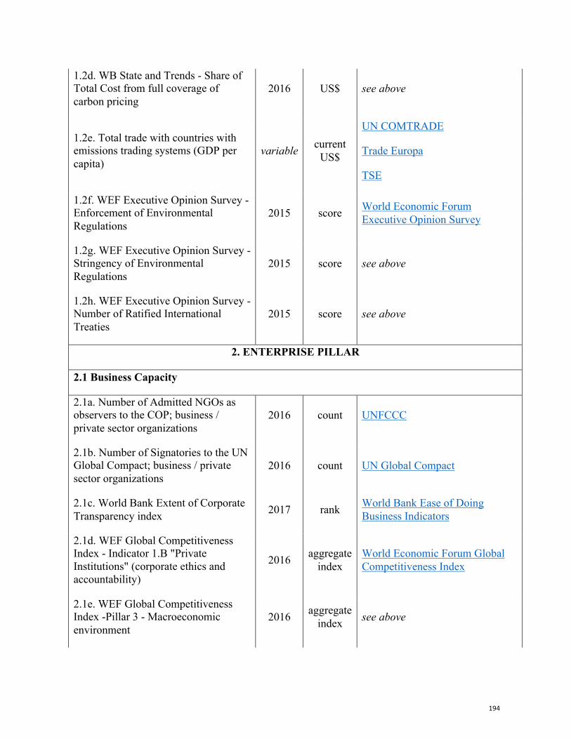
194

1.2d. WB State and Trends - Share of Total Cost from full coverage of carbon pricing

2016 US$ see above

1.2e. Total trade with countries with emissions trading systems (GDP per capita)

variable current US$

UN COMTRADE

Trade Europa

TSE

1.2f. WEF Executive Opinion Survey - Enforcement of Environmental Regulations

2015 score World Economic Forum Executive Opinion Survey

1.2g. WEF Executive Opinion Survey - Stringency of Environmental Regulations

2015 score see above

1.2h. WEF Executive Opinion Survey - Number of Ratified International Treaties


2. ENTERPRISE PILLAR

2.1 Business Capacity

2.1a. Number of Admitted NGOs as observers to the COP; business / private sector organizations

2016 count UNFCCC

2.1b. Number of Signatories to the UN Global Compact; business / private sector organizations

2016 count UN Global Compact

2.1c. World Bank Extent of Corporate Transparency index 2017 rank World Bank Ease of Doing

Business Indicators

2.1d. WEF Global Competitiveness Index - Indicator 1.B "Private Institutions" (corporate ethics and accountability)

2016 aggregate index

World Economic Forum Global Competitiveness Index

2.1e. WEF Global Competitiveness Index -Pillar 3 - Macroeconomic environment

2016 aggregate index see above

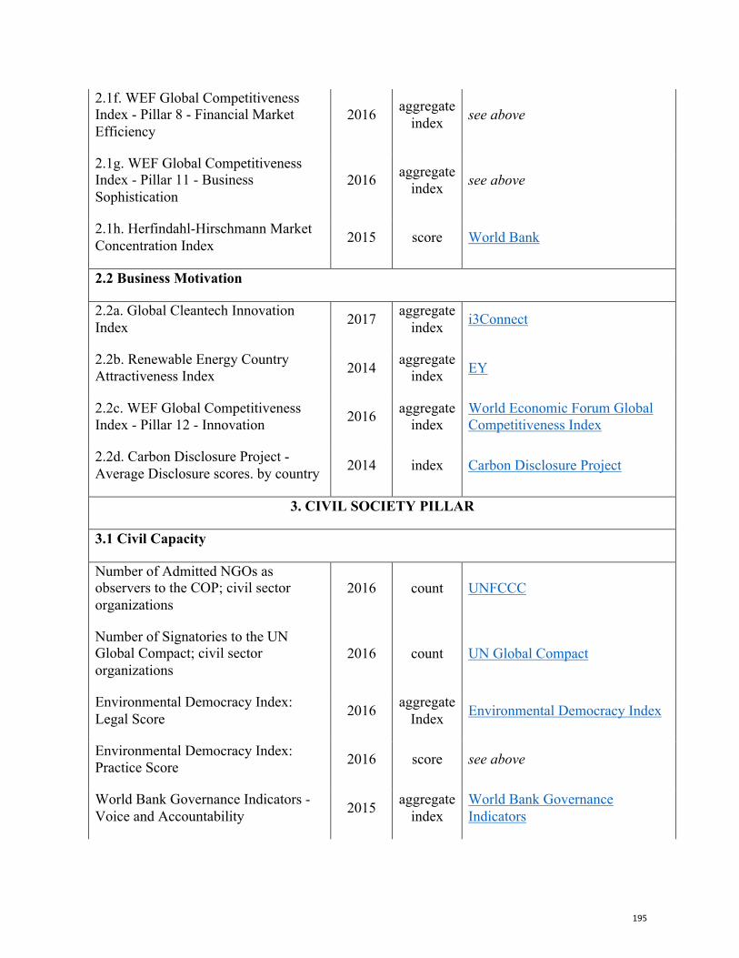
195

2.1f. WEF Global Competitiveness Index - Pillar 8 - Financial Market Efficiency


2.1g. WEF Global Competitiveness Index - Pillar 11 - Business Sophistication


2.1h. Herfindahl-Hirschmann Market Concentration Index 2015 score World Bank

2.2 Business Motivation

2.2a. Global Cleantech Innovation Index 2017 aggregate

index i3Connect

2.2b. Renewable Energy Country Attractiveness Index 2014 aggregate

index EY

2.2c. WEF Global Competitiveness Index - Pillar 12 - Innovation 2016 aggregate

index World Economic Forum Global Competitiveness Index

2.2d. Carbon Disclosure Project - Average Disclosure scores. by country 2014 index Carbon Disclosure Project

3. CIVIL SOCIETY PILLAR

3.1 Civil Capacity

Number of Admitted NGOs as observers to the COP; civil sector organizations

2016 count UNFCCC

Number of Signatories to the UN Global Compact; civil sector organizations

2016 count UN Global Compact

Environmental Democracy Index: Legal Score 2016 aggregate

Index Environmental Democracy Index

Environmental Democracy Index: Practice Score 2016 score see above

World Bank Governance Indicators - Voice and Accountability 2015 aggregate

index World Bank Governance Indicators

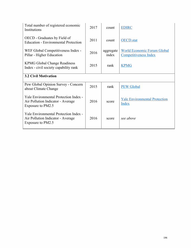
196

Total number of registered economic Institutions 2017 count EDIRC

OECD - Graduates by Field of Education - Environmental Protection 2011 count OECD.stat

WEF Global Competitiveness Index - Pillar - Higher Education 2016 aggregate

index World Economic Forum Global Competitiveness Index

KPMG Global Change Readiness Index - civil society capability rank 2015 rank KPMG

3.2 Civil Motivation

Pew Global Opinion Survey - Concern about Climate Change 2015 rank PEW Global

Yale Environmental Protection Index - Air Pollution Indicator - Average Exposure to PM2.5

2016 score Yale Environmental Protection Index

Yale Environmental Protection Index - Air Pollution Indicator - Average Exposure to PM2.5


197

Global Carbon Pricing System As A Mechanism to Strengthen Competitiveness And Reduce CO2 Emissions In Energy-Intensive Trade-Exposed Sectors, Such As Primary Aluminium Production Sergey Chestnoy, PhD, Adviser on Sustainable Development, UC RUSAL Dinara Gershinkova, Adviser on Climate, Directorate of International Projects, UC RUSAL

Abstract

The absence of global carbon pricing distorts the competitive environment. Countries that have carbon–pricing point out the additional competitive advantages the producers have in countries without carbon pricing. Universal charge for CO2 emissions would create an unbiased competitive environment for all producers. The sectoral approach in basic sectors may be the first step in creation of a global framework for carbon regulation, although it is a long–term objective. Using the example of emissions–intensive, trade–exposed industries such as aluminium production, which accounts for 3.5% of global electricity consumption, the authors considered low carbon initiatives that already have been implemented by aluminium producers (mostly promotion of clean energy use and aluminium recycling) and analysed how carbon pricing may fostering those.

The obvious advantages of sectoral approach are: a small group of countries– negotiators and relatively uniformed production processes and technologies in the industry around the globe. That makes the negotiations easier comparing with the UNFCCC process. There is a number of options for intergovernmental decision–making on this, including regional and intergovernmental platforms such as APEC and G–20. Negotiators should address such questions as: the size of carbon price itself, who will pay, who will collect money, how to use them and how to ensure transparency of the entire process.

A decision on the method of carbon pricing (cap and trade or carbon tax) could be taken at the final stage of negotiations, considering the financial and economic impact of introducing regulation as well as the preparedness of countries in adopting the method. Article 6 of the Paris agreement might be another incentive mechanism for low carbon development of the global aluminium sector. Key words: Aluminium, Climate change, carbon–pricing, sectoral approach.

Introduction

Carbon regulation in the form of taxes or markets exists in 45 national and 25 subnational jurisdictions (State and Trends of Carbon Pricing, 2018). Despite this, the price for emissions differs significantly from country to country, ranging from one to almost 140 USD/tCO2e.

198

Recent changes to EU Emissions Trade Systems (ETS) including more efficient allocation strategy have resulted in an increased price per tonne of CO2e emissions generated in Europe (above 20 Euro). At the same time, most carbon prices are still set at a maximum level of 10 USD/tCO2e.

Fundamentally, businesses and regulators cannot ignore the difference in climate commitments between countries. In the last few years, there have been more vocal calls for compensation around trade protection measures in those countries with more ambitious climate change policies.

This places producers on an unequal competitive footing in the market. Voicing this, Nobel Laureate Joseph Stiglitz wrote more a decade ago: “Not paying the cost of damage to the environment is a subsidy, just as not paying the full costs of workers would be”.1 Indeed, this is why at the highest political levels there are proposals to protect each country’s own producers whilst introducing limits on imports from countries that don’t have the relevant climate legislation. In 2018, the President of France, E. Macron, made a statement regarding the need to introduce “a border adjustment mechanism to avoid penalising our companies because of our climate commitments…we have to put in place a tax at the border for those who decide not to make the same environmental choice”.2

As such, the idea of an adjustment of a border tax is reflected in the Climate Leadership Council, initiated by a number of U.S. senators several years ago to promote a carbon dividends framework as the most cost–effective, equitable and politically–viable solution to limit carbon emissions. The authors argued that “border adjustments for the carbon content of both imports and exports would protect American competitiveness and punish free–riding by other nations, encouraging them to adopt carbon pricing of their own”.3

It is known that the WTO permits border tax adjustments (ВТА) as well as other trade restrictions with the aim to promote or protect important societal values and the interests of each country involved. This includes, for example, the necessity to protect human, animal or plant life or health (Article XX (b) of GATT) correlating to the conservation of exhaustible natural resources (Article XX (g) of GATT). WTO permits BTA exceptionally “if such measures are made effective in conjunction with restrictions on domestic production or consumption”.4 But here we face the potential threat of new trade conflicts.

In our opinion, there is a solution which is a universal approach towards carbon regulation. We propose a universal charge for CO2 emissions which would create an unbiased competitive environment for those trading internationally. With everyone being on an equal footing from the start, this will lead to an improvement in international relations and more importantly, deal with the worse effects of climate change. This approach would ensure worldwide incentives for introducing green technologies and green financing. Fundamentally, it would support the global economy’s transformation towards a low–carbon path of development.

Establishing a universal approach on carbon–pricing for all countries at once is undoubtedly an ambitious task that will require considerable time for debate and approval. Despite this, sectoral agreements across industries may be the first step in the right direction. It seems less complicated in practical terms. From there, we can move on to address the issues from a global carbon regulation point of view for the entire global economy. Helpfully, a

1 http://carbon-price.com/joseph-stiglitz/. 2 https://www.euractiv.com/section/energy/news/france-to-push-for-eu-carbon-price-floor-and-border-tariff/. 3 https://www.clcouncil.org/. 4 https://www.wto.org/english/tratop_e/envir_e/envt_rules_exceptions_e.htm.

199

precedent already exists – the 2016 ICAO's resolution to introduce a market mechanism reducing CO2 emissions from civil aviation flights through the Carbon Offsetting and Reduction Scheme for International Aviation (CORSIA)5 which applies to almost all ICAO members. CORSIA was introduced to achieve the goals set at the industrial level (aviation) which consisted of carbon–neutral growth from 2020 onwards.

Energy–intensive sectors such as the aluminium industry should also be considered.

Why is it important to address GHG emissions in energy–intensive trade–exposed sectors such as aluminium industry?

Industrial processes account for approximately 40% of global CO2e emissions

(S.Nabernegg et al, 2017). The main growth in emissions has been seen in Asia (Fischedick et al, 2014), where the production of emissions–intensive, trade–exposed (EITE) industries is concentrated, particularly from the production of basic materials including steel, cement, primary aluminium and glass. All these materials are drivers of industrialization and play an important role in global value chains as they make up essential products used in virtually all manufacturing sectors and construction applications.

For an extensive and stable global reduction of anthropogenic greenhouse gas emissions, it is required, as a matter of priority, to reduce emissions in these sectors – both directly (processing) and indirectly (relating to the generation of consumed thermal and electric power, that should be combined with switching to low–emission energy sources).

Aluminium production (electrolytic reduction process) consumes a lot of electricity – 14,145 Kilowatt hours (kWh) per tonne of metal to be exact (according to International Aluminium Institute, IAI).6 Emissions related directly to the electrolytic reduction process (scope 1) are not so significant on a global scale as the emissions related to the generation of electricity consumed in the reduction process (scope 2). Scope 2 emissions account for over 80% of total GHG emissions in the aluminium production process. Aluminium sector accounts for 3.5% of global electricity consumption (IPCC, Mitigation of Climate Change, 2014).

Aluminium is the second highest most in–demand metal in the world after steel and this demand for aluminium is steadily increasing by around 5% per annum. Owing to its characteristics such as low density, high thermal conductivity, low electrical resistance, high ductility and corrosion resistance, aluminium is widely used in various fields: construction, automotive, aerospace, consumer electronics and packaging to name but a few.

Aluminium has a high recycling capacity therefore the life cycle of an aluminium product is not the traditional "cradle–to–grave" sequence, but rather a "cradle–to–cradle". This infinite recyclability has led to a situation where today around 75% of the almost one billion tonnes of aluminium ever produced is still in productive use with some having been through countless loops of its lifecycle.7

Historically, aluminium smelters were built near hydropower plants, as they needed a powerful and cheap electricity source. However, according to IAI, nowadays over 60% of the metal in the world is produced using coal–based electricity generation. India and China largely

5 https://www.icao.int/environmental-protection/Pages/A39_CORSIA_FAQ2.aspx. 6 http://www.world-aluminium.org/statistics/primary-aluminium-smelting-energy-intensity/. 7 http://recycling.world-aluminium.org/review/sustainability.

200

rely on coal to power their aluminium smelters (90% in China).8 According to the International Energy Agency (IEA, 2017) modern global energy needs are increasingly slower than in the past but will still expand by 30% between today and 2040. The main demand – almost 30% – comes from India, whose share of global energy use will rise to 11% by 2040. Southeast Asia is another rising heavyweight in global energy, with demand growing at twice the pace of China. Overall, developing countries in Asia account for two–thirds of global energy growth, with the rest coming mainly from the Middle East, Africa and Latin America.

The policies of the aluminium industry in regards to climate change should be implemented in such a way as to avoid any growth of direct and indirect GHG emissions together with the need to increase the production and consumption of one of the basic materials in the world. In particular, subject to regional features of the forecasted growth in the demand for coal (in Asia), this should be taken into account. The key objective is switching the energy–intensive aluminium production process to use low–emission power sources. Another approach towards lower energy consumption in the industry is the use of metal recycling. Recycling aluminium requires 95% less energy and produces fewer greenhouse gas emissions (GHG), than manufacturing primary aluminium. According to some estimates, recycling of one tonne of aluminium avoids the generation of about 9 tonnes of carbon dioxide emissions.9

For the above–mentioned approaches to be multiplied on a global level, some stimulus would be required, including putting a price on carbon.

Benefits of sectoral approach

Sector–based international climate cooperation has been actively discussed during the process of preparation of the post–Kyoto international climate policy. There is considerable intellectual work on “sectoral approaches” in academic and policy circles that originate from around 2005–2010. Alongside this there was interest from a number of key governments, led by the Japanese Government (Bodansky, 2007, Meckling and Chung 2009). A sectoral approach was also suggested as a measure to reduce the divide between developed (Annex 1 to UNFCCC) and developing (non–Annex 1) countries in the post–Kyoto negotiations.

In more niche sectors with relatively few high profile individuals, such as aluminium, the small group size could make it easier to reach an agreement. This is for two main reasons. Firstly, the relevant actors would be easier to identify. Sectors such as steel, cement, aluminium, and auto manufacturing tend to be highly concentrated in terms of both companies and countries; therefore addressing them on a sectoral basis could encompass globally significant numbers of participants (Bodansky, 2007). Secondly, the complexity of negotiations increases as the number of players increase, so negotiations among a smaller number of parties would be easier and would be more likely to succeed.

The subject matter of a sectoral agreement may foresee carbon pricing through various technical regulations and standards, carbon footprint indicators etc. As for the substance of commitments, countries may develop national emissions targets by sector, and governments make international commitments to implement policies to achieve targets based on a staged sectoral approach or that can be developed as part of a portfolio of treaties. (Sawa, 2010, Barett, 2010).

8 http://www.world-aluminium.org. 9 https://www.novelisrecycling.co.uk.

201

It is quite possible to reach these agreements in the global aluminium industry from a practical perspective. The aluminium sector uses relatively uniformed production processes and technologies around the globe that allow for universal recommendations from all major producers. If we can move towards signing the agreement at the sectoral level by starting expert discussions under the IAI’s auspices, this will help to form the basis for providing recommendations to national governments. IAI has been chosen as an organization providing a fair representation of a certain global industry: its 27 members are responsible for a significant apportion of aluminium production worldwide. In any case for a sectoral agreement we need a wider intergovernmental format.

Carbon–pricing measures in the aluminium industry to combat climate change

As mentioned above, carbon regulation in the form of taxes or markets exists in 45

national and 25 subnational jurisdictions (State and Trends of Carbon Pricing, 2018). Since carbon regulation is fragmented in nature, existing measures cover just about 20% of global CO2 emissions which is obviously not enough to achieve the ambitious objective of combating global warming. The progress made with global regulation should be appreciated – the emissions covered by carbon pricing mechanisms have increased threefold over the past decade (State and Trends of Carbon Pricing, 2016).

Aluminium smelters typically fall under the regulation of existing ETSs in countries that have a developed aluminium industry, for example, in the EU. However, in the EU the introduced load is rather insignificant for producers because the aluminium production is exposed to a high risk of carbon leakages - i.e. the risk of transferring the production to countries where there is no carbon regulation. Therefore, the regulator (government) applies easement measures in the carbon regulation. In Europe such a measure is the carbon leakage list. Production facilities included in this list may have up to 100 per cent of emission quotas free of charge (under certain requirements for emission standards). Moreover, there is an option for compensation to cover the electricity payments of aluminium smelters (this benefit is at the discretion of national authorities).

Launched in late 2017, the Chinese ETS which is potentially the world's largest ETS, has included aluminium smelters within their development plan. However, these will only be put in place from 2020. Therefore, there is currently no large–scale emission regulation in practise as of yet within the aluminium industry and as part of the ETS framework.

Many companies implement climate change strategies on a voluntary basis, that are close to the carbon–pricing concept. For instance, Rio Tinto, Hydro and RUSAL, apply an internal carbon price (this is according to reports within the Carbon disclosure project10 (CDP) for 2017). The companies do this to analyse the pricing of new investment projects and how it changes depending on whether any carbon charges are introduced in the country. Since 2017, RUSAL has been applying an internal price of 20 USD/tCO2e.

In recent years, low–emission products have become a trend within the aluminium industry. As such, a number of specific brands are focused either on the producer's access to low–emission energy sources (including hydro, natural gas, nuclear energy) or on the metal

10 www.cdp.net

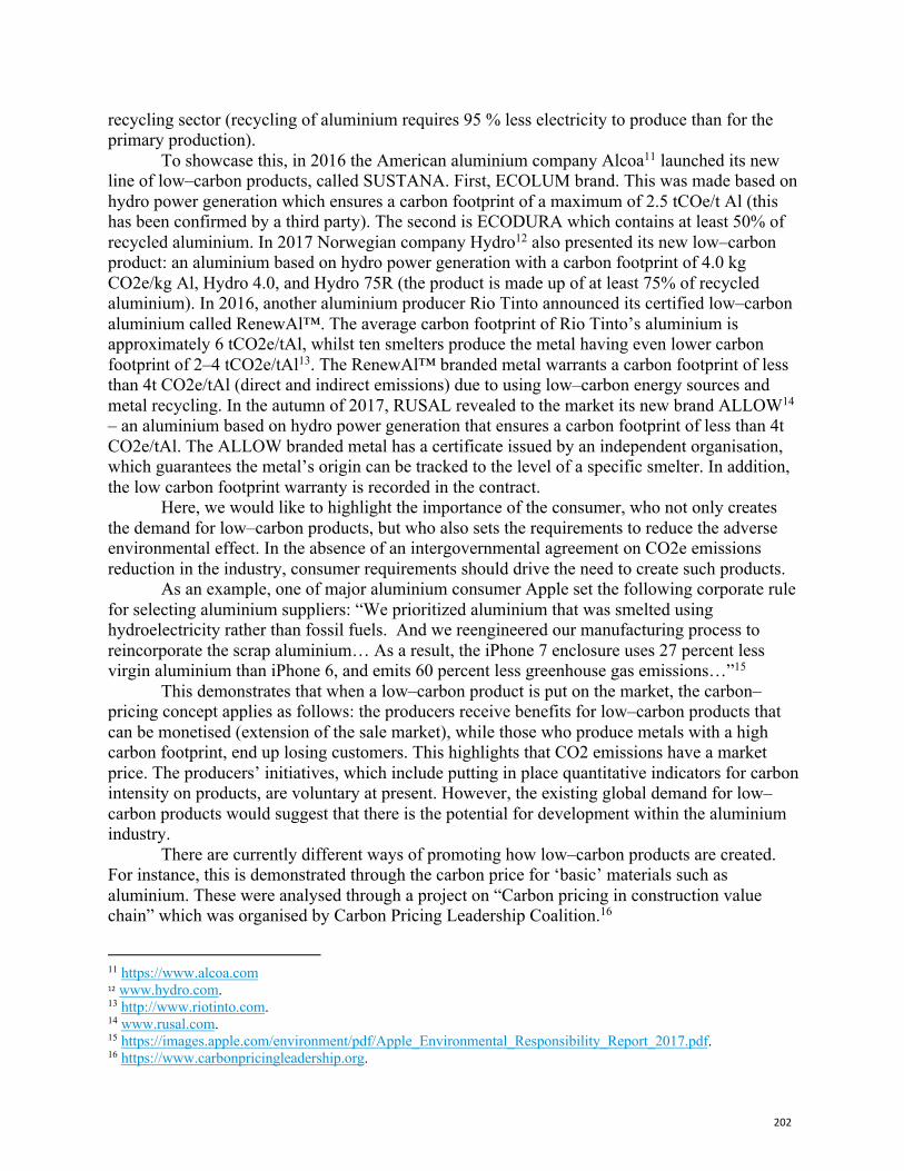
202

recycling sector (recycling of aluminium requires 95 % less electricity to produce than for the primary production).

To showcase this, in 2016 the American aluminium company Alcoa11 launched its new line of low–carbon products, called SUSTANA. First, ECOLUM brand. This was made based on hydro power generation which ensures a carbon footprint of a maximum of 2.5 tCOe/t Al (this has been confirmed by a third party). The second is ECODURA which contains at least 50% of recycled aluminium. In 2017 Norwegian company Hydro12 also presented its new low–carbon product: an aluminium based on hydro power generation with a carbon footprint of 4.0 kg CO2e/kg Al, Hydro 4.0, and Hydro 75R (the product is made up of at least 75% of recycled aluminium). In 2016, another aluminium producer Rio Tinto announced its certified low–carbon aluminium called RenewAl™. The average carbon footprint of Rio Tinto’s aluminium is approximately 6 tCO2e/tAl, whilst ten smelters produce the metal having even lower carbon footprint of 2–4 tCO2e/tAl13. The RenewAl™ branded metal warrants a carbon footprint of less than 4t CO2e/tAl (direct and indirect emissions) due to using low–carbon energy sources and metal recycling. In the autumn of 2017, RUSAL revealed to the market its new brand ALLOW14 – an aluminium based on hydro power generation that ensures a carbon footprint of less than 4t CO2e/tAl. The ALLOW branded metal has a certificate issued by an independent organisation, which guarantees the metal’s origin can be tracked to the level of a specific smelter. In addition, the low carbon footprint warranty is recorded in the contract.

Here, we would like to highlight the importance of the consumer, who not only creates the demand for low–carbon products, but who also sets the requirements to reduce the adverse environmental effect. In the absence of an intergovernmental agreement on CO2e emissions reduction in the industry, consumer requirements should drive the need to create such products.

As an example, one of major aluminium consumer Apple set the following corporate rule for selecting aluminium suppliers: “We prioritized aluminium that was smelted using hydroelectricity rather than fossil fuels. And we reengineered our manufacturing process to reincorporate the scrap aluminium… As a result, the iPhone 7 enclosure uses 27 percent less virgin aluminium than iPhone 6, and emits 60 percent less greenhouse gas emissions…”15

This demonstrates that when a low–carbon product is put on the market, the carbon–pricing concept applies as follows: the producers receive benefits for low–carbon products that can be monetised (extension of the sale market), while those who produce metals with a high carbon footprint, end up losing customers. This highlights that CO2 emissions have a market price. The producers’ initiatives, which include putting in place quantitative indicators for carbon intensity on products, are voluntary at present. However, the existing global demand for low–carbon products would suggest that there is the potential for development within the aluminium industry.

There are currently different ways of promoting how low–carbon products are created. For instance, this is demonstrated through the carbon price for ‘basic’ materials such as aluminium. These were analysed through a project on “Carbon pricing in construction value chain” which was organised by Carbon Pricing Leadership Coalition.16

11 https://www.alcoa.com 12 www.hydro.com. 13 http://www.riotinto.com. 14 www.rusal.com. 15 https://images.apple.com/environment/pdf/Apple_Environmental_Responsibility_Report_2017.pdf. 16 https://www.carbonpricingleadership.org.

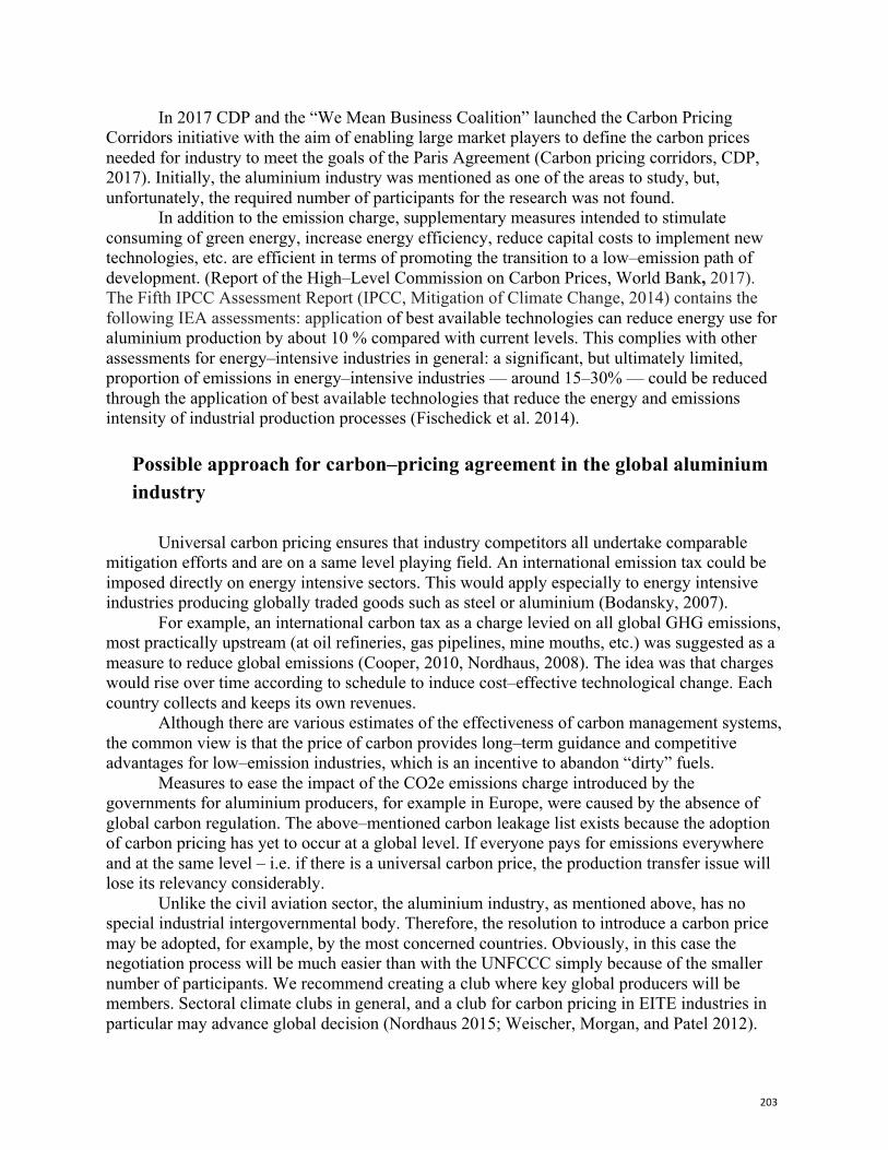
203

In 2017 CDP and the “We Mean Business Coalition” launched the Carbon Pricing Corridors initiative with the aim of enabling large market players to define the carbon prices needed for industry to meet the goals of the Paris Agreement (Carbon pricing corridors, CDP, 2017). Initially, the aluminium industry was mentioned as one of the areas to study, but, unfortunately, the required number of participants for the research was not found.

In addition to the emission charge, supplementary measures intended to stimulate consuming of green energy, increase energy efficiency, reduce capital costs to implement new technologies, etc. are efficient in terms of promoting the transition to a low–emission path of development. (Report of the High–Level Commission on Carbon Prices, World Bank, 2017). The Fifth IPCC Assessment Report (IPCC, Mitigation of Climate Change, 2014) contains the following IEA assessments: application of best available technologies can reduce energy use for aluminium production by about 10 % compared with current levels. This complies with other assessments for energy–intensive industries in general: a significant, but ultimately limited, proportion of emissions in energy–intensive industries — around 15–30% — could be reduced through the application of best available technologies that reduce the energy and emissions intensity of industrial production processes (Fischedick et al. 2014).

Possible approach for carbon–pricing agreement in the global aluminium industry

Universal carbon pricing ensures that industry competitors all undertake comparable

mitigation efforts and are on a same level playing field. An international emission tax could be imposed directly on energy intensive sectors. This would apply especially to energy intensive industries producing globally traded goods such as steel or aluminium (Bodansky, 2007).

For example, an international carbon tax as a charge levied on all global GHG emissions, most practically upstream (at oil refineries, gas pipelines, mine mouths, etc.) was suggested as a measure to reduce global emissions (Cooper, 2010, Nordhaus, 2008). The idea was that charges would rise over time according to schedule to induce cost–effective technological change. Each country collects and keeps its own revenues.

Although there are various estimates of the effectiveness of carbon management systems, the common view is that the price of carbon provides long–term guidance and competitive advantages for low–emission industries, which is an incentive to abandon “dirty” fuels.

Measures to ease the impact of the CO2e emissions charge introduced by the governments for aluminium producers, for example in Europe, were caused by the absence of global carbon regulation. The above–mentioned carbon leakage list exists because the adoption of carbon pricing has yet to occur at a global level. If everyone pays for emissions everywhere and at the same level – i.e. if there is a universal carbon price, the production transfer issue will lose its relevancy considerably.

Unlike the civil aviation sector, the aluminium industry, as mentioned above, has no special industrial intergovernmental body. Therefore, the resolution to introduce a carbon price may be adopted, for example, by the most concerned countries. Obviously, in this case the negotiation process will be much easier than with the UNFCCC simply because of the smaller number of participants. We recommend creating a club where key global producers will be members. Sectoral climate clubs in general, and a club for carbon pricing in EITE industries in particular may advance global decision (Nordhaus 2015; Weischer, Morgan, and Patel 2012).

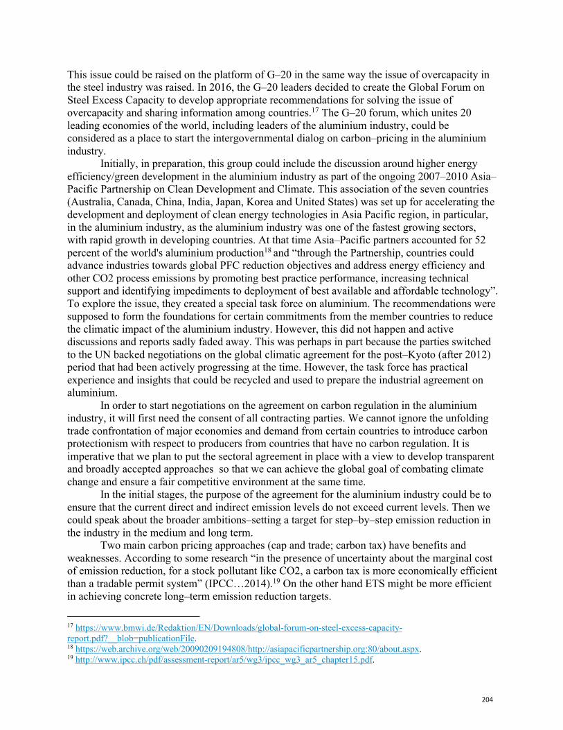
204

This issue could be raised on the platform of G–20 in the same way the issue of overcapacity in the steel industry was raised. In 2016, the G–20 leaders decided to create the Global Forum on Steel Excess Capacity to develop appropriate recommendations for solving the issue of overcapacity and sharing information among countries.17 The G–20 forum, which unites 20 leading economies of the world, including leaders of the aluminium industry, could be considered as a place to start the intergovernmental dialog on carbon–pricing in the aluminium industry.

Initially, in preparation, this group could include the discussion around higher energy efficiency/green development in the aluminium industry as part of the ongoing 2007–2010 Asia–Pacific Partnership on Clean Development and Climate. This association of the seven countries (Australia, Canada, China, India, Japan, Korea and United States) was set up for accelerating the development and deployment of clean energy technologies in Asia Pacific region, in particular, in the aluminium industry, as the aluminium industry was one of the fastest growing sectors, with rapid growth in developing countries. At that time Asia–Pacific partners accounted for 52 percent of the world's aluminium production18 and “through the Partnership, countries could advance industries towards global PFC reduction objectives and address energy efficiency and other CO2 process emissions by promoting best practice performance, increasing technical support and identifying impediments to deployment of best available and affordable technology”. To explore the issue, they created a special task force on aluminium. The recommendations were supposed to form the foundations for certain commitments from the member countries to reduce the climatic impact of the aluminium industry. However, this did not happen and active discussions and reports sadly faded away. This was perhaps in part because the parties switched to the UN backed negotiations on the global climatic agreement for the post–Kyoto (after 2012) period that had been actively progressing at the time. However, the task force has practical experience and insights that could be recycled and used to prepare the industrial agreement on aluminium.

In order to start negotiations on the agreement on carbon regulation in the aluminium industry, it will first need the consent of all contracting parties. We cannot ignore the unfolding trade confrontation of major economies and demand from certain countries to introduce carbon protectionism with respect to producers from countries that have no carbon regulation. It is imperative that we plan to put the sectoral agreement in place with a view to develop transparent and broadly accepted approaches so that we can achieve the global goal of combating climate change and ensure a fair competitive environment at the same time.

In the initial stages, the purpose of the agreement for the aluminium industry could be to ensure that the current direct and indirect emission levels do not exceed current levels. Then we could speak about the broader ambitions–setting a target for step–by–step emission reduction in the industry in the medium and long term.

Two main carbon pricing approaches (cap and trade; carbon tax) have benefits and weaknesses. According to some research “in the presence of uncertainty about the marginal cost of emission reduction, for a stock pollutant like CO2, a carbon tax is more economically efficient than a tradable permit system” (IPCC…2014).19 On the other hand ETS might be more efficient in achieving concrete long–term emission reduction targets.

17 https://www.bmwi.de/Redaktion/EN/Downloads/global-forum-on-steel-excess-capacity-report.pdf?__blob=publicationFile. 18 https://web.archive.org/web/20090209194808/http://asiapacificpartnership.org:80/about.aspx. 19 http://www.ipcc.ch/pdf/assessment-report/ar5/wg3/ipcc_wg3_ar5_chapter15.pdf.

205

A decision on the method for carbon pricing could be made at the final stage of negotiations, taking in to consideration the financial and economic impact of introducing regulation as well as the preparedness of countries in adopting the method.

Another approach at the industrial level could be carbon pricing on the carbon intensity (carbon footprint) of products. It could start with accounting for direct and indirect emissions (scope 1 and scope 2) and then setting acceptable minimum indicators of CO2e/t of aluminium subject to advanced technical capabilities and define a charge for exceeding these parameters. A progressive scale of the emission charge would encourage reducing GHG emissions and switching to low–emission energy sources more efficiently. The carbon footprint concept naturally encourages the use of highly recyclable aluminium since the energy consumption for its production is many times lower that for the production of primary aluminium. This creates an incentive for collecting used products, processing waste, and naturally implementing putting in to practice a circular economy.

Implementing the above–mentioned approaches towards carbon pricing in the aluminium industry will require exploring the following issues: — procedure for assessment of emissions and carbon footprint of products – methodology,

verification and transparency; — procedure for payment of carbon charges – rate and recipient of payments; — target use of collected funds – for what purpose and how to spend money; — coverage of administrative costs of implementing the carbon–pricing method; — and, of course, how compliance with the agreement will be ensured and what punishment

would be allocated in the instance of a breach of the obligations? If, however, such negotiations commence, it would be useful to discuss these issues

subject to the UNFCCC agenda, where the rules of applying Article 6 of the Paris Agreement on market and non–market mechanisms are discussed. The Paris Agreement permits the widest participation of stakeholders in global efforts to reduce the anthropogenic climatic impact. Article 6 creates the framework for public and private sector participation in the carbon market mechanisms (under Articles 6.2 and 6.4) and for exploring, applying and coordinating actions with respect to non–market approaches (6.8) which may include approaches that create non–tradable units such as carbon taxes and carbon standards, labelling, etc.20. Despite the fact that the recent UN climate conference in Katowice (December 2018) hasn’t come to a decision on the rules for implementation of Article 6 of the Paris Agreement, the market mechanisms (articles 6.2 and 6.4) were discussed more thoroughly then the non–market mechanisms (6.8). However, non–market instruments are equally interesting for the sectoral approach and Article 6.8 provides grounds for further elaboration on carbon price at the sectoral level. It is important to consider the UN climate negotiations because they develop rules for compliance with the mechanisms, control, and recording of transferred units, rules for the use of funds for adaptation purposes in developing countries, coverage of administrative costs, etc.

In the negotiations it is also vital to keep the spirit of the Paris Agreement, which has become a significant step forward and takes into account the situation today, under which all emitters participate in the global emission reduction measures within their national determined contributions.

Carbon regulation in the aluminium industry should become a mechanism that facilitates the industry's broad transition to a low–carbon path of development. Purchasing and producing

20 UNFCCC Technical paper “Non-market-based approaches “, document FCCC/TP/2014/10.

206

renewable energy as well as investing in low carbon technologies, working to improve energy efficiency, and offering new products and services aimed at reducing emissions are all meaningful strategies for the aluminium industry to undertake. Revenues from carbon pricing should underpin this process. Mobilized funds should be used for technological innovation, including research, development and demonstration projects – areas that require significant financial support also from additional sources.

We should not expect fast decision–making on the carbon–pricing agreement for the global aluminium industry simply because this issue has not been considered in detail yet, but there are all chances to put it into practice.

Conclusions — Any form of global carbon regulation is still fragmented, although we have seen the stable

growth of regulatory systems in the world. Only 20% of global GHG emissions are covered by carbon–pricing. The absence of global carbon regulation distorts the competitive environment. Countries that have carbon–pricing point out the additional competitive advantages that the producers have in countries without carbon regulation. A global carbon regulation may eliminate the distortions in the competitive environment, although it is a long–term objective. The sectoral approach in basic sectors may be the first step in this direction. Approving the carbon regulation mechanism with this group is a far simpler task.

— The aluminium industry is one of the energy–intensive basic industries that is responsible for consuming 3.5% of electricity in the world. Indirect GHG emissions from the energy generation account for over 80% of total GHG emissions in aluminium production. Moreover, more than 60% of aluminium in the world is produced based on coal electricity generation. Carbon regulation measures should be promoted to stimulate usage of low–emission energy sources in the industry and recycling measures.

— The aluminium industry is generally involved in carbon regulation systems in the countries and regions where such regulation exists, for example, across EU Member States, but the load is rather insignificant due to the risk of carbon leakage. Measures to ease the impact of the CO2e emission charge introduced by governments for aluminium producers, for example in Europe, were caused among other reasons by the absence of the global carbon pricing.

— The current trend is the increasing demand of consumers for low–carbon products. In response the leading aluminium companies began producing branded "low–carbon aluminium" products based on their access to clean energy or metal recycling. The initiatives of producers, including setting quantitative indicators for carbon intensity of products, are voluntary at the moment. However, the existing demand for low–carbon products in the world suggests their development potential in the aluminium industry.

— The aluminium industry does not have a special sectoral intergovernmental body. Therefore, the resolution to introduce a carbon price may be adopted through agreements between the most concerned countries. The G–20 forum, that unites the leading economies of the world, including leaders of the aluminium industry, could be used to start the intergovernmental dialogue on carbon–pricing in the aluminium industry. In 2016 the G–20 launched the Global Forum on Steel Excess Capacity to develop appropriate recommendations on solving this problem and share information between countries. This approach could be applied to initiate a discussion of carbon regulation measures in the aluminium industry within G–20.

207

— The intergovernmental discussion to agree a carbon pricing mechanism in the aluminium industry will require exploring the following issues:

o the procedure for the assessment of emissions and carbon footprint of products including methodology, verification, and transparency;

o the procedure for the payment of carbon charges including rate and recipient of payments;

o developing a target usage of collected funds – for what purpose and how to spend money;

o the covering of administrative costs of implementing the carbon–pricing mechanism;

o a mechanism of compliance – how compliance with the agreement will be ensured and what punishment may be inflicted for breach of the obligations by the parties to the agreement?

— A decision regarding a carbon regulation mechanism in the industry (cap and trade or carbon tax) could be taken at the final stage of negotiations considering financial and economic assessments of effects from introducing a certain form of regulatory change.

— It would be useful to discuss these issues subject to the UNFCCC agenda, including Article 6 of the Paris Agreement on market and non–market mechanisms. It is important to monitor the UN climate negotiations as they develop rules for compliance with the mechanisms, control, and recording of transferred units, rules for usage of funds for adaptation purposes in developing countries, coverage of administrative costs, etc.

— It is clear the WTO needs to be reformed to meet the current challenges of global trade related to climate change, including carbon regulation. The first step would be organizing a special conference of the WTO on "Trade and Carbon Regulation".We should not expect fast decision–making on the carbon–pricing agreement for the global aluminium industry as this issue has not been considered in detail yet, but there will be many chances to put it into practice.

References

Åhman, M., Nilsson, L.J. & Johansson, B. 2016. Global climate policy and Deep decarbonisation of energy–

intensive industries. Climate Policy, pp. 1–16. https://www.tandfonline.com/doi/full/10.1080/14693062.2016.1167009 (accessed April 15, 2019).

Baron, R., J. Reinaud, M. Genasci and C. Philibert. 2007. Sectoral Approaches to Greenhouse Gas Mitigation – Exploring Issues for Heavy Industry. OECD/IEA Information Paper, Paris.

Barrett S. 2010. A portfolio system of climate treaties. In: Post–Kyoto International Climate Policy: Implementing Architectures for Agreement. J. E. Aldy, R. N. Stavins, (eds.), Cambridge University Press, Cambridge, UK, pp. 240 – 270.

Bodansky, D. 2007. Sectoral Approaches in a Post–2012 Climate Framework. Working Paper. Washington, D.C., Pew Center on Global Climate Change.

CDP. 2017. Carbon–pricing corridors. http://b8f65cb373b1b7b15feb–c70d8ead6ced550b4d987d7c03fcdd1d.r81.cf3.rackcdn.com/cms/reports/documents/000/003/326/original/Carbon–Pricing–Corridors–2018.pdf?1524125838 (accessed April 15, 2019).

Fischedick M., J. Roy, A. Abdel–Aziz, A. Acquaye, J. M. Allwood, J.–P. Ceron, Y. Geng, H. Kheshgi, A. Lanza, D. Perczyk, L. Price, E. Santalla, C. Sheinbaum, and K. Tanaka, 2014: Industry. In: Climate Change 2014: Mitigation of Climate Change. Contribution of Working Group III to the Fifth Assessment Report of the Intergovernmental Panel on Climate Change [Edenhofer, O., R. Pichs–Madruga, Y. Sokona, E. Farahani, S. Kadner, K. Seyboth, A. Adler, I. Baum, S. Brunner, P. Eickemeier, B. Kriemann, J. Savolainen, S.

208

Schlömer, C. von Stechow, T. Zwickel and J.C. Minx (eds.)]. Cambridge University Press, Cambridge, United Kingdom and New York, NY, USA.

High–Level Commission on Carbon Prices. 2017. Report of the High–Level Commission on Carbon Prices. Washington, DC: World Bank. https://www.carbonpricingleadership.org/report–of–the–highlevel–commission–on–carbon–prices/ (accessed April 15, 2019).

IEA. 2007. Sectoral approaches to greenhouse gas mitigation. Exploring Issues for Heavy Industry. IEA. 2017. World Energy Outlook–2017. https://www.iea.org/Textbase/npsum/weo2017SUM.pdf (accessed April

15, 2019). IPCC. 2014. Fifth Assessment Report. Climate Change 2014: Mitigation of Climate Change. Kulovesi, K. & Keinänen, K. 2006. Long–Term Climate Policy: International Legal Aspects of a Sector Based

Approach. Climate Policy, vol. 6, no. 3, pp. 313–325. Maxwell F. 2015. What the Aluminium Industry Has to Say About Climate Change.

http://www.diplomaticourier.com/what–the–aluminum–industry–has–to–say–about–climate–change/ (accessed April 15, 2019).

Meckling, J. and Chung, Gu. Sectoral Approaches to a Post–2012 Climate Regime: A Taxonomy. 2009. Climate Policy. 9(6). 652–668 (2009). https://ssrn.com/abstract=2519854 (accessed April 15, 2019).

Nabernegg, S., Bednar–Friedl, B., Wagner, F., Schinko, T., Cofala, J., Mori Clemant, Y., 2017. The Deployment of Low Carbon Technologies in Energy Intensive Industries: A Macroeconomic Analysis for Europe, China and India. Energies forthcoming.

Nordhaus W. 2008. A Question of Balance: Weighing the Options on Global Warming Policies. Yale University Press, New Haven.

Nordhaus, W. 2015. Climate Clubs: Overcoming Free–Riding in International Climate Policy. In: American Economic Review. vol. 105, no. 4, pp. 1339–1370.

Sawa A. 2010. Sectoral approaches to a post–Kyoto international climate policy framework. In: Post–Kyoto International Climate Policy: Implementing Architectures for Agreement. J. E. Aldy, R. N. Stavins, (eds.), Cambridge University Press.

UNEP. 2009. Industry Sectoral Approaches and Climate Action: From Global to local level in a post–2012 climate framework. http://www.unep.org/pdf/industrial_sectoral.pdf.

UNEP. 2017. The Emissions Gap Report. http://wedocs.unep.org/bitstream/handle/20.500.11822/22070/EGR_2017.pdf (accessed April 15, 2019).

World Bank Group. 2016. State and Trend of Carbon Pricing. https://openknowledge.worldbank.org/handle/10986/25160 (accessed April 15, 2019).

World Bank Group. 2017. State and Trend of Carbon Pricing. https://openknowledge.worldbank.org/handle/10986/28510 (accessed April 15, 2019). World Bank Group. 2018. State and Trend of Carbon Pricing. https://openknowledge.worldbank.org/handle/10986/29687 (accessed April 15, 2019). Cooper R. N. 2010. The case for charges on greenhouse gas emissions. In: Post–Kyoto International Climate Policy:

Implementing Architectures for Agreement. J. E. Aldy, R. N. Stavins, (eds.), Cambridge University Press, Cambridge, UK, pp.151 – 178. ISBN: 9780521137850 (hbk.).

Carbon Pricing Leadership Coalition. 2018. How can consumption–based carbon pricing address carbon leakage and competitiveness concerns? Executive Brief. https://static1.squarespace.com/static/54ff9c5ce4b0a53decccfb4c/t/5ad8d232758d46c25386e589/1524159026153/27916–CPLC–ExecBrief–CarbonPricing–v7.pdf (accessed April 15, 2019).

209

Global carbon pricing When and What flexibilities revisited in a second-best framework (Working paper) Meriem HAMDI-CHERIF*, ‡ * CIRED- Centre International de Recherche sur l’Environnement et le Développement (ParisTech/ENPC & CNRS/EHESS) – 45bis avenue de la Belle Gabrielle 94736 Nogent sur Marne CEDEX, France. # SMASH - Société de Mathématiques Appliquées et de Sciences Humaines — 20, rue Rosenwald, 75015 Paris, France.

Abstract

This article analyzes the gap between the recommendations of public economics in favor of a unique carbon price throughout the world and the results of empirical nonstandard modeling exercises in a second best world. It uses the IMACLIM-R model, a computable hybrid general equilibrium model. It investigates the time profile of carbon emission reductions and the use of complementary instruments to carbon pricing in the design of policy packages that go further than a global and unique carbon price.

The article highlights the asymmetry between developed and developing countries when implementing a unique carbon price. It shows that the recycling of carbon tax revenues towards lower labor taxes and an early action on long-lived infrastructures offer important reductions of macroeconomic costs of low-carbon scenarios. It is found that such complementary measures to carbon pricing are as important determinants of social and economic implications of the transition to a low-carbon society as the time profile of emissions. Keywords: Global unique carbon price; Second best; Mitigation cost; Fiscal reform; Infrastructure policy; When flexibility.

1. Introduction

Although the Paris agreement on climate change has endorsed a “bottom-up” approach for the international climate architecture, many economists still consider a uniform global carbon tax as the most cost-efficient solution to reduce greenhouse gas emissions (GHG). The purpose of this paper is to provide a comprehensive understanding of the impacts of this instrument. This article analyzes the macroeconomic effects of a unique carbon price in a context of frictions and limited flexibility of adjustments. It provides comprehensive assessments of the costs of mitigation when using a Computable General Equilibrium (CGE), second-best modelling framework that includes multiple inertia constraints and behavioral determinants of emissions. This modelling framework is used to exhibit some important mechanisms at play when applying stringent global mitigation policies based on a uniform global carbon tax; furthermore, it allows

210

revealing levers that might be used to reduce social and economic costs of the transition to a low-carbon society.

In addition to the second best modeling framework used to develop the analysis, the perspective chosen is to look at the effects of the unique carbon pricing instrument under different timing of mitigation action. These two lines of attack have been chosen in particular because the definition of a global stabilization objective that would limit the risks linked to climate change and still be acceptable regarding the costs of the decarbonisation process is still at the core of the scientific debates about climate policies. The latest report of the Intergovernmental Panel on Climate Change (IPCC, 2014a,b) summarizes the findings about alternative options and concludes that mitigation costs remain limited (lower than 4% GDP reductions in 2030) even under the most ambitious reductions limiting the temperature increase bellow 2°C relative to industrial levels. The corresponding assessments, mainly provided by standard IAM (integrated assessment models) approaches, provide a normative vision based on three main assumptions: optimal functioning of economic interactions (perfect markets, intertemporal optimization), perfect implementation of mitigation measures through carbon pricing and least-cost trajectories of emissions reductions as summarized in an often disregarded caveat:

“Most models use a global least cost approach to mitigation portfolios and with universal emissions trading, assuming transparent markets, no transaction cost, and thus perfect implementation of mitigation measures throughout the 21st century” (IPCC, 2007, Box SPM.3).

In these exercises, the time schedule of emissions reductions results from the

optimization of economic functioning under a stabilization objective. Hammitt et al. (1992) and Wigley et al. (1996) show that delaying action reduces mitigation costs for three reasons: (1) the delay leaves time for technologies to develop, therefore when measures are implemented more efficient and cheaper technologies are available; (2) this allows to benefit from greater uptake of CO2 by the carbon sinks such as the oceans and the biosphere; (3) future costs weigh less due to discounting. Their arguments have been confirmed by the analysis of EMF-14 (Richels et al., 1999), but other authors, including Azar (1998), Azar and Dowlatabadi (1999), Ha-Duong et al. (1997) and Grubb (1997) showed that their conclusion could be reversed depending on the assumptions on discounting, inertia, uncertainty and technical change. A review of the arguments developed in this controversy over the economic benefits or costs of delaying mitigation actions can be found in Toman et al. (1999). A few years later, the controversy was revisited in the light of induced technical change mechanisms, like learning-by-doing or R&D, which give an incentive for early action (for example Goulder and Mathai, 2002; Manne and Richels, 2004). More recently, Riahi et al., (2014) show through a multi-model study that delaying mitigation action induces significant increases in mitigation costs and the latest report of the IPCC (2014b) indicates that a delay in mitigation action would reduce short-term costs but with subsequent costs raising much more rapidly to higher levels.

The basic intuitions of this study are that (1) the time profile of emission reduction will result from a political decision that may depart from economic optimization, which forces to consider the emission objective as an exogenous constraint on the economy rather than part of economic optimization, and (2) the timing of emission reductions is all the more important when considering the second-best nature of economic interactions where inertias and imperfect

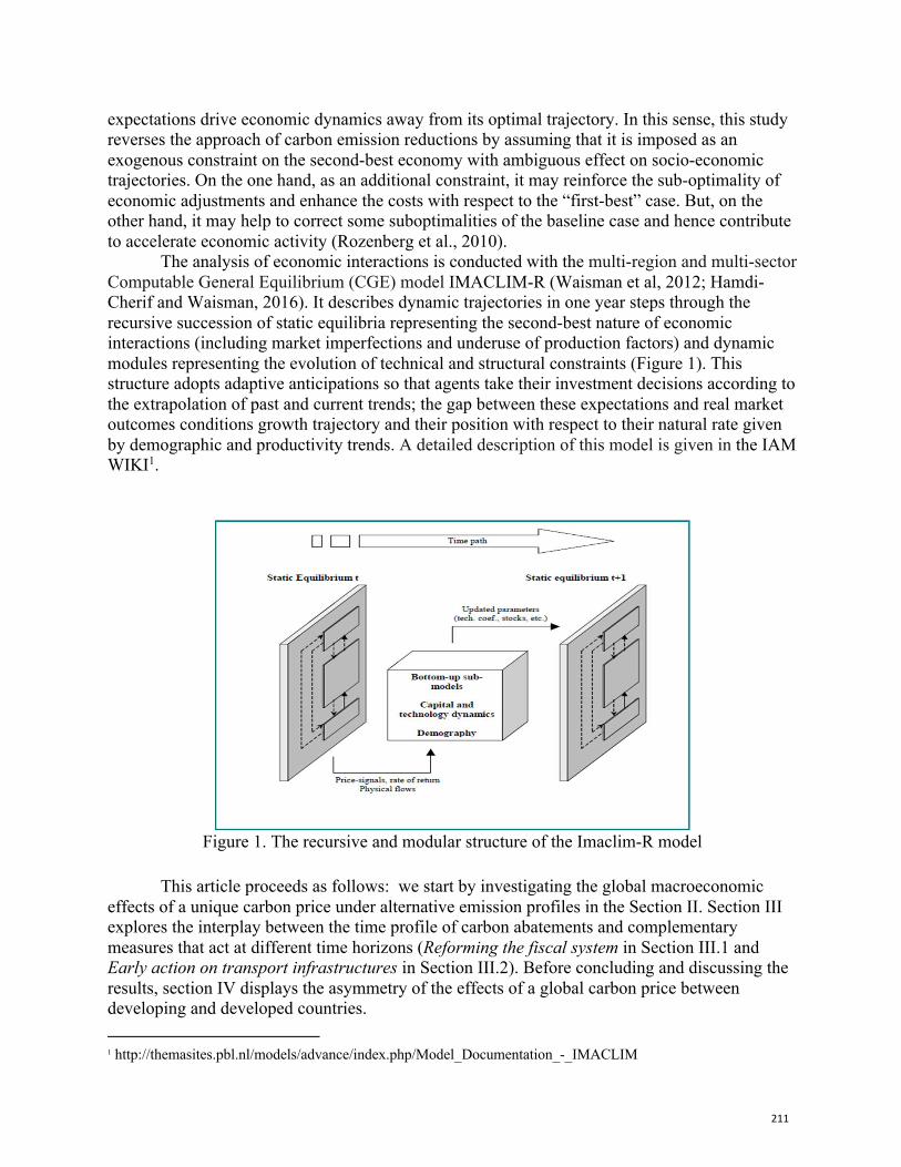
211

expectations drive economic dynamics away from its optimal trajectory. In this sense, this study reverses the approach of carbon emission reductions by assuming that it is imposed as an exogenous constraint on the second-best economy with ambiguous effect on socio-economic trajectories. On the one hand, as an additional constraint, it may reinforce the sub-optimality of economic adjustments and enhance the costs with respect to the “first-best” case. But, on the other hand, it may help to correct some suboptimalities of the baseline case and hence contribute to accelerate economic activity (Rozenberg et al., 2010).

The analysis of economic interactions is conducted with the multi-region and multi-sector Computable General Equilibrium (CGE) model IMACLIM-R (Waisman et al, 2012; Hamdi-Cherif and Waisman, 2016). It describes dynamic trajectories in one year steps through the recursive succession of static equilibria representing the second-best nature of economic interactions (including market imperfections and underuse of production factors) and dynamic modules representing the evolution of technical and structural constraints (Figure 1). This structure adopts adaptive anticipations so that agents take their investment decisions according to the extrapolation of past and current trends; the gap between these expectations and real market outcomes conditions growth trajectory and their position with respect to their natural rate given by demographic and productivity trends. A detailed description of this model is given in the IAM WIKI1.

Figure 1. The recursive and modular structure of the Imaclim-R model

This article proceeds as follows: we start by investigating the global macroeconomic

effects of a unique carbon price under alternative emission profiles in the Section II. Section III explores the interplay between the time profile of carbon abatements and complementary measures that act at different time horizons (Reforming the fiscal system in Section III.1 and Early action on transport infrastructures in Section III.2). Before concluding and discussing the results, section IV displays the asymmetry of the effects of a global carbon price between developing and developed countries.

1 http://themasites.pbl.nl/models/advance/index.php/Model_Documentation_-_IMACLIM

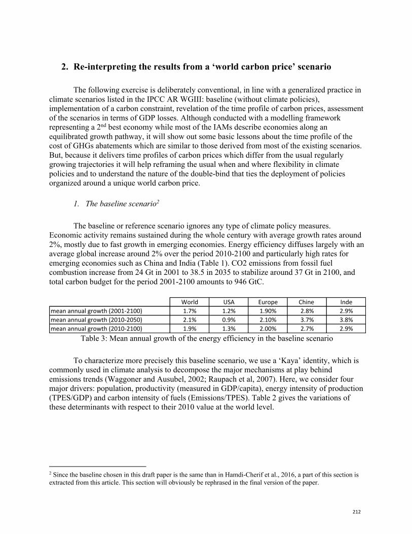
212

2. Re-interpreting the results from a ‘world carbon price’ scenario

The following exercise is deliberately conventional, in line with a generalized practice in

climate scenarios listed in the IPCC AR WGIII: baseline (without climate policies), implementation of a carbon constraint, revelation of the time profile of carbon prices, assessment of the scenarios in terms of GDP losses. Although conducted with a modelling framework representing a 2nd best economy while most of the IAMs describe economies along an equilibrated growth pathway, it will show out some basic lessons about the time profile of the cost of GHGs abatements which are similar to those derived from most of the existing scenarios. But, because it delivers time profiles of carbon prices which differ from the usual regularly growing trajectories it will help reframing the usual when and where flexibility in climate policies and to understand the nature of the double-bind that ties the deployment of policies organized around a unique world carbon price.

1. The baseline scenario2

The baseline or reference scenario ignores any type of climate policy measures. Economic activity remains sustained during the whole century with average growth rates around 2%, mostly due to fast growth in emerging economies. Energy efficiency diffuses largely with an average global increase around 2% over the period 2010-2100 and particularly high rates for emerging economies such as China and India (Table 1). CO2 emissions from fossil fuel combustion increase from 24 Gt in 2001 to 38.5 in 2035 to stabilize around 37 Gt in 2100, and total carbon budget for the period 2001-2100 amounts to 946 GtC.

Table 3: Mean annual growth of the energy efficiency in the baseline scenario

To characterize more precisely this baseline scenario, we use a ‘Kaya’ identity, which is

commonly used in climate analysis to decompose the major mechanisms at play behind emissions trends (Waggoner and Ausubel, 2002; Raupach et al, 2007). Here, we consider four major drivers: population, productivity (measured in GDP/capita), energy intensity of production (TPES/GDP) and carbon intensity of fuels (Emissions/TPES). Table 2 gives the variations of these determinants with respect to their 2010 value at the world level.

2 Since the baseline chosen in this draft paper is the same than in Hamdi-Cherif et al., 2016, a part of this section is extracted from this article. This section will obviously be rephrased in the final version of the paper.

World USA Europe Chine Indemean annual growth (2001-2100) 1.7% 1.2% 1.90% 2.8% 2.9%mean annual growth (2010-2050) 2.1% 0.9% 2.10% 3.7% 3.8%mean annual growth (2010-2100) 1.9% 1.3% 2.00% 2.7% 2.9%

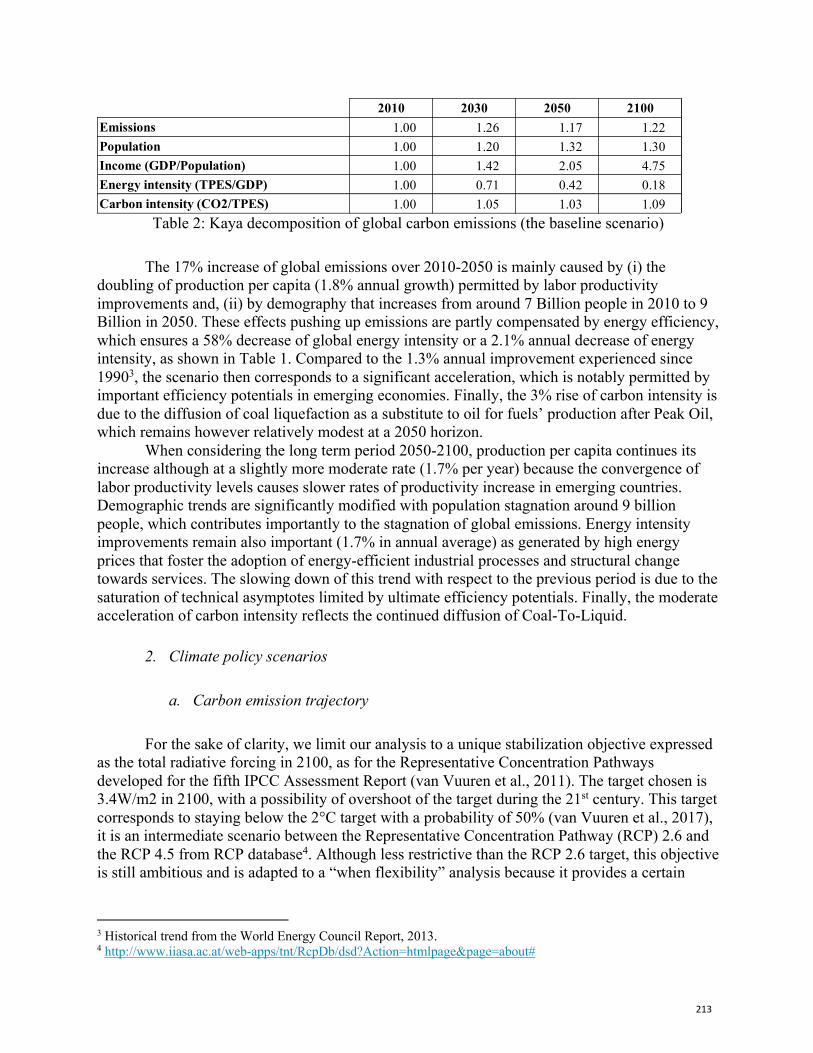
213

Table 2: Kaya decomposition of global carbon emissions (the baseline scenario)

The 17% increase of global emissions over 2010-2050 is mainly caused by (i) the

doubling of production per capita (1.8% annual growth) permitted by labor productivity improvements and, (ii) by demography that increases from around 7 Billion people in 2010 to 9 Billion in 2050. These effects pushing up emissions are partly compensated by energy efficiency, which ensures a 58% decrease of global energy intensity or a 2.1% annual decrease of energy intensity, as shown in Table 1. Compared to the 1.3% annual improvement experienced since 19903, the scenario then corresponds to a significant acceleration, which is notably permitted by important efficiency potentials in emerging economies. Finally, the 3% rise of carbon intensity is due to the diffusion of coal liquefaction as a substitute to oil for fuels’ production after Peak Oil, which remains however relatively modest at a 2050 horizon.

When considering the long term period 2050-2100, production per capita continues its increase although at a slightly more moderate rate (1.7% per year) because the convergence of labor productivity levels causes slower rates of productivity increase in emerging countries. Demographic trends are significantly modified with population stagnation around 9 billion people, which contributes importantly to the stagnation of global emissions. Energy intensity improvements remain also important (1.7% in annual average) as generated by high energy prices that foster the adoption of energy-efficient industrial processes and structural change towards services. The slowing down of this trend with respect to the previous period is due to the saturation of technical asymptotes limited by ultimate efficiency potentials. Finally, the moderate acceleration of carbon intensity reflects the continued diffusion of Coal-To-Liquid.

2. Climate policy scenarios

a. Carbon emission trajectory

For the sake of clarity, we limit our analysis to a unique stabilization objective expressed as the total radiative forcing in 2100, as for the Representative Concentration Pathways developed for the fifth IPCC Assessment Report (van Vuuren et al., 2011). The target chosen is 3.4W/m2 in 2100, with a possibility of overshoot of the target during the 21st century. This target corresponds to staying below the 2°C target with a probability of 50% (van Vuuren et al., 2017), it is an intermediate scenario between the Representative Concentration Pathway (RCP) 2.6 and the RCP 4.5 from RCP database4. Although less restrictive than the RCP 2.6 target, this objective is still ambitious and is adapted to a “when flexibility” analysis because it provides a certain

3 Historical trend from the World Energy Council Report, 2013. 4 http://www.iiasa.ac.at/web-apps/tnt/RcpDb/dsd?Action=htmlpage&page=about#

2010 2030 2050 2100Emissions 1.00 1.26 1.17 1.22 Population 1.00 1.20 1.32 1.30 Income (GDP/Population) 1.00 1.42 2.05 4.75 Energy intensity (TPES/GDP) 1.00 0.71 0.42 0.18 Carbon intensity (CO2/TPES) 1.00 1.05 1.03 1.09

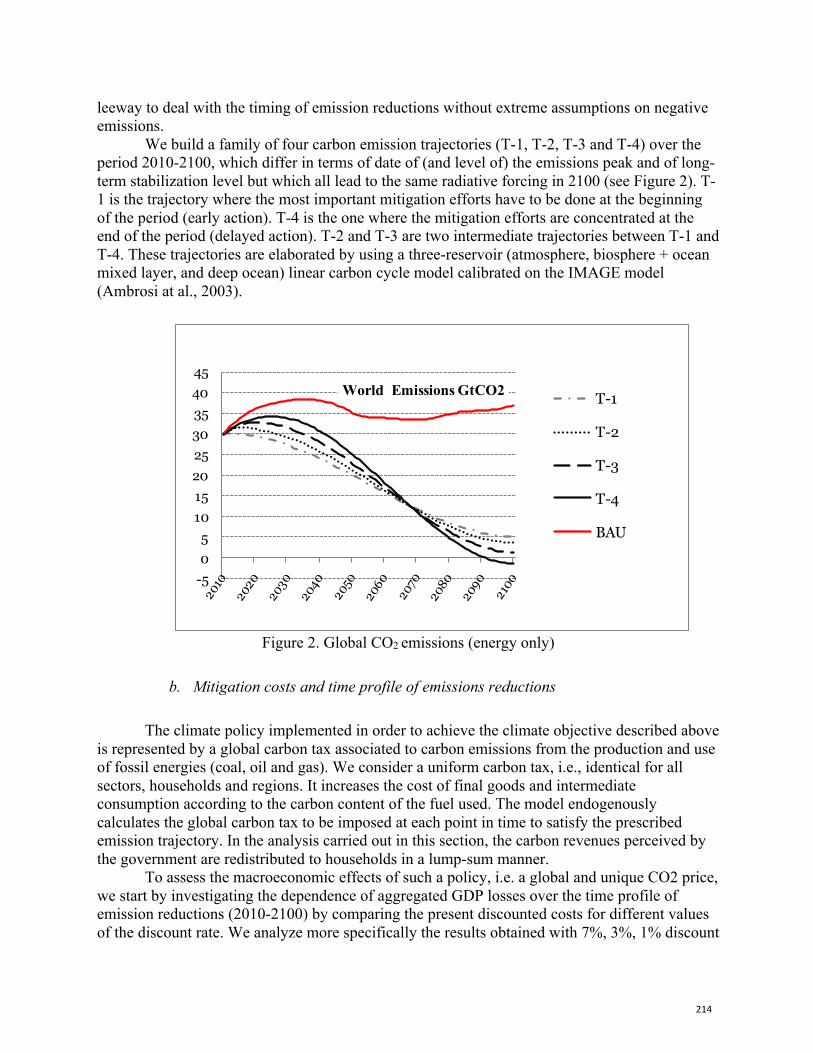
214

leeway to deal with the timing of emission reductions without extreme assumptions on negative emissions.

We build a family of four carbon emission trajectories (T-1, T-2, T-3 and T-4) over the period 2010-2100, which differ in terms of date of (and level of) the emissions peak and of long-term stabilization level but which all lead to the same radiative forcing in 2100 (see Figure 2). T-1 is the trajectory where the most important mitigation efforts have to be done at the beginning of the period (early action). T-4 is the one where the mitigation efforts are concentrated at the end of the period (delayed action). T-2 and T-3 are two intermediate trajectories between T-1 and T-4. These trajectories are elaborated by using a three-reservoir (atmosphere, biosphere + ocean mixed layer, and deep ocean) linear carbon cycle model calibrated on the IMAGE model (Ambrosi at al., 2003).

Figure 2. Global CO2 emissions (energy only)

b. Mitigation costs and time profile of emissions reductions

The climate policy implemented in order to achieve the climate objective described above

is represented by a global carbon tax associated to carbon emissions from the production and use of fossil energies (coal, oil and gas). We consider a uniform carbon tax, i.e., identical for all sectors, households and regions. It increases the cost of final goods and intermediate consumption according to the carbon content of the fuel used. The model endogenously calculates the global carbon tax to be imposed at each point in time to satisfy the prescribed emission trajectory. In the analysis carried out in this section, the carbon revenues perceived by the government are redistributed to households in a lump-sum manner.

To assess the macroeconomic effects of such a policy, i.e. a global and unique CO2 price, we start by investigating the dependence of aggregated GDP losses over the time profile of emission reductions (2010-2100) by comparing the present discounted costs for different values of the discount rate. We analyze more specifically the results obtained with 7%, 3%, 1% discount

-5051015202530354045

World Emissions GtCO2 T-1

T-2

T-3

T-4

BAU

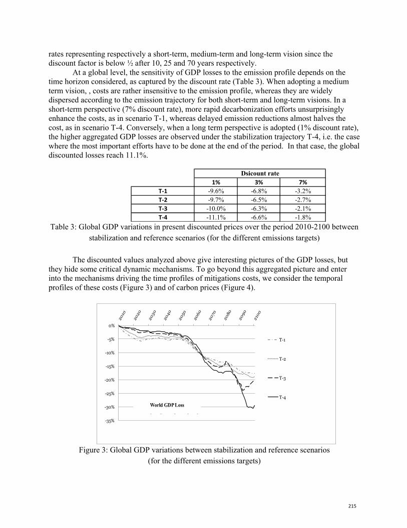
215

rates representing respectively a short-term, medium-term and long-term vision since the discount factor is below ½ after 10, 25 and 70 years respectively.

At a global level, the sensitivity of GDP losses to the emission profile depends on the time horizon considered, as captured by the discount rate (Table 3). When adopting a medium term vision, , costs are rather insensitive to the emission profile, whereas they are widely dispersed according to the emission trajectory for both short-term and long-term visions. In a short-term perspective (7% discount rate), more rapid decarbonization efforts unsurprisingly enhance the costs, as in scenario T-1, whereas delayed emission reductions almost halves the cost, as in scenario T-4. Conversely, when a long term perspective is adopted (1% discount rate), the higher aggregated GDP losses are observed under the stabilization trajectory T-4, i.e. the case where the most important efforts have to be done at the end of the period. In that case, the global discounted losses reach 11.1%.

Table 3: Global GDP variations in present discounted prices over the period 2010-2100 between

stabilization and reference scenarios (for the different emissions targets)

The discounted values analyzed above give interesting pictures of the GDP losses, but they hide some critical dynamic mechanisms. To go beyond this aggregated picture and enter into the mechanisms driving the time profiles of mitigations costs, we consider the temporal profiles of these costs (Figure 3) and of carbon prices (Figure 4).

Figure 3: Global GDP variations between stabilization and reference scenarios

(for the different emissions targets)

1% 3% 7%T-1 -9.6% -6.8% -3.2%T-2 -9.7% -6.5% -2.7%T-3 -10.0% -6.3% -2.1%T-4 -11.1% -6.6% -1.8%

Dsicount rate

-35%

-30%

-25%

-20%

-15%

-10%

-5%

0%

World GDP Loss"No recycling" no special policy

T-1

T-2

T-3

T-4

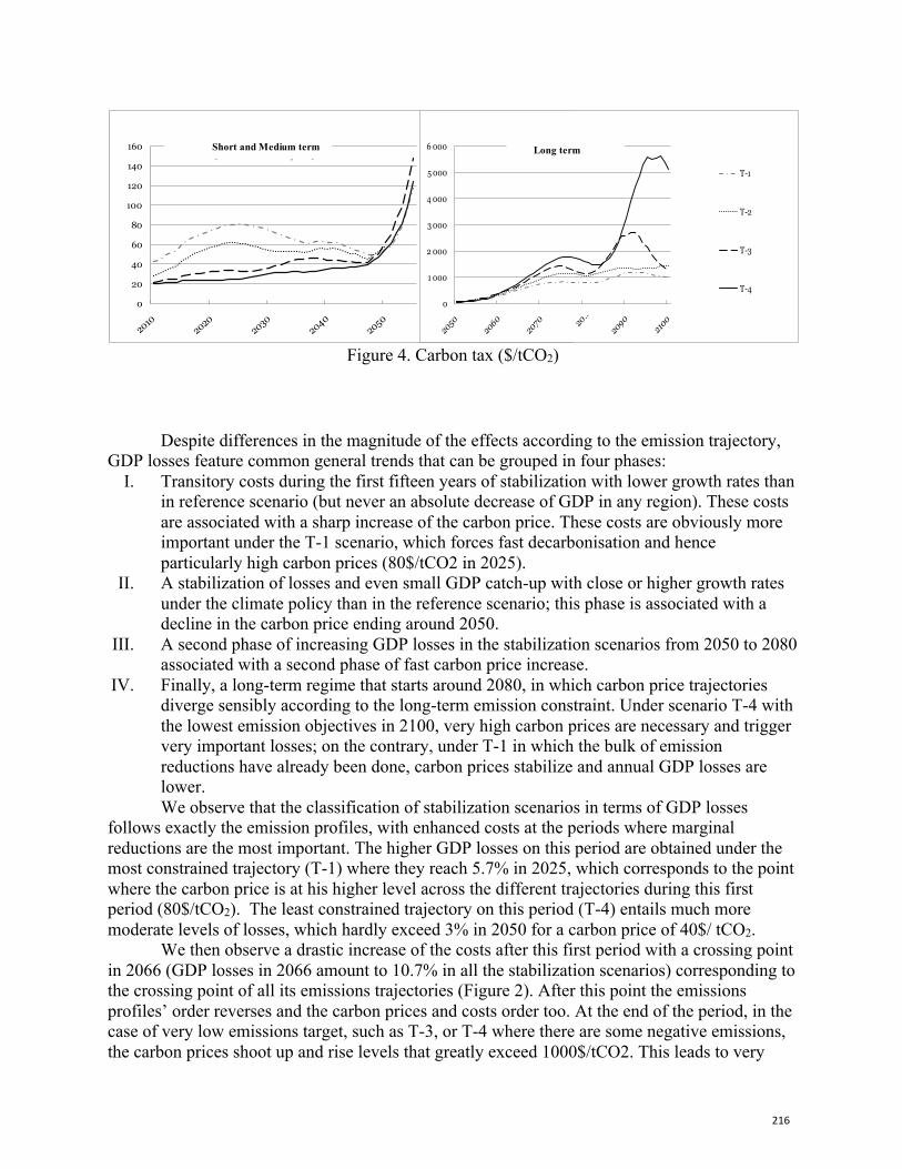
216

Figure 4. Carbon tax ($/tCO2)

Despite differences in the magnitude of the effects according to the emission trajectory,

GDP losses feature common general trends that can be grouped in four phases: I. Transitory costs during the first fifteen years of stabilization with lower growth rates than

in reference scenario (but never an absolute decrease of GDP in any region). These costs are associated with a sharp increase of the carbon price. These costs are obviously more important under the T-1 scenario, which forces fast decarbonisation and hence particularly high carbon prices (80$/tCO2 in 2025).

II. A stabilization of losses and even small GDP catch-up with close or higher growth rates under the climate policy than in the reference scenario; this phase is associated with a decline in the carbon price ending around 2050.

III. A second phase of increasing GDP losses in the stabilization scenarios from 2050 to 2080 associated with a second phase of fast carbon price increase.

IV. Finally, a long-term regime that starts around 2080, in which carbon price trajectories diverge sensibly according to the long-term emission constraint. Under scenario T-4 with the lowest emission objectives in 2100, very high carbon prices are necessary and trigger very important losses; on the contrary, under T-1 in which the bulk of emission reductions have already been done, carbon prices stabilize and annual GDP losses are lower. We observe that the classification of stabilization scenarios in terms of GDP losses

follows exactly the emission profiles, with enhanced costs at the periods where marginal reductions are the most important. The higher GDP losses on this period are obtained under the most constrained trajectory (T-1) where they reach 5.7% in 2025, which corresponds to the point where the carbon price is at his higher level across the different trajectories during this first period (80$/tCO2). The least constrained trajectory on this period (T-4) entails much more moderate levels of losses, which hardly exceed 3% in 2050 for a carbon price of 40$/ tCO2.

We then observe a drastic increase of the costs after this first period with a crossing point in 2066 (GDP losses in 2066 amount to 10.7% in all the stabilization scenarios) corresponding to the crossing point of all its emissions trajectories (Figure 2). After this point the emissions profiles’ order reverses and the carbon prices and costs order too. At the end of the period, in the case of very low emissions target, such as T-3, or T-4 where there are some negative emissions, the carbon prices shoot up and rise levels that greatly exceed 1000$/tCO2. This leads to very

0

20

40

60

80

100

120

140

160 CO2 prices short and medium termHsld recycl and no Infra policy

T-1

T-2

T-3

T-40

1 000

2 000

3 000

4 000

5 000

6 000 CO2 prices Long termHsld recycl and no Infra policy

T-1

T-2

T-3

T-4

Short and Medium term Long term

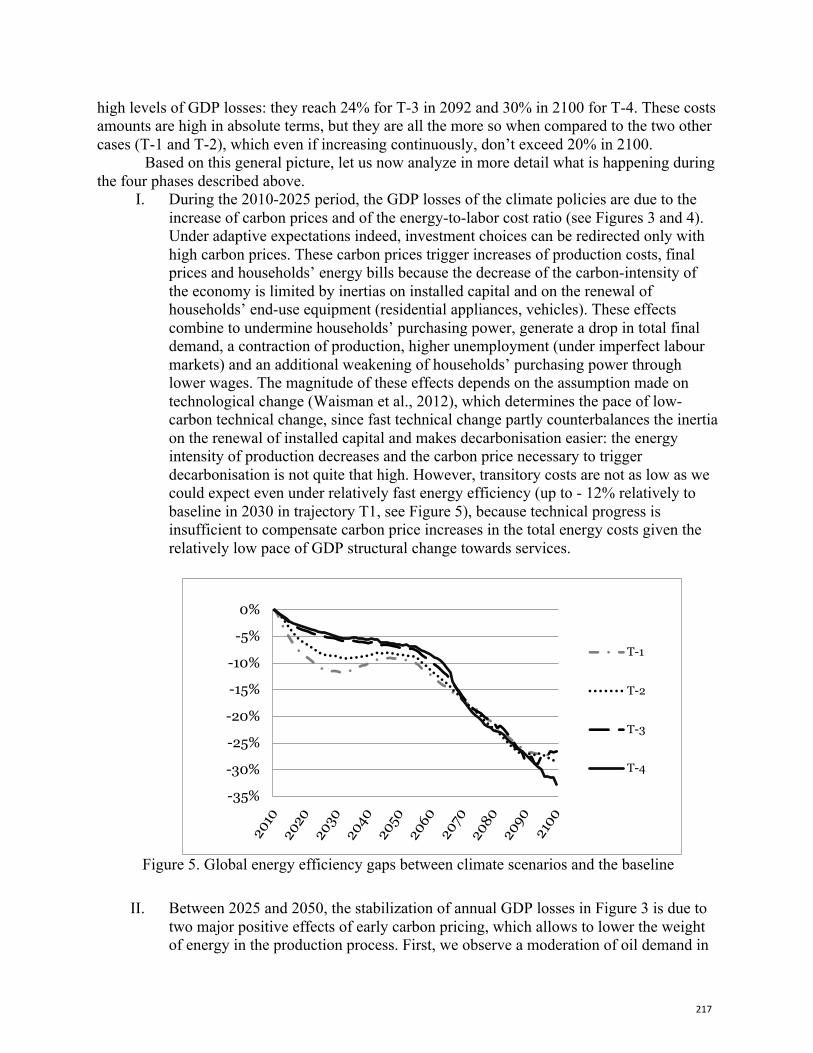
217

high levels of GDP losses: they reach 24% for T-3 in 2092 and 30% in 2100 for T-4. These costs amounts are high in absolute terms, but they are all the more so when compared to the two other cases (T-1 and T-2), which even if increasing continuously, don’t exceed 20% in 2100.

Based on this general picture, let us now analyze in more detail what is happening during the four phases described above.

I. During the 2010-2025 period, the GDP losses of the climate policies are due to the increase of carbon prices and of the energy-to-labor cost ratio (see Figures 3 and 4). Under adaptive expectations indeed, investment choices can be redirected only with high carbon prices. These carbon prices trigger increases of production costs, final prices and households’ energy bills because the decrease of the carbon-intensity of the economy is limited by inertias on installed capital and on the renewal of households’ end-use equipment (residential appliances, vehicles). These effects combine to undermine households’ purchasing power, generate a drop in total final demand, a contraction of production, higher unemployment (under imperfect labour markets) and an additional weakening of households’ purchasing power through lower wages. The magnitude of these effects depends on the assumption made on technological change (Waisman et al., 2012), which determines the pace of low-carbon technical change, since fast technical change partly counterbalances the inertia on the renewal of installed capital and makes decarbonisation easier: the energy intensity of production decreases and the carbon price necessary to trigger decarbonisation is not quite that high. However, transitory costs are not as low as we could expect even under relatively fast energy efficiency (up to - 12% relatively to baseline in 2030 in trajectory T1, see Figure 5), because technical progress is insufficient to compensate carbon price increases in the total energy costs given the relatively low pace of GDP structural change towards services.

Figure 5. Global energy efficiency gaps between climate scenarios and the baseline

II. Between 2025 and 2050, the stabilization of annual GDP losses in Figure 3 is due to

two major positive effects of early carbon pricing, which allows to lower the weight of energy in the production process. First, we observe a moderation of oil demand in

-35%

-30%

-25%

-20%

-15%

-10%

-5%

0%

2010

202020302040205020602070

208020902100

T-1

T-2

T-3

T-4

218

the stabilization scenario and the associated oil price increase (reduction of energy prices). Second, the accumulation of learning-by-doing favours the diffusion of carbon-free technologies over this time horizon, with the co-benefit of enhanced energy efficiency. The GDP losses are further moderated at this time horizon by the stabilization of carbon price towards around 40$/tCO2, which is a sufficient level to reach most mitigation potentials in the residential, industrial and power sectors (see Barker et al., 2007, Figure TS27). Those effects can be interpreted as a partial correction, via carbon pricing, of sub-optimal investment decisions in the baseline scenario thanks to the steady increase of fossil energy costs (carbon price included) which partly compensates for the imperfect anticipation of increases in oil prices in the reference scenario. It forces short-sighted decision-makers to progressively internalize constraints in fossil fuel availability, and accelerate learning-by-doing in low-carbon technologies. This provides a virtuous macroeconomic impact through a lower burden of imports in oil importing economies and reduced volatility of oil prices. In this sense, a carbon price is a hedging tool against the uncertainty on oil markets (Rozenberg et al., 2010).

III. From 2050 to 2080, a new phase of increasing GDP losses starts as a consequence of a sharp increase of carbon prices. Indeed, at this time horizon, most of the low cost mitigation potentials in the residential, industrial and power sectors have been exhausted, and the essential of emission reductions has to come from the transportation sector. A fast increase of carbon prices is then necessary to ensure emission reductions despite the weak sensitivity of the transportation sector to carbon prices and the trend of increasing carbon-intensive road-based mobility. This context is generated by the combination of four effects: i) the massive access to motorized mobility in developing countries, ii) the absence of targeted policies to control urban sprawl, which tends to increase the dependence on constrained mobility iii) the abundance of investments in road infrastructure, which favor the attractiveness of private cars at the expense of other transportation modes, iv) the rebound effect on mobility demand consecutive to energy efficiency gains, which offsets a significant part of the emissions reductions that would have resulted from technical energy efficiency improvement. These effects are particularly sensible in the T-4 scenario for which this period corresponds to the bulk of emission reductions with a division by 5 of total emissions between 2050 and 2080.

IV. Finally, over the very-long term the crucial determinant of GDP losses becomes the diffusion of power generation plants with biomass and CCS, since they are the only type of technologies enabling negative emissions. This possibility is crucial for the emission trajectories with very low or even negative emission levels in the long-term (T-3 and T-4), in which very high carbon prices are necessary to accelerate the progress on this technology and hence its diffusion on the markets. This effect also happens under T-1 and T-2 scenarios, but BioCCS technologies are less important, since targeted emission levels can be reached with only a marginal contribution of negative emissions.

We have observed that the more constrained carbon trajectory on the short term, the higher costs are generated in this period. This question of short-term costs is of the most importance, since it can create high social and political obstacles for implementing a climate policy. We could think that if we want to solve this issue, i.e. to reduce these high short term

219

costs, we can delay the action of mitigating emissions. But we have shown that doing this implies a persistence of the issue on the long term. Indeed, delaying the action on the short term allows reducing the early costs, but it makes things worse on the long term, generating higher economic losses than in the case of an early action. Moreover, albeit reduced, remaining short term costs can hinder (because of vested interests) the implementation of a low carbon transition. So we can shift the issue from short to long term, but it appears quite clearly that the question of “when flexibility” alone cannot solve the problem.

One of the direct corollaries is then to quickly implement innovation in order to ensure the availability of a new wave of technologies at very low costs for 2045-2050. That said, this indicates the objective, but not how to achieve it. In the technico-economic models, this technological acceleration occurs either (i) via an autonomous technical change, which implies a “manna from heaven” (Manne, 2002); or (ii) via induced technical change –triggered by learning-by-doing mechanisms obtained by setting adequately a simple coefficient without specifying its determinants (Grubb et al., 2002); or (iii) via Research and Development funding (Acemoglu et al., 2012) that induces a decrease of the costs of low carbon technologies obtained by the diffusion of the researchers’ knowledge, which is a kind of “manna from knowledge” since it is not specified how to overcome the “valley of death” of the innovation process (Grubb et al., 2014). The key is to trigger policies today that are able to launch such low carbon technologies processes. In the IMACLIM model, the only channel is the price signals; and due to inertia on technical systems and imperfect foresights, the necessary carbon price to induce technical progress is much higher than in other models. As highlighted above, such a high carbon price over the short run leads to significant macroeconomic losses, particularly in developing countries (see section IV). The short-term losses are admittedly lower than long-term ones, but they are nevertheless significant and represent a real barrier for the launching of the low carbon transition. Indeed, a cumulative growth reduction of 2 to 5% over a decade induces significant redistributive issues. It leads to a significant drop of public budgets that worsens the governments’ difficulties to meet short-term population’s expectations. It is thus necessary to rethink the question of “How to implement climate change policies?”, or more precisely, to think about complementary instruments that must be mobilized to reduce the costs of a mitigation target going beyond carbon pricing and the timing of the action.

3. Carbon prices within a broader policy-mix

In addition to the four options for carbon emissions trajectories that are described above, the analyses carried out in this article consider four groups of macroeconomic and sectoral measures adopted in the context of climate policies to accompany the carbon pricing policy.

I. Macroeconomic options The revenues of the carbon tax are perceived by the government. We limit our analysis to two standard possibilities according to the way these revenues are recycled: either fully redistributed to households in the form of a lump-sum transfer (Hsld) or used as a decrease of the pre-existing labor taxes (Labor).

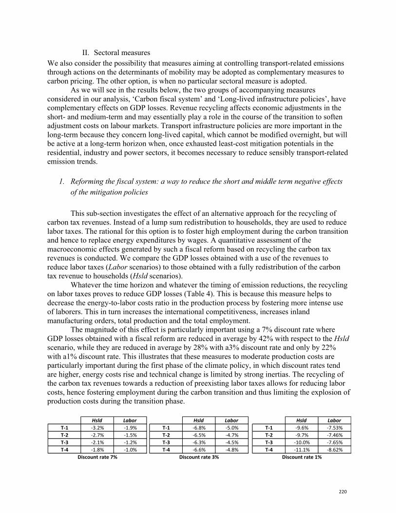
220

II. Sectoral measures We also consider the possibility that measures aiming at controlling transport-related emissions through actions on the determinants of mobility may be adopted as complementary measures to carbon pricing. The other option, is when no particular sectoral measure is adopted.

As we will see in the results below, the two groups of accompanying measures considered in our analysis, ‘Carbon fiscal system’ and ‘Long-lived infrastructure policies’, have complementary effects on GDP losses. Revenue recycling affects economic adjustments in the short- and medium-term and may essentially play a role in the course of the transition to soften adjustment costs on labour markets. Transport infrastructure policies are more important in the long-term because they concern long-lived capital, which cannot be modified overnight, but will be active at a long-term horizon when, once exhausted least-cost mitigation potentials in the residential, industry and power sectors, it becomes necessary to reduce sensibly transport-related emission trends.

1. Reforming the fiscal system: a way to reduce the short and middle term negative effects of the mitigation policies

This sub-section investigates the effect of an alternative approach for the recycling of

carbon tax revenues. Instead of a lump sum redistribution to households, they are used to reduce labor taxes. The rational for this option is to foster high employment during the carbon transition and hence to replace energy expenditures by wages. A quantitative assessment of the macroeconomic effects generated by such a fiscal reform based on recycling the carbon tax revenues is conducted. We compare the GDP losses obtained with a use of the revenues to reduce labor taxes (Labor scenarios) to those obtained with a fully redistribution of the carbon tax revenue to households (Hsld scenarios).

Whatever the time horizon and whatever the timing of emission reductions, the recycling on labor taxes proves to reduce GDP losses (Table 4). This is because this measure helps to decrease the energy-to-labor costs ratio in the production process by fostering more intense use of laborers. This in turn increases the international competitiveness, increases inland manufacturing orders, total production and the total employment.

The magnitude of this effect is particularly important using a 7% discount rate where GDP losses obtained with a fiscal reform are reduced in average by 42% with respect to the Hsld scenario, while they are reduced in average by 28% with a3% discount rate and only by 22% with a1% discount rate. This illustrates that these measures to moderate production costs are particularly important during the first phase of the climate policy, in which discount rates tend are higher, energy costs rise and technical change is limited by strong inertias. The recycling of the carbon tax revenues towards a reduction of preexisting labor taxes allows for reducing labor costs, hence fostering employment during the carbon transition and thus limiting the explosion of production costs during the transition phase.

Hsld Labor Hsld Labor Hsld LaborT-1 -3.2% -1.9% T-1 -6.8% -5.0% T-1 -9.6% -7.53%T-2 -2.7% -1.5% T-2 -6.5% -4.7% T-2 -9.7% -7.46%T-3 -2.1% -1.2% T-3 -6.3% -4.5% T-3 -10.0% -7.65%T-4 -1.8% -1.0% T-4 -6.6% -4.8% T-4 -11.1% -8.62%

Discount rate 7% Discount rate 1%Discount rate 3%

221

Table 4: Global GDP variations in present discounted prices over the period 2010-2100 between stabilization and reference scenarios

(for the different emissions targets, with different assumptions on the discount rate and the recycling modes of the carbon tax revenue)

This phenomenon suggests that a fiscal reform is really efficient on the short term, and

that complementary measures are necessary to improve the long term situation.

2. Early action on transport infrastructure: a way to reduce long term costs

The issue of the long term costs’ persistence is notably linked to the very specific dynamics of the transportation sector (Jaccard et al. 1997; IPCC, 2014c). The transport sector has proven to be the most difficult in which to reduce carbon emissions, and it represents a dominant share of remaining emissions in the long-term when ambitious mitigation objectives are set. As mentioned earlier, because of its weak reactivity to price increases, very high levels of carbon prices are needed in the second half of the century to reach low mitigation targets. That is why we finally test a design of climate policy where carbon pricing and the above described fiscal reform are complemented by measures aimed at controlling the long-term dynamics of transport-related emissions. More precisely, we consider:5

I. A shift in the modal structure of investment in transportation infrastructure favoring public modes against private cars. Instead of assuming that the allocation of investments follows modal mobility demand, we consider public policies that reallocate part of them from road to low-carbon transportation infrastructure (rail and water for freight transport, rail and non-motorized modes for passenger transport).

II. A spatial reorganization at the urban level with denser cities and soft measures towards less mobility-dependent conglomerations. We implement a reduction of households’ constrained mobility (essentially commuting and shopping).

These measures to control mobility growth offer mitigation potentials that are independent of carbon prices. Furthermore, these measures allow significant reductions of carbon price levels (on average 25% lower over 2050-2100) and hence help limiting the macroeconomic costs of climate change mitigation. The reduction of mobility needs and the shift towards low-carbon modes allow meeting the same climate objectives with far more moderate GDP losses, whatever the temporal perspective adopted and whatever the timing of emission reductions (Table 5). The comparison of the second and third columns of Table 5 shows that these investments have contrasted efficiency according to the time horizon considered. More specifically, they are more (respectively less) efficient in reducing mitigation costs than recycling measures towards labor taxes in the long term (respectively short term), as captured by the 1% (respectively 7%) discount rate results.

5 we assume a redirection of investments at constant total amount.

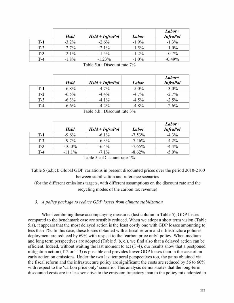
222

Hsld Hsld + InfraPol Labor Labor+ InfraPol

T-1 -3.2% -2.6% -1.9% -1.3% T-2 -2.7% -2.1% -1.5% -1.0% T-3 -2.1% -1.5% -1.2% -0.7% T-4 -1.8% -1.23% -1.0% -0.49%

Table 5.a : Discount rate 7%


T-1 -6.8% -4.7% -5.0% -3.0% T-2 -6.5% -4.4% -4.7% -2.7% T-3 -6.3% -4.1% -4.5% -2.5% T-4 -6.6% -4.2% -4.8% -2.6%

Table 5.b : Discount rate 3%


T-1 -9.6% -6.1% -7.53% -4.3% T-2 -9.7% -6.3% -7.46% -4.2% T-3 -10.0% -6.4% -7.65% -4.4% T-4 -11.1% -7.1% -8.62% -5.0%

Table 5.c :Discount rate 1% Table 5 (a,b,c): Global GDP variations in present discounted prices over the period 2010-2100

between stabilization and reference scenarios (for the different emissions targets, with different assumptions on the discount rate and the

recycling modes of the carbon tax revenue)

3. A policy package to reduce GDP losses from climate stabilization

When combining these accompanying measures (last column in Table 5), GDP losses compared to the benchmark case are sensibly reduced. When we adopt a short term vision (Table 5.a), it appears that the most delayed action is the least costly one with GDP losses amounting to less than 1%. In this case, these losses obtained with a fiscal reform and infrastructure policies deployment are reduced by 69% with respect to the ‘carbon price only’ policy. When medium and long term perspectives are adopted (Table 5. b, c.), we find also that a delayed action can be efficient. Indeed, without waiting the last moment to act (T-4), our results show that a postponed mitigation action (T-2 or T-3) is possible and provides lower GDP losses than in the case of an early action on emissions. Under the two last temporal perspectives too, the gains obtained via the fiscal reform and the infrastructure policy are significant: the costs are reduced by 56 to 60% with respect to the ‘carbon price only’ scenario. This analysis demonstrates that the long-term discounted costs are far less sensitive to the emission trajectory than to the policy mix adopted to

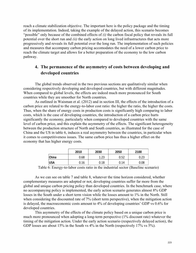
223

reach a climate stabilization objective. The important here is the policy package and the timing of its implementation. Indeed, taking the example of the delayed action, this scenario becomes “possible” only because of the combined effects of (i) the carbon fiscal policy that reveals its full potential over the short run and (ii) the early action on long lived infrastructures that acts more progressively and reveals its full potential over the long run. The implementation of such policies and measures that accompany carbon pricing accomodates the need of a lower carbon price to reach the climate target and allows for a better preparation of the economy to the low carbon pathway.

4. The permanence of the asymmetry of costs between developing and developed countries

The global trends observed in the two previous sections are qualitatively similar when

considering respectively developing and developed countries, but with different magnitudes. When compared to global levels, the effects are indeed much more pronounced for South countries while they are smoother for North countries.

As outlined in Waisman et al. (2012) and in section III, the effects of the introduction of a carbon price are related to the energy-to-labor cost ratio: the higher the ratio, the higher the costs. Thus, when the share of energy costs in production costs is significantly high comparing to labor costs, which is the case of developing countries, the introduction of a carbon price hurts significantly the economy, particularly when compared to developed countries with the same level of carbon price, and this explain the asymmetry of the effects. The significant heterogeneity between the production structure of North and South countries, as illustrated for the case of China and the US in table 6, induces a real asymmetry between the countries, in particular when it comes to competitiveness issues. The same carbon price has thus a higher effect on the economy that has higher energy costs.

Table 6: Energy-to-labor costs ratio in the industrial sector (Baseline scenario)

As we can see on table 7 and table 8, whatever the time horizon considered, whether

complementary measures are adopted or not, developing countries suffer far more from the global and unique carbon pricing policy than developed countries. In the benchmark case, where no accompanying policy is implemented, the early action scenario generates almost 8% GDP losses in the South under a short term vision while the losses amount to 1% in the North. Still when considering the discounted rate of 7% (short term perspective), when the mitigation action is delayed, the macroeconomic costs amount to 4% of developing countries’ GDP vs 0.6% for developed countries.

This asymmetry of the effects of the climate policy based on a unique carbon price is much more pronounced when adopting a long-term perspective (1% discount rate) whatever the timing of the mitigation action. Under the early action scenario (respectively delayed action), the GDP losses are about 15% in the South vs 4% in the North (respectively 17% vs 5%).

2010 2030 2050 2100China 0.68 1.23 0.52 0.23 USA 0.16 0.18 0.14 0.08

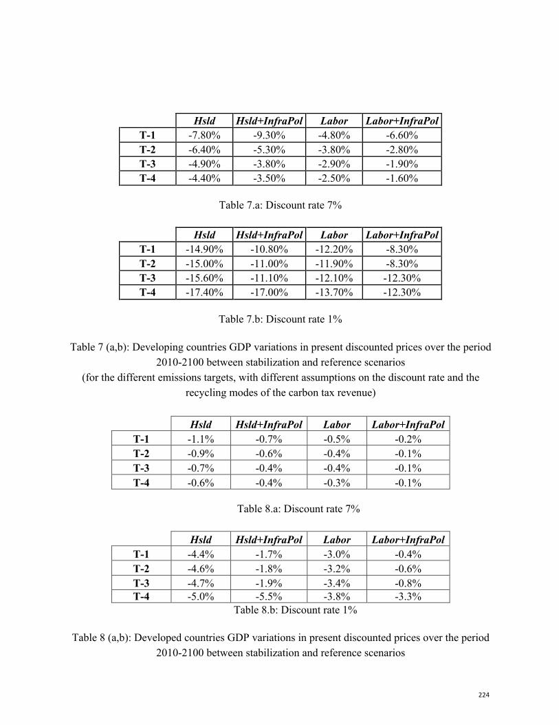
224

Hsld Hsld+InfraPol Labor Labor+InfraPol T-1 -7.80% -9.30% -4.80% -6.60% T-2 -6.40% -5.30% -3.80% -2.80% T-3 -4.90% -3.80% -2.90% -1.90% T-4 -4.40% -3.50% -2.50% -1.60%

Table 7.a: Discount rate 7%

Hsld Hsld+InfraPol Labor Labor+InfraPol

T-1 -14.90% -10.80% -12.20% -8.30% T-2 -15.00% -11.00% -11.90% -8.30% T-3 -15.60% -11.10% -12.10% -12.30% T-4 -17.40% -17.00% -13.70% -12.30%

Table 7.b: Discount rate 1%

Table 7 (a,b): Developing countries GDP variations in present discounted prices over the period

2010-2100 between stabilization and reference scenarios (for the different emissions targets, with different assumptions on the discount rate and the

recycling modes of the carbon tax revenue) Hsld Hsld+InfraPol Labor Labor+InfraPol

T-1 -1.1% -0.7% -0.5% -0.2% T-2 -0.9% -0.6% -0.4% -0.1% T-3 -0.7% -0.4% -0.4% -0.1% T-4 -0.6% -0.4% -0.3% -0.1%

Table 8.a: Discount rate 7% Hsld Hsld+InfraPol Labor Labor+InfraPol

T-1 -4.4% -1.7% -3.0% -0.4% T-2 -4.6% -1.8% -3.2% -0.6% T-3 -4.7% -1.9% -3.4% -0.8% T-4 -5.0% -5.5% -3.8% -3.3%

Table 8.b: Discount rate 1%

Table 8 (a,b): Developed countries GDP variations in present discounted prices over the period 2010-2100 between stabilization and reference scenarios

225

(for the different emissions targets, with different assumptions on the discount rate and the recycling modes of the carbon tax revenue)

Furthermore, it is worth noting that this asymmetry persists when the fiscal reform and

the transportation sector related measures are adopted. However, given the importance of the magnitude of the costs for the developing countries where an enriched population increasingly asks for basic infrastructure such as water supply, sewage, electricity, and transportation, and given thus the bifurcation challenge that most emerging economies are facing as they will build in the next decades the bulk of their long lived infrastructures, the implementation of measures allowing for a significant reduction of mitigation costs is all the more important. It is a real support to a bifurcation towards a low carbon development pathway.

This asymmetry between developed and developing countries is a major barrier to a unique carbon price at the world level and explains why, in the UNFCCC process, the article 136 of the decision de facto rules carbon pricing out of the negotiations, stating that it concerns only the national level. These numerical findings have robust theoretical reasons explained by Waisman et al. (2013). Basically, they result from the fact that in these countries, given the low level of wages and the high share of energy intensive industry to support the economic catch-up, the ratio of energy to labor cost is far higher than in developed countries. Hence the former see their productive system far more impacted than the latter. These costs propagate throughout the economy and the more energy represents a higher share of income, the more they will affect the purchasing power. The main finding is that the involvement of developing countries in the low carbon transition relies on other tools than carbon pricing which aim to accelerate low carbon investment.

5. Conclusion

The study carried out in this paper illustrates the macroeconomic effects of a global, unique and uniform carbon price and shows its limitations when considering a second-best framework.

It first revisits the role of the time profile of carbon emission reductions in the design of climate policies, when considering that it results from a political decision that may depart from economic optimization. This approach forces to consider the emission objective as an exogenous constraint on the economy and its effects become ambiguous when acknowledging the second-best nature of economic interactions where inertias and imperfect expectations drive economic dynamics away from its optimal trajectory. To investigate the effects of alternative emission profiles deciding the pace of the decarbonization process, we conduct a simulation exercise with the CGE energy-economy-environment model Imaclim-R. We demonstrate that the emission profile does not significantly change the time profile and the magnitude of GDP losses in the climate stabilization scenarios, but rather operates a time shift in their occurrence according to the period where most efforts are conducted.

Two principal sources of high costs are identified. On the one hand, the increase of the energy-to-labor costs ratio consecutive to the introduction of the carbon price in the short-term; on the other hand, transport-related emissions which force a rise of carbon prices in the long-term in all scenarios.

226

We then investigate the effect on these profiles of two complementary policies, an alternative recycling method for carbon revenues towards lower labor taxes and an infrastructure policy aimed at controlling transport emissions. Both measures taken separately prove to reduce notably mitigation costs by offsetting the short-term energy price increase and limiting the long-term rise of carbon prices respectively. Taken together, they even prove to combine their effects to offer very important reductions of GDP losses. This result is particularly important when considering the case of developing countries where the macroeconomic effects of a global price are much more pronounced than in developed countries. With an increased and enriched population, South countries are currently facing a real bifurcation challenge. They have the choice today, which will no longer be possible two decades ahead (Shukla and Dhar, 2011), of investing in long lived infrastructures that will place them on low carbon development pathways instead of on energy intensive pathways. This paper contributes to demonstrate that the involvement of developing countries in the low carbon transition relies on complementary tools to carbon pricing which aim to accelerate low carbon investment.

Going further the illustration of the limitations of a global carbon price, this quantitative study allows to illustrate that: — measures accompanying carbon pricing are as important determinant of GDP losses in

climate stabilization scenariosas the time profile of emission; — and that the sequencing of these options is closely related to the intertemporal tradeoff on

emission reduction. The second best modeling tool used here (IMACLIM-R) helps to illustrate that policy packages combining pricing instruments and other measures such as fiscal, sectoral and infrastructural measures, allow for meeting a climate target while reducing the significant GDP losses especially for developing countries.

It is worth noting that in all the considered scenarios of this study, as well as in the literature in this field like in all of the 5th IPCC report (2014), the financial constraint does not exist and technology changes are adopted in function of their merit order for a given discount rate. Thus, a logical outcome of this criticism requires the consideration of this caveat and the introduction of finance in climate policy modeling approaches. For future studies, the development of modeling tools that are able to capture and represent these phenomena is needed. This would help to bridge the gap and provide a common language between the environmental economy, which essentially considers a 'no-finance' universe, sectoral industrial economics and the debates in macro-finance. This would allow to link the discussions on carbon pricing and the financial framework that will continue to strongly influence economic policies in many regions. Agood understanding of their linkages is necessary to ensure that climate policies effectively contribute to lower investment risks.

6. References Acemoglu, D., Aghion, Ph., Burzstyn, L., Hemous, D. (2012) — « The Environment and Directed Technical Change

», The American Economic Review 102(1), p. 131–166. Cité p. 4, 28, 29, 34, 35, 42, 45, 52, 53, 54, 57, 59, 60, 61, 79, 84, 491, 492, 494, 496 et 498.

Ambrosi, P., J.-C. Hourcade, S. Hallegatte, F. Lecocq, P. Dumas and M. Ha-Duong. Optimal control models and elicitation of attitudes towards climate damages. 2003. Environmental Modeling and Assessment 8 (3), 135–147

Azar. C. 1998. The timing of CO2 emissions reductions: the debate revisited. International Journal of Environment and Pollution, 10(3):508-521

227

Azar C. and Dowlatabadi H. 1999. A review of the treatment of technical change in energy economics models. Annual Review of Energy and the Environment, 24:513-544

Goulder. L. H. 1995. Environmental taxation and the double dividend: a reader's guide. International Tax and Public Finance, 2(2):157_183

Goulder L. H., Mathai. K. 2002. Optimal CO2 abatement in the presence of induced technological change. Technological change and the environment, page 210

Grubb., M., Hourcade., J-C., Neuhoff., K., 2014 Planetary Economics, Earthscan, 517p Grubb. M. 1997. Technologies, energy systems and the timing of CO2 emissions abatement- an overview of

economic issues. Energy Policy, 25(2):159-172, 1997. Grubb., M., Köhler, J., Anderson, D. 2002. “Induced technical change in energy and environmental modeling:

analytic approaches and policy implications”, Annual Review of Energy and the Environment, 27, pp 271–308.

Hamdi-Cherif M. and Waisman H., 2016. “Global carbon pricing and the “Common but differentiated responsibilities” - The case of China”. International Environmental Agreements: Politics, Law and Economics. Volume 16, 671–689. DOI 10.1007/s10784-015-9289-2

Ha-Duong, M., Grubb, M. J. and J. C. Hourcade. 1997. Influence of socioeconomic inertia and uncertainty on optimal CO 2-emission abatement. Nature, 390:271

IPCC, 2014a: Clarke L., K. Jiang, K. Akimoto, M. Babiker, G. Blanford, K. Fisher-Vanden, J.-C. Hourcade, V. Krey, E. Kriegler, A. Löschel, D. McCollum, S. Paltsev, S. Rose, P. R. Shukla, M. Tavoni, B. C. C. van der Zwaan, and D.P. van Vuuren, 2014: Assessing Transformation Pathways. In: Climate Change 2014: Mitigation of Climate Change. Contribution of Working Group III to the Fifth Assessment Report of the Intergovernmental Panel on Climate Change [Edenhofer, O., R. Pichs-Madruga, Y. Sokona, E. Farahani, S. Kadner, K. Seyboth, A. Adler, I. Baum, S. Brunner, P. Eickemeier, B. Kriemann, J. Savolainen, S. Schlömer, C. von Stechow, T. Zwickel and J.C. Minx (eds.)]. Cambridge University Press, Cambridge, United Kingdom and New York, NY, USA.

IPCC, 2014b: Summary for Policymakers, In: Climate Change 2014, Mitigation of Climate Change. Contribution of Working Group III to the Fifth Assessment Report of the Intergovernmental Panel on Climate Change [Edenhofer, O., R. Pichs-Madruga, Y. Sokona, E. Farahani, S. Kadner, K. Seyboth, A. Adler, I. Baum, S. Brunner, P. Eickemeier, B. Kriemann, J. Savolainen, S. Schlomer, C. von Stechow, T. Zwickel and J.C. Minx (eds.)]. Cambridge University Press, Cambridge, United Kingdom and New York, NY, USA.

IPCC, 2014c, Sims R., R. Schaeffer, F. Creutzig, X. Cruz-Núñez, M. D’Agosto, D. Dimitriu, M. J. Figueroa Meza, L. Fulton, S. Kobayashi, O. Lah, A. McKinnon, P. Newman, M. Ouyang, J. J. Schauer, D. Sperling, and G. Tiwari, 2014: Transport. In: Climate Change 2014: Mitigation of Climate Change. Contribution of Working Group III to the Fifth Assessment Report of the Intergovernmental Panel on Climate Change [Edenhofer, O., R. Pichs-Madruga, Y. Sokona, E. Farahani, S. Kadner, K. Seyboth, A. Adler, I. Baum, S. Brunner, P. Eickemeier, B. Kriemann, J. Savolainen, S. Schlömer, C. von Stechow, T. Zwickel and J.C. Minx (eds.)]. Cambridge University Press, Cambridge, United Kingdom and New York, NY, USA.

IPCC Summary for Policymakers. In: B. Metz, O.R. Davidson, P.R. Bosch, R. Dave, L.A. Meyer (eds) Climate Change 2007: Mitigation. Contribution of Working Group III to the Fourth Assessment Report of the Intergovernmental Panel on Climate Change. CambridgeUniversity Press, Cambridge, United Kingdom and New York, NY, USA.

Jaccard M, Failing L and Berry T. 1997. From equipment to infrastructure: community energy management and greenhouse gas emission reduction. Energy Policy 25(13): 1065-1074

James K. Hammitt, Robert J. Lempert, and Michael E. Schlesinger. 1992. A sequential decision strategy for abating climate change. Nature, 357(6376):315-318

Manne, A., Richels, R. 2004. The impact of learning-by-doing on the timing and costs of CO2 abatement. Energy Economics, 26(4):603_619

Riahi, K., Kriegler, E., Johnson, N., Bertram, C., den Elzen, M., Eom, J., Schaeffer M., Jae Edmonds, J., Isaac, M., Krey, V., Longdon, T., Luderer, G., Mejean, M., McCollum, D.L., Mima, S., Turton, H., van Vuuren, D.P., Wada, K., Bosetti, V., Capros, P., Criqui, P., Hamdi-Cherif, M.; Kainuma, M., Edenhofer, O. 2015. "Locked into Copenhagen Pledges - Implications of short-term emission targets for the cost and feasibility of long-term climate goals".Technological Forecasting and Social Change, Volume 90, Part A, 8-23.

Richels, R., Edmonds, J. A. Gruenspecht, H. and T. M. L. Wigley. 1999. The berlin mandate: the design of cost-effective mitigation strategies. Energy and environmental policy modeling, page 67

Rozenberg J., Hallegatte S., Vogt-Schilb A., Sassi O., Guivarch C., Hourcade J.C., 2010 Climate policies as a hedge against the uncertainty on future oil supply, Climatic change 101 (3), 663-668

228

Shukla P.R, Dhar S. 2011. Climate Agreement in India: Aligning Options and Opportunities on a new track, International environmental agreements: politics, law and economics, 11 229-243

Toman, M. A. , Morgenstern, R. D. and J. Anderson. The economics of when flexibility in the design of greenhouse gas abatement policies. Annual Review of Energy and the Environment, 24:431-460, 1999.

Van Vuuren, D.P, Edmonds, J., Kainuma, M., Riahi, K., Thomson, A., Hibbard, K., Hurtt, G. C., Kram, T., Krey, V. and Jean-Francois Lamarque, et al. The representative concentration pathways: an overview. Climatic Change Volume 109, Numbers 1-2, 5-31, 2011.

Van Vuuren DP, Andries Hof, David Gernaat, Harmen Sytze de Boer, 2017. Limiting global temperature change to 1.5 °C - Implications for carbon budgets, emission pathways, and energy transitions. PBL Netherlands Environmental Assessment Agency, publication number 2743, November 2017.

Waisman H., Guivarch C., Grazi F. and Jean Charles Hourcade. 2012.The Imaclim-R model : infrastructures, technical inertia and the costs of low carbon futures under imperfect foresight. Climatic Change accepted for publication online first

Wigley, T. M. L. , Richels, R. and J. A. Edmonds., 1996. Economic and environmental choices in the stabilization of atmospheric CO2 concentrations. Nature, 379:240-243

229

Interaction between the carbon tax and renewable energy support schemes in Colombia: Complementary or overlapping? Author: Daniela Gutiérrez Torres1

Abstract

Colombia is advancing its climate change mitigation and renewable energy policy instruments. Specifically, the country has introduced support schemes for electricity generation from renewable energy sources (RES-E) and a national carbon tax. Therefore, these two instruments interact within the climate-energy policy mix. However, the interaction between them could be complementary or overlapping depending on the policy design of each instrument. The main objective of this paper is to analyze if the policy design elements of the carbon tax and the RES-E support schemes make them complementary or overlapping instruments. The methodology is mainly qualitative and encompasses descriptive, as well as, interpretative stages. Additionally, it comprises a comprehensive literature review and a content analysis based on interviews with related stakeholders. The analysis is made primarily through the comparison of the instruments’ policy objectives. Results show that the policy objective design element from the instruments was crucial to classify them as complementary and to conclude that their coexistence is justified. That is, the mitigation objective of the carbon tax and the energy security aim of the RES-E support schemes suggest the two instruments are complementary. Keywords: Colombia; carbon tax; renewable energy support schemes; interaction.

Acronyms AFOLU Agriculture, Forestry and Other Land Use ANLA National Authority of Environmental Licensing CO2 Carbon dioxide DIAN National Tax and Customs Directorate ECPI Energy and Climate Policy Interactions decision tool ETS Emissions trading scheme EU European Union GHG Greenhouse gases LAC Latin America and the Caribbean IDEAM Hydrology, Meteorology and Environmental Studies Institute IPCC Intergovernmental Panel on Climate Change NDC National Determined Contribution OECD Organization for Cooperation and Economic Development

1 Environmental engineer with a master’s degree in Environmental Management and Policy. E-mail: [email protected]

230

PROURE Rational and Efficient Energy Use Program RES Renewable energy sources RES-E Electricity from renewable energy sources R&D Research and development TGC Tradable Green Certificated UPME Mining and Energy Planning Unit VAT Value Added Tax

1. Introduction

Mitigation endeavors take form of legislation, policies, plans, strategies and instruments (IPCC 2014, 151). Low-carbon policy instrument portfolios are composed mainly by regulatory approaches, economic instruments, information schemes and voluntary agreements (Mundaca & Markandya 2016,1374 ). At a global level, the ones that are more widely used are the economic instruments. For instance, 73 percent of the low-carbon policy instruments implemented in Latin America and the Caribbean (LAC) correspond to subsidies, loans, tax credits, as well as, research and development (R&D) (Mundaca & Markandya 2016, 1378).

Colombia is not an exception when it comes to implementing climate change mitigation or renewable energy economic instruments. The national carbon tax was introduced in 2017 (Congreso de la República 2016,112) and the support schemes for electricity generated from renewable energy sources (RES-E) commenced in 2014 (Congreso de Colombia, 2014,1-26). As these two instruments coexist in Colombia’s climate-energy policy package, interactions among them take place (Oikonomou & Jepma 2008, 131-156). While such interactions can be mutually reinforcing, they can also work against each other, or can be redundant, depending on how both instruments are designed and implemented (Hood 2011, 9). Thus, a justification of their coexistence depends greatly on their design elements interaction.

The existence of a broad portfolio of climate and energy policy instruments in the European Union (EU) allows an increase in the number of analyses of individual policies. However, it is not the same trend for the interaction evaluation of these policies with each other (Hood 2013,15). Interaction evaluations between carbon pricing, Renewable Energy Sources (RES) support schemes and energy efficiency policies are still areas that require further investigation. This relates especially to the mitigation policy instruments and the renewable energy technology deployment (Philibert 2011, 20).

This paper essentially aims to understand whether the carbon tax and electricity from renewable energy sources (RES-E) support schemes in Colombia complement or overlap with each other based on their design elements to understand if their coexistence in the policy mix is justified. Two research questions guide this paper: 1) How do the policy instrument design elements of the Colombian carbon tax and the RES-E support schemes interact?, 2) Does the interaction between the design elements of the carbon tax and the RES-E support schemes justify, or not, their coexistence in Colombia’s climate-energy policy mix?

2. Literature Review

The notion that a robust climate-energy package is needed has increased the global trend of combining policy instruments (Oikonomou et al. 2008,132). For instance, (del Río 2010,

231

4978) shows that a complex policy portfolio including Emission Trading Schemes (ETS), carbon taxes, RES-E support schemes, energy-efficiency standards and voluntary agreements, has been introduced in the European Union (EU) to reduce GHG emissions and secure energy supply. Likewise, in Colombia, RES-E support schemes have been in place since 2014 (Congreso de Colombia 2014, 1-26), a carbon tax was introduced in 2017 (Congreso de la República, 2016, 112) and an ETS is currently designed (Minambiente, 2017).

(Del Río 2010,4978) states that policy instruments’ combination raises concerns about potential overlaps, conflicts or synergies in their interaction. Likewise, (Oikonomou and Jepma 2008,140), as well as, (Sorrel et al. 2003,135) indicate that policy instruments can be complementary and mutually reinforcing, but there is also a risk that different policy instruments will weaken the objectives and credibility of each other. Similarly, (Duval 2008,27) exposes that there are risks of poorly-designed policy mixes resulting in decrease of cost-effectiveness and environmental integrity. (Fais et al. 2015, 255) state that this has increased the attention to policy interaction and coordination.

(Sonnenschein 2016,135) claims that mitigation provided through low-cost abatement measures by an ETS is not enough to achieve a deep decarbonization. Thus, the RES technologies which are generally more expensive are essential to accelerate GHG reduction. Further, (Sonnenschein 2016,135) emphasizes that delaying the deployment of RES-E technology will increase the cost of reaching long-term GHG reduction targets. Similarly, (Philibert 2011, 5) states that immediate CO2 reductions driven by the early deployment of renewable energy may cost more than other options in the short term, but will reduce the costs of mitigating climate change in the future. Furthermore, (del Río 2017,829) claims that additional costs of CO2 mitigation resulting from the combination of targets and instruments could be interpreted as the costs of achieving non-CO2 goals added to the dynamic efficiency benefits of RES-E deployment. Therefore, he argues not to focus on the costs of achieving one goal in the presence of one market failure, but instead contemplate the costs of attaining different goals simultaneously, considering that there are several market failures (del Río, 2017,831). This also means that the interaction may result in higher compliance costs related to a specific mitigation target, but not necessarily to higher costs to reach all goals jointly.

Moreover, (del Río 2014, 268), as well as (Lehmann and Gawel 2013,603), stress that attention to the environmental benefits aside from CO2 reduction objective by RES-E support needs to be held. (Lehmann and Gawel 2013, 603) emphasize that, besides a CO2 reduction aim, additional objectives like energy supply security and industrial policy support provide a rationale for implementing RES-E support schemes in addition to a carbon pricing instrument. First, non-renewable energy sources as oil or coal cause ecological impacts, thus, introducing RES generate environmental benefits aside from GHG emission reduction. Second, energy supply security supplemented by RES increases the variety of domestic energy sources decreasing dependency on energy imports. Third, small and medium enterprises, as well as independent electricity producers, might be benefited by RES-E support schemes.

Tinbergen (1952) points out that multiple market failures require multiple policy instruments. The number of targets must also equal the number of instruments (del Río, 2017,829). In addition, the Organization for Cooperation and Economic Development (OECD 2013, 35) exposes that no single policy instrument can achieve a mitigation target at a reasonable cost. (Delbeke and Vis 2016, 2) attest this adding that mitigation occurs across a multitude of sectors and activities. Therefore, the implementation of a robust climate-energy instrument mix, potentially including carbon pricing instruments, renewable energy subsidies, energy efficiency

232

standards, to mention a few, is justified (World Bank, 2017c, 38). In this same line, (Hood 2011-8, 2013-5) considers that an appropriate cost-effective policy package, while country and region-specific, will be compound by energy efficiency policies, RES support schemes and a carbon price policy instrument.

Besides, (Duval 2008, 44) advocate that the multiplicity of market failures to be addressed, including environmental externalities generated by GHG emissions, imperfect information and innovation and diffusion failures, makes it unlikely that cost-effective climate mitigation can be achieved through a single policy instrument. Similarly, (Fankhauser et al. 2010, 4) conclude that a variety of models suggest that in presence of multiple market failures, a portfolio of policies to reduce emissions is more optimal than a single policy. In addition, it will achieve results at a significantly lower social cost.

In this same stream, (Lehmann and Gawel 2013,599) state that the existence of two market failures justifies adding an RES-E support scheme to an ETS. These are the externalities caused from GHG emissions and knowledge generation. The second, also known as knowledge spillover, refers to the new knowledge produced through innovation by one firm that spills to other firms.

(Lehmann and Gawel 2013) imply that the EU ETS which is designed to correct externalities from CO2 emissions, stand-alone won’t be enough to induce technological change. Along with (Twomey 2012, 14), they support that in the existence of knowledge spillovers, a policy combination which includes a RES-E support scheme is justified. Likewise, (Sonnenschein 2016,135) emphasizes that an ETS alone is not cost-effective because it does not capture positive externalities resulting from knowledge spill-overs.

Besides, (Lehmann & Gawel 2013,599) stress that adding RES-E support schemes is justifiable because the external costs of non-renewable energy sources are not internalized completely. Aside from GHG emissions, non-renewable energy sources generate additional external costs. For instance, ecological impacts from oil spills in offshore platforms or open-cast mining for coal. Nuclear energy can cause possible future accidents and the final storage of its waste generates externalities. Moreover, energy supply security can be affected when natural gas or oil are imported from politically unstable countries.

The OECD states that carbon pricing should be central in reducing GHG emissions at the least-cost. However, it alone is not sufficient to address other market failures and achieve other environmental, social and economic objectives (OECD, 2013,35). Similarly, although renewable energy technologies play an important role in reducing GHG emissions; they alone would not suffice to keep climate change manageable (Philibert 2011, 5). Therefore, a climate-energy policy mix is justified. Essentially, a carbon price instrument, whether a carbon tax or an ETS, or both, should be combined with an energy efficiency policy, technology development and deployment support (usually renewable energy) (Hood 2013,5).

(Fais et al. 2015, 355), (Görlach 2013,3) and (Mickwitz 2003, 426) pledge that evaluation of policy interaction often comprises criteria such as effectiveness, efficiency and political feasibility. (Del Río 2014, 269) claims that analysis of the interaction between a pair of policy instruments should often be developed through their design elements. Furthermore, (del Río 2017, 831) argues that discussion related to the climate and energy package often takes place at a very abstract level, leaving out specific instruments and design elements.

There are several ways to classify design element interaction. (Del Río 2014, 273) proposes to analyze interactions ranging from strong and weak conflict, full complementarity to synergy. (Sorrel et al. 2003,36), distinguishes five types of interaction: direct, indirect, operational,

233

sequencing and trading. An additional classification is presented by (Oikonomou et al. 2010, 4187- 2014,47). They propose to classify interactions between policy instrument design elements as overlapping, complementary or indifferent. If the interactions carry over positive impacts on the policy mix, they are considered complementary; if they reduce the overall effects that each instrument stand-alone could generate in the market in achieving their objectives, they are considered overlapping and if a design element is not influencing the same design element of the second policy instrument, they are considered indifferent.

3. Research design

3.1 Methodology

3.1.1 Descriptive stage

This part of the paper firstly applies the first two steps of the Energy and Climate Policy

Interactions (ECPI) decision tool. ECPI applies a qualitative framework for analyzing the interaction among policy instruments.It is mainly for policy mixes instead of pairwise combinations, however, the author has partially applied the methodology to the interaction between two policy instruments in Colombia, i.e. the carbon tax and the RES-E support schemes. The first step meant to describe the policy instruments to understand their nature. After this, the next step was to compare both policy instruments in six main design elements (Oikonomou et al., 2010,4190 -2014,50). Table 1 presents these design area with their key elements and definitions.

Main design area

Key elements Definition

Measure identification

Measure type Refers to the category of policy instrument, e.g., carbon tax, ETS, RES-E support scheme

Application in the market

The option for a policy target group to participate or not in the instrument’s objective accomplishment.

Scope Classifies the instrument into national or international Objectives Nature of targets General objective of a policy translated into targets in

different ambient levels, e.g., promote renewable energy, GHG reduction or increase energy efficiency

Level of targets Classify the instrument’s target into low or high stringency Energy/environmental goals

Catalogues the instrument into energy or environment oriented.

Type of energy Describes which category of energy the instrument is addressing: primary or final energy. Targeting sources of primary energy leads to a substitution effect and hence to cleaner production, while targeting final energy stimulates energy efficiency and reduction of energy use.

Target groups Obligated entities Refers to the market agent that participates in the fulfilment of the target, distinguished into energy producers, energy suppliers, industry or consumers

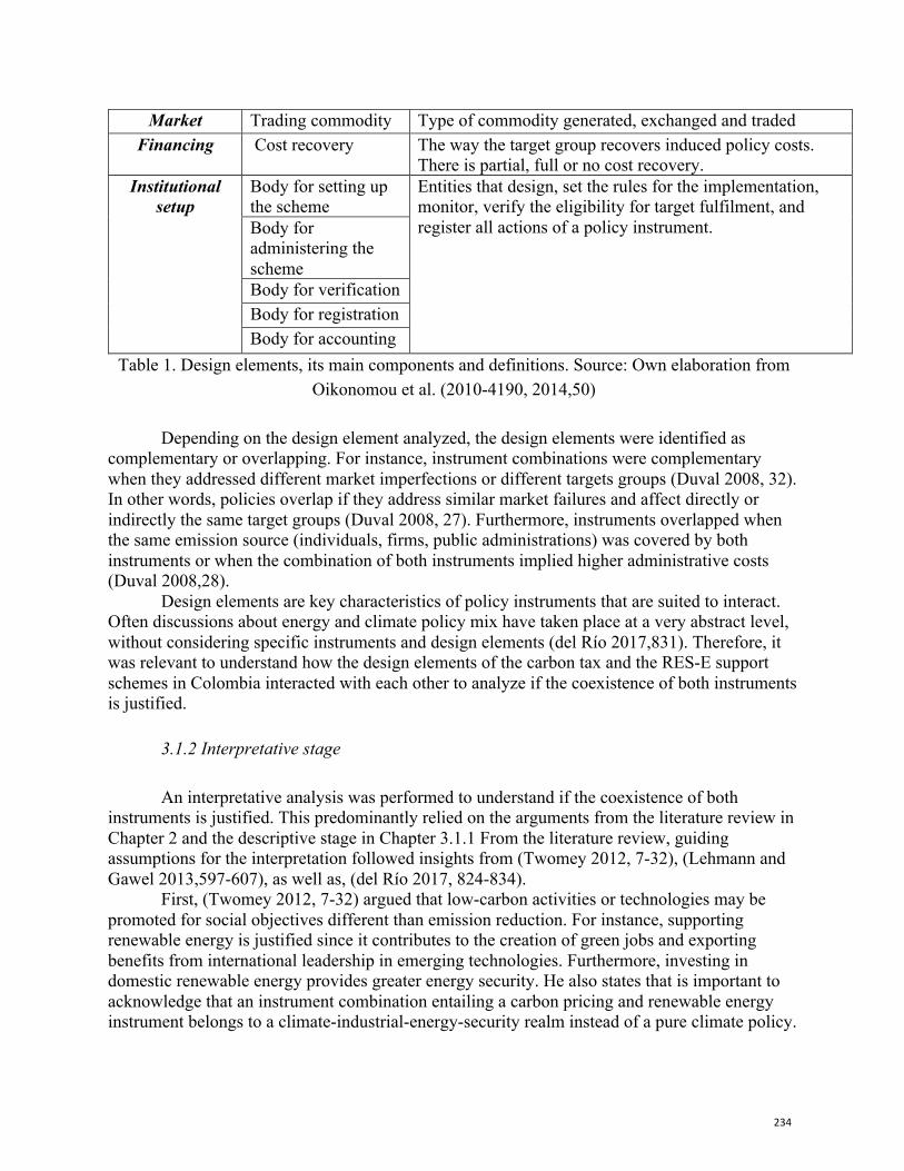
234

Market Trading commodity Type of commodity generated, exchanged and traded Financing Cost recovery The way the target group recovers induced policy costs.

There is partial, full or no cost recovery. Institutional

setup Body for setting up the scheme

Entities that design, set the rules for the implementation, monitor, verify the eligibility for target fulfilment, and register all actions of a policy instrument.

Body for administering the scheme Body for verification Body for registration Body for accounting

Table 1. Design elements, its main components and definitions. Source: Own elaboration from Oikonomou et al. (2010-4190, 2014,50)

Depending on the design element analyzed, the design elements were identified as

complementary or overlapping. For instance, instrument combinations were complementary when they addressed different market imperfections or different targets groups (Duval 2008, 32). In other words, policies overlap if they address similar market failures and affect directly or indirectly the same target groups (Duval 2008, 27). Furthermore, instruments overlapped when the same emission source (individuals, firms, public administrations) was covered by both instruments or when the combination of both instruments implied higher administrative costs (Duval 2008,28).

Design elements are key characteristics of policy instruments that are suited to interact. Often discussions about energy and climate policy mix have taken place at a very abstract level, without considering specific instruments and design elements (del Río 2017,831). Therefore, it was relevant to understand how the design elements of the carbon tax and the RES-E support schemes in Colombia interacted with each other to analyze if the coexistence of both instruments is justified.

3.1.2 Interpretative stage

An interpretative analysis was performed to understand if the coexistence of both instruments is justified. This predominantly relied on the arguments from the literature review in Chapter 2 and the descriptive stage in Chapter 3.1.1 From the literature review, guiding assumptions for the interpretation followed insights from (Twomey 2012, 7-32), (Lehmann and Gawel 2013,597-607), as well as, (del Río 2017, 824-834).

First, (Twomey 2012, 7-32) argued that low-carbon activities or technologies may be promoted for social objectives different than emission reduction. For instance, supporting renewable energy is justified since it contributes to the creation of green jobs and exporting benefits from international leadership in emerging technologies. Furthermore, investing in domestic renewable energy provides greater energy security. He also states that is important to acknowledge that an instrument combination entailing a carbon pricing and renewable energy instrument belongs to a climate-industrial-energy-security realm instead of a pure climate policy.

235

Second, (Lehmann and Gawel 2013,603) claimed that the existence of multiple policy objectives might provide a further, political rationale for implementing RES-E support schemes next to a carbon pricing instrument, e.g. EU ETS. For instance, they mention that an autonomous, politically set, RES-E deployment target justifies its existence in the policy mix along with an emission policy instrument. Moreover, they stated that using RES-E may also provide environmental benefits apart from GHG reduction, like air pollution reduction from fossil fuel combustion and conservation of non-renewable resources. Additionally, in some countries RES-E promotion suggests substituting oil and natural gas imports from unstable countries. Thus, RES-E support increases the variety of available domestic energy sources .Furthermore, (Lehmann and Gawel 2013, 603) claimed that RES-E support schemes have been identified to benefit small and medium-sized independent electricity producers. Thus, they have been considered as an effective tool of industry policy.

Third, (del Río 2017,829) emphasized that often, policymakers have other goals apart from CO2 mitigation. For instance, in the climate and energy realm, other goals involve energy supply security (diversification of energy sources), energy affordability, job and industry creation, as well as, regional development. While carbon-pricing instruments such as an ETS and RES-E support schemes share one common goal, i.e., CO2 emission reductions, RES-E support schemes contribute to other goals in addition to CO2 mitigation. However, these are not usually included in marginal abatement curves. Moreover, (del Río 2017,829) concluded that combinations of instruments may be justified if they address different goals. That is, if the existence of several goals cannot be achieved by only one instrument.

3.2 Methods

3.2.1 Data creation

For this paper, individual semi-structured interviews were performed. They were audio-recorded (when the interviewees agreed to) aiming to retain a full, uninterpreted record of what was mentioned in the interview and then were transcribed. Semi-structured interviews were conducted with representatives from the following institutions: Ministry of Environment and Sustainable Development, Ministry of Energy and Mining, National Planning Department, Mining and Energy Planning Unit, Interamerican Development Bank, World Bank and World Wildlife Fund.

3.2.2 Data collection A comprehensive literature review was conducted through the collection of data related to climate mitigation and renewable energy policy instruments interaction. The literature review included scientific and peer-reviewed journals, governmental and institutional reports.

3.2.3 Data analysis

With the purpose of identifying key analysis elements generated in the semi-structured interviews a content analysis was performed. An open-coding process was developed for each

236

interview. After the emergent codes were listed, the common ones were merged into sub-themes. After this, the procedure was repeated with sub-themes and final themes were identified.

4. Findings

4.1 Carbon tax in Colombia

The carbon tax in Colombia was part of the “green tax” package introduced by the Colombian government in the tax structural reform. Along with Mexico and Chile, Colombia is one of the pioneer countries in LAC that has adopted a carbon tax. However, the amount of emissions reductions that will be achieved by the tax remains uncertain (Görlach 2013,4).

A carbon price instrument, in this case a tax, provides an economic signal to emitters and allows them to decide to either transform their activities and lower their emissions or continue emitting and paying for their emissions. The overall environmental goal is to achieve this in the most flexible and least-cost way to society (World Bank, 2017b). Carbon pricing is often presented as a cross-sectoral cornerstone of a package of policy measures designed to achieve GHG emissions reductions at lowest cost (World Bank & OECD 2015, 11). It helps to minimize the market failure caused by firms and individuals not taking into account the costs, in terms of climate damages, that result from activities that lead to further emissions (World Bank et al., 2016, 58).

There are two main types of taxes which in some cases are used indistinguishably. Taxes can set a price per unit of pollutant emitted and can be directly applied to the pollution source or in contrast to the inputs or outputs of a production process (Görlach 2013,4). In this sense, the first tax type is an emission tax on GHG emissions which requires individual emitters to pay a fee, charge or a tax for every ton of GHG released into the atmosphere (Gupta et al. 2007, 755). The tax is directly applied to the pollution source and is imposed on the actual GHG emissions. In addition for this type of tax, taxpayers need to monitor and report their actual emissions (Görlach 2013,4). The second case is a carbon tax which directly sets a price on carbon by defining an explicit tax rate on the carbon content of fossil fuel (World Bank, 2017b).

The carbon tax in Colombia belongs to the second category of carbon taxes presented before. It is a tax on the carbon content of fossil fuels instead of a tax on the GHG emissions for direct sources. It entails all petroleum derivatives, as well as, all gaseous fuels used for energy purposes, but excludes coal. Transportation sector emits 38 percent of the GHG emitted by energy sector, which contributes with 44 percent of total GHG in Colombia (IDEAM et al. 2015, 93). Figure 2 presents the GHG inventory with an emphasis on energy sector.

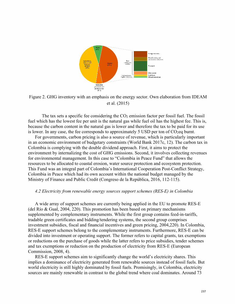
237

Figure 2. GHG inventory with an emphasis on the energy sector. Own elaboration from IDEAM

et al. (2015)

The tax sets a specific fee considering the CO2 emission factor per fossil fuel. The fossil fuel which has the lowest fee per unit is the natural gas while fuel oil has the highest fee. This is, because the carbon content in the natural gas is lower and therefore the tax to be paid for its use is lower. In any case, the fee corresponds to approximately 5 USD per ton of CO2eq burnt.

For governments, carbon pricing is also a source of revenue, which is particularly important in an economic environment of budgetary constraints (World Bank 2017c, 12). The carbon tax in Colombia is complying with the double dividend approach. First, it aims to protect the environment by internalizing the cost of GHG emissions. Second, it involves collecting revenues for environmental management. In this case to “Colombia in Peace Fund” that allows the resources to be allocated to coastal erosion, water source protection and ecosystem protection. This Fund was an integral part of Colombia’s International Cooperation Post-Conflict Strategy, Colombia in Peace which had its own account within the national budget managed by the Ministry of Finance and Public Credit (Congreso de la República, 2016, 112-115).

4.2 Electricity from renewable energy sources support schemes (RES-E) in Colombia

A wide array of support schemes are currently being applied in the EU to promote RES-E (del Río & Gual, 2004, 220). This promotion has been based on primary mechanisms supplemented by complementary instruments. While the first group contains feed-in-tariffs, tradable green certificates and bidding/tendering systems, the second group comprises investment subsidies, fiscal and financial incentives and green pricing, 2004,220). In Colombia, RES-E support schemes belong to the complementary instruments. Furthermore, RES-E can be divided into investment or operating support. The former refers to capital grants, tax exemptions or reductions on the purchase of goods while the latter refers to price subsidies, tender schemes and tax exemptions or reduction on the production of electricity from RES-E (European Commission, 2008, 4).

RES-E support schemes aim to significantly change the world’s electricity shares. This implies a dominance of electricity generated from renewable sources instead of fossil fuels. But world electricity is still highly dominated by fossil fuels. Promisingly, in Colombia, electricity sources are mainly renewable in contrast to the global trend where coal dominates. Around 73

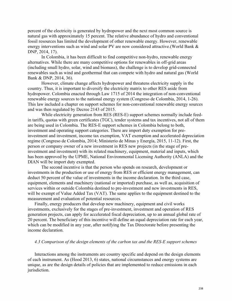
238

percent of the electricity is generated by hydropower and the next most common source is natural gas with approximately 15 percent. The relative abundance of hydro and conventional fossil resources has limited the development of other renewable energy. However, renewable energy interventions such as wind and solar PV are now considered attractive.(World Bank & DNP, 2014, 17).

In Colombia, it has been difficult to find competitive non-hydro, renewable energy alternatives. While there are many competitive options for renewables in off-grid areas (including small hydro, solar, wind and biomass), the challenge is to develop grid-connected renewables such as wind and geothermal that can compete with hydro and natural gas (World Bank & DNP, 2014, 36).

However, climate change affects hydropower and threatens electricity supply in the country. Thus, it is important to diversify the electricity matrix to other RES aside from hydropower. Colombia enacted through Law 1715 of 2014 the integration of non-conventional renewable energy sources to the national energy system (Congreso de Colombia, 2014, 1-26). This law included a chapter on support schemes for non-conventional renewable energy sources and was then regulated by Decree 2143 of 2015.

While electricity generation from RES (RES-E) support schemes normally include feed-in tariffs, quotas with green certificates (TGC), tender systems and tax incentives, not all of them are being used in Colombia. The RES-E support schemes in Colombia belong to both, investment and operating support categories. There are import duty exemption for pre-investment and investment, income tax exemption, VAT exemption and accelerated depreciation regime (Congreso de Colombia, 2014; Ministerio de Minas y Energía, 2015, 11-12). First, the person or company owner of a new investment in RES new projects (in the stage of pre-investment and investment) with its related machinery, equipment, material and inputs, which has been approved by the UPME, National Environmental Licensing Authority (ANLA) and the DIAN will be import duty exempted.

The second incentive is that the person who spends on research, development or investments in the production or use of energy from RES or efficient energy management, can deduct 50 percent of the value of investments in the income declaration. In the third case, equipment, elements and machinery (national or imported) purchase, as well as, acquisition of services within or outside Colombia destined to pre-investment and new investments in RES, will be exempt of Value Added Tax (VAT). The same applies to the equipment destined to the measurement and evaluation of potential resources.

Finally, energy producers that develop new machinery, equipment and civil works investments, exclusively for the stages of pre-investment, investment and operation of RES generation projects, can apply for accelerated fiscal depreciation, up to an annual global rate of 20 percent. The beneficiary of this incentive will define an equal depreciation rate for each year, which can be modified in any year, after notifying the Tax Directorate before presenting the income declaration.

4.3 Comparison of the design elements of the carbon tax and the RES-E support schemes

Interactions among the instruments are country specific and depend on the design elements of each instrument. As (Hood 2013, 6) states, national circumstances and energy systems are unique, as are the design details of policies that are implemented to reduce emissions in each jurisdiction.

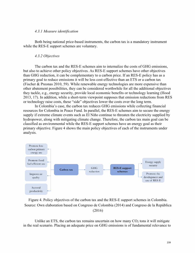
239

4.3.1 Measure identification

Both being national price-based instruments, the carbon tax is a mandatory instrument

while the RES-E support schemes are voluntary.

4.3.2 Objectives

The carbon tax and the RES-E schemes aim to internalize the costs of GHG emissions, but also to achieve other policy objectives. As RES-E support schemes have other objectives than GHG reduction, it can be complementary to a carbon price. If an RES-E policy has as a primary goal to reduce emissions it will be less cost-effective than an ETS or a carbon tax (Fischer & Preonas 2010, 59). While renewable energy technologies are more expensive than other abatement possibilities, they can be considered worthwhile for all the additional objectives they tackle, e.g., energy security, provide local economic benefits or technology learning (Hood 2013, 17). In addition, while a short-term viewpoint supposes that emission reductions from RES or technology raise costs, these “side” objectives lower the costs over the long term.

In Colombia’s case, the carbon tax reduces GHG emissions while collecting financial resources for Colombia in Peace Fund. In parallel, the RES-E schemes aim to secure the energy supply if extreme climate events such as El Niño continue to threaten the electricity supplied by hydropower, along with mitigating climate change. Therefore, the carbon tax main goal can be classified as environmental while the RES-E support schemes have an energy goal as their primary objective. Figure 4 shows the main policy objectives of each of the instruments under analysis.

Figure 4. Policy objectives of the carbon tax and the RES-E support schemes in Colombia.

Source: Own elaboration based on Congreso de Colombia (2014) and Congreso de la República (2016)

Unlike an ETS, the carbon tax remains uncertain on how many CO2 tons it will mitigate

in the real scenario. Placing an adequate price on GHG emissions is of fundamental relevance to

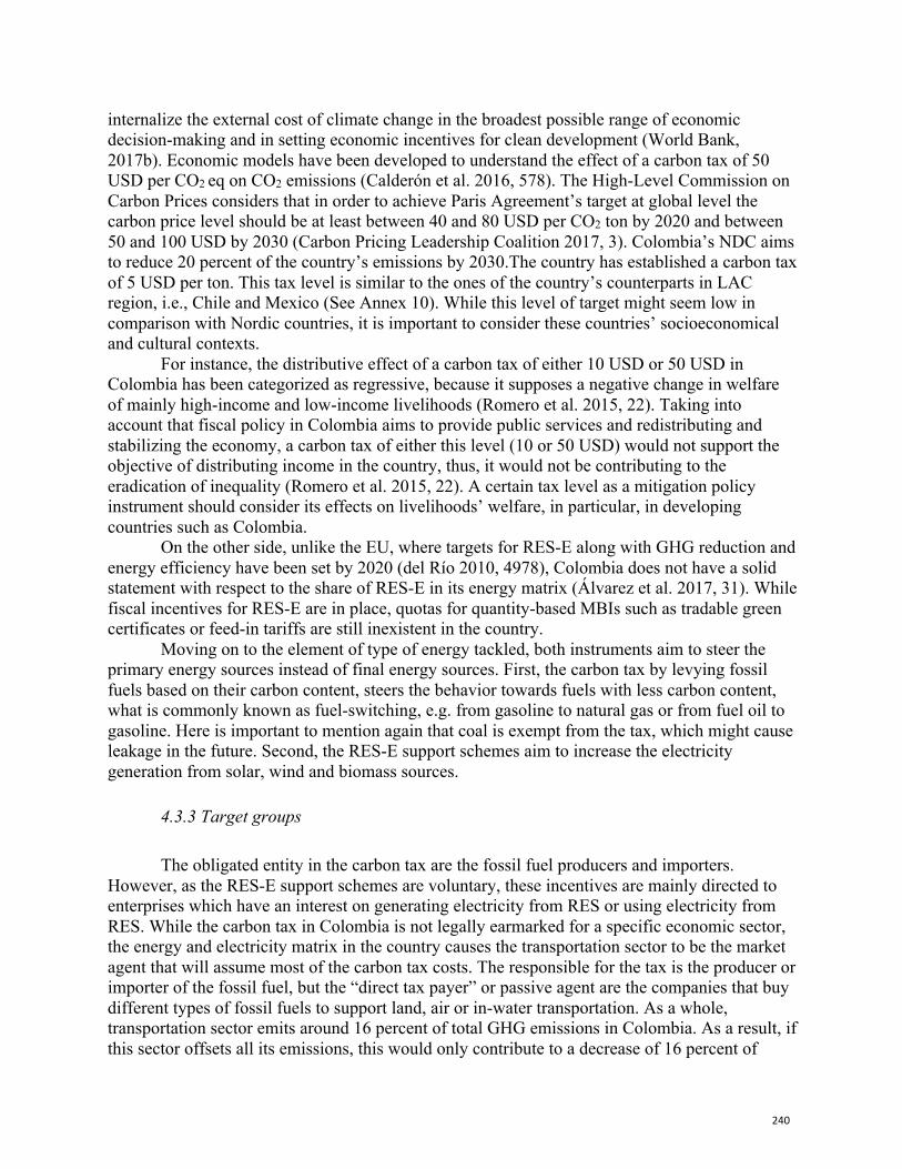
240

internalize the external cost of climate change in the broadest possible range of economic decision-making and in setting economic incentives for clean development (World Bank, 2017b). Economic models have been developed to understand the effect of a carbon tax of 50 USD per CO2 eq on CO2 emissions (Calderón et al. 2016, 578). The High-Level Commission on Carbon Prices considers that in order to achieve Paris Agreement’s target at global level the carbon price level should be at least between 40 and 80 USD per CO2 ton by 2020 and between 50 and 100 USD by 2030 (Carbon Pricing Leadership Coalition 2017, 3). Colombia’s NDC aims to reduce 20 percent of the country’s emissions by 2030.The country has established a carbon tax of 5 USD per ton. This tax level is similar to the ones of the country’s counterparts in LAC region, i.e., Chile and Mexico (See Annex 10). While this level of target might seem low in comparison with Nordic countries, it is important to consider these countries’ socioeconomical and cultural contexts.

For instance, the distributive effect of a carbon tax of either 10 USD or 50 USD in Colombia has been categorized as regressive, because it supposes a negative change in welfare of mainly high-income and low-income livelihoods (Romero et al. 2015, 22). Taking into account that fiscal policy in Colombia aims to provide public services and redistributing and stabilizing the economy, a carbon tax of either this level (10 or 50 USD) would not support the objective of distributing income in the country, thus, it would not be contributing to the eradication of inequality (Romero et al. 2015, 22). A certain tax level as a mitigation policy instrument should consider its effects on livelihoods’ welfare, in particular, in developing countries such as Colombia.

On the other side, unlike the EU, where targets for RES-E along with GHG reduction and energy efficiency have been set by 2020 (del Río 2010, 4978), Colombia does not have a solid statement with respect to the share of RES-E in its energy matrix (Álvarez et al. 2017, 31). While fiscal incentives for RES-E are in place, quotas for quantity-based MBIs such as tradable green certificates or feed-in tariffs are still inexistent in the country.

Moving on to the element of type of energy tackled, both instruments aim to steer the primary energy sources instead of final energy sources. First, the carbon tax by levying fossil fuels based on their carbon content, steers the behavior towards fuels with less carbon content, what is commonly known as fuel-switching, e.g. from gasoline to natural gas or from fuel oil to gasoline. Here is important to mention again that coal is exempt from the tax, which might cause leakage in the future. Second, the RES-E support schemes aim to increase the electricity generation from solar, wind and biomass sources.

4.3.3 Target groups

The obligated entity in the carbon tax are the fossil fuel producers and importers. However, as the RES-E support schemes are voluntary, these incentives are mainly directed to enterprises which have an interest on generating electricity from RES or using electricity from RES. While the carbon tax in Colombia is not legally earmarked for a specific economic sector, the energy and electricity matrix in the country causes the transportation sector to be the market agent that will assume most of the carbon tax costs. The responsible for the tax is the producer or importer of the fossil fuel, but the “direct tax payer” or passive agent are the companies that buy different types of fossil fuels to support land, air or in-water transportation. As a whole, transportation sector emits around 16 percent of total GHG emissions in Colombia. As a result, if this sector offsets all its emissions, this would only contribute to a decrease of 16 percent of

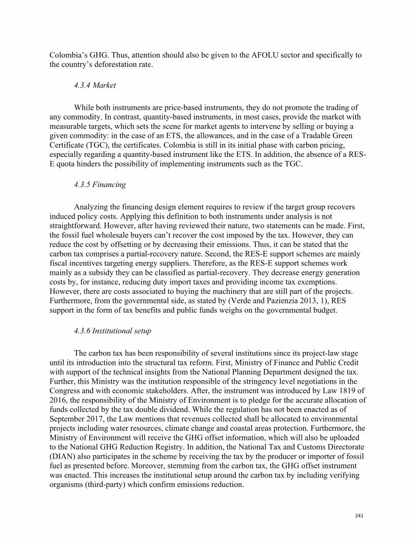
241

Colombia’s GHG. Thus, attention should also be given to the AFOLU sector and specifically to the country’s deforestation rate.

4.3.4 Market

While both instruments are price-based instruments, they do not promote the trading of any commodity. In contrast, quantity-based instruments, in most cases, provide the market with measurable targets, which sets the scene for market agents to intervene by selling or buying a given commodity: in the case of an ETS, the allowances, and in the case of a Tradable Green Certificate (TGC), the certificates. Colombia is still in its initial phase with carbon pricing, especially regarding a quantity-based instrument like the ETS. In addition, the absence of a RES-E quota hinders the possibility of implementing instruments such as the TGC.

4.3.5 Financing

Analyzing the financing design element requires to review if the target group recovers induced policy costs. Applying this definition to both instruments under analysis is not straightforward. However, after having reviewed their nature, two statements can be made. First, the fossil fuel wholesale buyers can’t recover the cost imposed by the tax. However, they can reduce the cost by offsetting or by decreasing their emissions. Thus, it can be stated that the carbon tax comprises a partial-recovery nature. Second, the RES-E support schemes are mainly fiscal incentives targeting energy suppliers. Therefore, as the RES-E support schemes work mainly as a subsidy they can be classified as partial-recovery. They decrease energy generation costs by, for instance, reducing duty import taxes and providing income tax exemptions. However, there are costs associated to buying the machinery that are still part of the projects. Furthermore, from the governmental side, as stated by (Verde and Pazienzia 2013, 1), RES support in the form of tax benefits and public funds weighs on the governmental budget.

4.3.6 Institutional setup

The carbon tax has been responsibility of several institutions since its project-law stage until its introduction into the structural tax reform. First, Ministry of Finance and Public Credit with support of the technical insights from the National Planning Department designed the tax. Further, this Ministry was the institution responsible of the stringency level negotiations in the Congress and with economic stakeholders. After, the instrument was introduced by Law 1819 of 2016, the responsibility of the Ministry of Environment is to pledge for the accurate allocation of funds collected by the tax double dividend. While the regulation has not been enacted as of September 2017, the Law mentions that revenues collected shall be allocated to environmental projects including water resources, climate change and coastal areas protection. Furthermore, the Ministry of Environment will receive the GHG offset information, which will also be uploaded to the National GHG Reduction Registry. In addition, the National Tax and Customs Directorate (DIAN) also participates in the scheme by receiving the tax by the producer or importer of fossil fuel as presented before. Moreover, stemming from the carbon tax, the GHG offset instrument was enacted. This increases the institutional setup around the carbon tax by including verifying organisms (third-party) which confirm emissions reduction.

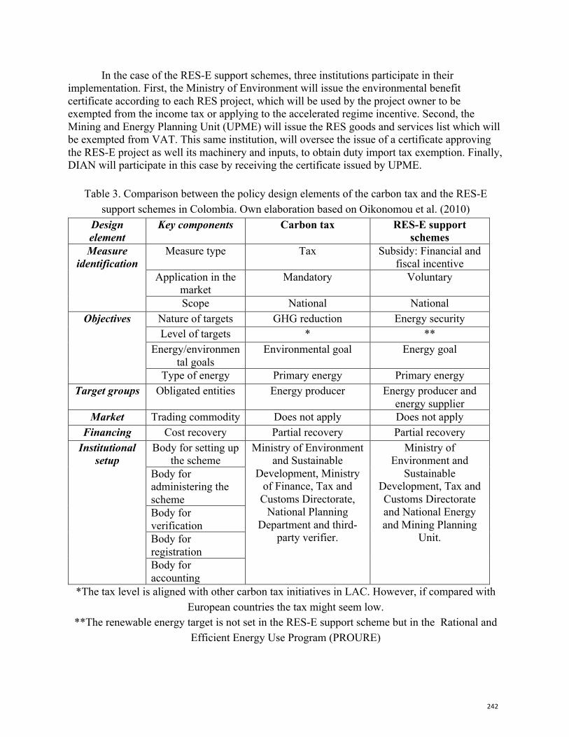
242

In the case of the RES-E support schemes, three institutions participate in their implementation. First, the Ministry of Environment will issue the environmental benefit certificate according to each RES project, which will be used by the project owner to be exempted from the income tax or applying to the accelerated regime incentive. Second, the Mining and Energy Planning Unit (UPME) will issue the RES goods and services list which will be exempted from VAT. This same institution, will oversee the issue of a certificate approving the RES-E project as well its machinery and inputs, to obtain duty import tax exemption. Finally, DIAN will participate in this case by receiving the certificate issued by UPME.

Table 3. Comparison between the policy design elements of the carbon tax and the RES-E support schemes in Colombia. Own elaboration based on Oikonomou et al. (2010)

Design element

Key components Carbon tax RES-E support schemes

Measure identification

Measure type Tax Subsidy: Financial and fiscal incentive

Application in the market

Mandatory Voluntary

Scope National National Objectives Nature of targets GHG reduction Energy security

Level of targets * ** Energy/environmen

tal goals Environmental goal Energy goal

Type of energy Primary energy Primary energy Target groups Obligated entities Energy producer Energy producer and

energy supplier Market Trading commodity Does not apply Does not apply

Financing Cost recovery Partial recovery Partial recovery Institutional

setup Body for setting up

the scheme Ministry of Environment

and Sustainable Development, Ministry

of Finance, Tax and Customs Directorate,

National Planning Department and third-

party verifier.

Ministry of Environment and

Sustainable Development, Tax and Customs Directorate and National Energy and Mining Planning

Unit.

Body for administering the scheme Body for verification Body for registration Body for accounting

*The tax level is aligned with other carbon tax initiatives in LAC. However, if compared with European countries the tax might seem low.

**The renewable energy target is not set in the RES-E support scheme but in the Rational and Efficient Energy Use Program (PROURE)

243

5. Analysis

This chapter aims to provide the reader with insights on why the carbon tax and RES-E support schemes in Colombia are complementary. First, Twomey (2012, 7-32) argues that low-carbon activities or technologies may be promoted for social objectives different than emission reduction. For instance, supporting renewable energy is justified since it contributes to the creation of green jobs and exporting benefits from international leadership in emerging technologies. Furthermore, investing in domestic renewable energy provides greater energy security. This is the case in Colombia, where energy security is threatened by climate change. Thus, renewable energy sources different than hydropower like solar or wind increases energy security. Moreover, (Lehmann and Gawel 2013, 603) stated that using RES-E may also provide environmental benefits apart from GHG reduction like air pollution reduction from fossil fuel combustion and conservation of non-renewable resources. Additionally, in some countries RES-E promotion suggest substituting oil and natural gas imports from unstable countries (Lehmann & Gawel, 2013, 603). While this is not the specific case for Colombia because the country does not rely on energy imports, RES-E support increases the variety of available domestic energy sources.

Second, (Lehmann and Gawel 2013, 603), claim that the existence of multiple policy objectives might provide a further, political rationale for implementing RES-E support schemes next to a carbon pricing instrument e.g. EU ETS. For instance, they mention that an autonomous RES-E deployment target politically set justifies its existence in the policy mix along with an emission policy instrument. In Colombia’s situation, this is visible by the renewable energy target exposed in PROURE which is autonomous from the mitigation target set in the NDC.

Similarly, (del Río 2017, 829) states that policy mixes can be justified to account for the coexistence of different market failures to achieve certain policy goals. This follows a general economic principle: governments should apply a given policy instrument most closely related to a particular market failure. Del Río (2017, 829) recalls what was claimed by Tinbergen (1952): “more targets than instruments make targets incompatible. More instruments than targets make instruments alternative”. Moreover, in the existence of different market failures, the most appropriate response will in many cases be to involve a combination of instruments. This also means that a policy overlap arises when a carbon pricing instrument is supplemented with other instruments to address only the environmental externality generated by GHG emissions. This means that renewable energy support schemes, for instance, are justified when they address other externalities than GHG reduction such as adoption spillovers and/or energy security (Duval, 2008, 31; Hood, 2013,17).

Furthermore, ( del Río 2017, 829) emphasizes that often, policy-makers have other goals apart from CO2 mitigation. For instance, in the climate and energy realm, other goals involve security of energy supply (diversification of energy sources), energy affordability, job and industry creation, as well as, regional development. While carbon-pricing instruments, in this case a carbon tax and RES-E support schemes share one common goal, i.e. CO2 emission reductions, RES-E support schemes contribute to other goals in addition to CO2 mitigation. This is the case in Colombia. In addition, carbon pricing works in synergy with policies to support policy objectives different than emission reductions. This offers the opportunity for decision-makers to develop a carbon pricing as one element of a broader policy package that enhances the performance of each policy (World Bank et al. 2016, 3). Moreover, as presented in the State and Trends of Carbon Pricing report, there is a case of complementarity when the interaction

244

between carbon pricing and other policies in a power market delivers greater reductions while also supporting energy access and reliability (World Bank et al. 2016, 3). In addition, improving access to finance in order to support emerging GHG reduction technologies and overall investments along with a carbon price is also considered complementary (World Bank et al. 2016, 3).

(Del Río 2017, 829) concludes that combinations of instruments may be justified if they address different goals. Moreover, (World Bank et al. 2016, 15) claim that an integrated package of climate policies that reduce emissions while also supporting other policy objectives will be more likely to gain widespread stakeholder support and to be implemented more effectively. The case between the carbon tax and the RES-E support schemes in Colombia, in relation to the policy objectives they tackle, does not result in an overlapping case. This is the consequence of considering national priorities in the instrument’s design and avoiding double efforts. While both instruments coincide in addressing GHG emissions externality, they also have other policy objectives to address. For instance, the carbon tax aims to collect revenues to support the Colombia in Peace Fund and contribute to the national budget. That is, to fundraise resources with the objective of designing and implementing projects of this type. At the same time, the RES-E support schemes aim to promote the development of renewable energy sources to decrease the country’s vulnerability to extreme events intensified by climate change such as droughts. Thus, RES-E support schemes are supporting the policy objective of increasing energy security in Colombia. The fact that both instruments under analysis tackle different market failures suggest that they are not overlapping. Moreover, in terms of target groups, while both instruments target primary energy producers their nature implies a different market behavior.

In addition, CO2 reductions from renewable energy policies could possibly add to the CO2 reductions driven by a carbon tax, depending on the strength of each (Philibert 2011, 16). In the presence of a carbon tax, energy policies that reduce emissions in the same sector and over the same timeframe can increase the total emissions reductions for a given fixed carbon tax level. On the contrary, but also in a enhancing manner, they can decrease the carbon tax level needed to achieve a given emissions outcome (Hood 2013,16). In the former case, an energy policy either energy efficiency or renewable energy related, drives emission reductions and adds to the abatement provided by the carbon tax signal. In the latter case, the required tax level to achieve an emissions goal should be set considering the additional abatement from energy policies.

Here it is particularly important to note that, as mentioned before, the carbon-pricing instrument in Colombia is a carbon tax instead of an ETS. If the case was the latter, other considerations would have to be considered. Efforts to increase the deployment of renewable energy have lowered the carbon price in the EU ETS, although at a higher short-term cost of avoided CO2 given the additional administrative cost and the loss of flexibility. Policy overlaps should be considered by policymakers in Colombia as they set the CO2 cap (OECD 2013, 35). Further, RES-E support schemes’ effectiveness should be considered in the design of the ETS.

Subsidizing environment-friendly activities should generally be avoided given the potentially large budgetary costs and the uncertain impact on negative externality. Here it is important to recall that RES-E support schemes are revenue spending instead of revenue generating. However, they can be an effective option in case where pricing instruments would be difficult or very costly to enforce and when the subsidized activity is a strong substitute for the dirty activity that is targeted. In the case of Colombia, the subsidized activity in this case, the RES-E, is not a strong substitute for the “dirty” activity mainly because the electricity in the country is vastly generated by hydropower.

245

Furthermore, the combination of the carbon tax and the RES-E support schemes is cost-minimizing. This considering that the policy package is exploiting the complementarities between the instruments (IPCC 2014, 30) which are given by the objectives that each of them is addressing. In addition, it also implies that mitigation cost as a result of their combination is lower than if these instruments would be implemented alone (IPCC 2014, 76). The potential for cost-reducing interactions is greatest when different instruments address different market failures. If this is not the case, there will be a policy overlap and double regulation, which will raise mitigation costs. Similarly, incoherent policy mixes leading to duplication or negative interactions will increase costs and could be object of resistance (World Bank et al. 2016, 9)

6. Conclusion

Low-carbon development usually entails to reduce an economy’s GHG intensity while increasing economic development. However, in the context of Colombia’s vulnerability to climate extreme events, it also means to secure energy supply, mainly given by the country’s dependence on hydropower for electricity. The vulnerability to extreme climate events, like droughts, has been further exacerbated by climate phenomena such as El Niño. Nonetheless, this has provided an opportunity to subsidize electricity from renewable energy sources differently than hydropower in the form of fiscal and financial incentives. Thus, the main policy objective for renewable energy policy instruments is not GHG reduction, but securing energy supply. This specific policy design element of the RES-E support schemes in Colombia suggests its interaction with the carbon tax to be complementary. While both instruments coincide on reducing GHG, each of them aims to solve multiple types of policy objectives. On the one hand, the carbon tax is internalizing the cost of GHG emission, thus contributing to the country’s climate change mitigation pledge, promoting industrial efficiency and improving air quality. On the other hand, the RES-E support schemes aim to promote the electricity connection from other renewable sources than hydropower and thus increasing the country’s energy security. In addition, even if both instruments are reducing GHG, the carbon tax is mitigating in the transportation sector while the RES-E support schemes are promoting electricity generation from other renewable energy sources. Both instruments are in theory mutually reinforcing. The carbon tax gives a signal to transit from fossil fuel technologies to renewable energy ones. This, at the same time possibly generates a higher use of renewable energy promotion incentives, either explicit or implicit.

7. Bibliography Álvarez, A., Burgos, J., & Sierra, D. (2017). Crecimiento verde en el sector energético y sus efectos en el

desempeño económico general: Desarrollo y aplicación de un modelo híbrido para Colombia (Working document). CAF.

BID. (2015). Colombia Sostenible- Building a sustainable Colombia in peace. Colombian Presidential Agency of International Cooperation. Retrieved from https://www.apccolombia.gov.co/sites/default/files/archivos_usuario/2016/colombiasostenible-new-dec2-web.pdf

Calderón, S., Alvarez, A. C., Loboguerrero, A. M., Arango, S., Calvin, K., Kober, T., … Fisher-Vanden, K. (2016). Achieving CO2 reductions in Colombia: Effects of carbon taxes and abatement targets. Energy Economics, 56, 575–586. https://doi.org/10.1016/j.eneco.2015.05.010

246

Carbon Pricing Leadership Coalition. (2017). Report of the High-Level Commisssion on Carbon Prices. Supported by World Bank, Agence de l’Environnement et de la Maitrise de l’Energie & Ministère de la transition Écologique et solidaire.

Congreso de Colombia. Ley 1715- Por medio de la cual se regula la integración de las energías renovables no convencionales al sistema energético nacional (2014).

Congreso de la República. Ley 1819- Por medio de la cual se adopta una reforma tributaria estructural, se fortalecen los mecanismos para la lucha contra la evasión y la elusión fiscal y se dictan otras disposiciones (2016).

del Río, P. (2010). Analysing the interactions between renewable energy promotion and energy efficiency support schemes: The impact of different instruments and design elements. Energy Policy, 38, 4978–4989. https://doi.org/10.1016/j.enpol.2010.04.003

del Río, P. (2014). On evaluating success in complex policy mixes: the case of renewable energy support schemes. Policy Sciences, 47(3), 267–287. https://doi.org/10.1007/s11077-013-9189-7

del Río, P. (2017). Why does the combination of the European Union Emissions Trading Scheme and a renewable energy target makes economic sense? Renewable & Sustainable Energy Reviews, 74, 824–834. https://doi.org/10.1016/j.rser.2017.01.122

del Río, P., & Gual, M. (2004). The promotion of green electricity in Europe: present and future. European Environment: The Journal of European Environmental Policy (Wiley), 14(4), 219–234. https://doi.org/10.1002/eet.357

Delbeke, J., & Vis, P. (2016). EU Climate Policy Explained. Routledge. Duval, R. (2008). A taxonomy of instruments to reduce greenhouse gas emissions and their interactions (Working

papers No. 636). Paris: OECD. Retrieved from http://dx.doi.org/10.1787/236846121450 European Commission. (2008). The support of electricity from renewable energy sources (Commission Staff

Working Document). Brussels: European Commission. Fais, B., Blesl, M., Fahl, U., & Voß, A. (2015). Analysing the interaction between emission trading and renewable

electricity support in TIMES. Climate Policy (Earthscan), 15(3), 355–373. https://doi.org/10.1080/14693062.2014.927749

Fankhauser, S., Hepburn, C., & Park, J. (2010). Combining multiple climate policy instruments: How not to do it, 1(3), 1–17.

Fischer, C., & Newell, R. G. (2008). Environmental and technology policies for climate mitigation. Journal of Environmental Economics and Management, 55, 142–162. https://doi.org/10.1016/j.jeem.2007.11.001

Fischer, C., & Preonas, L. (2010). Combining policies for renewable energy: is the whole less than the sum of its parts?

Görlach, B. (2013). What constitutes an optimal climate policy mix? Defining the concept of optimality, including political and legal framework conditions. Berlin: Ecologic Institute. Retrieved from www.cecilia2050.eu

Gupta, S., Tirpak, D., Burger, N., Gupta, J., Höhne, N., Boncheva, A., … Sari, A. (2007). Policies, instruments and cooperative agreements. In Climate change 2007: mitigation. Contribution of working group III to the Fourth Assessment Report of the Intergovernmental Panel on Climate Change. Cambridge United Kingdom and New York, NY, USA: Cambridge University Press.

Hood, C. (2011). Summing up the parts- Combining policy instruments for least-cost mitigation strategies. IEA. Hood, C. (2013). Managing interactions between carbon pricing and existing energy policies- Guidance for

policymakers. Paris, France: IEA. IDEAM, PNUD, MADS, DNP, & CANCILLERÍA. (2015). Primer Informe Bienal de Actualización de Colombia.

Bogotá DC, Colombia. IPCC. (2014). Climate change 2014: Synthesis report. Contribution of Working Groups I,II,III to the Fifth

Assessment Report of the Intergovernmental Panel on Climate Change (p. 151 pp). Geneva, Switzerland. Konidari, P., & Mavrakis, D. (2007). A multi-criteria evaluation method for climate change mitigation policy

instruments. Energy Policy, 35(12), 6235–6257. https://doi.org/10.1016/j.enpol.2007.07.007 Leal Filho, W. (2011). The Economic, Social and Political Elements of Climate Change. Springer Berlin Heidelberg

2011. Lehmann, P., & Gawel, E. (2013). Why should support schemes for renewable electricity complement the EU

emissions trading scheme? Energy Policy, 52, 597–607. https://doi.org/10.1016/j.enpol.2012.10.018 Mickwitz, P. (2003). A Framework for Evaluating Environmental Policy Instruments- Context and key concepts,

9(4), 415–436. Minambiente. (2017). Sitio para mantenerse actualizado y opinar sobre la evoluación del diseño de un sistema de

comercio de emisiones ETS en Colombia. Retrieved from https://asolanilla.wixsite.com/etscolombia

247

Ministerio de Minas y Energía. Decreto 2143-Por el cual se adiciona el Decreto Único Reglamentario del Sector Administrativo de Minas y Energía, 1073 de de 2015, en lo relacionado con la definición de los lineamientos para la aplicación de los incentivos establecidos en el Capítulo III de la Ley 1715 de 2014 (2015).

Mundaca, L., & Markandya, A. (2016). Assessing regional progress towards a “Green Energy Economy.” Applied Energy, 179, 1372–1394. https://doi.org/10.1016/j.apenergy.2015.10.098

OECD. (2013). Climate and carbon-Aligning prices and policies (OECD Environment policy paper No 1). OECD Publishing.

Oikonomou, V., Flamos, A., & Grafakos, S. (2010). Is blending of energy and climate policy instruments always desirable? Energy Policy, 38(8), 4186–4195.

Oikonomou, V., Flamos, A., & Grafakos, S. (2014). Combination of Energy Policy Instruments: Creation of Added Value or Overlapping? Energy Sources, Part B: Economics, Planning, and Policy, 9(1), 46–56. https://doi.org/10.1080/15567241003716696

Oikonomou, V., Flamos, A., Zeugolis, D., & Grafakos, S. (2012). A Qualitative Assessment of EU Energy Policy Interactions. Energy Sources, Part B: Economics, Planning, and Policy, 7(2), 177–187. https://doi.org/10.1080/15567240902788996

Oikonomou, V., & Jepma, C. J. (2008). A framework on interactions of climate and energy policy instruments. Mitigation and Adaptation Strategies for Global Change, 13(2), 131–156. https://doi.org/10.1007/s11027-007-9082-9

Philibert, C. (2011). Interactions of policies for renewable energy and climate. Paris, France: OECD/IEA. Romero, G., Álvarez, A., Calderón, S., & Ordoñez, D. (2015). Impactos distributivos de un impuesto verde en

Colombia, (Documento 439). Sonnenschein, J. (2016). Conditions for the Cost Effective Combination of Emissions Trading and Renewable

Energy Support Policies. Energy Procedia, 88, 133–138. https://doi.org/10.1016/j.egypro.2016.06.036 Sorrel, S., Smith, A., Betz, R., Walz, R., Boemare, C., Quirion, P., … Pilinis, C. (2003). Interaction in EU climate

policy. Science Policy Research Institute: University of Sussex. Tinbergen, J. (1952). On the Theory of Economic Policy. Amsterdam: North-Holland. Twomey, P. (2012). Rationales for Additional Climate Policy Instruments under a Carbon Price. Economic and

Labour Relations Review, 23(1), 7–31. Verde, S., & Pazienzia, M. G. (2013). Cost recovery of RES-E support in Italy: A new case for a carbon tax (EUI

Working paper RSCAS 2013/72). European University Institute-Robert Schuman Centre for Advanced Studies- Climate policy research unit.

World Bank. (2017b). Carbon Pricing Dashboard: What is carbon pricing? Retrieved from http://carbonpricingdashboard.worldbank.org/what-carbon-pricing

World Bank. (2017c). Carbon Tax Guide: A handbook for Policy Makers. Washington, DC. Retrieved from https://openknowledge.worldbank.org/bitstream/handle/10986/26300/Carbon%20Tax%20Guide%20-%20Main%20Report%20web%20FINAL.pdf?sequence=1&isAllowed=y

World Bank, & DNP. (2014). Low-carbon development for Colombia. Washington, DC. World Bank, Ecofys, & Vivid Economics. (2016). State and Trends of Carbon Pricing. Washington, DC. World Bank, & OECD. (2015). The FASTER Principles for succesful carbon pricing: An approach based on initial

experience.

248

Internal Corporate Carbon Pricing: An Analysis of Carbon Emission Reductions for U.S. Companies John W. Byrd and Elizabeth S. Cooperman Business School, University of Colorado Denver

Abstract

A growing trend among corporations is to utilize an internal carbon price to make energy-related investment decisions, with a rise from 100 in 2014 to about 1,400 companies at the end of 2017 reporting to the CDP they do or plan to use internal carbon pricing in the next two years (CDP 2018). Utilizing an internal carbon price tilts investments away from high-carbon emissions projects toward low-carbon emission alternatives. In this study we investigate whether early internal pricing adopters in the U.S. show any future carbon emission reductions, and whether reductions, if they occur, are related to the use of an internal carbon price. Our analysis uses CDP emissions data for 2011-2016 for 201 U.S. companies, with 52 currently reporting that they use an internal carbon price and another 20 planning to use a carbon price within the next two years. Examining changes in industry-adjusted carbon emissions intensity, we find strong evidence in support of an internal carbon price being associated with emissions reductions with one measure, but only weak evidence with the second metric. These mixed results may reflect the short period of time for U.S. companies in applying internal carbon pricing and the range of ways it is being applied. Keywords: Carbon Pricing; Energy Finance Capital Budgeting, Carbon Emissions, Cost of Carbon JEL: Q51, Q56, Q58, G38

Acknowledgement

Presented at the Worlds 1st International Conference on Carbon Pricing, February 14-15, 2019, New Delhi, India. The authors thank a reviewer for the Scientific Committee for the CPLC Conference for helpful comments, and thank the CU Denver Business School for a summer research grant to complete this study.

1. Introduction

As of November 6, 2016, 195 countries signed the United Nations (UN) Paris Agreement to make efforts to reduce their carbon emissions to keep global temperatures from rising above 2o C, relative to post-industrial levels. Countries have been called upon to implement robust policies for carbon pricing sufficiently high to encourage movement towards alternative, non-carbon sources of energy. Approximately 41 OECD and G20 governments developed or announced a carbon tax and/or a cap-and-trade scheme, along with other state and local schemes. By 2018, 70 jurisdictions (45 national and 25 sub-national, regional governments) are putting a

249

price on carbon, with 25 carbon emissions trading systems (ETSs) and 26 carbon taxes implemented, covering 15 to 20 percent of global carbon emissions, a rise from only 4 percent covered in 2010 (CDP 2018; World Bank 2018a,b; Economist 2018).

Globally, corporations have also been called upon to set ambitious carbon emission reduction targets. Putting an internal price on carbon emissions is one of several mechanisms that companies can use to meet these targets. Of nearly 2,000 firms globally reporting their carbon emission data to the CDP in 2017, 1,389 companies, (totaling $7 trillion in revenues) reported they are using (607 firms) or planned to use (782 firms) internal carbon pricing in the next two years, versus just 100 firms in these two categories in 2014.

Corporate internal carbon pricing includes both shadow pricing, which is more widespread, and carbon fees. In the 1990’s and early 2000’s, companies in carbon sensitive industries (i.e., oil and gas, minerals and mining, and electric power) began using internal shadow carbon prices for business decisions and risk mitigation strategies. Shell Oil Corporation as early as 2000, for example, used an internal carbon price of $40 to $80 per metric ton of carbon dioxide equivalent (MTCO2e) to evaluate investment decisions, contributing to reducing 2 million MTCO2e of its direct carbon emissions from its facilities over 2015-2016. Internal carbon prices can be used to help companies track carbon emissions from different sources, stress test scenarios to evaluate the cost of government-mandated carbon taxes for capital investments, and shift investments towards low-carbon emission alternatives (Ahluwalia 2017a,b; Economist 2018).

Carbon fees, using a fee and dividend approach are used less frequently, but have been used effectively. An example is Microsoft’s use of carbon fees (e.g. $5 to $10 per metric ton) for its business groups for electricity consumption and employee air travel, with fees used to purchase renewable energy, improve energy efficiency, buy carbon offsets, and engage in e-waste recycling. This contributed to Microsoft’s global operations carbon neutrality by July 2012. Disney also uses carbon fees (price based on carbon offset costs), to help meet a future zero carbon emissions goal (Ahluwalia 2017a,b; Economist 2018).

To be effective, the internal carbon price must be sufficiently high to fully reflect the social cost of carbon emissions (SCC). As noted in The Economist (2017), climate economists refer to the SCC as the most important number you’ve never heard of, by capturing in a single number the cost of an additional ton of carbon-dioxide pollution, with the use of a SCC priced at $47 estimated to provide over $1 trillion of future benefits (Economist 2017). SCC estimates range from $10 MtCO2e to over $200 (Pindyck 2016).

Critics point out potential flaws in early attempts to apply internal carbon prices, including setting prices too low to incentivize shifts to cleaner energy use (Crooks 2018a,b; Nesbit 2016). A report by Trucost observes that most firms fail to include Scope 3 emissions, often as large as 80% of a firm’s total emissions (Werner 2018). Other critics point out the failure of firms to include the carbon cost of imported goods (Moran, Hasanbeigi, and Springer 2018; Plumer 2018).

In this study we examine the effect that internal carbon pricing has on the emissions of U.S. firms reporting to the CDP during the period 2011 to 2016. We would like to know whether companies in the U.S. adopting internal carbon pricing show greater reductions in future carbon emissions (measured by carbon intensity ratios) versus non-adopting industry peers reporting to the CDP. We also examine if using an internal price on carbon is more or less effective in reducing carbon emission intensity than other reduction mechanisms. This research is timely since the CDP just launched the Carbon Pricing Corridors Initiative that is exploring

250

what internal corporate carbon prices need to be adopted to reach the de-carbonization targets of the 2015 UN Paris Climate Agreement.

The paper is organized as follows. Section 2 discusses the social cost of carbon and challenges. Section 3 describes our sample selection method and provides descriptive statistics for the sample. Our methodology and empirical results are presented in Section 4, and Section 5 presents a paper summary and our conclusions.

2. The Social Cost of Carbon And Challenges

In 2015, the U.S. government settled on $36 to $37 per MtCO2e as the social cost of carbon (SSC) with climate change. This SCC would increase by 3% per year, based on widely used economic impact models estimating economic damages (e.g. decreased agricultural yields, human health damages, and lower worker productivity). This is a much higher price than a commonly used price covering two-thirds of global emissions that is below $10 MtCO2e. However, other estimates for the SCC are higher, such as $40 to $80 MtCO2e by 2020, with a rise to $50 to $100 MtCO2e, that is recommended by the High-Level Commission on Carbon Prices (HLCC) in order to be consistent with the UN Paris Agreement goals (CPLC 2017; World Bank, 2017). Moore and Diaz (2015) using an integrated assessment model (IAM) including economic effects of climate change estimated a much higher cost of $220 per ton, suggesting that even costly means for reducing carbon emissions will be beneficial to society (Than, 2015).

With the pro-coal/fossil fuel agenda by the Trump administration (including withdrawal of the U.S. from the UN Paris Agreement as of June 1, 2017), the EPA’s 2020 social cost of carbon was adjusted down from $42 per ton of CO2 to between $1 and $7 per ton (EPA 2017A and EPA 2017B). On a national level several carbon tax proposals have failed to pass in Congress including a bill introduced in July 2018. In November 2018, voters in the state of Washington rejected a proposed state carbon tax. Because of these changes U.S. companies may have less incentive to use internal carbon pricing or to apply a sufficiently high price to carbon to have any effect.

3. Sample Selection Methodology and Descriptive Statistics

In this study we examine changes in carbon intensity ratios for 2014 to 2016 versus 2010 to 2012. Carbon emissions data and other carbon-related information was extracted from the annual CDP Global Investor Database for the years 2011 through 2017, which reports data for 2010 through 2016. We collected data for all U.S. companies reporting to the CDP. We began with a sample of 365 companies with data reported to CDP during the 2011-2012 and 2014-2016 periods. We limit our sample to industries in which at least one company definitively states it uses internal carbon pricing. The final sample consists of 201 companies in 16 industry groups (shown in Table 1 with the composition for the sample).

Of the 201 U.S. corporations in the sample, 72 corporations used or planned to use internal carbon pricing within two years. For the entire sample, 134 firms reported using a third party verification or assurance completed as of the beginning of 2015. The sample includes firms from a variety of industries. For the 20 firms in the electric utility industry, 17 used internal carbon pricing and three planned to use a carbon price in two years, reflecting regulatory mandates including using a range of carbon prices for long-term integrated resource planning

251

(IRP) and/or risk management scenario analysis. Utilities operating in California or Regional Greenhouse Gas Initiation (RGGI) northeastern states in the U.S. often used the cost of CO2 allowances for their evaluation. For the oil and gas sector, with greater carbon asset risk, about 64 percent of sample firms used or planned to use an internal carbon price, and for airlines, 50 percent, with smaller percentages for other sectors.

Table 2 shows the CO2 emissions data for the sample firms, categorized by industry group based on the average emissions for their operating years 2014 to 2016, with average global scope 1 emissions listed in column 1, average global scope 2 emissions in column 2, and average global scope 2 market-based emissions in column 3. The industry sectors with the largest CO2 emissions are electric utilities, followed by airlines, and oil and gas. For other industry sectors mining had the highest emissions of these, followed by chemicals, and containers and packaging, with much smaller emissions by other sectors.

Table 3 provides descriptive statistics for total assets, capital expenditures, employees, and total revenues. The average asset size for the sample is $64.237 billion, capital expenditures $1.76 billion, employees 48.3 thousand, and revenues of $22.266 billion, representing very large U.S. corporations in each industry sector. For the 52 companies using carbon pricing, only a few disclosed the price they used, with prices ranging from $6 to $35, lower than the recommended social cost of carbon of about $25 to $35 or higher.

4. Methodology and Empirical Results

4.1 Univariate Analysis

Our analysis examines changes in industry-adjusted carbon emission intensity ratios between 2011 and 2016. We use intensity measures to avoid problems of companies growing or contracting, often accompanied by changes in emissions. For example, a growing company could have higher absolute emissions despite making improvements in energy efficiency. Emissions intensity will show improvements despite corporate growth or contraction. We use industry-adjusted measures because, as discussed in Krabbe et al. (2015) and IEA (2014), industries have different abilities to reduce emissions. Industries that rely mainly on electricity can more easily change to low-carbon renewables than say airlines, which are highly dependent on fossil fuels.

Upon review, the carbon intensity measures included in the CDP database seemed unreliable, with the metric for a few companies changing from being in the thousands to being in the one-thousandths. This is probably due to using different units in the denominator. To assure we were using comparable metrics of emission intensity we computed our own emissions intensity measures using data from the COMPUSTAT database.

We use revenue and employee intensity. Revenue intensity is computed as CO2 emissions divided by total revenues (in millions US$), and employee intensity is CO2 emissions divided by the number of employees as reported on the COMPUSTAT database. For a few industries, there may be more relevant intensity metrics. Airlines tend to look at available seats miles. We computed the available seat mile intensity measure for the airlines in the sample. It had no effect on the results versus using the other measures.

Table 4 shows the carbon emission intensity ratios for each sector for the 2014 period to 2016 period. Column 1 shows Scope 1 & 2 Carbon Revenue Intensity Ratios. Column 2 shows

252

Scope 1 & 2 Carbon Employee Intensity ratios, and in Columns 3 and 4, ratios are based on Scope 1 & Market Based Scope 2 Revenue Intensity and Employee Intensity. The highest intensity ratios are for the electric utility sector, followed by mining, then airlines, chemicals, and oil and gas. The lowest intensity ratios are for the banking, media sector, and software & services sectors.

To examine whether there are changes in carbon intensity ratios for the two periods 2010 to 2012 versus 2014 to 2016, we perform t-tests for differences for respectively firms currently using internal carbon pricing, combined internal pricers & planners, and non-carbon pricing firms, shown in Table 5 for changes in the revenue carbon intensity ratio. As shown in column 1 for carbon pricing firms, eight sectors (banks, consumer durables, electric utilities, electrical equipment, mining, pharmaceuticals, semiconductors, and software) had a decline in their industry-adjusted carbon intensity ratio, with a mean change for carbon pricing firms of -0.029 (-2.90%) on average. As shown in Column 3, non-carbon pricing firms for seven industry sectors (aerospace, airlines, chemicals, consumer durables, containers, oil and gas, and semiconductors) had revenue carbon intensity ratio declines, with a mean of -0.016 (-1.16%), which is insignificantly different from the mean for the carbon-pricing firms. Column 2 shows the means for combined carbon pricing and carbon pricing planners, with a mean change of 0.002 (0.20%), which is not statistically different than the mean of non-pricing firms.

Table 6 shows the mean changes in the carbon intensity ratio based on employee carbon intensity for the 16 industry groups. Column 1 for carbon pricing firms shows a decline for 9 sectors (banks, consumer durables, containers, electric utilities, electrical equipment, mining, oil & gas, pharmaceuticals, and software) with a mean decline of -0.103 (i.e., -10.30%). Column 3 shows a decline in employee emissions intensity for 6 of the non-carbon pricing sectors (aerospace, airlines, consumer durables, containers, software, and technology). Overall, the non-pricing group had a mean rise of 0.007 (0.70%) from 2011-12 to 2014-16, which is significantly different from the -0.103 (-10.3%) decline for carbon pricing firms at a 10% level. Column 2 with both carbon pricing firms and carbon price planning firms has a mean decline of -0.0280 (-2.80%), which is not significantly different from the non-carbon pricing firms, suggesting that only the carbon pricing firms are more effective in reducing carbon emissions than non-carbon pricing firms or firms planning to use carbon pricing.

Companies can use a variety of mechanisms to reduce their carbon emissions. To test whether using an internal carbon price is effective we need to test it against these alternatives methods. The CDP database includes the following set of reduction mechanisms under its item 3.3c. — Compliance with regulatory requirements/standards — Partnering with governments on technology development — Dedicated budget for energy efficiency — Dedicated budget for low carbon product R&D — Dedicated budget for other emissions reduction activities — Employee engagement — Internal incentives/recognition programs — Financial optimization calculations — Internal finance mechanisms — Internal price of carbon — Lower return on investment (ROI) specifications — Marginal abatement cost curve

253

— Other To simplify Table 7, we combine related methods into a single category. Items 3, 4 and 5

are put into a Dedicated Budget group; Items 6 and 7 make up an Employee Engagement and Incentives group; and Items 7 through 12 are combined into a Financial Methods category. The other items (1,2 and 13) are self-standing.

Table 7 shows the number and types of carbon emission reduction methods used by sample firms. The 52 U.S. companies using carbon pricing, shown in the first row of the table, on average used 4.37 different reduction methods, including 61.5% complying with regulatory standards, 32.7% partnering with governments on technology development, 61.5% using a dedicated budget, 53.8% using employee engagement incentives, 65.4% using financial incentives, and 23.1% using other methods. The large percentage complying with regulatory standards partially reflects the more highly regulated utility firms that use internal carbon pricing.

For the 20 companies planning to use carbon pricing, 55% comply with regulatory standards, 10% partner with governments on technology development, 55% have a dedicated budget, 65% use employee engagement incentives, 50% use financial methods, and 15% use other methods. For non-carbon pricing corporations, a lower percentage (41.1%) comply with regulatory standards, 15.5% partner with governments on technology development, 45% use a dedicated budget, 63.6% use employee engagement incentives, 57.4% used financial methods, and 22.5% use other methods.

Comparing the average number of incentives used for the three categories for carbon pricing firms versus non-carbon pricing firms, the t-statistic is 3.412 (p-value 0.00039), significant at a .01 level, suggesting that internal carbon pricing corporations utilize a larger number of other types of engagement methods to reduce carbon emissions. Comparing the number of incentives used by carbon pricing firms versus carbon pricing planners, the t-statistic is 1.60583 (p-value .056407), significant at a .10 level. Carbon pricing planners versus non-planners have an insignificant different in the number of engagement method types they use. This suggests that firms using carbon pricing are more active in employing a number of other incentive methods to reduce carbon emissions.

4.2 Multivariate Analysis

We use regression analysis, with the dependent variable as the industry-adjusted change in the CO2 intensity ratio regressed against independent variables including an internal carbon pricing dummy variable, the number of CO2 reduction methods that a company uses as reported to the CDP for 2015, and a control dummy variable for high capital expenditures, equal to 1 if capital expenditures to revenues are greater than the mean for the sample; 0, otherwise.

Table 8 shows the results for models using the industry-adjusted change in CO2 employee intensity as the dependent variable. Column 1 shows the Model 1 regression excluding the number of CO2 reduction methods used, and including the dummy variable for firms that are internal carbon pricing firms, and the dummy variable for high capital expenditures. For this regression, the coefficient on the internal carbon pricing firm dummy variable is significant and negative at a .10 level, indicating a larger reduction in CO2 employee intensity for companies that use internal carbon pricing. The coefficient on the high capital expenditures dummy variable is negative, but insignificant.

254

Model 2 in Column 2 adds an additional variable for the number of CO2 reduction incentive methods that a corporations uses. For this model, the coefficient on internal carbon pricing dummy variable continues to be negative and significant at a .10 level. The coefficients for the high capital expenditure dummy variable and the number of CO2 reduction methods are similarly negative, but insignificant.

Model 3 in Column 3 uses the internal carbon pricing dummy variable and the number of CO2 reduction methods, but excludes the high capital expenditure variable. For this regression, the coefficient on the internal carbon pricing dummy variable is negative and is more significant at a .05 level, consistent with the previous models, and the coefficient on the number of CO2 reduction methods is negative but insignificant. Model 4 in Column 4 includes only the internal pricing variable. The coefficient on the internal pricing variable again is negative with a slightly larger negative coefficient and is significant a .035 level.

For Model 5, where the internal carbon pricing dummy variable includes current carbon pricing companies along with companies planning to carbon price in the next two years, the coefficient on the internal pricing variable is negative but insignificant. Reductions in employee carbon emission intensity appear not be associated with companies only just considering carbon pricing. The capital expenditure dummy variable is negative, and might be considered marginally significant at a 10.4% level. The coefficient for the number of different carbon reduction methods is insignificant.

In similar regression models, which are not presented, entering the various methods in a more fine-grained way, e.g., separate variables for Dedicated Budget, Employee Engagement, etc., produce no significant coefficients. We also did alternative regressions computing the dependent variable using an average of the carbon intensity metrics for 2014-2016 and intensity metrics using the latest available data (2016 for most firms, but 2015 or 2014 for a few firms). The results are invariant to the year used to compute the intensity measure. These regressions do not include the electric utility sector because almost all the utility companies use internal carbon pricing, so there is no difference between carbon-pricers and non-pricers. Including that sector weakens the overall results.

Summarizing the results in Table 8, we find that using an internal carbon price is the only reduction method associated with decreases in employee carbon emissions intensity.

Table 9 shows the regression results using the industry change in CO2 revenue intensity variable as the dependent variable, with similar alternative models estimated. For each model, the dummy internal carbon pricing variable is signed properly, with a negative coefficient, but not statistically significant. In Model 5, the dummy variable for using or planning to use carbon pricing in the future is also insignificant. The high capital expenditures dummy variable, and number of CO2 reduction methods variables are also insignificant for each model.

Hence, the results are mixed concerning the effect of using internal carbon pricing on intensity ratios, with support for internal carbon pricing being associated with a future lower carbon-intensity ratio using an employee carbon intensity measure, but an insignificant effect when a revenue based carbon intensity measure is used. The mixed results may reflect may reflect the need for a longer-time period to evaluate the effect of long-term capital investments to reduce their carbon emissions.

CDP data emissions data for the year 2017 (reported by companies to the CDP for 2018) became available in January 2019. In very preliminary tests, the inclusion of the 2017 data did not change any of our univariate results. For the 2017 sample, we observed that some U.S. firms that had reported themselves as using carbon pricing are no longer doing so, and a number of

255

firms were acquired, and did not report to the CDP in 2018, lowering the number of firms using internal carbon pricing in the sample, which will require reorganizing the sample for any future analysis.

5. Summary and Conclusion

To reduce their carbon emissions, corporations are utilizing a variety of methods including putting an internal price on carbon emissions. This paper examines the early stages of internal carbon pricing by corporations. Examining U.S. firms in industrial sectors with at least one company using carbon pricing, we find that carbon pricing has a statistically significant association with reductions in industry-adjusted carbon emissions intensity ratios that are based on the number of employees but not when the ratio is based on revenues.

We also examine whether other types of carbon reduction methods are as effective as internal carbon pricing, but find that they are not, which may reflect that the the 52 U.S. companies using carbon pricing are also using a higher number of other methods. At least for one of our carbon intensity ratios (employee-based), internal carbon pricing clearly dominates other methods in reducing emissions.

These somewhat inclusive results suggest that internal carbon pricing may have an effect, but a clear signal may take longer to appear than the short sample window we examine. The low price that some companies currently apply makes this tool less effective, and statistically significant results harder to find, than it could be. We also assume that all companies using an internal carbon price acknowledge doing so in their CDP filings. If some of the firms we have categorized as non-pricing firms actually do use a carbon price, this would weaken our statistical results. Conversely, some firms that we have categorized as using carbon pricing, by 2017, no longer report doing so to the CDP, which may be further weakening our results. A number of these caveats will get resolved a longer time period, as more and better data becomes available over time.

There are many ways that companies can implement an internal carbon price. The design of the programs will influence their impact on carbon emissions reductions. A policy that applies a carbon tax to capital expenditures could have only a marginal impact if it shifted expenditures from one option to another slightly less carbon intensive option. For example, a company using a carbon price when deciding on how to replace vehicles in their fleet might switch to models with slightly better fuel efficiency, but if choosing from fossil fuels, internal combustion vehicles, the carbon reduction benefits would be marginal. Programs based on a broader carbon footprint will have more impact depending on the carbon price applied and on how larger carbon emissions are penalized, or lower carbon emissions are rewarded.

References Ahluwalia, M. B. 2017a. “Companies Set Their Own Price on Carbon.” C2ES Center for Climate and Energy

Solutions, Accessed on February 19, 2018 at: https://www.c2es.org/2017/09/companies-set-their-own-price-on-carbon/

Ahluwalia, M. B. 2017b. “The Business of Pricing Carbon: How Companies Are Pricing Carbon to Mitigate Risks and Prepare for a Low-Carbon Future,” C2ES Center for Climate and Energy Solutions, Accessed on February 15, 2018 at https://www.c2es.org/site/assets/uploads/2017/09/business-pricing-carbon.pdf

256

CDP. 2017. “Putting a price on risk: Integrating Climate Risk into Business Planning, “CDP Website, October, 2017, Accessed on February 20, 2018 at: https://www.actu-environnement.com/media/pdf/news-29828-prix-carbone-entreprises-cdp.pdf

CDP. 2018. “Commit to Putting a Price on Carbon.” CDP Website, Accessed on September 19, 2018 at: https://www.cdp.net/en/campaigns/commit-to-action/price-on-carbon

CPLC. 2017. “Report of the High-Level Commission on Carbon Prices.” Carbon Pricing Leadership Coalition, World Bank Group, May 29, 2017; Accessed on February 22, 2018 at: https://static1.squarespace.com/static/54ff9c5ce4b0a53decccfb4c/t/5949402936e5d3af64b94bab/1497972781902/ENGLISH+EX+SUM+CarbonPricing.pdf

Crooks, E. 2018a. “Business Leaders Warn of Lack of Progress on Emissions Climate Change.” Financial Times, September 5, 2018, Accessed on September 13, 2018 at: https://www.ft.com/content/c0322a84-b08c-11e8-8d14-6f049d06439c

Crooks, E. 2018b. “Carbon pricing proposals tax U.S. politicians and theorists: Plans to tackle market failure of fossil fuel consumption stumble in Congress.” Financial Times, July 30, 2018, Accessed on September 16, 2018 at: https://www.ft.com/content/6a8c4594-7bab-11e8-af48-190d103e32a4

Economist. 2017. “The EPA is Rewriting the Most Important Number in Climate Economics: Reducing the Social Cost of Carbon Would Allow the EPA To Dispense with Regulations.” The Economist, November 16, 2017, Accessed on September 25, 2018, at: https://www.economist.com/united-states/2017/11/16/the-epa-is-rewriting-the-most-important-number-in-climate-economics

Economist. 2018. “Low Carb Diet: Companies are Moving Faster than Many Governments on Carbon Pricing.” The Economist, January 11, 2018 Accessed on

September 21, 2018 at: https://www.economist.com/business/2018/01/11/companies-are-moving-faster-than-many-governments-on-carbon-pricing

EPA. 2017A. “The Social Cost of Carbon: Estimating the Benefits of Reducing Greenhouse Gas Emissions.” January 19, 2017, Accessed on September 25, 2017, at: https://19january2017snapshot.epa.gov/climatechange/social-cost-carbon.htm

EPA. 2017B. “Regulatory Impact Analysis for the Review of the Clean Power Plan: Proposal, October 2017. Accessed February 4, 2019 at: https://www.epa.gov/sites/production/files/2017-10/documents/ria_proposed-cpp-repeal_2017-10.pdf

Hulac, B. 2017. “Exxon: this is how an oil giant uses internal carbon pricing.” E&E News, June 15, 2017, Accessed on September 21, 2018 at: https://www.eenews.net/stories/1060056076

IEA. 2014. “Energy Technology Perspective 2014,” IEA Website, Accessed on September 26, 2018 at: https://www.iea.org/publications/freepublications/publication/EnergyTechnologyPerspectives2014.pdf

Krabbe, O., G. Linthorst, K. Blok, W. Crijins-Graus, D. P. van Vuuren, N. Hohne, P. Faria, N. Aden, and A. C. Pineda. 2015. “Aligning Corporate Greenhouse-Gas Emissions Targets with Climate Goals.” Nature Climate Change Letters, August 2015, DOI:10.1038/INCLIMATE 2770

Moore, F. C. and D. B. Diaz. 2015. “Temperature Impacts on Economic Growth Warrant Stringent Mitigation Policy.” Nature Climate Change, 5, 127-131, published on February 25, 2015, Accessed on September 25, 2018, at: https://www.nature.com/articles/nclimate2481

Moran, D., A. Hasanbeigi and C. Springer. 2018. “ The Carbon Loophole in Climate Policy: Quantifying the Embodied Carbon in Traded Products.” Report sponsored by KGM & Associates, Global Efficiency Intelligence, and Climate Works Foundation, August 2018, Accessed on September 16, 2018 at: https://buyclean.org/media/2016/12/The-Carbon-Loophole-in-Climate-Policy-Final.pdf

Nesbit, J.. 2016. “Why ExxonMobil Is Supporting a Carbon Tax Now.” Fortune, July 10, 2016, Accessed on September 1, 2018 at: http://fortune.com/2016/07/10/exxonmobil-carbon-tax/

Pindyck, R. S. 2016. “The Social Cost of Carbon Revisited.” NBER Working Paper No. 22807, November 2016, Accessed on February 15, 2018 at: http://www.nber.org/papers/w22807

Plumer, B. 2018. “Trailing Carbon Footprints Across Borders.” New York Times, September 6, 2018, B2, B5. Than, K.. 2015. “Estimated Social Cost of Climate Change not Accurate.” Stanford Scientists Say.” Stanford

News, January 12, 2015, Accessed on September 25, 2018 at: https://news.stanford.edu/2015/01/12/emissions-social-costs-011215/

US Climate Alliance. 2018. United State Climate Alliance Website, Accessed on February 1, 2019, at: https://www.usclimatealliance.org

Werner, B. 2018. “CDP Data Reveals Shortfall in Carbon Disclosure by North American Companies,” February 15, 2018, Accessed on September 21, 2018 at: https://www.greenbiz.com/article/cdp-data-reveals-shortfall-carbon-disclosure-north-american-companies

257

World Bank. 2018a. “More Governments Taking Up Carbon Pricing and Seeing Big Benefits in Revenues: World Bank Report.” The World Bank Press Release, May 22,

2018, Accessed on September 16, 2018 at: https://www.worldbank.org/en/news/press-release/2018/05/22/more-governments-taking-up-carbon-pricing-and-seeing-big-benefits-in-revenues-world-bank-report

World Bank. 2018b. “State and Trends of Carbon Pricing 2018.” World Bank Group, Washington DC, May 2018, Accessed on September 17, 2018 at https://openknowledge.worldbank.org/handle/10986/29687

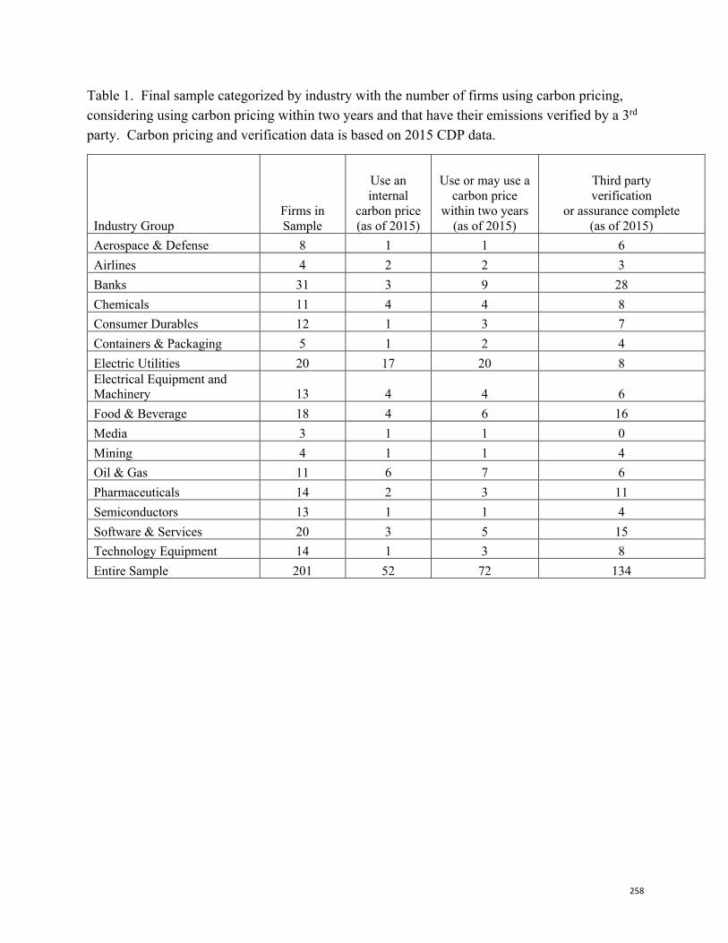
258

Table 1. Final sample categorized by industry with the number of firms using carbon pricing, considering using carbon pricing within two years and that have their emissions verified by a 3rd party. Carbon pricing and verification data is based on 2015 CDP data.

Industry Group Firms in Sample

Use an internal

carbon price (as of 2015)

Use or may use a carbon price

within two years (as of 2015)

Third party verification

or assurance complete (as of 2015)

Aerospace & Defense 8 1 1 6 Airlines 4 2 2 3 Banks 31 3 9 28 Chemicals 11 4 4 8 Consumer Durables 12 1 3 7 Containers & Packaging 5 1 2 4 Electric Utilities 20 17 20 8 Electrical Equipment and Machinery 13 4 4 6 Food & Beverage 18 4 6 16 Media 3 1 1 0 Mining 4 1 1 4 Oil & Gas 11 6 7 6 Pharmaceuticals 14 2 3 11 Semiconductors 13 1 1 4 Software & Services 20 3 5 15 Technology Equipment 14 1 3 8 Entire Sample 201 52 72 134

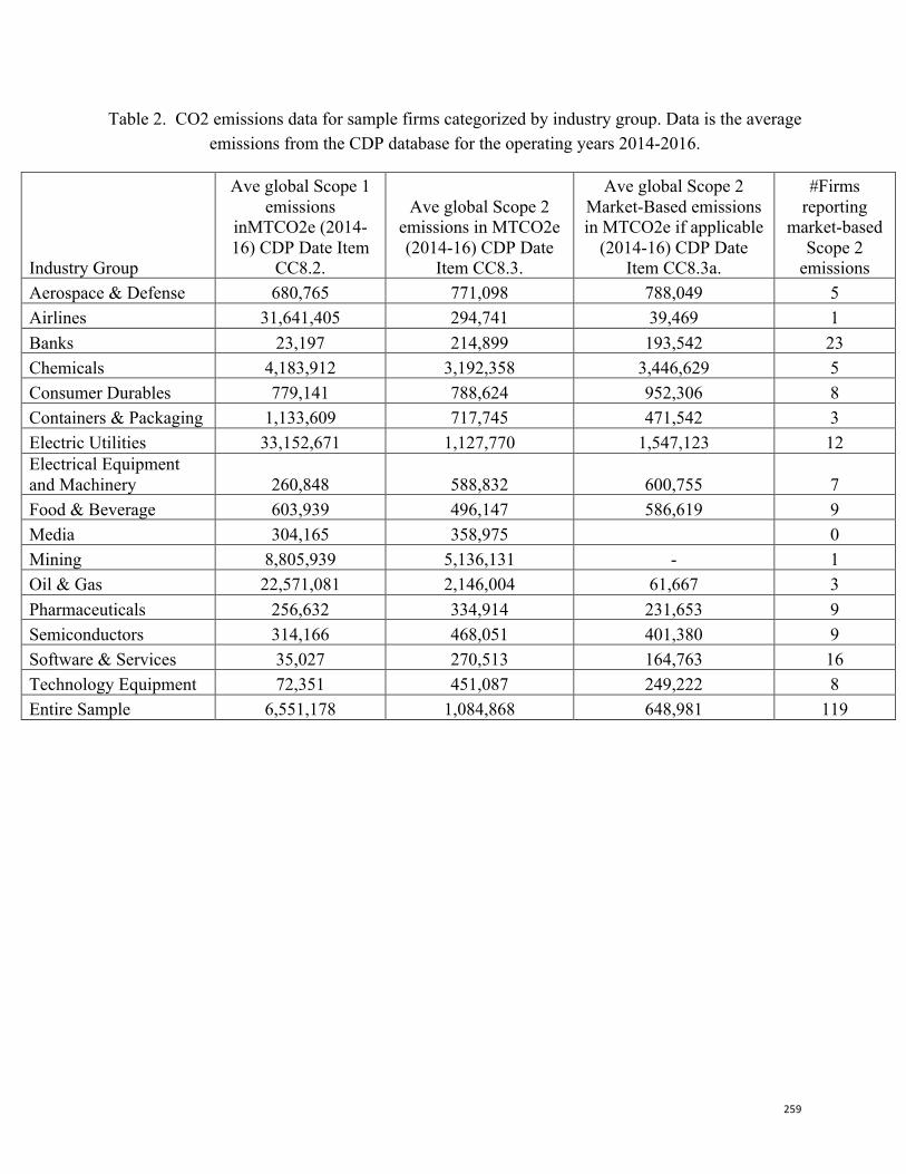
259

Table 2. CO2 emissions data for sample firms categorized by industry group. Data is the average emissions from the CDP database for the operating years 2014-2016.

Industry Group

Ave global Scope 1 emissions

inMTCO2e (2014-16) CDP Date Item

CC8.2.

Ave global Scope 2 emissions in MTCO2e (2014-16) CDP Date

Item CC8.3.

Ave global Scope 2 Market-Based emissions in MTCO2e if applicable

(2014-16) CDP Date Item CC8.3a.

#Firms reporting

market-based Scope 2

emissions Aerospace & Defense 680,765 771,098 788,049 5 Airlines 31,641,405 294,741 39,469 1 Banks 23,197 214,899 193,542 23 Chemicals 4,183,912 3,192,358 3,446,629 5 Consumer Durables 779,141 788,624 952,306 8 Containers & Packaging 1,133,609 717,745 471,542 3 Electric Utilities 33,152,671 1,127,770 1,547,123 12 Electrical Equipment and Machinery 260,848 588,832 600,755 7 Food & Beverage 603,939 496,147 586,619 9 Media 304,165 358,975 0 Mining 8,805,939 5,136,131 - 1 Oil & Gas 22,571,081 2,146,004 61,667 3 Pharmaceuticals 256,632 334,914 231,653 9 Semiconductors 314,166 468,051 401,380 9 Software & Services 35,027 270,513 164,763 16 Technology Equipment 72,351 451,087 249,222 8 Entire Sample 6,551,178 1,084,868 648,981 119

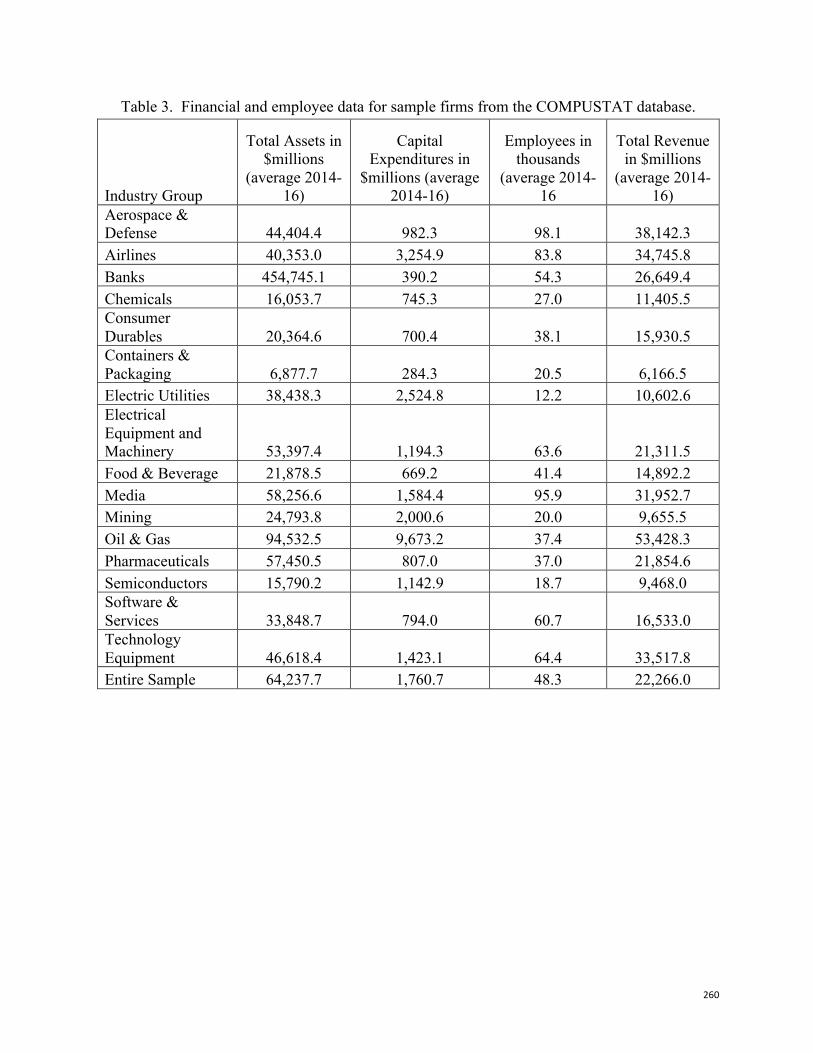
260

Table 3. Financial and employee data for sample firms from the COMPUSTAT database.

Industry Group

Total Assets in $millions

(average 2014-16)

Capital Expenditures in

$millions (average 2014-16)

Employees in thousands

(average 2014-16

Total Revenue in $millions

(average 2014-16)

Aerospace & Defense 44,404.4 982.3 98.1 38,142.3 Airlines 40,353.0 3,254.9 83.8 34,745.8 Banks 454,745.1 390.2 54.3 26,649.4 Chemicals 16,053.7 745.3 27.0 11,405.5 Consumer Durables 20,364.6 700.4 38.1 15,930.5 Containers & Packaging 6,877.7 284.3 20.5 6,166.5 Electric Utilities 38,438.3 2,524.8 12.2 10,602.6 Electrical Equipment and Machinery 53,397.4 1,194.3 63.6 21,311.5 Food & Beverage 21,878.5 669.2 41.4 14,892.2 Media 58,256.6 1,584.4 95.9 31,952.7 Mining 24,793.8 2,000.6 20.0 9,655.5 Oil & Gas 94,532.5 9,673.2 37.4 53,428.3 Pharmaceuticals 57,450.5 807.0 37.0 21,854.6 Semiconductors 15,790.2 1,142.9 18.7 9,468.0 Software & Services 33,848.7 794.0 60.7 16,533.0 Technology Equipment 46,618.4 1,423.1 64.4 33,517.8 Entire Sample 64,237.7 1,760.7 48.3 22,266.0

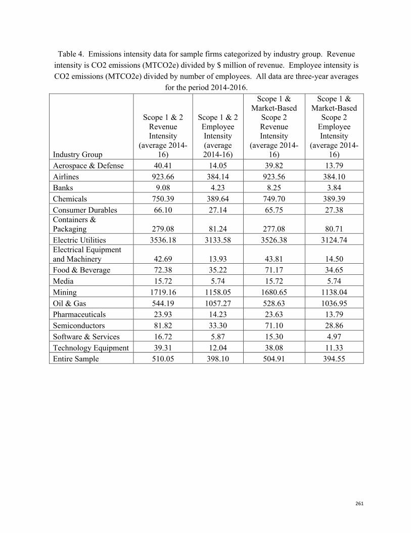
261

Table 4. Emissions intensity data for sample firms categorized by industry group. Revenue intensity is CO2 emissions (MTCO2e) divided by $ million of revenue. Employee intensity is CO2 emissions (MTCO2e) divided by number of employees. All data are three-year averages

for the period 2014-2016.

Industry Group

Scope 1 & 2 Revenue Intensity

(average 2014-16)

Scope 1 & 2 Employee Intensity (average 2014-16)

Scope 1 & Market-Based

Scope 2 Revenue Intensity

(average 2014-16)

Scope 1 & Market-Based

Scope 2 Employee Intensity

(average 2014-16)

Aerospace & Defense 40.41 14.05 39.82 13.79 Airlines 923.66 384.14 923.56 384.10 Banks 9.08 4.23 8.25 3.84 Chemicals 750.39 389.64 749.70 389.39 Consumer Durables 66.10 27.14 65.75 27.38 Containers & Packaging 279.08 81.24 277.08 80.71 Electric Utilities 3536.18 3133.58 3526.38 3124.74 Electrical Equipment and Machinery 42.69 13.93 43.81 14.50 Food & Beverage 72.38 35.22 71.17 34.65 Media 15.72 5.74 15.72 5.74 Mining 1719.16 1158.05 1680.65 1138.04 Oil & Gas 544.19 1057.27 528.63 1036.95 Pharmaceuticals 23.93 14.23 23.63 13.79 Semiconductors 81.82 33.30 71.10 28.86 Software & Services 16.72 5.87 15.30 4.97 Technology Equipment 39.31 12.04 38.08 11.33 Entire Sample 510.05 398.10 504.91 394.55

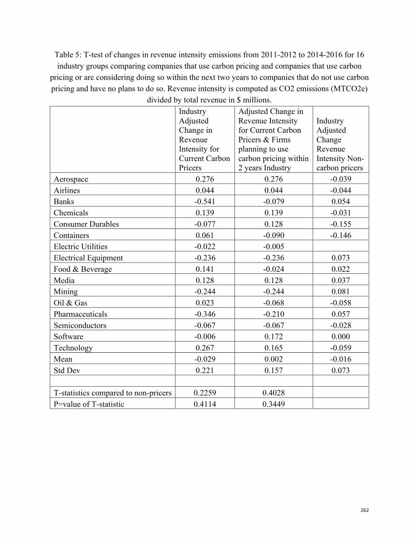
262

Table 5: T-test of changes in revenue intensity emissions from 2011-2012 to 2014-2016 for 16 industry groups comparing companies that use carbon pricing and companies that use carbon

pricing or are considering doing so within the next two years to companies that do not use carbon pricing and have no plans to do so. Revenue intensity is computed as CO2 emissions (MTCO2e)

divided by total revenue in $ millions.

Industry Adjusted Change in Revenue Intensity for Current Carbon Pricers

Adjusted Change in Revenue Intensity for Current Carbon Pricers & Firms planning to use carbon pricing within 2 years Industry

Industry Adjusted Change Revenue Intensity Non-carbon pricers

Aerospace 0.276 0.276 -0.039 Airlines 0.044 0.044 -0.044 Banks -0.541 -0.079 0.054 Chemicals 0.139 0.139 -0.031 Consumer Durables -0.077 0.128 -0.155 Containers 0.061 -0.090 -0.146 Electric Utilities -0.022 -0.005 Electrical Equipment -0.236 -0.236 0.073 Food & Beverage 0.141 -0.024 0.022 Media 0.128 0.128 0.037 Mining -0.244 -0.244 0.081 Oil & Gas 0.023 -0.068 -0.058 Pharmaceuticals -0.346 -0.210 0.057 Semiconductors -0.067 -0.067 -0.028 Software -0.006 0.172 0.000 Technology 0.267 0.165 -0.059 Mean -0.029 0.002 -0.016 Std Dev 0.221 0.157 0.073 T-statistics compared to non-pricers 0.2259 0.4028 P=value of T-statistic 0.4114 0.3449

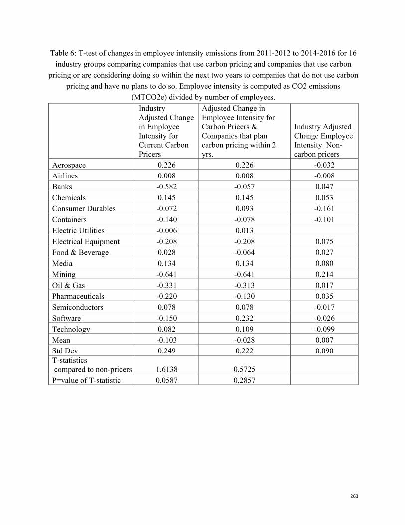
263

Table 6: T-test of changes in employee intensity emissions from 2011-2012 to 2014-2016 for 16 industry groups comparing companies that use carbon pricing and companies that use carbon

pricing or are considering doing so within the next two years to companies that do not use carbon pricing and have no plans to do so. Employee intensity is computed as CO2 emissions

(MTCO2e) divided by number of employees.

Industry Adjusted Change in Employee Intensity for Current Carbon Pricers

Adjusted Change in Employee Intensity for Carbon Pricers & Companies that plan carbon pricing within 2 yrs.

Industry Adjusted Change Employee Intensity Non-carbon pricers

Aerospace 0.226 0.226 -0.032 Airlines 0.008 0.008 -0.008 Banks -0.582 -0.057 0.047 Chemicals 0.145 0.145 0.053 Consumer Durables -0.072 0.093 -0.161 Containers -0.140 -0.078 -0.101 Electric Utilities -0.006 0.013 Electrical Equipment -0.208 -0.208 0.075 Food & Beverage 0.028 -0.064 0.027 Media 0.134 0.134 0.080 Mining -0.641 -0.641 0.214 Oil & Gas -0.331 -0.313 0.017 Pharmaceuticals -0.220 -0.130 0.035 Semiconductors 0.078 0.078 -0.017 Software -0.150 0.232 -0.026 Technology 0.082 0.109 -0.099 Mean -0.103 -0.028 0.007 Std Dev 0.249 0.222 0.090 T-statistics compared to non-pricers 1.6138 0.5725 P=value of T-statistic 0.0587 0.2857

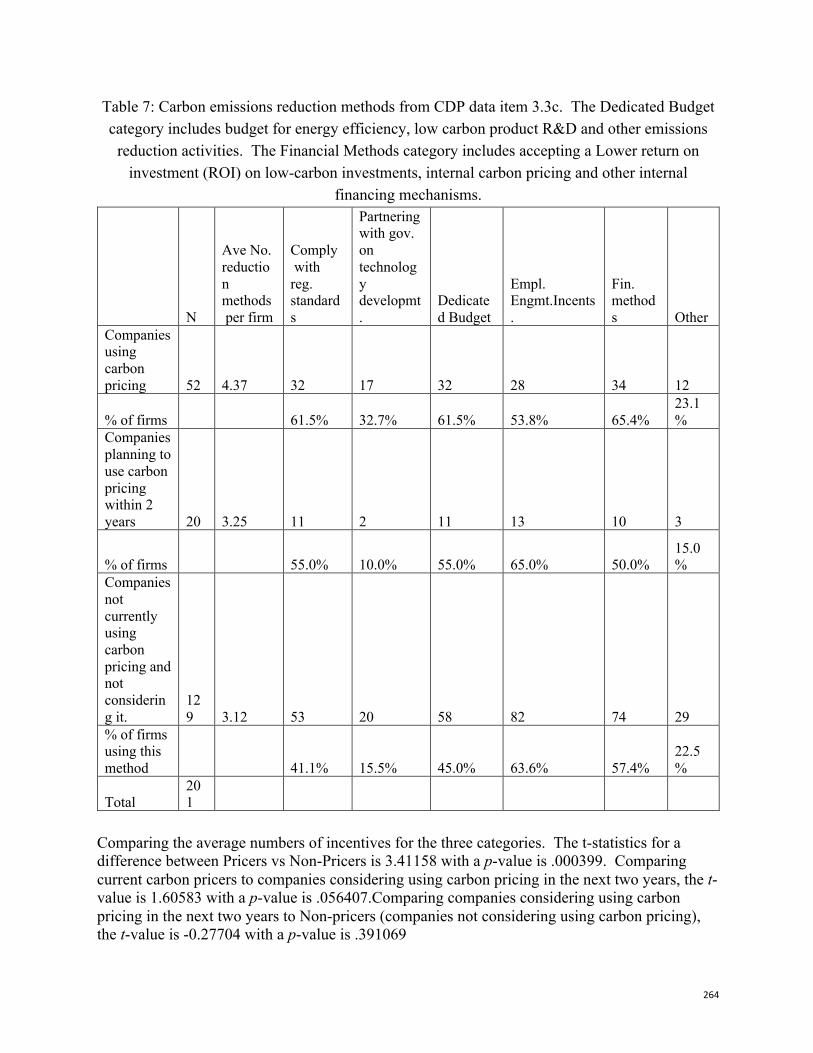
264

Table 7: Carbon emissions reduction methods from CDP data item 3.3c. The Dedicated Budget category includes budget for energy efficiency, low carbon product R&D and other emissions

reduction activities. The Financial Methods category includes accepting a Lower return on investment (ROI) on low-carbon investments, internal carbon pricing and other internal

financing mechanisms.

N

Ave No. reduction methods per firm

Comply with reg. standards

Partnering with gov. on technology developmt.

Dedicated Budget

Empl. Engmt.Incents.

Fin. methods Other

Companies using carbon pricing 52 4.37 32 17 32 28 34 12

% of firms 61.5% 32.7% 61.5% 53.8% 65.4% 23.1%

Companies planning to use carbon pricing within 2 years 20 3.25 11 2 11 13 10 3

% of firms 55.0% 10.0% 55.0% 65.0% 50.0% 15.0%

Companies not currently using carbon pricing and not considering it.

129 3.12 53 20 58 82 74 29

% of firms using this method 41.1% 15.5% 45.0% 63.6% 57.4%

22.5%

Total 201

Comparing the average numbers of incentives for the three categories. The t-statistics for a difference between Pricers vs Non-Pricers is 3.41158 with a p-value is .000399. Comparing current carbon pricers to companies considering using carbon pricing in the next two years, the t-value is 1.60583 with a p-value is .056407.Comparing companies considering using carbon pricing in the next two years to Non-pricers (companies not considering using carbon pricing), the t-value is -0.27704 with a p-value is .391069

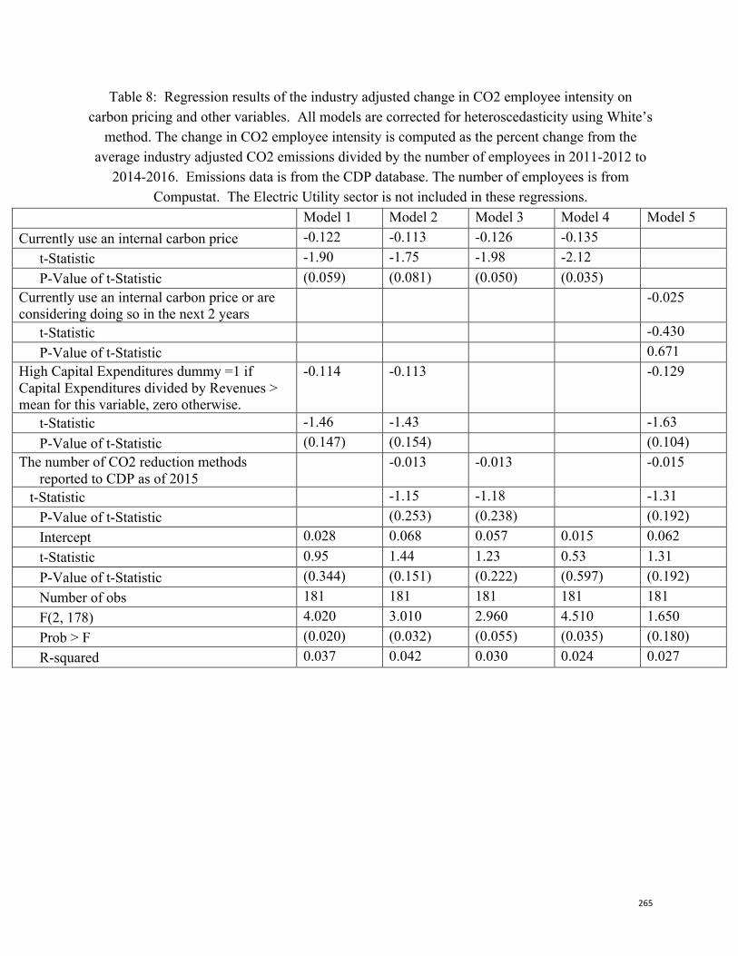
265

Table 8: Regression results of the industry adjusted change in CO2 employee intensity on carbon pricing and other variables. All models are corrected for heteroscedasticity using White’s

method. The change in CO2 employee intensity is computed as the percent change from the average industry adjusted CO2 emissions divided by the number of employees in 2011-2012 to

2014-2016. Emissions data is from the CDP database. The number of employees is from Compustat. The Electric Utility sector is not included in these regressions.

Model 1 Model 2 Model 3 Model 4 Model 5 Currently use an internal carbon price -0.122 -0.113 -0.126 -0.135

t-Statistic -1.90 -1.75 -1.98 -2.12

P-Value of t-Statistic (0.059) (0.081) (0.050) (0.035)

Currently use an internal carbon price or are considering doing so in the next 2 years

-0.025

t-Statistic

-0.430 P-Value of t-Statistic

0.671

High Capital Expenditures dummy =1 if Capital Expenditures divided by Revenues > mean for this variable, zero otherwise.

-0.114 -0.113

-0.129

t-Statistic -1.46 -1.43

-1.63 P-Value of t-Statistic (0.147) (0.154)

(0.104)

The number of CO2 reduction methods reported to CDP as of 2015

-0.013 -0.013

-0.015

t-Statistic

-1.15 -1.18


(0.253) (0.238)

(0.192)

Intercept 0.028 0.068 0.057 0.015 0.062 t-Statistic 0.95 1.44 1.23 0.53 1.31 P-Value of t-Statistic (0.344) (0.151) (0.222) (0.597) (0.192) Number of obs 181 181 181 181 181 F(2, 178) 4.020 3.010 2.960 4.510 1.650 Prob > F (0.020) (0.032) (0.055) (0.035) (0.180) R-squared 0.037 0.042 0.030 0.024 0.027

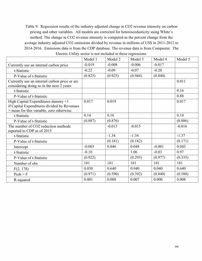
266

Table 9: Regression results of the industry adjusted change in CO2 revenue intensity on carbon pricing and other variables. All models are corrected for heteroscedasticity using White’s method. The change in CO2 revenue intensity is computed as the percent change from the

average industry adjusted CO2 emissions divided by revenue in millions of US$ in 2011-2012 to 2014-2016. Emissions data is from the CDP database. The revenue data is from Compustat. The

Electric Utility sector is not included in these regressions. Model 1 Model 2 Model 3 Model 4 Model 5

Currently use an internal carbon price -0.019 -0.008 -0.006 -0.017

t-Statistic -0.22 -0.09 -0.07 -0.20

P-Value of t-Statistic (0.825) (0.925) (0.944) (0.840)

Currently use an internal carbon price or are considering doing so in the next 2 years

0.011

t-Statistic

0.16 P-Value of t-Statistic

0.88

High Capital Expenditures dummy =1 if Capital Expenditures divided by Revenues > mean for this variable, zero otherwise.

0.017 0.019

0.017

t-Statistic 0.14 0.16

0.14 P-Value of t-Statistic (0.887) (0.876)

(0.886)

The number of CO2 reduction methods reported to CDP as of 2015

-0.015 -0.015

-0.016

t-Statistic

-1.34 -1.34


(0.181) (0.182)

(0.171)

Intercept -0.003 0.046 0.048 -0.001 0.043 t-Statistic -0.10

1.06 -0.03 0.97

P-Value of t-Statistic (0.922)

(0.293) (0.977) (0.335) Number of obs 181 181 181 181 181 F(2, 178) 0.030 0.640 0.940 0.040 0.640 Prob > F (0.971) (0.590) (0.392) (0.840) (0.588) R-squared 0.001 0.008 0.007 0.000 0.008

267

Leveraging Private Sector Investment in Energy Efficiency: Pilot Case Studies of Selected Sub-Saharan African Countries By Martin Burian, Joachim Schnurr, Grant A. Kirkman & Janak Shrestha

1. Introduction

The Paris Agreement (PA) and Sustainable Development Goals (SDG) are a call to action to address some of the world’s most pressing challenges, two of which are: meeting the goal of limiting global warming to well below 2⁰C; and mobilizing investment needed to bring electricity to more than 1 billion people without access. The World Economic Forum estimates that by 2020, about $5.7 trillion will need to be invested annually in green infrastructure (WEF, 2013), most of it in developing countries. But according to the Climate Policy Initiative, only around $410 billion is currently being invested annually (CPI, 2017) leaving a substantial investment gap to implement the Paris Agreement and achieve the SDGs - most which will need to be filled by the private sector.

The scale of the challenge is beyond that of public finance alone and given the commitments made by national governments in their Nationally Determined Contributions (NDC), a significant increase in support from the private sector is essential. Implementing the Paris Agreement not only presents a commercial opportunity, but also an opportunity to demonstrate social purpose, identifying economically viable abatement potentials in the transition to a low-carbon, sustainable world. Focusing on interventions that are characterized by negative marginal abatement costs allows for both reductions in greenhouse gas (GHG) emissions and expenditure where it is most needed (cp. World Bank, 2016, McKinsey, 2009).

Although falling technology costs have significantly lowered the capital needed to invest in new systems, financing efficient energy technologies is still difficult in many parts of the developing world. This is due to a lack of information, policy and a generally high cost of capital largely due to underlying market risk. Gaining access to capital often presents a key barrier even for financially attractive projects. Risks can be categorized into four categories: political, technical risks, commercial barriers and market risks, and other investor barriers that are not manageable or apparent at the project level. Combined they raise the overall market cost of borrowing from banks, even at short lending tenors. In this study, we note that this cost renders energy efficiency (abatement) technology, at an average payback period of 5-6 years, financially un-viable.

Policy makers, financial institutions and investors can help overcome these barriers, mitigate investment risk and improve access to capital for projects. Access to effective risk mitigation instruments and blending several sources of finance are essential for mobilizing cheaper rates of local currency commercial bank lending, especially for non-revenue generating energy efficiency projects in developing countries.

This paper shows that a combination of carbon finance (results-based), coupled with a local currency commercial loans that are insured for risks (as above) using export trade cover can significantly bring down the cost of capital, for technical loss energy saving measures in the electricity transmission and distribution (TD) system. The instrument proposed is both

268

sustainable in terms of long term finance: i) carbon finance is a non-grant source of finance with a deep market, also once rules and procedures for Article 6 of the Paris Agreement are agreed and become operational; and ii) trade cover is commonly used by developed countries to encourage the transfer of climate friendly technology and capacity.

In describing this innovative blended carbon finance instrument, an exploration of sectoral baselines and targets is undertaken, which offers insights in power sector policy design for wider uptake. The approach - reducing technical transmission and distribution losses through reactive power compensation - is explained based on work conducted in Mozambique, Uganda, Zambia and Zimbabwe. Complete datasets were constructed, which allowed for the determination of cost, benefit and amount of GHG emission reduction, for each industrial electricity consumer. The approach also allows for results-based payments that are tailored to the individual customer, which further increases the specific effectiveness of the program (targeted carbon pricing).

Consequently, we argue, that in implementing their NDCs developing countries may benefit from focusing on interventions that have a negative marginal abatement cost. Leveraging abatement potentials using the proposed approach also facilitates greater public private partnership, where public buffers risk and locks in long term private finance.

2. Concept of reactive power compensation

Real power, apparent power and reactive power

Electric power comprises two components, real power (measured in kilo Watts (kW)), which produces work, and reactive power (measured in Kilo Volt Ampere Reactive (kVAr)) necessary to generate magnetic fields specially required for rotating electrical equipment. The two components together constitute the apparent power measured in Kilo Volt Ampere (kVA). The ratio of useful power (in kW) to total power (in kVA) is known as Power Factor (PF) between 0 to 1, where typical industrial power factors from 0.4 to 0.9 (e.g. Hofmann et al, 2012).

Apparent power losses due lack of reactive compensation at the demand side

A utility must generate apparent power (kVA), which includes reactive power that increases if customers are operating equipment with a low power factor. Therefore, if the TD system is hampered by high technical losses (i.e. transmission and distribution) part of the apparent power is lost.

Information on technical losses in TD systems in Africa is scarce. Tallapragada et al. (2009) conducted a benchmarking exercise of Sub-Saharan Africa (SSA) power utilities. Eleven companies reported their technical losses (i.e. transmission and distribution), the average amounts to 11.54% of total apparent power. The World Bank (2018) reports total losses for 31 out of the 50 sub-Saharan (SSA) countries 25.48% on average (incl. losses due to theft). In general, low power factors lead to high energy losses and therefore unnecessary GHG emissions.

A common reason for poor power factor is operation of inductive loads such as motors at less than their rated capacity. Power factor correction occurs when customers generate their own reactive power for inductive loads from capacitor banks as depicted in Figure 1.

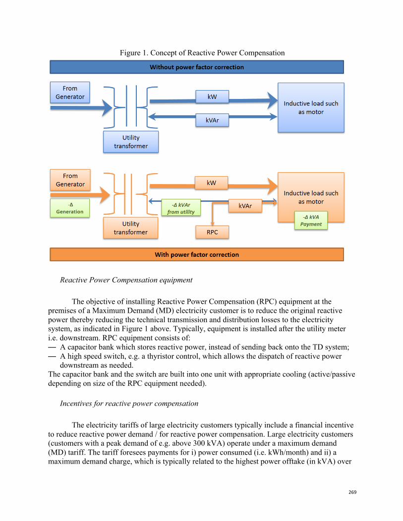
269

Figure 1. Concept of Reactive Power Compensation

Reactive Power Compensation equipment

The objective of installing Reactive Power Compensation (RPC) equipment at the premises of a Maximum Demand (MD) electricity customer is to reduce the original reactive power thereby reducing the technical transmission and distribution losses to the electricity system, as indicated in Figure 1 above. Typically, equipment is installed after the utility meter i.e. downstream. RPC equipment consists of: — A capacitor bank which stores reactive power, instead of sending back onto the TD system; — A high speed switch, e.g. a thyristor control, which allows the dispatch of reactive power

downstream as needed. The capacitor bank and the switch are built into one unit with appropriate cooling (active/passive depending on size of the RPC equipment needed).

Incentives for reactive power compensation

The electricity tariffs of large electricity customers typically include a financial incentive to reduce reactive power demand / for reactive power compensation. Large electricity customers (customers with a peak demand of e.g. above 300 kVA) operate under a maximum demand (MD) tariff. The tariff foresees payments for i) power consumed (i.e. kWh/month) and ii) a maximum demand charge, which is typically related to the highest power offtake (in kVA) over

270

a 30-minute period for one month. Some countries have differentiated MD payment schemes, which either reward or penalizes reactive power (e.g. Uganda) or charges for reactive power (Mozambique).

Political economy / weak financial standing of utilities leads to lack of investment in TD system

Under optimal conditions power utilities would install RPC equipment at their

substations, thus reducing the load and hence the technical losses of the TD system. In sub-Saharan Africa, utilities typically cannot invest in cost-efficient maintenance and upgrading of the TD system as many utilities lack the means also due to non-cost reflective tariffs they are required to charge customers.

A World Bank study (Trimble et al., 2016) investigated cost reflectiveness, comparing the operational and capital expenditures of generation and distribution with the average price of kWh billed for 39 Sub-Saharan African countries between 2010 to 2015. The results indicate that only two countries (i.e. Seychelles and Uganda) operate on cost reflective terms recovering both, operational- and capital expenditures. The cash collected in 19 countries barely covers operational expenditures, but is insufficient to cover any significant new capital layout. Hence many SSA countries suffer from poor TD infrastructure and resultant technical losses.

GHG accounting elements of a RPC program / baseline setting

The proposed RPC program makes use of GHG accounting elements from methods designed for and internationally recognized and approved for the UNFCCC Clean Development Mechanism: — An approved Clean Development Mechanism (CDM) methodology, AMS-II.T.: Emission

reduction through reactive power compensation in power distribution network, Version 1 (CDM EB94, Annex 8) to quantify the baseline emissions and emission reductions due to power factor improvements;

— Approved Standardized Baselines, (ASB) which are national emission factors for the electricity system, developed according to UNFCCC approved tool (CDM EB87, Annex 9. ASB0001 was used to determine the emission factor (in tCO2/MWh) of the electricity system covering Mozambique, Zambia and Zimbabwe; ASB0007 was used for Uganda.

Applying a UNFCCC approved methodologies ensures a consistent, transparent and reproducible estimation of GHG emissions.

3. Sectoral abatement potentials

Data sets and data treatment

For analyzing the sectoral abatement potentials, we collected detailed data sets for the four country studies using identical data reporting templates. The data was provided by Uganda’s power distribution company UMEME, Electicidate de Mozambique (EDM), Zambia Electricity

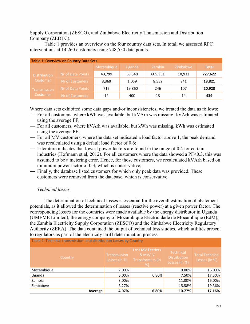
271

Supply Corporation (ZESCO), and Zimbabwe Electricity Transmission and Distribution Company (ZEDTC).

Table 1 provides an overview on the four country data sets. In total, we assessed RPC interventions at 14,260 customers using 748,550 data points. Table 1: Overview on Country Data Sets

Mozambique Uganda Zambia Zimbabwe Total

Distribution Customer

Nr of Data Points 43,799 63,540 609,351 10,932 727,622

Nr of Customers 3,369 1,059 8,552 841 13,821

Transmission Customer

Nr of Data Points 715 19,860 246 107 20,928

Nr of Customers 12 400 13 14 439

Where data sets exhibited some data gaps and/or inconsistencies, we treated the data as follows: — For all customers, where kWh was available, but kVArh was missing, kVArh was estimated

using the average PF; — For all customers, where kVArh was available, but kWh was missing, kWh was estimated

using the average PF; — For all MV customers, where the data set indicated a load factor above 1, the peak demand

was recalculated using a default load factor of 0.6; — Literature indicates that lowest power factors are found in the range of 0.4 for certain

industries (Hofmann et al, 2012). For all customers where the data showed a PF<0.3, this was assumed to be a metering error. Hence, for those customers, we recalculated kVArh based on minimum power factor of 0.3, which is conservative;

— Finally, the database listed customers for which only peak data was provided. These customers were removed from the database, which is conservative.

Technical losses

The determination of technical losses is essential for the overall estimation of abatement potentials, as it allowed the determination of losses (reactive power) at a given power factor. The corresponding losses for the countries were made available by the energy distributor in Uganda (UMEME Limited), the energy company of Mozambique Electricidade de Moçambique (EdM), the Zambia Electricity Supply Corporation (ZESCO) and the Zimbabwe Electricity Regulatory Authority (ZERA). The data contained the output of technical loss studies, which utilities present to regulators as part of the electricity tariff determination process. Table 2: Technical transmission- and distribution Losses by Country

Country Transmission Losses (in %)

Loss MV Feeders & MV/LV

Transformers (in %)

Technical Distribution Losses (in %)

Total Technical Losses (in %)

Mozambique 7.00% 9.00% 16.00% Uganda 3.00% 6.80% 7.50% 17.30% Zambia 3.00% 11.00% 16.00% Zimbabwe 3.27% 15.58% 19.36%

Average 4.07% 6.80% 10.77% 17.16%

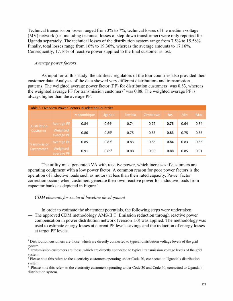
272

Technical transmission losses ranged from 3% to 7%; technical losses of the medium voltage (MV) network (i.e. including technical losses of step-down transformer) were only reported for Uganda separately. The technical losses of the distribution system range from 7.5% to 15.58%. Finally, total losses range from 16% to 19.36%, whereas the average amounts to 17.16%. Consequently, 17.16% of reactive power supplied to the final customer is lost.

Average power factors

As input for of this study, the utilities / regulators of the four countries also provided their customer data. Analyses of the data showed very different distribution- and transmission patterns. The weighted average power factor (PF) for distribution customers1 was 0.83, whereas the weighted average PF for transmission customers2 was 0.88. The weighted average PF is always higher than the average PF. Table 3: Overview Power Factors in selected Countries

Mozambique Uganda Zambia Zimbabwe Av. Min Max

Distribtion Customer

Average PF 0.84 0.643 0.74 0.79 0.75 0.64 0.84

Weighted average PF 0.86 0.855 0.75 0.85 0.83 0.75 0.86

Transmission Custommer

Average PF 0.85 0.834 0.83 0.85 0.84 0.83 0.85

Weighted average PF 0.91 0.856 0.88 0.90 0.88 0.85 0.91

The utility must generate kVA with reactive power, which increases if customers are

operating equipment with a low power factor. A common reason for poor power factors is the operation of inductive loads such as motors at less than their rated capacity. Power factor correction occurs when customers generate their own reactive power for inductive loads from capacitor banks as depicted in Figure 1.

CDM elements for sectoral baseline development

In order to estimate the abatement potentials, the following steps were undertaken: — The approved CDM methodology AMS-II.T: Emission reduction through reactive power

compensation in power distribution network (version 1.0) was applied. The methodology was used to estimate energy losses at current PF levels savings and the reduction of energy losses at target PF levels.

1 Distribution customers are those, which are directly connected to typical distribution voltage levels of the grid system. 2 Transmission customers are those, which are directly connected to typical transmission voltage levels of the grid system. 3 Please note this refers to the electricity customers operating under Code 20, connected to Uganda’s distribution system. 4 Please note this refers to the electricity customers operating under Code 30 and Code 40, connected to Uganda’s distribution system.

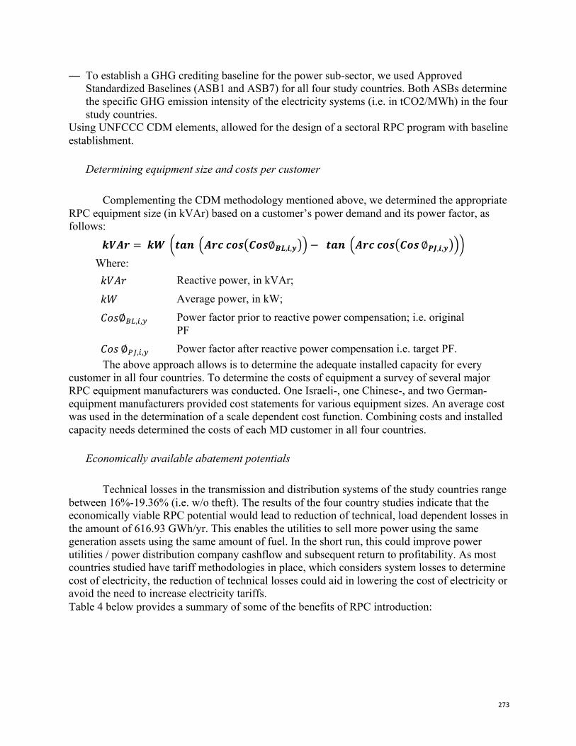
273

— To establish a GHG crediting baseline for the power sub-sector, we used Approved Standardized Baselines (ASB1 and ASB7) for all four study countries. Both ASBs determine the specific GHG emission intensity of the electricity systems (i.e. in tCO2/MWh) in the four study countries.

Using UNFCCC CDM elements, allowed for the design of a sectoral RPC program with baseline establishment.

Determining equipment size and costs per customer

Complementing the CDM methodology mentioned above, we determined the appropriate RPC equipment size (in kVAr) based on a customer’s power demand and its power factor, as follows:

𝒌𝑽𝑨𝒓 = 𝒌𝑾 {𝒕𝒂𝒏 Y𝑨𝒓𝒄𝒄𝒐𝒔;𝑪𝒐𝒔∅𝑩𝑳,𝒊,𝒚<Z − 𝒕𝒂𝒏 Y𝑨𝒓𝒄𝒄𝒐𝒔;𝑪𝒐𝒔∅𝑷𝑱,𝒊,𝒚<Z� Where: 𝑘𝑉𝐴𝑟 Reactive power, in kVAr;

𝑘𝑊 Average power, in kW;

𝐶𝑜𝑠∅�9,�,� Power factor prior to reactive power compensation; i.e. original PF

𝐶𝑜𝑠 ∅S�,�,� Power factor after reactive power compensation i.e. target PF. The above approach allows is to determine the adequate installed capacity for every

customer in all four countries. To determine the costs of equipment a survey of several major RPC equipment manufacturers was conducted. One Israeli-, one Chinese-, and two German- equipment manufacturers provided cost statements for various equipment sizes. An average cost was used in the determination of a scale dependent cost function. Combining costs and installed capacity needs determined the costs of each MD customer in all four countries.

Economically available abatement potentials

Technical losses in the transmission and distribution systems of the study countries range between 16%-19.36% (i.e. w/o theft). The results of the four country studies indicate that the economically viable RPC potential would lead to reduction of technical, load dependent losses in the amount of 616.93 GWh/yr. This enables the utilities to sell more power using the same generation assets using the same amount of fuel. In the short run, this could improve power utilities / power distribution company cashflow and subsequent return to profitability. As most countries studied have tariff methodologies in place, which considers system losses to determine cost of electricity, the reduction of technical losses could aid in lowering the cost of electricity or avoid the need to increase electricity tariffs. Table 4 below provides a summary of some of the benefits of RPC introduction:

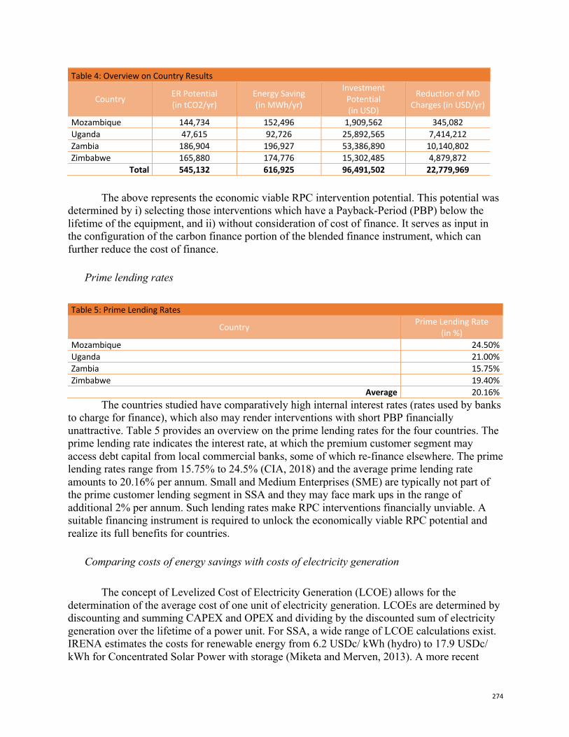
274

Table 4: Overview on Country Results

Country ER Potential (in tCO2/yr)

Energy Saving (in MWh/yr)

Investment Potential (in USD)

Reduction of MD Charges (in USD/yr)

Mozambique 144,734 152,496 1,909,562 345,082 Uganda 47,615 92,726 25,892,565 7,414,212 Zambia 186,904 196,927 53,386,890 10,140,802 Zimbabwe 165,880 174,776 15,302,485 4,879,872

Total 545,132 616,925 96,491,502 22,779,969

The above represents the economic viable RPC intervention potential. This potential was determined by i) selecting those interventions which have a Payback-Period (PBP) below the lifetime of the equipment, and ii) without consideration of cost of finance. It serves as input in the configuration of the carbon finance portion of the blended finance instrument, which can further reduce the cost of finance.

Prime lending rates

The countries studied have comparatively high internal interest rates (rates used by banks to charge for finance), which also may render interventions with short PBP financially unattractive. Table 5 provides an overview on the prime lending rates for the four countries. The prime lending rate indicates the interest rate, at which the premium customer segment may access debt capital from local commercial banks, some of which re-finance elsewhere. The prime lending rates range from 15.75% to 24.5% (CIA, 2018) and the average prime lending rate amounts to 20.16% per annum. Small and Medium Enterprises (SME) are typically not part of the prime customer lending segment in SSA and they may face mark ups in the range of additional 2% per annum. Such lending rates make RPC interventions financially unviable. A suitable financing instrument is required to unlock the economically viable RPC potential and realize its full benefits for countries.

Comparing costs of energy savings with costs of electricity generation

The concept of Levelized Cost of Electricity Generation (LCOE) allows for the determination of the average cost of one unit of electricity generation. LCOEs are determined by discounting and summing CAPEX and OPEX and dividing by the discounted sum of electricity generation over the lifetime of a power unit. For SSA, a wide range of LCOE calculations exist. IRENA estimates the costs for renewable energy from 6.2 USDc/ kWh (hydro) to 17.9 USDc/ kWh for Concentrated Solar Power with storage (Miketa and Merven, 2013). A more recent

Table 5: Prime Lending Rates

Country Prime Lending Rate (in %)

Mozambique 24.50% Uganda 21.00% Zambia 15.75% Zimbabwe 19.40%

Average 20.16%

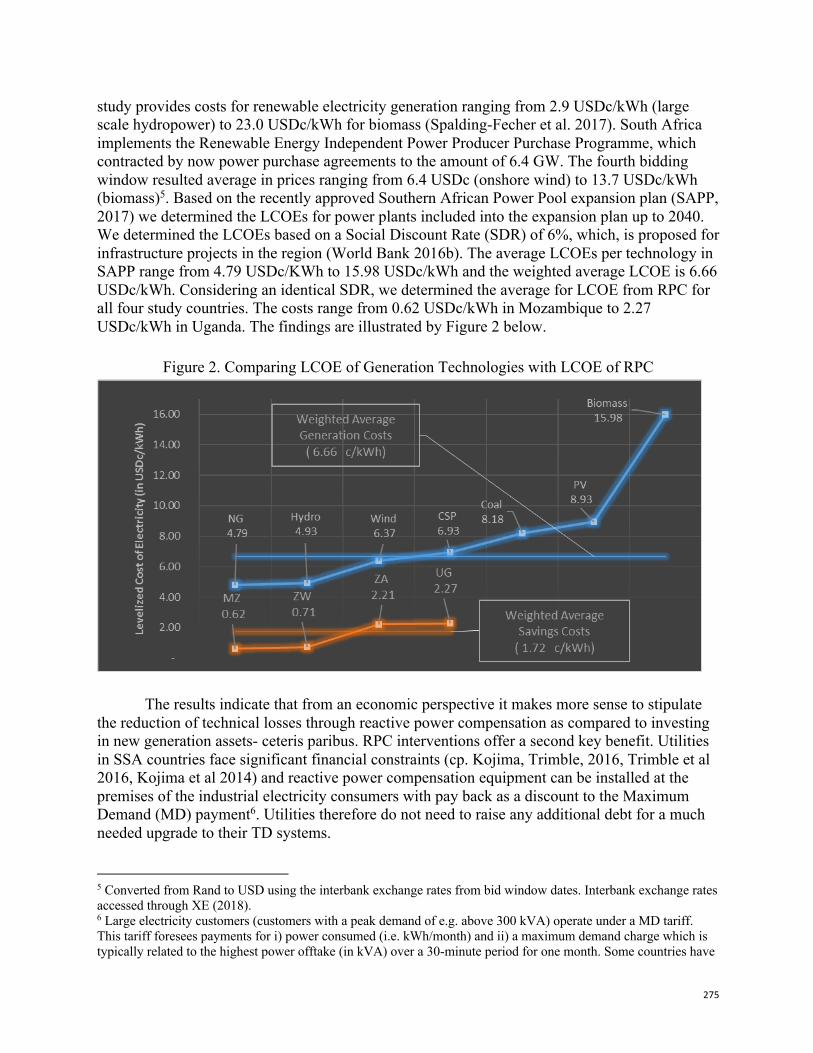
275

study provides costs for renewable electricity generation ranging from 2.9 USDc/kWh (large scale hydropower) to 23.0 USDc/kWh for biomass (Spalding-Fecher et al. 2017). South Africa implements the Renewable Energy Independent Power Producer Purchase Programme, which contracted by now power purchase agreements to the amount of 6.4 GW. The fourth bidding window resulted average in prices ranging from 6.4 USDc (onshore wind) to 13.7 USDc/kWh (biomass)5. Based on the recently approved Southern African Power Pool expansion plan (SAPP, 2017) we determined the LCOEs for power plants included into the expansion plan up to 2040. We determined the LCOEs based on a Social Discount Rate (SDR) of 6%, which, is proposed for infrastructure projects in the region (World Bank 2016b). The average LCOEs per technology in SAPP range from 4.79 USDc/KWh to 15.98 USDc/kWh and the weighted average LCOE is 6.66 USDc/kWh. Considering an identical SDR, we determined the average for LCOE from RPC for all four study countries. The costs range from 0.62 USDc/kWh in Mozambique to 2.27 USDc/kWh in Uganda. The findings are illustrated by Figure 2 below.

Figure 2. Comparing LCOE of Generation Technologies with LCOE of RPC

The results indicate that from an economic perspective it makes more sense to stipulate the reduction of technical losses through reactive power compensation as compared to investing in new generation assets- ceteris paribus. RPC interventions offer a second key benefit. Utilities in SSA countries face significant financial constraints (cp. Kojima, Trimble, 2016, Trimble et al 2016, Kojima et al 2014) and reactive power compensation equipment can be installed at the premises of the industrial electricity consumers with pay back as a discount to the Maximum Demand (MD) payment6. Utilities therefore do not need to raise any additional debt for a much needed upgrade to their TD systems.

5 Converted from Rand to USD using the interbank exchange rates from bid window dates. Interbank exchange rates accessed through XE (2018). 6 Large electricity customers (customers with a peak demand of e.g. above 300 kVA) operate under a MD tariff. This tariff foresees payments for i) power consumed (i.e. kWh/month) and ii) a maximum demand charge which is typically related to the highest power offtake (in kVA) over a 30-minute period for one month. Some countries have

276

4. Blended carbon finance instrument to leverage the sectoral GHG abatement potentials

Combining ‘push’ and ‘pull’ components to maximize widespread uptake by private sector

The proposed funding model was presented to Multilateral Development Banks (MDB)

and discussed with representatives of Power Regulators, Ministries of Energy, Ministries for the Environment and utilities, transmission and distribution companies in each of the countries in order to ensure adequate consideration of stakeholders’ recommendations. Based on this feedback the concept of “push & pull” was adopted.

The ‘push’ component’ comprises potential amendments of the regulatory framework in the countries aiming at stimulating subsector-specific investments of the private sector at no cost for the government: — Adjustment of national Grid Codes about higher mandatory power factor provisions; — Improvement of the kVA payment structure; — Introduction of a kVArh related scheme of penalty and reward payments.

Such amendments could lead to cost efficiency, i.e. parity of generation and energy saving costs (cp. Figure 2). In country stakeholder consultations showed that regulatory measures are only acceptable for the private sector and implementable along with financial and technical support (the ‘pull’). The fundamental program funding structure therefore addresses main non-policy barriers to implementation: — High capital cost that prevents investing in RPC energy efficiency by industries, — Insufficient competitiveness compared to companies’ Key Performance Indicators (KPI) and — Potential lack of awareness- and technical capacity in the countries.

The ‘pull’ component is low cost finance from domestic commercial lenders. Local currency loans are preferred as exposure to FX further increases the cost of capital, the burden of which is almost always placed in the borrower. The low-cost finance is made up of a blend of 3 sources (i) carbon (results-based) finance, (ii) export trade cover or risk insurance and (iii) commercial bank debt, which can be augmented with DFI debt as needed.

The blend is essential to achieve the lending rates needed and Export Credit Agency (ECA) support is key to as it can significantly reduce the overall cost of funding. ECAs can typically extend up to 85 % (5% for the applicant) of the export contract value for eligible exporters (i) as an exporter (supplier’s credit); (ii) through a commercial bank in the form of trade related credit provided either to the supplier or to the importer (buyer’s credit); or (iii) directly by another export credit agency of the exporting countries. This allows commercial banks to significantly adjust their risk assessment on the finance and thereby lower the cost of lending well below domestic rates.

applied differentiated MD payment schemes, which also foresee rewards and penalties for reactive power (e.g. Uganda) or charge reactive power (Mozambique).

277

Financing instrument structure

Some basic parameters determine the design of the financing instrument. The RPC equipment to be installed must adhere to defined quality standards7 and shall have a rated lifetime of 15 years. The financing instrument applied shall enable economically viable investments in RPC installations, while at the same time ensuring rapid uptake of the technology at maximum scale. For this, a financially attractive offer must be made to the MD customers, which allows for loan pay back within a maximum of 6 years from savings accruing from reduced kVA-related maximum demand payments, thus allowing the customer to profit from the installation for the remaining lifetime.

The financing structure required for reducing capital cost applies a blended finance approach:

1. A regional commercial bank sets up and administers a financing vehicle for on-lending to which it provides senior funding.

2. The bank enters into an agreement with a national ECA to reduce the cost of senior funding. ECA conditions depend on the origin of the equipment and services determining the cost of the ECA premium; the amount that is covered (maximum 80% of the export contract value) and on the rating of the recipient country. For all four countries ECA insurance comprising commercial (payment), political (change in government policy) and FX (transfer, convertibility) risks can be secured for a 6-year period.

3. A DFI provides first loss funding for the uncovered portion (e.g. 20%). Respective cost of finance is substantially higher than the ECA covered portion of the funding, usually approx. 8% above the cost of ECA backed funding.

4. In case up-front calculations reveal payback periods of more than 6 years, a carbon finance-based co-financing instrument can be employed, which considers the business case of each individual intervention in order to account for additionality issues and optimize carbon payments. The proposed carbon finance approach aims to improve on the CDM, where prices for

Certified Emission Reductions (CER) were set by supply and demand of CERs under uncertainty about the underlying marginal abatement costs of projects generating the credits. A carbon price of e.g. 10 USD/CER was paid irrespective whether e.g., a HFC-23 abatement project required 0.2 USD/CER (cp. IPCC/TEAP, 2005) or a hydropower project required 10 USD/CER (cp. Rahman et al., 2015) to become financially viable. This resulted in high producer rents for some project types, insufficient carbon incentives for other project types and an overall in a sub-optimal application of carbon finance.

Considering the substantial financing volumes required to achieve the objectives of the Paris Agreement and to implement the SDGs, it is generally understood that private sector involvement is needed with optimal use of public funding. Against this background, the carbon financing concept is conceived around a sectoral analysis which estimates the benefits and the costs of each single intervention and determines the marginal abatement costs of individual investments and the amount of carbon finance required to make the mitigation action financially viable, i.e. contribute to reaching a conditional emission mitigation target.

7 International standards: IEC 61642, IEC 61000-2-2, IEC 61000-2-4, IEC 61000-2-12, EN 50160 (in Europe), IEEE 519 (USA) and national standard such as NRS 048 in South Africa

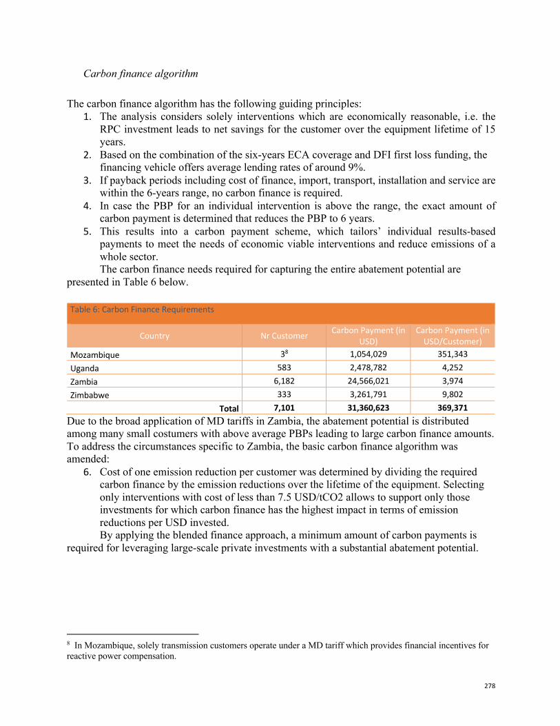
278

Carbon finance algorithm The carbon finance algorithm has the following guiding principles:

1. The analysis considers solely interventions which are economically reasonable, i.e. the RPC investment leads to net savings for the customer over the equipment lifetime of 15 years.

2. Based on the combination of the six-years ECA coverage and DFI first loss funding, the financing vehicle offers average lending rates of around 9%.

3. If payback periods including cost of finance, import, transport, installation and service are within the 6-years range, no carbon finance is required.

4. In case the PBP for an individual intervention is above the range, the exact amount of carbon payment is determined that reduces the PBP to 6 years.

5. This results into a carbon payment scheme, which tailors’ individual results-based payments to meet the needs of economic viable interventions and reduce emissions of a whole sector. The carbon finance needs required for capturing the entire abatement potential are

presented in Table 6 below.

Due to the broad application of MD tariffs in Zambia, the abatement potential is distributed among many small costumers with above average PBPs leading to large carbon finance amounts. To address the circumstances specific to Zambia, the basic carbon finance algorithm was amended:

6. Cost of one emission reduction per customer was determined by dividing the required carbon finance by the emission reductions over the lifetime of the equipment. Selecting only interventions with cost of less than 7.5 USD/tCO2 allows to support only those investments for which carbon finance has the highest impact in terms of emission reductions per USD invested. By applying the blended finance approach, a minimum amount of carbon payments is

required for leveraging large-scale private investments with a substantial abatement potential.

8 In Mozambique, solely transmission customers operate under a MD tariff which provides financial incentives for reactive power compensation.

Table 6: Carbon Finance Requirements

Country Nr Customer Carbon Payment (in USD)

Carbon Payment (in USD/Customer)

Mozambique 38 1,054,029 351,343 Uganda 583 2,478,782 4,252 Zambia 6,182 24,566,021 3,974 Zimbabwe 333 3,261,791 9,802

Total 7,101 31,360,623 369,371

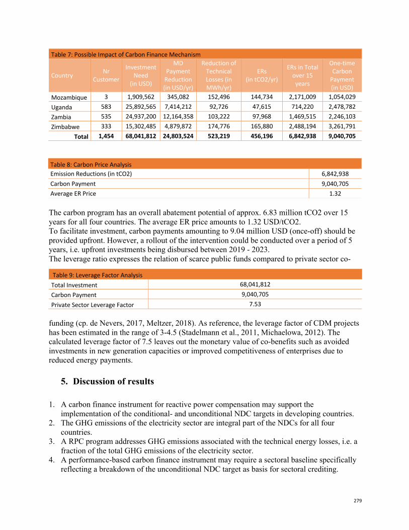
279

Table 7: Possible Impact of Carbon Finance Mechanism

Country Nr Customer

Investment Need

(in USD)

MD Payment

Reduction (in USD/yr)

Reduction of Technical Losses (in MWh/yr)

ERs (in tCO2/yr)

ERs in Total over 15 years

One-time Carbon

Payment (in USD)

Mozambique 3 1,909,562 345,082 152,496 144,734 2,171,009 1,054,029 Uganda 583 25,892,565 7,414,212 92,726 47,615 714,220 2,478,782 Zambia 535 24,937,200 12,164,358 103,222 97,968 1,469,515 2,246,103 Zimbabwe 333 15,302,485 4,879,872 174,776 165,880 2,488,194 3,261,791

Total 1,454 68,041,812 24,803,524 523,219 456,196 6,842,938 9,040,705

The carbon program has an overall abatement potential of approx. 6.83 million tCO2 over 15 years for all four countries. The average ER price amounts to 1.32 USD/tCO2. To facilitate investment, carbon payments amounting to 9.04 million USD (once-off) should be provided upfront. However, a rollout of the intervention could be conducted over a period of 5 years, i.e. upfront investments being disbursed between 2019 - 2023. The leverage ratio expresses the relation of scarce public funds compared to private sector co-

funding (cp. de Nevers, 2017, Meltzer, 2018). As reference, the leverage factor of CDM projects has been estimated in the range of 3-4.5 (Stadelmann et al., 2011, Michaelowa, 2012). The calculated leverage factor of 7.5 leaves out the monetary value of co-benefits such as avoided investments in new generation capacities or improved competitiveness of enterprises due to reduced energy payments.

5. Discussion of results 1. A carbon finance instrument for reactive power compensation may support the

implementation of the conditional- and unconditional NDC targets in developing countries. 2. The GHG emissions of the electricity sector are integral part of the NDCs for all four

countries. 3. A RPC program addresses GHG emissions associated with the technical energy losses, i.e. a

fraction of the total GHG emissions of the electricity sector. 4. A performance-based carbon finance instrument may require a sectoral baseline specifically

reflecting a breakdown of the unconditional NDC target as basis for sectoral crediting.

Table 8: Carbon Price Analysis Emission Reductions (in tCO2) 6,842,938 Carbon Payment 9,040,705 Average ER Price 1.32

Table 9: Leverage Factor Analysis Total Investment 68,041,812 Carbon Payment 9,040,705 Private Sector Leverage Factor 7.53

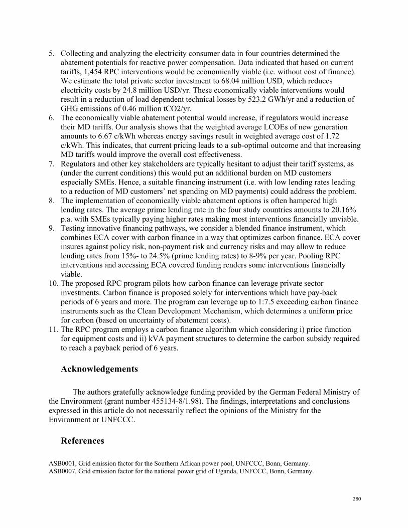
280

5. Collecting and analyzing the electricity consumer data in four countries determined the abatement potentials for reactive power compensation. Data indicated that based on current tariffs, 1,454 RPC interventions would be economically viable (i.e. without cost of finance). We estimate the total private sector investment to 68.04 million USD, which reduces electricity costs by 24.8 million USD/yr. These economically viable interventions would result in a reduction of load dependent technical losses by 523.2 GWh/yr and a reduction of GHG emissions of 0.46 million tCO2/yr.

6. The economically viable abatement potential would increase, if regulators would increase their MD tariffs. Our analysis shows that the weighted average LCOEs of new generation amounts to 6.67 c/kWh whereas energy savings result in weighted average cost of 1.72 c/kWh. This indicates, that current pricing leads to a sub-optimal outcome and that increasing MD tariffs would improve the overall cost effectiveness.

7. Regulators and other key stakeholders are typically hesitant to adjust their tariff systems, as (under the current conditions) this would put an additional burden on MD customers especially SMEs. Hence, a suitable financing instrument (i.e. with low lending rates leading to a reduction of MD customers’ net spending on MD payments) could address the problem.

8. The implementation of economically viable abatement options is often hampered high lending rates. The average prime lending rate in the four study countries amounts to 20.16% p.a. with SMEs typically paying higher rates making most interventions financially unviable.

9. Testing innovative financing pathways, we consider a blended finance instrument, which combines ECA cover with carbon finance in a way that optimizes carbon finance. ECA cover insures against policy risk, non-payment risk and currency risks and may allow to reduce lending rates from 15%- to 24.5% (prime lending rates) to 8-9% per year. Pooling RPC interventions and accessing ECA covered funding renders some interventions financially viable.

10. The proposed RPC program pilots how carbon finance can leverage private sector investments. Carbon finance is proposed solely for interventions which have pay-back periods of 6 years and more. The program can leverage up to 1:7.5 exceeding carbon finance instruments such as the Clean Development Mechanism, which determines a uniform price for carbon (based on uncertainty of abatement costs).

11. The RPC program employs a carbon finance algorithm which considering i) price function for equipment costs and ii) kVA payment structures to determine the carbon subsidy required to reach a payback period of 6 years.

Acknowledgements

The authors gratefully acknowledge funding provided by the German Federal Ministry of

the Environment (grant number 455134-8/1.98). The findings, interpretations and conclusions expressed in this article do not necessarily reflect the opinions of the Ministry for the Environment or UNFCCC.

References ASB0001, Grid emission factor for the Southern African power pool, UNFCCC, Bonn, Germany. ASB0007, Grid emission factor for the national power grid of Uganda, UNFCCC, Bonn, Germany.

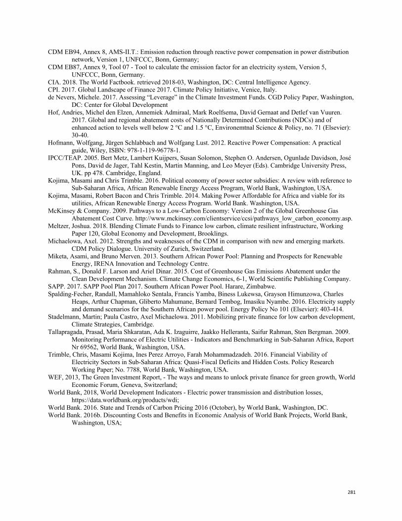
281

CDM EB94, Annex 8, AMS-II.T.: Emission reduction through reactive power compensation in power distribution network, Version 1, UNFCCC, Bonn, Germany;

CDM EB87, Annex 9, Tool 07 - Tool to calculate the emission factor for an electricity system, Version 5, UNFCCC, Bonn, Germany.

CIA. 2018. The World Factbook. retrieved 2018-03, Washington, DC: Central Intelligence Agency. CPI. 2017. Global Landscape of Finance 2017. Climate Policy Initiative, Venice, Italy. de Nevers, Michele. 2017. Assessing “Leverage” in the Climate Investment Funds. CGD Policy Paper, Washington,

DC: Center for Global Development Hof, Andries, Michel den Elzen, Annemiek Admiraal, Mark Roelfsema, David Gernaat and Detlef van Vuuren.

2017. Global and regional abatement costs of Nationally Determined Contributions (NDCs) and of enhanced action to levels well below 2 °C and 1.5 °C, Environemtnal Science & Policy, no. 71 (Elsevier): 30-40.

Hofmann, Wolfgang, Jürgen Schlabbach and Wolfgang Lust. 2012. Reactive Power Compensation: A practical guide, Wiley, ISBN: 978-1-119-96778-1.

IPCC/TEAP. 2005. Bert Metz, Lambert Kuijpers, Susan Solomon, Stephen O. Andersen, Ogunlade Davidson, José Pons, David de Jager, Tahl Kestin, Martin Manning, and Leo Meyer (Eds). Cambridge University Press, UK. pp 478. Cambridge, England.

Kojima, Masami and Chris Trimble. 2016. Political economy of power sector subsidies: A review with reference to Sub-Saharan Africa, African Renewable Energy Access Program, World Bank, Washington, USA.

Kojima, Masami, Robert Bacon and Chris Trimble. 2014. Making Power Affordable for Africa and viable for its utilities, African Renewable Energy Access Program. World Bank. Washington, USA.

McKinsey & Company. 2009. Pathways to a Low-Carbon Economy: Version 2 of the Global Greenhouse Gas Abatement Cost Curve. http://www.mckinsey.com/clientservice/ccsi/pathways_low_carbon_economy.asp.

Meltzer, Joshua. 2018. Blending Climate Funds to Finance low carbon, climate resilient infrastructure, Working Paper 120, Global Economy and Development, Brooklings.

Michaelowa, Axel. 2012. Strengths and weaknesses of the CDM in comparison with new and emerging markets. CDM Policy Dialogue. University of Zurich, Switzerland.

Miketa, Asami, and Bruno Merven. 2013. Southern African Power Pool: Planning and Prospects for Renewable Energy, IRENA Innovation and Technology Centre.

Rahman, S., Donald F. Larson and Ariel Dinar. 2015. Cost of Greenhouse Gas Emissions Abatement under the Clean Development Mechanism. Climate Change Economics, 6-1, World Scientific Publishing Company.

SAPP. 2017. SAPP Pool Plan 2017. Southern African Power Pool. Harare, Zimbabwe. Spalding-Fecher, Randall, Mamahloko Sentala, Francis Yamba, Biness Lukewsa, Grayson Himunzowa, Charles

Heaps, Arthur Chapman, Gliberto Mahumane, Bernard Tembog, Imasiku Nyambe. 2016. Electricity supply and demand scenarios for the Southern African power pool. Energy Policy No 101 (Elsevier): 403-414.

Stadelmann, Martin; Paula Castro, Axel Michaelowa. 2011. Mobilizing private finance for low carbon development, Climate Strategies, Cambridge.

Tallapragada, Prasad, Maria Shkaratan, Ada K. Izaguirre, Jaakko Helleranta, Saifur Rahman, Sten Bergman. 2009. Monitoring Performance of Electric Utilities - Indicators and Benchmarking in Sub-Saharan Africa, Report Nr 69562, World Bank, Washington, USA.

Trimble, Chris, Masami Kojima, Ines Perez Arroyo, Farah Mohammadzadeh. 2016. Financial Viability of Electricity Sectors in Sub-Saharan Africa: Quasi-Fiscal Deficits and Hidden Costs. Policy Research Working Paper; No. 7788, World Bank, Washington, USA.

WEF, 2013, The Green Investment Report, - The ways and means to unlock private finance for green growth, World Economic Forum, Geneva, Switzerland;

World Bank, 2018, World Development Indicators - Electric power transmission and distribution losses, https://data.worldbank.org/products/wdi;

World Bank. 2016. State and Trends of Carbon Pricing 2016 (October), by World Bank, Washington, DC. World Bank. 2016b. Discounting Costs and Benefits in Economic Analysis of World Bank Projects, World Bank,

Washington, USA;

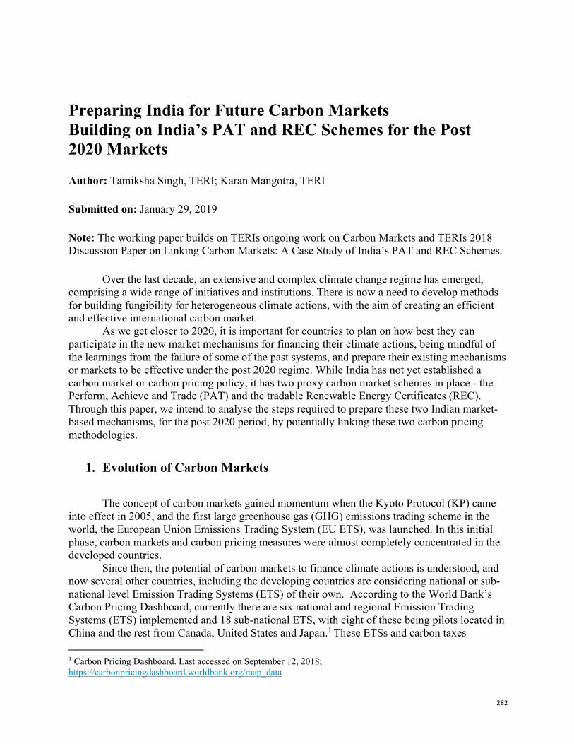
282

Preparing India for Future Carbon Markets Building on India’s PAT and REC Schemes for the Post 2020 Markets Author: Tamiksha Singh, TERI; Karan Mangotra, TERI Submitted on: January 29, 2019 Note: The working paper builds on TERIs ongoing work on Carbon Markets and TERIs 2018 Discussion Paper on Linking Carbon Markets: A Case Study of India’s PAT and REC Schemes.

Over the last decade, an extensive and complex climate change regime has emerged, comprising a wide range of initiatives and institutions. There is now a need to develop methods for building fungibility for heterogeneous climate actions, with the aim of creating an efficient and effective international carbon market.

As we get closer to 2020, it is important for countries to plan on how best they can participate in the new market mechanisms for financing their climate actions, being mindful of the learnings from the failure of some of the past systems, and prepare their existing mechanisms or markets to be effective under the post 2020 regime. While India has not yet established a carbon market or carbon pricing policy, it has two proxy carbon market schemes in place - the Perform, Achieve and Trade (PAT) and the tradable Renewable Energy Certificates (REC). Through this paper, we intend to analyse the steps required to prepare these two Indian market-based mechanisms, for the post 2020 period, by potentially linking these two carbon pricing methodologies.

1. Evolution of Carbon Markets

The concept of carbon markets gained momentum when the Kyoto Protocol (KP) came into effect in 2005, and the first large greenhouse gas (GHG) emissions trading scheme in the world, the European Union Emissions Trading System (EU ETS), was launched. In this initial phase, carbon markets and carbon pricing measures were almost completely concentrated in the developed countries.

Since then, the potential of carbon markets to finance climate actions is understood, and now several other countries, including the developing countries are considering national or sub-national level Emission Trading Systems (ETS) of their own. According to the World Bank’s Carbon Pricing Dashboard, currently there are six national and regional Emission Trading Systems (ETS) implemented and 18 sub-national ETS, with eight of these being pilots located in China and the rest from Canada, United States and Japan.1 These ETSs and carbon taxes

1 Carbon Pricing Dashboard. Last accessed on September 12, 2018; https://carbonpricingdashboard.worldbank.org/map_data

283

implemented cover around 20% of global GHG emissions from approximately 70 national and sub-national jurisdictions.

The second commitment period of the KP is to end in 2020 and the Paris Agreement (PA) will come into effect in the same year. Under the PA, the Article 6 focuses on a framework for countries to voluntarily cooperate using market and non-market based approaches, thus providing an opening for carbon markets in the post 2020 regime. The Article also creates conditions that could enable an international carbon market and possible convergence of domestic carbon pricing approaches.2 However, the guidance, rules, modalities, and procedures for operationalizing Article 6 are being negotiated among Parties, with basic issues such as scope, governance and infrastructure still to be agreed upon.

The carbon market mechanisms envisaged under the PA are distinct from those of the KP – with the KP approach being centralized and top-down, while the approach taken under the PA is bottom-up and so more decentralized. The PA approach has resulted in Parties developing a range of mitigation actions, in line with their NDCs, with different governance structures, procedures, timelines and jurisdictions. Under this, a complex network of international and domestic mechanisms from all Parties is envisaged which will pose challenges of double counting and lack of environmental integrity.

A key question emerging is how such existing markets are to be integrated with the mechanisms to be evolved under Article 6 of the Agreement. With a view to make progress towards an efficient and effective international carbon market, there is a need to develop methods for building fungibility for the different carbon markets.3

2. Overview of Carbon Markets in India

One of the instruments developed and adopted successfully to reduce greenhouse gases is carbon market-based mechanisms. Of these mechanisms, the Clean Development Mechanism (CDM) which was introduced under the Kyoto protocol, has been by far the most significant carbon market instrument which addressed mitigation of carbon emissions, while also supported developing countries to undertake emission reduction measures. The CDM is the first and the largest carbon offset instrument in the world today. It allows emission-reduction projects in developing countries to earn certified emission reduction (CER) credits through standardized sectoral methodologies, with each CER being equivalent to one tonne of CO2. These CERs can then be traded or sold, and used by industrialized countries to meet their emission reduction targets.

The pioneering market based instrument was successful in mobilizing private capital from developed and developing countries by incentivizing low emission projects in developing countries, and the 7800 projects registered under the CDM from across the world is an indicator of this.4 According to a study by the NewClimate Group, approximately 4.3 billion CERs (translating to 4.3 billion tonnes of carbon emissions mitigated) could be potentially supplied up to 2020 from the registered projects.5

2 TERI. “Market-based Approaches of the Paris Agreement” (2018). 3 TERI. Discussion Paper on “Linking Carbon Markets: A case study of India’s PAT and REC Schemes” (2018). 4 UNFCCC. Accessed on November 2018. Available at https://cdm.unfccc.int/Statistics/Public/CDMinsights/index.html#) 5 NewClimate Institute. Discussion paper on “Marginal cost of CER supply and implications of demand sources” (2018).

284

India played a pivotal role in the development of implementable projects for CDM, with the CDM playing a significant role in supporting Greenhouse Gas (GHG) emission reduction projects in India. The proactive approach of the Government of India together with the strong buy in from the Indian industry and private sector, India became the world’s second largest supplier, after China, of CERs with 1665 registered projects.6

However, the CDM market crashed in 2012, since when the demand levels for CERs are considerably lower than the supply potential from registered CDM projects, leading to low market prices for CERs, which are expected to remain in the range of Euro 0.20 – 0.30 till 2020.7 This has put the global carbon markets in a “critical and uncertain period.”8 Although a large number of projects continued their mitigation activities even post the market crash, without any clear financial incentive, there is possibility of a potential scenario in which the private sector loses confidence in the credibility of carbon market mechanisms which would have an adverse impact on attracting private climate finance.

This highlights the need for national level carbon markets and carbon pricing mechanisms to support domestic climate actions. While the negotiations are still taking place regarding operationalization of the international carbon market mechanisms, an array of national level mechanisms have been introduced with varying degrees of success. These have been effectively implemented, been able to get strong buy-in from the private sector through policy mandates and otherwise, and have significantly high carbon emission reductions potential – as can be seen in the case of India’s PAT and REC markets.

Going forward, it is unclear how CDM will be integrated into the new market mechanisms under Article 6, if at all. However, the new mechanisms will be influenced by the CDM to some degree. Given India’s vast experience with CDM and its processes and the understanding of the potential new mechanism through the implementation of the PAT and REC, it would be beneficial for India to start planning how best it can participate in the post 2020 markets, keeping in mind learnings from CDM to implement measures to ensure environmental integrity and transparency.

6 CDM Registry. Accessed on November 2018. Available at https://cdm.unfccc.int/Registry/index.html 7 Market Data from EEX website. Accessed on August 2018 Available at: https://www.eex.com/en/market-data/environmental-markets/derivatives-market/certified-emission-reductions-futures#!/2018/08/17 8 DEHSt. “Vulnerability of CDM Projects for Discontinuation of Mitigation Activities” (2017).

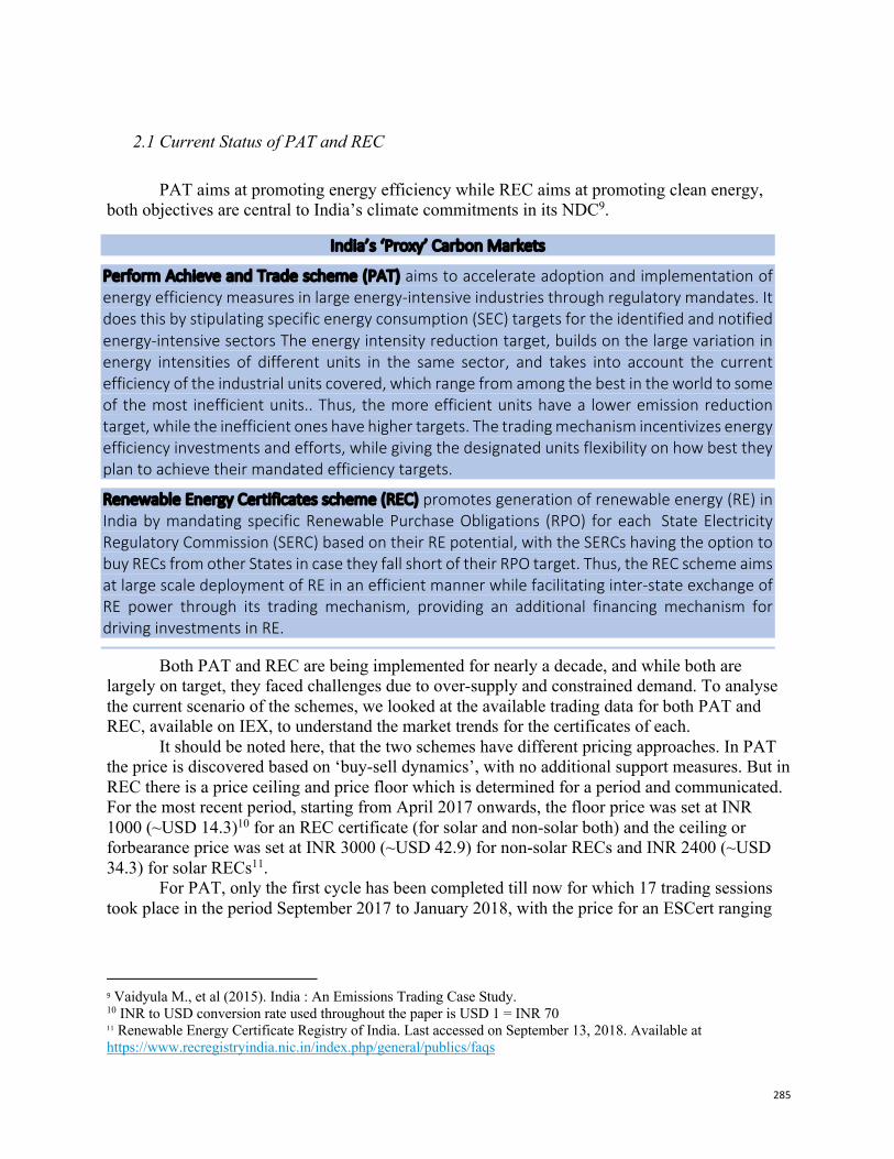
285

2.1 Current Status of PAT and REC

PAT aims at promoting energy efficiency while REC aims at promoting clean energy,

both objectives are central to India’s climate commitments in its NDC9.

Both PAT and REC are being implemented for nearly a decade, and while both are largely on target, they faced challenges due to over-supply and constrained demand. To analyse the current scenario of the schemes, we looked at the available trading data for both PAT and REC, available on IEX, to understand the market trends for the certificates of each.

It should be noted here, that the two schemes have different pricing approaches. In PAT the price is discovered based on ‘buy-sell dynamics’, with no additional support measures. But in REC there is a price ceiling and price floor which is determined for a period and communicated. For the most recent period, starting from April 2017 onwards, the floor price was set at INR 1000 (~USD 14.3)10 for an REC certificate (for solar and non-solar both) and the ceiling or forbearance price was set at INR 3000 (~USD 42.9) for non-solar RECs and INR 2400 (~USD 34.3) for solar RECs11.

For PAT, only the first cycle has been completed till now for which 17 trading sessions took place in the period September 2017 to January 2018, with the price for an ESCert ranging

9 Vaidyula M., et al (2015). India : An Emissions Trading Case Study. 10 INR to USD conversion rate used throughout the paper is USD 1 = INR 70 11 Renewable Energy Certificate Registry of India. Last accessed on September 13, 2018. Available at https://www.recregistryindia.nic.in/index.php/general/publics/faqs

India’s ‘Proxy’ Carbon Markets

Perform Achieve and Trade scheme (PAT) aims to accelerate adoption and implementation of energy efficiency measures in large energy-intensive industries through regulatory mandates. It does this by stipulating specific energy consumption (SEC) targets for the identified and notified energy-intensive sectors The energy intensity reduction target, builds on the large variation in energy intensities of different units in the same sector, and takes into account the current efficiency of the industrial units covered, which range from among the best in the world to some of the most inefficient units.. Thus, the more efficient units have a lower emission reduction target, while the inefficient ones have higher targets. The trading mechanism incentivizes energy efficiency investments and efforts, while giving the designated units flexibility on how best they plan to achieve their mandated efficiency targets.

Renewable Energy Certificates scheme (REC) promotes generation of renewable energy (RE) in India by mandating specific Renewable Purchase Obligations (RPO) for each State Electricity Regulatory Commission (SERC) based on their RE potential, with the SERCs having the option to buy RECs from other States in case they fall short of their RPO target. Thus, the REC scheme aims at large scale deployment of RE in an efficient manner while facilitating inter-state exchange of RE power through its trading mechanism, providing an additional financing mechanism for driving investments in RE.

286

from INR 200 to INR 1200.12 According to Bureau of Energy Efficiency (BEE), the nodal body for PAT, in PAT Cycle 1 there were 309 sellers and 110 buyers and overall, the ESCerts issued were 2.7 times the potential demand. Further, PAT overshot its target for energy efficiency target by 30% in PAT cycle 1. 13 The PAT is being implemented in Cycles, with the first cycle being completed in 2014-15 and the second and third cycle currently being implemented. In each subsequent cycle, PATs coverage is widened, with more sectors coming under its coverage, and deepened, with the SECs increasing.

Similarly, an analysis of REC trading for the period January 2018 to December 2018, shows that the average price for a Solar category REC was INR 1060, with sell bids on average being five times more than the buy bids, while for Non-solar category it was INR 1249, with sell bids on average being around 1.3 times the buy bids. Thus for both Categories supply was more than demand. Overall, nearly 9 million RECs were cleared in 2018.14 A key challenge with REC is regarding the compliance. With stronger focus on the implementation of REC from the regulators, the demand for REC is likely to strengthen. Further, the voluntary markets participation in buying RECs is very low. There is a need to sensitize potential voluntary private sector buyers to use REC for their offsets.15

As per India’s Second Biennial Update Report to the UNFCCC, India emitted 2607.49 million tonnes CO2 e (excluding LULUCF) in 2014.16 However, various research project a significant spike in emissions, estimating emissions to possibly nearly double by 2030, from 2012 levels, even as the per capita emission remains well below the global average and India continues to be in track with its Paris Agreement commitments.17 In this context, PAT’s goal 2020 which translates to approximately 50 million tCO2e emission reductions and REC’s target which converts to an estimated 25 million tCO2e, both together comprise around 3% of India’s 2016 emissions, is a significant achievement with a high potential of being scaled up in the post 2020 regime with functional international carbon markets and trade mechanisms.

2.2 Assessing the Possibility of Linking PAT and REC for the Post 2020 Regime

In the increasingly diverse carbon markets scenario, linking of carbon assets is required to enable the carbon assets in one program being recognized in another and traded. Linking of carbon pricing mechanisms or markets is considered to be beneficial as it would bring in greater price efficiency, increase the liquidity of carbon assets and thus lay the foundations for discovery of a more stable and correct price of carbon. This will also have the advantage of improving the resilience of the system as it creates a more practicable range of carbon prices in varying participating systems. A combination of market based policy instruments will also be more cost effective to implement as it would have the added economies of scale advantage of enhancing overall capacity development, spurring technological and process improvements, strengthening

12 IEX. Last accessed on September 13, 2018. Available at https://www.iexindia.com/marketdata/ESCerts_Market.aspx 13 Bureau of Energy Efficiency. Last accessed on September 13, 2018. Available at https://beeindia.gov.in/content/pat-cycle 14 IEX. Last accessed on January 25, 2019. Available at https://www.iexindia.com/marketdata/recdata.aspx 15 Soonee S.K., et al. “Analysis of Indian Renewable Energy Certificate (REC) Market” (2012). 16 INDIA Second Biennial Update Report. Accessed in January 15 2018. Available at: https://unfccc.int/sites/default/files/resource/INDIA%20SECOND%20BUR%202018.pdf 17 Navroz K Dubash et al. Environ. Res. Lett. 13 074018 (2018).

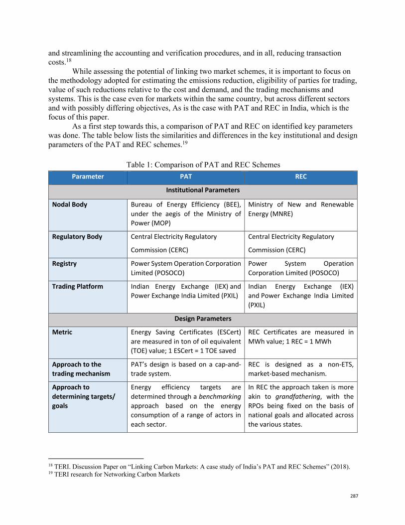
287

and streamlining the accounting and verification procedures, and in all, reducing transaction costs.18

While assessing the potential of linking two market schemes, it is important to focus on the methodology adopted for estimating the emissions reduction, eligibility of parties for trading, value of such reductions relative to the cost and demand, and the trading mechanisms and systems. This is the case even for markets within the same country, but across different sectors and with possibly differing objectives, As is the case with PAT and REC in India, which is the focus of this paper.

As a first step towards this, a comparison of PAT and REC on identified key parameters was done. The table below lists the similarities and differences in the key institutional and design parameters of the PAT and REC schemes.19

Table 1: Comparison of PAT and REC Schemes Parameter PAT REC

Institutional Parameters

Nodal Body Bureau of Energy Efficiency (BEE), under the aegis of the Ministry of Power (MOP)

Ministry of New and Renewable Energy (MNRE)

Regulatory Body Central Electricity Regulatory

Commission (CERC)

Central Electricity Regulatory

Commission (CERC)

Registry Power System Operation Corporation Limited (POSOCO)

Power System Operation Corporation Limited (POSOCO)

Trading Platform Indian Energy Exchange (IEX) and Power Exchange India Limited (PXIL)

Indian Energy Exchange (IEX) and Power Exchange India Limited (PXIL)

Design Parameters

Metric Energy Saving Certificates (ESCert) are measured in ton of oil equivalent (TOE) value; 1 ESCert = 1 TOE saved

REC Certificates are measured in MWh value; 1 REC = 1 MWh

Approach to the trading mechanism

PAT’s design is based on a cap-and-trade system.

REC is designed as a non-ETS, market-based mechanism.

Approach to determining targets/ goals

Energy efficiency targets are determined through a benchmarking approach based on the energy consumption of a range of actors in each sector.

In REC the approach taken is more akin to grandfathering, with the RPOs being fixed on the basis of national goals and allocated across the various states.

18 TERI. Discussion Paper on “Linking Carbon Markets: A case study of India’s PAT and REC Schemes” (2018). 19 TERI research for Networking Carbon Markets

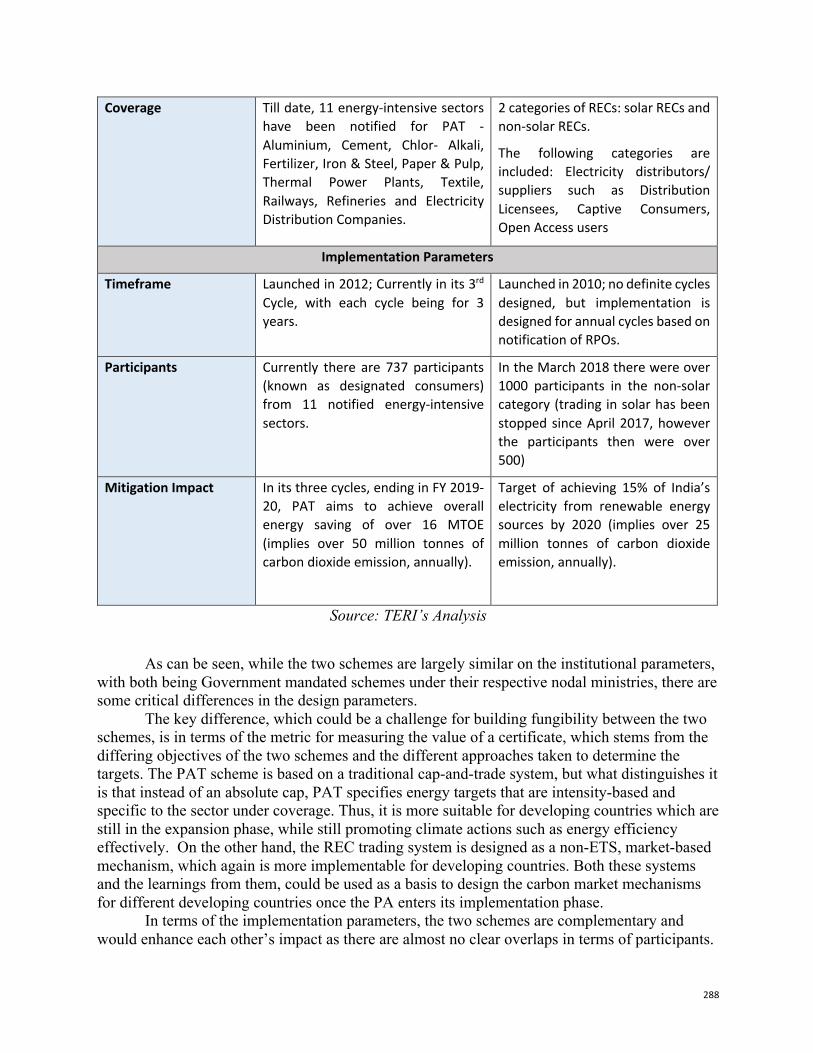
288

Coverage Till date, 11 energy-intensive sectors have been notified for PAT - Aluminium, Cement, Chlor- Alkali, Fertilizer, Iron & Steel, Paper & Pulp, Thermal Power Plants, Textile, Railways, Refineries and Electricity Distribution Companies.

2 categories of RECs: solar RECs and non-solar RECs.

The following categories are included: Electricity distributors/ suppliers such as Distribution Licensees, Captive Consumers, Open Access users

Implementation Parameters

Timeframe Launched in 2012; Currently in its 3rd Cycle, with each cycle being for 3 years.

Launched in 2010; no definite cycles designed, but implementation is designed for annual cycles based on notification of RPOs.

Participants Currently there are 737 participants (known as designated consumers) from 11 notified energy-intensive sectors.

In the March 2018 there were over 1000 participants in the non-solar category (trading in solar has been stopped since April 2017, however the participants then were over 500)

Mitigation Impact In its three cycles, ending in FY 2019-20, PAT aims to achieve overall energy saving of over 16 MTOE (implies over 50 million tonnes of carbon dioxide emission, annually).

Target of achieving 15% of India’s electricity from renewable energy sources by 2020 (implies over 25 million tonnes of carbon dioxide emission, annually).

Source: TERI’s Analysis

As can be seen, while the two schemes are largely similar on the institutional parameters,

with both being Government mandated schemes under their respective nodal ministries, there are some critical differences in the design parameters.

The key difference, which could be a challenge for building fungibility between the two schemes, is in terms of the metric for measuring the value of a certificate, which stems from the differing objectives of the two schemes and the different approaches taken to determine the targets. The PAT scheme is based on a traditional cap-and-trade system, but what distinguishes it is that instead of an absolute cap, PAT specifies energy targets that are intensity-based and specific to the sector under coverage. Thus, it is more suitable for developing countries which are still in the expansion phase, while still promoting climate actions such as energy efficiency effectively. On the other hand, the REC trading system is designed as a non-ETS, market-based mechanism, which again is more implementable for developing countries. Both these systems and the learnings from them, could be used as a basis to design the carbon market mechanisms for different developing countries once the PA enters its implementation phase.

In terms of the implementation parameters, the two schemes are complementary and would enhance each other’s impact as there are almost no clear overlaps in terms of participants.

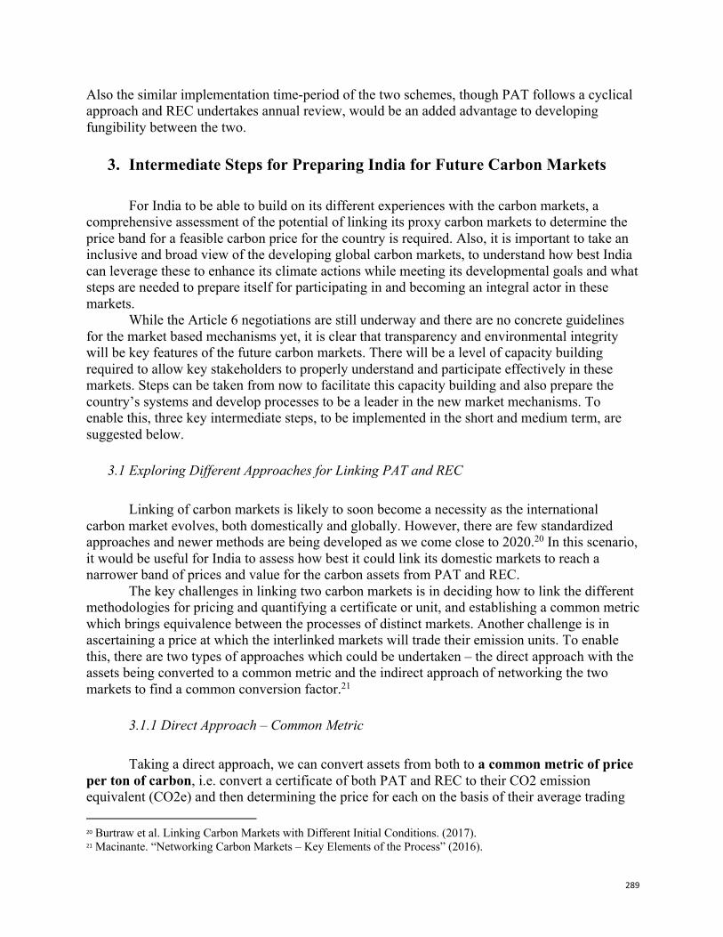
289

Also the similar implementation time-period of the two schemes, though PAT follows a cyclical approach and REC undertakes annual review, would be an added advantage to developing fungibility between the two.

3. Intermediate Steps for Preparing India for Future Carbon Markets

For India to be able to build on its different experiences with the carbon markets, a comprehensive assessment of the potential of linking its proxy carbon markets to determine the price band for a feasible carbon price for the country is required. Also, it is important to take an inclusive and broad view of the developing global carbon markets, to understand how best India can leverage these to enhance its climate actions while meeting its developmental goals and what steps are needed to prepare itself for participating in and becoming an integral actor in these markets.

While the Article 6 negotiations are still underway and there are no concrete guidelines for the market based mechanisms yet, it is clear that transparency and environmental integrity will be key features of the future carbon markets. There will be a level of capacity building required to allow key stakeholders to properly understand and participate effectively in these markets. Steps can be taken from now to facilitate this capacity building and also prepare the country’s systems and develop processes to be a leader in the new market mechanisms. To enable this, three key intermediate steps, to be implemented in the short and medium term, are suggested below.

3.1 Exploring Different Approaches for Linking PAT and REC

Linking of carbon markets is likely to soon become a necessity as the international carbon market evolves, both domestically and globally. However, there are few standardized approaches and newer methods are being developed as we come close to 2020.20 In this scenario, it would be useful for India to assess how best it could link its domestic markets to reach a narrower band of prices and value for the carbon assets from PAT and REC.

The key challenges in linking two carbon markets is in deciding how to link the different methodologies for pricing and quantifying a certificate or unit, and establishing a common metric which brings equivalence between the processes of distinct markets. Another challenge is in ascertaining a price at which the interlinked markets will trade their emission units. To enable this, there are two types of approaches which could be undertaken – the direct approach with the assets being converted to a common metric and the indirect approach of networking the two markets to find a common conversion factor.21

3.1.1 Direct Approach – Common Metric

Taking a direct approach, we can convert assets from both to a common metric of price per ton of carbon, i.e. convert a certificate of both PAT and REC to their CO2 emission equivalent (CO2e) and then determining the price for each on the basis of their average trading

20 Burtraw et al. Linking Carbon Markets with Different Initial Conditions. (2017). 21 Macinante. “Networking Carbon Markets – Key Elements of the Process” (2016).

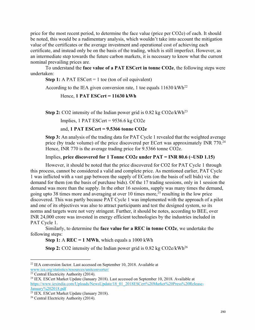
290

price for the most recent period, to determine the face value (price per CO2e) of each. It should be noted, this would be a rudimentary analysis, which wouldn’t take into account the mitigation value of the certificates or the average investment and operational cost of achieving each certificate, and instead only be on the basis of the trading, which is still imperfect. However, as an intermediate step towards the future carbon markets, it is necessary to know what the current nominal prevailing prices are.

To understand the face value of a PAT ESCert in tonne CO2e, the following steps were undertaken:

Step 1: A PAT ESCert = 1 toe (ton of oil equivalent) According to the IEA given conversion rate, 1 toe equals 11630 kWh22

Hence, 1 PAT ESCert = 11630 kWh

Step 2: CO2 intensity of the Indian power grid is 0.82 kg CO2e/kWh23 Implies, 1 PAT ESCert = 9536.6 kg CO2e

and, 1 PAT ESCert = 9.5366 tonne CO2e Step 3: An analysis of the trading data for PAT Cycle 1 revealed that the weighted average price (by trade volume) of the price discovered per ECert was approximately INR 770.24 Hence, INR 770 is the average trading price for 9.5366 tonne CO2e.

Implies, price discovered for 1 Tonne CO2e under PAT = INR 80.6 (~USD 1.15) However, it should be noted that the price discovered for CO2 for PAT Cycle 1 through

this process, cannot be considered a valid and complete price. As mentioned earlier, PAT Cycle 1 was inflicted with a vast gap between the supply of ECerts (on the basis of sell bids) viz. the demand for them (on the basis of purchase bids). Of the 17 trading sessions, only in 1 session the demand was more than the supply. In the other 16 sessions, supply was many times the demand, going upto 38 times more and averaging at over 10 times more,25 resulting in the low price discovered. This was partly because PAT Cycle 1 was implemented with the approach of a pilot and one of its objectives was also to attract participants and test the designed system, so its norms and targets were not very stringent. Further, it should be notes, according to BEE, over INR 24,000 crore was invested in energy efficient technologies by the industries included in PAT Cycle 1.

Similarly, to determine the face value for a REC in tonne CO2e, we undertake the following steps:

Step 1: A REC = 1 MWh, which equals a 1000 kWh Step 2: CO2 intensity of the Indian power grid is 0.82 kg CO2e/kWh26

22 IEA conversion factor. Last accessed on September 10, 2018. Available at www.iea.org/statistics/resources/unitconverter/ 23 Central Electricity Authority (2014). 24 IEX. ESCert Market Update (January 2018). Last accessed on September 10, 2018. Available at https://www.iexindia.com/Uploads/NewsUpdate/18_01_2018ESCert%20Market%20Press%20Release-January%202018.pdf 25 IEX. ESCert Market Update (January 2018). 26 Central Electricity Authority (2014).

291

Implies, 1 REC = 820 kg CO2e Or, 1 REC = 0.82 tonne CO2e

Step 3: As mentioned earlier, the average price for Solar REC in 2018 (January till December) was INR 1060 and the average price for Non-solar REC was INR 1249, which would be the REC trading price for 0.82 tonne CO2e. Implies, price discovered for 1 Tonne CO2e under Solar REC = INR 1293 (~USD 18.5); and for 1 Tonne CO2e under Non-solar REC = INR 1523 (~USD 21.8)

It should be noted, that unlike PAT, REC has a controlled trading band with price floors and price ceilings. The Solar REC has in the past traded largely at the floor price and the Non-solar REC too has been mostly trading close to the floor price. However, the last month’s data, from December 2018, shows an uptake in prices.

The wide difference in the price of a tonne CO2e for the two schemes through this approach, highlights the critical weakness of this method, as it is largely estimates-based and generalizes the values to compare two very disparate actions on a common metric, it overlooks the longer-term impact and related development co-benefits of the individual programs. This generalization also does not take into account the direct and indirect cost of implementing the different programmes.

3.1.2 Indirect Approach – Networking

To overcome the weaknesses of the direct approach, an alternate indirect approach for linking different market mechanisms, such as PAT and REC, is through Networking. In this the aim would be to facilitate the trade of a broad-range of outcomes which are derived from two programs. Instead of trying to align different types of mitigation actions, which would be a complex and time-consuming process, requiring change in methodologies, systems and regulations; or finding a common factor, which would be too generalized, Networking recognises the differences of the mitigation actions and evaluates the outcomes of these to find a common ‘conversion factor’.

Both, adoption of energy efficiency measures and adding renewable energy generation capacity, are crucial to India’s NDCs and climate goals. However, they come at different costs and have a varying impact on the country’s long-term mitigation and development strategy. Thus for networking the two distinct markets, it is necessary to determine this conversion factor between PAT and REC, the cost of achieving the desired and targeted outcomes as well as their strategic importance for and impact on the long-term development strategy of India will need to be assessed.

These issues related to cross-sectoral linkages, will always be challenging to resolve. A gradual phased-approach (with sub-sector level pilots at the national level, or categories of level of fungibility of credits across two markets) would help in improve the understanding of this and be a vital learning process.

A two-step methodology, as suggested by Dubash et al., for assessing different policies and programs in developing countries, which considers a co-benefits analysis, where an assessment is done of the various co-benefits delivered across multiple outcomes, as well as an

292

implementation analysis, where the transactional and financial costs of implementation are assessed, could also be adopted to derive the conversion factor. 27

However, while in a theoretical scenario it may be possible for a conversion factor to be determined purely through quantifiable assessments, in a factual case, it would probably require negotiations – involving both Government and industry, to reach a factor agreeable to key stakeholders of both markets.

3.2 Developing a National Registry and Inventory system

Lack of transparency and environmental integrity has been the key weaknesses of CDM and other smaller carbon markets. This should most likely be strengthened in the design of the post 2020 markets. As per Article 13 of the Paris Agreement, each Party is required to regularly provide a national inventory report of anthropogenic GHG emissions by sources and removal by sinks, prepared using good practice methodologies accepted by the Intergovernmental Panel on Climate Change (IPCC) and all Parties. For this, there is a clear need for national registries and inventories to account for various climate action initiatives.

At present, key elements of the rulebook for the Transparency Framework – such as the GHG inventory process, calculation methodologies, reporting formats, etc. – have recently been formalized at the COP 24 in Katowice in December 2018. It was agreed that developing countries require a certain degree of flexibility on some procedures, such as the content and frequency of reporting requirements. It was also recognised that improving developing country Party reporting will need to be a gradual process, that is dependent on the available capacity and adequate financial support. Although, measures to avoid double counting will need to be incorporated. 28 However, it is certain that to participate effectively in the post 2020 markets, all developing country Parties, including India, will eventually need to build capacity of trained manpower and improve the scope of data collection to be able to meet the transparency requirements.

Some developing country Parties have already started developing their methodologies and processes. For example, South Africa is developing a National Atmospheric Emissions Inventory System (NAEIS) to manage its GHG emissions reporting, with the aim of generating a national emissions profile from sector level models. The process is also focusing on strengthening the implementation arrangements and procedures for inventorisation. Ghana is another country which has been able to establish robust processes and take a lead with inventorisation of its emissions. The country’s inventory system evolved from a group of impromptu working experts to a more structured one, incorporating multiple institutions.29

India has existing capacity for this from its experience of submitting National Communications (NATCOM) and the Biennial Update Report (BUR) to the UNFCCC. India is also already in the process of assessing and developing a registry and inventory system. Building on its past experience with CDM and other mechanisms, it is possible for India too to develop a robust inventory process and enable it to be ready for the Post 2020 market requirements.

27 Dubash et al. “Indian Climate Change Policy: Exploring a Co-Benefits Based Approach” (2013). 28 TERI article. “Towards COP24: From Bangkok to Katowice” (2018). Available at http://www.teriin.org/sites/default/files/2018-09/Briefing%20note%20on%20SB48-2%20Bangkok.pdf 29 TERI. “Best Practices on national Inventory Management System” (2018).

293

A tracking system would enable India to improve its compliance measures for climate actions, which currently are relatively weak. The governance and monitoring and verification processes too need to be strengthened, including regular third party verification and reporting. This would be beneficial for India too, to be able to understand where its carbon assets are being traded and on what terms. For instance, some of the Indian CDM registered projects have committed their CERs to international buyers and there are other projects which are selling GHG credits in voluntary markets, both which may be consumed outside India. Also, there are potential mitigation projects which haven’t registered under any qualified process and their emission reductions are completely unaccounted for. All these potential carbon credits and assets could be used by India for its NDC and through other ways, if they are properly accounted for and inventorised.

Focusing on building the inventorisation process from now would give India scope and time for developing scientific understanding of the existing sector level models, intrinsically strengthening its institutional arrangements, effectively assigning roles and responsibilities, developing a monitoring and evaluation process, and conducting a comprehensive capacity building exercise. This could also result in more judicious policy formulation and implementation in regards to the country’s climate actions.

3.3 Building a ‘Warehousing’ System

Under this, an inventory-like system is envisaged, where carbon assets can be stored or “Warehoused” for later use. India has been consistently making large investments for its climate actions, which are generating carbon assets, even though these may not be internationally recognized yet. Through the application of standardized methodologies, such as those developed under CDM, it is possible for India to quantify its carbon assets from various actions, including the PAT and REC schemes. The aim is to create verifiable Mitigation Outcomes (MO) from India’s ongoing climate actions. This would also require a robust and relevant monitoring, reporting and verification (MRV) system for enhancing the environmental integrity and transparency of these assets.

In the post 2020 markets, MOs will play a key role in international transfers under Article 6’s cooperative approach mechanisms and also otherwise. Since there was no conclusion to Article 6 and the rulebook for carbon markets and trading, to prepare for the use of these carbon assets in the near future, it is proposed that the Government of India starts to quantify and warehouse these assets, which at this stage could be in different metrics and units of measurement, for future use when there is more clarity on the mechanisms and their processes. This would also give the country time to develop its institutional capacity to ensure compliance with its NDCs. As per the PAs requirements. The warehoused assets or MOs, could then be used for either NDC compliance, international mechanisms such as CROSIA or transferred internationally depending on India’s strategic requirements, the prevailing prices and the evolving situation.

The warehousing process itself, with it quantification and MRV of emission reductions from various identified investments, would lead capacity building and institutional strengthening, while also establishing the required regulatory infrastructure for participation in future carbon markets.

294

4. Conclusion

At the current stage of climate change related international negotiations, where the rulebook covering largely all issues has been adopted, except for Article 6 which deals with carbon markets, it is difficult to presume what the final rules, modalities and procedures for carbon markets would be like. However, it is understood that the post 2020 carbon markets under the Agreement would require enhanced transparency, robust accounting methodologies and a level of technical capacity on the functioning of the markets.

To be able to effectively participate in these systems from the start, it is important for developing countries to start preparing themselves and taking appropriate steps from now. India especially has an opportunity here to seize the leadership role and also introduce novel systems which can help Parties in better planning and controlling their climate investments. Some of the requires steps for these are around studying and assessing their existing carbon market or pricing systems and envisaging how best these can integrate into the post 2020 global markets and mechanisms. This may require certain academic studies to explore the best options which align with a country’s priorities, such as with the assessment of linking PAT and REC in India. It may also require certain pilot level projects to test the existing institutional arrangements and the implementation of the designed methodologies and processes, as is the case with the inventory systems being designed. Finally, with an eye towards the capacity development of relevant officials and other stakeholders, demonstration projects for innovative ideas to prepare for the post 2020 regime are also essential, as introduced in the idea for warehousing carbon assets.

References Burtraw et al. Linking Carbon Markets with Different Initial Conditions. (2017). DEHSt. “Vulnerability of CDM Projects for Discontinuation of Mitigation Activities” (2017). Dubash et al. Indian Climate Change Policy: Exploring a Co-Benefits Based Approach. (2013). Macinante. Networking Carbon Markets – Key Elements of the Process (2016). NewClimate Institute. Discussion paper on “Marginal cost of CER supply and implications of demand sources”

(2018). Soonee S.K., et al. “Analysis of Indian Renewable Energy Certificate (REC) Market” (2012). Vaidyula M., et al (2015). India : An Emissions Trading Case Study.

295

Pricing Carbon to Contain Violence Shiran Victoria Shen1,2*

Abstract

Violence is destructive to social order, economic growth, and the human condition. The annual total cost of violence is estimated to be 11 percent of the world’s GDP. However, violence has rarely made its way into economic models. In the meantime, increasing scientific evidence points to an active link between climate change and the incidence of interpersonal and inter–group violence. This study connects the climate–economy and the climate–violence systems by putting forth a new method to internalize the costs of climate–induced violence in the established MERGE integrated assessment model. It finds that such internalization can double the optimal carbon price, a relationship that holds across different specifications regarding climate sensitivity, GDP growth rate, and the willingness to pay (WTP) to avoid nonmarket climate damages. Normatively, under the realistic assumption that the WTP is at 1 percent of regional income, the avoided costs from climate–induced violence in sub–Saharan Africa is modeled to reach 3.7 percent of the region’s GDP in 2200, a very significant figure for an area that is already riddled with underdevelopment and violence. The approach of this paper is a first for the modeling community, indicating directions for future research. For the policy community, this paper takes recent econometric findings to the next step toward understanding required for decisions.

Violence is destructive to social order, economic growth, and the human condition. In Hobbesian terms, lives affected by insecurity can not only be “nasty, brutish, and short,” but, overall, “the condition of man… is a condition of war of everyone against everyone” (Hobbes and Gaskin 1998). Every year, 1.4 million people around the globe die from violence, and many more suffer from a range of physical, sexual, mental, and other problems because of it (WHO 2017). We live in a world that is currently struggling to respond to a ballooning number of increasingly complex conflicts, which forcibly displace record numbers of people – estimated at 65.3 million in 2015 – and pose record–breaking humanitarian needs (UNHCR 2015). The annual total cost of violence is estimated to be $9.4 trillion, which is equivalent to 11 percent of the world’s GDP, and interpersonal violence costs 6.4 times more than collective violence (IEP 2014; Fearon and Hoeffler 2014; Hoeffler 2017). Recognizing the dire consequences of violence, the United Nations has made containing violence a key target in its 2030 Agenda for Sustainable Development (UN 2017).

Increasing scientific evidence points to an active link between climate change and the incidence of interpersonal and inter–group conflicts. Hotter temperatures lead to higher levels of aggression and violence (Anderson 1989; Anderson et al. 2000; Kenrick and MacFarlane 1986; Larrick et al. 2011). Increasing temperatures can also contribute to more violence indirectly by

1 Department of Political Science and Department of Civil & Environmental Engineering, Stanford University. 2 Woodrow Wilson Department of Politics, University of Virginia. * Email: [email protected]. Address: 1540 Jefferson Park Avenue, Gibson Hall S266, Charlottesville, VA, USA 22904.

296

decreasing agricultural production, industrial outputs, and political stability (Dell, Jones, and Olken 2012). After surveying 60 of the most rigorous quantitative studies of the relationship between temperature change and violence, Hsiang, Burke, and Miguel identify strong evidence that climatic events cause human violence across substantial spatial and temporal scales (Hsiang, Burke, and Miguel 2013).

Surprisingly, while violence has shaped social and economic development tremendously across human history, most extant economic models have failed to take violence into account, and the impact of security on prosperity remains mostly understudied and underappreciated (North, Wallis, and Weingast 2009). Since violence plays a persistent role in human societies, more studies of this kind are urgently needed. Given the role that climate change plays in bringing about human violence, which affects the everyday lives of the public, how can researchers reassess carbon externality to help contain climate–induced violence? In this paper, I develop a new method to internalize the costs of climate–induced violence in the established MERGE integrated assessment model and evaluate how the internalization affects the optimal carbon price returned by the model, along with associated projections of temperature and damages under climate policy. I find that internalizing the damages from climate–induced violence can double the carbon externality priced by the model, and this relationship holds across time and different specifications regarding climate sensitivity, GDP growth rate, the willingness to pay (WTP) to avoid nonmarket climate damages, and the inclusion/exclusion of nonmarket damages. Under the assumption that the WTP to avoid nonmarket damages equates 1 percent of regional income, which is very close to reality based on existing empirical works (Carlsson et al. 2012), the avoided damages from climate–induced violence in sub–Saharan Africa is modeled to reach 3.7 percent of the region’s GDP in 2200.

The Externality of Climate–Induced Violence

Increasing scientific evidence suggests that climate change is a culprit for a more violent society. On an interpersonal scale, higher temperature has led to increased rates of a variety of personal violence (Ranson 2014), including violent crimes (Jacob, Lefgren, and Moretti 2007) and domestic violence (Auliciems and DiBartolo 1995). On a collective or intergroup level, growing scientific evidence points to an active link between climate change and conflicts in both sub–Saharan Africa (Miguel, Satyanath, and Sergenti 2004; Burke et al. 2009, 2010; Harari and La Ferrara 2014; O’Loughlin, Linke, and Witmer 2014) and globally (Hsiang, Meng, and Cane 2011; Bollfrass and Shaver 2015). The causal mechanisms of the effects of weather shocks on conflicts are sundry: crop yields (Schlenker and Lobell 2010) and their subsequent impact on economic growth (Miguel, Satyanath, and Sergenti 2004; Dell, Jones, and Olken 2012), government revenue (Shilling 2011), migration (Bhavnani and Lacina 2015), and the opportunity costs of joining a rebellion (Dube and Vargas 2013).

Pricing carbon can help contain carbon emissions. A model for this purpose trades off the benefits associated with carbon emissions, largely stemming from associated energy use, with the costs, categorized as market and nonmarket damages. Market damages refer to damages for marketed goods and services, such as property loss due to increased flood risk and productivity decline in agriculture due to temperature increase. Nonmarket damages include mortality, health, quality of life, as well as effects on environmental goods and services, habitats and ecosystems, and biodiversity. The discount rate captures the temporal dimension of paying at present to avoid future climate damages. To study this tradeoff, researchers have employed

297

integrated assessment models (IAMs), one of whose many functions is to simulate a “causal chain” where carbon emissions lead to climate change and finally to climate damages (Rose, Diaz, and Blanford 2017).

Growing unpredictability of temperature resulting from climate change will likely lead to sustained increases in violence. Nevertheless, there does not yet exist any study that considers the cost of climate change–induced violence in computing the optimal carbon price systematically. Existing studies that assess the impact of climate change on mortality and morbidity effects focus on thermal stress, ozone exposure, diarrhea, labor productivity loss, disease, but not violence (Hurd et al. 2004). To my knowledge, there is only one study that considers climate change–induced violence damage at all. In Economic Risks of Climate Change: An American Prospectus, a rich and informative book, the authors identify both violent and property crimes as climate change–induced damages in Chapter 9; however, they are excluded from the computable general equilibrium (CGE) model in Chapter 14 because of “the mixture of market and nonmarket factors in [their] direct impact estimates” (Houser et al. 2015, 205). Thanks to finely disaggregated and newly available data on the costs of a wide range and types of violence for different regions of the world, I seek to internalize the costs of climate–induced violence in the IAM’s damage function to calculate the optimal carbon price. I then examine how the newly priced carbon externality impacts future temperature and the avoided damages from climate–induced violence for different regions of the world. To assess the effect of uncertainties inherent to carbon pricing, I run models for multiple sets of scenarios that differ in climate sensitivity, GDP growth rate, the WTP to avoid nonmarket climate damages, and the inclusion/exclusion of nonmarket damages. It shall be noted that the purpose of this exercise is not to provide precise predictions or propose a new carbon pricing policy. Rather, this study seeks to understand how any increased risk of violence associated with climate change may affect the tradeoff in choices relating to carbon emissions. It assesses model outputs under different assumptions about climate damages.

Methods

Definition and data

I follow the WHO, which defines violence as “the intentional use of physical force or power, threatened or actual, against oneself, another person, or against a group or community, that either results in or has a high likelihood of resulting in injury, death, psychological harm, maldevelopment or deprivation (WHO 2002). The WHO records deadly violence in three general categories: self–directed violence, collective violence, and interpersonal violence. I focus here on the latter two types of violence, which correspond with the data on the costs of violence that became published in recent years by James Fearon and Anke Hoeffler (Fearon and Hoeffler 2014; IEP 2014; Hoeffler 2017). Collective violence refers to violence perpetrated by organized groups, such as states, rebel organizations, terrorists, street mobs, or criminal organizations. Interpersonal violence refers to violence committed by an individual, which, depending on the relationship between the perpetrator and the victim, can be further broken down into intimate partner violence and child abuse.

298

In this paper, I use the cost estimations by Hoeffler (Hoeffler 2017), who relied on unit cost estimates for various types of violence (e.g., homicides, assaults, and rapes) in the United States by McCollister et al. (McCollister, French, and Fang 2010) to estimate the cost of violence for the year 2013. Hoeffler extended the cost estimations to other countries by multiplying the US cost to homicide by the ratio of a country’s GDP to US GDP. There are assumptions associated with both the approach taken by Hoeffler and that by McCollister et al. McCollister et al. combined several approaches to pricing crimes, such as the cost of illness, contingent valuation, and jury compensation methods, and all of these approaches assume that the impacts of crimes are fully understood.3 Hoeffler’s approach also comes with nontrivial assumptions. First, applying social costs of homicide to calculate the costs of deaths from collective violence equates two drastically different types of death, which generate different social losses. Second, using the ratio of GDPs to map US–based estimates into other countries, especially non–high–income countries, ignores fundamental differences across geographies such as life expectancy, which would affect the social loss of homicidal and non–homicidal offenses.

Despite these nuances, the estimates made by Hoeffler (2017) are arguably the most comprehensive at the time of this writing. It is also worth noting that the cost estimates of violence are likely lower–bound on the real costs. As detailed by McCollister et al., their study excludes such costs as psychological injury and additional costs associated with sexual violence (e.g., sexually transmitted infections, pregnancy, suicide, and substance abuse) (McCollister, French, and Fang 2010). In other words, only the physical costs are included. In Hoeffler’s calculation, self–directed violence costs are excluded (Hoeffler 2017). Furthermore, Hoeffler excludes some relevant costs in cases where data is unavailable. These include the cost of injuries, widespread destruction of infrastructure, and economic and security concerns resulting from war, in addition to the costs of nonfatal domestic violence against women and children, violence perpetrated by women against their male partners, and violence amongst homosexual couples. In addition to the missing items specified by Hoeffler, scholarly classics in the social sciences enlighten us that one critical example of valuing the invaluable or pricing the priceless involves measuring the decline or loss of social capital. First put forth by Alexis de Tocqueville, the concept of social capital was developed further by Robert Putnam (Putnam 1993, 2000). Social capital refers to “features of social organization such as networks, norms, and social trust that facilitate coordination and cooperation for mutual benefit” (Putnam 2000, 67). The benefit of social capital is complicated to quantify because measures such as the number and membership size of associations cannot precisely fathom the frequency and quality of association. Violence provides a negative drag on social capital. Hence, any empirical attempt to quantify the costs of violence will lack most intangible costs, and existing estimates are best understood as appropriate underestimates.

I group the various costs into market damages (e.g., GDP losses from war, economic costs of medical care, criminal justice system, and lost income) and nonmarket damages (e.g., deaths from war, fear) as percentages of GDP for seven different regions of the world in Table 1.

3 The cost of illness approach tries to quantify the tangible costs of crime on outcomes of interest based on the best available information, which usually come from self-reports from the victims, and assigned prices. Similarly, the jury award approach seeks to assess the total social cost of crime by employing actual compensation from civil personal injury cases. Contingent valuation involves surveys to gauge respondents’ willingness to pay to avoid different crimes, which, in theory, should provide a measure of both tangible and intangible costs.

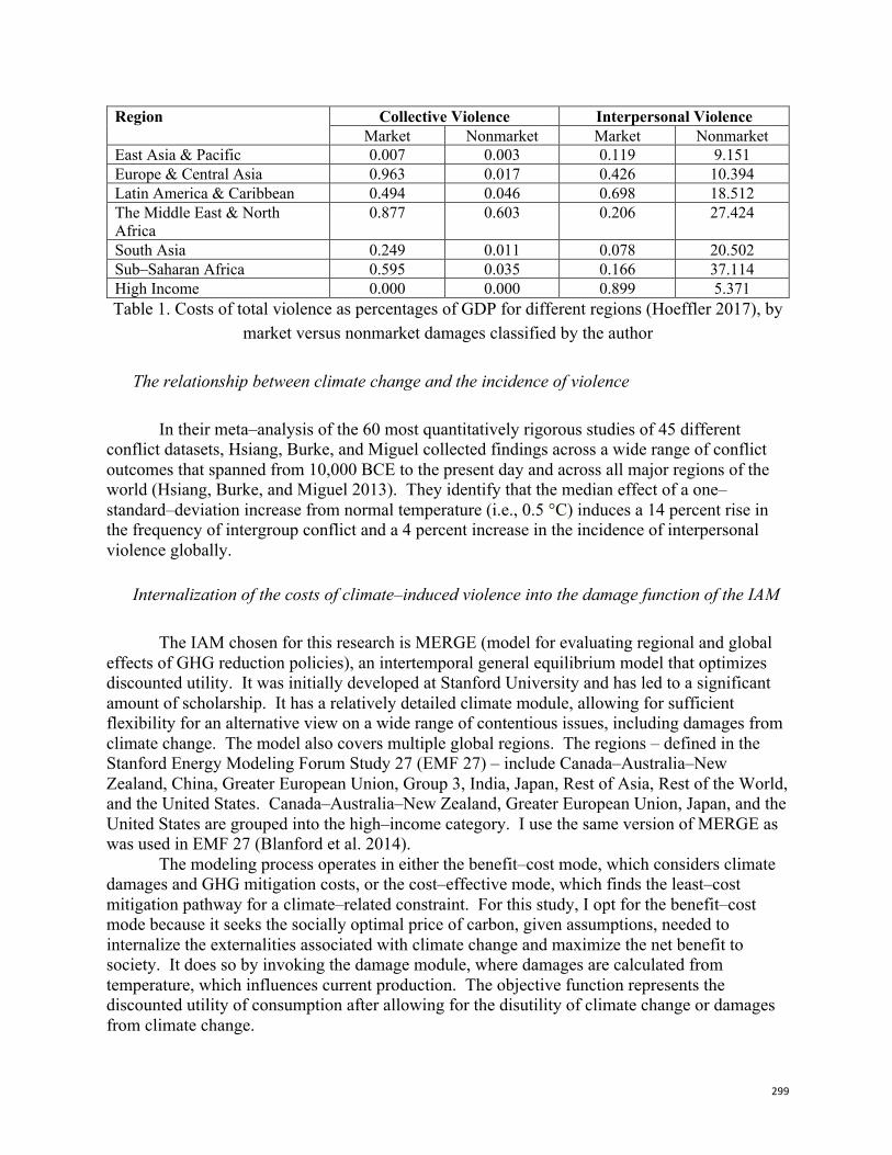
299

Region Collective Violence Interpersonal Violence Market Nonmarket Market Nonmarket

East Asia & Pacific 0.007 0.003 0.119 9.151 Europe & Central Asia 0.963 0.017 0.426 10.394 Latin America & Caribbean 0.494 0.046 0.698 18.512 The Middle East & North Africa

0.877 0.603 0.206 27.424

South Asia 0.249 0.011 0.078 20.502 Sub–Saharan Africa 0.595 0.035 0.166 37.114 High Income 0.000 0.000 0.899 5.371 Table 1. Costs of total violence as percentages of GDP for different regions (Hoeffler 2017), by

market versus nonmarket damages classified by the author

The relationship between climate change and the incidence of violence

In their meta–analysis of the 60 most quantitatively rigorous studies of 45 different conflict datasets, Hsiang, Burke, and Miguel collected findings across a wide range of conflict outcomes that spanned from 10,000 BCE to the present day and across all major regions of the world (Hsiang, Burke, and Miguel 2013). They identify that the median effect of a one–standard–deviation increase from normal temperature (i.e., 0.5 °C) induces a 14 percent rise in the frequency of intergroup conflict and a 4 percent increase in the incidence of interpersonal violence globally.

Internalization of the costs of climate–induced violence into the damage function of the IAM The IAM chosen for this research is MERGE (model for evaluating regional and global effects of GHG reduction policies), an intertemporal general equilibrium model that optimizes discounted utility. It was initially developed at Stanford University and has led to a significant amount of scholarship. It has a relatively detailed climate module, allowing for sufficient flexibility for an alternative view on a wide range of contentious issues, including damages from climate change. The model also covers multiple global regions. The regions – defined in the Stanford Energy Modeling Forum Study 27 (EMF 27) – include Canada–Australia–New Zealand, China, Greater European Union, Group 3, India, Japan, Rest of Asia, Rest of the World, and the United States. Canada–Australia–New Zealand, Greater European Union, Japan, and the United States are grouped into the high–income category. I use the same version of MERGE as was used in EMF 27 (Blanford et al. 2014). The modeling process operates in either the benefit–cost mode, which considers climate damages and GHG mitigation costs, or the cost–effective mode, which finds the least–cost mitigation pathway for a climate–related constraint. For this study, I opt for the benefit–cost mode because it seeks the socially optimal price of carbon, given assumptions, needed to internalize the externalities associated with climate change and maximize the net benefit to society. It does so by invoking the damage module, where damages are calculated from temperature, which influences current production. The objective function represents the discounted utility of consumption after allowing for the disutility of climate change or damages from climate change.

300

𝑈𝑡𝑖𝑙𝑖𝑡𝑦 = (1 − 𝐷𝑎𝑚𝑎𝑔𝑒) ∗ ∑ 𝛿6𝑢(𝑐)

6¡$ (1)

The carbon price is calculated endogenously in this recursive optimization process. An increase in temperature contributes to climate damage, resulting in a higher carbon price. A higher carbon price then exerts pressure on the producers, forcing them to reduce emissions, which leads to slowed temperature increase. The loop continues until the algorithm finds the optimal carbon price, which is the one that will yield the highest utility. The market and nonmarket damages are modified separately for the climate module. The abstract representation of damages is introduced and discussed in Manne, Mendelsohn, and Richels (1995), which is a high–level representation designed to focus on the core tradeoffs. Building on Manne, Mendelsohn, and Richels (1995), the market damage function can be expressed as:

𝑀𝐷(𝑟𝑔, 𝑡) = 𝑚𝑑𝑚𝑓𝑎𝑐(𝑟𝑔) ∗ 𝑔𝑑𝑝(𝑟𝑔, 𝑡) ∗ ¦6§(6)¨©¨sª«6ª¨§

(2) where 𝑀𝐷(𝑟𝑔, 𝑐𝑡𝑝) refers to the market damage in a given region 𝑟𝑔 at a given time 𝑡; 𝑚𝑑𝑚𝑓𝑎𝑐(𝑟𝑔) is the market damage factor in a given region 𝑟𝑔, which is represented by the proportion loss in GDP; 𝑔𝑑𝑝(𝑟𝑔, 𝑐𝑡𝑝)is the GDP in a given region 𝑟𝑔 at a given time 𝑡; 𝑎𝑡𝑝(𝑡) is actual temperature increase from the pre–industrial period at a given time 𝑡; 𝑚𝑑𝑚𝑟𝑒𝑓𝑡𝑒𝑚𝑝 is the reference temperature for market damage coefficients, which by default equals 2 °C.

To account for the market damages of climate–induced violence, the new market damage factor 𝑚𝑑𝑚𝑓𝑎𝑐𝑛𝑒𝑤(𝑟𝑔) is created by modifying the 𝑚𝑑𝑚𝑓𝑎𝑐(𝑟𝑔) in the following way:

𝑚𝑑𝑚𝑓𝑎𝑐𝑛𝑒𝑤(𝑟𝑔) = 𝑚𝑑𝑚𝑓𝑎𝑐(𝑟𝑔) + 𝑚𝑑𝑚𝑓𝑎𝑐𝑣(𝑟𝑔) (3) where 𝑚𝑑𝑚𝑓𝑎𝑐𝑣(𝑟𝑔) refers to the market damage factor from violence, both collective and interpersonal. The nonmarket damages of climate–induced violence are accounted for similarly. The economic loss factor (ELF), which is a component of the nonmarket damage function, hinges on two parameters: 𝑐𝑎𝑡𝑡 and ℎ𝑠𝑥 (Manne and Richels 2005).

𝐸𝐿𝐹(𝑟𝑔, 𝑡) = [1 − (sª«6ª¨§±¦66

)H]²³´(sµ,6)

= [1 − 𝑛𝑚𝑑𝑚(𝑟𝑒𝑓𝑤𝑡𝑝) ∗ Y ¦6§(6)¶¨©¨(sª«6ª¨§)

ZH]²³´(sµ,6) (4)

where 𝑟𝑒𝑓𝑡𝑒𝑚𝑝 is a variable that measures the rise in temperature above its level in 2000; 𝑐𝑎𝑡𝑡 is a catastrophic temperature parameter chosen in such a way that the entire regional product is wiped out; ℎ𝑠𝑥 is the hockey–stick parameter, representing the quadratic loss due to temperature increase. The ELF represents the fraction of consumption that remains available after accounting for nonmarket damages for conventional uses.

The modified ELF function that accounts for the costs of climate–induced violence is:

301

𝐸𝐿𝐹𝑛𝑒𝑤(𝑟𝑔) = 𝐸𝐿𝐹(𝑟𝑔) − 𝑛𝑚𝑑𝑚𝑓𝑎𝑐𝑣(𝑟𝑔) (5) where 𝑛𝑚𝑑𝑚𝑓𝑎𝑐𝑣(𝑟𝑔) is the nonmarket damage factor from climate–induced violence, both collective and interpersonal. The 𝑚𝑑𝑚𝑓𝑎𝑐𝑣(𝑟𝑔) and 𝑛𝑚𝑑𝑚𝑓𝑎𝑐𝑚𝑣(𝑟𝑔) are calculated by combining the relationship between climate change and the incidence of violence (Hsiang, Burke, and Miguel 2013) and the costs of collective and interpersonal violence as fractions of GDP for different regions of the world (Hoeffler 2017). For a given region 𝑟𝑔, the 𝑚𝑑𝑚𝑓𝑎𝑐𝑣(𝑟𝑔) and 𝑛𝑚𝑑𝑚𝑓𝑎𝑐𝑚𝑣(𝑟𝑔) are:

𝑚𝑑𝑚𝑓𝑎𝑐𝑣(𝑟𝑔) = 𝑚𝑑𝑚𝑓𝑎𝑐𝑣(𝑐𝑜𝑙𝑣𝑖𝑜, 𝑟𝑔) × (1 + 0.14)¹º»(º)U.¼ +

𝑚𝑑𝑚𝑓𝑎𝑐𝑣(𝑖𝑛𝑡𝑝𝑒𝑟𝑣𝑖𝑜, 𝑟𝑔) × (1 + 0.04)¹º»(º)U.¼ (6)

𝑛𝑚𝑑𝑚𝑓𝑎𝑐𝑣(𝑟𝑔) = 𝑛𝑚𝑑𝑚𝑓𝑎𝑐𝑣(𝑐𝑜𝑙𝑣𝑖𝑜, 𝑟𝑔) × (1 + 0.14)¹º»(º)U.¼ +

𝑛𝑚𝑑𝑚𝑓𝑎𝑐𝑣(𝑖𝑛𝑡𝑝𝑒𝑟𝑣𝑖𝑜, 𝑟𝑔) × (1 + 0.04)¹º»(º)U.¼ (7)

where 𝑐𝑜𝑙𝑣𝑖𝑜 denotes collective violence; 𝑖𝑛𝑡𝑝𝑒𝑟𝑣𝑖𝑜 denotes interpersonal violence; 𝑎𝑡𝑝(𝑡) represents actual temperature increase at a given time 𝑡.

Avoided damages from such internalization

To assess the normative significance of a slowed temperature increase, I calculate the avoided damages from climate–induced violence as a percentage of regional GDP. The avoided damages are the difference in damages between the business as usual (BAU) scenario and the Violence scenario, where the latter internalizes the costs of climate–induced violence. For a given region 𝑟𝑔 at time 𝑡, the avoided damage as a percentage of regional GDP ∆©¦¨¦µª³(sµ,6)

µ©§(sµ,6)

can be expressed as:

∆©¦¨¦µª³(sµ,6)µ©§(sµ,6)

= ¾¦¨¦µª�¿À(sµ,6)5¾¦¨¦µªÁ�ÂÃª¶±ª(sµ,6)µ©§(sµ,6)

(8)

Updating the Carbon Externality and Its Effects under Different Scenarios

This section presents changes in model outcomes when the social costs of climate–induced violence are internalized. For each scenario, I seek to compare between business as usual (BAU) and Violence scenarios to calculate avoided damages. I present results under default assumptions first and then perform four sets of sensitivity analysis: climate sensitivity, GDP growth rate, the WTP to avoid nonmarket climate damages, and the inclusion/exclusion of nonmarket damages.

302

Reference Scenario

I begin with projections for the reference scenario, where all variables other than the market and nonmarket damage factors are left to their default values. The “true” prices of carbon are shown in Figure 1. The model prices the externality of carbon for all regions of the world. The model trades off the benefits and costs of carbon emissions and prices carbon at $201/ton and $374/ton for the BAU and Violence scenarios, respectively, in 2020. The prices rise to $3534/ton and $6463/ton by 2200. The costs of climate–induced violence consistently raise the optimal carbon price by more than 0.8 times (a near doubling) during the 2020–2200 period. These very high prices may result from the default assumption in MERGE that the WTP to avoid nonmarket climate damages associated with 2 °C of warming is 4 percent of GDP as well as the way MERGE handles nonmarket damages in calculating the optimal carbon price. These considerations will be discussed at length in the sensitivity analysis.

Figure 1. Projections of the optimal carbon price under default assumptions in MERGE, 2020–

2200

With the cost of violence internalized, the optimal path of the model shows a lower speed of temperature increase. The projected temperature increases for both the BAU and Violence scenarios are 1.16 °C in 2020, but the values diverge to 3.25 °C and 2.72 °C in 2200 respectively (Figure 2).

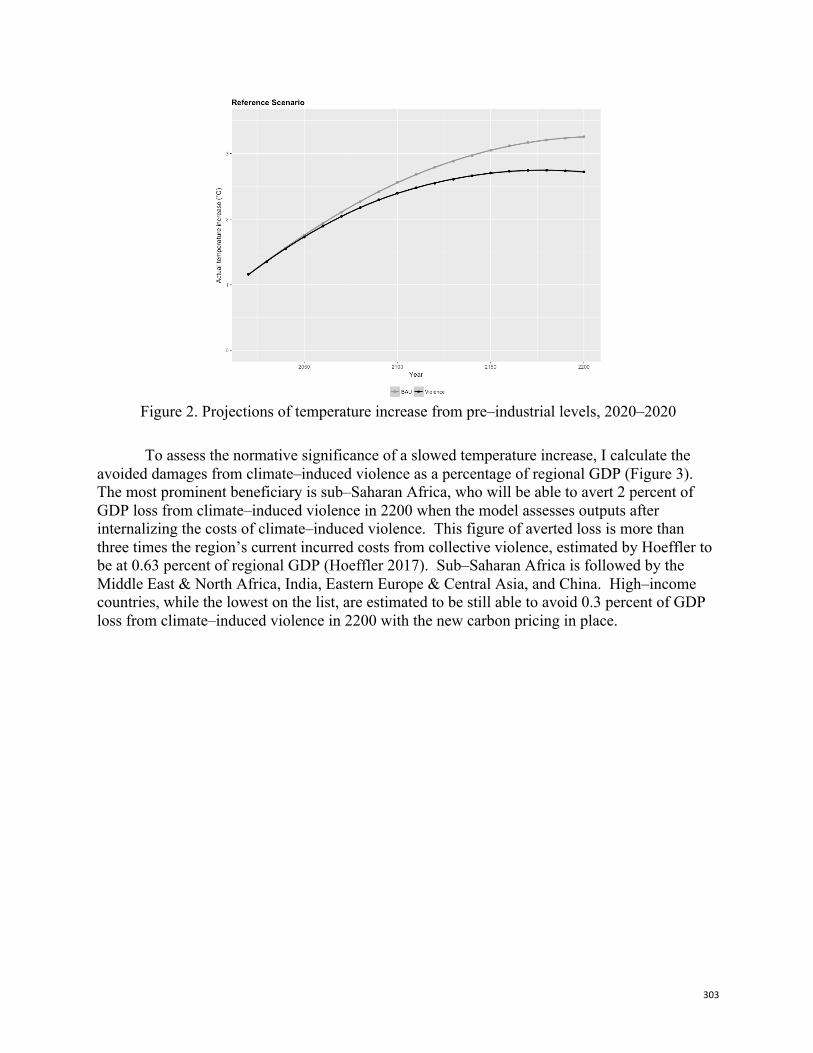
303

Figure 2. Projections of temperature increase from pre–industrial levels, 2020–2020

To assess the normative significance of a slowed temperature increase, I calculate the

avoided damages from climate–induced violence as a percentage of regional GDP (Figure 3). The most prominent beneficiary is sub–Saharan Africa, who will be able to avert 2 percent of GDP loss from climate–induced violence in 2200 when the model assesses outputs after internalizing the costs of climate–induced violence. This figure of averted loss is more than three times the region’s current incurred costs from collective violence, estimated by Hoeffler to be at 0.63 percent of regional GDP (Hoeffler 2017). Sub–Saharan Africa is followed by the Middle East & North Africa, India, Eastern Europe & Central Asia, and China. High–income countries, while the lowest on the list, are estimated to be still able to avoid 0.3 percent of GDP loss from climate–induced violence in 2200 with the new carbon pricing in place.

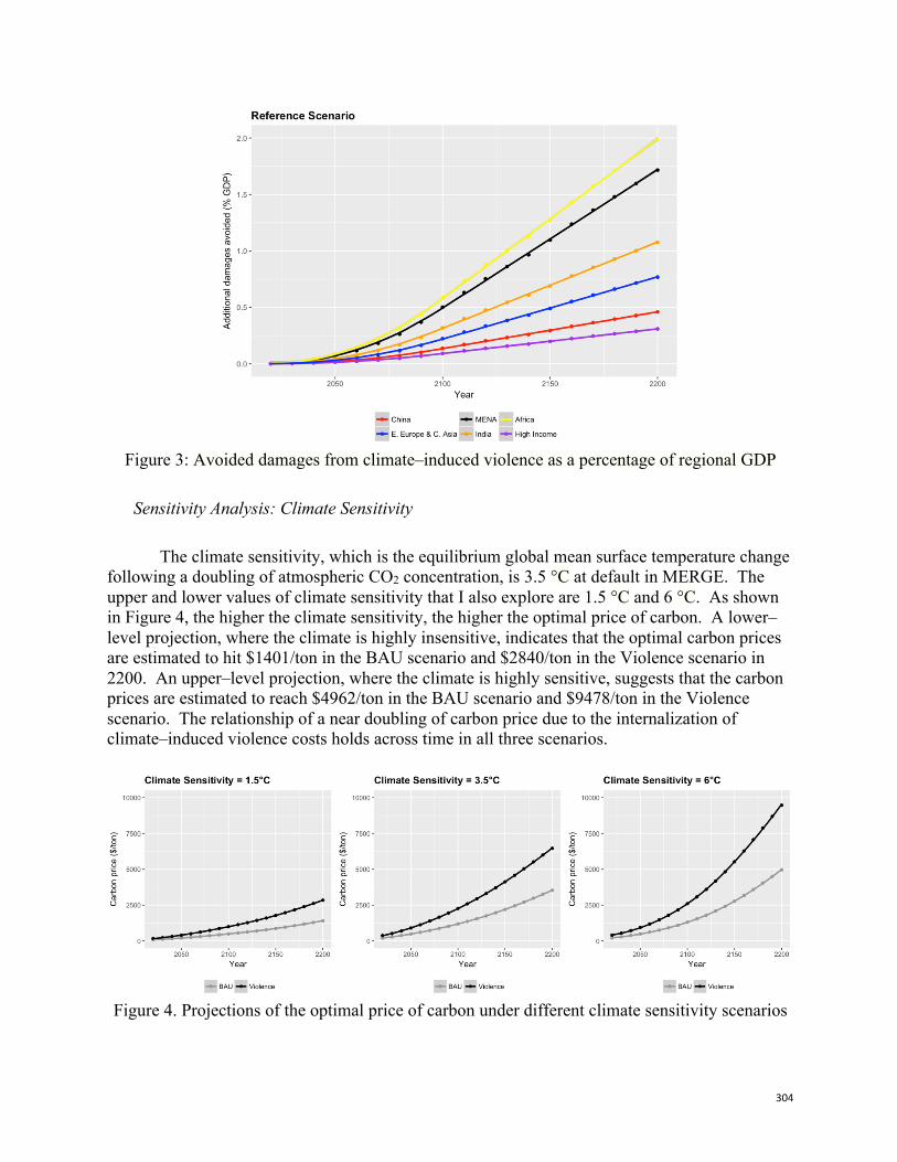
304

Figure 3: Avoided damages from climate–induced violence as a percentage of regional GDP

Sensitivity Analysis: Climate Sensitivity

The climate sensitivity, which is the equilibrium global mean surface temperature change following a doubling of atmospheric CO2 concentration, is 3.5 °C at default in MERGE. The upper and lower values of climate sensitivity that I also explore are 1.5 °C and 6 °C. As shown in Figure 4, the higher the climate sensitivity, the higher the optimal price of carbon. A lower–level projection, where the climate is highly insensitive, indicates that the optimal carbon prices are estimated to hit $1401/ton in the BAU scenario and $2840/ton in the Violence scenario in 2200. An upper–level projection, where the climate is highly sensitive, suggests that the carbon prices are estimated to reach $4962/ton in the BAU scenario and $9478/ton in the Violence scenario. The relationship of a near doubling of carbon price due to the internalization of climate–induced violence costs holds across time in all three scenarios.

Figure 4. Projections of the optimal price of carbon under different climate sensitivity scenarios

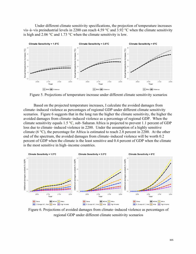
305

Under different climate sensitivity specifications, the projection of temperature increases vis–à–vis preindustrial levels in 2200 can reach 4.59 °C and 3.92 °C when the climate sensitivity is high and 2.06 °C and 1.73 °C when the climate sensitivity is low.

Figure 5. Projections of temperature increase under different climate sensitivity scenarios

Based on the projected temperature increases, I calculate the avoided damages from

climate–induced violence as percentages of regional GDP under different climate sensitivity scenarios. Figure 6 suggests that in the long run the higher the climate sensitivity, the higher the avoided damages from climate–induced violence as a percentage of regional GDP. When the climate sensitivity equals 1.5 °C, sub–Saharan Africa is projected to prevent 1.1 percent of GDP loss due to climate–induced violence in 2200. Under the assumption of a highly sensitive climate (6 °C), the percentage for Africa is estimated to reach 2.8 percent in 2200. At the other end of the spectrum, the avoided damages from climate–induced violence will be worth 0.2 percent of GDP when the climate is the least sensitive and 0.4 percent of GDP when the climate is the most sensitive in high–income countries.

Figure 6. Projections of avoided damages from climate–induced violence as percentages of

regional GDP under different climate sensitivity scenarios

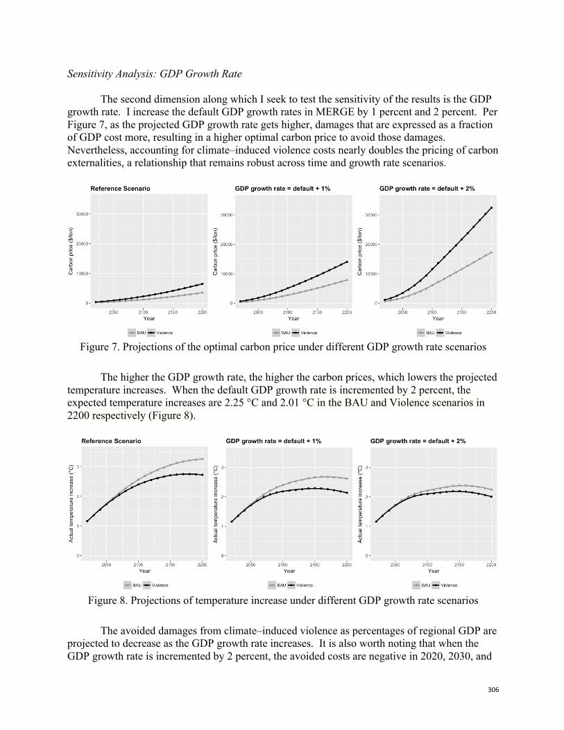
306

Sensitivity Analysis: GDP Growth Rate

The second dimension along which I seek to test the sensitivity of the results is the GDP growth rate. I increase the default GDP growth rates in MERGE by 1 percent and 2 percent. Per Figure 7, as the projected GDP growth rate gets higher, damages that are expressed as a fraction of GDP cost more, resulting in a higher optimal carbon price to avoid those damages. Nevertheless, accounting for climate–induced violence costs nearly doubles the pricing of carbon externalities, a relationship that remains robust across time and growth rate scenarios.

Figure 7. Projections of the optimal carbon price under different GDP growth rate scenarios

The higher the GDP growth rate, the higher the carbon prices, which lowers the projected

temperature increases. When the default GDP growth rate is incremented by 2 percent, the expected temperature increases are 2.25 °C and 2.01 °C in the BAU and Violence scenarios in 2200 respectively (Figure 8).

Figure 8. Projections of temperature increase under different GDP growth rate scenarios

The avoided damages from climate–induced violence as percentages of regional GDP are

projected to decrease as the GDP growth rate increases. It is also worth noting that when the GDP growth rate is incremented by 2 percent, the avoided costs are negative in 2020, 2030, and

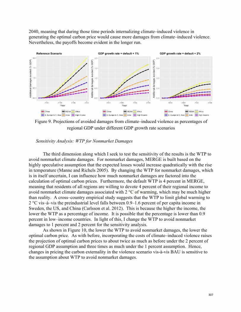
307

2040, meaning that during those time periods internalizing climate–induced violence in generating the optimal carbon price would cause more damages from climate–induced violence. Nevertheless, the payoffs become evident in the longer run.


regional GDP under different GDP growth rate scenarios

Sensitivity Analysis: WTP for Nonmarket Damages

The third dimension along which I seek to test the sensitivity of the results is the WTP to avoid nonmarket climate damages. For nonmarket damages, MERGE is built based on the highly speculative assumption that the expected losses would increase quadratically with the rise in temperature (Manne and Richels 2005). By changing the WTP for nonmarket damages, which is in itself uncertain, I can influence how much nonmarket damages are factored into the calculation of optimal carbon prices. Furthermore, the default WTP is 4 percent in MERGE, meaning that residents of all regions are willing to devote 4 percent of their regional income to avoid nonmarket climate damages associated with 2 °C of warming, which may be much higher than reality. A cross–country empirical study suggests that the WTP to limit global warming to 2 °C vis–à–vis the preindustrial level falls between 0.9–1.6 percent of per capita income in Sweden, the US, and China (Carlsson et al. 2012). This is because the higher the income, the lower the WTP as a percentage of income. It is possible that the percentage is lower than 0.9 percent in low–income countries. In light of this, I change the WTP to avoid nonmarket damages to 1 percent and 2 percent for the sensitivity analysis.

As shown in Figure 10, the lower the WTP to avoid nonmarket damages, the lower the optimal carbon price. As with before, incorporating the costs of climate–induced violence raises the projection of optimal carbon prices to about twice as much as before under the 2 percent of regional GDP assumption and three times as much under the 1 percent assumption. Hence, changes in pricing the carbon externality in the violence scenario vis-à-vis BAU is sensitive to the assumption about WTP to avoid nonmarket damages.

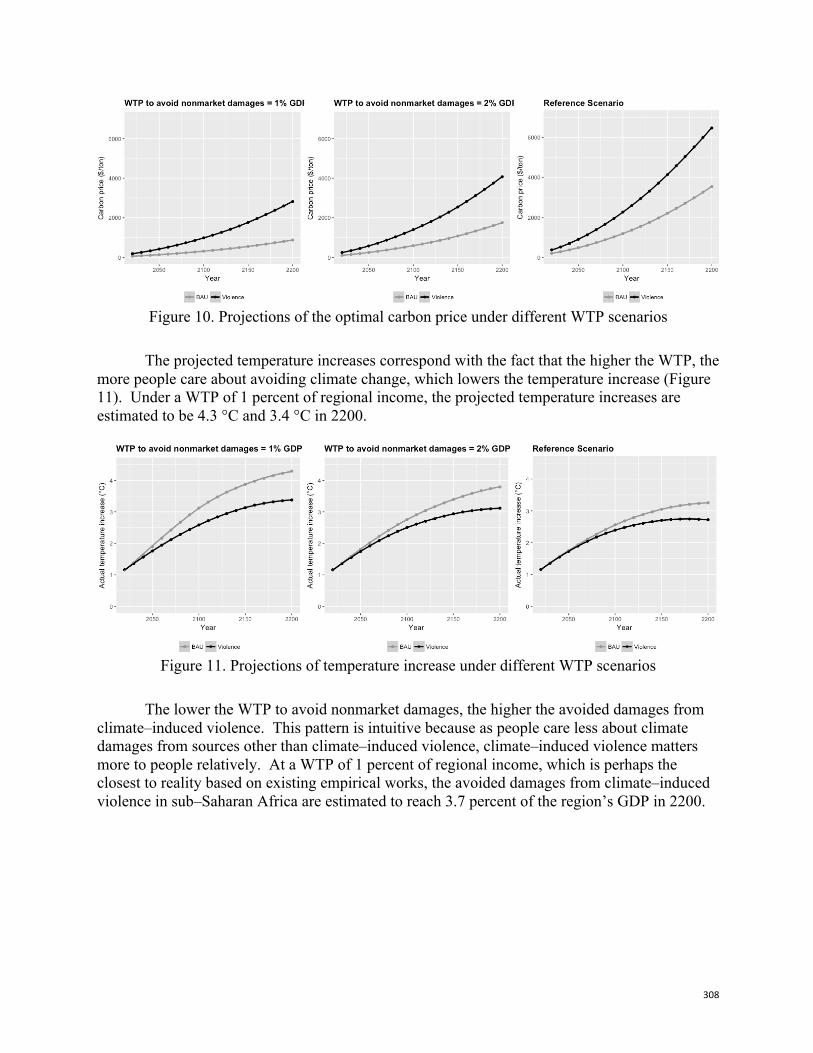
308

Figure 10. Projections of the optimal carbon price under different WTP scenarios

The projected temperature increases correspond with the fact that the higher the WTP, the more people care about avoiding climate change, which lowers the temperature increase (Figure 11). Under a WTP of 1 percent of regional income, the projected temperature increases are estimated to be 4.3 °C and 3.4 °C in 2200.

Figure 11. Projections of temperature increase under different WTP scenarios

The lower the WTP to avoid nonmarket damages, the higher the avoided damages from

climate–induced violence. This pattern is intuitive because as people care less about climate damages from sources other than climate–induced violence, climate–induced violence matters more to people relatively. At a WTP of 1 percent of regional income, which is perhaps the closest to reality based on existing empirical works, the avoided damages from climate–induced violence in sub–Saharan Africa are estimated to reach 3.7 percent of the region’s GDP in 2200.

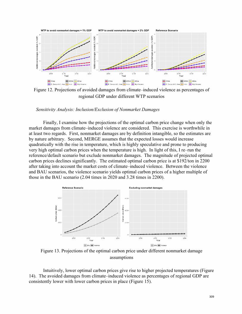
309


regional GDP under different WTP scenarios

Sensitivity Analysis: Inclusion/Exclusion of Nonmarket Damages Finally, I examine how the projections of the optimal carbon price change when only the market damages from climate–induced violence are considered. This exercise is worthwhile in at least two regards. First, nonmarket damages are by definition intangible, so the estimates are by nature arbitrary. Second, MERGE assumes that the expected losses would increase quadratically with the rise in temperature, which is highly speculative and prone to producing very high optimal carbon prices when the temperature is high. In light of this, I re–run the reference/default scenario but exclude nonmarket damages. The magnitude of projected optimal carbon prices declines significantly. The estimated optimal carbon price is at $192/ton in 2200 after taking into account the market costs of climate–induced violence. Between the violence and BAU scenarios, the violence scenario yields optimal carbon prices of a higher multiple of those in the BAU scenario (2.04 times in 2020 and 3.28 times in 2200).

Figure 13. Projections of the optimal carbon price under different nonmarket damage

assumptions Intuitively, lower optimal carbon prices give rise to higher projected temperatures (Figure 14). The avoided damages from climate–induced violence as percentages of regional GDP are consistently lower with lower carbon prices in place (Figure 15).

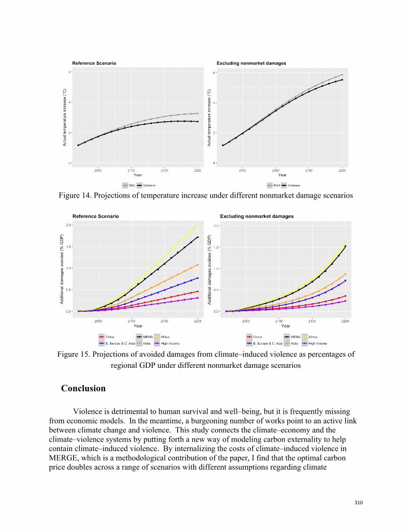
310

Figure 14. Projections of temperature increase under different nonmarket damage scenarios


regional GDP under different nonmarket damage scenarios

Conclusion

Violence is detrimental to human survival and well–being, but it is frequently missing from economic models. In the meantime, a burgeoning number of works point to an active link between climate change and violence. This study connects the climate–economy and the climate–violence systems by putting forth a new way of modeling carbon externality to help contain climate–induced violence. By internalizing the costs of climate–induced violence in MERGE, which is a methodological contribution of the paper, I find that the optimal carbon price doubles across a range of scenarios with different assumptions regarding climate

311

sensitivity, GDP growth rate, the WTP to avoid nonmarket climate damages, and the inclusion/exclusion of nonmarket damages.

For the modeling community, the take–home message is that violence has a material impact on results, and should be considered in any model trading off the costs and benefits of greenhouse gas emissions. This modeling exercise indicates directions for future research to refine and build upon the analysis undertaken here, the first attempt on this topic.

For the policy community, the approach of this paper bears normative significance. Existing approaches in the literature take the first step by establishing whether climate affects the risk of violence. The approach of this paper takes the next step by incorporating these findings into the broader tradeoff between the costs and benefits of carbon emissions across the global economy. Under the assumption that the WTP to avoid nonmarket damages equates 1 percent of regional income, which is very close to reality based on existing empirical works, the avoided damages from climate–induced violence in sub–Saharan Africa is estimated to reach 3.7 percent of the region’s GDP in 2200, a figure very significant for a region that is already riddled with underdevelopment and violence.

Acknowledgments

The author thanks Raphael Calel, James Merrick, and John Weyant for their feedback on previous drafts of this paper. James Merrick provided generous help with MERGE.

References Anderson, Craig A. 1989. “Temperature and Aggression: Ubiquitous Effects of Heat on Occurrence of Human

Violence.” Psychological Bulletin 106 (1): 74–96. Anderson, Craig A., Kathryn B. Anderson, Nancy Dorr, Kristina M. DeNeve, and Mindy Flanagan. 2000.

“Temperature and Aggression.” Advances in Experimental Social Psychology 32 (January): 63–133. https://doi.org/10.1016/S0065-2601(00)80004-0.

Auliciems, Andris, and L. DiBartolo. 1995. “Domestic Violence in a Subtropical Environment: Police Calls and Weather in Brisbane.” International Journal of Biometeorology 39 (1): 34–39.

Bhavnani, Rikhil R., and Bethany Lacina. 2015. “The Effects of Weather-Induced Migration on Sons of the Soil Riots in India.” World Politics 67 (4): 760–94.

Blanford, Geoffrey, James Merrick, Richard Richels, and Steven Rose. 2014. “Trade-Offs between Mitigation Costs and Temperature Change.” Climatic Change 123: 527–41.

Bollfrass, Alexander, and Andrew Shaver. 2015. “The Effects of Temperature on Political Violence: Global Evidence at the Subnational Level.” PLOS ONE 10 (5): e0123505.

Burke, Marshall, Edward Miguel, Shanker Satyanath, John A. Dykema, and David B. Lobell. 2010. “Climate Robustly Linked to African Civil War.” PNAS 107 (51): E185.

Burke, Marshall, Edward Miguel, Shanker Satyanath, John Dykema, and David Lobell. 2009. “Warming Increases Risk of Civil War in Africa.” PNAS 106 (49): 20670–74.

Carlsson, Fredrik, Mitesh Kataria, Alan Krupnick, Elina Lampi, Åsa Löfgren, Ping Qin, Susie Chung, and Thomas Sterner. 2012. “Paying for Mitigation: A Multiple Country Study.” Environment for Development 88 (2): 326–40.

Dell, Melissa, Benjamin F. Jones, and Benjamin A. Olken. 2012. “Temperature Shocks and Economic Growth: Evidence from the Last Half Century.” American Economic Journal: Macroeconomics 4 (3): 66–95.

Dube, Oeindrila, and Juan F. Vargas. 2013. “Commodity Price Shocks and Civil Conflict: Evidence from Colombia.” Review of Economic Studies 80: 1384–1421.

312

Fearon, James, and Anke Hoeffler. 2014. “Beyond Civil War: The Costs of Interpersonal Violence and the Next Round of MDGs.” Copenhagen, Denmark. https://editorialexpress.com/cgi-bin/conference/download.cgi?db_name=CSAE2015&paper_id=606.

Harari, Mariaflavia, and Eliana La Ferrara. 2014. “Conflict, Climate and Cells: A Disaggregated Analysis.” Cambridge, MA. http://economics.mit.edu/files/10058.

Hobbes, Thomas, and J. C. A. Gaskin. 1998. Leviathan. Oxford: Oxford University Press. Hoeffler, Anke. 2017. “What Are the Costs of Violence?” Politics, Philosophy & Economics 16 (4): 422–45. Houser, Trevor, Solomon Hsiang, Robert Kopp, and Kate Larsen. 2015. Economic Risks of Climate Change: An

American Prospectus. New York, NY: Columbia University Press. Hsiang, Solomon, Marshall Burke, and Edward Miguel. 2013. “Quantifying The Influence of Climate On Human

Conflict.” Science 341 (6151): 1235367. Hsiang, Solomon, Kyle C. Meng, and Mark A. Cane. 2011. “Civil Conflicts Are Associated with the Global

Climate.” Nature 476: 438–41. Hurd, Brian, Dale W. Jorgenson, Richard J. Goettle, and Joel Smith. 2004. “U.S. Market Consequences of Global

Climate Change.” Arlington. https://www.c2es.org/document/u-s-market-consequences-of-global-climate-change/.

IEP. 2014. “The Economic Cost of Violence Containment: A Comprehensive Assessment of the Global Cost of Violence.” Sydney, Australia. http://economicsandpeace.org/wp-content/uploads/2015/06/The-Economic-Cost-of-Violence-Containment.pdf.

Jacob, Brian, Lars Lefgren, and Enrico Moretti. 2007. “The Dynamics of Criminal Behavior: Evidence from Weather Shocks.” The Journal of Human Resources 42 (3): 489–527.

Kenrick, Douglas T., and Steven W. MacFarlane. 1986. “Ambient Temperature and Horn Honking: A Field Study of the Heat/Aggression Relationship.” Environment and Behavior 18 (2): 179–91.

Larrick, Richard P., Thomas A. Timmerman, Andrew M. Carton, and Jason Abrevaya. 2011. “Temper, Temperature, and Temptation: Heat-Related Retaliation in Baseball.” Psychological Science 22 (4): 423–28.

Manne, Alan, Robert Mendelsohn, and Richard Richels. 1995. “MERGE: A Model for Evaluating Regional and Global Effects of GHG Reduction Policies.” Energy Policy 23 (1): 17–34.

Manne, Alan S., and Richard G. Richels. 2005. “MERGE: An Integrated Assessment Model for Global Climate Change.” In Energy and Environment, edited by Richard Loulou, Jean-Philippe Waaub, and Georges Zaccour, 175–89. New York, NY: Springer.

McCollister, Kathryn, Michael French, and Hai Fang. 2010. “The Cost of Crime to Society: New Crime-Specific Estimates for Policy and Program Evaluation.” Drug and Alcohol Dependence 108 (1–2): 98–109.

Miguel, Edward, Shanker Satyanath, and Ernest Sergenti. 2004. “Economic Shocks and Civil Conflict: An Instrumental Variables Approach.” Journal of Political Economy 112 (4): 725–53.

North, Douglass, John Wallis, and Barry Weingast. 2009. Violence and Social Orders: A Conceptual Framework for Interpreting Recorded Human History. Cambridge, MA: Cambridge University Press.

O’Loughlin, John, Andrew M. Linke, and Frank D.W. Witmer. 2014. “Effects of Temperature and Precipitation Variability on the Risk of Violence in Sub-Saharan Africa, 1980–2012.” PNAS 111 (47): 16712–16717.

Putnam, Robert. 1993. Making Democracy Work: Civic Traditions in Modern Italy. Princeton: Princeton University Press.

———. 2000. Bowling Alone: The Collapse and Revival of American Community. New York, NY: Simon & Schuster Paperbacks.

Ranson, Matthew. 2014. “Crime, Weather, and Climate Change.” Journal of Environmental Economics and Management 67 (3): 274–302. https://doi.org/10.1016/J.JEEM.2013.11.008.

Rose, Steven, Delavane Diaz, and Geoffrey Blanford. 2017. “Understanding the Social Cost of Carbon: A Model Diagnostic and Inter-Comparison Study.” Climate Change Economics 8 (2): 1750009.

Schlenker, Wolfram, and David Lobell. 2010. “Robust Negative Impacts of Climate Change on African Agriculture.” Environmental Research Letters 5 (1).

Shilling, A. Kaitlin. 2011. “Climate Change and Conflict: Identifying the Mechanisms.” Stanford University. UN. 2017. “GOAL 16: Peace, Justice and Strong Institutions.” Progress towards the Sustainable Development

Goals. 2017. https://sustainabledevelopment.un.org/sdg16. UNHCR. 2015. “Global Trends: Forced Displacement in 2015.” http://www.unhcr.org/576408cd7. WHO. 2002. “World Report on Violence and Health.” ———. 2017. “10 Facts about Violence Prevention.” World Health Organization. 2017.

http://www.who.int/features/factfiles/violence/en/.

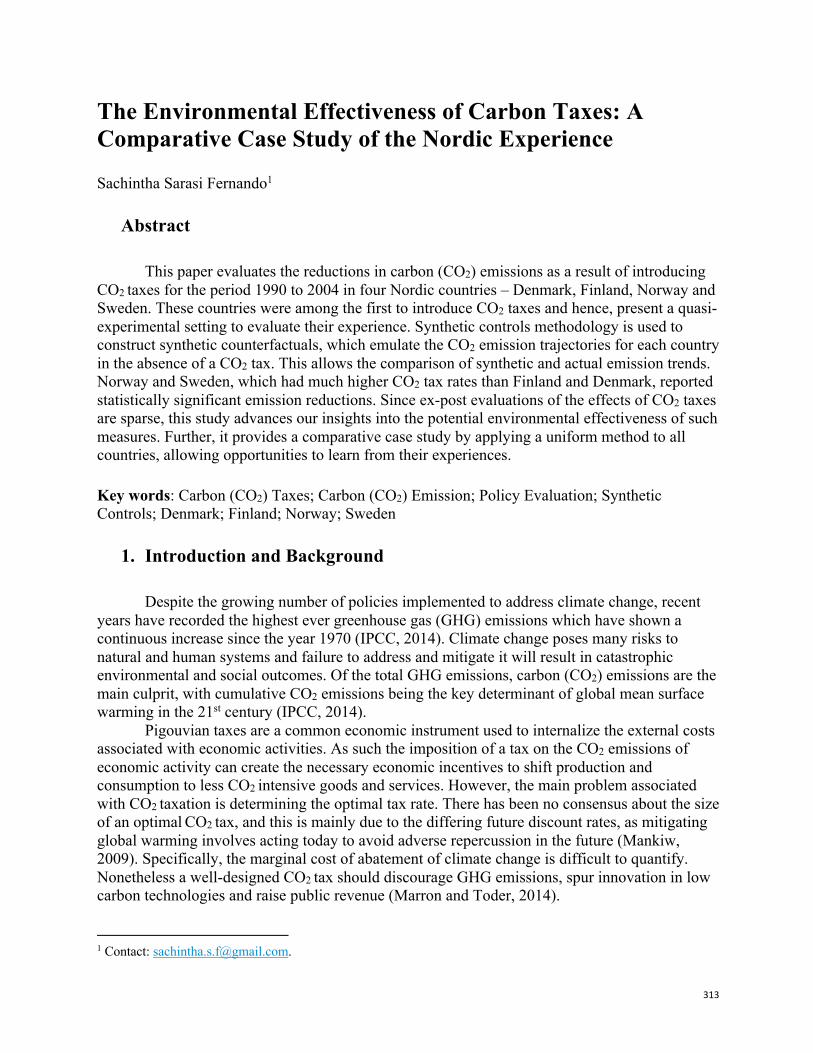
313

The Environmental Effectiveness of Carbon Taxes: A Comparative Case Study of the Nordic Experience Sachintha Sarasi Fernando1

Abstract

This paper evaluates the reductions in carbon (CO2) emissions as a result of introducing CO2 taxes for the period 1990 to 2004 in four Nordic countries – Denmark, Finland, Norway and Sweden. These countries were among the first to introduce CO2 taxes and hence, present a quasi-experimental setting to evaluate their experience. Synthetic controls methodology is used to construct synthetic counterfactuals, which emulate the CO2 emission trajectories for each country in the absence of a CO2 tax. This allows the comparison of synthetic and actual emission trends. Norway and Sweden, which had much higher CO2 tax rates than Finland and Denmark, reported statistically significant emission reductions. Since ex-post evaluations of the effects of CO2 taxes are sparse, this study advances our insights into the potential environmental effectiveness of such measures. Further, it provides a comparative case study by applying a uniform method to all countries, allowing opportunities to learn from their experiences. Key words: Carbon (CO2) Taxes; Carbon (CO2) Emission; Policy Evaluation; Synthetic Controls; Denmark; Finland; Norway; Sweden

1. Introduction and Background

Despite the growing number of policies implemented to address climate change, recent years have recorded the highest ever greenhouse gas (GHG) emissions which have shown a continuous increase since the year 1970 (IPCC, 2014). Climate change poses many risks to natural and human systems and failure to address and mitigate it will result in catastrophic environmental and social outcomes. Of the total GHG emissions, carbon (CO2) emissions are the main culprit, with cumulative CO2 emissions being the key determinant of global mean surface warming in the 21st century (IPCC, 2014).

Pigouvian taxes are a common economic instrument used to internalize the external costs associated with economic activities. As such the imposition of a tax on the CO2 emissions of economic activity can create the necessary economic incentives to shift production and consumption to less CO2 intensive goods and services. However, the main problem associated with CO2 taxation is determining the optimal tax rate. There has been no consensus about the size of an optimal CO2 tax, and this is mainly due to the differing future discount rates, as mitigating global warming involves acting today to avoid adverse repercussion in the future (Mankiw, 2009). Specifically, the marginal cost of abatement of climate change is difficult to quantify. Nonetheless a well-designed CO2 tax should discourage GHG emissions, spur innovation in low carbon technologies and raise public revenue (Marron and Toder, 2014).

1 Contact: [email protected].

314

Previous studies that investigated the environmental effectiveness of CO2 taxes can be categorized as ex-ante and ex-post evaluations. Ex-ante forecasts are conducted prior to the imposition of a tax and are usually based on models or other schematic projections whereas ex-post evaluations are classed as the actual evaluations because they are based on the actual observed outcomes (Andersen, Dengose and Pedersen, 2000). Most studies that have been conducted on the effects of CO2 taxes on emissions are ex-ante evaluations that scrutinize the potential effects of CO2 taxes. In contrast there is a dearth of ex-post studies that focus on the environmental effectiveness of CO2 taxes and other green taxes. This lack of empirical studies can be ascribed to the methodological difficulties and complexities especially in identifying a baseline scenario that can be used as a comparison group to establish causal effects (Andersen, 2004; Barazini, Goldemberg and Speck, 2000).

This paper investigates the environmental effectiveness of introducing CO2 taxes in four Nordic countries; Denmark, Finland, Norway and Sweden. These four countries were among the first to place a price on CO2 and have had taxes in place since the early 1990’s. Environmental effectiveness is measured in terms of the per capita (metric tons) reductions in CO2 emissions. The sample period investigated in this study spans from the year of introduction of the CO2 tax in each of the Nordic countries until the year 2004, which is the year prior to the introduction of the European Union emission trading system (EU ETS). Extending beyond this period would confound the study, making it difficult to attribute emission reductions to CO2 taxes only. Using Abadie et al., (2003, 2010 and 2014) synthetic control method for comparative case studies, an optimal comparison unit is constructed for each of the four Nordic countries from annual panel data of the Organization for Economic Co-operation and Development (OECD) economies that had not introduced any CO2 pricing instrument during the sample period. The results show that there is a significant drop in per capita metric tons of CO2 emissions for both Norway and Sweden after the introduction of their respective CO2 taxes.

This study advances the literature by presenting an ex-post empirical evaluation of the environmental effectiveness of CO2 taxes. In addition, this study investigates the effect on aggregate CO2 emissions for the entire economy. Most previous studies focused on partial effects and specific sectors. Further, the application of a uniform method across four countries provides a comparative case study setting, which leads to valuable insights. Finally, a methodological contribution is made by introducing a two-stage synthetic control method to address the predictor sensitivity problem identified in the standard synthetic control estimator.

2. Research Methodology

2.1 Identification strategy

The fundamental problem that arises in policy evaluation studies is the inability to observe the treated unit, in its untreated state. In this study, that translates to the difficulty in measuring the environmental effectiveness of introducing a CO2 tax in a country due to the inability to observe the CO2 emission trajectory of that country if the tax had not been introduced. This complicates the establishment of a causal relationship because the treated country cannot be observed in its untreated state. In order to overcome this a suitable comparison group that can be used as counterfactual to the treated country needs to be identified. In this study counterfactuals for each of the Nordic countries are constructed using a weighted

315

combination of other OECD countries that have not implemented a CO2 tax and resemble the Nordic countries on several key predictors of CO2 emissions. This method of constructing missing counterfactuals is known as the synthetic control method, which was developed and described in Abadie and Gardeazabal (2003) and Abadie, Diamond, and Hainmueller (2010; 2014). The counterfactuals are constructed from a donor pool of countries, which comprises of the OECD countries that have not implemented a CO2 pricing instrument during the period of investigation. The period from 1960 to 2004 is selected as the sample period of investigation. The starting year 1960 is chosen by reason of CO2 emission data availability. The ending year 2004 is chosen because it is the year prior to the introduction of the EU ETS. Extending beyond this year would limit the number of donor countries that can be included as well as result in possible confounding effects. Each country has a pre-intervention period greater that 30 years. Matching the outcome of interest over an extended pre-intervention period, helps control for unobserved factors. In addition, it lends confidence that a deviation in the outcome of interest in the post treatment period is produced by the intervention itself (Abadie, Diamond and Hainmueller, 2014). Table 1 provides a summary of the length of the sample period for each of the Nordic countries investigated.

Table 1. Sample period for each Nordic country Nordic

Country Year of introducing CO2

tax Number of Pretreatment

years Number of post treatment years

Denmark 1992 32 13 Finland 1990 30 15 Norway 1991 31 14 Sweden 1991 31 14

The World Bank’s State and Trends of Carbon Pricing Report (2016) provides an

informative summary of regional, national and subnational CO2 pricing initiatives that have been implemented. As such, in addition to the four Nordic countries, Estonia, Latvia, Slovenia and Poland implemented CO2 pricing instrument during the sample period and hence are excluded from the donor pool.2 Further Germany, Czech Republic, Luxembourg and Mexico are removed from the donor pool countries due to the lack of CO2 emission data. Thus, the final donor pool consists of 22 countries, namely Australia, Austria, Belgium, Canada, Chile, France, Greece, Hungary, Iceland, Ireland, Israel, Italy, Japan, Korea, Netherlands, New Zealand, Portugal, Spain, Switzerland, Turkey, United Kingdom and United States.

2.2 Predictors of per capita CO2 emissions

The key predictors of CO2 emissions are the observable characteristics used to construct the counterfactuals. The key predictors selected are real Gross Domestic Product (GDP) per capita, real GDP growth, total population, fossil fuel consumption as a percentage of total fuel consumption, energy use (Kt of oil equivalent per capita), methane emissions (Kt of CO2

2 Although the taxes implemented by these countries were a general environmental tax, they also addressed CO2 emissions. They have been excluded from the donor pool to avoid contamination of the donor sample and possible confounding effects.

316

equivalent) and nitrous oxide emissions (thousand metric tons of CO2 equivalent). Finally, three lagged years of CO2 emissions (1965, 1975, 1985) are included to the list of predictors due to their potential of capturing unobservable characteristics. Further, lagged CO2 emissions are a good predictor of future CO2 emission trends.

As stated in the IPCC 5th synthetic report (2014). “anthropogenic GHG emissions are mainly driven by population size, economic activity, life style, energy use, land use patterns, technology and climate policy”. This motivates the inclusion of the above key predictors. Real GDP and real GDP growth are the standard proxies used to measure economic activity in countries. As per the IPCC report, total population size as well as urban population as a percentage of total population have a direct impact of anthropogenic GHG emissions, hence their inclusion as predictors. Energy use is controlled for by the inclusion of fossil fuel energy consumption as a percentage of total energy consumption as well as energy use (Kt of oil equivalent). Methane and Nitrous oxide are GHG that contribute to climate change. Hence, the inclusion of these two variables can be considered as proxies for climate policy to capture countries that have more stringent environment policies.

2.3 Data

The study uses annual country level panel data from the World Bank World Development Indicators (WDI) data base and Penn World Tables (PWT) 7.0 (Hesten et al., 2011). The outcome variable, CO2 emissions per capita is measured in metric tons and the data for this is obtained from the WDI database. The data for the key predictors; total population, percentage of urban population, fossil fuel consumption as a percentage of total fuel consumption, energy use (kg of oil equivalent), methane emissions (kt of CO2 equivalent), nitrous oxide emissions (thousand metric tons of CO2 equivalent), were also sourced from the WDI database. The data for real GDP per capita and real GDP growth were obtained from the PWT 7.0. Appendix 1 provides the data sources.

2.4 Synthetic controls methodology

The synthetic counterfactuals for each of the Nordic countries are constructed using a weighted combination of the donor pool countries in the sample. Let 𝐽 + 1 , represent the number of OECD countries in the donor pool, indexed by 𝐽 and let 𝑗 = 1, denote the treated unit (Denmark/Finland/Norway/Sweden), and 𝑗 = 2,3, … . 𝐽, the donor pool countries.

Let 𝑡 = 1,2,3, …𝑇$, 𝑇$ + 1, 𝑇$ + 2, 𝑇$ + 3,… , 𝑇, be the sample time period, where 𝑇$, is the year in which the CO2 tax was introduced. In the case of each of the countries, Denmark, Finland, Norway and Sweden this would correspond to 1992, 1990, 1991 and 1991 respectively, with 𝑡 = 1960,and 𝑇 = 2004.

The objective of the study is to determine the environmental effectiveness of introducing the CO2 tax, by evaluating the post-tax emission reductions. This can be formalized using the potential outcome framework as follows:

𝛼V6 = 𝑌V6Í − 𝑌V6Î Where αVÐ measures the effects of the treatment at time t. YVÐÓ denotes the per capita CO2

emissions of the treated country, and YVÐÔ denotes the per capita CO2 emissions of the treated country, if not treated at time t (counterfactual scenario). However, YVÐÔ cannot be observed, thus

317

requiring the construction of a synthetic counterfactual to approximate the per capita CO2 emissions of the treated country if not treated for the post treatment period. As each Nordic country is exposed to the treatment only after 𝑇$, the effect that needs to be estimated is:

𝛼 U + 𝛼 UÕÖ + 𝛼 UÕX + ⋯+ 𝛼 The synthetic counterfactuals are constructed as a weighted average of the donor pool countries 𝑗 = 2,3, … 𝐽 + 1, where 𝐽 + 1 = 22, which is the number of donor pool countries in the sample. Each donor country is represented by a vector of weights 𝑊 = (𝑤H,…𝑤�ØV)m with 0 ≤ 𝑤Ú ≤ 1 and 𝑤H + 𝑤Û +⋯+𝑤�ØV = 1. Each choice of 𝑊 provides a certain set of weights assigned to each donor country which represent a possible synthetic counterfactual. However, the synthetic control should not only reproduce the per capita CO2 emission trajectory of each of the Nordic countries investigated but also be similar to each country on the selected pre-treatment key predictors of the outcome variable.

Assume 𝑍Ú represents the vector of key predictors that explain per capita CO2 emissions for each country in the sample. It is then possible to find 𝑊 =𝑊∗= (𝑤H∗, …𝑤�ØV∗ ). This would result in the following for the pretreatment period 𝑡 ≤ 𝑇$:

∑ 𝑤Ú∗�ØVÚ¡H 𝑌ÚV = 𝑌VV, ∑ 𝑤Ú∗

�ØVÚ¡H 𝑌ÚH = 𝑌VH, … , ∑ 𝑤Ú∗

�ØVÚ¡H 𝑌Ú U = 𝑌V U, and, ∑ 𝑤Ú∗𝑍Ú = 𝑍V

�ØVÚ¡H

Finally, as proved by Abadie et al. (2010), for the post treatment period 𝑇$ ≥ 𝑇,the unbiased estimator of 𝛼V6 is as follows:

𝛼ÝV6 = 𝑌V6 −Þ𝑤Ú∗𝑌Ú6

ÚØV

Ú¡H

Hence the treatment effect can be estimated as follows:

𝛼ÝV U + 𝛼ÝV UÕÖ + 𝛼ÝV UÕX + ⋯+ 𝛼ÝV 𝑊∗, is the optimal vector of weights is chosen such that the distance between the treated unit and its control unit are minimized. Assume 𝑘 represent the number of key predictors that explain per capita CO2 emissions. Let 𝑋$ be a 𝑘 × 𝐽 matrix representing the pretreatment values of the key predictors of per capita CO2 emissions of the donor pool countries. Let 𝑋V be a 𝑘 × 𝐽 matrix representing the pretreatment values of the key predictors of per capita CO2 emissions of each of the Nordic countries. 𝑊∗, is then chosen such that the distance ‖𝑋$ − 𝑋V𝑊‖is minimized for the pretreatment period subject to the convexity constraint 𝑤� ≥ 0 and ∑ 𝑤� = 1�

�¡V . 𝑊∗, is thus solved such that the mean square prediction error (MSPE) is minimized for the entire pretreatment period

à|𝑋V − 𝑋$𝑊|à𝜈 = ã(𝑋V − 𝑋$𝑊)′𝑉(𝑋V − 𝑋$𝑊) 𝑉, is a (𝑘 × 𝑘) symmetric and positive semi definitive matrix and it weights predictors and allows more weight to be given to more important predictors of the outcome variable. In this study 𝑉, is selected through a data driven procedure, thus eliminating the subjectivity of the researcher. For a more detailed account of the of synthetic control methodology, refer Abadie and Gardeazabal (2003) and Abadie et al. (2010).

During the practical implementation of synthetic control method, it was discovered that the synthetic control command in STATA3 is sensitive to the order in which the predictors are

3 STATA is the econometric software used to implement the synthetic controls

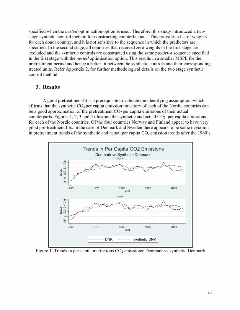
318

specified when the nested optimization option is used. Therefore, this study introduced a two-stage synthetic control method for constructing counterfactuals. This provides a list of weights for each donor country, and it is not sensitive to the sequence in which the predictors are specified. In the second stage, all countries that received zero weights in the first stage are excluded and the synthetic controls are constructed using the same predictor sequence specified in the first stage with the nested optimization option. This results in a smaller MSPE for the pretreatment period and hence a better fit between the synthetic controls and their corresponding treated units. Refer Appendix 2, for further methodological details on the two stage synthetic control method.

3. Results

A good pretreatment fit is a prerequisite to validate the identifying assumption, which affirms that the synthetic CO2 per capita emission trajectory of each of the Nordic countries can be a good approximation of the pretreatment CO2 per capita emissions of their actual counterparts. Figures 1, 2, 3 and 4 illustrate the synthetic and actual CO2 per capita emissions for each of the Nordic countries. Of the four countries Norway and Finland appear to have very good pre-treatment fits. In the case of Denmark and Sweden there appears to be some deviation in pretreatment trends of the synthetic and actual per capita CO2 emission trends after the 1980’s.

Figure 1. Trends in per capita metric tons CO2 emissions: Denmark vs synthetic Denmark

1.8

22.

22.

42.

6lg

CO

2

1960 1970 1980 1990 2000year

1.8

22.

22.

42.

6lg

CO

2

1960 1970 1980 1990 2000year

Log

CO

2 M

T Pe

r Cap

ita E

mis

sion

s

Denmark vs Synthetic DenmarkTrends in Per Capita CO2 Emissions

DNK synthetic DNK

Stage 01

Stage 02

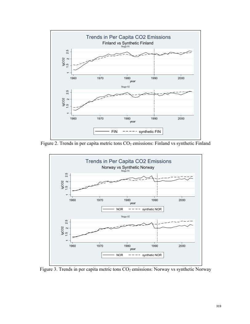
319

Figure 2. Trends in per capita metric tons CO2 emissions: Finland vs synthetic Finland

Figure 3. Trends in per capita metric tons CO2 emissions: Norway vs synthetic Norway

11.

52

2.5

lgC

O2

1960 1970 1980 1990 2000year

11.

52

2.5

lgC

O2

1960 1970 1980 1990 2000year

Log

CO

2 M

T Pe

r Cap

ita E

mis

sion

s

Finland vs Synthetic FinlandTrends in Per Capita CO2 Emissions

FIN synthetic FIN

11.

52

2.5

lgC

O2

1960 1970 1980 1990 2000year

NOR synthetic NOR

11.

52

2.5

lgC

O2

1960 1970 1980 1990 2000year

NOR synthetic NOR

Log

CO

2 M

T Pe

r Cap

ita E

mis

sion

s

Norway vs Synthetic NorwayTrends in Per Capita CO2 Emissions

Stage 01

Stage 02

Stage 01

Stage 02

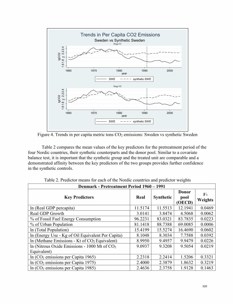
320

Figure 4. Trends in per capita metric tons CO2 emissions: Sweden vs synthetic Sweden

Table 2 compares the mean values of the key predictors for the pretreatment period of the

four Nordic countries, their synthetic counterparts and the donor pool. Similar to a covariate balance test, it is important that the synthetic group and the treated unit are comparable and a demonstrated affinity between the key predictors of the two groups provides further confidence in the synthetic controls.

Table 2. Predictor means for each of the Nordic countries and predictor weights Denmark - Pretreatment Period 1960 – 1991

Key Predictors Real Synthetic Donor pool

(OECD)

V- Weights

ln (Real GDP percapita) 11.5174 11.5513 12.1941 0.0469 Real GDP Growth 3.0141 3.8474 4.5068 0.0062 % of Fossil Fuel Energy Consumption 96.2231 83.0321 83.7835 0.0223 % of Urban Population 81.1418 88.7388 69.0085 0.0006 ln (Total Population) 15.4199 15.5274 16.4690 0.0602 ln (Energy Use - Kg of Oil Equivalent Per Capita) 8.1048 8.3034 7.7588 0.0392 ln (Methane Emissions - Kt of CO2 Equivalent) 8.9950 9.4957 9.9479 0.0226 ln (Nitrous Oxide Emissions - 1000 Mt of CO2 Equivalent)

9.0937 9.3208 9.5054 0.0219

ln (CO2 emissions per Capita 1965) 2.2318 2.2414 1.5206 0.3321 ln (CO2 emissions per Capita 1975) 2.4000 2.3879 1.8632 0.3219 ln (CO2 emissions per Capita 1985) 2.4636 2.3758 1.9128 0.1463

1.6

1.8

22.

22.

4lg

CO

2

1960 1970 1980 1990 2000year

SWE synthetic SWE

1.6

1.8

22.

22.

4lg

CO

2

1960 1970 1980 1990 2000year

SWE synthetic SWE

Log

CO

2 M

T Pe

r Cap

ita E

mis

sion

s

Sweden vs Synthetic SwedenTrends in Per Capita CO2 Emissions

Stage 01

Stage 02

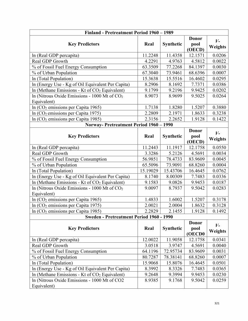
321

Finland - Pretreatment Period 1960 – 1989


(OECD)

V- Weights


8.9073 8.9699 9.5025 0.0264


Norway- Pretreatment Period 1960 – 1990


(OECD)

V- Weights


9.0097 8.7937 9.5042 0.0283


Sweden - Pretreatment Period 1960 - 1990


(OECD0

V- Weights


8.9385 9.1768 9.5042 0.0259

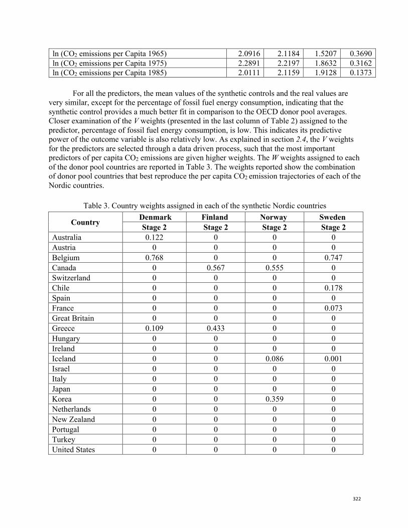
322


For all the predictors, the mean values of the synthetic controls and the real values are

very similar, except for the percentage of fossil fuel energy consumption, indicating that the synthetic control provides a much better fit in comparison to the OECD donor pool averages. Closer examination of the V weights (presented in the last column of Table 2) assigned to the predictor, percentage of fossil fuel energy consumption, is low. This indicates its predictive power of the outcome variable is also relatively low. As explained in section 2.4, the V weights for the predictors are selected through a data driven process, such that the most important predictors of per capita CO2 emissions are given higher weights. The W weights assigned to each of the donor pool countries are reported in Table 3. The weights reported show the combination of donor pool countries that best reproduce the per capita CO2 emission trajectories of each of the Nordic countries.

Table 3. Country weights assigned in each of the synthetic Nordic countries

Country Denmark Finland Norway Sweden Stage 2 Stage 2 Stage 2 Stage 2

Australia 0.122 0 0 0 Austria 0 0 0 0 Belgium 0.768 0 0 0.747 Canada 0 0.567 0.555 0 Switzerland 0 0 0 0 Chile 0 0 0 0.178 Spain 0 0 0 0 France 0 0 0 0.073 Great Britain 0 0 0 0 Greece 0.109 0.433 0 0 Hungary 0 0 0 0 Ireland 0 0 0 0 Iceland 0 0 0.086 0.001 Israel 0 0 0 0 Italy 0 0 0 0 Japan 0 0 0 0 Korea 0 0 0.359 0 Netherlands 0 0 0 0 New Zealand 0 0 0 0 Portugal 0 0 0 0 Turkey 0 0 0 0 United States 0 0 0 0

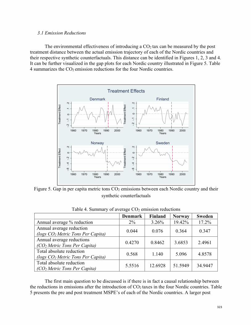
323

3.1 Emission Reductions The environmental effectiveness of introducing a CO2 tax can be measured by the post treatment distance between the actual emission trajectory of each of the Nordic countries and their respective synthetic counterfactuals. This distance can be identified in Figures 1, 2, 3 and 4. It can be further visualized in the gap plots for each Nordic country illustrated in Figure 5. Table 4 summarizes the CO2 emission reductions for the four Nordic countries.

Figure 5. Gap in per capita metric tons CO2 emissions between each Nordic country and their

synthetic counterfactuals

Table 4. Summary of average CO2 emission reductions Denmark Finland Norway Sweden Annual average % reduction 2% 3.26% 19.42% 17.2% Annual average reduction (logs CO2 Metric Tons Per Capita) 0.044 0.076 0.364 0.347

Annual average reductions (CO2 Metric Tons Per Capita) 0.4270 0.8462 3.6853 2.4961

Total absolute reduction (logs CO2 Metric Tons Per Capita) 0.568 1.140 5.096 4.8578

Total absolute reduction (CO2 Metric Tons Per Capita) 5.5516 12.6928 51.5949 34.9447

The first main question to be discussed is if there is in fact a causal relationship between

the reductions in emissions after the introduction of CO2 taxes in the four Nordic countries. Table 5 presents the pre and post treatment MSPE’s of each of the Nordic countries. A larger post

-.2-.1

0.1

.2

Trea

tmen

t Effe

ct

1960 1970 1980 1990 2000Years

Denmark

-.2-.1

0.1

.2

Trea

tmen

t Effe

ct

1960 1970 1980 1990 2000Years

Finland

-.6-.4

-.20

.2

Trea

tmen

t Effe

ct

1960 1970 1980 1990 2000Years

Norway

-.6-.4

-.20

.2

Trea

tmen

t Effe

ct

1960 1970 1980 1990 2000Years

Sweden

Treatment Effects

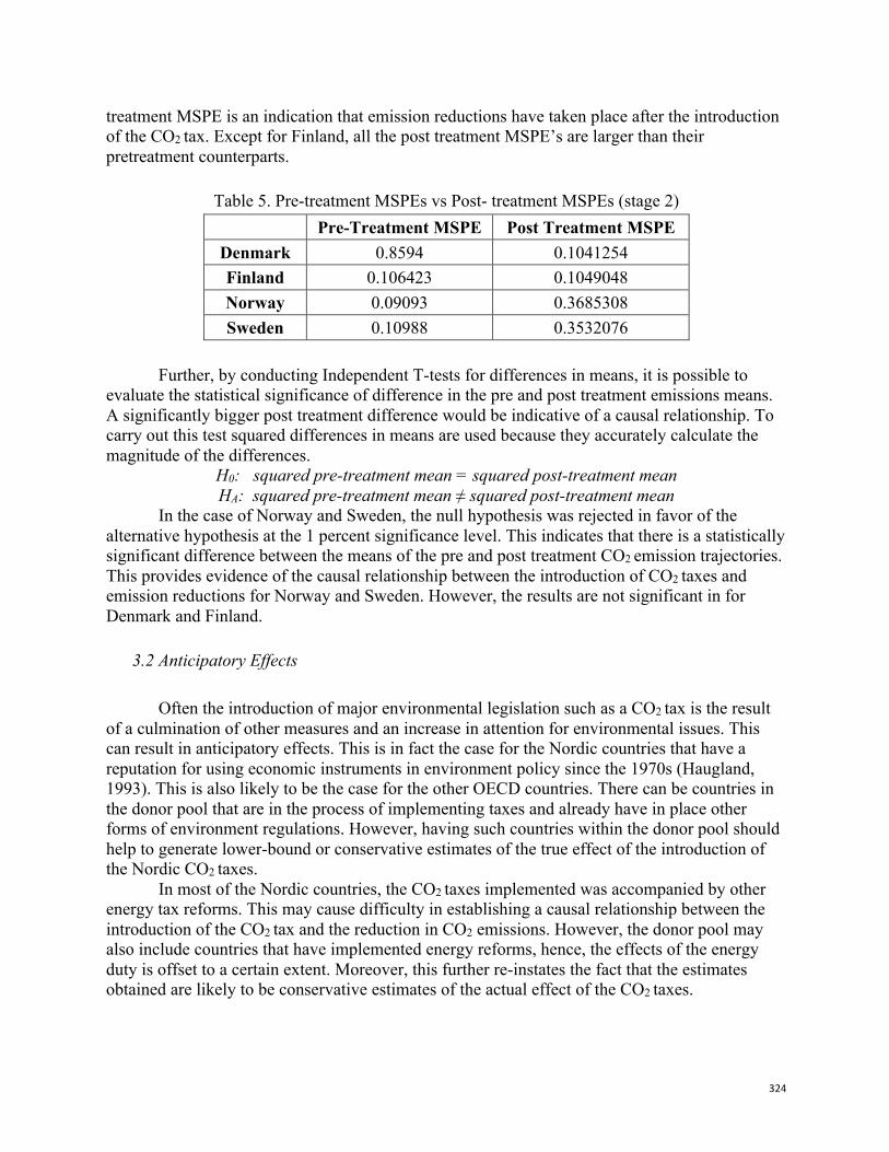
324

treatment MSPE is an indication that emission reductions have taken place after the introduction of the CO2 tax. Except for Finland, all the post treatment MSPE’s are larger than their pretreatment counterparts.

Table 5. Pre-treatment MSPEs vs Post- treatment MSPEs (stage 2) Pre-Treatment MSPE Post Treatment MSPE

Denmark 0.8594 0.1041254 Finland 0.106423 0.1049048 Norway 0.09093 0.3685308 Sweden 0.10988 0.3532076

Further, by conducting Independent T-tests for differences in means, it is possible to

evaluate the statistical significance of difference in the pre and post treatment emissions means. A significantly bigger post treatment difference would be indicative of a causal relationship. To carry out this test squared differences in means are used because they accurately calculate the magnitude of the differences.

H0: squared pre-treatment mean = squared post-treatment mean HA: squared pre-treatment mean ≠ squared post-treatment mean

In the case of Norway and Sweden, the null hypothesis was rejected in favor of the alternative hypothesis at the 1 percent significance level. This indicates that there is a statistically significant difference between the means of the pre and post treatment CO2 emission trajectories. This provides evidence of the causal relationship between the introduction of CO2 taxes and emission reductions for Norway and Sweden. However, the results are not significant in for Denmark and Finland.

3.2 Anticipatory Effects

Often the introduction of major environmental legislation such as a CO2 tax is the result of a culmination of other measures and an increase in attention for environmental issues. This can result in anticipatory effects. This is in fact the case for the Nordic countries that have a reputation for using economic instruments in environment policy since the 1970s (Haugland, 1993). This is also likely to be the case for the other OECD countries. There can be countries in the donor pool that are in the process of implementing taxes and already have in place other forms of environment regulations. However, having such countries within the donor pool should help to generate lower-bound or conservative estimates of the true effect of the introduction of the Nordic CO2 taxes.

In most of the Nordic countries, the CO2 taxes implemented was accompanied by other energy tax reforms. This may cause difficulty in establishing a causal relationship between the introduction of the CO2 tax and the reduction in CO2 emissions. However, the donor pool may also include countries that have implemented energy reforms, hence, the effects of the energy duty is offset to a certain extent. Moreover, this further re-instates the fact that the estimates obtained are likely to be conservative estimates of the actual effect of the CO2 taxes.

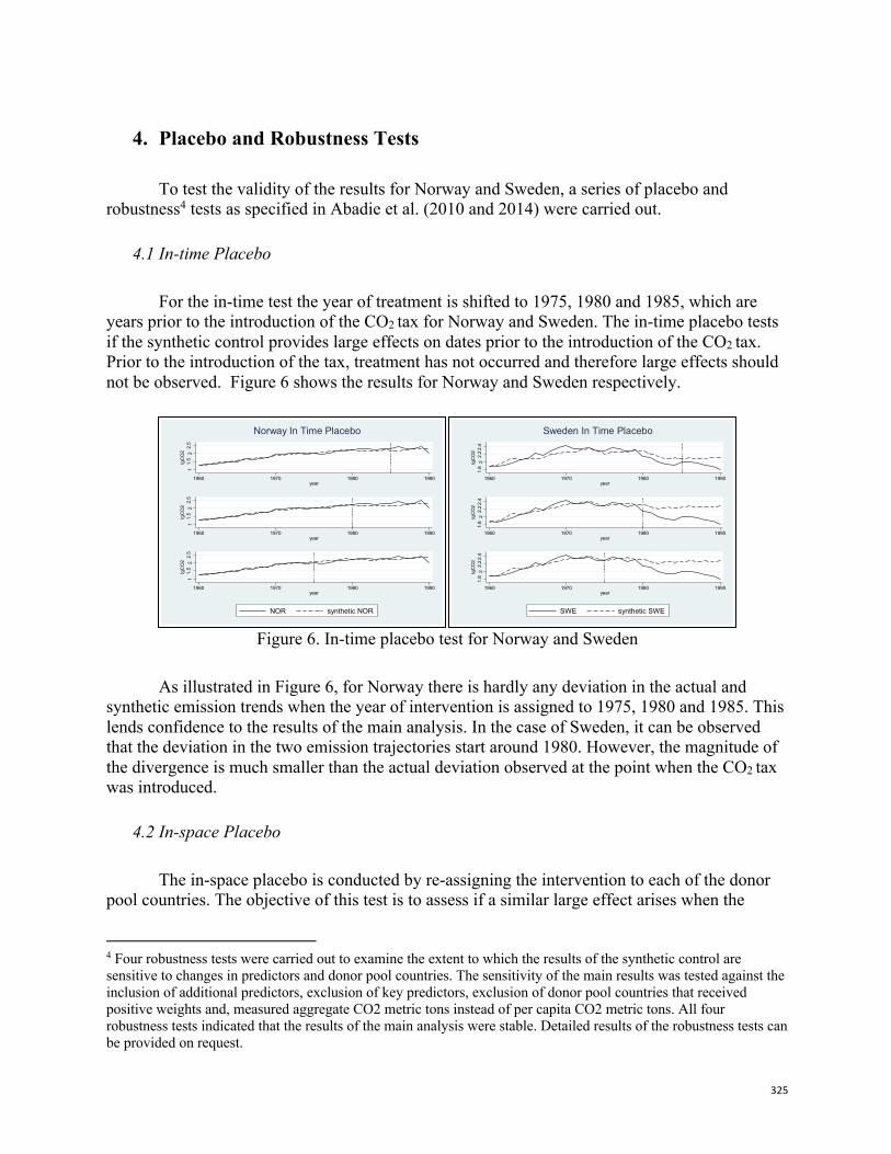
325

4. Placebo and Robustness Tests

To test the validity of the results for Norway and Sweden, a series of placebo and

robustness4 tests as specified in Abadie et al. (2010 and 2014) were carried out.

4.1 In-time Placebo

For the in-time test the year of treatment is shifted to 1975, 1980 and 1985, which are years prior to the introduction of the CO2 tax for Norway and Sweden. The in-time placebo tests if the synthetic control provides large effects on dates prior to the introduction of the CO2 tax. Prior to the introduction of the tax, treatment has not occurred and therefore large effects should not be observed. Figure 6 shows the results for Norway and Sweden respectively.

Figure 6. In-time placebo test for Norway and Sweden

As illustrated in Figure 6, for Norway there is hardly any deviation in the actual and

synthetic emission trends when the year of intervention is assigned to 1975, 1980 and 1985. This lends confidence to the results of the main analysis. In the case of Sweden, it can be observed that the deviation in the two emission trajectories start around 1980. However, the magnitude of the divergence is much smaller than the actual deviation observed at the point when the CO2 tax was introduced.

4.2 In-space Placebo

The in-space placebo is conducted by re-assigning the intervention to each of the donor pool countries. The objective of this test is to assess if a similar large effect arises when the

4 Four robustness tests were carried out to examine the extent to which the results of the synthetic control are sensitive to changes in predictors and donor pool countries. The sensitivity of the main results was tested against the inclusion of additional predictors, exclusion of key predictors, exclusion of donor pool countries that received positive weights and, measured aggregate CO2 metric tons instead of per capita CO2 metric tons. All four robustness tests indicated that the results of the main analysis were stable. Detailed results of the robustness tests can be provided on request.

11.

52

2.5

lgC

O2

1960 1970 1980 1990year

11.

52

2.5

lgC

O2

1960 1970 1980 1990year

11.

52

2.5

lgC

O2

1960 1970 1980 1990year

Log

CO

2 M

T Pe

r Cap

ita E

mis

sion

s

Norway In Time Placebo

NOR synthetic NOR

1.8

22.

22.

4lg

CO

21960 1970 1980 1990

year1.

82

2.2

2.4

lgC

O2

1960 1970 1980 1990year

1.8

22.

22.

4lg

CO

2

1960 1970 1980 1990year

Log

CO

2 M

T Pe

r Cap

ita E

mis

sion

s

Sweden In Time Placebo

SWE synthetic SWE

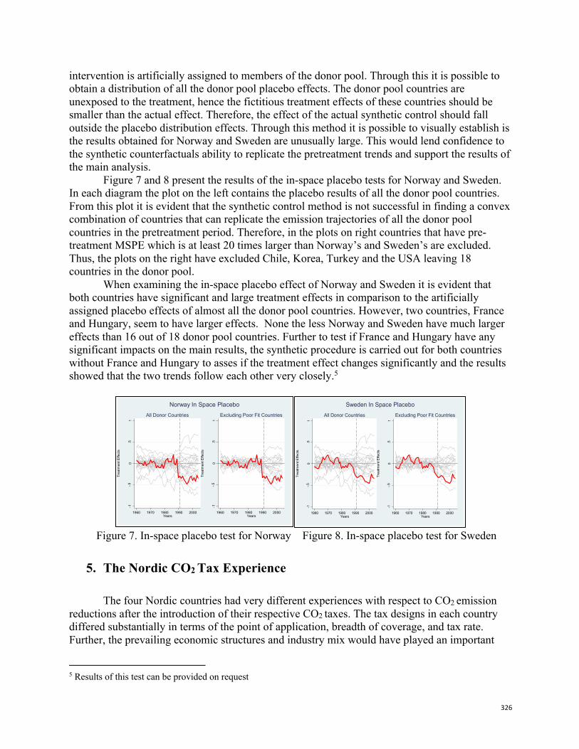
326

intervention is artificially assigned to members of the donor pool. Through this it is possible to obtain a distribution of all the donor pool placebo effects. The donor pool countries are unexposed to the treatment, hence the fictitious treatment effects of these countries should be smaller than the actual effect. Therefore, the effect of the actual synthetic control should fall outside the placebo distribution effects. Through this method it is possible to visually establish is the results obtained for Norway and Sweden are unusually large. This would lend confidence to the synthetic counterfactuals ability to replicate the pretreatment trends and support the results of the main analysis.

Figure 7 and 8 present the results of the in-space placebo tests for Norway and Sweden. In each diagram the plot on the left contains the placebo results of all the donor pool countries. From this plot it is evident that the synthetic control method is not successful in finding a convex combination of countries that can replicate the emission trajectories of all the donor pool countries in the pretreatment period. Therefore, in the plots on right countries that have pre-treatment MSPE which is at least 20 times larger than Norway’s and Sweden’s are excluded. Thus, the plots on the right have excluded Chile, Korea, Turkey and the USA leaving 18 countries in the donor pool.

When examining the in-space placebo effect of Norway and Sweden it is evident that both countries have significant and large treatment effects in comparison to the artificially assigned placebo effects of almost all the donor pool countries. However, two countries, France and Hungary, seem to have larger effects. None the less Norway and Sweden have much larger effects than 16 out of 18 donor pool countries. Further to test if France and Hungary have any significant impacts on the main results, the synthetic procedure is carried out for both countries without France and Hungary to asses if the treatment effect changes significantly and the results showed that the two trends follow each other very closely.5

Figure 7. In-space placebo test for Norway Figure 8. In-space placebo test for Sweden

5. The Nordic CO2 Tax Experience

The four Nordic countries had very different experiences with respect to CO2 emission

reductions after the introduction of their respective CO2 taxes. The tax designs in each country differed substantially in terms of the point of application, breadth of coverage, and tax rate. Further, the prevailing economic structures and industry mix would have played an important

5 Results of this test can be provided on request

-1-.5

0.5

1

Trea

tmen

t Effe

cts

1960 1970 1980 1990 2000Years

All Donor Countries

-1-.5

0.5

1

Trea

tmen

t Effe

cts

1960 1970 1980 1990 2000Years

Excluding Poor Fit Countries

Norway In Space Placebo

-1-.5

0.5

1

Trea

tmen

t Effe

cts

1960 1970 1980 1990 2000Years

All Donor Countries

-1-.5

0.5

1

Trea

tmen

t Effe

cts

1960 1970 1980 1990 2000Years

Excluding Poor Fit Countries

Sweden In Space Placebo

327

role. The evolution of the CO2 taxes over time is also an important determinant of its effectiveness. Thus, it is necessary to analyze each case individually to obtain a more comprehensive understanding in order to bridge the quantitative and qualitative divide.

In 1991 the Danish parliament passed the CO2 tax bill, which came into force in May 1992. The main objective of the tax was to create economic incentives for the consumption of less CO2 intensive energy sources (Haugland, 1993). The fundamental principle behind the tax during the period of 1992 to 2004 was an intended tax rate of 100DKK/ton of CO2 (20.78 Euro/ton of CO2 in 2015 prices6) regardless of fuel type (Withana et al., 2013). Initially the tax covered fuel oils, gas (except natural gases), coal and electricity and was applied to households and small enterprises which were not VAT registered (Nordic council of ministers, 1994 and Haugland, 1993). However, at the time of introduction, the increase in the CO2 tax was offset by a reduction in the energy tax in order to avoid an increase in the overall tax burden. In 1993 the tax was extended to the energy use of VAT registered companies however at a lower rate of 50DKK/ton of CO2 (10.26 Euro/ton of CO2 in 2015 prices). Throughout the sample period the CO2 rates between households and industries differed, except for heating where businesses were subject to the same rate as the households. The primary reason for setting different tax rates was to protect the competitiveness of industries (Withana et al., 2013). On average throughout the post treatment sample period approximately 45 percent of the CO2 emissions were covered by the CO2 tax (World Bank, 2014).

Finland was the first country to in the world to introduce a CO2 tax in 1990. The tax rate was initially set at an average rate of 7FIM/ton of CO2 (1.8 Euro/ton of CO2 in 2015 prices) and was based on the CO2 content of all fuels except for traffic fuels (Haugland, 1993). The tax was levied on oil products, other fossil fuels and electricity. The average tax rates had evolved to 14FIM/ton of CO2 (3.28 Euro/ton of CO2 in 2015 prices) by the year 1993. In 1994 the CO2 scheme was reformed and as a result of this change all primary energy sources were taxed according to both the energy content and CO2 content with 75 percent of the tax being determined by the CO2 content and 25 percent by the energy content. The tax scheme was further amended in 1997, returning back to a 100 percent CO2 tax based on CO2 content. In the year 2005 the average tax rate was 21 Euro/ton of CO2 (Nordic council of ministers, 1994 and Speck et al, 2006). On average during the sample period approximately 15 percent of the CO2 emissions were covered by the CO2 tax (World Bank, 2014). In comparison to the other Nordic countries, the Finnish CO2 tax scheme can be considered as the most homogenous in terms of special exemption, with only insignificant exemptions and tax reliefs granted to specific sectors.

The Norwegian CO2 tax was introduced in 1991. At the time of introduction, the tax rate was set to about 275NOK/ton of CO2 (49.6 Euro/ton of CO2 in 2015 prices) for gasoline and natural gases and 110NOK/ton of CO2 (19.84 Euro/ton of CO2 in 2015 prices) for other petroleum products (Haugland, 1993). The Norwegian CO2 scheme was not designed to have a fixed level regardless of fuel type. As in most tax schemes political interests result in a number of exceptions for many industries, and Norway was no exception. The fishmeal industry and the wood processing industry were charged approximately half of the normal level of CO2 taxes on mineral oils. Coal and coke used for non-energy purposes were also exempt from CO2 taxes as well as coal consumption in the cement industry (Speck et al., 2006). Further the CO2 tax rate levied on consumption of mineral oils on the continental shelf was twice as high as the tax rate levied on the mainland. Overall the tax rate was revised several times since its introduction and as of 2005 the CO2 on heavy fuels oil was equivalent to 171 NOK/ton of CO2 (23 Euro/ton of

6 Prices are adjusted for inflation (World bank WDI database) and then converted to Euro (Euro Stat Database)

328

CO2 in 2015 prices), the tax rate on light fuel oil was equivalent to 198 NOK/ton of CO2 (26.88 Euro/ton of CO2 in 2015 prices) and the tax rate on petrol was equivalent to 337 NOK/ton of CO2 (45 Euro/ton of CO2 in 2015 prices). Overall approximately 50 percent of the CO2 emissions during the sample period were covered by the CO2 taxes. (World Bank, 2014).

Sweden’s CO2 tax was also introduced in 1991. The tax rate at the time of introduction was 250 SEK/ton of CO2 (32 Euro/ton of CO2 in 2015 prices) based primarily on the fossil CO2 content of the fossil fuel (Haugland, 1993). The main objective of introducing the CO2 tax was to stimulate a strong economic incentive to reduce CO2 emissions. Moreover, the Swedish CO2 tax forms the most significant part of the excise duties levied on energy constituting more than three quarters of the total tax on fossil fuel consumption (Speck et al, 2006). The average tax rate in 1993 was 604SEK/ton of CO2 (74 Euro/ton of CO2 in 2015 prices). On average during the post treatment sample period CO2 taxes covered approximately 25 percent of the Swedish CO2 emissions (World Bank, 2014).

As explained above it is apparent that the tax schemes differed considerably between the four Nordic countries. While the tax rate applied varied substantially among the countries, there was also considerable variability within sectors of each country in terms of the rates applied as well as the exemptions and tax reliefs applicable. At the time of introduction, the average CO2 tax rates (based on CO2 content) for Denmark, Finland, Norway and Sweden were 20.78 Euro, 1.8 Euro, 19.84 – 49.6 Euro and 32 Euro respectively. Overall during the entire post treatment sample period Norway and Sweden have had much higher taxes with the average tax level of Finland and Denmark being about 40 percent of the Swedish level and 60 percent of the Norwegian level (Haugland, 1993). This could be one possible reason for Sweden and Norway showing much higher emission reductions in the synthetic control results. Further although Finland had the most homogenous tax design, the tax rate itself was rather low thus not providing very strong incentives to provide significant emission reductions. The Danish tax design had the most comprehensive exemption scheme thus most of the energy intensive industries and therefore the highest CO2 emitters were exempt from the tax system (Speck et al., 2006). Hence, these different experiences and different evolutions of the CO2 tax systems within each economy provide some insights to the reasons for the different levels of emission reductions experienced by each country.

6. Discussion and Conclusion

Economic theory is unequivocal about the impact of CO2 taxes on CO2 emissions. Ceteris paribus an increase in CO2 tax should reduce emissions. However, in the practical world, all things are rarely constant, and many forces can influence this mechanism. An optimal CO2 tax should have a uniform rate and be applicable to all sectors in an economy. In this context the CO2 taxes introduced in the four Nordic countries were suboptimal due to both exemptions and differentiation of the tax rates, resulting in different experiences for each country.

This study specifically investigates the event of introducing a CO2 tax, and the resulting effects on CO2 emissions in four Nordic countries; Denmark, Finland, Norway and Sweden. The synthetic control method is used to create the counterfactual emission trends in order to establish causal relations. From the four Nordic countries investigated, Norway reports the highest emission reduction of 51.59 metric tons per capita for the entire post treatment period. Norway also provides the most ideal settings, due a very good pretreatment fit and a clear downward deviation in emission reductions after the introduction of the CO2 tax. Sweden also reports a high

329

emission reduction of 34.94 metric tons per capita; but the pretreatment trend of the synthetic and actual starts to deviate in the early 1980’s. However, the MSPE’s is significantly larger in the post treatment period, thus indicating that there is in fact an effect due to CO2 taxes. It is somewhat difficult to establish causal relations for Denmark and Finland due to the absence of a significant deviation in per capita CO2 emissions after the treatment. Further, there is no significant difference between the pretreatment and post treatment MSPE for the two countries. The results of Norway and Sweden are stable to a series of placebo and robustness tests. Moreover, there is evidence for the existence of anticipatory effects and hence it is likely that the effects identified are conservative estimates of the true effect.

This study makes two primary contributions. First, it contributes to the much-needed empirical evaluation of the environmental effectiveness of CO2 taxes. The existing literature specifies the dearth of ex-post studies evaluating the effectiveness of already implemented CO2 taxes and hence this study expands the empirical literature.

Second, a methodological contribution is made. The study identified an implementation error in the standard synthetic control method, which has previously gone unnoticed. The use of the nested optimization option, although it yields better pretreatment fits, is sensitive to the order in which the predictors are specified. To counter this issue, this study adopts an innovative two stage synthetic control approach that increases both consistency and efficiency of the synthetic control.

There is ample opportunity for further research on this topic. This study looks at the aggregate effects on the entire economy. The next obvious step would be to analyze each country in detail and investigate the effects that the CO2 taxes had in specific sectors and industries. It will also be interesting to bring the experiences of the four countries together and investigate the effect of the different tax rates and emission reductions. However, this will be subject to the availability of good data.

Bibliography Abadie, Alberto, Alexis Diamond, and Jens Hainmueller. "Comparative Politics and the Synthetic Control Method."

American Journal of Political Science 59, no. 2 (2015): 495-510. Abadie, Alberto, and Javier Gardeazabal. "The Economic Costs of Conflict: A Case Study of the Basque Country."

The American Economic Review 93, no. 1 (2003): 113-132. Abadie, Alberto, Alexis Diamond, and Jens Hainmueller. "Synthetic Control Methods for Comparative Case

Studies: Estimating the Effect of California's Tobacco Control Program." Journal of the American Statistical Association 105, no. 490 (2010): 493-505.

Andersen, Mikael Skou, Niels Dengsoe and Anders B. Pedersen. “An evaluation of the impact of green taxes in the Nordic countries.” TemaNord 2000:561

Andersen, Mikael Skou. “Vikings and Virtues: A Decade of CO2 Taxation.” Climate Policy 4, no. 1 (2004): 13-24. Baranzini, Andrea, José Goldemberg, and Stefan Speck. "A Future for Carbon Taxes." Ecological Economics 32,

no. 3 (2000): 395-412. Johansson, Bengt. "Climate Policy Instruments and industry—effects and Potential Responses in the Swedish

Context." Energy Policy 34, no. 15 (2006): 2344-2360. Haugland, Torlief. "A comparison of carbon taxes in selected OECD countries." 1993. OECD Environment

Monographs No:78. Heston, A., Summers, R., and Aten, B. Penn World Table Version 7.0. Center for International Comparisons of

Production, Incomes and Prices at the University of Pennsylvania. 2011. IPCC. " Climate Change 2014: Synthesis Report." Contribution of Workings Groups I, II, III to the Assessment

Report of the Intergovernmental Panel for Climate Change. Geneva, Swithzerland: IPCC, 151 pp.

330

Mankiw, N. Gregory. "Smart Taxes: An Open Invitation to Join the Pigou Club." Eastern Economic Journal 35, no. 1 (2009): 14-23.

Marron, Donald B. and Eric J. Toder. "Tax Policy Issues in Designing a Carbon Tax." The American Economic Review 104, no. 5 (2014): 563-568.

Speck, Stefan, Miljø- og Økonomigruppen (MEG), Nordiska ministerrådet, and Nordisk Ministerråds sekretariat. The use of Economic Instruments in Nordic and Baltic Environmental Policy 2001-2005. S.l.: Nordic Council of Ministers, 2006. doi:10.6027/TN2006-525.

The use of Economic Instruments in Nordic Environmental Policy. Vol. 1994:561. Copenhagen: Nordic Council of Ministers, 1994.

Richard S. J. Tol. "The Economic Effects of Climate Change." The Journal of Economic Perspectives 23, no. 2 (2009): 29-51.

Whalley, John and Randall Wigle. "Cutting CO₂ Emissions: The Effects of Alternative Policy Approaches." The Energy Journal 12, no. 1 (1991): 109-124.

Withana, S., ten Brink, P., Krestchmer, B., Mazza, L., Hjerp, P., Sauter, R. 2013 "Evaluation of environmental tax reforms: international experiences" A report by the institute for European Environmental Policy (IEEP) for the State Secretariat for Economic Affairs (SECO) and the Federal Finance Administration (FFA) of Switzerland. Final Report. Brussels. 2013

World Bank. 2014. State and Trends of Carbon Pricing 2014. Washington D.C: World Bank. World Bank, Ecofys and Vivid Economics. 2016. State and Trends of Carbon Pricing 2016. Washington D.C: World

Bank.

Appendix 1: Data Sources Outcome variable — CO2 per capita emissions. Measured in metric tons per capita. Source: World Bank WDI

database (http://data.worldbank.org/indicator/EN.ATM.CO2E.PC?view=chart) Key predictors — Real GDP per capita. Measured expenditure side real GDP at chained PPPs (in mil.

2011US$). Source: Penn World Table 7 (http://www.rug.nl/ggdc/productivity/pwt/pwt-releases/pwt-7.0)

— Real GDP growth. Calculated based on above Real GDP per capita data. Source: Penn world Table (http://www.rug.nl/ggdc/productivity/pwt/pwt-releases/pwt-7.0)

— Total population. Source World Bank WDI database (http://data.worldbank.org/indicator/SP.POP.TOTL?view=chart)

— Percentage of urban population. Source: World Bank WDI database (http://data.worldbank.org/indicator/SP.URB.TOTL.IN.ZS?view=chart)

— Energy use. Measured in Kilo tons of oil equivalent. Source: World Bank WDI database (http://data.worldbank.org/indicator/EG.USE.PCAP.KG.OE?view=chart)

— Percentage of fossil fuel of total consumption. Source: World Bank WDI database (http://data.worldbank.org/indicator/EG.USE.COMM.FO.ZS?view=chart)

— Methane emissions. Measured in Kilo tons of CO2 equivalent. Source: World Bank WDI database (http://data.worldbank.org/indicator/EN.ATM.METH.KT.CE?view=chart)

— Nitrous oxide. Measured in thousand metric tons of CO2 equivalent. Source: World Bank WDI database (https://data.worldbank.org/indicator/EN.ATM.NOXE.KT.CE)

Data used to convert exchange rates — Inflation. Source: World Bank WDI database

(http://data.worldbank.org/indicator/FP.CPI.TOTL.ZG?view=chart)

331

— Exchange rates. Source: Euro stat database – ECU/EUR exchange rate vs national currencies and Euro/national currency exchange rate (http://ec.europa.eu/eurostat/data/database)

Appendix 2: Implementation of the two-stage synthetic control

The synthetic counterfactual assigns weights to each of the countries in the donor pool,

such that the MSPE is minimized for the entire pretreatment period. This is done through an objective, data driven procedure. However, when practically implementing this, it was discovered that the synthetic control command in STATAis sensitive to the order in which the predictors are specified when the nested optimization option is used. For example, assume that A, B, C, D, E, F, G, H are key predictors of the outcome variable CO2. The STATA command for this is as follows: synth A B C D E F G H trunit() trperiod() Where, trunit(), specifies the treated unit within the panel data set and trperiod(), specifies the time period in which treatment took place. The synth package further has an optimization option “nested”, which when included yields a better fit. As explained in the STATA synth package;

By default synth uses a data-driven regression based method to obtain the variable weights contained in the V-matrix. This method relies on a constrained quadratic programming routine that finds the best fitting W-weights conditional on the regression based V-matrix. This procedure is fast and often yields satisfactory results in terms of minimizing the MSPE. Specifying nested will lead to better performance, however, at the expense of additional computing time. If nested is specified synth embarks on a fully nested optimization procedure that searches among all (diagonal) positive semidefinite V-matrices and sets of W-weights for the best fitting convex combination of the control units. The fully nested optimization contains the regression based V as a starting point, but often produces convex combinations that achieve even lower MSPE (Synth - synthetic control methods for comparative case studies, authors Hainmeuller, Abadie and Diamond)

Hence, including the “nested” option would give the following command, synth A B C D E F G H trunit() trperiod() nested

The weights obtained for each country should provide the best fit and the lowest MSPE. However, a simple rearrangement of predictors yields different weights. For example, synth B C G F D A E H trunit() trperiod() nested, provides different weights to the donor countries.

The synth command does not provide the best fitting convex combination of the control units, but only provides a convex combination of the control units. In order to tackle this problem in this study, the synthetic control procedure is conducted in two stages. In the first stage synthetic controls are constructed excluding the nested optimization option. This provides a list of weights for each donor country, and it is not sensitive to the sequence in which the predictors are specified. In the second stage, all countries that received zero weights in the first stage are excluded and the synthetic controls are constructed using the same predictor sequence specified in the first stage with the nested optimization option. This provides a smaller MSPE for the

332

pretreatment period and hence a better fit between the synthetic controls and their corresponding treated units. Further the optimization is conducted only among countries that were originally assigned positive weights in stage one of the analysis. Sensitivity checks were conducted by generating 10 random8 sequences of the key predictors and constructing synthetic controls using each of the sequences and subsequently comparing the MSPE’s and treatment effects of each iteration9

8 The random sequences were generated using Microsoft Excel and the RAND function. 9 Results of the sensitivity checks can be provided on request

333

What if the Biggest EU Member States had Emulated Sweden’s Outstanding Carbon Tax? Eoin Ó BROIN (Centre International de Recherche sur l'Environnement et le Développement (CIRED), Paris, France; EnvEcon, Dublin, Ireland); Jens EWALD (Environmental Economics Unit, Department of Economics, University of Gothenburg, Sweden); Franck NADAUD (Centre International de Recherche sur l'Environnement et le Développement (CIRED), Paris, France); Érika MATA (IVL Swedish Environmental Research Institute, Gothenburg, Sweden); Magnus HENNLOCK (IVL Swedish Environmental Research Institute, Gothenburg, Sweden); Louis-Gaëtan GIRAUDET (Centre International de Recherche sur l'Environnement et le Développement (CIRED), Paris, France) ; Thomas STERNER (Environmental Economics Unit, Department of Economics, University of Gothenburg, Sweden)

Abstract

Across the EU substantial carbon taxes outside of sectors covered by the EU Emissions Trading Scheme (ETS) have only been applied in Sweden. This raises the question as to where the EU might currently be with respect to greenhouse gas emissions had other EU countries followed the Swedish example. We simulate how a high carbon tax would have affected demand in the residential sector in France, Germany, Italy, Spain and the UK. We utilize the residential sector’s price elasticity of demand for energy and use it to estimate the fall in energy demand that would have accrued had carbon taxes at the Swedish level been in place in these five countries. Our conservative estimates indicate reductions in demand for fossil fuels of a minimum of 10 to 20 percent. This means that at least 60 MtCO2eq yearly greenhouse gas reductions could have been achieved only in the five countries of focus if such carbon taxes would have been implemented at the time of the signing of the Kyoto Protocol in 1997.

Introduction

The European Union has committed to reducing greenhouse gas emissions by at least 40 percent by 2030 as compared with 1990 levels and reducing primary energy demand by between 27 and 40 percent (EC, 2017) . The former goal is the EU’s nationally determined contribution (NDC) under the 2015 Paris Climate Agreement. In the immediate future to 2020 the EU is committed to the 20-20-20 package whereby there is a mandatory 20 percent reduction in greenhouse gas emissions (relative to the levels in 1990), a mandatory 20 percent renewables in the primary energy mix and an aspirational 20 percent saving in primary energy use (relative to the projected baseline). The 2030 climate and energy goals should be met through increased diffusion of renewable energy sources, improvements in energy efficiency and without a lowering of standards of living. Despite these targets for 2030, which although ambitious in an international context are not enough for limiting global warming to the Paris target of 1.5 degrees, substantial carbon taxes outside of sectors covered by the EU Emissions Trading

334

Scheme (ETS) have only been applied in Sweden (€114/tonne CO2 in 2019; Regeringskansliet, 2018). This context raises the question as to where the EU might currently be with respect to greenhouse gas emissions had other EU countries followed the Swedish example. Coupled with this, concern has been expressed in the IPCC AR5 at the lack of research on carbon taxes (Somanathan et al., 2014a).

In political circles the appeal of carbon taxes as a policy instrument is broadening. The Climate Leadership Council, a conservative American think-tank supported by leading American Republicans, has recently stated that, “A sensible carbon tax might begin at $40 a ton and increase steadily over time sending a powerful signal to businesses and consumers while generating revenue to reward Americans for decreasing their collective carbon footprint (Baker III et al., 2017)…”. Support for a carbon tax from this quarter surely heralds that the concept has arrived. Nonetheless, the recent experience in France with the opposition to increased fuel taxes from the Gilets Jaunes or Yellow Vest movement has shown that proper policy design and tax-switching policies to weigh up for possible regressive effects are crucial. Credited to MIT professor David G. Wilson (Boston Globe, 2014), carbon taxes have their origins in the oil crisis of the 1970’s and the desire of some states to wean themselves off fossil fuels, but even more so in their advocacy as a Pigouvian tax on the global warming and environmental impact of CO2 and other greenhouse gas emissions. Finland (1990), Sweden (1990), Norway (1991) and Denmark (1992) have been frontrunners in launching specific Carbon-taxes to curb CO2 emissions. In the case of Sweden, taxes on industrial energy consumption had been in place since 1974 (first oil crisis), which then were modified in 1990 towards a carbon tax base (Andersen, 2010).

In 1992, under the United Nations Framework Convention on Climate Change (UNFCCC), developed countries committed to adopting national policies and taking corresponding measures on the mitigation of climate change. To do this, they agreed to limit their anthropogenic emissions of greenhouse gases and protect and enhance their greenhouse gas sinks and reservoirs. As of 2017, 42 countries and 25 subnational jurisdictions (cities, states, and regions) are putting a price on carbon through an Emissions Trading Scheme (ETS) or a carbon tax1. This consists of 24 ETSs, mostly in subnational jurisdictions, and 23 carbon taxes primarily implemented at a national level. Over the past decade, the number of jurisdictions with carbon pricing initiatives has doubled. These jurisdictions, which include seven out of the world’s ten largest economies, are responsible for about a quarter of global greenhouse gas emissions (World Bank, 2018). In addition, there are now more than 1,000 companies reporting that they price carbon internally or plan to do so in the next one to two years (up from 150 companies pricing carbon in 2014; Caring for Climate, 2015).

The observed carbon prices span a wide range, from less than US$1 up to US$139/tCO2eq. About half of the covered emissions remain priced at less than US$10/tCO2eq, which is substantially lower than the price levels that are consistent with achieving the temperature goal of the Paris Agreement, identified by the High-Level Commission on Carbon Prices to be in the range of US$40–80/tCO2eq in 2020 and US$50–100/tCO2eq by 2030. Also, the Carbon Pricing Corridors initiative, which is led by the Carbon Disclosure Project (CDP) and We Mean Business, projects that price levels of US$30–100/tCO2eq by 2030 are needed to

1 The existence of the EU ETS which is in place for over a decade shows that there is political acceptance of the principal of a price on carbon across the EU for large point sources. On the other hand, the general low level of the carbon taxes in place shows that there is less acceptance from the population at large to be paying for carbon emissions. As this article deals with the residential sector it is the latter case, i.e. carbon taxes, that we focus on.

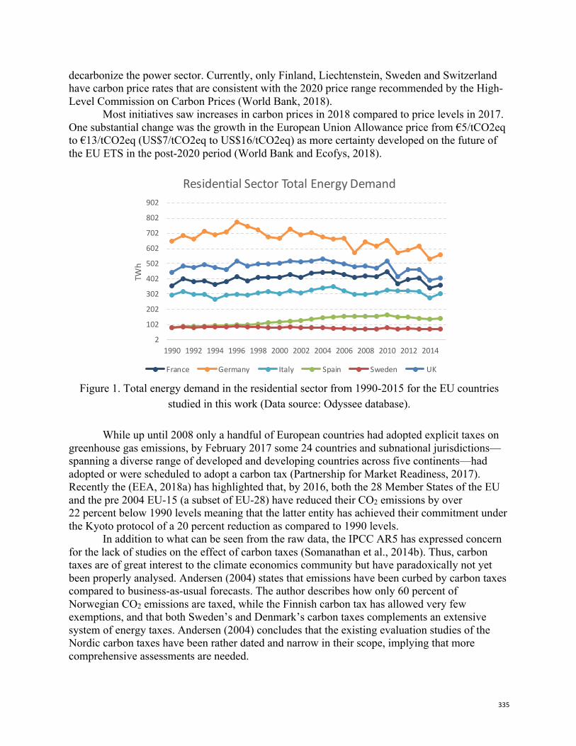
335

decarbonize the power sector. Currently, only Finland, Liechtenstein, Sweden and Switzerland have carbon price rates that are consistent with the 2020 price range recommended by the High-Level Commission on Carbon Prices (World Bank, 2018).

Most initiatives saw increases in carbon prices in 2018 compared to price levels in 2017. One substantial change was the growth in the European Union Allowance price from €5/tCO2eq to €13/tCO2eq (US$7/tCO2eq to US$16/tCO2eq) as more certainty developed on the future of the EU ETS in the post-2020 period (World Bank and Ecofys, 2018).

Figure 1. Total energy demand in the residential sector from 1990-2015 for the EU countries

studied in this work (Data source: Odyssee database).

While up until 2008 only a handful of European countries had adopted explicit taxes on greenhouse gas emissions, by February 2017 some 24 countries and subnational jurisdictions—spanning a diverse range of developed and developing countries across five continents—had adopted or were scheduled to adopt a carbon tax (Partnership for Market Readiness, 2017). Recently the (EEA, 2018a) has highlighted that, by 2016, both the 28 Member States of the EU and the pre 2004 EU-15 (a subset of EU-28) have reduced their CO2 emissions by over 22 percent below 1990 levels meaning that the latter entity has achieved their commitment under the Kyoto protocol of a 20 percent reduction as compared to 1990 levels.

In addition to what can be seen from the raw data, the IPCC AR5 has expressed concern for the lack of studies on the effect of carbon taxes (Somanathan et al., 2014b). Thus, carbon taxes are of great interest to the climate economics community but have paradoxically not yet been properly analysed. Andersen (2004) states that emissions have been curbed by carbon taxes compared to business-as-usual forecasts. The author describes how only 60 percent of Norwegian CO2 emissions are taxed, while the Finnish carbon tax has allowed very few exemptions, and that both Sweden’s and Denmark’s carbon taxes complements an extensive system of energy taxes. Andersen (2004) concludes that the existing evaluation studies of the Nordic carbon taxes have been rather dated and narrow in their scope, implying that more comprehensive assessments are needed.

2

102

202

302

402

502

602

702

802

902

1990 1992 1994 1996 1998 2000 2002 2004 2006 2008 2010 2012 2014

TWh

Residential Sector Total Energy Demand

France Germany Italy Spain Sweden UK

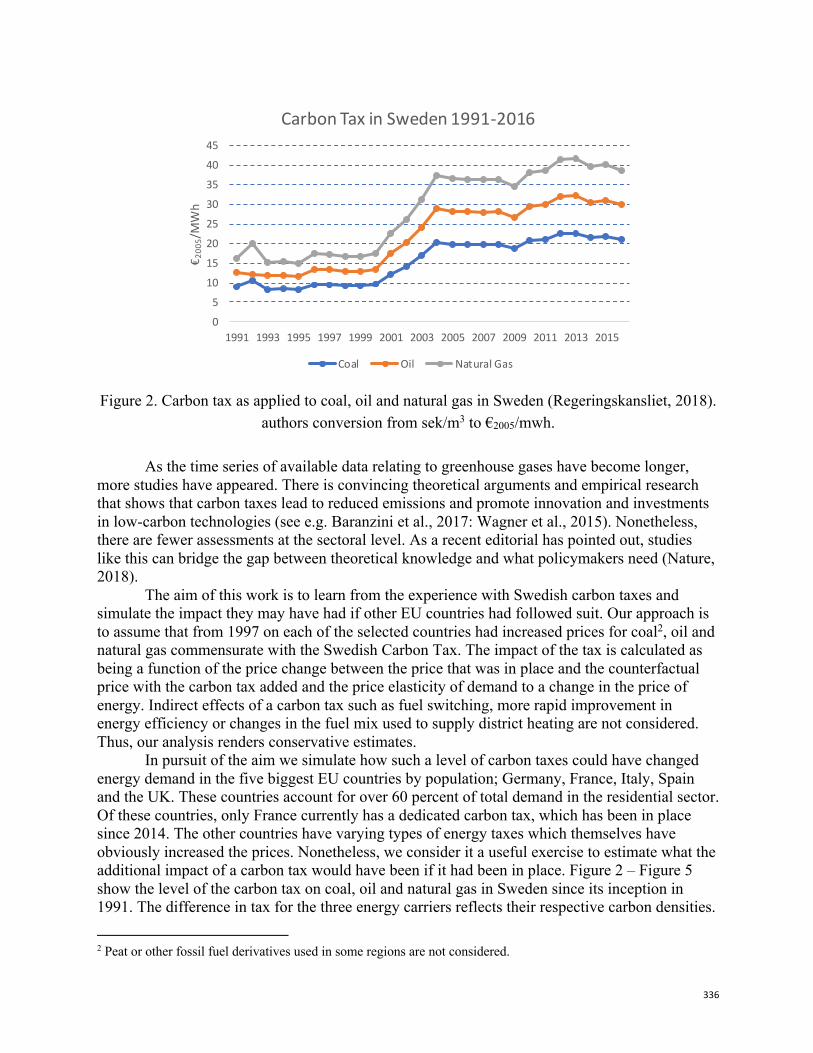
336

Figure 2. Carbon tax as applied to coal, oil and natural gas in Sweden (Regeringskansliet, 2018).

authors conversion from sek/m3 to €2005/mwh.

As the time series of available data relating to greenhouse gases have become longer, more studies have appeared. There is convincing theoretical arguments and empirical research that shows that carbon taxes lead to reduced emissions and promote innovation and investments in low-carbon technologies (see e.g. Baranzini et al., 2017: Wagner et al., 2015). Nonetheless, there are fewer assessments at the sectoral level. As a recent editorial has pointed out, studies like this can bridge the gap between theoretical knowledge and what policymakers need (Nature, 2018).

The aim of this work is to learn from the experience with Swedish carbon taxes and simulate the impact they may have had if other EU countries had followed suit. Our approach is to assume that from 1997 on each of the selected countries had increased prices for coal2, oil and natural gas commensurate with the Swedish Carbon Tax. The impact of the tax is calculated as being a function of the price change between the price that was in place and the counterfactual price with the carbon tax added and the price elasticity of demand to a change in the price of energy. Indirect effects of a carbon tax such as fuel switching, more rapid improvement in energy efficiency or changes in the fuel mix used to supply district heating are not considered. Thus, our analysis renders conservative estimates.

In pursuit of the aim we simulate how such a level of carbon taxes could have changed energy demand in the five biggest EU countries by population; Germany, France, Italy, Spain and the UK. These countries account for over 60 percent of total demand in the residential sector. Of these countries, only France currently has a dedicated carbon tax, which has been in place since 2014. The other countries have varying types of energy taxes which themselves have obviously increased the prices. Nonetheless, we consider it a useful exercise to estimate what the additional impact of a carbon tax would have been if it had been in place. Figure 2 – Figure 5 show the level of the carbon tax on coal, oil and natural gas in Sweden since its inception in 1991. The difference in tax for the three energy carriers reflects their respective carbon densities.

2 Peat or other fossil fuel derivatives used in some regions are not considered.

0

5

10

15

20

25

30

35

40

45

1991 1993 1995 1997 1999 2001 2003 2005 2007 2009 2011 2013 2015

€ 200

5/M

Wh

Carbon Tax in Sweden 1991-2016

Coal Oil Natural Gas

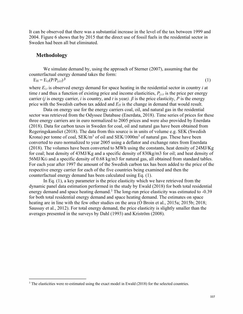
337

It can be observed that there was a substantial increase in the level of the tax between 1999 and 2004. Figure 6 shows that by 2015 that the direct use of fossil fuels in the residential sector in Sweden had been all but eliminated.

Methodology

We simulate demand by, using the approach of Sterner (2007), assuming that the counterfactual energy demand takes the form:

EH = Ei,t(P/Pj,i,t) β (1) where Ei,t is observed energy demand for space heating in the residential sector in country i at time t and thus a function of existing price and income elasticities, Pj,i,t is the price per energy carrier (j is energy carrier, i is country, and t is year). β is the price elasticity, P is the energy price with the Swedish carbon tax added and EH is the change in demand that would result.

Data on energy use for the energy carriers coal, oil, and natural gas in the residential sector was retrieved from the Odyssee Database (Enerdata, 2018). Time series of prices for these three energy carriers are in euro normalized to 2005 prices and were also provided by Enerdata (2018). Data for carbon taxes in Sweden for coal, oil and natural gas have been obtained from Regeringskansliet (2018). The data from this source is in units of volume e.g. SEK (Swedish Krona) per tonne of coal, SEK/m3 of oil and SEK/1000m3 of natural gas. These have been converted to euro normalized to year 2005 using a deflator and exchange rates from Enerdata (2018). The volumes have been converted to MWh using the constants, heat density of 24MJ/Kg for coal; heat density of 43MJ/Kg and a specific density of 830kg/m3 for oil; and heat density of 56MJ/KG and a specific density of 0.68 kg/m3 for natural gas, all obtained from standard tables. For each year after 1997 the amount of the Swedish carbon tax has been added to the price of the respective energy carrier for each of the five countries being examined and then the counterfactual energy demand has been calculated using Eq. (1).

In Eq. (1), a key parameter is the price elasticity which we have retrieved from the dynamic panel data estimation performed in the study by Ewald (2018) for both total residential energy demand and space heating demand.3 The long-run price elasticity was estimated to -0.39 for both total residential energy demand and space heating demand. The estimates on space heating are in line with the few other studies on the area (Ó Broin et al., 2015a; 2015b; 2018; Saussay et al., 2012). For total energy demand, the price elasticity is slightly smaller than the averages presented in the surveys by Dahl (1993) and Kriström (2008).

3 The elasticities were re-estimated using the exact model in Ewald (2018) for the selected countries.

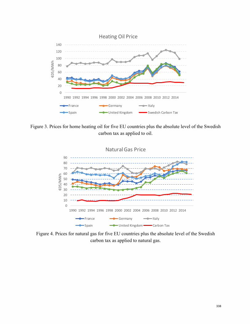
338

Figure 3. Prices for home heating oil for five EU countries plus the absolute level of the Swedish carbon tax as applied to oil.

Figure 4. Prices for natural gas for five EU countries plus the absolute level of the Swedish

carbon tax as applied to natural gas.

0

20

40

60

80

100

120

140

1990 1992 1994 1996 1998 2000 2002 2004 2006 2008 2010 2012 2014

€05/

MW

h

Heating Oil Price

France Germany Italy

Spain United Kingdom Swedish Carbon Tax

0102030405060708090

1990 1992 1994 1996 1998 2000 2002 2004 2006 2008 2010 2012 2014

€05/

MW

h

Natural Gas Price

France Germany Italy

Spain United Kingdom Carbon Tax

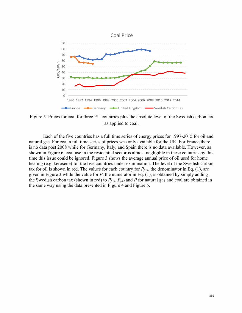
339

Figure 5. Prices for coal for three EU countries plus the absolute level of the Swedish carbon tax

as applied to coal.

Each of the five countries has a full time series of energy prices for 1997-2015 for oil and natural gas. For coal a full time series of prices was only available for the UK. For France there is no data post 2008 while for Germany, Italy, and Spain there is no data available. However, as shown in Figure 6, coal use in the residential sector is almost negligible in these countries by this time this issue could be ignored. Figure 3 shows the average annual price of oil used for home heating (e.g. kerosene) for the five countries under examination. The level of the Swedish carbon tax for oil is shown in red. The values for each country for Pj,i,t, the denominator in Eq. (1), are given in Figure 3 while the value for P, the numerator in Eq. (1), is obtained by simply adding the Swedish carbon tax (shown in red) to Pj,i,t. Pj,i,t and P for natural gas and coal are obtained in the same way using the data presented in Figure 4 and Figure 5.

0

10

20

30

40

50

60

70

80

90

1990 1992 1994 1996 1998 2000 2002 2004 2006 2008 2010 2012 2014

€05/

MW

h

Coal Price

France Germany United Kingdom Swedish Carbon Tax

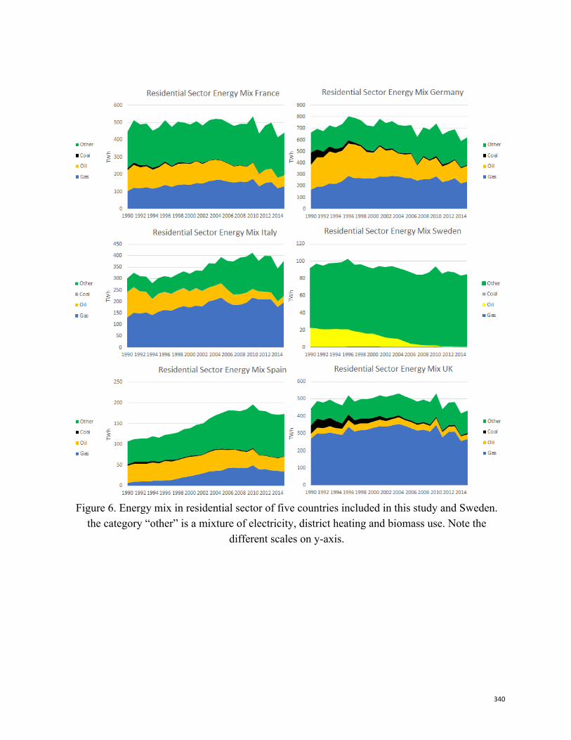
340

Figure 6. Energy mix in residential sector of five countries included in this study and Sweden.

the category “other” is a mixture of electricity, district heating and biomass use. Note the different scales on y-axis.

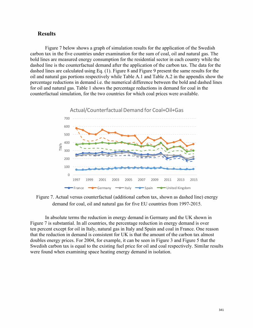
341

Results

Figure 7 below shows a graph of simulation results for the application of the Swedish carbon tax in the five countries under examination for the sum of coal, oil and natural gas. The bold lines are measured energy consumption for the residential sector in each country while the dashed line is the counterfactual demand after the application of the carbon tax. The data for the dashed lines are calculated using Eq. (1). Figure 8 and Figure 9 present the same results for the oil and natural gas portions respectively while Table A.1 and Table A.2 in the appendix show the percentage reductions in demand i.e. the numerical difference between the bold and dashed lines for oil and natural gas. Table 1 shows the percentage reductions in demand for coal in the counterfactual simulation, for the two countries for which coal prices were available.

Figure 7. Actual versus counterfactual (additional carbon tax, shown as dashed line) energy

demand for coal, oil and natural gas for five EU countries from 1997-2015.

In absolute terms the reduction in energy demand in Germany and the UK shown in Figure 7 is substantial. In all countries, the percentage reduction in energy demand is over ten percent except for oil in Italy, natural gas in Italy and Spain and coal in France. One reason that the reduction in demand is consistent for UK is that the amount of the carbon tax almost doubles energy prices. For 2004, for example, it can be seen in Figure 3 and Figure 5 that the Swedish carbon tax is equal to the existing fuel price for oil and coal respectively. Similar results were found when examining space heating energy demand in isolation.

0

100

200

300

400

500

600

700

1997 1999 2001 2003 2005 2007 2009 2011 2013 2015

TWh

Actual/Counterfactual Demand for Coal+Oil+Gas

France Germany Italy Spain United Kingdom

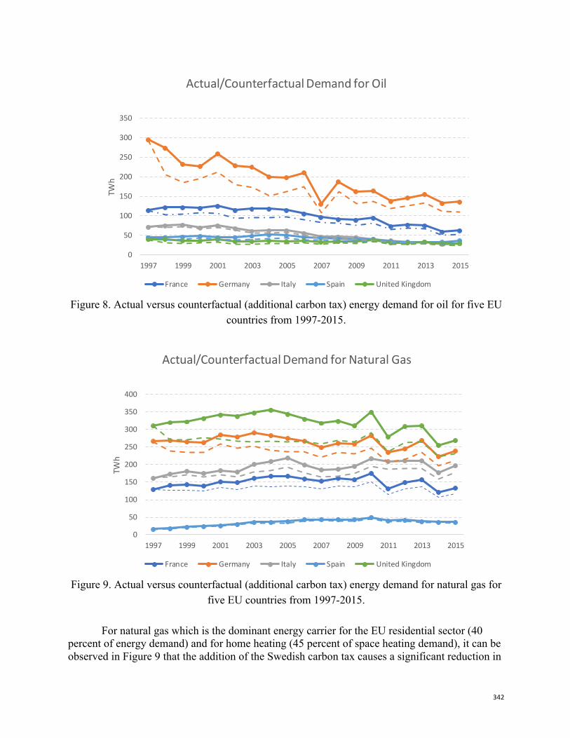
342

Figure 8. Actual versus counterfactual (additional carbon tax) energy demand for oil for five EU

countries from 1997-2015.

Figure 9. Actual versus counterfactual (additional carbon tax) energy demand for natural gas for

five EU countries from 1997-2015.

For natural gas which is the dominant energy carrier for the EU residential sector (40 percent of energy demand) and for home heating (45 percent of space heating demand), it can be observed in Figure 9 that the addition of the Swedish carbon tax causes a significant reduction in

0

50

100

150

200

250

300

350

1997 1999 2001 2003 2005 2007 2009 2011 2013 2015

TWh

Actual/Counterfactual Demand for Oil


0

50

100

150

200

250

300

350

400

1997 1999 2001 2003 2005 2007 2009 2011 2013 2015

TWh

Actual/Counterfactual Demand for Natural Gas


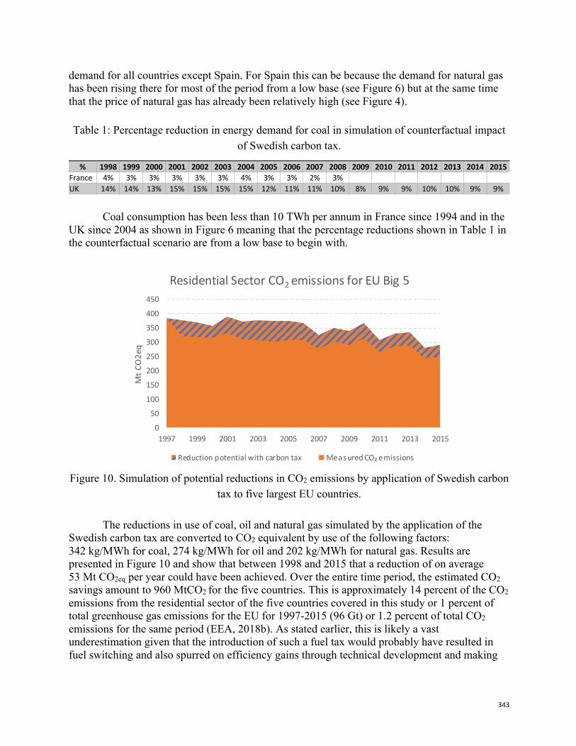
343

demand for all countries except Spain. For Spain this can be because the demand for natural gas has been rising there for most of the period from a low base (see Figure 6) but at the same time that the price of natural gas has already been relatively high (see Figure 4). Table 1: Percentage reduction in energy demand for coal in simulation of counterfactual impact

of Swedish carbon tax.

% 1998 1999 2000 2001 2002 2003 2004 2005 2006 2007 2008 2009 2010 2011 2012 2013 2014 2015 France 4% 3% 3% 3% 3% 3% 4% 3% 3% 2% 3% UK 14% 14% 13% 15% 15% 15% 15% 12% 11% 11% 10% 8% 9% 9% 10% 10% 9% 9%

Coal consumption has been less than 10 TWh per annum in France since 1994 and in the UK since 2004 as shown in Figure 6 meaning that the percentage reductions shown in Table 1 in the counterfactual scenario are from a low base to begin with.

Figure 10. Simulation of potential reductions in CO2 emissions by application of Swedish carbon

tax to five largest EU countries.

The reductions in use of coal, oil and natural gas simulated by the application of the Swedish carbon tax are converted to CO2 equivalent by use of the following factors: 342 kg/MWh for coal, 274 kg/MWh for oil and 202 kg/MWh for natural gas. Results are presented in Figure 10 and show that between 1998 and 2015 that a reduction of on average 53 Mt CO2eq per year could have been achieved. Over the entire time period, the estimated CO2 savings amount to 960 MtCO2 for the five countries. This is approximately 14 percent of the CO2 emissions from the residential sector of the five countries covered in this study or 1 percent of total greenhouse gas emissions for the EU for 1997-2015 (96 Gt) or 1.2 percent of total CO2 emissions for the same period (EEA, 2018b). As stated earlier, this is likely a vast underestimation given that the introduction of such a fuel tax would probably have resulted in fuel switching and also spurred on efficiency gains through technical development and making

0

50

100

150

200

250

300

350

400

450

1997 1999 2001 2003 2005 2007 2009 2011 2013 2015

Mt C

O2e

q

Residential Sector CO2 emissions for EU Big 5

Reduction potential with carbon tax Measured CO₂ emissions

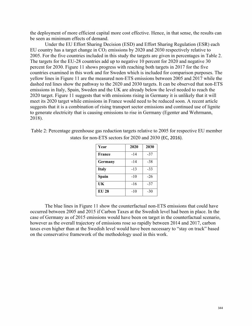
344

the deployment of more efficient capital more cost effective. Hence, in that sense, the results can be seen as minimum effects of demand.

Under the EU Effort Sharing Decision (ESD) and Effort Sharing Regulation (ESR) each EU country has a target change in CO2 emissions by 2020 and 2030 respectively relative to 2005. For the five countries included in this study the targets are given in percentages in Table 2. The targets for the EU-28 countries add up to negative 10 percent for 2020 and negative 30 percent for 2030. Figure 11 shows progress with reaching both targets in 2017 for the five countries examined in this work and for Sweden which is included for comparison purposes. The yellow lines in Figure 11 are the measured non-ETS emissions between 2005 and 2017 while the dashed red lines show the pathway to the 2020 and 2030 targets. It can be observed that non-ETS emissions in Italy, Spain, Sweden and the UK are already below the level needed to reach the 2020 target. Figure 11 suggests that with emissions rising in Germany it is unlikely that it will meet its 2020 target while emissions in France would need to be reduced soon. A recent article suggests that it is a combination of rising transport sector emissions and continued use of lignite to generate electricity that is causing emissions to rise in Germany (Egenter and Wehrmann, 2018). Table 2: Percentage greenhouse gas reduction targets relative to 2005 for respective EU member

states for non-ETS sectors for 2020 and 2030 (EC, 2016). Year 2020 2030

France -14 -37

Germany -14 -38

Italy -13 -33

Spain -10 -26

UK -16 -37

EU 28 -10 -30

The blue lines in Figure 11 show the counterfactual non-ETS emissions that could have

occurred between 2005 and 2015 if Carbon Taxes at the Swedish level had been in place. In the case of Germany as of 2015 emissions would have been on target in the counterfactual scenario, however as the overall trajectory of emissions rose so rapidly between 2014 and 2017, carbon taxes even higher than at the Swedish level would have been necessary to “stay on track” based on the conservative framework of the methodology used in this work.

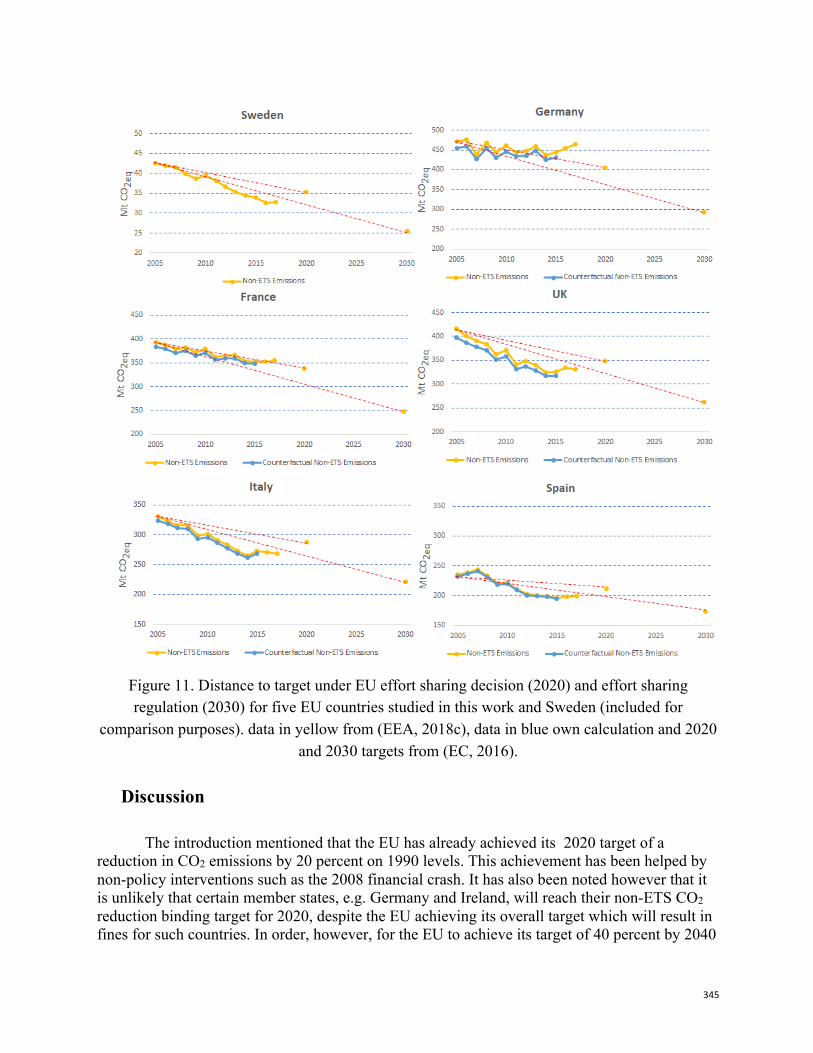
345

Figure 11. Distance to target under EU effort sharing decision (2020) and effort sharing regulation (2030) for five EU countries studied in this work and Sweden (included for

comparison purposes). data in yellow from (EEA, 2018c), data in blue own calculation and 2020 and 2030 targets from (EC, 2016).

Discussion

The introduction mentioned that the EU has already achieved its 2020 target of a

reduction in CO2 emissions by 20 percent on 1990 levels. This achievement has been helped by non-policy interventions such as the 2008 financial crash. It has also been noted however that it is unlikely that certain member states, e.g. Germany and Ireland, will reach their non-ETS CO2 reduction binding target for 2020, despite the EU achieving its overall target which will result in fines for such countries. In order, however, for the EU to achieve its target of 40 percent by 2040

346

new policies and measures will be necessary one of which could be to encourage member states to impose carbon taxes on non-ETS sectors. Taxes are outside the remit of the EC and likely to remain so for some time despite some moves towards tax harmonisation. With this in mind, this work has shown how the addition of a carbon tax could help individual states with achieving political targets and global leadership but also complement existing or new policies and measures.

It can also be observed in Figure 7 to Figure 9 that the difference between measured and counterfactual energy demand does not seem to change over time i.e. the gap does not grow. This is the case for a number of reasons. Figure 2 shows that the carbon taxes do not increase year on year while the energy prices themselves do not increase much until after 2004. The gap between the measured and counterfactual demand decreases somewhat after 2004 as the carbon tax makes up less of a proportion of overall price. In addition, although it is the long-run price elasticity which is used to calculate the counterfactual, in reality, sustained price increases like these would likely spur additional technical change not captured in our estimates. There may also be that the true elasticities are higher at a higher price level.

Possible developments on the work could be to account for more factors in the simulations. The most obvious being the inclusion of fuel switching and innovation. One could possibly also include information on the existing energy tax base e.g. vat and excise tax applied to energy carriers and their role in affecting demand. Such work could be useful in unpacking the role of the different taxes. For example (Andersen, 2010) notes that, “towards the close of the 1990s two of the largest EU economies, Germany (1998) and UK (2000) introduced carbon-energy taxation policies ... The UK introduced a specific climate change levy on fossil fuels while Germany increased more broadly its energy taxes as part of a so-called ‘ecological tax reform’.” Thus, despite there not being explicit carbon taxes in place in the Germany and the UK there are taxes and levies that give similar effects. This suggests that the increases in fuel prices promoted in this paper are politically difficult. However, a deeper analysis could bring further clarity. In addition, it can be observed in Figure 3 - Figure 5 that fuel prices were the highest for Italy and lowest for the UK. This suggests that the absolute amount of the British climate change levy was not significant, while it is known that regular excise taxes on energy in Italy are comparatively high. This lends further to the necessity to unpack the various taxes to establish their effects.

Conclusion

This paper has set out to simulate the effects of the imposition of a carbon tax at the Swedish level from year 1997 on the energy demand and carbon emissions of the residential sector of the five largest European countries (by population), which together account for over 60 percent of the residential energy use in the EU-28. Conservative simulations indicate that the tax would have achieved reductions in demand for fossil fuels of 15 percent (4000 TWH in total over the period) for the five countries examined. The resulting average greenhouse gas savings are calculated to 14 percent (960 MtCO2eq per year). A significant proportion of these reductions would have been made on the use of fossil fuels for space heating.

347

Acknowledgements

This work is funded by the Swedish Research Council for Sustainable Development,

FORMAS, under project number 2016-00371.

References Alberini, A., Filippini, M., 2011. Response of residential electricity demand to price: The effect of measurement

error. Energy Econ. 33, 889–895. https://doi.org/10.1016/j.eneco.2011.03.009 Andersen, M.S., 2004. Vikings and virtues: a decade of CO2 taxation. Clim. Policy 4, 13–24.

https://doi.org/10.1080/14693062.2004.9685507 Andersen, M.S., 2010. Europe’s experience with carbon-energy taxation. SAPI EN Surv. Perspect. Integrating

Environ. Soc. Arellano, M., Bond, S., 1991. Some tests of specification for panel data: Monte Carlo evidence and an application to

employment equations. Rev. Econ. Stud. 58, 277–297. Baker III, J.A., Feldstein, M., Halstead, T., Mankiw, N.G., Paulson Jr, H.M., Shultz, G.P., Stephenson, T., Walton,

R., 2017. The conservative case for carbon dividends. Clim. Leadersh. Counc. Baranzini, A., Van den Bergh, J.C., Carattini, S., Howarth, R.B., Padilla, E. and Roca, J., 2017. Carbon pricing in

climate policy: seven reasons, complementary instruments, and political economy considerations. Wiley Interdisciplinary Reviews: Climate Change, 8(4), p.e462.

Boston Globe, 2014. The unsung inventor of the carbon tax - The Boston Globe [WWW Document]. BostonGlobe.com. URL https://www.bostonglobe.com/ideas/2014/08/09/the-unsung-inventor-carbon-tax/f1xFyWmaXf2XzW3nVxrNJK/story.html (accessed 9.6.18).

Bun, M.J., Kiviet, J.F., 2003. On the diminishing returns of higher-order terms in asymptotic expansions of bias. Econ. Lett. 79, 145–152.

Caring for Climate, 2015. Executive Guide to Carbon Pricing Leadership. UN Global Compact. EC, 2016. Effort sharing: Member States’ emission targets [WWW Document]. Clim. Action - Eur. Comm. URL

https://ec.europa.eu/clima/policies/effort_en (accessed 12.31.18). EC, 2017. Climate and Energy Framework. EEA, 2018a. Tracking climate policies in European Union countries. EEA, 2018b. EEA greenhouse gas - data viewer [WWW Document]. Eur. Environ. Agency. URL

https://www.eea.europa.eu/data-and-maps/data/data-viewers/greenhouse-gases-viewer (accessed 12.30.18). EEA, 2018c. Greenhouse gas emissions under the Effort Sharing Decision (ESD) [WWW Document]. Eur. Environ.

Agency. URL https://www.eea.europa.eu/data-and-maps/data/esd-1 (accessed 12.31.18). EEW, 2013. Improving and implementing national energy efficiency strategies in the EU framework. Enerdata, 2018. Odyssee Database. [http://www.indicators.odyssee-mure.eu/energy-efficiency-database.html] Eurostat, 2018. Home - Eurostat [WWW Document]. URL https://ec.europa.eu/eurostat (accessed 12.30.18). Ewald, J., 2018. Determinants of Energy Demand for Heating in the European Residential Sector.

[https://gupea.ub.gu.se/handle/2077/57921] Filippini, M., Hunt, L.C., 2011. Energy demand and energy efficiency in the OECD countries: a stochastic demand

frontier approach. Energy J. 59–80. Gothenburg University, 2018. “Carbon Pricing in the Real World” by Meredith Fowlie. Judson, R.A., Owen, A.L., 1999. Estimating dynamic panel data models: a guide for macroeconomists. Econ. Lett.

65, 9–15. Nature, 2018. How to pay the price for carbon. Nat. Clim. Change 8, 647. https://doi.org/10.1038/s41558-018-0256-

0 Ó Broin, E., Nässén, J., Johnsson, F., 2015a. Energy efficiency policies for space heating in EU countries: A panel

data analysis for the period 1990–2010. Appl. Energy 150, 211–223. Ó Broin, E., Nässén, J., Johnsson, F., 2015b. The influence of price and non-price effects on demand for heating in

the EU residential sector. Energy 81, 146–158. Partnership for Market Readiness, 2017. Carbon Tax Guide : A Handbook for Policy Makers. World Bank.

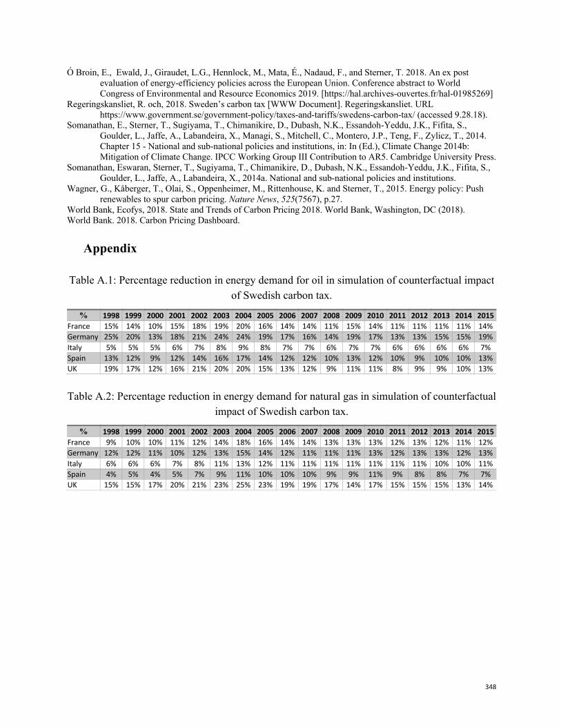
348

Ó Broin, E., Ewald, J., Giraudet, L.G., Hennlock, M., Mata, É., Nadaud, F., and Sterner, T. 2018. An ex post evaluation of energy-efficiency policies across the European Union. Conference abstract to World Congress of Environmental and Resource Economics 2019. [https://hal.archives-ouvertes.fr/hal-01985269]

Regeringskansliet, R. och, 2018. Sweden’s carbon tax [WWW Document]. Regeringskansliet. URL https://www.government.se/government-policy/taxes-and-tariffs/swedens-carbon-tax/ (accessed 9.28.18).

Somanathan, E., Sterner, T., Sugiyama, T., Chimanikire, D., Dubash, N.K., Essandoh-Yeddu, J.K., Fifita, S., Goulder, L., Jaffe, A., Labandeira, X., Managi, S., Mitchell, C., Montero, J.P., Teng, F., Zylicz, T., 2014. Chapter 15 - National and sub-national policies and institutions, in: In (Ed.), Climate Change 2014b: Mitigation of Climate Change. IPCC Working Group III Contribution to AR5. Cambridge University Press.

Somanathan, Eswaran, Sterner, T., Sugiyama, T., Chimanikire, D., Dubash, N.K., Essandoh-Yeddu, J.K., Fifita, S., Goulder, L., Jaffe, A., Labandeira, X., 2014a. National and sub-national policies and institutions.

Wagner, G., Kåberger, T., Olai, S., Oppenheimer, M., Rittenhouse, K. and Sterner, T., 2015. Energy policy: Push renewables to spur carbon pricing. Nature News, 525(7567), p.27.

World Bank, Ecofys, 2018. State and Trends of Carbon Pricing 2018. World Bank, Washington, DC (2018). World Bank. 2018. Carbon Pricing Dashboard.

Appendix Table A.1: Percentage reduction in energy demand for oil in simulation of counterfactual impact

of Swedish carbon tax.

% 1998 1999 2000 2001 2002 2003 2004 2005 2006 2007 2008 2009 2010 2011 2012 2013 2014 2015 France 15% 14% 10% 15% 18% 19% 20% 16% 14% 14% 11% 15% 14% 11% 11% 11% 11% 14% Germany 25% 20% 13% 18% 21% 24% 24% 19% 17% 16% 14% 19% 17% 13% 13% 15% 15% 19% Italy 5% 5% 5% 6% 7% 8% 9% 8% 7% 7% 6% 7% 7% 6% 6% 6% 6% 7% Spain 13% 12% 9% 12% 14% 16% 17% 14% 12% 12% 10% 13% 12% 10% 9% 10% 10% 13% UK 19% 17% 12% 16% 21% 20% 20% 15% 13% 12% 9% 11% 11% 8% 9% 9% 10% 13% Table A.2: Percentage reduction in energy demand for natural gas in simulation of counterfactual

impact of Swedish carbon tax.

% 1998 1999 2000 2001 2002 2003 2004 2005 2006 2007 2008 2009 2010 2011 2012 2013 2014 2015 France 9% 10% 10% 11% 12% 14% 18% 16% 14% 14% 13% 13% 13% 12% 13% 12% 11% 12% Germany 12% 12% 11% 10% 12% 13% 15% 14% 12% 11% 11% 11% 13% 12% 13% 13% 12% 13% Italy 6% 6% 6% 7% 8% 11% 13% 12% 11% 11% 11% 11% 11% 11% 11% 10% 10% 11% Spain 4% 5% 4% 5% 7% 9% 11% 10% 10% 10% 9% 9% 11% 9% 8% 8% 7% 7% UK 15% 15% 17% 20% 21% 23% 25% 23% 19% 19% 17% 14% 17% 15% 15% 15% 13% 14%

Papers - Open Knowledge Repository - World Bank Group

Documents

Transcript of Papers - Open Knowledge Repository - World Bank Group