Page Layout - Eprints@CMFRI - Central Marine Fisheries ...
423
-
Upload
khangminh22 -
Category
Documents
-
view
0 -
download
0
Transcript of Page Layout - Eprints@CMFRI - Central Marine Fisheries ...


Course ManualWinter School onStructure and Functions of Marine Ecosystem: FisheriesCMFRI Lecture Note Series No. 12/2017ICAR-Central Marine Fisheries Research Institute1-21 December 2017
Publisher : A. GopalakrishnanDirectorICAR-Central Marine Fisheries Research InstituteErnakulam North P.O., Pin - 682 018, Kochi, Kerala
Compilation : Mini K. G.Somy KuriakoseT. V. Sathianandan
Technical Assistance : Muhammad ShafeequeMonolisha S.Minu P.
Course Director : Grinson GeorgeSenior ScientistFishery Resources Assessment Division
Course Co-Directors : Mini K. G.Principal ScientistFishery Resources Assessment Division
Vivekanand BhartiScientistFishery Resources Assessment Division
Cover Design : Abhilash P. R.
© CMFRIThis manual has been prepared as a reference material for the ICAR-funded Winter school on "Structure and Function ofthe Marine Ecosystem: Fisheries” held at Central Marine Fisheries Research Institute, Kochi during 1-21 December 2017.
ISBN-978-93-82263-18-0

F O R E W O R D
Marine ecosystems comprises of diverse organismsand their ambient abiotic components in variedrelationships leading to an ecosystem functioning.These relationships provides the services that areessential for marine organisms to sustain in the nature.The studies examining the structure and functioningof these relationships remains unclear and henceunderstanding and modelling of the ecologicalfunctioning is imperative in the context of the threats
different ecosystem components are facing. The relationship between marinepopulation and their environment is complex and is subjected to fluctuationswhich affects the bottom level of an ecosystem pyramid to higher trophiclevels. Understanding the energy flow within the marine ecosystems withthe help of primary to secondary producers and secondary consumers arepotentially important when assessing such states and changes in theseenvironments.
Many of the physiological changes are known to affect the key functionalgroup, i.e., the species or group of organisms, which play an important rolein the health of the ecosystem. In marine environment, phytoplankton arethe main functional forms which serves as the base of marine food web.Any change in the phytoplankton community structure may lead to alterationin the composition, size and structure of the entire ecosystem. Hence, it iscritical to understand how these effects may scale up to population,communities, and entire marine ecosystem. Such changes are difficult topredict, particularly when more than one trophic level is affected. Theidentification and quantification of indicators of changes in ecosystemfunctioning and the knowledge base generated will provide a suitable wayof bridging issues related to a specific ecosystem. New and meaningfulindicators, derived from our current understanding of marine ecosystemfunctioning, can be used for assessing the impact of these changes and canbe used as an aid in promoting responsible fisheries in marine ecosystems.Phytoplantkon is an indicator determining the colour of open Ocean. In

recent years, new technologies have emerged which involves multi-disciplinary activities including biogeochemistry and its dynamics affectinghigher trophic levels including fishery. The winter school proposed willprovide the insights into background required for such an approach involvingteaching the theory, practical, analysis and interpretation techniques inunderstanding the structure and functioning of marine ecosystems fromground truth measurements as well as from satellite remote sensing data.This is organized with the full funding support from Indian council ofAgricultural Research (ICAR) New Delhi and the 25 participants who areattending this programme has been selected after scrutiny of theirapplications based on their bio-data. The participants are from differentStates across Indian subcontinent covering north, east, west and south.They are serving as academicians such as Professors/ scientists and in similarposts. The training will be a feather in their career and will enable them todo their academic programmes in a better manner. Selected participantswill be scrutinized initially to understand their knowledge level and classeswill be oriented based on this. In addition, all of them will be provided withan e-manual based on the classes. All selected participants are providedwith their travel and accommodation grants. The faculty include the scientistswho developed this technology, those who are practicing it and few usergroups who do their research in related areas. The programme is coordinatedby the Fishery Resources Assessment Division of CMFRI. This programmewill generate a team of elite academicians who can contribute to sustainablemanagement of marine ecosystem and they will further contribute tocapacity building in the sector by training many more interested researchersin the years to come.
A. GopalakrishnanDirector
CMFRI

P R E F A C EWorld marine fisheries are passing through a crisis dueto stagnation in yield from capture, increasedoperational costs, reduced profitability, emergingconcerns of sustainability, globalization, biodiversityloss, pollution, environmental degradation, loss ofcritical habitats, marginalization of small scale fishers,processors, vendors, increased costs of mariculturefeeds, high operation costs of marine farms, diseasesand problems in brood stock management, low coastal
productivity and trade concerns as well as market dynamics. Managementof marine fisheries through research based interventions assumes greaterimportance in this context.
Marine Capture Fisheries is basically utilization of a natural resource.Assessing the abundance of an invisible resource and monitoring itsdynamics through indirect methods are vital for providing policy supporttargeted at an informed fisheries governance. This is extremely importantfor management of an open access, multi-species, multi gear, migratoryresource. Therefore, this task is also a challenge to those involved in thetask of natural resource management. Ensuring sustainability in an openaccess natural resource is an onerous task.
Information on marine environment, its ecosystem structure and functionis imperative for an ecosystem based management. Enormous data isrequired for understanding marine ecosystems. Data collection in an oceanicenvironment is tedious and expensive. So as to enable wide use of in situdata, various organizations are hosting their databases on World Wide Web.But often marine f isheries research and management lack in situenvironmental time series data. Both modelled and Satellite Remote Sensing(SRS) data validated for time and space can be used to fill such gaps.Implementation of complex numerical models is frustrated by lack of datainputs whereas simple models ignore some complexities in the marineecosystem. As a result model outputs have not been analysed to the extentthey deserved. In case of SRS, algorithms for data retrieval vary spatially

and temporally depending on the nature of optical constituents present,especially in coastal waters. But modelled and SRS data can permit at leastqualitative inferences when we address some of the major unresolvedquestions in fisheries biology. With the advent of improved computingfacilities and SRS, last two decades have seen increased activity in bothecosystem modelling and ocean biology from space. The results are usedfor operational and applied marine fisheries research. This winter schoolon 'Structure and Function of the Marine Ecosystem: Fisheries' discussessome of the applications and illustrates them with particular case studies.
Grinson GeorgeDecember, 2017 Course director

C O N T E N T S
Chapter Topic Page
1 Indian marine fishery resources - Present status 1T. V. Sathianandhan
2 Fish biodiversity of Indian Exclusive Economic Zone 5K. K. Joshi, Sethulakshmi M. and Varsha M. S.
3 Fundamentals of ocean colour remote sensing 16Aneesh Lotliker, Minu P., Shalin Saleem, Muhammad Shafeeque and Grinson George
4 Satellite ocean colour sensors 22Muhammad Shafeeque, Minu P., Phiros Shah and Grinson George
5 Phytoplankton functional types 32Nandini Menon, Monolisha S. and Minu P.
6 Phytoplankton taxonomy, identification and enumeration 37Nandini Menon and Minu P.
7 Algal culture methods 43Shoji Joseph
8 Regional and seasonal variations in phytoplankton 54Nandini Menon, Minu P., Muhammad Shafeeque and Grinson George
9 Spatial and temporal variability of chlorophyll-a 59concentration in the South Eastern Arabian Sea (SEAS)Shalin S. and K. V. Sanilkumar
10 Statistical methods 65Somy Kuriakose
11 Data diagnostics and remedial measures 81Eldho Varghese
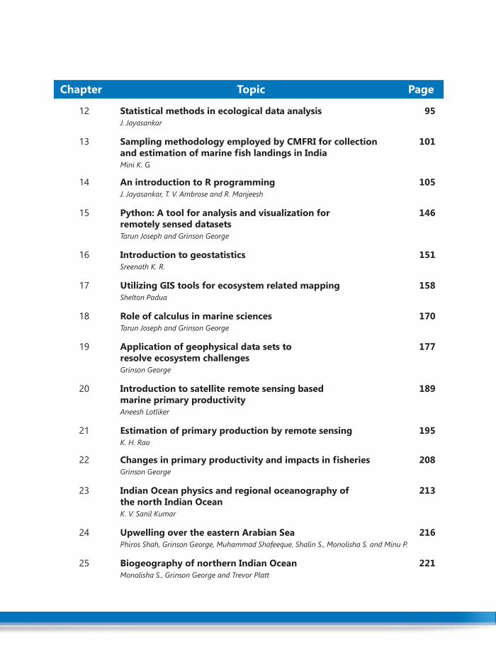
12 Statistical methods in ecological data analysis 95J. Jayasankar
13 Sampling methodology employed by CMFRI for collection 101and estimation of marine fish landings in IndiaMini K. G.
14 An introduction to R programming 105J. Jayasankar, T. V. Ambrose and R. Manjeesh
15 Python: A tool for analysis and visualization for 146remotely sensed datasetsTarun Joseph and Grinson George
16 Introduction to geostatistics 151Sreenath K. R.
17 Utilizing GIS tools for ecosystem related mapping 158Shelton Padua
18 Role of calculus in marine sciences 170Tarun Joseph and Grinson George
19 Application of geophysical data sets to 177resolve ecosystem challengesGrinson George
20 Introduction to satellite remote sensing based 189marine primary productivityAneesh Lotliker
21 Estimation of primary production by remote sensing 195K. H. Rao
22 Changes in primary productivity and impacts in fisheries 208Grinson George
23 Indian Ocean physics and regional oceanography of 213the north Indian OceanK. V. Sanil Kumar
24 Upwelling over the eastern Arabian Sea 216Phiros Shah, Grinson George, Muhammad Shafeeque, Shalin S., Monolisha S. and Minu P.
25 Biogeography of northern Indian Ocean 221Monolisha S., Grinson George and Trevor Platt
Chapter Topic Page
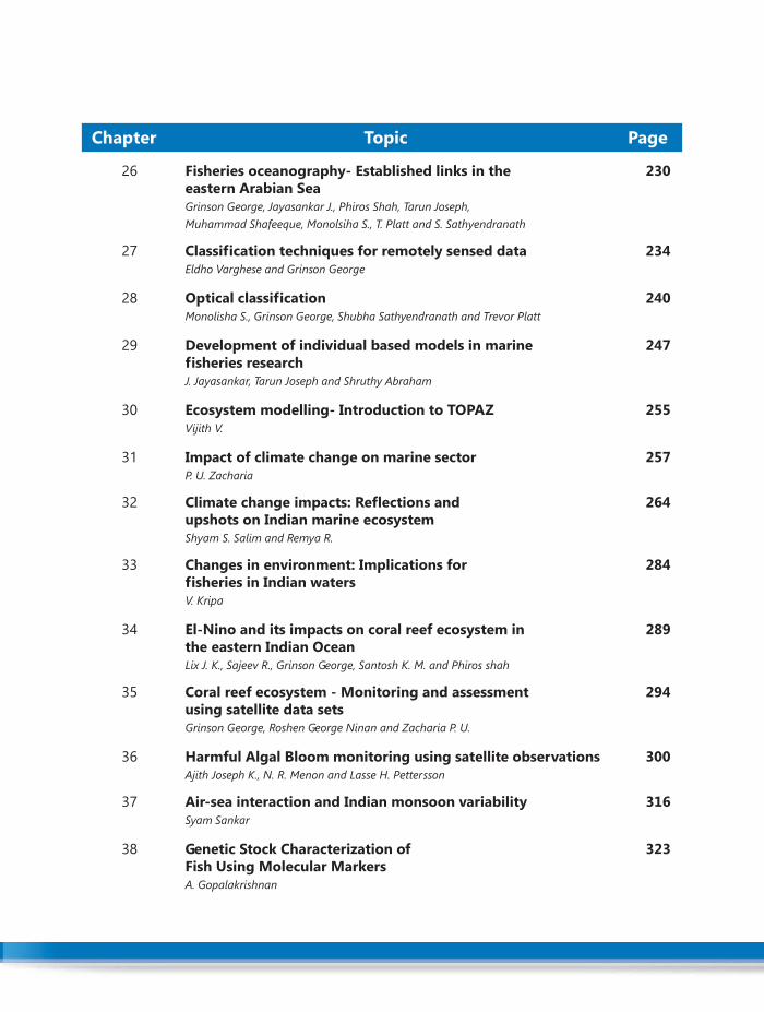
26 Fisheries oceanography- Established links in the 230eastern Arabian SeaGrinson George, Jayasankar J., Phiros Shah, Tarun Joseph,Muhammad Shafeeque, Monolsiha S., T. Platt and S. Sathyendranath
27 Classification techniques for remotely sensed data 234Eldho Varghese and Grinson George
28 Optical classification 240Monolisha S., Grinson George, Shubha Sathyendranath and Trevor Platt
29 Development of individual based models in marine 247fisheries researchJ. Jayasankar, Tarun Joseph and Shruthy Abraham
30 Ecosystem modelling- Introduction to TOPAZ 255Vijith V.
31 Impact of climate change on marine sector 257P. U. Zacharia
32 Climate change impacts: Reflections and 264upshots on Indian marine ecosystemShyam S. Salim and Remya R.
33 Changes in environment: Implications for 284fisheries in Indian watersV. Kripa
34 El-Nino and its impacts on coral reef ecosystem in 289the eastern Indian OceanLix J. K., Sajeev R., Grinson George, Santosh K. M. and Phiros shah
35 Coral reef ecosystem - Monitoring and assessment 294using satellite data setsGrinson George, Roshen George Ninan and Zacharia P. U.
36 Harmful Algal Bloom monitoring using satellite observations 300Ajith Joseph K., N. R. Menon and Lasse H. Pettersson
37 Air-sea interaction and Indian monsoon variability 316Syam Sankar
38 Genetic Stock Characterization of 323Fish Using Molecular MarkersA. Gopalakrishnan
Chapter Topic Page

39 Ecolabelling in fisheries: Boon or bane in improving trade ? 332K. Sunil Mohamed
40 Ecosystem concepts for sustainable mariculture 341Imelda Joseph
41 Economic valuation of marine ecosystem services 350R. Narayana Kumar
42 Marine microbial diversity and its role in ecosystem functioning 357Parvathy A.
43 Formation mechanism of mud bank along the 359southwest coast of IndiaMuraleedharan K. R.
44 Mud bank biology 360V. Kripa and R. Jeyabaskaran
45 Mud banks fishery estimates 365Vivekanand Bharti and Sindhu K. Augustine
46 Identifying mesoscale eddies- Relevance to mud banks and fishery 371Grinson George, Vivekanand Bharti, Phiros Shah, Muhammad Shafeeque and A. Anand
47 Peruvian anchovy fishery: Factors affecting the resource 376J. Rajasekharan Nair
48 Fisheries in atolls- Tradeoffs between harvest and conservation 381K. Mohammed Koya and Abdul Azeez
49 Responsible fisheries- A prelude to the concept, 388context and praxisRamachandran C., Vipinkumar V. P. and Shinoj Parappurathu
Chapter Topic Page
Winter School on Structure and Function of the Marine Ecosystem : Fisheries 1
Indian Marine Fishery Resources - Present Status
India being a tropical country is blessed with highly diverse nature of marine fisheryresources in its 2.02 million square kilometer Exclusive Economic Zone with an estimatedannual harvestable potential of 4.414 million metric tonnes. The marine fisheries sectorprovide livelihood to nearly 4.0 million people of India and meets the food and nutritionalrequirements of a significant proportion of the population. Also, it contributes to exportearnings of the country. Sustainable harvest of the marine fishery resources are necessaryas over-exploitation of the resources is likely to harm the diversity and cause reduction inthe availability of some of the resources. Monitoring of the harvest of the diverse marinefishery resources of the country is being carried out regularly by CMFRI since its inceptionthrough a scientific data collection and estimation system from all along the Indian coastleading to fish stock assessment for deriving management measures to keep the harvest ofthe resources at sustainable levels.
Marine fisheries is an important source of food, nutrition, employment and incomegeneration. In India, four million people depend for their livelihood on marine fisheriessector which provides employment to nearly one million fishermen and contributessignificantly to the export earnings of the country and balance of trade. The sectorcontributes to an economic wealth valued at nearly Rs. 65,000 crores annually. The marinefisheries of the country consist of small-scale and artisanal fishers belonging mechanized,motorized and non-mechanized sectors and a range of other stakeholders, includinggovernmental and non-governmental agencies. The marine fisheries resources are not in-exhaustive and over-exploitation would lead to loss of biodiversity and reduced availabilityof resources for our future generations. Uncontrolled harvest will result in depletion of theresources. Management and regulations are necessary for sustainable harvest of marinefishery resources.
India is one among the top marine fish producing countries of the world and at presentthe country is at 7th position in global marine capture fish production after China, Indonesia,USA, Russia, Japan and Peru. The global marine fish catch remains almost stagnant after1990 whereas the marine fish production in India showed a steady increase from 2.3 milliontonnes in 1990 to 3.94 million tonnes in 2012.
Many of the world’s fisheries have experienced series of environmental shifts in recentdecades involving collapse or fluctuations in the dominant fish assemblages and as a result,
01C H A P T E R INDIAN MARINE FISHERY RESOURCES -
PRESENT STATUS
T. V. Sathianandhan
Fishery Resources Assessment DivisionICAR-Central Marine Fisheries Research Institute
Winter School on Structure and Function of the Marine Ecosystem : Fisheries2
Indian Marine Fishery Resources - Present Status
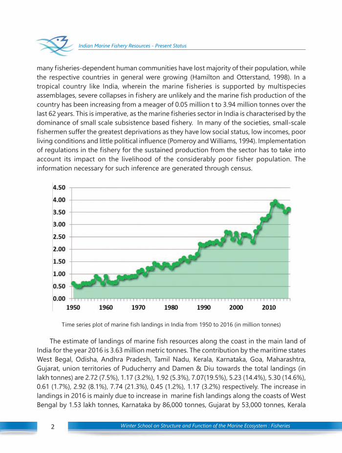
many fisheries-dependent human communities have lost majority of their population, whilethe respective countries in general were growing (Hamilton and Otterstand, 1998). In atropical country like India, wherein the marine fisheries is supported by multispeciesassemblages, severe collapses in fishery are unlikely and the marine fish production of thecountry has been increasing from a meager of 0.05 million t to 3.94 million tonnes over thelast 62 years. This is imperative, as the marine fisheries sector in India is characterised by thedominance of small scale subsistence based fishery. In many of the societies, small-scalefishermen suffer the greatest deprivations as they have low social status, low incomes, poorliving conditions and little political influence (Pomeroy and Williams, 1994). Implementationof regulations in the fishery for the sustained production from the sector has to take intoaccount its impact on the livelihood of the considerably poor fisher population. Theinformation necessary for such inference are generated through census.
The estimate of landings of marine fish resources along the coast in the main land ofIndia for the year 2016 is 3.63 million metric tonnes. The contribution by the maritime statesWest Begal, Odisha, Andhra Pradesh, Tamil Nadu, Kerala, Karnataka, Goa, Maharashtra,Gujarat, union territories of Puducherry and Damen & Diu towards the total landings (inlakh tonnes) are 2.72 (7.5%), 1.17 (3.2%), 1.92 (5.3%), 7.07(19.5%), 5.23 (14.4%), 5.30 (14.6%),0.61 (1.7%), 2.92 (8.1%), 7.74 (21.3%), 0.45 (1.2%), 1.17 (3.2%) respectively. The increase inlandings in 2016 is mainly due to increase in marine fish landings along the coasts of WestBengal by 1.53 lakh tonnes, Karnataka by 86,000 tonnes, Gujarat by 53,000 tonnes, Kerala
Time series plot of marine fish landings in India from 1950 to 2016 (in million tonnes)
Winter School on Structure and Function of the Marine Ecosystem : Fisheries 3
Indian Marine Fishery Resources - Present Status
by 40,000 tonnes, Damen & Diu by 35,000 tonnes and Maharashtra by 27,000 tonnes. Thereis reduction in landings in Andhra Pradesh by 1.03 lakh tonnes, Puducherry by 34,000 tonnes,Odisha by 24,000 tonnes, Goa by 7,000 tonnes and Tamil Nadu by 2,000 tonnes.
When examined at the resource level contribution, Indian mackerel had the maximumwith 2.49 lakh tonnes (6.8% of total landings) followed by oil sardine 2.45 lakh tonnes (6.7%),ribbonfishes 2.20 lakh tonnes (6.0%), penaeid prawns 2.01 lakh tonnes (5.5%) and lessersardines 1.95 lakh tonnes (5.4%). The resources showed increased landings in 2016 arePerches by about 77,000 tonnes (81%), Hilsa shad 73,000 tonnes (354%), Ribbon fishes43,000 tonnes (24%), Bombayduck 35,000 tonnes (31%), Squids 22,000 tonnes (24%) andNon-penaeid prawns 21,000 tonnes (14%). The resources with significant reduction inlandings are Lesser sardines 61,000 tonnes (24%) and oil sardine 21,000 tonnes (8%).
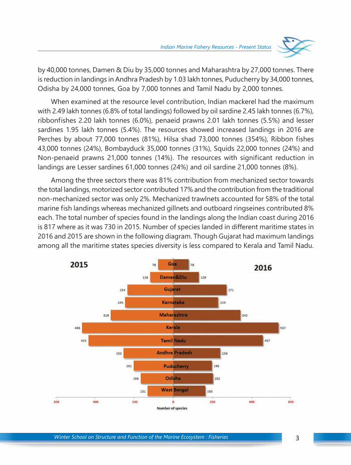
Among the three sectors there was 81% contribution from mechanized sector towardsthe total landings, motorized sector contributed 17% and the contribution from the traditionalnon-mechanized sector was only 2%. Mechanized trawlnets accounted for 58% of the totalmarine fish landings whereas mechanized gillnets and outboard ringseines contributed 8%each. The total number of species found in the landings along the Indian coast during 2016is 817 where as it was 730 in 2015. Number of species landed in different maritime states in2016 and 2015 are shown in the following diagram. Though Gujarat had maximum landingsamong all the maritime states species diversity is less compared to Kerala and Tamil Nadu.
Winter School on Structure and Function of the Marine Ecosystem : Fisheries4
Indian Marine Fishery Resources - Present Status
India is one among few countries where a system based on sampling theory is used tocollect marine fish catch statistics. The sampling design was developed by CMFRI inassociation with the Indian Agricultural Statistics Research Institute by conducting preliminarysurveys. The sampling design adopted is stratified multistage random sampling, stratificationbeing done over space and time.
Fish landings takes place at numerous locations all along the coastline in all seasonsduring day and night. Sampling and estimation are performed for geographical area referredas fishing zone. There are 75 fishing zones covering 9 maritime states and two coastalunion territories. All the 1,511 landing centres are covered under the sample design anddata collection is by qualified and trained field staff stationed at 25 locations across allmaritime states. The overall operation is coordinated by the Fishery Resources AssessmentDivision of CMFRI.
Fish is a natural resource with capacity to rebuild. If not monitored and managed over-exploitation will lead to stock depletion and some may become extinct. Harvest of thisresource needs to be maintained at sustainable level through monitoring and control. Theprimary objective of fish stock assessment is to provide advice on the optimum exploitationof aquatic living resources. Fish stock assessment can be described as the search for theexploitation level that in the long run gives maximum yield from the fishery. The aim of fishstock assessment is for a fishing strategy that gives the highest steady yield year after year.
The basic goal of fishery management is to estimate the amount of fish that can beremoved safely while keeping the fish population healthy. These estimates may be modifiedby political, economic, and social considerations to arrive at an optimum yield. Overlyconservative management can result in wasted fisheries production due to under-harvesting,while too liberal or no management may result in over-harvesting and severely reducedpopulations. Fisheries Management draws on fisheries science in order to find ways toprotect fishery resources so that sustainable exploitation is possible. Fisheries Managementis the integrated process of information gathering, data analysis, planning, consultation,decision making, allocation of the resources and implementation of regulations or rules togovern fishing activities with enforcement as and when necessary to ensure steady andsustainable harvest of the resources. Fisheries Management is not about managing fish butabout managing people and related businesses. Fish populations are managed by regulatingthe actions of people. These management regulations should also consider its implicationson the stakeholders.
Winter School on Structure and Function of the Marine Ecosystem : Fisheries 5
Fish Biodiversity of Indian Exclusive Economic Zone
Introduction
Indian fisheries have a long history, starting with Kautilya’s Arthasastra describing fishas a source for consumption and provide evidence that fishery was a well-established industryin India and fish was relished as an article of diet as early as 300 B.C, the ancient Hinduspossessed a considerable knowledge of the habit of fishes and the epic on the second pillarof Emperor Ashoka describing the prohibition of consumption of fish during a certain lunarperiod which can be interpreted as a conservation point of view. Modern scientific studieson Indian fishes could be traced to the initial works done by Linnaeus, Bloch and Schneider,Lacepède, Russell and Hamilton. The mid 1800s contributed much in the history of Indianfish taxonomy since the time of the expeditions was going through. Cuvier and Valenciennes(1828-1849) described 70 nominal species off Puducherry, Skyes (1839), Günther (1860,1872, 1880) and The Fishes of India by Francis Day (1865-1877) and another book Fauna ofBritish India Series in two volumes (1889) describing 1,418 species are the two mostindispensable works on Indian fish taxonomy to date. Alcock (1889, 1890) described 162species new to science from Indian waters.
In the 20th century, the basis of intensive studies on the different families and groups offreshwater fishes was done by Chaudhuri along with Hora and his co-workers. Misra publishedAn Aid to Identification of the Commercial Fishes of India and Pakistan and The Fauna ofIndia and Adjacent Countries (Pisces) in 1976. Jones and Kumaran described about 600species of fishes in the work Fishes of Laccadive Archipelago. Talwar and Kacker gave adetailed description of 548 species under 89 families in his work, Commercial Sea Fishes ofIndia. The FAO Species Identification Sheets for Fishery Purposes - Western Indian Ocean(Fischer and Bianchi) is still a valuable guide for researchers.
The long coastline of 8129 km2 with an EE2 of 2.02 million sq. km including the continentalshelf of 0.5 million sq. km harbors extensively rich multitude of species. Vast regions ofmangroves are found along the coast of West Bengal, Orissa, Andhra Pradesh, Tamilnadu,Maharashtra, Gujarat and Andaman Islands which extends up to about 6,82,000 ha area.Coral reefs are found in the Gulf of Kutch, along the Maharashtra coast, Kerala coast, in theGulf of Mannar, Palk Bay and the Wadge Bank along the Tamilnadu coast and aroundAndaman and Lakshadweep Islands. The variety of coastal ecosystems includes brackishwater lakes, lagoons, estuaries, back waters, salt marshes, rocky bottom, sandy bottom and
02C H A P T E R FISH BIODIVERSITY OF INDIAN EXCLUSIVE
ECONOMIC ZONEK. K. Joshi, Sethulakshmi, M. and Varsha M. S.
Marine Biodiversity DivisionICAR-Central Marine Fisheries Research Institute

Winter School on Structure and Function of the Marine Ecosystem : Fisheries6
Fish Biodiversity of Indian Exclusive Economic Zone
muddy areas provides a home and shelter for the mega biodiversity of India. These regionssupport very rich fauna and flora and constitute rich biological diversity of marine ecosystems.Diversity in the species complex, typical of tropical waters and co-existence of different fishand shellfish species in the same ground are important features of Indian Marine Biodiversity.
Species Diversity
Fin fishes
Of the 33,059 total fish species of the world, India contributes of about 2,492 marinefishes owing to 7.4% of the total marine fish resources. Of the total fish diversity knownfrom India, the marine fishes constitute 75.6 percent, comprising of 2,492 species belongingto 941 genera, under 240 families of 40 orders. Among the fish diversity-rich areas in themarine waters of India, the Andaman and Nicobar Archipelago, shows the highest numberof species, 1,431, followed by the east coast of India with 1,121 species and the west coastwith 1071. Detailed taxonomy of 18 families of fishes occurring in Indian EEZ was done asshown in the Table 1. As many as 91 species of endemic marine fishes are known to occurin the coastal waters of India. As of today, about 50 marine fishes known from India fall intothe Threatened category as per the IUCN Red List, and about 45 species are Near-Threatenedand already on the path to vulnerability. However, only some species (10 elasmobranchs, 10seahorses and one grouper) are listed in Schedule I of the Wildlife (Protection) Act, 1972 ofthe Government of India. The ecosystem goods and services provided by the fauna andflora and the interrelationship between the biodiversity and ecological processes are thefundamental issues in the sustainability and equilibrium of the ecosystem.Table 1. List of Fish families and corresponding authors
No Name of the Family /group Authors
1 Flatfishes Norman, 1934, Menon, 1977
2 Scombridae Jones and Silas, 1962
3 Mugilidae Sarojini, 1962
4 Clupeidae Whitehead, 1985
5 Trichiuridae James, 1967
6 Leiognathidae James, 1975
7 Chirocentridae Luther, 1968
8 Mullidae Thomas, 1969
9 Sphyraenidae De Sylva, 1975
10 Syngnathidae Dawson, 1976
11 Scorpaenidae Eschmeyer, 1969
Winter School on Structure and Function of the Marine Ecosystem : Fisheries 7
Fish Biodiversity of Indian Exclusive Economic Zone
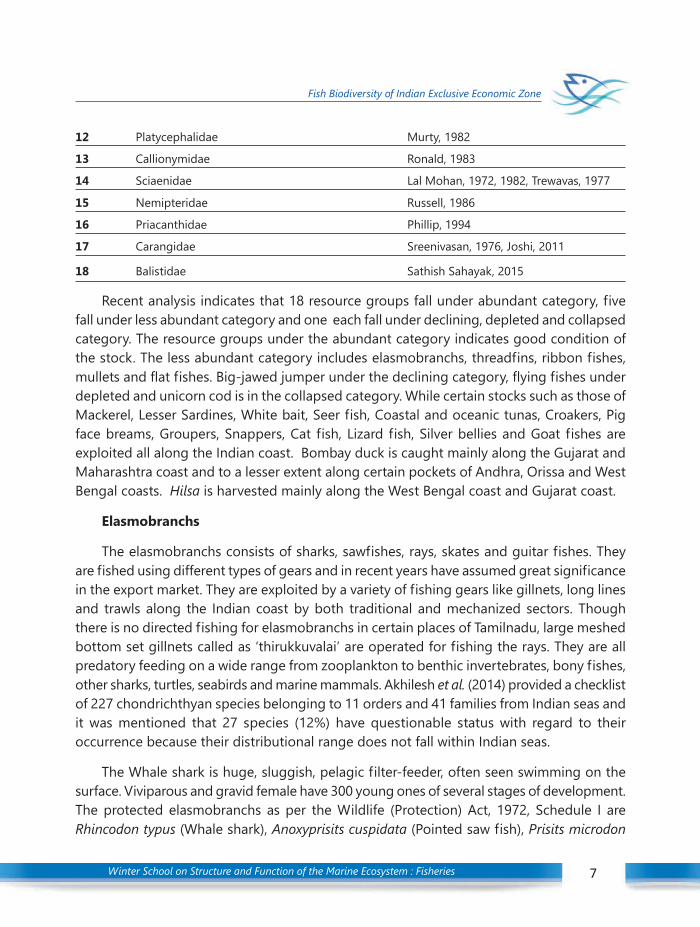
12 Platycephalidae Murty, 1982
13 Callionymidae Ronald, 1983
14 Sciaenidae Lal Mohan, 1972, 1982, Trewavas, 1977
15 Nemipteridae Russell, 1986
16 Priacanthidae Phillip, 1994
17 Carangidae Sreenivasan, 1976, Joshi, 2011
18 Balistidae Sathish Sahayak, 2015
Recent analysis indicates that 18 resource groups fall under abundant category, fivefall under less abundant category and one each fall under declining, depleted and collapsedcategory. The resource groups under the abundant category indicates good condition ofthe stock. The less abundant category includes elasmobranchs, threadfins, ribbon fishes,mullets and flat fishes. Big-jawed jumper under the declining category, flying fishes underdepleted and unicorn cod is in the collapsed category. While certain stocks such as those ofMackerel, Lesser Sardines, White bait, Seer fish, Coastal and oceanic tunas, Croakers, Pigface breams, Groupers, Snappers, Cat fish, Lizard fish, Silver bellies and Goat fishes areexploited all along the Indian coast. Bombay duck is caught mainly along the Gujarat andMaharashtra coast and to a lesser extent along certain pockets of Andhra, Orissa and WestBengal coasts. Hilsa is harvested mainly along the West Bengal coast and Gujarat coast.
Elasmobranchs
The elasmobranchs consists of sharks, sawfishes, rays, skates and guitar fishes. Theyare fished using different types of gears and in recent years have assumed great significancein the export market. They are exploited by a variety of fishing gears like gillnets, long linesand trawls along the Indian coast by both traditional and mechanized sectors. Thoughthere is no directed fishing for elasmobranchs in certain places of Tamilnadu, large meshedbottom set gillnets called as ‘thirukkuvalai’ are operated for fishing the rays. They are allpredatory feeding on a wide range from zooplankton to benthic invertebrates, bony fishes,other sharks, turtles, seabirds and marine mammals. Akhilesh et al. (2014) provided a checklistof 227 chondrichthyan species belonging to 11 orders and 41 families from Indian seas andit was mentioned that 27 species (12%) have questionable status with regard to theiroccurrence because their distributional range does not fall within Indian seas.
The Whale shark is huge, sluggish, pelagic filter-feeder, often seen swimming on thesurface. Viviparous and gravid female have 300 young ones of several stages of development.The protected elasmobranchs as per the Wildlife (Protection) Act, 1972, Schedule I areRhincodon typus (Whale shark), Anoxyprisits cuspidata (Pointed saw fish), Prisits microdon
Winter School on Structure and Function of the Marine Ecosystem : Fisheries8
Fish Biodiversity of Indian Exclusive Economic Zone
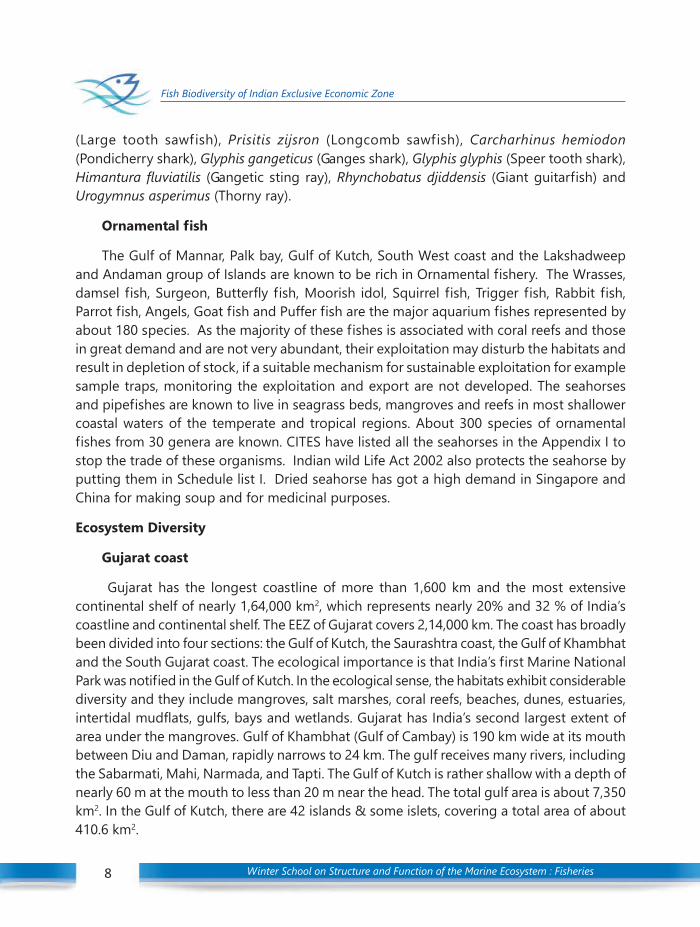
(Large tooth sawfish), Prisitis zijsron (Longcomb sawfish), Carcharhinus hemiodon(Pondicherry shark), Glyphis gangeticus (Ganges shark), Glyphis glyphis (Speer tooth shark),Himantura fluviatilis (Gangetic sting ray), Rhynchobatus djiddensis (Giant guitarfish) andUrogymnus asperimus (Thorny ray).
Ornamental fish
The Gulf of Mannar, Palk bay, Gulf of Kutch, South West coast and the Lakshadweepand Andaman group of Islands are known to be rich in Ornamental fishery. The Wrasses,damsel fish, Surgeon, Butterfly fish, Moorish idol, Squirrel fish, Trigger fish, Rabbit fish,Parrot fish, Angels, Goat fish and Puffer fish are the major aquarium fishes represented byabout 180 species. As the majority of these fishes is associated with coral reefs and thosein great demand and are not very abundant, their exploitation may disturb the habitats andresult in depletion of stock, if a suitable mechanism for sustainable exploitation for examplesample traps, monitoring the exploitation and export are not developed. The seahorsesand pipefishes are known to live in seagrass beds, mangroves and reefs in most shallowercoastal waters of the temperate and tropical regions. About 300 species of ornamentalfishes from 30 genera are known. CITES have listed all the seahorses in the Appendix I tostop the trade of these organisms. Indian wild Life Act 2002 also protects the seahorse byputting them in Schedule list I. Dried seahorse has got a high demand in Singapore andChina for making soup and for medicinal purposes.
Ecosystem Diversity
Gujarat coast
Gujarat has the longest coastline of more than 1,600 km and the most extensivecontinental shelf of nearly 1,64,000 km2, which represents nearly 20% and 32 % of India’scoastline and continental shelf. The EEZ of Gujarat covers 2,14,000 km. The coast has broadlybeen divided into four sections: the Gulf of Kutch, the Saurashtra coast, the Gulf of Khambhatand the South Gujarat coast. The ecological importance is that India’s first Marine NationalPark was notified in the Gulf of Kutch. In the ecological sense, the habitats exhibit considerablediversity and they include mangroves, salt marshes, coral reefs, beaches, dunes, estuaries,intertidal mudflats, gulfs, bays and wetlands. Gujarat has India’s second largest extent ofarea under the mangroves. Gulf of Khambhat (Gulf of Cambay) is 190 km wide at its mouthbetween Diu and Daman, rapidly narrows to 24 km. The gulf receives many rivers, includingthe Sabarmati, Mahi, Narmada, and Tapti. The Gulf of Kutch is rather shallow with a depth ofnearly 60 m at the mouth to less than 20 m near the head. The total gulf area is about 7,350km2. In the Gulf of Kutch, there are 42 islands & some islets, covering a total area of about410.6 km2.

Winter School on Structure and Function of the Marine Ecosystem : Fisheries 9
Fish Biodiversity of Indian Exclusive Economic Zone
About 306 fish species are listed from the sea and coastal waters of Gujarat. Some ofthe important group of fishes that are occurring in the Arabian sea and also ventured intoGujarat waters include sharks, rays, sea horses, catfishes, groupers, ribbon fishes, jewfishes,mullets, puffer fish, coral fish, lady fish, etc. Out of total 306 reported species, 23 fish specieswere found in the IUCN’s Red Data list. Importantly, 9 of these species belong to sharkfamilies, including the whale shark, are also listed in Schedule I of Wildlife Protection Act,1972. The fishery at present is dominated by fishes like ribbon fishes (Trchiurus lepturus),Bombay duck (Harpodon nehereus), croakers, carangids, threadfin breams, lizard fishes,tuna (Euthynnus affinis, Thunnus tonggol, Katsuwonus pelamis, Thunnus albacores and Sardaorientalis), seerfish, pomfrets, catfish, flatfishes and non penaeid prawns. The Bombay duck(Harpodon nehereus) fishery was dominant at Nawabunder, Rajpara and Jaffrabad alongthe Saurashtra coast.
Mumbai coast
The Maharashtra coast that stretches between Bordi/Dahanu in the North and Redi/Terekhol in the South is about 720 km long and 30-50 km wide. The shoreline is indented bynumerous west flowing river mouths, creeks, bays, headlands, promontories and cliffs. Thereare about 18 prominent creeks/estuaries along the coast many of which harbor mangrovehabitats. Bombay duck fisheries form the mainstay of the commercially important fisheriesof the coast from Ratnagiri to Broach. The coastline between Bombay and Kathiawar isfound to be productive for Sciaenids, Leptomelanosoma indicus (=Polynemus indicus),Polynemus spp., perches and eels. The Gulf of Cambay and North Bombay coast are alsorich in Bombay duck fisheries. About 285 species have been reported from the coast.Major finfishes along this coast was Bombay duck, ribbonfish, sharks, pomfrets, lizardfish,catfishes, oil sardine, anchovy, barracudas, fullbeaks, sailfish, Cobia, wolf herring, groupers,whitefish and mackerel.
Konkan coast
The Konkan coast stretches like a beautiful chain of 720 km formed from the coastaldistricts of the states of Maharashtra, Goa and Karnataka. Many river mouths, creeks, smallbays, cliffs and beaches, interspersed with historic forts, lend an alluring charm to thislandscape. Konkan is also rich in coastal and marine biodiversity. Mangrove forests, coralreefs, charismatic marine species like dolphins, porpoises, whales, sea turtles, many speciesof coastal birds and other fauna make the Konkan coast a veritable treasure trove biologicaldiversity. The Malvan Marine Sanctuary has spread over 29 km2; the sanctuary is rich in coraland marine life. The Karwar group of islands with its unique rocky with sandy shore supportsa wide range of fauna. There are more than 170 different species of food fishes landing inthe coast and is famous for its large shoals of mackerel, Rastrelliger kanagurta dominating
Winter School on Structure and Function of the Marine Ecosystem : Fisheries10
Fish Biodiversity of Indian Exclusive Economic Zone
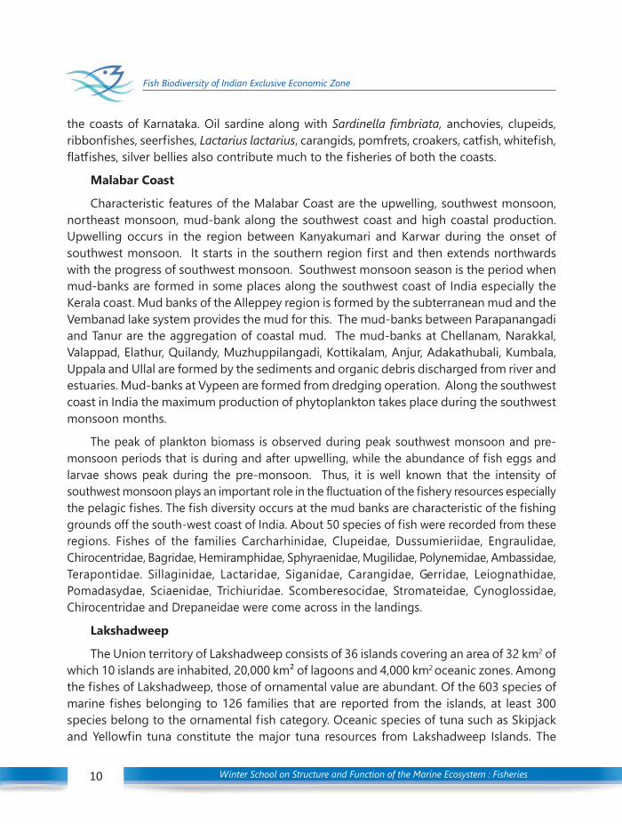
the coasts of Karnataka. Oil sardine along with Sardinella fimbriata, anchovies, clupeids,ribbonfishes, seerfishes, Lactarius lactarius, carangids, pomfrets, croakers, catfish, whitefish,flatfishes, silver bellies also contribute much to the fisheries of both the coasts.
Malabar Coast
Characteristic features of the Malabar Coast are the upwelling, southwest monsoon,northeast monsoon, mud-bank along the southwest coast and high coastal production.Upwelling occurs in the region between Kanyakumari and Karwar during the onset ofsouthwest monsoon. It starts in the southern region first and then extends northwardswith the progress of southwest monsoon. Southwest monsoon season is the period whenmud-banks are formed in some places along the southwest coast of India especially theKerala coast. Mud banks of the Alleppey region is formed by the subterranean mud and theVembanad lake system provides the mud for this. The mud-banks between Parapanangadiand Tanur are the aggregation of coastal mud. The mud-banks at Chellanam, Narakkal,Valappad, Elathur, Quilandy, Muzhuppilangadi, Kottikalam, Anjur, Adakathubali, Kumbala,Uppala and Ullal are formed by the sediments and organic debris discharged from river andestuaries. Mud-banks at Vypeen are formed from dredging operation. Along the southwestcoast in India the maximum production of phytoplankton takes place during the southwestmonsoon months.
The peak of plankton biomass is observed during peak southwest monsoon and pre-monsoon periods that is during and after upwelling, while the abundance of fish eggs andlarvae shows peak during the pre-monsoon. Thus, it is well known that the intensity ofsouthwest monsoon plays an important role in the fluctuation of the fishery resources especiallythe pelagic fishes. The fish diversity occurs at the mud banks are characteristic of the fishinggrounds off the south-west coast of India. About 50 species of fish were recorded from theseregions. Fishes of the families Carcharhinidae, Clupeidae, Dussumieriidae, Engraulidae,Chirocentridae, Bagridae, Hemiramphidae, Sphyraenidae, Mugilidae, Polynemidae, Ambassidae,Terapontidae. Sillaginidae, Lactaridae, Siganidae, Carangidae, Gerridae, Leiognathidae,Pomadasydae, Sciaenidae, Trichiuridae. Scomberesocidae, Stromateidae, Cynoglossidae,Chirocentridae and Drepaneidae were come across in the landings.
Lakshadweep
The Union territory of Lakshadweep consists of 36 islands covering an area of 32 km2 ofwhich 10 islands are inhabited, 20,000 km² of lagoons and 4,000 km2 oceanic zones. Amongthe fishes of Lakshadweep, those of ornamental value are abundant. Of the 603 species ofmarine fishes belonging to 126 families that are reported from the islands, at least 300species belong to the ornamental fish category. Oceanic species of tuna such as Skipjackand Yellowfin tuna constitute the major tuna resources from Lakshadweep Islands. The
Winter School on Structure and Function of the Marine Ecosystem : Fisheries 11
Fish Biodiversity of Indian Exclusive Economic Zone
main economy of the islanders is dependent on the tuna catch and fishing is done fornearly six months of the year from October to April. The most common species of sharksthat occur in Lakshadweep are the Spade-nose shark/Yellow dog shark, and the Milk shark.The Blacktip Shark and Hammerhead shark are also commonly found in the waters aroundLakshadweep.
Gulf of Mannar
The Gulf of Mannar located in the Southern part of the Bay of Bengal with a string of 21islands which has been declared as a marine National Park under the Wild Life (Protection)Act 1972 by the Government of India. The reserve covers 10,500 km2, which comprises of avariety of sensitive marine habitats like coral reefs, mangroves and sea grasses, and couldbe considered as one of the most productive ecosystems. The core area of the reserve iscomprised of a 560km2 of coral islands and shallow marine habitat. The Gulf of Mannaralone produces about 20% of the marine fish catch in Tamil Nadu. A total of 1,182 speciesbelonging to 476 genera in 144 families and 39 orders was reported from GOM ecosystem.The finfish resources, mainly comprises of small pelagics, barracudas, silverbellies, rays,skates, eels, carangids, flying fish, full beaks and half beaks. The demersal finfish resources,mainly associated coral reefs are threadfin breams, grouper, snappers, emperor and reefassociated fishes. Further, large pelagic species like skipjack tuna, yellowfin tuna, bigeyetuna, kawakawa, frigate tuna and seer fish, bill fishes, eagle rays are most abundant inoffshore and oceanic areas, but also occur in coastal waters are found in certain areas of theGulf of Mannar.
Palk Bay
Palk Bay is situated on the southeast coast of India encompassing the sea betweenPoint Calimere near Vedaranyam in the north and the northern shores of Mandapam toDhanushkodi in the south. The Palk Bay itself is about 110 km long and is surrounded onthe northern and western sides by the coastline of the State of Tamil Nadu in the mainlandof India. The coastline of Palk Bay has coral reefs, mangroves, lagoons, and sea grassecosystems. Elasmobranchs are the largest group of fishes and are well represented in thefishery wealth of the Ramewaram Island on the Palk Bay side. This is one of the best fishinggrounds for smaller sardines, silver bellies, common white fish and half beaks, mullets andsciaenids. The common fishes found in this area also include Sharks, Rays, Skates, Tiger-sharks and Hammer-headed sharks.
Coromandel Coast
Seer fishes are most abundant in the Coromandel Coast of Tamil Nadu along withmiscellaneous fisheries formed of trichiurids and percoids. The flying-fish fishery is an
Winter School on Structure and Function of the Marine Ecosystem : Fisheries12
Fish Biodiversity of Indian Exclusive Economic Zone
important seasonal fishery on the east coast of India extending from Madras to Point Calimerealong the Coromandel Coast. Three species of flying-fish, viz., Hirundichthys coromandelensis,Cheliopogon spilopterus and C. bahiensis, are generally found in these waters, but morethan 90% of the catch consists of C. coromandelensis.
Deep-sea fish diversity
A first authentic record of the deep-sea fishes from India was by Alcock in the book ADescriptive Catalogue of the Indian deep-sea fishes in the Indian museum based on thefishes collected during the explorations in the Indian Ocean by RIMS Investigator (1889-1900). Then comes the results of R.V. VARUNA cruises (1962-1968) showed the presence ofAnodontostoma chacunda, Atropus atropos, Benthodesmus tenuis, Brachirus orientalis,Chlorophthalmus agassizi, C. corniger, Carangoides malabaricus, Caranx kalla, Centropristisinvestigatoris, Chascanopsetta lugubris, Chlorophthalmus corniger, Cubiceps natalensis,Cynoglossus bilineatus, C. semifasciatus, Decapterus russelli, Drepane punctata, Epinnulaorientalis, Goniolosa manmina, Grammoplites scaber, Himantura urnak, Holocentrum rubrum,J. diacanthus, Johnius dussumieri, Kowala coval, L. argentimaculatus, L. bindus, L. johni, L.kasmira, L. malabaricus, Lactarius lactarius, Leiognathus splendens, Lepidopus caudatus,Lepturacanthus savala, Megalaspis cordyla, Myripristis murdjan, Nemipterus japonicus, Netumathalassinus, Opisthopterus tardoore, Otolithes argentatus, P. sexifilis, Parastromateus niger,Paseneopsis cyanea, Pastinachus sephen, Pellona ditchela, Polymixia nobilis, Polynemusplebius, Pomadasys hasta, Psenes indicus, Pseudorhombus arsius, Rexea prometheoides,Rhynchobatis djiddensis, Saurida tumbil, Scoliodon palasorrah, Scyllium hispidum, Sillagosihama, Solea elongata, Sphyraena acutipinnis, Synagrops japonicus, Synodus indicus,Thrissocles mystax, T. malabarica, Trichiurus lepturus and Tylosurus crocodilus from the depthzone of 1 to 450m.
A checklist of fishes of Indian EEZ was published based on the surveys of FORV SagarSampada in the EEZ of India during 1985-’87. This list is arranged alphabetically by familiesand genera. The list contains 242 species belonging to 87 families with both conventionaland nonconventional fish fauna of the Indian EEZ with the scientific and common names offishes, details of the depth of occurrence, depth of fishing, position and the gear were alsoincluded. The study by Hashim (2012) reported and the occurrence of 188 species of deep-sea fishes from Indian EEZ during the exploratory surveys. Deep sea fish species like Psenopsiscyanea, Bembrops caudimacula, Chlorophthalmus bicornis, C. agassizi, Uranoscopusarchionema, Gavialiceps taeniola, Priacanthus hamrur and Neoepinnula orientalis were foundto be the most abundant during the study. Hashim (2012) observed a highest diversity inArabian Sea (4.95) followed by Andaman Waters (4.12) and Bay of Bengal (3.55).
Winter School on Structure and Function of the Marine Ecosystem : Fisheries 13
Fish Biodiversity of Indian Exclusive Economic Zone
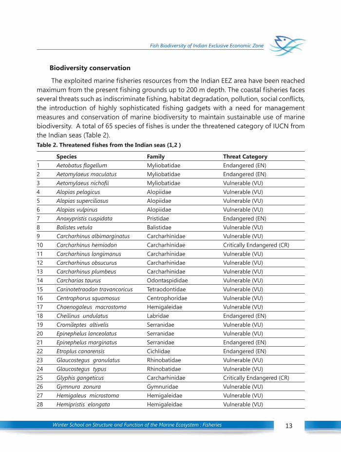
Biodiversity conservation
The exploited marine fisheries resources from the Indian EEZ area have been reachedmaximum from the present fishing grounds up to 200 m depth. The coastal fisheries facesseveral threats such as indiscriminate fishing, habitat degradation, pollution, social conflicts,the introduction of highly sophisticated fishing gadgets with a need for managementmeasures and conservation of marine biodiversity to maintain sustainable use of marinebiodiversity. A total of 65 species of fishes is under the threatened category of IUCN fromthe Indian seas (Table 2).Table 2. Threatened fishes from the Indian seas (1,2 )
Species Family Threat Category1 Aetobatus flagellum Myliobatidae Endangered (EN)2 Aetomylaeus maculatus Myliobatidae Endangered (EN)3 Aetomylaeus nichofii Myliobatidae Vulnerable (VU)4 Alopias pelagicus Alopiidae Vulnerable (VU)5 Alopias superciliosus Alopiidae Vulnerable (VU)6 Alopias vulpinus Alopiidae Vulnerable (VU)7 Anoxypristis cuspidata Pristidae Endangered (EN)8 Balistes vetula Balistidae Vulnerable (VU)9 Carcharhinus albimarginatus Carcharhinidae Vulnerable (VU)10 Carcharhinus hemiodon Carcharhinidae Critically Endangered (CR)11 Carcharhinus longimanus Carcharhinidae Vulnerable (VU)12 Carcharhinus obsucurus Carcharhinidae Vulnerable (VU)13 Carcharhinus plumbeus Carcharhinidae Vulnerable (VU)14 Carcharias taurus Odontaspididae Vulnerable (VU)15 Carinotetraodon travancoricus Tetraodontidae Vulnerable (VU)16 Centrophorus squamosus Centrophoridae Vulnerable (VU)17 Chaenogaleus macrostoma Hemigaleidae Vulnerable (VU)18 Cheilinus undulatus Labridae Endangered (EN)19 Cromileptes altivelis Serranidae Vulnerable (VU)20 Epinephelus lanceolatus Serranidae Vulnerable (VU)21 Epinephelus marginatus Serranidae Endangered (EN)22 Etroplus canarensis Cichlidae Endangered (EN)23 Glaucostegus granulatus Rhinobatidae Vulnerable (VU)24 Glaucostegus typus Rhinobatidae Vulnerable (VU)25 Glyphis gangeticus Carcharhinidae Critically Endangered (CR)26 Gymnura zonura Gymnuridae Vulnerable (VU)27 Hemigaleus microstoma Hemigaleidae Vulnerable (VU)28 Hemipristis elongata Hemigaleidae Vulnerable (VU)
Winter School on Structure and Function of the Marine Ecosystem : Fisheries14
Fish Biodiversity of Indian Exclusive Economic Zone
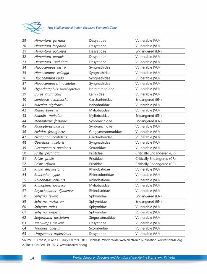
29 Himantura gerrardi Dasyatidae Vulnerable (VU)30 Himantura leoparda Dasyatidae Vulnerable (VU)31 Himantura polylepis Dasyatidae Endangered (EN)32 Himantura uarnak Dasyatidae Vulnerable (VU)33 Himantura undulata Dasyatidae Vulnerable (VU)34 Hippocampus histrix Syngnathidae Vulnerable (VU)35 Hippocampus kelloggi Syngnathidae Vulnerable (VU)36 Hippocampus kuda Syngnathidae Vulnerable (VU)37 Hippocampus trimaculatus Syngnathidae Vulnerable (VU)38 Hyporhamphus xanthopterus Hemiramphidae Vulnerable (VU)39 Isurus oxyrinchus Lamnidae Vulnerable (VU)40 Lamiopsis temminckii Carcharhinidae Endangered (EN)41 Makaira nigricans Istiophoridae Vulnerable (VU)42 Manta birostris Myliobatidae Vulnerable (VU)43 Mobula mobular Myliobatidae Endangered (EN)44 Monopterus fossorius Synbranchidae Endangered (EN)45 Monopterus indicus Synbranchidae Vulnerable (VU)46 Nebrius ferrugineus Ginglymostomatidae Vulnerable (VU)47 Negaprion acutidens Carcharhinidae Vulnerable (VU)48 Oostethus insularis Syngnathidae Vulnerable (VU)49 Plectropomus areolatus Serranidae Vulnerable (VU)50 Pristis pectinata Pristidae Critically Endangered (CR)51 Pristis pristis Pristidae Critically Endangered (CR)52 Pristis zijsron Pristidae Critically Endangered (CR)53 Rhina ancylostoma Rhinobatidae Vulnerable (VU)54 Rhincodon typus Rhincodontidae Vulnerable (VU)55 Rhinobatos obtusus Rhinobatidae Vulnerable (VU)56 Rhinoptera javanica Myliobatidae Vulnerable (VU)57 Rhynchobatus djiddensis Rhinobatidae Vulnerable (VU)58 Sphyrna lewini Sphyrnidae Endangered (EN)59 Sphyrna mokarran Sphyrnidae Endangered (EN)60 Sphyrna tudes Sphyrnidae Vulnerable (VU)61 Sphyrna zygaena Sphyrnidae Vulnerable (VU)62 Stegostoma fasciatum Stegostomatidae Vulnerable (VU)63 Taeniurops meyeni Dasyatidae Vulnerable (VU)64 Thunnus obesus Scombridae Vulnerable (VU)65 Urogymnus asperrimus Dasyatidae Vulnerable (VU)Source : 1. Froese, R. and D. Pauly. Editors. 2017. FishBase. World Wide Web electronic publication. www.fishbase.org.2. The IUCN Red List. 2017: www.iucnredlist.org
Winter School on Structure and Function of the Marine Ecosystem : Fisheries 15
Fish Biodiversity of Indian Exclusive Economic Zone
Human activities are the major causes for the loss of biodiversity and degradation ofmarine and coastal habitats, which needs immediate attention and comprehensive actionplan to conserve the biodiversity for living harmoniously with nature. Some of the measuressuch as control of excess fleet size, control of some of the gears like purse seines, ringseines, disco-nets, regulation of mesh size, avoid habitat degradation of nursery areas ofthe some of the species, reduce the discards of the low value fish, protection of spawners,implementation of reference points and notification of marine reserves are required for theprotection and conservation of marine and coastal biodiversity.
References
Alcock, A. 1899. A descriptive catalogue of the Indian deep-sea fishes in the Indian Museum. 228 pp.
Day, F. 1875. The Fishes of India being a natural history of the fishes part 1: know to inhabit the seas and freshwaters of India, Burma, and Ceylon. Bernard Quaritch.
Murty, V. Sriramachandra. 2002. Marine ornamental fish resources of Lakshadweep. CMFRI Special Publication,72. pp. 1-134.
Raje, S. G., Mathew, Grace , Joshi, K. K., Nair, Rekha J., Mohanraj, G., Srinath, M., Gomathy, S and Rudramurthy,N. 2002. Elasmobranch fisheries of India - An appraisal.CMFRI Special Publication, 71. pp. 1-76.
Raje, S. G., Sivakami, S., Mohanraj, G., Manojkumar, P. P., Raju, A. and Joshi, K. K. 2007. An atlas on theElasmobranch fishery resources of India. CMFRI, Special Publication, 95. pp. 1-253.
Silas, E G. 1969. Exploratory fishing by R.V. VARUNA. Technical Report. CMFRI Bulletin, 12, 1-141. CMFRI,Kochi.
Talwar, P. K., and Kacker, R. K. 1984. Commercial sea fishes of India. Zoologcal Survey of India

Winter School on Structure and Function of the Marine Ecosystem : Fisheries16
Fundamentals of Ocean colour Remote sensing
Remote sensing refers to collection of information about an object without being indirect contact with the object. Remote sensing aids in measuring remote areas which areinaccessible by any other means and offer less expense than in-situ measurements. Remotesensing facilitates creation of long time series and extended measurement. This has theadvantage that several parameters can be measured at same time and satellite-based remotesensing measurements allow global observations. Remote sensing has its own advantagesand disadvantages. The limitation includes indirect measurements of large areas which arenot of interest to the user. The automated instrument degradation creates retrieval errorsand are affected by several factors/processes, and not only by the object of interest.Additional assumptions and models are needed for the interpretation of the measurementsand before using these models in oceanographic studies, it is extremely important to validatethe performance of the various ocean colour algorithms with in-situ observations (Swirgonet al., 2015).
Two different types of remote sensing include active and passive remote sensing. Passiveremote sensing measures naturally available energy viz. solar light which are either attenuatedscattered and reflected. In active remote sensing, the sensor emits visible radiation towardstarget and reflected radiation in emitted bands are detected and measured. These type ofsensors can work day and night and can use wavelengths not available from natural sources.LIDAR comes under this category of active ocean colour remote sensing.
03C H A P T E R
(Image courtesy: https://commons.wikimedia.org)Fig. 1. Illustration of the Visible spectrum of the light
FUNDAMENTALS OF OCEAN COLOURREMOTE SENSINGAneesh Lotliker1, Minu P.2, Shalin Saleem2,Muhammad Shafeeque2 and Grinson George2
1Indian National Centre for Ocean Information Services, Hyderabad2ICAR-Central Marine Fisheries Research Institute
Winter School on Structure and Function of the Marine Ecosystem : Fisheries 17
Fundamentals of Ocean colour Remote sensing
17
Solar light is an electromagnetic radiation where waves are fluctuations of electric andmagnetic fields, which can transport energy from one location to another (Figure 1). Whensunlight strikes the ocean, some of it reflects off the surface back into the atmosphere. Theamount of energy that penetrates the surface of the water depends on the angle at whichthe sunlight strikes the ocean. Near the equator, the sun’s rays strike the ocean almostperpendicular to the ocean’s surface. Near the poles, the sun’s rays strike the ocean at anangle, rather than directly. The direct angle of the sun’s rays to the surface of the water atthe equator means that more energy penetrates the surface of the water at the equatorthan at the poles.
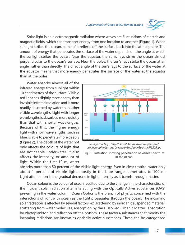
Water absorbs almost all of theinfrared energy from sunlight within10 centimetres of the surface. Visiblered light has slightly more energy thaninvisible infrared radiation and is morereadily absorbed by water than othervisible wavelengths. Light with longerwavelengths is absorbed more quicklythan that with shorter wavelengths.Because of this, the higher energylight with short wavelengths, such asblue, is able to penetrate more deeply(Figure 2). The depth of the water notonly affects the colours of light thatare noticeable underwater, it alsoaffects the intensity, or amount oflight. Within the first 10 m, waterabsorbs more than 50 percent of the visible light energy. Even in clear tropical water onlyabout 1 percent of visible light, mostly in the blue range, penetrates to 100 m.Light attenuation is the gradual decrease in light intensity as it travels through matter.
Ocean colour is the colour of ocean resulted due to the change in the characteristics ofthe incident solar radiation after interacting with the Optically Active Substances (OAS)prevailing in the water column. Ocean Optics is the branch of physics concerned with theinteractions of light with ocean as the light propagates through the ocean. The incomingsolar radiation is affected by several factors viz. scattering by inorganic suspended material,scattering from water molecules, absorption by the Dissolved Organic Matter, absorptionby Phytoplankton and reflection off the bottom. These factors/substances that modify theincoming radiations are known as optically active substances. These can be categorized
(Image courtesy : http://ksuweb.kennesaw.edu/~jdirnber/oceanography/Lectures()ceanogr/LecOceanStructur/0620B.jpg
Fig. 2. Illustration showing penetration of visible spectrumin the ocean
Winter School on Structure and Function of the Marine Ecosystem : Fisheries18
Fundamentals of Ocean colour Remote sensing
into two properties- Inherent and apparent optical properties. Inherent Optical Property(IOP) is an optical property of the water body which is totally independent of the spatialdistribution of the radiation and Apparent Optical Property (AOP) is an optical property ofthe water body that is dependent upon the spatial distribution of the incident radiation.Absorption (a) and scattering (b=bf +bb) are the main IOP’s and reflectance (Rrs) andattenuation (Kd) form the AOP which are interlinked. ‘bf’ and bb represents forward andbackward scattering, ‘µd’ represents average cosine of downwelling light (Morel et al., 2006).
kd = (a + bb) / µd ....................................(1)
Rrs = (f/q) (bb / a + bb ).........................(2)
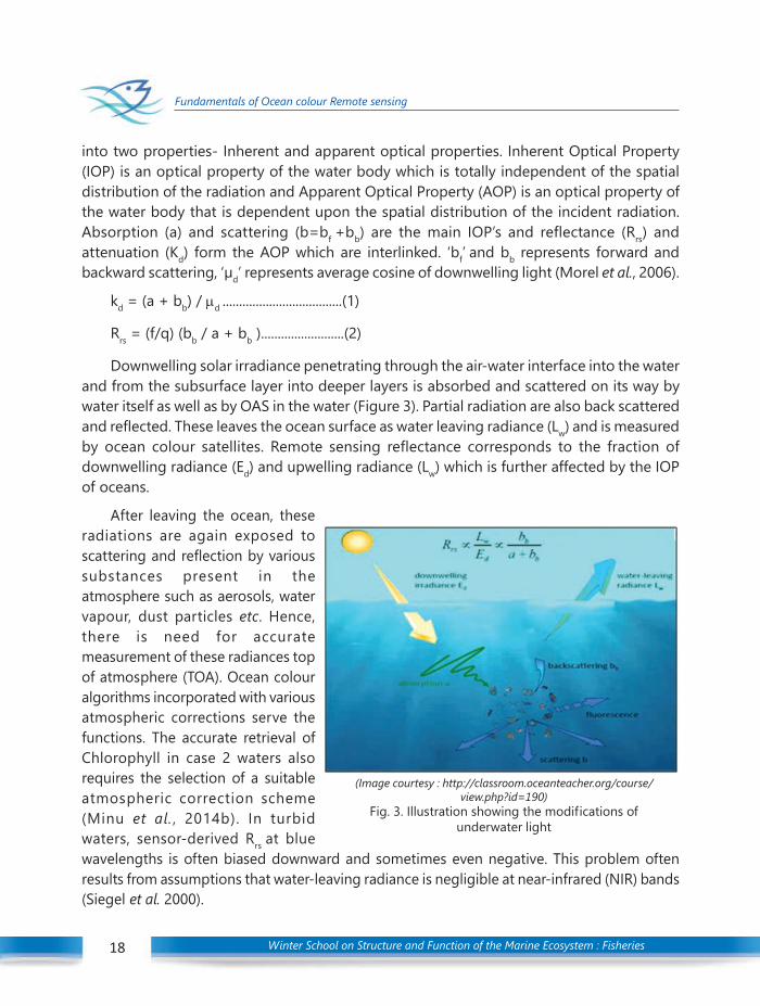
Downwelling solar irradiance penetrating through the air-water interface into the waterand from the subsurface layer into deeper layers is absorbed and scattered on its way bywater itself as well as by OAS in the water (Figure 3). Partial radiation are also back scatteredand reflected. These leaves the ocean surface as water leaving radiance (Lw) and is measuredby ocean colour satellites. Remote sensing reflectance corresponds to the fraction ofdownwelling radiance (Ed) and upwelling radiance (Lw) which is further affected by the IOPof oceans.
After leaving the ocean, theseradiations are again exposed toscattering and reflection by varioussubstances present in theatmosphere such as aerosols, watervapour, dust particles etc. Hence,there is need for accuratemeasurement of these radiances topof atmosphere (TOA). Ocean colouralgorithms incorporated with variousatmospheric corrections serve thefunctions. The accurate retrieval ofChlorophyll in case 2 waters alsorequires the selection of a suitableatmospheric correction scheme(Minu et al. , 2014b). In turbidwaters, sensor-derived Rrs at bluewavelengths is often biased downward and sometimes even negative. This problem oftenresults from assumptions that water-leaving radiance is negligible at near-infrared (NIR) bands(Siegel et al. 2000).
(Image courtesy : http://classroom.oceanteacher.org/course/view.php?id=190)
Fig. 3. Illustration showing the modifications ofunderwater light
Winter School on Structure and Function of the Marine Ecosystem : Fisheries 19
Fundamentals of Ocean colour Remote sensing
19
For the ocean–atmosphere system, top-of-atmosphere (TOA) reflectance, ρt(λ), asmeasured by the satellite sensor, can be written as a linear sum from various contributions(ignoring whitecaps and sun glint):
ρt(λ)= ρr(λ)+ρa(λ) + t(λ)ρw(λ)...........(3)where ρr(λ), ρa(λ), and ρw(λ) are the reflectance contributions from molecules (Rayleigh
scattering), aerosols (including Rayleigh-aerosol interactions), and ocean waters, respectively,and t(λ) is the diffuse transmittance of the atmosphere.
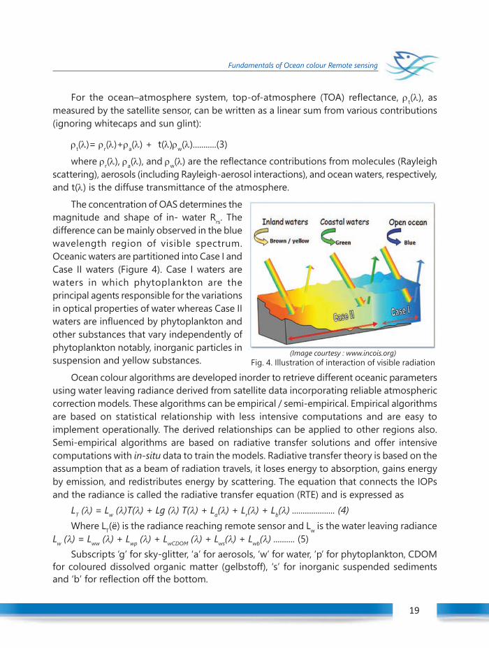
The concentration of OAS determines themagnitude and shape of in- water Rrs. Thedifference can be mainly observed in the bluewavelength region of visible spectrum.Oceanic waters are partitioned into Case I andCase II waters (Figure 4). Case I waters arewaters in which phytoplankton are theprincipal agents responsible for the variationsin optical properties of water whereas Case IIwaters are influenced by phytoplankton andother substances that vary independently ofphytoplankton notably, inorganic particles insuspension and yellow substances.
Ocean colour algorithms are developed inorder to retrieve different oceanic parametersusing water leaving radiance derived from satellite data incorporating reliable atmosphericcorrection models. These algorithms can be empirical / semi-empirical. Empirical algorithmsare based on statistical relationship with less intensive computations and are easy toimplement operationally. The derived relationships can be applied to other regions also.Semi-empirical algorithms are based on radiative transfer solutions and offer intensivecomputations with in-situ data to train the models. Radiative transfer theory is based on theassumption that as a beam of radiation travels, it loses energy to absorption, gains energyby emission, and redistributes energy by scattering. The equation that connects the IOPsand the radiance is called the radiative transfer equation (RTE) and is expressed as
LT (λ) = Lw (λ)T(λ) + Lg (λ) T(λ) + La(λ) + Lr(λ) + Lb(λ) .................... (4)Where LT(ë) is the radiance reaching remote sensor and Lw is the water leaving radiance
Lw (λ) = Lww (λ) + Lwp (λ) + LwCDOM (λ) + Lws(λ) + Lwb(λ) .......... (5)Subscripts ‘g’ for sky-glitter, ‘a’ for aerosols, ‘w’ for water, ‘p’ for phytoplankton, CDOM
for coloured dissolved organic matter (gelbstoff), ‘s’ for inorganic suspended sedimentsand ‘b’ for reflection off the bottom.
(Image courtesy : www.incois.org)Fig. 4. Illustration of interaction of visible radiation
Winter School on Structure and Function of the Marine Ecosystem : Fisheries20
Fundamentals of Ocean colour Remote sensing
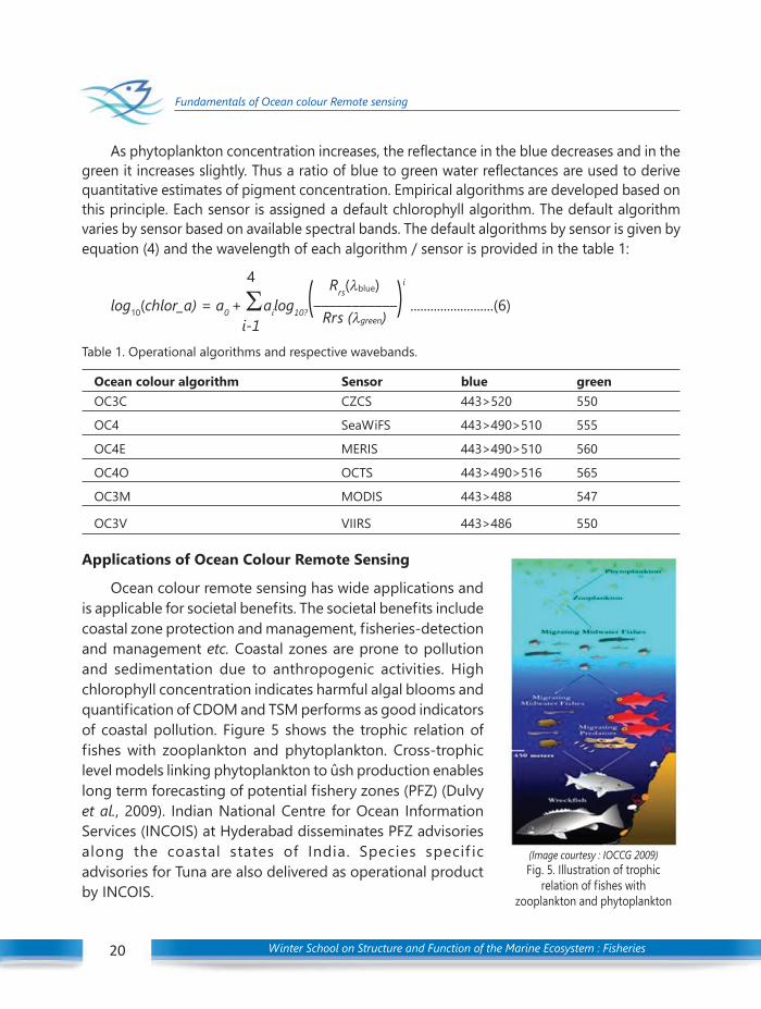
As phytoplankton concentration increases, the reflectance in the blue decreases and in thegreen it increases slightly. Thus a ratio of blue to green water reflectances are used to derivequantitative estimates of pigment concentration. Empirical algorithms are developed based onthis principle. Each sensor is assigned a default chlorophyll algorithm. The default algorithmvaries by sensor based on available spectral bands. The default algorithms by sensor is given byequation (4) and the wavelength of each algorithm / sensor is provided in the table 1:
4 Rrs(λblue)log10(chlor_a) = a0 + Σailog10?(–––––––––––)i
.........................(6)i-1 Rrs (λgreen)
Table 1. Operational algorithms and respective wavebands.
Ocean colour algorithm Sensor blue greenOC3C CZCS 443>520 550
OC4 SeaWiFS 443>490>510 555
OC4E MERIS 443>490>510 560
OC4O OCTS 443>490>516 565
OC3M MODIS 443>488 547
OC3V VIIRS 443>486 550
Applications of Ocean Colour Remote Sensing
Ocean colour remote sensing has wide applications andis applicable for societal benefits. The societal benefits includecoastal zone protection and management, fisheries-detectionand management etc. Coastal zones are prone to pollutionand sedimentation due to anthropogenic activities. Highchlorophyll concentration indicates harmful algal blooms andquantification of CDOM and TSM performs as good indicatorsof coastal pollution. Figure 5 shows the trophic relation offishes with zooplankton and phytoplankton. Cross-trophiclevel models linking phytoplankton to ûsh production enableslong term forecasting of potential fishery zones (PFZ) (Dulvyet al., 2009). Indian National Centre for Ocean InformationServices (INCOIS) at Hyderabad disseminates PFZ advisoriesalong the coastal states of India. Species specif icadvisories for Tuna are also delivered as operational productby INCOIS.
(Image courtesy : IOCCG 2009)Fig. 5. Illustration of trophic
relation of fishes withzooplankton and phytoplankton

Winter School on Structure and Function of the Marine Ecosystem : Fisheries 21
Fundamentals of Ocean colour Remote sensing
21
References
Dulvy, N.K., Chassot, E., Hyemans, J., Hyde, K. and Pauly, D., 2009. Climate change, ecosystem variability andfisheries productivity. Remote Sensing in Fisheries and Aquaculture: The Societal Benefits, IOCCG report,(8), pp.11-28.
Minu, P., Lotliker, A.A., Shaju, S.S., SanthoshKumar, B., Ashraf, P.M. and Meenakumari, B., 2014. Effect ofoptically active substances and atmospheric correction schemes on remote-sensing reflectance at acoastal site off Kochi. International journal of remote sensing, 35(14), pp.5434-5447.
Morel, A., Gentili, B., Chami, M. and Ras, J., 2006. Bio-optical properties of high chlorophyll Case 1 watersand of yellow-substance-dominated Case 2 waters. Deep Sea Research Part I: Oceanographic ResearchPapers, 53(9), pp.1439-1459.
Siegel, D. A., M. Wang, S. Maritorena, and W. Robinson., 2000. “Atmospheric Correction of Satellite OceanColor Imagery: The Black Pixel Assumption.” Applied Optics 39: 3582"3591. doi:10.1364/AO.39.003582.
Swirgon, M. and Stramska, M., 2015. Comparison of in situ and satellite ocean color determinations ofparticulate organic carbon concentration in the global ocean. Oceanologia, 57(1), pp.25-31.
Winter School on Structure and Function of the Marine Ecosystem : Fisheries22
Satellite ocean colour sensors
1. Introduction
The 70% of the earth’s surface is covered by the ocean and the life inhabiting theoceans play an important role in shaping the earth’s climate. Phytoplankton, also known asmicroalgae, are the single celled, autotrophic components of the plankton community anda key part of oceans, seas and freshwater basin ecosystems. They are significant factor inthe ocean carbon cycle and, hence, important in all pathways of carbon in the ocean.Phytoplankton contain chlorophyll pigments for photosynthesis, similar to terrestrial plantsand require sunlight in order to live and grow. Most of them are buoyant and float in theupper part of the ocean, where plenty of sunlight is available. They also require inorganicnutrients such as nitrates, phosphates, and sulphur which they convert into proteins, fats,and carbohydrates. In a balanced ecosystem, phytoplankton are the base of the food weband provide food for a wide range of sea creatures (NOAA). The measurement ofphytoplankton can be indexed as chlorophyll concentration and is important as they arefundamental to understanding how the marine ecosystem responds to climate variabilityand climate change.
In open ocean waters, the ocean colour is predominantly driven by the phytoplanktonconcentration and ocean colour remote sensing has been used to estimate the amount ofchlorophyll-a, the primary light-absorbing pigment in all phytoplankton. The marineecosystem captures the visible part of the solar spectrum (400nm - 700nm) forphotosynthesis with the help of the pigment molecules (principally chlorophyll) containedin phytoplankton. As they absorb and scatter light from the sun, phytoplankton exert aprofound influence on the submarine light field, including the flux upwards across thewater surface. As their concentration increases, the colour of the ocean changes from blueto green. Such shifts in ocean colour and the abundance of phytoplankton (chlorophyllconcentration) can be mapped by measuring the light reflecting from the sea with opticalsensors on-board earth-orbiting satellites. The technique is called ocean-colour radiometryor ocean colour remote sensing, and has proved to be one of the most fruitful of remote-sensing technologies.
For the last few decades, satellite data was used to estimate large-scale patterns ofchlorophyll and to model primary productivity across the global ocean from daily to inter-annual timescales. Such global estimates of chlorophyll and primary productivity have been
04C H A P T E R SATELLITE OCEAN COLOUR SENSORS
Muhammad Shafeeque, Minu P., Phiros Shah and Grinson George
Fishery Resources Assessment DivisionICAR-Central Marine Fisheries Research Institute

Winter School on Structure and Function of the Marine Ecosystem : Fisheries 23
Satellite ocean colour sensors
23
integrated into climate models illustrating the feedback between ocean life and globalclimate processes (Dierssen et al., 2013). The applications of ocean colour remote sensingare extensive, varied, and fundamental to understand and monitor the global ecosystem.They are being used for monitoring of harmful algal blooms, critical coastal habitats,eutrophication processes, oil spills, and a variety of hazards in the coastal zone. Majorapplications of ocean colour data are as follows (Ocean Optics Web Book).
Mapping of chlorophyll concentrations
Measurement of inherent optical properties such as absorption and backscatter
Determination of phytoplankton physiology, phenology, and functional groups
Studies of ocean carbon fixation and cycling
Monitoring of ecosystem changes resulting from climate change
Fisheries management
Mapping of coral reefs, sea grass beds, and kelp forests
Mapping of shallow-water bathymetry and bottom type for military operations
Monitoring of water quality for recreation
Detection of harmful algal blooms and pollution events
2. Ocean Colour sensors
Ocean colour (OC) is an oceanic Essential Climate Variable (ECV), which is used byclimate modellers and researchers. Remote sensing of ocean colour from space began in1978 with the successful launch of NASA’s Coastal Zone Color Scanner (CZCS) and it was amilestone in the history of satellite ocean colour remote sensing. Since then, more thantwenty ocean colour satellite sensors have been launched viz. MOS, OCTS, POLDER, SeaWiFS,OCI, OCM, OSMI, MERIS, CMODIS, COCTS CZI, OSMI, GLI, POLDER-2, MODIS_AQUA, MISR,POLDER-3, MERSI, HICO, OCM-2, GOCI and VIIRS (www.ioccg.org/sensors_ioccg.html). Moreocean colour sensors are planned over the next decade by various space agencies. Thesesensors capture continuous global ocean colour data (e.g. chlorophyll concentration, primaryproduction), which provide significant benefits for research in areas such as biologicaloceanography and climate change studies. According to the current framework for oceancolour remote sensing, the satellite sensor first measures the intensity of the upward spectralradiation at the top-of-atmosphere (TOA). The varying intensities are then used to retrievethe water-leaving radiance after atmospheric correction, leading to the further retrieval ofthe optically active marine components (e.g. phytoplankton, minerals and coloured dissolvedorganic matter). The characteristics of past, current and scheduled ocean colour sensors are
Winter School on Structure and Function of the Marine Ecosystem : Fisheries24
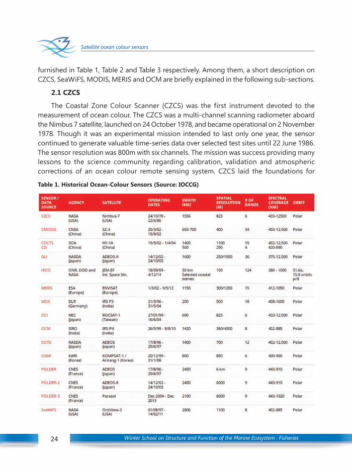
Satellite ocean colour sensors
furnished in Table 1, Table 2 and Table 3 respectively. Among them, a short description onCZCS, SeaWiFS, MODIS, MERIS and OCM are briefly explained in the following sub-sections.
2.1 CZCS
The Coastal Zone Colour Scanner (CZCS) was the first instrument devoted to themeasurement of ocean colour. The CZCS was a multi-channel scanning radiometer aboardthe Nimbus 7 satellite, launched on 24 October 1978, and became operational on 2 November1978. Though it was an experimental mission intended to last only one year, the sensorcontinued to generate valuable time-series data over selected test sites until 22 June 1986.The sensor resolution was 800m with six channels. The mission was success providing manylessons to the science community regarding calibration, validation and atmosphericcorrections of an ocean colour remote sensing system. CZCS laid the foundations for
Table 1. Historical Ocean-Colour Sensors (Source: IOCCG)

Winter School on Structure and Function of the Marine Ecosystem : Fisheries 25
Satellite ocean colour sensors
25
Table 2. Current Ocean-Colour Sensors (Source : IOCCG)
Table 3. Scheduled Ocean-Colour Sensors (Source : IOCCG)

Winter School on Structure and Function of the Marine Ecosystem : Fisheries26
Satellite ocean colour sensors
subsequent satellite ocean colour sensors, and formed a cornerstone for international effortsto understand the ocean’s role in the carbon cycle. It also provided oceanographers withnew insights into the biological and chemical properties of ocean water masses.
2.2 SeaWiFS
Sea-Viewing Wide Field-of-View Sensor (SeaWiFS) was the only scientific instrumenton GeoEye’s OrbView-2 (AKA SeaStar) satellite, and was a follow-on experiment to the CZCS.The satellite was launched 1 August 1997, SeaWiFS began scientific operations on 18September 1997. The spacecraft occupied a sun-synchronous orbit at an altitude of 705 kmwith an equatorial crossing time at 12 pm. The sensor resolution was 1.1 km in Local AreaCoverage (LAC) and 4.5 km Global Area Coverage (GAC). The instrument was specificallydesigned to monitor ocean colour characteristics such as chlorophyll-a concentration andwater clarity. During its operational period, the spacecraft telemetry became invalid due tofailure of GPS, SeaWiFS interface and battery. As a result, there are gaps in data collectionduring 1 January 2008- 12 April 2008. In order to make data available at same accuracy, thespacecraft orbit altitude changed from 705 to 690 km. Unfortunately, the sensor failed itsoperation on 14 December 2010.
2.3 MODIS
MODerate- resolution Imaging Spectroradiometer (MODIS) are the series of EOSsensors launched by NASA on TERRA (December 1999) and AQUA (May 2002) satellites.MODIS is one of the most successful sensor in the ocean colour series and it is operationaltill date. Unlike SeaWiFS, MODIS records SST also with a spatial resolution of 1.1 km. Theinstruments capture data in 36 spectral bands ranging in wavelength from 0.4 µm to 14.4µmand at varying spatial resolutions (2 bands at 250 m, 5 bands at 500 m and 29 bands at 1km). The instrument image the entire Earth every 1 to 2 days. They are designed to providemeasurements in large-scale global dynamics including changes in Earth’s cloud cover,radiation budget and processes occurring in the oceans, on land, and in the loweratmosphere. MODIS is succeeded by the VIIRS instrument onboard the Suomi NPP satellitelaunched in 2011 and future Joint Polar Satellite System (JPSS) satellites (http://modis.gsfc.nasa.gov).
2.4 Ocean Colour Monitor (OCM) and OCM-2
Ocean Colour Monitor (OCM) and OCM-2 on board OCEANSAT-1 and OCEANSAT-2respectively were launched by the Indian Space Research Organisation (ISRO) and designedto map the ocean colour, especially in Indian waters. OCM was the first satellite sensoremployed for oceanographic studies in the Indian waters. The OCM sensor was launchedon 26 May 1999 and it operated successfully till August 2010. OCM-2, the successor ofOCM launched on 23 September 2009, and is currently operational. In OCM, the sensor is a
Winter School on Structure and Function of the Marine Ecosystem : Fisheries 27
Satellite ocean colour sensors
27
solid state camera which collects data on atmospheric aerosols, suspended sediments andchlorophyll concentration, detect and monitor phytoplankton blooms. It operates in eightspectral bands. OCM provides a spatial resolution of 350 meters and a swath of 1420 km,and capable of covering the whole country every two days. The main applications aremeasurement of chlorophyll, detection of algal blooms, identification of potential fisheryzones, delineation of ocean currents and eddies, observation of pollution and sedimentinputs into the coastal zone and their impact on marine food, etc. (ISRO, 1999).
2.5 MERIS
Medium Resolution Imaging Spectrometer (MERIS) was launched in March 2002 andone of the main instruments on-board the European Space Agency (ESA)’s ENVISAT platform.The MERIS instrument was a moderate resolution wide field-of-view push-broom imagingspectro-radiometer capable of sensing in the 390 nm to 1040 nm spectral range. Theinstrument had a swath width of 1150 meters, providing a global coverage every 3 days at300 m resolution. The primary objective of MERIS was to observe the colour of the ocean,both in the open ocean (clear or Case I waters) and in coastal zones (turbid or Case IIwaters). These observations were used to derive estimates of the concentration of chlorophylland sediments in suspension in the water. In addition, this instrument was useful to monitorthe evolution of terrestrial environments, such as the fraction of the solar radiation effectivelyused by plants in the process of photosynthesis, amongst many others applications (LAADS-DAAC). ESA formally announced the end of ENVISAT’s mission on 9 May 2012.
3. Ocean Colour Climate Change Initiative (OC-CCI)
The European Space Agency (ESA) initiated Climate Change Initiatives (CCI) for allEssential Climate Variables (ECV). The Ocean Colour CCI (OC-CCI) is the one of them thatrelated to a ‘living’ variable and having the goal of providing stable, long-term, satellite-based ECV data products. They utilise data archives of from ESA’s MERIS and NASA’s SeaWiFS,MODIS and possibly CZCS (after careful evaluation) sensors. The OCCCI presents an integratedapproach by setting up a global database of in situ measurements and by inter-comparingOC-CCI products with pre-cursor datasets. The availability of in-situ databases is fundamentalfor the validation of satellite derived ocean colour products. A global distribution in-situdatabase was assembled, from several pre-existing datasets, with data spanning between1997 and 2016 (OC-CCI web).
The OC-CCI project aims to:
Develop and validate algorithms to meet the Ocean Colour ECV requirements forconsistent, stable, error-characterized global satellite data products from multi-sensor data archives.

Winter School on Structure and Function of the Marine Ecosystem : Fisheries28
Satellite ocean colour sensors
Produce and validate, within an R&D context, the most complete and consistentpossible time series of multi-sensor global satellite data products for climate researchand modelling.
Optimize the impact of MERIS data on climate data records.
Generate complete specifications for an operational production system.
Strengthen inter-disciplinary cooperation between international Earth observation,climate research and modelling communities, in pursuit of scientific excellence.
An inter-comparison analysis between OC-CCI chlorophyll-a product and satellite pre-cursor datasets was done with single missions and merged single mission products. Singlemission datasets considered were SeaWiFS, MODIS-Aqua, MERIS and VIIRS; merged missiondatasets were obtained from the GlobColour (GC) as well as the Making Earth Science DataRecords for Use in Research Environments (MEaSUREs). OC-CCI product was found to bemost similar to SeaWiFS record, and generally, the OC-CCI record was most similar to recordsderived from single mission than merged mission initiatives. Results suggest that CCI productis a more consistent dataset than other available merged mission initiatives (see Figure 1).In conclusion, climate related science, requires long term data records to provide robustresults, OC-CCI product proves to be a worthy data record for climate research, as it combinesmulti-sensor OC observations to provide a > 15-year global error-characterized record. The
Fig. 1. Inter-comparison analysis between OC-CCI chlorophyll-a product with MODIS, SeaWiFS andGlobColour
Winter School on Structure and Function of the Marine Ecosystem : Fisheries 29
Satellite ocean colour sensors
29
data can be accessed by several options, including FTP and composite browser, is availablein http://www.oceancolour.org/. A screen shot of the website is shown in Figure 2.
The OC-CCI project completed its third year with the release of version 3.1 product tothe international science community following internal quality control and analysis. Theproject is maintained through the participation of the different consortium members:Plymouth Marine Laboratory (Science lead) (UK), Telespazio VEGA (UK), Brockmann Consult(Germany), Helmholtz-Zentrum Geesthacht (Germany), Joint Research Centre (EU), HYGEOS(France), Nansen Environmental and Remote Sensing Centre (Norway) and Foundation ofthe Faculty of Sciences of the University of Lisbon (Portugal) but enhanced with new CRGmembers (University of Reading) and user engagement (Sam Lavender through VEGA). Inaddition to European partners, OC-CCI has identified partners in the USA (NationalAeronautics and Space Administration, National Oceanic and Atmospheric Administration,Naval Research Laboratory), Japan (Hokkaido University) and Canada (Bedford Institute ofOceanography). Additional international expertise is sought through interaction with theInternational Ocean Colour Coordination Group (IOCCG).
Fig. 2. screen shot of OC-CCI web portal

Winter School on Structure and Function of the Marine Ecosystem : Fisheries30
Satellite ocean colour sensors
4. International Ocean-Colour Coordinating Group (IOCCG)
The IOCCG is an international Committee of experts with representatives from nationalspace agencies as well as the ocean colour user community and was established in 1996.IOCCG promotes the application of remotely-sensed ocean-colour data throughcoordination, training, association between providers (space agencies) and users (scientists),advocacy and provision of expert advice. Objectives include developing consensus andsynthesis at the world scale in the subject area of satellite ocean colour radiometry,establishing specialised scientific working groups to investigate various aspects of ocean-colour technology and its applications, and addressing continuity and consistency of oceancolour radiance datasets. The IOCCG also has a strong interest in capacity building, andconducts and sponsors advanced ocean colour training courses in various countries aroundthe world (IOCCG). An overview and various activities of IOCCG are schematically representedin Figure 3.
Fig. 3. An overview and various activities of IOCCG (source: IOCCG)

Winter School on Structure and Function of the Marine Ecosystem : Fisheries 31
Satellite ocean colour sensors
31
References
Dierssen, Heidi and Randolph, Kaylan (2013). Remote Sensing of Ocean Color. Earth System Monitoring, byOrcutt, John, ISBN 978-1-4614-5683-4. Springer Science, New York, 2013, p. 439.
IOCCG (2008). Why Ocean Colour? The Societal Benefits of Ocean-Colour Technology. Platt, T., Hoepffner,N., Stuart, V. and Brown, C. (eds.), Reports of the International Ocean-Colour Coordinating Group, No.7, IOCCG, Dartmouth, Canada.
Level-1 and Atmosphere Archive & Distribution System (LAADS) Distributed Active Archive Center (DAAC),Goddard Space Flight Center, Greenbelt, Maryland.
NASA’s Ocean Colour web (https://oceancolor.gsfc.nasa.gov/).
National Space Science Data Center (2005). “Coastal Zone Colour Scanner”. NASA.
NOAA. What is eutrophication? National Ocean Service website (NOAA), https://oceanservice.noaa.gov/facts/eutrophication.html, 10/05/17.
OCCCI web (http://www.esa-oceancolour-cci.org/)
Ocean Colour Monitor of IRS-P4 Satellite, Department of Space, Indian Space Research Organisation, 1999.
Ocean Optics Web Book (http://www.oceanopticsbook.info)
Special issue on MERIS, International Journal of Remote Sensing (1999) Volume 20, No. 9.

Winter School on Structure and Function of the Marine Ecosystem : Fisheries32
Phytoplankton functional types
What are functional types ?
The term “functional types” emerged from biogeochemical studies. It represents thegroup of organisms that share common characteristic role in biogeochemical functions. Inecology, a functional type or group represents an aggregation of organisms according tosome well-defined property that sets a role or “function” for them in a system. PhytoplanktonFunctional types (PFT) are defined as a group of organisms (irrespective of taxonomicaffiliation) that carry out a particular chemical process such as calcification, silicification,nitrogen fixation, or dimethyl sulfide production; they are also referred to as “biogeochemicalguilds”. For example, in Nitrogen-Phytoplankton-Zooplankton (NPZ) models, P and Z arerepresentatives of functional types, i.e., producers and consumers. This aggregation isacceptable for some applications, but may be too coarse or even inappropriate for others.
Common Phytoplankton functional types and its Distribution
In pelagic zone, phytoplankton are the dominant diverse group of unicellular microalgae,metabolically and physiologically similar to higher plants. Phytoplankton play a major rolein indicating the ecology of the region and it highly contributes as a major primary producerin the food web. These organisms are key partners of carbon and nutrient cycles in theocean. Diatoms, cyanobacteria, dinoflagellates and coccolithophores are the most dominantphytoplankton taxa in the marine waters. These groups are named as “phytoplanktonfunctional types”. Phytoplankton community structures vary from one place to anotherdepending upon various environmental factors resulting in heterogeneous distributionpatterns. The major factors that influence the distribution of phytoplankton are: (1)environmental conditions (e.g. temperature and nutrient concentrations), (2) interspecificrelationships (i.e., predation and competition), and (3) dispersal (Follows et al., 2007). Thedistribution and species composition of phytoplankton determines the structure andfunctioning of the marine food web. Phytoplankton functional types are classified basedon size into Pico plankton, Nanoplankton and Net plankton; based on groups, they areclassified as Cyanobacteria, PicoEukaryotes, Diatoms and Dinoflagellates; based onecological functions, plankton are classified as Silicifiers, Calcifiers, Nitrogen fixers andDMS producers.
05C H A P T E R PHYTOPLANKTON FUNCTIONAL TYPES
Nandhini Menon1, Monolisha S.2 and Minu P.2
1Nansen Environmental Research Centre India, Kochi2ICAR-Central Marine Fisheries Research Institute

Winter School on Structure and Function of the Marine Ecosystem : Fisheries 33
Phytoplankton functional types
33
Phytoplankton based on size classes:
Size of phytoplankton ranges from ~0.6 µm to > 200 µm. The phytoplankton sizeclasses are classif ied into picoplankton (0.2-2 µm), nanoplankton (2-20 µm) andmicrophytoplankton (20-200 µm). These broad size classes occupy different physical andchemical niches based on their nutrient-uptake ability, light-harvesting efficiency and sinkingrate through the euphotic zone.
Nitrogen Fixers
Nitrogen is an essential component forphytoplankton growth. Phytoplankton takes up nitrogenin the form of nitrite, nitrate and ammonia. Nitrogenfixing phytoplankton are also called as Diazotrophs,belong to the class cyanobacteria (blue green algae).For example, Trichodesmicum, bloom causing genera ofblue green algae (See Image 1, source:https://alchetron.com/Trichodesmium). These organisms arecapable of utilizing dissolved nitrogen gas in seawater.These functional types are symbionts, present along withother phytoplankton groups. These groups are knownto contribute to nitrogen fixation. When nitrogen fixation is high,the oceanic primaryproduction may vary from nitrogen-limited to phosphorus limited and hence affects thephosphorus cycle.
Calcifiers
Coccolithophores belong to the phylumPrymnesiophyceae. In the process of biomineralization,calcium compounds react with Hydrogen carbonate toform calcium carbonate and dissolved carbondioxide(Ca + 2HCO3 —> CaCO3 + H2O + CO2). They producecalcium carbonate shells called coccoliths and arereferred to as calcifying phytoplankton.Coccolithophores are the most abundant primaryproducers and a large contributor to the primaryproductivity of both the tropical and subtropical oceans.Calcif iers are estimated to produce about 0.6 and 1.2 GT calcite carbon per year.(Coccolithophores: See Image 2, source: http://rwotton.blogspot.in/2016/04/jo-athertons-anthropocene)

Winter School on Structure and Function of the Marine Ecosystem : Fisheries34
Phytoplankton functional types
Silicifiers
Diatoms possess silica frustules that surroundand protect the cells and are commonly knownas Silicifeirs. This phytoplankton belongs to theclass, Bacillariophyceae. The presence of silicafrustules makes this phytoplankton negativelybuoyant. They sink into the deeper waters of theocean contributing to the transportation of carbonand nitrogen from surface to deeper waters. Otherphytoplankton such as chrysophytes,silicoflagellates, and xanthophytes are also known to be silicifiers (Brownlee and Taylor,2002).SeeImage3, source:https://sites.google.com/site/botany317/session2/eukaryotes/session3/heterokonts/diatoms).
DMS producers
Phytoplankton taxa of classes: Dinophyceae, Haptophyceae (includingCoccolithophores), Chrysophyceae, Pelagophyceae and prasinophyceae are referred to asDMS producers. These phytoplankton populations produce dimethyl sulfoniopropionate(DMSP) a volatile organic compound. The processes related to cell decay and grazing areinvolved in the transformation of DMSP to Dimethyl sulphide (DMS) in the water. DMS isresponsible for the characteristic smell in the seawater. DMS is thought to play a role in theEarth's heat budget by decreasing the amount of solar radiation that reaches the Earth'ssurface.
Role of Phytoplankton Functional types
Phytoplankton play an important role in the global carbon cycle. They are responsiblefor fixing carbon into organic material during the process of photosynthesis. The amountof carbon emission on an annual scale is estimated to about 7 GT per annum and theprocess is comparable to the net production by terrestrial plants at the global scale(Longhurst, 1995). Phytoplankton functional types are major primary producers involvedin the biogeochemical processes of nitrogen, phosphorous and other elements present inthe surface waters of the ocean. Phytoplankton are the source of food supply for thefishery resources of the marine ecosystem. Phytoplankton composition influences the foodwebs and the type of fish that live in a delineated region or environment. For example,some phytoplankton functional types such as flagellates favor the growth of clupeids.Thus, phytoplankton types are also relevant in studies of fish ecology, and hence are animportant ingredient in efforts towardsan ecosystem-based strategy for sustainablemanagement of fisheries. Phytoplankton leads to harmful algal blooms, if their occurrence
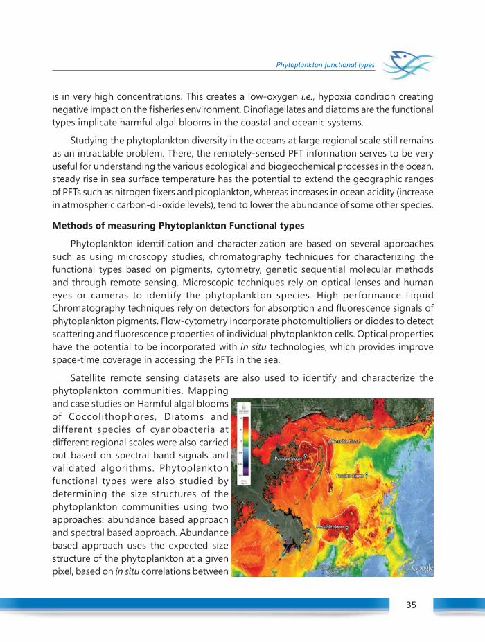
Winter School on Structure and Function of the Marine Ecosystem : Fisheries 35
Phytoplankton functional types
35
is in very high concentrations. This creates a low-oxygen i.e., hypoxia condition creatingnegative impact on the fisheries environment. Dinoflagellates and diatoms are the functionaltypes implicate harmful algal blooms in the coastal and oceanic systems.
Studying the phytoplankton diversity in the oceans at large regional scale still remainsas an intractable problem. There, the remotely-sensed PFT information serves to be veryuseful for understanding the various ecological and biogeochemical processes in the ocean.steady rise in sea surface temperature has the potential to extend the geographic rangesof PFTs such as nitrogen fixers and picoplankton, whereas increases in ocean acidity (increasein atmospheric carbon-di-oxide levels), tend to lower the abundance of some other species.
Methods of measuring Phytoplankton Functional types
Phytoplankton identification and characterization are based on several approachessuch as using microscopy studies, chromatography techniques for characterizing thefunctional types based on pigments, cytometry, genetic sequential molecular methodsand through remote sensing. Microscopic techniques rely on optical lenses and humaneyes or cameras to identify the phytoplankton species. High performance LiquidChromatography techniques rely on detectors for absorption and fluorescence signals ofphytoplankton pigments. Flow-cytometry incorporate photomultipliers or diodes to detectscattering and fluorescence properties of individual phytoplankton cells. Optical propertieshave the potential to be incorporated with in situ technologies, which provides improvespace-time coverage in accessing the PFTs in the sea.
Satellite remote sensing datasets are also used to identify and characterize thephytoplankton communities. Mappingand case studies on Harmful algal bloomsof Coccolithophores, Diatoms anddifferent species of cyanobacteria atdifferent regional scales were also carriedout based on spectral band signals andvalidated algorithms. Phytoplanktonfunctional types were also studied bydetermining the size structures of thephytoplankton communities using twoapproaches: abundance based approachand spectral based approach. Abundancebased approach uses the expected sizestructure of the phytoplankton at a givenpixel, based on in situ correlations between
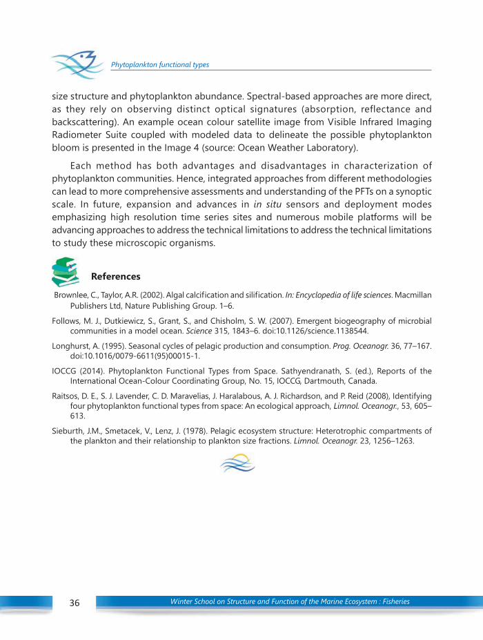
Winter School on Structure and Function of the Marine Ecosystem : Fisheries36
Phytoplankton functional types
size structure and phytoplankton abundance. Spectral-based approaches are more direct,as they rely on observing distinct optical signatures (absorption, reflectance andbackscattering). An example ocean colour satellite image from Visible Infrared ImagingRadiometer Suite coupled with modeled data to delineate the possible phytoplanktonbloom is presented in the Image 4 (source: Ocean Weather Laboratory).
Each method has both advantages and disadvantages in characterization ofphytoplankton communities. Hence, integrated approaches from different methodologiescan lead to more comprehensive assessments and understanding of the PFTs on a synopticscale. In future, expansion and advances in in situ sensors and deployment modesemphasizing high resolution time series sites and numerous mobile platforms will beadvancing approaches to address the technical limitations to address the technical limitationsto study these microscopic organisms.
References
Brownlee, C., Taylor, A.R. (2002). Algal calcification and silification. In: Encyclopedia of life sciences. MacmillanPublishers Ltd, Nature Publishing Group. 1–6.
Follows, M. J., Dutkiewicz, S., Grant, S., and Chisholm, S. W. (2007). Emergent biogeography of microbialcommunities in a model ocean. Science 315, 1843–6. doi:10.1126/science.1138544.
Longhurst, A. (1995). Seasonal cycles of pelagic production and consumption. Prog. Oceanogr. 36, 77–167.doi:10.1016/0079-6611(95)00015-1.
IOCCG (2014). Phytoplankton Functional Types from Space. Sathyendranath, S. (ed.), Reports of theInternational Ocean-Colour Coordinating Group, No. 15, IOCCG, Dartmouth, Canada.
Raitsos, D. E., S. J. Lavender, C. D. Maravelias, J. Haralabous, A. J. Richardson, and P. Reid (2008), Identifyingfour phytoplankton functional types from space: An ecological approach, Limnol. Oceanogr., 53, 605–613.
Sieburth, J.M., Smetacek, V., Lenz, J. (1978). Pelagic ecosystem structure: Heterotrophic compartments ofthe plankton and their relationship to plankton size fractions. Limnol. Oceanogr. 23, 1256–1263.

Winter School on Structure and Function of the Marine Ecosystem : Fisheries 37
Phytoplankton Taxonomy, Identification and Enumeration
Introduction
Phytoplankton are microscopic, free floating organisms and is the principal primaryproducers of the oceans. Their size range from 0.2 µm to 2 mm. Phytoplankton containsprimary pigments and accessory pigments such as chlorophyll (Chl), carotenoids etc. whichstrongly absorbs the blue and red light of the visible spectra. Phytoplankton also influencesthe total scattering properties of sea water. Due to their relatively large size, the largerphytoplankton species contributes relatively little to backscattering in the visible spectrum.The principal phytoplankton taxonomic groups include:-
Class Bacillariophyceae - DiatomsClass Pyrrophyceae - DinoflagellatesClass Prymnesiophyceae - CoccolithophoresClass Chrysophyceae - SilicoflagellatesClass Euglenophyceae - Euglenoid flagellatesClass Chlorophyceae - Green algaeClass Cyanophyceae - Blue-green algaeClass Haptophyceae - Brown colored Phytoflagellates (Kennish 2001).
Class Bacillariophyceae (Diatoms)
The class Bacillariphyceae comprises diatoms with fascinating shapes and ornatepatterns. The common shapes include rounded (centric) and elongated (pennate). Diatomsare embedded in an outer wall made of silica and known by the frustules. The shape ofdiatoms are like a lab Petri dish or a soap box, with one valve larger in diameter (the “epivalve”)and the other one overlapping the reversed second valve (the “hypovalve”). Some diatomsattach to each other, while some others attach end to end at an angle to form colonies.Diatoms reproduces by asexual or vegetative reproduction. Sexual reproduction producingauxospores and resting spores are also reported. The visible accessory pigmentation indiatoms are of golden colour.
Centric diatoms are characterized by their radial symmetry are common to the surfacewaters. Many centric diatoms have projecting spines, which increases their surface area inrelation to the volume of water holding them up, which helps them stay buoyant. Pennate
06C H A P T E R PHYTOPLANKTON TAXONOMY,
IDENTIFICATION AND ENUMERATIONNandini Menon1 and Minu P.2
1Nansen Environmental Research Centre India, Kochi2ICAR-Central Marine Fisheries Research Institute

Winter School on Structure and Function of the Marine Ecosystem : Fisheries38
Phytoplankton Taxonomy, Identification and Enumeration
diatoms have elongated valves and are more likely to be found on shallow bottoms. Pennatediatoms have a groove on their underside, called a “raphe,” which secretes mucus.
Class Pyrrophyceae (Dinoflagellates)
This name’s Greek origin means “spinning tail;” so named because these microscopicorganisms have flagella–tiny tails made of protein strands. As the name indicates these areembedded with 2 (dino) flagella. These whip-like flagella helps them to propel in the waterand are sometimes used for attachment . The two flagella are dissimilar in size, one wrappedaround the body and one extending outward from the body. In dinoflagellates, the accessorypigments are coloured of red to reddish brown. The outer wall of dinoflagellates are madeof cellulose. Dinoflagellates are differentiated into two owing to the presence or absence ofarmoured plates. Some dinoflagellates have thick armoured plates that fit together, like thearmour of medieval knights and these plates can slide apart or over each other. Others areunarmored or naked. Bioluminiscence is another peculiarity of dinoflagellates.
Class Prymnesiophyceae (Coccolithophores)
Coccolithophores surround themselves with a microscopic plating made of limestone(calcite). These scales, known as coccoliths, are shaped like hubcaps and are only three one-thousandths of a millimeter in diameter.
Class Chrysophyceae (Silicoflagellates)
Small single-celled flagellates and flagellated colonies. Common in oligotrophic clearwaters and humic waters. The algae coming under this family is commonly known as goldenalgae. The cells are naked or covered by scales, lorica or cell wall. The flagellate cell usuallypossesses two heterodynamic flagella. This algal family is unicellular or colonial. The pigmentsare chlorophyll-a, -c and fucoxanthin; this fucoxanthin which give the characteristic colour.It stores energy in the form both as carbohydrate and oil droplets. Presence silica depositionvesicle, flagella apical and unequal in length. Asexual reproduction by binary fission,sporogenesis. Sexual reproduction reported in some members. The lifecycle is haplontic inchrysophyceae.
Class Euglenophycea (Euglenoid flagellates)The euglenophyceans are basically unicellular flagellate. The cell is usually naked, but
some species such as Trachelomonas (Euglenales) possess lorica deposited by iron andmagnesium. The most unique feature of the Euglenophyceae is the presence of proteinaceousstrips, pelicler strips beneath the cell membrane. The species with many flexible pelliclerstrips. In the Euglenophyceae, a photosynthetic genus, as well as many colorless phagotrophicor osmotrophic species are present. The green chloroplast is originated via secondaryendosymbiosis with a green plant at the common ancestor of the Eutreptiales and Euglenales.
Winter School on Structure and Function of the Marine Ecosystem : Fisheries 39
Phytoplankton Taxonomy, Identification and Enumeration
Class Chlorophyceae (Green algae)
Chlorophyceae (chloros, green; phyceae, algal organisation) is commonly known asgreen algae. Green algae are characterized by the presence of green plastids known aschloroplast. This containing a starch storing region called pyrenoids. The members ofChlorophyceae generally grow in fresh water (about 90%) and the rest in saline water,terrestrial habitat etc. The fresh water members such as Volvox, Oedogonium, Spirogyra etc.grow in ponds, pools and lakes. Flagella are 1-many, equal in size and inserted either apicallyor sub-apically. The flagella show typical 9+2 arrangement when viewed under E.M. Thecells are eukaryotic in nature. The cell wall is mainly made up of cellulose, which comprisedof hydroxyproline glyco-sides or xylans and mannans. The flagellate cells have eye-spot orstigma in the anterior portion, which remain inser-ted at one side of the chloroplast.
Class Cyanophyceae (Blue-green algae)
Members of the class Myxophyceae (Cyanophyceae) are commonly known as bluegreen algae. The name blue green algae is given because of the presence of a dominantpigment c-phycocyanin, the blue green pigment. In addition, other pigments like chlorophylla (green), c-phycoerythrin (red), â-carotene and different xanthophylls are also present. Themembers of this class are the simplest living autotrophic prokaryotes. Nucleus is ofprokaryotic nature i.e., devoid of nuclear membrane and nucleolus, Absence of well-organisedcell orga-nelles, and Pigments are distributed throughout the chromoplasm (the outer partof proto-plasm). Locomotion is generally absent, but when occurs, it is of gliding or jerkytype.
Class Haptophyceae (Brown colored Phytoflagellates)
Unicellular, mostly marine, mostly photosynthetic. Around 80 genera, 500 species (=relatively low diversity). Ecologically important component of phytoplankton communitiesat all latitudes. Mostly nannoplankton (2-20 micron) size fraction. Mostly motile with 2flagella. Characteristic feature: presence of a haptonema. Two smooth flagella, equal orunequal in length. Almost all haptophytes are photosynthetic (one species isn’t), but mostmay actually be mixotrophic. All haptophytes contain chlorophylls a and c, as well as ?-carotene, diatoxanthin and diadinoxanthin. In this they resemble heterokonts.
Characters for phytoplankton identification
Phytoplankton are identified based on thier:-
Cell shape / size
Mode of life (solitary, colonies, filaments…)
Organelles : presence / absence
Winter School on Structure and Function of the Marine Ecosystem : Fisheries40
Phytoplankton Taxonomy, Identification and Enumeration
Plastids: colour, number, shape, ultrastructure
Cell covering (frustule, scales, theca, cyst…)
Flagella (number, length, insertion)
Reserve substances (nature, localisation)
Other characters (stigma, haptonema, pseudopods, …)
Sample Collection, Preservation and Enumeration
Sampling Design
Offshore and inshore sampling designs differ according to seasons, locations, depths,substrates, purpose of monitoring and available manpower and equipments. To detect earlyphases of phytoplankton blooms, frequency of sampling becomes important because bloomscan develop over a period of 2 to 3 weeks or be transported into an area. Monitoring ofsentinel filter feeding species is also beneficial, e.g., bivalves and tunicates.
Sample Collection
Before sampling begins, the manpower involved has to be thorough in sampling design(transects and adaptive sampling), frequency, collection methods, variables to be measured,data recording and storage, and the best approach to meet the goals of the program.Repetitive sampling at fixed stations is desired for statistical analysis of data (plankton,nutrients, salinity, temperature, etc.). Processing enough sample volume is also important.Distance between stations can be critical because of oceanographic conditions. Samplingfor planktonic blooms and conditions should involve sampling or profiling with depthbecause the water column is 3 dimensional. It may also involve monitoring “seed” beds inthe benthos to determine and even predict timing of blooms. Sampling for benthic algalblooms requires collecting substrate, e.g., sediments, on a routine basis. Processing requiresremoval of HA cells for analysis.
Equipments for collection of samples include Bucket, weighted, bottle or Niskin sampler.The bottles used for collecting live samples has to be properly labeled. The label shouldcontain Station Identification No, Latitude/Longitude, Depth at which sample was collected,name of fixatives used and date of sampling. Latitude /Longitude can be identified usingGPS unit. A data log sheet also has to be maintained specifying all the details collected forthe sample. This may include pH, temperature (using thermometer) etc. Lead weightedbottles can be used for collection of phytoplankton samples upto 40m depth. For collectingof sample at depths <200m, Niskin sampler can be used. This uses weights or ropes on wireto trigger the closing of openings in this sampler. The sample collection can be assistedwith a portable data profiler which is able to measure pH, Dissolved Oxygen, Conductivity,
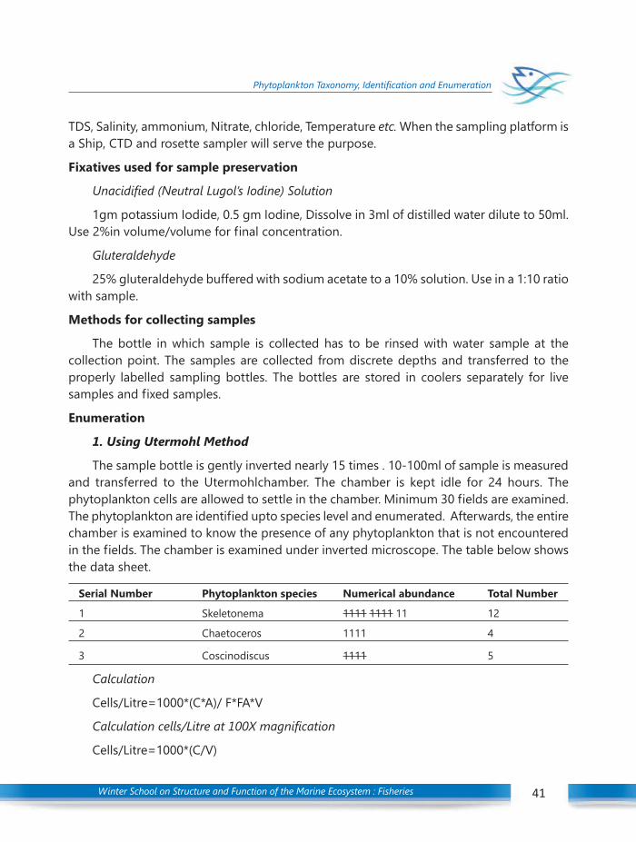
Winter School on Structure and Function of the Marine Ecosystem : Fisheries 41
Phytoplankton Taxonomy, Identification and Enumeration
TDS, Salinity, ammonium, Nitrate, chloride, Temperature etc. When the sampling platform isa Ship, CTD and rosette sampler will serve the purpose.
Fixatives used for sample preservation
Unacidified (Neutral Lugol’s Iodine) Solution
1gm potassium Iodide, 0.5 gm Iodine, Dissolve in 3ml of distilled water dilute to 50ml.Use 2%in volume/volume for final concentration.
Gluteraldehyde
25% gluteraldehyde buffered with sodium acetate to a 10% solution. Use in a 1:10 ratiowith sample.
Methods for collecting samples
The bottle in which sample is collected has to be rinsed with water sample at thecollection point. The samples are collected from discrete depths and transferred to theproperly labelled sampling bottles. The bottles are stored in coolers separately for livesamples and fixed samples.
Enumeration
1. Using Utermohl Method
The sample bottle is gently inverted nearly 15 times . 10-100ml of sample is measuredand transferred to the Utermohlchamber. The chamber is kept idle for 24 hours. Thephytoplankton cells are allowed to settle in the chamber. Minimum 30 fields are examined.The phytoplankton are identified upto species level and enumerated. Afterwards, the entirechamber is examined to know the presence of any phytoplankton that is not encounteredin the fields. The chamber is examined under inverted microscope. The table below showsthe data sheet.
Serial Number Phytoplankton species Numerical abundance Total Number
1 Skeletonema 1111 1111 11 12
2 Chaetoceros 1111 4
3 Coscinodiscus 1111 5
Calculation
Cells/Litre=1000*(C*A)/ F*FA*V
Calculation cells/Litre at 100X magnification
Cells/Litre=1000*(C/V)

Winter School on Structure and Function of the Marine Ecosystem : Fisheries42
Phytoplankton Taxonomy, Identification and Enumeration
C = Number of cells counted
A = Area of chamber bottom
F = Number of fields counted
FA = Area of Field view
V = Volume settled
2. Using Nunc Method
The bottle containing samples are inverted nearly 15 times. About 3ml of sample ismeasured using a pipette. The samples are transferred to Nunc chamber. Cells are allowedto settle for 30 minutes. The cells are identified and enumerated for entire bottom of chamberusing inverted microscope. For dense samples, reduced volume (0.3 ml - 0.03 ml) are usedfor enumeration. Sterile filtered seawater is added to the chamber to level out the sample.
The advantage of Using Nunc chamber is that resolution of cells and morphologyareright upto the edge of the chamber side without distortion, optical transects can be countedeasily, and cells can be moved easily for further analysis. The disadvantage includes use oflimited volume of sample and higher cost. Limited number of usage of Nunc chambers isalso a drawback.
3. Using Sedge-wick Rafter
Sedgewick rafter slides are used for examining 1ml of sample. The slide is designed tooccupy 1ml of sample and partitioned into 1000 grids each with an area of 1mm3.Identification and enumeration is done in 4x4 grids or on random selection. A minimum of3 such grids are examined under microscope. The average number is then calculated andscaled for 1ml.
N=(n*v*1000)V
Where N = number of cells per litren = number of cells per millilitreV = total volume filteredv = volume of sub-sample
References
1. http://nora.nerc.ac.uk/5654/1/Phytoplankton_Counting_Guidance_v1_2007_12_05.pdf
2. http://nio.org/userfiles/file/biology/Phytoplankton-manual.pdf

Winter School on Structure and Function of the Marine Ecosystem : Fisheries 43
Algal Culture Methods
Stock Culture
All algae culture systems require a set of ‘stock’ cultures, usually of about 250ml involume, to provide the reservoir of algal cells from which to start the larger-scale cultureswhich will be used for feeding.
Stock cultures are kept in small flasks, such as 500ml borosilicate glass, flat-bottomedboiling flasks fitted with cotton-wool bungs. Two types of culture medium can be used:
a) Erdschreiber culture medium, which is difficult to prepare but very reliable; and
b) simpler, but less reliable culture medium
Sub culture
Stock cultures must be sub-cultured frequently. Sub-culturing involves inoculating somecells from an old stock culture into fresh culture medium, so that the cells can continue togrow and divide and remain healthy. If sub-culturing is not carried out, the algal cells in thestock culture will eventually die. It is important to take precautions to prevent contaminantsfrom the air entering the stock cultures when sub-culturing.
To start a new stock culture, about 20ml of algae are taken from a stock culture whichhas been growing for 6 to 7 days and poured into a flask containing 250ml of fresh culturemedium. After removing the cotton-wool bungs, and before and after pouring, the necksof both flasks should be passed through a gas flame, such as that from a Bunsen burner orspirit lamp, to kill the new stock culture should be put about 20cm from a fluorescent lampthat is lit continually. The air temperature around the culture should be less than 25°C. Notethat stock cultures do not require an air/CO2 supply.
After sub-culturing, the remainder of the old stock culture can be used to start a batchculture of up to 10 litres. If the stock culture is not required immediately, it may be kept forup to 3 weeks on a shelf in a north-facing window (away from direct sunlight), But after thistime it should be discarded.
Types of Culture
There are many different ways of culturing algae. These range from closely-controlledmethods on the laboratory bench top, with a few litres algae, to less predictable methods in
07C H A P T E R ALGAL CULTURE METHODS
Shoji Joseph
Mariculture DivisionICAR-Central Marine Fisheries Research Institute
Winter School on Structure and Function of the Marine Ecosystem : Fisheries44
Algal Culture Methods
outdoor tanks, containing thousands of litres, in which production relies on natural conditions.Several methods have been developed at Conwy, for the production of algae for use asfood for various marine animals.
There are certain requirements for all methods. A culture must be inoculated, and thealgae left to grow and divide. The rate of growth and division varies with different types ofalgae left to grow and divide. The rate of growth and division varies with different types ofalgae and also depends on how well the various culture conditions necessary for growthhave been met. When there are sufficient algal cells in the container for feeding, one of thethree culture methods below may be followed:
Batch culture
Batch culture is a system where the total culture is harvested and used as food. Ifrequired, another culture can be set up to replace it.
Semi-continuous culture
Semi-continuous culture is a system where part of the culture is harvested and used asfood, and the amount taken is replaced with fresh culture medium (clean sea water andnutrient salts). After allowing 2-3 days for the remaining cells to grow and divide, the processis repeated. Semi-continuous cultures may be operated for up to 7 to 8 weeks.
Continuous culture
This falls into two categories:
i) turbidostat culture, in which the number of algal cells in the culture is monitoredand, as the cells divide and grow, an automatic system keeps the culture density ata pre-set level by diluting the culture with fresh medium; and
ii) chemostat culture, in which a flow of fresh medium is introduced into the cultureat a steady, pre-determined rate.
With both types, the surplus culture overflows into a collecting container, from which itcan be taken and used as food.
With semi-continuous and continuous culture methods, the number of food cellsproduced (the yield) varies with the density of the culture. For each type of algae, thegreatest yield is obtained by maintaining the culture at an optimum density. This optimumdensity can be determined experimentally and is given for each of the culture systems asdescribed in the following section.
Winter School on Structure and Function of the Marine Ecosystem : Fisheries 45
Algal Culture Methods
Some culture methods
Batch culture (small volumes of up to 10 litres)
Where small volumes of algae culture are required, for example, of 2 litres to 10 litresper day, production is most conveniently achieved in flasks. An example of a batch culturesystem for producing 3 litres of food per day from a culture of Chaetoceros calcitrans isgiven below and is described as daily procedures.
A set of three, 250 ml stock cultures is started by inoculating from one existing 250 mlstock culture on each of 3 successive days. The new stock cultures are grown at a temperatureof about 21°C, and at a distance of 15 to 20 cm from a 65 watt fluorescent tube. After 3days, and then daily, each of these stock cultures is used in turn to inoculate a new 250 mlstock culture then daily, each of these stock cultures is used in turn to inoculate a new 250ml stock culture and the remainder is added to the 3 litre sea-water culture medium in theflasks, which have been prepared as follows:
Three-litre borosilicate glass flasks with cotton wool plugs are filled with sea water. Thecontents are either autoclaved at 1.06kg per square centimeter (15 psi) for 20 minutes,boiled for 30-45 minutes, or pasteurized. Whichever method is used, the sea water in theflasks should be allowed to cool before adding nutrient salts, Alternatively, sea water thathas been filtered through a half micron filter may be used. To the 3 litres of sea water in theflask, 6 ml solution A, 0.6 ml of solution C and 6 ml of solution D are added.
A fresh 3 litre culture is started daily from a 3-day-old stock culture and aerated with amixture of air and CO2 at about 2 to 3 litres per minute. The gas mixture is filtered throughan in-line catridge unit containing a 0.3-0.45 micron filter to reduce the risk of airbornecontamination. When grown at about 21°C next to a continually lit, double flurescent lampunit, a density of 45000 to 60000 cells per microlitre is reached in 3 to 4 days in culturemedium prepared from heat treated sea water. In medium prepared from filtered sea water,growth of Chaetoceros is not as rapid and the density will only reach 20000 to 30000 cellsper microlitre in this time. The culture should immediately be used for feeding, as if kept itwill enter a declining phase, collapse, and become unsuitable.
Algae other than Chaetoceros usually take longer to grow under similar culture conditions.For these algae, stock cultures should be routinely sub-cultured every 6 to 7 days. Thebatch cultures, which are started from 6 or 7 day old stock cultures, will take 7 to 8 days togrow to a density suitable for feeding. Larger containers, of up to 10 litres, may be used forthis method of culture. Nutrient salt solutions are used a s follows:
Solution A- 1ml per litreSolution C- 0.1 ml per litre; and
Winter School on Structure and Function of the Marine Ecosystem : Fisheries46
Algal Culture Methods
Solution D (diatoms only) – 2ml per litre.
The batch cultures may be used directly as food or as inocula to start larger volumebatch, semi-continuous or continuous food cultures.
Semi-continuous culture
Two-hundred-litre vessels
A method for large scale production in 200 litre, internally illuminated, glass reinforcedplastic (grp) vessels, using semi-continuous culture is described below.
The vessels are 150 cm high, 40-45 cm in diameter and each has a central lighting unitinto which are fitted six fluorescent lamps. A glass- fibre cooling pipe is moulded onto theouter jacket. These vessels are most useful for growing diatoms, but they may also be usedfor flagellates. The vessels are sterilized by filling with a solution of sodium hypochlorite (50parts per million (ppm) free-chlorine concentrations). Note that domestic bleach containsabout 100000 to 150000 ppm chlorine, so a dilution of 1 ml per 2-3 litres would give therequired concentration. They are allowed to stand for 2-4 hours and the drained, and flushedwith filtered air for 24 hours to drive off residual chlorine.
The vessels are filled (200 litres come to about 15 cm from the top) with filtered seawater at 20 psu to 25 psu salinity for diatiom cultures or 25 psu to 30 psu for flagellatecultures. For diatom cultures, filtration to 2 microns is usually sufficient, while for culture offlagellates, filtration to half a micron is preferable. Two hundred milliliters of solution A 20ml of Solution C and, for diatom cultures, 1200 ml of Solution D are added to the vessels.The culture is inoculated with 2 to 5 litres of a 4 to 8 day-old batch culture, grown asdescribed in the previous section and aerated with a filtered air/CO2 supply at about 15litres per minute.
Cultures should reach densities suitable for harvesting after 4 to 7 days. The culturesshould be subsequently be diluted for the maximum yield. The amount of harvest whichachieves this yield can be calculated from the following equation:
200 x densities to which culture needs to be dilutedVolume to harvest in liters = ———————————————————————
Actual culture density of algae harvested
After harvesting, the vessels are topped-up to 200 litres with filtered sea water of thecorrect salinity. For each litre harvested, 1 ml of solution A, 0.1 ml of solution C and, fordiatom cultures, 6 ml of solution D are added. It is usually more convenient to harvest theculture every 2 to 3 days (e.g Mondays, Wednesdays and Fridays). That part of the harvestwhich is required for feeding on the intermediate days can be aerated in a plastic containeraway from bright light and in a cool place.
Winter School on Structure and Function of the Marine Ecosystem : Fisheries 47
Algal Culture Methods
The length of time during which the culture is able to produce food will vary with thetype of algae. Production of algae from 200 litre vessels should average the equivalent of60-80 litres per day at the cell densities. When the culture is no longer required, or it hascome to the end of its production period, the vessel can be drained and cleaned with a stiffbrush, to remove any algae adhering to the sides. The vessel can now be sterilized forpreparation for a new culture.
Continuous culture
This method is suitable for the culture of flagellates. The internally-illuminated,continuous culture vessels are made from polyethylene tubing supported by a metalframework. They consist of 160 cm lengths cut from 71 cm wide polyethylene, ‘layflat’tubing. The tubing is free of potential contaminants due to the heat used in the manufacturingprocess and no further sterilization is necessary. The cut length is heat sealed across thewidth of one end and positioned around the acrylic cylinder containing the lamps. The sixnuts and bolts securing the outer supporting mesh jacket are fastened and the outer reflectivesheet of white, corrugated plastic is held in place by 12.7mm nylon power belting, whichalso supports the sensor housing unit against the outer surface of the culture.
The polyethylene tubing is filled with sea water at 25 psu to 30 psu salinity that hasbeen filtered through a sterile, 0.45 micron, particle retention catridge filter. If the water hasa high silt load, it should first be passed through a 2 micron filter. Solution A (100ml) andSolution C (10ml) are added to the sea water in the vessel. This is 2.5 times the usual amount,and is added to ensure that nutrient levels do not become limiting at the high cell densitiesat which the cultures are maintained. A 2.5 cm diameter circle is cut from the tubing, with itscentre about 7 cm above the water level. Into this is fitted a 1.9 cm rigid, PVC tank connector,from which a 150 cm length of 1.5 cm bore flexible PVC tubing is run into a 125 litre collectingvessel. The overflow allows for automatic harvesting of the culture into the reservoir.
A supply of filtered air, enriched with sufficient carbon dioxide to maintain culture pHat 7.6-7.8 is introduced through a 0.4 cm bore, 150 cm long, acrylic tube inserted into thetop of the culture. A flow rate of about 15 litres per minute ensures efficient mixing of theculture.
Cooling water, at a flow rate of about 0.35 litre per minute, is allowed to run down overthe outer culture surface in order to maintain the culture temperature at about 21°C. The40 litre culture should be inoculated with a 2 litre batch culture that has grown for 7 to 8days.
Automatic harvesting of the culture is controlled by the following method. A cadmiumsulphide photo-conductive cell is enclosed in a light-proof housing against the outer surface
Winter School on Structure and Function of the Marine Ecosystem : Fisheries48
Algal Culture Methods
of the culture. The housing is placed about 50 cm from the base of the vessel and positionedso that the stream of air bubbles rising through the culture does not interfere with itsoperation. The resistance of the photo-conductive cell will increase as the light intensityreaching it from the lamps falls, when density of the culture increases, due to growth anddivision of the algal cells. A circuit switching the peristaltic pump will be energized when theresistance of the cell becomes greater than a present value on a relay sensitive to inputresistance in the range 50-5000 ohm. Sea water, at 25 psu to 30 psu and enriched with 2.5ml of solution A per litre and 0.25 ml of solution C per litre, is then pumped from the culturemedium reservoir through the filter into the vessel and the volume is maintained by anoverflow. The outflow of algae culture from the vessel is collected in an aerated container.As the culture is diluted, the decrease in resistance of the photo-conductive cell, caused bythe higher light intensity now reaching it, is sensed by the relay and the pump circuit isswitched off.
The relay should be set so that automatic harvesting of the culture occurs at the densitythat gives the most yield. When the yield begins to fall appreciably, all of the culture shouldbe harvested for feeding and the bag discarded. A new, clean bag should be fitted to thevessel and the above operating procedure repeated.
Photobioreactors
Design Considerations
Many configurations of photobioreactors have been devised and built. These rangefrom tubular and cylindrical systems to conical systems (Watanabe and Hall 1996, Morita etal., 2000) to flat-sided vessels (Delente et al., 1992, Iqbal et al., 1993, Hu et al., 1998), andthese systems employ a wide variety of light sources (Takano et al., 1992, Lee and Palsson1994, An and Kim 2000). As such, each is usually a highly customized system and theavailability of commercial photobioreactors is limited.
Despite various configurations, several basic design features must be considered whenbuilding a photobioreactor: how to provide light, how to circulate the algae, which materialsto use for construction, how to provide CO2 and remove O2, and how to control pH andtemperature. Sophistication is driven by purpose, and if whole algal biomass is the desiredfinal product, a relatively unsophisticated system will suffice. Glass and acrylic are widelyused in the construction of photobioreactors, and ultraviolet (UV)-stabilized acrylic is superiorbecause it is lighter, more flexible, stronger, and easier to machine, cut, bond, and so on.Construction requires some minimal construction skills, but certainly not professional skills.Assembly of the photobioreactor system is merely the integration of various monitor andcontrol subsystems (e.g., pH control and temperature control).
Winter School on Structure and Function of the Marine Ecosystem : Fisheries 49
Algal Culture Methods
Light
Light is the most important parameter in the design and construction of aphotobioreactor. Despite its importance, light can be a very difficult input to measure forefficient use (Pirt et al., 1983, Kirk 1994, Ogbonna et al., 1995, Janssen et al., 2002). Light canbe supplied continually or in light-dark cycles. As cell concentration changes, the lightrequirements change. Algal growth is limited by too little light, but too much light can be asdeleterious. Phototrophs must receive sufficient light to exceed their light compensationpoint for their net growth; insufficient growth detracts from the net growth of the culturebecause of respiratory loss (Radmer et al., 1987). Increasing light beyond the compensationpoint results in an increase in the growth rate until the culture becomes light saturated, andhigher light intensities can lead to photoinhibition (AcienFernandez et al. 1998, Csögör etal., 2001, Yun and Park 2001, Wu and Merchuk 2002, Barbosa et al., 2003, Suh and Lee2003). Incandescent lamps are inferior to the other lamps and are seldom used forphotobioreactors (Table 13.1). Both fluorescent and high-intensity discharge lamps havevery good electrical efficacy and substantial lifetimes. Fluorescent lamps distribute lightmore or less uniformly along the length of the lamp; light emanates from a point source inhigh-intensity discharge lamps, requiring distance between the lamp and algae for properlight dispersion. Although high-intensity discharge lamps are slightly more efficient thanfluorescent lamps, however, fluorescent lamps offer the best all-around choice (Radmer etal., 1987, Radmer 1990, Delente et al., 1992).
Circulation
Circulation is important to ensure optimum illumination of the algae, adequate gasexchange, and temperature and pH control within the culture. The “airlift” principle in whichcirculation is accomplished by creating differences in water density in different regions ofthe photobioreactor is the one in commonly using (Manfredini and Molina Grima et al.,1995, Blanch and Clark 1997). This principle is common in fermentors (see later discussion)and has been adapted for use in photobioreactors.
Photobioreactors can be bubbled with air, but the low CO2 concentration in air (0.033%)will often limit phototrophic growth. With an airflow of 1 L min-1, assuming all carbon dioxideis used and the biomass is 50% carbon, there is enough carbon to support 3.54 *10-4 gramsbiomass · min-1; this is a very low productivity. The simplest approach is to blend CO2 withair, for example, 0.2 to 5.0% of the total gas flow (Lee and Pirt 1984, Merchuk et al., 2000,Morita et al., 2001, Babcock et al., 2002). Care must be taken to ensure that the CO2 inputdoes not adversely lower the pH level of the culture. Also, with an open system, most of theCO2 will exit the vessel unused. Small bubble size helps facilitate diffusion.

Winter School on Structure and Function of the Marine Ecosystem : Fisheries50
Algal Culture Methods
Temperature and pH
After light, CO2, and O2, pH and temperature are the next most important parametersto measure and control. Fortunately, these are very simple parameters to control usingexisting off-the-shelf technology (Sonnleitner 1999). Commercially available pH controllers(Omega Engineering) are recommended. Photosynthetic systems will always generate heatbecause of the inefficiency of photosynthesis in converting light energy into chemical energy(Pirt, 1983, Morita et al., 2001). The theoretical conversion of red light into chemical energy(NADPH) is only 31%; 69% is lost as heat. The amount of cooling depends on the incidentlight intensity and the cell concentration (i.e., how much light is absorbed), but regardless,cooling will be necessary. In principal, it is quite easy to control the temperature usingcommercially available temperature controllers (Omega Engineering). Cooling is achievedwith a heat exchange system; external cool water is circulated through a good heatconducting material, which then draws heat from the photobioreactor. The more significantchallenge is how to install a cooling system on a photobioreactor. The most preferred systemis the one uses stainless steel cooling coils submerged in the culture medium. There isexcellent contact between the cooling coil and water, which provides good cooling, but thecooling coil sometimes interferes with the circulation within the vessel. A refrigerated watersource (or tap water, depending on the cooling demands of the culture) is used, and atemperature probe, connected to a controller, operates a solenoid to regulate cooling waterflow. The best strategy is to use a “normally open” solenoid so that if there is a failure of thecontroller, the photobioreactor will overcool, which is preferred to overheating.
Sterilization
For many phototrophs, gross contamination by bacteria and fungi is not a significantproblem because there is generally very little free organic carbon to support their growth(see Chapter 5 on sterility). A higher concern is to prevent contamination of thephotobioreactor by other phototrophs. Photobioreactors are made of optically clear materials(e.g., glass or acrylic) which do not lend themselves to steam sterilization. Furthermore, thesize of most photobioreactors exceeds what can be accommodated in an autoclave. Systemsexist for sterilization with ozone (Quesnel 1987), but these systems are expensive and difficultto use. A more practical solution is sanitization rather than sterilization. Photobioreactorsanitization can be easily accomplished with bleach. Air pumps, analyzers, and otherequipment can be kept free of algae and other microorganisms by the use of the appropriateprefilters.
Operational Strategies
With adequate measurement and control of the basic culture parameters of light, CO2,O2, pH, and temperature, it is possible to optimize these parameters to achieve the desired
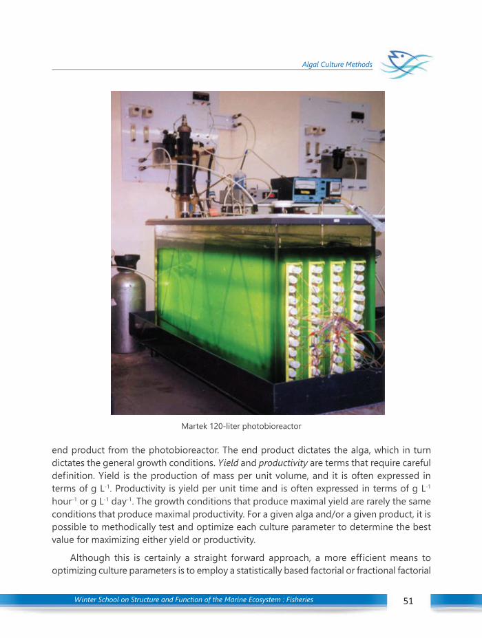
Winter School on Structure and Function of the Marine Ecosystem : Fisheries 51
Algal Culture Methods
end product from the photobioreactor. The end product dictates the alga, which in turndictates the general growth conditions. Yield and productivity are terms that require carefuldefinition. Yield is the production of mass per unit volume, and it is often expressed interms of g L-1. Productivity is yield per unit time and is often expressed in terms of g L-1
hour-1 or g L-1 day-1. The growth conditions that produce maximal yield are rarely the sameconditions that produce maximal productivity. For a given alga and/or a given product, it ispossible to methodically test and optimize each culture parameter to determine the bestvalue for maximizing either yield or productivity.
Although this is certainly a straight forward approach, a more efficient means tooptimizing culture parameters is to employ a statistically based factorial or fractional factorial
Martek 120-liter photobioreactor
Winter School on Structure and Function of the Marine Ecosystem : Fisheries52
Algal Culture Methods
approach to experimental design (Anderson and Whitcomb 2000).This method uses statisticsto identify the culture parameters and the interactions between culture parameters that aremost important for achieving maximal yield and/or productivity. Perhaps more importantly,this approach identifies those parameters that are not important for maximum yield and/orproductivity and thus eliminates the need for much unnecessary experimentation.
Harvesting Methods
The algal culture is still relatively dilute in a fully optimized photobioreactor. A dryweight concentration of even 5 to 10 g L-1 is far below that of a fermentor system(>50 g L-1). The two most common harvesting approaches for photobioreactors areflocculation and centrifugation (Sukenik and Shelef 1984, Becker 1994). Although flocculentsenable a concentration of the algal biomass, centrifugation is usually still necessary to achievea suitable volume reduction. Small-scale recovery can be easily done in large centrifugebottles, but larger scale cultures are best done with a continuous flow centrifuge such as aSharples (Sharples Penwalt).
Other methods
There are other, similar, methods for growing marine algae that may be more appropriatein certain circumstances. For example, externally-illuminated 20 litre glass jars can be operatedas batch cultures or semi-continuous cultures for a variety of algae. Another, widely used,type of culture container includes a mesh framework to support a 200-400 litre externally-illuminated polyethylene bag. Both of these methods have the disadvantage of being lessefficient, as the light energy cannot penetrate the culture as well as the internally- illuminatedunit, but they do have the advantage of being easier and cheaper to construct. Polyethylenebag cultures may also be operated as continuous, chemostat, cultures by using small pumpsto introduce fresh filtered medium to the culture at a pre-determined rate.
Extensive methods may be employed to culture marine algae. Outdoor tanks are nutrient-enriched with agricultural fertilizers. Adding 1.5 g of urea, 1.6 g of triple superphosphateand 10.6 g of sodium metasilicate will provide the required amounts of nitrogen, phosphorousand silica to stimulate growth and division of algal cells and, depending on the temperatureof the sea water and the amount of sunshine on the tanks, blooms of algae will develop.This system can be operated as a batch culture or managed as a semi-continuous orcontinuous culture with an in-flow of nutrient-enriched sea water to provide fresh mediumas an impetus to further algal growth. The method is especially suitable for providing algaefor feeding to bivalave mollusk spat held in nursery systems, or for mass ‘grow-out’ of brineshrimps (Artemia).
Winter School on Structure and Function of the Marine Ecosystem : Fisheries 53
Algal Culture Methods
Conclusions
Whatever method of large-scale algae culture is adopted, it is liable to be expensiveand technically difficult to operate. For this reason, a great deal of research is now beingdirected towards a suitable algae replacement diet for use in commercial aquaculture.Successful development of such a diet will perhaps eventually remove the need for large-scale production of algae for food.

Winter School on Structure and Function of the Marine Ecosystem : Fisheries54
Regional and Seasonal variations in Phytoplankton
The phytoplankton are the main energy source for marine ecosystems. They are themain producers of oxygen and form the basis of marine food web. The distribution ofphytoplankton is not unique all over the world. Some regions are more productive whileothers are not. The map (Figure 1) shows the phytoplankton production on a global scale.
Fig. 1. Map showing the phytoplankton productivity in the Oceans, Red and yellow are most productive,followed by green and blue. Black is least productive.
Vertical variation in phytoplankton production
Vertical variation in production is also observed in oceans. The deep layers of ocean arelight limited and hence photosynthesis, a process associated with sunlight cannot proceedleading low phytoplankton production. Another requirement for photosynthesis are sufficientconcentration of nutrients (nitrates, phosphates, silicates, iron, etc.). In stratified waters,growth of phytoplankton is “nutrient limited”. The nutrients in the upper mixed layer areconsumed by phytoplankton. The growth of phytoplankton occurs in the layer where bothlight and nutrient concentration are sufficient. The depth at which maximum phytoplanktongrowth occurs is known as deep chlorophyll maxima (Figure 2).
08C H A P T E R REGIONAL AND SEASONAL VARIATIONS IN
PHYTOPLANKTONNandini Menon1, Minu P.2, Muhammad Shafeeque2
and Grinson George2
1Nansen Environmental Research Centre India, Kochi2ICAR-Central Marine Fisheries Research Institute

Winter School on Structure and Function of the Marine Ecosystem : Fisheries 55
Regional and Seasonal variations in Phytoplankton
55
During upwelling, the bottom nutrients are broughtto the surface and hence the conditions of phytoplanktonbecome better and the maximum of its verticaldistribution moves to more shallow layer.
When intensive nutrient flux occurs, phytoplanktonbiomass proliferates and the maximum of verticaldistribution of phytoplankton is located at the surface.This results in a direct correlation between totalphytoplankton (or chlorophyll) concentration in watercolumn (or within the euphotic layer) and in the thinsurface layer (Figure 3). Hence, both the surfacechlorophyll concentration and the chlorophyll
concentration abovethe penetrationdepth can be used asa measure of waterproductivity, i.e., phytoplankton biomass. Verticaldistribution of ecosystem characteristics at a typicalstation in the oligotrophic waters shows deepphytoplankton maximum and nutricline. Deeper from thesurface less light is reflected or scattered byphytoplankton cells and contributes to the colour ofocean surface.Regional distribution of Phytoplankton
The distribution of phytoplankton varies spatially andtemporally. Nearshore waters are rich in phytoplankton.River runoff and upwelling are considered as the eventsfor higher production in coastal waters. In tropical regions,the production is comparatively low because of the limited
availability of trapped nutrients below the thermocline. In polar regions, insufficient light actsas the limiting source for phytoplankton production. Highest production occurs in the temperateregions. Sufficient light and nutrients acts as the driving forces for increased production inthese areas. The production pattern follows a two peak cycle in the regions. Spring peak isattributed with increased sunlight while fall peak is associated with increased mixing of nutrients.
Satellites equipped with colour scanners measure the concentration of chlorophyll inthe ocean. Chlorophyll is an indicator of plankton and can be used to study planktonpopulations.
Fig. 2. Vertical variation ofphytoplankton production in
stratified waters
Fig. 3. Vertical variation ofphytoplankton production in well
mixed waters
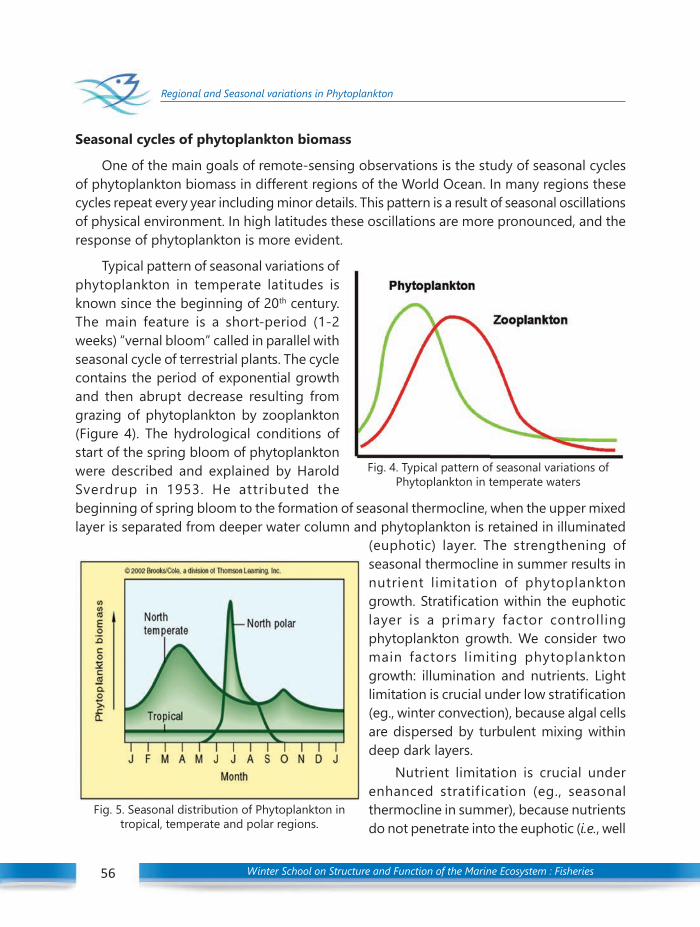
Winter School on Structure and Function of the Marine Ecosystem : Fisheries56
Regional and Seasonal variations in Phytoplankton
Fig. 4. Typical pattern of seasonal variations ofPhytoplankton in temperate waters
Seasonal cycles of phytoplankton biomass
One of the main goals of remote-sensing observations is the study of seasonal cyclesof phytoplankton biomass in different regions of the World Ocean. In many regions thesecycles repeat every year including minor details. This pattern is a result of seasonal oscillationsof physical environment. In high latitudes these oscillations are more pronounced, and theresponse of phytoplankton is more evident.
Typical pattern of seasonal variations ofphytoplankton in temperate latitudes isknown since the beginning of 20th century.The main feature is a short-period (1-2weeks) “vernal bloom” called in parallel withseasonal cycle of terrestrial plants. The cyclecontains the period of exponential growthand then abrupt decrease resulting fromgrazing of phytoplankton by zooplankton(Figure 4). The hydrological conditions ofstart of the spring bloom of phytoplanktonwere described and explained by HaroldSverdrup in 1953. He attributed thebeginning of spring bloom to the formation of seasonal thermocline, when the upper mixedlayer is separated from deeper water column and phytoplankton is retained in illuminated
(euphotic) layer. The strengthening ofseasonal thermocline in summer results innutrient limitation of phytoplanktongrowth. Stratification within the euphoticlayer is a primary factor controllingphytoplankton growth. We consider twomain factors limiting phytoplanktongrowth: illumination and nutrients. Lightlimitation is crucial under low stratification(eg., winter convection), because algal cellsare dispersed by turbulent mixing withindeep dark layers.
Nutrient limitation is crucial underenhanced stratif ication (eg., seasonalthermocline in summer), because nutrientsdo not penetrate into the euphotic (i.e., well
Fig. 5. Seasonal distribution of Phytoplankton intropical, temperate and polar regions.
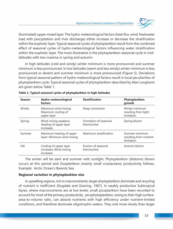
Winter School on Structure and Function of the Marine Ecosystem : Fisheries 57
Regional and Seasonal variations in Phytoplankton
57
illuminated) upper mixed layer. The hydro-meteorological factors (heat flux, wind, freshwaterload with precipitation and river discharge) either increase or decrease the stratificationwithin the euphotic layer. Typical seasonal cycles of phytoplankton result from the combinedeffect of seasonal cycles of hydro-meteorological factors influencing water stratificationwithin the euphotic layer. The most illustrative is the phytoplankton seasonal cycle in mid-latitudes with two maxima in spring and autumn:
In high latitudes (cold and windy) winter minimum is more pronounced and summerminimum is less pronounced. In low latitudes (warm and less windy) winter minimum is lesspronounced or absent and summer minimum is more pronounced (Figure 5). Deviationsfrom typical seasonal pattern of hydro-meteorological factors result in local peculiarities ofphytoplankton cycle. Typical seasonal cycles of phytoplankton described by Alan Longharstare given below Table 1.Table 1. Typical seasonal cycles of phytoplankton in high latitudes
Season Hydro-meteorological Stratification Phytoplanktonfactors growth
Winter Maximum wind mixing; Deep convection Winter minimumMaximum cooling of resulting from lightupper layer limitation
Spring Wind mixing weakens; Formation of seasonal Spring bloomHeating of upper layer thermoclineincreases
Summer Maximum heating of upper Maximum stratification Summer minimumlayer; Minimum wind mixing resulting from nutrient
limitation
Fall Cooling of upper layer Erosion of seasonal Autumn bloomincreases; Wind mixing thermoclineincreases
The winter will be dark and summer with sunlight. Phytoplankton (diatoms) bloomoccurs at this period and Zooplankton (mainly small crustaceans) productivity follows.Example: Arctic Ocean’s Barents Sea.
Regional variation in phytoplankton size
In upwelling regions, rich in macronutrients, larger phytoplankton dominate and recyclingof nutrient is inefficient (Dugdale and Goering, 1967). In weakly productive SubtropicalGyres, where macronutrients are at low levels, small picoplankton have been recorded toaccount for most of the primary productivity. picophytoplankton, owing to their high surface-area-to-volume ratio, can absorb nutrients with high efficiency under nutrient-limitedconditions, and therefore dominate oligotrophic waters. They sink more slowly than larger
Winter School on Structure and Function of the Marine Ecosystem : Fisheries58
Regional and Seasonal variations in Phytoplankton
cells. Microphytoplankton, represented chiefly by diatoms and dinoflagellates, dominatenutrient-rich waters and are the principal agents of the export of carbon to deeper waters. Thecontribution of smaller (eg., <2 µm) phytoplankton to total phytoplankton biomass decreasesin the colder, high-latitude waters and as temperature rises a shift to smaller species withina diatom community was reported.
References
Dugdale, R. C., Goering, J. J., 1967. Uptake of new and regenerated forms of nitrogen in primary productivity.Limnology and Oceanography 12, 677 – 680.
Sverdrup H.U., 1953. On conditions for the vernal blooming of phytoplankton. Journal du ConseilInternational pour l’Exploration du Mer, 18, pp. 287-295.
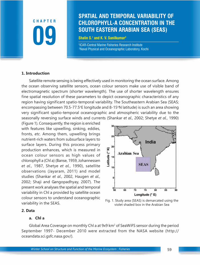
Winter School on Structure and Function of the Marine Ecosystem : Fisheries 59
Spatial and temporal variability of Chlorophyll-A concentration in the South Eastern Arabian Sea (SEAS)
1. Introduction
Satellite remote sensing is being effectively used in monitoring the ocean surface. Amongthe ocean observing satellite sensors, ocean colour sensors make use of visible band ofelectromagnetic spectrum (shorter wavelength). The use of shorter wavelength ensuresfine spatial resolution of these parameters to depict oceanographic characteristics of anyregion having significant spatio-temporal variability. The Southeastern Arabian Sea (SEAS;encompassing between 70.5-77.5oE longitude and 8-15oN latitude) is such an area showingvery significant spatio-temporal oceanographic and atmospheric variability due to theseasonally reversing surface winds and currents (Shankar et al., 2002; Shetye et al., 1990)(Figure 1). Consequently, the region is enrichedwith features like upwelling, sinking, eddies,fronts, etc. Among them, upwelling bringsnutrient-rich waters from subsurface layers tosurface layers. During this process primaryproduction enhances, which is measured inocean colour sensors as high values ofchlorophyll a (Chl a) (Banse, 1959, Johannessenet al., 1987, Shetye et al., 1990), satelliteobservations (Jayaram, 2011) and modelstudies (Shankar et al., 2002, Haugen et al.,2002; Shaji and Gangopadhyay, 2007). Thepresent work analyses the spatial and temporalvariability in Chl a provided by satellite oceancolour sensors to understand oceanographicvariability in the SEAS.
2. Data
a. Chl a
Global Area Coverage on monthly Chl a at 9x9 km2 of SeaWiFS sensor during the periodSeptember 1997- December 2010 were extracted from the NASA website (http://oceandata.sci.gsfc.nasa.gov/).
Fig. 1. Study area (SEAS) is demarcated using theviolet shaded box in the Arabian Sea
02C H A P T E R
09C H A P T E R
SPATIAL AND TEMPORAL VARIABILITY OFCHLOROPHYLL-A CONCENTRATION IN THESOUTH EASTERN ARABIAN SEA (SEAS)Shalin S.1 and K. V. Sanilkumar2
1ICAR-Central Marine Fisheries Research Institute 2Naval Physical and Oceanographic Laboratory, Kochi

Winter School on Structure and Function of the Marine Ecosystem : Fisheries60
Spatial and temporal variability of Chlorophyll-A concentration in the South Eastern Arabian Sea (SEAS)
b. Wind
Daily averaged wind data on zonal and meridional scale were extracted from QuikSCATfor the period 19 July 1999 – 19 November 2009 (ftp://www.ssmi.com). Monthly wind wasgenerated from the above dataset using ferret software. The alongshore component wascalculated for each area using the monthly averaged dataset.
c. SST
SST from MODIS / AQUA sensor at 9 km spatial resolutions were downloaded fromocean colour website (http://oceandata.sci.gsfc.nasa.gov) on monthly scale.
d. Sea Surface Height Anomaly (SSHA)
Monthly SSHA data during January 1992 - February 2010 were downloaded from AVISO(www.aviso.soest.hawaii.edu). The SSHA data obtained from AVISO is the merged productof TOPEX, ERS and Jason-1 altimetry. The data has a spatial resolution of 0.33o.
e. Rain data
Weekly rainfall data from TMI sensor (December 1997 – February 2011) at 0.25o x 0.25o
spatial resolution was downloaded to generate monthly rainfall rate.
3. Results
3.1. Spatial variability - Climatology of Chl a in the study area
Distribution of Chl a is examined to understand the climatology of these parameters inthe study area. In this regard, the monthly averages generated from the data provided bythe sensors SeaWiFS is used. The spatial distribution of Chl a brought out seasonal as wellas regional scale variability along the SEAS with maximum ranges of the variability duringthe southwest monsoon period (Figure 2).
Fig. 2. Monthly climatology of Chl a in the SEAS. The upper panels represent the distribution patternduring January to June and the lower panel during July to December.

Winter School on Structure and Function of the Marine Ecosystem : Fisheries 61
Spatial and temporal variability of Chlorophyll-A concentration in the South Eastern Arabian Sea (SEAS)
In general, the values of Chl a are high near the coast during all the months, whichdecreased towards offshore. During May, a marginal increase in Chl a sets in and this trendcontinues up to August. In addition, a significant cross-shore gradient is established in thesouthern area by June, which moves northward to encompass the entire study area byAugust and undergoes gradual decay during subsequent months. Similar to its intensification,the decay also starts from the south and moves northward. The gradient starts weakeningfrom September and disappears from the southern area by October. By November, it fadesoff the northern area too. Thereafter, low Chl a values continue up to April all through thearea.
3.2. Temporal variability
Most of the oceanographic and atmospheric parameters exhibit temporal variability.The time series observations on Chl a as obtained from SeaWiFS images during September1997 – December 2010 is analysed to understand the temporal variability on Chl a. Spatialdistribution has established the existence of large spatio-temporal variability in the studyarea especially during the southwest monsoon. Monthly Chl a were averaged for the selectedarea to explain their temporal variability. The influence of local environmental conditions(wind, ocean current, SSH and SST) on these parameters were also examined.
In general, Chl a in SEAS showed high values (> 1.20 mg m-3) during June – Septemberand very low values (~0.25 mg m-3) during December – April. May and October / Novembercan be considered as transition periods (Figure 3). The above three phases complete anannual cycle that recurs, while peak values occur during one of the months and found tovary each years between July and September (Table 1). In the following section, thecorresponding supporting parameters representing oceanographic and atmosphericconditions were examined, to understand their influence on Chl a distribution.
The supporting parameters showed that in general, low SST/ SSHA and high equatorwardcomponents of currents and winds existed during the southwest monsoon. SST was foundto follow a bi-annual oscillation, with lowest value in one of the months during the southwestmonsoon, whereas, SSHA showed an annual cycle again with minima in one of the monthsduring the southwest monsoon. The surface alongshore currents change its directionpoleward during the northeast monsoon, but the alongshore winds has equatorwardcomponents irrespective of the season (0 to -5 ms-1). The equatorward winds intensifiedduring the southwest monsoon, except during 2006 and 2007. Thus, in general, thesupporting parameters showed maximum equatorward current / wind and low SST / SSHAduring the southwest monsoon, with their peak in one of the months similar to Chl a. In thiscontext, it is to be noted that this low SST / SSHA and strong equatorward current / wind

Winter School on Structure and Function of the Marine Ecosystem : Fisheries62
Spatial and temporal variability of Chlorophyll-A concentration in the South Eastern Arabian Sea (SEAS)
are associated features of upwelling (Bruce et al., 1998; Shankar and Shetye, 1997; Shankaret al., 2002). Therefore, the co-occurrence of high Chl a along with the above maxima/minima of the supporting parameters during the southwest monsoon period suggests closelinkage to them with upwelling. Further, the low SST and highest Chl a values co-occurredwith the highest southward current/ wind in the same month or within the differences ofone month during most of the years. This observation showed the increase in Chl a wouldhave induced by upwelling as these factors are favorable for upwelling.
Fig. 3. Temporal variability in (i) Chl a, (ii) SST, (iii) SSH, (iv) alongshore surface current and (v) alongshoresurface wind averaged for SEAS. The dotted vertical lines denote peak values of Chl a. The gap indicates
non-availability of data. (Figure is redrawn from Shalin and Sanilkumar, 2014).

Winter School on Structure and Function of the Marine Ecosystem : Fisheries 63
Spatial and temporal variability of Chlorophyll-A concentration in the South Eastern Arabian Sea (SEAS)
Table 1. Months during which maxima/ minima occurred in Chl a, SST, SSHA, current and winds in SEAS
Year Maximum Minimum Lowest MaximumChl a SST SSHA southerly current southward wind
1998 Jul - Oct Jul -
1999 Jul - Oct Jul Aug
2000 Jul - Aug Jun Aug
2001 Sep - Oct Jul Aug
2002 Aug Aug Aug Aug Jul
2003 Aug Jul Sep Aug Aug
2004 Jul Aug Sep Jun Jul
2005 Jul Jul Sep Jul Sep
2006 Sep Jul Sep Jul Mar
2007 Jul Jul Oct Jul Mar
2008 Aug Aug Aug Jul Feb
2009 Jul Jul Sep Jul Aug
2010 Aug Aug - - -
Conclusion
In general, Chl a in the SEAS (70.5-77.5oE, 8.0-15.0oN) follows an annual cycle with theirmaxima during the southwest monsoon period. Moreover, significant cross-shore gradientis observed on Chl a during the period, with high values (>1.0 mg.m-3) near the coast. Thisgradient develops in the south by June and propagated north such that it encompasses theentire study area by August. Similarly, the decay of the gradient starts during Septemberfrom south and moves north and completes the process by November. The spatial distributionon the three parameters showed large regional variability.
The supporting parameters showed low values of SST and faster southward current/wind during the southwest monsoon period. These are the indicative features of intenseupwelling. In most of the cases, the month of lowest SSTs and faster southward currentscoincided with the month of peak Chl a. Therefore, the increase in Chl a were attributed toenhanced upwelling as evident from the supporting parameters. The present work bringsout the utility of ocean colour data to study the oceanographic features in the SEAS, especiallythe upwelling phenomenon and its spatio-temporal variability.
Influence of upwelling in controlling surface chlorophyll was corroborated by time seriesanalysis of monthly data on chla, SST, SSHA, winds, and currents. Peak values of chl-a werealways concomitant with the highest equator-wards surface currents and lowest SST/SSHA.
Winter School on Structure and Function of the Marine Ecosystem : Fisheries64
Spatial and temporal variability of Chlorophyll-A concentration in the South Eastern Arabian Sea (SEAS)
References
Banse K. (1959). On upwelling and bottom- trawling off the southwest coast of India, Journal of MarineBiological Association of India, 1, 33 – 49.
Bruce J. G., J. C. Kindle, L. H. Kantha, J. L. Kerling and J. F. Bailey (1998). Recent observations and modelingin the Arabian Sea Laccadive high region, Journal of Geophysical Research, 103 (C4), 7593 – 7600.
Haugen V. E., O. M. Johannessen, and G. Evensen (2002). Mesoscale modeling study of the oceanographicconditions off the southwest coast of India, Proceeding of the Indian Academy of Sciences (Earthand Planetary Sciences), 111(3), 321 – 337.
Jayaram V. C. (2011). Remote sensing the signatures of upwelling in the southeastern Arabian sea, Ph. D.thesis, 159 pp.
Johannessen O. M., G. Subbaraju and J. Blindheim (1987). Seasonal variation of oceanographic conditionsoff the southwest coast of India during 1971-1975, Fiskerdirektoratet Scripts Serial Havundersoekelser,18, 247 – 261.
S. Shalin and K.V. Sanilkumar (2014). Variability of chlorophyll-a off the southwest coast of India,International Journal of Remote Sensing, 35:14, 5420-5433, DOI: 10.1080/01431161.2014.926411
Shaji C. and A. Gangopadhyay (2007). Synoptic modeling in the eastern Arabian Sea during the southwestmonsoon using upwelling feature models, Journal of Atmospheric and Oceanic Technology, 24,877-893.
Shalin S. (2013). Application of ocean colour data to study the oceanographic and atmospheric featuresoff the southwest coast of India with special reference to upwelling. Ph. D. thesis, 141 pp.
Shankar D. and S. R. Shetye (1997). On the dynamics of the Lakshadweep high and low in the southeasternArabian Sea, Journal of Geophysical Research, 102(C6), 12551 – 12562.
Shankar D., P. N. Vinayachandran and A. S. Unnikrishnan (2002). The monsoon currents in the northIndian Ocean, Progress in Oceanography, 52, 63-120.
Shetye S. R., A. D. Gouveia, S. S. C. Shenoi, D. Sundar, G. S. Michael, A. M. Almeida and K. Santanam (1990).Hydrography and circulation off the west coast of India during the southwest monsoon 1987, Journalof Marine Research, 48, 359 – 378.

Winter School on Structure and Function of the Marine Ecosystem : Fisheries 65
Statistical Methods
Statistics plays a central role in research,planning and decision-making in almost allnatural and social sciences. It is the Scienceof collecting, organizing, analyzing,interpreting and presenting data. It deals withall aspects of this, including not only thecollection, analysis and interpretation of suchdata, but also the planning the collection ofdata, in terms of the design of surveys andexperiments. Two types of statistical methodsare used in analysing data: descriptive
statistics and inferential statistics. Inferentialstatistics makes inferences and predictionsabout a population based on a sample of datataken from the population in question.Descriptive statistics uses the data to providedescriptions of the population, either throughnumerical calculations or graphs ortables. Descriptive statistics therefore enablesus to present the data in a more meaningfulway, which allows simpler interpretation of thedata.
Measures of central tendency
Description of a variable usually beginswith the specif ication of its single mostrepresentative value, often called the measureof central tendency. The best way to reduce aset of data and still retain part of theinformation is to summarize the set with a
10C H A P T E R STATISTICAL METHODS
Somy Kuriakose
Fishery Resources Assessment DivisionICAR-Central Marine Fisheries Research Institute
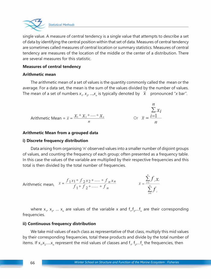
Winter School on Structure and Function of the Marine Ecosystem : Fisheries66
Statistical Methods
single value. A measure of central tendency is a single value that attempts to describe a setof data by identifying the central position within that set of data. Measures of central tendencyare sometimes called measures of central location or summary statistics. Measures of centraltendency are measures of the location of the middle or the center of a distribution. Thereare several measures for this statistic.
Measures of central tendency
Arithmetic mean
The arithmetic mean of a set of values is the quantity commonly called the mean or theaverage. For a data set, the mean is the sum of the values divided by the number of values.The mean of a set of numbers x1, x2, ...,xn is typically denoted by x pronounced “x bar”.
nΣ Xi
X1 + X2 + ........ + Xn i=1Arithmetic Mean = x = --------------------------- or x = ------------
n n
Arithmetic Mean from a grouped data
i) Discrete frequency distribution
Data arising from organising ‘n’ observed values into a smaller number of disjoint groupsof values, and counting the frequency of each group; often presented as a frequency table.In this case the values of the variable are multiplied by their respective frequencies and thistotal is then divided by the total number of frequencies.
Arithmetic mean,
x = --------------------------- ------------
where x1, x2, … xn are values of the variable x and f1,f2,…fn are their correspondingfrequencies.
ii) Continuous frequency distribution
We take mid values of each class as representative of that class, multiply this mid valuesby their corresponding frequencies, total these products and divide by the total number ofitems. If x1,x2…..xn represent the mid values of classes and f1, f2,…fn the frequencies, then
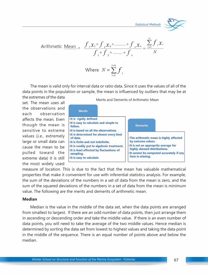
Winter School on Structure and Function of the Marine Ecosystem : Fisheries 67
Statistical Methods
The mean is valid only for interval data or ratio data. Since it uses the values of all of thedata points in the population or sample, the mean is influenced by outliers that may be atthe extremes of the dataset. The mean uses allthe observations andeach observationaffects the mean. Eventhough the mean issensitive to extremevalues (i.e., extremelylarge or small data cancause the mean to bepulled toward theextreme data) it is stillthe most widely usedmeasure of location. This is due to the fact that the mean has valuable mathematicalproperties that make it convenient for use with inferential statistics analysis. For example,the sum of the deviations of the numbers in a set of data from the mean is zero, and thesum of the squared deviations of the numbers in a set of data from the mean is minimumvalue. The following are the merits and demerits of arithmetic mean.
Median
Median is the value in the middle of the data set, when the data points are arrangedfrom smallest to largest. If there are an odd number of data points, then just arrange themin ascending or descending order and take the middle value. If there is an even number ofdata points, you will need to take the average of the two middle values. Hence median isdetermined by sorting the data set from lowest to highest values and taking the data pointin the middle of the sequence. There is an equal number of points above and below themedian.
Merits and Demerits of Arithmetic Mean
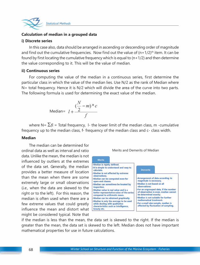
Winter School on Structure and Function of the Marine Ecosystem : Fisheries68
Statistical Methods
Calculation of median in a grouped datai) Discrete series
In this case also, data should be arranged in ascending or descending order of magnitudeand find out the cumulative frequencies. Now find out the value of (n+1/2)th item. It can befound by first locating the cumulative frequency which is equal to (n+1/2) and then determinethe value corresponding to it. This will be the value of median.
ii) Continuous seriesFor computing the value of the median in a continuous series, first determine the
particular class in which the value of the median lies. Use N/2 as the rank of Median whereN= total frequency. Hence it is N/2 which will divide the area of the curve into two parts.The following formula is used for determining the exact value of the median.
(N/2m)*CMedian= 1+ ---
f
where N= Σfi = Total frequency, l- the lower limit of the median class, m -cumulativefrequency up to the median class, f- frequency of the median class and c- class width.
Median
The median can be determined forordinal data as well as interval and ratiodata. Unlike the mean, the median is notinfluenced by outliers at the extremesof the data set. Generally, the medianprovides a better measure of locationthan the mean when there are someextremely large or small observations(i.e., when the data are skewed to theright or to the left). For this reason, themedian is often used when there are afew extreme values that could greatlyinfluence the mean and distort whatmight be considered typical. Note thatif the median is less than the mean, the data set is skewed to the right. If the median isgreater than the mean, the data set is skewed to the left. Median does not have importantmathematical properties for use in future calculations.
Merits and Demerits of Median
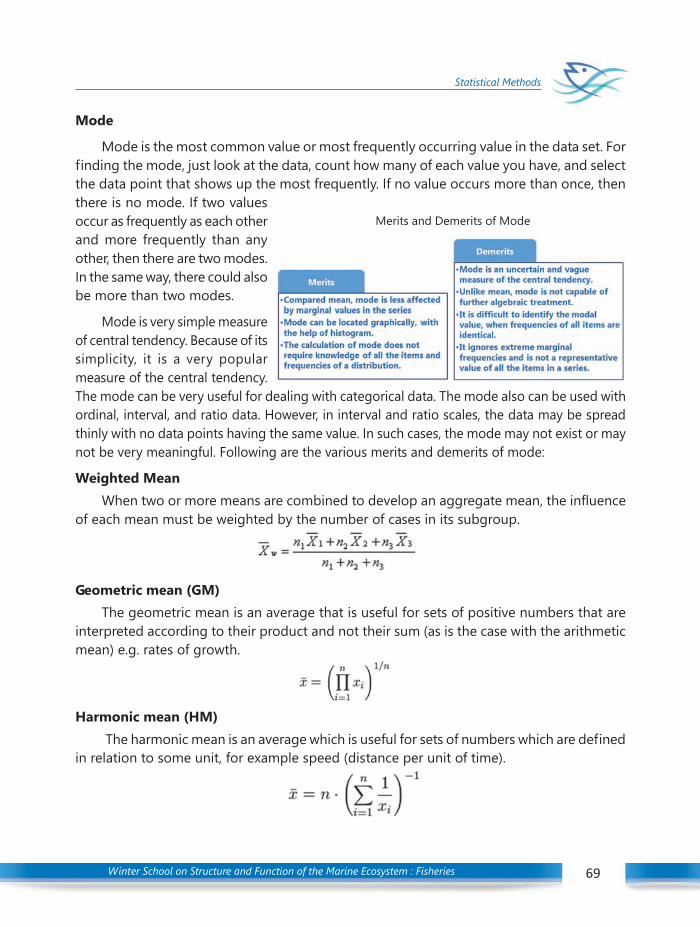
Winter School on Structure and Function of the Marine Ecosystem : Fisheries 69
Statistical Methods
Mode
Mode is the most common value or most frequently occurring value in the data set. Forfinding the mode, just look at the data, count how many of each value you have, and selectthe data point that shows up the most frequently. If no value occurs more than once, thenthere is no mode. If two valuesoccur as frequently as each otherand more frequently than anyother, then there are two modes.In the same way, there could alsobe more than two modes.
Mode is very simple measureof central tendency. Because of itssimplicity, it is a very popularmeasure of the central tendency.The mode can be very useful for dealing with categorical data. The mode also can be used withordinal, interval, and ratio data. However, in interval and ratio scales, the data may be spreadthinly with no data points having the same value. In such cases, the mode may not exist or maynot be very meaningful. Following are the various merits and demerits of mode:
Weighted MeanWhen two or more means are combined to develop an aggregate mean, the influence
of each mean must be weighted by the number of cases in its subgroup.
Geometric mean (GM)The geometric mean is an average that is useful for sets of positive numbers that are
interpreted according to their product and not their sum (as is the case with the arithmeticmean) e.g. rates of growth.
Harmonic mean (HM)The harmonic mean is an average which is useful for sets of numbers which are defined
in relation to some unit, for example speed (distance per unit of time).
Merits and Demerits of Mode

Winter School on Structure and Function of the Marine Ecosystem : Fisheries70
Statistical Methods
Relationship between AM, GM, and HM
AM, GM, and HM satisfy these inequalities:AM > GM > HM
Equality holds only when all the elements of the given sample are equal.The mean (often called the average) is most common measure of central tendency,
but there are others, such as, the median and the mode. The mean, median and mode areall valid measures of central tendency but, under different conditions, some measures ofcentral tendency become more appropriate to use than others.Measures of Dispersion
Measure of variation describes how spread out or scattered a set of data. It is alsoknown as measures of dispersion or measures of spread. Measures of variation determinethe range of the distribution, relative to the measures of central tendency. Measures ofaverage such as the mean and median represent the typical value for a dataset. Within thedataset the actual values usually differ from one another and from the average value itself.The extent to which the mean and median are good representatives of the values in theoriginal dataset depends upon the variability or dispersion in the original data. The measuresof central tendency are specific data points, measures of variation are lengths betweenvarious points within the distribution. It provide us with a summary of how much the pointsin our data set vary, e.g. how spread out they are or how volatile they are. Measures ofvariation together with measures of central tendency are important for identifying keyfeatures of a sample to better understand the population from which the sample comesfrom. Datasets are said to have high dispersion when they contain values considerablyhigher and lower than the mean value. The most common measures of variation are Range,Quartile déviation or semi Interquartile Range, Mean deviation, Variance, Standard deviationand Coefficient of Variation.Range
The range is the distance between the lowest data point and the highest data point. Inother words, it is difference between the highest value and the lowest value.
Range = Highest value–lowest valueThe range is the simplest measure of variation to find. Since the range only uses the
largest and smallest values, it is greatly affected by extreme values, that is - it is not resistantto change.
The range is simple to compute and is useful when you wish to evaluate the whole of adataset. It is useful for showing the spread within a dataset and for comparing the spreadbetween similar datasets.

Winter School on Structure and Function of the Marine Ecosystem : Fisheries 71
Statistical Methods
Since the range is based solely on the two most extreme values within the dataset, ifone of these is either exceptionally high or low (sometimes referred to as outlier) it willresult in a range that is not typical of the variability within the dataset. The range does notreally indicate how the scores are concentrated along the distribution. The range only involvesthe smallest and largest numbers, and is affected by extreme data values or outliers. Inorder to reduce the problems caused by outliers in a dataset, the inter-quartile range isoften calculated instead of the range.
Quartile Deviation or The semi inter-quartile Range
The inter-quartile range is a measure that indicates the extent to which the central 50%of values within the dataset are dispersed. If the sample is ranked in ascending order ofmagnitude two values of x may be found, the first of which is exceeded by 75% of thesample, the second by 25%; their difference is the interquartile range. It is based upon andrelated to the median. In the same way that the median divides a dataset into two halves, itcan be further divided into quarters by identifying the upper and lower quartiles. The lowerquartile, Q1 is found one quarter of the way along a dataset when the values have beenarranged in order of magnitude; the upper quartile Q3 is found three quarters along thedataset. Therefore, the upper quartile lies half way between the median and the highestvalue in the dataset whilst the lower quartile lies halfway between the median and thelowest value in the dataset. Between Q1 and Q3 there is half the total number of items. Q3-Q1 affords a convenient and often a good indicator of the absolute variability. Usually onehalf of the Q3-Q1 is used and given the name semi-interquartile range or quartile deviation.
The relative measure of quartile deviation is known as the coefficient of Q.D.
The larger the semi – interquartile range, the larger the spread of the central half ofthe data. Thus the semi –interquartile rang provides a measure of spread. Thus it indicatehow closely the data are clustered around the median.

Winter School on Structure and Function of the Marine Ecosystem : Fisheries72
Statistical Methods
Mean deviation
Mean deviation is the average of the absolute values of the deviation scores; that is,mean deviation is the average distance between the mean and the data points. It is calculatedas
Closely related to the measure of mean deviation is the measure of variance.
Variance
The variance is the most commonly accepted measure of variation. It represents theaverage of the squared deviations about the mean. Variance also indicates a relationshipbetween the mean of a distribution and the data points; it is determined by averaging thesum of the squared deviations. Squaring the differences instead of taking the absolutevalues allows for greater flexibility in calculating further algebraic manipulations of thedata. It is the average of the squared deviations between the individual scores and themean. The larger the variance the more variability there is among the scores. Whencomparing two samples with the same unit of measurement (age), the variances arecomparable even though the sample sizes may be different. Generally, however, smallersamples have greater variability among the scores than larger samples.
The average deviation from the mean is:
Ave. Dev =
The problem is that this summation is always zero. So, the average deviation will alwaysbe zero. That is why the average deviation is never used. So, to keep it from being zero, thedeviation from the mean is squared and called the “squared deviation from the mean”. This“average squared deviation from the mean” is called the variance. The formula for variancedepends on whether you are working with a population or sample:
The formula for the variance in a population is where where µ is the
mean and N is the number of scores.
When the variance is computed in a sample, the statistic
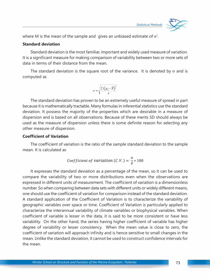
Winter School on Structure and Function of the Marine Ecosystem : Fisheries 73
Statistical Methods
where M is the mean of the sample and gives an unbiased estimate of σ2.
Standard deviation
Standard deviation is the most familiar, important and widely used measure of variation.It is a significant measure for making comparison of variability between two or more sets ofdata in terms of their distance from the mean.
The standard deviation is the square root of the variance. It is denoted by σ and iscomputed as
The standard deviation has proven to be an extremely useful measure of spread in partbecause it is mathematically tractable. Many formulas in inferential statistics use the standarddeviation. It possess the majority of the properties which are desirable in a measure ofdispersion and is based on all observations. Because of these merits SD should always beused as the measure of dispersion unless there is some definite reason for selecting anyother measure of dispersion.
Coefficient of Variation
The coefficient of variation is the ratio of the sample standard deviation to the samplemean. It is calculated as
It expresses the standard deviation as a percentage of the mean, so it can be used tocompare the variability of two or more distributions even when the observations areexpressed in different units of measurement. The coefficient of variation is a dimensionlessnumber. So when comparing between data sets with different units or widely different means,one should use the coefficient of variation for comparison instead of the standard deviation.A standard application of the Coefficient of Variation is to characterize the variability ofgeographic variables over space or time. Coefficient of Variation is particularly applied tocharacterize the interannual variability of climate variables or biophysical variables. Whencoefficient of variable is lesser in the data, it is said to be more consistent or have lessvariability. On the other hand, the series having higher coefficient of variable has higherdegree of variability or lesser consistency. When the mean value is close to zero, thecoefficient of variation will approach infinity and is hence sensitive to small changes in themean. Unlike the standard deviation, it cannot be used to construct confidence intervals forthe mean.
Winter School on Structure and Function of the Marine Ecosystem : Fisheries74
Statistical Methods
Correlation
Correlation is a statistical technique that can show whether and how strongly pairs ofvariables are related. The correlation analysis enables us to have an idea about the degree& direction of the relationship between the two variables under study. It is used to assessthe possible linear association between two variables. If there is any relation between twovariables i.e., when one variable changes the other also changes in the same or in theopposite direction, we say that the two variables are correlated. Thus correlation is thestudy of existence, magnitude and direction of the relation between two or more variables.The measure of correlation called the correlation coefficient. If the ratio of change betweentwo variables is uniform, then the correlation is said to be linear. If the amount of changein one variable does not bear a constant ratio to the amount of change in the other variable,then the correlation is said to be non-linear or curvilinear. The nature of the graph gives usthe idea of the linear type of correlation between two variables. If the graph is in a straightline, the correlation is called a “linear correlation” and if the graph is not in a straight line,the correlation is non-linear or curvi-linear.Positive and negative correlation
If two variables change in the same direction i.e., if one increases the other also increases,or if one decreases, the other also decreases), then this is called a positive correlation. Iftwo variables change in the opposite direction i.e., if one increases, the other decreases andvice versa), then the correlation is called a negative correlation. Through the coefficient ofcorrelation, we can measure the degree or extent of the correlation between two variables.On the basis of the coefficient of correlation we can also determine whether the correlationis positive or negative and also its degree or extent.
If two variables changes in the same direction and in the same proportion, the correlationbetween the two is perfect positive. According to Karl Pearson the coefficient of correlationin this case is +1. On the other hand if the variables change in the opposite direction and inthe same proportion, the correlation is perfect negative and its coefficient of correlation is-1. In practice we rarely come across these types of correlations.
If two variables exhibit no relations between them or change in variable does not leadto a change in the other variable, then we can say that there is no correlation between thetwo variables. In such a case the coefficient of correlation is 0.Methods of Determining Correlation
The following are the most commonly used methods of determining correlation..(1) Scatter Plot(2) Karl Pearson’s coefficient of correlation

Winter School on Structure and Function of the Marine Ecosystem : Fisheries 75
Statistical Methods
Scatter Plot (Scatter diagram or dot diagram)
The scatter diagram may be described as the diagram which helps us to visualize therelationship between two phenomena. This is the simplest method for finding out whetherthere is any relationship present between two variables. In this method the values of thetwo variables are plotted on a graph paper. One is taken along the x-axis and the otheralong the y-axis. By plotting the data, we get points on the graph which are generallyscattered and hence the name ‘Scatter Plot’. The manner in which these points are scattered,suggest the degree and the direction of correlation. The grater the scatter of the points onthe chart, the lesser is the relationship between the two variables. The more closely thepoints come to a straight line, the higher the degree of relationship. The degree of correlationis denoted by ‘r’ and its direction is given by the signs positive and negative. Scatter diagramswill generally show one of five possible correlations between the variables:
Strong Positive Correlation :The value of Y clearly increases as the value of X increases.Strong Negative Correlation: The value of Y clearly decreases as the value of X increases.Weak Positive Correlation : The value of Y increases slightly as the value of X increases.Weak Negative Correlation: The value of Y decreases slightly as the value of X increases.No Correlation: There is no demonstrated connection between the two variables.
Though this method is simple and provide a rough idea about the existence and thedegree of correlation, it is not reliable. As it is not a mathematical method, it cannot measurethe degree of correlation.
Illustrations

Winter School on Structure and Function of the Marine Ecosystem : Fisheries76
Statistical Methods
Karl Pearson’s coefficient of correlation:
The most widely-used type of correlation coefficient is Pearson r, also called linear orproduct- moment correlation. It gives the numerical expression for the measure of correlation.The value of ‘ r ’ gives the magnitude of correlation and sign denotes its direction. It isdefined as
Properties of Correlation coefficient
The value of correlation does not depend on the specific measurement units used; forexample, the correlation between height and weight will be identical regardless ofwhether inches and pounds, or centimeters and kilograms are used as measurementunits.
The value of correlation coefficient lies between -1 and +1, -1 means perfect negativelinear correlation and +1 means perfect positive linear correlation.
The correlation coefficient r only measures the strength of a linear relationship. Thereare other kinds of relationships besides linear.
If the two variables are independent, then the value of the correlation coefficient iszero. If the value of the correlation coefficient is zero, it does not mean that there is nocorrelation, but there may be non-linear correlation.
The value of r does not change if the independent (x) and dependent (y) variables areinterchanged.
The correlation coefficient r does not change if the scale on either variable is changed.You may multiply, divide, add, or subtract a value to/from all the x-values or y-valueswithout changing the value of r.
The correlation coefficient r has a Student’s t distribution.
Assumptions to use the Pearson product-moment correlation
The measures are approximately normally distributed
The variance of the two measures is similar (homoscedasticity)
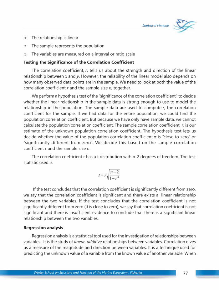
Winter School on Structure and Function of the Marine Ecosystem : Fisheries 77
Statistical Methods
The relationship is linear
The sample represents the population
The variables are measured on a interval or ratio scale
Testing the Significance of the Correlation Coefficient
The correlation coefficient, r, tells us about the strength and direction of the linearrelationship between x and y. However, the reliability of the linear model also depends onhow many observed data points are in the sample. We need to look at both the value of thecorrelation coefficient r and the sample size n, together.
We perform a hypothesis test of the ”significance of the correlation coefficient” to decidewhether the linear relationship in the sample data is strong enough to use to model therelationship in the population. The sample data are used to compute r, the correlationcoefficient for the sample. If we had data for the entire population, we could find thepopulation correlation coefficient. But because we have only have sample data, we cannotcalculate the population correlation coefficient. The sample correlation coefficient, r, is ourestimate of the unknown population correlation coefficient. The hypothesis test lets usdecide whether the value of the population correlation coefficient σ is “close to zero” or“significantly different from zero”. We decide this based on the sample correlationcoefficient r and the sample size n.
The correlation coefficient r has a t distribution with n-2 degrees of freedom. The teststatistic used is
If the test concludes that the correlation coefficient is significantly different from zero,we say that the correlation coefficient is significant and there exists a linear relationshipbetween the two variables. If the test concludes that the correlation coefficient is notsignificantly different from zero (it is close to zero), we say that correlation coefficient is notsignificant and there is insufficient evidence to conclude that there is a significant linearrelationship between the two variables.
Regression analysis
Regression analysis is a statistical tool used for the investigation of relationships betweenvariables. It is the study of linear, additive relationships between variables. Correlation givesus a measure of the magnitude and direction between variables. It is a technique used forpredicting the unknown value of a variable from the known value of another variable. When
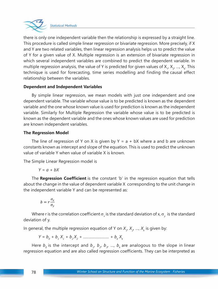
Winter School on Structure and Function of the Marine Ecosystem : Fisheries78
Statistical Methods
there is only one independent variable then the relationship is expressed by a straight line.This procedure is called simple linear regression or bivariate regression. More precisely, if Xand Y are two related variables, then linear regression analysis helps us to predict the valueof Y for a given value of X. Multiple regression is an extension of bivariate regression inwhich several independent variables are combined to predict the dependent variable. Inmultiple regression analysis, the value of Y is predicted for given values of X1, X2, …, Xk. Thistechnique is used for forecasting, time series modelling and finding the causal effectrelationship between the variables.
Dependent and Independent Variables
By simple linear regression, we mean models with just one independent and onedependent variable. The variable whose value is to be predicted is known as the dependentvariable and the one whose known value is used for prediction is known as the independentvariable. Similarly for Multiple Regression the variable whose value is to be predicted isknown as the dependent variable and the ones whose known values are used for predictionare known independent variables.
The Regression Model
The line of regression of Y on X is given by Y = a + bX where a and b are unknownconstants known as intercept and slope of the equation. This is used to predict the unknownvalue of variable Y when value of variable X is known.
The Simple Linear Regression model is
Y = a + bX
The Regression Coefficient is the constant ‘b’ in the regression equation that tellsabout the change in the value of dependent variable X corresponding to the unit change inthe independent variable Y and can be represented as:
Where r is the correlation coefficient σx is the standard deviation of x, σy is the standarddeviation of y.
In general, the multiple regression equation of Y on X1, X2, …, Xk is given by:
Y = b0 + b1 X1 + b2 X2 + …………………… + bk Xk
Here b0 is the intercept and b1, b2, b3, …, bk are analogous to the slope in linearregression equation and are also called regression coefficients. They can be interpreted as

Winter School on Structure and Function of the Marine Ecosystem : Fisheries 79
Statistical Methods
the change in the value of dependent variable (Y) corresponding to unit change in the valueof independent variable Xi.
Fitting of regression line
In scatter plot, we have seen that if the variables are highly correlated then the points(dots) lie in a narrow strip. If the strip is nearly straight, we can draw a straight line, such thatall points are close to it from both sides. Such a line can be taken as an ideal representationof variation. This line is called the line of best fit if it minimizes the distances of all datapoints from it and also called as the line of regression. Now prediction is easy because all weneed to do is to extend the line and read the value. Thus to obtain a line of regression, weneed to have a line of best fit.
The problem of choosing the best straight line then comes down to finding the bestvalues of a and b. By ’best’ we mean the values of a and b that produce a line closest to alln observations. This means that we find the line that minimizes the distances of eachobservation to the line. Choose the values of a and b that give the line such that the sum ofsquared deviations from the line is minimized. This method of estimation of parameters iscalled least square method. The best line is called the regression line, and the equationdescribing it is called the regression equation. The deviations from the line are also calledresiduals.
R2 - coefficient of determination
Once a line of regression has been constructed, one can check how good it is (in termsof predictive ability) by examining the coefficient of determination (R2), which is defined asthe proportion of variance of the dependent variable that can be explained by theindependent variables. The coefficient of determination is a measure of how well theregression equation y = a + bX performs as a predictor of y. Its value represents the percentage

Winter School on Structure and Function of the Marine Ecosystem : Fisheries80
Statistical Methods
of variation that can be explained by the regression equation. R2 always lies between 0 and1. Higher values of this are generally taken to indicate a better model. A value of 1 meansevery point on the regression line fits the data; a value of 0.5 means only half of the variationis explained by the regression. The coefficient of determination is also commonly used toshow how accurately a regression model can predict future outcomes.
Winter School on Structure and Function of the Marine Ecosystem : Fisheries 81
Data Diagnostics and Remedial Measures
The raw data consist of measurements of some attribute on a collection of individuals.The measurement would have been made in one of the following scales viz., nominal, ordinal,interval or ratio scale.
Levels of Measurement
Nominal scale refers to measurement at its weakest level when number or othersymbols are used simply to classify an object, person or characteristic, e.g., state ofhealth (healthy, diseased).
Ordinal scale is one wherein given a group of equivalence classes, the relationgreater than holds for all pairs of classes so that a complete rank ordering of classesis possible, e.g., socio-economic status.
When a scale has all the characteristics of an ordinal scale, and when in addition,the distances between any two numbers on the scale are of known size, intervalscale is achieved, e.g., temperature scales like centigrade or Fahrenheit.
An interval scale with a true zero point as its origin forms a ratio scale. In a ratioscale, the ratio of any two scale points is independent of the unit of measurement,e.g., height of trees.
The data can be classified as qualitative/quantitative depending on the levels based onwhich the observations are collected. There are several statistical procedures available inliterature for the analysis of data which are broadly classified in to two categories viz.,parametric tests and non-parametric tests. A parametric test specifies certain conditionsabout the distribution of responses in the population from which the research sample wasdrawn. The meaningfulness of the results of a parametric test depends on the validity ofthese assumptions. A nonparametric test is based on a model that specifies very generalconditions and none regarding the specific form of the distribution from which the samplewas drawn. Hence nonparametric tests are also known as distribution free tests. Certainassumptions are associated with most nonparametric statistical tests, but these are fewerand weaker than those of parametric tests.
Nonparametric test statistics utilize some simple aspects of sample data such as thesigns of measurements, order relationships or category frequencies. Therefore, stretching
03C H A P T E R
11C H A P T E R DATA DIAGNOSTICS AND REMEDIAL
MEASURESEldho Varghese
Fishery Resources Assessment DivisionICAR-Central Marine Fisheries Research Institute
Winter School on Structure and Function of the Marine Ecosystem : Fisheries82
Data Diagnostics and Remedial Measures
or compressing the scale does not alter them. As a consequence, the null distribution of thenonparametric test statistic can be determined without regard to the shape of the parentpopulation distribution. These tests have the obvious advantage of not requiring theassumption of normality or the assumption of homogeneity of variance. They comparemedians rather than means and, as a result, if the data have one or two outliers, theirinfluence is negated.
Besides, the interpretation of data based on analysis of variance (ANOVA)/Regression isvalid only when the following assumptions are satisfied:
1. The regression function is linear
2. The error terms do have constant variance
3. The error terms are independent
4. No outlying observations
5. The error terms are normally distributed
6. Predictor variables are uncorrelated.
Also the statistical tests t, F, z, etc. are valid under the assumption of independence oferrors and normality of errors. The departures from these assumptions make theinterpretation based on these statistical techniques invalid. Therefore, it is necessary todetect the deviations and apply the appropriate remedial measures.
The assumption of independence of errors, i.e., error of an observation is not related toor depends upon that of another. This assumption is usually assured with the use of properrandomization procedure. However, if there is any systematic pattern in the arrangement oftreatments from one replication to another, errors may be non-independent. This may behandled by using nearest neighbour methods in the analysis of experimental data.
Normality of Errors
The assumptions of homogeneity of variances and normality are generally violatedtogether. To test the validity of normality of errors for the character under study, one cantake help of Normal Probability Plot, Anderson-Darling Test, D’Augstino’s Test, Shapiro -Wilk’s Test, Ryan-Joiner test, Kolmogrov-Smirnov test, etc. In general moderate departuresfrom normality are of little concern in the fixed effects ANOVA as F - test is slightly affectedbut in case of random effects, it is more severely impacted by non-normality. The significantdeviations of errors from normality, makes the inferences invalid. So before analyzing thedata, it is necessary to convert the data to a scale that it follows a normal distribution. In thedata from designed field experiments, we do not directly use the original data for testing of

Winter School on Structure and Function of the Marine Ecosystem : Fisheries 83
Data Diagnostics and Remedial Measures
normality or homogeneity of observations because this is embedded with the treatmenteffects and some of other effects like block, row, column, etc. So there is need to eliminatethese effects from the data before testing the assumptions of normality and homogeneityof variances. For eliminating the treatment effects and other effects we fit the modelcorresponding to the design adopted and estimate the residuals. These residuals are thenused for testing the normality of the observations. In other words, we want to test the nullhypothesis H0: errors are normally distributed against alternative hypothesis H1: errors arenot normally distributed. For details on these tests one may refer to D’Agostino and Stephens(1986). Most of the standard statistical packages available in the market are capable oftesting the normality of the data. In SAS and SPSS commonly used tests are Shapiro-Wilktest and Kolmogrov-Smirnov test. MINITAB uses three tests viz. Anderson-Darling, Ryan-Joiner, Kolmogrov-Smirnov for testing the normality of data.
Homogeneity of Error Variances
A crude method for detecting the heterogeneity of variances is based on scatter plotsof means and variance or range of observations or errors, residual vs fitted values, etc. To beclearer, let Yij be the observation pertaining to ith treatment (i=1(1)v) in the jth replication(j = 1(1)ri). Compute the mean and variance for each treatment across the replications (therange can be used in place of variance) as
Mean = Variance =
Draw the scatter plot of mean vs variance (or range). If are equal(constant) or nearly equal, then the variances are homogeneous. Based on these scatterplots, the heterogeneity of variances can be classified into two types:
1. Where the variance is functionally related to mean.
2. Where there is no functional relationship between the variance and the mean.
For illustration some scatter - diagrams of mean and variances (or range) are given in below:
The first kind of variance heterogeneity (figure b) is usually associated with the datawhose distribution is non-normal viz., negative binomial, Poisson, binomial, etc. The secondkind of variance heterogeneity usually occurs in experiments, where, due to the nature oftreatments tested, some treatments have errors that are substantially higher (lower) thanothers. For example, in varietal trials, where various types of breeding material are beingcompared, the size of variance between plots of a particular variety will depend on thedegree of genetic homogeneity of material being tested. The variance of F2 generation, forexample, can be expected to be higher than that of F1 generation because genetic variabilityin F2 is much higher than that in F1. The variances of varieties that are highly tolerant of or
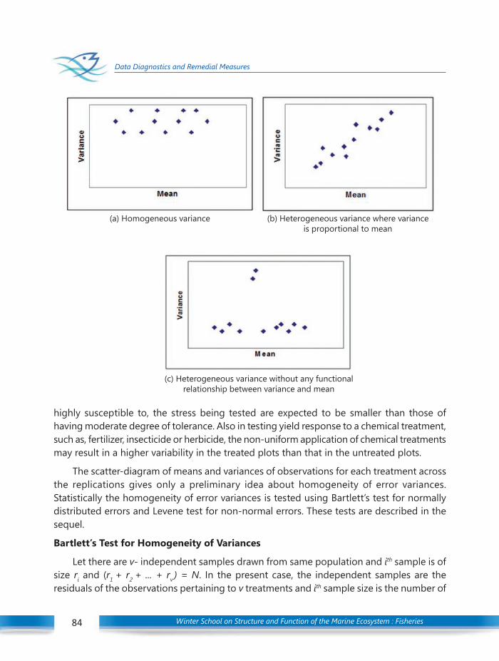
Winter School on Structure and Function of the Marine Ecosystem : Fisheries84
Data Diagnostics and Remedial Measures
highly susceptible to, the stress being tested are expected to be smaller than those ofhaving moderate degree of tolerance. Also in testing yield response to a chemical treatment,such as, fertilizer, insecticide or herbicide, the non-uniform application of chemical treatmentsmay result in a higher variability in the treated plots than that in the untreated plots.
The scatter-diagram of means and variances of observations for each treatment acrossthe replications gives only a preliminary idea about homogeneity of error variances.Statistically the homogeneity of error variances is tested using Bartlett’s test for normallydistributed errors and Levene test for non-normal errors. These tests are described in thesequel.
Bartlett’s Test for Homogeneity of Variances
Let there are v- independent samples drawn from same population and ith sample is ofsize ri and (r1 + r2 + ... + rv ) = N. In the present case, the independent samples are theresiduals of the observations pertaining to v treatments and ith sample size is the number of
(a) Homogeneous variance (b) Heterogeneous variance where varianceis proportional to mean
(c) Heterogeneous variance without any functionalrelationship between variance and mean

Winter School on Structure and Function of the Marine Ecosystem : Fisheries 85
Data Diagnostics and Remedial Measures
replications of the treatment i. One wants to test the null hypothesis H0: σ12= σ2
2=... = σv2
against the alternative hypothesis :1H at least two of the σ12’s are not equal, where σ1
2 isthe error variance for treatment i.
Let ije denotes the residual pertaining to the observation of treatment i from replicationj, then it can easily be shown that the sum of residuals pertaining to a given treatment iszero. In this test is taken as unbiased estimate of σi
2. The procedureinvolves computing a statistic whose sampling distribution is closely approximated by theχ2 distribution with v - 1 degrees of freedom. The test statistic is
and null hypothesis is rejected when χ02 > χ2
α,v-1, where 21, −vαχ is the upper α percentage
point of χ2 distribution with v - 1 degrees of freedom.To compute χ0
2, follow the steps:Step 1: Compute mean and variance of all v-samples.
Step 2: Obtain pooled variance
Step 3: Compute
Step 4: Compute
Step 5: Compute χ02.
Bartlett’s χ2 test for homogeneity of variances is a modification of the normal-theorylikelihood ratio test. While Bartlett’s test has accurate Type I error rates and optimal powerwhen the underlying distribution of the data is normal, it can be very inaccurate if thatdistribution is even slightly non-normal (Box 1953). Therefore, Bartlett’s test is notrecommended for routine use.
An approach that leads to tests that are much more robust to the underlying distributionis to transform the original values of the dependent variable to derive a dispersion variableand then to perform analysis of variance on this variable. The significance level for the testof homogeneity of variance is the p-value for the ANOVA F-test on the dispersion variable.Commonly used test for testing the homogeneity of variance using a dispersion variable isLevene Test given by Levene (1960). The procedure is described in the sequel.

Winter School on Structure and Function of the Marine Ecosystem : Fisheries86
Data Diagnostics and Remedial Measures
Levene Test for homogeneity of Variances
The test is based on the variability of the residuals. The larger the error variance, thelarger the variability of the residuals will tend to be. To conduct the Levene test, we dividethe data into different groups based on the number of treatments if the error variance iseither increasing or decreasing with the treatments, the residuals in the one treatment willtend to be more variable than those in others treatments. The Levene test than consistssimply F – statistic based on one way ANOVA used to determine whether the mean ofabsolute/ Square root deviation from mean are significantly different or not. The residualsare obtained from the usual analysis of variance. The test statistic is given as
where and dij is the jth residual for the ith plot, ei is the
mean of the residuals of the ith treatment.
This test was modified by Brown and Forsythe (1974). In the modified test, the absolutedeviation is taken from the median instead of mean in order to make the test more robust.
In the present investigation, the Bartlett’s χ2 − test has been used for testing thehomogeneity of error variances when the distribution of errors is normal and Levene testfor non-normal errors.
Remark 1: In a block design, it can easily be shown that the sum of residuals within agiven block is zero. Therefore, the residuals in a block of size 2 will be same with their signreverse in order. As a consequence, q in Bartlett’s test and numerator in Levene test statisticbecomes zero for the data generated from experiments conducted to compare only twotreatments in a RCB design. Hence, the tests for homogeneity of error variances cannot beused for the experiments conducted to compare only two treatments in a RCB design.Inferences from such experiments may be drawn using Fisher-Behren t-test. Further, Bartlett’stest cannot be used for the experimental situations where some of the treatments are singlyreplicated.
Remark 2: In a RCB design, it can easily be shown that the sum of residuals from aparticular treatment is zero. As a consequence, the denominator of Levene test statistic is
Winter School on Structure and Function of the Marine Ecosystem : Fisheries 87
Data Diagnostics and Remedial Measures
zero for the data generated from RCB designs with two replications. Therefore, Levene testcannot be used for testing the homogeneity of error variances for the data generated fromRCB designs with two replications.
Presence of Outliers
Outliers are extreme observations. Residual outliers can be identified from residualplots against X or Y. Outliers can create great difficulty. When we encounter one, our firstsuspicion is that the observation resulted from a mistake or other extraneous effect. On theother hand, outliers may convey significant information, as when an outlier occurs becauseof an interaction with another predictor omitted from the model. A safe rule frequentlysuggested is to discard an outlier only if there is direct evidence that it represents in error inrecording, a miscalculation, a malfunctioning of equipment, or a similar type of circumstances.
Omission of Important Predictor Variables
Residuals should also be plotted against variables omitted from the model that mighthave important effects on the response. The purpose of this additional analysis is to determinewhether there are any key variables that could provide important additional descriptive andpredictive power to the model. The residuals are plotted against the additional predictorvariable to see whether or not the residuals tend to vary systematically with the level of theadditional predictor variable.
Overview of Tests
Graphical analysis of residuals is inherently subjective. Nevertheless, subjective analysisof a variety of interrelated residuals plots will frequently reveal difficulties with the modelmore clearly than particular formal tests.
Tests for Randomness
A run test is frequently used to test for lack of randomness in the residuals arranged intime order. Another test, specially designed for lack of randomness in least squares residuals.
Durbin-Watson test:
The Durbin-Watson test assumes the first order autoregressive error models. The testconsists of determining whether or not the autocorrelation coefficient (p, say) is zero. Theusual test alternatives considered are:
H0 : p = 0
H0 : p > 0
The Durbin-Watson test statistic D is obtained by using ordinary least squares to fit the
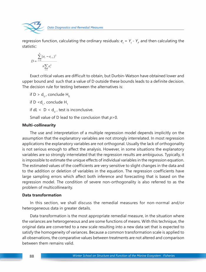
Winter School on Structure and Function of the Marine Ecosystem : Fisheries88
Data Diagnostics and Remedial Measures
regression function, calculating the ordinary residuals: et = Yt - Yt, and then calculating thestatistic:
Exact critical values are difficult to obtain, but Durbin-Watson have obtained lower andupper bound and such that a value of D outside these bounds leads to a definite decision.The decision rule for testing between the alternatives is:
if D > dU , conclude H0
if D <dL , conclude H1
if dL < D < dU , test is inconclusive.
Small value of D lead to the conclusion that p>0.
Multi-collinearity
The use and interpretation of a multiple regression model depends implicitly on theassumption that the explanatory variables are not strongly interrelated. In most regressionapplications the explanatory variables are not orthogonal. Usually the lack of orthogonalityis not serious enough to affect the analysis. However, in some situations the explanatoryvariables are so strongly interrelated that the regression results are ambiguous. Typically, itis impossible to estimate the unique effects of individual variables in the regression equation.The estimated values of the coefficients are very sensitive to slight changes in the data andto the addition or deletion of variables in the equation. The regression coefficients havelarge sampling errors which affect both inference and forecasting that is based on theregression model. The condition of severe non-orthogonality is also referred to as theproblem of multicollinearity.
Data transformation
In this section, we shall discuss the remedial measures for non-normal and/orheterogeneous data in greater details.
Data transformation is the most appropriate remedial measure, in the situation wherethe variances are heterogeneous and are some functions of means. With this technique, theoriginal data are converted to a new scale resulting into a new data set that is expected tosatisfy the homogeneity of variances. Because a common transformation scale is applied toall observations, the comparative values between treatments are not altered and comparisonbetween them remains valid.

Winter School on Structure and Function of the Marine Ecosystem : Fisheries 89
Data Diagnostics and Remedial Measures
Error partitioning is the remedial measure of heterogeneity that usually occurs inexperiments, where, due to the nature of treatments tested some treatments have errorsthat are substantially higher (lower) than others.
Here, we shall concentrate on those situations where character under study is non-normal and variances are heterogeneous. Depending upon the functional relationshipbetween variances and means, suitable transformation is adopted. The transformed variateshould satisfy the following:
1. The variances of the transformed variate should be unaffected by changes in themeans. This is also called the variance stabilizing transformation.
2. It should be normally distributed.
3. It should be one for which effects are linear and additive.
4. The transformed scale should be such for which an arithmetic average from thesample is an efficient estimate of true mean.
The following are the three transformations, which are being used most commonly, inbiological research.
a) Logarithmic Transformation
b) Square root Transformation
c) Arc Sine or Angular Transformation
a) Logarithmic Transformation
This transformation is suitable for the data where the variance is proportional to squareof the mean or the coefficient of variation (S.D./mean) is constant or where effects aremultiplicative. These conditions are generally found in the data that are whole numbers andcover a wide range of values. This is usually the case when analyzing growth measurementssuch as trunk girth, length of extension growth, weight of tree or number of insects per plot,number of eggmass per plant or per unit area etc.
For such situations, it is appropriate to analyze log X instead of actual data, X. Whendata set involves small values or zeros, log (X+1), log (2X + 1) or log should be usedinstead of log X. This transformation would make errors normal, when observations follownegative binomial distribution like in the case of insect counts.
b) Square-Root Transformation
This transformation is appropriate for the data sets where the variance is proportionalto the mean. Here, the data consists of small whole numbers, for example, data obtained in
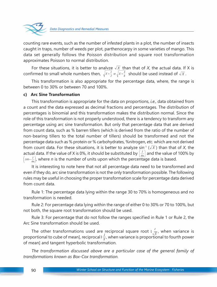
Winter School on Structure and Function of the Marine Ecosystem : Fisheries90
Data Diagnostics and Remedial Measures
counting rare events, such as the number of infested plants in a plot, the number of insectscaught in traps, number of weeds per plot, parthenocarpy in some varieties of mango. Thisdata set generally follows the Poisson distribution and square root transformationapproximates Poisson to normal distribution.
For these situations, it is better to analyze than that of X, the actual data. If X isconfirmed to small whole numbers then, should be used instead of .
This transformation is also appropriate for the percentage data, where, the range isbetween 0 to 30% or between 70 and 100%.c) Arc Sine Transformation
This transformation is appropriate for the data on proportions, i.e., data obtained froma count and the data expressed as decimal fractions and percentages. The distribution ofpercentages is binomial and this transformation makes the distribution normal. Since therole of this transformation is not properly understood, there is a tendency to transform anypercentage using arc sine transformation. But only that percentage data that are derivedfrom count data, such as % barren tillers (which is derived from the ratio of the number ofnon-bearing tillers to the total number of tillers) should be transformed and not thepercentage data such as % protein or % carbohydrates, %nitrogen, etc. which are not derivedfrom count data. For these situations, it is better to analyze sin-1 ( ) than that of X, theactual data. If the value of X is 0%, it should be substituted by and the value of 100% by
, where n is the number of units upon which the percentage data is based.It is interesting to note here that not all percentage data need to be transformed and
even if they do, arc sine transformation is not the only transformation possible. The followingrules may be useful in choosing the proper transformation scale for percentage data derivedfrom count data.
Rule 1: The percentage data lying within the range 30 to 70% is homogeneous and notransformation is needed.
Rule 2: For percentage data lying within the range of either 0 to 30% or 70 to 100%, butnot both, the square root transformation should be used.
Rule 3: For percentage that do not follow the ranges specified in Rule 1 or Rule 2, theArc Sine transformation should be used.
The other transformations used are reciprocal square root , when variance isproportional to cube of mean], reciprocal , when variance is proportional to fourth powerof mean] and tangent hyperbolic transformation.
The transformation discussed above are a particular case of the general family oftransformations known as Box-Cox transformation.

Winter School on Structure and Function of the Marine Ecosystem : Fisheries 91
Data Diagnostics and Remedial Measures
d) Box-Cox Transformation
By now we know that if the relation between the variance of observations and themean is known then this information can be utilized in selecting the form of thetransformation. We now elaborate on this point and show how it is possible to estimate theform of the required transformation from the data. The transformation suggested by Boxand Cox (1964) is a power transformation of the original data. Let yut be the observationpertaining to the uth plot; then the power transformation implies that we use yut’s as
The transformation parameter λ in may be estimated simultaneously withthe other model parameters (overall mean and treatment effects) using the method ofmaximum likelihood. The procedure consists of performing, for the various values of λ, astandard analysis of variance on
(A)
is the geometric mean of the observations. The maximum likelihood estimate of λis the value for which the error sum of squares, say SSE (λ), is minimum. Notice that wecannot select the value of λ by directly comparing the error sum of squares from analysis ofvariance on yλ because for each value of l the error sum of squares is measured on a differentscale. Equation (A) rescales the responses so that the error sums of squares are directlycomparable. This is a very general transformation and the commonly used transformationsfollow as particular cases. The particular cases for different values of are given below.
λ Transformation1 No Transformation½ Square Root0 Log-1/2 Reciprocal Square Root-1 Reciprocal
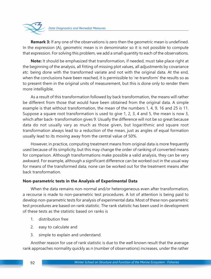
Winter School on Structure and Function of the Marine Ecosystem : Fisheries92
Data Diagnostics and Remedial Measures
Remark 3: If any one of the observations is zero then the geometric mean is undefined.In the expression (A), geometric mean is in denominator so it is not possible to computethat expression. For solving this problem, we add a small quantity to each of the observations.
Note: It should be emphasized that transformation, if needed, must take place right atthe beginning of the analysis, all fitting of missing plot values, all adjustments by covarianceetc. being done with the transformed variate and not with the original data. At the end,when the conclusions have been reached, it is permissible to ‘re-transform’ the results so asto present them in the original units of measurement, but this is done only to render themmore intelligible.
As a result of this transformation followed by back transformation, the means will ratherbe different from those that would have been obtained from the original data. A simpleexample is that without transformation, the mean of the numbers 1, 4, 9, 16 and 25 is 11.Suppose a square root transformation is used to give 1, 2, 3, 4 and 5, the mean is now 3,which after back- transformation gives 9. Usually the difference will not be so great becausedata do not usually vary as much as those given, but logarithmic and square roottransformation always lead to a reduction of the mean, just as angles of equal formationusually lead to its moving away from the central value of 50%.
However, in practice, computing treatment means from original data is more frequentlyused because of its simplicity, but this may change the order of ranking of converted meansfor comparison. Although transformations make possible a valid analysis, they can be veryawkward. For example, although a significant difference can be worked out in the usual wayfor means of the transformed data, none can be worked out for the treatment means afterback transformation.
Non-parametric tests in the Analysis of Experimental Data
When the data remains non-normal and/or heterogeneous even after transformation,a recourse is made to non-parametric test procedures. A lot of attention is being paid todevelop non-parametric tests for analysis of experimental data. Most of these non-parametrictest procedures are based on rank statistic. The rank statistic has been used in developmentof these tests as the statistic based on ranks is
1. distribution free
2. easy to calculate and
3. simple to explain and understand.
Another reason for use of rank statistic is due to the well known result that the averagerank approaches normality quickly as n (number of observations) increases, under the rather
Winter School on Structure and Function of the Marine Ecosystem : Fisheries 93
Data Diagnostics and Remedial Measures
general conditions, while the same might not be true for the original data see e.g. Conoverand Iman (1976, 1981). The non-parametric test procedures available in literature covercompletely randomized designs, randomized complete block designs, balanced incompleteblock designs, design for bioassays, split plot designs, cross-over designs and so on. For anexcellent and elaborate discussions on non-parametric tests in the analysis of experimentaldata, one may refer to Siegel and Castellan Jr. (1988), Deshpande, Gore and Shanubhogue(1995), Sen (1996), and Hollander and Wolfe (1999).
Kruskal-Wallis Test can be used for the analysis of data from completely randomizeddesigns. Skillings and Mack Test helps in analyzing the data from a general block design.Friedman Test and Durbin Test are particular cases of this test. Friedman Test is used for theanalysis of data from randomized complete block designs and Durbin test for the analysisof data from balanced incomplete block designs.
References
Anderson, V. L. and McLean, R. A. (1974). Design of Experiments: A realistic approach. Marcel Dekker Inc.,New York.
Bartlett, M. S. (1947). The use of transformation. Biometrics, 3, 39-52.
Brown, M. B. and Forsythe, A. B. (1974). Robust tests for the equality of variances. Journal of the AmericanStatistical Association, 69, 364-367.
Box, G. E. P., (1953). Non-normality and tests on variances. Biometrika, 40 (1 & 2), 318-335.
Box, G. E. P. and Cox, D. R. (1964). An analysis of transformation. J. Roy. Stastist. Soc. B, 26, 211-252.
Conover, W. J. and Iman, R. L. (1976). In Some Alternative Procedure Using Ranks for the Analysis ofExperimental Designs. Comm. Statist.: Theory & Methods, A5(14), 1349-1368.
Conover, W. J. and Iman, R. L. (1981). Rank transfomations as a bridge between parametric and non-parametricstatistics (with discussion). American Statistician, 35, 124-133.
D’Agostino, R. B. and Stephens, M. A. (1986). Goodness-of-fit Techniques. Marcel Dekkar, Inc., New York.
Deshpande, J. V., Gore, A. P. and Shanubhogue, A. (1995). Statistical Analysis of Non-normal Data. WileyEastern Limited, New Delhi.
Dean, A. and Voss, D. (1999). Design and Analysis of Experiments. Springer, New York.
Dolby, J. L. (1963). A quick method for choosing a transformation. Technometrics, 5, 317-326.
Draper, N. R. and Hunter, W. G. (1969). Transformations: Some examples revisited. Technometrics, 11, 23-40.
Hollander, M. and Wolfe, D. A. (1999). Nonparametric Statistical Methods, 2nd Ed, John Wiley, New York.
Levene, H., (1960). Robust Tests for Equality of Variances. I Olkin, ed., Contributions to Probability andStatistics, Palo Alto, Calif.: Stanford University Press, 278-292.
Royston, P. (1992). Approximating the Shapiro-Wilk W-Test for non-normality. Statistics and Computing, 2,117 -119.

Winter School on Structure and Function of the Marine Ecosystem : Fisheries94
Data Diagnostics and Remedial Measures
Shapiro, S. S. and Wilk, M. B. (1965). An analysis of variances test for normality (Complete Samples).Biometrika, 52, 591-611
Siegel, S. and Catellan, N. J. Jr. (1988). Non parametric statistics for the Behavioural Sciences, 2nd Ed., McGrawHill, New York.
Tukey, J. W. (1949). One degree of freedom for non-additivity. Biometrics, 5, 232-242.

Winter School on Structure and Function of the Marine Ecosystem : Fisheries 95
Statistical Methods in Ecological data analysis
IntroductionAlthough analytical methods in statistics have all along been generic and evolutionary
in the first half of past century, the developments happening in the field of computationalstatistics in the past couple of decades are more need based and custom tuned. A lot ofeffort is being put in by researchers in bundling methods, theory and procedures in classicalstatistical literature on their common applicability to a targeted exploration. It is commonplace to collate various univariate, multivariate, parametric, non-parametric, frequentist andnon-frequentist methods, which have applications in different domains like ecology, clinicaltrials, bioinformatics etc. and tag them as per the domain subject matter. Thus the genericand specific procedures which are of relevance in exploratory and confirmatory analyses inthe field of ecological studies of communities have been grouped under a common pivot.During the course of this discussion a couple of such statistical methods used in communitystructure studies would be dwelled upon.On the ecological datasets
The typical community structure dataset would have either or both the tags, viz. temporaland spatial. The data could have been collated over multiple sampling spots in a region andalso over a period of time. This makes these data to be looked upon from the time series aswell as space- series points of view. And another ubiquitous feature of such datasets aretheir being multivariate. Communities, comprising many species at various levels ofabundance, are always recorded as n-tuples at each sampling session and hence aremultivariate at core. Although there are possibilities of isolating responses and causes fromthe bunch and possible univariate procedures could be applied upon, thereafter.Multivariate tools
Analysis of ecological data involves almost the entire gamut of multivariate data analyticaltools. The pivot based (could be labelled region or cluster) comparison of the communityabundance has its roots in Hotelling’s T square(d) thereafter raising to the multiplecomparisons using MANOVA using Wilk’s Lambda, Pillai’s trace etc. Needless to add, a setof single response multiple regression analysis and univariate ANOVA get subsumed in themultivariate projection and analysis. The common thread in most of these analyses is thepolarization of near independent components which have a telling impact on the responsevariables or the system tracking as a whole.
12C H A P T E R STATISTICAL METHODS IN ECOLOGICAL
DATA ANALYSISJ. Jayasankar
Fishery Resources Assessment DivisionICAR-Central Marine Fisheries Research Institute
Winter School on Structure and Function of the Marine Ecosystem : Fisheries96
Statistical Methods in Ecological data analysis
Another important area in multivariate analysis is the clustering and discriminationdomain. The basic thrust in this sector is about measuring the closeness or remoteness ofthe multiple streaks of expressions of communities, which then gets utilized in grouping orclustering the similarly placed or paced dynamics or also for contrasting the most orthogonalor independent of bunches of variables which could sufficiently project the overall variabilityin the system. In a way these types of procedures aim at reducing the dimensionality of thebouquet of variables in such a way that inferences and depictions of scenario can be madewith two or three dimensional projections. The community datasets often indicate similarityin pattern amongst their subsets, which when zoomed in would yield more interesting bio-climatic cause- effect mechanisms. Tools like Principal Component Analysis (PCA), ordinationsby Principal Coordinate Analysis (PCoA) and Redundancy Analysis (RDA) fall broadly underthis conceptualization. Of this the RDA can be viewed as the multivariate extrapolation ofunivariate multiple regression analysis and it yields the proportion of variance of a set ofvariables that could be explained by a set of causative factors. PCoA has its action rootingon the distances (preferably Euclidean) between the multi-dimensional points and routinga starting point with its nearest neighbor in as much less a dimension possible so that theresultant scatter of these points clearly shows clusters based on which further PCA typerecasting can be done. This is otherwise referred to as Multi Dimensional Scaling (MDS), themetric variant of it. Also in the context of abundance of communities datasets, thedissimilarities (distances) between the observations can be estimated more nonparametrically(with less leanings on the traditional orthodox assumptions on the values thrown out bythe study variables, aka distribution) by using a “Stress” reducing monotonic transformationwhich simultaneously takes care of point-point contrast as well as distances between therealized observations.
The major bottleneck or invisible opportunity with ecological datasets is that they arepredominantly counts based with a large possibility of null entries. Also at times thecommunity sampling boils down to presence or absence type of information. Hence underthese circumstances parametric exploration and testing on orthodox moulds would be highlyinefficient and error prone. Hence a whole lot of quasi parametric or non-parametric toolshave been conceptualized by resonating or tweaking the existing parametric options. Onesuch set of tools is available in the Plymouth Routine In Multivariate Ecological Research(PRIMER). The following routines enshrined in the software are quite useful in numericallytesting and robustly inferring and graphically assimilating large sets of community samplesets.
(i) CLUSTER (grouping) (ii) MDS (Ordination) (iii) PCA (recast visualisation) (iv) ANOSIM(hypothesis testing) (v) SIMPER (sample discrimination) (vi) BEST (trend correlations)(vii) BIOENV (paired group comparison) and (viii) PERMANOVA (permutational multivariate

Winter School on Structure and Function of the Marine Ecosystem : Fisheries 97
Statistical Methods in Ecological data analysis
analysis of variance) among others. PRIMER also has extensive routines for estimating variousbeta, alpha and gamma diversity measuring indices. All these routines are built on a neartotal non-parametric platform thereby warding off the presumption and assumption blues.A classic routine worth focusing on is ANOSIM. Smartly worded to sound akin ANOVA thisroutine has a refreshingly different set of approach rooted deeply on all generated by thedata alone. Under this procedure the samples are treated as arrays whose rows are samplesand columns are the component resources like planktons etc. Based on the intensity of theresources available in each location, a rank based similarity matrix is generated equivalentto the sample dimension. This index popularly known as Bray- Curtis similarity is thensubjected to the inter and intra factor comparison yielding a functional known as R statistic.The value falling between 0 to 1 practically with lower limit indicating perfect similarity indivergence within factor groups and between them and the upper limit indicating nearperfect similarity between pairs within groups as compared to those between them, therebyindicating significant inter group heterogeneity. The measure of the R value’s robustness isalso arrived at by estimating the R estimate on prior number of large recombinations of thesample data and noting down the values of R falling above the one realized from the originalsample. Thus the non-parametric conceptualization right from estimating the group similarityto studying its distributional aspect is complete in this approach.
Modeling options with Ecological data setsTo start with even the simple multiple regression itself is a model in the strict statistical
sense which depicts the role and measure of causal factor upon explaining the variability ofthe response variables. These regression models fall under the category of linear modelswith normality assumptions. However with the responses being binary at times and highlyskewed and noisy counts on the other end of the spectrum, the classical assumptions ofnormality which validates the tests of significance are most inapplicable in these datasets.Hence the more liberated and broader versions of the linear model called Generalised AdditiveModels (GAM) are the most aptly poised set of paradigms to fit into such situations. With awide range of link functions, smooth functions and a range of distributions including nonGaussian like Poisson etc. GAMs can practically link any type of causative variable with anytype of response sets which can be foreseen in ecological studies. With many measures fortheir rates of success based on Information criterion, the best of such group of models canalways be zeroed in on.
The developments made in the time series modeling area including the methods tosplit the time spanned datasets into components of trend, cyclicity etc. have come in handywhile dealing with the biotic and temporal factors and their influence on the communitystructures. The direction oriented process based decomposition of time series like AsymmetricEigenvector Mapping and the direction free mapping like Morgan/s Eigenvector Mapping
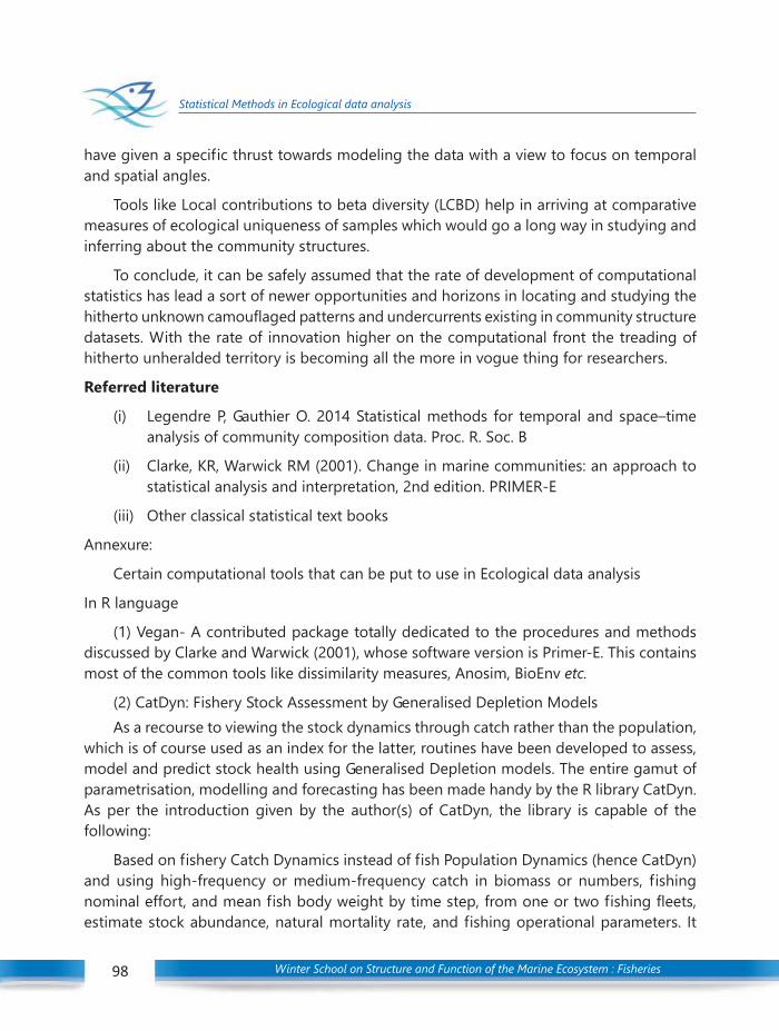
Winter School on Structure and Function of the Marine Ecosystem : Fisheries98
Statistical Methods in Ecological data analysis
have given a specific thrust towards modeling the data with a view to focus on temporaland spatial angles.
Tools like Local contributions to beta diversity (LCBD) help in arriving at comparativemeasures of ecological uniqueness of samples which would go a long way in studying andinferring about the community structures.
To conclude, it can be safely assumed that the rate of development of computationalstatistics has lead a sort of newer opportunities and horizons in locating and studying thehitherto unknown camouflaged patterns and undercurrents existing in community structuredatasets. With the rate of innovation higher on the computational front the treading ofhitherto unheralded territory is becoming all the more in vogue thing for researchers.
Referred literature
(i) Legendre P, Gauthier O. 2014 Statistical methods for temporal and space–timeanalysis of community composition data. Proc. R. Soc. B
(ii) Clarke, KR, Warwick RM (2001). Change in marine communities: an approach tostatistical analysis and interpretation, 2nd edition. PRIMER-E
(iii) Other classical statistical text books
Annexure:
Certain computational tools that can be put to use in Ecological data analysis
In R language
(1) Vegan- A contributed package totally dedicated to the procedures and methodsdiscussed by Clarke and Warwick (2001), whose software version is Primer-E. This containsmost of the common tools like dissimilarity measures, Anosim, BioEnv etc.
(2) CatDyn: Fishery Stock Assessment by Generalised Depletion ModelsAs a recourse to viewing the stock dynamics through catch rather than the population,
which is of course used as an index for the latter, routines have been developed to assess,model and predict stock health using Generalised Depletion models. The entire gamut ofparametrisation, modelling and forecasting has been made handy by the R library CatDyn.As per the introduction given by the author(s) of CatDyn, the library is capable of thefollowing:
Based on fishery Catch Dynamics instead of fish Population Dynamics (hence CatDyn)and using high-frequency or medium-frequency catch in biomass or numbers, fishingnominal effort, and mean fish body weight by time step, from one or two fishing fleets,estimate stock abundance, natural mortality rate, and fishing operational parameters. It
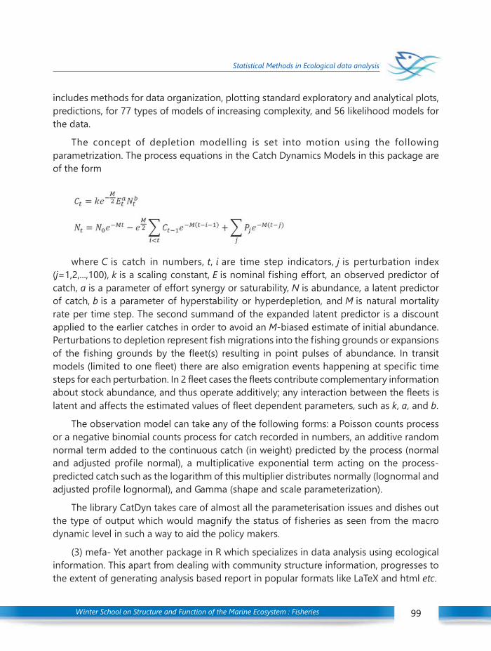
Winter School on Structure and Function of the Marine Ecosystem : Fisheries 99
Statistical Methods in Ecological data analysis
includes methods for data organization, plotting standard exploratory and analytical plots,predictions, for 77 types of models of increasing complexity, and 56 likelihood models forthe data.
The concept of depletion modelling is set into motion using the followingparametrization. The process equations in the Catch Dynamics Models in this package areof the form
where C is catch in numbers, t, i are time step indicators, j is perturbation index(j=1,2,...,100), k is a scaling constant, E is nominal fishing effort, an observed predictor ofcatch, a is a parameter of effort synergy or saturability, N is abundance, a latent predictorof catch, b is a parameter of hyperstability or hyperdepletion, and M is natural mortalityrate per time step. The second summand of the expanded latent predictor is a discountapplied to the earlier catches in order to avoid an M-biased estimate of initial abundance.Perturbations to depletion represent fish migrations into the fishing grounds or expansionsof the fishing grounds by the fleet(s) resulting in point pulses of abundance. In transitmodels (limited to one fleet) there are also emigration events happening at specific timesteps for each perturbation. In 2 fleet cases the fleets contribute complementary informationabout stock abundance, and thus operate additively; any interaction between the fleets islatent and affects the estimated values of fleet dependent parameters, such as k, a, and b.
The observation model can take any of the following forms: a Poisson counts processor a negative binomial counts process for catch recorded in numbers, an additive randomnormal term added to the continuous catch (in weight) predicted by the process (normaland adjusted profile normal), a multiplicative exponential term acting on the process-predicted catch such as the logarithm of this multiplier distributes normally (lognormal andadjusted profile lognormal), and Gamma (shape and scale parameterization).
The library CatDyn takes care of almost all the parameterisation issues and dishes outthe type of output which would magnify the status of fisheries as seen from the macrodynamic level in such a way to aid the policy makers.
(3) mefa- Yet another package in R which specializes in data analysis using ecologicalinformation. This apart from dealing with community structure information, progresses tothe extent of generating analysis based report in popular formats like LaTeX and html etc.

Winter School on Structure and Function of the Marine Ecosystem : Fisheries100
Statistical Methods in Ecological data analysis
Other sources
(1) XLSTAT- is an MS Excel friendly data analysis package which performs canonicalcorrespondence analysis in tandem with Excel spreadsheet and finds EC50 values etc. andomics data analysis.
(2) FLORA- is another software scripted for Windows environment, which handles themultivariate routines as applied to community structure data.
Summarizing, it can be recorded that the tools mostly applied for dealing with eco-biological data sets based on communities of flora and fauna stem from multivariate analysistools and the software variants focus mostly on the customized output and report generation.

Winter School on Structure and Function of the Marine Ecosystem : Fisheries 101
Sampling methodology employed by CMFRI for collection and estimation of marine fish landings in India
Fisheries sector plays a key role in Indian economy. The sector supports livelihood,nutritional security, and subsistence to large number of people as well as foreign exchangeearnings. India’s coast line stretches about 8129 km. There are 1511 landing centres scatteredalong the coastline of the main land as per the records from National Marine Fisheries DataCentre at Central Marine Fisheries Research Institute (CMFRI). Marine fish landings takeplace almost all along the coast line throughout the day and sometimes during night.Under these circumstances, collection of statistics by complete enumeration would involvea very large number of enumerators and a huge amount of money apart from the timeinvolved in collection of data. Therefore, a possible solution for quantifying marine fishlandings is adoption of a suitable sampling technique. As, monitoring and assessment ofthe exploited marine fishery resources of India is one of the important mandates of theCMFRI, institute made attempts to evolve the scientific methods for collection of data oncatch and effort, since its inception in 1947. Pilot surveys were conducted along the coastlineof India and different sampling designs were tested.
CMFRI introduced collectionof marine fish statistics througha stratif ied sampling designalong the west coast of India inthe year 1959 and extended toother states over the years.Keeping in pace with thechanging marine f isheriesscenario, the sampling design has been modified over the periods. Presently, CMFRI estimatemarine fish landings based on a multi-stage stratified random sampling technique,stratification is done over space and time. Each maritime state is divided into suitable, non-overlapping zones on the basis of fishing intensity and geographical considerations (Fig. 1).The number of landing centres varies from zone to zone.
Over space, each zone is regarded as a stratum and over time, a calendar month isconsidered as a stratum. Consequently, a zone and a calendar month constitute a space-*Reprinted from Course Manual of Summer School on Advanced Methods for Fish Stock Assessment and FisheriesManagement. Lecture Note Series No. 2/2017. CMFRI, Kochi, pp. 109-112
Fig. 1. Stratification over Space
13C H A P T E R SAMPLING METHODOLOGY EMPLOYED BY
CMFRI FOR COLLECTION AND ESTIMATIONOF MARINE FISH LANDINGS IN INDIAMini K. G.*
Fishery Resources Assessment DivisionICAR-Central Marine Fisheries Research Institute

Winter School on Structure and Function of the Marine Ecosystem : Fisheries102
Sampling methodology employed by CMFRI for collection and estimation of marine fish landings in India
time stratum. Suppose, in a zone, if there are 5 landing centres and 30 fishing days in themonth; then 5 x 30 = 150 landing centre days, combination of centre and day constitute theprimary stage units (PSU). The fishing craft that land on a landing centre day forms thesecond stage units (SSU). Furthermore, the fish landings vary considerably among the landingcentres in a multi-centre zone, mainly in different seasons and hence a zone is furtherstratified into substrata viz., major, minor and very minor. The centres in which eithermechanised crafts or 100 or more non-mechanised/motorised crafts are operating areconsidered as major centres. Likewise, other strata are defined based on the number andtype of fishing crafts operating.
Further, a month is divided into three groups each with ten days. A day is selected atrandom from the first five days of a month and 5 successive days are selected automatically.Three clusters of two successive days are made from the above selected days. To illustratethe selection of landing centres and days, let us consider a fishing zone in a month. Initially,select a date at random from the first five days, let it be 3. Then from the first 10 day group,three clusters of 2 days (3,4) (5,6) and (7,8) can be formed. From the second group of 10days, the clusters are systematically selected with an interval of 10 days. The clusters of daysformed are (13,14) (15,16) and (17,18). Similar selection can be done for the next group often days. Accordingly, 9 clusters of two days can be formed in a month. Afterwards, 9centres are selected with replacement from the total number of landing centres in a zoneand allotted to the 9 cluster days as explained before. Thus, a combination of a landingcentre and a day (landing centre day) forms the Primary Stage Units. A landing centre dayhas been divided into 3 periods as given in the infographic. That means a landing centreday is 24 hour duration which starts at noon of the first day and ends at noon of thefollowing day.
The marine fish landingsdata collection is done by thetechnical staff of CMFRI.Usually, one staff is identifiedto collect data from each zone.Data collection starts fromperiod 1 on each selectedlanding centre day. The staffwill be present throughout the periods 1 and 2 at the centres. The data on landings duringperiod 3 (night landings) is usually collected from the landing centre by enquiry on thefollowing day morning. The observations on the 3 periods contribute the data for onelanding centre day (24hrs). So, in a 10 day period, data from 3 centre-days are sampled andthus in a month 9 landing centre days are sampled.
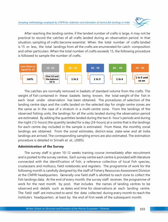
Winter School on Structure and Function of the Marine Ecosystem : Fisheries 103
Sampling methodology employed by CMFRI for collection and estimation of marine fish landings in India
After reaching the landing centre, if the landed number of crafts is large, it may not bepractical to record the catches of all crafts landed during an observation period. In thatsituation, sampling of crafts become essential. When the total number of crafts landedis 15 or less, the total landings from all the crafts are enumerated for catch compositionand other particulars. When the total number of crafts exceeds 15, the following procedureis followed to sample the number of crafts.
The catches are normally removed in baskets of standard volume from the crafts. Theweight of fish contained in these baskets being known, the total weight of the fish ineach boat under observation has been obtained. The procedures of selection of thelanding centre days and the crafts landed on the selected day for single centre zones arethe same as in the case of a stratum in a multi-centre zone. From the landings of theobserved fishing units, the landings for all the units landed during the observation periodare estimated. By adding the quantities landed during the two 6- hour’s periods and duringthe night (12-hours) the quantity landed for a day (24-hours) at a centre that is the landingsfor each centre day included in the sample is estimated. From these, the monthly zonallandings are obtained. From the zonal estimates, district-wise, state-wise and all Indialandings are arrived. The corresponding sampling errors are also estimated. The estimationprocedure is detailed in Srinath et. al., (2005).
Administration of the Survey
The survey staff is given 10-12 weeks training course immediately after recruitmentand is posted to the survey centres. Each survey centre each centre is provided with literatureconnected with the identification of fish, a reference collection of local fish species,crustaceans and molluscs, field notebooks and registers. The programme of work for thefollowing month is carefully designed by the staff of Fishery Resources Assessment Divisionat the CMFRI headquarters. Generally one field staff is allotted to each zone to collect thefish landings data. At the end of every month, the survey staff receives the programme ofwork for the next month by post, that includes the names of landing centres to beobserved and details such as dates and time for observations at each landing centre.The field staff are instructed to send the data collected during every month to reach theInstitute’s headquarters at least by the end of first week of the subsequent month.

Winter School on Structure and Function of the Marine Ecosystem : Fisheries104
Sampling methodology employed by CMFRI for collection and estimation of marine fish landings in India
Surprise inspections are carried out by the supervisory staff of the Institute andthe enumerators are inspected while at work in the field and their field notebooks anddiaries are scrutinised. The estimated zonal landings are always compared with the previousyear’s survey figures, and if any variation which cannot be explained is observed, thetechnique of interpenetrating sub-samples is adopted to detect observational errors. Zonalworkshops are held periodically to review the progress of work and update the samplingframe and to impart refresher courses to the field staff. Non-response occurs when theregular field staff is not available to observe the centre-day included in the sample. Usually,arrangements are made at the Headquarters/Research/Regional Centre to minimise thenon-response.
In the existing sampling methodology, the interest is to estimate gear-wise, species-wise landings for the state in a month, fishing effort according to different types of fishingcrafts and also in terms of man hours. The analysis is carried out at CMFRI headquarters.Before the data is processed for analysis it will be ensured that the data collection is madeas per the approved schedule, by checking the appropriate proforma. The responsibilitiesand functions of staff at the headquarters are data coding, estimation and databasemanagement. The data analysis is computerised and estimates are made using the softwaredeveloped by the Fishery Resources Assessment Division of the Institute. The processeddata are again counter- checked for errors. When discrepancies are detected, the estimationprocedure is scrutinised in detail.
References
M. Srinath, Somy Kuriakose and K.G. Mini, 2005. Methodology for the Estimation of Marine Fish Landingsin India, CMFRI Special Publication No. 86, p.57.
Winter School on Structure and Function of the Marine Ecosystem : Fisheries 105
An introduction to R programming
Introduction
R language is the GNU arm of S language, which has taken the computational world bystorm in the last decade. Starting as a compendium of statistical tools, this language hasgrown up into a canopy lording over a research analysis environment thereby subsumingmany hitherto complicated manoeuvres onto the realms of syntactical simplicity. As this anexponentially expanding field of development with ever exploding information downpour,it would be a near impossible task to frame it onto a short simple foundational discourse.However in the subsequent sections we would try to view the potential and the extent ofpracticality we would unravel the hidden features of the software through a GUI envelopalso apart from the regular console and syntax based one. To get its power moreunderstandable we would visualize its forays into the field of analytics using medium scaleexamples from marine fisheries data.
R is “GNU S” — A language and environment for data manipulation, calculationand graphical display.
– R is similar to the award-winning S system, which was developed at BellLaboratories by John Chambers et al.,
– a suite of operators for calculations on arrays, in particular matrices,
– a large, coherent, integrated collection of intermediate tools for interactivedata analysis,
– graphical facilities for data analysis and display either directly at the computeror on hardcopy
– a well developed programming language which includes conditionals, loops,user defined recursive functions and input and output facilities.
The core of R is an interpreted computer language.
– It allows branching and looping as well as modular programming usingfunctions.
– Most of the user-visible functions in R are written in R, calling upon a smallerset of internal primitives.
14C H A P T E R AN INTRODUCTION TO R PROGRAMMING
J. Jayasankar, T. V. Ambrose and R. Manjeesh
Fishery Resources Assessment DivisionICAR-Central Marine Fisheries Research Institute
Winter School on Structure and Function of the Marine Ecosystem : Fisheries106
An introduction to R programming
It is possible for the user to interface to procedures written in C, C++ or FORTRANlanguages for efficiency, and also to write additional primitives.
R, S and S-plus- a brief time line
S: an interactive environment for data analysis developed at Bell Laboratories since1976
– 1988 - S2: RA Becker, JM Chambers, A Wilks
– 1992 - S3: JM Chambers, TJ Hastie
– 1998 - S4: JM Chambers
Exclusively licensed by AT&T/Lucent to Insightful Corporation, Seattle WA. Productname: “S-plus”.
Implementation languages C, Fortran.
See: http://cm.bell-labs.com/cm/ms/departments/sia/S/history.html
R: initially written by Ross Ihaka and Robert Gentleman at Dep. of Statistics ofUniversity of Auckland, New Zealand during 1990s.
Since 1997: international “R-core” team of ca. 15 people with access to commonCVS archive.
What R does and does not
o data handling and storage: o is not a database, but connects tonumeric, textualo DBMSsmatrix algebrao
o hash tables and regular expressions o has no graphical user interfaces,but connects to Java, TclTko
o high-level data analytic and statistical o language interpreter can be veryfunctions slow, but allows to call own C/C++
codeo classes (Object Oriented “OO”) o no spreadsheet view of data, but
connects to Excel/MsOfficeo graphics o no professional / commercialo programming language: loops, support
branching, subroutines
R and statistics
o Packaging: a crucial infrastructure to efficiently produce, load and keep consistent

Winter School on Structure and Function of the Marine Ecosystem : Fisheries 107
An introduction to R programming
software libraries from (many) different sources / authors, which are updated at abest possible refresh rate
o Statistics: most packages deal with statistics and data analysis and there are manyconduit and value addition libraries which augment the statistical inference
o State of the art: many statistical researchers provide their methods as R packages
Statistical AnalysisData Analysis and Presentation happen to be the core strength of R software environment
and the ease with which this is performed makes the environment as the ultimate winner.Faster computational routines and amenability of access and modification to interim stepsand results makes the programming environment a winner.
The R distribution contains functionality for large number of statistical procedures.
– linear and generalized linear models
– nonlinear regression models
– time series analysis
– classical parametric and nonparametric tests
– clustering
– smoothing
R also has a large set of functions which provide a flexible graphical environmentfor creating various kinds of data presentations.
References For R
– The basic reference is The New S Language: A Programming Environmentfor Data Analysis and Graphics by Richard A. Becker, John M. Chambers andAllan R. Wilks (the “Blue Book”) .
– The new features of the 1991 release of S (S version 3) are covered in StatisticalModels in S edited by John M. Chambers and Trevor J. Hastie (the “WhiteBook”).
– Classical and modern statistical techniques have been implemented.
Some of these are built into the base R environment.
Many are supplied as packages. There are about 8 packages supplied
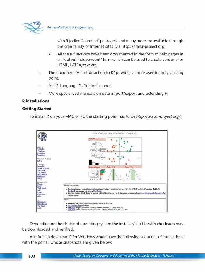
Winter School on Structure and Function of the Marine Ecosystem : Fisheries108
An introduction to R programming
with R (called “standard” packages) and many more are available throughthe cran family of Internet sites (via http://cran.r-project.org).
All the R functions have been documented in the form of help pages inan “output independent” form which can be used to create versions forHTML, LATEX, text etc.
– The document “An Introduction to R” provides a more user-friendly startingpoint.
– An “R Language Definition” manual
– More specialized manuals on data import/export and extending R.
R installations
Getting Started
To install R on your MAC or PC the starting point has to be http://www.r-project.org/.
Depending on the choice of operating system the installer/ zip file with checksum maybe downloaded and verified.
An effort to download R for Windows would have the following sequence of interactionswith the portal, whose snapshots are given below:

Winter School on Structure and Function of the Marine Ecosystem : Fisheries 109
An introduction to R programming
Its always a good idea to download all the files.

Winter School on Structure and Function of the Marine Ecosystem : Fisheries110
An introduction to R programming
MDI is when the windows will be contained within one large window.

Winter School on Structure and Function of the Marine Ecosystem : Fisheries 111
An introduction to R programming
This is similar to how Excel is setup. SDI is a single document interface where every itemwill get its own window. This is similar to how SPSS is set up where it has separate dataeditor, viewer, and syntax windows. Once you choose which your prefer, click next.
Choosing either html or plain text and clicking is the next step.
The installation may take awhile
To install packages on Windows, clicking on packages and install packages will be thenext step.

Winter School on Structure and Function of the Marine Ecosystem : Fisheries112
An introduction to R programming
Scrolling down to country nearest and choosing a "mirror" that is close is the nextstep.
Scrolling down list until the requisite package is the next step, keeping in mind that Rlists things in alphabetical order and by uppercase than lowercase. Once a package is clickedto load, R will install not only the package but all of the packages needed to run thepackage, including the dependencies.
To actually use the package, one has to go back to the package tab and click on loadpackage.
Using Help Command
?solve translates on to giving details of help information about “solve” function whilsthelp.search or ?? allows searching for help in various ways.

Winter School on Structure and Function of the Marine Ecosystem : Fisheries 113
An introduction to R programming
R Commander – A graphical interaction “skin” for R
R provides a powerful and comprehensive system for analysing data and when used inconjunction with the R-commander (a graphical user interface, commonly known as Rcmdr)it also provides one that is easy and intuitive to use. Basically, R provides the engine thatcarries out the analyses and Rcmdr provides a convenient way for users to input commands.The Rcmdr program enables analysts to access a selection of commonly-used R commandsusing a simple interface that should be familiar to most computer users. It also serves theimportant role of helping users to implement R commands and develop their knowledgeand expertise in using the command line — an important skill for those wishing to exploitthe full power of the program.( http://www.rcommander.com/)
a) Loading R Commander
– Packages -> Install Packages -> Cran Mirror Selection -> Rcmdr
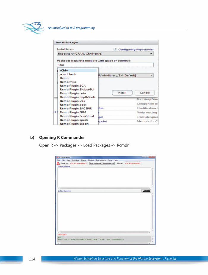
Winter School on Structure and Function of the Marine Ecosystem : Fisheries114
An introduction to R programming
b) Opening R Commander
Open R -> Packages -> Load Packages -> Rcmdr
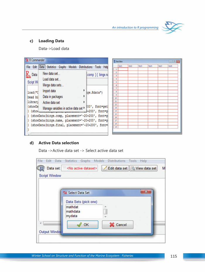
Winter School on Structure and Function of the Marine Ecosystem : Fisheries 115
An introduction to R programming
c) Loading Data
Data->Load data
d) Active Data selection
Data ->Active data set -> Select active data set
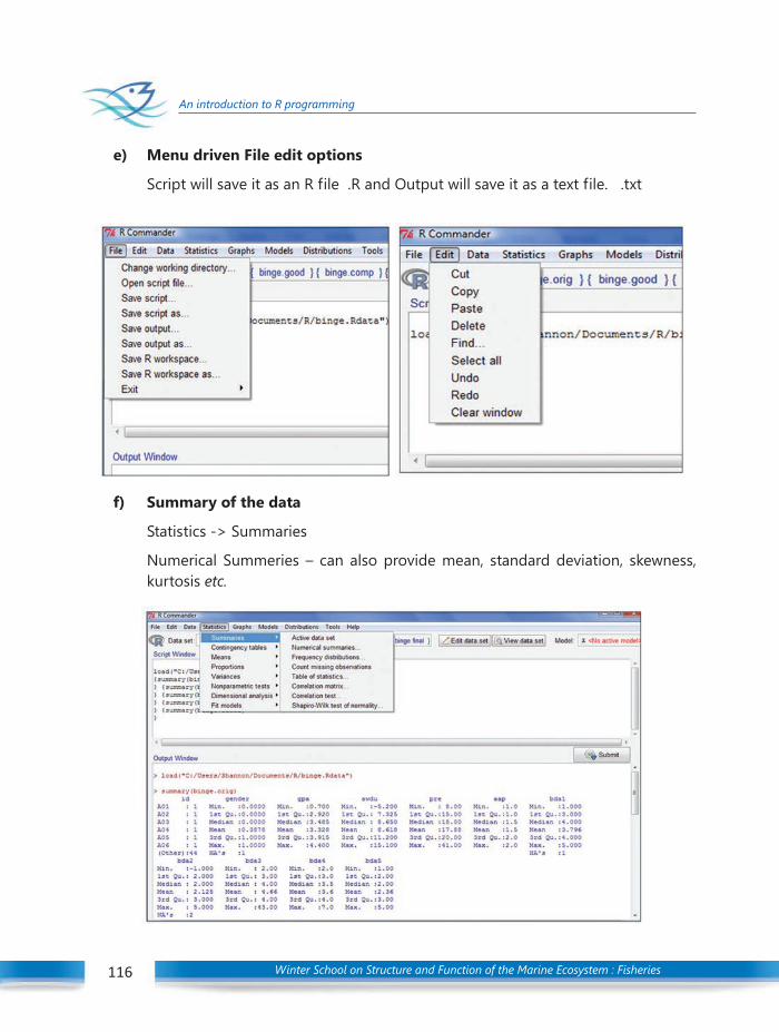
Winter School on Structure and Function of the Marine Ecosystem : Fisheries116
An introduction to R programming
e) Menu driven File edit options
Script will save it as an R file .R and Output will save it as a text file. .txt
f) Summary of the data
Statistics -> Summaries
Numerical Summeries – can also provide mean, standard deviation, skewness,kurtosis etc.

Winter School on Structure and Function of the Marine Ecosystem : Fisheries 117
An introduction to R programming
g) Mean, Standard Deviation, Skewness, Kurtosis
h) Contingency Tables

Winter School on Structure and Function of the Marine Ecosystem : Fisheries118
An introduction to R programming
i) Correlations in R Commander
Correlation analysis can be done with R as follows.
Correlation is a bivariate analysis that measures the strengths of association betweentwo variables and the direction of the relationship. In terms of the strength of relationship,the value of the correlation coefficient varies between +1 and -1. When the value of thecorrelation coefficient lies around ± 1, then it is said to be a perfect degree of associationbetween the two variables. As the correlation coefficient value goes towards 0, therelationship between the two variables will be weaker. the direction of the relationship issimply the + (indicating a positive relationship between the variables) or - (indicating anegative relationship between the variables) sign of the correlation. Usually, in statistics,we measure four types of correlations: Pearson Correlation, Kendall rank correlation,Spearman correlation, and the Point-Biserial correlation. The software below allows you tovery easily conduct a correlation.
j) Independent T-Test
The independent t-test, also referred to as an independent-samples t-test, independentmeasures t-test or unpaired t-test, is used to determine whether the mean of a dependentvariable (e.g., weight, anxiety level, salary, reaction time, etc.) is the same in two unrelated,independent groups (e.g., males vs females, employed vs unemployed, under 21 year oldsvs those 21 years and older, etc.). Specifically, you use an independent t-test to determinewhether the mean difference between two groups is statistically significantly different tozero.
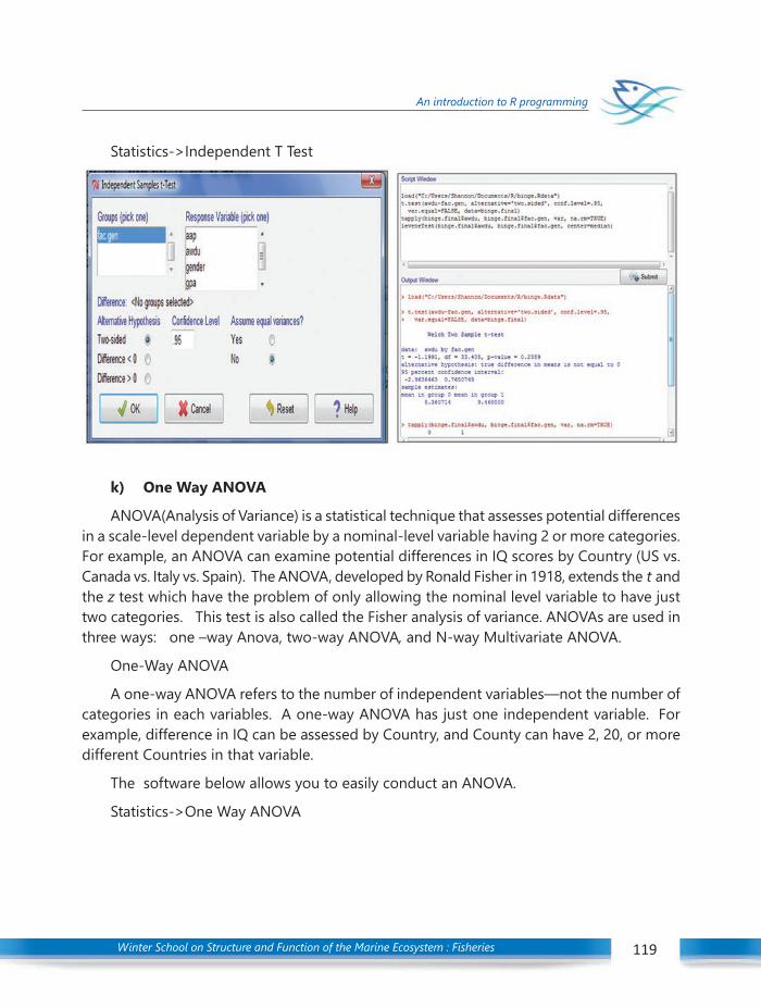
Winter School on Structure and Function of the Marine Ecosystem : Fisheries 119
An introduction to R programming
Statistics->Independent T Test
k) One Way ANOVA
ANOVA(Analysis of Variance) is a statistical technique that assesses potential differencesin a scale-level dependent variable by a nominal-level variable having 2 or more categories.For example, an ANOVA can examine potential differences in IQ scores by Country (US vs.Canada vs. Italy vs. Spain). The ANOVA, developed by Ronald Fisher in 1918, extends the t andthe z test which have the problem of only allowing the nominal level variable to have justtwo categories. This test is also called the Fisher analysis of variance. ANOVAs are used inthree ways: one –way Anova, two-way ANOVA, and N-way Multivariate ANOVA.
One-Way ANOVA
A one-way ANOVA refers to the number of independent variables—not the number ofcategories in each variables. A one-way ANOVA has just one independent variable. Forexample, difference in IQ can be assessed by Country, and County can have 2, 20, or moredifferent Countries in that variable.
The software below allows you to easily conduct an ANOVA.
Statistics->One Way ANOVA
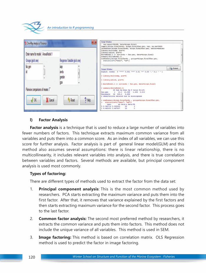
Winter School on Structure and Function of the Marine Ecosystem : Fisheries120
An introduction to R programming
l) Factor Analysis
Factor analysis is a technique that is used to reduce a large number of variables intofewer numbers of factors. This technique extracts maximum common variance from allvariables and puts them into a common score. As an index of all variables, we can use thisscore for further analysis. Factor analysis is part of general linear model(GLM) and thismethod also assumes several assumptions: there is linear relationship, there is nomulticollinearity, it includes relevant variables into analysis, and there is true correlationbetween variables and factors. Several methods are available, but principal componentanalysis is used most commonly.
Types of factoring:
There are different types of methods used to extract the factor from the data set:
1. Principal component analysis: This is the most common method used byresearchers. PCA starts extracting the maximum variance and puts them into thefirst factor. After that, it removes that variance explained by the first factors andthen starts extracting maximum variance for the second factor. This process goesto the last factor.
2. Common factor analysis: The second most preferred method by researchers, itextracts the common variance and puts them into factors. This method does notinclude the unique variance of all variables. This method is used in SEM.
3. Image factoring: This method is based on correlation matrix. OLS Regressionmethod is used to predict the factor in image factoring.
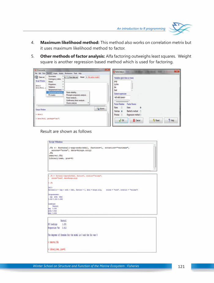
Winter School on Structure and Function of the Marine Ecosystem : Fisheries 121
An introduction to R programming
4. Maximum likelihood method: This method also works on correlation metrix butit uses maximum likelihood method to factor.
5. Other methods of factor analysis: Alfa factoring outweighs least squares. Weightsquare is another regression based method which is used for factoring.
Result are shown as follows

Winter School on Structure and Function of the Marine Ecosystem : Fisheries122
An introduction to R programming
J) Graphs
Gparhs->Scatter plot
Gparhs->Box plot
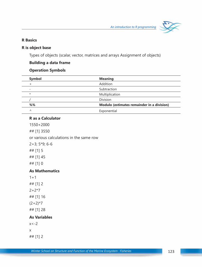
Winter School on Structure and Function of the Marine Ecosystem : Fisheries 123
An introduction to R programming
R Basics
R is object base
Types of objects (scalar, vector, matrices and arrays Assignment of objects)
Building a data frame
Operation Symbols
Symbol Meaning+ Addition- Subtraction* Multiplication/ Division%% Modulo (estimates remainder in a division)
^ Exponential
R as a Calculator1550+2000## [1] 3550or various calculations in the same row2+3; 5*9; 6-6## [1] 5## [1] 45## [1] 0
As Mathematics1+1## [1] 22+2*7## [1] 16(2+2)*7## [1] 28
As Variablesx<-2x## [1] 2

Winter School on Structure and Function of the Marine Ecosystem : Fisheries124
An introduction to R programming
y<-3y## [1] 35->z(x*y)+z## [1] 11Numbers in R: NAN and NA
NAN (not a number) NA (missing value) -Basic handling of missing values
Missing values are noise to statistical estimations. We are going to learn a basic commandfor handling missing values.
x<-c(1,2,3,4,5,6,NA)
mean(x)## [1] NA
mean(x,na.rm=TRUE)## [1] 3.5
Objects in RObjects in R obtain values by assignment.This is achieved by the gets arrow, <-, and not the equal sign, =.Objects can be of different kinds.
Built in Functions
R has many built in functions that compute different statistical procedures.
Functions in R are followed by ( ). Inside the parenthesis we write the object (vector,matrix, array, dataframe) to which we want to apply the function.
# Create a sequence of numbers from 32 to 44.
print(seq(32,44))## [1] 32 33 34 35 36 37 38 39 40 41 42 43 44# Find mean of numbers from 25 to 82.
print(mean(25:82))## [1] 53.5
# Find sum of numbers frm 41 to 68.

Winter School on Structure and Function of the Marine Ecosystem : Fisheries 125
An introduction to R programming
print(sum(41:68))## [1] 1526
VectorsVectors are variables with one or more values of the same type.
A variable with a single value is known as scalar. In R a scalar is a vector of length 1.There are at least three ways to create vectors in R: (a) sequence, (b) concatenation function,and (c) scan function.
Create two vectors of different lengths.
vector1 <- c(5,9,3)
vector2 <- c(10,11,12,13,14,15)
vector1
## [1] 5 9 3
vector2
## [1] 10 11 12 13 14 15
Arrays
Arrays are numeric objects with dimension attributes. The difference between a matrixand an array is that arrays have more than two dimensions.
# Take the above vectors as input to the array.
result <- array(c(vector1,vector2),dim = c(3,3,2))
print(result)
## , , 1#### [,1] [,2] [,3]## [1,] 5 10 13## [2,] 9 11 14## [3,] 3 12 15##

Winter School on Structure and Function of the Marine Ecosystem : Fisheries126
An introduction to R programming
## , , 2#### [,1] [,2] [,3]## [1,] 5 10 13## [2,] 9 11 14## [3,] 3 12 15
Matrices
A matrix is a two dimensional array. The command colnames
# Elements are arranged sequentially by row.
M <- matrix(c(3:14), nrow = 4, byrow = TRUE)
print(M)## [,1] [,2] [,3]## [1,] 3 4 5## [2,] 6 7 8## [3,] 9 10 11## [4,] 12 13 14
String Characters
In R, string variables are defined by double quotation marks.letters<-c(“a”,”b”,”c”)letters## [1] “a” “b” “c”
Subscripts and Indices
Select only one or some of the elements in a vector, a matrix or an array. We can do thisby using subscripts in square brackets [ ].
In matrices or dataframes the first subscript refers to the row and the second to thecolumn.
Dataframe
Researchers work mostly with dataframes. With previous knowledge you can builtdataframes in R. Also, import dataframes into R.

Winter School on Structure and Function of the Marine Ecosystem : Fisheries 127
An introduction to R programming
# Create the data frame.emp.data <- data.frame (emp_id = c (1:5),emp_name = c(“Rick”,”Dan”,”Michelle”,”Ryan”,”Gary”),
salary = c(623.3,515.2,611.0,729.0,843.25),
start_date = as.Date(c(“2012-01-01”, “2013-09-23”, “2014-11-15”, “2014-05-11”,
“2015-03-27”)),
stringsAsFactors = FALSE
)
# Print the data frame.
print(emp.data)
## emp_id emp_name salary start_date
## 1 1 Rick 623.30 2012-01-01## 2 2 Dan 515.20 2013-09-23## 3 3 Michelle 611.00 2014-11-15## 4 4 Ryan 729.00 2014-05-11## 5 5 Gary 843.25 2015-03-27
A journey wading through the amazing summarizing and analytical capabilitiesof R- a case study
Let the presumed data pertain to landings and standardized effort of a maritime stateestimated by ICAR-CMFRI during the interregnum 1997 to 2013
calling file in R
klm<-read.csv(“C:/Users/cmfri/Desktop/cpue_spcode_kldata.csv”,header=TRUE)
To know header portion of the data set
head(klm)
## year month species raised nomeff stdcpue## 1 1997 1 40 20595.35 122.0811 3.634042## 2 1997 2 40 24201.10 114.3719 4.532246## 3 1997 3 40 23497.64 255.0315 3.926130

Winter School on Structure and Function of the Marine Ecosystem : Fisheries128
An introduction to R programming
## 4 1997 4 40 50176.75 154.7663 6.762821## 5 1997 5 40 137626.24 314.6413 13.805531## 6 1997 6 40 38149.38 649.1328 16.071358
To check the last few rows of the dataset
tail (klm)
## year month species raised nomeff stdcpue## 245815 2013 7 4580 0 0.000000 0.000000## 245816 2013 8 4580 1674 2.059835 1.667304## 245817 2013 9 4580 0 0.000000 0.000000## 245818 2013 10 4580 0 0.000000 0.000000## 245819 2013 11 4580 0 0.000000 0.000000## 245820 2013 12 4580 0 0.000000 0.000000
to know the observations in the data
length(klm)
## [1] 6to know the structure of the dataframe
str(klm)## ‘data.frame’: 245820 obs. of 6 variables:## $ year : int 1997 1997 1997 1997 1997 1997 1997 1997 1997 1997 ...## $ month : int 1 2 3 4 5 6 7 8 9 10 ...## $ species: int 40 40 40 40 40 40 40 40 40 40 ...## $ raised : num 20595 24201 23498 50177 137626 ...## $ nomeff : num 122 114 255 155 315 ...## $ stdcpue: num 3.63 4.53 3.93 6.76 13.81 ...
Descriptive statistics analysis
summary(klm)
## year month species raised## Min. :1997 Min. : 1.00 Min. : 0 Min. : 0## 1st Qu.:2001 1st Qu.: 3.75 1st Qu.: 867 1st Qu.: 0## Median :2005 Median : 6.50 Median :1513 Median : 0
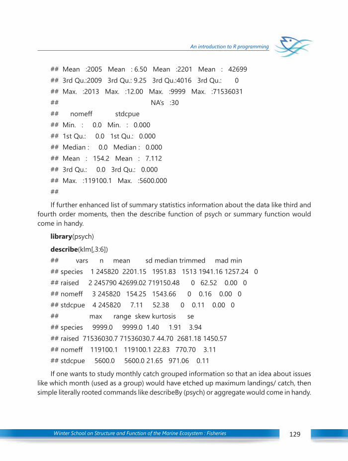
Winter School on Structure and Function of the Marine Ecosystem : Fisheries 129
An introduction to R programming
## Mean :2005 Mean : 6.50 Mean :2201 Mean : 42699## 3rd Qu.:2009 3rd Qu.: 9.25 3rd Qu.:4016 3rd Qu.: 0## Max. :2013 Max. :12.00 Max. :9999 Max. :71536031## NA’s :30## nomeff stdcpue## Min. : 0.0 Min. : 0.000## 1st Qu.: 0.0 1st Qu.: 0.000## Median : 0.0 Median : 0.000## Mean : 154.2 Mean : 7.112## 3rd Qu.: 0.0 3rd Qu.: 0.000## Max. :119100.1 Max. :5600.000##
If further enhanced list of summary statistics information about the data like third andfourth order moments, then the describe function of psych or summary function wouldcome in handy.
library(psych)
describe(klm[,3:6])## vars n mean sd median trimmed mad min## species 1 245820 2201.15 1951.83 1513 1941.16 1257.24 0## raised 2 245790 42699.02 719150.48 0 62.52 0.00 0## nomeff 3 245820 154.25 1543.66 0 0.16 0.00 0## stdcpue 4 245820 7.11 52.38 0 0.11 0.00 0## max range skew kurtosis se## species 9999.0 9999.0 1.40 1.91 3.94## raised 71536030.7 71536030.7 44.70 2681.18 1450.57## nomeff 119100.1 119100.1 22.83 770.70 3.11## stdcpue 5600.0 5600.0 21.65 971.06 0.11
If one wants to study monthly catch grouped information so that an idea about issueslike which month (used as a group) would have etched up maximum landings/ catch, thensimple literally rooted commands like describeBy (psych) or aggregate would come in handy.
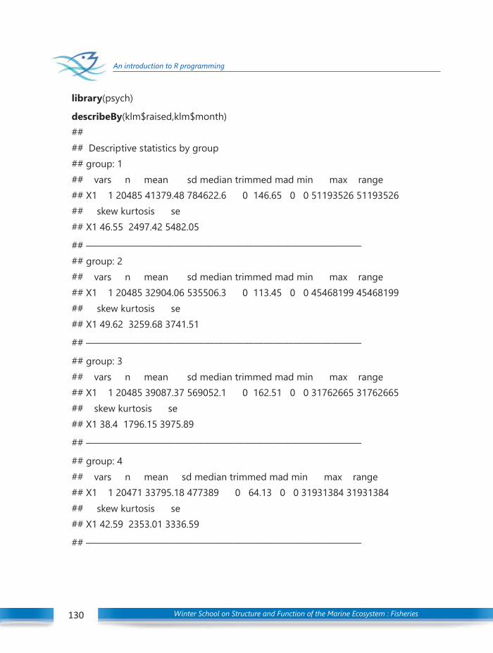
Winter School on Structure and Function of the Marine Ecosystem : Fisheries130
An introduction to R programming
library(psych)
describeBy(klm$raised,klm$month)#### Descriptive statistics by group## group: 1## vars n mean sd median trimmed mad min max range## X1 1 20485 41379.48 784622.6 0 146.65 0 0 51193526 51193526## skew kurtosis se## X1 46.55 2497.42 5482.05
## ————————————————————————————## group: 2## vars n mean sd median trimmed mad min max range## X1 1 20485 32904.06 535506.3 0 113.45 0 0 45468199 45468199## skew kurtosis se## X1 49.62 3259.68 3741.51
## ————————————————————————————
## group: 3## vars n mean sd median trimmed mad min max range## X1 1 20485 39087.37 569052.1 0 162.51 0 0 31762665 31762665## skew kurtosis se## X1 38.4 1796.15 3975.89
## ————————————————————————————
## group: 4## vars n mean sd median trimmed mad min max range## X1 1 20471 33795.18 477389 0 64.13 0 0 31931384 31931384## skew kurtosis se## X1 42.59 2353.01 3336.59
## ————————————————————————————

Winter School on Structure and Function of the Marine Ecosystem : Fisheries 131
An introduction to R programming
## group: 5## vars n mean sd median trimmed mad min max range## X1 1 20485 37566.67 469275.5 0 96.2 0 0 30492626 30492626## skew kurtosis se## X1 33.18 1478.99 3278.76
## ————————————————————————————## group: 6## vars n mean sd median trimmed mad min max range## X1 1 20485 34552.2 655525.6 0 30.67 0 0 65432961 65432961## skew kurtosis se
## X1 61.23 5239.89 4580.07
## ————————————————————————————## group: 7## vars n mean sd median trimmed mad min max range## X1 1 20485 32621.2 643003.1 0 0 0 0 49428947 49428947## skew kurtosis se## X1 42.19 2362.03 4492.57
## ————————————————————————————
## group: 8## vars n mean sd median trimmed mad min max range## X1 1 20484 57397.86 713381.8 0 31.03 0 0 38795185 38795185## skew kurtosis se## X1 26.21 920.16 4984.42
## ————————————————————————————
## group: 9## vars n mean sd median trimmed mad min max range## X1 1 20485 55833.65 901880.9 0 34.3 0 0 71536031 71536031## skew kurtosis se## X1 41.11 2415.63 6301.32
## ————————————————————————————
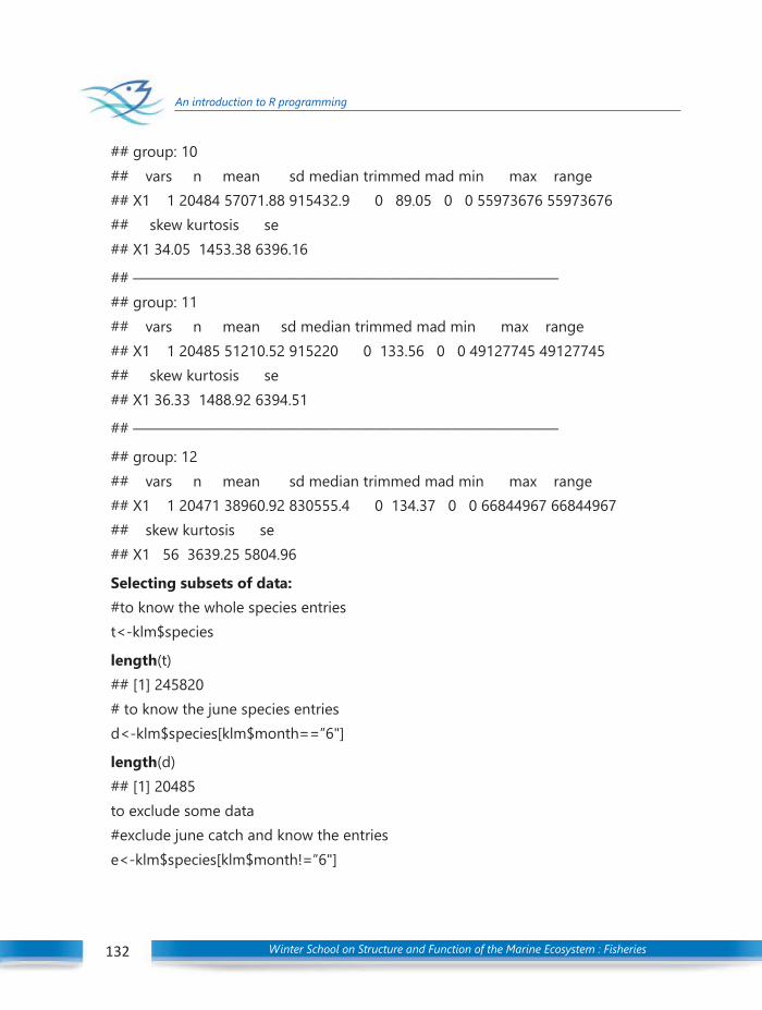
Winter School on Structure and Function of the Marine Ecosystem : Fisheries132
An introduction to R programming
## group: 10## vars n mean sd median trimmed mad min max range## X1 1 20484 57071.88 915432.9 0 89.05 0 0 55973676 55973676## skew kurtosis se## X1 34.05 1453.38 6396.16
## ————————————————————————————## group: 11## vars n mean sd median trimmed mad min max range## X1 1 20485 51210.52 915220 0 133.56 0 0 49127745 49127745## skew kurtosis se## X1 36.33 1488.92 6394.51
## ————————————————————————————
## group: 12## vars n mean sd median trimmed mad min max range## X1 1 20471 38960.92 830555.4 0 134.37 0 0 66844967 66844967## skew kurtosis se## X1 56 3639.25 5804.96
Selecting subsets of data:#to know the whole species entriest<-klm$species
length(t)## [1] 245820# to know the june species entriesd<-klm$species[klm$month==”6"]
length(d)## [1] 20485to exclude some data#exclude june catch and know the entriese<-klm$species[klm$month!=”6"]
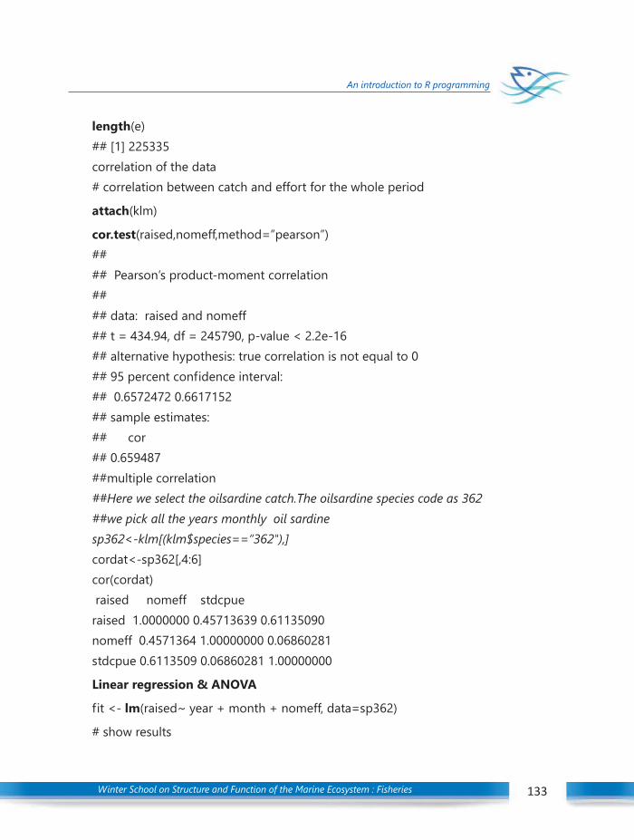
Winter School on Structure and Function of the Marine Ecosystem : Fisheries 133
An introduction to R programming
length(e)## [1] 225335correlation of the data# correlation between catch and effort for the whole period
attach(klm)
cor.test(raised,nomeff,method=”pearson”)#### Pearson’s product-moment correlation#### data: raised and nomeff## t = 434.94, df = 245790, p-value < 2.2e-16## alternative hypothesis: true correlation is not equal to 0## 95 percent confidence interval:## 0.6572472 0.6617152## sample estimates:## cor## 0.659487##multiple correlation##Here we select the oilsardine catch.The oilsardine species code as 362##we pick all the years monthly oil sardinesp362<-klm[(klm$species==”362"),]cordat<-sp362[,4:6]cor(cordat) raised nomeff stdcpueraised 1.0000000 0.45713639 0.61135090nomeff 0.4571364 1.00000000 0.06860281stdcpue 0.6113509 0.06860281 1.00000000
Linear regression & ANOVA
fit <- lm(raised~ year + month + nomeff, data=sp362)
# show results
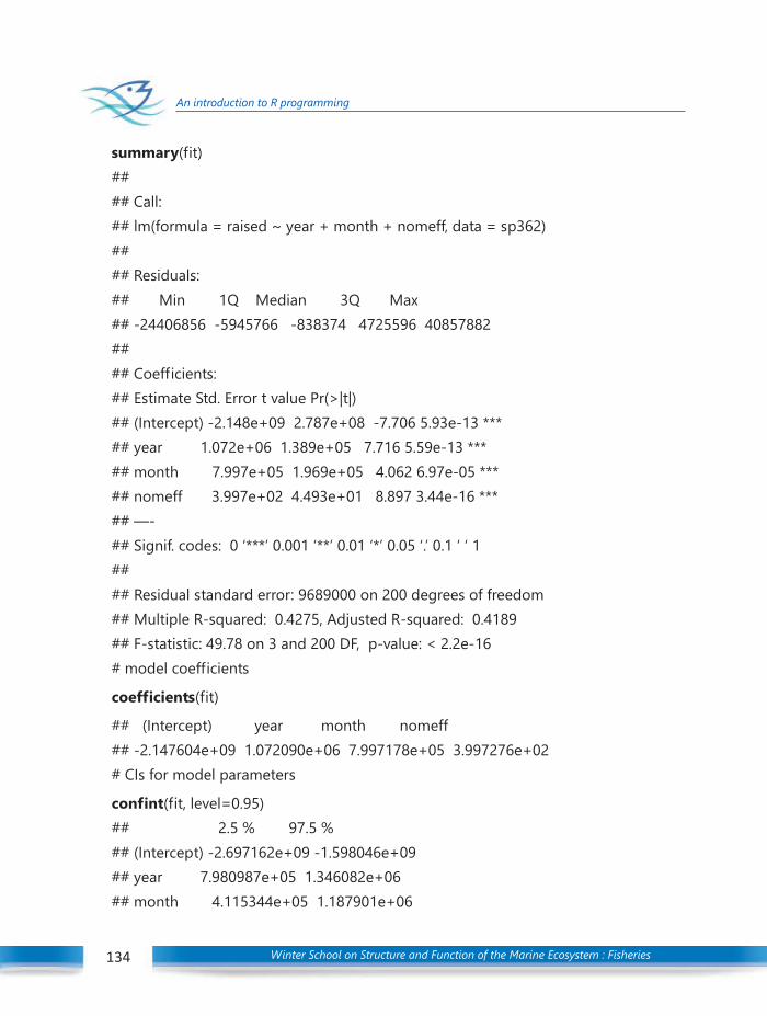
Winter School on Structure and Function of the Marine Ecosystem : Fisheries134
An introduction to R programming
summary(fit)#### Call:## lm(formula = raised ~ year + month + nomeff, data = sp362)#### Residuals:## Min 1Q Median 3Q Max## -24406856 -5945766 -838374 4725596 40857882#### Coefficients:## Estimate Std. Error t value Pr(>|t|)## (Intercept) -2.148e+09 2.787e+08 -7.706 5.93e-13 ***## year 1.072e+06 1.389e+05 7.716 5.59e-13 ***## month 7.997e+05 1.969e+05 4.062 6.97e-05 ***## nomeff 3.997e+02 4.493e+01 8.897 3.44e-16 ***## —-## Signif. codes: 0 ‘***’ 0.001 ‘**’ 0.01 ‘*’ 0.05 ‘.’ 0.1 ‘ ‘ 1#### Residual standard error: 9689000 on 200 degrees of freedom## Multiple R-squared: 0.4275, Adjusted R-squared: 0.4189## F-statistic: 49.78 on 3 and 200 DF, p-value: < 2.2e-16# model coefficients
coefficients(fit)
## (Intercept) year month nomeff## -2.147604e+09 1.072090e+06 7.997178e+05 3.997276e+02# CIs for model parameters
confint(fit, level=0.95)## 2.5 % 97.5 %## (Intercept) -2.697162e+09 -1.598046e+09## year 7.980987e+05 1.346082e+06## month 4.115344e+05 1.187901e+06
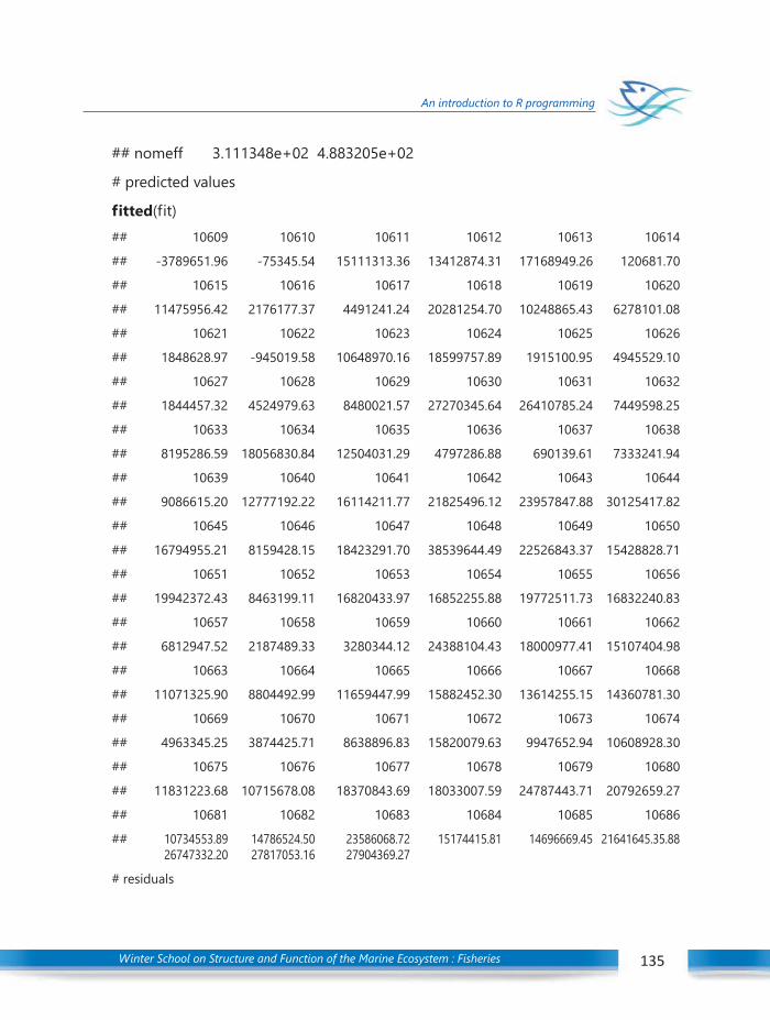
Winter School on Structure and Function of the Marine Ecosystem : Fisheries 135
An introduction to R programming
## nomeff 3.111348e+02 4.883205e+02
# predicted values
fitted(fit)## 10609 10610 10611 10612 10613 10614
## -3789651.96 -75345.54 15111313.36 13412874.31 17168949.26 120681.70
## 10615 10616 10617 10618 10619 10620
## 11475956.42 2176177.37 4491241.24 20281254.70 10248865.43 6278101.08
## 10621 10622 10623 10624 10625 10626
## 1848628.97 -945019.58 10648970.16 18599757.89 1915100.95 4945529.10
## 10627 10628 10629 10630 10631 10632
## 1844457.32 4524979.63 8480021.57 27270345.64 26410785.24 7449598.25
## 10633 10634 10635 10636 10637 10638
## 8195286.59 18056830.84 12504031.29 4797286.88 690139.61 7333241.94
## 10639 10640 10641 10642 10643 10644
## 9086615.20 12777192.22 16114211.77 21825496.12 23957847.88 30125417.82
## 10645 10646 10647 10648 10649 10650
## 16794955.21 8159428.15 18423291.70 38539644.49 22526843.37 15428828.71
## 10651 10652 10653 10654 10655 10656
## 19942372.43 8463199.11 16820433.97 16852255.88 19772511.73 16832240.83
## 10657 10658 10659 10660 10661 10662
## 6812947.52 2187489.33 3280344.12 24388104.43 18000977.41 15107404.98
## 10663 10664 10665 10666 10667 10668
## 11071325.90 8804492.99 11659447.99 15882452.30 13614255.15 14360781.30
## 10669 10670 10671 10672 10673 10674
## 4963345.25 3874425.71 8638896.83 15820079.63 9947652.94 10608928.30
## 10675 10676 10677 10678 10679 10680
## 11831223.68 10715678.08 18370843.69 18033007.59 24787443.71 20792659.27
## 10681 10682 10683 10684 10685 10686
## 10734553.89 14786524.50 23586068.72 15174415.81 14696669.45 21641645.35.8826747332.20 27817053.16 27904369.27
# residuals

Winter School on Structure and Function of the Marine Ecosystem : Fisheries136
An introduction to R programming
residuals(fit)
## 10609 10610 10611 10612 10613
## 5952459.84 12255563.09 -3371411.14 -4445741.27 -8889076.47
## 10614 10615 10616 10617 10618
## 986134.71 -5748266.48 -336390.21 2807133.26 1645172.74
## 10619 10620 10621 10622 10623
## -3629105.70 -4577842.81 3072907.21 3243308.73 -5672890.07
## 10624 10625 10626 10627 10628
## -15696727.40 289232.12 2042122.32 1117366.99 2926082.40
## 10629 10630 10631 10632 10633
## 5230228.43 -20382271.56 -5264124.44 -5075967.51 1491577.71
## 10634 10635 10636 10637 10638
## -9837151.49 -6712232.19 -764792.30 -437886.38 2231690.27
## 10639 10640 10641 10642 10643
## -1443831.23 -2440345.04 14926587.99 -6794617.92 2635516.43
## 10644 10645 10646 10647 10648
## -17311907.92 -5709093.26 4952910.28 -6048902.56 -6642668.40
## 10649 10650 10651 10652 10653
## -9406029.73 11491464.13 29486574.30 2963737.40 3482526.36
## 10654 10655 10656 10657 10658
## 764926.90 5721591.58 -8014761.85 -334238.52 5160023.79
## 10659 10660 10661 10662 10663
## 3802703.26 -10108379.25 -2107670.27 -3238790.51 6520269.00
## 10664 10665 10666 10667 10668
## 6117951.47 3707721.08 4118584.97 744008.66 -2535146.08
## 10669 10670 10671 10672 10673
## 5587891.61 247621.47 -2882708.00 800991.54 -911955.00
# anova table
anova(fit)
## Analysis of Variance Table
##
## Response: raised
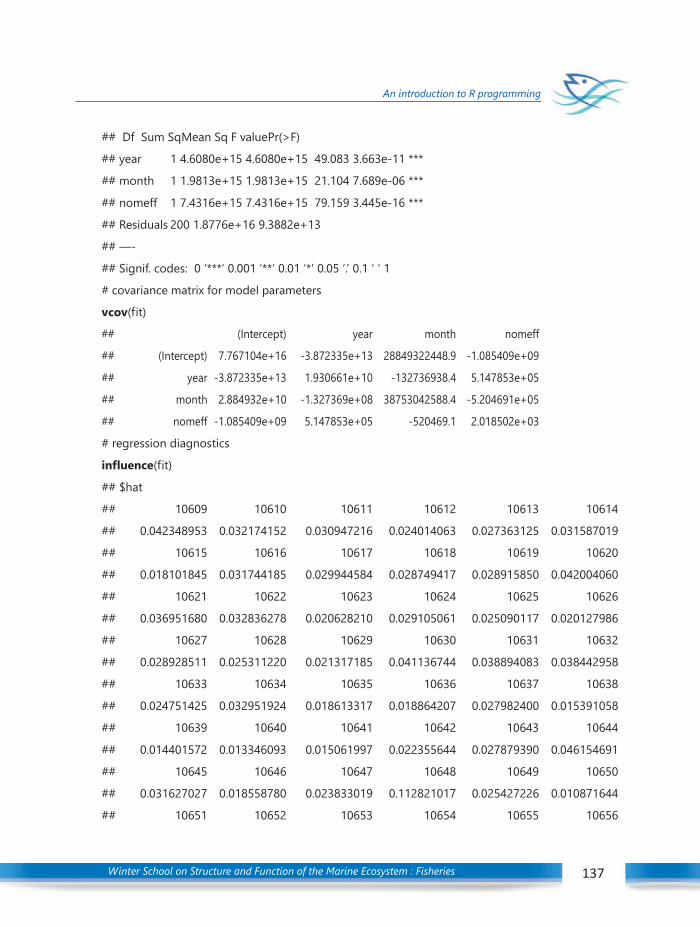
Winter School on Structure and Function of the Marine Ecosystem : Fisheries 137
An introduction to R programming
## Df Sum SqMean Sq F valuePr(>F)
## year 1 4.6080e+15 4.6080e+15 49.083 3.663e-11 ***
## month 1 1.9813e+15 1.9813e+15 21.104 7.689e-06 ***
## nomeff 1 7.4316e+15 7.4316e+15 79.159 3.445e-16 ***
## Residuals 200 1.8776e+16 9.3882e+13
## —-
## Signif. codes: 0 ‘***’ 0.001 ‘**’ 0.01 ‘*’ 0.05 ‘.’ 0.1 ‘ ‘ 1
# covariance matrix for model parameters
vcov(fit)
## (Intercept) year month nomeff
## (Intercept) 7.767104e+16 -3.872335e+13 28849322448.9 -1.085409e+09
## year -3.872335e+13 1.930661e+10 -132736938.4 5.147853e+05
## month 2.884932e+10 -1.327369e+08 38753042588.4 -5.204691e+05
## nomeff -1.085409e+09 5.147853e+05 -520469.1 2.018502e+03
# regression diagnostics
influence(fit)
## $hat
## 10609 10610 10611 10612 10613 10614
## 0.042348953 0.032174152 0.030947216 0.024014063 0.027363125 0.031587019
## 10615 10616 10617 10618 10619 10620
## 0.018101845 0.031744185 0.029944584 0.028749417 0.028915850 0.042004060
## 10621 10622 10623 10624 10625 10626
## 0.036951680 0.032836278 0.020628210 0.029105061 0.025090117 0.020127986
## 10627 10628 10629 10630 10631 10632
## 0.028928511 0.025311220 0.021317185 0.041136744 0.038894083 0.038442958
## 10633 10634 10635 10636 10637 10638
## 0.024751425 0.032951924 0.018613317 0.018864207 0.027982400 0.015391058
## 10639 10640 10641 10642 10643 10644
## 0.014401572 0.013346093 0.015061997 0.022355644 0.027879390 0.046154691
## 10645 10646 10647 10648 10649 10650
## 0.031627027 0.018558780 0.023833019 0.112821017 0.025427226 0.010871644
## 10651 10652 10653 10654 10655 10656
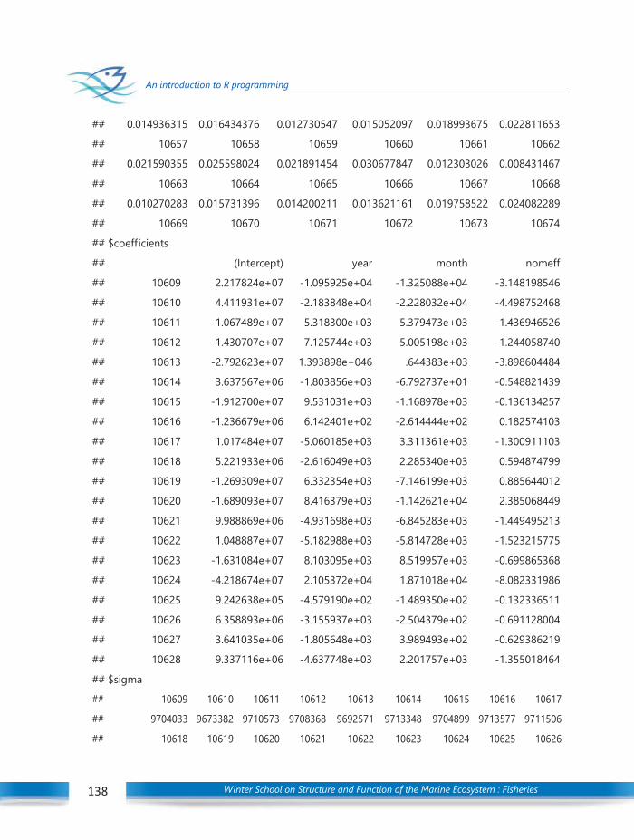
Winter School on Structure and Function of the Marine Ecosystem : Fisheries138
An introduction to R programming
## 0.014936315 0.016434376 0.012730547 0.015052097 0.018993675 0.022811653
## 10657 10658 10659 10660 10661 10662
## 0.021590355 0.025598024 0.021891454 0.030677847 0.012303026 0.008431467
## 10663 10664 10665 10666 10667 10668
## 0.010270283 0.015731396 0.014200211 0.013621161 0.019758522 0.024082289
## 10669 10670 10671 10672 10673 10674
## $coefficients
## (Intercept) year month nomeff
## 10609 2.217824e+07 -1.095925e+04 -1.325088e+04 -3.148198546
## 10610 4.411931e+07 -2.183848e+04 -2.228032e+04 -4.498752468
## 10611 -1.067489e+07 5.318300e+03 5.379473e+03 -1.436946526
## 10612 -1.430707e+07 7.125744e+03 5.005198e+03 -1.244058740
## 10613 -2.792623e+07 1.393898e+046 .644383e+03 -3.898604484
## 10614 3.637567e+06 -1.803856e+03 -6.792737e+01 -0.548821439
## 10615 -1.912700e+07 9.531031e+03 -1.168978e+03 -0.136134257
## 10616 -1.236679e+06 6.142401e+02 -2.614444e+02 0.182574103
## 10617 1.017484e+07 -5.060185e+03 3.311361e+03 -1.300911103
## 10618 5.221933e+06 -2.616049e+03 2.285340e+03 0.594874799
## 10619 -1.269309e+07 6.332354e+03 -7.146199e+03 0.885644012
## 10620 -1.689093e+07 8.416379e+03 -1.142621e+04 2.385068449
## 10621 9.988869e+06 -4.931698e+03 -6.845283e+03 -1.449495213
## 10622 1.048887e+07 -5.182988e+03 -5.814728e+03 -1.523215775
## 10623 -1.631084e+07 8.103095e+03 8.519957e+03 -0.699865368
## 10624 -4.218674e+07 2.105372e+04 1.871018e+04 -8.082331986
## 10625 9.242638e+05 -4.579190e+02 -1.489350e+02 -0.132336511
## 10626 6.358893e+06 -3.155937e+03 -2.504379e+02 -0.691128004
## 10627 3.641035e+06 -1.805648e+03 3.989493e+02 -0.629386219
## 10628 9.337116e+06 -4.637748e+03 2.201757e+03 -1.355018464
## $sigma
## 10609 10610 10611 10612 10613 10614 10615 10616 10617
## 9704033 9673382 9710573 9708368 9692571 9713348 9704899 9713577 9711506
## 10618 10619 10620 10621 10622 10623 10624 10625 10626

Winter School on Structure and Function of the Marine Ecosystem : Fisheries 139
An introduction to R programming
## 9712887 9710099 9707947 9711071 9710794 9705104 9647742 9713585 9712507
## 10627 10628 10629 10630 10631 10632 10633 10634 10635
## 9713275 9711335 9706375 9600885 9706147 9706674 9713017 9687689 9701725
## 10636 10637 10638 10639 10640 10641 10642 10643 10644
## 9713453 9713556 9712299 9713060 9712046 9654918 9701385 9711759 9631991
## 10645 10646 10647 10648 10649 10650 10651 10652 10653
## 9704897 9707140 9703907 9700734 9690097 9679013 9482552 9711297 9710429
## 10654 10655 10656 10657 10658 10659 10660 10661 10662
## 9713454 9704972 9696589 9713578 9706537 9709783 9686303 9712444 9710871
## 10663 10664 10665 10666 10667 10668 10669 10670 10671
## 9702490 9703766 9710000 9709158 9713461 9711904 9705335 9713591 9711428
## 10672 10673 10674 10675 10676 106771 0678 10679 10680
## 9713440 9713390 9713495 9706020 9709067 9620081 9679152 9556146 9705788
## 10681 10682 10683 10684 10685 10686 10687 10688 10689
## 9703041 9712489 9696177 9713305 9713033 9713274 9711229 9713210 9707532
## 10690 10691 10692 10693 10694 10695 10696 10697 10698
## 9484558 9670016 9694154 9710393 9710677 9712970 9696964 9665645 9703363
## 10699 10700 10701 10702 10703 10704 10705 10706 10707
## 9699470 9711903 9695548 9685330 9698839 9696413 9712539 9713605 9645521
## 10708 10709 10710 10711 10712 10713 10714 10715 10716
## 9692194 9657695 9711752 9708527 9712793 9693026 9705844 9708928 9616936
## 10717 10718 10719 10720 10721 10722 10723 10724 10725
## 9700975 9709924 9687368 9702069 9706975 9713608 9712002 9705092 9711736
##
## $wt.res
## 10609 10610 10611 10612 10613
## 5952459.84 12255563.09 -3371411.14 -4445741.27 -8889076.47
## 10614 10615 10616 10617 10618
## 986134.71 -5748266.48 -336390.21 2807133.26 1645172.74
## 10619 10620 10621 10622 10623
## -3629105.70 -4577842.81 3072907.21 3243308.73 -5672890.07
## 10624 10625 10626 10627 10628
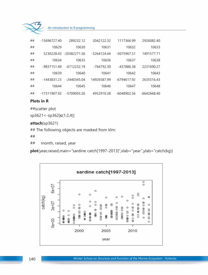
Winter School on Structure and Function of the Marine Ecosystem : Fisheries140
An introduction to R programming
## -15696727.40 289232.12 2042122.32 1117366.99 2926082.40
## 10629 10630 10631 10632 10633
## 5230228.43 -20382271.56 -5264124.44 -5075967.51 1491577.71
## 10634 10635 10636 10637 10638
## -9837151.49 -6712232.19 -764792.30 -437886.38 2231690.27
## 10639 10640 10641 10642 10643
## -1443831.23 -2440345.04 14926587.99 -6794617.92 2635516.43
## 10644 10645 10646 10647 10648
## -17311907.92 -5709093.26 4952910.28 -6048902.56 -6642668.40
Plots in R
##scatter plotsp3621<-sp362[c(1:2,4)]
attach(sp3621)## The following objects are masked from klm:#### month, raised, year
plot(year,raised,main=”sardine catch[1997-2013]”,xlab=”year”,ylab=”catch(kg))

Winter School on Structure and Function of the Marine Ecosystem : Fisheries 141
An introduction to R programming
##Histogram
hist(raised,main=”Histogram for oilsardine catch[1997-2013]”,
lab=”catch”,
col=”green”,
breaks=5)
##Bar plot
barplot(raised, main=”sardine catch Distribution”,
xlab=”Number of years”)
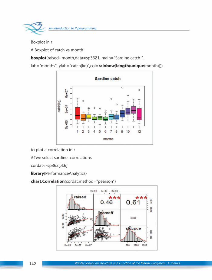
Winter School on Structure and Function of the Marine Ecosystem : Fisheries142
An introduction to R programming
Boxplot in r
# Boxplot of catch vs month
boxplot(raised~month,data=sp3621, main=”Sardine catch “,
lab=”months”, ylab=”catch(kg)”,col=rainbow(length(unique(month))))
to plot a correlation in r
##we select sardine correlations
cordat<-sp362[,4:6]
library(PerformanceAnalytics)
chart.Correlation(cordat,method=”pearson”)

Winter School on Structure and Function of the Marine Ecosystem : Fisheries 143
An introduction to R programming
R for reading NetCDF data
NetCDF files contain one or more variables, which are usually structured as regular N-dimensional arrays. For example, you might have a variable named “Temperature” that is afunction of longitude, latitude, and height. NetCDF files also contain dimensions, whichdescribe the extent of the variables’ arrays. In our Temperature example, the dimensions are“longitude”, “latitude”, and “height”. Data can be read from or written to variables in arbitraryhyperslabs (for example, you can read or write all the Temperature values at a given height,or at a given latitude).
The R package ’ncdf4’ allows reading from, writing to, and creation of netCDF files,either netCDF version 3 or (optionally) netCDF version 4. If you choose to create version 4output files, be aware that older netcdf software might only be able to read version 3 files.
In fact this package can help extracting details from HDF5 format files too. This packagecan create NetCDF files from data.frames also. Nc_open() is the function to be used foropening a NetCDF fils and for creating a NetCDF file the function is nc_creat(). Once openedthe attributes and variable names of the data can be got by using the generic print()command. To get specific variables the function is ncvar_get()
An example:
library(ncdf4)
ncold <- nc_open(“states_population.nc”)
data <- ncvar_get(ncold)
print(“here is the data in the file:”)
print(data)
nc_close( ncold )
The output is given below:
> ncold <- nc_open(“states_population.nc”)
> print(ncold)
File states_population.nc (NC_FORMAT_CLASSIC):
1 variables (excluding dimension variables):
int Pop[StateNo]
units: count
_FillValue: -1
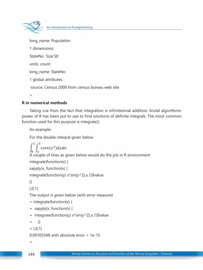
Winter School on Structure and Function of the Marine Ecosystem : Fisheries144
An introduction to R programming
long_name: Population
1 dimensions:
StateNo Size:50
units: count
long_name: StateNo
1 global attributes:
source: Census 2000 from census bureau web site
>
R in numerical methods
Taking cue from the fact that integration is infinitesimal addition, brutal algorithmicpower of R has been put to use to find solutions of definite integrals. The most commonfunction used for this purpose is integrate().
An example:
For the double integral given below
A couple of lines as given below would do the job in R environmentintegrate(function(x) sapply(x, function(x) integrate(function(y) x*sin(y^2),x,1)$value),0,1)The output is given below (with error measure)> integrate(function(x) + sapply(x, function(x) + integrate(function(y) x*sin(y^2),x,1)$value+ )+ ,0,1)0.09105548 with absolute error < 1e-15>
Winter School on Structure and Function of the Marine Ecosystem : Fisheries 145
An introduction to R programming
References
Bryant, F. B., and Yarnold, P. R. 1995. Principal components analysis and exploratory and confirmatoryfactor analysis. In L. G. Grimm & P. R. Yarnold (Eds.), Reading and understanding multivariate analysis.Washington, DC: American Psychological Association.
Crowley, M. J. 2007. The R Book. Chichester, New England: John Wiley & Sons, Ltd.Dunteman, G. H. 1989. Principal components analysis. Newbury Park, CA: Sage Publications.Fabrigar, L. R., Wegener, D. T., MacCallum, R. C., and Strahan, E. J. (1999). Evaluating the use of exploratory
factor analysis in psychological research. Psychological Methods, 4(3), 272-299. Fox, J. 2005. R commander: A basic-statistics user interface to R. Journal of Statistical Software. 14 (9): 1-42.Gorsuch, R. L. 1983. Factor Analysis. Hillsdale, NJ: Lawrence Erlbaum Associates.Hair, J. F., Jr., Anderson, R. E., Tatham, R. L., and Black, W. C. 1995. Multivariate data analysis with readings (4th
ed.). Upper Saddle River, NJ: Prentice-Hall.Hatcher, L. 1994. A step-by-step approach to using the SAS system for factor analysis and structural equation
modeling. Cary, NC: SAS Institute.http://www.statisticssolutions.com.Hutcheson, G., and Sofroniou, N. 1999. The multivariate social scientist: Introductory statistics using generalized
linear models. Thousand Oaks, CA: Sage Publications.Kim, J. O., and Mueller, C. W. 1978a. Introduction to factor analysis: What it is and how to do it. Newbury
Park, CA: Sage Publications.Kim, J. O., and Mueller, C. W. 1978b. Factor Analysis: Statistical methods and practical issues. Newbury Park,
CA: Sage Publications.Lawley, D. N., and Maxwell, A. E. 1962. Factor analysis as a statistical method. The Statistician, 12(3): 209-
229.Levine, M. S. 1977. Canonical analysis and factor comparison. Newbury Park, CA: Sage Publications.Pett, M. A., Lackey, N. R., and Sullivan, J. J. 2003. Making sense of factor analysis: The use of factor analysis for
instrument development in health care research. Thousand Oaks, CA: Sage Publications.Rosales de Veliz L., David S.L., McElhiney D., Price E., and Brooks G. 2012. . Introduction to R: The Basics
Contributions from Ragan. M., Terzi. F., & Smith. E.”— Presentation transcriptShapiro, S. E., Lasarev, M. R., and McCauley, L. 2002. Factor analysis of Gulf War illness: What does it add to
our understanding of possible health effects of deployment, American Journal of Epidemiology, 156,578-585.
Teetor, P. 2011. 25 Recipes for Getting Started with R. Sebastopol, CA: O’Reilly Media Inc.Teetor, P. 2011. R cookbook. Sebastopol, CA: O’Reilly Media Inc.Velicer, W. F., Eaton, C. A., and Fava, J. L. 2000. Construct explication through factor or component analysis:
A review and evaluation of alternative procedures for determining the number of factors or components.In R. D. Goffin & E. Helmes (Eds.), Problems and solutions in human assessment: Honoring DouglasJackson at seventy. Boston, MA: Kluwer.
Widaman, K. F. 1993. Common factor analysis versus principal component analysis: Differential bias inrepresenting model parameters, Multivariate Behavioral Research, 28, 263-311.

Winter School on Structure and Function of the Marine Ecosystem : Fisheries146
Python: A tool for Analysis and Visualization of Remotely sensed datasets
What is Python?
Python is a programming language which helps you to tell the computer what youwant to do with the data that you have.
Why should I bother to learn Python?
It is extremely user-friendly
Whether you are a beginner in using programming languages or have solid experiencein programming, Python is a tool that is going to be an asset in your repository. It providesyou with the basic building-blocks that you need in order to develop a solution to almostany problem that the data analysis/ visualization can throw at you.
A complete solution
It has built-in packages/libraries that allow you to deal with data files with differenttypes of files (example .csv, .txt, .xlsx, .netcdf, .grib, etc). So you don’t have to worry aboutfinding another software/tool in order to process a data set whose format is not very popular.
Automation
If you have come across situations where you want to automate the mundane taskssuch as data download, iterate a specific data analysis procedure (that you have done forone month/year) across multiple months/years, etc. Python can help you do so and in turnsave you a lot of time that you could invest in more demanding tasks.
Ok, now where do I get Python from and how do I install it?
For Python installation there are three key aspects that a beginner should be aware of:
An Editor named Spyder
As a beginner in programming, it is recommended to have an editor that helps you tomonitor the syntax and changes in variables as and when you type or run the code.
Python programming language
For you to have the full benefit of Python, it is recommended to have the Pythoncompiler installed which will help to convert the script you write into machine-readablecode which the computer can understand and execute.
15C H A P T E R
PYTHON: A TOOL FOR ANALYSIS ANDVISUALIZATION OF REMOTELY SENSEDDATASETSTarun Joseph1 and Grinson George2
1Cochin University of Science and Technology, Kochi2ICAR-Central Marine Fisheries Research Institute

Winter School on Structure and Function of the Marine Ecosystem : Fisheries 147
Python: A tool for Analysis and Visualization of Remotely sensed datasets
147
Installation of additional libraries/packages
Although Python comes with a pre-installed set of libraries/packages, at times youmight want to perform a particular task using Python that requires the installation ofadditional packages. Therefore, it is essential for the beginner to know how to install additionallibraries as and when required.
All three elements come together in a distribution named Anaconda which is freelyavailable for download and use from the following link:
https://www.anaconda.com/download/#download
The link is directed for Windows installation whose steps can be followed using thislink: https://conda.io/docs/user-guide/install/windows.html. Please remember the locationin which you have installed your Anaconda distribution (preferably in C drive itself)
So I got Python installed. What now? (For Windows users)
For you to start writing your f irst script, you need an interactive developmentenvironment (IDE) named Spyder.
To launch the Spyder editor, follow the steps mentioned below:
Step 1) Search for Terminal window by typing the keyword “cmd” in the Search window
Step 2) Select the command prompt icon (it appears as a small rectangular black icon)
Step 3) Your command prompt may look like this:
C:/Windows>blank space
You need to relocate the command prompt “>” to the folder where Anaconda distributionis installed. Let’s say the Anaconda distribution is installed in C drive. If so, there will be afolder named Anaconda2. If that’s the case type the following in the terminal window afterthe “>” symbol and press “Enter”.
C:/Windows>cd Anaconda2
Then the command prompt will appear like this:
C:/Windows/Anaconda2>blank space
Type the following command after the “>” symbol and press “Enter”
C:/Windows/Anaconda2>cd Scripts
The command prompt will again change its appearance and might look like this:
C:/Windows/Anaconda2/Scripts>blank space

Winter School on Structure and Function of the Marine Ecosystem : Fisheries148
Python: A tool for Analysis and Visualization of Remotely sensed datasets
Type “Spyder” after the “>” symbol and press “Enter” to launch the Python editor
C:/Windows/Anaconda2/Scripts>Spyder
If you have installed your Pythonic enviroment correctly, then Spyder environmentshould get launched automatically and you’ll see the IDE displayed on your screen (ReferFig. 1).
Now that we have Python up and running, let’s begin with the programming.
For running the case studies, we require an additional libraries namely netCDF4,matplotlib and Basemap. For installation of libraries, following steps will help.
Step 1) Search for Terminal window by typing the keyword “cmd” in the Search window
Step 2) Select the command prompt icon (it appears as a small rectangular black icon)
Step 3) your command prompt may look like this:
C:/Windows>blank space
You need to relocate the command prompt “>” to the folder where Anaconda distributionis installed. Let’s say the Anaconda distribution is installed in C drive. If so, there will be afolder named Anaconda2. If that’s the case type the following in the terminal window afterthe “>” symbol and press “Enter”.
C:/Windows>cd Anaconda2
Winter School on Structure and Function of the Marine Ecosystem : Fisheries 149
Python: A tool for Analysis and Visualization of Remotely sensed datasets
149
Then the command prompt will appear like this:
C:/Windows/Anaconda2>blank space
Type the following command after the “>” symbol and press “Enter”
C:/Windows/Anaconda2>cd Scripts
The command prompt will again change its appearance and might look like this:
C:/Windows/Anaconda2/Scripts>blank space
Type “conda install netcdf4”after the “>” symbol and press “Enter” to install the netcdf4library
C:/Windows/Anaconda2/Scripts> conda install netcdf4
The screen prompt will ask your permission to proceed once it is able to find the packagerequired. Type “y” and press the “Enter” key.
The installation might take a while.
Similarly, you can install other libraries such as matplotlib and Basemap using thecommand “conda install matplotlib” and “conda install basemap” respectively.
Upon getting the required libraries installed, launch the Spyder Editor. Click on File ->Open file and find the python_data_read_visualize.py file that you have been given for thissession. Click on “Open”. Once it the code opens in Spyder, you can inspect it line by lineand read the comments written along-side to better understand the code.
Things you should be aware of before running the script
Before you run the script, make sure you change the path of the input file in line 11 ofthe code and the path where the plot needs to be saved (line 57). The code is separated intosmaller chunks using “#—————————————————” symbol.
Make sure you understand each chunk individually with the help of comments, beforeattempting to run the code as a whole.
In order to run the statements in the code individually, select the statement and clickthe symbol on the top left corner of the IDE interface. Note the changes that occursimultaneously in the Ipython console. After the script gets run, if variables get created, youcan monitor them in the variable explorer space.
It is a good practice to always comment using “#” symbol your code so that when yourevisit your script after a few days, just by having a look at the code, you’ll be able tounderstand the purpose of each statement in the script.

Winter School on Structure and Function of the Marine Ecosystem : Fisheries150
Python: A tool for Analysis and Visualization of Remotely sensed datasets
Test run
Case study 1: Read data from a NetCDF file
For this exercise, we will use a Python code named python_data_read_visualize.py. Thiscode will read a data file and display its attributes. Additionally, it will extract the data fromthe file and store it in variables which can be easily visualized. Please take note of thecomments which will help you to better understand what exactly the python script is doing.
Case study 2: Visualization of data
Once you know how to extract the data and store them into variables, we’ll learn howto create a spatial plot and save it as per the desired resolution. The script imports therequired libraries at the beginning, creates a grid using latitude and longitude values providedin the file, creates a spatial plot along with the grids (parallels and meridians), provides thetitle, displays the plot and saves the file in the desired format.
Winter School on Structure and Function of the Marine Ecosystem : Fisheries 151
Indian Ocean Physics and regional oceanography of the north Indian Ocean
Geographical Information System (GIS) is a technological tool used to describe andcharacterize spatially referenced geographical information for the purpose of visualizing,querying and analyzing. The tool enables capturing, storing, analyzing, sharing, displayingand modelling of spatial data maintained with in single database. Making decision basedon geography is basics to human thinking and spatial analysis using GIS enable people tocombine information from many independent sources and derive entirely new layers ofinformation that are more accurate and reliable in decision making. Spatial analysis involvesstudy of phenomenon that varies with time and space. Geostatistics is a branch of statisticsused for analysis of spatial or spatiotemporal data set by applying sophisticated set ofvarious statistical and probabilistic models. Here, we estimate the value of phenomenonfrom unknown location where no measurements are available with the help of directmeasurements derived from known locations. GIS has emerged as powerful tool in therecent years by providing various geospatial solutions in urban planning, mining, naturalresource evaluation and management, pollution estimation, risk assessment and large scalemapping thus becoming integral tool in our day today life.
1. Data for GIS
Data for GIS are obtained from various sources like aerial & satellite imageries, digitaldata, conventional maps, census, meteorological department, field data (surveys/GPS) etc.The information obtained can be classified into types of database: spatial data which describethe location (where the object is?) and attribute data which characterize the location (whatthe object is? or how much the object is?)
1.1. Spatial Database
Spatial data is representation of complex real world in a simplified manner. Here thegeographical features are represented by three basic types- points, lines and area. Pointsrepresent dimensionless features such as wells, post box, tube well etc. that are very smalland their location can be explained by only coordinate’s values. Lines depict features withlength, such as roads, railways stations, administrative and international boundaries etc.and are two-dimensional. Area or polygons are used to represent three-dimensional objectsthat have height, width and length such as agriculture lands, water bodies, forest areas andadministrative areas.
16C H A P T E R INTRODUCTION TO GEOSTATISTICS
Sreenath K. R.
Marine Biodiversity DivisionICAR-Central Marine Fisheries Research Institute

Winter School on Structure and Function of the Marine Ecosystem : Fisheries152
Indian Ocean Physics and regional oceanography of the north Indian Ocean
1.2. Attribute database
Attribute data depicts various characteristics of different object/ features on earth surface.This can of qualitative types like land use type, soil type, name of the city/ river etc.) or ofquantitative types (like elevation, temperature, pressure of a particular place, crop yield peracre etc.). Thus, attribute data can be both numeric and textual.
2. Representation of Database
The way that location is represented in a geodatabase can be either a raster or a vectorposition.
2.1. Raster data
A raster based format uses imaginary grid of cells or matrix to displays, locates andstores graphical data. The fundamental unit of raster system is pixel. Here, the whole studyarea is divided into uniform rows and columns and each cell or pixel is used for storingpoint, line or area entities. Here, points are represented by individual column/ row entities,lines are depicted by connecting the adjacent cells or pixels and areas are stored as set ofcontiguous cells defining the interior. The accuracy of raster data formats depends on pixelor grid size and may vary from submeter to kilometres. Layers are functionally related mapfeatures that are used to represent different two-dimensional features on map. Differentlayers are used to in GIS for storing various unique information such as forest cover, soiltypes, land use pattern and wetlands. Satellite images, Digital terrain models (DTM) anddigital elevation models (DEM) are examples of raster data (Koeln et al., 1994 and Huxhold1991). Raster data formats require less processing over vector formats but they consumesmore computer space for storing of data.
2.2. Vector data
In vector maps, world is represented by points, lines and polygons. The fundamentalunit of vector system is point. Lines are set of mathematically connected points and area arerepresented by set of mathematically connected coordinates or lines joined together toform polygons which define the boundary of area. Unlike raster images, vector images canbe of high resolution. Vector data requires less computer storage space and maintainingtopological relationships is easier in this system (Koeln et al., 1994; and Huxhold 1991).
3. Projections
Once the spatial data have been collected, the data needs to be in same coordinatesystem for display and analysis. As earth surface is ellipsoidal therefore set of set of systematicmathematical transformation is needed to display earth’s latitude and longitude onto aplane.
Winter School on Structure and Function of the Marine Ecosystem : Fisheries 153
Indian Ocean Physics and regional oceanography of the north Indian Ocean
Projection is a method by which curved surface of the earth is portrayed on a flatsurface. Initially the earth was thought to be flat surface but later on it was proven thatearth is an ellipsoidal/spheroid, the circumference of the earth is about 1/300th smalleraround the poles vs equator. This difference in distance around the poles and equator useto cause error in the readings and to rectify the errors different projection systems werecreated. These are just different measurements of the “flattening” at the poles. The differentprojection systems are helpful in measuring and preserving one or more properties such asarea, shape, direction or distance over commonly used latitude longitude ( x, y, whichmeasures in degree and not in distance) coordinate system.
3.1 Different types of projections
Azimuthal or planner projection: Projection surface laid flat against the earth.
Conic- Cone is placed on or through the surface of earth.
Cylindrical- projection surface wrapped around the earth.
Coordinate system: A reference framework consisting of set of points that are used todefine its position in space either in two or three dimensions.
Cartesian Coordinate system: Two dimensional, planner coordinates system in whichthe horizontal distance is measures along the x axis and vertical distance is measures alongthe y axis. Each point ids are defined by x, y coordinate.
Datum: Set of coordinates that measures the position on a surface using x,y coordinates(horizontal) and height above or below the surface ( vertical datum).
Geocentric datum: A horizontal geodetic datum based on a ellipsoidal that has itsorigin at the earth centre’s mass and measures coordinate of every point on Earth usinglatitude longitude and height above its surface. Ex. World Geodetic system of 1984. (WSG84).
3.2 Common GIS projections
Mercator : It is cylindrical projection tangent to the equator of earth. Preserves thelocal shapes and display accurate compass bearing for sea travel.
Transverse Mercator: It is also a type of cylindrical projection similar to Mercator exceptthe cylinder is tangent along a meridian instead of the equator. It minimizes the distortionalong north-south line, but does not maintain true direction.
Universal Transverse Mercator (UTM): UTM is based on transverse Mercator projectionand divides the whole world in 60 north south zones, each zone having a width of 6o
longitude. Each zone is numbered consecutively beginning with zone one covering longitude180o to 174o West and progressing east word to zone 60, between 174o to 180o East longitude.
Winter School on Structure and Function of the Marine Ecosystem : Fisheries154
Indian Ocean Physics and regional oceanography of the north Indian Ocean
Lambert Conformal Conic – A conic, conformal projection typically intersectingparallels of latitude, standard parallels, in the northern hemisphere. This projection is oneof the best for middle latitudes because distortion is lowest in the band between the standardparallels. It portrays shape more accurately than area.
Most commonly used projection in GIS is UTM or the preference may change dependingon the area of interest.
4. Interpolation
Spatial data is important in making important decisions in natural resource management.Collection of spatially continuous data is often difficult and expensive. Most of the datacollected by field surveys will be typically from point sources. But scientists and managersrequires accurate spatial continuous data to make justified interpretations.
Spatial continuous data of environmental variables are in demand in the geographicinformation systems (GIS) and modelling techniques for studying the ecology and biologicalconservation (Collins and Bolstad, 1996; Hartkamp et al., 1999). Thus, spatial interpolationmethods have overarching importance in converting point data in to spatially continuousdata. Interpolation methods can fall under two categories 1. Global methods and 2. Localmethods. Global methods use all available data of the region of interest to derive theestimation and capture the general trend. Local methods operate within a small area aroundthe point being estimated (i.e., use samples within a search window) and capture the localor short-range variation (Burrough and McDonnell, 1998).
4.1 Global interpolators
4.1.1 Regression Models
Regression interpolation is using a linear regression model (LM) as interpolator andassumes that the data are independent of each other, normally distributed and homogeneousin variance. Regression methods explore a possible functional relationship between theprimary variable and explanatory variables that are easy to measure (Burrough andMcDonnell, 1998). The final model can be selected by a thorough understanding of therelationships between the primary variable and secondary variables and/or by Akaikeinformation criteria (AIC) or Bayesian information criteria (BIC) methods.
4.1.2 Trend surface models
An inexact method, trend surface analysis approximates points with known values witha polynomial equation. This is similar to the regression model but uses only geographiccoordinates as indirect variables for prediction of the primary response variable (Collinsand Bolstead, 1996).
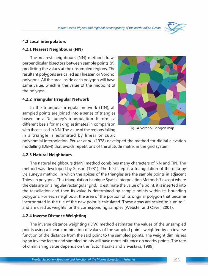
Winter School on Structure and Function of the Marine Ecosystem : Fisheries 155
Indian Ocean Physics and regional oceanography of the north Indian Ocean
4.2 Local interpolators
4.2.1 Nearest Neighbours (NN)
The nearest neighbours (NN) method drawsperpendicular bisectors between sample points (n),predicting the values at the unsampled regions. Theresultant polygons are called as Thiessen or Voronoipolygons. All the area inside each polygon will havesame value, which is the value of the midpoint ofthe polygon.
4.2.2 Triangular Irregular Network
In the triangular irregular network (TIN), allsampled points are joined into a series of trianglesbased on a Delauney’s triangulation. It forms adifferent basis for making estimates in comparisonwith those used in NN. The value of the regions fallingin a triangle is estimated by linear or cubicpolynomial interpolation. Peuker et al., (1978) developed the method for digital elevationmodelling (DEM) that avoids repetitions of the altitude matrix in the grid system.
4.2.3 Natural Neighbours
The natural neighbours (NaN) method combines many characters of NN and TIN. Themethod was developed by Sibson (1981). The first step is a triangulation of the data byDelauney’s method, in which the apices of the triangles are the sample points in adjacentThiessen polygons. This triangulation is unique Spatial Interpolation Methods 7 except wherethe data are on a regular rectangular grid. To estimate the value of a point, it is inserted intothe tessellation and then its value is determined by sample points within its boundingpolygons. For each neighbour, the area of the portion of its original polygon that becameincorporated in the tile of the new point is calculated. These areas are scaled to sum to 1and are used as weights for the corresponding samples (Webster and Oliver, 2001).
4.2.4 Inverse Distance Weighting
The inverse distance weighting (IDW) method estimates the values of the unsampledpoints using a linear combination of values of the sampled points weighted by an inversefunction of the distance from the said point to the sampled points. The weight diminishesby an inverse factor and sampled points will have more influence on nearby points. The rateof diminishing value depends on the factor (Isaaks and Srivastava, 1989).
Fig. A Voronoi Polygon map

Winter School on Structure and Function of the Marine Ecosystem : Fisheries156
Indian Ocean Physics and regional oceanography of the north Indian Ocean
Fig. NASA’s Cassini spacecraft gridded elevation data has been splined create the first global topographicmap of Saturn’s moon Titan [Image credit: NASA/JPL-Caltech/ASI/JHUAPL/Cornell/Weizmann]
4.2.6 Krigging
Basic concept of Geostatistics is that variables of a specific geographic region tend tohave a particular structure. Though this particular domain of spatial interpolation has itsorigin in 1910s in agronomy (Webster and Oliver, 2001), this is mostly developed in theworks of geology and mining by Krige (1951). Geostatistics includes several methods that
The weights can be expressed as:
where di is the distance between point of interest x0 and sampled point xi, p is a powerparameter, and n stands for the number of sampled points used for the estimation. Thepower parameter is arbitrary decided by the validation at field. Most popular value for p is2 and then the IDW is called as Inverse square or inverse distance squared (IDS) method.4.2.5 Splines
This is an inexact, gradual interpolation which uses piecewise polynomial equation asinterpolator. The polynomials describe pieces of a line or surface (i.e., they are fitted to asmall number of data points exactly) and are fitted together so that they join smoothly(Burrough and McDonnell, 1998; Webster and Oliver, 2001). For degree p = 1, 2, or 3, aspline is called linear, quadratic or cubic respectively. Typically, the splines are of degree 3and they are cubic splines (Webster and Oliver, 2001).
Winter School on Structure and Function of the Marine Ecosystem : Fisheries 157
Indian Ocean Physics and regional oceanography of the north Indian Ocean
use kriging algorithms for estimating continuous attributes. Kriging is a generic name for afamily of generalised least-squares regression algorithms, used in recognition of thepioneering work of Danie Krige (1951). Li and Heap (2008) gives a good review of all theavailable interpolation methods. In Krigging interpolation is performed by modelling aGaussian process which considers method of interpolation for which the interpolated valuesare modeled by a Gaussian process governed by prior assumptions and gives the bestunbiased estimate of the unsampled values.
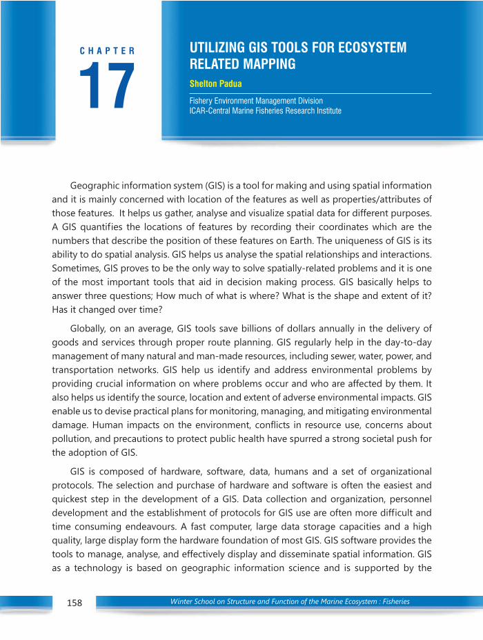
Winter School on Structure and Function of the Marine Ecosystem : Fisheries158
Utilizing GIS tools for ecosystem related mapping
Geographic information system (GIS) is a tool for making and using spatial informationand it is mainly concerned with location of the features as well as properties/attributes ofthose features. It helps us gather, analyse and visualize spatial data for different purposes.A GIS quantifies the locations of features by recording their coordinates which are thenumbers that describe the position of these features on Earth. The uniqueness of GIS is itsability to do spatial analysis. GIS helps us analyse the spatial relationships and interactions.Sometimes, GIS proves to be the only way to solve spatially-related problems and it is oneof the most important tools that aid in decision making process. GIS basically helps toanswer three questions; How much of what is where? What is the shape and extent of it?Has it changed over time?
Globally, on an average, GIS tools save billions of dollars annually in the delivery ofgoods and services through proper route planning. GIS regularly help in the day-to-daymanagement of many natural and man-made resources, including sewer, water, power, andtransportation networks. GIS help us identify and address environmental problems byproviding crucial information on where problems occur and who are affected by them. Italso helps us identify the source, location and extent of adverse environmental impacts. GISenable us to devise practical plans for monitoring, managing, and mitigating environmentaldamage. Human impacts on the environment, conflicts in resource use, concerns aboutpollution, and precautions to protect public health have spurred a strong societal push forthe adoption of GIS.
GIS is composed of hardware, software, data, humans and a set of organizationalprotocols. The selection and purchase of hardware and software is often the easiest andquickest step in the development of a GIS. Data collection and organization, personneldevelopment and the establishment of protocols for GIS use are often more difficult andtime consuming endeavours. A fast computer, large data storage capacities and a highquality, large display form the hardware foundation of most GIS. GIS software provides thetools to manage, analyse, and effectively display and disseminate spatial information. GISas a technology is based on geographic information science and is supported by the
17C H A P T E R UTILIZING GIS TOOLS FOR ECOSYSTEM
RELATED MAPPINGShelton Padua
Fishery Environment Management DivisionICAR-Central Marine Fisheries Research Institute

Winter School on Structure and Function of the Marine Ecosystem : Fisheries 159
Utilizing GIS tools for ecosystem related mapping
159
disciplines like geography, surveying, engineering, space science, computer science,cartography, statistics etc.
In GIS, we handle the spatial and attribute data sets. Spatial data describes the absoluteand relative location of geographic features while the attribute data describes characteristicsof the spatial features. These characteristics can be quantitative and/or qualitative in nature.Attribute data is also referred to as tabular data. Vector and raster are two different ways ofrepresenting spatial data. Raster data is made up of pixels (or cells), and each pixel has anassociated value. A digital photograph is a simple example of a raster dataset where eachpixel value corresponds to a particular colour. In GIS, the pixel values may represent elevationabove/below sea level, or chemical concentrations, or rainfall etc. The key point is that all ofthis data is represented as a grid of (usually square) cells. Vector data consists of points,lines, and polygons. The individual points are stored as pairs of (x, y) co-ordinates. Thepoints may be joined in a particular order to create lines, or joined into closed rings tocreate polygons, but all vector data fundamentally consists of lists of co-ordinates thatdefine vertices, together with rules to determine whether and how those vertices are joined.
As with many other systems, GIS basically works on the principle of ‘GIGO’ that is garbagein garbage out. Hence the quality of data that you feed into GIS is very important and itdetermines the quality of the end products. But, when used wisely, GIS can help us livehealthier, wealthier, and safer lives.
Hands on: Mapping the Progress of El Nino/La Nina using ONI
El Niño and La Niña are the two phases of the El Niño-Southern Oscillation (ENSO)cycle. The ENSO cycle describes the fluctuations in temperature between the ocean andatmosphere in the east-central Equatorial Pacific. La Niña is referred to as the cold phase ofENSO and El Niño as the warm phase of ENSO. These deviations from normal sea surfacetemperatures can have large-scale impacts not only on ocean processes, but also on globalweather and climate. El Niño and La Niña episodes typically last nine to 12 months, butsome prolonged events may last for years. The frequency of El Niño and La Niña episodescan be quite irregular, but El Niño and La Niña events occur on average every two to sevenyears. Typically, El Niño occurs more frequently than La Niña.
El Niño
El Niño means The Little Boy, or Christ Child in Spanish. El Niño was originally recognizedby fishermen off the coast of South America in the 1600s, with the appearance of unusuallywarm water in the Pacific Ocean around December. The term El Niño refers to the large-

Winter School on Structure and Function of the Marine Ecosystem : Fisheries160
Utilizing GIS tools for ecosystem related mapping
scale ocean-atmosphere climate interaction linked to a periodic warming in sea surfacetemperatures across the central and east-central Equatorial Pacific. Typical El Niño effectsare likely to develop over North America during the upcoming winter season. Those includewarmer-than-average temperatures over western and central Canada and over the westernand northern United States. Wetter-than-average conditions are likely over portions of theU.S. Gulf Coast and Florida, while drier-than-average conditions can be expected in theOhio Valley and the Pacific Northwest. The presence of El Niño can significantly influenceweather patterns, ocean conditions and marine fisheries across large portions of the globefor an extended period of time.
La Niña
La Niña means The Little Girl in Spanish. La Niña is also sometimes called El Viejo, anti-El Niño, or simply “a cold event.” La Niña episodes represent periods of below-average seasurface temperatures across the east-central Equatorial Pacific. Global climate La Niña impactstend to be opposite those of El Niño impacts. In the tropics, ocean temperature variationsin La Niña also tend to be opposite those of El Niño.
ENSO events are thought to have been occurring for thousands of years. Modern dayresearch and reanalysis techniques have find that at least 26 El Niño events since 1900 withthe 1982-83, 1997–98 and 2015–16 events among the strongest on record.
Different countries have different criteria to determine what constitutes an El Niño/ LaNiña event, which is tailored to their specific interests. For example, the Australian Bureauof Meteorology looks at the trade winds, Southern Oscillation Index (SOI), weather modelsand sea surface temperatures in the Nino 3 and 3.4 regions, before declaring an El Niño.However, the Japan Meteorological Agency declares that an El Niño event has started whenthe average five-month sea surface temperature deviation for the NINO 3 region, is over0.5 °C (0.90 °F) warmer for 6 consecutive months or longer. The Peruvian government declaresthat an El Nino is under way, if the sea surface temperatures in the Nino 1 and 2 regions,equal or exceed +0.4 °C for at least 3 months.
The Oceanic Niño Index (ONI) is the standard used by NOAA for identifying El Niño(warm) and La Niña (cool) events in the tropical Pacific. It is the running 3-month mean SSTanomaly for the Niño 3.4 region (i.e., 5oN-5oS, 120o-170oW). The events are defined as 5consecutive overlapping 3-month periods at or above the +0.5oC anomaly for warm (ElNiño) events and at or below the -0.5 oC anomaly for cold (La Niña) events. The threshold isfurther categorized as Weak (with a 0.5 to 0.9 SST anomaly), Moderate (1.0 to 1.4), Strong(1.5 to 1.9) and Very Strong (> 2.0) events.

Winter School on Structure and Function of the Marine Ecosystem : Fisheries 161
Utilizing GIS tools for ecosystem related mapping
161
Spatial Extent of Nino regions
It has been found that necessary condition for the development and persistence ofdeep convection (enhanced cloudiness and precipitation) in the Tropics develops when thelocal SST is 28°C or greater. Once the pattern of deep convection has been altered due toanomalous SSTs, the tropical and subtropical atmospheric circulation adjusts to the newpattern of tropical heating, resulting in anomalous patterns of precipitation and temperaturethat extend well beyond the region of the equatorial Pacific. An SST anomaly of +0.5°C inthe Niño 3.4 region is sufficient to reach this threshold from late March to mid-June. Duringthe remainder of the year a larger SST anomaly, up to +1.5°C in November-December-January, is required in order to reach the threshold to support persistent deep convectionin that region.
Task: Categorize the years into El Nino/ La Nina or normal year based on ONI.
Software Required: QGIS 2.18.14 and Microsoft Excel
Data sets required:
Climatic (1981-2010) monthly mean SST (1_JAN.tif, 2_FEB.tif, 3_MAR.tif, 4_APR.tif, ………..12_DEC.tif)
Actual monthly mean SST (2015_JUN.tif, 2015_JUL.tif, 2015_AUG.tif, …………. 2017_OCT.tif)
Shape file for Nino 3.4 region: NiNo_3.4_Poly.shp

Winter School on Structure and Function of the Marine Ecosystem : Fisheries162
Utilizing GIS tools for ecosystem related mapping
Loading SST data into QGIS:
Open QGIS -> Go to Layer menu -> Add raster layer -> Browse to the folder location -> Select the file -> 1_JAN.tif and load the file into the map view.

Winter School on Structure and Function of the Marine Ecosystem : Fisheries 163
Utilizing GIS tools for ecosystem related mapping
163
Now, to get a clear visual effect of the temperature variation, change the grey scale ofthe map to pseudo colour rendering. For that, right click the file name on the Layers panel(left side of the main view panel) and select the properties.
From the Layer Properties pane, go to style tab and change the band render type to‘Single band pseudo colour’.

Winter School on Structure and Function of the Marine Ecosystem : Fisheries164
Utilizing GIS tools for ecosystem related mapping
Then choose a ‘Colour’ band. Change the ‘Mode’ to ‘Equal interval’, set ‘Classes’ to ‘30’and press the ‘Classify’ button. The display will change to pseudo colour gradient as per theSST variations. Likewise, load all the SST layers.
Now, we have to load the shape file for Nino 3.4 region. Go to Layers menu -> AddLayers -> Add Vector Layer.
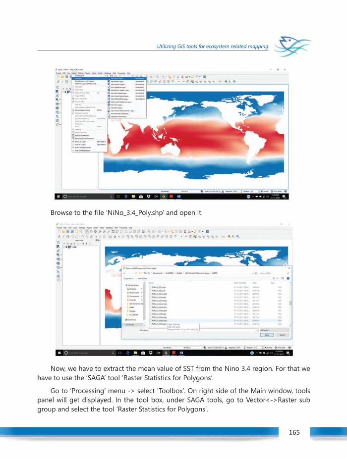
Winter School on Structure and Function of the Marine Ecosystem : Fisheries 165
Utilizing GIS tools for ecosystem related mapping
165
Browse to the file ‘NiNo_3.4_Poly.shp’ and open it.
Now, we have to extract the mean value of SST from the Nino 3.4 region. For that wehave to use the ‘SAGA’ tool ‘Raster Statistics for Polygons’.
Go to ‘Processing’ menu -> select ‘Toolbox’. On right side of the Main window, toolspanel will get displayed. In the tool box, under SAGA tools, go to Vector<->Raster subgroup and select the tool ‘Raster Statistics for Polygons’.

Winter School on Structure and Function of the Marine Ecosystem : Fisheries166
Utilizing GIS tools for ecosystem related mapping
In the ‘Raster Statistics for Polygons’ tool panel, in the Grids option, select the SSTdatasets. For ‘Polygons’ select NiNo_3.4_Poly.shp’, Method-> Standard, Grid Naming ->Grid Name, tick mark ‘Mean’ and press ‘Run’.
Now, you will get a ‘Statistics’ vector layer in the ‘Layers Panel’.
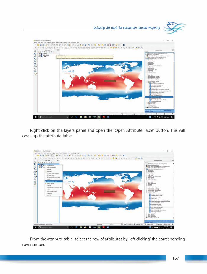
Winter School on Structure and Function of the Marine Ecosystem : Fisheries 167
Utilizing GIS tools for ecosystem related mapping
167
Right click on the layers panel and open the ‘Open Attribute Table’ button. This willopen up the attribute table.
From the attribute table, select the row of attributes by ‘left clicking’ the correspondingrow number.
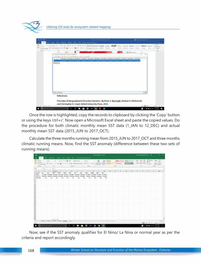
Winter School on Structure and Function of the Marine Ecosystem : Fisheries168
Utilizing GIS tools for ecosystem related mapping
Once the row is highlighted, copy the records to clipboard by clicking the ‘Copy’ buttonor using the keys ‘ctrl+c’. Now open a Microsoft Excel sheet and paste the copied values. Dothe procedure for both climatic monthly mean SST data (1_JAN to 12_DEC) and actualmonthly mean SST data (2015_JUN to 2017_OCT).
Calculate the three months running mean from 2015_JUN to 2017_OCT and three monthsclimatic running means. Now, find the SST anomaly (difference between these two sets ofrunning means).
Now, see if the SST anomaly qualifies for El Nino/ La Nina or normal year as per thecriteria and report accordingly.
Winter School on Structure and Function of the Marine Ecosystem : Fisheries 169
Utilizing GIS tools for ecosystem related mapping
169
References
Principles of Geographical Information Systems.: By Peter A. Burrough, Rachael A. McDonnell, and ChristopherD. Lloyd, Oxford University Press, 2015.
An Introduction to GIS: http://www.paulbolstad.net/5thedition/samplechaps/Chapter1_5th_small.pdf
Ferreira, J., João, P. and Martins, J. “GIS for Crime Analysis - Geography for Predictive Models” The ElectronicJournal Information Systems Evaluation Volume 15 Issue 1 2012, (pp36 -49) www.ejise.com/issue/download.html?idArticle=817
Overman, Henry G. (2010) GIS a job: what use geographical information systems in spatial economics.Journal of regional science, 50 (1). pp. 165-180. ISSN 0022-4146; http://eprints.lse.ac.uk/30784/1/Gis_a_job_%28LSERO_version%29.pdf
El Nino; https://en.wikipedia.org/wiki/El_Ni%C3%B1o
COBE SST, World mean monthly SST data from 1891- present. Earth Sciences Research Laboratory, PhysicalSciences Division; https://www.esrl.noaa.gov/psd/data/gridded/data.cobe.html
Monthly SST Climatology (1981-2010), World mean monthly SST data from 1891- present. Earth SciencesResearch Laboratory, Physical Sciences Division; https://www.esrl.noaa.gov/psd/data/gridded/data.cobe.html
QGIS: A Free and Open Source Geographic Information System; http://www.qgis.org/en/site/
Cold & Warm Episodes by Season: National Weather Service, Climate Prediction Centre; http://origin.cpc.ncep.noaa.gov/products/analysis_monitoring/ensostuff/ONI_v5.php
Trenberth, Kevin & National Center for Atmospheric Research Staff (Eds). Last modified 02 Feb 2016. “TheClimate Data Guide: Nino SST Indices (Nino 1+2, 3, 3.4, 4; ONI and TNI).” Retrieved from https://climatedataguide.ucar.edu/climate-data/nino-sst-indices-nino-12-3-34-4-oni-and-tni
Jan Null, CCM, 2017. El Niño and La Niña Years and Intensities Based on Oceanic Niño Index (ONI), http://ggweather.com/enso/oni.htm
NOAA, What are El Niño and La Niña? National Ocean Service Website, https://oceanservice.noaa.gov/facts/ninonina.html
NOAA, Equatorial Pacific Sea Surface Temperatures; https://www.ncdc.noaa.gov/teleconnections/enso/indicators/sst.php

Winter School on Structure and Function of the Marine Ecosystem : Fisheries170
Role of Calculus in Marine Sciences
18C H A P T E R
1. Introduction
Calculus has two parts: differential and integral calculus. Historically, differential calculuswas concerned with finding lines tangent to curves and with calculating extrema (i.e., maximaand minima) of curves. Integral calculus has its roots in attempting to determine the areas ofregions bounded by curves or in finding the volumes of solids. The two parts of calculus areclosely related: The basic operation of one can be considered the inverse of the other. Thisresult is known as the fundamental theorem of calculus and goes back to Newton and Leibniz,who were the first to understand its meaning and to put it to use in solving difficult problems(Reference 3).2. Worked out Examples
2.1 ) Differentiation
Differentiation is an aspect of calculus that enables us to determine how one quantitychanges with regard to another. It tells you how quickly (or slowly) a function changes at agiven point. Finding tangents, locating extrema, and calculating areas are basic geometricproblems, and it may be somewhat surprising that their solution led to the development ofmethods that are useful in a wide range of scientific fields. The main reason for this historicaldevelopment is that the slope of a tangent line at a given point is related to how quickly thefunction changes at that point. Knowing how quickly a function changes at a point opens upthe possibility of a dynamic description of biology, such as a description of population growth,the speed at which a chemical reaction proceeds, the firing rate of neurons, and the speed atwhich an invasive species invades a new habitat. For this reason, calculus has been one of themost powerful tools in the mathematical formulation of scientific concepts (Reference 3).
By working out the following examples, you will be able to develop an appreciation ofthe usefulness of calculus across multiple fields.
Example 1: Application of Differentiation (References 1.a and 1.b)Carlos has taken an initial dose of a prescription medication. The amount of medication, in
milligrams, in Carlos’s bloodstream after t hours is given by the following function:
M(t) = 20 * e(-0.8*t)
ROLE OF CALCULUS IN MARINE SCIENCESTarun Joseph1 and Grinson George2
1Cochin University of Science and Technology, Kochi2ICAR-Central Marine Fisheries Research Institute
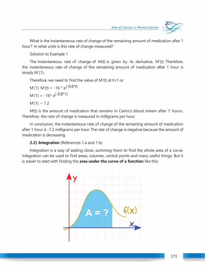
Winter School on Structure and Function of the Marine Ecosystem : Fisheries 171
Role of Calculus in Marine Sciences
171
What is the instantaneous rate of change of the remaining amount of medication after 1hour? In what units is this rate of change measured?
Solution to Example 1
The instantaneous rate of change of M(t) is given by its derivative, M’(t). Therefore,the instantaneous rate of change of the remaining amount of medication after 1 hour issimply M’(1).
Therefore, we need to find the value of M’(t) at t=1 or
M’(1) M’(t) = -16 * e(-0.8*t)
M’(1) = -16* e(-0.8*1)
M’(1) ~ 7.2
M(t) is the amount of medication that remains in Carlos’s blood stream after ‘t’ hours.Therefore, the rate of change is measured in milligrams per hour.
In conclusion, the instantaneous rate of change of the remaining amount of medicationafter 1 hour is -7.2 milligrams per hour. The rate of change is negative because the amount ofmedication is decreasing.
2.2) Integration (References 1.a and 1.b)
Integration is a way of adding slices, summing them to find the whole area of a curve.Integration can be used to find areas, volumes, central points and many useful things. But itis easier to start with finding the area under the curve of a function like this:
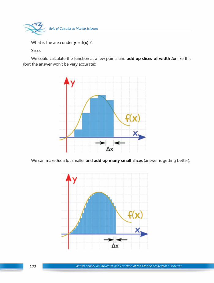
Winter School on Structure and Function of the Marine Ecosystem : Fisheries172
Role of Calculus in Marine Sciences
What is the area under y = f(x) ?
Slices
We could calculate the function at a few points and add up slices of width ∆∆∆∆∆x like this(but the answer won’t be very accurate):
We can make ∆∆∆∆∆x a lot smaller and add up many small slices (answer is getting better):

Winter School on Structure and Function of the Marine Ecosystem : Fisheries 173
Role of Calculus in Marine Sciences
173
And as the slices approach zero in width, the answer approaches the true answer.
We now write dx to mean the ∆∆∆∆∆x slices are approaching zero in width.
Example 2: Application of Integration (References 1.a and 1.b)
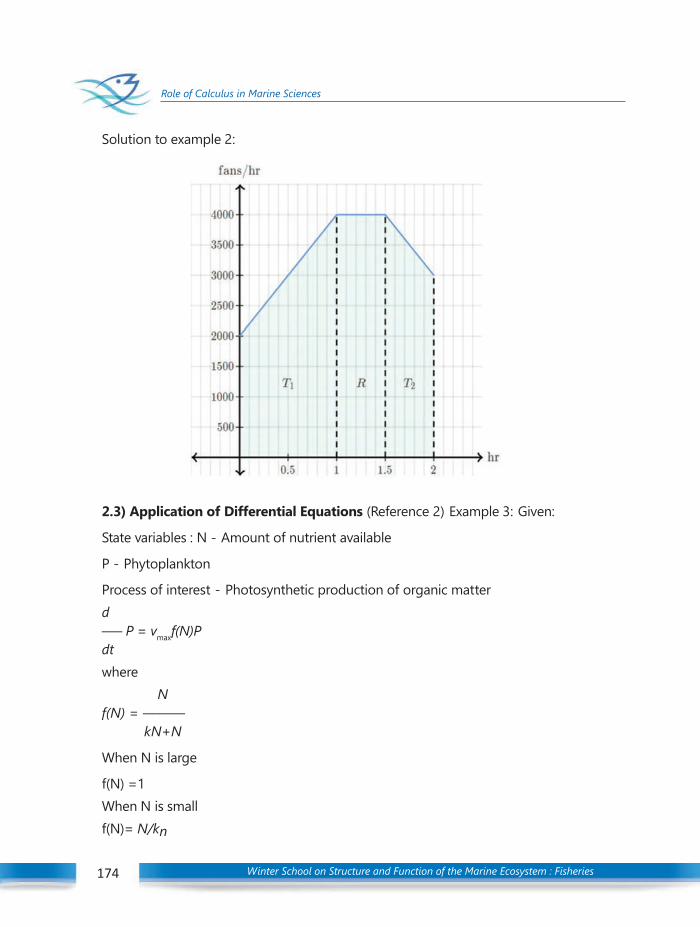
Winter School on Structure and Function of the Marine Ecosystem : Fisheries174
Role of Calculus in Marine Sciences
Solution to example 2:
2.3) Application of Differential Equations (Reference 2) Example 3: Given:
State variables : N - Amount of nutrient available
P - Phytoplankton
Process of interest - Photosynthetic production of organic matterd––– P = vmaxf(N)Pdtwhere
Nf(N) = ––––––
kN+N
When N is large
f(N) =1When N is smallf(N)= N/kn
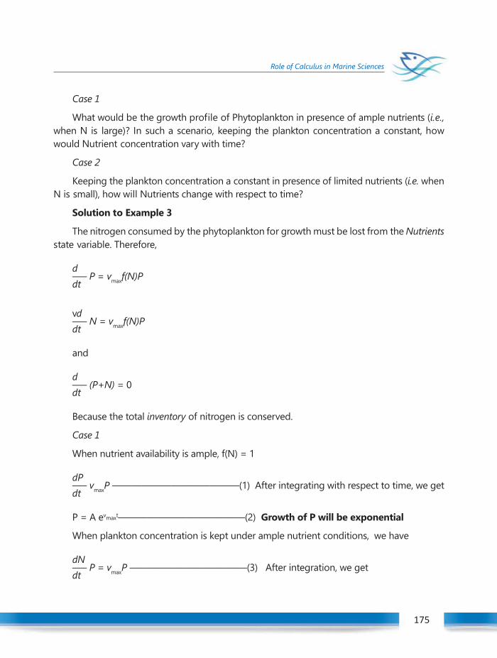
Winter School on Structure and Function of the Marine Ecosystem : Fisheries 175
Role of Calculus in Marine Sciences
175
Case 1
What would be the growth profile of Phytoplankton in presence of ample nutrients (i.e.,when N is large)? In such a scenario, keeping the plankton concentration a constant, howwould Nutrient concentration vary with time?
Case 2
Keeping the plankton concentration a constant in presence of limited nutrients (i.e. whenN is small), how will Nutrients change with respect to time?
Solution to Example 3
The nitrogen consumed by the phytoplankton for growth must be lost from the Nutrientsstate variable. Therefore,
d––– P = vmaxf(N)Pdt
vd––– N = vmaxf(N)Pdt
and
d––– (P+N) = 0dt
Because the total inventory of nitrogen is conserved.
Case 1
When nutrient availability is ample, f(N) = 1
dP––– vmaxP —————————————(1) After integrating with respect to time, we getdt
P = A evmaxt—————————————(2) Growth of P will be exponential
When plankton concentration is kept under ample nutrient conditions, we have
dN––– P = vmaxP ————————————(3) After integration, we getdt
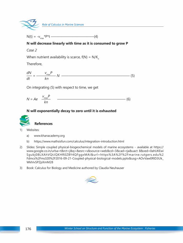
Winter School on Structure and Function of the Marine Ecosystem : Fisheries176
Role of Calculus in Marine Sciences
N(t) = -vmax*P*t ————————————(4)
N will decrease linearly with time as it is consumed to grow P
Case 2
When nutrient availability is scarce, f(N) = N/Kn
Therefore,
dN vmaxP––– = ––––––––––– N ——————————————————— (5)dt kn
On integrating (5) with respect to time, we get
vmaxPN = Ae ––––– ——————————————————— (6)kn
N will exponentially decay to zero until it is exhausted
References
1) Websites:
a) www.khanacademy.org
b) https://www.mathsisfun.com/calculus/integration-introduction.html
2) Slides: Simple coupled physical-biogeochemical models of marine ecosystems - available at https://www.google.co.in/urlsa=t&rct=j&q=&esrc=s&source=web&cd=3&cad=rja&uact 8&ved=0ahUKEwiSgubj08LXAhVQtJQKHR0ZBY4QFggxMAI&url=https%3A%2F%2Fmarine.rutgers.edu%2Fdmcs%2Fms320%2F2016-09-21-Coupled-physical-biological-models.pptx&usg=AOvVaw0RID3Uk_WkhIvSPZpXmM28
3) Book: Calculus for Biology and Medicine authored by Claudia Neuhauser
Winter School on Structure and Function of the Marine Ecosystem : Fisheries 177
Applications of geophysical data sets to resolve ecosystem challenges
Introduction
Satellite Remote Sensing (SRS) datasets are often used in empirical or semi-analyticalvalidated models, either to extrapolate regional datasets in space or to generate derivedgeo-physical products. A simple example for this can be the summation of thermal signalsfrom different wavelengths for generation of SST. In a similar way, some of the most usefuland relevant environmental properties in fisheries research such as sea surface salinity (SSS),Wind Speed (WS) and Wind Direction (WD), sea surface height (SSH), chlorophyll-a (Chl-a)and Chl-a derived primary production (PP) are available online as processed and unprocessedgeo-physical datasets. These datasets can be used to advantage in various fisheries researchand management programmes. A few such case studies are illustrated in this section:
SRS chlorophyll data providing cues on fish stock variability
Variations between years in the seasonal cycle of SRS Chl-a have been implicated influctuations in fish stock variability (Platt et al., 2003). In this section, we describe the resultsof an analysis of Chl-a with Indian oil sardine in the coastal waters of India. Fishing effort inthe coastal waters of India changed little in the period 1998-2006, with 238,772 fishing craftin 2005 (CMFRI 2005) in comparison with 239,000 craft in 1997 (Sathiadhas, 2006). Thus, thevariability in sardine landings during the study period, despite steady fishing effort, indicatesthat other factors such as environment or food to the sardines are involved. A correlationanalysis between available environmental factors (SST, sea bottom temperature, surfacesalinity, surface dissolved oxygen, bottom dissolved oxygen, pH, nutrients, chlorophyll,zooplankton, rainfall, multivariate El Niño Southern Oscillation index, coastal upwelling index,and derived SST) and sardine catch from the study area emphasised the high significance ofchlorophyll compared with other environmental factors in explaining the variability in sardinecatch (Krishnakumar and Bhat, 2008). Using their fine branchial apparatus, sardines feedpredominantly on phytoplankton and zooplankton. In a given area, Chl-a is a good index ofthe food availability to sardines. Summer surface Chl-a from the study area lies in the range0.1 to 5 mg/m3, and can be very high, from 5 to 10 mg/m3, during bloom periods. Given thewide dynamic range of chlorophyll concentration in the coastal waters of southwest Indiaand the dominant role of chlorophyll as a determinant of variability in sardine stocks, itseems likely that much will be gained in studying this link in detail.
19C H A P T E R
APPLICATIONS OF GEOPHYSICAL DATASETS TO RESOLVE ECOSYSTEMCHALLENGESGrinson George
Fishery Resources Assessment DivisionICAR-Central Marine Fisheries Research Institute
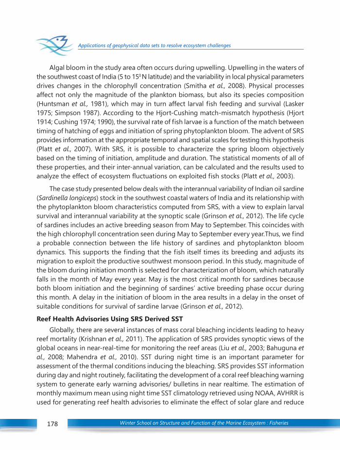
Winter School on Structure and Function of the Marine Ecosystem : Fisheries178
Applications of geophysical data sets to resolve ecosystem challenges
Algal bloom in the study area often occurs during upwelling. Upwelling in the waters ofthe southwest coast of India (5 to 150 N latitude) and the variability in local physical parametersdrives changes in the chlorophyll concentration (Smitha et al., 2008). Physical processesaffect not only the magnitude of the plankton biomass, but also its species composition(Huntsman et al., 1981), which may in turn affect larval fish feeding and survival (Lasker1975; Simpson 1987). According to the Hjort-Cushing match-mismatch hypothesis (Hjort1914; Cushing 1974; 1990), the survival rate of fish larvae is a function of the match betweentiming of hatching of eggs and initiation of spring phytoplankton bloom. The advent of SRSprovides information at the appropriate temporal and spatial scales for testing this hypothesis(Platt et al., 2007). With SRS, it is possible to characterize the spring bloom objectivelybased on the timing of initiation, amplitude and duration. The statistical moments of all ofthese properties, and their inter-annual variation, can be calculated and the results used toanalyze the effect of ecosystem fluctuations on exploited fish stocks (Platt et al., 2003).
The case study presented below deals with the interannual variability of Indian oil sardine(Sardinella longiceps) stock in the southwest coastal waters of India and its relationship withthe phytoplankton bloom characteristics computed from SRS, with a view to explain larvalsurvival and interannual variability at the synoptic scale (Grinson et al., 2012). The life cycleof sardines includes an active breeding season from May to September. This coincides withthe high chlorophyll concentration seen during May to September every year.Thus, we finda probable connection between the life history of sardines and phytoplankton bloomdynamics. This supports the finding that the fish itself times its breeding and adjusts itsmigration to exploit the productive southwest monsoon period. In this study, magnitude ofthe bloom during initiation month is selected for characterization of bloom, which naturallyfalls in the month of May every year. May is the most critical month for sardines becauseboth bloom initiation and the beginning of sardines’ active breeding phase occur duringthis month. A delay in the initiation of bloom in the area results in a delay in the onset ofsuitable conditions for survival of sardine larvae (Grinson et al., 2012).
Reef Health Advisories Using SRS Derived SSTGlobally, there are several instances of mass coral bleaching incidents leading to heavy
reef mortality (Krishnan et al., 2011). The application of SRS provides synoptic views of theglobal oceans in near-real-time for monitoring the reef areas (Liu et al., 2003; Bahuguna etal., 2008; Mahendra et al., 2010). SST during night time is an important parameter forassessment of the thermal conditions inducing the bleaching. SRS provides SST informationduring day and night routinely, facilitating the development of a coral reef bleaching warningsystem to generate early warning advisories/ bulletins in near realtime. The estimation ofmonthly maximum mean using night time SST climatology retrieved using NOAA, AVHRR isused for generating reef health advisories to eliminate the effect of solar glare and reduce

Winter School on Structure and Function of the Marine Ecosystem : Fisheries 179
Applications of geophysical data sets to resolve ecosystem challenges
the variation in SST caused by the heating during day time. Threshold hotspot (HS) anddaily heating week (DHW) values for a region are calculated the advisory (Mohanty et al.,2013). Depending on the intensity of HS and DHW there can be advisories such as ‘nostress’; ‘watch’; ‘warning’ and ‘alert levels-I & II’ which progressively indicate the severity ofa potential bleaching event. Based on this study INCOIS offers reef stress advisories to alertthe reef managers to take appropriate measures to reduce the damage caused to reefsduring bleaching events.
SRS Data for Cyclone Tracks Creating Productive Fishing Grounds
Even though cyclones are devastating, there are some positive effects of cyclones onthe fishery. Study of the effect of tropical cyclones on biological processes has gainedmomentum in the recent past. In thermally-stratified coastal waters, cyclones trigger thebreaking up of nutrient-depleted surface waters and bring in nutrient-rich sub-surface watersinducing sudden algal blooms and enhancing the regional scale PP. The effect of physicalforcings on PP, its variation and associated hydrography in the southwestern Bay of Bengalduring the southwest monsoon (July) and post-cyclone period (November) of 1999 wasstudied by Madhu et al., (2002). In the post cyclone period, the combined effects of well-mixed coastal waters and freshwater injection from the land runoff associated with thecyclone brought nutrients to the mixed layer, which enhanced PP. Potentially, suchenhancement of PP results in improving the regional fishery. But cyclone tracks alone willnot provide the information on enhanced PP. SRS is able to detect the environmental changescaused by tropical cyclones. Geo-physical data sets from SRS are useful in such studies forindicating possible productive fishing grounds after a lag following the cyclone (Rao et al.,2006).
Demarcation of Ecological Provinces in Support of an Ecosystem Approach to FisheriesManagement
Globally, the ecosystem approach to fisheries management (EAFM) is preferred as abasis for sustainable management of fish stock (Garcia et al., 2003). In this context, it isuseful to have a spatial structure for global oceans defined on the basis of ecological provincesrather than geo-political considerations. There are various approaches for classifying theglobal oceans into ecological provinces (Ekman 1953; Margelef 1961; Yentsch and Garside1986; Cushing 1989; Fanning 1992; Sathyendranath et al., 1995). The classification byLonghurst et al., (1995) is the most comprehensive, identifying some 50 biogeochemicalprovinces globally (Longhurst et al., 1995). Some other methodologies require huge datasets for demarcating ecological provinces (Hooker et al., 2000; Li et al., 2004; Alvain et al.,2005; Sherman et al., 2011). But there is lack of in situ data to suppport these approaches.As oceanic realms are dynamic, there are logistic issues in sampling. Consequently, SRS
Winter School on Structure and Function of the Marine Ecosystem : Fisheries180
Applications of geophysical data sets to resolve ecosystem challenges
data are very useful to clasification protocols. PP derived from SRS can be a very usefulinput as PP provinces subsume many oceanographic forcing mechanisms on synoptic scales(Platt and Sathyendranath 2008). These ecological provinces are useful in fisheriesmanagement as the physical processes and the ecosystems in each province supportcharacteristic fisheries different from those in nearby provinces (Stuart et al., 2011). Beyondstatic partitioning, there is a further goal for dynamic bio-geography at regional scales thatwould incorporate complexities of a dynamic marine environment and their effect on thephytoplankton. SRS will be an invaluable source of inputs in case of such partitioning. Changesin spatial extent of the ecological provinces arising from temporal variations in physicalforcing can be captured in a SRS climatology of ocean colour.
Coupling Modelled and SRS Data for Effective Fishery Management
So far in this chapter, we have discussed the usage of environmental data sets frommodels and SRS for various aspects in fisheries research and management. But lack ofenvironmental time series data sets pointed to the need for more data. Coupled with SRS,numerical modelling is an alternative tool to generate environmental and biological datasets,which can help to mitigate problems arising from data gaps.
Trophic Modelling Using SRS Data as an Ecosystem Approach To Fisheries Management
Trophic levels in the marine ecosystem are similar to those in terrestrial systems startingwith primary producers and ending in scavengers. But, the trophic structure in marine systemsis web like, rather than a linear food chain. Fishing often alters the ecosystem structure.Trophic webs will respond differently to fishing depending on whether the target species isa predator or prey species. Single-species fish stock-assessment models ignore food webinteractions. Ecosystem based fish stock assessement is offered as another option. EAFMmodels often resort to SRS-based PP as an input for forcing at the base of the food web toinvestigate energy transfers and biomass in an ecosystem without fishing, from lower toupper trophic levels (Chassot et al., 2011).
Generating Potential Fishing Zones (PFZ) and Their Dissemination along With OceanState Forecasts (OSF)
Identification of PFZ involves an understanding of oceanic processes and interaction ofhydro-biological parameters (Desai et al., 2000). The forage base and the physical gradientsof temperature and Chl-a help the predatory fish to locate their prey and the same cues areused by fishermen. A number of studies have examined the use of SRS as an aid to locatemore productive fishing areas (Waluda et al., 2001). Indian Remote Sensing Satellite P4Ocean Colour Monitor (IRS P4 OCM) derived chlorophyll concentration and NationalOceanographic Aerospace Administration Advanced Very High Resolution Radiometer
Winter School on Structure and Function of the Marine Ecosystem : Fisheries 181
Applications of geophysical data sets to resolve ecosystem challenges
(NOAA AVHRR) derived SST images have been used to characterise the relationship betweenthe biological and physical variables in coastal waters and it was observed that chlorophyllconcentration and SST were inversely correlated with each other (Solanki et al., 1998). Therelationship between these two parameters was estimated by a clustering technique calledARNONE (NCAER, 2010) and the matching features were selected for generating integratedPFZ forecasts from the composite images on the basis of latitude and longitude (Solanki etal., 2005; NCAER 2010).
Validation of studies of PFZ forecasts have shown that the forecast may lead to substantialincrease in fish catch (Solanki et al., 2001; 2003; Nayak et al., 2003). PFZ forecasts in near-real time indicating the likely availability of fish stocks for the next 2 days are disseminatedin the Indian EEZ by INCOIS to about 225 nodes for operational use (Nayak et al., 2003). Asignificant increase in total catch by following PFZ forecasts has been documented fromANI (Grinson-George et al., 2011, 2013).
Detection of Meso-Scale Features Such as Eddies and Fronts that may IndicateProductive Fishing Grounds
Oceanographic features such as eddies, currents and meanders are pervasive featuresin the world’s oceans. These conspicuous hydrographic features influence the horizontaland vertical distributions of the chemical (e.g. nutrients), physical (e.g. SST) and biological(e.g. Chl-a) propertiesin pelagic systems (Yoder et al., 1981, Seki et al., 2001). Eddies havebeen found to be localized regions of higher PP leading to aggregation and developmentof forage species base communities. The presence of mesoscale eddies and their detectionby the fishing fleet is an important factor in fishery performance, leading to increased catchper effort for most pelagic species (Laurs et al., 1984). The influence of mesoscale processesat fronts, such as the formation of rings, meanders and streamers arising or breaking offfrom these dynamic current systems, has also been shown to be important in shaping thedistribution of pelagic fish and shellfish (Waluda et al., 2001). Studies linking the physicaloceanographic processes with fish have been carried out around the major boundary currentsand related mesoscale processes, such as in the fishing grounds associated with Kuroshiofrontal regions (Yokouchi et al., 2000), mesoscale eddies and pelagic fisheries off Hawaiianwaters (Seki et al., 2001), upwelling and longline fishery of Portuguese waters (Santos et al.,2006), Atlantic tuna and Gulf of Mexico circulation (Block et al., 2005), oceanographicconditions of spawning grounds of bluefin tuna in the NE Indian ocean (Matsuura et al.,1997), bluefin and frigate tunaspawning along the Balaeric archipelago (Garcia et al., 2003)and tuna exploitation near the mesoscale processes near the Sechelles (Fonteneau et al.,2006).
Winter School on Structure and Function of the Marine Ecosystem : Fisheries182
Applications of geophysical data sets to resolve ecosystem challenges
The chlorophyll-SST based advisories depend on the surface manifestation by algalblooms and thermal fronts which result from eddies and upwelling. Using altimetry datahowever, one would be able to follow the evolution of feature from inception to maturationand dissipation with time. There is a time lag between physical upwelling of nutrients to theocean surface and development of phytoplankton blooms, and subsequently the aggregationof planktivorous and piscivorous fish. Altimetry data helps to identify the fish-aggregatingmeso-scale features from the outset giving valuable time to forecast and exploit theconsequences. Difficulties in getting cloud free imageries sometimes limits the scope ofthis approach. Altimetry data, especially the SSH have been useful to study the physicaloceanography and mesoscale circulation. Advances in SRS altimetry are making it possibleto extend the information to the coastal areas where the fishermen are most active. Inputsfrom the altimetry data on the mesoscale features can be used to augment the PFZ advisoriesand also provide data during cloud cover.
Forecasting Cyclones and Ocean State to Reduce Impacts on Coastal Fisher Folk andResources
Apart from elucidating the areas of likelihood of fish/ shellfish distributions during thePlanktonic Larval Duration (PLD) phase, the wind models used for generating wind inputs insimulation of physical process can be utilized for studying cyclone tracks. Fisheries is one ofthe sectors with high occupational hazard. The extent of direct mortality caused by stormsat local or regional scales is severe (Gardner et al., 2005; Done 1992). OSF derived as productsof numerical models are provided as input to fishermen to mitigate this risk. OSF provideswave and swell height as well as period, WS as well as wind direction (WD), Tsunami andrough sea warnings and coastal current details. To ensure safe navigation and operations atsea, and to forewarn the fishermen community, INCOIS started the OSF service in 2005 byissuing forecasts seven days in advance and at three hourly intervals, with daily updates.Fishermen utilize these forecasts to guide their daily operational activities and to ensuresafe navigation. Though international agencies such as National Centres for EnvironmentalPrediction (NCEP), USA and European Centre for Medium-Range Weather Forecasts (ECMWF)and UK issue sea state forecasts based on models such as WAVEWATCH III and WAM, theseforecasts are for the open ocean. The INCOIS model provide accurate location-specificforecast in the coastal waters using high resolution local bathymetry, and tuning themusing observed wave measurements. Real-time and on-line validation of the forecast productsis disseminated through various means by INCOIS (Nair et al., 2013).
Cyclones also render coastal resources vulnerable. The ecological effects of cycloneson coral reefs have been reviewed by Harmelin-Vivien (1994). Tropical storms cause severedamage to the reefs; their impacts include the removal of reef matrix, scouring andfragmentation (Rogers et al., 1991; Done 1992), deposition of loosened material onto beaches

Winter School on Structure and Function of the Marine Ecosystem : Fisheries 183
Applications of geophysical data sets to resolve ecosystem challenges
above sea level or transporting it into deeper sub-reef environments (Done 1992). The reefsin Andaman and Nicobar Islands (ANI) suffered severe damage following a tropical cyclonein the Bay of Bengal off Myanmar coast during13–17 March 2011 (Krishnan et. al., 2012). Theinvestigation exposed the vulnerability of the reefs to oceanographic features which generallyremain unnoticed unless they directly affect the life or the property of coastal inhabitants.The wind tracks of cyclone were generated using weather research and forecasting (WRF)models which clearly indicated the passage of cyclone where reefs suffered damage.
Estimation of Potential Fishery Resources of an Exclusive Economic Zone (EEZ) forFishing Fleet Management
Global marine fish production increased from less than 20 million tons per year in early1950’s to average around 90 million tons per year during the last decade. If the unreportedand discarded catches are also taken into account, the global catches will be around 120million tons per year (Zeller et al., 2005). The general trend in shortfall from traditionalfishing grounds in the EEZ’s of developed countries is compensated by the increasingexploitation of resources in developing countries. The United Nations Convention on theLaw of the Sea (UNCLOS) bestows the coastal states with the right to exploitation andresponsibility for management of fishery resources of their EEZs. Observations are ofparamount importance for managing the resources, and there is a need to establish acccuratecatch data collection systems. Fish captured are considered to reflect fish abundance incoastal waters. From marine fish catch data, we can estimate the potential harvestable fishby plotting the catch effort curve, and estimate the maximum sustainable yield (MSY). But,mere post-mortem analysis of landed fish may lead to imperfect estimates as fish catchdata without geotags of catching locations may not provide samples representative of thestock in the sea. Therefore, an estimate of harvestable fish based on in situ water productivity,taking into account the tropho-dynamics in the EEZ may afford very useful complimentaryinformation.
Chlorophyll, which is an index of algal biomass (ML-3) present in a water column (L) is aprerequisite for primary production and subsequent fish production (ML-2T-1) which is theannual rate of production of fish biomass per unit area of sea bed. The importance of thepotential link between PP and fish was understood decades ago (Ryther 1969), but theadvent of SRS Chl-a and modelled PP data sets now available on global and meso-scaleprompted policy planners to utilize this for estimation of fishery potential in the EEZ. Paststudies relied on in situ datasets resulting from different sampling and processing methodsand were generally characterized by low spatio temporal sampling coverage. SRS Chl-adata are now basic to cross-trophic-level analyses of ecosystem production, structure, andfunction because of the easy and free availability of a wide-ranging, high resolution, andconsistent sampling framework (Platt et al., 2007) at a reliable accuracy.
Winter School on Structure and Function of the Marine Ecosystem : Fisheries184
Applications of geophysical data sets to resolve ecosystem challenges
References
Alvain, S., Moulin, C., Dandonneau, Y. and Bre´on F.M. 2005. Remote sensing of phytoplankton groups incase 1 waters from global SeaWiFS imagery. Deep Sea Research I: Oceanographic Research Papers.52: 1989–2004
Bahuguna, A., Nayak, S. and Roy, D. 2008. Impact of the tsunami and earthquake of 26th December 2004 onthe vital coastal ecosystems of the Andaman and Nicobar Islands assessed using RESOURCESAT AWiFSdata. International Journal of Applied Earth Observation and Geoinformation, 10 (2): 29-237
Block, B. A., Steven, L.H., Andreas, W., Boustany, A., Michael, J., Stokesbury, W., Farwell, C.J,, Weng, K.C.,Dewar, H. and Williams, T.D. 2005. Electronic tagging and population structure of Atlantic bluefintuna. Nature, 434:1121-1127
Bruce, B.D., Evans, K., Sutton, C.A., Young, J.W. and Furlani, D.M. 2001. Influence of mesoscale oceanographicprocesses on larval distribution and stock structure in Jackass Morwong Nemadacty lusmacropterus:Cheilodactylidae. ICES Journal of Marine Science, 58:1072–1080
Chassot, E., Bonhommeau, S., Reygondeau, G., Nieto, K., Polovina, J.J., Huret, M., Dulvy, N.K.,and DemarcqH. 2011.) Satellite remote sensing for an ecosystem approach to fisheries management. ICES Journalof Marine Science: Journal du Conseil, 68(4), 651-666
CMFRI Marine fisheries census. 2005. volume Part I. Central Marine Fisheries Research Institute, Cochin
Cushing, D.H. 1989. A difference in structure between ecosystems in strongly stratified waters and in thosethat are only weakly stratified. Journal of Plankton Research, 11: 1–13
Cushing, D.H. 1990. Plankton production and year–class strength in fish populations: an update of thematch–mismatch hypothesis. Advances in Marine Biology, 26:249–294
Cushing D.H.A. 1974. The natural regulation of fish populations. In F. R. H. Jones, editor, Sea FisheriesResearch, volume 2, pages 399–412. Elek Sci., London
Desai, P.S., Honne Gowda H. and Kasturirangan, K. 2000. Ocean research in India: Perspective from space.Curr. Sci. 78(3): 268-278
Done, T.J. 1992. Effects of tropical cyclone waves on ecological and geomorphological structures on theGreat Barrier Reef. Continental Shelf Research, 12, 859–887
Ekman, S. 1953. Zoogeography of the Sea. Sidgwick and Jackson, London; 417 pp.
Fanning, K. 1992. Nutrient provinces in the sea—concentration ratios, reaction rate ratios, and idealcovariation. Journal of Geophysical Research, 97: 5693–5712
Fonteneau, A., Lucas, V., Delgado, A. and Demarcq H. 2006. Meso-scale exploitation of a major tunaconcentration in the Indian Ocean,Document- IOTC-2006-WPTT-24
García, A., Alemany, F., Velez-Belchí, P., Rodríguez, J.M., LópezJurado, J.L., González Pola C de la and Serna,J.M.2003. Bluefin and frigate tuna spawning off the Balearic archipelago in the environmental conditionsobserved during the 2002 spawning season, Col. Vol. Sci. Pap. ICCAT, 55(3): 1261-1270
Garcia, S. M., Zerb,i A., Do Chi T. and Lasserre G. 2003. The ecosystem approach to fisheries. Issues,terminology, principles, institutional foundations, implementation and outlook. FAO Fisheries TechnicalPaper, 443; 81 pp.
Winter School on Structure and Function of the Marine Ecosystem : Fisheries 185
Applications of geophysical data sets to resolve ecosystem challenges
Gardner, T.A., Gill, I.M.C.A, Grant, A., Watkinson, A.R. 2005. Hurricanes and Caribbean coral reefs: impacts,recovery patterns, and role in long-term decline. Ecology,86(1), 174–184
Grinson, G., Meenakumari, B., Raman, M., Kumar, S., Vethamony P., Babu M.T., Xivanand Verlecar 2012.“Remotely sensed chlorophyll: A putative trophic link for explaining variability in Indian oil sardinestocks.” Journal of Coastal Research 28, no. 1A : 105-113
Grinson, G. 2011. Fish larval transport in the coastal waters through ecological modelling. Ph.D. thesis, GoaUniversity- National Institute of Oceanography, Goa, India; 165pp.
Grinson, G., Pandian K/, Sibnarayan D.R., Kamal S., Goutham Bharathi M.P., Kaliyamoorthy, M., Krishnamurthy,V., Srinivasa K.T. 2013. Validation of Potential Fishing Zone (PFZ) forecasts from Andaman and NicobarIslands. Fishery Technology 50 : 1-5
Gross, T.F., Werner F.E., Eckman J.E. 1992. Numerical modelling of larval settlement in turbulent bottomboundary layers. Journal of Marine Research, 50:611–642
Grothues, T.M., Cowen R. 1999. Larval fish assemblages and water mass history in a major faunal transitionzone. Continental Shelf Research, 19:1171–1198
Hare, J.A., Churchill, J.H., Cowen, R.K., Berger T.J., Cornillion, P.C., Dragos, P., Glenn, S.M., Giovoni, J.J, Lee, T.N.2002. Routes and travel rates of larval fish transport from the southeast to the northeast United Statescontinental shelf. Limnology and Oceanography, 47(6):1774–1789
Hare, J.A., Fahay, M.P., Cowen, R.K. 2001. Spring time icthyoplankton of the slope region off the northeasternUnited States of America: larval assemblages, relation to hydrography and implications for larvaltransport. Fisheries Oceanography, 10(2):1774– 1789
Harmelin-Vivien M. 1994. The effects of storms and cyclones on coral reefs: a review. Journal of CoastalResearch, 12, 211–231
Hjort, J. 1914. Fluctuations in the great fisheries of Northern Europe viewed in the light of biological research.Rapports et Procs-Verbaux des Runions du Conseil Permanent International pour l’Exploration de laMer 20.
Hooker, S.B., Rees, N.W, Aiken, J. 2000. An objective methodology for identifying oceanic provinces. Progressin Oceanography, 45: 313–338
Huntsman S.A., Brink K.H., Barber R.T., Blasco D. 1981. The role of circulation and stability in controlling therelative abundance of dino-flagellites and diatoms over the Peru Shelf. In Richards FA editor, CoastalUpwelling, pages 357–365. American Geophysical Union, Washington D. C.
Krishnakumar P.K., Bhat G.S. 2008. Seasonal and interannual variations of oceanographic conditions offmangalore coast (karnataka, india) during 1995-2004 and their influences on pelagic fishery. FisheriesOceanography, 17:45–60
Krishnan P., Dam-Roy S., Grinson G., Srivastava R.C., Anand A., Murugesan S. 2011. Elevated sea surfacetemperature during May 2010 induces mass bleaching of corals in the Andaman. Current Science,100(1), 111–117
Krishnan, P., Grinson, G., Vikas N., Titus Titus-I., Goutham-Bharathi M.P., Anand A., Vinod K., Senthil K.S.2012. “Tropical storm off Myanmar coast sweeps reefs in Ritchie’s Archipelago, Andaman.” Environmentalmonitoring and assessment, 1-12.
Lasker, R. 1975. Field criteria for survival of anchovy larvae: the relation between inshore chlorophyll maximumlayers and successful first feeding. Fishery Bulletin, 73:453–462
Winter School on Structure and Function of the Marine Ecosystem : Fisheries186
Applications of geophysical data sets to resolve ecosystem challenges
Laurs, R.M., Fiedler, P.C., Montgomery, D.R. 1984. Albacore tuna catch distributions relative to environmentalfeatures observed from satellites. Deep Sea Research, 31: 1085–1099
Levin, L.A. 1990. A review of methods for labelling and tracking marine invertebrate larvae. Ophelia, 32:115–144
Li W.K.W., Head .EJ.H, Harrison W.G .2004. Macroecological limits of heterotrophic bacterial abundance inthe ocean. Deep Sea Research I: Oceanographic Research Papers,51: 1529–1540
Liu, G., Strong, A.E., Skirving, W. 2003. - Remote sensing of sea surface temperature during 2002 BarrierReef coral bleaching. EOS, 84 (15): 137-144
Longhurst A.R., Sathyendranath S., Platt T., Caverhill C. 1995. An estimate of global primary production inthe ocean from satellite radiometer data. Journal of Plankton Research, 17: 1245–1271.
Madhu N.V., Maheswaran P.A., Jyothibabu R., Sunil V., Revichandran C, Balasubramanian T, GopalakrishnanT.C., Nair K.K.C. 2002. Enhanced biological production off Chennai triggered by October 1999supercyclone (Orissa). Current Science 82, no. 12: 1472-1479p.
Mahendra R.S., Bisoyi H., Prakash C.M., Velloth S., Sinivasa K. T., Nayak S. 2010. Applications of the Multi-spectral Satellite data from IRS-P6 LISS-III and IRS-P4 OCM to Decipher Submerged Coral Beds aroundAndaman Islands. International Journal of Earth Science and Engineering, 3 (5): 626-631
Margalef, R. 1961. Correlations entre certainscaracte‘ressynthe´tiques des populations de phytoplancton.Hydrobiologia, 18: 155–164
Matsuura, Hiroshi, Sugimoto, T., Munenori N., Sachiko T. 1997. “Oceanographic conditions near thespawning ground of southern bluefin tuna; northeastern Indian Ocean.” Journal of Oceanography 53:421-434
Mohanty, P.C., Mahendra, R.S., Bisoyi, H., Tummula, S.K., Grinson, G., Nayak, S., Sahu, B.K. 2013. Assessmentof the coral bleaching during 2005 to decipher the thermal stress in the coral environs of the AndamanIsland using Remote Sensing. European Journal of Remote Sensing, 46: 417-430
Moser H.G., Smith P.E. 1993. Larval fish assemblages and oceanic boundaries. Bulletin of Marine Science,53: 283–289
Nair, T.B., Sirisha, P., Sandhya, K.G., Srinivas, K., SanilKumar, V., Sabique, L., Nherakkol, A., Krishna Prasad, B.,RakhiKumari, Jeyakumar, C., Kaviyazhahu, K., RameshKuma,r M., Harikumar, R., Shenoi, S.S.C, Nayak,S. 2013. Performance of the ocean state forecast system at Indian National Centre for Ocean InformationServices. Current Science, 105(2), 175-181
Nayak, S.R., Solanki, H.U., Dwivedi R.M. 2003. Utilization of IRS P4 ocean colour data for potential fishingzone-A cost benefit analysis. Ind. J. Mar. Sci. 32(3): 244-248
NCAER. 2010. Impact assessment and economic benefits of weather and marine services, 104 p, NationalCouncil of Applied Economic Research, New Delhi
Okubo A., 1994. The role of diffusion and related physical processes in dispersal and recruitment of marinepopulation. In P. Sammarco and M. Heron, editors, The Bio-Physics of Marine Larval Dispersal, pages5–32. American Association for the Advancement of Science, Washington, D. C, Washington DC,American Geophysical Union.
Oliver, M.P., Shelton P.A. 1993. Larval fish assemblages of the Benguela current. Bulletin of Marine Science,53(2):450–474
Platt, T., Sathyendranath, S. 2008. Ecological indicators for the pelagic zone of the ocean from remotesensing. Remote Sensing of Environment, 112: 3426–3436

Winter School on Structure and Function of the Marine Ecosystem : Fisheries 187
Applications of geophysical data sets to resolve ecosystem challenges
Platt, T., Sathyendranath, S., Fuentes-Yaco ,C. 2007. Biological oceanography and fisheries management:perspective after 10 years. ICES Journal of Marine Science: Journal du Conseil, 64(5), 863-869
Platt, T., Yaco C.F., Frank K.T. 2003. Spring algal bloom and larval fish survival. Nature, 423: 398–399
Rao, K.H., Smitha, A, Ali, M.M. 2006. A study on cyclone induced productivity in south-western Bay ofBengal during November-December 2000 using MODIS (SST and chlorophyll-a) and altimeter seasurface height observations. Indian Journal of Marine Sciences 35, no. 2: 153-160
Santos, A.M.P., Fiuza, A.F.G., Laurs, R.M. 2006. Influence of SST on catches of swordfish and tuna in thePortuguese domestic longline fishery, Int. Journal of Remote Sensing, 27(15): 3131–3152
Sathiadhas, R., Socio-economic scenario of marine fisheries in India- an overview. In Kurup BM, Ravindran,K. 2006. editors, Sustain Fish, pages 84–101. Paico press, School of Industrial Fisheries, Cochin
Sathyendranath, S., Longhurst, A., Caverhill, CM, Platt, T. 1995. Regionally and seasonally differentiatedprimary production in the North Atlantic. Deep Sea Research I: Oceanographic ResearchPapers, 42:1773–1802
Seki, M.P., Polovina, J.J., Brainard, R.E., Bidigare, R.R., Leonard, C.L., Foley, D.G. 2001. Observations of biologicalenhancement at cyclonic eddies tracked with GOES thermal imagery in Hawaiian waters, Geophys.Res. Letters,28 : 1583-1583
Sherman, K., O’Reilly, J, Belkin, I, Melrose, C, Friedland, K.D. 2010. The application of satellite remote sensingfor assessing productivity in relation to fisheries yields of the world’s large marine ecosystems. ICESJournal of Marine Science, 68: 667–676
Simpson, J.J. 1987. Transport processes affecting the survival of pelagic fish stocks in the California Current.In 10th Annual Larval Fish Conference: American Fisheries Society Symposium 2, pages 39–59. AmericanFisheries Society.
Smitha, B.R., Sanjeevan, V.N., Kuma,r K.G.V., Revichandran, C. 2008. On the upwelling off the southern tipand along the west coast of india. Journal of Coastal Research, 24: 95–102
Solanki, H.U., Dwivedi, RM, Nayak, S.R. 2001. Synergistic analysis of SeaWiFS chlorophyll concentration andNOAA-AVHRR SST features for exploring marine living resources. Int. J. Rem. Sen. 22: 3877-3882
Solanki, H.U., Dwivedi, R.M., Nayak, S.R., Gulati, D.K., John, M.E., Somavanshi V.S. 2003. Potential FishingZone (PFZs) forecast using satellite data derived biological and physical processes. J. Ind. Soci. Rem.Sen. 31(2): 67-69
Solanki, H.U., Raman, M., Kumari, B., Dwivedi, R.M., Narain, A. 1998. Seasonal trends in the fishery resourcesoff Gujarat: salient observations using NOAA-AVHRR. Ind. J. Mar. Sci. 27: 438-44
Solanki, H.U., Yashwant, Pradhan., Dwivedi, R.M., Nayak, S., Gulati, D.K., Somvamshi V.S. 2005. Applicationof QuikSCATSeaWinds data to improve remotely sensed Potential Fishing Zones (PFZs) forecastmethodology: Preliminary validation results. Ind. J. Mar. Sci. 34(4): 441-448
Stuart, V., Platt, T., Sathyendranath, S. 2011. The future of fisheries science in management: a remote sensingperspective. ICES Journal of Marine Science: Journal du Conseil, 68(4), 644-650
Waluda, C.M., Rodhouse, P.G., Trathan, P.N., Pierce, G.J. 2001. Remotely sensed mesoscale oceanographyand the distribution of Illexargentinus in the South Atlantic. Fisheries Oceanography, 10: 207–216
Yentsch, C.S., Garside, J.C. 1986. Patterns of phytoplankton abundance and biogeography. In PelagicBiogeography, pp. 153–163. Ed. by A. C. Pierrot-Bults, S. van der Spoel, B. J. Zahranec, and R. K. Johnson.UNESCO Technical Papers in Marine Science, 49. UNESCO, Paris.
Winter School on Structure and Function of the Marine Ecosystem : Fisheries188
Applications of geophysical data sets to resolve ecosystem challenges
Yoder, J.A., Atkinson, L.P., Lee, T.N., Kim, H.H., McLain, C.R. 1981. Role of upwelling on phytoplankton patcheson the outer southeast shelf.Limnol. Oceanogr, 26: 1103–1110
Yokouchi, K., Takeshi, K., Matsumoto, I., Fujiwara, G., Kawamura, H., Okudak, K. 2000. OCTS-DerivedChlorophyll-a Concentration and Oceanic Structure in the Kuroshio Frontal Region off the Joban/Kashima Coast of Japan. Remote Sens. Environ, 73: 188–197
Zeller, D., Pauly, D. 2005. Good news, bad news: global fisheries discards are declining, but so are totalcatches. Fish and Fisheries, 6(2), 156-159

Winter School on Structure and Function of the Marine Ecosystem : Fisheries 189
Introduction to Satellite Remote Sensing based Marine Primary Productivity
1. Primary productivity and Photosynthesis
Primary Productivity is the rate at which light energy or inorganic chemical energy isconverted to the chemical energy of organic compounds by autotrophs in an ecosystem. Toadequately define primary production it is require having basic understanding of the foodchain. All organisms feed off from the organisms below them on the food chain. Theseorganisms create their food through the process of photosynthesis. In the ocean,photosynthesis is performed by phytoplankton in the sunlit or euphotic zone. This processtakes carbon dioxide and water and combines them with the help of the energy containedin sunlight creates a monosaccharide and oxygen (Fig. 1).
Fig. 1. Schematic indicating process of photosynthesis
03C H A P T E R
20C H A P T E R INTRODUCTION TO SATELLITE REMOTE
SENSING BASED MARINE PRIMARYPRODUCTIVITYAneesh Lotliker
Indian National Centre for Ocean Information Services, Hyderabad
2. Productivity in the surface ocean
The many nested cycles of carbon are associated with ocean productivity. “Gross primaryproduction” (GPP) refers to the total rate of organic carbon production by autotrophs, while“respiration” refers to the energy-yielding oxidation of organic car-bon back to carbondioxide. “Net primary production” (NPP) is GPP minus the autotrophs’ own rate of res-piration;
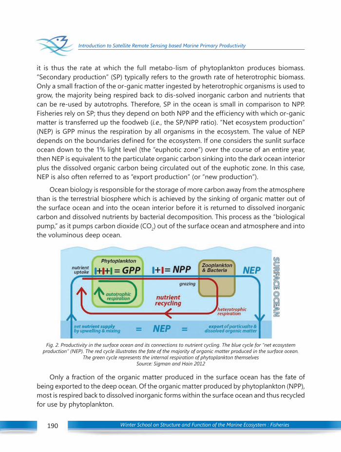
Winter School on Structure and Function of the Marine Ecosystem : Fisheries190
Introduction to Satellite Remote Sensing based Marine Primary Productivity
it is thus the rate at which the full metabo-lism of phytoplankton produces biomass.“Secondary production” (SP) typically refers to the growth rate of heterotrophic biomass.Only a small fraction of the or-ganic matter ingested by heterotrophic organisms is used togrow, the majority being respired back to dis-solved inorganic carbon and nutrients thatcan be re-used by autotrophs. Therefore, SP in the ocean is small in comparison to NPP.Fisheries rely on SP; thus they depend on both NPP and the efficiency with which or-ganicmatter is transferred up the foodweb (i.e., the SP/NPP ratio). “Net ecosystem production”(NEP) is GPP minus the respiration by all organisms in the ecosystem. The value of NEPdepends on the boundaries defined for the ecosystem. If one considers the sunlit surfaceocean down to the 1% light level (the “euphotic zone”) over the course of an entire year,then NEP is equivalent to the particulate organic carbon sinking into the dark ocean interiorplus the dissolved organic carbon being circulated out of the euphotic zone. In this case,NEP is also often referred to as “export production” (or “new production”).
Ocean biology is responsible for the storage of more carbon away from the atmospherethan is the terrestrial biosphere which is achieved by the sinking of organic matter out ofthe surface ocean and into the ocean interior before it is returned to dissolved inorganiccarbon and dissolved nutrients by bacterial decomposition. This process as the “biologicalpump,” as it pumps carbon dioxide (CO2) out of the surface ocean and atmosphere and intothe voluminous deep ocean.
Fig. 2. Productivity in the surface ocean and its connections to nutrient cycling. The blue cycle for “net ecosystemproduction” (NEP). The red cycle illustrates the fate of the majority of organic matter produced in the surface ocean.
The green cycle represents the internal respiration of phytoplankton themselvesSource: Sigman and Hain 2012
Only a fraction of the organic matter produced in the surface ocean has the fate ofbeing exported to the deep ocean. Of the organic matter produced by phytoplankton (NPP),most is respired back to dissolved inorganic forms within the surface ocean and thus recycledfor use by phytoplankton.
Winter School on Structure and Function of the Marine Ecosystem : Fisheries 191
Introduction to Satellite Remote Sensing based Marine Primary Productivity
3. Pre-requisite for Ocean Productivity and limitations
The ocean primary production largely depends upon three factors: Sunlight, dissolvedoxygen and nutrients.
Sunlight is the ultimate energy source — directly or indirectly — for almost all life onEarth, including in the deep ocean. However, light is absorbed and scattered such that verylittle of it penetrates below a depth of ~80 m (as deep as 150 m in the least productivesubtropical regions, but as shallow as 10 m in highly productive and coastal regions). Thus,photosynthesis is largely restricted to the upper light-penetrated skin of the ocean.
The availability of dissolved oxygen is also critical for the process of photosynthesiswhich depends upon the rate of oxygen utilization. However as the productivity is limited toeuphotic zone the concentration of DO is not limiting in this zone.
Phytoplankton requires a suite of chemicals, and those with the potential to be scarcein surface waters are typically identified as “nutrients.” Broadly important nutrients includenitrogen (N), phosphorus (P), iron (Fe), and silicon (Si). There appear to be relatively uniformrequirements for N and P among phytoplankton. The export of organic matter to depthdepletes the surface ocean of nutrients, causing the nutrients to accumulate in deep waterswhere there is no light available for photosynthesis. Because of the density difference betweensurface water and the deep sea across most of the ocean, ocean circulation can only veryslowly reintroduce dissolved nutrients to the euphotic zone. By driving nutrients out of thesunlit, buoyant surface waters, ocean productivity effectively limits itself.
Phytoplankton growth limitation has traditionally been interpreted in the context ofLiebig’s Law of the Minimum, which states that plant growth will be as great as allowed bythe least available resource, the “limiting nutrient” that sets the productivity of the system(de Baar 1994).
4. The measurement
Primary productivity can be measured in three ways: 1) The amount of carbon dioxideused, 2) The rate of sugar formation and 3) The rate of oxygen production. The first beingthe most accurate.
4.1. Oxygen measurement
Primary productivity can be measured from the amount of oxygen consumed by avolume of water in a fixed period of time; water for which productivity is to be determinedis enclosed in sealed white and dark bottles (bottle painted dark so light would not enter).DO (dissolved oxygen) measurement of water is made at the beginning of the immersionperiod. The two bottles are then immersed in the water body concerned at the level from

Winter School on Structure and Function of the Marine Ecosystem : Fisheries192
Introduction to Satellite Remote Sensing based Marine Primary Productivity
which the water is taken. The phytoplankton and other elements in the water produceoxygen in the water bottle, but some oxygen disappears due to respiration. The latter ismeasured from the readings of dark bottle, where only respiration takes place. Thus fromthe oxygen produced by photosynthesis of enclosed organism (representing a sample ofthe water body) can be known. However this oxygen production indicates net primaryproductivity only. From the DO difference in dark bottle oxygen consumed by the enclosedorganisms can be obtained and when this respiration value is added to the oxygen productionin the white bottle, a value for gross primary productivity is obtained.
4.2. Carbon measurement
The most accurate method for determining productivity is the method of using carbontracer. In this method, a known quantity of carbon tracer is added into a bottle containingwater with the phytoplankton and other organisms and after a short period of incubation,carbon fixed can be measured. The productivity measured thus is net primary productivityas the carbon fixed in the tissues only are measured here.
5. Primary productivity from satellite
By virtue of the broad synoptic coverage of remotely sensed images of ocean color areseen as important tools for the spatial extrapolation of local data collected from ships inocean biogeochemical studies. One of the principal applications of the imageries theestimation of ocean primary production at large geographical scale. Various methods havebeen proposed to convert pigment fields derived from ocean color images in to maps ofprimary production. These models differ in complexity and therefore in the computing timeand the amount of information required to implement them. Satellite based primaryproductivity models computed daily water column primary production as a function ofavailable light and biomass.
The simplest productivity models estimate time and depth integrated primary productionas a function of sea surface chlorophyll. The next step in algorithm complexity introducessurface irradiance as a second factor controlling productivity, where depth-integratedproduction is the product of depth-integrated chlorophyll, daily surface irradiance, and aconstant, water- column averaged quantum yield for photosynthesis.
At any depth z (positive downwards) and time t, the dependence of biomass-specificprimary production PB(z) on photon flux or irradiance (I) can be written as
PB (z,t) = P [I(z,t)]
Where the superscript indicates normalization to the pigment biomass B, and thefunction represents family of curves whose general shape is known from experiments.
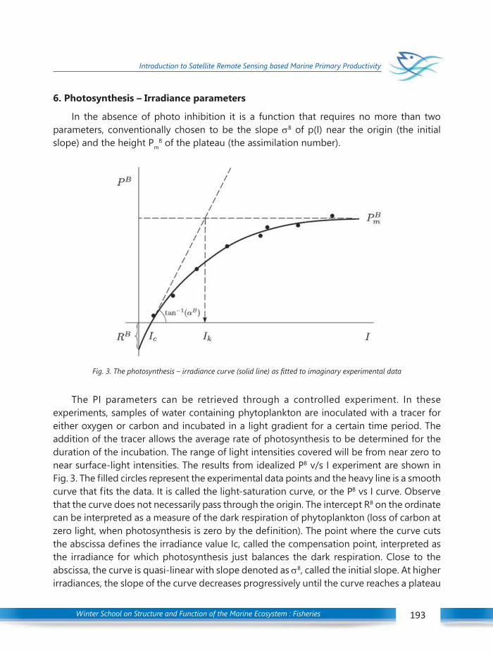
Winter School on Structure and Function of the Marine Ecosystem : Fisheries 193
Introduction to Satellite Remote Sensing based Marine Primary Productivity
6. Photosynthesis – Irradiance parameters
In the absence of photo inhibition it is a function that requires no more than twoparameters, conventionally chosen to be the slope σB of p(I) near the origin (the initialslope) and the height Pm
B of the plateau (the assimilation number).
The PI parameters can be retrieved through a controlled experiment. In theseexperiments, samples of water containing phytoplankton are inoculated with a tracer foreither oxygen or carbon and incubated in a light gradient for a certain time period. Theaddition of the tracer allows the average rate of photosynthesis to be determined for theduration of the incubation. The range of light intensities covered will be from near zero tonear surface-light intensities. The results from idealized PB v/s I experiment are shown inFig. 3. The filled circles represent the experimental data points and the heavy line is a smoothcurve that fits the data. It is called the light-saturation curve, or the PB vs I curve. Observethat the curve does not necessarily pass through the origin. The intercept RB on the ordinatecan be interpreted as a measure of the dark respiration of phytoplankton (loss of carbon atzero light, when photosynthesis is zero by the definition). The point where the curve cutsthe abscissa defines the irradiance value Ic, called the compensation point, interpreted asthe irradiance for which photosynthesis just balances the dark respiration. Close to theabscissa, the curve is quasi-linear with slope denoted as σB, called the initial slope. At higherirradiances, the slope of the curve decreases progressively until the curve reaches a plateau
Fig. 3. The photosynthesis – irradiance curve (solid line) as fitted to imaginary experimental data
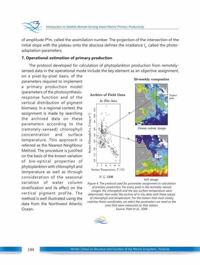
Winter School on Structure and Function of the Marine Ecosystem : Fisheries194
Introduction to Satellite Remote Sensing based Marine Primary Productivity
of amplitude PBm, called the assimilation number. The projection of the intersection of theinitial slope with the plateau onto the abscissa defines the irradiance Ik, called the photo-adaptation parameters.
7. Operational estimation of primary production
The protocol developed for calculation of phytoplankton production from remotely-sensed data in the operational mode include the key element as an objective assignment,on a pixel-by-pixel basis, of theparameters required to implementa primary production model(parameters of the photosynthesis-response function and of thevertical distribution of pigmentbiomass). In a regional context, theassignment is made by searchingthe archived data on theseparameters according to the(remotely-sensed) chlorophyllconcentration and surfacetemperature. This approach isreferred as the Nearest-NeighbourMethod. The procedure is justifiedon the basis of the known variationof bio-optical properties ofphytoplankton with chlorophyll andtemperature as well as throughconsideration of the seasonalvariation of water columnstratification and its effect on thevertical pigment prof ile. Themethod is well illustrated using thedata from the Northwest AtlanticOcean.
Figure 4. The protocol used for parameter assignment in calculationof primary production. For every pixel in the remotely-sensedimages, the chlorophyll and the sea-surface temperature were
determined, then enter the archive of in situ data with these valuesof chlorophyll and temperature. For the station that most closely
matches these coordinates, we select the parameters we need as theones that were measured on that station.
Source: Platt et al., 2008

Winter School on Structure and Function of the Marine Ecosystem : Fisheries 195
Estimation of Primary production by Remote Sensing
I. Introduction
Global concern over the atmospheric increase in carbon dioxide have lead to the studyof the sources and sinks responsible for regulating the increase, and to the conclusion thatthe oceans are the major sinks for atmospheric CO2. The uptake of atmospheric CO2 by theoceans is the flux of carbon through the surface mixed layer into the deep ocean controlledby the fixation of carbon by marine phytoplankton through photosynthetic processes ofprimary production. Primary production is defined as the amount of organic material(Biomass) present per unit space per unit time. Photosynthetic processes occur in bothoceanic and terrestrial ecosystems. About 50 % of total primary production in the biosphereoccurs in the sea, through phytoplankton ranging from chains of diatoms to 1 µm-sizedphotosynthetic bacteria. Oceanic photosynthetic organisms turn over much more rapidlythan terrestrial counterparts. Oceanic photosynthetic organisms are extremely efficient infixing carbon compared to terrestrial plants and mediate a large flux of organic carbon intothe ocean, often referred as the biological pump. In addition to sustaining the marine foodchain, phytoplankton strongly influence ocean chemistry. During photosynthesis, they removecarbon dioxide dissolved in seawater to produce sugars and other simple organic molecules,and release oxygen as a by-product. Phytoplankton also require inorganic nutrients (e.g.,nitrogen, phosphorus, silicon) as well as trace elements (e.g., iron) to synthesize complexmolecules, such as proteins. Ocean productivity thus plays a key role in the globalbiogeochemical cycles of carbon, oxygen, and other elements critical to both marine andterrestrial life. The magnitude and variability of primary production are poorly known on aglobal scale, largely because of the high spatial and temporal variability of marinephytoplankton concentrations. Study of large-scale variations in productivity; global coverageby ship borne instruments is impossible. Only ocean colour sensors provides the rapid,global coverage required for studies of ocean productivity at global over world ocean basins.The focus is on the estimation of oceanic phytoplankton biomass and primary productionon regional and global scales using both in-situ and Remote Sensing techniques and theobjective is to develop coupled climate and bio-geochemical models required for predictingclimate forcing and responses.
21C H A P T E R ESTIMATION OF PRIMARY PRODUCTION BY
REMOTE SENSINGK. H. Rao
National Remote Sensing Centre, ISRO, Hyderabad
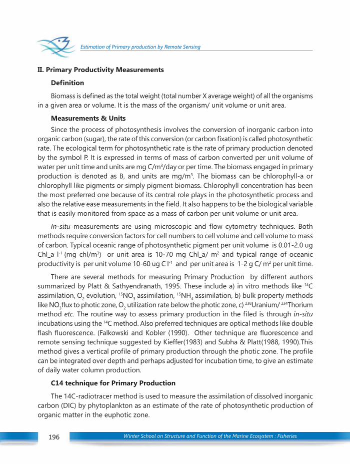
Winter School on Structure and Function of the Marine Ecosystem : Fisheries196
Estimation of Primary production by Remote Sensing
II. Primary Productivity Measurements
Definition
Biomass is defined as the total weight (total number X average weight) of all the organismsin a given area or volume. It is the mass of the organism/ unit volume or unit area.
Measurements & UnitsSince the process of photosynthesis involves the conversion of inorganic carbon into
organic carbon (sugar), the rate of this conversion (or carbon fixation) is called photosyntheticrate. The ecological term for photosynthetic rate is the rate of primary production denotedby the symbol P. It is expressed in terms of mass of carbon converted per unit volume ofwater per unit time and units are mg C/m3/day or per time. The biomass engaged in primaryproduction is denoted as B, and units are mg/m3. The biomass can be chlorophyll-a orchlorophyll like pigments or simply pigment biomass. Chlorophyll concentration has beenthe most preferred one because of its central role plays in the photosynthetic process andalso the relative ease measurements in the field. It also happens to be the biological variablethat is easily monitored from space as a mass of carbon per unit volume or unit area.
In-situ measurements are using microscopic and flow cytometry techniques. Bothmethods require conversion factors for cell numbers to cell volume and cell volume to massof carbon. Typical oceanic range of photosynthetic pigment per unit volume is 0.01-2.0 ugChl_a l-1 (mg chl/m3) or unit area is 10-70 mg Chl_a/ m2 and typical range of oceanicproductivity is per unit volume 10-60 ug C l-1 and per unit area is 1-2 g C/ m2 per unit time.
There are several methods for measuring Primary Production by different authorssummarized by Platt & Sathyendranath, 1995. These include a) in vitro methods like 14Cassimilation, O2 evolution, 15NO3 assimilation, 15NH4 assimilation, b) bulk property methodslike NO3flux to photic zone, O2 utilization rate below the photic zone, c) 238Uranium/ 234Thoriummethod etc. The routine way to assess primary production in the filed is through in-situincubations using the 14C method. Also preferred techniques are optical methods like doubleflash fluorescence. (Falkowski and Kobler (1990). Other technique are fluorescence andremote sensing technique suggested by Kieffer(1983) and Subha & Platt(1988, 1990).Thismethod gives a vertical profile of primary production through the photic zone. The profilecan be integrated over depth and perhaps adjusted for incubation time, to give an estimateof daily water column production.
C14 technique for Primary Production
The 14C-radiotracer method is used to measure the assimilation of dissolved inorganiccarbon (DIC) by phytoplankton as an estimate of the rate of photosynthetic production oforganic matter in the euphotic zone.

Winter School on Structure and Function of the Marine Ecosystem : Fisheries 197
Estimation of Primary production by Remote Sensing
The 14C method, originally proposed by Steeman - Nielsen (1952), is used to estimatethe uptake of dissolved inorganic carbon (DIC) by planktonic algae in the water column.The method is based on biological uptake of 14C-labeled DIC is proportional to the biologicaluptake of 12C-DIC. If one knows the initial concentration of DIC in a water sample, theamount of 14C-DIC added, the 14C retained in particulate organic matter (14C-POC) at theend of the incubation and the metabolic discrimination between the two isotopes of carbon(i.e., 5% discrimination against the heavier 14C isotope), then it is possible to estimate thetotal uptake of carbon from the following relationship:
DIC * 14C-POC * 1.05C uptake = ——————————
14C-DIC added
III. Productivity modeling & variables
Light intensity and photosynthesis relation
Light intensity is used as a forcing function both for the physical and the biologicalmodel. In the physical model, light intensity influences water temperature and thereforewater density. The basic aspects of irradiance or light having biological importance arequantity and quality. Light is qualitatively described by its spectral distribution dependingon difference in wavelengths. Total radiation at these wavelength is called as Photosyntheticactive radiation (PAR). PAR is for all practical purposes considered between 400-700 nmsince total energy shorter than 400 is lee than 10%. Thus light is the most important variableexpressed as flux of energy per unit area per unit time. In the biological model, thephotosynthetically active radiation (PAR) forces primary productivity. Properties of irradiancefield are ë, angular distribution of wavelength (zenith and azimuth angles). Estimation oflight intensity and radiation fluxes between the sea and the atmosphere was based onstandard formulations described in literature.
Photosynthesis and Irradiance (PI) curve
Since photosynthesis is a photochemical process, the functional response ofphytoplankton photosynthesis to available light is studied through the use of photosynthesislight experiments or PI experiments. The relationship between light and photosynthesis iscalled light saturation curve or PI curve. The curve is a reflection of environmental effectson photosynthesis and can be used to diagnose certain properties of algal species, ornatural samples of phytoplankton. Photosynthesis increases with increasing light intensityup to some asymptotic value where the system becomes light saturated. The curve doesnot necessarily pass through the origin. The intercept R on the ordinate can be interpretedas a measure of dark respiration of phytoplankton (loss of carbon at zero light when
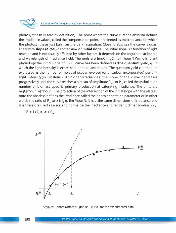
Winter School on Structure and Function of the Marine Ecosystem : Fisheries198
Estimation of Primary production by Remote Sensing
photosynthesis is zero by definition). The point where the curve cuts the abscissa definesthe irradiance value Ic called the compensation point, interpreted as the irradiance for whichthe photosynthesis just balances the dark respiration. Close to abscissa the curve is quasilinear with slope (∆∆∆∆∆P/∆∆∆∆∆I) denoted as ααααα or initial slope. The initial slope is a function of lightreaction and is not usually affected by other factors. It depends on the angular distributionand wavelength of irradiance field. The units are [mgC[mgChl a]-1 hour-1] Wm-2. In plantphysiology the initial slope of P vs. I curve has been defined as ‘the quantum yield, ϕϕϕϕϕ’ inwhich the light intensity is expressed in the quantum unit. The quantum yield can then beexpressed as the number of moles of oxygen evolved (or of carbon incorporated) per unitlight intensity(in Einsteins). At higher irradiances, the slope of the curve decreasesprogressively until the curve reaches a plateau of amplitude Pmax or Pm, called the assimilationnumber or biomass specific primary production at saturating irradiance. The units aremgC[mgChl a]-1 hour-1. The projection of the intersection of the initial slope with the plateauonto the abscissa defines the irradiance called the photo adaptation parameter or in otherwords the ratio of Pm to α is Ik (µ Em-2hour-1). It has the same dimensions of irradiance andit is therefore used as a scale to normalize the irradiance and render it dimensionless. i.e.,
I* = I / Ik = ααααα / Pm
A typical photosynthesis-light (P I) curve for the experimental data

Winter School on Structure and Function of the Marine Ecosystem : Fisheries 199
Estimation of Primary production by Remote Sensing
When the value I* = 1, corresponding to I = Ik , the curves are divided into two regimes.For I less than or equal to 1, photosynthesis depends strongly on irradiance. For I greaterthan 1, photosynthesis depends less strongly on irradiance, eventually becoming independentof it. If one assumes that the curve passes through the origin, then the curve can berepresented by two parameters á and Pm and can be written as
P(I) = p (I; ααααα, Pm) (1)
Thus it can be seen that the functional response of phytoplankton photosynthesis tothe available light is parameterized by two quantities, α and Pm or in other wordsphotosynthesis light curve is a function of one variable, irradiance and two parameters. Thisfunction p defines a family of curves, the individual members identified by the value ormagnitude of parameters α and Pm. Since α and Pm varies for different areas and seasons, itis necessary to know the magnitude of α and Pm to compute primary production instead oftaking a single value. The slope α is also depth dependent. In deeper depths due to itsexponential decay nature, magnitude of light will be less. Therefore at less light intensity áwill be sharper since it indicates the efficiency of phytoplankton to perform photosynthesisat available light conditions. Slope of the P vs. I curve is also spectral in nature. As seen fromequation (1) photosynthesis is dependent on the available irradiance and thereforephotosynthesis at depth is also dependent upon the irradiance available at that depth. Inorder to estimate the light reaching at a particular depth, a parameter known as diffuseattenuation coefficient or K is used. This K describes the behavior of light at a given depth.
Daily Water Column production – General equation
To estimate primary production P given information on biomass B and irradiance I, it isuseful to have an index of production from which the effects of variations in B have beenremoved. This is because both P and B are local variables since their magnitude can varyover short scales of time and space. Since variations in biomass are the principal biogeniccause of variation in the rate of primary production it is necessary to normalize the productionto biomass. This gives a quantity known as normalized production, PB which is of moresignificance than P because its variation between regions and seasons can be analysedwithout the complications that might arise from chance fluctuations in the local biomass.
PB = P / B (2)
When required the absolute production P can be recovered by inversion of (2)
P = B x PB (3)
The pigment biomass usually depends on depth, z, so that eqn. (3) can be written as
P(z) = B(z) x PB(z) (4)
Winter School on Structure and Function of the Marine Ecosystem : Fisheries200
Estimation of Primary production by Remote Sensing
From eqn. (1) it is evident that production is dependent on available irradiance and inaquatic systems, irradiance is always a function of depth. Therefore the dependence of PB(z)on photon flux may be stated as
PB(z) = pB(I(z)) (5)
From eqn. (4) and (5)
P(z) = B(z) x pB(I(z)) (6)
I(z) in the above eqn. is a time dependent variable. Therefore eqn. (6) can be rewritten as
P(z,t) = B(z,t) x pB(I(z,t)) (7)
The above equation computes production at discrete depths. To compute productionof a layer (mixed layer, euphotic layer) of water column the above eqn. has to be integratedover depth. Thus water column production Pz can be computed as
PZ = ∫z
P(z)dz = ∫∞
0B(z) pB(I(z,t)) dz (8)
It is also necessary to integrate the above eqn. which gives the instantaneous, watercolumn rates through time to compute primary production for the day. Thus
PZ,T = ∫∫∞
00
DB(z,t) pB(I(z,t)) dz dt (9)
Where time t is measured from sunrise and D is the day length. For integration throughtime, it is usual to consider that diurnal changes is sufficiently slow to be insignificant. i.e.,the time dependence of B in above equation is suppressed to give
PZ,T = B(z,t) pB(I(z,t)) dz dt (10)
his is the basic formalism for computation of water column primary production andevaluation of equation (10) about B, pB and I under various assumptions has resulted inempirical, semi-analytical, analytical algorithms.
IV. Estimation of Primary Productivity using Remote Sensing TechniquesSatellite measurements of ocean color have played a key role in understanding of
oceanographic processes from local to regional to global scales. The measurement ofocean color from space has revealed for the first time, the global-scale variability in thedistribution and concentration of phytoplankton, which provides the ultimate source offood for marine life. Since phytoplankton pigments absorb energy primarily in the red andblue regions of the spectrum and reflect green light, there is a relationship between thespectrum of sunlight backscattered by upper ocean layers and the distribution of
Winter School on Structure and Function of the Marine Ecosystem : Fisheries 201
Estimation of Primary production by Remote Sensing
phytoplankton pigments in these layers. Satellite measurements of ocean radiance at selectedwavelengths can thus be used to estimate near-surface phytoplankton concentrations andthe extent of primary productivity.
For the last 20 years ocean colour data became widely available and provided anopportunity to analyze the spatial and temporal variability in upper ocean chlorophylldistribution. The fundamental problem is regarding the utilization of ocean colourmeasurements for estimating the Primary production. This includes 1) algorithmdevelopment, classification and similarities and differences among the available productivityalgorithms 2) algorithm parameterization 3) algorithm testing and validation. The problemin the development of PP models has been that the sea truth has changed with time. Withinthe past two decade estimates of global Oceanic primary production have been revisedupward by about two fold, to about 50 Gt C/y. The increase in estimated global pp is basedon the belief that the historical radiocarbon measurements were poisoned by metals. Thesecond problem is the in consistency in model development and structure.
Empirical, semi-empirical and analytical methods are used to estimate the concentrationof chlorophyll-a and its degradation products from satellite measurements of backscatteredsunlight at three wavebands centered at 443, 520, and 550 nm, covering the blue and greenregions of the spectrum. These radiances are not merely reflected from the sea surface, butare derived from sunlight that has entered the ocean, been selectively absorbed, scatteredand reflected by phytoplankton and other suspended material in the upper layers, and thenbackscatter through the surface. This approach permits quantitative estimates ofphytoplankton pigment concentrations within the upper tens of meters of the open ocean,and within somewhat lesser depths in coastal waters
For the non-specialist (and others) the Standard Products might be just what youneed if you are looking for ocean productivity data. For more specialist applications whereyou want to compare or use productivity products from different models or sensors ( OCM,SeaWiFS and MODIS), you should refer to the defined in Custom Products.
Standard Products
Global PP products are derived using two operational semi-empirical and mixed layermodel. NASA is providing the Global PP data at different time and space scales. Suchalgorithms are Vertical Generalized Production Model (VGPM). The VGPM algorithmintegrates productivity over the euphotic depth and uses a seventh order polynomial toestimate the quantum efficiency for photosynthesis as a function of sea surface temperature.The Howard-Yoder-Ryan algorithm differs from the VGPM algorithm in that it calculates theaverage radiative energy over the mixed-layer, and the maximum photosynthetic yield, asan exponential function of temperature. The algorithm uses these to compute carbon
Winter School on Structure and Function of the Marine Ecosystem : Fisheries202
Estimation of Primary production by Remote Sensing
fixation per volume over the depth of the mixed-layer, Pz, which is multiplied by the mixed-layer depth, Zml, to integrate productivity to that depth. The algorithm, as it was firstpresented in a master’s thesis by Howard in 1995 and currently NASA is producing globalPP products using parameters.
A standard productivity product initially has been developed using the VerticallyGeneralized Production Model (VGPM) (Behrenfeld and Falkowski, 1997a) as the standardalgorithm. The VGPM is a “chlorophyll-based” model that estimate net primary productionfrom chlorophyll using a temperature-dependent description of chlorophyll-specificphotosynthetic efficiency. For the VGPM, net primary production is a function of chlorophyll,available light, and the photosynthetic efficiency.
VGPM Net Primary Production (NPP) calculationsThe VGPM was first described by Behrenfeld and Falkowski (1997a) and is a commonly
used algorithm for estimating regional to global ocean NPP. The foundation of the VGPMand other chlorophyll-based models is that NPP varies in a predictable manner withchlorophyll concentration (chl) that is a NPP = f(chl).
Because NPP is a rate and chlorophyll is a standing stock, derivation of the former fromthe later requires a “rate” term, specifically a chlorophyll-specific assimilation efficiency forcarbon fixation. The description of this rate term is the single most important uncertainty inall chlorophyll based models.
The VGPM employs a variable termed Pb_opt, which is the maximum daily net primaryproduction found within a given water column and expressed in units of mg carbon fixedper mg chlorophyll per hour. NPP at the depth of Pb_opt is thus:
NPP = chl * pb_opt * day length
where day length is the number of hours of day light at the location of interest and NPPis milligrams of carbon fixed per day per unit volume.
Water column NPP is generally regarded as the primary production taking place fromthe surface to the depth at which 1% of surface light is available, this light depth the “euphoticdepth” or “z_eu”. If you were to consider the hypothetical condition where photosyntheticrates were uniform from the surface to z_eu, then water column production could simply becalculated as:
NPP = chl * pb_opt * day length * z_euor, in words, surface production times the euphotic depth.
In the real world, however, photosynthesis through the water column is far from constant.The most important factor driving this vertical variability is light. As sunlight penetrates the
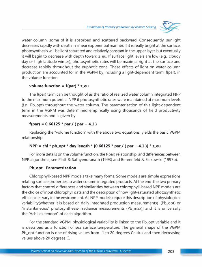
Winter School on Structure and Function of the Marine Ecosystem : Fisheries 203
Estimation of Primary production by Remote Sensing
water column, some of it is absorbed and scattered backward. Consequently, sunlightdecreases rapidly with depth in a near exponential manner. If it is really bright at the surface,photosynthesis will be light saturated and relatively constant in the upper layer, but eventuallyit will begin to decrease with depth toward z_eu. If surface light levels are low (e.g., cloudyday or high latitude winter), photosynthetic rates will be maximal right at the surface anddecrease rapidly throughout the euphotic zone. These effects of light on water columnproduction are accounted for in the VGPM by including a light-dependent term, f(par), inthe volume function:
volume function = f(par) * z_eu
The f(par) term can be thought of as the ratio of realized water column integrated NPPto the maximum potential NPP if photosynthetic rates were maintained at maximum levels(i.e., Pb_opt) throughout the water column. The paramterization of this light-dependentterm in the VGPM was determined empirically using thousands of field productivitymeasurements and is given by:
f(par) = 0.66125 * par / ( par + 4.1 )
Replacing the “volume function” with the above two equations, yields the basic VGPMrelationship:
NPP = chl * pb_opt * day length * [0.66125 * par / ( par + 4.1 )] * z_eu
For more details on the volume function, the f(par) relationship, and differences betweenNPP algorithms, see Platt & Sathyendranath (1993) and Behrenfeld & Falkowski (1997b).
Pb_opt Parametrization
Chlorophyll-based NPP models take many forms. Some models are simple expressionsrelating surface properties to water column integrated products. At the end the two primaryfactors that control differences and similarities between chlorophyll-based NPP models arethe choice of input chlorophyll data and the description of how light-saturated photosyntheticefficiencies vary in the environment. All NPP models require this description of physiologicalvariability(whether it is based on daily integrated production measurements) (Pb_opt) or“instantaneous” photosynthesis-irradiance measurements (Pb_max)] and it is universallythe “Achilles tendon” of each algorithm.
For the standard VGPM, physiological variability is linked to the Pb_opt variable and itis described as a function of sea surface temperature. The general shape of the VGPMPb_opt function is one of rising values from -1 to 20 degrees Celsius and then decreasingvalues above 20 degrees C.
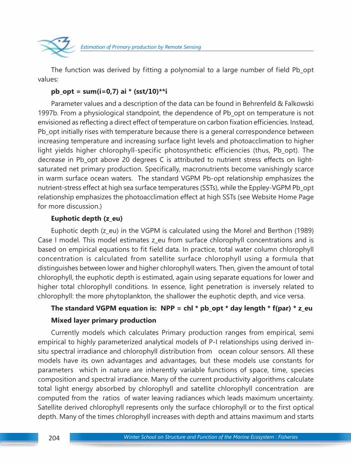
Winter School on Structure and Function of the Marine Ecosystem : Fisheries204
Estimation of Primary production by Remote Sensing
The function was derived by fitting a polynomial to a large number of field Pb_optvalues:
pb_opt = sum(i=0,7) ai * (sst/10)**i
Parameter values and a description of the data can be found in Behrenfeld & Falkowski1997b. From a physiological standpoint, the dependence of Pb_opt on temperature is notenvisioned as reflecting a direct effect of temperature on carbon fixation efficiencies. Instead,Pb_opt initially rises with temperature because there is a general correspondence betweenincreasing temperature and increasing surface light levels and photoacclimation to higherlight yields higher chlorophyll-specific photosynthetic efficiencies (thus, Pb_opt). Thedecrease in Pb_opt above 20 degrees C is attributed to nutrient stress effects on light-saturated net primary production. Specifically, macronutrients become vanishingly scarcein warm surface ocean waters. The standard VGPM Pb-opt relationship emphasizes thenutrient-stress effect at high sea surface temperatures (SSTs), while the Eppley-VGPM Pb_optrelationship emphasizes the photoacclimation effect at high SSTs (see Website Home Pagefor more discussion.)
Euphotic depth (z_eu)
Euphotic depth (z_eu) in the VGPM is calculated using the Morel and Berthon (1989)Case I model. This model estimates z_eu from surface chlorophyll concentrations and isbased on empirical equations to fit field data. In practice, total water column chlorophyllconcentration is calculated from satellite surface chlorophyll using a formula thatdistinguishes between lower and higher chlorophyll waters. Then, given the amount of totalchlorophyll, the euphotic depth is estimated, again using separate equations for lower andhigher total chlorophyll conditions. In essence, light penetration is inversely related tochlorophyll: the more phytoplankton, the shallower the euphotic depth, and vice versa.
The standard VGPM equation is: NPP = chl * pb_opt * day length * f(par) * z_eu
Mixed layer primary production
Currently models which calculates Primary production ranges from empirical, semiempirical to highly parameterized analytical models of P-I relationships using derived in-situ spectral irradiance and chlorophyll distribution from ocean colour sensors. All thesemodels have its own advantages and advantages, but these models use constants forparameters which in nature are inherently variable functions of space, time, speciescomposition and spectral irradiance. Many of the current productivity algorithms calculatetotal light energy absorbed by chlorophyll and satellite chlorophyll concentration arecomputed from the ratios of water leaving radiances which leads maximum uncertainty.Satellite derived chlorophyll represents only the surface chlorophyll or to the first opticaldepth. Many of the times chlorophyll increases with depth and attains maximum and starts

Winter School on Structure and Function of the Marine Ecosystem : Fisheries 205
Estimation of Primary production by Remote Sensing
decreasing with depth with in the mixed layer. This shows that the seasonal changes PP ismainly depends upon the vertical profiles of the chlorophyll and its changes with in themixed layer. For computing annual PP it requires seasonal PP, its variability and accountingthe peaks of Primary production with in the water column (seasonal and spatial variability).The basic requirements are the structure of Vertical chlorophyll profile and Mixed layervariability and description of chlorophyll & MLD relation. High insolation and week windsresults in thin Mixed layer representing oligotrophic conditions during inter monsoon periodin Arabian sea. During May MLD is mostly less than 50 meters and pigment concentrationis less than 0.1 mg/l. In contrast to this winter and summer season results in deepening ofMLD and strong regional phytoplankton blooms observed in most part of the Arabian sea.(Banse and McClain1986, Bauer et al., 1991, Brock et al., 1991 and Brock & McClain 1992),Blooms are due to vertical mixing or due to convective overturn. These studies reveals thatthe column PP mainly depends upon the vertical structure of chlorophyll and MLD and itsseasonal variability (Plat 1986).
Basic methodology
1. Compute light available at sea surface2. Estimate biomass at surface3. Define biomass profile4. Estimate parameters of P-I model5. Compute parameters of light transmission6. Compute primary production
Required Parameters
Surface Irradiance (PAR)Irradiance (PAR) Profile Or ( K )Surface Chlorophyll and Chlorophyll ProfilesP-I Parameters (PBm, αB)Sea Surface Temperature (SST), Mixed Layer Depth (MLD )
and in-situ PP measurements at selected places and also to construct compute estimationP I parameters.
Conclusions
The entire marine food chain depends on the rate of primary production of organicmatter. For most of the ocean, photosynthetic primary production dominates, and is carried
Winter School on Structure and Function of the Marine Ecosystem : Fisheries206
Estimation of Primary production by Remote Sensing
out by the phytoplankton. To first order, the rate of primary production is proportional tothe biomass, either measured in carbon or chlorophyll units. Photosynthesis consists of thephotolysis of water, and the subsequent reduction of carbon dioxide to form organic matter.Oxygen is produced as a byproduct. Photosynthesis consists of light and dark reactions,and can be measured using the uptake of radioactive carbon dioxide, or the evolution ofoxygen. The relationship between primary production and irradiance typically is linear atlow light, then saturates, and may be inhibited at high light. The rate of primary productionon a local and global scale can be estimated from the solar irradiance, the attenuation oflight, the distribution of biomass, and the photosynthesis-irradiance curve, suitably integratedin time and space.
References
Balch, W.M. and C.F. Byrne. (1994). Factors effecting the estimate of primary production from space. J.Geophys. Res. 99. 7555-7530.
Behrenfeld, M.J. and Paul G. Falkowski (1997). A cosumers guide to phytoplankton primary productivitymodels. Limnol. Oceanogr. 42(7). 1479-1491.
Kiefer, D.A., and B.G. Mitchell. (1983). A simple , steady state description of phytoplankton growth based onabsorption cross section and quantum efficiency. Limnol. Oceanogr. 28. 770-776.
Kirk, J.T.O. 1994. Light and photosynthesis in aquatic ecosystems. 2nd ed. Cambridge.
Falkowski, P.G. M.J. Behrenfeld, W.E. Esaias, W. Balch, J. W. Campbell, R.L. Iverson, D.A. Kiefer, Andre Moreland James Yoder (1998). Satellite primary productivity data and algorithm development: A scienceplan for Mission to Planet Earth. NASA Technical Memo. 104566, Vol.42. S.B. Hooker and E.R. Firestone,Eds. NASA Goddard Space Flight Centre. Maryland, 36pp.
Platt,T., and Sathyendranath, S. (1988). Oceanic primary production : estimation by remote sensing at localscales and regional scales. Science.241: 1613-1620.
Platt,T., S. Sathyendranath and P. Ravindran (1990). Primary production by phytoplankton : analytical solutionsfor daily rates per unit area of water surface. Proc. R. Soc. London. Ser. B. 241. 101-111.
Platt, T. 1986. Primary production of the ocean water column as a function of surface light intensity: algorithmsfor remote sensing. Deep-Sea Res., 33: 149-163.
Platt, T, C. Caverhill and S. Sathyendranath, 1991. Basin –scale estimates of oceanic primary production byremote sensing: The north atlantic. J. Geophys. Res. 96 (C8): 15147-15159.
Ryther, J. H. 1956. Photosynthesis in the ocean as a function of light intensity. Limnol. Oceanogr. 1: 61-70.
Ryther, J. H. and C.S. Yentsch (1957). The estimation of phytoplankton production in the ocean fromchlorophyll and light data. Limnol. Oceanogr. 2. 281-286.

Winter School on Structure and Function of the Marine Ecosystem : Fisheries 207
Estimation of Primary production by Remote Sensing
Sathyendranath, S., Platt, T., Caverhill, C. M., Warnock, R. E. and Lewis, M. R. 1989. Remote sensing ofoceanic primary production: computations using a spectral model. Deep-Sea Res., 36: 431-453
Steemann Nielsen, E. (1952). The use of radio-active carbon (C14) for measuring organic production in thesea. J. Cons. Int. Explor. Mer. 18. 117-140.
Yoder, J.A. C.R. McClain, G.C. Feldman and W.E. Esaias (1993). Annual cycles of phytoplankton chlorophyllconcentrations in the global ocean: A. satellite view. Global Biogeochem, Cycles, 181-193.

Winter School on Structure and Function of the Marine Ecosystem : Fisheries208
Changes in Primary productivity and impacts in fisheries
Introduction
Fixation of inorganic carbon to organic carbon in the ocean is driven purely byphytoplankton. Phytoplankton carbon fixation plays an important role in maintaining thequasi-steady state level of atmospheric CO2. Relative contribution of marine primaryproductivity to global photosynthetic production is between 10 and 50 percent. Themagnitude ranges from 20 to 55 Gt of C/ year (Ryther, 1969; Walsh, 1984; Martin 1992).Ocean-atmospheric coupled climate models predict changes in the ocean circulation andhypothesize that changes in the ocean circulation will stimulate phytoplankton biomassproduction in the nutrient depleted areas in the open ocean (Roemmich and Wunsch, 1985).The effect on atmospheric CO2 is uncertain because the relationship between the enhancedprimary production and air-sea exchange of CO2 is not understood. The challenge is tostudy the magnitude and variability of primary productivity, its time scales and changes inatmospheric forcing and upscale it into secondary and tertiary productivity.
Northern Indian Ocean (NIO)- atmospheric composition of productive zones
The Northern Indian Ocean (NIO) comprises a unique variety of biogeochemicalprovinces, including eutrophic, oligotrophic, upwelling, and oxygen-depleted zones, all withinan area of relatively small geographic extent. This reflects the pronounced semi-annualreversals in regional winds (the seasonal monsoons) that make this region a focus for intensestudy. Previously published sea-air flux estimates indicate that the NIO could account for12-52% and 0.1-133 % respectively of the known oceanic sources of N2O and CH4. Eventhough the uncertainties are large, particularly for CH4, the Arabian Sea/NWIO could be animportant contributor to the marine CH4 source and a dominant global source of atmosphericN2O. The atmospheric inventories of N2O and CH4 are currently both increasing by about0.3% per year. Both gases are strongly active and together account for 18% of enhancedgreenhouse forcing. N2O is implicated in the generation of stratospheric NO2, which influencesstratospheric O3 levels, and CH4 participates in the photochemistry or tropospheric O3 andOH and in the formation of stratospheric H2O. Existing estimates of oceanic N2O and CH4sources are dominated by disproportionately large contributions from biologically productiveareas such as the NIO. However, because the spatial and temporal coverage of such regionsremains limited, our global estimates remain unsatisfactory. Future climatically inducedmodifications to the upwelling and circulation characteristics of the NIO and other regions
22C H A P T E R
CHANGES IN PRIMARY PRODUCTIVITY ANDIMPACTS IN FISHERIESGrinson George
Fishery Resources Assessment DivisionICAR-Central Marine Fisheries Research Institute

Winter School on Structure and Function of the Marine Ecosystem : Fisheries 209
Changes in Primary productivity and impacts in fisheries
209
experiencing strong wind-driven upwelling may have profound effects on future biogasemissions from the oceans.
Computing and integrating column Primary Production using satellite remote sensing-A preliminary approach
Integrated in-situ column primary production (PP) can be estimated and computed atbiome level using in-situ and satellite remote sensing (SRS) data by adopting suitable mixedlayer PP model. SRS methods can be applied for computing primary productivity to integrateat biome level.
Chlorophyll is an important indicator of the quality of aquatic ecosystems that areamenable to in situ and space borne measurement. This property can be retrieved fromocean colour data after removal of the atmospheric signal from the detected radiance.Phytoplankton blooms (indicated by rapid increase in chlorophyll concentration) and spurtsin primary productivity are important for maintaining the marine organisms at higher tropiclevels, but when associated with eutrophication and harmful algal blooms, as noticed in thecoastal waters of India, such events are directly linked (negatively) to the quality of water.Another important measure of water quality in the coastal environment is the suspendedsediment load. Together with chlorophyll concentration they determine water lightpenetration, and light available for photosynthesis. Optical instruments such as spectralradiometers are able to monitor changes in chlorophyll and suspended sediment load inreal time. Furthermore, such measurements can form the basis of local algorithms forapplication in remote sensing, allowing the results to be extrapolated to the entire studyarea through remote sensing. Optical methods for monitoring water quality and productivityhave been established in other marine environments, for example in the USA. In India, astart in this direction has been established and operationalized by the SATCORE programmeof ESSO-INCOIS.
Can we reach to fish biomass from primary production estimates?
Marine resources, especially fishery resources, have a strikingly important place ofprominence in the biodiversity map of the earth. Their dynamics have very importantinfluence; both direct as well as derived, on the wealth, health and eco-balance of many amaritime nations. Context to the afore mentioned issue in the region can never be overstatedwith a prominent chunk of future requirement of socio-economic and nutritional sustenancecentered in the marine sector. Towards establishing a scientifically deduced relationshipbetween the marine environment and the resource availability on a realistic basis, there is aneed for a focused application of established easy-to-surveil oceanic, geophysical andphysicochemical parameters and their direct or latent influence upon plankton, whichhappens to be the self-replenishing source of food and nutrition for fishery resources.
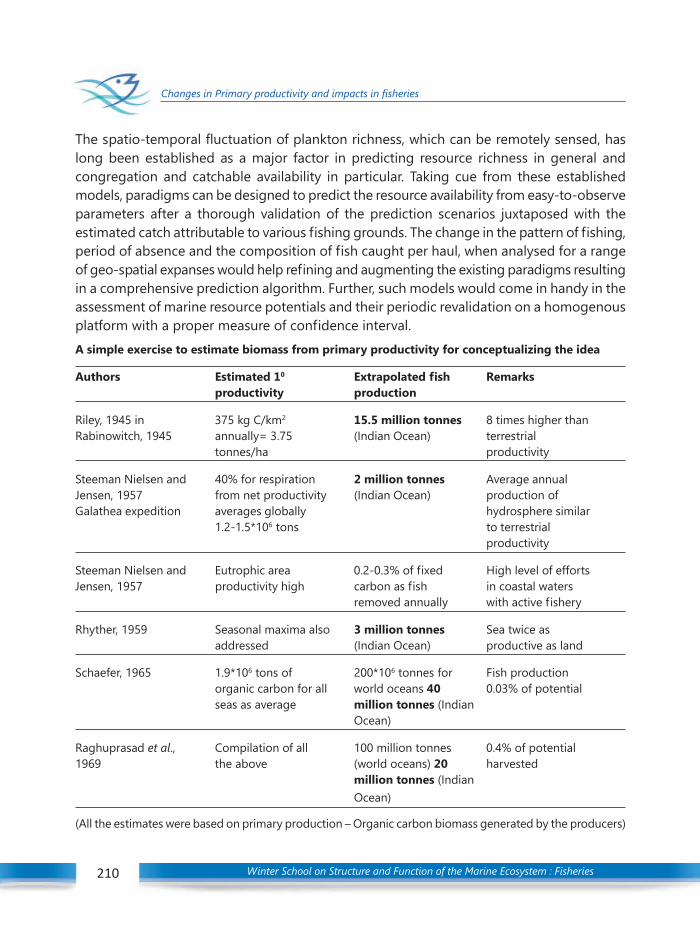
Winter School on Structure and Function of the Marine Ecosystem : Fisheries210
Changes in Primary productivity and impacts in fisheries
The spatio-temporal fluctuation of plankton richness, which can be remotely sensed, haslong been established as a major factor in predicting resource richness in general andcongregation and catchable availability in particular. Taking cue from these establishedmodels, paradigms can be designed to predict the resource availability from easy-to-observeparameters after a thorough validation of the prediction scenarios juxtaposed with theestimated catch attributable to various fishing grounds. The change in the pattern of fishing,period of absence and the composition of fish caught per haul, when analysed for a rangeof geo-spatial expanses would help refining and augmenting the existing paradigms resultingin a comprehensive prediction algorithm. Further, such models would come in handy in theassessment of marine resource potentials and their periodic revalidation on a homogenousplatform with a proper measure of confidence interval.A simple exercise to estimate biomass from primary productivity for conceptualizing the idea
Authors Estimated 10 Extrapolated fish Remarksproductivity production
Riley, 1945 in 375 kg C/km2 15.5 million tonnes 8 times higher thanRabinowitch, 1945 annually= 3.75 (Indian Ocean) terrestrial
tonnes/ha productivity
Steeman Nielsen and 40% for respiration 2 million tonnes Average annualJensen, 1957 from net productivity (Indian Ocean) production ofGalathea expedition averages globally hydrosphere similar
1.2-1.5*106 tons to terrestrialproductivity
Steeman Nielsen and Eutrophic area 0.2-0.3% of fixed High level of effortsJensen, 1957 productivity high carbon as fish in coastal waters
removed annually with active fishery
Rhyther, 1959 Seasonal maxima also 3 million tonnes Sea twice asaddressed (Indian Ocean) productive as land
Schaefer, 1965 1.9*106 tons of 200*106 tonnes for Fish productionorganic carbon for all world oceans 40 0.03% of potentialseas as average million tonnes (Indian
Ocean)
Raghuprasad et al., Compilation of all 100 million tonnes 0.4% of potential1969 the above (world oceans) 20 harvested
million tonnes (IndianOcean)
(All the estimates were based on primary production – Organic carbon biomass generated by the producers)
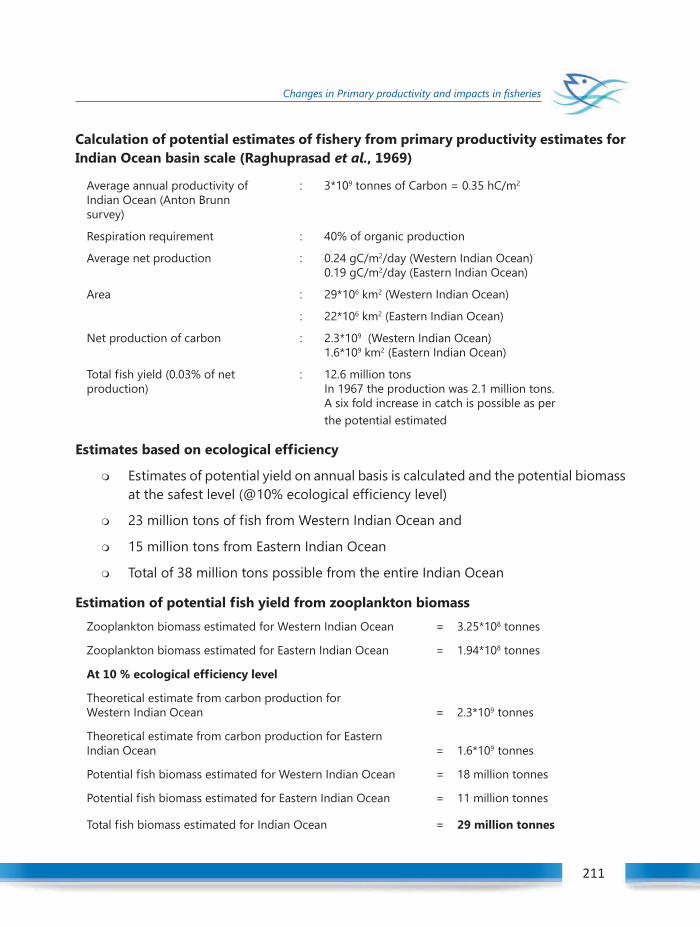
Winter School on Structure and Function of the Marine Ecosystem : Fisheries 211
Changes in Primary productivity and impacts in fisheries
211
Calculation of potential estimates of fishery from primary productivity estimates forIndian Ocean basin scale (Raghuprasad et al., 1969)
Average annual productivity of : 3*109 tonnes of Carbon = 0.35 hC/m2
Indian Ocean (Anton Brunnsurvey)
Respiration requirement : 40% of organic production
Average net production : 0.24 gC/m2/day (Western Indian Ocean)0.19 gC/m2/day (Eastern Indian Ocean)
Area : 29*106 km2 (Western Indian Ocean)
: 22*106 km2 (Eastern Indian Ocean)
Net production of carbon : 2.3*109 (Western Indian Ocean)1.6*109 km2 (Eastern Indian Ocean)
Total fish yield (0.03% of net : 12.6 million tonsproduction) In 1967 the production was 2.1 million tons.
A six fold increase in catch is possible as perthe potential estimated
Estimates based on ecological efficiency
Estimates of potential yield on annual basis is calculated and the potential biomassat the safest level (@10% ecological efficiency level)
23 million tons of fish from Western Indian Ocean and
15 million tons from Eastern Indian Ocean
Total of 38 million tons possible from the entire Indian Ocean
Estimation of potential fish yield from zooplankton biomass
Zooplankton biomass estimated for Western Indian Ocean = 3.25*108 tonnes
Zooplankton biomass estimated for Eastern Indian Ocean = 1.94*108 tonnes
At 10 % ecological efficiency level
Theoretical estimate from carbon production forWestern Indian Ocean = 2.3*109 tonnes
Theoretical estimate from carbon production for EasternIndian Ocean = 1.6*109 tonnes
Potential fish biomass estimated for Western Indian Ocean = 18 million tonnes
Potential fish biomass estimated for Eastern Indian Ocean = 11 million tonnes
Total fish biomass estimated for Indian Ocean = 29 million tonnes

Winter School on Structure and Function of the Marine Ecosystem : Fisheries212
Changes in Primary productivity and impacts in fisheries
References
Martin, J. H. 1992. Iron as a Limiting Factor in Oceanic Productivity, In: Primary Productivity andBiogeochemical Cycles in the Sea, P. G. Falkowski& A. D. Woodhead (eds.), pp. 123-137, Plenum Press,ISBN 0306441926, New York, United States.
Rabinowitch E. I. 1945. Photosynthesis and related processes, Vol. I. Wiley Interscience, NY.
Raghu Prasad, R., S.K. Banerji and P.V. Ramachandran Nair. 1969. A quantitative assessment of the potentialfishery resources of the Indian Ocean and adjoining seas. Indian J. Anim. Sci., 40: 73-98.
Roemmich, D. and C. Wunsch. 1985. Two transatlantic sections: Meridional circulation and heat flux in thesubtropical North Atlantic Ocean. Deep-Sea Res. 32: 619-664.
Ryther, J. H., 1959. Potential productivity of the sea. Science, 130 : 602-608. Ryther, J.H. 1969. Photosynthesisand fish production in the sea. Science, 166: 72-76.
Schaefer, M.B. 1965. The potential harvest from the sea. Trans. Am. Fish. Soc. 9i(2) : 123-28.
Steemann Nielsen, E. and A. Jensen. 1957. Primary oceanic production, the autotrophic production oforganic matter in the oceans. Galathea Report 1, 47-135.
Walsh, J. J. 1984. The role of the ocean biota in accelerated global ecological cycles: a temporal view.Bioscience, 34, 499-507.

Winter School on Structure and Function of the Marine Ecosystem : Fisheries 213
Indian Ocean Physics and regional oceanography of the north Indian Ocean
Underlying physics
Currents and associated features in the oceans can be addressed by Newton’s secondlaw of motion as follows:
acceleration = force/unit mass
where force is the sum of pressure gradient, coriolis force, gravity and friction. Amongthem, the pressure gradient on the ocean surface is generated by the differential heatingby the sun, unequal distribution of salinity and gravitational force. Coriolis force is an apparentforce that deflects moving objects towards right in the northern hemisphere and towardsleft in the southern hemisphere due to earth’s rotation. Gravity is the force that attracts allobjects towards its centre, whereas friction is a retarding force.
Upwelling / downwelling
In some coastal areas of the ocean, the combination of persistent winds, Earth’s rotation(the Coriolis effect) and restrictions on lateral movements of water caused by shorelines andshallow bottoms induces upward and downward water movements. Due to Coriolis effect,surface water moves at about 90 degrees to the right of the wind direction in the NorthernHemisphere and to the left of the wind direction in the Southern Hemisphere. Consequently,wherever coast is on the left side of the coast in northern hemisphere, surface water movesaway from coast and subsequently, subsurface moves vertically upward to compensate thedisplaced water at the surface. This vertical movement is known as upwelling. Upwellingbrings nutrient rich waters to the surfaces and thus induces high productivity. Contrary tothis, when coast is on the right side to the wind direction in the northern hemisphere, reverseprocess of vertically downward movement occurs. This process is known as downwelling,which is counterproductive. Off the Somali coast, southwest coast of India and certain portionsalong the east coast of India are well known upwelling regions during the southwest monsoonperiod in the north Indian Ocean. Generally, downwelling happens during the northeastmonsoon season. In addition, along the equator, when winds are easterly (going to west) dueto the opposing directions of Coriolis force on either side of the equator, upwelling is inducedalong the equator, whereas downwelling occurs when the winds westerly (going to east).Due to the seasonality, wind regimes are becoming easterly (during Jan-Feb and Aug-Sep)and westerly (during Apr-May and Oct-Nov) alternatively twice in a year.
23C H A P T E R INDIAN OCEAN PHYSICS AND REGIONAL
OCEANOGRAPHY OF THE NORTH INDIAN OCEANK. V. Sanil Kumar
Naval Physical and Oceanographic Laboratory, Kochi

Winter School on Structure and Function of the Marine Ecosystem : Fisheries214
Indian Ocean Physics and regional oceanography of the north Indian Ocean
Kelvin waves
Due to the occurrences of alternate wind regimes along the equator as described above,both upwelling and downwelling Kelvin waves are generated and propagate eastward.Reaching at eastern boundary, these waves are bifurcated and one branch encircles theentire Bay of Bengal as coastally trapped wave with the coast on right side. Among the fourwaves mentioned above, the second downwelling Kelvin wave reaches even up to the SouthEastern Arabian Sea (SEAS) and induces anticyclonic eddy. Similarly, during the initial phasesof upwelling, the influence of upwelling Kelvin wave has also been observed in SEAS.
Indian Ocean Currents
The South Indian Ocean currents follow generally the pattern of the Atlantic and Pacificbut with differences in the North Indian Ocean caused principally by the seasonal monsoonsinduced by the land masses that limit northward extent of the ocean in the NorthernHemisphere. Moreover, the Indian Ocean is connected to the Pacific Ocean through theIndonesian Sea, which is the only pathway that connects different ocean basins in the tropics,and therefore plays a pivotal role in the coupled ocean and climate system. During thenorthern hemisphere winter, the North Equatorial Current and South Equatorial Currentflow toward the west, with the weaker, eastward Equatorial Countercurrent flowing betweenthem, as in the Atlantic and Pacific (but somewhat south of the equator). But during thenorthern hemisphere summer, the North Equatorial Current and the EquatorialCountercurrent are replaced by the Southwest Monsoon Current, which flows eastward andsoutheastward across the Arabian Sea and the Bay of Bengal. Near Sumatra, this currentcurves in a clockwise direction and flows westward, augmenting the South Equatorial Current,and setting up a clockwise circulation in the northern part of the Indian Ocean. Off thecoast of Somalia, the Somali Current reverses direction during the northern hemispheresummer with northward currents reaching speeds of 5 knots or more and with intenseupwelling unlike in the other oeans. Twice a year, around May and November, westerlywinds along the equator result in an eastward Equatorial Jet which feeds warm water towardsSumatra. As the South Equatorial Current approaches the coast of Africa, it curves towardthe southwest, part of it flowing through the Mozambique Channel between Madagascarand the mainland, and part flowing along the east coast of Madagascar. At the southernend of this island the two join to form the strong Agulhas Current, which is analogous to theGulf Stream. South of South Africa, the Agulhas Current retroflects, and most of the flowcurves sharply southward and then eastward to join the West Wind Drift; this junction isoften marked by a broken and confused sea, made much worse by westerly storms. A smallpart of the Agulhas Current rounds the southern end of Africa and helps form the BenguelaCurrent; occasionally, strong eddies are formed in the retroflection region and these toomove into the Southeastern Atlantic. The eastern boundary currents in the Indian Ocean

Winter School on Structure and Function of the Marine Ecosystem : Fisheries 215
Indian Ocean Physics and regional oceanography of the north Indian Ocean
are quite different from those found in the Atlantic and Pacific. The seasonally reversingSouth Java Current has strongest westward flow during August when monsoon winds areeasterly and the Equatorial jet is inactive. Along the coast of Australia, a vigorous polewardflow, the Leeuwin Current, runs against the prevailing winds. West India Coastal Current(WICC) off the southwest coast of India is analogous to the above current during northeastmonsoon. However, during southwest monsoon, WICC is southward and support significantupwelling as seen in the eastern boundary currents in the other ocean basins. Similarly, EastIndia Coastal Current (EICC) off the east coast of India is analogous to the other ocean basincurrents during pre-monsoon with the presence of a very significant northward boundarycurrent. This current also is associated with upwelling at most of the regions. During theprogress of the southwest monsoon, EICC reverses its direction to southward.
Ocean Eddies
Eddies with horizontal diameters varying from 50-150 km have their own pattern ofsurface currents with circulation around their axis at centre. These features may have eithera warm or a cold core and currents flow around this core, either cyclonically for cold coresor anticyclonically for warm cores. Maximum speed associated with these features is about2 knots. Rings have also been observed to pinch off from the Agulhas retroflexion in thesouth Indian Ocean. Similarly, strong anticyclonic eddies are occasionally spawned at manylocations in the north Indian Ocean. These eddies induces vertical movement of waterscausing upwelling/downwelling at the centre and periphery.
El Nino / La Nina (Tele connection to Indian Ocean)
El Niño and La Niña events are a natural part of the global climate system. They occurwhen the Pacific Ocean and the atmosphere above it change from their neutral (‘normal’)state. El Niño events are associated with a warming of the central and eastern tropicalPacific, while La Niña events are the reverse, with a sustained cooling of these same areas.These changes in the Pacific Ocean and its overlying atmosphere occur in a cycle known asthe El Niño–Southern Oscillation (ENSO). The atmosphere and ocean interact, reinforcingeach other and creating a ‘feedback loop’ which amplifies small changes in the state of theocean into an ENSO event. Influence of these events on variability of the Indian Oceansurface layer characteristics and monsoon conditions is well established.
Indian Ocean Dipole
The Indian Ocean Dipole (IOD), also known as the Indian Niño, is an irregular oscillationof sea-surface temperatures in which the western Indian Ocean becomes alternately warmerand then colder than the eastern part of the ocean. Monsoons in India are generally affectedby this phenomenon.
Winter School on Structure and Function of the Marine Ecosystem : Fisheries216
Upwelling over the eastern Arabian Sea
Introduction
Upwelling is a vital oceanographic phenomena determining the biological productivityof the coastal oceanic provinces in a greater extent. The annual pelagic fisheries of coastalrim countries, adjacent to the eastern boundary of the Ocean, over the trade wind zone aregreatly dependent on upwelling. Over the North India Ocean (NIO), west coast of India,adjacent to the eastern Arabian Sea is well known for its seasonal occurrence of upwellingand downwelling annually. Over the past, several authors have studied upwelling along thewest coast of India (Banse 1959, 1968; Sharma 1978; Johannessen et al., 1987; Gopalakrishnaet al., 2008; Smitha et al., 2008; Jayaram et al., 2010: Shah et al., 2015). Smith (1962) provideda generally accepted definition of upwelling in 1962 and as follows. “Upwelling is theascending motion of some minimum duration and extent by which water from the subsurfacelayers is brought in to the surface layer and is removed from the area of upwelling by meansof horizontal flow”. Wherever they occur, upwelling was characterized by upward movementof Isotherms/Isopycnals, lowering of sea surface height, cooling of sea surface temperaturethan the surrounding areas and enhanced primary productivity.
According to the previous studies, upwelling sets in during April/May at deeper levelsalong the southern tip of India (8ºN) and progressively advances to the northern latitudesas the summer monsoon progresses. Surface manifestation of upwelling along the westcoast of India is less conspicuous towards north above 15ºN latitude. Most intense upwellingwas observed during July from 8ºN to 15ºN. Nevertheless summer monsoon winds areconducive for upwelling over the eastern Arabian Sea.
Rest of this tutorial will discusses the several proxies used in the study of verticalcirculation and provided some insight on general phenomenon of upwelling and downwellingwith a special emphasis to the eastern Arabian Sea.
Indices used for the study of upwelling
Several proxies are used in the study of upwelling and downwelling, some of them arebased on the causative forces or the generation mechanisms, while the others are relies onthe aftermath of these vertical motions.
24C H A P T E R UPWELLING OVER THE EASTERN
ARABIAN SEAPhiros Shah, Grinson George, Muhammad Shafeeque, Shalin S.,Monolisha S. and Minu P.
Fishery Resources Assessment DivisionICAR-Central Marine Fisheries Research Institute
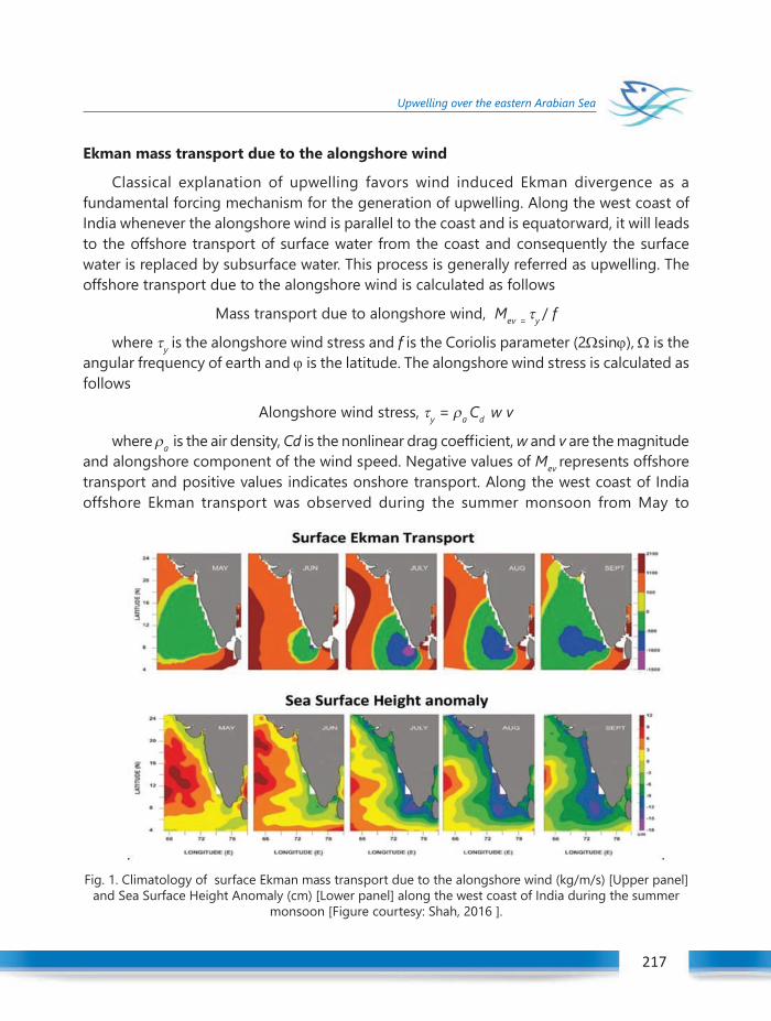
Winter School on Structure and Function of the Marine Ecosystem : Fisheries 217
Upwelling over the eastern Arabian Sea
217
Ekman mass transport due to the alongshore wind
Classical explanation of upwelling favors wind induced Ekman divergence as afundamental forcing mechanism for the generation of upwelling. Along the west coast ofIndia whenever the alongshore wind is parallel to the coast and is equatorward, it will leadsto the offshore transport of surface water from the coast and consequently the surfacewater is replaced by subsurface water. This process is generally referred as upwelling. Theoffshore transport due to the alongshore wind is calculated as follows
Mass transport due to alongshore wind, Mev = τy / f
where τy is the alongshore wind stress and f is the Coriolis parameter (2Ωsinϕ), Ω is theangular frequency of earth and ϕ is the latitude. The alongshore wind stress is calculated asfollows
Alongshore wind stress, τy = ρa Cd w v
where ρa is the air density, Cd is the nonlinear drag coefficient, w and v are the magnitudeand alongshore component of the wind speed. Negative values of Mev represents offshoretransport and positive values indicates onshore transport. Along the west coast of Indiaoffshore Ekman transport was observed during the summer monsoon from May to
Fig. 1. Climatology of surface Ekman mass transport due to the alongshore wind (kg/m/s) [Upper panel]and Sea Surface Height Anomaly (cm) [Lower panel] along the west coast of India during the summer
monsoon [Figure courtesy: Shah, 2016 ].

Winter School on Structure and Function of the Marine Ecosystem : Fisheries218
Upwelling over the eastern Arabian Sea
September and intense offshore transport and upwelling was noticed during the peaksummer monsoon month July. Figure 1 (upper panel) represents the surface transport dueto the alongshore wind.
Vertical movement of Isotherms
Since the upwelling areas are characterized by the replacement of the surface water bythe subsurface water, upward movement of isotherms are used as a proxy for the study ofupwelling. The analyses of figure 2 represents these upward movements are happenedduring May to September along the west coast of India. This is also substantiate thegeneration of upwelling during the summer monsoon months. Compared to the surroundingareas upwelling areas are cool because of the presence of subsurface water.
Fig. 2. Vertical oscillation of isotherms at particular latitudes along the westcoast of India during a year (Climatology).

Winter School on Structure and Function of the Marine Ecosystem : Fisheries 219
Upwelling over the eastern Arabian Sea
219
Sea Surface Height Anomaly
Because of the presence of subsurface water upwelling areas are characterized by seasurface cooling compared to the surrounding areas. Hence, inorder to maintain the isostaticbalance upwelling areas are experienced by lowering of sea level than the surroundings. Intune with the observations on sea surface temperature, isotherms and Ekman mass transport,analysis on sea level anomaly along the west coast of India also shown a fall in Sea levelanomaly during the summer monsoon and this fall is intensified during July (Fig.2, lowerpanel).
Chlorophyll-a
Along the west coast of India, upwelling enhances the nutrient concentration in thesurface water during the summer monsoon from May to September. Consequentlychlorophyll-a concentration along the coast increases compared to the surroundings (Fig.3). Hence Chlorophyll-a concentration along coastal areas are used as a suggested proxyfor the study of upwelling.
Fig 3. Chlorophyll -a concentration along the west coast of India during summer monsoon [climatology]
Winter School on Structure and Function of the Marine Ecosystem : Fisheries220
Upwelling over the eastern Arabian Sea
References
Banse, K., 1959: On upwelling and bottom trawling off the southwest coast of India, J.Mar. Biol. Assoc. India,1, 33 – 49.
Banse, K., 1968: Hydrography of the Arabian Sea shelf of India and Pakistan and effects on demersal fishes,Deep Sea Res 15: 45-79.
Gopalakrishna, V. V., Rao, R. R., Nisha, K., Girish Kumar, M. S., Pankajackshan, T., Ravichandran, M., Johnson,Z., Girish, K., Aneeshkumar, N., Srinath, M., Rajesh, S., and Rajan, C. K., 2008: Observed anomalousupwelling in the Lakshadweep Sea during the summer monsoon season of 2005, Journal of GeophysicalResearch, 113(C5), 1–12.
Jayaram, C., Neethu, C., Ajith Joseph, K. and Balchand, A. N., 2010: Interannual variability of upwellingindices in the Southeastern Arabian Sea: A satellite based study, Ocean Sci. J., 45 (1), 27 – 40, DOI10.1007/ s12601-010-0003-6.
Johannessen, O.M., Subbaraju, G., Blindheim, J., 1987: Seasonal variation of oceanographic conditions offthe southwest coast of India during 1971-1975. Fisk. Dir. Skr. Ser. Hav Unders. 18: 247-261.
Shah, P., Sajeev, R. and Gopika, N., 2015: Study of upwelling along the West Coast of India-A climatologicalApproach, Journal of Coastal Research, 31(5), 1151 – 1158. Coconut Creek (Florida), ISSN 0749-0208.
Shah, P., 2016: Upwelling and downwelling along the west coast of India- Relative roles of local versusremote forcing, Ph.D. thesis, Cochin University of Science and Technology, Kochi-22.
Sharma, G.S., 1978: Upwelling of the southwest coast of India, Indian J. of Mar. Sci. 7, 209-218.
Smith, R. L., 1964: An investigation of upwelling along the Oregon Coast, Ph.D. thesis, Oregon State University.Corvallis.
Smitha, B. R., Sanjeevan, V. N., Vimalkumar, K. G. and Revichandran, C., 2008: On the upwelling off thesouthern tip and along the west coast of India, J. Coast. Res., 24 (3), 95-102.
Winter School on Structure and Function of the Marine Ecosystem : Fisheries 221
Biogeography of Northern Indian Ocean
Biogeography is defined as the branch of science that deals with the large-scaledistribution of flora and fauna in the context of environmental properties and topographicfeatures. Studies on biogeography in Northern Indian Ocean have been relatively few. Theselectures will survey the available literature, will mention as-yet unpublished work and willdiscuss possible future directions for biogeographical research in the Northern Indian Ocean.
General Characteristics of the Arabian Sea and Bay of Bengal
The Indian coastline is about 7517 km long, with 5423 km along the mainland and 2094km in the Andaman and Nicobar, and Lakshadweep Islands (Table. 1). The Northern IndianOcean includes the Arabian Sea to the west and the Bay of Bengal to the east of India.Arabian Sea is bounded by Pakistan and Iran in the north, Northeastern Somalia and theArabian Peninsula in the west and by India in the east. Its total area is 3,862,000 sq.km andits maximum depth is 4,652 meters. Bay of Bengal is the largest one among the world bays.It forms the northeastern part of the Indian Ocean. It is bordered by India and Sri Lanka tothe west, Bangladesh to the north and by Myanmar and the Andaman and Nicobar islandsto the east. The Bay of Bengal occupies an area of 2,172,000 sq. km. A number of largerivers – the Ganges and its tributaries such as the Padma and Hooghly, the Brahmaputra andits tributaries such as the Jamuna and Meghna, and other rivers such as the IrrawaddyRiver, Godavari, Mahanadi, Krishna and Kaveri flow into the Bay of Bengal. Geographically,the Northern Indian Ocean is subdivided by several major islands – the Andaman andNicobar Islands in the Bay of Bengal and the Lakshadweep in the Arabian Sea. The islandswere formed as a result of various geological processes such as volcanism, seafloor spreadingand continental drift. The Lakshadweep islands are a group of 36 low-lying coral islands,10 of which are inhabited. The Andaman and Nicobar Archipelago in the Bay of Bengal,comprises 554 islands, some of which are merely large rocks. If these are excluded, the totalnumber of islands is 294, of which 36 are inhabited.
The Arabian Sea covers the Gulf of Oman, the Persian Gulf and Red Sea, which is in total1.8 times the area of the Bay of Bengal. The Carlsberg-Murray Ridge (Fig. 1) is one of theimportant features of the Arabian Sea. It plays a vital role in the process of upwelling (mixingup of nutrient rich dense cold water towards the ocean surface by wind driven motion). Thecontinental shelf width is greater in the Arabian Sea compared with the Bay of Bengal(Table 1). Seven large rivers and several smaller ones discharge into the Bay of Bengal.
25C H A P T E R BIOGEOGRAPHY OF NORTHERN INDIAN
OCEANMonolisha S., Grinson George and Trevor Platt
Fishery Resources Assessment DivisionICAR-Central Marine Fisheries Research Institute
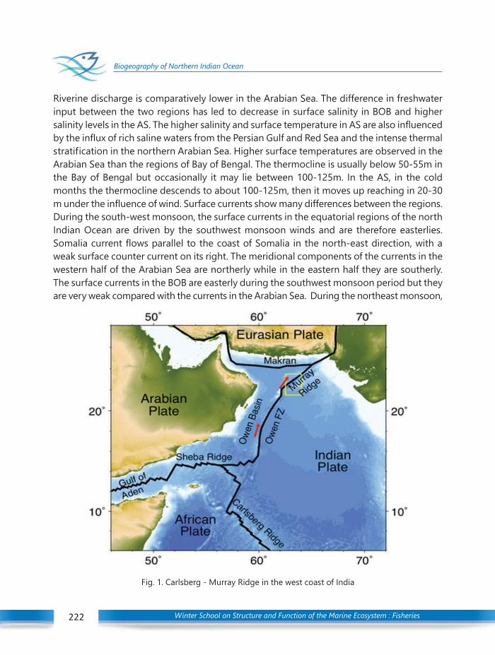
Winter School on Structure and Function of the Marine Ecosystem : Fisheries222
Biogeography of Northern Indian Ocean
Riverine discharge is comparatively lower in the Arabian Sea. The difference in freshwaterinput between the two regions has led to decrease in surface salinity in BOB and highersalinity levels in the AS. The higher salinity and surface temperature in AS are also influencedby the influx of rich saline waters from the Persian Gulf and Red Sea and the intense thermalstratification in the northern Arabian Sea. Higher surface temperatures are observed in theArabian Sea than the regions of Bay of Bengal. The thermocline is usually below 50-55m inthe Bay of Bengal but occasionally it may lie between 100-125m. In the AS, in the coldmonths the thermocline descends to about 100-125m, then it moves up reaching in 20-30m under the influence of wind. Surface currents show many differences between the regions.During the south-west monsoon, the surface currents in the equatorial regions of the northIndian Ocean are driven by the southwest monsoon winds and are therefore easterlies.Somalia current flows parallel to the coast of Somalia in the north-east direction, with aweak surface counter current on its right. The meridional components of the currents in thewestern half of the Arabian Sea are northerly while in the eastern half they are southerly.The surface currents in the BOB are easterly during the southwest monsoon period but theyare very weak compared with the currents in the Arabian Sea. During the northeast monsoon,
Fig. 1. Carlsberg - Murray Ridge in the west coast of India
Winter School on Structure and Function of the Marine Ecosystem : Fisheries 223
Biogeography of Northern Indian Ocean
the complete reversal of the surface currents takes place and the currents are westerlies inboth Arabian Sea and the BOB. The seasonally reversing monsoon current is one of theimportant characteristic features of the Northern Indian Ocean.Table 1. Coastal Resources of the Indian Ocean
Maritime states Total length of Length of coast Continental shelfcoastline (sq. km) affected by erosion width (‘000 km)
(km)
Gujarat 1214.7 36.4 184Maharashtra 652.6 263 112Goa 151 10.5 10Karnataka 280 249.6 27Kerala 569.7 480 40Tamil Nadu 906.9 36.2 41Andhra Pradesh 973.7 9.2 33Orissa 476.6 107.6 26West Bengal 157.5 49 17Daman and Diu 9.5 0 -Pondicherry 30.6 6.4 1Total Mainland 5422.6 1247.9 -Lakshadweep 132 132 4Andaman and Nicobar 1962 0 35
(*Sanil Kumar et al., 2006 obtained from Naval Hydrographic chart )
Biogeographic partitioning of an ocean or a region means finding the borders betweenbiogeographical area based on the distribution of floral and faunal species (Golikov et al.,1990). The Indian coast has important geological features and biologically productive areassuch as sandy beaches, estuaries, sandy beaches, bays and creeks, lagoons, rocky shores,coral reefs, mangroves, marshes and mudflats. The East and west coast of India provide awide range of habitats to plants and animals. The distributional patterns of floral and faunalspecies can be homogenous or heterogeneous, depending on both abiotic and biotic factorssuch as physical-chemical conditions and trophic structures. These factors shape thedistribution of organisms, such that the biological communities are in harmony with theirenvironment in space and time.
Phytoplankton
Phytoplanktons are a diverse group of unicellular microalgae metabolically andphysiologically similar to higher plants. Phytoplankton play a major role in indicating theecology of the region and it highly contributes as primary producer in the food web and are

Winter School on Structure and Function of the Marine Ecosystem : Fisheries224
Biogeography of Northern Indian Ocean
key partners in cycling of carbon and nutrients in the ocean. Diatoms, cyanobacteria,dinoflagellates and coccolithophores are the most dominant phytoplankton taxa in theIndian coastline. These groups are named as “phytoplankton functional types” becausethey play vital role in biogeochemical cycles of the marine ecosystem. Phytoplanktoncommunity structures vary from one place to another depending upon various environmentalfactors resulting in heterogeneous biogeographical patterns. The major factors that influencethe biogeographical patterns of phytoplankton are (1) environmental conditions (e.g.temperature and nutrient concentrations), (2) interspecific relationships (i.e., predation andcompetition), and (3) dispersal (Follows et al., 2007). The distribution and species compositionof phytoplankton determines the structure and functioning of the marine food web(Finkel et al., 2007). Therefore, detailed investigations of the mechanisms that lead to certainphytoplankton biogeographical patterns can help us to understand better the processesinvolved in pelagic ecosystems and their response to a changing environment.
Early research in the phytoplankton of the Indian Ocean was conducted during theInternational Indian Ocean Expedition (1963). From the surveyed literature, approximately600 species represent the phytoplankton community structure in the Northern Indian Ocean.Chrysophytes, cryptophytes, haptophytes, chlorophytes and prasinophytes are the diversephytoplankton communities representing the Indian coastal waters. Dominant speciesreported in the Bay of Bengal region are Proboscia alata, Climacodium frauenfeldianum andThalassionema nitzchioides. Associated species reported includes Pseudo-nitzschia Pseudodelicatissima, Chaetoceros messanensis, Chaetoceros compressus, Thalassionema frauenfeldii,Thalassiothrix longissima, Leptocylinfrus minimus, Lauderia annulata, Guinardia striata,Thalassionema nitzchoides and cyanobacterium Trichodesmium (D’Silva et al., 2012;Paul et al., 2007; Subrahmanyan et al., 1971). Diatoms are the dominant groups found in theeast and west coast of India. Proliferation of diatoms in these regions has been reportedwith sharp pycnocline, thermal stratification and deficiency of nutrients in the upper mixedlayer (Sukhanova et al., 2006; Tomas, 1997). There are reports of replacement of diatomdominance by the presence of Trichodesmium during the onset of monsoon in the Chennai,Port-Blair and Kolkata regions of the southeast coast and southwest coast of India (Mohantyet al., 2010; Sahu et al., 2014). Noctiluca scintillans and Trichodesmium erythraeum are thetwo common causative species of phytoplankton blooms in the Indian coast. Some speciesof diatoms and cyanobacteria (presence of cyanobionts) are capable of utilizing nitrogenand ammonium as a urea source. This indicates the symbiosis of nitrogen fixation byphytoplankton’s in the nitrogen depleted environment of Bay of Bengal. Species such asChaetoceros coarctatum, Nitzschia sp, Dactyliosolen fragilissimus, Leptocylindrus danicus andPseudo-nitzschia heimii, Oxytoxum nanum, Scrippsiella sp. are the major dominant speciesoccurred along the southwest coast and Gulf of Kutch and Khambhat (Ahmed et al., 2016).Picoplankton such as Synechococcus and Prochlorococcus are reported from the tropical
Winter School on Structure and Function of the Marine Ecosystem : Fisheries 225
Biogeography of Northern Indian Ocean
waters with influx of higher nutrients, representing the systems of regenerated production;which states that the north and southern eastern Arabian sea is one of the major regionwith higher nutrients reported during the upwelling in the summer monsoon season(Bhattathiri et al., 1996; Madhupratap et al., 1996; Ramaiah et al., 1996; Roy et al., 2006).There are two peaks of plankton distribution observed during March-April and October-November off the Mumbai (North West) coast of India. This peak coincides with the seasonof peak abundance of the commercial pelagic fishes Bregmaceros mcclellandi and Harpodonneherus in the North west coast of India (Gulf of Kutch and Khambhat) (Raghuprasad, 1968).These water masses are found throughout the stronger upwelling region, Somalia and Gulfof Aden with similar phytoplankton community structure.
Going by the literature, phytoplankton species in classified water masses undergocontinuous changes over time in their dominance and diversity, a process that may becompared to terrestrial succession.
Zooplankton
Zooplankton plays an important role in the pelagic community structure as consumersof primary production. Literature on the plankton biomass and diversity of the NorthernIndian Ocean covering all the seasons and regions is limited. The International Indian OceanExpedition (IIOE) of 1960-1965 was the first attempt to describe the biogeography ofzooplankton in the Arabian Sea based on quantitative data such as biomass and density(Currie, 1963). Based on the literature of Zooplankton diversity and distribution of theNorthern Indian Ocean, approximately 7100 species of zooplankton were recorded fromthe Indian seas (Venkataraman and Wafar, 2005). The most common distribution ofzooplankton includes copepods (Gajbhiye et al., 1991; Haq et al., 1973; Madhupratap et al.,1990), ostracods (George and Nair, 1980; Stephen, 1996), euphausiid species (Mathew, 2000),amphipods (Nair and Jayalakshmi, 1992), total hydromedusae (Santhakumari, 1976, 1978,1997), and chaetognatha (Nair et al., 2002; Wishner et al., 2001). The zooplankton biomasswas reported to be highest in the northern and western Arabian Sea, the coasts of Somaliaand Arabia (Somalia and Gulf of Aden and Persian Gulf), and also on the southwest coast ofIndia (Southwest coast). Crustaceans followed by copepoda, rotifera, cirripede larvae,polycheates and cladocerans are the dominant groups found in these regions.Species reported are Acartia sp., Acartia pacifica, Acartiella faoensis, Arctodiaptomus salinus,Oithona sp., Oncae sp., Alona affinis, Moina brachiate, Mysid larvae and Zoea larvae ofcrabs (Ajeel, 2012). The southwest monsoon experiences two offshore current jets, oneassociated with the parting of the Somali Current from the coast. This jet brings up theupwelling of cooler rich water developing the blooms of diatoms Nitzschia delicatissima(Smith and Codispoti, 1980). Adult females and copepodites of Calanoides carinatus andEucalanus spp., which can readily ingest the diatoms, were markedly more abundant only

Winter School on Structure and Function of the Marine Ecosystem : Fisheries226
Biogeography of Northern Indian Ocean
within upwelling areas along the Somalia coast during the southwest monsoon and notfound elsewhere in the northern Arabian Sea.
The northwestern Arabian Sea i.e., the Gulf of Kutch and Khambhat represents thehigher density of Copepods. Some copepod species reported are Gaussia princeps,Euchaeta spp., Haloptilus spp., Pontella spp., and Candacia spp. Of the large calanoidcopepods the family Eucalanidae dominates the Arabian Sea. During the summer monsoon,the peak and high densities of copepod abundances occur in the upwelling regions offSomalia and Gulf of Aden and far offshore regions of the Arabian Sea (Southwest and Gulfof Kutch and Khambhat). Copepods are the major dominant species reported in dominantduring the southwest monsoon which is replaced by Oithona sp (Madhupratap et al., 1990;Piontkovski et al., 2013). The other dominant copepods, Paracalanus, Clausocalanus, Acartianegligens, and Acrocalanus sp., present in both the northeast and southwest monsoons areequally abundant within and outside the areas of upwelling. During the summer coastalupwelling, Calanoides carinatus, is an indicator species for upwelling in the tropical Indianand Atlantic Oceans. In offshore, non-upwelled waters, Eucalanus attenuatus, Pleuromammaindica, and Pleuromamma abdominalis were dominant (Smith, 1982, 1984, 1995). Someendemic species of the Arabain Sea and Bay of Bengal are copepod Gaussia sewelli,hydromedusae Aglaura hemistoma and Solmundella bitentaculata. Mysids belonging to thegenera Paralophogaster are confined to the Red Sea and Arabian Sea, while the speciesSiriella ionesi is limited to the Arabian Sea. The Arabian Sea is stratified for several variables,with particular importance to zooplankton and fish associated to the intense oxygenminimum layer from about 150 to 1500 m, particularly on the east side.
The southeast coast of India was recorded with dominance of Ostracods, Salps,Chaetognaths and Decapods (Santhakumari and Saraswathy, 1981). Other taxa includeForaminifera, Calanoida, Cheatognatha, Appendicularia, Polychaeta, Hydrozoa andEchinodermata. Fish eggs and larvae occurrence was noted throughout the year and hadpeak abundance in summer (Soundarapandian and Varadharajan, 2013). The characterizationof the zooplankton community structure is essential in detail to understand the life cycles,recruitment of the dominant species (zooplankton and fishes) of the physical domains ofthe coastal waters of the NIO.
Plankton Diversity and Pelagic fisheries
Plankton diversity is said to be an index of fertility not only in the water column but alsoat the sea bottom. Earlier attempts on studying the relationship between the planktondiversity and fisheries along the coasts of India were restricted mostly to specific areaseither on the east or west coast of India. Studying the production of phytoplankton andzooplankton should give insight into the fishery potential of the study regions.
Winter School on Structure and Function of the Marine Ecosystem : Fisheries 227
Biogeography of Northern Indian Ocean
Indian Ocean is with rich plankton biomass, highly concentrated to the upwelling regions.There are several investigations on plankton biomass and relationship to potential fisheryrich regions. From the surveyed literatures, it is seen that the seasonal rhythm in the organicproduction is well reflected in the fishery trends, i.e., the peak of organic productioncorresponds with the low fishery periods and vice versa, suggesting an inverse relationship.Higher fishery yields were found after the peak organic production allowing some time forthe conversion of the organic matter synthesized to form fish protein. Applying this concept,analyzing the trends of annual fish production in the recent years, the seasonal abundanceof the pelagic fishes including Clupeidae, Scrombidae, Carangidae and Engraulidae areobserved during October in the west coast of India. In the east coast, the seasonal abundanceof pelagic resources is found during June-September. This abundance pattern in the westcoast of India coincides with the post southwest monsoon with enrichment of nutrients byupwelling and plankton production. April to September remains calm and is favorable forfishing activities on the east coast.
Zooplankton distribution was 3.5 times higher in the southerly half of the west coastand 2.5 times more productive than the east coast. This is well reflected in the fish landingsalso, since the landings along the west coast are about three times those of the east coast.It is very evident that the zooplankton biomass is higher in the Arabian Sea than in the Bayof Bengal. If the abundance of zooplankton is an indication of the potential fishery resourcesof an area, there is possibility of substantial increase in the rate of exploitation particularly inareas such as the south-eastern coast of India, west Pakistan and Iran in the Arabian Searegion, Burma coasts, East Pakistan, West Bengal, Orissa and Sri Lankan coast, AndamanSea in the Bay of Bengal. There are several reports on exploratory and commercial fishingactivities in these areas of high plankton production and potentially rich fishing grounds. Agood understanding of the biogeography of the region will support possible expansion ofsustainable fisheries in Northern Indian Ocean.
References
Ahmed, A., Kurian, S., Gauns, M., Chndrasekhararao, A. V., Mulla, A., Naik, B., et al., (2016). Spatial variabilityin phytoplankton community structure along the eastern Arabian Sea during the onset of south-westmonsoon. Cont. Shelf Res. 119, 30–39. doi:10.1016/j.csr.2016.03.005.
Ajeel, S. G. (2012). Distribution and abundance of zooplankton in Shatt Al-Basrah and Khour Al-ZubairChannels, Basrah, IRAQ. J. Basrah Res. 38, 10–28.
Bhattathiri, P. M. A., Pant, A., Sawant, S., Gauns, M., Matondkar, S. G. P., and Mohanraju, R. (1996).Phytoplankton production and chlorophyll distribution in the eastern and central Arabian Sea in 1994-1995. Curr. Sci. 71, 857–862.
Currie, R. I. (1963), The Indian Ocean Standard Net, Deep Sea Res., 10, 27–32. Available at: http://www.sciencedirect.com/science/article/pii/0011747163901761.

Winter School on Structure and Function of the Marine Ecosystem : Fisheries228
Biogeography of Northern Indian Ocean
D’Silva, M. S., Anil, A. C., Naik, R. K., and D’Costa, P. M. (2012). Algal blooms: A perspective from the coastsof India. Nat. Hazards 63, 1225–1253. doi:10.1007/s11069-012-0190-9.
Finkel, Z. V, Sebbo, J., Irwin, A. J., Katz, M. E., Schofield, O. M. E., and Young, J. R. (2007). A universal driver ofmacroevolutionary change in the size of marine phytoplankton over the Cenozoic. PNAS 104, 20416–20420. doi:doi10.1073pnas.0709381104.
Follows, M. J., Dutkiewicz, S., Grant, S., and Chisholm, S. W. (2007). Emergent biogeography of microbialcommunities in a model ocean. Science 315, 1843–6. doi:10.1126/science.1138544.
Gajbhiye, S. N., Stephen, R., Nair, V. R., and Desai, B. N. (1991). Copepods of the nearshore waters of Bombay.Indian J. Mar. Sci. 20, 187–194.
George, J., and Nair, V. R. (1980). Planktonic ostracods of the northern Indian Ocean. Mahasagar 13, 29–44.
Golikov, A.N., Dolgolenko, M., Maximovich, N., and Scarlato, O. (1990). Theoretical approaches to marinebiogeography. Mar. Ecol. Prog. Ser. 63, 289–301. doi:10.3354/meps063289.
Haq, S., Ali Khan, J., and Chugtai, S. (1973). “The distribution and abundance of zooplankton along thecoast of Pakistan during post monsoon and premonsoon periods,” in Biology of the Indian Ocean,257–272.
Kusum, K. K., Vineetha, G., Raveendran, T. V., Nair, V. R., Muraleedharan, K. R., Achuthankutty, C. T., et al.,(2014). Chaetognath community and their responses to varying environmental factors in the northernIndian Ocean. J. Plankton Res. 36, 1146–1152. doi:10.1093/plankt/fbu024.
Madhupratap, M., Kumar, S. P., Bhattathiri, P. M. A., Kumar, M. D., Raghukumar, S., Nair, K. K. C., et al., (1996).Mechanism of the biological response to winter cooling in the northeastern Arabian Sea. Nature 384,549–552. doi:10.1038/384549a0.
Madhupratap, M., Nair, S. R. S., Haridas, P., and Padmavati, G. (1990). Response of Zooplankton to physicalvhanges in the environment: coastal upwelling along the central west coast of India. J. Coast. Res. 6,413–426.
Mathew, K. J. (2000). Studies on Euphausiacea (crustacea) of the indian ocean with special reference to theEEZ of india. Mar. Fish. Res. Manag., 49–68.
Mohanty, A. K., Satpathy, K. K., Sahu, G., Hussain, K. J., Prasad, M. V. R., and Sarkar, S. K. (2010). Bloom ofTrichodesmium erythraeum (Ehr.) and its impact on water quality and plankton community structurein the coastal waters of woutheast coast of India. Indian J. Mar. Sci. 39, 323–333.
Nair, K. K. C., and Jayalakshmi, K. J. (1992). Distribution of Oxycephalidae (Hyperiidea-Amphipoda) in theIndian Ocean-A statistical study. Oceanogr. Indian Ocean, 201–210.
Nair, V., Terazaki, M., and Jayalakshmy, K. (2002). Abundance and community structure of chaetognaths inthe northern Indian Ocean. Plankt. Biol. Ecol. 49, 27–37. Available at: http://www.plankton.jp/PBE/issue/vol49_1/vol49_1_027.pdf.
Paul, J. T., Ramaiah, N., Gauns, M., and Fernandes, V. (2007). Preponderance of a few diatom species amongthe highly diverse microphytoplankton assemblages in the Bay of Bengal. Mar. Biol. 152, 63–75.doi:10.1007/s00227-007-0657-5.
Piontkovski, S. A., Al-maawali, A., Al-manthri, W. A., Al-hashmi, K., and Popova, E. A. (2013). Zooplankton ofOman Coastal Waters. Agricultural and Marine Sciences 50, 37–50.
Raghuprasad, R. (1968). Zooplankton biomass in the Arabian sea and the Bay of bengal with a discussionon the fisheries of the regions. Proc. Nat. Inst. Sci. India Vol.35 (5), 399-437.

Winter School on Structure and Function of the Marine Ecosystem : Fisheries 229
Biogeography of Northern Indian Ocean
Ramaiah, N., Raghukumar, S., and Gauns, M. (1996). Bacterial abundance and production in the central andeastern Arabian Sea. Curr. Sci. 71, 878–882.
Stephen, P.R. and Meenakshikunjamma, P. P. (1996). Ostracods of Andaman Sea. In Proceedings of FORVSagar Sampada, 197–203.
Roy, S., Ursulines, A., Blouin, F., and Gl, C. (2006). Particulate , Detrital and Phytoplankton absorption fromthe Gulf and Estuary of St . Lawrence , Canada - Influence of Community Composition. Ocean OpticsXVIII 1–7.
Sahu, B. K., Begum, M., Kumarasamy, P., Vinithkumar, N. V, and Kirubagaran, R. (2014). Dominance ofTrichodesmium and associated biological and physico- chemical parameters in coastal water of PortBlair, South Andaman Island. Indian Journal of Geo-Marine Sciences 43, 1739–1745.
Sanil Kumar, V., Pathak, K. C., Pednekar, P., Raju, N. S. N., and Gowthaman, R. (2006). Coastal processes alongthe Indian coastline. Curr. Sci. 91, 530–536.
Santhakumari, V and Saraswathy, M. (1981). Zooplankton along the Tamil Nadu coast. Mahasagar- Bull.Natl. Inst. Oceanogr. 14, 289–302.
Santhakumari, V. (1978). Distribution of scyphomedusae in the Indian ocean. Mahasagar- Bull. Natl. Inst.Oceanogr. 11, 217–220.
Santhakumari, V. (1997). Species composition, Distribution and Abundance of Hydromedusae inthe ExclusiveEconomic Zone of the East coast of India. Publ. Secto. Mar. Biol. Lab. 38, 53–61.
Smith, S. L. (1982). The northwestern Indian Ocean during the monsoons of 1979: distribution, abundance,and feeding of zooplankton. Deep Sea Res. Part A, Oceanogr. Res. Pap. 29, 1331–1353. doi:10.1016/0198-0149(82)90012-7.
Smith, S. L. (1984). Biological indications of active upwelling in the Northwestern Indian Ocean in 1964 and1979, and a comparison with Peru and Northwest Africa. Deep Sea Res. Part A, Oceanogr. Res. Pap. 31,951–967. doi:10.1016/0198-0149(84)90050-5.
Smith, S. L. (1995). The Arabian Sea: Mesozooplankton response to seasonal climate in a tropical ocean.ICES J. Mar. Sci. 52, 427–438. doi:10.1016/1054-3139(95)80058-1.
Smith, S. L., and Codispoti, L. A. (1980). Southwest monsoon of 1979: chemical and biological response ofsomali coastal waters. Science (80-. ). 209, 597–600. doi:10.1126/science.209.4456.597.
Soundarapandian P, Varadharajan, D. (2013). Zooplankton Abundance and Diversity from Pointcalimere toManamelkudi, South East Coast of India. Earth Sci. Clim. Chang. 4. doi:10.4172/2157-7617.1000151.
Subrahmanyan, R., Gopinathan, C. P., and Thankappan Pillai, C. (1971). Phytoplankton of the Indian Ocean:Some Ecological Problems. J. mar. biol. Ass. India 17, 608–612.
Sukhanova, I. N., Flint, M. V, Whitledge, T. E., Stockwell, D. A., and Rho, T. K. (2006). Mass development of theplanktonic diatom Proboscia alata over the Bering Sea shelf in the summer season. Oceanology 46,200–216. doi:10.1134/S000143700602007X.
Tomas, C. (1997). Identifying Marine Phytoplankton. academic press Available at: https://www.elsevier.com/books/identifying-marine-phytoplankton/tomas/978-0-12-693018-4.
Venkataraman, K and Wafar. (2005). Coastal and marine biodiversity of India. Indian J. Mar. Sci. 34, 57–75.doi:10.1016/B978-0-12-801948-1/00019-7.
Wishner, K. F., Gowing, M. M., Gelfman, C., Gowing, M. M., Outram, D. M., Rapien, M., et al., (2001). SpeciesAssociations of Calanoid Copepods in an Estuary. Deep. Res. Part II Top. Stud. Oceanogr. 48, 1345–1368. doi:10.1016/j.pocean.2005.03.007.

Winter School on Structure and Function of the Marine Ecosystem : Fisheries230
Fisheries Oceanography- Established links in Eastern Arabian Sea
Introduction
Fish distribution along the western Indian coastal waters indicates a bias for pelagic-planktivores to the southern coast and carnivores to the northern coast. Southwest coast ofIndia is an upwelling zone rich inphytoplankton dominated by diatoms duringsummer monsoon. The landing centreobservation data since 1985 clearly indicate adominance of Indian oil sardine (Sardinellalongiceps) in this upwelling zone. Thephysiological activity of the fish is also tunedto the arrival of summer monsoon. A restingseason is expected with the retrieval ofmonsoon in this area. Further north of ourcoastal waters, we see that the dominantgroup of f ishes includes the Sciaenidspopularly known by the name ‘Ghol’(Protonibea diacanthus), ‘Koth’ (Otolithoidesbiauritus) and ‘Dhoma’ (Johnius dussumieri). These fishes seem to flourish on the winterproductivity in the northern coastal waters. The winter primary productivity in southernwaters is not good enough to support carnivores with physiological active season duringthe winter. The productivity differences in the coastal waters in time and space and theoceanographic features supporting these could be studied from a synoptic scale with thehelp of satellite remote sensing and geographical information system. In this study, wehave utilized the various open sources remote sensing data to identify the oceanographicresponses and the physical forcing that govern the distributional preferences of somedominant marine fish species.
Variability in fish biodiversity – north and south of eastern Arabian Sea
The tropical waters are often characterized by high species diversity. Along the westcoast of India, the number of species that contribute to the commercial fisheries is found tobe higher in tropical waters than temperate regions. India, being one of the most prominenttropical fishing nations contribute about 3.5 million tons of fish annually. With a coastline
26C H A P T E R
FISHERIES OCEANOGRAPHY- ESTABLISHEDLINKS IN EASTERN ARABIAN SEAGrinson George, Jayasankar J., Phiros Shah, Tarun Joseph,Muhammad Shafeeque, Monolsiha S., Platt T. and Sathyendranath S.
Fishery Resources Assessment DivisionICAR-Central Marine Fisheries Research Institute

Winter School on Structure and Function of the Marine Ecosystem : Fisheries 231
Fisheries Oceanography- Established links in Eastern Arabian Sea
231
of formidable (8129 km approximately) length, regional differences in catch compositionhave been observed consistently. Such differences may arise due to influence of multipleforcing factors of physical, chemical, geological and biological origin.
There exists a strong difference in catch composition along the west coast across the150 N latitude with the planktivorous species dominating the South Eastern region andcarnivorous species thriving in the North Eastern Arabian Sea (NEAS). However, the studywas unable to explain this difference in catch composition and also highlights the dueimportance of the role played by feeding and breeding behaviour of fishes in order toadequately understand their response to oceanographic forcing. The relationship betweenoceanographic forcing (physical and chemical) upon fish response (spatial distribution) hasremained largely elusive owing to the lack of synoptic-level datasets on the oceanographicvariables which differentiates multiple ocean sites from each other.
Satellite remote sensing have played a pivotalrole in addressing this data gap by offering theopportunity to systematically measure andmonitor multiple oceanographic variables atdesired resolutions. With the advent of remotesensing capabilities, optical responses of coastalwaters can easily be monitored which makesecological classification based on remote sensingreflectance possible. The South Eastern ArabianSea (SEAS) exhibits a strong seasonality in remotesensing reflectance comparison to its northeastern counterpart. However, the general notionis that seasonal extremes in weather are moredominant in the temperate latitudes than in thetropics. Seasonal changes in the biologicalbehaviour (breeding/ feeding) of fish have stronglinks with weather conditions. In order to ensureimproved chances for survival of fish larvae, thephysiological activity of adult fish should coincide with the onset of better food conditionsin close proximity both temporally and spatially. Fish also exhibit a natural tendency toavoid predators and provide its larvae with best possible resources to ensure their survivalto adulthood. In general, the most dominant commercial tropical fishes can be classifiedbased on their feeding behaviour as planktivorous and carnivorous and their breedingresponses exhibit a strong seasonality with the onset of summer and winter monsoonrespectively.
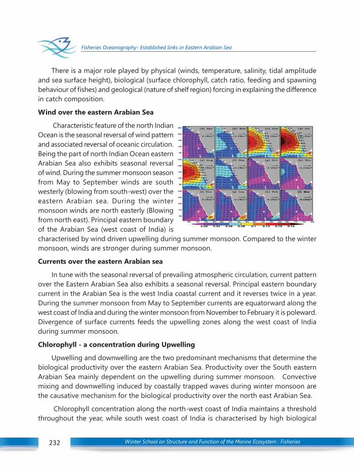
Winter School on Structure and Function of the Marine Ecosystem : Fisheries232
Fisheries Oceanography- Established links in Eastern Arabian Sea
There is a major role played by physical (winds, temperature, salinity, tidal amplitudeand sea surface height), biological (surface chlorophyll, catch ratio, feeding and spawningbehaviour of fishes) and geological (nature of shelf region) forcing in explaining the differencein catch composition.
Wind over the eastern Arabian Sea
Characteristic feature of the north IndianOcean is the seasonal reversal of wind patternand associated reversal of oceanic circulation.Being the part of north Indian Ocean easternArabian Sea also exhibits seasonal reversalof wind. During the summer monsoon seasonfrom May to September winds are southwesterly (blowing from south-west) over theeastern Arabian sea. During the wintermonsoon winds are north easterly (Blowingfrom north east). Principal eastern boundaryof the Arabian Sea (west coast of India) ischaracterised by wind driven upwelling during summer monsoon. Compared to the wintermonsoon, winds are stronger during summer monsoon.
Currents over the eastern Arabian sea
In tune with the seasonal reversal of prevailing atmospheric circulation, current patternover the Eastern Arabian Sea also exhibits a seasonal reversal. Principal eastern boundarycurrent in the Arabian Sea is the west India coastal current and it reverses twice in a year.During the summer monsoon from May to September currents are equatorward along thewest coast of India and during the winter monsoon from November to February it is poleward.Divergence of surface currents feeds the upwelling zones along the west coast of Indiaduring summer monsoon.
Chlorophyll - a concentration during Upwelling
Upwelling and downwelling are the two predominant mechanisms that determine thebiological productivity over the eastern Arabian Sea. Productivity over the South easternArabian Sea mainly dependent on the upwelling during summer monsoon. Convectivemixing and downwelling induced by coastally trapped waves during winter monsoon arethe causative mechanism for the biological productivity over the north east Arabian Sea.
Chlorophyll concentration along the north-west coast of India maintains a thresholdthroughout the year, while south west coast of India is characterised by high biological
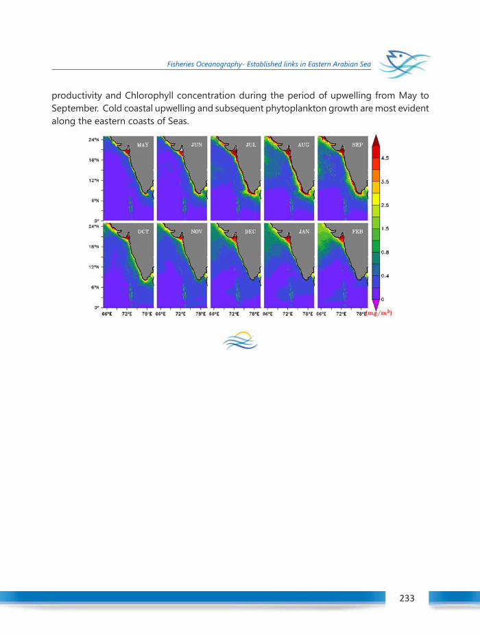
Winter School on Structure and Function of the Marine Ecosystem : Fisheries 233
Fisheries Oceanography- Established links in Eastern Arabian Sea
233
productivity and Chlorophyll concentration during the period of upwelling from May toSeptember. Cold coastal upwelling and subsequent phytoplankton growth are most evidentalong the eastern coasts of Seas.

Winter School on Structure and Function of the Marine Ecosystem : Fisheries234
Classification techniques for remotely sensed data
1. Introduction
Hyperspectral imaging sensors measure the radiance of the materials within each pixelarea at a very large number of contiguous spectral wavelength bands. So, they can generatehundreds of images of a scene on the real surface. The radiance is converted intohyperspectral data cube digital form. The spectral information available in a hyperspectralimage (cube) may serve to classify the nature of the target object because every materialhad a unique fixed spectrum and could be used as a spectral signature of the material andperhaps provide additional information for further processing and exploitation. Hyperspectraldata contain extremely rich spectral attributes, which offer the potential to discriminatemore detailed classes with classification accuracy.
2. Cluster Analysis (Unsupervised learning)
Unsupervised learning is a type of machine learning algorithm used to draw inferencesfrom datasets consisting of input data without labeled responses. The most commonunsupervised learning method is cluster analysis, which is used for exploratory data analysisto find hidden patterns or grouping in data.
Cluster analysis is usually done in an attempt to combine cases into groups when thegroup membership is not known prior to the analysis. Cluster analysis is a technique forgrouping individual or objects into unknown groups.
There are 4 basic steps to conduct cluster analysis for any data. Those are given below:
1. Select a suitable distance measure.
2. Select a clustering algorithm.
3. Determine the number of clusters.
4. Validate the analysis.
2.1 Clustering Methods (Johnson and Wichern, 2006)
The commonly used methods of clustering fall into two general categories.
(i) Hierarchical and
(ii) Non hierarchical.
03C H A P T E R
27C H A P T E R CLASSIFICATION TECHNIQUES FOR
REMOTELY SENSED DATAEldho Varghese and Grinson George
Fishery Resources Assessment DivisionICAR-Central Marine Fisheries Research Institute

Winter School on Structure and Function of the Marine Ecosystem : Fisheries 235
Classification techniques for remotely sensed data
235
2.1.1 Hierarchical cluster Analysis
Hierarchical clustering techniques proceed by either a series of mergers or a series ofsuccessive divisions. Agglomerative hierarchical method starts with the individual objects,thus there are as many clusters as objects. The most similar objects are first grouped andthese initial groups are merged according to their similarities. Eventually, as the similaritydecreases, all subgroups are fused into a single cluster.
Divisive hierarchical methods work in the opposite direction. An initial single group ofobjects is divided into two sub groups such that the objects in one sub group are far fromthe objects in the others. These subgroups are then further divided into dissimilar subgroups.The process continues until there are as many subgroups as objects i.e., until each objectform a group. The results of both agglomerative and divisive method may be displayed inthe form of a two dimensional diagram known as Dendrogram. It can be seen that theDendrogram illustrate the mergers or divisions that have been made at successive levels.
Linkage methods are suitable for clustering items, as well as variables. This is not truefor all hierarchical agglomerative procedure. The following types of linkage are now discussed:
(i) Single linkage (minimum distance or nearest neighbour),
(ii) Complete linkage (maximum distance or farthest neighbour) and
(iii) Average linkage (average distances).
Also other methods of hierarchical clustering techniques like Ward’s method andCentroid method are available in the literature.
Steps of Agglomeration in Hierarchical Cluster analysis
The following are the steps in the agglomerative hierarchical clustering algorithm forgroups of N objects (items or variables).
i. Start with N clusters, each containing a single entity and an N×N symmetric matrixof distance (or similarities) D = dik .
ii. Search the distance matrix for the nearest (most similar) pair of clusters. Let thedistance between most similar clusters U and V be duv.
iii. Merge clusters U and V. Label the newly formed cluster (UV). Update the entries inthe distance matrix by (a) deleting the rows and columns corresponding to clustersU and V and (b) adding a row and column giving the distances between cluster(UV) and the remaining clusters.

Winter School on Structure and Function of the Marine Ecosystem : Fisheries236
Classification techniques for remotely sensed data
iv. Repeat steps (ii) and (iii) a total of N-1 times (All objects will be in a single clusterafter the algorithm terminates). Record the identity of clusters that are mergedand the levels (distances or similarities) at which the mergers take place.
2.1.2 Non Hierarchical Clustering Method
Non-hierarchical clustering techniques are designed to group items, rather than variables,into a collection of K clusters. The number of clusters, K, may either be specified in advanceor determined as part of the clustering procedure. Because a matrix of distance does nothave to be determined and the basic data do not have to be stored during the computerrun. Non hierarchical methods can be applied to much larger data sets than can hierarchicaltechniques. Non hierarchical methods start from either (1) an initial partition of items intogroups or (2) an initial set of seed points which will form nuclei of the cluster.
2.1.2.1 K means Clustering ( Afifi, Clark and Marg, 2004)
The K means clustering is a popular non hierarchical clustering technique. For a specifiednumber of clusters K the basic algorithm proceeds in the following steps:
Divide the data into K initial cluster. The number of these clusters may be specifiedby the user or may be selected by the program according to an arbitrary procedure.
Calculate the means or centroid of the K clusters.
For a given case, calculate its distance to each centroid. If the case is closest to thecentroid of its own cluster, leave it in that cluster; otherwise, reassign it to thecluster whose centroid is closest to it.
Repeat step (iii) for each case.
Repeat steps (ii), (iii), and (iv) until no cases are reassigned.
2.2. Dendrogram
Dendrogram is also called hierarchical tree diagram or plot, and shows the relative sizeof the proximity coefficients at which cases are combined. The bigger the distance coefficientor the smaller the similarity coefficient, the more clustering involved combining unlike entities,which may be undesirable. Cases showing low distance are close, with a line linking them ashort distance from the left of the Dendrogram, indicating that they are agglomerated intoa cluster at a low distance coefficient, indicating alikeness. When, on the other hand, thelinking line is to the right of the Dendrogram the linkage occurs at a high distance coefficient,indicating the cases/clusters were agglomerated even though much less alike.

Winter School on Structure and Function of the Marine Ecosystem : Fisheries 237
Classification techniques for remotely sensed data
237
2.3. Distance Measures
Some distance measures commonly used for assessing spectral similarity/dissimilarityare as follows:
1) Spectral Similarity Index or Spectral Correlation or Spectral Angle Mapper (SAM)
2) Spectral Contrast Angle
3) Spectral Information Divergence (SID)
4) Spectral Absorption Index (SAI)
5) Euclidian Distance
6) Mahalanobis D2
7) City-Block Distance
2.4. Validations
Relative clustering validation, which evaluates the clustering structure by varyingdifferent parameter values for the same algorithm (e.g., varying the number ofclusters k). It’s generally used for determining the optimal number of clusters.
External clustering validation, which consists in comparing the results of a clusteranalysis to an externally known result, such as externally provided class labels.Since we know the “true” cluster number in advance, this approach is mainly usedfor selecting the right clustering algorithm for a specific dataset.
Internal clustering validation, which use the internal information of the clusteringprocess to evaluate the goodness of a clustering structure without reference toexternal information. It can be also used for estimating the number of clusters andthe appropriate clustering algorithm without any external data.
Clustering stability validation, which is a special version of internal validation. Itevaluates the consistency of a clustering result by comparing it with the clustersobtained after each column is removed, one at a time.
3. Dicriminant Function Analysis (Supervised learning)
Discriminant function analysis is a statistical analysis to predict a categoricaldependent variable (called a grouping variable) by one or more continuous or binaryindependent variables (called predictor variables). The original dichotomous discriminantanalysis was developed by Sir Ronald Fisher in 1936. Discriminant function analysis is usefulin determining whether a set of variables is effective in predicting category membership.Discriminant analysis is used when groups are known a priori (unlike in cluster analysis).

Winter School on Structure and Function of the Marine Ecosystem : Fisheries238
Classification techniques for remotely sensed data
Each case must have a score on one or more quantitative predictor measures, and a scoreon a group measure. In simple terms, discriminant function analysis is classification - the actof distributing things into groups, classes or categories of the same type.
The assumptions of discriminant analysis are the same as those for MANOVA. Theanalysis is quite sensitive to outliers and the size of the smallest group must be larger thanthe number of predictor variables. The major assumptions are:
Multivariate normality: Independent variables are normal for each level of thegrouping variable.
Homogeneity of variance/covariance (homoscedasticity): Variances among groupvariables are the same across levels of predictors. Can be tested with Box’s M statistic.
It has been suggested, however, that linear discriminant analysis be used whencovariances are equal, and that quadratic discriminant analysis may be used whencovariances are not equal.
Multicollinearity: Predictive power can decrease with an increased correlationbetween predictor variables.
Independence: Participants are assumed to be randomly sampled, and a participant’sscore on one variable is assumed to be independent of scores on that variable forall other participants.
It has been suggested that discriminant analysis is relatively robust to slight violationsof these assumptions, and it has also been shown that discriminant analysis maystill be reliable when using dichotomous variables (where multivariate normality isoften violated).
Discriminant analysis works by creating one or more linear combinations of predictors,creating a new variable for each function. These functions are called discriminant functions.The number of functions possible is either Ng-1 where Ng = number of groups, or p (thenumber of predictors), whichever is smaller. The first function created maximizes thedifferences between groups on that function. The second function maximizes differenceson that function, but also must not be correlated with the previous function. This continueswith subsequent functions with the requirement that the new function not be correlatedwith any of the previous functions.
Summary
Unsupervised learning is a heuristic technique for classifying cases into groups whenknowledge of the actual group membership is unknown. Unless there is considerableseparation among the inherent group, it is not realistic to expect very clear results with
Winter School on Structure and Function of the Marine Ecosystem : Fisheries 239
Classification techniques for remotely sensed data
239
unsupervised learning. In particular if the observations are distributed in a nonlinear manner,it may be difficult to achieve distinct groups. Cluster analysis is quite sensitive to outliers.The data should be carefully screened before running cluster programs.
Discriminant analysis is a multivariate technique concerned with classifying distinct setof objects (or set of observations) and with allocating new objects or observations to thepreviously defined groups. It involves deriving variates, which are combination of two ormore independent variables that will discriminate best between a priori defined groups.
References
Afifi, A., Clark, V. A. and Marg, S. (2004). Computer Aided Multivariate Analysis. USA, Chapman & Hall.
Chatfield, C. and Collins, A. J. (1990). Introduction to Multivariate Analysis. Chapman and Hall Publications.
Hair, J. F., Anderson R. E., Tatham, R. L. and Black, W. C. (2006). Multivariate Data Analysis. 5th Edn., PearsonEducation Inc.
Johnson, R. A. and Wichern, D. W. (2006). Applied Multivariate Statistical Analysis. 5th Edn., London, Inc.Pearson Prentice Hall.
Timm, N. H. (2002). Applied Multivariate Analysis. 2nd Edn. , New York, Springer-Verlag
Anderson, T. W., 1984, An Introduction to applied Multivariate Statistical Analysis, John Wiley & Sons, NewYork.

Winter School on Structure and Function of the Marine Ecosystem : Fisheries240
Optical Classification
Marine Optics
Optical oceanography or Marine optics is the study of light propagation in the oceansurface through absorption or scattering processes. Marine bio-optics is the term usedwhen the absorption and scattering by particles and dissolved substances are of biologicalorigin. Ocean color is defined as the spectral variation of the water leaving radiance thatcan be related to the optical constituents present in the medium (Jerlov, 1976; Morel, 1974).Visible Spectral radiometry or Ocean colour remote sensing is the study on spectral signalsof optically active materials using satellite observations. When sunlight reaches the upperwater column or the photic zone of the ocean surface, the light propagation is determinedby the optical properties of seawater. It depends on concentration of the optical constituentsof seawater containing Coloured dissolved organic matter (CDOM), suspended sedimentsand phytoplankton (IOCCG, 2000). The contribution of particulate and dissolved constituentsto the variability of optical properties and ocean color in coastal waters requires a betterunderstanding of the linkages between the concentration of these constituents, the inherentoptical properties (IOPs) of absorption and scattering coefficients, and the apparent opticalproperties (AOPs) such as the spectral attenuation for downward irradiance Kd(λ) and remotesensing reflectance Rrs(λ). Knowledge of these relationships is important for characterizingthe marine optical environment and developing remote sensing ocean color algorithms forcoastal waters.
The approach of Optical classification is the analysis on identification of a water type interms of dissolved and suspended organic and inorganic materials, biological substancesor the phytoplankton diversity. It has practical applications including the quantitativedescription of ocean color and the satellite remote sensing of chlorophyll (Wozniak andPelevin, 1991). Based on the optical properties, different versions of optical classification ofwater types were proposed by many authors (Jerlov, 1976; Kirk, 1976; Morel and Prieur,1977; Sathyendranath and Morel, 1989; Smith and Baker, 1977). Jerlov (1976) introduced aclassification of water bodies based on their spectral optical attenuation depth. Jerlovclassified his observations into a set of five typical oceanic spectra and nine typical coastalspectra. Morel and Prieur, (1977) carried out an independent analysis of spectral irradiancewith the aim of describing ocean color in terms of dissolved and suspended material, inparticular, phytoplankton pigment concentrations. Morel’s analysis makes use of the inherentoptical properties of water (Preisendorfer, 1976). Morel and Prieur (1977) presented the
28C H A P T E R OPTICAL CLASSIFICATION
Monolisha S., Grinson George, Shubha Sathyendranathand Trevor Platt
Fishery Resources Assessment DivisionICAR-Central Marine Fisheries Research Institute
Winter School on Structure and Function of the Marine Ecosystem : Fisheries 241
Optical Classification
241
rationale for separating all water masses into two types: Case 1 and Case 2 waters. Accordingto the classif ication system used in remote sensing studies, Case-1 represents thephytoplankton-dominated waters and the clear waters with algal or biological materials,and Case-2 represents all other possible water bodies rich in organic and inorganicsubstances. In Case-1 water, simple algorithms to retrieve pigment concentrations areused globally, but for Case-2 waters, the use of site-specific algorithms is necessary. Smithand Baker, (1977) used the apparent optical property K
T, the optical parameter that relatesthe spectral irradiance just beneath the ocean surface E
d (0, A) to the downwelling spectral
irradiance at depth Ed(Z,A). Their classification also provides direct input to mathematical
models of phytoplankton dynamics. Sathyendranath and Prieur, (1989) used a triangularplot, on which a point would represent the relative contributions from phytoplankton, non-algal particles, and CDOM to the total absorption coefficient (excluding that of pure seawater),at a specific wavelength. A point at the center of the triangle designates equal contributionsby each component, while each point at the apex designates cases where all the contributionis from a single component. There are several studies on optical classification of the watertypes based on insitu optical measurements by Hoepffner, 2005; McKee and Cunningham,2006; Reinart et al., 2003; Roff et al., 2003. Babin et al., 2003 gave results based on absorptionat various wavelengths for European coastal waters. The study explains how at differentwavelengths different constituents (dissolved material, algae and non-algal particles)dominate absorption. Mélin and Vantrepotte, (2015) classified the global ocean into sixteenoptical classes using the normalised remotely sensed reflectance data, an apparent opticalproperty. He also classified the water types of each class into Case-1 and Case-2 using themean spectral reflectance values. Recent studies on optical classification in the Indian coastusing the empirical algorithms for the retrieval of chl-a from CZCS, MOS-B, IRS-P4-OCMand Sea-WiFS were carried out in the southeastern Arabian Sea (Nagamani et al., 2008;Chauhan et al., 2002; Sathe and Jadhav, 2001). Study on the phytoplankton communitycharacteristics using absorption properties in the coastal waters of the southeastern ArabianSea was done by Minu et al., 2014; Minu et al., 2016, measured the in-situ remote sensingreflectance (Rrs) and optically active substances (OAS) using hyper spectral radiometer andclassified the coastal waters of the southeastern Arabian Sea. The authors proposed threedistinct water types: Type-I, Type-II and Type-III based on variability in Optically ActiveSubstance (OAS) such as chlorophyll-a (chl-a), chromophoric dissolved organic matter(CDOM) and volume scattering function at 650 nm (β650).
Optical classification of Northern Indian Ocean
We made an initial attempt to optically classify the coastal waters of the Northern IndianOcean using remotely-sensed ocean colour datasets. Monthly climatological dataset ofremote sensing reflectance for the years 1998 – 2013 was obtained from the Ocean Colour
Winter School on Structure and Function of the Marine Ecosystem : Fisheries242
Optical Classification
Climate Change Initiative (OC-CCI, www.oceancolour.org). Normalization and log-transformation of remote sensing reflectance values were done according to the method ofMélin and Vantrepotte (2015). Optical classification implemented uses the fuzzy logicclassification method, based on Moore et. al., (2009). Optimal cluster validity methods suchas Xie-Beni Index and Partition Coefficient are computed to determine the optimal cluster(class) number to perform the classification.
Optical classification techniques used for the study:
Cluster validity measures
Cluster validity measures are chosen to validate the quality of clustering algorithms.Cluster validity methods are statistical functions that determine the performance of aclustering procedure. Criteria of merit for a clustering method includes the distance betweenclusters (separation) and the distribution of points around a cluster (compactness) (Deborahet al., 2010). We can rely on multiple validity functions to aid selection of the optimal clusternumber. The principal strategy used is to cluster the data over a range of cluster values (nc)and evaluate each clustering result with each validity function (Moore et al., 2009).
The Partition co-efficient and the Xie-Beni index are cluster validity methods designedspecifically for use with fuzzy algorithms. These two methods are preferred to select theoptimal number of clusters in fuzzy classification (Halkidi et al., 2002).
Xie-Beni Index
Xie-Beni index is used to determine the best cluster number for the fuzzy classificationmethod in a particular application. Xie-Beni index depends on the geometric properties ofthe dataset and the membership matrix. This index is defined as the ratio of the meanquadratic error to the minimum of squared distances between all points in the cluster. Incluster validation, the quadratic error is defined as the mean of the squared distances of allthe points with respect to the centroid of the cluster they belong to (Xie and Beni, 1991).
The variation in cluster i, (i = 1,…,nc) is designated as ói, it is the sum of the squares ofthe fuzzy deviation of the data points in dataset X. The average variation in cluster i,ηi= (σ
i/η
i), ηi is the number of points in the cluster belonging to the cluster i. Xie-Beni index
is defined as XB = η/N*Dmin,, N is the number of points in the dataset and Dmin is the minimumdistance between the centroids of the clusters.
The smallest value of index indicates the optimal cluster number. When Xie-Beni index ismonotonically decreasing, the number of clusters nc becomes very large and close to ni.One way to eliminate the decreasing tendency of the index is to determine a starting point,the maximum of the cluster number (cmax) of the monotonic behavior and to search for the
Winter School on Structure and Function of the Marine Ecosystem : Fisheries 243
Optical Classification
243
minimum value of Xie-Beni in the range [2, cmax]. Moreover, the values of the Xie-Beniindex depend on the fuzzy membership values (F) and the maximum cluster number of thedatasets (Halkidi et al., 2002; Zhao et al., 2009).
Partition Co-efficient
The Partition Coefficient is a validity function that uses the membership values (Fij) toprovide the best cluster number. It measures the amount of “overlap” between clusters.Partition co-efficient (PC) is defined as follows:
N nc
1PC = –––Σ Σ Fij
2
N i=j j=1
The PC index values lie in the range [1/nc, 1], where nc is the number of clusters. The
closer this value is to one the better the data are classified. The cluster number with amaximum partition coefficient is said to be the best cluster number to choose forclassification. In case of a hard partition, we obtain the maximum value PC(nc) = 1. Thedisadvantages of the partition coefficient are its monotonic decrease with cluster numbersnc (Bezdek, 1974; Bezdek et al., 1984).
Fuzzy C Mean Classification
Fuzzy classification evolved from classical set theory. The classical clustering approachdetermines whether the object is a member or non-member of a given set of that system.In contrast, fuzzy logic allows that an object or data may have partial memberships of morethan one set. This method allows for overlap between boundaries of particular classes orsets, and recognizes that more than one class may be represented at a particular location atany given time. The membership Fij of a class in the data from a particular point is given by(1-Fij(Zij
2)) where Zij is the Mahalanobis distance given by (X-M)/S where M is the mean andS is the standard deviation, and F is a cumulative χ2 distribution (Zadeh, 1965).
Results of the studyThe cluster validity measures showed that the cluster number 8 gave the best compromise,
with low numbers of both under-classified and over-classified pixels. Therefore, eight classeswere selected as the optimal cluster number for further analyses. Preliminary analyses ofoptical classification showed month-to-month variations (See Figure 1.Optical classificationfor the summer monsoon seasons - June to September). The mean spectra of the eightselected optical classes were calculated and shown in Figure 2. The optical classes alsorelates to Case-1 and Case-2 waters as defined by Morel and Prieur (1977); Prieur andSathyendranath, (1989) based on spectral shapes. From the shapes of the spectra, it appears
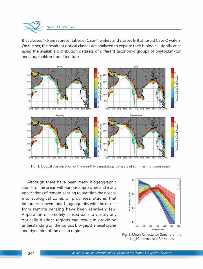
Winter School on Structure and Function of the Marine Ecosystem : Fisheries244
Optical Classification
that classes 1-6 are representative of Case-1 waters and classes 6-8 of turbid Case-2 waters.On further, the resultant optical classes are analyzed to explore their biological significanceusing the available distribution datasets of different taxonomic groups of phytoplanktonand zooplankton from literature.
Fig. 1. Optical classification of the monthly climatology datasets of summer monsoon season
Although there have been many biogeographicstudies of the ocean with various approaches and manyapplications of remote-sensing to partition the oceansinto ecological zones or provinces, studies thatintegrates conventional biogeography with the resultsfrom remote sensing have been relatively few.Application of remotely sensed data to classify anyoptically distinct regions can result in providingunderstanding on the various bio-geochemical cyclesand dynamics of the ocean regions.
Fig. 2. Mean Reflectance Spectra of theLog10-normalised Rrs values
Winter School on Structure and Function of the Marine Ecosystem : Fisheries 245
Optical Classification
245
References
Babin, M., Stramski, D., Ferrari, G. M., Claustre, H., Bricaud, A., Obolensky, G., et al., (2003). Variations in thelight absorption coefficients of phytoplankton , nonalgal particles and dissolved organic matter incoastal waters around Europe. J. Geophys. Res. Ocean. 108, 1–20. doi:10.1029/2001JC000882.
Bezdek, J. C. (1974). Cluster validity with fuzzy sets. J. Cybern. 3, 58–73. doi:10.1080/01969727308546047.
Bezdek, J. C., Ehrlich, R., and Full, W. (1984). FCM: The fuzzy c-means clustering algorithm. Comput. Geosci.10, 191–203. doi:10.1016/0098-3004(84)90020-7.
Halkidi, M., Batistakis, Y., and Vazirgiannis, M. (2002). Clustering validity checking methods. ACM SIGMODRec. 31, 19. doi:10.1145/601858.601862.
Hoepffner, N. and Dowell, M. (2005). Assessing the Dynamics of Ecological Provinces in the European Seas.European Commission – Joint Research Centre Institute for Environment and Sustainability Inland &Marine Waters Unit, 1-43.
Deborah, L.J., Baskaran, R., and Kannan, A. (2010). A Survey on Internal Validity Measure for Cluster Validation.Int. J. Comput. Sci. Eng. Surv. 1, 85–102. doi:10.5121/ijcses.2010.1207.
Jerlov, N. G. (1976). Marine Optics. Elsevier Oceanography Series, 276. doi:10.1016/S0422-9894(08)70794-3.
Kirk J.T.O (1976). A theoretical analysis of the contribution of algal cells to the attenuation of light withinnatural waters. New Phytol. 77, 341–358. doi:10.1111/j.1469-8137.1976.tb01524.x.
McKee, D., and Cunningham, A. (2006). Identification and characterisation of two optical water types in theIrish Sea from in situ inherent optical properties and seawater constituents. Estuar. Coast. Shelf Sci. 68,305–316. doi:10.1016/j.ecss.2006.02.010.
Mélin, F., and Vantrepotte, V. (2015). How optically diverse is the coastal ocean? Remote Sens. Environ. 160,235–251. doi:10.1016/j.rse.2015.01.023.
Minu P., Shaju S. S, Muhammed Ashraf P., Meenakumari, B. (2014). Phytoplankton community characteristicsin the coastal waters of the southeastern Arabian Sea. Acta Oceanoglogia 33, 170–179. doi:10.1007/s13131-014-0571-x.
Minu, P., Lotliker, A. A., Shaju, S. S., Ashraf, P. M., Kumar, T. S., and Meenakumari, B. (2016). ScienceDirectPerformance of operational satellite bio-optical algorithms in different water types in the southeasternArabian Sea. Oceanologia 58, 317–326. doi:10.1016/j.oceano.2016.05.005.
Moore, T. S., Campbell, J. W., and Dowell, M. D. (2009). A class-based approach to characterizing andmapping the uncertainty of the MODIS ocean chlorophyll product. Remote Sens. Environ. 113, 2424–2430. doi:10.1016/j.rse.2009.07.016.
Morel, A. (1974). Optical Properites of Pure Water and Pure Sea Water, 1–24.
Morel, A., and Prieur, L. (1977). Analysis of variations in ocean color. Limnol. Oceanogr. 22, 709–722.doi:10.4319/lo.1977.22.4.0709.
Nagamani P.V., Chauhan, P. and Dwived, R.M. (2008). Development of chlorophyll a algorithm for OceanColour Monitor onboard OCEANSAT-2 satellite. IEEE Geosci. Remote Sens. Lett. 5, 527–531. doi:10.1109/LGRS.2008.923213.
Winter School on Structure and Function of the Marine Ecosystem : Fisheries246
Optical Classification
Chauhan, P., Mohan, M., Sarngi, R.K., MeenaKumari, B., Nayak, S. and Matondkar, S.G.P. (2002). Surfacechlorophyll-a estimation in the Arabian Sea using IRS-P4 Ocean Colour Monitor (OCM) satellite data.Int. J. Remote Sens. 23, 1663–1676. doi:http://dx.doi.org/10.1080/01431160110075866.
Preisendorfer, R. W. (1976). Hydrologic Optics. Honolulu/ : U.S. Dept. of Commerce, National Oceanic andAtmospheric Administration, Environmental Research Laboratories, Pacific Marine EnvironmentalLaboratory Available at: http://udspace.udel.edu/handle/19716/1577.
Reinart, A., Herlevi, A., Arst, H., and Sipelgas, L. (2003). Preliminary optical classification of lakes and coastalwaters in Estonia and south Finland. J. Sea Res. 49, 357–366. doi:10.1016/S1385-1101(03)00019-4.
IOCCG (2000). Remote Sensing of Ocean Colour in Coastal, and Other Optically-Complex, Waters.Sathyendranath, S. (ed.), Reports of the International Ocean-Colour Coordinating Group, No. 3, IOCCG,Dartmouth, Canada.
Roff, J. C., Taylor, M. E., and Laughren, J. (2003). Geophysical approaches to the classiûcation, delineationand monitoring of marine habitats and their communities. Aquat. Conserv. Mar. Freshw. Ecosyst. 13,77–90.
Sathe, P.V and Jadhan, N. (2001). Retrieval of chlorophyll from the sea-leaving radiance in the Arabian Sea.J. Indian Soc. Remote Sens. 29, 97–106.
Sathyendranath, S. and Morel, A. (1989). A three-component model of ocean colour and its application toremote sensing of phytoplankton pigments in coastal waters. Int. J. Mar. Sci. 10, 1373–1394.
Smith, R. C., and Baker, K. S. (1977). Optical Classification Of Natural Waters University Of California , SanDiego Scripps Institution Of Oceanography Visibility Laboratory Lajolla, California.
Wozniak, B., and Pelevin, V. N. (1991). Optical classifications of the seasin relation to phytoplanktoncharacteristics. Oceanologia, 25–55.
Xie, X. L., and Beni, G. (1991). A validity measure for fuzzy clustering. IEEE Trans. Pattern Anal. Mach. Intell.13, 841–847. doi:10.1109/34.85677.
Zadeh (1965). Fuzzy Sets, 25.
Zhao, Q., Xu, M., and Fränti, P. (2009). Sum-of-squares based cluster validity index and significance analysis.Lect. Notes Comput. Sci. (including Subser. Lect. Notes Artif. Intell. Lect. Notes Bioinformatics) 5495LNCS, 313–322. doi:10.1007/978-3-642-04921-7_32.

Winter School on Structure and Function of the Marine Ecosystem : Fisheries 247
Development of Individual Based Models in Marine Fisheries Research
Setting
Fish population dynamics describe how a stock or a combination of them changes overtime as a function of growth, recruitment, mortality, immigration and emigration (Quinn &Deriso, 1999). It is the basis for understanding fish populations and associated fisheries andis the central component of any effort to assess the population dynamics so as to providequantitative advice for fishery management (Hilborn & Walters, 1992).
Modern fisheries stock assessment models are evolving towards increasing complexity(Maunder & Punt, 2013), with capabilities to assimilate a diverse suite of data and incorporatespatial structure (Cadrin & Secor, 2009) and the influence of environmental factors. As thenumber of such efforts increase, the behavior and performance of these complex modelsneed to be tested to assure a scientific basis for fishery management. These efforts to testthe plethora of models have resulted in extensive simulation studies. These have beenconducted to examine the robustness of the models and incorporate various process andmeasurement errors, including data quality and quantity (Chen et al., 2003), mis-specificationsof life history parameters (Deroba & Schueller, 2013; Punt, 2003), fishery characteristics(Cope & Punt, 2011), and violations of model assumptions (Guan, Cao, Chen, & Cieri, 2013).
Amongst these approaches one stream was oriented towards focussing on the habitatand ecosystem wherein the entire blend of biological dynamics are seen in action andmodels were built to suit them, leading to the ecosystem based models. Several approacheshave been developed at the ecosystem level, motivated by the observation of some recurrentpatterns of marine ecosystems, suggesting that interactions within the ecosystem areimportant structuring factors (Dickie and Kerr, 1982). For example, a widespread observationis the stability of the production of many marine ecosystems compared to that of individualspecies (e.g. Sutcliffe et al., 1977; May et al., 1979; Murawski et al., 1991). The maximumsustainable yield (MSY) is extended to a set of exploited species that are considered to forma single stock (Brown et al., 1976; FAO, 1978): the equilibrium production of the multispeciesassemblage would then be a parabolic function of fishing effort and the MSY wouldcorrespond to the exploitation of half the virgin biomass of the whole assemblage. Morerecently, Polovina (1984) and Christensen and Pauly (1992) developed the ecosystem modelECOPATH, which is widely used among fisheries scientists. In this model, species are
29C H A P T E R DEVELOPMENT OF INDIVIDUAL BASED
MODELS IN MARINE FISHERIES RESEARCHJ. Jayasankar, Tarun Joseph and Shruthy Abraham
Fishery Resources Assessment DivisionICAR-Central Marine Fisheries Research Institute

Winter School on Structure and Function of the Marine Ecosystem : Fisheries248
Development of Individual Based Models in Marine Fisheries Research
aggregated into functional groups, which are related by fluxes of matter. Forming the basisof the model are two equations of mass conservation, describing the production and theconsumption at equilibrium for each group of species.
This leads to the most important aspect of modelling, testing the sensitivity of assessmentmodels for mis-specifications requires an operating model to predict population dynamicswith known or assumed population parameters. However, most operating models areformulated identically to the population dynamic component built into the assessmentmodel (Cope & Punt, 2011; Deroba & Schueller, 2013; Guan et al., 2013; Punt, 2003), whichimplicitly assumes that the dynamic processes of the population are fully understood. Toavoid this problem and test the assessment rigorously, an alternatively structured operatingmodel is necessary to simulate the population dynamics.
Individual-based models (IBM), which consider each individual of a population as anindependent entity, have been widely used in ecology (Grimm & Railsback, 2005). Theevents (e.g., birth, death and predation) that occur within the simulation are at an individualrather than population level and the overall population dynamics that emerged is the sumof the individual interactions and behaviours.
The majority of individual-based models in fisheries science are developed toinvestigating fish behavior and fleet dynamics. They have been used to simulate the behaviorof individual fish or fishermen with rules that determine their movement (Tyler & Rose,1994; Wilson & Yan, 2009). Spatial heterogeneities in individuals and/or their environmenthave been added to develop spatially explicit individual-based models (Werner, Quinlan,Lough, & Lynch, 2001). However, only a few of these models have been developed forsimulating fishery population dynamics. Kanaiwa, Chen, and Wilson (2008) developed anindividual-based lobster simulator to simulate seasonal, sex-specific population dynamicsfor the American lobsters to evaluate the assessment model for that species. Further, themodels that have been developed are either species-specific or focused on one particularaspect of fish life history (Kanaiwa et al., 2008).
A typical IBM framework
Although many leads can be followed to formulate a framework under which IBMscould be modelled, the ringside view of the process can best be obtained from a simpledepiction of an algorithm, one such being given below (Cao et al., 2016).
The below figure depicts the steps and sequences alongside the checks and balanceswhich create the sequences in a cogent way. Now the different life stages like, naturaldeath, fishery mortality, growth , enhancement of age and stage, spawning and recruitmentcould have there own sub-conceptualisations of being either deterministic or probabilistic
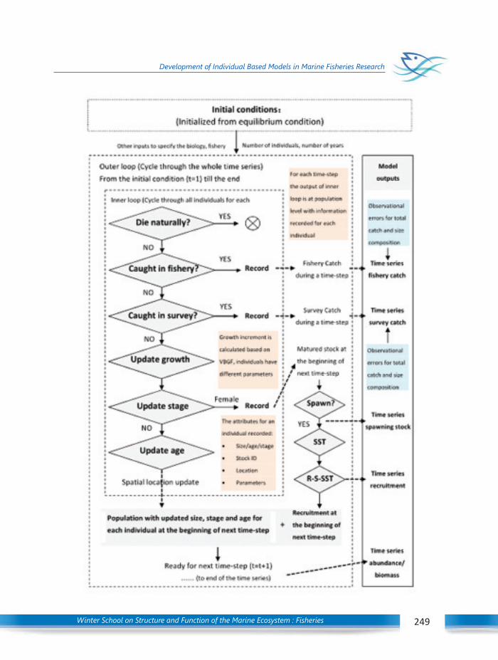
Winter School on Structure and Function of the Marine Ecosystem : Fisheries 249
Development of Individual Based Models in Marine Fisheries Research

Winter School on Structure and Function of the Marine Ecosystem : Fisheries250
Development of Individual Based Models in Marine Fisheries Research
and under either whichever established process presumed, thereby leading to a combinationof options in the programming and software sense. A typical look at the possibilities couldresult in the following steps;
Stage Model definition
Initial condition Equilibrium; with an assumed period to attain that
Stock spatial structure Multiple stocks each with unique biological identities
Stock recruitment relationship Specified functional relationship between spawning stock andits recruitment rate; Beverton- Holt, Ricker etc. or evenincorporation of environmental parameters like SST
Recruitment Can be directly put or could be derived from the S/R relationshipwith random fluctuation added; must be adjusted as per theintra annual pattern expressed by the resource(s) modelled
Natural mortality Could be randomness added to the base value defined basedon length or age
Fishing mortality Classic method of merging catchability, effort and selectivity;random threshold could be used to simulate fishing mortality
Growth VBGF based depiction
Life stage Number of stages and the mean size at each stage could bethe core with random normal deviations completing simulatedvalues
Survey Modelled similar to Fishing mortality
Observational error A lognormal based error term added to the catch figureaggregated over time, length and area
Multi-species Parallel replication of these steps for as many resources asplanned to be simulated/ studied
A broad-based IBM
Another more holistic variant of this type of IBM could be one including much morebroader habitat based components like availability of lower trophic level (LTL) biomass andthe higher level foragers and their predators. The availability of food and the growth stagecombination clearly heralding the status of larval mortality and the resultant niche basedcompetitions between resources could also be included through IBM thereby scaling up tosimulate regional ecosystems. One such comprehensive model is “Object oriented Simulatorof Marine Ecosystem Exploitation (OSMOSE)” (Shin and Cury, 2001, 2004). Herein the criterionfor the selection of prey by a predator was considered to be firmly based on body sizes withopportunism applied at individual level with a localization principle based on the vicinitycoming into picture. A cohort or super individual was made as pivot and the bio-phologicaldynamics applied on that and replicated to the tune existing in the area and focus. Four

Winter School on Structure and Function of the Marine Ecosystem : Fisheries 251
Development of Individual Based Models in Marine Fisheries Research
model classes, which representparticular ecological entities, areused: the class “system”, the class“species”, the class “age class”, andthe class “fish group” (Shin andCury, 2001). From each class,which is characterized byattributes and functions (e.g.,growth, predation), a number ofobjects are created that are partof the simulated system. The archi-tecture of OSMOSE is hierarchical,because a fish group belongs toan age class, which in turn belongsto a species. This structure enablesthe investigation of some key vari-ables at different levels ofaggregation, in particular the sizespectrum of fish assemblages.
The process of implemen-tation of OSMOSE can bestexplained using the flow-chartgiven here:
As can be seen from thefigure, the dynamics associatedwith growth, mortality, reproduc-tion (spawning) etc. could bemodelled using the conceptu-alisation described in the previouscase. But the new broadbasedhabitat and trophism basedcomponents need someelaboration. The parameterizationof the components is presented inthe following table.
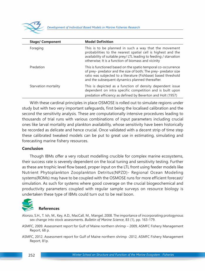
Winter School on Structure and Function of the Marine Ecosystem : Fisheries252
Development of Individual Based Models in Marine Fisheries Research
Stage/ Component Model Definition
Foraging This is to be planned in such a way that the movementprobabilities to the nearest spatial cell is highest and theavailability of suitable prey/ LTL leading to feeding / starvationotherwise; It is a function of biomass and vicinity
Predation This is functioned based on the spatio temporal co-occurrenceof prey- predator and the size of both; The prey- predator sizeratio was subjected to a literature (Fishbase) based thresholdand the subsequent dynamics planned thereafter.
Starvation mortality This is depicted as a function of density dependent issuedependent on intra specific competition and is built uponpredation efficiency as defined by Beverton and Holt (1957)
With these cardinal principles in place OSMOSE is rolled out to simulate regions understudy but with two very important safeguards, first being the localised calibration and thesecond the sensitivity analysis. These are computationally intensive procedures leading tothousands of trial runs with various combinations of input parameters including crucialones like larval mortality and plankton availability, whose sensitivity have been historicallybe recorded as delicate and hence crucial. Once validated with a decent strip of time stepthese calibrated tweaked models can be put to great use in estimating, simulating andforecasting marine fishery resources.
Conclusion
Though IBMs offer a very robust modelling crucible for complex marine ecosystems,their success rate is severely dependent on the local tuning and sensitivity testing. Furtheras these are trophic level flow based, proper input on the LTL front using feeder models likeNutrient Phytoplankton Zooplankton Detritus(NPZD)- Regional Ocean Modelingsystems(ROMs) may have to be coupled with the OSMOSE runs for more efficient forecast/simulation. As such for systems where good coverage on the crucial biogeochemical andproductivity parameters coupled with regular sample surveys on resource biology isundertaken these type of IBMs could turn out to be real boon.
References
Alonzo, S.H., T. Ish, M., Key, A.D., MacCall, M., Mangel, 2008. The importance of incorporating protogynoussex change into stock assessments. Bulletin of Marine Science, 83 (1), pp. 163-179.
ASMFC, 2009. Assessment report for Gulf of Maine northern shrimp – 2009, ASMFC Fishery ManagementReport, 68 p.
ASMFC, 2012. Assessment report for Gulf of Maine northern shrimp -2012, ASMFC Fishery ManagementReport, 81p.
Winter School on Structure and Function of the Marine Ecosystem : Fisheries 253
Development of Individual Based Models in Marine Fisheries Research
Cadrin, S.X., Secor, D.H., 2009. Accounting for spatial population structure in stock assessment: Past, presentand future, R.J. Beamish, B.J. Rothschild (Eds.). The future of f ishery science in NorthAmerica, Springer, Dordrecht, pp. 405-426.
Cao, J., Guan, W., Truesdell, S., Chen, Y., Tian. S., 2016. An individual-based probabilistic model for simulatingûsheries population dynamics J. Aquaculture and Fisheries, 1(1): 34-40.
Chen, Y., L. Chen, L., Stergiou, K. 2003. Quantity of fisheries data and uncertainty in stock assessment,Aquatic Science, 65, pp. 92-98.
Chen, Y., Hunter, M., Vadas, R., Beal, B., 2003. Developing a growth-transition matrix for the stock assessmentof the green sea urchin (Strongylocentrotus droebachiensis) off Maine, Fishery Bulletin, 101 (4), pp. 737-744.
Cope, J.M., Punt, A.E., 2011. Reconciling stock assessment and management scales under conditions ofspatially varying catch histories, Fisheries Research, 107, pp. 22-38.
Deroba, J.J., Schueller, A.M., 2013. Performance of stock assessments with misspecified age-and time-varyingnatural mortality, Fisheries Research, 146, pp. 27-40.
Francis, R.I.C.C., 1992. Use of risk analysis to assess fishery management strategies: A case study usingorange roughy (Hoplostethus atlanticus) on the Chatham Rise, New Zealand, Canadian Journal ofFisheries and Aquatic Sciences, 49, pp. 922-930.
Grimm, V., Railsback, S.F., 2005. Individual-based modeling and ecology, Princeton university press.Guan, W.J., Cao, J., Chen, Y., Cieri, M., 2013. Impacts of population and fishery spatial structures on fishery
stock assessment, Canadian Journal of Fisheries and Aquatic Sciences, 70 (8) , pp. 1178-1189.Hilborn, R., Walters, C., 1992. Quantitative fisheries stock assessment: Choice, dynamics, and uncertainty,
Chapman and Hall, N.Y. Kanaiwa, M., Chen, Y., Wilson, C., 2008. Evaluating a seasonal, sex-specific size-structured stock assessment
model for the American lobster, Homarus americanus, Marine and Freshwater Research, 59 (1), pp. 41-56.
Kanwit, J.K., Libby, D.A., 2009. Seasonal movements of atlantic herring (Clupea harengus): Results from afour year tagging study conducted in the Gulf of Maine and Southern New England, Journal of theNorthwest Atlantic Fishery Science, 40, pp. 29-39.
Legault, C.M., Restrepo, V.R., 1998, A flexible forward age-structured assessment program 49, Collect. Vol.Sci. Pap. ICCAT, pp. 246-253.
Maunder, M.N., Punt, A.E., 2013. A review of integrated analysis in fisheries stock assessment, FisheriesResearch, 142 (2013), pp. 61-74.
Overholtz, W.J., Jacobson, L.D., Melvin, G.D., Cieri, M., Power, M., Libby, D. et al., 2004. Stock assessment ofthe Gulf of Maine - Georges Bank atlantic herring complex 2003, Northeast Fisheries Science CenterReference Document 04-06 Available from: http://www.nefsc.noaa.gov/publications/crd/crd0406/crd0406.pdf
Punt, A.E., 2003. The performance of a size-structured stock assessment method in the face of spatialheterogeneity in growth, Fisheries Research, 65 (1), pp. 391-409.
Quinn, T.J., Deriso, R.B., 1999. Quantitative fish dynamics, Oxford University Press, New York.Reid, R.N., et. al., 1999. Essential Fish Habitat Source Document: Atlantic Herring, Clupea harengus, Life
History and Habitat Characteristics, NOAA Technical Memorandum NMFS-NE-126, Available from:http://www.nefsc.noaa.gov/publications/tm/tm126/.

Winter School on Structure and Function of the Marine Ecosystem : Fisheries254
Development of Individual Based Models in Marine Fisheries Research
Reid, R.N., Cargnelli, L.M., Griesbach, S.J., Packer, D.B., Johnson, D.L., Zetlin, C.A., et al., Essential fish habitatsource document: Atlantic herring, Clupea harengus, life history and habitat characteristics, NOAATech. Memo. NMFS-NE-126.
Richards, R., Fogarty, M.J., Mountain, D.G., Taylor, M.H. 2012. Climate change and northern shrimp recruitmentvariability in the Gulf of Maine, Marine Ecology Progress Series, 464, pp. 167-178.
Scheffer, M., Baveco, J.M., DeAngelis, D.L., Rose, K.A., Van Nes, E.H., 1995. Super-individuals a simple solutionfor modelling large populations on an individual basis, Ecological modelling, 80 (2), pp. 161-170.
Shepherd, G., Cieri, M., Powers, M., Overholtz, W., 2009. Transboundary resources assessment Committee:Gulf of Maine/Georges Bank atlantic herring stock assessment update, Reference Document 2009/04,NOAA Fisheries, Northeast Fisheries Science Center, Woods Hole, Massachusetts.
Shin, Y.J., and Cury, P. 2001. Exploring fish community dynamics through size-dependent trophic interactionsusing a spatialized individual-based model. Aquat. Living Resour. 14: 65–80.
Shin, Y.J. and Cury, P. 2004. Using an individual-based model of fish assemblages to study the response ofsize spectra to changes in fishing Canadian Journal of Fisheries and Aquatic Sciences, 2004, 61(3):414-431, https://doi.org/10.1139/f03-154.
Tyler, J.A., Rose, K.A., 1994. Individual variability and spatial heterogeneity in fish population models, Reviewsin Fish Biology and Fisheries, 4, pp. 91-123.
Werner, F.E., Quinlan, J.A., Lough, R.G., Lynch, D.R., 2001. Spatially-explicit individual based modeling ofmarine populations: A review of the advances in the 1990s. Sarsia, 86 (6), pp. 411-421.
Wilson, J.A., Yan, L., 2009. Self-organizing economic activity with costly information, Proceedings of the11th annual conference companion on genetic and evolutionary computation conference.

Winter School on Structure and Function of the Marine Ecosystem : Fisheries 255
Ecosystem modelling - Introduction to TOPAZ
1. Outline of the lecture
The lecture have three major sections. The first section will briefly discuss how importantphysical processes influence the biological processes in the ocean. The two important physicalprocesses that will be discussed are upwelling and entrainment. I then briefly introduce anecosystem model named Tracers of Phytoplankton with Allometric Zooplankton. This modelis referred to using the acronym, TOPAZ [Dunne et al., 2010]. This ecosystem model has thecapability to be coupled to a physical Ocean General Circulation Model (OGCM) known asModular Ocean Model (MOM4p1). Both MOM and TOPAZ are developed by the GeophysicalFluid Dynamics Laboratory. In the third section of this lecture, I’ll be presenting an exampleof an application of the physical-ecosystem model based on MOM-TOPAZ to explain thebiological consequences of inhibition of deepening of mixed layer in the northeastern ArabianSea [Vijith et al., 2016].
2. TOPAZ
TOPAZ is a widely used ecosystem model. It has been used by several researchers toaddress a variety of physical-ecosystem interaction that happens during large scale oceanprocesses such as El Nino Southern Oscilaltion (ENSO), Indian Ocean Dipole etc. TOPAZincludes carbon, nitrate, ammonium, phosphate, silicate, dissolved oxygen, iron, and calciumand three phytoplankton groups: diazotrophs (cyanobacteria), small (picoplankton andnanoplankton), and large (diatoms and algae) phytoplankton. The model also includesbiogeochemical processes such as the atmospheric deposition of iron, nitrification, anddenitrification. The parametrisation of growth rate of phytoplankton, limitation of nutrientsand light, and grazing will be described using simple schematic diagrams. I’ll also discusshow size considerations of phytoplankton are dealt in the model.
3. Application of TOPAZ
The seasonally reversing monsoon winds over the north Indian Ocean produce seasonallyreversing currents that exchange water between the Arabian Sea and the Bay of Bengal.One such current is the West India Coastal Current that takes low-salinity waters of the Bayof Bengal into the Arabian Sea. As the current takes the waters poleward along the westcoast of India, the contrast between salinity of the waters of the current with ambient waters
30C H A P T E R ECOSYSTEM MODELLING -
INTRODUCTION TO TOPAZVijith V.
Cochin University of Science and Technology, Kochi

Winter School on Structure and Function of the Marine Ecosystem : Fisheries256
Ecosystem modelling - Introduction to TOPAZ
has an impact on mixed-layer physics. This impact in the northeastern Arabian Sea wasdiscussed by Shankar et al., (2016) and Vijith et al., (2016). During the lecture I’ll demonstratean how the TOPAZ was employed to investigate consequences of inhibition of mixed-layerdeepening by the West India Coastal Current to winter phytoplankton bloom in thenortheastern Arabian Sea.
References
Dunne, J. P., A. Gnanadesikan, J. L. Sarmiento, and R. D. Slater (2010). Technical description of the prototypeversion (v0) of Tracers of Phy-toplankton with Allometric Zooplankton (TOPAZ) ocean bio-geochemicalmodel as used in the Princeton IFMIP model, Biogeosciences, 7, 3593–3624.
Shankar, D., R. Remya, P. N. Vinayachandran, A. Chatterjee, and A. Behera (2016). Inhibition of mixed-layerdeepening during winter in the northeastern Arabian Sea by the West India Coastal Current, Clim.Dyn., 47, 1049–1072, doi:10.1007/s00382-015-2888-3.
Vijith, V., P. N. Vinayachandran, V. Thushara, P. Amol, D. Shankar, and A. C. Anil (2016). Consequences ofinhibition of mixed-layer deepening by the West India Coastal Current for winter phytoplankton bloomin the northeastern Arabian Sea, J. Geophys. Res. Oceans, 121, doi:10.1002/ 2016JC012004.
Winter School on Structure and Function of the Marine Ecosystem : Fisheries 257
Impact of climate change on marine sector
Climate over the Earth is showing perceptible changes over both global and regionalscales and the warming effects are now being felt across many parts of the world includingIndia (Vivekanandan, 2010). Human activities are increasing the levels of carbon dioxideand other greenhouse gases in the atmosphere leading to a rise in atmospheric temperature.Since the year 1750, the level of atmospheric CO2 has risen from 280 ppm to 401 ppm in2015, and if unchecked, will be at around 560 ppm by the year 2050.
Climate change is one of the most important global environmental challenges withimplications on food production including fisheries and aquaculture sector, naturalecosystems, freshwater supply, health, etc. Climatic scenarios generated by computer modelsshows that India could experience warmer and wetter conditions as a result of climatechange including an increase in the frequency and intensity of heavy rains and extremeweather events (EWEs). The effects of climate change in aquatic ecosystems can be direct,through rise in sea surface temperature (SST), and associated changes in the phenology ofthe organisms, or indirect i.e., through ocean acidification, through shifts in hydrodynamicsand rise in sea level. Climate change will intensify by 2050 and though climate outcomescannot be precisely predicted, the probability towards greater impacts of climate challengeis becoming clearer.
How does the ocean affect the climate ? ? ? ? ?
The oceans play an important role in regulating climate as its heat uptake capacity isapproximately 1000 times larger than the atmosphere. The world ocean has warmedsubstantially since 1955 and warming account for 80% of the change in energy content ofthe Earth’s climate system (Cochrane, 2010). These deviations from normal surfacetemperatures can have large-scale impacts not only on ocean processes, but also onglobal weather and climate.
Impact on Climatic and Oceanographic Parameters
Changes in the important oceanic weather systems such as sea surface temperature,pH, salinity, El Niño Southern Oscillation (ENSO), precipitation, sea level, frequencyand intensity of cyclones and droughts are becoming evident as a result of climatechange.
31C H A P T E R IMPACT OF CLIMATE CHANGE ON
MARINE SECTORP. U. Zacharia
Demersal Fisheries DivisionICAR-Central Marine Fisheries Research Institute

Winter School on Structure and Function of the Marine Ecosystem : Fisheries258
Impact of climate change on marine sector
• El Niño-Southern Oscillation (ENSO) cycle, describes the fluctuations in temperaturebetween the ocean and atmosphere in the east-central Equatorial Pacific.
• La Niña is the cold phase of ENSO and El Niño as the warm phase of ENSO
Climate change impact on coastal fisheries and aquaculture
World’s Oceans are currently affected by global warming with likely impacts in changesin ocean currents and winds, precipitation, ocean acidification etc. which will have strongimpact on fisheries with serious consequences on food and livelihood security of considerablesection of the population. In India marine fisheries have very important roles in augmentingfood supply, nutritional security and livelihood for millions. With the major share of marinefish catch coming from coastal and near-coastal waters, environmental change in this zonewould have debilitating impact on the sector in specific and the country’s food basket ingeneral.
o Source: Vivekanandan E. CMFRI Newsletter No.112. October-December 2006
Climate change on fishery habitat
Marine ecosystems are not in a steady state, but are affected by the environment,which varies on many spatial and temporal scales. Fish populations respond to variation indifferent ways. Decadal variations may have unforeseen impacts, including cyclic changesin the production level of marine ecosystems that favor one species or group over another.
Sea surface Temperature (SST) increase: Temperature is likely the single most importantfactor affecting the growth and development of aquatic organisms. Earth has been in radiativeimbalance since at least the 1970s, where less energy leaves the atmosphere than enters it.Most of this extra energy (~90%) has been absorbed by the oceans (IPCC,2014). The variationof Sea surface Temperature (SST) along Indian seas during the 40 years from 1976 to 2015revealed that SST increased by 0.602°C along the northeast India (NEI), by 0.597°C along
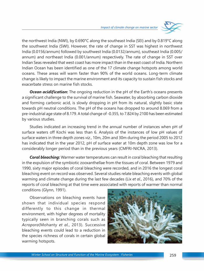
Winter School on Structure and Function of the Marine Ecosystem : Fisheries 259
Impact of climate change on marine sector
the northwest India (NWI), by 0.690°C along the southeast India (SEI) and by 0.819°C alongthe southwest India (SWI). However, the rate of change in SST was highest in northwestIndia (0.0156/annum) followed by southwest India (0.0132/annum), southeast India (0.005/annum) and northeast India (0.001/annum) respectively. The rate of change in SST overIndian Seas revealed that west coast has more impact than in the east coast of India. NorthernIndian Ocean has been identified as one of the 17 climate change hotspots among worldoceans. These areas will warm faster than 90% of the world oceans. Long-term climatechange is likely to impact the marine environment and its capacity to sustain fish stocks andexacerbate stress on marine fish stocks.
Ocean acidification: The ongoing reduction in the pH of the Earth’s oceans presentsa significant challenge to the survival of marine fish. Seawater, by absorbing carbon dioxideand forming carbonic acid, is slowly dropping in pH from its natural, slightly basic statetowards pH neutral conditions. The pH of the oceans has dropped to around 8.069 from apre-industrial age state of 8.179. A total change of -0.355, to 7.824 by 2100 has been estimatedby various studies.
Studies indicated an increasing trend in the annual number of instances when pH ofsurface waters off Kochi was less than 6. Analysis of the instances of low pH values ofsurface waters in three depth zones viz., 10m, 20m and 30m during the period 2005 to 2012has indicated that in the year 2012, pH of surface water at 10m depth zone was low for aconsiderably longer period than in the previous years (CMFRI-NICRA, 2013).
Coral bleaching: Warmer water temperatures can result in coral bleaching that resultingin the expulsion of the symbiotic zooxanthellae from the tissues of coral. Between 1979 and1990, sixty major episodes of coral bleaching were recorded, and in 2016 the longest coralbleaching event on record was observed. Several studies relate bleaching events with globalwarming and climate change during the last few decades (Lix et al., 2016), and 70% of thereports of coral bleaching at that time were associated with reports of warmer than normalconditions (Glynn, 1991).
Observations on bleaching events haveshown that individual species responddifferently to this change in thermalenvironment, with higher degrees of mortalitytypically seen in branching corals such asAcropora(Mohanty et al., 2013). Successivebleaching events could lead to a reduction inthe species richness of corals in certain globalwarming hotspots.
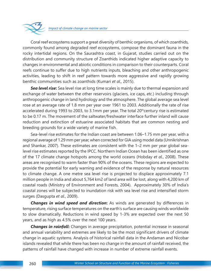
Winter School on Structure and Function of the Marine Ecosystem : Fisheries260
Impact of climate change on marine sector
Coral reef ecosystems support a great diversity of benthic organisms, of which zoanthids,commonly found among degraded reef ecosystems, compose the dominant fauna in therocky intertidal regions. On the Saurashtra coast, in Gujarat, studies carried out on thedistribution and community structure of Zoanthids indicated higher adaptive capacity tochanges in environmental and abiotic conditions in comparison to their counterparts. Coralreefs continue to suffer due to high nutrients inputs, bleaching and other anthropogenicactivities, leading to shift in reef pattern towards more aggressive and rapidly growingbenthic communities such as zoanthids (Kumari et al., 2015).
Sea level rise: Sea level rise at long time scales is mainly due to thermal expansion andexchange of water between the other reservoirs (glaciers, ice caps, etc.) including throughanthropogenic change in land hydrology and the atmosphere. The global average sea levelrose at an average rate of 1.8 mm per year over 1961 to 2003. Additionally the rate of riseaccelerated during 1993 to 2003, to 3.1mm per year. The total 20thcentury rise is estimatedto be 0.17 m. The movement of the saltwater/freshwater interface further inland will causereduction and extinction of estuarine associated habitats that are common nesting andbreeding grounds for a wide variety of marine fish.
Sea-level rise estimates for the Indian coast are between 1.06–1.75 mm per year, with aregional average of 1.29 mm per year, when corrected for GIA using model data (Unnikrishnanand Shankar, 2007). These estimates are consistent with the 1–2 mm per year global sea-level rise estimates reported by the IPCC. Northern Indian Ocean has been identified as oneof the 17 climate change hotspots among the world oceans (Hobday et al., 2008). Theseareas are recognised to warm faster than 90% of the oceans. These regions are expected toprovide the potential for early warning and evidence of the response by natural resourcesto climate change. A one metre sea level rise is projected to displace approximately 7.1million people in India and about 5,764 km2 of land area will be lost, along with 4,200 km ofcoastal roads (Ministry of Environment and Forests, 2004). Approximately 30% of India’scoastal zones will be subjected to inundation risk with sea level rise and intensified stormsurges (Dasgupta et al., 2009).
Changes in wind speed and direction: As winds are generated by differences intemperature, rising surface temperatures on the earth’s surface are causing winds worldwideto slow dramatically. Reductions in wind speed by 1-3% are expected over the next 50years, and as high as 4.5% over the next 100 years.
Changes in rainfall: Changes in average precipitation, potential increase in seasonaland annual variability and extremes are likely to be the most significant drivers of climatechange in aquatic systems. Analysis of historical rainfall data in the Andaman and Nicobarislands revealed that while there has been no change in the amount of rainfall received, thepatterns of rainfall have changed with increase in number of extreme rainfall events.
Winter School on Structure and Function of the Marine Ecosystem : Fisheries 261
Impact of climate change on marine sector
Variations in annual rainfall intensity, dry season rainfall and the resulting growing seasonlength are likely to create impact on shrimp/ fish farming and could lead to conflict withother agricultural, industrial and domestic users in water scarce areas.
Impact on fish stock
A metabolic increase of 10% corresponds to a 1oC increase in temperature, implying ofseawater as low as 1ºC could affect the distribution and life processes of fish. This constraintin physiology will result in changes in distributions, recruitment and abundance. Changes intiming of life history events are expected with climate change. Species with short-life spanand rapid turnover of generations such as plankton and small pelagic fishes are most likelyto experience such changes. At intermediate time scales of a few years to a decade, thechanges in distributions, recruitment and abundance of many species will be acute at theextremes of species’ ranges. Changes in abundance will alter the species composition andresult in changes in the structure and functions of the ecosystems. At long time scales ofmulti-decades, changes in the net primary production and its transfer to higher trophiclevels are possible.
Changes in timing of life history events are also likely to result from the warming of theEarth’s waters. Many tropical fish stocks are already exposed to high extremes of temperaturetolerance, and already face regional extinction, and some others may move towards higherlatitudes. Shifts in spawning periods of fishes have already been observed in a number ofcommercially important fish stocks, such as threadfin bream (Zacharia et al., 2016). Changesin distribution patterns of two key species in Indian fisheries have already been established-migration patterns of the Indian oil sardine and Indian mackerel have changed greatly overthe past 50 years (Vivekanandan et al., 2009).
Ocean-atmospheric coupled climate models predict changes in the ocean circulationand hypothesize that changes in the ocean circulation will stimulate phytoplankton biomassproduction in the nutrient depleted areas in the open ocean. The effect on atmospheric CO2is uncertain because the relationship between the enhanced primary production and airsea exchange of CO2 is not understood.
Most models show decreasing primary production with changes of phytoplanktoncomposition to smaller forms, although with high regional variability. Marked effects inplankton distribution have also been noticed concurrent to changes in sea surfacetemperature. These changes may affect the distribution of fish stocks that predate onplankton. Ocean acidification is believed to have negative consequences for marine denizens,particularly calcifying organisms, subjecting them to the risk of dissolution. A decline inprimary productivity has also been forecast.
Winter School on Structure and Function of the Marine Ecosystem : Fisheries262
Impact of climate change on marine sector
Impact on fish stock availability
Evidence exists for increasing damage by extreme weather events, particularly cyclones,over time. There are various explanations for this, ranging from greater population densitiesto the wider effects of climate change (IPCC, 2013).
Until the mid-1980s, the restricted distribution of oil sardine ensured that the entirecatch of oil sardine was obtained from the southwestern coast of India. North of 14oN, littleto no oil sardine was caught previously. In the last two decades, however, the oil sardinecatch from 14oN to 20oN has gradually and consistently increased, contributing 15% to theall-India oil sardine catch by 2006 (Vivekanandan et al., 2009). Since the catch in theSouthwestern regions has not decreased in overall terms, this represents an extension ofthe distributional boundaries of the oil sardine.
Studies on the seasonal distribution of skipjack tuna reveal that during winter months,when sea surface temperature is lower, migration occurs towards offshore areas, and duringwarmer months, migration occurs towards inshore areas during warmer months. Changesin sea surface temperature due to global warming could result in changes in the seasonaldistribution of certain species, and ultimately disruption in their harvest, which is usuallybased on indigenous knowledge (Zacharia et al., 2016). Changes in distributional boundariesalso bear the potential to bring up delicate questions of fishing rights, especially within thecontext of geopolitics and exploitation of the resources found within neighbouring exclusiveeconomic zones.
References
IPCC, 2013: Summary for Policymakers. In: Climate Change 2013: The Physical Science Basis. Contributionof Working Group I to the Fifth Assessment Report of the Intergovernmental Panel on Climate Change[Stocker, T.F., D. Qin, G.-K. Plattner, M. Tignor, S. K. Allen, J. Boschung, A. Nauels, Y. Xia, V. Bex and P.M.Midgley (eds.)]. Cambridge University Press, Cambridge, United Kingdom and New York, NY, USA.
IPCC, 2014: Climate Change 2014: Synthesis Report. Contribution of Working Groups I, II and III to the FifthAssessment Report of the Intergovernmental Panel on Climate Change [Core Writing Team, R.K. Pachauriand L.A. Meyer (eds.)]. IPCC, Geneva, Switzerland, 151 pp.
Vivekanandan, 2010. Climate change-impact and mitigation in ICAR handbook of fisheries/aquaculture.ICAR New Delhi 794-821
Vivekanandan, E., Rajagopalan, M., Pillai, N.G.K., 2009. Recent trends in sea surface temperature and itsimpact on oil sardine. In: Global Climate Change and Indian Agriculture. Indian Council of AgriculturalResearch, New Delhi: 89-92.
Vivekanandan, E. 2006. CMFRI Newsletter 112. Impact of climate change on marine fisheries. October-December 2006.
Winter School on Structure and Function of the Marine Ecosystem : Fisheries 263
Impact of climate change on marine sector
CMFRI-NICRA, 2013. NICRA Research Highlights 2013-14. National Initiatives on Climate Resilient AgricultureResearch Highlights (Eds. M.Mahaeswari et al., 2014), ICAR-CRIDA, Hyderabad, 116 p. (ISBN: 978-93-80883-28-1).
Mohanty, P.C, Mahendra R.S, Bisoyi, Hrusikesh Tummula Srinivasa Kumar, George Grinson, Nayak Shaileshand Sahu, B K., 2013. Assessment of the coral bleaching during 2005 to decipher the thermal stress inthe coral environs of the Andaman Islands using Remote Sensing. European Journal of Remote Sensing,46:417-430
Bimal Mohanty, Sasmita Mohanty, Jnanendra Sahoo and Anil Sharma, 2010. Climate Change: Impacts onFisheries and Aquaculture, Climate Change and Variability, Suzanne Simard (Ed.), ISBN: 978-953-307-144-2, In Tech, Available from: http://www.intechopen.com/ books/ climate-change-and-variability/climate-change impacts-on-fisheries- and-aquaculture
A.J. Hobday, E.S. Poloczanska, R.J. Matear, 2008. Implications of climate change for Australian fisheries andaquaculture: a preliminary assessment. AJ Hobday et al., (Ed.) Implications of climate change forAustralian fisheries and aquaculture: a preliminary assessment 2008 pp.ix + 74 pp
Kumari, Sonia., Zacharia, P.U., Kripa, V., Sreenath, K.R. and George, Grinson., 2015. Distribution pattern andcommunity structure of Zoanthids (Zoantharia) along the coast of Saurashtra, Gujarat, India. Journal ofthe Marine Biological Association of the United Kingdom, 96(8): 1577-1584.
Unnikrishnan, A.S. and Shankar, D., 2007. Are sea-level-rise trends along the coasts of the north IndianOcean consistent with global estimates? Global and Planetary Change, 57(3-4): 301-307.
Zacharia, P.U., Dineshbabu, A.P., Thomas Sujitha., Shoba J.K., Vivekanandan E., Pillai, Lakshmi, S., Sivadas M.,Ghosh Shubadeep, Ganga U., Rajesh K.M., Nair Rekha, J., Najmudeen T.M., Koya Mohammed, ChellappanAnulekshimi, Dash Gyanranjan., Divipala Indira, Akhilesh K.V., Muktha M., Sen Dash, Swathipriyanka,2016. Relative vulnerability assessment of Indian marine fishes to climate change using impact andadaptation attributes. CMFRI Special Publication No.125, (CMFRI-NICRA Publication No. 5), CentralMarine Fisheries Research Institute, Kochi, India, 192pp.
Zacharia P.U., A. Gopalakrishnan, Grinson George, M. Muralidhar and K. K. Vijayan, 2016. Climate changeimpact on coastal fisheries and aquaculture in the SAARC region: Country paper- India
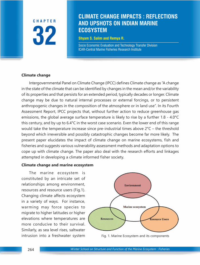
Winter School on Structure and Function of the Marine Ecosystem : Fisheries264
Climate change impacts : - Reflections and Upshots on Indian marine ecosystem
Fig. 1. Marine Ecosystem and its components
Climate change
Intergovernmental Panel on Climate Change (IPCC) defines Climate change as “A changein the state of the climate that can be identified by changes in the mean and/or the variabilityof its properties and that persists for an extended period, typically decades or longer. Climatechange may be due to natural internal processes or external forcings, or to persistentanthropogenic changes in the composition of the atmosphere or in land use”. In its FourthAssessment Report, IPCC projects that, without further action to reduce greenhouse gasemissions, the global average surface temperature is likely to rise by a further 1.8 - 4.0°Cthis century, and by up to 6.4°C in the worst case scenario. Even the lower end of this rangewould take the temperature increase since pre-industrial times above 2°C – the thresholdbeyond which irreversible and possibly catastrophic changes become far more likely. Thepresent paper elucidates the impact of climate change on marine ecosystems, fish andfisheries and suggests various vulnerability assessment methods and adaptation options tocope up with climate change. The paper also deal with the research efforts and linkagesattempted in developing a climate informed fisher society.
Climate change and marine ecosystem
The marine ecosystem isconstituted by an intricate set ofrelationships among environment,resources and resource users (Fig.1).Changing climate affects ecosystemin a variety of ways. For instance,warming may force species tomigrate to higher latitudes or higherelevations where temperatures aremore conducive to their survival.Similarly, as sea level rises, saltwaterintrusion into a freshwater system
32C H A P T E R
CLIMATE CHANGE IMPACTS : REFLECTIONSAND UPSHOTS ON INDIAN MARINEECOSYSTEMShyam S. Salim and Remya R.
Socio Economic Evaluation and Technology Transfer DivisionICAR-Central Marine Fisheries Research Institute

Winter School on Structure and Function of the Marine Ecosystem : Fisheries 265
Climate change impacts : - Reflections and Upshots on Indian marine ecosystem
265
may force some key species to relocate or die, thus removing predators or prey that arecritical in the existing food chain. Climate change not only affects ecosystems and resourcesdirectly, it also interacts with the general well being of resource users or community as awhole.
I. Impact of climate change on environment
Marine ecosystems are not in a steady state, but are affected by the environment,which varies on many spatial and temporal scales. Changes in temperature are related toalterations in oceanic circulation patterns that are affected by changes in the direction andspeed of the winds that drive ocean currents and mix surface waters with deeper nutrientrich waters (Kennedy et al., 2002). These processes in turn affect the distribution andabundance of plankton, which are food for small fish. Understanding the importance andthe implication of the climate changes on coastal areas may be one of the major issues forthis and next centuries.
Climate changes may, indeed, impact the nearshore marine environment, as coastalareas are very sensitive to the strength and the variability of the meteorological forcings. Anincrease of a few degrees in atmospheric temperature will not only raise the temperature ofthe oceans, but also cause major hydrologic changes affecting the physical and chemicalproperties of water. These will lead to fish, invertebrate, and plant species changes in marineand estuarine communities (McGinn, 2002). Fishes have evolved physiologically to live withina specific range of environmental variation, and existence outside of that range can bestressful or fatal (Barton et al., 2002). These ranges can coincide for fishes that evolved insimilar habitats (Attrill, 2002). Estuarine and coastal regions are extremely productive becausethey receive inputs from several primary production sources and detrital food webs. Yet,these systems present the biota with a harsh environment, forcing organisms to evolvephysiological or behavioral adaptations to cope with wide ranging physical and chemicalvariables (Horn et al., 1999). Temperature, along with other variables, causes active movementof mobile species to areas encompassing the preferred range of environmental variables,influencing migration patterns (Rose and Leggett, 1988; Murawski, 1993; Soto, 2002). Thepredicted increase in major climatic events, such as ENSO (Timmermann et al., 1999; IPCC,2001), may have drastic effects on fish stocks, especially when combined with other factors,such as overfishing (Pauly and Christensen, 1995). It has been suggested that reducedsurvival, reduced growth rate, and diversions of traditional migratory routes can all be causedby ENSO events, exacerbating the effects of intensive harvesting (Miller and Fluharty, 1992).The El Nino phenomenon generates substantial changes in oceanographic and
Winter School on Structure and Function of the Marine Ecosystem : Fisheries266
Climate change impacts : - Reflections and Upshots on Indian marine ecosystem
meteorological conditions in the Pacific Ocean, with manifestations impacting the Peruviancoast (Zuta et al., 1976); this has mainly affected pelagic resources, producing alterations intheir biological processes, behaviour, and gradual decrease in their population levels (Valdivia,1976).
(i) Sea level rise in the Indian seas
The IPCC (2007) has projected that the global annual seawater temperature and sealevel would rise by 0.8 to 2.5° C and 8 to 25 cm, respectively by 2050. At present, 23% of theshoreline along the Indian mainland is affected by sea erosion (Sanil Kumar et al., 2006).The large inflow of freshwater into the seas around India due to rainfall over the ocean andrunoff from rivers, forces large changes in sea level especially along the coasts of Bay ofBengal. During June-October, the inflow of freshwater from the Ganges and Brahmaputrainto the northern Bay Bengal is about 7.2x10¹¹m3, the fourth largest discharge in the world(Shankar, 2000). Increase in sea level, in addition to causing threats to human lives, will poseproblems on freshwater availability due to intrusion of seawater and salinisation ofgroundwater. This would also result in loss of agricultural land. A rise in sea level is likely tohave significant impact on the agriculture performance in India. A one metre sea level riseis projected to displace approximately 7.1 million people in India and about 5,764 km2 ofland area will be lost, along with 4,200 km of coastal roads (Ministry of Environment andForests, 2004). Approximately 30% of India’s coastal zones will be subjected to inundationrisk with sea level rise and intensified storm surges (Dasgupta et al., 2009).
(ii) Sea Surface Temperature
Prasanna Kumar et al., (2009) examined the signature of global warming using variousdatasets for the Arabian Sea region and found that the disruption in the natural decadalcycle of SST after 1995 was a manifestation of regional climate-shift. They propose thatupwelling driven cooling was maintained till 1995 despite oceanic thermal inertia andincreasing CO2 concentrations but this system broke down after 1995 though it is notknown yet how long this process will continue. Vivekanandan et al., (2009a) found warmingof the sea surface along the entire Indian coast. The SST increased by 0.2oC along thenorthwest, southwest and northeast coasts and by 0.3oC along the southeast coast duringthe 45-year period from 1960 to 2005. The team has predicted that the annual average SSTin the Indian seas would increase by 2.0oC to 3.5oC by 2099. Upwelling in the waters of thesouthwest coast of India is restricted to 5 to 150N, and the variability in physical parametersis manifested in the chlorophyll intensity [Smitha et al., 2008]. Remotely sensed sea surfacetemperature (SST) and ocean-colour images reveal eddies and fronts. These features
Winter School on Structure and Function of the Marine Ecosystem : Fisheries 267
Climate change impacts : - Reflections and Upshots on Indian marine ecosystem
267
frequently coincide with areas where fish species aggregate as a result of enhanced primaryproductivity and phytoplankton biomass, which in turn is linked with increased nutrientsupply. Since, higher plant biomass is associated with zooplankton abundance, this couldprovide supplementary information on fish stock distribution from ocean-colour pigmentfields.
II. Impact of climate change on resources
Climate change will affect individuals, populations and communities through theindividuals’ physiological and behavioral responses to environmental changes (Boesch andTurner, 1984). Extremes in environmental factors, such as elevated water temperature, lowdissolved oxygen or salinity, and pH, can have deleterious effects on fishes (Moyle andCech, 2004). Suboptimal environmental conditions can decrease foraging, growth, andfecundity, alters metamorphosis, and affects endocrine homeostasis and migratory behavior(Barton and Barton, 1987; Donaldson, 1990; Portner et al., 2001). These organismal changesdirectly influence population and community structure by their associated effects onperformance, patterns of resource use, and survival (Ruiz et al., 1993; Wainwright, 1994).Climate affects the distribution and abundance of species in ecosystems around the world.In the face of rising temperatures, the ocean may experience variations in circulation, watertemperature, ice cover, and sea level (McCarthy et al., 2001). Climate-driven fluctuations inregional temperature can further affect growth, maturity, spawning time, egg viability, foodavailability, mortality, and spatial distribution of marine organisms (Ottersen et al., 2001;Perry et al., 2005; Nye et al., 2009). Also affected by climate change are the size and timingof plankton blooms, a major driver of marine ecosystem function with a direct impact onrecruitment success and population sizes (Walther et al., 2002; Fischlin et al., 2007).
Studies on the impact of climate change on fisheries (fish species, stock distributionetc.) have been carried out mainly by the CMFRI, Kochi. Investigations carried out by theCMFRI show that different Indian marine species will respond to climate change as follows:(i) Changes in species composition of phytoplankton may occur at higher temperature; (ii)Small pelagics may extend their boundaries; (iii) Some species may be found in deeperwaters as well; and (iv) Phenological changes may occur.
a. Indian mackerel is getting deeper: Besides exploring northern waters, the Indianmackerel R. kanagurta has been descending deeper as well during the last two decades(CMFRI, 2008). The fish normally occupies surface and subsurface waters. During 1985-89,only 2 percent of the mackerel catch was from bottom trawlers, the remainder was caughtby pelagic gear such as drift gillnet. During 2003-2007, however, an estimated 15 percent of
Winter School on Structure and Function of the Marine Ecosystem : Fisheries268
Climate change impacts : - Reflections and Upshots on Indian marine ecosystem
the mackerel has been caught by bottom trawlers along the Indian coast. It appears thatwith the warming of sub-surface waters, the mackerel has been extending deeper anddownward as well.
b. Small pelagics extend their boundaries: The oil sardine Sardinella longiceps andthe Indian mackerel Rastrelliger kanagurta accounted for 21 percent of the marine fishcatch in 2006. These small pelagics, especially the oil sardine, have been known for restricteddistribution – between latitude 8oN and 14oN and longitude 75oE and 77oE (Malabar upwellingzone along the southwest coast of India) where the annual average SST ranges from 27 to29oC. Until 1985, almost the entire catch was from the Malabar upwelling zone, there waslittle or no catch from latitudes north of 14oN. During the last two decades, however, catchesfrom latitude 14oN - 20 ON are increasing. In 2006, catches in this area accounted for about15 percent of the all-India oil sardine catch. The higher the SST, the better the oil sardinecatch (Vivekanandan et al., 2009a). The surface waters of the Indian seas are warming by0.04oC per decade. Since the waters in latitudes north of 14oN are warming, the oil sardineand Indian mackerel are moving to northern latitudes. It is seen that catches from theMalabar upwelling zone have not gone down. Inference: The sardines are extendingnorthward, not shifting northward. The Indian mackerel is also found to be extendingnorthward in a similar way. According to CMFRI, the catch of oil sardines along the coast ofTamil Nadu has gone up dramatically, with a record landing of 185 877 tonnes in 2006. Thepresence of the species in new areas is a bonus for coastal fishing communities. Assessingtheir socio-economic needs will greatly help in developing coping strategies for adaptationto climate impacts. WWF is currently documenting community perceptions and experiencesin relation to the oil sardine fishery of the eastern coasts.
c. Spawning: threadfin breams like it cool: Fish have strong temperature preferencesso far as spawning goes. The timing of spawning, an annually occurring event, is an importantindicator of climate change. Shifts in the spawning season of fish are now evident in theIndian seas. The threadfin breams Nemipterus japonicus and N. mesoprion are distributedalong the entire Indian coast at depths ranging from 10 to 100 m. They are short-lived(longevity: about 3 years), fast growing, highly fecund and medium-sized fishes (maximumlength: 35 cm). Data on the number of female spawners collected every month off Chennaifrom 1981 to 2004 indicated wide monthly fluctuations. However, a shift in the spawningseason from warmer to relatively cooler months (from April- September to October-March)was discernible (Vivekanandan and Rajagopalan, 2009). These changes may have an impacton the nature and value of fisheries (Perry et al., 2005). If small-sized, low value fish species

Winter School on Structure and Function of the Marine Ecosystem : Fisheries 269
Climate change impacts : - Reflections and Upshots on Indian marine ecosystem
269
with rapid turnover of generations are able to cope up with changing climate, they mayreplace large-sized high value species, which are already declining due to fishing and othernon-climatic factors (Vivekanandan et al., 2005). Such distributional changes might lead tonovel mixes of organisms in a region, leaving species to adjust to new prey, predators,parasites, diseases and competitors (Kennedy et al., 2002), and result in considerable changesin ecosystem structure and function.
d. Vulnerability of corals: In the Indian seas, coral reefs are found in the Gulf ofMannar, Gulf of Kachchh, Palk Bay, Andaman Sea and Lakshadweep Sea. Indian coral reefshave experienced 29 widespread bleaching events since 1989 and intense bleaching occurredin 1998 and 2002 when the SST was higher than the usual summer maxima. By using therelationship between past temperatures and bleaching events and the predicted SST foranother 100 years, Vivekanandan et al., (2009b) projected the vulnerability of corals in theIndian Seas. They believe that the coral cover of reefs may soon start declining. The numberof decadal low bleaching events will remain between 0 and 3 during 2000-2089, but thenumber of decadal catastrophic events will increase from 0 during 2000-2009 to 8 during2080-2089. Given the implication that reefs will not be able to sustain catastrophic eventsmore than three times a decade, reef building corals are likely to disappear as dominantorganisms on coral reefs between 2020 and 2040. Reefs are likely to become remnantbetween 2030 and 2040 in the Lakshadweep sea and between 2050 and 2060 in otherregions in the Indian seas. These projections take into consideration only the warming ofseawater. Other factors such as increasing acidity of seawater are not considered. Ifacidification continues in future as it does now, all coral reefs would be dead within 50years. Given their central importance in the marine ecosystem, the loss of coral reefs is likelyto have several ramifications.
III. Impact of climate change on resource users
Climate change poses a great threat to resource users, in particular, the fishercommunities who are emotionally attached to their living environment as their livelihood isheavily dependent on sea. The impact of climate change in marine resource users includes,displacement of family members, food security issues, Migration of fisherfolk, fall in incomelevel, seasonal employment, change in employment pattern, increased fishing cost, reductionof fishing days etc.
a. Demography and Social standards: Displacement of family members increasedover the years, the young generation has a tendency to move out of fishing, Food securityissues increased rapidly in recent years. Disguised unemployment is rampant in all sectors

Winter School on Structure and Function of the Marine Ecosystem : Fisheries270
Climate change impacts : - Reflections and Upshots on Indian marine ecosystem
since earnings from marine fisheries are not proportionate to the increase in fishers. Thishas instigated labour migration induced by the earning potential in the distant waters coupledwith limited resources in their vicinity.
b. Infrastructure sensitivity: Increased frequency and severity of storms or weather,and sea conditions are, unsuitable to fishing as well as damaging to communities on shorethrough flooding, erosion, and storm damage. There is proximity to hazard areas the fisherhousehold are highly prone to disaster dwellings and the property loss increased over theyears.
c. Income Effect: The income levels of fishers decreased substantially over the years.The employment pattern has been mostly seasonal, and alternate avocation options areminimal, there is also economic loss due to loss in number of fishing days. Changed fishingground caused increased cost of fishing and fish storage. The fuel cost, the cost of fishinggear and boat are increasing significantly over the years.
Fig. 2. Ecological, direct and socioeconomic impacts of climate change on fisheries
Winter School on Structure and Function of the Marine Ecosystem : Fisheries 271
Climate change impacts : - Reflections and Upshots on Indian marine ecosystem
271
Climate Change and Coastal Communities – Need for awareness
Coasts are experiencing the adverse consequences of hazards related to climate andsea level, extreme events, such as storms, which impose substantial costs on coastal societies(Shyam and Manjusha, 2015). The coastal regions around globe are more prone to theimpacts of climate change than the inlands, fishing being one of the primary occupationsof the coast, the fishermen community is the most vulnerable group to be affected by theClimate change. Adaptation for the coasts of developing countries will be more challengingthan for coasts of developed countries, due to constraints on adaptive capacity. Climatechange has the potential to affect all natural systems thereby becoming a threat to humandevelopment and survival socially, politically and economically. Beyond basic findings aboutlevels of concern, awareness and belief in human impact on the climate, some recent studieshave attempted to delve deeper into public attitudes about climate change. Furthermore,awareness on climate change is a prerequisite to kick start any adaption and mitigationplans and programs in any community. In addition, it is quiet relevant to take advantage ofthe key informants within the community to disseminate the need for long term and shortterm adaptation and mitigation options to combat the climate change impacts and therebymaking the community more resilient to climate change issues.
Community perception on climate change
A study was carried out to assess the level of awareness of vulnerable fishing communitiesof Ernakulam district of Kerala, about climate change and to identify the level of adaptationand mitigation strategies available and adopted by them (Shyam et al., 2015). Njarackal(highly vulnerable village) and Ochanthuruth (moderately vulnerable village) were selectedfor the study. This was done by carrying out Vulnerability assessments- by employingvulnerability indices and preparing awareness schedules. Across the villages it was foundthat 98% of the respondents have heard about climate change at a time or the other buthowever it was found that awareness about climate change was less than 40 percent. Thereis discrepancy between hearing and awareness about climate change stems from the factthat hearing means it is only superficial knowledge about climate change. The major sourcesof information about hearing climate change could be different media, friends, relatives etc.but awareness involve an in depth understanding about climate change which indicate thatthe people know the causes , impacts, consequences, the society need and commitmenttowards its preparedness, adaptation measures etc. The perception of the visible featuresconsequent to climate change is the extent of their agreement to the variables such as sealevel rise, temperature increase, change in wind pattern, extreme weather events, sea waterintrusion, water scarcity, property loss, erratic weather, diseases etc. affected them.

Winter School on Structure and Function of the Marine Ecosystem : Fisheries272
Climate change impacts : - Reflections and Upshots on Indian marine ecosystem
More than 72 percent of the respondents strongly believed that climate change is due tothe aftermath of industrialization which can be attributed to urbanization, habitat destruction,pollution and transportation, which they held as equally important sources of causes ofclimate change.
Respondents’ perception on the major impact of climate change on resources includingcatch reduction, increased efforts in fishing, migration of fishes, varied catch composition,shift in spawning seasons, temporal shift in the species availability, loss in craft and gear,occurrence of invasive species, alterations in fishing seasons, depletion of farm andinventories, non-availability of regular species etc. In the context of the study, resources
Fig. 3. Perception of climate change impact on resources
Fig. 4. Perception of climate change on resource users
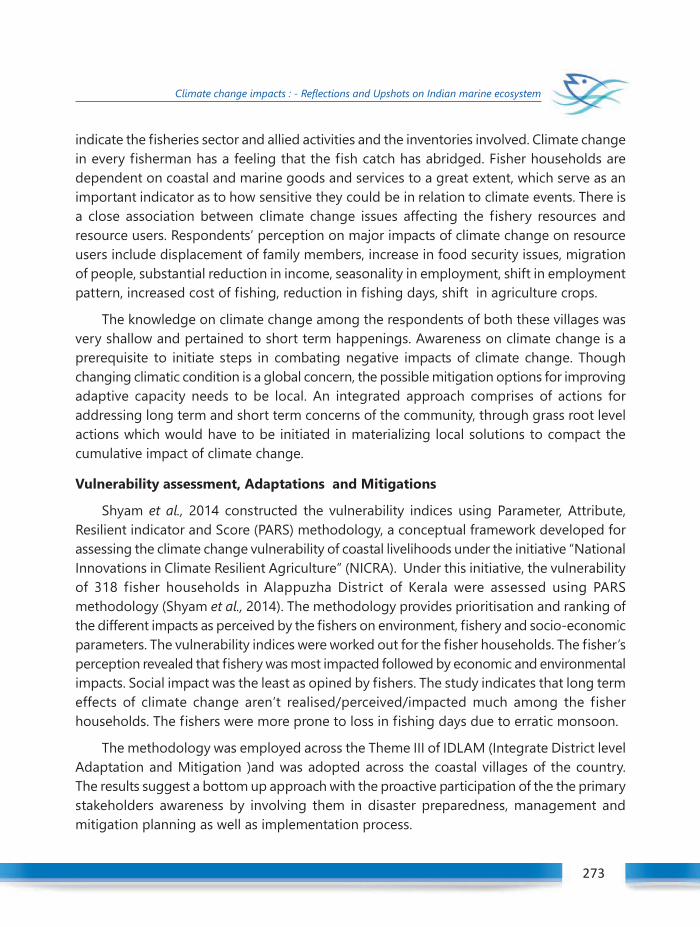
Winter School on Structure and Function of the Marine Ecosystem : Fisheries 273
Climate change impacts : - Reflections and Upshots on Indian marine ecosystem
273
indicate the fisheries sector and allied activities and the inventories involved. Climate changein every fisherman has a feeling that the fish catch has abridged. Fisher households aredependent on coastal and marine goods and services to a great extent, which serve as animportant indicator as to how sensitive they could be in relation to climate events. There isa close association between climate change issues affecting the fishery resources andresource users. Respondents’ perception on major impacts of climate change on resourceusers include displacement of family members, increase in food security issues, migrationof people, substantial reduction in income, seasonality in employment, shift in employmentpattern, increased cost of fishing, reduction in fishing days, shift in agriculture crops.
The knowledge on climate change among the respondents of both these villages wasvery shallow and pertained to short term happenings. Awareness on climate change is aprerequisite to initiate steps in combating negative impacts of climate change. Thoughchanging climatic condition is a global concern, the possible mitigation options for improvingadaptive capacity needs to be local. An integrated approach comprises of actions foraddressing long term and short term concerns of the community, through grass root levelactions which would have to be initiated in materializing local solutions to compact thecumulative impact of climate change.
Vulnerability assessment, Adaptations and Mitigations
Shyam et al., 2014 constructed the vulnerability indices using Parameter, Attribute,Resilient indicator and Score (PARS) methodology, a conceptual framework developed forassessing the climate change vulnerability of coastal livelihoods under the initiative “NationalInnovations in Climate Resilient Agriculture” (NICRA). Under this initiative, the vulnerabilityof 318 fisher households in Alappuzha District of Kerala were assessed using PARSmethodology (Shyam et al., 2014). The methodology provides prioritisation and ranking ofthe different impacts as perceived by the fishers on environment, fishery and socio-economicparameters. The vulnerability indices were worked out for the fisher households. The fisher’sperception revealed that fishery was most impacted followed by economic and environmentalimpacts. Social impact was the least as opined by fishers. The study indicates that long termeffects of climate change aren’t realised/perceived/impacted much among the fisherhouseholds. The fishers were more prone to loss in fishing days due to erratic monsoon.
The methodology was employed across the Theme III of IDLAM (Integrate District levelAdaptation and Mitigation )and was adopted across the coastal villages of the country.The results suggest a bottom up approach with the proactive participation of the the primarystakeholders awareness by involving them in disaster preparedness, management andmitigation planning as well as implementation process.
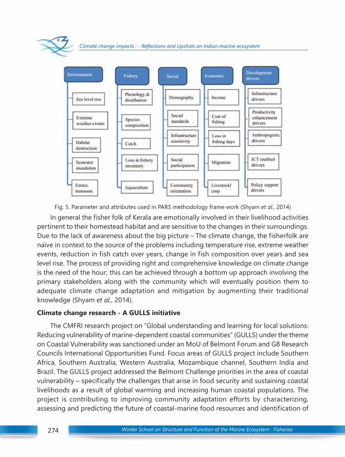
Winter School on Structure and Function of the Marine Ecosystem : Fisheries274
Climate change impacts : - Reflections and Upshots on Indian marine ecosystem
In general the fisher folk of Kerala are emotionally involved in their livelihood activitiespertinent to their homestead habitat and are sensitive to the changes in their surroundings.Due to the lack of awareness about the big picture – The climate change, the fisherfolk arenaïve in context to the source of the problems including temperature rise, extreme weatherevents, reduction in fish catch over years, change in fish composition over years and sealevel rise. The process of providing right and comprehensive knowledge on climate changeis the need of the hour; this can be achieved through a bottom up approach involving theprimary stakeholders along with the community which will eventually position them toadequate climate change adaptation and mitigation by augmenting their traditionalknowledge (Shyam et al., 2014).
Climate change research - A GULLS initiative
The CMFRI research project on “Global understanding and learning for local solutions:Reducing vulnerability of marine-dependent coastal communities” (GULLS) under the themeon Coastal Vulnerability was sanctioned under an MoU of Belmont Forum and G8 ResearchCouncils International Opportunities Fund. Focus areas of GULLS project include SouthernAfrica, Southern Australia, Western Australia, Mozambique channel, Southern India andBrazil. The GULLS project addressed the Belmont Challenge priorities in the area of coastalvulnerability – specifically the challenges that arise in food security and sustaining coastallivelihoods as a result of global warming and increasing human coastal populations. Theproject is contributing to improving community adaptation efforts by characterizing,assessing and predicting the future of coastal-marine food resources and identification of
Fig. 5. Parameter and attributes used in PARS methodology frame work (Shyam et al., 2014)

Winter School on Structure and Function of the Marine Ecosystem : Fisheries 275
Climate change impacts : - Reflections and Upshots on Indian marine ecosystem
275
suitable adaptation options. The rationale for selection of the focus area included earlyobservation of the impacts, strong incentives to initiate adaptive strategies, developingmodels for early prediction and validation, developing adaptation options and testing forchallenges to be met efficiently and effectively.
Fig. 6. Vulnerability model
Identification of climate change hot spots
Since hot spots in climate change parlance has not been identified yet in Indian context,it is high time to define and identify climate change hot spots in India to initiatecomprehensive planning for adaptation and conservation measures. In this context Climatechange Hot spots –can be defined as the ‘‘live labs’ where the manifestation of the climatechange impacts are observed “first”. The identification of the climate change hot spotswould help policy makers in priority setting and in planning adaptation and conservationmeasures.
The coastal vulnerability assessment in GULLS project underlines, a demarcation betweenfishery hotspots (based on fish abundance, phenology, distribution, range shifts, recruitmentsuccess etc.) and social hotspots (determining vulnerability, displacement, marginalizationof traditional community) would be a novel idea to have representation of diverse factors inthe project. Consistent with the objectives of GULLS, the activities will be aiming at assessing

Winter School on Structure and Function of the Marine Ecosystem : Fisheries276
Climate change impacts : - Reflections and Upshots on Indian marine ecosystem
the current status of the fishery resources and ecosystem services and would attempt atpredicting the future impacts of climate change on these resources and services apart fromidentification of key vulnerable marine species to climate change and assessing thecommunity vulnerability.
The review done in addition to the discussions with the Belmont team resulted in boilingdown the hotpsot region to (South West and South East Region of India).The South EastIndia encompassing Ramanathapuram and Tuticorin districts of Tamil Nadu could be one ofthe Hotspot and the other be South West India(coastal districts of Kerala including Ernakulum,Alappuzha, Kollam and Trivandrum) with fisheries abundance and distribution shifts.
Fig.7. Hemisphere hotspots ocean regions experiencing fast warming and those with heightened socialtensions as a result of change.
Vulnerability of coastal regions will be characterized using a linked socio-economic andecological vulnerability model .The project will be in operation in the different hotspots andwill lead to build regional skill-sets that can reduce coastal vulnerability by evaluating andcharacterizing likely impacts, create predictive systems that will inform decision makersabout the expected consequences of coastal changes; deliver alternative options in termsof adaptation and transformation within coastal communities; and to define the long-termimplications of selecting a particular option in terms of economic, social and environmental

Winter School on Structure and Function of the Marine Ecosystem : Fisheries 277
Climate change impacts : - Reflections and Upshots on Indian marine ecosystem
277
outcomes. Thus, along Kerala, two major fishing villages namely Elamkunnapuzha ofErnakulam district and Poonthura of Thiruvananthapuram district in the south west hotspotsof India was selected under GULLS project to assess the overall vulnerability of fisherybased livelihood due to the impact of climate variation.
A composite vulnerability index approach was used in this study to evaluate relativeexposure, sensitivity, and adaptive capacity (Islam et al., 2014). The mean values of thethree sub-indices of Exposure (E), Sensitivity (S), and Adaptive Capacity (AC) were combinedto develop a composite vulnerability index by using the following additive (averaging)equation (Islam et al., 2014).
Vulnerability (V) = Exposure (E) + Sensitivity (S) - Adaptive Capacity (AC)
The overall vulnerability values indicate that Poonthura village is slightly more vulnerablethan Elamkunnapuzha . The proximity of Poonthura village to the sea can be attributed asthe major factor contributing the increase in vulnerability compared to Elamkunnapuzha. Inaddition higher exposure on account of environmental changes, occurrence of droughtand shoreline changes is also attributed to higher vulnerability in Poonthura. However, the
(Modified form IPCC climate change vulnerability frame work)Fig 8 . Conceptual Frame work of GULLS Fisheries Climate Change Vulnerability Assessment

Winter School on Structure and Function of the Marine Ecosystem : Fisheries278
Climate change impacts : - Reflections and Upshots on Indian marine ecosystem
sensitivity values are high in Elamkunnapuzha when compared to Poonthura due to highsocial dependence, economic dependence on other resources as well as historical and culturaldependence on fishing. The adaptive capacity of the selected villages were low whencompared to exposure and sensitivity values, indicating the urgent need for developingappropriate adaptive interventions. Therefore, more adaptation options like better policyframework, proper planning measures, and effective disaster management techniques shouldbe implemented to increase the adaptive capacity of the fishermen community to climatechange. Improvement of natural capital like steps to curb marine pollution, maintainingprey-predator relationship in the oceans, promoting the culture of species in marine habitats(Cage culture), regulation of fishing rights across the Indian seas, extending the period oftrawl ban so as to prevent the recruitment of juveniles entering the fishery maybe lookedinto as major elements while framing adaptation options.
CReVAMP’ – “Climate Resilient Village Adaptation and Mitigation Plan”
A new framework titled ‘CReVAMP’ – “Climate Resilient Village Adaptation and MitigationPlan” conceptualised for planning and implementing village level adaption and mitigationplan which is given in the figure no 9. Consistent with the project objectives, CReVAMP isdeveloped to identify existing climate adaptation and mitigation- probing alternatives andtheir trade-offs, sensitizing and improving the resilience of community towards climatechange and initiating a multi stakeholders platform for developing a climate knowledgeand information systems. The ‘CReVAMP’ framework presents major elements andapproaches through which the desirable outcome is envisaged across different playersincluding individuals, community and the government. This also offers room for definingthe ‘elements’ and ‘approaches’ in accordance with the village scenario and also for iterativeplanning of participatory as well as systems-based approaches under which different activitiescould be implemented with stakeholder engagement for achieving desirable outcome.Considering the sustainability of the adaption and mitigation activities even after the projectperiod, involvement of the climate change agents in the entire process is vital and we haveidentified a group of people with representation from different age, gender and experience,encompassing articulate children, proactive youth, experienced fishers and committedwomen as climate change agents in the project. This framework is centered on people andit would help different practitioners to synergize their thoughts and ideas towards planningand implementing different adaptation and mitigation programs thereby helping thecommunity to become climate resilient. In GULLS project we are adopting an integratedapproach which would synergize the knowledge system of scientific and indigenousknowledge between the researchers and different stakeholders of the community. It is abalancing act between (i) ‘Top Down and Bottom up Approaches’, (ii) Prioritized needs ofexperts and felt need of the communities, (iii) Scientific Knowledge and Traditional wisdom,

Winter School on Structure and Function of the Marine Ecosystem : Fisheries 279
Climate change impacts : - Reflections and Upshots on Indian marine ecosystem
279
(IV) Community Solutions and Policy Solutions. This process would be facilitated using multistakeholder governance model by bringing different stakeholders together to participatein the dialogue, decision making, and knowledge sharing and there by instigate knowledgegeneration process within the community during the course of the process. The wholeprocess is directed to create village information system within the community, enable greenfishing practices and prepare A&M plan for a community which would in turn helps incommunity empowerment, thus enabling in building resilient community /Climate ChangeInformed Fisher Community (CCIF). The CCIF is expected to influence the society andgovernment in decision making and actions related to climate change mitigation and wouldeventually be able to influence the policy making process.
Fig. 9. CReVAMP Model- Climate Resilient Village Adaptation and Mitigation Plan
Various Phases are involved in the implementation of CReVAMP which are listed belowin the table. These phases could be made operational withPhase I Identification of hot spot areas / districts/ delineation of villagesPhase II Linkages with Department of Fisheries ( DoF, Local Self Government(LSG)Phase III Conduct baseline and household vulnerability surveyPhase IV Developing reports / Conducting awareness workshops / Engagement of fishers in climate
change activitiesPhase V Creation of Climate Information KiosksPhase VI Formation of climate change communitiesPhase VII Planning and implementation of Adaptation and Mitigation plansPhase VIII Climate resilient village adaptation and mitigation plan (CReVAMP) with Climate Change
informed fishers.
Winter School on Structure and Function of the Marine Ecosystem : Fisheries280
Climate change impacts : - Reflections and Upshots on Indian marine ecosystem
Way Forward
Climate change is no unidirectional issue, it brings along with its effects on both theresources and resource users, thus the adaptation to it should ensure that the multifariousimpacts it brings along can be tackled. Development cannot be ceased, nor can exploitationbe hailed, the key to successful climate change adaptation is implementing sustainabledevelopment through incentive based polices and empowering the economically weakersections of the society with environmentally friendly livelihoods. This could be achievedthrough ’blue economy’ which is a recently developed business model which will shiftsociety from scarcity to abundance “with what is locally available”, by tackling issues thatcause environmental and related problems in new ways. Blue economy could enhance theocean technologies, provide marine governance, helps to improve ocean health and managecoastal urbanization. It is the marine based economic development which improves thehuman well -being and also social equity which in general greatly decreases theenvironmental risks and ecological scarcities.
References
Attrill, M.J. (2002) Community-level indicators of stress in aquatic ecosystems. In: Adams, S.M. (ed.), BiologicalIndicators of Ecosystem Stress. American Fisheries Society, Bethesda, MD, pp. 473–508.
Barton, B.A., Morgan, J.D. and Vijayan, M.M. (2002) Physiological and condition-related indicators ofenvironmental stress in fish. In: Adams, S.M. (ed.), Biological Indicators of Ecosystem Stress. AmericanFisheries Society, Bethesda, MD, pp. 111–148
Barton, M. and Barton, A.C. (1987) Effects of salinity on oxygen consumption of Cyprinodon variegatus.Copeia 1987, 230–232.
Boesch, D.F. and Turner, R.E. (1984) Dependence of fishery species on salt marshes: the role of food andrefuge. Estuaries 7, 460–468.
CMFRI (2008) Research Highlights 2007-2008. Central Marine Fisheries Research Institute, Cochin, India,pp. 36.
Dasgupta, S., B. Laplante, S. Murray and D. Wheeler, 2009. Sea-level rise and storm surges. A comparativeanalysis of impacts in developing countries. World Bank Development Research Group, Policy ResearchWorking Paper, 4901: 43 pp
Donaldson, E.M. (1990) Reproductive indices as measures of the effects of environmental stressors. Am.Fish. Soc. Symp. 8, 145–166.
Fischlin, A., Midgley, G. F., Price, J. T., Leemans, R., Gopal, B., Turley, C., Rounsevell, M. D. A., et al., 2007.Ecosystems, their properties, goods, and services. In Climate Change 2007: Impacts, Adaptation andVulnerability, pp. 211–272. Ed. by M. L. Parry, O. F. Canziani, J. P. Palutikof, P. J. van der Linden, and C. E.Hanson. Contribution of Working Group II to the Fourth Assessment Report of the IntergovernmentalPanel on Climate Change. Cambridge University Press, Cambridge.
Winter School on Structure and Function of the Marine Ecosystem : Fisheries 281
Climate change impacts : - Reflections and Upshots on Indian marine ecosystem
281
IPCC (Intergovernmental Panel on Climate Change) (2001) Coastal zones and marine ecosystems. In:McCarthy, J.J., Canziani, O.F., Leary, N.A., Dokken, D.J. and White, K.S. (ed.), Climate Change 2001:Impacts, Adaptation, and Vulnerability.Cambridge University Press, UK, 1032 pp.
IPCC. 2007. Impacts, Adaptation and Vulnerability summary for policy makers. IPCC Working Group II,Fourth Assessment Report, 16 pp.
Kennedy, V. S., Twilley, R. R., Kleypas, J. A., Cowan Jr., J. H., Hare, S. R. (2002): Coastal and marine ecosystems& global climate change. Potential effects on U S resources. Pew Center on Global Climate Change,Arlington, USA, pp. 52.
Kim, J.Y. and N.C.H. Lo. 2001. Temporal variation of seasonality of egg production and the spawning biomassof Pacific anchovy, Engraulis Japonicus, in the southern waters of Korea. Fish. Oceanogr. 10(3), 297-310.
McCarthy, J. J., Canziani, O. F., Leary, N. A., Dokken, D. J., and White, K. S. (Eds). 2001. Climate Change 2001:Impacts, Adaptation, and Vulnerability. Contribution of Working Group II to the Third AssessmentReport of the Intergovernmental Panel on Climate Change. Cambridge University Press, Cambridge.1032 pp.
McGinn, N.A. 2002. Fisheries in a Changing Climate. American Fisheries Society Symposium 32, Bethesda,MD, 295 pp.
Miller, K.A. and Fluharty, D.L. (1992) El Nin˜o and variability in the northeastern Pacific salmon fishery:implications for coping with climate change. In: Glantz, M. (ed.), Climate Variability, Climate Changeand Fisheries. Cambridge University Press, UK, pp. 49–88.
Moyle, P. B. and Cech, Jr. J.J. 2004. Fishes: An Introduction to Ichthyology, 5th Ed. Prentice Hall, UpperSaddle River, NJ, 726 pp.
Murawski, S.A. (1993) Climate change and marine fish distributions: forecasting from historical analogy.Trans. Am. Fish. Soc. 122, 647–658.
Nye, J. A., Link, J. S., Hare, J. A., and Overholtz, W. J. 2009. Changing spatial distribution of fish stocks inrelation to climate and population size on the Northeast United States continental shelf. Marine EcologyProgress Series, 393: 111–129.
Ottersen, G., Planque, B., Belgrano, A., Post, E., Reid, P. C., and Stenseth, N. C. 2001. Ecological effects of theNorth Atlantic Oscillation. Oceologia, 128: 1–14.
Pauly, D. and Christensen, V. (1995) Primary production required to sustain global fisheries. Science 374,255–257.
Perry, A. L., Low, P. J., Ellis, J. R., Reynolds, J. D. (2005). Climate change and distribution shifts in marine fishes.Science 308, 1912 – 1915.
Portner, H.O., Berdal, B., Blust, R., Brix, O., Colosimo, A., De Wachter, B., Giuliani, A., Johansen, T., Fischer, T.,Knust, R., Lannig, G., Naevdal, G., Nedenes, A., Nyhammer, G., Sartoris, F.J., Serendero, I., Sirabella, P.,Thorkildsen, S. and Zakhartsev, M. (2001) Climate induced temperature effects on growth performance,fecundity and recruitment in marine fish: developing a hypothesis for cause and effect relationshipsin Atlantic cod (Gadus morhua) and common eelpout (Zoarces viviparus). Cont. Shelf Res. 21, 1975–1997.
Prasanna Kumar, S., Raj P. Roshin, Jayu Narvekar, P.K. Dinesh Kumar and E. Vivekanandan, 2009. Responseof the Arabian Sea to global warming and associated regional climate shift. Marine EnvironmentalResearch, 68: 217-222
Winter School on Structure and Function of the Marine Ecosystem : Fisheries282
Climate change impacts : - Reflections and Upshots on Indian marine ecosystem
Rose, G. A. and Leggett, W.C. (1988) Atmosphere-ocean coupling and Atlantic cod migrations: effects ofwind-forced variations in sea temperatures and currents on nearshore distributions and catch rates ofGadus morhua. Can. J. Fish. Aquat. Sci. 45, 1234–1243.
Ruiz, G.M., Hines, A.H. and Posey, M.H. (1993) Shallow water as a refuge habitat for fishes and crustaceansin nonvegetated estuaries: An example from Chesapeake Bay. Mar. Ecol. Prog. Ser. 99, 1–16.
Sanil Kumar, V., K.C. Pathak, P. Pednekar, N.S.N. Raju and R. Gowthaman, 2006. Coastal processes along theIndian coastline. Curr. Sci., 91: 530-536.
Shyam, S. Salim and Kripa, V. and Zacharia, P. U. and Mohan, Anjana and Ambrose, T. V. andManjurani, (2014) Vulnerability assessment of coastal fisher households in Kerala: A climate changeperspective. Indian Journal of Fisheries, 61 (4). pp. 99-104.
Shyam, S. Salim and Sathianandan, T. V. and Swathi Lekshmi, P. S. and Narayanakumar, R. and Zacharia, P.U. and Rohit, Prathibha and Manjusha, U. and Antony, Bindu and Safeena, P. K. and Sridhar, N. andRahman, M. Ramees and Jayakumar, Rajani and Kumar, Nimmy S. and Nimisha, C. P. (2015). Assessmentof fishers perception in developing climate change adaptation and mitigation plans. Journal of theMarine Biological Association of India, 57 (1). pp. 21-30. ISSN 2321-7898.
Shyam, S. Salim and Manjusha, U. (2015) Climate change impacts: Implications on marine resources andresource users. [Teaching Resource]
Smitha, B. R; V. N. Sanjeevan, K. G. V. Kumar, and C. Revichandran. On the upwelling off the southern tip andalong the west coast of india. Journal of Coastal Research, 24: 95–102, 2008.
Soto, C.G. (2002) The potential impacts of global climate change on marine protected areas. Rev. Fish Biol.Fish. 11, 181–195.
Timmermann, A., Oberhuber, J., Bacher, A., Esch, M., Latif, M. and Roeckner, E. (1999) Increased El Nin˜ofrequency in a climate model forced by future greenhouse warming. Nature 398, 694–696.
Valdivia, J., 1976. Aspectos biolo´ gicos del Feno´ meno El Nin˜ o 1972–73. Parte I: La poblacio´ n de anchoveta.In: Proceedings of the Workshop El Nin˜ o, Guayaquil, Ecuador, 4–12 December 1974. FAO Fishing Inf.185, 80–93.
Vivekanandan, E, and Rajagopalan, M (2009): Impact of rise in seawater temperature on the spawning ofthreadfin breams. In: Aggarwal P K (Ed.) Impact, Adaptation and Vulnerability of Indian Agriculture toClimate Change, Indian Council of Agricultural Research, New Delhi (in press).
Vivekanandan, E, Hussain Ali, M, Rajagopalan, M (2009b): Vulnerability of corals to seawater warming. In:Aggarwal, P K (ed) Impact, Adaptation and Vulnerability of Indian Agriculture to Climate Change,Indian Council of Agricultural Research, New Delhi
Vivekanandan, E, Rajagopalan, M, Pillai, N G K (2009a): Recent trends in sea surface temperature and itsimpact on oil sardine. In: Aggarwal P K (Ed) Impact, Adaptation and Vulnerability of Indian Agricultureto Climate Change,Indian Council of Agricultural Research, New Delhi
Vivekanandan, E, Srinath, M and Somy Kuriakose (2005): Fishing the food web along the Indian coast.Fisheries Research, 72, 241- 252.
Wainwright, P.C. (1994) Functional morphology as a tool in ecological research. In: Wainwright, P.C. andReilly, S.M. (eds.), Functional Morphology: Integrative Organismal Biology. Chicago University Press,IL, pp. 42–59.

Winter School on Structure and Function of the Marine Ecosystem : Fisheries 283
Climate change impacts : - Reflections and Upshots on Indian marine ecosystem
283
Walther, G-R., Post, E., Convey, P., Menzel, A., Parmesan, C., Beebee, T. J., Fromentin, J-M., et al., 2002.Ecological responses to recent climate change. Nature, 416: 389–395.
Zuta, S., Enfield, D., Valdivia, J., Lakes, P., Blandin, C., 1976. Physical aspects of 1972–73 El Nin˜ o event. In:Proceedings of the Workshop El Nin˜ o, Guayaquil, Ecuador, 4–12 December 1974. FAO Fishing Inf.185, 3–61.
Winter School on Structure and Function of the Marine Ecosystem : Fisheries284
Changes in Environment: Implications for fisheries in Indian waters
Introduction
The coastal and marine ecosystems are dynamic and the seasonal and inter-annualfluctuations of the abiotic ecological parameters reflect on the biological functioning of theplankton, nekton and all other biota. Apart from the natural variations, anthropogenic impactsincluding climate change and habitat degradations and alterations have affected thesustainability, productivity and diversity of almost all critical habitats like the mangroves, seagrasses and the coral reefs. Each critical habitat has its own unique characteristics and thebiota which depend on these have suitable adaptive characters to survive, grow and reproducein these. However, variations which are significantly wide and large lead to mis-matches eco-biological links. These affect the recruitment of the species which cascades down the foodweb and the fisheries. Some of the major environmental factors are the monsoon andupwelling and specifically, if we take environmental variables like sea surface temperature,oxygen, salinity and nutrients. Similarly habitat alterations due to marine litter and shrinkingof habitats due to land filling and other activities have severely affected the estuarine fauna.
The Indian fisheries is composed of major small pelagic fishes like sardine, mackereland anchovies; the large pelagic like the tunas and bill fishes, several demersals andshellfishes. Also, the ecological characters of the west coast which is influenced by upwellingis different from east coast. A brief description of the variations in environmental factorsand their impact on the fisheries is given below.
Natural variations in ecosystems and impacts on fisheries
Upwelling and fisheries
Upwelling is a process in which deep, cold water rises toward the surface. Upwellingoccurs when winds push surface water away from the shore and are replaced by cold,nutrient-rich water that wells up from below. Deep ocean water is more nutrient-rich thansurface water as nutrients, dead and decaying plankton and other fish carcasses sink to thebottom. During upwelling these are brought back to the surface and these fertile systemssupport blooming of diatoms and zooplankton. This rich food supports growth andmaturation of several fishes. Along the Indian west coast, upwelling is strong along Keralacoast and is known to occur in varying intensities. El-Nino has been found to affect theintensity of upwelling.
33C H A P T E R CHANGES IN ENVIRONMENT: IMPLICATIONS
FOR FISHERIES IN INDIAN WATERSV. Kripa
Fishery Environment Management DivisionICAR-Central Marine Fisheries Research Institute
Winter School on Structure and Function of the Marine Ecosystem : Fisheries 285
Changes in Environment: Implications for fisheries in Indian waters
285
Along Kerala –Karnataka coast upwelling sets in by May –June and the rich food availableprepares the pelagic fishes especially sardine for spawning. When upwelling is poor, themajor factors supporting gonad development like blooming of diatoms and lowering ofambient temperature does not happen and this can lead to poor maturation or delayedmaturation. In 2015, upwelling was poor and maturation was affected.
Upwelling can also bring in low oxygen water which can lead to hypoxic conditions.Sometimes along Kerala coast, low oxygen in upwelled waters can be seen in the sardinehabitat during August –September. If the dissolved oxygen levels are below one ml /l thenthis has been found to affect recruitment and the fishery. Low mixing of waters can causestratification and along with hypoxic conditions cause stress to the early life stages.
Monsoon and Fisheries
When maturation is largely influenced by upwelling, the onset and intensity of southwestmonsoon has a good influence on spawning and recruitment of pelagic fishes like sardine.Though there is no direct affect, the changes triggered by monsoon especially the bloomingof plankton in near-shore waters supports early larval development. The high levels ofphosphate, nitrate and silicate in the river runoff triggers and supports blooming of diatoms.These support the large shoals of early life stages of sardine. Similarly, there will be negativeimpacts when the river runoff is high and there is no proper mixing. This can lead tostratification and adversely affect recruitment.
Temperature-Food combination and links with El nino
Globally, 2015 has been considered as a warm year with high temperature and lowfood. The average seawater temperature in sardine habitat was 29.8o C during 2015, whichis nearly 1.1 oC higher than the average observed (28.6 o C) for the last 5 years. Positive SSTAexceeding 0.6 oC dominated in the tropical Indian Ocean. There was a substantial warmingin the tropical Indian Ocean, partially due to influences of the 2015 El Nino. The mean SSTin the tropical Indian Ocean was reported to increase by 0.13-0.2oC in 2015. Phytoplanktondensity was also low during April/ May 2015 compared to the high during 2012. This lowfood availability in the habitat was found to affect maturation which resulted in poorrecruitment.
Environment changes and recruitmentTwo important theories in ecology have been found to be applicable to the Indian
fisheries scenario. The theory of Optimal Environmental Window (OEW) states that inupwelling.
Systems, wind, storm, and other energetic events cause turbulence that, within an optimalrange, increase larval recruitment; dependent upon the presence/ absences of Ekman
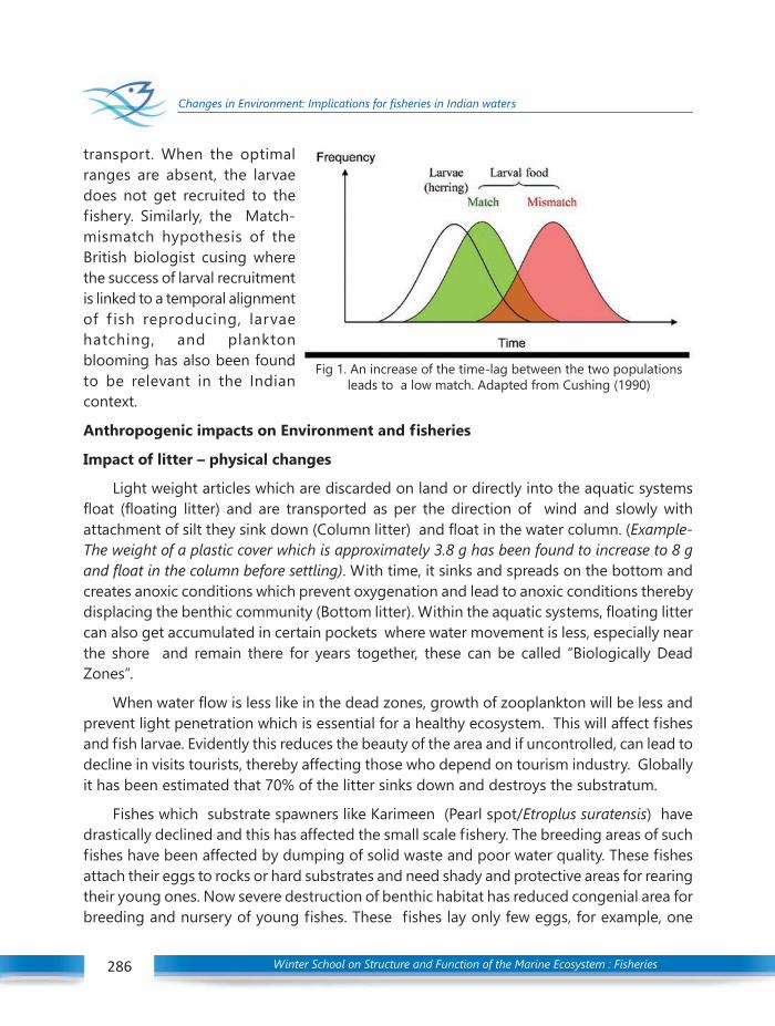
Winter School on Structure and Function of the Marine Ecosystem : Fisheries286
Changes in Environment: Implications for fisheries in Indian waters
transport. When the optimalranges are absent, the larvaedoes not get recruited to thefishery. Similarly, the Match-mismatch hypothesis of theBritish biologist cusing wherethe success of larval recruitmentis linked to a temporal alignmentof f ish reproducing, larvaehatching, and planktonblooming has also been foundto be relevant in the Indiancontext.
Anthropogenic impacts on Environment and fisheries
Impact of litter – physical changes
Light weight articles which are discarded on land or directly into the aquatic systemsfloat (floating litter) and are transported as per the direction of wind and slowly withattachment of silt they sink down (Column litter) and float in the water column. (Example-The weight of a plastic cover which is approximately 3.8 g has been found to increase to 8 gand float in the column before settling). With time, it sinks and spreads on the bottom andcreates anoxic conditions which prevent oxygenation and lead to anoxic conditions therebydisplacing the benthic community (Bottom litter). Within the aquatic systems, floating littercan also get accumulated in certain pockets where water movement is less, especially nearthe shore and remain there for years together, these can be called “Biologically DeadZones”.
When water flow is less like in the dead zones, growth of zooplankton will be less andprevent light penetration which is essential for a healthy ecosystem. This will affect fishesand fish larvae. Evidently this reduces the beauty of the area and if uncontrolled, can lead todecline in visits tourists, thereby affecting those who depend on tourism industry. Globallyit has been estimated that 70% of the litter sinks down and destroys the substratum.
Fishes which substrate spawners like Karimeen (Pearl spot/Etroplus suratensis) havedrastically declined and this has affected the small scale fishery. The breeding areas of suchfishes have been affected by dumping of solid waste and poor water quality. These fishesattach their eggs to rocks or hard substrates and need shady and protective areas for rearingtheir young ones. Now severe destruction of benthic habitat has reduced congenial area forbreeding and nursery of young fishes. These fishes lay only few eggs, for example, one
Fig 1. An increase of the time-lag between the two populationsleads to a low match. Adapted from Cushing (1990)

Winter School on Structure and Function of the Marine Ecosystem : Fisheries 287
Changes in Environment: Implications for fisheries in Indian waters
287
pearl spot produces about 2700 eggs per spawning which is low compared to fishes likemullets and sardines. Hence these are more vulnerable to habitat loss.
Floating and submerged debris has reduced the habitat area available for the fishesand thus has reduced the biomass of fishes. The commercially important benthic resourceslike crabs, shrimps and clams are the most affected by benthic habitat destruction. Dumpingof solid waste from slaughter houses and its decaying also adds to poor water quality.Clogging of canals by plastics and other litter has led to increased sedimentation and reducedthe depth of the estuary. Lack of water flow has caused low oxygen condition which hasalso reduced the quantity of plankton available as food for the fishes.
The surveys conducted on the seed availability have clearly indicated a significant declinein seed resources of all species of shrimps in Vembanad Lake. Peneaus (Fennerpenaeus)indicus, Penaeus mondoan, Metapenaeus dobsoni, Metapenaeus monoceros and Metapenaeusaffinis. This is reflected in the shrimp catches of stake net units where the catch per uniteffort has declined from 3.2 kg in 1997 to an average of 0.508 kg indicating nearly 84%decline.
The abundance of all species of shrimp seed in Cochin backwaters has declined drasticallyduring the last two and half decades. Surveys conducted in 2013 have indicated that themajor resources like white shrimp (Fenneropenaeus indicus and Metapenaeus dobsoni) havedeclined. Shrimp seed mainly feed on detritus; now the backwaters substrates haveconsiderable quantity of litter. Survey results have indicated that traditional shrimp farmsare affected by low shrimp seed availability.
When efforts are made to remove solid waste from land, there are no programs forremoving litter accumulated in rivers, estuaries and sea. Since estuaries which are criticalhabitats are already impacted byuntreated effluents from industries, directdumping of solid wastes, invasion ofaquatic weeds, reduced water flow, highsiltation and landing filling there is anurgent need to initiate programs tocontrol these and start restorationprograms.
Habitat alterations
Shrinking of estuarine areas due toreclamation, sand mining, excessivesedimentation due to physical manmade
Fig. 2. A branch of estuarine canal completely cloggedby invasive aquatic weed in Cochin backwaters
Winter School on Structure and Function of the Marine Ecosystem : Fisheries288
Changes in Environment: Implications for fisheries in Indian waters
barriers and degradation of critical habitats like mangroves and sea grasses have affectedthe structure and ecosystem services of these aquatic systems. The most affected areas arethe coastal wet lands. The increase in floating weeds and clogging of estuarine branches bythe invasion of these weeds have affected fishers, especially the clam fishers.
Increasing incidences of harmful algal blooms
Globally, the intensity and frequency of occurrence of HABs have increased. Indianfisheries is also affected by blooms of Noctiluca sp, Tricodesmium sp and other dinoflagellateblooms. These reduce the diversity of phytoplankton community and create imbalances inthe plankton community. These are found more during the late monsoon or early premonsoon which is a major spawning period of both pelagic and demersal fishes.
Increasing incidences of jelly fishes
Along both the coasts, the jelly fishes have increased in number. Only few speciesbloom. But the occurrence of hydrozoan and schyphozoan medusae in the coastal watershave led to decrease in fishing days and also low fish catches in seines and trawlers. Thespread of jelly fishes in the estuarine areas due to salinity intrusion has also createdconsiderable problems to inshore gill netters. Globally jellyfishes are considered as a threatto fisheries. The major reasons for this new problem is considered as eutrophication, increasedepisodes of hypoxic conditions and spread of underwater structures which serve as a nichefor the dormant stages of jellyfishes.
Conclusion
The influence of environmental variations on the productivity of the aquatic systemsand the fishery of the area has become more evident now. The impact of fluctuations inseasons and intensity of natural ecological variations on the recruitment of major fisheryresources is slowly being understood. There is an urgent need to have deeper understandingof these eco-biological links and develop the skill to predict the impacts under differentscenarios. This would help to increase the preparedness of the fishers against fishery declines.
Though, there are rules protecting the habitats from unplanned human activities, theseare not strictly implemented. Understanding the need to reduce the anthropogenic activitieson habitats, it is suggested that micro- level environment management plans are developedin close association with the researchers and the coastal villagers. Effective implementationof co-management systems would help in effective governance.
Winter School on Structure and Function of the Marine Ecosystem : Fisheries 289
El Niño and its impact on coral reef ecosystem in the Eastern Indian Ocean
Introduction
The coral reef bleaching associated with the elevated Ocean temperature has beenwidely reported in the last three decades from different regions of the world. The risingtemperature and acidification of Oceans makes a big challenge for the survival of reefs inthe world. The other important stresses for the reefs include increased UV radiation, sealevel variations, suspended sediments and increased turbidity of water. There are differentstudies which relate bleaching events with global warming and climate change. However,the increased frequency of mass bleaching events could not be sufficiently explained withcurrent warming rates of the Ocean. Stone et al., (1999) put forward a new theory thatrecent increases in mass bleaching events were in response to the relative increase in ElNiño experienced over the last two decades. The bleaching threshold temperature is sitedependent and it may vary from one reef region to other. The threshold temperature forthe Indian reefs is approximately 31°C (Vivekanandan et al., 2008). In the Indian Ocean, thecoral reefs around the Andaman Islands suffered bleaching events during 1998, 2002, 2005,2010 and 2016. In the Andaman Sea, the rise in temperature was abnormal during 1998 and2010 and hence mass bleaching events were happened during that period (Krishnan et al.,2011; Vivekanandan et al., 2008). The coral reef bleaching associated with warm wateranomalies in the Pacific Ocean during an El Niño period is well studied and documented.However, the link between the massive bleaching events in the Indian Ocean and El Niño isnot straightforward as in the Pacific. For example, the massive bleaching event of 1998 inthe Indian Ocean was happened in May and that was a transition period from a strong ElNiño to a strong La Niña in the Pacific. Hence, in the Indian Ocean, the role of El Niño in themass coral reef bleaching event of 1997-98 was not clear (Wilkinson, 1999). Moreover, theocean temperature variability in the Indian Ocean can be significantly modulated by thedifferent regional processes in the Indian Ocean itself such as Indian Ocean Dipole, formationof cyclone, early arrival of monsoon etc. However, a recent study shows that massive bleachingevents in the Andaman reefs of the Indian Ocean is directly linked with the strong El Niñoevents in the Pacific Ocean (Lix et al., 2016). The atmospheric teleconnections between thetwo Ocean basins is the primary reason for this link.
03C H A P T E R
34C H A P T E R EL NIÑO AND ITS IMPACT ON CORAL REEF
ECOSYSTEM IN THE EASTERN INDIAN OCEANLix J. K.1, Sajeev R.1, Grinson George2, Santosh K. M.1 and Phiros Shah2
1Cochin University of Science and Technology, Kochi2ICAR-Central Marine Fisheries Research Institute

Winter School on Structure and Function of the Marine Ecosystem : Fisheries290
El Niño and its impact on coral reef ecosystem in the Eastern Indian Ocean
Hot spot Method
By using long term satellite data sets, Goreau and Hayes (1994) developed a ‘hot spot’method to predict the possibility of bleaching events in the reef region. A hot spot is thearea of the ocean with sea surface temperature anomalies over 1°C above long-term averagesof monthly maximum. AVHRR Pathfinder SST with 4x4 km resolution that available from1982 onwards can be used to estimate the hot spot area.
Hot Spot = Weekly average SST – Monthly Mean Maximum Climatology
Hot spot products based on satellite data sets is also directly available from NOAAcoral reef watch program. The details of the NOAA products such as hot spot, degree heatingweek, bleaching alert area, SST anomaly are available in the NOAA website https://coralreefwatch.noaa.gov/satellite/index.php. If the hot spot anomaly greater than 1°C existsfor greater than or equal to 4 weeks, there is a strong chance for severe bleaching. Hot spotregion around the Andaman reefs for a mass bleaching event (2010) and non bleachingevent (2011) is shown in figure 1 and figure 2.
Figure 1. The spatial distribution of the weekly hot spot images from March 18 to June 9, 2010 around the AndamanIslands ( Lix, Venkatesan, Grinson et al., 2016)

Winter School on Structure and Function of the Marine Ecosystem : Fisheries 291
El Niño and its impact on coral reef ecosystem in the Eastern Indian Ocean
El Niño and its impact on Andaman Sea temperature and coral reefs
El Niño is a warming of the tropical Pacific that occurs roughly every three to sevenyears and lasts for 12 to 18 months (McPhaden, 2002). During El Niño, trade winds weakenalong the equator and that causes for the reduction in the upwelling and subsequent warmingin the central and eastern Pacific. For more detail of El Niño physics see McPhaden (2002).A strong El Niño in the Pacific causes a similar warming in the Andaman Sea and EasternIndian Ocean and that warming may lag the peak of El Niño by 4 to 6 months. The delayedresponse of Indian Ocean to an El Niño event leads to the formation of unusual warmanomalies during the pre monsoon months of an El Niño followed year. Niño 3 index andNiño 3.4 index are the most commonly used indices to define El Niño events which arebased on SST anomalies averaged across a specific region. The Niño 3 Region is boundedby 90°W-150°W and 5°S- 5°N. The Niño 3.4 Region is bounded by 120°W-170°W and 5°S-5°N. The change in cloud cover can significantly modulate the incoming solar radiation thatreaches the Ocean surface. The net incoming shortwave radiation is the primary factor thatdetermines the heat budget of a shallow reef region. Hence the change in cloud cover due
Figure 2. The spatial distribution of the weekly hot spot images from March 17 to June 8,2011 around the Andaman Islands
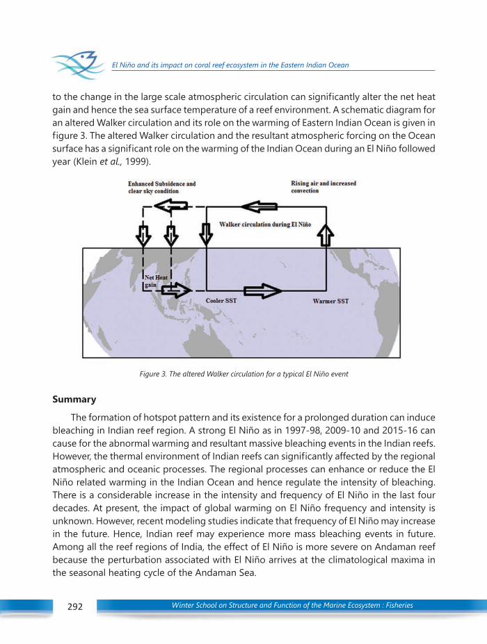
Winter School on Structure and Function of the Marine Ecosystem : Fisheries292
El Niño and its impact on coral reef ecosystem in the Eastern Indian Ocean
to the change in the large scale atmospheric circulation can significantly alter the net heatgain and hence the sea surface temperature of a reef environment. A schematic diagram foran altered Walker circulation and its role on the warming of Eastern Indian Ocean is given infigure 3. The altered Walker circulation and the resultant atmospheric forcing on the Oceansurface has a significant role on the warming of the Indian Ocean during an El Niño followedyear (Klein et al., 1999).
Figure 3. The altered Walker circulation for a typical El Niño event
Summary
The formation of hotspot pattern and its existence for a prolonged duration can inducebleaching in Indian reef region. A strong El Niño as in 1997-98, 2009-10 and 2015-16 cancause for the abnormal warming and resultant massive bleaching events in the Indian reefs.However, the thermal environment of Indian reefs can significantly affected by the regionalatmospheric and oceanic processes. The regional processes can enhance or reduce the ElNiño related warming in the Indian Ocean and hence regulate the intensity of bleaching.There is a considerable increase in the intensity and frequency of El Niño in the last fourdecades. At present, the impact of global warming on El Niño frequency and intensity isunknown. However, recent modeling studies indicate that frequency of El Niño may increasein the future. Hence, Indian reef may experience more mass bleaching events in future.Among all the reef regions of India, the effect of El Niño is more severe on Andaman reefbecause the perturbation associated with El Niño arrives at the climatological maxima inthe seasonal heating cycle of the Andaman Sea.
Winter School on Structure and Function of the Marine Ecosystem : Fisheries 293
El Niño and its impact on coral reef ecosystem in the Eastern Indian Ocean
References
Goreau, T. J., & Hayes, R. L. (1994). Coral Bleaching and Ocean “HotSpots”. Ambio, 23, 176-180.
Klein, S. A., Soden, B. J., & Lau, N. (1999). Remote Sea Surface Temperature Variations during ENSO: Evidencefor a Tropical Atmospheric Bridge. Journal of Climate, 12, 917-932.
Krishnan, P., Dam Roy, S., Grinson George, Srivastava, R. C., Anand, A., Murugesan, S., Kaliyamoorthy, M.,Vikas, N., & Soundararajan, R. (2011). Elevated sea surface temperature during May 2010 inducesmass bleaching of corals in the Andaman. Current Science, 100, 111-117.
Lix J. K., Venkatesan R., George Grinson, Rao R. R., Jineesh V. K., Arul M. M., Vengatesan G., RamasundaramS., Sundar R., Atmanand M. A. (2016). Differential bleaching of corals based on El Nino type andintensity in the Andaman Sea, southeast Bay of Bengal. Environmental Monitoring and assessment,DOI 10.1007/s10661-016-5176-8, 188:175.
McPhaden M. J. (2002). El Nino and La Nina: causes and global consequences. In: MacCracken M. C., PerryJ. S. (eds) Encyclopedia of global environmental change, Vol 1. Wiley, Chicester, 353-370.
Stone, L., Huppert, A., Rajagopalan, B., Bhasin, H. and Loya, Y. (1999). Mass coral reef bleaching: A recentoutcome of increased El Niño activity? Ecology Letters, 2, 325-330.
Vivekanandan, E., Ali, M. H., Jasper, B. and Rajagopalan, M. (2008). Thermal thresholds for coral bleachingin the Indian seas. Journal of Marine Biological Association of India, 50, 209-214.
Wilkinson, C., Linden, O., Cesar, H., Hodgson, G., Rubens, J. and Strong, A. E. (1999). Ecological andsocioeconomic impacts of 1998 coral mortality in the Indian Ocean: An ENSO impact and a warning offuture change? Ambio, 28, 188-196.
Winter School on Structure and Function of the Marine Ecosystem : Fisheries294
Coral reef ecosystem-monitoring and assessment using satellite data sets
Introduction
Remaining in splendid isolation, the Andaman and Nicobar Islands have a great relevancein the study of marine ecosystems. The islands, though remotely located in an ostensiblypristine environment have born witness to serious issues with regard to their ecosystemhealth. There are significant changes in the temperature and rain fall pattern in the islandsand predictive modelling has forecasted further damage in the near future. The inundationof saline water into inland terrestrial ecosystems has created salinity stress to freshwaterspecies while reducing the water available for domestic consumption. Terrestrial flora andfauna are vulnerable to the intruding saline waters. The marine ecosystem also faces gravechallenges. There are issues of anthropogenic pollution resulting in damage of corals, regimeshifts in community structure, water quality deterioration and other damage to marinefauna. Climate change has taken a toll on the ecosystem with coral bleaching which wasobserved during 1998, 2002, 2005, 2010 and most recently in 2016. An interactive digitaldatabase on corals has been developed to address the regular health status of corals. Withthe help of satellite remote sensing data, mechanisms of reef bleaching can be uncoveredand the probable threats can be addressed by providing advisories developed in collaborationwith INCOIS, Hyderabad. The increased incidence of tropical cyclones in the region is alsowreaking havoc in the reef and related ecosystem. There are recent changes in the communitystructure due to the aforementioned challenges and changes are notable in all marinerelated ecosystems such as reefs and mangroves. There are instances of reefs exposure dueto tilting of islands, proliferation of unwanted island flora and fauna due to inadvertenthuman interventions, wastage of natural resources due to unscientific policy decisions andillegal poaching of island resources by neighbouring countries. Despite all these issues thefishery in the islands remains under-utilized. There is a huge scope for utilizing the fisheryto the benefit of the island community. Possible methods of harvesting these resources willalso be discussed in the lecture.
Status of coral reefs in Andaman after two major catastrophic events - tsunami ofDecember 2004 and bleaching of May 2005 (Dam Roy et al., 2014)
The 26th December 2004 tsunami, caused by a massive earthquake off the west coast ofSumatra, resulted in widespread devastation of coral reefs in the Andaman and NicobarIslands. A reef survey carried out in January 2005 indicated that many exposed corals were
35C H A P T E R
CORAL REEF ECOSYSTEM-MONITORINGAND ASSESSMENT USING SATELLITEDATA SETSGrinson George1, Roshen G. Ninan2 and Zacharia P. U.2
1Fishery Resources Assessment Division2Demersal Fisheries DivisionICAR-Central Marine Fisheries Research Institute

Winter School on Structure and Function of the Marine Ecosystem : Fisheries 295
Coral reef ecosystem-monitoring and assessment using satellite data sets
295
dead and corals that suffered breakage were precariously living. Dislocated corals and cracksin the coral reefs were also noted. Coral composition remained the same in protected baysas most of them were shielded from the brunt of earthquake and tsunami.
Shortly after the tsunami, the same area was subjected to a bleaching event in themonth of May 2005. Surveys revealed that the live coral cover amounted to only 6.5%. Thepartially bleached, fully bleached, dead and other coral components were 4.8, 13.3, 19.7and 55.7% respectively. The extent of coral damage and their subsequent recovery wasstudied during the following months in order to monitor reef health and it was observedthat live coral had increased to 17.9% and the total amount of dead coral was 22.7%,suggesting the recovery of partially bleached corals and the death of fully beached corals.The bleaching was similar to the 1998 bleaching event. Satellite Remote Sensing (SRS) datasets was unable to be utilised during the study. In the subsequent years SRS data wasemployed for monitoring corals in Andaman Sea. Later on, compilations of SRS data wereused to develop a coral reef bleaching alert system with the help of a team from INCOIS,Hyderabad.
Assessment of the coral bleaching during 2005 to decipher the thermal stress in thecoral environs of the Andaman Islands using Remote Sensing (Mohanty, P. C. et al.,2013)
SST values derived from NOAA AVHRR satellite data were used to generate both Degreeof Heating Weeks (DHW) and Hot Spot (HS) products. Combination of the cumulativetemperature anomalies and the thermal stress values were utilized to synoptically identifythe probable areas of bleaching. Areas with Hot Spot products > 1oC were assigned a warning.Any areas assigned a warning with Degree of Heating Weeks between 4 and 8o C- weekwere elevated to Alert Level-1, with areas having Degree of Heating Weeks greater than 8o
C- week assigned status Alert Level-2. At Havelock Island, a bleaching status up to AlertLevel-1 was recorded with a maximum HS of 3o C and DHW 6o C- week. Simultaneous in-situreef observations conducted in the Andaman Sea confirmed coral bleaching event at thissite. The highest rates of mortality in the region due to coral bleaching were shown by theAcropora species (43%) followed by Montipora species (22%) and Porites species (14%). Thisstudy focused on facilitation of a coral bleaching warning system based on the SST incomplement with in-situ observationsfor verification carried out at selected sites.
Elevated sea surface temperature during May 2010 induces mass bleaching of coralsin the Andaman (P. Krishnan et al., 2011)
In a study taken up to asses bleaching the 2010 bleaching event, surveys of sites in theAndaman revealed that significant bleaching occurred during April and May 2010. As muchas 70 % of certain sites suffered the effects of bleaching. While similar bleaching events
Winter School on Structure and Function of the Marine Ecosystem : Fisheries296
Coral reef ecosystem-monitoring and assessment using satellite data sets
occurred in 1998 and 2002, this has been judged to be one of the most devastating eventsof this kind to have occurred in the Andamans. Through Line Transect studies, it was foundthat the fully bleached corals as a percentage of total coral cover were highest at HavelockIsland (69.49), followed by South Button Island (67.28), Nicolson Island (56.45), Red SkinIsland (43.39), North Bay (41.65) and Chidiyatapu (36.54). SST maps for selected time periodsfor the areas surrounding these Islands showed consistently high temperatures in the range31–32° C during the last two weeks of April 2010 in the sites, except in Chidiyatapu, whereit ranged from 32.1° C to 33.3° C. Branching corals were the worst affected, whereas themassive corals were found to have relatively withstood the elevated SST. The status of reefsand the variability in bleaching with the fluctuations in SST with respect to different coralspecies could be studied in detail during 2010.
Studies on the Recovery of Bleached Corals in Andaman: Fishes as Indicators of ReefHealth (P. Krishnan et al., 2013)
This study evaluates the degree of recovery of the coral reefs and reef fishes at threesites – North Bay, Tarmugli and Chidiyatapu - a year after the bleaching event in 2010. It wasobserved that all sites were severely affected during the bleaching period with more than95 % of the corals being fully or partially bleached. Out of the bleached corals surveyed atthe study sites, only 54 % recovered at North Bay, whereas Tarmugli and Chidiyatapu showedsignificant recovery - 81 and 86% respectively. Live coral cover, which was densest at NorthBay prior to bleaching,was most strongly affected at North Bay among the three sites -most likely due to the higher percentage of branching corals such as Acropora sp. in thisarea. Chidiyatapu exhibited significantly fainter signs of bleaching owing to the higherpercentage of boulder corals such as Porites sp. in these areas. Recovery patterns indicatethat the rapid recovery rate of fast growing corals such as Acropora, however, have resultedin greater dominance by these species suggesting that climate forcing of coral communitiesmay initially favour coral species with rapid recovery potential, rather than slow growingcorals that might otherwise have greater resistance to bleaching. Due to this recovery andnew recruitment of corals, live coral cover has increased, resulting in an increase in anapparent abundance of fishes. Understanding the associations between fish and coralscould lead to the designationof certain species of fish as indicators of reef health. Theresults of the study lead to the hypothesis that obligate corallivores, such as those belongingto the families Chaetodontidae, Pomacentridae, Acanthuridae and Scaridae, are strongpotential candidates to serve as indicators of reef health.
Tropical storm off Myanmar coast sweeps reefs in Ritchie’s Archipelago, Andaman(P. Krishnan et al., 2012)
The reefs in Ritchie’s Archipelago, Andaman suffered severe damage following a tropical
Winter School on Structure and Function of the Marine Ecosystem : Fisheries 297
Coral reef ecosystem-monitoring and assessment using satellite data sets
297
storm in the Bay of Bengal off Myanmar coast where maximum wind speeds of 11 m/s wasobserved during a tropical storm that occurred in March 2011. Satellite Altimetry-basedMap of Sea Level Anomaly (MSLA) data of Near Real Time (NRT) available with the Archival,Validation and Interpretation of Satellite Oceanographic Data (AVISO) was used to studythe Sea Level Anomaly and Surface Geostrophic currents in the region during 13–23 March2011. Sea level anomaly and surface geostrophic current vector data were processed togenerate sea level anomaly and current maps using ARC-GIS software with the data for theperiod 13–23 March 2011. Satellite surveys of South Button Island clearly showed theprogression of the storm. Physical damage to corals was greater in the northern andnorthwestern side of the island, which corroborated with the direction of the storm.
Corals in the shallow inshore reefs were broken and dislodged by the thrust of thewaves generated in the wake of these winds. Significant damage in the deeper regions andoffshore reefs were caused by the settlement of debris and sand brought down from theshallower regions. The fragile branching corals (Acropora sp.) were reduced to rubble andthe larger boulder corals (Porites sp.) were toppled over or scarred by falling debris. Reefson the windward side which were directly in the path of the storm winds were the worstaffected. The investigation exposes the vulnerability of the reefs in the Andamans tooceanographic features which generally go unnoticed unless there is associated damagecaused to coastal habitats in these regions.
Differential bleaching of corals based on El Niño type and intensity in the AndamanSea, southeast Bay of Bengal (J.K. Lix et al., 2016)
The purpose of this study was to investigate the role of the El Niño in the coral reefbleaching events of the Andaman region.Both Niño 3.4 and 3 indices were examined tofind out the relationship between the mass bleaching events and El Niño, and correlatedwith sea surface temperature (SST) anomalies in the Andaman Sea.
Inter-annual variability of SST around the Andaman Islands was investigated with NOAAAVHRR Pathfinder V4.1 SST (1985–2002) and AVHRR (GAC) SST (2003–2012) with dataaveraged over the study area. This data was coupled with monitoring of reef benthiccompositions at two stations – North Bay and Chidyapatu during 2010-2012. Areas aroundthe Andaman Islands where the SST exceeded long-term averages by more than 1 °C duringthe warmest months (March–June) were identified for the mass bleaching during 1998 and2010.
Field surveys conducted before, during and after bleaching in 2010 show that therehave not been any additional bleaching episodes in the Andamans since 2010. Salientobservations made at different zones of selected coral reefs aided in identifying the indicatorsthat give information on the health status of the reefs and to identify the reefs at risk.

Winter School on Structure and Function of the Marine Ecosystem : Fisheries298
Coral reef ecosystem-monitoring and assessment using satellite data sets
The analysis demonstrates that a strong El Niño in the Pacific causes a similar warmingin the Andaman Sea which leads to mass coral bleaching events around the AndamanIslands. The result shows that abnormal warming and mass bleaching events in the AndamanSea were seen only during strong El Niño years of 1997 to 1998 and 2009 to 2010. TheAndaman Sea SST was more elevated and associated with El Niño Modoki (central Pacific ElNiño) than conventional El Niño (eastern Pacific El Niño) occurrences. It is suggested thatthe development of hot spot patterns around the Andaman Islands during May 1998 andApril to May 2010 may be attributed to zonal shifts in the Walker circulation driven by ElNiño during the corresponding period. It can be concluded from this study that the effectof El Niño on a particular coral reef region will depend on the timing when the El Niñoperturbation propagates to those reefs. The effect is typically more extreme if timingcorresponds to the climatological maxima in the seasonal heating cycle.
Box averaged (11.5–14° N; 91.5–94° E) monthly mean SST (°C) for the Andaman region during 1985–2012with the corresponding 13-month moving average shown as a black curve. The line drawn at 30.84 °Crepresents a bleaching threshold temperature and line drawn at 29.84 °C represents the climatology inMay. The corresponding bleaching events are represented by red dots and their size indicating the intensityof the bleaching event.
Winter School on Structure and Function of the Marine Ecosystem : Fisheries 299
Coral reef ecosystem-monitoring and assessment using satellite data sets
299
Acknowledgement
The second author would like to acknowledge financial assistance provided by NationalInnovations in Climate Resilient Agriculture (NICRA) sponsored by Indian Council ofAgricultural Research (ICAR).
References
S. Dam Roy, Grinson George, R. Soundarajan, P. Krishnan, S. Murugesan and M. Kaliyamoorthy (2014).Status of coral reefs in Andaman after two major catastrophic events - tsunami of December 2004 andbleaching of May 2005. Eco. Env. & Cons. 20(2): 2014; pp. 137-142.
Mohanty, P. C., Mahendra, R. S., Bisoyi, H., Tummula, S. K., Grinson, G., Nayak, S. & Sahu, B. K. (2013).Assessment of the coral bleaching during 2005 to decipher the thermal stress in the coral environs ofthe Andaman Islands using Remote Sensing. European Journal of Remote Sensing, 46(1), 417-430.
Krishnan, P., Dam Roy, S., George, Grinson, Srivastava, R. C., Anand, A., Murugesan, S., Kaliyamoorthy, M.,Vikas, N., Soundararajan, R. (2011) Elevated sea surface temperature during May 2010 induces massbleaching of corals in the Andaman. Current Science, 100 (1). pp. 111-117.
Krishnan, P., George, Grinson and Immanuel, Titus and Bitopan, Malakar and Anand, A. (2013) Studies onthe Recovery of Bleached Corals in Andaman: Fishes as Indicators of Reef Health. In: Ecology andConservation of Tropical Marine Faunal Communities. Springer-Verlag Berlin Heidelberg, pp. 395-407.
Krishnan, P., George, Grinson, Vikas, N., Titus, Immanuel, Goutham Bharathi, M. P., Anand, A. Vinod Kumar,K., Senthil Kumar, S. (2012) Tropical storm off Myanmar coast sweeps reefs in Ritchie’s Archipelago,Andaman. Environmental Monitoring and Assessment. pp. 1-12.
Lix, J. K., Venkatesan, R., George, Grinson, Rao, R. R., Jineesh, V. K., Arul, Muthiah M., Vengatesan, G.,Ramasundaram, S., Sundar, R., Atmanand, M. A. (2016) Differential bleaching of corals based on ElNiño type and intensity in the Andaman Sea, southeast Bay of Bengal. Environmental Monitoring andAssessment, 188 (175). pp. 1-13. ISSN 0167-6369.

Winter School on Structure and Function of the Marine Ecosystem : Fisheries300
Harmful algal bloom monitoring using Satellite Observations
Introduction
Satellite based Earth observations on ocean color provides an efficient tool formonitoring primary productivity in the oceans in terms of phytoplankton abundance, i.e.,the Chlorophyll-a (Chl-a) concentration. Occasionally the phytoplankton species ‘blooms’to form extensive patches covering large surface area of the coastal and off shore waters.Information on the presence, absence and timing of plankton blooms are prerequisites forestimating the marine productivity and the temporal seasonality of particle fluxes in to thedeep sea. The algae blooms can form rapidly and it is often difficult to assess theirdevelopment and extent from traditional sampling methods mainly due to inadequacy ofproper techniques other than classical sea truth data analyses.
The increasing number of harmful algal blooms (HABs) in the past few decades havereceived a lot of attention due to their negative impact on the marine environment(Hallegraeff et al., 2003). HAB events are characterised by two main features; they are causedby micro algae and they have a negative impact on human health and/or activities such asfisheries, aquaculture, and tourism. In addition to these common features, HABs are verydiverse in terms of harmfulness, causative organisms, dynamics of blooms and types ofimpact. The harmfulness of algal blooms could be toxic or just massive in abundance thatcauses the harm. The impact of toxic blooms can vary from mass mortality of invertebratesand fishes to serious threat to human beings. Local residents of the coastal area whodepend on clams, mussels, fishes etc as a major food source would be seriously affected.
In the case of non-toxic algal blooms also, the damage done to the environment issevere. The anoxic conditions developed due to the blooms and the foul smell of thesurroundings affect the aesthetic value of the area. They also pose damage to the fishinggear. Therefore, in order to monitor HAB events, the first step is to create a regional databasefrom available scientific information regarding the diversity of the common bloom causingalgae growth, the extent of damage caused by each of them and the physico-chemicalfactors affecting the growth and multiplication of these harmful algae.
Satellite ocean colour sensors provide estimates of concentrations of the phytoplanktonpigment chlorophyll-a (Chl-a) in the water. Since 1998 ocean colour data has been regularlyused to monitor the daily algal status in many oceanic waters particularly in Norwegian
36C H A P T E R HARMFUL ALGAL BLOOM MONITORING
USING SATELLITE OBSERVATIONSAjith Joseph K.,1 N. R. Menon1 and Lasse H. Pettersson1,2
1Nansen Environmental Research Centre (India), Kochi2Nansen Environmental and Remote Sensing Center, Norway
Winter School on Structure and Function of the Marine Ecosystem : Fisheries 301
Harmful algal bloom monitoring using Satellite Observations
301
coastal waters (Pettersson and Pozdnuyakov, 2013, Durand et al., 2000, Folkestad et al.,2006). Initially, data from the NASA Sea-Viewing Wide Field-of-View sensor (SeaWiFS, Hooker1992) were used and the data products were obtained from standard global operationalalgorithms. In the event of a HAB, early warning and subsequent prediction of the bloomevolution are essential for national fishery authorities and for the aquaculture/fisheriesindustry in order to implement mitigation actions. Therefore, a routine monitoring of theproductivity and environmental parameters of the coastal and open ocean waters would beof immense help in evaluating and predicting algal blooms, including HAB.
In this context, Indian fishery industry is not an exception, faced major challenges inthe last few years due to natural calamities affecting the marine environment like cyclones,tsunami, storm surges and also threats from Harmful Algal Blooms (HAB). All these eventshave created the need for evolving disaster management strategies for early implementationof adequate mitigation measures. Field studies have revealed their inefficiency in assessingthe sudden occurrence and extent of such blooms by in situ sampling. It is in this context,satellite based observations on ocean colour find relevance for monitoring the bloom eventsin the marine environment. Since the spectral behaviour of phytoplankton species differ,high spectral resolution satellite like MODIS (Moderate resolution ImagingSpectroradiometer) probably would help in delineating species responsible for the blooms.Such attempts to identify, understand and demonstrate the application of Earth Observationdata from different ocean colour sensors can lead to improved monitoring of bloom eventsand henceforth serve as a tool in predicting hazards of the marine environment (Pozdnyakovet al., 2017).
International programmes like ECOHAB(The Ecology and Oceanography of HarmfulAlgal Blooms), EUROHAB ( Harmful Algae Blooms in European waters)and GEOHAB (GlobalEcology and Oceanography of Harmful Algal Blooms) were initiated by many countries tounderstand HAB population dynamics. Similarly, in India, such initiatives were already beentaken and an integrative study on the distribution of the Toxic Algal Blooms along the EEZof India under the Marine Living Resources Programme sponsored by the Department ofOcean Development, Govt. of India (MLR-DOD) from 1998 onwards signifies the need formonitoring of HAB events in Indian waters. As a follow up on this programme, the Oceansat-2 OCM products from Space Application Centre of ISRO are operationally available for localarea coverage (LAC) at 360m resolution and Global coverage(GAC) at 1 km resolution arebeing used to study the HAB events.
A satellite based information service for Detection and Monitoring of Harmful AlgalBloom (HAB) based on three key parameters: rolling chlorophyll anomaly (RCA), rolling seasurface temperature (SST) anomaly (RSA) and bloom index (BI) is in operational at INCOIS.The information on occurrences of HABs has been provided daily on experimental basis

Winter School on Structure and Function of the Marine Ecosystem : Fisheries302
Harmful algal bloom monitoring using Satellite Observations
(Fig.1) at near real-time (NRT) to regions: North Arabian Sea, Goa, Mangalore, Kochi, Gulf ofMannar, Perrangipetai and Visakhapatnam.
Nansen Centre, Norway has already established an algal bloom monitoring serviceweb-site http://HAB.nersc.no under GMES MarCoast for North European waters in the 1990s.Daily, running 7-days and monthly average EO based information products are generated,for a wide range of water quality and SST ocean products, using both global and regionaltuned processing algorithms for retrieval of the water constituents.
Reprocessed global ocean color data are available through the European Space Agency(ESA) Climate Change Initiative (CCI) currently updated until the end of 2016 at http://www.esa-oceancolour-cci.org/ and similarly from ChloroGIN (Chlorophyll Global integratedNetwork) for the Indian waters (http://www.incois.gov.in/portal/ChloroGIN).
Fig. 1. A conceptual framework for operational monitoring and dissemination of HAB informationservice by INCOIS (Courtesy: http://www.incois.gov.in)
Literature Review
Phytoplankton blooms are considered, generally, as a nuisance to the coastal community.Blooms mostly occur in shallow coastal waters during spring season in the presence of lightand enrichment of water by nutrients. The source of the nutrients may be from river runoffor coastal upwelling. The blooms are often reported with a variety of colors from green to
Winter School on Structure and Function of the Marine Ecosystem : Fisheries 303
Harmful algal bloom monitoring using Satellite Observations
303
red depending on the dominant species of plankton and algae, reflecting their spectralabsorbing or scattering characteristics. Blooms of blue-green algae, Trichodesmiumerythraeum, are more common in the coastal waters of India. Red tide blooms caused bydinoflagellates have also been reported (Sasamal et al., 2005). The following paragraphillustrates the various studies carried out in abroad and in India, using ocean color data,which incidentally reflects the capability of ocean color data for studying algal blooms inthe marine environment.
Tang et al., (2004) have studied the oceanography of a harmful algal bloom off thecoast of southeastern Vietnam using remote sensing tools. Harmful algal blooms (HABs) inthe southeastern Vietnamese coastal waters have caused large economic losses inaquaculture and wild fisheries in recent years; however, there have been few oceanographicstudies on these HAB events. This study reports an extensive HAB off southeasternVietnamese waters during late June to July 2002 with in situ observations and subsequentanalyses of the oceanographic conditions using satellite remote sensing data. The HAB,which covered 200 km off the coast and 200 km northeast of the Mekong River mouth fora period of 6 weeks, had high chlorophyll a (Chl a) concentrations (up to 4.5 mg m-3). Thebloom was dominated by the harmful algal haptophyte Phaeocystis cf. globosa and causedsignificant mortality of cultured fish and other marine life. In the same period, sea surfacetemperature (SST) imagery showed a cold water plume extending from the coast to theopen sea, and QuikSCAT data showed strong southwesterly winds blowing parallel to thecoastline. This study indicated that the HAB was induced and supported by offshore upwellingthat brings nutrient rich waters from the deep ocean to the surface and from coastal waterto offshore water and that the upwelling was driven by strong winds and Ekman transportwhen prevailing winds were parallel to the coastline. This study demonstrated the possibilityof utilizing a combination of satellite data of Chl a, SST, and wind velocity together withcoastal bathymetric information and in situ observations to give a better understanding ofthe biological oceanography of HABs.
Tang et al., (2006) have elucidated the satellite evidence of harmful algal blooms andrelated oceanographic features in the Bohai Sea during autumn 1998. Some HAB occurrencesare different to observe because of their high spatial and temporal variability and theiradvection, once formed, by surface currents. The study analyzed the formation, distribution,and advection of a serious HAB occurred in the Bohai Sea during autumn 1998, causing thelargest f ishery economic loss, using satellite SeaWiFS ocean color data and otheroceanographic data. The results showed that the bloom originated in the western coastalwaters of the Bohai Sea in early September, and developed southeastward when sea surfacetemperature (SST) increased to 25–26 °C. The bloom with high Chl-a concentration(6.5 mg-3) in center portion covered an area of 60 × 65 km2. By the end of September, the

Winter School on Structure and Function of the Marine Ecosystem : Fisheries304
Harmful algal bloom monitoring using Satellite Observations
bloom decayed when SST decreased to 22–23 °C. It was concluded that HAB might havebeen initiated by a combination of the high riverine input of nutrients and increase in SST inthe western coastal waters; afterwards it may have been transported eastward by the localcirculation that was enhanced by northwesterly winds in late September and early October.
Costas (2004) has done the rapid monitoring for the potentially ichthyotoxicdinoflagellate Cochlodinium polykrikoides in Korean coastal waters using fluorescent probetools. Cochlodinium polykrikoides has occurred annually in Korean coastal waters since1982, where it has caused extensive fish mortality. Rapid and accurate monitoring is veryimportant to reduce the economic damage caused by C. polykrikoides. However, beforeoutbreaks of C. polykrikoides occur, single cells are often more abundant than chain-formingcells. During this period, it is very difficult to discriminate C. polykrikoides from closely relateddinoflagellates and other phytoplankton species.
Reinart and Kutser (2006) have compared the different sensors in detectingcyanobacterial alage bloom events in the Baltic Sea. Potentially toxic cyanobacterial bloomsoccur in the Baltic Sea in the middle of summer. Aggregations of cyanobacteria often formdense subsurface blooms or even surface scum, which are spatially extremely patchy. It hasbeen shown by using bio-optical modelling together with the hyperspectral sensor Hyperionimage from the western part of the Gulf of Finland that chlorophyll concentration may varybetween 1-100 mg m-3 within the 10m scale during heavy bloom. The SeaWiFS, MODIS/Aqua and MERIS products over heavy bloom region were compared with each other, andwith that of the modelling results, the bio-optical modelling data and the available in situdata. During the massive bloom of cyanobacteria, at the time of surface scum formation,results from different sensors were variable, the values of chlorophyll concentration exceededthe standard processing limits causing the atmospheric correction to fail. The study showedgood capability of MERIS and MODIS fine resolution spectral bands to detect cyanobacterialbloom quantitatively.
Kutser et al., (2006) have also done the monitoring of cyanobacterial blooms by satelliteremote sensing in the Baltic Sea. The problems caused by cyanobacterial blooms wereespecially acute in the Baltic Sea where they occur every summer covering areas of morethan 100,000 km2. It has been shown that quantitative mapping of cyanobacteria duringbloom conditions is possible with hyperspectral instruments. These sensors, however, cannotprovide synoptic spatial coverage and high revisit times are needed for near real-timemonitoring of potentially harmful blooms. The aim was to estimate whether spectralresolution of multispectral sensors, which could provide needed coverage, is adequate forquantitative mapping of cyanobacteria and whether it was possible to separate potentiallyharmful blooms of cyanobacteria from waters dominated by algae using ocean coloursatellites. The modelling results showed that multispectral sensors like ALI, Landsat or MODIS

Winter School on Structure and Function of the Marine Ecosystem : Fisheries 305
Harmful algal bloom monitoring using Satellite Observations
305
were not capable of separating waters dominated by cyanobacteria from waters dominatedby other algal species, as their spectral band configuration does not allow spectral separationof absorption features caused by phycocyanin (present primarily in cyanobacteria) or anyother spectral features that are characteristic to cyanobacteria alone. MERIS bands 6 and 7allowed detecting phycocyanin absorption feature near 630 nm and a small peak inreflectance spectra near 650 nm characteristic to only cyanobacteria. Thus, MERIS can beused in detecting cyanobacteria if they are present in relatively high quantities. Unfortunatelyit is not possible to use MERIS for early warning of emerging potentially harmful blooms asthe minimum biomass needed to cause features in reflectance spectra typical to cyanobacteriais higher than the biomass already considered as a bloom in the Baltic Sea. Howerer,Pettersson and Pozdyanakov (2012) have covered the various aspects of HAB monitoringusing satellite observations particularly for the Norwegian waters. A recent study by Kondriket al., (2017) observed that the particulate inorganic carbon production within Emiliniahuxleyi blooms in sub polar and polar oceans has the impact to block the carbon uptake inthe ocean waters.
In Indian waters, Rao (1969) reported for the first time a diatom bloom of Asterionellain the coastal waters of Vishakhapatanam. In 1983, another bloom was also observed nearthe Mangalore coast and several people were hospitalized due to the consumption ofintoxicated shellfish and the causative species was not identified (Karunasagar et al., 1984).Other algal blooms were also reported in Vellar estuary by Mani et al., (1986) and later byChoudhary and Panigrahy (1989), Panigrahy and Gouda (1990), Mishra and Panigrahy (1995)along the coast of Orissa. These reports indicated that the blooming of Asterionella specieswere common in the NW Bay of Bengal during pre-monsoon months. The southwestmonsoon winds and associated rainfall resulted in increased river runoff from June toSeptember, enriching the coastal waters with terrestrial nutrients from coastal upwelling.During the Northeast monsoon, i.e., from October to January, the coastal waters are enrichedby upwelling of sub-surface water. This increases the productivity of the NW Bay of Bengalmany times during late winter and in the early monsoon months leading to blooming ofphytoplankton along the east coast of India.
In 1996, a bloom of Gymnodinium catenatum was reported from Mangalore coast(Godhe et al., 1996, Karunasagar, 1996). In the year 1997, in the Kerala coast a paralyticshellfish poisoning was reported (Karunasagar et al., 1998) causing seven deaths and over500 were hospitalized following consumption of intoxicated mussel, Perna indica.
The moderate to intense blooms of the dinoflagellate Noctiluca scintillans occurred inPort Blair Bay, Andamans during June and July of 2000. The blooms occurred thrice insuccession after short periods of waning. The second bloom in the sequence, which occurredbetween 11 and 20 July 2000, was subjected to scientific study by assessing the changes in
Winter School on Structure and Function of the Marine Ecosystem : Fisheries306
Harmful algal bloom monitoring using Satellite Observations
water characteristics associated with the event. Results indicated that variations in dissolvedoxygen concentration were fairly small, whilst nutrient levels and plankton compositionswere altered. Primarily the bloom not only led to the exclusion of other phytoplankton, butalso limited the zooplankton prevalence to essentially copepods. The bloom resulted inexceptionally high levels of chlorophyll-c, which exceeded chlorophyll-a levels by severalfolds. Nutrient levels were characterized by decrease of nitrate during active periods of thebloom, and sharp decrease in phosphate, particularly during the waning phase.
A thick bloom of the marine prymnesiophycean, Phaeocystis globosa was observed inthe central Arabian Sea during the summer monsoon period (July–August, 1996). The cellswere mostly in colonial form, embedded in gelatinous matrices. The cell diameter wasapproximately 7nm and showed a distinct double feature form. The intensity of the bloomwas as high as 3750×106 cells m-2 and the carbon content ranged between 33 and 550mg L-1. Almost 90 % of the phytoplankton population was composed of P. globosa in thebloom area. Other common forms were chain-forming diatoms like Rhizosolenia spp.,Nitzschia spp. and Chaetoceros spp. The photosynthetic pigment chlorophyll a however didnot show any concomitant rise with the bloom intensity probably because the bloom wassampled during a senescent phase. The carbon - chlorophyll ratio varied between 112 to810. This was the first report on the occurrence of Phaeocystis from the Arabian Sea(Madhupratap et al., 2000). It seems pertinent to ask whether this was a result of the genusbeing introduced and adapted to new environments due to human influence and whetherthis would influence food chains in the future.
The cruises of FORV Sagar Sampada in the year 2003 and a repeat cruise in 2004 duringthe same period (Feb 26 to Mar 15) and along the same location (between Goa and Porbandersector; NE Arabian sea, 10-22N and 66-75°E) together with satellite data revealed an extensiveblooming of Noctiluca scintillans which was found gradually extending westward as far asOman. A sudden intense bloom of Noctiluca scintillans was observed on 20 December2002 in Minnie Bay (11°38.705’N; 92°42.513’E). The bloom persisted for three days anddisappeared suddenly; a similar bloom was reported here earlier in 2001.
Sasamal et al., (2005) have reported Asterionella blooms in the NW Bay of Bengal during2004. Dark brown patches of phytoplankton bloom were observed in the near shore watersat Gopalpur in the NW Bay of Bengal towards the end of March and beginning of April2004. During the bloom period, phytoplankton population density increased by 70 to 80times relative to the pre-bloom situation.
On 29th September 2004, a red tide was also observed along the West coast of India.Noctiluca miliaris is the most common dinoflagellate, which forms red tides along the westcoast (Sahayak et al., 2005). The red tide observed seemed to be significant since the
Winter School on Structure and Function of the Marine Ecosystem : Fisheries 307
Harmful algal bloom monitoring using Satellite Observations
307
phenomenon had occurred within a fortnight of the stench event that had created panicamong people living along southern Kerala coast. Mass fish kill was noticed on 17th September2004 along the Trivandrum coast.
Horizontal distribution of temperature, salinity and dissolved oxygen showed interestingvariations in the bloom area. Relatively low temperature and high salinity prevailed in thebloom area and the lower concentrations of dissolved oxygen found in the bloom areawere apparently due to the large scale respiration by Noctiluca. Low nutrient contentobserved in the bloom area indicated the retreating phase of upwelling in the area. Upwellingweakens in the southern most part of West coast of India by October and as a result, thehigh concentrations of nutrients initially available at the surface waters get exhausted dueto autotrophic production. Primary production was also lower in the bloom area. Abundanceof micro zooplankton (ciliates) in the bloom region was low compared to other coastalstations (Sahayak et al., 2005).
During the 3rd week of September 2004, particularly on 16th and 17th, an unusual andstrong stench was experienced in the coasts of Kollam and Vizhinjam in Kerala, followed bylarge-scale fish mortality. The in situ measurements revealed the cause of the observedphenomenon to be the blooming of Holococcolithophore (Ramaiah et al., 2005).
HABs, including those caused by coccolithophorids (e.g. E. huxleyi), arise whenappropriate levels of nutrients, light and temperature, for those particular algae are present.Following the bloom, the right conditions disappear (often because the nutrients areassimilated into their cell masses), and the cells begin to decay. Many autotrophs, in particularmost HAB-forming phytoplankton, form crysts that fall to the bottom and lie dormant untilthe right conditions arise again. It appears that the HAB off the southern coast of Keralaoccurred in September 2004 peaked about the time the stench set in. The coccolithophoridHAB appears to have clogged the fish gills, leading to mass mortality as also the stench.After the HAB peaked, the conditions turned unfavorable, and apparently there was areduction in its abundance.
Along the coasts of Goa, bloom of a dinoflagellate, Cochlodinium polykricoides wasreported by Bhat and Matondkar (2004). This species hitherto unreported from the Indianwaters is a known fish killer in Korean waters. In addition, during September 2004, the samedinoflagellate Cochlodinium polykrikoides bloomed in Kerala waters causing large scale fishmortality in the different coastal villages and hospitalization of over 200 school childrendue to illness caused by the nauseating stench from the bloom and putrefying fish. But insitu studies by Ramaiah et al., (2005) from the bloom regions along the southern Malabarcoast found that the most abundant species were holo-coccolithophorids. However studiesby Sahayak et al., (2005) along the coast of Kerala, during the same bloom period revealed
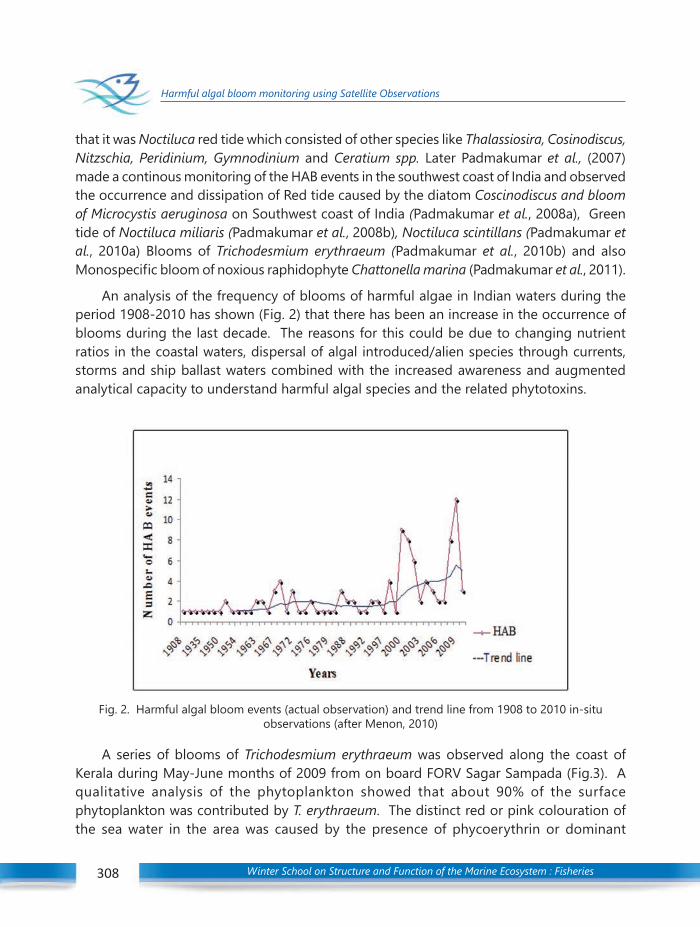
Winter School on Structure and Function of the Marine Ecosystem : Fisheries308
Harmful algal bloom monitoring using Satellite Observations
that it was Noctiluca red tide which consisted of other species like Thalassiosira, Cosinodiscus,Nitzschia, Peridinium, Gymnodinium and Ceratium spp. Later Padmakumar et al., (2007)made a continous monitoring of the HAB events in the southwest coast of India and observedthe occurrence and dissipation of Red tide caused by the diatom Coscinodiscus and bloomof Microcystis aeruginosa on Southwest coast of India (Padmakumar et al., 2008a), Greentide of Noctiluca miliaris (Padmakumar et al., 2008b), Noctiluca scintillans (Padmakumar etal., 2010a) Blooms of Trichodesmium erythraeum (Padmakumar et al., 2010b) and alsoMonospecific bloom of noxious raphidophyte Chattonella marina (Padmakumar et al., 2011).
An analysis of the frequency of blooms of harmful algae in Indian waters during theperiod 1908-2010 has shown (Fig. 2) that there has been an increase in the occurrence ofblooms during the last decade. The reasons for this could be due to changing nutrientratios in the coastal waters, dispersal of algal introduced/alien species through currents,storms and ship ballast waters combined with the increased awareness and augmentedanalytical capacity to understand harmful algal species and the related phytotoxins.
Fig. 2. Harmful algal bloom events (actual observation) and trend line from 1908 to 2010 in-situobservations (after Menon, 2010)
A series of blooms of Trichodesmium erythraeum was observed along the coast ofKerala during May-June months of 2009 from on board FORV Sagar Sampada (Fig.3). Aqualitative analysis of the phytoplankton showed that about 90% of the surfacephytoplankton was contributed by T. erythraeum. The distinct red or pink colouration ofthe sea water in the area was caused by the presence of phycoerythrin or dominant

Winter School on Structure and Function of the Marine Ecosystem : Fisheries 309
Harmful algal bloom monitoring using Satellite Observations
309
extracellular pigment leachate of this species. The presence of this pigment in the seawater signals the initial decay phase of Trichodesmium. As a rule the blooming ofTrichodesmium occurs during hot weather with brilliant sunlight and stable high salinity.Normally Trichodesmium growth is not stimulated in classical upwelling areas. In this contextthe blooming of these filamentous algae during the monsoon period in an upwelling areawould be considered quite unusual. Very high biomass of zooplankton (11.59 ml/m3) clearlyindicates the congenial conditions prevailing in the area for zooplankton growth. The factthat no fish mortality was observed in the bloom area probably opens up an area for furtherstudies on the relationship between Trichodesmium bloom and zooplankton abundance. Itis apparent that Trichodesmium blooms are ecologically significant to the productivitypatterns of the south eastern Arabian Sea.
Fig. 3. Trichodesmium bloom off Kochi (June 2009). Courtesy: Menon, 2010.
Excessive ponderance of Noctiluca scintillans in a region where a multispecies diatombloom existed was also recorded from the waters off Kochi (lat. 10o00’ – 10o3’ N and 75 o.32E) during the peak monsoon months of August ( Padmakumar et al., 2010a) . The bloomwas of brick red colouration and was spread over an area of 5 sq. km. The discolourationwas caused by the predominance of Noctiluca scintillans.
Noctiluca formed around 56% of the phytoplankton and the rest was constituted ofspecies belonging to 14 genera of diatoms. The single celled protest Noctiluca scintillans ishighly bioluminescent and this quality is controlled by a luciferin-luciferase system locatedin numerous spherically shaped “micro sources”. This protist is a voracious feeder of diatomsbelonging to the genera Thalassiosira and Pseudonitsczhia. Among food items of Noctiluca,
Winter School on Structure and Function of the Marine Ecosystem : Fisheries310
Harmful algal bloom monitoring using Satellite Observations
Pseudonitsczhia is found to produce toxins that can cause fish kill and lead to shellfishpoisoning to humans, indicating that N. scintillans could be a vector for transfer of phyto-toxins to higher trophic levels. Blooms of Noctiluca are known to prevent aggregation ofshoaling herbivorous fishes especially sardines. The waters where the bloom of Noctilucawas observed contained very high silicate (ca. 18.20 µmol/l), which probably indicatesexcessive secretion of silicate by this diatom feeding protest. High primary production alongthe west coast of India during the monsoons probably sets the stage for blooming of non-autotrophic forms like Noctiluca.
The prediction and occurrence of the algal blooms and in situ measurements whichare restricted only to the bloom period are the major practical difficulties in the studiesrelated to it. Remote sensing of near surface pigment concentrations provides the onlypractical means of obtaining large scale observations of phytoplankton distributions overappropriate time scales.
Why do we need HAB monitoring?
Regular monitoring of algae bloom situation in coastal and nearshore waters andimprovement of the in situ sampling strategy is to provide information on;
early warning of potential bloom developments.
identification of near surface and deeper water layer algae blooms.
geo-positioning of ocean fronts (in pigment concentrations and thermal structures)and advection of water masses of different origin.
EO data assimilation in geobiochemical ocean ecosystem modelling for improvedprediction and forecasting of HAB events.
Map inter-annual variability on the occurrence, extent, life time, etc. of blooms inthe oceanic and adjacent seas.
Approaches / methodologies:
Ocean colour data of chlorophyll-a and sea surface temperature (SST) can be accessedfrom satellite sensors like SeaWiFS, MODIS, MERIS (Medium Resolution ImagingSpectrometer Instrument), Oceansat I & II through Giovanni software and other GIS softwareand be processed after spatial sub-setting. Similarly, SeaWiFS and MODIS Aqua data onHAB events can also be accessed from GES DISC data site of NASA and processed throughSeaDAS software or MATLAB. Similarly Oceansat I & II data on cloud free days can beaccessed and processed using PrimeWin software developed by SAC-ISRO. Additionallyocean colour data can be downloaded from the ESA CCI Ocean Colour project http://www.esa-oceancolour-cci.org/.

Winter School on Structure and Function of the Marine Ecosystem : Fisheries 311
Harmful algal bloom monitoring using Satellite Observations
311
The methodology includes access to Ocean colour level 2 data products for the studyregion by Data downloading, processing, integration, analysis and assessment visualisationwhich includes the following steps:
Download Ocean colour data download· Data on any server
Processing Processing of Ocean Colour data Application of global/ regionalalgorithm for the waters of the study regionPost processingGenerationof Algal bloom distribution maps
Visualisation/ Integration Web visualisation Data on the screen by integrating Indian satellitedata with MERIS/MODIS data
Data Collection and Analysis
Secondary data on chlorophyll, SST, CDOM and SLA by altimetry can be collected fromthe bloom region for visualization and integration into the webGIS. The data binningprocedures are most efficient in order to reduce the impact of cloud cover contaminationof the ocean colour data as well as swath limitations in the daily acquired images. In additionto graphical image products (GeoTIFF) the data can be made available in MatLab and GoogleEarth (KML) formats for export and other use.
GIS analysis
Geographic Information System is defined by Burrough, (1986) as “a powerful set oftool for collecting, storing, retrieving at will, transforming and displaying spatial data fromthe real world for a particular set of purposes. Hence it is a decision support system involvingthe integration of spatially referenced data in a problem solving environment (Cowen, 1988).The Geographic Information System for the particular study can be created using the GISSoftware for web applications.
The study region’s survey map can be digitized and the values for the particularcomponents will be placed into the system on a grid pattern for each month based onhistoric data and satellite imageries. The following figure (Fig.4) describes the variouscomponents of GIS application tools for Algal bloom monitoring in the above context.
The major components of GIS application tools for Algal bloom monitoring mainlyfocus on the Data collection of bio-physical characteristics, SST, Chlorophyll-a with routinefield survey. This can generate data sets that are stored for further access, maintenance andupdates of the data. This is finally pooled into the major Data base which provides an inputto the geo-data base of the GIS software. This will be further used for mapping informationlike hotspots in water quality identified in the region, siting of potential fish breeding zoneswhich are not affected by deterioration in water quality, locating areas of harmful algae andtoxic algal blooms etc. which are of prime importance to the management of fisheries. All
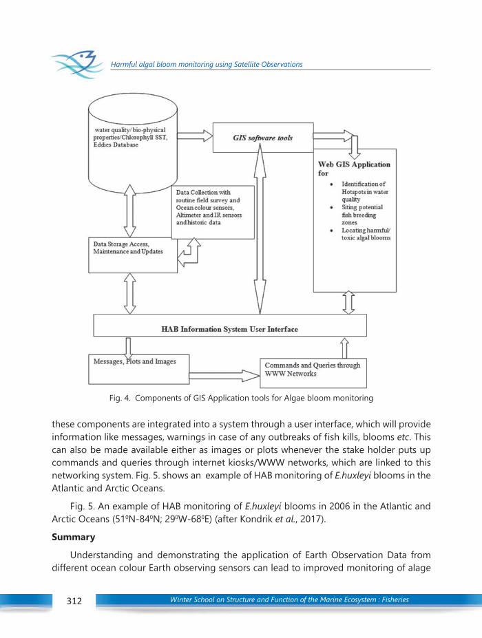
Winter School on Structure and Function of the Marine Ecosystem : Fisheries312
Harmful algal bloom monitoring using Satellite Observations
these components are integrated into a system through a user interface, which will provideinformation like messages, warnings in case of any outbreaks of fish kills, blooms etc. Thiscan also be made available either as images or plots whenever the stake holder puts upcommands and queries through internet kiosks/WWW networks, which are linked to thisnetworking system. Fig. 5. shows an example of HAB monitoring of E.huxleyi blooms in theAtlantic and Arctic Oceans.
Fig. 5. An example of HAB monitoring of E.huxleyi blooms in 2006 in the Atlantic andArctic Oceans (510N-840N; 290W-680E) (after Kondrik et al., 2017).
Summary
Understanding and demonstrating the application of Earth Observation Data fromdifferent ocean colour Earth observing sensors can lead to improved monitoring of alage
Fig. 4. Components of GIS Application tools for Algae bloom monitoring
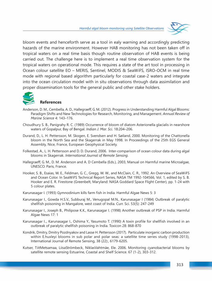
Winter School on Structure and Function of the Marine Ecosystem : Fisheries 313
Harmful algal bloom monitoring using Satellite Observations
313
bloom events and henceforth serve as a tool in ealy warning and accordingly predictinghazards of the marine environment. However HAB monitoring has not been taken off intropical waters on a real time basis though routine observation of HAB events is beingcarried out. The challenge here is to implement a real time observation system for thetropical waters on operational mode. This requires a state of the art tool in processing inOcean colour satellite EO – MERIS, Sentinel, MODIS & SeaWiFS, ISRO-OCM in real timemode with regional based algorithm particularly for coastal case-2 waters and integrateinto the ocean circulation model with in situ observations through data assimilation andproper dissemination tools for the general public and other stake holders.
References
Anderson, D. M., Cembella, A. D., Hallegraeff, G. M. (2012). Progress in Understanding Harmful Algal Blooms:Paradigm Shifts and New Technologies for Research, Monitoring, and Management. Annual Review ofMarine Science 4: 143–176.
Choudhury S. B., Panigrahy R. C. (1989) Occurrence of bloom of diatom Asterionella glacialis in nearshorewaters of Gopalpur, Bay of Bengal. Indian J. Mar. Sci. 18:204–206.
Durand, D., L. H. Pettersson, M. Skogen, E. Svendsen and H. Søiland, 2000. Monitoring of the Chattonellabloom in the North Sea and the Skagerrak in May 1998. In Proceedings of the 25th EGS GeneralAssembly, Nice, France, European Geophysical Society.
Folkestad, A., L. H. Pettersson and D. D. Durand, 2006. Inter-comparison of ocean colour data during algalblooms in Skagerrak. International Journal of Remote Sensing.
Hallegraeff, G. M., D. M. Anderson and A. D Cembella (Eds.), 2003, Manual on Harmful marine Microalgae,UNESCO. Paris, France.
Hooker, S. B., Esaias, W. E., Feldman, G. C., Gregg, W. W., and McClain, C. R., 1992. An Overview of SeaWiFSand Ocean Color. In SeaWiFS Technical Report Series, NASA TM 1992-104566, Vol. 1, edited by S. B.Hooker and E. R. Firestone (Greenbelt, Maryland: NASA Goddard Space Flight Center), pp. 1-24 with5 colour plates.
Karunasagar I. (1993) Gymnodinium kills farm fish in India. Harmful Algae News 5: 3
Karunasagar I., Gowda H.S.V., Subburaj M., Venugopal M.N., Karunasagar I (1984) Outbreak of paralyticshellfish poisoning in Mangalore, west coast of India. Curr. Sci. 53(5): 247-249
Karunasagar I., Joseph B., Philipose K.K., Karunasagar I. (1998) Another outbreak of PSP in India. HarmfulAlgae News 17: 1
Karunasagar I.., Karunasagar I., Oshima Y., Yasumoto T. (1990) A toxin profile for shellfish involved in anoutbreak of paralytic shellfish poisoning in India. Toxicon 28: 868-870
Kondrik, Dmitry, Dmitry Pozdnyakov and Lasse H. Pettersson (2017). Particulate inorganic carbon productionwithin E.huxleyi blooms in sub polar and polar seas: a satellite time series study (1998-2013),International Journal of Remote Sensing, 38 (22):, 6179-6205.
Kutser, TiitMetsamaa, LiisaStrömbeck, NiklasVahtmäe, Ele. 2006. Monitoring cyanobacterial blooms bysatellite remote sensing Estuarine, Coastal and Shelf Science. 67 (1-2), 303-312.
Winter School on Structure and Function of the Marine Ecosystem : Fisheries314
Harmful algal bloom monitoring using Satellite Observations
Madhupratap M., Sawant S. and Gauns M. (2000) A f irst report on a bloom of the marineprymnesiophycean,Phaeocystis globosa from the Arabian Sea. Oceanol Acta 23: 83–90
Mani P., Krishnamurty K. and Palaniappan R. (1986) Ecology of phytoplankton blooms in Vellar estuary, EastCoast of India. Indian J. Mar. Sci. 15: 24–28.
Menon, N.R. (2010). Investigation on the Harmful Algal blooms of the EEZ of India. NERCI annual report,2010.
MERIS Product Handbook, issue 1.2, European Space Agency, 1 September 2004. Available at http://envisat.esa.int/dataproducts/.
Mishra S. and Panigrahy R.C. (1995) Occurrence of diatom blooms in Bahuda estuary, East Coast of India.Indian J. Mar. Sci. 24: 99–101.
Padmakumar K.B., N. R. Menon and V. N. Sanjeevan, 2012. Is occurrence of Harmful algal blooms in the EEZof India on the rise? International Journal of Oceanography, Volume 2012, Article ID 263946, 7 pages,Doi:10.1155/2012/263946.
Padmakumar K.B. and Menon, N.R. 2016. Harmful Algal Blooms and Zooplankton community- a fieldstudy from south west coast of India, 260pp, LAMBERT, Academic publishing, Germany
Padmakumar K.B., Sanilkumar M.G. and Saramma A.V. (2007). A ‘Red tide’ caused by the diatom Coscinodiscuson the southwest coast of India. Harmful Algae News, An IOC Newsletter on toxic alage and algalblooms 35: 14.
Padmakumar K.B., Sanilkumar M.G., Saramma A.V., Sanjeevan V.N. and Menon N.R. (2008a) Microcystisaeruginosa bloom on Southwest coast of India. Harmful Algae News, An IOC Newsletter on toxicalage and algal blooms 37: 11–12.
Padmakumar K.B., Sanilkumar, M.G., Saramma, A.V., Sanjeevan, V.N. and Menon, N.R. (2008b) “Green tide”of Noctiluca miliaris in the Northern Arabian Sea. Harmful Algae News, An IOC Newsletter on toxicalage and algal blooms 36: 12.
Padmakumar K.B., Sree Renjima, G., Fanimol, C.L., Menon, N.R. and Sanjeevan, V.N. (2010a) Preponderanceof heterotrophic Noctiluca scintillans during a multi–species diatom bloom along the southwest coastof India. Int J Oc Oceanogr 4: 5-63.
Padmakumar K.B., Thomas, L.C., Salini, T.C., John, E, Menon N.R. and Sanjeevan, V.N. (2011) Monospecificbloom of noxious raphidophyte Chattonella marina in the coastal waters of South–West coast ofIndia. Int J.Biosci 1(1): 57– 69.
Padmakumar N.R., Smitha B.R., Thomas L.C., Fanimol C.L., SreeRenjima G., Menon N.R. and Sanjeevan V.N.(2010b) Blooms of Trichodesmium erythraeum in the South Eastern Arabian Sea during the onset of2009 Summer Monsoon. Ocean Sci. J. 45(3): 51–157.
Panigrahy R.C. and Gouda R. (1990) Occurrence of bloom of the diatom Asterionella glacialis (Castracane)in the Rushikulya estuary, east coast of India. Mahasagar 23: 179–182.
Pettersson, L. H. and Pozdnyakov, D. V., (2012): Monitoring of harmful algal blooms. Nansen Centers seriesno. 6, Springer –Praxis Publishing, pp. 312, ISBN 978-3-540-22892-9. July 2012.
Pozdnyakov, D., L.H. Pettersson and A. Korosov (2017): Exploring the marine ecology from space: Experiencefrom Russian-Norwegian cooperation. Springer International Publisher, Book no. 7 in Nansen Centerspolar series. ISBN 978-3-319-30074-0, pp 215, doi: 10.1007/978-3-319-30075-7.
Ramaiah N., Paul J.T., Fernandes V., Raveendran T., Raveendran O., Sundar D., Ravichandran C., Shenoy D.M.,Mangesh G., Kurian S., Gerson V.J., Shoji D.T., Madhu N.V., Kumar S.S., Lokabharathi P.A., Shetye S.R.

Winter School on Structure and Function of the Marine Ecosystem : Fisheries 315
Harmful algal bloom monitoring using Satellite Observations
315
(2005). The September 2004 stench off the southern Malabar coast—a consequence ofholococcolithophore bloom. Curr. Sci. 88: 551–554.
Reinart, Anu and Kutser, Tiit, (2006). Comparison of different satellite sensors in detecting cyanobacterialbloom events in the Baltic Sea. Remote Sensing of Environment. 102: 74-85.
Sahayak S., Jyothibabu R., Jayalakshmi K.J., Habeebrehman H., Sabu P., Prabhakaran M.P., Jasmine P., ShaijuP.,Rejomon G., Thresiamma J. and Nair K.K.C. (2005) Red tide of Noctiluca miliaris off south ofThiruvananthapuram subsequent to the ‘stench event’ at the southern Kerala coast. Curr Sci 89: 1472–1473.
Sasamal S.K., Panigraphy R.C. and Misra S. (2005) Asterionella blooms in the northwestern Bay of Bengalduring 2004. Int J Remote Sens 26: 3853–3858.
Tang, Dan Ling Kawamura, Hiroshi Oh, Im Sang Baker, Joe (2006). Satellite evidence of harmful algal bloomsand related oceanographic features in the Bohai Sea during autumn 1998. Advances in Space Research.,37(4): 681-689.
Tang, Dan LingKawamura, HiroshiDoan-Nhu, Hai Takahashi, Wataru, (2004). Remote sensing oceanographyof a harmful algal bloom off the coast of southeastern Vietnam. Journal of Geophysical Research:Oceans. 109, c.

Winter School on Structure and Function of the Marine Ecosystem : Fisheries316
Air-Sea interaction and Indian monsoon variability
Introduction to the Indian summer monsoon
Indian southwest / summer monsoon occurs from June though September. The evolutionof strong cross equatorial winds off the Somalia coast during the month of May, in responseto the heating of the South Asian continent marks the beginning of the summer monsoonevolution process over the Arabian Sea. The Mascarene High and the monsoon trough overnorth east India are two of the major elements of the Indian summer monsoon. The pressuredifference between the Mascarene High and the monsoon trough is in fact a measure ofthe differential heating that drives the monsoon. A schematic of the typical sea surfacetemperature (SST) and cross equatorial wind regimes during southwest monsoon is shownin Fig. 1. The monsoon sets over Kerala around 1 June with a standard deviation of about 8days (Ananthakrishnan and Soman, 1988). Once the monsoon sets in, its further progresstakes place due to rain bearing systems like monsoon trough, lows, depressions etc. Thesesynoptic scale systems are considered as perturbations embedded in the basic monsooncurrent. A late or weak start to the monsoon season and extended breaks in monsoon rains
Fig. 1. Cross equatorial flow and SST during southwest/summer monsoon
37C H A P T E R AIR-SEA INTERACTION AND
INDIAN MONSOON VARIABILITYSyam Sankar
Nansen Environemental Research Centre India, Kochi
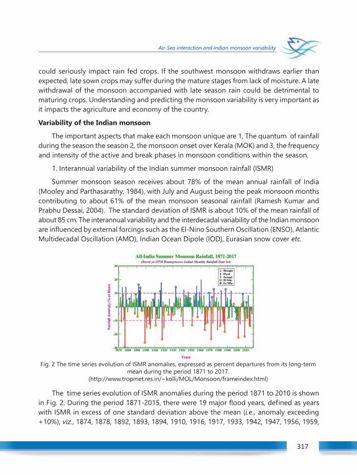
Winter School on Structure and Function of the Marine Ecosystem : Fisheries 317
Air-Sea interaction and Indian monsoon variability
317
could seriously impact rain fed crops. If the southwest monsoon withdraws earlier thanexpected, late sown crops may suffer during the mature stages from lack of moisture. A latewithdrawal of the monsoon accompanied with late season rain could be detrimental tomaturing crops. Understanding and predicting the monsoon variability is very important asit impacts the agriculture and economy of the country.
Variability of the Indian monsoon
The important aspects that make each monsoon unique are 1, The quantum of rainfallduring the season the season 2, the monsoon onset over Kerala (MOK) and 3, the frequencyand intensity of the active and break phases in monsoon conditions within the season.
1. Interannual variability of the Indian summer monsoon rainfall (ISMR)
Summer monsoon season receives about 78% of the mean annual rainfall of India(Mooley and Parthasarathy, 1984), with July and August being the peak monsoon monthscontributing to about 61% of the mean monsoon seasonal rainfall (Ramesh Kumar andPrabhu Dessai, 2004). The standard deviation of ISMR is about 10% of the mean rainfall ofabout 85 cm. The interannual variability and the interdecadal variability of the Indian monsoonare influenced by external forcings such as the El-Nino Southern Oscillation (ENSO), AtlanticMultidecadal Oscillation (AMO), Indian Ocean Dipole (IOD), Eurasian snow cover etc.
Fig. 2 The time series evolution of ISMR anomalies, expressed as percent departures from its long-termmean during the period 1871 to 2017.
(http://www.tropmet.res.in/~kolli/MOL/Monsoon/frameindex.html)
The time series evolution of ISMR anomalies during the period 1871 to 2010 is shownin Fig. 2. During the period 1871-2015, there were 19 major flood years, defined as yearswith ISMR in excess of one standard deviation above the mean (i.e., anomaly exceeding+10%), viz., 1874, 1878, 1892, 1893, 1894, 1910, 1916, 1917, 1933, 1942, 1947, 1956, 1959,
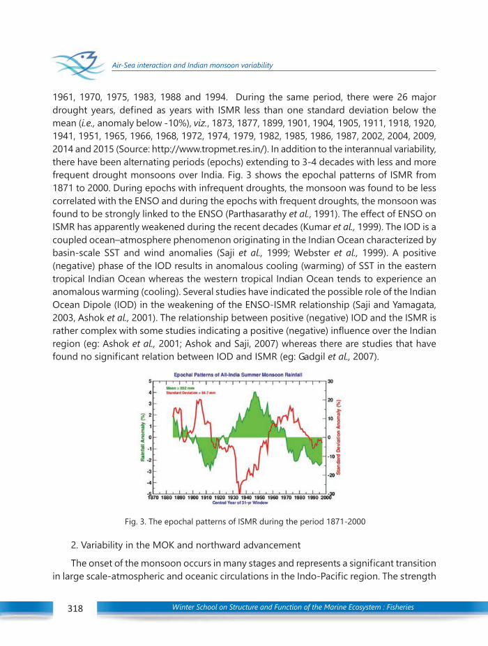
Winter School on Structure and Function of the Marine Ecosystem : Fisheries318
Air-Sea interaction and Indian monsoon variability
1961, 1970, 1975, 1983, 1988 and 1994. During the same period, there were 26 majordrought years, defined as years with ISMR less than one standard deviation below themean (i.e., anomaly below -10%), viz., 1873, 1877, 1899, 1901, 1904, 1905, 1911, 1918, 1920,1941, 1951, 1965, 1966, 1968, 1972, 1974, 1979, 1982, 1985, 1986, 1987, 2002, 2004, 2009,2014 and 2015 (Source: http://www.tropmet.res.in/). In addition to the interannual variability,there have been alternating periods (epochs) extending to 3-4 decades with less and morefrequent drought monsoons over India. Fig. 3 shows the epochal patterns of ISMR from1871 to 2000. During epochs with infrequent droughts, the monsoon was found to be lesscorrelated with the ENSO and during the epochs with frequent droughts, the monsoon wasfound to be strongly linked to the ENSO (Parthasarathy et al., 1991). The effect of ENSO onISMR has apparently weakened during the recent decades (Kumar et al., 1999). The IOD is acoupled ocean–atmosphere phenomenon originating in the Indian Ocean characterized bybasin-scale SST and wind anomalies (Saji et al., 1999; Webster et al., 1999). A positive(negative) phase of the IOD results in anomalous cooling (warming) of SST in the easterntropical Indian Ocean whereas the western tropical Indian Ocean tends to experience ananomalous warming (cooling). Several studies have indicated the possible role of the IndianOcean Dipole (IOD) in the weakening of the ENSO-ISMR relationship (Saji and Yamagata,2003, Ashok et al., 2001). The relationship between positive (negative) IOD and the ISMR israther complex with some studies indicating a positive (negative) influence over the Indianregion (eg: Ashok et al., 2001; Ashok and Saji, 2007) whereas there are studies that havefound no significant relation between IOD and ISMR (eg: Gadgil et al., 2007).
Fig. 3. The epochal patterns of ISMR during the period 1871-2000
2. Variability in the MOK and northward advancement
The onset of the monsoon occurs in many stages and represents a significant transitionin large scale-atmospheric and oceanic circulations in the Indo-Pacific region. The strength

Winter School on Structure and Function of the Marine Ecosystem : Fisheries 319
Air-Sea interaction and Indian monsoon variability
319
of the low level jet and upper tropospheric tropical easterly jet increase rapidly during thetime of the evolution of summer monsoon. There have been several studies that havefocused on the ocean-atmospheric interactions during the onset of monsoon (Eg: Somanand Krishnakumar, 1993; Joseph et al., 1994, Ramesh and Prabhu Dessai, 2004). The onsetof monsoon is declared by India Meteorological Department (IMD) when,
a, If after 10th May, 60% of the 14 stations enlisted*, viz., Minicoy, Amini,Thiruvananthapuram, Punalur, Kollam, Allapuzha, Kottayam, Kochi, Thrissur, Kozhikode,Thalassery, Kannur, Kasargode and Mangalore report rainfall of 2.5 mm or more for twoconsecutive days, the onset over Kerala be declared on the 2nd day, provided the followingcriteria are also in concurrence.
b) Wind field - Depth of westerlies should be maintained upto 600 hPa, in the boxequator to Lat. 10ºN and Long. 55ºE to 80ºE. The zonal wind speed over the area boundedby Lat. 5-10ºN, Long. 70-80ºE should be of the order of 15 – 20 Kts. at 925 hPa.
c). Outgoing Longwave Radiation (OLR) - OLR can be used as a proxy for deep convectivesystems in the tropics. Negative (positive) OLR are indicative of enhanced (suppressed)convection. INSAT derived OLR value should be below 200 wm-2 in the box confined by Lat.5- 10ºN and Long. 70-75ºE.
Once monsoon has set in it surges northwards and covers the country by around 15th
July. NLM is defined as the northern most limit of monsoon up to which it has advanced onany given day. The monsoon advancement also exhibits considerable interannual variability,for eg: in 2002 which was a severe drought year, even though the monsoon onset was ontime (June 1), it covered the entire Indian subcontinent only by August 15th, a delay ofalmost one month.
3. Active and beak spells within the monsoon season
The rainfall distribution is not continuous within the life-cycle of a monsoon, but it isassociated with multiple spells of active and break spells. There are several studies thathave used the same term ‘break’, to denote diûerent features of convection and/or circulationover diûerent regions. Rajeevan et al., (2010) defined active and break events as periodsduring the months of July and August, in which the normalized anomaly of the rainfall overthe monsoon core zone (roughly from 18ºN-28ºN, 65ºE-88ºE) exceeds 1 or is less than “1.0respectively, provided the criterion is satisûed for at least three consecutive days. Prolongedbreaks can create drought conditions over the country. One of the longest recorded breakspell occurred in the year 2002 and it lasted for about 34 days (Ramesh and Prabu Dessai,2004). Fig. 4 and Fig. 5 shows the wind field at 850 hPa level (~1.5 kms above msl) duringbreak and active conditions respectively. It can be seen that the cross equatorial flow (CEF)

Winter School on Structure and Function of the Marine Ecosystem : Fisheries320
Air-Sea interaction and Indian monsoon variability
is stronger during active conditions and its core is directed towards the Indian subcontinent.During break conditions, winds are considerably weaker and the CEF acquires a southwardcurvature and appears to be blowing away from the subcontinent. Ramesh Kumar et al.,(2007) found that the frequency of break-spells and the number of break days showed anincreasing trend during the recent decades. They also found that there was a clear increasein the number of long breaks (breaks longer than 7 days) post mid-1970s. They attributedthis to the altering large-scale ocean-atmosphere processes in the tropical Indian Oceansuch as weakening of the southwest monsoon winds and decreased moisture transportfrom the tropical Indian Ocean into the subcontinent.
Air-sea interaction processes in the southeastern Arabian Sea and their influence onprimary productivity/fisheries during the summer monsoon season
The Malabar upwelling zone along the Kerala coast is one of the important upwellingsystems of the world (Bakun et al., 1998). Under the influence of the south-westerly windsalong the west coast, the surface waters move away from the coast and are replaced bycolder, nutrient-rich and often oxygen depleted waters from the subsurface (Ekman pumping/transport). This leads to phytoplankton blooms (mostly diatoms and dinoflagellates) andincreased productivity (Madhupratap et al., 2001). Shanker and Shetye (1997) showed thatupwelling along the area 9°N to 13°N is under the combined influence of wind stress, andthe upwelling Kelvin and Rossby waves. This area contributes about 20% to the marine fishcatch of India (Manjusha et al., 2013). An important feature of the Malabar upwelling zoneis the predominance of pelagic resources such as oil sardine (Sardinella longiceps) and Indianmackerel (Rastrelliger kanagurta), which support the western Indian Ocean’s largest coastalpelagic fishery (Vivekanandan et al., 2005). The coastal upwelling index (CUI) during south-
Fig. 4 Cross equatorial flow at 850 hPa level duringbreak monsoon conditions (2002)
Fig. 5 Cross equatorial flow at 850 hPa level duringactive monsoon conditions (2002)
Winter School on Structure and Function of the Marine Ecosystem : Fisheries 321
Air-Sea interaction and Indian monsoon variability
321
west monsoon increased by nearly 50% during the period 1998 to 2007 and during thesame period the annual average chlorophyll_a concentration increased by more than 200%(Manjusha et al., 2013). The increasing CUI and chlorophyll_a during monsoon sustained anincreasing catch of oil sardine during post-monsoon season. Further studies are required toinvestigate the variability of fisheries/primary productivity on an interannual scale.
References
Ashok, K., Guan, Z. and Yamagata, T., 2001. Impact of the Indian Ocean dipole on the relationship betweenthe Indian monsoon rainfall and ENSO. Geophysical Research Letters, 28(23), pp.4499-4502.
Ashok, K. and Saji, N.H., 2007. On the impacts of ENSO and Indian Ocean dipole events on sub-regionalIndian summer monsoon rainfall. Natural Hazards, 42(2), pp.273-285.
Ananthakrishnan, R. and Soman, M.K., 1988. The onset of the southwest monsoon over Kerala: 1901–1980.International Journal of Climatology, 8(3), pp.283-296.
Bakun, A., Roy, C. and Lluch-Cota, S., 1998. Coastal upwelling and other processes regulating ecosystemproductivity and fish production in the western Indian Ocean. In: Sherman, K., Okemwa, E. and Nitiba,M. Malden (Eds.), Large marine ecosystems of the Indian Ocean: Assessment, sustainability andmanagement. Massachusettes: Blackwell Sciences Inc., p. 103–141.
Gadgil, S., Rajeevan, M. and Francis, P.A., 2007. Monsoon variability: Links to major oscillations over theequatorial Pacific and Indian oceans. Current Science, 93(2), pp.182-194.
Kumar, K.K., Rajagopalan, B. and Cane, M.A., 1999. On the weakening relationship between the Indianmonsoon and ENSO. Science, 284(5423), pp.2156-2159.
Madhupratap, M., Nair, K.N.V., Gopalakrishnan, T.C., Haridas, P., Nair, K.K.C., Venugopal, P. and Gauns, M.,2001. Arabian Sea oceanography and fisheries of the west coast of India. Current Science, 81(4), pp.355-361.
Manjusha, U., Jayasankar, J., Remya, R., Ambrose, T.V. and Vivekanandan, E., 2013. Influence of coastalupwelling on the fishery of small pelagics off Kerala, south-west coast of India. Indian Journal ofFisheries, 60(2), pp.37-42.
Parthasarathy, B., Kumar, K.R. and Munot, A.A., 1991. Evidence of secular variations in Indian monsoonrainfall–circulation relationships. Journal of Climate, 4(9), pp.927-938.
Rajeevan, M., Gadgil, S. and Bhate, J., 2010. Active and break spells of the Indian summer monsoon. Journalof earth system science, 119(3), pp.229-247.
Ramesh Kumar, M.R. and Prabhu Dessai, U.R., 2004. A new criterion for identifying breaks in monsoonconditions over the Indian subcontinent. Geophysical research letters, 31(18).
Saji, N.H., Goswami, B.N., Vinayachandran, P.N. and Yamagata, T., 1999. A dipole mode in the tropical IndianOcean. Nature, 401(6751), pp.360-363.
Saji, N.H. and Yamagata, T., 2003. Possible impacts of Indian Ocean dipole mode events on global climate.Climate Research, 25(2), pp.151-169.
Soman, M.K. and Kumar, K.K., 1993. Space-time evolution of meteorological features associated with theonset of Indian summer monsoon. Monthly Weather Review, 121(4), pp.1177-1194.

Winter School on Structure and Function of the Marine Ecosystem : Fisheries322
Air-Sea interaction and Indian monsoon variability
Shankar, D. and Shetye, S.R., 1997. On the dynamics of the Lakshadweep high and low in the southeasternArabian Sea. Journal of Geophysical Research: Oceans, 102(C6), pp.12551-12562.
Vivekanandan, E., Srinath, M. and Kuriakose, S., 2005. Fishing the marine food web along the Indian coast.Fisheries Research, 72(2), pp.241-252.
Webster, P.J., Moore, A.M., Loschnigg, J.P. and Leben, R.R., 1999. Coupled ocean–atmosphere dynamics inthe Indian Ocean during 1997–98. Nature, 401(6751), pp.356-360

Winter School on Structure and Function of the Marine Ecosystem : Fisheries 323
Genetic Stock Characterization of fish using Molecular Markers
IntroductionAccurate Identification of genetic resources is necessary for detecting new species and
varieties for products of commercial value. Fish, as a group, apart from their economic valuefrom a biodiversity viewpoint, have the highest species diversity among all vertebrate taxa.They exhibit enormous diversity in size, shape, biology and in the habitats they occupy. Interms of habitat diversity, fishes live in almost all conceivable aquatic habitats, ranging fromAntarctic waters to desert springs. Of the 62,305 species of vertebrates recognized worldover, 34,090 (nearly 52%) are valid fish species; a great majority of them (97%) are bonyfishes and the remaining (3%) are cartilaginous (sharks and rays) and jawless fishes (lampreysand hagfishes). Further, on an average, 300 new fish species are described each year, andglobal surveys indicate that there could well be at least 5,000 species more to be discovered.
Loss of biodiversity is one of the greatest challenges facing modern society. Thisenvironmental crisis is increasingly evidenced by the loss or deterioration of genetic resourcesand habitats, as well as recent attempts to highlight and address the issue at the highestinternational levels. Appropriate conservation efforts for protection of the natural biologicalwealth warrant right attention for their sustainable utilization and for posterity. Public concernfor biodiversity conservation has risen in the last 50 years and led to national and inter-national policies, legislation, and actions to conserve biodiversity, notably the Convention onBiological Diversity (CBD). To conserve and sustainably utilize the bioresources of the countryand for maintaining sovereignty over them, several nations enacted the Biological DiversityAct (BDA). This encompasses guide-lines to address a wide range of issues related to theutilization of bioresources and information within the country as well as by other countries.Management of Fish Genetic Resources
The objective of management (documentation + conservation + sustainable utilization)of species and their habitats is to maintain the genetic identity and integrity of the speciesin their natural habitat as well as a genetically sustainable fishery. Hence, documentation ofgenetic variation and diversity is of vital significance to evolve conservation strategies withlong-term impact. Genetic resources can be viewed as genetic differences at three hierarchicallevels of organization, viz., species, populations and individuals. At the highest level, species
38C H A P T E R GENETIC STOCK CHARACTERIZATION OF
FISH USING MOLECULAR MARKERSA. Gopalakrishnan*
ICAR- Central Marine Fisheries Research Institute
*Reprinted from Course Manual of Summer School on Advanced Methods for Fish Stock Assessment and Fisheries Management. Lecture Note Series No. 2/2017. CMFRI, Kochi, pp. 308-316.
Winter School on Structure and Function of the Marine Ecosystem : Fisheries324
Genetic Stock Characterization of fish using Molecular Markers
consist of ‘populations’ or ‘genetic stocks’ that are reproductively isolated from populationsof other species. Each species harbours a unique set of genetic material and therefore,conservation, may aim at a specific species, which requires sound knowledge about itsbiology, biogeography and within species (inter-populational) level genetic diversity. At thepopulation level of organization, the identification of discrete genetic breeding units(usually called a ‘stock’ in fisheries biology; this is roughly equivalent to a ‘population’ or‘genetic stock’ to a geneticist) has been a major theme in fisheries research. The definitionof a stock can vary, as the motivations of fishery managers may be influenced by political,economic or biological mandates. Finally, the largest store of genetic variability in mostspecies exists as genetic differences among individuals within a population. Hence,the goal of pre-serving genetic variability in a population coincides with the goal ofmaintaining large ecologically sound natural populations. A fundamental need is to definedistinct entities that range from individuals to species to ecosystems and beyond.
Population/Genetic Stock Identification (GSI)
Assessment of genetic variability is important for the management of wild geneticresources of fish. Most species are composed of populations, also called genetic stocks,between which limited gene flow occurs. These populations maintain their genetic makeupor characteristics distinct from other populations of the same species because of geneticvariation within the species. This differentiation depends upon forces such as migration,mutation, selection, and genetic drift, which act on the species/population during itsevolution. If such units are overfished, it is unlikely that population sizes will recover becauseof migration, and hence a collapse of the fishery may occur. Therefore, with the loss of agenetic stock, a species also loses the animals that are adapted to a particular habitatthrough evolution. Moreover, interbreeding of non-native fish stocks/species with a differentmake up tends to reduce the genetic variation that naturally exists between genetic stocks.In other words, different natural genetic identities available for a species in different habitatsare lost.
A fundamental problem for fisheries management is the identification of populations/stock of a species and this idea has been brought together with the definition of stock formanagement. The term stock has been used in various management contexts with little orno genetic content. Several approaches have been advocated to solve this problem.
Ihssen et al., (1981) defines a stock as ‘an intra-specific group of randomly matingindividuals with temporal or spatial integrity’.
Larkin (1972) defined a stock as ‘a population of organisms which share a common genepool, is sufficiently discrete to warrant consideration as a self-perpetuating system whichcan be managed’.
Winter School on Structure and Function of the Marine Ecosystem : Fisheries 325
Genetic Stock Characterization of fish using Molecular Markers
In fishery management, a unit of stock is normally regarded as a group of fish exploitedin a specific area or by a specific method.
If fishery managers are to include genetic considerations in their decisions, they willneed information on the biological differences between discrete local groups of a speciesand they will need to understand the genetic and ecological processes that influencediscreteness. Thus, the implementation of management strategies based on moleculargenetic data can have indirect benefits for population biodiversity, as the main objective ofsuch management plans is to avoid population crashes, which in turn benefits themaintenance of population genetic diversity.
Molecular Genetic Markers: The primary objective of the genetic stock identification(GSI) in fish is to assess the distribution and pattern of genetic variability at intra-as well asinter-specific population levels. The first priority for such research is identification ofappropriate molecular genetic markers to assess genetic diversity. Fish stock identificationwas initially based solely upon morphological and meristic differences. Because thesecharacters can be influenced by the environment, their variations may not have a geneticbasis, and hence do not necessarily provide information on genetic and evolutionaryrelationships. In the 1950s, dissatisfaction with performance of phenotypic methods forstock identification encouraged early exploration of genetic markers. The markers developedhave spurred development of statistical algorithms and revolutionized the analytical powernecessary to explore genetic diversity among populations. Methods that take advantage ofnaturally occurring genetic markers have attracted a good deal of attention becauseapplication of physical tags is very labour intensive, and biological markers, such as scalepatterns, can vary dramatically from year to year. The first GSI methods using soluble proteinsand gene products such as allozymes (enzymes at cellular level) for estimating thecontributions of two or more salmon stocks to a mixed harvest were developed in the late1970s. Since then, the rapidly expanding availability of highly variable genetic markers andrefinements in statistical analyses have considerably increased the ability to analyze thestock structure of different fish species; but this has also led to the genetic ‘marker wars’among fish geneticists during the past several decades. For many years, allozymes were theuniversal workhorse genetic makers, and they made many valuable contributions to basicand applied conservation and management. Around 1980, the first applications ofmitochondrial DNA (mtDNA) analysis to natural populations were published, and gradually,it replaced allozymes and provided answers to key management questions regarding stockstructure. The development of DNA amplification using the polymerase chain reaction(PCR) technique has opened up possibility of examining genetic changes in populationsover the past 100-years or more even using archive material. In PCR reaction, a DNA sequencecan be amplified many thousand folds to provide sufficient product for restriction analysis
Winter School on Structure and Function of the Marine Ecosystem : Fisheries326
Genetic Stock Characterization of fish using Molecular Markers
or direct sequencing. Once appropriate primers are available, large number of individualscan be assayed quickly thus facilitating large population screening for variability. Portionsof the mtDNA such as, the ATPase 6 and 8 and hypervariable trans-membrane segments ofcytochrome b (Cytb) that evolve exceptionally rapidly have been used for high-resolutionanalysis of genetic stock structure in fish. Although mtDNA has indeed provided a wealth ofnew insights, it is not a solution and has some limitations with respect to fishery management(e.g., it is maternally inherited, so provides information only about female migration orgene flow, and it is only a single marker and hence has much less power than a full suite ofnuclear markers).
In the 1990s, microsatellites (Short Tandem Repeats-STRs or Simple SequenceRepeats-SSRs) muscled aside mtDNA and these highly variable co-dominant markershave provided greatly increased power and opened up exciting new opportunities (e.g.parentage analysis and individual assignments) that were generally not feasible with allozymesor mtDNA. Microsatellites are repeated DNA sequences having a unit length of 2-6 basepairs tandemly repeated minimum 6 times usually; maximum several times at each locus.They are found in all prokaryote and eukaryote genomes investigated to date. Individualalleles at a locus differ in the number of tandem repeats of the unit sequence owing to gainor loss of one or more repeats and they as such can be differentiated by electrophoresisaccording to their size.
There are four types of microsatellites
1. Perfect: Perfect tandem repeat sequences.2. Imperfect: Tandem repeat sequences with intervening sequences.3. Compound: More than one kind of repeats, adjacent ones.4. Complex: More than one kind of repeats, with intermediary sequences.
Based on the number of base pairs in a repeat unit, microsatellites can be again classifiedinto mono (e.g. C or A), di (e.g. CA), tri (e.g. CCA), tetra (e.g. GATA), penta (e.g. CGATA) andhexa (e.g. ATGGCA) repeat unit microsatellites. Microsatellites that are used in stockidentification studies typically contain di- (AC)n, tri-(ACC)n, or tetra-nucleotide (GATA)nrepeats. The most common ones are dinucleotide repeats. Tetra-nucleotide microsatellitesare gradually replacing dinucleotide loci as the preferred genetic marker for stock analysis.Microsatellite loci are abundant in all eukaryote genomes and it has been estimated thatthere are from 103 to 105 microsatellite loci dispersed at 7 to 1010 base pair (bp) intervals orone locus at every 100-300 kilobase pair (kbp) intervals in the eukaryotic genome. Fishgenomes may contain more microsatellite loci than most other invertebrate and vertebratetaxa. Mapping studies suggest more or less even distributions of microsatellites throughoutgenomes, although they are somewhat rarer within coding sequences.
Winter School on Structure and Function of the Marine Ecosystem : Fisheries 327
Genetic Stock Characterization of fish using Molecular Markers
Several features of STR render them invaluable for examining fish population structure.Microsatellites are codominant in nature and inherited in Mendelian fashion, revealingpolymorphic amplification products from all individuals in a population. They containinformation, which are directly related to the effective number of alleles at each locus. PCRfor microsatellites can be automated for identifying simple sequences repeat polymorphism.Small amount of samples of blood or alcohol preserved tissue is adequate for analyzingthem. Because they are highly variable in nature, abundant variants are ensured forcharacterization of populations. However, sample size in excess of 50 may be required torepresent the genotype frequencies. The microsatellites are non-coding and thereforevariations are independent of natural selection. These properties make microsatellites idealgenetic markers for defining population genetic diversity and distance measures. Becausemost STR loci are unlinked and inherited independently, the greater the number of lociscreened, the greater the likelihood of selecting loci that reveal significant allelic frequencydifferences among populations and more statistical power is gained in quantifying theextent of genetic differentiation among populations. Additionally, analysis of a larger numberof loci may provide a more accurate picture of the evolutionary history of the geneticstocks.
Analysis of microsatellite polymorphisms is a PCR-based approach in whicholigonucleotide primers are designed based on unique single-copy sequences flanking themicrosatellite repeats. DNA extracted from tissue samples are subjected to PCR reactions.PCR primer pairs are selected such that PCR products are of small molecular size (usually<350bp), providing relative ease in amplification from low-quality DNAs and also allowingfor distinguishing small differences in the molecular size of alleles among individuals byusing polyacrylamide-gel electrophoresis or automated DNA sequencers. Ideally, eachindividual shows a single (homozygote) or two-band (heterozygote) DNA pattern, with oneband inherited from each parent. Polymorphic alleles at a locus are usually characterized bytheir molecular sizes. For dinucleotide repeats, these will differ by two base units. Based onthe STR allele frequency data, powerful statistical tests are employed to arrive at a decisionwhether the genetic stocks of a species are significantly different from one another.
However, the field now seems poised to shift towards another type of marker, single-nucleotide polymorphisms (SNPs). Like allozymes, SNPs are generally diallelic, so eachmarker has less power than a single microsatellite locus. They occur in vast numbersthroughout the genome; therefore, eventually large overall increases in power are possible.Furthermore, once developed, SNPs can be assayed more reliably and cheaply thanmicrosatellites, which could be a considerable advantage in large-scale fishery managementapplications. However, development of sufficient numbers of SNP markers will be neithereasy nor cheap, and analytical issues such as minimizing ascertainment bias remain to be

Winter School on Structure and Function of the Marine Ecosystem : Fisheries328
Genetic Stock Characterization of fish using Molecular Markers
resolved. Despite growing competition from new genotyping and sequencing techniquesand latest class of markers, the use of the versatile and cost-effective microsatellites continuesto increase, boosted by successive technical advances. Next-generation sequencing (NGS)technologies and the rise of commercial services allow the identification of large numbers ofmicrosatellite loci at reduced cost in non-model species. As a result, more stringent selectionof loci is possible, thereby further enhancing multiplex quality and efficiency. Numerousexamples also exist where microsatellite analysis is used for fish population analysis andmanagement of Pacific salmon (Fisheries and Oceans Canada website: http://www.pac.dfo-mpo.gc.ca/science/facilities-installations/pbs-sbp/mgl-lgm/proj/ index eng. htm online.) andalso for cod where microsatellites have even been used as evidence in a court cases againsta fishermen claiming a false origin of his catch. Use of 20-25 polymorphic microsatelliteloci (preferably tetra-nucleotide repeats) and 70–100 individuals from each populationhas become the standard and scientifically accepted protocol for population geneticanalysis of fish along with information on biology and morphometry (TRUSS) data.Sequence information of mitochondrial complete ATPase 6/8 and Cytb genes of at least20 individuals per population are also often generated along with this.
Genetic Stock Structure in fish
Distinct population structure has been observed in many fish species across the worldindicating that propagation-assisted restoration programmes must be stock-specific toreplenish declining populations. Generally, between populations of marine and freshwaterspecies, marked differences exist in the level of genetic differentiation and genetic diversity,with marine species generally exhibiting lower levels of inter-population differentiation andgreater genetic diversity. This is mainly due to the higher effective population sizes and/orhigher inter-population migration rates in marine environments compared with freshwater.In addition, marine fishes and invertebrates are generally broadcast spawners and hencehave large potential for movement between areas by larval drift in currents. In addition,adults of many species are capable of making long distance migrations. Early genetic studiesof commercially important marine fishes using allozymes and proteins indicated that theygenerally had moderate levels of gene diversity and little population subdivision, oftencovering over several hundred kilometers. However, unexpected fine-scale population sub-structuring and deep genetic lineages have been observed in recent studies with high-resolution markers in many fishes which calls for further in-depth integrated approaches ofmolecular genetics with life-history traits. This will prove whether the variability is due toisolation or adaptations to particular marine habitats or as a result of non-genetic factorssuch as large reproductive variation among families. Regular monitoring of populations isalso essential to enable a distinction between normal population-size fluctuations and thosesevere enough to warrant conservation measures.
Winter School on Structure and Function of the Marine Ecosystem : Fisheries 329
Genetic Stock Characterization of fish using Molecular Markers
The greatest genetic threats in the marine ecosystem are the extinction of genetically uniquesubpopulations and loss of genetic diversity primarily through overfishing and climatechange. Illegal unreported and unregulated (IUU) fishing also contributes to this condition,and thus poses a severe threat to marine ecosystems. Controlling for compliance andenforcing fishing regulations is hampered by difficulties in identifying the geographicalorigin of fish and fish products, at point of landing and further down the food supply chain.Presently, there are no validated genetic methods for identifying the geographical origin ofmarine f ish and investigate commercial fraud. ‘FishPop-Trace ’(https://fishpoptrace.jrc.ec.europa.eu/web/fishpop trace/) is an international project, funded by theEuropean Union (EU) framework programme (FP7), aiming to generate forensically validatedreference panels of SNP markers for geographical origin assignment in four commerciallyimportant fish species, cod (Gadus morhua), hake (Merluccius merluccius), herring (Clupeaharengus) and common sole (Solea solea). SNP markers are selected these are subsequentlygenotyped across populations to provide high resolution data to analyze genetic variation.These markers are validated to be used as tags for traceability and enforcement applicationsleading to a reduction in IUU fishing and conservation of remaining marine resources.
For a successful stocking programme such as sea ranching of endangered seahorse orsacred chank, genetic structure of the original wild population must be determined beforeany new fish are released into the waters. This information can be used to develop hatcheryguidelines for breeding fish for stocking purposes. By ensuring that the stocked populationis having the same genetic make-up as the wild population, re-integration of the stockedfish will likely be more successful and deviations from the original genetic structure will beminimal.
Integrating Population Genetics Data into Marine Fisheries Management
Maintaining the maximum level of genetic variations in fish stocks is vital for thepreservation of genetic resources. Therefore, excessive loss of genetic variability should beavoided for sustainable management of resources. Application of molecular marker techniquesto a number of species has shown that these methods can provide information on geneticstock structure that can be of direct management relevance. However, such information hasnot always been incorporated into fishery management and policy decisions in severalcountries. The complex problem requires agreement among scientists, governmentalorganizations and policy makers to define and implement policies on the sustainablemanagement of these natural resources. Numerous factors (as mentioned below) havecontributed to the imperfect integration of genetic data into management of aquatic species.
The fish stock assessment teams generally include quantitative fishery biologists andstatisticians. In appropriate situations, the teams should be expanded to include geneticists
Winter School on Structure and Function of the Marine Ecosystem : Fisheries330
Genetic Stock Characterization of fish using Molecular Markers
as well as field biologists. It is always better that fish geneticists fully understand thecomplexities of the management process so that genetic information can be packaged inthe most effective manner, and importance of GSI can be portrayed effectively for thepolicy makers. Also the managers involved in monitoring of fishery resources shouldacknowledge that GSI can provide valuable management information. Scientists, managersand policymakers could work together more effectively to foster productive dialogue tolink statutory definitions and management or conservation goals.
It is diff icult to develop an ideal sampling design for a genetic study withoutunderstanding the details of the life history of the target species and physical processes inthe aquatic ecosystem. Genetic data can be integrated with other types of biological andoceanographical information. The sampling design of genetic studies does not always matchthe geographical regions to which management controls are applied. This can rarely resultin discrepancy between biological and genetic management units. Implementing GSI overa broad geographical area requires extensive efforts to collect baseline data for populationsfrom different coasts and to standardize laboratory procedures so that comparable datacan be obtained by different laboratories. This requires funds, broad collaboration amonglaboratories and a willingness to share unpublished data.
Most fish geneticists are unfortunately, not exposed to the techniques of statisticalmodel and decision analysis that form the basis for modern stock assessment science. Equally,managers and assessment biologists similarly would benefit from a greater literacy regardingthe genetic principles that can profoundly affect the aquatic living resources for which theyshare stewardship responsibility. Therefore, it might be necessary to develop brief integratedtraining courses to equip geneticists and managers to work on assessment teams.
The purpose of stock assessment in fisheries is to provide timely and appropriatescientific advice on fisheries management for sustained production. Though there are fewmulti-species models, the assessments are almost mostly conducted for single species,whereas in reality, stocks are influenced by multi-species interactions. In addition, gearsmostly harvest many species at a time, leading to difficulty in implementation of themanagement measures derived from single species stock assessment. Due to the lack ofadequate and efficient models for multi-species interactions, stock assessments will generallycontinue to be based on single species models. Although the main approach in populationgenetic studies of natural populations still involves collecting individuals from two or moregeographical locations and considering them as putative populations, landscape genetics/seascape genetics—the study of spatial genetic patterns in continuously distributed species—is rapidly evolving and the methods are beginning to be applied especially to marine speciesas well. These studies are expected to provide important insights into biological processesleading to effective multi-species stock assessment and management of marine ecosystems.

Winter School on Structure and Function of the Marine Ecosystem : Fisheries 331
Genetic Stock Characterization of fish using Molecular Markers
However, considerable dialogue between geneticists, stock assessment scientists andmanagers, as well as creative thinking on both sides are required to develop effective waysto integrate these insights into fisheries management.
In conclusion, fish genetic stock diversity conservation requires preservation of as muchvariation as possible at all taxonomic levels and concerted efforts by integrating capture,culture fisheries and environmental programmes using latest technological innovations.The genetic tools will provide innovative means in the future and are an assuring approachfor food security of the world and in reducing the fishing pressure on natural resources.Genetic data need to be integrated with other types of biological and oceanographicalinformation for understanding the details of the life history of the target species and physicalprocesses in the marine ecosystem. Although better monitoring of biodiversity, betterassessment of risk and a more strategic approach to conserving biodiversity are all essentialcomponents to successful risk management, an equally important need is the open dialogueamong geneticists, quantitative fishery biologists, statisticians, conservationists and plannersthat would help sustainable management of stocks of the world’s amazingly rich assemblageof fishes.
References
Ayyappan S., Jena J. K. and Gopalakrishnan A., 2014. Molecular Tools for Sustainable Management ofAquatic Germplasm Resources of India. Agricultural Research 3(1): 1-21.
Ihssen P.E., Booke H.E., Casselman J.M., McGlade J.M., Payne N.R., Utter F.M., 1981. Stock identification:materials and methods. Can J. Fish. Aquat. Sci., 38:1838–1855.
Larkin P.A., 1972. The stock concept and management of Pacific salmon. In: Simon R.C., Larkin P. A. (Eds)The stock concept in Pacific salmon, H.R. MacMillan Lectures in fisheries. University of British Columbia,Vancouver, p 231.

Winter School on Structure and Function of the Marine Ecosystem : Fisheries332
Ecolabelling in Fisheries: Boon or Bane in improving trade?
Introduction
This document is a collation of information, mainly from FAO documents on fisheriesecolabelling (FAO, 2001; Sainsbury, 2010; Washington and Ababouch, 2011). Fish is one ofthe most highly traded commodities in the world, and as a natural resource, there is worldwideconcern about long-term sustainability of the resources. Ecolabels are a new and growingfeature of international fish trade and marketing. They have emerged in the context ofincreased demand for fish and seafood, and a perception that many governments are failingto manage the sustainability of marine resources adequately. Many mechanisms to ensurethe sustainability of fish stocks have been introduced by international bodies which arebinding on national governments. These include:
The United Nations Convention on the Law of the Sea (UNCLOS) (1982);
The FAO Code of Conduct for Responsible Fisheries (the Code) (1995);
The United Nations Fish Stocks Agreement (1995); and
Various regional fisheries management organizations (RFMOs).
The RFMOs facilitate international cooperation at the regional level for the conservationand management of highly migratory and straddling fish stocks. At the nationallevel, governments are attempting to embed the principles and goals of the Code– now inits second decade of implementation – into their national fisheries management policies(FAO, 2009a). However, they are having varying degrees of success. Disappointment withthe pace of regulatory measures to curb overfishing and to improve fisheries sustainabilityhas led environmental groups to develop alternative market-based strategies for protectingmarine life and promoting sustainability. These private market mechanisms are designedto influence the purchasing decisions of consumers and the procurement policies of retailersselling fish and seafood products, as well as to reward producers using responsible fishingpractices. Ecolabels are one such market-based mechanism.
39C H A P T E R ECOLABELLING IN FISHERIES:
BOON OR BANE IN IMPROVING TRADE?K. Sunil Mohamed*
Molluscan Fisheries DivisionICAR-Central Marine Fisheries Research Institute
*Reprinted from manual of ICAR funded short course on 'World Trade Agreements and Indian Fisheries Paradigms: A Policy Outlook', pp. 357- 363, held during 17-26 September 2012 at CMFRI, Kochi.
Winter School on Structure and Function of the Marine Ecosystem : Fisheries 333
Ecolabelling in Fisheries: Boon or Bane in improving trade?
333
The FAO Guidelines for the Ecolabelling of Fish and Fishery Products from Marine CaptureFisheries state that voluntary standards, including environmental standards, should not distortglobal markets and should not create unnecessary obstacles to international trade. Underthe general principles and definitions, they state that any ecolabelling scheme should beconsistent with inter alia the World Trade Organization (WTO) rules and mechanisms.
What is an Ecolabel ?
Ecolabelling is a market-based tool to promote the sustainable use of natural resources.Ecolabels are seals of approval given to products that are deemed to have fewer impacts onthe environment than functionally or competitively similar products. The ecolabel itself is atag or label placed on a product that certifies that the product was produced in anenvironmentally friendly way. The label provides information at the point of sale that linksthe product to the state of the resource and/or its related management regime. Sittingbehind the label is a certification process. Organizations developing and managing anecolabel set standards against which applicants wishing to use the label will be judged and,if found to be in compliance, eventually certified. The parent organization also markets thelabel to consumers to ensure recognition and demand for labelled products. The theory isthat ecolabels provide consumers with sufficient information to enable them to recognizeand choose environmentally friendly products.
A range of ecolabelling and certification schemes exists in the fisheries sector, with eachscheme having its own criteria, assessment processes, levels of transparency and sponsors.What is covered by the schemes can vary considerably: bycatch issues, fishing methods andgear, sustainability of stocks, conservation of ecosystems, and even social and economicdevelopment. The sponsors or developers of standards and certification schemes for fisheriessustainability also vary: private companies, industry groups, NGOs, and even somecombinations of stakeholders. A few governments have also developed national ecolabels.
The first fisheries ecolabelling initiatives appeared in the early 1990s and were largelyconcerned with incidental catch, or bycatch, during fishing. For example, the “Dolphin-Safe” label was based on standards developed by the United States NGO Earth Island Instituteand is focused on dolphin bycatch in the tuna industry (rather than the sustainability oftuna stocks).
Marine Stewardship Council (MSC)
One of the first scientifically developed ecolabelling schemes, the MSC was set up bythe WWF and Unilever in 1997, but has been independent of them for more than ten years.The MSC is arguably the most comprehensive fisheries certification scheme in that it coversa range of species and deals with all aspects of the management of a fishery. MSC sets thestandard for the ecolabel through its board, supported by a Technical Advisory Board.
Winter School on Structure and Function of the Marine Ecosystem : Fisheries334
Ecolabelling in Fisheries: Boon or Bane in improving trade?
The MSC has qualified for membership of the ISEAL (International Social andEnvironmental Accreditation and Labelling Alliance) as being consistent with its “Code ofgood practice for setting social and environmental standards”. The MSC has two standards:on “sustainable fishing” and on “seafood trace ability”. The MSC owns the standards againstwhich independent third-party certifiers assess conformance. Its “Fisheries AssessmentMethodology”, and “standardized assessment tree” focus on three pillars: independentscientific verification of the sustainability of the stock; the ecosystem impact of the fishery;and the effective management of the fishery. All three pillars are assessed on the basis of arange of indicators. Aspects related to the species, the fishing gear used, andthe geographical area, are all included in the assessment. A study by Caswell and Anders(2009) concluded that it is the scheme most often referred to in the seafood industry media,and has variously been described as the “industry standard”. Another recent study (MRAG,2009) revealed that a significant number of retailers and brand owners refer to the MSC intheir sea food sustainability procurement policies.
Some 150 fisheries around the world are engaged in some stage of the MSC assessmentprocess (including pre-assessment) (MSC, 2009). Fifty-six fisheries have so far been certified.The MSC claims to cover “about 7 per cent of the annual global wild harvest” of fish andseafood, accounting for 42 per cent of the global wild salmon catch and 40 per cent of theglobal white fish catch. However, not all fish from a certified fishery will end up with theMSC label attached. The actual volume of MSC-labelled product on the market as aproportion of overall traded fish products is likely to be considerably less significant interms of global trade. While there are no robust statistics on the proportion of MSC-labelledproducts on the global market, FAO estimates suggest that the volume of MSC- labelledproducts on the market may only be statistically significant in the context of specific Europeanmarkets. Ina study carried out for FAO in 2007, Poseidon Ltd. estimated MSC products asthen accounting for 0.3 per cent of globally traded seafood by value. Sales of MSC-labelledfish and seafood of an estimated US$1.5 billion is minor when seen against a fisheriescommodity market amounting to US$101 billion in global export sales (FAO, 2010).
As of late 2009, more than 2 500 MSC-labelled products were available on the market(MSC, 2009); this is double the number (1 200) on sale at the beginning of 2008,and morethan four times the number (600) available in early 2007,24 showing just how dynamic themarket for certified fish and seafood is. Today, MSC products are sold in52 countries aroundthe world.Friend of the Sea
Friend of the Sea (FOS) has its origins in the Earth Island Institute. Set up in 2006, itsfounder is also the European Director of Dolphin Safe. It covers both wild and farmed fishand its criteria also include requirements related to carbon footprint and “social
Winter School on Structure and Function of the Marine Ecosystem : Fisheries 335
Ecolabelling in Fisheries: Boon or Bane in improving trade?
335
accountability”. Certification is based on the sustainability of the stock, rather than whetherthe fishery is sustainably managed. Its certification methodology is based on existing officialdata in terms of stock assessment. Friend of the Sea says it will not certify stocks that are“overexploited” (based on FAO definitions of levels of exploitation), fisheries using methodsthat affect the seabed and those that generate more than 8 percent discards. Certificationis undertaken by independent third-party certifiers. Friend of the Sea claims to be “themain sustainable seafood certification scheme in the world” covering some 10 per cent ofthe world’s wild capture fisheries. It should be noted that 80 per cent of the 10 milliontonnes of landed FOS certified product from capture fisheries (8 million tonnes) comesfrom Peruvian anchovies. Again, it is unclear what proportion of that product ends up aslabelled products for retail sale. There are about 600 FOS products (including fish oil andomega-3 supplements) sold in 26 countries28 and covering 70 species both from wildcapture and aquaculture.Marine Aquarium Council
The Marine Aquarium Council (MAC) was established in 1998 and by 2001 had adopteda standard and process to certify the wild capture and subsequent treatment of fish for theornamental aquarium trade. In 2004, a standard for live fish for human consumption wasdeveloped because many of the operators and communities involved with the aquariumtrade are also involved in the trade of live fish for consumption. However, this standard forlive fish for human consumption was not formally adopted by the MAC and no fisherieshave been certified for this trade.Other NGO schemes
Other NGO-driven schemes include KRAV, a Swedish NGO that specializes in organicfarming but which has recently developed a “standard for sustainable fishing” and Naturlandin Germany also with a background in certifying organic farmed seafood but now with a“Scheme for the Certification of Capture Fishery Project”, which includes social, economicand ecological sustainability criteria. To date, Naturland has only certified one fishery (Nileperch from Buboka in the United Republic of Tanzania).Fishing company in-house ecolabels
A few individual fishing companies have created their own ecolabels. Forexample, the Spanish group Pescanova, one of Europe’s largest fishing companies, whichfishes globally and has interests in the processing sector, has created a logo that appearson a limited range of its packaged products. The logo states that the fish concerned hasbeen caught in a way that “preserves the aquatic and marine ecosystem for maintaining thequality, diversity and availability of fish resources for today and future generations”. This in-house scheme claims to be based on the Code.

Winter School on Structure and Function of the Marine Ecosystem : Fisheries336
Ecolabelling in Fisheries: Boon or Bane in improving trade?
Fishing industry association ecolabelling schemes
The Japan Fisheries Association, an umbrella group for some 400 fishing companies,founded the Marine EcoLabel- Japan (MEL) in December 2007. The MEL operates as a non-profit part of that association. It could be seen as a response to a developing interest inecolabelled fish and seafood in the Japanese market. Indeed the stated rationale behindthe label was to “respond to the situation proactively and establish their own ecolabellingscheme, which is most suitable to the situation of the Japanese fisheries”. As of January2010, only three fisheries have been certified to the fledgling label. It is likely to havesignificance only in the Japanese market.
Public ecolabelling schemes
Recently, some public authorities, most notably the Government of France and Iceland,have set up their own ecolabels. The Government of France has chosen to create its ownnational ecolabel and related certification scheme. This decision was based on a feasibilitystudy undertaken in 2008 by the French authority, FranceAgriMer. As part of that process, itexamined existing private ecolabels, including for consistency with the FAO Guidelines forthe Ecolabelling of Fish and Fishery Products from Marine Capture Fisheries. It concludedthat, of the existing ecolabels, only the MSC was fully compliant with those guidelines.However, it also concluded that the MSC model would not fit all fisheries. It decided toadopt a public framework to meet the needs of its fishing industry as defined by the feasibilitystudy; a scheme that was less costly than the MSC, easily recognized by consumers, andone that was consistent with the FAO guidelines but went beyond them with the inclusionof social and economic criteria.
The public label does not preclude the certification of French fisheries toother private ecolabels. Indeed, certification to other labels has been encouraged; a numberof French fisheries are currently in assessment with the MSC.
Most of the descriptions provided in this document refers most often to the MSC andFOS, as the two schemes that – on the basis of their international scope, the number offisheries certified and the claimed volumes of certified fish and seafood products enteringinternational markets – stand out as the most internationally significant private voluntaryecolabelling schemes.
Principles and Criteria for Sustainable Fishing of MSC
At the centre of the MSC is a set of Principles and Criteria for Sustainable Fishing whichis used as a standard in a third party, independent and voluntary certification programme.These were developed by means of an extensive, international consultative process throughwhich the views of stakeholders in fisheries were gathered.

Winter School on Structure and Function of the Marine Ecosystem : Fisheries 337
Ecolabelling in Fisheries: Boon or Bane in improving trade?
337
Fig. 1. Principles and Criteria for Sustainable Fishing of MSC

Winter School on Structure and Function of the Marine Ecosystem : Fisheries338
Ecolabelling in Fisheries: Boon or Bane in improving trade?
These Principles reflect a recognition that a sustainable fishery should be based upon:
The maintenance and re-establishment of healthy populations of targeted species;
The maintenance of the integrity of ecosystems;
The development and maintenance of effective fisheries management systems,taking into account all relevant biological, technological, economic, social,environmental and commercial aspects; and
Compliance with relevant local and national local laws and standardsand international understandings and agreements.
MSC’s Risk Based Framework
The MSC began work to develop suitable methodology to assess data-limited fisheriesin 2005. A series of expert workshops and consultations were undertaken. These led to thedevelopment of a set of risk-based tools referred to at the time as the Guidance for theAssessment of Data-Deficient and Small-Scale Fisheries. In early 2008, a pilot projectcommenced to test these tools using seven pilot fisheries from around the globe, resultingin the Risk-Based Framework (RBF). In February 2009, Version One of the RBF was releasedfor public consultation and provisional use by certifiers. Following this consultation and asubsequent final revision, the RBF was integrated into the MSC Fisheries AssessmentMethodology (FAM), Version Two, and approved by the MSC Technical Advisory Board andMSC Board of Trustees for official use as of 31 July 2009. The RBF can now be used in anyfishery assessment that uses the default assessment tree in the FAM as its basis.
Criteria for FOS Ecolabel
Friend of the Sea Criteria are categorical in nature and based on the most restrictiveand worldwide acknowledged and accepted definition of ‘sustainable fisheries’. On thismatter Friend of the Sea has taken in due consideration requests from stakeholders, suchas NGOs and traditional and artisanal fisheries, for a more limitative definition of‘sustainable fisheries’.
A Sustainable Fishery, of FOS is one that:
1. Does not insist on an overexploited, depleted or data deficient stock;2. Has no impact on the seabed;3. Has lower than average discard level;4. Complies with all local national and international legislation5. Apply a management system that assures the respect of above mentioned
requirements.
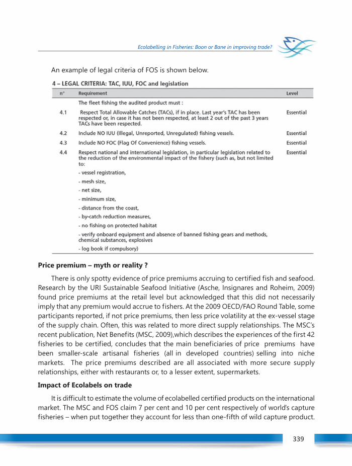
Winter School on Structure and Function of the Marine Ecosystem : Fisheries 339
Ecolabelling in Fisheries: Boon or Bane in improving trade?
339
An example of legal criteria of FOS is shown below.
Price premium – myth or reality ?
There is only spotty evidence of price premiums accruing to certified fish and seafood.Research by the URI Sustainable Seafood Initiative (Asche, Insignares and Roheim, 2009)found price premiums at the retail level but acknowledged that this did not necessarilyimply that any premium would accrue to fishers. At the 2009 OECD/FAO Round Table, someparticipants reported, if not price premiums, then less price volatility at the ex-vessel stageof the supply chain. Often, this was related to more direct supply relationships. The MSC’srecent publication, Net Benefits (MSC, 2009),which describes the experiences of the first 42fisheries to be certified, concludes that the main beneficiaries of price premiums havebeen smaller-scale artisanal fisheries (all in developed countries) selling into nichemarkets. The price premiums described are all associated with more secure supplyrelationships, either with restaurants or, to a lesser extent, supermarkets.
Impact of Ecolabels on trade
It is difficult to estimate the volume of ecolabelled certified products on the internationalmarket. The MSC and FOS claim 7 per cent and 10 per cent respectively of world’s capturefisheries – when put together they account for less than one-fifth of wild capture product.
Winter School on Structure and Function of the Marine Ecosystem : Fisheries340
Ecolabelling in Fisheries: Boon or Bane in improving trade?
It is certain that the real volume of traded ecolabelled products is significantly less thanthat. Indeed, of the MSC’s 6 million tonnes of seafood landed from certified fisheries, onlyabout 2.5 million tonnes ends up carrying the MSC label (MSC, 2009). A significant proportionof FOS-certified fish goes into products such as fishmeal and fish food that will not end upas labelled products on supermarket shelves(although the farmed fish they feed may do).Other schemes in existence currently cover fairly insignificant volumes of product. Overall,the market presence of ecolabelled products is likely to be modest, and significantly lowerthan the publicity surrounding such products would suggest (Washington and Ababouch,2011).
Boon or Bane ?
In a world in which the demand for fishery products are increasing in leaps and bounds,and the pressure on the natural resources are rising, ecolabelling appears to be a possibleway to bring about a greater degree of control and sanity in the system. The increasingproportion of aquaculture in the production system for aquatic products is also beingaddressed by global organizations. Following on from its involvement in the certification ofsustainable forestry (Forestry Stewardship Council - FSC) and wild-capture fisheries (MarineStewardship Council - MSC), the WWF has developed standards for aquaculture certification,with an emphasis on eliminating the negative environmental and social impacts ofaquaculture called the Aquaculture Stewardship Council (ASC). It has organized a range ofround tables involving aquaculture producers, buyers, NGOs and other stakeholders in anattempt to develop standards for aquaculture certification. The first ASC certificate isexpected to be issued in 2012.
A recent study evaluating the effectiveness of certified seafood showed that thoughthere are debatable shortcomings, for a consumer, it is reasonable to buy certified seafood,because the percentage of moderately exploited, healthy stocks is 3–4 times higher in certifiedthan in non-certified seafood (Froese and Proelss, 2012).
Winter School on Structure and Function of the Marine Ecosystem : Fisheries 341
Ecosystem concepts for sustainable mariculture
Introduction
Almost 50% of all seafood eaten worldwide today is farmed, compared to only 9% in1980, primarily from the expansion of aquaculture in China and India. Increasing seafoodproduction in an environmentally and socially responsible way will likely require the use ofpolicy tools, such as good management practices (GMPs) and performance standards. Thesepolicy tools are commonly utilized to reduce effects associated with the use of naturalresources in commercial activities like mariculture. Although mariculture operations mayexpand the production of seafood without additional exploitation of wild populations, theystill depend upon and affect natural ecosystems and ecosystem services. GMPs andperformance standards are useful for protecting the environment while increasing maricultureproduction.
Mariculture can have both positive and negative ecological impacts on the marineenvironment. For instance, culture operations and the associated gear can alter water flow,composition of the sediment, and rate of sedimentation and in some cases can disturb thebenthic flora, including sea grass, which provide habitat for fish and invertebrates. However,mariculture gear increases the availability of hard substrates, thereby supporting higherdensities of fish and invertebrates that associate with structured habitat, but the presenceof artificial hard substrates can also promote colonization and spread of introduced species,such as non-native ones. Such a mix of beneficial and negative effects illustrates thecomplexity of ecosystem responses to mariculture operations.
From organism to ecosystem, there is no free lunch-every additional animal has anincremental effect arising from food extraction and waste excretion. The scope of impactsof cultured organisms is a function of the scale and location of mariculture operations, afact that needs to be recognized and quantified. Some effects may be beneficial to theecosystem, while others may be detrimental, depending on the scale and location of thefarm.
Economic activities in marine and coastal areas, whether fisheries, aquaculture, ortourism, depend on the capacity of marine and coastal ecosystems to provide seafood forhuman consumption and fish for feed production, as well as coastal and marine waterssuitable for recreation.
40C H A P T E R ECOSYSTEM CONCEPTS FOR SUSTAINABLE
MARICULTUREImelda Joseph
Mariculture DivisionICAR-Central Marine Fisheries Research Institute
Winter School on Structure and Function of the Marine Ecosystem : Fisheries342
Ecosystem concepts for sustainable mariculture
The development of modern aquaculture has been founded on social norms and rulesthat rely on technology, indicators of welfare, and world views that mentally alienate peoplefrom their dependence on functional ecosystems.
Since global marine fish stocks show signs of serious overharvesting, and spawningand breeding areas worldwide are increasingly degraded, it is necessary to develop conceptsand management tools that take into account the support of coastal and marine ecosystems.The marine and coastal footprint of seafood production and waste assimilation, and reporton estimates of regional and global appropriation of marine and coastal ecosystems isuseful in ecological footprint analyses in relation to the management of mariculture forsustainability.
The capacity of marine and coastal ecosystems to sustain seafood production andconsumption is seldom accounted for. Estimates of marine and coastal areas appropriatedby farming for seafood production-the ecological footprint-ranges from negligible to asmuch as 50 000 ha/ha activity, largely depending on the methods of farming and fishing.The area for waste assimilation ranges from 2 to 275 ha/ha seafood production. The capacityof marine and coastal ecosystems to produce seafood is not included in the signals thatguide economic development. Practices that make use of this capacity without degrading ithave to be developed and protected from economic and social driving forces that createincentives for misuse of coastal and marine ecosystems.
Marine and coastal ecosystem support of aquaculture and fisheriesDue to current overexploitation of the world fisheries resources, aquaculture is often
promoted to be the most likely source of additional seafood production. Its expansion hasbeen given high priority, both in developed and developing countries. However, the rapidlyexpanding modern aquaculture technology (predominantly monocultures) has mainly usedecosystems as a medium for culturing, and has taken the necessity of a supply of resourceslike feed, water etc. and ecosystem services like waste assimilation, for granted. Intensiveaquaculture is not a substitute for fisheries and on the contrary, intensive aquaculture largelydepends on fisheries to harvest the seafood that is given to the cultured species in the formof pellets unless and until suitable replacement for fishmeal and fish oil are found out.
Ecological footprints and farming intensityThe dependence on external ecosystems for resource production and waste assimilation
generally decreases from intensive to extensive techniques. While intensive cage farminghas been increasingly dependent on external inputs and affecting the environment throughreleases of waste, semi-intensive farming is characterized by a more complete utilization ofmaterial and energy and a higher recycling of organic matter and nutrients within the pondsystem. Semi-intensive aquaculture relies both on natural food production in the ponds,
Winter School on Structure and Function of the Marine Ecosystem : Fisheries 343
Ecosystem concepts for sustainable mariculture
and supplementary feed, usually from locally available plants or agriculture by-products.Thus, fish can obtain a major part of their nutritional requirements from local natural sourceswhen reared at low densities in a pond.
Integrated cultures are often based on recycling or eco-cyclic production, and have thepotential to be more in tune with the processes and functions of the supporting marineecosystem.
Integrated multi-trophic aquaculture (IMTA)
IMTA refers to the explicit incorporation of species from different trophic positions ornutritional levels in the same system. Integrated marine aquaculture can cover a diverserange of co-culture/ farming practices, and even more specialized forms of integrationsuch as mangrove planting with aquaculture, called aquasilviculture. Integrated mariculturehas many benefits, among which bioremediation is one of the most relevant, and yet is notvalued in its real social and economic potential for the integration benefits derived frombioremediation. Reducing risks is also an advantage and profitable aspect of farming multiplespecies in marine environments. A diversified product portfolio increases the resilience ofthe operation, for instance when facing changing prices for one of the farmed species orthe accidental catastrophic destruction of a crop.
Integrated mariculture systems must be developed in order to assist sustainableexpansion of the sector in coastal and marine ecosystems thus responding to the globalincrease for seafood demand but with a new paradigm of more efficient food productionsystems. Successful integrated mariculture operations must consider all relevant stakeholdersinto its development plan; government, industry, academia, the general public and non-governmental organizations must work together and the role of integrated mariculturewithin integrated coastal zone management plans must be clearly defined.
An important issue of IMTA is to adopt management practices that avoid or reduce thelikelihood of disease transmission within and between aquaculture facilities or to the naturalaquatic fauna. Also, careful consideration should be paid to the selection of species used inpolyculture or IMTA to reduce potential stress and suffering of culture individuals. Integratedaquaculture should be looked upon as a very important tool to facilitate the growth ofmarine aquaculture and promote sustainable development.
IMTA for Mariculture Sustainability
The rapid development of intensive fed aquaculture of monospecies (e.g. finfish andshrimp) throughout the world is associated with concerns about the environmental impacts,especially where activities are highly concentrated or located in suboptimal sites whoseassimilative capacity is poorly understood and, consequently, prone to being exceeded.

Winter School on Structure and Function of the Marine Ecosystem : Fisheries344
Ecosystem concepts for sustainable mariculture
One of the main environmental issues is the direct discharge of nutrient loads into coastalwaters from open water systems and with the effluents from land-based systems. In itssearch for best management practices, the aquaculture industry should develop innovativeand responsible practices that optimize its efficiency and create diversification, while ensuringthe remediation of the consequences of its activities to maintain the health of coastal waters.To avoid pronounced shifts in coastal processes, conversion, not dilution, is a solution usedfor centuries in Asian countries. By integrating fed aquaculture (finfish, shrimp) with inorganicand organic extractive aquaculture (seaweed and shellfish), the wastes of one resource userbecome a resource (fertilizer or food) for the others. Such a balanced ecosystem approachprovides nutrient bioremediation capability, mutual benefits to the co-cultured organisms,economic diversification by producing other value-added marine crops and increasedprofitability per cultivation unit for the aquaculture industry.
As guidelines and regulations on aquaculture effluents are forthcoming in severalcountries, using appropriately selected seaweeds as renewable biological nutrient scrubbersrepresents a cost-effective means for reaching compliance by reducing the internalizationof the total environmental costs. By adopting integrated polytrophic practices, theaquaculture industry should find increasing environmental, economic, and social acceptabilityand become a full and sustainable partner within the development of integrated coastalmanagement frameworks.
Good management practices (GMPs) and performance standards
GMPs represent one approach to protecting against undesirable consequences ofmariculture. GMPs for farming have been prepared by industry groups, nongovernmentalorganizations, and governments with the common goal of sustainability. An alternativeapproach to voluntary or mandatory GMPs is the establishment of performance standardsfor mariculture. In mariculture, variability in environmental conditions makes it difficult todevelop GMPs that are sufficiently flexible and adaptable to protect ecosystem integrityacross a broad range of locations and conditions. Because GMPs address mariculture methodsrather than monitoring actual ecosystem responses, they do not guarantee that detrimentalecosystem impacts will be controlled or that unacceptable impact will be avoided. Adoptionof performance standards is likely to encourage innovation among growers. Withperformance standards, mariculture operations are managed adaptively to maintain keyindicators within acceptable bounds, through direct monitoring of ecosystem indicatorsrather than tracking compliance with specific management practices.
Carrying capacity and aquaculture
Carrying capacity can be defined as the maximum population or biomass that an areawill support sustainably, as set by available space, food and other potentially limiting resources
Winter School on Structure and Function of the Marine Ecosystem : Fisheries 345
Ecosystem concepts for sustainable mariculture
but within the limits set by the capacity of the ecosystem to process biological wastes andby social tolerance for the change in environmental attributes. The concept of carryingcapacity is increasingly and appropriately invoked as a quantitative guide to identify limitsto stocking densities of finfish/ shellfishes in mariculture operations. Application of a carryingcapacity concept to setting mariculture stocking limits requires a determination on whatrepresents acceptable versus unacceptable impacts. Carrying capacity models can be usedto optimize production of the cultured organisms; reduce the ecological impacts on thefood web; or maintain societal values, such as scenic amenity or recreational opportunity.All carrying capacity approaches require models of the mariculture activity and its interactionswith living and non-living components of the ecosystem.
Mariculture contrasted with capture fisheries
Many ecological effects of mariculture closely parallel the corresponding ecologicaleffects of wild-stock harvests. Mariculture conducted on lines, racks, or cages does notrequire dredging and is thus less damaging to the ecosystem than wild-stock harvesting.Wild-stock harvests tend to be more frequent and more dispersed, thus causing greaterdamage to the ecosystem than the less frequent, more localized, and managed harvest offarmed animals. Basic economics suggests that increasing supply through mariculture willreduce seafood prices if other factors remain unchanged. Lower prices will tend to reduceeconomic incentives to harvest the wild population, thereby reducing fishing pressure onthe wild stock. However, this effect can be masked in practice if wild-harvest fisheries remainprofitable even at lower prices, if overall demand for the product increases, or if a strongniche market develops for the wild-harvest product.
Ecosystem services by mariculture
Filter-feeding bivalves have the ability to reduce water turbidity through their filtration,and they do fertilize benthic habitats through bio deposition, induce denitrification,counteract some detrimental effects of eutrophication in shallow waters, sequester carbon,provide structural habitats for other marine organisms, and stabilize habitats and shorelines.These ecosystem services of bivalves, along with recognition that oysters, clams, and scallopshave been depleted dramatically below historical baselines in many estuaries, explain whybivalve mollusc restoration has become an important component of many programs forrestoring impaired estuaries and some coastal waters.
Applying an ecosystem-based approach to mariculture
The ecosystem approach to aquaculture is defined as a strategic approach todevelopment and management of the sector aiming to integrate aquaculture within thewider ecosystem such that it promotes sustainability of interlinked social-ecological systems.
Winter School on Structure and Function of the Marine Ecosystem : Fisheries346
Ecosystem concepts for sustainable mariculture
An ecosystem approach to aquaculture (EAA) is not a new approach, and has been in away practiced since the early stages of aquaculture in small-scale inland aquaculture activitiesparticularly in Asia where poultry wastes (or other organic wastes) are commonly used asfeed resources for the culture of carps and other freshwater fish. However, the EAA becomesmore difficult and a real challenge in the case of intensive, industrial production but also asa result of the added effect of many small-scale aquaculture. It is not uncommon thatnutrient cycling and re-utilization of wastes by other forms of aquaculture or local fisheries,is not allowed, or is discouraged.
An ecosystem approach accounts for a complete range of stakeholders, spheres ofinfluences and other interlinked processes. In the case of aquaculture, applying an ecosystem-based approach must involve physical, ecological, social and economic systems, in theplanning for community development, also taking into account stakeholders in the widersocial, economic and environmental contexts of aquaculture. The first principle for anecosystem approach, as described by the Convention on Biological Diversity (CBD), is thatthe objectives of management of land, water and living resources are matters of societalchoice (UNEP/CBD/COP/5/23/ decision V/6, 103-106).
Key principles
The EAA can be regarded as “the” strategy to ensure aquaculture contribution tosustainable development and should be guided by three main principles which are alsointerlinked:
Principle 1: “Aquaculture development and management should take account of thefull range of ecosystem functions and services, and should not threaten the sustained deliveryof these to society”. It is only realistic to expect that aquaculture, being a human activity, willlead to some loss of biodiversity or affect ecosystem services to some extent. IntegratedMultitrophic Aquaculture (IMTA) has been practised in Asia/China since the beginning ofaquaculture, this due to their ancient concept of treating effluents and residues from farmingpractices as resources rather than as pollutants.
In the case of biodiversity, local declines may be acceptable (e.g. below fish cages) aslong as such losses can be compensated and restored, at least at the water body scale, inorder to preserve ecosystem functions and services. For example after a cage farm operationis halted it is expected that the relevant biodiversity recovers if there is enough greeninfrastructure, that is conservation areas or more pristine areas to provide relevantcolonization and restoration. Efforts need to be made in order to permanently monitoraquaculture effects on biodiversity to make sure that such effects do not result in serious/significant losses of ecosystem functions and services. In this respect real values of ecosystem“goods” and services should be integrated into micro and macro environmental accounting.
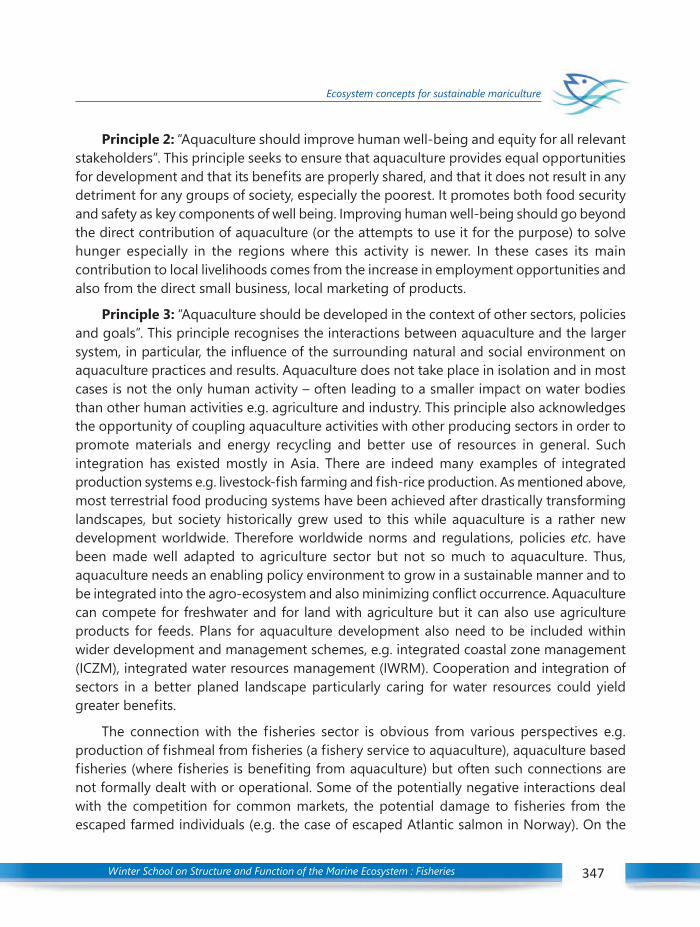
Winter School on Structure and Function of the Marine Ecosystem : Fisheries 347
Ecosystem concepts for sustainable mariculture
Principle 2: “Aquaculture should improve human well-being and equity for all relevantstakeholders”. This principle seeks to ensure that aquaculture provides equal opportunitiesfor development and that its benefits are properly shared, and that it does not result in anydetriment for any groups of society, especially the poorest. It promotes both food securityand safety as key components of well being. Improving human well-being should go beyondthe direct contribution of aquaculture (or the attempts to use it for the purpose) to solvehunger especially in the regions where this activity is newer. In these cases its maincontribution to local livelihoods comes from the increase in employment opportunities andalso from the direct small business, local marketing of products.
Principle 3: “Aquaculture should be developed in the context of other sectors, policiesand goals”. This principle recognises the interactions between aquaculture and the largersystem, in particular, the influence of the surrounding natural and social environment onaquaculture practices and results. Aquaculture does not take place in isolation and in mostcases is not the only human activity – often leading to a smaller impact on water bodiesthan other human activities e.g. agriculture and industry. This principle also acknowledgesthe opportunity of coupling aquaculture activities with other producing sectors in order topromote materials and energy recycling and better use of resources in general. Suchintegration has existed mostly in Asia. There are indeed many examples of integratedproduction systems e.g. livestock-fish farming and fish-rice production. As mentioned above,most terrestrial food producing systems have been achieved after drastically transforminglandscapes, but society historically grew used to this while aquaculture is a rather newdevelopment worldwide. Therefore worldwide norms and regulations, policies etc. havebeen made well adapted to agriculture sector but not so much to aquaculture. Thus,aquaculture needs an enabling policy environment to grow in a sustainable manner and tobe integrated into the agro-ecosystem and also minimizing conflict occurrence. Aquaculturecan compete for freshwater and for land with agriculture but it can also use agricultureproducts for feeds. Plans for aquaculture development also need to be included withinwider development and management schemes, e.g. integrated coastal zone management(ICZM), integrated water resources management (IWRM). Cooperation and integration ofsectors in a better planed landscape particularly caring for water resources could yieldgreater benefits.
The connection with the fisheries sector is obvious from various perspectives e.g.production of fishmeal from fisheries (a fishery service to aquaculture), aquaculture basedfisheries (where fisheries is benefiting from aquaculture) but often such connections arenot formally dealt with or operational. Some of the potentially negative interactions dealwith the competition for common markets, the potential damage to fisheries from theescaped farmed individuals (e.g. the case of escaped Atlantic salmon in Norway). On the

Winter School on Structure and Function of the Marine Ecosystem : Fisheries348
Ecosystem concepts for sustainable mariculture
other hand, terrestrial food production systems and other industrial activities can impacton aquaculture deteriorating water quality and quantity; they can also affect feed’s qualityand potential safety (Hites et al., 2004).
Some management measures to assist policy-making that ensure environmental, socialand economic sustainability of the aquaculture sector In general and at all levels, policiesshould be generated from a participatory processes, they should be adaptive, transparentand open to the general public; they must ensure and promote people consciousness ofthe value of ecosystem approach. They should also reconcile temporal scales facing the factthat aquaculture growth/development and governance capabilities have been moving attwo different speeds. It is also important to consider that management measures shouldaim to the compliance of the three EAA principles in order to ensure aquaculture contributionto sustainable development.
A precautionary approach to aquaculture production should involve developingstrategies to avoid specific undesirable outcomes. Overloading of a waterbody’s carryingcapacity will affect the biodiversity or ecosystem services and a management plan shouldinclude estimates of the carrying capacity and mechanisms to monitor and control furtherloading of the system. Another example is that of culturing exotic species or genotypes,where plans should be developed or revised to incorporate precautionary elements; adaptivemanagement practices and tools such as risk analysis and geographic information systems.Adaptive management (AM) has emerged as the “best practices” approach to ecosystemmanagement. Adaptive management is an iterative process of taking actions, evaluatingthe consequences of those actions and adjusting future actions in the light of changedconditions.
Existing management models, hydrodynamic circulation/deposition models and theknowledge of local institutions, universities etc. can be used for the estimation of carryingcapacity and use of indicators. For example, be aware of local regional particularities whenimporting technological packages developed in other regions as it may be necessary to developproper management models or other tools that are more appropriate to specific localcharacteristics. Farm scale research should focus on developing tools to evaluate externalitiesof inputs and outputs, to estimate carrying capacity for individual farms, and tools andtechnologies for improving the feeding process and conversion ratios. It is also very importantto promote permanent and proactive research on new species and strains offering enoughinformation for the selection of the right species based on ecosystem functions and marketdemands, considering species requirements and ecological/nutritional efficiency.
Different kinds of incentives can be developed in isolation or in combination. E.g. improvethe institutional framework (definition of rights and participatory processes); develop
Winter School on Structure and Function of the Marine Ecosystem : Fisheries 349
Ecosystem concepts for sustainable mariculture
collective values (education, information, and training); create non-market economicincentives (e.g. tax mechanisms and subsidies) such as special advantageous licences (forexample for integrated aquaculture, polyculture or for implemented better management,etc.); and establish market incentives (eco-labelling and aquaculture concessions).
Promote education and disseminate information on better practices consideringecosystem based management. At the farm scale it is important to target education andtraining to the stakeholders (farm owners, workers, site managers) focusing on EAA andemphasizing on management-oriented knowledge. The development of collective valuesand the understanding of externalities of the farming process are very relevant at this scale.The valuation and understanding of ecosystem services has to start at this scale. To developa sustainable production in aquaculture EAA should be followed as early as possible inIndia also.

Winter School on Structure and Function of the Marine Ecosystem : Fisheries350
Economic valuation of marine ecosystem services
Introduction
The marine and coastal ecosystem provides a variety of services. Fisheries is an importantprovisioning service with supplements from supporting and cultural services. The potentialservices that can be provided by the marine coastal ecosystem includes, sustainable catch,which provides assured income to the fishers, regulates natural phenomena as certain marinefauna acts as bio-filters, provides a rich treasure of marine bio-diversity.
Types of ecosystem: Structure of the Ecosystem
The different types of ecosystem are presented below. (Figure 1)
Fig. 1. Types of ecosystem
41C H A P T E R
The marine and coastal ecosystem is coming under the aquatic ecosystem. The coastalecosystem includes following component like estuaries, salt marshes, rocky/sandy shores,mud-flats, coral reef, mangrove, nesting Grounds/Habitats (Birds, Horse Shoe Crab andTurtle), sea grass, marine parks and sanctuaries, archeological and heritage Sites (Bhatta,2015).
ECONOMIC VALUATION OF MARINEECOSYSTEM SERVICESR. Narayana Kumar
Socio Economic Evaluation and Technology Transfer DivisionICAR-Central Marine Fisheries Research Institute

Winter School on Structure and Function of the Marine Ecosystem : Fisheries 351
Economic valuation of marine ecosystem services
351
In general the services provided by the ecosystems include, provisioning, regulatory,supporting and cultural services (MEA, 2005). These services are described for eachecosystems.
Economic valuation of ecosystems
Ecosystem have three distinct characteristics in valuation namely (i) Existence value; (ii)Intrinsic value and (iii) Option value.
Productive use value: It is the value assigned to the products that can be harvestedfor exchange in formal market and is the only value of biological resources that appearsin the national income account. Example: Fuel wood, fodder, timber, f ish,medicinal plants
Consumptive use value: The value assigned to natural products that are consumeddirectly i.e., the goods that do not enter normal channels of trade; Example: A variety ofNon Timber Forest Products (NTFP)
Intrinsic value: It is the value related primarily with the functions of the ecosystem butsometimes outweigh the consumptive/non-use values like, maintenance of ecologicalbalance, Prevention of soil erosion etc.
Types of values
The various types of values that are used in environment and ecological economicsparlance are given below (Table 1).Table 1 Types of values
Value type Sub type Example
Use value-Direct Consumptive Productive Variety of home consumed forest productsPlant breeding
Indirect use value Non-consumptive Tourism
Option Non-consumptive Ecological process , future values of drugs
Quasi-option Non-consumptive Value of being able to ascertain option value
Non-use values Non-consumptive Existence value of elephants, turtles
Why economic valuation?
The link between economics and ecology/environment is vital to understand their value.Most of the natural resources that we use have value but not priced and also not traded inthe market. eg., Air.
The natural resources (NRS) need valuation because they do not have a regular market
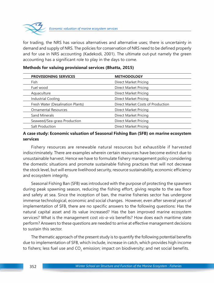
Winter School on Structure and Function of the Marine Ecosystem : Fisheries352
Economic valuation of marine ecosystem services
for trading, the NRS has various alternatives and alternative uses; there is uncertainty indemand and supply of NRS. The policies for conservation of NRS need to be defined properlyand for use in NRS accounting (Kadekodi, 2001). The ultimate out-put namely the greenaccounting has a significant role to play in the days to come.
Methods for valuing provisional services (Bhatta, 2015)
PROVISIONING SERVICES METHODOLOGYFish Direct Market PricingFuel wood Direct Market PricingAquaculture Direct Market PricingIndustrial Cooling Direct Market PricingFresh Water (Desalination Plants) Direct Market Costs of ProductionOrnamental Resources Direct Market PricingSand Minerals Direct Market PricingSeaweed/Sea-grass Production Direct Market PricingSalt Production Direct Market Pricing
A case study: Economic valuation of Seasonal Fishing Ban (SFB) on marine ecosystemservices
Fishery resources are renewable natural resources but exhaustible if harvestedindiscriminately. There are examples wherein certain resources have become extinct due tounsustainable harvest. Hence we have to formulate fishery management policy consideringthe domestic situations and promote sustainable fishing practices that will not decreasethe stock level, but will ensure livelihood security, resource sustainability, economic efficiencyand ecosystem integrity.
Seasonal Fishing Ban (SFB) was introduced with the purpose of protecting the spawnersduring peak spawning season, reducing the fishing effort, giving respite to the sea floorand safety at sea. Since the inception of ban, the marine fisheries sector has undergoneimmense technological, economic and social changes. However, even after several years ofimplementation of SFB, there are no specific answers to the following questions: Has thenatural capital asset and its value increased? Has the ban improved marine ecosystemservices? What is the management cost vis-a-vis benefits? How does each maritime stateperform? Answers to these questions are needed to arrive at effective management decisionsto sustain this sector.
The thematic approach of the present study is to quantify the following potential benefitsdue to implementation of SFB, which include, increase in catch, which provides high incometo fishers; less fuel use and CO2 emission; impact on biodiversity; and net social benefits.

Winter School on Structure and Function of the Marine Ecosystem : Fisheries 353
Economic valuation of marine ecosystem services
353
The Impact of SFB on resource group-wise and sector-wise marine fish landings wasassessed for major resources (fish species/ groups) and for different craft types. The crafttype (sector) categorization assumes significance as SFB applies to all mechanized boats,which operate trawls and gillnets, but only partially at varying proportions for motorizedboats which operate gears like seines. The methodology involved the following twoapproaches:
(i) Regression approach aims at studying dependence of landings and catch rates (catchper unit craft trip and catch per hour of actual fishing) upon effort (boat trips or actualfishing hours) and an indicator variable signalling the initiation of SFB in respective state.
(ii) The second approach was more general wherein the catch rates were considered aparameter of fishery health/ wealth as well as fisher’s success and its compound growthrate in pre SFB and post SFB periods were computed using semi logarithmic model (Powerfunction).
The economic benefit of SFB was assessed by estimating the value of incremental growthattained due to fishing ban. The incremental weight (in tonnes) of each species was multipliedby price/tonne (geometric mean of the last three years at landing centre and retail pricelevel) of respective species and final values were estimated. The impact of SFB on variousresource group/species caught including small pelagics, large pelagics, demersal finishes,crustaceans and cephalopods were assessed by their growth rates of catches during preand post ban period). The annual compound growth rates (ACGR) were estimated fordepicting variation in catches/ catch rates over a time period, here pre and post SFB period.
Post fishing ban registered an overall increase in volume of fish catches as well as theirspecies diversity across all states. Stock status also indicates that states with higher level ofmechanisation such as Karnataka and Gujarat have higher percentage of exploited stocksthat are seriously depleted and require serious attention to rejuvenate stocks compared tostates like Andhra Pradesh and Tamil Nadu.The analysis indicated that incremental biomassdue to SFB ranged from five to nine per cent in the selected states. This indicated that theSFB has a positive impact on the fish harvest after the ban and need to be recommendedfor continued implementation as a tool for sustainable marine fisheries management.
The estimated value of the incremental biomass due to SFB ranged from Rs.1,266 lakhsin Andhra Pradesh to Rs.2,809 lakhs in Tamil Nadu at landing centre price level. In AndhraPradesh, all the resource groups showed a positive trend after the ban while in Tamil Nadu,except crustaceans, all other resource groups exhibited a positive trend after the ban period.The net social benefit was positive in all the States (Kerala-Rs.2,480.86 lakhs, Andhra Pradesh-Rs.1.097.42 lakhs). (Table 3)
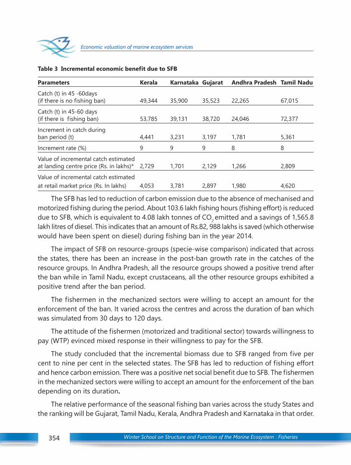
Winter School on Structure and Function of the Marine Ecosystem : Fisheries354
Economic valuation of marine ecosystem services
Table 3 Incremental economic benefit due to SFB
Parameters Kerala Karnataka Gujarat Andhra Pradesh Tamil Nadu
Catch (t) in 45 -60days(if there is no fishing ban) 49,344 35,900 35,523 22,265 67,015
Catch (t) in 45-60 days(if there is fishing ban) 53,785 39,131 38,720 24,046 72,377
Increment in catch duringban period (t) 4,441 3,231 3,197 1,781 5,361
Increment rate (%) 9 9 9 8 8
Value of incremental catch estimatedat landing centre price (Rs. in lakhs)* 2,729 1,701 2,129 1,266 2,809
Value of incremental catch estimatedat retail market price (Rs. In lakhs) 4,053 3,781 2,897 1,980 4,620
The SFB has led to reduction of carbon emission due to the absence of mechanised andmotorized fishing during the period. About 103.6 lakh fishing hours (fishing effort) is reduceddue to SFB, which is equivalent to 4.08 lakh tonnes of CO2 emitted and a savings of 1,565.8lakh litres of diesel. This indicates that an amount of Rs.82, 988 lakhs is saved (which otherwisewould have been spent on diesel) during fishing ban in the year 2014.
The impact of SFB on resource-groups (specie-wise comparison) indicated that acrossthe states, there has been an increase in the post-ban growth rate in the catches of theresource groups. In Andhra Pradesh, all the resource groups showed a positive trend afterthe ban while in Tamil Nadu, except crustaceans, all the other resource groups exhibited apositive trend after the ban period.
The fishermen in the mechanized sectors were willing to accept an amount for theenforcement of the ban. It varied across the centres and across the duration of ban whichwas simulated from 30 days to 120 days.
The attitude of the fishermen (motorized and traditional sector) towards willingness topay (WTP) evinced mixed response in their willingness to pay for the SFB.
The study concluded that the incremental biomass due to SFB ranged from five percent to nine per cent in the selected states. The SFB has led to reduction of fishing effortand hence carbon emission. There was a positive net social benefit due to SFB. The fishermenin the mechanized sectors were willing to accept an amount for the enforcement of the bandepending on its duration.
The relative performance of the seasonal fishing ban varies across the study States andthe ranking will be Gujarat, Tamil Nadu, Kerala, Andhra Pradesh and Karnataka in that order.

Winter School on Structure and Function of the Marine Ecosystem : Fisheries 355
Economic valuation of marine ecosystem services
355
But it is important to note that the period of ban in Gujarat and Karnataka are different fromthat of the remaining three states.
The above findings indicate that the SFB is having predominantly a positive impact onthe resources and on the fishers who are dependent on the sector for their livelihood. Itwas also found that, the net social benefit was positive in all the States (In Kerala Rs.2,480.8lakhs and in Andhra Pradesh Rs.1.097.4 lakhs). It can be concluded that there is substantialpositive net social benefit due to enforcement of Seasonal Fishing Ban in the selectedStates and hence SFB can be recommended to continue.
Implications and Recommendations of this study
SFB has resulted in a positive net social benefit in the study states. This indicated thatthe enforcement of SFB can be continued in the study states, which will facilitate sustainabilityof resources as well as an increase in catch and income to the fishers. SFB can also beconsidered as a measure to reduce carbon emissions. While it is recommended that the SFBmay continue in future, considering the complexities of the economic valuation of SFB, it isrecommended that the present analysis may be improved in future by taking into accountseveral externalities which have not been included in the present analysis. It is alsorecommended that the analysis may be extended to other maritime states not consideredin this study.
It has been recognized that SFB alone could not be a complete measure to sustain thefisheries. SFB should be considered as one of the tools in a bundle of several input andoutput management measures, such as ecosystem approach, Marine Protected Area, No-take zone, regulated entry, catch quotas, certification, minimum legal size at capture etc. Ina combination of several other measures, SFB will become more effective for sustainingmarine fisheries. (Narayana Kumar et al., 2015, 2017)
Payment for ecosystem services (PES)
This is an important aspect that needs to be looked into seriously. The PES includesboth demand and supply side. This includes identification of potential buyers (users ) ofthe ecosystem and the payment charged. This also requires to undertake social cost benefitanalysis. This is one of the important policy instruments in the field of ecosystem valuationwhich will ultimately lead to green accounting. The Economics of Ecosystem and Biodiversity(TEEB) has undertaken lots of studies in this aspect across major continents.
Conclusion
In this lecture, an attempt is made to give an insight into the structure, functions andeconomic valuation of ecosystem services. This can be further expanded to study thedifferent components of ecosystems and incorporate into the green accounting frame work.
Winter School on Structure and Function of the Marine Ecosystem : Fisheries356
Economic valuation of marine ecosystem services
It is also important to note that Economics helps to put the things in proper perspectiveto the policy planners by assigning value to the ecological or environmental services orbenefits. However not all services can be brought under valuation as this is a subjectiveconcept. The dynamic nature of the system and the related developments should beconsidered thoroughly before applying any of these methods to formulate practical policymeasures.
References
Barzel, Yoram, 1985. Transaction costs: Are they just costs? J. Instt. Theor. Econ., 141 (1): 4-16
Coase, Ronald., 1937. The Nature of the Firm. Economica., 4 (16): 386–405
Demsetz, Harold., 1968. The cost of transacting. Q.J. of Econ., 82(1): 33-53
CMFRI, 2012. Marine Fisheries Census 2010. Central Marine Fisheries Research Institute, Cochin. Six volumes
CMFRI, 2014. Annual Report 2013–14. Central Marine Fisheries Research Institute, Cochin, 246 pp.
CMFRI,2015. Marine Fish landings in India, 2014, Central Marine Fisheries Research Institute, Kochi, 6 pp
Gordon, R. L., 1994, Regulation and Economic Analysis: A Critique Over Two Centuries. Kluwer AcademicPublishers, Dordrecht, The Netherlands
Mohamad, K.S. V. Kripa, R.Narayanakumar, D. Prema, M. Vinod, Jenny Varma and Sajikumar (2015).Assessment of eco-labelling as tool for conservation and sustainable use of biodiversity in AshtamudiLake, Kerala GIZ TEEB
Narayanakumar, R. and Jayasankar, J. and Shyam, S, Salim and Ganga, U. and Vivekanandan, E. (2016).Fishing holiday. In: The Economics of Ecosystem and Biodiversity-India Initiative: Factsheets. DeutscheGesellschaft für Internationale Zusammenarbeit (GIZ) GmbH, New Delhi
Narayanakumar R., J. Jayasankar, Shyam S. Salim, U. Ganga and E. Vivekanandan, (2015). Economic valuationof SFB in selected maritime States in India GIZ-TEEB
Sathiadhas, R. and R. Narayanakumar 2003. Environmental economic analysis of coastal fishery resourcesof Kerala. IGIDR Project Report
Srinath, M. and Pillai, N.G.K., 2008. Status of Marine Fisheries in India. In : Lecture Notes of Winter School onImpact of Climate change on Indian Marine Fisheries. Central Marine Fisheries Research Institute, pp1-7
Srinath, M., Somy Kuriakose, J. Jaayasankar and K. G. Mini, 2006. Generalized Fishery Development Model(GFDM) approach for analysis of marine fish landings in India. J. Mar. Ass. India, 48(1): 68-75
Vivekanandan, E. and Narayanakumar, R. and Najmudeen, T. M., Jayasankar, J and Ramachandran, C, 2010Marine Fisheries Policy Brief-2; Seasonal Fishing Ban. CMFRI Spl. Publn., No. 103. 44pp.
Vivekanandan, E., and Upadhyay, 2010 TEEB Initiation Report. GIZ India and MOEF&CC, 2010

Winter School on Structure and Function of the Marine Ecosystem : Fisheries 357
Marine microbial diversity and its role in ecosystem functioning
Seas and oceans cover more than 70% of the Earth’s surface, host the majority of itsbiomass, and contribute significantly to all global cycles of matter and energy. All life onEarth most likely originated from microbes in the sea. Microbes such as Bacteria, Archaea,viruses, fungi and protists (including microalgae), dominate the living biomass. On the treeof life, the Eukarya (including plants, animals and protists) comprise only a tiny branch;Bacteria and Archaea encompass virtually all genetic diversity, notwithstanding their limitedmorphological diversity. Marine microbes thrive not only in the surface waters of the sea,but also in the lower and abyssal depths from coastal to the offshore regions, and from thegeneral oceanic to the specialized niches like blue waters of coral reefs to black smokers ofhot thermal vents at the sea floor. Marine microorganisms occur in vast numbers andrepresent a huge genetic diversity: ocean water contains up to one million microorganismsper milliliter and several thousand microbial types. These numbers may be an order ofmagnitude higher in coastal waters with their higher productivity and higher load of organicmatter and nutrients.
Marine microorganisms are the key to all biogeochemical cycles and are crucial for thefunctioning of marine ecosystems. The element carbon which forms the basis of all organicmatter undergoes a constant cycle in nature by various heterotrophic bacteria. Nitrogen, aconstituent of the protein, is cycled in aquatic environment by several bacteria. Nitrificationis an aerobic process, whereas denitrification is the process used by facultative anaerobicbacteria. Microbial oxidation progresses to sulphate, represents the terminal step ofmineralization of organic sulphur compounds and serves as a source of sulphur for plants.
Most importantly, marine phototrophic microorganisms (Cyanobacteria, diatoms andpico- and nanophytoplankton) are responsible for more than 80% of the oxygen productionon Earth. Marine microorganisms and their activities are, and will continue to be, affectedby global change and may also promote or alleviate climate change. Marine microbialcommunities are an integral part of the ocean and are also responsible for the uptake of alarge part of the anthropogenic carbon dioxide from the atmosphere that causes globalwarming. The biological pump transports CO2 to the seafloor, a process entirely driven bymicrobes. The constantly increasing level of atmospheric CO2 would otherwise result in theacidification of the ocean leading to the dissolution of carbonates, and the change of the
42C H A P T E R MARINE MICROBIAL DIVERSITY AND ITS
ROLE IN ECOSYSTEM FUNCTIONINGParvathi A.
National Institute of Oceanography, Kochi

Winter School on Structure and Function of the Marine Ecosystem : Fisheries358
Marine microbial diversity and its role in ecosystem functioning
carbonate equilibrium. Marine microbial communities through the biological pump andmicrobial carbon pump sequester CO2 and helps in the storage of carbon in the deeperoceans, thereby influencing the climate change.
Additionally, they are responsible for the degradation of organic matter in the oceanand are thus the key for maintaining the balance between produced and fixed carbondioxide. Bacteria play a decisive role in the cycle of matter in water, as they are able tobreakdown all natural organic compounds into the components from which they haveoriginated. The heterotrophic bacterial action promotes organic degradation, decompositionand mineralization processes in sediments and in the overlying water, and releases dissolvedorganic and inorganic substances. The mineralization of organic matter, which is derivedfrom primary producers, results in its being recycled, so that these substances are againavailable for primary producers. Heterotrophic microorganisms are the major agents shapingthe organic composition of the ocean. The bulk of microbial populations are constituted byheterotrophic bacteria inhabiting the oceans which are responsible for much of the biologicaltransformation of organic matter and production of CO2. Bacteria also serve as an importantsource of food for a variety of marine organisms.
Society relies on marine microbial communities for its own health as well as for thehealth of the environment. Marine microbial communities are the source of a large varietyof bioactive compounds which may have medical applications and, as such, contribute tohuman health. Marine microbial communities also provide a variety of services, such asbioremediation of polluted environments
Although microbial diversity is one of the difficult areas of biodiversity research,estimation of microbial diversity is required for understanding the biogeography, communityassembly and ecological processes. Recent developments in molecular ecology,metagenomics and ecological modeling illustrate that microbes represent the most importantbiological group on Earth in terms of phylogenetic and functional diversity. In addition,interdisciplinary research has uncovered new and unexpected roles of microbes in thebiogeochemical cycling of carbon, nitrogen, sulphur, iron and many other (trace) elementsin our seas and oceans. Study of marine microbial biodiversity is of vital importance to theunderstanding of the different processes of the ocean. As the microbial communities havea complex ecosystem process, biodiversity study explores the distribution and roles in thehabitat. The presentation would cover the marine microbial diversity, discuss the variousconventional and modern approaches for better understanding the genetic and functionaldiversity, and their roles in major elemental cycling in the ocean.
Winter School on Structure and Function of the Marine Ecosystem : Fisheries 359
Formation mechanism of mud bank along the southwest coast of India
Mud bank formation during southwest monsoon along the southwest coast of Indiaremains an enigma to the researchers and coastal community in spite of several earlierstudies. The present study attempts to unravel the mystery through a high-frequency, season-long time-series observation at Alappuzha, located at the southern part of the west coastof India, a region of frequent occurrence of mud bank. Using 7-month long weekly time-series observation, we identified strong winds and high waves associated with onset of thesouthwest monsoon and subsequent three episodic atmospheric low-pressure events (LPEs).With the help of in situ time-series data we showed that the strong winds and high wavesassociated with southwest monsoon pre-conditions the near shore bottom sediment tobring it into suspension. The high amplitude waves associated with the southwest monsoon,while propagating from the deep water to shallow water region, interacts with the bottominitiating bottom-sediment movement and its suspension due to wave refraction andshoaling. The sporadic occurrence of the atmospheric LPEs enhances the process ofsuspension of bottom sediment in the near shore region leading to the formation of fluidmud. Simulations with a cohesive sediment transport model yielded realistic estimates ofsediment transport, in presence of an onshore current, a pre-requisite for transporting thefluid mud towards the coast. The prevailing onshore upwelling current during southwestmonsoon provides the favorable pre-requisite conditions for transporting the fluid mudthrough depression channel network towards the coast. Once sufficient quantity andthickness of fluid mud is accumulated in the near shore region, it acts as a wave damper forsubsequent high monsoon waves, as indicated by the time-series wave data, leading to theformation of tranquil mud bank region. Depression channel network extending from shelfto the coast off Alappuzha, Kochi, Ponnani, Beypore and Ullal were found in the bathymetriccharts thus explains why mud bank occur only at few locations in spite of the prevalence ofsimilar monsoon conditions.
43C H A P T E R FORMATION MECHANISM OF MUD BANK
ALONG THE SOUTHWEST COAST OF INDIAMuraleedharan K. R.
National Institute of Oceanography, Kochi

Winter School on Structure and Function of the Marine Ecosystem : Fisheries360
Mud Bank Biology
IntroductionMud banks are unique, clearly demarked naturally occurring calm areas which occur
mainly in the inshore waters along the Kerala coast during the southwest monsoon period.Formation of mud banks can be either just before the onset of SW monsoon or during themonsoon. Mud banks are popularly known as “Chakara” or “Shanthakara “ (meaning calmarea) and fishermen consider mud banks as ‘gift of God’ since these are safe fishing areasfor launching and berthing the fishing crafts when the rest of coastal belt is surf ridden,with high swells and unsuitable for small scale fishing operations.
Though mud banks are known to occur in the region between Kannur and Kollam, themost popular is the Alappuzha mud bank which occurs every year. However, considerableannual variations have been observed on the location of mud banks even along theAlappuzha coast and the extent (area) of mud bank which can range from 10 to 50 sq km.Apart from this, the duration for which one area remains clam as a mud bank has alsoshown wide variation and this can vary from few days to months.
The cause for formation and dissipation formation of mud banks still remains an unsolvedmystery, though several theories have been put forth by researchers including factors likeabsorption of wave energy near the bottom by thixotrophic drag and subterranean flowfrom adjoining backwaters or Vembanad Lake. The observations on the ecology of mudbanks have shown presence of upwelled water with low levels of dissolved oxygen and lowtemperatures. The turbidity has been found to be very high and during July August, unique‘mud cones’ are formed very close to the shore.
Mud bank FisheryThe productivity has been found to be high with good plankton biomass. Mud banks
are considered as good fishing areas. Every year during mud bank season several smallscale fishers from neighbouring districts move to Alappuzha district where mud banks areknown to form.
During SW monsoon, fishing by mechanized sector comes to standstill primarily dueto the ban on trawling implemented by the Government of Kerala for a period of 47 daysfrom June 15th to July 31st every year. Rough weather also hinders fishing to a large extent.However, in the mud bank area seines, gill nets and cast nets are operated. Among these,
44C H A P T E R MUD BANK BIOLOGY
V. Kripa. and R. Jeyabaskaran
Fishery Environment Management DivisionICAR- Central Marine Fisheries Research Institute
Winter School on Structure and Function of the Marine Ecosystem : Fisheries 361
Mud Bank Biology
361
mini ring seines with 10 to 15m OAL fitted with outboard engine of 25 to 50 hp operategears which are popularly known as chooda /disco vala which are small meshed (8-10mm).Large crafts of 20 to 24m OAL with inboard engines also operate ring seines with 20mmmesh size. Each craft is manned by several fishers, ranging from 12 to 15 in ring seines without board engine while almost double (30 to 35) the number in inboards ring seine operations.
Gill netters in 7 to 9m OAL with out board engine use slightly larger mesh net (28 to32mm chala vala) and in a single craft 5 to 6 fishers will be involved in fishing. In addition tothis, small (2-3m OAL) thermocol non mechanized gill netter (28-32mm chala vala)commonly known as Ponthu vallam operate in the mud bank area . These operate in veryshallow areas within 2 to 20m depth. Fishing in the shallower areas is mainly by the thermocolcrafts which are manned by one or two fishers.
Fishery Resources
The Indian oil sardine, Sardinella longiceps, Stolephorus spp and shrimps mainlyFenneropenaeus indicus and Metapenaeus dobsoni, form the main fishery resources of themud bank area. Shoals of sardine and anchovies are sighted very near to the coast andthese two resources together contribute more than 50 to 60% of the catch. Penaeus monodon,Metapenaeus affinis, Parapenaeopsis stylifera. Rastrelliger kanagurta, Secutor insidiator, Thryssamystax, Esculosa thoracata, Otolithes ruber, Anodontostoma chacunda, Dussumieria acuta.Opisthopterus tardoore, Leiognathus spp, Pellona sp and Johniops spp are other mainresources which occur in the fishery during the mud bank season. The catch of these resourcesrange from few kilograms to about 50 tonnes per season. Apart from these, about 50 otherresources occur in negligible quantities in the fishery. Mud bank fishery is also observed inErnakulam, Thrissur and Malappuram districts of Kerala and the same resources are seen inthese mud banks also. However, formation of mud banks is not common in these districts.
Mud banks are not major feeding or breeding grounds of the finfish and shellfishresources. Wide fluctuations have been observed in the mud bank fishery. The dominantfishery resource on each day of the mud bank has shown wide variation in the past and thesame trend continues now also. If sardine shoals are observed one day, the following day itmay be anchovy shoal or there may not be any shoal at all. Very high variability has beenobserved indicating that these are shoals are moving and they accidently reach the mudbank area. Shoals of sardine and anchovies are sighted in the non mud bank areas also andmost often the non mud bank areas are more productive with higher catch rates than mudbank areas.
During a targeted study on mud banks conducted by CMFRI during 1966 to 1975, itwas observed that the catch from the mud bank area of Alappuzha was higher than the nonmud bank area from 1966 to 1970 and was considerably lower than the non mud bank area

Winter School on Structure and Function of the Marine Ecosystem : Fisheries362
Mud Bank Biology
during 1971-72 and 1974-75 (CMFRI Bulletin 31, 1984). The average catch during themonsoon season (June-August) during the period 1966 to 75 was estimated at 2868 tonnes.In 2012, the catch for same season was estimated at 5240 tonnes from Alappuzha district(MFIS, 217; 2013). The increase in landing can be attributed to the increased effort andgear efficiency.
The landing centres adjacent to mud banks are the main markets during monsoon.These landing centres are used by merchants to auction and market the catch fished fromthe mud bank and non mud bank areas also, hence it is difficult to estimate catch from mudbank areas separately. Experimental fishing by CMFRI in mud bank (MB) and non mud areas(NMB) in 2014 have shown that mud banks are not special fishing areas. Usually morefishes are in the adjacent non mud bank areas.
In recent years, fishermen communicate to the merchants through mobile phones assoon as the catch is hauled and the catches are landed in mud bank areas where berthingthe fishing craft is easy. Several fishery related ancillary small trade units like the ice plantsin the village and other temporary units including tea stalls are set up in beaches wheremud banks usually form and the coastal villages of Alappuzha become festive during mudbank. More than 8000 fishermen are actively involved in fishing in mud bank area. Mudbanks play a significant role in improving coastal village economy and many villagers clearoff their debts during this period. The Government of Kerala has protected the countrycrafts and provided permission to fish during the monsoon.
Targeted study on the trophic links in the mud bank area
Experimental trawling mud bank (6m depth ) and non mud bank area (6m and 12 mdepth)-RV Silver Pompano was conducted during 2014 from April to October. The catchobtained were analysed and species wise contribution of fish, shellfish and other invertebratesin each haul were studied. The feeding and reproductive biology of these resources wereinvestigated and the trophic levels identified. Apart from this the occurrence of sea birdsand their links with the major fishery resources identified. Biological details of the majorresources landed during 2013 and 2014 were also analysed.
Primary and secondary productivities
Analysis of phytoplankton of the 3 sites mud bank and non mud bank indicated veryhigh densities of diatoms like Fragilaria, Skeletonem, Melosira, Biddulphia. Chaetoceros andother groups. In one sampling, even shrimp guts were found to have Fragilaria spp. whichwas in full bloom. Zooplankton biomass was also high with dominance by copepods, Lucifer,bivalve larvae, etc. The benthic community was dominated by bivalves in the beginning.

Winter School on Structure and Function of the Marine Ecosystem : Fisheries 363
Mud Bank Biology
363
Twelve trophic groups were identified based on diet, size and habitat preference(Fig 1). Among these the community was dominated by small pelagic omnivores(eg. anchovies, mackerel), small benthic omnivore (eg. shrimps, crabs etc) and small pelagicherbivore (oil sardine)(Fig 2).
Fig. 1. Schematic diagram of the trophic structure of mud bank of Alapuzha
Fig. 2. Major trophic links in the mud bank of Alapuzha.The size of the box indicates relative abundance
Winter School on Structure and Function of the Marine Ecosystem : Fisheries364
Mud Bank Biology
Anchovies, mackerel and sardines were found to be in actively feeding state, indicatingthe rich plankton in the MB and NMB area which supports the high biomass of theseresources. Very strong similarity between gut contents and plankton & benthos. Othertrophic groups found to feed on these resources (eg Ribbon fishes, Indo-Pacific humpbackdolphin etc).
The large biomass of shrimps in the upper column water masses indicates disturbancein the bottom, mainly due to cold and low oxygen upwelled water. Their half filled stomachindicated active feeding. The shoals of all the three groups were found beyond the calmarea. Beaked sea snake Enhydrina schistosa (Daudin, 1803) was caught in the experimentalhauls. It was observed that in the snakes caught at 6 m depth the main food item was catfishes while the stomach of snakes caught at 12 m depth had more puffer fishes.
The teleost Trypauchan vagina was present just before the formation of mud bankand was present throughout the mud bank period. This species lives in a self made burrowand when the bottom is disturbed, it comes up and gets caught in the fishing gears. Notonly mud bank, any region which is disturbed either by low oxygen, churning , lowtemperature or any other abiotic or biotic stress would make it rise to the column waters.Presence of Trypauchan vagina which is called chakara mani just before the onset of mudbank and all through the mud bank period indicates disturbance in the bottom. This speciescan be considered as an indicator of upwelling /mud bank.
Flocking of sea birds (migratory) especially terns and gulls for foraging on anchovies,sardines and shrimps was observed all along Ernakulam-Alappuzha area and their role innutrient enrichment was also observed.
Conclusion
The targeted study on mud banks of Kerala indicated that though mud banks arephysically different from the adjoining areas by their calmness, biologically they arecomparable. The resources found within the mud bank and outside were similar and themain reason for the high catch of shrimps was the disturbance due to low oxygen conditionat the bottom. Active feeding by small pelagic and bentho-pelagic fishes indicated that therich plankton and benthos support these groups. Their presence in the inshore waterssupports good fishery.
Winter School on Structure and Function of the Marine Ecosystem : Fisheries 365
Mud Banks Fishery Estimates
Introduction
Most of the natural processes are common to all coastlines and their physico-chemicalcharacteristics are quite well known. But, there are some localised and seasonal process,have significant role in socio-economic benefit of coastal habitant and require continuousstudy to understand for sustainable exploration. Mud banks are such an inquisitive coastalphenomenon which occurs only at a few locations in the nearshore waters of the worldocean. Muddy shores and adjacent shore faces are found along several open coasts of theworld including south west coast of India. They are generally associated with the dispersalpathways of rivers that discharge large quantities of fine-grained sediment. The high mudsupply also has considerable coastal ecological and economic impacts on several coastalcountries. In the world, the mud bank formation has been identified at the area betweenCabo Cassipore and Cabo Orange (Capes region), between the mouths of the Amazon andthe Orinoco: Brazil, French Guiana, Surinam, Guyana and Venezuela and Kerala coast underthe influence of rivers and surface oceanic circulation. These mud bank may show themigration at nearby region. The longest of these muddy coasts, however, is the 1500 kmlong stretch between the mouths of the Amazon and the Orinoco Rivers in north-easternSouth America, which is strongly impacted by the mud supply from the Amazon. Mudbanks constitute the overarching control on the morph-dynamics and the ecosystems ofthe coastal area.
Mud Banks at Kerala
Mud banks of Kerala can be defined as those areas of the sea adjoining the coast,which have a special property of dampening the waves resulting in clearly demarcatedareas of calm water even during the roughest monsoon conditions of the sea. These areasbecome distinct from the other areas which may have a muddy bottom, and the tranquillityis caused as a result of dissipation of wave energy in the large quantity of mud kept insuspension. Mud banks are seen within a water depth of 15 m, often in a semi-circularshape with a radius ranging from 4 to 8 km. Due to the prevalence of calm waters within themud bank during south west monsoon, which is a period of very high wind and waveactivity, fishermen use this region for launching and landing of small boats for fishing activitiesand large numbers of canoes are brought to the mud bank areas, even from far off places.
45C H A P T E R MUD BANKS FISHERY ESTIMATES
Vivekanand Bharti and Sindhu K. Augustine
Fishery Resources Assessment DivisionICAR-Central Marine Fisheries Research Institute

Winter School on Structure and Function of the Marine Ecosystem : Fisheries366
Mud Banks Fishery Estimates
The fisheries sector is a vital component in Kerala’s economy. It is an important source offood and cheaper animal protein, besides a major root of avenue generation throughproviding employment for coastal populations. The fish consumption of Kerala is four timesthan that of the national average. But, the south west monsoon period is generally an off-season for the fisher folk on the west coast of India due to seasonal closure of mechanizedfishing and also fishermen do not have courage to take risk of fishing venture in very highrough of sea condition. In this period, the calm areas created by the mud banks to attractfishermen from far and wide.
‘Mud bank fishery’ is very popular among the fishermen as ‘Chakara’. Though mudbanks are reported at several places along the Kerala coast, the most prominent and persistentone occurs at Alappuzha. The formation of mud bank plays a major role in moulding thesocial and economic set up of the coastal people of that region by providing a stable fishingground during the monsoon season. Mud banks have scientific and societal attention fromtime immemorial, predominantly due to the large fisheries associated with them. Mud banks,as they appear and disappear in the sea, have been considered as unique formations andseem to occur nowhere else except along the Kerala coast. Therefore, the existence of mudbanks along Kerala coast is known as God’s gift for Kerala fishermen.
Types of Mud Banks
There are some following types of the mud bank:
1. Active mud banks - This is area where the waves are dampened by the specialproperty of the mud bank along its periphery during the south west monsoonand calm water demarcated within the mud bank.
2. Passive mud banks – These are the same areas at a time when the characteristicsin the region are similar to those of other areas.
3. Persistent mud banks – Persistent mud banks are those mud banks which becomeactive every year during the south west monsoon or whenever there is strongwave action. These mud banks are not permanent at a particular place. Whenactive they can shift from one inshore region to another, but maintain their form.Hence the word persistent indicates their recurrence year after in a particular area.
Hypothesis
Various hypotheses have been postulated for explaining the formation of mud banksalong the Kerala coast, which can be broadly, classified into two, (I) Local water-columndynamics in the near shore region and (II) Remotely mediated processes such as subterraneanflow of mud and fresh water from hinterlands or adjacent lagoons.

Winter School on Structure and Function of the Marine Ecosystem : Fisheries 367
Mud Banks Fishery Estimates
There are four hypothesis under the former classification, which are;
1) Formation of fluid mud due to upwelling and Ekman divergence
2) Suspended sediment transport under littoral current and rip current system
3) Wave-induced oscillation and wave dampening and
4) Infra-gravity waves interacting with undertow and reflections from shore leadingto mud suspension.
Similarly, there are five hypothesis under the remotely-mediated processes. The centralpremise of the remotely mediated process hypothesis is the fresh water from either theadjacent lagoon or from hinterland through underground facilitates mud suspension in themud bank region. There are following hypothesis;
1) Passage for soft mud from rivers and backwater during monsoon throughsubterranean channels as evidenced by the mud cones observed in the beachesof Alappuzha
2) Water-bearing subsurface strata churning up mud within the region of mud bank
3) Seepage of methane gas, produced by marsh deposit, due to injection of freshwater from lagoon following heavy monsoonal rain or due to the pressurefluctuations of the short-period storm waves associated with the monsoon
4) Existence of submerged trending faults from Achankovil shear zone to Alappuzha
5) A combination of subterranean fresh water flow from the adjacent VembanadLake through the shallow trending faults over the lime shell bed during summermonsoon.
Fishery
Mud bank fishery can be observed at various localized coastal area of Kerala. For example,During the period of 25th to 30th June, 2012, mud bank fishery was observed in ThrissurDistrict. During the six days of mud bank fishery, the landings of the district concentratedonly at five centres, namely Puthan Kadapuram, Blangad, Chettuva, Kaipamangalam(Companykadavu) and Perijanam (Bhajanamadam). The phenomenon was first noticed alongthe west coast, off Chettuva and Kaipamangalam, mostly in 5 to 16 m depth range. Very lowfish catch may be seen at nearby landing centre prior to the formation of mud bank, but asudden increase may be observed in catch after onset of mud bank. Fishing at the mudbank area is done normally from the early hours of the day till noon. On heavy fishing days,fishing may be observed to continue till late in the afternoon.

Winter School on Structure and Function of the Marine Ecosystem : Fisheries368
Mud Banks Fishery Estimates
Crafts and gears
Fishing by mechanised trawlers is prohibited at the mud bank and nearby areas. Ringseiners, motorised mini trawlers and non-motorised crafts are operated at mud bank region.Motorised wooden mini trawlers with either double or single outboard motor, each boathaving 9.9 hp power are also employed for fishing. Dugout canoes and rigged canoescalled locally as ‘Vallam’ or ‘Vanchi’ are the crafts used as non-motorised crafts in fishingoperations. Mainly two lengths of canoes are operated in the mud bank areas, a larger oneof 9.5 m manned by 15 persons and a smaller one of 6 m manned by 9 persons. The maingears of operation at the mud bank regions are ring seine (Choodavala and Thanguvala)and gill nets. Since mini trawl is operated with two attached crafts, it was locally known asdouble net.
Catch compositions
Mud banks fisheries are often rich in penaeid prawns, oil sardine, mackerel, Stolephorousand various other soles. Around fifty species of fish and six species of prawns have beenidentified from the mud bank areas. The different species may land from mud bank areainclude Oil Sardine - Sardinella longiceps, Croaker- Otolithes cuivre, Malabar Anchovy -Thryssamalabarica, Mustached anchovy - Thryssa mystax, Flower shrimp- Metapenaeus dobsoni,Hilsa Shad -Tenualosa ilisha, Indian White Prawn - Fenneropenaeus indicus, Silver belliesspecies, Indian Anchovy -Stolephorus commersoni, White sardine- Escualosa thoracata. IndianMackerel - Rastrelliger and Bigjawed jumper- Lactarius lactarius. The pattern of fishdistribution in the mud banks has been observed to change very frequently even rangingfrom day to seasonal. Catch was dominated by shrimps including in the landings Penaeusindicus, Metapenaeus dobsoni, Parapenaeopsis stylifera, Metapenaeus monoceros and M.affinis. Fishes belonging to the families Carcharinidae, Clupeidae, Dussumieridae,Dorosomidae, Engraulidae, Chirocentridae, Tachysuridae, Hemiramphidae, Sphyraenidae,Mugilidae, Polynemidae, Ambassidae, Theraponidae. Sillaginidae, Lactaridae, Siganidae,Carangidae, Gerridae, Leiognathidae, Pomadasydae, Sciaenidae, Trichiuridae.Scomberomoridae, Stromateidae, Cynoglossidae, Chirocentridae and Drepanidae may beencountered in mud bank fishery.
Socio-economics
Majority of the fishermen who used to engage in fishing at the mud bank area are notpermanent dwellers of this region; but have come from far off places for the sake of fishingduring monsoon season and stay with their relatives, friends or in rented apartments or onthe beach itself. For an instant, if mud bank forms near chethua, many fishers from nearbyfishing villages such as Kalamukku (Ernakulam district); Chettuva, Azhikode and Thalikulam

Winter School on Structure and Function of the Marine Ecosystem : Fisheries 369
Mud Banks Fishery Estimates
(Thrissur district) and Ponnani (Malappuram district) to temporarily migrate to these fishinggrounds during the period. They come with own or hired crafts and gears. The fisher folkwho assemble at the mud banks are not a homogenous group. They belong to variouscastes and religions and speak different languages, but they all live in perfect harmony.Mud bank formation commensurate with the fishing holidays or closed season in fisheriesin Kerala. The fishermen who are devoid of fishing activities finds this as an opportunity togain the sole income during this particular period. Revenues depend on species and quantitiescaught and prices obtained, which again depend on marketing channels and markets,seasonal fluctuations and other factors. For example, a huge landing of Stolephorus sp. maylead to steep fall in prices.
General considerations
The monsoon fishery along the coast of Kerala in calm area by traditional and motorizedcraft is often called as mud bank fishery. There is a common belief that mud bank andfishery are interrelated i.e., a good mud bank means a good fishery to the public. Thefishermen believe that a good mud bank formation will provide them a good catch. In fact,it has been found that the mud bank and the fishery are independent. Similarly, there havebeen cases of heavy catch from the coastal waters even when there was no mud bankformation.
Estimation of catch
Even though, mud banks appear at localized area for a certain period, but theinformation about its appearance spreads very fast among fishermen. The appearance ofmud bank able to harbourage a large number of fishing crafts, resulted a large quantity ofmarine fishes are landed even in lean fishing season. Therefore, estimation of fish catchfrom mud bank area is essential. The harvested fish catch from mud banks region may landeither at regular landing centre or at other place according convenience landing andmarketing facilities. Thus, the monitoring and data collection of marine fish catch duringmud bank is done by the field staff of the Fishery Resources Assessment Division, CMFRI.The survey duty for field staffs is assigned to these centres to collect the details of the catchand effort for mud bank fisheries. They record the information about craft and gearcombinations, species caught, quantity, price, duration of fishing, etc. as well as the periodof the mud bank in that particular centre. The survey can be repeated in the same landingcentre depending on the intensity and the duration of mud bank fishery. As the appearedmud bank may shift to another nearby region, the survey field staffs may also shiftedaccordingly to collect the catch details. After the mud bank ceases, the collected data isentered in computer and estimated separately for each centre of mud bank fishery.

Winter School on Structure and Function of the Marine Ecosystem : Fisheries370
Mud Banks Fishery Estimates
References
Baby, K. G., 2012. Mud bank fishery observed in Thrissur District, Kerala during June, 2012. Marine FisheriesInformation Service; Technical and Extension Series. (213): p. 12.
Gopinathan C. K. and Quasim S. Z., 1974. Mud banks of Kerala- their formation & Characteristics. IndianJournal of Marine science. 3: 105-114.
Muraleedharan, P.K. Dinesh Kumar, S. Prasanna Kumar, B. Srijith, Sebin John and K.R. Naveen Kumar, 2017.Observed salinity changes in the Alappuzha mud bank, southwest coast of India and its implication tohypothesis of mud bank formation. Continental Shelf Research. 137: 39–45.
Parvathy K. G., Noujas V., Thomas K. V., Ramesh H., 2015. Impact of Mudbanks on Coastal Dynamics.International conference on water resources, coastal and ocean engineering (ICWRCOE 2015). AquaticProcedia .4: 1514 – 1521.
Regunathan, K. J. Mathew, N. S. kurup and A. V. S. Murthy. Monsoon Fishery and Mud Banks of KeralaCoast. CMFRI Bulletin 30. P 37- 41.
Shyam Salim S, Manjusha U, Pushkaran KN, Suresh VK, Sunil PV, 2016. Assessment of socio-economicimpact of mud bank fisheries along Punnapra, Kerala. International Journal of Fisheries and AquaticStudies. 4(2): 32-39.
Vivekanand Bharti, Sijo Paul, K. G. Baby,Grinson George and T. V. Sathianandan, 2016. Mud bank fisheries atChettuva. Mar. Fish. Infor. Serv., T & E Ser. (230): p-35.

Winter School on Structure and Function of the Marine Ecosystem : Fisheries 371
Identifying Mesoscale eddies-relevance to mud banks and fishery
Mud bank fisheries - an introduction
The most popular fishing area during mud bank formation in Kerala is off Punnapracoast in Alapuzha district. This place is equipped with unique crafts such as one-man operatedexpanded polystyrene thermocol made gill netters, and several other traditional crafts. Thefishermen community along this coast is vigilant against any mechanized fishing duringmud bank period which falls in the southwest monsoon months when there is a ban onmechanized crafts. There are comparable datasets, from mud bank vis-à-vis non mud bankin this region, which indicate that, the catch per unit effort (CPUE) do not vary significantly.Fishing in Thrissur and Malappuram districts are not restricted by the formation of mudbanks. In these districts modified outboard crafts such as pair trawlers operating doublenet and the high horse power of the out board engines are generally on a look out for non-mud bank resources also. In Malappuram district, the occurrence of the mud bank fishery isfor limited days and generally less reported. Therefore, the analysis of data sets indicatedbetter production and CPUE from non-mud banks in Malappuram. In general we can saythat there is no significant increase in abundance of fishes reported from the mud bankregions. But the calm waters generated at certain pockets of the otherwise disturbed coastalwaters act as areas for seasonal landings of fish.
The pattern of occurrences of different fish species during the mud bank season is alsoassociated with the physical formations. A highly benthic fish Trypauchen vagina which isnot a commercial fishery is considered as an indicator of mud bank formation. The possibletriggering for the upward movement of this benthic fish is due to the physical presence ofanoxic or low oxygenated waters associated with upwelling which is setting along with thephysical formation of mud banks. There is a progressive succession of other benthiccrustaceans such as Metapenaeus dobsoni of higher size popularly known as ‘PoovalanChemmeen’ and Fenneropenaeus indicus, Indian white shrimp. During certain years thereare notable landings of Indian oil sardines in the mud bank which are the dominant pelagicfishes in these regions. But during sardine deficient years, mackerel, lesser sardines andanchovies tend to dominate in the pelagic fishery of mud banks.
46C H A P T E R IDENTIFYING MESOSCALE EDDIES-
RELEVANCE TO MUD BANKS AND FISHERYGrinson George1, Vivekanand Bharti1, Phiros Shah1
Muhammad Shafeeque1 and A. Anand2
1ICAR-Central Marine Fisheries Research Institute2Regional Remote Sensing Centre, Nagpur

Winter School on Structure and Function of the Marine Ecosystem : Fisheries372
Identifying Mesoscale eddies-relevance to mud banks and fishery
Table: Fishing pattern and catch per unit effort (kg/hr) in mud bank and non-mud bank regions inKerala
District Year Mechanized Non-motorized Motorized p-valueMB NMB MB NMB MB NMB
Alappuzha 2013 0.00 633.48 10.15 13.43 269.18 208.09 0.2672014 0.00 924.32 18.20 17.37 364.05 163.272015 777.03 460.75 23.74 16.33 329.66 121.61
Thrissur 2013 948.57 2094.54 163.42 12.85 218.58 64.24 0.772014 1090.91 1204.93 29.35 8.17 207.14 26.462015 493.10 1904.58 22.63 13.43 148.60 32.63
Malappuram 2013 1874.65 1526.33 0.00 10.24 385.60 43.58 02014 1814.81 716.16 0.00 18.86 222.82 34.412015 1083.53 1116.15 9.81 21.12 258.73 34.83
Map 1. Map showing the sea level anomaly along Kerala coast
Winter School on Structure and Function of the Marine Ecosystem : Fisheries 373
Identifying Mesoscale eddies-relevance to mud banks and fishery
The mean sea level anomaly was slightly positive along Malappuram coast of Keralabefore second week of June in 2013. During second of June, the mean sea level anomalystarted to become negative (fall) at Malappuram, while same was positive in southern coast.The intensity of fall in sea level further increased in third week of July and at same time dropin sea level anomaly appeared at Thrissur, Alappuzha and Kanyakumari. The appeared fallin sea level was further intensified at these coasts and reached a peak during the first weekof August (Map 1).
Coastal eddy forms in Malappuram Thrissur, Alappuzha and Kanyakumari coast duringsouthwest monsoon. Coastal eddies pumping nutrients and biogenic material from deepto shallow waters, whereby generate large productivity in the centre of upwelling cycloniceddies and at the periphery of convergent anticyclonic eddies (Oschlies and Garcon, 1998;Mordasova et al., 2002, Kahru et al., 2007 and Waite et al., 2007). The change in the WestIndian coastal current (WICC) is associated with the change in season. By early January,positive anomalies of sea level spread offshore and northward along the west coast of Indiaand by April, positive anomalies in the sea level are seen all over the Arabian Sea. But thesea level anomalies become low during south-west monsoon (Shetye, 1998), which wasobserved in current study, the mean sea level anomaly was slightly positive alongMalappuram coast of Kerala before second week of June in 2013, while sea level anomaliesdrops in second week of June at Malappuram coast. Similar result was observed in southwest coast of India by (Shetye, 1998). Negative Sea Surface Height Anomalies (SSHA)associated to a negative Indian Ocean Dipole phase induce a shift in the intensity andposition of the tropical eddies (Palastanga et al., 2006), which support our result where lastweek of May, coastal eddy started at Malappuram region. Further, the oceanographic featuremight have changed comparatively in southern coast of Kerala and favoured the developmentof coastal eddy at Thrissur, Alappuzha and Vizhinjam region. The chlorophyll-a concentrationin seawater is increased during upwelling, associated with negative mean sea level anomalies,while positive sea level anomalies create down welling in the sea (Kahru et al., 2007). Coastaleddy enhances biological production in the ocean by increasing the net upward flux oflimiting nutrients. Here, we examine temporal and spatial relationship between satellite-derived eddy appearance and sea surface anomalies.Temperature inversion takes place 30-50 metres depth due to the eddy (Beena et al., 2005), which might favour the severalpoikilothermic fish species in the eddy region. We have examined that fishermen are involvedin fishing up to 40 m depth by comparatively high inboard seine netter, where there was nosignificance difference in the catch per unit effort between mud bank and non-mud bankregion at Alappuzha and Thrissur. Mud banks are seen within the depth 15 m (Muraleedharanet al., 2017), provide a favourable and calmness water condition even roughest monsoonseason for traditional fishermen. Thus, our result show that the appearance of eddy improves

Winter School on Structure and Function of the Marine Ecosystem : Fisheries374
Identifying Mesoscale eddies-relevance to mud banks and fishery
the productivity rather than only the mud has the role in enhancement of fish biomass. Weexamine that mud bank is dominated by small pelagic resources such as Sardinella longiceps,Anchovy, other clupeids, sciaenid, carangid and Rastrelliger kanagurta, which areplanktivorous fish and directly associated with primary productivity in the eddy occurrencezone (Cury et al., 2000). The high biomass of M. dobsoni in the mud bank area might belinked with high load of detritus organic material in the mud bank where sunlight penetrationis less (Reghunathan et al., 1981). The mud deposition focus on physical and geologicalaspects of the process rather than on biodiversity (Mont’Alverne et al., 2012). This is supportedby our result that there are no statistically significant (p values > 0.05) in CPUE of mud bankis same as CPUE of non-bank for Alleppey and Thrissur districts. However, large number ofdifferent types of non-mechanized and motorized crafts are engaged in mud bank areadue to calmness of surface in mud bank region.
A localized eddy started to appear in last week of May along the coast of Malappuram,before the monsoon strike in India at first time at Kerala. But by the entering of monsoon inKerala, the expansion of eddy at pre-existed area is taken place and at the same time theformation of eddy is taken place on different possible zone such as near Thrissur, Alappuzhaand Vizhinjam. By the starting of monsoon, a huge river discharge brings the mud throughthe coastal region of Kerala coast, but appear at northern coast due to the demarcation incoastal topography. Therefore, southern part of Kerala does not show the appearance ofmud bank even though there is an existing negative sea level anomaly and eddy during thesouth west monsoon. Muddy/sandy bottom of northern part of Kerala support to formcalm sea surface, which provide the stability of fishing craft in monsoon season, but theprimary productivity might be enhanced by localized appearance of eddy and negativelevel anomalies with huge nutrient rich river discharge rather than only mud bank formationin the area.
References
Oschlies A., V. Garcon, 1998. Eddy induced enhancement of primary production in a model of the NorthAtlantic Ocean Nature, 394: pp. 266–269.
Mordasova, N. V., N. V. Arzhanova, V. V. Sapozhnikov (2002). Influence of eddies on the distribution ofnutrients and chlorophyll in the northeastern part of the Black Sea Oceanology, 42 (4): pp. 487–493.
Kahru M., Fiedler P. C., Gille S. T., Manzano M. and Mitchell B. G., 2007. Sea level anomalies controlphytoplankton biomass in the Costa Rica Dome area. Geophysical Research Letters, Vol. 34, L22601,doi:10.1029/2007GL031631.
Waite A. M., Thompson P. A., Pesant S., M. Feng, Beckley L. E., Domingues C. M., D. Gaughanj, Hanson C. E.,Holl C. M.,Koslow T., Meuleners M., Montoya J.P. and Moore T., 2007. The Leeuwin Current and itseddies: An introductory overview. Deep Sea Research Part II: Topical Studies in Oceanography. Volume54, Issues 8–10: 789–796.

Winter School on Structure and Function of the Marine Ecosystem : Fisheries 375
Identifying Mesoscale eddies-relevance to mud banks and fishery
Shetye S., 1998. West Indian Coastal and Lakshadweep High/low. Indian Academy of Science. 23: 637-651.
Palastanga V., van Leeuwen, P. J. and de Ruijter W. P. M., 2006. A link between low-frequency mesoscaleeddy variability around Madagascar and the large-scale Indian Ocean variability. Journal of GeophysicalResearch, Vol. 111, C09029, doi:10.1029/2005JC003081, 2006.
Beena kumarai, H. Mass, R. C. Panigrahy and R. R. Navalgund, 2005. A persistent eddy in the CentralArabian Sea: Potential trophic significance. Indian Journal of Marine Science, 449-458
Muraleedharan K. R., Dinesh Kumar P. K., Prasanna Kumar S., Srijith B., John S., and Naveen KumarK. R.,2017. Observed salinity changes in the Alappuzha mud bank, southwest coast of India and its implicationto hypothesis of mudbank formation. Cont. Shelf Res., vol.137; 39-45
Cury P., Bakun A., Crawford R. J. M., Jarre A., Quin˜ones R. A., Shannon L. J. and Verheye H. M., 2000. Smallpelagics in upwelling systems: patterns of interaction and structural changes in ‘‘wasp-waist’’ ecosystems.ICES Journal of Marine Science, 57: 603–618
Reghunathan, A., Mathew, K.J., Kurup, N.S., Murty, A.V.S., 1981. Monsoon fishery and mudbanks of Keralacoast. CMFRI Bull. 30, 37–41.
Mont’Alverne R., Moraes L. E., Rodrigues F. L. and Vieira J. P., 2012. Do mud deposition events on sandybeaches affect surf zone ichthyofauna ? A southern Brazilian case study. Estuarine, Coastal and ShelfScience 102-103,116-125.
Winter School on Structure and Function of the Marine Ecosystem : Fisheries376
Peruvian anchovy fishery: Factors affecting the resource
47C H A P T E R PERUVIAN ANCHOVY FISHERY: FACTORS
AFFECTING THE RESOURCEJ. Rajasekharan Nair
College of Fisheries, Kerala Agricultural University, Kochi
Introduction
The Peruvian anchovy f ishery is constituted by the species Engraulis ringens(Engraulididae: Clupeiformes) and is locally known as ‘anchoveta peruvana’. The speciesdistribution extends from northern Peru to central Chile (5OS – 25OS. Lat.) along the westcoast of South American. A marine coastal species distributed within 30 km off the coast.These fishes are seen in huge shoals mainly in surface waters and during day time maydescend down to 50 m.
Bionomics
The anchovy is a very efficient filter feeder. The early larvae (apterolarvae) consumephytoplankton, late larvae (pterolarvae) and juveniles mainly feed on small zooplankton.The adults are entirely phytophagous, more than 90% of the diet
consisting of diatoms. The species breeds throughout the year along the Peru coastwith two peaks. The first peak is shown during the southern summer in January -Februaryand the major one during late winter in August– September. The absolute fecundity rangesfrom 10,000 to 20,000 for the fish length range of 10 to 15 cm. The longevity is three yearsand the growth potential is around 20 cm. The growth is 8.0 cm Standard Length in sixmonths, 10.5 cm SL in 12 months and 12.0 cm SL in 18 months. The interesting aspect isthat the fish is recruited to the fishery at around 8.0 cm SL from the sixth month onwards.Three fishery stocks are identified, one off Peru and two off Chile. The Peru stock is themost productive.
Hydrography
The southeast Pacific FAO fishing region constitutes the west coast of South Americaalong the coasts of Ecuador, Columbia, Peru and Chile. Off the coasts of Peru and northernChile lies one of the richest marine environments on earth – the Peruvian upwelling region– a typical west coast upwelling zone. This is the region of the cold Peru or HumboldtCurrent. The Peru Current carries cool, nutrient rich waters to the north. The upwellingcaused by the offshore drift of the surface waters (due to the trade winds and the Coriolisforce) brings the cool (10 – 22OC) nutrient rich waters of the Peru Current to the surface.These waters are rich in phosphates and nitrates. This is the cause of an enormous growth
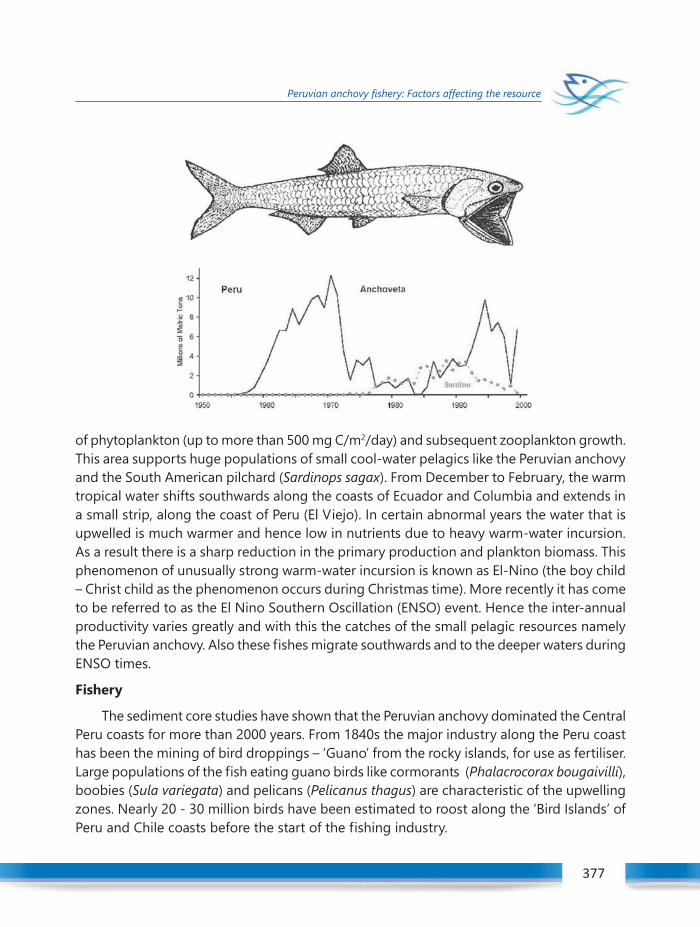
Winter School on Structure and Function of the Marine Ecosystem : Fisheries 377
Peruvian anchovy fishery: Factors affecting the resource
377
of phytoplankton (up to more than 500 mg C/m2/day) and subsequent zooplankton growth.This area supports huge populations of small cool-water pelagics like the Peruvian anchovyand the South American pilchard (Sardinops sagax). From December to February, the warmtropical water shifts southwards along the coasts of Ecuador and Columbia and extends ina small strip, along the coast of Peru (El Viejo). In certain abnormal years the water that isupwelled is much warmer and hence low in nutrients due to heavy warm-water incursion.As a result there is a sharp reduction in the primary production and plankton biomass. Thisphenomenon of unusually strong warm-water incursion is known as El-Nino (the boy child– Christ child as the phenomenon occurs during Christmas time). More recently it has cometo be referred to as the El Nino Southern Oscillation (ENSO) event. Hence the inter-annualproductivity varies greatly and with this the catches of the small pelagic resources namelythe Peruvian anchovy. Also these fishes migrate southwards and to the deeper waters duringENSO times.
Fishery
The sediment core studies have shown that the Peruvian anchovy dominated the CentralPeru coasts for more than 2000 years. From 1840s the major industry along the Peru coasthas been the mining of bird droppings – ‘Guano’ from the rocky islands, for use as fertiliser.Large populations of the fish eating guano birds like cormorants (Phalacrocorax bougaivilli),boobies (Sula variegata) and pelicans (Pelicanus thagus) are characteristic of the upwellingzones. Nearly 20 - 30 million birds have been estimated to roost along the ‘Bird Islands’ ofPeru and Chile coasts before the start of the fishing industry.
Winter School on Structure and Function of the Marine Ecosystem : Fisheries378
Peruvian anchovy fishery: Factors affecting the resource
After the Second World War a small Peruvian anchovy fishery started, mainly for exportas canned fish. The high oil content and hence less palatability coupled with the hugedemand for an alternate cheap protein source (fish-meal) for the giant poultry and pigindustry of the developed world kick-started a highly successful anchovy fishery. In 1949,seven fish meal plants started in Peru. The fish landings increased to an average of 1.0million tonnes (m t) per year during 1955 – 1959. Anchovy trawlers and purse-seiners locallyknown as ‘Bolicheras’ are the crafts used for the fishery. From around 100 vessels and 30fish-meal plants in 1954-’55, the industry grew to around 2000 vessels and 175 plants in1968-69. This was the boom period for the now ‘Industrial Fishery’. The fishery peaked at13.0 m t in 1970. Many scientists unofficially peg the landings at 15.0 m t in 1970. SoutheastPacific area ranked first among the Pacific fishing areas. The total biomass was estimated tobe 23.0 m t in 1970 and around 9.0 to14.0 m t in 1971.
The climate-dependent dynamics of Peruvian anchovy is affected by strong El-Ninoevents. The 1972-73 ENSO event led to the drastic decrease in the anchovy landings. Thecatches dropped to around 2.0 – 4.0 m t. After the 1975-76 event, the landings furtherdecreased to 1.0 – 2.0 m t. The landings further crashed to 1.0 m t after the 1977-78 event.The 1982-83 ENSO, the severest of them all led to an all time low of 0.5 – 0.1 m t catches in1983 and 1984 with a total biomass of less than a million tons. The environmental conditionsstabilised after this. Thus after a protracted period (1974 to 1985) of highly fluctuating lowlandings the fishery started to recover. In 1986 it exploded back to 5.0 m t. The fisheryfluctuated between 2.0 to 5.0 m t till it reached a peak in 1994 (12.0 m t). The strong ENSOevent of 1996-97 led to a collapse in 1998 (1.8 m t), the fishery coming back strongly thenext year with a catch of 8.7 mt, the year-class strength being independent of the parentalpopulation.
Factors affecting the resource
The question was whether it was over fishing or environmental changes or a combinationof both which led to the repeated collapse of the anchovy fishery.
Environmental conditions
Drastic reduction in primary production and plankton biomass due to the El Nino eventshad a major impact on the biology of the Peruvian anchovy. The following causes areattributed:
a) Larvae fail to survive and get recruited to the fishery due to lack of phytoplanktonfood. The resultant drop in catches is felt immediately because the anchovies arerecruited when six months old.
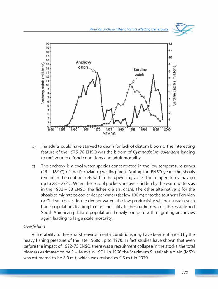
Winter School on Structure and Function of the Marine Ecosystem : Fisheries 379
Peruvian anchovy fishery: Factors affecting the resource
379
b) The adults could have starved to death for lack of diatom blooms. The interestingfeature of the 1975-76 ENSO was the bloom of Gymnodinium splendens leadingto unfavourable food conditions and adult mortality.
c) The anchovy is a cool water species concentrated in the low temperature zones(16 - 18O C) of the Peruvian upwelling area. During the ENSO years the shoalsremain in the cool pockets within the upwelling zone. The temperatures may goup to 28 – 29O C. When these cool pockets are over- ridden by the warm waters asin the 1982 – 83 ENSO, the fishes die en masse. The other alternative is for theshoals to migrate to cooler deeper waters (below 100 m) or to the southern Peruvianor Chilean coasts. In the deeper waters the low productivity will not sustain suchhuge populations leading to mass mortality. In the southern waters the establishedSouth American pilchard populations heavily compete with migrating anchoviesagain leading to large scale mortality.
Overfishing
Vulnerability to these harsh environmental conditions may have been enhanced by theheavy fishing pressure of the late 1960s up to 1970. In fact studies have shown that evenbefore the impact of 1972-73 ENSO, there was a recruitment collapse in the stocks, the totalbiomass estimated to be 9 – 14 m t in 1971. In 1966 the Maximum Sustainable Yield (MSY)was estimated to be 8.0 m t, which was revised as 9.5 m t in 1970.
Winter School on Structure and Function of the Marine Ecosystem : Fisheries380
Peruvian anchovy fishery: Factors affecting the resource
Predation and Competition
Another interesting aspect is the heavy predation on the anchovy populations by theguano birds. Nearly 80–95% of their diet consists of the anchovies. So the huge birdpopulations (estimates as high as 30 million) before the industrial fishery has now dwindledto as low as 5 million, mainly due to the fluctuations in the anchovy populations. Anothermajor predator is the Chilean jack mackerel (Trachurus murphyi), whose population increasesduring the El-Nino years due to enhanced spawning success. During El Nino years otherpredators like the yellowfin tuna, dolphinfish and Chilean bonito migrate southward to theanchovy domain. So the trophic dynamics is greatly affected by these events. Competitionwith the South American pilchard especially when the anchovies migrate southwards isanother major factor. The pilchard populations are not much affected by the El-Nino. Theinverse relationship between the two tandem fisheries can be clearly seen in the figure.After the 1972-73 ENSO, the pilchard stock began to increase and an important fisherydeveloped over the next 15 years coinciding with the decline and rebuild of the anchovyfishery.
Management
In 1963, the Instituto del Mar del Peru (IMARPE) was established with a strong FAObacking to study the fishery and to advise the Government. In 1965 a five-day week fishingwas established. In 1966 three months of closed season (veda) was put in place duringJanuary to March. Catch quotas were fixed as per the MSY levels (8.0 – 9.5 m t). So a secondclosed season was envisaged after around six months fishing when the quota would betaken. But many of these measures were hard to implement. It is now estimated that onlyless than 1500 vessels are required to catch around 10 m t of anchovies.
The Peruvian anchovy fishery is one example to understand how the climate andenvironment influence the fisheries. Another interesting parallel is the story of a warm-water species (Sardinops melanosticta – Japanese pilchard) and the impact of cool-waterincursion into its domain in the Northwest Pacific fishing area.
Winter School on Structure and Function of the Marine Ecosystem : Fisheries 381
Fisheries in atolls- tradeoffs between harvest and conservation
Introduction
Atolls are ring shaped coral reefs including a coral rim that encircles a lagoon partiallyor completely and with or without a coral island/cays on the rim. Most of the world’s atollsare in the Pacific Ocean and Indian Ocean. Lakshadweep islands, Maldives and the ChagosArchipelago are the atolls in the Indian Ocean. Lakshadweep are the only atoll islands inIndia. They lie scattered in the Arabian Sea between Latitude 8.26° to 12.4° N and Longitude71.7°-73.75° E, comprising of 36 islands, 3 reefs and 5 submerged banks. These islandsconsist of coral formations built upon the Laccadive-Chagos submarine ridge rising steeplyfrom a depth of about 1500 m to 4000 m off the west coast of India. While the total landarea is 30 sq.km, the length of the coastline is 132 km and lagoon area of 4200 sq.km. Itsterritorial water spread is 20000 sq.km and it constitutes 0.4 million sq.km to the EEZ ofIndian Union. Out of the 36 islands, 11 are inhabited with a population of 64,473 (2011census). The atolls have 4 distinct biomes comprising of the islands, lagoons, reefs and theOpen Ocean. Few threats to the atoll systems are sea level rise, salt water intrusion, reducedavailability of fresh water, coral bleaching, disturbances to reef ecosystem, shrinking oflivelihood and excessive dependence on external resources, excessive harvest of reefresources etc.
Marine Biodiversity of Lakshadweep: Corals are represented by 148 species; fish-126 families and 601 species; crustaceans-68 species; mollusks-227 species; sponges-91species; mangroves-2 species; seaweeds-114 species; echinoderms-78 species, sea grass-6species; sea turtles-4 species; 101 species of birds and 12 species of cetaceans. Pitti, a tinysand bank situated nearly 24km northwest of Kavaratti with an area of only 1.21 ha is anIsland of Birds. This is a breeding ground for 4 species of terns and therefore the island hasgreat significance since such breeding colonies are very rare in the Indias territorial areas.
Fishes: The fishes that occur in the coralline niches of the lagoon exhibit the characteristicvariety of colours and mainly consist of perches, gar-fishes, half-beaks, scarids, goat-fishes,carangids, grey mullets, antherinids, spyraenids, polynemids, balistids, blennids and globe-fishes (Balan, 1958; Kumaran et al., 1989). Jones and Kumaran (1980) recorded 603 speciesof fish from the Laccadive archipelago. The offshore fishery is constituted by fishes viz.,tunnies, wahoo, sharks, rays, sail fish, flying fish, carangids etc. Fishes such as Crenimugilcrenilabis, Polynemus sexfilis, Naso tuberosus, Naso unicornis, Gomphousus varius,
48C H A P T E R FISHERIES IN ATOLLS- TRADEOFFS
BETWEEN HARVEST AND CONSERVATIONK. Mohammed Koya and Abdul Azeez
Pelagic Fisheries Division
ICAR-Central Marine Fisheries Research Institute

Winter School on Structure and Function of the Marine Ecosystem : Fisheries382
Fisheries in atolls- tradeoffs between harvest and conservation
Novacutichthys taeniurus and Anampses diadematus are common in the waters ofLakshadweep (James et al., 1989). Of the 603 species of marine fishes belonging to 126families that are reported from the islands, at least 300 species are of ornamental value. Theornamental fish such as Abudefdus, Amphiprion, Apogon, Coris, Balistes, Platax are commonin Lakshadweep lagoons (Murthy et al., 1989).
Fisheries in the islandsPresent day fisheries in Lakshadweep are built on the traditional fishing and trade
practices prevalent ever since settlement in the islands. Fishing here range from hand picking,cloth fishing, spear fishing, cast netting etc. in the lagoons to pole and line, troll line, handline,harpooning etc. in the deeper areas of the sea around the islands. Plank built country canoesor modified country canoes with or without outboard motors are the basic craft. Opendecked Pablo type boats, motorized using inboard engines are the major fishing crafts in allthe islands. Principal fishing method- Pole & Line is presently practiced in such boats. Oflate, a modified version of these boats, which are larger and with wheel house on the stemare gaining popularity in the islands.
The fisheries in the islands can be broadly divided into Tuna Fishery and Non Tunafisheries. Tuna fisheries comprise mainly of capture of oceanic tunas- skipjack (Katsuwonuspelamis) and Yellwofin tuna (Thunnus albacores). Other tunas like the Little tunny (Euthynusaffinis), Bullet tunas (Auxis spp) and the Dog tooth tuna (Gymnosarda unicolor) also formcatch at varying rates in differentseasons. Non-tuna f isheriescomprises of fishing for other largepelagic resources like rainbowrunner, Mahi mahi, Wahoo, sharksrays etc. and Reef associated fisheslike snappers, groupers, carangids,full beaks, half beaks etc. The fishinggrounds for these resources are thedeep sea in the vicinity of all theislands, reef areas and submergedbanks. It may be noted that theprincipal f ishing methods in theislands are hook and line based,which are considered to be the mostideal fishing tackle in view of itsselectivity and harvest limitations. Use of gillnet, the only major net used for fishing arelimited to reef and lagoon areas for reef associated resources like the fullbeaks and halfbeaks.
Fig. 1. Gross catch composition of island fisheries
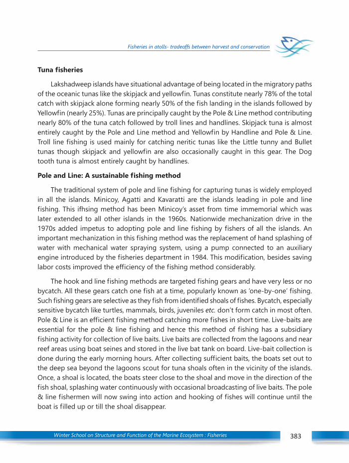
Winter School on Structure and Function of the Marine Ecosystem : Fisheries 383
Fisheries in atolls- tradeoffs between harvest and conservation
Tuna fisheries
Lakshadweep islands have situational advantage of being located in the migratory pathsof the oceanic tunas like the skipjack and yellowfin. Tunas constitute nearly 78% of the totalcatch with skipjack alone forming nearly 50% of the fish landing in the islands followed byYellowfin (nearly 25%). Tunas are principally caught by the Pole & Line method contributingnearly 80% of the tuna catch followed by troll lines and handlines. Skipjack tuna is almostentirely caught by the Pole and Line method and Yellowfin by Handline and Pole & Line.Troll line fishing is used mainly for catching neritic tunas like the Little tunny and Bullettunas though skipjack and yellowfin are also occasionally caught in this gear. The Dogtooth tuna is almost entirely caught by handlines.
Pole and Line: A sustainable fishing method
The traditional system of pole and line fishing for capturing tunas is widely employedin all the islands. Minicoy, Agatti and Kavaratti are the islands leading in pole and linefishing. This ifhsing method has been Minicoy’s asset from time immemorial which waslater extended to all other islands in the 1960s. Nationwide mechanization drive in the1970s added impetus to adopting pole and line fishing by fishers of all the islands. Animportant mechanization in this fishing method was the replacement of hand splashing ofwater with mechanical water spraying system, using a pump connected to an auxiliaryengine introduced by the fisheries department in 1984. This modification, besides savinglabor costs improved the efficiency of the fishing method considerably.
The hook and line fishing methods are targeted fishing gears and have very less or nobycatch. All these gears catch one fish at a time, popularly known as ‘one-by-one’ fishing.Such fishing gears are selective as they fish from identified shoals of fishes. Bycatch, especiallysensitive bycatch like turtles, mammals, birds, juveniles etc. don’t form catch in most often.Pole & Line is an efficient fishing method catching more fishes in short time. Live-baits areessential for the pole & line fishing and hence this method of fishing has a subsidiaryfishing activity for collection of live baits. Live baits are collected from the lagoons and nearreef areas using boat seines and stored in the live bat tank on board. Live-bait collection isdone during the early morning hours. After collecting sufficient baits, the boats set out tothe deep sea beyond the lagoons scout for tuna shoals often in the vicinity of the islands.Once, a shoal is located, the boats steer close to the shoal and move in the direction of thefish shoal, splashing water continuously with occasional broadcasting of live baits. The pole& line fishermen will now swing into action and hooking of fishes will continue until theboat is filled up or till the shoal disappear.
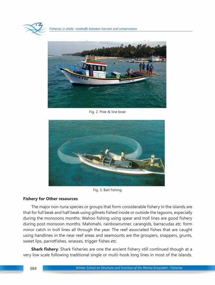
Winter School on Structure and Function of the Marine Ecosystem : Fisheries384
Fisheries in atolls- tradeoffs between harvest and conservation
Fishery for Other resources
The major non-tuna species or groups that form considerable fishery in the islands arethat for full beak and half beak using gillnets fished inside or outside the lagoons, especiallyduring the monsoons months. Wahoo fishing using spear and troll lines are good fisheryduring post monsoon months. Mahimahi, rainbowrunner, carangids, barracudas etc. formminor catch in troll lines all through the year. The reef associated fishes that are caughtusing handlines in the near reef areas and seamounts are the groupers, snappers, grunts,sweet lips, parrotfishes, wrasses, trigger fishes etc.
Shark fishery: Shark fisheries are one the ancient fishery still continued though at avery low scale following traditional single or multi-hook long lines in most of the islands.
Fig. 2. Pole & line boat
Fig. 3. Bait fishing

Winter School on Structure and Function of the Marine Ecosystem : Fisheries 385
Fisheries in atolls- tradeoffs between harvest and conservation
Large mesh drift gillnetting done during monsoon months also catch sharks along withother large pelagics. The most common species of sharks that occur in Lakshadweep arethe Spade-nose shark/Yellow dog shark, Scoliodon laticaudus and the Milk shark, Rhizopriodonacutus (Devdoss et al., 1985). The Blacktip Shark, Carcharhinus limbatus and Hammerheadshark, Sphyrna mokarran are also commonly found in the waters around Lakshadweep(Hanfee, 1997; Basudev Tripathy, Pers. Obs.).
Other Traditional Fishing practices in the islandsOwing to the typical geographical features of an atoll and its natural isolation from
mainland, the people of the islands have used varieties of indigenous methods for catchingfishes and other marine creatures from lagoon and the adjoining sea for food. Some of theimportant fishing activities/gears used in lagoons given in table 1.Table 1: fishing activities/gears used in lagoons
Local Name Description Target Resource
Appal kuthal Octopus hunting using sharp iron spears Octopus
Chilla Fishing using wooden spike Flying fishes, Garfishes, half beaks
Chadal Harpooning for catching fish Wahoo
Bala adiyal Shore seine, used mainly in the western Juvenile and sub-adults of reeflagoon associated fishes
Bala attal Long, small meshed nets used inside the Juvenile and sub-adults of reeflagoons around the island associated fishes
Bala fadal Large drag net involving 15-30 people, Juvenile and sub-adults of reefoperated in both eastern and western associated fisheslagoons together with scare lines
Bala idal Set gillnets in the lagoon Reef associated fishes, sharks, rays etc.
Cast net Small mesh cast net operated in the lagoon Juvenile of carangids, surgeons,from shore during low tide damsels etc.
Nool bikel Baited hook and line set from shore or from Snappers, carangids etc.a boat
Kalmoodal “Boulder trap” – a net set around a coral Juvenile of reef associated fishesboulder which is then agitated using rods todrive out fish.
Kurakkal Light and spear or sword. Not commonlyused, only practised in shallow water Juvenile of reef associated fishes
Rod and line Baited hook and line, used opportunistically Sub adults of Reef associated fishesaround the island and mainly from the shore
Shal kakal Gillnet set in reef channels, used mainly Reef associated fishes like snappers,during the monsoon and at spring tide. carangids, etc.
Winter School on Structure and Function of the Marine Ecosystem : Fisheries386
Fisheries in atolls- tradeoffs between harvest and conservation
Coral reefs and their importance to island fisheries
Islands are formed inside the lagoon of atoll through continuous accumulation of coralsand due to wave action driven mainly by the South-west monsoon. Shore of these islandsare protected from the hazards of the waves by the reef crest as all the waves surf on thereef crest before proceeding to the shore as low energy waves. The lagoons are doing anexcellent service by way of being the nursery grounds for the fishes and other organismsbesides being home to a plethora of flora and fauna, especially the corals. It is estimatedthat the coral lagoon of Lakshadweep is the habitat for about 75 species of marine ornamentalfishes belonging to 13 families. Similarly, the lagoon is the source of live-bait fishes, whichis the most essential component of the Pole & Line fishery of Tuna. The rich bio-diversity ofthe coral lagoon is also the base for the development of tourism in the Lakshadweep forevents like coral reef diving and snorkeling. Therefore, the survival of these islands fullydepends on the survival of the coral reefs and the lagoon ecosystem. Scientific managementof resources within the coral reefs therefore is of paramount importance.
Conservation of the Atoll Ecosystem
Extraction of marine resources is the major anthropogenic threat to the ecosystem.Harvest of the natural resources therefore should be at levels that can be regained withnatural recruitment and rebuilding. Every organism in the lagoon performs an ecologicalservice and therefore the harvest should be balanced not affect the ecosystem functioning.Many fishes inhabiting the lagoons like the parrot fishes do the service of cleaning the coralboulders of algae and other foulers to create space suitable for attachment by the corallarvae leading replenishment of corals. Similarly, many herbivore fishes like the surgeonfishes, butterfly fishes etc. do such services. Dependence of lagoon for fish supply is muchlimited in Lakshadweep as the major commercial fishing activity is tuna based. This makesthe fishing in the islands more sustainable. Besides, there are quite a lot of conservationsmeasures adopted by the Govt in tandem with the international obligations.
Compliance to National and International Obligations
The point number 11 of the Aichi biodiversity targets, says that “By 2020, at least 17percent of terrestrial and Inland water, and 10 percent of coastal and marine areas, especiallyareas of particular importance for biodiversity and ecosystem services are conserved througheffectively and equitably managed, ecologically representative and well connected systemsof protected area and other effective area based conservation measures, and integratedinto the wider landscape and seascapes”, which is integrated in India’s National BiodiversityTargets, 2012-2020. The Environment Protection Act (1986) provides for identification ofecologically sensitive areas based on the sensitivity and conservation value of a spatial unit.In case of Lakshadweep islands, the Integrated Island Management Plans, prepared as per
Winter School on Structure and Function of the Marine Ecosystem : Fisheries 387
Fisheries in atolls- tradeoffs between harvest and conservation
the Island Protection Zone Notification (2011), demarcate the preservation and conservationzones for spatial conservation of the coral reef areas. The Pitti Island, because of being abird nesting area has been declared as an MPA. The report of the Planning Commission ofIndia (2008) proposed to declare one or two reefs among the Suheli par, Baliyapani par,Cheriyapani par and Perumal par as Marine National Park to protect and preserve the marinebiodiversity. The Bombay Natural History Society, based on a detailed study on the giantclam resources in the Islands proposed declaring the reefs of Agatti Island to be aconservation reserve. International Union for Conservation of Nature (IUCN) andoceanographer Sylvia Earle of Mission Blue named 31 new hope spots, among them Andaman& Nicobar and Lakshadweep islands have been named as the new “hope spots” from India.A Hope Spot is an area of ocean that merits special protection because of its wildlife andsignificant underwater habitats. Some are already formally protected, while others still needprotection.
Winter School on Structure and Function of the Marine Ecosystem : Fisheries388
Responsible Fisheries- A prelude to the Concept, Context and Praxis
The concept of Responsible Fisheries is synonymous with the FAO Code of Conduct forResponsible Fisheries (CCRF). CCRF is an international instrument for fisheries managementwhich was developed and released by Food And Agriculture Organisation ( FAO) functioningunder the United Nations on 31 October 1995 after a series of international deliberationsthat began in 1992. More than 160 countries, including India are signatories to thisinternational instrument which is considered as a landmark document symbolizing theinternational consensus achieved on the necessity for providing guidelines to ensuresustainable utilization of fisheries resources of the world. The most salient feature of thisglobal instrument is its voluntary nature. The Code is often referred to as the Bible of FisheriesManagement.
Why the Code?
The term “Responsible Fisheries” may evoke a doubt whether we have been irresponsiblein the way we have been developing or managing our fisheries resources. In fact such adoubt is the stepping stone to understand the concept of Responsible Fisheries.
In common parlance the term “responsibility” is immediately read with the notions ofrights or ownership. We tend to have a better sense of responsibility to things we ownourselves. Thus, we feel responsible in taking care of our properties or assets like land orhouse or vehicle. The lesser the sense of our ownership lesser will be our sense ofresponsibility. Thus we feel less responsible for the affairs of our ecosystem or politicalsystem because we deem them as owned by all. A property belonging to everyone tends tobe nobody’s property though nobody is excluded from its utilization. This is an importantpoint because in the case of fisheries what we are talking about is a Common Property. Ormore correctly an Open access resource. An important question here is “Who actually ownsthe fish or who actually owns the sea? The de jure owner of the fisheries is the State or thegovernment. That is, fish in our waters is owned by the people. But by all practical sensethe fish , once caught by the fisher, becomes his or her property. If so, what about his or hersense of responsibility to ensure its conservation? It may sound a bit puzzling. That is whythe Code makes it very clear in the very first article which is given under the generalprinciples of the Code.
49C H A P T E R RESPONSIBLE FISHERIES- A PRELUDE TO
THE CONCEPT, CONTEXT AND PRAXISRamachandran C., Vipinkumar V. P. and Shinoj Parappurathu
Socio Economic Evaluation and Technology Transfer DivisionICAR-Central Marine Fisheries Research Institute
Winter School on Structure and Function of the Marine Ecosystem : Fisheries 389
Responsible Fisheries- A prelude to the Concept, Context and Praxis
389
“ States and users of living aquatic resources should conserve aquatic eco systems. Theright to fish carries with it the obligation to do so in a responsible manner so as to ensureeffective conservation and management of the living aquatic resources. “ (Article 6.1).
What is in principle a property of every one, becomes the property of none in practice.This is the most fundamental challenge in scientific fisheries management. There is a notionthat if a sense of ownership is assured, the likelihood of it being taken care of in a responsiblemanner is more. There are people who argue that it is a misplaced notion. The above-mentioned article of the Code, in fact, is a preemptive answer to this commonmisunderstanding.
It is for the same reason that , of the more than 230 clauses in the Code classified under12 articles, a large number vest the responsibility with the State. This, in a way also helpsto clear the doubts regarding the real meaning of implementing the Code.
Another doubt could be on the real meaning of the voluntary nature of the Code.Being a voluntary instrument the question could be, “Is it something like a “barking dogthat seldom bites”? The code answers this question in its fundamental philosophy calledthe Precautionary Approach, which is enshrined in Article 7.5.1.
“The absence of adequate scientific information should not be used as a reason forpostponing or failing to take conservation and management measures.”
In simple words what it means is “ Better safe than sorry”. It also has a deeper meaningwhich implies that when a person is given the license or permission or right to fish, what isbeing transferred is part of the stewardship obligation of the State. One needs to clearlyunderstand this because, when individuals operate in a common property with the soleobjective of making profitable livelihoods, the sustainable utilization of such a resourcebecomes an impossible task in the absence of mutually respected and endorsed regulations.The precautionary principle is further elaborated under the Foundations of the Code below.
Being a global guideline there is much practical sense for keeping it as a voluntaryinstrument too. Each nation can contextualize the code in sync with its own local realitiesand requirements at the same time respecting the globally agreed principles and norms.However, there are scholars who argue for making the CCRF a binding instrument giventhe sorry state of fisheries governance in most parts of the world.
Foundations of the CodeThat the sustainability of marine capture fisheries at the current level of harvesting is at
stake is no longer a moot point. It is being realized that fisheries anywhere in the world ismore a socioeconomic process with biological constraints than anything else. The openaccess nature of the resource coupled with unregulated penetration of advanced, but not
Winter School on Structure and Function of the Marine Ecosystem : Fisheries390
Responsible Fisheries- A prelude to the Concept, Context and Praxis
necessarily eco-friendly, harvesting technologies (a phenomenon called technological creep)has enacted a virtual “tragedy of the commons” in our seas. Making the issue still morecomplex, especially in the context of the Millennium Development Goals, is the rampantpoverty/income inequality existing among our fisher folk though the capture fisheriesmake significant foreign exchange contribution in our country. The plateauing of the resourceas revealed by recent trends in landings doesn’t augur well for the ecologic and economicsustainability of the marine fisheries sector.
If there are no technological magical bullets for the current impasse what is the wayout? This is precisely the question the FAO code is trying to answer. As we have seen ,”theright to fish carries along with it an obligation to do it responsibly” is the cardinal principle ofthe code. This principle is built on the foundation of what is known as a PrecautionaryApproach. Precautionary approach, which originally was proposed as Principle 15 of Agenda21 the Rio Earth Summit meeting in 1992, enunciates that,
“where there are threats of serious or irreversible damage, lack of full scientific certaintyshall not be used as a reason for postponing cost-effective measures to prevent environmentaldegradation”.
While in simple terms the precautionary approach means “better safe than sorry”, itclearly recognizes that changes in fisheries systems are only slowly reversible, difficult tocontrol, not well understood, and subject to changing environment and human values. AsRestrepo et al., define, “the precautionary approach in fisheries is about applying judiciousand responsible fisheries management practices, based on sound scientific research andanalysis, proactively (to avoid or reverse overexploitation) rather than reactively (once alldoubt has been removed and the resource is severely overexploited), to ensure thesustainability of fishery resources and associated ecosystems for the benefit of future aswell as current generations”.
It involves the application of prudent foresight. It is about applying judicious andresponsible fisheries management practices, based on sound scientific research and analysisproactively rather than reactively to ensure the sustainability of fishery resources andassociated ecosystems for the benefit of future as well as current generations.
Taking account of the uncertainties in fisheries systems and the need to take action onincomplete knowledge, it requires, inter alia:
a. consideration of the needs of future generations and avoidance of changes thatare not potentially reversible;
b. prior identification of undesirable outcomes and of measures that will avoid themor correct them promptly;
Winter School on Structure and Function of the Marine Ecosystem : Fisheries 391
Responsible Fisheries- A prelude to the Concept, Context and Praxis
391
c. that any necessary corrective measures are initiated without delay, and that theyshould achieve their purpose promptly, on a timescale not exceeding two or threedecades;
d. that where the likely impact of resource use is uncertain, priority should be givento conserving the productive capacity of the resource;
e. that harvesting and processing capacity should be commensurate with estimatedsustainable levels of resource, and that increases in capacity should be furthercontained when resource productivity is highly uncertain;
f. all fishing activities must have prior management authorization and be subject toperiodic review;
g. an established legal and institutional framework for fishery management, withinwhich management plans that implement the above points are instituted for eachfishery, and
h. appropriate placement of the burden of proof by adhering to the requirementsabove.
The reversal of burden of proof means that those hoping to exploit our marine resourcesmust demonstrate that no ecologically significant long-term damage will result due to theiraction. Or in other words human actions are assumed to be harmful unless proven otherwise.
Contents of the Code
The code provides a necessary framework for national and international efforts to ensuresustainable exploitation of aquatic living resources in harmony with the environment. It isachieved through 12 articles covering areas like
a) Nature and scope of the code (article 1)
b) Objectives of the code (article 2),
c) Relationship with other international instruments (article 3),
d) Implementation, monitoring and updating (article 4),
e) Special requirements of developing countries (article 5),
f) General principles (article 6),
g) Fisheries management (article 7),
h) Fishing operations (article 8),
i) Aquaculture development (article 9),
Winter School on Structure and Function of the Marine Ecosystem : Fisheries392
Responsible Fisheries- A prelude to the Concept, Context and Praxis
j) Integration of fisheries into coastal area management (article 10),
k) Post-harvest practices and trade (article 11), and
l) Fisheries research (article 12).
(The full text of the FAO CCRF ( hereafter referred to as the Code) translated intoMalayalam was published by CMFRI in 2002 under an agreement with the FAO (Ramachandran,2002). Thus, Malayalam became the second language, after Tamil, to havea translated version of this very important international fisheries management instrument.You can access it at www.cmfri.org.in. The pdf of the English full text is supplied with theWinter school CD rom).
Characteristics of the CodeAs we have seen, the most salient feature of the code is that it is voluntary in nature.
Unlike other international agreements like UN Agreement to Promote Compliance withInternational Conservation and Management Measures by Fishing vessels on the High Seasor the Straddling Stock Agreement, 1995, it is not legally binding and violation of the codecannot be challenged in a court of law.
It would be tempting to castigate it as an Achilles’ heel and thus the futility of the code.But it should be remembered, “open access imbroglios’’ cannot be resolved through attemptsthat fail to recognize altruistic spirit of the human actors. In a situation where, “you and yourenemy belong to the same eco-system”, solutions must be found in managing relationshipsof the actors that make or move the ecosystem. It doesn’t mean that the code is impracticalor ineffective. What it demands is to construe responsible fisheries management as a politicalprocess rather than a technical process. This insight is a significant contribution of socialscientists studying natural resource management (Wilson et al., 2006).
A fundamental objective of the Code is “to serve as an instrument of reference to helpstates to establish or to improve the legal and institutional framework required for theexercise of responsible fisheries and in the formulation and implementation of appropriatemeasures.” The policies of the state for managing the fisheries resources should be basedon the provisions of the code.
If world fisheries are to be sustainable in the long term, structural adjustment withinthe fisheries sector is required. Although policy decisions in this regard must be made bynational governments, effective implementation of the code requires the participation andcooperation of a wide range of stakeholders, including fishers, processors, NGOs andconsumers. Implementation of the code is primarily the responsibility of states. The codewill require regional and sectoral implementation in order to address the particular needsof fisheries in different regions or sub-sectors.
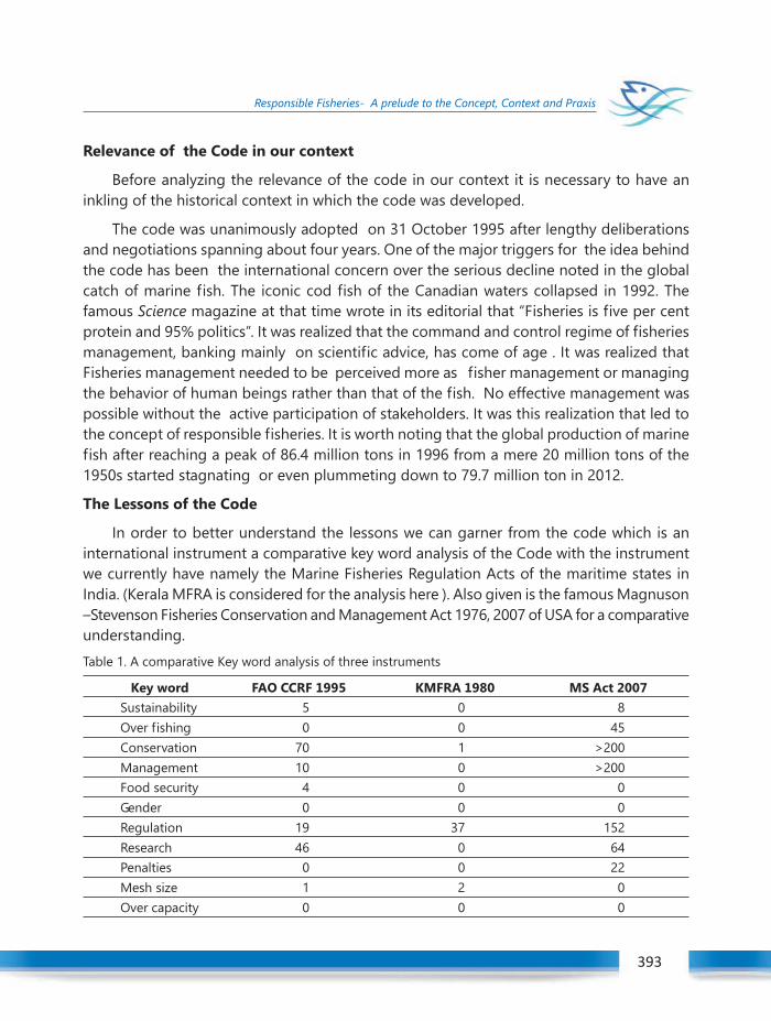
Winter School on Structure and Function of the Marine Ecosystem : Fisheries 393
Responsible Fisheries- A prelude to the Concept, Context and Praxis
393
Relevance of the Code in our context
Before analyzing the relevance of the code in our context it is necessary to have aninkling of the historical context in which the code was developed.
The code was unanimously adopted on 31 October 1995 after lengthy deliberationsand negotiations spanning about four years. One of the major triggers for the idea behindthe code has been the international concern over the serious decline noted in the globalcatch of marine fish. The iconic cod fish of the Canadian waters collapsed in 1992. Thefamous Science magazine at that time wrote in its editorial that “Fisheries is five per centprotein and 95% politics”. It was realized that the command and control regime of fisheriesmanagement, banking mainly on scientific advice, has come of age . It was realized thatFisheries management needed to be perceived more as fisher management or managingthe behavior of human beings rather than that of the fish. No effective management waspossible without the active participation of stakeholders. It was this realization that led tothe concept of responsible fisheries. It is worth noting that the global production of marinefish after reaching a peak of 86.4 million tons in 1996 from a mere 20 million tons of the1950s started stagnating or even plummeting down to 79.7 million ton in 2012.
The Lessons of the Code
In order to better understand the lessons we can garner from the code which is aninternational instrument a comparative key word analysis of the Code with the instrumentwe currently have namely the Marine Fisheries Regulation Acts of the maritime states inIndia. (Kerala MFRA is considered for the analysis here ). Also given is the famous Magnuson–Stevenson Fisheries Conservation and Management Act 1976, 2007 of USA for a comparativeunderstanding.Table 1. A comparative Key word analysis of three instruments
Key word FAO CCRF 1995 KMFRA 1980 MS Act 2007Sustainability 5 0 8Over fishing 0 0 45Conservation 70 1 >200Management 10 0 >200Food security 4 0 0Gender 0 0 0Regulation 19 37 152Research 46 0 64Penalties 0 0 22Mesh size 1 2 0Over capacity 0 0 0

Winter School on Structure and Function of the Marine Ecosystem : Fisheries394
Responsible Fisheries- A prelude to the Concept, Context and Praxis
MSY 1 0 5Fisherman 15 0 43Justice 0 0 6Discard 9 0 18By catch 1 0 68Participation 4 0 32Fisheries development 0 0 1Poverty 1 0 2Conflicts 3 0 3Rights 33 0 0Safety 11 0 26Ecosystem 27 0 13Code of conduct NA 0 0
The table reveals certain interesting things. The greater importance given to ResourceConservation both by the CCRF and the MS Act compared to KMFRA is indicative of thenature of exploitation in our waters. Remember that the KMFRA was developed in 1980.Today the situation has definitely changed given the declining trends we have witnessed inrecent times. Another key word to take note of is MSY, the Maximum Sustainable Yield,which is the most fundamental creed of fisheries stock assessment science. MS act of USAhas given much more importance to MSY indicating the extent to which scientific stockassessment has influenced the fisheries management regime in that country. FAO CCRF hasmentioned MSY only once ( Article 7.2). It indicates the lesser global applicability of MSY asa management reference point. All the three instruments give importance to fisheriesregulations. CCRF obviously does not deal with penalties. But what is relevant here for usis the fact that out of the 24 keywords used in this analysis only three keywords appear inKMFRA. They are conservation, regulation and mesh size . (What are your impressions overthis finding?). The absence of these key words in our Act indicates that there is a need forreforming it taking into cognizance the new ecologic and economic realities emerging inour fisheries sector.
Another interesting thing is the fact that the MS Act of USA is silent about the FAOCCRF. But, in an international study published in Nature 2009, which assessed the extent towhich the FAO CCRF is being complied by different nations USA got second rank. Out of the53 countries where the assessment was made India got 27 th position. The lesson we haveto draw from this study is the importance accorded by Nation States in adopting problem-based management measures in ensuring sustainable utilization of their marine fisheriesresources and the kind of policy significance these countries bestow to the importance ofsustainable fisheries in the economy of those nations. It is worth noting that all of the 10
Winter School on Structure and Function of the Marine Ecosystem : Fisheries 395
Responsible Fisheries- A prelude to the Concept, Context and Praxis
395
highly ranked countries belong to temperate regions of the world. The issues like overfishingare more visible in these countries and hence there is no wonder that these countries areahead of other nations in adopting conservation oriented- fisheries management andregulations in their waters. In this context a question may creep in our minds. Should wealso follow these nations where overfishing has become a reality? Can we continue ourbusiness as usual attitude in the absence of fisheries collapses or severe decline in ourresources? It indeed is a challenging poser.
It is here that the science of fisheries management and the knowledge base we haveaccumulated so far regarding the status of our marine resources become relevant.
There are only two fundamental questions in fisheries management anywhere in theworld.
i) “How much fish we can safely catch?”ii) “How much is the fish available ?”
These questions are very simple. But answers are not so simple to come. That is preciselythe reason why Precautionary approach has become the driving philosophy of the globalthinking over sustainable or responsible fisheries. We should not fail to see the intellectualhumility enshrined in this approach. It is the deep ecological insight that in the face of theexcruciating uncertainty and ignorance attached to our fisheries management knowledgebase, we need to respect the self rejuvenating capacity of the ecosystem. This realization isthe basic idea behind new approaches like Ecosystem based Fisheries Management and ofcourse this demands new and complex approaches in fisheries research and governance.
What is the Problem?The most important problem a fishery faces is what is known as Over Fishing. It takes
place over time as the fishing is intensified. It is the stage where a stock of fish loses itscapacity to keep on providing the Maximum Sustainable Yield. It is at this stage that thefishery is at the verge of an almost irredeemable loss, economically and biologically. MSYas a logic is easy to understand . But as a quantitative reference point, MSY is a methodologicalchallenge especially in our multi-species tropical water scenario. This is still considered asthe Holy Grail in fisheries stock assessment science. Remember, this should not be construedas a weakness of the scientist. It is the epistemological challenge the fisheries scientists allover the world share , lament and endeavour to overcome.
MSY is like a Laxman Rekha. The most frightening aspect about this Laxman Rekha isthat we need to cross it to realize that we have trespassed it. Hence we can build ourdefense against the specter of overfishing only on the basis of a stronger understandingand contextual analysis of its symptoms.
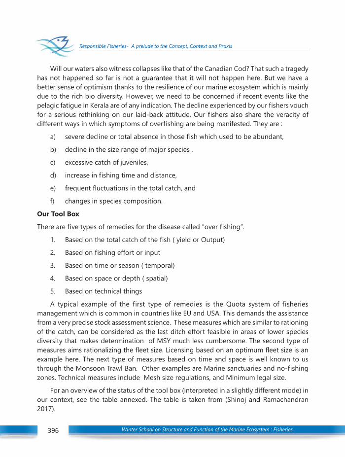
Winter School on Structure and Function of the Marine Ecosystem : Fisheries396
Responsible Fisheries- A prelude to the Concept, Context and Praxis
Will our waters also witness collapses like that of the Canadian Cod? That such a tragedyhas not happened so far is not a guarantee that it will not happen here. But we have abetter sense of optimism thanks to the resilience of our marine ecosystem which is mainlydue to the rich bio diversity. However, we need to be concerned if recent events like thepelagic fatigue in Kerala are of any indication. The decline experienced by our fishers vouchfor a serious rethinking on our laid-back attitude. Our fishers also share the veracity ofdifferent ways in which symptoms of overfishing are being manifested. They are :
a) severe decline or total absence in those fish which used to be abundant,
b) decline in the size range of major species ,
c) excessive catch of juveniles,
d) increase in fishing time and distance,
e) frequent fluctuations in the total catch, and
f) changes in species composition.
Our Tool Box
There are five types of remedies for the disease called “over fishing”.
1. Based on the total catch of the fish ( yield or Output)
2. Based on fishing effort or input
3. Based on time or season ( temporal)
4. Based on space or depth ( spatial)
5. Based on technical things
A typical example of the first type of remedies is the Quota system of fisheriesmanagement which is common in countries like EU and USA. This demands the assistancefrom a very precise stock assessment science. These measures which are similar to rationingof the catch, can be considered as the last ditch effort feasible in areas of lower speciesdiversity that makes determination of MSY much less cumbersome. The second type ofmeasures aims rationalizing the fleet size. Licensing based on an optimum fleet size is anexample here. The next type of measures based on time and space is well known to usthrough the Monsoon Trawl Ban. Other examples are Marine sanctuaries and no-fishingzones. Technical measures include Mesh size regulations, and Minimum legal size.
For an overview of the status of the tool box (interpreted in a slightly different mode) inour context, see the table annexed. The table is taken from (Shinoj and Ramachandran2017).

Winter School on Structure and Function of the Marine Ecosystem : Fisheries 397
Responsible Fisheries- A prelude to the Concept, Context and Praxis
397
As long as a fishery remains a common property resource, a regulated fishery is moreprofitable than an unregulated fishery in the long run. Our fishers have started acceptingthis truism. But they are helpless to avoid competitive fishing due to two main reasons. Oneis the increase in fuel cost. And the other is the high demand for fish which has led to asituation where you are economically rewarded whatever be the catch. So fishers tend todo indiscriminate fishing. This has resulted in an illusion of super abundance which againdrives more fishing effort. This is leading to a very dangerous situation. There are fishers(like Mr Jossy Palliparambil, Munambam Kerala) who characterize this ugly scenario as aphase of “Foolish Fishing” (“mandan fishing” in Malayalam). It is high time each fisher takemore care in analyzing the fluctuations observed in the economics of their operations. AsCharles Glover, the author of the book End of the Line, notes “ what makes a fishermangreat now is what he leaves in the sea”.
Challenges in the praxis
Sustainable Management of resources is no different from fisheries development. Theyare no longer considered as dichotomous. There will be no fisheries development if thereis not enough fish in the sea. There won’t be enough fish in the sea, if human beings, bothas harvesters and consumers, do not act in a precautionary manner which is nothing but tonurture a feeling of “better safe today than sorry tomorrow”. What it means is to understandclearly the limits to which nature can be tapped. The requirements of both the presentgeneration and future generation are to be given equal importance. It is also about respectingthe co-evolutionary culture of a fisheries-resource dependent community. Thus ResponsibleFisheries management takes place at the dynamic interface between the behavior of manand that of fish. So the knowledge base for responsible fisheries ought to be a convergenceof different disciplines like fisheries biology, socio-politics, ecology, economics, engineering,law and communication. The aim of fisheries management is to ensure optimum utilizationof a common pool resource without jeopardising the inherent regenerative ability of theresource leading to livelihood security of the dependent community.
Much has been said about rights-based fisheries, f isheries co-management andecosystem-based fisheries management with fisheries managers, policy-makers, scientistand researchers racking their brains about the meaning of each of these fisheriesmanagement approaches. In trying to find definitions and formulating “how-to” guidelinesand handbooks on such fisheries management approaches, their essential ingredient oftenis overlooked, namely dialogue. Whether talking of co-management and partnershipsbetween fisheries stakeholders or of the adaptive nature of ecosystem-based fisheriesmanagement the fundamental nature of any f isheries management effort is thecommunication process among its various protagonists. Neither a partnership between

Winter School on Structure and Function of the Marine Ecosystem : Fisheries398
Responsible Fisheries- A prelude to the Concept, Context and Praxis
fishing communities, fisheries managers, researchers and other stakeholders, nor the mergingof the development goals of human well-being with that of ecological well-being throughan ecosystem-based fisheries management approach would be possible without free-flowinginformation among the various partners in the management process. It thus becomes apolitical or governance process.
These communication processes can take many different forms and can be designedaccording to a diversity of purposes: (1) to meet specific fisheries management objectives,needs and aspirations for the fisheries sector; and 2) to generate new information aboutlocal fisheries systems through participatory (eg. catch-reporting) mechanisms. Theexperiences from these activities should encourage fisheries managers, scientists, and fishingcommunities to actively seek such dialogue and information exchange as a basis forimproving fisheries management on an ecosystem approach.
The efforts to engender a scientifically- informed fisheries management or governanceregime are always challenged by the inherent uncertainty that characterizes the epistemologyof fisheries science. The complexity of an otherwise resilient tropical marine ecosystemadds fuel to the fire and on the Human dimension we have a plethora of challenges despitepromising perspectives from Hardin to Ostrom.
It is here that we need to fully appreciate the multitude of challenges we face in aprecautionary and participatory framework. We have the instruments/tool box. But thecredo of responsible fisheries is yet to become part of the community ethos (including thatof researchers and managers). What could be the reasons and how we can overcome thebarriers? As a concerned stakeholder each one of us has a responsibility to be part of acollective process to not only decipher the answers but also translate them into pragmaticameliorative strategies.
The Code and CMFRI Initiatives
Our fisheries have undergone tremendous changes during the past six decades. Beforethe advent of modernization, (motorization, mechanization , refrigeration, export orientationand transportation) the access to sea was limited to a few skillful and adventurous peoplewho were by birth fishers. The community could afford to have self regulations orientedtowards resource conservation which were arrived through the ecological experience of thecommunity over generations. These concerns or tacit knowledge were institutionalizedtoo. An example of such an institution still, surprisingly, surviving in Kerala is the Kadakkodyof the Malabar coast (Ramachandran, 2006). The self regulations and community regulationswhich were rooted in the traditional wisdom have given way to technological skills. Theseskills, unleashed by what we generally refer to as an era modernization, most often take a
Winter School on Structure and Function of the Marine Ecosystem : Fisheries 399
Responsible Fisheries- A prelude to the Concept, Context and Praxis
399
dehumanized manifestation thus weakening the hold of the community. This is where thecrucial role of the State comes into play in the management as well as development of thefishery. This is better known as fisheries governance.
Fisheries governance is dependent on the particular stage of economic developmentand local ecological status of the fishery resources. This varies with each country. It is becauseof this contextual nature that the Code has been made as a voluntary tool. Each governmentis free to make its own rules, regulations and strategies based on the guidelines and principleselaborated in the Code. Thus article 4.3 says “FAO through its competent bodies, may revisethe code, taking into account developments in fisheries as well as reports to COFI on theimplementation of the Code. (But in recent times an argument against this position has alsoemerged).
It is in this context that the actions and initiatives being taken by CMFRI, mainly throughan NATP funded research project titled “Designing and validation of communication strategiesfor responsible fisheries –a co-learning approach” become relevant. A Responsible FisheriesExtension Module (RFEM), which consists of 13 tools including a Malayalam translation ofthe code, animation films in all maritime languages etc. developed have been widely usedto create awareness among the fisherfolk. A state-wide campaign on Responsible Fisherieswas launched and the RFEM was released for further scaling up by the respective StateFisheries Departments. These mass communication tools have the potential to reach almost85 % of the fisher folk and other stakeholders in the country. It is reasonable to concludethat CMFRI has made a pioneering initiative in the cause of popularization of the concept ofResponsible Fisheries in India (Ramachandran, 2004).
Though the voluntary nature of the code has been necessary in garnering the all-nation agreement when it was drafted in the early 1990s, our attitudes to the oceans havechanged since then (Pitcher et al., 2009). There is now widespread scientific consensus onthe ecological impacts of continued over-fishing and the threats to seafood security andbroad agreement on policy issues such as curtailing illegal catches and minimizing theimpacts of fishing on marine ecosystems. The basic requirement for adoption of EcosystemApproach is a dynamic knowledge base on stock assessment. The stock assessmentknowledge base generated and continuously maintained by CMFRI is a unique achievementamong the developing tropical context countries. But the utility of this Knowledge base intranslating into management praxis is less appreciated. There still exists a communicationdivide between the research system and the fisheries management system in the country.
Though the communication tools and strategies already developed by the institutehave been useful in creating awareness on the need for sustainable/responsible fisheries

Winter School on Structure and Function of the Marine Ecosystem : Fisheries400
Responsible Fisheries- A prelude to the Concept, Context and Praxis
there is a need to develop and scale up specific communication interventions to sensitizethe stakeholders in making a transition towards ecosystem based approaches that ensureresponsible management of our waters. Fisheries management is fisher management andparticipatory approaches informed/initiated by a proactive research system taking place ina democratic and decentralized civil society space is globally accepted as the key toEcosystem Based Fisheries Management. The future is decided by the capacity we buildtoday amongst the different stakeholders responsible for sustainably utilizing the marinefisheries resources of our country. It is with this objective that we are continuing the effortsin this line through innovative research projects in Capacity Development for complianceto Ecosystem Based Responsible Fisheries Management in India through Co-Learning andMulti-disciplinary action research under the leadership of Extension scientists in CMFRI.
Pathways before us
Taking into consideration the inherent epistemological limitations of the Fisheries science,it is essential to make a transition towards more participatory efforts fisheries governanceand research. There cannot be any management without measurement. What our fisherslack is the big picture on the status of our fisheries resources. The science has the tools todraw this picture. But its precision depends on the accuracy of the data on landings. Webadly need a National Marine Fisheries Data Acquisition Plan. The active and informedparticipation of fishers in providing the catch data needs to be encouraged through properincentive mechanisms.
Engendering a scientifically informed fisheries management governance system is theneed of the hour. As recent events like the Kochi Initiative (Ramachandran and Mohamed2015) is of any indication, formation of multi stakeholder platforms of responsible fisheriesco-governance is not an impossible task in our context. The response of the State in facilitatingthis transition is essential. With the landmark promulgation of insisting Minimum Legal Sizefor 55 species of fish by the Government of Kerala (GoK, 2017) done based on therecommendation of CMFRI (Mohamed et al., 2014), the State of Kerala has shown an instanceof proactive engagement with responsible fisheries governance which is worthy of emulationby other maritime states. It is, however, worth remembering that regulatory measures likeMLS would become impotent in the absence of strong-arm measures to eliminate (or atleast rationalize) external drivers like demand for the juveniles either for reduction orconsumption. As scholars of regulatory politics argue, legislative coercion though necessarycan not be open to tendencies for inefficient rent seeking in a public good.
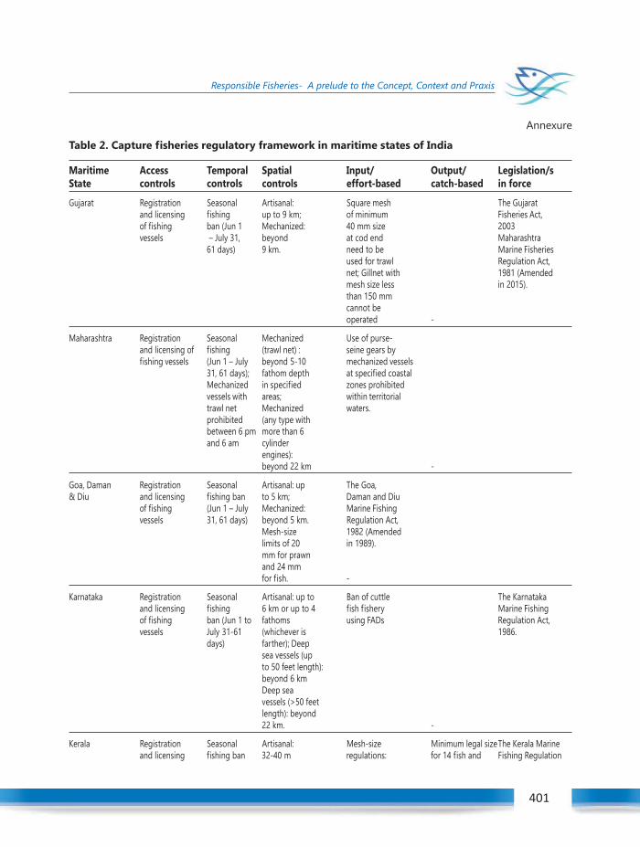
Winter School on Structure and Function of the Marine Ecosystem : Fisheries 401
Responsible Fisheries- A prelude to the Concept, Context and Praxis
401
Annexure
Table 2. Capture fisheries regulatory framework in maritime states of India
Maritime Access Temporal Spatial Input/ Output/ Legislation/sState controls controls controls effort-based catch-based in force
Gujarat Registration Seasonal Artisanal: Square mesh The Gujaratand licensing fishing up to 9 km; of minimum Fisheries Act,of fishing ban (Jun 1 Mechanized: 40 mm size 2003vessels – July 31, beyond at cod end Maharashtra
61 days) 9 km. need to be Marine Fisheriesused for trawl Regulation Act,net; Gillnet with 1981 (Amendedmesh size less in 2015).than 150 mmcannot beoperated -
Maharashtra Registration Seasonal Mechanized Use of purse-and licensing of fishing (trawl net) : seine gears byfishing vessels (Jun 1 – July beyond 5-10 mechanized vessels
31, 61 days); fathom depth at specified coastalMechanized in specified zones prohibitedvessels with areas; within territorialtrawl net Mechanized waters.prohibited (any type withbetween 6 pm more than 6and 6 am cylinder
engines):beyond 22 km -
Goa, Daman Registration Seasonal Artisanal: up The Goa,& Diu and licensing fishing ban to 5 km; Daman and Diu
of fishing (Jun 1 – July Mechanized: Marine Fishingvessels 31, 61 days) beyond 5 km. Regulation Act,
Mesh-size 1982 (Amendedlimits of 20 in 1989).mm for prawnand 24 mmfor fish. -
Karnataka Registration Seasonal Artisanal: up to Ban of cuttle The Karnatakaand licensing fishing 6 km or up to 4 fish fishery Marine Fishingof fishing ban (Jun 1 to fathoms using FADs Regulation Act,vessels July 31-61 (whichever is 1986.
days) farther); Deepsea vessels (upto 50 feet length):beyond 6 kmDeep seavessels (>50 feetlength): beyond22 km. -
Kerala Registration Seasonal Artisanal: Mesh-size Minimum legal sizeThe Kerala Marineand licensing fishing ban 32-40 m regulations: for 14 fish and Fishing Regulation
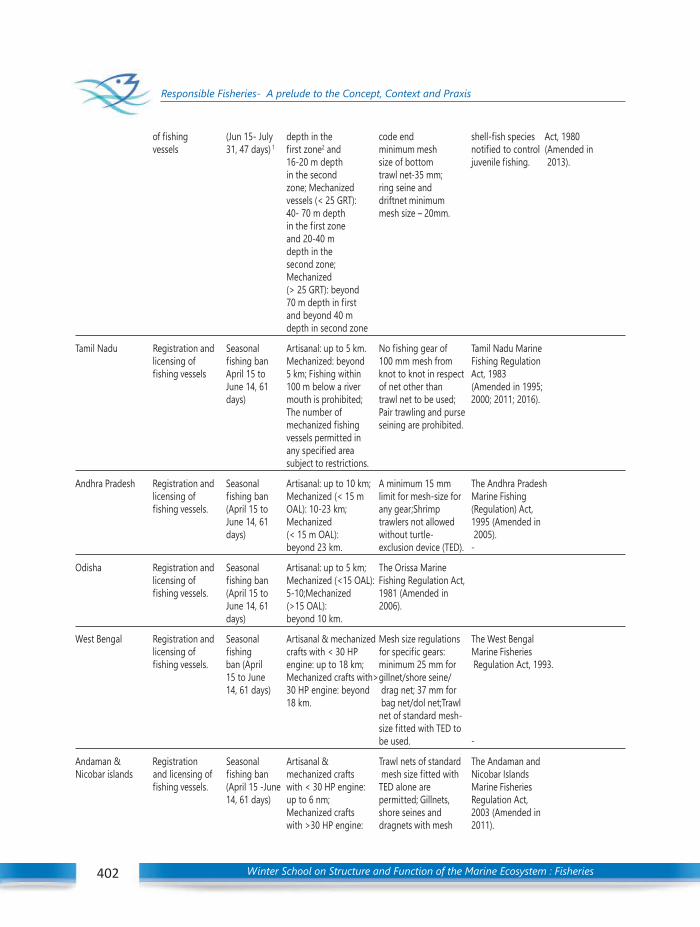
Winter School on Structure and Function of the Marine Ecosystem : Fisheries402
Responsible Fisheries- A prelude to the Concept, Context and Praxis
of fishing (Jun 15- July depth in the code end shell-fish species Act, 1980vessels 31, 47 days) 1 first zone2 and minimum mesh notified to control (Amended in
16-20 m depth size of bottom juvenile fishing. 2013).in the second trawl net-35 mm;zone; Mechanized ring seine andvessels (< 25 GRT): driftnet minimum40- 70 m depth mesh size – 20mm.in the first zoneand 20-40 mdepth in thesecond zone;Mechanized(> 25 GRT): beyond70 m depth in firstand beyond 40 mdepth in second zone
Tamil Nadu Registration and Seasonal Artisanal: up to 5 km. No fishing gear of Tamil Nadu Marinelicensing of fishing ban Mechanized: beyond 100 mm mesh from Fishing Regulationfishing vessels April 15 to 5 km; Fishing within knot to knot in respect Act, 1983
June 14, 61 100 m below a river of net other than (Amended in 1995;days) mouth is prohibited; trawl net to be used; 2000; 2011; 2016).
The number of Pair trawling and pursemechanized fishing seining are prohibited.vessels permitted inany specified areasubject to restrictions.
Andhra Pradesh Registration and Seasonal Artisanal: up to 10 km; A minimum 15 mm The Andhra Pradeshlicensing of fishing ban Mechanized (< 15 m limit for mesh-size for Marine Fishingfishing vessels. (April 15 to OAL): 10-23 km; any gear;Shrimp (Regulation) Act,
June 14, 61 Mechanized trawlers not allowed 1995 (Amended indays) (< 15 m OAL): without turtle- 2005).
beyond 23 km. exclusion device (TED). -
Odisha Registration and Seasonal Artisanal: up to 5 km; The Orissa Marinelicensing of fishing ban Mechanized (<15 OAL): Fishing Regulation Act,fishing vessels. (April 15 to 5-10;Mechanized 1981 (Amended in
June 14, 61 (>15 OAL): 2006).days) beyond 10 km.
West Bengal Registration and Seasonal Artisanal & mechanized Mesh size regulations The West Bengallicensing of fishing crafts with < 30 HP for specific gears: Marine Fisheriesfishing vessels. ban (April engine: up to 18 km; minimum 25 mm for Regulation Act, 1993.
15 to June Mechanized crafts with>gillnet/shore seine/14, 61 days) 30 HP engine: beyond drag net; 37 mm for
18 km. bag net/dol net;Trawlnet of standard mesh-size fitted with TED tobe used. -
Andaman & Registration Seasonal Artisanal & Trawl nets of standard The Andaman andNicobar islands and licensing of fishing ban mechanized crafts mesh size fitted with Nicobar Islands
fishing vessels. (April 15 -June with < 30 HP engine: TED alone are Marine Fisheries14, 61 days) up to 6 nm; permitted; Gillnets, Regulation Act,
Mechanized crafts shore seines and 2003 (Amended inwith >30 HP engine: dragnets with mesh 2011).
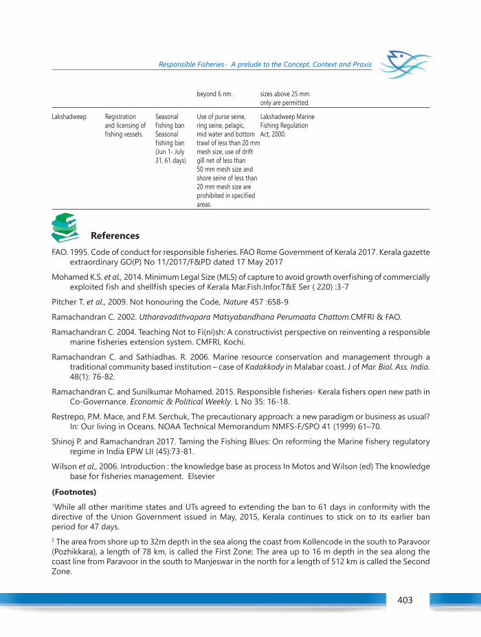
Winter School on Structure and Function of the Marine Ecosystem : Fisheries 403
Responsible Fisheries- A prelude to the Concept, Context and Praxis
403
beyond 6 nm. sizes above 25 mmonly are permitted.
Lakshadweep Registration Seasonal Use of purse seine, Lakshadweep Marineand licensing of fishing ban ring seine, pelagic, Fishing Regulationfishing vessels. Seasonal mid water and bottom Act, 2000.
fishing ban trawl of less than 20 mm(Jun 1- July mesh size, use of drift31, 61 days) gill net of less than
50 mm mesh size andshore seine of less than20 mm mesh size areprohibited in specifiedareas.
References
FAO. 1995. Code of conduct for responsible fisheries. FAO Rome Government of Kerala 2017. Kerala gazetteextraordinary GO(P) No 11/2017/F&PD dated 17 May 2017
Mohamed K.S. et al., 2014. Minimum Legal Size (MLS) of capture to avoid growth overfishing of commerciallyexploited fish and shellfish species of Kerala Mar.Fish.Infor.T&E Ser ( 220) :3-7
Pitcher T. et al., 2009. Not honouring the Code, Nature 457 :658-9
Ramachandran C. 2002. Utharavadithvapara Matsyabandhana Perumaata Chattom.CMFRI & FAO.
Ramachandran C. 2004. Teaching Not to Fi(ni)sh: A constructivist perspective on reinventing a responsiblemarine fisheries extension system. CMFRI, Kochi.
Ramachandran C. and Sathiadhas. R. 2006. Marine resource conservation and management through atraditional community based institution – case of Kadakkody in Malabar coast. J of Mar. Biol. Ass. India.48(1): 76-82.
Ramachandran C. and Sunilkumar Mohamed. 2015. Responsible fisheries- Kerala fishers open new path inCo-Governance. Economic & Political Weekly. L No 35: 16-18.
Restrepo, P.M. Mace, and F.M. Serchuk, The precautionary approach: a new paradigm or business as usual?In: Our living in Oceans. NOAA Technical Memorandum NMFS-F/SPO 41 (1999) 61–70.
Shinoj P. and Ramachandran 2017. Taming the Fishing Blues: On reforming the Marine fishery regulatoryregime in India EPW LII (45):73-81.
Wilson et al., 2006. Introduction : the knowledge base as process In Motos and Wilson (ed) The knowledgebase for fisheries management. Elsevier
(Footnotes)1While all other maritime states and UTs agreed to extending the ban to 61 days in conformity with thedirective of the Union Government issued in May, 2015, Kerala continues to stick on to its earlier banperiod for 47 days.2 The area from shore up to 32m depth in the sea along the coast from Kollencode in the south to Paravoor(Pozhikkara), a length of 78 km, is called the First Zone; The area up to 16 m depth in the sea along thecoast line from Paravoor in the south to Manjeswar in the north for a length of 512 km is called the SecondZone.

ANNEXURES

Typewritten text

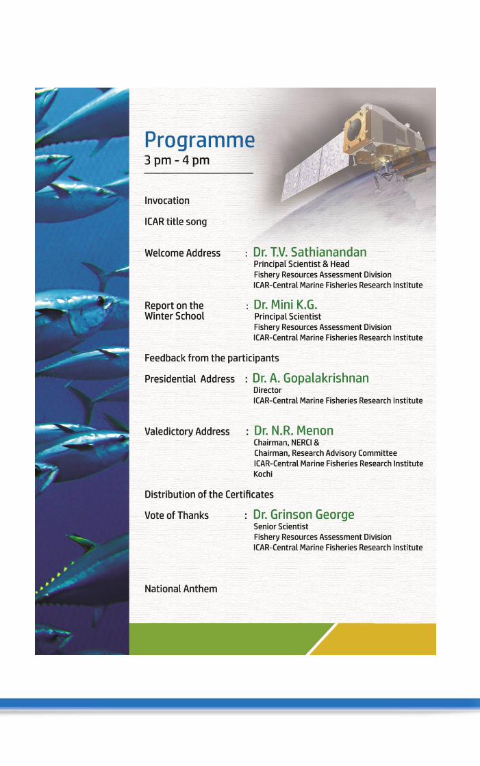

ICA
R Fu
nd
ed
Win
ter Sch
oo
l on
STRU
CTU
RE A
ND
FUN
CTIO
N O
F THE M
AR
INE EC
OSY
STEM: FISH
ERIES
1st to
21
st De
cem
be
r 20
17
at CM
FRI, K
och
i
Date
0
9:3
0 - 1
0:30
10
:45 - 1
1:45
1
1:4
5 - 13
:00
14
:00 - 1
5:00
15
:15 - 1
6:30
1-D
ec-17
Re
gistration
Tea break (10:30 – 10:45)
Orien
tation
pro
gramm
e A
ssessmen
t o
f trainees
Lunch break (13:00 – 14:00)
Inau
guratio
n
Tea break (15:00 – 15:15)
Intro
du
ction
D
r. Grin
son
Ge
orge
2-D
ec-17
H
olid
ay (Milad
-un
-Nab
i)
3
-Dec-17
Sun
day
4-D
ec-17
Ph
ysics of th
e Ind
ian O
cean
Dr. K
. V. San
il Ku
mar
Re
gion
al Ocean
ograp
hy o
f the A
rabian
Sea an
d B
ay of B
engal
Dr. K
. V. San
il Ku
mar
Spatial an
d tem
po
ral variab
ility in C
hlo
rop
hyll-a
con
centratio
n o
ver the
Sou
theastern
Arab
ian Sea
Dr. Sh
alin Saleem
Ph
ytop
lankto
n fu
nctio
nal typ
es D
r. Nan
din
i Me
no
n / M
rs. Min
u
5-D
ec-17
Re
gion
al and
Season
al Distrib
utio
n
of P
hyto
plan
kton
D
r. Nan
din
i Me
no
n
Data d
iagno
stic and
remed
ial measu
res D
r. Eldh
o V
arghese
HA
B M
on
itorin
g usin
g satellite d
atasets D
r. Ajith
Josep
h
Bio
geograp
hy o
f the n
orth
ern In
dian
O
cean an
d its O
ptical C
lassification
M
s. Mo
no
lisha S.
6-D
ec-17
Ro
le of C
alculu
s in M
arine Scien
ces M
r. Tarun
Josep
h
Ro
le of C
alculu
s in M
arine
Sciences
Mr. Taru
n Jo
seph
Basic
Statistics D
r. Som
y K
uriako
se
Ph
ytop
lankto
n
Iden
tification
- Practical
Dem
on
stration
D
r. Nan
din
i Me
no
n /
Mrs. M
inu
Ph
ytop
lankto
n So
rting –
Practical D
emo
nstratio
n
Dr. Sh
oji Jo
seph
/ Mrs. M
inu
7-D
ec-17
Samp
ling m
etho
do
logy e
mp
loye
d
by C
MFR
I for co
llection
and
estim
ation
of m
arine fish
land
ings
in In
dia
Dr. M
ini K
. G.
Ind
ian m
arine fish
ery reso
urces - P
resent statu
s D
r. T. V. Sath
ianan
dh
an
Ocean
Co
lou
r sen
sors
Mr.
Shafe
equ
e M
Ch
anges in
Prim
ary p
rod
uctivity an
d im
pacts in
fish
eries D
r. Grin
son
Ge
orge
Algae cu
lture m
etho
ds :
Practical D
emo
nstratio
n
Dr. Sh
oji Jo
seph
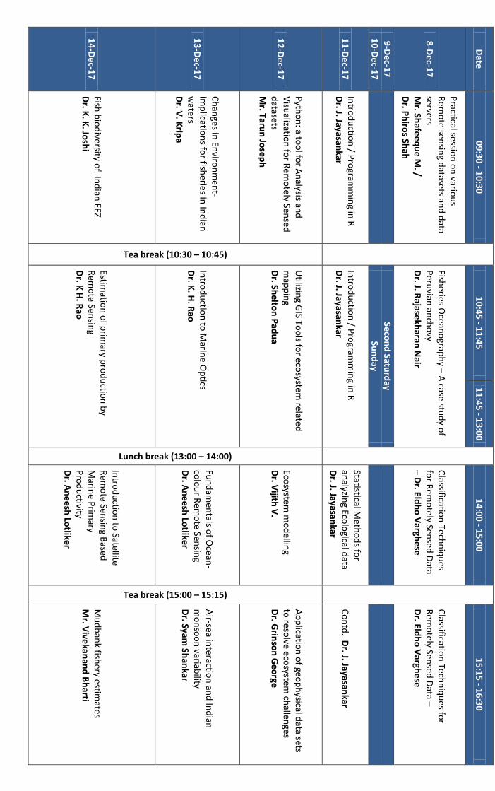
Date
0
9:3
0 - 1
0:30
1
0:4
5 - 11
:45
11
:45 - 1
3:00
1
4:0
0 - 15
:00
15
:15 - 1
6:30
8-D
ec-17
Practical sessio
n o
n vario
us
Re
mo
te sensin
g datasets an
d d
ata servers M
r. Shafe
equ
e M. /
Dr. P
hiro
s Shah
Fisheries O
ceano
graph
y – A case stu
dy o
f P
eruvian
anch
ovy
Dr. J. R
ajasekharan
Nair
Classificatio
n Tech
niq
ues
for R
emo
tely Sensed
Data
– Dr. Eld
ho
Vargh
ese
Classificatio
n Tech
niq
ues fo
r R
em
otely Sen
sed D
ata – D
r. Eldh
o V
arghese
9-D
ec-17
Seco
nd
Saturd
ay
1
0-Dec-1
7
Su
nd
ay
11-D
ec-17
In
trod
uctio
n / P
rogram
min
g in R
D
r. J. Jayasankar
Intro
du
ction
/ Pro
gramm
ing in
R
Dr. J. Jayasan
kar
Statistical Meth
od
s for
analyzin
g Ecolo
gical data
Dr. J. Jayasan
kar C
on
td. D
r. J. Jayasankar
12-D
ec-17
Pyth
on
: a too
l for A
nalysis an
d
Visu
alization
for R
em
otely Sen
sed
datasets
Mr. Taru
n Jo
seph
Tea break (10:30 – 10:45)
Utilizin
g GIS To
ols fo
r ecosystem
related
map
pin
g D
r. Shelto
n P
adu
a
Lunch break (13:00 – 14:00)
Ecosystem
mo
dellin
g D
r. Vijith
V.
Tea break (15:00 – 15:15)
Ap
plicatio
n o
f geop
hysical d
ata sets to
resolve eco
system ch
allenges
Dr. G
rinso
n G
eo
rge
13-D
ec-17
Ch
anges in
Enviro
nm
ent-
imp
lication
s for fish
eries in In
dian
w
aters D
r. V. K
ripa
Intro
du
ction
to M
arine O
ptics
Dr. K
. H. R
ao
Fun
dam
entals o
f Ocean
-co
lou
r Rem
ote Sen
sing
Dr. A
nee
sh Lo
tliker
Air-sea in
teraction
and
Ind
ian
mo
nso
on
variability
Dr. Syam
Shan
kar
14-D
ec-17
Fish
bio
dive
rsity of In
dian
EEZ D
r. K. K
. Josh
i
Estimatio
n o
f prim
ary pro
du
ction
by
Re
mo
te Sensin
g D
r. K H
. Rao
Intro
du
ction
to Satellite
Re
mo
te Sensin
g Based
M
arine Prim
ary P
rod
uctivity
Dr. A
nee
sh Lo
tliker
Mu
db
ank fish
ery estimates
Mr. V
ivekan
and
Bh
arti

Date
0
9:3
0 - 1
0:30
Tea break (10:30 – 10:45)
10
:45 - 1
1:45
1
1:4
5 - 13
:00
14
:00 - 1
5:00
1
5:1
5 - 16
:30
15-D
ec-17
Fish
eries in ato
lls- tradeo
ffs b
etween
harve
st and
con
servation
D
r. K. M
. Ko
ya
Ap
plicatio
n o
f geop
hysical d
ata sets to
resolve eco
system ch
allenges
Dr. G
rinso
n G
eo
rge
El-Nin
o an
d its im
pacts
on
Co
ral reef ecosystem
in
the B
ay of B
engal
Mr. Lix Jo
hn
K.
Co
ral reef ecosystem
- mo
nito
ring
and
assessmen
t usin
g satellite data
sets D
r. Grin
son
Ge
orge
16-D
ec-17
Glo
bal U
nd
erstand
ing an
d Learn
ing
for Lo
cal Solu
tion
s (GU
LLS) - R
ed
ucin
g Vu
lnerab
ility of th
e M
arine D
epen
den
t Co
astal C
om
mu
nities
Dr. Sh
yam S. Salim
Mo
dellin
g the P
elagic Ecosystem
of th
e A
rabian
Sea and
Bay o
f Ben
gal D
r. J. Jayasankar
Ecosystem
con
cepts fo
r su
stainab
le maricu
lture
Dr. Im
elda Jo
seph
Intro
du
ction
to G
eo-statistics
Dr. Sreen
ath
17-D
ec-17
Sun
day
18-D
ec-17
Field
visit
Field visit
Pro
du
ct certification
and
eco
-labellin
g for fish
eries su
stainab
ility D
r. K. S. M
oh
amm
ed
Mo
lecular m
etho
ds u
sed in
fish
abu
nd
ance estim
ation
/ co
nservatio
n/gen
etic imp
rove
men
t D
r. P. Jayasan
kar
19-D
ec-17
Sp
ecies Diversity in
marin
e fished
taxa D
r. T. V. Sath
ianan
dan
Marin
e C:N
:P Sto
ichio
metry
Dr. Satya P
rakash
Marin
e micro
bial d
iversity an
d its ro
le in eco
system
fun
ction
ing
Dr. P
arvathy A
.
Imp
act of clim
ate ch
ange o
n
marin
e ecosystem
D
r. P. U
. Zacharia
20-D
ec-17
M
ud
ban
k bio
logy
Dr. V
. Krip
a M
ud
ban
k ph
ysics M
r. Mu
raleedh
aran K
. R.
Econ
om
ics of Eco
system
and
Bio
diversity
Dr. R
. Narayan
akum
ar
Clim
ate chan
ge and
An
thro
po
genic
imp
acts on
Marin
e Nitro
gen C
ycling
Dr. Satya P
rakash
21-D
ec-17
R
esp
on
sible Fish
eries- A p
relud
e to
the C
on
cept, C
on
text and
Praxis
Dr. C
. Ram
achan
dran
Fisheries O
ceano
graph
y – estab
lished
links in
the
Eastern A
rabian
Sea D
r. Grin
son
Ge
orge
Iden
tifying M
esoscale
edd
ies- relevance to
mu
d
ban
ks and
fishery
Dr. G
rinso
n G
eo
rge
Synth
esis D
r. Grin
son
G
eorge
Evalu
ation
V
aledicto
ry Fun
ction
Lunch break (13:00 – 14:00)
Tea break (15:00 – 15:15)