Oxygen Depletion Risk Indices - OXYRISK & PSA V2.0: New developments, structure and software content

Oxygen Depletion Risk Indices - OXYRISK & PSA V2.0: New developments, structure and software content

SAMUEL DJAVIDNIA, JEAN-NOËL DRUON, WOLFRAM SCHRIMPF, ADOLF STIPS, ELISAVETA PENEVA, SRDJAN DOBRICIC, PETER VOGT

2005 EUR 21509 EN

____________________________________________________ *Corresponding author. Email address: [email protected]

Oxygen Depletion Risk Indices - OXYRISK & PSA V2.0: New developments, structure and software content

SAMUEL DJAVIDNIA*, JEAN-NOËL DRUON, WOLFRAM SCHRIMPF, ADOLF STIPS, ELISAVETA PENEVA, SRDJAN DOBRICIC, PETER VOGT

European Commission – Joint Research Centre Institute for Environment and Sustainability

Inland & Marine Waters Unit TP 272, I-21020 Ispra (VA) – Italy

2005 EUR 21509 EN

iv

LEGAL NOTICE

Neither the European Commission nor any person acting on behalf of the Commission is responsible for

the use which might be made of the following information.

A great deal of additional information on the European Union is available on the Internet. It can be accessed through the Europa server

(http://europa.eu.int)

EUR 21509 EN © European Communities, 2005

Reproduction is authorised provided the source is acknowledged Printed in Italy

Contents 0. Summary and Objective 2

1. Introduction 4

2. OXYRISK Processing and Program Structure 6

2.1 Module 1 8

2.2 Module 2 9

2.3 Module 3 10

2.4 Module 4 10

3. New Input Data in OXYRISK V2.0 11

3.1 Model Benthic Layer Advection 11

3.2 Model Bottom Friction Velocity 11

3.3 Satellite SST vs. Model Mixed Layer Temperature Comparison 11

3.4 SeaWiFS Yearly Specific K490 Data 15

3.5 SeaWiFS Photosynthetically Available Radiation Data 15

3.6 MODIS Primary Production Data 16

4. New Developments and Processes in OXYRISK V2.0 19

4.1 Graphical User Interface 19

4.2 Re-gridding of Model Data on SeaWiFS Grid 20

4.3 POM Deposition Rate Function of Bottom Friction 20

4.4 Use of AVHRR SST Data to Account for Inter-annual Variability 21

4.5 The DENSITY Function 25

4.6 Light Availability in Euphotic Layer Index 25

4.7 Index of Particulate Organic Matter Degradation Velocity at the Bottom 28

4.8 The Horizontal Diffusion Process 29

5. Conclusion 31

6. Appendix A – Inter-annual Variability Introduction Flow Chart 35

7. Appendix B – Inventory of Available Images 36

8. Appendix C – Governing Equations and Flow Chart 37

9. Appendix D – Intermediate Product Images 42

10. List of Acronyms 55

11. Acknowledgements 56

12. References 57

OXYRISK V2.0 - S. Djavidnia, J-N. Druon, W. Schrimpf, A. Stips, E. Peneva, S. Dobricic, P. Vogt - 2005

1


2

Summary & Objective

The ‘OXYgen depletion RISK index’ (‘OXYRISK’) is a bio-physical indicator representing the

temporal and spatial distribution of potential hypoxia in shallow marine ecosystems. Version 2.0

of the OXYRISK program has been developed and is now available.

The major improvements since V1.0 are the enlargement of modelled areas (Baltic Sea, Black

Sea, Western Iberia, Western Mediterranean and Eastern Mediterranean seas, Channel and Bay

of Biscay areas, in addition to the North Sea and the Adriatic Sea), together with the addition of

the inter-annual variability covering the period 1998 to 2003 (with the inclusion of satellite

derived ‘Primary Production’, ‘Sea Surface Temperature’ and ‘Photosynthetically Available

Radiation’ data).

This report will focus on the changes between V1.0 (described in Druon et al., 2002 & Druon et

al., 2004) and the new available V2.0.

The aim of this indicator development is to identify the major physical and biological processes

which play a key role in the vulnerability to hypoxia when the organic matter production

increases. The selected processes will then be used to quantitatively model the carbon and

oxygen cycles in the coastal environment with an optimized number of variables and parameters.

Important note on the meaning of the colour bar indices: Low index values (0 = blue colour)

characterize an unfavourable condition for hypoxia risk near the sea bed, while high index values

(1 = red colour) highlight favourable conditions for oxygen depletion or hypoxia.


3


4

1. Introduction

In the European Union Urban Waste Water Treatment Directive [European Communities, 1991],

eutrophication is defined as “the enrichment of water by nutrients, especially compounds of

nitrogen and/or phosphorus, causing an accelerated growth of algae and higher forms of plant

life to produce an undesirable disturbance to the water balance of organisms present in the

water and to the quality of the water concerned”. Eutrophication is also defined by Nixon [1995]

as “the increase in the rate of supply of organic matter to an ecosystem”, which is most

commonly related to nutrient enrichment enhancing the primary production in the system.

Marine eutrophication is considered to be the cause of various biological effects such as green

tides, phytoplanktonic blooms, deep-water anoxia and fish population changes [EEA, 2000].

There is a need to identify an indicator system to compare the status and trends of eutrophication

over different coastal areas [Cognetti, 2001]. In this context two spatial indices (‘PSA’ and

‘OXYRISK’) addressing a specific aspect of eutrophication (oxygen depletion) of coastal marine

ecosystems [Druon et al., 2004] have been further developed to include temporal variability on a

European scale.

The OXYRISK software developed at the Inland & Marine Waters (IMW) Unit of the Institute of

Environment & Sustainability (IES), is a software program used to derive two eutrophication-

linked indices: ‘PSA’ and ‘OXYRISK’. The ‘Physically Sensitive Area Index’ (‘PSA’) integrates

the various supporting factors of eutrophication to locate sensitive areas to oxygen deficiencies

assuming primary production and nutrients are evenly distributed [Druon et al., 2002]. The

‘OXYgen depletion RISK index’ (‘OXYRISK’) characterizes the spatial distribution of potential

hypoxia for a given month performing an oxygen budget [Druon et al., 2002] between the

physical supporting factors (source term) and the flux of organic matter (sink term) estimated

primarily from satellite derived ‘Chlorophyll-a’ or ‘Primary Production’ data.

The major improvements since version 1.0 have been the inclusion of inter-annual variability for

the physics - through the use of ‘Sea Surface Temperature’ and ‘Photosynthetically Available

Radiation’ - as well as for the biology - through with the introduction of satellite derived

‘Primary Production’ data for the period 1998 - 2003. In addition, the V2.0 applies the

https://www.researchgate.net/publication/234462651_The_physical_environment_as_a_key_factor_in_assessing_the_eutrophication_status_and_vulnerability_of_shallow_seas_PSA_and_EUTRISK?el=1_x_8&enrichId=rgreq-4d290afe-adc4-4166-ab26-4b84ffce4e06&enrichSource=Y292ZXJQYWdlOzI0MjA4Njc1MjtBUzoxMDI2NzU5NTM3NTAwMjdAMTQwMTQ5MTI2MzkxMw==

https://www.researchgate.net/publication/234462651_The_physical_environment_as_a_key_factor_in_assessing_the_eutrophication_status_and_vulnerability_of_shallow_seas_PSA_and_EUTRISK?el=1_x_8&enrichId=rgreq-4d290afe-adc4-4166-ab26-4b84ffce4e06&enrichSource=Y292ZXJQYWdlOzI0MjA4Njc1MjtBUzoxMDI2NzU5NTM3NTAwMjdAMTQwMTQ5MTI2MzkxMw==


5

methodology to all European coastal Seas except the Irish Sea (the North Sea, the Adriatic Sea,

the Baltic Sea, Black Sea, the Western Iberia coastal area, the Western and Eastern

Mediterranean Sea, the Channel and the Bay of Biscay). This report will first describe the

general program structure and processes and then focus on the changes between V1.0 [Druon et

al., 2002 & Druon et al., 2004] and V2.0.


6

2. Processing and Program Structure

To run OXYRISK V2.0 the following hardware, software and data are required:

Linux, or Unix machine running IDL v5.5 or higher.

The OXYRISK_v2.pro software

European hydro-dynamical model data (Baltic, North Sea, Black Sea, Adriatic Sea,

Eastern Mediterranean, Western Iberia, Channel, Biscay, Western Mediterranean). Size:

1 GB. A listing of the models and their geographic domain is given in Table 2.1.1.

Processed SeaWiFS ‘Chlorophyll-a’, ‘K490’ and ‘PAR’ data archive. Size: 5.4 GB

Processed MODIS ‘Primary Production’ data archive. Size: 155 MB

Processed AVHRR ‘Sea Surface Temperature’ data archive. Size: 72 MB

Region Geographical Coverage Model Horizontal Resolution Data Provider Adriatic Sea Lon: 12.2E → 20.3E

Lat: 39.0N → 45.8N 5.0 km JRC - IES/IMW

Baltic Sea Lon: 9.0E → 30.5E Lat: 52.7N → 66N

5.5 km JRC - IES/IMW

Biscay Lon: -7.0E → -0.7E Lat: 44.0N → 49.0N

5.0 km IFREMER - France

Black Sea Lon: 27.3E → 42.0E Lat: 40.9N → 47.4N


Channel Lon: -5.0E → 4.3E Lat: 48.5N → 52.0N


Eastern Mediterranean Lon: 20.0E → 36.0E Lat: 30.0N → 41.0N

5.5 km OPAM, Uni. of Athens - Greece

North Sea Lon: -4.5E → 8.9E Lat: 50.7N → 60.0N


Western Iberia Lon: -12.9E → -6.1E Lat: 36.1N → 44.8N

5.0 km HIDROMOD - Portugal

Western Mediterranean Lon: -6.0E → 16.5E Lat: 34.4N → 44.5N


Table 2.1.1 Regional marine hydrodynamical numerical model characteristics for the European seas.

The IDL program OXYRISK_v2.pro uses a set of input parameters to derive, amongst other

marine and statistical parameters, the risk of near bottom oxygen deficiency of European coastal

seas*. The program is structured into four main modules:

________________________________________________________________________________________________________________________________________________

* Throughout this report, the term ‘coastal’ will refer to marine areas shallower than 100 metres.


7

Module 3

Module 3 Module 1

Module 2

Module 3

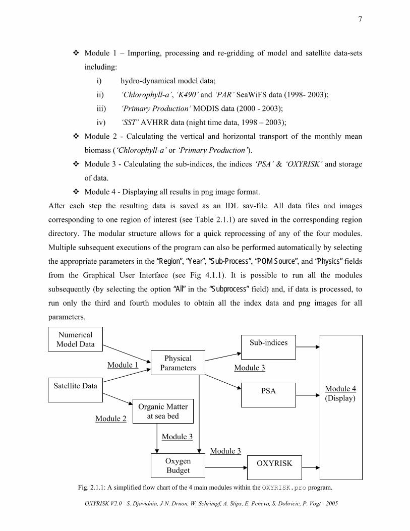
Module 1 – Importing, processing and re-gridding of model and satellite data-sets

including:

i) hydro-dynamical model data;

ii) ‘Chlorophyll-a’, ‘K490’ and ‘PAR’ SeaWiFS data (1998- 2003);

iii) ‘Primary Production’ MODIS data (2000 - 2003);

iv) ‘SST’ AVHRR data (night time data, 1998 – 2003);

Module 2 - Calculating the vertical and horizontal transport of the monthly mean

biomass (‘Chlorophyll-a’ or ‘Primary Production’).

Module 3 - Calculating the sub-indices, the indices ‘PSA’ & ‘OXYRISK’ and storage

of data.

Module 4 - Displaying all results in png image format.

After each step the resulting data is saved as an IDL sav-file. All data files and images

corresponding to one region of interest (see Table 2.1.1) are saved in the corresponding region

directory. The modular structure allows for a quick reprocessing of any of the four modules.

Multiple subsequent executions of the program can also be performed automatically by selecting

the appropriate parameters in the “Region”, “Year”, “Sub-Process”, “POM Source”, and “Physics” fields

from the Graphical User Interface (see Fig 4.1.1). It is possible to run all the modules

subsequently (by selecting the option “All” in the “Subprocess” field) and, if data is processed, to

run only the third and fourth modules to obtain all the index data and png images for all

parameters.

Fig. 2.1.1: A simplified flow chart of the 4 main modules within the OXYRISK.pro program.

PSA

Sub-indices

Physical Parameters

OXYRISK Oxygen Budget

Satellite Data

Numerical Model Data

Organic Matter at sea bed

Module 4 (Display)


8

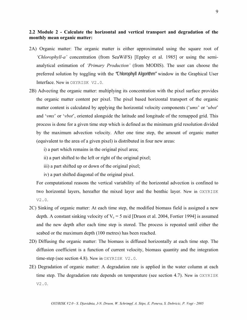
In the following sections a detailed description of the processing steps taking place in the

OXYRISK_V2.pro modules is given:

2.1 Module 1 - Import, process and re-grid the model and satellite data sets: 1A) Read the SeaWiFS derived ‘Chlorophyll-a’ data in SeaWiFS grid resolution: Depending on

the initial settings, a region specific monthly mean ‘OC4’ or ‘OC5’ ‘Chlorophyll-a’ data set

(as well as the land/sea mask) is read from the corresponding HDF file.

1B) Read the hydro-dynamical model data: The monthly parameters are restructured in monthly

data arrays for further processing. New in OXYRISK V2.0.

1C) Remap the hydro-dynamical model variables to the SeaWiFS grid points: The model data is

provided in an irregular grid in longitude as well as latitude and is therefore converted to the

gridded locations of the SeaWiFS window (ca. 2km by 2km pixels). New in OXYRISK V2.0.

1D) Read and remap the monthly mean SeaWiFS ‘Photosynthetically Available Radiation’ data:

The satellite ‘PAR’ data is read, processed and remapped on the SeaWiFS 2km by 2km

window. New in OXYRISK V2.0.

1E) Read and remap the monthly mean MODIS ‘Primary Production’ data: The satellite

‘Primary Production’ data is read, processed and remapped on the SeaWiFS 2km by 2km

window. New in OXYRISK V2.0.

1F) Read the monthly mean AVHRR ‘Sea Surface Temperature’ data: The satellite ‘SST’ data is

read, processed and remapped on the SeaWiFS 2km by 2km window. New in OXYRISK

V2.0.

1G) Calculate the satellite derived yearly specific ‘Mixed Layer Depth’ and ‘Maximum Gradient

Density’ variables using the satellite ‘SST’ and model remapped data. New in OXYRISK

V2.0.

1H) Calculate the ‘Light Availability in Euphotic Layer’ variable as a function of ‘PAR’ and

‘K490’. New in OXYRISK V2.0.

1I) Store the satellite and remapped hydro-dynamical model data into two IDL sav-files:

chlor_aOC5_YEAR_ROI.sav (chl_sm, k490_sm, par_sm, light_sm, p2_sat, sst_sat, depmx_sat,

sigm_sat, delta_T, delta_sigm)

chlor_aOC5_clim_ROI.sav (lon_sm, lat_sm, depth_sm, depmx_sm, depmx_sm, sigm_sm, umx_sm,

vmx_sm, ubot_sm, vbot_sm, bfri_sm, bfri_std_sm, smx_sm, sbot_sm, wtot_sm, irr0_sm, sea_mod_land,

sea_mod_sea, coast_miss, eps, sea, sea_mod, sea_ctr)


9

2.2 Module 2 - Calculate the horizontal and vertical transport and degradation of the monthly mean organic matter: 2A) Organic matter: The organic matter is either approximated using the square root of

‘Chlorophyll-a’ concentration (from SeaWiFS) [Eppley et al. 1985] or using the semi-

analytical estimation of ‘Primary Production’ (from MODIS). The user can choose the

preferred solution by toggling with the “Chlorophyll Algorithm” window in the Graphical User

Interface. New in OXYRISK V2.0.

2B) Advecting the organic matter: multiplying its concentration with the pixel surface provides

the organic matter content per pixel. The pixel based horizontal transport of the organic

matter content is calculated by applying the horizontal velocity components (‘umx’ or ‘ubot’

and ‘vmx’ or ‘vbot’, oriented alongside the latitude and longitude of the remapped grid. This

process is done for a given time step which is defined as the minimum grid resolution divided

by the maximum advection velocity. After one time step, the amount of organic matter

(equivalent to the area of a given pixel) is distributed in four new areas:

i) a part which remains in the original pixel area;

ii) a part shifted to the left or right of the original pixel;

iii) a part shifted up or down of the original pixel;

iv) a part shifted diagonal of the original pixel.

For computational reasons the vertical variability of the horizontal advection is confined to

two horizontal layers, hereafter the mixed layer and the benthic layer. New in OXYRISK

V2.0.

2C) Sinking of organic matter: At each time step, the modified biomass field is assigned a new

depth. A constant sinking velocity of Vc = 5 m/d [Druon et al. 2004, Fortier 1994] is assumed

and the new depth after each time step is stored. The process is repeated until either the

seabed or the maximum depth (100 metres) has been reached.

2D) Diffusing the organic matter: The biomass is diffused horizontally at each time step. The

diffusion coefficient is a function of current velocity, biomass quantity and the integration

time-step (see section 4.8). New in OXYRISK V2.0.

2E) Degradation of organic matter: A degradation rate is applied in the water column at each

time step. The degradation rate depends on temperature (see section 4.7). New in OXYRISK

V2.0.


10

2F) Deposition of organic matter: When biomass reaches the bottom a deposition rate estimates

the deposition in the case bottom friction velocity is below the Critical Friction Velocity for

deposition (see section 4.3). New in OXYRISK V2.0.

2G) Storage of advection products in an IDL sav-file:

chlor_aOC5_clim_ROI_adv.sav (surf, POM_bot_sm, clouds, vc, ratio_pp_left)

2.3 Module 3 - Calculate sub-indices, ‘PSA’ & ‘OXYRISK’ indices and storage: 3A) Calculate statistics: Evaluate a set of statistics on the parameters ‘Bottom Friction’,

‘Stratification’, ‘Bottom & Surface Advection’. The evolution over time as a mean for the Region

of Interest (ROI) for these parameters may be displayed on screen when the parameter “statistics”

is selected in the “On Screen Display” option of the Graphical User Interface (GUI) (see Fig 4.1.1).

3B) Calculate the general physical indices: Derive the ‘Bottom & Surface Physics, ‘Bottom

Friction’, ‘Bottom & Surface Advection’, ‘Oxygen Saturation’, ‘Stratification’, ‘Light

Availability’, ‘Benthic Layer Thickness’ and ‘Bottom Degradation’ Indices.

3C) Calculate ‘PSA’ & ‘OXYRISK’: Derive the Eutrophication Indices.

3D) Store the statistical data + general indices, and the indices data into two IDL sav-files:

chlor_aOC5_YEAR_ROI_eut.sav (OXYRISK, CPOM)

chlor_aOC5_YEAR_ROI_stats.sav (Cphys_bott, Cphys_surf, PSA, Cbfri, Cstrat, Cadvmx, Cadvbl,

Coxy_sat, Cblt, Ck490, Ctx_deg, Clight)

2.4 Module 4 - Display all results in png image format based on the previously calculated and stored data: 4A) Display all previously derived results as a pixmap image and subsequently save the output to

a file in png format. A slide-image of the results can be kept on screen when the corresponding

parameter has been selected in the “On Screen Display” option of the GUI (see Fig 4.1.1).

Important note: To have a more thorough and complete picture of the physical and biological

processes guiding OXYRISK V2.0, please refer to the ‘Governing Equations and Flow Chart’

diagrams in Appendix C. The flow chart illustrates the governing equations and describes the

interactions of the various parameters and variables used to calculate both the ‘OXYRISK’ and

‘PSA’ indices.


11

3. New Input Data in OXYRISK V2.0 3.1 Model Benthic Layer Advection

In order to have a better representation of the horizontal transport of the ‘Particulate Organic

Matter’ (hereafter ‘POM’) while sinking, the mean of current velocity in the benthic layer (from

the mixed layer to the bottom) was added in the dataset (monthly mean based on climatology).

As for the mixed layer advection, the ‘benthic layer advection’ data is composed of the x (‘ubot’)

and y (‘vbot’) components in m s-1. A bottom layer advection index is also derived in order to

represent the capacity of the system to renew the water masses (and the oxygen contained) below

the stratification (see ‘Cphys_bott’ in case of stratification).

3.2 Model Bottom Friction Velocity

OXYRISK_V1.0 used the diffusion coefficient of the deepest layer derived from the physical

model. This method had the disadvantage to depend on the thickness of that last layer of

calculation and was an important source of noise in the data. In order to better represent the

bottom friction, the friction velocity (U* named ‘bfri’ hereafter, in m s-1) replaces the diffusion

coefficient in V2.0. In addition to the better quantification of the derived index, the inclusion of

the friction velocity (U*) also allows us to introduce a specific deposition rate of the ‘POM’ at

the bottom.

3.3 Satellite SST vs. Model Mixed Layer Temperature Comparison

A study has been carried out to compare the model Mixed Layer Temperature (‘tmx’) and the

satellite skin temperature (‘SST’) annual variability. This study was performed in the North Sea

and Baltic Sea: fourteen years of data from 1989 to 2002 were processed and then compared.

The data processing consisted in computing the monthly mean of the fourteen years and then

comparing monthly values with the climatology. This operation was done for both the AVHRR

‘SST’ data and the model ‘tmx’ data. After comparing the 'climatology - monthly mean' data (as

well as the standard deviation) between the AVHRR ‘SST’ data and the Model ‘tmx’ data, fitting

coefficients were calculated to understand if the two data sets were comparable.


12

Here is a set of results for the Central North Sea region (56°N-57°N, 3°E-5°E):

Fig 3.3.1: Absolute Satellite SST Temperature and Model Mixed Layer Temperature for the Central North Sea. Note

the model winter Temperature over-estimation which is due to the under-estimation (~15%) of cloud cover in the

ECMWF dataset.

Fig 3.3.2: Climatology Satellite SST Temperature and Model Mixed Layer Temperature for the Central North Sea.

Fig 3.3.3: (Satellite SST – Satellite Climatology) and (Model Mixed Layer – Model Climatology) Temperature data

for the Central North Sea.


13

Fig 3.3.4: Correlation coefficients for Absolute (Satellite vs. Model) and Delta (Satellite vs. Model) Temperature for

the Central North Sea.

Here is a set of results for the Baltic Proper region (55.5°N-56.5°N, 18°E-20°E):

Fig 3.3.5: Absolute Satellite SST Temperature and Model Mixed Layer Temperature for the Central Baltic Sea. Note

the increasing trend in model winter Temperature.

Fig 3.3.6: Climatology Satellite SST Temperature and Model Mixed Layer Temperature for the Central Baltic Sea.


14

Fig 3.3.7: (Satellite SST – Satellite Climatology) and (Model Mixed Layer – Model Climatology) Temperature data

for the Central Baltic Sea.

Fig 3.3.8: Correlation coefficients for Absolute (Satellite vs. Model) and Delta (Satellite vs. Model) Temperature for

the Central Baltic Sea.

The study showed that for the Central North Sea and Baltic Sea the monthly ‘SST’ satellite data

(skin temperature) and the monthly mixed layer temperature estimated by the physical model

(‘tmx’) had an absolute mean error (RMS) of 1.34°C (see Figs. 3.3.4 and 3.3.8). This error is

equivalent to the error of the satellite SST measurement (0.5°C) and in the model estimate of the

mixed layer temperature (~0.8°C). Although the mixed layer temperature and the skin

temperature cannot be strictly compared due to secondary thermocline and skin effect which can

affect the comparison, the satellite ‘SST’ values are estimated to be a good proxy of the

simulated mixed layer temperature (‘tmx’) and can therefore be used to include the inter-annual

variability of physical variables in the indices computation.


15

3.4 SeaWiFS Yearly Specific K490 Data

The ‘Diffuse Attenuation Coefficient at 490nm’ (‘K490’) is a measure of the attenuation of light

in the water column. This satellite derived variable is used as part of the calculation of the

‘Surface Physics Index’ (‘Cphys_surf’) for the evaluation of the light availability. The ‘K490’

values used primarily were the 1998-2001 mean values. The further development of the program

now allows the use of yearly specific ‘K490’ values. For points where no data is available due to

clouds, the climatological value is used.

3.5 SeaWiFS Photosynthetically Available Radiation Data

The ‘PAR’ (‘Photosynthetically Available Radiation’) is defined as the quantum energy flux

from the Sun in the spectral range 400 to 700 nm, and it is usually expressed in Einstein m-2 day-1

(where 1 Einstein is equivalent to the energy of 1 mole of photons of monochromatic light).

‘PAR’ data is used in OXYRISK V2.0 to calculate the ‘Light Availability Index’. This sub-

index is included in the formulation of the ‘Surface Physics Index’ (‘Cphys_surf’ index) in order

to estimate if light is a limiting factor of primary production.

In V2.0 the user has the option to choose between Climatological or Yearly Specific

‘Photosynthetically Available Radiation’ data. This latter option implies the “Physics” option to

be set to “Yearly”. Alternatively the “Physics” option has to be set to “Climatological” in the GUI

interface. The ‘PAR’ data archive currently holds data ranging from 1998 to 2003.

Figure 3.5.1 shows the ‘PAR’ expressed in Einstein m-2 day-1:

Fig 3.5.1: ‘Photosynthetically Available Radiation’ in February 1998 (on the left) and in August 1998 (on the right)

in Einstein m-2 day-1.


16

3.6 MODIS Primary Production Data

MODIS (Moderate Resolution Imaging Spectro-radiometer) is an instrument on-board NASA

satellites Aqua and Terra, providing high radiometric sensitivity in 36 spectral bands ranging in

wavelength from 0.4 µm to 14.4 µm. It acquires data at three spatial resolutions: 250 m, 500 m,

and 1000m and provides global coverage every one to two days. One of the products of MODIS

is ‘Ocean Primary Production’, i.e. the time rate of change of phytoplankton biomass, which

represents the photosynthesis in the water column integrated over a given time scale (see Fig

3.6.1).

Fig 3.6.1: Post-processed MODIS Primary Productivity for May and July 2002.


17

The MODIS regridded ‘Primary Productivity’ monthly data files are used in OXYRISK V2.0

as an estimate of the ‘Particulate Organic Matter’ (‘POM’) content in the surface layer.

Previously, this quantity was derived only from SeaWiFS ‘Chlorophyll-a’ data. The explicit

calculation of Primary Productivity’ adopts a model proposed by Howard [1995], which was

implemented by NASA as one of the two archived products (P2). It uses ‘Chlorophyll-a’, ‘PAR’,

‘SST’ and the ‘Mixed Layer Depth’ (‘MLD’) to estimate carbon fixation within the mixed layer.

A more detailed description of the implementation of this model can be found in the MODIS

Algorithm Theoretical Basis Document [Esaias, 1996].

In order to use the MODIS ‘Primary Production’ product you have to choose the “PP (Global)” option in the “POM Source” window of the GUI (see Fig 4.1.1).

Figures 3.6.2 and 3.6.3 compare the estimation of ‘POM’ at sea-bed (or 100 m) derived from

MODIS primary production product and SeaWiFS ‘OC5 Chlorophyll-a’ data in the Baltic Sea

area in February, April and August 2002. The MODIS product represents better the annual

primary productivity cycle where the maximum is during the spring bloom, the medium level of

productivity occurs in summer and the minimum is in winter.

February 2002 April 2002 August 2002

Fig. 3.6.2: Baltic Sea region ‘Particulate Organic Matter Index’ evaluated with SeaWiFS ‘Chl-a’ data (in relative

units). High values to correspond to high concentrations of POM at the sea-bed.


18

February 2002 April 2002 August 2002

Fig. 3.6.3: Baltic Sea region ‘Particulate Organic Matter Index’ evaluated with MODIS ‘P2’ data (in relative units).

High values to correspond to high concentrations of POM at the sea-bed.


19

4. New Developments and Processes in OXYRISK V2.0

4.1 Graphical User Interface

Since V1.0, the program is driven by a Graphical User Interface (GUI). In V2.0, the GUI has

been further developed to allow the user to have a choice between running a “Climatology” or

“Yearly” specific version. Previously the program could only use the climatology for the physical

variables to evaluate the indices, while the new version introduces the possibility of using

satellite derived (monthly averaged) values (‘SST’, ‘K490’, and ‘PAR’) for a yearly specific

evaluation.

In the GUI interface accompanying V2.0, the user has now an option called “Physics” in which

he can choose either “Climatology” or “Yearly”. The “Climatology” choice will set the program

running with the climatology for physical parameters. The “Yearly” option on the other hand will

introduce the yearly specific values for ‘SST’, ‘K490’, ‘PAR’ and organic matter (either

‘Chlorophyll-a’ in case the “POM Source” is set to either “OC4” or “OC5”, or ‘Primary Production’

if the “POM Source” option is set to “PP (Global)”).

Fig. 4.1.1: The OXYRISK V2.0 Graphical User Interface.


20

4.2 Re-mapping of Model Data on SeaWiFS Grid

The model data is provided in an irregular grid in both longitude and latitude. The conversion of

the model parameters to the regular gridded locations of the SeaWiFS window is performed by

assigning each SeaWiFS pixel the data value of the closest model pixel. In case the model data

resolution is greater than twice the size of the SeaWiFS grid resolution (~2km), the remapped

grid is smoothed. The size of the boxcar used within this function is automatically adapted to the

minimum model resolution as specified at the end of the model data input file.

4.3 POM Deposition Rate as a Function of Bottom Friction

The organic (or mineral) particles which sink to the seabed are effectively reaching the water–

sediment interface only if the bottom friction is below a given threshold (which depends on the

particles size, density and shape). A typical critical friction velocity for the deposition of small

mineral particles (U*) is 1 cm s-1. The range of critical friction velocity for mineral particles with

a diameter between 4.10-3 and 3.10-5 m is of 0.9 – 1.6 cm s-1 (using ρ = 1025 kg m-3 [Cacchione

et al. 1994], ρτ

=*U ), and from 0.10 to 0.17 cm s-1 for single cells and small algal particles

(using the same values for ρ [Peterson 1999]). Peterson [1999] shows that a value of 0.31 cm s-1

(0.01 N m-2) is sufficient to keep all organic matter in suspension. The main problem faced here

is that the data available are monthly means where minimum values for few days are not

represented and may increase drastically the POM deposition. In order to estimate the minimum

values representative of the POM deposition within the considered month, (especially in tidal

areas where the variability is high [neap tide]), the standard deviation of the friction velocity is

used, considering the data is normally distributed.

In a normally distributed data set, )( σµ − contains 68% of the lowest values of instantaneous U*

which may increase the POM deposition. The value )55.0( σµ − associated to a critical value of

friction velocity for POM deposition of U*d = 0.5 cm s-1 was found to correctly represent the

POM deposition in tidal and non tidal areas. The deposition rate is set to 0 if )55.0( σµ − is

higher than *dU , while if *

dU)55.0( <− σµ equation 4.3.1 is used [Buller et al. 1975, Ribbe and

Holloway 2001]:


21

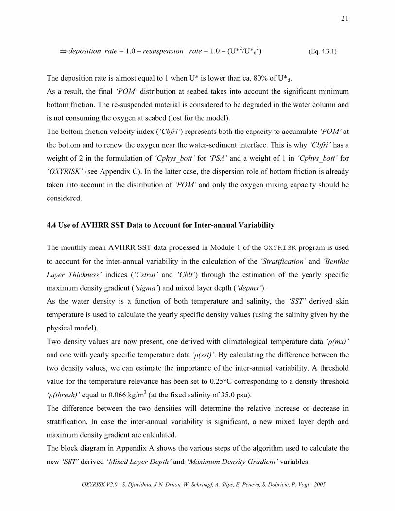
⇒deposition_rate = 1.0 – resuspension_ rate = 1.0 – (U*2/U*d2) (Eq. 4.3.1)

The deposition rate is almost equal to 1 when U* is lower than ca. 80% of U*d.

As a result, the final ‘POM’ distribution at seabed takes into account the significant minimum

bottom friction. The re-suspended material is considered to be degraded in the water column and

is not consuming the oxygen at seabed (lost for the model).

The bottom friction velocity index (‘Cbfri’) represents both the capacity to accumulate ‘POM’ at

the bottom and to renew the oxygen near the water-sediment interface. This is why ‘Cbfri’ has a

weight of 2 in the formulation of ‘Cphys_bott’ for ‘PSA’ and a weight of 1 in ‘Cphys_bott’ for

‘OXYRISK’ (see Appendix C). In the latter case, the dispersion role of bottom friction is already

taken into account in the distribution of ‘POM’ and only the oxygen mixing capacity should be

considered.

4.4 Use of AVHRR SST Data to Account for Inter-annual Variability

The monthly mean AVHRR SST data processed in Module 1 of the OXYRISK program is used

to account for the inter-annual variability in the calculation of the ‘Stratification’ and ‘Benthic

Layer Thickness’ indices (‘Cstrat’ and ‘Cblt’) through the estimation of the yearly specific

maximum density gradient (‘sigma’) and mixed layer depth (‘depmx’).

As the water density is a function of both temperature and salinity, the ‘SST’ derived skin

temperature is used to calculate the yearly specific density values (using the salinity given by the

physical model).

Two density values are now present, one derived with climatological temperature data ‘ρ(mx)’

and one with yearly specific temperature data ‘ρ(sst)’. By calculating the difference between the

two density values, we can estimate the importance of the inter-annual variability. A threshold

value for the temperature relevance has been set to 0.25°C corresponding to a density threshold

‘ρ(thresh)’ equal to 0.066 kg/m3 (at the fixed salinity of 35.0 psu).

The difference between the two densities will determine the relative increase or decrease in

stratification. In case the inter-annual variability is significant, a new mixed layer depth and

maximum density gradient are calculated.

The block diagram in Appendix A shows the various steps of the algorithm used to calculate the

new ‘SST’ derived ‘Mixed Layer Depth’ and ‘Maximum Density Gradient’ variables.


22

The following conventions and equations are used in equations 4.4.1 to 4.4.19 as well as in the

Appendix A block diagram:

ρ(mx) = density(Model T in mixed layer, Model S in mixed layer)

ρ(sst) = density(satellite SST, Model S in mixed layer)

ρ(bot) = density(Model T bottom, Model S bottom)

σ(thresh) = density(T=19.75 °C, S=35.0 psu) – density(T=20.0 °C, S=35.0 psu) ≡ 0.066 kg/m3

T(sst) = Satellite SST

T(mx) = Mixed Layer Temperature given by the model for climatology

T(bot) = Near Bottom Temperature given by the model for climatology

Conservation of Internal Energy (Heat):

∫ −=H

rpi dzTTCE0

)(ρ (Eq 4.4.1)

where iE = Internal Energy and Tr = reference temperature Hhrp

hrpi zTTCzTTCE

1

1 ])([])([ 0 −+−= ρρ (Eq 4.4.2) where h1 is the mixed layer depth

[ ]))(()( 122111 hHTThTTCE rrpi −−+−= ρρ (Eq 4.4.3)

Assuming Tr = T2 (constant bottom temperature)

1211 )( hTTCE pi −= ρ and '1

'2

'1

'1

' )( hTTCE pi −= ρ (Eq 4.4.4)

where '1

'1

'1 ,, hTρ refer to the new surface layer density, temperature and depth.

'12

'1

'11211 )()( hTThTT −=− ρρ (Eq 4.4.5)

)()(**

2'

1

21'1

11

'1 TT

TThh−−

=ρρ (Eq 4.4.6)

)()()()(*

)()(*(mod))(

botTsstTbotTmxT

sstmxdepmxsatdepmx

−−

=⇒ρρ (Eq 4.4.7)

Conservation of Internal Potential Energy:

∫=H

p gdzE0

ρ (Eq 4.4.8)

where pE = Potential Energy Hh

hp gzgzE 1

10 ][][ ρρ += (Eq 4.4.9)

where h1 refers to the surface layer depth 12211 ghgHghEp ρρρ −+= & '

122'1

'1

' ghgHghEp ρρρ −+= (Eq 4.4.10)


23

where ρ1, ρ2 refer to the surface and bottom layer density and '1

'1,hρ refer to the new surface layer

density and depth. '12

'1121 )()( ghgh ρρρρ −=− (Eq 4.4.11)

Assuming a constant thickness of the thermocline: cteZ =∆

Zhh

Z ∆∆

=∆∆ ρρ *'

1

1'

(Eq 4.4.12)

(mod)*)(

(mod))( sigmsatdepmx

depmxsatsigm =⇒ (Eq 4.4.13)

Fresh Water Influence (i.e. when the vertical density gradient is mainly caused by a vertical

salinity gradient). In this case the mixed layer depth is considered to be constant as well as the

thickness of the thermocline:

(mod))( depmxsatdepmx =⇒ (Eq 4.4.14)

Z

SSZ old ∆

−=⎟

⎠⎞

⎜⎝⎛∆∆ ),(),( 2211 θρθρρ (Eq 4.4.15)

oldnew ZSSSS

ZSS

Z⎟⎠⎞

⎜⎝⎛∆∆

⎥⎦

⎤⎢⎣

⎡−−

=∆−

=⎟⎠⎞

⎜⎝⎛∆∆ ρ

θρθρθρθρθρθρρ

),(),(),(),(),(),(

2211

22122212 (Eq 4.4.16)

assuming cteZ =∆

)()()()(*(mod))(

botmxbotsstsigmsatsigm

ρρρρ

−−

=⇒ (Eq 4.4.17)

No New Stratification, Mixed Water Column:

bottomdepthsatdepmx _)( =⇒ (Eq 4.4.18)

0)( =⇒ satsigm (Eq 4.4.19)

Figures 4.4.1 and 4.4.2 show an example for the climatological version vs. the yearly specific

version datasets.


24

Fig 4.4.1: Model climatological ‘Mixed Layer Temperature’ for September (on the left) and Satellite ‘Sea Surface

Temperature’ (on the right) data for September 2002.

Fig 4.4.2: ‘Maximum Density Gradient’: model climatological data for September (on the left) and satellite derived

data for September 2002 (on the right).

In the case that only climatological model results are available the aforementioned described

method provides a tool for introducing temporal variability into the derived indices. There are

however some limitations to this method, the most serious being that in regions of significant

advection the applied 1-dimensional heat and energy budgets do not hold and hence the

estimated new ‘Mixed Layer Depth’ and ‘Maximum Density Gradient’ will be incorrect. The

method will therefore provide reliable results, only for open waters away from coasts and

without significant currents.


25

Further to this, it should be considered that the model ‘Mixed Layer Temperature’ and satellite

‘SST’ do not completely correspond to each other, but they are used together for determining the

new ‘MLD’. This introduces a methodological inconsistency in this ‘MLD’ calculation, which is

difficult to quantify. It is therefore recommend to use this method only in cases when temporal

varying model ‘MLD’ are not available, alternatively only the model derived data should be

used.

4.5 The DENSITY Function

The water density, function of temperature and salinity, is calculated using the formulation of

UNESCO (1981). This function is used in Module 1G of OXYRISK_V2.pro, when comparing

the density derived from the model data and the density calculated using the satellite ‘SST’. The

formulation is described in detail in Appendix C.

4.6 Light Availability in the Euphotic Layer Index

The ‘Light Availability in the Euphotic Layer’ is an estimate of the ‘Photosynthetically Available

Radiation’ integrated on the euphotic layer. It is a function of both ‘K490’ (‘Diffuse Attenuation

Coefficient’ [m-1]) and ‘PAR’ (‘Photosynthetically Available Radiation’ [Wm-2]) at sea surface.

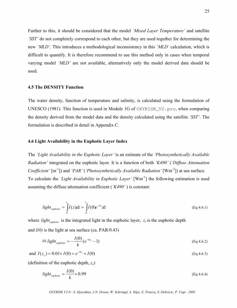
To calculate the ‘Light Availability in Euphotic Layer’ [Wm-1] the following estimation is used

assuming the diffuse attenuation coefficient (‘K490’ ) is constant:

dzeIdzzIlight kzzz

euphotic

ee−∫∫ ==

00

)0()( (Eq 4.6.1)

where euphoticlight is the integrated light in the euphotic layer, ze is the euphotic depth

and I(0) is the light at sea surface (ca. PAR/0.43)

)1()0(−−= − ekz

euphotic ek

Ilight (Eq 4.6.2)

and )0()0(01.0)( IeIzI ekze ×=×= − (Eq 4.6.3)

(definition of the euphotic depth, ze)

99.0)0(×=

kIlighteuphotic (Eq 4.6.4)


26

490

_ 99.0KPARlight PAReuphotic ×=⇒ (Eq 4.6.5)

where lighteuphotic_PAR is the integrated PAR in the euphotic layer.

The corresponding ‘Light Availability in Euphotic Layer Index’ is calculated using the following

formulation:

min__max__min__

lightthreshlightthreshlightthreshlight

Clight euphotic

−

−=⇒ (Eq 4.6.6)

where ‘thresh_light_min’ = 0 and ‘thresh_light_max’ = 1.93x104 Wm-1

It is understood that the ‘Diffusive Attenuation Coefficient’ at 490nm is not equivalent to the

‘Diffuse Attenuation Coefficient’ for the total ‘PAR’. However in the context of generating the

current qualitative indices it can be considered adequate. Ongoing developments will include a

specific parameterization converting the satellite measured ‘K490’ to the required ‘KPAR’.

These threshold values referring to Equation 4.6.6 were chosen in order to identify areas where

light is a limiting factor of primary productivity in the surface layer. Either solar irradiance or

turbidity can be responsible of low light availability.

Figures 4.6.1 and 4.6.2 show the winter and summer distribution of ‘Clight’ index for the

Adriatic and Baltic Sea regions.

‘Clight’ is used in the ‘Physics Surface Index’ (‘Cphys_surf’) in order to estimate if light is a

limiting factor of primary productivity (see Equation 4.6.7). The other two components of

‘Cphys_surf’ are Cstrat, which favours primary productivity assuming nutrients are not limiting

and Cadvmx (the mixed layer advection index), which estimates the dispersion capacity of

nutrients in the surface layer:

3_ ClightCstratCadvmxsurfCphys ++

=⇒ (Eq 4.6.7)

where ‘Cadvmx’ = ‘Mixed Layer Advection Index’, ‘Cstrat’ = ‘Stratification Index’ and ‘Clight’

= ‘Light Availability in Euphotic Layer Index’. In V1.0 ‘Cphys_surf’ was calculated using only

‘Cadvmx’ and ‘Cstrat’.


27

Fig 4.6.1: ‘Clight’ Index for the Adriatic Region in February and July (climatology run). High values correspond to

high light availability in the euphotic layer.

Fig 4.6.2: ‘Clight’ Index for the Baltic Sea Region in February and July (climatology run). High values correspond

to high light availability in the euphotic layer.


28

4.7 Index of POM Degradation Velocity at the Bottom

A new index of ‘POM Bottom Degradation Velocity’ (‘CTx_deg’) has been introduced in V2.0

to take into account the variability of biological oxygen demand in different temperature

conditions resulting of ‘POM’ degradation. This index, function of bottom temperature,

estimates the risk of high oxygen uptake within few days. This assessment is useful considering

that the maximum degradation rate for organic carbon in oxygenic conditions [ca. 0.15 d-1 for a

temperature range of 20-30°C, Avnimelech et al., 1995] leads to high oxygen uptake in a time

period significantly shorter than the monthly time step of the indices.

A Q10 = 2 function is used to calculate the degradation velocity (‘Tx_deg’) given the temperature

input variable (‘T’) [Eppley, 1972]. The formulation is the following: TeTx ∗∗=⇒ 07.0-1 0264.0]ddeg[_ (Eq 4.7.1)

where ‘T’ is the bottom temperature in ºC.

‘Tx_deg’ ranges from values of 0.03 d-1 at 2ºC (in agreement with the values found by Heiskanen

and Leppänen [1995]: 0.022 ± 0.018 d-1 for a temperature range of 1-6ºC), to values of 0.14 d-1 at

24ºC.

The ‘Index of POM Degradation Velocity at the Bottom’ (‘CTx_deg’) is calculated using

Equation 4.7.2:

min__max__min__deg_deg_

threshTxthreshTxthreshTxTxCTx

−−

=⇒ (Eq 4.7.2)

where ‘Tx_thresh_max’ = 0.14 d-1 and ‘Tx_thresh_min’ = 0.03 d-1 are respectively the values of

the degradation velocity at 24ºC and 2ºC.

Fig 4.7.1: ‘CTx_deg’ for August. High values correspond to high degradation rates.


29

4.8 The Horizontal Diffusion Process

In Module 2 of V1.0 of the program, the particulate organic material is exposed to the following

physical processes: advection, sinking, degradation and deposition. The lack of horizontal

diffusion tended to accumulate organic matter in areas of low advection. In order to alleviate this

problem, a horizontal diffusive process has therefore been introduced between the advection and

the sinking process.

Equation 4.8.1 describes an explicit linear Forward Time Centred Space (FTCS) finite different

approximation solution to the diffusion equation [Kantha and Clayson 2000]:

⎥⎥⎦

⎤

⎢⎢⎣

⎡ +×−+

+×−××+=⇒ −+−++

21,,1,

2,1,,1

,,1

,

22dy

QQQdx

QQQAmdtQQ

nji

nji

nji

nji

nji

nji

jin

jin

ji (Eq 4.8.1)

where Qn+1 = Tracer to diffuse at time step n+1; Qn = Tracer to diffuse at time step n;

dt = diffusion and advection time step (s) ; dx = grid-size in x (m) ; dy = grid-size in y (m) ;

Ami,j = diffusion coefficient (m2s-1); i, j = grid indices.

The diffusion coefficient Am is calculated using the shear velocity gradient component:

Cdydxdy

vvdxvv

dyuu

dxuu

Am jijiJijijiJijijiji ×××

⎪⎭

⎪⎬⎫

⎪⎩

⎪⎨⎧

⎟⎟⎠

⎞⎜⎜⎝

⎛

×

−×+

⎥⎥⎦

⎤

⎢⎢⎣

⎡⎟⎟⎠

⎞⎜⎜⎝

⎛

×

−+

×

−×+⎟⎟

⎠

⎞⎜⎜⎝

⎛

×

−×= −+−+−+−+

21

2

21,1,

2

2,1,1

21,1,

2

2,1,1

, 24

222

24

(Eq 4.8.2) where i, j = grid indices ; dx = grid-size in x direction (m); dy = grid-size in y direction (m)

C = Smagorinsky constant = 0.04 ; u = east component of mean current velocity (m s-1) ;

v = north component of mean current velocity (m s-1).

This representation of the diffusion process is stable only if the time step (‘dt’) obeys the Courant

condition of stability:

⎟⎟⎠

⎞⎜⎜⎝

⎛+×

×≤⇒

2211

121

dydxAm

dt (Eq 4.8.3)

Figure 4.8.1 illustrates the result of the diffusion process taking the example of a sub-area of the

Bay of Biscay (latitude ≈ 48N to 50N and longitude ≈ 2W to 0).


30

Fig 4.8.1: ‘CPOM’ distribution without horizontal diffusion (left) and with diffusion (right) in the Bay of Biscay for

August 2002 (relative units). High values correspond to high POM concentrations.


31

5. Conclusion

The aim of this work is to develop an environmental tool to assist European policy managers to

tackle the difficult issue of large-scale marine eutrophication and associated oxygen deficiencies.

The ‘OXYRISK’ & ‘PSA’ indices blend hydro-dynamical model data with remote sensing data to

provide temporal distribution of the risk of oxygen depletion near the sea-bed in European

coastal Seas (depth < 100 m). Version V2.0 includes all major European seas (except the Irish

Sea) and the monthly inter-annual variability of the physics as well as improvements in the

methodology. The indicators provide large-scale maps which can help European policy managers

to identify problematic areas (hot spots) where more detailed analysis through in-situ sampling

should be performed. The ‘OXYRISK’ & ‘PSA’ map products are available on a monthly basis

(upon satellite data availability), and therefore offer a synoptic and dynamic view of the oxygen

depletion risk and physical vulnerability in European coastal areas.

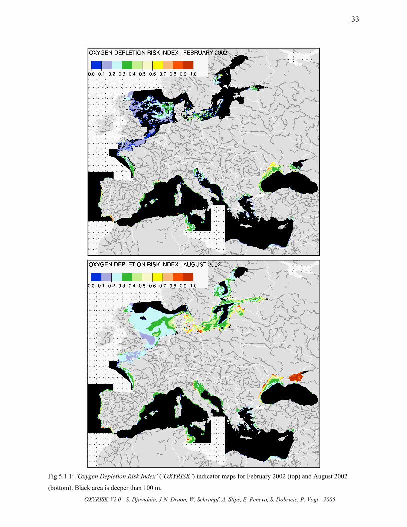
The ‘OXYRISK’ index shows (Fig. 5.1.1) that the main regions subject to a hypoxia/anoxia risk

are the eastern North Sea, the Kattegat and Belt Sea, the southern near shore Baltic Sea, the

northern Gulf of Riga, coastal regions of the Gulf of Finland, the north-western Adriatic Sea and

the north-western coastal region of the Black Sea. All these areas are reported in the literature as

problem areas concerning near bottom oxygen in the last three decades.

In these areas, oxygen deficiencies are mainly caused by an increase of primary production

(eutrophication, see Fig D.19: e.g. north-western Adriatic Sea) or by weak hydro-morphological

conditions (low ventilation, see Fig D.22: e.g. Kattegat and Belt Sea), or by both in variable

degrees (eutrophication and low ventilation: e.g. north-western coastal region of the Black Sea,

eastern North Sea). The overestimation of oxygen deficiency in the Azov Sea is due to the

overestimation of primary productivity. The Azov Sea is few meters deep and most probably

either suspended matter (in case of wind), or sea bottom (in case of calm conditions) is detected

by the optical remote sensor.

The ‘PSA’ index (Fig. 5.1.2) shows that the seasonal variability of physical vulnerability to

oxygen depletion is important. However, some regions of the Baltic Sea, the Belt Sea and

Kattegat are always physically sensitive and the Channel and southern North Sea are always


32

resistant due to, respectively, permanently stratified and mixed waters. Areas where the

stratification is seasonal and the hydrodynamics is low are identified as vulnerable independently

of nutrient conditions (Central North Sea, Bay of Biscay outside of the river plume areas, Gulf of

Lion, Eastern Spanish coastal area, outer part of the Black Sea shelf). Where primary production

is low (Fig D.19), these areas are not classified as problem areas in terms of oxygenation (see

Fig. 5.1.1). These vulnerable areas are however very sensitive to an increase of primary

production and linked nutrient loads. Note that the Azov Sea is not identified as a physically

vulnerable area.

Future improvements for the calculation of oxygen depletion risk in coastal marine waters are

currently under development. A new primary production algorithm specific to coastal areas is

currently being developed which will improve the estimation of ‘POM’ production in coastal

waters. To improve the overall consistency the ‘Primary Production’ product should be

estimated with the satellite derived ‘Chlorophyll-a’ and ‘PAR’, using the actual available ‘Mixed

Layer Depth & Temperature’ from the numerical model data. The inclusion of yearly variable

‘Mixed Layer Depth’ and ‘Maximum Density Gradient’ from hydro-dynamical modelling will

improve the inter-annual variability of the physical environment forcing the biology. Finally, the

implementation of a quantitative biogeochemical model of the oxygen and carbon cycles will

improve the estimation of hypoxia at sea-bed, which will allow the link with the nutrients.


33

Fig 5.1.1: ‘Oxygen Depletion Risk Index’ (‘OXYRISK’) indicator maps for February 2002 (top) and August 2002

(bottom). Black area is deeper than 100 m.


34

Fig 5.1.2: ‘Physically Sensitive Area Index’ (‘PSA’) indicator maps for February 2002 (top) and August 2002

(bottom). Index represents high (high value = red)/low (low values = blue) physical sensitivity to eutrophication due

to diverse physical conditions. Note that tidal areas (Channel and southern North Sea) are well protected against

oxygen depletion. Black area is deeper than 100 m.


35

Appendix A – Inter-annual Variability Introduction Flow Chart

| ρ(mx) - ρ(sst) | ≤ σ(thresh) NO DENSITY CHANGE

Old Stratification f(S)

ρ(mx) - ρ(sst) < - σ(thresh) Decrease in Stratification

| ρ(sst) - ρ(bot) | ≤ σ(thresh)

ρ(sst) - ρ(bot) > σ(thresh)

ρ(sst) - ρ(bot) < - σ(thresh)

New Stratification f(T)

Old Stratification f(T)

ρ(mx) - ρ(bot) < - σ(thresh)


New Stratification f(S)

NO NEW STRATIFICATION MIXED WATER COLUMN

FRESH WATER INFLUENCE

NO NEW STRATIFICATION MIXED WATER COLUMN

CONSERVATION OF HEAT AND POTENTIAL ENERGY



There is still Stratification

There was Stratification

(Unstable)

ρ(mx) - ρ(sst) > σ(thresh)

New Stratification f(T)

| ρ(mx) - ρ(bot) | ≤ σ(thresh)

New Stratification f(S)

ρ(mx) - ρ(sst) < - σ(thresh)


Increase in Stratification

Old Stratification f(T)

TEMPORAL (MONTHLY) INTERPOLATION


CONSERVATION OF HEAT AND POTENTIAL ENERGY

There was Stratification

There was no Stratification

New Stratification dominated by S or T ?





36

Appendix B – Inventory of Available Images

Variable Yearly Climatology Bathymetry : Depth (m) Cadvmx : Mixed Layer Advection Index Cadvbl : Benthic Layer Advection Index tmx_sm : Mixed Layer Temperature (degC) smx_sm : Mixed Layer Salinity (psu) sigm_sm : Maximum Density Gradient (kg m-4) depmx_sm : Mixed Layer Depth (m) sst_sat : Satellite Sea Surface Temperature (degC) sigm_sat : Satellite corrected Maximum Density Gradient (kg m-4) depmx_sat : Satellite corrected Mixed Layer Depth (m) delta_T : Satellite – Model Temperature Difference (degC) delta_sigm : Satellite – Model Maximum Density Gradient Difference (kg m-4) delta_depmx : Satellite – Model Mixed Layer Depth Difference (m) Cstrat : Stratification Index Cblt : Benthic Layer Thickness Index Cbfri : Friction Velocity Index at the Bottom Coxy_sat : Oxygen Saturation Index CTx_deg : Degradation Velocity Index at the Bottom Clight : Light Availability in Euphotic Layer Index K490 : Diffuse Attenuation Coefficient at 490nm (m-1) Chl: Chlorophyll-a conc. (mg m-3) / P2 : Primary Production (gC m-2 month-1) POM_bot : Particulate Organic Matter at the Bottom (mg C m-2 month-1) CPOM : Particulate Organic Matter Index Cphys_surf : Surface Layer Physics Index Cphys_bott : Bottom Layer Physics Index PSA : Physically Sensitive Area Index OXYRISK : Oxygen depletion Risk Index

Table B.1 Images available from OXYRISK_V2.pro


37

Appendix C - Governing Equations and Flow Chart

Quantity Description (monthly means) Units Model or Satellite depth Depth of sea bed m M umx Mean current velocity of the mixed layer: x component m s-1 M vmx Mean current velocity of the mixed layer: y component m s-1 M ubot Mean current velocity of the bottom layer: x component m s-1 M vbot Mean current velocity of the bottom layer: y component m s-1 M bfri Bottom friction velocity m s-1 M

bfri_std Standard deviation of monthly bottom friction velocity m s-1 M sst Sea Surface Temperature degC S

tmx Mean temperature of the mixed layer degC M tbot Bottom temperature degC M smx Mean salinity of the mixed layer psu M sbot Bottom salinity psu M sigm Maximum of the density gradient kg m-4 M

depmx Depth of the mixed layer m M k490 Diffuse attenuation coefficient m-1 S par Photosynthetically available radiation W m-2 S chl Chlorophyll-a mg m-3 S p2 Primary Productivity g C m-2 month-1 S

Table C.1 Variables used in the OXYRISK_V2.pro program

Density [UNESCO, 1981]

54325.1

5.125.1

1)21()21()321()321()4321(

TFTSEETSDDTSCSCCTSBSBBSASASAA

×+××++××++××+×+

+××+×++×+×+×+=ρ (Eq C.1)

where ρ= density () ; S = Salinity (psu) ; T = Temperature () ; A1 = 999.842594 ; A2 = 0.824493 ; A3 = -5.72466x10–3 ; A4 = 4.8314x10–4 ; B1= 6.793952x10–2 ; B2 = -4.0899x10–3 ; B3 = 1.0227x10–4 ; C1 = -9.09529x10–3 ; C2 = 7.6438x10–5 ; C3 = -1.6546x10–6 ; D1 = 1.001685x10–6 ; D2 = -8.2467x10–7 ; E1 = -1.120083x10–6 ; E2 = 5.3875x10–9 ; F1 = 6.5633210–9 oxy_sat – Oxygen Saturation [Weiss, 1970]

)])100

(3100

21()100

(4)100

ln(3)100(21exp[1_ 2TBTBBsbotTATAT

AACsatoxy ×−×+×+×+×+×+×=

where A1 = -173.4292 ; A2 = 249.6339 ; A3 = 143.3483 ; A4 = -21.8492 and B1 = -0.033096 ; B2=0.014259 ; B3 = 0.0017 ; C1 = 1.4276 (mgl-1) and T(Kelvin) = tbot (degC) + 273.15 (Eq C.2) Tx_deg – Bottom Degradation Velocity [Eppley, 1972] )2exp(1deg_ tbotAATx ××= (Eq C.3) where A1 = 0.0264 ; A2 = 0.07 light – Light Availability in the Euphotic Layer

490

30.2KPARlight ×= (Eq C.4)

POM_bot – Particulate Organic Matter at the Bottom Advection Sinking Diffusion Degradation Deposition

where pp = chl or pp = p2

pp pp pp pp pp POM_bot


38

Cbfri – Bottom Friction Velocity Index

1_

1 ≤−=threshbfri

bfriCbfri (Eq C.5)

where bfri_thresh = 0.017 m s-1 Cstrat – Stratification Index

1_

≤=threshsigm

sigmCstrat (Eq C.6)

where sigm_thresh = 0.07 kg m-4 Cadvmx – Mixed Layer Advection Index

1_

)(121

22

≤+

−=threshadvmx

vmxumxCadvmx (Eq C.7)

where advm_thresh = 0.09 m s-1 Cadvbl – Bottom Layer Advection Index

1_

)(121

22

≤+

−=threshadvblvbotubotCadvbl (Eq C.8)

where advm_thresh = 0.09 m s-1 Cblt – Bottom Layer Thickness Index IF threshdepthdepmxdepth _)(0 <−<

14)(3)(2)(1 23 ≤+−×+−×+−×= AdepmxdepthAdepmxdepthAdepmxdepthACblt ELSE Cblt = 0 (Eq C.9) where depth_thresh = 40m and A1 = 5x10-5 ; A2 = -0.0032 ; A3 = 0.0199 ; A4 = 0.9901 Coxy_sat – Oxygen Saturation Index

1min_max_min__1_ ≤

−−

−=satsatsatsatoxysatCoxy (Eq C.10)

where min_sat = oxy_sat(T = 22 degC ; S = 38 psu) and max_sat = oxy_sat (T = 8 degC ; S = 5 psu) CTx_deg – Bottom Degradation Velocity Index

1min__max__

min__deg_deg_ ≤−

−=

threshtauthreshtauthreshtauTxCTx (Eq C.11)

where Tx_thresh_min = 0.03oC ; Tx_thresh_max = 0.14oC Clight – Index of Light Availability in the Euphotic Layer

1min__max__

min__≤

−−

=threshlightthreshlight

threshlightlightClight (Eq C.12)

where light_thresh_min = 0 Wm-1 ; light_thresh_max = 4.5x104Wm-1


39

Cphys_bott – Bottom Layer Physics Index (for PSA) IF Cstrat LT Cstrat_thresh

6

deg__)2(_ CTxCadvmxCstratsatCoxyCbfribottCphys ++++×=

IF Cstrat GE Cstrat_thresh (Eq C.13)

7deg__)2(_ CTxCadvblCbltCstratsatCoxyCbfribottCphys +++++×

=

where Cstrat_thresh = 0.2 Cphys_surf – Surface Layer Physics Index

3

_ ClightCstratCadvmxsurfCphys ++= (Eq C.14)

PSA- Physically Sensitive Area Index

2

__ surfCphysbottCphysPSA += (Eq C.15)

Cphys_bott – Bottom Layer Physics Index (for OXYRISK) IF Cstrat LT Cstrat_thresh

5

deg__)1(_ CTxCadvmxCstratsatCoxyCbfribottCphys ++++×=

IF Cstrat GE Cstrat_thresh (Eq C.16)

6deg__)1(_ CTxCadvblCbltCstratsatCoxyCbfribottCphys +++++×

=

where Cstrat_thresh = 0.2 CPOM – Particulate Organic Matter Index threshppadvppCPOM __ ×= (Eq C.17) where pp_thresh = 0.64 (Chl case) or pp_thresh = 0.025 (P2 case) OXYRISK – Oxygen Depletion Risk Index

12

_≤

+=

bottCphysCPOMOXYRISK (Eq C.18)


40

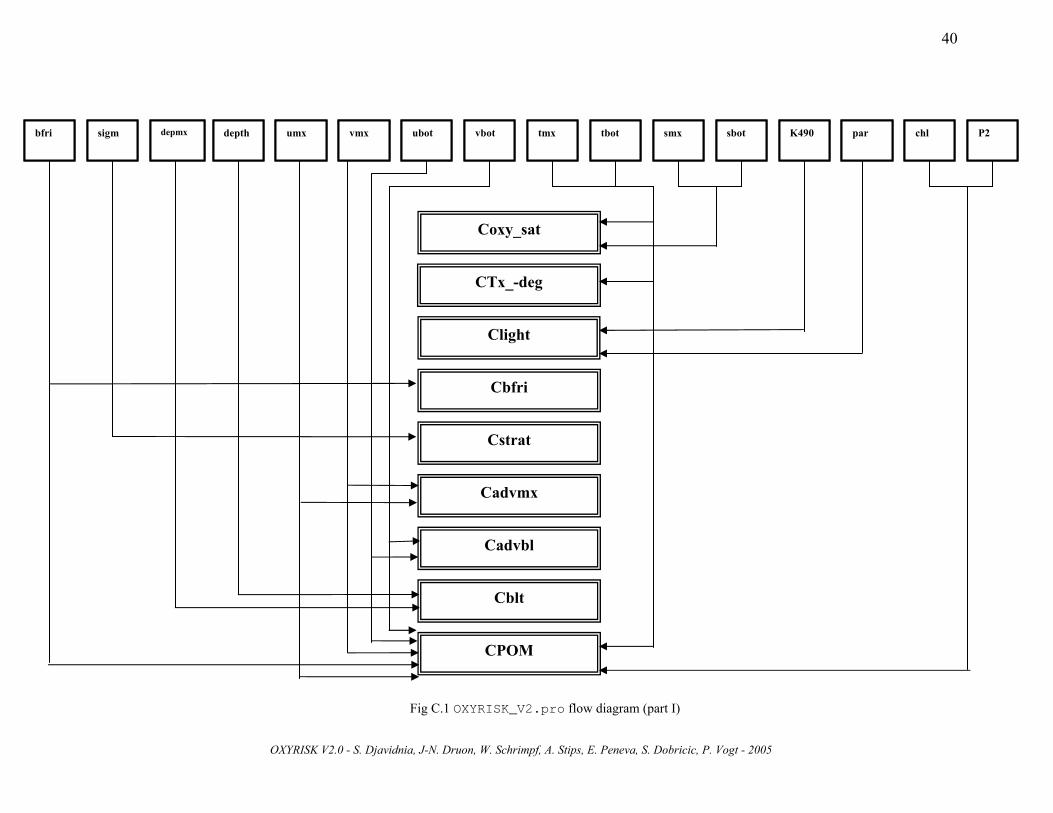
bfri sigm depmx depth umx vmx ubot vbot tmx tbot smx sbot K490 par chl P2 bfri sigm depmx depth umx vmx ubot vbot tmx tbot smx sbot K490 par chl P2

Coxy_sat

Cbfri

CTx_-deg

Clight

Cstrat

Cadvmx

Cadvbl

Cblt

CPOM

Fig C.1 OXYRISK_V2.pro flow diagram (part I)


41

Cadvmx Clight Cbfri Coxy_sat CTx_deg Cblt Cadvbl POM_b

Cphys_surf Cphys_bott CPOM

PSA

OXYRISK

Cstrat

Fig C.2 OXYRISK_V2.pro flow diagram (part II)


42

Appendix D – Intermediate Product Images

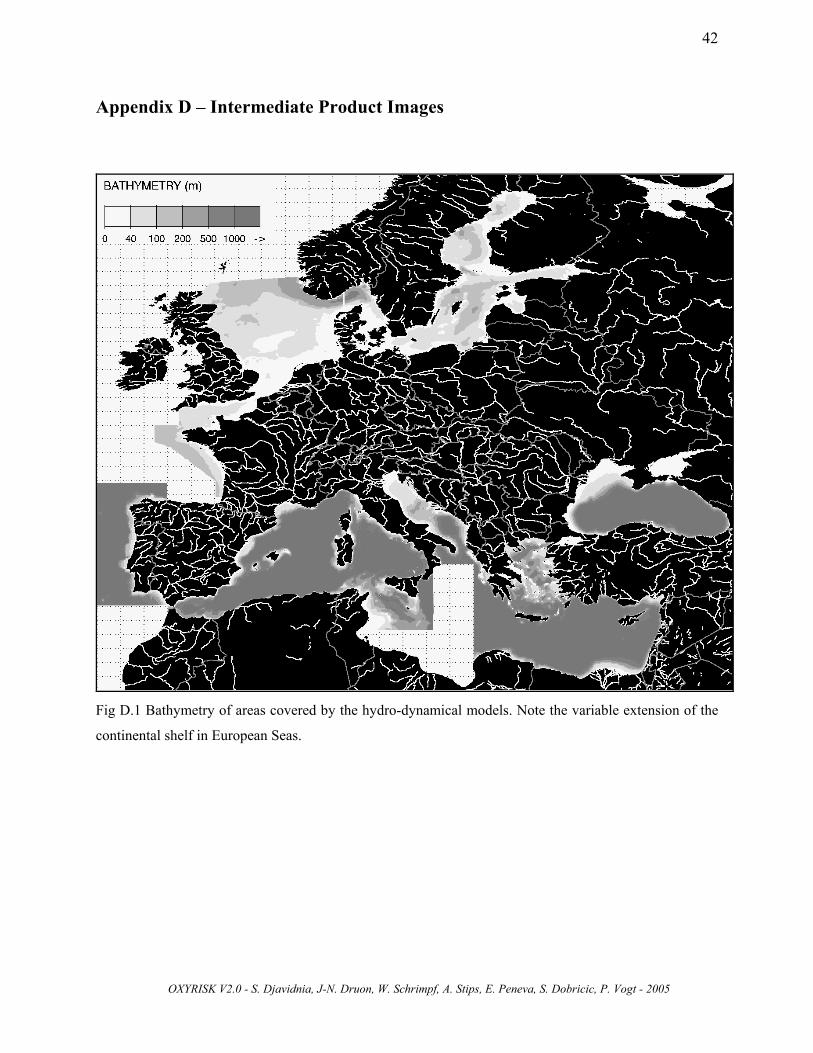
Fig D.1 Bathymetry of areas covered by the hydro-dynamical models. Note the variable extension of the

continental shelf in European Seas.


43

Fig D.2 ‘Mixed Layer Advection Index’ (February and August). Low index values correspond to high

current velocities.

Fig D.3 ‘Benthic Layer Advection Index’ (February and August). Low index values correspond to high

current velocities.


44

Fig D.4 Mixed layer temperature given by the hydro-dynamical models (February and August).

Fig D.5 Satellite Sea Surface Temperature (February and August 2002, AVHRR). Note the significantly

warmer surface temperature in summer 2002 compared to climatology (Fig D.4).


45

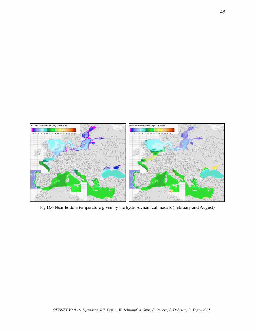
Fig D.6 Near bottom temperature given by the hydro-dynamical models (February and August).


46

Fig D.7 Mixed layer salinity given by the hydro-dynamical models (February and August).

Fig D.8 Bottom layer salinity given by the hydro-dynamical models (February and August). Note the

permanent vertical salinity gradient (see also Fig D.8) in the Skagerrak-Kattegat-Belt Sea, the Baltic

Proper and Black Sea.


47

Fig D.9 Maximum density gradient given by the hydro-dynamical models (kg m-4, February and August).

Fig D.10 Maximum density gradient modified using satellite sea surface temperature (kg m-4, February

and August 2002).


48

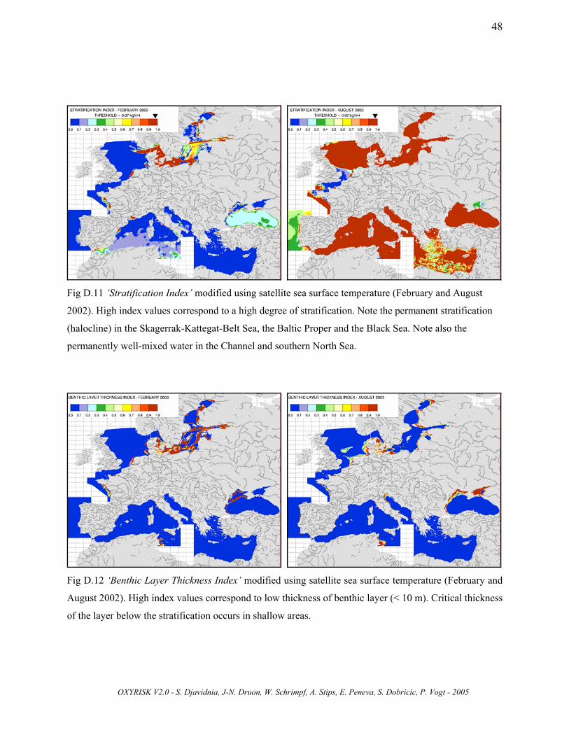
Fig D.11 ‘Stratification Index’ modified using satellite sea surface temperature (February and August

2002). High index values correspond to a high degree of stratification. Note the permanent stratification

(halocline) in the Skagerrak-Kattegat-Belt Sea, the Baltic Proper and the Black Sea. Note also the

permanently well-mixed water in the Channel and southern North Sea.

Fig D.12 ‘Benthic Layer Thickness Index’ modified using satellite sea surface temperature (February and

August 2002). High index values correspond to low thickness of benthic layer (< 10 m). Critical thickness

of the layer below the stratification occurs in shallow areas.


49

Fig D.13 ‘Bottom Friction Velocity Index’ (February and August). Low index values correspond to high

levels of bottom friction velocity (> 1.9 cm s-1). Note that bottom friction maxima are mainly occurring in

tidal areas (Channel and southern North Sea).

Fig D.14 ‘Oxygen Saturation Index’ (February and August). High index values correspond to low oxygen

saturation at sea bed.


50

Fig D.15 ‘Index of degradation velocity at seabed’ (February and August). High index values correspond

to high degradation velocities near sea bed (0.14 d-1 for index=1.0 and 0.03 d-1 for index=0.0).

Fig D.16 ‘Index of light availability in euphotic layer’ (February and August). High index values

correspond to low light availability in euphotic layer. Both solar irradiance and turbidity are able to limit

the light availability for primary productivity.


51

Fig D.17 Chlorophyll-a monthly means derived from SeaWiFS-OC4 algorithm (mg Chl m-3, February

and August 2002).

Fig D.18 Chlorophyll-a monthly means derived from SeaWiFS-OC5 algorithm (mg Chl m-3, February

and August 2002).


52

Fig D.19 Primary Production derived from MODIS (mg C m-2 month-1, February and August 2002).

Fig D.20 Diffuse attenuation coefficient derived from SeaWiFS (m-1, February and August 2002).


53

Fig D.21 ‘Surface Layer Physics Index’ (February and August). Index represents surface physical

conditions favourable (high values = red) / unfavourable (low values = blue) for phytoplankton growth

(assuming nutrients are not limiting).

Fig D.22 ‘Bottom Layer Physics Index’ (February and August). Index represents low (high

values = red)/high (low values = blue) physical availability (reserve and renewal) of oxygen near bottom.

Black area is water deeper than 100 m.


54

Fig D.23 Particulate organic matter at bottom or 100 m if deeper (gC m-2 month-1) derived from MODIS

primary production (February and August 2002).

Fig D.24 ‘Particulate Organic Matter Index’ (relative units) derived from MODIS primary production

(February and August 2002). Index represents monthly relative organic load of matter that reaches the sea

bed (or 100 m for deep waters), which has undergone horizontal and vertical transport, horizontal

diffusion, degradation in the water column and resuspension/deposition.


55

List of Acronyms

AVHRR Advanced Very High Resolution Radiometer

Chl-a Chlorophyll-a

OXYRISK Oxygen depletion Risk Index

GUI Graphical User Interface

HDF Hierarchical Data Format

IDL Interactive Data Language

K490 Diffusive Attenuation Coefficient at 490nm

MLD Mixed Layer Depth

MLT Mixed Layer Temperature

MODIS MODerate resolution Imaging Spectroradiometer

OC4 Ocean Colour Algorithm 4

OC5 Ocean Colour Algorithm 5

PAR Photosynthetically Available Radiation

PNG Portable Network Graphics

POM Particulate Organic Matter

PP Primary Production

PSA Physically Sensitive Area

ROI Region Of Interest

SeaWiFS Sea-viewing Wide Field-of-view Sensor

SST Sea Surface Temperature

UNESCO United Nations Economic Social and Cultural Organisation

YOI Year Of Interest


56

Acknowledgments

This work was performed under the 'ECOMAR' institutional project (no. 2121) of the JRC Framework Programme 6 in support of the European Environment Agency (EEA) and DG Environment. We thank A. Lascaratos1, S. Sofianos1, P. Lazure2, P. Garreau2 and H. Coelho3 for providing the physical modelling data which contributed in enlarging the results of the present study, and G. Zibordi4 and F. Mélin4 for providing the SeaWiFS chlorophyll-a data processed using the JRC-IMW processing chain and specific atmospheric correction algorithm. We also thank M. Dowell4 for his valuable and constructive comments.

The AVHRR Oceans Pathfinder SST data was obtained from the Physical Oceanography Distributed Active Archive Centre (PO.DAAC) at the NASA Jet Propulsion Laboratory, Pasadena, CA, USA. The SeaWiFS Chlorophyll data was obtained from the Distributed Active Archive Centre (DAAC) at the NASA Goddard Space Flight Centre, Greenbelt, MD, USA. The MODIS Terra Primary Production data was obtained from the Distributed Active Archive Centre (DAAC) at the NASA Goddard Space Flight Centre, Greenbelt, MD, USA. ______________________________________________________________________________ 1 University of Athens, Ocean Physics and Modelling Group, University Campus, Building PHYS-V, 15784, Athens, Greece. 2 Ifremer, Centre of Brest, DEL/AO, BP 70, 29280 Plouzané, France. 3 Hidromod, Modelação em Engenharia Lda., Taguspark - Núcleo Central, n. 349, 2780-920 Oeiras, Portugal. 4 Joint Research Centre, Institute of Environment & Sustainability, Inland & Marine Waters Unit, Via E. Fermi 1,TP 272, Ispra (VA),Italy.


57

References Avnimelech, A., Mozes, N., Diab, S. and Kochba, M., 1995. Rates of organic-carbon and nitrogen degradation in intensive fish ponds. Aquaculture, 134:211-216. Buller, R.J., 1975. Redistribution of waterfowl: influence of water, protection, and feed. International Waterfowl Symposium, 1, 143-154. Cacchione, D.A., Drake, D.E., Ferreira, J.T., Tate, G.B., 1994. Bottom stress estimates and sand transport on northern California inner continental shelf. Continental Shelf Research, 14, 1273-1289. Cognetti, G., 2001. Marine eutrophication: the need for a new indicator system. Marine Pollution Bulletin, 42, 163-164. Druon, J-N., Schrimpf, W., Dobricic, S. and Stips, A., 2002. The physical environment as a key factor in assessing the eutrophication status and vulnerability of shallow Seas: PSA & EUTRISK (v1.0). Project “ECOWAT”, EUR20419 (EN), European Commission – Joint Research Centre, IES-IMW. Druon, J-N., Schrimpf, W., Dobricic, S. and Stips, A., 2004. Comparative assessment of large-scale marine eutrophication: North Sea area and Adriatic Sea as case studies. Marine Ecology Progress Series, 272, 1-23. EEA, 2000. Nutrients in European Ecosystems. Environmental Assessment Report No. 4. Eppley, R.W., 1972. Temperature and phytoplankton growth in the sea. Fishery Bulletin, 70, 1063-1085. Eppley, R.W., Stewart, E., Abbott, M.R. and Heyman, U., 1985. Estimating ocean primary production from satellite chlorophyll. Introduction to regional differences and statistics for the Southern California Bight. Journal of Plankton Research, 7, 57-70. Esaias, W.E., 1996. Algorithm Theoretical Basis Document for MODIS Product MOD-27 Ocean Primary Productivity. Code 971, Goddard Space Flight Centre, 44pp. European Communities, 1991. Directive 91/271/EEC. Council Directive of 21 May 1991 concerning urban waste water treatment. O.J. L135/40 vol. 30/5/91. Heiskanen, A.S. and Leppänen, J.M., 1995. Estimation of export production in the coastal Baltic Sea: effect of resuspension and microbial decomposition on sedimentation measurements. Hydrobiologia, 316:211-224. Howard, K., 1995. Estimating global ocean primary production using satellite derived data. Master of Science Thesis. University of Rhode Island, 98 pp.


58

Kantha, L.H. and Clayson C.A., 2000. Numerical Models of Oceans and Oceanic Processes. International Geophysics Series (Edited by Dmowska R., Holton J. R. and Rossby H. T.), Vol. 66. Nixon, S.W., 1995. Coastal marine eutrophication: A definition, social causes and future concerns. Ophelia, 41, 199-219. Peterson, E.L., 1999. Benthic Shear stress and sediment condition. Aquacultural Engineering, 21, 85-111. Ribbe J., Holloway, P.E., 2001. A model of suspended sediment transport by internal tides. Continental Shelf Research, 21, 4, 395-422. UNESCO, 1981. Tenth report on oceanographic tables and standards. UNESCO Technical Papers in Marine Sci., No. 36, UNESCO, Paris. Weiss, R.F., 1970. The solubility of nitrogen, oxygen and argon on water and sea-water. Deep Sea Research, 17, 721-735.

Oxygen Depletion Risk Indices - OXYRISK & PSA V2.0: New developments, structure and software content

Documents

Transcript of Oxygen Depletion Risk Indices - OXYRISK & PSA V2.0: New developments, structure and software content