arX

iv:0

905.

2841

v2 [

hep-

ph]

17

Nov

200

9

Overview of the spin structure function g1 at arbitrary x and Q2

B.I. ErmolaevIoffe Physico-Technical Institute, 194021 St.Petersburg, Russia

M. GrecoDepartment of Physics and INFN, University Rome III, Rome, Italy

S.I. TroyanSt.Petersburg Institute of Nuclear Physics, 188300 Gatchina, Russia

In the present paper we summarize our results on the structure function g1 and present explicitexpressions for the non-singlet and singlet components of g1 which can be used at arbitrary xand Q2. These expressions combine the well-known DGLAP-results for the anomalous dimensionsand coefficient functions with the total resummation of the leading logarithmic contributions andthe shift of Q2 → Q2 + µ2, with µ/ΛQCD ≈ 10 (≈ 55) for the non-singlet (singlet) componentsof g1 respectively. In contrast to DGLAP, these expressions do not require the introduction ofsingular parameterizations for the initial parton densities. We also apply our results to describe theexperimental data in the kinematic regions beyond the reach of DGLAP.

PACS numbers: 12.38.Cy

I. INTRODUCTION

As it is well-known, the spin structure function g1 is introduced through the following conventional parametrizationof the spin-dependent part W spin

µν of the hadronic tensor of the Deep Inelastic lepton- hadron Scattering:

W spinµν = ıMhεµνλρ

qλPq

[Sρg1(x,Q

2) +(Sρ − Pρ

Sq

q2

)g2(x,Q

2)]

(1)

where we have used the standard notations: P is the hadron momentum, Mh is the hadron mass, S is the hadron spin,q is the virtual photon momentum. Traditionally, −q2 ≡ Q2 > 0 and x = Q2/2Pq. The scalar functions g1(x,Q

2) andg2(x,Q

2) are called the spin structure functions. Both of them contribute to the asymmetry between the DIS crosssections when the lepton and hadron spins are antiparallel and parallel. In particular, g1 describes such asymmetrywhen both spins are longitudinal, i.e. they lie in the plane formed by P and q. Obviously, in order to calculate thestructure functions g1(x,Q

2) and g2(x,Q2) in the framework of QCD, one should know the QCD behaviour at large

and small momenta of virtual particles, i.e. one should be able to account for the perturbative and non-perturbativeeffects. At present this is impossible, so the standard description involves the factorization hypothesis: W spinµν isrepresented as a convolution:

W spinµν = W q

µν ⊗ Ψq + W gµν ⊗ Ψg (2)

where Ψq and Ψg are the probabilities to find a polarized quark or gluon in the polarized hadron, while W q,gµν describe

the DIS of the quarks and gluons. There is no rigorous proof of this factorization, especially at small x, in theliterature. However, discussing this point is beyond the scope of our paper. Also, there is no model-independenttheoretical description of the probabilities Ψq and Ψg in the literature because QCD at small momenta is not known.

On the contrary, W qµν and W g

µν can be calculated with the methods of Pertubative QCD, by summing the contributionsof the involved Feynman graphs. So, the standard procedure is to replace Ψq and Ψg by the initial parton densitiesδq and δg. Both of them are found by fitting the experimental data at large x and not very large momenta Q2

(Q2 = µ2 ∼ 1 GeV2 ). Therefore,

g1 = gq1 ⊗ δq + gg

1 ⊗ δg. (3)

It is well-known that in the Born approximation

gBorn1 = (e2q/2)δ(1 − x) ⊗ δq (4)

2

where eq is the electric charge of the quark interacting with the virtual photon. Accounting for the QCD radiativecorrections to gBorn

1 and other DIS structure functions, especially by trying to perform a complete resummation ofthe corrections, has been the subject of great interest in recent years. Surely, such resummation cannot be performedprecisely, so it would be important to resum, in the first place, the most essential corrections. They are different fordifferent values of x and Q2. For example for describing g1 in the region of x ∼ 1 and large Q2, the contributions∼ lnk x are negligibly small compared to lnk(Q2/µ2). In contrast, lnk x becomes quite important at x≪ 1 and shouldbe accounted for.

The goal of obtaining an universal description of the structure function g1, which could be used for arbitrary xand arbitrary Q2 would be appealing both for theorists and experimentalists. Most generally, one encounters variouskinematic regions where the DIS structure functions have been thoroughly studied. The first kinematic region is theso-called hard region A of large x and large Q2:

A: w & Q2 ≫ µ2, x . 1 (5)

where w = 2pq and µ2 is the starting point of the Q2 -evolution. Usually, the value of µ is chosen ≈ 1 GeV orso. Through the paper we use the standard notations: q is the virtual photon momentum, p is the initial partonmomentum, and x = Q2/w. The region A was described first by the LO DGLAP evolution equations obtained inRef. [1]:

d∆q

dt= Pqq ⊗ ∆q + Pqg ⊗ ∆g , (6)

d∆g

dt= Pgq ⊗ ∆q + Pgg ⊗ ∆g

where we have used the standard notation t = ln(Q2/µ2) and Pik (with i, k = q, g) are the splitting functions. ∆q and∆g are the evolved (with respect to Q2) parton distributions. The splitting functions Pik in the DGLAP evolutionequations (6) include the QCD coupling αs. In order to account for the running αs -effects, one should define theargument of αs. The DGLAP -prescription is

αs = αs(Q2) . (7)

Through the paper we will address the parametrization of αs in Eq. (7) as the DGLAP -parametrization. The DGLAPEqs. (6) describe the Q2-evolution of the parton distributions from Q2 = µ2, with µ ∼ 1 GeV, to larger Q2. Whengeneral solutions to Eqs. (6) are obtained, one needs to specify appropriate initial conditions. Conventionally, theinitial conditions to Eqs. (6) are

∆q|t=0 = δq , ∆g|t=0 = δg , (8)

with δq, δg being called the initial parton densities. They are found by fitting the experimental data . After ∆q and∆q have been fixed, the DIS structure functions, including g1, are found by convoluting them with the coefficientfunctions Cq, Cg:

g1(x,Q2) = Cq(x/y) ⊗ ∆q(y,Q2) + Cg(x/y) ⊗ ∆g(y,Q2) . (9)

The Mellin transformations of Pik are called the anomalous dimensions. The splitting functions Pik and coefficientfunctions Ck for the unpolarized DIS were calculated with LO accuracy in Ref. [1]. The LO expressions for Pik

and Ck for the polarized DIS were obtained in Ref. [2]. Later, the LO expressions of Refs [1, 2] for Pik and Ck

were complemented by the NLO results[3]. A detailed review on that subject can be found in Ref. [4]. From puretheoretical grounds, this approach should not be used outside the region A. However, introducing special fits[5, 6] forthe initial parton densities DGLAP has been extended to the region B of large Q2 and small x:

B: w ≫ Q2 ≫ µ2 , x≪ 1 . (10)

Indeed the parameterizations for δq, δg of Ref. [5, 6] contain singular factors x−a, and used in Eq. (8), they provideg1 with a fast growth at small x. As a result, combining the LO evolution equations of Ref. [1] and NLO DGLAPresults of Ref. [3] with the standard fits of Ref. [5, 6] it has been possible to describe the available experimental dataon g1 in regions A and B, i.e. for large Q2 and arbitrary x. In the present paper we refer to this as the StandardApproach (SA). In addition to regions A and B, there are two more interesting kinematic regions:

C: 0 ≤ Q2 . µ2 , x≪ 1 , (11)

3

D: 0 ≤ Q2 . µ2 , x . 1 . (12)

Besides a purely theoretical interest, the knowledge of g1 in the regions C and D is needed because they correspondto the kinematic region investigated experimentally by the COMPASS collaboration. Obviously, the regions C andD are beyond the reach of SA. Strictly speaking, the same could be said about the region B: In fact the expressionsfor Pik are obtained (see Refs. [1, 3] for detail) under the assumption of the ordering

µ2 < k21 ⊥ < k2

2 ⊥ < ... < Q2 (13)

where ki ⊥ are the transverse momenta of virtual ladder partons and they are numbered from the bottom of theladders to the top. Once this ordering is kept one is led inevitably to neglect the double-logarithmic (DL) contributions∼ αs ln2(1/x) and other contributions independent of Q2. Such contributions are small in the region A where theyare correctly neglected in the SA. However, they become essential in the region B. In order to account for them, theDGLAP-ordering of Eq. (13) should be replaced by the other ordering:

µ2 <k21 ⊥

β1<k22 ⊥

β2< ... < w (14)

where βj are the longitudinal Sudakov variables 1 for the virtual parton momenta kj as follows:

kj = −αj(q + xp) + βjp+ kj⊥ . (15)

In order to account for such logarithmic contributions, Eq. (14) should be implemented by the ordering for βi:

1 > β1 > β2 > .. > µ2/w . (16)

This ordering does not exist in DGLAP because in this approach βi ≥ x ∼ 1. The ordering (14,16) was first introducedin Ref. [8] in the context of QED but it applies in QCD as well. Replacing the ordering (13) by Eqs. (14, 16) makespossible to sum up all DL contributions, regardless of their argument, to all orders in αs, i.e. to perform calculationsin the double-logarithmic approximation (DLA). Explicit expressions for g1 in DLA were obtained in Ref. [10]. Thedrawback of those expressions is that αs is kept fixed at an unknown scale. The effect of running αs were takeninto account in Ref. [11]. The parametrization of αs in Refs. [11] differs from the DGLAP- parametrization. Thetheoretical grounds for this new parametrization were given in Ref. [12] and a numerical comparison with the standardparameterizations can be found in Ref. [13]. On the other hand, the reason why, in spite of the lack of the resummationof quite important contributions, the SA turned out to be working well in the region B remained unclear until inRefs. [14, 15] we proved that the factors x−a in the DGLAP-fits for the initial parton densities mimic the totalresummation of the leading logarithms of x. Besides, in Ref. [14] we suggested to combine the DGLAP- results for g1with the results of Ref. [11] in order to obtain an unified description of g1 in the regions A and B, without singularinitial parton densities. A prescription for extending g1 into regions C and D was given in Ref. [16].

In the present paper we present a unified description of g1 valid in all of the regions A-D . The paper is organizedas follows: in Sect. II we briefly remind the DGLAP-description of g1. For the sake of simplicity we consider inmore detail, throughout the paper, the non-singlet component of g1 , and summarize the singlet results only. Asthe expressions for g1 involve convolutions, they look simpler when an integral transform has been applied. Theconventionally used transform is the Mellin one. However, in the small-x, region, it is more convenient the use ofthe Sommerfeld-Watson transform, whose asymptotics partly coincides with the Mellin transform. This formalism isthe content of Sect. III. Before dealing explicitly with g1, we consider in Sect. IV the appropriate treatment of theQCD coupling and compare it with the DGLAP-parametrization. The total resummation of the leading logarithmsof x is quite essential in the small-x region B. We discuss it in Sect. V by composing and solving appropriateInfrared Evolution Equations (IREE). Such equations involve new anomalous dimensions and coefficient functionsand contain the total resummation of the leading logarithms of x. The singlet and non-singlet anomalous dimensionsare calculated in Sect. VI. The non-singlet coefficient function is obtained in Sect. VII and is used to write down theexplicit expression for the non-singlet g1 in the region B. The singlet g1 in the region B is obtained in Sect. VIII. InSect. IX the small-x asymptotics of the non-singlet g1 is discussed, whereas the singlet asymptotics is considered inSect. X. Both asymptotic results are of the Regge type and their intercepts are found not so small. This may leadto the wrong conclusion that the IREE method cannot be applied safely to g1. In order to make this point clear, wediscuss the applicability of our method in Sect. XI. In Sect. XII we compare our results for g1 in the region B to the

1 Sudakov variables were introduced in Ref. [7]

4

DGLAP expressions. We show that DGLAP works well in the region B only because of the singular factors presentin the parameterizations for the initial parton densities. On the other hand, when such fits are used, gDGLAP

1 alsobehaves asymptotically as a sum of Reggeon contributions. The Regge behaviour in the two approaches is discussedin Sect. XIII. Combining the total resummation of the logarithms with the DGLAP results, we give in Sec. XIV theinterpolation expressions describing g1 in the unified region A⊕B. Furthermore we show in Sects. XV and XVI howit is possible to describe g1 in the small-Q2 regions C and D and arrive thereby to the interpolation expressions forg1 which can be used in the whole region A⊕B⊕C⊕D. In particular the small-Q2 regions C and D are describedby a shift of Q2. Such shift is a source of new power Q2- corrections and we discuss them in Sect. XVII. Due to theexperimental investigation of the singlet g1 by the COMPASS collaboration, in Sect. XVIII we give an interpretationto the recent COMPASS data. Finally Sect. XIX contains our concluding remarks.

II. DGLAP -EXPRESSIONS FOR g1

The Standard Approach to g1 is based on the DGLAP evolution equations and also involves some standard param-eterizations for the initial parton densities δq and δg. As the notations for the anomalous dimensions, the coefficientfunctions and the fits for the parton densities vary widely in the literature, we explain below the notation we usetrough the present paper.

We will denote gNS DGLAP1 and gS DGLAP

1 the non-singlet and singlet parts of g1 when the SA is invoked. As theexpressions for g1 involve convolutions, it is convenient to write them down in the Mellin integral form. In particular,the non-singlet g1 is:

gNS DGLAP1 (x,Q2) = (e2q/2)

∫ ı∞

−ı∞

dω

2ıπ(1/x)ωCNS DGLAP (ω, αs(Q

2))δq(ω) (17)

exp[ ∫ Q2

µ2

dk2⊥

k2⊥

γNS DGLAP (ω, αs(k2⊥))

]

where CNS DGLAP (ω, αs(Q2)) is the non-singlet coefficient function, γNS DGLAP (ω, αs(Q

2)) is the non-singlet anoma-lous dimension and δq(ω) is the initial quark density in the Mellin (momentum) space. With the one-loop accuracy(NLO) (see e.g. Ref. [3]), the expression for CNS DGLAP is

CNS DGLAP = CNS DGLAPLO +

αs(Q2)

2πCNS DGLAP

NLO , (18)

with

CNS DGLAPLO = 1, CNS DGLAP

NLO = CF

[ 1

n2+

1

2n+

1

2n+ 1− 9

2+

(3

2− 1

n(1 + n)

)S1(n) + S2

1(n) − S2(n)]. (19)

Similarly, with two-loop accuracy,

γNS DGLAP =αs(Q

2)

2πγ(0)(n) +

(αs(Q2)

2π

)2

γ(1)(n) (20)

where

γ(0)(n) = CF

[ 1

n(1 + n)+

3

2− S2(n)

]. (21)

We have used the standard notations S1,2 in Eqs. (19,21):

S1(n) =

j=n∑

j=1

1

j, S2(n) =

j=n∑

j=1

1

j2. (22)

They are defined for integer n. Their generalization for arbitrary n is well-known:

S1(n) = C + ψ(n− 1), S2(n− 1) =π2

6+ ψ′(n) , (23)

5

with C being the Euler constant. The standard fits for the initial parton densities include the normalization constantsNq,g, the power factors x−a, with a > 0 and more complicated structures; for example,

δq(x) = Nqx−α(1 − x)β(1 + γxδ) ≡ Nqx

−αϕ(x). (24)

All parameters Nq, α, β, γ, δ in Eq. (24) are fixed by fitting the experimental data at large x and Q2 ≈ 1 GeV2.The expressions for gS DGLAP

1 are similar but more involved and we do not discuss them in detail in the presentpaper. For the sake of simplicity through the paper we use g1 non-singlet for illustration, when it is possible, but wepresent the final expressions for both the non-singlet and singlet explicitly.

III. SOMMERFELD-WATSON TRANSFORM

As it is well known, the DGLAP expressions for g1 involve convolutions and in our approach we use them too.The standard way is to use an appropriate integral transform. Traditionally, the SA uses the Mellin transform. Wewill proceed slight differently. Our goal is to obtain expressions for g1 at small x and will start by considering thespin-dependent forward Compton amplitude Tµν related to W spin

µν as follows:

W spinµν =

1

2πℑTµν (25)

where the symbol ℑ means the discontinuity (imaginary part) of Tµν with respect to the invariant total energys = (p+ q)2) of the Compton scattering. At large s, when hadron masses can be neglected,

s ≈ 2pq(1 − x) ≡ w(1 − x) , (26)

so s ≈ w at small x. The amplitude Tµν can be parameterized similarly to W spinµν :

Tµν = ıMhεµνλρqλpq

[SρT1(x,Q

2) +(Sρ − pρ

Sq

q2

)T2(x,Q

2)]

(27)

so that

g1 =1

2πℑT1 , g2 =

1

2πℑT2 . (28)

We call T1,2 the invariant amplitudes. Exploiting the factorization, T1,2 can be represented as the convolution of theperturbative and non-perturbative contributions (cf. Eq. (3)). In particular,

T1 = Tq ⊗ δq + Tg ⊗ δg (29)

where δq and δg are related to δq and δg through Eq. (28). In the Born approximation (cf. Eq. (4)),

TBornq = e2q

s

w −Q2 + ıǫ, TBorn

g = 0 . (30)

From the mathematical point of view, Eq. (29) as well as the DGLAP equations (6) and the expressions (9) for g1are convolutions, so an appropriate integral transform can be used. On the other hand, the phenomenological Reggetheory (see e.g. [17]) states that in order to study accurately the scattering amplitudes at high energies, one shoulduse the Sommerfeld-Watson (SW) transform[18]. The asymptotic form of the SW transform partly coincides withthe Mellin transform and often this form is especially convenient to account for the logarithmic radiative corrections.The SW transform is actually related to the signature invariant amplitudes T (±) defined, in the context of DIS, asfollows:

T (+) =1

2[T (s,Q2) + T (−s,Q2)] , T (−) =

1

2[T (s,Q2) − T (−s,Q2)] (31)

so that

T (s,Q2) = T (+) + T (−) , T (−s,Q2) = T (+) − T (−). (32)

Let us demonstrate that the signature of the Compton invariant amplitude T1 in Eq. (27) is negative. Using Eq. (32),

we can represent T1 in Eq. (27) as the sum of the signature amplitudes T(±)1 . In order to satisfy the Bose statistics,

6

Tµν should be invariant to the permutation of the incoming and outgoing photons in Eq. (27), i.e. to the replacementcombining µ ν and q −q. On the other hand, in the limit of large s, where the SW transform makes sense, theproton spin remains unchanged under such replacement because Sρ ≈ Pρ/M whereas s ≈ 2pq → −s. It immediately

allows one to conclude that the amplitude T(+)1 should not be present in Eq. (27). Therefore,

g1(x,Q2) =

1

πℑT (−)

1 (s,Q2) . (33)

The Compton amplitudes with the positive signature contribute to the structure functions F1 and F2 describingthe unpolarized DIS. The calculation of the non-singlet component of F1 and the non-singlet g1 is quite similar, so inthe present paper we consider gNS

1 in detail and give the results for FNS1 in Appendix A. In order to account for the

logarithmic contributions it is convenient to use the asymptotic SW transform for amplitudes T (±) in the followingform:

T (±) =

∫ ı∞+δ

−ı∞+δ

dω

2πı

( s

µ2

)ω

ξ(±)(ω)F (±)(ω, y) (34)

where y = ln(Q2/µ2) and ξ are the signature factors:

ξ(±) = −[e−ıπω ± 1]/2 ≈ [1 ± 1 + ıπω]/2 . (35)

The integration line in Eq. (34) runs parallel to ℑω and δ should be larger than the rightmost singularity of F (±)(ω, y).Quite often in the literature δ in Eq. (34) is dropped. In the phenomenological Regge theory, the mass scale µ inEq. (34) should obey µ2 ≪ s, otherwise it is arbitrary. We are going to specify it later in the context of g1. Theintegration contour in Eq. (34), which includes the line parallel to the imaginary ω-axis, as stated above, must beclosed up to the left.Then the contour includes all ω-singularities of F (±)(ω, y). As Eq. (34) partly coincides with thestandard Mellin transform, it is often addressed as the Mellin transform and we will do the same through the paper.Nevertheless, we will use the inverse transform to Eq. (34) in its proper form:

F (±)(ω, y) =2

πω

∫ ∞

0

dρe−ωρ ℑT (±)(s/µ2, y) (36)

where we have denoted ρ = ln(s/µ2) . Eqs. (36) and (C2) are supposed to be used at large s (s≫ µ2) where the bulkof the integrals comes from the region of small ω (ω ≪ 1). Obviously, Eq. (36) does not coincide with the standardMellin transform. Finally Eqs. (25,27,31) lead to

g1 =1

2

∫ ı∞

−ı∞

dω

2πı

( s

µ2

)ω

ωF (−)(ω, y) . (37)

IV. TREATMENT OF αs AT LARGE AND SMALL x

The rigorous knowledge on αs is provided by the renormalization group equation (RGE). According to it, the totalresummation of the leading radiative corrections to the Born value of αs leads to the well-known expression

αs =1

b ln(−s/Λ2)(38)

where Λ ≡ ΛQCD and b = (11N − 2nf)/12π, with N = 3 and nf being the number of involved flavors. Eq. (38)is the asymptotic expression valid at |s| ≫ Λ2. The value of s in Eq. (38) is negative. Eq. (38) is often addressedas the leading order expression for αs and is obtained with the total resummation of the leading, single-logarithmiccontributions. Corrections to Eq. (38) are also available in the literature2 but we will not use them in the presentpaper because in practice the accuracy of the total resummations of the other radiative corrections, usually accountedfor with various evolution equations, never exceeds the single-logarithmic accuracy. The minus sign at s in Eq. (38)isrelated to the analyticity: αs(s) should be real at negative s, but when s is positive, αs(s) acquires an imaginary

2 For recent progress in RGE see e.g. the review [19].

7

part. Conventionally, αs(s) at positive s is understood as the value of αs on the upper side of the s -cut. Therefore,−s = s exp(−ıπ) and

αs(s) =1

b

1

[ln(s/Λ2) − ıπ]=

1

b

( ln(s/Λ2) + ıπ

ln2(s/Λ2) + π2

). (39)

Expressions (38,39) are perturbative and asymptotic. In order to be consistent with the applicability of the pertur-bative QCD, µ defined in Eqs. (13,14) should be large enough:

µ≫ Λ. (40)

An alternative way is to modify Eq. (38) in order to be able to investigate αs at s . Λ2. For example, there is the socalled Analytic Perturbation Theory (APT) suggested in Ref. [20]. It is based on subtracting from Eq. (38) its polecontribution at s = −Λ2. In the vicinity of the pole

αs(s) =1

b ln((Λ2 + |s| − Λ2)/Λ2

) ≈ 1

b

[ Λ2

|s| − Λ2+

1

2

]+ O

(|s| − Λ2

). (41)

The result of the subtraction is called the effective coupling and is used instead of αs. Such a coupling can be used atany value of s. The recent results in this approach can be found in Refs. [21]. However, APT does not allow one toget rid of the cut-off µ when the Sudakov contributions of the higher-loop Feynman graphs are involved. So, in thepresent paper we do not follow this approach.

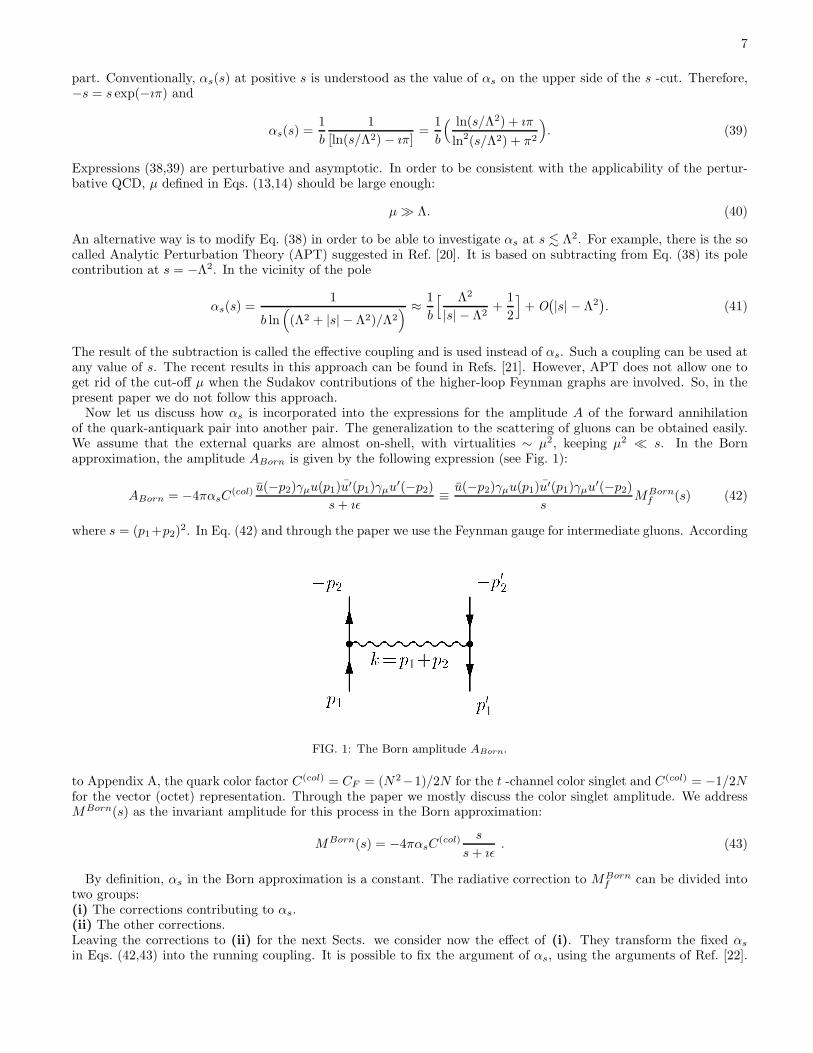
Now let us discuss how αs is incorporated into the expressions for the amplitude A of the forward annihilationof the quark-antiquark pair into another pair. The generalization to the scattering of gluons can be obtained easily.We assume that the external quarks are almost on-shell, with virtualities ∼ µ2, keeping µ2 ≪ s. In the Bornapproximation, the amplitude ABorn is given by the following expression (see Fig. 1):

ABorn = −4παsC(col) u(−p2)γµu(p1)u′(p1)γµu

′(−p2)

s+ ıǫ≡ u(−p2)γµu(p1)u′(p1)γµu

′(−p2)

sMBorn

f (s) (42)

where s = (p1+p2)2. In Eq. (42) and through the paper we use the Feynman gauge for intermediate gluons. Accordingk=p1+p2p1p2 p01p02

FIG. 1: The Born amplitude ABorn.

to Appendix A, the quark color factor C(col) = CF = (N2−1)/2N for the t -channel color singlet and C(col) = −1/2Nfor the vector (octet) representation. Through the paper we mostly discuss the color singlet amplitude. We addressMBorn(s) as the invariant amplitude for this process in the Born approximation:

MBorn(s) = −4παsC(col) s

s+ ıǫ. (43)

By definition, αs in the Born approximation is a constant. The radiative correction to MBornf can be divided into

two groups:(i) The corrections contributing to αs.(ii) The other corrections.Leaving the corrections to (ii) for the next Sects. we consider now the effect of (i). They transform the fixed αs

in Eqs. (42,43) into the running coupling. It is possible to fix the argument of αs, using the arguments of Ref. [22].

8

Incorporating the radiative corrections from (i) to ABorn leads, in particular, to insert the quark bubbles into the(horizontal) propagator of the intermediate gluon. In the logarithmic approximation, each quark bubble brings thecontribution ∼ nf ln s. The gluon logarithmic contributions, each ∼ N , come from more involved graphs but eventuallyall contributions lead to the factor b = (11N − 2nf)/(12π) which multiplies the overall logarithm. Obviously, theargument of this logarithm coincides with the argument of the logarithm from the fermion bubble contribution andit is s. The total resummation of the leading radiative corrections from group (i) converts the fixed αs of Eq. (42)into the well-known expression of Eq. (38) and therefore converts the Born invariant amplitude MBorn of Eq. (43)into M (0):

M (0)(s) = −4παs(s)C(col) s

s+ ıǫ. (44)

In order to apply the Mellin transform to M (0), we allow for the shift s→ s− µ2, with s≫ µ2, in Eq. (44). Then wecan write

M (0)(s) =

∫ ı∞

−ı∞

dω

2πı

( s

µ2

)ω

F (0)(ω), (45)

with

F (0)(ω) = 4πC(col)A(ω)

ω(46)

where A(ω) corresponds to αs(s) in the ω -space :

A(ω) =1

b

[ η

η2 + π2−

∫ ∞

0

dρe−ωρ

(ρ+ η)2 + π2

]. (47)

In Eq. (47) we have denoted η = ln(µ2/Λ2QCD). The first term in Eq. (47) corresponds to the cut of the bare gluon

propagator while the second term comes from the cut of αs(s). They have opposite signs because of the famous

anti-screening in QCD, which is the basis of the asymptotic freedom for αs. In the literature M(0)f and F

(0)f are

often called Born amplitudes (and we also follow this tradition ) in spite of the fact that they include the leading

radiative correction from group (i). The radiative corrections to M(0)f , i.e. the corrections from the group (ii), are

often included by using evolution equations. Such equations involve convolutions of M(0)f , so they look simpler in

the ω -space. We discuss this in detail in the next Section and focus now on the parametrization of αs in the partonladders. As the treatment of αs for the color singlet M0 and octet MV amplitudes is the same, we will not specifythe channel below.First we remind that the well-known result αs = αs(Q

2) in the DGLAP equations follows from the parametrization

αs = αs(k2⊥) (48)

in every rung of the ladder Feynman graphs, where the ladder (vertical) partons can be either quarks or gluons.The notation k⊥ in Eq. (48) stands for the transverse components of momenta k of the vertical partons (quarks andgluons). The theoretical grounds for this parametrization can be found in refs. [23, 24, 25]. The analysis of theparametrization of αs directly for the DGLAP equations was discussed in details in Ref. [26]. In Ref. [12] we hadshown that the arguments of Ref. [26] in favor of using the parametrization (48) in DGLAP can be used at large xonly. Later, in Ref. [27] we made a more detailed investigation on this issue and showed that the parametrization (48)is always an approximation regardless of value of x. As the matter of fact, αs(k

2⊥) should be replaced by the effective

coupling αeffs given by the following expression:

αeffs = αs(µ

2) +1

πb

[arctan

( π

ln(k2⊥/βΛ2)

)− arctan

( π

ln(µ2/Λ2)

)](49)

= αs(µ2) +

1

πb

[arctan

(πbαs(k

2⊥/β)

)− arctan

(πbαs(µ

2))],

where the longitudinal Sudakov variable β is defined in Eq. (15). However when the starting point µ2 of the Q2

-evolution obeys the strong inequality

µ2 ≫ Λ2eπ ≈ 23Λ2, (50)

9

αeffs can be approximated by the much simpler expression:

αeffs ≈ αs(k

2⊥/β). (51)

If additionally x is large, αeffs ≈ αs(k

2⊥). For practical use, the inequality in Eq. (50) can be expressed in terms of

the discrepancy R(µ) defined as

R(µ) =|(1/πb) arctan(π/ ln(µ2/Λ2)) − αs(µ

2)|αs(µ2)

. (52)

A simple calculation shows that R(µ) rapidly grows when µ decreases, ranging, for example, from R(µ) = 5% atµ2 = 2800Λ2 to R(µ) = 10% at µ2 = 250Λ2 and R(µ) = 50% at µ2 = 8.7Λ2. As the DGLAP starting point of the Q2

-evolution is typically chosen close to 1 GeV2, the latter example shows that the DGLAP parametrization Eq. (48)has an error of 50 % at such low scale . This statement is true for all DIS structure functions. In order to deriveEq. (49) we consider now the parametrization of αs in the integral expressions for the DIS structure functions. Herewe partly follow the approach of Ref. [26]. To this aim we consider the forward Compton amplitude T (x,Q2) relatedto the structure functions by Eq. (28). Obviously, this equation is true for all DIS structure functions, so we drophere the signature superscript in T as unessential. One can show (and in this paper we will do it in the context ofDGLAP and our Infrared Evolution Equations) that T obeys the following Bethe-Salpeter equation:

T (x,Q2) = TBorn + ı

∫d4k

(2π)42wk2

⊥

(k2 + ıǫ)2M((q + k)2, k2, Q2) 4π

αs((p− k)2)

(p− k)2 + ıǫ. (53)

The integral term in Eq. (53) is shown in Fig. 2. The notation M((q + k)2, k2, Q2) in Eq. (53) corresponds to the

p p−k

q

k

M

FIG. 2: The integral contribution in Eq. (53). The w -cut is implied, though is not shown explicitly.

blob in Fig. 2. Besides the amplitude T , it can also include a kernel (splitting functions). The inhomogeneous termTBorn is T in the Born approximation. To be specific, we consider the case when the horizontal parton in Fig. 2 is thevirtual gluon with momentum p− k whereas the vertical partons, with momentum k, can be either quarks or gluons.When they are quarks, k2 + ıǫ should be replaced by k2 −m2

q + ıǫ, with mq being the quark mass, but this shift does

not play any role for our consideration below. The factor 2wk2⊥ in Eq. (53) appears as a result of the simplification of

the spin structure of the ladder Feynman graph in Fig. 2. We use the Sudakov parametrization (15) for momentumk of the vertical partons. In terms of the Sudakov variables α, β, k⊥,

k2 = −wαβ − k2⊥, 2qk = wxα + wβ, 2pk = −wα. (54)

where w = 2pq. It is convenient to introduce a new variable m2 = (p− k)2 instead of α. Therefore,

α =m2 + k2

⊥

w(1 − β), k2 = −βm

2 + k2⊥

1 − β. (55)

Using Eqs. (54,55), we can rewrite Eq. (53) in a simpler way:

T (x,Q2) = TBorn +ı

4π2

∫ w

µ2

dk2⊥

∫ 1

β0

dβ

∫ ı∞

−ı∞

dm2 w(1 − β)k2⊥

[m2β + k2⊥ − ıǫ]2

M((q + k)2, (βm2 + k2⊥), Q2)

αs(m2)

m2 + ıǫ. (56)

10

The integration over β and k2⊥ in Eq. (56) runs over the region

β0 < β < 1, µ2 < k2⊥ < w. (57)

The value of β0 follows from the requirement of positivity of the invariant energy (q + k)2 of the blob in Fig. 2:

β0 ≈ x+k2⊥

w −m2. (58)

Let us notice that the m2 -dependence in Eq. (58) can be neglected to the leading logarithmic accuracy that we keepthrough this paper.

A. Integration in Eq. (56) at fixed αs

Let us consider first the calculation of Eq. (56) under the approximation of fixed αs. From the analysis of the ladderFeynman graphs (see e.g. the review [9]) one can see that DL contribution comes from the region of large k2

⊥ where

− k2 ≈ k2⊥ ≫ k2

|| = βm2. (59)

It allows to neglect the dependence of M on βm2 in Eq. (56). It is convenient to integrate Eq. (56) over m2, usingthe Cauchy theorem. The singularities of the integrand are: the double pole from the vertical propagators

βm2 + k2⊥ − ıǫ = 0 (60)

and the simple pole from the horizontal gluon propagator

m2 + ıǫ = 0. (61)

The integration contour can be equally closed up or down. Traditionally (see e.g. Ref. [9]) the integration contour isclosed down which involves taking the residue at the simple pole (61), so we arrive at the following result:

T (x,Q2) = TBorn +αs

2π

∫ w

µ2

dk2⊥

k2⊥

∫ 1

β0

dβ(1 − β)M(β,Q2, k2⊥). (62)

Obviously, when x is large enough, one can change the upper limit of the integration over k2⊥ for Q2. Similarly,

β0 ≈ x. Extracting the Born factor 1/β from M we can write

M(β, k2⊥) = (1/β)PT (63)

where P is a kernel. To specify it, let us provide T with the quark and gluon subscripts through the replacement Tby Tr (with r = q, g). It leads to specifying PT in Eq. (63): PT = Prr′Tr′ . At last, assuming that we have usedthe planar gauge allows to identify (1 − β)Prr′ with the standard LO DGLAP splitting functions. Differentiation ofEq. (62) with respect to the upper limit of the k2

⊥) -integration (which is Q2 at large x) leads to the standard integro-differential DGLAP equations for the Compton amplitudes Tq, Tg.

B. Integration in Eq. (56) with running αs

When αs is running, it is also convenient to use the Cauchy theorem for integrating Eq. (56) over m2. Theintegration contour can again be closed down. However, the spectrum of singularities in the lower semi-plane nowincludes the pole (61) and the cut of αs running along the real axis:

µ2 < m2 − ıǫ < +∞. (64)

Therefore, instead of Eq. (62) we arrive at the more complicated expression:

T (x,Q2) = TBorn +1

2π

∫ w

µ2

dk2⊥

∫ 1

β0

dβ (1 − β)[αs(µ

2)

k2⊥

M(β,Q2, k2⊥) + (65)

∫ ∞

µ2

dm2

m2M(β,Q2, βm2 + k2

⊥)ℑαs(m2)

k2⊥

(βm2 + k2⊥)2

].

11

where we have not used the assumption of Eq. (59). The second term in the rhs of Eq. (65) is the result of takingthe residue in the pole (61) and the third terms corresponds to accounting for the cut (64). Eq. (65) demonstratesexplicitly that it is impossible to factorize αs, i.e. to integrate αs(m

2) over m2, without making the approximationof Eq. (59). When this approximation has been made, we immediately obtain

T (x,Q2) = TBorn +1

2π

∫ w

µ2

dk2⊥

k2⊥

∫ 1

β0

dβ(1 − β)M(β,Q2, k2⊥) αeff

s , (66)

with αeffs given by Eq. (49). Indeed, in this case the integral over m2 in Eq. (66) is

I =1

b

∫ k2⊥/β

µ2

dm2

m2

1

ln2(m2) + π2=

1

πb

[arctan

( π

ln(µ2/Λ2)

)− arctan

( π

ln(k2⊥/β)

)]. (67)

Obviously, the term π2 in the integrand in Eq. (67) can be neglected when µ obeys Eq. (50). It leads to theapproximative expression of Eq. (51) for αeff

s . The approximation βm2 ≪ k2⊥ was also made in Ref. [26] for the

integration Eq. (56) over m2 in the case of running αs. However, the integration contour in that paper was closed upin order to take the residue of the double pole at k2 = βm2 + k2

⊥ = 0, which contradicts the assumption of Eq. (59)made in Ref. [26]. Taking this residue automatically led to the wrong conclusion that αeff

s = αs(−k2⊥/β) regardless

of the value of µ. This error was found and corrected in Ref. [27].

V. DESCRIPTION OF g1 IN THE REGION B: TOTAL RESUMMATION OF THE LEADINGLOGARITHMS

The region B is defined in Eq. (10). As it includes small x and large Q2, both logs of 1/x and Q2 are equallyimportant in this region and should be summed up. The most important logarithmic contributions to g1 in region Bare the double-logarithmic (DL) ones, i.e. the terms

∼ αns ln2n−k(1/x) lnk(Q2/µ2), (68)

with k = 0, 1, .., n, so they should be accounted for in the first place. Then the sub-leading, single-logarithmic (SL),contributions can also be taken into account etc. Therefore, an appropriate evolution equation for g1 in region Bshould account for the evolution both with respect to x and Q2 while DGLAP controls the Q2 -evolution only andcannot sum up the logarithms of x. In addition, the running coupling effects in Eq. (68) should be taken into account.To this end, a special attention should be given to the parameterizations of αs in region B and we will use herethe results of Sect. IV. In order to resum DL contributions we use the alternative method of the Infrared EvolutionEquations (IREE), first suggested by L.N. Lipatov (see Ref. [28]). Then it was applied to the elastic scattering ofquarks in Ref. [29] and in Ref. [30], with the generalization to inelastic processes (radiative e+e− annihilation). Sincethen the IREE method has been applied to various problems and a brief review of the applications can be found inRef. [31]. It is convenient to compose IREE for the Compton amplitudes T (−) related to g1 by Eq. (33).

A. The essence of the method

As we have mentioned above, the DGLAP -ordering of Eq. (13) makes impossible to collect all DL contributions,regardless of their arguments, to all powers in αs. In order to account for them, the ordering of Eq. (13) should bechanged as in Eq. (14). This leads to the infrared (IR) singularities emerging from the graphs with soft gluons. Inorder to regulate them an IR cut-off µ should be introduced and therefore the result of such calculation becomesµ -dependent. The fermion (quark) ladders contributing e.g. to the non-singlet components of the DIS structurefunctions do not need an IR cut-off as long as the quark masses are accounted for. But in order to treat themsimilarly to the graphs with soft gluons, one can choose µ ≫ masses of involved quarks. After that the quark massescan be dropped and the only remaining mass scale is µ. Generally, the value of µ is arbitrary, with one importantexception: in order to use the perturbative QCD, µ should obey Eq. (40).On one hand, such flexibility can be used to resum DL contributions through the use of evolution equations withrespect to µ, which is the basis of our approach.On the other hand, after such a resummation has been done, we arrive to a result which depends on this indefinite

12

parameter3. Of course, the problem of fixing the IR cut-off is not a new one. It has been known since long time ago,appearing first in QED, where µ is replaced in the final expressions by a suitable mass or energy scales. However, inthe context of QCD this problem becomes more involved. Indeed, besides regulating the IR divergencies, µ acts alsoas a border line between Perturbative and Non-Perturbative QCD. Of course such a border is totally artificial fromthe point of view of the physics of hadrons .Below we will discuss how we fix the value of µ for the non-singlet (where µ = 1 GeV approximately) and singlet (µ = 5.5 GeV) components of the structure function g1.The last point deserving a discussion concerns the possible dependence of our results on the way of introducing theIR cut-off: basically, different ways can lead to different results as it was shown explicitly in Ref. [32]. However, sucha discrepancy appears far beyond the leading logarithmic approximation (LLA), that we keep through this paper. Wewill discuss now the technical details of our approach.

B. The IREE for T (−) in DLA

We will consider, from now on, the invariant amplitude T(−)1 , defined in Eqs. (27) and (31) and related to the

structure function g1 by Eq. (33). To simplify our notations, we drop both the subscript and superscript at T(−)1

and denote T ≡ T(−)1 . When the cut-off µ is used for calculating Feynman graph contributions to T , this amplitude

acquires the additional dependence:

T = T (w,Q2, µ2). (69)

This amplitude is in the left-hand side of the equation in Fig. 3. Beyond the Born approximation, T depends on its

= + k?k k?FIG. 3: The IREE for the Compton amplitude T (−).

arguments through their logarithms, so we can parameterize it in terms of logarithms:

T = T(

ln(w/µ2), ln(Q2/µ2))≡ T (ρ, y). (70)

Therefore,

− µ2 ∂T

∂µ2=∂T

∂ρ+∂T

∂y. (71)

Eqs. (70) and (71) are the left-hand sides of the IREE for T (see Fig. 3) in the integral and differential form respectively.

The right-hand side of the IREE includes, in the first place, the Born amplitude T(−)Born given by Eq. (30). It corresponds

to the second term in Fig. 3. In general, the other terms of IREE are obtained by factorizing the DL contributions

3 We remind that DGLAP is free of this problem due to the different ordering of Eq. (13).

13

of the softest partons. It is well-known that the DL contributions are technically obtained from the integration overboth longitudinal and transverse momenta, each integration bringing a logarithm. Logarithmic contributions fromthe integration over each transverse momentum come from the kinematic regions where those momenta differ fromeach other: ki ⊥ ≫ kj ⊥. This implies that the set of virtual partons (quarks and gluons) always contains a partonwith minimal transverse momentum. In other words, the transverse phase space can be represented as the sum ofsub-regions Di, each of them contains the parton with a minimal transverse momentum. We address such a parton asthe softest parton even if its energy is not small and denote k⊥ its transverse momentum. The IR divergence arisingby integrating dk⊥/k⊥ can be regulated with the IR cut-off µ:

k⊥ > µ. (72)

Of course, µ should obey Eq. (40) to guarantee applicability of the Pert. QCD. It was shown in Ref. [8] that in QEDthe DL contributions can be of two different kinds:(A): the Sudakov DL contributions coming from soft non-ladder partons;(B): non-Sudakov DL contributions calculated first in Ref. [8]. They arise from ladder Feynman graphs. Thisclassifications stands also for QCD. The DL contributions of the softest partons from groups (A) and (B) arefactorized differently.

Factorization of the softest gluon from group A:The DL contributions from the softest non-ladder gluons can be factorized by using the QCD -generalization[30, 33, 34]of the Gribov factorization theorem (often called the Gribov bremsstrahlung theorem) of the soft photons obtainedin Ref. [35]. According to it, the non-ladder gluon having the minimal k⊥ and being polarized in the plane formed bythe external momenta can be factorized, i.e. its propagator is attached to the external lines only. When the Feynmangauge is used, the softest gluon propagator connects all available pairs of the external lines. The integration overother transverse momenta have k⊥ as the lowest integration limit. Such a factorization deals with k⊥ only and doesnot involve longitudinal momenta. Obviously, there is no way to attach the softest gluon propagator to the externallines of amplitude T (−) with the DL accuracy4.

Factorization of the softest partons from the group B:Both the DGLAP-ordering in Eq. (13) and the ordering in Eq. (14) imply that one can always find a ladder (vertical)parton (quark or gluon) with minimal transverse momentum. However, there is a difference between the two cases:the softest parton in (13) is always the lowest parton at the ladder whereas in (14) the softest gluon can be anywherein the ladder, from the bottom to the top. Therefore, it corresponds to the factorization of the lowest ladderrung in the DGLAP ordering (13), and the factorization of an arbitrary ladder rung under (14). The latter optioncorresponds to the last term in Fig. 3. By definition, in both cases the integration over k⊥ involves µ as the lowestlimit whereas integrations over other ki ⊥ are µ -independent.

Now we can compose the IREE for T in the integral form. The lhs is just T while the rhs consists of the Borncontribution and the term obtained by using the factorization B, therefore we arrive at the following IREE

Tr(ρ, y) = Tr Born + ı

∫d4k

(2π)42wk2

⊥

(k2 + ıǫ)2Tr′((q + k)2, Q2, k2)Mr′r((p− k)2, k2) (73)

where any of r, r′ denotes q or g; the factor 2wk2⊥comes by simplifying the spin structure; The negative signature

amplitudes Mr′r of the 2 → 2 -forward scattering of partons correspond to the lower blobs in the rhs of Fig. 3. Thiswill account for the total resummation of the leading logarithms as we’ll see in detail in the next Sect. When the

DGLAP-ordering (13) is used instead of (14), only the lowest ladder rung can be factorized and therefore M(−)r′r are

in this case given by the DL part of the LO DGLAP splitting functions. In other words, we arrive in this case toEq. (53). Applying the operator −µ2∂/∂µ2 to Eq. (73) it converts the lhs into Eq. (71). On the other hand Eq. (30)shows that the Born contribution in the rhs of Eq. (73) vanishes under the differentiation.because it does not dependon µ. Using the SW transform as in Eq. (34) we rewrite Eq. (73) in terms of the amplitudes Fr, related to Tr throughEq. (34):

ωFr(ω, y) +∂Fr(ω, y)

∂y=

1

8π2Fr′(ω, y)Lr′r(ω) (74)

4 We will use this kind of factorization in the next Sect. for calculating the lower blob in Fig. 3

14

where Lr′r is related to Mr′r by the transform Eq. (34). The derivation of Eq. (74) from Eq. (73) is given in detailin Ref. [11]. The general technique of simplifying the convolution in Eq. (73) is given in Appendix C. It is usefulto rewrite Eq. (74) in terms of the flavor singlet, T S, and non-singlet, TNS, components of the Compton amplitude

T(−)r :

∂FNS(ω, y)

∂y=

(− ω +

1

8π2Lqq(ω)

)FNS(ω, y), (75)

and

∂FSq (ω, y)

∂y=

(− ω +

1

8π2Lqq(ω)

)FS

q (ω, y) +1

8π2FS

g (ω, y)Lgq(ω), (76)

∂FSg (ω, y)

∂y=

(− ω +

1

8π2FS

q (ω, y)Lqg(ω))FS

g (ω, y) +1

8π2Lgg(ω)FS

g (ω, y).

It is also convenient to introduce the amplitudes Hik related to Lik as follows:

Hik =1

8π2Lik. (77)

FS , and FNS are related to the singlet and non-singlet components of g1 with Eq. (37). Eqs. (75,76) are written inthe DGLAP-like form, with the derivative with respect to Q2, but actually they combine the evolution with respectto Q2 and w.

Let us consider how to incorporate the single-logarithmic corrections from group (ii) of Sect. IV into Eqs. (75,76).

C. Inclusion of single-logarithmic contributions into Eq. (74)

Technically, the DL contributions appear from the integrals over the loop momenta ki of the following form:

∼∫dk2

i ⊥

k2i ⊥

dβi

βiϕ(pr, kj), (78)

where we have used notations pr for external momenta and presumed that j 6= i. The function ϕ(pr, kj) is independentof ki, which follows from imposing the strong inequalities giving rise to the DL integration region:

ki ⊥ ≪ kj ⊥, βi ≪ βj . (79)

When, for example, linear terms in ki are present in ϕ, one of the integrations in Eq. (78) does not give rise to alogarithm and as a consequence a single-logarithmic (SL) contributions appears. This takes place in the integrationregion where the strong inequalities (79) do not apply. In particular,when the inequality ki ⊥ ≪ kj ⊥ is not fulfilledthere is not a single soft parton in this region and therefore the method we use cannot account for such contributions.On the other hand, replacing the DL inequality βi ≪ βj by the single-logarithmic one, βi < βj is not essential for themethod and these SL contributions can be taken into account. This replacement converts Eqs. (75,76) into

ωFNS(ω, y) +∂FNS(ω, y)

∂y=

1

8π2(1 + λqqω)hqq(ω)FNS(ω, y), (80)

and

ωFSq (ω, y) +

∂FSq (ω, y)

∂y= (1 + λqqω)hqq(ω) FS

q (ω, y) + (1 + λgqω)hgq(ω) FSg (ω, y), (81)

ωFSg (ω, y) +

∂ FSg (ω, y)

∂y= (1 + λqgω)hqg(ω) FS

q (ω, y) + (1 + λggω)hgg(ω) FSg (ω, y)

with λrr′ given by the following expressions:

λqq = 1/2 , λqg = −1/2 , λgq = −2 , λgg = −13/24 + nf/(12N), (82)

15

obtained with one-loop calculations in the planar gauge. The new amplitudes hik are defined similarly to Hik andaccount not only for the total resummation of the DL contributions but also contain the resummation of the SLcontributions. Therefore Eqs. (80,81) account for the resummation of the leading (DL) together with sub-leading (SL)contributions to the w -evolution and for the resummation of the leading (DL) contributions to the Q2 -evolution.For this reason they can be considered as the generalization of the DGLAP equations to the region (B). In contrastto the well-developed technology of resummation of double logarithms, no regular methods for the total resummationof SL contributions are presently available in the literature.

VI. IREE FOR THE AMPLITUDES Hik AND hik

The expressions for the parton amplitudes Hik and hik in Eqs. (75-81) can be found by explicitly solving the IREEfor them. Such equations were obtained and discussed in detail first in Ref. [10] where αs was kept fixed, whilethe running coupling effects were implemented in Ref. [11]. The technique for solving the IREE for the anomalousdimensions is similar to the one for amplitudes T S, so we give below just a short comment on it. As it was donebefore for the Compton amplitudes, we begin with the IREE for amplitudes Mik(ρ) related to the Mellin amplitudesHik(ω) through Eq. (34). The amplitudes Lik(ρ) do not depend on Q2, so the left-hand side of the IREE for Hik(ω)does not involve derivatives and is equal to ωHik(ω). The invariant amplitudes M in the Born approximation wereintroduced in Eq. (44). It was shown that in the ω -space all of them are ∼ 1/ω, so we can write

HBornik = aik/ω, (83)

with

aqq =A(ω)CF

2π, aqg =

A′(ω)CF

π, agq = −nfA

′(ω)

2π, agg =

4NA(ω)

2π, (84)

where we have used the standard notations CF = (N2 − 1)/2N = 4/3, nf is the number of the quark flavors, A isdefined in Eq. (47) and

A′(ω) =1

b

[1

η−

∫ ∞

0

dρe−ωρ

(ρ+ η)2

]. (85)

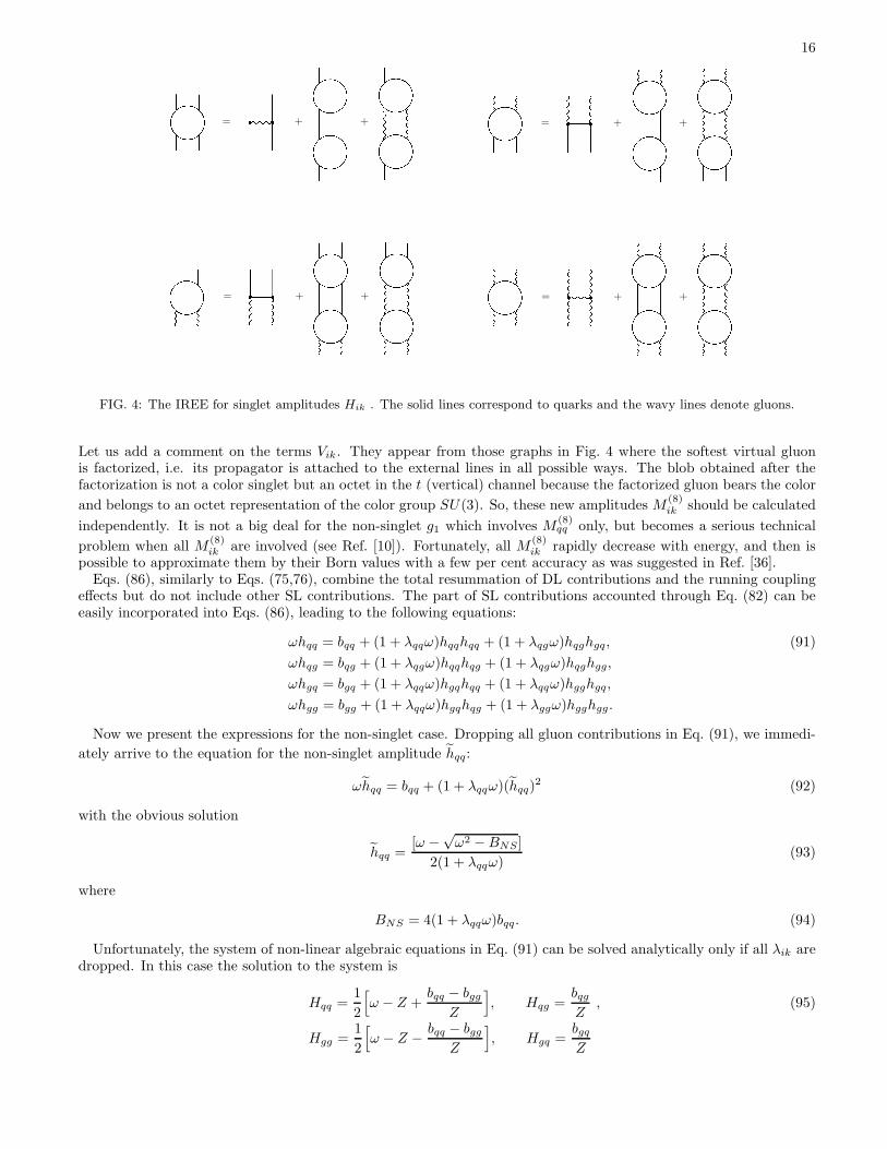
The reason for the replacement of A(ω) by A′(ω) is that the argument of αs in Lqg and Lgq is space-like, so the couplingdoes not lead to π -terms. The next term in the rhs of the IREE are the convolutions of the anomalous dimensionsappearing as the convolution in Eqs. (75,76). At last, the rhs contains the contribution from the factorization of thesoft (Sudakov) gluons. We account for this contribution approximately (see Ref. [11]) for more details. Eventuallywe arrive at the system of IREE for the singlet anomalous dimensions Hik represented in Fig. 4. In the case of thenon-singlet anomalous dimension, all gluon contributions in Eq. (86) should be dropped. Rewriting Fig. 4 in a detailedform, we arrive at the system of the algebraic non-linear equations for Hik :

ωHqq = bqq +HqqHqq +HqgHgq, ωHqg = bqg +HqqHqg +HqgHgg, (86)

ωHgq = bgq +HgqHqq +HggHgq, ωHgg = bgg +HgqHqg +HggHgg .

where we have denoted

bik = aik + Vik, (87)

with aik given by Eq. (84). Then

Vik =mik

π2D(ω) , (88)

mqq =CF

2N, mgg = −2N2 , mgq = nf

N

2, mqg = −NCF , (89)

and

D(ω) =1

2b2

∫ ∞

0

dρe−ωρ ln((ρ+ η)/η

)[ ρ+ η

(ρ+ η)2 + π2+

1

ρ+ η

]. (90)

16

= +

+

= +

+

= +

+

= +

+

FIG. 4: The IREE for singlet amplitudes Hik . The solid lines correspond to quarks and the wavy lines denote gluons.

Let us add a comment on the terms Vik. They appear from those graphs in Fig. 4 where the softest virtual gluonis factorized, i.e. its propagator is attached to the external lines in all possible ways. The blob obtained after thefactorization is not a color singlet but an octet in the t (vertical) channel because the factorized gluon bears the color

and belongs to an octet representation of the color group SU(3). So, these new amplitudes M(8)ik should be calculated

independently. It is not a big deal for the non-singlet g1 which involves M(8)qq only, but becomes a serious technical

problem when all M(8)ik are involved (see Ref. [10]). Fortunately, all M

(8)ik rapidly decrease with energy, and then is

possible to approximate them by their Born values with a few per cent accuracy as was suggested in Ref. [36].Eqs. (86), similarly to Eqs. (75,76), combine the total resummation of DL contributions and the running coupling

effects but do not include other SL contributions. The part of SL contributions accounted through Eq. (82) can beeasily incorporated into Eqs. (86), leading to the following equations:

ωhqq = bqq + (1 + λqqω)hqqhqq + (1 + λqgω)hqghgq, (91)

ωhqg = bqg + (1 + λqgω)hqqhqg + (1 + λqgω)hqghgg,

ωhgq = bgq + (1 + λqqω)hgqhqq + (1 + λqqω)hgghgq,

ωhgg = bgg + (1 + λqqω)hgqhqg + (1 + λggω)hgghgg.

Now we present the expressions for the non-singlet case. Dropping all gluon contributions in Eq. (91), we immedi-

ately arrive to the equation for the non-singlet amplitude hqq:

ωhqq = bqq + (1 + λqqω)(hqq)2 (92)

with the obvious solution

hqq =[ω −

√ω2 −BNS ]

2(1 + λqqω)(93)

where

BNS = 4(1 + λqqω)bqq. (94)

Unfortunately, the system of non-linear algebraic equations in Eq. (91) can be solved analytically only if all λik aredropped. In this case the solution to the system is

Hqq =1

2

[ω − Z +

bqq − bgg

Z

], Hqg =

bqg

Z, (95)

Hgg =1

2

[ω − Z − bqq − bgg

Z

], Hgq =

bgq

Z

17

where

Z =1√2

√(ω2 − 2(bqq + bgg)) +

√(ω2 − 2(bqq + bgg))2 − 4(bqq − bgg)2 − 16bgqbqg . (96)

The non-linear algebraic equations in Eq. (92) and Eq. (86) have more than one solution, however the solution chosenin Eqs. (93,95) obeys the matching condition

hqq → aqq/ω, Hik → HBornik = aik/ω (97)

at ω → ∞, with aik given by Eq. (84) . In other words, this matching condition in Eq. (97) implies that theseamplitudes are represented at low energies by their Born values. Indeed, from Eq. (34) high energies correspond tosmall ω and vice versa.

VII. SOLUTION TO THE IREE (80) FOR g1 NON-SINGLET

As soon as the expressions for hqq are obtained, one can easily find the general solution to the linear differentialequation (80) for the Mellin amplitude FNS. As the procedure between the non-singlet and singlet cases has a purelytechnical difference, we consider in detail the former case and proceed to the singlet case in a much shorter way.

A. General solution to the non-singlet equation (80)

Obviously, the general solution to Eq. (80) is

FNS = FNS(ω)e−ωy+y(1+λω)ehqq (98)

and therefore

TNS(x,Q2) =

∫ ı∞

−ı∞

dω

2ıπ

(w/µ2

)ω

FNS(ω)e−ωy+y(1+λqqω)ehqq =

∫ ı∞

−ı∞

dω

2ıπ(1/x)ωFNS(ω)ey(1+λqqω)ehqq (99)

with FNS(ω) being arbitrary. In order to specify it, we use the matching condition

TNS(x,Q2) = TNS(w/µ2) (100)

when y = 0. The new amplitude TNS(w/µ2) describes again the forward Compton scattering off the same quark,

however the virtual photon has now a virtuality ≈ µ2. The IREE for TNS(w/µ2) should be obtained independently.

B. Composing the IREE for eT NS(w/µ2).

The IREE for TNS(w/µ2) is similar to the IREE for TNS(x,Q2), Eq. (73). It has the same structure and involvesthe same amplitude Mqq. Still, it differs from Eq. (73) because of two following points:

(a) TNS(w/µ2) does not depend on Q2, so the differential IREE for it does not involve ∂/∂y;

(b) the Born amplitude TNSBorn(w/µ2) can be obtained from TNS(x,Q2), putting Q2 = µ, so its contribution does not

vanish under differentiation with respect to µ. Then introducing the Mellin amplitude FNS(ω) related to TNS(w/µ2)through the transform (34), we arrive at the following IREE:

ωFNS(ω) = (e2q/2) + (1 + λqqω)hqqFNS(ω). (101)

and therefore

FNS(ω) =(e2q/2)

ω − (1 + λqqω)hqq(ω)(102)

18

C. Expression for gNS1 in the Region B

Combining Eqs. (102, 98) and (37) and convoluting the perturbative expression with the initial quark densityimmediately leads to

gNS1 =

e2q2

∫ ı∞

−ı∞

dω

2πı

( wµ2

)ω ωδq(ω)

ω − (1 + λqqω)hqq(ω)e−ωy+yehqq (103)

=e2q2

∫ ı∞

−ı∞

dω

2πı

( 1

x

)ω ωδq(ω)

ω − (1 + λqqω)hqq(ω)eyehqq

where δq(ω) is the initial quark density in ω -space. Confronting Eq. (103) to Eq. (17) it is clear that

hNS(ω) = (1 + λqqω)hqq(ω) = (1/2)[ω −

√ω2 −BNS(ω)

](104)

is the new non-singlet anomalous dimension. It contains the total resummation of DL contributions together withthe running αs effects and a part of SL contributions as explained in the previous Sect. Similarly,

CNS =ω

ω − (1 + λqqω)hqq(ω)=

ω

ω − hNS(ω)=

2ω

ω +√ω2 −BNS(ω)

(105)

is the new non-singlet coefficient function. It is expressed through the anomalous dimension and therefore incorporatesthe same kind of logarithmic contributions. Eventually we arrive at the final expression for gNS

1 in the region B oflarge Q2 and small x:

gNS1 (x,Q2) =

e2q2

∫ ı∞

−ı∞

dω

2πıx−ω CNS(ω) δq(ω) ehNS(ω) ln(Q2/µ2). (106)

VIII. SOLUTION TO THE IREE (76) FOR THE SINGLET g1

Eq. (76) for gS1 can be solved in a similar way as the IREE for gNS

1 . First a general solution should be obtainedand then constrained with a boundary condition. The general solution is easy to obtain:

Fq = e−ωy[C(+)eΩ(+)y + C(−)eΩ(−)y

], (107)

Fg = e−ωy[C(+)X +

√R

2HqgeΩ(+)y + C(−)X −

√R

2HqgeΩ(−)y

]

where

X = Hgg −Hqq (108)

and

R = (Hgg −Hqq)2 + 4HqgHgq . (109)

We remind that the anomalous dimensions Hik are found in Eq. (95). The exponents Ω(±) are also expressed in termsof Hik :

Ω(±) =1

2

[Hqq +Hgg ±

√(Hgg −Hqq)2 + 4HqgHgq

]. (110)

Finally the quantities C(+) and C(−) have to be specified.In order to constrain Eq. (107) we use the matching condition at Q2 = µ2:

Fq(ω,Q2 = µ2) = C(+) + C(−) = Fq(ω) , (111)

Fg(ω,Q2 = µ2) = C(+)X +

√R

2Hqg+ C(−)X −

√R

2Hqg= Fg(ω) .

19

The new Mellin amplitudes Fq,g(ω) correspond to the forward Compton scattering, when the photon virtuality is µ2.They should be found independently. We again proceed by using new IREE for them. They have a structure similarto Eq. (76). The difference is that the new equations do not contain derivatives with respect to y and account for theBorn contributions

FBornq =

< e2q >

ω, FBorn

g = 0 , (112)

where < e2q > is the standard notation for the averaged e2q. So, the IREE for amplitudes Fq,g are

ωFSq =< e2q > hqq(ω) FS

q (ω) + hgq(ω) FSg (ω, y) , (113)

ωFSg = hqg(ω) FS

q (ω) + hgg(ω) FSg (ω)

and the solution to Eq. (113) is

FSq = < e2q >

ω −Hgg

ω2 − ω(Hqq +Hgg) + (HqqHgg −HqgHgq), (114)

FSg = < e2q >

Hgq

ω2 − ω(Hqq +Hgg) + (HqqHgg −HqgHgq).

Combining Eqs. (114) and (111), we obtain the explicit expressions for C(±):

C(+) = < e2q >2HgqHqg − (X −

√R)(ω −Hgg)

2√R[ω2 − ω(Hqq +Hgg) + (HqqHgg −HqgHgq)]

, (115)

C(−) = < e2q >−2HgqHqg + (X +

√R)(ω −Hgg)

2√R[ω2 − ω(Hqq +Hgg) + (HqqHgg −HqgHgq)]

.

Introducing the initial quark and gluon densities δq and δg respectively and using Eq. (37), we finally arrive at thefollowing expression for gS

1 in region B:

gS1 (x,Q2) =

1

2

∫ ı∞

−ı∞

dω

2πı

(1

x

)ω[(C(+)eΩ(+)y + C(−)eΩ(−)y

)ωδq(ω) + (116)

(C(+) (X +

√R)

2HqgeΩ(+)y + C(−) (X −

√R)

2HqgeΩ(−)y

)ωδg(ω)

].

where δq(ω) and δg(ω) are the initial quark and gluon densities in the ω -space. C(±)q (ω) and C

(±)g (ω) are the singlet

coefficient functions calculated in LLA. The exponents Ω(±) are expressed in terms of Hik in the same way as theDGLAP exponents are related to the DGLAP anomalous dimensions. So, we conclude that Hik are the anomalousdimensions for gS

1 in LLA. The total resummation of DL contributions to the singlet g1 under the approximation offixed αs was done in Ref. [10]. This result was used in Ref. [37] where αs was running: αs = αs(Q

2) according tothe renorm group concept. However, in Sect. IV we showed that this parametrization does not stand at the small-xregion and should be changed by the parameterizations of Eqs. (47,85). The application of the expressions for g1 inEqs. (106,116) and the study of their impact on the Bjorken sum rule can be found in Ref. [38].

IX. ASYMPTOTICS OF THE NON-SINGLET g1 IN THE REGION B

The expressions Eqs. (106,116) represent g1 in the region B. Before discussing them in detail, we consider firsttheir asymptotics at fixed Q2 ≫ µ2 and x → 0. Strictly speaking, such asymptotics can be obtained by applyingthe saddle-point method. When the small-x behaviour is proved to be of the Regge type (power-like), one can use ashort cut by finding the position of the leading (rightmost) singularity in the ω -plane. Of course, such singularitiescan be different for gNS

1 and gS1 and should be found independently. In the present Sect. we consider the small -x

asymptotics of the non-singlet g1.

20

A. Asymptotic scaling

Let us assume that the initial quark density δq in Eq. (106) is non-singular in x at x→ 0, so it does not contributeto the small- x asymptotics. Then by applying the saddle-point method to Eq. (106) one deals with the non-singletcoefficient function and the anomalous dimension only. In this case the stationary point is (see Appendix E for details)

ω0 =√BNS

[1 + (1 − κ)2(y/2 + 1/

√BNS)2/(2 ln2 ξ)

], (117)

with

κ = d√B/dω|ω=ω0 (118)

and y = ln(Q2/µ2), ξ =√Q2/(x2µ2).

It immediately leads to the Regge asymptotics for the non-singlets:

gNS1 ∼

e2q2δq(ω0)ΠNSξ

ω0/2, (119)

with

ΠNS =

[2(1 − κ)

√BNS

]1/2(y/2 + 1/

√BNS

)

π1/2 ln3/2 ξ. (120)

When in Eq. (117) y ≪ 2/√BNS(ω) (let us notice in advance that at ω = ∆NS it means that y ≪ 150 µ2), the

value of ω0 does not depend on y at all. Therefore Eq. (119) can be rewritten as:

gNS1 (x,Q2) ∼ (e2q/2)δq(ω0)cNSTNS(ξ) (121)

with

TNS(ξ) = ξω0/2/ ln3/2 ξ. (122)

The factor cNS is

cNS =[2(1 − κ)/(π

√BNS)

]1/2

(123)

and does not depend on y. Eq. (121) predicts the scaling behavior for the non-singlet structure functions: in theregion Q2 ≪ 150µ2, with T (±) depending on one argument ξ instead of x and Q2 independently. Therefore in thisregion

gNS1 ∼ gNS

1 ≡ ΠNS(ω0)δq(ω0)(Q2/x2µ2

)ω0/2(124)

at x→ 0, with ω0 being the largest root of Eq. (125):

ω2 −BNS = 0. (125)

We call the result of Eq. (124) asymptotic scaling: gNS1 asymptotically depends on one variable Q2/x2 only, instead

of two variables x and Q2. The DGLAP prediction for the asymptotics of gNS1 in Eq. (132) is quite different. Below

we compare these results in detailAccording to the results of Ref. [14] (see also Appendix E), in the opposite case, when Q2 & 150 µ2, the rightmost andnon-vanishing at w → ∞ stationary point is again given by Eq. (125) but the pre-exponential factor ΠNS essentiallydepends on y, so the asymptotic scaling in this region holds for gNS

1 /y.Let us notice that the sign of the non-singlet asymptotic behaviour is positive when δq(ω0) is positive and coincideswith the sign of gNS

1 in the Born approximation. In other words, both the x and Q2 -evolutions do not affect the signof gNS

1 . Now we focus on solving Eq. (125).

21

B. Estimate for the non-singlet intercept

In a more detailed form, equation Eq. (125) is

ω2 − (1 + λqqω)[(2CF

πb

)( η

η2 + π2−

∫ ∞

0

dρe−ωρ

ρ2 + π2

)+ (126)

(2CF

πb

)2 1

4NCF

∫ ∞

0

dρe−ωρ ln((ρ+ η)/η)( ρ+ η

(ρ+ η)2 + π2+

1

ρ+ η

)]= 0

where we have used the notation η = ln(µ2/Λ2). Let us remind that in the case of fixed αs Eq. (126) is much simplerand can be solved analytically:

ω2 − 2αsCF

π−

(2αsCF

π

)2 1

ω24NCF= 0, (127)

with the obvious solution ωDL0 given by the following expression[10]:

ωDL0 = (2αsCF /π)1/2

√1

2

[1 +

(1 +

4

N2 − 1

)1/2]. (128)

In contrast, Eq. (126) cannot be solved analytically. Besides, there is a big qualitative difference between the cases offixed and running αs. Although the IR cut-off µ is used for regulating the IR divergencies in both cases, Eq. (127) isfree of any µ -dependence whereas Eq. (126) is obviously µ -dependent and therefore the solution ω0 also depends onµ: ω0 = ω0(µ). The value of µ is restricted by Eq. (40) only. As a result, we arrive at the solution to Eq. (126) in theform of the curve plotted in Fig. 5. Eq. (126) shows that ω0 depends on µ through η, therefore ω0 depends on the

10 100

0.1

0.2

0.3

0.4

0.5 ω0

1

2

3

4

µ/Λ

FIG. 5: Dependence of the intercept ω0 on infrared cutoff µ : 1– for F NS1 ; 2– for gNS

1 ; 3– and 4– for F NS1 and gNS

1 respectivelywithout account of π2-terms. The structure function F NS

1 is discussed in the Appendix B.

ratio µ/Λ and on nf . Besides the η -dependence, ω0 is not sensitive to the value of Λ. The plot in Fig. 5 shows thatthe curve ω0 = ω0(µ) rapidly grows at µ . Λ, however this region contradicts Eq. (40), so the perturbative expression(38) for αs cannot be used at so small µ. Both Eq. (126) and the plot in Fig. 5 are consistent in the region (40) onlyand should not be considered out of this region. Eq. (126) has one maximum in region (40):

∆NS ≡ max[ω0

]= ω0(µNS) = 0.42 (129)

at

µ = µNS ≡ Λe2.3 ≈ 10Λ. (130)

22

For the sake of simplicity we chose in Ref. [11] nf = 3 and Λ = 0.1 GeV. It would have been more realistic to chooseΛ = 0.5 GeV, and Eq. (130) shows that such a change of Λ leads to multiply by a factor of 5 the values of µ for thesinglet and non-singlet obtained in Ref. [11]. Comparison of the curves 1 and 2 in Fig. 5 to the curves 3 and 4 showsthat the important role played by the π2 -terms in αs (i.e. respecting the analyticity) for producing a maximum inthe curves and 2. Furthermore in the vicinity of this maximum, the power expansion

ω0(µ) = ω0(µNS) +dω0(µNS)

dµ(µ− µNS) +

1

2

d2ω0(µNS)

dµ2(µ− µNS)2 + ... (131)

does not contain the linear term, so ω0(µNS) ≡ ∆NS is much less dependent on µ than all other points on the curves1 and 2. This remarkable feature allows us to identify ∆NS as the best candidate5 for the perturbative estimate ofthe genuine intercept of the non-singlet g1. According to the prediction of the Regge approach, the genuine interceptshould be a constant, with no other dependence. However, Eq. (126) and its solution (129) account for the leadinglogarithmic contributions only and leave aside sub-leading perturbative contributions and possible non-perturbativeones, so it is hardly possible to identify (129) with the genuine intercept. Nevertheless, it turned out that our estimate(129) is in a good agreement with the results of Ref. [39] obtained by fitting all available experimental data. Thisleads to a very interesting conclusion: by some unknown reason all sub-leading and non-perturbative contributions tothe non-singlet intercept happen to be either small or irrelevant at µ = µNS , so that the LLA prediction (129) provesto be a good estimate for the non-singlet intercept. Motivated by this result, we call µNS the Optimal non-singletmass scale. However, it is worth stressing that this scale is an artefact of our approach and should disappear whennon-perturbative contributions (also dependent on the same scale) would be accounted for. To conclude, let us noticethat the Regge form of the small-x asymptotics of g1 is the direct consequence of the total resummation of logarithmsof x and cannot appear at fixed orders in αs. This small-x asymptotics depends on Q2 only through the factor(Q2/µ2)∆NS/2 (see Eq. (124)). In particular it means that the intercept ∆NS has no dependence on Q2. On the otherhand, the well-known DGLAP small- x asymptotics

gNS DGLAP1 ∼ exp

[√2CF

πbln(1/x) ln

( ln(Q2/Λ2)

ln(µ2/Λ2)

)]. (132)

can also be obtained (see Appendix F for detail) with the saddle-point method providing the initial parton densitiesare not singular at x→ 0 (In Sect. XII we consider the alternative case presently used in the Standard Approach forthe analysis of experimental data at small x). The DGLAP -asymptotics (132) clearly does not exhibit the Reggebehavior. The same is true for the case where the anomalous dimensions and coefficient functions are calculated inhigh but fixed orders in αs which would correspond to the NN..NLO DGLAP accuracy (see Appendix G for detail).In principle, one might think that a generalization of Eq. (132) could lead to the Regge asymptotics, however with theintercept depending on Q2. We show now that there are no theoretical grounds for such a scenario. Indeed, it followsfrom Eq. (F7) that the Q2 -dependence in Eq. (132) is the consequence of the use of the DGLAP -parametrizationαs = αs(k

2⊥) and the DGLAP -ordering (13). As explained in detail in Appendix F, at small x this ordering should be

changed by the ordering (14). Then the upper limit Q2 in Eq. (13) in the small-x region should be modified to w (seeRef. [27] for detail). After that the DGLAP asymptotics will not depend on Q2 but at the same time will not have aRegge-type form. The Regge asymptotics is achieved by accounting for the resummation of the leading logarithms ofx. It exhibits an asymptotic behavior much steeper than the DGLAP result (132), not only with respect to x but alsowith respect to Q2. The comparison of Eq. (132) to Eq. (124) shows that gNS DGLAP

1 /gNS1 → 0 when x → 0. The

question however arises: how small should x be in order to allow our asymptotic expression Eq. (124) to representgNS1 reliably? We answer this question below.

C. Applicability region of the small-x asymptotics

The asymptotic expression (124) for gNS1 is obviously much simpler than the integral representation (106) and also

much easier to work with. However, it is valid for very small x only. In order to determine when Eq. (124) reliablyrepresents Eq. (106), let us study numerically the ratio

RNSas (x,Q2) =

gNS1 (x,Q2)

gNS1 (x,Q2)

(133)

5 We are grateful to P. Castorina for this very useful observation.

23

at fixed Q2 and different values of x. The result is plotted in Fig. 6. According to it, gNS1 is reliably represented

10-3 10-4 10-5 10-6 10-7 10-8

0.2

0.4

0.6

0.8

110-3 10-4 10-5 10-6 10-7 10-8

x

RNSas

1

2

FIG. 6: Rate of the gNS1 approach to asymptotics for different Q2: solid curve 1 for Q = 10µ , solid curve 2 for Q = 100µ ,

dashed curve for Q = µ.

by its asymptotic expression gNS1 (x,Q2) at x . 10−6 only. So, strictly speaking, Eq. (124) should not be used at

available values of x. However, in the literature one can find that Regge type (∼ x−a) fits of the experimentaldata are used at much larger values of x, and such fits are reported to work well. We suggest a simple explanationto this: the phenomenological parameterizations including the Regge type fits have nothing in common with theexpression in Eq. (124) obtained with the saddle-point method. In order to use such parameterizations at relativelylarge values of x (at x ≫ 10−6), one can choose the exponents a in the fits greater than the genuine intercepts. Ananalysis of such Regge parameterizations can be found in Ref. [13]. To conclude, we also notice also that sometimesRegge parameterizations are used with intercepts depending on Q2: they have no theoretical ground and contradictEq. (124).

X. SMALL-x ASYMPTOTICS OF THE SINGLET g1 IN THE REGION B

The small- x asymptotics of gS1 in the region B can be obtained quite similarly to the non-singlet case, by applying

the saddle-point method to Eq. (116). The singlet asymptotics also exhibits the Regge behavior:

gS1 (x,Q2) ∼ (1/x)ω0(Q2/µ2)ω0/2[A(ω0)δq(ω0) +B(ω0)δg(ωo)] (134)

where ω0 is the stationary point and A, B include the asymptotic form of the coefficient functions. The position ofthe leading singularity corresponds the largest root of the equation

(ω2 − 2(bqq + bgg))2 − 4(bqq − bgg)

2 − 16bgqbqg = 0. (135)

Similarly to the non-singlet case, the position of the singlet leading singularity depends on µ, with one maximum

ωS0 ≡ ∆S = 0.86 (136)

achieved at (we choose again nf = 3)

µ = µS ≈ Λe4 ≈ 55Λ (137)

which gives µS/Λ ≈ 55 GeV when Λ = 0.1 GeV. By repeating the arguments given also in the previous Sect., wecall ∆S the singlet intercept and call µS the Optimal singlet mass scale. The Optimal singlet and non-singlet massscales are quite different. Our perturbative estimate (136) is also in a very good agreement with the result obtainedin Ref. [40] by fitting the experimental data. Eq. (134) shows that the asymptotic scaling is also valid for the singletg1: asymptotically gS

1 depends on one argument Q2/x2 only. In contrast to the case of the non-singlet asymptotics(124), the interplay between δq and δg can affect the sign of gS

1 . Indeed, in the Born approximation gS1 > 0 but it

can be negative (positive) asymptotically depending on the sign of Aδq +Bδg in Eq. (134).

24

XI. APPLICABILITY REGION OF THE IREE METHOD

In this Sect. we discuss the region of applicability of our approach and also answer a claim on a possible contradictionin our method that we have got in the past: in the IREE technology that we use to sum up the leading logarithmswe work in the ω -space and systematically keep ω small. On the other hand when we calculate the non-singlet andespecially the singlet intercepts, they are found not so small. Therefore we should guarantee the validity of our methodnot only at small but also at large ω. We start from the conventional analysis of the double-logarithmic QCD powerseries (138), so we would like to stress at once that the use of (138) for analysis of QCD processes and all estimates(e.g. the one in Eq. (139)) based on it originate from the QED results (see e.g. Ref. [9]) where the running couplingeffects can be neglected. They can become unreliable in QCD and therefore these conventional estimates should bereplaced by more accurate estimates which we present in this Sect.

Now let us remind the basic principle of the Leading Logarithmic Approximation, and DLA in particular. Thestraightforward calculation of the Feynman graphs contributing to a certain quantity (for instance, to the non-singlet coefficient) yields the double-logarithmic contributions. In the n-th order of the perturbation theory they are∼ αn

s ln2n(1/x). For the sake of simplicity we keep here αs fixed and leave out other numerical parameters like 1/π,color factors, etc. Accounting for the running coupling effects and sub-leading logarithmic contributions does notchange the essence of the problem. The series of such contributions, for example

c1αs ln(1/x) + c2α2s ln3(1/x) + c3α

4s ln5(1/x) + ... (138)

converges when αs ln2(1/x) < 1 only. It brings us to a rough estimate for the lowest limit for x:

x > xmin = exp[−1/√αs]. (139)

On the other hand, it is interesting to know the result of the total resummation of the DL terms at really smallx < xmin and even at x → 0. The reason is that the DL terms are not so large compared to other contributions atx & xmin but dominate at small x. However, the series in Eq. (138) diverges at x < xmin and cannot be summed upin this region. The solution to this problem is well-known: in the first place the series Eq. (138) should be summedup at x > xmin and then the result of the resummation can be analytically continued into the region x < xmin. Letus notice that the series Eq. (138) becomes divergent in region x < xmin and is called an asymptotic series. In the ω-space the series Eq. (138), according to the relation

∫ ı∞

−ı∞

dω

2πıeω ln(1/x) 1

ω1+2n=

1

(2n)!ln2n(1/x), (140)

is given by:

c1α

ω2+ c2

α2

ω4+ c3

α3

ω6+ ... (141)

This series converges when, roughly,

ω > ωmin =√αs (142)

whereas the DL terms becomes large at ω < ωmin. To be specific, let us notice that the expressions for the coefficientfunctions in Eqs. (105,115) represent the total sum of the DL contributions. Strictly speaking, the coefficient functionsshould first be calculated for large ω: ω > ωmin (where the DL contributions are small) and then continued to theregion of small ω. However, anticipating the analytical continuation into the small -ω region, quite often a shortcut is taken and we follow this way: we treat ω as small since the beginning. It gives us the reason to neglect allnon-logarithmic corrections regardless of their relatively large values in the region (142). After the total resummationof the DL terms has been done, the formulae obtained are insensitive to the value of ω and therefore can be used atany x. The resummed expressions (105,115) contain new singularities ω0 (branching points in our case but, generally,they can also be poles), which are absent in the series (141). The rightmost singularities, i.e. the intercepts (∆NS and∆S in our case), determine the range of convergence of the series Eq. (138) instead of

√αs: the series (141) converges

only if

ω > ∆, (143)

with ∆ being the intercept. However, after the total resummation in (141) has been performed, the result of theresummation can be used at arbitrary values of ω. To conclude, we note that all equations for the resummation ofthe leading logarithms, and in particular the IREE we have used, are not the equations for finding the intercepts.Indeed, the intercepts are the singularities and the values of ω in the IREE should be kept pretty far away from themby definition. The intercepts appear in the asymptotic expressions and therefore they should be found independentlyof the resummation methods, usually by applying the saddle-point method.

25

XII. COMPARISON OF g1 TO gDGLAP1 IN THE REGION B

In this Sect. we compare our results (106,116) to the DGLAP expressions for g1 at small x. We are not going touse here the asymptotic expressions in Eqs. (124,134) or (132), but we compare the two approaches at small but finitex. First we will compare the basic ingredients of the expressions for g1: the anomalous dimensions and the coefficientfunctions. Whenever it is possible, we will consider in detail, for the sake of simplicity, the non-singlet g1 and morebriefly generalize our results to the case of gS

1 .

A. Comparison of the coefficient functions and the anomalous dimensions

Eqs. (106) and (17) have a similar structure: each integrand contains the initial parton density, the coefficientfunction and the exponent with the non-singlet anomalous dimension to govern the Q2 -evolution. However, CNS

and hNS in Eq. (106) contain the total resummation of the leading logarithms of x whereas in Eq. (17) the coefficientfunction and the anomalous dimension are considered to LO and NLO accuracy, namely they are given in Eqs. (18,20).Originally DGLAP was suggested for studying the region A of large x and large Q2. Due to the oscillating factorx−ω in the Mellin integrals, the main contribution to g1 in the region B comes from small ω. On the contrary, themain contribution in region A comes from large ω. At large ω, the expressions for CNS and hNS in Eq. (106) can beexpanded into a converging series in 1/ω:

CNS = 1 +A(ω)CF

2π

[ 1

ω2+

1

2ω

]+ ..., (144)

hNS =A(ω)CF

2π

[ 1

ω+

1

2

]+ ... (145)

Obviously we observe a large discrepancy between Eqs. (144,145) and the LO DGLAP expressions in Eqs. (18,20).However, this discrepancy almost disappears when we come back to the region B where ω is small and therefore regularterms ∼ ωk in Eqs. (18,20) can be dropped. The remaining discrepancy is due to the different treatment of the QCDcoupling. When the starting point of the Q2 -evolution obeys Eq. (40), then A(ω) with very good approximationcan be replaced by αs(k

2⊥/x), but definitely not by αs(k

2⊥). Taking into account more terms in the series and adding

them to Eqs. (144,145) does not change the situation. So, we conclude that in region B the first and second terms ofthe 1/ω -expansion of Eqs. (104,105) reproduce the most important LO and NLO DGLAP results in the non-singletanomalous dimension and coefficient function, with the exception of the different treatment of the QCD coupling.Expanding Eqs. (95,115) into a series in 1/ω and comparing the result to the singlet DGLAP anomalous dimensionsand coefficient functions, we arrive at the same conclusion.

B. Numerical comparison of the x -evolutions in Eqs. (17) and (106)

The integrands in Eqs. (17) and (106) for the non-singlet g1 contains also a phenomenological ingredient: the initialquark densities δq. Let us introduce the ratio

RNS =gNS1

gNS DGLAP1

(146)

and study its x -dependence at fixed Q2, for example at Q2 = 10 GeV2. Obviously, this cannot be done until δq isfixed. The choice

δq(x) = Nqδ(1 − x) (147)

corresponds to approximate the initial hadron by a quark and to neglect all influence of the hadron structure. Ofcourse, such a choice cannot be used for phenomenological applications, but it makes possible to compare the x-evolutions in Eqs. (17) and (106). The substitution of the bare quark input into Eqs. (17) and (106) leads to the x-dependence of RNS plotted in Fig. 7. This shows that the impact of the leading logarithms becomes quite sizable atx0 ≈ 10−2. So, we arrive to a sort of puzzle:

According to the different behaviour of the x -evolution in Eqs. (17) and (106), the DGLAP -description of gNS1

should have failed for x < 10−2, but phenomenologically it is well-known that DGLAP works well at x < 10−2. Thesolution to this puzzle is given below.

26

10-1 10-2 10-3 10-4 10-5

0.5

1

1.5

2

2.5

3

3.5

4

x

RNS

FIG. 7: Rise of RNS of Eq. (146) at small x in case of bare quark input and for Q2 = 10 GeV2.

C. The role of the initial parton densities

In order to clarify the problem, let us consider in more detail a standard fit to the initial quark density, as inEq. (201):

δq(x) = Nqx−α(1 − x)β(1 + γxδ) ≡ Nqx

−αϕ(x).

with all parameters Nq, α, β, γ, δ being positive. As the fit is defined at certain fixed values of x = x0 and Q2 = Q20,

all its parameters depend on x0, Q20. We define Nq as the normalization. As the term x−α → ∞ when x → 0, we

call it the singular term, although the fit is introduced at large x. We call ϕ the regular part of the fit because ϕ→ 1when x→ 0. Once transformed into the ω -space, the fit becomes a sum of pole contributions:

δq(ω) = Nq

[(ω − α)−1 +

∞∑

k=1

(mk(ω + k − α) + γ(ω + k + δ − α)−1

)](148)

where mk = β(β − 1)...(β − k + 1)/k!. The first pole in Eq. (148) corresponds to the singular term x−a in Eq. (24).We call it the leading pole. The other, non-leading poles in Eq. (148) originate from the interference between ϕ(x)and x−a. Substituting Eq. (148) into the DGLAP expression (17), we see that the contribution of the leading pole,gNS DGLAP1 to gNS DGLAP

1 is (we drop the NLO contribution here)

gNS DGLAP1 (x,Q2) =

e2q2Nq

(1

x

)α

CNS DGLAP (α)( ln(Q2/Λ2)

ln(µ2/Λ2)

)γ(0)(α)/(2πb)

. (149)

Substituting the other terms of Eq. (148) into Eq. (17) it leads to a contribution quite similar to that in Eq. (149),however with α → αk = α − k and α − k − 1. Obviously, α > αk. Therefore gNS DGLAP

1 in Eq. (149) is really theleading contribution to gNS DGLAP

1 at small x and actually it represents the small- x asymptotics of gNS DGLAP1 .

Confronting Eq. (149) to the very well-known expression (132) for the DGLAP asymptotics, we see that they aretotally different. The singular terms are also included into the DGLAP parametrization of the singlet parton densities.It leads to the steep growth of g1 at small x and provides the reason for the agrement between the DGLAP -descriptionof the structure functions and the experimental data. Therefore the DGLAP success st small x is related to the use ofsingular fits for the initial parton densities.This is the solution to the puzzle. Now let us discuss the most importantconsequences of this result.

First, let us confront the asymptotics of Eqs. (149) and (124). We see that the x -dependence in these expressions isidentical: both formulae exhibit the Regge (power-like) behavior. It allows us to conclude that the singular term x−α

in the standard DGLAP fits mimics the total resummation of the leading logarithms of x. Therefore, the singularfactors can be dropped when the total resummation of the leading logarithms of x is accounted for. In order to show itexplicitly, let us study numerically RNS , using the standard DGLAP fit of Eq. (24). The results are plotted in Fig. 8.We can observe that RNS is pretty close to unity only when the fit (24) is used in the expression for gNS DGLAP

1 ,whereas only the regular part, ϕ, of the fit is used in the resummed expression (106). All other options drive RNS faraway from unity at small x. So, the resummation of the leading logarithms leads to simplify the standard fits. Fig. 8

27

10-1 10-2 10-3 10-4 10-5

0.25

0.5

0.75

1

1.25

1.5

1.75

2

x

RNS

1

2

3

FIG. 8: Examples of the small x -behaviour of RNS for different singular terms in the initial quark distribution fits of Eq. (24):α = 0 (curve 1), α = 0.576 (curve 2), α = 0.36 (curve 3). All curves correspond to Q2 = 10 GeV2, and involve only a regularpart, ϕ, in the parametrization of the initial quark density used for g1 of Eq. (106).

explicitly demonstrates that the singular fit (24) and the total resummation of the logarithms lead to close valuesof g1 in region B. From a practical point of view, the use of the resummation is preferable because it allows one toconstruct new fits with a reduced number of parameters. From the theoretical point of view, the resummation is evenmore preferable. Indeed, the DGLAP intercept α in Eq. (149) depends on the starting point x0, Q

20, where α is fixed,

and such a dependence can hardly be deduced from theoretical considerations. On the contrary, the intercept ∆NS

in Eq. (124) is independent of the initial parton densities.Now we would like to comment on an apparent puzzle arising first from the results of Refs. [5, 41] and then also in

other subsequent publications (see e.g. the recent review [42]):On one hand, the direct comparison in Ref. [41] of the NLO DGLAP result, gNS DGLAP

1 to the expression for gNS1

obtained in Ref. [10] in the limit of fixed αs showed that

gNS1 /gNS DGLAP

1 ≪ 1 (150)

at the small values of x available in experiment and therefore the conclusion was made that the resummation oflnk(1/x) can yield a small impact. On the other hand, it is clear that the small-x asymptotics (124) is much steeperthan the well-known DGLAP asymptotics (132), which proves that asymptotically

gNS1 /gNS DGLAP

1 ≫ 1 (151)

and therefore the total resummation of lnk(1/x) should be essential. So, Eqs. (150) and (151) obviously contradicteach other, which is puzzling.

Eq. (150) was interpreted in the literature as follows: the resummation of leading logarithms at values of x availablein experiment is much less important than the impact of the sub- leading (compared to the double-logarithmiccontributions) terms in the DGLAP coefficient functions and anomalous dimensions.However, a close inspection of Eqs. (24,148) for the standard fit suggests another solution to this puzzle. Fig. 8clearly demonstrates that the main impact on the small-x behavior of gNS DGLAP

1 comes not from the NLO DGLAPcoefficient functions but from the singular term x−α in Eq. (24). Indeed, when this factor is removed from Eq. (24),we arrive at curve 1 despite the sub-leading contributions are accounted in gNS DGLAP

1 . Therefore, their impact leadsto Eq. (151) instead of Eq. (150). On the contrary, when the singular term is accounted for, we arrive at curve 2where RNS ∼ 1. It proves that the conclusion of the extreme importance of the sub-leading contributions on thesmall-x behavior of g1 advocated in Refs. [37, 41] is groundless. Now let us compare the small-x asymptotics of gNS

1

and gNS DGLAP1 . Parameters α in the DGLAP fits obey

α > ∆, (152)

28

with ∆ in Eq. (152) being either the non-singlet or singlet intercept, depending on the case. Eq. (152) naturallyleads to Eq. (150). When the singular factor x−α in Eq. (24) is dropped, the small-x behavior of gDGLAP

1 is givenby Eq. (132) and the strong inequality sign in Eq. (150) should be reversed. The reason why the exponents α inthe singular factors of the DGLAP fits should obey Eq. (152) is clear: indeed, we have just shown above that theasymptotic regime is actually achieved at very small x, so in order to reproduce it at values of x accessible at presentexperiments, the parameter α, playing the role of the intercept, should be larger than the intercepts ∆. In thisconnection we remind that our predictions agree very well with results of Refs [39, 40], whereas the phenomenologicalvalue of the intercept α in Eq. (24) contradicts those results. It is clear that combining singular fits with the totalresummation of logarithms also implies a double counting of the same logarithmic contributions: explicitly in thefirst case and implicitly in the latter, through the singular factors x−α. Furthermore, Eqs. (124) and (149) explicitlyshow that neither the DGLAP intercept α nor our intercept ∆NS depend on Q2. Such a dependence, sometimesappearing in the literature as a possible generalization of Eq. (132) is an ad hoc assumption and never appears as aresult of QCD calculations.Finally, let is notice that it is commonly believed that the expression for the fit in Eq. (24) mimics the effect of thehadron structure, including basically unknown non-perturbative contributions. On the other hand, when the leadinglogarithms are accounted for and the initial parton densities are fitted at not too large x, the x -dependent terms inϕ can be almost dropped, so the fit can be simplified down to Nq. It means that the impact of the non-perturbativecontributions is greater at large x whereas in the small-x region it is reduced to a simple normalization.

XIII. REGGEON STRUCTURE OF g1

According to the Regge theory (see e.g. Ref. [17]), any forward scattering amplitude, including the invariantCompton amplitude T related to g1 through Eq. (33), asymptotically exhibits the Regge (power-like) behavior andcan be written as a sum of such power-like terms called Reggeons. The same should be true for g1. In this Sect. weshow that both the standard approach (SA) and our description of g1 agree with such a representation. However,the Reggeons in these two approaches are different and the reasons for this Reggeon representation are also quitedifferent. As usually we begin with considering in detail the non-singlet g1.

A. Reggeon structure of g1 in the SA description

Eq. (148) with the standard DGLAP fit in the ω -representation can be re-written as:

δq(ω) =r

ω − j+

∞∑

k=1

rkω − jk

+

∞∑

k=1

rk

ω − jk(153)

where r, rk, rk and j, jk, jk are expressed through the parameters of the fit as follows:

j = α, jk = α− k, jk = α− k − δ, (154)

r = Nq, rk = (1 + γ)Nqβ(β − 1)..(β − k + 1)/(k!), rk = γNqβ(β − 1)..(β − k + 1)/(k!). (155)

By inserting Eq. (153) into Eq. (17), integrating over ω, and taking the residues of the poles of Eq. (153), allows usto write gNS DGLAP

1 in the region B as the following series:

gNS DGLAP1 (x,Q2) =

e2q2

[S(x,Q2) +

∞∑

k=1

(Sk(x,Q2) + Sk(x,Q2)

)](156)

where, to the LO accuracy, the terms S, Sk, Sk are

S(x,Q2) =( 1

x

)j

CNS DGLAP (j) r( ln(Q2/Λ2)

ln(µ2/Λ2)

)γDGLAP (j)/(2πb)

, (157)

Sk(x,Q2) =( 1

x

)jk

CNS DGLAP (jk) rk

( ln(Q2/Λ2)

ln(µ2/Λ2)

)γDGLAP (jk)/(2πb)

,

Sk(x,Q2) =( 1

x

)jk

CNS DGLAP (jk) rk

( ln(Q2/Λ2)

ln(µ2/Λ2)

)γDGLAP (jk)/(2πb)

.

29

It is clear that the x -dependence of each of the terms S, Sk, Sk is Regge-like, so we call them the DGLAP Reggeonscontributing to the non-singlet g1. The intercept j of the Reggeon S is the largest, and we call S the leading Reggeon

and address Sk and Sk as the sub-leading Reggeons. Only the leading Reggeon has the positive intercept. All otherintercepts are negative. We remind that all features of the DGLAP Reggeons are due to the assumed form of theinitial quark density and are related to the phenomenological parameters of the fit (24). Obviously, one can decomposethe DGLAP expression for the singlet g1 quite similarly into a set of Reggeons.

B. Reggeon structure of Eq. (106)

Let us consider once more the limit of g1 at x→ 0. In Sects. X, XI we have shown that the use of the saddle-pointmethod to Eqs. (106,116) led to the Regge asymptotics (124,134). The intercepts ∆NS and ∆S were determined inEqs. (129,136) as the largest roots of Eqs. (126) and (135) respectively. They are not simple poles in the ω -planebut the rightmost square-root branching points. They were found by solving numerically Eqs. (126,135). However,each of this equations can have more than one root. Applying the same argument we are able to find the additional

non-singlet and singlet intercepts ∆(k)NS and ∆

(k)S , with k = 1, 2, ... Accounting for these contributions allows us to

represent the non-singlet and singlet g1 in a form similar to Eq. (156):

g1(x,Q2) ∼ e2

2

[B(x,Q2) +

∑

k

Bk(x,Q2)]

(158)

where the leading contribution B(x,Q2) is given by Eq. (124) for gNS1 and by Eq. (134) for gS

1 . The other ReggeonsBk(x,Q2) look quite similarly. Namely, they can be obtained from Eqs. (124) and (134) with the replacement

∆NS → ∆(k)NS and ∆S → ∆

(k)S respectively. In particular, for gNS

1 we have

Bk = Π(∆(k)NS)δq(∆

(k)NS)

(Q2/x2µ2

)∆(k)NS

/2(159)

and Reggeons for gS1 have the structure of Eq. (134). We call B,Bk QCD Reggeons because they are obtained from

the total resummation of the leading logarithms in the QCD perturbation series. The Reggeon B has the maximalintercept compared to Bk, so we call it the leading QCD Reggeon and Reggeons Bk are the sub-leading (secondary)QCD Reggeons. It turns out that only the leading non-singlet Reggeon has the positive intercept (129) whereas the

next non-singlet intercept is ∆(1)NS ≈ 0. On the contrary, there are three singlet Reggeons with positive intercepts:

∆(1)S = 0.55, ∆

(2)S = 0.35, ∆

(3)S = 0.21.

C. Comparison between the DGLAP and the QCD Reggeons

The Regge theory, in the DIS context, states that the Regge (power-like) form of g1 should be achieved at x → 0only, while g1 looks quite differently at large x. It perfectly agrees with the features of the QCD Reggeons B, Bk

obtained with the saddle-point method from the expressions for g1 due to the QCD radiative corrections. Theyappear as a result of the total resummation of the QCD perturbation series and are never present to any fixed orderof the perturbative expansions, including, of course, the Born term. Also they are not simple poles but square-rootbranching points, Their intercepts are found in terms of the basic QCD constants as the number of the colors N , thenumber of the flavors nf , and ΛQCD.

On the contrary, the SA Reggeons are produced by the poles present in any fixed order in αs, including the Bornapproximation. They exist at any x, even at x ∼ 1, because they are generated by the structure of the fit for δq insteadof QCD radiative corrections. The intercepts of the SA Reggeons are expressed in terms of the phenomenologicalparameters of the fit (24) and have nothing to do with QCD calculations, so we call them input Reggeons in contrastto the QCD Reggeons B, Bk. On one hand, the existence of such Reggeons contradicts the concepts of the Reggetheory, On the other hand, we have shown that the phenomenological success of DGLAP at small x is due to thesingular factors x−α in the fits for the initial parton densities which mimic the total resummation of the QCD radiativecorrections. Obviously, these parameters are chosen to match the experimental data. So one should not be surprised

that a truncated set of input Reggeons S, Sk, Sk could be close to the experiments with a good accuracy, theagreement being entirely due to the choice of their phenomenological parameters. So any theoretical interpretationof such Reggeons in the QCD context would be groundless.

30

XIV. DESCRIPTION OF g1 IN THE UNIFIED REGION AL

B

In this Sect. we construct a description of g1 valid in both regions A and B. Again, we focus on the non-singletg1 in the first place. To begin with, let us remind that in region A , where x is large, the non-singlet g1 is describedby the DGLAP expression Eq. (17) where both the coefficient function and the anomalous dimension are known tothe NLO (two-loop) accuracy. In order to describe gNS

1 in the small- x region B, we took into account the leadinglogarithms of x and arrived at Eq. (106). When Eq. (106) is considered in the region A , the LL contributions becomesmall. On the other hand, non-logarithmic contributions accounted for in Eqs. (18,20) are quite important in thisregion. So, a possible option is to create an interpolation formula for gNS

1 which would coincide with Eq. (17) and

Eq. (106) in regions A and B respectively. To this aim, let us define new coefficient function CNS and anomalous

dimension CNS by combining directly the DGLAP results of Eqs. (18,20) and the LL results of Eqs. (105,104):

CNS = CNS + CNS DGLAPLO +

A(ω)

2πCNS DGLAP

LO , (160)

hNS = hNS +A(ω)

2πγ(0)(ω) +

(A(ω)

2π

)2

γ(1)(ω) .

Because of the obvious double counting in Eq. (160), let us make the necessary subtractions and define CNScomb and

hNScomb, which we call the combined coefficient function and anomalous dimension:

CNScomb = CNS − ∆CNS , (161)

hNScomb = hNS − ∆hNS

where ∆CNS and ∆hNS are the first- and second- loop terms of the expansion of CNS and hNS into the series (seeEqs. (144,145)):

∆CNS = 1 +A(ω)CF

2π

[ 1

ω2+

1

2ω

], (162)

∆hNS =A(ω)CF

2π

[ 1

ω+

1

2

].

By inserting CNScomb and hNS

comb in Eq. (106), we arrive at the final expression for gNS1 valid in the region A

⊕B :

gNS1 (x,Q2) =

e2q2

∫ ı∞

−ı∞

dω

2πı

( 1

x

)ω

CNScomb(ω) δq(ω) eyhNS

comb(ω). (163)

Quite similarly we obtain the combined coefficient functions C(±)comb(ω) and anomalous dimensions hcomb

ik for thesinglet g1:

C(±)comb = C(±) + C

(±)DGLAP − ∆C(±), hcomb

ik = hik + hDGLAPik − ∆hik (164)

where C(±)DGLAP correspond to the DGLAP coefficient functions with the replacement αs → A(ω) and hDGLAP

ikare the DGLAP anomalous dimensions with the same replacement. The subtraction terms in Eq. (164) to the LOaccuracy are:

∆hik =aik

ω, ∆C(±) =

< e2q >

2ω

[1 ∓ agg − aqq√

(aqq − agg)2 + 4aqgagq

]. (165)

Replacing C(±) and hik in Eq. (116) by C(±)comb and hcomb

ik , we finally obtain the expression for gS1 valid in both

regions A and B:

gS1 (x,Q2) =

1

2

∫ ı∞

−ı∞

dω

2πı

(1

x

)ω[(C

(+)combe

Ω(+)y + C(−)combe

Ω(−)y)ωδq(ω) + (166)

(C

(+)comb

(X +√R)

2hcombqg

eΩ(+)y + C(−)comb

(X −√R)

2hcombqg Ω(−)

eΩ(−)y)ωδg(ω)

]

31

where Ω(±), X and R are also expressed in terms of hcombik . In the sub-region A of A

⊕B the main contribution

in Eqs. (163,166) comes from the DGLAP terms in the coefficient functions and anomalous dimensions while thelogarithmic terms are small, so that Eqs. (163,166) almost coincide with the DGLAP expressions. On the contrary,in the sub-region B the main role is played by the LL terms and therefore Eqs. (163,166) are pretty close to theexpressions of Eqs. (106,116). Therefore Eqs. (163,166) really represent the interpolation expressions for g1 in regionA

⊕B.

XV. DESCRIPTION OF g1 IN THE REGION C

The small Q2 -region C is defined in Eq. 11. Contrary to the regions A and B, the SA cannot be used in regionC at all. Indeed, the basic ingredient of SA, the DGLAP evolution equations, control the evolution with respect toln(Q2/µ2) in the regions A, B and do not apply at small Q2. In Ref.[16] we have proposed a method to describe g1at small Q2, which is a kinematic region studied experimentally. It turned out that our results for g1 in region B canbe generalized into the region C by introducing the shift

Q2 → Q2 ≡ Q2 + µ2 (167)

where µ is the infrared cut-off. Numerically, we have suggested to use the Optimal mass scales µNS = 1 GeV andµS = 5.5 GeV for the non-singlet and singlet case, respectively. The reasons for introducing those scales were givenin Sect. X. Other shifts in Q2 similar to Eq. (167) were suggested in various papers, see e.g. Refs. [43, 44]. In theliterature, such shifts were introduced from phenomenological considerations whereas we suggest it from the analysisof the Feynman graphs contributing to g1. Let us notice that introducing this shift we go beyond the logarithmicapproximation we have kept so far, so in this sense we consider our description of g1 in the region C model-dependent.To begin with, let us notice that both the singlet and non-singlet component of g1 obey the Bethe-Salpeter equationshown in Fig. 9. In the analytical form this equation is written

g1 = +pq pkq

MFIG. 9: The Bethe-Salpeter equation for g1 in the region C .

g1 = gBorn1 + ıκ

∫d4k

(2π)4(−2πı)δ((q + k)2 −m2

q)2wk2

⊥

(k2 −m2q)

2

E(2pk, k2)

2pk, (168)

where κ stands for the numerical factors e2/2 and < e2/2 > for the non-singlet and the singlet respectively. We haveskipped in Eq. (168) the convolution with the initial parton densities in order to prove the shift in Eq. (167), thatthe densities cannot affect. The δ -function (together with the factor −2πı) corresponds to the cut propagator of theupper quark with momentum k and mass mq coupled to the virtual photon lines and the factor 2k2

⊥ appears after

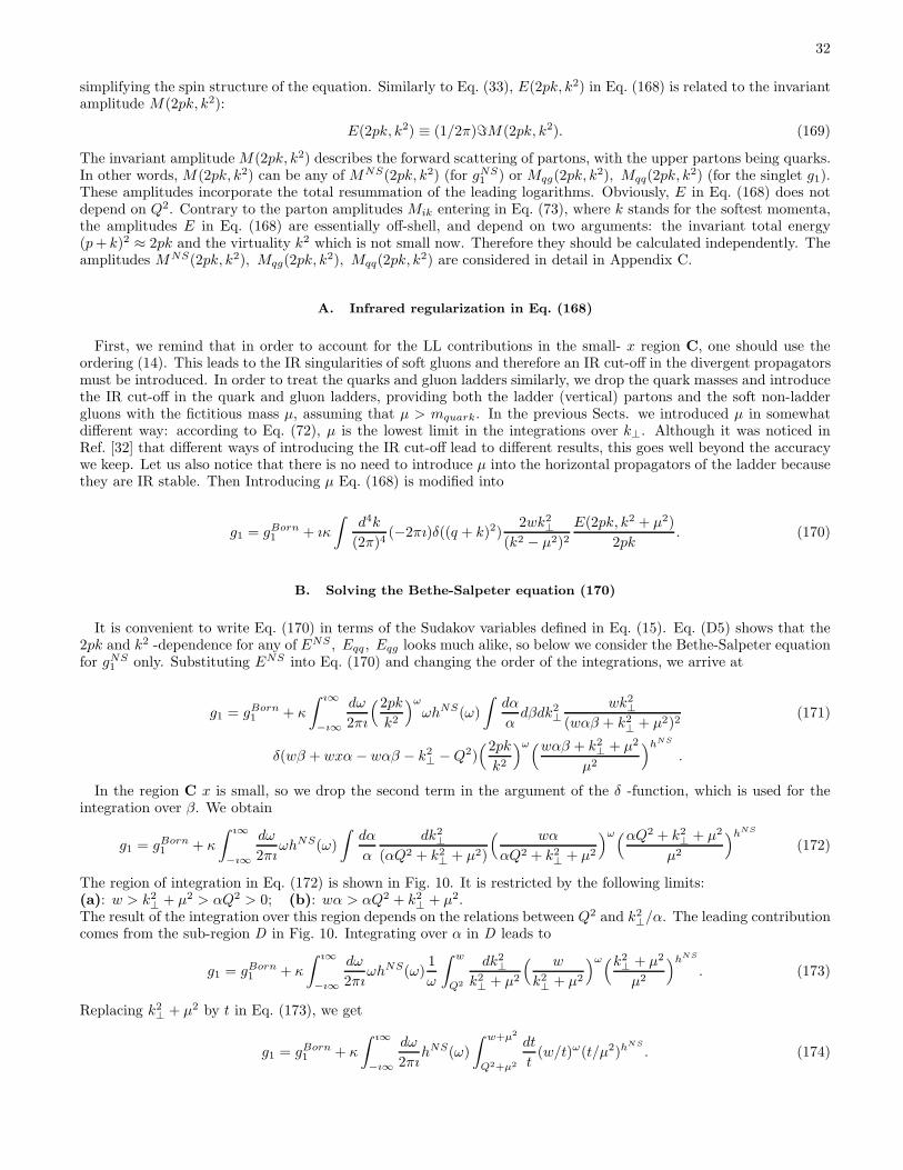
32

simplifying the spin structure of the equation. Similarly to Eq. (33), E(2pk, k2) in Eq. (168) is related to the invariantamplitude M(2pk, k2):

E(2pk, k2) ≡ (1/2π)ℑM(2pk, k2). (169)

The invariant amplitude M(2pk, k2) describes the forward scattering of partons, with the upper partons being quarks.In other words, M(2pk, k2) can be any of MNS(2pk, k2) (for gNS

1 ) or Mqg(2pk, k2), Mqq(2pk, k

2) (for the singlet g1).These amplitudes incorporate the total resummation of the leading logarithms. Obviously, E in Eq. (168) does notdepend on Q2. Contrary to the parton amplitudes Mik entering in Eq. (73), where k stands for the softest momenta,the amplitudes E in Eq. (168) are essentially off-shell, and depend on two arguments: the invariant total energy(p+ k)2 ≈ 2pk and the virtuality k2 which is not small now. Therefore they should be calculated independently. Theamplitudes MNS(2pk, k2), Mqg(2pk, k

2), Mqq(2pk, k2) are considered in detail in Appendix C.

A. Infrared regularization in Eq. (168)

First, we remind that in order to account for the LL contributions in the small- x region C, one should use theordering (14). This leads to the IR singularities of soft gluons and therefore an IR cut-off in the divergent propagatorsmust be introduced. In order to treat the quarks and gluon ladders similarly, we drop the quark masses and introducethe IR cut-off in the quark and gluon ladders, providing both the ladder (vertical) partons and the soft non-laddergluons with the fictitious mass µ, assuming that µ > mquark. In the previous Sects. we introduced µ in somewhatdifferent way: according to Eq. (72), µ is the lowest limit in the integrations over k⊥. Although it was noticed inRef. [32] that different ways of introducing the IR cut-off lead to different results, this goes well beyond the accuracywe keep. Let us also notice that there is no need to introduce µ into the horizontal propagators of the ladder becausethey are IR stable. Then Introducing µ Eq. (168) is modified into

g1 = gBorn1 + ıκ

∫d4k

(2π)4(−2πı)δ((q + k)2)

2wk2⊥

(k2 − µ2)2E(2pk, k2 + µ2)

2pk. (170)

B. Solving the Bethe-Salpeter equation (170)

It is convenient to write Eq. (170) in terms of the Sudakov variables defined in Eq. (15). Eq. (D5) shows that the2pk and k2 -dependence for any of ENS , Eqq , Eqg looks much alike, so below we consider the Bethe-Salpeter equationfor gNS

1 only. Substituting ENS into Eq. (170) and changing the order of the integrations, we arrive at

g1 = gBorn1 + κ

∫ ı∞

−ı∞

dω

2πı

(2pk

k2

)ω

ωhNS(ω)

∫dα

αdβdk2

⊥

wk2⊥

(wαβ + k2⊥ + µ2)2

(171)

δ(wβ + wxα − wαβ − k2⊥ −Q2)

(2pk

k2

)ω(wαβ + k2⊥ + µ2

µ2

)hNS

.

In the region C x is small, so we drop the second term in the argument of the δ -function, which is used for theintegration over β. We obtain

g1 = gBorn1 + κ

∫ ı∞

−ı∞

dω

2πıωhNS(ω)

∫dα

α

dk2⊥

(αQ2 + k2⊥ + µ2)

( wα

αQ2 + k2⊥ + µ2

)ω(αQ2 + k2⊥ + µ2

µ2

)hNS

(172)

The region of integration in Eq. (172) is shown in Fig. 10. It is restricted by the following limits:(a): w > k2

⊥ + µ2 > αQ2 > 0; (b): wα > αQ2 + k2⊥ + µ2.

The result of the integration over this region depends on the relations between Q2 and k2⊥/α. The leading contribution

comes from the sub-region D in Fig. 10. Integrating over α in D leads to

g1 = gBorn1 + κ

∫ ı∞

−ı∞

dω

2πıωhNS(ω)

1

ω

∫ w

Q2

dk2⊥

k2⊥ + µ2

( w

k2⊥ + µ2

)ω(k2⊥ + µ2

µ2

)hNS

. (173)

Replacing k2⊥ + µ2 by t in Eq. (173), we get

g1 = gBorn1 + κ

∫ ı∞

−ı∞

dω

2πıhNS(ω)

∫ w+µ2

Q2+µ2

dt

t(w/t)ω(t/µ2)hNS

. (174)

331 2 Q2 w k2?D

FIG. 10: The integration region in Eq. (172) .

In the region C w ≫ µ2, so the upper limit of integration in Eq. (174) can be approximated by w. The lowest limitis definitely Q2 +µ2 which proves the validity of the shift we have suggested in Eq. (167). Performing the integrationover t in Eq. (174) leads to the expression of Eq. (106) but with the shifted value of Q2. Indeed, the integration overt yields

g1 = gBorn1 + κ

∫ ı∞

−ı∞

dω

2πı

hNS

(ω − hNS)

[( w

Q2

)ω(Q2

µ2

)hNS

−( wµ2

)hNS]. (175)

The integration of the second term in the squared bracket yields zero, by closing the integration contour to the rightof the singularity of hNS/(ω − hNS). Using the identity

hNS

(ω − hNS)= −1 +

ω

(ω − hNS)(176)

and noticing that the first term in Eq. (176) cancels the term gBorn1 in Eqs. (168- 175), we arrive at the following

expression:

gNS1 = κ

∫ ı∞

−ı∞

dω

2πı

ω

(ω − hNS)

( 1

x

)ω(Q2

µ2

)hNS

(177)

which coincides with gNS1 from Eq. (106) with the replacement Q2 → Q2. We have used here the shifted variable

x = Q2/w = x+ µ2/w ≡ x+ z. (178)

So, we have proved that our result for gNS1 in region B can be extended to region C with the shift Q2 → Q2 = Q2+µ2.

It is not difficult to repeat the above calculations for the singlet g1. Eventually we conclude that our expressions

(106,116) for g1 in region B (≡ g(B)1 (x,Q2)) can represent g1 in the region C with the shifts Q2 → Q2 = Q2+µ2, x→

x = x+ z:

g(C)1 (x, z,Q2, µ2) = g

(B)1 (x, Q2). (179)

Obviously, Eq. (179) is valid in the unified region B⊕ C.

XVI. DESCRIPTION OF g1 IN THE FULL REGION A⊕B⊕C⊕D

In this Sect we will show that combining the shift of Q2 introduced in Eq. (167) and the interpolation expressionsof Eqs. (163 166) for g1 in region A, it allows us to generalize expressions for g1 which can be used in the full regionA ⊕ B⊕ C⊕ D. Let us first discuss the perturbative description of g1 in the region D.

34

The interpolation expression for gNS1 valid at large x and small Q2 is

g(D)1 NS(x, Q2) = (e2q/2)

∫ ı∞

−ı∞

dω

2πı

( 1

x

)ω

CNScomb(ω)δq(ω)eyhNS

comb(ω) , (180)

where x = x+ z, y = ln[(Q2 + µ2)/µ2] and the combined coefficient function CNScomb and anomalous dimension hNS

combare given in Eq. (161).

Similarly, combining the shift and Eq. (166), the expression for the singlet g1 in region D is:

g(D)1 S (x,Q2) =

1

2

∫ ı∞

−ı∞

dω

2πı

(1

x

)ω[(C

(+)comb(ω)eΩ(+)y + C

(−)comb(ω)eΩ(−)y

)ωδq(ω) + (181)

(C

(+)comb(ω)

(X +√R)

2hcombqg

eΩ(+)y + C(−)comb(ω)

(X −√R)

2hcombqg

eΩ(−)y)ωδg(ω)

],

Actually, Eqs. (180,181) represent g1 not only in region D but also in the full region A⊕B⊕C⊕D. Indeed, theyare expressed in terms of the shifted variables x, y and therefore can be used at any values of Q2. Also they includethe total resummation of the leading logarithms, so can be used in the regions B and C. Finally, they contain non-logarithmic one-loop contributions 6 to the coefficient functions and anomalous dimensions obtained by the DGLAP-expressions, so this makes it possible to use them in the large-x regions A and D. Let us remind that the use ofthe shift in Q2 drives us out of the logarithmic accuracy and also recall our suggestion is to use different values of µfor the singlet and non-singlet components of g1, given in Eqs. (130,137). We proceed now to the applications of theresults on g1 obtained so far..

XVII. PERTURBATIVE Q2 -POWER CORRECTIONS

In this Section we discuss the power-1/(Q2)k corrections to g1. Basically, there are various sources of such correctionsbut we focus only on those arising when the experimental results of gexp

1 are confronted to the theoretical predictionsgtheor1 . The numerical analysis of the discrepancy between the non-singlet component of gexp

1 and gtheor1 shows (see

for example Ref. [45] and Refs. therein) that

(gNS1

)exp −(gNS1

)theor ∼∑

k=1,2,..

Tk

(Q2)k(182)

and the reason of the discrepancy is attributed to the impact of higher twists. Conventionally, the DGLAP expression

of Eq. (20) is used for describing(gNS1

)theorand this is called the leading twist contribution. Naively one could expect

from Eq. (182) that the impact of the power corrections should increase when Q2 decreases, especially in the limitQ2 → 0. On the contrary, the power corrections become negligible when Q2 decreases down to values ∼ 1 GeV2.We are going now to explain this behavior and give an alternative description of the power corrections. To thisaim, first let us notice that the kinematic region of gNS

1 studied in Ref. [45] mainly coincides with the region B ⊕ Cand therefore the total resummation of the leading logarithms together with the shift of Q2 should be included intoexpressions for gtheor

1 . Eq. (179) contains both terms and therefore in the region B⊕ C

gNS1 =

e2q2

∫ ı∞

−ı∞

dω

2πı

( w

Q2 + µ2NS

)ω(Q2 + µ2NS

µ2NS

)hNS

CNS(ω)δq(ω) (183)

where w = 2pq and µNS defined in Eq. (130). The terms with Q2 + µ2NS in Eq. (183) can be expanded in the region

B, where by definition Q2 > µ2NS , as follows:

( w

Q2 + µ2NS

)ω(Q2 + µ2

NSµ2NS

)hNS

=( 1

x

)ω( Q2

µ2NS

)hNS[1 +

∑

k=1

TNSk (ω)

(µ2NS

Q2

)k](184)

6 The second-loop contributions can be included similarly.

35

with

TNSk =

(−ω + hNS)(−ω + hNS − 1)..(−ω + hNS − k + 1)

k!. (185)

Obviously, the power terms in the series of Eq. (184) have a perturbative origin and have nothing to do with the highertwists. Such terms are absent in the Standard Approach. Of course we are aware that higher twists can contribute tog1 but we argue that the perturbative power contributions of Eq. (184) should be accounted for first, and only aftera reliable estimate of the impact of the higher twists can be made. In contrast, in the region C where Q2 < µ2

NS , thepower Q2 -expansion takes the different form:

( w

Q2 + µ2NS

)ω(Q2 + µ2NS

µ2NS

)hNS

=(1

z

)ω[1 +

∑

k=1

TNSk (ω)

( Q2

µ2NS

)k]. (186)

The power series in Eqs. (184,186) for large and small Q2 are derived from the same formulae. However after theexpansion has been made, they cannot be related to each other by simply varying Q2. Our estimate µNS ≈ 1 GeVgives a natural explanation to the observation made in Refs. [45] that the power Q2 -corrections die out when Q2

approaches values ∼ 1 GeV2 and do not appear at smaller values of Q2. Let us remind that our estimate of µNS inEq. (130) was obtained by studying the asymptotic properties of gNS

1 , i.e. absolutely independently of any analysisof the power corrections. We suggest that the new source of the power contributions given by Eqs. (184,186) cansizably change the conventional analysis of the higher twists contributions to the Polarized DIS. Obviously, the powerexpansion of the singlet g1 can be made quite similarly.

XVIII. APPLICATION TO THE COMPASS EXPERIMENT

Now let us discuss the application of our results to the recent COMPASS data on the singlet g1. We consider herethe results of Refs. [16, 48]. The COMPASS experiment, carried out at the Super Proton Synchrotron at CERN.has investigated g1 by measuring the asymmetries in the scattering of a polarized 160 GeV µ+ -beam on polarizeddeuterons from a fixed 6LiD target (see Ref. [46]). As there is only one target, the COMPASS collaboration canmeasure the singlet g1 only. Values of Q2 at the COMPASS data are basically small: events with Q2 < 1 GeV2

correspond to about 90% of the total data set. From Refs. [46, 47] one can conclude that the COMPASS kinematicregion for measuring g1, GCOMPASS , is

GCOMPASS : 10−4 . x . 10−1 , 10−1 GeV 2 . Q2 . 1 GeV 2 . (187)

This makes clear that the Standard Approach cannot be used for the analysis of the COMPASS data. On the contrary,our expressions (116, 181) can be used in the COMPASS kinematic region. In the region GCOMPASS Q2 ≪ µ2

S andtherefore in this region

( w

Q2 + µ2S

)ω(Q2 + µ2S

µ2S

)Ω(±)

=(1

z

)ω[1 +

∑

k=1

T(±)k (ω)

(Q2

µ2S

)k], (188)

with

T(±)k =

(−ω + Ω±)(−ω + Ω± − 1)..(−ω + Ω± − k + 1)

k!. (189)

Substituting Eq. (188) into Eq. (181) leads to the following expression:

g1(x, z,Q2) ≈ g1(z) + (Q2/µ2

S)∂g1(z, x,Q

2)

∂Q2/µ2S

+O((Q2/µ2

S)2)

(190)

where z = µ2S/w. The first term in Eq. (190) is

g1(z) =< e2q >

2

∫ ı∞

−ı∞

dω

2πı

(1

z

)ω[Cq(ω)δq + Cg(ω)δg

]. (191)

As stated earlier, the combined coefficient functions Cq,g include the total resummation of the leading logarithms ofz and the non-logarithmic contributions ∼ αs. They are defined as follows:

Cq = Cq + CDGLAPq − ∆Cq , Cg = Cg + CDGLAP

g − ∆Cg . (192)

36

The terms CDGLAPq and CDGLAP

g in Eq. (192) are the NLO DGLAP coefficient functions and

Cq =ω(ω −Hgg)

ω2 − ω(Hgg +Hqq) +HqqHgg −HqgHgq, ∆Cq = 1 +

aqq

ω2, (193)

Cg =ωHgq

ω2 − ω(Hgg +Hqq) +HqqHgg −HqgHgq, ∆Cg =

agq

ω2.

The presence of the terms CDGLAPq,g in Eqs. (192,193), as the DGLAP coefficient functions, may sound irrelevant

or strange because the DGLAP description of g1 cannot be used in the small-Q2 kinematics we are discussing.Nevertheless, the direct calculation of g1(z) to order ∼ αs yields a contributions coinciding with the NLO DGLAPcoefficient functions. In other words the presence of the coefficient functions has nothing to do with the Q2-evolution.Eq. (190) explicitly shows that the Q2- dependence of gS

1 in the region GCOMPASS should be weak, and also thatgS1 practically does not depend on x in the kinematical region GCOMPASS , even at very small x. However, its

absolute value cannot be fixed from theoretical grounds. Indeed, Eq. (191) implies that sign of gS1 (z) at any given z

is determined by the interplay between the quark and gluon contributions and eventually depends on δq/δg, whichcannot be determined theoretically. At the same time, Eq. (190) predicts that the z-dependence of gS

1 is prettyfar from being trivial, so the experimental investigation of this dependence would be quite interesting: it can yieldinformation about the initial quark and gluon densities. The predictions of the essential independence of gS

1 on xmade in Ref. [16], was confirmed in Ref. [47] where a flat dependence of gS

1 was found. More precisely, Ref. [47]reported that

gS1 ≈ 0 (194)

in the regionGCOMPASS with small errors. Unfortunately, the COMPASS data do not allow to study the z-dependenceof gS

1 in the proper way. Nevertheless, the COMPASS result (194) was used in Ref. [48] in order to obtain some roughestimates for δq/δg. Below we consider this issue in detail.

A. Interpretation of the COMPASS data on gS

1

The variable w = 2pq in the COMPASS experiment runs in the interval

30 GeV 2 . w . 270 GeV 2 (195)

and therefore the range for z is

1 . z . 0.1. (196)

The variable z is related to the standard variable ν = w/(2M) measured in GeV, with M = 1 GeV:

z =( µ2

2M

)1

ν≈ 15

ν, (197)

so the region (196) covered in the COMPASS experiment corresponds to the ν-region (in GeV)

15 . ν . 150. (198)

We remind that only the x -dependence of gS1 was studied in the COMPASS experiment. The values of w and Q2

were not reported in the COMPASS data, which makes impossible the straightforward application of Eq. (191) to theCOMPASS results. However there are several options for the interpretation of Eq. (194) and below we consider themin detail:Option (i):

Eq. (194) means that gS1 (z) = 0 for any z from the whole interval of Eq. (196).

In this case Eq. (191) implies a strong correlation between δq and δg at any ω :

Cq(ω)δq(ω) + Cg(ω)δg(ω) = 0. (199)

We don’t find theoretical grounds for understanding this fact and think that next option is more realistic.Option (ii):

37

Eq. (194) holds in the average, namely in the region (196):

< gS1 (z) >= 0 . (200)

Obviously, in order to fulfill the Eq. (200), g1(z) should acquire both positive and negative values in the region (196).This could be realized by an appropriate choice for the initial parton densities δq(z) and δg(z). In ref. [14] we suggestedthat in region B one can approximate the initial parton densities by constants. Guided by this result, we suggestedin Ref. [16] to approximate δq(z) and δg(z) at small z by simple constants to get a rough estimate. However, in theCOMPASS region (196) z is not small enough to use such a simple approximation. As the DGLAP-fits from Ref. [5]work quite well and also other parameterizations have a similar structure, we suggest a similar but regular fit :

δq(z) = Nqz(1 − z)3(1 + 3z), δg(z) = Ng(1 − z)4(1 + 3z) . (201)

The main difference with Ref. [5] is in the absence of the power factors za while the terms in the brackets inEq. (201) and in Ref. [5] coincide ( x in Ref. [5] is replaced by z in Eq. (201)). Indeed in Ref. [14], as also discussedpreviously, we have proved that the role played by the singular terms x−a in the DGLAP fits is to mimic the totalresummation of lnk(1/x) . On the other hand, we would like to keep the same ratio δq/δg as in Ref. [5] and thereforewe also change the power factor for δq in Eq. (201). Now it is easy to check that the fit (201) do not lead to a flatz-dependence for g1 and cannot keep g1(z) = 0 in the whole COMPASS region (187).

In more detail by substitution of Eq. (201) into Eq. (181) and performing the integration over ω numerically, withfixed and positive Nq , and varying the values of Ng , we plot our results in Fig. 11 .

By a close inspection of the various configurations shown, we can easily conclude that these fits could be compatiblewith Eq. (200) only if Ng > 0 and Ng > Nq .

As the way of averaging g1 over z in the COMPASS data is unknown to us, we can try another possibility,approximating

< g1(z) >≈ g1(< z >) = 0 , (202)

where < z >= 0.25 (i.e. < ν >≈ 60 GeV) is the mean value of z from the region (196). Then using Eqs. (181,201),keeping positive Nq and varying Ng , as shown in Fig. 11, we suggest again that Ng are positive and Ng > Nq .

B. Comments on the measurement of g1 in different kinematic regions.

To conclude this Sect., let us make a brief comment on the parametrization of g1. In the Born approximation g1is given by Eq. (4) and depends on the only argument x which corresponds to the famous scaling in the DIS. Theradiative corrections in the higher loops bring the violation of scaling, so g1 acquires, additionally, the Q2 -dependence.At this stage one can parameterize g1 by the set of variables x, Q2 or, alternatively, w, Q2, or ν, Q2. As it is well-known, in the target rest frame w ≡ 2pq = 2M(E − E′) where M is the target (nucleon) mass and E (E′) is theenergy of the incoming (outgoing) lepton. Then Q2 in the same frame involves the above energies and the scatteringangle θ. Therefore, both x and Q2 depend on E′ and θ and these variables are not always independent of each other.Indeed, there are experiments where the x -dependence of g1 is measured at fixed Q2; then Q2 is varied to anothervalue and the x -dependence is studied again. In this case x and Q2 are really independent variables. In the oppositecase of fixed w and varying Q2, Then x = x(Q2) and therefore these variables are not exactly independent, so it ismore convenient to use w instead of x, as independent variable. These examples show that using w and Q2 insteadof the standard set x, Q2 could be more convenient for g1 . In particular, when Q2 is very small, using x insteadof w becomes really inconvenient. Nevertheless, the w -dependence of g1 in the COMPASS experiments predicted inEq. (190) can be clearly extracted from the dependence on x and Q2. Indeed, the variable x defined in Eq. (178) canbe written in the following form:

x = µ2x/Q2 + x ≈ µ2x/Q2. (203)

Although g1 depends on x and on Q2 at small Q2 very weakly, its dependence on x/Q2 is quite essential. IndeedEq. (190) can be regarded as a sort of a new scaling law where g1 depends on the variable x/Q2 only.

38

102 103 104

-0.04

-0.02

0

0.02

0.04

102 103 104

102 103 104

-0.04

-0.02

0

0.02

0.04

102 103 104

g1

ν /GeV/

(a)

|←COMPASS

→|

g1

ν /GeV/

(b)

|←COMPASS

→|

102 103 104

-0.04

-0.02

0

0.02

0.04

102 103 104

102 103 104

-0.04

-0.02

0

0.02

0.04

102 103 104

g1

ν /GeV/

(c)

|←COMPASS

→|

g1

ν /GeV/

(d)

|←COMPASS

→|

102 103 104

-0.04

-0.02

0

0.02

0.04

102 103 104

102 103 104

-0.04

-0.02

0

0.02

0.04

102 103 104

g1

ν /GeV/

(e)

|←COMPASS

→|

g1

ν /GeV/

(g)

|←COMPASS

→|

FIG. 11: The ν -dependence of g1(ν), with δq, δg defined in Eq. (201), for Nq = 0.5 and different values of Ng: (a) -1.5, (b)-0.5, (c) 0, (d) 0.5, (e) 2, (g) 3.5; the COMPASS ν -region corresponds to Eq. (198) .

39

XIX. SUMMARY AND OUTLOOK

In the present paper we have presented an overview of our results on the spin structure function g1 at arbitraryx and Q2. We have divided the whole kinematic region of x and Q2 into the set of four regions A - D defined inEqs. (5, 10-12) and considered g1 in each of these regions. The region A is covered by the Standard Approach, basedon the DGLAP evolution equations. This is briefly discussed in Sect. II. The application of the integral transforms tog1 is given in Sect. III. In Sect. IV we have discussed in detail the parametrization of αs and shown that the popularparametrization αs = αs(k

2⊥) is valid at large x only. Otherwise it should be replaced by the effective coupling αeff

s

defined in Eq. (49). When µ2 obeys Eq. (50), αeffs can be approximated by αs(k

2⊥/β) (with β being the longitudinal

Sudakov variable) and when, in addition, x is large, it can be simplified down to αs(k2⊥). According to Eq. (50), the

deviation of αeffs from αs strongly depends on µ2. For example, when µ2 = 2.5 GeV2, αs(µ

2)/αeffs (µ2) ≈ 0.9 but

very quickly αs(µ2)/αeff

s (µ2) ≈ 0.5 at µ2 ≈ 1 GeV2, which is a typical DGLAP starting point of the Q2 -evolutionThe small-x region B, where the total resummation of the leading logarithms of x is essential, was considered inSect. V. We account there for the resummation of the leading logarithms by solving an Infrared Evolution Equations(IREE), so in Sect. V the essence of the method together with the technology of IREE was discussed and the IREEfor g1 were obtained. These IREE involve new anomalous dimensions and coefficient functions. Explicit expressionsfor them were obtained in Sect. VI. Then the expression of Eq. (106) for the non-singlet component of g1 in the regionB was obtained in Sect. VII, while in Sect. VIII the result for the singlet g1 in region B was given in Eq. (116).Obviously, the impact of the total resummation of logarithms of x is big at small x and becomes maximal at x→ 0,where the expressions in Eqs. (106,116) behave asymptotically as in Eqs. (124,134). The small-x asymptotics ofthe non-singlet g1 is considered in detail in Sect. IX while Sect. X contains the asymptotics of the singlet g1. Bothasymptotic behaviors are of the Regge type. The estimates for their the intercepts are given by Eqs. (129) and (136).The small-x rise of g1 predicted by Eqs. (124,134) is much steeper than the well-known small-x DGLAP predictionin Eq. (132). On the other hand, a numerical analysis shows that the use of the asymptotic formulae at the presentlyavailable x is not reliable, so Eqs. (106,116) should not be replaced by their asymptotic expressions of Eqs. (124,134)in the region B. The comparison of our results to the DGLAP -expressions for g1, which is impossible without fixingthe initial parton densities δq and δg, shows that the impact of the resummation of the logarithms becomes essentialfor values smaller x ≈ 10−2 In Sect. XII, by considering in detail a standard DGLAP fit (24) for the initial partondensities, we have shown that the singular factors in the fits mimic the total resummation of the logarithms andprovide the rise of g1 at small x which is observed in the experimental data. On the other hand, when the totalresummation of the logarithms is taken into account, the singular factors in the fits can be dropped. This allows oneto simplify the parametrization of the initial parton densities..The Reggeon structure in the two approaches has been discussed in Sect. XIII, However, in the case of the SA thoseReggeons are, in a sense, fictitious: they are generated by the fits for the initial parton densities and because of thatare present at any x instead of appearing in the asymptotic expressions at x→ 0.The total resummation of the small-x logarithms is important in the region B, but also non-logarithmic contributionsare quite essential in the DGLAP region A, where they are accounted for to NLO accuracy. Then the interpolatingexpressions for g1 are presented in Eqs. (163) and (166). On one hand, they almost coincide with gDGLAP

1 in theregion A and on the other hand, with Eqs. (106,116) in the region B, and at the same time do not require the use ofthe singular parameterizations of the parton densities.The small-Q2 region C is absolutely beyond the reach of DGLAP. On the other hand, the analysis of the Feynmandiagrams contributing to g1 shows that a shift of Q2 allows us to extend Eqs. (106,116) into the region C. Similarly,Eqs. (163,166) can be extended into the region D. Eventually we arrived at the Eqs. (180,181) which are the interpo-lation expressions which can describe g1 in the whole region A⊕B⊕C⊕D. This was the subject of Sects. XIV-XVI.This shift of Q2, given in Eq. (167), inevitably causes the appearance of power 1/Q2 -corrections. Q2 power correctionswere found earlier phenomenologically by confronting gDGLAP

1 and the experimental data. They were attributed tothe impact of higher twists. In Sect. XVII we argued that the role played by the higher twists can be estimatedreliably only after accounting for the pertubative power corrections.Finally, in Sect. XVIII we have used the small-Q2 description of the singlet g1 in Eq. (181) for the interpretation ofthe recent COMPASS data. First we have shown that g1 in the COMPASS kinematic region does not depend on x,even at very small x. Then, we have suggested that the COMPASS data are compatible with positive gluon densities. We also argued in favor of studying the dependence of g1 on 2pq in the COMPASS experiment rather than on x, inorder to estimate the ratio δg/δq.

40

XX. ACKNOWLEDGMENTS

We are grateful to G. Altarelli, A.V. Efremov, S. Jadach, W. Schafer and O.V. Teryaev for useful discussions. Thework is partly supported by Grant RAS 9C237, Russian State Grant for Scientific School RSGSS-3628.2008.2 and byan EU Marie-Curie Research Training Network under Contract No. MRTN-CT-2006-035505 (HEPTOOLS).

APPENDIX A: SIMPLIFICATION OF THE COLOR STRUCTURE OF THE FORWARD SCATTERINGAMPLITUDES

We consider below in more detail the color structure of the Born amplitude ABorn defined in Eq. (42). As theexternal partons in ABorn are quarks or gluons,

ABorn = −C(col)4παsu(−p2)γµu(p1)u′(p1)γµu

′(−p2)

s+ ıǫ(A1)

where the SU(3) -matrix C(col) describes the color structure of ABorn. When all external partons are quarks,C(col) = tata, with ta (a = 1, .., 8) being the SU(3) -generators in the fundamental (three-dimensional) representation;when the quarks are replaced by gluons, ta are replaced by the SU(3) -generators T a in the vector representation.Each of the initial and final color two-parton states in Eq. (A1) corresponds to a reducible representation of SU(3)and can be expanded into a sum of irreducible states. It is convenient to do it in the t -channel where the amplitudeABorn describes the quark-antiquark annihilation qq → q′q′ and therefore the irreducible initial qiq

j and final qpqq

color states (with i, j, p, q = 1, 2, 3) are the singlet (S) and octet (V ). The initial 3 ⊗ 3 color state in the t -channelstate is qiq

j . It can be expanded into the sum of the singlet and octet, each one is the irreducible state: 3⊗3 = 1 ⊕8.We denote them (qiq

j)S and (qiqj)V respectively. It can be done by applying the projection operators PS and PV to

the quark-antiquark states:

(qiqj)S = (PS)i′j

ij′qi′ qj′ , (qiq

j)V = (PV )i′jij′qi′ q

j′ (A2)

where

PS)jj′

ii′ =1

Nδi′

i δjj′ , (PV )jj′

ii′ = 2(ta)i′

i (ta)jj′ . (A3)

Obviously, these operators are orthogonal to each other and the factors 1/N (with N = 3) and 2 in Eq. (A3) are intro-duced to guarantee the property P 2 = P for each of PS and PV . Let us notice that ||PS ||2 = Tr[P+

S PS ] = 1, ||PV ||2 =

Tr[P+V PV ] = 2NCF where CF = (N2 − 1)/2N . Applying the projection operators PS and PV to the color factor

C(col) in Eq. (A1) allows us to write down C(col) as the sum of the scalar C(col)S and octet C

(col)V color factors:

(C(col))jpiq = C

(col)S (PS)jp

iq + C(col)V (PV )jp

iq , (A4)

where

C(col)S =

(PS)iqjp(t

a)ji (t

a)pq

||PS ||2=

1

NTr[tata] = CF ,

C(col)V =

(PV )iqjp(ta)j

i (ta)p

q

||PV ||2 =2Tr[tatbtatb]

2NCF= − 1

2N. (A5)

Substituting Eq. (A4) into Eq. (A1), we rewrite it as

ABorn = ABornS PS +ABorn

V PV , (A6)

with

ABornS = −C(col)

S 4παsu(−p2)γµu(p1)u′(p1)γµu

′(−p2)

s+ ıǫ,

ABornV = −C(col)

V 4παsu(−p2)γµu(p1)u′(p1)γµu

′(−p2)

s+ ıǫ. (A7)

41

When the external quarks in Eq. (A1) are replaced by gluons, generators ta in the factor C(col) are replaced by theSU(3) -generators T a in the vector representation. It allows one to generalize Eq. (A7) to the gluons case, expandingthe initial t -channel gluon state 8 ⊗ 8 into scalar and octet (see Refs. [10, 11] for detail). The projection operators

P(gg)S and P

(gg)V projecting the two-gluon t -channel state on the scalar and octet states are:

P(gg)S =

1

N2 − 1δa′b′δab , P

(gg)V =

1

N(Tc)a′b′(Tc)ab . (A8)

Strictly speaking, the normalization for projector operators with the gluon-quark transitions can be arbitrary but inorder to match DGLAP it can be chosen as follows:

P(qg)S =

1

N2 − 1δji δab , P

(qg)V =

1

N(tc)

ji (Tc)ab , (A9)

P(gq)S =

1

Nδabδij , P

(gq)V = 2(Tc)ab(tc)

ji .

In Eqs. (A8,A9) we have kept the notation i, j for the quark color states while a, b, a′, b′ denote the gluon states. Incontrast to the quark-quark case, the expansion of 8⊗8 into the sum of the irreducible SU(3) -representations includesthe singlet 1, the antisymmetric 8A and symmetric 8S octets and other contributions which cannot be organized outof the gluon fields and therefore can be left out, so for the gluons 8⊗ 8 = 1⊕ 8A ⊕ 8S. The symmetric octet 8S doesnot contribute to g1 with the leading logarithmic accuracy (see Ref. [10] for detail). An additional argument in favorof neglecting the amplitudes with high color dimensions is that they die out quickly with energy.

APPENDIX B: NON-SINGLET CONTRIBUTION TO THE STRUCTURE FUNCTION F1

The technology for calculating the leading logarithmic contributions to FNS1 (x,Q2) is quite similar to the one for

gNS1 (x,Q2) (see Refs. [11] for detail). Similarly to gNS

1 , FNS1 is expressed through the forward Compton amplitude

T(+)NS in the following way:

FNS1 =

1

2πℑT (+)

NS . (B1)

The superscript (+) in Eq. (B1) stands for the positive signature. Then it is convenient to define the Mellin amplitude

FNS1 (ω, y) related to T

(+)NS through the Mellin transform (34). As a consequence, the IREE for FNS

1 is almost identicalto Eq. (80):

ωFNS1 (ω, y) +

∂FNS1 (ω, y)

∂y=

1

8π2(1 + λqqω)L(+)

qq (ω)FNS1 (ω, y) . (B2)

The amplitude L(+)qq (ω) again corresponds to the quark-quark scattering but its signature is now positive. It should be

found independently. Eq. (B2) can be solved similarly to Eq. (80). The only difference between them is replacementof hNS by h(+). The amplitude h(+) obeys the following IREE:

ωh(+) = b(+) + (1 + λqqω) (h(+))2. (B3)

The difference between Eq. (B3) and Eq. (80) is the inhomogeneous term b(+). It is expressed through aqq defined in

Eq. (84) and V(+)qq :

b(+) = aqq + V (+)qq . (B4)

Similarly to Vqq introduced in Eq. (88), V(+)qq is expressed in terms of mqq defined in Eq. (89) and a new quantity

D(+) instead of D:

V (+)qq = mqqD

(+) (B5)

42

with

D(ω) =1

2b2

∫ ∞

0

dρe−ωρ ln((ρ+ η)/η

)[ ρ+ η

(ρ+ η)2 + π2− 1

ρ+ η

]. (B6)

So, the expression for FNS1 in region B is

FNS1 (x,Q2) =

e2q2

∫ ı∞

−ı∞

dω

2πıx−ωC

(+)NS (ω)δq(ω)eh

(+)NS

(ω) ln(Q2/µ2) . (B7)

where

C(+)NS =

2ω

ω +

√ω2 −B

(+)NS (ω)

, (B8)

h(+)NS(ω) = (1/2)

[ω −

√ω2 −B

(+)NS (ω)

](B9)

and

B(+)NS = 4(1 + λqqω)b(+)

qq . (B10)

The small- x asymptotics of FNS1 (x,Q2) is also of the Regge type but the value of the intercept ∆

(+)NS is smaller

than the one of gNS1 :

∆(+)NS = 0.38 . (B11)

APPENDIX C: CONVOLUTION OF TWO AMPLITUDES

Let us consider the t- channel convolution of two amplitudes: Q = A(p1)1

⊗A

(p2)2 of the scattering amplitudes A

(p1)1

and A(p2)2 where p1,2 = ± stand for the signatures. It is convenient to describe amplitudes M

(pa)a in terms of the

invariant amplitudes Ma. For example, the invariant amplitude M (±) for the quark-antiquark forward annihilationq(p1) + q(p2) → q(p′1) + q(p′2) are introduced as follows:

A(±) =jνjνsM (±) (C1)

where jν are the quark currents. We remind we use the Feynman gauge.It is also convenient to use the asymptotics of the Sommerfeld-Watson transform (often called the Mellin represen-

tation) for each of those amplitudes in the following form:

M (p)a (s, µ2) =

∫ ı∞

−ı∞

dω

2πı

( s

µ2

)ω

ξ(pa)(ω)F (pa)a (ω) , (C2)

with a = 1, 2 . The signature factor

ξ(±)(ωa) = −e−ıπω ± 1

2≈ (1 ± 1) + ıπω

2(C3)

and the transform inverse to Eq. (C2) is

F (±)(ω) = − 1

πω

∫ ∞

µ2

ds

s

( s

µ2

)−ω ℑsM ±ℑuM

2. (C4)

Using Eqs. (C1,C2) and skipping the overall factor jνjν/s allows us to write the convolution Q through the invariantconvolution Qinv as

Q =jνjνsQp1p2

inv (C5)

43

with7

Qp1p2

inv = ı

∫ ı∞

−ı∞

dω1

2πı

dω2

2πıξ(p1)(ω1)ξ

(p2)(ω2)f(p1)1 (ω1)f

(p2)2 (ω2)

∫d4k

16π4

2k2⊥

(k2 −m2 + ıǫ)2

( s1|k2|

)ω1( s2|k2|

)ω2 s

s1

s

s2(C6)

where the factor 2k2⊥ appears as the result of simplifying the spinor structure, s1 = 2p1k, s2 = 2p2k. Both of them

are understood as s1,2 + ıǫ.For integration over k in Eq. (C6) we use the Sudakov variables (15):

Qp1p2

inv =ı

16π4

∫ ı∞

−ı∞

dω1

2πı

dω2

2πıξ(p1)(ω1)ξ

(p2)(ω2)f(p1)1 (ω1)f

(p2)2 (ω2)Ψ

(p1,p2)(ω1, ω2, s/µ2) (C7)

with

Ψ(p1,p2)(ω1, ω2, s/µ2) =

∫dαdβd2k⊥

k2⊥

(sαβ − k2⊥ + ıǫ)2

( sα

|k2|)ω1

( sβ

|k2|)ω2 s

sα

s

sβ. (C8)

Let us first integrate Eq. (C8) over α. The integration can be done in the complex plane by applying the Cauchyformula. The singularities in the complex α -plane are the double pole sαβ− k2

⊥ + ıǫ = 0 and the cut from the Mellinfactor (sα)ω1 . The integration yields a non-zero result when the pole and the cut have opposite imaginary parts.The imaginary part of the cut is positive while the imaginary part of the pole is negative provided β > 0. Whenβ < 0, both singularities have positive imaginary parts and therefore the integration over α yields zero. Closing upthe integration contour in the lower hemi-plane and taking the residue of the pole

α = (k2⊥ − ıǫ)/sβ (C9)

we perform the integration over α and arrive at

Ψ(p1,p2)(ω1, ω2, s/µ2) = −2π2ı

∫ s

µ2

dk2⊥

k2⊥

( s

k2⊥

)ω2∫ 1

k2⊥

/s

dββω2−ω1−1 = (C10)

−2π2ı

ω2 − ω1

∫ s

µ2

dk2⊥

k2⊥

[( s

k2⊥

)ω2

−( s

k2⊥

)ω1]

=−2π2ı

ω2 − ω1

[ 1

ω2

( s

µ2

)ω2

− 1

ω1

( s

µ2

)ω1]

Therefore we obtain the following expression for Qinv:

Qp1p2

inv =1

8π2

∫ ı∞

−ı∞

dω1

2πı

dω2

2πıξ(p1)(ω1)ξ

(p2)(ω2)f

(p1)1 (ω1)f

(p2)2 (ω2)

ω2 − ω1

[ 1

ω2

( s

µ2

)ω2

− 1

ω1

( s

µ2

)ω1]. (C11)

Eq. (C11) involves two integrations, however one of them can be done easily. The integration lines over ω1,2 inEq. (C11) are parallel to the imaginary axes and lie to the right of the rightmost singularities of f1,2. Let us assumethat additionally to it

0 < ℜω1 < ℜω2 . (C12)

The opposite case ℜω1 > ℜω2 can be discussed similarly. The integrand of Eq. (C11) includes two similar terms in

the squared brackets. Let us focus on integrating the first term,(s/µ2

)ω2and let us integrate this part of Eq. (C11)

with respect to ω1. In this case closing up the ω1 -integration contour to the left involves accounting for singularitiesof f1(ω1). On the contrary, when we close up the ω1 -contour to the right, the only singularity inside the contour isthe pole 1/(ω2 − ω1), so we can do this integration without considering f1, just by taking the residue at ω1 = ω2. At

the same time, integrating the remaining, proportional to(s/µ2

)ω1part of Eq. (C11) with respect to ω1 yields zero.

Therefore Eq. (C11) is reduced to the simpler form:

Qp1p2

inv =1

8π2

∫ ı∞

−ı∞

dω

2πı

(s/µ2

)ωξ(p1)(ω)ξ(p2)(ω)

f(p1)1 (ω)f

(p2)2 (ω)

ω(C13)

7 The factor ı is the product of the overall factor −ı and (±ı)2 from the t-channel quark or gluon propagators.

44

Obviously,

ξ(p1)(ω)ξ(p2)(ω) ≈ (1/4)[(1 + P1P2) − ıπω(P1 + P2)] = ξ(p1)(ω) δp1p2 (C14)

where P1,2 = ±1 . It means that the leading contribution to Qp1p2

inv is diagonal in the signatures. Strictly speaking,this should be checked in advance, with using the Sommerfeld-Watson transform where analytical properties of theinvolved amplitudes are explicitly accounted for.

APPENDIX D: OFF-SHELL INVARIANT AMPLITUDE M IN EQ. (169)

The invariant amplitude M in Eq. (169) is a generic notation for the following invariant off-shell am-plitudes: MNS(2pk, k2) contributing to the Bethe-Salpeter for gNS

1 and the flavor singlet amplitudesMqq(2pk, k

2), Mqg(2pk, k2). They are related to the amplitudes Aqq(2pk, k

2), Aqg(2pk, k2) of the forward quark-

quark and quark-gluon scattering:

Aqq = − u(−k)γλu(p)u(p)γλu(−k)(p+ k)2 + ıǫ

Mqq(2pk, k2) , (D1)

Aqg = −eλe∗µ

u(−k)γλ(p− k)γµu(−k)(p+ k)2 + ıǫ

Mqg(2pk, k2) .

The outgoing momenta −k in Eq. (D1) are assigned to the final (upper) off-shell quarks whereas the initial quarksand gluons have momenta p ; eλ and eµ are the polarization vectors of the gluons. We remind that the amplitudesMqq(2pk, k

2), Mqg(2pk, k2) are off-shell and therefore they differ from the amplitudes Mik introduced in Eq. (73):

Mqq and Mqg logarithmically depend on two arguments, 2pk and k2, i.e.

Mqq = Mqq(ρ, z); Mqg = Mq,g(ρ, z) (D2)

where ρ = ln(2pk/µ2), z = ln(k2/µ2) .It is convenient to introduce the Mellin amplitudes ϕik(ω, z) conjugate to Mik(ρ, z) through Eq. (34). The IREE

for ϕik(ω, z) is quite similar to Eqs. (75,76), and we put here all λik = 0 for the sake of simplicity:

∂ϕNS

∂z+ ωϕNS =

1

8π2ϕNSLqq(ω) , (D3)

∂ϕqq

∂z+ ωϕqq =

1

8π2ϕqqLqq(ω) +

1

8π2ϕqgLgq(ω) ,

∂ϕqg

∂z+ ωϕqg =

1

8π2ϕqqLqg(ω) +

1

8π2ϕqgLgg(ω) .

The amplitudes LNS, Lik in Eq. (D3) are on-shell, so in accordance with Eq. (77) they can be expressed in termsof hNS(ω) = (1/8π2)LNS(ω), hik(ω) = (1/8π2)Lik(ω) which are obtained in Eqs. (104,95). General solutions to thelinear equations (D3) can easily be found (cf Eq. (107)):

ϕNS = ΦNS(ω)ez[−ω+hNS] , (D4)

ϕqq = Ψ1(ω)e−ωz+zΩ(+) + Ψ2(ω)e−ωz+zΩ(−) ,

ϕqg = Ψ1(ω)X +

√R

2hgqe−ωz+zΩ(+) + Ψ2(ω)

X −√R

2hgqe−ωz+zΩ(−) ,

with Ω(±), X and R defined in Eqs. (110, 108,109) respectively whereas Ψ1,2 should be specified. Therefore, E(2pk.k2)

used in Eq. (168) can be any of ENS(2pk.k2), Eqq(2pk.k2), Eqg(2pk.k2) given by the following expressions:

ENS(2pk.k2) =

∫ ı∞

−ı∞

dω

2πı

(2pk

k2

)ω

ωΦNS(ω)ezhNS

, (D5)

Eqq(2pk.k2) =

∫ ı∞

−ı∞

dω

2πı

(2pk

k2

)ω

ω[Ψ1(ω)ezΩ(+) + Ψ2(ω)ezΩ(−)

],

Eqg(2pk.k2) =

∫ ı∞

−ı∞

dω

2πı

(2pk

k2

)ω

ω[Ψ1(ω)

X +√R

2hgqezΩ(+) + Ψ2(ω)

X −√R

2hgqezΩ(−)

].

45

In order to specify Ψ1,2, we use the obvious matching condition:

ϕNS(ω, z = 0) = 8π2hNS(ω) , ϕqq(ω, z = 0) = 8π2hqq(ω) , ϕqg(ω, z = 0) = 8π2hqg(ω) . (D6)

It immediately fixes ϕNS :

ϕNS = 8π2hNS(ω)ez[−ω+hNS(ω)] (D7)

and leads to the explicit expressions for Ψ1,2:

Ψ1 = 8π2

[2hqghgq − hqq(hgg − hqq −

√R)

]

2√R

, Ψ2 = 8π2

[− 2hqghgq + hqq(hgg − hqq +

√R)

]

2√R

. (D8)

APPENDIX E: CALCULATING THE SMALL-x ASYMPTOTICS OF THE NON-SINGLET g1.

Eq. (106) for gNS1 1(x,Q2) in region B can be written as follows:

gNS1 (x,Q2) =

∫ ı∞

−ı∞

dω

2πıeΦ(ω,x,Q2) (E1)

where the phase Φ is

Φ(ω, x,Q2) = ω ln(1/x) + lnCNS(ω) + yhNS(ω) = ωξ + lnCNS(ω) − y

2

√ω2 −BNS(ω) (E2)

where we have used the expression (104) and denoted ξ = ln(w/√Q2µ2). We remind that y = ln(Q2/µ2). We are

going to calculate the asymptotics of gNS1 at x→ 0 and fixed Q2, i.e. at fixed Q2 and w → ∞. The standard way to

calculate asymptotics is to apply the saddle-point method to Eq. (E1). According to it,

gNS1 ∼ ΠNS(ω0, w,Q

2)eΦ0(ω0,w,Q2) , (E3)

with the stationary phase Φ0 = Φ(ω0, w,Q2) and the stationary point ω0 is defined from the requirement dΦ/dω = 0,

i.e. ω0 is a solution to the equation

ξ +C′

NS(ω)

CNS(ω)− y

4

(2ω −B′NS(ω))√

ω2 −BNS(ω)= 0 . (E4)

Obviously, Eq. (E4) can have much more the one solution. In this case ω0 is the solution with the largest ℜω.It is often called the rightmost stationary point. Substituting the explicit expressions (105) for CNS , we transformEq. (E4) into

ξωBNS

√ω2 −BNS = (BNS − ωB′

NS/2)(ω −√ω2 −BNS) +

y

2ωBNS(ω −B′

NS/2) . (E5)

Obviously this equation cannot be solved analytically. The analytical solution can be found for the particular casewhen B does not depend on ω (it corresponds to the case of fixed αs) and y = 0. In this case Eq. (E4) can be reducedto the algebraic equation

ω4 + (2/ρ)ω3 − ω2BNS − (2BNS/ρ)ω − (BNS/ρ2) = 0 (E6)

where ρ = ln(w/µ2). Eq. (E6) has four roots which can be found with using the known from the literature Ferrariformulae but only two of them, namely ω = ±

√BNS do not go to zero when w → ∞. Obviously, in this case the

rightmost root is ω0 =√BNS . It is easy to make this conclusion, without solving Eq. (E6). Indeed, Eq. (E6) can be

written as

ω2(ω2 −BNS) + (2/ρ)ω(ω2 −BNS) − (BNS/ρ2) = 0 . (E7)

When the terms ∼ 1/ρ2 and ∼ 1/ρ are dropped, Eq. (E7) can be solved immediately and the rightmost root caneasily be found. Applying the same arguments allows one to solve Eq. (E4) at w → 0 drives us to conclude that therightmost and non-vanishing at w → ∞ root of Eq. (E4) does not depend on y and it can be found as the rightmostroot of the much simpler equation ω2 = BNS(ω) as is stated in Eq. (125). This leads to the Regge asymptotics ofEq. (124) quite different from the well-known DGLAP asymptotics (132). Let us notice that, in the perfect agreementwith the concepts of the phenomenological Regge theory, this root corresponds to the branching point singularity ofEq. (E4).

46

APPENDIX F: THE DGLAP SMALL-x ASYMPTOTICS

Let us remind how the DGLAP asymptotics of gNS1 in Eq. (132) was obtained. As this topic is well-known, for the

sake of simplicity we consider gNS1 DGLAP with the LO accuracy. When the singular term in δq is absent, the small-x

asymptotics of gNS1 DGLAP can also be obtained with the saddle-point method. Similarly to Eq. (E1), gNS

1 DGLAP canbe written as

gNS1 DGLAP (x,Q2) =

∫ ı∞

−ı∞

dω

2πıeΦDGLAP (ω,x,Q2) (F1)

where the phase ΦDGLAP is

ΦDGLAP = ω ln(1/x) +

∫ Q2

µ2

dk2⊥

k2⊥

αs(k2⊥)

2πγ(0), (F2)

with γ(0) being given by Eq. (21). The bulk of the integral in Eq. (F1) comes from the region of ω obeying

ω ln(1/x) . 1 (F3)

because the factor eω ln(1/x) in Eq. (F1) strongly oscillates beyond this region. So, the values of ω mainly contributingto the integral become small when x → 0. As a consequence, the most important term in γ(0) is now the singular inω term ADGLAP (Q2)/ω, with

ADGLAP (Q2) =

∫ Q2

µ2

dk2⊥

k2⊥

αs(k2⊥)CF

2π. (F4)

Therefore, approximately

ΦDGLAP ≈ ω ln(1/x) +ADGLAP (Q2)/ω . (F5)

The equation for the stationary point is

Φ′DGLAP = ln(1/x) −ADGLAP (Q2)/ω2 = 0 , (F6)

which leads to the stationary point

ωDGLAP0 =

√ADGLAP (Q2)/ ln(1/x) (F7)

and eventually to the DGLAP -asymptotic given in Eq. (132). Contrary to the case considered in Appendix E, theDGLAP stationary point depends on ln(1/x). Eq. (F7) shows that the Q2 -dependence in the DGLAP asymptoticsfollows from the DGLAP parametrization αs = αs(k

2⊥) and mostly from keeping Q2 as the upper limit of the

integration in Eq. (F4). The latter takes place because of the use the DGLAP ordering (13). However in the small-xregion the ordering (13) becomes unreliable and should be replaced by the ordering of Eq. (14) where the upper limitis w. Obviously, the Q2 -dependence in Eq. (F7) vanishes after replacing Q2 by w. We remind that the DGLAPasymptotics (132) can be obtained only under the assumption that the initial parton densities are not singular atx→ 0 otherwise the asymptotics (F7) is changed for the Regge asymptotics (149).

APPENDIX G: THE SMALL-x ASYMPTOTICS OF gNS1 WITH THE TRUNCATED SERIES FOR THE

COEFFICIENT FUNCTIONS AND ANOMALOUS DIMENSIONS.

We consider here the case where the coefficient functions and anomalous dimensions are calculated in high ordersin αs, however without the total resummation of those contributions. According to Eq. (F3) the essential values of ωin Eq. (F1) are small at x → 0, so the most important terms in expressions for the non-singlet coefficient functionsand anomalous dimensions are the most singular terms in ω, i.e. the double-logarithmic contributions. They can

47

be obtained, expanding Eqs. (104, 105) into series absolutely in the same way as was done in Eqs. (144, 145). Theexpansion for the coefficient function in expressions (106) and (20) have the same form

CNS = 1 +a

4ω2+ 2

( a

4ω2

)2

+ 5( a

4ω2

)3

+ ... (G1)

however, with different a. For CNS of Eq. (106)

a = BNS(ω), (G2)

with BNS given by Eq. (94). Alternatively, when the DL contributions to CNS are calculated in the DGLAPframework, a = aDGLAP :

aDGLAP = αs(Q2)CF /(2π) . (G3)

In contrast, the expansions for the exponent in Eq. (17) involves integrations of αs(k2⊥) and therefore those two cases

look quite different. As this difference it is not essential for the topic we consider here, we will use the approximationof fixed QCD coupling for the DGLAP description of gNS

1 . In this case the most singular, i.e. DL contributions to theDGLAP expression for the anomalous dimension of gNS

1 can easily be obtained from the series for HNS . By doingso, we arrive at the following series for the exponent in Eq. (106):

ΓDL ≡ yHNS = y[ a

4ω+

a2

16ω3+

a3

32ω5

]+ ..., (G4)

with a defined in Eq. (G2) and y = ln(Q2/µ2), whereas in the DGLAP case the DL contribution to the exponent inEq. (17) can again be obtained with replacement a by aDGLAP :

ΓDLDGLAP ≡

∫ Q2

µ2

dk2⊥

k2⊥

γ(ω, αs)aDGLAP y

4ω+ c2

a2DGLAP y

2

ω2+ c3

a3DGLAP y

3

ω3+ ... (G5)

with c2, c3 being numerical factors. Therefore, in the n-th order in αs the most singular contribution to CNS can bewritten as follows:

C(n)NS = c(n)

an

ω2n+O(1/ω2n−1) (G6)

where c(n) is a numerical factor. It can be obtained with further expansion of Eq. (105) into series. Similarly, the

most singular contributions, ΓDL n and ΓDL nDGLAP are

Γ(n) DL = ycnan

ω2n−1,Γ

(n) DLDGLAP = cn

anDGLAP y

n

ωn, (G7)

with cn, cn be numerical factors.The phase Φ in the Mellin integrals (E1) and (F1) can now be written as follows:

Φ ≈ ωζ + lnCNS + ycnan

ω2n−1, (G8)

ΦDGLAP ≈ ω ln(1/x) + lnCDGLAPNS + cn

anDGLAP y

n

ωn,

where we have denoted ζ = (1/2) ln(Q2/(x2µ2)). Let us first consider the asymptotics of gNS1 at Q2 ∼ µ2. In this

case the last term in each of the equations in (G8) is zero and the stationary point is determined from the followingequation:

ζ +C′

NS

CNS= 0. (G9)

Obviously, this equation does not have solutions leading to the Regge behavior of gNS1 because all terms in Eq. (G1)

are positive.

48

Let us consider now the case of large Q2: Q2 ≫ µ2. The equations for the stationary points of the phases in Eq. (G8)are:

Φ′ = ζ +C′

NS

CNS− yc(n)(2n− 1)

an

ω2n= 0 , (G10)

Φ′DGLAP = ln(1/x) +

C′ DGLAPNS

CDGLAPNS

− cnnan

DGLAPyn

ωn+1= 0 .

The use of Eq. (G6) for the coefficient function makes easy to see that the term C′NS/CNS and C

′ DGLAPNS /CDGLAP

NS

are proportional to 1/ω, so these terms are much less singular than the last terms in Eq. (G10) and therefore theycan be dropped. After that solving Eq. (G10) is easy and we arrive at the following approximate expression for thestationary point:

ω0 ≈((2n− 1)c(n)a(n)y/ζ

)1/2n, ωDGLAP

0 ≈(ncna

nDGLAPy

n/ ln(1/x)))1/(n+1)

(G11)

and leads to the following asymptotics:

gNS1 ∼ exp

[(a(n)

)1/2n

y1/2nζ(1−1/2n)], gNS DGLAP

1 ∼ exp[(an

DGLAP

)1/(n+1)

y1/(n+1)(ln(1/x)

)(1−1/(n+1))]

(G12)Obviously, Eq. (G12) coincides with the LO DGLAP asymptotics (132) at n = 1. Eq. (G12) demonstrates explicitlythat the asymptotics of gNS DGLAP

1 always depends on Q2 and the Regge behavior of gNS1 and gNS DGLAP

1 cannotbe achieved at any fixed n. On the other hand, the Regge behavior of gNS

1 and gNS DGLAP1 is approached closer and

closer when n grows, and is eventually achieved when the total resummation is performed. It is interesting to notice

that the ”intercept” of gNS DGLAP1 in this case could depend on Q2 through the Q2 -dependence of a

(n)DGLAP . Such a

dependence originates from the Q2 -dependence of αs. However, we have shown in Sect. IV that the parametrizationαs = αs(Q

2) should not be used at small x.

[1] G. Altarelli and G. Parisi, Nucl. Phys.B126 (1977) 297; V.N. Gribov and L.N. Lipatov, Sov. J. Nucl. Phys. 15 (1972) 438;L.N.Lipatov, Sov. J. Nucl. Phys. 20 (1972) 95; Yu.L. Dokshitzer, Sov. Phys. JETP 46 (1977) 641.

[2] M.A. Ahmed and G.G.Ross. Nucl. Phys.B 111(1976)441.[3] E.B. Zijlstra and W.L. van Neerven. Nucl. Phys. B 417 (1994) 61, R. Mertig and W.L. van Neerven. J. Phys. C70 (1996)

637; W. Vogelsang. Phys. Rev. D 54 (1996) 2023; R. Hamberg and W.L. van Neerven. Nucl. Phys. B 379 (1992) 143;J. Kodaira, S. Matsuda, K. Sasaki, T. Kematsu. Nucl. Phus. B 159 (1979) 99; J. Kodaira, S. Matsuda, T. Muta, K. Sasaki,T. Kematsu. Phys. Rev. D 20 (1979) 627; M. Anselmino, A. Efremov, E. Leader. Phys. Rep. 261 (1995) 1. Erratum B 426(1994) 245; W. Furmanski and R. Petronzio. Z. Phys. C 11 (1982) 293; M. Gluck, E. Reya, A. Vogt. Z. Phys. C 48 (1990)471; M. Gluck, E. Reya, A. Vogt. Phys. Rev. D 45 (1992) 3986; M. Gluck, E. Reya, M. Stratmann, W. Vogelsang. Phys.Rev. D63(1996)4775 (hep-ph/9508347); E.G. Floratos, C. Kounnas and R. Lacaze. Nucl. Phys. B192 (1981) 417.

[4] M. Anselmino, A. Efremov, E. Leader. Phys.Rept.261(1995)1,1995, Erratum-ibid.281 (1997)399.[5] G. Altarelli, R.D. Ball, S. Forte and G. Ridolfi, Nucl. Phys. B496 (1997) 337; Acta Phys. Polon. B29(1998)1145.[6] E. Leader, A.V. Sidorov and D.B. Stamenov. Phys. Rev. D73 (2006) 034023; J. Blumlein, H. Botcher. Nucl. Phys. B636

(2002) 225; M. Hirai at al. Phys. Rev. D69 (2004) 054021.[7] V.V. Sudakov. Sov. Phys. JETP 3 (1956) 65.[8] V.N. Gorshkov, V.N. Gribov, G.V. Frolov, L.N. Lipatov. Yad.Fiz.6(1967)129; Yad.Fiz.6(1967)361.[9] V.G. Gorshkov. Uspekhi Fiz. Nauk 110(1973)45.

[10] B.I. Ermolaev, S.I. Manaenkov, M.G. Ryskin. Z. Phys. C 69 (1996) 259; J. Bartels, B.I. Ermolaev, M.G. Ryskin. Z. Phys.C 70 (1996) 273; J. Bartels, B.I. Ermolaev, M.G. Ryskin. Z. Phys. C 72 (1996) 627.

[11] B.I. Ermolaev, M. Greco, S.I. Troyan. Phys.Lett. B579(2004)330; B.I. Ermolaev, M. Greco and S.I. Troyan. Nucl.Phys.B594 (2001)71; ibid 571(2000)137.

[12] B.I. Ermolaev, M. Greco, S.I. Troyan. Phys.Lett. B522(2001)57.[13] A. Kotlorz and D. Kotlorz. Acta Phys. Polon. B39(2008) 1913.[14] B.I. Ermolaev, M. Greco, S.I. Troyan. Phys. Lett. B622(2005)93.[15] B.I. Ermolaev, M. Greco, S.I. Troyan. hep-ph/0511343.[16] B.I. Ermolaev, M. Greco, S.I. Troyan. Eur. Phys. J. C50(2007)823. B.I. Ermolaev, M. Greco, S.I. Troyan. Eur. Phys. J.

C51(2007)859.[17] P.B.D. Collins. An introduction to Regge theory and high energy physics. Cambridge, 1977.[18] A. Sommerfeld. Partial differential equations in physics. Ac. press, 1949; G.N. Watson. Proc. Roy. Soc. 95 (1918) 83.[19] G.M. Prosperi, M. Raciti, C. Simolo. Prog.Part.Nucl.Phys.58 (2007).

49

[20] D.V. Shirkov, I.L. Solovtsov. hep-ph/9604363; Phys.Rev.Lett.79 (1997)1209.[21] D.V. Shirkov, I.L. Solovtsov. Theor.Math.Phys.150 (2007)132; A.P. Bakulev, S.V. Mikhailov. arXiv:0803.3013; A.P.

Bakulev, S.V. Mikhailov, N.G. Stefanis. Phys.Rev.D72 (2005)074014, Erratum-ibid.D72 (2005)119908; A.P. Bakulev.arXiv:0809.0761; R.S. Pasechnik, D.V. Shirkov, O.V. Teryaev. Phys.Rev.D78:071902,2008.

[22] S. Brodsky, G.P. Lepage, P. B. Makenzie. Phys. Rev. D 28 (1983) 228.[23] Yu.L. Dokshitzer, D.I. Diakonov, S.I. Troyan. Phys.Rep.58(1980)269.[24] G.Curci and M. Greco. Phys.Letts. B79 (1978)406; G. Curci, M. Greco, Y Srivastava. Phys.Rev.Letts. 43(1979)834; G.Curci

and M. Greco. Phys.Letts. B92 (1980)175[25] D. Amati, A. Bassetto, M. Ciafaloni, G. Marchesini, G. Veneziano. Nucl.Phys.B 173(1980)429; A. Bassetto, M. Ciafaloni

G. Marchesini. Phys.Rept.100(1983)201.[26] Yu.L. Dokshitzer, D.V. Shirkov. Z. Phys. C 67 (1995) 449.[27] B.I. Ermolaev, S.I. Troyan. Phys. Lett. B 666(2008)256.[28] L.N. Lipatov. Zh.Eksp.Teor.Fiz.82 (1982)991; Phys.Lett.B116 (1982)411.[29] R. Kirschner and L.N. Lipatov. ZhETP 83(1982)488; Nucl. Phys. B 213(1983)122.[30] B.I. Ermolaev, V.S. Fadin, L.N. Lipatov. Yad. Fiz. 45 (1987) 817.[31] B.I. Ermolaev, M. Greco, S.I. Troyan. Acta Physica Pol. B 38 (2007) 2243.[32] S.D. Bass, B.L. Ioffe, N.N. Nikolaev, A.W. Thomas. J. Moscow Phys.Soc. 1 (1991) 317.[33] B.I. Ermolaev. Sov. J. Nucl. Phys. 49(1989)341.[34] M. Chaichian, B. Ermolaev. Nucl. Phys. B 451 (1995) 194.[35] V.N. Gribov. Yad. Fiz. 5 (1967) 399.[36] B.I. Ermolaev, S.I. Troyan. Proc of 5th Int Workshop on DIS. NY, 1998, p 861.[37] J. Blumlein, A. Vogt. Phys.Lett.B386 (1996) 350.[38] A. Kotlorz and D. Kotlorz. Acta Phys. Polon. B35 (2004)2503; Eur.Phys.J.C48 (2006)457.[39] J. Soffer and O.V. Teryaev. Phys. Rev.56( 1997)1549; A.L. Kataev, G. Parente, A.V. Sidorov. Phys.Part.Nucl 34(2003)20;

Nucl.Phys.A666/667(2000)184; A.V. Kotikov, A.V. Lipatov, G. Parente, N.P. Zotov. Eur.Phys.J.C26(2002)51; V.G. Krivo-hijine, A.V. Kotikov, hep-ph/0108224; A.V. Kotikov, D.V. Peshekhonov hep-ph/0110229.

[40] N.I. Kochelev, K. Lipka, W.D. Nowak, V. Vento, A.V. Vinnikov. Phys. Rev. D 67 (2003) 074014.[41] J. Blumlein, A. Vogt. Phys.Lett.B370 (1996) 149; J. Blumlein, A. Vogt. Acta Phys. Polon. B27 (1996) 1309; J. Blumlein,

S. Riemersma, A. Vogt. Nucl.Phys.Proc.Suppl.51C (1996) 30; Acta Phys. Polon. B28 (1997) 577.[42] S.E. Kuhn, J.-P. Chen, E. Leader. Prog.Part.Nucl.Phys.63 (2009) 1.[43] O.Nachtmann. Nucl. Phys. B 63 (1973) 237.[44] B. Badelek and J. Kwiecinski. Z. Phys. C 43 (1989) 251; Rev. Mod. Phys. 68 (1996)445; Phys. Lett. B 418 (1998) 229.[45] E. Leader, A.V. Sidorov, D.B. Stamenov. hep-ph/0509183; E. Leader, A.V. Sidorov, D.B. Stamenov. Phys. Rev.D 67

(2003) 074017; Phys.Part.Nucl.35 (2004)S38-S43; Phys.Rev.D75 (2007) 074027.[46] COMPASS collab (E.S. Ageev et al). Phys.Lett.B633 (2006) 25.[47] COMPASS collab (E.S. Ageev et al). Phys.Lett.B647(2007)330.[48] B.I. Ermolaev, M. Greco, S.I. Troyan. Eur. Phys. J. C 58 (2008)29.

102 103 104

-0.04

-0.02

0

0.02

0.04

102 103 104

102 103 104

-0.04

-0.02

0

0.02

0.04

102 103 104

g1

ν /GeV/

(a)

|←COMPASS

→|

g1

ν /GeV/

(b)

|←COMPASS

→|

102 103 104

-0.04

-0.02

0

0.02

0.04

102 103 104

102 103 104

-0.04

-0.02

0

0.02

0.04

102 103 104

g1

ν /GeV/

(c)

|←COMPASS

→|

g1

ν /GeV/

(d)

|←COMPASS

→|

102 103 104

-0.04

-0.02

0

0.02

0.04

102 103 104

102 103 104

-0.04

-0.02

0

0.02

0.04

102 103 104

g1

ν /GeV/

(e)

|←COMPASS

→|

g1

ν /GeV/

(g)

|←COMPASS

→|