OS IDOWU MSc Dissertation Cover Page - University of Pretoria

Verification of numerical weather predictions for the

western Sahel by the United Kingdom Met Office

Limited Area Model over Africa

by

Oluseun Samuel IDOWU

Submitted in partial fulfillment of the requirements

for the degree

MASTER OF SCIENCE

in the

Faculty of Natural and Agricultural Sciences

University of Pretoria

May 2008

©© UUnniivveerrssiittyy ooff PPrreettoorriiaa

ii

Verification of numerical weather predictions for the western Sahel by the United Kingdom Met Office Limited Area Model over Africa

Oluseun Samuel IDOWU

Promoter: Prof. C.J.deW. Rautenbach Department: Department of Geography, Geoinformatics and Meteorology Faculty: Faculty of Natural and Agricultural Sciences University: University of Pretoria Degree: Master of Science Summary Numerical Weather Predictions (NWPs) are subject to systematic errors and biases. Hence, the continuous verification of NWP model outputs in order to contribute to model improvement became very important over recent years. Verification results provide numerical measures of how well NWP models perform, in an objective way. It also allows for monitoring of how NWPs improve over time. In the day-to-day operation of weather forecasting one might find biases in either forecasts generated by the NWP model, or biases that result from the weather forecaster’s interpretation of NWP output, or both. The use of verification statistics might help to identify the source of these biases, which might lead to research targeted to improve the scientific understanding of the underlying processes required to improve NWP forecasts. This study investigates the potential of the 20km x 20km resolution Limited Area Model over Africa (Africa LAM) developed by the United Kingdom Meteorological Office (UK Met Office) to be used as supplementary tool to improve weather forecast output to end-users over the Western Sahel (WS) and Nigeria. In the study, Africa LAM T+24h forecasts dataset was verified against daily observed rainfall, maximum and minimum temperature data, of 36 selected meteorological point stations over the WS from January 2005 to December 2006. 12 meteorological point stations were selected across each of the three identified climate zones of the WS, namely (1) Wet Equatorial (WE) climate zone (from the southern coastline up to a latitude of 8.00ºN), (2) Wet and Dry Tropics (WDT) climate zone (between latitude 8.00ºN and 12.00ºN) and (3) Semi-Arid (SA) climate zone (between latitude 12.00ºN and 15.00ºN). The dataset was also stratified into four seasons, namely (1) January-February-March (JFM), (2) April-May-June (AMJ), (3) July-August-September (JAS) and (4) October-November-December (OND). The verification algorithms and measures used in this study are in accordance with the WMO NWP verification standards. The verification results indicate that the Africa LAM model temperature forecasts show skill, more so during the raining seasons (AMJ and JAS) than during the dry seasons (JFM and OND) over the WS. The model rainfall forecasts, however, show more skill during the dry seasons (JFM and OND) than during the raining seasons (AMJ and JAS). The results further indicate that, on a regional basis, the model temperature forecasts show more spatial skill over the WE climate zone than over the WDT and SA climate zones of the WS, while rainfall forecasts show more skill over the SA climate zone than over the WDT and WE climate zones of the WS. Additional results from simple bias corrections and Model Output Statistics (MOS) which are some of the suggested post-processing techniques in this study are presented. These results give a better understanding of the model forecast errors, and also provide the feedback necessary for a possible improvement of Africa LAM forecasts by scientists at the UK Met Office.

iii

ACKNOWLEDGEMENTS

The author wishes to express his appreciation to the following persons and institutions who

have contributed immensely towards the success of this research work:

• The leadership team of the Nigerian Meteorological Agency (NIMET) who nominated

the author for the World Meteorological Organization (WMO) Fellowship and approved

his release for study. • The United Kingdom Met Office and in particular Messer’s Steve Palmer, Tom Butcher

and Ian Lisk, Dr. Luke Jones and their colleagues at the International Office, for

providing the funding through the WMO Voluntary Cooperation Program (VCP) and

also for providing the model data sets used in the study. • The World Meteorological Organization (WMO) especially the Education and Training

Division (ETR) for approving the Fellowship and co-coordinating the timely release of

funds throughout the study, through the United Nations Development Programme

(UNDP) Office in Pretoria. • Prof. C.J. deW. Rautenbach, the study promoter for his advice, mentorship and for

creating great opportunities to expose the author in this field of study. He is also

greatly appreciated for providing a suitable and conducive working and learning

environment at the University of Pretoria. • Dr. Wassila Thiaw, the Director of African Desk at NOAA National Centre for

Environmental Prediction (NCEP) for his encouragement and contributions during this

study. • Prof. Willem Landman, Dr. Francois Engelbrecht, Mr. Joel Bothai and other staff of the

Department of Geography, Geoinformatics and Meteorology for all their technical

assistance during the course of this work. The author specifically appreciates the help

of Mr. Joel Bothai in writing the MATLAB scripts used in this work. • My special thanks go to my lovely wife and the children for being very close to me to

provide the needed warmth during the course of this work. • The utmost gratitude goes to the almighty God for granting me the strength and

wisdom to begin and conclude this study in good health and in sound mind.

iv

TABLE OF CONTENTS

CHAPTER 1 Introduction 1

1.1 Background 1

1.2 Model errors and statistical post-processing 3

1.3 Motivation for the research 4

1.4 The aim and objectives of the research 4

1.5 Organization of the report 6

CHAPTER 2 The study domain 8

2.1 Introduction 8

2.2 The Western Sahel 8

2.2.1 Geographical location 8

2.2.2 Topography and drainage 9

2.2.3 Climate 10

2.2.3.1 The Wet Equatorial (WE) climate zone 10

2.2.3.2 The Wet and Dry Tropics (WDT) climate zone 12

2.2.3.3 The Semi-Arid (SA) climate zone 14

2.3 Nigeria as part of the study domain 14

2.3.1 Geographical location 14

2.3.2 Topography 15

2.3.3 Population 15

2.3.4 Climate 16

2.3.5 The relationships between weather and the ITCZ over Nigeria 17

2.4 Summary 19

CHAPTER 3 Numerical Weather Prediction 21

3.1 Introduction 21

3.2 Historical review of the development of NWP models 21

3.3 Richardson’s Forecast Factory 26

3.4 The Barotropic, Baroclinic and Primitive equation models 29

3.4.1 Barotropic models 29

3.4.2 Baroclinic models 30

3.4.3 Primitive equations 31

3.5 Parameterizations in NWP models 32

v

3.6 The Limited Area Model over Africa 34

3.6.1 The UK Met Office Unified Model 35

3.6.2 Technical description of the Africa LAM 38

3.7 Summary 40

CHAPTER 4 Research methodology 41

4.1 Introduction 41

4.2 Data collection 41

4.2.1 Point station observations 42

4.2.2 Africa LAM datasets 42

4.3 Data processing and software 42

4.3.1 MATLAB 43

4.3.2 Model validation methods 43

4.3.2.1 Pearson’s product moment correlation coefficient (rp) 43

4.3.2.2 Spearman’s rank order correlation coefficient (rs) 44

4.3.2.3 Mean Squared Error (MSE) and Root Mean Squared Error (RMSE) 44

4.3.2.4 Mean Absolute Error (MAE) 45

4.3.2.5 Bias 45

4.3.2.6 Proportion Correct (PC) 45

4.3.2.7 Linear Error in Probability Space (LEPS) 46

4.4 Summary 46

CHAPTER 5 Africa LAM forecast verification results 47

5.1 Introduction 47

5.2 Africa LAM verification results for maximum temperature 47

5.2.1 Semi-Arid (SA) climate zone 49

5.2.2 Wet and Dry Tropics (WDT) climate zone 50

5.2.3 Wet Equatorial (WE) climate zone 51

5.3 Africa LAM verification results for minimum temperature 54




5.4 Africa LAM verification results for rainfall 60



vi


5.5 Summary 66

CHAPTER 6 Weather Forecasting in Nigeria 68

6.1 Introduction 68

6.2 NWP models and weather forecasting in Nigeria 69

6.2.1 A brief overview of some NWP models used in Nigeria 72

6.2.1.1 The Africa LAM model 72

6.2.1.2 ECMWF model 74

6.2.1.3 NCEP/GFS model 76

6.2.1.4 ARPEGE and ALADIN model 77

6.3 Weather forecasting shortcomings and needs in Nigeria 79

6.4 Summary 80

CHAPTER 7 Suggested post-processing methods 82

7.1 Introduction 82

7.2 Suggested post-processing techniques 82

7.2.1 Simple bias correction 83

7.2.1.1 Bias correction results 84

7.2.2 Model Output Statistics / Updateable Model Output Statistics 86

7.2.2.1 MOS regression Analysis 87

7.2.2.2 MOS equations 88

7.2.2.3 The MOS results 90

7.2.2.4 Comparison between the bias correction and the MOS results 93

7.2.3 Ensemble Prediction System 96

7.2.3.1 Ensemble mean and spread 98

7.2.3.2 Epsgram and Spaghetti Diagrams 98

7.2.3.3 Equal likelihood frequency plot 99

7.2.3.4 Analysis rank histogram 99

7.2.3.5 Time consistency histogram 100

7.2.4 Multi-model forecasting / poor man’s ensemble system 100

7.3 Summary 101

vii

CHAPTER 8 Conclusions 102

APPENDIX A 105

APPENDIX B 108

References 109

viii

LIST OF SYMBOLS

Ae : Mean model bias

A : MOS regression intercepts

ß : Average anomalies from the mean of original model forecasts

C : Correction values

: Difference between each rank of corresponding values of

forecasts and observations

F : Model forecast

F : Mean model forecast

FADJ : Regression-based correction

ƒMOS : MOS regression coefficient

Fx : Empirical cumulative distribution function of observations

n : The number of pairs of values

MSE' : Mean Squared Error between corrected model forecasts and observations

N : Number of events

O : Point station observation

O : Mean point station observation

Ostn : Archived point station observations

Ot : MOS forecast

rOF : Product-moment correlation between the forecasts and observations.

rp : Pearson’s product moment correlation coefficient

rs : Spearman’s rank order correlation coefficient

SO : Standard deviation of point station observations

SF : Standard deviation of Africa LAM raw forecasts

T+24h : Forecasts of 24 hours from time T

x : Independent variable

Xnwp : Archived raw model forecasts

xt : Africa LAM Forecast pertaining to the future time t

y : Dependent variable

ix

LIST OF ABBREVIATIONS

ACMAD African Center of Meteorological Applications and Development

ADS Administration and Supply

Africa LAM UK Met Office Limited Area Model over Africa

ALADIN Aire Limitée Adaptation dynamique Développement InterNational

AMJ April May June

AMS Applied Meteorological Services

AMSL Above Mean Sea Level

ARPEGE Action de Recherché Petite Echelle Grande

AS Administration and Supply

AWS Automatic Weather Stations

BESK Binary Electronic Sequence Calculator

BMSL Below Mean Sea Level

CAPE Convective Available Potential Energy

CFO Central Forecast Office

DG Director General

ECMWF European Center for Medium-Range Weather Forecasts

ENIAC Electronic Numerical Integrator and Computer

EPS Ensemble Prediction System

ESMF Earth System Modelling Framework

ETS Engineering and Technical Services

FA Finance and Accounts

FEWS Famine Early Warning System

GCM Global Circulation Model

GLOBE Global Land One-km Base Elevation

GMT Greenwich Mean Time

Grib Gridded Binary

GTS Global Telecommunication System

HadAM4 Hadley Centre Atmospheric Model version 4

IAS Institute for Advanced Study

IRI International Research Institute, USA.

ITCZ Inter-tropical Convergence Zone

JAS July August September

JFM January February March

x

LAM Limited Area Model

LBCs Lateral Boundary Conditions

LCA Legal and Corporate Affairs

LEPS Linear Error in Probability Space

MAE Mean absolute error

MATLAB Matrix Laboratory

MDD Meteorological Data Distribution

MOS Model Output Statistics

MOSES UK Met Office Surface Exchange Scheme

MPP Massively Parallel Processor

MSE Mean Squared Error

MSG Meteosat Second Generation

MSLP Mean Sea Level Pressure

NCDC National Climatic Data Centre

NCEP National Centers for Environmental Prediction

NCEP/GFS NCEP Global Forecast System

NIMET Nigerian Meteorological Agency

NMHS National Meteorological and Hydrological Services

NWP Numerical Weather Prediction

OND October November December

PC Proportion Correct

PDF Probability Density Function

PDUS Primary Data User System

R&T Research and Training

RH Relative Humidity

RMSE Root Mean Squared Error

RMSE’ Root Mean Squared Errors of raw model forecasts

RMSEmos Root Mean Squared Errors of MOS forecasts

SA Semi-Arid climate zone

TKE Turbulent Kinetic Energy

UK Met Office United Kingdom Meteorological Office

UM UK Met Office Unified Model

UNDP United Nations Development Programme

USA United States of America

xi

WAM West African Monsoon

WDT Wet and Dry Tropics climate zone

WE Wet Equatorial climate zone

WFS Weather Forecasting Services

WMO World Meteorological Organization

WS Western Sahel

3DVAR 3-dimensional variation data assimilation

4DVAR 4-dimensional variation data assimilation

%IM Percentage Improvement

xii

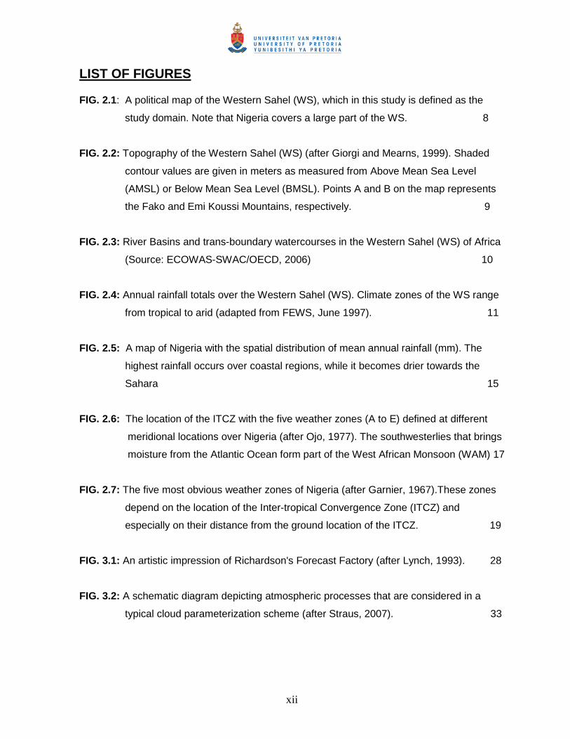
LIST OF FIGURES

FIG. 2.1: A political map of the Western Sahel (WS), which in this study is defined as the

study domain. Note that Nigeria covers a large part of the WS. 8

FIG. 2.2: Topography of the Western Sahel (WS) (after Giorgi and Mearns, 1999). Shaded

contour values are given in meters as measured from Above Mean Sea Level

(AMSL) or Below Mean Sea Level (BMSL). Points A and B on the map represents

the Fako and Emi Koussi Mountains, respectively. 9

FIG. 2.3: River Basins and trans-boundary watercourses in the Western Sahel (WS) of Africa

(Source: ECOWAS-SWAC/OECD, 2006) 10

FIG. 2.4: Annual rainfall totals over the Western Sahel (WS). Climate zones of the WS range

from tropical to arid (adapted from FEWS, June 1997). 11

FIG. 2.5: A map of Nigeria with the spatial distribution of mean annual rainfall (mm). The

highest rainfall occurs over coastal regions, while it becomes drier towards the

Sahara 15

FIG. 2.6: The location of the ITCZ with the five weather zones (A to E) defined at different

meridional locations over Nigeria (after Ojo, 1977). The southwesterlies that brings

moisture from the Atlantic Ocean form part of the West African Monsoon (WAM) 17

FIG. 2.7: The five most obvious weather zones of Nigeria (after Garnier, 1967).These zones

depend on the location of the Inter-tropical Convergence Zone (ITCZ) and

especially on their distance from the ground location of the ITCZ. 19

FIG. 3.1: An artistic impression of Richardson's Forecast Factory (after Lynch, 1993). 28

FIG. 3.2: A schematic diagram depicting atmospheric processes that are considered in a

typical cloud parameterization scheme (after Straus, 2007). 33

xiii

FIG. 5.1: Africa LAM T+24h forecasts for maximum temperature compared with observations

over Semi-Arid (SA) climate zone of the Western Sahel (WS) (a) Forecast vs.

Observed and (b) Forecast minus Observed. The time series plotted are the mean

values of the observations and model forecasts over the regions. 49

FIG. 5.2: Same as in FIG. 5.1 but for the Wet and Dry Tropics (WDT) climate zone of the

Western Sahel (WS). 50

FIG. 5.3: Same as in FIG. 5.2 but for the Wet Equatorial (WE) climate zone of the Western

Sahel (WS). 51

FIG. 5.4: The magnitude of Africa LAM errors (RMSE and MAE) in predicting maximum

temperatures T+24h ahead in time over the WE, WDT and SA climate zones of the

WS and for the (a) JFM, (b) AMJ, (c) JAS and (d) OND seasons, and over the

period January 2005 to December 2006. 52

FIG. 5.5: Same as in FIG. 5.3 but for minimum temperature over the Semi-Arid (SA) climate

zone of the Western Sahel (WS). 56

FIG. 5.6: Same as in FIG. 5.5 but over the Wet and Dry Tropics (WDT) climate zone of the


FIG. 5.7: Same as in FIG. 5.6 but over the Wet Equatorial (WE) climate zone of the Western

Sahel (WS). 58

FIG. 5.8: As in FIG. 5.4 but for minimum temperatures. 59

FIG. 5.9: Same as in FIG. 5.7 but for Rainfall over the Semi-Arid (SA) climate zone of the


FIG. 5.10: Same as in FIG. 5.9 but over the Wet and Dry Tropics (WDT) climate zone of the


xiv

FIG. 5.11: Same as in FIG. 5.10 but over the Wet Equatorial (WE) climate zone of the


FIG. 5.12: As in FIG. 5.8 but for rainfall. 65

FIG. 6.1: Typical television weather forecasting presentation on national television in Nigeria.

Current weather forecast issued incorporated NWP model results. 70

FIG. 6.2: Africa LAM simulated forecasts of 850hPa winds for 00:00GMT (T+6h) (left) and

06:00GMT (T+12h) (right) for 19 October 2006. Marked red lines indicate troughs,

while C denotes a vortex. 73

(Source: http://www.metoffice.gov.uk/weather/africa/lam)

FIG. 6.3: Satellite images for 00:00GMT (left) and 03:00GMT (right) on 19 October 2006.

Convective weather over West Africa is clearly indicated. 73

(Source: EUMETSAT)

FIG. 6.4: Africa LAM forecasts of Relative Humidity (RH) T+6h forecasts for 00:00GMT (top

left) and T+12h forecasts for 06:00GMT (top right) with accumulated precipitation

T+6h forecasts (bottom) for 19 October 2006. 74


FIG. 6.5: ECMWF Mean Sea Level Pressure (MSLP) T+24h forecasts at 00:00GMT on 13

and 14 March 2006 (top, left and right, respectively) compared to observed MSLP

across Nigeria (bottom, left and right). 75

(Source: http://www.ecmwf.int/products/forecasts/d/charts/medium/deterministic/)

FIG. 6.6: ECMWF Mean Sea Level Pressure (MSLP) T+24h forecasts at 00:00GMT on 15

and 16 March 2006 (top, left and right, respectively) compared to observed MSLP

across Nigeria (bottom, left and right). 75 (Source: http://www.ecmwf.int/products/forecasts/d/charts/medium/deterministic/)

xv

FIG. 6.7: Examples of NCEP/GFS 850hPa heights, combined with Mean Sea Level Pressure

(MSLP) T+24h forecasts (left) and the 10m winds combined with 2m temperatures

T+24h forecasts (right), as used to assist weather forecasters in their duties at the

Nigerian Meteorological Agency (NIMET). 77

(Source: http://www.nco.ncep.noaa.gov/pmb/nwpara/analysis/index_africa.shtml)

FIG. 6.8: ALADIN 850hPa temperature, Relative Humidity (RH) and winds for the T+24h

forecast (left), and precipitable water and Convective Available Potential Energy

(CAPE) for the T+24h forecast (right) over North and Equatorial Africa. 79

(Source: http://www.marocmeteo.ma/spn).

FIG. 7.1: A schematic flow diagram that illustrates a typical statistical post-processing

approach. Solid arrows indicate information sources required in the development of

the statistical forecasting equations, and dashed arrows indicate the information flow

when the corrections are implemented (adapted from Wilks, 1995). 82

FIG. 7.2: Root Mean Squared Errors (RMSEs) of the Africa LAM T+24h forecast output of

maximum temperatures compared to that of the bias corrected and MOS forecasts.

RMSE is for original model forecasts, while RMSE’ and RMSEmos are for the bias-

corrected and MOS forecasts, respectively. 94

FIG. 7.3: Root Mean Squared Errors (RMSEs) of the Africa LAM T+24h forecast output of

minimum temperatures compared to that of the bias corrected and MOS forecasts.

RMSE is for original model forecasts, while RMSE’ and RMSEmos are for the bias-

corrected and MOS forecasts, respectively. 95

FIG. 7.4: An example of an ECWMF Ensemble Prediction System (EPS) forecast. Solid

contours represent the ensemble mean and the shaded contours represent the

ensemble spread. Areas with high ensemble spread values indicate areas of high

forecast uncertainties. 97

xvi

LIST OF TABLES

Table 5.1: Africa LAM NWP verification results for T+24h maximum temperatures forecasts

during the JFM, AMJ, JAS and OND seasons over the WE, WDT and SA climate

zones of the Western Sahel (WS), and over the period January 2005 to

December 2006. 48

Table 5.2: Africa LAM NWP verification results for T+24h minimum temperatures forecasts

during the JFM, AMJ, JAS and OND seasons over the WE, WDT and SA climate

zones of the Western Sahel (WS), and over the period January 2005 to

December 2006. 55

Table 5.3: Africa LAM NWP verification results for T+24h rainfall forecasts during the JFM,

AMJ, JAS and OND seasons over the WE, WDT and SA climate zones of the

Western Sahel (WS), and over the period January 2005 to December 2006. 61

Table 7.1: Africa LAM T+24h forecast output of maximum temperatures compared to that of

the bias corrected forecasts. The RMSE is for the original model forecasts, RMSE’

for the bias-corrected forecasts and %IM is the percentage forecast improvement

achieved by introducing bias corrections. 85

Table 7.2: Africa LAM T+24h forecast output of minimum temperatures compared to that of

the bias corrected forecasts. The RMSE is for the original model forecasts, RMSE’

for the bias-corrected forecasts and %IM is the percentage forecast improvement

achieved by introducing bias corrections. 86

Table 7.3: MOS correction terms used to formulate the MOS equations required for adjusting

Africa LAM T+24h forecasts of maximum temperatures. Ae is negative of the mean

model bias, ƒMOS the MOS regression coefficient and ß the average anomaly from

the mean of model forecasts. 91

Table 7.4: The MOS equations required to adjust Africa LAM T+24h forecasts of maximum

temperatures over the five (5) selected Nigerian meteorological stations for the

JFM, AMJ, JAS and OND seasons. 91

xvii

Table 7.5: MOS correction terms used to formulate the MOS equations required for adjusting

Africa LAM T+24h forecasts of minimum temperatures. Ae is negative of the mean

model bias, ƒMOS the MOS regression coefficient and ß the average anomaly from

the mean of model forecasts. 92

Table 7.6: The MOS equations required to adjust Africa LAM T+24h forecasts of minimum

temperatures over the five (5) selected Nigerian meteorological stations for the

JFM, AMJ, JAS and OND seasons. 92

1

CHAPTER 1

INTRODUCTION 1.1 BACKGROUND

Processes in the atmosphere are not perfectly predictable in a deterministic sense

because the atmosphere is regarded as a non-linear dynamic or “chaotic” system. This

implies that the dynamic flow of the atmosphere is inherently non-predictable. In addition

many physical parameterization schemes have been introduced in efforts to resolve

physical processes in the atmosphere, such as cloud processes, rainfall and radiation

fluxes, which all also have an influence on the atmospheric flow dynamics (Lorenz, 2006).

Our ability to predict atmospheric flow and processes is also restricted by limitations in

spatial as well as temporal observations of the weather. Numerical Weather Prediction

(NWP) models incorporates most of these aspects by numerically integrating (estimating)

the equations of atmospheric flow dynamics, and by estimating physical processes,

mostly by means of parameterization (Straus, 2007). Many NWP models are currently

operational to forecast weather all over the world on various spatial scales. These models

are still far from perfect, although much progress has been made over recent years to

improve on NWP (Mesinger, 2005). NWPs results might be improved by the use of

statistics. The reason for this is because there are fundamental surface and atmospheric

forcing that influences weather events, and that allow for weather events to be repeated to

a certain degree. As a result, stochastic or statistical methods have recently become a

very useful application as a post-processing tool, which is employed to improve on

weather forecasting at meteorological centers. As emphasized by Kalnay et. al. (1990),

Wilks (1995) and Kalnay (2003) statistics has many roles to play in the atmospheric

sciences.

It is known that surface conditions are simplified and homogenized in NWP models, and

that the atmosphere is regarded as a medium that consists of square grid boxes to

facilitate the mathematical treatment of the atmosphere. In most models, land use

characteristics are represented as an array of horizontal grid squares, while associated

grid boxes extend throughout horizontal layers in the vertical atmosphere. Within surface

grid squares, one finds smoothed values of important small-scale boundary conditions

such as topography, vegetation and soil types, or even small-scale bodies of water, which

are spatially variable in reality and important to local weather conditions. Atmospheric

turbulence, which plays an important role in atmospheric convection, is another small-

scale process that is difficult to resolve analytically. Inaccuracies caused by these

2

estimations of reality in NWP models are a result of limitations in resolving complex

processes that occur in the atmosphere. Some NWP models need strong computers to

simulate estimated atmospheric flow and processes in order to generate operational

weather forecasts, an asset or luxury that many meteorological centers simply cannot

afford (Grell, 1993; Lorenz, 2006).

Because of the above-mentioned limitations, NWPs are subjected to systematic errors

and biases. Hence, the continuous verification of NWP model outputs in order to

contribute to model improvement became very important over recent years. Verification

results provide numerical measures of how well NWP models perform, in an objective

way. It also allows for monitoring of how NWPs improve over time. In the day-to-day

operation of weather forecasting one might find biases in either forecasts generated by

the NWP model, or biases that result from the weather forecaster’s interpretation of NWP

output, or both. The use of verification statistics might help to identify the source of these

biases, which might lead to research targeted to improve the scientific understanding of

the underlying processes required to improve NWP model forecasts (Jolliffe and

Stephenson, 2003). For application, NWP model forecasts or even verification results

need to be prepared and presented in such a way that it addresses the need of weather

forecasters, and eventually the requirements of end-users, which include a diversity of

sectors in the economy, decision making of social society, agricultural and even disaster

management activities.

As mentioned before, stochastic methods might be useful to improve NWPs. For example,

statistical relationships might be developed between the simulated information generated

by NWP models and the desired forecast quantities to reduce the problem of

homogenization – known as downscaling (Glahn and Lowry, 1972; Wilks 1995). Since

current NWP models have limitations which emanate from both a lack of detailed initial

conditions and boundary input, as well as the inherent problem of non-linearity in flow

dynamics and the estimation of physical processes, a combination of statistics trained

over a long enough record of model output compared to observation might help to quantify

and express forecast uncertainties. Statistical re-interpretation or “post-processing’ of

NWP products might improve weather forecasts from NWP models, and is increasingly

regarded as an important addition to assist operational weather forecasters in their duties.

Statistical “post-processing” provides a first guess of expected local conditions. Although

uncertainties in weather forecasts generated by NWP models or prepared by weather

forecasters are difficult to avoid (Wilks, 1995), statistical tools might always be of value to

3

improve weather forecasts. Statistical guidance could add value to NWP model output by

providing objective model interpretation in order to reduce systematic biases, to quantify

uncertainties, to predict parameters that the model does not predict, and to produce site-

specific weather forecasts (Kalnay, 2003).

Despite of the increased importance of the application of NWP as a sophisticated weather

forecasting tool, most meteorological centers in Africa have little knowledge of NWP

model development, or do not even have the required computer resources to generate in-

house NWPs. These centers mostly rely on NWP results from overseas, which are

normally made available via the Internet. Currently, the majority of operational National

Meteorological and Hydrological Services (NMHS) in Africa only interpret NWP model

outputs subjectively when preparing and issuing daily weather forecasts, and not in all

cases are these model products a reflection of actual weather conditions. As a result,

weather forecasts over Africa are often of poor quality.

However, many other institutions, such as the United Kingdom Meteorological Office (UK

Met Office), are running finer resolutions models over Africa, and had even became

involved in NWP development for Africa. One such model from the UK Met Office is

known as the Limited Area Model (LAM) over Africa (hereafter called Africa LAM). In this

study, NWPs generated by the Africa LAM over the Western Sahel (WS) are verified

against point observations using internationally recognized verification algorithms. In

addition, statistical “post-processing” methods that could be of value in improving model

forecasts are proposed. Although, most of the classical statistical post-processing method

derives separate regression coefficients for each location and forecast lead time using a

number of forecast parameters, the post-processing method advanced in this study is

based on a simple bias correction and regression of the model forecast parameter

corresponding to the station observations. Results from this study might contribute to a

better understanding of NWP over the WS, and maybe, to improved weather forecasting

over the region of investigation.

1.2 MODEL ERRORS AND STATISTICAL POST-PROCESSING

Most NWP models generate forecasts with systematic errors or biases. Systematic NWP

model forecast errors or biases, for example, include progressive atmospheric cooling or

warming biases with increasing forecast projections, the tendency for modeled synoptic

features to move too slow or too fast during the process of model simulation, and the

unavoidable decrease in forecast accuracy with an increase in lead time (Kalnay et. al.,

4

1990). A number of statistical post-processing techniques developed over recent years

might allow for the compensation of these model systematic errors or biases. Kalnay

(2003; p276) stated that “In order to optimize the use of numerical weather forecasts as

guidance for human forecasters, it has been customary to use statistical methods to “post-

process” the model forecasts and adapt them to produce local forecasts”. Glahn and

Lowry (1972), Carter et. al. (1989) and Wilks (1995) also suggested that statistical

guidance is necessary to add value to NWP.

1.3 MOTIVATION FOR THE RESEARCH

The growing demand at NMHS in Africa to issue more accurate weather forecasts, and to

improve their capacity to produce these forecasts, inspired the interest in NWP research

as documented in this dissertation. Because of the UK Met Office’s interest in NWP

development for Africa, and because of the important influence of tropical weather

systems on global weather events (which includes the UK), the UK Met Office had

decided to develop and implement the Africa LAM to generate NWPs at a 20km horizontal

resolution over Africa. An important motivation for the operational implementation of the

Africa LAM was obviously to provide a NWP asset to the NMHS in Africa who mostly find

it difficult to run NWP models in-house. The Africa LAM project is co-funded by the British

Government and the World Meteorological Organization (WMO).

As mentioned before, a need for knowledge of the development, implementation,

interpretation and verification of NWP models over Africa inspired interest for the research

documented in this dissertation. In particular, the verification of NWP results and the

possibility to introduce stochastic techniques to improve NWP results are important focus

points in the research. The improvement and interpretation of NWPs are important fields

of study at some national meteorological centers in Europe (for example the Netherlands,

Britain, Italy and Spain) and some other countries such as China, Canada and the United

States of America (USA) (Lemcke and Kruizinga, 1988; Carter et. al., 1989). The

verification results and statistical post-processing suggestions in this study will contribute

to a better understanding of the performance and value of NWP models in not only the

WS region of Africa, but also for the rest of Africa.

1.4 THE AIM AND OBJECTIVES OF THE RESEARCH

The overall aim of this study is to verify NWPs generated by the Africa LAM of the UK Met

Office over the WS of Africa in order to investigate the potential of the model to be used

as a weather forecasting tool to assist operational weather forecasters in their duties. In

5

addition the study will suggest post-processing statistical tools that might be of value to

improve NWPs and eventually weather forecasts.

The overall aim will be achieved by the following objectives:

OBJECTIVE 1

The first objective of this study is to examine the performance of the Africa LAM

developed by the UK Met Office against point observations and against regional

averages of meteorological variables over the WS of Africa by using internationally

recognized verification algorithms.

The essence of the verification is to ascertain and evaluate the performance of the Africa

LAM to predict rainfall, as well as maximum and minimum temperatures over the study

domain, which is the WS of Africa. During this process systematic forecast errors and

biases are to be identified.

a) Daily T+24h (forecasts of 24 hours from time T) Africa LAM forecasts data for rainfall

as well as for maximum and minimum temperatures (screen temperatures) will be used

as predictors (Antolik, 2003). Africa LAM output that is in Grib format will be

interpolated to observational point stations by using MATLAB software (a mathematical

analysis software package).

b) Daily observed data over the WS of Africa obtained from the National Climatic Data

Centre (NCDC) of the USA, and station observations (where available) will be used as

predictands.

c) As recommended by Wilks (1995), Kalnay (2003) and Antolik (2003), the data sets will

be stratified into seasons (dry and wet seasons) and pooled according to climatic

zones over the WS.

d) The datasets will be seasonally stratified into two dry seasons (January-February-

March (JFM) and October-November-December (OND)) and two wet seasons (April-

May-June (AMJ) and July-August-September (JAS)). This, according to Wilks (1995),

allows for the incorporation of different relationships between predictors and

predictands at different periods of the year

e) The data will also be pooled into regions in accordance with the climate zones of the

WS, namely the Wet Equatorial (WE) (0.00 ºN to 8.00 ºN), Wet and Dry Tropics (WDT)

(8.00 ºN to 12.00 ºN) and Semi-Arid (SA) (12.00 ºN to 15.00 ºN) climate zones. This

allows for the developmental data used to incorporate groups of nearby climatologically

similar stations (Wilks, 1995).

6

OBJECTIVE 2

The second objective of this study is to investigate if the Africa LAM has the

potential to be employed as NWP model to assist operational weather forecasters in

their duty to issue more accurate forecasts.

In order to investigate if the Africa LAM has potential to serve as a weather forecasting

tool over the WS of Africa, the study will specifically investigate and outline weather

forecasting operations as they happen on a daily basis at the Nigerian Meteorological

Agency (NIMET). The study will make suggestions of how NWPs might be incorporated to

support operational weather forecasters in their duties.

OBJECTIVE 3

The third objective is to suggest possible statistical post-processing tools that

might be of value for improving basic NWPs over the WS of Africa.

Statistical post-processing results derived from using historical observations, and raw

NWP output data generated by the Africa LAM, will be discussed. The variables

considered will be maximum and minimum temperatures over five (5) selected Nigerian

meteorological observation stations.

1.5 ORGANIZATION OF THE REPORT

The study mainly examines the performance of the Africa LAM NWPs generated over the

WS against point observations, by using internationally prescribed verification statistics.

Also included in the study is the suggestion of post-processing techniques that could

improve weather forecasts over the region. The content and results presented in the

dissertation is expected to guide scientists especially in the WS, who are interested to

issue improved weather forecasts.

In CHAPTER 2, a general overview of the characteristics and natural resources of the

study domain is introduced. The chapter is sub-divided into two sections. The first section

gives a summary of the overall West African climate, and how it relates to the climate of

the WS, while the characteristic of the climate of Nigeria, which forms an integral part of

the WS (and the West African) climate, is discussed in the second section.

CHAPTER 3 first gives an historical overview of the development of NWP at various

international research centers. Because the study focuses on NWPs generated by the

7

Africa LAM from the UK Met Office, the historical overview is followed by a technical

description of the Africa LAM, and also to some extent, the Unified Model (UM) of the UK

Met Office, which forms the basis of the Africa LAM.

CHAPTER 4 explains the statistical formulation and algorithms used to verify NWPs by

the Africa LAM against observations over the WS and Nigeria. These algorithms are in

accordance to NWP verification standards as required by the WMO.

In CHAPTER 5 the Africa LAM is verified against observations. The verification results

highlight the strengths and weaknesses of the model to predicting rainfall, maximum and

minimum temperatures over the study domain. The chapter gives an evaluation of the

magnitude of the model systematic forecast errors and biases, which might be improved

by the statistical post-processing techniques suggested in the study.

CHAPTER 6 provides a general overview on conventional forecasting, and current

forecasting that incorporate NWPs in Nigeria. The shortcomings and needs of NIMET,

which are also applicable to other NMHS in the WS, to issue improved weather forecasts

are examined. A typical weather forecasting process at NIMET is also discussed as part

of this chapter, with the view to provide an example for other NMHS in the WS (and

beyond) that might consider the incorporation of NWP model results in future.

In CHAPTER 7 statistical post-processing techniques such as simple bias corrections,

MOS and Ensemble Forecasting Systems are suggested and discussed. These post-

processing methods are useful, and sometimes necessary, to improve systematic errors

and biases in NWPs. Some post-processing technique results are also discussed in this

chapter through application at five selected Nigerian meteorological stations and during

the JFM, AMJ, JAS, and OND seasons.

Concluding remarks are outlined in CHAPTER 8, which is followed by APPENDICES

where analyses tools adopted, including the MATLAB scripts applied in this study, are

attached.

8

CHAPTER 2

THE STUDY DOMAIN 2.1 INTRODUCTION

This chapter provides a general overview of the characteristics of the study domain, which

is the WS of Africa, as indicated in Fig 2.1. The WS exhibits typical characteristics of the

general West African climate, and the country Nigeria covers an extended part of the WS.

As such, the climate of Nigeria represents most of the dominant climatic characteristics of

the broader WS. The chapter is sub-divided into two sections. The first section gives a

summary of the overall West African climate, and how it relates to the climate of the WS,

while the characteristic of the climate of Nigeria, which forms an integral part of the WS

(and the West African) climate, is discussed in the second section.

2.2 THE WESTERN SAHEL (WS)

2.2.1 Geographical location

The area that extends from longitude 20.00°West (W) to 30.00°East (E), and latitude 0.00

(Equator) to 20.00°North (N) is defined as the WS ( Fig 2.1). The WS of Africa is bordered

in the north by the Sahara desert, and in the south and west by the Atlantic Ocean. It

includes the following countries: Benin Republic, Burkina Faso, Cape Verde, Cote d'Ivoire,

Cameroon, Chad, The Gambia, Ghana, Guinea, Guinea Bissau, Liberia, Mali, Mauritania,

Niger, Nigeria, Senegal, Sierra Leone, Togo and Sudan (Fig. 2.1). It is estimated that

more than 290million people live in the WS, which covers a total area of approximately

eight million km2 (ECOWAS-SWAC/OECD, 2006)

FIG. 2.1: A political map of the Western Sahel (WS), which in this study is defined as

the study domain. Note that Nigeria covers a large part of the WS.

9

2.2.2 Topography and drainage

The highest geographical point in the WS is the Fako Mountain in Cameroon (also known

as the Cameroon mountain), which is about 4 095m Above Mean Sea Level (AMSL), and

the lowest point is at the Djourab depression in the Chad Republic, which is 160m Below

Mean Sea Level (BMSL). Apart from these two extreme elevation points, there are several

other high grounds in the study domain, which includes mount Emi Koussi in Chad

(3 415m AMSL), mount Kinyeti in Sudan (3 187m AMSL), and mount Chappal Waddi in

Nigeria (2 419m AMSL). In general, the WS topography (Fig. 2.2) ranges from low coastal

plains to flat, hills, plateaus, mountains and desert plains.

FIG. 2.2: Topography of the Western Sahel (WS) (after Giorgi and Mearns, 1999). Shaded contour values

are given in meters as measured from Above Mean Sea Level (AMSL) or Below Mean Sea

Level (BMSL). Points A and B on the map represents the Fako and Emi Koussi

Mountains, respectively.

Runoff over the WS takes place through a large number of fast moving rivers flowing from

higher altitude locations in the WS region towards the Atlantic Ocean. Some of the most

important rivers in the WS are the Senegal River, Gambia River, Niger River, Benue River

and Volta River. The Niger, Senegal and Gambia rivers originate from the Futa Djallon

Highland. There are 28 transboundary river basins in the WS extending over almost 71%

of the region’s total surface area (Fig. 2.3). Of these trans-boundary river basins, the Niger

River Basin, Senegal River Basin, Volta River Basin, Lake Chad Basin and the Comoe

River Basin are the most prominent (Anyadike, 1992). In the WS, each country shares at

10

least one watercourse with the other. A watercourse is part of the inland territory where all

surface water flows towards the same outlet. There are eight watercourses in Cote

d’Ivoire, seven in Cameroon and Liberia, and five in Nigeria and Sierra Leone.

FIG. 2.3: River Basins and trans-boundary watercourses in the Western Sahel (WS) of Africa

(Source: ECOWAS-SWAC/OECD, 2006).

2.2.3 Climate

The WS of Africa has diverse climate characteristics, ranging from wet equatorial climates

(from the southern coastline up to a latitude of 8.00ºN), to wet and dry tropics climates

(between latitude 8.00ºN and 12.00ºN) in the central region, and semi arid climates

(between latitude 12.00ºN and 15.00ºN) in the northern region (see Fig. 2.4).

2.2.3.1 The Wet Equatorial (WE) climate zone

The Wet Equatorial (WE) climate zone (located in the southern part of the WS) receives a

significant amount of rainfall each year, with not more than three months recording a total

monthly rainfall of less than 50mm. As part of the study domain, the WE climate zone

extends across the coasts of Liberia, Sierra Leone, Ivory Coast and Nigeria, southern

Cameroon and Equatorial Guinea. The most important economic and agricultural activities

found in the WE climate zone include palm kernels and oil, peanuts, rubber and cotton,

timber (mahogany), coffee and the most prominent natural resources are copper,

manganese, gold, zinc, diamond, tin, petroleum, bauxite and water for hydro-power.

11

FIG. 2.4: Annual rainfall totals over the Western Sahel (WS). Climate zones of the WS range

from tropical to arid. (adapted from FEWS, June 1997).

The WE climate zone is close to the equator, meaning that total outgoing long wave

radiation at ground level is relatively high throughout the year. This does not only results

in fairly uniform annual temperatures, but also allow for little variability between day and

night (or maximum and minimum) temperatures. The WE climate zone falls in the

equatorial belt of relatively lower surface pressures, also known as the Inter-tropical

Convergence Zone (ITCZ). The ITCZ follows a distinct seasonal meridional propagation

across the region. The ITCZ is often associated with rainfall, because of extensive

convection and cloud development that occur at the location of the ITCZ. The ITCZ is

therefore an important driver of seasonal rainfall over Africa. A larger portion of the

available atmospheric energy over the WE climate zone occurs as latent heat of

evaporation from soil or water. The high evapo-transpiration rate from the thick vegetation

cover, and higher outgoing long wave radiation, are diffused by turbulence in the lower

layers of the atmosphere resulting into important vertical fluxes of water vapor and

sensible heat (Ojo, 1977). The most dominant wind flow pattern, for most of the year, over

the WE climate zone is warm, moist westerly to southerly winds, mostly associated with

the West African Monsoon (WAM), which are responsible for high rainfall being recorded

over the region. However, drier northeasterly winds prevail over the WE climate zone for a

short period of the year (November and December), resulting in a season of lower rainfall

12

totals (as low as 50mm per month). Mean annual rainfall totals over the WE climate zone

are high, ranging from 5 000mm over the coast of Liberia to about 1 200mm near the

latitude of 10°N. The WE climate zone receives its lowest annual rainfall from mid-

December until late March (Griffiths, 1966), from where rainfall again increases to a

maximum in June, and a second maximum in September, which is generally lower than

the peak in June. This indicates two rainy seasons, which are linked to the south-north

propagation of the ITCZ. In the WE climate zone one also finds a so called “little dry

season” from late July to August. Daily rainfall in excess of 200mm may be experienced

anytime from May to October, and rain may also fall for about 25days during each month

from June to October. Rainfall over the WE climate zone is convective of nature and

therefore mostly falls during late afternoon hours and during night, with little chance of rain

in the morning (Swan, 1958).

Mean annual temperatures over the WE climate zone ranges from 15°C to 37°C, the

highest being recorded in March and October and the lowest in December and August.

Relative Humidity (RH) over the WE climate zone is generally high, especially along the

coast. The lowest RH readings, usually recorded during January in the afternoon, are in

the order of 70%, which may increase to about 95% during the early hours of the day.

However, RH values significantly decreases during the harmattan period (November to

February) when dry continental northeasterly winds prevail. The WE climate zone is

exposed to sunshine, especially during the early afternoon hours, and most of the coastal

and inland cities experience early morning fog from October to February, with a peak in

fog event frequencies in January. The ITCZ influences the prevailing wind direction by

means of the WAM. However, local effect of the land and sea breezes are also noticeable

during the early morning hours and late at night. Over the coastal cities of the WS

(situated within the wet equatorial climate zone), west to southerly WAM winds starts

during July and, together with local topographic characteristics, can give rise to a

maximum monthly rainfall experienced when the ITCZ is located in its most northern

position (Nieuwolt, 1977)

2.2.3.2 The Wet and Dry Topics (WDT) climate zone

The Wet and Dry Tropics (WDT) climate zone (located in the central part of the WS) is a

transfer region between semi-arid conditions in the north and wet equatorial conditions in

the south. The area approximately extends across latitude 8.00°N to 12.00°N. The WDT

climate zone has about seven to nine months of rainfall in excess of 50mm per month.

The countries that fall in this climate zone of the WS are the Ivory Coast, Ghana, Togo,

13

southern Sudan, central Cameroon and a large part of Sierra Leone and Nigeria. Average

annual rainfall amounts over the WDT climate zone ranges from 1 000mm to 4 000mm.

This high rainfall allows for better agricultural production than in the semi-arid areas to the

north.

The most prominent agricultural activities over the WDT climate zone are rice, yams,

mahogany, corn, cotton, groundnuts, cattle rearing, bananas, palms, citrus fruits,

pineapples and coffee. Natural resources include limestone, salt, gypsum, granite and

phosphate. Over this climate zone, a warm and humid tropical maritime air mass from the

Atlantic Ocean dominates during most of the year, giving rise to adequate rainfall for

successful farming. However, for a short period each year (January-February and

November-December), continental airflow dominates, which results in low humidity and

lower rainfall (Trewartha, 1961). The WDT climate zone experiences both single and

double annual peaks of maximum rainfall, and therefore has both one and two rainfall

seasons per year. These seasons are related to the meridional shift of the ITCZ. The

single annual peak of maximum rainfall over the WDT climate zone is recorded around

latitude 10.00°N to 12.00°N, and July (or sometimes August) is the month of highest

rainfall. In the double peaked maximum rainfall season (latitude 8.00°N to 10.00°N), June

is generally the wettest month with some areas that experience maximum rain in

September. February to April is a period with a high number of disturbance lines, which

are well-defined belts of intense thunderstorms moving at an average speed of 25kmh-1

from east to west, with intense rain over relative short time intervals (Ojo, 1977). These

disturbance lines usually occur 300 to 600km south of the ITCZ, where humid and hot air

are deeper to allow for the development of unstable conditions with the associate heavy

rainfall (Adejokun, 1966). Humid WAM air that flows from the ocean, disturbance lines, the

ITCZ and topography are the major atmospheric influences that contribute to rainfall

development over the WDT climate zone.

The mean annual temperature over the WDT climate zone ranges from 30°C to 36°C, with

a small variation of about ± 2°C to 4°C during the year. The mean annual minimum

temperature is generally from 19°C to 21°C, but can sometimes increase to 23°C to 24°C.

Temperature reaches its highest peaks in February, or March, and its lowest dips in

December or January. The lowest maximum temperature occurs in July or August, while

the highest minimum temperature occurs in April or May. Over the WDT climate zone, RH

is extremely high throughout the year, reaching percentages of about 85% to 95% in most

months, especially during the early hours of the day. Afternoon mean annual RH ranges

14

from 50% to 75%, which are still relatively high. However, during December and January,

some stations occasionally record an afternoon RH low of about 25% to 30% (Jackson,

1977).

2.2.3.3 The Semi-Arid (SA) climate zone

The Semi-Arid (SA) climate zone (located in the north of the WS) is close to the southern

fringes of the Sahara desert (Fig. 2.4). Mean annual rainfall totals over the SA climate

zone are normally less than 400mm. The beginning and end of the rain seasons are

usually abrupt due to the rapid northward advancement and southward retreat of the ITCZ

(Adejokun, 1966). The dominant wind is associated with the advection of a dry and dusty

continental air mass, mostly northeasterly in direction. The SA climate zone mostly

experiences extensive diurnal variation in temperature, and is also very prone to natural

hazards such as drought, sand storms and dust storms. The countries that fall within the

SA climate zone are Senegal, Gambia, Mali, Burkina Faso, and Niger, the northern fringes

of Nigeria, Chad and Sudan. Agricultural products and activities in the SA climate zone

include groundnuts, cattle rearing, livestock, corns, rice, cotton and millets, and are

usually aided by flood plain cultivation and irrigation. Some of the natural resources

available in the SA climate zone are sand, kaolin, uranium, limestone and granite (Tuller,

1968).

The highest monthly radiation total over the SA climate zone is usually recorded during

April, and the lowest is recorded during July or August. The climate zone also has, on

average, 7.5h.day-1 to 9.3h.day-1 sunshine. The mean annual maximum temperature over

the SA climate zone ranges from 40°C to 47°C, which are extremely high, and the mean

annual minimum temperature ranges from 7°C to 9°C. Squall lines are most frequent in

April, May, June and October, especially during the late afternoon hours. These squall

lines often produce maximum winds gusts of around 80knots, which are usually very

destructive (Okulaja, 1970).

2.3 NIGERIA AS PART OF THE STUDY DOMAIN

2.3.1 Geographical location

Nigeria is a West African country, and falls within the WS – as a matter of fact Nigeria

covers a substantial part of the WS region. The country extends from latitude 3.30°N to

13.20°N and longitude 3.20°E to 13.20°E (Fig. 2.5), bordered in the north by the Niger

Republic, in the south by the Atlantic Ocean, in the east by the Republic of Cameroon and

in the west by the Benin Republic. Nigeria covers a total area of 923 770km2 and a total

15

land area of 910 770km2. The land boundary is 4 047km long, and the country’s coastline

is about 853km long. The available irrigated land is estimated at 9 570km2, land use 35%

arable, permanent crops 5%, and permanent pastures 54% and 18% of forests and

woodland. The 2006 census figures in the country reveals that Abuja has an estimated

population of 1.5million, Lagos 9million, Ibadan 5.6million, Kano 9.4million and Enugu

3.3million (Thisday online, 2007).

FIG. 2.5: A map of Nigeria with the spatial distribution of mean annual rainfall (mm).

The highest rainfall occurs over coastal regions, while it becomes drier

towards the Sahara.

2.3.2 Topography

Topographical features of Nigeria range from coastal swamps in the south towards a

propagation that ranges from tropical forests, open woodlands, grasslands, and eventually

semi deserts in the north. The lowest elevation contour in the country obviously runs along

the Atlantic Ocean coastline, and the highest point can be found at Chappal Waddi in

Plateau State (about 2 419m AMSL). Some of the major rivers are Rivers Niger, Benue,

Anambra, Cross, Gongola, Hadejia, Kaduna, Katsina-Ala, Kamadugu, Ogun, Osun,

Owena, Osse, Sokoto, Yedseram, Yobe, and Zamfara.

2.3.3 Population

It is estimated that about 140million people live in Nigeria (Thisday Online, 2007). The

country has about 250 ethnic groups, from which the most prominent are the Hausa-

Fulani, Igbo and the Yoruba. The Hausa-Fulani dominate over the northern parts of the

16

country, while the Igbo dominate over the eastern parts and the Yoruba over the southern

parts of Nigeria. There are also other ethnic groups, such as the Nupe, Tiv, Kanuri, Efik,

Ibibio and Ijaw, who also live in the country. The most commonly practiced religions

amongst the population are Islam, Christianity and the indigenous African believe.

Although the official language in Nigeria is English, most people have a good knowledge

of two or more indigenous languages. Hausa, Yoruba, and Igbo are the most widely

spoken indigenous languages. About 32% of all male and 27% of all female citizens of the

country are educated. Less than 25% of the population is urban dwellers, and at least 24

cities each have a population of more than one million people.

(Reference: http://www.CountryReports.org).

2.3.4 Climate

As Nigeria falls in the WS, its climate zones are similarly distributed than those of the WS

discussed earlier in this dissertation. The climate of Nigeria is generally classified

according to dry and wet seasons. There is a clear contrast between the dry and wet

seasons, which are, as in the WS climate, closely correlated with the south-northward

propagation of the ITCZ over the country (Adejokun, 1966). Over Nigeria, the ITCZ

retreats to its most southern position (close to the Equator) in January, and advances to

its most northern position (around latitude 20.00°N ) in July. The south-north meridional

propagation of the ITCZ is also associated with the dominant wind flow over the country,

which includes the WAM. During July, the prevailing wind are moist southwesterly winds

from the Atlantic Ocean (which is a component of the WAM), and during January the

dominant winds are dry northeasterly winds blowing across the Sahara towards the

country.

Mean annual rainfall totals over Nigeria ranges from approximately 3 800mm along the

coastline to less than 500mm over the far northern parts (Fig. 2.5). In most events rainfall

over Nigeria are characterized by local convective thunderstorms and disturbance lines

(discussed in section 2.2). The local impact of thunderstorms is usually sporadic, and

these storms occur widely over the interior of the country, especially during the peak of

the rain season (JAS). The coastal part of the country extends over about 30km in width,

and exhibits a very strong oceanic influence on coastal weather. In Nigeria, rainfall

patterns run roughly parallel to latitude lines, with exceptions over some of the high

elevation areas (Ojo, 1977; Ayoade, 1975). From the coastline to about latitude 10.00°N,

one finds two peaks per year in monthly rainfall totals (two seasons) and from latitude

10.00°N and further north, one finds a single seaso n – most probably because the ITCZ

17

does not often propagate that far to the north. The two peaks are usually recorded in June

and September, respectively, and the single peak in the north is recorded in August.

Average monthly temperatures in Nigeria range from 28°C to 34°C (from the coastline to

latitude 10.00°N) and 12°C to 43°C (from latitude 1 0.00°N to 14.00°N) (Odekunle, 2004).

2.3.5 The relationships between weather and the ITCZ over Nigeria

As noted earlier, the ITCZ and the associated WAM, play an important role in climate

characteristics of the WS and Nigeria. The ITCZ retreats to its most southern position in

January, and advances to its most northern position in July, when easterly trade winds

crosses the geographical equator, and under the influence of the Coriolis force, turns

westwards to form the WAM. As a result, moist onshore maritime air from the Atlantic

Ocean enters Nigeria in July, while dry and dusty offshore continental winds blows across

the Sahara desert towards Nigeria during January. According to the location of the ITCZ

five weather zones (A to E) have been defined (see Fig. 2.6) (Adejokun, 1966; Garnier,

1967; Ojo, 1977).

FIG. 2.6: The location of the ITCZ with the five weather zones (A to E) defined at different meridional

locations over Nigeria (after Ojo, 1977). The southwesterlies that brings moisture from the Atlantic

Ocean form part of the West African Monsoon (WAM).

The weather zone located immediately north of the surface location of the ITCZ has been

classified as weather zone A. Weather zone A is a predominantly dry region with dusty

continental easterly to northeasterly winds from the Sahara desert. High cloud types do

mostly occur with the occasional occurrences of medium cloud types. The zone is usually

cool with clear skies during night hours.

Weather zone B covers areas over Nigeria that is located directly south of the surface

location of the ITCZ. This weather zone extends over a distance of about 200 to 300km

south of the ITCZ. The zone experiences a mixture of the dry easterly to northeasterly

winds (at higher altitudes) and moist southwesterly winds (closer to the surface) (Fig. 2.6).

18

The weather of zone B is characterized with relatively high night temperatures and high

humidity values. Early morning fog in the form of stratus (low) clouds is often experienced.

A zone located at a distance of approximately 700km to 1 000km to the south of the

surface location of the ITCZ is known as weather zone C. In this zone moist southwesterly

winds are found at an altitude of about 6 000m above the land surface. Weather zone C

mostly experiences unstable atmospheric conditions, which are characterized by

disturbance lines and local thunderstorm activities, resulting in variable and sporadic

rainfall (Garnier, 1967). Weather zone C is generally characterized by high RH values,

with little diurnal variability in temperatures.

Weather zone D is found at a distance of 1 000km to 1 300km south of the surface

location of the ITCZ. It is also a zone with high RH values, and relatively low and mostly

constant temperatures (Fig. 2.6). In this zone, the “little dry season” (as mentioned in the

discussion of the WS climate) is experienced when inversion or stable conditions above

the stratus (low) clouds inhibits the upward movement of air, which results in very little

rain, but often in fog events.

The most southerly weather zone is known as weather zone E. This zone only affects a

relatively narrow strip along the coastline of Nigeria during July and August. It is a zone of

decreasing stratocumulus and stratus clouds, and increasing altostratus, altocumulus and

cirrus clouds. Drizzle and rain are the most frequently found over weather zone E.

Although defined in location, Garnier (1967) argued that the type, frequency and duration

of weather zones A to E over Nigeria fluctuate, because of fluctuations in position of the

ITCZ due to the meridional propagation of the ITCZ. He therefore went one step further by

classifying Nigeria into four weather regions (regions I to IV) using the annual frequency

distribution of the five weather zones (see Fig. 2.7).

19

FIG. 2.7: The five most obvious weather zones of Nigeria (after Garnier, 1967).

These zones depend on the location of the Inter-tropical Convergence Zone (ITCZ)

and especially on their distance from the ground location of the ITCZ.

Accordingly, the area over Nigeria that is mostly affected by weather conditions defined in

weather zone A (earlier discussed and illustrated in Fig. 2.6) for at least six months,

weather zone B for almost a month and weather zone C for four months during the period

of one year is classified as region I. Over region II, the weather conditions of weather zone

B are experienced during the greatest part of the year, especially when the ITCZ

advances northwards. The area that is predominantly influenced by the weather

conditions of all the five weather zones (weather zones A to E) is classified as region III. In

region IV weather conditions of weather zone C dominates, with occasional influence from

the weather of zone A.

2.4 Summary

The lack of knowledge and resources at many NMHS in Africa to not only run NWP

models, but also to interpret and apply NWP model output inspired this research. The

researcher is an operational weather forecaster at NIMET who has a passion for weather

forecasting and also appears on National Television to present weather forecasts to end-

users. Over recent years he became interested in various tools that can help improve

weather forecasts, and started to investigate the use, application of NWPs, as well as the

improvement of these predictions by means of post-processing techniques.

20

The objectives of this study are to introduce the Africa LAM from the UK Met Office as a

NWP model for Africa, and in particular the WS region, and to investigate the potential of

this model to be used as supplementary tool to improve weather forecast output to end-

users over the WS and Nigeria. At the end of the study selected post-processing

techniques are suggested.

It is advisable for weather forecasters to have a good background of the general weather

and climate of the region they forecast for, and to be aware of the economic, agricultural

and social activities (amongst others) of these regions that are influenced by the weather.

That is why it was decided to include a discussion on the geography, population,

agriculture, economy, and most importantly the climate and weather of the WS and

Nigeria. These discussions might serve as background information in the rest of the

dissertation where the Africa LAM is investigated in more details.

21

CHAPTER 3

NUMERICAL WEATHER PREDICTION 3.1 INTRODUCTION

Recent advances in the knowledge and understanding of atmospheric dynamics and

physics, improved meteorological observations, modern communication facilities and

increasing supercomputer power have played an ever expanding role in the performance

and development of NWP models. This chapter first gives an historical overview of the

development of NWP at various international research centers. Since the study focuses

on NWPs generated by the Africa LAM from the UK Met Office, the historical overview is

followed by a technical description of the Africa LAM, and also to some extent, the Unified

Model (UM) of the UK Met Office, which forms the basis of the Africa LAM.

3.2 HISTORICAL REVIEW OF THE DEVELOPMENT OF NWP MODELS

Scientific understanding of the atmospheric equations of motion, following the work of

Leonhard Euler (1707 – 1783), motivated Cleveland Abbe (1838 – 1916) to propose a

mathematical approach to weather forecasting through the solution of the hydrodynamic

and thermodynamic equations. Abbe (1901) published his ideas in a paper with the title

“The physical basis of long-range weather forecasting” in 1901. Around 1904 he has met

with Vilhelm Bjerknes during a visit by Bjerknes to the United States. Bjerknes first

mentioned the idea of NWP as a solution to the problem of predicting the state of the

atmosphere through the integration of the fundamental atmospheric equations (Mesinger,

2005; Lynch, 2006). Bjerknes further pursued his NWP idea by building on the concept

that if subsequent atmospheric states develop from the preceding ones according to

physical laws, as every scientist believes, then the rational solution to weather forecasting

problems will be a sufficient accurate knowledge of the initial state of the atmosphere, and

the understanding of the governing laws that describe how one state of the atmosphere

develops from another. He recognized that the future state of the atmosphere is

completely determined by its detailed initial state and known boundary conditions,

together with Newton's equations of motion, the Boyle-Charles-Dalton equations of state,

the equation of mass continuity and the thermodynamic energy equation (Lynch, 2006).

Although, meteorologists long knew about the difficulties of predicting the weather since

they could not find a simple set of causal relationships to relate the state of the

atmosphere at one instant of time to its state at another (Kalnay, 2003; Mesinger, 2005).

Bjerknes (1904) proposed two steps to be followed in NWP, namely (1) diagnostic and (2)

22

prognostic steps. The diagnostic step requires observational data to define the three-

dimensional structure of the atmosphere at a particular time, while the prognostic step

requires the assembling of a set of equations which describe the forward propagation of

atmospheric processes, one for each dependent variable describing atmospheric

propagation. He agreed that for convenience, the prognostic procedure could be

separated into two parts, namely (1) a hydrodynamic part and (2) a thermodynamic part.

The hydrodynamic part could determine the propagation of an air mass over a defined

time interval, whereas the thermodynamic part could then be used to deduce changes in

its state. In order to further enrich Bjerknes understanding of the atmospheric systems, he

persuaded the Norwegians to support an expanded network of observation stations and

also established the Bergen School of Synoptic and Dynamic Meteorology in Norway.

Bjerknes provided a clear goal and physical approach towards NWP, and even transferred

his ideas towards his students - some of whom were Rossby, Eliassen and Fjortoft

(Kalnay, 2003). Bjerknes embarked most systematically on achieving his NWP idea, and

he never seemed to have doubts on the feasibility of producing a relatively accurate

weather prediction. He emphasized that, once the initial conditions and the governing

atmospheric equations are known with sufficient accuracy, the state of the atmosphere

could be determined completely by some super-mathematician at any subsequent time

with a fundamental scientific study of atmospheric processes based upon the laws of

mechanics and physics.

The first tentative attempt to generate a mathematical forecast of synoptic changes by the

application of physical principles was made by Felix Exner (1908). Though Bjerknes

proposed that the full system of hydrodynamic and thermodynamic equations be used to

predict the weather, Exner followed a different approach. Exner’s method assumed the

atmospheric flow to be geostrophically balanced, and the thermal forcing to be constant in

time. He used observed temperature values to deduce a mean zonal wind, and then

derived a prediction equation representing advection of pressure patterns with a constant

westerly speed, modified by the effects of adiabatic heating. This method yielded a

realistic forecast between the predicted and the observed changes, although the method

could not be used as a general utility. Exner understood the limitations of his method as

he recognized the difficulty identified by Margules (1904) who suggested that wind

measurements are not nearly as accurate as needed to calculate pressure changes.

Later, during World War I, the English scientist Lewis Fry Richardson (1883 - 1953) went

ahead and performed the numerical integration of a full set of governing equations. His

23

work was published in 1922. Many of his numerical calculations were performed by hand,

and not by a computer. The single 6-hour time step he considered for the prognoses of

the atmosphere produced unreasonable results wherein errors increased rapidly with

follow up time steps. Richardson (1922) then introduced the use of an Index of Weather

Map. This index was constructed by classifying old synoptic charts into categories.

According to Gold (1960) the index assisted forecasters by finding previous maps that

resembled the same pressure patterns as the current one, and therewith deduce the likely

development after carefully studying the evolution of the weather during previous events.

Richardson’s commitment to a sound scientific approach towards NWP made him

uncomfortable with the idea of using the Index of Weather Map. He compared the Nautical

Almanac used by Astronauts, which is not based on the principle that astronomical history

repeats itself in the aggregate to weather forecasting, and concluded that there is no

reason to believe that weather maps could exactly be represented in a catalogue of past

weather events. He therefore introduced a scheme of weather prediction resembling a

process which is founded upon the principle of using prognostic differential equations, and

not upon partial occurrence of phenomena in their ensemble (Lynch, 2006).

Richardson’s forecasting scheme, where he had proposed to integrate the equations of

motion numerically, was a precise and detailed implementation of the prognostic

component of Bjerknes’ method. Richardson assumed that the state of the atmosphere at

any point could be specified by seven atmospheric variables, namely pressure,

temperature, density, water content and the three orthogonal coordinate velocity

components of the wind. He subsequently formulated seven differential equations that

described atmospheric phenomena. To solve these equations, a numerical method was

developed, where Richardson divided the atmosphere into discrete columns of three

degree east-west and 200km north-south, giving 120 x 100 = 12 000 columns that

covered the entire globe. In addition, each one of these columns was divided vertically

into five cells. By using this, the values of the atmospheric variables were calculated

arithmetically (Lynch, 2006). Richardson, however, had agreed that his scheme was as

complicated as the atmosphere, but was optimistic that some day in the future it would

become possible to advance the computations faster than actual weather system

advances. Paucity of observational network, the need for large computational task and

gross inadequacies of computational facilities were some of the barriers faced by

Richardson in the realization of his dream. His original computing tool was a 10-inch slide

ruler and a table of five–place logarithms. Richardson then was not aware of the

computational stability criterion of Courant et. al. (1928), which put restrictions on

24

numerical time steps according to model grid resolution. He did also not understand the

necessity for geostrophic balance between mass and motion in the initial conditions

(Shuman, 1989). Despite of this, Richardson’s efforts had led to the first NWPs, which

escalated significantly in complexity and accuracy over recent decades.

Professor Milutin Milankovic (1909 – 1958) who accepted his professorship in applied

mathematics in 1913 at Belgrade had also contributed to the development of NWP. He

was looking for a field in which he could use his mathematical talents and came across

the science of meteorology. At first, Milankovic was struck by the difficulty of the task of

numerically predicting the weather. He explained that at least for the time being, since the

atmosphere evolves in such a complicated manner, it seems impossible to subject both

diagnostic and prognostic processes in the atmosphere by a simple mathematical

analysis. Milankovic was, however, encouraged to solve the NWP problem through his

assumption that every region on Earth has its average climate that has not changed much

over the centuries. He used this principle as basis for his mathematical analysis. As efforts

continued by atmospheric scientists to provide solution to the problem of predicting the

atmosphere through numerical models, a stepwise approach was adopted. In the

stepwise method, instead of attempting to deal with the atmosphere in all its complexity,

assumptions were introduced where initial model simulations were performed by

incorporating the most important forces that govern atmospheric flow. Subsequently other

influences were gradually introduced. This approach ensured that the pitfalls encountered

by earlier scientists were avoided (Ellsaesser, 1968).

By the mid-1940s electronic computers were invented. This was rapidly followed by new

efforts by Vladimir Zworykin and John von Neumann to compute atmospheric prognoses,

which contributed to the development of NWP. They have both agreed in late 1945 to

make use of computers to solve meteorological problems. Zworykin had an interest in

weather modification while Neumann’s interest was in fluid dynamics, which allow for

them to address a wide spectrum of the atmospheric sciences. Interesting to note is that

they had a dream of connecting a television and a computer into what is now referred to

as a Personal Computer (Kalnay, 2003; Shuman, 1989). The first electronic computer,

then called the Electronic Numerical Integrator and Computer (ENIAC), was developed by

the Moore School of Electrical Engineering at the University of Pennsylvania in the USA in

the 1940s. In 1946, John von Neumann organized the Electronic Computer Project at the

Institute for Advanced Studies (IAS) in Princeton, New Jersey, USA. The goal of the

project was to design and build an electronic computer that would by far exceed the power

25

of any other electronic computers that were available in 1948. The Meteorology Group

that was established by Charney as part of the project aimed to apply physical flow

dynamic laws to address the problem of weather forecasting, and to use the electronic

computer developed by the project to simulate atmospheric propagation. The concept of

NWP was one of the three thrusts of the Electronic Computer Project, with the two other

components defined as numerical mathematics and engineering (Goldstine, 1972). The

two most important features of the electronic computer was that it was build so that

computer programs could be stored in internal memory, and computing could be done in

parallel on more than one processor. On 10 June 1952, the IAS announced the successful

development of their first new computer (Shuman, 1989).

Eliassen (1949) and Charney et. al. (1950) proffered a solution to the atmospheric

problem by deriving the “filtered” equation of motion, where gravity and sound waves were

filtered out. These equations were based upon pressure fields alone. The approach where

wind fields could serve as a basis for dynamic weather forecasting, instead of pressure

fields as explained by Rossby (1940), was a great challenge for Charney. He was inspired

to develop the equations that later became the basis for NWP modeling. Like Richardson,

Charney looked forward to a day when weather forecasts could be generated numerically.

Charney (1950) solved the atmospheric equations by first simplifying the equations, and

subsequently to start introducing more complex features (Lorenz, 2006).

The Charney’s quasi-geostrophic equations were three-dimensional, and would demand

extensive computing power from the ENIAC computer that was then available. Charney

therefore decided to first test the two-dimensional barotropic vorticity equation, which was

effectively what the three-dimensional equation reduces to if one disregards vertical

variations of atmospheric flow. It is, however, relevant to mention that the simplified

barotropic model of Charney et. al. (1950) took 24-hours to complete a 24hour forecast on

the ENIAC computer, but required less than 5-minutes to complete the same set of

equations on a new computer developed at IAS in 1952 (Shuman, 1989). The Charney et.

al. (1950) NWPs were considered a great success. The barotropic model, however, does

not have the capability to explicitly predict thunderstorm development. Charney concluded

that NWPs should make use of the full set of primitive equations, and further came up with

a list of the physical processes at scales too small to be resolved. These processes are

currently incorporated in NWP models through the parameterization of sub grid-scale

physics (Kalnay, 2003). Phillips (1952) further contributed to the development of NWP

when he simplified the atmosphere’s vertical dimension into two discrete sigma (terrain

26

following) layers. This was the beginning of baroclinic forecasting and soon afterward

came the introduction of refined two-layer models as suggested by Eady (1952), Sawyer

and Bushby (1953) and Thomson (1953). In a two-layer model, it is a common practice to

use the sum and difference of the stream functions as prognostic variables, which are

usually identified geostrophically. The development of two-layer models has continued to

be one of the most popular tools in basic atmospheric modeling research (Lorenz, 2006).

The Royal Swedish Air Force Weather Service in Stockholm, Sweden, was the first to

introduce a successful operational NWP system in December 1954. This NWP model was

developed by the Institute of Meteorology at the University of Stockholm, in association

with Carl – Gustaf Rossby. Forecasts were made three times a week for the North Atlantic

region on the Binary Electronic Sequence Calculator (BESK) using the barotropic model.

In 1954, Charney, Fjortoft and von Neumann had established the Joint NWP Unit in

Maryland, USA, where routine real-time weather forecasting using NWPs began in May,

1955. Until the 1960’s, when NWP models were based upon the Bjerknes/Richardson’s

primitive equations, NWP models used simplifying assumptions of barotropic and

baroclinic methods (Kalnay, 2003).

Recent advances in our understanding of the physics and dynamics of the atmosphere, as

well as the ocean, are now being fully exploited in NWP models, and these models

continuously provide us with powerful information towards exploring the real behavior of

the atmosphere and ocean. NWP modeling has currently reached a high level of

sophistication, with an increasing level of accuracy in atmospheric predictability (Shuman,

1989). Modern NWP models manage to predict atmospheric conditions up to a week or

more in advance. With sophisticated satellite systems to observe the atmosphere and

oceans continuously, we now also have dedicated communication networks to distribute

weather data at a high speed.

3.3 RICHARDSON’S FORECAST FACTORY

As part of Richardson’s contribution to improved weather forecasting through numerical

processes, he proposed a system in 1922 that is referred to as the “Forecast Factory”. He

described his Forecast Factory (Fig. 3.1) as follows …“imagine a large hall like a theatre,

except that the circles and galleries go right round through the space usually occupied by

the stage. The walls of this chamber are painted to form a map of the globe. The ceiling

represents the north Polar Regions; England is in the gallery, the tropics in the upper

circle, Australia on the dress circle and the Antarctic in the pit. Myriad computers are at

27

work upon the weather of the part of the map where each sits, but each computer attends

only to one equation or part of an equation. The work of each region is coordinated by an

official of higher rank. Numerous little “night signs” display the instantaneous values so

that neighboring computers can read them. Each number is thus displayed in three

adjacent zones so as to maintain communication to the North and South on the map.

From the floor of the pit a tall pillar rises to half the height of the hall. It carries a large

pulpit on its top. In this sits the man in charge of the whole theatre; he is surrounded by

several assistants and messengers. One of his duties is to maintain a uniform speed of

progress in all parts of the globe. In this respect he is like the conductor of an orchestra in

which the instruments are slide-rules and calculating machines. But instead of waving a

baton he turns a beam of rosy light upon any region that is running ahead of the rest, and

a beam of blue light upon those who are behindhand. Four senior clerks in the central

pulpit are collecting the future weather as fast as it is being computed, and dispatching it

by pneumatic carrier to a quiet room. There it will be coded and telephoned to the radio

transmitting station. Messengers carry piles of used computing forms down to a

storehouse in the cellar. In a neighboring building there is a research department, where

they invent improvements. But there is much experimenting on a small scale before any

change is made in the complex routine of the computing theatre. In a basement an

enthusiast is observing eddies in the liquid lining of a huge spinning bowl, but so far the

arithmetic proves the better way. In another building are all the usual financial,

correspondence and administrative offices. Outside are playing fields, houses, mountains

and lakes, for it was thought that those who compute the weather should breathe of it

freely…” (Richardson, 1922, p. 219-220 cited by Lynch, 1993).

28

FIG. 3.1: An Artistic impression of Richardson’s Forecast Factory (after Lynch, 1993).

Richardson’s idea of a Forecast Factory has since been explored by many scientists. As

of June 2005, the fastest computer (IBM BlueGene/L) which is a modern Massively

Parallel Processor (MPP), has 65 536 processors. This is very close to the 64 000

processors required by Richardson in his Forecast Factory, though his computers are not

the silicon chip machines of today but human-beings using slide-rules and tables to

undertake the task of making calculations for a weather forecast. Richardson also

subdivided or parallelized the forecasting tasks, a procedure similar to the domain

decomposition method being used nowadays by the MPPs. He used the ‘night signs’ to

provide nearest neighbor communication which is analogous to the message-passing

techniques in MPP. The man in the pulpit in the Forecast Factory with the blue beams is

similar to the synchronization and control unit of the MPP. Although, the processing speed

of the modern day MPP are by far more than that proposed in the Forecast Factory, they

both have very similar logical structures (Lynch, 2006).

Knox (1997) wrote in his paper “The Forecast Factory: A Technique for Teaching Science

through Active Learning” that he has transformed his university lectures on weather

forecasting into an experiment in active learning using the example of the Forecast

Factory in a play. This is done by means of having students role-play the various stages of

the forecasting process. He used the active learning format to enhance comprehension

29

and retention amongst students, excite and involve students who find passive lectures

interesting, link weather forecasting to its historical roots while emphasizing the scientific

nature of modern weather forecasting, highlight the importance of observation in modern

science, portray the interconnection in science between observation, theory, and

computing and reinforce the importance of negative results or “failures” in advancing

science (Knox, 1997).

3.4 THE BAROTROPIC, BAROCLINIC AND PRIMITIVE EQUATION MODELS

Long ago Bjerknes (1904) and Richardson (1922) have identified that the solution to the

problem of NWP requires essential knowledge and understanding of the mathematics of

fluid dynamics in the atmosphere. However, due to limited skill and inadequate computer

facilities at that time, the solution of simplified assumptions that is representative of a

barotropic and baroclinic atmosphere was adopted. It is only until the early 1960s, when

computers have become increasingly available and when mathematical skills improved,

that NWP models based on the Bjerknes/Richardson’s primitive equations were

considered for the simulation of future atmospheric conditions (Lorenz, 2006).

3.4.1 Barotropic Models

Barotropic models are developed on the assumption that throughout the motion of the

idealized atmosphere, that pressure and temperature surfaces coincides, that vertical

motion and vertical wind shear are absent, and that no horizontal velocity divergence and

conservation of the vertical component of absolute vorticity exist. A barotropic atmosphere

has its density dependent only on pressure, so that pressure surfaces are the same as the

surfaces of constant density. The isobaric surfaces in a barotropic atmosphere are also

isothermal surfaces where the geostropic wind is independent of height. The simplest

form of a barotropic model is based upon the barotropic vorticity advection equation. This

equation is derived by assuming that the vertical portion of the atmosphere is barotropic

(density is constant on pressure surfaces) and non-divergent. There are no vertical

variations or thermal advection processes in a barotropic model, and therefore such a

model does not predict the development of thunderstorms (Shuman, 1989).

Typically, the barotropic assumption is not regarded as very realistic, and therefore the

single-level, two dimensional barotropic vorticity equation model developed by Charney

(1950) was found to be lacking in essential skill, although it was founded on sound theory

for research. In principle, there are three shortcomings in barotropic models (Shuman,

1989), from which two are fundamental. The two fundamental issues with early barotropic

30

models were firstly that it was found that the models have generated too many

anticyclones over the mid-latitudes, and secondly, had excessive retrogression of the

planetary-scale waves. The large model errors in the development of anticyclones were

due to the divergence of the geostrophic wind, which was explicitly used in the early

barotropic model. This error was resolved by replacing the geostrophic wind with a non-

divergent wind defined by a stream function derived from the balance equation (Shuman,

1989). The retrogression of the planetary-scale wave errors was due to a lack of an

adjustment mechanism between mass and motion, and was at first resolved by holding

wave numbers 1, 2, and 3 fixed during the period of prediction (Wolff, 1958). Later, a more

natural solution was applied that was derived from free-surface models (Cressman, 1958).

The third deficiency of barotropic models was related to restrictions in stability during

integration, although this problem was generally confined to integrations of longer than 24

hours. The ideal solution to these shortcomings in barotropic models would be to allow for

variations in the zonal wind with latitude. This was suggested by Kuo (1949), where he

had introduced a simplification related to Rossby numbers through the two-dimensional

non-divergent basic flow. To add to the problem of numerical stability, Kuo (1949)

explained that the presence of neutral and amplifying waves between maximum and

minimum wind velocities along the belt of strong westerly jet is because of the existence

of critical points where the absolute vorticity is the largest. He concluded that waves

moving at a velocity of the flow at a critical point become neutral, while waves with speeds

intermediate to the minimum speed and critical point speed become unstable. The

problem arising from the two dimensional variation in the amplitudes of the perturbation

quantities was bypassed in barotropic stability conditions through the introduction of

multilayer models (Wiin-Nielson, 1961).

3.4.2 Baroclinic Models

The first comprehensive study on baroclinic models was performed by Charney (1950)

following the initial attempt by Rossby (1939) to establish a relationship between the

equations of hydrodynamics and the observed upper-air waves in extra-tropical and mid-

latitude regions (Lynch, 2006). In baroclinic models, density depends upon both

temperature and pressure, thereby adequately accounting for factors such as atmospheric

energy balance. Charney’s (1950) baroclinic model includes derived stability criteria

where it was assumed that perturbation quantities are independent of latitude. He showed

that instability increases with vertical wind shear, lapse rate and latitude but decreases

with wavelength. The local effect of the vertical variation of the vertical component of the

earth’s rotation, coupled with the basic zonal westerly flow, was therefore first recognized

31

as the main determinant of the speed of atmospheric perturbations. The two main

shortcomings of the earlier baroclinic models were the retrogression of very long waves

and their neural character. Solar radiation is known as the source of energy for

atmospheric motion and it is therefore generally accepted that large-scale disturbances

are energy conversion agents participating in the transport of momentum and heat (Lynch,

2006).

In an effort to address the problems that models had to predict the development of

thunderstorms, a three-level filtered baroclinic equation model was developed by

Cressman (1963). In developing the model, Cressman (1963) not only utilized the theory

and structure of the Princeton three-level model (Blumberg and Mellor, 1987) along with

new corrections and theory essential for filtered baroclinic models. He had also derived an

additional term to account for the advection of vorticity by the divergent component of the

wind, and used the balance equation to maintain a proper relationship between the mass

field and the wind field during integration. In addition, he carefully constructed a finite

difference formulation to prevent systematic accumulation of truncation errors. Another

important success in addressing atmospheric instability in baroclinic models was the

simplification of the eigenvalue problem that governs the vertical velocity (Ellsaesser,

1968). These simplifications were based upon the introduction of small Rossby number.

The remarkable success of baroclinic models to predict upper level winds was realized by

the skill in which meteorologists were capable to forecast winds for aviation purposes

(Shuman, 1989).

3.4.3 Primitive Equations

The primitive equations are mathematical equations that describe the atmospheric flow

dynamics according to the laws of Newton, and its associated heat and flux exchanges.

The total set of equations comprises of three main coupled individual vector equations,

namely (1) the momentum equation, (2) the continuity equation and (3) the

thermodynamic energy equation. The terms in the momentum equation originate from the

laws of Newton, and therefore involve forces such as gravity, pressure gradient, Coriolis

and friction. For synoptic scale circulation, the vertical component of the momentum

vector equation is often replaced by the hydrostatic balance assumption. The continuity

equation represents conservation of mass in the atmosphere, while the thermodynamic

equation addresses the conservation of energy. The latter is related to changes in internal

energy of an air parcel due to adiabatic heating, heat fluxes and pseudo adiabatic heating

(specific heat capacity of air at constant volume). Adiabatic warming is due to changes in

32

the volume of the air parcel for example, through ascent, and the diffusion components

with radiation. The thermodynamic energy equation may also be expressed in terms of

potential temperature.

Early developers of NWP models have recognized that a complete solution of the primitive

equations is a crucial requirement when resolving atmospheric prognosis, but were

hindered to achieve this due to limited skill and inadequate computer facilities. They

thereby proposed the use of simplified assumptions - an approach that has led to the

development of barotropic and baroclinic models. However, the limitation of NWP models

to generate reliable weather forecasts was partially attributed to simplified assumptions,

which have contributed, apart from non-linearity significantly to the accumulation of

truncation errors (Krishnamurti, 1967). The time-forward difference systems used have

been devised to address this problem, which currently allows for NWP models to run well

beyond the limits of predictability with little or no significant loss of energy (Shuman,

1989).

3.5 PARAMETERIZATIONS IN NWP MODELS

The physical processes associated with radiative transfer, turbulent mixing, sub grid-scale

orographic drag, moist convection, clouds and surface/soil processes have a significant

impact on the large scale flow of the atmosphere. However, these mechanisms are often

active at scales smaller than the model’s horizontal grid size. As a result, most NWP

models could not explicitly resolve and predict convection on the space and time scales at

which they occur. Physical parameterizations are therefore necessary in NWP models to

properly describe the impact of these sub grid-scale mechanisms on the large scale flow

of the atmosphere. In other words the ensemble effect of the sub grid-scale processes

has to be formulated in NWP models in terms of the resolved grid-scale variables.

The procedures whereby NWP models attempt to effectively predict convection, and also

account for the collective influence of small-scale convective processes on large-scale

model variables in each grid box, are referred to as cumulus or convective

parameterization schemes (see Fig. 3.2). The sub grid-scale parameterization schemes

are therefore the most important components of any NWP model performance, since they

represent those processes not explicitly governed by the equations in the model dynamics

(Kuo et. al., 1996). For example, the forecast weather parameters such as the two-meter

temperature, precipitation and cloud cover, are computed by the parameterization part of

NWP models.

33

FIG. 3.2: A schematic diagram depicting atmospheric processes that are considered in a typical

cloud parameterization scheme (after Straus, 2007).

A major challenge in convective parameterization is to effectively describe the interaction

between latent heating, evaporative cooling and outflow boundaries using all available

large-scale model variables. Cumulus parameterization, for example, is an attempt to

represent the collective effect of cumulus clouds without predicting the individual clouds.

This is a closure problem that requires a limited number of equations. The heart of any

parameterization scheme lies in the choice of the closure assumptions it uses (Tiedtke,

1989). Although cumulus assumptions vary in formulation, it must address aspects of how

the atmosphere in the larger model will rise or sink, and to what extent these processes

will feed back into atmospheric circulation of the larger model. The validity of these

assumptions is somewhat scale-dependent, which allows for some schemes to be more

appropriate for specific grid scales than others. Convective feedback occurs in a model

when the vertical temperature and moisture profiles are changed as a result of adiabatic

processes, phase changes of water and latent heat exchange. Convective feedback might

also affect other processes in the larger model that also may, or may not, be well

parameterized (Grell, 1993).

In the real atmosphere, areas of convective activity collectively modify the large-scale

temperature and moisture fields through detrainment and storm-induced subsidence in the

34

surrounding environment. Detrainment creates large-scale cooling and moistening, while

local subsidence creates large-scale warming and drying. For instance, a thunderstorm

might have a significant effect on atmospheric vertical stability by distributing heat,

moisture, and momentum throughout layers in the vertical. Likewise, cloud cover

associated with convection might noticeably affect both surface heating and other

components of the radiation budget. All of this is important since it significantly modifies

the static stability and large-scale flow patterns in NWP models over time.

It is therefore essential that a convective parameterization scheme should demonstrate

how large-scale weather pattern controls the initiation, location, and intensity of

convection, as well as how convection modifies the environment through feedback. In

addition, these schemes need to illustrate the most important properties of the

parameterized clouds. The methods used in parameterization schemes to evaluate these

parameters is often referred to as the dynamic control in the model (Arakawa and

Schubert, 1974). However, as horizontal resolutions in NWP models increase, the

distinction in scale between the model grid-scale precipitation and convective precipitation

might eventually disappear. It is an open question if we will ever have a powerful enough

computer to simulate all these processes in great detail, and even if that become possible,

will we ever have the detailed observational network to drive or validate these models.

One might therefore argue that physical parameterization of small-scale turbulence in

NWP models will, at least over the next few decades, remain necessary (Wang and

Seaman, 1997).

3.6 THE LIMITED AREA MODEL OVER AFRICA

The implementation of NWP simulations by the Africa LAM over Africa was a special

development initiative by the UK Met Office to support a major technical cooperation

project for NWP development over Africa. The Africa LAM has the same mathematical

and physical configuration as the UM, which is also a LAM commonly used to generate

fine resolution NWPs over various regions of the world.

The Africa LAM has a 20km x 20km horizontal resolution that covers the entire African

continent and the model consider height (z) as its vertical coordinate. It is a relatively

advanced model since it is non-hydrostatic, and finite differences are used as numerical

technique during model integrations. The model uses the full set of primitive equations,

with virtually no approximations. NWP products generated by the Africa LAM were made

available since 2005 to all NMHS in Africa through the UK Met Office’s website. Data is

35

also available to other institutions that are interested in using it for research purposes.

3.6.1 The UK Met Office Unified Model (UM)

The UK Met Office UM is an atmosphere-ocean coupled model developed and used to

support both global and regional domains. The model configuration consists of a number

of numerical sub-models representing different aspects of the earth’s environment that

influence weather and climate. It allows for “splitting” in a number of different ways, with

various sub- model components switched “on” or “off” for a variety of specific modeling

applications. The model was developed to be applicable in both climate and NWP studies,

which indicates that it can be applied on wide range of temporal and spatial scales. It can

also be used as an excellent research tool.

The UK Met Office operationally runs two configurations of the UM, namely the global

model and the meso-scale model. The global model normally has a horizontal resolution

of 0.5625° longitude (640 columns) by 0.375° latitu de (481 rows) over the globe. The mid-

latitude horizontal resolution is therefore approximately 40 km. The global UM has 50

levels (with an extended top domain to 63 km rather than to 40 km). The global model is

used to generate boundary conditions to feed the meso-scale model across its lateral

boundaries when nested over a confined domain. The UM meso-scale model is a regional

model that is currently centered over the UK, although the model can be implemented

over other locations of the earth as well. Over the UK domain the model has a horizontal

resolution of approximately 11 km with 0.11° longit ude (146 columns) and 0.11° latitude

(182 rows), which might be adjusted according to need. To broaden the area of forecast,

the UM meso-scale model was extended in 2006 over a domain that covers the North

Atlantic and European. The new horizontal resolution is still 0.11°. A finer scale UM model

over the UK is now operational with a 0.036° horizo ntal resolution (~4km). All the UM

models used an Arakawa C grid in the horizontal, with the u-wind components staggered

east and west of temperature grids, and the v-wind components staggered north to south

from temperature grids. In the vertical, a Charney-Phillips grid staggering is used, thus

potential temperature, moisture variables and tracers and vertical velocity are staggered

from pressure, density and horizontal wind (more information is available on:

www.metoffice.gov.uk).

A major upgrade referred to as “New Dynamics” was introduced to the UM in 2002. Some

details of the “New Dynamics”, as provided by the UK Met Office on the web page

www.metoffice.gov.uk/research/nwp/numerical, are listed below:

36

a) The model is a non-hydrostatic model with height as the vertical co-ordinate. The

model uses the full set of primitive equations with almost no approximations. This

means that the improved UM could be run at a very high resolution.

b) A Charney-Phillips grid-staggering is used in the vertical. The improved UM has

potential temperature on the same level as the vertical velocity, including top and

bottom boundaries where the vertical velocity is zero. This has led to an improved

model thermal wind balance with no computational mode and better coupling with

the physics and the data assimilation, with less noise and better stability.

c) An Arakawa C-grid staggering is used in the horizontal. The u-component of the

wind is staggered east-west from temperatures, and the v-component of the wind

is staggered north-south from temperatures, which resulted into improved

geostrophic adjustment, no grid-splitting, better coupling with the physics and data

assimilation, and better model stability with less noise.

d) A two time-level, semi-Lagrangian advection and semi-implicit time stepping was

introduced. This brought greater accuracy, efficiency, shape preservation and

conservation, reduced filtering, and allowed for greater time steps.

e) The Edwards-Slingo radiation scheme with non-spherical ice spectral files was

introduced. This scheme models ice crystal as planar polycrystals with sizes

related to the temperature as documented by Kristjansson et. al. (2000). The

model now treated gaseous transmission by using correlated-k methods with six

bands in the short wave and nine bands in the long wave, according to Cusack et.

al., (1999). However Cusack et. al., (1999) suggested eight bands in the long

wave, but the ninth band was obtained by splitting one of the bands in the Hadley

Centre Atmospheric Model version 4 (HadAM4). The cloud fraction in the UM is

therefore treated by distinguishing the convective cloud from the large-scale cloud

(Geleyn and Hollingsworth, 1979).

f) Large-scale precipitation includes prognostic ice microphysics. The new model

employs a more detailed representation of the micro-physics of cloud formation.

Water is contained in vapor, liquid, ice and rain categories, with physically based

parameterization of energy and moisture transfer between the categories. Ice

content is now a prognostic variable within the model, instead of being diagnosed

37

from the cloud scheme (Wilson and Ballard, 1999).

g) A vertical gradient area large-scale cloud scheme is used. The vertical gradient

method calculates the standard Smith large-scale cloud scheme at three heights

per grid box (on the grid level and at equal space above and below the grid box),

using interpolated input data according to the estimated sub-grid vertical profiles.

In the calculation of the volume data of the grid box weighted means are used,

while the area cloud fraction is taken to be the maximum sub-grid value. The

standard Smith large-scale cloud scheme gives a cloud volume fraction, assumed

to occupy the entire vertical depth of the grid box and is therefore taken to be

equal to the cloud area fraction, but the modification to the UM using the vertical

gradient method allows for the area cloud fraction to exceed the volume fraction

and, hence, the radiation scheme, which uses area clouds, can respond to larger

cloud area coverage and smaller liquid water paths in cloud.

h) Convection with Convective Available Potential Energy (CAPE) closure,

momentum transports and convective anvils are considered. The deep and

shallow convection are now included with the adoption of the Lock et. al. (2000)

boundary layer scheme. Convective cloud base is defined at the local

condensation level, thereby preventing overlapping with convection schemes. A

new parameterization scheme based on a flux gradient relationship was

introduced for convective momentum transports. This is obtained by associating

the gradient term with the mean wind shear and the non-gradient term with the

transport. The new thermodynamic closure for shallow convection relates the

cloud-base mass flux to a convective velocity scale as suggested by Grant (2001),

while the thermodynamic closure for deep convection reduces CAPE to zero over

a given time scale based on the methods used by Fritsch and Chappell (1980).

These new thermodynamic closures assume the large-scale horizontal pressure

gradients to be continuous across cloud base, and it replaces the standard

buoyancy closure initially in the model. The similarity theory of Grant and Brown

(1999) which assumes the entrainment rate is related to the rate of production of

Turbulent Kinetic Energy (TKE) is used in the parameterization of the entrainment

and detrainment rates of shallow convection.

i) A boundary-layer scheme, which is non-local in unstable regimes, was suggested.

The new boundary-layer scheme applies a more direct physical coupling between

38

the turbulent forcing of unstable boundary layers and the transports generated

within them. This method is numerically more robust than the Richardson-based

scheme, which relates fluxes to local gradients within the boundary-layer.

j) A gravity-wave drag scheme, which includes flow blocking are used. The new

parameterization scheme in the UM consists of a bit of gravity-wave drag (due to

flow over topography) and a bit of non-gravity wave drag (due to flow around

topography). This simplified gravity wave drag scheme includes flow blocking.

k) Topography dataset from the Global Land One-km Base Elevation (GLOBE)

Project (approximately 1 km in horizontal resolution) is used to replace the US

Navy topography data previously used in the UM. However, before the new

GLOBE data was introduced to the model, the data are filtered using a sixth-order

low pass implicit tangent filter, so that the filtering is isotropic in real space. This

makes the topographic representation in the UM more reliable.

l) The UK Met Office Surface Exchange Scheme (MOSES) surface hydrology and

soil moisture scheme is considered. This was developed by Cox et. al. (1999) as

a parameterization scheme for the UM to represent the surface hydrology and soil

moisture.

3.6.2 Technical description of the Africa LAM

As mentioned earlier, the Africa LAM is a 20km x 20km horizontal resolution limited area

model, configured from the UM, to provide NWP products for use in operational weather

forecasting by NMHS in Africa, as well as by other relevant institutions. Since the Africa

LAM is an extension of the UM, most of the improvements implemented in the UM (listed

in the previous section) are also available. The Africa LAM has a fixed orthogonal

horizontal grid, consisting of 432 rows and 432 columns on an un-rotated latitude –

longitude grid which span a latitude range of 37.5ºS to 40.1ºN, and a longitude range of

20.0ºW to 57.6ºE (covering the entire Africa continent). The column and row spacing of

the model are both 0.18º (approximately 20km at the equator). In the vertical the model

uses the standard 38-level configuration, with the model levels following the terrain at the

surface, but smoothed out as heights increases. The lowest model level is at 10 m and the

highest level is at 39 km.

39

During operational NWP simulations, lateral boundary conditions are supplied to the Africa

LAM on a three-hourly basis from the UK Met Office global model, and are applied in an

eight-grid-point buffer zone around the edge of the nested area. Sea-surface

temperatures are kept constant as in the initial state throughout simulations, and lakes are

assigned surface temperatures equal to that of their nearest sea-point. The model does

not incorporate any diffusion. A time-step of 7.5 minutes is normally used during model

simulations.

Before 14 June 2006, the Africa LAM ran once a day from 00:00 Greenwich Mean Time

(GMT) up to T+48h, where T is the initial time at 00:00GMT, and T+48h is 48 hours ahead

of 00:00GMT. Initial conditions are derived by interpolation from a T+6h output produced

by the global model’s T=18:00GMT simulation. However, from 14 June 2006 data

assimilation was introduced as addition to the NWP process. Most of the UK Met Office

limited area models use continuous data assimilation, in which each forecast cycle

provides the background fields required for data assimilation in the next cycle. Thus the

only role of the global model is to provide boundary conditions and not initial conditions.

The Africa LAM uses intermittent data assimilation in which the model is initialized from an

interpolated global model state, but is then run like a continuous data assimilation model

for a few cycles, before starting again from an interpolated global model state. The reason

for doing this is because the global UM uses 4-Dimensional Variational Data Assimilation

(4DVAR), while the Africa LAM uses 3-Dimensional Variational Data Assimilation

(3DVAR). Although the added benefit of 4DVAR is of such a nature that an interpolated

global 4DVAR analysis can be of better quality than the 3DVAR analysis (as directly

produced at the Africa LAM resolution) some 3DVAR cycles are still included to reduce

spin-up effects that occur when starting directly from an interpolated global model state.

Currently the Africa LAM runs three times per day – 06:00GMT, 12:00GMT and

18:00GMT. The 06:00GMT forecast is a “cold start” from an interpolated global model

state, just like the 00:00GMT run described in the previous section. The 12:00GMT and

18:00GMT runs consider 3DVAR data assimilation, using output from the previous cycle

as the forecast background fields. The 06:00GMT and 12:00GMT forecasts are relatively

short as they simulate forecasts of only nine hours in advance to provide the fields

required for the next cycle. The 18:00GMT run is the main run and goes out to T+54h.

There is no 00:00GMT run, and the whole process starts again from the 06:00GMT run

the following day.

40

3.7 Summary

In this chapter the history of NWP has been reviewed in order to give the reader a

perspective of the major advances that took place over a relatively short period – not only

in model development, but also in improved computer technology. Atmospheric or NWP

modeling, however, remains a highly complex field of science, as indicated by the many

difficulties faced when trying to solve the atmospheric equations and address physical

processes through parameterization.

The Africa LAM version of the UM has been selected as the model to investigate in this

study. The UK Met Office put in a tremendous effort to contribute to NWP over Africa by

making the Africa LAM available. As indicated, the Africa LAM is a highly sophisticated

model which includes most of the most advanced dynamics and physics currently

available. The application of the Africa LAM in NWP operations over Africa is therefore

worth investigating. One of the key focuses of this study is to verify the Africa LAM against

observations in order to determine the potential of using the model output as

supplementary aid in operational weather forecasting. This is addressed in the following

chapters.

41

CHAPTER 4

RESEARCH METHODOLOGY 4.1 INTRODUCTION

This chapter gives the formulation and explains the algorithms that will be used to verify

NWPs by the Africa LAM against observations over the WS and Nigeria. These algorithms

are according to NWP verification standards as required by the WMO. The verification of

NWPs is not trivial, firstly because model grid points and station points are not always

located at the same geographical position. Model grid points also represent the spatial

average of boundary and meteorological variables over an entire grid box, while station

points are representative of smaller-scale local conditions. For example, in grid boxes with

a high variance in actual topography within the specific grid box, the altitude of a model

grid point (representative of the average topography) might be completely different than

the altitude of a station point (actual altitude value AMSL). This poses problems when

trying to verify winds (which are influenced by turbulence) and temperatures (which is a

function of height because of adiabatic temperature lapse rates). Temperature data from

models (or the observations) are usually adjusted for height differences between the

model and the station height using a standard lapse rate. This height adjustment,

however, was not been performed in the study. One must therefore be cautious to draw

direct conclusions from NWP model verification results, meaning that a broader

knowledge of the area of investigation is required when interpreting NWP model

verifications.

4.2 DATA COLLECTION

Over the 24-month period January 2005 to December 2006, daily observed

meteorological station point data of rainfall, as well as maximum and minimum

temperatures were collected from 36 selected weather stations across the study domain,

which is the WS region as illustrated in Fig. 2.1. The station data were primarily retrieved

from the NCDC in the USA (to be found at: http://www.ncdc.noaa.gov/oa/ncdc.html ) with

some additional information obtained directly from some local stations. Grid data of total

precipitation and maximum and minimum temperatures over the same period (January

2005 to December 2006) were also retrieved from NWP output that was generated by the

Africa LAM. In order to compare observations with NWP model results, the model value of

the nearest grid point to the selected meteorological station was chosen as the predictor,

and the point station data as the predictand (see Appendix B for a list of the grid points

and stations selected for this purpose).

42

4.2.1 Point station observations

As mentioned above, 36 meteorological point stations were selected in this study over the

WS: 12 stations across each of the three identified climate zones (SA, WDT and WE

climate zones of the WS - see Fig. 2.4). A discussion on characteristics and the spatial

coverage of these climate zones can be found in Chapter 2. As suggested by Wilks

(1995), the data sets were stratified into seasons (JFM, AMJ, JAS and OND) in order to

incorporate different relationships between predictors and predictands at different times of

the year. The meteorological variables selected for the verification study are daily rainfall,

daily maximum temperatures and daily minimum temperatures. The NCDC point station

data for temperatures and rainfall were originally archived in Fahrenheit and Inches,

respectively, but were converted to degree Celsius (oC) and Millimeter (mm) for the

purpose of model verification. The precision of the station observed temperature and

rainfall datasets are to the nearest 0.5 oC and nearest mm respectively.

4.2.2 Africa LAM datasets

T+24h forecast dataset for total precipitation, as well as maximum and minimum

temperature were retrieved from the Africa LAM forecasting data. This study only focuses

on T+24h projections as an approach to improve the short-range forecasting ability of the

model over the WS. The Africa LAM data were originally coded in Gridded Binary (Grib)

format, and span over the latitudes 0.12ºN to 19.92ºN and longitudes 20.0ºW to 29.86ºE.

In order to extract the NWP model’s precipitation data that would correspond to point

station rainfall, 06:00GMT to 06:00GMT forecast accumulation of precipitation from the

previous day of the model was obtained. This corresponds to 24h accumulated rainfall

observed on the day up to 06:00GMT. The latter was carefully done to properly relate the

correct model forecast with station values. Temperature values from both the model grid

and point stations were values generated and measured instantaneously.

4.3 DATA PROCESSING AND SOFTWARE

Several methods were used to get the data in an acceptable format for the verification

analysis. Africa LAM data sets, which were originally coded in Grib format, were converted

to ‘NetCDF’ using the ‘Xconv’ software. The ‘Xconv version 1.9.1.0’ software is a relatively

new data converter designed and released by Jeff Cole (contact e-mail:

[email protected]) of the University of Reading on the 3rd of March 2006. The

software, for example, makes it easy to convert Grib fields to NetCDF fields. The model’s

NetCDF files were subsequently imported into Matrix Laboratory (MATLAB) (discussed in

the following section) to extract model grid values that are closest to point observational

43

station locations (see Appendix A for the MATLAB scripts developed for this purpose).

4.3.1 MATLAB

MATLAB is a simple and interactive high-performance programming language that is

suitable for use in mathematical or statistical programming and visualization. Data

elements in MATLAB are normally required to be in an array or vector format, which does

not require dimensioning, and thereby allowing for the quick processing of many technical

computing problems. MATLAB features a family of add-on application-specific solutions

called toolboxes. Toolboxes are comprehensive collections of MATLAB functions (M-files)

that extend the MATLAB environment to solve particular classes of problems.

4.3.2 MODEL VALIDATION METHODS

In the following sections verification algorithms, as recommended by WMO, are listed and

explained. A focal objective of this study is to determine the skill of the NWP model (Africa

LAM) to forecast the three selected meteorological variables (rainfall, maximum

temperature and minimum temperature) over the WS. Such a skill evaluation is necessary

in order to quantify the magnitude of the model systematic errors and biases that might

substantially degrade the quality of the generated weather forecasts that emanate from

the NWP output (Wilks, 1995; Erickson et al., 2002). The following algorithms represent

different measures of the performance of the Africa LAM.

4.3.2.1 Pearson’s product moment correlation coefficient (r p)

Pearson’s product moment correlation coefficient (Pearson’s correlation) is a measure of

the linear association (overall strength) between individual pairs of forecasts and

observations. Pearson’s correlation does not vary under any shift or re-scaling of the

forecast or observed values and is defined as;

where:

F = Model forecast

O = Station observation.

F and O represent mean values.

44

4.3.2.2 Spearman’s rank order correlation coefficient (r s)

The Spearman’s rank correlation coefficient (Spearman’s correlation) describes the

strength of the monotonic association between the model forecasts and observations. It is

a statistical correlation method that describes properties that are related to the ranking of

forecast data (i.e. related to the position of the values when arranged in increasing order).

Spearman's rank correlation coefficient is equivalent to Pearson correlation of the ranks of

the data (Wilks, 1995; Jolliffe and Stephenson, 2003). The rank correlation is more

resistant (less sensitive) to large extreme values than the product moment correlation

coefficient (see section 4.4.2.1). The Spearman’s correlation (rs) is given by:

where:

= Difference between the corresponding values from the forecasts and

observations - both ranked in increasing order.

= Number of pairs of values.

4.3.2.3 Mean Squared Error (MSE) and Root Mean Squared Error (RMSE)

The Mean Squared Error (MSE) and Root Mean Squared Error (RMSE) are two of the

most widely used forecasting skill scores (Wilks, 1995; Jolliffe and Stephenson, 2003),

and is given by;

As shown in equation 4.3, the MSE represents the mean of the squares of the differences

of the forecasts and observations. It is a widely used measure of accuracy that depends

on bias, resolution and uncertainty. The square root of MSE is known as the RMSE. Both

the MSE and RMSE have the same units as the forecast variable. The RMSE measures

the average magnitude of forecast errors. The average errors are weighted according to

the square of the error and as such become more sensitive to large forecast errors than

smaller errors. A perfect score is zero.

4.3.2.4 Mean Absolute Error (MAE)

The Mean Absolute Error (MAE) defines the average of differences between the forecasts

and observations, and is given by;

45

4.3.2.5 Bias

Bias defines the difference between the mean of the forecasts and the mean of the

observations. The bias is given by;

Where:

F and O represent the mean values of the forecasts and observations,

respectively.

4.3.2.6 Proportion Correct (PC)

The PC defines the percentage of times the forecast category corresponds with the

observed category. It is defined in terms of raw cell counts:

PC = Correct (number of hits) (4.6)

Total number of events

The model predicted values cross-checked with exactly the observed values (without any

allowance) was considered in counting the number of hits.

However, PC – A and PC – B were used in this study. PC – A defines the PC index of the

model predicting the observed values and PC – B defined the PC index of the model

predicting the events (Yes, Misses or No), specifically adopted for rainfall.

PC – A = Correct (Values) (4.7)


PC – B = Correct (Events) (4.8)


The PC for rainfall, for example, represents the number of times that the model forecast

rain, and rain occurred (as a percentage), plus the number of times that the model

forecast no rain, and no rain occurred (as a percentage) - as a fraction of the total number

46

of events considered. The rainfall threshold value was taken as zero (0) to 0.005 mm.

Although one might argue that the PC score is not a very robust statistical verification

measure, the PC values as provided in this study compliments the other verification

results.

4.3.2.7 Linear Error in Probability Space (LEPS)

The Linear Error in Probability Space (LEPS) score is defined as the mean absolute

difference between the cumulative frequency of the forecast and the cumulative frequency

of the observations (Jolliffe and Stephenson, 2003).

Where:

Fx is the (empirical) cumulative distribution function of the observations.

As explained by Jolliffe and Stephenson (2003), the idea of LEPS is that an error of 1ºC in

temperature in the tail of the distribution is less important than the same error nearer the

mean where it corresponds to a greater discrepancy in cumulative probability. LEPS is a

negatively oriented score with values in the range (0, 1). It is only zero when the forecasts

are perfect. The LEPS score is sensitive to model biases and is generally best when the

median of the forecasts is close to the median of the observations. Potts et al. (1996),

however, introduced a positively oriented LEPS score as given below. The improved

version of LEPS by Potts et.al.(1996) is equitable (it does not give better scores for worse

forecasts near the extremes).

The LEPS score (equation 4.10), calculates a score defined by using a scoring table that

gives different scores for hits depending on the observed category and on the prior

probabilities of the categories.

4.4 Summary

In this chapter, the data used in this study, as well as the software used were introduced.

Since NWP model verification is a very important and an essential requirement for

improved weather forecasting, the Africa LAM NWP output verification was done as part

of this study. Model verification measures used in accordance with WMO standards were

introduced and briefly discussed.

47

CHAPTER 5

AFRICA LAM FORECAST VERIFICATION RESULTS 5.1 INTRODUCTION

The primary goal of this chapter is to verify Africa LAM NWPs against observations over

the WS by using the skill measures as defined in chapter 4. Shortcomings that might arise

from such verification were also mentioned in chapter 4 – for example the fact that NWP

model grid points are not always precisely located at point observation locations. Even

when spatial averages are considered, verification results may be misleading because

they could miss a large error over non-observed regions and so imply the NWP model

forecasts are better than they are. The best one can do is to use the NWP model and

observational data that are available, and then to be cautious when drawing conclusions

by keeping the shortcomings in mind.

It took a significant effort to acquire the data used for the verification, and to prepare the

data for the analyses. Not only was software developed to rewrite output results from the

Africa LAM in a more appropriate format, but observational records were also not easy to

obtain. Appendix A, for example, contains the MATLAB script used in extracting the Africa

LAM temperature and rainfall data

The verification in this chapter is done for the seasons JFM, AMJ, JAS, and OND over the

WE, WDT and SA climate zones (see section 2.2.3 and Fig. 2.4) of the WS (Figs. 5.1 to

5.12 and Tables 5.1 to 5.3). The verification period extends from January 2005 to

December 2006 (24 months). The Verification results should provide adequate information

about the NWP model’s skill and might also provide the feedback required for the possible

improvement of model forecast.

5.2 AFRICA LAM VERIFICATION RESULTS FOR MAXIMUM TEMPERATURE

Results of the skill measures (defined in chapter 4) used to evaluate the Africa LAM NWP

model’s performance to forecast maximum temperature over the WE, WDT and SA

climate zones of the WS during the JFM, AMJ, JAS and OND seasons, and over the

period January 2005 to December 2006, are presented in Table 5.1 and Figs. 5.1 to 5.4.

Table 5.1 lists Africa LAM’s verification results for T+24h forecast maximum temperatures.

Fig 5.1 illustrates Africa LAM T+24h forecasts for maximum temperature compared to

observations over the SA climate zone, while Figs. 5.2 and 5.3 illustrates the same for the

WDT and WE climate zones, respectively. Fig. 5.4, again, depicts the magnitude of Africa

48

LAM errors (RMSE and MAE) in predicting maximum temperatures over the regions and

periods mentioned above.

Table 5.1: Africa LAM NWP verification results for T+24h maximum temperatures forecasts during the

JFM, AMJ, JAS and OND seasons over the WE, WDT and SA climate zones of the Western

Sahel (WS), and over the period January 2005 to December 2006.

JFM AMJ

SA zone WDT zone WE zone SA zone WDT zone WE zone

rp 0.72 0.43 0.27 0.60 0.61 0.62

rs 0.75 0.44 0.31 0.62 0.63 0.63

MSE 1.96 1.18 9.15 0.97 0.58 7.68

RMSE 1.40 1.09 3.03 0.98 0.76 2.77

MAE 1.21 0.94 3.03 0.79 0.55 2.76

BIAS -0.51 0.53 -2.98 -0.67 0.37 -2.70

%Above 24.44 60.00 0.00 6.59 41.76 0.00

%Below 58.89 17.67 100.00 64.84 7.69 100.00

PC – A 0.17 0.22 0.00 0.28 0.50 0.00

LEPS (%) 57.08 36.09 21.56 51.64 53.07 49.86

JAS OND


rp 0.33 0.26 0.31 0.58 0.48 0.44

rs 0.36 0.26 0.30 0.55 0.47 0.47

MSE 3.77 3.88 6.10 4.31 3.55 12.80

RMSE 1.94 1.97 2.47 2.07 1.88 3.58

MAE 1.74 2.01 2.50 1.89 1.64 3.61

BIAS -1.71 -1.86 -2.40 -1.28 -1.43 -3.54

%Above 0.00 1.09 0.00 16.30 9.78 0.00

%Below 89.13 96.74 100.00 72.83 73.91 100.00

PC – A 0.11 0.02 0.00 0.11 0.16 0.00

LEPS (%) 24.58 16.15 15.24 46.92 35.92 33.28

49

5.2.1 SEMI-ARID CLIMATE ZONE

(A) JFM SEASON

a b

2527293133

35373941

1 11 21 31 41 51 61 71 81

Days

Max

. T

emp.

(OC

)

Forecast Observed

-4

-3

-2

-1

0

1

2

3

1 11 21 31 41 51 61 71 81

Days

For

ecas

t -

Obs

erve

d

Residual

(B) AMJ SEASON

a b

35

36

37

38

39

40

1 11 21 31 41 51 61 71 81 91

Days

Max

. T

emp

(OC

)

Forecast Observed

-3

-2

-1

0

1

2

1 11 21 31 41 51 61 71 81 91

Days

For

ecas

t -

Obs

erve

d

Residual

(C) JAS SEASON

a b

30

31

32

33

34

35

36

37

1 11 21 31 41 51 61 71 81 91

Days

Max

. T

emp.

(OC

)

Forecast Observed

-5

-4

-3

-2

-1

0

1

2

1 11 21 31 41 51 61 71 81 91

Days

For

ecas

t -

Obs

erve

d

Residual

(D) OND SEASON

a b

26

28

30

32

34

36

38

1 11 21 31 41 51 61 71 81 91

Days

Max

. T

emp.

(OC

)

Forecast Observed

-5-4-3-2-1012345

1 11 21 31 41 51 61 71 81 91

Days

For

ecas

t -

Obs

erve

d

Residual

FIG. 5.1: Africa LAM T+24h forecasts for maximum temperature compared with observations over Semi-Arid

(SA) climate zone of the Western Sahel (WS) (a) Forecast vs. Observed and (b) Forecast minus Observed.

The time series plotted are the mean values of the observations and model forecasts over the regions.

50

5.2.2 WET AND DRY TROPICS CLIMATE ZONE

(A) JFM SEASON

a b

25

27

29

31

33

35

37

39

1 11 21 31 41 51 61 71 81

Days

Max

. T

emp

(OC

)

Forecast Observed

-3

-2

-1

0

1

2

3

1 11 21 31 41 51 61 71 81

Days

For

ecas

t -

Obs

erve

d

Residual

(B) AMJ SEASON

a b

29

31

33

35

37

39

1 11 21 31 41 51 61 71 81 91

Days

Max

. T

emp.

(OC

)

Forecast Observed

-1

0

1

2

3

1 11 21 31 41 51 61 71 81 91

Days

For

ecas

t -

Obs

erve

d

Residual

(C) JAS SEASON

a b

25

26

27

28

29

30

31

32

1 11 21 31 41 51 61 71 81 91

Days

Max

. T

emp

(OC

)

Forecast Observed

-4

-3

-2

-1

0

1

2

1 11 21 31 41 51 61 71 81 91

Days

For

ecas

t -

Obs

erve

d

Residual

(D) OND SEASON

a b

25

27

29

31

33

35

37

1 11 21 31 41 51 61 71 81 91

Days

Max

. T

emp.

(OC

)

Forecast Observed

-4

-3

-2

-1

0

1

2

1 11 21 31 41 51 61 71 81 91

Days

For

ecas

t -

Obs

erve

d

Residual

FIG. 5.2: Same as in FIG. 5.1 but for the Wet and Dry Tropics (WDT) climate zone of the Western Sahel (WS).

51

5.2.3 WET EQUATORIAL CLIMATE ZONE

(A) JFM SEASON

a b

25262728293031323334

1 11 21 31 41 51 61 71 81

Days

Max

. T

emp.

(OC

)

Forecast Observed

-5

-4

-3

-2

-1

0

1

2

1 11 21 31 41 51 61 71 81

Days

For

ecas

t -

Obs

erve

d

Residual

(B) AMJ SEASON

a b

2526272829

30313233

1 11 21 31 41 51 61 71 81 91

Days

Max

. T

emp.

(OC

)

Forecast Observed

-5

-4

-3

-2

-1

0

1

2

1 11 21 31 41 51 61 71 81 91

Days

For

ecas

t -

Obs

erve

d

Residual

(C) JAS SEASON

a b

24

25

26

27

28

29

30

1 11 21 31 41 51 61 71 81 91

Days

Max

. T

emp

(OC

)

Forecast Observed

-5

-4

-3

-2

-1

0

1

2

1 11 21 31 41 51 61 71 81 91

Days

For

ecas

t -

Res

idua

l

Residual

(D) OND SEASON

a b

2526272829

30313233

1 11 21 31 41 51 61 71 81 91

Days

Max

. T

emp.

(OC

)

Forecast Observed

-6-5-4-3-2

-1012

1 11 21 31 41 51 61 71 81 91

Days

For

ecas

t -

Obs

erve

d

Residual

FIG. 5.3: Same as in FIG. 5.2 but for the Wet Equatorial (WE) climate zone of the Western Sahel (WS).

52

a b

0.00

0.50

1.00

1.50

2.00

2.50

3.00

3.50

4.00

SA zone WDT zone WE zone

Regions

RM

SE

, M

AE

RMSE MAE

0.00

0.50

1.00

1.50

2.00

2.50

3.00

3.50

4.00


Regions

RM

SE

, M

AE

RMSE MAE

c d

0.00

0.50

1.00

1.50

2.00

2.50

3.00

3.50

4.00


Regions

RM

SE

, M

AE

RMSE MAE

0.00

0.50

1.00

1.50

2.00

2.50

3.00

3.50

4.00


Regions

RM

SE

, M

AE

RMSE MAE

FIG. 5.4: The magnitude of Africa LAM errors (RMSE and MAE) in predicting maximum temperatures T+24h

ahead in time over the WE, WDT and SA climate zones of the WS and for the (a) JFM, (b) AMJ, (c) JAS and

(d) OND seasons, and over the period January 2005 to December 2006.

Over the SA climate zone of the WS (Fig. 5.1), results indicate that Africa LAM generally

under-estimated the magnitude of maximum temperature values in T+24h forecasts, with

the largest negative bias on an individual day (day 76) being -4.0ºC during the JAS

season. The results further show that the model generated the highest PC of 28% during

the AMJ season (Table 5.1). Fig. 5.4 illustrates that the maximum temperature forecast

error magnitude (RMSE and MAE) over the SA climate zone of the WS is smaller during

the AMJ to JAS seasons than during the OND to JFM seasons, meaning that the model

had performed better during the rain seasons than during dry seasons, which is a plus

point for the model. However, the highest correlation coefficient of about 0.75 was

recorded during the JFM season. This could be as a result of the harmattan weather (dry

and cold) that prevails over the SA climate zone of the WS during the JFM season, which

might have led to lower maximum temperature values which were also less variable in

magnitude. This implies that, although the PC was not the highest during the JFM season,

the changes between the observed and model forecasts for maximum temperatures over

this region during the JFM season were comparable.

53

Fig. 5.2 illustrates that the model mostly over-estimated maximum temperature values in

NWPs over the WDT climate zone of the WS during the JFM and AMJ seasons, but

under-estimated values in the equivalent predictions of the JAS and OND seasons. Over

the WDT climate zone of the WS, the largest mean negative bias of about -3.2ºC was

recorded on an individual day (day 38) during OND, and the largest mean positive bias of

2.5ºC was recorded on an individual day (day 4) during JFM season. The mean bias

(Table 5.1) also shows that the model’s maximum temperature forecast were not too high,

especially over the first few months of the year (JFM). From the time when the rain started

(AMJ) over the WDT climate zone, towards the peak of the rainy season (JAS), the model

generated lower than observed maximum temperatures, which later returned back to

values that are closer to observations when the rain season ended. This could mean that

rainfall events are relatively well captured by the model over this region, but that the

model’s evaporation and downdraught might be incorrect. It could also mean that the

interaction with surface properties and hydrology, or even the cloud and radiation, with too

much solar flux reflected from over-bright clouds, might have been responsible for the

errors. There is scope for improvement of the Africa LAM convective parameterization

scheme. The highest PC calculated from model data over the WDT climate zone of the

WS was 50%, which was recorded during the AMJ season (Table 5.1). The forecast error

magnitude (Fig. 5.4) was also the smallest during this season. The highest correlation

coefficient (rs) of 0.63 was calculated for the AMJ season over the central region of the

WS.

Results from Fig. 5.3 indicate that the model under-estimated maximum temperature

forecasts over the WE climate zone of the WS, with the largest negative bias of -4.8ºC on

an individual day (day 35) recorded during the OND season. The magnitude of the model

forecast error over the climate zone was relatively high throughout the year, except for the

JAS season when it was slightly lower. This means that the model, in general, could not

adequately capture seasonal maximum temperature changes over the WE climate zone of

the WS. The model generated the largest under-estimates of the maximum temperature

over the WE zone (Fig. 5.3, compared to Figs. 5.1, 5.2). Fig. 5.4 shows that the RMSE

and MAE are the largest over WE zone. The model forecasts of maximum temperature

were best correlated (rs = 0.63) to the observed over the WE climate zone during the AMJ

season when the rains normally begins to fall (Table 5.1).

54

Fig. 5.4 illustrates that the magnitude in model forecast errors was greater during the JFM

and OND seasons than during the AMJ and JAS seasons. This suggests that the model

has skill to generate better T+24h forecasts of maximum temperature over all three

climate zones of the WS during the rain season (AMJ and JAS) than during the dry

seasons (JFM and OND). The results (Fig. 5.4) also show that during all the seasons

(JFM, AMJ, JAS and OND), the magnitude of the model forecast error was in general the

lowest over the WDT and SA climate zones, and higher over the WE climate zone –

meaning that the model maximum temperature forecasts were generally better over the

north than over the south of the study domain.

5.3 AFRICA LAM VERIFICATION RESULTS FOR MINIMUM TEMPERATURE


model’s performance to forecast minimum temperature over the WE, WDT and SA climate

zones of the WS during the JFM, AMJ, JAS and OND seasons, and over the period

January 2005 to December 2006, are presented in Table 5.2 and Figs. 5.5 to 5.8.

Table 5.2 lists Africa LAM’s verification results for T+24h forecast minimum temperatures.

Fig 5.5 illustrates Africa LAM T+24h forecasts for minimum temperature compared to

observations over the SA climate zone, while Figs. 5.6 and 5.7 illustrates the same for the

WDT and WE climate zones, respectively. Fig. 5.8, again, depicts the magnitude of Africa

LAM errors (RMSE and MAE) in predicting minimum temperatures over the regions and

periods mentioned above.

55

Table 5.2: Africa LAM NWP verification results for T+24h minimum temperatures forecasts during the

JFM, AMJ, JAS and OND seasons over the WE, WDT and SA climate zones of the Western

Sahel (WS), and over the period January 2005 to December 2006.

JFM AMJ


rp 0.48 0.44 0.18 0.54 0.48 0.35

rs 0.51 0.46 0.23 0.54 0.51 0.41

MSE 8.21 2.17 3.60 8.81 0.45 3.45

RMSE 2.87 1.47 1.90 2.97 0.67 1.86

MAE 2.46 1.14 1.76 2.82 0.51 1.77

BIAS -2.46 -0.56 1.76 -2.77 -0.17 1.77

%Above 0.00 23.33 97.78 0.00 16.48 100.00

%Below 95.56 48.89 0.00 98.90 31.87 0.00

PC - A 0.04 0.28 0.02 0.01 0.52 0.00

LEPS (%) 43.77 32.66 16.80 46.37 40.50 23.47

JAS OND


rp 0.22 -0.02 0.13 0.63 0.31 0.08

rs 0.26 0.19 0.39 0.62 0.34 0.16

MSE 0.50 0.43 0.62 3.53 1.54 2.46

RMSE 0.71 1.07 0.53 1.88 1.24 1.57

MAE 0.63 0.32 0.66 1.67 0.98 1.49

BIAS -0.51 -0.20 0.53 -1.58 0.00 1.49

%Above 1.09 4.35 58.70 2.17 27.17 100.00

%Below 59.78 27.17 0.00 86.96 38.04 0.00

PC - A 0.39 0.69 0.41 0.11 0.35 0.00

LEPS (%) 20.75 10.76 17.58 50.08 31.22 14.14

56


(A) JFM SEASON

a b

12

14

16

18

20

22

24

1 11 21 31 41 51 61 71 81

Days

Min

. T

emp

(OC

)

Forecast Observed

-7-6-5-4-3-2-1012

1 11 21 31 41 51 61 71 81

Days

For

ecas

t -

Obs

erve

d

Residual

(B) AMJ SEASON

a b

15

17

19

21

23

25

27

29

1 11 21 31 41 51 61 71 81 91

Days

Min

. T

emp.

(OC

)

Forecast Observed

-6-5-4-3-2

-1012

1 11 21 31 41 51 61 71 81 91

Days

For

ecas

t -

Obs

erve

d

Residual

(C) JAS SEASON

a b

22

23

23

24

24

25

25

26

1 11 21 31 41 51 61 71 81 91

Days

Min

. T

emp.

(OC

)

Forecast Observed

-3

-2

-1

0

1

2

1 11 21 31 41 51 61 71 81 91

Days

For

ecas

t -

Obs

erve

d

Residual

(D) OND SEASON

a b

12

14

16

18

20

22

24

26

1 11 21 31 41 51 61 71 81 91

Days

Min

. T

emp.

(OC

)

Forecast Observed

-5

-4

-3

-2

-1

0

1

2

1 11 21 31 41 51 61 71 81 91

Days

For

ecas

t -

Obs

erve

d

Residual

FIG. 5.5: Same as in FIG. 5.3 but for minimum temperature over the Semi-Arid (SA) climate zone of the

Western Sahel (WS).

57


(A) JFM SEASON

a b

15

17

19

21

23

25

1 11 21 31 41 51 61 71 81

Days

Min

. T

emp.

(OC

)

Forecast Observed

-5-4-3-2-1

0123

1 11 21 31 41 51 61 71 81

Days

For

ecas

t -

Obs

erve

d

Residual

(B) AMJ SEASON

a b

21

22

23

24

25

26

1 11 21 31 41 51 61 71 81 91

Days

Min

. T

emp.

(OC

)

Forecast Observed

-3

-2

-1

0

1

2

1 11 21 31 41 51 61 71 81 91

Days

For

ecas

t -

Obs

erve

d

Residual

(C) JAS SEASON

a b

21

22

23

1 11 21 31 41 51 61 71 81 91

Days

Min

. T

emp.

(OC

)

Forecast Observed

-2

-1

0

1

1 11 21 31 41 51 61 71 81 91

Days

For

ecas

t -

Obs

erve

d

Residual

(D) OND SEASON

a b

15161718192021222324

1 11 21 31 41 51 61 71 81 91

Days

Min

. T

emp.

(OC

)

Forecast Observed

-4-3-2-10

1234

1 11 21 31 41 51 61 71 81 91

Days

For

ecas

t -

Obs

erve

d

Residual

FIG. 5.6: Same as in FIG. 5.5 but over the Wet and Dry Tropics (WDT) climate zone of the Western Sahel

(WS).

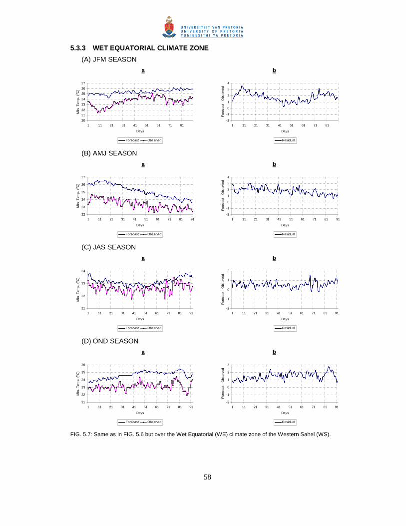
58


(A) JFM SEASON

a b

20

21

22

23

24

25

26

27

1 11 21 31 41 51 61 71 81

Days

Min

. T

emp.

(OC

)

Forecast Observed

-2

-1

0

1

2

3

4

1 11 21 31 41 51 61 71 81

Days

For

ecas

t -

Obs

erve

d

Residual

(B) AMJ SEASON

a b

22

23

24

25

26

27

1 11 21 31 41 51 61 71 81 91

Days

Min

. T

emp.

(OC

)

Forecast Observed

-2

-1

0

1

2

3

4

1 11 21 31 41 51 61 71 81 91

DaysF

orec

ast

- O

bser

ved

Residual

(C) JAS SEASON

a b

21

22

23

24

1 11 21 31 41 51 61 71 81 91

Days

Min

. T

emp.

(OC

)

Forecast Observed

-2

-1

0

1

2

1 11 21 31 41 51 61 71 81 91

Days

For

ecas

t -

Obs

erve

d

Residual

(D) OND SEASON

a b

21

22

23

24

25

26

1 11 21 31 41 51 61 71 81 91

Days

Min

. T

emp.

(OC

)

Forecast Observed

-2

-1

0

1

2

3

1 11 21 31 41 51 61 71 81 91

Days

For

ecas

t -

Obs

erve

d

Residual

FIG. 5.7: Same as in FIG. 5.6 but over the Wet Equatorial (WE) climate zone of the Western Sahel (WS).

59

a b

0.00

0.50

1.00

1.50

2.00

2.50

3.00

3.50

4.00


Regions

RM

SE

, M

AE

RMSE MAE

0.00

0.50

1.00

1.50

2.00

2.50

3.00

3.50

4.00


Regions

RM

SE

, M

AE

RMSE MAE

c d

0.00

0.50

1.00

1.50

2.00

2.50

3.00

3.50

4.00


Regions

RM

SE

, M

AE

RMSE MAE

0.00

0.50

1.00

1.50

2.00

2.50

3.00

3.50

4.00


Regions

RM

SE

, M

AE

RMSE MAE

FIG. 5.8: As in FIG. 5.4 but for minimum temperatures.

Results illustrated in Fig. 5.5 and listed in Table 5.2 show that the Africa LAM had

generated negative biases in forecasting minimum temperature of T+24h over the SA

climate zone of the WS, with the largest mean negative bias of -6.0ºC on an individual day

(day 68) during JFM. This implies that the model under-estimated minimum temperature

forecasts over the SA climate zone of the WS. The model generated its highest PC of

39% during the JAS season. The magnitude in model forecast error (Fig. 5.8) over the SA

climate zone of the WS was greater during the JFM, AMJ and OND seasons than during

the JAS season, suggesting that the model performed better in predicting minimum

temperatures during most of the rainy season than during the dry seasons (the same

results were found for maximum temperature forecasts). The best correlation (rs) of 0.62

appeared during the OND season over the SA climate zone of the WS.

Fig. 5.6 and Table 5.2 indicate that the model generated a generally negative bias in

predicting minimum temperature over the WDT climate zone of the WS. The largest PC of

almost 70% was generated during JAS over this climate zone, meaning that the model

produced improved predictions in minimum temperature values during JAS. The best

correlation (rs) of 0.51 was recorded during the AMJ season. The greatest errors (Fig. 5.8)

appeared during the dry seasons (JFM and OND), implying that the model did well during

the rainy seasons over the WDT climate zone of the WS. This suggests that the model

60

adequately captured the minimum temperature characteristics during the onset of rains

(AMJ) over the WDT climate zone.

From Fig 5.7, it becomes evident that the Africa LAM generally over-estimates minimum

temperature forecasts over the WE climate zone of the WS, with the largest positive bias

of about 3.5ºC on an individual day (day 10) during JFM. Results in Fig. 5.8 also indicate

that the model performed better in predicting minimum temperature values during the AMJ

and JAS seasons than during the JFM and OND seasons. This means that the model did

better in predicting minimum temperature values over the south during the rainy seasons

(AMJ and JAS) than during the dry seasons (JFM and OND). The largest forecasting error

(Table 5.2, Fig. 5.8) was generated in the WE climate zone of the WS during the JFM

season. The model also generated a comparatively low PC and low forecasting error (Fig.

5.7, Fig. 5.8) when predicting minimum temperature values over the WE climate zone of

the WS. The highest correlation coefficient (rs) of 0.41 was recorded during the AMJ

season.

In general, the results in Figs. 5.5 to 5.7 show that the Africa LAM under-estimates

minimum temperature forecasts over the SA and WDT climate zones of the WS, but over-

estimates the associated forecasts over the WE climate zone of the WS. Fig. 5.8

illustrates that the model, in general, generated relatively smaller forecasting errors during

the rainy season (AMJ and JAS) than during the dry season (JFM and OND), further

suggesting that the model predicts minimum temperature values better during rainy

seasons than during the harmattan (dry and cold) seasons over the WS study domain.

5.4 AFRICA LAM VERIFICATION RESULTS FOR RAINFALL


model’s performance to forecast rainfall over the WE, WDT and SA climate zones of the

WS during the JFM, AMJ, JAS and OND seasons, and over the period January 2005 to

December 2006, are presented in Table 5.3 and Figs. 5.9 to 5.12.

Table 5.3 lists Africa LAM’s verification results for T+24h rainfall forecasts. Fig 5.9

illustrates Africa LAM T+24h forecasts for rainfall compared to observations over the SA

climate zone, while Figs. 5.10 and 5.11 illustrates the same for the WDT and WE climate

zones, respectively. Fig. 5.12, again, depicts the magnitude of Africa LAM errors (RMSE

and MAE) in predicting rainfall over the regions and periods mentioned above.

61

Table 5.3: Africa LAM NWP verification results for T+24h rainfall forecasts during the JFM, AMJ, JAS and

OND seasons over the WE, WDT and SA climate zones of the Western Sahel (WS), and over

the period January 2005 to December 2006.

JFM AMJ


rp -0.07 -0.03 0.02 0.07 0.05 0.07

rs 0.35 0.39 0.25 0.37 0.19 0.21

MSE 0.18 4.32 6.37 1.10 11.21 12.39

RMSE 0.42 2.08 2.52 1.05 3.35 3.52

MAE 0.13 1.70 2.19 0.70 2.55 2.78

BIAS -0.04 1.69 0.87 -0.05 1.83 1.37

%Above 14.44 98.89 66.67 59.34 72.53 68.13

%Below 15.56 1.11 33.33 30.77 26.37 31.77

PC – A 0.70 0.00 0.00 0.10 0.01 0.00

%YES 4.44 32.22 95.56 67.03 97.80 98.90

%NO 68.89 0.00 0.00 7.69 0.00 0.00

%MISSES 27.00 68.00 4.44 25.27 2.20 1.10

PC – B) 0.73 0.32 0.96 0.75 0.98 0.99

LEPS (%) 75.00 100.00 83.02 96.20 55.35 52.20

JAS OND


rp -0.02 -0.06 0.04 0.10 0.20 -0.04

rs 0.10 0.00 0.19 0.41 0.48 0.13

MSE 11.65 25.09 14.44 0.38 3.04 30.25

RMSE 3.41 5.01 3.80 0.62 1.74 5.50

MAE 2.35 3.85 2.68 0.27 1.17 4.34

BIAS -0.50 1.24 -1.55 -0.06 0.64 2.94

%Above 43.48 66.30 33.70 27.17 78.26 79.35

%Below 52.17 33.70 66.30 14.13 14.13 19.57

PC – A 0.05 0.00 0.00 0.59 0.08 0.01

%YES 97.83 100.00 98.91 28.26 53.26 92.39

%NO 0.00 0.00 0.00 56.52 6.52 1.09

%MISSES 2.17 0.00 1.10 15.22 40.22 6.52

PC – B 0.98 1.00 0.99 0.85 0.60 0.93

LEPS (%) 52.10 34.01 58.20 91.67 98.45 70.87

62


(A) JFM SEASON

a b

0.0

0.5

1.0

1.5

2.0

2.5

3.0

1 11 21 31 41 51 61 71 81

Days

Rai

nfal

l (m

m)

Forecast Observed

-3.0-2.5-2.0-1.5-1.0-0.50.00.51.01.5

1 11 21 31 41 51 61 71 81

Days

For

ecas

t -

Obs

erve

d

Residual

(B) AMJ SEASON

a b

0.0

1.0

2.0

3.0

4.0

5.0

1 11 21 31 41 51 61 71 81 91

Days

Rai

nfal

l (m

m)

Forecast Observed

-5.0-4.0-3.0-2.0-1.0

0.01.02.03.0

1 11 21 31 41 51 61 71 81 91

Days

For

ecas

t -

Obs

erve

d

Residual

(C) JAS SEASON

a b

0.02.04.06.08.0

10.012.014.016.018.0

1 11 21 31 41 51 61 71 81 91Days

Rai

nfal

l (m

m)

Forecast Observed

-15.0

-10.0

-5.0

0.0

5.0

10.0

15.0

1 11 21 31 41 51 61 71 81 91

Days

For

ecas

t -

Obs

erve

d

Residual

(D) OND SEASON

a b

0.00.51.01.52.0

2.53.03.54.0

1 11 21 31 41 51 61 71 81 91

Days

Rai

nfal

l (m

m)

Forecast Observed

-4.0

-3.0

-2.0

-1.0

0.0

1.0

2.0

3.0

1 11 21 31 41 51 61 71 81 91

Days

For

ecas

t -

Obs

erve

d

Residual

FIG. 5.9: Same as in FIG. 5.7 but for Rainfall over the Semi-Arid (SA) climate zone of the Western Sahel

(WS).

63


(A) JFM SEASON

a b

0.0

1.0

2.0

3.0

4.0

5.0

6.0

7.0

1 11 21 31 41 51 61 71 81

Days

Rai

nfal

l (m

m)

Forecast Observed

0.0

1.0

2.0

3.0

4.0

5.0

6.0

7.0

1 11 21 31 41 51 61 71 81

Days

For

ecas

t -

Obs

erve

d

Residual

(B) AMJ SEASON

a b

0.0

2.0

4.0

6.0

8.0

10.0

12.0

14.0

1 11 21 31 41 51 61 71 81 91

Days

Rai

nfal

l (m

m)

Forecast Observed

-6.0-4.0-2.00.02.04.06.08.0

10.012.014.0

1 11 21 31 41 51 61 71 81 91

Days

For

ecas

t -

Obs

erve

d

Residual

(C) JAS SEASON

a b

0.0

5.0

10.0

15.0

20.0

25.0

1 11 21 31 41 51 61 71 81 91

Days

Rai

nfal

l (m

m)

Forecast Observed

-15.0

-10.0

-5.0

0.0

5.0

10.0

15.0

20.0

1 11 21 31 41 51 61 71 81 91

Days

For

ecas

t -

Obs

erve

d

Residual

(D) OND SEASON

a b

0.0

2.0

4.0

6.0

8.0

10.0

12.0

14.0

1 11 21 31 41 51 61 71 81 91

Days

Rai

nfal

l (m

m)

Forecast Observed

-10.0-8.0-6.0-4.0-2.0

0.02.04.06.0

1 11 21 31 41 51 61 71 81 91

Days

For

ecas

t -

Obs

erve

d

Residual

FIG. 5.10: Same as in FIG. 5.9 but over the Wet and Dry Tropics (WDT) climate zone of the Western Sahel

(WS).

64


(A) JFM SEASON

a b

0.0

2.0

4.0

6.0

8.0

10.0

12.0

1 11 21 31 41 51 61 71 81

Days

Rai

nfal

l (m

m)

Forecast Observed

-8.0

-6.0

-4.0

-2.0

0.0

2.0

4.0

6.0

1 11 21 31 41 51 61 71 81

Days

For

ecas

t -

Obs

erve

d

Residual

(B) AMJ SEASON

a b

0.02.04.06.08.0

10.012.014.016.0

1 11 21 31 41 51 61 71 81 91

Days

Rai

nfal

l (m

m)

Forecast Observed

-10.0

-5.0

0.0

5.0

10.0

15.0

1 11 21 31 41 51 61 71 81 91

DaysF

orec

ast

- O

bser

ved

Residual

(C) JAS SEASON

a b

0.02.04.06.08.0

10.012.014.016.018.0

1 11 21 31 41 51 61 71 81 91

Days

Rai

nfal

l (m

m)

Forecast Observed

-15.0

-10.0

-5.0

0.0

5.0

10.0

1 11 21 31 41 51 61 71 81 91

Days

For

ecas

t -

Obs

erve

d

Residual

(D) OND SEASON

a b

0.0

5.0

10.0

15.0

20.0

1 11 21 31 41 51 61 71 81 91

Days

Rai

nfal

l (m

m)

Forecast Observed

-15.0

-10.0

-5.0

0.0

5.0

10.0

15.0

20.0

1 11 21 31 41 51 61 71 81 91

Days

For

ecas

t -

Obs

erve

d

Residual

FIG. 5.11: Same as in FIG. 5.10 but over the Wet Equatorial (WE) climate zone of the Western Sahel (WS).

65

a b

0.00

0.50

1.00

1.50

2.00

2.50

3.00

3.50

4.00


Regions

RM

SE

, M

AE

RMSE MAE

0.00

0.50

1.00

1.50

2.00

2.50

3.00

3.50

4.00


Regions

RM

SE

, M

AE

RMSE MAE

c d

0.00

0.50

1.00

1.50

2.00

2.50

3.00

3.50

4.00

4.50

5.00

5.50


Regions

RM

SE

, M

AE

RMSE MAE

0.00

0.50

1.001.50

2.002.50

3.00

3.504.00

4.50

5.005.50

6.00


Regions

RM

SE

, M

AE

RMSE MAE

FIG. 5.12: As in FIG. 5.8 but for rainfall.

The Africa LAM’s performance in predicting rainfall amounts and rainfall events for a

period of T +24h in advance has been listed in Table 5.3. PC – A in Table 5.3 indicates

the model’s proportional correct index in predicting rainfall amounts, while PC – B

indicates the model’s proportional correct index in predicting rainfall events.

Fig. 5.9 shows that the model under-estimated rainfall amount forecasts over the SA

climate zone of the WS, with the largest negative bias of about -12.0mm on an individual

day (day 50) during the peak of the rainy season (JAS). Results (Table 5.3) also denote a

relatively high PC – A value of 70% (JFM) and 60% (OND), but a relatively low PC – A

value of 10% (AMJ) and 5% (JAS). On the other hand, the results indicate consistently

high PC – B for all seasons. This suggests that the model performed very well in

predicting rainfall events throughout the year, but has greater success in predicting rainfall

amounts during the dry seasons (JFM and OND) than during rainy seasons (AMJ and

JAS), especially as indicated by the comparatively low PC – A values calculated during

the rain seasons. The magnitudes of forecasting errors (Fig. 5.12) were also

correspondingly lower during dry seasons than during rain seasons. The best correlation

coefficient (rs) of 0.41 was also recorded during the dry OND season.

Results from Fig. 5.10 point towards a generally positive bias by the model in predicting

rainfall amounts over the WDT climate zone of the WS, with the largest positive bias of

66

about 17.0mm on an individual day (day 47) during JAS. This means that the model

generally over-estimated rainfall amount forecasts over the WDT climate zone of the WS.

From the PC – A and PC – B results in Table 5.3, the model showed a relatively high

success in predicting rainfall events, but has a relatively low success in predicting the

exact rainfall amounts over the WDT climate zone of the WS. The magnitude of

forecasting errors (Table 5.3, Fig. 5.12) was also the greatest during the JAS season. The

best correlation coefficient (rs) of 0.48 was recorded during the dry season of OND, similar

to that of the SA climate zone of the WS.

Over the WE climate zone of the WS (Fig. 5.11), results indicates that the Africa LAM

over-estimated rainfall amount forecasts, except for JAS, when the model showed under-

estimation over the same region. The results (Table 5.3, Fig. 5.11) further show that the

model had the largest positive bias of 15mm on an individual day (day 85) during OND

season, and the largest negative bias of 13mm on an individual day (day 22) during JAS.

The PC – A and PC – B (Table 5.3) indicate that the model has a high proportional correct

index in forecasting rainfall events than when forecasting rainfall amounts over the WE

climate zone of the WS. This is in agreement with findings over the WDT climate zone of

the WS. Fig. 5.12 illustrates that the model has generated its lowest forecast error during

the JFM season over the WE climate zone of the WS, meaning that the model

successfully captured rainfall events and rainfall amounts during this season, when less

rainfall activity are normally expected. Again, the highest correlation coefficient (rs) of 0.25

was recorded during the JFM season, which also agrees with the conclusion that the

model has a better chance to succeed in predicting rainfall amounts and events during the

dry seasons than during the rain seasons over the WE climate zone of the WS. It is also

shown in Fig. 5.12 that the model has the largest forecast error over the WE climate zone

if compared to other regions of the WS. This could be due to the high frequencies of

rainfall events and uneven rainfall amounts (monsoon rains) that are more prevalent over

the south than over the central and north, which were not well captured in Africa LAM

forecasts.

5.5 Summary

The Africa LAM has been verified against station observations over the three different

climatic zones and four seasons of the year. In summary, the verification results indicate

that the model temperature forecasts show skill, more so during the raining seasons (AMJ

and JAS) than during the dry seasons (JFM and OND) over the WS. The model rainfall

forecasts, however, show more skill during the dry seasons (JFM and OND) than during

67

the raining seasons (AMJ and JAS). The results further indicate that, on a regional basis,

the model temperature forecasts show more spatial skill over the WE climate zone than

over the WDT and SA climate zones of the WS, while rainfall forecasts show more skill

over the SA climate zone than over the WDT and WE climate zones of the WS. These

results give a better understanding of the model forecast errors, and could also provide

the feedback necessary for a possible improvement of Africa LAM forecasts by scientists

at the UK Met Office.

68

CHAPTER 6

WEATHER FORECASTING IN NIGERIA 6.1 INTRODUCTION

NWP models have great value when they are employed as an essential tool to assist

weather forecasters in their daily duties. One might be able to forecast the weather

without NWP models, but over a relatively short period ahead in time. There are two ways

to predict the weather without NWP models:

• Assuming persistence, in other words to assume that current synoptic patterns and

atmospheric variables will remain in the same state over the period of forecasting.

This might work for variables such as temperatures that are fairly constant in

diurnal variability over barotropic equatorial regions, but as soon as a variable

increases in variance, weather forecasting by assuming persistence becomes less

useful and less successful.

• Projecting the propagation of synoptic situation forward in time by using one’s

knowledge of meteorology and experience of the propagation of similar previous

events. This approach has its limitations, especially over regions like the tropics

where a zero Coriolis force does not allow for well defined pressure systems. The

latter involve the forecast of pressures which might be regarded as a primary

variable. As soon as one starts to consider secondary variables, such as rainfall,

weather forecasting becomes extremely difficult – even for a day or less in

advance.

NWP models have improved significantly over the past decades, and have the ability to

forecast most atmospheric variables with a high degree of accuracy over a period of 24

hours, or even two to three days in advance. The incorporation of NWP models in modern

forecasting operations therefore becomes unavoidable. Unfortunately NMHSs in Africa

currently do not have the infrastructure or human resources to run NWP models in-house,

and they therefore have to rely on NWP results from other countries in the international

community. These NWP results are in most cases downloaded from the Internet, which is

also sometimes not reliable in African countries. Despite of these obstacles, it is worth

investigating how NWP could be incorporated in weather forecasting operations in

NMHSs of Africa.

69

This study addresses the use of the Africa LAM over the WS, although the Nigerian

Meteorological Agency (NIMET) is regarded as the focus point from where weather

forecasts are issued. The following chapter provides a general overview on conventional

forecasting, and current forecasting that incorporate NWPs (mostly downloaded from the

Internet), in Nigeria. The shortcomings and needs of NIMET, which are also applicable to

other NMHSs in the WS, to issue improved weather forecasting are examined. A typical

weather forecasting process at NIMET is discussed, with the view to provide an example

for other NMHSs in the WS (and beyond) that might consider the incorporation of NWP

model results in future. It might also serve as an indication of the overall value that the

Africa LAM might have in NWP over the WS.

Some NWP output are shown and compared to observations. It is not the purpose of this

part of the study to perform a detailed verification of the NWP models used, but rather to

introduce the models used at NIMET, and to briefly consider a few case study examples

to indicate how the model output are used in an effort to improve on weather forecasting.

6.2 NWP MODELS AND WEATHER FORECASTING IN NIGERIA

The history of weather forecasting in Nigeria dates back to the time of British colonization

when the Nigerian Meteorological Services Department was established in around 1914.

A recent need for independence, with the inspiration to develop higher quality

meteorological services to end-users in Nigeria, led to the enactment of the NIMET Act in

June 2003 by the Federal Government of Nigeria. The Act made NIMET a semi

autonomous body which has an obligation to generate part of its income. NIMET is

currently managed by a Director-General (DG), under the supervision of the Federal

Ministry of Transportation. Apart from the Office of the DG, NIMET operates under seven

sub-directorates, namely the directorates of (1) Weather Forecasting Services (WFS), (2)

Applied Meteorological Services (AMS), (3) Engineering and Technical Services (ETS),

(4) Research and Training (R&T), (5) Finance and Accounts (FA), (6) Administration and

Supply (AS) and (7) Legal and Corporate Affairs (LCA).

Weather forecasting activities of the agency are supervised by the WFS directorate. There

are five major forecasting offices in Nigeria, namely (1) the Ikeja forecasting office in

Lagos State, (2) the Abuja forecasting office in the Federal Capital Territory, (3) the Port

Harcourt forecasting office in Rivers State, (4) the Kano forecasting office in Kano State

and (5) the Central Forecast Office (CFO) in the operational meteorological Headquarters

Oshodi in Lagos State. The CFO co-ordinates all other forecast offices and also issue the

70

daily national public weather forecast. Seasonal weather forecasts and results of any

research findings are also disseminated through the CFO. Apart from the forecast offices,

NIMET controls a network of about 43 observational weather stations, and many other

Automatic Weather Stations (AWS) distributed all around the country. Meteorological

observations available from this network of stations are collected on a regular basis -

some very close to real time.

Before 1996, when the CFO was established, weather forecasting in Nigeria were issued

purely by an analog procedure. As explained by Gutzler and Shukla (1984), the idea of

analog forecasting is to search archives of past synoptic maps that closely resembles

current observations, and then to assume that the future evolution of the atmosphere will

be similar to those that followed from the historical analogs. Wilks (1995) points out that

the analog forecasting method is only an estimation of reality because atmospheric

synoptics are not often repeated. Fortunately some Nigerian forecasters returned in 1996

from On-Job-Training at the African Center of Meteorological Applications and

Development (ACMAD), Niamey, Niger Republic, where they were trained on the use and

interpretation of NWP models in weather forecasting. From then, Nigeria started to use

NWP model outputs to assist them in the process of routine weather forecasting (Fig. 6.1).

FIG. 6.1: Typical television weather forecasting presentation on national television in Nigeria. Current weather

forecast issued incorporated NWP model results.

In Nigeria, as in most other NMHS in Africa, it is difficult to run models in-house, due to a

lack of computer resources and limited knowledge of the field of numerical modeling. As a

result, available information from international NWP models is currently downloaded from

71

the Internet, in conjunction with the collection of real time observations and satellite

imageries, when preparing a weather forecast. The introduction of statistical method to

improve forecasts and to provide quantitative information from available NWP products

will be a very useful addition in the process of weather forecasting - not only in Nigeria,

but also in other NMHS in Africa.

Some of the equipment available for the retrieval and interpretation of NWP model results

in Nigeria are the Meteorological Data Distribution (MDD) equipment for T4 chart

preparation and the Primary Data User System (PDUS) for satellite image display, which

was recently upgraded from funding provided by the PUMA project to the Meteosat

Second Generation (MSG) system. From the MSG system, images of the near real time

state of the atmosphere are retrieved on a 15 minutes interval. Nigeria also contributes to

the global meteorology data network since observed meteorological information is

disseminated on a regular basis via the Global Telecommunication System (GTS),

although some network problems are experienced from time to time.

Currently a typical weather forecasting process in NIMET, with the inclusion of NWP

model results, may be outlined as follows:

a) Available NWP output is carefully studied by the weather forecaster on duty. This

is done by comparing model initialization fields with actual observations (such as

station reports, satellite imageries, upper-air soundings) in order to identify any

possible errors so that adjustments could be made. NWP output from (1) the UK

Met Office (Africa LAM), (2) the European Center for Medium-Range Weather

Forecasts (ECMWF), (3) the National Centers for Environmental Prediction

(NCEP) GFS model and (4) Action de Recherché Petite Echelle Grande

(ARPEGE) from Metéo France with the Aire Limitée Adaptation dynamique

Développement InterNational (ALADIN) model are considered on a daily basis to

incorporate NWP model output in routine weather forecasting in Nigeria.

b) At the same time the weather forecaster needs to use his/her discretion to add

extra details to the NWP model forecasts, such as the position of the ITCZ,

vortices, troughs and ridges. This is essential since NWP models do not always

adequately resolve all micro-scale weather systems. It is here where the

experienced weather forecaster can use his/her knowledge of local weather to add

value to NWP forecasts

72

c) A detailed comparison of NWP model results from different global modeling

centers are prepared to build the weather forecaster’s confidence in the available

model results. If all the NWP models are suggesting approximately the same

solution, the confidence in the model forecast would be high, but if all the NWP are

showing different prognoses, the confidence in the model forecasts reduces.

d) Following a critical debate, discussions and adequate consultation with colleagues,

a consensus weather forecast is issued.

From the activities above, it become obvious that NMP model output, even if downloaded

from the web, may add significant value to weather forecasting in Africa. However, the

ideal would be if a meteorological centre runs their NWP model in-house, since these

models have certain limitation (maybe as a result of assumptions) which would not be

known to users unless they have hands-on experience in model simulations, or even

model development.

6.2.1 A brief overview of some NWP models used in Nigeria

The following sections present an overview of some NWP models used for weather

forecasting in Nigeria (as listed in (a) above). A brief assessment of errors and biases in a

few cases are illustrated. Please note again that it is not the purpose of this part of the

study to perform a detailed verification of the NWP models used, but rather to introduce

the models used at NIMET, and to briefly consider a few case study examples to indicate

how the model output are used in an effort to improve on weather forecasting.

6.2.1.1 The Africa LAM model

A description and technical details of the Africa LAM is outlined in Chapter 3. However, in

this section, a case study (19 October 2006) is considered in a discussion of the possible

strengths and weaknesses of the Africa LAM in forecasting significant weather events

over Nigeria. There are obviously also other cases that could have been discussed, but

due to the availability of information, the case of 19 October 2006 was chosen. On that

day, observed synoptic conditions were typical of what is experienced during the rain

season. A week before this event, the ITCZ shifted northwards and the moisture laden

southwesterly winds picked up in strength. Most of the meteorological stations in the

country, especially those in the southern region, recorded unusually high temperatures

and their Mean Sea Level Pressure (MSLP) generally maintained a decreasing trend.

73

A comparison between the Africa LAM wind forecasts at 850hPa level (Fig. 6.2) for 19

October 2006, and the observed satellite image (Fig. 6.3) shows that Africa LAM areas of

troughs and vortices (in the wind forecasts) correspond well to the locations where active

thunderstorms occurred in satellite image. 850hPa wind forecast is chosen since the

850hPa pressure level is normally considered as the atmospheric reference level when

predicting convective weather systems over Nigeria. Troughs and vortices are very useful

when tracking the development and propagation of convective weather systems over

West Africa, especially over Nigeria. The results therefore suggest that the 850hPa

forecast winds from the Africa LAM, especially at 00:00GMT and 06:00GMT, proved to be

very useful in forecasting convective weather events over Nigeria and south Cameroon.

FIG. 6.2: Africa LAM simulated forecasts of 850hPa winds for 00:00GMT (T+6h) (left) and 06:00GMT (T+12h)

(right) for 19 October 2006. Marked red lines indicate troughs, while C denotes a vortex.


FIG. 6.3: Satellite images for 00:00GMT (left) and 03:00GMT (right) on 19 October 2006. Convective weather

over West Africa is clearly indicated (Source: EUMETSAT).

Africa LAM RH forecasts (Fig. 6.4) were also very useful. Vertical wind profile forecasts

from the Africa LAM (not shown) indicated that the model in fact did simulate the vertical

profile over the West African region very well, with the exception of slight disparities in

surface wind directions. Accumulated precipitation forecasts (also depicted in Fig. 6.4)

74

captured observed rainfall patterns that occurred along the coasts of Liberia, Sierra

Leone, Guinea, south Cameroon, and especially Nigeria reasonably well. The model

forecasts also captured some convective cloud development.

FIG. 6.4: Africa LAM forecasts of Relative Humidity (RH) T+6h forecasts for 00:00GMT (top left) and T+12h

forecasts for 06:00GMT (top right) with accumulated precipitation T+6h forecasts (bottom) for 19 October

2006 (Source: http://www.metoffice.gov.uk/weather/africa/lam).

6.2.1.2 ECMWF model

The ECMWF NWP model has recently been upgraded from a spectral triangular

truncation of TL319L60 (60km grid to point spacing at mid-latitudes) to TL511L60 (40km

grid to point spacing at mid-latitudes). The model consists of dynamical, physical and

coupled ocean wave components. The upgraded version of the model has a new cycle

which includes a new formulation of convective entrainment and relaxation timescales

with reduced free atmospheric vertical diffusion. The model also has a new soil hydrology

scheme, new radiosonde temperature and humidity bias corrections. The model uses a 4-

dimensional data assimilation scheme to estimate the actual state of the atmosphere. In

the model, dynamical quantities, such as pressure and velocity gradients, are evaluated in

spectral space, while computations involving processes such as radiation, moisture

conversion, turbulence, are calculated in grid point space. This combination preserves the

local nature of physical processes, and retains the superior accuracy of the spectra

method for dynamical computation. The physical processes associated with radiative

transfer, turbulent mixing and moist processes are active at scales smaller than the

horizontal grid size. ECMWF model products are widely used for medium range forecasts,

75

but in many African countries, especially in Nigeria, the model products are used for short

range forecasts together with other NWP models (Palmer, 1997).

FIG. 6.5: ECMWF Mean Sea Level Pressure (MSLP) T+24h forecasts at 00:00GMT on 13 and 14 March 2006

(top, left and right, respectively) compared to observed MSLP across Nigeria (bottom, left and right)

(Source: http://www.ecmwf.int/products/forecasts/d/charts/medium/deterministic/).

FIG. 6.6: ECMWF Mean Sea Level Pressure (MSLP) T+24h forecasts at 00:00GMT on 15 and 16 March 2006

(top, left and right, respectively) compared to observed MSLP across Nigeria (bottom, left and right).

(Source: http://www.ecmwf.int/products/forecasts/d/charts/medium/deterministic/).

76

Results from an investigation carried out to evaluate the forecasting performance of some

ECMWF products over Nigeria are presented in Figs. 6.5 and 6.6. Only verification results

for ECMWF MSLP compared to actual MSLP across Nigeria at 00:00GMT on 13, 14, 15

and 16 March 2006 are considered.

Figs. 6.5 and 6.6 indicate that ECMWF MSLP forecasts from 13 to the 16 of March 2006

successfully captured the general spatial and temporal variability of MSLP over Nigeria,

especially over the north eastern part of the country. Values are, however, slightly

underestimated. These results further show that the model did not perform very well over

the southern parts of Nigeria. It is necessary to mention here that ECMWF cloud cover

output remains very important as a diagnostic tool for predicting coastal rainfall over

Nigeria. More so, the 925hPa level winds and the 10m wind plots are very relevant in

diagnosing the interaction between ocean and continental winds. The 850 and 700hPa

level winds are also regarded as important for weather forecasts over the country.

6.2.1.3 NCEP/GFS model

The NCEP Global Forecast System (NCEP/GFS) is a NWP forecasting system with global

spectral data assimilation. The NCEP/GFS model’s horizontal resolution has been

increased from May 2005 to approximately 35km (T382) for both the analysis and forecast

products. The model has 64 horizontal levels in the vertical with its top at approximately

0.2hPa, and it has a hybrid (sigma / pressure) vertical coordinate. It contains a full suite of

parameterized physics with an accompanying sea-ice and land-surface models. The

NCEP/GFS model’s structure is computationally efficient for use in the Earth System

Modelling Framework (ESMF). NCEP/GFS forecast products are available for every six

hours at 00:00, 06:00, 12:00 and 18:00GMT. The model’s main time integration is leapfrog

for nonlinear advection terms, and semi implicit for zonal advection of vorticity and

moisture. The time step is 7.5 minutes for computation of dynamics and physics, except

that full calculation of long-wave radiation is done once every 3 hours and shortwave

radiation every hour (but corrections made at every time step for diurnal variations in the

shortwave fluxes and in the surface upward long-wave flux).

As mentioned before, the NCEP/GFS model forecasts (Fig.6.7) are also downloaded from

the Internet for use in weather forecasting at NIMET. The NCEP/GFS model’s 850hPa

temperature combined with MSLP forecast maps, as well as 10m winds combined with

the 2m temperature forecast maps, as depicted in Fig. 6.7, are the two most commonly

used NCEP/GFS model forecast maps in Nigeria. The 850hPa heights combined with the

77

MSLP forecast map provides information about the above-continental level (850hPa)

temperature and MSLP distribution over the country. Experience reveals that for any

location where the MSLP forecast is less than or equal than 1008hPa, and the 850hPa

temperature less than or equal than 20°C, there is a strong possibility that convective

weather, for example thunderstorms or at least strong winds might be experienced. The

10m winds combined with the 2m temperature maps are also used for forecast

information about low level wind characteristics and 2m temperature distribution over the

country. When ocean track winds are converging at low levels, forecasters are informed

about the extent of the low level moisture influx into the country. These NCEP/GFS model

forecast products have proved very useful, and to some extent, reliable in providing

forecast guidance over Nigeria and in other part of the WS. However, the experience of

the forecasters and the continuous improvements on the model products are still regarded

as essential.

FIG. 6.7: Examples of NCEP/GFS 850hPa heights, combined with Mean Sea Level Pressure (MSLP) T+24h

forecasts (left) and the 10m winds combined with 2m temperatures T+24h forecasts (right), as used to assist

weather forecasters in their duties at the Nigerian Meteorological Agency (NIMET)

(Source: http://www.nco.ncep.noaa.gov/pmb/nwpara/analysis/index_africa.shtml)

6.2.1.4 ARPEGE and ALADIN model

As outlined in (a) above (under a typical weather forecasting process in NIMET), the

ARPEGE and ALADIN models are also available for use in weather forecasting over

78

Nigeria. The ARPEGE model has a horizontal representation that is based on spectral

harmonic functions, which transforms to a Gaussian grid in order to calculate the

nonlinear quantities and physics. However, the Gaussian grid in the ARPEGE model is

reduced longitudinally near the poles to avoid clustering of grids at Polar Regions – a

known problem in global models. The ARPEGE model has code that allows for the

spectral basis functions to be mapped con-formally from a geographical sphere to a

transformed sphere with the poles and latitude-dependent local derivatives preserved. As

such, the model’s resolution may vary, and the centre of highest resolution may be

located at any geographical point. The model dynamics are expressed in terms of the

vorticity, divergence, temperature and specific humidity equations, and natural logarithm

of the surface pressure. Land surface characteristics in the model are represented by

specifying both the primary and secondary vegetation cover in each grid box.

The ALADIN model, however, is a limited area bi-spectral model with 31 horizontal levels

in the vertical. The model uses initial conditions of both 12:00GMT and 00:00GMT from

ARPEGE models. The ALADIN model allows for a zoom effect on the ARPEGE global

model with a very small computer power requirement. The ALADIN model project was

initiated by Metéo France with the aim to prepare and maintain a NWP system for smaller

domains, with high spatial resolution, on the assumption that important meteorological

events at those finer scales (such as local land and sea breezes) are mainly the result of

the so called dynamical adaptation to the characteristics of the earth’s surface. In Africa,

ALADIN model simulations are performed at the Kingdom of Morocco National Weather

Service.

Maps of 850hPa temperatures, RH and winds, as well as a map of precipitable water and

CAPE (Fig. 6.8) are the most common ALADIN model forecast products used for weather

forecasting at NIMET. Since the ALADIN model runs on a relatively high resolution over a

limited area (extending over North and Equatorial Africa), most of the meso-scale weather

systems over Nigeria are captured by the model. Local wind patterns, especially over high

elevation points in Nigeria, are also clearly defined in most cases by the ALADIN 850hPa

wind forecasts. The ALADIN CAPE forecast products are very useful for forecast

diagnosis on the effectiveness of any identified trough or vortex at the 850hPa level over

the country. For instance, when a vortex is located over a particular area, and the CAPE

value over the same area is not significant (less than 1 500J/Kg), the forecaster knows to

put less emphasis on the presence of the vortex and also knows that the vortex might not

produce any significant storm or active weather over Nigeria.

79

FIG. 6.8: ALADIN 850hPa temperature, Relative Humidity (RH) and winds for the T+24h forecast (left), and

precipitable water and Convective Available Potential Energy (CAPE) for the T+24h forecast (right) over North

and Equatorial Africa (Source: http://www.marocmeteo.ma/spn).

6.3 Weather forecasting shortcomings and needs in Ni geria

In Nigeria, and at most other NMHS in Africa, NWP model forecasts are not generated in-

house, mainly due to a lack of adequate computer resources, and in many cases also

because of limited knowledge of the code/theory of numerical modeling or technical

aspects of NWP. As a result, available information from NWP model simulations provided

by global modeling centers are currently downloaded, in conjunction with real time

observations and satellite images, during the process of weather forecasting. Meso-scale

convective weather systems are the most common weather events over Nigeria, which

are often not well captured in the output of these NWP models. A major challenge to

weather forecasters is therefore to decide whether meso-scale weather is correctly

simulated by these models, or not. Since the models are not developed or simulated in-

house very little can be done to adjust model code in order to improve simulations of

Nigerian weather conditions. The long term experience and judgment of forecasters by

using previous weather events forms an essential part in the interpretation of NWP model

results. The WMO Severe Weather Forecasting Demonstration Project (SWFDP) recently

implemented at Southern Hemisphere meteorological centers, is a good example of

international efforts to improve weather forecasting skills and capabilities at African

meteorological centers, especially for forecasting severe weather events. Hopefully, WMO

might extend the training that forms part of the project in future to the West African sub-

region. NIMET will benefit tremendously from such an initiative. The SWFDP aims to

contribute to capacity-building and to help developing countries to access NWP results,

80

and to make the best possible use of existing NWP products for improving warnings of

hazardous weather conditions.

The availability of more accurate and near real time station observations is also very

important in ensuring that accurate and timely weather forecasts are issued over Nigeria.

Currently, most of the weather observatories in the country do not perform sufficiently.

Most of the weather observation equipment needs to be upgraded and recalibrated to

meet internationally acceptable standards. Although, very recently there have been

conscientious moves by NIMET to improve on meteorological observation over the

country. International cooperation might complement this effort. Effective data

transmission from observation stations to the major forecasting offices is regarded as

essential to complement available information from NWP models in order to issue better

weather forecasts. Apart from national networks, the ability to provide locally observed

data on time to global modelling centres via the GTS to be included in the analysis or

initial conditions of running NWP is also regarded as very important. One can conclude by

mentioning that the observation and communication network over Nigeria needs further

improvement to allow for the country to optimally benefit from NWPs.

In Nigeria, the distribution of weather forecasts to end-users, such as agriculture, aviation,

marine, hydrology, tourism, sports and many more, is an important process. As a matter

of fact, it is the national responsibility of NIMET to prepare and make these weather

forecasts available. For instance agriculture which is regarded as a key economic sector,

need weather forecast information in an applicable and easily understandable format for

application. Efforts should therefore be geared towards research and application studies

that will further improve NIMET capacities to issue useful and relevant weather forecast

information to different end-users. Acknowledged as some efforts by NIMET to meet these

demands are the Public Weather Forecasts issued on TV (see Fig. 6.1), Radio and the

Print Media; the Agro-meteorological, hydrological and marine bulletins etc. However,

more funding and international cooperation should be harnessed by NIMET in order to

sustain these efforts, especially since it is very relevant to economic growth in the country.

6.4 Summary

In summary, this chapter provided information on the current status and applications of

NWP products for weather forecasting in Nigeria, and on how NWPs are incorporated in

the day-to-day duties of weather forecasters. The sequence of events during a typical

weather forecasting process at NIMET is discussed, also with the view to document a

81

baseline approach for consideration by some weather centers in the WS. Characteristic

features of some of the available NWP models that are used for operational weather

forecasting in the country were discussed. Examples of NWP products are shown and

discussed in order to introduce the reader to the type of maps and variables used during

the weather forecasting process, and some emphasis was put on the evaluation of NWP

maps generated by the Africa LAM and the ECMWF models over the country – although it

was not an objective in this chapter to provide a detailed verification of the NWP models.

Brief highlights on the shortcomings and needs of NIMET to ensure improved weather

forecasting were also provided.

82

CHAPTER 7

SUGGESTED POST-PROCESSING METHODS 7.1 INTRODUCTION

The first and second objectives of this study are to verify Africa LAM NWPs against

observations over the WS, and to determine the value of Africa LAM to be used by

weather forecasters at NIMET in their daily duties. The third, and last, objective is to

suggest possible statistical post-processing tools that might be of value for improving

basic NWPs over the WS of Africa. As previously indicated, NWPs are not perfect, and it

might be appropriate to employ statistical post-processing techniques, where historical

forecast are compared to observations, in order to minimize systematic errors and biases

(see discussion in chapter 5).

This chapter presents results from some suggested post-processing techniques as

applied at each one of five (5) randomly selected meteorological point stations in Nigeria.

The post-processing is applied over the same seasons as used in the Africa LAM NWPs

(chapter 5), namely JFM, AMJ, JAS and OND. The variables considered are maximum

and minimum temperatures (rainfall is excluded). The purpose of this chapter is to serve

as background for researchers and weather forecasters who might be interested to use

post-processing techniques in the WS in future.

7.2 SUGGESTED POST-PROCESSING TECHNIQUES

An important feature of statistical post-processing techniques is that historical

observations are used, and compared with historical forecasts, in an effort to correct or

minimize systematic errors and biases in NWPs (see Fig. 7.1).

FIG. 7.1: A schematic flow diagram that

illustrates a typical statistical post-

processing approach. Solid arrows indicate

information sources required in the

development of the statistical forecasting

equations, and dashed arrows indicate the

information flow when the corrections are

implemented (adapted from Wilks, 1995).

83

7.2.1 SIMPLE BIAS CORRECTION

In general, a simple bias correction might significantly improve output generated by a

NWP model. The decomposition of MSE (equations 7.1 to 7.4), according to Wilks (1995),

is used to determine how Africa LAM forecasts might be improved when applying a simple

bias correction method:

where MSE = MSE between the model forecasts and observations

B = Mean bias of the model forecasts

SO and SF = standard deviations of the observations and forecasts

rOF = product-moment correlation between forecasts and observations.

Replacing F' = Fi – C to correct the model forecast bias at each of the station, gives

where MSE' is the MSE between the corrected model forecasts and observations and C is

the correction value. However, since SO, SF and rOF are unaffected by a constant shift,

minimizing MSE' implies that C = B. Equation (7.2) may therefore be written as

As suggested by Davis (2004), the percentage improvement by the bias-corrected

forecasts relative to the NWP forecast is measured by:

Improvement (%) = ((RMSE – RMSE') /RMSE) x 100 (7.4)

84

7.2.1.1 Bias correction results

To quantify improvements that might be made to original Africa LAM forecasts of

maximum and minimum temperatures over Nigeria, the MSE of the original model

forecasts and of the bias-corrected forecasts are calculated (see equations 7.2 and 7.3).

The percentage improvements (%IM) are also calculated by using equation 7.4. Results

are as presented in Tables 7.1 and 7.2.

The bias correction results for maximum temperatures (Table 7.1) shows a very significant

improvement of about 75% to the original Africa LAM forecasts over Lagos, especially

during the JFM and OND seasons. When compared to the improvements introduced to

the model forecasts at other stations, Lagos recorded a significantly high %IM throughout

the year. The results shows very little improvement (%IM = 0) of Africa LAM maximum

temperature forecasts at Abuja during the JFM season. Abuja also recorded a relatively

low %IM in maximum temperature forecasts throughout the year, except for the JAS

season when a 33% improvement was calculated. This suggests that the Africa LAM

perform better in predicting maximum temperatures over Abuja, in comparison to other

stations.

Furthermore, results in Table 7.1 suggest that for most of the stations in the north of

Nigeria (i.e. Kano, Jos and Abuja), %IM to Africa LAM maximum temperature forecasts

are lower than for stations over the south, except for Jos where a relatively high %IM were

calculated. This could be due to the high elevation of Jos, in comparison to the other

stations. Applying simple bias corrections could add more value to the original NWP

model forecasts and could consequently lead to improved weather forecasts issued by

NIMET.

85

Table 7.1: Africa LAM T+24h forecast output of maximum temperatures compared to that of the bias corrected

forecasts. The RMSE is for the original model forecasts, RMSE’ for the bias-corrected forecasts and %IM is

the percentage forecast improvement achieved by introducing bias corrections.

JFM AMJ

RMSE

RMSE’

%IM RMSE

RMSE’

%IM

Kano 2.53 2.01 21 4.01 2.07 49 Jos

6.10 3.19 48 5.98 3.79 37 Abuja 2.24 2.24 0 2.67 2.28 14 Lagos 4.88 1.20 75 3.62 1.40 61 PortHarcourt 4.52 2.20 51 3.58 2.10 41

JAS OND

RMSE

RMSE’

%IM RMSE

RMSE’

%IM

Kano 2.04 1.88 8 3.12 2.66 15 Jos

3.49 2.03 42 4.26 2.63 38 Abuja 2.31 1.55 33 2.06 1.73 16 Lagos 3.25 1.28 61 4.00 1.18 71 PortHarcourt 2.63 1.73 34 3.76 1.75 53

Bias correction results for minimum temperatures (Table 7.2) generally indicate lower %IM

to the original Africa LAM forecasts when bias corrections are applied - compared to the

%IM of maximum temperatures (Table 7.1), especially at the southern stations. This

suggests that the Africa LAM performs better when predicting minimum temperatures than

when predicting maximum temperatures. Of significance is the obvious lower %IM values

recorded in Abuja. This could imply that the Africa LAM has higher skill in predicting

minimum temperatures in Abuja than at other stations. Results also show that Kano

(located in the northern part of Nigeria) records the biggest %IM value of about 66% when

compared with the %IM values recorded at other stations, except for the AMJ and JAS

seasons. The JFM and OND seasons are seasons when the dry and cold northeasterly

trade winds are prevalent over the north, and as such, minimum temperatures values are

extremely lower than during the AMJ and JAS seasons. This suggests that Africa LAM

minimum temperature forecasts over the northern part of Nigeria are more biased during

the dry and cold harmattan season than during the rain seasons.

86

Table 7.2: Africa LAM T+24h forecast output of minimum temperatures compared to that of the bias corrected

forecasts. The RMSE is for the original model forecasts, RMSE’ for the bias-corrected forecasts and %IM is

the percentage forecast improvement achieved by introducing bias corrections.

JFM AMJ

RMSE

RMSE’

%IM RMSE

RMSE’

%IM

Kano 8.69 2.99 66 6.22 3.73 40 Jos 4.19 2.64 37 1.86 1.13 40 Abuja 3.12 2.97 5 1.40 1.38 1 Lagos 2.10 1.34 36 2.96 1.45 51 PortHarcourt 1.77 1.63 7 1.60 1.51 5

JAS OND

RMSE

RMSE’

%IM RMSE

RMSE’

%IM

Kano 2.06 1.56 24 6.26 3.07 51 Jos 1.97 1.01 49 2.71 1.97 27 Abuja 1.02 0.96 6 2.61 2.47 6 Lagos 1.40 1.21 14 2.27 1.50 34 PortHarcourt 0.94 0.85 10 1.64 1.41 14

7.2.2 MODEL OUTPUT STATISTICS / UPDATEABLE MODEL OUTPUT STATISTICS

In order to reduce systematic errors and biases between observed maximum and

minimum temperatures, and the corresponding Africa LAM output over the WS, Model

Output Statistics (MOS) is also suggested as a valuable post-processing statistical

technique. MOS is a statistical method that relates weather elements (predictands) to

appropriate variables (predictors). In this study, the predictands are observed atmospheric

variables, while the predictors are forecasts as generated by the Africa LAM. Predictors

may also be obtained from NWPs, prior surface weather observations and geo-climatic

information (Antolik, 2003; Kalnay, 2003; Wilks, 1995). MOS uses large multiple

regression equations (Wilks, 1995; Breiman et. al., 1997), but in this study, a simple linear

regression approach is adopted where the same model variable was related to the

predictand variable. MOS has the advantage of recognizing model predictability, removing

some systematic model bias, providing optimal predictor selection, providing reliable

probabilities and producing specific element forecasts. The MOS technique is regarded as

a good standard for post-processing of NWP output when applied under ideal

87

circumstances. The MOS technique is usually employed to incorporate NWP information

into statistical weather forecasts, because of its capacity to directly include the influences

of specific characteristics of different NWPs into the MOS regression equations (Glahn

and Lowry 1972).

Although several years of archived NWP model data (generated by the same NWP model

configuration) is required to develop a stable set of MOS equations, it is often difficult to

obtain such long records, since most NWP models are in a state of internal development

over time, meaning that the model configuration might change over time. To overcome

this problem, other techniques, such as the Updateable MOS (UMOS) where relationships

are continually re-derived using Kalman Filter, are proposed (see: Mao et. al., 1999). A

typical application of the UMOS system is described by Wilson and Vallée (2002). Note

that Ross (1986), Wilks (1995), Antolik (2003) and Kalnay (2003) argued that MOS

equations could still be developed using data over limited time periods, since long time

series of predictors from NWP models are not always available.

7.2.2.1 MOS Regression Analysis

MOS regression analysis has the advantage of recognizing model predictability, and

thereby to provide the adjustment coefficients required to remove systematic model

biases (Antolik, 2003; Kalnay, 2003). It maximizes inter-relationships between predictors

and predictands (in this study Africa LAM NWPs and station observations). In essence,

MOS linear regression summarizes the relationship between predictors and predictands

as a single straight line which produces the least error in providing future predictands from

given predictors. The MOS regression analysis therefore assumes that the relationship

between predictands and predictors is a linear function, although this assumption does not

often appear in reality. Another limitation of all the regression techniques is that despite of

the fact that a regression line expresses the best prediction of the dependent variable (y),

given the independent variable (x), nature is rarely perfectly predictable. As such, there is

sometimes a noticeable variation between observed points and the fitted regression line.

These limitations however do not greatly affect results from MOS regression techniques

(Wilks, 1995).

In order to determine the relationship between two variables x and y, where y is the

predicted value based on a given x, the linear regression equation is expressed as:

88

y = a + bx+ e (7.5)

where

a = regression intercept

b = regression coefficient (or the slope)

e = error or residual.

Here the regression coefficient b is calculated as:

and the regression intercept is calculated as:

7.2.2.2 MOS Equations

The MOS equations in this study are suggested equations to be used as post-processing

tool in order to improve Africa LAM forecasts over the WS. The MOS equation may be

written as:

Ot = Xt + FADJ (7.8)

where Ot = the MOS forecast

Xt = Africa LAM forecast pertaining to the future time t

FADJ = the MOS adjustment term.

Equation (7.8) is derived by using equations (7.9 to 7.11). As stated by Wilks (1995),

Glahn and Lowry (1972), the multivariate linear regression approach to MOS forecasting

uses an equation of the form;

89

Ot = A + ƒMOS1 *Xt1 + ƒMOS 2*Xt2 + …… ƒMOS n*Xtn (7.9)

where Ot = the MOS forecast

A = the MOS regressions intercept

ƒMOS’s = the MOS regression coefficients

Xt’s = the predictors (future model forecasts)

n = the number of predictors used in the equation

However, a simple linear regression approach is adopted in this study, since we are

looking for MOS equations to adjust Africa LAM forecasts at selected Nigerian point

stations and for selected variables (maximum and minimum temperatures) separately.

Hence, equation (7.9) becomes:

Ot = A + ƒMOS * Xt (7.10)

An alternative MOS formulation was suggested by Mao et. al. (1999), where the MOS

regression is used to forecast corrections rather than forecast the particular value directly.

This is referred to as the regression-based correction (FADJ) to NWP model forecasts (Mao

et. al., 1999; Neilley et. al., 2004).

Equation (7.10) is therefore re-written as:

Ostn – Xnwp = A + ƒMOS * ß (7.11)

where Ostn = archived observations

Xnwp = archived raw model forecasts

ß = average anomalies from the mean of original model forecasts, or

The approach of Mao et. al. (1999) adopted in equation (7.11) regresses historical model

forecast errors against a set of model parameters. However, in this study only one model

parameter is considered, namely the regression of Ostn – Xnwp – Ae against ß, where Ae is

the negative of the mean model bias.

90

Substituting FADJ = Ostn – Xnwp into equation (7.11), where FADJ is the MOS adjustment,

yields

FADJ = A + ƒMOS * ß (7.13)

The term A in equation (7.13) represents the negative of the mean model bias (Ae), and

ƒMOS is the MOS regression coefficient (calculated from equation 7.7). These two terms

are treated and computed separately. Equation (7.13) therefore becomes;

FADJ = Ae + ƒMOS * ß (7.14)

7.2.2.3 The MOS results

For each of the seasons (JFM, AMJ, JAS and OND), and for each of the five (5) selected

Nigerian point stations, the MOS adjustment terms and the corresponding MOS equations

suggested above are listed in Tables 7.3 to 7.6. FADJ could be computed and automatically

implemented as part of the operational MOS forecast procedure. However, since most of

the NMHSs in Africa have limited computer resources, station dependent correction

biases could be obtained from the result tables and manually incorporated into operational

weather forecasting.

91

Table 7.3: MOS correction terms used to formulate the MOS equations required for adjusting Africa LAM

T+24h forecasts of maximum temperatures. Ae is negative of the mean model bias, ƒMOS the MOS regression

coefficient and ß the average anomaly from the mean of model forecasts.

Table 7.4: The MOS equations required to adjust Africa LAM T+24h forecasts of maximum temperatures over

the five (5) selected Nigerian meteorological stations for the JFM, AMJ, JAS and OND seasons.

JFM AMJ JAS OND

Kano Ot = Xt – 1.57 Ot = Xt – 3.55 Ot = Xt – 0.71 Ot = Xt + 1.68

Jos Ot = Xt – 5.07 Ot = Xt – 4.63 Ot = Xt – 2.84 Ot = Xt – 3.42

Abuja Ot = Xt – 0.06 Ot = Xt – 1.35 Ot = Xt + 1.65 Ot = Xt + 1.17

Lagos Ot = Xt + 5.00 Ot = Xt + 3.35 Ot = Xt + 3.18 Ot = Xt + 3.84

PortHarcourt Ot = Xt + 3.89 Ot = Xt + 2.85 Ot = Xt + 2.04 Ot = Xt + 3.34

JFM AMJ

Ae ƒMOS ß Ae ƒMOS ß

Kano -1.53 11.37 -0.0033 -3.44 3.48 -0.0330

Jos -5.20 28.71 0.0044 -4.63 15.34 0.0000

Abuja -0.10 33.43 0.0011 -1.39 17.16 0.0022

Lagos 4.73 23.97 0.0111 3.34 -3.26 -0.0022

PortHarcourt 3.94 46.63 -0.0011 2.90 10.85 -0.0044

JAS OND


Kano -0.79 18.20 0.0048 1.62 20.79 0.0033

Jos -2.84 7.50 0.0000 -3.35 21.84 -0.0033

Abuja 1.72 23.48 -0.0030 1.11 15.44 0.0038

Lagos 2.99 26.02 0.0074 3.83 -5.55 -0.0016

PortHarcourt 1.99 10.69 0.0044 3.32 2.75 0.0044

92

Table 7.5: MOS correction terms used to formulate the MOS equations required for adjusting Africa LAM

T+24h forecasts of minimum temperatures. Ae is negative of the mean model bias, ƒMOS the MOS regression

coefficient and ß the average anomaly from the mean of model forecasts.

JFM AMJ


Kano 8.16 15.23 -0.0022 4.98 25.27 -0.0033

Jos -3.26 3.21 0.0056 -1.48 10.74 0.0022

Abuja -0.97 1.86 -0.0033 0.24 5.68 0.0055

Lagos -1.61 0.90 0.0056 -2.58 1.17 0.0011

PortHarcourt -0.67 -16.94 0.0022 -0.52 9.45 0.0033

JAS OND


Kano 1.35 21.19 -0.0035 5.46 15.00 0.0005

Jos -1.70 16.89 0.0000 -1.86 6.30 -0.0000

Abuja 0.37 19.61 0.0009 -0.86 7.28 -0.0000

Lagos -0.72 15.10 0.0035 -1.71 21.26 0.0038

PortHarcourt -0.39 19.74 0.0009 -0.83 7.16 -0.0011

Table 7.6: The MOS equations required to adjust Africa LAM T+24h forecasts of minimum temperatures over

the five (5) selected Nigerian meteorological stations for the JFM, AMJ, JAS and OND seasons.

JFM AMJ JAS OND

Kano Ot = Xt + 8.12 Ot = Xt + 4.90 Ot = Xt + 1.27 Ot = Xt + 5.46

Jos Ot = Xt – 3.24 Ot = Xt – 1.46 Ot = Xt – 1.70 Ot = Xt – 1.86

Abuja Ot = Xt – 0.97 Ot = Xt + 0.27 Ot = Xt + 0.39 Ot = Xt – 0.86

Lagos Ot = Xt – 1.61 Ot = Xt – 2.58 Ot = Xt – 0.67 Ot = Xt – 1.63

PortHarcourt Ot = Xt – 0.70 Ot = Xt – 0.50 Ot = Xt – 0.37 Ot = Xt – 0.83

93

The results listed in Tables 7.3 to 7.6 suggest that the MOS equations proposed in this

study might be useful in adjusting Africa LAM forecast biases over Nigeria, since most of

the FADJ values used in formulating the MOS equations (Table 7.4 and 7.6) are relatively

close to the mean model biases. However, there are some marginal differences between

the adjustment values and mean model biases, which also suggest that one also needs to

be cautious when considering these MOS equations for application in weather forecasting.

Also important to note is that the MOS equations were derived from seasonally stratified

datasets, and as such, the correction coefficients may not directly be applicable to daily

forecasting operations. Nevertheless, this section gave some valuable background on the

formulation of general MOS equations and the advantages of using MOS. A

comprehensive study to ensure an understanding of MOS is recommended before the

consideration of MOS as a post-processing tool in NWP to improve weather forecasts.

7.2.2.4 Comparison between the bias correction and the MOS results

Graphs of the RMSEs of the original Africa LAM forecasts, the bias corrected forecasts

and those of the MOS forecasts are presented in this section. These graphs (Figs. 7.2 and

7.3) are used to compare the benefits that the two statistical post-processing techniques

discussed above hold in improving the original Africa LAM forecasts of maximum and

minimum temperatures over the five selected meteorological stations in Nigeria.

Fig. 7.2 shows that the RMSE’ and the RMSEmos values for maximum temperatures are

almost the same throughout the year, especially at the southern stations (Lagos and

PortHacourt). Of significance is that both the post-processing techniques resulted in

improvements to the original model maximum temperature forecasts, as depicted by the

consistently lower RMSE’ and RMSEmos values when compared to the RMSE values - with

the exception of Kano during the JFM season, where the bias correction techniques had

failed to improve the original forecast. At Jos and Abuja (northern part of Nigeria), results

indicate that MOS had a higher skill in improving original maximum temperature forecasts

than bias corrections, especially during the JFM, AMJ and OND seasons.

Fig. 7.2 suggests that the best maximum temperature forecast improvement by both post-

processing techniques was noted throughout the year at Jos and Lagos. This is supported

by the large differences recorded between the RMSE of the original Africa LAM forecast,

the RMSE’ of the bias corrected forecasts and the RMSEmos for the MOS forecasts over

Jos and Lagos, especially during the JFM, JAS and OND seasons.

94

JFM AMJ

0.00

1.00

2.00

3.00

4.00

5.00

6.00

7.00

Kano Jos Abuja Lagos PortHact

Stations

RM

SE

RMSE RMSE' RMSEmos

0.00

1.00

2.00

3.00

4.00

5.00

6.00

7.00


Stations

RM

SE

RMSE RMSE' RMSEmos

JAS OND

0.00

1.00

2.00

3.00

4.00


Stations

RM

SE

RMSE RMSE' RMSEmos

0.00

1.00

2.00

3.00

4.00

5.00


Stations

RM

SE

RMSE RMSE' RMSEmos

FIG. 7.2: Root Mean Squared Errors (RMSEs) of the Africa LAM T+24h forecast output of maximum

temperatures compared to that of the bias corrected and MOS forecasts. RMSE is for original model

forecasts, while RMSE’ and RMSEmos are for the bias-corrected and MOS forecasts, respectively.

Fig 7.2 also suggests that better maximum temperature forecasts could be generated by

post-processing techniques during the peak of the rain season (JAS) towards the end of

the rain season (OND) over Jos and Lagos. It is also evident that the best MOS

modification to the original NWP of maximum temperature over Kano appears at the onset

of the rain season (AMJ), compared to other seasons. Over the southern stations of

Nigeria (Lagos and PortHarcourt), the RMSE error difference between Africa LAM

forecasts and that of the MOS forecasts in Fig. 7.2 indicates higher values during the JFM

and OND seasons. This implies that better MOS modification is expected in the dry

seasons of JFM and OND.

For minimum temperature forecasts (Fig. 7.3), results indicate that the MOS forecasts are

better than the bias corrected forecasts over Kano, especially during the AMJ and OND

seasons. The result also shows that in Abuja, both post-processing methods could not

introduce any meaningful improvements to the original Africa LAM forecasts, since RMSE

95

values are almost the same as that of the original Africa LAM forecasts throughout the

year. This suggests that the model performs better in predicting minimum temperatures

over Abuja, in comparison to the other stations. It is important to mention that with the

exception of Kano, where the model RMSE value appears very large, model errors in

predicting minimum temperatures were minimal. In comparison to maximum temperature

forecasts (Fig. 7.2), the model predicted minimum temperatures much better than

maximum temperatures.

JFM AMJ

0.00

2.00

4.00

6.00

8.00

10.00


Stations

RM

SE

RMSE RMSE' RMSEmos

0.00

1.00

2.00

3.00

4.00

5.00

6.00

7.00


Stations

RM

SE

RMSE RMSE' RMSEmos

JAS OND

0.00

0.50

1.00

1.50

2.00

2.50


Stations

RM

SE

RMSE RMSE' RMSEmos

0.00

1.00

2.00

3.00

4.00

5.00

6.00

7.00


Stations

RM

SE

RMSE RMSE' RMSEmos

FIG. 7.3: Root Mean Squared Errors (RMSEs) of the Africa LAM T+24h forecast output of minimum

temperatures compared to that of the bias corrected and MOS forecasts. RMSE is for original model

forecasts, while RMSE’ and RMSEmos are for the bias-corrected and MOS forecasts, respectively.

.

The RMSE error difference between Africa LAM forecasts, the MOS and the bias

corrected forecasts are depicted in Fig. 7.3. It is indicated that the best improvement in

minimum temperature forecasts by MOS over Jos (northern station) should be expected

during the JAS season, which is during the peak of rainfall over the northern parts of the

WS. The MOS method, however, could not contribute much improvement in minimum

temperature forecasts over most of the other stations in comparison to the bias correction

method. The noticeably low RMSE differences between the model forecasts and the post-

96

processed forecasts during the JFM, JAS and OND seasons over Abuja, Lagos and

PortHarcourt might be due to the fact that the model forecast error in predicting minimum

temperatures was the lowest during these seasons.

Both Figs. 7.2 and 7.3 indicate that adjustments introduced to Africa LAM forecasts by

using bias correction and MOS post-processing techniques often brought forecasts closer

to what have been observed – note the reduced RMSE values. This means that

systematic errors and biases in maximum and minimum temperatures forecasts by the

Africa LAM could be reduced when using these post-processing techniques.

7.2.3 ENSEMBLE PREDICTION SYSTEM

The introduction of the technique of Ensemble Prediction System (EPS), which involves

the use of more than one NWP model or the generation of more than one NWP simulation

by the same model but with different initial conditions, has resulted in noticeable

improvement in weather forecasting (Tracton and Kalnay, 1993; Toth and Kalnay, 1993;

Molteni et. al., 1996; Hamill and Colucci, 1997). EPS techniques have benefits since the

atmosphere is sensitive to initial conditions in that small error in the initial conditions might

grow exponentially during model integrations (Lorenz, 1993). Since atmospheric

observations are limited, it remains impossible to start a mathematical atmospheric model

in exactly the same state as the real atmosphere. Deterministic forecasts of future

atmospheric behavior will therefore always be uncertain. The EPS tends to predict the

probability of future weather conditions (Wilks, 1995). EPS is currently one of the most

commonly used methods to generate probability forecasts from NWPs. The EPS is a

relatively new operational weather forecasting tool that allows for more rapid and

scientifically based comparison of multiple NWP model forecasts.

Each individual forecast within a particular EPS is known as an ensemble member.

Ensemble members run from analyses that are slightly adjusted to reflect initial condition

uncertainty - called ensemble perturbations. The ensemble forecast that is (usually) made

from an interpolated higher resolution analysis, with unperturbed model (no stochastic

physics or other parameter variations) is called an ensemble control. There are quite a

few assumptions usually made when applying the EPS in forecasting. For example, when

an ensemble member’s forecast is being examined at a given location, the forecast value

is assumed to be representative of an independent sample from the underlying true

forecast Probability Density Function (PDF) at that location. Hence, with an infinite set of

97

ensemble forecasts, the relative frequency would converge to the PDF. Again within an

EPS, a perfect forecasting model is assumed and the unknown true evolution of the

atmospheric state is considered a plausible member of the ensemble. Under these

assumptions, each forecast will have independent and identically distributed errors (Hamill

and Colucci, 1997).

FIG. 7.4: An example of an ECWMF Ensemble Prediction System (EPS) forecast. Solid contours represent

the ensemble mean and the shaded contours represent the ensemble spread. Areas with high ensemble

spread values indicate areas of high forecast uncertainties.

An EPS is said to be a perfect ensemble (in a perfect reliability sense) when the EPS is

statistically consistent with observations, meaning that for a perfectly reliable EPS, the

observations (or verifying analysis) should not be statistically distinguishable from the

forecasts of each of the ensemble members. Most of the EPS verification tools are

specifically developed and designed to evaluate the statistical consistency of the

ensemble forecasts, which in most cases, reveals in considerable more detail the nature

and causes of statistically inconsistent behavior of the EPS. These ensemble-based

measures provide important information necessary for improved probability forecasts

(Jolliffe and Stephenson, 2003). In general, reliability and resolution are the two main

98

attributes of any forecasting systems. However, in verifying probability and ensemble

forecasts, there are some limitations. One of such limitations is that probability forecasts

can only be evaluated on a statistical (and not individual) basis using a sufficiently large

sample of past forecasts and matching observations. Additional limiting factors include the

presence of observation error, and the use of ensembles of limited size (Jolliffe and

Stephenson, 2003).

In order to assist operational weather forecasters in the WS to understand the potential of

EPS products, some graphical representation methods and performance measures of

EPS are discussed below (note that much of this section is adopted from Jolliffe and

Stephenson, 2003; p156 – 161);

7.2.3.1 Ensemble Mean and Spread

Ensemble mean and spread are measures used to assess the most likely outcome and

uncertainty in EPS. A small spread indicates low forecast uncertainty and a large spread

indicates high forecast uncertainty. The ensemble spread shows how far into the forecast

the ensemble mean can provide informative values to forecasters in order to express

forecast uncertainties. When the verifying analysis (or observation) is statistically

indistinguishable from the ensemble members, its mean distance from the mean of the

ensemble members (ensemble mean) must be equal to the mean distance of the

individual members from their mean (ensemble standard deviation or spread) – see

Buizza (1997). “For a perfectly reliable EPS, the spread of the ensemble forecasts is

equal to the error in the ensemble mean. For such systems the spread can also be

considered as a measure of resolution and therefore forecast skill in general. For

example, an ensemble with a lower average ensemble spread can more efficiently

separate likely and unlikely events from each another, and therefore contains more

information. It is worth mentioning that the skill of the ensemble mean forecast is often

compared to that of a single control forecast obtained by starting of with the best initial

conditions (control analysis). Once non-linearity becomes pronounced, the mean of an

ensemble that properly describes the case-dependent forecast uncertainty provides a

better estimate of the future state of the system than the control forecast in itself. In good

EPS, the ensemble mean error should therefore be equal to, or less than, the error of the

control forecast. It follows that in a reliable ensemble, the spread of the ensemble

members around the mean will be less than that around the control forecasts.” (Jolliffe

and Stephenson, 2003; p156 – 157)

99

7.2.3.2 Epsgrams and Spaghetti Diagrams

EPS information at individual grid-point locations are sometimes displayed using the

probabilistic meteogram (Epsgram), which indicates the time evolution of a given

parameter by all the ensemble members. The spread is indicated by the range of the

forecast values. An Epsgram therefore provides discrete probability information sufficient

for many applications. The spaghetti diagrams are maps where an isoline for each of the

members is plotted. This diagram provides a very efficient way of summarizing EPS

information. However, care must be taken when interpreting information from spaghetti

diagrams since they are sensitive to gradients of model forecast fields. For instance, over

areas with weak contour gradients they easily show large isoline spread, even when the

situation is highly predictable. On the other hand, in areas with strong gradients, spaghetti

diagrams have the tendency of showing small isoline spread even when there are

important forecast variations.

7.2.3.3 Equal Likelihood Frequency Plot

EPSs are designed to generate a finite set of forecast scenarios. “When ensemble

forecasts are used to define forecast probabilities, it is important to know if all ensemble

members can be treated in an undistinguishable fashion. This can be tested by generating

a frequency plot showing the number of cases (accumulated over space and time) when

each member was the forecast closest to the verifying diagnostic. Information from such a

frequency plot can be useful as to how the various ensemble members might be used in

defining forecast probability values. Equal frequencies indicate that all ensemble members

are equally likely and can be considered as independent realizations of the same random

process, indicating that the simple procedure for converting ensemble forecasts into

probabilistic information is applicable. For short forecast lead-times characterized by too

large ensemble spread, flat equal likelihood values at intermediate lead-times are

indicative of proper ensemble spread and hence good reliability”. (Jolliffe and Stephenson,

2003; p157)

7.2.3.4 Analysis Rank Histogram

When all ensemble members are equally likely and statistically indistinguishable from

nature – meaning that the ensemble members and the verifying observation are mutually

independent realizations of the same probability distribution, then according to Jolliffe and

Stephenson (2003), each of the m+1 intervals defined by an ordered series of m

ensemble members, including the two open ended intervals, is likely to contain the

100

verifying observed value. Anderson (1996) further suggested constructing a histogram by

accumulating the number of cases over space and time when the verifying analysis falls in

any of the m+1 interval. “Such a graph is often referred to as analysis rank histogram.

Reliable or statistically consistent ensemble forecasts lead to an analysis rank histogram

that is close to flat, indicating that each interval between the ordered series of ensembles

forecast values is likely. An asymmetrical distribution is usually an indication of bias in the

mean of the ensemble forecasts while a U or inverted U-shape distribution may be an

indication of a negative or positive bias in the variance of the ensemble, respectively”

(Jolliffe and Stephenson, 2003; p159). Whenever any operational EPS exhibits U-shaped

analysis rank histograms, it implies that the verifying analysis more often falls outside of

the cloud of ensemble forecasts than one can expect by chance, given the finite size of

the ensemble. In other words, the ensemble forecasts underestimate the true uncertainty

in the forecasts (Adapted from Jolliffe and Stephenson, 2003; p159).

7.2.3.5 Time Consistency Histogram

“The concept of rank histograms can be used not only to test the reliability of ensemble

forecasts, but also to evaluate the time consistency between ensembles issued on

consecutive days. Given a certain level of skill, an ensemble system that exhibits less

change from one issuing time to the next may be of more value to some users. When

constructing an analysis rank histogram, in place of the verifying analysis one can use

ensemble forecasts generated at the next initial time. The time consistency histogram will

then asses whether the more recent ensemble is a randomly chosen subset of the earlier

ensemble set. Ideally, one would like to see that with more information, more recently

issued ensembles narrow the range of the possible earlier indicated solutions, without

shifting the new ensemble into a range that has not been included in the earlier forecast

distribution. Such ‘jumps’ in consecutive probabilistic forecasts would result in a U-shaped

time consistency histogram, indicating sub-optimal forecast performance. While control

forecasts, representing a single scenario within a large range of possible solutions, can

exhibit dramatic jumps from one initial time to the next, ensembles typically show much

smoother variations in time” (Jolliffe and Stephenson, 2003; p161).

7.2.4 Multi-model forecasting / poor man’s ensemble system

As mentioned earlier, it is currently difficult for most of the meteorological centers in Africa

to run NWP models in-house due to a lack of computer resources and limited knowledge

in the field of numerical modeling. Majority of these NMHSs therefore only extract and

subjectively interpret available information from NWP model outputs when issuing daily

101

weather forecasts. In a way to improvise the usual EPS, forecasters manually compare

model results as much as available from different global modeling centers in order to build

confidence in the available model results. If all the models suggest approximately the

same solution, forecasters confidence in the NWP model output would be high, but if all

shows different prognoses, the confidence would rapidly diminish. This improvisation of

the usual EPS commonly referred to as the poor man’s ensemble or multi-model

forecasting is generally acceptable and practiced in Africa, especially over the WS.

7.3 Summary

In this chapter, statistical post-processing techniques such as simple bias corrections,

MOS and Ensemble Forecasting Systems are suggested and discussed. These post-

processing methods are useful, and sometimes necessary, to improve systematic errors

and biases in NWPs. Some post-processing technique results were discussed through

application at five selected Nigerian meteorological stations and during the JFM, AMJ,

JAS, and OND seasons. Graphs of the RMSEs between the original African LAM

forecasts, the bias corrected forecasts and the modified MOS forecasts were used to

demonstrate the potential of these post-processing techniques to improve NWPs. From

the results it became evident that both of the bias correction and MOS methods generally

produced lower RMSE when compared to the RMSE of the Africa LAM (illustrated in Figs.

7.2 and 7.3) and therefore have value in operational forecasting. As earlier mentioned,

information given in this chapter is expected to guide scientists and weather forecasters in

the WS who are interested to further explore these post-processing techniques in order to

improve on weather forecasting in their respective regions.

102

CHAPTER 8

CONCLUSIONS

This dissertation that addresses weather forecasting and weather forecasting tools over

the WS had three principle objectives.

• The first objective was to examine the performance of the Africa LAM developed

by the UK Met Office against point observations and against regional averages of

meteorological variables over the WS of Africa by using internationally recognized

verification algorithms.

• The second objective was to investigate if the Africa LAM has the potential to be

employed as NWP model to assist operational weather forecasters in their duty to

issue more accurate forecasts.

• The third objective was to suggest possible statistical post-processing tools that

might be of value for improving basic NWPs over the WS of Africa.

The study was therefore structured to not only determine the performance of the Africa

LAM over the WS, but also to determine the potential of the model to be used as NWP

model over the WS, which include the suggestion of post-processing techniques that

could improve weather forecasts over the region. This was achieved by firstly verifying

rainfall as well as maximum and minimum temperature forecasts generated by the Africa

LAM against observations over the study domain of the WS in Africa. Results of the

verification statistics were presented and discussed in chapter five. These results provide

a baseline for the performance of the model from where improvements by some of the

suggested statistical post-processing techniques could be considered, or from where the

model could be developed at the UK Met Office in order to generate more accurate

NWPs. In order to explore the possibility of employing some statistical post-processing

techniques in order to improve on forecasting errors generated by the Africa LAM over the

WS, careful attention was given to ensure the incorporation of different relationships

between predictors and predictands at different periods of the year. The study had also

examined weather forecasting activities at NIMET with the specific aim to determine how

NWPs are incorporated in the decision making process before weather forecasts are

issued.

103

In agreement with previous findings (Glahn, 1985; Stanski et. al., 1989; Kalnay, 2003;

Jolliffe and Stephenson, 2003), results captured in the dissertation had demonstrated that

NWP model simulations, such as simulations by the Africa LAM, are subject to systematic

errors and biases. An important reason for this is because the non-linear flow dynamics

and complex physics of the atmosphere can not yet be resolved in the code of these

models. Apart from these constraints, incomplete initial conditions and smoothed

boundary forcing further contribute to the propagation of errors in NWP model simulations.

Major errors in the development of rainfall systems are difficult to notice and might

negatively affect the confidence that a forecaster might have in a NWP model, although, a

systematic error in surface temperature due to a mismatch between model and actual

altitude at point locations are more readily corrected. Despite of these shortcomings, NWP

models remains very useful, and their products still serves as an important aid in all

modern weather forecasting bodies. A lot of research and development is currently taking

place in efforts to improve output results from NWP models.

One approach that could improve NWP output is to compare NWPs with what have been

observed in history, and to use that as an aid to try and, at least, reduce biases in NWPs.

Such a process would involve post-process statistics. Hence stochastic methods, such as

bias corrections and MOS, have become very useful, and have even become a necessary

part of weather forecasting (Wilks, 1995; Kalnay, 2003) at meteorological centers. While

the improvement, interpretation and extension of NWP products are a priority at many

national meteorological centers in Europe and other developed countries (Lemcke and

Kruizinga, 1988; Carter et al., 1989), very little has been done to make NWP results more

usable in Africa. In this dissertation selected post-processing techniques have been

introduced in an effort to demonstrate how the impact of systematic model errors and

biases in the Africa LAM could be reduced. By using both NWP output from the Africa

LAM and observations over the period January 2005 to December 2006, MOS equations

were derived that might be used to improve NWP results from Africa LAM NWPs. Such

improvements might contribute to improved weather forecasting products over Nigeria and

the WS, since the principle researcher of this study is a Weather Forecaster at the NIMET,

and he might implement similar post-processing techniques for application at NIMET on

completion of his MSc studies.

Since the provision of more accurate and reliable weather forecasts to the public,

government and other users remains one of the greatest challenges of most NMHSs of

Africa, it is required to enhance and strengthen their weather forecasting capacities.

104

Although, the WMO through its various scientific and technical programmes and network

of regional training and specialized centers offer some support in this regard, more active

regional collaborative training efforts between NMHSs of Africa should be encouraged.

This would involve the development of conceptualized training programmes to address

the basic fundamental issues relating to the improvement of weather forecasting capacity

across Africa, especially in equatorial Africa and the WS. This regional training

collaborative approach, as is being proposed here is expected to contribute significantly to

development in the regions indicated.

Weather, climate and water-related disasters have been known to account for more than

90% of disasters worldwide, and the trend is growing, most probably because of an

increase of population and infrastructure, and maybe because of greenhouse warming.

Despite of this, most of the NMHSs in Africa that are supposed to issue the early warnings

are inadequately equipped and poorly funded. Most of these NMHSs operate with little

infrastructures and poor training and research facilities. Increased financial support to

develop and strengthen these NMHSs, especially by way of promoting and encouraging

relevant training and research, should be seen as an investment aimed at reducing the

cost of disasters – human mortalities as well as infrastructure damage. Governments and

other funding institutions should be encouraged to increase their contributions to the

implementation of national, regional and international initiatives aimed at establishing and

strengthening mechanisms that would help to improve the weather forecasting capacities

of these NMHSs, from which NWP is an important component.

NMHSs in Africa should be strategically well-positioned to make weather related

information readily available to policy makers and the general public in an easily

understandable manner. Without the appropriate use of available knowledge and

information on weather, climate and water, sustainable development efforts of

governments would be undermined. Improved weather forecasts information, must

therefore be incorporated into the development policies and strategies of all governments

because of the influence of weather on society wealth and economic growth – and

therefore even on political stability. However, much remains to be done to link advances in

weather forecasting to policy and action. Science can improve weather forecasting

capacity when integrated into public policy, it can help alleviate poverty and prevent the

burden of underdevelopment from growing. Research studies that could further contribute

to the provision of improved weather forecasts (such as done in this study) should

therefore be encouraged.

105

APPENDIX A THE MATLAB SCRIPT USED IN EXTRACTING THE AFRICA LAM TEMPERATURE

AND RAINFALL DATA

*************************************************************************

This MATLAB script extracts required parameters from the generated NetCDF

files of the Africa LAM

*************************************************************************

% input: netcdf file, latlon.txt, stime

%

clear all;

close all;

N=1:111;

M=1:278;

count=0;

for i=1:12;

count=count+1;

dom=num2str(i,'%2i');

rainA_2005_05.day(count).rain=getnc(['max',dom,'oct2006'],'temp');

AA=rainA_2005_05.day(count).rain;

rain_2005_05.day(count).time=timenc(['max',dom,'oct2006'],'t');

BB=rain_2005_05.day(count).time;

I=find(BB(:,4)==18);

MM6.day(count).rain(:,:)=AA(I(1),:,:);

for j=1:111

for k=1:278

MM6.day(count).rain(j,k)= MM6.day(count).rain(j,k)-273.15;

end

end

end

M0610=MM6;

clear MM6;

clear AA;

clear count;

clear i;

clear j;

clear k;

clear AA;

106

clear BB;

clear rainA_2005_05;

clear rain_2005_05;

clear dom;

clear I;

clear N;

clear M;

save M0610;

*************************************************************************

This section reads the Africa LAM precipitation data.

**********************************************************************

% function M5=cpt_rain_reader (N, M);

% script to read netcdf file

%

% input: netcdf file, latlon.txt, stime

%

clear all;

close all;

N=1:111;

M=1:278;

count=0;

for i=1:12;

count=count+1;

dom=num2str(i,'%2i');

rainA_2005_05.day(count).rain=getnc(['rr',dom,'oct2006'],'tot_precip');

AA=rainA_2005_05.day(count).rain;

rain_2005_05.day(count).time=timenc(['rr',dom,'oct2006'],'t');

BB=rain_2005_05.day(count).time;

I=find(BB(:,4)==6);

MM6.day(count).rain(:,:)=AA(I(2),:,:);

for j=1:111

for k=1:278

if (MM6.day(count).rain(j,k))<0;

MM6.day(count).rain(j,k)=0;

end

end

end

end

% count

107

M0610=MM6;

clear MM6;

clear AA;

clear count;

clear i;

clear j;

clear k;

clear AA;

clear BB;

clear rainA_2005_05;

clear rain_2005_05;

clear dom;

clear I;

clear N;

clear M;

save M0610;

% M6=M5;

*************************************************************************

This section extracts both the minimum and maximum temperature from the

Africa LAM NetCDF files.

*************************************************************************

% %

% % pick maximum and mean

stt=mod(stt,24);

ii=find(stt==6);

rain=rain_west(ii,:,:);

%

for r=1:length(ii);

for m=1:length(lat);

for n=1:length(lon);

sam.time(r).rain(m,n)=rain_west(r,m,n);

end

end

end

clear stt, ii, rain r,m,n

save sam

108

APPENDIX B

THE METEOROLOGICAL STATIONS LIST

North (Lat 12-20ºN) *** Alamlon = The original coding for the Africa LAM longitude Station Model

S/N Station Name Country Lat. Lon. Lat. Lon. Alamlon

1 61017 Bilma Niger 18.41N 12.55E 18.48 -12.5 137.35 2 61052 Niamey Niger 13.29N 02.10E 13.26 -2.1 202.28 3 61090 Zinder Niger 13.47N 08.59E 13.44 -8.6 161.98 4 61223 Tombouctou Mali 16.43N 3.00W 16.5 3.1 234.75 5 61257 Kayes Mali 14.26N 11.26W 14.34 11.2 285.14 6 61291 Bamako Mali 12.32N 07.57W 12.36 7.6 262.74 7 61641 Dakar Senegal 14.39N 17.30W 14.34 17.3 323.21 8 61695 Ziguinchor Senegal 12.33N 16.16W 12.36 16.2 316.49 9 61701 Banjul The Gambia 13.13N 16.12W 13.08 16 315.37

10 65046 Kano Nigeria 12.03N 08.32E 12 -8.4 163.1 11 64700 Ndjamena Chad 12.08N 15.02E 12 -15 121.67 12 64753 Faya Chad 18.00N 19.10E 18.12 -19.1 95.919

Central (Lat 08-12ºN) S/N Station Name Country Lat Lon Lat Lon Alamlon

13 61766 Bissau Aeroport

Guinea Bissau 11.53N 15.39W 11.46 15.3 310.89

14 61831 Conakry Guinea 09.34N 13.37W 9.3 13.4 298.57 15 61856 Lungi Sierra Leone 08.37N 13.12W 8.4 13 296.33 16 65125 Abuja Nigeria 09.15N 07.00E 9.12 -6.9 172.05 17 65134 Jos Nigeria 09.52N 08.54E 9.48 -8.6 161.98 18 65306 Kandi Benin 11.08N 02.56E 11.1 -2.6 198.93 19 65418 Tamale Ghana 09.30N 00.51W 9.3 0.6 219.08 20 65516 Boromo Burkina Faso 11.45N 02.56W 11.46 2.6 231.4 21 65522 Mangodara Burkina Faso 09.54N 04.21W 9.48 4.2 241.47 22 65528 Odienne Cote d'Ivoire 09.30N 07.34W 9.3 7.4 261.63 23 65404 Wa Ghana 10.03N 02.30W 10.02 2.4 230.28 24 65361 Sokode Togo 08.59N 01.09E 8.58 -1 209

South (Lat 0-08ºN) S/N Station Name Country Lat Lon Lat Lon Alamlon

25 61931 Sou Tome S Tome Prin. 00.23N 06.43E 0.3 -6.4 175.41 26 64500 Libreville Gabon 00.27N 09.25E 0.3 -9.3 157.5 27 64556 Makokou Gabon 00.34N 12.52E 0.3 -12.5 137.35 28 64650 Bangui Cent. Af.Rep 04.24N 18.31E 4.26 -18.3 101.52 29 64810 Malabo Equ. Guinea 03.45N 08.46E 3.54 -8.4 163.1 30 64910 Douala Cameroon 04.00N 09.44E 4.08 -9.5 156.38 31 64950 Yaounde Cameroon 03.50N 11.31E 3.54 -11.2 145.18 32 65201 Lagos Nigeria 06.33N 03.21E 6.42 -3.2 195.57 33 65250 PortHarcourt Nigeria 04.51N 07.01E 4.44 -6.9 172.05 34 65344 Cotonou Benin 06.21N 02.23E 6.24 -2.4 200.05 35 65387 Lome Togo 06.10N 01.15E 6.06 -1.2 207.88 36 65472 Accra Ghana 05.36N 00.10W 5.34 0.1 215.72

109

REFERENCES

Academic Services Citing References, 2005: Academic Services, Bournemouth

University, 7 pp.

Adejokun, J.A., 1966: The three-dimensional structure of the inter-tropical discontinuity

over Nigeria. Nigerian Meteorol. Serv. Tech. Note, 39, 9 pp.

America on line service, 2002: Lonely planet World Guide.

http://www.lonelyplanet.com/destination/africa

Anderson, J.L., 1996: A method for producing and evaluating probabilistic forecasts from

ensemble model integrations. Journal of Climate, 9, 1518-1530.

Antolik, M.S., 2003: Model Output Statistics (MOS) - Objective Interpretation of NWP

model output. Presented at the University of Maryland USA. 56 pp.

Anyadike, R.N.C., 1992: Hydrological regions of West Africa: A preliminary survey based

on moisture regimes. Geogr. Ann. 74 A (4), 375-382.

Arakawa A., and W. H. Schubert, 1974: Interaction of a cumulus cloud ensemble with the

large-scale environment: Part 1. J. Atmos. Sci., 31, 674-701.

Ayoade, J.O., 1975: Water Resources and their development in Nigeria. Hydrological

Sciences Bulletin. Vol. 4(12), 581-591.

Bjerknes, V., 1904: Das Problem der Wettervorhersage, betrachetet vom Standpunkte

der Mechanik und der Physik, Meteor. Z., 21, 1-7.

Blumberg, A.F. and G.L. Mellor, 1987: A description of a three-dimensional coastal ocean

circulation model, In Three-Dimensional Coastal Ocean Models. American

Geophysical Union, N.S. HeEPS (Ed.), 1-16 pp.

Breiman, L. and Friedman, J. H., 1997: Predicting Multivariate Responses in Multiple

Linear Regression (with discussion) J. Roy. Statist. Soc. B 59, 3 pp.

Buizza, R., 1997: Potential forecast skill of ensemble prediction and spread and skill

distributions of the ECMWF ensemble prediction system. Mon. Weather Rev., 125,

99-119.

Carter, G.M., J.P. Dallavalle, and H.R. Glahn, 1989: Statistical Forecasts based on the

National Meteorological Center's numerical weather prediction system. Weather

and Forecasting, 4, 401-412.

Central Intelligence Agency (CIA), 2006: World fact book of 2006.

http://www.cia.gov/cia/publications/factbook/goes/er.html

Charney, J.G., 1950: On a physical basis for numerical prediction of large-scale motions

in the atmosphere. J. Meteor., 6, 371-385.

Country Report 2006: http://www.CountryReports.org

110

Courant, R.K, Friedrichs and H. Lewy 1928: Uber die partiellen Differenzgleichungen der

mathematischen Physik. Math. Ann., 100, 32-74.

Cox, P.M., Betts, R.A, Bunton, C.B., Essery, R.L.H., Rowntree, P.R., and Smith, J., 1999:

The impact of new land surface physics on the GCM simulation of climate

sensitivity. Clim Dyn, 15, 183-203.

Cressman, G.P., 1958: Barotropic divergence and very long atmospheric waves. Mon.

Wea. Rev., 86, 293-297.

Cressman, G.P., 1963: A three-level model suitable for daily numerical forecasting.

National Meteorological Centre, Tech. Memo No. 22, 22 pp.

Cusack, S., Edwards, J.M., and Crowther, J.M., 1999: Investigating k distribution methods

for parameterizing gaseous absorption in the Hadley Centre Climate Model. J.

Geophys Res. (Atmos), 104, 2051-2057.

Davis, J.T., 2004: Bias Removal and Model Consensus Forecasts of Maximum and

Minimum Temperatures Using the Graphical Forecast Editor. NOAA NWS Office

Tucson, Arizona, WR Technical Attachment Note No: 04-10, 13pp.

Documentary of Activities 2005: A documentary of the Nigerian Meteorological Agency.

Eady, E.T., 1952: Note on weather computing and the so-called 2-1/2-dimensional model.

Tellus 4: 157-167.

ECOWAS-SWAC/OECD, 2006: Atlas on Regional Integration in West Africa. Annual

Report for the Economic Community of West African States (ECOWAS), by the

Sahel and West Africa Club (SWAC) of the Organization for Economic Co-

operation and Development (OECD), 20 pp.

Eliassen A. 1949: The quasi-static equations of motion with pressure as independent

variable. Geophys. Publ. 17(3), 1-44.

Ellsaesser, H. W., 1968: Diagnosis of Early Baroclinic NWP Models. Journal of Applied

Meteorology, Vol. 7(2), 153-159.

Erickson, M.C., J.P. Dallavalle, and K.L. Carroll, 2002: The new AVN/MRF MOS

development and model changes: A volatile mix? Preprints, 16th Conference on

Probability and Statistics in the Atmospheric Sciences, Orlando, FL. Amer. Meteor.

Soc., 82-87.

FEWS, 1997: United States Agency for International Development (USAID) Famine Early

Warning System Report 1997.

Fritsch, J.M. and Chappel, C.F., 1980: Numerical prediction of convectively driven

mesoscale pressure systems. Part I. Convective parameterization. Part II,

Mesoscale model. J. Atmos Sci, 37, 1, 722-762.

111

Ganier, B.J., 1967: Weather conditions in Nigeria. McGill Univ., Dept. Geography,

Climatological Res. Ser., 2, 163 pp.

Geleyn, J.F., and A. Hollingsworth, 1979: An economical analytical method for the

computation of the interaction between scattering and line absorption of radiation.

Beitr. Phys. Atmos., 52, 1-16.

Giorgi, F., and L.O. Mearns, 1999: Introduction to special section: regional climate

modeling revisited. J. Geophys. Res. 104, 6335-6352

Glahn, H. R., and D. A. Lowry, 1972: The use of Model Output Statistics (MOS) in

objective weather forecasting. J. Appl. Meteorol., 11, 1203-1211.

Glahn, H.R., 1985: Statistical Weather Forecasting. In Probability, Statistics, and Decision

Making in the Atmospheric Sciences, A. H. Murphy and R. W. Katz, Eds,

Westview, Boulder, CO, 289-335.

Gold, T., 1960: Cosmic Garbage. Air Force and Space Digest, 65 pp.

Goldstine, H.H., 1972: The computer from Pascal to von Neumann. Princeton University

Press, 378 pp.

Grant, A.L.M. and Brown, A.R., 1999: A similarity hypothesis for shallow-cumulus

transports. Quart. J. R. Meteorol Soc., 125, 1913-1936.

Grant, A.L.M., 2001: Cloud-base fluxes in the cumulus-capped boundary layer. Quart J.R.

Meteorolo Soc. 127, 401-421.

Grell, G.A., 1993: Prognostic evaluation of assumptions used by cumulus

parameterizations. Mon. Wea. Rev., 121, 764-787.

Griffiths, J.F., 1966: Applied Climatology, An Introduction. Oxford University Press,

London, 118 pp.

Gutzler, D.S., and J. Shukla, 1984: Analogs in the wintertime 500mb height filed. J.

Atmos. Sci., 41, 177-189.

Hamill, T.M., and S.J. Colucci, 1997: Verification of Eta-RSM Short-Range Ensemble

Forecasts. Mon. Wea. Review, 125, 1312 – 1327.

Jackson, I.J., 1977: Climate, Water and Agriculture in the tropics. Longman, 190 pp.

Jolliffe, I.T., and D.B. Stephenson, 2003: Forecast Verification. A Practitioners Guide in

Atmospheric Science. Wiley and Sons Ltd, 240 pp.

Kalnay, E., M. Kanamitsu, and W.E. Baker, 1990: Global numerical weather prediction at

the National Meteorological Center. Bull. Am. Meteorol. Soc., 71, 1410-1428.

Kalnay, E., 2003: Atmospheric modeling, data assimilation and predictability. Cambridge

University Press, Cambridge. 281 pp.

Knox, J.A., 1997: The Forecast Factory: A technique for Teaching Science through Active

Learning. NASA Education Resource Materials (www.giss.nasa.gov/edu/factory/).

112

Krishnamurti, T.N., 1967: A Calculation of Percentage Area Covered by Convective

Clouds from Moisture Convergence. Journal of Applied Meteorology. Vol. 7(2).

184- 195.

Kristjansson, J.E., Edwards, J.M., and Mitchell, D.L., 2000: Impact of a new scheme for

optical properties of ice crystals on climate of two GCMs. J Geophys Res

(Atmos), 105, 10063-10079.

Kuo, H.L., 1949: Dynamic instability of a two-dimensional non divergent flow in a

barotropic atmosphere. J Meteor. 6: 105-122.

Kuo Y.H., Reed, R.J., and Liu, Y.B., 1996: The ERICA IOP 5 storm. Part III: Mesoscale

cyclogenesis and precipitation parameterization. Mon. Wea. Rev., 124, 1409-1434.

Leedy, P. D., 1974: Practical research: planning and design 2nd Edition. 52 pp.

Lemcke, C., and S. Kruizinga, 1988: Model output statistics forecasts: Three years of

operational experience in the Netherlands. Mon. Weather Rev., 116, 1077-1090.

Lock, A.P., Brown, A.R., Bush, M.R., Martin, G.M. and Smith, R.N.B., 2000: A new

boundary layer mixing scheme. Part I. Scheme description and single-column

model tests. Mon. Weather Rev., 128, 187-199.

Lorenz, E.N., 2006: Reflections on the Conception, Birth, and Childhood of Numerical

Weather Prediction. Annual Rev. Earth. Sci. 34, 37-45.

Lynch, P., 1993: Richardson’s Forecast-Factory: the $64,000 Question. The Meteor.

Magazine, 122, 69-70.

Lynch, P., 2006: The Emergence of Numerical weather Prediction: Richardson’s Dream.

University College Dublin. 25 pp.

Mao, Q., McNider, R. T., Mueller, S.F., and H. H., Juang, 1999: An optimal model output

calibration algorithm suitable for objective temperature forecasting. Wea.

Forecasting, 14, 190-202.

Margules, M., 1904: Ober die Beziehung zwischen Barometerschwankungen und

Kontiniutatsgleichung. In: Ludwig Boltzmann Festschrift, J.A. Barth, Leipzig,

585-589.

Mathew, E., 1999: Research toolbox. http://www.researchtoolbox.com.

Mesinger, F., 2005: Regional NWP Modeling and Predictability, Introduction. The Eta

Model Numerical Design. Spring Colloquium Lecture, ICTP 11-22 April 2005.

Michaelson, J., 1987: Cross-validation in statistical climate forecast models. J. Clim. Appl.

Meteorol. 26, 1589-1600.

Molteni, F, R. Buizza, T.N. Palmer, and T. Petroliagis, 1996: The ECMWF ensemble

prediction system: Methodology and validation. Quart. J. Roy. Meteor. Soc., 122,

73-119.

113

Motherland Nigeria, 2006: http://www. motherlandnigeria.com

Neilley, P., W. Myers and G. Young, 2004: Dynamic Ensemble MOS. Proceedings of the

20th

AMS Conf. On Prob and Statistics. 22 pp.

Nieuwolt, S., 1977: Tropical climatology. An introduction to the climates of the low

latitudes. John Wiley, New York. pp 85-88.

Odekunle, T.O., 2004: Rainfall and the length of the growing season in Nigeria. Int. J.

Climatol. 24, 467-479.

Ojo, O., 1977: The Climates of West Africa. Heinemann Educational Books Ltd. 1-218

Okulaja, F.O., 1970: Synoptic Flow Perturbations over West Africa. Tellus, 22 (6),

663 - 679.

Palmer, T.N., 1997: On parametrizing scales that are only somewhat smaller than the

smallest resolved scales, with application to convection and orography.

Proceedings of the ECMWF workshop on new insights and approaches to

convective parameterization. ECMWF, Shinfield Park, Reading, 328-337.

Phillips, N.A., 1957: A coordinate system having some special advantages for numerical

forecasting. J. Meteor., 14, 184-185.

Potts, J.M., C.K. Folland, I.T. Jolliffe, and D. Sexton, 1996: Revised “LEPS” scores for

assessing climate model simulations and long-range forecasts. J. Climate, 9,

34-53.

Ross, G.H., 1986: Met 0 9 MOS Temperature Verification. SITN 47. U.K. Met Office

internal report. 15 pp.

Rossby, C.G., 1939: Relation between variations in the intensity of the zonal circulation of

the atmosphere and the displacements of the semi-permanent centers of action. J.

Marine Res., 2, 39-55.

Sawyer J.S. and Bushby F.H., 1953: A baroclinic model suitable for numerical integration.

Journal of Meteorol. 10, 54-59.

Shuman F.G., 1989: History of Numerical Weather Prediction at the National

Meteorological Center. Weather and Forecasting. Vol. 4, 286-296.

Stanski, H.R, Wilson, L.J. and Burrows, W.R., 1989: Survey of common verification

methods in meteorology. WMO Research Report, 89-5, 1 – 81.

Straus, D., 2007: Predictability of Weather. Large Atmospheric Models. Lecture

Presentation at ICTP Weather Predictability Workshop 2007.

Swan, A.D., 1958: The West African Monsoon. Ghana Met. Dep. Tec No 8 Accra 12 pp.

Thisday Online, 2007: Kano Tops Population Chart. Nigeria 2006 Population

census report. http://www.thisdayonline.com/nview.php?id=67668.

114

Tiedtke, M., 1989: A comprehensive mass flux scheme for cumulus parameterization in

large-scale models. Mon. Wea. Rev., 117, 1779-1800.

Toth, Z, and E. Kalnay, 1993: Ensemble forecasting at NMC: The generation of

perturbations. Bull Amer. Meteor. Soc., 74, 2317-2330.

Tracton, M.S., 1990: Predictability and its relationship to scale interaction process in

blocking. Mon. Wea. Rev., 118, 1666-1695.

Tracton, M.S, and E. Kalnay, 1993: Operational ensemble prediction at the National

Meteorological Center: Practical aspects. Wea Forecasting, 8, 379-398.

Trewartha, G.T., 1961: The Earth's Problem Climates. Univ. Wisconsin Press, Madison.

334 pp.

Tuller, S., 1968: World Distribution of Mean Monthly and Annual Precipitable Water.

Monthly Weather Rev., 96, 785-797.

UK Met Office website, 2007: http://www.metoffice.gov.uk

Wang, W. and N. Seaman, 1997: A comparison of convective parameterization schemes

in a mesoscale model. Mon. Wea. Rev., 125, 252-278.

Wiin-Nielson, A., 1961: On short and long term variations in quasibarotropic flow. Mon.

Weather Review, 89, 461 pp.

Wilks, D., 1995: Statistical Methods in the Atmospheric sciences, Academic Press.

255 pp.

Wilson, D.R., and Ballard, S.P., 1999: A microphysically based precipitation scheme for

the UK Meteorological Office Unified Model. Quart J R Meteorol Soc, 125,

1607-1636.

Wolff, P.M., 1958: The error in numerical forecasts due to retrogression of ultra-long

waves. Tech. Memo. No. 13, Joint Numerical Weather Prediction Unit, Weather

Bureau, US Department of Commerce, 22 pp.

OS IDOWU MSc Dissertation Cover Page - University of Pretoria

Documents

Transcript of OS IDOWU MSc Dissertation Cover Page - University of Pretoria