ORDER LEARNING AND ITS APPLICATION TO AGE ...

Published as a conference paper at ICLR 2020

ORDER LEARNING AND ITS APPLICATION TOAGE ESTIMATION

Kyungsun Lim, Nyeong-Ho Shin, Young-Yoon Lee, and Chang-Su KimSchool of Electrical Engineering, Korea University and Samsung Electronics Co., Ltd{kslim, nhshin, cskim}@mcl.korea.ac.kr, [email protected]

ABSTRACT

We propose order learning to determine the order graph of classes, representingranks or priorities, and classify an object instance into one of the classes. To thisend, we design a pairwise comparator to categorize the relationship between twoinstances into one of three cases: one instance is ‘greater than,’ ‘similar to,’ or‘smaller than’ the other. Then, by comparing an input instance with reference in-stances and maximizing the consistency among the comparison results, the classof the input can be estimated reliably. We apply order learning to develop a facialage estimator, which provides the state-of-the-art performance. Moreover, the per-formance is further improved when the order graph is divided into disjoint chainsusing gender and ethnic group information or even in an unsupervised manner.

1 INTRODUCTION

To measure the quality of something, we often compare it with other things of a similar kind. Beforeassigning 4 stars to a film, a critic would have thought, “It is better than 3-star films but worse than5-stars.” This ranking through pairwise comparisons is done in various decision processes (Saaty,1977). It is easier to tell the nearer one between two objects in a picture than to estimate the distanceof each object directly (Chen et al., 2016; Lee & Kim, 2019a). Also, it is easy to tell a higher pitchbetween two notes, but absolute pitch is a rare ability (Bachem, 1955).

Ranking through comparisons has been investigated for machine learning. In learning to rank (LTR),the pairwise approach learns, between two documents, which one is more relevant to a query (Liu,2009). Also, in ordinal regression (Frank & Hall, 2001; Li & Lin, 2007), to predict the rank ofan object, binary classifications are performed to tell whether the rank is higher than a series ofthresholds or not. In this paper, we propose order learning to learn ordering relationship betweenobjects. Thus, order learning is related to LTR and ordinal regression. However, whereas LTR andordinal regression assume that ranks form a total order (Hrbacek & Jech, 1984), order learning canbe used for a partial order as well. Order learning is also related to metric learning (Xing et al.,2003). While metric learning is about whether an object is ‘similar to or dissimilar from’ anotherobject, order learning is about ‘greater than or smaller than.’ Section 2 reviews this related work.

In order learning, a set of classes, Θ = {θ1, θ2, · · · , θn}, is ordered, where each class θi representsone or more object instances. Between two classes θi and θj , there are three possibilities: θi > θjor θi < θj or neither (i.e. incomparable). These relationships are represented by the order graph.The goal of order learning is to determine the order graph and then classify an instance into oneof the classes in Θ. To achieve this, we develop a pairwise comparator that determines orderingrelationship between two instances x and y into one of three categories: x is ‘greater than,’ ‘similarto,’ or ‘smaller than’ y. Then, we use the comparator to measure an input instance against multiplereference instances in known classes. Finally, we estimate the class of the input to maximize theconsistency among the comparison results. It is noted that the parameter optimization of the pair-wise comparator, the selection of the references, and the discovery of the order graph are jointlyperformed to minimize a common loss function. Section 3 proposes this order learning.

We apply order learning to facial age estimation. Order learning matches age estimation well, since itis easier to tell a younger one between two people than to estimate each person’s age directly (Changet al., 2010; Zhang et al., 2017a). Even when we assume that age classes are linearly ordered, theproposed age estimator performs well. The performance is further improved, when classes are

1


divided into disjoint chains in a supervised manner using gender and ethnic group information oreven in an unsupervised manner. Section 4 describes this age estimator and discusses its results.Finally, Section 5 concludes this work.

2 RELATED WORK

Pairwise comparison: It is a fundamental problem to estimate the priorities (or ranks) of objectsthrough pairwise comparison. In the classic paper, Saaty (1977) noted that, even when direct esti-mates of certain quantities are unavailable, rough ratios between them are easily obtained in manycases. Thus, he proposed the scaling method to reconstruct absolute priorities using only relativepriorities. The scaling method was applied to monocular depth estimation (Lee & Kim, 2019a) andaesthetic assessment (Lee & Kim, 2019b). Ranking from a pairwise comparison matrix has beenstudied to handle cases, in which the matrix is huge or some elements are noisy (Braverman & Mos-sel, 2008; Jamieson & Nowak, 2011; Negahban et al., 2012; Wauthier et al., 2013). On the otherhand, the pairwise approach to LTR learns, between two documents, which one is more relevant toa query (Liu, 2009; Herbrich et al., 1999; Burges et al., 2005; Tsai et al., 2007). The proposed orderlearning is related to LTR, since it also predicts the order between objects. But, while LTR sortsmultiple objects with unknown ranks and focuses on the sorting quality, order learning compares asingle object x with optimally selected references with known ranks to estimate the rank of x.

Ordinal regression: Ordinal regression predicts an ordinal variable (or rank) of an instance. Sup-pose that a 20-year-old is misclassified as a 50-year old and a 25-year old, respectively. The formererror should be more penalized than the latter. Ordinal regression exploits this characteristic in thedesign of a classifier or a regressor. In Frank & Hall (2001) and Li & Lin (2007), a conversionscheme was proposed to transform an ordinal regression problem into multiple binary classificationproblems. Ordinal regression based on this conversion scheme has been used in various applications,including age estimation (Chang et al., 2010; 2011; Niu et al., 2016; Chen et al., 2017) and monoc-ular depth estimation (Fu et al., 2018). Note that order learning is different from ordinal regression.Order learning performs pairwise comparison between objects, instead of directly estimating therank of each object. In age estimation, ordinal regression based on the conversion scheme is con-cerned with the problem, “Is a person’s age bigger than a threshold θ?” for each θ. In contrast,order learning concerns “Between two people, who is older?” Conceptually, order learning is easier.Technically, if there are N ranks, the conversion scheme requires N − 1 binary classifiers, but orderlearning needs only a single ternary classifier. Moreover, whereas ordinal regression assumes thatranks form a total order, order learning can be used even in the case of a partial order (Hrbacek &Jech, 1984).

Metric learning: A distance metric can be learned from examples of similar pairs of points andthose of dissimilar pairs (Xing et al., 2003). The similarity depends on an application and is implic-itly defined by user-provided examples. If a learned metric generalizes well to unseen data, it can beused to enforce the desired similarity criterion in clustering (Xing et al., 2003), classification (Wein-berger et al., 2006), or information retrieval (McFee & Lanckriet, 2010). Both metric learning andorder learning learn important binary relations in mathematics: metric and order (Hrbacek & Jech,1984). However, a metric decides whether an object x is similar to or dissimilar from another objecty, whereas an order tells whether x is greater than or smaller than y. Thus, a learned metric is usefulfor grouping similar data, whereas a learned order is suitable for processing ordered data.

Age estimation: Human ages can be estimated from facial appearance (Kwon & da Vitoria Lobo,1994). Geng et al. (2007) proposed the aging pattern subspace, and Guo et al. (2009) introducedbiologically inspired features to age estimation. Recently, deep learning has been adopted for ageestimation. Niu et al. (2016) proposed OR-CNN for age estimation, which is an ordinal regressorusing the conversion scheme. Chen et al. (2017) proposed Ranking-CNN, which is another ordinalregressor. While OR-CNN uses a common feature for multiple binary classifiers, Ranking-CNNemploys a separate CNN to extract a feature for each binary classifier. Tan et al. (2018) groupedadjacent ages via the group-n encoding, determined whether a face belongs to each group, and com-bined the results to predict the age. Pan et al. (2018) proposed the mean-variance loss to train a CNNclassifier for age estimation. Shen et al. (2018) proposed the deep regression forests for age esti-mation. Zhang et al. (2019) developed a compact age estimator using the two-points representation.Also, Li et al. (2019) proposed a continuity-aware probabilistic network for age estimation.

2


31

2 4

5

6

7

8

9

(a)

2 22 23 24

3 32 33 34

5 52 53 54

(b)

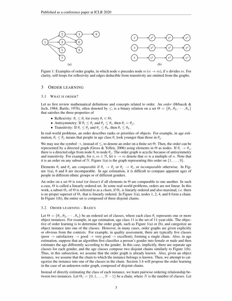
Figure 1: Examples of order graphs, in which node n precedes nodem (n→ m), if n dividesm. Forclarity, self-loops for reflexivity and edges deducible from transitivity are omitted from the graphs.

3 ORDER LEARNING

3.1 WHAT IS ORDER?

Let us first review mathematical definitions and concepts related to order. An order (Hrbacek &Jech, 1984; Bartle, 1976), often denoted by ≤, is a binary relation on a set Θ = {θ1, θ2, · · · , θn}that satisfies the three properties of

• Reflexivity: θi ≤ θi for every θi ∈ Θ;• Antisymmetry: If θi ≤ θj and θj ≤ θi, then θi = θj ;• Transitivity: If θi ≤ θj and θj ≤ θk, then θi ≤ θk.

In real-world problems, an order describes ranks or priorities of objects. For example, in age esti-mation, θi ≤ θj means that people in age class θi look younger than those in θj .

We may use the symbol→, instead of≤, to denote an order on a finite set Θ. Then, the order can berepresented by a directed graph (Gross & Yellen, 2006) using elements in Θ as nodes. If θi → θj ,there is a directed edge from node θi to node θj . The order graph is acyclic because of antisymmetryand transitivity. For example, for n,m ∈ N, let n → m denote that m is a multiple of n. Note thatit is an order on any subset of N. Figure 1(a) is the graph representing this order on {1, . . . , 9}.Elements θi and θj are comparable if θi → θj or θj → θi, or incomparable otherwise. In Fig-ure 1(a), 6 and 8 are incomparable. In age estimation, it is difficult to compare apparent ages ofpeople in different ethnic groups or of different genders.

An order on a set Θ is total (or linear) if all elements in Θ are comparable to one another. In sucha case, Θ is called a linearly ordered set. In some real-world problems, orders are not linear. In thiswork, a subset Θc of Θ is referred to as a chain, if Θc is linearly ordered and also maximal, i.e. thereis no proper superset of Θc that is linearly ordered. In Figure 1(a), nodes 1, 2, 4, and 8 form a chain.In Figure 1(b), the entire set is composed of three disjoint chains.

3.2 ORDER LEARNING – BASICS

Let Θ = {θ1, θ2, · · · , θn} be an ordered set of classes, where each class θi represents one or moreobject instances. For example, in age estimation, age class 11 is the set of 11-year-olds. The objec-tive of order learning is to determine the order graph, such as Figure 1(a) or (b), and categorize anobject instance into one of the classes. However, in many cases, order graphs are given explicitlyor obvious from the contexts. For example, in quality assessment, there are typically five classes(poor → satisfactory → good → very good → excellent), forming a single chain. Also, in ageestimation, suppose that an algorithm first classifies a person’s gender into female or male and thenestimates the age differently according to the gender. In this case, implicitly, there are separate ageclasses for each gender, and the age classes compose two disjoint chains similarly to Figure 1(b).Thus, in this subsection, we assume that the order graph is already known. Also, given an objectinstance, we assume that the chain to which the instance belongs is known. Then, we attempt to cat-egorize the instance into one of the classes in the chain. Section 3.4 will propose the order learningin the case of an unknown order graph, composed of disjoint chains.

Instead of directly estimating the class of each instance, we learn pairwise ordering relationship be-tween two instances. Let Θc = {0, 1, . . . , N − 1} be a chain, where N is the number of classes. Let

3


CNN feature extractor

Ternary classifier

CNN feature extractor

Shared parameters

(Siamese)c

x

yx ≺ yx ≈ yx y≺

Figure 2: Illustration of the pairwise comparator, where c© denotes concatenation.

x and y be two instances belonging to classes in Θc. Let θ(·) denote the class of an instance. Then,x and y are compared and their ordering relationship is defined according to their class difference as

x � y if θ(x)− θ(y) > τ, (1)x ≈ y if |θ(x)− θ(y)| ≤ τ, (2)x ≺ y if θ(x)− θ(y) < −τ, (3)

where τ is a threshold. To avoid confusion, we use ‘�, ≈, ≺’ for the instance ordering, while ‘>,=, <’ for the class order. In practice, the categorization in (1)∼(3) is performed by a pairwisecomparator in Figure 2, which consists of a Siamese network and a ternary classifier (Lee & Kim,2019b). To train the comparator, only comparable instance pairs are employed.

We estimate the class θ(x) of a test instance x by comparing it with reference instances ym, 0 ≤m ≤ M − 1, where M is the number of references. The references are selected from training datasuch that they are from the same chain as x. Given x and ym, the comparator provides one of threecategories ‘�, ≈, ≺’ as a result. Let θ′ be an estimate of the true class θ(x). Then, the consistencybetween the comparator result and the estimate is defined asφcon(x, ym, θ

′) = (4)[x � ym

][θ′ − θ(ym) > τ

]+[x ≈ ym

][|θ′ − θ(ym)| ≤ τ

]+[x ≺ ym

][θ′ − θ(ym) < −τ

]where [·] is the indicator function. The function φcon(x, ym, θ

′) returns either 0 for an inconsistentcase or 1 for a consistent case. For example, suppose that the pairwise comparator declares x ≺ ymbut θ′− θ(ym) > τ . Then, φcon(x, ym, θ

′) = 0 ·1 + 0 ·0 + 1 ·0 = 0. Due to a possible classificationerror of the comparator, this inconsistency may occur even when the estimate θ′ equals the true classθ(x). To maximize the consistency with all references, we estimate the class of x by

θMC(x) = arg maxθ′∈Θc

M−1∑m=0

φcon(x, ym, θ′), (5)

which is called the maximum consistency (MC) rule. Figure 3 illustrates this MC rule.

It is noted that ‘�, ≈, ≺’ is not an mathematical order. For example, if θ(x) + 34τ = θ(y) =

θ(z)− 34τ , then x ≈ y and y ≈ z but x ≺ z. This is impossible in an order. More precisely, due to

the quantization effect of the ternary classifier in (1)∼(3), ‘�, ≈, ≺’ is quasi-transitive (Sen, 1969),and ‘≈’ is symmetric but intransitive. We use this quasi-transitive relation to categorize an instanceinto one of the classes, on which a mathematical order is well defined.

3.3 ORDER LEARNING – SUPERVISED CHAINS

3.3.1 SINGLE-CHAIN HYPOTHESIS (1CH)

In the simplest case of 1CH, all classes form a single chain Θc = {0, 1, . . . , N − 1}. For example,in 1CH age estimation, people’s ages are estimated regardless of their ethnic groups or genders.

We implement the comparator in Figure 2 using CNNs, as described in Section 4.1. Let qxy =(qxy0 , qxy1 , qxy2 ) be the one-hot vector, indicating the ground-truth ordering relationship betweentraining instances x and y. Specifically, (1, 0, 0), (0, 1, 0), and (0, 0, 1) represent x � y, x ≈ y,and x ≺ y. Also, pxy = (pxy0 , pxy1 , pxy2 ) is the corresponding softmax probability vector of thecomparator. We train the comparator to minimize the comparator loss

`co = −∑x∈T

∑y∈R

2∑j=0

qxyj log pxyj (6)

4


0 1 2 3 4 5 6 7 8 9 10 11 12 13 14 0 1 2 3 4 5 6 7 8 9 10 11 12 13 14

1 1 1 1 1 1 1 1 1 1 0 1 1 1 1 1 1 1 0 0 1 1 1 1 1 0 1 0 0 1

1 1 1 1 1 1 1 1 1 1 1 0 1 1 1 1 1 1 0 0 1 1 1 1 1 1 0 0 0 1

1 1 0 1 1 1 1 1 1 1 1 1 1 1 1 1 1 0 0 0 1 1 1 1 1 1 1 0 0 1

1 1 0 1 1 1 1 1 1 1 1 1 0 1 1 1 1 0 0 0 1 1 1 1 1 1 1 1 0 1

1 0 1 1 1 1 1 1 1 1 1 1 1 1 1 1 0 1 0 0 1 1 1 1 1 1 1 0 0 1

Class

Figure 3: Consistency computation in the MC rule: It is illustrated how to compute the sum in (5) fortwo candidates θ′ = 7 and 9. Each box represents a reference ym. There are 5 references for eachclass in {0, . . . , 14}. Comparison results are color-coded (yellow for x � ym, gray for x ≈ ym, andgreen for x ≺ ym). The bold black rectangle encloses the references satisfying |θ′ − θ(ym)| ≤ τ ,where τ = 4. The computed consistency φcon(x, ym, θ

′) in (5) is written within the box. Forθ′ = 7, there are six inconsistent boxes. For θ′ = 9, there are 24 such boxes. In this example, θ′ = 7

minimizes the inconsistency, or equivalently maximizes the consistency. Therefore, θMC(x) = 7.

where T is the set of all training instances and R ⊂ T is the set of reference instances. First,we initialize R = T and minimize `co via the stochastic gradient descent. Then, we reduce thereference setR by sampling references from T . Specifically, for each class in Θc, we choose M/Nreference images to minimize the same loss `co, where M is the number of all references and N isthe number of classes. In other words, the reliability score of a reference candidate y is defined as

α(y) =∑x∈T

2∑j=0

qxyj log pxyj (7)

and the M/N candidates with the highest reliability scores are selected. Next, after fixing thereference setR, the comparator is trained to minimize the loss `co. Then, after fixing the comparatorparameters, the reference setR is updated to minimize the same loss `co, and so forth.

In the test phase, an input instance is compared with the M references and its class is estimatedusing the MC rule in (5).

3.3.2 K-CHAIN HYPOTHESIS (KCH)

In KCH, we assume that classes form K disjoint chains, as in Figure 1(b). For example, in thesupervised 6CH for age estimation, we predict a person’s age according to the gender in {female,male} and the ethnic group in {African, Asian, European}. Thus, there are 6 chains in total. In thiscase, people in different chains are assumed to be incomparable for age estimation. It is supervised,since gender and ethnic group annotations are used to separate the chains. The supervised 2CH or3CH also can be implemented by dividing chains by genders only or ethnic groups only.

The comparator is trained similarly to 1CH. However, in computing the comparator loss in (6), atraining instance x and a reference y are constrained to be from the same chain. Also, during thetest, the type (or chain) of a test instance should be determined. Therefore, a K-way type classifieris trained, which shares the feature extractor with the comparator in Figure 2 and uses additionalfully-connected (FC) layers. Thus, the overall loss is given by

` = `co + `ty (8)

where `co is the comparator loss and `ty is the type classifier loss. The comparator and the typeclassifier are jointly trained to minimize this overall loss `.

During the test, given an input instance, we determine its chain using the type classifier, and compareit with the references from the same chain, and then estimate its class using the MC rule in (5).

3.4 ORDER LEARNING – UNSUPERVISED CHAINS

This subsection proposes an algorithm to separate classes into K disjoint chains when there are nosupervision or annotation data available for the separation. First, we randomly partition the trainingset T into T0, T1, . . . , TK−1, where T = T0∪ . . .∪TK−1 and Tk∩Tl = ∅ for k 6= l. Then, similarly

5


Algorithm 1 Order Learning with Unsupervised ChainsInput: T = training set of ordinal data, K = # of chains, N = # of classes in each chain, and M = # ofreferences in each chain1: Partition T randomly into T0, . . . , TK−1 and train a pairwise comparator2: for each chain k do . Reference Selection (Rk)3: From Tk, select M/N references y with the highest reliability scores αk(y)4: end for5: repeat6: for each instance x do . Membership Update (Tk)7: Assign it to Tk∗ , where k∗ = argmaxk βk(x) subject to the regularization constraint8: end for9: Fine-tune the comparator and train a type classifier using T0, . . . , TK−1 to minimize ` = `co + `ty

10: for each instance x do . Membership Refinement (Tk)11: Assign it to Tk′ where k′ is its type classification result12: end for13: for each chain k do . Reference Selection (Rk)14: From Tk, select M/N references y with the highest reliability scores αk(y)15: end for16: until convergence or predefined number of iterationsOutput: Pairwise comparator, type classifier, reference setsR0, . . . ,RK−1

to (6), the comparator loss `co can be written as

`co = −K−1∑k=0

∑x∈Tk

∑y∈Rk

2∑j=0

qxyj log pxyj = −K−1∑k=0

∑y∈Rk

αk(y) = −K−1∑k=0

∑x∈Tk

βk(x) (9)

where Rk ⊂ Tk is the set of references for the kth chain, αk(y) =∑x∈Tk

∑j q

xyj log pxyj is the

reliability of a reference y in the kth chain, and βk(x) =∑y∈Rk

∑j q

xyj log pxyj is the affinity

of an instance x to the references in the kth chain. Note that βk(x) = −∑y∈Rk

D(qxy‖pxy)where D is the Kullback-Leibler distance (Cover & Thomas, 2006). Second, after fixing the chainmembership Tk for each chain k, we select references y to maximize the reliability scores αk(y).These references form Rk. Third, after fixing R0, . . . ,RK−1, we update the chain membershipT0, . . . , TK−1, by assigning each training instance x to the kth chain that maximizes the affinityscore βk(x). The second and third steps are iteratively repeated. Both steps decrease the same loss`co in (9).

The second and third steps are analogous to the centroid rule and the nearest neighbor rule in the K-means clustering (Gersho & Gray, 1991), respectively. The second step determines representativesin each chain (or cluster), while the third step assigns each instance to an optimal chain according tothe affinity. Furthermore, both steps decrease the same loss alternately.

However, as described in Algorithm 1, we modify this iterative algorithm by including the mem-bership refinement step in lines 10 ∼ 12. Specifically, we train a K-way type classifier usingT0, . . . , TK−1. Then, we accept the type classification results to refine T0, . . . , TK−1. This refine-ment is necessary because the type classifier should be used in the test phase to determine the chainof an unseen instance. Therefore, it is desirable to select the references also after refining the chainmembership. Also, in line 7, if we assign an instance x to maximize βk(x) only, some classes maybe assigned too few training instances, leading to data imbalance. To avoid this, we enforce theregularization constraint so that every class is assigned at least a predefined number of instances.This regularized membership update is described in Appendix A.

4 AGE ESTIMATION

We develop an age estimator based on the proposed order learning. Order learning is suitable for ageestimation, since telling the older one between two people is easier than estimating each person’sage directly (Chang et al., 2010; Zhang et al., 2017a).

4.1 IMPLEMENTATION DETAILS

It is less difficult to distinguish between a 5-year-old and a 10-year-old than between a 65-year-old and a 70-year-old. Therefore, in age estimation, we replace the categorization based on the

6


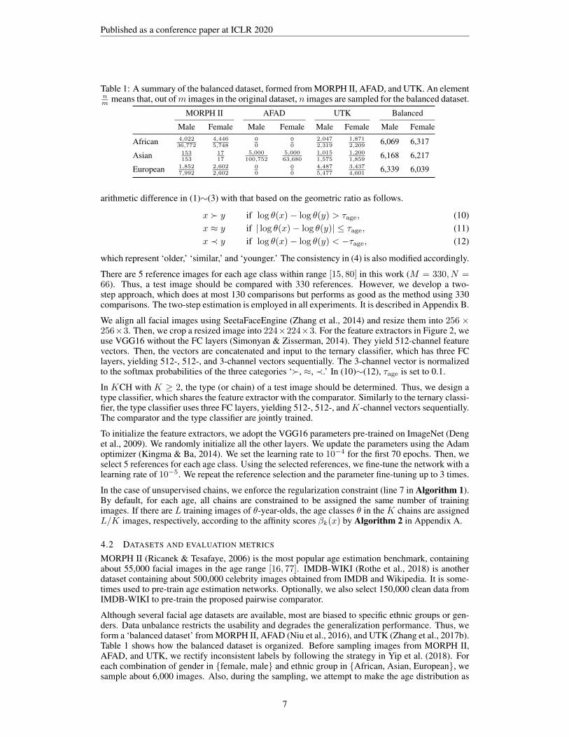
Table 1: A summary of the balanced dataset, formed from MORPH II, AFAD, and UTK. An elementnm means that, out ofm images in the original dataset, n images are sampled for the balanced dataset.

MORPH II AFAD UTK Balanced

Male Female Male Female Male Female Male Female

African 4,02236,772

4,4465,748

00

00

2,0472,319

1,8712,209

6,069 6,317

Asian 153153

1717

5,000100,752

5,00063,680

1,0151,575

1,2001,859

6,168 6,217

European 1,8527,992

2,6022,602

00

00

4,4875,477

3,4374,601

6,339 6,039

arithmetic difference in (1)∼(3) with that based on the geometric ratio as follows.

x � y if log θ(x)− log θ(y) > τage, (10)x ≈ y if | log θ(x)− log θ(y)| ≤ τage, (11)x ≺ y if log θ(x)− log θ(y) < −τage, (12)

which represent ‘older,’ ‘similar,’ and ‘younger.’ The consistency in (4) is also modified accordingly.

There are 5 reference images for each age class within range [15, 80] in this work (M = 330, N =66). Thus, a test image should be compared with 330 references. However, we develop a two-step approach, which does at most 130 comparisons but performs as good as the method using 330comparisons. The two-step estimation is employed in all experiments. It is described in Appendix B.

We align all facial images using SeetaFaceEngine (Zhang et al., 2014) and resize them into 256 ×256×3. Then, we crop a resized image into 224×224×3. For the feature extractors in Figure 2, weuse VGG16 without the FC layers (Simonyan & Zisserman, 2014). They yield 512-channel featurevectors. Then, the vectors are concatenated and input to the ternary classifier, which has three FClayers, yielding 512-, 512-, and 3-channel vectors sequentially. The 3-channel vector is normalizedto the softmax probabilities of the three categories ‘�, ≈, ≺.’ In (10)∼(12), τage is set to 0.1.

In KCH with K ≥ 2, the type (or chain) of a test image should be determined. Thus, we design atype classifier, which shares the feature extractor with the comparator. Similarly to the ternary classi-fier, the type classifier uses three FC layers, yielding 512-, 512-, andK-channel vectors sequentially.The comparator and the type classifier are jointly trained.

To initialize the feature extractors, we adopt the VGG16 parameters pre-trained on ImageNet (Denget al., 2009). We randomly initialize all the other layers. We update the parameters using the Adamoptimizer (Kingma & Ba, 2014). We set the learning rate to 10−4 for the first 70 epochs. Then, weselect 5 references for each age class. Using the selected references, we fine-tune the network with alearning rate of 10−5. We repeat the reference selection and the parameter fine-tuning up to 3 times.

In the case of unsupervised chains, we enforce the regularization constraint (line 7 in Algorithm 1).By default, for each age, all chains are constrained to be assigned the same number of trainingimages. If there are L training images of θ-year-olds, the age classes θ in the K chains are assignedL/K images, respectively, according to the affinity scores βk(x) by Algorithm 2 in Appendix A.

4.2 DATASETS AND EVALUATION METRICS

MORPH II (Ricanek & Tesafaye, 2006) is the most popular age estimation benchmark, containingabout 55,000 facial images in the age range [16, 77]. IMDB-WIKI (Rothe et al., 2018) is anotherdataset containing about 500,000 celebrity images obtained from IMDB and Wikipedia. It is some-times used to pre-train age estimation networks. Optionally, we also select 150,000 clean data fromIMDB-WIKI to pre-train the proposed pairwise comparator.

Although several facial age datasets are available, most are biased to specific ethnic groups or gen-ders. Data unbalance restricts the usability and degrades the generalization performance. Thus, weform a ‘balanced dataset’ from MORPH II, AFAD (Niu et al., 2016), and UTK (Zhang et al., 2017b).Table 1 shows how the balanced dataset is organized. Before sampling images from MORPH II,AFAD, and UTK, we rectify inconsistent labels by following the strategy in Yip et al. (2018). Foreach combination of gender in {female, male} and ethnic group in {African, Asian, European}, wesample about 6,000 images. Also, during the sampling, we attempt to make the age distribution as

7


Table 2: Performance comparison on the MORPH II dataset: * means that the networks are pre-trained on IMDB-WIKI, and † the values are read from the reported CS curves or measured byexperiments. The best results are boldfaced, and the second best ones are underlined.

Setting A Setting B Setting C (SE) Setting D (RS)

MAE CS(%) MAE CS(%) MAE CS(%) MAE CS(%)

OHRank (Chang et al., 2011) - - - - - - 6.07 56.3OR-CNN (Niu et al., 2016) - - - - - - 3.27 73.0†

Ranking-CNN (Chen et al., 2017) - - - - - - 2.96 85.0†

DMTL (Han et al., 2018) - - - - 3.00 85.3 - -DEX* (Rothe et al., 2018) 2.68 - - - - - - -DRFs (Shen et al., 2018) 2.91 82.9 2.98 - - - 2.17 91.3MO-CNN* (Tan et al., 2018) 2.52 85.0† 2.70 83.0† - - - -MV (Pan et al., 2018) - - - - 2.80 87.0† 2.41 90.0†

MV* - - - - 2.79 - 2.16 -BridgeNet* (Li et al., 2019) 2.38 91.0† 2.63 86.0† - - - -Proposed (1CH) 2.69 89.1 3.00 85.2 2.76 88.0 2.32 92.4Proposed* (1CH) 2.41 91.7 2.75 88.2 2.68 88.8 2.22 93.3

uniform as possible within range [15, 80]. The balanced dataset is partitioned into training and testsubsets with ratio 8 : 2.

For performance assessment, we calculate the mean absolute error (MAE) (Lanitis et al., 2004) andthe cumulative score (CS) (Geng et al., 2006). MAE is the average absolute error between predictedand ground-truth ages. Given a tolerance level l, CS computes the percentage of test images whoseabsolute errors are less than or equal to l. In this work, l is fixed to 5, as done in Chang et al. (2011),Han et al. (2018), and Shen et al. (2018).

4.3 EXPERIMENTAL RESULTS

Table 2 compares the proposed algorithm (1CH) with conventional algorithms on MORPH II. Asevaluation protocols for MORPH II, we use four different settings, including the 5-fold subject-exclusive (SE) and the 5-fold random split (RS) (Chang et al., 2010; Guo & Wang, 2012). Ap-pendix C.1 describes these four settings in detail and provides an extended version of Table 2.

OHRank, OR-CNN, and Ranking-CNN are all based on ordinal regression. OHRank uses traditionalfeatures, yielding relatively poor performances, whereas OR-CNN and Ranking-CNN use CNN fea-tures. DEX, DRFs, MO-CNN, MV, and BridgeNet employ VGG16 as backbone networks. Amongthem, MV and BridgeNet achieve the state-of-the-art results, by employing the mean-variance lossand the gating networks, respectively. The proposed algorithm outperforms these algorithms in set-ting C, which is the most challenging task. Furthermore, in terms of CS, the proposed algorithmyields the best performances in all four settings. These outstanding performances indicate that orderlearning is an effective approach to age estimation.

In Table 3, we analyze the performances of the proposed algorithm on the balanced dataset accordingto the number of hypothesized chains. We also implement and train the state-of-the-art MV on thebalanced dataset and provide its results using supervised chains.

Let us first analyze the performances of the proposed algorithm using ‘supervised’ chains. TheMAE and CS scores on the balanced dataset are worse than those on MORPH II, since the balanceddataset contains more diverse data and thus is more challenging. By processing facial images sepa-rately according to the genders (2CH), the proposed algorithm reduces MAE by 0.05 and improvesCS by 0.2% in comparison with 1CH. Similar improvements are obtained by 3CH or 6CH, whichconsider the ethnic groups only or both gender and ethnic groups, respectively. In contrast, in thecase of MV, multi-chain hypotheses sometimes degrade the performances; e.g., MV (6CH) yieldsa lower CS than MV (1CH). Regardless of the number of chains, the proposed algorithm trains asingle comparator but uses a different set of references for each chain. The comparator is a ternaryclassifier. In contrast, MV (6CH) should train six different age estimators, each of which is a 66-wayclassifier, to handle different chains. Thus, their training is more challenging than that of the singleternary classifier. Note that, for the multi-chain hypotheses, the proposed algorithm first identifiesthe chain of a test image using the type classifiers, whose accuracies are about 98%. In Table 3, these

8


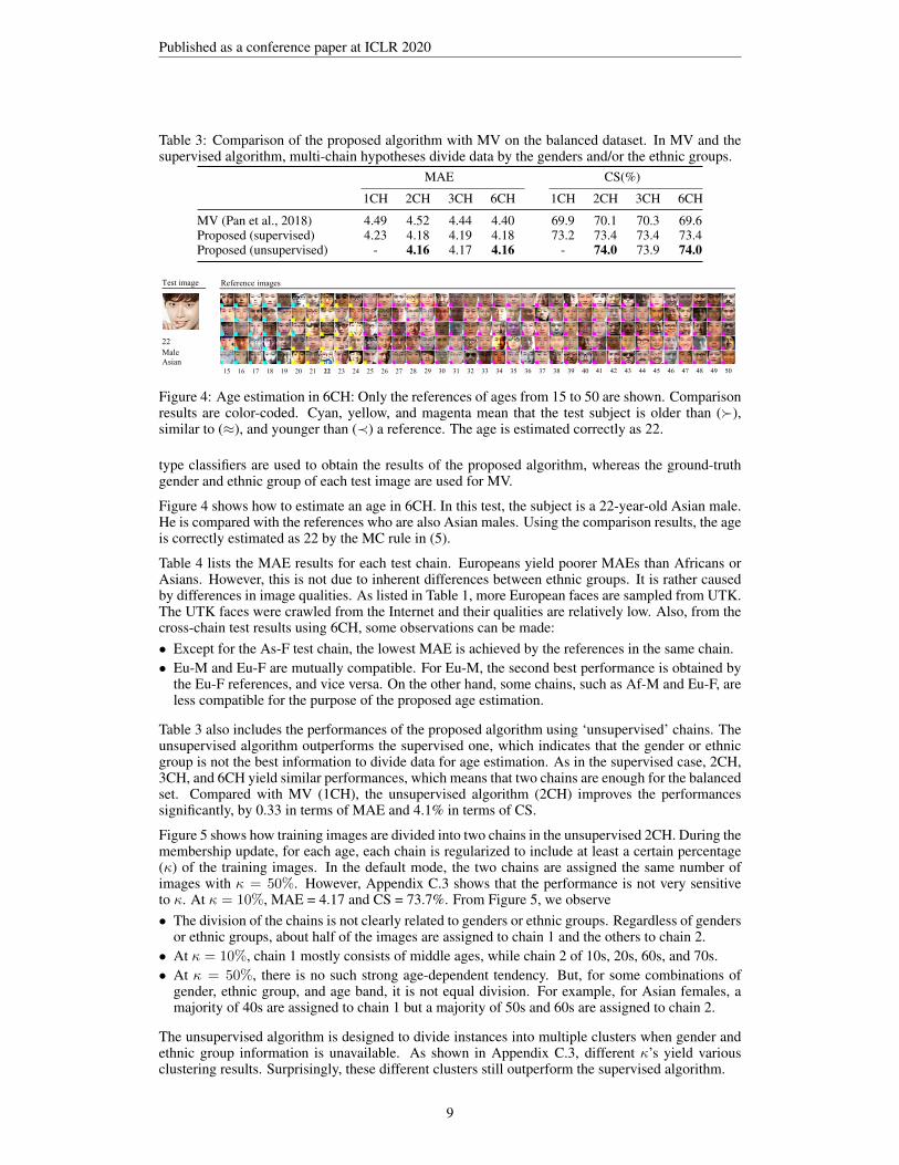
Table 3: Comparison of the proposed algorithm with MV on the balanced dataset. In MV and thesupervised algorithm, multi-chain hypotheses divide data by the genders and/or the ethnic groups.

MAE CS(%)

1CH 2CH 3CH 6CH 1CH 2CH 3CH 6CH

MV (Pan et al., 2018) 4.49 4.52 4.44 4.40 69.9 70.1 70.3 69.6Proposed (supervised) 4.23 4.18 4.19 4.18 73.2 73.4 73.4 73.4Proposed (unsupervised) - 4.16 4.17 4.16 - 74.0 73.9 74.0

22

Male

Asian

Test image Reference images

15 16 17 18 19 20 21 22 23 24 25 26 27 28 29 30 31 32 33 34 35 36 37 38 39 40 41 42 43 44 45 46 47 48 49 50

Figure 4: Age estimation in 6CH: Only the references of ages from 15 to 50 are shown. Comparisonresults are color-coded. Cyan, yellow, and magenta mean that the test subject is older than (�),similar to (≈), and younger than (≺) a reference. The age is estimated correctly as 22.

type classifiers are used to obtain the results of the proposed algorithm, whereas the ground-truthgender and ethnic group of each test image are used for MV.

Figure 4 shows how to estimate an age in 6CH. In this test, the subject is a 22-year-old Asian male.He is compared with the references who are also Asian males. Using the comparison results, the ageis correctly estimated as 22 by the MC rule in (5).

Table 4 lists the MAE results for each test chain. Europeans yield poorer MAEs than Africans orAsians. However, this is not due to inherent differences between ethnic groups. It is rather causedby differences in image qualities. As listed in Table 1, more European faces are sampled from UTK.The UTK faces were crawled from the Internet and their qualities are relatively low. Also, from thecross-chain test results using 6CH, some observations can be made:• Except for the As-F test chain, the lowest MAE is achieved by the references in the same chain.• Eu-M and Eu-F are mutually compatible. For Eu-M, the second best performance is obtained by

the Eu-F references, and vice versa. On the other hand, some chains, such as Af-M and Eu-F, areless compatible for the purpose of the proposed age estimation.

Table 3 also includes the performances of the proposed algorithm using ‘unsupervised’ chains. Theunsupervised algorithm outperforms the supervised one, which indicates that the gender or ethnicgroup is not the best information to divide data for age estimation. As in the supervised case, 2CH,3CH, and 6CH yield similar performances, which means that two chains are enough for the balancedset. Compared with MV (1CH), the unsupervised algorithm (2CH) improves the performancessignificantly, by 0.33 in terms of MAE and 4.1% in terms of CS.

Figure 5 shows how training images are divided into two chains in the unsupervised 2CH. During themembership update, for each age, each chain is regularized to include at least a certain percentage(κ) of the training images. In the default mode, the two chains are assigned the same number ofimages with κ = 50%. However, Appendix C.3 shows that the performance is not very sensitiveto κ. At κ = 10%, MAE = 4.17 and CS = 73.7%. From Figure 5, we observe• The division of the chains is not clearly related to genders or ethnic groups. Regardless of genders

or ethnic groups, about half of the images are assigned to chain 1 and the others to chain 2.• At κ = 10%, chain 1 mostly consists of middle ages, while chain 2 of 10s, 20s, 60s, and 70s.• At κ = 50%, there is no such strong age-dependent tendency. But, for some combinations of

gender, ethnic group, and age band, it is not equal division. For example, for Asian females, amajority of 40s are assigned to chain 1 but a majority of 50s and 60s are assigned to chain 2.

The unsupervised algorithm is designed to divide instances into multiple clusters when gender andethnic group information is unavailable. As shown in Appendix C.3, different κ’s yield variousclustering results. Surprisingly, these different clusters still outperform the supervised algorithm.

9


Table 4: Cross-chain tests on the balanced dataset (MAEs). For example, in 6CH, when Africanmale references are used to estimate the ages of Asian females, the resultant MAE is 3.82.

Test chain

Method Reference chain Af-M Af-F As-M As-F Eu-M Eu-F

1CH All 3.87 3.82 3.98 3.79 5.21 4.69

6CH African-Male 3.85 3.79 4.03 3.82 5.50 5.00African-Female 4.02 3.65 4.18 3.85 5.42 5.02Asian-Male 3.97 3.75 3.97 3.81 5.48 4.87Asian-Female 4.06 3.78 4.05 3.78 5.69 4.89European-Male 3.99 3.71 4.02 3.80 5.13 4.66European-Female 4.45 3.79 4.11 3.77 5.21 4.65

0%

100%

10s 20s 30s 40s 50s 60s 70s

0%

100%

0%

100%

0%

100%

0%

100%

0%

100%

0%

100%

10s 20s 30s 40s 50s 60s 70s

0%

100%

0%

100%

0%

100%

0%

100%

0%

100%

Age Age

k = 10% k = 50%

Af-M

Af-F

As-M

As-F

Eu-M

Eu-F

chain 1 chain 2

Figure 5: Distributions of training images in the unsupervised algorithm (2CH).

For example, at κ = 10%, let us consider the age band of 20s and 30s. If the references in chain 2are used to estimate the ages of people in chain 1, the average error is 4.6 years. On the contrary, ifthe references in chain 1 are used for chain 2, the average error is −5.4 years. These opposite biasesmean that people in chain 1 tend to look older than those in chain 2. These ‘looking-older’ people in20s and 30s compose the blue cluster (chain 1) together with most people in 40s and 50s in Figure 5.In this case, ‘looking-older’ people in 20s and 30s are separated from ‘looking-younger’ ones by theunsupervised algorithm. This is more effective than the gender-based or ethnic-group-based divisionof the supervised algorithm. Appendix C presents more results on age estimation.

5 CONCLUSIONS

Order learning was proposed in this work. In order learning, classes form an ordered set, and eachclass represents object instances of the same rank. Its goal is to determine the order graph of classesand classify a test instance into one of the classes. To this end, we designed the pairwise comparatorto learn ordering relationships between instances. We then decided the class of an instance bycomparing it with reference instances in the same chain and maximizing the consistency among thecomparison results. For age estimation, it was shown that the proposed algorithm yields the state-of-the-art performance even in the case of the single-chain hypothesis. The performance is furtherimproved when the order graph is divided into multiple disjoint chains.

In this paper, we assumed that the order graph is composed of disjoint chains. However, there aremore complicated graphs, e.g. Figure 1(a), than disjoint chains. For example, it is hard to recognizean infant’s sex from its facial image (Porter et al., 1984). But, after puberty, male and female takedivergent paths. This can be reflected by an order graph, which consists of two chains sharingcommon nodes up to a certain age. It is an open problem to generalize order learning to find anoptimal order graph, which is not restricted to disjoint chains.

ACKNOWLEDGEMENTS

This work was supported by ‘The Cross-Ministry Giga KOREA Project’ grant funded by the Koreagovernment (MSIT) (No. GK19P0200, Development of 4D reconstruction and dynamic deformableaction model based hyperrealistic service technology), and by the National Research Foundation ofKorea (NRF) grant funded by the Korea government (MSIP) (No. NRF-2018R1A2B3003896).

10


REFERENCES

A. Bachem. Absolute pitch. J. Acoust. Soc. Am., 27(6):1180–1185, November 1955.

Robert G. Bartle. The Elements of Real Analysis. John Wiley & Sons, 2nd edition, 1976.

Mark Braverman and Elchanan Mossel. Noisy sorting without resampling. In Symp. Discrete Algo-rithms, pp. 268–276, 2008.

Chris Burges, Tal Shaked, Erin Renshaw, Ari Lazier, Matt Deeds, Nicole Hamilton, and Greg Hul-lender. Learning to rank using gradient descent. In ICML, pp. 89–96, 2005.

Kuang-Yu Chang, Chu-Song Chen, and Yi-Ping Hung. A ranking approach for human ages estima-tion based on face images. In ICPR, pp. 3396–3399, 2010.

Kuang-Yu Chang, Chu-Song Chen, and Yi-Ping Hung. Ordinal hyperplanes ranker with cost sensi-tivities for age estimation. In CVPR, pp. 585–592, 2011.

Shixing Chen, Caojin Zhang, Ming Dong, Jialiang Le, and Mike Rao. Using Ranking-CNN for ageestimation. In CVPR, pp. 5183–5192, 2017.

Weifeng Chen, Zhao Fu, Dawei Yang, and Jia Deng. Single-image depth perception in the wild. InNIPS, pp. 730–738, 2016.

Thomas M. Cover and Joy A. Thomas. Elements of Information Theory. Wiley, 2006.

Jia Deng, Wei Dong, Richard Socher, Li-Jia Li, Kai Li, and Li Fei-Fei. ImageNet: A large-scalehierarchical image database. In CVPR, pp. 248–255, 2009.

Eibe Frank and Mark Hall. A simple approach to ordinal classification. In ECML, pp. 145–156,2001.

Huan Fu, Mingming Gong, Chaohui Wang, Kayhan Batmanghelich, and Dacheng Tao. Deep ordinalregression network for monocular depth estimation. In CVPR, pp. 2002–2011, 2018.

Xin Geng, Zhi-Hua Zhou, Yu Zhang, Gang Li, and Honghua Dai. Learning from facial agingpatterns for automatic age estimation. In ACM Multimedia, pp. 307–316, 2006.

Xin Geng, Zhi-Hua Zhou, and Kate Smith-Miles. Automatic age estimation based on facial agingpatterns. IEEE Trans. Pattern Anal. Mach. Intell., 29(12):2234–2240, December 2007.

A. Gersho and R. M. Gray. Vector Quantization and Signal Compression. Kluwer Academic Pub-lishers Norwell, 1991.

Jonathan L. Gross and Jay Yellen. Graph Theory and Its Applications. Chapman & Hall, 2ndedition, 2006.

Guodong Guo and Guowang Mu. Simultaneous dimensionality reduction and human age estimationvia kernel partial least squares regression. In CVPR, pp. 657–664, 2011.

Guodong Guo and Xiaolong Wang. A study on human age estimation under facial expressionchanges. In CVPR, pp. 2547–2553, 2012.

Guodong Guo, Guowang Mu, Yun Fu, and Thomas S. Huang. Human age estimation using bio-inspired features. In CVPR, pp. 112–119, 2009.

Hu Han, Anil K. Jain, Fang Wang, Shiguang Shan, and Xilin Chen. Heterogeneous face attributeestimation: A deep multi-task learning approach. IEEE Trans. Pattern Anal. Mach. Intell., 40(11):2597–2609, November 2018.

Ralf Herbrich, Thore Graepel, and Klaus Obermayer. Support vector learning for ordinal regression.In ICANN, pp. 97–102, 1999.

Karel Hrbacek and Thomas Jech. Introduction to Set Theory. Marcel Dekker, Inc., 2nd edition,1984.

11


Ivan Huerta, Carles Fernandez, Carlos Segura, Javier Hernando, and Andrea Prati. A deep analysison age estimation. Pattern Recog. Lett., 68:239–249, December 2015.

Kevin G. Jamieson and Robert D. Nowak. Active ranking using pairwise comparisons. In NIPS, pp.2240–2248, 2011.

Diederik P. Kingma and Jimmy Ba. Adam: A method for stochastic optimization. arXiv preprintarXiv:1412.6980, 2014.

Young Ho Kwon and Niels da Vitoria Lobo. Age classification from facial images. In CVPR, pp.762–767, 1994.

Andreas Lanitis, Chrisina Draganova, and Chris Christodoulou. Comparing different classifiers forautomatic age estimation. IEEE Trans. Syst., Man, Cybern. B, Cybern., 34(1):621–628, February2004.

Jae-Han Lee and Chang-Su Kim. Monocular depth estimation using relative depth maps. In CVPR,pp. 9729–9738, 2019a.

Jun-Tae Lee and Chang-Su Kim. Image aesthetic assessment based on pairwise comparison - aunified approach to score regression, binary classification, and personalization. In ICCV, pp.1191–1200, 2019b.

Ling Li and Hsuan-Tien Lin. Ordinal regression by extended binary classification. In NIPS, pp.865–872, 2007.

Wanhua Li, Jiwen Lu, Jianjiang Feng, Chunjing Xu, Jie Zhou, and Qi Tian. BridgeNet: A continuity-aware probabilistic network for age estimation. In CVPR, pp. 1145–1154, 2019.

Tie-Yan Liu. Learning to rank for information retrieval. Foundations and Trends in InformatioonRetrieval, 3(3):225–331, 2009.

Brian McFee and Gert Lanckriet. Metric learning to rank. In ICML, pp. 775–782, 2010.

Sahand Negahban, Sewoong Oh, and Devavrat Shah. Iterative ranking from pair-wise comparisons.In NIPS, pp. 2474–2482, 2012.

Zhenxing Niu, Mo Zhou, Le Wang, Xinbo Gao, and Gang Hua. Ordinal regression with multipleoutput CNN for age estimation. In CVPR, pp. 4920–4928, 2016.

Hongyu Pan, Hu Han, Shiguang Shan, and Xilin Chen. Mean-variance loss for deep age estimationfrom a face. In CVPR, pp. 5285–5294, 2018.

Gabriel Panis, Andreas Lanitis, Nicholas Tsapatsoulis, and Timothy F. Cootes. Overview of researchon facial ageing using the FG-NET ageing database. IET Biometrics, 5(2):37–46, 2016.

Richard H. Porter, Jennifer M. Cernoch, and Rene D. Balogh. Recognition of neonates by facial-visual characteristics. Pediatrics, 74(4):501–504, October 1984.

Karl Ricanek and Tamirat Tesafaye. MORPH: A longitudinal image database of normal adult age-progression. In FGR, pp. 341–345, 2006.

Rasmus Rothe, Radu Timofte, and Luc Van Gool. Deep expectation of real and apparent age from asingle image without facial landmarks. Int. J. Comput. Vis., 126(2):144–157, April 2018.

Thomas L. Saaty. A scaling method for priorities in hierarchical structures. J. Math. Psychol., 15(3):234–281, June 1977.

Amartya Sen. Quasi-transitivity, rational choice and collective decisions. Rev. Econ. Stud., 36(3):381–393, July 1969.

Wei Shen, Yilu Guo, Yan Wang, Kai Zhao, Bo Wang, and Alan Yuille. Deep regression forests forage estimation. In CVPR, pp. 2304–2313, 2018.

12


Karen Simonyan and Andrew Zisserman. Very deep convolutional networks for large-scale imagerecognition. In ICLR, 2014.

Zichang Tan, Shuai Zhou, Jun Wan, Zhen Lei, and Stan Z. Li. Age estimation based on a singlenetwork with soft softmax of aging modeling. In ACCV, 2016.

Zichang Tan, Jun Wan, Zhen Lei, Ruicong Zhi, Guodong Guo, and Stan Z. Li. Efficient group-nencoding and decoding for facial age estimation. IEEE Trans. Pattern Anal. Mach. Intell., 40(11):2610–2623, November 2018.

Ming-Feng Tsai, Tie-Yan Liu, Tao Qin, Hsin-Hsi Chen, and Wei-Ying Ma. FRank: A rankingmethod with fidelity loss. In SIGIR, pp. 383–390, 2007.

Fabian L. Wauthier, Michael I. Jordan, and Nebojsa Jojic. Efficient ranking from pairwise compar-isons. In ICML, pp. 109–117, 2013.

Kilian Q. Weinberger, John Blitzer, and Lawrence K. Saul. Distance metric learning for large marginnearest neighbor classification. In NIPS, pp. 1473–1480, 2006.

Eric P. Xing, Andrew Y. Ng, Michael I. Jordan, and Stuart Russell. Distance metric learning withapplication to clustering with side-information. In NIPS, pp. 521–528, 2003.

Dong Yi, Zhen Lei, and Stan Z. Li. Age estimation by multi-scale convolutional network. In ACCV,2014.

Benjamin Yip, Garrett Bingham, Katherine Kempfert, Jonathan Fabish, Troy Kling, Cuixian Chen,and Yishi Wang. Preliminary studies on a large face database. In ICBD, pp. 2572–2579, 2018.

ByungIn Yoo, Youngjun Kwak, Youngsung Kim, Changkyu Choi, and Junmo Kim. Deep facial ageestimation using conditional multitask learning with weak label expansion. IEEE Signal Process.Lett., 25(6):808–812, June 2018.

Chao Zhang, Shuaicheng Liu, Xun Xu, and Ce Zhu. C3AE: Exploring the limits of compact modelfor age estimation. In CVPR, pp. 12587–12596, 2019.

Jie Zhang, Shiguang Shan, Meina Kan, and Xilin Chen. Coarse-to-fine auto-encoder networks(CFAN) for real-time face alignment. In ECCV, pp. 1–16, 2014.

Yunxuan Zhang, Li Liu, Cheng Li, and Chen Change Loy. Quantifying facial age by posterior ofage comparisons. In BMVC, 2017a.

Zhifei Zhang, Yang Song, and Hairong Qi. Age progression/regression by conditional adversarialautoencoder. In CVPR, pp. 5810–5818, 2017b.

13


A REGULARIZED MEMBERSHIP UPDATE

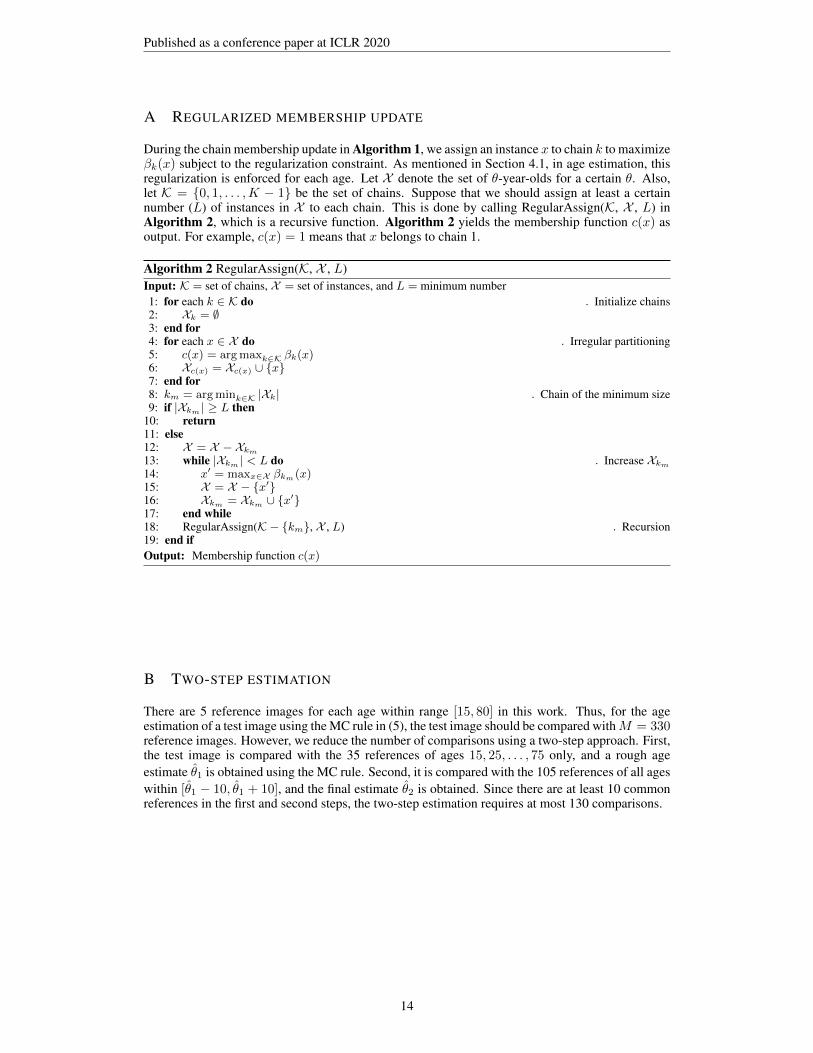
During the chain membership update in Algorithm 1, we assign an instance x to chain k to maximizeβk(x) subject to the regularization constraint. As mentioned in Section 4.1, in age estimation, thisregularization is enforced for each age. Let X denote the set of θ-year-olds for a certain θ. Also,let K = {0, 1, . . . ,K − 1} be the set of chains. Suppose that we should assign at least a certainnumber (L) of instances in X to each chain. This is done by calling RegularAssign(K, X , L) inAlgorithm 2, which is a recursive function. Algorithm 2 yields the membership function c(x) asoutput. For example, c(x) = 1 means that x belongs to chain 1.

Algorithm 2 RegularAssign(K, X , L)Input: K = set of chains, X = set of instances, and L = minimum number1: for each k ∈ K do . Initialize chains2: Xk = ∅3: end for4: for each x ∈ X do . Irregular partitioning5: c(x) = argmaxk∈K βk(x)6: Xc(x) = Xc(x) ∪ {x}7: end for8: km = argmink∈K |Xk| . Chain of the minimum size9: if |Xkm | ≥ L then

10: return11: else12: X = X − Xkm

13: while |Xkm | < L do . Increase Xkm

14: x′ = maxx∈X βkm(x)15: X = X − {x′}16: Xkm = Xkm ∪ {x′}17: end while18: RegularAssign(K − {km}, X , L) . Recursion19: end ifOutput: Membership function c(x)

B TWO-STEP ESTIMATION

There are 5 reference images for each age within range [15, 80] in this work. Thus, for the ageestimation of a test image using the MC rule in (5), the test image should be compared withM = 330reference images. However, we reduce the number of comparisons using a two-step approach. First,the test image is compared with the 35 references of ages 15, 25, . . . , 75 only, and a rough ageestimate θ1 is obtained using the MC rule. Second, it is compared with the 105 references of all ageswithin [θ1 − 10, θ1 + 10], and the final estimate θ2 is obtained. Since there are at least 10 commonreferences in the first and second steps, the two-step estimation requires at most 130 comparisons.

14


C MORE EXPERIMENTS

C.1 PERFORMANCE COMPARISON ON MORPH II

Four experimental settings are used for performance comparison on MORPH II (Ricanek &Tesafaye, 2006).

• Setting A: 5,492 images of Europeans are randomly selected and then divided into trainingand testing sets with ratio 8:2 (Chang et al., 2011).

• Setting B: About 21,000 images are randomly selected, while restricting the ratio betweenAfricans and Europeans to 1:1 and that between females and males to 1:3. They are di-vided into three subsets (S1, S2, S3). The training and testing are done under two sub-settings (Guo & Mu, 2011).

– (B1) training on S1, testing on S2 + S3– (B2) training on S2, testing on S1 + S3

• Setting C (SE): The entire dataset is randomly split into five folds, subject to the con-straint that the same person’s images should belong to only one fold, and the 5-fold cross-validation is performed.

• Setting D (RS): The entire dataset is randomly split into five folds without any constraint,and the 5-fold cross-validation is performed.

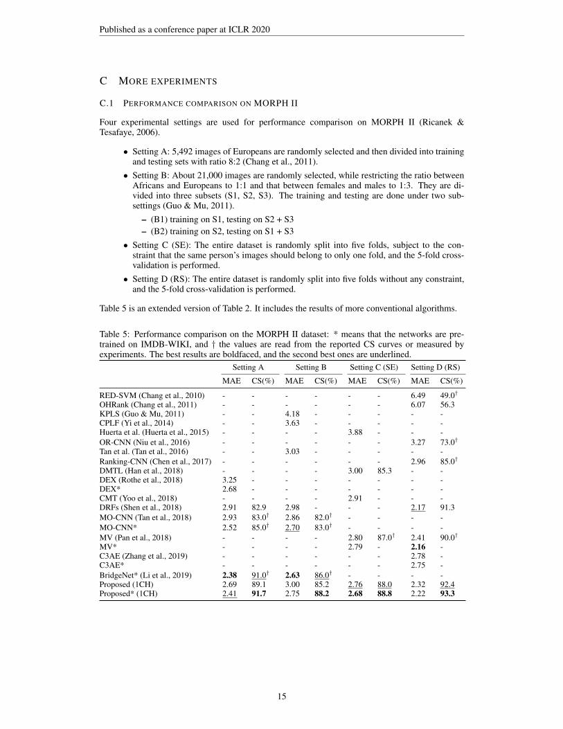
Table 5 is an extended version of Table 2. It includes the results of more conventional algorithms.

Table 5: Performance comparison on the MORPH II dataset: * means that the networks are pre-trained on IMDB-WIKI, and † the values are read from the reported CS curves or measured byexperiments. The best results are boldfaced, and the second best ones are underlined.

Setting A Setting B Setting C (SE) Setting D (RS)

MAE CS(%) MAE CS(%) MAE CS(%) MAE CS(%)

RED-SVM (Chang et al., 2010) - - - - - - 6.49 49.0†

OHRank (Chang et al., 2011) - - - - - - 6.07 56.3KPLS (Guo & Mu, 2011) - - 4.18 - - - - -CPLF (Yi et al., 2014) - - 3.63 - - - - -Huerta et al. (Huerta et al., 2015) - - - - 3.88 - - -OR-CNN (Niu et al., 2016) - - - - - - 3.27 73.0†

Tan et al. (Tan et al., 2016) - - 3.03 - - - - -Ranking-CNN (Chen et al., 2017) - - - - - - 2.96 85.0†

DMTL (Han et al., 2018) - - - - 3.00 85.3 - -DEX (Rothe et al., 2018) 3.25 - - - - - - -DEX* 2.68 - - - - - - -CMT (Yoo et al., 2018) - - - - 2.91 - - -DRFs (Shen et al., 2018) 2.91 82.9 2.98 - - - 2.17 91.3MO-CNN (Tan et al., 2018) 2.93 83.0† 2.86 82.0† - - - -MO-CNN* 2.52 85.0† 2.70 83.0† - - - -MV (Pan et al., 2018) - - - - 2.80 87.0† 2.41 90.0†

MV* - - - - 2.79 - 2.16 -C3AE (Zhang et al., 2019) - - - - - - 2.78 -C3AE* - - - - - - 2.75 -BridgeNet* (Li et al., 2019) 2.38 91.0† 2.63 86.0† - - - -Proposed (1CH) 2.69 89.1 3.00 85.2 2.76 88.0 2.32 92.4Proposed* (1CH) 2.41 91.7 2.75 88.2 2.68 88.8 2.22 93.3

15


C.2 GENERALIZATION PERFORMANCE OF COMPARATOR ON FG-NET

We assess the proposed age estimator (1CH) on the FG-NET database (Panis et al., 2016). FG-NETis a relatively small dataset, composed of 1,002 facial images of 82 subjects. Ages range from 0 to69. For FG-NET, the leave one person out (LOPO) approach is often used for evaluation. In otherwords, to perform tests on each subject, an estimator is trained using the remaining 81 subjects.Then, the results are averaged over all 82 subjects.

In order to assess the generalization performance, we do not retrain the comparator on the FG-NETdata. Instead, we fix the comparator trained on the balanced dataset and just select references fromthe remaining subjects’ faces in each LOPO test. For the comparator, the arithmetic scheme in(1)∼(3) is tested as well as the default geometric scheme in (10)∼(12).

For comparison, MV (Pan et al., 2018) is tested, but it is trained for each LOPO test.

Table 6 summarizes the comparison results. MV provides better average performances on the entireage range [0, 69] than the proposed algorithm does. This is because the balanced dataset does notinclude subjects of ages between 0 and 14. If we reduce the test age range to [15, 69], the proposedalgorithm outperforms MV, even though the comparator is not retrained. These results indicatethat the comparator generalizes well to unseen data, as long as the training images cover a desiredage range. Also, note that the geometric scheme provides better performances than the arithmeticscheme.

Table 6: Performance comparison on FG-NET. The average performances over test ages withinranges [0, 69] and [15, 69] are reported, respectively.

0 to 69 15 to 69

MAE CS(%) MAE CS(%)

MV 3.98 79.5 6.00 63.7Proposed (1CH, Geometric τage = 0.15) 8.04 41.4 4.90 64.3Proposed (1CH, Arithmetic τ = 7) 9.26 33.1 5.32 64.1

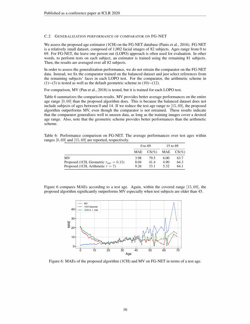
Figure 6 compares MAEs according to a test age. Again, within the covered range [15, 69], theproposed algorithm significantly outperforms MV especially when test subjects are older than 45.

� ��

�

��

��

��

��

��

��

Figure 6: MAEs of the proposed algorithm (1CH) and MV on FG-NET in terms of a test age.

16


C.3 PERFORMANCE ACCORDING TO κ

Table 7: MAE and CS performances of the unsupervised algorithm (2CH) on the balanced dataset,according to the minimum percentage (κ) constraint during the regularized membership update. Theperformances are not very sensitive to κ. The best performances are achieved in the default mode,i.e. at κ = 50%.

κ (%) 10 20 30 40 50

MAE 4.17 4.18 4.17 4.16 4.16CS (%) 73.7 73.6 73.6 73.7 74.0

0%

100%

10s 20s 30s 40s 50s 60s 70s

0%

100%

0%

100%

0%

100%

0%

100%

0%

100%

Age

0%

100%

10s 20s 30s 40s 50s 60s 70s

0%

100%

0%

100%

0%

100%

0%

100%

0%

100%

Age

k = 20%

k = 40%

Af-M

Af-F

As-M

As-F

Eu-M

Eu-F

chain 1 chain 2

0%

100%

10s 20s 30s 40s 50s 60s 70s

0%

100%

0%

100%

0%

100%

0%

100%

0%

100%

k = 30%

Af-M

Af-F

As-M

As-F

Eu-M

Eu-F

Af-M

Af-F

As-M

As-F

Eu-M

Eu-F

Age

Figure 7: Distributions of training images in the unsupervised algorithm (2CH) at κ = 20%, 30%,and 40%. From Figures 5 and 7, we see that stronger age-dependent tendencies are observed, as κgets smaller.

17


C.4 PERFORMANCE ACCORDING TO THRESHOLDS τ AND τage

The ordering relationship between two instances can be categorized via the arithmetic scheme in(1)∼(3) using a threshold τ or the geometric scheme in (10)∼(12) using a threshold τage. Ta-ble 8 lists the performances of the proposed algorithm (1CH) according to these thresholds. We seethat the geometric scheme outperforms the arithmetic scheme in general. The best performance isachieved with τage = 0.1, which is used in all experiments in the main paper. Note that the scoresare poorer than those in Table 3, since the comparator is trained for a smaller number of epochs tofacilitate this test. At τage = 0.1, two teenagers are declared to be not ‘similar to’ each other if theirage difference is larger than about 1. Also, two forties are not ‘similar’ if the age difference is largerthan about 5.

Table 8: The performances of the proposed algorithm (1CH) on the balanced dataset according tothresholds τ and τage.

τ for arithmetic scheme τage for geometric scheme

0 2 5 7 9 0.05 0.10 0.15 0.20 0.25

MAE 4.42 4.36 4.33 4.32 4.33 4.38 4.31 4.32 4.41 4.41CS(%) 71.0 71.7 72.2 72.2 72.5 71.4 72.8 72.2 71.8 71.7

C.5 PERFORMANCE ACCORDING TO NUMBER OF REFERENCES

Table 9: The performances of the proposed algorithm (supervised) on the balanced dataset accordingto the number of references for each age class (M/N ). In general, the performances get better withmore references. However, the performances are not very sensitive to M/N . They saturate whenM/N ≥ 5. Therefore, we set M/N = 5 in this work.

1CH 2CH 3CH 6CH Average

M/N MAE CS(%) MAE CS(%) MAE CS(%) MAE CS(%) MAE CS(%)

1 4.321 72.43 4.180 72.98 4.199 73.20 4.168 73.76 4.217 73.092 4.318 72.43 4.182 73.00 4.200 73.23 4.170 73.64 4.218 73.083 4.313 72.61 4.175 73.04 4.200 73.29 4.170 73.68 4.214 73.164 4.311 72.58 4.178 72.96 4.197 73.24 4.176 73.62 4.215 73.105 4.309 72.61 4.177 73.02 4.197 73.27 4.168 73.72 4.213 73.166 4.308 72.66 4.178 73.01 4.195 73.20 4.170 73.76 4.213 73.167 4.308 72.70 4.179 73.00 4.196 73.24 4.167 73.81 4.213 73.198 4.306 72.69 4.178 72.94 4.196 73.31 4.172 73.71 4.213 73.169 4.305 72.63 4.180 73.04 4.194 73.36 4.172 73.72 4.213 73.19

10 4.305 72.65 4.180 73.07 4.193 73.35 4.173 73.75 4.213 73.21

C.6 REFERENCE IMAGES

Figure 8 shows all references in the supervised 6CH.

18


Mal

eA

fric

an

Ref

eren

ce im

ages

1516

1718

1920

2122

2324

2526

2728

2930

3132

3334

3536

3738

3940

4142

4344

4546

4748

4950

6CH

1516

1718

1920

2122

2324

2526

2728

2930

3132

3334

3536

3738

3940

4142

4344

4546

4748

4950

5152

5354

5556

5758

5960

6162

6364

6566

6768

6970

7172

7374

7576

7778

7980

5152

5354

5556

5758

5960

6162

6364

6566

6768

6970

7172

7374

7576

7778

7980

1516

1718

1920

2122

2324

2526

2728

2930

3132

3334

3536

3738

3940

4142

4344

4546

4748

4950

5152

5354

5556

5758

5960

6162

6364

6566

6768

6970

7172

7374

7576

7778

7980

Fem

ale

Afr

ican

Mal

eA

sian

Fem

ale

Asi

an

Mal

eEu

rope

an

Fem

ale

Euro

pean

Figu

re8:

All

refe

renc

eim

ages

inth

esu

perv

ised

6CH

.For

som

eag

esin

cert

ain

chai

ns,t

heba

lanc

edda

tase

tinc

lude

sle

ssth

an5

face

s.In

such

case

s,th

ere

are

less

than

5re

fere

nces

.

19


C.7 AGE ESTIMATION EXAMPLES

16 Af-F (16 Af-F) 20 Af-M (20 Af-M) 22 Af-M (22 Af-M) 27 Af-F (27 Af-F) 30 Af-M (30 Af-M) 32 Af-F (32 Af-F) 35 Af-M (35 Af-M) 42 Af-M (42 Af-M) 59 Af-M (59 Af-M)

18 As-M (18 As-M) 20 As-F (20 As-F) 23 As-F (23 As-F) 26 As-M (26 As-M) 30 As-F (30 As-F) 35 As-M (35 As-M) 39 As-F (39 As-F) 44 As-M (44 As-M) 60 As-M (60 As-M)

15 Eu-F (15 Eu-F) 17 Eu-M (17 Eu-M) 28 As-F (28 Eu-F) 29 Eu-M (29 Eu-M) 34 Eu-M (34 Eu-M) 36 Eu-F (36 Eu-F) 43 Eu-F (43 Eu-F) 58 Eu-M (58 Eu-M) 65 Eu-F (65 Eu-F)

(a) Success cases

27 Af-F (16 Af-F) 39 Af-F (28 Af-F) 23 Af-M (32 Af-M) 24 Af-F (35 Af-F) 27 Af-M (40 Af-M) 35 Af-M (56 Af-M) 66 Af-F (53 Af-F) 31 Af-F (42 Af-F) 74 Af-M (61 Af-M)

33 As-M (20 As-M) 24 As-F (38 As-F) 27 As-M (38 As-M) 27 As-M (17 As-M) 27 As-F (18 As-F) 29 As-M (20 As-M) 25 As-F (18 As-F) 27 As-F (17 As-F) 66 As-M (80 As-M)

28 Eu-M (15 Eu-M) 25 Eu-F (18 Eu-F) 35 Eu-F (24 Eu-F) 37 Eu-F (25 Eu-F) 42 Eu-M (30 Eu-M) 50 Eu-F (33 Eu-F) 35 Eu-M (74 Eu-M) 38 As-F (60 Eu-F) 67 Eu-M (45 Eu-M)

(b) Failure cases

Figure 9: Age estimation results of the proposed algorithm (supervised 6CH). For each face, the es-timated label is provided together with the ground-truth in parentheses. In (a), the ages are estimatedcorrectly. In the last row, third column, the ethnic group is misclassified. This happens rarely. In(b), failure cases are provided. These are hard examples due to various challenging factors, such aslow quality photographs and occlusion by hairs, hats, hands, and stickers.

20

ORDER LEARNING AND ITS APPLICATION TO AGE ...

Documents

Transcript of ORDER LEARNING AND ITS APPLICATION TO AGE ...