1

Optimum detection of ultrasonic echoes applied to the analysis of the first layer of

a restored dome

Luis Vergara, Ignacio Bosch, J. Gosálbez, A. Salazar Departamento de Comunicaciones, Universidad Politécnica de Valencia, 46022 Valencia, Spain lvergara@dcom.upv.es

Abstract

Optimum detection is applied to ultrasonic signals corrupted with significant levels of

grain noise. The aim is to enhance the echoes produced by the interface between the

first and second layers of a dome to obtain interface traces in echo-pulse B-scan mode.

This is useful information for the restorer before restoration of the dome paintings.

Three optimum detectors are considered: matched filter, signal gating, and prewhitened

signal gating. Assumed models and practical limitations of the three optimum detectors

are considered. The results obtained in the dome analysis show that prewhitened signal

gating outperforms the other two optimum detectors.

Keywords

Ultrasonics, grain noise, detection, dome analysis

2

Optimum detection of ultrasonic echoes applied to the analysis of the first layer of

a restored dome

L. Vergara, I.Bosch, J. Gosálbez, A. Salazar

1. Introduction

In [1] the authors have considered the ultrasonic echo pulse technique to help in the

analysis of a dome. The first four layers of the dome were respectively: mortar (0.3 cm),

plaster (1.2 cm), mortar (1.5 cm) and bricks. The work presented in paper [1] was

devoted to the problem of determining the state of adhesion of the interface between the

third and fourth layers. The depth of such an interface (3 cm) and the type of materials

(mortar-bricks), allowed working with a transducer of 1 MHz, so that grain noise due to

reflections from the micro-grains of the involved materials, is not present at all. No

sophisticated signal processing techniques were required in [1]. Actually, the first two

interfaces were not detected at 1 MHz of operating frequency, and the only echoes were

obtained from the mortar-bricks interface.

The problem considered in this paper is outlining the first interface which is only at a

depth of 0.3 cm. This implies the need for increasing spatial resolution and we require

transducers with higher operating frequencies to reduce the wavelength. The

consequence will be the apparition of significant amounts of grain noise, thus leading to

the need of using the statistical signal processing techniques presented in this paper.

The first layer of the dome is a 0.3 cm stratum of mortar, and the second one consists of

a 1.2 cm stratum of plaster. The objective is to trace the interface between the first and

second layers to provide valuable information to the restorers. Information about the

state of conservation of the first layer is especially important, as this is usually painted

over. Essentially we want to determine if the layer of mortar is present or not in a given

location of the dome under analysis. This is needed by the restorer before to proceed

with the restoration of painting. If the layer of mortar is not present in a given location,

it is necessary to add some mortar and then painting over it. Mortar layer could not be

present because of deterioration due to the pass of time. It is not always easy to visually

determine the presence or absence of the layer of mortar, hence ultrasonic information

may be valuable for the restorer. Note that the technique is not intended to detect

variation in mortar thickness, although, in principle, it could be possible to obtain such

3

information if more than one successive echoes of the mortar-plaster interface could be

traced and the ultrasound speed of propagation in mortar could be assumed or

estimated. The minimal detectable mortar thickness will depend on the pulse time

duration.

We thus carried out a non-destructive ultrasonic analysis using the echo pulse

inspection mode: an ultrasonic pulse is sent into the first layer of the mortar, expecting

reception of the echo from the mortar-plaster interface. We successively locate the

sensor along a vertical linear array of locations. At every location we collect an A-scan

(a record of the signal echoed by the material). Finally, aligning the A-scans one under

the other, we built a B-scan where, hopefully, the interface would be outlined (see

scheme in figure 1, where possible multiple reflections in the interface have been

considered). Gel contact was used to coupling the sensor to the wall.

With the aim of selecting the most appropriate transducer, some experiments were made

with 1 and 2 MHz, but the spatial resolution was too low. We also tested a 10 MHz

transducer, but attenuation was too high to allow reception of the interface echoes.

Finally, a 5 MHz transducer was selected to give an adequate balance between

resolution and the capacity to penetrate into the mortar. It should be noted that mortar is

a material composed of sand and cement paste. Two essential parts of its microstructure

are air pores (sizes may vary from 10-10 to 10-4 m) and sand grains (10-4 to 10-3 m). On

the other hand we have estimated the speed of propagation in this type of mortar by

using transmission mode in a cylindrical section which was built specifically for this

goal. A value smc /5,1562= was obtained so that the wavelength corresponding to 5

MHz, mfc 3

6 10312,0105

5.1562 −⋅=⋅

==λ , is of the order of the sand grains diameter. That

means that significant amounts of grain noise should be expected, probably hiding the

echoes from the first and second layer interface.

The expectation was certainly true, as one can verify by observing figure 3, where we

represent a portion of the original B-scan and two arrows indicating delays where the

the interface should be outlined (the details of the experiment are described in Section

4). Hence, signal processing is necessary in this case to enhance the presence of the

interface echoes (if possible). This problem may be approached in an optimum manner

in different ways. The most obvious is that of maximizing signal-to-noise ratio (SNR) at

the output of the processor, but it is also possible to think about maximization of the

probability of detection of the interface echoes in a grain noise background. This latter

4

approach is the one selected here, although, for an appropriate definition of SNR

maximization, both approaches are equivalent, as we mention in Section 2.

The paper is set out as follows. First, in the next section we define the problem from an

optimum detection perspective. Then in section 3 we derive the different solutions

corresponding to different assumptions about the implicit models. Finally in section 4

we apply the optimum detection algorithms to the problem in hand. Some conclusions

end the paper.

2. Optimum detection approach We wish to detect the presence of a possible ultrasonic echo pulse ( )np in a segment of

the recorded and sampled ultrasonic signal ( )nr . Therefore, we have two possible

hypotheses

( ) ( ) ( )

( ) ( )ngnrHNnnn

ngnpnrH

ss

=−+=

+=

2

1

1,..., , (1)

where 1, −+ Nnn ss are respectively the starting and the final sample numbers

delimiting the segment (i.e., N is the segment length), and ( )ng corresponds to the grain

noise samples under hypothesis i.

Detecting the presence of ( )np implies some processing [ ]⋅f on the segment

( ) [ ] ( ) ( )[ ]Tsss Nnrnrfnz 1..., −+== rr , (2)

and comparison with a threshold

( )( )⎪⎩

⎪⎨⎧

<

>

2

1

decide

decide

Htnzif

Htnzif

s

s . (3)

If we move the value sn along the recorded signal we may obtain a non-binary output

signal in the form

5

( ) ( )⎩⎨⎧

=decided is0decided is

2

1

HifHifnr

nr ssout , (4)

which is the output sequence after processing the input sequence ( )snr .

Optimum design of [ ].f can be made by maximizing the signal to noise ratio

enhancement (SNRE) factor

( )[ ]( )[ ]

( )[ ]( )[ ]2

2

1

22

1

/

/

/

/

HnrE

HnrESNR

HnrE

HnrESNR

SNRSNR

SNREs

sin

sout

soutout

in

out === , (5)

where [ ]⋅E means statistical expectation. It can be easily shown (see for example [2],

page 111) that

5.0PFAPDSNRE = , (6)

where PD and PFA are respectively the probability of detection and the probability of

false alarm corresponding to the detection problem defined in equations (1)-(3). Hence,

maximizing PD for a given PFA (Neyman-Pearson optimum detector) in (1)-(3)

implies maximization of SNRE for all the possible gating post-processors of the type

(4). Thus, optimum design of [ ]⋅f implies solving an optimum detection problem, and

this will be the approach adopted in this paper.

3. Optimum detectors

Let us start from the detection problem defined in equation (1). We will consider in the

following the Neyman-Pearson criterion for the design of the optimum detectors. Note

that maximizing PD for a given PFA is more suitable for ultrasonic pulse detection, as it

is in other related areas like radar or sonar, where the “a priori” probability of 1H is

much smaller than the “a priori” probability of 2H . Let us consider the different models,

their corresponding optimum solutions and the practical limitations.

Model 1. We assume:

6

• perfect knowledge of vector s defined by 1=⋅= sssp Ta ,

( ) ( )[ ]Tss Nnpnp 1... −+=p .

• ( ){ }ng is locally stationary Gaussian inside every interval

[ ]1, −+ Nnn ss having the power spectrum ( )ωgS .

The optimum solution is the well-known matched filter detector ([3] and Appendix A)

( ) ( ) sCrr 1−== gT

s fnz , (7)

where [ ]Tg E ggC = is the grain noise local covariance matrix.

Note that the value a in model 1 is not required. It will depend on the object reflectivity

and on the attenuation of the pulse in the go and return path through the first layer.

Besides, it will be affected by the surface and by the pressure on the transducer in the

manual measurement. In detection theory the test is said to be Uniformly Most Powerful

(UMP) in the unknown parameter a.

On the other hand, the spectrum of the grain noise ( )ωgS (and so the covariance matrix

gC ) can be estimated to some extent if some training material samples, resembling the

actual operating materials under test, were available. It could be estimated also from

sample records measured on the specimen under test, if they are mostly composed by

grain noise.

Finally, the vector s, which represents the form of the pulse to be detected, depends on

the pulse arriving at the possible reflector, which, due to the propagation effects, is a

distorted version of the actual pulse sent into the material. It also depends on the

reflector itself. Some approximation to s could be obtained by “off-line” estimation of

the pulse waveform using a material with good propagation properties for ultrasound at

the corresponding operating frequency. But good knowledge of s cannot be assumed in

general. Let us consider some simple forms to overcome the need for estimating s.

Model 2. Same as model 1 regarding the grain noise model, but we assume, with respect

to the pulse, that:

• ksC =−1g [ ]Tk 0...0=k

7

From (7), the optimum solution is a simple gating of the original signal

( ) ( ) ( )sT

s nrkfnz ⋅=== krr . (8)

The above assumption is a simple form to overcome the need for estimating s (note that

knowledge of k is not required as this factor can be absorbed by the threshold t in

equation (3)). Unfortunately, there are no arguments justifying that the assumption

which makes optimum the gating detector, will be verified in general. Hence, one

should not expect good results using a simple gating detector, except for cases of high

signal to noise ratio (but in these cases all detectors work fine).

Model 3. Same as model 1 regarding the grain noise model, but we assume, with respect

to the pulse, that:

• ksC =− 2

1g [ ]Tk 0...0=k

From (7), the optimum solution is a gating of the signal pre-whitened by matrix

21−

gC

( ) ( ) ( )swTwgg

Ts nrkfnz ⋅====

−− krsCCrr 21

21

, (9)

where rCr 21−

= gw .

The above assumption is again a simple form to overcome the need for estimating s. In

this case some justification may be found about the general verification of the assumed

pulse model. It is clear that matrix 21−

gC implements a linear transformation that

“whitens” the grain noise component in r (equation (1)):

[ ] [ ] ( ) 121

21

21

21

=⇔===−−−− ωgwgggg

Tg

Tww SEE ICCCCggCgg . (10)

But the assumption with respect to the pulse implies that 21−

gC also “whitens” the

spectrum of the pulse (it changes s to a delta vector k). This suggests that this

assumption is equivalent to consider that grain noise has a generative model consisting

in white noise filtered by a linear filter having impulse response s. This is a simple but

reasonable model, if we take into account that grain noise could be considered the result

of the superposition of many echoes coming from the material grains, i.e., the result of

8

convolving the material reflectivity with the ultrasonic pulse sent into it [5]. As far as

this linear generative model of grain noise could be a good approximation of the actual

behaviour of the material, one should expect good results by using the optimum detector

(9).

In the following we will consider the three optimum detectors for the problem in hand.

4. Analysis of the first layer of a restored dome

The research of this work is done under the framework of a collaboration between our

Signal Processing Group and the Institute for Cultural Heritage Conservation of the

Polytechnic University of Valencia. A final goal was to develop a versatile prototype

for ultrasonic non-destructive testing which could be applied to different problems

relative to restoration of domes or walls in historical buildings. Versatility was achieved

by allowing the use of different sensors and by developing different signal processing

modules, both things adapted to every particular problem. That, for example, in

reference [1] we described a different problem which was worked with essentially the

same equipment, but using a different sensor and different (simpler) signal processing

algorithms. Of course some parameters to set up the equipment must be also selected for

every problem (amplifier gain, analog filter, sampling frequency,…). On the other hand

a requirement is that this equipment could be used by people with no special skills in

ultrasonics or in signal processing: the user interface must be simple and the calibration

must be essentially automatic for every problem. Requirements of both versatility an

ease of operation justify not using more advanced systems that could be more adapted

to the particular problem considered in this manuscript. Moreover developing our own

signal processing algorithms allows us a total control of the work.

The study was made on a 1:1 scale model of the actual dome to overcome the problems

of accessibility and the danger of damaging paintings. A photograph of the 1:1 scale

model is shown in figure 4. Model dimensions are: 2.5 m width, 2 m height and 0.5 m

thick. There is a convex curve in the wall, as in the actual dome.

Relevant information on the acquisition follows:

• Ultrasonic pulse generation: PR5000 Matec Instruments with a 2500 watts

maximum power output.

9

• Transducer: 5.0 MHz/.250 KB-A 66492, Krautkramer. Excitation signal 5 MHz

burst tone.

• Amplifier gain 65 dB.

• Analog filter: 2.5 MHz-6 MHz.

• Tektronix TDS3012 digitalization equipment. Sampling frequency 20 MHz.

Amplitude resolution 16 bits. Dynamic range 5.2± V.

• Labtop PC for signal transferring and storage.

Note, that a 5 MHz burst tone excitation signal was used with the aim of tuning most of

the emitted ultrasonic energy in a band centred at 5 MHz. Every ultrasonic pulse sent

into the material is the result of convolving a (approximate) five cycles segment of a 5

MHz sinusoid with the impulse response of the piezoelectric crystal.

We collected 75 A-scan of 100 µs in the locations indicated in the figure 5. The vertical

array of locations (separation between two consecutive locations was 2 cm) crossed

some areas where modifications had been made to the surface (a special type of paper

was attached to the wall after preparation of the paintings). This affected the transducer-

wall coupling in such a way that different signals were recorded in the affected

locations. Note that, except for significant changes of the surface, variability of coupling

(due for example to different hand pressure on the sensor) may produce variability in

the injected ultrasonic energy. But signal to grain noise ratio will be the same, so that, in

principle, all the four detectors will be affected in a similar manner. The only concern is

that ultrasonic energy could reduce in such a manner that reflections from the interface

could not be detectable at all.

Normally, the restorer has the prior knowledge about the layer structure of the dome

because some destructive inspections have been done in appropriate parts of it, because

part of the dome is deteriorated and the inner structure of layers is visible or because

there are documents available describing the dome. Thus the scale model was built after

that prior knowledge of the actual dome. The interest for the restorer is to have

information about the state of the layers in some specific areas of the domes; in this

particular case to know the presence or absence of the mortar layer in every part were

painting is to be restored, as explained before. We know that the first layer of mortar (if

present) is 0.3 cm thick, so we can predict what the results should be if the ultrasonic

technique could be able to trace the interface between the first and second layers after

10

the first, second, third,…or n-th reverberant echoes. We need an estimate of the

expected delay between echoes from the interface (the value T in figure 1). This was

done in a small cylindrical section (0.3 cm height) of the same type of mortar, by

measuring the transmission delay between two identical 5 MHz transducers, each

located on the opposite face of the cylinder. A value of 1.92 µs was obtained (see figure

2), so we considered a raw estimate T=2x1.92=3.84 µs. This meant that a possible first

reflection from the interface should arrive at 3.84 µs, a second one at 2x3.84=7.68 µs, a

third one at 11.52 µs and so on.

Figure 3 showed the original B-scan (75 A-scans) in the delay interval of 4 to 20 µs.

This is because the idle time of the receiver is approximately 4 µs, and that after 20 µs

ultrasonic energy practically disappears. This means that the only expected indications

(if any) from the interface would be due to a second reflection at a delay of 7.68 µs and

/or the third reflection at a delay of 11.52 µs. This is indicated by two arrows in the axis

time of figure 3. It should be noted that no echo trace from the interface is apparent in

the original B-scan, which is composed of multiple echoes, probably coming from

surface irregularities and from the mortar grain noise. Note that in the locations

corresponding to modified surfaces the backscattered ultrasonic energy is much lower

than in the other locations, hence when we represent all the A-scan together, using a

common amplitude scale, it seems that there are no ultrasonic responses at these

locations. It should be mentioned that the received signals were pre-filtered by an

analog band-pass filter adapted to the useful bandwidth (2.5 MHz-6 MHz), previously

to digitalization. However, looking at figure 3 where we represent the digital records, it

can be appreciated that magnitude of grain noise is still comparable to magnitude of the

echoes from the interface. That is the essence of the justification for using statistical

digital signal processing to extract relevant information. It should be noted that grain

noise is due to echoes from small grains of the materials, thus the grain noise power

spectral density overlaps with the interface echoes spectrum. That is why the analog

pre-filtering does not help us too much in this problem.

Before presenting the results of the processing, we will consider some aspects of the

selection of the parameters involved in the algorithms. We need to fit N and gC . The

length of the moving window N depends on the duration of the pulse; hence we have

estimated “off-line” the ultrasonic pulse by using a piece of a material having good

ultrasound propagation properties (methacrylate). We measured a duration of the pulse

11

of 1 µs (i.e., 5 cycles of the nominal frequency of the 5 MHz transducer). This duration

seems to be a correct estimate also for mortar (see the first part of the received signal in

figure 2). In any case, this is not a critical parameter and a raw estimate of the pulse

duration suffices. A different matter is the capability for measuring an appropriate

waveform for implementing matched filtering; this is the problem with model 1, as we

illustrate with the results below.

On the other hand, we tested different alternatives for estimating the grain noise matrix

gC , which produced rather similar results in this application. In the case of the results

shown below, they were obtained by estimating a grain noise matrix for every A-scan

using the classical sample estimate

∑=

=R

i

Tiig R 1

1 rrC)

, (11)

where Rii ...1=r , indicate all the possible intervals to be processed in the

corresponding A-scan.

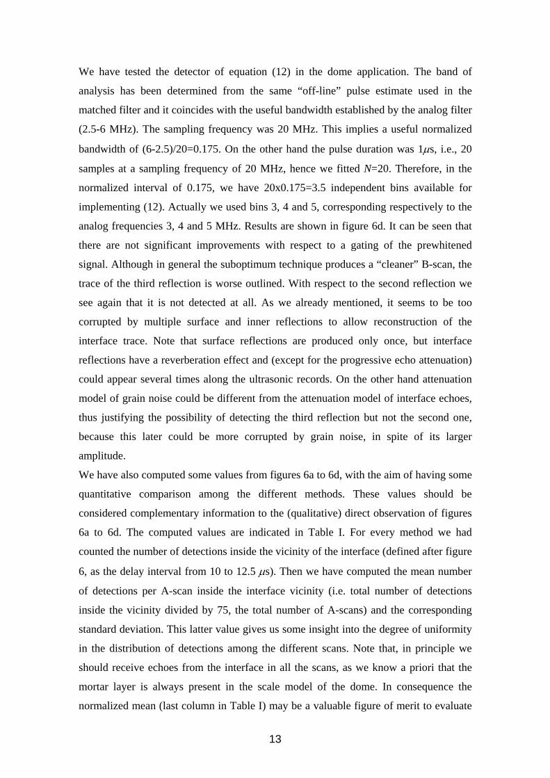
In the figures 6a, 6b and 6c we show the detections (binary B-scan) respectively

obtained with the optimum detectors corresponding to models 1, 2 and 3. The required

vector s needed in the matched filter detector was obtained from the ultrasonic pulse

measured in the methacrylate piece; PFA=0.001 in all cases. Detectors corresponding

to models 1 and 2 (figures 6a and 6b), are not able to obtain the trace of the third

reflection. However the detector of model 3 (figure 6c), which corresponds to a gating

of the prewhitened signals, is able to outline the interface. The second reflection is too

corrupted by multiple surface and inner reflections to allow reconstruction of the

interface trace. A possible fourth reflection seems to be too attenuated to appear. It is

noticeable in figure 6c that some detections are also obtained in those scans

corresponding to modified surfaces, even though it was no apparent backscattered

energy (figure 3).

For completeness, we have also tried some suboptimum techniques. We use the term

suboptimum in the sense that these algorithms do not come from optimum solutions

corresponding to a well defined model as 1, 2 or 3. But they may have general

applicability even when the assumptions of models 1, 2 and 3 are not appropriate. For

example, Gaussianity is not a correct hypothesis for some coarse-grained materials [4],

due to the obtained “spiky” grain noise records, or for materials exhibiting regular

spreading of the grains [6]. It is also reasonable to assume that the presence of the

12

interface may alter the grain noise statistics, so that we should consider a different grain

noise model under every hypothesis.

These techniques [2], [7] decompose the signal into different narrowband frequency

channels, and nonlinearly process the channel outputs in different forms depending on

the particular algorithm selected. Enhancing of the possible presence of the echo is

based in the assumption that grain noise will exhibit large level variation at the different

channel outputs, meanwhile the possible target echo distributes its energy uniformly

among the different channels. In essence, this is a similar assumption to that one made

in model 3, because frequency sensitive of the grain noise appears with the linear

generative model mentioned above: the echoes due to the grains of the material may

add in a constructive (synchronized phase) or destructive manner for every frequency

component, thus affecting the grain noise level at every channel output. The difference

with model 3, is that now Gaussianity and identical noise distribution under both

hypotheses are not assumed. Moreover, there is not any assumption about the pulse

waveform s, except its insensitivity to the center frequency of the channel.

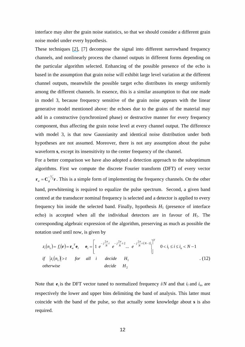
For a better comparison we have also adopted a detection approach to the suboptimum

algorithms. First we compute the discrete Fourier transform (DFT) of every vector

rCr 21−

= gw . This is a simple form of implementing the frequency channels. On the other

hand, prewhitening is required to equalize the pulse spectrum. Second, a given band

centred at the transducer nominal frequency is selected and a detector is applied to every

frequency bin inside the selected band. Finally, hypothesis H1 (presence of interface

echo) is accepted when all the individual detectors are in favour of H1. The

corresponding algebraic expression of the algorithm, preserving as much as possible the

notation used until now, is given by

( ) ( ) ( )

( )2

1

12222

10...1

HdecideotherwiseHdecideiallfortnzif

Niiieeefnz

si

ul

TNi

Nji

Nji

Nj

iiT

wisi

>

−<≤≤<⎥⎥⎦

⎤

⎢⎢⎣

⎡===

−⋅−⋅−−πππ

eerr

. (12)

Note that ie is the DFT vector tuned to normalized frequency i/N and that il and iu, are

respectively the lower and upper bins delimiting the band of analysis. This latter must

coincide with the band of the pulse, so that actually some knowledge about s is also

required.

13

We have tested the detector of equation (12) in the dome application. The band of

analysis has been determined from the same “off-line” pulse estimate used in the

matched filter and it coincides with the useful bandwidth established by the analog filter

(2.5-6 MHz). The sampling frequency was 20 MHz. This implies a useful normalized

bandwidth of (6-2.5)/20=0.175. On the other hand the pulse duration was 1µs, i.e., 20

samples at a sampling frequency of 20 MHz, hence we fitted N=20. Therefore, in the

normalized interval of 0.175, we have 20x0.175=3.5 independent bins available for

implementing (12). Actually we used bins 3, 4 and 5, corresponding respectively to the

analog frequencies 3, 4 and 5 MHz. Results are shown in figure 6d. It can be seen that

there are not significant improvements with respect to a gating of the prewhitened

signal. Although in general the suboptimum technique produces a “cleaner” B-scan, the

trace of the third reflection is worse outlined. With respect to the second reflection we

see again that it is not detected at all. As we already mentioned, it seems to be too

corrupted by multiple surface and inner reflections to allow reconstruction of the

interface trace. Note that surface reflections are produced only once, but interface

reflections have a reverberation effect and (except for the progressive echo attenuation)

could appear several times along the ultrasonic records. On the other hand attenuation

model of grain noise could be different from the attenuation model of interface echoes,

thus justifying the possibility of detecting the third reflection but not the second one,

because this later could be more corrupted by grain noise, in spite of its larger

amplitude.

We have also computed some values from figures 6a to 6d, with the aim of having some

quantitative comparison among the different methods. These values should be

considered complementary information to the (qualitative) direct observation of figures

6a to 6d. The computed values are indicated in Table I. For every method we had

counted the number of detections inside the vicinity of the interface (defined after figure

6, as the delay interval from 10 to 12.5 µs). Then we have computed the mean number

of detections per A-scan inside the interface vicinity (i.e. total number of detections

inside the vicinity divided by 75, the total number of A-scans) and the corresponding

standard deviation. This latter value gives us some insight into the degree of uniformity

in the distribution of detections among the different scans. Note that, in principle we

should receive echoes from the interface in all the scans, as we know a priori that the

mortar layer is always present in the scale model of the dome. In consequence the

normalized mean (last column in Table I) may be a valuable figure of merit to evaluate

14

the quality of the corresponding method in conjunction with the qualitative information.

Model 3 gives the largest normalized mean. The suboptimum technique gives

significantly more detections per scan than the optimum techniques, but variance is very

large (see in figure 6d, that there are a lot of detections in some scans, but only a little or

even zero in many other).

To gain further insights into the capability of the methods to deal with the grain noise

problem, we have represented in figure 7 the processed A-scans. This has been done

after equation (4), that is, every time a detection is produced, we keep the (magnitude)

of the sample value, otherwise a zero is given. We have selected in figure 7 the scans 46

to 56, which includes the modified surface section where, apparently, there was not

ultrasonic energy. Note that only model 3 and suboptimum techniques exhibit a

significant signal level at the delays corresponding to the third echo, including some of

the A-scans corresponding to the modified surface.

We conclude that in this application, the hypothesis assumed in model 3 seems to be

appropriate for a reasonable extraction of the interface trace.

5. Conclusions

We have presented in this paper the application of optimum detectors to the problem of

outlining the interface between the first and second layer of a dome. From a signal

processing perspective the problem is automatic detection of pulses embedded in a grain

noise background. We have considered three models and their corresponding solutions:

matched filter, gating of the original signal and gating of the prewhitened original

signal. The use of a matched filter requires knowledge of the waveform of the signal

which is to be detected. Gating of the original signal is optimum only if the pulse

verifies a condition which cannot be justified by physical arguments of grain noise

generation. However gating of the prewhitened original signal is optimum if the grain

noise admits a linear generative model consisting in the convolution of the material

reflectivity and the pulse waveform. A suboptimum technique exploiting frequency

sensitivity of grain noise has also been tested, with no significant improvements with

respect to the prewhitening of the original signal. Therefore, model 3 seems to be

appropriate in the considered application.

15

Although focused to dome analysis, the general procedure followed in this work may be

applied in other non destructive analysis involving materials which produce high levels

of grain noise.

Acknowledgements

This work has been supported by Spanish Administration, under grant TEC2005-01820,

and by European Community, FEDER programme.

Appendix A

Let us express the hypotheses of equation (1) in vector form (to ease the notation

dependence on ns of the different vectors is not expressed)

( ) ( )[ ]( ) ( )[ ]Tss

Tss

NngngH

NnpnpH

1...

1...

2

1

−+==

−+=+=

ggr

pgpr . (A.1)

The optimum detector is obtained by comparing the log-likelihood ratio with a

threshold λ [3]. The log-likelihood ratio is the quotient of the probability density

functions of the observation vector r conditioned to hypotheses H1 and H2, respectively,

i.e.

( )( ) λ>

<

1

22

1

//log

H

HHPHP

rr . (A.2)

Given the conditions of Model 1, we have that both ( )1/ HP r and ( )2/ HP r will be

multivariate Gaussian having vector mean 0 and as, respectively

( )( )

( ) ( )

( )( ) ⎭

⎬⎫

⎩⎨⎧−=

⎭⎬⎫

⎩⎨⎧ −−−=

−

−

rCrC

r

srCsrC

r

12

11

21exp

2

1/

21exp

2

1/

gT

gN

gT

gN

HP

aaHP

π

π . (A.3)

16

Substituting in (A.2) we arrive to

'111211

2

1

2

λλλ =+⇔− −><

−><

−− sCssCrsCssCr gT

H

Hg

TH

Hg

Tg

T aa

aa . (A.4)

Under H2, the statistic ( ) sCr 1−= gT

snz is a zero mean Gaussian random variable having

unit variance, so that λ’ can be easily computed to obtain a given PFA . Optimality

guarantees that PD will be maximum.

References

[1] J. Gosálbez, A. Salazar, I. Bosch, R. Miralles, L. Vergara: “Application of

ultrasonic nondestructive testing to the diagnosis of consolidation of a restored dome”,

Materials Evaluation, vol. 64, no5, pp 492-497, May 2006.

[2] M. G. Gustafsson: “Nonlinear clutter suppression using split spectrum processing

and optimal detection”, IEEE Trans. on Ultrasonics, Ferroelectrics and Frequency

Control, Vol. 43, pp. 109-124, No. 1, January 1996.

[3] L.L.Scharf: Statistical Signal Processing, Addison Wesley, New York, 1991.

[4] L. Vergara, J.M. Páez: “Backscattering grain noise modelling in ultrasonic non-

destructive testing”, Waves in Random Media , vol. 1, no 1, pp 81-92, Jan. 1991.

[5] L. Vergara, J. Gosálbez, J.V. Fuente, R. Miralles, I. Bosch: “Measurement of

cement porosity by centroid frequency profiles of ultrasonic grain noise”. Signal

Processing, vol 84, no.12, pp. 2315-2324, Dec. 2004.

[6] V.M. Narayanan, P.M. Shankar, L. Vergara, J.M. Reid: “Studies on ultrasonic

scattering from quasi-periodic structures”, IEEE Trans. on Ultrasonics, Ferroelectrics

and Frequency Control, Vol. 44, No. 1, January 1997.

17

[7] L. Ericsson, T. Stepinsky: “Algorithms for suppressing ultrasonic backscattering

from material structure”, Ultrasonics, vol. 40, pp. 733-734, May 2002.

Mean of number of detections per scan inside the interface

vicinity

Standard deviation of number of

detections per scan inside the interface

vicinity

Mean Std

Matched filter (Model 1)

0.84 1.15 0.730

Gating of the original signal (Model 2)

0.97 1.16 0.836

Gating of the prewhitened signal (Model 3)

1.52 1.29 1.178

Suboptimum technique

11.15 12.98 0.859

Table I. Quantitative comparison of the results obtained with the different methods (interface vicinity is defined after figure 6 as the delay interval from 10 to 12.5 µs)

18

Figure 1. Schematic representation of the first layer interface

Figure 2. A-scan corresponding to the estimation of the delay in 0.3 cm mortar thickness

0 1 2 3 4 5 6 7-5

-4

-3

-2

-1

0

1

2

3

4

5

Time (us)

Am

plitu

de (V

)

5MHz Through/transmission signal over a testing probe - Mortar Layer (0.3cm).

Stablished arrival point

Flight time:1.92us

mortar plaster

T

19

Figure 3. A portion of the original B-scan; the arrows indicate the delays where the trace of the mortar layer interface should be outlined

Figure 4. Picture of the 1:1 dome scale model.

t(µs)

20

Figure 5. Photographic composition indicating the vertical array where the A-scans were collected, and the locations where some modifications were observed in the

surface.

Modified surfaces

Modified surface

21

(a) (b)

(c) (d)

Figure 6. Detection results: a) Matched filter (model 1) b) Gating of the original signal (model 2) c) Gating of the prewhitened signal (model 3) d) Suboptimum technique

22

4 6 8 10 12 14 16 18 2046

47

48

49

50

51

52

53

54

55

56

t(us) 4 6 8 10 12 14 16 18 20

46

47

48

49

50

51

52

53

54

55

56

t(us) (a) (b)

6 8 10 12 14 16 1846

47

48

49

50

51

52

53

54

55

56

t(us) 6 8 10 12 14 16 18

46

47

48

49

50

51

52

53

54

55

56p

t(us) (c) (d)

Figure 7. Processed A-scans (46 to 56): a) Original A-scans b) Matched filter (model 1) c) Gating of the prewhitened signal (model 3) d) Suboptimum technique