Entry and Exit Echoes∗

Boyan Jovanovic and Chung-Yi Tse†

July 29, 2009

Abstract

While aggregate data do not show the investment echoes predicted byvintage-capital models, echoes arise in rates of entry and exit of firms at theindustry level. Moreover, industries where prices decline rapidly experienceearly ‘shakeouts’. The relation emerges naturally in a vintage-capital modelin which exit of firms sometimes accompanies the replacement of their capital,and in which a shakeout is the first replacement ‘echo’ of the capital createdwhen the industry is born.

1 IntroductionIn a class of models of embodied technological change, capital is periodically replaced.1

In the same class of models, any burst of investment activity creates an “echo” whenthe investment becomes obsolete.2 Faster technological progress then implies fasterreplacement of capital and, hence, more frequent investment echoes.

We argue that this by now standard vintage capital model has strong predictionsfor industry lifecycle dynamics – the existence of ‘shakeouts’ and ‘echoes.’ In par-ticular, our model links these features to the rate of technological progress. We findthat the data do support the ‘vintage capital’ view.

Two key assumptions deliver the simple link between technological progress andentry and exit echoes. First, we assume that the need to replace capital is associated∗We thank G. Violante (editor), an associate editor of the journal, an anonymous referee, A.

Gavazza, M. Gort, X. Gabaix, S. Greenstein, C. Helfat, O. Licandro, S. Klepper, S. Kortum andM. Kredler for comments, R. Agarwal for providing data, and the NSF and Kauffman Foundationfor support. In earlier versions, the title of this paper was “Creative Destruction at the IndustryLevel.”

†NYU and Hong Kong University, respectively.1Early examples are Johansen (1959), Arrow (1962) who model steady states.2Boucekkine, Germain and Licandro (1997) and Mitra, Ray and Roy (1991) study dynamics in

this class of models.

1

0

10

20

30

40

50

60

70

0 0.1 0.2 0.3 0.4 0.5 0.6

Average annual rate of decline of the product price

Fluorescent lamps

PenicillinElectric Shavers

DDT

StyreneTV

Records

Zippers

Age of the industry at the shakeout date (years)

Figure 1: Technological progress and industry age at shakeout

with exit of firms faced with that need. We shall provide evidence from the airline in-dustry that suggests this link is empirically important. Second, we assume that whenan industry comes into being, a burst of investment is required. When that capitalcomes up for replacement, the investment echo then generates exit. We interpret thisexit as the shakeout.

When an industry is competitive, technological progress leads to a reduction inthe price of the output. Competitive producers, in other words, pass on the benefitsof technological change to consumers. This means that we can proxy industry-specifictechnological change by the reduction in the product price. At first pass, the argumentlooks plausible: Figure 1 which shows that industries where prices decline rapidlyexperience early ‘shakeouts’ — simultaneous exits of a fraction of incumbent firms —just as the amended vintage-capital model implies.3 This pattern will stand up whenmore data are added. Moreover, repeated echoes in entry and exit occur in severalindustries, and the interval of time between the first and second echoes is also shorterin industries where prices decline more rapidly: The faster the technological progress,the more frequent the echoes.

3The Figure uses data from Gort and Klepper (1982, henceforth GK). GK measure an industry’sage from the date that the product was commercially introduced, i.e., from the date of its first sales.The shakeout period is defined as the epoch during which the number of firms is declining. GK saythat an ‘exit’ occurs when a firm stops making the product in question, even if that firm continuesto make other products. GK time the start of the shakeout when net entry becomes negative foran appreciable length of time. The shakeout era typically begins when the number of producersreaches a peak and ends when the number of producers again stabilizes at a lower level.

2

Ours is primarily a model of investment echoes. To make it a theory of exitechoes then requires explaining why capital replacement may sometimes cause exit.Our explanation is that as firms age, they sometimes lose the ability to implementnew technology (which in turn is embodied in new capital). The assertion is roughlythat ‘old dogs can’t learn new tricks’. We do not explain why they cannot, we insteadparameterize this tendency in the form of a hazard rate of losing implementation skillexogenously and randomly.4 A loss of implementation skill does not induce an exitright away. Rather, it induces an exit when all the capital that a firm owns reachesreplacement age.

We also provide direct new evidence that firms with old capital are more likelyto exit: In the air-transportation industry, exiting firms have capital that is on av-erage eight years older than the capital of the surviving firms; in Section 5 we shalldisplay this highly significant relation both for the U.S. and for the world as a whole.A related pattern emerges at the two-digit-industry level: Sectors that face morerapidly declining equipment-input prices experience higher rates of entry and exit(Samaniego, forthcoming). In other words, a sector that enjoys a high rate of embod-ied technological change will have a high rate of entry and exit, or what one wouldnormally understand to be a higher level of creative destruction.

All technological change in our model is embodied in capital, which means thatTFP should be constant when one adjusts inputs for quality. During the shakeout, afraction of the capital stock is replaced by new capital; the number of efficiency unitsof capital stays the same but the productivity of capital per physical unit rises.

The model is of a standard vintage-capital type; Mitchell (2002) and Aizcorbe andKortum (2005) use it to analyze industry equilibrium in steady state, i.e., the station-ary case in which the effect of initial conditions has worn off, and after any possibleinvestment spikes that may be caused by initial conditions have vanished. Jovanovicand Lach (1989) use it to analyze transitional dynamics but they generate neither ashakeout nor repeated investment echoes. We shall derive damped investment echoesthat relate to the constant investment echoes derived by Boucekkine, Germain andLicandro (1997, henceforth BGL) in a similar GE model and by Mitra, Ray and Roy(1991) in a model where there is no progress but in which capital is replaced becauseit wears out. A number of other papers relate Figure 1, among them, Caballero andHammour (1994), Klepper (1996), and Utterback and Suarez (1993). Some relatealso to the repeated echoes that we shall document below. We shall discuss this workin Section 6.

Plan of the paper.–Section 2 presents the model. Section 3 and 4 describe tests ofthe two main propositions. Section 5 links capital replacement to firm exit empirically.Section 6 discusses other models in some detail and section 7 concludes the paper.The Appendix contains some proofs.

4Deeper reasons for why firms find it hard to adopt new technology are modeled by Klepper andThompson (2009) and Chatterjee and Rossi-Hansberg (2008).

3

2 ModelConsider a small industry that takes as given the rate of interest, r, and the priceof its capital. The product is homogeneous, and technology improves exogenously atthe rate g. To use a technology of vintage t, however, a firm must buy capital ofthat vintage. The productivity of vintage-0 capital is normalized to 1, and so theproductivity of vintage-t capital is egt.

Each firm is of measure zero and takes prices as given. Let p be industry price,q industry output, and D (p, t) the demand curve at date t, assumed continuous inboth arguments. Production of the good becomes feasible at t = 0.

The price of capital is unity for all t. Capital must be maintained at a cost ofc per unit of time; c does not depend on the vintage of the capital, nor on time.Capital cannot be resold to firms outside the industry; it has a salvage value of zero.We assume that willingness to pay at small levels of q is high enough to guaranteethat investment will be positive immediately.5

Implementation costs.–Let τ denote the age of a firm and let ε (τ) be that firm’scost of installing a unit of frontier capital. Since the cost of all capital is unity, the totalcost of buying and installing capital of a τ -year old firm then is 1 + ε (τ). In section5, we will discuss evidence on how relative to their contribution to industry output,new firms implement new technologies more than incumbents do. This would happenif incumbents face some additional costs of adopting new technology. To model thistendency, we assume that ε (τ) is a Poisson process, independent over firms, withinitial condition ε (0) = 0, Poisson parameter λ, and jump size κ > 0. This meansthat among firms aged τ , a fraction e−λτ will be on a par with entrants in their abilityto adopt technology, and a fraction 1− e−λτ will face costs of at least 1 + κ.

Industry output.–Capital is the only input. Let Kt (s) be the date-t stock ofactive capital of vintage s or older, not adjusted for quality. Industry output at timet is the sum of the outputs of all the active capital

q (t) =

Z t

0

egsdKt (s) . (1)

Capital ceases to be active when it is scrapped.

Evolution of the capital stock.–Because capital is supplied to the industry ata constant price, the investment rate will exhibit damped echoes. Any mass pointthat occurs will repeat itself, though in a damped form. That is, if a mass-pointof investment ever forms, will recur at a periodicity of T , and the size of the masspoint will diminish over time. Moreover, there must be an initial mass point att = 0 because no capital is in place when the industry comes into being. After thatinitial mass point, capital evolves smoothly until date T when the original capital

5Sufficient for this is thatR∞0 e−rtD−1 (0, t) dt > 1, where D−1 (q, t) denotes the inverse demand

curve.

4

t T

1

2

0

3

2T 3T

i(t)i(t)

Figure 2: The number of spikes, i (t).

is completely replaced by vintage-T capital. This is the second industry investmentspike. The third investment spike then occurs at date 2T , when all the vintage-Tcapital is replaced, and so on. Since the inter-spike waiting times are T , and sincethe first spike occurs at t = 0, the date of the i’th investment spike is (i− 1)T , fori = 1, 2, .... Let i (t) be the integer index of the most recent spike.6 We plot i (t) inFigure 2.We shall show that equilibrium is indeed of the form described in the previous

paragraph: All the capital created at one spike date is replaced at the followingspike date, T periods later. Therefore the capital stock at date t comprises capitalcreated at the most recent spike date i (t), plus the flow of investment, x (t) , over thepreceding T periods.Let Xi denote the size of the i’th investment spike. At date t, then, the amount of

capital accounted for by the last spike is Xi(t), and the date-t cumulative distributionof capital by vintage is

Kt (s) = Xi(t) +

Z s

max(0,t−T )x (u) du. (2)

We portray Kt (s) in Figure 3. It has exactly one discontinuity at (i (t)− 1)T .

2.1 Equilibrium

The definition of equilibrium is simple if x (t) > 0 for all t. BGL call this the ‘noholes’ assumption because when it holds, the vintage distribution of capital in usehas no gaps in it. To ensure a positive investment flow at all dates, i.e., x (t) > 0 allt, it is necessary and sufficient that output is increasing at all t > 0 :

d

dtD (p, t) =

∂D

∂p

dp

dt+

∂D

∂t> 0. (3)

6Formally, i (t) = max {i ∈ integers | i ≥ 1 and (i− 1)T ≤ t}.

5

Kt(s)

s

Xi(t)

t(i(t)-1)T t-T

.

Figure 3: The date-t distribution of capital by vintage, s.

Thus it is possible for the time-derivative of D to be negative, but not too negative tooffset the positive effect on output of the fall in price. Now, condition (3) is of limitedvalue because it involves the endogenous variable p. One can, however, reduce (3) toa condition on primitives in some special cases. Take the case where population growsat the rate γt and where each consumer’s demand is iso-elastic, i.e., the case where

D (p, t) = Ap−λ exp³R t

0γsds

´. In an equilibrium in which price falls at a constant

rate g, dp/dt = −gp. Then (3) is equivalent togλ > −γt

for all t ≥ 0. Thus (3) can hold even if population is declining, as long as its rateof decline, γt, never exceeds gλ, or that demand be sufficiently elastic to offset anyexogenous demand declines.DEFINITION: A constant-T equilibrium consists of a product-price function p (t) ,

a retirement-age of capital, T, investment flows x (t) > 0, and investment spikes Xiaccruing at dates (i− 1)T, (i = 1, 2, ...) that satisfy, for each t ≥ 0, the followingthree conditions:

1. Optimal retirement of capital : The revenue of a vintage-t machine at datet0 ∈ [t, t+ T ] is egtp (t0). Since price declines monotonically, it is optimal toreplace vintage-t capital as soon as its revenue equals its maintenance cost:

egtp (t+ T ) = c. (4)

2. Optimal investment : Only entrants and incumbents for whom ε (τ ) = 0 willinvest, because for them the total cost of a new machine is unity. If investment

6

x (t) > 0, the present value of a new capital good must equal its cost. Thepresent value of the net revenues derived from that (vintage-t) unit of capitalmust satisfy

1 =

Z t+T

t

e−r(s−t)¡egtp (s)− c¢ ds. (5)

If the RHS of (5) were ever less than unity, x (t) would be zero.7

3. Market clearing:

D (p (t) , t) = eg(i(t)−1)TXi(t) +Z t

max(0,t−T )egsx (s) ds. (6)

Since the industry does not exist before date zero, x (t) = 0 for t < 0, so thatD (p (0) , 0) = X1.

Proposition 1 If demand satisfies (3), a constant-T equilibrium exists, with

p (t) = p0e−gt, (7)

wherep0 = ce

gT . (8)

and where T uniquely solvesµr + c

c

¶(r + g) = ge−rT + regT . (9)

Proof. (i) First we show that (7), (8), and (9) imply (4) and (5): Eq. (7) and(8) imply (4) for all t ≥ 0, i.e., exit occurs at all t ≥ T . When substituted into (5),(7) and (8) also imply 1 = c

R t+Tt

e−r(s−t)¡eg(t−s)egT − 1¢ ds, which is equivalent to

1 + c1− e−rT

r= cegT

1− e−(r+g)Tr + g

. (10)

Multiplying by r (r + g) /c we have r (r + g)+c (r + g)¡1− e−rT¢ = cr ¡egT − e−rT¢ ,

and cancelling cre−rT and combining terms we reach (9). Therefore if T solves (9),(5) holds.(ii) Exactly one solution T to (9): The LHS of (9) is constant and exceeds r + g.

On the other hand, the RHS of (9) is continuous and strictly increases from r + gto infinity, having the derivative rg

¡egT − e−rT¢ > 0 for T > 0. Therefore the two

curves have exactly one strictly positive intersection.(iii) If (3) is satisfied with dp/dt = −gp, there exists a sequence of x (t) > 0 that

satisfies (6).7Proposition 4 of BGL covers that case which arises when there is too high an initial stock of

capital. This cannot be true at t = 0 in our model, and we shall state conditions in (3) that excludeit as an equilibrium possibility at any date.

7

2.2 The nature and frequency of the spikes

Relation to Figure 1.–The negative pattern arises across steady states indexed byg; a situation in which each industry experiences its specific rate of technologicalprogress g. Implicitly differentiating (9) in the Appendix, we reach the result:

Proposition 2 The replacement cycle is shorter if technological progress is faster:

∂T

∂g= −

r+cc+ (gT − 1) egT

g2 (egT − e−rT ) < 0. (11)

Thus, industries with higher productivity growth should have an earlier shakeout andmore frequent subsequent spikes.8

The second relation concerns the rate at which investment echoes or investmentspikes die off:

Proposition 3 Investment spikes decay geometrically. That is,

Xn = e−gT (n−1)X1 (12)

for n = 1, 2, ....

Proof. Because p (t) is continuous at T , the number of efficiency units replacedat the spikes is a constant, X1, which means that Xn = e−gTXn−1, and (12) follows.

The spike dates remain T periods apart, at 0, T, 2T, 3T, .... The spikes occurregularly because technological progress occurs at the steady rate g. The assumptionthat g is constant is essential for both the constancy of T and for the geometricnature of the decay in the mass of investment. Asymptotically, however, the spikesvanish and the equilibrium becomes like the one that Mitchell (2002) and Aizcorbeand Kortum (2005) analyze.

Firm exit at the investment spike.–At a replacement spike at date t, say, allfirms that need to replace their capital bought that capital at date t− T . All firms,whatever their age was at date t−T had ε = 0 at that time Among those, a fraction1 − e−λT will have experienced a jump in ε and will not find it profitable to invest.These firms will then exit.

The remaining parameters of the model are the maintenance cost c and the rateof interest r. The following claim is proved in the Appendix:

8We interpret g as an invariant property of an industry. But it can be interpreted as applying onlyto a given epoch in the lifetime of a given industry, and subject to occasional shifts. In Aizcorbe andKortum (2005), e.g., one can think of such shifts as tracing out the relation between technologicalchange and the lifetime of computer chips.

8

Proposition 4

(i)∂T

∂c< 0. And, if gc < r2, (ii)

∂T

∂r> 0, (iii)

∂ (gT )

∂g> 0.

A rise in the maintenance cost, c, reduces the lifetime of capital as one would expect.Since replacing capital constitutes an investment, when the rate of interest rises thatform of investment is discouraged, and it will occur less frequently.The role of the demand curve.–As long as the demand curve is sufficiently elastic

and as long as exogenous forces do not lead demand to fall too much (as specified in(3)), only X1 — industry capacity created at the outset, and the rate of investmentto follow x (t) depend on the demand for the product. Neither the time-path ofprices, nor the frequency of the spikes depends on it. These results also rest on theassumption that capital is supplied perfectly elastically at a unit price, an assumptionthat seems reasonable if the industry at hand is a small fraction of the economy orif, as in a one-sector growth model, capital is produced linearly, at constant returnsto scale.

3 T vs. g: Testing Proposition 2We shall begin by proxying the age, T , of an industry at its first replacement spike,by the industry’s age at which the shakeout of its firms begins. This measure willunderlie the first test of the model. And as suggested by (7), we shall proxy the rateof technological progress, g, by the rate at which the price of the product declines.Since replacement episodes are in the model caused by technological progress, wefirst check if industries with higher productivity growth experience earlier shakeouts.That is, we ask whether industries with a high g have a low T as Proposition 2 claimsand, if so, how well the solution for T to (9) fits the cross-industry data on g and T .We now describe the procedure by which we choose the model’s parameters. By

Proposition 1, a unique solution to (9) for T exists; denote it by T (r, c, g). In Table 1,T (1) is the date that GK find that Stage 4 (the shakeout stage) begins in their variousindustries. In a couple of cases the shakeout had not yet begun, and they are censored.The annual rate at which the price declines, averaged over the period

h0, T (1)

iis g(1)i .

We do not have observations on r and c; we find r = .07 a reasonable guess, butwish to check robustness with respect to this assumption and therefore choose threealternative values for r, namely .02, .07 and .12 and in each case estimate c. Theestimation assumes that the distribution of c over industries is log-normal: For allfirms in industry i, ln ci is a draw from N (ln c, σ2). We then estimate c and σ to fitthe model to the data; the details are in the Appendix.The data and the three implicit functions T (g, r, c) fitted to them are shown in

Figure 4.9 The estimates of c are reported in the figure. Since r makes little difference9Table 7 of GK reports the number of years until shakeout for 39 industries. But only for 8 of

9

to the predicted relation we shall proceed with the value r = .07 for the remainder ofthe analysis.

Product name g(1) T (1) g(2) T (2)

Auto tires 0.03 21Ball-point pens 0.07 >28 0.07 >18CRT 0.04 24Computers 0.07 19DDT 0.20 12 0.13 16Electric shavers 0.05 8 0.01 5.5Fluorescent lamps 0.21 2 0.21 2.5Nylon 0.03 >34 0.03 >21Home & farm freezers 0.02 18Penicillin 0.57 7 0.57 8.5Phonograph records 0.03 36 0.02 8.5Streptomycin 0.31 22Styrene 0.06 31 0.07 12Television 0.05 33 0.08 8Transistors 0.17 15Zippers 0.04 63 0.05 38

Table 1 : The data in Figures 4 and 5.10

Our estimate of c is in the range of typical maintenance spending. McGrattanand Schmitz (1999) report that in Canada, total maintenance and repair expenditureshave averaged 5.7 percent of GDP over the period from 1981 to 1993, and 6.1 percent ifone goes back to 1961. These estimates are relative to output, however, whereas oursare relative to the purchase price of the machine which is normalized to unity. Relativeto output, maintenance costs are one hundred percent at the point when the machineis retired (this is equation [4]). Maintenance costs are constant over the machine’slifetime, whereas the value of the machine’s output relative to the numeraire good isegT when the machine is new. For instance if g = 0.1 and c = 0.05, our model givesa value of T = 16; then egT = 4.9, so that as a percentage of output, maintenancespending ranges between 20 and 100 percent. Therefore, c must stand partly forwages to workers as a fixed-proportion input as in the original vintage-capital modelslike Arrow (1962) and Johansen (1959) that had a fixed labor requirement.

them does Table 5 report data on the rate of price decline up to the shakeout. These are the eightreported in Figures 1 and 4.10The variable definitions are: T (1) = age at the start of shakeout, g(1) = average annual price

decline onh0, T (1)

i, T (2) = the number of years elapsed between the start of stage 2 and the midpoint

of the shakeout stage, and g(2) = annual price decline over stages 2 and 3.

10

0

10

20

30

40

50

60

70

0 0.1 0.2 0.3 0.4 0.5 0.6

Annual price decline, g

T

FLL

PENESH

DDT

STE

TVPHR

ZP

Figure 4: The relation between T and g for the eight uncensored GKobservations

3.0.1 Testing Proposition 2 using an alternative definition of T

We now entertain a different definition of T ; one that may provide a better test ofthe model, and one that will provide us with more observations. The main reason fordoing this is that GK’s ‘Stage 1,’ defined as the period during which the number ofproducers is still small (usually two or three), may not contain what we would callan investment spike. During stage 1, only a few firms enter, a number that is in someindustries — autos and tires, e.g., — much smaller than the number of firms that exitduring the shakeout.

The model predicts a date-zero investment spike X1 = D (p0, 0), without whichthere would be no exit spike at date T . Not all the GK industries will fit this,however. Indeed, GK state that rarely is a product’s initial commercial introductionimmediately followed by rapid entry. Autos, e.g., had very low sales early on, and ittook years for sales to develop.11 Therefore the spike is better defined at or aroundthe time when the entry of firms was at its highest. Moreover, in GK, for manyindustries, the shakeouts were not completed until a few years after they first began.It may thus be more appropriate to designate the shakeout date as the midpoint ofthe shakeout episode instead of as the start date of the shakeout episode.

In light of this, let T (2) be the time elapsed between the industry’s ‘Takeoff’ date(which is when Stage 2 begins) and the midpoint of the the industry’s shakeoutepisode (the midpoint of Stage 4). This revised definition for bT calls for adjusting11Klepper and Simons (2005), however, do find an initial spike for TVs and Penicillin — both start

out strong after WW2. There may be a problem with the TV birthday being set at 1929 as GKhave it. During WW2 the Government had banned the sale of TVs.

11

0

10

20

30

40

50

60

0 0.1 0.2 0.3 0.4 0.5 0.6

Annual price decline, g

T

ESH

PHR

ZP

STE

TV

DDT

FLL

PEN

Transistor

Cathode Ray

Computer

Ball Point

Auto Tire

Freezer

Streptomycin

Nylon

Figure 5: T and g using the alternative definition of T

bg to be the rate of the average annual price decline between the takeoff date (whichcomes after the industry has completed stage 1), and the first shakeout date. We callthis variable g(2). This allows us to enlarge the sample. The additions are as follows:

1. For six of the GK industries, complete information for price-declines in Stages2 and 3 (but not Stage 1) is available. They can now be added to the analysis.

2. The two censored observations listed in Table 2 will also be added.12

3. We replace the GK information for the TV by that reported in Wang (2006),who compiled the data from the Television Factbook. This change may betterreflect the history of the TV industry as GK dated the birth of the industryas early as 1929, while according to Wang, the commercial introduction of TVstarts only in 1947.

Figure 5 plots eT for the various industries.13 The estimate of c = 0.078 is a bithigher than with the estimate in the previous sample (c = 0.05). This is because T issmaller under the new definition, and a higher replacement cost is needed to generatethe earlier replacement.12The likelihood function is amended accordingly. See Appendix for details.13For the two truncated observations, Ball—point pens and Nylon, the data points in Figure 5

represent the respective means conditional on their truncated values. The Appendix explains howthe conditional means are computed.

12

4 Echoes: Testing Proposition 3Let us first elaborate on the content of Proposition 3.

1. Shakeouts should diminish geometrically in absolute terms. Relative to the sizeof the industry, however, the decline will be faster than (12) indicates becauseindustry output increases from its date-zero level — both because price declinesand because the demand curve tends to shift to the right over time.

2. Moreover, exit spikes should coincide with entry spikes.

3. The inter-spike waiting times should depend negatively on g as Proposition 2claims.

This section tests these implications using Agarwal’s extension and update of theGK data, described fully in Agarwal (1998).14 The products are listed and somestatistics on them presented in Table 3 in the Appendix.

A procedure for detecting spikes must recognize the following features of the data:

(A) Length of histories differ by product.–Coverage differs widely over products,from 18 years (Video Cassette Recorders) to 84 years (Phonograph Records).

(B) The volatility of entry and exit declines as products age.–The model predictsthat the volatility of entry and exit should decline with industry age. Other factorsalso imply such a decline: (i) Convex investment costs at the industry level, as inCaballero and Hammour (1994), and (ii) Firm-specific c’s. Both (i) and (ii) wouldtransform our Xn from spikes into waves and, eventually, ripples.15

Hodrick-Prescott residuals in entry and exit rates.–Our spike-detection procedureis in the spirit of the investment-spike literature that defines a spike as an unusuallyhigh investment rate.16 Roughly speaking, we shall say that a spike in a series Ytoccurs whenever its HP residual is more than two standard deviations above its mean.‘Roughly’, because of adjustments for (A) and (B) above. We constrain industry i’s14The evidence hitherto is mixed: Cooper and Haltiwanger (1996) find industry-wide retooling

spikes, but GK did not report second shakeouts, though this may in part be because the GK datararely cover industry age to the point t = 2T where we ought to observe a second shakeout. In anycase, Agarwal’s data cover more years and contain entry and exit separately, and we shall use themto study this question.15Spikes may also dissipate because (i) A positive shock to demand would start a new spike

and series of echoes following it; these would mix with the echoes stemming from the initialinvestment spike, (ii) Random machine breakdowns at the rate δ would transform (12) intoXn = e−(g+δ)T (n−1)X1, which decays faster with n.16Gourio and Kashyap (2007) record a spike whenever investment exceeds twenty percent of the

beginning-of-period capital stock, which is roughly 2.5 times the level of replacement investment.This leads to 15-20 percent of the years being spike years. Our procedure produces a weightedaverage of 4.3 percent of the years as exit-spike years and 5.6 percent as entry-spike years.

13

trend, τ , byAiXt=2

(τ t − τ t−1) ≤ aAbi ,

where Ai is the age at which an industry’s coverage ends. We set a = 0.005 for bothseries. Because both series are heteroskedastic, with higher variances in earlier years,we chose b = 0.7 for both entry and exit (If b were unity, an industry with longercoverage would have a larger fraction of its observations explained by the trend). Thetrend therefore explains about the same fraction of the variation in short-coverageindustries as in long-coverage industries.This fixes problem (A), but not (B): The HP residual, ut ≡ Yt − τ t, is still

heteroskedastic, the variance being higher at lower ages. To fix this, we assume thatthe standard-deviation depends on product age as follows:

σt = σ0t−γ , (13)

where σ0 ≥ 0 and γ ≥ 0 are product-specific parameters estimated by maximizingthe normal likelihood17

AiYt=1

1p2πσ2t

exp

Ã−12

∙utσt

¸2!.

The spike-detection algorithm.–If at some date the HP residual is more than twostandard deviations above its mean of zero, then that date is a spike date. But weshall allow for the possibility that unusually high replacement will take up to threeperiods. Thus we shall say that a series Yt in a certain time window is above ‘normal’if one or more of the following events occurs

1-period spike: ut > 2σt,

2-period spike: ut > σt and ut+1 > σt+1,

3-period spike: ut >2

3σt and ut+1 >

2

3σt+1 and ut−1 >

2

3σt−1.

The cutoff levels of 2, 1, and 23times σt were chosen in the expectation that each

of the three events would carry the same (small) probability of being true under thenull. The latter depends on the distribution and the serial correlation of the ut whichwe do not know. But, again for the normal case, these probabilities turned out to beroughly the same. That is,

1−Φ (2) = 0.023, (1− Φ (1))2 = 0.025, andµ1−Φ

µ2

3

¶¶3= 0.016.

17Although the HP residuals are not independent and unlikely to be normal, this procedure stillappears to have removed the heteroskedasticity in the sense that the spikes were as likely to occurlate in an industry’s life as they were to occur early on.

14

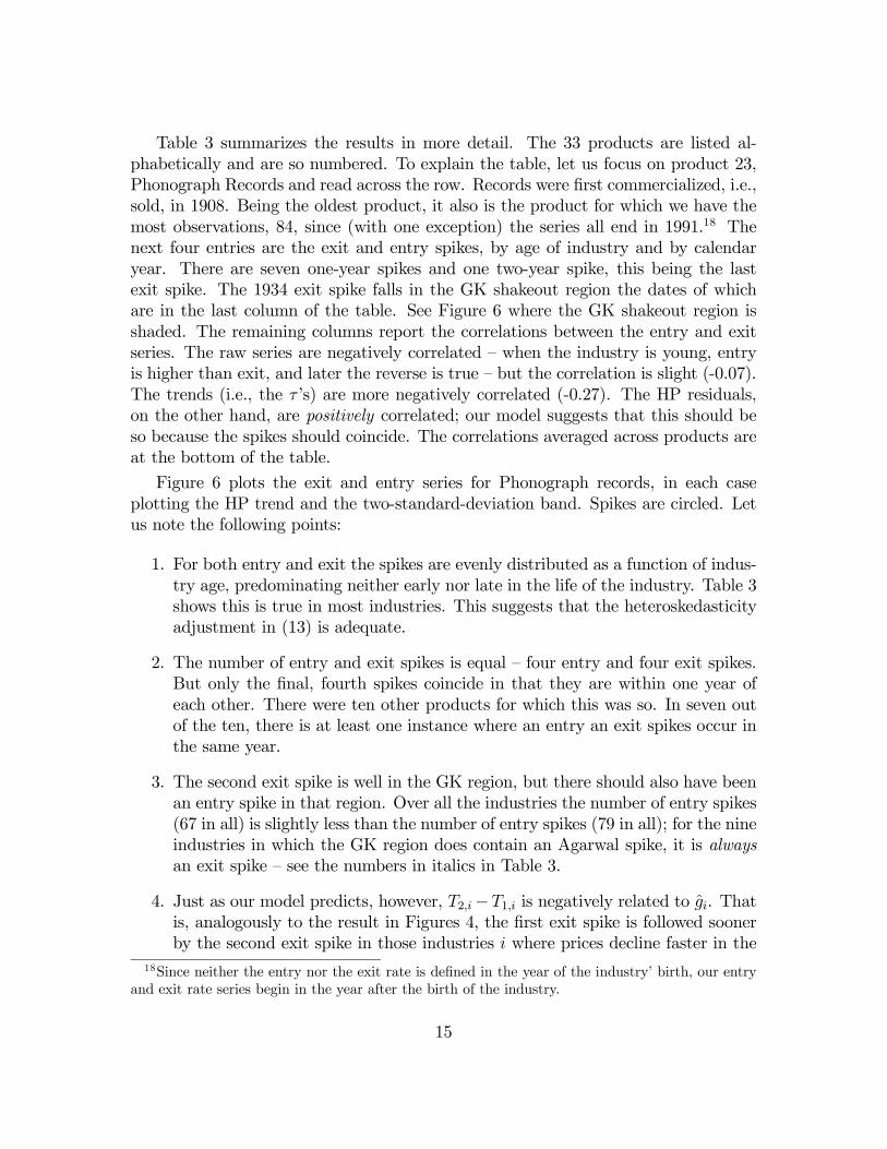
Table 3 summarizes the results in more detail. The 33 products are listed al-phabetically and are so numbered. To explain the table, let us focus on product 23,Phonograph Records and read across the row. Records were first commercialized, i.e.,sold, in 1908. Being the oldest product, it also is the product for which we have themost observations, 84, since (with one exception) the series all end in 1991.18 Thenext four entries are the exit and entry spikes, by age of industry and by calendaryear. There are seven one-year spikes and one two-year spike, this being the lastexit spike. The 1934 exit spike falls in the GK shakeout region the dates of whichare in the last column of the table. See Figure 6 where the GK shakeout region isshaded. The remaining columns report the correlations between the entry and exitseries. The raw series are negatively correlated — when the industry is young, entryis higher than exit, and later the reverse is true — but the correlation is slight (-0.07).The trends (i.e., the τ ’s) are more negatively correlated (-0.27). The HP residuals,on the other hand, are positively correlated; our model suggests that this should beso because the spikes should coincide. The correlations averaged across products areat the bottom of the table.

Figure 6 plots the exit and entry series for Phonograph records, in each caseplotting the HP trend and the two-standard-deviation band. Spikes are circled. Letus note the following points:

1. For both entry and exit the spikes are evenly distributed as a function of indus-try age, predominating neither early nor late in the life of the industry. Table 3shows this is true in most industries. This suggests that the heteroskedasticityadjustment in (13) is adequate.

2. The number of entry and exit spikes is equal — four entry and four exit spikes.But only the final, fourth spikes coincide in that they are within one year ofeach other. There were ten other products for which this was so. In seven outof the ten, there is at least one instance where an entry an exit spikes occur inthe same year.

3. The second exit spike is well in the GK region, but there should also have beenan entry spike in that region. Over all the industries the number of entry spikes(67 in all) is slightly less than the number of entry spikes (79 in all); for the nineindustries in which the GK region does contain an Agarwal spike, it is alwaysan exit spike — see the numbers in italics in Table 3.

4. Just as our model predicts, however, T2,i−T1,i is negatively related to gi. Thatis, analogously to the result in Figures 4, the first exit spike is followed soonerby the second exit spike in those industries i where prices decline faster in the

18Since neither the entry nor the exit rate is defined in the year of the industry’ birth, our entryand exit rate series begin in the year after the birth of the industry.

15

Phonograph Record Entry Rates

0

0.5

1

1.5

2

2.5

3

1909 1914 1919 1924 1929 1934 1939 1944 1949 1954 1959 1964 1969 1974 1979 1984 1989

GK Stage 4

NBER recession years

=

Phonograph Record Exit Rates

0

0.1

0.2

0.3

0.4

0.5

0.6

1909 1914 1919 1924 1929 1934 1939 1944 1949 1954 1959 1964 1969 1974 1979 1984 1989

GK Stage 4

Figure 6: Spikes in the Phonograph-Record Industry

16

0

5

10

15

20

25

30

35

40

45

0 0.02 0.04 0.06 0.08 0.1 0.12 0.14 0.16

g

T(2)

-T(1

)

Jet Engines

Phonograph records

Heat Pumps

Radiant Heating Antibiotics

Outboard Motors

Recording Tapes

Figure 7: Exits: The relation between T2 − T1 and g

interim. We now calculate bg as the rate of average price decline during theyears covered by T2 − T1. To maximize the number of observations, we includeproducts for which price information is available for as little as 70% of the timeduring the years covered by T2−T1. For Outboard Motors and Recording Tapes,however, price went up during those years which is inconsistent with the model.But they both had above-average T2 − T1 values, 42 and 17 respectively, andwhile we did not include them in the estimation routine, we include them inFigure 7, setting g to zero in both cases.

5. The same test is also done on entry spikes. Once again, T2,i− T1,i is negativelyrelated to gi. The results are in Figure 8.19

4.0.2 Entry- and exit-spike coincidence

If the entry and exit spikes did not coincide, industry price would not fall at therate needed to satisfy the free-entry condition. Thus entry and exit spikes in capi-tal should occur simultaneously: Capital retired at the spike date should equal thecapital brought in at that date. If the fraction of exiting capital accounted for bythe exiting firms (as opposed to continuing incumbents) was the same as the fraction19For both plots we assume, as before, that ln ci ∼ N

¡ln c,σ2

¢in the estimation. Instead of

fitting a eT curve to the observations independently, a more rigorous procedure would perhaps be tocalibrate a eT curve with c set equal to the estimates in Figures 4 and 7. After all, the theory assumesa stationary c. But the products in the Agarwal dataset for which we can construct measures ofT2 − T1 and g are not the same products in Figures 4 and 7 from the GK dataset. Our procedurefor designating spike dates also differs from GK’s procedure for designating shakeout dates.

17

0

5

10

15

20

25

30

35

40

0 0.02 0.04 0.06 0.08 0.1 0.12 0.14 0.16 0.18 0.2

g

T(2)

-T(1

)

Jet Engines

Electric Shavers

Ball-point Pens Styren

Antibiotics

Phonograph RecordsVideo Cassette

Recorders

Figure 8: Entries: The relation between T2 − T1 and g

of new capital accounted for by the new entrants (again, as opposed to continuingincumbents) then the capacity and output relinquished by the exiting firms shouldequal the capacity brought in by the entering capital. And, in particular, the mar-ket share of the exiting firms would equal the market share of the entrants. Moregenerally, if the fractions were unequal but fixed over time, the model still predictsa positive correlation of entering and exiting capital over time and, hence a positivecorrelation between the market shares of entrants and exiters.

This implication gets support from Table 7 of Dunne, Roberts and Samuelson(1988, ‘DRS’) which reports that whether or not one controls for industry effects, themarket shares of entering and exiting firms are positively correlated over time, whenthe unit of time is five-years. Because our data do not have information on marketshares or on the output of individual entrants and exiters, we can deal only with firmnumbers. For numbers of entrants and exits, Table 7 of DRS find that the numbersof entrants and exits is negatively correlated once they control for industry effects.Our data show a positive correlation, probably because they are much more finelydisaggregated than the DRS data are.20

In our data, a period lasts one year, and entry and exit spikes coincide only in aminority of cases. We shall now test the null hypothesis that the entry and exit spikesare not correlated. We shall find that the number of coincidences highly significantly20For instance, Antibiotics, the first product in Table 3, is just one of the 63 products classified

under the 4-digit industry Pharmacetical Preparations (2834). And Electric Shavers, the 9th productin Table 3, is just one of 67 products classified under the 4-digit industry Electric Housewares andFans (3634).

18

exceeds the fraction that would be expected to arise if the two sets of dates wereuncorrelated.

Test of coincidence.–Under the null that the entry dates are uncorrelated withthe exit dates, we now derive the probability that there will be no coincidences indates. This will be a limited-information test because we are unable to derive theprobability distribution of the full sample. Suppose an industry has τ periods ofcoverage and that during these τ periods there were NE entry spikes and NX exitspikes. Suppose entry spikes happened at dates t1, t2, ..., tientry (τ). Suppose that thedates of the entry spikes were not correlated with the dates of the exit spikes. Suppose,moreover, that an exit spike was equally likely to fall at any date. No match will ariseif and only if none of the NX exit spikes matches any of the NE entry spikes. In otherwords, under the null hypothesis, H0, the spikes are exchangeable random variableswhich are correlated only in so far as they cannot fall at the same date as anotherspike. Exit-spike i is equally likely to fall in each ‘free’ year that the data cover.We condition on the entry-spike dates. Only their number matters, not their actualdates: Any set of dates would produce the same likelihood.

To derive the likelihood, begin by placing the exit spikes in random order i =1, ..., NX . Then under H0: “entry and exit dates are uncorrelated”, the probabilitythat the first exit spike falls in one of the τ − NE bins not occupied by an entryspike is τ−NE

τ. Since no two exit spikes can occupy the same bin, conditional on this

event, the probability that the second randomly chosen spike date will produce nomatch is τ−NE−1

τ−1 . Proceeding in this way sequentially until the NX ’th exit spike, theprobability under H0 that there is no match is

1− ρ ≡NXYi=1

µτ −NE − (i− 1)

τ − (i− 1)¶. (14)

Denote the solution for ρ by ρ = ψ (τ ,NX , NE). The formula conditions on τ ,NX and NE all three of which generally differ over industries. For industry j write

ρj = ψ¡τ j ,N j

X ,NjE

¢. (15)

Then ρj is the probability that industry j has at least one match. Now define thedichotomous random variable mj as follows: Let

mj =

½1 if industry j has at least one exit-entry match0 otherwise

so that mj = 1 with probability ρj and mj = 0 with probability 1− ρj. That is, mj

is binomially distributed.

19

0

0.05

0.1

0.15

0.2

0.25

0 1 2 3 4 5 6 7 8 9 10 11

# industries with at least one coincidence

Freq

uenc

y un

der H

0

# observed

Figure 9: Frequency distribution of M under H0

The Likelihood function. — Let ρj be the parameter for industry j, defined in (15).Among the 31 industries for which ρj can be defined, let J be the set of industriesfor which mj = 1. The likelihood of the sample is

L (m1, ...,m31) =Yj∈J

ρjYj /∈J

¡1− ρj

¢= 4.6852846× 10−9. (16)

The p-value.–The p-value is the probability of obtaining a result at least asextreme as the one that was actually observed (in our case 7 industries for whichm = 1), given H0. Let the collection of industries be I; that is, I = {1, 2, ..., 31} is aset consisting of 31 elements. Let M =

Pj∈Imj . In our context,

p7 = PrnM ≥ 7 | ¡τ j , N j

X , NjE

¢31j=1

and H0o.

Of course, H0 determines the ρj via (14). Let JM be the collection of M -elementsubsets of I. That is, JM = {J ⊂ I | #J =M}. Then,

pn =XM≥n

XJ∈JM

Yj∈J

ρjYj /∈J

¡1− ρj

¢This is the likelihood of all possible values ofM that equal n or more. The probabilitydistribution ofM under H0 is pn+1−pn and it is shown in Figure 9. Since p7 = 0.0217,we reject H0 at the 5% but not at the 1% level.

5 Capital replacement and exitOur model assumes that ε (τ) jumps at the rate λ, but really only the first jumpmatters, since that first jump suffices to disqualify a firm from competing in the

20

market for new capital. The general question can be put as follows: ‘Do incumbentfirms develop a disadvantage in setting up machines and plants of the newest vintagesand, if so, how quickly?’ The literature offers some indirect evidence. Prusa andSchmitz (1994) find that a firm’s initial product is better than its second product, itssecond better than its third, and so on. Christensen (1997) cites examples of disk-drive producers and printer producers that failed to invest in the new technologiesthat entrants brought in. Henderson (1993) finds that incumbents are less successfulat research efforts to exploit radical innovation than entrants are. Supporting thevintage-capital model generally, Filson and Gretz (2004, Tables 1-5) support theproportion that ‘new firms and industry laggards are the most likely pioneers of newproduct generations.’ Their Tables 1-5 show that in the early days of a product (herea diameter of a disk), new entrants lead the pack in terms of quality (here defined asstorage capacity). As the format matures, the incumbents become leaders. There are5 new generations of drives in the data set; all of them were pioneered by spin-outs.21

We now show evidence that airline companies are more likely to exit when theircapital is old. We use data on aircraft where accurate information on age is available.Among exiting firms, the age of the capital stock is always T .22 Surviving capital isgenerally younger than that. If demand was almost perfectly inelastic, there would bevery little investment between the spike dates, and the capital stock among survivingfirms would be almost as old as that among exiting firms. On the other hand, ifdemand is highly elastic, most of the existing capital would be quite young. Thus ifwe let aS be the average age of the surviving firms’ capital stock, unless we specifythe demand curve all we can say is that

0 < aS < T. (17)

Figure 10 shows the empirical counterparts of aS (white dots) and T (black dots)for the U.S. airline industry, in which the airplanes of exiting airlines were on average7 years older than those of the surviving airlines. After weighing by the numberof observations, the difference is highly significant. Balloon size is for each seriesproportional to the square root of the number of observations, but the constant of21The evidence is not unanimous, however. Dunne (1994) finds that the age of a plant is unrelated

to the tendency to adopt advanced technology.22The presence of an active market for leased planes in the airline industry leaves this implication

largely intact. First, the competitive leasing price for a vintage-τ plane at date t would be p(t)egτ−cwith airlines making zero profits at each instant. Our argument is that whether an airline leases orbuys its equipment does not affect its ability to make use of it. An airline that has not experiencedany jumps in ε can make use of the latest vintage at zero additional cost after paying the competitiverental. One that has experienced a shock to ε must also pay a positive amount in addition to thecompetitive rental to fly latest-vintage planes. But it can buy or rent planes of an older vintage,a vintage that it can still operate as efficiently as anyone else can. Suppose that the firm followsthis strategy for as long as it can, thus hanging on for T periods following the shock to its ε. Whenit does finally exit, its rented planes will be T years old, i.e., the earliest vintage still in use in theindustry, which also is when the equilibrium rental price of the vintage reaches zero.

21

0

5

10

15

20

25

30

1955 1960 1965 1970 1975 1980 1985 1990 1995 2000 2005

year

Age of capital in years

Surviving airlines

Exiting airlines

no. of planes operated by surviving airlines = 87

1122

200

278302

4159

no. of planes operated by exiting airlines = 1

9

28 43

8

76

33

10

2514

5

Figure 10: Age of capital among exiters and survivors in the U.S. airlineindustry, 1960-2003.

proportionality is larger for the exiting capital series so as to allow us to see howsample size of that series too evolves over time.

Figure 11 shows almost as strong a difference among all the world airlines. Capitalof exiting airlines was four years older than the capital of surviving airlines and thedifference in the means is again highly significant. Surprisingly, perhaps, the U.S.carriers operated older planes than the carriers based in other countries. A descriptionof the data is in the Appendix, but a summary is in Table 2:

U.S. WorldSurvivors Exiters Survivors Exiters

Average age (yrs) 10.4 17 9.8 13.7Std. dev. of age 7.5 9.4 7.4 9.4# of airlines 231 181 1140 659# of plane-year obs. 95,147 530 213,650 2,092

Table 2 : The data in Figures 10 and 11.

As reported in the table, a plane is counted as one observation for each year of its life.An airline is counted at most twice — as a survivor and then possibly as an exiter.Three other pieces of evidence link exit decisions to the need to replace capital to

the decision to exit.

22

0

5

10

15

20

25

1955 1960 1965 1970 1975 1980 1985 1990 1995 2000 2005

year

Age of capital in years

Exiting airlines

Surviving airlines

97

871300

406

552 7118

11169210

24

35

49

86

25

12

178

53

2

Figure 11: Age of capital of exiters and survivors in among all theworld’s airlines, 1960-2003.

1. Plant exit.–Salvanes and Tveteras (2004) find that old plants are (i) less likelyto exit, but (ii) more likely to exit when their equipment is old. Fact (i) theyattribute to the idea that plants gradually learn their productivity and exit ifthe news is unfavorable as Jovanovic (1982) argued. Fact (ii) they attribute tothe vintage-capital effect on exit.

2. The trading of patent rights.–The renewal of a patent is similar to replacing apiece of capital in the sense that a renewal cost must be paid if the owner ofthe patent is to continue deriving value from it. If that owner sells the patentright, he effectively exits the activity that the patent relates to. Serrano (2008)finds that the probability of a patent being traded rises at its renewal dates,indicating that the decision to exit is related to the wearing out of a patentright.

3. Higher embodied technical progress raises exit.–A faster rate of decline in theprice of capital makes it optimal to replace capital more frequently. If re-placement sometimes leads to exit, we should see more exit where there is moreembodied progress. Samaniego (forthcoming) indeed finds that in sectors wherethe prices of machinery inputs fall faster, the firms using those machines expe-rience higher rates of exit.

23

5.0.3 Firm exit

A firm ‘exits’ in the GK data when it stops producing a product. In the theorypresented so far, firms can exit only at ages T, 2T, and so on. Pooling over products,Agarwal and Gort (1996, Figure 2) show that hazard rates for firm exit tend torise once age exceeds 30 or 40 years, and perhaps this is because their capital is oldand needs replacing. It is conceivable that mixtures over industries could producedownward-sloping hazards. The fact is, however, that firms in every industry canand do fail at young ages and for reasons often unrelated to the age of their capital.Thus as a theory of exit within a particular industry, the model as it stands is quiteinadequate. The object here is not to seek a general theory of firm exit but, rather,only to show that our theory of the shakeout is robust to the introduction of otherreasons for exit.

We shall now show that the model can produce exit spikes every T periods, andstill have a realistic exit hazard. To do it, we shall assume that firms experience costshocks and that there is a frictionless used-capital market within the industry. Thismarket becomes active if firms have different c’s. We continue to assume that capitalhas zero value to anyone outside the industry. Suppose, then, that c rises permanentlywhen the firm or plant is τ years old, and suppose further that the hazard, h (τ ), ofsuch an event is decreasing in τ , perhaps because of a positive effect that learning bydoing exerts on the firm’s production efficiency.

A firm that experiences a rise in c will immediately sell its capital to firms in theindustry that have not experienced such a rise, and extract the full value of the profitsthat the machine will yield until its replacement date. The investment condition (5)is then unchanged because the resale value of the capital fully captures what thefirm would have obtained for itself had its c remained at its original level. The newowner of the capital would choose to retire it at the same date that the original ownerwould have had he not experienced a rise in c and therefore the exit condition (4) alsoremains unchanged, as does (6). Equilibrium is therefore exactly the same. However,now there will be two kinds of exit: (i) When the firm’s capital is up for replacementand that the firm’s implementation cost has gone up since the last time capital wasinstalled, and this hazard is zero except for spikes every T periods, (ii) When thefirm’s c has risen, which has the hazard h (τ). For τ < T , the exit hazard is just hand it is decreasing in τ . At τ = T , (i) dominates (ii) since time is continuous. Butover a discrete time period, (ii) could dominate (i), in which case the exit hazardwould decrease monotonically.23

The general point is that the GK observations that Figure 1 portrays concern in-dustry aggregates. Our model too is mainly about these aggregates and it is probablyconsistent with a wide variety of assumptions about turbulence at the more microlevel.23This applies only to a firm that enters with frontier technology. If an entrant were to come in

with used capital, he would replace it before his firm reached age T .

24

6 Other explanationsOur paper explains the existence of investment spikes using a vintage-capital argu-ment. Proposition 3 goes further and predicts a geometric decay of the spikes whichno other models generate in a natural way. On a general level, other forces have beenheld to be possible causes of concentrated episodes of investment and exit. Sinceour model omits these other forces, we now try to place our paper in a more generalcontext by briefly reviewing these arguments and assessing their ability to explainthe data at hand. It helps to divide them into demand-side and supply-side types ofexplanations.

6.1 Demand-side explanations

Some papers consider fluctuations in aggregate demand, others focus on shifts indemand at the industry level. We take these up in turn.

6.1.1 Aggregate demand

Gourio and Kashyap (2007) find investment spikes to be procyclical, and other workfinds exits to be countercyclical. The concern this raises is that what we have termedas ‘echoes’ are instead reflections of the business cycle.

Be they aggregate or industry demand shocks, however, it would seem that theyshould produce an asynchronicity between entry and exit: Entry should occur whendemand is high and exits should happen when demand is low. Our clustering testshows, however, that entry and exit spikes tend to go together. More directly we canask if entry spikes are less likely and exit spikes more likely to occur during NBERrecession years.24

This logic would seem to have been at work in the Phonograph industry in that, asFigure 6 shows, that in the two of the four exit spikes — the 1913 and the 1974 spikes —occurred during recession years and none of the entry spike dates did. However, thisasymmetry does not show up in other industries. When we consider all the industriesthere is no correlation between recession years and spike dates. Our tests are simplecomparisons of means. Let τ j be the number of years of coverage of industry j, andτRj the number of recession years contained in τ j. Similarly, let φj be the number of24The NBER dates are in quarters but our spike dates are in years. We designate a given year a

recession year if any of the following criteria was met: (1) if a NBER recession was underway forthe whole year, (2) if a NBER recession started in the first 2 quarters of the year, or (3) if a NBERrecession ended in the last 2 quarters of the year. There are two exceptions. Both the 1918 and1990 recessions started in the 3rd quater and ended in the 1st quater of the following year. Theyare nonetheless considered recession years, for otherwise the two recessions would not show in thedata at all.

25

spikes in industry j and φRj the number of those spikes that fall in a recession year.25

Then we ask if either of the following inequalities is significant:Pj φ

RjP

j φj≷P

j τRjP

j τ j.

The demand hypothesis implies that for exits the LHS should exceed the RHS andthat for entry the LHS should be less than the RHS. It turns out that the LHS issmaller for both exit and entry, but neither difference is significant. We interpretthis as a test of differences in the means based on

Pj τ j independent samplings. See

Appendix Table 4.

6.1.2 Industry demand

We assumed that the demand curve is elastic enough and that large exogenous de-mand shifts are ruled out (the details are in (3)). When this assumption fails, demandcan play a major role. This is shown by Caballero and Hammour (1994) who findthat if replacement of capital causes interruptions in production, it is optimal to re-place capital when demand temporarily drops, for then the foregone sales are at theirlowest. Klenow (1998) finds that when, in addition, the productivity of new capitalrises with cumulative output, a firm will replace capital when the recovery is aboutto start. This raises the productivity growth of the new capital.

If an exit spike is caused by a fall in industry demand, we should observe a fallin output around the time of the spike. Moreover, a demand decline produces ashakeout and a decline in p. If demand does not decline then there is no shakeoutand no decline in p. We divide the GK industries into those in which output fell duringthe shakeout period, and into those in which output rose. For the analysis in Figure4, among the industries where output fell during the shakeout,26 the average pair was³bg, bT´ = (0.07, 30.4), whereas among the industries where output rose,27 the averagepair

³bg, bT´ = (0.28, 13.3) . For the analysis in Figure 5, the corresponding figures

are³bg, bT´ = (0.05, 17.3)28 and ³g, bT´ = (0.21, 11.2) .29 Yet the demand hypothesis

25Take for example product 23, Phonograph Records. Here τ = 83. The coverage was from 1909

to 1991 during which 19 years were recession years. ThusτRjτj= 19

83 . For exit spikes, the second and

the fourth spikes, in 1933 and 1973-74, respectively, were in recession years. Then φRj = 2 andφRjφj= 2

19 . Because of time aggregation, demand fluctuations can induce a spike in that x(t) reactspositively to changes in demand.26DDT, Electic shavers, Phonograph records, TV, and Zippers.27Fluorescent lamps, Penicillin, and Styrene.28The industries in note 26 plus Auto tyres and CRT.29The industries in note 27 plus Freezers and Transistors. GK did not report whether output fell

or rose during the shakeout for Computers and Streptomycin.

26

implies the opposite: Prompted by the decline in output, g (the measured decline inp) should have been higher and T should have been lower in the first sample than inthe second. Thus demand shifts do not seem to explain the patterns in GK’s sample.

6.2 Supply-side explanations

Echo effects were first discussed in the growth literature. In a one-consumption-goodGE model, for the interest rate to remain constant in the face of variations in the rateof investment that inevitably occur along the transition path from arbitrary initialconditions, the instantaneous utility of consumption must be linear. Then, if therate of technological progress is also constant, the investment echoes will have theconstant periodicity that they also have in our model, but they will not be damped.Rather, the investment profile simply repeats itself every T periods — see Mitra et al.(1991) and BGL. Johansen (1959) and Arrow (1962) assume a production functionfor the sole final good that is Leontieff in capital and labor. In that case the effectivemaintenance cost is the wage multiplied by the labor requirement per machine. Sincewages rise at the same rate as the rate at which the labor requirement declines, andthe maintenance rate is then constant in units of the consumption good. Thus ourmaintenance cost, c, has an exact counterpart in these models. Since these modelshave no costs of rapid adjustment, the infinitely-elastic supply of capital that weassume amounts to the same thing.

Endogenous technological change.–Our model assumes that technological changeis exogenous. Klepper (1996) assumes firms do research, and his model appears toimply that leading firms would squeeze out the inefficient fringe more quickly inindustries where there is more technological opportunity and, hence, faster-decliningproduct prices. The difference between our model and his concerns the fate of thefirms in the first cohort of entrants: In our model the first cohort is the least efficient,whereas in Klepper’s model, the first cohort is the most efficient because it has donethe most research. In Grossman and Helpman (1991) and Aghion and Howitt (1992),monopoly incumbents are periodically replaced by more efficient entrants. Tse (2001)extends the model to allow for more than a single producer.

Exit after learning through experience.– GK observed that a shakeout usuallycomes after a wave of entry. Horvath, Schivardi and Woywode (2003, ‘HSW’) arguethat if a run-up in entry occurs at some point in the industry’s life, then some timelater, a fraction of the entrants will have found themselves unfit to be in that industry— a type of learning that Jovanovic (1982) stresses — and will then exit en masse.The argument of HSW would measure the learning period by T . After exactly Tperiods, a firm discovers whether it has high costs and should exit. To developthis argument fully one would have to somehow to show first that a firm’s learningabout productivity is likely to take place all at once and not gradually as one usuallyassumes. And, second, one would need to explain why learning should occur soonerin those industries where p is declining rapidly. Nevertheless, HSW get some support

27

from the results in Table 7 of DRS where they find that at the industry level, thenumber of entering and exiting firms (as opposed to their market shares) is notpositively correlated but that, rather, entry leads exit at a five-year frequency. In ourdata, however, the causality runs the other way: Exit appears to cause entry. Foreach industry, i, in Table 3 we define the dummy variables xi,t (exit) and yi,t (entry)taking on the value of unity if our procedure detects a spike at date t, and the valueof zero if no spike is detected. Now we have a pair of sequences of dummy variablesfor each industry. We then run Probit regressions of the form

Pr (xi,t = 1) = Φ

Ãα+

SXs=0

αsyi,t−s +SXs=1

βsxi,t−s

!(18)

and

Pr (yi,t = 1) = Φ

Ãα+

SXs=0

αsxi,t−s +SXs=1

βsyi,t−s

!(19)

where Φ is the normal probability function. We pool the observations over (i, t).We report the results in Appendix, with S ranging from zero to five, and with andwithout restricting the coefficients. Generally, the contemporaneous relation is alwayspositive — the estimate of α0 is positive and significant at the 5% level in both (18)and (19) regardless of what other lags are included in them. The tendency is for exitto cause entry and not the other way around. This, however, was to be expectedgiven the outcome of the coincidence test. Causality, on the other hand, tends clearlyto run from exit to entry. Tables 5a and 5b tell the story in greater detail.

Technological advances by incumbents.–When a new technology raises the effi-cient scale of firms, it crowds some of them out of the industry; so argue Hopenhayn(1993) and Jovanovic and MacDonald (1994). The assembly-line technology, e.g.,probably raised the optimal scale of auto-manufacturing plants and caused a largereduction in the number of auto producers. Klepper (1996) argues that larger firmsdo more R&D than small firms because they can spread its results over a larger num-ber of units; because they invent at a faster rate, large firms then drive smaller firmsout, often by acquiring them.

Consolidations for other reasons.–Some shakeouts no doubt occur because of thestandardization of products so that some of the variants fall by the wayside and theirproducers exit. The focus on the diesel technology was one reason for the mass exodusof automobile producers that relied on other technologies as a source of power for themodels they built. The winning model forces out other models and their producers.Utterback and Suarez (1993) argue that a dominant design emerges: More generally,consolidations and merger waves can occur for reasons unrelated to drops in demandand to advances in technology. Deregulation, for instance, has led to merger wavesin the airlines and banking industries (Andrade et al. 2001) and to a sharp fall in thenumbers of producers.

28

Evidence shows there are investment spikes — Cooper and Haltiwanger (1996),Gourio and Kashyap (2007). Repeated echo effects in entry and exit seem to bepresent in the data and they are clear indications that a vintage-capital replacementmotive is one of their causes.

7 ConclusionThis paper started out with a graphical display of evidence that industry shake-outs of firms occur earlier in industries where technological progress is faster. Weargued that other models of shakeouts were not able to explain this fact, whereasour vintage-capital model does so by predicting earlier replacement when capital-embodied technological progress is fast. We supported this claim with evidence fromthe airline industry that showed firm exits to be positively related to the age of thecapital stock.By inferring technological progress in the inputs from the decline in the price

of the output as our model predicted, we found that the model fits fairly well thenegative relation between technological progress and the onset of the shakeout. More-over, we found that subsequent investment spikes, too, are also more frequent wheretechnological progress is fast.To study further the role of the vintage model in explaining industry dynamics,

more can be done with richer data sets. First, the age of a firm’s capital stock andthe pressure that replacement of that stock places on the firm to exit should belinked empirically more firmly; we have studied only the airline industry. Second,the vintage-capital model that we have presented is primarily a theory of investmentat the level of an industry, and could just as well be tested with data on industry-level gross and net investment; spikes should occur in the gross-investment seriesonly, provided the quality of capital is properly measured. Third, we have abstractedentirely from mergers, yet horizontal mergers provide a way for exiting firms to beabsorbed by those firms that remain; industry-level time series of horizontal mergersshould, on these grounds, also exhibit echoes.

References[1] Agarwal, Rajshree. “Evolutionary Trends of Industry Variables.” International

Journal of Industrial Organization 16, no. 4 (July 1998): 511-25.

[2] –––, and Michael Gort. “The Evolution of Markets and Entry, Exit andSurvival of Firms.” Review of Economics and Statistics 78, no. 3. (Aug., 1996):489-98.

[3] Aghion, Philippe and Howitt, Peter, “A Model of Growth Through CreativeDestruction,” Econometrica, March 1992, 60(2), 323-351.

29

[4] Aizcorbe, Ana and Samuel Kortum. “Moore’s Law and the Semiconductor In-dustry: A Vintage Model.” Scand. J. of Economics 107, no. 4 (2005): 603—630.

[5] Andrade, Gregor; Mitchell, Mark and Stafford, Erik. “New Evidence and Per-spective on Mergers.” Journal of Economic Perspectives, Spring 2001, 15(2), pp.103-120.

[6] Arrow, Kenneth. “The Economic Implications of Learning by Doing.” Review ofEconomic Studies 29, no. 3 (June 1962): 155 - 173.

[7] Atkeson, Andrew and Patrick Kehoe. “Industry Evolution and Transition: TheRole of Information Capital.” FRB Minneapolis staff report 162 (August 1993).

[8] Boucekkine, Raouf, Marc Germain, and Omar Licandro. “Replacement Echoesin the Vintage Capital Growth Model.” Journal of Economic Theory 74 (1997):333-48.

[9] Caballero, Ricardo and Mohamad L. Hammour. “The Cleansing Effect of Reces-sions.” American Economic Review 84, no. 5 (December 1994): 1350-68.

[10] Chatterjee, Satyajit and Rossi-Hansberg, Esteban. “Spinoffs and the Market forIdeas.” FRB of Philadelphia Working Paper No. 08-26 (October 2008).

[11] Christensen, Clayton. The Innovator’s Dilemma. Cambridge: HBS Press, 1997.

[12] Cooper, Russell and John Haltiwanger “Evidence on Macroeconomic Comple-mentarities.” Review of Economics and Statistics 78, no. 1 (February 1996):78-93.

[13] Dunne, Timothy, Mark Roberts; Larry Samuelson. “Patterns of Firm Entry andExit in U.S. Manufacturing Industries.” RAND Journal of Economics 19, no. 4(Winter, 1988): 495-515.

[14] Dunne, Timothy. “Plant Age and Technology use in U.S. Manufacturing Indus-tries.” RAND Journal of Economics 25, no. 3 (Autumn, 1994): 488-499.

[15] Evans, David. “The Relationship Between Firm Growth, Size, and Age: Esti-mates for 100 Manufacturing Industries.” Journal of Industrial Economics 35,no. 4 (June 1987): 567-81.

[16] Filson, Darren and Richard Gretz. “Strategic Innovation and Technology Adop-tion in an Evolving Industry.” Journal of Monetary Economics 51, no. 1 (January2004): 89-121.

[17] Gavazza, Alessandro. “Leasing and Secondary Markets: Theory and Evidencefrom Commercial Aircraft”, New York University, (February 2009).

30

[18] Gort, Michael and Steven Klepper “Time Paths in the Diffusion of Market In-novations,” Economic Journal 92 (1982): 630-53.

[19] Gourio, Francois and Anil Kashyap. “Investment spikes: New facts and a generalequilibrium exploration.” Journal of Monetary Economics 54 (2007): 1—22.

[20] Grossman, Gene M. and Helpman, Elhanan, “Quality Ladders in the Theory ofGrowth,” Review of Economic Studies, January 1991, 58(1), 43—61.

[21] Henderson, Rebecca. “Underinvestment and Incompetence as Responses to Rad-ical Innovation: Evidence from the Photolithographic Alignment Equipment In-dustry.” RAND Journal of Economics 24, no. 2 (Summer 1993): 248-270.

[22] Hopenhayn, Hugo. “The Shakeout.” wp#33 Univ. Pompeu Fabra, April 1993.

[23] Horvath, Michael, Fabiano Schivardi and Michael Woywode. “On Industry Life-Cycles: Delay, Entry, and Shakeout in Beer Brewing.” International Journal ofIndustrial Organization 19, no. 7 (2003): 1023-1052.

[24] Johansen, Leif. “Substitution versus Fixed Production Coefficients in the Theoryof Economic Growth: A Synthesis.” Econometrica 27, no. 2 (April 1959): 157-176.

[25] Jovanovic, Boyan. “Selection and the Evolution of Industry.” Econometrica 50,no. 3 (June 1982): 649-70.

[26] –––, and Saul Lach “Entry, Exit, and Diffusion with Learning by Doing.”American Economic Review 79, no. 4 (September 1989): 690-99.

[27] –––, and Glenn MacDonald. “The Life Cycle of a Competitive Industry.”Journal of Political Economy 102 (April 1994): 322-47.

[28] –––, and Peter L. Rousseau. “General-Purpose Technologies.” Handbook ofEconomic Growth vol. 1B Amsterdam: Elsevier (2006): 1181-224.

[29] Klenow, Peter. “Learning Curves and the Cyclical Behavior of ManufacturingIndustries.” Review of Economic Dynamics 1, no. 2 (May 1998): 531-50.

[30] Klepper, Steven, “Entry, Exit, Growth, and Innovation over the Product LifeCycle,” American Economic Review 86 no. 3 (June 1996): 562 - 83.

[31] –––, and Kenneth Simons. “Industry Shakeouts and Technological Change.”International Journal of Industrial Organization 23, no. 2-3 (2005): 23-43.

[32] –––, and Peter Thompson. “Disagreements and Intra-Industry Spinoffs.”Florida International University working paper 09-07 (March 2009).

31

[33] McGrattan Ellen, and James A. Schmitz, Jr.. “Maintenance and Repair: TooBig to Ignore.” Federal Reserve Bank of Minneapolis Quarterly Review 23, no. 4(Fall 1999): 2—13.

[34] Mitchell, Matthew. “Technological Change and the Scale of Production.” Reviewof Economic Dynamics 5, no. 2 (April 2002): 477-88.

[35] Mitra, Tappan, Debraj Ray and Rahul Roy. “The Economics of Orchards: AnExercise in Point-input, Flow-output Capital Theory.” Journal of Economic The-ory, 53, no. 1 (1993): 12-50.

[36] Prusa, Thomas and James Schmitz. “Are New Firms an Important Source ofInnovation? : Evidence from the PC Software Industry.” Economics Letters 35,no. 3 (March 1991): 339-342.

[37] Prusa, Thomas and James Schmitz. “Can Companies Maintain Their InitialInnovation Thrust? A Study of the PC Software Industry.” Review of Economicsand Statistics 76, no. 3 (August 1994): 523-40.

[38] Salvanes, Kjell and Ragnar Tveteras. “Plant Exit, Vintage Capital and the Busi-ness Cycle.” Journal of Industrial Economics LII, no. 2 (June 2004): 255-76.

[39] Samaniego, Roberto M. “Entry, Exit and Investment-Specific TechnicalChange.” American Economic Review, forthcoming.

[40] Serrano, Carlos. “The Dynamics of the Transfer and Renewal of Patents.” NBERWorking Paper 13938 (April 2008).

[41] Tse, Chung Yi, “The Distribution of Demand, Market Structure and Investmentin Technology,” Journal of Economics, October 2001, 73(3), 275—297.

[42] Utterback, James, and Fernando Suárez, “Innovation, Competition, and Indus-try Structure,” Research Policy 22 (1993): 1-21.

[43] Wang, Zhu, “Learning, Diffusion and Industry Life Cycle.” Federal Reserve Bankof Kansas City Working Paper 04-01 (January 2006).

32

EXIT ENTRY

spike dates

spike dates

Product &

yr of comm intr.

Length of raw series

in yrs since comm intro

in calendar

yr

in yrs since comm intro

in calendar

yr

Corr btw smoothed entry and exit rates

Corr btw entry and

exit residuals

Corr btw

entry and exit rates

G-K Stage 4

1 Antibiotics 44 7 1955 2 1950 -0.46 -0.04 -0.30 not in G-K 1948 19 1967 39 1987

32 1980

2 Artificial Christmas Trees

54 8 1946 35 1973 -0.52 -0.02 -0.21 1968-1969

1938 18 1956 49 1987 43 1981

45 1983

3 Ball-point Pens 44 23 1971 9-10 1957-58 0.81 -0.32 0.55 S4 not reached

1948 26 1973-74

4 Betaray Gauges 36 7 1963 7* 1963 0.18 0.34 0.26 1973-

1956 33 1989

5 Cathode Ray Tubes

57 54 1989 10 1945 0.92 0.55 0.79 1963-1967

1935 15 1950

52 1987

6

Combination Locks

80

13 1925 21 1933 0.41 0.01 0.21 not in G-K 1912 16 1928 29 1941 65 1977 53 1965

75 1987

7 Contact Lenses 56 10 1946 6 1942 0.09 -0.15 -0.13 not in G-K

1936 29 1965 12 1948 35 1971 30 1966

39 1975

8 Electric Blankets 76 3 1919 6-7 1922-23 -0.13 0.07 -0.09 1962-1973 1916 35 1951 30 1946 41 1957 46 1962 63 1979 70* 1986

69-70 1985-86

9 Electric Shavers 55 36 1973 36-39* 1973-76 0.22 -0.09 -0.11 1938-1945 1937 49 1986

10

Electrocardiographs

50

6 1948 6* 1948 0.25 0.41 0.37 1964-1969

1942 32 1974 48 1990

11 Freezers 46 27 1973 40 1986 0.41 -0.13 0.23 1947-1957

1946

italics - Is or may be in GK Stage 4 * - Within 1 year of exit spike

Table 3: Entry and Exit Statistics in Agarwal’s data 33

EXIT ENTRY

spike dates

spike dates

Product &

yr of comm intr.

Length of raw series

in yrs since comm intro

in calendar

yr

in yrs since comm intro

in calendar

yr

Corr btw smoothed entry and exit rates

Corr btw entry and

exit residuals

Corr btw

entry and exit rates

G-K stage 4

12 Freon Compressors

57 5 1940 3 1938 -0.21 -0.12 -0.17 1971-1973

1935 37 1972 46 1981

52 1987

13 Gas Turbines 48 20 1964 2 1946 -0.42 0.00 -0.22 1973- 1944 36 1980

41 1985

14 Guided Missiles 41 2 1953 8 1959 -0.32 -0.43 -0.41 1965-1973 1951 35 1986

15 Gyroscopes 77 10 1925 4 1919 0.36 0.10 0.24 1966-1973 1915 31-32 1946-47 30-32* 1945-47

39-40 1954-55

16 Heat Pumps 38 5 1959 25 1979 -0.42 -0.08 -0.24 1970-1973 1954 16 1970

32 1986

17 Jet Engines 44 6 1954 6* 1953-54 -0.26 0.42 0.07 1960-1962 1948 22 1970 32 1980

35 1983

18 Microfilm Readers

52 5-6 1945-46 8 1948 0.37 -0.24 -0.12

S4 not reached

1940 16 1956 22-23 1962-63 33 1973

45 1985

19 Nuclear Reactors 37 30 1985 30* 1985 -0.57 0.12 -0.38 1965-1973

1955 33 1988 35 1990

20 Outboard Motors 79 22 1935 2-4 1915-17 -0.18 0.07 -0.08 1921-1923

1913 67 1980 28 1941 34 1947

72 1985

21 Oxygen Tents 60 41 1973 4 1936 -0.32 -0.17 -0.26 1967-1973 1932 48 1980 56 1988

52-53 1984-85

22 Paints 58 39 1973 13-14 1947-48 -0.41 0.04 -0.20 1967-1973

1934 43 1977 20 1954 italics - Is or may be in GK Stage 4 * - Within 1 year of exit spike

Table 3, continued

34

EXIT ENTRY

spike dates

spike dates

Product &

Yr of Comm

Intr.

Length of raw series

in yrs since comm intro

in calendar

yr

in yrs since comm intro

in calendar

yr

Corr btw smoothed entry and exit rates

Corr btw entry and

exit residuals

Corr btw

entry and exit rates

G-K stage 4

23

Phonograph Records

84

5 1913 9 1917 -0.23 0.08 -0.07 1923-1934 1908 25 1933 13 1921 51 1959 40 1948

65-66 1973-74 67* 1975

24

Photocopying Machines

52

34 1974 42 1982 -0.30 -0.20 -0.25 1965-1973

1940 39 1979

25

Piezoelectric Crystals

51

13 1953 3 1943 -0.28 -0.06 -0.21 1955-1957

1940 40 1980 45 1985

26 Polariscopes 64 15 1943 18 1946 0.20 -0.26 -0.03 1964-1967

1928 45 1973 23 1951 25 1953

44* 1972

27 Radar Antenna Assemblies

40 15 1967 4 1956 -0.50 -0.10 -0.32 1957-1968

1952 21 1973 33 1985

28

Radiant Heating Baseboards

45

25 1972 27 1974 -0.42 0.02 -0.19 1972-1973

1947 37 1984

29 Radiation Meters 43 6 1955 -0.28 0.20 -0.13 not in G-K

1949 37 1986

no spike dates 41 1990

30 Recording Tapes 40 11 1963 33 1985 -0.53 0.06 -0.31 1973-

1952 28 1980

31 Rocket Engines 34 32 1990 7 1965 -0.34 -0.08 -0.19 1973-

1958 33* 1991

32 Styrene 54 17 1955 4-5 1942-43 -0.55 -0.09 -0.27 1966-1973

1938 20-1 1958-59

33

Video Cassette Recorders

18

7 1981 -0.33 -0.18 -0.11 not in G-K

1974 no spike dates 11 1985

average 51.94 -0.11 -0.01 -0.07 max 84.00 0.92 0.55 0.79 min 18.00 -0.57 -0.43 -0.41

std deviation 14.97 0.40 0.22 0.27 italics - Is or may be in GK Stage 4 * - Within 1 year of exit spike

Table 3, continued 35

8 Appendix

8.1 The aircraft data

The data that Figures 10 and 11 portray come from a file, complied by a producer of acomputer based aviation market information system and safety management software,that records the history of every non—military aircraft manufactured. They are de-scribed by Gavazza (2009, Sec. 5.1) and at http://www.flightglobal.com/StaticPages/Acas.html. Coverage begins in 1942 and ends at April 2003. For each aircraft, it records theusual identification information, such as the manufacturer, the model, etc., and (mostimportant for our purposes) the first and the last date that each aircraft was operatedby individual carriers. We aggregate such information at the level of an individualcarrier to calculate the average age of capital of the carrier at a given point in time.The analysis is restricted to narrow-body (100 seats +) and wide—body passengerjets.

Measurement of entry and exit.–We say that a carrier has “entered” in the year inwhich it was first recorded as having operated a passenger jet. A carrier has “exited”in the year in which it was last recorded as having operated a passenger jet. A carrierhas “survived” a certain year if it entered before that year and if it has not exited bythe end of the year. The data contain information on mergers; a company that wasacquired is not counted as an exit.

Measurement of age.–The age of a jet at a point in time is the time elapsed sincethe jet was first delivered. The average age of a carrier’s capital is the average age ofall the jets that it operated on January 1 of the year.

8.2 Proofs and derivations

Proof of Proposition 2.–Rewrite (9) as

ge−rT + regT −µr + c

c

¶(r + g) ≡ Φ (T, g, c, r) = 0.

We have ∂Φ∂T= rg

¡egT − e−rT¢ > 0. Therefore (11) follows if ∂Φ

∂g> 0. Now

∂Φ

∂g= e−rT + rTegT − r + c

cand, by eliminating e−rT ,

=

µr + c

c

¶r + g

g− rgegT + rTegT − r + c

c

=

µr + c

c

¶r

g− rgegT + rTegT =

r

g

µr + c

c− egT

¶+ rTegT

=r

g

µr + c

c+ (gT − 1) egT

¶> 0.

36

The strict inequality follows because (i) The function (gT − 1) egT is increasing in gT,with derivative egT [1 + (gT − 1)] = gTegT , and because (ii)As gT → 0, (gT − 1) egT →−1, so that at its smallest point, ∂Φ

∂g= r2

gd> 0. Then, since ∂T

∂g= −∂Φ

∂g/∂Φ∂T, and since

∂Φ∂T> 0, (11) follows. ¥Proof of Proposition 4.–(i)We showed that ΦT > 0 in the proof of Proposition 2.

Moreover, ∂Φ∂c> 0 because the ratio r+c

cis decreasing in c. Therefore ∂T

∂c= −∂Φ

∂c/∂Φ∂T<

0. (ii) When gc < r2, ∂T∂r= −∂Φ

∂r/∂Φ∂T

∂Φ

∂r= −Tge−rT + egT −

µr + g

c

¶−µr + c

c

¶and, by eliminating egT ,

= −Tge−rT − ge−rT

r+

µr + c

c

¶(r + g)

r−µr + g

c

¶−µr + c

c

¶= −Tge−rT − ge

−rT

r+

µr + c

c

¶g

r−µr + g

c

¶=

g

r

¡1− e−rT¢− ³r

c+ Tge−rT

´<g

r− rc.

so that then ∂T∂r= −∂Φ

∂r/∂Φ∂T> 0. ¥

Derivation of the Likelihood Function for the estimates in Figures 4, 5, 7, and8–. For each industry i, if we know ci and bgi, we know eTi = eT (r, ci, bgi). We wouldlike to solve eTi as a function of ci, so that we can derive the distribution of eTi from theassumed log—normal distribution on ci. But since eT (r, ci, bgi) does not admit a closedform solution, the exact functional relationship between eTi and ci is unknown, andwe linearize it in x = ln c. After substituting xi ≡ log ci and g = gi into (9), it reads³ r

exi+ 1´(r + gi) = gie

−r eTi + regi eTi . (20)

Taking total derivatives at xi = x, gives

−re−x (r + gi) dxi = rgi³egiT i − e−rT i

´dTi

where Ti ≡ T (r, ex, gi). Then

−dTidxi

= e−xr + gigi

1

egiTi − e−rTi ≡ βi

Hence Ti ' T (r, x, gi) − (xi − x) βi. If xi ∼ N (x, σ2), then approximately, Ti ∼N¡Ti,β

2iσ2¢. The density of Ti is f (Ti) = 1√

2πβiσexp

µ−12

hTi−T iβiσ

i2¶. When there

are no censored observations, the likelihood is

L =nYi=i

fTi (Ti) ;

37

otherwiseL =

Yi/∈CfTi (Ti)

Yi∈C(1− FTi (Ti)) ,

where C is the set of censored observations and FTi (Ti) the CDF of f (Ti).Conditional Expectation in Figure 5.–Take the Nylon observation for exam-

ple. The observation is truncated at 21. As we showed in the previous paragraph,Ti ∼ N

¡Ti, β

2iσ2¢approximately. By setting x and σ equal to their respective point

estimates of -2.56 and 2.27, we obtain estimates of Ti and β2iσ2. Then we calculate

the expected value of Ti conditional on Ti ≥ 21.

8.3 Tests

8.3.1 NBER recessions tests

The dates come from http://www.nber.org/cycles/cyclesmain.html. Table 4 summa-rizes our findings on the incidences of exit and entry spikes during the recessions:

Exit Spikes Entry SpikesPj τ j 1681

Pj φj 72

Pj φj 95P

j τRj 364

Pj φ

Rj 14

Pj φ

Rj 15P

j τRjP

j τj0.22

Pj φ

RjP

j φj0.19

Pj φ

RjP

j φj0.16

Table 4 : Spikes and recessions

For both exit and entry spikes thenP

j φRj /P

j φj <P

j τRj /P

j τ j. The differenceshowever are not significant at even the 10% level in chi-square tests of independencein both cases.

8.3.2 Causality tests

The tables below present the results of Granger causality tests of exit by entry (Table5a) and of entry by exit (Table 5b). All regressions are Probit regressions. In each setof results, the first table presents the results where the coefficients are not restricted,whereas the second table presents the results where the coefficients of the various lagsof each variable are restricted to be equal. Note how the results in general supportexit causing entry but not the other way around.

38

Dep var = xit

S 0 1 2 3 4 5

Constant -1.75* -1.74* -1.71* -1.69* -1.65* -1.66*

(0.057) (0.059) (0.061) (0.064) (0.065) (0.069)

yit 0.37† 0.38† 0.40† 0.41† 0.44† 0.46†

(0.193) (0.196) (0.199) (0.201) (0.204) (0.206)

yit-1 -0.25 -0.24 -0.23 -0.24 -0.17

(0.268) (0.277) (0.278) (0.282) (0.289)

yit-2 -0.101 -0.07 -0.07 -0.24

(0.247) (0.238) (0.259) (0.327)

yit-3 -0.56‡ -0.53‡ -0.49‡

(0.383) (0.386) (0.390)

yit-4 -0.57‡ -0.55‡

(0.391) (0.394)

yit-5 -0.08

(0.265)

xit-1 0.23 0.23 0.22 0.20 0.22

(0.236) (0.237) (0.238) (0.238) (0.238)

xit-2 -0.51‡ -0.52‡ -0.55‡ -0.52‡

(0.394) (0.395) (0.398) (0.400)

xit-3 -0.15 -0.18 -0.16

(0.311) (0.313) (0.325)

xit-4 -0.20 -0.19

(0.319) (0.325)

xit-5 -0.19

(0.322)

Dep var = xit

S 0 1 2 3 4 5

Constant -1.75* -1.96* -1.68* -1.61* -1.55* -1.57* (0.057) (0.226) (0.108) (0.233) (0.254) (0.148)

∑=

−

S

ssity

0

0.37† 0.12 0.06 -0.20 -0.08 -0.08

(0.193) (0.139) (0.118) (0.120) (0.123) (0.101)

∑=

−

S

ssitx

1

0.22 -0.03 -0.07 -0.10 -0.10

(0.208) (0.087) (0.202) (0.216) (0.116) * significant at the 1% level † significant at the 5% level ‡ significant at the 10% level

Table 5a: Causality Tests: Entry causes exit

39

Dep var = yit

S 0 1 2 3 4 5

Constant -1.61* -1.67* -1.68* -1.70* -1.73* -1.74*

(0.051) (0.056) (0.059) (0.062) (0.067) (0.069)

xit 0.39† 0.37† 0.40† 0.41† 0.44† 0.48†

(0.203) (0.207) (0.208) (0.210) (0.210) (0.211)

xit-1 0.21 0.20 0.24 0.27 0.28

(0.22) (0.220) (0.222) (0.223) (0.222)

xit-2 0.22 0.20 0.25 0.25

(0.220) (0.227) (0.225) (0.228)

xit-3 0.45† 0.46† 0.48†

(0.207) (0.208) (0.209)

xit-4 0.32‡ 0.32‡

(0.221) (0.222)

xit-5 0.32‡ (0.225)

yit-1 0.68* 0.71* 0.68* 0.65* 0.61* (0.164) (0.167) (0.171) (0.177) (0.183)

yit-2 -0.21 -1.53 -0.23 -0.23

(0.245) (0.244) (0.270) (0.269)

yit-3 -0.47‡ -0.43‡ -0.42‡

(0.322) (0.319) (0.322)

yit-4 -0.11 -0.13

(0.266) (0.255)

yit-5 -0.02

(0.148)

Dep var = yit

S 0 1 2 3 4 5

Constant -1.61* -2.34* -2.01* -1.84* -1.78* -1.76* (0.051) (0.190) (0.156) (0.131) (0.137) (0.084)

∑=

−

S

ssitx

0

0.39† 0.29† 0.28† 0.33* 0.37* 0.38*

(0.203) (0.146) (0.122) (0.106) (0.097) (0.091)

∑=

−

S

ssity

1

0.67* 0.33* 0.14‡ 0.05 0.02

(0.165) (0.126) (0.100) (0.099) (0.042) * significant at the 1% level † significant at the 5% level ‡ significant at the 10% level

Table 5b: Causality Tests: Exit causes entry

40