Optimizing study design for multi-species avian

monitoring programmes

Jamie S. Sanderlin*, William M. Block and Joseph L. Ganey

Rocky Mountain Research Station, U. S. Forest Service, 2500 S. Pine Knoll Dr., Flagstaff, AZ 86001, USA

Summary

1. Many monitoring programmes are successful at monitoring common species, whereas rare

species, which are often of highest conservation concern, may be detected infrequently. Study

designs that increase the probability of detecting rare species at least once over the study period,

while collecting adequate data on common species, strengthen programme ability to address

community-wide hypotheses about how an ecosystem functions or responds to management

actions. Study design guidelines exist for single-species occupancy models, but practical guid-

ance for monitoring species communities is needed. Single-species population-level designs are

necessarily optimal for targeted species, whereas community study designs may be optimal for

the assemblage of species, but not for every species within the community. Our objective was to

provide a general optimization tool for multi-species models and to illustrate this tool using

data from two avian community studies.

2. We conducted a simulation study with a Bayesian hierarchical model to explore design and

cost trade-offs for avian community monitoring programmes. We parameterized models using

two long-term avian studies from Arizona, USA and evaluated bias and accuracy for different

combinations of species in the regional species pool and sampling design combinations of num-

ber of sites and sampling occasions. We optimized for maximum accuracy of species richness,

detection probability and occupancy probability of rare species, given a fixed budget.

3. Statistical properties for species richness and detection probability of species within the

community were driven more by sampling occasions, whereas rare species occupancy proba-

bility was influenced more by percentage of area sampled. These results are consistent with

results from single-species models, suggesting some similarities between community-level and

single-species models with occupancy and detection.

4. Synthesis and applications. Study designs must be cost-efficient while providing reliable

knowledge. Researchers and managers have limited funds for collecting data. Our template

can be used by researchers and managers to evaluate trade-offs and efficiencies for allocating

samples between the number of occasions and sites in multi-species studies, and allow them

to identify the optimal study design in order to achieve specific study objectives.

Key-words: avian community, Bayesian hierarchical model, cost-efficient, detection probabil-

ity, occupancy, rare species, simulation study, species richness

Introduction

Community models are commonly used for conservation

and management (Russell et al. 2009; Zipkin et al. 2010;

Sauer et al. 2013) and within long-term monitoring pro-

grammes (DeWan & Zipkin 2010; Noon et al. 2012).

Multi-species monitoring programmes reduce risk of

selecting species as surrogates for entire communities

(Simberloff 1998) that do not represent those communities

well, have weak environmental relationships with manage-

ment actions, may not serve as future indicators, and/or

have so much parameter uncertainty that single-species

responses cannot be translated into a community response

(Manley et al. 2004). In the USA, the National Forest

Management Act (1976) focused monitoring efforts on

maintaining biodiversity. Monitoring biodiversity in a

scientific or management context requires clear objectives

(Yoccoz, Nichols & Boulinier 2001). Scientific objectives

focus on learning and evaluating hypotheses about*Correspondence author. E-mail: jlsanderlin@fs.fed.us

Published 2014. This article is a U.S. Government work and is in the public domain in the USA

Journal of Applied Ecology 2014, 51, 860–870 doi: 10.1111/1365-2664.12252

ecosystem function. Management objectives focus on eval-

uating ecosystem response to explicit management actions

(e.g. prescribed fire) in a structured decision-making

framework (Sauer et al. 2013). Species richness, or num-

ber of species in the community, is one useful state vari-

able representing community structure at one point in

time. Other relevant variables or rate parameters include

species diversity, biomass, population size, and coloniza-

tion and extinction probabilities. Recent programmes that

monitor species richness for science or management objec-

tives include the North American Breeding Bird Survey

(Boulinier et al. 1998), Swiss Breeding Bird Survey (K�ery

& Schmid 2006), and Amphibian Research and Monitor-

ing Initiative (Walls, Waddle & Dorazio 2011).

Occupancy is an ecological parameter relevant to

understanding species distribution, habitat selection and

metapopulation dynamics (e.g. Hanski 1994; Bailey, Si-

mons & Pollock 2004). Occupancy also is a useful state

variable for long-term monitoring programmes (Bailey, Si-

mons & Pollock 2004; Noon et al. 2012) owing to a

higher perceived cost-efficiency compared to estimating

abundance (Joseph et al. 2006) and analysis programme

availability (e.g. PRESENCE MacKenzie et al. 2006). Occu-

pancy models (MacKenzie et al. 2002, 2006) allow infer-

ence on occupancy probability (w), probability a species

occupies a patch, in systems where species detection prob-

abilities (P) are < 1. To account for imperfect species

detection during sampling events, spatial replication is

applied by adding sites (s), and temporal replication is

applied by adding sampling occasions (K). The multi-

species occupancy model is an extension of single-species

occupancy models (MacKenzie et al. 2006; Royle & K�ery

2007) to all species in the community of interest. With

recent analytical advances (Dorazio et al. 2006; Royle &

K�ery 2007; K�ery & Royle 2008; Waddle et al. 2010), we

can estimate species richness and community dynamics

while accounting for detection.

Since the original occupancy study design paper (Mac-

Kenzie & Royle 2005), there have been several occupancy

study design developments, especially for small sample

sizes (Guillera-Arroita, Ridout & Morgan 2010; Mckann,

Gray & Thogmartin 2013), and with study design soft-

ware (GENPRES Bailey et al. 2007; SODA Guillera-Arroita,

Ridout & Morgan 2010). These applications were for sin-

gle-species studies and may not extend to whole commu-

nities. For single-species studies, the rare species optimal

design is to sample more sites fewer times, whereas for

common species, it is better to sample fewer sites on more

occasions (Field, Tyre & Possingham 2005; MacKenzie &

Royle 2005). In general, the optimal number of sampling

occasions at each site decreases as detection probability

increases.

For managers facing decreasing budgets, development of

cost-efficient ecological monitoring programmes is para-

mount. Ability to display costs explicitly within the study

design process allows researchers and managers to evaluate

trade-offs between sampling design and resulting parameter

accuracy, to determine whether there is sufficient power to

show a given effect size. If information is insufficient to

detect monitoring indicator changes, the decision-making

process is poorly informed and resources are wasted (Legg

& Nagy 2006). A monitoring programme should address

three basic questions: why collect data (i.e. clear objec-

tives); what type of data should be collected; and how

should data be collected, analysed and interpreted (Yoccoz,

Nichols & Boulinier 2001). In the context of monitoring

species richness (the ‘what’) to evaluate hypotheses about

ecosystem function (the ‘why’), we should evaluate infor-

mation gain relative to cost to inform our study design and

decision-making process (the ‘how’).

We evaluated design trade-offs in a simulation study

with single-season multi-species models. Our objective was

to provide a general optimization tool for single-season

multi-species models and to illustrate this tool using two

real avian community studies. Our intent was not to pro-

vide explicit study design recommendations, but to pro-

vide a general framework and process for allowing

managers or researchers to make informed decisions

about avian community study design. We had four steps

related to this objective: (i) conduct a simulation study

using data from real avian communities and parameter-

ized to model communities with varying number of spe-

cies; (ii) use simulation results to summarize accuracy and

bias for species richness, detection probability of all spe-

cies and occupancy probability of all species; (iii) given

these statistical properties for our avian community data

and other simulated communities, evaluate trade-offs

between design and parameter accuracy; and (iv) with our

avian data sets and more general communities, optimize

for maximum parameter accuracy of the following param-

eters, given a fixed sampling effort cost from sites and

sampling occasions: species richness, average detection

probability over all species and average rare species occu-

pancy probability. These four steps demonstrate the opti-

mization process with single-season, multi-species models

and illustrate general design trade-offs.

Materials and methods

AVIAN DATA SETS

To illustrate our avian community design optimization tool, we

used empirical parameter estimates of occupancy and detection

from two long-term (5 and 10 years) avian community studies

from Arizona, USA (see Appendix S1, Supporting information).

In our simulations, we used species intercept parameter estimates

for occupancy and detection from the full data sets covering 5

and 10 years. Multiple years of data collection allowed us to

record more species than we would have detected in a single sea-

son, allowing for more reliable estimates of species richness, num-

ber of species in the regional species pool, and rare species

occupancy and detection. Since our focus was on single-season

occupancy models, we used mean occupancy probability across

years as the occupancy estimate for a single season, coded as an

intercept model. Occupancy probability of transient species with

Published 2014. This article is a U.S. Government work and is in the public domain in the USA, Journal of Applied Ecology, 51, 860–870

Optimizing multi-species study design 861

high local extinction and colonization probabilities may be under-

estimated within seasons (K�ery & Royle 2008) and between years,

but we assumed the logit scale normal distribution adequately

accounted for species occupancy heterogeneity. Overdispersion in

mean annual occupancy probability may have led to underestima-

tion of sampling variance.

We based our model on multiple sampling occasions within a

closed system (i.e. no local extinction and colonization). Our

estimates were based on collapsed species detection data over all

sampling occasions at each site standardized by number of points

per site. We used a data matrix y, where element yis was a sum

of binary indicators for species detection, rather than the binary

indicators of species detection typically used in single- or multi-

species occupancy models. When binary indicator of species

detection xjis = 1, we detected species i (i = 1,. . .,N ) at site s

[s = 1,. . .,max(sites)] during sampling occasion j (j = 1,. . .,K ),

where site had two different habitats hab (hab = 0, 1). Because

we did not have covariates that differed for detection between

sampling occasions, we used the sum of all binary species i detec-

tions over all K sampling occasions at each site, where

yis ¼PK

j¼1 xjis and yis = {0,. . .,K}, and modelled detection of indi-

viduals using a binomial distribution. Collapsed data simplified

computation in simulation and inference steps.

SIMULATION STUDY: MODEL

The multi-species occupancy model extends the single-species

occupancy model (MacKenzie et al. 2006) to all species in a com-

munity, whether or not they were detected during sampling. We

used Bayesian hierarchical models (Gelman et al. 2004) with

unknown species richness (Royle & Dorazio 2008: 384–387) to

evaluate our simulated data. We were interested in the entire

avian community, including observed species and species present

but not detected. We defined wi as a latent Bernoulli random var-

iable, with probability Ω, indicating whether species i from the

supercommunity was available for sampling during the season:

½wijX� �BernðXÞ: eqn 1

This assumed all of our avian community species were part of the

same supercommunity, an important assumption for data aug-

mentation. We modelled probability of Bernoulli latent variable

zis for occupancy, given occupancy probability wis and wi as:

½zisjwis;wi� �Bernðwis � wiÞ; eqn 2

where occupancy probability wis was a function of covariates and

categorical variable habs:

logitðwisÞ ¼ ai0 þ ai1 � habs: eqn 3

These terms described species-specific normal random effects: ai0(intercept), ai1 (habitat type). Therefore, occupancy parameter

estimates for each species were random variables governed by

community-level parameters, whereas these terms are fixed effects

in single-species occupancy models. Our model assumes the same

distribution of species occurrences at potential sites of the same

habitat type.

We modelled probability of observation of species i, yis, given

number of secondary periods K, detection probability Pi and

latent variable zis, using a binomial distribution with K trials and

success probability Pi 9 zis:

½yisjK;Pi; zis� �BinðK;Pi � zisÞ: eqn 4

We used species as the only covariate (bi0) to model detection

probability P:

logit ðPiÞ ¼ bi0: eqn 5

Covariate bi0 was a species-specific normal random effect. Simi-

larly, detection parameter estimates for each species were random

variables governed by a community-level parameter. We modelled

heterogeneity among species using a covariance term (q) betweenspecies intercepts of occurrence (ai0) and detection probability

(bi0) (Royle & Dorazio 2008: 391). We assumed a multivariate

logit scale normal distribution, where the only non-zero off-

diagonal elements of the variance–covariance matrix with occu-

pancy and detection parameters were between ai0 and bi0. This

covariance term, coupled with our data augmentation step and

the assumption that species covariates were random variables

from a common distribution, allowed for inference on occupancy

and detection probability of species never detected.

SIMULATION STUDY: S IMULATION PROCESS

For our simulations, we used a 3000-ha study area, with two

evenly distributed habitats and 100 sampling sites (30 ha each).

Each habitat was equally likely in all simulations. All species in

the supercommunity N could be present at any site during the

sampling period. Each site represented one transect consisting of

10 points per transect on average, with each point representing

an area of 3 ha. We chose a grid-sampling unit for generaliza-

tion to more studies, rather than restricting results to studies

involving point count transects. Species from the supercommuni-

ty were simulated with occupancy and detection parameters gov-

erned by community-level parameters. This means selected

species did not necessarily correspond to specific species within

our studies, but that selected species had attributes of species

from these avian communities. We used parameter estimates

from two scenarios:

Scenario 1. Larger occupancy and detection probability hyperpri-

or means, but the same hyperprior variances for occupancy and

detection probability as our empirical data.

Scenario 2. Occupancy and detection probability hyperprior

means and variances from our empirical data.

We assumed occupancy did not change during the sample per-

iod. Given habitat for each cell, we determined occupancy using

a Bernoulli distribution for each species at each site as a function

of covariates associated with habitat for each species (Eqn 3). We

derived species occupancy at each site using logit scale normal

random effects with sufficient rare and common species deter-

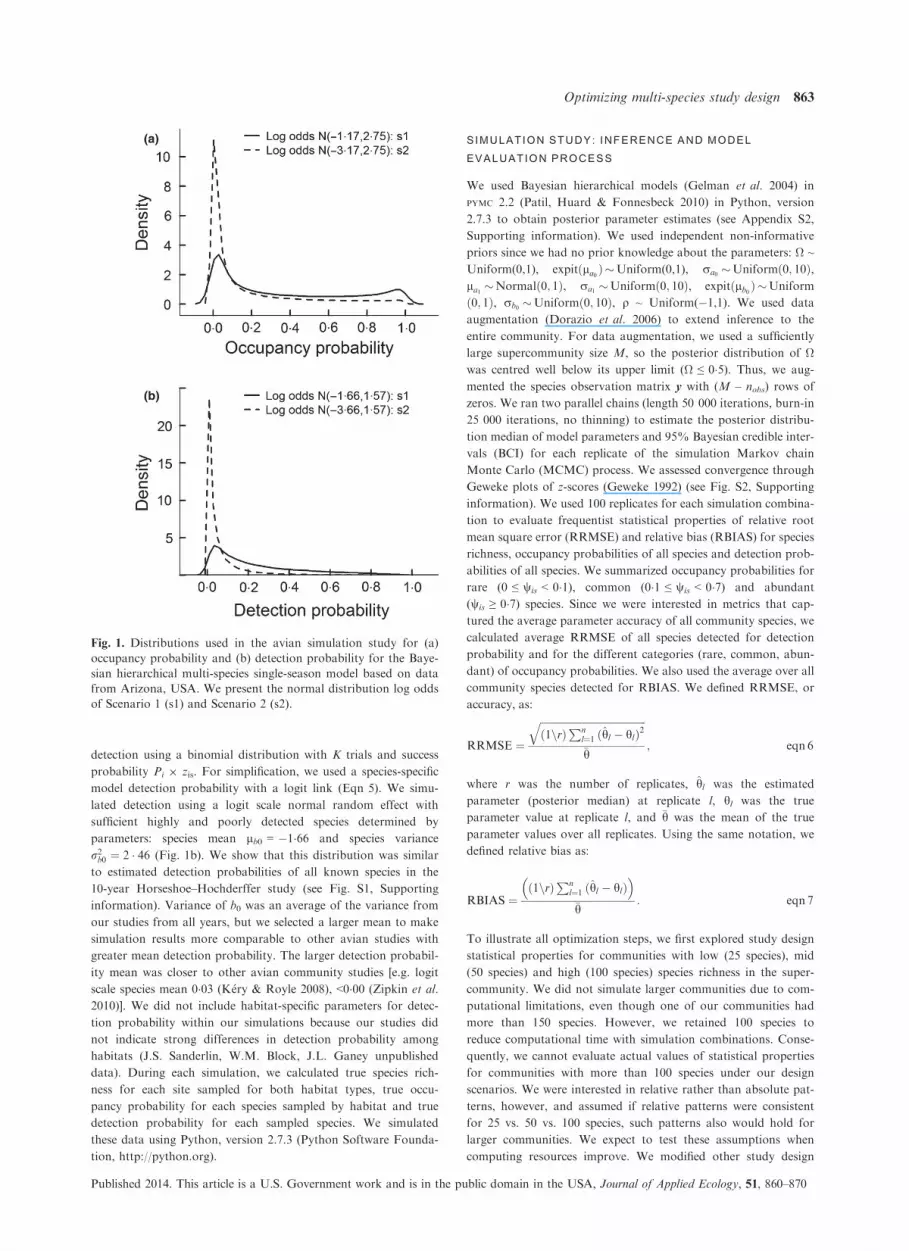
mined by parameters: species mean la0 = �1�17, species variance

r2a0 ¼ 7 � 56, habitat mean la1 = 0 and habitat variance r2a1 ¼ 1

(Fig. 1a). Variance of a0 was an average of the estimated variance

for mean occupancy across all years from our studies, but we

chose a larger mean to make simulation results more comparable

to other avian studies [e.g. logit scale species mean ~0�00 (Zipkin

et al. 2010)]. Increasing the occupancy mean facilitated our abil-

ity to generalize results to other avian studies with higher mean

occupancy.

We used stratified random sampling by habitat for sampling

site selection. Since habitat was evenly distributed across the

landscape in our simulations, this translates to ~50% survey

effort for each habitat. Given occupancy, we simulated species

Published 2014. This article is a U.S. Government work and is in the public domain in the USA, Journal of Applied Ecology, 51, 860–870

862 J. S. Sanderlin, W. M. Block & J. L. Ganey

detection using a binomial distribution with K trials and success

probability Pi 9 zis. For simplification, we used a species-specific

model detection probability with a logit link (Eqn 5). We simu-

lated detection using a logit scale normal random effect with

sufficient highly and poorly detected species determined by

parameters: species mean lb0 = �1�66 and species variance

r2b0 ¼ 2 � 46 (Fig. 1b). We show that this distribution was similar

to estimated detection probabilities of all known species in the

10-year Horseshoe–Hochderffer study (see Fig. S1, Supporting

information). Variance of b0 was an average of the variance from

our studies from all years, but we selected a larger mean to make

simulation results more comparable to other avian studies with

greater mean detection probability. The larger detection probabil-

ity mean was closer to other avian community studies [e.g. logit

scale species mean 0�03 (K�ery & Royle 2008), <0�00 (Zipkin et al.

2010)]. We did not include habitat-specific parameters for detec-

tion probability within our simulations because our studies did

not indicate strong differences in detection probability among

habitats (J.S. Sanderlin, W.M. Block, J.L. Ganey unpublished

data). During each simulation, we calculated true species rich-

ness for each site sampled for both habitat types, true occu-

pancy probability for each species sampled by habitat and true

detection probability for each sampled species. We simulated

these data using Python, version 2.7.3 (Python Software Founda-

tion, http://python.org).

SIMULATION STUDY: INFERENCE AND MODEL

EVALUATION PROCESS

We used Bayesian hierarchical models (Gelman et al. 2004) in

PYMC 2.2 (Patil, Huard & Fonnesbeck 2010) in Python, version

2.7.3 to obtain posterior parameter estimates (see Appendix S2,

Supporting information). We used independent non-informative

priors since we had no prior knowledge about the parameters: Ω ~

Uniform(0,1), expitðla0 Þ�Uniform(0,1), ra0 �Uniformð0; 10Þ,la1 �Normalð0; 1Þ, ra1 �Uniformð0; 10Þ, expitðlb0 Þ�Uniform

ð0; 1Þ, rb0 �Uniformð0; 10Þ, q ~ Uniform(�1,1). We used data

augmentation (Dorazio et al. 2006) to extend inference to the

entire community. For data augmentation, we used a sufficiently

large supercommunity size M, so the posterior distribution of Ωwas centred well below its upper limit (Ω ≤ 0�5). Thus, we aug-

mented the species observation matrix y with (M – nobs) rows of

zeros. We ran two parallel chains (length 50 000 iterations, burn-in

25 000 iterations, no thinning) to estimate the posterior distribu-

tion median of model parameters and 95% Bayesian credible inter-

vals (BCI) for each replicate of the simulation Markov chain

Monte Carlo (MCMC) process. We assessed convergence through

Geweke plots of z-scores (Geweke 1992) (see Fig. S2, Supporting

information). We used 100 replicates for each simulation combina-

tion to evaluate frequentist statistical properties of relative root

mean square error (RRMSE) and relative bias (RBIAS) for species

richness, occupancy probabilities of all species and detection prob-

abilities of all species. We summarized occupancy probabilities for

rare (0 ≤ wis < 0�1), common (0�1 ≤ wis < 0�7) and abundant

(wis ≥ 0�7) species. Since we were interested in metrics that cap-

tured the average parameter accuracy of all community species, we

calculated average RRMSE of all species detected for detection

probability and for the different categories (rare, common, abun-

dant) of occupancy probabilities. We also used the average over all

community species detected for RBIAS. We defined RRMSE, or

accuracy, as:

RRMSE ¼ffiffiffiffiffiffiffiffiffiffiffiffiffiffiffiffiffiffiffiffiffiffiffiffiffiffiffiffiffiffiffiffiffiffiffiffiffiffiffiffiffiffið1nrÞPn

l¼1 ðhl � hlÞ2q

�h; eqn 6

where r was the number of replicates, hl was the estimated

parameter (posterior median) at replicate l, hl was the true

parameter value at replicate l, and �h was the mean of the true

parameter values over all replicates. Using the same notation, we

defined relative bias as:

RBIAS ¼ð1nrÞPn

l¼1 ðhl � hlÞ� �

�h: eqn 7

To illustrate all optimization steps, we first explored study design

statistical properties for communities with low (25 species), mid

(50 species) and high (100 species) species richness in the super-

community. We did not simulate larger communities due to com-

putational limitations, even though one of our communities had

more than 150 species. However, we retained 100 species to

reduce computational time with simulation combinations. Conse-

quently, we cannot evaluate actual values of statistical properties

for communities with more than 100 species under our design

scenarios. We were interested in relative rather than absolute pat-

terns, however, and assumed if relative patterns were consistent

for 25 vs. 50 vs. 100 species, such patterns also would hold for

larger communities. We expect to test these assumptions when

computing resources improve. We modified other study design

(a)

(b)

Fig. 1. Distributions used in the avian simulation study for (a)

occupancy probability and (b) detection probability for the Baye-

sian hierarchical multi-species single-season model based on data

from Arizona, USA. We present the normal distribution log odds

of Scenario 1 (s1) and Scenario 2 (s2).

Published 2014. This article is a U.S. Government work and is in the public domain in the USA, Journal of Applied Ecology, 51, 860–870

Optimizing multi-species study design 863

parameters of number of sampling occasions and sites (or per-

centage of area covered since one site is equivalent to 1% of area

sampled within our simulations). We ran 47 simulation combina-

tions under Scenario 1 (Table 1). This was not a complete facto-

rial of all design combinations due to computing resource

limitations. Since we were interested in relative sampling design

performance and not specific statistical property estimates for

each design, we made inductive inference on incomplete designs

assuming these designs followed general complete design patterns

(e.g. relative study design performance for 25 vs. 50 vs. 100 spe-

cies was similar given species had the same community-level

parameters in our simulations). These assumptions would not be

valid for actual statistical property estimates. We recognize infer-

ence outside our parameter space may be weak if relative perfor-

mance does not hold for communities with >100 species.

We used Scenario 2 to illustrate the study design optimization

process using empirical avian data under step four and to explore

effects of decreased occupancy and detection on study design

with steps one, two and three. This scenario is applicable to simi-

lar communities in other study areas with similar occupancy and

detection parameter estimates. We decreased logit scale hyperpri-

or means for w to �3�17 and P to �3�66 to reflect our avian

study empirical estimates. To reduce computational time, we

focused on a subset of 40 parameter combinations with N = 25,

K = {2,. . .,11}, and s = {5,10,15,25}. Again, since we were inter-

ested in relative sampling design performance rather than specific

statistical property estimates for each design, we chose to opti-

mize with communities of size 25, since relative patterns were

consistent with 25, 50 and 100 species.

OPTIMIZATION PROCEDURE

Our final step illustrating the optimization process included use

of a constrained optimization framework to select optimal study

designs for species richness, occupancy for all rare species and

detection probability for all species in the community. Con-

strained optimization has three components: (i) decision vari-

ables, (ii) objective function and (iii) constraints (Taha 2011: 14).

Decision variables were number of sites and sampling occasions,

and constraints included project cost and maximized RRMSE

(minimized accuracy). We used the following cost function within

our optimization procedure:

C ¼ C0 þ C1 � sþ C2 � K� s; (eqn 8)

where s [s = 1,. . .,max(sites)] was the number of sites (all sites

had equal number of points on a transect); K [K = 1,. . .,max

(sampling occasions)] was the number of sampling occasions; C

was total cost; C0 was the initial project start-up cost which

included study design and equipment costs; C1 was the additional

establishment cost per site; and C2 was the additional cost to

sample each site per sampling occasion. For our example, we

used the following estimates: C0 = $20 000, C1 = $196 (1 day

technician salary, $10 equipment per site, $30 travel from pro-

rated vehicle rental and mileage) and C2 = $252 (one technician

salary for 6 h, including travel time, $100 equipment, $30 travel

and $5 data entry). Based on our field studies, we assumed that

one technician could sample 1 site per day. Increasing the number

of technicians would decrease C1 per site due to greater travel

efficiency.

Given RRMSE simulation values for each combination of sites

s and sampling occasions K, we optimized RRMSEðhÞs;K separately

for each parameter h (average rare species occupancy, species

richness, average detection probability of all species). Our objec-

tive function was: Minimize RRMSEðhÞs;K, subject to constraints:

C ¼ C0 þ C1 � sþ C2 � K� s� f;

RRMSEðhÞs;K � g

We constrained project cost limit below f and RRMSE below g.

We demonstrated the optimization process graphically using Sce-

nario 1 with 25 species and one habitat type. We also went

through the optimization process using our avian study hyperpri-

or estimates (Scenario 2), since RRMSE patterns were similar for

number of true species (25, 50, 100) and habitats within our sim-

ulations. Managers and researchers do not have to use RRMSE

for optimization; they could use RBIAS or any parameter suit-

able to their objectives.

Results

SIMULATION STUDY: SCENARIO 1

Under Scenario 1, species richness relative bias decreased

with increased sampling occasions (~50% RBIAS decrease

for each additional sampling occasion until approaching

RBIAS of zero) and slightly decreased with more sampled

area across all superpopulation size combinations (see

Fig. S3, Supporting information). For all design combina-

tions, RBIAS approached zero with increased sampling

occasions. Similarly, accuracy increased with increased

sampling occasions (~25% RRMSE decrease for each

additional sampling occasion) and slightly increased with

more sampled area across all superpopulation size combi-

nations (Fig. 2).

For all superpopulation size combinations, average

RBIAS for occupancy probability of all species was simi-

lar across percentage of area sampled and number of sam-

pling occasions for common and abundant species, but

rare species RBIAS decreased by ~33% for each

additional 5% of area sampled (see Figs S4, S5 and S6,

Table 1. Simulation study parameter combinations for illustrating

the avian study design optimization process with different super-

population sizes (N)

Parameter

Levels* for

N = 25

Levels for

N = 50

Levels†

for N = 100

K (sampling

occasions)

2, 3, 4, 5 2, 3, 4, 5 2, 3, 4, 5

s (sample sites)‡ 5, 10, 15,

25, 50, 75

5, 10,

15, 25

5, 10, 15

*We ran simulation combinations with 50 sites and 5 sampling

occasions, 50 sites and 10 sampling occasions, and 75 sites and 5

sampling occasions due to memory limitations.†We did not run simulation combinations with 25 sites due to

memory limitations.‡Number of sites = percentage of area sampled, because each

site = 1% of area.

Published 2014. This article is a U.S. Government work and is in the public domain in the USA, Journal of Applied Ecology, 51, 860–870

864 J. S. Sanderlin, W. M. Block & J. L. Ganey

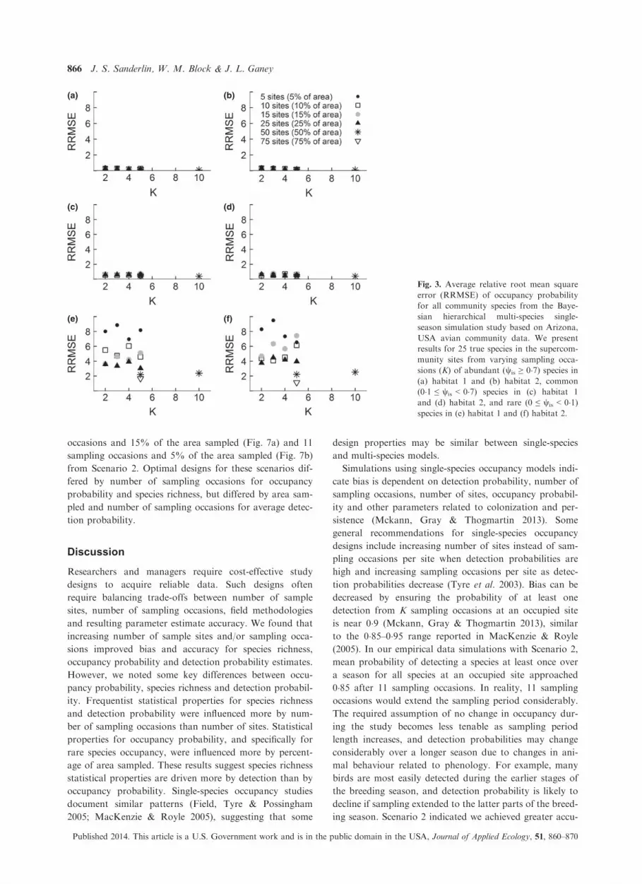
Supporting information). Average occupancy probability

RBIAS was positive for all rare species and close to zero

for abundant and common species. Similarly, accuracy

increased with increased percentage of sampled area for

rare species (on average, ~11% RRMSE decrease for each

additional 5% of area sampled, although not necessarily

true for all percentages of area sampled), but was the

same for abundant and common species across all super-

population size combinations (Fig. 3, see Figs S7 and S8,

Supporting information). Average detection probability

RBIAS of all species decreased with increased sampling

occasions across all superpopulation size combinations

(see Fig. S9, Supporting information). RBIAS was posi-

tive for all simulation combinations and approached zero

with increased sampling occasions at a decreasing rate of

~33% with each additional sampling occasion, although

this decline is not apparent for all sampling occasions.

Detection probability accuracy increased with increased

sampling occasions across all superpopulation size combi-

nations (Fig. 4).

SIMULATION STUDY: SCENARIO 2

Under Scenario 2, average detection probability RBIAS

(see Fig. S10, Supporting information) decreased

(approaching zero) with increased sampling occasions

and was positive. The pattern of average occupancy

probability RBIAS (see Fig. S11, Supporting informa-

tion) was the same as Scenario 1 across percentage of

area sampled and number of sampling occasions for all

species. Average occupancy probability RBIAS was posi-

tive for rare species and close to zero for abundant and

common species. Species richness RBIAS (see Fig. S12,

Supporting information) decreased with increased sam-

pling occasions and slightly decreased with more sampled

area. RBIAS converged to zero with increased sampling

occasions (~10) and was positively biased after 10

sampling occasions. Patterns of average RRMSE for

detection probability, occupancy probability and species

richness (see Figs S13–15, Supporting information) were

the same as Scenario 1. However, we did not achieve

the same level of average RRMSE for detection proba-

bility and species richness as Scenario 1, even after 11

sampling occasions.

OPTIMIZATION

Finally, to illustrate the last optimization process steps,

the species richness optimal study design from Scenario 1

required 5 sampling occasions and 10% of area sampled

(Fig. 5a). The optimal design for Scenario 2, where simu-

lations were based on our avian study hyperprior means

and variations, required 9 sampling occasions and 10% of

area sampled (Fig. 5b). Since the only variation in aver-

age occupancy probability RRMSE was with rare species,

we optimized only over rare species occupancy probabil-

ity. The rare species occupancy probability optimal study

design was to sample 25% of the area over 3 sampling

occasions under Scenario 1 (Fig. 6a) and 25% of the area

over 2 sampling occasions (Fig. 6b) from Scenario 2. The

detection probability optimal study design for Scenario 1

was similar to that for species richness with 5 sampling

(a) (b) (c)

(d) (e) (f)

Fig. 2. Species richness relative root mean square error (RRMSE) from the Bayesian hierarchical multi-species single-season simulation

study based on Arizona, USA avian community data sets. We display results from sampling occasions (K) for sites in habitat 2 for true

number of species in the supercommunity (a) 25, (b) 50 and (c) 100 and in habitat 1 for true number of species in the supercommunity

(d) 25, (e) 50 and (f) 100.

Published 2014. This article is a U.S. Government work and is in the public domain in the USA, Journal of Applied Ecology, 51, 860–870

Optimizing multi-species study design 865

occasions and 15% of the area sampled (Fig. 7a) and 11

sampling occasions and 5% of the area sampled (Fig. 7b)

from Scenario 2. Optimal designs for these scenarios dif-

fered by number of sampling occasions for occupancy

probability and species richness, but differed by area sam-

pled and number of sampling occasions for average detec-

tion probability.

Discussion

Researchers and managers require cost-effective study

designs to acquire reliable data. Such designs often

require balancing trade-offs between number of sample

sites, number of sampling occasions, field methodologies

and resulting parameter estimate accuracy. We found that

increasing number of sample sites and/or sampling occa-

sions improved bias and accuracy for species richness,

occupancy probability and detection probability estimates.

However, we noted some key differences between occu-

pancy probability, species richness and detection probabil-

ity. Frequentist statistical properties for species richness

and detection probability were influenced more by num-

ber of sampling occasions than number of sites. Statistical

properties for occupancy probability, and specifically for

rare species occupancy, were influenced more by percent-

age of area sampled. These results suggest species richness

statistical properties are driven more by detection than by

occupancy probability. Single-species occupancy studies

document similar patterns (Field, Tyre & Possingham

2005; MacKenzie & Royle 2005), suggesting that some

design properties may be similar between single-species

and multi-species models.

Simulations using single-species occupancy models indi-

cate bias is dependent on detection probability, number of

sampling occasions, number of sites, occupancy probabil-

ity and other parameters related to colonization and per-

sistence (Mckann, Gray & Thogmartin 2013). Some

general recommendations for single-species occupancy

designs include increasing number of sites instead of sam-

pling occasions per site when detection probabilities are

high and increasing sampling occasions per site as detec-

tion probabilities decrease (Tyre et al. 2003). Bias can be

decreased by ensuring the probability of at least one

detection from K sampling occasions at an occupied site

is near 0�9 (Mckann, Gray & Thogmartin 2013), similar

to the 0�85–0�95 range reported in MacKenzie & Royle

(2005). In our empirical data simulations with Scenario 2,

mean probability of detecting a species at least once over

a season for all species at an occupied site approached

0�85 after 11 sampling occasions. In reality, 11 sampling

occasions would extend the sampling period considerably.

The required assumption of no change in occupancy dur-

ing the study becomes less tenable as sampling period

length increases, and detection probabilities may change

considerably over a longer season due to changes in ani-

mal behaviour related to phenology. For example, many

birds are most easily detected during the earlier stages of

the breeding season, and detection probability is likely to

decline if sampling extended to the latter parts of the breed-

ing season. Scenario 2 indicated we achieved greater accu-

(a) (b)

(c) (d)

(e) (f)

Fig. 3. Average relative root mean square

error (RRMSE) of occupancy probability

for all community species from the Baye-

sian hierarchical multi-species single-

season simulation study based on Arizona,

USA avian community data. We present

results for 25 true species in the supercom-

munity sites from varying sampling occa-

sions (K) of abundant (wis ≥ 0�7) species in(a) habitat 1 and (b) habitat 2, common

(0�1 ≤ wis < 0�7) species in (c) habitat 1

and (d) habitat 2, and rare (0 ≤ wis < 0�1)species in (e) habitat 1 and (f) habitat 2.

Published 2014. This article is a U.S. Government work and is in the public domain in the USA, Journal of Applied Ecology, 51, 860–870

866 J. S. Sanderlin, W. M. Block & J. L. Ganey

racy for species richness and detection probability using a

higher detection probability mean hyperprior. Detection

probability could be increased using rigorous field methods,

such as double observers (Nichols et al. 2000).

Some caution is needed with regard to number of sam-

pling occasions for rare species occupancy, as small sample

stochasticity may have influenced rare species occupancy

optimization. Additionally, small sample stochasticity may

have influenced species richness and detection probability

optimization with number of sites. Optimization patterns

were consistent with number of sampling occasions for

species richness and detection probability and percentage

of area covered for rare species occupancy for different spe-

cies assemblages (25, 50, 100 species) (See Figs S16–18,

Supporting information), but caution is needed when mak-

ing inference on other species assemblages.

Application of our results is largely restricted to our

study areas. Application of our approach, however, can

extend to other situations. To make simulations more

broadly applicable, general guidelines are desirable based

on >2 avian data sets or a broader parameter space than

our simulations. Optimal study designs resulting from

empirical estimates in Scenario 2 differed from those

resulting from the more general Scenario 1. For species

richness and detection probability, the optimal number of

sampling occasions from Scenario 2 was almost double

the optimal number of sampling occasions from Scenario

1. However, for rare species, the optimal number of

sampling occasions was nearly identical to the optimal

number of sampling occasions under Scenario 1. For

species richness and rare species occupancy probability,

the area sampled was identical to Scenario 1, but was

reduced for detection probability. Based on these compar-

isons, we recommend increasing the number of sampling

occasions as much as possible within the sampling season

when detection probability per sampling occasion is low.

Our simulations were not an exhaustive set of study

design combinations, and the number of simulation itera-

tions was low for robust frequentist summaries. This low

number of iterations could affect error variance among

iterations of each simulation combination. If the error

variance among iterations was greater than the error vari-

ance among simulation combinations, this could affect

inference on optimal study designs. Variation among iter-

ations may be reduced with increased iterations. Addition-

ally, studies with real animals may require slightly more

sampling occasions and/or sites because real data are unli-

kely to conform to all parametric assumptions from simu-

lated data. We suggest practitioners look at general

patterns for optimal designs from our simulation combi-

nations instead of specific design recommendations.

Although beyond the scope of this paper, habitat config-

uration (random versus clumped) and the relationship of

avian detection and occupancy probabilities with habitat

configuration warrant further work. Our results should be

used with caution in highly heterogeneous areas, since we

assumed random habitat allocation across the landscape.

For example, rare species occupancy is likely to increase

with clumped habitat, whereas common species occupancy

may increase with dispersed habitat or be similar to occu-

pancy in clumped habitat. Optimal study design may vary

among landscapes depending on habitat composition and

configuration. We also may be able to increase overall

detection probabilities with fewer sampling occasions using

a double-observer approach (Nichols et al. 2000), although

the cost-efficiency of adding another observer while reduc-

ing the number of sampling occasions should be evaluated.

In addition, we could explore hybrid designs with some

sites sampled for more sampling occasions, while sampling

(a)

(b)

(c)

Fig. 4. Average relative root mean square error (RRMSE) of

detection probability for all community species from the Bayesian

hierarchical multi-species single-season simulation study based on

Arizona, USA avian community data sets. We display results

from sampling occasions (K), and true number of species for sites

in the supercommunity of (a) 100, (b) 50 and (c) 25 species.

Published 2014. This article is a U.S. Government work and is in the public domain in the USA, Journal of Applied Ecology, 51, 860–870

Optimizing multi-species study design 867

some sites for fewer sampling occasions. This could

allow for more sites sampled within fixed project cost,

allowing for better rare species occupancy probability

estimates. This is similar to the double sampling approach

(MacKenzie & Royle 2005), but instead of a portion of

sites sampled once they would be sampled at least twice

so detection and occupancy probability are estimable

within the occupancy model. Hybrid designs could

include other designs suited for rare species [e.g. adaptive

sampling (Thompson 1992), two-phase adaptive

approaches (Pacifici, Dorazio & Conroy 2012)].

Management implications

People work with fixed and limited budgets, whether for

research or management. Given budget constraints,

study designs must be cost-efficient while providing

reliable knowledge. Our results indicate the need to

ensure adequate sampling of rare species and demon-

strate that optimal design features differ among statisti-

cal parameters and between rare and common species.

Our approach allows researchers and managers to better

understand trade-offs between increasing sampling

occasions versus sites relative to parameter statistical

properties. These results and optimization process may

assist with designing studies that adequately and effi-

ciently monitor most species using a coarse-filter

approach (e.g. Noss 1987), while focusing resources on a

reduced number of species within a fine-filter approach.

Optimal design issues are important for implementing

monitoring programmes that meet objectives given

limited funds.

(a) (b)

Fig. 5. Species richness optimization of

relative root mean square error (RRMSE)

at fixed total project cost ($50 000 USD)

based on the Bayesian hierarchical multi-

species single-season simulation study from

Arizona, USA avian community data sets.

Arrows indicate optimal study designs for

Scenario 1 (a) and Scenario 2 using empir-

ical data (b). The figure does not show

sampling occasions, but these data are

available from the authors.

(a) (b)

Fig. 6. Optimization of average relative

root mean square error (RRMSE) in rare

species occupancy probability at fixed total

project cost ($50 000 USD) based on the

Bayesian hierarchical multi-species single-

season simulation study from Arizona,

USA avian community data sets. Arrows

indicate optimal study designs for Scenario

1 (a) and Scenario 2 using empirical data

(b). The figure does not show sampling

occasions, but these data are available

from the authors.

(a) (b)

Fig. 7. Optimization of average relative

root mean square error (RRMSE) in

detection probability over all community

species at fixed total project cost ($50 000

USD) based on the Bayesian hierarchical

multi-species single-season simulation

study from Arizona, USA avian commu-

nity data sets. Arrows indicate optimal

study designs for Scenario 1 (a) and

Scenario 2 using empirical data (b). The

figure does not show sampling occasions,

but these data are available from the

authors.

Published 2014. This article is a U.S. Government work and is in the public domain in the USA, Journal of Applied Ecology, 51, 860–870

868 J. S. Sanderlin, W. M. Block & J. L. Ganey

Acknowledgements

National Fire Plan supported J.S.S. We thank J.A. Royle for helpful

analysis discussions, field crews, and Coronado National Forest, Coconino

National Forest, The Nature Conservancy, Fort Huachuca, Santa Rita

Experimental Range and Audubon Research Ranch for logistical

assistance. B. J. Bird reviewed statistical methods, and K. McKelvey,

V. Ruiz-Guti�errez and three anonymous reviewers provided helpful

reviews on manuscript versions.

References

Bailey, L.L., Simons, T.R. & Pollock, K.H. (2004) Estimating site occu-

pancy and species detection probability parameters for terrestrial sala-

manders. Ecological Applications, 14, 692–702.Bailey, L.L., Hines, J.E., Nichols, J.D. & MacKenzie, D.I. (2007) Sam-

pling design trade-offs in occupancy studies with imperfect detection:

examples and software. Ecological Applications, 17, 281–290.Boulinier, T., Nichols, J.D., Sauer, J.R., Hines, J.E. & Pollock, K.H.

(1998) Estimating species richness: the importance of heterogeneity in

species detectability. Ecology, 79, 1018–1028.DeWan, A.A. & Zipkin, E.F. (2010) An integrated sampling and analysis

approach for improved biodiversity monitoring. Environmental Manage-

ment, 45, 1223–1230.Dorazio, R.M., Royle, J.A., S€oderstr€om, B. & Glimsk€ar, A. (2006) Esti-

mating species richness and accumulation by modeling species occur-

rence and detectability. Ecology, 87, 842–854.Field, S.A., Tyre, A.J. & Possingham, H.P. (2005) Optimizing allocation

of monitoring effort under economic and observational constraints.

Journal of Wildlife Management, 69, 473–482.Gelman, A., Carlin, J.B., Stern, H.S. & Rubin, D.B. (2004) Bayesian Data

Analysis, 2nd edn. Chapman and Hall/CRC, New York.

Geweke, J. (1992) Evaluating the accuracy of sampling-based approaches

to the calculation posterior moments. Bayesian Statistics, Vol. 4 (eds

J.M. Bernardo, J.O. Berger, A.P. Dawid & A.F.M. Smith), pp. 169–193. Oxford University Press, Oxford.

Guillera-Arroita, G., Ridout, M.S. & Morgan, B.J.T. (2010) Design of

occupancy studies with imperfect detection. Methods in Ecology and

Evolution, 1, 131–139.Hanski, I. (1994) A practical model of metapopulation dynamics. Journal

of Animal Ecology, 63, 151–162.Joseph, L.N., Field, S.A., Wilcox, C. & Possingham, H.P. (2006) Pres-

ence-absence versus abundance data for monitoring threatened species.

Conservation Biology, 20, 1679–1687.K�ery, M. & Royle, J.A. (2008) Hierarchical Bayes estimation of species

richness and occupancy in spatially replicated surveys. Journal of

Applied Ecology, 45, 589–598.K�ery, M. & Schmid, H. (2006) Estimating species richness: calibrating a

large avian monitoring programme. Journal of Applied Ecology, 43,

101–110.Legg, C.J. & Nagy, L. (2006) Why most conservation monitoring is, but

not need be, a waste of time. Journal of Environmental Management, 78,

194–199.MacKenzie, D.I. & Royle, J.A. (2005) Designing occupancy studies: gen-

eral advice and allocating survey effort. Journal of Applied Ecology, 42,

1105–1114.MacKenzie, D.I., Nichols, J.D., Lachman, G.B., Droege, S., Royle, J.A. &

Langtimm, C.A. (2002) Estimating site occupancy rates when detection

probabilities are less than one. Ecology, 83, 2248–2255.MacKenzie, D.I., Nichols, J.D., Royle, J.A., Pollock, K.P., Bailey, L.L. &

Hines, J.E. (2006) Occupancy Estimation and Modeling: Inferring Patterns

and Dynamics of Species Occurrence. Academic Press, San Diego, CA, USA.

Manley, P.N., Zielinski, W.J., Schlesinger, M.D. & Mori, S.R. (2004)

Evaluation of a multi-species approach to monitoring species at the eco-

regional scale. Ecological Applications, 14, 296–310.Mckann, P.C., Gray, B.R. & Thogmartin, W.E. (2013) Small sample bias in

dynamic occupancy models. Journal ofWildlife Management, 77, 172–180.Nichols, J.D., Hines, J.E., Sauer, J.R., Fallon, F.W., Fallon, J.E. &

Heglund, P.J. (2000) A double-observer approach for estimating

detection probability and abundance from point counts. The Auk, 117,

393–408.Noon, B.R., Bailey, L.L., Sisk, T.D. & McKelvey, K.S. (2012) Efficient

species-level monitoring at the landscape scale. Conservation Biology,

26, 432–441.

Noss, R.F. (1987) From plant communities to landscapes in conservation

inventories: a look at the Nature Conservancy (USA). Biological

Conservation, 41, 11–37.Pacifici, K., Dorazio, R.M. & Conroy, M.J. (2012) A two-phase sampling

design for increasing detections of rare species in occupancy surveys.

Methods in Ecology and Evolution, 3, 721–730.Patil, A., Huard, D. & Fonnesbeck, C.J. (2010) PyMC: Bayesian stochas-

tic modeling in Python. Journal of Statistical Software, 35, 1–81.Royle, J.A. & Dorazio, R.M. (2008) Hierarchical Modeling and Inference

in Ecology. Academic Press, New York.

Royle, J.A. & K�ery, M. (2007) A Bayesian state-space formulation of

dynamic occupancy models. Ecology, 88, 1813–1823.Russell, R.E., Royle, J.A., Saab, V.A., Lehmkuhl, J.F., Block, W.M. &

Sauer, J.R. (2009) Modeling the effects of environmental disturbance on

wildlife communities: avian responses to prescribed fire. Ecological

Applications, 19, 1253–1263.Sauer, J.R., Blank, P.J., Zipkin, E.F., Fallon, J.E. & Fallon, F.W.

(2013) Using multi-species occupancy models in structured decision

making on managed lands. Journal of Wildlife Management, 77, 117–127.

Simberloff, D. (1998) Flagships, umbrellas, and keystones: is single-species

management pass�e in the landscape era? Biological Conservation, 83,

247–257.Taha, H.A. (2011) Operations Research An Introduction, 9th edn. Prentice

Hall, New Jersey, USA.

Thompson, S.K. (1992) Sampling. Wiley and Sons, New York, NY, USA.

Tyre, A.J., Tenhumberg, B., Field, S.A., Niejalke, D., Parris, K. &

Possingham, H.P. (2003) Improving precision and reducing bias in

biological surveys by estimating false negative error rates in pres-

ence-absence data. Ecological Applications, 13, 1790–1801.Waddle, J.H., Dorazio, R.M., Walls, S.C., Rice, K.G., Beauchamp, J.,

Schuman, M.J. & Mazzottii, F.J. (2010) A new parameterization for

estimating co-occurrence of interacting species. Ecological Applications,

20, 1467–1475.Walls, S.C., Waddle, J.H. & Dorazio, R.M. (2011) Estimating occupancy

dynamics in an anuran assemblage from Louisiana, USA. Journal of

Wildlife Management, 75, 751–761.Yoccoz, N.G., Nichols, J.D. & Boulinier, T. (2001) Monitoring of biologi-

cal diversity in space and time. Trends in Ecology and Evolution, 16,

446–453.Zipkin, E.F., Royle, J.A., Dawson, D.K. & Bates, S. (2010) Multi-species

occurrence models to evaluate the effects of conservation and manage-

ment actions. Biological Conservation, 143, 479–484.

Received 17 August 2013; accepted 11 March 2014

Handling Editor: J. Matthiopoulos

Supporting Information

Additional Supporting Information may be found in the online version

of this article.

Appendix S1. Methodological details for avian community data

sets.

Appendix S2. PyMC computer code.

Fig. S1. Histogram of median posterior estimates of detection

probabilities of known species from 10-year avian study.

Fig. S2. Geweke plot of z-scores for one replicate of the simula-

tion-MCMC process.

Fig. S3. RBIAS of species richness from the Bayesian hierarchical

multi-species single-season simulation study.

Fig. S4. RBIAS of occupancy probability for 25 species in the su-

percommunity from the Bayesian hierarchical multi-species sin-

gle-season simulation study.

Published 2014. This article is a U.S. Government work and is in the public domain in the USA, Journal of Applied Ecology, 51, 860–870

Optimizing multi-species study design 869

Fig. S5. RBIAS of occupancy probability for 50 species in the

supercommunity from the Bayesian hierarchical multi-species

single-season simulation study.

Fig. S6. RBIAS of occupancy probability for 100 species in the

supercommunity from the Bayesian hierarchical multi-species

single-season simulation study.

Fig. S7. RRMSE of occupancy probability for 50 species in the

supercommunity from the Bayesian hierarchical multi-species

single-season simulation study.

Fig. S8. RRMSE of occupancy probability for 100 species in the

supercommunity from the Bayesian hierarchical multi-species sin-

gle-season simulation study.

Fig. S9. RBIAS of detection probability from the Bayesian

hierarchical multi-species single-season simulation study.

Fig. S10. RBIAS of detection probability from the Bayesian hier-

archical multi-species single-season simulation study from the

Scenario 2.

Fig. S11. RBIAS of occupancy probability from the Bayesian

hierarchical multi-species single-season simulation study from

Scenario 2.

Fig. S12. RBIAS of species richness from the Bayesian hierarchi-

cal multi-species single-season simulation study from Scenario 2.

Fig. S13. RRMSE of detection probability from the Bayesian

hierarchical multi-species single-season simulation study from

Scenario 2.

Fig. S14. RRMSE of occupancy probability from the Bayesian

hierarchical multi-species single-season simulation study Scenario

2.

Fig. S15. RRMSE of species richness from the Bayesian hierar-

chical multi-species single-season simulation study from Scenario

2.

Fig. S16. Species richness optimization from the Bayesian hierar-

chical multi-species single-season simulation study based on avian

community data sets from Arizona, USA for different species

assemblages.

Fig. S17. Occupancy probability of rare species optimization

from the Bayesian hierarchical multi-species single-season simula-

tion study based on avian community data sets from Arizona,

USA for different species assemblages.

Fig. S18. Detection probability optimization from the Bayesian

hierarchical multi-species single-season simulation study based on

avian community data sets from Arizona, USA for different

species assemblages.

Published 2014. This article is a U.S. Government work and is in the public domain in the USA, Journal of Applied Ecology, 51, 860–870

870 J. S. Sanderlin, W. M. Block & J. L. Ganey