Optimizing denominator data estimation through a multimodelapproach

Ward Bryssinckx1, Els Ducheyne1, Veerle Versteirt1, Herwig Leirs2, Guy Hendrickx1

1Avia-GIS, Zoersel, Belgium; 2Evolutionary Ecology Group, University of Antwerp, Antwerp, Belgium

Abstract. To assess the risk of (zoonotic) disease transmission in developing countries, decision makers generally rely on dis-tribution estimates of animals from survey records or projections of historical enumeration results. Given the high cost oflarge-scale surveys, the sample size is often restricted and the accuracy of estimates is therefore low, especially when spatialhigh-resolution is applied. This study explores possibilities of improving the accuracy of livestock distribution maps with-out additional samples using spatial modelling based on regression tree forest models, developed using subsets of the Uganda2008 Livestock Census data, and several covariates. The accuracy of these spatial models as well as the accuracy of anensemble of a spatial model and direct estimate was compared to direct estimates and “true” livestock figures based on theentire dataset. The new approach is shown to effectively increase the livestock estimate accuracy (median relative errordecrease of 0.166-0.037 for total sample sizes of 80-1,600 animals, respectively). This outcome suggests that the accuracylevels obtained with direct estimates can indeed be achieved with lower sample sizes and the multimodel approach present-ed here, indicating a more efficient use of financial resources.

Keywords: spatial modelling, survey design, extensive livestock systems, multimodel models, Uganda.

Introduction

Animal distribution maps are essential for assessingdisease transmission risk and providing estimates ofpoverty and nutritional needs (Kruska et al., 2003;IFPRI, 2010). In most developed countries this infor-mation is available through a mandatory livestock reg-istration procedure (Augsburg, 1990). In developingcountries, however, this information often is poor;often based on outdated distribution data or projec-tions of enumeration results (Wanyoike et al., 2005).

Direct estimates of livestock numbers are made bymultiplying the average number of livestock observedin sampled households by the total number of house-holds. These data can be aggregated and mapped ondifferent administrative unit levels as done for theGlobal Livestock Production and Health Atlas(GLiPHA) (Clements et al., 2002). This surveyapproach is very straightforward and easy to imple-ment but it also has drawbacks. Being far from a fullcensus, the results of are prone to sampling error. Incase of a large sample size, sufficiently qualified staff isdifficult to find and less well-trained enumerators and

data entry personnel might lead to inaccuricies (FAO,1996). In addition, survey costs can be high for largesamples and the accuracy of livestock estimates indeveloping countries is therefore often restricted byavailable funding. In order to improve accuracy with-out increasing the number of samples, methods forimproving data processing for livestock abundancemaps are needed.

Spatial modelling is commonly adopted and spatialmultiple regression has already been used for livestockestimates and this approach is extensively documentedfor the Gridded Livestock of the World (GLW) (Wintand Robinson, 2007). However, the assumptions madeby this spatial modelling technique require statisticiansto assess whether it is appropriate to apply them usinggiven data. The livestock distribution maps from linearregression models offer continuous estimates of live-stock abundance on a pixel by pixel basis, even inregions lacking samples. This leads to a false sense ofaccuracy since, in most cases, single pixel values cannotbe used directly and data must be interpreted onregional basis. The extent at which individual pixel val-ues must be aggregated in order to obtain reliable fig-ures is unknown (Wint and Robinson, 2007).

Modelling can fill these gaps if adjusted to matchtotal livestock numbers at the country level estimates,e.g. by the Food and Agriculture Organization (FAO).Another approach is to include more than one esti-mate in an ensemble of models using multimodel infer-ence. This technique has been applied in a variety of

Corresponding author:Ward BryssinckxAvia-GISRisschotlei 33, BE-2980 Zoersel, BelgiumTel./Fax +32 3458-2979E-mail: wbryssinckx@avia-gis.be

Geospatial Health 8(2), 2014, pp. 573-582

W. Bryssinckx et al. - Geospatial Health 8(2), 2014, pp. 573-582574

fields including species distribution modelling (Wintleet al., 2003). Bayesian inference and multimodel infer-ence are most commonly used when combining multi-ple models (Link and Barker, 2006). Both theseapproaches require weighting of the different modelsto represent how well each model approximates the“true values”. The methodologies also differ withrespect to the selection criterion used to assess whichmodel fits observed data best. Both Akaike’s informa-tion criterion (AIC) and a Bayesian information crite-rion (BIC) have been used for this purpose (Wintle etal., 2003; Burnham and Anderson, 2004; Link andBarker, 2006). The latter two authors suggest thatassigning weights should be based on model evalua-tion using different datasets. Regardless which weightassignment method is applied, the models included inthe ensemble should have sufficient informative valuein order to contribute to the added value of the ensem-ble. As livestock distribution data in countries withpredominantly extensive livestock systems are sparseand often outdated, prior knowledge for a BIC is inmost cases inaccurate. The ensemble approach pro-posed in this study includes direct estimate of livestocknumbers. When looking at this direct estimate as oneof the models in the ensemble, the AIC would assignmost of the weight to the direct estimate as it perfect-ly fits the training data. Therefore, AIC is not suitablefor weight allocation either. Hence, with the overallaim of increasing accuracy in extensive systems wherethe number of survey samples is limited, anotherensemble approach is proposed for processing georef-erenced livestock counts. Direct estimates were aver-aged with regression tree forests (RTF), or randomforest results, for which use is not restricted to contin-uous predictor variables or unimodal data. The aim ofthis work is to assess if this data processing techniqueis able to increase the accuracy of livestock abundancereports based on agricultural survey data.

Since the multimodel approach was foreseen to bepart of an unsupervised algorithm based on modellingtechniques less prone to collinearity and distributionalassumptions, linear regression was avoided and insteadrandom forests adopted to estimate denominator data.A random forest consists of multiple regression trees,which partition data according to a series of splits inone or more dimensions. This results in a structurewhich can be used to classify a data point for which thevalue is not known. The value to be addressed at thedata point is the mean of values within the class whichwas found by answering the binary questions at eachsplit of the regression tree.

With the aim in mind to assess if this data process-

ing technique would be able to increase the accuracyof livestock abundance reports based on agriculturalsurvey data, direct estimates were averaged with ran-dom forest results, for which the use is not restrictedto continuous predictor variables or unimodal data.

Materials and methods

Study site

Uganda is a middle-sized country in the eastern partof Africa (mostly between 4° N and 2° S, and 29° Eand 35° E) surrounded by South Sudan, Kenya,Tanzania, Rwanda and the Democratic Republic of theCongo. The total area is 241,139 km2, 18% of whichis covered by fresh-water lakes. Although this could bean ideal water source for livestock, the major lakes(Lake Victoria, Lake Wamala, Lake Albert, LakeGeorge and the Kyoga/Kwania lake complex) thatmake it up is more of interest for the fishery industry(Ibale, 1998). While the average altitude is about 1,100metres above mean sea level (with Mount Stanley thehighest peak at 5,113 m), lower altitudes are foundnear the South Sudanese plain in the north. The rela-tively high altitude tempers the tropical climate at 16-26 °C between April and November but 30 °C is gen-erally exceeded between December and March. Whilerainfall is most abundant in the South (>2,100 mm),where areas are well covered by vegetation, it decreas-es towards the Northeast (500 mm) resulting in savan-nas and dry plains.

In rural communities, agricultural production andlivestock abundance do not only indicate food security,but also reflect current and future economic security asreplacement of livestock owned by a household isbelieved to be home-bred thus limiting the extra needfor financial capital to sustain or increase herd sizes. Incontrast, without previous livestock ownership, start-upis difficult requiring spending savings (Upton, 2004). Inthe eastern, northern and western region, the majorityof households live in rural communities in which 72%of all households owns at least one kind of livestock. Inthe central region, urban settlements are more numer-ous and only 56% of all households owns livestock(MAAIF, 2009). However, agriculture also plays amajor role in urban areas, as food prices determine thelivelihood of people living there.

Livestock-rearing in some parts of northern Ugandais complicated by the presence of armed rebel move-ments forcing people to stay in refugee settlementswith uncertainty of feeding an the general economy.Although relative safety has returned, there is still a

W. Bryssinckx et al. - Geospatial Health 8(2), 2014, pp. 573-582 575

long way to restore livestock numbers to previousnumbers (USAID, 2008). Uganda is currently subdi-vided in 111 districts, an increase compared to theperiod between 2007 and 2009 when only 80 districtsexisted (mean surface 3,000 km2). Districts are furtherdivided into counties (mean surface 1,500 km2), sub-counties (mean surface 200 km2) and parishes (meansurface 45 km2) containing several villages.

Livestock data

In 2008, the Animal Industry and Fisheries (MAAIF)division of the Ministry of Agriculture, implementedan extensive livestock survey with technical supportfor data collection, processing and reporting from theUganda Bureau of Statistics (UBOS). A two-stage sam-pling approach was applied with sub-counties wererandomly selected from each district at the first stage.At the second stage, at least 50 enumeration areas(EAs) were sampled from each selected sub-county.One EA includes 200 households. The same enumera-tion area sampling frame as developed for the 2002Population and Housing Census was applied. In total8,870 EAs were enumerated. Previous livestock countsdate from 2002, i.e. the Population and HousingCensus (UBOS, 2002) and 2005, i.e. the UgandaNational Household Survey (UBOS, 2007).

Modelling livestock distribution

Obtaining direct estimates of cattle numbersthrough aggregating sampled data on a specifiedadministrative unit level is straightforward. It is alsoself-evident that the accuracy of direct estimates willbe higher for a larger number of samples. Reportingdenominator data on a lower administrative unit level(smaller area size) will diminish the number of EAsthat belong to one unit and therefore rato of estimatesensitivity to sampling error will increase. When vali-dating a statistical model using resampling procedures,the estimated values for training data entries will tendto regress towards an average value of observed casesin similar conditions. This generalization is used in theproposed methodology to lower the degree of under-and over-estimation of cattle numbers. Given therestrictions associated with unsupervised modelling,e.g. using linear regression techniques, a random for-est approach was followed. For each forest 500 treeswere grown. At each split one third of the predictorvariables were randomly sampled as candidates. Theminimum size of terminal nodes was set to five obser-vations. Before the models were trained, a logarithmic

transformation was applied on the denominator datain order to have similar residuals for different livestocknumbers. Before error assessment, back transforma-tion was done.

Predictor variables

Distance to water in km was deduced from the con-solidated VMap0 river-surface water body networkdata (NIMA, 1997) and used as proxy for access todrinking water for herds (Luke, 1987). A preliminaryanalysis indicated that the majority of large herds werelocated at moderate altitudes (1,000-1,500 m) withlow slope values (0°-2°). Given that denominator dataresponded differently for increasing altitude and slopevalues, both variables were retained as candidate pre-dictor variables.

The total human population estimates, as preparedby the FAO for the World Bank’s rural developmentstrategy review, was included since it was shown thatthere is a positive correlation between human and live-stock population densities (Lapar and Jabbar, 2003).However, for urban areas with high population densi-ties, industrialisation might offer job opportunitiesother than agricultural activities such as livestock rear-ing (Iruonagbe, 2009). As surrogate for this urbancharacter, “night-time lights” (NOAA NationalGeophysical Data Center, 2003) was used (Amaral etal., 2006). Accessibility is another auxiliary variablerelated to economic activities, which gives the estimat-ed travel time (in min) needed to reach a major city, i.e.a city with 50,000 or more people in the year 2000(JRC Global Environmental Monitoring Unit, 2008).

Long-term, average monthly temperature and precip-itation values were derived from the WorldClim dataset(Hijmans et al., 2005). For all continuous variables, themean value was assigned to the administrative units.Finally, the GLC 2000 1-km global land cover (JRCLand Resource Management Unit, 2000) was used forland cover classification. The majority class wasassigned to the administrative unit resulting in fourpredominant land cover types: crop/forest, croplands,forest and shrublands. A suitability mask was used toexclude unpopulated areas such as water-bodies, gameand nature reserves from the predictor variable layers.

The targetted added value of applying random for-est consists in averaging under- and over-estimates ofcattle numbers. This generalisation of denominatordata will not always be beneficial for the accuracy ofestimates as is the case when the number of animalsreally deviates from what one would expect based onthe assessment of environmental parameters. A wrong

W. Bryssinckx et al. - Geospatial Health 8(2), 2014, pp. 573-582576

estimate of cattle numbers can arise from an incom-plete set of predictor variables. Missing predictor vari-ables are very likely as herding of cattle or otherdomestic animals remains the choice of the individualsin the human population. Their decision to rear ani-mals depends on many variables, which may not all becovered by available datasets.

Because direct estimates do capture local differencesin livestock abundance, the performance of a multi-model approach was assessed as well. The mostnotable difference with existing multimodelapproaches is that only two models were considered:(i) a direct estimate of livestock numbers where inac-curacies mostly result from sampling error; and (ii) aregression tree forest which generalises livestockabundance for subsets of similar administrative units.Both these models are averaged using uninformativeweights (unweighted average). A multimodelapproach is also more likely to represent a consensusopinion of the two approaches, the closest of whichto what would have been observed if a total censuswas performed, would not be known (Millington andPerry, 2011).

Sample subsets

In order to test the robustness of the multimodelapproach, 250 survey simulations were tested withdifferent sample subsets for each run. For reasons ofsimplicity, tests were restricted to a spatially randomsampling strategy. No other strategies such as strati-fied or clustered sampling were considered. Becausethe sample density of the Uganda 2008 NationalLivestock Census is not homogeneous throughout theentire country, it is not sufficient to take a randomsample from the list of visited EAs. Instead, locationswithin the study area had to be selected randomly andthe nearest visited EA sought to approximate a spa-tially random sample. As long as the number of sam-ples in the subset remains small as compared to thetotal dataset, it was assumed that samples were notdepleted locally and randomness was assured. Thevast number of samples taken during the Uganda 2008Livestock Census enabled generating input datasetsfor all repetitions as well as comparing results from aseries of increasing sample sizes. In this study, totalsample sizes of 80, 240, 400, 560, 720, 880, 1,040,1,200, 1,360, 1,520 and 1,600 EAs were considered toevaluate the impact of varying sample size. The ran-dom selection of samples was automated in the R sta-tistical computing and graphics environment (RDevelopment Core Team, 2012).

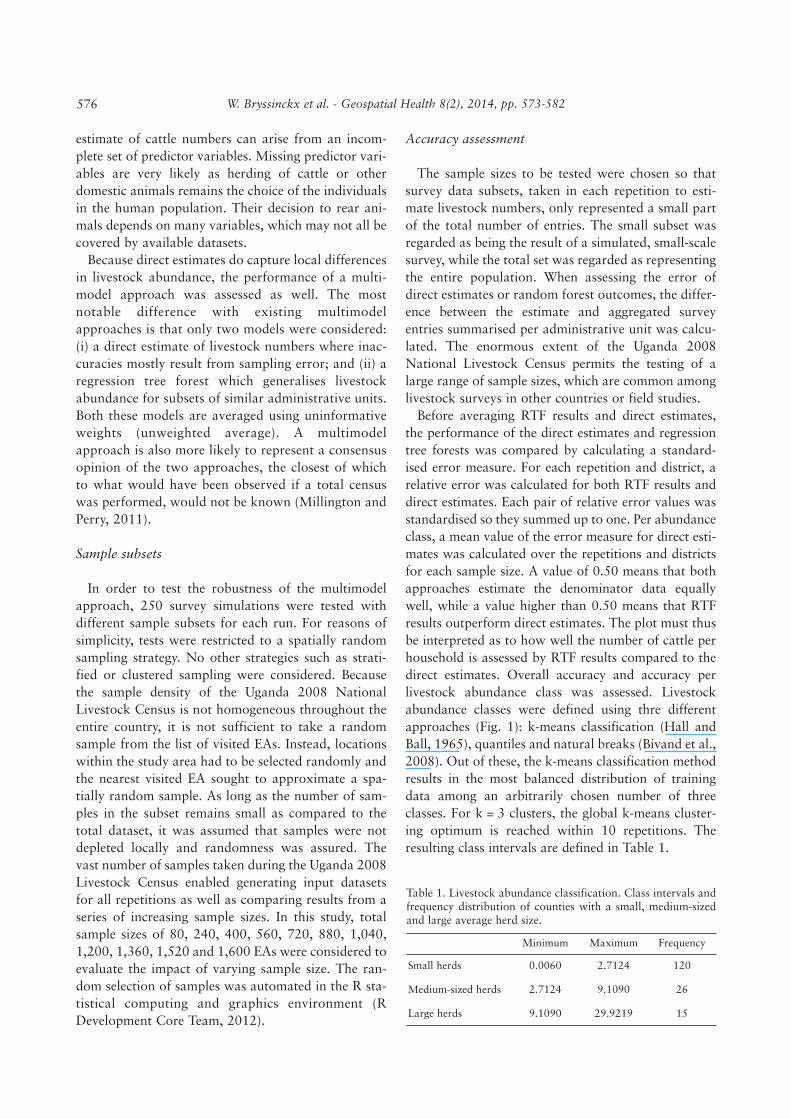
Accuracy assessment

The sample sizes to be tested were chosen so thatsurvey data subsets, taken in each repetition to esti-mate livestock numbers, only represented a small partof the total number of entries. The small subset wasregarded as being the result of a simulated, small-scalesurvey, while the total set was regarded as representingthe entire population. When assessing the error ofdirect estimates or random forest outcomes, the differ-ence between the estimate and aggregated surveyentries summarised per administrative unit was calcu-lated. The enormous extent of the Uganda 2008National Livestock Census permits the testing of alarge range of sample sizes, which are common amonglivestock surveys in other countries or field studies.

Before averaging RTF results and direct estimates,the performance of the direct estimates and regressiontree forests was compared by calculating a standard-ised error measure. For each repetition and district, arelative error was calculated for both RTF results anddirect estimates. Each pair of relative error values wasstandardised so they summed up to one. Per abundanceclass, a mean value of the error measure for direct esti-mates was calculated over the repetitions and districtsfor each sample size. A value of 0.50 means that bothapproaches estimate the denominator data equallywell, while a value higher than 0.50 means that RTFresults outperform direct estimates. The plot must thusbe interpreted as to how well the number of cattle perhousehold is assessed by RTF results compared to thedirect estimates. Overall accuracy and accuracy perlivestock abundance class was assessed. Livestockabundance classes were defined using thre differentapproaches (Fig. 1): k-means classification (Hall andBall, 1965), quantiles and natural breaks (Bivand et al.,2008). Out of these, the k-means classification methodresults in the most balanced distribution of trainingdata among an arbitrarily chosen number of threeclasses. For k = 3 clusters, the global k-means cluster-ing optimum is reached within 10 repetitions. Theresulting class intervals are defined in Table 1.

Minimum Maximum Frequency

Small herds

Medium-sized herds

Large herds

0.0060

2.7124

9.1090

2.7124

9.1090

29.9219

120

26

15

Table 1. Livestock abundance classification. Class intervals andfrequency distribution of counties with a small, medium-sizedand large average herd size.

W. Bryssinckx et al. - Geospatial Health 8(2), 2014, pp. 573-582 577

A Wilcoxon matched pairs signed rank test was per-formed to assess whether pairwise comparison showedthe unweighted approach resulting in a location shiftto lower relative error values compared to the directestimate. The statistical difference in accuracy amongdifferent dominating land cover classes per districtswas determined using a Mann Whitney U test (RDevelopment Core Team, 2012). Accuracy improve-ment was expressed as the relative error of theunweighted mean approach divided by the relativeerror of the direct estimate. The first, second and thirdquantiles were tested. To evaluate land cover class dif-ferences no distinction was made between differentherd sizes in order to retain sufficient training data.The null hypothesis states that there is no significantdifference between accuracy improvements within dif-ferent land cover classes.

Results

The relative performance of direct estimates andRTF is shown in Fig. 2. The lower the sample size, thebetter the RTF approach estimates the denominatordata compared to the direct estimates. For one sampleper district, relative error values of aggregated sampledata are 1.58, 1.47 and 1.16 times larger than modeloutputs for the low, medium and high abundanceclass, respectively. For a number of five samples perdistrict, performance of both approaches was compa-rable for large herds. While relative error values ofaggregated sample data compared to model outputskept decreasing for larger sample sizes, the rate ofdecay diminishes. For a number of 20 sampled EAs perdistrict, the mean relative error of aggregated sampledata equaled that of model outputs.

Because of multiple districts within one denomina-tor data class and a multitude of repetitions, the accu-racy is described by a distribution. To get a clearerview on relative error differences between the appliedmethodologies, a minimum value, a maximum valueand all three quartiles were computed for each repeti-tion. The median relative error values for 250 repeti-tions are given for each abundance class in Fig. 3. Fordistricts with small, medium-sized and large herds,the mean differences over all tested sample sizesbetween median relative error values of direct esti-mates and unweighted averages were 5.3%, 11.4%and 6.9%, respectively. Differences between directestimates and model results were 5.1%, 9.0% and -2.8%, respectively.

For small sample sizes, aggregated denominator datagenerally performed far worse than model outputs.

1st quantile 2nd quantile (median) 3rd quantile

Crop forest

Croplands

Forest

Shrublands

0.8789

0.9390

0.5747

0.4977

0.8411

0.7376

0.9336

0.6956

0.8537

0.8557

0.9424

0.6202

Table 2. Statistical significance testing of the land cover classes.The resulting P-values of the Mann Whitney U test show that nosignificant difference in accuracy improvements was foundamong different land cover classes.

Fig. 1. Livestock abundance classification. Classification ofdenominator data into three categories using quantiles (red),natural breaks (blue) and k-means (purple) classificationmethods.

Fig. 2. Comparison of relative error values between model pre-dictions and aggregated denominator data. The complete set ofsimulation results was split into districts with small herds, withmedium sized herds and with large herds. Although a highernumber of samples improves model performance, aggregateddenominator data (direct estimate) benefits more of an increa-sed sample size (hence the descending lines on the graph). Forlarge sample sizes, the mean error distribution approaches 0.50suggesting that the direct estimate method and model predic-tions perform equally well.

W. Bryssinckx et al. - Geospatial Health 8(2), 2014, pp. 573-582578

Therefore, the model outputs showed smaller relativeerror values than both aggregated denominator dataand the unweighted mean. When the sample size wasincreased, the model output did not outperform aggre-gated denominator data consistently and unweightedmean values were better than both aggregated andmodelled values. For large herds, this happened whenthe sample size exceeded one sample per district, formedium-sized herds more than two samples per districtwere required and small herd districts generally neededmore than three samples per district to let unweightedmean values outperform the other approaches.

In districts with high livestock abundance, the spa-tial model only performed better than the direct esti-mate when the sample sizes were low. From three sam-ples per district and onward, the model was outper-formed by the direct estimate. However, the model stillcontributed to making more accurate predictionswhen both results were combined into a joint livestockabundance estimate (unweighted average). Also foradministrative units smaller than districts, relativeerror comparisons showed that an unweighted meanvalue of aggregated and predicted denominator datagenerally performs better than the direct estimate (notshown in the figures).

When combining all livestock abundance classes, themean median relative error difference between directestimates and RTF results equaled 5.3%. For the dif-ference between direct estimates and unweighted aver-ages, the mean accuracy increase equaled 6.5% with amaximum of 16.6% for low sample sizes and a mini-mum of 3.7% for high sample sizes (Fig. 4). When cal-culating these mean differences, tests for all samplesizes were included. Both for district level as well ascounty administrative unit ones, the null-hypothesis ofindependence of estimates was rejected at the 99%level of significance for all tested sample sizes based onWilcoxon matched pairs signed rank tests. For indi-vidual land cover classes, similar negligible P-valueswere observed.

When the administrative units were categorised intosubsets according to their land cover class, similar P-val-ues were obtained. Within each class the relative errorsof the unweighted mean approach were also divided bythe relative errors of the direct estimate, to get an indexof accuracy improvement (Figs. 5 and 6). In each landcover class, only few districts performed worse (i.e.those where the relative error of the unweighted meanwas larger than the relative error of the direct estimate).

For low sample sizes (n = 80, i.e. 1 sample per dis-trict), a similar small number of districts experiencedan adverse effect of the unweighted mean approach. In

Fig. 3. Accuracy increase (districts split according to averageherd size). Results given at the district level with separate plotsfor different herd sizes. Median relative error values for aggre-gated sample data (blue), model outputs (brown) and unweigh-ted model-aggregate data (green). In general, the unweightedmodel-aggregate data performs best, except for very small sam-ples where aggregated sample data generally performs far worsethan the model suggesting the model on its own as the bestapproach.

Fig. 4. Accuracy increase (all districts). Median relative errorvalues for livestock number estimates including districts of alllivestock abundance classes.

W. Bryssinckx et al. - Geospatial Health 8(2), 2014, pp. 573-582 579

the croplands land cover class, one district (Kampala)showed a relative error for the unweighted meanapproach, which was 1.8 times larger than the relativeerror of the direct estimate. The Kampala district,which is conterminous with Uganda’s capital city, onlyholds 0.085 cattle per household which is by far thesmallest number compared to other districts.

When the accuracy improvements of the unweightedmean approach over the direct estimate were com-pared for the sample size of 1,040 using the MannWhitney U test (Mann and Whitney, 1947), the p-val-ues found indicate that there is no significant differ-ence in accuracy between the different land coverclasses (Table 2). Also for the other sample sizes, nosignificant difference among the land cover classes wasobserved. The same phenomenon was seen at thecounty level. For Bwamba county in the Bindibungyodistrict, the mean number of cattle per household was0.0225 (compared to 2.9510 animals per householdfor the whole of Uganda). Even a small overestimationof this number by the spatial model could, in this case,lead to a very large relative error.

The populated area of Bwamba measures 181.5 km2

which makes it one of the 10 smallest, populated areaswithin a county. In such small areas, the risk of only

encountering uncommonly low or high livestock num-bers among the local population is larger as variationamong livestock numbers becomes more likely to varywith larger distances. Such distances cannot be foundbetween households within small administrative unitssuch as Bwamba. In total 3,643 households were sam-pled in Bwamba (as compared to a median number of4,623 households per county and a minimum numberof 202). While a direct estimate can estimate livestocknumbers accurately based on such a large sample size,a spatial model would experience difficulties by doingso as the number of cases with extreme livestock num-bers is limited among the training data.

Discussion

Livestock numbers in Uganda have more than dou-bled over the last three livestock surveys, carried out in2002, 2005 and 2008. As an increase of 6.2 millionanimals (as compared to 5.2 million in 2002) within 6years is rather unlikely, this may be partly attributed tothe use of different sampling frames and the huge sam-ple size in 2008 (15.1% of the total number of house-holds were visited). Re-stocking under the nationallivestock productivity improvement project, livestock

Fig. 5. Median accuracy improvement indices per land cover class on district level. Values larger than 1 indicate an accuracy decrea-se. As can be seen clearly, the vast majority of districts shows a small to large improvement. The sample size used here was 1,040enumeration areas.

W. Bryssinckx et al. - Geospatial Health 8(2), 2014, pp. 573-582580

becoming a lucrative enterprise due to an increasingdemand for beef, is another possible reason, as arestrategies implemented by MAAIF, such as carrying outeffective disease control and increasing acreage of landutilised for cattle rearing (MAAIF, 2009).

Based on the 2008 livestock survey data, modellingdenominator data appeared to be an effective way ofimproving the accuracy of estimates compared to directestimates. However, when the results were subdividedby livestock abundance, it became clear that in the fewdistricts with large herds, prediction performance wasworse compared to the direct estimate when samplesizes were small (<400 EAs for all 80 districts).Moreover, when only a small livestock survey is avail-able, and no extensive validation dataset (such as inthis testing framework) is at hand, there is uncertaintyabout which model results are closest to the truth. AsWintle et al. (2003) noted, there is considerable risk inignoring alternative arguments (i.e. outcomes fromother models) when selecting one single model. A moreconservative approach would be to consider any of thecompeting models by calculating an average estimateand assign weights according to the degree of belief. Inthis case, the degree of belief depends on the number ofadministrative units with a similar number of livestockcompared to the number of administrative units in

other livestock abundance classes. As the true numberof livestock is not known (sampling error may cause avast increase or decrease of the direct livestock numberestimate), no weights were given to either the direct orthe spatial model estimate.

When an ensemble estimate was made by computingthe unweighted mean of a direct estimate and spatialmodel prediction, the relative error values were furtherreduced and a general accuracy improvement wasobtained over the entire range of tested sample andherd sizes. This shows the proposed approach to be arobust way of improving denominator data estimateswithout increasing sample size. This is accomplishedthrough averaging under- and over-estimations, andthrough the introduction of data from outside theadministrative unit of interest.

Observed accuracy differences are the result of anunbalanced training dataset with many administrativeunits with small cattle numbers per household andonly few administrative units where households own arelatively large number of cattle. When using the pro-posed methodology, accuracy will therefore be highestfor administrative units in the livestock abundanceclass, which is most common among the training data.As this plays to the advantage of those who will usethe livestock distribution maps, there is no need to bal-

Fig. 6. Median accuracy improvement indices per land cover class on district level. Values larger than 1 indicate an accuracy decrea-se. The sample size used here was 80 enumeration areas (one sample per district).

W. Bryssinckx et al. - Geospatial Health 8(2), 2014, pp. 573-582 581

ance the training dataset by removing some of theadministrative units of the most common livestockabundance class. This would only diminish theamount of training data greatly and they are usuallyalready sparse.

Because a very comprehensive sample size was avail-able for validating the proposed methodology, largesample sizes could be tested. Therefore, the results areconsidered to be applicable in many countries as sam-ple sizes are usually much smaller in most nationallivestock surveys covering mixed-farming systems.Which additional predictor variables should be addedto the model may depend on country-specific situa-tions and might require specific adaptation. While thespatial level on which denominator data is evaluatedwas crucial for the positive outcome of amelioratingdenominator data estimates by applying spatial inter-polation (Bryssinckx et al., 2012), this is much less ofa concern when averaging direct estimates and spatialmodel outcomes. The reason is mainly because of thedependency on very local data for the spatial interpo-lation methodology, while the unweighted meanapproach depends on data from the entire study areathrough a regression tree based model. In addition, theuse of fixed weights given to the model predictionsand aggregated survey results provides a more robustway of processing survey data compared to spatialinterpolation, where spatial scale and geometry ofadministrative units have a significant impact on howweights are distributed.

Sampling more EAs resulted in an increased per-formance of the spatial model. Therefore the accuracyof the unweighted mean approach should alsoimprove with the size of the sample. The greatest chal-lenge for the spatial model in this approach seems tolay in estimating extremely low denominator data val-ues. Therefore, it is important to include predictorvariables capable of differentiating between livestocknumbers when the abundance is low.

Conclusion

Using an ensemble of aggregated livestock numbersand spatial model outputs as a joint denominator dataestimate proved to be a viable method for improvingaccuracy without raising survey costs. While accuracyimprovements were clear on each administrative unitlevel, maximum relative errors of the unweightedmean approach were higher than those of the directestimates when data was aggregated on an adminis-trative unit level smaller than districts. This was due toextremely small denominator data values which the

spatial model was not able to predict. In those fewcases, the absolute error was small. This also showsthat the proposed method should not be applied whenthe objective is to detect areas with extremely low orhigh livestock numbers. Instead, the method results inmore robust estimates by using data of similar envi-ronments. This also means that aggregated denomina-tor data from the administrative unit’s sample will, tosome extent, regress towards the mean of denominatordata in environmentally corresponding parts of thestudy area. Although the performance of spatial mod-els in other settings (areas) is difficult to assess withoutfurther research, this study shows how livestock sur-vey results can be improved without additional dataneeds (except for spatial covariate data which is easilyaccessible through various sources at no additionalcost). This also implies that the cost-efficiency can beenhanced due to reduced sample size requirements forsimilar accuracy levels. How sample size requirementsfor this new method can be assessed in detail is subjectfor further work.

Acknowledgements

The authors wish to thank the Ministry for Agriculture, Animal

Industry and Fisheries (MAAIF) and the Uganda Bureau of

Statistics (UBOS) for making available the Uganda 2008 National

Livestock Census data and Albert Mugenyi for his valuable assis-

tance and contributions. The authors also gratefully acknowledge

the funding support from IWT and the ICONZ project.

References

Amaral S, Monteiro V, Camara G, Quintanilha JA, 2006.

DMSP/OLS night-time light imagery for urban population esti-

mates in the Brazilian Amazon. Int J Remote Sens 27, 855-870.

Augsburg JK, 1990. The benefits of animal identification for

food safety. J Anim Sci 68, 880-883.

Bivand RS, Pebesma EJ, Gómez-Rubio V, 2008. Applied spatial

data analysis with R. Use R! New York: Springer (second edi-

tion), 374 pp.

Bryssinckx W, Ducheyne E, Muhwezi B, Godfrey S, Mintiens K,

Leirs H, Hendrickx G, 2012. Improving the accuracy of live-

stock distribution estimates through spatial interpolation.

Geospat Health 7, 101-109.

Burnham KP, Anderson DR, 2004. Multimodel inference:

understanding AIC and BIC in model selection. Sociol

Methods Res 33, 261-304.

Clements ACA, Pfeiffer DU, Otte MJ, Morteo K, Chen L, 2002.

A global production and health atlas (GLiPHA) for interactive

presentation, integration and analysis of livestock data. Prev

Vet Med 56, 19-32.

W. Bryssinckx et al. - Geospatial Health 8(2), 2014, pp. 573-582582

FAO, 1996. Conducting agricultural censuses and surveys.

Rome: Food and Agriculture Organization.

Hall DJ, Ball GB, 1965. ISODATA: a novel method of data

analysis and pattern classification. Technical report, Stanford

Research Institute, California. Available at:

http://www.dtic.mil/cgi-bin/GetTRDoc?AD=AD0699616

(accessed on February 2014).

Hijmans RJ, Cameron JL, Parra PGJ, Jarvis A, 2005. Very high

resolution interpolated climate surfaces for global land areas.

Int J Climatol 25, 1965-1978.

Ibale RDW, 1998. Towards an appropriate management regime

for the fisheries resources of Uganda, Entebbe. Ministry of

Agriculture, Animal Inustry and Fisheries.

IFPRI, 2010. Livestock development planning in Uganda: iden-

tification of areas of opportunity and challenge. Kampala:

International Food Policy Research Institute.

Iruonagbe TC, 2009. Rural-urban migration and agricultural

development in Nigeria. Arts Soc Sci Int J 1, 28-49.

JRC Global Environmental Monitoring Unit, 2008. Travel time.

Available at: http://bioval.jrc.ec.europa.eu/products/gam/

index.htm (accessed on February 2014).

JRC Land Resource Management Unit, 2000. Global Land

Cover 2000 Project. Available at http://bioval.jrc.ec.europa.eu/

products/glc2000/glc2000.php (accessed on February 2014).

Kruska RL, Reid RS, Thornton PK, Henninger N, Kristjanson

PM, 2003. Mapping livestock-oriented agricultural produc-

tion systems for the developing world. Agr Syst 77, 39-63.

Lapar MLA, Jabbar MA, 2003. A GIS-based characterisation of

livestock and feed resources in the humid and sub-humid

zones in fove countries in South-East Asia. Nairobi:

International Livestock Research Institute. CASREN paper

no. 2, 72 pp.

Link WA, Barker RJ, 2006. Model weights and the foundations

of multimodel inference. Ecology 87, 2626-2635.

Luke GJ, 1987. Consumption of water by livestock. Technical

report. Australia: Department of Agriculture Western Australia.

Available at: http://www.agwestinternational.wa.gov.au/objtwr/

imported_assets/content/aap/sl/nut/tr060.pdf (accessed on

February 2014).

MAAIF, 2009. The national livestock census report 2008.

Entebbe: Ministry of Agriculture, Animal Industry and

Fisheries. Available at: http://www.agriculture.go.ug/userfiles/

National%20Livestock%20Census%20Report%202009.pdf

(accessed on February 2014).

Mann HB, Whitney DR, 1947. On a test of whether one of two

random variables is stochastically larger that the other. Ann

Math Stat 18, 1-164.

Millington JDA, Perry GLW, 2011. Multi-model inference in

biogeography. Geography Compass 5, 448-463.

NIMA, 1997. VMAP_1V10 - Vector Map Level 0 (digital chart

of the world). Fairfax: National Imagery and Mapping Agency

Available at: www.mapability.com/info/vmap0_download.html

(accessed on February 2014).

NOAA National Geophysical Data Center, 2003. Nighttime

lights of the world. Available at: http://sabr.ngdc.noaa.gov/ntl/

(accessed on December 2011).

R Development Core Team, 2012. R: a language and environ-

ment for statistical computing. Vienna: R Foundation for

Statistical Computing.

UBOS, 2002. 2002 population and housing census. Provisional

results. Entebbe: Government of Uganda. Available at:

http://www.ubos.org/onlinefiles/uploads/ubos/pdf%20docu-

ments/2002%20Census%20Final%20Reportdoc.pdf

(accessed on February 2014).

UBOS, 2007. Uganda national household survey 2005/2006.

Report on the agricultural module. Entebbe: Uganda Bureau

of Statistics. Available at: http://siteresources.worldbank.org/

INTLSMS/Resources/3358986-1181743055198/3877319-

1328111100912/UNHS.2005-06.Agriculture.Report.FINAL.pdf

(Accessed on February 2014).

Upton M, 2004. The role of livestock in economic development

and poverty reduction. PPLPI Working Papers. Rome: Food

and Agriculture Organization of the United Nations. Available

at: http://www.fao.org/ag/againfo/programmes/en/pplpi/docarc/

wp10.pdf (accessed on February 2014).

USAID, 2008. Livestock health services in northern Uganda

baseline survey. Washington DC: United States Agency for

International Development. Available at: http://pdf.usaid.gov/

pdf_docs/PNADP078.pdf (accessed on February 2014).

Wanyoike F, Nyangaga J, Kariuki E, Mwangi DM, Wokabi A,

Kembe M, Staal S, 2005. The Kenyan cattle population: the

need for better estimation methods. Nairobi: Smallholder

Dairy Project. Available at: http://cgspace.cgiar.org/han-

dle/10568/2214 (accessed on February 2014).

Wint W, Robinson T, 2007. Gridded livestock of the world.

Rome: Food and Agriculture Organization of the United

Nations.

Wintle BA, McCarthy MA, Volinsky CT, Kavanagh RP, 2003.

The use of Bayesian model averaging to better represent uncer-

tainty in ecological models. Conserv Biol 17, 1579-1590.