Optimizing a General Optimal Replacement Model by Fractional Programming Techniques

Journal of Global Optimization 10: 405–423, 1997. 405c 1997 Kluwer Academic Publishers. Printed in the Netherlands.

Optimizing a General Optimal Replacement Modelby Fractional Programming Techniques

A. I. BARROS, R. DEKKER, J. B. G. FRENK and S. VAN WEERENEconometric Institute, Erasmus University Rotterdam, P.O. Box 1738, 3000 DR Rotterdam,The Netherlands.

(Received: 4 September 1995; accepted: 8 November 1996)

Abstract. In this paper we adapt the well-known parametric approach from fractional programmingto solve a class of fractional programs with a noncompact feasible region. Such fractional problemsbelong to an important class of single component preventive maintenance models. Moreover, for aspecial but important subclass we show that the subproblems occurring in this parametric approachare easy solvable. To solve the problem directly we also propose for a related subclass a specializedversion of the bisection method. Finally, we present some computational results for these two methodsapplied to an inspection model and a minimal repair model having both a unimodal failure rate.

Key words: Fractional programming, parametric approach, single component maintenance.

1. Introduction

In [2] a framework in the form of an optimization problem is presented whichincorporates almost all of the single component preventive replacement modelsin the literature where age is the only decision variable. Since in most preventivereplacement models in practice this is the only decision variable it is useful forunification purposes to have at hand a general framework describing all theseapparently different models. Classical examples of the above models are given byage-replacement, block-replacement, inspection and minimal repair [4, 27]. Havingthis general framework it is important to present efficient algorithms to solve thecorresponding optimization problem. Unfortunately this issue is highly neglectedin the maintenance literature which is primarily focused on the construction ofmodels and so the purpose of this paper will be to present two algorithms whichsolve the optimization problem of [2]. Since the objective function in the generalframework is a cost/time ratio with a noncompact feasible region it seems naturalto apply fractional programming techniques. This shows another example of apractical problem to which these techniques can be applied and as stressed by [26]in his recent survey on fractional programming this issue is of importance.

We begin by presenting in Section 2 the parametric approach for a special classof fractional programs with a noncompact feasible region. Next we introduce inSection 3 the framework of [2], which can be solved by the described parametricprocedure. Since in most cases of practical interest the objective function of the

PIPS No.: 125684 MATHKAP

*125684* jogo357.tex; 9/09/1997; 15:43; v.6; p.1

406 A. I. BARROS ET AL.

maintenance framework has some nice additional properties we are able to furthersimplify the parametric approach. In particular, we will show in Section 3.1 for animportant subclass that the parametric problem is easy to solve and simultaneouslyderive localization results for global minima. In Section 3.2 we will derive fora related class an alternative algorithm which can be seen as a specializationof the classical bisection method. Finally, in Section 4 we present and comparethe computational results obtained when applying these two procedures to theinspection and the minimal repair model having both a unimodal failure ratefunction.

To conclude this introduction we like to observe that [1] discuss in very gen-eral terms the parametric approach for a more general framework involving alsocondition based replacement policies. However, their paper is mainly focused onthe probabilistic properties of the underlying model and without being aware ofrelated results in fractional programming rediscovers the validity of the paramet-ric approach. Due to the generality of their model they did not give a solutionprocedure for the parametric problem, which stopping rule to use or derive rateof convergence results. Observe all these issues are addressed in this paper for aslightly less general framework which has important applications in practice [2].

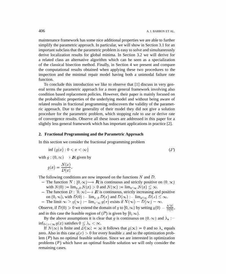
2. Fractional Programming and the Parametric Approach

In this section we consider the fractional programming problem

inf fg(x) : 0 < x <1g (P )

with g : (0;1)�! IR given by

g(x) =N(x)

D(x):

The following conditions are now imposed on the functions N and D.� The function N : [0;1)�! IR is continuous and strictly positive on (0;1)

with N(0) := limx#0 N(x) > 0 and N(1) := limx"1N(x) � 1.� The function D : [0;1)�! IR is continuous, strictly increasing and positive

on (0;1), with D(0) := limx#0 D(x) and D(1) := limx"1D(x) � 1.� The limit 1 � g(1) := limx"1 g(x) exists if N(1) = D(1) =1.

Observe, if D(0) > 0 we extend the domain of g to [0;1) by setting g(0) = N(0)D(0) ,

and in this case the feasible region of (P ) is given by [0;1).By the above assumptions it is clear that g is continuous on (0;1) and �? :=

inf0<x<1 g(x) satisfies 0 � �? <1.If N(1) is finite and D(1) = 1 it follows that g(1) = 0 and so �? equals

zero. Also in this case g(x) > 0 for every feasible x and so the optimization prob-lem (P ) has no optimal feasible solution. Since we are interested in optimizationproblems (P ) which have an optimal feasible solution we will only consider theremaining cases.

jogo357.tex; 9/09/1997; 15:43; v.6; p.2

OPTIMAL REPLACEMENT MODELS AND FRACTIONAL PROGRAMMING 407

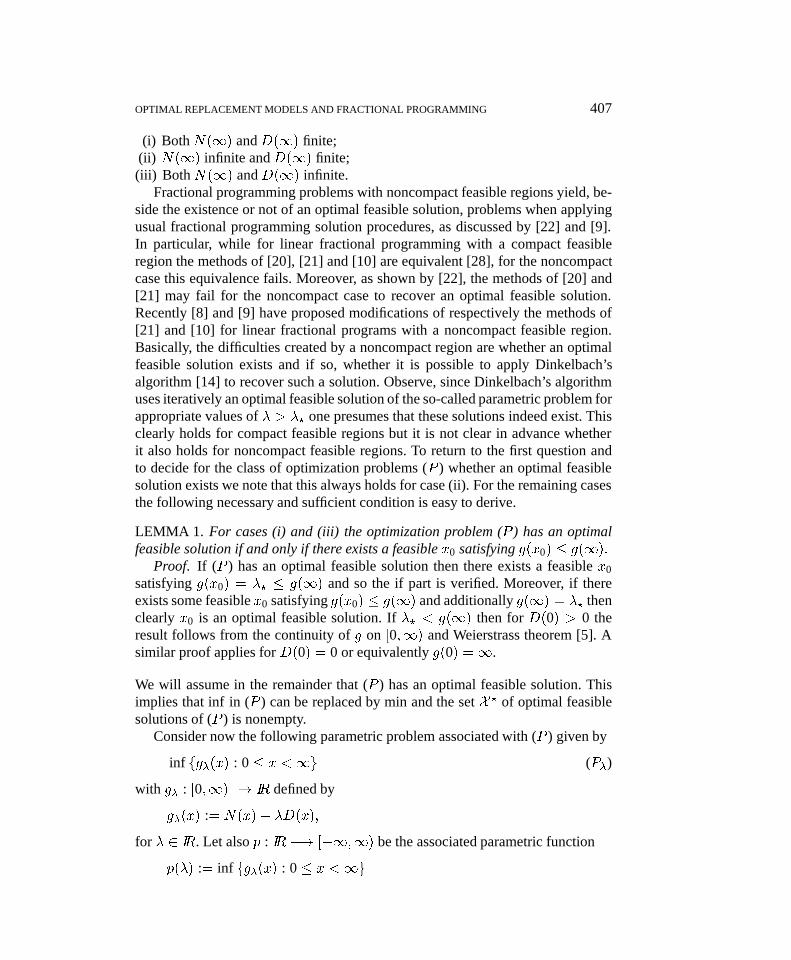
(i) Both N(1) and D(1) finite;(ii) N(1) infinite and D(1) finite;(iii) Both N(1) and D(1) infinite.

Fractional programming problems with noncompact feasible regions yield, be-side the existence or not of an optimal feasible solution, problems when applyingusual fractional programming solution procedures, as discussed by [22] and [9].In particular, while for linear fractional programming with a compact feasibleregion the methods of [20], [21] and [10] are equivalent [28], for the noncompactcase this equivalence fails. Moreover, as shown by [22], the methods of [20] and[21] may fail for the noncompact case to recover an optimal feasible solution.Recently [8] and [9] have proposed modifications of respectively the methods of[21] and [10] for linear fractional programs with a noncompact feasible region.Basically, the difficulties created by a noncompact region are whether an optimalfeasible solution exists and if so, whether it is possible to apply Dinkelbach’salgorithm [14] to recover such a solution. Observe, since Dinkelbach’s algorithmuses iteratively an optimal feasible solution of the so-called parametric problem forappropriate values of � > �? one presumes that these solutions indeed exist. Thisclearly holds for compact feasible regions but it is not clear in advance whetherit also holds for noncompact feasible regions. To return to the first question andto decide for the class of optimization problems (P ) whether an optimal feasiblesolution exists we note that this always holds for case (ii). For the remaining casesthe following necessary and sufficient condition is easy to derive.

LEMMA 1. For cases (i) and (iii) the optimization problem (P ) has an optimalfeasible solution if and only if there exists a feasible x0 satisfying g(x0) � g(1):

Proof. If (P ) has an optimal feasible solution then there exists a feasible x0

satisfying g(x0) = �? � g(1) and so the if part is verified. Moreover, if thereexists some feasible x0 satisfying g(x0) � g(1) and additionally g(1) = �? thenclearly x0 is an optimal feasible solution. If �? < g(1) then for D(0) > 0 theresult follows from the continuity of g on [0;1) and Weierstrass theorem [5]. Asimilar proof applies for D(0) = 0 or equivalently g(0) =1.

We will assume in the remainder that (P ) has an optimal feasible solution. Thisimplies that inf in (P ) can be replaced by min and the set X ? of optimal feasiblesolutions of (P ) is nonempty.

Consider now the following parametric problem associated with (P ) given by

inf fg�(x) : 0 � x <1g (P�)

with g� : [0;1)�! IR defined by

g�(x) := N(x)� �D(x);

for � 2 IR. Let also p : IR �! [�1;1) be the associated parametric function

p(�) := inf fg�(x) : 0 � x <1g

jogo357.tex; 9/09/1997; 15:43; v.6; p.3


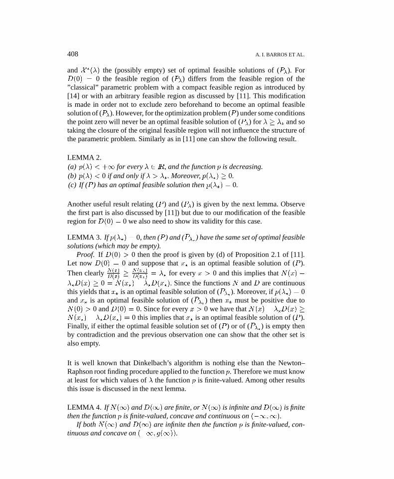
and X ?(�) the (possibly empty) set of optimal feasible solutions of (P�). ForD(0) = 0 the feasible region of (P�) differs from the feasible region of the”classical” parametric problem with a compact feasible region as introduced by[14] or with an arbitrary feasible region as discussed by [11]. This modificationis made in order not to exclude zero beforehand to become an optimal feasiblesolution of (P�). However, for the optimization problem (P ) under some conditionsthe point zero will never be an optimal feasible solution of (P�) for � � �? and sotaking the closure of the original feasible region will not influence the structure ofthe parametric problem. Similarly as in [11] one can show the following result.

LEMMA 2.(a) p(�) < +1 for every � 2 IR, and the function p is decreasing.(b) p(�) < 0 if and only if � > �?. Moreover, p(�?) � 0.(c) If (P ) has an optimal feasible solution then p(�?) = 0.

Another useful result relating (P ) and (P�) is given by the next lemma. Observethe first part is also discussed by [11]) but due to our modification of the feasibleregion for D(0) = 0 we also need to show its validity for this case.

LEMMA 3. If p(�?) = 0, then (P ) and (P�?) have the same set of optimal feasiblesolutions (which may be empty).

Proof. If D(0) > 0 then the proof is given by (d) of Proposition 2:1 of [11].Let now D(0) = 0 and suppose that x? is an optimal feasible solution of (P ).Then clearly N(x)

D(x) �N(x?)D(x?)

= �? for every x > 0 and this implies that N(x) �

�?D(x) � 0 = N(x?) � �?D(x?). Since the functions N and D are continuousthis yields that x? is an optimal feasible solution of (P�?). Moreover, if p(�?) = 0and x? is an optimal feasible solution of (P�?) then x? must be positive due toN(0) > 0 and D(0) = 0. Since for every x > 0 we have that N(x)� �?D(x) �N(x?) � �?D(x?) = 0 this implies that x? is an optimal feasible solution of (P ).Finally, if either the optimal feasible solution set of (P ) or of (P�?) is empty thenby contradiction and the previous observation one can show that the other set isalso empty.

It is well known that Dinkelbach’s algorithm is nothing else than the Newton–Raphson root finding procedure applied to the function p. Therefore we must knowat least for which values of � the function p is finite-valued. Among other resultsthis issue is discussed in the next lemma.

LEMMA 4. If N(1) and D(1) are finite, or N(1) is infinite and D(1) is finitethen the function p is finite-valued, concave and continuous on (�1;1).

If both N(1) and D(1) are infinite then the function p is finite-valued, con-tinuous and concave on (�1; g(1)).

jogo357.tex; 9/09/1997; 15:43; v.6; p.4


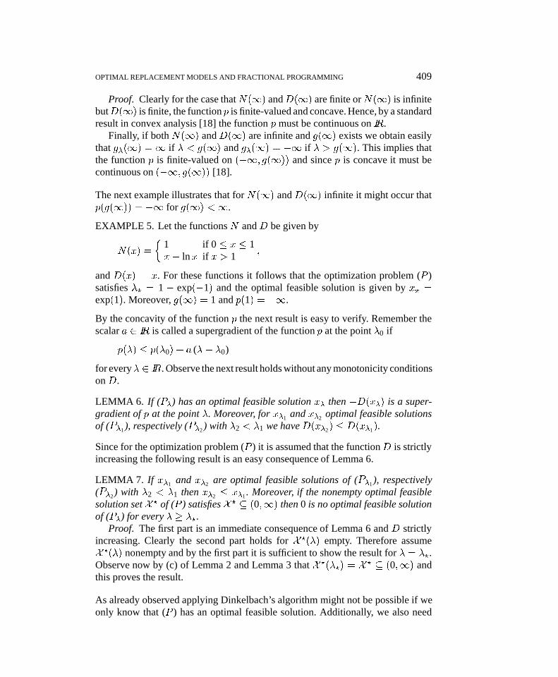
Proof. Clearly for the case that N(1) and D(1) are finite or N(1) is infinitebutD(1) is finite, the function p is finite-valued and concave. Hence, by a standardresult in convex analysis [18] the function p must be continuous on IR.

Finally, if both N(1) and D(1) are infinite and g(1) exists we obtain easilythat g�(1) = 1 if � < g(1) and g�(1) = �1 if � > g(1). This implies thatthe function p is finite-valued on (�1; g(1)) and since p is concave it must becontinuous on (�1; g(1)) [18].

The next example illustrates that for N(1) and D(1) infinite it might occur thatp(g(1)) = �1 for g(1) <1.

EXAMPLE 5. Let the functions N and D be given by

N(x) =

�1 if 0 � x � 1x� lnx if x > 1

;

and D(x) = x. For these functions it follows that the optimization problem (P )satisfies �? = 1 � exp(�1) and the optimal feasible solution is given by x? =exp(1). Moreover, g(1) = 1 and p(1) = �1.

By the concavity of the function p the next result is easy to verify. Remember thescalar a 2 IR is called a supergradient of the function p at the point �0 if

p(�) � p(�0) + a (�� 0)

for every� 2 IR. Observe the next result holds without any monotonicity conditionson D.

LEMMA 6. If (P�) has an optimal feasible solution x� then �D(x�) is a super-gradient of p at the point �. Moreover, for x�1 and x�2 optimal feasible solutionsof (P�1), respectively (P�2 ) with �2 < �1 we have D(x�2) � D(x�1).

Since for the optimization problem (P ) it is assumed that the function D is strictlyincreasing the following result is an easy consequence of Lemma 6.

LEMMA 7. If x�1 and x�2 are optimal feasible solutions of (P�1), respectively(P�2) with �2 < �1 then x�2 � x�1 . Moreover, if the nonempty optimal feasiblesolution set X ? of (P ) satisfies X ? � (0;1) then 0 is no optimal feasible solutionof (P�) for every � � �?.

Proof. The first part is an immediate consequence of Lemma 6 and D strictlyincreasing. Clearly the second part holds for X ?(�) empty. Therefore assumeX ?(�) nonempty and by the first part it is sufficient to show the result for � = �?.Observe now by (c) of Lemma 2 and Lemma 3 that X ?(�?) = X ? � (0;1) andthis proves the result.

As already observed applying Dinkelbach’s algorithm might not be possible if weonly know that (P ) has an optimal feasible solution. Additionally, we also need

jogo357.tex; 9/09/1997; 15:43; v.6; p.5


to identify some interval containing �? on which the parametric problem has anoptimal feasible solution. Unfortunately we cannot use Lemma 4 to identify suchan interval since it might happen for p(�) finite that the corresponding problem(P�) has no optimal feasible solution as shown by the next example.

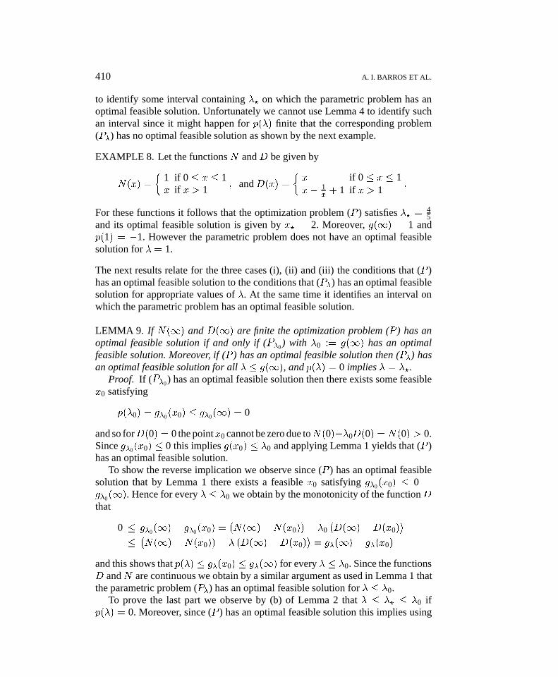
EXAMPLE 8. Let the functions N and D be given by

N(x) =

�1 if 0 � x � 1x if x > 1

; and D(x) =

�x if 0 � x � 1x� 1

x+ 1 if x > 1

:

For these functions it follows that the optimization problem (P ) satisfies �? = 45

and its optimal feasible solution is given by x? = 2. Moreover, g(1) = 1 andp(1) = �1. However the parametric problem does not have an optimal feasiblesolution for � = 1.

The next results relate for the three cases (i), (ii) and (iii) the conditions that (P )has an optimal feasible solution to the conditions that (P�) has an optimal feasiblesolution for appropriate values of �. At the same time it identifies an interval onwhich the parametric problem has an optimal feasible solution.

LEMMA 9. If N(1) and D(1) are finite the optimization problem (P ) has anoptimal feasible solution if and only if (P�0) with �0 := g(1) has an optimalfeasible solution. Moreover, if (P ) has an optimal feasible solution then (P�) hasan optimal feasible solution for all � � g(1), and p(�) = 0 implies � = �?.

Proof. If (P�0) has an optimal feasible solution then there exists some feasiblex0 satisfying

p(�0) = g�0(x0) � g�0(1) = 0

and so forD(0) = 0 the pointx0 cannot be zero due toN(0)��0D(0) = N(0) > 0.Since g�0(x0) � 0 this implies g(x0) � �0 and applying Lemma 1 yields that (P )has an optimal feasible solution.

To show the reverse implication we observe since (P ) has an optimal feasiblesolution that by Lemma 1 there exists a feasible x0 satisfying g�0(x0) � 0 =g�0(1). Hence for every � � �0 we obtain by the monotonicity of the function Dthat

0 � g�0(1)� g�0(x0) =�N(1)�N(x0)

�� 0

�D(1)�D(x0)

��

�N(1)�N(x0)

��

�D(1)�D(x0)

�= g�(1)� g�(x0)

and this shows that p(�) � g�(x0) � g�(1) for every � � �0. Since the functionsD and N are continuous we obtain by a similar argument as used in Lemma 1 thatthe parametric problem (P�) has an optimal feasible solution for � � �0.

To prove the last part we observe by (b) of Lemma 2 that � � �? � �0 ifp(�) = 0. Moreover, since (P ) has an optimal feasible solution this implies using

jogo357.tex; 9/09/1997; 15:43; v.6; p.6


the just proved result that (P�) has an optimal feasible solution. Hence, there existssome feasible x� such that

0 = p(�) = N(x�)� �D(x�) � N(x)� �D(x)

for every x � 0. Clearly for D(0) = 0 it follows that x� cannot be zero and sog(x) � g(x�) = � for every feasible x proving the last result.

Using the same arguments as in Lemma 9 one can show the following result, forcase (ii), i.e. N(1) infinite and D(1) finite.

LEMMA 10. If N(1) is infinite and D(1) is finite the optimization problems (P )and (P�) for all � 2 IR, have an optimal feasible solution. Moreover, if p(�) = 0then � = �?.

Finally we will consider case (iii).

LEMMA 11. If both N(1) and D(1) are infinite then the parametric problem(P�) has an optimal feasible solution for every � < g(1). Moreover, if (P ) has anoptimal feasible solution and p(�) = 0 then � = �?.

Proof. The first part is easy to verify and so we omit its proof.To verify the second part observe since p(�) = 0 that g�(x) � 0 for everyx > 0.

This implies that g(x) � � for every x > 0 and hence �? � �. If � < �? � g(1)then by the first part the problem (P�) has an optimal feasible solution and so thereexists some x� � 0 for D(0) > 0 or x� > 0 for D(0) = 0 satisfying g�(x�) = 0and hence g(x�) = � < �?. This yields a contradiction with the definition of �?and so � = �?.

As shown by Example 8 it is in general not true that also (P�0 ) has an optimalfeasible solution and so the above result is the best possible.

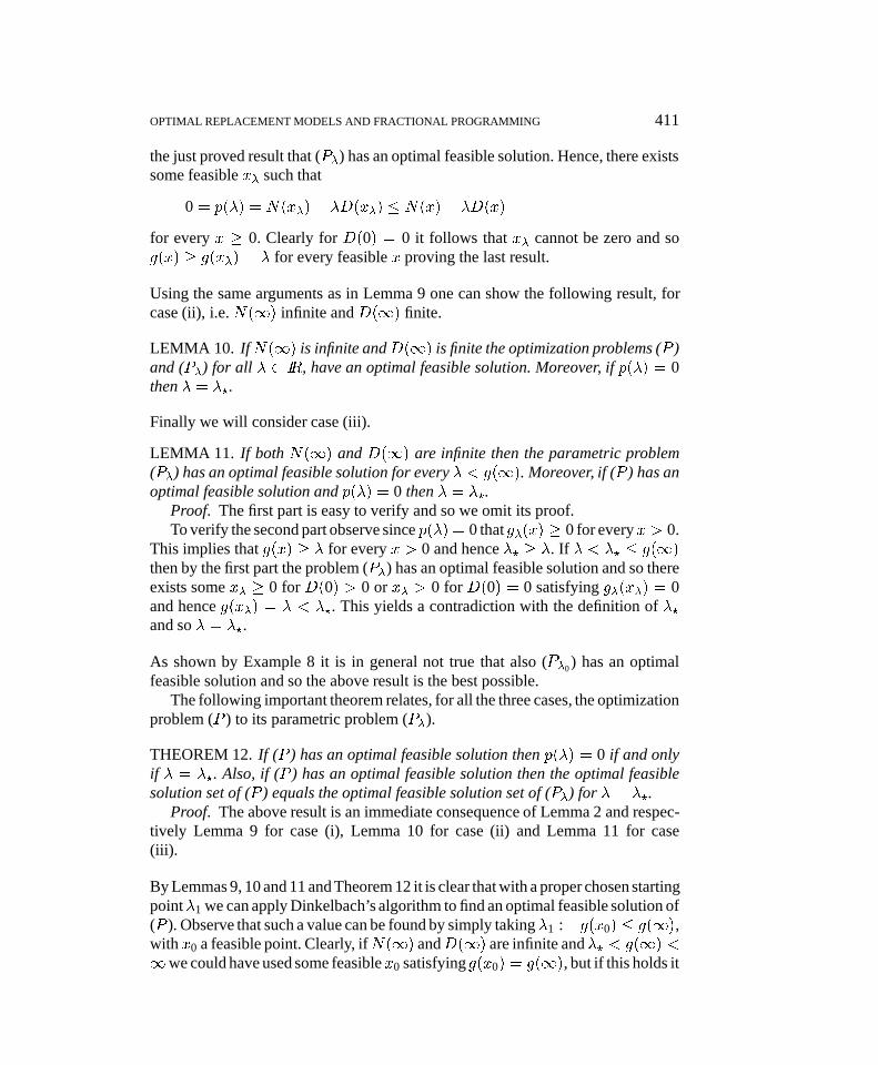
The following important theorem relates, for all the three cases, the optimizationproblem (P ) to its parametric problem (P�).

THEOREM 12. If (P ) has an optimal feasible solution then p(�) = 0 if and onlyif � = �?. Also, if (P ) has an optimal feasible solution then the optimal feasiblesolution set of (P ) equals the optimal feasible solution set of (P�) for � = �?.

Proof. The above result is an immediate consequence of Lemma 2 and respec-tively Lemma 9 for case (i), Lemma 10 for case (ii) and Lemma 11 for case(iii).

By Lemmas 9, 10 and 11 and Theorem 12 it is clear that with a proper chosen startingpoint�1 we can apply Dinkelbach’s algorithm to find an optimal feasible solution of(P ). Observe that such a value can be found by simply taking �1 := g(x0) � g(1),with x0 a feasible point. Clearly, ifN(1) andD(1) are infinite and �? < g(1) <1we could have used some feasiblex0 satisfying g(x0) = g(1), but if this holds it

jogo357.tex; 9/09/1997; 15:43; v.6; p.7


may happen that (P�0 ) does not have an optimal feasible solution. However, due to�? < g(1) there must exist some feasible x0 satisfying g(x0) < g(1) and hence,by using this value we can still properly apply Dinkelbach’s algorithm. Notice, byLemma 1 we know that there exists some feasible x0 satisfying g(x0) � g(1) or incase N(1) and D(1) infinite and �? < g(1) some x0 satisfying g(x0) < g(1).

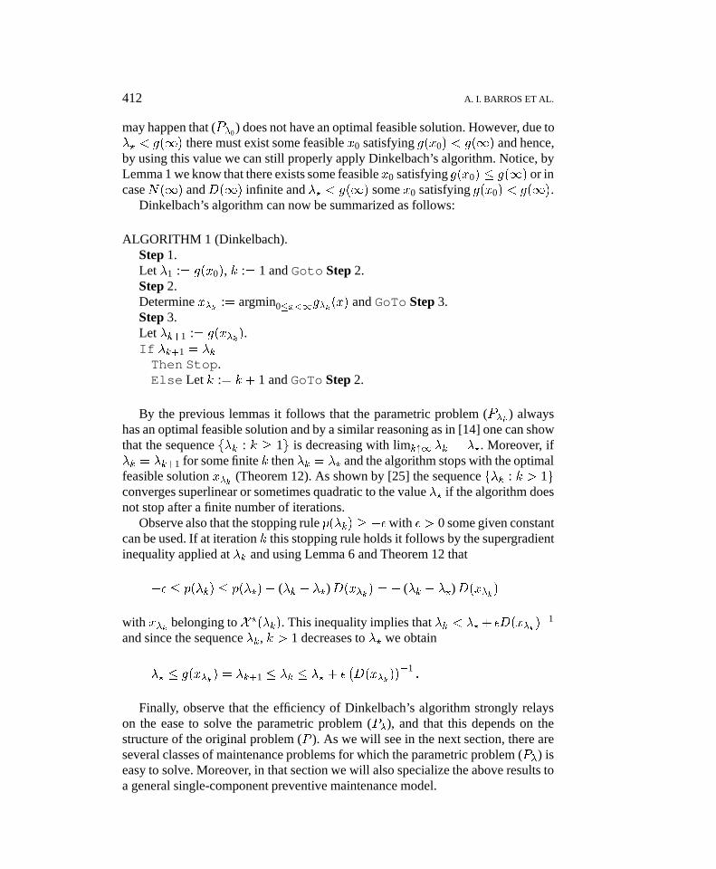
Dinkelbach’s algorithm can now be summarized as follows:

ALGORITHM 1 (Dinkelbach).Step 1.Let �1 := g(x0), k := 1 and Goto Step 2.Step 2.Determine x�k := argmin0�x<1g�k(x) and GoTo Step 3.Step 3.Let �k+1 := g(x�k).If �k+1 = �kThen Stop.Else Let k := k + 1 and GoTo Step 2.

By the previous lemmas it follows that the parametric problem (P�k ) alwayshas an optimal feasible solution and by a similar reasoning as in [14] one can showthat the sequence f�k : k � 1g is decreasing with limk"1 �k = �?. Moreover, if�k = �k+1 for some finite k then �k = �? and the algorithm stops with the optimalfeasible solution x�k (Theorem 12). As shown by [25] the sequence f�k : k > 1gconverges superlinear or sometimes quadratic to the value �? if the algorithm doesnot stop after a finite number of iterations.

Observe also that the stopping rule p(�k) � ��with � > 0 some given constantcan be used. If at iteration k this stopping rule holds it follows by the supergradientinequality applied at �k and using Lemma 6 and Theorem 12 that

�� p(�k) � p(�?)� (�k � �?)D(x�k) = � (�k � �?)D(x�k)

with x�k belonging to X ?(�k). This inequality implies that �k < �? + �D(x�k)�1

and since the sequence �k, k > 1 decreases to �? we obtain

�? � g(x�k) = �k+1 � �k � �? + ��D(x�k)

��1:

Finally, observe that the efficiency of Dinkelbach’s algorithm strongly relayson the ease to solve the parametric problem (P�), and that this depends on thestructure of the original problem (P ). As we will see in the next section, there areseveral classes of maintenance problems for which the parametric problem (P�) iseasy to solve. Moreover, in that section we will also specialize the above results toa general single-component preventive maintenance model.

jogo357.tex; 9/09/1997; 15:43; v.6; p.8


3. A General Single-Component Maintenance Model

[2] argue that the objective function of any preventive maintenance model, whereage is the only decision variable to start preventive maintenance, necessarily hasthe form of the optimization problem (P ) with

N(x) := c+

Z x

0m(z)h(z) dz

and

D(x) := d+

Z x

0h(z) dz

with c > 0; d � 0 and m : [0;1)�! IR a continuous and positive function, whilethe function h : [0;1)�! IR is continuous and strictly positive on (0;1). Aproof of their result can be found in [15]. Well-known examples are the averagecost and expected total discounted cost versions of the age replacement and blockreplacement model [6], the minimal repair and standard inspection model [12] andmodels where preventive maintenance is only possible at opportunities [13, 2].Other less known models which fit into the above framework are discussed in[7, 12] and [2].

Observe that this problem falls into the fractional programming class discussedin the previous section. Introducing

1 � �0 := limx"1

Z x

0m(z)h(z) dz � 0

and

1 � �1 := limx"1

Z x

0h(z) dz > 0

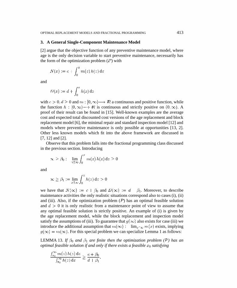
we have that N(1) := c + �0 and D(1) := d + �1. Moreover, to describemaintenance activities the only realistic situations correspond also to cases (i), (ii)and (iii). Also, if the optimization problem (P ) has an optimal feasible solutionand d > 0 it is only realistic from a maintenance point of view to assume thatany optimal feasible solution is strictly positive. An example of (i) is given bythe age replacement model, while the block replacement and inspection modelsatisfy the assumptions of (iii). To guarantee that g(1) also exists for case (iii) weintroduce the additional assumption that m(1) := limx"1m(x) exists, implyingg(1) = m(1). For this special problem we can specialize Lemma 1 as follows:

LEMMA 13. If �0 and �1 are finite then the optimization problem (P ) has anoptimal feasible solution if and only if there exists a feasible x0 satisfyingR

1

x0m(z)h(z) dzR1

x0h(z) dz

�c+ �0

d+ �1:

jogo357.tex; 9/09/1997; 15:43; v.6; p.9


Moreover, if �0 and �1 are infinite and m(1) < 1 then the optimizationproblem (P ) has an optimal feasible solution if and only if there exists somefeasible x0 satisfyingZ x0

0

�m(1)�m(z)

�h(z) dz � c� dm(1):

The above result does not exclude for d > 0 that 0 is an optimal feasible solutionof (P ). However, in the remainder we will always assume that for d > 0 the point 0is not an optimal feasible solution and so the nonempty set X ? of optimal feasiblesolutions satisfies X ? � (0;1). Observe that, for �0 and �1 finite it is easy toverify, if m(1) exists and m(1) > g(1) = c+�0

d+�1, that the sufficiency condition

stated in Lemma 13 holds. Also for this case, if we have found some x0 satisfyingm(x) > g(1) for every x � x0, then g(x0) < g(1) and so �1 = g(x0) can beused to start Dinkelbach’s algorithm.

3.1. APPLYING THE PARAMETRIC APPROACH

Before specializing the results derived in Section 2 notice that if (P ) has anoptimal feasible solution and d > 0 it can be easily shown that X ? � (0;1) ifm(0) < g(0). Using now Lemma 7 it is relatively easy to prove the validity of thefollowing lower bound on the optimal feasible solution of (P�) for � appropriatelychosen.

LEMMA 14. If the nonempty optimal feasible solution set X ? of (P ) satisfiesX ? � (0;1) and the continuous function m : [0;1)�! IR is decreasing on [0; b]for some b � 0 then x� > b for any optimal feasible solution x� of (P�) with�? � �. Moreover, the same result holds for any optimal feasible solution of (P ).

Proof. Clearly, for b = 0 the result follows by Lemma 7 and so we assumethat b > 0. Using Lemma 6 and the function D strictly increasing it is enough toprove these results for �?. Hence, suppose x�? is an optimal feasible solution of(P�?). By Lemma 7 it follows that x�? > 0 and so by the first order necessaryconditions for a global minimum and h strictly positive on (0;1) we obtain thatm(x�?)� �? = 0. If x�? � b this implies since m is decreasing on [0; b] and h isstrictly positive on (0;1) that

g0�?(x) = h(x)(m(x) � �?) � h(x)�m(x�?)� �?

�= 0

for every 0 < x � x�? . Hence by the mean value theorem [24] this yieldsg�?(0) � g�?(x�?) and since x�? is an optimal feasible solution it must follow that0 is also an optimal feasible solution contradicting Lemma 7. This proves the firstpart and by the first part and Theorem 12 the second part follows immediately.

Before discussing a class of functions for which the parametric problem is easyto solve we observe if (P ) has an optimal feasible solution that for any scalar �k

jogo357.tex; 9/09/1997; 15:43; v.6; p.10


generated by Dinkelbach’s algorithm with starting value �1 := g(x0) it followsby Lemmas 9, 10 and 11 that the set X ?(�k) of optimal feasible solutions of(P�k) is a nonempty set. Moreover, if additionally 0 is no optimal feasible solutionof (P ) (only needed for d > 0) and m is decreasing on [0; b] with b � 0 weknow by Lemma 14 that x�k > b for every x�k belonging to X ?(�k). By theseobservations it follows that the constrained optimization problem (P�k) is actuallyunconstrained and so by the Karush–Kuhn–Tucker conditions for an optimum andthe strict positivity of h on (0;1) we obtain that

X ?(�k) � fx 2 IR : m(x)� �k = 0; b < xg : (1)

Hence to find an optimal feasible solution of the parametric problem (P�) we haveto generate in the general case all stationary points x > b.

Another way to solve the global optimization problem (P�) is given by oneof the algorithms discussed by [16] if we know additionally an upper boundu on the set of optimal feasible solutions of (P�) and an upper bound on thevalues maxfm(x) : b � x � ug and maxfh(x) : b � x � ug. In this case theoptimization problem (P�) reduces to the optimization of an univariate Lipschitzcontinuous function over a compact interval. Moreover, by Lemma 7 it follows for�k+1 � �k that

x�k+1 � x�k

and hence we have an upper bound on the set X ?(�k+1)

X ?(�k+1) � fx 2 IR : m(x)� �k+1 = 0; b < x � x�kg :

At the same time it shows using Theorem 12 that limk"1 x�k = xb with xb thebiggest optimal feasible solution of (P ). By the previous observation it is now easyto introduce a class of functions for which the parametric problem (P�) has a nicestructure and is therefore almost trivially solvable.

DEFINITION 15. [3] A function f : [0;1) is called unimodal if there exists some0 � z0 <1 such that f is decreasing on [0; z0] and increasing on (z0;1).

It is clear for any unimodal function f that 1 � f(1) := limz"1 f(z) exists.Moreover, if additionally f is continuous, one can also find constants 0 � b1 �

b2 � 1 satisfying f attains its minimum on [b1; b2]. In this case the continuousfunction f is called unimodal with parameters 0 � b1 � b2 � 1. The nexttheorem characterizes the optimal feasible solution set of (P�) and (P ) and showsthat under a unimodality assumption the inclusion in (1) can be replaced by anequality. Observe a weaker result for the optimization problem (P ) with d = 0using a completely different approach is given by [12].

THEOREM 16. If the optimal feasible solution set X ? of (P ) satisfies X ? �

(0;1), the continuous function m : [0;1)�! IR is unimodal with parameters

jogo357.tex; 9/09/1997; 15:43; v.6; p.11


0 � b1 � b2 < 1 and for � � �? the parametric problem (P�) has an optimalfeasible solution then the optimal feasible solution set X ?(�) of (P�) equals theclosed interval

fx 2 IR : m(x)� � = 0; b2 < xg :

Moreover, under the same conditions the optimal feasible solution set of (P ) isgiven by the closed interval

fx 2 IR : m(x)� �? = 0; b2 < xg :

Proof. Clearly by (1) we have that

X ?(�) � fx 2 IR : m(x)� � = 0; b2 < xg :

Consider therefore an arbitrary point x > b2 satisfying m(x) � � = 0 and let x�denote an optimal feasible solution of (P�). Since by Lemma 14 the inequalityx� > b2 holds and m is increasing on [b2;1) we obtain due to m(x�) = � thatm(y) = � for every

min fx; x�g � y � max fx; x�g

and so g0�(y) = 0. Applying now the mean value theorem yields g� is constant onthe interval [minfx; x�g;maxfx; x�g] and hence g�(x) = g�(x�). This shows thefirst part and the second part follows immediately from this and Theorem 12.

By Theorem 16 it is relatively easy using for example a standard bisection algorithm[5] to compute an optimal feasible solution of (P�) for the appropriate �. Clearlyfor the subset of unimodal functions m which are strictly increasing on (b2;1) weobtain that (P�) for the appropriate � has a unique optimal feasible solution andthis implies by Theorem 16 that the optimization problem (P ) also has a uniqueoptimal feasible solution.

Finally, if the continuous function m is unimodal with parameters 0 � b1 �

b2 < 1 and the function h is decreasing it is also possible for d = 0 to solve (P )by using a specialized version of the bisection method. This will be discussed inthe next section.

3.2. SPECIALIZED BISECTION METHOD

Besides the Newton–Raphson root finding approach, another important method tofind the unique root of the univariate equation p(�) = 0 is given by the classicalbisection method. Basically this method constructs a succession of smaller intervalscontaining the root. Although at each iteration the diameter of the interval is halved,the convergence rate of this method is only linear in opposition to the Dinkelbachalgorithm. [19] proposes a variant of this method, resorting to the bounds produced

jogo357.tex; 9/09/1997; 15:43; v.6; p.12


by the Dinkelbach method, which converges superlinearly. However, the bisection-like method introduced in this section aims at solving directly (P ), and fully exploitsthe very special structure of the maitenance model discussed in this section.

Since the function D is strictly increasing its inverse D : [d; d + �1) �![0;1) exists and is also strictly increasing. Let us consider also the function� : ( 1

d+�1; 1d] �! [0;1) given by

�(y) = yN(D ( 1y)):

Clearly by the above definition it follows that the objective function g of theoptimization problem (P ) equals g(x) = �( 1

D(x) ). It is now possible to prove thefollowing result for the function �. In the next lemma notice that if both b = 0 andD(0) = d = 0 then 1

D(b) =1.

LEMMA 17. The function � is convex on ( 1d+�1

; 1D(b) ) if and only if the continuous

function m is increasing on (b;1).Proof. Clearly, the function � is convex on ( 1

d+�1; 1D(b) ) if and only if the

function y 7�! yN(D ( 1y)) is convex on ( 1

d+�1; 1D(b) ). Adapting slightly the proof

of Theorem I:1:1:6 of [18] one can easily show using the criteria of increasingslopes that y 7�! yN(D ( 1

y)) is convex on ( 1

d+�1; 1D(b) ) if and only if y 7�!

N(D (y)) is convex on (D(b); d+�1). The derivative of the last function equalsm(D (y)) and since by our assumption the function m is increasing on (b;1)and D is strictly increasing the equivalence follows.

A direct consequenceof the above lemma and the subgradient inequality for convexfunctions is given by the next result.

LEMMA 18. If the continuous function m is increasing on (b;1) and a > b issome arbitrary point then

g(x) � m(a) +�g(a) �m(a)

� D(a)

D(x)

for every x > b.Proof. By Lemma 17 it follows that the function � is convex on ( 1

d+�1; 1D(b) ).

This implies by the subgradient inequality that

g(x) = �( 1D(x) ) � �( 1

D(a) ) + �0( 1D(a) )

�1

D(x) �1

D(a)

�= g(a) + �0( 1

D(a) )�

1D(x) �

1D(a)

�:

It is easy to verify that �0(y) = �(y)�m(D (y�1))y

and substituting y = 1D(a) yields

the desired inequality.

jogo357.tex; 9/09/1997; 15:43; v.6; p.13


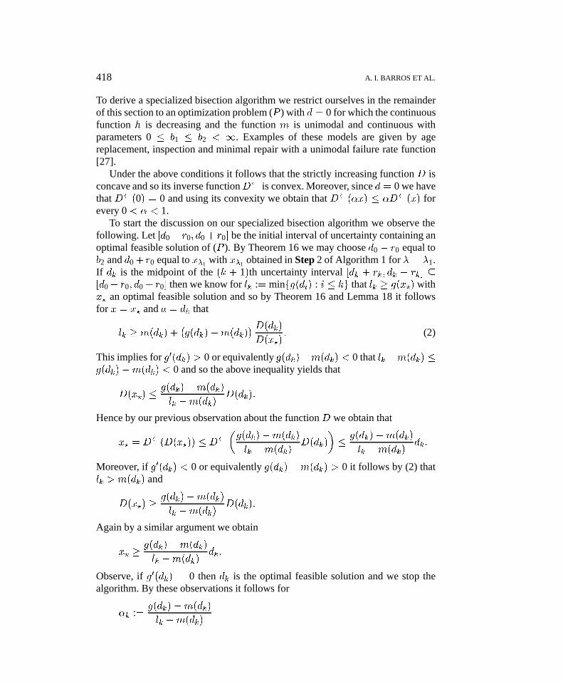
To derive a specialized bisection algorithm we restrict ourselves in the remainderof this section to an optimization problem (P ) with d = 0 for which the continuousfunction h is decreasing and the function m is unimodal and continuous withparameters 0 � b1 � b2 < 1. Examples of these models are given by agereplacement, inspection and minimal repair with a unimodal failure rate function[27].

Under the above conditions it follows that the strictly increasing function D isconcave and so its inverse function D is convex. Moreover, since d = 0 we havethat D (0) = 0 and using its convexity we obtain that D (�x) � �D (x) forevery 0 < � < 1.

To start the discussion on our specialized bisection algorithm we observe thefollowing. Let [d0 � r0; d0 + r0] be the initial interval of uncertainty containing anoptimal feasible solution of (P ). By Theorem 16 we may choose d0 � r0 equal tob2 and d0 + r0 equal to x�1 with x�1 obtained in Step 2 of Algorithm 1 for � = �1.If dk is the midpoint of the (k + 1)th uncertainty interval [dk + rk; dk � rk] �[d0 � r0; d0 + r0] then we know for lk := minfg(di) : i � kg that lk � g(x?) withx? an optimal feasible solution and so by Theorem 16 and Lemma 18 it followsfor x = x? and a = dk that

lk � m(dk) +�g(dk)�m(dk)

� D(dk)

D(x?): (2)

This implies for g0(dk) > 0 or equivalently g(dk)�m(dk) < 0 that lk�m(dk) �g(dk)�m(dk) < 0 and so the above inequality yields that

D(x?) �g(dk)�m(dk)

lk �m(dk)D(dk):

Hence by our previous observation about the function D we obtain that

x? = D (D(x?)) � D �g(dk)�m(dk)

lk �m(dk)D(dk)

��

g(dk)�m(dk)

lk �m(dk)dk:

Moreover, if g0(dk) < 0 or equivalently g(dk)�m(dk) > 0 it follows by (2) thatlk > m(dk) and

D(x?) �g(dk)�m(dk)

lk �m(dk)D(dk):

Again by a similar argument we obtain

x? �g(dk)�m(dk)

lk �m(dk)dk:

Observe, if g0(dk) = 0 then dk is the optimal feasible solution and we stop thealgorithm. By these observations it follows for

�k :=g(dk)�m(dk)

lk �m(dk)

jogo357.tex; 9/09/1997; 15:43; v.6; p.14


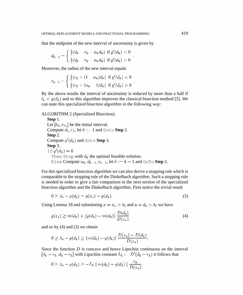
that the midpoint of the new interval of uncertainty is given by

dk+1 =

( 12(dk + rk + �kdk) if g0(dk) < 012(dk � rk + �kdk) if g0(dk) > 0

:

Moreover, the radius of the new interval equals

rk+1 =

( 12(rk + (1� �k)dk) if g0(dk) < 012(rk + (�k � 1)dk) if g0(dk) > 0

:

By the above results the interval of uncertainty is reduced by more than a half iflk < g(dk) and so this algorithm improves the classical bisection method [5]. Wecan state this specialized bisection algorithm in the following way:

ALGORITHM 2 (Specialized Bisection).Step 1.Let [b2; x�1 ] be the initial interval.Compute d1; r1, let k := 1 and Goto Step 2.Step 2.Compute g0(dk) and Goto Step 3.Step 3.If g0(dk) = 0Then Stop with dk the optimal feasible solution.Else Compute �k; dk+1; rk+1, let k := k + 1 and GoTo Step 2.

For this specialized bisection algorithm we can also derive a stopping rule which iscomparable to the stopping rule of the Dinkelbach algorithm. Such a stopping ruleis needed in order to give a fair comparison in the next section of the specializedbisection algorithm and the Dinkelbach algorithm. First notice the trivial result

0 � �? � g(dk) = g(x?)� g(dk): (3)

Using Lemma 18 and substituting x = x? > b2 and a = dk > b2 we have

g(x?) � m(dk) +�g(dk)�m(dk)

� D(dk)

D(x?)(4)

and so by (4) and (3) we obtain

0 � �? � g(dk) ��m(dk)� g(dk)

� D(x?)�D(dk)

D(x?):

Since the function D is concave and hence Lipschitz continuous on the interval[dk � rk; dk + rk] with Lipschitz constant Lk := D0(dk � rk) it follows that

0 � �? � g(dk) � �Lk j m(dk)� g(dk) jrk

D(x?):

jogo357.tex; 9/09/1997; 15:43; v.6; p.15


Hence, the specialized bisection algorithm stops if the stopping rule

�Lk j m(dk)� g(dk) j rk > ��

for some positive � > 0 holds and by the above inequality this guarantees theabsolute error � �

D(x?). This stopping rule is comparable with the stopping rule

for the Dinkelbach algorithm discussed in Section 2. Observe, if g0(dk) = 0 andhence dk is the optimal point then m(dk) � g(dk) = 0 and the stopping rule isautomatically satisfied.

In the next section we will present some computational results comparing bothmethods.

4. Computational Results

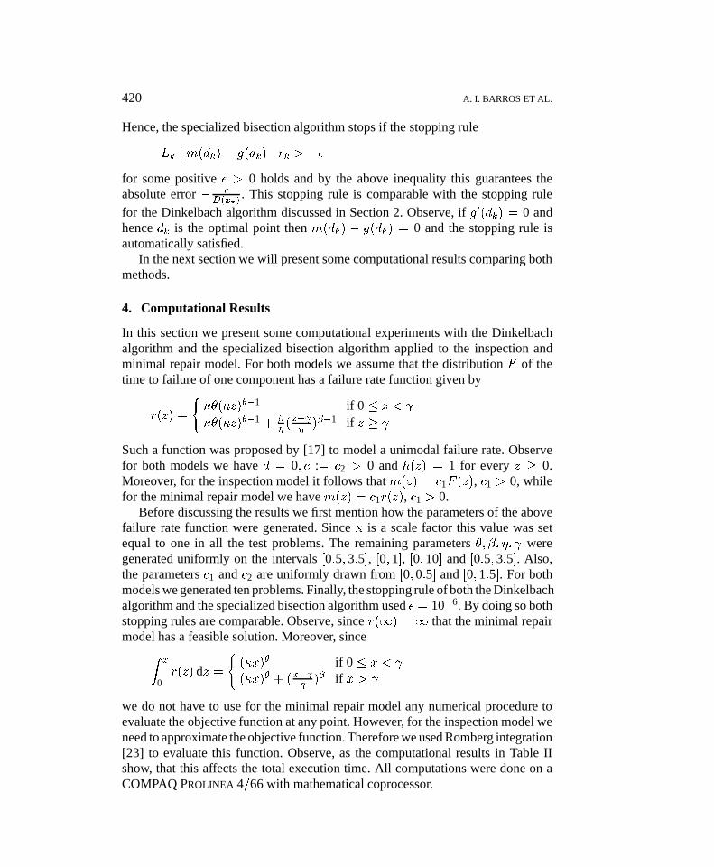
In this section we present some computational experiments with the Dinkelbachalgorithm and the specialized bisection algorithm applied to the inspection andminimal repair model. For both models we assume that the distribution F of thetime to failure of one component has a failure rate function given by

r(z) =

(��(�z)��1 if 0 � z <

��(�z)��1 + ��( z�

�)��1 if z �

Such a function was proposed by [17] to model a unimodal failure rate. Observefor both models we have d = 0; c := c2 > 0 and h(z) = 1 for every z � 0.Moreover, for the inspection model it follows that m(z) = c1F (z), c1 > 0, whilefor the minimal repair model we have m(z) = c1r(z), c1 > 0.

Before discussing the results we first mention how the parameters of the abovefailure rate function were generated. Since � is a scale factor this value was setequal to one in all the test problems. The remaining parameters �; �; �; weregenerated uniformly on the intervals [0:5; 3:5], [0; 1], [0; 10] and [0:5; 3:5]. Also,the parameters c1 and c2 are uniformly drawn from [0; 0:5] and [0; 1:5]. For bothmodels we generated ten problems. Finally, the stopping rule of both the Dinkelbachalgorithm and the specialized bisection algorithm used � = 10�6. By doing so bothstopping rules are comparable. Observe, since r(1) =1 that the minimal repairmodel has a feasible solution. Moreover, since

Z x

0r(z) dz =

((�x)� if 0 � x <

(�x)� + (x� �

)� if x >

we do not have to use for the minimal repair model any numerical procedure toevaluate the objective function at any point. However, for the inspection model weneed to approximate the objective function. Therefore we used Romberg integration[23] to evaluate this function. Observe, as the computational results in Table IIshow, that this affects the total execution time. All computations were done on aCOMPAQ PROLINEA 4=66 with mathematical coprocessor.

jogo357.tex; 9/09/1997; 15:43; v.6; p.16


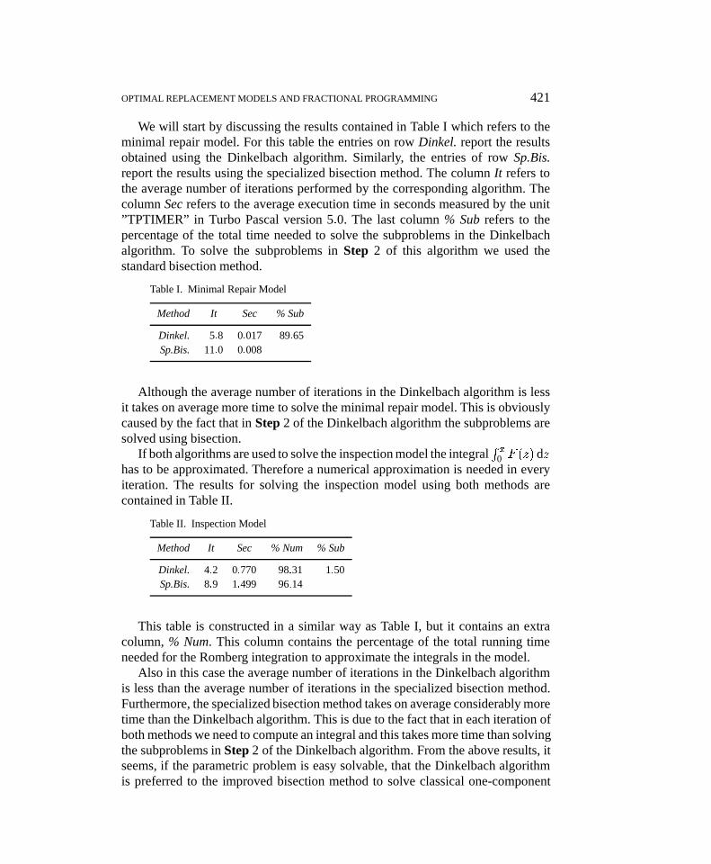
We will start by discussing the results contained in Table I which refers to theminimal repair model. For this table the entries on row Dinkel. report the resultsobtained using the Dinkelbach algorithm. Similarly, the entries of row Sp.Bis.report the results using the specialized bisection method. The column It refers tothe average number of iterations performed by the corresponding algorithm. Thecolumn Sec refers to the average execution time in seconds measured by the unit”TPTIMER” in Turbo Pascal version 5:0. The last column % Sub refers to thepercentage of the total time needed to solve the subproblems in the Dinkelbachalgorithm. To solve the subproblems in Step 2 of this algorithm we used thestandard bisection method.

Table I. Minimal Repair Model

Method It Sec % Sub

Dinkel. 5:8 0:017 89:65Sp.Bis. 11:0 0:008

Although the average number of iterations in the Dinkelbach algorithm is lessit takes on average more time to solve the minimal repair model. This is obviouslycaused by the fact that in Step 2 of the Dinkelbach algorithm the subproblems aresolved using bisection.

If both algorithms are used to solve the inspection model the integralR x

0 F (z) dzhas to be approximated. Therefore a numerical approximation is needed in everyiteration. The results for solving the inspection model using both methods arecontained in Table II.

Table II. Inspection Model

Method It Sec % Num % Sub

Dinkel. 4:2 0:770 98:31 1:50Sp.Bis. 8:9 1:499 96:14

This table is constructed in a similar way as Table I, but it contains an extracolumn, % Num. This column contains the percentage of the total running timeneeded for the Romberg integration to approximate the integrals in the model.

Also in this case the average number of iterations in the Dinkelbach algorithmis less than the average number of iterations in the specialized bisection method.Furthermore, the specialized bisection method takes on average considerably moretime than the Dinkelbach algorithm. This is due to the fact that in each iteration ofboth methods we need to compute an integral and this takes more time than solvingthe subproblems in Step 2 of the Dinkelbach algorithm. From the above results, itseems, if the parametric problem is easy solvable, that the Dinkelbach algorithmis preferred to the improved bisection method to solve classical one-component

jogo357.tex; 9/09/1997; 15:43; v.6; p.17


maintenance models whenever we need to call for a numerical procedure to evaluatethe objective function.

Acknowledgements

The authors like to thank the anonymous referees for their constructive remarkswhich greatly improved the presentation of the paper.

References

1. Aven, T. and Bergman, B. (1986), Optimal Replacement Times. A General Setup, Journal ofApplied Probability 23, 432–442.

2. Aven, T. and Dekker, R. (1996), A Useful Framework for Optimal Replacement Models.Technical Report TI 96 – 64/9, Tinbergen Institute Rotterdam, to appear in Reliability Engineeringand System Safety.

3. Avriel, M., Diewert, W.E., Schaible, S., and Zang, I. (1988), Generalized Concavity, volume 36of Mathematical Concepts and Methods in Science and Engineering, Plenum Press, New York.

4. Barlow, R.E. and Proschan, F. (1965), Mathematical Theory of Reliability, Wiley, New York.5. Bazaraa, M.S., Sherali, H.D., and Shetty, C.M. (1993), Nonlinear Programming: Theory and

Algorithms, Wiley, New York. (Second edition).6. Berg, M. (1980), A Marginal Cost Analysis for Preventive Maintenance Policies, European

Journal of Operational Research 4, 136–142.7. Berg, M. (1995), The Marginal Cost Analysis and Its Application to Repair and Replacement

Models, European Journal of Operational Research 82(2), 214–224.8. Cambini, A. and Martein, L. (1992), Equivalence in Linear Fractional Programming, Optimiza-

tion 23, 41–51.9. Cambini, A., Schaible, S., and Sodini, C. (1993), Parametric Linear Fractional Programming for

an Unbonded Feasible Region, Journal of Global Optimization 3, 157–169.10. Charnes, A. and Cooper, W. (1962), Programming with Linear Fractional Functionals, Naval

Research Logistics Quarterly 9, 181–186.11. Crouzeix, J.P., Ferland, J.A., and Schaible, S. (1985), An Algorithm for Generalized Fractional

Programs, Journal of Optimization Theory and Applications 47(1), 35–49.12. Dekker, R. (1995), Integrating Optimization, Priority Setting, Planning and Combining of

Maintenance Activities, European Journal of Operational Research 82(2), 225–240.13. Dekker, R. and Dijkstra, M.C. (1992), Opportunity Based Age Replacement: Exponentially

Distributed Times Between Opportunities, Naval Research Logistics 39, 175–192.14. Dinkelbach, W. (1967), On Nonlinear Fractional Programming, Management Science 13(7),

492–498.15. Frenk, J.B.G., Dekker, R., and Kleijn, M.J. (1996), A Note on the Marginal Cost Approach in

Maintenance, Technical Report TI 96 – 25/9, Tinbergen Institute Rotterdam, to appear in Journalof Optimization Theory and Applications, November 1997.

16. Hansen, P. and Jaumard, B. (1995), Lipschitz Optimization. In R. Horst and P. Pardalos, editors,Handbook of Global Optimization, volume 2 of Nonconvex Optimization and Its Applications,pages 407–493. Kluwer Academic Publishers, Dordrecht.

17. Hastings, N.A.J. and Ang, J.Y.T. (1995), Developments in Computer Based Reliability Analysis,Journal of Quality in Maintenance Engineering 1(1), 69–78.

18. Hiriart-Urruty, J.B. and Lemarechal, C. (1993), Convex Analysis and Minimization AlgorithmsI: Fundamentals, volume 1. Springer-Verlag, Berlin.

19. Ibaraki, T. (1983), Parametric Approaches to Fractional Programs, Mathematical Programming26, 345–362.

20. Isbell, J.R. and Marlow, W.H. (1956), Attrition Games, Naval Research Logistics Quarterly 3,71–93.

jogo357.tex; 9/09/1997; 15:43; v.6; p.18


21. Martos, B. (1964), Hyperbolic Programming, Naval Research Logistics Quarterly 11, 135–155.English translation from: Publications of Mathematic Institute Hungarian Academy Sciences, 5:383–406, 1960.

22. Mond, B. (1981), On Algorithmic Equivalence in Linear Fractional Programming, Mathematicsof Computation 37(155), 185–187.

23. Press, W.H., Flannery, B.P., Tenkolsky, S.A., and Vetterling, W.T. (1992), Numerical Recipes inPascal. The Art of Science Computing. Cambridge University Press, Cambridge.

24. Rudin, W. (1976), Principles of Mathematical Analysis, Mathematical Series. McGraw-Hill,New York.

25. Schaible, S. (1976), Fractional Programming. II, On Dinkelbach’s Algorithm, ManagementScience 22, 868–873.

26. Schaible, S. (1995), Fractional Programming, In R. Horst and P. Pardalos, editors, Handbook ofGlobal Optimization, volume 2 of Nonconvex Optimization and Its Applications, pages 495–608.Kluwer Academic Publishers, Dordrecht.

27. Tijms, H.C. (1994), Stochastic Models. An Algorithmic Approach, John Wiley, Chichester.28. Wagner, H.M. and Yuan, J.S.C. (1968), Algorithmic Equivalence in Linear Fractional Program-

ming, Management Science 14(5), 301–306.

jogo357.tex; 9/09/1997; 15:43; v.6; p.19

Optimizing a General Optimal Replacement Model by Fractional Programming Techniques

Documents

Transcript of Optimizing a General Optimal Replacement Model by Fractional Programming Techniques