Optimized ensemble learning and its application in agriculture

by

Mohammad Mohsen Shahhosseini

A dissertation submitted to the graduate faculty

in partial fulfillment of the requirements for the degree of

DOCTOR OF PHILOSOPHY

Major: Industrial Engineering

Program of Study Committee: Guiping Hu, Major Professor

Qing Li Cameron Mackenzie Sotirios Archontoulis

Danica Ommen

The student author, whose presentation of the scholarship herein was approved by the program of study committee, is solely responsible for the content of this dissertation. The Graduate

College will ensure this dissertation is globally accessible and will not permit alterations after a degree is conferred.

Iowa State University Ames, Iowa

2021

Copyright © Mohammad Mohsen Shahhosseini, 2021. All rights reserved.

ii

DEDICATION

To my loving parents, the reason of what I become today.

To my brother and sister, for their endless love, support, and encouragement.

iii

TABLE OF CONTENTS

Page

ACKNOWLEDGMENTS .....................................................................................................................................................v

ABSTRACT ....................................................................................................................................................................... vi

CHAPTER 1. GENERAL INTRODUCTION ........................................................................................................................... 1 References ................................................................................................................................................................. 5

CHAPTER 2. OPTIMIZING ENSEMBLE WEIGHTS AND HYPERPARAMETERS OF MACHINE LEARNING MODELS FOR REGRESSION PROBLEMS ......................................................................................................................................... 8

Abstract ..................................................................................................................................................................... 8 Introduction ............................................................................................................................................................... 9 Background .............................................................................................................................................................. 12 Materials and Methods ........................................................................................................................................... 16 Generalized Ensemble Model with Internally Tuned hyperparameters (GEM-ITH) ................................................ 20

GEM-ITH with Bayesian search ........................................................................................................................... 22 Results and Discussion ............................................................................................................................................. 23

Numerical experiments ....................................................................................................................................... 23 Base models generation...................................................................................................................................... 24 Benchmarks ........................................................................................................................................................ 26 Numerical results ................................................................................................................................................ 27

Conclusion ............................................................................................................................................................... 30 References ............................................................................................................................................................... 31

CHAPTER 3. FORECASTING CORN YIELD WITH MACHINE LEARNING ENSEMBLES ....................................................... 37 Abstract ................................................................................................................................................................... 37 Introduction ............................................................................................................................................................. 38 Materials and Methods ........................................................................................................................................... 42

Data set ............................................................................................................................................................... 43 Data Pre-processing ............................................................................................................................................ 44 Hyperparameter tuning and model selection ..................................................................................................... 48 Analyzed models ................................................................................................................................................. 50 Statistical performance metrics .......................................................................................................................... 57

Results and Discussion ............................................................................................................................................. 58 Numerical results ................................................................................................................................................ 59 Partial knowledge of in-season weather information ......................................................................................... 64 Partial dependence plots (PDPs) of optimized weighted ensemble ................................................................... 65 Feature importance ............................................................................................................................................ 67

Conclusion ............................................................................................................................................................... 69 References ............................................................................................................................................................... 71

CHAPTER 4. COUPLING MACHINE LEARNING AND CROP MODELING IMPROVES CROP YIELD PREDICTION IN THE US CORN BELT .............................................................................................................................................................. 78

Abstract ................................................................................................................................................................... 78 Introduction ............................................................................................................................................................. 79 Materials and Methods ........................................................................................................................................... 83

Agricultural Production Systems sIMulator (APSIM) ........................................................................................... 84 Machine Learning (ML) ....................................................................................................................................... 88

iv

Predictive models................................................................................................................................................ 94 Performance metrics .......................................................................................................................................... 97

Results ..................................................................................................................................................................... 98 Numerical results of hybrid simulation – ML framework.................................................................................... 98 Models performance on an extreme weather year (2012) .............................................................................. 101 Partial inclusion of APSIM variables .................................................................................................................. 102 Variable importance.......................................................................................................................................... 104

Discussion .............................................................................................................................................................. 106 Conclusion ............................................................................................................................................................. 108 References ............................................................................................................................................................. 108

CHAPTER 5. CORN YIELD PREDICTION WITH ENSEMBLE CNN-DNN ........................................................................... 117 Abstract ................................................................................................................................................................. 117 Introduction ........................................................................................................................................................... 118 Materials and Methods ......................................................................................................................................... 122

Data Preparation ............................................................................................................................................... 122 Base Models Generation ................................................................................................................................... 125 Ensemble Creation ............................................................................................................................................ 131

Results ................................................................................................................................................................... 133 Discussion .............................................................................................................................................................. 137

Models’ performance comparison with the literature ..................................................................................... 137 Comparing the models’ performance across US Corn Belt states .................................................................... 138 Generalization power of the designed Ensemble CNN-DNN models................................................................ 141

Conclusion ............................................................................................................................................................. 142 References ............................................................................................................................................................. 143

CHAPTER 6. GENERAL CONCLUSION .......................................................................................................................... 148

v

ACKNOWLEDGMENTS

First and foremost, I would like to thank my parents for their love, support, and

encouragement throughout my life. I will always appreciate all you did for me until the day I die.

My brother and sister deserve my wholehearted thanks as well.

I would like to sincerely thank my major professor, Dr. Hu, for her guidance and support

throughout this challenging period of my life, and especially for her confidence in me. I would

also like to thank my committee members, Dr. Li, Dr. Mackenzie, Dr. Archontoulis, and Dr.

Ommen, for their assistance. I would not have been able to complete my dissertation without

their valuable comments and suggestions.

Lastly, I would like to thank my friends, colleagues, the department faculty, and staff for

making my time at Iowa State University a wonderful experience.

vi

ABSTRACT

It has been shown that combining multiple machine learning base learners, results in

better prediction accuracy, given that the base learners are diverse enough. Assuming each of

the base learners as a decision-maker, a committee of decision-makers is able to make better

decisions as long as they are not very similar to each other i.e. they are diverse. More

importantly, it is crucial to figure out the best way to combine these base learners in order to

maximize the committee’s prediction accuracy. Many well-known ensemble creation methods

such as Basic Ensemble Model (BEM), Generalized Ensemble Model (GEM), stacked

generalization, etc. have been proposed to address the ensemble creation problem. However,

considering the ensemble as the linear combination of the base learners’ predictions, those

models consider the base model construction and the weighted aggregation to be independent

steps. We designed a framework that can find optimal ensemble weights as well as

hyperparameter combinations and result in better ensemble performance. Although extensive

studies have applied sophisticated machine learning (ML) models on ecological problems,

especially crop yield prediction, the use of ensemble models has been limited. We developed

several ensemble frameworks to address the corn yield prediction problem. We have shown that

an ensemble of some individual models can outperform the individual models. In addition, we

have shown that a hybrid ML-simulation crop modeling framework could further improve the

quality of yield predictions as the ML ensembles benefit significantly from the agricultural

information and insights derived from simulation crop models. Lastly, we have designed

sophisticated ensemble frameworks from the convolutional neural network – deep neural

vii

network (CNN-DNN) base learners. The promising predictions made by this model prove its

performance and its dominance over the state-of-the-art models found in the literature.

1

CHAPTER 1. GENERAL INTRODUCTION

Combining multiple base learners through an ensemble of models has shown to increase

machine learning (ML) prediction accuracy. Essentially, a committee of diverse decision makers

can make better decisions when they are combined in an optimal way. There are various

ensemble creation methods, such as bagging, boosting, and stacking/blending with different

approaches to reduce prediction bias and/or variance. The pioneer method in creating weighted

ensembles was proposed by Perrone and Cooper (1992) entitled Basic Ensemble Method (BEM),

which forms regression ensembles by averaging the base learners’ estimates. Generalized

Ensemble Method (GEM) was a more general case of BEM. GEM created regression weighted

ensembles by creating a linear combination of the regression base learners and solving an

optimization model using validation data to find the optimal weights.

Soon after Perrone and Cooper (1992), another study by Krogh and Vedelsby (1995)

proposed an optimization model to find the optimal weights of combining an ensemble of neural

networks, in which the weights were constrained to be positive and sum to one. This enabled the

explanation of the bias-variance tradeoff using the generalization error and ambiguity of the

ensemble. Other methods to build optimal weighted ensemble include using linear regression

(stacked regression) by Breiman (1996) and combining base learners by a multi-stage neural

network (Baker and Ellison, 2008; Yu et al., 2010). In this method, a second level of neural

network estimator was trained on the first level base neural networks to create the ensemble

(Yang and Browne, 2004). The base first level learners can be any combination of machine

learning models as long as they are diverse and show decent performance. There also have been

some studies that used dynamic weighting, in which the weights are assigned to each of the base

2

learners according to their performance on the validation set (Jimenez and Walsh, 1998; Shen

and Kong, 2004).

The ecological predictions such as crop yield, nitrate loss, or biomass predictions can be

done either using crop simulation models, or machine learning (ML). Although the studies using

ML to perform ecological predictions have become increasingly popular, the use of ensemble

learning in ecological predictions has been limited to homogenous ensemble models, which are

created using same-type base learners. Bagging and specifically random forest (Vincenzi et al.,

2011; Mutanga et al., 2012; Fukuda et al., 2013; Jeong et al., 2016), and boosting (De’ath, 2007;

Heremans et al., 2015; Belayneh et al., 2016; Stas et al., 2016; Sajedi-Hosseini et al., 2018) are

the more common ensemble prediction models used in this practice. However, there have been

some studies that used heterogeneous ensemble creation models such as stacking, which are

formed using different types of base learners (Conţiu and Groza, 2016; Cai et al., 2017). Stacking

(stacked generalization) is defined as a method to minimize the generalization error of some ML

models by performing at least one more level of learning task using the outputs of ML base

models as inputs, and the actual response values of some part of the data set (training data) as

outputs (Wolpert, 1992). Neural network ensembles have also used in ecological prediction

applications. In these studies, the final prediction is based on the weighted average of the

population of base neural networks (Baker and Ellison, 2008; Yu et al., 2010; Linares-Rodriguez

et al., 2013; DeWeber and Wagner, 2014; Kung et al., 2016; Fernandes et al., 2017).

It can be observed that the existing ensembling studies all consider the base model

construction and the weighted aggregation to be independent steps. It should be noted that

considering the tuning of model parameters in conjunction with the weighted average should

3

produce a superior ensemble. This is analogous to local optimality vs global optimality. From the

perspective of the bias-variance tradeoff (Yu et al. 2006) if each base model is tuned individually,

then by definition they will have low bias but will have high variance. Moreover, when dealing

with time-dependent prediction tasks such as corn yield prediction, generating out-of-bag

predictions as the inputs to the optimization model for finding the ensemble weights is

problematic. Another possible problem with current ensemble models is the black-box nature of

the ensemble framework and difficulty of providing useful insights for decision makers. In

addition, there has not been much attention in the literature to the ensemble neural network

approaches in predicting ecological variables.

Designing a framework that can find optimal ensemble weights as well as

hyperparameter combinations can provide better ensemble performance. Considering biological

problems, especially corn yield prediction, ensemble models help the decision makers with

insightful and accurate predictions and assist them with making decisions in improving crop

management, economic trading, food production monitoring, and global food security. In

addition, designing an ensemble deep neural network ensemble could possibly provide better

ecological predictions.

It should also be noted that we understand that the ensemble models we have

developed here for agricultural problems are built based on the independency assumption in the

response variables. However, this assumption might not always stand in the real-world. We have

tried to address this dependency by measures like constructing a feature that explain the

increasing trend in yield, and creating convolutional neural networks that can capture the

dependencies. Nonetheless, inspired by the idea proposed by Saha et al. (2020) which have

4

developed random forests for dependent data, we have saved the idea for future research and

have started working on another research project trying to develop ensemble models for

dependent data and investigating its application in crop yield prediction.

The objectives of this dissertation research study are manifold.

1) Design a nested optimization approach that finds the best combination of

ensemble weights and hyperparameter values of the diverse base learners and

succeeds in outperforming base learners as well as the state-of-the-art ensemble

models.

2) Develop ML ensembles to predict corn yield across US. Corn Belt states using

blocked sequential procedure to generate out-of-bag predictions.

3) Develop ML ensembles to predict corn yields across US. Corn Belt states with a

hybrid machine learning –simulation crop model approach and explore whether a

hybrid approach (simulation crop modeling + ML) would result in better corn yield

predictions. In addition, investigate which combinations of hybrid models (various

ML x crop model) provide the most accurate predictions Investigate.

4) Design an ensemble CNN-DNN neural network framework to predict corn yield

across all US Corn Belt states and compare the results with other state-of-the-art

ensemble models.

In addition to the mentioned research objectives, we have designed procedures to

increase interpretability of the black-box ML ensembles. To this end, we have calculated partial

dependency of the optimized ensemble model to quantify the marginal effect of changing each

input feature on the forecasts made be the ML ensemble model in order to provide agricultural

5

insights of the input features and the predictions. Furthermore, we have estimated the

importance of input features using partial dependencies of the optimized weighted ensemble to

help prioritize which data to be collected in the future and inform agronomists to explain causes

of high or low yield levels in some years.

This dissertation is organized into five chapters: Chapter 2 presents the designed model

for optimizing ensemble weights and hyperparameters of machine learning models for

regression problems. Forecasting corn yield with machine learning ensembles is discussed in

Chapter 3. Chapter 4 is dedicated to coupling machine learning and crop modeling for crop yield

prediction in the US Corn Belt. And finally, Chapter 5 presents the ensemble CNN-DNN neural

network model to predict corn yield across all US Corn Belt states.

References

Baker, L., & Ellison, D. (2008). Optimisation of pedotransfer functions using an artificial neural network ensemble method. Geoderma, 144(1), 212-224.

Belayneh, A., Adamowski, J., Khalil, B., & Quilty, J. (2016). Coupling machine learning methods with wavelet transforms and the bootstrap and boosting ensemble approaches for drought prediction. Atmospheric Research, 172-173, 37-47.

Breiman, L. (1996). Stacked regressions. Machine learning, 24(1), 49-64.

Cai, Y., Moore, K., Pellegrini, A., Elhaddad, A., Lessel, J., Townsend, C., et al. (2017). Crop yield predictions-high resolution statistical model for intra-season forecasts applied to corn in the US. Paper presented at the 2017 Fall Meeting.

Conţiu, Ş., & Groza, A. (2016). Improving remote sensing crop classification by argumentation-based conflict resolution in ensemble learning. Expert Systems with Applications, 64, 269-286.

De'ath, G. (2007). BOOSTED TREES FOR ECOLOGICAL MODELING AND PREDICTION. Ecology, 88(1), 243-251.

6

DeWeber, J. T., & Wagner, T. (2014). A regional neural network ensemble for predicting mean daily river water temperature. Journal of Hydrology, 517, 187-200.

Fernandes, J. L., Ebecken, N. F. F., & Esquerdo, J. C. D. M. (2017). Sugarcane yield prediction in Brazil using NDVI time series and neural networks ensemble. International Journal of Remote Sensing, 38(16), 4631-4644.

Fukuda, S., Spreer, W., Yasunaga, E., Yuge, K., Sardsud, V., & Müller, J. (2013). Random Forests modelling for the estimation of mango (Mangifera indica L. cv. Chok Anan) fruit yields under different irrigation regimes. Agricultural water management, 116, 142-150.

Heremans, S., Dong, Q., Zhang, B., Bydekerke, L., & Orshoven, J. V. (2015). Potential of ensemble tree methods for early-season prediction of winter wheat yield from short time series of remotely sensed normalized difference vegetation index and in situ meteorological data. Journal of Applied Remote Sensing, 9(1), 1-20, 20.

Jeong, J. H., Resop, J. P., Mueller, N. D., Fleisher, D. H., Yun, K., Butler, E. E., et al. (2016). Random forests for global and regional crop yield predictions. PLoS One, 11(6), e0156571.

Jimenez, D. (1998, 4-9 May 1998). Dynamically weighted ensemble neural networks for classification. Paper presented at the 1998 IEEE International Joint Conference on Neural Networks Proceedings. IEEE World Congress on Computational Intelligence (Cat. No.98CH36227).

Krogh, A., & Vedelsby, J. (1995). Neural network ensembles, cross validation, and active learning. Paper presented at the Advances in neural information processing systems.

Kung, H.-Y., Kuo, T.-H., Chen, C.-H., & Tsai, P.-Y. (2016). Accuracy Analysis Mechanism for Agriculture Data Using the Ensemble Neural Network Method. Sustainability, 8(8).

Linares-Rodriguez, A., Ruiz-Arias, J. A., Pozo-Vazquez, D., & Tovar-Pescador, J. (2013). An artificial neural network ensemble model for estimating global solar radiation from Meteosat satellite images. Energy, 61, 636-645.

Mutanga, O., Adam, E., & Cho, M. (2012). High density biomass estimation for wetland vegetation using WorldView-2 imagery and random forest regression algorithm. International Journal of Applied Earth Observation and Geoinformation, 18, 399-406 (Vol. 18).

Perrone, M. P., & Cooper, L. N. (1992). When networks disagree: Ensemble methods for hybrid neural networks: BROWN UNIV PROVIDENCE RI INST FOR BRAIN AND NEURAL SYSTEMS.

Saha, A., Basu, S., & Datta, A. (2020). Random Forests for dependent data. arXiv preprint arXiv:2007.15421.

7

Sajedi-Hosseini, F., Malekian, A., Choubin, B., Rahmati, O., Cipullo, S., Coulon, F., et al. (2018). A novel machine learning-based approach for the risk assessment of nitrate groundwater contamination. Science of The Total Environment, 644, 954-962.

Shen, Z.-Q., & Kong, F.-S. (2004). Dynamically weighted ensemble neural networks for regression problems. Paper presented at the Proceedings of 2004 International Conference on Machine Learning and Cybernetics (IEEE Cat. No. 04EX826).

Stas, M., Orshoven, J. V., Dong, Q., Heremans, S., & Zhang, B. (2016, 18-20 July 2016). A comparison of machine learning algorithms for regional wheat yield prediction using NDVI time series of SPOT-VGT. Paper presented at the 2016 Fifth International Conference on Agro-Geoinformatics (Agro-Geoinformatics).

Vincenzi, S., Zucchetta, M., Franzoi, P., Pellizzato, M., Pranovi, F., De Leo, G. A., et al. (2011). Application of a Random Forest algorithm to predict spatial distribution of the potential yield of Ruditapes philippinarum in the Venice lagoon, Italy. Ecological Modelling, 222(8), 1471-1478.

Wolpert, D. H. (1992). Stacked generalization. Neural Networks, 5(2), 241–259. https://doi.org/https://doi.org/10.1016/S0893-6080(05)80023-1

Yang, S., & Browne, A. (2004). Neural network ensembles: combining multiple models for enhanced performance using a multistage approach. Expert Systems, 21(5), 279-288.

Yu, H., Liu, D., Chen, G., Wan, B., Wang, S., & Yang, B. (2010). A neural network ensemble method for precision fertilization modeling. Mathematical and Computer Modelling, 51(11), 1375-1382.

Yu, L., Lai, K. K., Wang, S., & Huang, W. (2006). A bias-variance-complexity trade-off framework for complex system modeling. Paper presented at the International Conference on Computational Science and Its Applications.

8

CHAPTER 2. OPTIMIZING ENSEMBLE WEIGHTS AND HYPERPARAMETERS OF MACHINE LEARNING MODELS FOR REGRESSION PROBLEMS

Mohsen Shahhosseini1, Guiping Hu1*, Hieu Pham1

1 Department of Industrial and Manufacturing Systems Engineering, Iowa State University, Ames,

Iowa, 50011, USA

* Corresponding author: E-mail: gphu@iastate.edu

Modified from manuscript under review in Machine Learning with Applications journal

Abstract

Aggregating multiple learners through an ensemble of models aim to make better

predictions by capturing the underlying distribution of the data more accurately. Different

ensembling methods, such as bagging, boosting, and stacking/blending, have been studied and

adopted extensively in research and practice. While bagging and boosting focus more on

reducing variance and bias, respectively, stacking approaches target both by finding the optimal

way to combine base learners. In stacking with the weighted average, ensembles are created

from weighted averages of multiple base learners. It is known that tuning hyperparameters of

each base learner inside the ensemble weight optimization process can produce better

performing ensembles. To this end, an optimization-based nested algorithm that considers

tuning hyperparameters as well as finding the optimal weights to combine ensembles

(Generalized Weighted Ensemble with Internally Tuned Hyperparameters (GEM-ITH)) is

designed. Besides, Bayesian search was used to speed-up the optimizing process and a heuristic

was implemented to generate diverse and well-performing base learners. The algorithm is

shown to be generalizable to real data sets through analyses with ten publicly available data sets.

9

Introduction

Many predictions can be based on a single model such as a single decision tree, but there

is strong evidence that a single model can be outperformed by an ensemble of models, that is, a

collection of individual models that can be combined to reduce bias, variance, or both (Dietterich

2000). A single model is unlikely to capture the entire underlying structure of the data to achieve

optimal predictions. This is where integrating multiple models can improve prediction accuracy

significantly. By aggregating multiple base learners (individual models), more information can be

captured on the underlying structure of the data (Brown et al. 2005). The popularity of ensemble

modeling can be seen in various practical applications such as the Netflix Prize, the data mining

world cup, and Kaggle competitions (Töscher and Jahrer 2008; Niculescu-Mizil et al. 2009; Koren

2009; Yu et al. 2010; Taieb and Hyndman 2014; Hoch 2015; Sutton et al. 2018; Kechyn et al.

2018; Khaki et al. 2019; Khaki and Wang 2019; Barri et al., 2020; Peykani and Mohammadi 2020;

Aboah et al., 2021).

Although ensembling models in data analytics are well-motivated, not all ensembles are

created equal. Specifically, different types of ensembling include bagging, boosting, and

stacking/blending (Breiman 1996a; Freund 1995; Wolpert 1992). Bagging forms an ensemble

with sampling from training data with replacement (bootstrap) and averaging or voting over

class labels (Breiman 1996a); boosting constructs ensemble by combining weak learners with the

expectation that subsequent models would compensate for errors made by earlier models

(Brown 2017); and stacking takes the output of the base learners on the training data and

applies another learning algorithm on them to predict the response values (Large et al. 2019).

Each method has its strengths and weaknesses. Bagging tends to reduce variance more than bias

10

and does not work well with relatively simple models; boosting aims at reducing bias and

variance by sequentially combining weak learners but is sensitive to noisy data and outliers and

is susceptible of overfitting; while stacking tries to reduce variance and bias, that is, to fix the

errors that base learners made by fitting one or more meta-models on the predictions made by

base learners (Brown 2017; Large et al. 2019). In this study, we focus on stacking with weighted

average as the second level learner, in which based learners are integrated with a weighted

average. Although seemingly straightforward, the procedure for creating an ensemble is a

scientific process. In order for an ensemble to outperform any of its individual components, the

individual learners must be accurate and diverse enough to effectively capture the structure of

the data (Hansen and Salamon 1990). However, determining the diversities of models to include

is one challenging part of constructing an optimal ensemble. For the 2017 KDD cup, the winning

team utilized an ensemble of 13 models including trees, neural networks and linear models (Hu

et al. 2017). This diversity in the base learners is where the strength of an ensemble lies.

Specifically, trees and neural networks are nonlinear models, where they partition the data

space differently than linear models. As such, these models represent different features of the

data, and once combined, can collectively represent the entire data space better than they

would individually. However, in addition to determining the base models to be included there

are two additional components that must be addressed. The first is how to tune the

hyperparameters of each base model and the second is how to weight the base models to make

the final predictions.

As previously stated, the construction of an ensemble model is a systematic process of

combining many diverse base predictive learners. When aggregating predictive learners, there is

11

always the question of how to weight each model as well as how to tune the parameters of the

individual learners. One area that has not been given much attention is how to optimally tune

hyperparameters of the diverse base models to obtain a better-performing ensemble model. The

most straightforward approach is simply to average the pre-tuned base models, that is, all base

models are given equal weight. However, numerous studies have shown that a simple average of

models is not always the best and that a weighted ensemble can provide superior prediction

results (Bhasuran 2016; Ekbal and Saha 2013; Winham et al. 2013; Peykani et al. 2019;

Shahhosseini et al. 2019). Moreover, the hyperparameter tuning process for each base model is

often carried out separately as an independent procedure when in fact it should be part of the

training/learning framework. That is, implementations of a weighted ensemble consider the

tuning of hyperparameters and weighting of models as two independent steps instead of as an

integrated process. These gaps in the ensemble modeling serve as the major motivations for this

study.

In this paper, we design an admissible framework for creating an optimal ensemble by

considering the tuning of hyperparameters and weighting of models concurrently, something

that is not previously considered by others. We implement a nested algorithm that is able to fill

the gaps of finding optimal weights and tuning hyperparameters of ensembles in the literature.

Moreover, we speed-up the learning and optimizing procedures by using a heuristic method

based on Bayesian search instead of exhaustive search methods like grid search. For the

traditional weighted ensemble creation methods, the hyperparameters are optimally tuned and

they consider the tuning of hyperparameters and weights as independent processes, while this

12

study’s methodology does both at the same time and may select individually-non-optimal

hyperparameters to create best ensembles.

To evaluate the designed algorithm, numerical experiments on several data sets from

different areas have been conducted to demonstrate the generalizability of the designed

scheme.

The main questions that we want to address in this paper are:

1) Does the designed method improve the diverse base learners?

2) How does the designed method compare to state-of-art ensemble techniques?

3) What is the effect of tuning hyperparameters as part of finding optimal ensemble

weights on the quality of predictions?

4) Can the results be generalized to multiple data sets?

The remainder of this paper is organized as follows. Section 2 reviews the literature in the

related fields; mathematics and concepts of the optimization model is presented in Section 3;

the designed scheme (GEM-ITH) is introduced in Section 4; the results of comparing the

designed method with benchmarks are presented and discussed in Section 5; and finally, Section

6 concludes the paper with major findings and discussions.

Background

A learning program is given data in the form 𝐷 = {(𝑋𝑖 , 𝑦𝑖): 𝑋𝑖 ∈ ℝ𝑛 × 𝑝, 𝑦𝑖 ∈ ℝ} with

some unknown underlying function 𝑦 = 𝑓(𝑥) where the 𝑥𝑖′s are predictor variables and the

𝑦𝑖′s are the responses with 𝑛 instances and 𝑝 predictor variables. Given a subset 𝑆 of 𝐷, a

predictive learner is constructed on 𝑆, and given new values of 𝑋 and 𝑌 not in 𝑆, predictions will

be made for a corresponding 𝑌. These predictions can be computed from any machine learning

13

method or statistical model such as linear regression, trees or neural networks (Large et al.

2019). In the case where 𝑌 is discrete, the learning program is a classification problem. If 𝑌 is

continuous, the learning program is a regression problem. The focus of this paper is on

regression where the goal is to accurately predict continuous responses.

There have been extensive studies on weighted ensembles in the literature. The

proposed approaches can be divided into constant and dynamic weighting. Perrone and Cooper

(1992) presented two ensembling techniques in the neural networks’ community. Basic

Ensemble Method (BEM) combines several regression base learners by averaging their

estimates. They demonstrate that BEM can reduce mean square error of the predictions by a

factor of 𝑁, number of estimators. Moreover, Generalized Ensemble Method (GEM) was

presented as the linear combination of the regression base learners and it was claimed that this

ensemble method will avoid overfitting the data. The authors used cross-validation to make use

of all training data in order to construct the ensemble estimators. Soon after, Krogh and

Vedelsby (1995) proposed an optimization model to find the optimal weights of combining an

ensemble of 𝑁 networks. They constrained the weights to be positive and sum to one in order to

formulate generalization error and ambiguity of the ensemble to subsequently explain the bias-

variance tradeoff using them. In addition, this study showed the importance of diversity and as

they put it “it is important for generalization that the individuals disagree as much as possible”.

Another approach for constant ensemble weighting was using linear regression for finding the

weights which was referred as stacked regression. This approach is similar to GEM, with a

difference that the weights are not constrained to sum to one (Breiman 1996b). Another

proposed method to combine base learners to build a better-performing ensemble is multi-stage

14

neural network. In this method a second level of neural network estimator is trained on the first

level base neural networks to create the ensemble (Yang and Browne 2004). It is obvious that

the base first level learners can be any combination of machine learning models. Pham and

Olafsson (2019a) proposed using the method of Cesaro averages for their weighting scheme

essentially following a weighting pattern in line with Riemann zeta function with another

generalization in Pham and Olafsson (2019b).

In the dynamic weighting approaches, the weights are assigned to each of the base

learners according to their performance on the validation set. Jimenez (1998) suggested a

framework of dynamically averaging weights of a population of neural network estimators

instead of using static performance-based weights. They formulated the prediction certainty and

came up with a method to dynamically compute ensemble weights based on the certainty level

each time the ensemble output was evaluated. The experimental results showed that the

proposed methodology performed at least as well as the other ensemble methods and provided

minor improvements in some cases. Shen and Kong (2004) proposed another dynamically

weighted ensemble of neural networks for regression problems using the natural idea that

higher training accuracy results in higher weight for a model.

Moreover, the applications areas in which ensemble approaches are used span a variety

of areas. Belayneh et al. (2016) constructed an ensemble of bootstrapped artificial neural

networks to predict drought conditions of a river basis in Ethiopia, whereas Martelli et al. (2003)

constructed an ensemble of neural networks to predict membrane protein achieving superior

results than previous methods. Aside from neural networks, Van Rijn et al. (2018) investigated

the use of heterogeneous ensembles for data streams and introduced an online estimation

15

framework to dynamically update the prediction weights of base learners. Zhang and

Mahadevan (2019) constructed an ensemble of support vector machines to model the incident

rates in aviation. Conroy et al. (2016) proposed a dynamic ensemble approach for imputing

missing data in classification problems and compared the results of their proposed method with

other common missing data approaches. A multi-target regression problem was addressed in a

study by Breskvar et al. (2018) where ensembles of generalized decision trees with added

randomization were used. Large et al. (2019) introduced a probabilistic ensemble weighting

scheme based on cross-validation for classification problems. As evidenced in the literature,

constructing an ensemble of models has many real-world applications due to the potential to

achieve superior performance to that of a single model.

It can be observed that the existing ensembling studies all consider the base model

construction and the weighted averaging to be independent steps. Intuitions tell us that

considering the tuning of model parameters in conjunction with the weighted average should

produce a superior ensemble. This intuition can be thought of in terms of the bias-variance

tradeoff (Yu et al. 2006). Namely, if each base model is optimally tuned individually, then by

definition they will have low bias but will have high variance. Therefore, by further combining

these optimally tuned models we will create an ensemble that ultimately has low bias and high

variance. However, by considering the model tuning and weighting as two concurrent processes

(as opposed to independent), then we can balance both bias and variance to obtain an optimal

ensemble – the goal of this paper. In this study, we designed a method that integrates the

parameter tuning of the individual models and the ensemble weights design where the bias and

variance trade-off is considered altogether in one decision-making framework.

16

To the best of our knowledge, there have not been studies that combine the model

hyperparameter tuning and the model weights aggregation for optimal ensemble design in one

coherent process. Motivated by this gap in the literature, we implement a nested optimization

approach using cross-validation that accounts for optimizing hyperparameters and ensemble

weights in different levels to address this issue. We formulated our model with the objective to

minimize the prediction’s mean squared error and account for the model hyperparameters and

aggregate weights for each diverse predictive learner with a nonlinear convex program to find

the best possible solution to the objective function from the considered search space.

Materials and Methods

Ensemble learning has been shown to outperform individual base models in various

studies (Perrone and Cooper 1992; Krogh and Vedelsby 1995; Brown 2017), but as mentioned

previously, designing a systematic method to combine base models is of great importance. Based

on many data science competitions, the winners are the ones who achieved superior

performance by finding the best way to integrate the merits of different models (Puurula et al.

2014; Hong et al. 2014; Hoch 2015; Wang et al. 2015; Zou et al. 2017, Peykani et al. 2018). It has

been shown that the optimal choice of weights aims to obtain the best prediction error by

designing the ensembles for the best bias and variance balance (Krogh and Vedelsby 1995;

Shahhosseini et al. 2020).

Prediction error of a model includes two components: bias and variance. Both are

determined by the interactions between the data and model choice. Bias is a model’s

understanding of the underlying relationship between features and target outputs; whereas,

variance is the sensitivity to perturbations in training data. For a given data set 𝐷 =

17

{(𝑋𝑖 , 𝑦𝑖): 𝑋𝑖 ∈ ℝ𝑛 × 𝑝, 𝑦𝑖 ∈ ℝ}, we assume there exists a function 𝑓: ℝ𝑛×𝑝 → ℝ with noise 𝜖 such

that 𝑦 = 𝑓(𝑥𝑖) + 𝜖 where 𝜖 ~ 𝑁(0,1).

Assuming the prediction of a base learner for the underlying function 𝑓(𝑥) to be 𝑓(𝑥),

We define bias and variance as follows.

𝐵𝑖𝑎𝑠 [𝑓(𝑥)] = 𝐸[𝑓(𝑥)] − 𝑓(𝑥) [2.1]

𝑉𝑎𝑟[𝑓(𝑥)] = 𝐸[𝑓(𝑥)2] − 𝐸[𝑓(𝑥)]2

[2.2]

Based on bias-variance decomposition (Hastie et al. 2005) the above definitions for bias

and variance can be aggregated to the following:

𝐸 [(𝑓(𝑥) − 𝑓(𝑥))2

] = (𝐵𝑖𝑎𝑠 [𝑓(𝑥)])2

+ 𝑉𝑎𝑟[𝑓(𝑥)] + 𝑉𝑎𝑟(𝜖) [2.3]

The third term, 𝑉𝑎𝑟(𝜖), in Equation [2.3] is called irreducible error, which is the variance

of the noise term in the true underlying function (𝑓(𝑥)) and cannot be reduced by any model

(Hastie et al. 2005).

The learning objective of every prediction task is to approximate the true underlying

function with a predictive model that has low bias and low variance, but this is not always

accessible. Common approaches to reduce variance are cross-validation and bagging

(bootstrapped aggregated ensemble). On the other hand, reducing bias is done commonly with

boosting. Although each of these approaches has its own merits and shortcomings, finding the

optimal balance between them is the main challenge (Zhang and Ma 2012).

To find the optimal way to combine base learners, a mathematical optimization approach

is used that is able to find ensemble optimal weights. We consider regression problems that have

continuous targets to predict in this article. Majorly taking prediction bias into account, and

18

knowing that mean squared error (MSE) is defined as the expected prediction error (𝐸[(𝑓(𝑥) −

𝑓 ̂(𝑥))^2 ]) (Hastie et al. 2005), the objective function in the mathematical model for optimizing

ensemble weights is chosen to be MSE (Shahhosseini et al. 2020).

Moreover, as several studies have shown, using cross-validation to find optimal weights is

effective in reducing the variance to some extent. The smoothing property of ensemble

estimators which is defined as the ability of the ensemble model to make use of regression

ensembles coming from different sources, alleviates the over-fitting problem (Perrone and

Cooper 1992). In addition, to ensure the base learners are diverse, it makes sense to train them

on different training sets using cross-validation procedures, as well as selecting diverse

estimators as base learners (Krogh and Vedelsby 1995).

The following optimization model (GEM) which was proposed by Perrone and Cooper

(1992) intends to find the best way to combine predictions of base learners by finding the

optimal weight to aggregate them in a way that the created ensemble minimizes the total

expected prediction error (MSE). Note that the out-of-bag predictions of each base learner (�̂�𝑖)

are the predictions of trained base learners on the hold-out set of an 𝑚-fold cross-validation.

𝑀𝑖𝑛 𝑀𝑆𝐸(𝑤1�̂�1 + 𝑤2�̂�2 + ⋯ + 𝑤𝑘�̂�𝑘 , 𝑌) [2.4] 𝑠. 𝑡.

∑ 𝑤𝑗𝑘𝑗=1 = 1,

𝑤𝑗 ≥ 0, ∀𝑗 = 1, … , 𝑘.

where 𝑤𝑗 is the weights corresponding to base model j (𝑗 = 1, … , 𝑘), �̂�𝑗 represents the

vector of out-of-bag predictions of base model j on the validation instances of cross-validation,

and 𝑌 is the vector of true response values. Assuming 𝑛 is the total number of instances, 𝑦𝑖 as

19

the true value of observation 𝑖, and �̂�𝑖𝑗 as the prediction of observation 𝑖 by base model 𝑗, the

optimization model is as follows.

𝑀𝑖𝑛 1

𝑛∑ (𝑦𝑖 − ∑ 𝑤𝑗�̂�𝑖𝑗

𝑘𝑗=1 )

2𝑛𝑖=1 [2.5]

𝑠. 𝑡. ∑ 𝑤𝑗

𝑘𝑗=1 = 1,

𝑤𝑗 ≥ 0, ∀𝑗 = 1, … , 𝑘.

The above formulation is a nonlinear convex optimization problem. As the constraints are

linear, computing the Hessian matrix will demonstrate the convexity of the objective function.

Hence, since a local optimum of a convex function (objective function) on a convex feasible

region (feasible region of the above formulation) is guaranteed to be a global optimum, the

optimal solution of this problem is proved to be the global optimal solution (Boyd and

Vandenberghe 2004).

The GEM algorithm is displayed below.

Inputs: Data set 𝐷 = {(𝒙, 𝑦): 𝒙 ∈ ℝ𝑛×𝑝 , 𝑦 ∈ ℝ𝑛};

𝑘 base learning algorithm;

For 𝑗 = 1, … , 𝑘:

For 𝑖 = 1, … , 𝑚 splits: % 𝑚-fold cross-validation

Split 𝐷 into 𝐷𝑖𝑡𝑟𝑎𝑖𝑛 , 𝐷𝑖

𝑡𝑒𝑠𝑡 for the 𝑖th split

Train base learner 𝑗 on 𝐷𝑖𝑡𝑟𝑎𝑖𝑛

𝑃𝑖𝑗: Predict on 𝐷𝑖𝑡𝑒𝑠𝑡

End.

�̂�𝑗 = (𝑃1𝑗 , … , 𝑃𝑚𝑗) % Concatenate 𝑚 predictions on 𝐷𝑖𝑡𝑒𝑠𝑡

End.

Use �̂�𝑗 ’s to Compute 𝑤𝑗 from optimization problem [2.4]

Combine base learners 1, … , 𝑘 with weights 𝑤1, … , 𝑤𝑘.

Outputs: Optimal objective value (𝑀𝑆𝐸∗) Optimal ensemble weights (𝑤1

∗ , … , 𝑤𝑘∗)

Predictions of the ensemble with optimal weights (�̂�∗) The Generalized Ensemble Model (GEM) algorithm

The input data set is 𝑫 = {(𝒙, 𝒚): 𝒙 ∈ ℝ𝒏×𝒑, 𝒚 ∈ ℝ𝒏}. 𝒌 base learners are considered as input base learners. 𝒎-fold cross-validation is used to

generate out-of-bag predictions which are the inputs to the optimization model (�̂�𝒋). The optimal weights (𝒘𝒋∗) are used to combine 𝒋 base learners

and make final predictions (�̂�∗).

20

The Generalized Ensemble Model (GEM) assumes hyperparameters of each base learner

is tuned before conducting the ensemble weighting task. For example, if one of the base learners

is the random forest, its hyperparameters are tuned with one of the many common tuning

approaches and the predictions made with the tuned model act as the inputs of the optimization

model to find the optimal ensemble weights. One of the main questions of this study is whether

the best performing ensemble results from the set of tuned hyperparameters. To answer this

question, an algorithm is designed which is based on optimization. This algorithm makes it

possible to find the best set of hyperparameters from the considered search space, that results

in the best-performing ensemble.

Generalized Ensemble Model with Internally Tuned hyperparameters (GEM-ITH)

Generalized Ensemble Model (GEM), which is a nonlinear optimization model was

presented in the previous section to find the optimal weights of combining different base learner

predictions. In this section, we want to investigate the effect of tuning hyperparameters of each

base learner on the optimal ensemble weights. A common approach in creating ensembles is

tuning hyperparameters of each base model with different searching methods like grid search,

random search, Bayesian optimization, etc., independently and then combine the predictions of

those tuned base learners by some weights. We claim here that the ensemble with the best

prediction accuracy (the least mean squared error) may not be created from hyperparameters

tuned individually. To this end, we have designed an optimization based nested algorithm that

aims to find the best combination of hyperparameters from the considered combinations that

results in the least prediction error. Figure 2.1 demonstrates a flow chart of traditional weighted

ensemble creation (GEM) and GEM–ITH, respectively.

21

The designed nested algorithm can find the best optimal solution from the considered

search space when using greedy search methods such as grid search. However, in that case,

performing optimization task may not be efficient. Therefore, to speed-up this process we make

use of a heuristic based on Bayesian search that aims at finding some candidate hyperparameter

values for each base learner and obtain the best weights and hyperparameters combination for

the ensemble of all base models. Although the best weights and hyperparameters found by this

heuristic are not necessarily as good as best combinations found by grid search, they approach

those values after enough iterations.

Figure 2.1: traditional weighted ensemble creation flowchart (GEM) vs. GEM-ITH flowchart. For the GEM ensemble creation methods, the

hyperparameters are optimally tuned as an independent process. The GEM-ITH method searches across all hyperparameter combinations of 𝒌

base learners (𝒉 = |𝒉𝟏| × … × |𝒉𝒌| when 𝒉𝒋 is the set of all hyperparameter combinations of model 𝒋).

22

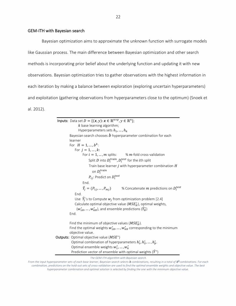
GEM-ITH with Bayesian search

Bayesian optimization aims to approximate the unknown function with surrogate models

like Gaussian process. The main difference between Bayesian optimization and other search

methods is incorporating prior belief about the underlying function and updating it with new

observations. Bayesian optimization tries to gather observations with the highest information in

each iteration by making a balance between exploration (exploring uncertain hyperparameters)

and exploitation (gathering observations from hyperparameters close to the optimum) (Snoek et

al. 2012).

Inputs: Data set 𝐷 = {(𝒙, 𝑦): 𝒙 ∈ ℝ𝑛×𝑝, 𝑦 ∈ ℝ𝑛}; 𝑘 base learning algorithm; Hyperparameters sets ℎ1 , … , ℎ𝑘

Bayesian search chooses 𝑏 hyperparameter combination for each learner For 𝐻 = 1, … , 𝑏𝑘:

For 𝑗 = 1, … , 𝑘: For 𝑖 = 1, … , 𝑚 splits: % 𝑚-fold cross-validation

Split 𝐷 into 𝐷𝑖𝑡𝑟𝑎𝑖𝑛, 𝐷𝑖

𝑡𝑒𝑠𝑡 for the 𝑖th split

Train base learner 𝑗 with hyperparameter combination 𝐻

on 𝐷𝑖𝑡𝑟𝑎𝑖𝑛

𝑃𝑖𝑗: Predict on 𝐷𝑖𝑡𝑒𝑠𝑡

End.

�̂�𝑗 = (𝑃1𝑗 , … , 𝑃𝑚𝑗) % Concatenate 𝑚 predictions on 𝐷𝑖𝑡𝑒𝑠𝑡

End.

Use �̂�𝑗’s to Compute 𝑤𝑗 from optimization problem [2.4]

Calculate optimal objective value (𝑀𝑆𝐸𝐻∗ ), optimal weights,

(𝑤1𝐻∗ , … , 𝑤𝑘𝐻

∗ ), and ensemble predictions (�̂�𝐻∗)

End. Find the minimum of objective values (𝑀𝑆𝐸𝐻

∗ ). Find the optimal weights 𝑤1𝐻

∗ , … , 𝑤𝑘𝐻∗ corresponding to the minimum

objective value. Outputs: Optimal objective value (𝑀𝑆𝐸∗)

Optimal combination of hyperparameters ℎ1∗ , ℎ2

∗ , … , ℎ𝑝∗ .

Optimal ensemble weights 𝑤1∗ , … , 𝑤𝑘

∗

Prediction vector of ensemble with optimal weights (�̂�∗)

The GEM-ITH algorithm with Bayesian search.

From the input hyperparameter sets of each base learner, Bayesian search selects 𝒃 combinations, resulting in a total of 𝒃𝒌combinations. For each combination, predictions on the hold-out sets of cross-validation are used to find the optimal ensemble weights and objective value. The best

hyperparameter combination and optimal solution is selected by finding the one with the minimum objective value.

23

Given 𝑏 iterations of Bayesian optimization, 𝑏 hyperparameter combinations for each

base learner have been identified resulting in 𝑏𝑘 total number of combinations that should be

considered by GEM-ITH model. Each of these combinations in turn is used to calculate out-of-

bag predictions of each base learner and treat them as the inputs to the optimization model

[2.4].

Results and Discussion

Numerical experiments

To evaluate the designed algorithm, numerical experiments on multiple data sets from

UCI Machine Learning Repository1 (Dua and Graff 2019), Scikit learn data sets (Pedregosa et al.

2011), and Kaggle data sets from a variety of domains have been conducted to demonstrate the

generalizability of the designed scheme. Details of these data sets are shown in Table 2.1

(Ferreira et al. 2010; Yeh 1998; Efron et al. 2004; Arzamasov et al. 2018; Tsanas and Xifara 2012;

Acharya et al. 2019; Grisoni et al. 2016; Cassotti et al. 2015; Cortez et al. 2009)

Table 2.1: data sets chosen to evaluate GEM-ITH

Data sets

Number of Instances

Number of Attributes Number of Target Attributes Area

Nominal Numeric

1 Behavior of Urban Traffic of Sao Paolo 135 1 16 1 Computer

2 Concrete Compressive Strength 1030 0 9 1 Physical

3 Diabetes Data 442 0 10 1 Life 4 Electrical Grid Stability Simulated Data 10000 1 13 2 Physical

5 Energy efficiency 768 0 8 2 Computer

6 Graduate Admissions 500 1 8 1 Education

7 QSAR Bioconcentration Classes 779 3 11 1 Life

8 QSAR Fish Toxicity Data 908 0 6 1 Physical

9 Wine Quality 4898 0 11 1 Business 10 Yacht Hydrodynamics 308 0 6 1 Physical

1 https://archive.ics.uci.edu/ml/index.php

24

Minimal pre-processing tasks were done on the selected data sets and the designed

GEM-ITH algorithm is applied to them. Five-fold cross-validation was used for generating out-of-

bag predictions for all designed ML models and the entire process was repeated 5 times. In

addition, 20% of each data set was reserved for testing and the training and optimizing

procedure was done on the remaining 80%.

Base models generation

A heuristic method was used here to generate base learners. Two important aspects of

the base learners were considered in this heuristic: 1) diversity, 2) performance. We intended to

select four base learners that show a certain level of diversity and performance to eventually

create a well-performing ensemble model. The following steps were taken to generate base

learners.

1) Trial training: Many machine learning models were trained on each of the

considered data sets and their performance were evaluated using unseen test

observations (See Table 2.2 for the hyperparameter settings of the models).

2) Performance pruning: The trained models whose prediction error were higher

than the average prediction error of all trained models, were removed from the

pool of the initial models.

3) Correlation: Pair-wise correlation of the remaining models were calculated.

4) Rank: The pair-wise correlations were ranked from the lowest correlation to the

highest.

25

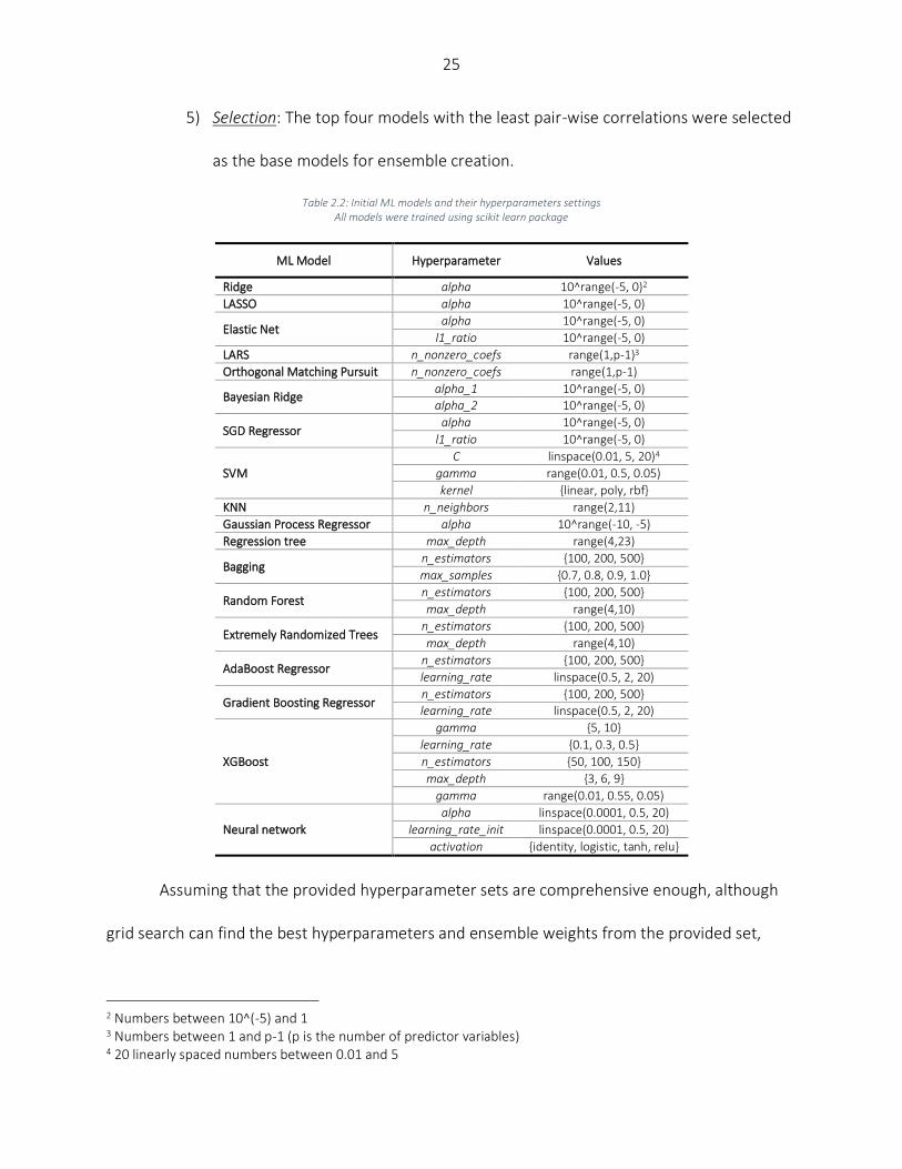
5) Selection: The top four models with the least pair-wise correlations were selected

as the base models for ensemble creation.

Table 2.2: Initial ML models and their hyperparameters settings All models were trained using scikit learn package

ML Model Hyperparameter Values

Ridge alpha 10^range(-5, 0)2

LASSO alpha 10^range(-5, 0)

Elastic Net alpha 10^range(-5, 0)

l1_ratio 10^range(-5, 0)

LARS n_nonzero_coefs range(1,p-1)3

Orthogonal Matching Pursuit n_nonzero_coefs range(1,p-1)

Bayesian Ridge alpha_1 10^range(-5, 0)

alpha_2 10^range(-5, 0)

SGD Regressor alpha 10^range(-5, 0)

l1_ratio 10^range(-5, 0)

SVM

C linspace(0.01, 5, 20)4

gamma range(0.01, 0.5, 0.05)

kernel {linear, poly, rbf}

KNN n_neighbors range(2,11)

Gaussian Process Regressor alpha 10^range(-10, -5)

Regression tree max_depth range(4,23)

Bagging n_estimators {100, 200, 500}

max_samples {0.7, 0.8, 0.9, 1.0}

Random Forest n_estimators {100, 200, 500}

max_depth range(4,10)

Extremely Randomized Trees n_estimators {100, 200, 500}

max_depth range(4,10)

AdaBoost Regressor n_estimators {100, 200, 500}

learning_rate linspace(0.5, 2, 20)

Gradient Boosting Regressor n_estimators {100, 200, 500} learning_rate linspace(0.5, 2, 20)

XGBoost

gamma {5, 10}

learning_rate {0.1, 0.3, 0.5}

n_estimators {50, 100, 150}

max_depth {3, 6, 9}

gamma range(0.01, 0.55, 0.05)

Neural network

alpha linspace(0.0001, 0.5, 20)

learning_rate_init linspace(0.0001, 0.5, 20)

activation {identity, logistic, tanh, relu}

Assuming that the provided hyperparameter sets are comprehensive enough, although

grid search can find the best hyperparameters and ensemble weights from the provided set,

2 Numbers between 10^(-5) and 1 3 Numbers between 1 and p-1 (p is the number of predictor variables) 4 20 linearly spaced numbers between 0.01 and 5

26

since that is computationally expensive and difficult to implement in practice, we use Bayesian

search to find top 12 combinations of the hyperparameters of each ML model. Therefore, since

we select four ML models with the heuristic explained above, the model should consider 124

combination of ML models hyperparameters. It should be noted that uniform settings have been

selected for Bayesian search. In other words, Bayesian search looks through all uniform values in

the range of hyperparameters. All other ensemble models and base learners are trained using

discrete settings of grid search.

To conduct the Bayesian search hyperopt package (Bergstra et al. 2013) was used in

Python 3. Also, Sequential Least Squares Programming algorithm (SLSQP) from Python’s SciPy

optimization library were used to solve optimization problems (Jones et al. 2001)

Benchmarks

Apart from the Generalized Ensemble Method introduced earlier (GEM), four other state-

of-art benchmarks have been used to compare the results of the designed learning methodology

with them.

1) The first benchmark is the Generalized Ensemble Method introduced before

(GEM).

2) The second benchmark is the ensembles constructed with averaging the input

base models (BEM).

3) Stacked ensemble with linear regression as the second level learner serves as the

third benchmark, which we call stacked regression. This benchmark has been

widely used as one of the most effective methods to create ensembles and is

27

created with fitting a linear regression model on the predictions made by

different base learners (Clarke 2003; Yao et al. 2018; Matlock 2018; Pavlyshenko

2019).

4) Considering random forest as one of the most powerful machine learning models

as the second level of stacking, we construct stacked ensemble with random

forest as the fourth benchmark (Thøgersen et al. 2016; Zhang et al. 2018).

5) Lastly, Stacked ensemble with k-nearest neighbor model as the 2nd level training

model is added as the fifth state-of-art benchmark (Ozay and Yarman-Vural 2016;

Pakrashi and Mac Namee 2017).

Numerical results

Table 2.3 shows the average results of GEM-ITH based off of Bayesian search methods

along with mean squared error of predictions made by each base learner and benchmarks. The

superiority of the designed ensemble techniques can be seen by comparing their prediction

errors with base learners. This answers the first question asked in the Introduction section and

demonstrates the improvements of the GEM-ITH over base learners.

Table 2.3: The average results of applying ML models and created ensembles on 10 public data sets Base models (Models 1 to 4) are different for different data sets and are generated using a heuristic. The best prediction accuracy (lowest

prediction error) in each row is shown in bold

Data set

Objective value on test set (MSE)

Model 1 Model 2 Model 3 Model 4 BEM Stacked

Regression Stacked

RF Stacked

KNN GEM GEM-ITH

Behavior of Urban Traffic 8.42 7.63 7.83 7.46 7.10 7.69 7.85 7.30 7.67 7.06

Concrete Compressive Strength 39.02 19.53 23.36 28.94 19.44 18.85 23.32 24.04 19.12 18.61

Diabetes Data 3042.27 3066.53 3110.75 5165.84 3122.05 3055.35 3884.18 3572.87 3038.89 2987.23

Electrical Grid Stability (× 𝟏𝟎𝟒) 3.55 2.79 13.58 4.70 3.70 1.82 2.14 2.12 2.36 2.25

Energy efficiency 4.06 10.63 1.62 11.64 4.49 1.45 2.01 2.12 1.62 1.42

Graduate Admissions (× 𝟏𝟎𝟑) 3.63 4.26 19.74 4.62 5.01 3.58 4.31 4.22 3.60 3.52

QSAR Bioconcentration (× 𝟏𝟎) 6.69 5.54 5.83 5.59 5.51 5.36 6.55 6.09 5.34 5.27

QSAR Fish Toxicity 8.51 7.67 7.68 7.03 7.05 7.09 9.27 8.78 7.04 6.93

Wine Quality (× 𝟏𝟎) 4.49 4.55 4.24 3.64 4.01 3.63 4.23 4.27 3.64 3.62

Yacht Hydrodynamics 70.93 1.15 0.88 69.42 15.55 0.96 1.66 1.61 0.91 0.77

28

Table 2.4 demonstrates the different choices of hyperparameters as the optimal

selections for creating optimal ensembles from GEM and GEM-ITH for Energy Efficiency data set

(the same was observed for other data sets, but they are not shown here). Comparing the tuned

hyperparameters before creating ensembles, with the ones found by GEM-ITH, the main claim of

this paper is proved to be true. The hyperparameters found to be optimal by GEM-ITH method

are different from the hyperparameters tuned separately (GEM). This means that in order to

create better performing ensembles, the hyperparameters should not necessarily be the ones

that are proved to be the best independently. This addresses the third question from questions

raised in the introduction section and expresses that tuning hyperparameters as part of finding

optimal ensemble weights results in higher quality predictions.

Table 2.4: Comparing optimal hyperparameters of GEM and GEM-ITH for Energy Efficiency data set

Hyperparameter Ensemble Method

Hyperparameter value

Regression Tree (max_depth)

GEM 6

GEM-ITH 19

Elastic Net (alpha)

GEM 0.00001

GEM-ITH 0.76785

Elastic Net (l1_ratio)

GEM 0.00001

GEM-ITH 0.01317

XGBoost (gamma) GEM 5

GEM-ITH 6.92567

XGBoost (learning_rate)

GEM 0.1

GEM-ITH 0.41613

XGBoost (n_ estimators)

GEM 150

GEM-ITH 150

XGBoost (max_depth)

GEM 9

GEM-ITH 9

SVM (C) GEM 1.32315

GEM-ITH 4.92209

SVM (gamma) GEM 0.01

GEM-ITH 0.35520

Figure 2.2 exhibits the normalized error rates of data sets under study for the designed

ensemble models. It visualizes the comparison between GEM-ITH and the state-of-art

benchmarks. The figure shows almost complete dominance of GEM-ITH over the benchmarks

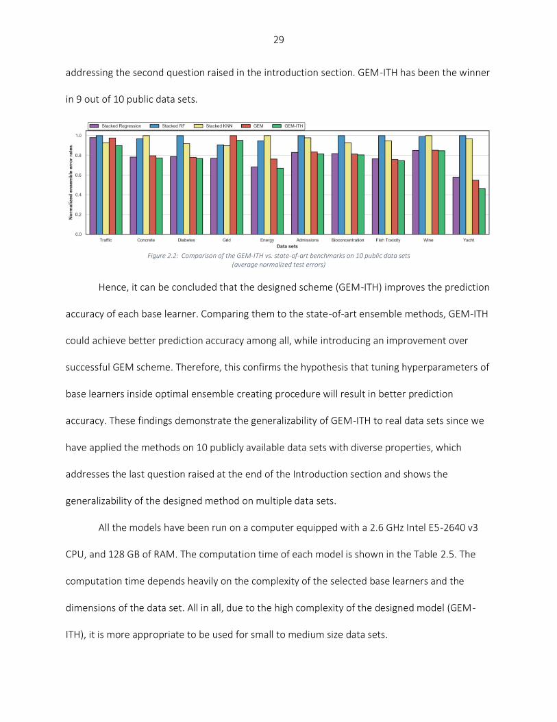
29

addressing the second question raised in the introduction section. GEM-ITH has been the winner

in 9 out of 10 public data sets.

Figure 2.2: Comparison of the GEM-ITH vs. state-of-art benchmarks on 10 public data sets

(average normalized test errors)

Hence, it can be concluded that the designed scheme (GEM-ITH) improves the prediction

accuracy of each base learner. Comparing them to the state-of-art ensemble methods, GEM-ITH

could achieve better prediction accuracy among all, while introducing an improvement over

successful GEM scheme. Therefore, this confirms the hypothesis that tuning hyperparameters of

base learners inside optimal ensemble creating procedure will result in better prediction

accuracy. These findings demonstrate the generalizability of GEM-ITH to real data sets since we

have applied the methods on 10 publicly available data sets with diverse properties, which

addresses the last question raised at the end of the Introduction section and shows the

generalizability of the designed method on multiple data sets.

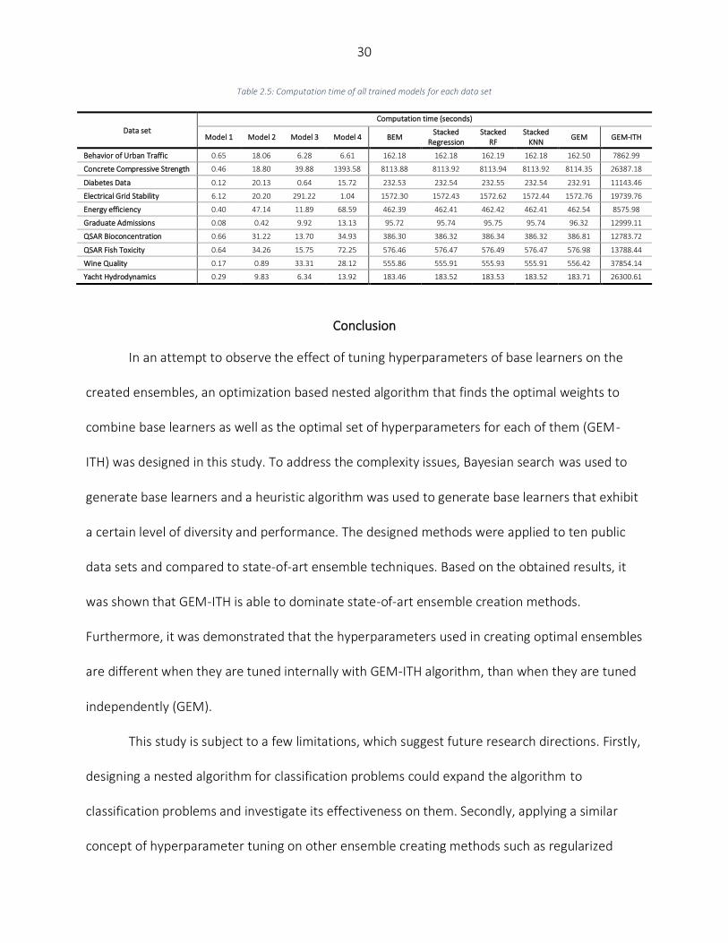
All the models have been run on a computer equipped with a 2.6 GHz Intel E5-2640 v3

CPU, and 128 GB of RAM. The computation time of each model is shown in the Table 2.5. The

computation time depends heavily on the complexity of the selected base learners and the

dimensions of the data set. All in all, due to the high complexity of the designed model (GEM-

ITH), it is more appropriate to be used for small to medium size data sets.

30

Table 2.5: Computation time of all trained models for each data set

Data set

Computation time (seconds)

Model 1 Model 2 Model 3 Model 4 BEM Stacked

Regression Stacked

RF Stacked

KNN GEM GEM-ITH

Behavior of Urban Traffic 0.65 18.06 6.28 6.61 162.18 162.18 162.19 162.18 162.50 7862.99

Concrete Compressive Strength 0.46 18.80 39.88 1393.58 8113.88 8113.92 8113.94 8113.92 8114.35 26387.18

Diabetes Data 0.12 20.13 0.64 15.72 232.53 232.54 232.55 232.54 232.91 11143.46

Electrical Grid Stability 6.12 20.20 291.22 1.04 1572.30 1572.43 1572.62 1572.44 1572.76 19739.76

Energy efficiency 0.40 47.14 11.89 68.59 462.39 462.41 462.42 462.41 462.54 8575.98

Graduate Admissions 0.08 0.42 9.92 13.13 95.72 95.74 95.75 95.74 96.32 12999.11

QSAR Bioconcentration 0.66 31.22 13.70 34.93 386.30 386.32 386.34 386.32 386.81 12783.72

QSAR Fish Toxicity 0.64 34.26 15.75 72.25 576.46 576.47 576.49 576.47 576.98 13788.44

Wine Quality 0.17 0.89 33.31 28.12 555.86 555.91 555.93 555.91 556.42 37854.14

Yacht Hydrodynamics 0.29 9.83 6.34 13.92 183.46 183.52 183.53 183.52 183.71 26300.61

Conclusion

In an attempt to observe the effect of tuning hyperparameters of base learners on the

created ensembles, an optimization based nested algorithm that finds the optimal weights to

combine base learners as well as the optimal set of hyperparameters for each of them (GEM-

ITH) was designed in this study. To address the complexity issues, Bayesian search was used to

generate base learners and a heuristic algorithm was used to generate base learners that exhibit

a certain level of diversity and performance. The designed methods were applied to ten public

data sets and compared to state-of-art ensemble techniques. Based on the obtained results, it

was shown that GEM-ITH is able to dominate state-of-art ensemble creation methods.

Furthermore, it was demonstrated that the hyperparameters used in creating optimal ensembles

are different when they are tuned internally with GEM-ITH algorithm, than when they are tuned

independently (GEM).

This study is subject to a few limitations, which suggest future research directions. Firstly,

designing a nested algorithm for classification problems could expand the algorithm to

classification problems and investigate its effectiveness on them. Secondly, applying a similar

concept of hyperparameter tuning on other ensemble creating methods such as regularized

31

stacking will more demonstrate the impact of hyperparameter tuning when creating ensembles.

Lastly, trying to speed-up the ensemble creating process even more when considering

hyperparameter tuning will create a competitive edge for the algorithm over competitions.

References

Aboah, A., Shoman, M., Mandal, V., Davami, S., Adu-Gyamfi, Y., & Sharma, A. (2021). A vision-based system for traffic anomaly detection using deep learning and decision trees. arXiv preprint arXiv:2104.06856.

Acharya, M., Armaan, A., & Antony, A. (2019). A Comparison of Regression Models for Prediction of Graduate Admissions. IEEE International Conference on Computational Intelligence in Data Science 2019.

Arzamasov, V., Böhm, K., & Jochem, P. (2018, 29-31 Oct. 2018). Towards Concise Models of Grid Stability. Paper presented at the 2018 IEEE International Conference on Communications, Control, and Computing Technologies for Smart Grids (SmartGridComm).

Barri, K., Jahangiri, B., Davami, O., Buttlar, W. G., & Alavi, A. H. (2020). Smartphone-based molecular sensing for advanced characterization of asphalt concrete materials. Measurement, 151, 107212.

Belayneh, A., Adamowski, J., Khalil, B., & Quilty, J. (2016). Coupling machine learning methods with wavelet transforms and the bootstrap and boosting ensemble approaches for

Bergstra, J., Yamins, D., & Cox, D. D. (2013). Making a science of model search: Hyperparameter optimization in hundreds of dimensions for vision architectures.

Bhasuran, B., Murugesan, G., Abdulkadhar, S., & Natarajan, J. (2016). Stacked ensemble combined with fuzzy matching for biomedical named entity recognition of diseases. Journal of biomedical informatics, 64, 1-9.

Boyd, S., & Vandenberghe, L. (2004). Convex optimization: Cambridge university press.

Breiman, L. (1996a). Bagging predictors. Machine learning, 24(2), 123-140.

Breiman, L. (1996b). Stacked regressions. Machine learning, 24(1), 49-64.

Breskvar, M., Kocev, D., & Džeroski, S. (2018). Ensembles for multi-target regression with random output selections. [journal article]. Machine Learning, 107(11), 1673-1709.

32

Brown, G. (2017). Ensemble Learning. In C. Sammut & G. I. Webb (Eds.), Encyclopedia of Machine Learning and Data Mining (pp. 393-402). Boston, MA: Springer US.

Brown, G., Wyatt, J., Harris, R., & Yao, X. (2005). Diversity creation methods: a survey and categorisation. Information Fusion, 6(1), 5-20.

Cassotti, M., Ballabio, D., Todeschini, R., & Consonni, V. (2015). A similarity-based QSAR model for predicting acute toxicity towards the fathead minnow (Pimephales promelas). SAR and QSAR in Environmental Research, 26(3), 217-243.

Clarke, B. (2003). Comparing Bayes model averaging and stacking when model approximation error cannot be ignored (Vol. 4): JMLR.org.

Conroy, B., Eshelman, L., Potes, C., & Xu-Wilson, M. (2016). A dynamic ensemble approach to robust classification in the presence of missing data. [journal article]. Machine Learning, 102(3), 443-463.

Cortez, P., Cerdeira, A., Almeida, F., Matos, T., & Reis, J. (2009). Modeling wine preferences by data mining from physicochemical properties. Decision Support Systems, 47(4), 547-553.

Dietterich, T. G. (2000). Ensemble methods in machine learning. Paper presented at the International workshop on multiple classifier systems.

Dua, D., & Graff, C. (2017). UCI machine learning repository (2017). URL http://archive.ics.uci.edu/ml.

Efron, B., Hastie, T., Johnstone, I., & Tibshirani, R. (2004). Least angle regression. The Annals of statistics, 32(2), 407-499.

Ekbal, A., & Saha, S. (2013). Stacked ensemble coupled with feature selection for biomedical entity extraction. Knowledge-Based Systems, 46, 22-32.

Ferreira, R. P., Affonso, C., & Sassi, R. J. (2010, 16-19 June 2010). Application of a neuro fuzzy

Freund, Y. (1995). Boosting a weak learning algorithm by majority. Information and computation, 121(2), 256-285.

Grisoni, F., Consonni, V., Vighi, M., Villa, S., & Todeschini, R. (2016). Investigating the mechanisms of bioconcentration through QSAR classification trees. Environment International, 88, 198-205.

Hansen, L. K., & Salamon, P. (1990). Neural network ensembles. IEEE Transactions on Pattern Analysis & Machine Intelligence (10), 993-1001.

Hastie, T., Tibshirani, R., Friedman, J., & Franklin, J. (2005). The elements of statistical learning: data mining, inference and prediction. The Mathematical Intelligencer, 27(2), 83-85.

33

Hoch, T. (2015). An Ensemble Learning Approach for the Kaggle Taxi Travel Time Prediction Challenge. Paper presented at the DC@ PKDD/ECML.

Hong, T., Pinson, P., & Fan, S. (2014). Global energy forecasting competition 2012: Elsevier.

Hu, K., Huang, P., Chen, H., & Peng, Y. (2017). KDD CUP 2017 Travel Time Prediction Predicting Travel Time – The Winning Solution of KDD CUP 2017. KDD.

Jimenez, D. (1998, 4-9 May 1998). Dynamically weighted ensemble neural networks for classification. Paper presented at the 1998 IEEE International Joint Conference on Neural Networks Proceedings. IEEE World Congress on Computational Intelligence (Cat. No.98CH36227).

Jones, E., Oliphant, T., & Peterson, P. (2001). SciPy: Open source scientific tools for Python.

Kechyn, G., Yu, L., Zang, Y., & Kechyn, S. (2018). Sales forecasting using WaveNet within the framework of the Kaggle competition. arXiv preprint arXiv:1803.04037.

Khaki, S., Khalilzadeh, Z., & Wang, L. (2019). Classification of crop tolerance to heat and drought—a deep convolutional neural networks approach. Agronomy, 9(12), 833.

Khaki, S., & Wang, L. (2019). Crop Yield Prediction Using Deep Neural Networks. Frontiers in Plant Science, 10(621). https://doi.org/10.3389/fpls.2019.00621

Koren, Y. (2009). The bellkor solution to the netflix grand prize. Netflix prize documentation, 81(2009), 1-10.

Krogh, A., & Vedelsby, J. (1995). Neural network ensembles, cross validation, and active learning. Paper presented at the Advances in neural information processing systems.

Large, J., Lines, J., & Bagnall, A. (2019). A probabilistic classifier ensemble weighting scheme based on cross-validated accuracy estimates. Data Mining and Knowledge Discovery, 1-36.

Martelli, P. L., Fariselli, P., & Casadio, R. (2003). An ENSEMBLE machine learning approach for the prediction of all-alpha membrane proteins. Bioinformatics, 19(suppl_1), i205-i211.

Matlock, K., De Niz, C., Rahman, R., Ghosh, S., & Pal, R. (2018). Investigation of model stacking for drug sensitivity prediction. BMC Bioinformatics, 19(3), 71.

Niculescu-Mizil, A., Perlich, C., Swirszcz, G., Sindhwani, V., Liu, Y., Melville, P., et al. (2009). Winning the KDD cup orange challenge with ensemble selection. Paper presented at the KDD-Cup 2009 Competition.

Ozay, M., & Yarman-Vural, F. T. (2016). Hierarchical distance learning by stacking nearest neighbor classifiers. Information Fusion, 29, 14-31.

34

Pakrashi, A., & Namee, B. M. (2017). Stacked-MLkNN: A stacking based improvement to Multi-Label k-Nearest Neighbours. Paper presented at the Proceedings of the First International Workshop on Learning with Imbalanced Domains: Theory and Applications. Retrieved from http://proceedings.mlr.press.

Pavlyshenko, B. M. (2019). Machine-Learning Models for Sales Time Series Forecasting. Data, 4(1), 15.

Pedregosa, F., Varoquaux, G., Gramfort, A., Michel, V., Thirion, B., Grisel, O., et al. (2011). Scikit-learn: Machine learning in Python. Journal of machine learning research, 12(Oct), 2825-2830.

Perrone, M. P., & Cooper, L. N. (1992). When networks disagree: Ensemble methods for hybrid neural networks: BROWN UNIV PROVIDENCE RI INST FOR BRAIN AND NEURAL SYSTEMS.

Peykani, P., & Mohammadi, E. (2020). Window Network Data Envelopment Analysis: An Application to Investment Companies. International Journal of Industrial Mathematics, 12(1), 89-99.

Peykani, P., Mohammadi, E., Emrouznejad, A., Pishvaee, M. S., & Rostamy-Malkhalifeh, M. (2019). Fuzzy data envelopment analysis: An adjustable approach. Expert Systems with Applications, 136, 439-452.

Peykani, P., Mohammadi, E., Pishvaee, M. S., Rostamy-Malkhalifeh, M., & Jabbarzadeh, A. (2018). A novel fuzzy data envelopment analysis based on robust possibilistic programming: possibility, necessity and credibility-based approaches. RAIRO-Oper. Res., 52(4-5), 1445-1463.

Peykani, P., Mohammadi, E., Saen, R. F., Sadjadi, S. J., & Rostamy-Malkhalifeh, M. (n.d.). Data envelopment analysis and robust optimization: A review. Expert Systems, n/a(n/a), e12534. https://doi.org/10.1111/exsy.12534

Pham, H., & Olafsson, S. (2019a). Bagged ensembles with tunable parameters. Computational Intelligence, 35(1), 184-203.

Pham, H., & Olafsson, S. (2019b). On Cesaro Averages for Weighted Trees in the Random

Puurula, A., Read, J., & Bifet, A. (2014). Kaggle LSHTC4 winning solution. arXiv preprint arXiv:1405.0546.

Shahhosseini M., Hu G., Pham H. (2020) Optimizing Ensemble Weights for Machine Learning Models: A Case Study for Housing Price Prediction. In: Yang H., Qiu R., Chen W. (eds) Smart Service Systems, Operations Management, and Analytics. INFORMS-CSS 2019. Springer Proceedings in Business and Economics. Springer, Cham.

35

Shahhosseini, M., Martinez-Feria, R. A., Hu, G., & Archontoulis, S. V. (2019). Maize yield and nitrate loss prediction with machine learning algorithms. Environmental Research Letters, 14(12), 124026.

Shen, Z.-Q., & Kong, F.-S. (2004). Dynamically weighted ensemble neural networks for regression problems. Paper presented at the Proceedings of 2004 International Conference on Machine Learning and Cybernetics (IEEE Cat. No. 04EX826).

Snoek, J., Larochelle, H., & Adams, R. P. (2012). Practical bayesian optimization of machine learning algorithms. Paper presented at the Advances in neural information processing systems.

Sutton, C., Ghiringhelli, L. M., Yamamoto, T., Lysogorskiy, Y., Blumenthal, L., Hammerschmidt, T., et al. (2018). NOMAD 2018 Kaggle Competition: Solving Materials Science Challenges Through Crowd Sourcing. arXiv preprint arXiv:1812.00085.

Taieb, S. B., & Hyndman, R. J. (2014). A gradient boosting approach to the Kaggle load forecasting competition. International journal of forecasting, 30(2), 382-394.

Thøgersen, M., Escalera, S., Gonzàlez, J., & Moeslund, T. B. (2016). Segmentation of RGB-D indoor scenes by stacking random forests and conditional random fields. Pattern Recognition Letters, 80, 208-215.

Töscher, A., & Jahrer, M. (2008). The bigchaos solution to the netflix prize 2008. Netflix Prize, Report.

Tsanas, A., & Xifara, A. (2012). Accurate quantitative estimation of energy performance of residential buildings using statistical machine learning tools. Energy and Buildings, 49, 560-567.

Van Rijn, J. N., Holmes, G., Pfahringer, B., & Vanschoren, J. (2018). The online performance estimation framework: heterogeneous ensemble learning for data streams. [journal article]. Machine Learning, 107(1), 149-176.

Wang, H., Xu, Q., & Zhou, L. (2015). Large unbalanced credit scoring using Lasso-logistic regression ensemble. PloS one, 10(2), e0117844.

Winham, S. J., Freimuth, R. R., & Biernacka, J. M. (2013). A weighted random forests approach to improve predictive performance. Statistical Analysis and Data Mining: The ASA Data Science Journal, 6(6), 496-505.

Wolpert, D. H. (1992). Stacked generalization. Neural Networks, 5(2), 241–259. https://doi.org/https://doi.org/10.1016/S0893-6080(05)80023-1

Yang, S., & Browne, A. (2004). Neural network ensembles: combining multiple models for enhanced performance using a multistage approach. Expert Systems, 21(5), 279-288.

36

Yao, Y., Vehtari, A., Simpson, D., & Gelman, A. (2018). Using Stacking to Average Bayesian Predictive Distributions (with Discussion). Bayesian Anal., 13(3), 917-1007.

Yeh, I.-C. (1998). Modeling of strength of high-performance concrete using artificial neural networks. Cement and Concrete research, 28(12), 1797-1808.

Yu, H.-F., Lo, H.-Y., Hsieh, H.-P., Lou, J.-K., McKenzie, T. G., Chou, J.-W., et al. (2010). Feature engineering and classifier ensemble for KDD cup 2010. Paper presented at the KDD Cup.

Yu, L., Lai, K. K., Wang, S., & Huang, W. (2006). A bias-variance-complexity trade-off framework for complex system modeling. Paper presented at the International Conference on Computational Science and Its Applications.

Zhang, C., & Ma, Y. (2012). Ensemble machine learning: methods and applications: Springer.

Zhang, X., & Mahadevan, S. (2019). Ensemble machine learning models for aviation incident risk prediction. Decision Support Systems, 116, 48-63.

Zou, H., Xu, K., Li, J., & Zhu, J. (2017). The Youtube-8M kaggle competition: challenges and methods. arXiv preprint arXiv:1706.09274.

37

CHAPTER 3. FORECASTING CORN YIELD WITH MACHINE LEARNING ENSEMBLES

Mohsen Shahhosseini1, Guiping Hu1*, Sotirios V. Archontoulis2

1 Department of Industrial and Manufacturing Systems Engineering, Iowa State University, Ames, Iowa, USA 2 Department of Agronomy, Iowa State University, Ames, Iowa, USA * Corresponding author e-mail: gphu@iastate.edu

Modified from manuscript published in Frontiers in Plant Sciences journal

Abstract

The emerge of new technologies to synthesize and analyze big data with high-

performance computing, has increased our capacity to more accurately predict crop yields.

Recent research has shown that Machine learning (ML) can provide reasonable predictions,

faster, and with higher flexibility compared to simulation crop modeling. However, a single

machine learning model can be outperformed by a “committee” of models (machine learning

ensembles) that can reduce prediction bias, variance, or both and is able to better capture the

underlying distribution of the data. Yet, there are many aspects to be investigated with regards

to prediction accuracy, time of the prediction, and scale. The earlier the prediction during the

growing season the better, but this has not been thoroughly investigated as previous studies

considered all data available to predict yields. This paper provides a machine leaning based

framework to forecast corn yields in three US Corn Belt states (Illinois, Indiana, and Iowa)

considering complete and partial in-season weather knowledge. Several ensemble models are

designed using blocked sequential procedure to generate out-of-bag predictions. The forecasts

are made in county-level scale and aggregated for agricultural district, and state level scales.

38

Results show that ensemble models based on weighted average of the base learners (average

ensemble, exponentially weighted average ensemble (EWA), and optimized weighted ensemble)

outperform individual models. Specifically, the proposed ensemble model could achieve best

prediction accuracy (RRMSE of 7.8%) and least mean bias error (-380 Kg/ha) compared to other

developed models. On the contrary, although random k-fold cross validation is replaced by

blocked sequential procedure, it is shown that stacked ensembles perform poorly for time series

data sets as they require the data to be non-IID to perform favorably. Comparing our proposed

model forecasts with the literature demonstrates the superiority of forecasts made by our

proposed ensemble model. Results from the scenario of having partial in-season weather

knowledge reveals that decent yield forecasts with RRMSE of 8.2% can be made as early as June

1st. Moreover, it was shown that the proposed model performed better than individual models

and benchmark ensembles at agricultural district and state-level scales as well as county-level

scale. To find the marginal effect of each input feature on the forecasts made by the proposed

ensemble model, a methodology is suggested that is the basis for finding feature importance for

the ensemble model. The findings suggest that weather features corresponding to weather in

weeks 18-24 (May 1st to June 1st) are the most important input features.

Introduction

Providing 11% of total U.S. employment, agriculture and its related industries are

considered as a significant contributor to the US economy, with $1.053 trillion of U.S. gross

domestic product (GDP) in 2017 (USDA Economic Research Center, 2019). Crop yield prediction

is of high significance since it can provide insights and information for improving crop

39

management, economic trading, food production monitoring, and global food security. In the

past, farmers relied on their experiences and past historical data to predict crop yield and make

important cropping decisions based on the prediction. However, the emergence of new

technologies such as simulation crop models, and machine learning in the recent years, and the

ability to analyze big data with high-performance computing, has resulted in more accurate yield

predictions (Drummond et al., 2003; Vincenzi et al., 2011; González Sánchez et al., 2014; Pantazi

et al., 2016; Jeong et al., 2016; Cai et al., 2017; Chlingaryan et al., 2018; Crane-Droesch, 2018;

Basso and Liu, 2019; Shahhosseini et al., 2019a).

Forecasting crop production is different from prediction, as it requires interpreting future

observations only using the past data (Griffiths et al., 2010; Johnson, 2014; Cai et al., 2017).

Previous studies considered all the data for forecasting, while the next challenge is to consider

partial data as it reflects reality better if we are to use a forecast model to inform farmers and

decision makers. Also, the scale of prediction is of interest. Yet we do not know if predictions are

more accurate at a finer (county) or course (agricultural district) scale. Previous research by

Sakamoto et al. (2014) and Peng et al. (2018) suggested better prediction accuracy for course

scale compared to a finer scale.

Simulation crop modeling has a reasonable prediction accuracy, but due to user skill, data

calibration requirements, long runtimes and data storage constraints, it is not as easily applicable

as machine learning (ML) models (Drummond et al., 2003; Puntel et al., 2016; Shahhosseini et al,

2019a). On the other hand, ML has enjoyed wide range of applications in various problems

including ecological predictive modeling, because of its ability in dealing with linear and

40

nonlinear relationships, non-normal data, and quality of results along with significantly lower

runtimes (De’ath and Fabricius, 2000).

Generally, supervised learning is categorized into regression and classification problems,

based on the type of response variables. Many studies have approached regression problems, in

which the response variable is continuous, with machine learning to solve an ecological problem

(James et al., 2013). These studies include but not limited to crop yield predictions (Drummond

et al., 2003; Vincenzi et al., 2011; González Sánchez et al., 2014; Pantazi et al., 2016; Jeong et al.,

2016; Cai et al., 2017; Chlingaryan et al., 2018; Crane-Droesch, 2018; Basso and Liu, 2019;

Shahhosseini et al., 2019a; Emirhüseyinoğlu and Ryan, 2019; Khaki and Wang, 2019; Khaki et al.,

2019), crop quality (Hoogenboom et al., 2004; Karimi et al., 2008; Mutanga et al., 2012;

Shekoofa et al., 2014; Qin et al., 2018; Lawes et al., 2019), water management (Mohammadi al.,

2015; Mehdizadeh et al., 2017; Feng et al., 2017), soil management (Morellos et al., 2016; Nahvi

et al., 2016; Johann et al., 2016) and others.

Studies show that a single machine learning model can be outperformed by a

“committee” of individual models, which is called a machine learning ensemble (Zhang and Ma,

2012). Ensemble learning is proved to be effective as it can reduce bias, variance, or both, and is

able to better capture the underlying distribution of the data in order to make better

predictions, if the base learners are diverse enough (Dietterich, 2000; Pham and Olafsson,

2019a, Pham and Olafsson, 2019b, Shahhosseini et al., 2019b; Shahhosseini et al., 2020). The

usage of ensemble learning in ecological problems is becoming more widespread, for instance,

bagging and specifically random forest (Vincenzi et al., 2011; Mutanga et al., 2012; Fukuda et al.,

2013; Jeong et al., 2016), boosting (De’ath, 2007; Heremans et al., 2015; Belayneh et al., 2016;

41

Stas et al., 2016; Sajedi-Hosseini et al., 2018), and stacking (Conţiu and Groza, 2016; Cai et al.,

2017; Shahhosseini et al., 2019b), are some of the ensemble learning applications in agriculture.

Although, there have been studies using some of ensemble methods in agriculture domain, to

the best of our knowledge, there is no study to compare the effectiveness of ensemble learning

for ecological problems, especially when there are temporal and spatial correlations in the data.

In this paper, we develop machine learning algorithms to forecast corn yields in three US

Corn Belt states (Illinois, Indiana, and Iowa), using data from 2000-2018. These three states

together produce nearly 50% of the total corn produced in the USA, which has an economic

value of $20 billion per year (NASS, 2019). In 2019, corn was the largest produced crop in the

United States (Capehart et al., 2019) and with the increasing movement towards ethanol to

replace gas in cars, it is almost necessary to increase the amount of corn being produced. Hence,

forecasting the corn yield for important US corn producing states could provide valuable insights

for decision making.

Therefore, we design several ML and ML ensemble models using blocked sequential

procedure (Cerqueira et al., 2017; Oliveira et al., 2018) to generate out-of-bag predictions and

evaluate their performance when forecasting corn yields. In addition, we investigate the effect of

having complete or partial in-season weather knowledge, when forecasting yields. The forecasts

are made in three scales: county, agricultural district, and state level, and the state-level

forecasts are compared with USDA NASS forecasts. Furthermore, a methodology to calculate

partial dependency of the proposed ensemble model is proposed which can quantify the

marginal effect of changing each input feature on the forecasts made be the ML ensemble

model. Based on the computed partial dependencies, a measure to calculate the importance of

42

input features from optimized weighted ensemble model is proposed which ranks input features

based on the variations in their partial dependency plots (PDPs). This analysis can help prioritize

which data to be collected in the future and inform agronomists to explain causes of high or low

yield levels in some years.

The remainder of this chapter is organized as follows. The data and methodologies are

described first. Then, the model performance results, discussions and potential improvements

are presented. Finally, the paper concludes with the findings.

Materials and Methods

The designed machine learning models aim at forecasting corn yield in three US Corn Belt

states with a data set including environmental (soil and weather) and management variables for

two different scenarios; complete knowledge of in-season weather, partial knowledge of in-

season weather (until August 1st) and three scale; county, agricultural district, and state level.

We selected three major corn production states in the US Corn Belt to explore our research

questions considering also the computational complexity of the developed ensemble models.

The data inputs used to drive ML were approximately the same that were used to drive a

crop model predictions (APSIM) in this region (Archontoulis and Licht, 2019). They were selected

because all of them are agronomically relevant for yield predictions (Archontoulis et al., 2020).

The data contains several soil parameters at a 5 km resolution (Soil Survey Staff, 2019), weather

data at 1 km resolution (Thornton et al., 2012), crop yield data at different scales (NASS, 2019),

and management information at the state level (NASS, 2019).

43

Data set

County-level historical observed corn yields were obtained from USDA National

Agricultural Statistics Service (NASS, 2019) for years 2000-2018. A data set was developed

containing observed information of corn yields, management (plant population and planting

date), and environment (weather and soil) features.

• Plant population: plant population measured in plants/acre, downloaded from

USDA NASS

• Planting progress (planting date): The weekly cumulative percentage of corn

planted over time within each state (NASS, 2019)

• Weather: 7 weather features aggregated weekly, downloaded from Daymet

(Thornton et al., 2012)

o Daily minimum air temperature in degrees Celsius.

o Daily m aximum air temperature in degrees Celsius.

o Daily total precipitation in millimeters per day

o Shortwave radiation in watts per square meter

o Water vapor pressure in pascals

o Snow water equivalent in kilograms per square meter

o Day length in seconds per day

• Soil: The following soil features were considered in this study: soil organic matter,

sand content, clay content, soil pH, soil bulk density, wilting point, field capacity,

saturation point and hydraulic conductivity. Because these features change across

the soil profile, we used different values for different soil layers, which resulted in

44

180 features for soil characteristics of the selected locations, downloaded from

Web Soil Survey (Soil Survey Staff, 2019)

• Yield: Annual corn yield data, downloaded from USDA National Agricultural

Statistics Service (NASS, 2019)

The developed data set consists of 5342 observations of annual average corn yields for

293 counties across three states on Corn Belt, and 597 input features mentioned above. The

reason to choose these components as the explanatory features is that the factors affecting yield

performance are mainly environment, genotype, and management. Weather and soil features

were included in the data set to account for environment component, as well as management,

but since there is no publicly available genotype data set, the effect of genotype on the yield

performance is not considered. In this study we used many input parameters that are probably

less likely to be available in other parts of the world. In this case we recommend use of gridded

public soil or weather databases used to drive global crop production models (Rosenzweig et al.,

2013; Hengl et al., 2014; Elliott et al., 2015; Han et al., 2019).

Data Pre-processing

Data pre-processing tasks were performed before training the machine learning models.

First off, the data of the years 2016-2018 were reserved as the test subset and the remaining

data was used to build the models. Second, all input variables were scaled and transformed to a

range between 0 and 1 to prevent the magnitude of some features mislead the machine learning

models. Third, new features were constructed that account for the yearly trends in the yields,

and finally, random forest-based feature selection was performed to avoid overfitting in model

training.

45

Feature construction for the yearly trends

Figures 3.1(a) and 3.1(b) suggest an increasing trend in the corn yields for the locations

under study. This trend is due to improved genetics (cultivars), improved management, and

other technological advances such as farming equipment (range of yield increase was from 32 to

189 Kg/ha/year). Since there is no feature in the input variables that can explain this observed

trend, we decided to add new features to the developed data set that can explain the trend

Temperature is one of the many factors influence historical yield increase. Other factors

are changes in weather (precipitation), increase in plant density, improved genetics, improved

planting technology and improvements in soil and crop management over time. Because there is

not enough information to separate the contribution of each factors with the available data, we

simply considered all these factors as one factor in this study.

Two measures were done to account for the trend in yields.

1) To observe the trend in corn yields, a new feature (yield_trend) was created. A

linear regression model was built for each location as the trends for each site tend

to be different. The independent and dependent variables of this linear regression

model were comprised of the year (𝑌𝐸𝐴𝑅) and yield (𝑌), respectively. Afterwards,

the predicted value for each data point (�̂�) is added as the value of the new

feature. The data used for fitting this linear trend model was only training data

and for finding the corresponding values of the newly added feature for the test

set observations, the prediction made by this trend model for the data of the test

years (�̂�𝑖,𝑡𝑒𝑠𝑡 = 𝑏0𝑖+ 𝑏1𝑖

𝑌𝐸𝐴𝑅𝑖,𝑡𝑒𝑠𝑡) was used. The trend value (�̂�𝑖) calculated for

46

each location (𝑖), that is added to the data set as a new feature is shown in the

following equation.

�̂�𝑖 = 𝑏0𝑖 + 𝑏1𝑖𝑌𝐸𝐴𝑅𝑖 [3.1]

2) Moreover, another new variable (yield_avg) was constructed that defines the

average yield of each year for each state when considering training data. The

procedure to find the average value of the yields of each state (𝑗) as the values of

the new feature, is shown mathematically in the equation [3.2].

𝑦𝑖𝑒𝑙𝑑_𝑎𝑣𝑔𝑗 = 𝑎𝑣𝑒𝑟𝑎𝑔𝑒(𝑦𝑖𝑒𝑙𝑑𝑗) [3.2]

3) It should be noted that the corresponding values of this feature for the unseen

test observations are calculated as follows. The last training year (2015) in each

state is used as a baseline and the average increment in the average yield of each

state is used as a measure of increase the state-wide average yield. The following

equation demonstrates the calculation of the values of newly created feature for

unseen test observations of state 𝑗 (years 2016-2018).

𝑦𝑖𝑒𝑙𝑑𝑎𝑣𝑔𝑗,𝑡= 𝑎𝑣𝑒𝑟𝑎𝑔𝑒(𝑦𝑖𝑒𝑙𝑑𝑗,2015) [1 + 𝑎𝑣𝑒𝑟𝑎𝑔𝑒 (

𝑦𝑖𝑒𝑙𝑑𝑎𝑣𝑔𝑗,𝑛− 𝑦𝑖𝑒𝑙𝑑𝑎𝑣𝑔𝑗,𝑛−1

𝑦𝑖𝑒𝑙𝑑𝑎𝑣𝑔𝑗,𝑛−1

)]

𝑡−2015

[3.3]

4) where 𝑗 shows each state, 𝑡 denotes the test year (2016-2018), and 𝑛 represents

the training year from the year 2001.

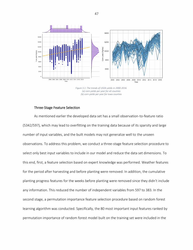
47

Three-Stage Feature Selection

As mentioned earlier the developed data set has a small observation-to-feature ratio

(5342/597), which may lead to overfitting on the training data because of its sparsity and large

number of input variables, and the built models may not generalize well to the unseen

observations. To address this problem, we conduct a three-stage feature selection procedure to

select only best input variables to include in our model and reduce the data set dimensions. To

this end, first, a feature selection based on expert knowledge was performed. Weather features

for the period after harvesting and before planting were removed. In addition, the cumulative

planting progress features for the weeks before planting were removed since they didn’t include

any information. This reduced the number of independent variables from 597 to 383. In the

second stage, a permutation importance feature selection procedure based on random forest

learning algorithm was conducted. Specifically, the 80 most important input features ranked by

permutation importance of random forest model built on the training set were included in the

Figure 3.1: The trends of USDA yields in 2000-2016. (a) corn yields per year for all counties

(b) corn yields per year for Iowa counties

48

training data set. The final stage of feature selection was a filter-based feature selection based

on Pearson correlation values. In this procedure, assuming linear relationships between

independent variables, features that were highly correlated (with a Pearson correlation higher

than 0.9) were identified and from each pair of linearly dependent features only one feature

were remained in the data set. This can be justified by the fact that when two features are highly

correlated, they have almost the same effect on the response variable, hence one of them is

redundant. This three-stage process is depicted in the Figure 3.2. It should be noted that the

constructed features for yearly yield trends were kept in the analysis data set.

Hyperparameter tuning and model selection

Walk-forward cross-validation

Optimizing hyperparameters of machine learning models could improve the prediction

accuracy and generalizability of the trained models. Traditionally, k-fold cross-validation is used

to find the best hyperparameter values using only training data. However, the assumption of the

data being independent and identically distributed (IID) does not hold for time series data sets

and disregarding this assumption will result in a cross-validation scheme that does not emulate

the test distribution well (Bergmeir et al., 2018). Hyndman and Athanasopoulos (2018)

introduced a walk-forward cross-validation procedure for time series analysis. In this method, a

set of validation sets are defined, each consisting of data from a single point in time. The training

set is formed by all the time points that occurred before each validation observation. Therefore,

future observations are not used in forecasting. Hence, to optimize the hyperparameter values

of machine learning models and select the best models only using the training set, a variation of

the walk-forward cross-validation introduced in Hyndman and Athanasopoulos (2018) is used,

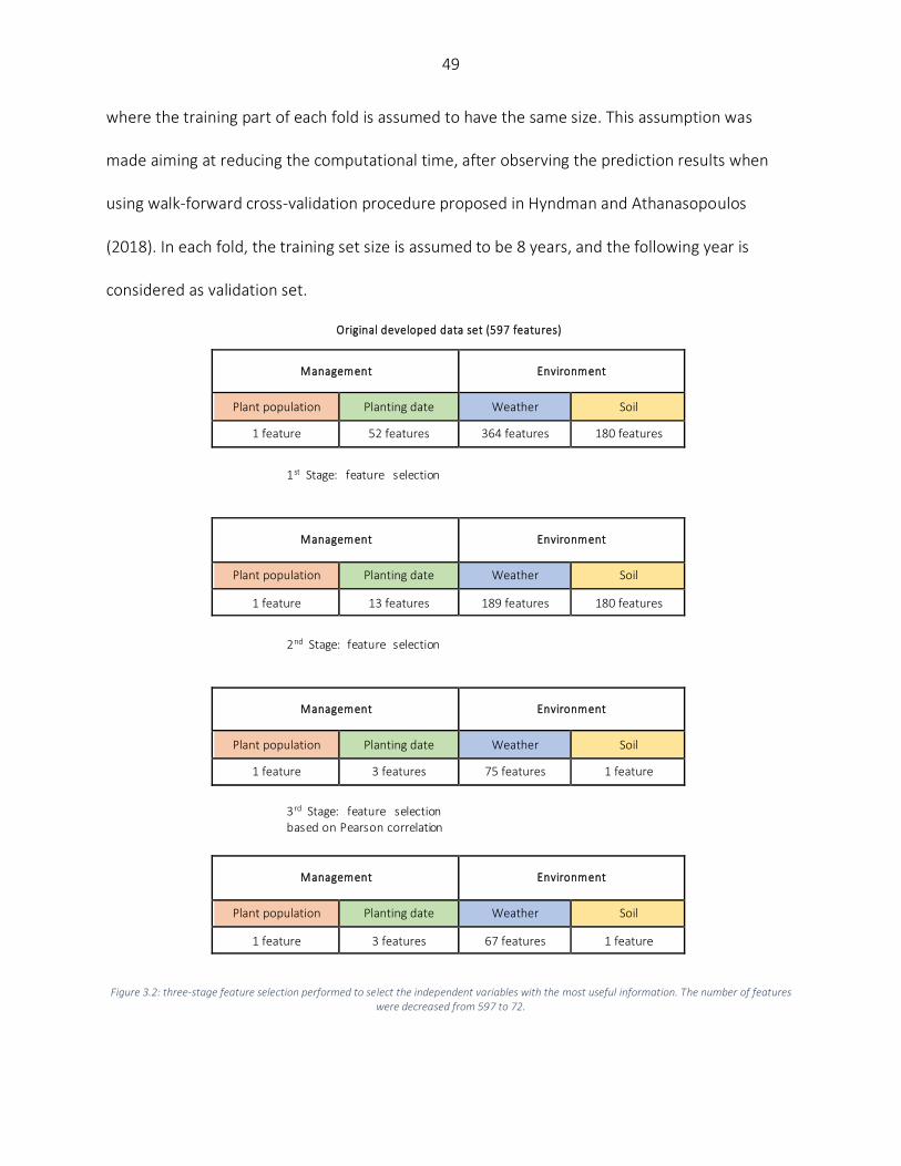
49

where the training part of each fold is assumed to have the same size. This assumption was

made aiming at reducing the computational time, after observing the prediction results when

using walk-forward cross-validation procedure proposed in Hyndman and Athanasopoulos

(2018). In each fold, the training set size is assumed to be 8 years, and the following year is

considered as validation set.

Figure 3.2: three-stage feature selection performed to select the independent variables with the most useful information. The number of features were decreased from 597 to 72.

Original developed data set (597 features)

Management Environment

Plant population Planting date Weather Soil

1 feature 52 features 364 features 180 features

Management Environment

Plant population Planting date Weather Soil

1 feature 13 features 189 features 180 features

Management Environment

Plant population Planting date Weather Soil

1 feature 3 features 75 features 1 feature

Management Environment

Plant population Planting date Weather Soil

1 feature 3 features 67 features 1 feature

1st Stage: feature selection based on expert knowledge

2nd Stage: feature selection with random forest

3rd Stage: feature selection based on Pearson correlation

50

Bayesian search

Assuming an unknown underlying distribution, Bayesian optimization intends to

approximate the unknown function with surrogate models such as Gaussian process. Bayesian

optimization is mainly different from other search methods in incorporating prior belief about

the underlying function and updating it with new observations. This difference makes Bayesian

search for hyperparameter tuning faster than exhaustive grid search, while finding a better

solution compared to random search. Bayesian optimization collects instances with the highest

information in each iteration by making a balance between exploration (exploring uncertain

hyperparameters) and exploitation (gathering observations from hyperparameters close to the

optimum) (Snoek et al. 2012). Thus, Bayesian search was selected as the hyperparameter tuning

search method, under the look-forward cross-validated procedure. Bayesian optimization is

conducted with the objective of minimizing training mean squared error (MSE), on the search

space consisting of hyperparameter values, and using Tree-structured Parzen Estimator

Approach (TPE) which uses the Bayes rule to construct the surrogate model (Bergstra et al.,

2011).

Analyzed models

Well-performing ensemble models require the base learners to exhibit a certain element

of “diversity” in their predictions along with retaining good performance individually (Brown,

2017). Therefore, a set of different models were selected and trained including linear regression,

LASSO regression, Extreme Gradient Boosting (XGBoost), LightGBM, and random forest. Random

forest uses ensembles of fully-grown trees, and therefore tend to have lower bias and higher

variance. Differently, gradient boosting is iteratively built on weak learners that tend to be on the

51

opposite end of the bias/variance tradeoff. Linear regression is also added as a benchmark and

LASSO regression is included due to its intrinsic feature selection. In addition, multiple two-level

stacking ensemble models, as well as average ensemble, and exponentially weighted average

ensemble (EWA) were constructed and evaluated on test unseen observations. Furthermore, an

optimized weighted ensemble model that accounts for both bias and variance of the predictions

was proposed that can use out-of-bag predictions to find the optimal weights in making optimal

weighted ensembles. The mentioned models can deal with features that have linear or nonlinear

correlation with the response variable.

Linear regression

Assuming a linear relationship between the predictors and the response variable, normal

distribution of residuals (normality), absence of correlation between predictors (no

multicollinearity), and similar variance of error across predictors (homoscedasticity), linear

regression predicts a quantitative response based on multiple predictor variables. A multiple

linear regression model is in the following form (James et al., 2013).

𝑌 = 𝛽0 + 𝛽1𝑋1 + 𝛽2𝑋2 + ⋯ + 𝛽𝑝𝑋𝑝 + 𝜖 [3.4]

in which 𝑌 is the response variable, 𝑋𝑗 are the independent variables, 𝛽𝑗 are the

coefficients, and 𝜖 is the error term. The coefficients are estimated by minimizing the loss

function 𝐿, as shown below.

𝐿 = ∑ (𝑦𝑖 − �̂�𝑖)2𝑛𝑖=1 = ∑ (𝑦𝑖 − �̂�0 − �̂�1𝑋𝑖1 − �̂�2𝑋𝑖2 − ⋯ − �̂�𝑝𝑋𝑖𝑝)2𝑛

𝑖=1 [3.5]

where �̂�𝑖 is the prediction for 𝑦𝑖.

52

LASSO regression

Least absolute shrinkage and selection operator (LASSO) is a regularization method that is

able to exclude some of the variables by setting their coefficient to zero (James et al., 2013). A

penalty term (|𝛽𝑗|) is added to linear regression model in LASSO which is able to shrink

coefficients towards zero (L1 regularization). The loss function of LASSO is as follows (Tibshirani,

1996).

𝐿 = ∑ (𝑦𝑖 − 𝑦�̂�)2𝑛

𝑖=1 + 𝜆 ∑ |𝛽𝑗|𝑝𝑗=1 [3.6]

where 𝜆 is the shrinkage parameter that needs to be determined before performing the learning

task.

XGBoost and LightGBM

Gradient boosting, a tree-based ensemble method, makes predictions by sequentially

combining weak prediction models. In other words, gradient boosting predicts by learning from

mistakes made by previous predictors. In this study, we made use of two relatively new and fast

implementations of gradient boosting: XGBoost and LightGBM. XGBoost, proposed in 2016 is

capable of handling sparse data, and makes use of an approximation algorithm, Weighted

Quantile Sketch, to determine splits and speed-up the learning process (Chen and Guestrin,

2016). LightGBM from Microsoft, published in 2017, introduced two ideas to improve

performance and reduce the computational time. First, gradient-based one-side sampling helps

selecting the most informative observations. Second, Exclusive Feature Bundling (EFB) takes

advantage of data sparsity and bins similar input features (Ke et al., 2017).

53

Random forest

Bootstrap aggregating (Bagging) is another tree-based ensemble model, which tries to

reduce the variance of predictions, consequently, increase the model’s generalizability, by

generating multiple trees from training data using sampling with replacement (Breiman, 1996).

Random forest is a special case of bagging ensemble in which each tree depends on a random

value, number of predictors chosen as split candidates in each iteration. (Breiman, 2001). This

makes random forest superior than bagging since random forest de-correlates the trees. In

addition, random forest makes use of observations not included in the bootstrapped samples

(out-of-bag observations) to compute error rates (Cutler et al., 2007).

Stacked generalization

Stacked generalization aims to minimize the generalization error of some ML models by

performing at least one more level of learning task using the outputs of ML base models as

inputs, and the actual response values of some part of the data set (training data) as outputs

(Wolpert, 1992). Stacked generalization assumes the data to be IID and performs a 𝑘-fold cross-

validation to generate out-of-bag predictions for validation set of each fold. Collectively, the 𝑘

out-of-bag predictions create a new training set for the second level learning task, with the same

size of the original training set (Cai et al., 2017). However, here the IID assumption of the data

does not hold and we cannot use 𝑘-fold cross-validation to generate out-of-bag predictions. To

work around this issue, blocked sequential procedure (Cerqueira et al., 2017; Oliveira et al.,

2018) was used to generate inputs of the stacked generalization method only using past data

(See Figure 3.3).

The following steps describe this procedure:

54

a) Consider first 8 years as training and the following year as validation set.

b) Train each base learner on the training data and make predictions for the

validation set (out-of-bag predictions).

c) Record the out-of-bag predictions and move the training and validation sets one

year forward.

d) Repeat (a)-(c) until reach the end of original training set.

Here it should be noted that the size of the generated out-of-bag predictions matrix is

smaller than the original training set since it does not include first 8 years of data in the

validation sets.

As the second level predictive model, four machine learning models were selected

resulting in four stacked generalization models:

1. Stacked regression: linear regression as the second level model

2. Stacked LASSO: LASSO regression as the second level model

3. Stacked random forest: random forest as the second level model

4. Stacked LightGBM: LightGBM as the second level model

55

Figure 3.3: Generating out-of-bag predictions with blocked sequential procedure

Proposed optimized weighted ensemble

Optimized weighted ensembles can be created with an optimization model. Due to the

tradeoff between bias and variance of the prediction, the optimized ensemble should be able to

predict with the least possible bias and variance. Specifically, we take advantage of bias and

variance decomposition as follows.

𝐸 [(𝑓(𝑥) − 𝑓(𝑥))

2] = (𝐵𝑖𝑎𝑠 [𝑓(𝑥)])

2+ 𝑉𝑎𝑟[𝑓(𝑥)] + 𝑉𝑎𝑟(𝜖)

[3.7]

Based on bias and variance tradeoff, the objective function of the optimization problem

can be mean squared error (MSE) of out-of-bag predictions for the ensemble (Hastie et al. 2005).

The out-of-bag predictions matrix created previously can be used as an emulator of unseen test

56

observations (Shahhosseini et al., 2019b). Using the out-of-bag predictions, we propose an

optimization problem which is a nonlinear convex optimization problem as follows.

𝑀𝑖𝑛 1

𝑛∑ (𝑦𝑖 − ∑ 𝑤𝑗�̂�𝑖𝑗

𝑘𝑗=1 )

2𝑛𝑖=1 [3.8]

𝑠. 𝑡.

∑ 𝑤𝑗𝑘𝑗=1 = 1,

𝑤𝑗 ≥ 0, ∀𝑗 = 1, … , 𝑘.

where 𝑤𝑗 is the weights corresponding to base model 𝑗 (𝑗 = 1, … , 𝑘), 𝑛 is the total

number of instances (𝑛 is smaller than the number of original training set observations because

first 8 years of training data never were included in the validation set), 𝑦𝑖 is the true value of

observation 𝑖, and �̂�𝑖𝑗 is the prediction of observation 𝑖 by base model 𝑗. Since other ensemble

learning models such as stacking strictly require the data to be IID, and that the proposed model

does not have such requirement, we expect this model to outperform the stacking ensembles as

well as base models.

Average ensemble

Average ensemble is the weighted average of out-of-bag predictions made by base

learners when they all have equal weights (𝑤𝑗 = 1/𝑘). When the base machine learning models

are diverse enough, the average ensemble can perform better than each of base learners

(Brown, 2017).

Exponentially weighted average ensemble (EWA)

Exponentially weighted average ensemble is different from other ensemble creation

methods, as it does not require the out-of-bag predictions. In fact, the weights for each model

can be computed using its past performance. In this case, we find the prediction error of out-of-

57

bag predictions made by each ML base learner and calculate their corresponding weights as

follows (Cesa-Bianchi and Lugosi, 2006).

𝑤𝑗 =𝑒𝑥𝑝(−𝑒𝑗)

∑ 𝑒𝑥𝑝(−𝑒𝑗)𝑘𝑗=1

[3.9]

where 𝑒𝑗 is the out-of-bag prediction error of base learner 𝑗.

Statistical performance metrics

Root mean squared error (RMSE)

Root mean squared error (RMSE) is defined as the square root of the average squared

deviation of predictions from actual values (Zheng, 2015).

𝑅𝑀𝑆𝐸 = √

∑ (𝑦𝑖−�̂�𝑖)2𝑖

𝑛

[3.10]

where 𝑦𝑖 denotes the actual values, �̂�𝑖 is the predictions and 𝑛 denotes the number of

data points.

Relative root mean squared error (RRMSE)

Relative root mean squared error (or normalized root mean squared error) is the RMSE

normalized by the mean of the actual values and is often expressed as percentage. Lower values

for RRMSE are preferred.

𝑅𝑅𝑀𝑆𝐸 =𝑅𝑀𝑆𝐸

𝑦 [3.11]

Mean bias error (MBE)

Mean bias error (MBE) is a measure to describe the average bias in the prediction.

𝑀𝐵𝐸 =∑ (�̂�𝑖−𝑦𝑖)𝑖

𝑛 [3.12]

58

Mean directional accuracy (MDA)

Mean directional accuracy (MDA) provides a metric to find the probability that the

prediction model can detect the correct direction of time series (Cicarelli, 1982; Schnader and

Stekler, 1990). While other metrics such as RMSE, RRMSE, and MBE are crucial to evaluate the

performance of the forecast, the directional movement of the forecast is important to

understand the capture of trend. This measure is commonly used in economics and

macroeconomics studies.

𝑀𝐷𝐴 =∑ 1𝑠𝑖𝑔𝑛(𝑦𝑡−𝑦𝑡−1)==𝑠𝑖𝑔𝑛(�̂�𝑡−𝑦𝑡−1)𝑡

𝑛 [3.13]

where 𝑦𝑡 and �̂�𝑡 are actual values and prediction at time 𝑡, 𝟏∙ is the indicator function,

and 𝑠𝑖𝑔𝑛(∙) denotes the sign function.

Results and Discussion

After presenting the numerical results of designed forecasting ML models and comparing

them with the literature, this section discusses the effect of in-season weather information on

the quality of forecasts by comparing the prediction accuracy of designed ensemble models on

different subsets of in-season weather information. In addition, we propose an approach to

calculate the partial dependency of the input features to the forecasts made by the optimized

weighted ensemble model and interpret the subsequent partial dependence plots. Moreover, a

method for computing importance of input features based on partial dependency is designed

and implemented to find the most influential independent variables for optimized weighted

ensemble.

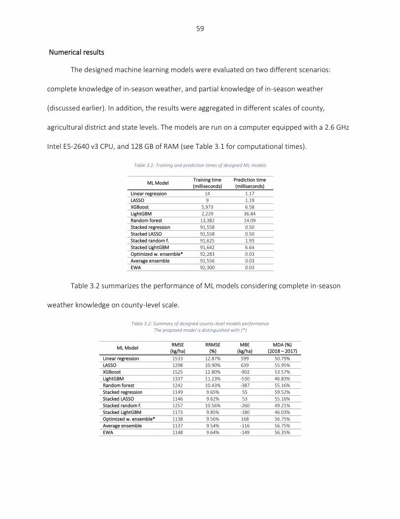
59

Numerical results

The designed machine learning models were evaluated on two different scenarios:

complete knowledge of in-season weather, and partial knowledge of in-season weather

(discussed earlier). In addition, the results were aggregated in different scales of county,

agricultural district and state levels. The models are run on a computer equipped with a 2.6 GHz

Intel E5-2640 v3 CPU, and 128 GB of RAM (see Table 3.1 for computational times).

Table 3.1: Training and prediction times of designed ML models

ML Model Training time (milliseconds)

Prediction time (milliseconds)

Linear regression 14 1.17

LASSO 9 1.19

XGBoost 5,973 6.58

LightGBM 2,229 36.84

Random forest 13,382 14.09

Stacked regression 91,558 0.50

Stacked LASSO 91,558 0.50

Stacked random f. 91,625 1.93

Stacked LightGBM 91,642 6.64

Optimized w. ensemble* 92,283 0.03

Average ensemble 91,556 0.03

EWA 92,300 0.03

Table 3.2 summarizes the performance of ML models considering complete in-season

weather knowledge on county-level scale.

Table 3.2: Summary of designed county-level models performance The proposed model is distinguished with (*)

ML Model RMSE

(kg/ha) RRMSE

(%) MBE

(kg/ha) MDA (%)

(2018 – 2017)

Linear regression 1533 12.87% 599 50.79%

LASSO 1298 10.90% 639 55.95%

XGBoost 1525 12.80% -902 53.57%

LightGBM 1337 11.23% -530 46.83%

Random forest 1242 10.43% -387 55.16%

Stacked regression 1149 9.65% 55 59.52%

Stacked LASSO 1146 9.62% 53 55.16%

Stacked random f. 1257 10.56% -260 49.21%

Stacked LightGBM 1173 9.85% -180 46.03%

Optimized w. ensemble* 1138 9.56% 168 56.75%

Average ensemble 1137 9.54% -116 56.75%

EWA 1148 9.64% -149 56.35%

60

As Table 3.2 shows, from the base ML models, random forest makes the least prediction

error based on RMSE and RRMSE indices. The MBE results show that the linear regression and

LASSO regression are the only prediction model that overestimates the true values and other ML

models underestimate the yields. Furthermore, random forest predictions are not as biased as

other base learners based on MBE values.

Ensemble models provide better performance compared to the base learners. The

proposed optimized weighted ensemble and the average ensemble are the most precise models

with RRMSE of 9.5%, which improves the prediction error of best base learner (random forest)

by about 8%. Stacked LASSO makes the least biased predictions (MBE of 53 kg/ha), while other

ensemble models also outperformed the base learners in terms of bias (See Figure 3.4).

It can be seen that weighted ensembles (optimized weighted ensemble, average

ensemble, and exponentially weighted ensemble) outperform base learners and stacked

ensembles. This can be explained by the IID requirement of stacking models. Although random k-

fold cross validation was replaced by blocked sequential procedure to generate out-of-bag

predictions, it seems that stacked ensemble models will not perform as good as weighted

ensemble models for non-IID data sets. Regarding mean directional accuracy (MDA) of year 2018

based on year 2017, Stacked regression predicted the correct direction of corn yields 60% of the

time, while optimized weighted ensemble model predictions are on the right direction 57% of

the time.

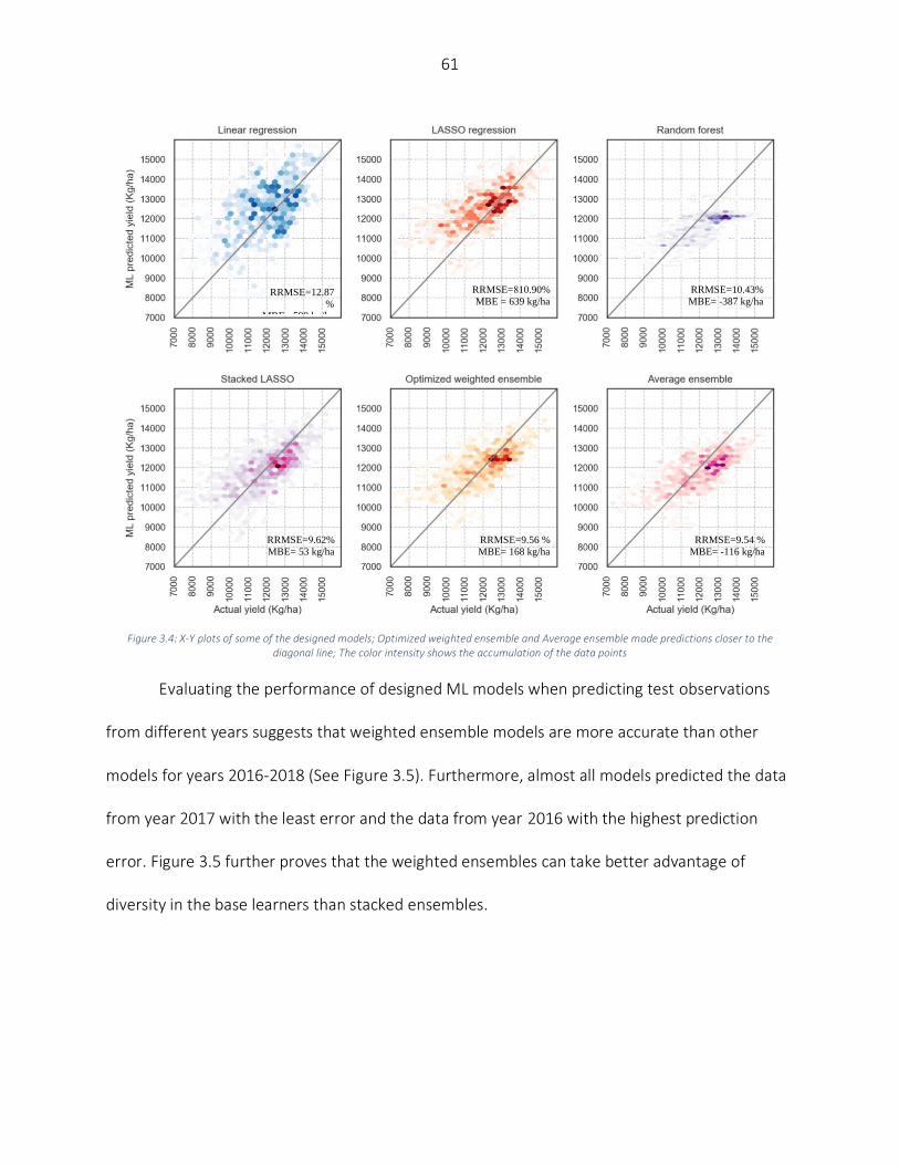
61

Figure 3.4: X-Y plots of some of the designed models; Optimized weighted ensemble and Average ensemble made predictions closer to the

diagonal line; The color intensity shows the accumulation of the data points

Evaluating the performance of designed ML models when predicting test observations

from different years suggests that weighted ensemble models are more accurate than other

models for years 2016-2018 (See Figure 3.5). Furthermore, almost all models predicted the data

from year 2017 with the least error and the data from year 2016 with the highest prediction

error. Figure 3.5 further proves that the weighted ensembles can take better advantage of

diversity in the base learners than stacked ensembles.

RRMSE=12.87

%

MBE= 599 kg/ha

RRMSE=810.90%

MBE = 639 kg/ha

RRMSE=10.43%

MBE= -387 kg/ha

RRMSE=9.62%

MBE= 53 kg/ha

RRMSE=9.56 %

MBE= 168 kg/ha

RRMSE=9.54 %

MBE= -116 kg/ha

62

Figure 3.5: Performance of ML models in predicting test observations from different years

The performance of our proposed optimized weighted ensemble model is also compared

to the models developed in similar studies that tried to use machine learning to predict US corn

yield. Jeong et al. (2016) could predict US corn yield with 30 years of data using random forest

with the prediction RRMSE of 16.7%; while Crane-Droesch (2018) could achieve out-of-bag USDA

corn prediction error of 13.4% using semiparametric neural network with a data set comprised

of the information for years 1979-2016. Kim et al. (2019) designed a model which predicted

cross-validation out-of-bag samples with a RRMSE of 7.9% (Table 3.3). It should be noted that

because of non-IID nature of yield prediction data sets, it is not entirely appropriate to

demonstrate cross-validation out-of-bag errors as the estimators of the true error. The

presented error of our model is drawn from testing the developed model on unseen

observations of future years.

Based on the results, the purpose of analysis can make one or more models more

favorable against others. For instance, if the objective is to forecast corn yields with the lowest

prediction error, weighted ensemble models should be selected; whereas, in the event that the

goal is to detect the correct forecast direction, stacked LASSO regression could be chosen.

However, overall performance of weighted ensemble models, with having the least prediction

7%

8%

9%

10%

11%

12%

13%

14%

15%

LR LASSO XGB LGB RF S-Reg. S-LASSO S-RF S-LGB Opt.Ens. Avg.Ens. EWA

RR

MSE

(%

)

2016 2017 2018

63

error and acceptable bias, and a quite high probability in detecting the right forecast direction, is

better than other models.

Table 3.3: Comparing prediction error of the proposed model (optimized weighted ensemble) with the literature. The error values of some studies were converted from different units to Kg/ha to have the same unit

Data years Forecast

level Forecast

date Test set Developed model RMSE (Kg/ha)

RRMSE (%)

Optimized w. ensemble* 2000-2018 County Oct 2016-2018 Optimal weighted ensemble 1138 9.5%

Bolton and Friedl (2013) 2004-2008 County Sep 2009 MODIS5-based Linear regression 809 8.0%

Johnson (2014) 2006-2011 County Oct 2012 Cubist 1260 17.1%

Sakamoto et al. (2014) 2008-2011 State Aug 2002-2007 & 2012 MODIS-based bias correction 950 11.8%

Jeong et al. (2016) 1984-2013 County Oct 50% of the data split randomly Random forest 1130 16.7%

Kuwata and Shibasaki (2016) 2008-2013 County Oct 20% of the data split randomly Deep neural network 1142 14.0%

Jin et al. (2017) 2001-2015 County Aug 2008-2015 from 6 other states Ensemble of crop models 1286 18.6%

Crane-Droesch (2018) 1979-2016 County Oct Out-of-bag samples Semiparametric neural net 998 13.4%

Peng et al. (2018) 1982-2016 National August Forward CV Out-of-bag samples Linear regression 275 2.8%

Kim et al. (2019) 2006-2015 County Jul - Aug CV Out-of-bag samples Deep neural network 765 7.9%

Schwalbert et al. (2020) 2008-2017 County Aug CV Out-of-bag samples Linear regression 1040 11.0%

Archontoulis et al. (2020) 2015-2018 Field Jun-Aug Field data APSIM model - 14-20%

Table 3.4 summarizes the performance of the designed models when the forecasts are

aggregated on agricultural district and state levels. Total area harvested was used as the

measure to compute weighted average of county-level yields to obtain agricultural district and

state-level corn yields. The results are in line with the county-level forecasts and optimized

weighted ensemble and average ensemble as well as stacked LightGBM outpace base learners

and other ensemble models in term of prediction error (RRMSE). Mean directional accuracy

results are a bit different from county-level analysis and the reason seems to be smaller number

of data points. Linear regression and LASSO appear to be the only base learners that

overestimate the yields and have a higher probability to predict in the correct forecast direction.

5 Moderate Resolution Imaging Spectroradiometer

64

Table 3.4: Summary of state and agricultural district - level models performance

ML model

(a) Agricultural district – level forecasts

(b) State – level forecasts

RMSE (Kg/ha)

RRMSE (%)

MBE (Kg/ha)

MDA (%) (2018 – 2017)

RMSE (Kg/ha)

RRMSE (%)

MBE (Kg/ha)

MDA (%) (2018 – 2017)

Linear regression 1556 12.99% 542 62.96% 985 8.05% 305 100.00%

LASSO 1364 11.39% 569 48.15% 662 5.41% 321 100.00%

XGBoost 1628 13.60% -967 40.74% 1393 11.38% -1221 66.67%

LightGBM 1427 11.91% -607 37.04% 1087 8.88% -853 0.00%

Random forest 1328 11.09% -469 29.63% 945 7.72% -712 33.33%

Stacked regression 1266 10.57% -13 40.74% 742 6.06% -251 66.67%

Stacked LASSO 1264 10.55% -15 40.74% 632 5.17% -269 66.67%

Stacked random f. 1270 10.60% -335 29.63% 836 6.83% -601 66.67%

Stacked LightGBM 1242 10.37% -253 37.04% 756 6.18% -503 66.67%

Optimized w. ensemble* 1251 10.45% 99 33.33% 608 4.97% -151 66.67%

Average ensemble 1262 10.54% -186 33.33% 761 6.22% -432 66.67%

EWA 1329 11.09% -468 29.63% 946 7.73% -711 33.33%

Partial knowledge of in-season weather information

To evaluate the impact of partial in-season weather knowledge on corn yield forecasts,

the machine learning ensemble models were trained on a subset of weather features, including

information from planting time up to June 1st, July 1st, August 1st, September 1st, and October 1st.

Hyperparameter tuning and model selection has been done separately when considering each

scenario. Figure 3.6 demonstrates the RRMSE of ensemble forecasts when having partial in-

season weather information. As the figure suggests, although the forecasts become more

accurate with more recent weather data, decent forecasts can be made from weighted

ensemble models as early as June 1st. This is a very important result because maize market price

is usually high during that period (due to uncertainty in weather) and thus knowledge of yield

can be very valuable. In addition, Figure 3.6 proves it further that weighted ensemble models

perform better than stacking ensembles even considering all partial weather scenarios.

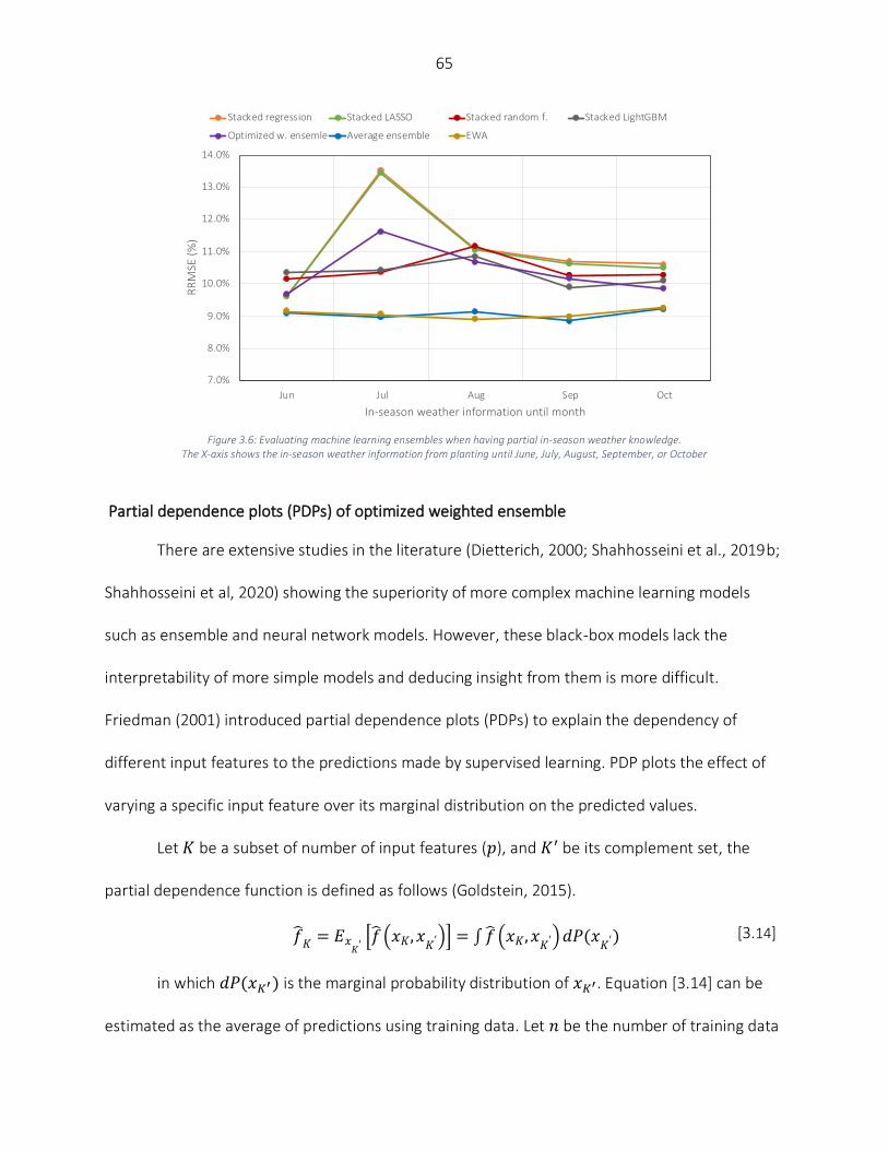
65

Figure 3.6: Evaluating machine learning ensembles when having partial in-season weather knowledge.

The X-axis shows the in-season weather information from planting until June, July, August, September, or October

Partial dependence plots (PDPs) of optimized weighted ensemble

There are extensive studies in the literature (Dietterich, 2000; Shahhosseini et al., 2019b;

Shahhosseini et al, 2020) showing the superiority of more complex machine learning models

such as ensemble and neural network models. However, these black-box models lack the

interpretability of more simple models and deducing insight from them is more difficult.

Friedman (2001) introduced partial dependence plots (PDPs) to explain the dependency of

different input features to the predictions made by supervised learning. PDP plots the effect of

varying a specific input feature over its marginal distribution on the predicted values.

Let 𝐾 be a subset of number of input features (𝑝), and 𝐾′ be its complement set, the

partial dependence function is defined as follows (Goldstein, 2015).

�̂�𝐾 = 𝐸𝑥𝐾′

[�̂� (𝑥𝐾, 𝑥𝐾′)] = ∫ �̂� (𝑥𝐾, 𝑥

𝐾′) 𝑑𝑃(𝑥𝐾′) [3.14]

in which 𝑑𝑃(𝑥𝐾′) is the marginal probability distribution of 𝑥𝐾′. Equation [3.14] can be

estimated as the average of predictions using training data. Let 𝑛 be the number of training data

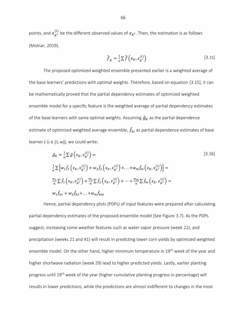
66

points, and 𝑥𝐾′(𝑖)

be the different observed values of 𝑥𝐾′. Then, the estimation is as follows

(Molnar, 2019).

�̂�𝐾 =1

𝑛∑ �̂� (𝑥𝐾, 𝑥

𝐾′(𝑖)

) [3.15]

The proposed optimized weighted ensemble presented earlier is a weighted average of

the base learners’ predictions with optimal weights. Therefore, based on equation [3.15], it can

be mathematically proved that the partial dependency estimates of optimized weighted

ensemble model for a specific feature is the weighted average of partial dependency estimates

of the base learners with same optimal weights. Assuming �̂�𝐾 as the partial dependence

estimate of optimized weighted average ensemble, 𝑓𝑘𝑖 as partial dependence estimates of base

learner 𝑖 (𝑖 ∈ [1, 𝑚]), we could write:

�̂�𝐾 =1

𝑛∑ �̂� (𝑥𝐾 , 𝑥

𝐾′(𝑖)

) =

1

𝑛∑ [𝑤1�̂�1 (𝑥𝐾 , 𝑥

𝐾′(𝑖)

) + 𝑤2𝑓2 (𝑥𝐾 , 𝑥𝐾′(𝑖)

) +. . . +𝑤𝑚𝑓𝑚 (𝑥𝐾 , 𝑥𝐾′(𝑖)

)] =

𝑤1

𝑛∑ 𝑓1 (𝑥𝐾 , 𝑥

𝐾′(𝑖)

) +𝑤2

𝑛∑ 𝑓2 (𝑥𝐾 , 𝑥

𝐾′(𝑖)

) + ⋯ +𝑤𝑚

𝑛∑ 𝑓𝑚 (𝑥𝐾 , 𝑥

𝐾′(𝑖)

) =

𝑤1𝑓𝑘1 + 𝑤2𝑓𝑘2+. . . +𝑤𝑚𝑓𝑘𝑚

[3.16]

Hence, partial dependency plots (PDPs) of input features were prepared after calculating

partial dependency estimates of the proposed ensemble model (See Figure 3.7). As the PDPs

suggest, increasing some weather features such as water vapor pressure (week 22), and

precipitation (weeks 21 and 41) will result in predicting lower corn yields by optimized weighted

ensemble model. On the other hand, higher minimum temperature in 19th week of the year and

higher shortwave radiation (week 29) lead to higher predicted yields. Lastly, earlier planting

progress until 19th week of the year (higher cumulative planting progress in percentage) will

results in lower predictions, while the predictions are almost indifferent to changes in the most

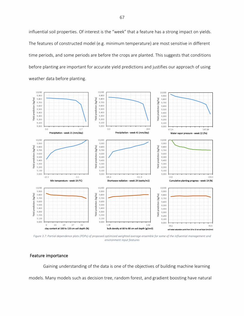
67

influential soil properties. Of interest is the “week” that a feature has a strong impact on yields.

The features of constructed model (e.g. minimum temperature) are most sensitive in different

time periods, and some periods are before the crops are planted. This suggests that conditions

before planting are important for accurate yield predictions and justifies our approach of using

weather data before planting.

Figure 3.7: Partial dependence plots (PDPs) of proposed optimized weighted average ensemble for some of the influential management and

environment input features

Feature importance

Gaining understanding of the data is one of the objectives of building machine learning

models. Many models such as decision tree, random forest, and gradient boosting have natural

68

ways of quantifying the importance of input features. However, interpreting the features for

more complex models like ensembles and deep neural network models are more difficult,

making these models black-box. An approach to estimate the relative influence of each input

feature for these black-box models, especially for ensemble models is introduced here. This

method is based on partial dependency of input features. Essentially, it can be derived from

PDPs that input features that have more variability in their PDP, are more influential in the final

predictions made by the ML model (Greenwell, 2018). Consequently, the features for which the

PDP is flat is likely to be less important than input variables with more variable PDP across range

of their values.

To this end, sample standard deviation of the partial dependency values for optimized

weighted ensemble calculated earlier is used as a measure of variable importance. In other

words, the predictors with higher sample standard deviation are more important features.

Assuming 𝑘 levels for the 𝑖th input feature and based on �̂�𝑖(𝑥𝑖𝑗) calculated earlier in equation

[3.16], we can define importance of features as follows.

𝑖𝑚𝑝𝑜𝑟𝑡𝑎𝑛𝑐𝑒(𝑥

𝑖) = √ 1

𝑘−1∑ [�̂�𝑖(𝑥𝑖𝑗) −

1

𝑘∑ �̂�𝑖(𝑥𝑖𝑗)𝑘

𝑗=1 ]2

𝑘𝑗=1

[3.17]

Table 3.5 presents the feature importance results for the top 20 input variables found by

optimized weighted ensemble model. Based on the proposed feature importance method, the

constructed features for capturing yield’s trend, namely yield_trend and yield_avg, are the most

important features. All other features from the top 20 input variables are consisted of weather

parameters along with cumulative planting progress until 19th week of the year. In addition, it

seems that weather in weeks 18-24 (May 1st to June 1st) is of greater importance compared to

weather in other periods of the year.

69

Table 3.5: Feature importance from optimized weighted ensemble: Top 20 input features

Feature name Week Importance

1 yield_trend (kg/ha) - 1711.65

2 yield_avg (kg/ha) - 1257.70

3 precipitation (mm/day) 21 221.14

4 precipitation (mm/day) 41 215.32

5 water vapor pressure (Pa) 22 164.14

6 minimum temperature (ᵒC) 19 155.29

7 shortwave radiation (watts/m2) 29 129.36

8 water vapor pressure (Pa) 26 120.49

9 precipitation (mm/day) 34 115.61

10 shortwave radiation (watts/m2) 44 109.33

11 water vapor pressure (Pa) 30 108.87

12 minimum temperature (ᵒC) 33 107.03

13 Cumulative planting progress (%) 19 106.04

14 precipitation (mm/day) 32 89.15

15 precipitation (mm/day) 38 79.95

16 shortwave radiation (watts/m2) 37 77.77

17 precipitation (mm/day) 18 76.23

18 shortwave radiation (watts/m2) 27 75.73

19 minimum temperature (ᵒC) 28 75.07

20 shortwave radiation (watts/m2) 35 59.94

The framework developed here can be expended to more US states. In addition, more

input features such as forecasted weather data, and N-fertilization inputs by county can be

added that may result in even higher prediction accuracy. This is something to be explored in the

future along with procedures to forecast corn yields with more extensive input features. Further,

the developed machines learning models can be used to provide insight into key factors which

determine inter-annual yield variability and therefore inform plant breeders and agronomists.

Conclusion

Motivated by the needs to forecast crop yields as early as possible and across scales as

well as compare the effectiveness of ensemble learning for ecological problems, especially when

there are temporal and spatial correlations in the data, we designed a machine learning based

framework to forecast corn yield using weather, soil, plant population, and planting date data.

70

Several ensemble models were designed using blocked sequential procedure to generate

out-of-bag predictions. In addition, an optimized weighted ensemble model was proposed that

accounts for both bias and variance of predictions and makes use of out-of-bag predictions to

find the optimal weight to combine multiple base learners. The forecasts considered two

weather scenarios: complete knowledge of in-season weather, and partial knowledge of in-

season weather (weather information until June 1st, July 1st, August 1st, September 1st, and

October 1st) and three scales: county, agricultural district, and state levels. The prediction results

of the scenario of having partial in-season weather demonstrated that ample corn yield forecasts

can be made as early as June 1st. Comparing the proposed model with the existing models in the

literature, it was demonstrated that the proposed optimized ensemble model is capable of

making improved yield forecasts compared to existing ML based models. Furthermore, weighted

average ensembles were the leaders among all developed ML models and stacked ensemble

models could not perform favorably due to non-IID nature of data set. In addition, a method to

find partial dependency and consequently feature importance of optimized weighted ensemble

model is proposed which can find the marginal effect of varying each input variable on the

ensemble predictions and rank the input features based on the variability of their partial

dependence plots (PDPs). The procedure proposed here for finding partial dependency and

feature importance for optimized weighted ensemble model can be easily applied on other

ensemble models.

This study is subject to a few limitations, which suggest future research directions. Firstly,

it was shown that stacked ensemble models suffer from non-IID nature of the data and blocked

sequential procedure could not help those models predict better than base learners. Working

71

more on the cross-validation procedure to generate improved out-of-bag predictions that

emulate test observations better can be considered as a future research direction. Secondly, the

performance of ensemble modeling is dependent on the diversity of the selected base ML

models and finding models that are diverse enough is a challenge that needs to be addressed.

Therefore, quantifying base models’ diversity in order to select more diverse models to create

better-performing ensembles can be thought of as future research recommendations. Lastly,

adding more input features such as forecasted weather data, and N-fertilization inputs by county

can improve the model performance. Future research can be done on what additional features

should be collected and analysis can be conducted on prediction model.

References

Archontoulis, S. V, Castellano, M. J., Licht, M. A., Nichols, V., Baum, M., Huber, I., Martinez-Feria, R., Puntel, L., Ordóñez, R. A., Iqbal, J., Wright, E. E., Dietzel, R. N., Helmers, M., Vanloocke, A., Liebman, M., Hatfield, J. L., Herzmann, D., Córdova, S. C., Edmonds, P., … Lamkey, K. R. (2020). Predicting crop yields and soil-plant nitrogen dynamics in the US Corn Belt. Crop Science, 60(2), 721–738. https://doi.org/10.1002/csc2.20039

Archontoulis, S., & Licht, M. (2019). New Regional Scale Feature Added to FACTS. ICM blog news, Iowa State University. from https://crops.extension.iastate.edu/blog/mark-licht-sotirios-archontoulis/new-regional-scale-feature-added-facts

Basso, B., & Liu, L. (2019). Chapter Four - Seasonal crop yield forecast: Methods, applications, and accuracies. In D. L. Sparks (Ed.), Advances in Agronomy (Vol. 154, pp. 201–255). Academic Press. https://doi.org/https://doi.org/10.1016/bs.agron.2018.11.002

Belayneh, A., Adamowski, J., Khalil, B., & Quilty, J. (2016). Coupling machine learning methods with wavelet transforms and the bootstrap and boosting ensemble approaches for drought prediction. Atmospheric Research, 172-173, 37-47.

Bergmeir, C., Hyndman, R. J., & Koo, B. (2018). A note on the validity of cross-validation for evaluating autoregressive time series prediction. Computational Statistics & Data Analysis, 120, 70-83.

72

Bergstra, J. S., Bardenet, R., Bengio, Y., & Kégl, B. (2011). Algorithms for hyper-parameter optimization. In Advances in neural information processing systems (pp. 2546-2554).

Breiman, L. (1996). Bagging predictors. Machine learning, 24(2), 123-140.

Breiman, L. (2001). Random forests. Machine learning, 45(1), 5-32.

Brown, G. (2017). Ensemble Learning. In C. Sammut & G. I. Webb (Eds.), Encyclopedia of Machine Learning and Data Mining (pp. 393-402). Boston, MA: Springer US.

Cai, Y., Moore, K., Pellegrini, A., Elhaddad, A., Lessel, J., Townsend, C., et al. (2017). Crop yield predictions-high resolution statistical model for intra-season forecasts applied to corn in the US. Paper presented at the 2017 Fall Meeting.

Capehart, T., & Proper , S. (2019). Corn is America’s Largest Crop in 2019. Retrieved Aug 01, 2019, from https://www.usda.gov/media/blog/2019/07/29/corn-americas-largest-crop-2019

Cerqueira, V., Torgo, L., Pinto, F., & Soares, C. (2017). Arbitrated Ensemble for Time Series Forecasting, Cham.

Cesa-Bianchi, N., & Lugosi, G. (2006). Prediction, learning, and games: Cambridge university press.

Chen, T., & Guestrin, C. (2016). XGBoost: A Scalable Tree Boosting System. https://doi.org/10.1145/2939672.2939785

Chlingaryan, A., Sukkarieh, S., & Whelan, B. (2018). Machine learning approaches for crop yield prediction and nitrogen status estimation in precision agriculture: A review. Computers and Electronics in Agriculture, 151, 61-69.

Cicarelli, J. (1982). A new method of evaluating the accuracy of economic forecasts. Journal of Macroeconomics, 4(4), 469-475.

Conţiu, Ş., & Groza, A. (2016). Improving remote sensing crop classification by argumentation-based conflict resolution in ensemble learning. Expert Systems with Applications, 64, 269-286.

Crane-Droesch, A. (2018). Machine learning methods for crop yield prediction and climate change impact assessment in agriculture. Environmental Research Letters, 13(11), 114003.

Cutler, D. R., Edwards Jr, T. C., Beard, K. H., Cutler, A., Hess, K. T., Gibson, J., & Lawler, J. J. (2007). Random forests for classification in ecology. Ecology, 88(11), 2783–2792.

73

De'ath, G. (2007). BOOSTED TREES FOR ECOLOGICAL MODELING AND PREDICTION. Ecology, 88(1), 243-251.

De'ath, G., & Fabricius, K. E. (2000). Classification and regression trees: a powerful yet simple technique for ecological data analysis. Ecology, 81(11), 3178-3192.

Dietterich, T. G. (2000). Ensemble methods in machine learning. Paper presented at the International workshop on multiple classifier systems.

Drummond, S. T., Sudduth, K. A., Joshi, A., Birrell, S. J., & Kitchen, N. R. (2003). Statistical and neural methods for site–specific yield prediction. Transactions of the ASAE, 46(1), 5.

Elliott, J., Müller, C., Deryng, D., Chryssanthacopoulos, J., Boote, K. J., Büchner, M., ... & Izaurralde, R. C. (2015). The global gridded crop model intercomparison: data and modeling protocols for phase 1 (v1. 0). Geoscientific Model Development (Online), 8(2).

Emirhüseyinoğlu, G., & Ryan, S. M. (2020). Land use optimization for nutrient reduction under stochastic precipitation rates. Environmental Modelling & Software, 123, 104527.

Feng, Y., Peng, Y., Cui, N., Gong, D., & Zhang, K. (2017). Modeling reference evapotranspiration using extreme learning machine and generalized regression neural network only with temperature data. Computers and Electronics in Agriculture, 136, 71-78.

Friedman, J. H. (2001). Greedy Function Approximation: A Gradient Boosting Machine. The Annals of Statistics, 29(5), 1189-1232.

Goldstein, A., Kapelner, A., Bleich, J., & Pitkin, E. (2015). Peeking Inside the Black Box: Visualizing Statistical Learning With Plots of Individual Conditional Expectation. Journal of Computational and Graphical Statistics, 24(1), 44-65.

González Sánchez, A., Frausto Solís, J., & Ojeda Bustamante, W. (2014). Predictive ability of machine learning methods for massive crop yield prediction.

Greenwell, B. M., Boehmke, B. C., & McCarthy, A. J. (2018). A simple and effective model-based variable importance measure. arXiv preprint arXiv:1805.04755.

Griffiths, W. E., Newton, L. S., & O’Donnell, C. J. (2010). Predictive densities for models with stochastic regressors and inequality constraints: Forecasting local-area wheat yield. International Journal of Forecasting, 26(2), 397-412.

Han, E., Ines, A. V., & Koo, J. (2019). Development of a 10-km resolution global soil profile dataset for crop modeling applications. Environmental modelling & software, 119, 70-83.

Hastie, T., Tibshirani, R., Friedman, J., & Franklin, J. (2005). The elements of statistical learning: data mining, inference and prediction. The Mathematical Intelligencer, 27(2), 83-85.

74

Hengl, T., de Jesus, J. M., MacMillan, R. A., Batjes, N. H., Heuvelink, G. B., Ribeiro, E., ... & Gonzalez, M. R. (2014). SoilGrids1km—global soil information based on automated

Heremans, S., Dong, Q., Zhang, B., Bydekerke, L., & Orshoven, J. V. (2015). Potential of ensemble tree methods for early-season prediction of winter wheat yield from short time series of remotely sensed normalized difference vegetation index and in situ meteorological data. Journal of Applied Remote Sensing, 9(1), 1-20, 20.

Hoogenboom, G., White, J. W., & Messina, C. D. (2004). From genome to crop: integration through simulation modeling. Field Crops Research, 90(1), 145-163.

Hyndman, R. J., & Athanasopoulos, G. (2018). Forecasting: principles and practice: OTexts.

James, G., Witten, D., Hastie, T., & Tibshirani, R. (2013). An introduction to statistical learning (Vol. 112). Springer.

Jeong, J. H., Resop, J. P., Mueller, N. D., Fleisher, D. H., Yun, K., Butler, E. E., et al. (2016). Random forests for global and regional crop yield predictions. PLoS One, 11(6), e0156571.

Johann, A. L., de Araújo, A. G., Delalibera, H. C., & Hirakawa, A. R. (2016). Soil moisture modeling based on stochastic behavior of forces on a no-till chisel opener. Computers and Electronics in Agriculture, 121, 420-428.

Johnson, D. M. (2014). An assessment of pre- and within-season remotely sensed variables for forecasting corn and soybean yields in the United States. Remote Sensing of Environment, 141, 116-128.

Karimi, Y., Prasher, S., Madani, A., & Kim, S. (2008). Application of support vector machine technology for the estimation of crop biophysical parameters using aerial hyperspectral observations. Canadian Biosystems Engineering, 50(7), 13-20.

Ke, G., Meng, Q., Finley, T., Wang, T., Chen, W., Ma, W., et al. (2017). Lightgbm: A highly efficient gradient boosting decision tree. Paper presented at the Advances in Neural Information Processing Systems.

Khaki, S., & Wang, L. (2019). Crop Yield Prediction Using Deep Neural Networks. Frontiers in Plant Science, 10(621). https://doi.org/10.3389/fpls.2019.00621

Khaki, S., Khalilzadeh, Z., & Wang, L. (2019). Classification of crop tolerance to heat and drought—a deep convolutional neural networks approach. Agronomy, 9(12), 833.

Kim, N., Ha, K.-J., Park, N.-W., Cho, J., Hong, S., & Lee, Y.-W. (2019). A Comparison Between Major Artificial Intelligence Models for Crop Yield Prediction: Case Study of the Midwestern United States, 2006–2015. ISPRS International Journal of Geo-Information, 8(5), 240.

75

Lawes, R. A., Oliver, Y. M., & Huth, N. I. (2019). Optimal Nitrogen Rate Can Be Predicted Using Average Yield and Estimates of Soil Water and Leaf Nitrogen with Infield Experimentation. Agronomy Journal, 111, 1155 - 1164.

Mehdizadeh, S., Behmanesh, J., & Khalili, K. (2017). Using MARS, SVM, GEP and empirical equations for estimation of monthly mean reference evapotranspiration. Computers and Electronics in Agriculture, 139, 103-114.

Mohammadi, K., Shamshirband, S., Motamedi, S., Petković, D., Hashim, R., & Gocic, M. (2015). Extreme learning machine based prediction of daily dew point temperature. Computers and Electronics in Agriculture, 117, 214-225.

Morellos, A., Pantazi, X.-E., Moshou, D., Alexandridis, T., Whetton, R., Tziotzios, G., et al. (2016). Machine learning based prediction of soil total nitrogen, organic carbon and moisture content by using VIS-NIR spectroscopy. Biosystems Engineering, 152, 104-116.

Mutanga, O., Adam, E., & Cho, M. (2012). High density biomass estimation for wetland vegetation using WorldView-2 imagery and random forest regression algorithm. International Journal of Applied Earth Observation and Geoinformation, 18, 399-406 (Vol. 18).

Nahvi, B., Habibi, J., Mohammadi, K., Shamshirband, S., & Al Razgan, O. S. (2016). Using self-adaptive evolutionary algorithm to improve the performance of an extreme learning machine for estimating soil temperature. Computers and Electronics in Agriculture, 124, 150-160.

NASS, U. (2019). Surveys. National Agricultural Statistics Service, U.S. Department of Agriculture.

Oliveira, M., Torgo, L., & Santos Costa, V. (2019). Evaluation Procedures for Forecasting with Spatio-Temporal Data, Cham.

Pantazi, X. E., Moshou, D., Alexandridis, T., Whetton, R. L., & Mouazen, A. M. (2016). Wheat yield prediction using machine learning and advanced sensing techniques. Computers and Electronics in Agriculture, 121, 57-65.

Peng, B., Guan, K., Pan, M., & Li, Y. (2018). Benefits of seasonal climate prediction and satellite data for forecasting US maize yield. Geophysical Research Letters, 45(18), 9662-9671.

Pham, H., & Olafsson, S. (2019a). Bagged ensembles with tunable parameters. Computational Intelligence, 35(1), 184-203.

Pham, H., & Olafsson, S. (2019b). On Cesaro Averages for Weighted Trees in the Random

Puntel, L. A., Sawyer, J. E., Barker, D. W., Dietzel, R., Poffenbarger, H., Castellano, M. J., et al. (2016). Modeling long-term corn yield response to nitrogen rate and crop rotation. Frontiers in plant science, 7, 1630.

76

Qin, Z., Myers, D. B., Ransom, C. J., Kitchen, N. R., Liang, S.-Z., Camberato, J. J., et al. (2018). Application of Machine Learning Methodologies for Predicting Corn Economic Optimal Nitrogen Rate. Agronomy Journal, 110, 2596 - 2607.

Rosenzweig, C., Jones, J. W., Hatfield, J. L., Ruane, A. C., Boote, K. J., Thorburn, P., ... & Asseng, S. (2013). The agricultural model intercomparison and improvement project (AgMIP): protocols and pilot studies. Agricultural and Forest Meteorology, 170, 166-182.

Sajedi-Hosseini, F., Malekian, A., Choubin, B., Rahmati, O., Cipullo, S., Coulon, F., et al. (2018). A novel machine learning-based approach for the risk assessment of nitrate groundwater contamination. Science of The Total Environment, 644, 954-962.

Sakamoto, T., Gitelson, A. A., & Arkebauer, T. J. (2014). Near real-time prediction of U.S. corn yields based on time-series MODIS data. Remote Sensing of Environment, 147, 219–231. https://doi.org/https://doi.org/10.1016/j.rse.2014.03.008

Schnader, M. H., & Stekler, H. O. (1990). Evaluating Predictions of Change. The Journal of Business, 63(1), 99-107.

Shahhosseini M., Hu G., Pham H. (2020) Optimizing Ensemble Weights for Machine Learning Models: A Case Study for Housing Price Prediction. In: Yang H., Qiu R., Chen W. (eds) Smart Service Systems, Operations Management, and Analytics. INFORMS-CSS 2019. Springer Proceedings in Business and Economics. Springer, Cham.

Shahhosseini, M., Hu, G., & Pham, H. (2019b). Optimizing Ensemble Weights and Hyperparameters of Machine Learning Models for Regression Problems. arXiv preprint arXiv:1908.05287.

Shahhosseini, M., Martinez-Feria, R. A., Hu, G., & Archontoulis, S. V. (2019a). Maize yield and nitrate loss prediction with machine learning algorithms. Environmental Research Letters, 14(12), 124026.

Shekoofa, A., Emam, Y., Shekoufa, N., Ebrahimi, M., & Ebrahimie, E. (2014). Determining the most important physiological and agronomic traits contributing to maize grain yield through machine learning algorithms: a new avenue in intelligent agriculture. PloS one, 9(5), e97288.

Snoek, J., Larochelle, H., & Adams, R. P. (2012). Practical bayesian optimization of machine learning algorithms. Paper presented at the Advances in neural information processing systems.

Soil Survey Staff, Natural Resources Conservation Service, United States Department of Agriculture, Web Soil Survey. (2019). from https://websoilsurvey.nrcs.usda.gov/

77

Stas, M., Orshoven, J. V., Dong, Q., Heremans, S., & Zhang, B. (2016, 18-20 July 2016). A comparison of machine learning algorithms for regional wheat yield prediction using NDVI time series of SPOT-VGT. Paper presented at the 2016 Fifth International Conference on Agro-Geoinformatics (Agro-Geoinformatics).

Thornton, P. E., Thornton, M. M., Mayer, B. W., Wilhelmi, N., Wei, Y., Devarakonda, R., et al. (2012). Daymet: Daily surface weather on a 1 km grid for North America, 1980-2008. Oak Ridge National Laboratory (ORNL) Distributed Active Archive Center for Biogeochemical Dynamics (DAAC).

Tibshirani, R. (1996). Regression shrinkage and selection via the lasso. Journal of the Royal Statistical Society. Series B (Methodological), 58, 267-288.

United States Department of Agriculture, E. R. S. (2019). What is agriculture's share of the overall U.S. economy? Retrieved April 16, 2019, 2019, from https://www.ers.usda.gov/data-products/chart-gallery/gallery/chart-detail/?chartId=58270

Vincenzi, S., Zucchetta, M., Franzoi, P., Pellizzato, M., Pranovi, F., De Leo, G. A., et al. (2011). Application of a Random Forest algorithm to predict spatial distribution of the potential yield of Ruditapes philippinarum in the Venice lagoon, Italy. Ecological Modelling, 222(8), 1471-1478.

Wolpert, D. H. (1992). Stacked generalization. Neural Networks, 5(2), 241–259. https://doi.org/https://doi.org/10.1016/S0893-6080(05)80023-1

Zhang, C., & Ma, Y. (2012). Ensemble machine learning: methods and applications: Springer.

Zheng, A. (2015). Evaluating machine learning models: a beginner’s guide to key concepts and pitfalls. O’Reilly Media.

78

CHAPTER 4. COUPLING MACHINE LEARNING AND CROP MODELING IMPROVES CROP YIELD PREDICTION IN THE US CORN BELT

Mohsen Shahhosseini1, Guiping Hu1*, Sotirios V. Archontoulis2, Isaiah Huber2

1 Department of Industrial and Manufacturing Systems Engineering, Iowa State University, Ames, Iowa, USA 2 Department of Agronomy, Iowa State University, Ames, Iowa, USA * Corresponding author e-mail: gphu@iastate.edu Modified from manuscript published in Nature Scientific Reports journal

Abstract

This study investigates whether coupling crop modeling and machine learning (ML)

improves corn yield predictions in the US Corn Belt. The main objectives are to explore whether

a hybrid approach (crop modeling + ML) would result in better predictions, investigate which

combinations of hybrid models provide the most accurate predictions, and determine the

features from the crop modeling that are most effective to be integrated with ML for corn yield

prediction. Five ML models (linear regression, LASSO, LightGBM, random forest, and XGBoost)

and six ensemble models have been designed to address the research question. The results

suggest that adding simulation crop model variables (APSIM) as input features to ML models can

decrease yield prediction root mean squared error (RMSE) from 7 to 20%. Furthermore, we

investigated partial inclusion of APSIM features in the ML prediction models and we found soil

moisture related APSIM variables are most influential on the ML predictions followed by crop-

related and phenology-related variables. Finally, based on feature importance measure, it has

been observed that simulated APSIM average drought stress and average water table depth

during the growing season are the most important APSIM inputs to ML. This result indicates that

79

weather information alone is not sufficient and ML models need more hydrological inputs to

make improved yield predictions.

Introduction

Advances in machine learning and simulation crop modeling have created new

opportunities to improve prediction in agriculture (Archontoulis et al., 2020; Bogard et al., 2020;

Ersoz et al., 2020; Washburn et al., 2020). These technologies have each provided unique

capabilities and significant advancements in the prediction performance, however, they have

been mainly assessed separately and there may be benefits integrating them to further increase

prediction accuracy (Karpatne et al., 2017).

Simulation crop models predict yield, flowering time, and water stress using

management, crop cultivar and environmental inputs and science-based equations of crop

physiology, hydrology and soil C and N cycling (Asseng et al., 2014; Basso & Liu, 2019;

Shahhosseini et al., 2019). In fact, these crop models are pre-trained using a diverse set of

experimental data from various environments and are further refined (calibrated) for more

accurate predictions in each study (Ahmed et al., 2016; Gaydon et al., 2017). Numerous studies

have used crop models for forecasting applications. For instance, Dumont et al. (2015) compared

the within-season yield predictive performance of two crop models, one model based on

stochastically generated climatic data, and the other on mean climate data. The results show

similar performance of both models with relative root mean square error (RRMSE) of 10% in 90%

of the climatic situations. However, the model based on mean climate data had far less running

time. Togliatti et al. (2017) used APSIM maize and soybean to forecast phenology and yields with

and without including weather forecast data. They found that inclusion of 7 to 14 day weather

80

forecast did not improve end of season yield prediction accuracy. There are many other

examples in the literature, in which crop modeling was used to forecast various aspects of the

cropping system (Li et al., 2016; Manatsa et al., 2011; Mishra et al., 2008).

On the other hand, machine learning (ML) intends to make predictions by finding

connections between input and response variables. Unlike simulation crop models, ML includes

methods in which the system “learns” a transfer function to predict the desired output based on

the provided inputs, rather than the researcher providing the transfer function. In addition, it is

more easily applicable than simulation crop models as it does not require expert knowledge and

user skills to calibrate the model, has lower runtimes, and less data storage constraints

(Shahhosseini et al., 2019). In recent years, there are several applications of ML algorithms to

predict agronomic variables (Cai et al., 2019; Crane-Droesch, 2018; Jeong et al., 2016; Kang et al.,

2020; L Hoffman et al., 2020; Leng & Hall, 2020). Drummond et al. (2003) applied stepwise

multiple linear regression (SMLR), projection pursuit regression (PPR), and several types of

neural networks on a data set constructed with soil properties and topographic characteristics

for 10 “site-years” with the purpose of predicting grain yields. They found that neural network

models outperformed SMLR and PPR in every site-year. Khaki and Wang (2019) designed residual

neural network models to predict yield with prediction. Khaki et al. (2020) developed a

convolutional neural network – recursive neural network (CNN-RNN) framework to predict corn

and soybean yields of 13 states in the US Corn Belt. Their model outperformed random forest,

deep fully connected neural networks (DFNN), and least absolute shrinkage and selection

operator (LASSO) models, achieving an RRMSE of 9% and 8% for corn and soybean prediction,

respectively. Jiang et al. (2020) devised a long short-term memory (LSTM) model that

81

incorporates heterogeneous crop phenology, meteorology, and remote sensing data in

predicting county-level corn yields. This model outperformed LASSO and random forest and

explain 76% of yield variations across the Corn Belt. Mupangwa et al. (2020) evaluated the

performance of several ML models in predicting maize grain yields under conservation

agriculture. The problem was formatted as a classification problem with the objective of labeling

unseen observations’ agro-ecologies (highlands or lowlands). They found that Linear discriminant

analysis (LDA) performed better than other trained models, including logistic regression, K-

nearest neighbor, decision tree, naïve Bayes, and support vector machines (SVM), with

prediction accuracy of 61%.

We hypothesized that merging prediction tools, namely simulation crop models and

machine learning models will improve prediction in agriculture. To our knowledge, there are no

systematic studies in this area other than a few papers on combining crop models with simple

regression. The main method has been the use of regression analysis to incorporate yield

technology trends into the crop model simulations (Chipanshi et al., 2015; Nain et al., 2002,

2004; Supit, 1997). Some studies have used simulation crop model outputs as inputs to a

multiple linear regression model and formed a hybrid simulation crop–regression framework to

predict yields (Busetto et al., 2017; Mavromatis, 2016; Pagani et al., 2017; Roberts et al., 2017).

However, only two recent studies created hybrid simulation crop modeling–ML models for yield

prediction. Everingham et al. (2016) considered simulated biomass from the APSIM sugarcane

crop model, seasonal climate prediction indices, observed rainfall, maximum and minimum

temperature, and radiation as input variables of a random forest regression algorithm to predict

annual variation in regional sugarcane yields in northeastern Australia. The results showed that

82

the hybrid model was capable of making decent yield predictions explaining 67%, 72%, and 79%

of the total variability in yield, when predictions are made on September 1st, January 1st, and

March 1st, respectively. In another recent study, Feng et al. (2019) claimed that incorporating

machine learning with a biophysical model can improve the evaluation of climate extremes'

impact on wheat yield in south-eastern Australia. To this end, they designed a framework that

used the APSIM model outputs and growth stage-specific extreme climate events (ECEs)

indicators to predict wheat yield using a random forest (RF) model. The developed hybrid APSIM

+ RF model outperformed the benchmark (hybrid APSIM + multiple linear regression (MLR)) and

the APSIM model alone. The APSIM + RF introduced 19% and 33% improvements in the

prediction accuracy of APSIM + MLR and APSIM alone, respectively. None of these studies

compared the performance of various ML models and their ensembles in creating hybrid

simulation crop modeling – ML frameworks and partial inclusion of the simulation crop modeling

outputs is not studied in the literature.

The goal of this paper is to investigate the effect of coupling process-based modeling

with machine learning algorithms towards improved crop yield prediction. The specific research

objectives include:

1. Explore whether a hybrid approach (simulation crop modeling + ML) would result

in better corn yield predictions in three major US Corn Belt states (Illinois, Indiana,

and Iowa);

2. Investigate which combinations of hybrid models (various ML x crop model)

provide the most accurate predictions;

83

3. Determine the features from the crop modeling that are most relevant for use by

ML for corn yield prediction.

Figure 4.1 depicts the conceptual framework of this paper.

Figure 4.1: Conceptual framework of this study’s objective. Note that yield data are not an input in crop modeling. However, yield data are

indirectly used to test and improve crop model predictions as needed.

The remainder of this paper is organized as follows. First, we describe the methodology

and the materials used in this study, and then present and discuss the results and the possible

improvements. Afterwards, we discuss the analysis and findings and finally, conclude the paper .

Materials and Methods

Since the main objective is to evaluate the performance of a hybrid simulation-machine

learning framework in predicting corn yield, this section is split into two parts. The first describes

the Agricultural Production Systems sIMulator (APSIM) and the second the Machine learning

(ML) algorithms. Each of them explains the details of the prediction/forecasting

framework, including the inputs to the models, the data processing tasks, the details of selected

predictive models, and evaluation metrics used to compare the results, for simulation and

machine learning.

Yield data Weather data

Soil data Management

data

Machine learning

Crop modelling

Yield prediction

Yield prediction Flowering prediction Biomass prediction

Water stress prediction Etc.

This study

84

Agricultural Production Systems sIMulator (APSIM)

APSIM run details

The Agricultural Production Systems sIMulator (APSIM) (Holzworth et al., 2014) is an

open source advanced simulator of cropping systems. It includes many crop models along with

soil water, C, N, crop residue modules, which all interact on a daily time step. In this project, we

used the APSIM maize version 7.9 and in particular the calibrated model version for US Corn Belt

environments as outlined by Archontoulis et al. (2020) that includes simulation of shallow water

tables and inhibition of root growth due to excess water stress (Ebrahimi-Mollabashi et al., 2019)

and waterlogging functions (Pasley et al., 2020). Within APSIM we used the following modules:

maize (Keating et al., 2003), SWIM soil water (I. Huth et al., 2012), soil N and carbon (Probert et

al., 1998), surface residue (Probert et al., 1998; Thorburn et al., 2005), soil temperature

(Campbell, 1985) and various management rules to account for tillage and other management

operations. The crop models simulate potential biomass production based on a combined

radiation and water use efficiency concept. This potential is reduced to attainable yields by

incorporating water and nitrogen limitation to crop growth (For additional information, we refer

to www.apsim.info).

To run APSIM across the three states Illinois, Indiana, and Iowa, we used the parallel

system for integrating impact models and sectors (pSIMS) software (Elliott et al., 2014). pSIMS is a

platform for generating simulations and running point-based agricultural models across large

geographical regions. The simulations used in this study were created on a 5-arcminute grid

across Iowa, Illinois and Indiana considering only cropland area when creating soil profiles. Soil

profiles for these simulations were created from Soil Survey Geographic database (SSURGO) (Soil

85

Survey Staff, 2019), a soil database based off of soil survey information collected by the National

Cooperative Soil Survey. Climate information used by the simulations came from a synthetic

weather data set called “IEM Reanalysis”, which was engineered at Iowa Environmental Mesonet

(mesonet.agron.iastate.edu). This database is developed from a combination of several weather

sources. The temperature data comes from National Weather Service Cooperative Observer

Program (NWS COOP) observers (www.weather.gov/coop). The precipitation data is derived

from radar-based estimates of National Oceanic and Atmospheric Administration Multi-Radar /

Multi-Sensor System (NOAA MRMS) (www.nssl.noaa.gov/projects/mrms), Oregon State’s PRISM

data set (https://prism.oregonstate.edu/), and NWS COOP reports. Finally, the radiation data

comes from NASA POWER (power.larc.nasa.gov). The synthetic product was tested against point

weather stations and proved accurate (see more information here:

https://crops.extension.iastate.edu/facts/weather-tool). Current management APSIM model

input databases include changes in plant density, planting dates, cultivar characteristics and N

fertilization rate to corn from 1984 to 2019. Planting date and plant density data derived from

USDA-NASS (NASS, 2019). Cultivar traits data derived through regional scale model calibration. N

fertilizer data derived from a combined analysis of USDA-NASS (NASS, 2019) and Cao et al.

(2018) including N rates to corn by county and by year. Over the historical period, 1984-2019,

APSIM captured 78% of the variability in the NASS yields having a RMSE of 1 Mg/ha and RRMSE

of 10% (See Figure 4.2). This version of the model is used to provide outputs to the machine

learning.

86

Figure 4.2: Measured (USDA-NASS) corn yields vs. simulated corn yields at the state level from 1984 to 2019 using the pSIMS-APSIM framework.

APSIM output variables used as inputs to ML models

The first step to combine the developed data set with APSIM variables was to extract all

APSIM simulations from its outputs and prepare the obtained data to be added to the

mentioned data set. The APSIM outputs include 22 variables (the details are presented in Table

4.1). The granularity level for the APSIM variables was different from USDA obtained data, as the

APSIM variables made at 5 arc (approximately 40 fields within a county). Therefore, to calculate

a county-level value for each of them, the median of all corresponding values is used. The reason

to use median instead of a simple average is to reduce the impact of outliers on yields. Among

the 40 fields/county * 300 counties * 35 yields there were some model failures or zero yields

that bias the county level yield predictions.

All 22 APSIM output values were prepared and added to the developed data set. The pre-

processing tasks done for APSIM data were:

- Imputing zero values with the average of other values of the same feature

- Removing rows with missing values

- Normalizing the data to be between 0 and 1

y = 0.9601x + 0.812RMSE = 1000 Kg/ha

RRMSE = 10%R² = 0.7853

0

2

4

6

8

10

12

14

16

0 2 4 6 8 10 12 14 16Si

mu

late

d S

tate

Lev

el Y

ield

(M

g/h

a)

USDA-NASS State Level Yields (Mg/ha)

Illinois

Indiana

Iowa

87

- Cross-referencing the new data with the developed data set

Then, all feature selection procedures explained in section 2.2.2 were executed on the

newly created data set to keep only the variables that carry the most relevant information for

the prediction task.

Table 4.1: Description of all APSIM outputs added to the developed data set for building ML models

Acronym Description

1 Crop Yield Crop yield (kg/ha) 2 Biomass Crop above ground biomass (kg/ha) 3 Root Depth Maximum root depth (mm) 4 Flower Date Flowering time (doy) 5 Maturity Date Maturity time (doy) 6 LAI maximum Maximum leaf area index (m2/m2) 7 ET Annual Actual evapotranspiration (mm) 8 Crop Transpiration Crop transpiration (mm) 9 Total Nupt Above ground crop N uptake (Kg N/ha)

10 Grainl Nupt Grain N uptake (kg N/ha) 11 Avg Drought Stress Average drought stress on leaf development (0-1) 12 Avg Excessive Stress Average excess moisture stress on photosynthesis (0-1) 13 Avg N Stress Average N stress on grain growth (0-1) 14 Avg WT Inseason Depth to water table during the growing season (mm) 15 Runoff Annual Runoff (mm) 16 Drainage Drainage from tiles and below 1.5 m (mm) 17 Gross Miner Soil gross N mineralization (kg N/ha) 18 Nloss Total Total N loss (denitrification and leaching) kg N/ha 19 Avg WT Depth to water table during the entire year (mm) 20 SWtoDUL30Inseason Growing season average soil water to field capacity ratio at 30 cm 21 SWtoDUL60Inseason Same as above but at 60 cm 22 SWtoDUL90Inseason Same as above but at 90 cm

The developed data set considers data from 1984 to 2018. The data from three years,

namely 2012, 2017, and 2018 are in turn considered as the test data and for each scenario, the

training data is set to be the data from the other years. In essence, we considered average to

wet years (2017 and 2018) and an extremely dry year (2012) as the test years to assess the

model performance in all situations.

88

Machine Learning (ML)

The machine learning models are developed using a data set spanning from 1984 to 2018

to predict corn yield in three US Corn Belt states (Illinois, Indiana, and Iowa). The data set is

comprised of the environment (soil and weather) and management as input variables, and actual

corn yields for the period under study as the target variable. The input data are comprised of

weather, management, and soil data (Archontoulis et al., 2020). Environment data includes

several soil parameters at a 5 km resolution (Soil Survey Staff, 2019) and weather data.

Data set

The county-level historical corn yields were downloaded from the USDA National

Agricultural Statistics Service (NASS, 2019) for years 1984-2018. A data set including observed

information of the environment, management, and yields was developed, which consists of

10,016 observations of yearly average corn yields for 293 counties. The factors that mainly affect

crop yields are alleged to be the environment, genotype, and management. To this end, weather

and soil as environmental features and plant population and planting progress as management

features were included in the data set. It should be noted that data preprocessing has been

designed to address the increasing trends in yields due to technological and genotypic advances

over the years (Moeinizade et al., 2019, 2020b). This is mainly due to that there is no publicly

available genotype data set. The data set with 598 variables (including target variable) are

described below.

• Plant population: one feature describing the plant population per year and per

state measured in plants per square meter, obtained from USDA-NASS (NASS,

2019)

89

• Planting progress (planting date): 52 features describing the weekly cumulative

percentage of corn planted within each state (NASS, 2019)

• Weather: Five weather variables accumulated weekly (260 features),

obtained from Iowa Environmental Mesonet

1. Daily minimum air temperature in degrees Celsius

2. Daily maximum air temperature in degrees Celsius

3. Daily total precipitation in millimeters per day

4. Growing degree days in degrees Celsius (base 10 ceiling 30)

5. Daylight average incident shortwave radiation in Megajoules per square

meter

• Soil: The soil features soil organic matter, sand content, clay content, soil pH, soil

bulk density, wilting point, field capacity, and saturation point, were considered in

this study. Different values for different soil layers were used as the features

mentioned above change across the soil profile. Consequently, 180 features for

soil characteristics of the locations under study were obtained from the Web Soil

Survey (Soil Survey Staff, 2019)

• Corn Yield: Yearly corn yield data in bushel per acre, collected from USDA-NASS

(NASS, 2019)

Data pre-processing

Several pre-processing tasks were conducted to ensure the data is prepared for fitting

machine learning models. Since it is favorable for some machine learning models especially

weighted ensemble models for the data input to have similar ranges, the first pre-processing

90

task was to scale the input data between 0 and 1 using min-max scaling. The most common

scaling methods include min-max scaling and normalization, from which min-max scaling is

selected as it keeps the distributions of the input variables. The next pre-processing tasks

include adding yearly trends, cumulative weather feature construction, and feature selection.

Add yearly trends feature

Figure 4.3 suggests an increasing trend in the yields over time. It is evident that there is

no input feature in the developed data set that can explain this observed increasing trend in the

corn yields. This trend is commonly described as the effect of technological gains over time, such

as improvements in genetics (cultivars), management (Günay et al., 2020), equipment, and other

technological advances (Moeinizade et al., 2020a, 2020c).

Therefore, to account for the trend as mentioned above, the following actions were

taken.

A new feature (yield_trend) was constructed that only explained the observed trend in

corn yields. For building this new feature, a linear regression model was built for each location as

the trends for each site tend to be different. The year (𝑌𝐸𝐴𝑅) and yield (𝑌) features formed the

independent and dependent variables of this linear regression model, respectively. Then the

predicted value for each data point (�̂�) is added as a new input variable that explains the

increasing annual trend in the target variable. Only training data was used for fitting this linear

regression model and the corresponding values of the newly added feature for the test set is set

to be the predictions made by this model for the data of that year (�̂�𝑖,𝑡𝑒𝑠𝑡 = 𝑏0𝑖+

𝑏1𝑖𝑌𝐸𝐴𝑅𝑖,𝑡𝑒𝑠𝑡). The following equation shows the trend value (�̂�𝑖) calculated for each location (𝑖),

that is added to the data set as a new feature.

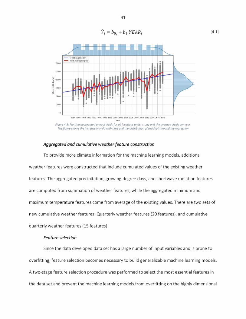
91

�̂�𝑖 = 𝑏0𝑖 + 𝑏1𝑖𝑌𝐸𝐴𝑅𝑖 [4.1]

Figure 4.3: Plotting aggregated annual yields for all locations under study and the average yields per year

The figure shows the increase in yield with time and the distribution of residuals around the regression

Aggregated and cumulative weather feature construction

To provide more climate information for the machine learning models, additional

weather features were constructed that include cumulated values of the existing weather

features. The aggregated precipitation, growing degree days, and shortwave radiation features

are computed from summation of weather features, while the aggregated minimum and

maximum temperature features come from average of the existing values. There are two sets of

new cumulative weather features: Quarterly weather features (20 features), and cumulative

quarterly weather features (15 features)

Feature selection

Since the data developed data set has a large number of input variables and is prone to

overfitting, feature selection becomes necessary to build generalizable machine learning models.

A two-stage feature selection procedure was performed to select the most essential features in

the data set and prevent the machine learning models from overfitting on the highly dimensional

92

training data. The two steps to perform feature selection were feature selection based on expert

knowledge, and permutation feature selection using random forest.

Feature selection based on expert knowledge

Using expert knowledge, weather features were reduced by removing features for

the period between the end of harvesting and the beginning of next year’s planting.

Additionally, the number of planting progress features were lowered by eliminating the

cumulative planting progress for the weeks before planting, as they did not include useful

information. The feature selection based on expert knowledge could reduce the number of

features from 550 to 387.

Permutation feature selection with random forest

Strobl (Strobl et al., 2007) pointed out that the default random forest variable

importance (impurity-based) is not reliable when dealing with situations where independent

variables have different scales of measurement or different number of categories. This is

specifically important for biological and genomic studies where independent variables are often

a combination of categorical and numeric features with varying scales. Therefore, to overcome

this bias and find decisive importance of input features, permutation feature importance is

decided to be used (Altmann et al., 2010).

Permutation feature importance measures the importance of an input feature by

calculating the decrease in the model’s prediction error when one feature is not available

(Breiman, 2001). To make the unavailability of one feature possible, each feature is permuted in

the validation or test set, that is, its values are shuffled, and the effect of this permutation on the

quality of the predictions is measured. Specifically, if permutation increases the model error, the

93

permuted feature is considered important, as the model relies on that feature for prediction. On

the other hand, if permutation does not change the prediction error significantly, the feature is

thought to be unimportant, as the model ignores it for making the prediction (Molnar, 2020).

The second stage of feature selection and likely the most effective one, includes fitting a

random forest model with 100 number of trees as the base model and calculating permutation

importance of input features with 10 times of repetition and considering a random 10-fold cross-

validation schema. It should be noted that the number of trees hyperparameter of this random

forest model is tuned using a 10-fold cross-validation. Afterward, the top 80 input features were

selected in the second stage of feature selection.

Model selection

Tuning hyperparameters of machine learning models and selecting best models with

optimal hyperparameter values is necessary to achieve high prediction accuracies. Cross-

validation is commonly used to evaluate the predictive performance of fitted models by dividing

the training set to train and validation subsets. Here, we use a random 10-fold cross-validation

method to tune the hyperparameter of ML models.

Grid search is an exhaustive search method that tries all the possible combinations of

hyperparameter settings to find the optimal selection. It is both computationally expensive and

generally dependent on the initial values specified by the user. However, Bayesian search

addresses both issues and is capable of tuning hyperparameters faster and using a continuous

range of values.

Bayesian search assumes an unknown underlying distribution and tries to approximate

the unknown function with surrogate models such as Gaussian process. Bayesian optimization

94

incorporates prior belief about the underlying function and updates it with new observations.

This makes tuning hyperparameters faster and ensures finding an acceptable solution, given that

enough number of observations are observed. In each iteration, Bayesian optimization gathers

observations with the highest amount of information and intends to make a balance

between exploration (exploring uncertain hyperparameters) and exploitation (gathering

observations from hyperparameters close to the optimum) (Snoek, 2012). That being so, to tune

hyperparameters, Bayesian search with 20 iterations was selected as the search method under

10-fold cross-validation procedure.

Predictive models

In this study, we combine diverse models in different ways and create ensemble models

to make a robust and precise machine learning model. One prerequisite for creating well-

performing ensemble models is to show a particular element of diversity in the predictions of

base learners as well as preserve excellent performance individually (Brown, 2017). Thus, several

base learners made with different procedures were selected and trained, including linear

regression, LASSO regression, Extreme Gradient Boosting (XGBoost), Light Gradient Boosting

Machine (LightGBM), and random forest. Moreover, an average weighted ensemble that assigns

equal weights to all base learners is the simplest ensemble model created. Additionally,

optimized weighted ensemble method proposed in Shahhosseini et al. (2020a) was applied here

to test its predictive performance. Several two-level stacking ensembles, namely stacked

regression, stacked LASSO, stacked random forest, and stacked LightGBM, were built, which are

expected to demonstrate excellent performance. The details of each model can be found at

Shahhosseini et al. (2020b).

95

Linear regression

Linear regression intends to predict a measurable response using multiple predictors. It

assumes the existence of a linear relationship between the predictors and response variable,

normality, no multicollinearity, and homoscedasticity (James et al., 2013).

LASSO regression

LASSO is a regularization method that is equipped with in-built feature selection. It can

exclude some variables by setting their coefficient to zero (James et al., 2013). Specifically, it

adds a penalty term to the linear regression loss function, which can shrink coefficients towards

zero (L1 regularization) (Tibshirani, 1996).

XGBoost and LightGBM

XGBoost and LightGBM are two implementations of gradient boosting tree-based

ensemble methods. These types of ensemble methods make predictions sequentially and try to

combine weak predictive tree models and learn from their mistakes. XGBoost was proposed in

2016 with new features, such as handling sparse data, and using an approximation algorithm for

a better speed (Chen & Guestrin, 2016), while LightGBM was published in 2017 by Microsoft,

with improvements in performance and computational time (Ke, 2017).

Random forest

Random forest is built on the concept of bagging, which is another tree-based ensemble

model. Bagging tries to reduce prediction variance by averaging predictions made by sampling

with replacement (Breiman, 1996). Random forest adds a new feature to bagging, which is

randomly choosing a random number of features and constructing a tree with them and

repeating this procedure many times and eventually averaging all the predictions made by all

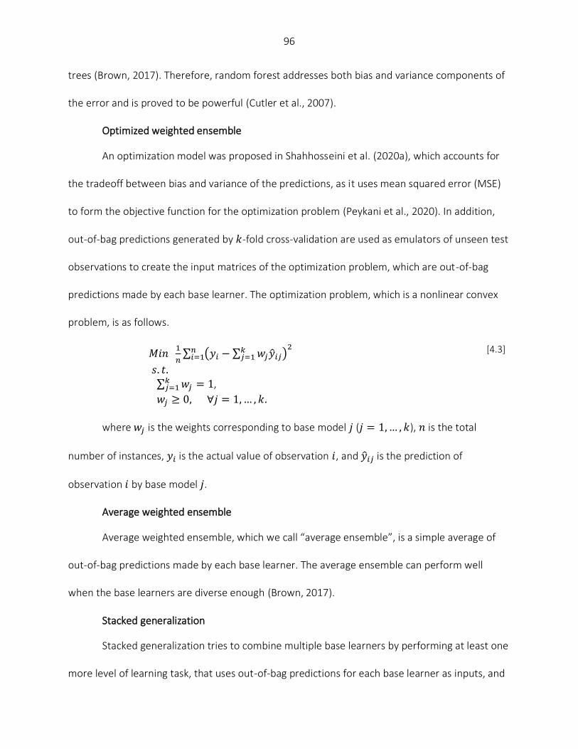
96

trees (Brown, 2017). Therefore, random forest addresses both bias and variance components of

the error and is proved to be powerful (Cutler et al., 2007).

Optimized weighted ensemble

An optimization model was proposed in Shahhosseini et al. (2020a), which accounts for

the tradeoff between bias and variance of the predictions, as it uses mean squared error (MSE)

to form the objective function for the optimization problem (Peykani et al., 2020). In addition,

out-of-bag predictions generated by 𝑘-fold cross-validation are used as emulators of unseen test

observations to create the input matrices of the optimization problem, which are out-of-bag

predictions made by each base learner. The optimization problem, which is a nonlinear convex

problem, is as follows.

𝑀𝑖𝑛 1

𝑛∑ (𝑦𝑖 − ∑ 𝑤𝑗 �̂�𝑖𝑗

𝑘𝑗=1 )

2𝑛𝑖=1 [4.3]

𝑠. 𝑡. ∑ 𝑤𝑗

𝑘𝑗=1 = 1,

𝑤𝑗 ≥ 0, ∀𝑗 = 1, … , 𝑘.

where 𝑤𝑗 is the weights corresponding to base model 𝑗 (𝑗 = 1, … , 𝑘), 𝑛 is the total

number of instances, 𝑦𝑖 is the actual value of observation 𝑖, and �̂�𝑖𝑗 is the prediction of

observation 𝑖 by base model 𝑗.

Average weighted ensemble

Average weighted ensemble, which we call “average ensemble”, is a simple average of

out-of-bag predictions made by each base learner. The average ensemble can perform well

when the base learners are diverse enough (Brown, 2017).

Stacked generalization

Stacked generalization tries to combine multiple base learners by performing at least one

more level of learning task, that uses out-of-bag predictions for each base learner as inputs, and

97

the actual target values of training data as outputs (Wolpert, 1992). The out-of-bag predictions

are generated through a 𝑘-fold cross-validation and have the same size of the original training

set (Cai et al., 2017). The steps to design a stacked generalization ensemble are as follows.

a) Learn first-level machine learning models and generate out-of-bag predictions for

each of them by using 𝑘-fold cross-validation.

b) Create a new data set with out-of-bag predictions as the input variables and actual

response values of data points in the training set as the response variable.

c) Learn a second-level machine learning model on the created data set and make

predictions for unseen test observations.

Considering four predictive models as the second-level learners, four stacking ensemble

models were created, namely stacked regression, stacked LASSO, stacked random forest, and

stacked LightGBM.

Performance metrics

To evaluate the performance of the developed machine learning models, three statistical

performance metrics were used.

- Root Mean Squared Error (RMSE): the square root of the average squared deviation

of predictions from actual values (Zheng, 2015).

- Relative Root Mean Squared Error (RRMSE): RMSE normalized by the mean of the

actual values

- Mean Bias Error (MBE): a measure that describes the average bias in the predictions.

98

- Coefficient of determination (R2): the proportion of the variance in the dependent

variable that is explained by independent variables.

These metrics together provide estimates of the error (RMSE, RRMSE, MBE) and of the

variance explained by the models (R2).

Results

Numerical results of hybrid simulation – ML framework

Table 4.2 shows the test set prediction errors of the 11 developed ML models for the

benchmark (the case that no APSIM variable is added to the data set) and the hybrid simulation-

ML (where all 22 APSIM outputs are added to the data set) cases. The relative RMSE (RRMSE) is

calculated using the average corn yield value of the test set. Adding APSIM variables as input

features to ML models improved the performance of the 11 developed ML models. In terms of

RMSE, the hybrid model boosted ML performance up to 27%. In addition, comparing the lowest

prediction errors (RMSE) of the benchmark and the hybrid scenario, we found that the use of

hybrid models achieved 8%-9% better corn yield predictions.

Looking at the average test results (Figure 4.4), it can be observed that adding APSIM

features makes improvements to all designed ML models. Moreover, considering the smallest

decrease in the prediction error (RRMSE) which is the worst-case scenario and is obtained by

LASSO model, the hybrid model still is proved to be better than the benchmark. Another

observation is the superiority of weighted ensemble models compared to other ML models. It

should be noted that the negative R2 value of some models (XGBoost, Stacked Random forest,

and Stacked LightGBM) when having no APSIM variables shows that this models’ predictions are

worse than taking the mean value as the predictions.

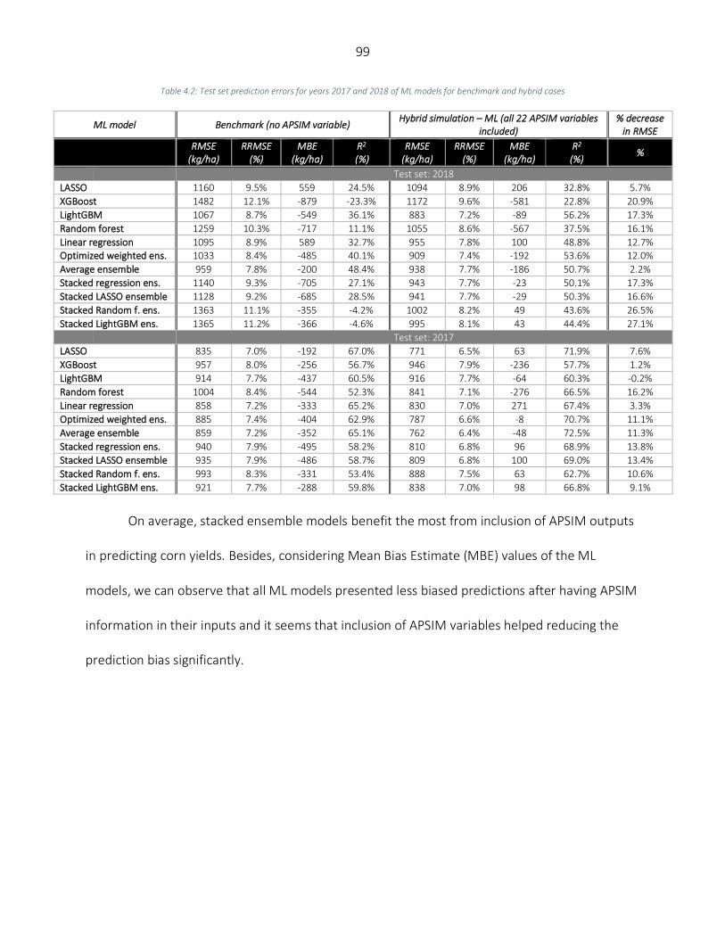
99

Table 4.2: Test set prediction errors for years 2017 and 2018 of ML models for benchmark and hybrid cases

ML model Benchmark (no APSIM variable) Hybrid simulation – ML (all 22 APSIM variables

included) % decrease

in RMSE

RMSE

(kg/ha) RRMSE

(%) MBE

(kg/ha) R2

(%) RMSE

(kg/ha) RRMSE

(%) MBE

(kg/ha) R2

(%) %

Test set: 2018

LASSO 1160 9.5% 559 24.5% 1094 8.9% 206 32.8% 5.7%

XGBoost 1482 12.1% -879 -23.3% 1172 9.6% -581 22.8% 20.9%

LightGBM 1067 8.7% -549 36.1% 883 7.2% -89 56.2% 17.3%

Random forest 1259 10.3% -717 11.1% 1055 8.6% -567 37.5% 16.1%

Linear regression 1095 8.9% 589 32.7% 955 7.8% 100 48.8% 12.7% Optimized weighted ens. 1033 8.4% -485 40.1% 909 7.4% -192 53.6% 12.0%

Average ensemble 959 7.8% -200 48.4% 938 7.7% -186 50.7% 2.2%

Stacked regression ens. 1140 9.3% -705 27.1% 943 7.7% -23 50.1% 17.3%

Stacked LASSO ensemble 1128 9.2% -685 28.5% 941 7.7% -29 50.3% 16.6%

Stacked Random f. ens. 1363 11.1% -355 -4.2% 1002 8.2% 49 43.6% 26.5%

Stacked LightGBM ens. 1365 11.2% -366 -4.6% 995 8.1% 43 44.4% 27.1%

Test set: 2017

LASSO 835 7.0% -192 67.0% 771 6.5% 63 71.9% 7.6%

XGBoost 957 8.0% -256 56.7% 946 7.9% -236 57.7% 1.2%

LightGBM 914 7.7% -437 60.5% 916 7.7% -64 60.3% -0.2%

Random forest 1004 8.4% -544 52.3% 841 7.1% -276 66.5% 16.2%

Linear regression 858 7.2% -333 65.2% 830 7.0% 271 67.4% 3.3%

Optimized weighted ens. 885 7.4% -404 62.9% 787 6.6% -8 70.7% 11.1%

Average ensemble 859 7.2% -352 65.1% 762 6.4% -48 72.5% 11.3%

Stacked regression ens. 940 7.9% -495 58.2% 810 6.8% 96 68.9% 13.8%

Stacked LASSO ensemble 935 7.9% -486 58.7% 809 6.8% 100 69.0% 13.4%

Stacked Random f. ens. 993 8.3% -331 53.4% 888 7.5% 63 62.7% 10.6%

Stacked LightGBM ens. 921 7.7% -288 59.8% 838 7.0% 98 66.8% 9.1%

On average, stacked ensemble models benefit the most from inclusion of APSIM outputs

in predicting corn yields. Besides, considering Mean Bias Estimate (MBE) values of the ML

models, we can observe that all ML models presented less biased predictions after having APSIM

information in their inputs and it seems that inclusion of APSIM variables helped reducing the

prediction bias significantly.

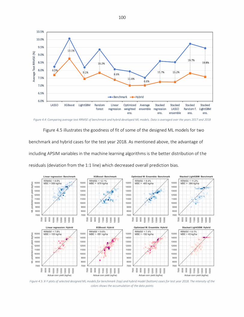
100

Figure 4.4: Comparing average test RRMSE of benchmark and hybrid developed ML models. Data is averaged over the years 2017 and 2018

Figure 4.5 illustrates the goodness of fit of some of the designed ML models for two

benchmark and hybrid cases for the test year 2018. As mentioned above, the advantage of

including APSIM variables in the machine learning algorithms is the better distribution of the

residuals (deviation from the 1:1 line) which decreased overall prediction bias.

Figure 4.5: X-Y plots of selected designed ML models for benchmark (top) and hybrid model (bottom) cases for test year 2018. The intensity of the

colors shows the accumulation of the data points

101

Models performance on an extreme weather year (2012)

To assess the performance of the trained models on an extreme weather year, here the

data from the year 2012, which was an exceptionally dry year, is considered as unseen test

observations and the quality of the predictions made by the benchmark and the hybrid models

are compared.

Table 4.3 demonstrates lower prediction accuracy of the models in year 2012 (extreme

dry year) compared to average to wet years model predictions (2017 and 2018, see Table 4.2).

This result was consistent for both ML and hybrid models. However, the hybrid model managed

to provide improvements over the benchmark in the 2012 year. This was ranging from 5% to

43% decrease in the prediction RMSE. Comparing the best model of the benchmark (LightGBM)

with the best model of the hybrid scenario (Stacked regression ensemble), we observed that the

use of hybrid model provided 22% better predictions.

Table 4.3: Test set prediction errors of ML models for benchmark and hybrid cases when considering an extreme weather year (2012) – The average yield of the year 2012 is 6646 kg/ha

ML model Benchmark (no APSIM variable) Hybrid simulation – ML (all 22 APSIM variables

included) % decrease

in RMSE

RMSE

(kg/ha) RRMSE

(%) MBE

(kg/ha) R2

(%) RMSE

(kg/ha) RRMSE

(%) MBE

(kg/ha) R2

(%) %

Test set: 2012

LASSO 4311 64.9% 3775 -221.3% 3160 47.5% 2519 -72.6% 26.7%

XGBoost 3664 55.1% 3102 -132.1% 2602 39.2% 1942 -17.1% 29.0%

LightGBM 3245 48.8% 2671 -82.0% 2608 39.2% 2016 -17.5% 19.6%

Random forest 3782 56.9% 3368 -147.3% 3591 54.0% 3157 -122.9% 5.0%

Linear regression 4869 73.3% 4450 -309.8% 2784 41.9% 2144 -34.0% 42.8%

Optimized weighted ens. 3380 50.9% 2818 -97.5% 2664 40.1% 2066 -22.7% 21.2%

Average ensemble 3946 59.4% 3473 -169.2% 2908 43.8% 2356 -46.2% 26.3%

Stacked regression ens. 3398 51.1% 2816 -99.6% 2545 38.3% 1894 -12.0% 25.1%

Stacked LASSO ensemble 3403 51.2% 2835 -100.1% 2561 38.5% 1925 -13.4% 24.7%

Stacked Random f. ens. 3289 49.5% 2668 -87.0% 2571 38.7% 1968 -14.3% 21.8%

Stacked LightGBM ens. 3462 52.1% 2934 -107.2% 2588 38.9% 1995 -15.8% 25.2%

102

Partial inclusion of APSIM variables

This section investigates the effect of partial inclusion of APSIM variables considering

three different scenarios for the test year 2018 (see Table 4.4). The scenarios are (1) include only

phenology-related APSIM variables (silking date and physiological maturity date); (2) include only

crop-related APSIM variables (crop yield, biomass, maximum rooting depth, maximum leaf area

index, cumulative transpiration, crop N uptake, grain N uptake, season average water stress

(both drought and excessive water), and season average nitrogen stress), and (3) include soil and

weather-related APSIM variables (annual evapotranspiration, growing season average depth to

the water table, annual runoff, annual drainage, annual gross N mineralization, total N loss that

accounts for leaching and denitrification, annual average water table depth, ratio of soil water to

field capacity during the growing season at 30, 60, and 90 cm profile depth). When including

only phenology-related APSIM variables, results demonstrate that stacked regression ensemble

model makes the best predictions, while the least biased predictions are generated from stacked

random forest ensemble.

In case of having crop-related APSIM variables as ML inputs, results indicate that stacked

regression and stacked random forest ensembles make the best and the least biased predictions,

respectively.

When the soil and weather-related APSIM variables are considered as ML inputs, the

results show that stacked regression ensemble makes decent predictions with having the least

amount of prediction error as well as bias.

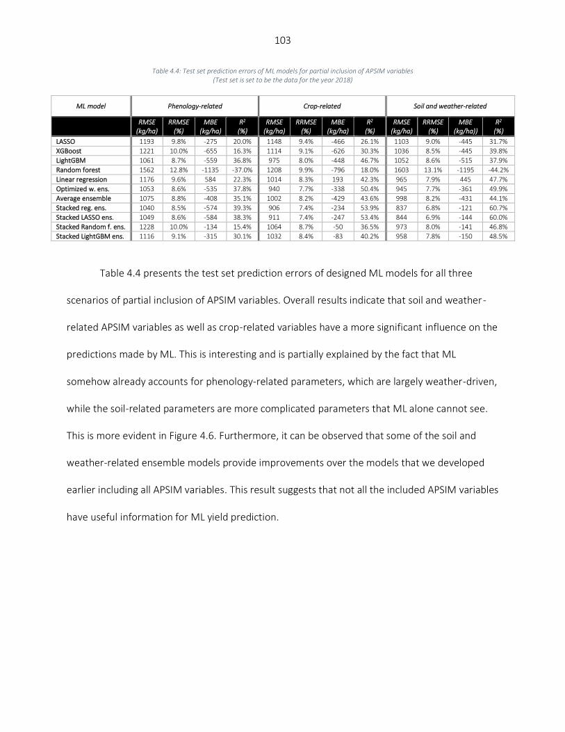
103

Table 4.4: Test set prediction errors of ML models for partial inclusion of APSIM variables (Test set is set to be the data for the year 2018)

ML model Phenology-related Crop-related Soil and weather-related

RMSE

(kg/ha) RRMSE

(%) MBE

(kg/ha) R2

(%) RMSE

(kg/ha) RRMSE

(%) MBE

(kg/ha) R2

(%) RMSE

(kg/ha) RRMSE

(%) MBE

(kg/ha)) R2

(%)

LASSO 1193 9.8% -275 20.0% 1148 9.4% -466 26.1% 1103 9.0% -445 31.7%

XGBoost 1221 10.0% -655 16.3% 1114 9.1% -626 30.3% 1036 8.5% -445 39.8%

LightGBM 1061 8.7% -559 36.8% 975 8.0% -448 46.7% 1052 8.6% -515 37.9%

Random forest 1562 12.8% -1135 -37.0% 1208 9.9% -796 18.0% 1603 13.1% -1195 -44.2%

Linear regression 1176 9.6% 584 22.3% 1014 8.3% 193 42.3% 965 7.9% 445 47.7%

Optimized w. ens. 1053 8.6% -535 37.8% 940 7.7% -338 50.4% 945 7.7% -361 49.9%

Average ensemble 1075 8.8% -408 35.1% 1002 8.2% -429 43.6% 998 8.2% -431 44.1%

Stacked reg. ens. 1040 8.5% -574 39.3% 906 7.4% -234 53.9% 837 6.8% -121 60.7%

Stacked LASSO ens. 1049 8.6% -584 38.3% 911 7.4% -247 53.4% 844 6.9% -144 60.0%

Stacked Random f. ens. 1228 10.0% -134 15.4% 1064 8.7% -50 36.5% 973 8.0% -141 46.8%

Stacked LightGBM ens. 1116 9.1% -315 30.1% 1032 8.4% -83 40.2% 958 7.8% -150 48.5%

Table 4.4 presents the test set prediction errors of designed ML models for all three

scenarios of partial inclusion of APSIM variables. Overall results indicate that soil and weather-

related APSIM variables as well as crop-related variables have a more significant influence on the

predictions made by ML. This is interesting and is partially explained by the fact that ML

somehow already accounts for phenology-related parameters, which are largely weather-driven,

while the soil-related parameters are more complicated parameters that ML alone cannot see.

This is more evident in Figure 4.6. Furthermore, it can be observed that some of the soil and

weather-related ensemble models provide improvements over the models that we developed

earlier including all APSIM variables. This result suggests that not all the included APSIM variables

have useful information for ML yield prediction.

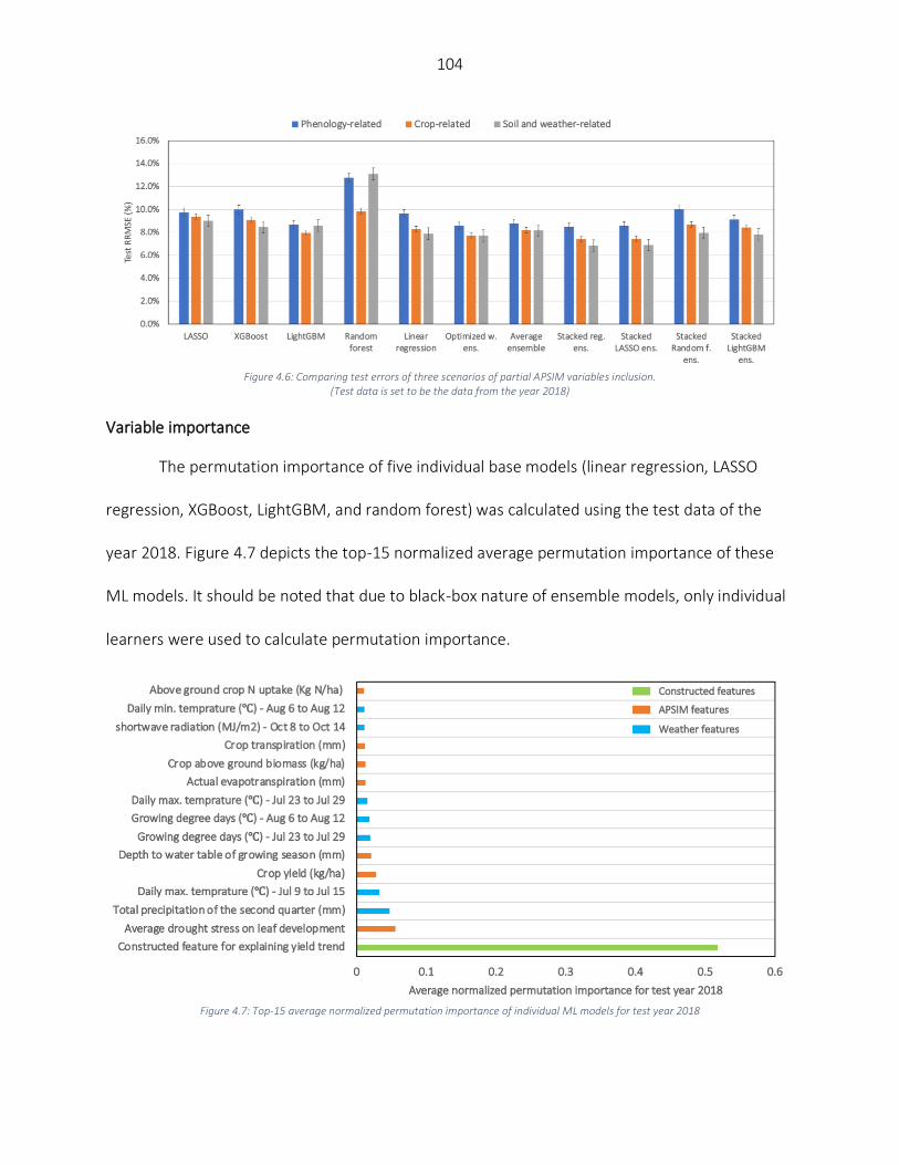
104

Figure 4.6: Comparing test errors of three scenarios of partial APSIM variables inclusion.

(Test data is set to be the data from the year 2018)

Variable importance

The permutation importance of five individual base models (linear regression, LASSO

regression, XGBoost, LightGBM, and random forest) was calculated using the test data of the

year 2018. Figure 4.7 depicts the top-15 normalized average permutation importance of these

ML models. It should be noted that due to black-box nature of ensemble models, only individual

learners were used to calculate permutation importance.

Figure 4.7: Top-15 average normalized permutation importance of individual ML models for test year 2018

105

Figure 4.7 indicates that the most important input feature for ML models is “yield_trend”

which is the feature we constructed for explaining the increasing trend in corn yields and

incorporated technological advances over the years (genetics and management improvement).

Of the next 14 most important input features, seven variables were APSIM variables, while the

remaining seven are weather input variables. Regarding the APSIM variables, five input features

are part of crop-related APSIM variables, and the other two APSIM features are as soil and

weather-related variables. This is in-line with the results of partial inclusion of APSIM variables

discussed before.

To find out which APSIM features have been more influential in predicting yields, the

average permutation importance of five individual models (linear regression, LASSO regression,

LightGBM, XGBoost, and random forest) was calculated for each test year. Figure 4.8

demonstrates the ranking of top 10 APSIM features. Results indicate that the AvgDroughtStress,

AvgWTInseason, and CropYield were the most important features for machine learning models

to predict yield. Most of these are water-related features suggesting the importance of soil

hydrology in crop yield prediction in the US Corn belt. This result was consistent across three

years, including the year drought 2012, in which model prediction was lower than the other

years.

106

Figure 4.8: Average normalized permutation importance of APSIM features for all test years.

AvgDroughtStress: Average drought stress on leaf development, AvgWTInseason: Depth to water table of growing season (mm), NlossTotal: Total N loss (denitrification and leaching) (kg N/ha), CropYield: Crop yield (kg/ha), GrainINupt: Grain N uptake (kg N/ha), Bioma: Crop above ground

biomass (kg/ha), SWtoDUL30Inseason: Growing season average soil water to field capacity ratio at 30 cm, ETAnnual: Actual evapotranspiration (mm), CropTraspiration: Crop transpiration (mm)

Discussion

We proposed a hybrid simulation-machine learning approach that provided improved

county-scale crop yield prediction. To the best of our knowledge, this is the first study that

designs ensemble models to increase corn yields predictability. This study demonstrated that

introducing APSIM variables into machine learning models and utilizing them as inputs to a

prediction task on average can decrease the prediction error measure by RMSE between 7% and

20%. In addition, the predictions made by the hybrid model show less bias toward actual yields.

Other studies in this area, are mainly limited in coupling simplest statistical models, i.e. linear

regression variants, with simulation crop models and apart from two recent studies (Everingham

et al., 2016; Feng et al., 2019) there has been no study combining machine learning and

simulation crop models. Considering the hybrid models, some of the developed models provided

predictions with RRMSE values as small as 6-7%. This indicates that the developed models

107

outperform the corn yield prediction models developed in the literature (Bolton & Friedl, 2013;

Khaki et al., 2020; Kuwata & Shibasaki, 2016; Sakamoto et al., 2014; Schwalbert et al., 2020).

In addition to the prediction advantages achieved by coupling ML and simulation crop

modelling, we investigated the value of different types of APSIM variables in the ML prediction

and found out that soil water related APSIM variables contributed the most in improving yield

prediction. The inclusion of APSIM consistently improved ML yield prediction in all years (2012,

2017, 2018). We also noticed that neither ML nor the hybrid model could sufficiently predict

yields of the 2012 dry year. This suggests that more work is needed to adequately predict yields

in extreme weather years, which are expected to increase with climate change (Bassu et al.,

2014; Baum et al., 2020; Jin et al., 2017; Xu et al., 2016), but we noticed that yield prediction of

the dry year was better done by the hybrid model. Developing models that are more robust to

extreme values, including additional climate information that can help the model to detect the

drought, and including remote sensing data can be future research directions.

Designing a method that enables the ML models to capture the yearly increasing trends

in corn yields was the main challenge of this work. To address this challenge, an innovative

feature was constructed that could explains the trend to a great extent and as the variable

importance results showed, it is by far the most important input feature for predicting corn

yields.

The significant merits of coupling ML and simulation crop models shown in this study

raise the question that whether the ML models can further benefit from addition of more input

features from other sources. Hence, a possible extension of this study could be inclusion of

108

remote sensing data into the ML prediction task and investigate the level of importance each

data source can exhibit.

It should be also acknowledged that APSIM simulations that used as inputs to ML model

leveraged the full weather of each test year. In real word applications, the weather will be

unknown and the APSIM model would need to run in a forecasting mode (Archontoulis et al.,

2020; Carberry et al., 2009; Togliatti et al., 2017) introducing some additional uncertainty. This is

something to be explored further in the future.

Conclusion

We demonstrated improvements in yield prediction accuracy across all designed ML

models when additional inputs from a simulation cropping systems model (APSIM) are included.

Among several crop model (APSIM in this study) variables that can be used as inputs to ML,

analysis suggested that the most important ones were those related to soil water, and in

particular growing season average drought stress, and average depth to water table. We

concluded that inclusion of additional soil water related variables (either from simulation model

or remote sensing or other sources) could further improve ML yield prediction in the central US

Corn Belt.

References

Ahmed, M., Akram, M. N., Asim, M., Aslam, M., Hassan, F., Higgins, S., Stöckle, C. O., & Hoogenboom, G. (2016). Calibration and validation of APSIM-Wheat and CERES-Wheat for spring wheat under rainfed conditions: Models evaluation and application. Computers and Electronics in Agriculture, 123, 384–401. https://doi.org/https://doi.org/10.1016/j.compag.2016.03.015

109

Altmann, A., Toloşi, L., Sander, O., & Lengauer, T. (2010). Permutation importance: a corrected feature importance measure. Bioinformatics, 26(10), 1340–1347. https://doi.org/10.1093/bioinformatics/btq134

Archontoulis, S. V, Castellano, M. J., Licht, M. A., Nichols, V., Baum, M., Huber, I., Martinez-Feria, R., Puntel, L., Ordóñez, R. A., Iqbal, J., Wright, E. E., Dietzel, R. N., Helmers, M., Vanloocke, A., Liebman, M., Hatfield, J. L., Herzmann, D., Córdova, S. C., Edmonds, P., … Lamkey, K. R. (2020). Predicting crop yields and soil-plant nitrogen dynamics in the US Corn Belt. Crop Science, 60(2), 721–738. https://doi.org/10.1002/csc2.20039

Asseng, S., Zhu, Y., Basso, B., Wilson, T., & Cammarano, D. (2014). Simulation Modeling: Applications in Cropping Systems. In N. K. Van Alfen (Ed.), Encyclopedia of Agriculture and Food Systems (pp. 102–112). Academic Press. https://doi.org/https://doi.org/10.1016/B978-0-444-52512-3.00233-3

Basso, B., & Liu, L. (2019). Chapter Four - Seasonal crop yield forecast: Methods, applications, and accuracies. In D. L. Sparks (Ed.), Advances in Agronomy (Vol. 154, pp. 201–255). Academic Press. https://doi.org/https://doi.org/10.1016/bs.agron.2018.11.002

Bassu, S., Brisson, N., Durand, J.-L., Boote, K., Lizaso, J., Jones, J. W., Rosenzweig, C., Ruane, A. C., Adam, M., Baron, C., Basso, B., Biernath, C., Boogaard, H., Conijn, S., Corbeels, M., Deryng, D., De Sanctis, G., Gayler, S., Grassini, P., … Waha, K. (2014). How do various maize crop models vary in their responses to climate change factors? Global Change Biology, 20(7), 2301–2320. https://doi.org/https://doi.org/10.1111/gcb.12520

Baum, M. E., Licht, M. A., Huber, I., & Archontoulis, S. V. (2020). Impacts of climate change on the optimum planting date of different maize cultivars in the central US Corn Belt. European Journal of Agronomy, 119, 126101. https://doi.org/https://doi.org/10.1016/j.eja.2020.126101

Bogard, M., Biddulph, B., Zheng, B., Hayden, M., Kuchel, H., Mullan, D., Allard, V., Gouis, J. Le, & Chapman, S. C. (2020). Linking genetic maps and simulation to optimize breeding for wheat flowering time in current and future climates. Crop Science, 60(2), 678–699. https://doi.org/10.1002/csc2.20113

Bolton, D. K., & Friedl, M. A. (2013). Forecasting crop yield using remotely sensed vegetation indices and crop phenology metrics. Agricultural and Forest Meteorology, 173, 74–84. https://doi.org/https://doi.org/10.1016/j.agrformet.2013.01.007

Breiman, L. (1996). Bagging predictors. Machine learning, 24(2), 123-140.

Breiman, L. (2001). Random forests. Machine learning, 45(1), 5-32.

Brown, G. (2017). Ensemble Learning. In C. Sammut & G. I. Webb (Eds.), Encyclopedia of Machine Learning and Data Mining (pp. 393-402). Boston, MA: Springer US.

110

Busetto, L., Casteleyn, S., Granell, C., Pepe, M., Barbieri, M., Campos-Taberner, M., et al. (2017). Downstream Services for Rice Crop Monitoring in Europe: From Regional to Local Scale. [Article]. IEEE Journal of Selected Topics in Applied Earth Observations and Remote Sensing, 10(12), 5423-5441.

Cai, Y., Moore, K., Pellegrini, A., Elhaddad, A., Lessel, J., Townsend, C., et al. (2017). Crop yield predictions-high resolution statistical model for intra-season forecasts applied to corn in the US. Paper presented at the 2017 Fall Meeting.

Cai, Yaping, Guan, K., Lobell, D., Potgieter, A. B., Wang, S., Peng, J., Xu, T., Asseng, S., Zhang, Y., You, L., & Peng, B. (2019). Integrating satellite and climate data to predict wheat yield in Australia using machine learning approaches. Agricultural and Forest Meteorology, 274, 144–159. https://doi.org/https://doi.org/10.1016/j.agrformet.2019.03.010

Campbell, G. S. (1985). Soil physics with BASIC: transport models for soil-plant systems. Elsevier.

Cao, P., Lu, C., & Yu, Z. (2018). Historical nitrogen fertilizer use in agricultural ecosystems of the contiguous United States during 1850–2015: application rate, timing, and fertilizer types. Earth Syst. Sci. Data, 10(2), 969–984. https://doi.org/10.5194/essd-10-969-2018

Carberry, P. S., Hochman, Z., Hunt, J. R., Dalgliesh, N. P., McCown, R. L., Whish, J. P. M., Robertson, M. J., Foale, M. A., Poulton, P. L., & van Rees, H. (2009). Re-inventing model-based decision support with Australian dryland farmers. 3. Relevance of APSIM to commercial crops. Crop and Pasture Science, 60(11), 1044–1056. https://doi.org/https://doi.org/10.1071/CP09052

Chen, T., & Guestrin, C. (2016). XGBoost: A Scalable Tree Boosting System. https://doi.org/10.1145/2939672.2939785

Chipanshi, A., Zhang, Y., Kouadio, L., Newlands, N., Davidson, A., Hill, H., Warren, R., Qian, B., Daneshfar, B., Bedard, F., & Reichert, G. (2015). Evaluation of the Integrated Canadian Crop Yield Forecaster (ICCYF) model for in-season prediction of crop yield across the Canadian agricultural landscape. Agricultural and Forest Meteorology, 206, 137–150. https://doi.org/https://doi.org/10.1016/j.agrformet.2015.03.007

Crane-Droesch, A. (2018). Machine learning methods for crop yield prediction and climate change impact assessment in agriculture. Environmental Research Letters, 13(11), 114003.

Cutler, D. R., Edwards Jr, T. C., Beard, K. H., Cutler, A., Hess, K. T., Gibson, J., & Lawler, J. J. (2007). Random forests for classification in ecology. Ecology, 88(11), 2783–2792.

Drummond, S. T., Sudduth, K. A., Joshi, A., Birrell, S. J., & Kitchen, N. R. (2003). Statistical and neural methods for site–specific yield prediction. Transactions of the ASAE, 46(1), 5.

111

Dumont, B., Basso, B., Leemans, V., Bodson, B., Destain, J. P., & Destain, M. F. (2015). A comparison of within-season yield prediction algorithms based on crop model behaviour analysis. Agricultural and Forest Meteorology, 204, 10–21. https://doi.org/https://doi.org/10.1016/j.agrformet.2015.01.014

Ebrahimi-Mollabashi, E., Huth, N. I., Holzwoth, D. P., Ordóñez, R. A., Hatfield, J. L., Huber, I., Castellano, M. J., & Archontoulis, S. V. (2019). Enhancing APSIM to simulate excessive moisture effects on root growth. Field Crops Research, 236, 58–67. https://doi.org/https://doi.org/10.1016/j.fcr.2019.03.014

Elliott, J., Kelly, D., Chryssanthacopoulos, J., Glotter, M., Jhunjhnuwala, K., Best, N., Wilde, M., & Foster, I. (2014). The parallel system for integrating impact models and sectors (pSIMS). Environmental Modelling & Software, 62, 509–516. https://doi.org/https://doi.org/10.1016/j.envsoft.2014.04.008

Ersoz, E. S., Martin, N. F., & Stapleton, A. E. (2020). On to the next chapter for crop breeding: Convergence with data science. Crop Science, 60(2), 639–655. https://doi.org/10.1002/csc2.20054

Everingham, Y., Sexton, J., Skocaj, D., & Inman-Bamber, G. (2016). Accurate prediction of sugarcane yield using a random forest algorithm. Agronomy for Sustainable Development, 36(2), 27. https://doi.org/10.1007/s13593-016-0364-z

Feng, P., Wang, B., Liu, D. L., Waters, C., & Yu, Q. (2019). Incorporating machine learning with biophysical model can improve the evaluation of climate extremes impacts on wheat yield in south-eastern Australia. Agricultural and Forest Meteorology, 275, 100–113. https://doi.org/https://doi.org/10.1016/j.agrformet.2019.05.018

Gaydon, D. S., Balwinder, S., Wang, E., Poulton, P. L., Ahmad, B., Ahmed, F., Akhter, S., Ali, I., Amarasingha, R., Chaki, A. K., Chen, C., Choudhury, B. U., Darai, R., Das, A., Hochman, Z., Horan, H., Hosang, E. Y., Kumar, P. V., Khan, A. S. M. M. R., … Roth, C. H. (2017). Evaluation of the APSIM model in cropping systems of Asia. Field Crops Research, 204, 52–75. https://doi.org/https://doi.org/10.1016/j.fcr.2016.12.015

Günay, E. E., Okudan Kremer, G. E., & Zarindast, A. (2020). A multi-objective robust possibilistic programming approach to sustainable public transportation network design. Fuzzy Sets and Systems. https://doi.org/https://doi.org/10.1016/j.fss.2020.09.007

Holzworth, D. P., Huth, N. I., Zurcher, E. J., Herrmann, N. I., McLean, G., Chenu, K., van Oosterom, E. J., Snow, V., Murphy, C., & Moore, A. D. (2014). APSIM–evolution towards a new generation of agricultural systems simulation. Environmental Modelling & Software, 62, 327–350.

I. Huth, N., Bristow, K., & Verburg, K. (2012). SWIM3: Model use, calibration, and validation (Vol. 55). https://doi.org/10.13031/2013.42243

112

James, G., Witten, D., Hastie, T., & Tibshirani, R. (2013). An introduction to statistical learning (Vol. 112). Springer.

Jeong, J. H., Resop, J. P., Mueller, N. D., Fleisher, D. H., Yun, K., Butler, E. E., et al. (2016). Random forests for global and regional crop yield predictions. PLoS One, 11(6), e0156571.

Jiang, H., Hu, H., Zhong, R., Xu, J., Xu, J., Huang, J., Wang, S., Ying, Y., & Lin, T. (2020). A deep learning approach to conflating heterogeneous geospatial data for corn yield estimation: A case study of the US Corn Belt at the county level. Global Change Biology, 26(3), 1754–1766. https://doi.org/10.1111/gcb.14885

Jin, Z., Zhuang, Q., Wang, J., Archontoulis, S. V, Zobel, Z., & Kotamarthi, V. R. (2017). The combined and separate impacts of climate extremes on the current and future US rainfed maize and soybean production under elevated CO2. Global Change Biology, 23(7), 2687–2704. https://doi.org/https://doi.org/10.1111/gcb.13617

Kang, Y., Ozdogan, M., Zhu, X., Ye, Z., Hain, C., & Anderson, M. (2020). Comparative assessment of environmental variables and machine learning algorithms for maize yield prediction in the US Midwest. Environmental Research Letters, 15(6), 64005. https://doi.org/10.1088/1748-9326/ab7df9

Karpatne, A., Watkins, W., Read, J., & Kumar, V. (2017). Physics-guided neural networks (pgnn): An application in lake temperature modeling. ArXiv Preprint ArXiv:1710.11431.

Ke, G., Meng, Q., Finley, T., Wang, T., Chen, W., Ma, W., et al. (2017). Lightgbm: A highly efficient gradient boosting decision tree. Paper presented at the Advances in Neural Information Processing Systems.

Keating, B. A., Carberry, P. S., Hammer, G. L., Probert, M. E., Robertson, M. J., Holzworth, D., Huth, N. I., Hargreaves, J. N. G., Meinke, H., & Hochman, Z. (2003). An overview of APSIM, a model designed for farming systems simulation. European Journal of Agronomy, 18(3–4), 267–288.

Khaki, S., & Wang, L. (2019). Crop Yield Prediction Using Deep Neural Networks. Frontiers in Plant Science, 10(621). https://doi.org/10.3389/fpls.2019.00621

Khaki, S., Wang, L., & Archontoulis, S. V. (2020). A CNN-RNN Framework for Crop Yield Prediction. Frontiers in Plant Science, 10(1750). https://doi.org/10.3389/fpls.2019.01750

Kuwata, K., & Shibasaki, R. (2016). Estimating corn yield in the United States with MODIS EVI and machine learning methods. ISPRS Ann. Photogramm. Remote Sens. Spat. Inf. Sci, 3(8), 131–136.

L Hoffman, A., R Kemanian, A., & E Forest, C. (2020). The response of maize, sorghum, and soybean yield to growing-phase climate revealed with machine learning. Environmental Research Letters, 15(9), 94013. https://doi.org/10.1088/1748-9326/ab7b22

113

Leng, G., & Hall, J. W. (2020). Predicting spatial and temporal variability in crop yields: an inter-comparison of machine learning, regression and process-based models. Environmental Research Letters, 15(4), 44027. https://doi.org/10.1088/1748-9326/ab7b24

Li, Z., Song, M., Feng, H., & Zhao, Y. (2016). Within-season yield prediction with different nitrogen inputs under rain-fed condition using CERES-Wheat model in the northwest of China. Journal of the Science of Food and Agriculture, 96(8), 2906–2916. https://doi.org/10.1002/jsfa.7467

Manatsa, D., Nyakudya, I. W., Mukwada, G., & Matsikwa, H. (2011). Maize yield forecasting for Zimbabwe farming sectors using satellite rainfall estimates. Natural Hazards, 59(1), 447–463. https://doi.org/10.1007/s11069-011-9765-0

Mavromatis, T. (2016). Spatial resolution effects on crop yield forecasts: An application to rainfed wheat yield in north Greece with CERES-Wheat. Agricultural Systems, 143, 38–48. https://doi.org/https://doi.org/10.1016/j.agsy.2015.12.002

Mishra, A., Hansen, J. W., Dingkuhn, M., Baron, C., Traoré, S. B., Ndiaye, O., & Ward, M. N. (2008). Sorghum yield prediction from seasonal rainfall forecasts in Burkina Faso. Agricultural and Forest Meteorology, 148(11), 1798–1814. https://doi.org/https://doi.org/10.1016/j.agrformet.2008.06.007

Moeinizade, S., Han, Y., Pham, H., Hu, G., & Wang, L. (2020a). A Look-ahead Monte Carlo Simulation Method for Improving Parental Selection in Trait Introgression. BioRxiv, 2020.09.01.278242. https://doi.org/10.1101/2020.09.01.278242

Moeinizade, S., Hu, G., Wang, L., & Schnable, P. S. (2019). Optimizing Selection and Mating in Genomic Selection with a Look-Ahead Approach: An Operations Research Framework. G3: Genes|Genomes|Genetics, 9(7), 2123. https://doi.org/10.1534/g3.118.200842

Moeinizade, S., Kusmec, A., Hu, G., Wang, L., & Schnable, P. S. (2020b). Multi-trait Genomic Selection Methods for Crop Improvement. Genetics, 215(4), 931. https://doi.org/10.1534/genetics.120.303305

Moeinizade, S., Wellner, M., Hu, G., & Wang, L. (2020c). Complementarity-based selection strategy for genomic selection. Crop Science, 60(1), 149–156. https://doi.org/https://doi.org/10.1002/csc2.20070

Molnar, C. (2020). Interpretable Machine Learning. Lulu. com.

Mupangwa, W., Chipindu, L., Nyagumbo, I., Mkuhlani, S., & Sisito, G. (2020). Evaluating machine learning algorithms for predicting maize yield under conservation agriculture in Eastern and Southern Africa. SN Applied Sciences, 2(5), 952. https://doi.org/10.1007/s42452-020-2711-6

114

Nain, A. S., Dadhwal, V. K., & Singh, T. P. (2002). Real time wheat yield assessment using technology trend and crop simulation model with minimal data set. Current Science, 82(10), 1255–1258. https://www.scopus.com/inward/record.uri?eid=2-s2.0-0042349238&partnerID=40&md5=c6e033b802ec983edb72b11f5e4e605e

Nain, A. S., Dadhwal, V. K., & Singh, T. P. (2004). Use of CERES-wheat model for wheat yield forecast in central indo-gangetic plains of India. Journal of Agricultural Science, 142(1), 59–70. https://doi.org/10.1017/S0021859604004022

NASS, U. (2019). Surveys. National Agricultural Statistics Service, U.S. Department of Agriculture.

Pagani, V., Stella, T., Guarneri, T., Finotto, G., van den Berg, M., Marin, F. R., Acutis, M., & Confalonieri, R. (2017). Forecasting sugarcane yields using agro-climatic indicators and Canegro model: A case study in the main production region in Brazil. Agricultural Systems, 154, 45–52. https://doi.org/https://doi.org/10.1016/j.agsy.2017.03.002

Pasley, H. R., Huber, I., Castellano, M. J., & Archontoulis, S. V. (2020). Modeling Flood-Induced Stress in Soybeans. Frontiers in Plant Science, 11(62). https://doi.org/10.3389/fpls.2020.00062

Peykani, P., & Mohammadi, E. (2020). Window Network Data Envelopment Analysis: An Application to Investment Companies. International Journal of Industrial Mathematics, 12(1), 89-99.

Probert, M. E., Dimes, J. P., Keating, B. A., Dalal, R. C., & Strong, W. M. (1998). APSIM’s water and nitrogen modules and simulation of the dynamics of water and nitrogen in fallow systems. Agricultural Systems, 56(1), 1–28. https://doi.org/https://doi.org/10.1016/S0308-521X(97)00028-0

Roberts, M. J., Braun, N. O., Sinclair, T. R., Lobell, D. B., & Schlenker, W. (2017). Comparing and combining process-based crop models and statistical models with some implications for climate change. Environmental Research Letters, 12(9), 95010. https://doi.org/10.1088/1748-9326/aa7f33

Sakamoto, T., Gitelson, A. A., & Arkebauer, T. J. (2014). Near real-time prediction of U.S. corn yields based on time-series MODIS data. Remote Sensing of Environment, 147, 219–231. https://doi.org/https://doi.org/10.1016/j.rse.2014.03.008

Schwalbert, R., Amado, T., Nieto, L., Corassa, G., Rice, C., Peralta, N., Schauberger, B., Gornott, C., & Ciampitti, I. (2020). Mid-season county-level corn yield forecast for US Corn Belt integrating satellite imagery and weather variables. Crop Science, 60(2), 739–750. https://doi.org/https://doi.org/10.1002/csc2.20053

115

Shahhosseini M., Hu G., Pham H. (2020a) Optimizing Ensemble Weights for Machine Learning Models: A Case Study for Housing Price Prediction. In: Yang H., Qiu R., Chen W. (eds) Smart Service Systems, Operations Management, and Analytics. INFORMS-CSS 2019. Springer Proceedings in Business and Economics. Springer, Cham.

Shahhosseini, M., Hu, G., & Archontoulis, S. V. (2020b). Forecasting Corn Yield With Machine Learning Ensembles. [Methods]. Frontiers in Plant Science, 11(1120).

Shahhosseini, M., Martinez-Feria, R. A., Hu, G., & Archontoulis, S. V. (2019). Maize yield and nitrate loss prediction with machine learning algorithms. Environmental Research Letters, 14(12), 124026.

Snoek, J., Larochelle, H., & Adams, R. P. (2012). Practical bayesian optimization of machine learning algorithms. Paper presented at the Advances in neural information processing systems.

Soil Survey Staff, Natural Resources Conservation Service, United States Department of Agriculture, Web Soil Survey. (2019). from https://websoilsurvey.nrcs.usda.gov/

Strobl, C., Boulesteix, A.-L., Zeileis, A., & Hothorn, T. (2007). Bias in random forest variable importance measures: Illustrations, sources and a solution. BMC Bioinformatics, 8(1), 25. https://doi.org/10.1186/1471-2105-8-25

Supit, I. (1997). Predicting national wheat yields using a crop simulation and trend models. Agricultural and Forest Meteorology, 88(1), 199–214. https://doi.org/https://doi.org/10.1016/S0168-1923(97)00037-3

Thorburn, P. J., Meier, E. A., & Probert, M. E. (2005). Modelling nitrogen dynamics in sugarcane systems: Recent advances and applications. Field Crops Research, 92(2), 337–351. https://doi.org/https://doi.org/10.1016/j.fcr.2005.01.016

Tibshirani, R. (1996). Regression shrinkage and selection via the lasso. Journal of the Royal Statistical Society. Series B (Methodological), 58, 267-288.

Togliatti, K., Archontoulis, S. V, Dietzel, R., Puntel, L., & VanLoocke, A. (2017). How does inclusion of weather forecasting impact in-season crop model predictions? Field Crops Research, 214, 261–272. https://doi.org/https://doi.org/10.1016/j.fcr.2017.09.008

Washburn, J. D., Burch, M. B., & Franco, J. A. V. (2020). Predictive breeding for maize: Making use of molecular phenotypes, machine learning, and physiological crop models. Crop Science, 60(2), 622–638. https://doi.org/10.1002/csc2.20052

Wolpert, D. H. (1992). Stacked generalization. Neural Networks, 5(2), 241–259. https://doi.org/https://doi.org/10.1016/S0893-6080(05)80023-1

116

Xu, H., Twine, T. E., & Girvetz, E. (2016). Climate Change and Maize Yield in Iowa. PLOS ONE, 11(5), e0156083. https://doi.org/10.1371/journal.pone.0156083

117

CHAPTER 5. CORN YIELD PREDICTION WITH ENSEMBLE CNN-DNN

Mohsen Shahhosseini1, Guiping Hu1*, Saeed Khaki1, Sotirios V. Archontoulis2

1 Department of Industrial and Manufacturing Systems Engineering, Iowa State University, Ames, Iowa, USA 2 Department of Agronomy, Iowa State University, Ames, Iowa, USA * Corresponding author: E-mail: gphu@iastate.edu

Modified from manuscript published in Frontiers in Plant Sciences journal

Abstract

We investigate the predictive performance of two novel CNN-DNN machine learning

ensemble models in predicting county-level corn yields across the US Corn Belt (12 states). The

developed data set is a combination of management, environment, and historical corn yields

from 1980-2019. Two scenarios for ensemble creation are considered: homogenous and

heterogenous ensembles. In homogenous ensembles, the base CNN-DNN models are all the

same, but they are generated with a bagging procedure to ensure they exhibit a certain level of

diversity. Heterogenous ensembles are created from different base CNN-DNN models which

share the same architecture but have different levels of depth. Three types of ensemble creation

methods were used to create several ensembles for either of the scenarios: Basic Ensemble

Method (BEM), Generalized Ensemble Method (GEM), and stacked generalized ensembles.

Results indicated that both designed ensemble types (heterogenous and homogenous)

outperform the ensembles created from five individual ML models (linear regression, LASSO,

random forest, XGBoost, and LightGBM). Furthermore, by introducing improvements over the

heterogenous ensembles, the homogenous ensembles provide the most accurate yield

predictions across US Corn Belt states. This model could make 2019 yield predictions with a root

118

mean square error of 866 kg/ha, equivalent to 8.5% relative root mean square and could

successfully explain about 77% of the spatio-temporal variation in the corn grain yields.

The significant predictive power of this model can be leveraged for designing a reliable

tool for corn yield prediction which will in turn assist agronomic decision makers.

Introduction

Accurate crop yield prediction is essential for agriculture production, as it can provide

insightful information to farmers, agronomists, and other decision makers. However, this is not

an easy task, as there is a myriad of variables that affect the crop yields, from genotypes,

environment, and management decisions to technological advancements. The tools that are

used to predict crop yields are mainly divided into simulation crop modeling and machine

learning (ML).

Although these models are usually utilized separately, there have been some recent

studies to combine them towards improving prediction. The outputs of crop models have served

as inputs to multiple linear regression models in an attempt to make better crop yield

predictions (Mavromatis, ,2016; Busetto et al., 2017; Pagani et al., 2017). Some other studies

have made additional advancement and created hybrid crop model-ML methodologies by using

crop model outputs as inputs to a ML model (Everingham et al., 2016; Feng et al., 2019). In a

recent study, Shahhosseini et al., (2021) designed a hybrid crop model-ML ensemble framework,

in which APSIM was used to provide additional inputs to the yield prediction task. The results

demonstrated that coupling APSIM and ML could improve ML performance up to 29% compared

to ML alone.

119

On the other hand, the use of more complex machine learning models with the intention

of better using numerous ecological variables to predict yields has been recently becoming more

prevalent (Basso and Liu, 2019). Although there is always a tradeoff between the model

complexity and its interpretability, the recent complex models could better capture all kinds of

associations such as linear and nonlinear relationships between the variables associated with the

crop yields, resulting in more accurate predictions and subsequently better helping decision

makers (Chlingaryan et al., 2018). These models span from models as simple as linear regression,

k-nearest neighbor, and regression trees (González Sánchez et al., 2014; Mupangwa et al. ,2020),

to more complex methods such as support vector machines (Stas et al., 2016), homogenous

ensemble models (Vincenzi et al., 2011; Fukuda et al., 2013; Heremans et al., 2015; Jeong et al.,

2016; Shahhosseini et al., 2019), heterogenous ensemble models (Cai et al., 2017; Shahhosseini

et al., 2020; Shahhosseini et al., 2021), and deep neural networks (Liu et al., 2001; Drummond et

al., 2003; Jiang et al., 2004; Pantazi et al., 2016; You et al., 2017; Crane-Droesch, 2018; Wang et

al., 2018; Khaki and Wang, 2019; Kim et al., 2019; Yang et al., 2019; Jiang et al., 2020; Khaki et

al., 2020a; Khaki et al., 2020b). Homogeneous ensemble models are the models created using

same-type base learners, while the base learners in the heterogenous ensemble models are

different.

Although deep neural networks demonstrate better predictive performance compared to

single layer networks, they are computationally more expensive, more likely to overfit, and may

suffer from vanishing gradient problem. However, some studies have proposed solutions to

address these problems and possibly boost deep neural network’s performance (Bengio et al.,

120

1994; Srivastava et al., 2014; Ioffe and Szegedy, 2015; Szegedy et al., 2015; Goodfellow et al.,

2016; He et al., 2016).

Convolutional neural networks (CNNs) have mainly been developed to work with two-

dimensional image data. However, they are also widely used with one-dimensional and three-

dimensional data. Essentially, CNNs apply a filter to the input data which results in summarizing

different features of the input data into a feature map. In other words, CNN paired with pooling

operation can extract high-level features from the input data that includes the necessary

information and has lower dimension. This means CNNs are easier to train and have fewer

parameters compared to fully connected networks (Goodfellow et al., 2016; Zhu et al., 2018;

Feng et al., 2020).

Since CNNs are able to preserve the spatial and temporal structure of the data, they have

recently been used in ecological problems, such as yield prediction. Khaki et al. (2020b)

proposed a hybrid CNN-RNN framework for crop yield prediction. Their framework consists of

two one-dimensional CNNs for capturing linear and nonlinear effects of weather and soil data

followed by a fully connected network to combine high-level weather and soil features, and a

recursive neural network (RNN) that could capture time dependencies in the input data. The

results showed that the model could achieve decent relative root mean square error of 9% and

8% when predicting corn and soybean yields, respectively. You et al. (2017) developed CNN and

LSTM models for soybean yield prediction using remote sensor images data. The developed

models could predict county-level soybean yields in the U.S. better than the competing

approaches including ridge regression, decision trees, and deep neural network (DNN).

Moreover, Yang et al. (2019) used low-altitude remotely sensed imagery to develop a CNN

121

model. The experimental results revealed that the designed CNN outperformed the traditional

vegetation index-based regression model for rice grain yield estimation, significantly.

Another set of developed models to capture complex relationships in the input raw data

are ensemble models. It has been proved that combining well-diverse base machine learning

estimators of any types, can result in a better-performing model which is called an ensemble

model (Zhang and Ma, 2012). Due to their predictive ability, ensemble models have also been

used recently by ecologists. Several heterogenous ensemble models including optimized

weighted ensemble, average ensemble, and stacked generalized ensembles were created using

five base learners, namely LASSO regression, linear regression, random forest, XGBoost, and

LightGBM. The computational results showed that the ensemble models outperformed the base

models in predicting corn yields. Cai et al. (2017) combined several ML estimators to form a

stacked generalized ensemble. The back-testing numerical results demonstrate that their

model’s performance is comparable to the USDA forecasts.

Although these models have provided significant advances towards making better yield

predictions, there is still a need to increase the predictive capacity of the existing models. This

can be done by improving the data collections, and by the means of developing more advanced

and forward-thinking models. The ensemble models are excellent tools that have the potential

to turn very good models to outstanding predictor models.

Motivated by the high predictive performance of CNNs and ensemble models in ecology

(Cai et al., 2017; You et al., 2017; Yang et al., 2019; Shahhosseini et al., 2020; Khaki et al., 2020b;

Shahhosseini et al., 2021), we propose a set of ensemble models created from multiple hybrid

CNN-DNN base learners for predicting county-level corn yields across US Corn Belt states.

122

Building upon successful studies in the literature (Shahhosseini et al., 2020; Khaki et al., 2020b),

we designed a base architecture consisting of two one-dimensional CNNs and one fully

connected network (FC) as the first layer networks, and another fully connected network that

combined the outputs of the first-layer networks and made final predictions, as the second-layer

network. Afterwards, two scenarios are considered for base learner generation: heterogenous

and homogenous ensemble creation. In the heterogenous scenario, the base learners are neural

networks with the same described architecture, but with different depth levels. On the contrary,

the homogenous ensembles are created with bagging the same architecture and forming diverse

base learners. In each scenario, the generated base learners are combined by several methods

including simple averaging, optimized weighted averaging, and stacked generalization.

Materials and Methods

The designed ensemble framework uses a combination of historical yield and

management data obtained from USDA NASS, historical weather and soil data as the data inputs.

The details of the created data set and the developed model will be explained below.

Data Preparation

Data sources

The main variables that affect corn yields are environment, genotype, and management.

To this end, we created a data set that includes weather, soil, and management data considering

12 US Corn Belt states (Illinois, Indiana, Iowa, Kansas, Michigan, Minnesota, Missouri, Nebraska,

North Dakota, Ohio, South Dakota, and Wisconsin). It is also noteworthy that since only some of

the locations across US Corn Belt states are irrigated, to keep the consistency across the entire

developed data set, we assumed that all farms are rainfed and didn’t consider irrigation as a

123

feature. The variables weekly planting progress per state and corn yields per county were

downloaded from USDA National Agricultural Statistics Service (NASS, 2019). The weather was

obtained from a reanalysis weather database based off of NASA Power

(https://power.larc.nasa.gov) and Iowa Environmental Mesonet

(https://mesonet.agron.iastate.edu). Finally, the soil data was created from SSURGO, a soil

database based off of soil survey information collected by the National Cooperative Soil Survey

(Soil Survey Staff, 2019). These variables are described below. Across 12 states, on average the

data from 950 counties in total were used per year.

- Planting progress (planting date): 52 features explaining weekly cumulative

percentage of corn planted within each state (NASS, 2019)

- Weather: Five weather features accumulated weekly (208 features),

obtained from NASA Power and Iowa Environmental Mesonet.

o Daily minimum air temperature in degrees Celsius

o Daily maximum air temperature in degrees Celsius

o Daily total precipitation in millimeters per day

o Shortwave radiation in watts per square meter

o Growing degree days

- Soil: The soil features wet soil bulk density, dry bulk density, clay percentage,

plant available water content, lower limit of plant available water content,

hydraulic conductivity, organic matter percentage, pH, sand percentage, and

saturated volumetric water content. All variables determined at 10 soil profile

124

depths (cm): 0–5, 5–10, 10–15, 15–30, 30–45, 45–60, 60–80, 80–100, 100–120,

and 120-150. (Soil Survey Staff, 2019)

- Corn Yield: Yearly corn yield in bushel per acre, collected from USDA-NASS (NASS,

2019).

Data pre-processing

The following pre-processing tasks were performed on the created data set to make it

prepared for training the designed ensemble models.

- Imputing missing planting progress data for the state North Dakota before the

year 2000 by considering average progress values of two closest states (South

Dakota and Minnesota).

- Removing out-of-season planting progress data before planting and after

harvesting.

- Removing out-of-season weather features before planting and after harvesting.

- Aggregating weather features to construct quarterly and annually weather

features. The features solar radiation and precipitation were aggregated by

summation, while other weather features (minimum and maximum temperature,

and growing degree days) were aggregated by a row-wise average.

- The observations with the yield less than 10 bu/acre were considered as outliers

and dropped from the data set.

- Investigating the historical corn yields over the time reveals an increasing trend in

the yield values. This could be explained as the effect of technological advances,

like genetic gains, management progress, advanced equipment, and other

125

technological advances. Hence, a new input feature was constructed using the

observed trends that enabled the models to account for the increasing yield

trend.

o yield_trend: this feature explained the observed trend in corn yields. A

linear regression model using the training data was built for each location

as the trends for each site tend to be different. The year (𝑌𝐸𝐴𝑅) and yield

(𝑌) features served as the predictor and response variables of this linear

regression model, respectively. Then the predicted value for each data

point (�̂�) is added as a new input variable that explains the increasing

annual trend in the target variable. The corresponding value for the

observations in the test data set was estimated by plugging in their

corresponding year in the trained linear regression models (�̂�𝑖,𝑡𝑒𝑠𝑡 = 𝑏0𝑖+

𝑏1𝑖𝑌𝐸𝐴𝑅𝑖,𝑡𝑒𝑠𝑡). The following equation shows the trend value (�̂�𝑖)

calculated for each location (𝑖), that is added to the data set as a new

feature.

- �̂�𝑖 = 𝑏0𝑖 + 𝑏1𝑖𝑌𝐸𝐴𝑅𝑖 [5.1]

- All independent variables were scaled to be ranged between 0 and 1.

Base Models Generation

We propose the following CNN-DNN architecture as the foundation for generating

multiple base learners that serve as the inputs to the ensemble creation models. The

architecture consists of two layers of deep neural networks.

126

First layer:

Due to the ability of CNNs in capturing the spatial and temporal dependencies that exist

in the soil and weather data, respectively, we decided to build two separate set of one-

dimensional CNNs for each of the weather (W-CNN) and soil (S-CNN) groups of features. Such

networks have been used before in different studies and have been proved to be effective in

capturing linear and nonlinear effects in the soil and weather (Ince et al., 2016; Borovykh et al.,

2017; Kiranyaz et al., 2019). In addition, a fully connected network (FC1) was built that took

planting progress, and other constructed features as inputs and the output is concatenated with

the outputs of the CNN components to serve as inputs of the second layer of the networks.

Specifically, the first layer includes three network types:

1) Weather CNN models (W-CNN):

CNN is able to capture the temporal effect of weather data measured over time. In

the case of the developed data set, we will use a set of one-dimensional CNNs inside

the W-CNN component.

2) Soil CNN models (S-CNN):

CNN can also capture the spatial effect of soil data which is measured over time and

on different depths. Considering the data set, we will use a set of one-dimensional

CNNs to build this component of the network.

3) Other variables FC model (FC1):

This fully connected network can capture the linear and nonlinear effect of other

input features.

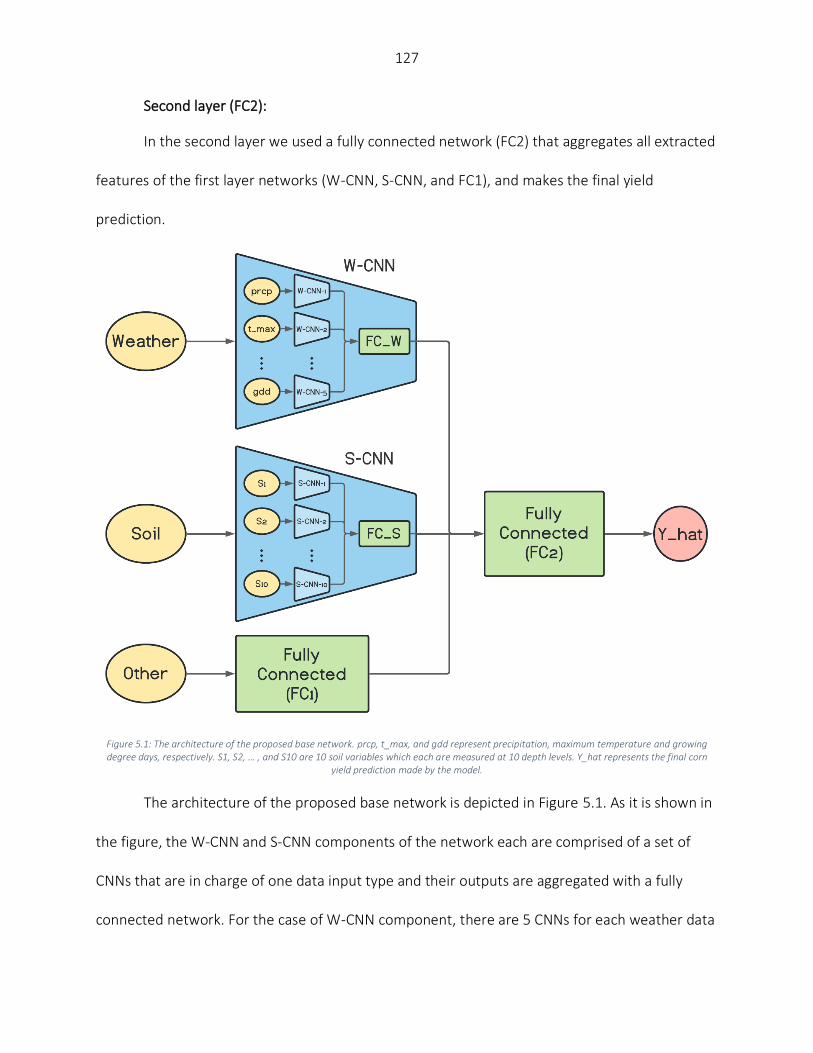
127

Second layer (FC2):

In the second layer we used a fully connected network (FC2) that aggregates all extracted

features of the first layer networks (W-CNN, S-CNN, and FC1), and makes the final yield

prediction.

Figure 5.1: The architecture of the proposed base network. prcp, t_max, and gdd represent precipitation, maximum temperature and growing degree days, respectively. S1, S2, … , and S10 are 10 soil variables which each are measured at 10 depth levels. Y_hat represents the final corn

yield prediction made by the model.

The architecture of the proposed base network is depicted in Figure 5.1. As it is shown in

the figure, the W-CNN and S-CNN components of the network each are comprised of a set of

CNNs that are in charge of one data input type and their outputs are aggregated with a fully

connected network. For the case of W-CNN component, there are 5 CNNs for each weather data

128

type (precipitation, maximum temperature, minimum temperature, solar radiation, and growing

degree days). Similarly, 10 internal CNNs are designed inside S-CNN component for each of the

10 soil data types. The reason we decided to design one CNN for each data type is the

differences in the natures of different data types and our experiments showed that separate

CNNs for each data type could extract more useful information and will result in better final

predictions. The two inner fully connected networks (FC_W and FC_S) both have one hidden

layer with 60 and 40 neurons, respectively.

We used VGG-like architecture for the CNN models (Simonyan and Zisserman, 2014). The

details about each of the designed CNN networks are presented in Table 5.1. We performed

downsampling in the CNN models by average pooling with a stride of size 2. The feed-forward

fully connected network in the first layer (FC1) has three hidden layers with 64, 32, and 16

neurons. The final fully connected network of the second layer (FC2) is grown with two hidden

layers with 128 and 64 neurons. In addition, two dropout layers with dropout ratio of 0.5 are

located at the two last layers of the FC2 to prevent the model from overfitting. We used Adam

optimizer with the learning rate of 0.0001 for the entire model training stage and trained the

model for 1000 iterations considering batches of size 16. Rectified linear unit (ReLU) was used as

the activation function of all networks throughout the architecture except the output layer that

had a linear activation function.

To ensure that the ensemble created from a set of base learners performs better than

them, the base learners should have a certain level of diversity and prediction accuracy (Brown,

2017). Hence, two scenarios for generating diverse base models are considered which are

systematically different: homogenous and heterogenous ensemble base model generation.

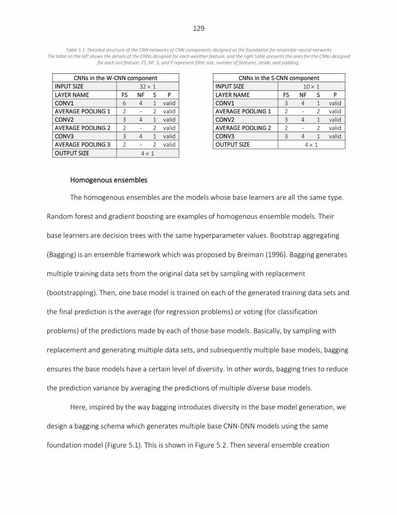
129

Table 5.1: Detailed structure of the CNN networks of CNN components designed as the foundation for ensemble neural networks The table on the left shows the details of the CNNs designed for each weather feature, and the right table presents the ones for the CNNs designed

for each soil feature. FS, NF, S, and P represent filter size, number of features, stride, and padding.

CNNs in the W-CNN component CNNs in the S-CNN component

INPUT SIZE 32 1 INPUT SIZE 10 1

LAYER NAME FS NF S P LAYER NAME FS NF S P

CONV1 6 4 1 valid CONV1 3 4 1 valid AVERAGE POOLING 1 2 - 2 valid AVERAGE POOLING 1 2 - 2 valid

CONV2 3 4 1 valid CONV2 3 4 1 valid

AVERAGE POOLING 2 2 - 2 valid AVERAGE POOLING 2 2 - 2 valid

CONV3 3 4 1 valid CONV3 3 4 1 valid

AVERAGE POOLING 3 2 - 2 valid OUTPUT SIZE 4 1

OUTPUT SIZE 4 1

Homogenous ensembles

The homogenous ensembles are the models whose base learners are all the same type.

Random forest and gradient boosting are examples of homogenous ensemble models. Their

base learners are decision trees with the same hyperparameter values. Bootstrap aggregating

(Bagging) is an ensemble framework which was proposed by Breiman (1996). Bagging generates

multiple training data sets from the original data set by sampling with replacement

(bootstrapping). Then, one base model is trained on each of the generated training data sets and

the final prediction is the average (for regression problems) or voting (for classification

problems) of the predictions made by each of those base models. Basically, by sampling with

replacement and generating multiple data sets, and subsequently multiple base models, bagging

ensures the base models have a certain level of diversity. In other words, bagging tries to reduce

the prediction variance by averaging the predictions of multiple diverse base models.

Here, inspired by the way bagging introduces diversity in the base model generation, we

design a bagging schema which generates multiple base CNN-DNN models using the same

foundation model (Figure 5.1). This is shown in Figure 5.2. Then several ensemble creation

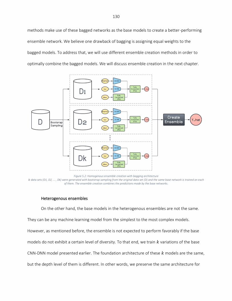
130

methods make use of these bagged networks as the base models to create a better-performing

ensemble network. We believe one drawback of bagging is assigning equal weights to the

bagged models. To address that, we will use different ensemble creation methods in order to

optimally combine the bagged models. We will discuss ensemble creation in the next chapter.

Figure 5.2: Homogenous ensemble creation with bagging architecture

𝑘 data sets (D1, D2, … , Dk) were generated with bootstrap sampling from the original data set (D) and the same base network is trained on each of them. The ensemble creation combines the predictions made by the base networks.

Heterogenous ensembles

On the other hand, the base models in the heterogenous ensembles are not the same.

They can be any machine learning model from the simplest to the most complex models.

However, as mentioned before, the ensemble is not expected to perform favorably if the base

models do not exhibit a certain level of diversity. To that end, we train 𝑘 variations of the base

CNN-DNN model presented earlier. The foundation architecture of these 𝑘 models are the same,

but the depth level of them is different. In other words, we preserve the same architecture for

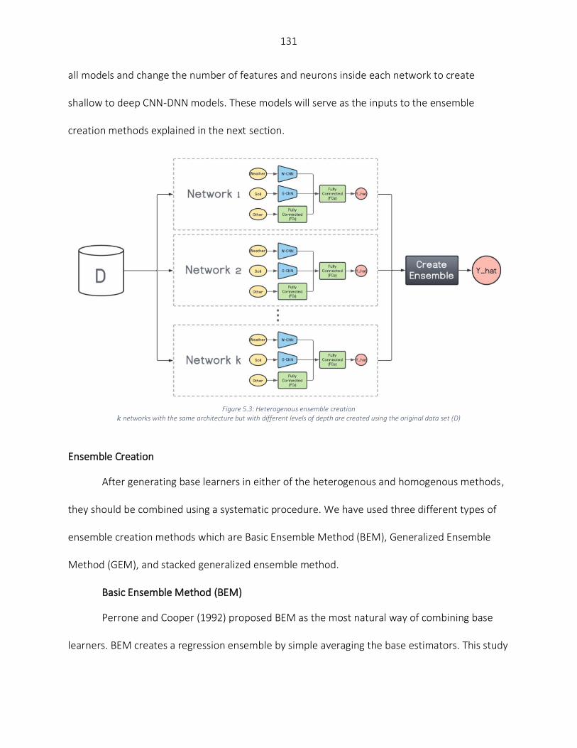
131

all models and change the number of features and neurons inside each network to create

shallow to deep CNN-DNN models. These models will serve as the inputs to the ensemble

creation methods explained in the next section.

Figure 5.3: Heterogenous ensemble creation

𝑘 networks with the same architecture but with different levels of depth are created using the original data set (D)

Ensemble Creation

After generating base learners in either of the heterogenous and homogenous methods,

they should be combined using a systematic procedure. We have used three different types of

ensemble creation methods which are Basic Ensemble Method (BEM), Generalized Ensemble

Method (GEM), and stacked generalized ensemble method.

Basic Ensemble Method (BEM)

Perrone and Cooper (1992) proposed BEM as the most natural way of combining base

learners. BEM creates a regression ensemble by simple averaging the base estimators. This study

132

claims that BEM can reduce mean squared error of predictions, given that the base learners are

diverse.

Generalized Ensemble Method (GEM)

GEM is the general case of a BEM ensemble creation method and tries to create a

regression ensemble as the linear combination of the base estimators. Cross-validation is used to

generate out-of-bag predictions and optimize the ensemble weights and the model was claimed

to avoid overfitting the data (Perrone and Cooper, 1992).

The nonlinear convex optimization problem is as follows.

𝑀𝑖𝑛 1

𝑛∑ (𝑦𝑖 − ∑ 𝑤𝑗�̂�𝑖𝑗

𝑘𝑗=1 )

2𝑛𝑖=1 [5.2]

𝑠. 𝑡. ∑ 𝑤𝑗

𝑘𝑗=1 = 1,

𝑤𝑗 ≥ 0, ∀𝑗 = 1, … , 𝑘.

In which 𝑤𝑗 is the weight of base model 𝑗 (𝑗 = 1, … , 𝑘), 𝑛 is the total number of

observations, 𝑦𝑖 is the true value of observation 𝑖, and �̂�𝑖𝑗 is the prediction of observation 𝑖 by

base model 𝑗.

Stacked generalized ensemble method

Stacked generalization is referred to combining several base estimators by performing at

least one more level of machine learning task. Usually, cross-validation is used to generate out-

of-bag predictions form the training samples and learn the higher-level machine learning models

(Wolpert, 1992). The second level learner can be any choice of ML models. In this study we have

selected linear regression, LASSO, random forest and LightGBM as the second level learners.

133

Results

The historical county-level data of the US Corn Belt states (Illinois, Indiana, Iowa, Kansas,

Michigan, Minnesota, Missouri, Nebraska, North Dakota, Ohio, South Dakota, and Wisconsin)

spanning across years 1980-2019 were used to train all considered models. The data from the

years 2017, 2018, and 2019, in turn, were reserved as the test data and the data from the years

before each of them formed the training data.

As mentioned earlier, the ensemble creation methods require out-of-bag (OOB)

predictions from all the input models that represent the test data to optimally combine the base

models. The current procedure to create these OOB predictions is using a cross-validation

method. However, due to time-dependency in the training data and the fact that in the

homogenous ensemble models the training data is resampled 𝑘 times, it is not possible to find a

consistent vector of OOB predictions across all models and use it to combine the base models.

Therefore, 20% of the training data was considered as the validation data and was not used in

model training. It is noteworthy that the training data is split to %20-%80 with a stratified split

procedure to ensure the validation data has a similar distribution with the training data. To

achieve the stratified splits, we binned the observations in the training data into 5 linearly

spaced bins based on their corresponding yield values.

The CNN structure of the base models trained for creating homogenous ensemble

models are same as the one shown in Table 5.1. We have resampled the training data 10 times

(with replacement) and trained the same CNN-DNN model on each of the 10 newly created

training data. The OOB predictions are the predictions made by each of the 10 mentioned

models on the validation data.

134

Table 5.2: Detailed structure of the CNN networks of CNN components designed for heterogenous ensemble models The tables on the left show the details of the CNNs designed for each weather feature, and the right tables present the ones for the CNNs designed

for each soil feature. FS, NF, S, and P represent filter size, number of features, stride, and padding.

CNNs in the W-CNN component of Model 1 CNNs in the S-CNN component of Model 1

INPUT SIZE 32 1 INPUT SIZE 10 1

LAYER NAME FS NF S P LAYER NAME FS NF S P

CONV1 6 2 1 valid CONV1 3 2 1 valid

AVERAGE POOLING 1 2 - 2 valid AVERAGE POOLING 1 2 - 2 valid

CONV2 3 2 1 valid CONV2 3 2 1 valid

AVERAGE POOLING 2 2 - 2 valid AVERAGE POOLING 2 2 - 2 valid

CONV3 3 2 1 valid CONV3 3 2 1 valid

AVERAGE POOLING 3 2 - 2 valid OUTPUT SIZE 2 1

OUTPUT SIZE 2 1

CNNs in the W-CNN component of Model 2 CNNs in the S-CNN component of Model 2

INPUT SIZE 32 1 INPUT SIZE 10 1

LAYER NAME FS NF S P LAYER NAME FS NF S P

CONV1 6 3 1 valid CONV1 3 3 1 valid

AVERAGE POOLING 1 2 - 2 valid AVERAGE POOLING 1 2 - 2 valid

CONV2 3 3 1 valid CONV2 3 3 1 valid

AVERAGE POOLING 2 2 - 2 valid AVERAGE POOLING 2 2 - 2 valid

CONV3 3 3 1 valid CONV3 3 3 1 valid

AVERAGE POOLING 3 2 - 2 valid OUTPUT SIZE 3 1

OUTPUT SIZE 3 1

CNNs in the W-CNN component of Model 3 CNNs in the S-CNN component of Model 3

INPUT SIZE 32 1 INPUT SIZE 10 1

LAYER NAME FS NF S P LAYER NAME FS NF S P

CONV1 6 4 1 valid CONV1 3 4 1 valid

AVERAGE POOLING 1 2 - 2 valid AVERAGE POOLING 1 2 - 2 valid

CONV2 3 4 1 valid CONV2 3 4 1 valid

AVERAGE POOLING 2 2 - 2 valid AVERAGE POOLING 2 2 - 2 valid

CONV3 3 4 1 valid CONV3 3 4 1 valid

AVERAGE POOLING 3 2 - 2 valid OUTPUT SIZE 4 1

OUTPUT SIZE 4 1

CNNs in the W-CNN component of Model 4 CNNs in the S-CNN component of Model 4

INPUT SIZE 32 1 INPUT SIZE 10 1

LAYER NAME FS NF S P LAYER NAME FS NF S P

CONV1 6 5 1 valid CONV1 3 5 1 valid

AVERAGE POOLING 1 2 - 2 valid AVERAGE POOLING 1 2 - 2 valid

CONV2 3 5 1 valid CONV2 3 5 1 valid

AVERAGE POOLING 2 2 - 2 valid AVERAGE POOLING 2 2 - 2 valid

CONV3 3 5 1 valid CONV3 3 5 1 valid

AVERAGE POOLING 3 2 - 2 valid OUTPUT SIZE 5 1

OUTPUT SIZE 5 1

CNNs in the W-CNN component of Model 5 CNNs in the S-CNN component of Model 5

INPUT SIZE 32 1 INPUT SIZE 10 1

LAYER NAME FS NF S P LAYER NAME FS NF S P

CONV1 6 6 1 valid CONV1 3 6 1 valid

AVERAGE POOLING 1 2 - 2 valid AVERAGE POOLING 1 2 - 2 valid

CONV2 3 6 1 valid CONV2 3 6 1 valid

AVERAGE POOLING 2 2 - 2 valid AVERAGE POOLING 2 2 - 2 valid

CONV3 3 6 1 valid CONV3 3 6 1 valid

AVERAGE POOLING 3 2 - 2 valid OUTPUT SIZE 6 1

OUTPUT SIZE 6 1

On the other hand, the base models trained for creating heterogenous ensemble models

are not the same and they differ in their CNN depth levels. We trained 5 different CNN-DNN base

models on the same training data and formed the OOB predictions by each of those 5 models

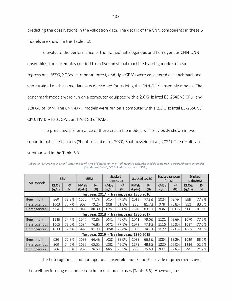
135

predicting the observations in the validation data. The details of the CNN components in these 5

models are shown in the Table 5.2.

To evaluate the performance of the trained heterogenous and homogenous CNN-DNN

ensembles, the ensembles created from five individual machine learning models (linear

regression, LASSO, XGBoost, random forest, and LightGBM) were considered as benchmark and

were trained on the same data sets developed for training the CNN-DNN ensemble models. The

benchmark models were run on a computer equipped with a 2.6 GHz Intel E5-2640 v3 CPU, and

128 GB of RAM. The CNN-DNN models were run on a computer with a 2.3 GHz Intel E5-2650 v3

CPU, NVIDIA k20c GPU, and 768 GB of RAM.

The predictive performance of these ensemble models was previously shown in two

separate published papers (Shahhosseini et al., 2020; Shahhosseini et al., 2021). The results are

summarized in the Table 5.3.

Table 5.3: Test prediction error (RMSE) and coefficient of determination (R2) of designed ensemble models compared to the benchmark ensembles (Shahhosseini et al., 2020; Shahhosseini et al., 2021).

ML models BEM GEM

Stacked regression

Stacked LASSO Stacked random

forest Stacked

LightGBM RMSE (kg/ha)

R2

(%) RMSE (kg/ha)

R2

(%) RMSE (kg/ha)

R2

(%) RMSE (kg/ha)

R2

(%) RMSE (kg/ha)

R2

(%) RMSE (kg/ha)

R2

(%)

Test year: 2017 - Training years: 1980-2016

Benchmark 960 79.6% 1002 77.7% 1014 77.2% 1012 77.3% 1024 76.7% 999 77.9%

Heterogenous 1003 77.7% 969 79.2% 908 81.8% 908 81.7% 978 78.8% 933 80.7% Homogenous 954 79.8% 944 80.3% 875 83.0% 874 83.1% 936 80.6% 906 81.8%

Test year: 2018 - Training years: 1980-2017

Benchmark 1145 74.7% 1047 78.8% 1041 79.0% 1041 79.0% 1101 76.6% 1070 77.9%

Heterogenous 1065 78.0% 1094 76.8% 1072 77.8% 1072 77.8% 1116 75.9% 1087 77.2%

Homogenous 1033 79.4% 992 81.0% 1058 78.4% 1056 78.4% 1077 77.6% 1065 78.1%

Test year: 2019 - Training years: 1980-2018

Benchmark 936 72.6% 1035 66.4% 1028 66.9% 1035 66.5% 1084 63.2% 1029 66.9%

Heterogenous 900 74.6% 1083 63.3% 1282 48.5% 1279 48.8% 1225 53.0% 1234 52.3%

Homogenous 866 76.5% 867 76.5% 885 75.5% 883 75.6% 932 72.8% 895 74.9%

The heterogenous and homogenous ensemble models both provide improvements over

the well-performing ensemble benchmarks in most cases (Table 5.3). However, the

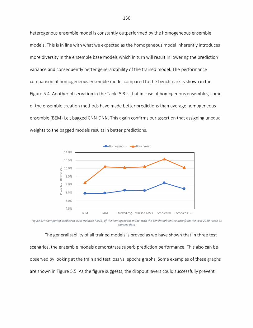
136

heterogenous ensemble model is constantly outperformed by the homogeneous ensemble

models. This is in line with what we expected as the homogeneous model inherently introduces

more diversity in the ensemble base models which in turn will result in lowering the prediction

variance and consequently better generalizability of the trained model. The performance

comparison of homogeneous ensemble model compared to the benchmark is shown in the

Figure 5.4. Another observation in the Table 5.3 is that in case of homogenous ensembles, some

of the ensemble creation methods have made better predictions than average homogeneous

ensemble (BEM) i.e., bagged CNN-DNN. This again confirms our assertion that assigning unequal

weights to the bagged models results in better predictions.

Figure 5.4: Comparing prediction error (relative RMSE) of the homogeneous model with the benchmark on the data from the year 2019 taken as

the test data

The generalizability of all trained models is proved as we have shown that in three test

scenarios, the ensemble models demonstrate superb prediction performance. This also can be

observed by looking at the train and test loss vs. epochs graphs. Some examples of these graphs

are shown in Figure 5.5. As the figure suggests, the dropout layers could successfully prevent

137

overfitting of the CNN-DNN models, and the test errors tend to stay stable across the iterations.

The generalizability of the trained models will further be discussed in the Discussion section.

Figure 5.5: Train and test loss vs. epochs of some of the trained CNN-DNN models

Discussion

Models’ performance comparison with the literature

We designed a novel CNN-DNN ensemble model with the objective of providing the most

accurate prediction model for county-level corn yield across US Corn Belt states. The numerical

results confirmed the superb performance of the designed ensemble models compared to

literature models. Table 5.3 showed that the homogenous ensemble models outperform the

benchmark (Shahhosseini et al., 2020) by 10-16%. In addition, comparing the results with

another well-performing prediction model in the literature (Khaki et al., 2020b), the

homogeneous ensemble could outperform the prediction results of Khaki et al. (2020b) by 10-

12% in common test set scenarios (2017 and 2018 test years). The CNN-RNN model developed

by Khaki et al. (2020b) presented test prediction errors of 988 kg/ha (15.74 bu/acre) and 1107

kg/ha (17.64 bu/acre) for the test years 2017 and 2018, respectively, while the homogeneous

ensemble model designed here resulted in test prediction errors of 874 kg/ha (13.93 bu/acre)

and 992 kg/ha (15.8 bu/acre) for the test years 2017 and 2018, respectively.

Model CNN-DNN 1 - 2017 Model CNN-DNN 1 - 2018 Model CNN-DNN 1 - 2019

138

This is the first study that designed a novel ensemble neural network architecture that

has the potential to make the most accurate yield predictions. The model developed here is

advantageous compared to the literature due to the ability of the ensemble model in decreasing

prediction variance by combining diverse models as well as reducing prediction bias by training

the ensemble model based on powerful base models. Shahhosseini et al. (2020) had used

ensemble learning for predicting county-level yield prediction, but neural network-based

architectures were not considered, and the models were trained only on three states (IL, IA, IN).

Khaki et al. (2020b) trained a CNN-RNN model for predicting US Corn Belt corn and soybean

yields, but the model developed there is unable to make predictions as accurate as the models

designed in this study and is not benefitting from the diversity in the predictions.

Including remote sensing data as well as simulated data from crop model like APSIM

could potentially improve the predictions made by our models further which can be pursued as

the future research direction. In addition, we assumed all considered farms are rainfed, while in

states such as Kansas and Nebraska many of the farms are irrigated. Surprisingly, the prediction

accuracy in these states was comparable with other states (Figures 5.6 and 5.7). We believe this

is because of the use of average or rainfed corn yields from these states, not irrigated yields to

train our models. Including the irrigation data can result in better prediction and perhaps new

models for those states and is another possible future research direction.

Comparing the models’ performance across US Corn Belt states

Figure 5.6 compares the prediction errors of the test year of 2019 for some of the

designed ensemble models represented by relative root mean squared error (RRMSE) for each of

139

the 12 US Corn Belt states under study. The models performed the best in Iowa, Illinois, and

Nebraska, and worst in Kansas and South Dakota. The worse prediction error in Kansas can be

explained by the fact that the majority of the farms in Kansas state are irrigated and this

irrigation is not considered as one of the variables when training the ensemble models. It is clear

that including irrigation variable can improve the predictions. However, that was not the case for

Nebraska, suggesting that irrigation may not be the only reason for the low performance in

Kansas. Upon further investigate, we realized the corn yields in the Nebraska state are highly

correlated with the weather features especially maximum temperature, while the corn yields in

the Kansas state don’t show this amount of correlation to weather features and are slightly

correlated with both weather and soil features. In other words, it seems that although the

weather features are adequate for making decent predictions in the Nebraska state, this is not

the case for the Kansas.

Figure 5.6: Comparing prediction error (relative RMSE) of the some of the designed ensembles across all US Corn Belt states on the data from the

year 2019 taken as the test data

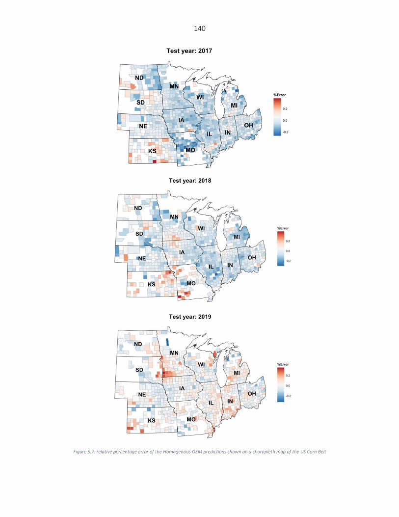
140

Figure 5.7: relative percentage error of the Homogenous GEM predictions shown on a choropleth map of the US Corn Belt

141

Figure 5.7 depicts the relative error percentage of each year’s test predictions on a

county choropleth map of the US Corn Belt. The errors are calculated by dividing over/under

prediction of the homogenous GEM model divided by the yearly average yield. This figure proves

that the model is robust and can be easily generalized to other environments/years. One

observation is that the model keeps overpredicting the yields in the Kansas state. This could be

explained by the irrigation assumption we made when developing the data set. We assumed all

the farms are rainfed and did not consider irrigation in states like Kansas in which some of the

farms are irrigated.

Generalization power of the designed Ensemble CNN-DNN models

To further test the generalization power of the designed ensembles, we gathered the

data of all considered US Corn Belt states for the year 2020 and applied the trained

heterogeneous and homogeneous ensemble models as well as the benchmarks on the new

unseen observations of the year 2020. As the results imply (Table 5.4), both heterogenous and

homogeneous ensemble models provide better predictions than the benchmark ensemble

models, with the homogeneous Generalized Ensemble Model (GEM) being the most accurate

prediction model. This model could provide predictions with 958 kg/ha root mean squared error

and explain about 77% of the total variability in the response variable.

Table 5.4: Test prediction error (RMSE) and coefficient of determination (R2) of designed ensemble models compared to the benchmark ensembles (Shahhosseini et al., 2020; Shahhosseini et al., 2021) when applied on 2020 test data

ML models BEM GEM

Stacked regression

Stacked LASSO Stacked random

forest Stacked

LightGBM RMSE (kg/ha)

R2

(%) RMSE (kg/ha)

R2

(%) RMSE (kg/ha)

R2

(%) RMSE (kg/ha)

R2

(%) RMSE (kg/ha)

R2

(%) RMSE (kg/ha)

R2

(%)

Test year: 2020 - Training years: 1980-2018

Benchmark 1115 68.4% 1165 65.5% 1166 65.4% 1170 65.2% 1210 62.8% 1183 64.4%

Heterogenous 972 76.0% 989 75.1% 992 75.0% 991 75.0% 1048 72.1% 1000 74.6% Homogenous 982 75.5% 958 76.7% 1001 74.5% 999 74.6% 1053 71.8% 1018 73.6%

142

Conclusion

In this study we designed two novel CNN-DNN ensemble types for predicting county-level

corn yields across US Corn Belt states. The base architecture used for creating the ensembles is a

combination of convolutional neural networks and deep neural networks. The CNNs were in

charge of extracting useful high-level features from the soil and weather data and provide them

to a fully connected network for making the final yield predictions. The two ensemble types were

heterogeneous and homogeneous which used the same base CNN-DNN structure but generated

the base models in different manners. The homogenous ensemble used one fixed CNN-DNN

network but applied it on multiple bagged data sets. The bagged data sets introduced a certain

level of diversity that the created ensembles had benefited from. On the other hand, the

heterogeneous ensemble used different base CNN-DNN networks which shared the same

structure but differed in their depth levels. The different depth levels were considered as

another method of introducing diversity into the ensembles. All base models generated from

either of these two ensemble types were combined with each other using three ensemble

creation methods: Basic Ensemble Method (BEM), Generalized Ensemble Method (GEM), and

stacked generalized ensembles. The numerical results showed that the ensemble models of

both homogeneous and heterogeneous types could outperform the benchmark ensembles

which had previously proved to be effective (Shahhosseini et al., 2020, Shahhosseini et al., 2021)

as well as well-performing CNN-RNN architecture designed by Khaki et al. (2020b). In addition,

homogeneous ensembles provide the most accurate predictions across all US Corn Belt states.

The results demonstrated that in addition to the fact that these ensemble models benefitted

from higher level of diversity from the bagged data sets, they provided a better combination of

143

base models compared to simple averaging in the bagging. The generalization power of the

designed ensembles was proved by applying them on the unseen observations of the year 2020.

Once again heterogeneous and homogeneous ensemble models outperformed the benchmark

ensembles.

References

Basso, B., & Liu, L. (2019). Chapter Four - Seasonal crop yield forecast: Methods, applications, and accuracies. In D. L. Sparks (Ed.), Advances in Agronomy (Vol. 154, pp. 201–255). Academic Press. https://doi.org/https://doi.org/10.1016/bs.agron.2018.11.002

Bengio, Y., Simard, P., & Frasconi, P. (1994). Learning long-term dependencies with gradient descent is difficult. IEEE Transactions on Neural Networks, 5(2), 157-166.

Borovykh, A., Bohte, S., & Oosterlee, C. W. (2017). Conditional time series forecasting with convolutional neural networks. arXiv preprint arXiv:1703.04691.

Breiman, L. (1996). Bagging predictors. Machine learning, 24(2), 123-140.

Busetto, L., Casteleyn, S., Granell, C., Pepe, M., Barbieri, M., Campos-Taberner, M., et al. (2017). Downstream Services for Rice Crop Monitoring in Europe: From Regional to Local Scale. [Article]. IEEE Journal of Selected Topics in Applied Earth Observations and Remote Sensing, 10(12), 5423-5441.

Cai, Y., Moore, K., Pellegrini, A., Elhaddad, A., Lessel, J., Townsend, C., et al. (2017). Crop yield predictions-high resolution statistical model for intra-season forecasts applied to corn in the US. Paper presented at the 2017 Fall Meeting.

Chlingaryan, A., Sukkarieh, S., & Whelan, B. (2018). Machine learning approaches for crop yield prediction and nitrogen status estimation in precision agriculture: A review. Computers and Electronics in Agriculture, 151, 61-69.

Crane-Droesch, A. (2018). Machine learning methods for crop yield prediction and climate change impact assessment in agriculture. Environmental Research Letters, 13(11), 114003.

Drummond, S. T., Sudduth, K. A., Joshi, A., Birrell, S. J., & Kitchen, N. R. (2003). Statistical and neural methods for site–specific yield prediction. Transactions of the ASAE, 46(1), 5.

Everingham, Y., Sexton, J., Skocaj, D., & Inman-Bamber, G. (2016). Accurate prediction of sugarcane yield using a random forest algorithm. Agronomy for Sustainable Development, 36(2), 27. https://doi.org/10.1007/s13593-016-0364-z

144

Feng, P., Wang, B., Liu, D. L., Waters, C., & Yu, Q. (2019). Incorporating machine learning with biophysical model can improve the evaluation of climate extremes impacts on wheat yield in south-eastern Australia. Agricultural and Forest Meteorology, 275, 100–113. https://doi.org/https://doi.org/10.1016/j.agrformet.2019.05.018

Feng, S.-H., Xu, J.-Y., & Shen, H.-B. (2020). Chapter Seven - Artificial intelligence in bioinformatics: Automated methodology development for protein residue contact map prediction. In D. D. Feng (Ed.), Biomedical Information Technology (Second Edition) (pp. 217-237): Academic Press.

Fukuda, S., Spreer, W., Yasunaga, E., Yuge, K., Sardsud, V., & Müller, J. (2013). Random Forests modelling for the estimation of mango (Mangifera indica L. cv. Chok Anan) fruit yields under different irrigation regimes. Agricultural water management, 116, 142-150.

González Sánchez, A., Frausto Solís, J., & Ojeda Bustamante, W. (2014). Predictive ability of machine learning methods for massive crop yield prediction.

Goodfellow, I., Bengio, Y., & Courville, A. (2016). Deep learning (Vol. 1): MIT press Cambridge.

He, K., Zhang, X., Ren, S., & Sun, J. (2016). Deep residual learning for image recognition. Paper presented at the Proceedings of the IEEE conference on computer vision and pattern recognition.

Heremans, S., Dong, Q., Zhang, B., Bydekerke, L., & Orshoven, J. V. (2015). Potential of ensemble tree methods for early-season prediction of winter wheat yield from short time series of remotely sensed normalized difference vegetation index and in situ meteorological data. Journal of Applied Remote Sensing, 9(1), 1-20, 20.

Ince, T., Kiranyaz, S., Eren, L., Askar, M., & Gabbouj, M. (2016). Real-Time Motor Fault Detection by 1-D Convolutional Neural Networks. IEEE Transactions on Industrial Electronics, 63(11), 7067-7075.

Ioffe, S., & Szegedy, C. (2015). Batch normalization: Accelerating deep network training by reducing internal covariate shift. arXiv preprint arXiv:1502.03167.

Jeong, J. H., Resop, J. P., Mueller, N. D., Fleisher, D. H., Yun, K., Butler, E. E., et al. (2016). Random forests for global and regional crop yield predictions. PLoS One, 11(6), e0156571.

Jiang, D., Yang, X., Clinton, N., & Wang, N. (2004). An artificial neural network model for estimating crop yields using remotely sensed information. International Journal of Remote Sensing, 25(9), 1723-1732.

Khaki, S., & Wang, L. (2019). Crop Yield Prediction Using Deep Neural Networks. Frontiers in Plant Science, 10(621). https://doi.org/10.3389/fpls.2019.00621

145

Khaki, S., Khalilzadeh, Z., & Wang, L. (2020a). Predicting yield performance of parents in plant breeding: A neural collaborative filtering approach. PLOS ONE, 15(5), e0233382.

Khaki, S., Wang, L., & Archontoulis, S. V. (2020b). A CNN-RNN Framework for Crop Yield Prediction. Frontiers in Plant Science, 10(1750). https://doi.org/10.3389/fpls.2019.01750

Kim, N., Ha, K.-J., Park, N.-W., Cho, J., Hong, S., & Lee, Y.-W. (2019). A Comparison Between Major Artificial Intelligence Models for Crop Yield Prediction: Case Study of the Midwestern United States, 2006–2015. ISPRS International Journal of Geo-Information, 8(5), 240.

Kiranyaz, S., Ince, T., Abdeljaber, O., Avci, O., & Gabbouj, M. (2019, 12-17 May 2019). 1-D Convolutional Neural Networks for Signal Processing Applications. Paper presented at the ICASSP 2019 - 2019 IEEE International Conference on Acoustics, Speech and Signal Processing (ICASSP).

Liu, J., Goering, C., & Tian, L. (2001). A neural network for setting target corn yields. Transactions of the ASAE, 44(3), 705.

Mavromatis, T. (2016). Spatial resolution effects on crop yield forecasts: An application to rainfed wheat yield in north Greece with CERES-Wheat. Agricultural Systems, 143, 38–48. https://doi.org/https://doi.org/10.1016/j.agsy.2015.12.002

Mupangwa, W., Chipindu, L., Nyagumbo, I., Mkuhlani, S., & Sisito, G. (2020). Evaluating machine learning algorithms for predicting maize yield under conservation agriculture in Eastern and Southern Africa. SN Applied Sciences, 2(5), 952. https://doi.org/10.1007/s42452-020-2711-6

NASS, U. (2019). Surveys. National Agricultural Statistics Service, U.S. Department of Agriculture.

Pagani, V., Stella, T., Guarneri, T., Finotto, G., van den Berg, M., Marin, F. R., Acutis, M., & Confalonieri, R. (2017). Forecasting sugarcane yields using agro-climatic indicators and Canegro model: A case study in the main production region in Brazil. Agricultural Systems, 154, 45–52. https://doi.org/https://doi.org/10.1016/j.agsy.2017.03.002

Pantazi, X. E., Tamouridou, A. A., Alexandridis, T. K., Lagopodi, A. L., Kashefi, J., & Moshou, D. (2017). Evaluation of hierarchical self-organising maps for weed mapping using UAS multispectral imagery. Computers and Electronics in Agriculture, 139, 224-230.

Perrone, M. P., & Cooper, L. N. (1992). When networks disagree: Ensemble methods for hybrid neural networks: BROWN UNIV PROVIDENCE RI INST FOR BRAIN AND NEURAL SYSTEMS.

Shahhosseini, M., Hu, G., & Archontoulis, S. V. (2020). Forecasting Corn Yield With Machine Learning Ensembles. [Methods]. Frontiers in Plant Science, 11(1120).

146

Shahhosseini, M., Hu, G., Huber, I., & Archontoulis, S. V. (2021). Coupling machine learning and crop modeling improves crop yield prediction in the US Corn Belt. Scientific Reports, 11(1), 1606. https://doi.org/10.1038/s41598-020-80820-1

Shahhosseini, M., Martinez-Feria, R. A., Hu, G., & Archontoulis, S. V. (2019). Maize yield and nitrate loss prediction with machine learning algorithms. Environmental Research Letters, 14(12), 124026.

Simonyan, K., & Zisserman, A. (2014). Very deep convolutional networks for large-scale image recognition. arXiv preprint arXiv:1409.1556.

Soil Survey Staff, Natural Resources Conservation Service, United States Department of Agriculture, Web Soil Survey. (2019). from https://websoilsurvey.nrcs.usda.gov/

Srivastava, N., Hinton, G., Krizhevsky, A., Sutskever, I., & Salakhutdinov, R. (2014). Dropout: a simple way to prevent neural networks from overfitting. J. Mach. Learn. Res., 15(1), 1929–1958.

Stas, M., Orshoven, J. V., Dong, Q., Heremans, S., & Zhang, B. (2016, 18-20 July 2016). A comparison of machine learning algorithms for regional wheat yield prediction using NDVI time series of SPOT-VGT. Paper presented at the 2016 Fifth International Conference on Agro-Geoinformatics (Agro-Geoinformatics).

Szegedy, C., Liu, W., Jia, Y., Sermanet, P., Reed, S., Anguelov, D., et al. (2015). Going deeper with convolutions. Paper presented at the Proceedings of the IEEE conference on computer vision and pattern recognition.

Vincenzi, S., Zucchetta, M., Franzoi, P., Pellizzato, M., Pranovi, F., De Leo, G. A., et al. (2011). Application of a Random Forest algorithm to predict spatial distribution of the potential yield of Ruditapes philippinarum in the Venice lagoon, Italy. Ecological Modelling, 222(8), 1471-1478.

Wang, A. X., Tran, C., Desai, N., Lobell, D., & Ermon, S. (2018). Deep transfer learning for crop yield prediction with remote sensing data. Paper presented at the Proceedings of the 1st ACM SIGCAS Conference on Computing and Sustainable Societies.

Wolpert, D. H. (1992). Stacked generalization. Neural Networks, 5(2), 241–259. https://doi.org/https://doi.org/10.1016/S0893-6080(05)80023-1

Yang, Q., Shi, L., Han, J., Zha, Y., & Zhu, P. (2019). Deep convolutional neural networks for rice grain yield estimation at the ripening stage using UAV-based remotely sensed images. Field Crops Research, 235, 142-153.

You, J., Li, X., Low, M., Lobell, D., & Ermon, S. (2017). Deep gaussian process for crop yield prediction based on remote sensing data. Paper presented at the Thirty-First AAAI conference on artificial intelligence.

147

Zhang, C., & Ma, Y. (2012). Ensemble machine learning: methods and applications: Springer.

Zhu, W., Ma, Y., Zhou, Y., Benton, M., & Romagnoli, J. (2018). Deep Learning Based Soft Sensor and Its Application on a Pyrolysis Reactor for Compositions Predictions of Gas Phase Components. In M. R. Eden, M. G. Ierapetritou & G. P. Towler (Eds.), Computer Aided Chemical Engineering (Vol. 44, pp. 2245-2250): Elsevier.

148

CHAPTER 6. GENERAL CONCLUSION

This dissertation was built on the idea that combining multiple machine learning base

learners i.e. creating an ensemble model from them, results in better prediction accuracy.

Considering Generalized Ensemble Model (GEM) as the ensemble creation method, which

creates an optimal linear combination of the base learners’ regression predictions, we found that

existing ensemble studies consider the base model construction and the weighted aggregation

to be independent steps. In other words, the base models were tuned in a separate stage before

creating the ensemble. Addressing this issue, we designed a framework (GEM-ITH) that can find

optimal ensemble weights as well as hyperparameter combinations and result in better

ensemble performance. This study addressed the computational complexity issue by the means

of Bayesian search to generate base learners. The numerical results showed that the proposed

GEM-ITH could outperform the state-of-the-art ensemble models in 9/10 considered data sets.

Designing a similar model for the classification problems and trying to further improve the

computational complexity of the problem and possibly decreasing its computation time were

suggested as future research directions.

To address the need of agricultural decision makers to forecast crop yields as early as

possible, we deigned several ensemble models using blocked sequential procedure to generate

out-of-bag predictions. This enabled the ensembles to account for the time-dependency in the

corn yields and make better predictions. The results demonstrated the ability of ensemble

models in decently forecasting corn yields as early as June 1st. In addition, to improve the

interpretability of ensemble models, a method to find partial dependency and consequently

feature importance of the optimized weighted ensemble model was proposed which could find

149

the marginal effect of varying each input variable on the ensemble predictions and rank the

input features based on the variability of their partial dependence plots (PDPs). For future

research directions, we suggested to work on a more efficient cross-validation procedure to

make out-of-bag predictions that can better represent the test data. Moreover, quantifying base

learners’ diversity to select more diverse models was suggested which could potentially further

improve the ensemble performance. Lastly, adding more informative input features such as

forecasted weather data, and N-fertilization inputs by county was mentioned as another future

research direction.

Motivated by the effect of additional input features on the quality of predictions, we

designed a hybrid ML-crop modeling approach which benefitted from additional inputs from a

simulation cropping model (APSIM). The hybrid model could significantly improve the predictions

ML models made and it was shown that the input features related to soil water, and in particular

growing season average drought stress, and average depth to water table were the most

important input features. The noteworthy merits of coupling ML and simulation crop models

shown in this study raised the question that whether the ML models can further benefit from

addition of input features from other sources. Hence, a possible extension of this study was

suggested to be the inclusion of remote sensing data into the ML prediction task and to

investigate the level of importance each data source can exhibit.

To develop a more robust and accurate yield prediction framework, we designed two

novel CNN-DNN ensemble types for predicting county-level corn yields across US Corn Belt

states. The base models were comprised of convolutional neural networks (CNN) and deep

neural networks (DNN). The CNNs could successfully capture the spatial and temporal

150

relationships in the soil and weather data, respectively. Homogeneous and heterogeneous

ensemble models were designed based on this CNN-DNN architecture and it was shown that by

benefitting from higher level of diversity from the bagged data sets, the homogeneous

ensembles could outperform state-of-the-art yield prediction models in the literature. The

generalizability and robustness of the ensemble models were proved by applying them on the

unseen observations of the year 2020. Including remote sensing data as well as crop modeling

simulated data (such as APSIM) were suggested as one possible future research direction.

Additionally, accounting for the irrigation in states that are not only rainfed (Kansas, Nebraska,

etc.) was suggested as another future research direction.

Lastly, for the future research directions, due to the observed dependence the crop

yields, we suggest designing ensemble models from new variations of ML models which can be

applied on dependent data. In addition, coupling these models with models such as

convolutional neural networks that are able to capture the temporal and spatial dependencies is

another suggested future research direction. This could potentially further improve the yield

predictions.

ProQuest Number:

INFORMATION TO ALL USERS The quality and completeness of this reproduction is dependent on the quality

and completeness of the copy made available to ProQuest.

Distributed by ProQuest LLC ( ). Copyright of the Dissertation is held by the Author unless otherwise noted.

This work may be used in accordance with the terms of the Creative Commons license or other rights statement, as indicated in the copyright statement or in the metadata

associated with this work. Unless otherwise specified in the copyright statement or the metadata, all rights are reserved by the copyright holder.

This work is protected against unauthorized copying under Title 17, United States Code and other applicable copyright laws.

Microform Edition where available © ProQuest LLC. No reproduction or digitization of the Microform Edition is authorized without permission of ProQuest LLC.

ProQuest LLC 789 East Eisenhower Parkway

P.O. Box 1346 Ann Arbor, MI 48106 - 1346 USA

28495731

2021