
Optimization of Multi-standards Software Defined Radio ...
319
HAL Id: tel-00446230 https://tel.archives-ouvertes.fr/tel-00446230 Submitted on 12 Jan 2010 HAL is a multi-disciplinary open access archive for the deposit and dissemination of sci- entific research documents, whether they are pub- lished or not. The documents may come from teaching and research institutions in France or abroad, or from public or private research centers. L’archive ouverte pluridisciplinaire HAL, est destinée au dépôt et à la diffusion de documents scientifiques de niveau recherche, publiés ou non, émanant des établissements d’enseignement et de recherche français ou étrangers, des laboratoires publics ou privés. Optimization of Multi-standards Software Defined Radio Equipments: A Common Operators Approach Sufi Tabassum Gul To cite this version: Sufi Tabassum Gul. Optimization of Multi-standards Software Defined Radio Equipments: A Common Operators Approach. Sciences of the Universe [physics]. Université Rennes 1, 2009. English. tel- 00446230
-
Upload
khangminh22 -
Category
Documents
-
view
1 -
download
0
Transcript of Optimization of Multi-standards Software Defined Radio ...

HAL Id: tel-00446230https://tel.archives-ouvertes.fr/tel-00446230
Submitted on 12 Jan 2010
HAL is a multi-disciplinary open accessarchive for the deposit and dissemination of sci-entific research documents, whether they are pub-lished or not. The documents may come fromteaching and research institutions in France orabroad, or from public or private research centers.
L’archive ouverte pluridisciplinaire HAL, estdestinée au dépôt et à la diffusion de documentsscientifiques de niveau recherche, publiés ou non,émanant des établissements d’enseignement et derecherche français ou étrangers, des laboratoirespublics ou privés.
Optimization of Multi-standards Software Defined RadioEquipments: A Common Operators Approach
Sufi Tabassum Gul
To cite this version:Sufi Tabassum Gul. Optimization of Multi-standards Software Defined Radio Equipments: A CommonOperators Approach. Sciences of the Universe [physics]. Université Rennes 1, 2009. English. tel-00446230

N° d’ordre : 3976 ANNÉE 2009
THÈSE / UNIVERSITÉ DE RENNES 1
sous le sceau de l’Université Européenne de Bretagne
pour le grade de
DOCTEUR DE L’UNIVERSITÉ DE RENNES 1 Mention : Traitement du Signal et Télécommunications
Ecole doctorale : Matisse
présentée par
Sufi Tabassum GUL Préparée à l’unité de recherche : SCEE-SUPELEC/IETR UMR 6164
Nom développé de l’unité : Institut d’Electronique et de Télécommunications de Rennes
Composante universitaire : S.P.M.
Optimization of Multi-standards Software Defined Radio Equipments: A Common Operators Approach
Thèse soutenue à Supélec-Rennes le 12 Novembre 2009
devant le jury composé de :
Olivier SENTIEYS Président, Professeur, Université de Rennes-I, Rennes, FRANCE
Michel AUGUIN Rapporteur, Professeur, Université de Nice – Sophia Antipolis, FRANCE
Arnd-Ragnar RHIEMEIER Rapporteur, Dr. – Ingénieur , EADS Defence and Security, Ulm, GERMANY
Guido MASERA Examinateur, Professeur, Politecnico di Torino, ITALY
Jacques PALICOT Directeur de thèse, Professeur, SUPELEC/IETR, Rennes, FRANCE
Christophe MOY Co-directeur de thèse, Professeur, SUPELEC/IETR, Rennes, FRANCE


Dedications
To my parentsfor their prayers, unmatched love and endless support
To Maryam,To Asma & M. Hassan.
i


Acknowledgments
Research is an exciting journey and I started this journey by stepping onto the unpavedpath of research three years ago in Signal Communication and Embedded Electronics Lab(SCEE)/Supélec-Rennes campus, FRANCE. By taking small strides I was able to drawa map of this journey and I hope it can be useful for other travellers. I have been downmany frustrating sidings, but I have also found new useful paths that may lead to newdiscoveries, which is very rewarding and the source of my motivation.
First of all, countless thanks to Almighty Allah, Whose innumerable blessings, acknowl-edged and unacknowledged, perceptible and imperceptible, bestow our lives from cradle tograve. I express my deep and sincere gratitude to Almighty Allah Who has given me theknowledge, will and courage to take up this work and has bestowed upon me His blessings.
I wish to convey my warmest thanks to my parents who have given me endless support,encouraged me in all my decisions and provided me the opportunity with their sacrificesto reach this far with my studies.
I want to express my indebtedness to all, especially my professors, right from very begin-ning of my educational career till now who guided me throughout my life. I would like toexpress my gratitude to my good natured and devoted director and co-director of thesis,Dr. Jacques Palicot and Dr. Christophe Moy for their support and for always believingin my capabilities, particularly when I was lost for a while. I am very grateful to them forall their help, encouraging words during the years and constructively criticizing my work.
I especially want to acknowledge three members of our research team who actively par-ticipated in the collaborative work presented in last part of this thesis. Firstly, Dr. AliAl-Ghouwayel, a former Ph.D student in SCEE lab, with whom I spent several weeksworking on a combined research. Secondly, I acknowledge Laurent ALAUS who is workingin CEA Grenoble for his cooperation and help. Thirdly, I am thankful to Dr. R. P. Maheshfor always providing me the valuable inputs.
I gratefully acknowledge all my former and present colleagues at the SCEE for creatingsuch a pleasant work environment and for helping me to solve many problems. I alsoacknowledge 5050 team for their cooperation and technical support.
I am very thankful to the reviewers and examiners of my thesis for spending their precioustime for reading, evaluating the quality of work and giving me extremely encouraging re-
iii

iv
marks.
Some friends have had a special impact on me during these three years. I would like tothank Abdul Sattar, an excellent researcher who gladly discussed anything from signalprocessing to Star Trek episodes. Also Sajjad Hussain is thanked for being an invigoratingdiscussion partner.
I would particularly like to express my deepest thanks and appreciation to my wife andchildren, for their love and patience. You have been with me the whole journey. Thankyou for all support, without you this thesis would never have been completed.
Finally, I would like to acknowledge the financial support provided by Higher EducationCommission of Pakistan right from the very beginning to the end of my Ph.D. studies.
Sufi Tabassum GulCesson Sévigné, FRANCE
November, 2009.

Contents
Contents v
Abbreviations xi
Thesis Summary in French 11 Emergence de la radio logicielle . . . . . . . . . . . . . . . . . . . . . . . . . 5
1.1 La radio logicielle . . . . . . . . . . . . . . . . . . . . . . . . . . . . . 51.2 Les avantages de la radio logicielle . . . . . . . . . . . . . . . . . . . 71.3 Projets et travaux les plus marquants de la radio logicielle . . . . . . 71.4 Les défis de la conception radio logicielle . . . . . . . . . . . . . . . . 8
2 Techniques de paramétrisation pour la radio logicielle . . . . . . . . . . . . . 102.1 La paramétrisation . . . . . . . . . . . . . . . . . . . . . . . . . . . . 102.2 Approche par fonctions communes . . . . . . . . . . . . . . . . . . . 102.3 Approche par opérateurs communs . . . . . . . . . . . . . . . . . . . 112.4 Exemple d’opérateur commun . . . . . . . . . . . . . . . . . . . . . . 13
3 Modélisation graphique pour les systèmes de radio logicielle . . . . . . . . . 173.1 Les graphes . . . . . . . . . . . . . . . . . . . . . . . . . . . . . . . . 173.2 Modèle de graphe théorique pour la radio logicielle multi-standards . 193.3 Reformulation réseau du problème . . . . . . . . . . . . . . . . . . . 23
4 Paramètres de coûts et coûts d’optimisation pour les systèmes de radiologicielle multi-standards . . . . . . . . . . . . . . . . . . . . . . . . . . . . . 244.1 Paramètres de coût . . . . . . . . . . . . . . . . . . . . . . . . . . . . 244.2 Types de coût . . . . . . . . . . . . . . . . . . . . . . . . . . . . . . . 254.3 Formulation de la fonction de coût . . . . . . . . . . . . . . . . . . . 284.4 Interface graphique . . . . . . . . . . . . . . . . . . . . . . . . . . . . 30
5 Technique d’optimisation . . . . . . . . . . . . . . . . . . . . . . . . . . . . . 305.1 Les techniques d’optimisation . . . . . . . . . . . . . . . . . . . . . . 315.2 La recherche exhaustive . . . . . . . . . . . . . . . . . . . . . . . . . 315.3 Le recuit simulé . . . . . . . . . . . . . . . . . . . . . . . . . . . . . . 355.4 Les algorithmes génétiques . . . . . . . . . . . . . . . . . . . . . . . . 365.5 Application . . . . . . . . . . . . . . . . . . . . . . . . . . . . . . . . 395.6 Conclusion sur le choix de l’algorithme d’optimisation . . . . . . . . 41
6 Cas d’étude : opérateur commun FFT dans un équipement de radio logi-cielle multi-standards . . . . . . . . . . . . . . . . . . . . . . . . . . . . . . . 476.1 Opérateur DMFFT . . . . . . . . . . . . . . . . . . . . . . . . . . . . 486.2 Application de l’approche de conception dans le contexte DMFFT . 50
v

vi contents
6.3 Résultats et conclusions . . . . . . . . . . . . . . . . . . . . . . . . . 557 Cas d’étude : opérateur commun LFSR dans un équipement de radio logi-
cielle multi-standards . . . . . . . . . . . . . . . . . . . . . . . . . . . . . . . 557.1 Opérateur LFSR . . . . . . . . . . . . . . . . . . . . . . . . . . . . . 557.2 LFSR et approche de conception par graphe . . . . . . . . . . . . . . 567.3 Conception d’un équipement tri-standards . . . . . . . . . . . . . . . 607.4 Résultats et conclusions . . . . . . . . . . . . . . . . . . . . . . . . . 62
8 Cas d’étude : opérateur commun FRMFB . . . . . . . . . . . . . . . . . . . 628.1 Bancs de filtres . . . . . . . . . . . . . . . . . . . . . . . . . . . . . . 638.2 Graphe du canaliseur multi-standards . . . . . . . . . . . . . . . . . 638.3 Optimisation du graphe canaliseur . . . . . . . . . . . . . . . . . . . 638.4 Résultats et conclusion . . . . . . . . . . . . . . . . . . . . . . . . . . 66
9 Cas d’étude d’un graphe complexe . . . . . . . . . . . . . . . . . . . . . . . 669.1 Opérateurs communs . . . . . . . . . . . . . . . . . . . . . . . . . . . 669.2 Graphe de conception . . . . . . . . . . . . . . . . . . . . . . . . . . 679.3 Coûts . . . . . . . . . . . . . . . . . . . . . . . . . . . . . . . . . . . 679.4 Résultats de l’optimisation . . . . . . . . . . . . . . . . . . . . . . . 689.5 Resultats et conclusion . . . . . . . . . . . . . . . . . . . . . . . . . . 72
General Introduction 751 Background and context . . . . . . . . . . . . . . . . . . . . . . . . . . . . . 752 Thesis outline . . . . . . . . . . . . . . . . . . . . . . . . . . . . . . . . . . . 763 Contributions . . . . . . . . . . . . . . . . . . . . . . . . . . . . . . . . . . . 79
I 83
1 Emergence of Software Radio 871.1 Introduction . . . . . . . . . . . . . . . . . . . . . . . . . . . . . . . . . . . . 881.2 Software radio . . . . . . . . . . . . . . . . . . . . . . . . . . . . . . . . . . . 891.3 Transceiver architectures . . . . . . . . . . . . . . . . . . . . . . . . . . . . . 92
1.3.1 Radio frequency front end . . . . . . . . . . . . . . . . . . . . . . . . 931.3.2 The classical superheterodyne architecture . . . . . . . . . . . . . . . 941.3.3 Software radio architecture . . . . . . . . . . . . . . . . . . . . . . . 951.3.4 Direct conversion architecture . . . . . . . . . . . . . . . . . . . . . . 961.3.5 Sub-sampling architecture . . . . . . . . . . . . . . . . . . . . . . . . 971.3.6 Feasible SDR architecture . . . . . . . . . . . . . . . . . . . . . . . . 99
1.4 Drivers for software radio . . . . . . . . . . . . . . . . . . . . . . . . . . . . 1001.5 Research projects in software radio design technology . . . . . . . . . . . . . 101
1.5.1 SPEAKeasy . . . . . . . . . . . . . . . . . . . . . . . . . . . . . . . . 1011.5.1.1 SPEAKeasy phase-I . . . . . . . . . . . . . . . . . . . . . . 1011.5.1.2 SPEAKeasy phase-II . . . . . . . . . . . . . . . . . . . . . . 102
1.5.2 JTRS . . . . . . . . . . . . . . . . . . . . . . . . . . . . . . . . . . . 1021.5.3 Digital modular radio . . . . . . . . . . . . . . . . . . . . . . . . . . 1031.5.4 Wireless information transfer system . . . . . . . . . . . . . . . . . . 1031.5.5 CHARIOT . . . . . . . . . . . . . . . . . . . . . . . . . . . . . . . . 1031.5.6 SpectrumWare . . . . . . . . . . . . . . . . . . . . . . . . . . . . . . 104

contents vii
1.5.7 GNU radio . . . . . . . . . . . . . . . . . . . . . . . . . . . . . . . . 1041.5.8 SDR forum . . . . . . . . . . . . . . . . . . . . . . . . . . . . . . . . 1051.5.9 European and French SDR projects . . . . . . . . . . . . . . . . . . . 105
1.6 Challenges in designing SDR . . . . . . . . . . . . . . . . . . . . . . . . . . 1061.7 Conclusions . . . . . . . . . . . . . . . . . . . . . . . . . . . . . . . . . . . . 107
2 Parametrisation Techniques for Software Radio 1092.1 Introduction . . . . . . . . . . . . . . . . . . . . . . . . . . . . . . . . . . . . 1092.2 Fundamentals of the techniques of parametrisation . . . . . . . . . . . . . . 110
2.2.1 The common function technique . . . . . . . . . . . . . . . . . . . . 1112.2.2 The common operator technique . . . . . . . . . . . . . . . . . . . . 1142.2.3 Comparison of the two techniques . . . . . . . . . . . . . . . . . . . 1162.2.4 Approaches to design common operators . . . . . . . . . . . . . . . . 117
2.2.4.1 Pragmatic approach . . . . . . . . . . . . . . . . . . . . . . 1172.2.4.2 Theoretical approach . . . . . . . . . . . . . . . . . . . . . 117
2.3 Examples of COs . . . . . . . . . . . . . . . . . . . . . . . . . . . . . . . . . 1182.3.1 FFT operator . . . . . . . . . . . . . . . . . . . . . . . . . . . . . . . 1192.3.2 LFSR operator . . . . . . . . . . . . . . . . . . . . . . . . . . . . . . 120
2.4 Conclusions . . . . . . . . . . . . . . . . . . . . . . . . . . . . . . . . . . . . 121
II 123
3 Graph Modeling of SDR Systems 1273.1 Introduction . . . . . . . . . . . . . . . . . . . . . . . . . . . . . . . . . . . . 127
3.1.1 Basics of graphs . . . . . . . . . . . . . . . . . . . . . . . . . . . . . 1283.1.2 Graph algorithms . . . . . . . . . . . . . . . . . . . . . . . . . . . . . 130
3.1.2.1 Related work . . . . . . . . . . . . . . . . . . . . . . . . . . 1303.1.2.2 Related work in SDR . . . . . . . . . . . . . . . . . . . . . 1323.1.2.3 Discussion . . . . . . . . . . . . . . . . . . . . . . . . . . . 135
3.2 Graph theoretical models of multi-standards SDR systems . . . . . . . . . . 1363.2.1 Objective . . . . . . . . . . . . . . . . . . . . . . . . . . . . . . . . . 1363.2.2 Definition of the graph structure . . . . . . . . . . . . . . . . . . . . 1363.2.3 Simplified example of tri-standard WiFi, WiMAX and UMTS trans-
mitter . . . . . . . . . . . . . . . . . . . . . . . . . . . . . . . . . . . 1383.3 Network theory reformulation . . . . . . . . . . . . . . . . . . . . . . . . . . 141
3.3.1 Motivation . . . . . . . . . . . . . . . . . . . . . . . . . . . . . . . . 1413.3.2 Network design problem . . . . . . . . . . . . . . . . . . . . . . . . . 1413.3.3 Graph to network conversion . . . . . . . . . . . . . . . . . . . . . . 141
3.4 Conclusions . . . . . . . . . . . . . . . . . . . . . . . . . . . . . . . . . . . . 144
4 Cost Parameters and Costs for Optimization of Multi-Standards SDRSystems 1474.1 Introduction . . . . . . . . . . . . . . . . . . . . . . . . . . . . . . . . . . . . 1474.2 Cost parameters . . . . . . . . . . . . . . . . . . . . . . . . . . . . . . . . . 1484.3 Types of costs . . . . . . . . . . . . . . . . . . . . . . . . . . . . . . . . . . . 149
4.3.1 Analytical costs . . . . . . . . . . . . . . . . . . . . . . . . . . . . . . 150

viii contents
4.3.2 Implementation costs . . . . . . . . . . . . . . . . . . . . . . . . . . . 1514.3.2.1 Digital hardware choices . . . . . . . . . . . . . . . . . . . . 1514.3.2.2 Field programmable gate arrays . . . . . . . . . . . . . . . 1524.3.2.3 Digital signal processors . . . . . . . . . . . . . . . . . . . . 1534.3.2.4 Algorithmic partitioning of typical transceiver tasks . . . . 155
4.3.3 Execution Costs . . . . . . . . . . . . . . . . . . . . . . . . . . . . . 1554.4 Approaches to formulate cost/objective function . . . . . . . . . . . . . . . . 155
4.4.1 Weighted sum approach . . . . . . . . . . . . . . . . . . . . . . . . . 1574.4.2 Objective function . . . . . . . . . . . . . . . . . . . . . . . . . . . . 158
4.5 Graphical user interface . . . . . . . . . . . . . . . . . . . . . . . . . . . . . 1594.6 Conclusions . . . . . . . . . . . . . . . . . . . . . . . . . . . . . . . . . . . . 163
5 Selected Optimizations Techniques 1655.1 Introduction . . . . . . . . . . . . . . . . . . . . . . . . . . . . . . . . . . . . 1655.2 Overview of general optimization techniques . . . . . . . . . . . . . . . . . . 166
5.2.1 Exhaustive search techniques . . . . . . . . . . . . . . . . . . . . . . 1705.2.1.1 Implementation . . . . . . . . . . . . . . . . . . . . . . . . 1705.2.1.2 Design example . . . . . . . . . . . . . . . . . . . . . . . . . 170
5.2.2 Simulated annealing . . . . . . . . . . . . . . . . . . . . . . . . . . . 1735.2.2.1 Implementation . . . . . . . . . . . . . . . . . . . . . . . . 1745.2.2.2 Design example . . . . . . . . . . . . . . . . . . . . . . . . . 176
5.2.3 Genetic algorithms . . . . . . . . . . . . . . . . . . . . . . . . . . . . 1765.2.3.1 Basic terminology of genetic algorithms . . . . . . . . . . . 1775.2.3.2 Rules of genetic algorithms . . . . . . . . . . . . . . . . . . 1775.2.3.3 Implementation of CGA . . . . . . . . . . . . . . . . . . . . 180
5.3 Application . . . . . . . . . . . . . . . . . . . . . . . . . . . . . . . . . . . . 1815.4 Conclusions . . . . . . . . . . . . . . . . . . . . . . . . . . . . . . . . . . . . 187
III 189
6 Case Study: FFT as a common operator in multi-standard SDR systems1936.1 Introduction . . . . . . . . . . . . . . . . . . . . . . . . . . . . . . . . . . . . 1936.2 Channel coding and fast Fourier transform . . . . . . . . . . . . . . . . . . . 195
6.2.1 Frequency domain decoder for RS codes . . . . . . . . . . . . . . . . 1956.2.2 Fermat number transforms . . . . . . . . . . . . . . . . . . . . . . . 197
6.3 Dual mode FFT operator . . . . . . . . . . . . . . . . . . . . . . . . . . . . 1986.4 Application . . . . . . . . . . . . . . . . . . . . . . . . . . . . . . . . . . . . 2006.5 Conclusions . . . . . . . . . . . . . . . . . . . . . . . . . . . . . . . . . . . . 205
7 Case Study: LFSRs as Common Operators in multi-standards SDR sys-tems 2077.1 Introduction . . . . . . . . . . . . . . . . . . . . . . . . . . . . . . . . . . . . 2077.2 Linear feedback shift register . . . . . . . . . . . . . . . . . . . . . . . . . . 2087.3 Implementation of common operators . . . . . . . . . . . . . . . . . . . . . . 208
7.3.1 Classical approach . . . . . . . . . . . . . . . . . . . . . . . . . . . . 2087.3.2 Proposed solution: common operator bank . . . . . . . . . . . . . . . 209

contents ix
7.3.3 Use of common operator banks . . . . . . . . . . . . . . . . . . . . . 2097.3.4 Implementation issues . . . . . . . . . . . . . . . . . . . . . . . . . . 211
7.4 Application . . . . . . . . . . . . . . . . . . . . . . . . . . . . . . . . . . . . 2127.4.1 Integration of LFSR in the graphical approach . . . . . . . . . . . . 2127.4.2 Design scenario . . . . . . . . . . . . . . . . . . . . . . . . . . . . . . 214
7.5 Conclusions . . . . . . . . . . . . . . . . . . . . . . . . . . . . . . . . . . . . 217
8 Case Study: FRMFB as Common Operator 2198.1 Introduction . . . . . . . . . . . . . . . . . . . . . . . . . . . . . . . . . . . . 2198.2 Filter bank techniques for SDR channelizers . . . . . . . . . . . . . . . . . . 220
8.2.1 Discrete Fourier transform filter bank . . . . . . . . . . . . . . . . . 2208.2.2 Goertzel filter bank . . . . . . . . . . . . . . . . . . . . . . . . . . . . 2208.2.3 Hybrid filter bank . . . . . . . . . . . . . . . . . . . . . . . . . . . . 2218.2.4 Multi-mode DFT filter bank . . . . . . . . . . . . . . . . . . . . . . . 2218.2.5 Modulated perfect reconstruction filter bank . . . . . . . . . . . . . . 2218.2.6 Tunable pipelined frequency transform filter bank . . . . . . . . . . . 2218.2.7 Tree structured quadrature mirror filter bank . . . . . . . . . . . . . 2228.2.8 Frequency response masking filter bank . . . . . . . . . . . . . . . . 222
8.2.8.1 FRMFB technique . . . . . . . . . . . . . . . . . . . . . . . 2238.2.8.2 Graph model for multi-standards SDR channelizers . . . . . 223
8.3 Complexity analysis of filter banks for SDR channelizers . . . . . . . . . . . 2238.3.1 Design scenario #1 . . . . . . . . . . . . . . . . . . . . . . . . . . . . 2248.3.2 Design scenario #2 . . . . . . . . . . . . . . . . . . . . . . . . . . . . 226
8.4 Optimization of channelizers . . . . . . . . . . . . . . . . . . . . . . . . . . . 2278.5 Conclusions . . . . . . . . . . . . . . . . . . . . . . . . . . . . . . . . . . . . 229
9 Case study of a complex graph 2319.1 Introduction . . . . . . . . . . . . . . . . . . . . . . . . . . . . . . . . . . . . 2319.2 Common operators . . . . . . . . . . . . . . . . . . . . . . . . . . . . . . . . 2329.3 Graph model . . . . . . . . . . . . . . . . . . . . . . . . . . . . . . . . . . . 2339.4 Cost issues . . . . . . . . . . . . . . . . . . . . . . . . . . . . . . . . . . . . 2349.5 Optimization results . . . . . . . . . . . . . . . . . . . . . . . . . . . . . . . 2359.6 Conclusions . . . . . . . . . . . . . . . . . . . . . . . . . . . . . . . . . . . . 239
General Conclusions and Perspectives 241
Appendix 245
247
A SDR projects 247A.1 European SDR projects . . . . . . . . . . . . . . . . . . . . . . . . . . . . . 247A.2 French SDR Projects . . . . . . . . . . . . . . . . . . . . . . . . . . . . . . . 248
249

x contents
B Complexity evaluation of air interface standards 249B.1 Complexity evaluation of IEEE 802.11a . . . . . . . . . . . . . . . . . . . . 249B.2 Complexity evaluation of UMTS . . . . . . . . . . . . . . . . . . . . . . . . 249
254
C Optimization tool 255C.1 Introduction . . . . . . . . . . . . . . . . . . . . . . . . . . . . . . . . . . . . 255
C.1.1 Methods of nodes . . . . . . . . . . . . . . . . . . . . . . . . . . . . . 255C.1.2 Methods of arcs . . . . . . . . . . . . . . . . . . . . . . . . . . . . . . 255C.1.3 Methods of graph . . . . . . . . . . . . . . . . . . . . . . . . . . . . . 255C.1.4 Methods of optimization . . . . . . . . . . . . . . . . . . . . . . . . . 256
257
D Channel coding and FFT 257D.1 The Fourier transform over finite fields . . . . . . . . . . . . . . . . . . . . . 257
D.1.1 Frequency encoding of RS codes over GF (2m) . . . . . . . . . . . . . 257D.1.2 Frequency decoding of RS codes over GF (2m) . . . . . . . . . . . . . 258D.1.3 Comparison between time and frequency domain decoding of RS codes263
D.2 Fermat Transform Based RS Codes . . . . . . . . . . . . . . . . . . . . . . . 264D.2.1 Encoding of RS codes defined over GF (Ft) . . . . . . . . . . . . . . 264D.2.2 Decoding of RS codes defined over GF (Ft) . . . . . . . . . . . . . . 264D.2.3 Performances comparison between RS over GF (Ft) and RS over
GF (2m) . . . . . . . . . . . . . . . . . . . . . . . . . . . . . . . . . . 264D.3 DMFFT architecture . . . . . . . . . . . . . . . . . . . . . . . . . . . . . . . 267
D.3.1 Stage architecture . . . . . . . . . . . . . . . . . . . . . . . . . . . . 269D.3.2 RBPE complexity study . . . . . . . . . . . . . . . . . . . . . . . . . 269
D.4 Altera’s Stratix-II FPGA family . . . . . . . . . . . . . . . . . . . . . . . . . 271
273
E LFSR architectures 273E.1 Linear feedback shift register basics and its architectures . . . . . . . . . . . 273
E.1.1 RF-LFSR architecture . . . . . . . . . . . . . . . . . . . . . . . . . . 273E.1.2 RG-LFSR architecture . . . . . . . . . . . . . . . . . . . . . . . . . . 274E.1.3 R-LFSR architecture . . . . . . . . . . . . . . . . . . . . . . . . . . . 274E.1.4 ER-LFSR architecture . . . . . . . . . . . . . . . . . . . . . . . . . . 275
E.2 Preeminent functions of LFSR COs . . . . . . . . . . . . . . . . . . . . . . . 276
List of Figures 279
List of Tables 283
Publications 301

Abbreviations
2G 2nd Generation3G 3rd Generation4G 4th Generation3GPP 3rd Generation Partnership Project3GPP LTE 3GPP Long Term EvolutionACTS Advanced Communications Technologies and ServicesA/D Analog to Digital ConverterADC Analog to Digital ConverterADSL Asymmetric Digital Subscriber LineAFE Analog Front EndAGC Automatic Gain ControlAGU Address Generating UnitALUT Adaptive Lookup TableALM Adaptive Logic ModuleAMPS Advanced Mobile Phone SystemASIC Application Specific Integrated CircuitATSC Advanced Television Systems CommitteeB3G Beyond 3GBC Buliding CostBER Bit Error RateBPF Band Pass FilterCB Communication BlockCC Computational CostCCM Custom Computing MachineCDMA Code Division Multiple AccessCEA Commissariat à l’Energie AtomiqueCF Common FunctionCHARIOT Changeable Advanced Radio for Inter-Operable TelecommunicationsCO Common OperatorCR Cognitive RadioCRC Cyclic Redundancy CheckCRCC Communications Research Centre of CanadaD/A Digital to Analog ConverterDAC Digital to Analog ConverterDAB Digital Audio BroadcastingDAG Directed Acyclic GraphDC Direct Current
xi

xii Abbreviations
DECT Digital Enhanced Cordless TelecommunicationsDFE Digital Front EndDFT Discrete Fourier TransformDFTFB Discrete Fourier Transform FBDIF Decimation In FrequencyDIT Decimation In TimeDMB Digital Multimedia BroadcastingDMFFT Dual Mode FFTDMR Digital Modular RadioDRM Digital Radio MondialeDSamp Down SamplingDSP Digital Signal ProcessorDVB-H Digital Video Broadcasting-HandheldDVB-T Digital Video Broadcasting-TerrestrialE3 End-to-End EfficiencyE2R End-to-End ReconfigurabilityEA Evolutionary AlgorithmsEMI Electro Mechanical InterferenceEP Evolutionay ProgrammingER-LFSR Extended Reconfigurable LFSRES Exhaustive SearchEVS Evolution StrategiesFB Filter BankFD Frequency DomainFER Frame Error RateFEC Forward Error CorrectionFFT Fast Fourier TransformFFT-C FFT defined over complex fieldFFT-GF2 FFT defined over GF (2m)FIR Finite Impulse ResponseFLMS Fast Least Mean SquaresFM3TR Future Multi-band Multi-waveform Modular Tactical RadioFNT Fermat Number TransformFPGA Field Programmable Gate ArrayFRM Frequency Response MaskingGA Genetic AlgorithmsGCU Global Control UnitGF Galois FieldGFB Goertzel FBGMSK Gaussian Minimum Shift KeyingGPP General Purpose ProcessorGPS Global Positioning SystemGSM Global System for Mobile CommunicationHDTV High Definition TVHF High FrequencyHLL High Level Language

xiii
HR Hardware RadioIC Integrated circuitIF Intermediate FrequencyIIR Infinite Impulse ResponseINFOSEC INFOrmation SECurityI/O Input/OutputI/Q In phase/ Quadrature phase (modulator, data)IS Interim Standard for US Code Division Multiple AccessIS-95/136 Interim Standard 95/136ISR Ideal Software RadioIST Information Society TechnologiesITS Information Technology ServicesITU International Telecommunications UnionJTRS Joint Tactical Radio SystemLFSR Linear Feedback Shift RegisterLNA Low Noise AmplifierLO Local OscillatorLRA Layered Radio ArchitectureLSB Least Significant BitLUT Look Up TableMAC Multiplier ACcumulatorMAP Maximum A Posteriori probabilityMBMMR Multi Band Multi Mode RadioMExE Mobile Execution EnvironmentMILS Multiple Independent Levels of SecurityMIT Massachusetts Institute of TechnologyMLSE Maximum Likelihood Sequence EstimationMMITS Modular Multifunction Information Transfer SystemMOP Multi Objective ProblemMPRB Modulated Perfect Reconstruction BankMSPS Million Samples Per SecondMRateFilt Multi Rate FilteringNoC Number of CallsNTT Number Theoretic TranformOFDM Orthogonal Frequency Division MultiplexingOS Operating SystemPA Pragmatic ApproachPE Processing ElementPFT Pipelined Frequency TransformPHY Physical Layerπ-DQPSK π Differential QPSKPLD Programmable Logic DevicePMCS Programmable Modular Communications SystemsPMR Professional Mobile RadioPN Pseudo NoisePSK Phase Shift Keying
xiv Abbreviations
QoS Quality of ServiceQPSK Quadrature Phase Shift KeyingR-LFSR Reconfigurable LFSRRF-LFSR Reconfigurable Fibonacci LFSRRG-LFSR Reconfigurable Galois LFSRRS Reed-SolomonRF Radio FrequencyRNRT Réseau National de Recherche en TélécommunicationsSA Simulated AnnealingSATCOM SATellite COMmunicationsSCA Software Communication ArchitectureSCU Stage Control UnitSDR Software Defined RadioSoC System on ChipSR Software RadioSCR Software Controlled RadioSFDR Spurious Free Dynamic RangeSIMO Single-Input Multi-OutputSRC Sample Rate ConvertersTA Theoretical ApporachTAJPSP Tactical AntiJam Programmable Signal ProcessorTPFT Tunable PFTTQMFB Tree Structured Quadrature Mirror FBTV TelevisionUFLMS Unconstrained Frequency-domain Least Mean SquaresUHF Ultra High FrequencyU.S. United States of AmericaUMTS Universal Mobile Telecommunication SystemUSR Ultimate Software RadioUTRA-FDD UMTS Terrestrial Radio Access-Frequency Division DuplexingUTRA-TDD UMTS Terrestrial Radio Access-Time Division DuplexingVHF Very High FrequencyVLIW Very Long Instruction WordVITURBO A Reconfigurable Architecture For Viterbi And TurboWiFi Wireless Fidelity (IEEE 802.11)WITS Wireless Information Transfer SystemWiMAX Worldwide Interoperability for Microwave Access, Inc. (IEEE 802.16)WLAN Wireless Local Area NetworkWP Work PackagexDSL Digital Subscriber Line Technologies

Résumé en français
Introduction générale
Cette thèse propose de contribuer à la conception des équipements de radio logicielle multi-standards sous un angle particulier comparativement aux efforts de recherche effectués engénéral dans la communauté. En effet, elle ne propose pas d’étudier comment il fautadapter les outils de conception actuels aux nouveaux défis proposés par la radio logicielle(co-conception matérielle-logicielle, outils d’abstraction de haut-niveau, etc.), mais com-ment ré-organiser les traitements afin d’exploiter de nouveaux degrés de liberté dans laconception.
La conception actuelle des équipements multi-standards consiste en une juxtapositionde circuits dédiés à chacun des standards. Dans un contexte à moyen terme, où de plusen plus de standards de communications sans fil sont destinés à être intégrés dans unmême terminal, une telle approche va bientôt atteindre ses limites, aussi bien en termesde coût, d’encombrement que de possibilité d’offrir des services combinés entre les stan-dards. On parle de conception de type velcro car on débranche une application radio pouren mettre une nouvelle en marche. On comprend bien les limites en termes de flexibil-ité, qui ne peut être que de très gros grain (au niveau d’un standard). A l’opposé, uneapproche radio logicielle pure repose sur l’utilisation d’opérateurs très fins (ceux du oudes processeurs) donc ré-utilisables de manière très flexible. Mais cela n’est réalisable quedans peu de cas réels. N’y aurait-il pas entre ces deux extrêmes des niveaux intermédi-aires permettant de combiner à la fois les avantages des deux ? Cela consiste à trouverune décomposition à différents niveaux de granularité des traitements afin d’identifier etd’exploiter des redondances appelées "opérateurs communs". Cela ne concerne pas seule-ment les traitements associés à la couche physique, mais aussi toutes les couches du modèleOSI présentes dans un même équipement. L’objectif est d’optimiser la conception suivantdifférents critères impliquant par exemple la flexibilité, la vitesse de reconfiguration ou lasurface occupée sur une cible matérielle. Cette étude se positionne dans le contexte pluslarge de la paramétrisation. Le terme paramétrisation regroupe l’ensemble des techniquesutilisées pour modifier une opération par un simple changement de paramètres (et non enmodifiant sa structure de base).
Le manuscrit est découpé en trois parties. La partie I est constituée de deux chapitres.Le chapitre 1 rappelle ce qu’est la radio logicielle et les défis qui y sont associés en termesde conception. Le chapitre 2 porte sur les techniques de paramétrisation pour la radio

2 Résumé en Français
logicielle et en particulier l’approche "opérateurs communs".
La partie II comporte trois chapitres. Le chapitre 3 explique comment modéliser lesstandards de communications sans fil sous forme de graphes hiérarchiques. Le chapitre 4évoque les problèmes des paramètres de coût et les techniques d’optimisation associées.Le chapitre 5 explique le choix de la technique d’optimisation multi-critères utilisée.
La partie III est composée de quatre chapitres, chacun traitant d’un cas concret deconception illustrant la méthode issue des travaux. L’utilisation de l’opérateur FFT dou-ble mode fait l’objet de chapitre 6, le chapitre 7 étudie différentes variantes de l’opérateurLFSR, dans le chapitre 8 les bancs de filtres à réponse masquée sont ciblés au départ, puisun exemple de conception à plus grande échelle est étudié pour conclure dans le chapitre 9.
Enfin, en dernier lieu, des conclusions sont données à ce travail ainsi que des perspec-tives pouvant étendre ses résultats à l’avenir.

3


Introduction à la partie I
La première partie de ce manuscrit positionne dans un premier chapitre les travaux dansle contexte de conception associé à la radio logicielle, et plus précisément à la concep-tion d’équipements de radio logicielle multi-standards. En effet, la radio logicielle a trèstôt été identifiée comme une solution prometteuse pour la conception de tels équipementspuisque le principe premier est d’utiliser un même matériel pour effectuer différentes sortesde modulations/démodulations. Le chapitre 1 explique pourquoi cela est envisageable etcomment la radio logicielle propose de le mettre en oeuvre. Il existe en fait plusieursniveaux de réalisation, plus ou moins réalistes suivant les contraintes (technologiques oude coût) et suivant l’échéance prévue pour que de tels équipements soient commercialisés.Un survol des projets marquants l’histoire de la radio logicielle permet de voir que l’élanest bien réel dans ce domaine de recherche. Enfin, de nombreux défis restent à relever entermes de conception radio logicielle et nous positionnerons l’approche proposée dans cetravail par rapport à celles proposées par ailleurs dans la communauté de la radio logicielle.
Dans le second chapitre de cette partie, les techniques de paramétrisation sont décrites,avec différents niveaux envisagés : fonctions communes et opérateurs communs. Deuxexemples d’opérateurs communs sont détaillés, à titre d’illustration : FFT et LFSR.
1 Emergence de la radio logicielle
1.1 La radio logicielle
La radio logicielle est à l’origine un ensemble de techniques visant à répondre aux évo-lutions de la conception des équipements de radiocommunications. Elle est ensuite aussila source de nouvelles utilisations possibles des équipements radio (en cours de fonction-nement), grâce aux propriétés de flexibilité apportées par la radio logicielle. Ce n’est pasle coeur du sujet des travaux présentés ici si ce n’est que la contrainte de flexibilité estconsidérée comme une priorité afin de permettre à l’équipement de modifier de fonction-nement en temps-réel.
Suivant l’architecture de l’émetteur-récepteur, on peut distinguer plusieurs déclinaisonsplus ou moins généralisées du principe de la radio logicielle, depuis la structure super-hétérodyne de la Fig. 1 (très peu "radio logicielle") jusqu’à celle de la radio logicielleidéale de la Fig. 2(a) en passant par celle plus réaliste (dans certains cas) de la Fig. 2(b)et enfin la version de la radio logicielle réalisable dans de nombreux cas, celle de la Fig. 3.
5

6 Résumé en Français
LNA
LO
LNA AGC
LO
LO90°
AGC ADC
DSP
AGC ADC
HPA
LO LO
LO90°
AGC DAC
DSP
AGC DAC
AGC
Figure 1: Emetteur/récepteur super-hétérodyne
ADC
DSP
LNA
DuplexerA/D
DSP DSP
DACAMP
DuplexerD/A DSP
(a) (b)
Figure 2: Une architecture réaliste d’une radio logicielle
Dans le cas de la radio logicielle, la conversion analogique numérique est directementeffectuée en radio fréquence, suivie de processeurs pour effectuer les calculs du récepteur.Cela est souvent impossible en raison des contraintes technologiques que cela implique surles convertisseurs et les processeurs. Ainsi, la radio logicielle restreinte (Software DefinedRadio - SDR) relaxe les contraintes. Par exemple, elle peut correspondre à une numéri-sation en fréquence intermédiaire (cas de la Fig. 3) ou même en bande de base. On peutcontinuer à parler quand même dans ce cas de radio logicielle restreinte si la reconfigura-bilité de l’équipement est exploitée. Dans le meilleur cas, une large bande de fréquence estalors directement numérisée englobant ainsi plusieurs signaux associés à différents stan-dards. Cette fonctionnalité fait alors référence à un système dit multi-standards, capabled’opérer selon différents modes et offrant plusieurs services. Le passage d’un mode à un

1 Emergence de la radio logicielle 7
AFE
ADC DSPData
LO
DFE
I/Q down conversion
Sample rateconversion Channelization
RF IF
LNA
Figure 3: Une architecture de récepteur réalisable
autre est alors possible à condition que les processeurs de traitement du signal soient pro-grammables ou reconfigurables.
Afin de réaliser d’une façon optimale un tel système, il est nécessaire de rechercher lespoints de convergence entre les standards à supporter par le terminal de façon à rendreles traitements communs. Cet aspect est connu sous le nom de la paramétrisation et estdéveloppé dans le chapitre suivant.
1.2 Les avantages de la radio logicielle
La radio logicielle est pour une grande partie une évolution naturelle de la radio car elleprocure de nombreux avantages pour tous les acteurs du domaine, aussi bien les fabricants,les opérateurs (et fournisseurs de service) que les utilisateurs. La radio logicielle promet eneffet dans ses principes des équipements multi-standards et multi-services. Il est possibled’en corriger les mal-fonctions, voire de les faire évoluer au niveau du traitement radio partéléchargement de logiciel, ce qui est à la fois bénéfique pour les utilisateurs (vous et moi,ainsi que les opérateurs), les fournisseurs de services et les constructeurs. Le rêve d’unemobilité totale peut être atteint grâce à la radio logicielle car elle permettra à l’équipementde s’adapter à tout standard en fonction des besoins. L’abandon des approches de concep-tion de type velcro permet en outre aux fabricants d’envisager des économies puisqu’unemême plate-forme peut supporter plusieurs standards même si ce n’est qu’avec un grandnombre de standards supportés que cela devient réellement le cas. En tout état de cause,le passage dans le domaine numérique d’une grande partie des traitements effectués enanalogique auparavant permet de tirer bénéfice des techniques de conception numériqueet de s’affranchir de beaucoup d’inconvénients liés à la conception analogique.
1.3 Projets et travaux les plus marquants de la radio logicielle
Historiquement, le projet SPEAKeasy a joué le rôle de projet pionnier dans le domaine dela radio logicielle, dès le début des années 90 [1, 2]. Il s’agit d’un projet mené par l’arméeaméricaine dans le but de créer un modem reprogrammable qui devait supporter plusieurs

8 Résumé en Français
modes de transmission à plusieurs fréquences porteuses (de 2 MHz à 2 GHz). C’est decette mouvance que sont apparus les experts américains qui ont crée le SDR Forum et lescompagnies américaines leader du domaine.
Le projet JTRS (Joint Tactical Radio System) s’est attelé à définir et proposer unearchitecture logicielle afin d’abstraire la forme d’onde logicielle (application radio) de laplate-forme d’exécution matérielle [3, 4]. Le résultat obtenu est le SCA (Software Com-munication Architecture) [5] qui est une architecture ouverte ayant pour but de permettreà tout fournisseur de pouvoir proposer du matériel ou du logiciel compatible avec les sous-systèmes d’autres fournisseurs. Cela repose sur la définition d’interfaces (API - ApplicationProgramming Interfaces) en langage IDL (Interface Definition Language), l’usage du buslogiciel CORBA et du système d’exploitation POSIX. Le SCA est désormais un standardimposé pour tout fournisseur de l’armée américaine, mais il peine à faire preuve de sonefficacité en termes de contraintes temps-réel.
Pendant ce temps, les universitaires américains se sont lancés également dans le do-maine de la radio logicielle. Citons Chariot de Virginia Tech [2] et SpectrumWare du MIT.SpectrumWare en particulier chercha à évaluer la faisabilité d’utiliser un processeur général(GPP - General Purpose Processeur) pour mettre en oeuvre la radio logicielle, notammentpour des standards civils cette fois, comme AMPS et GSM [6].
Comme la radio se tourne vers le monde du logiciel, c’est tout naturellement qu’aémergé l’idée d’une GNU radio [7] dans le but d’ouvrir à une large communauté un outil-lage associant logiciel et matériel.
L’organe de référence au niveau international pour la radio logicielle est le SDR Forum.Il représente des sociétés, des universités et des organismes membres qui portent un intérêtpour le développement de la radio logicielle. C’est notamment le SDR Forum (secondépar l’Object Management Group - OMG - à un moment) qui encadre les développementsréalisés autour du SCA.
L’Europe n’est pas en reste et la recherche sur le vieux continent est notammentsoutenue par la Commission Européenne et les organismes nationaux d’aide à la recherche.De très nombreux projets sont liés au domaine de la radio logicielle (voir l’annexe A dudocument en anglais). A titre d’exemple le plus significatif, le projet E2R (End-to-EndReconfigurability) et sa suite E2R-II a regroupé plus de 30 partenaires pendant un totalde quatre années dédiées à l’étude de la radio logicielle sous tous ses aspects.
1.4 Les défis de la conception radio logicielle
Comme déjà évoqué, la radio logicielle offre de nombreux avantages par rapport aux ra-dios classiques, notamment grâce à la flexibilité qu’elle apporte. Cependant, concevoirun équipement de radio logicielle qui n’a plus un unique mode de fonctionnement, dontles paramètres peuvent varier énormément pendant le cycle de vie, qui associe à la foisdu matériel et du logiciel, présente d’autres défis que ceux auxquels la conception d’un

1 Emergence de la radio logicielle 9
équipement radio classique devait faire face.
En effet, il est nécessaire de faire appel à des techniques de co-conception logicielle/matériellepuisqu’un système de radio logicielle est désormais constitué d’unités de traitement quiexécutent une application radio en logiciel. Et cela serait trop simple ainsi. Pour desraisons d’efficacité en terme de traitement ou de consommation de puissance, il est en effetsouvent obligatoire de combiner des unités de traitement de natures différentes, tels que lesGPP, DSP (Digital Signal Processor), les FPGA (Field Programmable Gate Array) et lesASIC (Application-Specific Integrated Circuit) numériques et même analogiques. Cettepluralité et cette mixité rendent la conception très difficile. Il n’existe pas actuellement desolution intégrée qui permettent de le faire véritablement. Seules des solutions partiellesexistent. Cette étude mérite en soi plusieurs travaux de thèses. Citons une approche quiest utilisée dans l’industrie de la radio logicielle et qui repose sur Simulink. Cette approchepermet de passer d’une simulation fonctionnelle (de type Matlab) à une implantation surcible hétérogène associant des DSP, des FPGA et des convertisseurs grâce à certains arti-fices qu’il serait trop long de détailler ici. Citons également une approche de prototypagerapide organisée autour de SynDEx [8] qui permet de mettre en oeuvre rapidement uneapplication radio logicielle sur différentes plates-formes matérielles.
Une solution prometteuse au niveau industriel, mais qui n’en est qu’à ses débuts etreste un espace de recherches, concerne l’utilisation d’approches de conception de hautniveau pour la radio logicielle. Comme en effet un système de radio logicielle est devenuun système complexe associant conception logicielle et matérielle, architecture de gestionet intergiciels (middleware), de nombreux modes de fonctionnement sont possibles. Uneétape d’exploration de ces modes et d’exploration architecturale est nécessaire très enamont dans la phase de conception. C’est-à-dire qu’il est primordial de faire des choixbien avant l’implantation sur cible car d’une part celle-ci est très longue à obtenir, etd’autre part toute remise en cause si tard dans le cycle est très pénalisante en termesde coûts et de temps de développement. L’utilisation d’approches de conception de styleMDA (Model Driven Architecture) qui repose sur une modélisation de type UML est par-ticulièrement visée [9]. Le but est d’utiliser un flot basé sur UML tout au long du cycle deconception. Cela peut contribuer notamment à passer d’un niveau de modélisation à unautre par transformation de modèles [10] et peut aider à la production de documentation,tache primordiale dans une processus industriel certifié ou non.
Un autre effort particulièrement poussé dans le domaine de la radio logicielle concernele développement d’outils permettant d’intégrer le SCA dans les équipements [11, 12, 13].Ceci vise plus particulièrement les systèmes destinés à fonctionner dans un cadre militaire,mais on peut imaginer que le SCA devienne un standard même pour des applicationsciviles. L’approche proposée dans ce manuscrit n’est pas de cet ordre et peut tout aussibien être utilisée dans un cadre SCA ou sans SCA.

10 Résumé en Français
2 Techniques de paramétrisation pour la radio logicielle
2.1 La paramétrisation
Le chapitre 2 du manuscrit expose les principes de la paramétrisation. Le but est derechercher dans un premier temps les caractères communs entre les traitements de dif-férents standards [14] puis d’en proposer des architectures communes et flexibles, à l’opposéd’une approche de type velcro. Un exemple est fourni dans la Fig. 4.
Figure 4: Taches d’un émetteur multi-standards
La paramétrisation se décline selon deux approches : l’approche théorique et l’approchepragmatique. L’approche théorique consiste à lister de façon hiérarchique tous les appelsde fonctions possibles dans un terminal. A titre d’exemple, si l’on considère la modula-tion OFDM à gros grain, elle peut faire appel à la FFT à grain moyen, qui elle mêmepeut faire appel à l’opérateur papillon et ce dernier faisant appel aux opérateurs arithmé-tiques classiques à grain très fin. On peut même envisager d’aller plus bas et retomberainsi sur les portes logiques de base, voire les transistors. Mais il n’est sans doute pasnécessaire de descendre si bas. De cette façon, on pressent qu’il est possible de choisir unjeu d’opérateurs pertinents à un niveau de granularité adéquat pour la conception d’unéquipement multi-standards donné.
L’autre approche, dite pragmatique, consiste dans un premier temps à identifier lestraitements communs puis dans un second temps à réaliser un opérateur générique quidevra alors être reconfigurable par changement de paramètres.
Ces traitements communs peuvent être classés en deux catégories que nous proposonsde détailler ci-après :
• fonctions communes,
• opérateurs communs.
2.2 Approche par fonctions communes
Le premier type de paramétrisation se fait au niveau fonction. Le niveau de granular-ité est élevé. Bien souvent, les travaux ayant eu pour objet de proposer des fonctions
2 Techniques de paramétrisation pour la radio logicielle 11
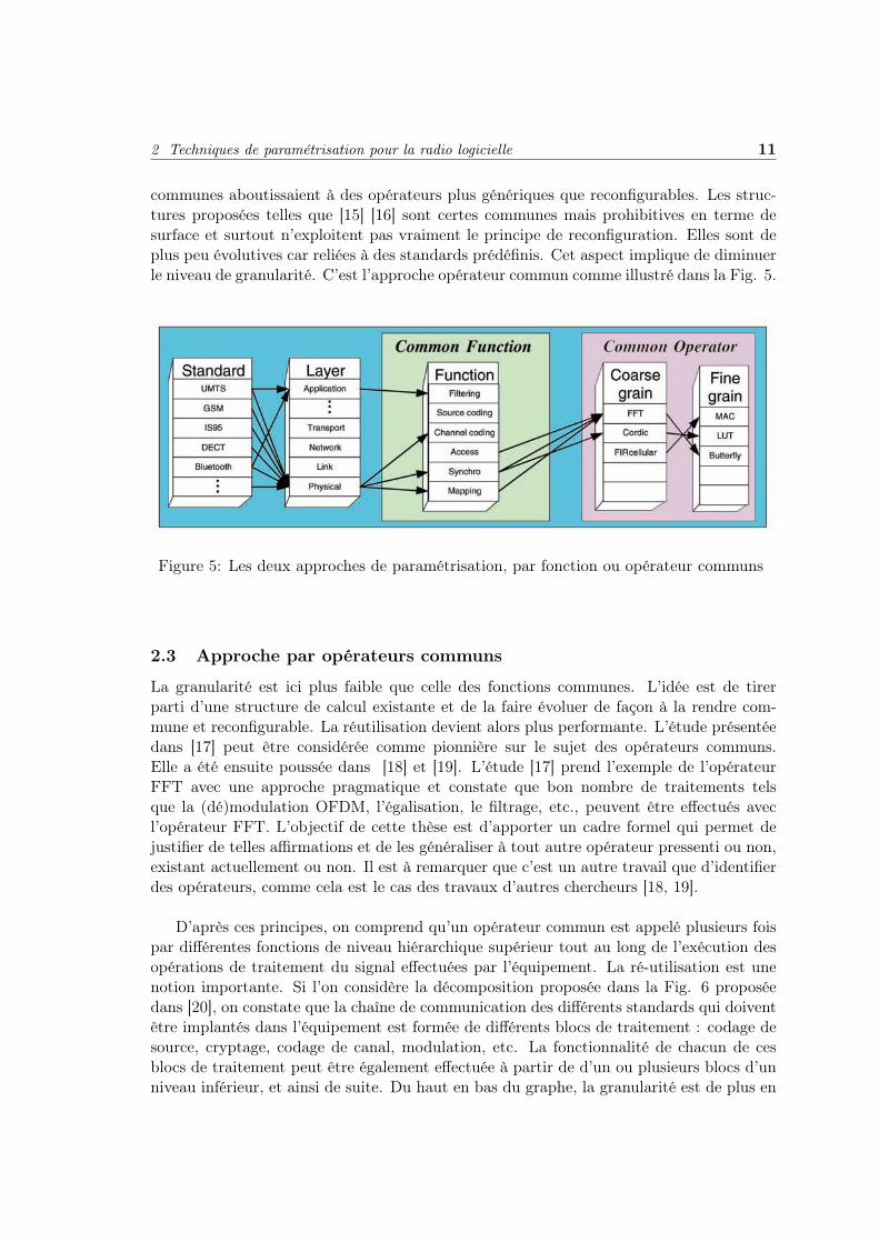
communes aboutissaient à des opérateurs plus génériques que reconfigurables. Les struc-tures proposées telles que [15] [16] sont certes communes mais prohibitives en terme desurface et surtout n’exploitent pas vraiment le principe de reconfiguration. Elles sont deplus peu évolutives car reliées à des standards prédéfinis. Cet aspect implique de diminuerle niveau de granularité. C’est l’approche opérateur commun comme illustré dans la Fig. 5.
Figure 5: Les deux approches de paramétrisation, par fonction ou opérateur communs
2.3 Approche par opérateurs communs
La granularité est ici plus faible que celle des fonctions communes. L’idée est de tirerparti d’une structure de calcul existante et de la faire évoluer de façon à la rendre com-mune et reconfigurable. La réutilisation devient alors plus performante. L’étude présentéedans [17] peut être considérée comme pionnière sur le sujet des opérateurs communs.Elle a été ensuite poussée dans [18] et [19]. L’étude [17] prend l’exemple de l’opérateurFFT avec une approche pragmatique et constate que bon nombre de traitements telsque la (dé)modulation OFDM, l’égalisation, le filtrage, etc., peuvent être effectués avecl’opérateur FFT. L’objectif de cette thèse est d’apporter un cadre formel qui permet dejustifier de telles affirmations et de les généraliser à tout autre opérateur pressenti ou non,existant actuellement ou non. Il est à remarquer que c’est un autre travail que d’identifierdes opérateurs, comme cela est le cas des travaux d’autres chercheurs [18, 19].
D’après ces principes, on comprend qu’un opérateur commun est appelé plusieurs foispar différentes fonctions de niveau hiérarchique supérieur tout au long de l’exécution desopérations de traitement du signal effectuées par l’équipement. La ré-utilisation est unenotion importante. Si l’on considère la décomposition proposée dans la Fig. 6 proposéedans [20], on constate que la chaîne de communication des différents standards qui doiventêtre implantés dans l’équipement est formée de différents blocs de traitement : codage desource, cryptage, codage de canal, modulation, etc. La fonctionnalité de chacun de cesblocs de traitement peut être également effectuée à partir de d’un ou plusieurs blocs d’unniveau inférieur, et ainsi de suite. Du haut en bas du graphe, la granularité est de plus en

12 Résumé en Français
plus fine.
Figure 6: Diagrame généralisé de la décomposition de plusieurs standards
L’idée est de trouver le jeu d’éléments communs et de les partager entre les fonctionnal-ités de plusieurs taches de traitement. L’optimisation qui en découle est donc directementfonction de la manière dont sont exécutés ces opérateurs et de leur fabrication tant auniveau matériel que logiciel. Comme le but est d’atteindre le meilleur compromis entreperformance et complexité, il est important de déterminer le niveau de granularité idéalque le concepteur devra choisir pour concevoir un équipement multi-standards, ni tropproche de l’approche velcro qui sera de grande complexité (mais hautement parallèle), nitrop proche des opérateurs arithmétiques qui sera très séquentielle (mais de complexitémoindre).
2 Techniques de paramétrisation pour la radio logicielle 13
2.4 Exemple d’opérateur commun
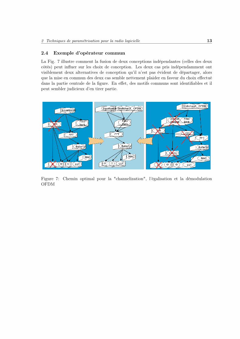
La Fig. 7 illustre comment la fusion de deux conceptions indépendantes (celles des deuxcôtés) peut influer sur les choix de conception. Les deux cas pris indépendamment ontvisiblement deux alternatives de conception qu’il n’est pas évident de départager, alorsque la mise en commun des deux cas semble nettement plaider en faveur du choix effectuédans la partie centrale de la figure. En effet, des motifs communs sont identifiables et ilpeut sembler judicieux d’en tirer partie.
Figure 7: Chemin optimal pour la "channelization", l’égalisation et la démodulationOFDM


15


Introduction à la partie II
Dans cette partie, nous expliquons comment nous envisageons la modélisation d’un équipementmulti-standards sous la forme d’un graphe. Mais il reste alors différentes alternatives qu’ilfaut convertir ensuite sous la forme d’un problème d’optimisation. Des coûts sont associésaux noeuds et aux arcs du graphe. On constate alors que différents coûts sont nécessaires,en fonction de la cible d’exécution matérielle (DSP, FPGA, etc.). Nous proposons en-suite une formulation de la fonction objectif associée au problème d’optimisation. Enfinplusieurs manières de résoudre le problème d’optimisation sont présentées.
Le chapitre 3 présente la structure de l’hypergraphe qui a été choisi pour poser le problèmed’optimisation que nous cherchons à résoudre. Le détail des coûts utilisés est donné dans lechapitre 4, ainsi que la formulation de la fonction objectif à optimiser. Le chapitre 5 enfinconcerne la méthode d’optimisation multi-critères elle-même en montrant sur un exemplesimple comment elle fonctionne.
3 Modélisation graphique pour les systèmes de radio logi-cielle
3.1 Les graphes
Nous choisissons dans ce chapitre 3 le formalisme graphique convenant au problème quel’on cherche à résoudre. Survolons pour cela quelques principes et théories associées auxgraphes. Les graphes sont utilisés dans un très grand nombre d’applications. Tout prob-lème mathématique impliquant des points et des connexions peut être représenté sous laforme d’un graphe. Un graphe peut être représenté dans un plan ou dans un espace à troisdimensions par des sommets (ou noeuds) et des arêtes [21]. Sur la Fig. 8, les noeuds sontu, v, w, x et les arêtes a, b, c, d, e, f. Le couple a, b est une arête multiple car deuxarêtes relient la même paire de points.
Catégories de graphes
Graphe simple : C’est un graphe qui n’a ni boucle ni arêtes multiples (dédoubléesentre deux noeuds). Beaucoup de problèmes à base de graphes peuvent être ramenés à ungraphe simple.
17

18 Résumé en Français
w
b f
w
auv
e
d
x c
Figure 8: Exemple de graphe
Graphe orienté : C’est un graphe dont toutes les connexions sont unidirectionnelles.Une arête orientée est appelée arc. C’est un cas que l’on retrouve très souvent en ingénierieet dans le domaine scientifique. Des attributs peuvent être associés aux noeuds et aux arcs,tels que des poids, des coûts, etc.
Graphe acyclique orienté : C’est un graphe orienté qui n’a pas de cycle direct, c’est-à-dire de chemin fermé. Il s’agit de DAG en anglais (Direct Acyclic Graph). Même sicela semble être une contrainte forte, il existe de nombreux cas où les graphes acycliquess’appliquent, dès que les noeuds sont naturellement ordonnés (par exemple dans le tempsou en termes de hiérarchie).
Hypergraphe : Un hypergraphe est une généralisation d’un graphe dans laquelle unearête peut se connecter à plusieurs noeuds.
Travaux d’optimisation à partir de graphes
La théorie des graphes a été utilisée pour résoudre de nombreux problèmes d’optimisation,comme celui du voyageur de commerce [22] qui cherche à optimiser la distance à parcourirpour visiter tous ses clients. On en trouve une première forme en 1831 puis des travauxcélèbres par Dantzig, Fulkerson et Jonhson [23] en 1954 puis Padberg et Rinaldi dans lesannées 80 [24]. Il y a plusieurs algorithmes pour trouver les chemins le plus court à traversun réseau, mais citons celui de Dijkstra [25] en 1959. Dans les années 60, les problèmesont été classés par complexité. Edmonds a étudié les problèmes qui peuvent être résolusen un temps polynomial [26]. Cook [27] et Karp [28] ont établi les principes N-P complets.
Théorie des graphes et conception SDR
La théorie de graphes a déjà été utilisée dans le contexte de la conception d’équipementsde radio logicielle. C’est le cas de l’approche utilisée pour le prototypage rapide dans [8].La méthode de conception s’appuie sur l’utilisation de l’outil SynDEx [29] de l’INRIA quirepose sur la théorie des graphes pour déployer un graphe d’application sur un graphe

3 Modélisation graphique pour les systèmes de radio logicielle 19
d’architecture matérielle. SynDEx propose un partitionnement ordonnancement optimisépour le déploiement d’une application logicielle sur une plate-forme matérielle multi-processeurs. Dans le graphe d’application, les noeuds sont des traitements et les arcsreprésentent des échanges de données. Dans le graphe d’architecture matérielle, les noeudssont des unités de traitement (typiquement des processeurs) et les arêtes des médiasde communication. A chaque noeuds du graphe d’architecture correspond un tempsd’exécution pour chaque traitement du graphe d’application que l’unité de traitementsupporte. A chaque type de données de l’application correspond un temps de transfertsur le média du graphe d’architecture. L’objectif de l’optimisation de SynDEx est deminimiser le temps global d’exécution à partir des temps d’exécution des traitements surchaque processeur et des temps de communication. SynDEx utilise pour cela un algo-rithme glouton. Il est à noter que SynDEx est originellement dédié au monde des stationsde travail reliées en réseau. L’effort effectué dans les travaux [30] et [8] a permis de rap-procher la méthodologie vers le monde de l’embarqué. Cela s’est effectué en particulierpour des besoins en termes de conception radio logicielle et d’applications vidéo.
Le travail proposé dans cette thèse, bien que portant également sur la conception radiologicielle et reposant sur la théorie des graphes, est cependant très différent et attaque leproblème de manière orthogonale. En effet, ce n’est pas un graphe flot de données quiest envisagé ici, mais un graphe structurel. Les liens entre les noeuds des Fig. 6 et 7 nereprésentent pas des échanges de données, mais des relations de hiérarchie structurelle.L’ordonnancement n’est pas pris en compte dans les travaux présentés pour cette thèse.
Discussion
Dans le cas des graphes acycliques orientés ou DAG, on peut utiliser un algorithmed’aller simple car il est possible d’ordonner les noeuds. Dans le cas plus général desgraphes orientés, les algorithmes d’optimisation peuvent être plus compliqués et moinsefficaces pour trouver l’optimum.
Comme nous n’avons pas identifié de cas existant se rapportant exactement à nos be-soins, notre objectif est de trouver d’abord la bonne manière de représenter le prob-lème de conception d’équipement de radio logicielle multi-standards, et ensuite de trou-ver la meilleure manière d’associer des poids aux noeuds et aux arêtes afin d’identifierl’algorithme d’optimisation le plus intéressant pour résoudre ce problème.
3.2 Modèle de graphe théorique pour la radio logicielle multi-standards
Objectif
Notre problème de conception peut être ramené à celui d’une description à différentsniveaux de granularité, donc en couches successives. Il vise à aider le concepteur à choisirle jeu d’opérateurs de traitement (chacun à un niveau de granularité idéal) nécessaires pourque l’équipement multi-standards supporte tous les cas d’utilisation prévus. L’idée sous-jacente est qu’à un certain niveau de granularité, les opérateurs peuvent être ré-utilisésplusieurs fois à l’intérieur d’une même couche protocolaire (ou standard) ou entre couchesprotocolaires. Le but est de fournir au concepteur des moyens d’exploration de sa concep-

20 Résumé en Français
tion à différents niveaux de granularité.
Définition de la structure du graphe
Afin de répondre aux besoins exprimés ci-dessus, voici le choix effectué pour la struc-ture du graphe. Chaque noeud représente un élément de traitement (du signal) élémentaire(PE - processing element). Afin d’effectuer ce traitement, le concepteur a le choix soit del’implanter tel quel, donc en tant qu’élément insécable (atomique), soit en invoquant deséléments plus petits d’un niveau inférieur. Dans ce cas, plusieurs éléments peuvent êtrenécessaires, ou plusieurs fois le même, afin d’effectuer le calcul correspondant à l’élémentde niveau supérieur.
Il s’avère donc nécessaire d’utiliser un hypergraphe afin de représenter cela puisque desarêtes peuvent avoir plusieurs destinations et qu’il faut des arcs de type ET ou OU. Onparle alors d’hyperarcs, comme illustré sur les Fig. 9 et Fig. 10, qui indiquent une dépen-dance entre noeuds de niveaux différents. Un noeud d’un niveau plus élevé (disons n) estappelé noeud parent s’il est relié à un noeud de niveau inférieur (disons n−1) qui est alorsappelé noeud enfant ou descendant. De manière assez intuitive, un hyperarc OU signi-fie qu’un seul descendant est nécessaire pour effectuer le traitement équivalent au noeudparent. Dans le cas d’un hyperarc ET, tous les noeuds descendants sont nécessaires pourremplacer le noeud parent. La manière de représenter la différence est illustrée sur les 9et 10.
Figure 9: Hyperarc OU
Figure 10: Hyperarc ET

3 Modélisation graphique pour les systèmes de radio logicielle 21
La Fig. 11 représente un graphe qu’il est possible d’obtenir dans le cas d’un équipementtri-standards (simplifié). L’hypergraphe est donc constitué d’éléments de traitement deplus en plus simples au fur et à mesure que l’on descend vers le bas du graphe, les troisstandards étant représentés en haut du graphe. Il est à noter qu’il n’y a pas d’assignementstrict du niveau et que la seule information importante est le niveau relatif entre les noeudsqui sont reliés entre eux, pas leur niveau absolu. Cette notion n’existe pas en fait. Lesarcs issus du bloc S1 montrent que la fonctionnalité de S1 peut être réalisée soit par lenoeud A1, soit le noeud B1 soit le noeud A2. On voit que ces trois noeuds ne sont pasreprésentés au même niveau sans que cela n’ait d’incidence. En revanche, pour mettre enoeuvre le standard S3, il faut à la fois utiliser le noeud A4 et le noeud A5. Dans certainscas, un noeud peut à la fois avoir des dépendances en ET et OU, comme dans le cas dustandard S2 qui peut être réalisé par le noeud A4 ou les deux noeuds A2 et A3. A titred’exemple plus concret, pour réaliser un équipement supportant le standard S2, il est doncpossible soi de réaliser le standard S2 dans un bloc unitaire donc insécable, que ce soitsous la forme d’un ASIC ou d’un programme. Lorsque tout l’équipement est conçu ainsi,c’est le cas velcro puisque si l’on veut changer de standard, il faut commuter sur un autrebloc unitaire pour la totalité des calculs associé au standard. Une autre possibilité deréalisation du standard S2 est d’implanter les noeuds A2 et A3. On remarque alors quesi l’équipement passe au standard S1, A2 peut être conservé et ainsi économiser beaucoupd’efforts en termes de reconfiguration par rapport au cas velcro, par exemple en termesde temps de reconfiguration. C’est tout l’intérêt de l’approche proposée dans cette thèse.On remarque qu’il ne peut pas y a voir de cycle dans le graphe, c’est-à-dire par d’arc quiremonte, ce qui simplifie la résolution mathématique du problème.
Standard S1 Standard S2 Standard S3
A1 A2 A3 A4 A5
B4B1 B2 B3
C1 C2
Figure 11: Graphe généralisé correspondant à un équipement de radio logicielle tri-standards
Exemple simplifié pour un équipement tri-standards WiFi, WiMAX et UMTS
La Fig. 12 illustre les mêmes principes dans le cas des standards WiFi, WiMAX etUMTS. Seul l’émetteur est représenté ici et seulement une toute petite partie de l’émetteurest véritablement prise en compte et on comprend qu’un graphe complet serait très grand

22 Résumé en Français
d’une part (surtout si l’on généralise aux autres couches que la couche physique), et qued’autre part, il y aurait de nombreuses manières de représenter le graphe, suivant le con-cepteur.
WiFi WiMAX UMTS
RandomiserConvolutional
Coder InterleaverConstellation
Mapper FFT-N RSEncoder
Scrambler Spreader
ButterflyLUT Real Spreader
Over Sampler
Adder MultiplierFlip Flop
Spreader Sampler
Adder MultiplierFlip Flop
NAND NOT XOR AND OR
Figure 12: Structure d’un graphe pour le cas d’un équipement de radio logicielle tri-standards (émetteur simplifié)
On remarque qu’il peut y avoir autant de niveaux intermédiaires que souhaité et que"dessiner" le graphe est un travail en soi. Ce n’est pas le but de cette thèse que dedévelopper de tels graphes complets, et les graphes qui seront utilisés le seront parce qu’ilssont fournis par d’autres études, menées par exemple afin d’identifier des opérateurs com-muns, ce qui est également une tache en soi, indépendante du travail de cette thèse. C’estpourquoi nous considérerons souvent des sous-graphes du graphe total, qui ne partent pasde standards en haut du graphe, et qui n’arrivent pas forcément aux opérateurs arith-métiques et bas du graphe. C’est le cas de la Fig. 13 ne représentant que les partieségalisation, channelisation et OFDM d’un équipement. De même seuls certains exemplesde décomposition sont proposés. D’autres seraient possibles. Cependant, cela illustre quele nombre d’alternatives de conception peut très vite croître et que même si l’on peutestimer déduire intuitivement des choix optimaux sur de petits graphes, cela devient trèsdifficile sur des graphes plus conséquents sans outillage.
Dans cet exemple pour la "channelisation", c’est-à-dire le filtrage et la séparation descanaux numérisés par la conversion analogique numérique en réception, une approcheclassique canal par canal peut être utilisée, ou une approche par bancs de filtres. Dansle cas d’un banc de filtres, on peut utiliser une FFT, ce qui est une alternative possibledans ce cas, mais de toute manière la FFT est indispensable pour la démodulation OFDM.

3 Modélisation graphique pour les systèmes de radio logicielle 23
Equalization Channelization OFDM
Channel per Channel Filter Bank
Multi-rate Filtering Digital Down Conversion
FIR Down Sampling CIC
FFT
Butterfly
CORDICMAC
Delay Multiplier Adder LUT
Figure 13: Exemple d’un graphe partiel
La question qui se pose alors est quelle est la meilleure décomposition ? En fonctionde quel critère ? Quel est le chemin dans le graphe qui donne ce résultat ? Il est nécessairepour cela d’ajouter des poids, autrement dit des coûts associés aux noeuds du graphe, d’endéduire une fonction de coût et d’exécuter un algorithme d’optimisation sur cette fonctionde coût. C’est l’objet du prochain chapitre. Auparavant examinons brièvement une autrealternative de graphe qui a été étudiée pour résoudre ce problème.
3.3 Reformulation réseau du problème
Il s’agit de faire ici une reformulation de notre problème sous la forme d’un problèmed’optimisation de réseau à source unique. Le but est de pouvoir ensuite bénéficier desnombreux algorithmes d’optimisation existant dans ce domaine.
Nous n’allons pas développer ce point dans ce résumé en français, mais nous invitons lelecteur à se référer au document en anglais. Il s’est avéré que la traduction des hyperarcsET est compliquée et peut même devenir rédhibitoire dans certains cas. C’est pourquoicette solution n’a pas été retenue.

24 Résumé en Français
4 Paramètres de coûts et coûts d’optimisation pour les sys-tèmes de radio logicielle multi-standards
Nous explorons dans ce chapitre 4 les paramètres de coût qu’il faut associer au grapheafin de pouvoir effectuer ensuite (au chapitre 5) l’optimisation du graphe. Nous allons voirque plusieurs sortes de coûts sont envisageables. Cela dépend notamment de la manièred’implanter les traitements et de la nature de la cible matérielle les exécutant, cible ditelogicielle (DSP et autres processeurs) ou dite matérielle (FPGA et ASIC). De là, une fonc-tion de coût associée au problème de conception d’équipement de radio logicielle multi-standards est dérivée en fin de chapitre.
4.1 Paramètres de coût
Il peut y avoir de nombreux paramètres de coûts. Nous considérons dans nos travauxd’une part les deux coûts suivants associés aux noeuds : le coût de fabrication (buildingcost - BC ) et le coût d’exécution (computational cost - CC ) d’un élément de traitement(processing element - PE. D’autre part, sont associés aux arcs un nombre d’appels (Num-ber of Calls - NoC ).
Coût de fabrication
Ce paramètre concerne les noeuds du graphe. Ce coût fait référence à la dépense en ter-mes d’implantation associée à un élément de traitement. Il sera donc à "payer" une seulefois dans l’équipement, autrement dit une fois pour toute la durée de vie de l’équipement.S’il est fait plusieurs fois appel à cet élément de traitement dans l’équipement, le coût defabrication associé à ce traitement ne sera pas multiplié par autant. Ré-utiliser un noeudoffre donc une idée de réduction du coût.
Coût d’exécution
Ce paramètre concerne les noeuds du graphe. Il y a donc deux coûts différents pourles noeuds du graphe. Ce coût est associé au temps nécessaire à l’exécution de l’élémentde traitement. Il est donc multiplié par le nombre d’appels qu’il est fait à l’élément enquestion pendant le fonctionnement de l’équipement.
Nombre d’appels
Ce paramètre concerne les arcs du graphe. Comme évoqué précédemment, une fonc-tionnalité peut-être exécutée par un noeud unique ou par l’appel de un ou plusieurs noeudsde hiérarchie inférieure. Chacun de ces noeuds peut nécessiter plusieurs appels afin de pou-voir effectuer la fonctionnalité initiale. C’est cette notion que reprend le paramètre nombred’appels.
Discussion

4 Paramètres de coûts et coûts d’optimisation pour les systèmes de radio logicielle multi-standards25
Il est à noter que de manière générale, un noeud de hiérarchie supérieure a un coûtde fabrication plus élevé que les noeuds de hiérarchie inférieure auquel il fait appel. Demême le temps d’exécution d’un noeud de hiérarchie supérieure, s’il est en général pluslong que pour un seul appel à un noeud inférieur, est d’ordinaire plus faible que l’ensembledes appels et exécutions nécessaires à faire pour effectuer le même calcul à l’aide de noeudsde hiérarchie inférieure.
Prenons le cas plus concret d’une implantation matérielle ou le BC représente un coûten nombre de portes (ou surface), comme pour une implantation dans un FPGA ou unASIC numérique. Dans l’exemple d’un élément de traitement de type filtre, il existe denombreuses options de conception. Certaines vont chercher à paralléliser au plus leur ar-chitecture afin de gagner en vitesse d’exécution mais au prix d’un surcoût en surface. C’estle cas de l’élément de hiérarchie supérieure. En revanche, afin d’économiser en termes desurface (en coût de fabrication), il est possible de faire appel plusieurs fois à une unité detype MAC (Multiply Accumulate) qui serait alors l’élément de hiérarchie inférieure ayantun coût en surface beaucoup moins élevé (coût de fabrication), peut être aussi un coûtd’exécution moins élevé aussi, mais auquel il faudra faire appel de nombreuses fois (nom-bre d’appels de l’arc reliant le filtre au MAC) de manière séquentielle pour effectuer unfiltrage. Le coût d’exécution résultant pour le filtrage devient alors plus cher que le coûtd’exécution du filtre seul. On comprend bien le compromis qu’il faut trouver entre com-plexité et vitesse d’exécution, entre le haut et le bas du graphe, entre granularité grossièreou fine.
La Fig. 14 reprend l’exemple de la Fig. 13 avec des valeurs de paramètres abstraits.Ils n’ont ici pas de réalité en termes de temps ou de nombre de portes, mais ils respectentune certaine logique en relatif entre paramètres de même nature. On voit q’un FIR peutêtre utilisé pour un coût de fabrication de 500 et un coût d’exécution de 1000. Ou alors unautre choix de conception consiste à implanter les trois opérateurs "Delay", "Multiplier"et "Adder" pour un coût total de fabrication de 15 et un coût pour chaque exécution de8 (si on considère une exécution séquentielle à cause des dépendances de données). Maisil est nécessaire de faire appel 180 fois à cet opérateur dans cet exemple, soit un coûtd’exécution total de 1440. Cette solution a donc un coût supérieur à celle consistant àutiliser le filtre directement.
4.2 Types de coût
Nous proposons une étude plus approfondie des différentes possibilités qui peuvent êtrepertinentes pour notre approche en termes de coûts de fabrication. Ils peuvent être con-sidérés comme faisant partie de deux catégories :
• coût analytique
• coût d’implantation
Coût analytique

26 Résumé en Français
Equalization Channelization OFDM
Channel per Channel Filter Bankx1
Multi‐rate Filtering Digital Down Conversion
FIR Down Sampling CIC
500/1000 x2
x2 x1
FFT
1000/500
Butterfly
15/20
x180 x180 x180
x2x2x4
CordicMAC
15/815/8x4 x6
x2
x2x2
Delay Multiplier Adder LUT
1/1 10/5 4/2 1/1
Figure 14: Exemple de graphe avec les coûts associés aux noeuds et aux arcs
Ces coûts sont issus d’une analyse de complexité des éléments de traitement composantsles différents standards à implanter dans l’équipement. Cette analyse donne une estimationdu nombre requis d’opérations élémentaires (par données de sortie par exemple). Lesopérations élémentaires considérées peuvent être :
• Opérations arithmétiques telles que les additions et les multiplications,
• Opérations logiques,
• Opérations d’accès à la mémoire (Load/Store).
Elles ne sont pas toujours toutes prises en compte. On retrouve souvent une évalua-tion de complexité simplement en termes de nombre d’additions ou de multiplications. Ilfaut noter que le coût analytique peut être très différent du coût d’implantation, suivantl’architecture matérielle visée. Il peut même y avoir des éléments ayant un coût analytiquesupérieur à un autre, mais un coût d’implantation inférieur si l’architecture est propice.Les Tables en annexe B.1 et B.2 donnent des chiffres pour certains éléments de traitementdu standard IEEE.802.11a et les Tables B.3 et B.4 en donnent pour le standard UMTS.
Coût de fabrication
Les plates-formes de radio logicielle requièrent la présence d’unités de traitementnumériques flexibles de natures différentes en raison de la complexité des applications

4 Paramètres de coûts et coûts d’optimisation pour les systèmes de radio logicielle multi-standards27
qu’elles peuvent être susceptibles de supporter. Parmi ces choix, deux grandes catégoriesse distinguent puisqu’elles reposent sur deux domaines de calcul différents, l’un séquentielet l’autre parallèle, et donc sur deux langages de programmation différents, le langage Cet le VHDL. Certains traitements seront avantageusement exécutés par des processeurs(monde logiciel), et d’autres par des FPGA (monde matériel). Le coût de fabrication estune conséquence directe du choix de la cible d’implantation. Deux cas sont à distinguerselon qu’il s’agit d’une implantation matérielle ou logicielle.
Cas d’une implantation sur FPGA :
Le FPGA contribue à apporter au monde matériel de la flexibilité (qui n’existait pasauparavant). Cette flexibilité est jusqu’à présent surtout utilisée lors de la conceptionen reprogrammant (complètement) de tels composants avant de relancer une application.Les dernières familles de FPGA permettent désormais d’effectuer une reprogrammationpartielle, donc d’une sous partie du FPGA (mais cela reste encore au niveau expérimentaldans le domaine de la recherche [31, 32]) pendant que l’autre partie continue à fonctionnernormalement. En plus de la souplesse que cela procure, un gros avantage est que le tempsde reconfiguration est d’autant diminué, puisqu’il est proportionnel à la surface mise à jour.Des reconfigurations extrêmement rapides d’éléments de traitement matériels deviennentdonc possibles. C’est la combinaison de la puissance de calcul du matériel (parallélisme)avec la flexibilité du logiciel (reprogrammation).
Revenons à notre propos. Quelles unités de "surface" ou de "fabrication" doit on pren-dre ? Dans un FPGA, on peut prendre comme coût de fabrication le nombre de slices, deCLB, de LUT, de cellules logiques, ou de bascules, etc. La Table 1 donne des chiffres pourl’implantation des standards WiFi (IEEE.802.11a) et WiMAX (IEEE.802.16-2004) [33][34] et exprime le pourcentage d’occupation d’un FPGA donné en fonction des différentescatégories d’éléments le constituant.
Cas d’une implantation sur processeur :
Dans le monde de l’embarqué, il s’agira plutôt d’un cible de type DSP que GPP,pour des raisons de consommation. Un DSP est capable d’effectuer un certain nombred’instructions en un seul coup d’horloge, donc en parallèle, mais ce parallélisme est limitépar construction. Par exemple le C6x de Texas Instrument a 8 unités de calcul parallèle(architecture VLIW).
Le coût de fabrication peut également être appelé coût d’implantation ou coût d’achat.On peut penser à le considérer dans le cas d’un DSP, comme un coût forfaitaire.
Coût d’exécution
Le coût d’exécution est clairement fonction du temps mis pour qu’un élément de traite-ment fasse les calculs propres à sa fonctionnalité. Le temps d’exécution est par conséquentun bon coût d’exécution, quelle que soit la cible d’implantation. Dans le cas d’une implan-tation sur un processeur, le nombre de cycles nécessaires pour l’exécution d’un élément de

28 Résumé en Français
Table 1: IEEE 802.11a and IEEE 802.16 implementation on FPGA
Area Metrics for a XC2V3000-4FG676 Device
IEEE 802.11a IEEE 802.16-2004
Parameter Used % Used %
Number of Slices 1678 11 2614 18
Number of Slice Flip Flops 2353 8 3566 12
Number of 4 input LUTs 2814 9 4304 15
Number of Bonded IOBs 29 5 29 5
Number of BRAMS 12 12 12 12
Number of GCLKs 1 6 1 6
traitement peut également être considéré comme un coût d’exécution.
4.3 Formulation de la fonction de coût
Le contexte de cette étude est clairement celui d’une optimisation multi-critères, multi-objectifs. Il y a de nombreuses manières d’envisager la résolution de tels problèmes, depuisla combinaison simple des objectifs en un seul objectif, jusqu’à l’utilisation de la théoriedes jeux pour coordonner l’importance relative des critères. Cependant, le flou reste quantà à la définition d’un optimum en comparaison du cas mono-critère, si bien qu’il n’est pasévident de comparer les résultats d’une méthode par rapport à une autre. On utilise desfonctions d’agrégation pour combiner plusieurs objectifs au sein d’une même fonction. Lesplus courantes sont la somme pondérée, la programmation objectif, la méthode ε aveccontrainte.
La fonction de coût à optimiser dans notre cas est composée d’une combinaison des coûtsde fabrication et des coûts d’exécution. Comme déjà évoqué auparavant, ce sont deuxnotions a priori antagonistes puisque minimiser le coût de fabrication implique une aug-mentation du coût d’exécution, et vice-versa. D’où la nécessité de trouver un compromis,qui peut d’ailleurs changer suivant le concepteur ou les intérets du constructeur. En effet,suivant qu’il veut vendre des circuits ou des processeurs par exemple on comprend que lesintérêts peuvent être très différents.
Développons la fonction de coût. Minimiser le coût de fabrication s’écrit :

4 Paramètres de coûts et coûts d’optimisation pour les systèmes de radio logicielle multi-standards29
min∑
i
BCi.Ni (1)
avec
• BCi représente le coût de fabrication du ith élément de traitement de l’équipement,
• Ni ∈ 1, 0 indique si le ith noeud est présent dans l’équipement ou pas,
•∑i
BCi.Ni est le coût total de fabrication de tous les éléments de traitement qui sont
présents dans l’équipement multi-standards.
Maintenant, considérons le second objectif, c’est-à-dire minimiser le coût d’exécution.Il peut s’écrire ainsi :
min∑
k
CCk (2)
avec
• CCk représente le coût d’exécution du kth élément de traitement de l’équipement.
Dans le contexte d’un équipement multi-standards à n standards, l’équation (2) devient:
min∑
n
∑k
CCk((Sn)n ∈ N) (3)
avec
• ((Sn)n ∈ N) indique qu’il peut y avoir n standards présents dans l’équipement avecn = 1, 2, . . . , N. Si l’on prend par exemple N = 3 alors il s’agit d’un équipementtri-standards supportant S1, S2 et S3,
•∑k
CCk((Sn)n ∈ N) est le coût d’exécution total pour chaque standard Sn,
avec n = 1, 2, . . . , N.
•∑n
∑k
CCk((Sn)n ∈ N) est le coût d’exécution total pour tous les standards Sn,
avec n = 1, 2, . . . , N.
En combinant les deux fonctions objectif des équations (1) et (3) on obtient :
min( ∑
i
BCi.Ni +∑
n
∑k
CCk((Sn)n ∈ N))
(4)
Mais ces deux ojectifs ne sont pas d’importance équivalente et il est par conséquent néces-saire d’introduire des poids relatifs à chaque coût. L’équation (4) devient :
min(ω
∑i
BCi.Ni +∑
n
∑k
ωnCCk((Sn)n ∈ N))
(5)

30 Résumé en Français
avec ω le poids octroyé au coût de fabrication de l’équipement, et ωn est le poids d’un seulstandard Sn. En effet, un seul standard est censé s’exécuter à un instant donné.La fonction de coût à optimiser pour la conception d’un équipement de radio logicielle estdonc :
CSDR = minbool((Sn)n∈N)
(ω
∑i
BCi.Ni +∑
n
∑k
ωnCCk((Sn)n ∈ N))
(6)
La contrainte bool((Sn)n ∈ N) vérifie si tous les standards sont implantés dans l’équipement.
Le coût à n’importe quel niveau du graphe peut être calculé ainsi :
Costlevel =( ∑
i
CCi.NoCi
).NoCi+1 +
∑i
BCi.Ni (7)
Nous présenterons dans le chapitre suivant comment effectuer l’optimisation de ce prob-lème.
4.4 Interface graphique
Une interface graphique a été développée en langage Java afin de faciliter la constructiondes graphes et des paramètres de coûts associés aux arcs et aux noeuds. La Fig. 15 enmontre une capture d’écran.
Les fonctionnalités sont les suivantes :
• Create Processing Element : pour insérer un nouveau noeud dans le graphe.
• Delete Processing Element : pour supprimer un noeud.
• Create AND hyperarc: pour créer entre des noeuds un arc ET. Il faut pour celasélectionner dans des listes un noeud parent et des noeuds enfants.
• Create OR hyperarc: idem que précédemment, pour un arc OU.
• Delete hyperarc: pour supprimer un arc.
• Add Parameters: ouvre la fenêtre de gestion des paramètres des noeuds et desarcs.
Le graphe peut être sauvegardé dans un format qui après être "parsé" peut être utilisécomme entrée du code d’optimisation.
5 Technique d’optimisation
Nous avons formulé dans le précédent chapitre la fonction de coût bi-objectifs. Dansce chapitre 5, nous allons étudier les différentes techniques pour résoudre le problèmed’optimisation associé à la conception d’équipements de radio logicielle multi-standardstel que nous l’avons formulé. La résolution du problème par une solution exacte requerraitune complexité exponentielle avec le nombre de noeuds considérés, ce qui n’est possible en

5 Technique d’optimisation 31
Figure 15: Capture d’écran de l’interface graphique développée pour contruire les graphes
un temps acceptable que pour un nombre de noeuds restreint même sur les calculateursles plus rapides. C’est pourquoi des méthodes sous-optimales sont considérées. Nous al-lons parcourir différentes solutions possibles et discuter de leurs avantages et inconvénients.
5.1 Les techniques d’optimisation
Les techniques d’optimisation peuvent être classées en deux grandes familles :
• déterministe,
• stochastique.
La Fig. 16 illustre diverses techniques d’optimisation en les classifiant suivant ces deuxcatégories.
Nous ne parcourrons pas dans ce résumé l’ensemble des cas évoqués dans la Fig. 16.
5.2 La recherche exhaustive
Une recherche exhaustive consiste à parcourir toutes les solutions de l’espace d’explorationarchitecturale afin d’en trouver la meilleure. Cette approche n’est malheureusement pas

32 Résumé en Français
Figure 16: Approches d’optimisation [35]
faisable lorsque l’espace d’exploration devient grand, ce qui est le cas dans la réalité d’uneconception d’équipement de radio logicielle multi-standards.
Réfléchir à la mise en oeuvre d’une telle approche présente l’intérêt de devoir trouverle moyen de parcourir de manière systématique l’ensemble des cas possibles de conception.La Fig. 17 montre comment une telle recherche est effectuée. D’abord les noeuds et lescoûts sont initialisés. Pour les noeuds, cela revient à les classer par ordre, ainsi que lescatégoriser en tant que noeuds utiles, inutiles, hauts ou bas. Les noeuds hauts sont desbranches et les noeuds bas sont des feuilles.
Une fois que les noeuds sont classés, le coût total de l’équipement est calculé à partirdes noeuds utiles. Puis un noeud est retiré de l’ensemble des noeuds et la faisabilité dugraphe est vérifiée et le coût est mis à jour. Si le nouveau coût est inférieur au coût initial,il est accepté. Et ainsi de suite, les autres noeuds sont éliminés jusqu’à ce que le coûtminimal donnant un graphe valide soit obtenu. Cela donne la solution optimale ayant lecoût minimal.
Considérons le cas du graphe de la Fig. 18 où l’on a représenté des coûts que surcertains noeuds et arcs afin de garder le problème suffisamment simple pour être résolu

5 Technique d’optimisation 33
Figure 17: Algorithme de la méthode par recherche exhaustive
par la méthode de la recherche exhaustive.
A titre d’exemple, considérons le noeud FFT car il est simple de voir qu’il permetl’implantation de l’égaliseur, du "channelizer" et de l’OFDM. Il existe peut-être d’autressolutions moins évidentes, mais c’est le rôle d’un programme de parcourir toutes les pos-sibilités, au-delà de l’intuition. La fonction de coût pour le noeud FFT peut être extraitede l’équation (7) rappelée ici :
Costlevel =( i=m∑
i=1
CCi.NoCi
)×NoCi+1 +
i=m∑i=1
BCi.Ni (8)
CostFFT = CCFFT + BCFFT (9)
soit
CostFFT = 50 + 3000 = 3050 (10)
Ou en utilisant le niveau inférieur, soit l’opérateur papillon ou Butterfly (on ne considèrepas le cas de l’opérateur Cordic dans ce petit exemple) :
CostFFT−1 = CCButterfly.NoCButterfly + BCButterfly (11)

34 Résumé en Français
Figure 18: Exemple de graphe avec les coûts associés
soit
CostFFT−1 = 2.5× 192 + 380 = 860 (12)
Ou en utilisant le niveau inférieur au Butterfly, soit les opérateurs MAC, LUT et Adderou les opérateurs LUT, Adder et Multiplier :
Cost(FFT−2) =( i=3∑
i=1
CCiNoCi
)×NoCi+1 +
i=3∑i=1
BCi.Ni (13)
soit
Cost(FFT−2)a =(4× CCMAC + 2× CCLUT + 2× CCAdder
)× 192 (14)
+ BCMAC + BCLUT + BCAdder
ou encore
Cost(FFT−2)a =(4× 2 + 2× 0.5 + 2× 1
)× 192 + 380 + 40 + 40 = 2572 (15)
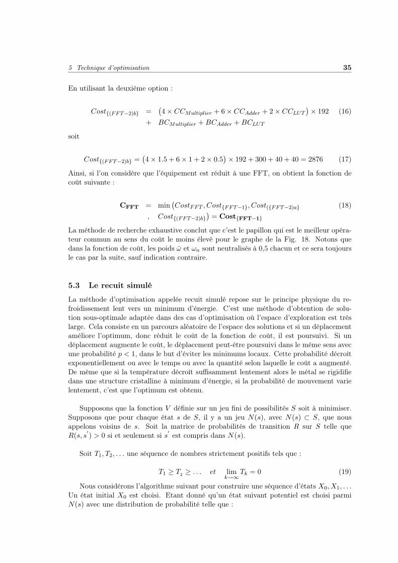
5 Technique d’optimisation 35
En utilisant la deuxième option :
Cost(FFT−2)b =(4× CCMultiplier + 6× CCAdder + 2× CCLUT
)× 192 (16)
+ BCMultiplier + BCAdder + BCLUT
soit
Cost(FFT−2)b =(4× 1.5 + 6× 1 + 2× 0.5
)× 192 + 300 + 40 + 40 = 2876 (17)
Ainsi, si l’on considère que l’équipement est réduit à une FFT, on obtient la fonction decoût suivante :
CFFT = min(CostFFT , CostFFT−1, Cost(FFT−2)a (18)
, Cost(FFT−2)b)
= CostFFT−1
La méthode de recherche exhaustive conclut que c’est le papillon qui est le meilleur opéra-teur commun au sens du coût le moins élevé pour le graphe de la Fig. 18. Notons quedans la fonction de coût, les poids ω et ωn sont neutralisés à 0,5 chacun et ce sera toujoursle cas par la suite, sauf indication contraire.
5.3 Le recuit simulé
La méthode d’optimisation appelée recuit simulé repose sur le principe physique du re-froidissement lent vers un minimum d’énergie. C’est une méthode d’obtention de solu-tion sous-optimale adaptée dans des cas d’optimisation où l’espace d’exploration est trèslarge. Cela consiste en un parcours aléatoire de l’espace des solutions et si un déplacementaméliore l’optimum, donc réduit le coût de la fonction de coût, il est poursuivi. Si undéplacement augmente le coût, le déplacement peut-être poursuivi dans le même sens avecune probabilité p < 1, dans le but d’éviter les minimums locaux. Cette probabilité décroîtexponentiellement ou avec le temps ou avec la quantité selon laquelle le coût a augmenté.De même que si la température décroît suffisamment lentement alors le métal se rigidifiedans une structure cristalline à minimum d’énergie, si la probabilité de mouvement varielentement, c’est que l’optimum est obtenu.
Supposons que la fonction V définie sur un jeu fini de possibilités S soit à minimiser.Supposons que pour chaque état s de S, il y a un jeu N(s), avec N(s) ⊂ S, que nousappelons voisins de s. Soit la matrice de probabilités de transition R sur S telle queR(s, s
′) > 0 si et seulement si s
′ est compris dans N(s).
Soit T1, T2, . . . une séquence de nombres strictement positifs tels que :
T1 ≥ T2 ≥ . . . et limk→∞
Tk = 0 (19)
Nous considérons l’algorithme suivant pour construire une séquence d’états X0, X1, . . .Un état initial X0 est choisi. Etant donné qu’un état suivant potentiel est choisi parmiN(s) avec une distribution de probabilité telle que :

36 Résumé en Français
P [Yk = s′ |Xk = s] = R(s, s
′) (20)
Alors nous établissons
Xk+1 =
Yk avec Pk
Xk sinon(21)
avecPk =
[−[V (Yk)− V (s)]
Tk
](22)
limk→∞
P [Xk ∈ S∗] = 1 (23)
L’équation (21) spécifie comment la séquence X1, X2, . . .. est choisie. L’idée du recuitsimulé est d’essayer d’obtenir (23) en faisant tendre Tk vers zéro quand k tend vers l’infini,avec S∗ qui représente le jeu d’états de S pour lesquels V atteint sa valeur minimale.
La mise en oeuvre de l’algorithme de recuit simulé est illustrée par la Fig. 19. leséléments suivants sont nécessaires :
• une représentation des solutions possibles,
• un générateur de changements aléatoires dans les solutions,
• un moyen d’évaluation des fonctions problèmes
• un plan de refroidissement - une température initiale et des règles pour la fairedécroître pendant la recherche
Un programme de recuit simulé a été développé en langage C++. L’exécution duprogramme sur l’exemple de la Fig. 18 retrouve bien la solution révélée par la rechercheexhaustive, à savoir le papillon comme opérateur commun à ce sous-graphe. C’est unepreuve du bon choix de l’algorithme de recuit simulé et de sa bonne programmation.
5.4 Les algorithmes génétiques
Les algorithmes génétiques font partie de la famille des modèles de calcul inspirés parl’évolution. Ils visent à traduire un problème sous la forme d’une structure de chromo-somes et comme indiqué sur la Fig. 20. Ils appliquent les lois naturelles de l’évolution pourcombiner, sous forme itérative, les solutions d’une population de chromosomes, à savoir :la sélection, les croisements et les mutations. Ces algorithmes sont utilisés pour résoudrede nombreux problèmes, de natures extrêmement variées.
Initialisation
Une population initiale est tirée au hasard. Elle est constituée de chromosomes consti-tués chacun d’un jeu de gènes. On peut calculer un coût pour chaque chromosome et lesclasser par ordre croissant de la fonction de coût qui leur est associée. La Fig. 21 donneune représentation simplifiée de quelques chromosomes d’une population dont les gènes

5 Technique d’optimisation 37
Figure 19: Algorithme du recuit simulé
prennent leur valeur dans 0, 1.
Sélection
A chaque génération, une sélection est effectuée avec une probabilité en relation avecle coût de chacun des membres de la population.
Croisements
Comme indiqué sur la Fig. 22, des gènes de deux chromosomes de la génération précé-dente sont combinés, comme les parents biologiques mêlent leur gènes lorsqu’ils ont un

38 Résumé en Français
Figure 20: Schéma simplifié d’un algorithme génétique
Chromosome
0 0 1 1 . . . 1 0 0 1 1 0 1
1 0 1 0 . . . 1 0 1 0 1 1 1 Population
0 1 1 0 . . . 0 1 0 0 0 0 1
Gene
Figure 21: Représentation simplifiée d’une population
enfant.
Figure 22: Croisements

5 Technique d’optimisation 39
Mutations
Des gènes sont arbitrairement modifiés dans des chromosomes afin d’amener de nou-veaux motifs dans la population, comme illustré sur la Fig. 23. Cela permet d’éviter desminimums locaux associés au tirage de la population initiale.
Figure 23: Mutations
Déroulement
Les générations se succèdent et cela conduit peu à peu à la production de chromosomesminimisant la fonction de coût associée au problème. La problématique des algorithmesgénétiques consiste à trouver le nombre de générations qu’il faut faire succéder, la propor-tion entre mutations, croisements et sélection, etc.
5.5 Application
Afin de mieux évaluer les trois techniques d’optimisation exposées précédemment, con-frontons les à l’exemple générique de la Fig. 24. Les valeurs des paramètres BC, CC etNoC ont été prises arbitrairement et seul un jeu limité de 8 noeuds en possèdent afin desimplifier le cas d’étude.
Les résultats de la recherche exhaustive sont montrés sur la Fig 25 où sont représen-tés les coûts des solutions obtenues en fonction du nombre d’itérations de l’optimisation.Une solution est bonne si elle est meilleure que celles trouvées auparavant. Les colonnessombres sont de bonnes solutions et la ligne en pointillé montre la tendance. Mais dans larecherche exhaustive, tous les cas possibles sont parcourus donc la progression n’est pasrégulière et la meilleure solution pourrait être trouvée (para hasard) très rapidement, maiscela n’arrêterait pas l’algorithme qui doit aller à son terme.
La Fig. 26 reprend le même principe que la figure précédente dans le cas du recuitsimulé. Comme on s’y attendait l’algorithme converge plus rapidement que le cas précé-dent de la recherche exhaustive. En fait la recherche exhaustive sert de référence pour voirsi les autres algorithmes envisagés convergent bien vers la bonne solution. Ces résultatsont été obtenus en exécutant le programme développé.
L’étude d’un algorithme génétique est complexe et aurait nécessité un travail qui vaau-delà de cette thèse. Cependant, nous avons évalué cette possibilité avant de faire unchoix d’algorithme. Dans l’exemple de la Fig. 27, seulement 10 chromosomes ont été
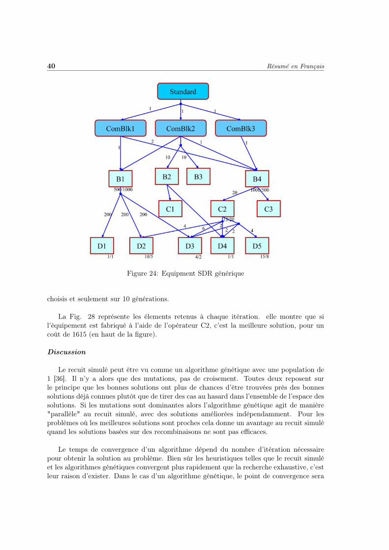
40 Résumé en Français
Figure 24: Equipment SDR générique
choisis et seulement sur 10 générations.
La Fig. 28 représente les élements retenus à chaque itération. elle montre que sil’équipement est fabriqué à l’aide de l’opérateur C2, c’est la meilleure solution, pour uncoût de 1615 (en haut de la figure).
Discussion
Le recuit simulé peut être vu comme un algorithme génétique avec une population de1 [36]. Il n’y a alors que des mutations, pas de croisement. Toutes deux reposent surle principe que les bonnes solutions ont plus de chances d’être trouvées près des bonnessolutions déjà connues plutôt que de tirer des cas au hasard dans l’ensemble de l’espace dessolutions. Si les mutations sont dominantes alors l’algorithme génétique agit de manière"parallèle" au recuit simulé, avec des solutions améliorées indépendamment. Pour lesproblèmes où les meilleures solutions sont proches cela donne un avantage au recuit simuléquand les solutions basées sur des recombinaisons ne sont pas efficaces.
Le temps de convergence d’un algorithme dépend du nombre d’itération nécessairepour obtenir la solution au problème. Bien sûr les heuristiques telles que le recuit simuléet les algorithmes génétiques convergent plus rapidement que la recherche exhaustive, c’estleur raison d’exister. Dans le cas d’un algorithme génétique, le point de convergence sera

5 Technique d’optimisation 41
Optimization tendency
Figure 25: Resultats de la recherche exhaustive sur l’exemple générique
obtenu après un nombre plus important d’itérations que pour le recuit simulé.
Notons par ailleurs au-delà de cette conclusion de nombreuses comparaison de ces deuxsolutions ont été effectuées dans la littérature donnant l’avantage au recuit simulé. Cepen-dant il est bien sûr impossible de dire arbitrairement que le recuit simulé est meilleurque les algorithmes génétiques en général. Cela dépend du problème à optimiser. Dans[37] des problèmes de minimisation de coûts d’arbres ont été confrontés notamment à desalgorithmes génétiques et de recuit simulé. Les résultats montrent que pour un mêmetemps d’exécution, le recuit simulé donne de meilleurs résultats. Pour des problèmes detransport-allocation il est montré dans [38] que dans tous les cas, les résultats basés sur lerecuit simulé sont meilleurs que toutes les autres techniques. D’autre part, une compara-ison directe a été effectuée entre du recuit simulé adaptatif et des algorithmes génétiquesdisponibles publiquement, sur des problèmes pour lesquels les algorithmes génétiques sontadaptés et adoptés. Dans tous les cas, le recuit simulé a battu l’algorithme génétique [39].D’une manière générale les algorithmes génétiques sont très consommateurs en mémoirecar il faut stocker les états intermédiaires de toutes les populations [40].
5.6 Conclusion sur le choix de l’algorithme d’optimisation
A la suite de l’étude de la bibliographie, ainsi que de la structure du graphe et des dif-férentes possibilités en termes d’algorithmes d’optimisation, le choix a été fait d’utiliserun algorithme de recuit simulé qui a été programmé en C++. Le programme prend en
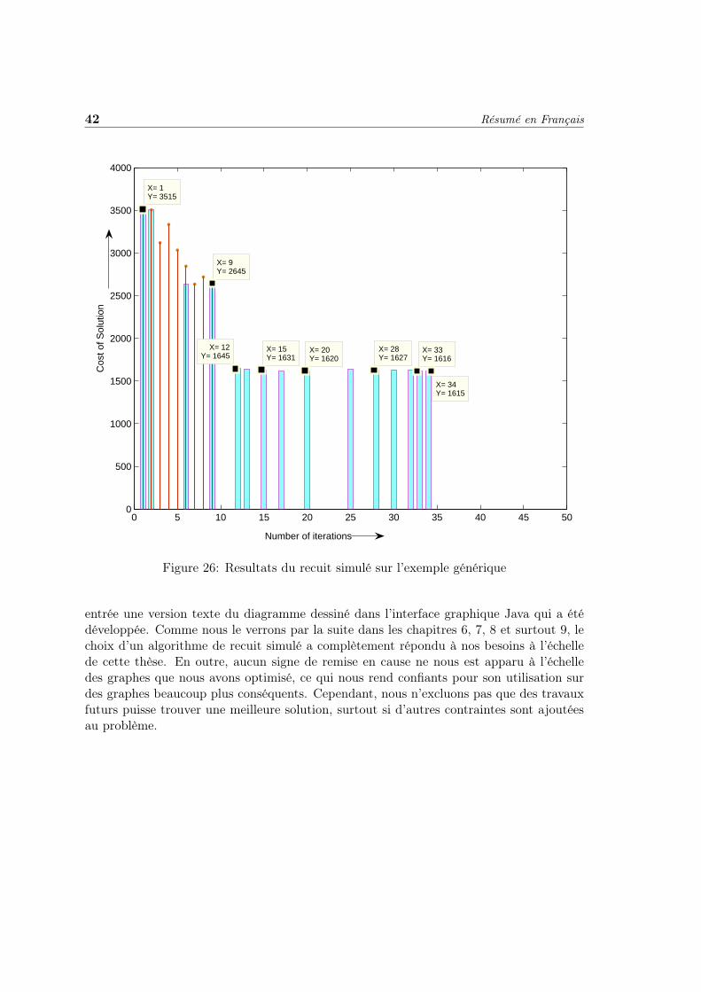
42 Résumé en Français
0 5 10 15 20 25 30 35 40 45 500
500
1000
1500
2000
2500
3000
3500
4000
X= 33Y= 1616
X= 34Y= 1615
X= 28Y= 1627
X= 20Y= 1620
X= 15Y= 1631
X= 12Y= 1645
X= 9Y= 2645
X= 1Y= 3515
Cos
t of S
olut
ion
Number of iterations
Figure 26: Resultats du recuit simulé sur l’exemple générique
entrée une version texte du diagramme dessiné dans l’interface graphique Java qui a étédéveloppée. Comme nous le verrons par la suite dans les chapitres 6, 7, 8 et surtout 9, lechoix d’un algorithme de recuit simulé a complètement répondu à nos besoins à l’échellede cette thèse. En outre, aucun signe de remise en cause ne nous est apparu à l’échelledes graphes que nous avons optimisé, ce qui nous rend confiants pour son utilisation surdes graphes beaucoup plus conséquents. Cependant, nous n’excluons pas que des travauxfuturs puisse trouver une meilleure solution, surtout si d’autres contraintes sont ajoutéesau problème.

5 Technique d’optimisation 43
C
Optimization tendency
Stall State
50
Figure 27: Resultats d’un algorithme génétique sur l’exemple générique

44 Résumé en Français
Cost=3146
Cost=2646
Cost=1645
Cost=1631
Cost=1630
Cost=1629
Cost=1620
Cost=1616
Cost=1615
D1 D1 D1 D1 D1 D1 D1
3146 2646 1645 1631 1630 1629 1620 1616 1615
D2
D3
D2
D3
D2
D3
D2
D3
D2 D2
t ite
rrtio
ns
D3
D4
D3
D4
D3
D4
D3
D4 D4 D4 D4
dat
diff
eren
t
D5 D5 D5
nts r
etai
nded
B1
C2 C2 C2 C2 C2 C2 C2 C2 C2
essi
ng e
lem
en
B4
B1
B4
Proc
e
24 52 80 176 200Iteration Number
1 2 8 22
Figure 28: Elements retenus aux différentes itérations

45


Introduction à la partie III
Lors des chapitres précédents, il a été discuté de l’approche de conception par opérateurscommuns pour les équipements multi-standards, puis de la manière de la représenter sousla forme d’un graphe. Plusieurs techniques d’optimisation ont été alors passées en revueafin d’obtenir une solution de conception optimale. Cette partie illustre par des exemples lamise en oeuvre de la méthode de conception proposée dans ce manuscrit en la confrontantnotamment à des travaux effectués dans d’autres recherches menées afin d’identifier desopérateurs communs. Les quatre chapitres de cette partie portent donc sur trois candidatspotentiels d’opérateurs communs et la mise en commun de deux d’entre eux dans un ex-emple à plus large échelle. Les chapitres 6, 7 et 8 reposent sur une collaboration avec troisautres doctorants de l’équipe, chacun d’entre eux ayant travaillé sur l’opérateur communconsidéré dans le chapitre. Notre travail met notamment en perspectives leurs résultats entermes d’implantation sur cible FPGA grâce à l’approche d’optimisation graphique pro-posée ici.
Le chapitre 6 présente une étude portant sur l’utilisation de la FFT comme opérateurcommun. Dans le chapitre 7, c’est l’opérateur LFSR qui est étudié. Puis le chapitre 8porte plus particulièrement sur le front-end numérique et le filtrage de canalisation autourde l’opérateur FRMFB. Enfin, ce problème est étendu dans le chapitre 9 à un exemple deconception plus large afin de mieux discuter de l’approche de conception proposée dans saglobalité.
6 Cas d’étude : opérateur commun FFT dans un équipementde radio logicielle multi-standards
La transformée de Fourier est réputée pour son utilisation dans la conversion d’un signaltemporel en un signal fréquentiel [41]. Mais elle a bien d’autres vertus et a particulièrementgagné en intérêt grâce à l’introduction de la FFT (Fast Fourier Transform) par Cooley etTukey [42]. Cela a permis de décroître la complexité d’exécution , permettant ainsi del’utiliser de manière efficace dans le domaine numérique. La complexité d’une FFT bru-tale est de N2 multiplications complexes et N.(N − 1) additions complexes, et elle passeà N.log2N multiplications et additions complexes si N est la longueur de la transformée.
Partant du constat qu’on retrouve la FFT dans de nombreux cas dans les chaînes decommunications numériques, [17] a considéré la FFT comme opérateur commun poten-tiel. Ajoutons qu’au-delà des traitements spécifiques au traitement de la radio, la FFT
47

48 Résumé en Français
peut aussi être utilisée dans des algorithmes de traitement de la couche applicative (parexemple vidéo), ce qui entre en compte dans l’approche de conception inter-couche qui estenvisagée ici.
Dans ce contexte, il peut être intéressant d’envisager d’effectuer dans le domainefréquentiel des calculs qui le sont habituellement dans le domaine temporel afin de béné-ficier de la présence de la FFT. Dans ce chapitre 6, nous considérons le cas de l’utilisation dela FFT pour le codage de canal et plus particulièrement pour le codage de Reed Solomon,issu des travaux de [43]. Ces travaux ont permis de mettre en évidence qu’il est possibled’utiliser une FFT paramétrable capable d’effectuer les traitements habituels d’une FFTdans C, mais aussi ceux du codage RS dans GF . Cela est possible en fait pour un sous-ensemble des codes de RS, ceux définis dans le corps GF (Ft) alors que les codes de RShabituels sont définis dans GF (2m). La Fig. 29 illustre comment un tel opérateur peutêtre utilisé dans ces différents cas. Elle détaille aussi que l’algorithm d’encodage/décodageRS inclut les étapes de calcul du syndrome, de recherche de Chien, d’un calcul polynomial,de l’algorithme de Berlekamp Massey et celui de Forney. La Fig. 29 montre que parmiceux-ci, les algorithmes de recherche de Chien et de calcul de syndrome, qui sont les pluscomplexes, peuvent être exécuté par l’opérateur FFT reconfigurable proposé.
Serial /
Parallel
Parallel /
Serial
Equalization
/ demodulation
Berlekamp
algorithm
(x) ’(x)
computation
Common FFT operator :
Syndrome computation
and Chien search
or OFDM demodulation
Forney
algorithm
RS channel coding
over GFFt
OFDM demodulation
over complex field
Figure 29: Exemple d’une FFT partagée entre un démodulateur OFDM et un décodeurRS dans GF (Ft).
6.1 Opérateur DMFFT
Cet opérateur commun de FFT reconfigurable a été nommé DMFFT (Dual Mode FFT)[19]. Il permet à la fois d’opérer des transformations de Fourier dans C appelées FFT,et des transformées de Fourier dans le corps de Galois de taille Ft GF (Ft) appelées FNT

6 Cas d’étude : opérateur commun FFT dans un équipement de radio logicielle multi-standards49
(Ft est pour Fermat). Son implantation repose sur le papillon reconfigurable (RBPE -Reconfigurable Butterfly Processing Element) de la Fig. 30.
X
X
X+
+-Ft-1
+
+
Ft-1
+
Wr
Wi
Pipeline stage
nc bits
nc bits
nc bits
X
DM
nc bits
n+1=2t +1 bits
n
n
nc
"i
1
0
01
1
0
0
1
1
001
10
10
01
01
01
10
10
Bi
Br
Ai
Ar
1rP1
iP
2rP2
iP
mux 1
Figure 30: Architecture du papillon reconfigurable
Si l’on compare un équipement utilisant l’opérateur reconfigurable DMFFT ou uneapproche de type velcro pour effectuer la FFT et le codage RS, voici ce que l’on obtient.La Table 2 relève les résultats après implantation sur un composant FPGA de type Stratix-II et pour des mots de différentes longueurs nc, d’une part de la DMFFT-64, d’autre part dela FFT-64 et de la FNT-64 (velcro operator). Les résultats sont en faveur de la DMFFT-64,aussi bien en termes de nombre d’ALUT (adaptive look-up table), de vitesse d’exécution,d’occupation mémoire, que de taux performance sur coût. Le nombre de ALUT est relatifà l’occupation en nombre de portes. Le taux performance sur coût η = 1
T.C ∗ 106 issude [44], avec T est le temps d’exécution en nanosecobdes (ns) et C le nombre de blockslogiques relativement à un circuit FPGA. Quand η augmente, un meilleur compromis entretemps d’exécution et coût est obtenu.
La table 3 compare la DMFFT-256 avec la solution velcro FFT/FNT-256. On retrouveles mêmes avantages en termes de mémoire et des résultats toujours positifs mais moindrepour les autres paramètres. Cela illustre l’intérêt d’avoir recours à des opérateurs communsplutôt que des solutions velcro dans la conception, en terme de complexité de réalisation.Un autre avantage primordial en radio logicielle est que dans le cas d’une approche vel-cro, le temps de reconfiguration est plus pénalisant que dans celui d’un changement deparamètres de la DMFFT. En dehors d’un contexte de radio intelligente avec un hand-oververtical, cela n’a pas d’importance dans le cas d’une utilisation inter-standards d’un mêmeopérateur puisque nous faisons l’hypothèse d’une utilisation séquentielle des standardsavec un temps non contraint entre deux communications. Mais dans le cas où l’opérateur

50 Résumé en Français
Table 2: Comparaison entre la DMFFT-64 et la FFT/FNT-64 Velcro sur un Stratix-II,EP2S15F484C3
nc 9 10 12 14 16
Velcrooperator
4205 4768 5831 6844 8143ALUTs ALUTs ALUTs ALUTs ALUTs4.86 ns 5.27 ns 5.46 ns 5.81 ns 6.62 ns
DMFFT3109 3744 4857 5975 7387ALUTs ALUTs ALUTs ALUTs ALUTs4.78 ns 4.97 ns 5.45 ns 5.85 ns 6.65 ns
Memorysaving 33 % 31 % 27.2 % 24.3 % 21.9 %
ALUT’sgain 26 % 21.4 % 16.7 % 12.7 % 9.2 %
η’s gain 37.4 % 35 % 20 % 13.9 % 9.7 %
est partagé entre plusieurs fonctionnalités d’un même standard, cela est crucial puisquel’on va effectuer à un rythme très élevé des changement de fonctionnalité de l’opérateur.
Table 3: Comparaison entre la DMFFT-256 et la FFT/FNT-256 Velcro sur un Stratix-II,EP2S15F484C3
nc 9 10 12 14 16
Velcrooperator
5327 6079 7518 8966 10770ALUTs ALUTs ALUTs ALUTs ALUTs5.02 ns 4.95 ns 5.45 ns 5.84 ns 6.55 ns
DMFFT4466 5365 6819 8564 10389ALUTs ALUTs ALUTs ALUTs ALUTs4.86 ns 4.90 ns 5.50 ns 5.90 ns 6.58 ns
Memorysaving 33 % 31 % 27 % 24 % 21.9 %
ALUT’sgain 16.2 % 11.7% 9.29 % 4.68 % 3.5%
η’s gain 24 % 15.1 % 9.4% 4.2 % 3.54 %
6.2 Application de l’approche de conception dans le contexte DMFFT
De l’étude de l’opérateur commun du paragraphe précédent, nous déduisons qu’il est pos-sible de mettre en oeuvre l’opérateur DMFFT à la fois pour effectuer tout calcul de FFT etle décodage RS dans GF (Ft) ses deux algorithmes les plus complexes (calcul du syndromeer recherche de Chien). C’est ce sur quoi le graphe de la Fig. 31 insiste en prenant le cas

6 Cas d’étude : opérateur commun FFT dans un équipement de radio logicielle multi-standards51
xDSLWiFi WiMAX
FFT-NRS DecodingScrambling Convolutional Interleaving FFT-NRS DecodingScramblingCoding
Interleaving
RS-GF(2m) RS GF(Ft)( ) ( t)
Chien SearchSyndrome
CalculationsPolynomial
ComputationsBerlekamp Massey
AlgorithmForney
Algorithm
DMFFT Operator
RBPE
Adder Multiplier
Figure 31: Graphe d’un équipement tri-standards en utilisant GF (Ft) pour le codage RS
imaginaire où les trois standards WiFi, WiMAX et xDSL auraient utilisé ce codage RS àla place de celui dans GF (2m). La décomposition de l’algorithme de décodage RS n’estpas détaillée dans ce résumé hormis dans la Fig. 29, mais elle peut être trouvée dans letexte anglais complet. Précisons juste que la DMFFT peut être notamment utilisée pourles 2 étapes suivantes du décodage RS : le calcul du syndrome et la recherche de Chien.
Les noeuds à gauche en gris ont été représentés pour illustrer ce que devrait intégrerun graphe complet, au-delà de l’étude de la DMFFT. La Fig. 32 zoome sur la partie bassedu graphe.
Les paramètres associés aux arcs sont les nombres d’appels (NoC ), ceux représentés icisur les noeuds sont les coûts de fabrication (BC ) en termes de nombre d’ALUT, et le coûtd’exécution est exprimé en nanosecondes. On remarque qu’il est possible de paramétrercertains poids associés aux arcs, comme c’est le cas entre le noeud DMFFT-N et le noeudRBPE suivant la taille de la FFT. On retrouve dans la Table 4 les valeurs des coûts pourla DMFFT et les noeuds sous-jacents.
Prenons l’exemple du cas du décodage RS pour détailler les résultats du calcul d’optimisation.La Table 5 donne les coûts en termes d’additions et de multiplications pour différentes fonc-

52 Résumé en Français
DMFFT-NFFT -C FNT-GF(Ft) N=64; 4857 ALUTs/5.45 ns ( t)
(N/2)log2N
N=256; 6819 ALUTs/5.5 ns
RBPE514 ALUTs/5.18 ns
R fi bl R fi bl
46
Reconfigurable Adder
Reconfigurable Multiplier
26 ALUTs/2.369 ns 104 ALUTs/5.18 ns
Figure 32: Décomposition possible de la DMFFT
Table 4: Nombre d’appels du bloc DMFFTBlock Name No of ALUT Execution Time(ns) No of CallsDMFFT-256 6819 5.5 1RBPE 514 5.18 128= (N/2)Re-Adder 26 2.37 6Re-Multiplier 104 5.18 4
tions dans le cas d’un décodage RS classique.
Le coût du noeud de décodage RS peut être obtenu par l’équation (7) :
Costlevel =( i=m∑
i=1
CCiNoCi
)×NoCi+1 +
i=m∑i=1
BCi.Ni (24)
Comme nous ne considérons que le noeud de décodage RS, alors NoCi+1 = 1 et l’équation(24) devient :
Table 5: Nombre d’appels en termes de multiplications et additions pour le décodage RSclassique pour t=8 et N=256
No. of Calls Additions MultiplicationsSyndrome Comp. 4096 4096Chien Search 2048 2048Polynomial Comp. 384 392Berlekamp Massey 512 512Forney Algorithm 8 16

6 Cas d’étude : opérateur commun FFT dans un équipement de radio logicielle multi-standards53
CostRSDecoding =( i=5∑
i=1
CCiNoCi
)×NoCi+1 +
i=5∑i=1
BCi.Ni (25)
En utilisant le première option pour concevoir le décodage RS, alors :
CostRS−GF (2m) = CostSyndrome + CostChien + CostPoly (26)+ CostBerlekamp + CostForney
soit,
CostRS−GF (2m) =((4096 + 2048 + 392 + 512 + 16)× CCMultiplier (27)
+ (4096 + 2048 + 384 + 512 + 8)× CCAdder
)× 1
+ BCMultiplier + BCAdder
et donc,
CostRS−GF (2m) =(7064× 5.18 + 7048× 2.37
)× 1 + 104 + 26 = 53425.28 (28)
Alors qu’en utilisant la seconde pour réaliser le décodage RS, l’équation (25) devient:
CostRS−GF (Ft) = CostPoly + CostBerlekamp + CostForney + CostDMFFT (29)
soit,
CostRS−GF (Ft) =((392 + 512 + 16)× CCMultiplier (30)
+ (384 + 512 + 8)× CCAdder + 2× CCDMFFT
)× 1
+ BCMultiplier + BCAdder + BCDMFFT
et donc,
CostRS−GF (Ft) =(920×5.18+904×2.37+2×5.5
)×1+104+26+6819 = 13868.08 (31)
On obtient donc la fonction de coût suivante pour le cas d’un graphe réduit au noeud dedécodage RS :
CRSDecoding = min(CostRS−GF (2m), CostRS−GF (Ft)
)= CostRS−GF(Ft) = 13868.08
Cela montre que le coût du décodage RS est bien moindre dans GF(Ft) grâce à l’utilisationde l’opérateur DMFFT.
Poussons plus loin l’exploration dans la branche de décodage RS avec GF(Ft), afin de voirsi l’opérateur DMFFT peut être un candidat en tant qu’opérateur commun.

54 Résumé en Français
Notons que le coût de la DMFFT seule est :
CostDMFFT = BCDMFFT + CCDMFFT (32)= 6819 + 5.5 = 6824.5
Si maintenant nous utilisons l’opérateur RBPE pour la mettre en oeuvre, le coût de laDMFFT devient en utilisant l’équation (7) :
CostDMFFTRBPE= CCRBPE ×NoC + BCRBPE (33)= 5.18× 128 + 514= 1177.04
En descendant encore dans le graphe, le RBPE peut être constitué par un additionneuret un multiplieur. Le coût de la DMFFT utilisant un additionneur et un multiplieur estdonc de :
CostDMFFTAdder+Multiplier=
( i=2∑i=1
CCiNoCi
)×NoCi+1 +
i=2∑i=1
BCi (34)
soit,
CostDMFFTAdder+Multiplier=
(CCAdder ×NoCAdder + (35)
CCMultiplier ×NoCMultiplier
)× 128 +
BCAdder + BCMultiplier
(36)
et donc,
CostDMFFTAdder+Multiplier=
(2.369× 6 + 5.18× 4
)× 128 + (37)
26 + 104 = 4601.55(38)
Cela montre que réaliser la DMFFT avec le RBPE donne un coût minimal comme :
CostDMFFTRPBE< CostDMFFTAdder+Multiplier
< CostDMFFT (39)
En d’autres termes, le résultat de l’équation (31) en utilisant maintenant l’opérateur RBPEpour la DMFFT devient :
CostRS−GF (Ft) = 8876.16 (40)
soit,
CRSDecoding = CostRS−GF(Ft) = 8876.16 (41)

7 Cas d’étude : opérateur commun LFSR dans un équipement de radio logicielle multi-standards55
Cela montre que la mise en oeuvre de la DMFFT via l’opérateur RBPE permet une ré-duction de coût. C’est donc le noeud RBPE qui donne la solution au coût minimal pourle décodage RS.
6.3 Résultats et conclusions
Le cas de l’utilisation de la FFT pour le codage de canal de type RS a été exploré dansce chapitre. Un opérateur DMFFT a été proposé comme opérateur commun par [43].L’implantation sur FPGA a permis d’en mesurer le coût de fabrication et d’exécution etainsi de pouvoir l’insérer dans la méthode proposée dans ce manuscrit. Ce travail a donnélieu à une publication revue [45].
Par ailleurs, afin de voir la portée que peut avoir la méthode proposée, il est démontrédans cet exemple que si l’approche par opérateur commun pour ses avantages en terme dereconfiguration et de complexité avait été pris en considération comme ici (contexte pos-sible d’équipements multi-standards) dans les standardisations WiFi, WiMAX et xDSL,alors le codage de canal RS aurait été choisi dans GF (Ft) au lieu de GF (2m).
7 Cas d’étude : opérateur commun LFSR dans un équipementde radio logicielle multi-standards
Ce chapitre 7 étudie particulièrement le cas de l’opérateur LFSR (Linear feedback shiftregister). Quatre architectures communes sont développées afin de concevoir 16 opéra-teurs communs LFSR qui permettent de supporter plusieurs opérations d’un équipementde radio intelligente suivant la manière dont ils sont combinés. Les détails d’implantationsont donnés dans le cas d’un FPGA Cyclone-II d’Altera.
7.1 Opérateur LFSR
L’annexe E rappelle les fondements et les architectures de l’opérateur LFSR. Quatre ar-chitectures ont été proposées par Alaus dans [46], basées sur les deux familles de LFSR,Fibonacci ou Galois, et sur le fait qu’elles sont reconfigurables :
• RG-LFSR (Reconfigurable Galois LFSR),
• RF-LFSR (Reconfigurable Fibonacci LFSR),
• R-LFSR (Reconfigurable LFSR),
• ER-LFSR (Extended Reconfigurable LFSR).
Un LFSR est un registre à décalage (shift register) dont le bit d’entrée est une com-binaison linéaire des contenus précédents de ses registres. Ceci présente la particularitéque si l’on veut faire appel à une sous-structure du LFSR comme opérateur commun etordonnancer ses appels ensuite, il faut garder en mémoire les valeurs de tous les registres,les indices des rebouclages, les entrées et les sorties, ce qui implique un surcoût de mé-moire (et sa gestion) important. D’autre part, même si des structures sont remplaçables,

56 Résumé en Français
Table 6: Décomposition en LFSR IndépendantsLFSR common operators Logic cellsRG-LFSR4 5RG-LFSR8 10RF-LFSR4 5RF-LFSR8 10R-LFSR4 6R-LFSR8 10ER-LFSR4 11ER-LFSR8 16
disons par le ER-LFSR (dont la structure est exposée en annexe E), elles peuvent avoirdifférentes configurations. Par exemple, dans ce chapitre, l’opérateur commun requis doitavoir une chaîne LFSR de 32 registres, deux chaînes de 27 registres ou trois chaînes de 8registres. Ainsi, la conception et la mise en place d’un seul opérateur commun basé surl’architecture ER-LFSR présente une difficulté certaine.
Afin de s’affranchir des problèmes d’ordonnancement, nous avons choisi de masquer leproblème en créant une banque d’opérateurs communs (COB - Common Operator Bank)où de petits opérateurs ER-LFSR de taille identique sont interconnectés. Ces connectionssont paramétrables et permettent de mettre en oeuvre des chaînes ER-LFSR de taillesdifférentes. Le but est d’éviter les problèmes liés à l’ordonnancement en implantant autantd’opérateurs que requis par le standard le plus exigeant.
Prendre ainsi le pire cas peut paraître en contradiction avec la philosophie des opéra-teur communs car l’approche par opérateurs communs approche tend à trouver la pluspetite entité commune (en fait la moins coûteuse, ce qui peut être un peu différent dela plus petite). De plus, l’approche par le pire cas peut paraître évidente, mais elle al’avantage d’offrir déjà une première économie par rapport au cas velcro (où le coût multi-standards est la somme des coûts de chacun des standards), ce qui est cohérent avec lesbuts de l’approche par opérateurs communs. Cependant, nous verrons par la suite quec’est l’opérateur commun étant capable d’effectuer le pire cas (ce qui signifie automatique-ment tous les autres qui sont nécessaires dans l’équipement aussi - voir Table 7) que nouschoisirons, et nous pas la structure entière du pire cas.
Ainsi, la Fig. 33 illustre plusieurs cas d’allocations possibles. Avec le COB il est pos-sible de replacer exactement la structure dont on a besoin. En fonction des structures lesplus petites à mettre en oeuvre nous avons choisi des tailles de 4 et 8 comme il est expliquéci-après.
7.2 LFSR et approche de conception par graphe
Dans le cas d’un FPGA ALTERA Cyclone-II, la Table 6 donne le nombre de celluleslogiques nécessaires pour la réalisation de chaque catégorie de LFSR étudiée.
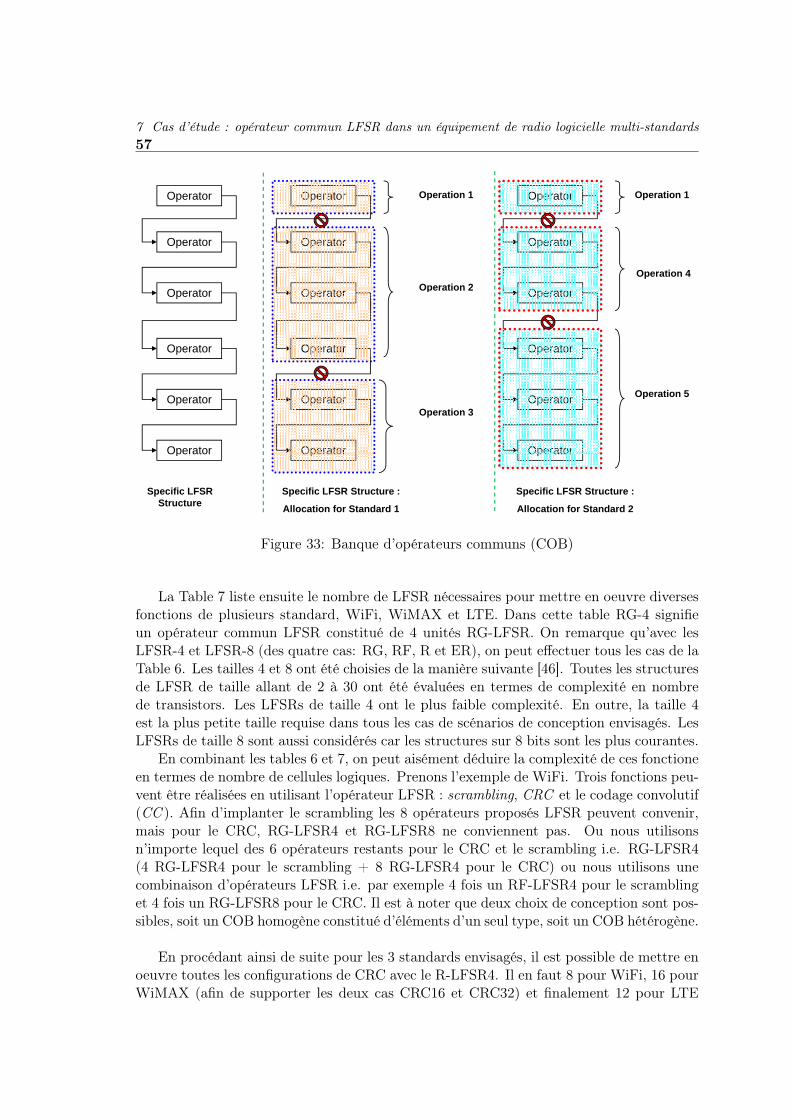
7 Cas d’étude : opérateur commun LFSR dans un équipement de radio logicielle multi-standards57
Operator Operator OperatorOperation 1 Operation 1
Operator Operator Operator
Operation 2Operation 4
Operator Operator OperatorOperation 2
Operator
Operator
Operator
Operator
Operator
Operator
Operation 5Operator
Operator
Operator
Operator
Operator
Operator
Operation 3
p
Operator Operator Operator
Specific LFSR Structure
Specific LFSR Structure :
Allocation for Standard 1
Specific LFSR Structure :
Allocation for Standard 2Allocation for Standard 1 Allocation for Standard 2
Figure 33: Banque d’opérateurs communs (COB)
La Table 7 liste ensuite le nombre de LFSR nécessaires pour mettre en oeuvre diversesfonctions de plusieurs standard, WiFi, WiMAX et LTE. Dans cette table RG-4 signifieun opérateur commun LFSR constitué de 4 unités RG-LFSR. On remarque qu’avec lesLFSR-4 et LFSR-8 (des quatre cas: RG, RF, R et ER), on peut effectuer tous les cas de laTable 6. Les tailles 4 et 8 ont été choisies de la manière suivante [46]. Toutes les structuresde LFSR de taille allant de 2 à 30 ont été évaluées en termes de complexité en nombrede transistors. Les LFSRs de taille 4 ont le plus faible complexité. En outre, la taille 4est la plus petite taille requise dans tous les cas de scénarios de conception envisagés. LesLFSRs de taille 8 sont aussi considérés car les structures sur 8 bits sont les plus courantes.
En combinant les tables 6 et 7, on peut aisément déduire la complexité de ces fonctioneen termes de nombre de cellules logiques. Prenons l’exemple de WiFi. Trois fonctions peu-vent être réalisées en utilisant l’opérateur LFSR : scrambling, CRC et le codage convolutif(CC ). Afin d’implanter le scrambling les 8 opérateurs proposés LFSR peuvent convenir,mais pour le CRC, RG-LFSR4 et RG-LFSR8 ne conviennent pas. Ou nous utilisonsn’importe lequel des 6 opérateurs restants pour le CRC et le scrambling i.e. RG-LFSR4(4 RG-LFSR4 pour le scrambling + 8 RG-LFSR4 pour le CRC) ou nous utilisons unecombinaison d’opérateurs LFSR i.e. par exemple 4 fois un RF-LFSR4 pour le scramblinget 4 fois un RG-LFSR8 pour le CRC. Il est à noter que deux choix de conception sont pos-sibles, soit un COB homogène constitué d’éléments d’un seul type, soit un COB hétérogène.
En procédant ainsi de suite pour les 3 standards envisagés, il est possible de mettre enoeuvre toutes les configurations de CRC avec le R-LFSR4. Il en faut 8 pour WiFi, 16 pourWiMAX (afin de supporter les deux cas CRC16 et CRC32) et finalement 12 pour LTE

58 Résumé en Français
Table
7:O
pérationsde
WiF
i/WiM
AX
/3GP
P-LT
Eet
nombre
deLF
SRs
Function
RG
-LFSR
4R
G-L
FSR
8R
F-L
FSR
4R
F-L
FSR
8R
-LFSR
4R
-RLFR
8ER
-LFSR
4ER
-LFSR
8W
iFi-C
omplexity
interm
sof
num
ber
ofLFSR
sScram
bler4
24
24
24
2C
RC
16-
-8
48
48
4C
C-802.1 1b
--
--
42
42
CC
-802.1 1g-
--
--
-6
6IE
EE
802.16d/e
(WiM
AX
)C
omplexity
interm
sof
num
ber
ofLFSR
sScram
bler-158
48
48
48
4+
Scrambler-11
64
64
64
64
or+
Scrambler-22
126
126
126
126
CR
C32
--
168
168
168
CR
C16
--
84
84
84
CC
-1/2-
--
-4
24
2T
C-1/2
--
--
--
11
TC
-1/3-
--
--
-2
23G
PP
LTE
Com
plexity
interm
sof
num
ber
ofLFSR
sScram
bler-UL
84
84
84
84
+Scram
bler-DL
64
64
64
64
CR
C32
--
126
126
126
CR
C24
--
84
84
84
CR
C16
--
64
64
64
CR
C8
--
--
42
42
CC
-1/2-
--
-4
24
2C
C-1/3
--
--
63
63
TC
--
--
22
22

7 Cas d’étude : opérateur commun LFSR dans un équipement de radio logicielle multi-standards59
ER-LFSR
R-LFSRR-LFSR
RG-LFSR RF-LFSRER-LFSR R-LFSR RG-LFSR RF-LFSRMapping Mapping
Logic Cell Basic Element
Figure 34: LFSRs Combinés
(pour supporter les CRC8, CRC16, CRC24 et CRC32). On en déduit que 16 R-LFSR4 per-mettent d’assurer l’exécution de tous les cas de CRC exigés dans les 3 standards considérés.
La mise en oeuvre de cette approche intuitive se révèle finalement contre-productivepuisque dans le cas d’un équipement tri-standards avec 2 modes LTE et un mode WiFi,une telle implantation présente un surnombre de 5 % en termes de nombre de celluleslogiques par rapport à une approche Velcro. En effet, ce sont des COB utilisant des ER-LFSR8 qui sont utilisés, ce qui représente 352 cellules logiques contre 336 pour l’approcheVelcro (obtenus après synthèse).
Il est bien sûr possible également de combiner plusieurs jeux de LFSR afin d’obtenirde meilleurs résultats. Lançons le processus d’optimization pour explorer les solutions. Lafigure 34 explique que les différentes structures de LFSR peuvent se combiner entre ellesen ajoutant des portes logiques de liaison ou mapping.
On obtient alors en terme de complexité la nouvelle Table 8. Avec une telle décom-position, on peut remarquer que les (E)R-LFSR sont la combinaison de R(G)-LFSR avecd’autres structures basées sur des éléments logiques :
• R-LFSR = RG-LFSR + 1.Logic Cells (R-LFSR Mapping)
• R-LFSR4 = RG-LFSR4 + 5.Logic Cells (R-LFSR4 Mapping)
• R-LFSR8 = RG-LFSR8 + 9.Logic Cells (R-LFSR8 Mapping)
et
• ER-LFSR = R-LFSR + Logic Cells (ER-LFSR Mapping) = RG-LFSR + 1.LogicCells

60 Résumé en Français
Table 8: LFSRs combinésCombined LFSR common operators Logic cellsRG-LFSR4 5RG-LFSR8 10RF-LFSR4 6RF-LFSR8 11R-LFSR4 11R-LFSR8 20ER-LFSR4 17ER-LFSR8 27
• ER-LFSR4 = R-LFSR4 + 6.Logic Cells (ER-LFSR4 Mapping)= RG-LFSR4 +11.Logic Cells.
• ER-LFSR8 = R-LFSR8 + 7.Logic Cells (ER-LFSR8 Mapping) = RG-LFSR8+16.Logic Cells.
Remarquez que les relations ci-dessus expriment juste le principe de combinaison (struc-turelle) des opérateurs et ne doivent pas être considérées pour calculer le coût équivalent.Par conséquent, tous les opérateurs LFSR combinés peuvent avoir plus d’un seul coût, enfonction du type de LFSR de plus bas niveau choisi pour être combinés ensemble.
La section suivante montre comment le processus d’optimisation peut aider à réduirele précédent coût en utilsant des LFSR combinés.
7.3 Conception d’un équipement tri-standards
Revenons au problème de conception multi-standard dans le cas d’un équipement tri-standards LTE1, LTE2 et WiFi. La Fig. 35 restreint le graphe aux fonctions pouvantutiliser l’opérateur LFSR. TBxx signifie blocks transparents. Ils ne sont là que pour al-léger visuellement le graphe. La décomposition des opérateurs LFSRs n’est pour l’instantpas utilisée mais le sera ensuite. Les opérateurs LFSR en bas de la Fig. 35 sont précédésd’un nombre qui indique le facteur de duplications de l’opérateur, i.e. que 22ER signifieun ER-LFSR4/8 dupliqué 22 fois.
Le but est de trouver la meilleure combinaison d’opérateurs donnant un coût mini-mal. Pour cela le coût de chaque noeud est calculé. Le coût BC est directement calculédepuis le nombre de LFSRs requis et du nombre de cellules logiques requis pour mettre enoeuvre un LFSR. Pour le coût CC, comme le problème d’ordonnancement a été masquépar l’utilisation des COBs, nous le fixons à 1. Nous pouvons considérer en effet qu’ilssont exécutés en 1 coup d’horloge. Comme par ailleurs chaque opérateur ou combinaisond’opérateurs est appelé en une fois pour faire sa tache, le NoC est égal à 1.
Rappelons que dans le cas de la Fig. 35, les opérateurs LFSR ne sont pas combinés.En appliquant alors le programme d’optimisation sur le graphe de la Fig. 35 on obtientfinalement l’équation :

7 Cas d’étude : opérateur commun LFSR dans un équipement de radio logicielle multi-standards61
Scrambler CRC CC
LTE 1Scrambler CRC CC
LTE 2Scrambler CRC CC
WiFi 1
TB13TB11 TB12 TB21 TB22 TB23 TB31 TB32 TB33 TB34
22ER 8R 14ER 2R 6RG 6R 4RG 20ER 4R 2RG 2RF 8ER
Figure 35: Equipement tri-standards avec l’opérateur commun LFSR
CLTE1,LTE2,WiFi1 = Cost14ER+8R+2R+4RG (42)= 14× 16 + 8× 10 + 2× 10 + 4× 10= 364
Il est à noter que les coûts des LFSR-8 sont ici utilisés pour les raisons évoquées dansparagraph 7.2. L’optimisation donne donc dans ce cas les noeuds 14ER, 8R, 2R and 4RGafin d’obtenir le coût minimal pour la mise en oeuvre de l’équipement tri-standards.
Si maintenant nous compliquons l’exemple en introduisant la décomposition de l’opérateur22ER de la Fig. 36 comme évoqué précédemment. L’équation (42) devient alors :
CLTE1,LTE2,WiFi1 = Cost14ER+2R+4RG (43)= 14× 16 + 2× 10 + 4× 10= 284
La nouvelle optimisation sélectionne les opérateurs 14ER, 2R and 4RG afin d’obtenirle coût minimal pour la mise en oeuvre de l’équipement tri-standards. Les opérateurs14ER et 2RG sont communs aux deux solutions. En revanche, l’opérateur 8R du casprécédent est remplacé par l’opérateur 2R qui peut à la fois mettre en oeuvre le R-LFSR4et le R-LFSR8.
Il est à noter que l’impact de l’utilisation d’opérateurs communs est d’autant plusimportant que le nombre de standards considérés est grand. Dans le cas simple de 3standards ici, le nombre de cellules logiques passe de 336 (obtenus par synthèse) dans lecas velcro à la combinaison de 14 ER, 2R et 4 RG soit 284 cellules logiques (équation(43)).

62 Résumé en Français
22ER
TB41 TB42
MAP6R 6R
MAP4R 4R
TB61
4ER
14ER
8ER6ER
TB51 TB52
MAP8R 8R20ER 2ER
MAP2R 2R
MAP2RG 2RG MAP4RG 4RG MAP6RG 6RG
Figure 36: Décomposition de l’opérateur 22ER en opérateurs plus petits
7.4 Résultats et conclusions
Cette étude montre l’intérêt à considérer l’opérateur LFSR comme un opérateur communafin d’être utilisé pour de nombreuses fonctions tels que scrambling, le CRC et le codageconvolutif. Nous nous sommes appuyés pour cela sur des chiffres d’implantation sur cibleFPGA Cyclone-II de Altera afin d’avoir des résultats réalistes. Ce travail a donné lieu àune publication revue [47].
8 Cas d’étude : opérateur commun FRMFB
Un élément clef d’un équipement multi-standards est l’organe qui est capable de "canaliser"le signal reçu (on parle de channelizers en anglais ou canaliseurs), autrement dit d’extraireun canal (fréquentiel) correspondant à un standard. En effet, idéalement, une numérisationà large bande de plusieurs canaux est effectuée en tête de réception dans la philosophieradio logicielle. Dans le chapitre 8, plusieurs propositions de bancs de filtres sont détaillées[48] et intégrée dans un graphe afin de lancer la méthode proposée dans cette thèse.

8 Cas d’étude : opérateur commun FRMFB 63
8.1 Bancs de filtres
La solution classique de l’extraction canal par canal (PC - Per Channel) par des filtresfigés n’est plus rentable dans le cas où le nombre de canaux à extraire en réception aug-mente. Et cela s’avère d’autant plus vrai s’il est nécessaire d’extraire plusieurs canaux àla fois tel que dans une station de base [49].
La solution passe alors par les bancs de filtres. Les plus connus sont les bancs de filtresbasés sur la transformée de Fourier discrète (DFTFB pour Discrete Fourier TransformFilter Bank) [49, 50]. Au lieu de N filtres, seul un filtre passe bas suivi par une FFTest nécessaire. Cependant, cela implique des contraintes et notamment que les bandes àextraire soient identiques.
Une alternative a été aussi proposée dans [49]: GFB (Goerzel Filter Bank). Cette solu-tion résoud les problèmes liés aux contraintes de localisation en fréquence et de sélectivitédu filtre prototype qui existent dans le cas DFTFB. Notons aussi que [51] propose un bancde filtres basé sur la combinaison de filtres polyphase et de DFT.
Une quatrième limitation n’est pas encore résolue dans ces 3 cas. Il s’agit de cellequi permet de reconfigurer le même banc de filtres pour s’adapter à différents standards.La version anglaise de la thèse donne des exemples de canaliseurs issus de la littérature.Citons seulement [48] qui propose un banc de filtres reconfigurable basé sur les techniquesde masquage de la réponse en fréquence (Frequency Response Masking Filter Bank orFRMFB). Les avantages supplémentaires par rapport aux autres solutions sont que la re-configurabilité est désormais possible au niveau du filtre mais aussi de sa structure, que lavitesse de filtrage est améliorée et que la complexité en est réduite [48].
La méthode frequency masking a été introduite en 1986 dans [52] afin de mettre enoeuvre des filtre FIR très sélectifs d’ordre réduit. L’architecture d’un tel filtre est proposéedans la Fig. 37. Elle est constituée de :
• Filtre prototype filter: H1(zM )
• Filtre complémentaire à H1(z): zM(Na−1)/2
• Filtre de masquage haut : HFMA(z)
• Filtre de masquage bas : HFMC(z)
8.2 Graphe du canaliseur multi-standards
Si l’on restreint l’étude de conception d’un équipement au canaliseur, on peut retrouverle graphe de la Fig. 38. Dans cet exemple, nous considérons le coût des noeuds en termesde nombres d’additions et de soustractions.
8.3 Optimisation du graphe canaliseur
L’étude porte sur la conception d’un équipement bi-standards GSM, WCDMA dont onveut extraire 5 canaux pour chaque standard. Les canaux sont de 200 kHz pour le GSM

64 Résumé en Français
Figure 1. FIR filter architecture based on FRM technique.
Figure 2. Frequency Response illustration of FRM approach.
Ha(z)
HC(z) = 1-H(z)
H(zM)
HC (zM)
HMA(z)
HMC(z)
fap fas π
π
π
π
π
w
w
w
w
w
fap fas
(m-fap)/M fp
fp
fs
fs
(m+1-fas)/M
(a)
(c)
(d)
(e)
Input
-
+
H1 (zM) HFMA (z)
z-M(Na-1)/2 HFMC (z)
Output
(b)
Figure 37: FIR filter architecture based on FRM technique
Standard S1 Standard Sn
Single Standard M lti t d d
CHANNELIZERSEqualization
Single Standard Channelizers
Multi‐standard Channelizers
Filter Banks
DFTFB GFB FRMFBCperC DFTFBp
CostDFTFB CostGFBCostCperC CostFRMFB
Figure 38: Canaliseurs pour un équipement SDR multi-standards
et de 3.86 MHz pour l’UMTS.
L’étude est restreinte aux possibilités dont on a les chiffres de complexité PC, DFTFBet FRMFB. Le processus d’optimisation consiste à trouver la solution à l’équation :
CChannelizer = min(CostCPerC , CostDFTFB, CostGFB, CostFRMFB
)(44)
Si nous expliquons plus en détail le coût du noeud FRMFB à l’aide de l’équation(7) rappelée ci-dessous :

8 Cas d’étude : opérateur commun FRMFB 65
Table 9: Complexité du FRMFB pour l’extraction de 5 canaux GSM et 5 canaux WCDMAName of Filter No. of Taps No. of Adders No. of MultipliersModal Filter 81 41 80FMA_GSM 600 300× 5 = 1500 599× 5 = 2995FMA_WCDMA 250 125× 5 = 625 249× 5 = 1245FMC_WCDMA 250 125× 5 = 625 249× 5 = 1245Total complexity - 2791 5565Complexity of PC/ 1400 7000 13990DFTFB
Costlevel =( i=m∑
i=1
CCiNoCi
)×NoCi+1 +
i=m∑i=1
BCi.Ni (45)
Si l’on considère le noeud FRMFB, NoCi+1 = 1 et (45) devient :
CostFRMFB =( i=4∑
i=1
CCiNoCi
)× 1 +
i=4∑i=1
BCi.Ni (46)
So
CostFRMFB = CostModalF ilter + CostFMAGSM+ CostFMAWCDMA
(47)+ CostFMCWCDMA
La Table 9 donne les complexités des différents éléments des FRMFB.On en déduit que :
CostFRMFB =((41 + 1500 + 625 + 625)× CCAdder (48)
+ (80 + 2995 + 1245 + 1245+)× CCMultiplier
)+ BCAdder + BCMultiplier
Considérant une implantation du FRMFB sur un composant FPGA Stratix-II de Altera,on peut reprendre les BC et CC du multiplieur et de l’additionneur dans la table 4, etalors :
CostFRMFB =(2791× 2.37 + 5565× 5.18
)× 1 + 26 + 104 = 35571.37 (49)
De la même manière, le coût du canaliseur PC ou DFTFB se calcule ainsi car il n’y apas vraiment de différence de complexité pour ces 2 cas dans le contexte considéré ici parrapport à celle du FRMFB :
CostPC/DFTFB =(NoCAdder × CCAdder + NoCMultiplier × CCMultiplier
)(50)
+ BCAdder + BCMultiplier

66 Résumé en Français
soit
CostPC/DFTFB =((7000)× CCAdder + (13990)× CCMultiplier
)(51)
+ BCAdder + BCMultiplier
et donc
CostPC/DFTFB =(7000× 2.37 + 13990× 5.18
)+ 26 + 104 = 89188.20 (52)
Le FRMFB est donc l’opérateur commun de la Fig. 38.
8.4 Résultats et conclusion
Le FRMFB est choisi comme candidat dans ce cas d’étude de la canalisation pris seulpour un équipement SDR multi-standards. Cependant, si nous ajoutions le standardWiFi au cas d’étude et que nous considérions aussi la FFT nécessaire pour effectuer lamodulation/démodulation OFDM de WiFi, alors le résultat pourrait être différent. Caralors, la FFT pourrait être utilisée à la fois pour la modulation/démodulation et pour lacanalisation. C’est l’intérêt de la méthode de conception proposée ici : éviter de choisirdes optimisations locales et permettre d’envisager des optimisations globales à l’ensemblede la chaîne de traitement. C’est ce que laissait entrevoir la Fig. 7 du chapitre 2 et quenous allons étudier dans le chapitre 9.
9 Cas d’étude d’un graphe complexe
Nous combinons dans ce chapitre 9 deux des cas étudiés dans la section III de ce documentafin d’effectuer un premier pas (à bien sûr poursuivre dans une conception complète) ducas de conception d’un équipement multi-standards SDR. La cas d’étude vise à regrouperdans un même graphe les opérateurs DMFFT du chapitre 6 et FRMFB du chapitre 8 pourla conception d’un équipement multi-standards WiFi/WiMAX/UMTS. Le but est de trou-ver un optimum global dans ce cas, qui peut se distinguer des optimums locaux trouvédans chacun des cas (ce sur quoi portent habituellement les travaux d’optimisation archi-tecturale). Ce dernier exemple a pour but de véritablement mettre en évidence l’avantagede l’approche préconisé dans ce travail de thèse.
9.1 Opérateurs communs
La Fig. 39 reprend les opérateurs DMFFT du chapitre 6 et FRMFB du chapitre 8. Lebut est d’essayer de voir s’il y a des possibilités de ré-utilisation des opérateurs com-muns trouvés pour l’un dans le cas de l’autre. Ainsi, on pressent que l’opérateur DMFFTpourraient aussi être utilisé dans les bancs de filtre, en plus des cas déjà identifiés de lamodulation/démodulation OFDM et du codage/décodage RS. Cela pourrait contredirela conclusion (locale) du chapitre 8 qui a fait le choix FRMFB au profit de la DFTFBqui pourrait alors effectuer sa transformée de Fourier avec l’opérateur DMFFT. C’esttout l’intérêt du travail de cette thèse qui consiste à fournir une méthode et un outillage

9 Cas d’étude d’un graphe complexe 67
pour trouver un optimum global à la conception, au détriment d’a priori sur les optimumslocaux parfois préconisés. La condition est de disposer de graphes suffisamment complétés.
Common Operators
DMFFT FRMFB
Block 1 Block 2
DMFFTOperator
Chapter #6
FRMFBOperator
Chapter #8
Figure 39: An generalized view of common operators
9.2 Graphe de conception
Le graphe du système tri-standards étudié est proposé dans la Fig. 40. Comme dans lesétudes précédentes, il ne comporte pas toutes les opérations des couches protocolaires com-plètes des trois standards (ce qui aurait été impossible à obtenir lors de la thèse et qui nefaciliterait pas les explications voulues ici), mais il est réduit aux fonctions de démodula-tion OFDM, de décodage RS et de canalisation. Ainsi, nous pouvons espérer combiner lesrésultats obtenus pour les opérateurs DMFFT et FRMFB. L’interface graphique dévelop-pée dans ces travaux est utilisée sur la Fig. 40 pour représenter le graphe et associer lesparamètres de coût à chaque entité (arc ou noeud).
Afin d’améliorer la lisibilité, le graphe a été repris dans la Fig. 41.
9.3 Coûts
Les coûts sont extraits des tableaux de complexité de l’Annexe B (de la version anglaise).Mais ils ne sont pas dans la même unité, ceux de la DMFFT étant en nombre d’ALUTs etceux du LFSR étant en nombre de cellules logiques (LC) de multiplieurs et d’additionneurs.
Les paramètres de coût des différents noeuds de la Fig. 41 sont donnés en Table 10.
Certains de ces coûts sont extraits de la Table 4. Les coûts BC/CC pour les FRMFBet DFTFB sont issus de [48] en nombre de portes. Ils sont alors convertis en nombred’ALUTs avec la règle suivante : 1 ALUT ≈ 1.5 × LC et 1 LC = 30 to 40 Gates sur unFPGA de la famille Virtex. Les coûts associés au arcs i.e. NoC sont issus des Table 5 et 9.

68 Résumé en Français
Figure 40: Copie d’écran du graphe dans l’interface graphique
Table 10: Cost parameters for different blocks of Fig. 41Name of Function BC (ALUTs) CC (ns)DMFFT 4857 5.5RBPE 514 5.18Re-Adder 26 2.37Re-Multiplier 104 5.18DFTFB 11868 77FRMFB 7938 38.67
9.4 Résultats de l’optimisation
Après avoir lancée l’optimisation, les opérateurs RBPE, PloyCompt (polynomial compu-tation), Berkelamp et Forney sont sélectionnés pour une implantation à coût minimal. LaFig. 42 résume à différentes étapes clef les résultats du processus d’optimisation.
Détaillons ces résultats. Le coût de l’équipement (reduit aux tris éléments de décodageRS, démodulation OFDM et canalisation) de la Fig.41 peut s’écrire :
CSystem = CostRSDecoding+ CostOFDM + CostChannelizer (53)
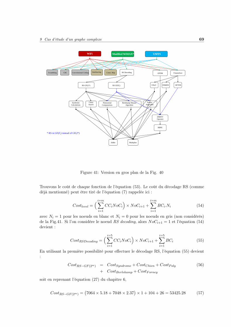
9 Cas d’étude d’un graphe complexe 69
WiFi Modified WiMAX* UMTS
OFDMRS DecodingScrambling CRC Convolutional Coding Interleaving Const. Map Channelizer
RS-GF(2m) RS GF(Ft) CPerC DFTFBFRMFB
ChienSearch
Syndrome Calculations
Polynomial Computations
Berlekamp Massey Algorithm
Forney Algorithm
DMFFT Operator
RBPE
* RS in GF(Ft) instead of GF(2m)
Adder Multiplier
Figure 41: Version en gros plan de la Fig. 40
Trouvons le coût de chaque fonction de l’équation (53). Le coût du décodage RS (commedéjà mentionné) peut être tiré de l’équation (7) rappelée ici :
Costlevel =( i=m∑
i=1
CCiNoCi
)×NoCi+1 +
i=m∑i=1
BCi.Ni (54)
avec Ni = 1 pour les noeuds en blanc et Ni = 0 pour les noeuds en gris (non considérés)de la Fig.41. Si l’on considère le noeud RS decoding, alors NoCi+1 = 1 et l’équation (54)devient :
CostRSDecoding =( i=5∑
i=1
CCiNoCi
)×NoCi+1 +
i=5∑i=1
BCi (55)
En utilisant la première possibilité pour effectuer le décodage RS, l’équation (55) devient:
CostRS−GF (2m) = CostSyndrome + CostChien + CostPoly (56)+ CostBerlekamp + CostForney
soit en reprenant l’équation (27) du chapitre 6,
CostRS−GF (2m) =(7064× 5.18 + 7048× 2.37
)× 1 + 104 + 26 = 53425.28 (57)

70 Résumé en Français
Cost=22785.29
Cost=21627.79
Cost=15322.79
DFTFB
CperC
DFTFB
CperC
DFTFB
CperC
DFTFB DFTFB DFTFB DFTFB
GF(Ft)
FRMFB
GF(Ft)
FRMFB
GF(Ft)
FRMFB FRMFB FRMFB FRMFB FRMFB
GF(2m)
errti
ons
Synd. Synd.
t diff
eren
t ite Calc.
ChienSearch
Poly
Calc.
ChienSearch
Poly Poly Poly Poly Poly Poly Poly Poly
reta
inde
dat Poly.
Comp.
Berme-Kamp
F
Poly.Comp.
Berme-Kamp
Forne
Poly.Comp.
Berme-Kamp
Forne
Poly.Comp.
Berme-Kamp
F
Poly.Comp.
Berme-Kamp
Forne
Poly.Comp.
Berme-Kamp
F
Poly.Comp.
Berme-Kamp
Forne
Poly.Comp.
Berme-Kamp
Forne
Poly.Comp.
Berme-Kamp
F
ng e
lem
ents
ForneyAlgo.
DMFFT
ForneyAlgo.
DMFFT
ForneyAlgo.
DMFFT
ForneyAlgo.
DMFFT
ForneyAlgo.
DMFFT
ForneyAlgo.
DMFFT
ForneyAlgo.
DMFFT
ForneyAlgo.
DMFFT
ForneyAlgo.
Proc
essi
n
RBPE
Adder
RBPE
Adder
RBPE
Adder
RBPE
Adder Adder
RBPE
70 100 127 136 142Iteration Number
2 12 45
Multiplier Multiplier Multiplier Multiplier Multiplier
1
Figure 42: Number of operators kept at different number of iterations
Avec la seconde option pour le décodage RS, l’équation (55) devient :
CostRS−GF (Ft) = CostPoly + CostBerlekamp + CostForney + CostDMFFT (58)
soit en reprenant l’équation (30) du chapitre 6,
CostRS−GF (Ft) =(920×5.18+904×2.37+2×5.5
)×1+104+26+6819 = 13868.08 (59)
Dans le cas du décodage RS, c’est donc la deuxième option, i.e. l’implantation dansGF (Ft) qui minimise le coût.
Nous avons considéré jusqu’à présent la mise en oeuvre de RS dans GF (Ft) via l’opérateurDMFFT. MAis si l’on pousse encore le raisonnement, la DMFFT peut elle-même êtreréalisée via l’opérateur RBPE et alors sont coût devient en utilisant l’équation (7) :
CostDMFFTRBPE= CCRBPE ×NoC + BCRBPE (60)= 5.18× 128 + 514= 1177.04

9 Cas d’étude d’un graphe complexe 71
Le coût de la DMFFT implantée à l’aide du RBPE présente donc un coût minimal. Enl’appliquant aussi au décodage RS, et en reprenant l’équation (58) pour laquelle on obtenaitun coût de 13868,08, le coût du décodage RS devient :
CostRS−GF (Ft) =(920×5.18+904×2.37+2×(128×5.18
)+104+26+514 = 8878.16 (61)
Considérons maintenant la démodulation OFDM. Elle requiert le noeud FFT-N qui estréalisé par l’opérateur DMFFT. Donc le coût de la démodulation OFDM est de :
CostOFDM = CostDMFFT = BCDMFFT + CCDMFFT (62)= 6819 + 5.5 = 6824.5
(63)
Mais la DMFFT est déjà réalisée avec le RBPE pour le décoadeg RS. Il n’est donc pasnécessaire de repayer son coût d’achat BC et seul le coût d’exécution CC est à mettre àjour. Donc pour la démodulation OFDM BC = 0 et CC dépend de NoC = 128. Le coûtde l’OFDM devient :
CostOFDM = CostDMFFT = BCDMFFT + CCDMFFT (64)= BCDMFFTRBPE
+ CCDMFFTRBPE
= 0 + 1× (128× 5.18)= 663.04 (65)
La réduction du coût est manifeste entre l’équation (62) et l’équation (64) grâce à l’utilisationconjointe du RBPE pour le décodage RS et la démodulation OFDM.
La canalisation peut être effectué des trois manières exposées dans la in Fig. 41. Pour lesoptions FRMFB et DFTFB les coûts du canaliseur sont :
CostChannelizerDFTFB= BCDFTFB + CCDFTFB (66)= 11868 + 77 = 11945
et,
CostChannelizerFRMFB= BCFRMFB + CCFRMFB (67)= 7938 + 38.67 = 7976.67
On retrouve donc bien le résultat du chapitre 8, à savoir que lorsque la canalisation estconsidérée seule, le coût du FRMFB est inférieur à celui du DFTFB.
Maintenant, nous considérons la conception entière. Dans ce cas, le DFTFB peut utiliserl’opérateur DMFFT qui est par ailleurs indispensable pour la démodulation OFDM. Ledécodage RS dans GF (Ft) donnant un coût inférieur pour cette partie décodage, cela

72 Résumé en Français
renforce encore l’opérateur DMFFT, via le RBPE. En présence de la DMFFT le coûtd’achat BC du DFTFB est réduit à 11868 − CostDMFFT = 5043.5 ce qui le place à uncoût inférieur à celui de la FRMFB (which is 7976.67), et alors le coût du canaliseurDFTFB utilisant l’opérateur RBPE est :
CostChannelizerDFTFB= BCDFTFB + CCDFTFB (68)= BCDFTFB + 77 + CCDMFFT
= 5043.5 + 77 + 1× (128× 5.18)= 5783.54
(69)
En utilisant alors les équations (61), (64) et (68), l’équation (53) donne :
CSystem = CostRS−GF (Ft) + CostOFDM + CostChannelizerDFTFB
+ 8876.16 + 663.09 + 5783.54= 15322.79
(70)
C’est le résultat du coût de la conception dans une approche par opérateur commun résoluepar notre méthode. Si l’on ne tient pas compte de cela, on retombe alors sur une approchede conception plus classique par optimisation locale et alors le coût de conception auraitété de :
CSystem = CostRS−GF (Ft) + CostOFDM + CostChannelizer
+ 13686.08 + 6824.5 + 7976.5= 28669.25
(71)
La différence entre les deux coûts des équations (70) et (71) donne le gain obtenu grâce àl’approche de conception par opérateurs communs.
9.5 Resultats et conclusion
Ce chapitre résume la philosophie de la solution d’exploration architecturale proposéedans cette thèse, à savoir fournir les moyen à un concepteur de trouver un optimal globalen termes d’opérateurs communs pour un équipement SDR multi-standards. Dans lechapitre 6, nous avons relevé l’intérêt de l’opérateur DMFFT pour la modulation OFDMet le codage canal, et dans le chapitre 8 celui du FRMFB pour la canalisation. Dans ungraphe plus complet, nous montrons dans ce chapitre que cela peut changer les équilibreset remettre en cause les optimums trouvés localement. C’est tout l’intérêt de ce travail dethèse. Nous n’avons pas étudié de graphe plus complexe encore en raison du manque dechiffres d’implantation sur cibles. Il n’était pas non plus possible d’envisager développerdes chaînes entières de communication (en VHDL par exemple), ce qui était en-dehors desobjectifs de cette thèse qui devait rester concentrée sur la méthode de conception.
9 Cas d’étude d’un graphe complexe 73
Conclusion générale et perspectives
Ce manuscrit a présenté mon travail de recherche effectué au sein de l’équipe SCEE deSUPELEC/IETR sur l’optimisation d’équipements SDR multi-standards en utilisant uneapproche théorique. Cette approche, qui est basée sur un formalisme de graphe, fait partiede la catégories des techniques de paramétrisation par opérateurs communs.
Nous avons commencé le manuscrit en situant notre problème de conception au sein dudomaine de la radio logicielle dans le chapitre 1. L’approche de conception de type velcroencore majoritairement utilisée ne sera bientôt plus viable. D’où la nécessité d’introduirede nouvelles méthodes d’optimisation de la conception, en particulier d’équipements multi-standards, qui vont se généraliser.
Partant de ce constat, le chapitre 2 détaille l’approche de conception par paramétri-sation et met en particulier en valeur l’approches dite par opérateurs communs. Celaconsiste à étudier les opérations du système à plusieurs niveaux de granularité. La sélec-tion du niveau optimal permet de faire l’équilibre entre complexité et performance. Unereprésentation du problème sous la forme d’un graphe est retenue.
Dans le chapitre 3, les caractéristiques du graphe permettant de modéliser les traite-ments effectué par un équipement de radio communication sont définies.
Le chapitre 4 étudie les différentes possibilités en termes de paramètres de coût qu’ilfaut ajouter pour annoter le graphe, en fonction des composants cibles visés. La fonctionde coût associée au graphe est aussi définie. Une interface graphique a été développée pourpermettre de construire les graphes de l’étude.
Une étude de différentes techniques d’optimisation fait l’objet du chapitre 5 et les con-fronte à notre problème d’optimisation. Le choix d’un algorithme de recuit simulé y estexpliqué.
Les chapitres 6, 7, 8 et 9 des exemples de problèmes de conception sont traités pourdes problèmes restreints à un sous-graphe. Cela permet de valider l’approche pour le casdes opérateurs DMFFT et LFSR notamment. Enfin, un dernier exemple tend à mon-trer le problème de manière plus complète et comment l’approche de conception proposées’applique à un cas de conception plus étendu, ce qui est sa raison d’être.
Les perspectives à la suite de ce travail sont très nombreuses. Tous les problèmes n’ontd’une part pas été résolus, et d’autre part de nombreux axes de recherches ont été identifiéspour de futures investigations. En voici les plus importants :
• La solution proposée vise à ré-utiliser des opérateurs communs. Par conséquent unproblème d’ordonnancement en découle automatiquement. Ceci a été volontaire-ment éludé dans nos travaux en raison de nombreux autres points à régler en prior-ité. Cependant, nous pouvons déjà y apporter cet éclairage. A un premier niveau,tant que les opérateurs peuvent répondre en temps-réel quel que soit le nombred’opérations faisant appel à eux, le problème se ramène à un cas conventionnel. Soit

74 Résumé en Français
des solutions d’ordonnancement statique sont envisagées (par période temporelle cor-respondant à la durée de vie d’un standard), soit des solutions d’ordonnancement entemps-réel exécutée par un processus gestionnaire de l’équipement (par exemple unprocesseur ayant un RTOS). A un second niveau, si un opérateur est surchargé, unesolution consiste à dupliquer l’opérateur, une autre à changer le jeu d’opérateurssélectionné. Il faudrait que cela soit pris en compte dans la méthodologie, ce quisemble nécessiter au moins un autre travail de thèse.
• De nouveaux algorithmes d’optimisation seraient à investiguer. D’autant plus si leproblème étudié ici est combiné avec celui de l’ordonnancement évoqué ci-dessus.Notamment cela replacerait les algorithmes génétiques en position de prétendant.
• Un travail très important pour continuer ce travail est d’identifier de nouveaux opéra-teurs communs qui soient existent déjà soit sont à inventer.
• Des graphes de plus en plus complets, c’est-à-dire incluant plus de fonctions d’unmême standard et plus de standard, sont à construire. Nous n’avons regardé que dessous-graphes de la partie couche physique jusqu’à présent. L’un des buts de cetteapproche est justement de pouvoir trouver des opérateurs communs à des traitementsdes différentes couches OSI afin d’effectuer de l’optimisation inter-couches au niveaudes traitements.
• Il pourrait être aussi possible de reformuler la fonction de coût. Nous avons utiliséune somme pondérée mais d’autre possibilités existent.
• Un problème en ce qui concerne les coûts a été identifié en particulier dans le casd’une conception hétérogène impliquant du matériel (de type FPGA ou ASIC parexemple) et du logiciel (de type processeur ou DSP par exemple). Cela requiertune analyse complémentaire. Résoudre ce problème serait très prometteur car laméthode proposée permettrait alors de’effectuer un partitionnement automatiquematériel/logiciel.
• Une perspective à long terme est de fournir un outil industriel aux concepteursd’équipements SDR multi-standards qui leur permette d’optimiser leur conceptionet d’orienter leur choix en termes de granularité en fonction des intérêts de leurentreprise. En effet, suivant qu’ils font partie d’une société de micro-électroniqueou celle d’un fabricant de processeur, le choix en terms de granularité peut varierconsidérablement.
Chacun de ces sujets mériterait une thèse au moins pour y répondre ou commencer ày répondre.

General Introduction
1 Background and context
Wireless signal processing technology is experiencing a period of radical change, for bothhandsets and basestation applications. There has been an enormous proliferation of stan-dards in broadcast television, radio and mobile communications in a short duration oftime. At present we have two or three standards at maximum, in our mobile phones likeGlobal System for Mobile Communication (GSM), Universal Mobile TelecommunicationSystem (UMTS) and Bluetooth etc. In the near future we will have in our mobile phones,standards like Wireless Fidelity (WiFi), Worldwide Interoperability for Microwave Access(WiMAX) for Wireless Local Area Networks (WLAN), Galileo and Global PositioningSystem (GPS) for positioning, Digital Video Broadcasting-Handheld/Terrestrial (DVB-H/T) for digital video broadcast, Digital Radio Mondiale (DRM) for digital radio etc. toname a few. Further, the rate of technology innovation is also accelerating and predictingtechnological change. These standards form the basis for an ever-growing number of sophis-ticated consumer electronic devices, each with the potential to sell in very high volumes.A multi-standards system is the right solution to successfully communicate with differ-ent systems using different air-interfaces. Multi-standard systems can work within onestandard family e.g. UMTS Terrestrial Radio Access-Frequency Division Duplexing/TimeDivision Duplexing (UTRA-FDD/TDD) for UMTS, or across different networks e.g. Digi-tal Enhanced Cordless Telecommunications (DECT), GSM, UMTS, WLAN etc. The needfor transparency, i.e., the ability of radios to operate with some, preferably all, of thesestandards in different geographical regions of the world is ever increasing.
In conventional multi-standards designs, these complex standards are implemented usingdedicated architectures, which are optimized to reduce cost to the absolute minimum.Products developed using dedicated architectures are often difficult to upgrade in order tosupport changes in the standards or to add new features.
In the beginning of 90’s, the concept of Software Radio (SR) emerged from demonstrationsin military research to become a cornerstone of the 3G strategy for affordable, ubiquitousand global communications. In addition, the need for a multi-band system which supportsmore than one frequency band used by a wireless standard (e.g., GSM 900, GSM 1800,GSM 1900), and a multi-channel system that supports two or more independent transmis-sion and reception channels at the same time has cherished the growth of the SR concept.

76 Introduction
The SR technology is a way to design a sufficiently programmable and reconfigurable ar-chitecture able to support many different transmission standards on a common platform.The reconfigurability of a SR system can offer a range of benefits at different levels. Aradio system implemented on a reconfigurable architecture can be upgraded to fix bugs orto add functionalities, and it can also support new standards as it is assumed that thereis sufficient flexibility in the architecture. Demand for a multi-services system, whichprovides different services e.g. telephony, data, video streaming, GPS and soon handheldtelevision (TV) broadcast, Information Technology Services (ITS) etc. is rising. With thedevelopment of short-range networks like Bluetooth and IEEE 802.11, it is now possibleto enhance the services of a radio by leveraging other devices that provide complementaryservices. Software radio’s reconfiguration capability will enable to support an almost infi-nite variety of service capabilities in a system.
The communication chains of different air interface standards, intended to be imple-mented on a common platform, have some common signal processing operations suchas channel coding, modulation, equalization, etc. In order to exploit to a great advantagethe commonalities among these communication tasks for different standards, one needfirstly to identify these commonalities and secondly find the optimal way to implement ageneric hardware platform with programmable modules. In this sense, a technique calledparametrisation was introduced. Parametrisation is a very promising technique that con-sists of designing radio systems entities in a way which permits to take advantage of theprogrammable or at least reconfigurable capabilities of the underlying hardware of SR sys-tems. The key idea is to get an optimal sharing between hardware and software resourcesand find a best way to reuse some hardware and software modules that can be adaptedjust by a parameter change without affecting the system’s performances.
This thesis aims to contribute to the design of multi-standard SR equipment from a partic-ular angle compared to research efforts in general, carried out in SR community. Indeed,it does not propose to study how to adapt the current design tools for new challenges pro-posed by the software defined radio (hardware/software co-design, high-level abstractiontools, etc.) but how to re-organize the processing chain, in order to exploit new degrees offreedom in design. It fits into the context of SR and more precisely in the Common Op-erators’ (CO) technique for parametrisation. Further it explores in detail, two approachesof CO’s technique; The Pragmatic Approach in general and The Theoretical Approach inparticular. CO technique can help reduce the cost, size and power consumption of SDRequipments, which are required to support a wide range of existing and future wirelesstechnologies and services.
2 Thesis outline
The manuscript of this thesis is divided into three parts.
Part-I consists of two chapters.
Chapter 1 provides an introduction to SR technology in general and outlines some of thelimitations associated with it. This chapter further describes what software defined radio

2 Thesis outline 77
(SDR) is, plus various commercial and military efforts put in this regard. It also looksinto various transceiver architectures. It highlights the need/drivers for SR and differentchallenges in designing SR. In addition to this, it presents our point of view of tackling thedesign of multi-standards SDR equipment as a problem of granularity adjustment. TheSR’s problematic, in this thesis is considered from the viewpoint of a research of com-monalities across several standards and in the standards themselves. In this context, animportant technique called parametrisation that aims to optimize the resources use in theSR system is presented in detail in chapter 2.
Chapter 2 is about the parametrisation techniques in SRs and in particular about CO’stechnique. According to the methodology of parametrisation, the common aspects of thedifferent standards will become one common processing procedure, which could be in-stalled in the device. This common procedure could be executed by a simple call, therebyresulting in a gain of both size and time with respect to the amount of code to be down-loaded or read (only parameters) in order to modify the radio behavior. From the designpoint of view, the parametrisation will optimize the co-design and will probably reduce thetime to market by enabling incremental design. The parametrisation techniques can bedivided into two categories 1) Common Function Technique and 2) CO’s Technique. CO’stechnique can be further divided into: 1)The Pragmatic Approach and 2)The TheoreticalApproach. It is explained how the theoretical approach to find the common operatorsin the graph model of multi-standards SDR equipment can help the SDR designer, infinding global optimality. Various criteria for measuring this optimality could be memorysize, downloading speed, reconfiguration speed, computation complexity etc. Chapter 1,2 form the foundation for the development of solution to multi-standards design problempresented in Part-II of thesis.
Part-II consist of three chapters and these chapters explain different steps to solve themulti-standards SDR design problem using theoretical approach in the context of CO’stechnique for parametrisation described in Part-I of this manuscript. These steps include1) The definition of the graph 2) The definition of cost parameters and development ofthe cost function and 3) The optimization algorithms.
Chapter 3 explains how to model air interface standards as graphs. Starting from the fun-damentals of graph theory and after exploring the already present graphs it is concludedthat for the multi-standards SDR design problem, the best choice is to use hypergraph.This is because of the dependencies needed for problem which were not available for othergraph types. After this it describes the development of graph theoretic models for multi-standards SDR systems. Simplified versions of graphs for tri-standards SDR equipmentsare presented. In addition, because of availability of extensive literature in the domainof network theory this chapter illustrate a way to recast the problem as network designproblem. Later because of some difficulties it is decided not to convert the graph into anetwork design problem.
Chapter 4 looks for different cost parameters and types of the costs. Various costs param-eters are identified and explained. Based on the selected costs associated with differentgraph entities, a cost/objective function is formulated that is to be solved by optimiza-

78 Introduction
tion techniques which are presented in chapter 5. The objective function is formulatedas multi-objective optimization problem (MOP) also known as multi-performance/vectoroptimization problem. Many real-world scientific and engineering MOPs are irregular andhence deterministic search techniques are not suitable for them. To solve these irregularproblems, stochastic search and optimization approaches such as Simulated Annealing,Monte Carlo methods, Tabu search and Evolutionary Computation Algorithms were de-veloped as alternative approaches. A graphical user interface is being developed in Java,to facilitate drawing of graphs and annotating the cost parameters and costs to variousentities of graphs.
Chapter 5 discusses the selected optimization techniques. In chapter 5 of this part, vari-ous optimization techniques available in literature with their pros and corns are explained.Based on this investigation, some techniques are selected that seem to be most appropriateto the problem at hand. A tool based on these techniques is developed in C++, that canbe used to solve the problem. Also presented is a generic design example with the costsbased on intuition. This example is solved by the selected techniques of optimizationsimplemented by tool. The objective is to find the best suited technique. Results provedthat simulated annealing technique is better than other selected techniques.
Part III consists of four chapters and these chapters are composed of design scenariosbased on different common operators.
Chapter 6 describes the use of dual mode fast Fourier transform (FFT) operator as CO.This chapter investigates the frequency processing of Reed Solomon (RS) codes with theaim to insert the classical FFT operator, initially used for complex Fourier transform, inthe encoding and decoding processes of RS codes. To be able to exploit the whole FFT-Cstructure, it explores finite field transforms having a highly composite length. The can-didate transforms are the Fermat transforms defined over GF (Ft). These transforms ledus to revive a specific class of RS codes defined over GF (Ft). The redesign of the FFT-Cis elaborated in such a way to be able to provide two functionalities: complex Fouriertransform and Fermat number transform (FNT). Conceptually, the design of such a dualmode operator implies the design of arithmetical operators capable to operate over thetwo domains: C and GF (Ft). Proposed in this chapter, is a reconfigurable architecture forthe butterfly that constitutes the core of the dual mode operator. Based on the FFT-Cstructural strategy, the architecture of the dual mode FFT (DMFFT) operator is designed.To evaluate the complexity and speed performances of this operator, DMFFT is imple-mented on ALTERA’s Field Programmable Gate Array (FPGA) devices. We illustrateour design approach through a simplified sub-design example. Results show that RBPEoffers minimal cost when designing of multi-standard systems is considered. Comparedto a Velcro FFT/FNT operator, the DMFFT presented an important gain in terms ofAdaptive Lookup Table (ALUTs) and memory saving.
Chapter 7 explains the use of linear feedback shift register (LFSR) and its different variantsas COs, that can be used to perform various tasks in an SDR equipment. Use of LFSRas a CO is one of the first implementation of CO’s technique on the area of techniques ofparameterizations. Reconfigurable LFSR (R-LFSR) and Extended Reconfigurable LFSR

3 Contributions 79
(ER-LFSR) which are derived from an improved classical LFSR structure, can be con-figured to implement functions such as pseudo random sequence generation, scrambling,convolutional coding, cyclic coding and RS coding/decoding. These developed LFSRs re-place functions that can be derived from LFSR operations and are particularly suited forOrthogonal Frequency Division Multiplexing (OFDM) based air interface standards likeIEEE 802.11, IEEE 802.16 and 3GPP LTE, etc. We explain our four developed common ar-chitectures to design 16 LFSR COs that can carry out several operations of multi-standardSDR transceivers. We also give the implementation details on Altera Cyclone II. Eithera single or combination of these LFSR operators can be used to perform the functions asnecessitated by the different air interfaces to be supported by SDR. Further we illustrateour design approach through a simplified sub-design and by running the optimization al-gorithms on subpart of the graph. We prove that different common operators are chosendepending upon the considered scenarios and they give efficient solutions as compared toVelcro methods.
Chapter 8 presents and compares various channelization techniques in order to find whichone is best suited to SDR applications. In the context of multi-standard SDR equipments,channelization is an extremely important task, which can be performed by a variety offilter banks. Channelizer is the most computationally intensive part of an SDR receiversince it operates at the highest sampling rate. It extracts multiple narrow-band channelsfrom a wide-band signal. Low complexity, high-speed and reconfigurable channelizers arerequired in the SDR receivers. The flexibility of an SDR depends on its capability to oper-ate in multi-standard wireless communication environments. To evaluate the complexityof various filter bank techniques, we perform a quantitative analysis based on the under-lying mathematical equations/formulas in the presented design scenarios. Compared to aVelcro approach (PC approach) and the discrete Fourier transform filter bank (DFTFB)approach, the frequency response masking filter bank (FRMFB) approach presents an im-portant gain in terms of number of multiplier and adders.
Chapter 9 presents a case study of a complex graph. It presents the idea of looking intothe design of multi-standards equipment from a system level point of view. It integratesmore than one CO in the graph model and then seeks for the opportunities of findingthe global optimum. In the previous three chapters the focus was on the sub-parts of aglobal graph. This chapter extends the research towards the ultimate aim of developingan optimized and complete graph.A section of general conclusions is provided at the end, which summarizes the major resultsobtained in this thesis, and outlines possible future work in this field.
3 Contributions
This thesis makes several distinct contributions to the literature:
1. We examine the impact of parametrisation techniques on design of multi-standardsSDR equipment. Our focus is on the common operator’s technique of parametrisa-tion. We particularly target on the theoretical approach under the CO technique.The results were presented in:

80 Introduction
S. T. Gul, L. Alaus, D. Noguet, C. Moy and J. Palicot “The Common OperatorTechnique: An Optimization Process to Identify and Design a Set of Common Opera-tors to Perform SDR Equipment (project NEWCOM++),” Dynamic Spectrum Man-agement in Cognitive Radio Networks, ICT-MobileSummit 2009, Santander, Spain,June 2009.
2. We explain the modeling of multi-standard SDR systems as hypergraphs. A GUIhas been developed in Java to help in drawing graph models. Graph modeling ofmulti-standard SDR systems was presented in:
S. T. Gul, C. Moy and J. Palicot, “Two scenarios of flexible multi-standard ar-chitecture designs using a multi-granularity exploration,” The 18th Annual IEEEInternational Symposium on Personal, Indoor and Mobile Radio Communication-PIMRC’07, Athens, Greece, pp. 1-5, September 2007.
3. We illustrate the conversion of simple hypergraphs to weighted hypergraphs. In thiscontext we discuss various possibilities for cost parameters and costs that can beassociated with entities of graph. By doing this we convert our the graph models toan optimization problem. Results were presented in:
S. T. Gul, C. Moy and J. Palicot, “Graphical Modeling and Optimization of Air In-terface Standards for Software Defined Radios,” 12th IEEE International MultitopicConference-INMIC2008, Karachi, Pakistan, pp. 473-479, December 2008.
4. We investigate various optimization techniques that can be applied to solve the graphoptimization problem. We demonstrate the effectiveness of selected optimizationtechniques with examples. By using the optimization tool developed in C++ weperform a comparison to check which of the selected techniques is most suitable forour problem.
5. We illustrate the use of DMFFT operator as a common operator. We present the useof this DMFFT operator in OFDM demodulation and RS decoding in a theoreticalapproach based on graphical formalism. Results are accepted to be published in:
S. T. Gul, Ali Al-Ghouwayel, C. Moy and Y. Louët, “A Novel Design of Reconfig-urable Fourier Transform Operator Over C and GF(Ft) for Future Multi-standardsSDR Equipments,” International Journal of Communication Networks and DistributedSystems-IJCNDS, Accepted in June 2009 for publication by the end of 2009.
6. We explain the use of LFSR operator as a common operator. We elaborate howwe can use a single LFSR operator or a combination of different LFSRs, dependingupon the standards to be supported and functionalities needed to be preformed byLFSRs. Results of this work are accepted to be published in:
S. T. Gul, L. Alaus, C. Moy, J. Palicot and D. Noguet, “Optimal set of LFSRCommon Operators for Multi-Standards Cognitive Radio Terminals,” InternationalJournal of Autonomous and Adaptive Communications-IJAACS, Special Issue onCognitive Radio Systems, Accepted in July 2009 for publication in 2010.
7. We examine the various channelization techniques and use of FRMFB as a channel-izer that can be as a common operator in the SDR design. Results were publishedin:

3 Contributions 81
S. T. Gul, R. Mahesh, C. Moy, A. P. Vinod and J. Palicot, “A Graphical Approachfor the Optimization of SDR Channelizers,” International Union of Radio Science(Union Radio Scientifique Internationale-URSI); XXIX General Assembly, Chicago,Illinois, USA, August 2008.
and are also submitted in:
S. T. Gul, R. Mahesh, C. Moy, J. Palicot and A. P. Vinod “Filter Bank Techniquesfor SDR Channelizers and their Optimization using Graph Theoretical Approach,”EURASIP Journal on Advances in Signal Processing, Special Issue on Filter Banksfor Next Generation Multicarrier Wireless Communications, Submitted, June, 2009.


Part I


85
Introduction to Part-I
Increasing demands of users for flexibility, scalability, multi-functional and multi-servicecommunication equipments has motivated the need towards the potential realization ofsoftware radio (SR) technology. We can envision that SR as a technology will help bringtogether various forms of communications. The incorporation of mobile communications,broadcast receivers, multimedia, personal computing, internet is possible with the help ofSRs.
Let us start with the first part of this thesis that consists of two chapters. Chapter 1highlights the emergence of SR technology. This chapter starts with an introduction toSR technology and its practical version i.e. software defined radio (SDR). We discussdifferent transceiver architectures with their advantages and limitations. We explain dif-ferent challenges and drivers for SDR. We present our point of view of considering thedesign of multi-standards SDR equipment as a granularity adjustment problem. Then wepresent SDR projects’ survey that shows, how the SR concept is developing and identifieskey concepts and technologies useful for the practical implementation of a software radio.This chapter ends with a conclusions’ section.
Chapter 2 discusses the parametrisation techniques for SDR. In SDR, parametrisation is avery promising technique that consists of designing radio systems entities in a way whichpermits to take advantage of the programmable or at least reconfigurable capabilities ofthe underlying hardware of SDR systems. We begin this chapter with the fundamentalsof techniques of parametrisation. In this context we explain with examples, two impor-tant techniques of parametrisation. Then we describe two approaches under the commonoperators’ (CO) technique of parametrisation namely, pragmatic approach and theoreticalapproach. The later approach forms the core of this thesis. Finally a conclusions’ sectionends this chapter.


Chapter 1
Emergence of Software Radio
Contents1.1 Introduction . . . . . . . . . . . . . . . . . . . . . . . . . . . . . 881.2 Software radio . . . . . . . . . . . . . . . . . . . . . . . . . . . . 891.3 Transceiver architectures . . . . . . . . . . . . . . . . . . . . . . 92
1.3.1 Radio frequency front end . . . . . . . . . . . . . . . . . . . . . . 931.3.2 The classical superheterodyne architecture . . . . . . . . . . . . . 941.3.3 Software radio architecture . . . . . . . . . . . . . . . . . . . . . 951.3.4 Direct conversion architecture . . . . . . . . . . . . . . . . . . . . 961.3.5 Sub-sampling architecture . . . . . . . . . . . . . . . . . . . . . . 971.3.6 Feasible SDR architecture . . . . . . . . . . . . . . . . . . . . . . 99
1.4 Drivers for software radio . . . . . . . . . . . . . . . . . . . . . 1001.5 Research projects in software radio design technology . . . . 101
1.5.1 SPEAKeasy . . . . . . . . . . . . . . . . . . . . . . . . . . . . . . 1011.5.2 JTRS . . . . . . . . . . . . . . . . . . . . . . . . . . . . . . . . . 1021.5.3 Digital modular radio . . . . . . . . . . . . . . . . . . . . . . . . 1031.5.4 Wireless information transfer system . . . . . . . . . . . . . . . . 1031.5.5 CHARIOT . . . . . . . . . . . . . . . . . . . . . . . . . . . . . . 1031.5.6 SpectrumWare . . . . . . . . . . . . . . . . . . . . . . . . . . . . 1041.5.7 GNU radio . . . . . . . . . . . . . . . . . . . . . . . . . . . . . . 1041.5.8 SDR forum . . . . . . . . . . . . . . . . . . . . . . . . . . . . . . 1051.5.9 European and French SDR projects . . . . . . . . . . . . . . . . 105
1.6 Challenges in designing SDR . . . . . . . . . . . . . . . . . . . 1061.7 Conclusions . . . . . . . . . . . . . . . . . . . . . . . . . . . . . . 107
This chapter presents the development of software radio (SR) technology from func-tional and historical perspectives. It then examines the evolving spectrum of requirementsfrom mobile devices that resulted in the emergence of Software Defined Radio (SDR).The requirement challenges are then discussed in the context of currently available (andemerging) technologies for implementing SDR processing subsystems.
87

88 Emergence of Software Radio
1.1 Introduction
With the emergence of new standards and protocols, wireless communications is developingat a furious pace. The challenge in creating sophisticated wireless Internet connectivity iscompounded by the desire for future-proof radios, which keep radio hardware and softwarefrom becoming obsolete as new standards, techniques, and technology become available.The concept of integrated seamless global coverage requires that the radio supports twodistinct features [2]:
1. Global roaming or seamless coverage across geographical regions
2. Interfacing with different systems and standards to provide seamless services at afixed location
Multi-mode phones that can switch between different cellular standards like GSM andUMTS fall in the first category, while the ability to interface with other services like Blue-tooth or IEEE 802.11 networks falls in the second category. Further, the rate of technologyinnovation is accelerating and predicting technological change. As a result, to keep theirsystems up to date, wireless systems manufacturers and service providers must respondto changes as they occur by upgrading systems to incorporate the latest innovations orto fix bugs as they are discovered. Since frequent redesign is expensive, time-consuming,and inconvenient to end users, interest is increasing in future-proof radios. The desire toreduce the cost, size and power consumption, and to make devices easier to manage inthe field while taking full advantage of technology improvements wherever possible, hasdriven the technology evolution path we are still on today.
Existing technologies for voice, video, and data use different packet structures, data types,and signal processing techniques. Integrated services can be obtained with either a singledevice capable of delivering various services or with a radio that can communicate withdevices providing complementary services. The supporting technologies and networks thatthe radio might have to use can vary with the physical location of the user. To successfullycommunicate with different systems, the radio has to communicate and decode the signalsof devices using different air-interfaces.
Reconfigurability became familiar to many radio researchers with the publication of specialissue on software radios [53]. Reconfigurability denotes the potential capability of a systemto be changed. First step consists in changing at design time. Second step is during oper-ation. First step is a natural evolution in a radio design while second step is a new featurebrought by software radio. However, in the context of wireless communication reconfig-urability tackles the changeable behavior of wireless networks and associated equipment,specifically in the fields of radio spectrum, radio access technologies, protocol stacks, andapplication services. Such radios can be implemented efficiently using SR architectures inwhich the radio is reconfigured, based on the system it will be interfacing with and thefunctionalities it will be supporting [54].
Today, wireless communication research is in its Fourth Generation (4G) phase. Second-generation (2G) wireless technology consists of a handful of incompatible standards, andthe goal behind the development of third-generation (3G) standards was compatibility

1.2 Software radio 89
among these standards within and between different generations’ standards. Even if cellu-lar standards globally converge, 3G systems require multi-mode operation and automaticmode selection.The Third Generation Wireless age (3G) has provided an increase in data rate to theusers which allows them to experience more than just voice over the air. The Interna-tional Telecommunications Union (ITU) proposes for next steps a maximum data rate of100Mbps for high mobility situations and 1Gbps for stationary and low mobility situationslike hot spots. These targets are being used by most research on 4G today.
With 4G the user’s application will likely have the ability to control the quality of serviceand obtain a higher QoS for a higher cost. Higher QoS can be achieved through prior-ity scheduling of packets, changes in data packaging, improved protection coding, betterchannel equalization techniques, implementation of smart antennas, and so on. The mo-bile subscriber must have the ability to select the network provider as well as the servicesneeded. It is also envisioned that 4G will include earlier standards and their protocols,and that they will work harmoniously together. In both cases SR will be an irrefutabletechnology to achieve 4G goals and will contribute to the convergence of different solu-tions, each dedicated to a certain situation of mobility, coverage, data rate, QoS and cost.SR solutions can help reduce the cost, size of systems, which are required to support sucha wide range of existing and future wireless technologies and services [55].
1.2 Software radio
The term software radio was coined by Joe Mitola in 1991 to refer to the class of repro-grammable or reconfigurable radios [56]. In other words, the same piece of hardware canperform different functions at different times.
A radio that has defined, in software, its modulation, error correction, and encryption pro-cesses, exhibits some control over the RF hardware, and can be reprogrammed is termeda SR. A good working definition of a SR is a radio that is substantially defined in softwareand whose physical layer behavior can be significantly altered through changes to its soft-ware [2]. The degree of reconfigurability is largely determined by a complex interactionbetween a number of common issues in radio design, including systems engineering, an-tenna, RF electronics, baseband processing, speed and reconfigurability of the hardware,and power supply management.
The SDR Forum defines different levels of SR as listed in Table 1.1. According to SDRForum, the ultimate software radio (USR) is defined as a radio that accepts fully pro-grammable traffic and control information and supports a broad range of frequencies,air-interfaces, and applications software. The user can switch from one air-interface for-mat to another in milliseconds, use the Global Positioning System (GPS) for location,store money using smart card technology, or watch a local broadcast station or receive asatellite transmission. USR is defined for comparison purposes only.
In a nutshell, we refer to a transceiver as a software radio if its communication functionsare realized as programs running on a suitable processor. Based on the same hardware,

90 Emergence of Software Radio
Table 1.1: Levels of SDRTier Name Description
Tier 0 Hardware Radio (HR) Implemented Using hardware components.Cannot be modified.
Tier 1 Software Controlled Radio (SCR) Only control functions are implementedin software, e.g. inter-connects, power levels, etc.
Tier 2 Software Defined Radio (SDR)Software control of variety of modulationtechniques, wide-band or narrow-bandoperation, security functions, etc.
Tier 3 Ideal Software Radio (ISR) Programmability extends to the entire systemswith analog conversion only at the antenna.
Tier 4 Ultimate Software Radio (USR) Defined for comparison purposes only.
different transmitter/receiver algorithms, which build radio transmission chains of differentstandards, are implemented in software. An ideal SR (ISR) directly samples the antennaoutput. A software defined radio (SDR) is a practical version of an SR: the received signalsare sampled after a suitable band selection filter, thus incorporating some analog front end.A SR transceiver comprises all the layers of a communication system. The discussion inthis thesis, however, mainly concerns the physical layer (PHY) but is compatible with theentire protocol stack of a radio communication system. A detailed discussion relating theperformance of enabling hardware technologies to SR requirements, portending a decade ofshift from hardware radios towards software intensive approaches can be found in [57, 58].
The concept of software radio, originally conceived for military applications has attractedmuch attention lately in the context of commercial applications [54, 59, 60].
The drivers of these two applications are somewhat different. The main driver for the mil-itary software radio is the need for a single radio which can communicate with the manytypes of military radios that use different RF bands and different modulation schemes [59].In the commercial arena, software radio applications can be divided into user terminalsand radio base stations. The computational load of software radios is of billion of oper-ations per second [54] depending upon the radio standards; hence given today’s state ofthe art implementation hardware technologies, it is extremely challenging to implementsoftware radio at an acceptable cost and acceptable power consumption.
Moreover, in a multi-standards cellular environment, with the rapid growth in demand forcellular services and with the proliferation of micro-cells and pico-cells, there is tremendousinterest in reducing the cost, complexity and size of radio terminals/base stations.
A great number of important contributions on software defined radio can be found in[53, 54, 61]). SDR is both a product of, and comes to the market in the context of dra-matic changes in the worlds’ information technology and usage environments [62].

1.2 Software radio 91
Significant work on the reconfigurability issue of SDR can be found in the literature[63, 64, 65, 66, 67].
However, many authors narrow down their research interest to one particular aspect ofthe signal processing chain as SDR requires expertise in diverse domains. Explanations ofsample rate adaptation techniques can be see in [68, 69, 70]
The design of the RF component of SDR is a challenging task. The wideband linear trans-mitter is one of the critical components in the flexible mobile terminals. This transmitterwill be required to operate at frequencies extending from 900MHz to 5.5GHz covering theGSM, DECT, UTRA, Bluetooth and HIPERLAN/2 bands. High output power, linear-ity, efficiency and carrier frequency accuracy are some of the important parameters to beconsidered for this transmitter in all the frequency bands. As most of the transmitterdesigns previously reported are of a narrowband nature, an SDR transmitter will needto be a state-of-the art design. The transmitter proposed in [71] for TRUST project hasthree main components: a two-stage up-converter, a local oscillator and a power ampli-fier. The power amplifier block is the one that imposes the strongest design challenges.It should guarantee high power, efficiency and linearity in different bands. Linearity overwide bandwidths is an issue also with receiver. Details of TRUST approach for transmit-ter and receiver design can be found in [71]. Basic architectural solutions derived with inthe TRUST project are presented in [72]. Moreover, RF front-end design techniques andissues are discussed in [73, 74, 75, 76, 77].
An SDR receiver uses an ADC to digitize the analog signal in the receiver as close to theantenna as practical. A/D conversion and state-of-art in ADC technology can be found in[78, 79].
A functional clustering for software radio based on a multi-standards analysis of base-band processing tasks was proposed in [80]. Instead of designing multiple architectures formultiple standards, SR targets single transceiver architecture for multiple standards. Inan entire multi-standards baseband chain, the functions are very different, hence variousfunctions can be categorized into 3 classes [80] namely; coding class, data structuring classand modulation class. Each class of functions is dedicated to a specific reconfigurablehardware in order to optimize the implementations.
The coding class includes functions like cyclic, convolutional and turbo coding. Thesefunctions are generally based on a linear shift register structure for 1-bit data. Softwareimplementations are possible but hardware ones are more efficient and consume fewer re-sources. A software implementation accelerated through efficient dedicated co-processorscorresponds to a suitable architecture for this class of processing functions.
Data handling class combines functions that manipulate data packets. These functionsare exclusively dedicated to data transfers who demand a lot of memory. This class ofalgorithms is largely control-oriented. The high processing flexibility offered by processorscombined with arrays of memory blocks can be efficient solution for functions of this class.

92 Emergence of Software Radio
The Modulation Class corresponds to the baseband functions which take place beforetransposition on frequency carrier. In this class, the functions are computation-orientedand data are often oversampled. High throughput is needed. A combination of FPGA,DSP and hardware accelerators can be used for this class.
The classification of functions and their consequences on hardware cluster is depicted inFig. 1.1. The general goal in each class of processing is to group similar processing tomaximize the reuse of hardware. Grouping functions into classes helps when dealing withconfiguration management.
ModulationData Structuring Coding ModulationClass
Computation Computation IntensiveIntensive
Data StructuringClass
Memory Memory IntensiveIntensive
CodingClass
Flexibility Flexibility IntensiveIntensive IntensiveIntensiveIntensiveIntensive IntensiveIntensive
ay o
f B
lock
s DSP FPGA HAcc.
µP
Arr
aM
emB
CoP
CoP
CoP DSP
HAcc.
Figure 1.1: Classification of functions and their consequences on hardware cluster
A detailed discussion about channel coding techniques can be found in [81, 82, 83].
Notably, work related to signal processing in the digital baseband is centered around al-gorithms [84, 15]. One major contribution of Mitola [85] attempts to reexamine softwareradio from a truly unorthodox point of view, but his findings still pertain to algorithmsand eventually do not reach beyond the Turing’s theory of computing.
The motivation for introducing optimization aspects of flexible radio system design is thetremendous interest in reducing the cost, complexity and size of the radio terminal/base-station in the long term. The goal of this thesis is to focus on one particular point of theglobal SR issues and to establish general guidelines for optimizing multi-standards flexibleSDR systems in order to give option to the SDR designer to orientate his/her design eithertoward Velcro or gate level primitive elements.
1.3 Transceiver architectures
At the highest level, all wireless equipments can be decomposed into four subsystemsas shown in Fig. 1.2 [62]. The baseband subsystem sits between the RF front-end andthe controller. It is responsible for end-user data encoding/decoding and signal modu-

1.3 Transceiver architectures 93
lation/demodulation. The encoding/decoding function can be classified as a low speedsignal-processing task and the modulation/demodulation task can be classified as a highspeed signal-processing task.
Antenna RFFront End Baseband
Controller
Figure 1.2: A top level view of wireless equipment architecture
The multi-band, multi-mode operation of a SR introduces stringent requirements on theunderlying system architecture. The requirement of supporting multiple frequency bandsaffects the design of the Radio Frequency (RF) front end and the requirement of Analog-to-Digital (ADC) and Digital-to-Analog (DAC) converters [2]. The RF front end shouldbe adjustable or directly suitable for different frequencies and bandwidths required by thedifferent standards that the SR equipment intends to support. In the following subsectionswe discuss the various RF front end architectures and then we present the today’s feasibleSR architecture.
1.3.1 Radio frequency front end
Architecture of a typical digital radio system can be represented by the block diagramof Fig. 1.3. The transmitter is divided into an information source, a source encoder, anencryptor, a channel encoder, a modulator, a DAC and a RF front end block. Corre-spondingly, the receiver consists of an RF front end, an ADC, a synchronization block, ademodulator, a detector, a channel decoder, a decryptor and a source decoder. The mainfunctions of RF front end are down and up conversion, channel selection, interference rejec-tion and amplification. The exact point where the conversion between digital and analogwaveforms is done depends on the architecture. In conventional radio architectures, theconversion is done at the baseband, whereas in some specific SR sub-architectures suchas SDR that will be presented in subsection 1.3.6, the typical place for the ADC andDAC is between the stages of channel modulation, at an intermediate frequency. To betransformed into an ideal SR architecture, the architecture of the Fig. 1.3 must employthe digital processing block (i.e. the ADC and DAC) right beside the antenna which iscurrently feasible for very low RF systems, but rather impossible at a low cost and at alow power consumption for higher RF frequencies.
Although an ideal SR would have a very minimal Analog Front End (AFE), consistingof an ADC placed as close as possible to the antenna, any practical implementation stillneeds some analog parts of RF front end, and the design of a reconfigurable RF partremains a very complicated issue [2, 54]. The receiver section is more complex than the

94 Emergence of Software Radio
transmitter and the ADC in particular is one of the most critical part limiting the choiceof the RF front end architecture [2]. The transmitter side of the RF front end takes thesignal from the DAC, converts the signal to the transmission radio frequency, amplifiesthe signal to a desired level, limits the bandwidth of the signal by filtering in order toavoid interference and feeds the signal to the antenna [14]. The receiver side converts thesignal from the antenna to a lower center frequency such that the new frequency range iscompatible with the ADC, filters out noise and undesired channels and amplifies the signalto the level suitable for the ADC. The common part of every receiver architecture apartfrom fully digital ones is that the antenna feeds signal through an RF Band Pass Filter(BPF) to a Low Noise Amplifier (LNA). Automatic Gain Control (AGC) keeps the signallevel compatible with the ADC. A main objective during the design of an optimal RF frontend is to achieve a suitable dynamic range and minimizing additive noise while minimizingthe power consumption. Usually, there has to be trade-off between power consumptionand dynamic range.
Information source
Sourceencoder Encryptor Modulator RF Front End
RF Front EndDemodulatorInformationSourcedecoder Decryptor Channel
decoder
Timing & synchronisation
Detector
DACChannelencoder
ADC
Figure 1.3: Block diagram of a digital radio system
1.3.2 The classical superheterodyne architecture
The superheterodyne architecture has become an obvious choice in receivers since itsinvention by Armstrong in 1917. Fig. 1.4 shows the classical superheterodyne architecture.In this architecture, the received signal is translated into a fixed Intermediate Frequency(IF) that is lower than the center of the RF signal. The frequency translation is done intwo stages because of many advantages of such an architecture: it has lower filtering andquality factor requirements and relaxes the need for isolation between the mixer inputs andthe Local Oscillator (LO). The bandwidth or center frequency of the superheterodyne’sfilters cannot be changed. They are designed according to specific standards that makesthis architecture unsuitable for the wideband RF front end of a SR system.

1.3 Transceiver architectures 95
LNA
LO
LNA AGC
LO
LO90°
AGC ADC
DSP
AGC ADC
HPA
LO LO
LO90°
AGC DAC
DSP
AGC DAC
AGC
Figure 1.4: Superheterodyne transmitter/receiver
1.3.3 Software radio architecture
A SR architecture is shown in the Fig. 1.5a. SR intends to put the converters as closeas possible to the antenna and then compute the radio signal processing in a processoras shown in Fig. 1.5a. A more realistic SR architecture is given in Fig.1.5b. In thisarchitecture the digital part of the transceiver is placed as close to the antenna as possiblebut some RF front end is indispensable, at least for amplifying and filtering.The need for this software radio architecture raises a number of technical challenges, whichplay a significant role in the development of future personal communication systems gen-eration. Most important of these technical challenges are related to analog to digitalconversion (ADC) and digital to analog conversion (DAC), which in many cases cannotprovide the advanced hardware features needed to support the demanding telecommuni-cation services.
Then, the major problem that the SR technology faces is that the actual ADCs are notable to cope with that very high frequency signals. All signals need to be converted tothe digital domain, otherwise digital processing makes no sense. The ADC and DAC areamong the key components [2, 86] for SR equipments. In many cases, they define thebandwidth, the dynamic range and have a deep impact on the power consumption of theradio. The wideband ADC is one of the most challenging tasks in SR design. The wide-band and the dynamic range of the analog signal has to be compatible with the ADC.
The physical upper bound for capabilities of ADCs can be derived from Heisenberg’s un-certainty principle. For instance, at 1 GHz bandwidth the upper limit for dynamic range

96 Emergence of Software Radio
ADC
DSP
LNA
DuplexerA/D
DSP DSP
DACAMP
DuplexerD/A DSP
(a) (b)
Figure 1.5: a) SR transceiver architecture b) A more realistic SR architecture
is 20 bits or 120 dB [56]). However there are other limiting factors including aperturejitter(1) and thermal effects. Unfortunately, the advances in ADC performances are veryslow, unlike in many other technologies related to SR. The number of bits in the ADCdefines the upper limit for achievable dynamic range. A higher dynamic range requires ahigher stop-band filter attenuation. For instance, a 16-bit ADC needs over 100 dB atten-uation in order to reduce the power of aliased signal under the half of the energy of theLeast Significant Bit (LSB) [56].
The state of the art ADCs for wireless devices sample at rates of nearly 100 Million Sam-ples Per Second (MSPS), quantize the signal with 14-bit resolution and 100 dB SpuriousFree Dynamic Range (SFDR(2)). A large SFDR is needed to allow recovery of small scalesignal when strong interferences are present. These performances do not fulfill the desiredlevel of the required dynamic range mainly when the ADCs have to cope with signals oflarge bandwidth and high dynamic range. Commercially there is already a demand foreven better converters for base stations [14]. Still, it should be mentioned that beside thedynamic range, the sample rate has to fulfill the Nyquist criterion. Higher frequenciescause aliasing and therefore the ADC should be preceded by an anti-aliasing filter.
The relationships that exist between some basic parameters of an ADC are illustrated atan abstract level in Fig 1.6. Simultaneously working towards a high bandwidth and widedynamic range results in increased power consumption and cost, which are undesirable.These considerations lead us to conclude that, the bandwidth, the ADC has to digitizemust be reduced. The solution would be provided by software defined radio’s (SDR)architectures as shown in the following subsections.
1.3.4 Direct conversion architecture
The direct conversion architecture needs lower number of parts and it is conceptuallyattractive due to its simplicity. Its main advantage is that there are no need for any trans-lation into IF. In the receiver side, the signal is directly down converted to baseband. The
(1)APERTURE JITTER is the variation in aperture delay from sample to sample. Aperture jitter showsup as input noise
(2)SFDR is a measure of the relative size of the largest harmonic with respect to the fundamental for adefined range of pure sine-wave input frequencies.

1.3 Transceiver architectures 97
Fabrication Technology
Bandwidth
Technology Limitation
Cost
Power Consumption
Dynamic Range
Figure 1.6: Trade-offs and limitations of converter performance
down converted signal is then prefiltered by a variable frequency anti-aliasing filter and,after analog-to-digital conversion, desired channels are chosen by software filters. Fig. 1.7illustrates the transmitter-receiver architecture. Direct conversion has been so far suitableonly for modulation methods that do not have significant part of signal energy near DC(Direct Current). Despite its advantages, this architecture presents two main drawbacks.The first one is associated with the fact that the LO is at the signal band which posespossible unauthorized emissions and internal interference. Thus, this architecture needs anextremely stable LO. This problem can be compensated with digital post processing. Thesecond inconvenience comes from the fact that this LO is not capable to synthesize all thecarrier frequencies of the different standards the receiver has to support. Although theseinconveniences, the direct conversion architecture was suggested as promising architecturefor the future SDR systems [87] since it can offer the possibility to switch between somespecific bands.
1.3.5 Sub-sampling architecture
A simplified diagram of a sub-sampling receiver architecture is shown in Fig. 1.8. A sub-sampling receiver is different than an ideal SR in that the sampling frequency can be muchlower than the incoming RF frequency. The channel select filtering of the sub-samplingreceiver is done mostly in the digital baseband processor, so it does provide some of theflexibility desired from an SDR. In practice a completely flexible receiver is very difficultto design particularly if low power consumption is required.
In a sub-sampling receiver architecture as shown in Fig. 1.8, the incoming RF signal isdown-converted to baseband using a sample and hold circuit (sometimes referred to as asubsampling mixer or simply sampler). The sampler is clocked at a lower frequency fs
than twice the maximum of incoming RF signal, but higher than the bandwidth of the

98 Emergence of Software Radio
LNA LO90°
ADC
DSP
ADC
HPA LO90°
DAC
DSP
DAC
Figure 1.7: Direct conversion architecture
modulated information signal. This type of a receiver can be thought of as similar tothe superheterodyne receiver. The first mixing stage is replaced with the subsamplingstage and the second mixing it done directly to baseband, but in the digital domain.In a subsampling system, the sampling frequency is usually much lower than the RFinput frequency. This requires some appropriate analog filtering in order to avoid aliasingwith other signals of the spectrum. The nature of the sub-sampling receiver results ina different architectural design than the more traditional architectures. Sub-samplingreceiver architecture is perceived to have limitations due to high noise figure and up-conversion of phase noise [88]. A major drawback of this architecture is that, although,the ADC may just have a low sampling frequency compared to the carrier frequency butit must have an analog bandwidth at least as high as the highest frequency of the signal.
Figure 1.8: Simplified sub-sampling receiver architecture

1.3 Transceiver architectures 99
1.3.6 Feasible SDR architecture
Under the strong constraints discussed above, many publications [68, 14, 89] claim that tocover all services to be supported by the software radio terminal, a limited bandwidth hasto be selected out of the full band by means of analog conversion and IF filtering. Thisconcept leads to feasible SDR architecture sketched in Fig.1.9, where the ADC splits thecommunication chain into two parts: the AFE and the Digital Front End (DFE).
AFE
ADC DSPData
LO
DFE
I/Q down conversion
Sample rateconversion Channelization
RF IF
LNA
Figure 1.9: The feasible software radio receiver architecture
The AFE selects a bundle of channels and shifts their bandwidth from RF to an IF withwhich the ADC has to cope with. The DFE is a part of the receiver realizing front-endfunctionalities digitally that were formerly realized by means of analog signal processing(i.e., down conversion, channelization and sample rate conversion). Channelization com-prises of all tasks necessary to select the channel of interest. This includes conversion tobaseband, channel filtering, and possibly despreading. Sample rate conversion is a func-tionality that comes from the statement that it is appropriate to sample the analog signalat a fixed rate. This simplifies clock generation for the ADC, which would otherwise beparameterizable. However, generally signals are often processed at multiples of symbols orchip rates dictated by the different standards. Both facts lead to the necessity to digitallyconvert the digitization rate to the rate of the current standard of operation.
The conclusion we can draw from the above discussion is that the SR system able to berealized today is a system at half digitized and the second half cannot be digitized be-fore several years at low cost and low power consumption for most of popular wirelessstandards. That is, before having the availability of advanced ADCs able to provide anextreme dynamic range and very high sample rate capable to digitize the bandwidth of allservices to be supported by the terminal and directly after the antenna. A lot of researchis being done on advanced ADCs and more solutions will appear in future. The stringentconstraints imposed by SR are relaxed by SDR e.g. it may correspond to a digitizationat intermediate frequency (as in Fig. 1.9) or even to baseband. We can continue talkingabout SDR if the reconfigurability of equipment is exploited. In the next section we discussvarious reasons that are paving the path of SR technology.

100 Emergence of Software Radio
1.4 Drivers for software radio
Following are the factors that are expected to push wider acceptance of software radiofrom the point of view of end users, service providers and manufacturers:
• Multi-functional systems (End user): a multi-services system which provides dif-ferent services e.g., telephony, data, video streaming, GPS and soon handheld TVbroadcast, ITS etc. With the development of short-range networks like Bluetoothand IEEE 802.11, it is now possible to enhance the services of a radio by leverag-ing other devices that provide complementary services. For instance, a Bluetooth-enabled fax machine may be able to send a fax to a nearby laptop computer equippedwith a software radio that supports the Bluetooth interface. Software radio’s recon-figuration capability should enable to support an almost infinite variety of servicecapabilities in a system.
• Global mobility (End user): A number of communication standards exist today anda multi-standards system is needed that can support more than one standard. In the2G alone, there are IS-136, GSM, IS-95/CDMA1, and many other, less well knownstandards. The 3G technology tried to harmonize all the standards. However, thereare many standards under the 3G umbrella. Multi-standard systems can work withinone standard family (e.g., UTRA-FDD, UTRA-TDD for UMTS) or across differentnetworks (e.g. DECT, GSM, UMTS, WLAN). The need for transparency, i.e., theability of radios to operate with some, preferably all, of these standards in differentgeographical regions of the world is ever increasing. In addition the need for a multi-band system which is supporting more than one frequency band used by a wirelessstandard (e.g., GSM 900, GSM 1800, GSM 1900), and a multichannel system thatsupports two or more independent transmission and reception channels at the sametime has cherished the growth of the software radio concept.
• Compactness and power efficiency (Manufacturer): Multi-function, multi-mode ra-dios designed using the Velcro approach of including separate silicon for each systemcan become bulky and inefficient as the number of systems increases. The softwareradio approach, however, results in a compact and, in the long term, a power-efficientdesign, especially as the number of systems increases, since the same piece of hard-ware is reused to implement multiple systems and interfaces.
• Ease of manufacture (Manufacturer): RF components are notoriously hard to stan-dardize and may have varying performance characteristics. Optimization of thecomponents in terms of performance may take a few years and thereby delay prod-uct introduction. In general, digitization of the signal early in the receiver chaincan result in a design that incorporates significantly fewer parts, meaning a reducedinventory for the manufacturer.
• Easy Infrastructure upgrade (Service provider): In the course of deployment, cur-rent services may need to be updated or new services may have to be introduced.Such enhancements have to be made without disrupting the operation of the cur-rent infrastructure. A flexible architecture allows for improvements and additionalfunctionality without the expense of recalling all the units or replacing the user ter-minals. Vocoder technology, for example, is constantly improving to offer higher

1.5 Research projects in software radio design technology 101
quality voice at lower bit rates. As new vocoders are developed, they can be quicklyfielded in software radio systems. Furthermore, as new devices are integrated intoexisting infrastructures, software radio allows the new devices to interface seamlessly,from the air-interface all the way to the application, with the legacy network.
1.5 Research projects in software radio design technology
In this section we review some principal International, European and French SDR projectsthat contributed to the evolution of SDR from 1990 up till today.
1.5.1 SPEAKeasy
SPEAKeasy, a joint project of the branches of the U.S. military, was one of the first at-tempts to create a formalized software radio architecture [1]. Research was originallyinitiated as part of the Air Force’s Tactical AntiJam Programmable Signal Processor(TAJPSP), which sought to create a programmable modem that would support the futureevolution of waveforms. This project expanded the original goals of TAJPSP to the cre-ation of a software-defined multi-band multi-mode radio (MBMMR) [90]. The SPEAKeasyprogram was broken into Phase-I and Phase-II.
1.5.1.1 SPEAKeasy phase-I
SPEAKeasy Phase-I was researched from 1992 to 1995. This phase was intended to showthat software radio had the potential to [2, 59]:
• alleviate the military’s interoperability issues
• simplify the process of incorporating new technology
• provide more advanced security functions,
• simplify information security (INFOSEC) implementations
• add f1exibility without significantly increasing power consumption,
• demonstrate that the use of reprogrammable hardware in the place of dedicatedhardware would incur no major performance penalties.
The SPEAKeasy Phase-I system was successfully demonstrated in June 1995. Multi-mode capabilities were demonstrated by interfacing with existing radios employing severaldifferent protocols. Programmability was demonstrated by altering standard waveformson two SPEAKeasy units. The radio was defined to operate from 2 MHz to 2 GHz. Animportant software radio architecture concept-the division of a wide frequency range intoselectable smaller sub-bands was used to simplify RF implementation.

102 Emergence of Software Radio
1.5.1.2 SPEAKeasy phase-II
Phase-II sought to design successively more refined software radios and to formalize anarchitecture. The primary goals of Phase II architecture were to [2, 91]:
• implement an open architecture
• implement a reconfigurable architecture
• achieve cross-channel connectivity
• incorporate reconfigurable hardware
Phase-II designed and implemented a complete software radio architecture based upon amodular design, utilized an open software architecture, and incorporated reconfigurablehardware [92].
After the successful completion of the SPEAKeasy program, the focus was shifted tothe Programmable Modular Communications Systems (PMCS) research program. Thedevelopments of the PMCS program [3], particularly its entity reference model, were usedto form a basis for the U.S. military’s continuing software radio research in JTRS. It wasalso used to help develop U.S. allied software radio projects, particularly in the U.K.,Germany, and France, by serving as a basis for the Future Multi-band Multi-waveformModular Tactical Radio (FM3TR) project and as part of the Atlantic Paw program. Totransition the technology into the commercial market, SPEAKeasy technology was alsopresented to the Modular Multifunction Information Transfer System (MMITS) Forum,now known as the SDR Forum.
1.5.2 JTRS
Joint Tactical Radio System (JTRS) is the U.S. military’s ongoing software radio architec-ture program. Evolving from SPEAKeasy and PMCS, JTRS envisions a radio that aims[3, 4]:
• support operating frequencies ranging from 2 MHz to 2 GHz
• be reconfigurable through waveform software
• support voice, video, and data applications
• be scalable in both software and hardware
• be interoperable with different waveforms, with legacy equipment, and with radiosdesigned for different domains.
For the JTRS program, five unique domains have been identified; airborne, fixed/ mar-itime, vehicular, dismounted, and hand-held [93, 94]. Rather than impractically tryingto construct a single one-size-fits-all radio able to meet the demands of each of these do-mains, JTRS represents a family of software radios. Each radio is designed to address thechallenges of its domain. However, each JTRS radio uses the same baseline architectureto ensure interoperability across domains [95]. The baseline (parent) architecture of the

1.5 Research projects in software radio design technology 103
JTRS family is the Software Communication Architecture (SCA) ([5]. The SCA is beingbuilt around two key concepts: an open systems architecture and the extensive use ofobject-oriented methodologies.
The JTRS program is ensuring that its SCA will be able to operate as a domain inde-pendent software radio architecture through its validation process and through interactionwith software radio standards bodies. By defining itself through an SCA, the JTRS soft-ware radio model continues the software radio process of shifting away from a hardwaredependent radio architecture to a software-defined radio architecture.
1.5.3 Digital modular radio
The Digital Modular Radio (DMR), is the first software defined radio to have become acommunications system standard for the U.S. Military. The compact, multi-channel DMRprovides multiple waveforms and multi-level information security for voice and data com-munications from the core of the network to the tactical edge [4].
DMR currently operate aboard U.S. Navy surface and subsurface vessels, fixed-sites andother Department of Defense communication platforms using frequencies ranging from 2MHz to 2 GHz. Certified to pass secure voice and data at Multiple Independent Levelsof Security (MILS) over HF, VHF, UHF, and SATCOM channels, the DMR system wasdeveloped to the U.S. Navy’s specifications and meets all the stringent environmental,EMI and performance requirements for use in the U.S. Fleet.
1.5.4 Wireless information transfer system
The Wireless Information Transfer System (WITS) [96] evolved from Motorola’s partici-pation in the SPEAKeasy project and later in the JTRS program and the Navy’s DMRprogram. The WITS radio is the first instantiation of the JTRS/SDR Forum architecture.Today, as a JTRS-compliant and SDR Forum-based architecture, WITS-based systemsare used extensively by the Navy and are migrating to other government agencies and thebroad commercial market.
The WITS radio achieves its high degree of flexibility by creating a software defined radiobased upon a dynamically linkable object-oriented design methodology supported by well-defined layers and interfaces coupled with an intelligent hardware design.
1.5.5 CHARIOT
The Changeable Advanced Radio for Inter-Operable Telecommunications (CHARIOT)software radio was developed at Virginia Tech. CHARIOT is most valuable in the mo-bile/handset domain. In this domain, it is particularly challenging to include enoughprocessing power using only DSPs and microprocessors to support the high data rates ofmodern systems within the required form factor. Previously, these requirements had re-quired an ASIC solution, which severely limits the flexibility of radio, typically preventingthe implementation of a software radio in a handset.

104 Emergence of Software Radio
CHARIOT sought to solve this problem by creating a formalized structure to implementa software radio using reconfigurable hardware e.g., FPGAs and PLDs, in a runtime envi-ronment. CHARIOT’s architecture provides a way for small form factor radios to performcomplex data processing at high data rates with efficient resource allocation while main-taining the reconfigurability, flexibility, and scalability expected of a software radio [2].CHARIOT’s Layered Radio Architecture (LRA) was created to address these goals. ThisLRA leverages the concepts of layers, stream-based processing, custom computing ma-chines (CCMs), and hardware paging.
1.5.6 SpectrumWare
SpectrumWare project began at MIT in the mid-1990s to investigate the suitability ofgeneral-purpose processors (GPPs) for implementing software radios. This project soughtto leverage the rapid advances in performance and cost-reductions of general-purpose pro-cessors to software radio applications. It illustrates the strengths and weakness of applyinggeneral purpose processors to software radios while also supporting applications for theradio.
The project produced some innovative approaches to software design to allow for reusingcode, adapting the physical layer, and reducing overall processing cycles. The approachto buffering I/O to circumvent processing jitter inherent to non-real-time OSs and theapplication level guarantee of processing rate using pulling pipelines are some key innova-tions introduced by Spectrum Ware. The SpectrumWare approach has been successfullyapplied to AMPS, GSM, and wireless networking interfacing [6]. The feasibility of thisapproach will continue to improve as general-purpose computers become more powerfuland less expensive over time.
1.5.7 GNU radio
GNU Radio is a free software development toolkit (reasonably hardware-independent) thatprovides the signal processing runtime and processing blocks to implement software radiosusing readily-available, low-cost external RF hardware and commodity processors [7]. Itis widely used in hobbyist, academic and commercial environments to support wirelesscommunications research as well as to implement real-world radio systems.
GNU Radio applications are primarily written using the Python programming language,while the supplied, performance-critical signal processing path is implemented in C++using processor floating point extensions where available. Thus, the developer is able toimplement real-time, high-throughput radio systems in a simple-to-use, rapid-application-development environment. While not primarily a simulation tool, GNU Radio does supportdevelopment of signal processing algorithms using prerecorded or generated data, avoidingthe need for actual RF hardware.
In addition to these projects, some forums involving governmental and industrial actorsplay important roles in SDR activities. The most active one is the SDR Forum.

1.5 Research projects in software radio design technology 105
1.5.8 SDR forum
The SDR Forum is an independent organization comprised of member companies andassociations with experience and/or interest in software radio related issues. The SDRForum is attempting to address the diverse interests associated with software radios andto formulate a standard for use in all future software radios [97]. By utilizing a standard,the SDR Forum hopes to foster the growth of software radio technology and the creationof an open and diverse commercial market.
SDR Forum’s architecture has closely paralleled the development of the JTRS architecture.The SDR Forum is expanding on the JTRS’s SCA and is examining how different structureswill fit into the SDR Forum’s architecture. The goals of the SDR Forum architecture areto:
• implement an open systems architecture,
• be domain independent across all commercial, civil, and military implementations
• support all existing waveforms, i.e., commercial, civil, and military
• support the insertion of future technology
The SDR Forum’s architecture is primarily focused on the creation of a standard that canbe applied to all implementations and used as a measuring stick to determine architecturalcompliance.
1.5.9 European and French SDR projects
European Commission funded research activities that are mainly implemented within twoframe work programs: ACTS (Advanced Communications Technologies and Services) andIST (Information Society Technologies). A list of the main projects is provided in sectionA.1 of Appendix A. In this section we describe, End-to-End Reconfigurability (E2R) whichis the major European project in SDR.
E2R
The End-to-End Reconfigurability (E2R) is one of the major European projects that areinfluencing the structure of the wireless industry today. E2R is composed of 32 partners(Motorola, Alcatel, France Telecom, CEA, Supélec, Eurecom ...). E2R aims at realizingthe full benefits of the diversity within the radio eco-space, composed of wide range ofsystems such as cellular, fixed, wireless local area and broadcast [98]. The key objectiveof the E2R project is to devise, develop, trial and showcase architectural designs of adap-tive communication systems to offer an extensive set of operational choices to the users,application and service providers, operators, manufacturers, and regulators in the contextof heterogeneous systems.
The E2R Project is structured in eight technical workpackages (WP), corresponding to fivemain research challenges and three research domain skills [99]. One additional workpackageis dedicated to project management (WP0).

106 Emergence of Software Radio
• WP1-E2R Sustainable Business Development and Project Exploitation
• WP2-End-to-End Reconfiguration Management and Control Architecture
• WP3-Efficiency Enhancements for Radio Resource and Spectrum
• WP4-Unified Robust Reconfigurable Connectivity
• WP5-E2R European Reference Prototyping Environment
• WP6-Cognitive Networks
• WP7-Reconfigurable Equipment
• WP8-Proof-of-concept
E2R-II will contribute to the realization of the ambient intelligence vision [100] throughwhich a modern society will interact and communicates with key capabilities of the eco-system and finally actively influence European industrial and economic competitiveness.Standardization, dissemination and knowledge sharing under training instruments will beintensely used to consolidate this influence.
E3
The End-to-End Efficiency (E3) project, a continuation of E2R, aims at integrating cog-nitive wireless systems in the Beyond 3G (B3G) world, evolving current heterogeneouswireless system infrastructures into an integrated, scalable and efficiently managed B3Gcognitive system framework. The key objective of the E3 project is to design, develop,prototype and showcase solutions to guarantee interoperability, flexibility and scalabilitybetween existing legacy and future wireless systems, manage the overall system complexity,and ensure convergence across access technologies, business domains, regulatory domainsand geographical regions.
French SDR Projects
In France, several RNRT (Réseau National de Recherche en Télécommunications) projectsare funded. RNRT priorities for year 2002 focused among others on high level systemdesign and associated verification tools of the Software Radio architecture implementationon the platform. The main targeted application domains are Software Radio system for3G and 4G and SoC in particular. A list of some main RNRT projects is given in sectionA.2 of Appendix A.
1.6 Challenges in designing SDR
In this thesis, we try to tackle the design of SDR equipment as a problem of granularityadjustment. We cut into pieces the radio chain differently in order to take benefits ofanother dimension in order to more easily reach the final goal of an ideal SDR designtool. Our view of looking into the SDR design problem is an original contribution and it

1.7 Conclusions 107
does not have to do anything with already existing challenges. One of the biggest existingchallenges is hardware/software co-design, which is not only related to the SDR designbut any real time embedded system designer faces this problem [101, 102, 103, 104, 105].
Because of the complexity increase and mix of hardware/software, researchers are lookingfor high level design for SDR [10, 106, 107].
Another focus in SDR domain is SCA [5] for military applications. Specific tools aredeveloped and researches are done in this respect. Zeligsoft [12], PrismTech [13, 108])and Communications Research Center of Canada (CRCC) [11] have developed specifictools based on SCA. For researches we can quote Wireless INTeroperability for SECurity(WINTSEC) project [109] and Thales Communications researches topics.
After this brief introduction of SR technology and the various related architectures andaspects, our studies will focus on the digital part of the receivers and specifically on thephysical layer. The SR’s problematic, in this work, will be tackled from the viewpoint ofa research of commonalities between several standards and in the standards themselves.In this context, an important technique called parametrisation that aims to optimize theresources use in the SR system was introduced [15]. This technique will be presented indetails in the next chapter.
1.7 Conclusions
In this chapter, we have traced the evolution of software radio technology. We started withthe discussion about the need for the SR. We came to the conclusion that to cope with everincreasing demands of users, manufactures and service providers, the focus has been shiftedtoward SR approach and conventional Velcro approach of designing radio terminals andbasestations will become obsolete very soon. The motivation for introducing optimizationaspects of flexible radio system design is the tremendous interest in reducing the cost,complexity and size of the radio terminal/base station which are required to supportsuch a wide range of existing and future wireless technologies and services We discusseddifferent receiver architectures and identified the feasible SDR architecture. SDR projects’survey showed how the software radio concept is developing and identifies key concepts andtechnologies useful for the practical implementation of a software radio. Software radiosand their architectures will continue to progress as new technologies become available.Technologies are advancing the state-of-the-art software radio architecture [62], leading tothe implementation of an ideal software radio and eventually cognitive radio [110].


Chapter 2
Parametrisation Techniques forSoftware Radio
Contents2.1 Introduction . . . . . . . . . . . . . . . . . . . . . . . . . . . . . 1092.2 Fundamentals of the techniques of parametrisation . . . . . . 110
2.2.1 The common function technique . . . . . . . . . . . . . . . . . . 1112.2.2 The common operator technique . . . . . . . . . . . . . . . . . . 1142.2.3 Comparison of the two techniques . . . . . . . . . . . . . . . . . 1162.2.4 Approaches to design common operators . . . . . . . . . . . . . . 117
2.3 Examples of COs . . . . . . . . . . . . . . . . . . . . . . . . . . . 1182.3.1 FFT operator . . . . . . . . . . . . . . . . . . . . . . . . . . . . . 1192.3.2 LFSR operator . . . . . . . . . . . . . . . . . . . . . . . . . . . . 120
2.4 Conclusions . . . . . . . . . . . . . . . . . . . . . . . . . . . . . . 121
2.1 Introduction
Wireless communications is based upon transmission standards, e.g. the air interface aswell as protocol stack of transmission. A standard completely describes how a signal lookson air and which procedures are used to set up, maintain, and to close down a connection.A conventional approach to the implementation of multi-standard radio is the utilizationof multiple transceiver chains each dedicated to an individual standard. Such an approachis not flexible, as most of the hardware needs to be replaced whenever the characteristicsof the interface change. This conventional approach called Velcro approach does not ex-ploit any common aspects between different standards in order to factorize some hardwaredevices.
In order to exploit to great advantage the commonalities among the various signal pro-cessing operations of a multi-standards equipment a technique called parametrisation wasintroduced in [14]. Parametrisation is an important aspect of the SR concept. It consistsin identifying all the common aspects of the mobile communication modes and standards
109

110 Parametrisation Techniques for Software Radio
which the receiver is intended to handle and then to make a generic operation, the be-haviour can be changed just by changing parameters. Parametrisation can be consideredas a sub-part of the digital radio design methodology.
With the tremendous increase in technology development and proliferation, design of amulti-standards equipment having; several wireless access modes (GSM, UMTS, etc.), lo-cal area networks (WiFi, WiMAX, etc.), broadcast (DVB-H, DVB-T, DAB, DRM, DMB,etc.), positioning (GPS, Galileo, etc.), ITS etc., is gaining popularity. In this context,parametrisation can be considered as crucial optimization process which can help in thedesign of reconfigurable equipments.
According to the methodology of parametrisation, the common aspects of the differentstandards will become one common processing procedure, which could be installed in thedevice. This common procedure could be executed by a simple call, thereby resulting in again of both size and time with respect to the amount of code to be downloaded or readin order to modify the radio behavior. From the design point of view, the parametrisa-tion will optimize the co-design and will probably reduce the time to market by enablingincremental design.
To perform parametrisation, a first technique, the common function (CF) technique, wasintroduced in [15, 16]. The author in [15] highlights the fact that the CF technique canbe seen as highly dependent upon the standards under consideration. As a remedy tothis problem, the common operator technique presented in section 2.2.2, aims to be lessstandards dependent.
Study presented in [17] can be considered as a foundation stone of CO technique, latercomplemented by additional CO as described in [18, 19]. Furthermore, in [20, 111], atheoretical approach (TA) and an optimization process are proposed to identify CO in amulti-standard terminal, viewed as a graph. It is precisely the objective of work presentedin this thesis.
This chapter is organized as follow: in the first section, we discuss the concept of parametri-sation techniques as a methodology to design SR. First, we highlight the importance ofparametrisation and then we present the state of the art that lead to the definition of CFtechnique. Next, the CO technique is introduced and two approaches for designing CO arediscussed, i.e., the pragmatic and the theoretical approach. The theoretical approach isthe foundation of this thesis. In the next section we apply the common operator techniqueto two operators i.e. FFT operator and LFSR operator. We present some examples of theusage of these operator. Finally a conclusions’ section ends this chapter.
2.2 Fundamentals of the techniques of parametrisation
The initial work of J. Mitola [54] and W. Tuttlebee [14] defined the SR as a set of tech-niques that permit the reconfiguration of a communication system without the need tochange any hardware system element. A multi-standards system can be implemented byVelcro technique as mentioned earlier. It consists in instantiating all required standard

2.2 Fundamentals of the techniques of parametrisation 111
implementations and enabling reconfiguration by activating the desired one. This tech-nique does not exploit the inter and/or intra standard commonalities. Parametrisationwas introduced in order to exploit these commonalities by minimizing the size of the codethat permits to change the behaviour just by changing parameters which are 1) fast totransfer inside the equipment, and 2) fast to upload from somewhere else in the network(less bandwidth consuming).
2.2.1 The common function technique
The techniques of parametrisation originated with the proposition of function sharingamong different standards. This led to the definition of the common function (CF) tech-nique as stated in [14]: It seems natural to ask whether there are construction principlesthat are common to all standards and, if so, to describe the standards according to theseprinciples.
Figure 2.1: Multi-standards transmitter data processing tasks
Let us explain the CF technique. This technique can be illustrated by Fig. 2.1. For eachtransmitter data processing tasks, all the components dedicated to the same functionalitywere aggregated in the same CF. Fig. 2.1 delineates three CFs, namely; channel coding,interleaving and modulation. Each CF is depicted as the combination of one common andseveral dedicated slices. The common part includes the components required by at leasttwo functions and each dedicated part is characterized by non-related components of eachindividual CF.
The resource sharing inferred by the CF technique allows the non-duplication of redun-dant components and a possible save of complexity (memory size, downloading speed,reconfiguration speed, computation complexity, etc.). From this point and based on theprevious definitions, it is suggested in [112] that a parametrisation technique should be amethod that searches for and finds all the commonalities between several different stan-dards in order to optimize the resources during the equipment’s implementation and/orthe execution phases.

112 Parametrisation Techniques for Software Radio
Examples
In this section we explain with examples the implications of the parametrisation method.Let us start with the example that focuses on the development of a general parameteriz-able modulator [15]. Author explains in detail how one can develop a general modulatorstructure that can process signals for several standards : GSM, IS-136, UTRA-FDD andDigital Enhanced Cordless Telecommunications (DECT). The modulation mode used inGSM is Gaussian Minimum Shift Keying (GMSK). GMSK is a special form of frequencyshift keying which is a non linear modulation mode. In contrast to GMSK, the modula-tion modes Quadrature Phase Shift Keying (QPSK) (used in UMTS) and its derivativeπ-DQPSK (used in IS-136) are linear. Therefore, the authors in [84] proposed to introducethe linearized version of GMSK into a SDR system. This procedure consists in splitting-upthe complex envelope for the GMSK signal into two summands with one representing thelinear and the other representing the nonlinear part. Moreover, the linear part containsabout 99% of the signal energy. Therefore the GMSK signal may be well approximated byits linear part, i.e. in a software radio the symbols to be transmitted by a GMSK signalmay be pulse shaped with an impulse C0(t) that leads to a linear modulation. Using thislinear approximation, GMSK signals can be produced by the same linear I/Q modulatoremployed for PSK signals [15]. The proposed general modulator is shown in Fig.2.2. Thismodulator is driven by several parameters and the modulation mode can change by anadjustment of these parameters. More details about the parametrisation and functioningprinciple of this modulator can be found in [15].
An architecture for SR receiver for GSM and UMTS (UTRA-FDD) is proposed in [113].In this architecture several signal processing blocks dedicated to an individual standardare duplicated and another is built in such a way to be common to the two consideredstandards. For instance, there are two different methods used for equalization. In thecase of GSM a trellis-based equalizer according to the Maximum A Posteriori Probability(MAP) criterion is employed while for UMTS-FDD a Rake receiver is used, which exploitsthe advantage of the orthogonality of the different multi-path signals generated by usingspreading codes. For channel estimation, both standards use the same function consistingin correlating the known training or pilot sequence with the received sequence. As forthe demodulation, the authors explain in [84] the demodulation process for both GSMand UMTS signals. Moreover, two MAP algorithms are implemented in this architecturerequired for the turbo decoder of UMTS. In order to share common functions the authorsproposed to adapt these two algorithms to be used as Viterbi-equalizer and consecutiveconvolutional decoder in the case of GSM. The received sequence of symbols may be inter-preted as the output of convolutional encoder of rate 1 [84]. Therefore for GSM, basicallyidentical algorithms can be used for equalization and for decoding. For UTRA FDD, thedata may also be turbo encoded by using a second encoder and an interleaver betweenthe two encoders [114]. The second-MAP algorithm or convolutional decoder can be usedby GSM for ordinary convolutional decoding as well as for the UTRA-FDD. In this latestcase, the MAP-algorithm should be adapted for the use as a second convolutional decoderin the case of turbo decoding.
As stated in [115], the third generation mobile communication system UMTS will enablea very flexible communication technology which means variable data rates from 8 kbit/s

2.2 Fundamentals of the techniques of parametrisation 113
Figure 2.2: Generalized parameterizable modulator [15]
speech up to 2 Mbit/s data transmission. But the new standard can not replace estab-lished systems like the European GSM and DECT, instead it is planed as an expansionof the second generation systems. That means future UMTS handhelds must be able toperform second and third generation communication technologies and also seamless sys-tem handover. A proposed solution in [115] is to implement all baseband functions likechannel coding, modulation, spreading and receiver algorithms in a general, parametrizedway, so that all of them can be used for the selected standards. This structure reduces thesize of the hardware platform and has a fast performance by changing the air interface fora system handover, because only another set of parameters has to be used. In order toidentify common baseband functions the air interfaces of the DECT, GSM and WBCDMAstandards have been analyzed.
Another example of the common function approach, for GSM, UMTS and ProfessionalMobile Radio (PMR), concerning channel coding aspects is given in [16]. As in the previ-ous examples, it is more a matter of an assembly of boxes than a common function. Allthe boxes are not used at the same time; their use depends on the considered standard.As stated by the author, when a box is not used, the corresponding software is not usedand therefore it is not time or CPU consuming.

114 Parametrisation Techniques for Software Radio
In [116], a common structure called VITURBO for ordinary convolutional decoder andturbo decoder was proposed. This structure permits to perform the Viterbi and Turbodecoding.
From the CF examples presented above, we can conclude the CF technique depends highlyupon the selected standards. The basic design of the CF consists in the aggregation ofthe required components in only one function with minor sharing. The evolution to newstandards must require the addition of the distinct components of each function in the as-sociated CF. As a consequence, the CF should be redefined and redesigned to be capableto meet the requirements of the advanced standards.
Finally, according to the concluding remarks of author in [16] parametrisation (imple-mented with Common Function) makes it possible to build communication systems withflexible components, under the restrictive assumption that these components belong to apredefined set of transmission modes. Using a single processing function, one can cover allstandards under consideration.
In consequence of its standards’ dependency, the CF technique is considered as a FixedTechnique [112]. From here, comes the idea to proceed toward another approach that willgive the possibility to built an open structure. By open structure, we mean a structurewhose functionality can be used independently of the processing context or of the commu-nication mode. This new approach called Common Operator approach will be discussedin details in the next section with examples.
2.2.2 The common operator technique
The common operator technique follows the principles of the techniques of parametrisationand consists in identifying common elements based on structural aspects. In reference tothe definition of the pragmatic approach given in 2.2.4, the intrinsic design of the CO iscreated independently of any standards. In essence, a CO is used to perform operationswithout knowing their application and must be defined by a general equation. In practicalterms, we want to design CO independent of calling functions and as a consequence oftypical standards. In contrast to the CF, CO is not specific to the implementation of aterminal; common operator technique is to be considered as an open technique [112].
Following all these requirements, it is only appropriate that a common operator could becalled and re-called by distinct functions several times all along the terminal. This reuseis an important issue in the design and the implementation of the operator. One of theobjectives is to execute the common operator in a minimal clock cycle number (analogywith the well known MAC operator in DSP). Let us consider the graphical breakdownof communication chains of a multi-standards terminal as shown in Fig. 2.3 proposed in[20]. This Figure shows that a communication chain is composed of different processingblocks, e.g. source encoding, encryption, channel encoding, modulation and some func-tions performed by the RF front end. The functionality of each of these processing blocksis achieved by lower level processing operations. From top to bottom, we decrease thegranularity level of the considered components up to basic LUT or MAC or even to the

2.2 Fundamentals of the techniques of parametrisation 115
level of primitive operators e.g. adders, multipliers, etc.
Figure 2.3: Generalized block diagram showing the breakdown of several standards
Although the goal is to find the maximum of common elements and then share their func-tionalities between several processing tasks, this research becomes useless and ineffectivewhen the latency of systems exceeds certain limitations [117]. So, the optimization interms of hardware or software resources is directly dependent on the performance in termsof delay or execution time. In order to attain the best cost-performance trade-off, oneshould identify a level of granularity at which the designer will be based to implementthe processing elements of communication standards. Hence, the CO technique consists inincreasing the granularity of the basic primitive levels elements to address in an SDR. Thisoperator could be used by as many future standards as possible. This operator has to becompletely and successfully checked, optimized and tested. It is expected that the higherthe level of the operator is, the shorter the development time of new functionalities will

116 Parametrisation Techniques for Software Radio
be. As the goal is to achieve the best compromise between performance and complexity, itis important to determine the ideal level of granularity that designers will choose to designmulti-standard equipments, neither the Velcro approach that will of high complexity (buthighly parallel), nor the arithmetic operators that will be very sequential (but will havelower complexity).
A consequence of CO technique is a scheduling issue at run time as common parts arereused several times. The scheduling issue for inter/intra standard cases has partiallybeen addressed in [118]. However, in this thesis we do not go into details of schedulingissue and it may be addressed in future by other Ph.D students. In the following sectionwe explain the use of FFT and LFSRs as COs that are shown encircled in the Fig. 2.3.
2.2.3 Comparison of the two techniques
According to the previous discussion about CF and CO, both techniques converge to thesame objective: a reconfigurable architecture, which becomes optimal in the sense of thetheoretical approach. That means finding paths in the TA, which decrease some costs orwhich provide a cost/efficiency trade-offs. These two technical methods are very close.The main difference between them consists in the common blocks considered. The CF fo-cuses on similarities between functions whereas the CO looks for architectural similaritiesinside the functions. Obviously the CO technique is identified to be at a lower level ofgranularity than the CF technique.
Both CO and CF techniques could be carried out in a hardware manner (by instance onFPGA or even on ASIC) in order to optimize their occupancy, execution rate, general use,etc. As presented in Fig. 2.4, depending on the CF or CO standpoint we can addresseither the common function technique or the common operator technique.
Figure 2.4: Two techniques of parametrisation
Let us conclude the discussion about the two techniques by the following remarks: TheCF Technique consists in seeking an optimized generic function (the expected commonfunction) like coding, mapping, etc. which can replace the initial task present in a prede-

2.2 Fundamentals of the techniques of parametrisation 117
fined set of standards (NB: a CF should be not considered in this thesis as a mathematicalfunction). It is a fixed technique [112]. The CO technique claims to be independent ofthe standards by finding the smallest set of highest-level operators like MAC, FFT, etc.,which are used by the maximum number of functions.
A trade-off could be proposed between CF and CO, with the following rule: 1) a CF cancall (one or several) functions, 2) a CF can use (one or several) operators and 3) a CO cannot call a function. In the next section we discuss the techniques to design COs.
2.2.4 Approaches to design common operators
In the context of techniques of parametrisation, the approaches to identify/design commonoperators can be divided into two categories:
• Pragmatic approach
• Theoretical approach
These two approaches are distinct but convergent in nature to specify the COs. In thisthesis, we are basically concerned with the theoretical approach to specify the COs formulti-standard equipments.
2.2.4.1 Pragmatic approach
The pragmatic approach (PA) is the initial approach developed to identify or create possi-ble COs. The approach follows two stages; an Existing Search and a Constructive Search.The Existing Search consists in identifying in literature and in existing works, some opera-tors potentially common. The main interest is to enlarge the classical operations availablewith the operator considered to non-expected operations and define a new CO.
The Constructive Search is basically the next step in the design of the CO, following theprevious Existing Search. It consists in the handmade building of CO. The approach triesto transpose like-looking architectures into a drawn up general block and step by step,merge them into Common Operators of Higher Levels.
2.2.4.2 Theoretical approach
The theoretical approach (TA) consists in moving the classical breaking down of Fig. 2.3into a graphical approach. In the context of graph optimization problem, the TA appliesan optimization process in order to find the most relevant CO (or combination of CO)present in the graph (explanation of this with examples is given in Part-II). The optimiza-tion process related to the TA is performed by a specific cost function to be minimized.The definition of this cost function is given in Part-II of this thesis.
Most of the systems we considered here are standard based. This means, their air interfaceas well as all their protocols are completely known. Using this standard description of Fig.2.3, we are able to draw some of the possible paths between the functions so as to performthe required standard.

118 Parametrisation Techniques for Software Radio
Based on the scheme introduced by TA, let us give another vision of the parametrisation:the parametrisation techniques are the means to find the optimal path in the tree derivedfrom Fig. 2.3. Here we are considering a global optimality. This means that even if apath is not locally optimal for one function, but it contributes to the global optimality,then we consider it. Various criteria for measuring this optimality e.g. memory size, down-loading speed, reconfiguration speed, computation complexity, etc. are mentioned in [111].
From the point of view of above definition, three challenges arise:
1. The definition of the graph
2. The definition and development of the cost function
3. The optimization algorithms
These issues are addressed in the forth coming chapters in greater details. The devel-opment of graph and its related issues are discussed in chapter 3. The cost parameters,types of the costs and the cost function is described in chapter 4. Different optimizationalgorithms are addressed in chapter 5.
In a nutshell, both approaches have the same objectives i.e. find the best set of COs. Thetheoretical approach selects the best set among several operators, already in the graph.As a consequence the approach is circumscribed by the quantity and the relevance of theoperator present in the graph. The pragmatic approach allows us to identify and createpossible CO, without necessarily certifying their relevance. Actually, the PA improves thegraph of the TA and the TA validates (or not) the CO created by the PA. As a result, oncea CO obtained by the PA, it can be integrated in the TA to find out the best optimization.It is worth mentioning here that common functions which, back at that time [113, 115],were considered out of a pragmatic point of view on mobile communication standards.However in our work we back the pragmatism by the theoretical approach as explainedearlier.
2.3 Examples of COs
In this section, as an illustration, we propose and describe briefly two different commonoperators: the Fast Fourier Transform (FFT) operator and the Reconfigurable LinearFeedback Shift Register (R-LFSR) operator, which are results of the Existing Search ap-proach presented in 2.2.4.
We first identify the well known FFT operator as a fair common operator with a largerange of practical applications [17, 43]. Next, we focus on the general Linear FeedbackShift Registers architecture and point out that a large diversity of operations could beexecuted by a LFSR [119].
There are many ways of designing a FFT and LFSR structures. In this chapter, wedescribe only the existing architectures called FFT and R-LFSR. Afterwards, following therequirement of the Constructive Search we present a new FFT operator called DMFFToperator and Extended Reconfigurable LFSR operator in details in Part-III of this thesis.

2.3 Examples of COs 119
2.3.1 FFT operator
The Discrete Fourier Transform (DFT), or its special and attractive class FFT, is ex-tremely important in the area of frequency (spectrum) analysis as it takes a discrete signalin the time domain and transforms that signal into its discrete frequency domain repre-sentation. This area in digital signal processing was started with the publication of theCooley-Tukey algorithm [42] which allows to reduce the order of complexity of some crucialcomputational tasks in FFT computation e.g. convolution from N2 to N log2N , where Nis the transform length. This processing technique was rapidly credited by the tremendousincrease of interest in Digital Signal Processors (DSP) beginning in the seventies and con-tinued to play a key role in the widespread use of digital signal processing in a variety ofapplications like telecommunications, medical electronics, seismic processing, radars, etc.
This FFT operator, identified as a common element, can be allotted during a given timeslot to each function that necessitates the use of Fourier transform, which is exactly whatthe concept of common operator is about. Then, we can define a CO as an operator that,independently of the application context, can be reused by each function or processingrequiring its functionality. However, this operator needs to be parameterizable by someparameters (for example the size of transform, the word length, etc) to perfectly meet therequirements of each application.
The FFT can be used in the implementation of numerous important tasks of a communi-cation transceiver, e.g. filtering, equalization, channelization, OFDM modulation, etc. asstated in [17]. In addition, FFT can also be used for video processing and other domainsthat will be more and more merged inside the same equipments as radio systems.
The authors begin their discussion by presenting the filtering function, initially defined asa convolution product, as a product of the signal transform (input of the filter) and thefrequency response of the filter. To keep the circular characteristics of the convolution,it is necessary to use specific techniques known as overlap-add and overlap-save techniques.
For the channel equalization, the authors show that any type of equalizer (except theMLSE) can be implemented in Frequency Domain (FD); starting from Fast Least MeanSquares (FLMS) [120] and Unconstrained FLMS (UFLMS) [121] through implementationin FD [122], Quasi Newton algorithm in FD [123] and Decision Feedback Equalizer in FD[124] to new Single-Input Multi-Output (SIMO) semi-blind algorithms [125].
It was also shown in [17], that the channelization, channel estimation, (de)correlationmulti-user detection, OFDM (de)modulation, despreading and Rake function can all beperformed in FD using FFT. Channelization function is one of the main functions im-plemented by the Digital Front End as already shown in Fig.1.9 [89]. For channelizationtwo approaches are possible. The first one is the classical per channel approach and thesecond one is the filterbank channelizer [49, 126], which could be performed, under someassumptions, with transform operators, particularly with the FFT. Having enough saidabout the relevance to use FFT in a radio equipment, let us present an example showingthe benefits of FFT as CO.

120 Parametrisation Techniques for Software Radio
Parametrisation examples with the FFT operator
The decomposition of three functions: equalization, multi-channel and OFDM is illus-trated by a graph in Fig. 2.3. The implementation of the CO i.e. FFT (in frequencydomain) in Fig. 2.3 results in the removal of unnecessary paths and leads to the newgraph of Fig. 2.5. Fig. 2.5 focuses on a sub-graph of Fig. 2.3 to clearly present thedecrease of path with a basic example. In this diagram, the use of the CO not only causesan outstanding decrease of the number of paths but also eliminates the need for somefunctions (such as the FIR function). Like in Fig. 2.3, only one part of the possible pathsare represented in the scheme of Fig. 2.5.
Although the FD version is not locally optimal (like in the short FIR case), taking intoaccount the fact that the FFT operator is mandatory for multi-carrier modulation, weglobally optimize its use with this method. This results in saving of some processingelements and consequently optimize the manufacturing cost of the corresponding multi-standard system. After taking a more detailed look at all these functions, it becomesvery clear that, if they are performed in the Frequency Domain, the FFT used could bevery different from one function to another. For example, for a short FIR, or for a GSMchannelization function, we need a short FFT (typically 128 points), whereas for DVB-Tdemodulation, the length of the FFT should be 8 K points. Knowing that it is possibleto perform large FFT with a short FFT [127, 128], thus, the optimal operator will be ashort FFT or may be the basic butterfly.
Figure 2.5: Optimal path for the channelization, equalization and OFDM demodulation
2.3.2 LFSR operator
Several architectures called Shift Registers and Linear Feedback Shift Registers can befound in literature that are extensively used in various standards and/or existing transceivers.Let us explore the implementation of a specific LFSR: the Reconfigurable Linear FeedbackShift Register [46]. The R-LFSR can be considered as an interesting common operator for

2.4 Conclusions 121
transceiver functions at the bit level.
The genesis of R-LFSR structures came from the observation that many operations ofseveral ongoing standards derive from Linear Feedback Shift Registers or Shift Regis-ters. These operations mainly concern pseudo random sequences generators, scramblers,convolutional coder, cyclic redundancy check and block channel coding (extended to Reed-Solomon codes).
The so-considered R-LFSR was designed to substitute these operations as a common op-erator with specific parameterizations. This operator has been implemented for threestandards.
As a consequence, it should be called a large number of times. But in a real implementa-tion it is not sensible to consider only one instance of a R-LFSR cell that would be calledby the functions of the standards. Thus is due to data and control dependency whichexist between these functions and would lead to inefficient buffering and synchronizationoverhead. Following the examples of filters banks, the problem has been solved by imple-menting a bank of Common Operators. A comprehensive discussion about the LFSR COsand their applications with examples is presented in Part-III of this thesis.
2.4 Conclusions
In this chapter we have discussed the common function and common operator techniquesin the context of techniques of parametrisation. Starting with some conceptual consid-erations we can say that the parametrisation is a technique that aims at optimizing thecost-performance trade off while building a multi-standard terminal. These techniques,explained with examples will be further justified in next chapters. Two approaches toidentify and develop CO technique have been explained. Theoretical approach involvesthe identification of an optimal level of granularity, from which a component can be con-sidered as a common communication block enabling its reuse by several applications. Theselection of the most appropriate level of granularity helps to balance between economyand computing efficiency. Questions that were being raised during the discussion about thetheoretical approach will be answered one by one in the forth coming chapters of Part-IIof this thesis.


Part II


125
Introduction to part II
In this part of thesis, we will discuss our idea of modeling air interface standards as graphs.After drawing these graphs we get a clear picture of different alternative that are availableto perform the same task.Here the main question that comes to our mind is that OK, different alternatives areavailable but which of these alternatives gives the optimal solution? Which path in thegraph is the most efficient? Which of the available alternatives balances between cost andeconomy? To answer these questions we are left with no other choice but to turn our graphmodel into an optimization problem. To do this one of the many possible solutions is toassociate cost parameters with the functional blocks and arrows of the graph i.e. turn thegraphs into weighted hypergraphs.
Finding these cost parameters and then associating them to graph is a challenging prob-lem. We identify some cost parameters that can be associated with graph entities. Nowexpressing the costs in terms of identified cost parameters, itself is a real hard task as evenwith a single cost parameter, there are hundreds of different possibilities depending uponplatforms, target technologies, clock speeds etc. Hence these costs depend upon the choiceof digital hardware e.g. DSP, FPGA and ASIC.
After considering these parameters and associating them with the graph entities (blocksand arrows), our graph is turned into an optimization problem. Here starts another hardtask of formulating our objective function. This formulation is discussed in detail in thesection 4.4. After having the objective function our next step is to find its solution. Thisoptimization problem can be solved by different techniques. Among these techniques wehave the choice to select between the optimal and near optimal solutions. Due to certainlimitations, techniques providing optimal solution are no longer feasible and we are leftwith no choice but to switch to techniques that provide near optimal solution. Theselimitations are discussed in chapter 5 of this part. Having considered many techniquesthat give sub-optimal solution we have come to the conclusion that Simulated Annealingand Genetic Algorithms are best suited to the kind of the problem that we have at hand.
This part starts with the chapter 3 in which we explain how to model air interface stan-dards are graphs. Starting from the fundamentals of graph theory and after exploring thealready graphs we conclude that for our problem we are to use hypergraph. This is becauseof the dependencies needed for our problem which were not available for other graph types.After this we describe the development of graph theoretic models for multi-standards SDRsystems. Since we have extensive literature available in the domain of network theory sowe try to recast our problem as network design problem. Later because of some difficultieswe decide not to convert our graph into a network.
In chapter 4 of this part we start our discussion with different cost parameters and typesof the costs. Then we discuss the digital hardware composition of SDR. Following this weprovide a brief summary of trade-offs in using three foundational digital hardware avail-able: DSPs, FPGAs, and ASICs. Based on the selected costs associated with differentgraph entities we formulate our cost/objective function to be solved by optimization tech-niques presented in chapter 5. We formulate our objective function as multi-objective opti-

126
mization problem (MOP) also known as multi-performance/vector optimization problem.Many real-world scientific and engineering MOPs are irregular and hence deterministicsearch techniques are not suitable for them. To solve these irregular problems, stochasticsearch and optimization approaches such as Simulated Annealing, Monte Carlo methods,Tabu search and Evolutionary Computation Algorithms were developed as alternative ap-proaches that are addressed in chapter 5.
In chapter 5 of this part, we first discuss the optimization techniques. We explain theselected optimization techniques that are most suited to our problem. We develop a toolbased on these techniques that can be used to solve our problem. We present a designscenario with the costs based on our intuition and solve it by the selected techniques ofoptimizations implemented by our tool. Further, we use this tool in part III of this thesiswhere we present real design scenarios using different common operators with real costsand solve the optimization problem with our tool.

Chapter 3
Graph Modeling of SDR Systems
Contents3.1 Introduction . . . . . . . . . . . . . . . . . . . . . . . . . . . . . 127
3.1.1 Basics of graphs . . . . . . . . . . . . . . . . . . . . . . . . . . . 1283.1.2 Graph algorithms . . . . . . . . . . . . . . . . . . . . . . . . . . . 130
3.2 Graph theoretical models of multi-standards SDR systems . 1363.2.1 Objective . . . . . . . . . . . . . . . . . . . . . . . . . . . . . . . 1363.2.2 Definition of the graph structure . . . . . . . . . . . . . . . . . . 1363.2.3 Simplified example of tri-standard WiFi, WiMAX and UMTS
transmitter . . . . . . . . . . . . . . . . . . . . . . . . . . . . . . 1383.3 Network theory reformulation . . . . . . . . . . . . . . . . . . . 141
3.3.1 Motivation . . . . . . . . . . . . . . . . . . . . . . . . . . . . . . 1413.3.2 Network design problem . . . . . . . . . . . . . . . . . . . . . . . 1413.3.3 Graph to network conversion . . . . . . . . . . . . . . . . . . . . 141
3.4 Conclusions . . . . . . . . . . . . . . . . . . . . . . . . . . . . . . 144
3.1 Introduction
In the previous chapter we concluded our discussion by saying that our work in thisthesis is centered around the common operators’ technique of parametrisation and for COtechnique we will concentrate on theoretical approach that is based on graphical formalism.In this chapter we address the first question raised in this regard i.e. defining the graphfor the TA. We start this chapter with an introduction to the graph theory and we presentdifferent types of graphs already available. We mention some of their applications in diversedomains. After that we explain the development of a hypergraph that is well suited to theproblem at hand. We explain this with different examples in a step by step manner. Thenwe explain an other perspective in which we consider the conversion of hypergraph intoa network design problem. This aspect may be thought as a result of a search to exploreextensive literature available for the network theory. Finally, a conclusions’ section endsthis chapter.
127

128 Graph Modeling of SDR Systems
3.1.1 Basics of graphs
Configurations of nodes and connections occur in a great diversity of applications. Theymay represent physical networks, such as electrical circuits, roadways, or organic molecules.They are also used in representing less tangible interactions as might occur in eco-systems,sociological relationships, databases, or in the flow of control in a computer program [21].
Graph-theoretical ideas can be traced back to 1735 when Leonhard Euler (1703-83) pre-sented his solution of the Königsberg bridges problem, although the first mention of agraph was not until 1878.
Any mathematical object involving points and connections between them may be called agraph. In computer science, the word graph is commonly used either to mean a graph asG = (V,E) (defined below) or to mean a computer-represented data structure whose valueis a graph. A graph is realized in a plane or in 3-space as a set of points, representingthe vertices, and a set of curved or straight line segments, representing the edges. Thecurvature or length of such a line segment is irrelevant to the meaning. However, if adirection is indicated, that is significant. Let us start with basic terminology of graphs.
Basic Terminology [21]
• A graph G = (V,E) consists of two sets V and E.
• The elements of V are called vertices (or nodes).
• The elements of E are called edges.
• Each edge has a set of one or two vertices associated to it, which are called itsendpoints. An edge is said to join its endpoints.
A line drawing of a graph G = (V,E) is shown in Fig. 3.1. It has vertex-set V = u, v, w, xand edge-set E = a, b, c, d, e, f. The set a, b is a multi-edge with endpoints u and v,and edge c is a self-loop.
Simple Graphs: Most of theoretical graph theory is concerned with simple graphs.This is partly because many problems regarding general graphs can be reduced to prob-lems about simple graphs. A simple graph is a graph that has no self-loops or multi-edges.
Digraph: If all the connections in a graph are unidirectional, it is called a digraph. Anedge between two vertices creates a connection, and it can have two opposite senses. Assigning a direction makes one of these senses forward and the other backward. Viewingdirection as an edge attribute is partly motivated by its impact on computer implemen-tations of graph algorithms. A directed edge (or arc) is said to be directed from its tailand directed to its head (The tail and the head of a directed self-loop are the same vertex.).
Many problems in science and engineering can be modeled in terms of directed and undi-rected graphs. The data structures and algorithms used to represent graphs can have asignificant impact on the size of problems that can be implemented on a computer andthe speed with which they can be solved. Moreover, allowing graphs to have additional

3.1 Introduction 129
w
b f
w
auv
e
d
x c
Figure 3.1: A graph
attributes beyond vertices and edges e.g. weights, costs etc. enables them to serve asmathematical models for a wide variety of applications.
Directed Acyclic Graph: When a digraph has no directed cycles, it is called a directedacyclic graph, or a DAG (A cycle is a closed path of length at least 1, while length isnumber of edges). While being acyclic may seem to be a stringent condition, it arisesquite naturally because vertices often have a natural ordering. For instance, vertices mayrepresent events ordered in time or ordered by hierarchy. This ordering makes results andalgorithms for DAGs relatively simple.
Hypergraph: A hypergraph is a generalization of a graph, where edges can connect anynumber of vertices. Formally, a hypergraph H is a pair H = (X, E) where X is a set ofnodes or vertices, and E is a set of non-empty subsets of X called hyper-edges or links.While graph edges are pairs of nodes, hyper-edges are arbitrary sets of nodes, and cantherefore contain an arbitrary number of nodes. A hypergraph is also called a set systemor a family of sets drawn from the universal set X.
Let us describe some applications of graphs in different research domains.
• Operations Research: A large project consists of many smaller tasks with a prece-dence relation some tasks must be completed before certain others can begin. Onegraphical representation of such a project has a vertex for each task and an arc fromu to v if task must be completed before v can begin.
• Sociology and Sociobiology : A business (or army, or society, or ant colony) has ahierarchical dominance structure. The nodes are the employees (soldiers, citizens,ants) and there is an arc from u to v if u dominates v. If the chain of command isunique, with a single leader, and if only arcs representing immediate authority areincluded, then the result is a rooted tree, as in Fig 3.2.
• Genealogy : A family tree is a digraph, where the orientation is traditionally givennot by arrows but by the direction down for later generations. Despite the name,

130 Graph Modeling of SDR Systems
a family tree is usually not a tree, since people commonly marry distant cousins,knowingly or unknowingly. However, it is always a DAG, because if there were acycle, everyone on it would be older than everyone else on the cycle.
• State Diagrams: Let the vertices of D be a set of states of some process, and letthe arcs represent possible transitions. For instance, the process might be a boardgame, where the states are the configurations and each arc represents the transitionof a single move. Then walks through D represent histories that the process/gamecan follow. If the game can never return to a previous configuration (e.g., as intic-tac-toe), the state diagram of the game is a DAG.
Dept. Headp
Supervisors
W kWorkers
Figure 3.2: A corporate hierarchy
3.1.2 Graph algorithms
Graph theory algorithms can be traced back to the 19th century, when Fleury gave asystematic method for tracing an Eulerian graph and G. The 20th century saw algorithmicsolutions to such problems as the minimum connector problem, the shortest and longestpath problems, and the Chinese postman problem, as well as to a number of problemsarising in operational research. In each of these problems we are given a network, orweighted graph, to each edge (and/or vertex) of which has been assigned a number, suchas its length or the time taken to traverse it.
3.1.2.1 Related work
In the following we highlight some of the most important problems that researchers triedto solve by graph theoretic algorithms/approaches.
The Traveling Salesman Problem [22], in which a salesman wishes to make a cyclic tour ofa number of cities in minimum time or distance, appeared in rudimentary form in 1831.It reappeared in mathematical circles in the early 1930s, at Princeton, and was later pop-ularized at the RAND Corporation. This led to a fundamental paper of G. B. Dantzig, D.R. Fulkerson, and S. M. Johnson [23] that included the solution of a traveling salesmanproblem with 49 cities. In the 1980s a problem with 532 cities was settled by Padberg andRinaldi [24].

3.1 Introduction 131
The Chinese postman problem, for finding the shortest route that covers each edge of agiven weighted graph, was originated by Meigu Guan (Mei-Ku Kwan) [129] in 1960.
In matching and assignment problems one wishes to assign people as appropriately aspossible to jobs for which they are qualified. This work developed from work of König andfrom a celebrated result on matching due to Philip Hall [130], later known as the marriagetheorem [131]. These investigations led to the subject of polyhedral combinatorics andwere combined with the newly emerging study of linear programming.
Graphs play an important role in the analysis of electrical networks. An electrical networkis a collection of interconnected electrical elements such as resistors, capacitors, transistorsetc. The behavior such as response to a unit impulse of an electrical network is a functionof two factors [132]: 1) the characteristics of each electrical element and 2) how they areconnected together i.e. their topology. It is the latter factor that brings graph theory intothe picture. An electrical network is considered as a connected directed graph.
Most problems in analysis of a linear system are eventually reduced to solving a set ofsimultaneous, linear algebraic equations. These problems, usually solved by matrix meth-ods, can also be solved via graph theory. The graph theoretic analysis of a linear systemconsists of two parts: 1) constructing a labeled, weighted digraph called signal flow graph,and 2) solving for the required dependent variable from the signal flow graph. A signalflow graph can be compared to a signal transmission network [132]. The signals travelalong the edges and are multiplied by the weights of the edges traversed. The signal flowgraph method of analysis is most useful when we want to solve for only one unknownvariable.
Channel coding is an important building block in communication systems since it ensuresthe quality of service. Irregular repeat-accumulate (IRA) codes belong to the class ofLow-Density Parity-Check (LDPC) codes and even outperform the recently introducedTurbo-Codes of current communication standards. IRA codes can be represented by aTanner graph [133] with arbitrary connections between nodes of given degrees [134]. ATanner graph is used to specify constraints or equations which specify error correctingcodes. In coding theory, Tanner graphs are used to construct longer codes from smallerones. Both encoders and decoders employ these graphs extensively [133].
Graphs play a major role in problems arising in the specification and translation of pro-gramming languages. A special kind of graph called a finite automaton is used in languagetheory to specify and recognize sets of strings called regular expressions. Regular expres-sions are used to specify the lexical structure of many programming language constructs.They are also widely used in many string-pattern-matching applications.
One of the most fundamental tasks in algorithms involving graphs is visiting the verticesand edges of a graph in a systematic order. Depth-first and breadth-first search are fre-quently used traversal techniques for both directed and undirected graphs.

132 Graph Modeling of SDR Systems
The greedy algorithm for the minimum connector problem, in which one seeks a minimum-length spanning tree in a weighted graph, can be traced back to O. Boruvka [135] and waslater rediscovered by J. B. Kruskal [136].
Graph algorithms were developed by G. B. Dantzig and D. R. Fulkerson [23] for findingthe maximum flow of a commodity between two nodes in a capacitated network, and by R.E. Gomory and T. C. Hu [137] for determining maximum flows in multi-terminal networks.
Graph algorithms have been used to solve sequencing problems. For example [138], de-scribes the sequencing problem in which n jobs with ordering restrictions have to bedone by men of equal ability, by using graphs. This shows that how late only (but massivethenceforward) in the 20th century the scientific interest in commodity flow problems arose.
Finding a longest path, or critical path, in an activity network dates from the 1940s and1950s, with PERT (Program Evaluation and Review Technique) used by the US Navy forproblems involving the building of submarines and CPM (Critical Path Method) devel-oped by the Du Pont de Nemours Company to minimize the total cost of a project.
There are several efficient algorithms for finding the shortest path in a given network, ofwhich the best known is due to E. W. Dijkstra [25].
By the late 1960s it became clear that some problems seemed to be more difficult than oth-ers, and Edmonds [26] discussed problems for which a polynomial-time algorithm exists.Cook [27], Karp [28], and others later developed the concept of NP-completeness. The as-signment, transportation, and minimum spanning-tree problems are all in the polynomial-time class P, while the traveling salesman and Hamiltonian cycle problems are NP-hard.Further information can be found in [139].
3.1.2.2 Related work in SDR
In this section we discuss a tool called SynDEx (Synchronized Distributed Executives),developed by INRIA which is used in SDR design. This tool is based on graph theory.SynDEx entries for the design flow are two graphs:
1. a hardware platform diagram and
2. a software application diagram
In order to speed up the design phase, it is deliberately chosen to have only a restrictedset of parameters and to take into account the architectural exploration:
• execution time of each IP
• atomic communication time for each data type
• communication media features
The goal is to obtain an implementation on the HW platform as quickly as possible, inorder to deal with realistic constraints instead of having approximated simulations of thoseconstraints in the design flow itself. Partitioning optimization of SynDEx is performed

3.1 Introduction 133
using graph theory. The SW application graph is modeled by an extended Data FlowGraph (DFG), which is an oriented hypergraph. Each vertex corresponds to an algorithmoperation or a processing element, which is activated by the fullness of its input bufferand each edge represents a data transfer between operations. An example of a SynDExsoftware application graph is given in Fig. 3.3.
Figure 3.3: An example of SynDEx software application graph
Moreover, the model includes hierarchy, delay, conditioning (if/ then/ else) and factor-ization (for loops), in order to express the potential parallelism. Factorization, which isassociated with a repetition factor, is used to repeat operations and requires additionalspecific vertexes in the DFG:
1. Fork/Join vertexes: the fork vertex explodes each element of the data it receives foreach parallel repetition of the consumer operation, whereas the Joint vertex buildsthe data it sends, via the concatenation of each separated element produced by eachproducer operation repetition.
2. Iterate vertex : this vertex aims at sequentially duplicating a producer/consumeroperation, where the outputs of the current operation can be the input of the nextone, if the data names are similar. More details can be found in [30].
Figure 3.4: An example of SynDEx hardware platform graph

134 Graph Modeling of SDR Systems
The hardware architecture is modeled by a non-oriented hyper-graph, where each vertexis a processor (hardware component) and each hyper-edge represents a communicationmedium, as shown in Fig. 3.4. In this model, a processor consists of one operator and asmany communicators as there are connected media. An operator executes the operations,which are a part of the algorithm, and a communicator executes a communication opera-tion, when a data transfer is required. By doing this, a multi-component architecture canbe represented by a network of Finite State Machines (FSM) interconnected with commu-nication media (FIFO, shared memories etc.).
The aim of this tool is to find the best combination of an algorithm which specifies therunning of the application, and a multi-component architecture. In addition to this, real-time and embedding constraints must be satisfied. This methodology is based on a graphtheory, in order to model the software application and the hardware architecture. The soft-ware and hardware are described by two distinct graphs. SynDEx transforms those twographs with graph transformations in order to generate an optimized code implementation.An efficient implementation graph is obtained thanks to optimizations and simultaneousdistribution and scheduling operations, while trying to minimize the execution time.
There are a large number of possible implementations. The optimization problem aimsat selecting the most efficient one between all of them (best latency). The latency isthe total DFG execution time on a given HW architecture, between the first scheduledoperation and the last one. Moreover, the distribution and scheduling problem in thecase of HW multi-component is known to be NP-hard (an exhaustive research on allthe possible fulfillments is inconceivable). This is why heuristics are used to find thethe optimal solution best approximation (greedy and genetic algorithm). The currentheuristic approach attempts to minimize the total running algorithm execution time on themulti-component architecture. Moreover, since the Synchronized Distributed Executives(SynDEx) are automatically generated and safe, this consequently eliminates some of thetests and low-level hand-coding, and decrease the life cycle development as well. SynDExprovides a timing graph, as in Fig. 3.5, which includes simulation results of the distributedapplication and thus enables SynDEx to be used as a virtual prototyping tool.SynDEx is also providing a static scheduling, which is of major importance for hard real-time requirements. It gives the guarantee of an execution within a restricted given latencyperiod. SDR equipment will have very strong real-time constraints to respect. The intro-duction of SW in radio design must not cause customer’s suspicion, or even worse, themrejecting it. This has already been witnessed in the mobile phone area with the collapse ofWAP (Wireless Application Protocol), illustrating the fact that a badly introduced tech-nological advance can turn into an economic disappointment.
Comparison between SynDEx and our approach
SynDEx uses a totally different approach than the one proposed in this thesis. SynDExindeed addresses a mapping and scheduling problem on application graph to a hardwareplatform graph. Whereas we address a structural composition of the SDR design issue. Tosum up, in SynDEx application graph, nodes are IPs and arrows are data exchanges, andin SynDEx hardware platform graph, nodes are processors and arrows are communication

3.1 Introduction 135
Figure 3.5: An example of SynDEx partitioning and scheduling
media. In the graph of this thesis, there is neither a notion of data exchange in arrowsnor a hardware communication media representation. Arrows are just the expression ofhierarchy: parent node may be made alone or by children nodes. It is just a structuralview of the application (radio) at different levels of granularity.
Graph applications for partitioning and scheduling
Software partitioning is an important aspect in the design and operation of SDR. A funda-mental graph partitioning algorithm was adapted and enhanced in [140], for applications inthis domain. Real-time requirements have been derived from the radio interface timing fordedicated channels (DCH) of an IMT-2000W-CDMA transmission mode. The large varietyof its potential SDR implementations has been modeled by a stochastic linear resource-runtime relation. Another application of graphs, particularly focusing on scheduling issuesof SDR has been described in [141]. Authors describe the mathematical modeling of SDRdesign problems using directed acyclic graph (DAG), as the data flow can be representedin an abstract way by using a DAG. Further they analytically derive the speedup behaviorof a DAG primitive that can be extended to bigger graphs. Both contributions [140, 141]are based on DAG, however, for applications in partitioning and scheduling.
3.1.2.3 Discussion
There are many computational problems about graphs, with important real-world appli-cations, when the graphs have weights on their vertices and/or edges. For DAGs, many ofthese problems can be solved by essentially the same single-pass algorithm. This algorithmis the basic form of the sort of staged algorithm called dynamic programming in operationsresearch circles.
In a DAG, the vertices can always be numbered consecutively so that all arcs go from lowerto higher numbers. Using this numbering, many optimization problems can be solved byessentially the same algorithm, one that makes a single pass through the vertices in num-

136 Graph Modeling of SDR Systems
bered order. For more general digraphs, algorithms for these optimization problems areless efficient or at least more complicated to describe.
Let us recall our aim. Firstly, our objective is to find the graph representation/model ofmulti-standards SDR systems; Secondly we want to optimize this graph for multi-standardsand to do this we are to develop graphs with weights (costs) on their vertices.
Having discussed the basics of graph theory and highlighting some of the popular applica-tions we come to the conclusion that the definitions of standard graphs already availablein the literature cannot be applied directly to our problem. In order to graphically modelthe systems we are to incorporate some new modifications/dependencies that satisfy ourneeds and at the same time give us the opportunity to use the available graph algorithms.
3.2 Graph theoretical models of multi-standards SDR sys-tems
3.2.1 Objective
In section 3.1.1, we described the basic terminology of graphs and in section 3.1.2, weexplained some graph algorithms available in literature to solve some real world problemsmodeled as graphs. In this section we present our idea of developing graph theoretic mod-els of multi-standards SDR systems.
We propose that a multi-standard SDR system can be represented as a graph with severallayers. These layers depend upon the granularity level of considered processing elements(PEs). Our approach aims at providing the options to the designer, to select a set ofoperators, each of them at the most appropriate level of granularity as dictated by hisneeds. The expected advantage is that at certain levels of granularity, the operators canbe re-used several times, inside and between different standards and the result will be animproved design of SDR system. We aim at helping the designer to make a granularityexploration for the design of multi-standards wireless equipments.
3.2.2 Definition of the graph structure
In order to achieve the objectives, described in above paragraph, we present here, ourchoice in terms of graph structure. Each node of the graph represents an elementary func-tional PE. In order to perform the processing of this PE, the designer may either directlyimplement the PE in the system, as an atomic piece (non divisible), or s/he can invokelower-level smaller PEs. In this last case, several PEs may be necessary, or one PE calledseveral times, in order to perform the processing corresponding to the higher-level PE.
In order to develop a graph model of multi-standards system, it is necessary to use ahypergraph instead of simple graph because in this hypergraph, we introduce two kindof dependencies between nodes, namely OR dependency and AND dependency as shownin Fig. 3.6 and Fig. 3.7 respectively. Node dependencies can occur between nodes ofdifferent levels. A node at a higher level (say at n), called a parent node, has dependencies

3.2 Graph theoretical models of multi-standards SDR systems 137
upon underlying nodes at lower level (say at n − 1), called descendants/children nodes.An OR hyperarc (direct arrow) means that only one of the descendant nodes is necessaryto implement the parent node. An AND hyperarc (inverted Y connection) means thatall descendant nodes are needed to implement the parent node. It should be noted thatthere is no strict assignment of level and the only important information is the relativelevel between nodes that are interconnected, not their absolute level. In fact this notionof absolute level does not exist
Figure 3.6: OR hyperarc
Figure 3.7: AND hyperarc
Using these hyperarcs we draw a generalized hypergraph corresponding to a conceivabletri-standard SDR system as shown in Fig. 3.8. The system is represented as a hypergraphof progressively simpler functional modules. Each node (module) represents a functional-ity that can either be implemented via a dedicated hardware/software component (e.g. anASIC, or an intellectual property core), or can be achieved by invoking lower level mod-ules. The hyperarcs leaving a node (parent) specify the simpler modules (descendants)that could provide the required functionality through multiple calls. Descendant nodesmay not all be at the same level.
OR arcs from S1 show that S1 can be implemented through any one of A1, A2 or B1. AnAND arc as pointing from S3 to A4 and A5, means that all descendant nodes are neededto implement the functionality of the parent node. In some cases, a parent node may haveboth AND and OR dependencies with its descendants. As a more concrete example, torealize an equipment that supports the standard S2, it is possible to realize the standardS2 in a unified block which is non divisible whether an ASIC or a program. When all the
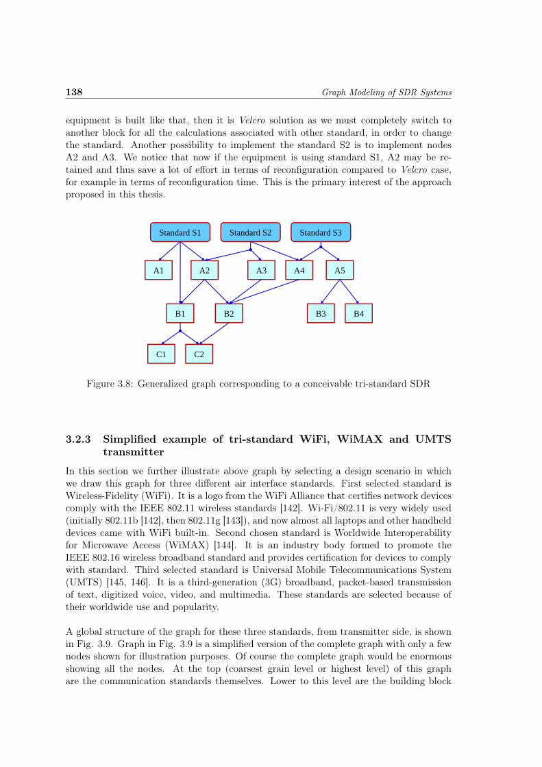
138 Graph Modeling of SDR Systems
equipment is built like that, then it is Velcro solution as we must completely switch toanother block for all the calculations associated with other standard, in order to changethe standard. Another possibility to implement the standard S2 is to implement nodesA2 and A3. We notice that now if the equipment is using standard S1, A2 may be re-tained and thus save a lot of effort in terms of reconfiguration compared to Velcro case,for example in terms of reconfiguration time. This is the primary interest of the approachproposed in this thesis.
Standard S1 Standard S2 Standard S3
A1 A2 A3 A4 A5
B4B1 B2 B3
C1 C2
Figure 3.8: Generalized graph corresponding to a conceivable tri-standard SDR
3.2.3 Simplified example of tri-standard WiFi, WiMAX and UMTStransmitter
In this section we further illustrate above graph by selecting a design scenario in whichwe draw this graph for three different air interface standards. First selected standard isWireless-Fidelity (WiFi). It is a logo from the WiFi Alliance that certifies network devicescomply with the IEEE 802.11 wireless standards [142]. Wi-Fi/802.11 is very widely used(initially 802.11b [142], then 802.11g [143]), and now almost all laptops and other handhelddevices came with WiFi built-in. Second chosen standard is Worldwide Interoperabilityfor Microwave Access (WiMAX) [144]. It is an industry body formed to promote theIEEE 802.16 wireless broadband standard and provides certification for devices to complywith standard. Third selected standard is Universal Mobile Telecommunications System(UMTS) [145, 146]. It is a third-generation (3G) broadband, packet-based transmissionof text, digitized voice, video, and multimedia. These standards are selected because oftheir worldwide use and popularity.
A global structure of the graph for these three standards, from transmitter side, is shownin Fig. 3.9. Graph in Fig. 3.9 is a simplified version of the complete graph with only a fewnodes shown for illustration purposes. Of course the complete graph would be enormousshowing all the nodes. At the top (coarsest grain level or highest level) of this graphare the communication standards themselves. Lower to this level are the building block

3.2 Graph theoretical models of multi-standards SDR systems 139
of these standards. At present, we have selected some of the important building blocks(transmitter side only) of the standards’ physical layer (PHY) for clarity purposes, butultimately, we aim at adding all the layers i.e., from application layer to PHY layer. Aswe move down to further lower levels in the graph, we pass through various granular-ity levels and finally we reach at the primitive elements level (finest grain level or lowestlevel). There might be many intermediate levels in between the top level and bottom level.
WiFi WiMAX UMTS
RandomiserConvolutional
Coder InterleaverConstellation
Mapper FFT-N RSEncoder
Scrambler Spreader
ButterflyLUT Real Spreader
Over Sampler
Adder MultiplierFlip Flop
Spreader Sampler
Adder MultiplierFlip Flop
NAND NOT XOR AND OR
Figure 3.9: Global structure of the graph for tri-standard SDR system (transmitter side),simplified version
Let us explore the Fig. 3.9 in bit more detail. Each operation in Fig. 3.9 is processedsequentially for each new block of incoming data. For instance, to implement WiFi weare to use the common operators (COs). Let us assume that the selected COs are FlipFlop (FF), Butterfly and XOR. Procedure for selection of these operators is outlined innext chapters. We need to call a common operator different number of times to performthe functionality of WiFi. This is the way, how our graphical approach of Fig. 3.9 has tobe interpreted. One box e.g. Butterfly, corresponds to one call. For instance, to imple-ment FFT-N, this box will be called (N/2)× log2N times. (N/2)× log2N is a parameterattached with the arrow from FFT-N to Butterfly block just as different parameters areassociated with arrows as explained in next chapters. Inside each operation there is aneed to make scheduling as it is necessary to call FF/XOR/Butterfly operators severaltimes. This scheduling issue which is a consequence of common operators approach hasbeen partially addressed in [118].
From the graph of Fig. 3.9, it is clear that there are many ways to perform the function-ality of a PE and to draw all these possibilities in a graph is a tedious job. This is not thepurpose of this thesis to develop complete graphs. Graphs that will be used are providedby other studies e.g. identification of joint operations, which is also a task in itself, inde-

140 Graph Modeling of SDR Systems
pendent of the work of this thesis. Due to this fact, we often consider sub-graphs of thetotal graph that does not present standards at the top of the graph, and not necessarilycome to arithmetic operators and bottom of the graph. Let us consider a more specificscenario of a complete hypergraph of transceiver for multi-standards SDR system. Inthis scenario, we restrict ourselves to three main communication tasks i.e. channelization,equalization and OFDM and draw a partial hypergraph. These communication tasks arerequired by most of the air interfaces. Various alternatives to do perform these functionsare shown in Fig. 3.10.
Equalization Channelization OFDM
Channel per Channel Filter Bank
Multi-rate Filtering Digital Down Conversion
FIR Down Sampling CIC
FFT
Butterfly
CORDICMAC
Delay Multiplier Adder LUT
Figure 3.10: An example of partial hypergraph
Looking at this graph gives us the pictorial view of numerous alternatives that are availableto do the same task. This illustrates that the number of design alternatives can grow veryquickly. Although, we can estimate or intuitively deduce optimal choices on small graphs,it becomes very difficult for bigger graphs. For instance, for channelization, we can useeither channel per channel or filter bank approach. If we choose the filter bank approachthen this can be done by FFT. The same FFT can be used by OFDM and equalizationas well. Now the questions that comes in our mind are; We have different alternative butwhich one is the best? Best according to which criteria? Which path in the graph will giveus the optimal solution? To do this, first we have to put weights i.e. costs on the nodes ofour graph in order to derive a cost function and then we have to run some optimizationalgorithm to find the optimized path. These cost parameters and costs are discussed inchapter 4 while optimization algorithms are discussed in chapter 5.

3.3 Network theory reformulation 141
3.3 Network theory reformulation
3.3.1 Motivation
In the present section, we explore the possibilities of finding some smart algorithms whichfully utilizes the special structure of the graph to efficiently search the solution, by recastingour problem as a single- source (or single terminal (sink)) network-design problem. Thismove of ours’ is motivated by the fact that the network-design problem is well known andcounts with a very extensive literature, which offers algorithms, computational complexityresults and many practical applications in a variety of contexts such as telecommunication,transportation, water resources and even social interactions [147].
Below, we show how to perform the problem reformulation and give a specific examplegrounded on a practical design. In support of our approach, we identify and discuss severalspecific algorithms which seem particularly well suited to our purposes [148, 149, 150].
3.3.2 Network design problem
A simple illustration of the single-source network-design problem is shown in Fig. 3.11.Suppose that there is an initial point called the origin, O, and three terminals (desti-nations), t1, t2 and t3. We wish to connect O to each ti in a way that satisfies certainoptimality criteria. There may also be some intermediate nodes, which themselves maybe (partially) interconnected. There are many conceivable solutions. The most obviousone is simply to build three direct roads, one from O to t1, a different one from O to t2and a third one from O to t3. This solution is certainly plausible and probably providesthe shortest travel times, but it is unlikely to be ideal. By building dedicated roads, weare possibly missing the savings resulting from having common segments which may beused by all traffic, regardless of the destination. For example we could build a road fromO to some intermediate point A, plus dedicated segments from A to each ti. Becausethe segment O → A is used by all traffic, certain savings may result (although this maylengthen the travel time to all traffic).
By the same reasoning, building dedicated segments from A to each ti may not be optimal.Perhaps we can build a dedicated road A → t3, but also a segment from A to someintermediate point B, followed by segments B → t1 and B → t2. In the latter proposal,all traffic would travel over the O → A segment, the t3 traffic would go directly overA → t3 while both the traffic to t1 and to t2 would continue over A → B, and from Bover B → t1 and B → t2, respectively. There may be many other possibilities
3.3.3 Graph to network conversion
Our problem can be recast as a network-design problem by proceeding as follows. Thecommunication standards correspond to terminals we wish to reach. Building a directroad from the origin to each terminal corresponds to the Velcro solution: choosing a self-contained dedicated complex component to support each standard. This will provide thefastest routes to be sure, but probably not the ideal solution. Installing a self-containedcomponent of medium complexity is the equivalent of building a road from the origin to theintermediate point A in the example above. For instance, [17] shows that many importanttasks of a communication receiver can be implemented through the FFT as mentioned

142 Graph Modeling of SDR Systems
t1t1
B
t2
B
O A
t33
Figure 3.11: A simple single-source network design problem
earlier. In turn, the FFT functionality can be implemented with a butterfly operator.Thus, we can build a road from the origin to the FFT (i.e. install a self-contained FFTcomponent) to be shared by several tasks. This will likely reduce the overall cost of thedesign, although it will generally increase the travel time. But we could also reach the FFTnode (i.e. provide the functionality of the FFT operator), by first building a road from theorigin to the intermediate junction butterfly and from there utilize an existing road to theFFT (i.e. install a self-contained butterfly component, and invoke it repeatedly to providethe FFT functionality).
The network-design problem, corresponding to a section of the partial hypergraph of de-sign choices given by Fig. 3.10 is shown in Fig. 3.12. The parts of the graph that concernlowest level components and the channelizer have been ignored for pedagogical reasons.
Recall that now the objective is to build a road network that provides a path from theorigin to each terminal. The solid arrows mark free (pre-built) roads that take time totravel, but require no monetary expenditure. These represent known algorithms which canbe used to provide a higher level functionality. For example from the FFT node there is apre-built (free) road to OFDM, another to equalization and yet another to the FIR node,because there are known algorithms that allow the implementation of equalization, OFDMand FIR through the FFT operator [17]. The dashed arrows indicate possible roads thatdefinitely cost money to build (but possibly negligible time to travel).
Building a road means installing a self-contained component to provide the functionalitypointed by the arrow. For example there is a dashed arrow from the origin to FFT (mean-ing we can provide the FFT functionality by installing a self-contained FFT component).There is also a possible road from the origin to butterfly. If we build this road (i.e. if weinstall a self-contained butterfly component) we can reach the FFT node via a free (algo-rithmic) path (shown by a solid arrow from butterfly to FFT), because one can providethe FFT functionality by repeatedly invoking a butterfly operator. Fig. 3.13 shows in
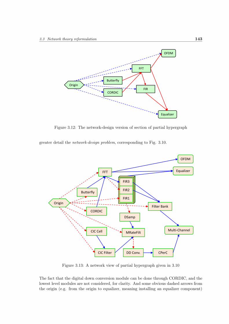
3.3 Network theory reformulation 143
OFDM
FFT
ButterflyOrigin
CORDICFIR
EqualizerEqualizer
Figure 3.12: The network-design version of section of partial hypergraph
greater detail the network-design problem, corresponding to Fig. 3.10.
OFDM
Equalizer
FIR3
FFT
Butterfly
FIR3
FIR2
CORDIC
OriginFIR1
Filter BankCORDIC
DSamp
Multi‐ChannelCIC Cell MRateFilt
CIC Filter DD Conv CPerCCIC Filter DD Conv. CPerC
Figure 3.13: A network view of partial hypergraph given in 3.10
The fact that the digital down conversion module can be done through CORDIC, and thelowest level modules are not considered, for clarity. And some obvious dashed arrows fromthe origin (e.g. from the origin to equalizer, meaning installing an equalizer component)

144 Graph Modeling of SDR Systems
are omitted to reduce clutter. The main purpose of Fig. 3.13 is to show that representingthe AND dependencies is challenging in some cases, and may require some ingenuity andadditional research. The FIR triple node illustrates some of the main issues. A tripleFIR node is used in Fig. 3.13 to show that there are three different routes to get theFIR functionality, and the route has an impact on what can be done from there. Thesub-node FIR3 concerns the case where the FFT is used to implement the FIR. The sub-node FIR2 refers to the case when an FIR component is installed, even though the FFTfunctionality is present (this may be done to reduce execution time). FIR1 denotes a casein which an FIR component is installed and the FFT functionality is not available (perhapsOFDM and equalizer dedicated components have been installed, and the FFT module isunnecessary). In the cases FIR2 and FIR3, the functionality of the filter-bank module canbe achieved algorithmically, because both the FFT and the FIR are available. However,under FIR1, there is no FFT module, thus, the filter-bank functionality would require aninstalled component. For this reason, there is no arrow pointing to the filter-bank modulefrom the FIR1 sub-node. On the other hand, the solid arrow pointing to the equalizerfrom the FIR is drawn from the oval, around the various FIR sub-nodes. This indicatesthat we can achieve equalization through the FIR, irrespective of how we achieve the FIRfunctionality (contrary to the filter-bank case).A simpler case of AND dependency is also shown in Fig. 3.13, which involves achievingmulti-rate filtering (MRateFilt) through both FIR and down sampling (DSamp). Thedash line from the FIR oval to DSamp, followed by a solid arrow from DSamp to MRate-Filt, shows that if we have the FIR functionality (no matter how) and we install (build aroad to) a down sampler, then we can achieve multi-rate filtering for free (algorithmically).
The reformulation of this provides us with several well-studied algorithms. A network-design problem with two metrics: cost and distance is described in [148]. This fits well withour formulation, with execution time as distance but this algorithm is probabilistic. [149]modifies it to make it deterministic, utilizing linear programming. The basic idea of [148] isas follows: The algorithm has several stages. At each stage, it forms a matching (pairing)of terminal nodes (not previously eliminated). Then, of each pair of nodes, it choosesa center. At this point, the non-center nodes are removed from further considerationand a new stage of the algorithm starts (with a new matching among the centers only).Because for us, the terminals correspond to standards to be supported by the radio, theyshould be relatively few. Thus, this algorithm will give an answer in a relatively shortnumber of stages. The algorithm provided in [150] minimizes costs, while keeping length(time/latency) under a specified budget. These and many other algorithms available inthe rich network-design literature are to be explored to find the best fit for our purposes.However because of the problems involved in the conversion of the hypergraph to network-design especially from the AND hyperarc point of view because it fast becomes impossibleto manage complex AND hyperarc relations as mentioned earlier, we keep our energiesfocused on the hypergraph design for multi-standards systems.
3.4 Conclusions
After stating the common operators’ technique of parametrisation and then illustratingthe theoretical approach of finding common operators in chapter 2 we tried in this chapter

3.4 Conclusions 145
to address the question of defining a suitable graph model of multi-standard SDR systems.After exploring different possibilities we came up with the idea of modeling the graph ashypergraph to meet our needs. We also explored an other perspective of conceiving thehypergraph as a network design problem which was a study done by a post doctoral fellowin our laboratory [20]. Due to the unsuitability of the network design approach because ofcomplex relations of AND hyperarcs we reverted back to the hypegraph approach to modelmulti-standards SDR systems. After having the graph, now we are faced with the task ofputting the weights to the nodes and arcs of hypergraph. Theses weight parameters thatare to be associated with graph entities i.e. with nodes and arcs are discussed in detail inchapter 4.


Chapter 4
Cost Parameters and Costs forOptimization of Multi-StandardsSDR Systems
Contents4.1 Introduction . . . . . . . . . . . . . . . . . . . . . . . . . . . . . 1474.2 Cost parameters . . . . . . . . . . . . . . . . . . . . . . . . . . . 1484.3 Types of costs . . . . . . . . . . . . . . . . . . . . . . . . . . . . 149
4.3.1 Analytical costs . . . . . . . . . . . . . . . . . . . . . . . . . . . . 1504.3.2 Implementation costs . . . . . . . . . . . . . . . . . . . . . . . . 1514.3.3 Execution Costs . . . . . . . . . . . . . . . . . . . . . . . . . . . 155
4.4 Approaches to formulate cost/objective function . . . . . . . 1554.4.1 Weighted sum approach . . . . . . . . . . . . . . . . . . . . . . . 1574.4.2 Objective function . . . . . . . . . . . . . . . . . . . . . . . . . . 158
4.5 Graphical user interface . . . . . . . . . . . . . . . . . . . . . . 1594.6 Conclusions . . . . . . . . . . . . . . . . . . . . . . . . . . . . . . 163
4.1 Introduction
Graph modeling of different SDR systems gives us a pictorial view of available alternativesto perform the same tasks. To determine that which alternative is best suited for a giventask we try to convert this graph in an optimization problem. The graphs can be trans-lated in a boolean formula with respect to AND and OR arcs and then can be solved bysome optimization technique. To do this we are to find and associate the necessary costparameters and costs with graph models.
In this chapter we start our discussion with different cost parameters and types of thecosts. These costs can be analytical costs or implementation costs. Analytical costsdepend upon the mathematical equations/operations behind a particular task while im-plementation costs depend upon the chosen target technology. Then we discuss the digital
147

148 Cost Parameters and Costs for Optimization of Multi-Standards SDR Systems
hardware composition of SDR in section 4.3.2.1 which is a key design step in its creation.The hardware design is, of course, much more complex for a software radio than a con-ventional radio because of the software radio’s additional capability. In section 4.3.2.4, weprovide a brief summary of general algorithmic partitioning for three foundational digitalhardware available: DSPs, FPGAs and ASICs. We describe which tasks are suitable forwhich hardware technology. Each exhibits a certain level of re-programmability, that is,an ability to alter device hardware or software. Based on the selected costs associated withdifferent graph components we formulate our cost/objective function which is presentedin section 4.4. Our objective function represents a multi-objective optimization problem(MOP). Objective functions corresponding to MOPs form a mathematical description ofperformance criteria which are usually in conflict with each other. Finally a conclusions’section ends this chapter.
4.2 Cost parameters
There can be many cost parameters, among them, we consider that the building cost (BC)of processing elements (PE), computational cost (CC) of the PE of the systems and Num-ber of Calls (NoC) are the principle ones that are to be associated with entities (PE andarrows) of graph models.
The two identified cost parameters that we think appropriate to be associated with pro-cessing elements (PE) of the graph are explained below:
• Building cost of processing element that is capable of computing a function. Bybuilding cost of the PE we mean its installation cost. This cost can be considered asimplementation cost of PE. BC is paid once during the useful life of a radio system.If it is required to call several a PE in equipment, the BC associated with elementis not multiplied. Re-use of PEs thus provide an idea of cost reduction.
• Computational cost of the PE. By computational cost of the PE we mean the timetaken by a PE to compute a function. This cost is incurred every time a PE isinvoked or called by higher PE.
These costs can be thought of in terms of number of multiplications, number of additions,number of LUT, number of slices, number of gates, number of execution cycles, area,power, execution time, just to name a few.
Let us consider the cost parameters that are to be associated with arrows of the graph.The graph of any system consists of various granularity levels [118]. The task at highergranularity level can be performed with the aid of components that are at lower granularitylevel with less building cost but with more time. Hence we call the parameter associatedwith the arrows, number of calls (NoC), i.e. number of times a processing element atlower granularity level n− 1 will be called to perform the task of the component at highergranularity level n. This means that same task can be performed by a PE at level ninstead of PE at level n-1, in less time but with much higher cost and vice versa.

4.3 Types of costs 149
In general, a node having higher hierarchy has a higher building/manufacturing cost thanthe nodes with lower hierarchy that it calls. Similarly, the execution time of a node withhigher hierarchy is usually lower than all the executions and calls needed to be done tomake the same calculation using the lower hierarchy nodes.
To elaborate further, we consider the concrete case of a hardware implementation, whereBC represents a cost in number of gates (or area), as for an FPGA or digital ASIC im-plementation. In the example of a filter processing, there are many design options. Somedesigners will try to parallelize their architectures in order to gain in speed of executionbut at the cost of an additional area. This is the case of the higher hierarchy element.However, in order to save in terms of area (building cost), it is possible to call severaltimes a single unit of type MAC (Multiply Accumulate), which would be the element oflower hierarchy with a much lower area cost (building cost) and may also have a lowercomputational cost, but which will be required many times (number of calls from the arcconnecting the filter to the MAC) in a sequential manner to perform filtering. The result-ing computational cost becomes more expensive than the building cost of the filter alone.Hence it is clearly evident that we need to find compromises; 1) between complexity andspeed of execution and 2) between the top and bottom of the graph i.e. between fine andcoarse granularity.
For a deeper insight, let us explain Fig. 4.1, that reconsiders the example of Fig. 3.10with parameters’ values that are chosen arbitrarily. Fig. 4.1 shows the graph model ofa standard that requires OFDM, Equalization and Channelization. Costs are associatedwith entities of the graph of Fig. 4.1. PEs are tagged with BC/CC e.g. Multiplier istagged with 10/5 i.e. building cost is 10 and CC is 5. Arrows are tagged with NoC e.g.x10 means that higher PE will call the lower PE 10 times. It is to be noted that these pa-rameters’ values are not the real ones but chosen arbitrarily. They have no reality here interms of time or number of gates, but they follow a certain logic on relationships betweenparameters of the same nature. We see that an FIR can be used for a building cost of500 and a computational cost of 1000, or an alternative design is to implement the threeoperators Delay, Multiplier and Adder for a total building cost of 1 + 10 + 4 = 15 and acomputational cost of 1 + 5 + 2 = 8 (if we consider a sequential execution because of datadependencies). But it is necessary to call each of three operators 180 times to perform thefunctionality of FIR with a total execution cost of 180× 8 = 1440.
In some SDR architectures, BC can also be represented by the number of logic unitsrequired by an FPGA implementation e.g. number of ALUTs etc. This allows severalstandards to use the same components and share their costs and this is exactly what theconcept of common operators is all about. The CC parameter requires more consideration.Some nodes will be implemented by invoking several descendant nodes, each a certainnumber of times, where we may use an average number if this is not constant.
4.3 Types of costs
In this section we investigate a bit further the available choices for different building costs.Determining these costs is a very importance step in optimization procedure, and hence,

150 Cost Parameters and Costs for Optimization of Multi-Standards SDR Systems
Equalization Channelization OFDM
Channel per Channel Filter Bankx1
Multi‐rate Filtering Digital Down Conversion
FIR Down Sampling CIC
500/1000 x2
x2 x1
FFT
1000/500
Butterfly
15/20
x180 x180 x180
x2x2x4
CordicMAC
15/815/8x4 x6
x2
x2x2
Delay Multiplier Adder LUT
1/1 10/5 4/2 1/1
Figure 4.1: Graph model with associated costs; PEs tagged with BC/CC and arrowstagged with NoC
a fair number of various possibilities have been considered. The costs can be divided intothree major categories.
• Analytical costs
• Implementation costs
• Execution costs
These costs are discussed in detail in the following section.
4.3.1 Analytical costs
These costs are a result of the analysis of computational complexity of different PEscomposing air interface standards. This analysis gives us the estimates of number ofrequired basic operations per output data item in each function. The basic operationsinclude the following:
• Arithmetic operations
• Logic operations and
• Memory load/store operations

4.3 Types of costs 151
Analytical costs are based on actual calculation of above mentioned basic operations.These costs can be quite different from implementation costs. The implementation costswill be based on selected hardware for SDR implementation as discussed in section 4.3.2.
Complexity evaluation of IEEE 802.11a and UMTS
In this section we present the computational complexity of major transceiver tasks of IEEE802.11a [151] by estimating the number of required basic operations per output data itemin each task. We also present the computational complexity of UMTS (FDD mode), Uplinktransmitter blocks and Downlink receiver blocks, according to particular test cases definedin 3GPP specification documents [145, 146]. The analytical costs of different transmit andreceive tasks of IEEE 802.11a (by evaluating the computational complexity) are given inTable B.1 and Table B.2 respectively of Appendix B. The complexity figures mentionedin Tables B.1 and B.2 are computed with the help of [152, 153]. The results of analysis incase of UMTS, are given in Appendix B’s Table B.3 and Table B.4. The complexity figuresmentioned in Table B.3 and Table B.4 are derived from [154]. Having the computationalcomplexity at hand now, here comes one major question; How we can use these complexityfigures as costs?
As far as the complexity figures are concerned, we have different types of basic operationsfor different functions in selected standards. From the computational analysis of IEEE802.11a presented in Table B.1 and Table B.2 it becomes clear that on the transmitterside IFFT is the most computationally complex task while Viterbi decoding and FFTdominates the complexity on the receiver side. Based on this conclusion we decided thatnumber of multipliers and adders can be used as BC. The tasks that are related to LUTaccesses e.g. Interleaving etc., can be considered to be some sort of addressing schemeand is not computationally intensive. In case of UMTS also, we have counted only thearithmetic operations. Logical operations have been neglected because they are basis cellsin hardware and thus much simpler than multiplier or adder. The complexity figuresshown in Appendix B’s Table B.1 and Table B.2 can be drawn for IEEE 802.16 withminor difference in some functions e.g. FFT etc.
4.3.2 Implementation costs
We can envision that the implementation costs are a direct consequence of selected hard-ware for the implementation of SDR terminals. Details of these available hardware withtheir pros and cons are presented in the following section.
4.3.2.1 Digital hardware choices
Requirements for SDR’s signal processing are very demanding. Tasks for SDR are quiteheterogeneous, ranging from data flow processing of the baseband signals, error correctionon bit level, sophisticated protocol handling, and on top level, the operating systems forapplications. This implies that several processor technologies should be used for SDRdesigns. For maximum flexibility, all functions of SDR mobile terminal should be definedin software. However, because of computing requirements, implementing them in software

152 Cost Parameters and Costs for Optimization of Multi-Standards SDR Systems
over strains the possibilities of even sophisticated VLIW DSPs. Furthermore, power con-sumption, silicon area, and last but not the least, engineering time and development costsfor new products must be minimized.
Real-time SDR hardware can be built using a variety of digital hardware consisting ofFPGAs, DSPs and ASICs. While a DSP represents the most generalized type of hardwarethat can be programmed to perform various functions, an ASIC is the most specializedpiece of hardware and can be used only in the specific application for which it has beendesigned. An FPGA offers a compromise in flexibility between an ASIC and a DSP.
4.3.2.2 Field programmable gate arrays
The first breakthrough in SDR came with the use of FPGAs. FPGAs were developed inthe mid-1980s as an alternative to glue logic arrays and DSPs. FPGAs are commonly usedin logic emulation and prototyping in most systems. They are ideal for prototyping sincethe chips are reusable after the bugs have been fixed or the system has been upgraded.Though software simulations can verify the accuracy of a circuit, they do so at a muchslower rate than logic emulation circuits using FPGAs. Though the mapping of the circuitto the FPGA takes a long time to complete, once it is done, the system can evaluate thecircuits at millions of cycles per second.
In the case of software radios, FPGAs have the additional advantage of adding adaptabilityand flexibility in the final product. FPGAs at times can also help conserve silicon areasince one chip can be configured to perform more than one function and the configurationscan be changed on-the-fly. The following is a list of situations in which the use of FPGAsin digital signal processing applications is most beneficial:
• Systems with high sample rates
• Systems involving variable or non-conventional word length FPGA-based DSP de-signs because they are more efficient since the word length on the FPGA can be setexactly to the required length
• Systems with very-high-order FIR filters because the algorithm can be implementedin parallel decreasing the time required
• Systems with fast correlators because the LUT architecture of FPGAs provides afast and efficient way to build correlators.
In the case of FPGAs the cost parameters that we can use are number of slices, number ofCLB, number of LUT, number of Logic Cells, number of Flip Flops, etc. In design scenariopresented in section 6.4 we use number of ALUTs as building cost of the communicationblock (CB)/processing element (PE). The design scenario presented in section 7.4.2 usesnumber of logic cells (LC) as building cost of CB/PE. In these scenarios we have consideredthe building costs that are based on the FPGA implementations. We may consider thesecosts based on DSP implementations (number of cycles). However, we prefer to use thecosts based on FPGA hardware implementation. The reasons for doing this are explainedin the forthcoming section 4.3.2.4.

4.3 Types of costs 153
Table 4.1: IEEE 802.11a and IEEE 802.16 implementation on FPGA
Area Metrics for a XC2V3000-4FG676 Device
IEEE 802.11a IEEE 802.16-2004
Parameter Used % Used %
Number of Slices 1678 11 2614 18
Number of Slice Flip Flops 2353 8 3566 12
Number of 4 input LUTs 2814 9 4304 15
Number of Bonded IOBs 29 5 29 5
Number of BRAMS 12 12 12 12
Number of GCLKs 1 6 1 6
Example of FPGA based costs
In this section we present an example of FPGA based costs as discussed above. InTable 4.1 we have costs in terms of different parameters of FPGA e.g.number of slices,number of LUTs, etc. These parameters can be used as building costs in our optimizationtool. In this table costs are given for the full implementation of IEEE 802.11a and IEEE802.16-2004 on selected device of Xilinx family of FPGAs [33, 34]. However, we can getthese cost figures for different functions of these air interface standards e.g. scrambling,convolutional coding, interleaving etc. This point is further illustrated in part III of thisthesis where design scenarios are discussed.
4.3.2.3 Digital signal processors
The DSP is essentially a microprocessor optimized for digital signal processing applica-tions. DSPs are flexible because they can be programmed repeatedly even with a high-levellanguage (HLL) like C. Modifications and upgrades can be made via this HLL, reducingthe design time for each iteration. The flexibility, however, sometimes comes at the cost ofefficiency. For instance, applications requiring several computations that could be done inparallel may have to be broken into sets of sequential computations based on the numberof multipliers/accumulators available on the DSP.
Even if the DSP has provisions for parallel execution of instructions, like parallel multiplyand accumulate (MAC) DSPs, the size and number of units are fixed, and they may notbe optimal for a particular task. In general, the more processing per data sample, themore cycles needed and the slower the data is processed. One way to reduce the execution

154 Cost Parameters and Costs for Optimization of Multi-Standards SDR Systems
Table 4.2: DSP Blackfin processor performance on DSP functions
Function Cycle Count
N sample T tap real FIR filter NT/2
N sample B stage Biquad IIR filter 5NB/2
N sample T tap convolution NT/2
N dimensional vector sum N
Complex FFT Radix-2 butterfly 3
256-point complex FFT (Radix-2) 3176
256-point complex FFT (Radix-4) 2630
Viterbi for GSM (16 states, 378 soft decision symbols) 6069
time is to employ more than one DSP to implement an algorithm. However, coordinatingthese DSPs is a challenging task for the programmer. Other solutions include using lessgeneralized hardware, which can be configured to optimize a particular application.
Gate arrays offer the designer a higher degree of parallelism than DSP. An ASIC goes astep further than the gate array, where the entire IC including the positioning of the logicgates are determined by the designer. ASICs are generally used when a DSP has insuffi-cient processing power or when the system has a sufficiently high volume of production tojustify a custom solution.
Example of DSP based costs
In this section we present an example of DSP based costs as discussed above. In Table4.2 we have costs in terms of cycle counts for a Blackfin processor. The Blackfin DSPprocessor [155] is a recent technology development targeted at cellular handset applicationsand is very appealing for SDR development [62]. Number of cycle counts can be used asexecution costs in our optimization tool. However finding the costs in terms of cyclecounts is more difficult than finding the costs in terms of FPGA parameters. Determiningthe BC in case of DSP based solution is extremely difficult. For the BC, when systemimplementation on DSP is considered, the designer may put a fixed price cost for thehardware architecture of the DSP.

4.4 Approaches to formulate cost/objective function 155
4.3.2.4 Algorithmic partitioning of typical transceiver tasks
ASICs to FPGAs to DSPs represent the options for a designer ranging from high speedand minimum flexibility to maximum flexibility and very little hardware optimization.While general communication problems of relatively low complexity can be solved witha DSP, FPGAs and ASICs tend to be more useful when the complexity of the problemincreases as in 3G and 4G wireless communication systems or when the product has to bemanufactured in large volumes.
In this section we explore form algorithmic point of view that why designer of SDR systemsconsider FPGAs as their first choice? A multi-standard SDR terminal require the imple-mentation of several protocols as desired by designer. Wireless protocol implementationstasks can be divided into two algorithmic categories:
• Control Flow
• Data Flow
The data flow part is delineated by extensive arithmetic computations on data streams.These algorithms provide most of the processing needs of the standards. These algorithmsprovide implicit parallelism and are best suited to run on hardware that can exploit thisparallelism such as reconfigurable hardware. The tasks for several standards with the besthardware technology to realize them, are given in Table. 4.3.
We are concerned here with the data flow category since our work is related to the opti-mization of air interface protocols at physical layer level. Apart from other air interfacewe mainly concentrate on the systems based on OFDM because of the advantages thatwe may have as explained in design scenarios of part III. Hence in design scenarios, costparameter of PE are principally based on reconfigurable hardware/processors i.e. FPGAsalthough other options can also be explored. This choice is based on the fact that thefunctions that are related to the data flow are considered to be performed best by FPGAs.Arguments of Table. 4.3 [62] reinforces our choice.
4.3.3 Execution Costs
Execution cost is clearly a function of time required by a processing element to do itsown calculations in order to achieve its functionality. The execution time can thereforeact as a good execution cost, whatever is the target of implementation. In the case ofimplementation on a processor, the number of cycles necessary for the execution of aprocessing element can also be considered a cost execution.
4.4 Approaches to formulate cost/objective function
Multiobjective optimization also known as multi-criteria or multi-attribute optimization iswith no doubt a very important research topic both for scientists and engineers because ofthe multiobjective nature of most real world problems. In Operations Research more than20 techniques have been developed over the years to try to deal with functions that havemultiple objectives, and many approaches have been suggested, going all the way from

156 Cost Parameters and Costs for Optimization of Multi-Standards SDR Systems
Table 4.3: Algorithm partitioning of typical baseband processing tasksTechnology Tasks ArgumentsDSP/ Protocol stacks and management. Complex software structure withMicrocontroller Portion of channel estimation, large decision trees. Requires
control flow type of processing. little raw arithmetic or notcontinuous usage.Signal processing tasks thatdo not require continuousprocessing can be executed.
Hardwired FEC Viterbi decoder or turbo decoderfunctions CDMA Hardwired functions require
minimum energy and areaAnalog Currently no programmableRF solution expected.
Reconfigurable Rake receiver, correlations, These algorithms require most ofArchitecture searcher, header detection, arithmetic processing power.
channel correction, Requires real time processingdownsampling, FFT, of data streamsdemodulator, short PN code
naïve combinations of objectives into a single one to the use of game theory to coordinatethe relative importance of each objective. However, the fuzziness of this area lies on thefact that there is no accepted definition of optimum as in single-objective optimization,and therefore is difficult to even compare results of one method to another, because nor-mally the decision about what the best answer corresponds to the so-called human decisionmaker.
The approach of combining objectives into a single function is normally denominated ag-gregating functions, and it has been attempted several times in literature with relativesuccess in problems in which the behavior of the objective functions is more or less known[35, 156]. There are many popular aggregating approaches like weighted sum approach,goal programming, the ε-constraint method, etc.
Weighted sum approach was the first technique for the generation of non-inferior solutionsfor MOPs. This method is very efficient (computationally speaking). The problem withthis approach is how to determine the appropriate weights when we do not have enoughinformation about the problem. Goal programing may be a very efficient approach if weknow the desired goals that we wish to achieve. However, the decision maker is given thetask of devising the appropriate weights or priorities for the objectives that will eliminatethe non commensurable characteristics of the problem, which is most cases is difficultunless there is prior knowledge about the shape of the search space [35, 156]. ε-constraintmethod is based on minimization of one (the most preferred or primary) objective function,and considering the other objectives as constraints bound by some allowable levels εi.This method is time consuming, and coding of the objective functions is difficult, or evenimpossible for certain problems, particularly if there are too many objectives [35, 156].

4.4 Approaches to formulate cost/objective function 157
Hence we consider only the weighted sum approach to define our objective function becauseof its popularity and simplicity.
4.4.1 Weighted sum approach
This method consists of adding all the objective functions together using different weight-ing coefficients for each of them. This means that our multiobjective optimization problemis transformed into a scalar optimization problem of the form:
mink∑
i=1
ωifi(x) (4.1)
where ωi ≥ 0 are the weighting coefficients representing the relative importance of theobjectives and fi represents the ith objective function of vector of decision variables x. Itis usually assumed that,
k∑i=1
ωi = 1 (4.2)
Since the results of solving an optimization model using equation (4.1) can vary signifi-cantly as the weighting coefficients change, and since very little is known about how tochoose these coefficients, a necessary approach is to solve the same problem for many dif-ferent values of ωi. But in this case, the designer is still, of course, confronted with thedecision of having to choose the most appropriate solution based on his/her intuition.
Note that the weighting coefficients do not reflect proportionally the relative importanceof objectives, but are only factors which, when varied, locate points in the Pareto set [157].For the numerical methods that can be used to seek the minimum of equation (4.1), thislocation depends not only on ωi values, but also on the units in which the functions areexpressed.
If we want ωi to reflect closely the importance of all the objectives, all functions should beexpressed in units of approximately the same numerical values. Additionally, we can alsotransform equation (4.1) to the form:
mink∑
i=1
ωifi(x)ci (4.3)
where ci are constant multipliers that will scale properly the objectives.
Many applications that uses this technique can be found in literature. Syswerda andPalmucci [158] used weights in their fitness function to add or subtract values during theschedule evaluation of a resource scheduler. Wilson and Macleod [159] used this approachas one of the methods incorporated into a GA to design multiplier-less IIR filters in whichthe two conflicting objectives were to minimize the response error and the implementationcost of the filter. Jakob et al. [160] used a weighted sum of the several objectives involvedin a task planning problem. Some other examples can be found in [161, 162, 163].

158 Cost Parameters and Costs for Optimization of Multi-Standards SDR Systems
Based on the approach described above we develop our objective function in followingsection, and this function will be optimized by our optimizer tool.
4.4.2 Objective function
In this section we describe the development of our objective function. There are two keyparameters that will enter in our cost/objective function i.e. building cost and computa-tional cost. Details of these parameters have already been discussed in section 4.2. Basedon these parameters we have two objectives that are conflicting in nature. If we want tominimize building cost then computational cost will increase and vice versa. Hence wewant to find a the balance between economy and computation efficiency.
Let us start developing cost function which is a bi-objective function:
Our first objective is to minimize the building cost. This can be written as:
min∑
i
BCi.Ni (4.4)
where
• BCi denotes the building cost of ith component in the system.
• Ni ∈ 1, 0 indicates if the ith node is present in the system or not.
•∑i
BCiNi is the total building cost of all the components that are present in the
SDR system.
Now let us consider our second objective i.e. to minimize the computational cost. Thiscan be written as:
min∑
k
CCk (4.5)
where
• CCk denotes the computational cost of kth component in the system.
Since we are concerned with the optimization of a multi-standards SDR systems, (4.5) cantake the form:
min∑
n
∑k
CCk((Sn)n ∈ N) (4.6)
where
• ((Sn)n ∈ N) indicates that there may be n standards present in an SDR wheren = 1, 2, . . . , N i.e. if we choose N = 3 then it means that there are threestandards namely S1, S2 and S3 present in an SDR system.
•∑k
CCk((Sn)n ∈ N) is the total computational cost of any of Sn,
where n = 1, 2, . . . , N.
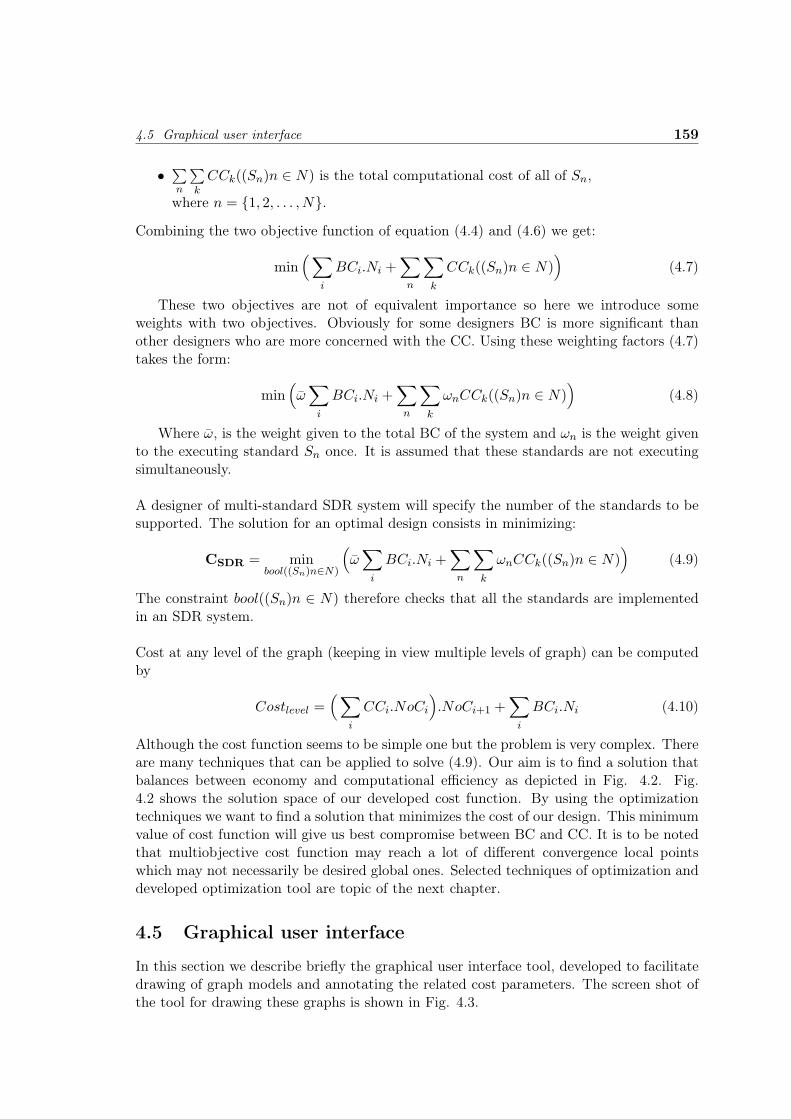
4.5 Graphical user interface 159
•∑n
∑k
CCk((Sn)n ∈ N) is the total computational cost of all of Sn,
where n = 1, 2, . . . , N.
Combining the two objective function of equation (4.4) and (4.6) we get:
min( ∑
i
BCi.Ni +∑
n
∑k
CCk((Sn)n ∈ N))
(4.7)
These two objectives are not of equivalent importance so here we introduce someweights with two objectives. Obviously for some designers BC is more significant thanother designers who are more concerned with the CC. Using these weighting factors (4.7)takes the form:
min(ω
∑i
BCi.Ni +∑
n
∑k
ωnCCk((Sn)n ∈ N))
(4.8)
Where ω, is the weight given to the total BC of the system and ωn is the weight givento the executing standard Sn once. It is assumed that these standards are not executingsimultaneously.
A designer of multi-standard SDR system will specify the number of the standards to besupported. The solution for an optimal design consists in minimizing:
CSDR = minbool((Sn)n∈N)
(ω
∑i
BCi.Ni +∑
n
∑k
ωnCCk((Sn)n ∈ N))
(4.9)
The constraint bool((Sn)n ∈ N) therefore checks that all the standards are implementedin an SDR system.
Cost at any level of the graph (keeping in view multiple levels of graph) can be computedby
Costlevel =( ∑
i
CCi.NoCi
).NoCi+1 +
∑i
BCi.Ni (4.10)
Although the cost function seems to be simple one but the problem is very complex. Thereare many techniques that can be applied to solve (4.9). Our aim is to find a solution thatbalances between economy and computational efficiency as depicted in Fig. 4.2. Fig.4.2 shows the solution space of our developed cost function. By using the optimizationtechniques we want to find a solution that minimizes the cost of our design. This minimumvalue of cost function will give us best compromise between BC and CC. It is to be notedthat multiobjective cost function may reach a lot of different convergence local pointswhich may not necessarily be desired global ones. Selected techniques of optimization anddeveloped optimization tool are topic of the next chapter.
4.5 Graphical user interface
In this section we describe briefly the graphical user interface tool, developed to facilitatedrawing of graph models and annotating the related cost parameters. The screen shot ofthe tool for drawing these graphs is shown in Fig. 4.3.
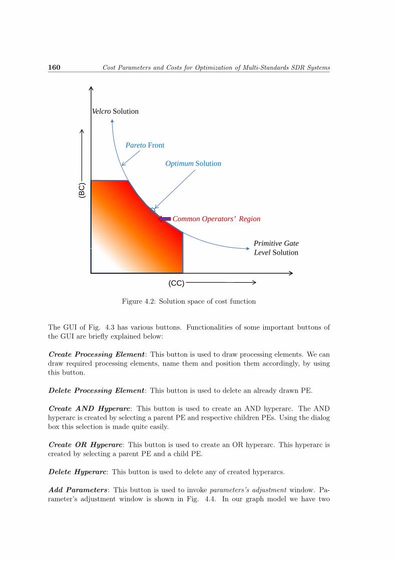
160 Cost Parameters and Costs for Optimization of Multi-Standards SDR Systems
Velcro Solution
Optimum Solution
Pareto Front
(BC
)
Primitive Gate
Common Operators’ Region
(CC)
Level Solution
(CC)
Figure 4.2: Solution space of cost function
The GUI of Fig. 4.3 has various buttons. Functionalities of some important buttons ofthe GUI are briefly explained below:
Create Processing Element : This button is used to draw processing elements. We candraw required processing elements, name them and position them accordingly, by usingthis button.
Delete Processing Element : This button is used to delete an already drawn PE.
Create AND Hyperarc: This button is used to create an AND hyperarc. The ANDhyperarc is created by selecting a parent PE and respective children PEs. Using the dialogbox this selection is made quite easily.
Create OR Hyperarc: This button is used to create an OR hyperarc. This hyperarc iscreated by selecting a parent PE and a child PE.
Delete Hyperarc: This button is used to delete any of created hyperarcs.
Add Parameters : This button is used to invoke parameters’s adjustment window. Pa-rameter’s adjustment window is shown in Fig. 4.4. In our graph model we have two

4.5 Graphical user interface 161
Figure 4.3: Screen shot of GUI for drawing graph models
entities i.e. processing elements (PEs)/blocks and hyperarcs (OR and AND). The purposeof this window is, firstly, to list all the parameters that can be associated with these twoentities and secondly, to associate the appropriate parameters and their values with re-spective graph entities. All this is done by using this window. In this window we have thefollowing functions that give us all the statistics of graph model and help us in parameters’adjustment.
• Parameters of Processing Elements
• List of Processing Elements
• Parameters of Hyperarcs
• List of OR hyperarcs
• List of AND hyperarcs
Parameters of Processing Elements, lists all the parameters that are associated with theprocessing elements. We can expand the drop down box in Fig. 4.4 to see all of theseparameters. Here we have the options to add new parameters for the PEs, delete and/orrename existing parameters. List of Processing Elements gives a list of all the PE used tograph model the multi-standards SDR equipment. By using the drop down box in Fig. 4.4we can see all the processing elements that are present in the graph model. We can select

162 Cost Parameters and Costs for Optimization of Multi-Standards SDR Systems
Figure 4.4: GUI with parameters’ adjustment window
any of these PE and then by using Parameter’s button located right next to selected PE,we can associate any parameter/s to this PE or delete any associated parameter/s. Allthe parameters are defined by using the Parameters of Processing Elements, and here, weonly associate the appropriate parameters with the PEs from the already defined list. Inaddition to association we can adjust the value of respective parameters, e.g. selected PEis MAC, associated parameter is building cost and value is 20. Same procedure is repeatedfor other parameters of this PE and for all PE that are present in the graph model.
Parameters of Hyperarcs, lists all the parameters that are associated with the hyperarcs.We can expand the drop down box in Fig. 4.4 to see all of these parameters. Here wehave the option to add new parameters for the hyperarcs, delete and/or rename existingparameters. List of OR/AND hyperarcs, lists all of OR/AND hyperarcs as evident fromname. By using the drop down box in Fig. 4.4 we can have a look at all the OR/ANDhyperarcs that are present in the graph model. We can select any of these OR/AND hy-perarcs and then by using Parameter’s button located right next to selected hyperarc, wecan associate any parameter/s to this hyperarc or delete any associated parameter/s. Allthe parameters are defined by using Parameters of Hyperarcs, and here, we only associatethe appropriate parameters with the hyperarcs from the already defined list. In additionto associating, values of these parameters are also adjusted as explained above in case ofprocessing elements.
4.6 Conclusions 163
After drawing the graph and annotating the cost parameters, the graph is saved in aspecial format to be used by parser for our optimization tool. GUI tool also provides theoptions of loading and printing graph models.
4.6 Conclusions
We started our discussion with the fundamental question: how to select the best availablealternative to design a multi-standard SDR system. We came to the conclusion that thereis no other solution rather then turning graph into an optimization problem and apply thevarious established optimization techniques to find the best possible solution.
We discussed various cost parameters that can be associated with graph entities and var-ious cost factors that can be attributed to these cost parameters. We also discussed theavailable hardware choices for SDR implementation and how these choices can effect ourdesign and consequently the cost parameters.
We addressed the problem of formulating a cost function that is to be minimized in orderto find a solution that is a best compromise between cost and computing efficiency. Wewere able to find a cost function that look fairly appropriate to our goals.
In the next chapter we are going to address various optimization techniques that areavailable to solve/minimize this cost function.


Chapter 5
Selected Optimizations Techniques
Contents5.1 Introduction . . . . . . . . . . . . . . . . . . . . . . . . . . . . . 1655.2 Overview of general optimization techniques . . . . . . . . . . 166
5.2.1 Exhaustive search techniques . . . . . . . . . . . . . . . . . . . . 1705.2.2 Simulated annealing . . . . . . . . . . . . . . . . . . . . . . . . . 1735.2.3 Genetic algorithms . . . . . . . . . . . . . . . . . . . . . . . . . . 176
5.3 Application . . . . . . . . . . . . . . . . . . . . . . . . . . . . . . 1815.4 Conclusions . . . . . . . . . . . . . . . . . . . . . . . . . . . . . . 187
5.1 Introduction
In the previous chapter we formulated our bi-objective cost function. In this chapter wediscuss different techniques to solve this cost function. We want to minimize this costfunction. Our aim is to find a solution that balances between economy and computationalefficiency as mentioned in previous chapter.
To determine a solution of our problem we have two choices; either we can use techniquesthat give exact optimal solution or we can use techniques that provide near-optimal solu-tion in less computing time. All exact methods known for determining an optimal solutionrequire a computing effort that increases exponentially with number of nodes, so that inpractice exact solutions can be attempted only on problems involving fewer nodes.
We start with an overview of major optimization techniques available and discuss theirpros and cons. Based on this exploration, we select some techniques that are most suitableto the problem at hand.
We describe the exhaustive/enumerative search method that computes values of all thefeasible solution every time. Since the problem is NP-complete, this method becomes im-practical for large number of nodes. However, we will use this method for simple cases, tovalidate the results given by the stochastic techniques.
165

166 Selected Optimizations Techniques
To obtain a near-optimal solution we discuss two stochastic techniques in detail namely,simulated annealing (SA) and genetic algorithms (GA).
Annealing is the process of slowly cooling a physical system in order to obtain stateswith globally minimum energy. By simulating such a process, near globally-minimum-cost solutions can be found for very large optimization problems. Simulated Annealing isa random-search technique which exploits the analogy between the way in which metalcools and freezes into a minimum energy crystalline structure and search for a minimumin a more general system. SA and its implementation is discussed in section 5.2.2
A genetic algorithm is an iterative procedure that maintains a population of individualsand these individuals are candidate solutions to the problem being solved. Each iterationof the algorithm is called a generation. During each generation the individuals of the cur-rent population are rated for their effectiveness as solutions. Based on these ratings a newpopulation of candidate solutions is formed using specific genetic operators as explainedin section 5.2.3.
In 5.3 we present a generic design example. We apply selected optimization techniques tothis generic example in order to find out that which of these techniques is most appropriatefor the problem at hand. A conclusion’s section ends this chapter.
5.2 Overview of general optimization techniques
General search and optimization techniques can be classified into two major categories:
• Deterministic
• Stochastic
Various optimization techniques that can be grouped into above categories are shown inFig. 5.1.
Exhaustive/enumerative search finds the best global solution after checking each and everysolution in the search space. Even if it finds the best solution at the very beginning ofthe search, the search duration is not reduced. This technique is simplest in its imple-mentation but it is inefficient or even infeasible as search spaces become large. The timerequired to compute each and every possible solution, in case of large search spaces, willbe large enough even with fastest worldwide computers. Size of the search space of realworld problems is usually enormous.
Basic depth-first is uninformed in that the search order is independent of solution loca-tion (except for search termination). It expands a node, generates all successors, expandsa successor, and so forth. if the search is blocked e.g. it reaches a tree’s bottom level,it resumes from the deepest node left behind [164]. Backtracking is a depth-first searchvariant which backtracks to a node’s parent if the node is determined unpromising [165].
Breadth-first search also fall in the category of uninformed search techniques. It differsfrom depth-first search in its actions after node expansion. It progressively explores the

5.2 Overview of general optimization techniques 167
Figure 5.1: Global optimization approaches [35]
graph one layer at a time [164].
Best-first search uses heuristic information to place numerical value on a node’s promise.The node with highest promise is examined first [164]. A∗ and Z∗ and others are popularbest-first search variants selecting a node to expand and are based on promise and theoverall cost to arrive at that node.
Greedy algorithms make locally optimal choices, assuming optimal sub-solutions are al-ways part of the globally optimal solution [166, 167]. Thus these algorithms fail unlessthat is the case.
Hill climbing algorithms search in the direction of steepest ascent from the current posi-tion. These algorithms work best on unimodal functions, but the presence of local optima,plateaus or ridges in the fitness (search) landscape reduce algorithms’ effectiveness [168].Greedy and hill climbing strategies are irrevocable. They repeatedly expand a node, ex-amine all possible successors then expanding the most promising node and keep no recordof the past expanded nodes [164].

168 Selected Optimizations Techniques
Branch and bound search techniques need problem specific heuristics/decision algorithmsto limit search space [164, 169]. They compute some bound at a given node which deter-mines whether the node is promising or not; then several nodes bounds are compared andthe algorithm branches to the most promising node [165].
Finally calculus-based search methods at a minimum require continuity in some variabledomain for an optimal value to be found [170].
Depth-and breadth-first search, best-first search, greedy and hill climbing algorithms,branch and bound tree/graph search techniques and calculus-based methods are all de-terministic methods used in solving a wide variety of problems [165, 166, 171]. However,many multi-objective problems (MOPs) are high dimensional, NP-complete, discontin-uous and/or multi-modal. Deterministic methods are often ineffective when applied toNP-complete or other high dimensional problems because they are handicapped to director limit search in these exceptionally large search spaces. Problems exhibiting one or moreof these above characteristics are termed irregular [172].
Many real-world scientific and engineering MOPs are irregular and hence deterministicsearch techniques are not suitable for them. To solve these irregular problems, stochasticsearch and optimization approaches such as Simulated Annealing (SA) [173], Monte Carlomethods [174], Tabu search [175] and Evolutionary Computation Algorithms [171, 176,177] were developed as alternative approaches. SA is a generalization of Monte Carlomethods for examining the equations of state and frozen states of n-body systems [178].
Stochastic methods require a function assigning fitness values to possible or partial solu-tions, and an encode/decode (mapping) mechanism between the problem and algorithmdomains. Some of these methods are shown to eventually find the optimum solution butmost of them cannot guarantee the optimal solution. In general they provide good solu-tions to wide range of problems which traditional deterministic methods find difficult asdiscussed in [171, 167].
A random search is the simplest stochastic search strategy, as it simply evaluates a givennumber of randomly selected solutions. A random walk is very similar, except that thenext solution evaluated is randomly selected using the last evaluated solution as a startingpoint [179]. These strategies are not efficient for many MOPs because of their failure toincorporate problem domain knowledge. Random searches are generally expected to dono better than enumerative ones [171].
Simulated Annealing algorithm is explicitly modeled on an annealing analogy. Annealingis the process of slowly cooling a physical system in order to obtain states with globallyminimum energy. By simulating such a process, near globally-minimum-cost solutions canbe found for very large optimization problems. Where a hill-climbing algorithm choosesthe best move from some node, SA a random one. If the move improves the currentoptimum it is always executed, else it is made with some probability p < 1 as explainedin Fig 5.2. This probability exponentially decreases either by time or with the amountby which the current optimum is worsened [168]. If the metal temperature is lowered

5.2 Overview of general optimization techniques 169
slowly enough then metal cools and freezes into a minimum energy crystalline structure;the analogy for SA is that if the move probability decreases slowly enough then we willfind the global optimum.
Figure 5.2: Principal of SA for the selection of new states
Monte Carlo methods involve simulations dealing with stochastic events. They employ apure random search where any selected trail solution is fully independent of any previouschoice and outcome [174, 180]. The current best and associated decision variables arestored as a comparator.
Tabu search is a meta-strategy developed to avoid getting stuck on local minima. Is keepstrack of both visited solutions and the paths which reached them in different memories.This information restricts the choice to evaluate next. Tabu search is often integrated withother optimization methods [175, 180].
Evolutionary computation is a generic term for several stochastic search methods whichcomputationally simulate the natural evolutionary process. Evolutionary computationembodies the techniques of genetic algorithms (GA), evolution strategies (ESs) and evolu-tionary programming (EP), collectively known as Evolutionary Algorithms (EAs). Thesetechniques are loosely based on natural evolution and the Darwinian concept of Survivalof the Fittest [171]. In general, an EA consists of population of encoded solutions, manip-ulated by a set of operators and evaluated by some fitness function.

170 Selected Optimizations Techniques
5.2.1 Exhaustive search techniques
As the name implies, exhaustive search checks each and every solution in the search spaceuntil the best global solution has been found. That means if we do not know the value thatcorresponds to the evaluated worth of best solution, there is no way to be sure that wehave found the best solution using exhaustive search unless we have examined everything.No wonder it’s called exhaustive search. However, it is easily seen that this technique isinefficient or even infeasible as search spaces become large. Size of the search space of realworld problems is usually enormous. It might require centuries or more of computationaltime to check every possible solution.
Exhaustive algorithms (also called enumerative) are interesting in some respects. At thevery least, they are perhaps the simplest search strategy. The only requirement is togenerate every possible solution to the problem systematically. There are ways to reducethe amount of work we have to do. The basic question to answer when applying anexhaustive search is: How can we generate a sequence of every possible solution to theproblem? The order in which the solution are generated and evaluated is irrelevant becausethe plan is to evaluate every one of them. The answer for the questions depends upon theselected representation.
5.2.1.1 Implementation
The implementation of the algorithm is very simple. Fig. 5.3 shows its structure. We startby initializing nodes and cost. Initialization of nodes is done by sorting of nodes. Thesenodes are categorized as useful nodes, useless nodes, high nodes and low nodes. Usefulnodes are directly implementable and have the necessary costs associated with them whileuseless nodes are non implementable. High nodes are stem nodes in the graph and lownodes are leafs. Once nodes are sorted, the total cost of the system is calculated based onuseful nodes.
Primarily a set of nodes that consists of all the useful nodes in a graph is taken into accountfor finding the cost. Then a different set of useful nodes formed (by taking out/replacingback, one/many nodes out of total useful nodes); graph feasibility is checked and cost isupdated. If the new cost is less than the initial cost it is accepted. Same procedure is doneto check all the other alternatives having different set of nodes. Having checked all thepossible alternatives we select the solution that gives minimum cost. This is the optimalsolution with global minimum cost. Details of the coding methods/functions related tonodes, arcs, graph and exhaustive/brute force technique can be be found in Appendix C.
5.2.1.2 Design example
Let us consider the graph shown in Fig. 5.4. This figure shows the graph model of systemthat requires equalization, multichannel and OFDM. Different alternatives for the real-ization of these functions are shown. It is to be noted that only some block are taggedwith the costs and some arrows are tagged with the number of call parameters. This isbecause of the fact the we want to run the exhaustive search to find the best solution andfor running the exhaustive search the number of nodes must be small. So the number ofPE/nodes considered with costs are less than 10. The nodes with the costs are designated

5.2 Overview of general optimization techniques 171
Figure 5.3: Flow diagram of exhaustive search algorithm
as useful nodes while sorting of nodes as mentioned earlier. The costs associated with thePE are BC/CC e.g. for Multiplier BC/CC=300/1.5. The costs associated with PEs areanalytical costs. Having these costs we can run our optimization tool.
As an example let us consider the FFT node as it is obvious that it permits to implementall the three major communication blocks. May be other less obvious solutions exist butit is the role of program to find them beyond intuition. The cost of the FFT node atdifferent levels of implementation can be computed by equation (4.10) duplicated below:
Costlevel =( i=m∑
i=1
CCiNoCi
)×NoCi+1 +
i=m∑i=1
BCi.Ni (5.1)

172 Selected Optimizations Techniques
Standard
x1 1 x1
ChannelizationEqualization OFDM
x1 x1 x1
Filter BanksChannel per Channel
x2
x1 x1
DFTFBGFBFRMFBFIR CIC
FFTMapping
x21200/ 40
ButterflyCordic
pp g3000/ 50
x180 x180 x180
x192
380/ 2.5
x6x4 x2
x2
x2 x4
Delay Multiplier Adder LUT MAC
20/ 0.1 300/ 1.5 40/ 1.0 40/ 0.5 380/ 2.0
Figure 5.4: Graph model with associated costs
Ni = 1 since cost involves only those nodes that are present in the system. FFT isconsidered as the basic level in this example, hence NoC = 1 and, equation 5.1 becomes:
CostFFT = CCFFT + BCFFT (5.2)
CostFFT = 50 + 3000 = 3050 (5.3)
Let us use a level, lower than FFT to implement the functionality of FFT. Here weuse Butterfly operator to implement FFT. The use of CORDIC operator for the FFT’simplementation is not considered in this small example. As we are now at one level lowerthan FFT so NoC will have a value depending upon the number of points of FFT. If weconsider the case of IEEE 802.11a WLAN [151] then N = 64 and NoC = 192 because forthe implementation of 64-point FFT, we need to call a butterfly (N/2)× log2 N times andhence equation 5.1 becomes:
CostFFT−1 = CCButterfly ×NoCButterfly + BCButterfly (5.4)
or,CostFFT−1 = 2.5× 192 + 380 = 860 (5.5)

5.2 Overview of general optimization techniques 173
We can further go down, lower than level of butterfly, to implement the functionalityof FFT i.e. either we can use the operators: MAC, LUT and Adder or we can use theoperators: LUT, Adder and Multiplier. In first case 4 MAC, 2 LUT and 2 Adders arerequired and in second case 4 Multipliers, 6 Adders and 2 LUT are required to build aButterfly. A Butterfly is called 192 times to make the FFT. Building cost of each operatorin either case is involved only once. However the computational cost is multiplied by thenumber of calls done at the operator to make run the global processing of system e.g. 192calls of butterfly for the FFT with one occurrence of FFT to run the OFDM. Equation5.1 now becomes:
Cost(FFT−2) =( i=3∑
i=1
CCiNoCi
)×NoCi+1 +
i=3∑i=1
BCi (5.6)
Using the first option to implement the functionality of FFT, equation 5.6 becomes:
Cost(FFT−2)a =(4× CCMAC + 2× CCLUT + 2× CCAdder
)× 192 (5.7)
+ BCMAC + BCLUT + BCAdder
or,
Cost(FFT−2)a =(4× 2 + 2× 0.5 + 2× 1
)× 192 + 380 + 40 + 40 = 2572 (5.8)
Using the second option to implement the functionality of FFT, equation 5.6 becomes:
Cost(FFT−2)b =(4× CCMultiplier + 6× CCAdder + 2× CCLUT
)× 192 (5.9)
+ BCMultiplier + BCAdder + BCLUT
or,
Cost(FFT−2)b =(4× 1.5 + 6× 1 + 2× 0.5
)× 192 + 300 + 40 + 40 = 2876 (5.10)
Considering the design of equipment by FFT only we have the following cost function:
CFFT = min(CostFFT , CostFFT−1, Cost(FFT−2)a, (5.11)
Cost(FFT−2)b)
= CostFFT−1
Results of running the exhaustive search tool shows that Butterfly is the best commonoperator that implements the design with minimum cost for the graph of Fig. 5.4. Notethat in the cost function, the weights ω and ωn are neutralized with 0.5 each and it willalways be the cases thereafter, unless otherwise indicated.
5.2.2 Simulated annealing
Simulated Annealing (SA) is one of the most applicable metaheuristics in the optimizationcommunity. One of the most powerful features of SA is its ability of escaping from beingtrapped in local minima by accepting up-hill moves through a probabilistic procedure es-pecially in the earlier stages of the search.

174 Selected Optimizations Techniques
The algorithm is based upon that of Metropolis et al. [178], which was originally proposedas a means of finding the equilibrium configuration of a collection of atoms at a giventemperature. The connection between this algorithm and mathematical minimization wasfirst noted by [181], but it was Kirkpatrick et al. [173] who proposed that this algorithmforms the basis of an optimization technique for combinatorial (and other) problems.
The algorithm employs a random search, which not only accepts changes that decreaseobjective function, but also some changes that increase it. The latter are accepted witha probability given by equation 5.15, where ∆ = [V (Yk)− V (s)] is the increase in V andTk is a control parameter, which by analogy with the original application is known as thesystem temperature irrespective of the objective function involved.
Suppose that a function V defined on some finite set S is to be minimized. We assumethat for each state s in S that there is a set N(s), with N(s) ⊂ S, which we call the setof neighbors of s. Typically the sets N(s) are small subsets of S. In addition, we supposethat there is a transition probability matrix R over S such that R(s, s
′) > 0 if and only if
s′ is in N(s).
Let T1, T2, . . . be a sequence (called a temperature schedule) of strictly positive numberssuch that:
T1 ≥ T2 ≥ . . . and limk→∞
Tk = 0 (5.12)
Consider the following sequential algorithm for constructing a sequence of states X0, X1, . . ..An initial state X0 is chosen. Given that a potential next state is chosen from N(s) withprobability distribution as given in following equation:
P [Yk = s′ |Xk = s] = R(s, s
′) (5.13)
Then, we set
Xk+1 =
Yk with Pk
Xk otherwise(5.14)
wherePk =
[−[V (Yk)− V (s)]
Tk
](5.15)
limk→∞
P [Xk ∈ S∗] = 1 (5.16)
Equation (??) specifies how the sequence X1, X2, . . .. is chosen. The idea of the simulatedannealing is to try to achieve (??) by letting Tk tend to zero as k tends to infinity, whereS∗ denote the set of states in S at which V attains its minimum value.
5.2.2.1 Implementation
The implementation of the algorithm is straightforward. Fig. 5.5 shows its structure. Thefollowing elements must be provided:
• A representation of possible solutions

5.2 Overview of general optimization techniques 175
Figure 5.5: Flow diagram of simulated annealing algorithm
• A generator of random changes in solutions
• A means of evaluating the problem functions
• An annealing schedule - an initial temperature and rules for lowering it as the searchprogresses
The simulated annealing algorithm has been implemented by using C++. Details of thecoding methods/functions related to nodes, arcs, graph and simulated annealing techniquecan be be found in Appendix C. Further details of the annealing algorithms for finite state-space (discrete time and continuous time) can be found in [173]. In the next section weapply the SA algorithm to solve the sub-graph as shown in Fig. 5.4 which has alreadybeen solved with exhaustive search technique in previous section.

176 Selected Optimizations Techniques
Table 5.1: Results of SA at certain temperaturesTemperature C Selected PEs at different temperatures Cost
100 Delay, Multiplier, Adder, FIR, FFT 476070 FFT, Butterfly 301565 Butterfly 2200
5.2.2.2 Design example
For the design example we consider the same system used in 5.2.1.2. We start the SAalgorithm with an initial temperature of 100C. For this simple example, the function ofdecreasing temperature used is a linear function. Hence in each next step we decrease thetemperature by 1C, which is step size. First, a set of operators is selected at randomby SA algorithm with a temperature of 100C, graph feasibility is verified and cost corre-sponding to this set is calculated. After decreasing the temperature a new set of operatorsis selected at random by SA and cost for the new set is found. This procedure is repeateduntil a global minimum is found. Let us further explain the results of running SA algo-rithm (for certain temperatures) as given in Table 5.1. At 65C, SA finds its minimumsolution. However SA further lowers its temperature till 0C (stopping criteria) in orderto avoid being trapped in local minima and to search for global minimum. At end thesolution found at 65C appears to be global minimum. The results in Table 5.1 show theprogress of SA algorithm. The procedure to determine the cost of a solution has alreadybeen detailed in section 5.2.1.2.
Results of running the SA algorithm show that selection of Butterfly as a common oper-ator gives us the minimum cost. So our results of sub-optimal algorithm i.e. SA are inaccordance with optimal solution.
5.2.3 Genetic algorithms
Genetic Algorithms are a family of computational models inspired by evolution. Thesealgorithms encode a potential solution to a specific problem on a simple chromosome-likedata structure and apply recombination operators to these structures so as to preservecritical information.
An implementation of a genetic algorithm [182, 171] begins with a population of (typicallyrandom) chromosomes. One then evaluates these structures and allocates reproductiveopportunities in such a way that those chromosomes which represent a better solution tothe target problem are given more chances to reproduce than those chromosomes whichare poorer solutions. At each step, the GA selects individuals at random from the currentpopulation to be parents and uses them produce the children for the next generation. Oversuccessive generations, the population evolves toward an optimal solution. The goodnessof a solution is typically defined with respect to the current population.
GAs are often viewed as function optimizers although the range of problems to whichgenetic algorithms have been applied is quite broad. In general, a genetic algorithm is anypopulation based model that uses selection and recombination operators to generate new

5.2 Overview of general optimization techniques 177
sample points in a search space. Many genetic algorithm models have been introduced byresearchers largely working from an experimental perspective. Many of these researchersare application oriented and are typically interested in GAs as optimization tools. GAs canbe applied to solve a variety of optimization problems that are not well suited for standardoptimization algorithms, like problems in which the objective function is discontinuous,stochastic etc.
5.2.3.1 Basic terminology of genetic algorithms
In this section we explain some basic terminology for the genetic algorithms.
Fitness Function: The fitness function also know as objective function is the functionwe want to optimize.
Individuals: An individual also referred to as a chromosome is composed of entries calledgenes. The fitness function is applied to an individual.
Populations and Generations: A population consists of chromosomes. For example,in our problem we may use the population of 100 chromosomes. The same chromosomecan appear more than once in the population. At each iteration, the genetic algorithmperforms a series of computations on the current population to produce a new population.Each successive population is called a new generation.
Diversity: Diversity refers to the average distance between chromosomes in a population.A population has high diversity if the average distance is large; otherwise it has low diver-sity.
Fitness Values: The fitness value of a chromosome is the value of the fitness functionfor that chromosome.
Parents and Children: To create the next generation, the genetic algorithm selectscertain individuals in the current population, called parents, and uses them to createindividuals in the next generation, called children. Parents contribute their genes to theirchildren. Typically, the algorithm is more likely to select parents that have better fitnessvalues.
5.2.3.2 Rules of genetic algorithms
The genetic algorithm uses three main rules at each step to create the next generationfrom the current population:
1. Selection rules select the chromosomes, called parents, that contribute to the popu-lation at the next generation.
2. Crossover rules combine two parents to form children for the next generation.
3. Mutation rules apply random changes to chromosome parents to form children.

178 Selected Optimizations Techniques
To understand these concepts, let us consider the canonical genetic algorithm (CGA) whichwas originally developed by Holland [182] as shown in Fig. 5.6. The key parts of Fig. 5.6are described below in detail.
Figure 5.6: Canonical genetic algorithm
Initialization
The algorithm begins by creating a random initial population. To create the population,the coding structure is decided in the initialization phase. Coding for a solution, termeda chromosome in GA literature, is usually described as a string of symbols from 0, 1.These components of the chromosome are then labeled as genes. The number of bits thatmust be used to describe the parameters is problem dependent. Let each solution in thepopulation of m such solutions xi, i = 1, 2, . . . ,m, be a string of symbols 0, 1 of length l.Typically, the initial population of m solutions is selected completely at random, with eachbit of each solution having a 50% chance of taking the value 0. A simplified representationof population of chromosomes is shown in Fig. 5.7.
Selection
Proportional selection is used in canonical genetic algorithm. The population of the nextgeneration is determined by n independent random experiments. The probability thatan individual xi is selected from the tuple (x1, x2, . . . , xm) to be a member of the nextgeneration at each experiment is given by the equation 5.17
Pxi is selected =f(xi)∑m
j=1(f(xi))> 0 (5.17)
This process is called roulette wheel parent selection. It may be viewed as a roulette wheelwhere each member of the population is represented by a slice that is directly proportionalto the member’s fitness. A selection step is then a spin of the wheel, which in the long

5.2 Overview of general optimization techniques 179
run tends to eliminate the least fit population members. Other selection techniques canbe found in the literature [171, 183].
Chromosome
0 0 1 1 . . . 1 0 0 1 1 0 1
1 0 1 0 . . . 1 0 1 0 1 1 1 Population
0 1 1 0 . . . 0 1 0 0 0 0 1
Gene
Figure 5.7: A simplified representation of population of chromosomes
Crossover
By using crossover rule we generate child chromosomes from two parent chromosomesby combining the genes extracted from parents. One point crossover method is used inCGA as shown in Fig. 5.8. In this method, for a chromosome of a length l, a randomnumber r between 1 and l is first generated. The first child chromosome is formed byappending the last l − r elements of the first parent chromosome to the first r elementsof the second parent chromosome. The second child chromosome is formed by appendingthe last l − r elements of the second parent chromosome to the first r elements of thefirst parent chromosome. Typically, the range of crossover probability is from 0.6 to 0.95.Crossover enables the algorithm to extract the best genes from different individuals andrecombine them into potentially superior children. Different crossover techniques can befound in [171].
Figure 5.8: Crossover rule in CGA
Mutation
Mutation is another important rule in GA. This rule is applied independently on eachindividual by probabilistically perturbing each bit string. A usual way to mutate used

180 Selected Optimizations Techniques
Figure 5.9: Mutation rule in CGA
in CGA is to generate a random number k between 1 and l and then make a randomchange in the kth element of the string with probability pm ∈ (0, 1), as shown in Fig. 5.9.Typically, range of probability for bit mutation is from 0.001 to 0.01. Mutation adds tothe diversity of a population and thereby increases the likelihood that the algorithm willgenerate individuals with better fitness values.Without mutation, the algorithm could only produce individuals whose genes were a sub-set of the combined genes in the initial population. In addition to crossover children andmutation children as explained above, genetic algorithm creates another type of childrencalled elite children. Elite children are the individuals in the current generation with thebest fitness values. These individuals automatically survive to the next generation.
We can specify how many of each type of children the algorithm creates as follows: Elitecount, specifies the number of elite children. Crossover fraction/probability, specifies thefraction of the population, other than elite children, that are crossover children. Forexample, if the population size is 100, the elite count is 20, and the crossover probabilityis 0.8, the numbers of each type of children in the next generation will be; There are 20elite children. There are 80 individuals other than elite children, so the algorithm uses0.8*80 = 64 to get the number of crossover children. The remaining 16 individuals, otherthan elite children, are mutation children. In this way we create the next generation of100 chromosomes.
5.2.3.3 Implementation of CGA
In this section we describe the steps to implement the canonical genetic algorithm.
1. Create 10 chromosomes, randomly of 8 genes.
2. During random creation take care of repetition of combination of genes.
3. Distinct 10 chromosomes, randomly of 8 genes.
4. Check either the solution presented by a chromosome is valid or not (invalid();)
5. Calculate cost for each solution by chromosome.
6. Best chromosome (only the best one). For elitism save the best solution of currentpopulation.
7. Apply roulette wheel parent selection to create a parent population of 5 chromo-somes.
8. Apply one point crossover with the probability rate of 80%.

5.3 Application 181
9. Apply mutation to change the status of each gene.
10. Apply step 4 & 5 on 5 child chromosomes and retain valid children.
11. Combine children with previous population and select best 10 chromosomes to keeppopulation constant.
12. Compare previous best to current best and save the current best.
13. Repeat step 7 to 13 for 100 generations or till the stall condition is reached.
Results of dry running the CGA on generic design example are provided in section 5.3
5.3 Application
In this section we apply the three selected optimization algorithms i.e. ES, SA and GA,on a generic example and try to evaluate the results to show which of the three techniqueis most suited to our problem.
Figure 5.10: A generic view of SDR equipment
Let us consider a radio system as shown in the Fig. 5.10. This system consists of threemajor processing elements namely ComBlk1/2/3 and several small processing elementslike B1, B2, ... C1, C2, ... and D1, D2, .... For running the optimization algorithms onsystem of Fig. 5.10 we need to associate cost parameters with PEs and arrows as men-tioned earlier. Parameters that are associated with PEs are building cost/execution cost

182 Selected Optimizations Techniques
(BC/EC). Parameter that is associated with arrows is number of calls (NoC). So we putvalues of all the parameters related to the entities of the graph as shown in Fig 5.10. It isto be noted that the values of all parameters are chosen arbitrarily and these values arenot the real ones. In this section our purpose is to apply the optimization techniques asdiscussed above on the system of Fig. 5.10 and to find which one is best, so we considerhere a generic system and not the real one.
Now as we are to compare the results of running ES, SA and GA. In order to run thesealgorithms on the system of Fig. 5.10, we are to restrict the number of PE; firstly becauseof the fact that if we take large number of PEs into consideration then it will be verydifficult to run ES as it will take quite long time and, secondly, the comparison of threetechniques will be very difficult because of large variations in the costs of solutions havinglarge number of PEs. The restriction imposed on total number of PEs helps us to deter-mine the suitability of one technique than others and it does not effects the generality ofFig. 5.10.
In order to restrict the number of PEs, we put the costs of only 8 PEs and in this way wedeclare the nodes with the costs as useful nodes. This serves our purpose of running andcomparing the results of three algorithms.
Results of running the ES on design example of Fig. 5.10 are shown in Fig 5.11. Fig 5.11shows the number of iterations versus costs of solutions. In the Fig. 5.11 all the solutionwhether good or bad are shown. We say that solution is good one if its cost is less ascompared to the previous solution found, otherwise we call it a bad solution. The solidbars in Fig. 5.11 show the good solutions and dotted line shows the general optimizationtrend. Fig. 5.11 also shows that we find the minimum around 200th iteration for ES afterchecking all the possible solutions in case of ES.
Let us make the results of Fig. 5.11 more clearer. In Fig. 5.12 we show only the goodsolutions. By good solution we mean the solution that gives lower cost as compared toprevious good one as mentioned earlier. Hence, Fig. 5.12 shows the bar graph of goodsolutions only. The dotted line shows the optimization tendency.
Now we run the SA algorithm on the same example of Fig. 5.10. Fig. 5.13 shows a bargraph of number of iterations versus costs of solutions in case of SA algorithm. It is evidentfrom Fig. 5.13 that number of iterations required to reach the global optimal solution ismuch less as in the case of ES. Global minimum is found at 34th iteration in case of SA ascan be seen in Fig. 5.13 while ES founds the same solution at 200th iteration. It is worthnoting that SA outperforms ES in this comparison.
Results of dry running the CGA on generic design example are shown in Fig. 5.14. Thepopulation size of only 10 chromosomes is taken to facilitate the calculations by hand.Normally the population size are much higher e.g. 100, 200 etc. Crossover probability isassumed to be 0.8. Further the algorithm is dry run for only 10 generations for the reasonsdescribed above. In the Fig. 5.14 only elite (fittest) solution in each population is shownand not the complete population (10 chromosomes) at each generation. The purpose of

5.3 Application 183
124568 2224 52 7880 104 174176 2000
500
1000
1500
2000
2500
3000
3500
4000
X= 176Y= 1616
X= 174Y= 1617
X= 200Y= 1615
X= 104Y= 1619
X= 52Y= 1629
X= 24Y= 1630
X= 8Y= 1645
X= 5Y= 2146
X= 4Y= 2645
X= 1Y= 3146
X= 80Y= 1620
Cos
t of f
unct
ion
0 50 100 150 250
Number of iterations200
Figure 5.11: Results of running ES on generic design example
doing all this is to illustrate the GA running on Fig 5.10. The complete procedure for GAhas already been outlined in 5.2.3.
It is to be noted that GA has been dry-run to a very small population size as it is extremelydifficult to run the GA without its implementation on computer. The implementation ofGA, its rules and determining the decision criteria for the rules of GA is a PhD topic initself and therefore out of the scope of this thesis. However we present it here for thecomparison purposes only.
Let us give another view of solutions versus iteration numbers. In Fig.5.15 we give a pic-torial view of processing elements retained (that constitute the solution) versus number ofiterations. In Fig. 5.15 we show only the good solutions at different number of iterations.Results show that if we implement the system with C2 then it will give us the least cost.
Cost mentioned at the top of each solutions in Fig. 5.15 is not the BC or EC alone. In factthis is the total cost that includes the BC and execution cost. The procedure to calculatethese costs has already been explained in section 5.2.1.2. Fig. 5.15 gives an idea of costof the system, number of iterations and number of processing elements contributing to

184 Selected Optimizations Techniques
Optimization tendency
Figure 5.12: Results of running ES on generic design example with good solutions
that cost at the same time. Of course this is very small example but the purpose is tocompletely elaborate our idea and choose the appropriate technique. The real system willhave huge number of PEs and in that case we have to use SA or GA as ES is not feasibleconsidering the number of iterations and consequently the time required to evaluate thecomplete solution space and find the global optimal in case of ES.
Discussion
SA can be thought as GA where the population size is only one [36]. The current solu-tion is the only individual in the population. Since there is only one individual, there isno crossover, but only mutation. This is in fact the key difference between SA and GA.While SA creates a new solution by modifying only one solution with a local move, GAalso creates solutions by combining two different solutions. Both SA and GA share thefundamental assumption that good solutions are more probably found near already knowngood solutions than by randomly selecting from the whole solution space. The relativeweight given to mutation and recombination is a crucial parameter affecting what a GAactually does. If mutation is the dominant way of creating new solutions, then the GA infact acts as a parallelized version of SA, where several solutions are being independentlyimproved. For some problems, evaluating solutions that are near an existing solution maybe very efficient, which may give a big performance advantage to SA, when compared to

5.3 Application 185
0 5 10 15 20 25 30 35 40 45 500
500
1000
1500
2000
2500
3000
3500
4000
X= 33Y= 1616
X= 34Y= 1615
X= 28Y= 1627
X= 20Y= 1620
X= 15Y= 1631
X= 12Y= 1645
X= 9Y= 2645
X= 1Y= 3515
Cos
t of S
olut
ion
Number of iterations
Figure 5.13: Results of running SA on generic design example
GA, if evaluating recombined solutions is not so efficient.
The execution time to determine the optimal solution which is a direct consequence ofnumber of iterations is quite important in comparisons of optimization algorithms. Ifthere were no limits on execution time/number of iterations, one could always perform acomplete search, and get the best possible solution. As in case of generic design example,the number of iterations required by the SA algorithm is much less as compared to the ES.In the case of GA we can foresee that the stall condition will reach at higher number ofgenerations as compared to number of iterations required in SA algorithm. Moreover, fora fair comparison (in case of GA) we need to convert number of generations into number ofiterations. As population size taken for each generation is 10 chromosomes so we multiplynumber of generations with number of chromosomes to get an equivalent value in terms ofnumber of iterations. Therefore as result we can say that SA algorithm outperforms theES and GA in case of our generic design example. Hence SA algorithm is our choice fordesigning multi-standard SDR equipment. Let us present some examples from literatureadvocating the advantages of SA over GA, even if we cannot arbitrarily say that SA isbetter than GA in general. It depends on each optimization problem.

186 Selected Optimizations Techniques
C
Optimization tendency
Stall State
50
Figure 5.14: Results of running CGA on generic design example
In [37], a comparison of several algorithms including SA and GA for a tree cost mini-mization problem with carefully normalized execution time given to different algorithmsis presented. Results indicate that given the same amount of time, SA consistently gavebetter solutions than GA.
In application of SA and GAs to the reconstruction of electrical permittivity images incapacitance tomography it is stated that memory allocation is much higher for the GAmethod because it requires the storage of a large binary coded matrix of models population[40]. SA gets slightly better results at the end of the whole inversion process.
In a comparison of the GA to SA algorithm in solving transportation location-allocationproblems with euclidean distances it was shown that in all cases, the algorithm based onSimulated Annealing was superior to the other techniques [38]. The results illustrate that,the two tiered hybrid SA and Linear Programming (LP) method is better than the twotiered hybrid GA and LP method for solving transportation location problems.
Direct comparisons have been made between adaptive simulated annealing (ASA)/very fastsimulated re-annealing (VFSR) and publicly-available genetic algorithm (GA) codes, usinga test suite already adapted and adopted for GA [39]. In each case, ASA outperformed theGA problem. GA was not originally developed as an optimization algorithm, and basicGA does not offer any statistical guarantee of global convergence to an optimal point.

5.4 Conclusions 187
Cost=3146
Cost=2646
Cost=1645
Cost=1631
Cost=1630
Cost=1629
Cost=1620
Cost=1616
Cost=1615
D1 D1 D1 D1 D1 D1 D1
3146 2646 1645 1631 1630 1629 1620 1616 1615
D2
D3
D2
D3
D2
D3
D2
D3
D2 D2
t ite
rrtio
ns
D3
D4
D3
D4
D3
D4
D3
D4 D4 D4 D4
dat
diff
eren
t
D5 D5 D5
nts r
etai
nded
B1
C2 C2 C2 C2 C2 C2 C2 C2 C2
essi
ng e
lem
en
B4
B1
B4
Proc
e
24 52 80 176 200Iteration Number
1 2 8 22
Figure 5.15: Processing elements retained at different iterations
Nevertheless, it should be expected that GA may be better suited for some problems thanSA.
5.4 Conclusions
We started our discussion with an overview of general optimization techniques. We brieflymentioned the advantages and disadvantages of each of these techniques. Due to the limita-tion on number of nodes in case of optimal search methods we considered two sub-optimaltechniques to solve our problem, namely, simulated annealing and genetic algorithm.
We discussed in detail the exhaustive search technique and its implementation using a smallsub-design example. The evaluation of cost function at different levels of graph model wasdescribed. Then we addressed the simulated annealing algorithm and its implementation.Following this, the genetic algorithms and guidelines for their implementation were pro-vided.
A generic design example was developed in order to compare the three techniques i.e.exhaustive search, simulated annealing and genetic algorithm. In addition to a bibli-ographical study, results of the comparison in small generic example presented in this

188 Selected Optimizations Techniques
chapter show that among the three, simulated annealing is the best choice to solve ouroptimization problem. This is not a definitive conclusion since GAs are very convenientfor problems involving large number of parameters and when no other solution appearsto be feasible. However, this was not the case for the problem at hand. As expected SAout performs ES because it finds the optimum solution in much less number of iterationsthan ES. May be the work for the selection of best optimization technique could have beenextended, but anyway this selection perfectly matched our needs for different case studiesas presented later in this manuscript. Moreover, we are quite confident on the pertinenceof our choice for much more complex graphs than the ones we faced. It is worth mention-ing here that ES is not an algorithm studied to be used as candidate solution. ES (withfewer nodes) is used for the verification and comparison of the results obtained from othertechniques.
In the next chapters we are going to address various common operators developed to beused in SDR equipment and apply the selected optimization techniques on sub-parts ofreal world SDR systems.

Part III


191
Introduction to Part III
In previous chapters we discussed the idea of common operators and their use in the designof multi-standards SDR systems. It was shown how the design problem can be modeledas graph. We also described various optimizations techniques to obtain optimal and nearoptimal solutions to design these systems. In the forthcoming chapters we are going toapply the discussed ideas on sub-parts of real world systems.
One aim of this thesis is to investigate/propose new common operators. Hence in this partwe present three potential candidates for common operators to be used in multi-standardsSDR systems and show how these CO can play their role in optimization of radio systems.This is one of our major contribution to the knowledge base. We describe these operatorsnamely Dual Mode Fast Fourier Transform (DMFFT) operator, Linear Feedback Shift Reg-ister (LFSR) operator and Frequency Response Masking Filter Banks (FRMFB) operator,in detail and explain their respective architectures and various possible implementationsstrategies. We introduce some design scenarios and draw graphs for these scenarios. Weintegrate these operators in graphical models of aforementioned scenarios and run the op-timization algorithms. Our ultimate aim is to integrate all the CO available in completesystem graph and run the optimizations on it. However for the purpose of clarity each ofthe next chapters is focusing on one of the common operator and in each chapter a sub-design scenario is presented focusing around one CO. Results of running these algorithmshighlight the advantages that we may have by using these operators in future SDR systems.
The research work described in this part is a result of collaboration with different Ph.D.student of our research team working in different labs. Each of these students has concen-trated his research efforts on one CO study and its related necessary implementation onFPGA target technology. We feel privileged having been part of these collaborations and,having worked with different professors and fellow students from different labs.
The novel design of reconfigurable Fourier transform operator over C and GF (Ft) is aresult of combined effort with a post doctoral fellow working in Lab-STICC, University ofSouth Brittany, Lorient, France. Chapter 6 provides all details regarding this work.
Development of LFSR operators to be used as common operators is the result of a jointwork between us and a Ph.D fellow in CEA, Grenoble, France. Chapter 7 presents acomplete description of this work.
Use of FRMFB as common operators is a joint effort between our laboratory and NanyangTechnological University, Singapore. Details of this work are given in chapter 8.Our idea is to develop more and more complete graphs involving more and more COs andthen find an optimized solution for designing a multi-standards equipment. In order toexplain this we present a case study of a complex graph. In this graph we try to mergethe COs presented in this part of thesis to find a global optimal solution. Details of thisstudy are provided in chapter 9.


Chapter 6
Case Study: FFT as a commonoperator in multi-standard SDRsystems
Contents6.1 Introduction . . . . . . . . . . . . . . . . . . . . . . . . . . . . . 1936.2 Channel coding and fast Fourier transform . . . . . . . . . . . 195
6.2.1 Frequency domain decoder for RS codes . . . . . . . . . . . . . . 1956.2.2 Fermat number transforms . . . . . . . . . . . . . . . . . . . . . 197
6.3 Dual mode FFT operator . . . . . . . . . . . . . . . . . . . . . . 1986.4 Application . . . . . . . . . . . . . . . . . . . . . . . . . . . . . . 2006.5 Conclusions . . . . . . . . . . . . . . . . . . . . . . . . . . . . . . 205
6.1 Introduction
The discrete Fourier transform (DFT) and the algorithms for its fast computation, the fastFourier transform (FFT), are the best known and probably the most important in areaof spectral analysis as they permit adequate representation in the frequency domain forall but the shortest of data lengths. Fourier analysis has been in existence since its pub-lication in 1822 by Fourier [41] and has therefore achieved a higher degree of familiarity,respectability and development, as well as wide range of applications like telecommunica-tions, medical electronics, seismic processing, radars, etc. This area was started in digitalsignal processing (DSP) with the publication of the Cooley-Tukey algorithm [42] whichallows to reduce the order of complexity of some crucial computational tasks like com-plex multiplications from N2 to N × log2N and complex additions from N × (N − 1) toN × log2N , where N is the transform length.
Starting from the useful considerations of the FFT in several and important steps of digitalcommunications, the authors in [17] have considered the FFT as common operator (CO)and have detailed the various tasks which can be performed using the FFT operator as
193

194 Case Study: FFT as a common operator in multi-standard SDR systems
mentioned earlier. Discussion in [17] implies that the FFT could become a CO for a ter-minal supporting several standards where the OFDM modulation and frequency domainalgorithms are involved.
In this chapter, the channel coding (particularly Reed Solomon (RS) codes) in frequencydomain which is of significant interest in many wireless systems (because the FFT operatoris already present, at least in OFDM based ones) is examined. We draw an analogybetween this frequency processing and the classical frequency signal processing based inthe domain of complex field. Considering the performance comparison given in sectionD.2.3 of Appendix D, we propose to use RS codes defined over GF (Ft) instead of RScodes over GF (2m). Based on this proposition we design a reconfigurable architecture ofa common FFT operator able to operate over two different domains: C and GF . In thisway, the designed FFT operator can be used in two different contexts: channel coding andany communication task requiring the FFT-C functionality as shown in the Fig. 6.1.
Serial /
Parallel
Parallel /
Serial
Equalization
/ demodulation
Berlekamp
algorithm
(x) ’(x)
computation
Common FFT operator :
Syndrome computation
and Chien search
or OFDM demodulation
Forney
algorithm
RS channel coding
over GFFt
OFDM demodulation
over complex field
Figure 6.1: An example of FFT sharing between OFDM demodulation and RS decodingover GF (Ft).
To support multi-standards in SDR, this operator called dual mode FFT (DMFFT) oper-ator is able to reconfigure its hardware for the new standard/mode of operation. Variousimplementation strategies for DMFFT operator are discussed in section 6.3. The generalarchitecture of DMFFT operator and architectures of its stages can be found in section D.3of Appendix D. The architecture of core of DMFFT operator i.e. reconfigurable butterflyprocessing element (RBPE) is explained in same section. In this section we also present acomplexity comparison of DMFFT operators with Velcro approach. These operators areimplemented on Altera’s Stratix-II FPGA family. A brief overview of Stratix-II FPGA

6.2 Channel coding and fast Fourier transform 195
family is given in section D.4 of Appendix D. Results show that using DMFFT we gain interms of Adaptive Lookup Table (ALUTs), memory and efficiency to perform FFT. We tryto prove the same result by integrating this operator in our graph and running the opti-mization. In section 6.4, we present a design scenario that explains our approach to designmulti-standard systems. We incorporate the DMFFT operator in our graph as mentionedearlier and solve optimization problem by selected optimization techniques discussed inchapter 5. Using results we infer that this DMFFT operator is a strong candidate forcommon operators in future air interface standards. The section of results and conclusionsends this chapter.
6.2 Channel coding and fast Fourier transform
In real world communication, errors are introduced in messages sent from one point toanother. The received signal is always affected by various kinds of parasites, Gaussian ornon-Gaussian noise, interference, fading, dispersion, etc. During the last decades since therise of data-transmission, coding techniques have been necessary in digital communicationsand storage devices to reduce the error rate in the received data stream and improve theefficiency of the information transmission. RS is an error correcting coding system thatwas devised to address the issue of correcting multiple errors especially burst-type errorsin mass storage devices [184], wireless and mobile communication units, satellite links,audio systems [185], High-Definition (HD) TV [186] etc. Reed Solomon (RS) codes areone of the most promising codes that are being adopted by many wireless standards likeWiMAX, xDSL etc.
The choice of most important classes of cyclic codes, the RS codes is based on our moti-vation to investigate the channel coding in the frequency domain in order to find a wayto implement some steps of channel coding with FFT. The originality of our work doesnot lie in the discovery of the frequency processing of the cyclic codes but the idea is tohighlight the use of the Fourier transform for channel coding to prove that it is worth toconsider FFT as a common operator. We emphasize the benefit of such a transform onthe encoding and decoding processes of RS codes. The codes used for channel coding aredefined in a less familiar domain known as Galois Field (GF ).
Application of the discrete Fourier transform in the complex field occurs throughout thesubject of signal processing. Fourier transforms also exist in the Galois Field GF (q), andcan play an important role in the study and processing of GF (q)-valued signals. By usingthe Fourier Transform, the idea of coding theory can be described in a setting that is muchcloser to the methods of signal processing. Details of frequency encoding/decoding of RScodes over GF (2m) are given in section D.1 of Appendix D.
6.2.1 Frequency domain decoder for RS codes
A time-domain encoder and frequency-domain decoder for RS codes is shown in Fig. 6.2.In Fig. 6.2 a Fourier transform is placed at the front end of the decoder and an inverseFourier transform is needed at the end to provide the time domain decoder.

196 Case Study: FFT as a common operator in multi-standard SDR systems
FFT Bufferregister computation
Recursiveextension
)(x IFFT+-
Data
Time-domainencoder
(using division circuit)
Recovereddata
Channel
Frequency-domain decoder
Figure 6.2: A time-domain encoder and frequency-domain decoder for RS codes
We note here that the decoder can be used with an encoder in the time domain, as shownin Fig. 6.2, or an encoder in the frequency domain, as shown in Fig. 6.3. If a time domainencoder is used, then the inverse Fourier transform of the corrected codeword spectrum Cmust be computed to obtain the time-domain codeword c, from which the data is recov-ered. If instead, the encoder uses the data symbols in the frequency domain to specify thevalues of the spectrum, then the corrected spectrum gives the data symbols directly. Thatdecoder does not compute an inverse Fourier transform. The decoder shown in Fig. D.1has a simple structure for k > 2t but when a pipelined decoder is desired, a more attractiveapproach can be used. A comparison between time and frequency domain decoding of RScodes can be found in section D.1.3 of Appendix D.
FFT Bufferregister computation
Recursiveextension
)(x +-
Data
Recovereddata
Channel
Frequency-domain decoder
Load datasymbols IFFT
Frequency-domain encoder
Pad obligatorysymbols
Figure 6.3: A frequency-domain encoder and frequency-domain decoder for RS codes
Frequency processing can play an important and central role in the encoding and decodingprocesses of RS codes. Compared to the time domain processing, the frequency domainprocessing presents important advantages in terms of running time and efficiency of hard-ware and software implementation of principal algorithms. But, the transforms used in

6.2 Channel coding and fast Fourier transform 197
that frequency domain processing are defined over GF (2m) and they have the followingtwo principal characteristics:
1. The transform length is equal to 2m − 1, where m is an integer.
2. The arithmetic operations are done modulo 2.
6.2.2 Fermat number transforms
Our aim is to insert the complex FFT operator in the channel coding function. However,the first characteristic which is the transform length of the finite field transform overGF (2m) does not match the one of the complex FFT defined over the complex field C,which is of the form 2m. This characteristic is a strong constraint that challenges theadaptation or the combination of the GF (2m) FFT structure with the complex FFT one,since the most efficient algorithms for the FFT computations are applied to transformsof length 2m. Under this strong constraint, we are to find out a transform satisfying thecomplex FFT criteria while keeping in mind to include the classical finite field transform,used in the RS coding defined over GF (2m), in the intended common and reconfigurableFFT structure. Next section is dedicated to find the appropriate transforms. The strongconstraint discussed above, has led us to seek other class of transforms which in turnwill lead to other and specific class of RS codes. Our research on the state of the art offinite field transform and RS codes led us to spot specific class of transforms and get outthe corresponding class of RS codes. These specific finite field transforms as well as thecorresponding RS codes are defined over GF (Ft), where
Ft = 22t+ 1, (6.1)
and Ft is called the tth Fermat number. These transforms called Fermat Number Trans-forms(FNT) constitute a subclass of the Number Theoretic Transforms (NTT).
The definition of NTT appeared in 1971 when Pollard [187], discussed transforms havingthe cyclic convolution property in a finite ring of integers. Agarwal [188], extended Rader’s[189] Fermat Number transform theory by lengthening the transform size and showed thatthe usual FFT algorithm can be used to calculate the Fermat transforms. Justesen [190],proposed that transforms over the finite field GF (Ft) can be used to define RS codes andimprove the decoding efficiency of these codes. The treatment of RS codes over GF (Ft)in frequency domain will constitute the window through which we look at the channelcoding as being one of the communication tasks that can be performed using the FFToperator in the Software Radio context. Details of Fermat transform based RS codes isgiven in section D.2 of Appendix D. However we will show here the efficient role of theFNT in performing the most time-consuming steps of the decoding process. To betterillustrate the task, we divide the decoding process into three phases as illustrated in Fig.6.4. The first step consists of a Fermat transform to perform the syndrome computation,and the second performs the spectral analysis using the Berlekamp-Massey algorithm andsome polynomial computations. The third step also consists of a Fermat transform toperform the Chien search followed by Forney algorithm to correct the erroneous symbols.As illustrated in Fig. 6.4, each of the syndrome computation and Chien search takes nclock cycles, where n is the block length of the code, which is the most long time in the

198 Case Study: FFT as a common operator in multi-standard SDR systems
decoding process. The suggested FNT to be implemented to replace the correspondingcircuit of each of the syndrome computation and Chien search has a transform lengthequal to power of 2. Thus, using the fast algorithms to compute the transforms, FNTcan be implemented into log2n stages where each stage is composed of n/2 computationalunits. By computational unit, we mean the butterfly consisting of a multiplier, adder andsubtracter. This efficient implementation of the FNT permits to reduce each n cycles tolog2n cycles. A detailed performance comparison between RS over GF (Ft) and RS overGF (2m) is presented in section D.2.3 of Appendix D.
Phase 3Phase 1Forney
algorithmBerlekampalgorithm
Phase 2
2t cycles8t cycles 3 cycles+ +
ncomputatioxx )(),( 'ΛΓ
Phase 3Syndrome
computation
Phase 1Chien search
Forneyalgorithm
Berlekampalgorithm
Phase 2
n cycles 2t cycles8t cycles n cycles 3 cycles+ +
ncomputatioxx )(),( 'ΛΓ
Syndrome Computation
with FNT log n cycles
Chien Search
with FNT
log n cycles
With FNT
Figure 6.4: The three phases of RS decoding process over GF (Ft)
6.3 Dual mode FFT operator
In the previous section we described the efficient use of the FNT in the decoding processof the RS codes defined over GF (Ft) and we discussed the possibility for designing it ontothe FFT architecture. Now we turn our attention to the implementation of the globaldual mode FFT (DMFFT) operator. We present the design and FPGA implementationof a reconfigurable DMFFT operator. In the present work, the target hardware for theimplementation and evaluation of the proposed architectures is the Altera’s FPGA de-vices using the traditional hardware description language VHDL. The design is based onthe realization of reconfigurable arithmetical operators (multiplier, adder and subtracter)leading to Reconfigurable Butterfly Processing Element (RBPE) and ultimately DMFFToperator. This operator provides two functionalities: FFT and FNT. We can reconfigureDMFFT operator to perform either of the transforms. In case of Velcro operator we haveFFT and FNT both, but each of the transform is implemented independently and due tothis reason we call this operator as Velcro operator. Many different ways of implementingDMFFT operator are presented in section D.3 of Appendix D.

6.3 Dual mode FFT operator 199
DMFFT Complexity Study
To evaluate the performances, the DMFFT operator was implemented on Stratix II andit was compared to Velcro FFT/FNT operator implemented on the same device.
Table 6.1: Comparison between the DMFFT-64 and the Velcro FFT/FNT-64 operator ona Stratix II, EP2S15F484C3
nc 9 10 12 14 16
Velcrooperator
4205 4768 5831 6844 8143ALUTs ALUTs ALUTs ALUTs ALUTs4.86 ns 5.27 ns 5.46 ns 5.81 ns 6.62 ns
DMFFT3109 3744 4857 5975 7387ALUTs ALUTs ALUTs ALUTs ALUTs4.78 ns 4.97 ns 5.45 ns 5.85 ns 6.65 ns
Memorysaving 33 % 31 % 27.2 % 24.3 % 21.9 %
ALUT’sgain 26 % 21.4 % 16.7 % 12.7 % 9.2 %
η’s gain 37.4 % 35 % 20 % 13.9 % 9.7 %
Table 6.1 shows the implementation measures for the DMFFT-64 implemented for differ-ent nc i.e. word-lengths in C. The Fourier/Fermat transforms that can be performed inthis same architecture have N = 64 as transform length. Regarding the Fourier trans-forms, the wordlength plays an important role on the accuracy of the computations. Thisaccuracy increases as the wordlength increases. As for the Fermat transforms, they aredefined over GF (257) whose symbols are represented by 9 bits. The complexity studyfor Velcro FFT and FNT-64 operators, given in Table 6.1 was drawn by evaluating theirperformance-to-cost ratio defined in [44]. The ratio η is expressed as 1
TC ∗ 106, where C isthe number of logic blocks related to the cost of a FPGA-based circuit and T the executiontime in nanoseconds (ns). As η increases, a better trade-off between execution time andcost is obtained. The implementation results showed, in favor of the DMFFT operator,an important memory saving and gains in terms of ALUTs and in terms of performance-to-cost ratio which vary with the wordlength and the transform length.
Table 6.2 represents the implementation measures of the DMFFT-256 and the VelcroFFT/FNT-256 operator. The memory saving is practically the same and the other gainsevolve in the same manner of that of DMFFT-64 but with lower values. This is due to thefact that the DMFFT complexity is dominated by that of the FFT and when the transformlength increases, the FFT complexity increases rapidly while the FNT complexity remainsmoderate.
This illustrates the interest to use common operators’ solutions rather than Velcro in thedesign, in terms of complexity of implementation. Another important advantage in soft-

200 Case Study: FFT as a common operator in multi-standard SDR systems
Table 6.2: Comparison between the DMFFT-256 and the Velcro FFT/FNT-256 operatoron a Stratix II, EP2S15F484C3
nc 9 10 12 14 16
Velcrooperator
5327 6079 7518 8966 10770ALUTs ALUTs ALUTs ALUTs ALUTs5.02 ns 4.95 ns 5.45 ns 5.84 ns 6.55 ns
DMFFT4466 5365 6819 8564 10389ALUTs ALUTs ALUTs ALUTs ALUTs4.86 ns 4.90 ns 5.50 ns 5.90 ns 6.58 ns
Memorysaving 33 % 31 % 27 % 24 % 21.9 %
ALUT’sgain 16.2 % 11.7% 9.29 % 4.68 % 3.5%
η’s gain 24 % 15.1 % 9.4% 4.2 % 3.54 %
ware radio is that in the case of a Velcro, the reconfiguration time is more disadvantageousthan a change of parameters of the DMFFT i.e. parametrisation allows us to minimizereconfiguration time. Apart from a CR vertical handover scheme, it does not matter inthe case of inter-standards’ use of the same operator as we make the assumption of asequential use of standards with a time between two unconstrained communications. Butif the operator is split among several features of a single standard, this is crucial since itwill perform at a very high rate of change of functionality of the operator.
In a nutshell the built DMFFT operator is a potential candidate for a common operator, tobe integrated in an SDR system intending to support several standards where the complexFourier transform and the RS coding are required. The RS codes that can be teated withthis operator are the RS codes defined over GF (Ft). In the next section we describe ourproposed methodology for the design of multi-standard systems based on idea of commonoperators.
6.4 Application
In this section we present a design scenario that explains our approach to design multi-standards systems. Let us first summarize our discussion. So far we have come to theconclusion that our DMFFT operator can be used to compute FFT and FNT and that ifwe use RS defined over GF (Ft) instead of GF (2m) then we have the advantage of usingthe same DMFFT to compute some steps of RS as well. As a design scenario we selectthree air interface standards namely WiFi, WiMAX and xDSL. We are well aware of thefact that the WiMAX and xDSL standards have already been established with GF (2m)RS coding scheme. We argue here that with the proposed RS coding scheme over GF (Ft)in this chapter, some complexity could have been saved because two computationally in-tensive steps of RS decoding (syndrome calculations and Chien search) can be performedwith the DMFFT. As mentioned earlier this DMFFT operator can be a good candidate

6.4 Application 201
xDSLWiFi WiMAX
FFT-NRS DecodingScrambling Convolutional Interleaving FFT-NRS DecodingScramblingCoding
Interleaving
RS-GF(2m) RS GF(Ft)( ) ( t)
Chien SearchSyndrome
CalculationsPolynomial
ComputationsBerlekamp Massey
AlgorithmForney
Algorithm
DMFFT Operator
RBPE
Adder Multiplier
Figure 6.5: Graph of tri-standard system if RS coding in GF (Ft) had been used
for common operator. If we consider DMFFT as one of the common operators and LFSRas the other common operator then the whole system can be implemented by these twooperators. Complete details of the procedure for selection of these operators can be foundin part II of this thesis, as mentioned earlier.
Let us consider the graph of tri-standard system as shown in the Fig. 6.5. On the top of thisfigure are the standards themselves and as we move from top to bottom we pass throughvarious granularity levels and finally reach at the bottom level that consists of adder andmultiplier. The boxes shown in the gray color are not to be considered in this chapterbecause they are implemented with LFSR common operator as mentioned in next chapter.
In this figure we concentrate only on the Reed Solomon decoding and FFT-N blocks. All ofthe three standards require FFT of different size and in addition WiMAX and xDSL requirethe RS. For the RS we have two options, either we can use a classical RS decoding schemebased on GF (2m) or we can use the proposed RS decoding scheme based on GF (Ft). It isto be noted here that if we may have selected this new type of RS coding/decoding schemein WiFi, WiMAX and xDSL then;
1. We would have obtained the same performance results as mentioned in section D.2.3.
2. With reduced complexity as given in tables 6.1 and 6.2.

202 Case Study: FFT as a common operator in multi-standard SDR systems
Let us design this tri-standard systems with minimal cost. Instead of considering the wholesystem we concentrate first on the most computational intensive part of the system i.e.the computations of FFT. Then we integrate in the graph, the steps of the RS that can beperformed by the DMFFT i.e syndrome computations and Chien search. As shown in theFig. 6.5 we have two choices to do the RS decoding; either we can use the classical oneor we can take the advantage of using the DMFFT. Zooming the dotted portion from thecomplete graph results is the Fig. 6.6. As visible in this Figure we have some parametersassociated with each arrow and with each block. These parameters are not shown in thecomplete graph for the purpose of clarity.
DMFFT-NFFT -C FNT-GF(Ft) N=64; 4857 ALUTs/5.45 ns ( t)
(N/2)log2N
N=256; 6819 ALUTs/5.5 ns
RBPE514 ALUTs/5.18 ns
R fi bl R fi bl
46
Reconfigurable Adder
Reconfigurable Multiplier
26 ALUTs/2.369 ns 104 ALUTs/5.18 ns
Figure 6.6: Building block of DMFFT
The parameter associated with the arrows corresponds to the number of calls. These arethe number of times a block at level n-1 will be invoked to perform the task of the block atlevel n. This means that same task can be performed by a block at level n instead of blockat level n-1, in less time but with much higher cost and vice versa as explained in partII. It is to be noted that certain weights that are associated with arcs are parameterizablee.g. the weight associated with OR hyperarc between DMFFT-N and RBPE as shownin Fig. 6.6. Suppose we are to perform FFT-64. Now this FFT-64 can be performed byDMFFT-64 or we can do the same with the RBPE. The only difference will be that theDMFFT-64 will be called once whereas RBPE will be called (N/2) times to perform FFT-64. This is because of the fact that for FFT-N we have chosen to implement 1 butterflyper stage, where total number of stages are log2N . Hence in our design scheme we alreadyhave log2N butterflies that are to be called (N/2) times to perform FFT-N.
The parameter associated with the block corresponds to its cost. By cost of the block wemean its installation cost and it can be the implementation cost of the block in FPGA interms of ALUT. Here in this figure the cost mentioned is in terms if ALUTs. These costsfor the DMFFT and lower blocks are listed in Table 6.3.

6.4 Application 203
Table 6.3: No. of call of individual blocks of DMFFTBlock Name No of ALUT Execution Time(ns) No of CallsDMFFT-256 6819 5.5 1RBPE 514 5.18 128= (N/2)Re-Adder 26 2.37 6Re-Multiplier 104 5.18 4
Table 6.4: No. of calls of multiplications and additions for classical RS decoding for t=8and N=256
No. of Calls Additions MultiplicationsSyndrome Comp. 4096 4096Chien Search 2048 2048Polynomial Comp. 384 392Berlekamp Massey 512 512Forney Algorithm 8 16
As an example of cost computation, let us consider the RS decoding node in the graph.Complete procedure for cost computations has already been explained in chapter 5. Table6.4 list the number of calls for additions and multiplications for different functions (clas-sical RS decoding), e.g. for syndrome calculations, an adder will be called 4096 time andmultiplier will be called 4096 times. For the RS decoding node we have two options tofind the costs: either by classical RS or by RS defined over GF (Ft). Our aim here is justto further illustrate the cost computations.
The cost of the RS decoding node can be computed by equation (4.10) duplicated below:
Costlevel =( i=m∑
i=1
CCiNoCi
)×NoCi+1 +
i=m∑i=1
BCi.Ni (6.2)
Ni = 1 since cost involves only those nodes that are present in the system. As we areconsidering RS decoding node only, hence NoCi+1 = 1 and, equation (6.2) becomes:
CostRSDecoding =( i=5∑
i=1
CCiNoCi
)×NoCi+1 +
i=5∑i=1
BCi (6.3)
Using the first option to perform RS decoding, equation (6.3) becomes:
CostRS−GF (2m) = CostSyndrome + CostChien + CostPoly (6.4)+ CostBerlekamp + CostForney
or,
CostRS−GF (2m) =((4096 + 2048 + 392 + 512 + 16)× CCMultiplier (6.5)
+ (4096 + 2048 + 384 + 512 + 8)× CCAdder
)× 1
+ BCMultiplier + BCAdder

204 Case Study: FFT as a common operator in multi-standard SDR systems
or,
CostRS−GF (2m) =(7064× 5.18 + 7048× 2.37
)× 1 + 104 + 26 = 53425.28 (6.6)
Using the second option to perform the RS decoding, equation (6.3) becomes:
CostRS−GF (Ft) = CostPoly + CostBerlekamp + CostForney + CostDMFFT (6.7)
or,
CostRS−GF (Ft) =((392 + 512 + 16)× CCMultiplier (6.8)
+ (384 + 512 + 8)× CCAdder + 2× CCDMFFT
)× 1
+ BCMultiplier + BCAdder + BCDMFFT
or,
CostRS−GF (Ft) =(920×5.18+904×2.37+2×5.5
)×1+104+26+6819 = 13868.08 (6.9)
Considering the RS decoding node only we have the following cost function:
CRSDecoding = min(CostRS−GF (2m), CostRS−GF (Ft)
)= CostRS−GF(Ft) = 13868.08
Results show that the cost is much less in case of RS decoding in GF(Ft). This illustratesthe interest of using DMFFT as a common operator.Let us further explore the costs of this DMFFT operator. If the DMFFT is consideredonly then the cost will be as follows:
CostDMFFT = BCDMFFT + CCDMFFT (6.10)= 6819 + 5.5 = 6824.5
As DMFFT operator can be implemented by RBPE. If we use RBPE for its implementationthe cost of DMFFT (using equation (4.10)) will be the following:
CostDMFFTRBPE= CCRBPE ×NoC + BCRBPE (6.11)= 5.18× 128 + 514= 1177.04
By going down in the graph the RBPE can be implemented by adders and multiplier. Usingadders and multiplier for implementation, the cost of DMFFT using equation (4.10)) canbe found as follows:
CostDMFFTAdder+Multiplier=
( i=2∑i=1
CCiNoCi
)×NoCi+1 +
i=2∑i=1
BCi (6.12)
or,
CostDMFFTAdder+Multiplier=
(CCAdder ×NoCAdder + (6.13)
CCMultiplier ×NoCMultiplier
)× 128 +
BCAdder + BCMultiplier
(6.14)

6.5 Conclusions 205
or,
CostDMFFTAdder+Multiplier=
(2.37× 6 + 5.18× 4
)× 128 + (6.15)
26 + 104 = 4601.55(6.16)
These results show that implementation of DMFFT by RBPE gives minimum cost as:
CostDMFFTRPBE< CostDMFFTAdder+Multiplier
< CostDMFFT (6.17)
In other words result of equation (6.9) using RBPE for DMFFT’s implementation will nowbecome:
CostRS−GF (Ft) = 8878.16 (6.18)
or,CRSDecoding = CostRS−GF(Ft) = 8878.16 (6.19)
This indicate that implementation of DMFFT through RBPE results in a further reduc-tion in cost.
Let us discuss the trade-off between BC and CC. Considering equation 6.10 (in which weconsider the cost at level of DMFFT node) we can see that compared to BC, the CC isnegligible. Now if we consider the equation 6.15, we can see that compared to CC, theBC is negligible. These are two extreme levels for finding the cost of DMFFT. At highestlevel (6.10) BC is higher but CC is lower and at lowest level (6.15) BC is lower and CC ishigher. Considering the cost of DMFFT using an intermediate level of RBPE in equation6.11, we see that BC and CC are comparable. RBPE is at the best level of granularitythat we are seeking for. This is exactly in accordance with our aim of finding a balancebetween complexity and computational efficiency.
This optimization problem can be solved by simulated annealing as explained in part IIof this thesis. But for very small portions of the graph we can use exhaustive search tosolve the optimization problem. After substituting the values of parameters for arrowsand blocks as given in Table 6.4, we run the optimization algorithm. Result of optimiza-tion algorithm choose RBPE to be used as common operator as it gives the solution withminimal cost. It is fair enough to use exhaustive search here for finding the optimizedsolution instead of using the simulated annealing as the part of the graph which is beingaddressed is quite small. Of course for the complete graph we do not have the choice ofexhaustive search and we have to use simulated annealing.
6.5 Conclusions
In this chapter we addressed the problem of parametrisation using the common operators’technique, where it is in line with the optimal design of a SDR system intended to supportseveral communication standards.

206 Case Study: FFT as a common operator in multi-standard SDR systems
In this context, we investigated the frequency processing of RS codes with the aim to insertthe classical FFT operator, initially used for complex Fourier transform, in the encodingand decoding processes of RS codes. To be able to exploit the whole FFT-C structure weexplored finite field transforms having a highly composite length. The candidate trans-forms were the Fermat transforms defined over GF (Ft). These transforms led us to revivea specific class of RS codes defined over GF (Ft).
The redesign of the FFT-C was explained in such a way to be able to provide two func-tionalities: complex Fourier transform and Fermat transform [19, 45]. Conceptually, thedesign of such a dual mode operator implies the design of arithmetical operators capableto operate over the two domains: C and GF (Ft). We proposed a reconfigurable archi-tecture for the butterfly that constitutes the core of the dual mode operator. Based onthe FFT-C structural strategy, we have designed the architecture of the DMFFT operator.
To evaluate the complexity and speed performances of this operator, we have consideredits implementation on Altera’s FPGA devices. Compared to a Velcro FFT/FNT operator,the DMFFT presented an important gain in terms of ALUTs and memory saving.We illustrated our design approach through a simplified sub-design. Results of runningthe optimization algorithms on subpart of the graph show that RBPE offers minimal costwhen designing of multi-standard systems is considered i.e. RBPE is selected as CO.Hence the implementation results are being validated by our tool. These results have beenaccepted for a joint publication in [45].
Moreover, in order to show the scope of the proposed design method, we also demonstratedin this study that if the CO approach for reconfigurability and implementation complexitywould have been considered like this (the context of possible multi-standards equipments)in WiFi, WiMAX, xDSL standardization, then RS decoding in GF (Ft) could have beenchosen.
In the next chapter we present the use of LFSR as common operators in the design ofmulti-standards SDR systems.

Chapter 7
Case Study: LFSRs as CommonOperators in multi-standards SDRsystems
Contents7.1 Introduction . . . . . . . . . . . . . . . . . . . . . . . . . . . . . 2077.2 Linear feedback shift register . . . . . . . . . . . . . . . . . . . 2087.3 Implementation of common operators . . . . . . . . . . . . . . 208
7.3.1 Classical approach . . . . . . . . . . . . . . . . . . . . . . . . . . 2087.3.2 Proposed solution: common operator bank . . . . . . . . . . . . 2097.3.3 Use of common operator banks . . . . . . . . . . . . . . . . . . . 2097.3.4 Implementation issues . . . . . . . . . . . . . . . . . . . . . . . . 211
7.4 Application . . . . . . . . . . . . . . . . . . . . . . . . . . . . . . 2127.4.1 Integration of LFSR in the graphical approach . . . . . . . . . . 2127.4.2 Design scenario . . . . . . . . . . . . . . . . . . . . . . . . . . . . 214
7.5 Conclusions . . . . . . . . . . . . . . . . . . . . . . . . . . . . . . 217
7.1 Introduction
In the previous chapter we described the DMFFT as a common operator. In this chapterwe describe the linear feedback shift register (LFSR) as a common operator (CO) which isone of the first implementation of common operator technique on the area of techniquesof parameterizations. We explain our four developed common architectures to design 16LFSR COs that can carry out several operations of multi-standard SDR/CR receivers. Wealso give the implementation details on Altera Cyclone II. Either a single or combinationof these LFSR operators can be used to perform the functions as necessitated by the dif-ferent air interfaces to be supported by SDR.
We start this chapter with a brief introduction to LFSR. A detailed introduction to basicsof LFSRs and the architectures of different LFSR operators are given in section E.1 of
207

208 Case Study: LFSRs as Common Operators in multi-standards SDR systems
Appendix E. In section E.1 of Appendix E, we start our discussion with classical LFSRand then identify the operations that can be performed with LFSRs. Based on two basicfamilies of LFSRs i.e. Fibonacci and Galois we explain the structure of ReconfigurableFibonacci LFSR (RF-LFSR) and Reconfigurable Galois LFSR (RG-LFSR) operators [46].Extending the functionality of these basic LFSR operators we explain the architectures ofdeveloped R-LFSR and ER-LFSR which are generic in nature and support more LFSRbased operations than the basic LFSR operators. These architectures are dimensioned toobtain two common operators, namely x-LSFR4 and x-LFSR8. We give the implemen-tation details of these operators in section 7.3. We present a design scenario in section7.4 which consists of designing the 3GPP LTE (Two modes) and WiFi (Single mode) tri-standard transceiver. For the design we have choice between different LFSR operators.We explain the decomposition of different LFSR operators. By using procedures detailedin part II of this thesis, we determine which combinations of LFSR are best suited for per-forming multi-functions of single standard and multi-functions of multi-standards. Finally,results and conclusions’ section ends this chapter.
7.2 Linear feedback shift register
A linear feedback shift register is a shift register whose input bit is a linear function of itsregisters’ previous contents. The operation of the register is deterministic and the sequenceof values produced by the register is completely determined by its current (or previous)state. Two families of LFSR are clearly discriminated in the literature [119]:
• Fibonacci LFSRs and
• Galois LFSRs
These two types are able to carry out dissimilar functionalities and as a consequence,we design two distinct COs, called Reconfigurable Fibonacci LFSR (RF-LFSR)and Re-configurable Galois LFSR (RG-LFSR). In order to enlarge the workable operations ofRF/RG-LFSRs, we undergo the second step of the pragmatic approach as explained inpart I of this thesis and design step by step two new common operators; the ReconfigurableLFSR (R-LFSR) and the Extended Reconfigurable LFSR (ER-LFSR). In the next sectionwe explain the implementation of LFSR COs.
7.3 Implementation of common operators
7.3.1 Classical approach
Once, the COs designed, we must find an implementation to carry out all the structuresto replace. The classical approach to execute a CO is to schedule the operator, i.e. im-plement the minimum number of entities required and allocate the different calls on theso-implemented operators as explained in part II. LFSR architectures should be consid-ered differently. Actually, for each output, the LFSR process needs not only the inputbut also the value of all the registers. As a result to schedule a LFSR operator and use itseveral times for successive operations, we have no choice but to store all the content ofthe registers, the parameters of the loops, the inputs and outputs. Moreover, even if the

7.3 Implementation of common operators 209
structures are replaceable, say by the ER-LFSR, they exhibit different configurations. Forinstance, in this chapter, the CO required must deal with one LFSR chain of 32 registers,two chains of 27 registers or three chains of 8 registers. From this point, the design andthe set-up of one specific Common Operator based on ER-LFSR architectures is a mainissue.
7.3.2 Proposed solution: common operator bank
To overcome all the drawbacks inferred by scheduling, we decide to obscure the schedulingissue. Following the design of filter banks, we create a Common Operator Bank (COB),where small ER-LFSR operators (Constituent Component) of identical sizes are intercon-nected. These connections are parameterizable and allow us to implement at the same timeER-LFSR chains of different sizes. The purpose of this bank is to avoid the scheduling, bysettling down as many operators as required by the most demanding standard. Taking theworst case may seem in contradiction to CO philosophy because CO technique tends tofind the smallest common entity (in fact it is the less expensive entity). Moreover, worstcase approach may seem obvious but it offers an economic advantage compared to Velcrowhich is coherent with CO’s goals. However, we will see later that it is the CO able torun the worst case (which means automatically all the other cases) which are necessaryin the equipment will be chosen. The operator bank was created to replace all the opera-tions enforceable at the same time by one standard. Fig. 7.1 illustrates different possibleallocations. With the COB, we replace exactly the structure to address, without the needto add extra mapping. With respect to the smallest and the most restated structures toimplement, we use constituent components of size 4 and 8 which will be explained in thebeginning of next section.
7.3.3 Use of common operator banks
Let us describe the implementation of operators on Field Programmable Gated Array(FPGA). In the implementation on Altera Cyclone II the basic element is logic cell. Num-ber of logic cells required to implement a single structure are given in Table 7.1. Minimalnumber of constituent components required to implement various operators for differentfunctions are listed in Table 7.2. Using Table 7.1 and 7.2 the number of logic cells requiredcan be easily found.In these Tables RG-LFSR4/8 means that an LFSR CO is constituted of 4/8 RG-LFSRunits. This is also the size of the CO. As mentioned earlier, we have chosen the size of4 and 8 only. Let us explain the selection of size 4 and 8. Before selecting these sizes,different LFSR structures with sizes starting from 2, 4, 5 . . . 30 were evaluated with respectto their complexity in terms of transistors. LFSRs of size 4 gives smallest complexity thanall other sizes. In addition, size 4 is the smallest size required by any structure to bereplaced. Size 8 is the most used size in the structures to be replaced because of multipleof 8. So we consider only LFSR-4 or LFSR-8 whatever the type of LFSR may be i.eRG/RF/R/ER-LFSR.Let us explain the figures given in Table 7.2. This table gives the number of LFSRs re-quired to implement different functions of different standards. We first consider the caseof single standard only (say WiFi) and explain the table for WiFi. In WiFi, three func-tions, namely scrambling, CRC and convolutional coding (CC) can be performed by the

210 Case Study: LFSRs as Common Operators in multi-standards SDR systems
Operator Operator OperatorOperation 1 Operation 1
Operator Operator Operator
Operation 2Operation 4
Operator Operator OperatorOperation 2
Operator
Operator
Operator
Operator
Operator
Operator
Operation 5Operator
Operator
Operator
Operator
Operator
Operator
Operation 3
p
Operator Operator Operator
Specific LFSR Structure
Specific LFSR Structure :
Allocation for Standard 1
Specific LFSR Structure :
Allocation for Standard 2Allocation for Standard 1 Allocation for Standard 2
Figure 7.1: Common operator bank
Table 7.1: Independent LFSR decompositionLFSR common operators Logic cellsRG-LFSR4 5RG-LFSR8 10RF-LFSR4 5RF-LFSR8 10R-LFSR4 6R-LFSR8 10ER-LFSR4 11ER-LFSR8 16
use of LFSRs. As far as LFSRs are concerned we have eight different LFSR operators toimplement these functions listed on top row of the Table 7.2. From here onwards in thetext in this chapter, operators means LFSR operators.
To implement scrambling we can use either of these eight operators. Now if we want toimplement scrambling and CRC at the same time we note that RF-LFSR4 and RF-LFSR8cannot be used to implement CRC and for CRC we have a choice between remaining sixoperators. Either we can use any of remaining six operators to implement both scramblingand CRC e.g. RG-LFSR4 (4×RG-LFSR4 for scrambling + 8 ×RG-LFSR4 for CRC) orwe can use a combination of different LFSR operators e.g. we may implement scramblingby RF-LFSR4 (4×RF-LFSR4 for scrambling) and CRC by RG-LFSR8 (4×RG-LFSR8 for

7.3 Implementation of common operators 211
CRC).
Further if we want to implement scrambling, CRC and CC (IEEE 802.11b) we cannotuse RF-LFSR4/8 and RG-LFSR4/8 for CC and now we have choice between remainingfour operators for CC. As discussed above a single operator or a combination of differentoperators can be used to implement these three functions. If we want to implement allthe functions of WiFi (based on LFSR) we note that for CC’s (IEEE 802.11g) we are leftwith no choice but ER-LFSR4/8. Again we can use single operator or a combination ofoperators to implement all the four functions for WiFi. Let us assume that we want toimplement both CC schemes for WiFi. In this case we have to use either ER-LFSR4 orER-LFSR8. Assume that we choose ER-LFSR4 and now in this case we take max(6, 4) = 6ER-LFSR4 operators to implement both CC schemes. It is important to note that withsix ER-LFSR4 operators we are able to implement the more complex of the two schemesand hence less complex will be automatically taken into account by the complex one sowe need only 6 ER-LFSR4 operators and not 6 + 4 = 10 ER-LFSR operators.
Let us consider the case of multi-standards systems. Suppose that we want to support thestandards WiFi, WiMAX and 3GPP LTE and we want to implement CRC for all the threestandards. For WiFi we need to support CRC-16 and it can be implemented by either of 6operators. For WiMAX we need to support CRC-32 and CRC-16 and these can be imple-mented by either of six operators. For 3GPP LTE we need to support CRC-24/16/12/8and we have choice between six operators. Let us suppose that we select R-LFSR4 opera-tor to implement CRC for the three standards. So for WiFi we need 8 R-LFSR4 operators,for WiMAX we need max(16, 8) = 16 R-LFSR4 operators and for 3GPP LTE we needmax(12, 8, 6, 4) = 12 R-LFSR4 operators. Considering all the three systems to implementCRC for all by R-LFSR4 we need max(8, 16, 12) = 16 R-LFSR4 operators. As mentionedearlier, if the more complex is implemented the less complex will be automatically takencare of. Same principle applies for the implementation of other functions mentioned inTable 7.2.
7.3.4 Implementation issues
From this previous explanation, it is appropriate to say that many implementation arepossible depending upon the standard to be implemented. We may decide on one homoge-neous COB with only one type of constituent component or we can opt for a combinationof distinct constituent components and design a heterogeneous COB. The choice is versa-tile. An implementation for each possibility is inconceivable. All this previous work needsa specific mean to point out the best solution to implement and the present optimizationprocess comes up to that expectation.
A first attempt on a tri-standard terminal considering two LTE modes and one WIFI moderevealed that the implementation of the COB designed with ER-LFSR8 as a constituentcomponent required almost 5% of Logic Cells more than the equivalent Velcro Method.In fact these are the COB designed with ER-LFSR8 that use 352 Logic Cells as comparedto 336 Logic Cells used by Velcro method (results obtained by synthesis). The initial willof the CO is to make implementation better. As result in the next section, we will apply

212 Case Study: LFSRs as Common Operators in multi-standards SDR systems
ER-LFSR
R-LFSRR-LFSR
RG-LFSR RF-LFSRER-LFSR R-LFSR RG-LFSR RF-LFSRMapping Mapping
Logic Cell Basic Element
Figure 7.2: Combined LFSRs
the optimization process on this example to identify the best reachable solution, using allthe possible size and type of COB.
7.4 Application
7.4.1 Integration of LFSR in the graphical approach
In this section we consider the different LFSRs as the evolution of other LFSRs of smallersize and as a consequence, we modify the design of the different operators to evolve in amore complex LFSR with a simple add-on. In this new design both functional perimetersand LFSR are nested. As explained in the previous section, the basic entity in the FPGAimplementation is the Logic Cell. The combined LFSR approach is shown in Fig. 7.2.The results of this implementation are summed up in the Table 7.3.
With this kind of decomposition, we could see the (E)R-LFSR as an addition of R(G)-LFSR plus others structures based on Logic Elements:
• R-LFSR = RG-LFSR + 1.Logic Cells (R-LFSR Mapping)
• R-LFSR4 = RG-LFSR4 + 5.Logic Cells (R-LFSR4 Mapping)
• R-LFSR8 = RG-LFSR8 + 9.Logic Cells (R-LFSR8 Mapping)
and
• ER-LFSR = R-LFSR + 1.Logic Cells (ER-LFSR Mapping) = RG-LFSR + 1.LogicCells
• ER-LFSR4 = R-LFSR4 + 6.Logic Cells (ER-LFSR4 Mapping)= RG-LFSR4 +11.Logic Cells.

7.4 Application 213
Tab
le7.
2:O
pera
tion
sof
WiF
i/W
iMA
X/3
GP
PLT
Ean
dN
umbe
rof
LFSR
sFu
nct
ion
RG
-LFSR
4R
G-L
FSR
8R
F-L
FSR
4R
F-L
FSR
8R
-LFSR
4R
-LFSR
8ER
-LFSR
4ER
-LFSR
8W
iFi-C
omple
xity
inte
rms
ofnu
mber
ofLFSR
sSc
ram
bler
42
42
42
42
CR
C16
--
84
84
84
CC
-802
.11b
--
--
42
42
CC
-802
.11g
--
--
--
66
IEEE
802.
16d/e
(WiM
AX
)C
omple
xity
inte
rms
ofnu
mber
ofLFSR
sSc
ram
bler
-15
84
84
84
84
+Sc
rm.-11
64
64
64
64
or+
Scrm
.-22
126
126
126
126
CR
C32
--
168
168
168
CR
C16
--
84
84
84
CC
-1/2
--
--
42
42
TC
-1/2
--
--
--
11
TC
-1/3
--
--
--
22
3GP
PLT
EC
omple
xity
inte
rms
ofnu
mber
ofLFSR
sSc
ram
bler
-UL
84
84
84
84
+Sc
rm.-D
L6
46
46
46
4C
RC
32-
-12
612
612
6C
RC
24-
-8
48
48
4C
RC
16-
-6
46
46
4C
RC
8-
--
-4
24
2C
C-1
/2-
--
-4
24
2C
C-1
/3-
--
-6
36
3T
C-
--
-2
22
2

214 Case Study: LFSRs as Common Operators in multi-standards SDR systems
Table 7.3: Combined LFSR decompositionCombined LFSR common operators Logic cellsRG-LFSR4 5RG-LFSR8 10RF-LFSR4 6RF-LFSR8 11R-LFSR4 11R-LFSR8 20ER-LFSR4 17ER-LFSR8 27
• ER-LFSR8 = R-LFSR8 + 7.Logic Cells (ER-LFSR8 Mapping) = RG-LFSR8+16.Logic Cells.
It is to be noted that above relations are just to show the principle of combining theoperators. These relations are not to be considered for calculating equivalent costs. Asa consequence, every LFSR operator can have more than one costs depending upon thetype of lower LFSR chosen to combine it into the higher one.In the combined operator’s approach, we create a first entity, in this case, the R-LFSR andwe supplement this basic entity with other structures to obtain evolved operators such asR-LFSR and ER-LFSR. The difference with the independent operator’s approach consistsin the implementation of the R-LFSR and ER-LFSR. In the second one, they are directlyimplemented whereas in the first one, they are the result of the mapping and the additionof existing structures. Consequently, the combined operator approach is more demandingthan the independent operator approach.
7.4.2 Design scenario
In this section we present a design scenario that explains our approach to design multi-standards systems. Let us first summarize our discussion. So far we have presented ourLFSR operators that can be used to replace many functions of various air interface stan-dards. We had the results of implementing these operators on FPGA and we wanted toverify these results by our graphical approach using the optimization algorithm. So ouraim is to validate the results already obtained by our simulation tool. The results of imple-mentation cannot be used directly into our graphical approach hence we made appropriatechanges so that we can use these results as mentioned earlier.
As a design scenario we select two OFDM based air interface standards namely 3GPP LTE(Two modes) and WiFi (Single mode). We want to replace the functions of scrambling,CRC and convolutional coding (CC) by our operators. To replace these functions we havechoice among different available LFSR operators. We can use either a single operator ora combination of multiple operators to perform the various operations depending upondesigner’s needs. Procedure for selection of these has already been addressed in part II ofthis thesis.

7.4 Application 215
Scrambler CRC CC
LTE 1Scrambler CRC CC
LTE 2Scrambler CRC CC
WiFi 1
TB13TB11 TB12 TB21 TB22 TB23 TB31 TB32 TB33 TB34
22ER 8R 14ER 2R 6RG 6R 4RG 20ER 4R 2RG 2RF 8ER
Figure 7.3: Implementation of a tri-standard systems with COs
Let us design this system with minimal cost. Instead of considering the whole system weconcentrate only on the functions that can be performed by LFSRs. The graph of thissystem is shown in the Fig. 7.3. In Fig. 7.3 TBxx stands for transparent box, introducedto facilitate the grouping of different LFSR operators. At the bottom of this figure eachLFSR operator is preceded by a number that indicates the number of duplications of thatoperator, e.g. 22ER means that one ER-LFSR4/8 operator is duplicated 22 times. Sameis the case with other operators like 8R, 14ER etc.
On the top of this figure are the standards themselves i.e. LTE1, LTE2 and WiFi1. All thethree standards require scrambling, convolutional coding and CRC to be performed. Letsconsider LTE1 only. The three functions for the LTE1 can be performed by either a singleCO i.e. 22ER or a combination of 8R and 14ER or a combination of 14ER, 2R and 6RGas shown in the left part of Fig. 7.3. LTE2 can use either a single CO or a combinationof new and existing COs for LTE1. Same is the case with WiFi1. All the possibilities forimplementing the three functions for three standards are shown in Fig. 7.3. Now, we wantto find out the best combination of the operators that will give us the minimum numberof operators with minimum cost. This should be noted that in this figure we have notconsidered the decomposition of bigger operators into smaller ones to keep the examplefairly simple. This decomposition will be introduced in the second half of this example.To find the minimum cost we are to run the optimization algorithm.
For the optimization, we calculate the cost of each block and associate this cost with eachblock. Let us discuss the cost parameters here. We are to put BC/CC with each node/PEand NoC with arrows as mentioned earlier. The BC costs can be directly calculated fromthe number of LFSRs required and number of LC required to implement one LFSR. Nowwe explain CC.
LFSR operators considered in this design scenario are duplicated and as consequence wedo not take into account their scheduling. These operators are precisely organized inspecific structures described in [46]. Any kind of LFSR implemented is used and re-usedby distinct functions through the whole chain. For a particular parametrisation dedicated

216 Case Study: LFSRs as Common Operators in multi-standards SDR systems
to a definite standard, one LFSR is specific to an operation and it is only used in thatconfiguration. So, in that context, we do not focus on a basic execution time of one LFSRas long as LFSR is able to execute different standards under the constraint of each one.In the case of Scrambler, CRC or CC, we replace LFSR structures by their exact replicasbased on LFSR COs of same size; the implementation is immediate. As a consequence,LFSR are not defined with a specific execution time. Each and every LFSR designeddiffers from more or less additional logic elements. For the same size, they implement thesame number of registers as a consequence, we can estimate that they have basically thesame execution time equal to 1 clock cycle. As a result we put CC of each LFSR equalto 1. Since a single operator or a combination of different operators is called only once toperform the required functionality, hence we put NoC equal to 1. Putting 1 for CC andNoC makes the cost function fairly simple.After putting the costs , we run the optimization algorithm on the graph of the Fig. 7.3.We get the final cost equation as follows:
CLTE1,LTE2,WiFi1 = Cost14ER+8R+2R+4RG (7.1)= 14× 16 + 8× 10 + 2× 10 + 4× 10= 364
Optimization process selects 14ER, 8R, 2R and 4RG nodes that give minimum cost toimplement this tri-standards system.Let us make this example a bit complicated. We introduce the decomposition of higheroperators e.g. 22ER into smaller/basic operators. Decomposition of 22ER is shown in theFig. 7.4. The higher operators i.e. ER-LFSR can be decomposed into R-LFSR and LogicCells (R-LFSR Mapping) and similarly R-LFSR can be decomposed into RG-LFSR andRF-LFSR as discussed earlier. In Fig. 7.4, decomposition of 22ER to the basic operators isshown and now we add this decomposition into Fig. 7.3. This results in quite a complicatedscenario. After addition of this decomposition we run again the optimization algorithm tofind the operators with the minimum cost. In this case equation (7.1) becomes:
CLTE1,LTE2,WiFi1 = Cost14ER+2R+4RG
= 14× 16 + 2× 10 + 4× 10= 284
Optimization process selects 14ER, 2R and 4RG nodes that give minimum cost to imple-ment this tri-standards system. It is to be noted that the values used in above equationsare from independent LFSR operators i.e. from Table 7.1.Let us explain the results. In the second part of the example the operators selected arenot exactly the same as in the first part. The first operator i.e. 14ER is same in bothcases. The operator 8R is not selected. This is because of the fact that when we includethe decomposition, 8R can be implemented by the 2R and this operator i.e. 2R is selected.Finally operator 4RG is selected which is the same as in the first part of the example.
It should be noted that here we have considered three modes (2×LTE +1×WiFi) onlyto elaborate our chosen example. The impact of the CO technique is really noticeable

7.5 Conclusions 217
22ER
TB41 TB42
MAP6R 6R
MAP4R 4R
TB61
4ER
14ER
8ER6ER
TB51 TB52
MAP8R 8R20ER 2ER
MAP2R 2R
MAP2RG 2RG MAP4RG 4RG MAP6RG 6RG
Figure 7.4: Decomposition of 22ER into smaller/basic operators
with more than 3 modes. However, in our specific case the equivalent Velcro method re-quired 336 logic cells (reference percentage of 100%). The rough implementation of theER-LFSR8 (22ER) costs 352 (22 × 16) logic cells (105%). The implementation of thecombination of 14 ER, 2R and 4 RG costs 14×16+2×10+4×10 = 284 logic cells (84%).
The first results of the 22ER are over the cost of the Velcro Method and hence justify theenforcement of the optimization process in our case. By using the breakdown of operatorsin second half of the example we get a reduction of 21% in the cost for designing the samesystem. These results prove the efficiency of the optimization process in the framework ofthe CO technique with a gain. Moreover, the results of running the optimization algorithmvalidates our implementation results.
7.5 Conclusions
In this chapter we provided a detailed treatment of the 2nd potential candidate of COsi.e. LFSR operator that can be used to perform various tasks in an SDR equipment. Wedescribed our developed LFSRs which is one of the first implementation of in the contextof techniques of parametrisation under the CO approach. We explained the redesign theclassical LFSR operators in such a way to be able to provide various functionalities for

218 Case Study: LFSRs as Common Operators in multi-standards SDR systems
multi-standard SDR systems. To evaluate the complexity and speed performances of theseoperators, we have considered their implementation on ALTERA’s Cyclone II FPGA de-vices. Compared to a Velcro operators, our developed operators presented an importantgain in terms of number of logic cells’ saving. Graphs of this comparison can be found in[18, 46].
We applied our graphical approach for the design of multi-standard systems. We illustratedour design approach through a simplified sub-design and by running the optimization al-gorithms on subpart of the graph we proved that different common operators chosendepending upon the considered scenarios give efficient solutions as compared to Velcromethods. These results have been accepted for publication in [47].
In the next chapter we present another CO for the channelization of multi-standards SDRsystems.

Chapter 8
Case Study: FRMFB as CommonOperator
Contents8.1 Introduction . . . . . . . . . . . . . . . . . . . . . . . . . . . . . 2198.2 Filter bank techniques for SDR channelizers . . . . . . . . . . 220
8.2.1 Discrete Fourier transform filter bank . . . . . . . . . . . . . . . 2208.2.2 Goertzel filter bank . . . . . . . . . . . . . . . . . . . . . . . . . 2208.2.3 Hybrid filter bank . . . . . . . . . . . . . . . . . . . . . . . . . . 2218.2.4 Multi-mode DFT filter bank . . . . . . . . . . . . . . . . . . . . 2218.2.5 Modulated perfect reconstruction filter bank . . . . . . . . . . . 2218.2.6 Tunable pipelined frequency transform filter bank . . . . . . . . 2218.2.7 Tree structured quadrature mirror filter bank . . . . . . . . . . . 2228.2.8 Frequency response masking filter bank . . . . . . . . . . . . . . 222
8.3 Complexity analysis of filter banks for SDR channelizers . . 2238.3.1 Design scenario #1 . . . . . . . . . . . . . . . . . . . . . . . . . . 2248.3.2 Design scenario #2 . . . . . . . . . . . . . . . . . . . . . . . . . . 226
8.4 Optimization of channelizers . . . . . . . . . . . . . . . . . . . . 2278.5 Conclusions . . . . . . . . . . . . . . . . . . . . . . . . . . . . . . 229
8.1 Introduction
One of the key issues in designing SDR’s multi-standards equipments is the development ofefficient channelizers that extract individual channels from the digitized wide-band inputsignal. In this chapter we describe various filter bank techniques for channelization andcompare them to find the best filter bank for channelization. We build on the alreadypresented concept of theoretical approach based on graphical formalism to design multi-standard SDR systems. Based on the general graph models for SDR systems, we focus onthe channelizer’s branch and draw sub-graph for channelization’s task. We explain how wecan integrate different channelizers in theoretical approach based on graphical formalism.We illustrate the potential of theoretical approach for optimizing multi-standard SDR
219

220 Case Study: FRMFB as Common Operator
systems by considering realistic examples of channelizers for SDR systems that extract 5GSM and 5 W-CDMA channels from a wide-band input. Results show that frequencyresponse masking (FRM) technique is most suitable candidate as compared to others, forfuture SDR channelizers. We discuss the possibilities of considering FRM filter bank (FB)as a common operator. A conclusions’s section ends this chapter.
8.2 Filter bank techniques for SDR channelizers
In the context of SDR architectures, one of the challenging issue is the extraction ofindividual channels from the wide-band digitized signal. To extract multiple channels anobvious approach is to have a separate channelizer for each channel. This so-called per-channel (PC) approach does not look very elegant, although PC approach is an efficientapproach, if the number of channels to be received is less [49]. The complexity of the PCapproach is directly proportional to the number of channels. Hence the PC approach isnot efficient when the number of channels is large. In this section we explore various FBtechniques for channelization along with their merits and demerits.
8.2.1 Discrete Fourier transform filter bank
Discrete Fourier Transform Filter Bank technique (DFTFB) is the most popular of all.Efficient implementations of a channelizer using DFTFBs are available in literature [49, 50].A uniform DFT filter bank can be realized by implementing one low-pass filter and acorresponding modulator such as DFT. Thus instead of implementing N separate channelfilters, a single low-pass filter followed by DFT is only required [49]. The limitations ofDFTFBs for SDR receiver applications are summarized below [49]:
1. DFTFBs cannot extract channels with different bandwidths. This is because DFTFBsare modulated filter banks with equal bandwidth of all bandpass filters. Therefore,for multi-mode receivers, distinct DFTFBs are required for each standard. Hence thecomplexity of a DFTFB channelizer increases linearly with the number of receivedstandards.
2. Due to fixed channel stacking, the channels must be properly located for selectingthem with the DFT filter bank. The channel stacking of a particular standarddepends on the sample rate and the DFT size. To use the same DFT filter bankfor another standard, the sample rate at the input of the DFT filter bank must beadapted accordingly. This requires additional sample rate converters (SRCs), whichwould increase the complexity and cost of DFTFBs.
3. If the channel bandwidth is very small compared to wide-band input signal (ex-tremely narrow-band channels), the prototype filter must be highly selective result-ing in very high-order filter. As the order of the filter increases, the complexityincreases linearly. Also the DFT size needs to be increased.
8.2.2 Goertzel filter bank
A filter bank channelizer based on modified Goertzel algorithm was proposed in [49] as asolution of second and third problems of the DFTFB. We call this architecture as Goertzel

8.2 Filter bank techniques for SDR channelizers 221
filter bank (GFB). But since the GFB is also a type of modulated filter bank, the firstproblem remains unsolved.
In addition to the above three limitations reported in [49], there is a fourth limitationwith the DFTFB and the GFB, related to the reconfigurability of the SDR receiver, whichcan be stated as follows: The reconfigurability of an SDR receiver must be accomplished byreconfiguring the same filter bank for a new communication standard instead of employingseparate filter banks for each standard. The GFB in [49] is incapable of achieving thisreconfigurability.
8.2.3 Hybrid filter bank
A FB based on a combination of polyphase filter bank and DFT modules has been pro-posed in [51]. The computational complexity of this hybrid FB is less when compared toconventional DFTFBs. However the four limitations mentioned above are not overcomein [51].
8.2.4 Multi-mode DFT filter bank
A multi-mode channelizer that has two stages of DFTFBs and efficient sample rate con-verter has been proposed in [191]. In this architecture, the front end DFTFB has fixednumber of channels, but the passband supports overlap with each other considerably re-sulting in easier isolation of channels with center frequencies of successive bandpass filters.The outputs of the front end DFTFBs are then fractionally decimated using SRCs. Thesedecimated outputs are fed to the back end DFTFBs. Since the sample rate is consider-ably lowered in the back end, the DFTFBs at the back end need to operate only at lowspeed for either fixed or variable number of channels. The drawback of this architectureis that, hardware optimization can be done only for the front end because the back endneeds to be changed according to the new communication standard. Another limitationof the channelizer in [191] is its inability to extract channels of different bandwidths (firstlimitation discussed earlier).
8.2.5 Modulated perfect reconstruction filter bank
In [192], a channelizer based on modulated perfect reconstruction bank (MPRB) has beenproposed. The computational complexity of the MPRB is significantly reduced comparedto DFTFBs. Also the MPRB can be used for the channelization of signals of unequalbandwidths. A new method for the efficient designing of the MPRB is also proposed in[192]. But when the number of channels to be extracted increases, the computationalcomplexity of the MPRB is larger than the polyphase implementation of DFTFBs. Inaddition, the channelizer in [192] has the same disadvantage of the methods in [51, 191]:distinct FBs are required for each communication standard.
8.2.6 Tunable pipelined frequency transform filter bank
A pipelined frequency transform (PFT)-based technique has been modified in [193] todevelop a channelizer known as tunable PFT (TPFT). This technique allows splittingof frequency bands of a given spectrum of frequencies into a low frequency and high

222 Case Study: FRMFB as Common Operator
frequency bands successively at different stages. A PFT divides the wide-band signalinto two frequency bands using efficient interleaved connection of complex up and downconverters. In TPFT, two levels of tuning are done, a coarse tuning at the PFT level anda fine tuning using another complex up/down converter assisted by a numerical controlledoscillator (NCO) [193]. This channelizer [193] suffers from the drawback that it can onlyextract signals whose channel spacing are related by a factor-of-two
8.2.7 Tree structured quadrature mirror filter bank
A reconfigurable channelizer using tree structured quadrature mirror filter bank (TQMF)has been proposed in [194]. This channelizer consists of different stages of TQMF, splittingthe frequency band into a high and low frequencies at quadrature frequency in each stage.The desired frequency bandwidth is obtained at an appropriate stage. The channelizerproposed in [194] offered reconfigurability at architectural and filter levels of operations.The main drawback of the method in [194] is the delay in obtaining the desired outputdue to multistage filtering and decimation processes. Also, complexity of TQMF approachin [194] can be further reduced by doing decimation before filtering employing polyphasedecomposition.
The channelizer in [194] also suffers from the drawback that it can only extract signalswhose channel spacing are related by a factor-of-two. This constraint is imposed by thepower-of-two sub-band stacking adopted in these architectures. Another problem of themethods in [193] and [194] is that, as the sub-band decomposition tree extends, the word-length of the output increases linearly and finite precision multiplication would introducetruncation error, which propagates along the tree. Also methods in [193, 194] do not satisfythe reconfigurability principle of SDR as these methods fail to address fourth limitationdiscussed earlier. It can be noted that the methods in [51, 191, 192, 193, 194] do not offeran efficient trade off between complexity and reconfigurability.
8.2.8 Frequency response masking filter bank
In [195], a reconfigurable filter based on the frequency response masking (FRM) technique[52] was proposed. In [48] a new reconfigurable filter bank based on the FRM approachis proposed called FRM filter bank (FRMFB). Authors have modified the original FRMapproach to achieve following advantages: (1) incorporate reconfigurability at the filterlevel and architectural level, (2) improve the speed of filtering operation and (3) reducethe complexity. The FRM approach has been modified in [48] for improving the speed ofoperation and to reduce the complexity of the FRM based filter architectures. The pro-posed FRM based channelizer is able to overcome the limitations 1 to 3 mentioned earlierin this section. The proposed FRM approach offers reconfigurability both at the archi-tectural level and also at the filter level while ensuring low complexity. FRMFB becomethe ultimate choice for future multi-standard SDR equipment because of the importantfeature of reconfigurability. Further details can be found in [48].

8.3 Complexity analysis of filter banks for SDR channelizers 223
8.2.8.1 FRMFB technique
Many DSP applications can benefit from the presence of highly-selective linear phase FIRfilters. Unfortunately, such filters are historically very complex. Fortunately there is areduced-order FIR design strategy that provides a means of synthesizing a steep-skirt filter.The method, called frequency masking, was introduced in 1986 by [52]. The architectureof a frequency-masked FIR is shown in Fig. 8.1 and consists of the following subsystems:
• Prototype filter: H1(zM )
• Complement of H1(z): zM(Na−1)/2
• Upper masking filter: HFMA(z)
• Lower masking filter: HFMC(z)
Further details about FRM can be found in [52, 196].
Figure 1. FIR filter architecture based on FRM technique.
Figure 2. Frequency Response illustration of FRM approach.
Ha(z)
HC(z) = 1-H(z)
H(zM)
HC (zM)
HMA(z)
HMC(z)
fap fas π
π
π
π
π
w
w
w
w
w
fap fas
(m-fap)/M fp
fp
fs
fs
(m+1-fas)/M
(a)
(c)
(d)
(e)
Input
-
+
H1 (zM) HFMA (z)
z-M(Na-1)/2 HFMC (z)
Output
(b)
Figure 8.1: FIR filter architecture based on FRM technique
8.2.8.2 Graph model for multi-standards SDR channelizers
The general graph explained in 3 is originally planned to support the complete design of amulti-standard SDR system including all the signal processing elements it contains as in[118]. Here we concentrate only on channelizers’ branch. To implement channelizers fora single/multi-standard system we have different alternatives available as shown in Fig.8.2. The box in the gray color indicate that other communication function are there butignored at present. In order to implement the optimization procedure of [20, 197], weneed to have the costs for each box of Fig. 8.2. These costs can be e.g., installation cost,execution cost, area, number of gates etc. as explained in detail in 4. In design scenarios,presented in the next section we consider that the cost is proportional to the number ofmultipliers and adders.
8.3 Complexity analysis of filter banks for SDR channelizers
In this section we present two design scenarios based on different FRMFB architectures,that can aid in explaining our approach to design multi standards systems. We performthe complexity analysis of PC approach, DFTFB and FRMFB for channelization.

224 Case Study: FRMFB as Common Operator
Standard S1 Standard Sn
Single Standard M lti t d d
CHANNELIZERSEqualization
Single Standard Channelizers
Multi‐standard Channelizers
Filter Banks
DFTFB GFB FRMFBCperC DFTFBp
CostDFTFB CostGFBCostCperC CostFRMFB
Figure 8.2: Channelizers for single/multi-standard SDR
8.3.1 Design scenario #1
Let us consider the case of dual channel extraction. We replace the standards S1 and S2in Fig. 8.2 by GSM and WCDMA. The objective is to extract 5 channels of GSM (200kHz) and 5 channels of WCDMA (3.84 MHz) from a 20MHz wide-band input (sampledat 40 MHz) under abundantly occupied spectrum scenario. The distributions of the GSMchannels and WCDMA channels are shown in Fig. 8.3 and Fig. 8.4 respectively. Thearchitecture for FRMFB for extracting the above 5 GSM and 5 WCDMA channels isshown in Fig 8.5.
Modal filter specifications:
• Passband edge (fp): 2 MHz
• Stopband edge (fs): 4 MHz
• Passband ripple (δp): 0.1 dB
• Stopband attenuation: (δs)-60 dB
The optimum filter length, N , of the filter can be calculated by the formula ((8.1)) pre-sented in [198].
N = −2log10(10δpδs)3(fs − fp)
− 1 (8.1)

8.3 Complexity analysis of filter banks for SDR channelizers 225
Figure 8.3: GSM channel distribution
Figure 8.4: WCDMA channel distribution
Using the specifications of the modal filter the optimum length for filters is given in Table8.1. The complexity associated with each filter for the FRMFB in Fig. 8.5 is also mentionedin Table 8.1.

226 Case Study: FRMFB as Common Operator
Figure 8.5: Architecture of FRMFB - Design-1
Table 8.1: Computational complexity of FRMFB for the extraction of 5 GSM and 5WCDMA Channels - Design-1
Name of Filter No. of Taps No. of Adders No. of MultipliersModal Filter 81 41 80FMA_GSM 600 300× 5 = 1500 599× 5 = 2995FMA_WCDMA 250 125× 5 = 625 249× 5 = 1245FMC_WCDMA 250 125× 5 = 625 249× 5 = 1245Total complexity - 2791 5565Complexity of PC/ 1400 7000 13990DFTFB
8.3.2 Design scenario #2
In this design scenario objective is the same as in design scenario 1 i.e. to extract 5 chan-nels of GSM (200 kHz) and 5 channels of WCDMA (3.84 MHz) from a 20MHz wide-bandinput. However we change the architecture of FRMFB. This new architecture of FRMFBfor extracting the above 5 GSM and 5 WCDMA channels is shown in Fig 8.6.
New Modal filter specifications:
• Passband edge (fp): 1 MHz
• Stopband edge (fs): 2 MHz
• Passband ripple (δp): 0.1 dB
• Stopband attenuation (δs): -60 dB
Using the specifications of the modal filter the optimum length for filters is mentionedin Table 8.2. The complexity associated with each filter for the FRMFB in Fig. 8.2 isalso given in Table 8.2. The complexity of PC/DFTFB is given in the last row of Table8.1 and Table 8.2 for both scenarios. For PC and DFTFB, the complexity figures are

8.4 Optimization of channelizers 227
Figure 8.6: Architecture of FRMFB - Design-2
Table 8.2: Computational complexity of FRMFB for the extraction of 5 GSM and 5WCDMA Channels - Design-2
Name of Filter No. of Taps No. of Adders No. of MultipliersModal Filter 181 91 180FMA_GSM 300 150× 5 = 750 299× 5 = 1495FMC_WCDMA 250 125× 5 = 625 249× 5 = 1245Total complexity - 1466 2920Complexity of PC/ 1400 7000 13990DFTFB
considered to be same because there is no much difference in their complexities in thepresented scenarios compared to FRMFB complexity.
8.4 Optimization of channelizers
Let us describe the optimization process for SDR channelizers. We needed costs to put onthe nodes of graph model. These costs are found in the 8.3 in terms of number of multiplierand adders. These costs are to be used in the optimization process. In the design scenariosof section 8.3, we have used only the PC, DFTFB and FRMFB. The optimization processconsists in finding the solution to the following equation:
CChannelizer = min(CostCPerC , CostDFTFB, CostGFB, CostFRMFB
)(8.2)
Let us explain the cost computation of FRMFB node. The cost of the FRMFB node canbe computed by equation (4.10) duplicated below:
Costlevel =( i=m∑
i=1
CCiNoCi
)×NoCi+1 +
i=m∑i=1
BCi.Ni (8.3)

228 Case Study: FRMFB as Common Operator
Ni = 1 since cost involves only those nodes that are present in the system. ConsideringFRMFB node only we put NoCi+1 = 1, so equation (8.3) becomes:
CostFRMFB =( i=4∑
i=1
CCiNoCi
)× 1 +
i=4∑i=1
BCi (8.4)
For FRMFB node, equation (8.4) becomes:
CostFRMFB = CostModalF ilter + CostFMAGSM+ CostFMAWCDMA
(8.5)+ CostFMCWCDMA
The costs for different components for FRMFB in terms of number of adders and multiplierare expressed in Table 8.1.
CostFRMFB =((41 + 1500 + 625 + 625)× CCAdder (8.6)
+ (80 + 2995 + 1245 + 1245+)× CCMultiplier
)+ BCAdder + BCMultiplier
Considering the implementation of FRMFB on Altera Stratix-II FPGA family, same BCand CC costs for the adder and multiplier can be used as given in Table 6.3.
CostFRMFB =(2791× 2.37 + 5565× 5.18
)× 1 + 26 + 104 = 35571.37 (8.7)
Similarly, the cost of PC/DFTFB channelizer can be computed as follows:
CostPC/DFTFB =(NoCAdder × CCAdder + NoCMultiplier × CCMultiplier
)(8.8)
+ BCAdder + BCMultiplier
or,
CostPC/DFTFB =((7000)× CCAdder + (13990)× CCMultiplier
)(8.9)
+ BCAdder + BCMultiplier
or,
CostPC/DFTFB =(7000× 2.37 + 13990× 5.18
)+ 26 + 104 = 89188.20 (8.10)
The design scenario presented in section 8.3.2, where we just change the FRMFB archi-tecture, gives us the advantage in terms of further lower complexity. The cost of FRMFBin this case will be as follows:
CostFRMFB#2=
(1466× 2.37 + 2920× 5.18
)× 1 + 26 + 104 = 18730.02 (8.11)
Result of running the optimization chose FRMFB to be a good candidate for SDR chan-nelizers. These results may seem to be obvious since FRMFB has much lower complexityas compared to other approaches as shown in Table 8.1 and Table 8.2. However, if weinclude one more standard e.g. WiFi, result will not be obvious at all. This is becauseof the fact that WiFi requires the use of FFT for the OFDM (de)modulation and in this
8.5 Conclusions 229
case our optimization algorithm may choose DFTFB as best candidate. The reason forthis is that now two communication blocks i.e. Channelization and OFDM can use theFFT. Hence in this case our optimization tool will find the global optimality. However inthe presented scenario FRMFB is clearly the best choice.
This is almost what is always done. Researchers are proposing local optimums on theirsub-parts of interest. We aim at showing that their local optimum may be in contradictionto the global optimum. As our tool results aim at finding global optimum so in the nextchapter a case study is presented to elaborate this.
8.5 Conclusions
In the context of multi-standard SDR design, we elaborated the theoretical approach tofind the common operators based on graphical formalism. We illustrated our design ap-proach through a simplified sub-design concentrating only on the channelization part ofSDR. To evaluate the complexity of various filter bank techniques, we performed a quanti-tative analysis based on the underlying mathematical equations/formulas in the two designscenarios. Compared to a Velcro approach (PC approach) and the DFTFB approach, theFRMFB approach resented an important gain in terms of number of multiplier and adders.We can foresee from the complexity analysis performed in design scenarios, that FRMFBcan be chosen for a multi-standard, multi-channel channelizer as it offers minimal cost.Consequently, this reinforces the interest of FRM technique for SDR design.
The full potential of our theoretical approach cannot be fully exploited as the sub-designschosen are fairly simple ones (for illustration purposes). However if we include one morestandard to be supported, say WiFi, the design scenario will become quite interesting.This is because of the fact that now DFTFB will be of greater importance as the FFTused in DFTFB can also be used by the OFDM (de)modulation, which is not the case inthe presented scenario. This scenario is presented in next chapter in which we design amore complete hypergraph having more COs supporting multiple air interfaces.


Chapter 9
Case study of a complex graph
Contents9.1 Introduction . . . . . . . . . . . . . . . . . . . . . . . . . . . . . 2319.2 Common operators . . . . . . . . . . . . . . . . . . . . . . . . . 2329.3 Graph model . . . . . . . . . . . . . . . . . . . . . . . . . . . . . 2339.4 Cost issues . . . . . . . . . . . . . . . . . . . . . . . . . . . . . . 2349.5 Optimization results . . . . . . . . . . . . . . . . . . . . . . . . . 2359.6 Conclusions . . . . . . . . . . . . . . . . . . . . . . . . . . . . . . 239
9.1 Introduction
In this chapter we try to summarize/present the combined results of COs discussed inpart-III. We try to integrate the two common operators i.e. DMFFT operator presentedin chapter 6 and FRMFB operator presented in Chapter 8 in a more complete scenariothat can be considered as a step towards achieving the ultimate aim of getting a completeand optimized graph model of multi-standards system involving the common operators.
One of the aim of this thesis was to use the COs in the graph and prove the worth of usingthese operators using the theoretical approach under the umbrella of common operator’stechnique for parametrisation. This was done in last three chapters. But our approachaims at thinking the whole design at a complete system level, so in this section we try tolook from the system level point of view. We explain how we can use these operators de-scribed in previous chapters to design a multi-standards SDR equipment. So far if we lookat the development of these COs, these COs were developed by looking at the functionsthat can be grouped together. Here we try to seek for the integration of these COs into asingle graph. This graph of multi-standards SDR system, that we try to build and thenoptimize by using the graph optimization techniques as discussed in chapter 5 consists ofdesigning a tri-standard system. This system consists of WiFi, WiMAX and UMTS. WiFiand WiMAX are OFDM based systems and UMTS is W-CDMA based one. These systemsconsists of a wide range of different types of functionalities that are to be carried out toprocess the data packets. We want to build a more detailed graph incorporating morethan one common operator discussed so far as this may permit to find a global minimum
231

232 Case study of a complex graph
in the design that can be different from the local minimum found for each sub-part of thedesign. Usually the optimization research is focused on sub-parts and consequently findslocal optimum. This is real worth of this PhD to propose a way to find the global optimum.
9.2 Common operators
Let us start our discussion with Fig 9.1. This figure consists of two blocks. Block 1corresponds to DMFFT operator and Block 2 corresponds to FRMFB operator.
Common Operators
DMFFT FRMFB
Block 1 Block 2
DMFFTOperator
Chapter #6
FRMFBOperator
Chapter #8
Figure 9.1: An generalized view of common operators
Till now the work presented corresponds to the individual blocks as detailed in Chapter6 &8. But here we try to look for the possibilities that whether we can use the CO of oneblock to perform the functionality of other block or not. For example, the DMFFT oper-ator can be used for OFDM (de)modulation and some steps of RS decoding but the sameDMFFT operator can be used in the filter bank branch of channelizers i.e. for the DFTFB.Although in Chapter 8 we discussed that FRMFB is the best option for the channelization,but the above scenario presents a very interesting case as in above scenario DFTFB cannotbe neglected since it may give us a global optimal as it uses the already present DMFFToperator for OFDM (de)modulation and RS decoding. Our objective is to find the globaloptimum, so above scenario describes exactly our philosophy. Here we look from a toplevel, the possibilities of using the same DMFFT for the channelization as well.
Let us explain Fig. 9.1 in more detail. DMFFT can do the OFDM demodulation andsome steps of RS decoding which is a big achievement in itself. This was comprehensivelydetailed in chapter 6. The FRMFB is best for the channelization as detailed in chapter 8.Now what makes the DMFFT even more interesting is the arrow that is coming from thechannelizer’s branch i.e. from DFTFB. In this case we may reach at the result; for block 1DMFFT was choice, for block 2 FRMFB was the choice but because of arrow coming fromblock 1 to Block 2 DMFFT may result in global optimal solution which is to be checkedby the optimization tool.

9.3 Graph model 233
9.3 Graph model
Let us develop a graph of the system. Consider a more complete graph of a multi-standardsSDR system to be optimized. We consider the possibility that the tri-standards systempresented in Fig. 9.2 requires only the functionality of OFDM, RS decoding and chan-nelizers. In this way we will be able to combine the results of two COs i.e. DMFFT andFRMFB. The best would be to imply all the functions of the whole protocol stack of allthree standards (like scrambling, interleaving etc.) but it is far beyond the possibility ofthis PhD work and the scope of this thesis. In addition, representing a too complicatedgraph would not be of much help (for understanding purposes) regarding the explanationsthat we wanted to give in this thesis.
Let us draw the graph model for this system. We draw this model by using our developedGUI as described in section 4.5. This GUI tool can help us in drawing graph models andassociating the respective cost parameters as mentioned earlier. The result is shown inFig. 9.2. As evident from the Fig 9.2 the visibility is not very clear, so in Fig. 9.3 wepresent an enlarged version of the same figure. As in previous chapters this graph also doesnot contain all the operations of full protocol layers of the three standards (which wouldhave been impossible to obtain during the thesis and would not facilitate the explanationsnecessary here), but it is reduced to OFDM demodulation, RS decoding and channelizationfunctions.
Figure 9.2: Screen shot of graph drawn in GUI

234 Case study of a complex graph
WiFi Modified WiMAX* UMTS
OFDMRS DecodingScrambling CRC Convolutional Coding Interleaving Const. Map Channelizer
RS-GF(2m) RS GF(Ft) CPerC DFTFBFRMFB
ChienSearch
Syndrome Calculations
Polynomial Computations
Berlekamp Massey Algorithm
Forney Algorithm
DMFFT Operator
RBPE
* RS in GF(Ft) instead of GF(2m)
Adder Multiplier
Figure 9.3: Zoomed version of graph in Fig. 9.2
9.4 Cost issues
Let us put the costs. These costs can be obtained from the complexity evaluation as givenfor WiFi and UMTS in the Appendix B. The costs used in the previous chapters are notcompatible. By non compatible we mean that they are not in the same unit i.e. the costsfor the DMFFT are in terms of ALUTs, costs of LFSRs are in terms of Logic Cells andcosts of channelizers are in terms of multiplications and additions. So we try to expressthe costs in a common unit i.e. for each block of the systems either we will express thecost in terms of LC or ALUTs or adders and multiplier. This will be explained later whenwe will put the costs on the blocks. The costs that are to be put on the blocks are basedon the actual complexity evaluation of the systems.
Now we describe the cost parameters of different blocks of Fig. 9.3 that are mentioned inTable 9.1. Some of the costs are taken from Table 6.3. The BC/CC costs for FRMFB andDFTFB are taken from [48], where the costs are given in number of gates. These costsare then converted into number of ALUTs. This conversion can be achieved by the rule1 ALUT ≈ 1.5 × LC and 1 LC = 30 to 40 Gates on a Virtex FPGA family. The costsassociated with arrows i.e. NoC are taken from Table 6.4 and Table 8.1. The DFTFBcan use the complexity of DMFFT operator which is necessary for OFDM and some stepsof RS decoding, so we expect that in the overall design channelization may be performed

9.5 Optimization results 235
Table 9.1: Cost parameters for different blocks of Fig. 9.3Name of Function BC (ALUTs) CC (ns)DMFFT 4857 5.5RBPE 514 5.18Re-Adder 26 2.37Re-Multiplier 104 5.18DFTFB 11868 77FRMFB 7938 38.67
by DFTFB. In the next section we see whether our tool permits to validate it or not.
9.5 Optimization results
After putting the costs of PEs and arrows, we run our optimization tool. Results of run-ning the optimization tool selects RPBE, PolyCompt (short for polynomial computation),Berlekamp (short for Berlekamp Massey Algorithm) and Forney (short for Forney Algo-rithm) to implement the system with minimum cost. The results at different index ofiterations are shown in Fig. 9.4.
Let us explain these results. The cost for the system shown in Fig.9.3 can be written asfollows:
CSystem = CostRSDecoding+ CostOFDM + CostChannelizer (9.1)
Let us find the cost of each function of equation (9.1). The cost of the RS decoding (alsomentioned earlier) can be computed by equation (4.10) duplicated below:
Costlevel =( i=m∑
i=1
CCiNoCi
)×NoCi+1 +
i=m∑i=1
BCi.Ni (9.2)
Ni = 1 since cost involves only those nodes that are present in the system. As we areconsidering RS decoding node only, hence NoCi+1 = 1 and, equation (9.2) becomes:
CostRSDecoding =( i=5∑
i=1
CCiNoCi
)×NoCi+1 +
i=5∑i=1
BCi (9.3)
Using the first option to perform RS decoding, equation (9.3) becomes:
CostRS−GF (2m) = CostSyndrome + CostChien + CostPoly (9.4)+ CostBerlekamp + CostForney
or,
CostRS−GF (2m) =((4096 + 2048 + 392 + 512 + 16)× CCMultiplier (9.5)
+ (4096 + 2048 + 384 + 512 + 8)× CCAdder
)× 1
+ BCMultiplier + BCAdder

236 Case study of a complex graph
Cost=22785.29
Cost=21627.79
Cost=15322.79
DFTFB
CperC
DFTFB
CperC
DFTFB
CperC
DFTFB DFTFB DFTFB DFTFB
GF(Ft)
FRMFB
GF(Ft)
FRMFB
GF(Ft)
FRMFB FRMFB FRMFB FRMFB FRMFB
GF(2m)
errti
ons
Synd. Synd.
t diff
eren
t ite Calc.
ChienSearch
Poly
Calc.
ChienSearch
Poly Poly Poly Poly Poly Poly Poly Poly
reta
inde
dat Poly.
Comp.
Berme-Kamp
F
Poly.Comp.
Berme-Kamp
Forne
Poly.Comp.
Berme-Kamp
Forne
Poly.Comp.
Berme-Kamp
F
Poly.Comp.
Berme-Kamp
Forne
Poly.Comp.
Berme-Kamp
F
Poly.Comp.
Berme-Kamp
Forne
Poly.Comp.
Berme-Kamp
Forne
Poly.Comp.
Berme-Kamp
F
ng e
lem
ents
ForneyAlgo.
DMFFT
ForneyAlgo.
DMFFT
ForneyAlgo.
DMFFT
ForneyAlgo.
DMFFT
ForneyAlgo.
DMFFT
ForneyAlgo.
DMFFT
ForneyAlgo.
DMFFT
ForneyAlgo.
DMFFT
ForneyAlgo.
Proc
essi
n
RBPE
Adder
RBPE
Adder
RBPE
Adder
RBPE
Adder Adder
RBPE
70 100 127 136 142Iteration Number
2 12 45
Multiplier Multiplier Multiplier Multiplier Multiplier
1
Figure 9.4: Number of operators kept at different number of iterations
or,
CostRS−GF (2m) =(7064× 5.18 + 7048× 2.37
)× 1 + 104 + 26 = 53425.28 (9.6)
Using the second option to perform the RS decoding, equation (9.3) becomes:
CostRS−GF (Ft) = CostPoly + CostBerlekamp + CostForney + CostDMFFT (9.7)
or,
CostRS−GF (Ft) =((392 + 512 + 16)× CCMultiplier (9.8)
+ (384 + 512 + 8)× CCAdder + 2× CCDMFFT
)× 1
+ BCMultiplier + BCAdder + BCDMFFT
or,
CostRS−GF (Ft) =(920×5.18+904×2.37+2×5.5
)×1+104+26+6819 = 13868.08 (9.9)
Considering the RS decoding node only, we clearly see that second option i.e. implemen-tation of RS in GF (Ft) gives the minimum cost. So far we have considered the imple-mentation of RS in GF (Ft) by using the DMFFT operator. But DMFFT operator can

9.5 Optimization results 237
itself be implemented by RBPE. Let us find the cost of DMFFT (using equation (4.10))implemented through RBPE.
CostDMFFTRBPE= CCRBPE ×NoC + BCRBPE (9.10)= 5.18× 128 + 514= 1177.04
This shows that cost of DMFFT when implemented through RBPE is less as compared toimplemented alone. Hence using the this implementation, equation (9.7) becomes:
CostRS−GF (Ft) =(920×5.18+904×2.37+2×(128×5.18
)+104+26+514 = 8878.16 (9.11)
Let us consider the OFDM demodulation. It requires FFT-N node which is implementedby DMFFT. The DMFFT node will be called to perform this functionality. So cost of theOFDM (de)modulation will be:
CostOFDM = CostDMFFT = BCDMFFT + CCDMFFT (9.12)= 6819 + 5.5 = 6824.5
(9.13)
But the DMFFT node is already present in case of RS decoding. According to equation(9.10) DMFFT node can be implemented with less cost by using RBPE. Moreover, in thepresence of RBPE (in case of RS decoding), BC will not be duplicated and only CC willchange, i.e. effectively for OFDM, BC = 0 (due to already present RBPE in case of RSdecoding) and CC depends upon NoC. To perform ODFM demodulation DMFFT willbe called once or RBPE will be called 128 times. Hence cost of OFDM will become:
CostOFDM = CostDMFFT = BCDMFFT + CCDMFFT (9.14)= BCDMFFTRBPE
+ CCDMFFTRBPE
= 0 + 1× (128× 5.18)= 663.04 (9.15)
Reduction in the cost is clearly evident from equation (9.12) to equation (9.14). It is tobe noted that in the presence of DMFFT operator in RS decoding the cost of OFDM isreduced because of re-use of already present operator. In addition, if we use the RBPEto implement the DMFFT the cost is even further reduced which will result in an overallreduction in the cost of the design.
Now we explain cost for channelization. It can be performed by any of the three optionsshown in Fig. 9.3. For the option of FRMFB and DFTFB the cost of channelizer is:
CostChannelizerDFTFB= BCDFTFB + CCDFTFB (9.16)= 11868 + 77 = 11945

238 Case study of a complex graph
and,
CostChannelizerFRMFB= BCFRMFB + CCFRMFB (9.17)= 7938 + 38.67 = 7976.67
Looking at the costs for channelizers separately it is clear that FRMFB has low cost thanDFTFB.
Now we consider the design as a whole. In this case DFTFB can use the DMFFT operatorto implement its functionality. This DMFFT is must in case of OFDM demodulation andRS decoding in GF (Ft). In the presence of DMFFT the BC of the DFTFB now reducesto 11868−CostDMFFT = 5043.5 which results in an overall BC of DFTFB (5043.5) whichis less than cost of FRMFB (which is 7976.67). It is to be noted that cost of DMFFThas already been taken care of (in case of combined design) by RS Decoding. We knowthat CC depends upon NoC. If DMFFT is called once and we consider implementationof DMFFT through RBPE, then NoC = 128. Hence, cost of DFTFB in the presence ofDMFFT becomes:
CostChannelizerDFTFB= BCDFTFB + CCDFTFB (9.18)= BCDFTFB + 77 + CCDMFFT
= 5043.5 + 77 + 1× (128× 5.18)= 5783.54
(9.19)
Using equations (9.11), (9.14) and (9.18), equation (9.1) become:
CSystem = CostRS−GF (Ft) + CostOFDM + CostChannelizerDFTFB
+ 8876.16 + 663.09 + 5783.54= 15322.79
(9.20)
In an independent implementation which does not consider the COs and hence there is nosharing of operators, the cost of the system will be:
CSystem = CostRS−GF (Ft) + CostOFDM + CostChannelizer
+ 13686.08 + 6824.5 + 7976.5= 28669.25
(9.21)
Above results show the advantages we get in the overall cost of the system in case ofCOs’ usage. These results confirm our expectation that in the overall design, DMFFTcan be chosen because of its complexity sharing. Results of running the optimizationtool show that starting from all the nodes it chooses RBPE to implement the system as

9.6 Conclusions 239
indicated in Fig. 9.4. RPBE is the core of DMFFT operator. Selection of RPBE impliesthat the global optimal solution comes through DMFFT operator. Selection of RPBEimplies that for channelizers implemented by DFTFB gives global minimum, althoughwhen considering independently FRMFB was the option. In general we can conclude thatfor global optimality, channelizers’ implementation with DFTFB is the choice and notthe FRMFB because of the presence of DMFFT operator which is mandatory for OFDMdemodulation and some steps of RS decoding. This further reinforces our interest in usingDMFFT in OFDM based standards. Let us recall again that we are well aware of the factthat the standards in our example are already established with GF(2m).
9.6 Conclusions
This chapter summarized the philosophy of finding a solution by architectural explorationproposed in this thesis. It explained the means for a designer to find a global optimum interms of COs for multi-standard SDR equipment.
In chapter 6 we explained and proved the worth of DMFFT operator. It was shown thatDMFFT has a potential to be used as CO especially in OFDM based systems and alsoin the systems requiring RS coding. In chapter 8, we explored different channelizers andfound FRMFB to be a good candidate for CO.
As an attempt towards more complete graph we tried to integrate the DMFFT operatorand FRMFB operator in the same graph model.
It is worth mentioning that as long as we were working on separate sub-parts, the resultswith optimum for those sub-parts or we can say that we were involved in finding the localoptimum. But merging the two sub-parts together resulted in the search to find the globaloptimum for the whole system.
We have not shown bigger/complete graph examples in this thesis because of a lack in termsof implementation figures for all the PEs of all standards’ protocol stack (of interest). It wasout of the scope of this thesis as the major concentration was on the design methodologyproposed in this manuscript. It would have required a lot of development time to developa protocol stack (in VHDL). It was not affordable spending much time at developmentinstead of focusing on the main research of this thesis.


General Conclusions andPerspectives
This thesis presented the research work carried out in SCEE team at Supélec, Rennescampus, on the optimization of multi-standards software radio equipments using a theo-retical approach. The approach that is based on graphical formalism approach falls intoCOs’ technique for parametrisation which is a promising technique in SR context.
General conclusions
We began this manuscript by presenting the evolution of software radio (SR) technologyfrom functional and historical perspectives. After emphasizing on the need for the softwareradio in Chapter 1, we came to the conclusion that to cope with ever increasing demandsof users, manufactures and service providers, the focus has been shifted toward SR ap-proach and conventional Velcro approach of designing radio terminals and basestationswill become obsolete very soon. The motivation for introducing optimization aspects offlexible radio system design is the tremendous interest in reducing the cost, complexity andsize of the radio terminal/base station which are required to support such a wide range ofexisting and future wireless technologies and services. SDR projects’ survey in Chapter1 showed how the software radio concept is developing and identified key concepts andtechnologies useful for the practical implementation of a software radio.
Starting with some conceptual considerations we can say that the parametrisation is atechnique that aims at optimizing the cost-performance trade off while building a multi-standards SDR equipment. In the context of techniques of parametrisation we discussedthe common function and common operator techniques in Chapter 2. Two approachesto identify and develop CO technique were explained. We illustrated the theoretical ap-proach of finding common operators in greater details. Theoretical approach involves theidentification of an optimal level of granularity, from which a component can be consid-ered as a common communication block enabling its reuse by several applications. Theselection of the most appropriate level of granularity helps to balance between economyand computing efficiency. In the context of theoretical approach we addressed the issuesof 1)definition of graph, 2) definition and development of the cost function and 3) opti-mization of developed graph models in subsequent chapters.
In Chapter 3 we discussed the idea of modeling air interface standards as graphs. Weaddressed the question of defining a suitable graph model of multi-standard SDR equip-

242 General Conclusions and Perspectives
ments. Starting from the fundamentals of graph theory and after exploring the alreadypresent graphs we came up with the idea of modeling the graph as hypergraph to meetour needs. This is because of the dependencies needed for our problem which were notavailable for other graph types. By doing this we adequately addressed the problem ofdefinition of the graph. Based on this definition we described the development of graphtheoretic models for multi-standards SDR systems. After having the graph we got a clearpicture of various alternatives to implement the SDR equipment. In order to find the bestof the available alternatives that balances between cost and economy we turned our graphmodel into an optimization problem to address the 2nd and 3rd problems posed in chapterChapter 3. To do this one of the many possible solutions was to associate cost parameterswith nodes and arcs of the graph i.e. turn the graphs into weighted hypergraphs.
Costs and cost parameters were discussed in Chapter 4. Finding these cost parametersand then associating them to graph was a challenging problem. We identified three mostappropriate types of cost parameters i.e. BC, CC and NoC, but there can be many more.The identified cost parameters are to be associated with graph entities. Now expressing thecosts in terms of identified cost parameters, itself was a real hard task as even with a singlecost parameter, there exist hundreds of different possibilities depending upon platforms,target technologies, clock speeds etc. Hence these costs depend upon the choice of digitalhardware e.g. DSP, FPGA and ASIC. The problematic for the costs in case of FPGAimplementation was solved. The BC for the FPGA implementation can be expressed inLC, LUT, ALUTs or number of gates etc. CC can be considered in terms execution time.However, we did not find a good way to express the costs in case of DSP implementationi.e. the problems of costs in case of DSP is yet to be solved. For designs consisting ofFPGAs only, costs’ problem is solved but for heterogeneous design consisting of DSPs andFPGAs we need further investigation of the problem. After considering these parametersand associating them with the graph entities, our graph is turned into an optimizationproblem.
Based on the selected costs associated with different graph entities we formulated ourcost/objective function to be solved by optimization techniques presented in Chapter 5.We formulated our objective function as multi-objective optimization problem (MOP) alsoknown as multi-performance/vector optimization problem. After having formulated theobjective function our next step was to find its solution. This optimization problem couldbe solved by different techniques. Among these techniques we had the choice to selectbetween the optimal and near optimal solutions. Due to certain limitations, techniquesproviding optimal solution were no longer feasible and we were left with no choice but toswitch to techniques that provide near optimal solution.
Many real-world scientific and engineering MOPs are irregular and hence deterministicsearch techniques are not suitable for them. To solve these irregular problems, stochasticsearch and optimization approaches such as Simulated Annealing, Evolutionary Compu-tation Algorithms etc. were developed as alternative approaches that were addressed inChapter 5. Having considered many techniques that give sub-optimal solution we cameto the conclusion that Simulated Annealing and Genetic Algorithms are best suited to thekind of the problem that we had at hand. We developed a tool based on these techniques

General Conclusions and Perspectives 243
that can be used to solve our problem. A generic design example was developed in orderto compare the three techniques i.e. exhaustive search, simulated annealing and geneticalgorithm. Results of the comparison showed that among the three, SA was the best choiceto solve our optimization problem. Exhaustive search (with fewer nodes) could only beused for the verification of the results obtained from other techniques.
As examples, we presented three COs namely LFSR, DMFFT and FRMFB that weredeveloped to be used in SDR equipment and applied the selected optimization techniqueson sub-parts of real world SDR systems. One aim of this thesis was to investigate/proposenew common operators. We presented three potential candidates for COs to be used inmulti-standards SDR systems and showed how these CO can play their role in optimizationof radio systems. Of course design and development of these operators is a tedious tasksand every operator requires a work of PhD. These operators were developed by differentPhD students working in different Labs. We collaborated with these student to find waysto use these operators in our graph model. In this effort some of the operator were speciallymodified to use them in the graph models e.g. LFSR operators. We addressed the issueof resolving complexity of these operators to be used in our models. In Chapters 6, 7, &8, we described these three operator in detail and explained their respective architecturesand various possible implementations strategies. We introduced some design scenariosand drew graphs for these scenarios. We integrated these operators in graphical models ofaforementioned scenarios and ran the optimization algorithms. Results of running thesealgorithms highlighted the advantages that we may have by using these operators in futureSDR systems.
In Chapter 9 we presented a more complete example involving two COs in order to ex-plain the idea of obtaining a global optimal solution by our approach. Our ultimate aimwas to develop complete system graphs and integrate all the available and new COs inthem and run the optimizations. Further work is needed to achieve this goal as describedin perspectives.
Perspectives
This thesis provided a framework that naturally extends to investigate future researchtopics of interest among which we mention the following:
• The proposed approach implies the re-use of operators. As a consequence schedulingissues have to be considered. At a first level, as long as an operator may run inreal-time whatever the number of operations call it, the problem can be solved byconventional static scheduling facilities or by some RT-scheduling algorithm playedby some manager (why not an RTOS on a processor) of the equipment. At a secondlevel, if the operator is over-used, it should be considered in the methodology toduplicate this operator. The way to do this is a Ph.D topic in itself.
• A step ahead can be an investigation regarding other optimization algorithms toaddress future heuristics combining scheduling issues with current graph resolution.

244 General Conclusions and Perspectives
Among the optimization techniques, we implemented only the ES and SA tech-niques. Other techniques e.g. GA which is also a very promising technique can tobe implemented.
• More and more complete graphs including more and more standards can be drawn.We only dealt with PHY layer however the aim is to draw graph from applicationto PHY layer including intermediate layers to make cross-layer optimizations.
• A related research topic is to investigate other techniques to formulate cost function.We used the weighted sum approach to formulate our cost function. However thereare other techniques that can be probed.
• An important continuation of this work is to find common operators: already existingones or invent new ones and devise ways to use these operators to their utmostpotential.
• An identified problem with costs needs to be further explored especially in the caseof mixed designs consisting of FPGA, DSP et. This problem has been partiallyaddressed and requires further analysis. Considering heterogeneous targets such asFPGAs and DSPs is not done yet. If so, this approach could be a real opportunityto make automatic HW/SW partitioning.
• A desirable continuation of this work will be towards the new paradigm called cross-layer optimization that seeks for performance improvements between different layers.Wireless communications are the most interesting research target for cross layering,due to the inherent variability of the radio channel and the potential enhancementsthat other layers can attain from knowing information about its state. Regard-ing wireless networks with infrastructure-based support, CDMA-based systems andWLAN systems have been also a extensive research target for cross-layer design,focusing also in specific applications as multimedia transmissions [199, 200]. Severalissues must be considered when undertaking cross-layer designs [201]. Cross-layercan play a key role to achieve the ultimate goals of SDR.
• Long term perspective is to provide an industrial tool for designers of future SDRand CR equipments’
– that allows to optimize multi-standards SDR design and
– that permit to choose to orientate the design towards high granularity or lowgranularity (depending on designers’ company interest), so that the approachcan be used as well in a microelectronics company building ASICs (more lowlevel CO oriented) or a processor builder (more high level CO oriented).
but many problems need to be solved for that as discussed above.
It is certainly interesting to follow the research directions mentioned above to furtherenhance the ideas proposed in this thesis. Each of above topics would require at least oneif not several new Ph.D.

Appendix


Appendix A
SDR projects
This appendix lists various European and French SDR projects.
A.1 European SDR projects
In the context of the ACTS and IST, Europe has funded several projects related to SDR[202, 203]. The main projects are listed below:
CAST: Configurable radio with Advanced Software Technology
DRIVE: Dynamic Radio for IP services in Vehicular Environments
E2R: End-to-End Reconfigurability
E2R-II: End-to-End Reconfigurability phase-II
FIRST: Flexible Integrated Radio System Technology
FRAMES: Future Radio Wideband Multiple Access Systems
MEDIAN: Wireless Broadband CPN/LAN for Professional and Residential MultimediaApplications
MOBIVAS: Download Mobile Value Added Services Through Software Radio and Switch-ing integrated Platform
NEWCOM: Network of Excellence in Wireless Communications
ORACLE: Opportunistic Radio Communications in Unlicensed Environments
PASTORAL: Platform and Software for Terminals Operationally Reconfigurable
RAISIN: RAINbow extenSion for trial INtegration
247

248 SDR projects
SCOUT: Smart User-centric Communication Environment
SODERA: Reconfigurable radio for Software Defined Radio for 3rd generation mobileterminals
SORT: Software Radio Technology
SUNBEAM: Smart Universal Beamforming
TRUST: Transparent Reconfigurable Ubiquitous Terminal
In addition to these projects, the European Commission has participated to severalactions (conferences, meeting and workshops) related to the SDR: ACTS in 1998 and ISTMobile and Wireless Communication Summit’00 to Summit’07.
A.2 French SDR Projects
In this section we quote the main RNRT projects:
A3S: Adéquation Architecture/Application Système
IDROMel: Impact des Equipements Reconfigurables pour le Déploiement des FuturesRéseaux Mobiles
MOPCOM: Modélisation et spécialisatiOn de Plates-formes et COmposants MDA
PETRUS: Plateforme d’Evaluation des Technologies Radio pour l’UMTS-TDD et desServices
PLATON: PLATeforme Ouverte pour les Nouvelles générations de communications mo-biles
PLATONIS: PLATeforme de validaTiOn et d’expérimentatioN multI-protocoles et multi-Services
RHODOS: Réseau Hybride Ouvert pour le Déploiement des Services mobiles

Appendix B
Complexity evaluation of airinterface standards
This appendix lists complexity evaluation of various air interface standards.
B.1 Complexity evaluation of IEEE 802.11a
B.2 Complexity evaluation of UMTS
249

250 Complexity evaluation of air interface standards
Table
B.1:
Com
putationalcomplexity
ofIE
EE
802.11atransm
ittertasks
TA
SK
SC
omputation
alC
omplexity
ofD
ataP
rocessing
Tasks
Logical
Shift
Reg.
I/PO
/PLU
TM
iscellaneou
sO
prs .
Accesses
Oprs .
Oprs .
Accesses
Oprs .
Scrambling
2X
OR
14(bit
11-bit
11-bit
o/poprs
8X
OR
lev el)p er
inputbit
Con volutional
19(bit
11-bit
21-bit
o/poprs
En coding
lev el)p er
inputbit
Rate
Independent13
(bit13
(bit13
1-bit12
1-bito/p
oprsP
u ncturingP
1lev el)
lev el)p er
inputbit
K=
3for
3(bit3(bit
31-bit
21-bit
o/poprs
Rate
Dependent
r=
3/4
level)level)
per3
inputbit
Puncturing
P2
K=
9for
9(bit
9(bit
91-bit
81-bit
o/poprs
r=
9/16
level)level)
per9
inputbit
Interleaving(N
CB
PS
NC
BP
SN
CB
PS
1-bitoprs
2xN
CB
PS
LUT
worst
casevalue
2881-bit
p erN
CB
PS
bit(N
CB
PSx9
bits)
Con stellation
Map
BP
SK1
1-bit2
o/poprs
per2
LUT
(2entries
p er1
inputbit
x1
bit
QP
SK2
1-bit2
o/poprs
per2
LUT
(2entries
p er2
inputbits
x2
bits
16-QA
M4
1-bit2
o/poprs
per2
LUT
(2entries
per4
inputbits
x4
bits
64-QA
M6
1-bit2
o/poprs
per2
LUT
(2entries
p er6
inputbits
x6
bits
Pilot
Insertion2x48
word
2x64w
ordlev el
lev el2x168
word
Mul tiplications:
336lev el2x84
Additions:
33664
Point
Com
plexco eff.
accessesSu btractions:
336IF
FT
(radix4
DIF
,and
transfersper
64i/p
Csam
plesin
placew
ith
384A
ND
Additions:384
per64
bi treversal
i/ pC
samples
(bitr.)
implem
entation2x256
word
768LU
T2x64
divw
ithK
mod
lev elO
p rs.p er
64i/p
Csam
ples(norm
alizations)C
yclicP
refix2x64
word
2x80w
ordIns ertion
lev ellev el

B.2 Complexity evaluation of UMTS 251
Tab
leB
.2:
Com
puta
tion
alco
mpl
exity
ofIE
EE
802.
11a
rece
iver
task
s
TA
SK
SC
omputa
tion
alC
omple
xity
ofD
ata
Pro
cess
ing
Tas
ksLog
ical
Shift
Reg
.I/
PO
/PLU
TM
isce
llan
eous
Oprs
.A
cces
ses
Oprs
.O
prs
.A
cces
ses
Oprs
.C
yclic
Pre
fix2x
642x
64w
.le
velp
erE
xtra
ctio
nw
.le
vel
64i/
pc.
sam
ples
Freq
uenc
yE
rror
2x64
2x64
wor
d76
8LU
TC
orre
ctio
nw
.le
vel
leve
lO
pera
tion
s2x
168
w.
Mul
tp.:
336
leve
l2x8
4A
dd.:
336
FFT
coeff
.ac
c.Su
bt:
336
per
&t/
fs64
i/p
C.s
ampl
es
384
AN
D2x
256
768
LUT
Add
.:384
per
64w
.le
vel
Ope
rati
ons
i/p
Csa
mpl
esFr
eque
ncy
Dom
ain
2x48
2x48
Mul
tp.:6
x48
Equ
aliz
atio
nw
.le
vel
w.
leve
lA
dd.:2
x48
per
48i/
pc.
sam
ples
BP
SK2
wor
d1
1-bi
to/
pop
rle
vel
per
i/p
c.sa
mpl
e
QP
SK2
wor
d2
2-bi
to/
pop
rs2(
6en
trie
s)M
ultp
.:2C
onst
ella
tion
leve
lpe
ri/
pc.
sam
ple
2(2
entr
ies)
1-bi
tA
dd.:6
Dem
appi
ng16
-QA
M2
wor
d4
4-bi
to/
pop
rs2(
6en
trie
s)M
ultp
.:2le
vel
per
i/p
c.sa
mpl
e4(
2en
trie
s)4-
bit
Add
.:6
64-Q
AM
2w
ord
68-
bit
o/p
oprs
2(6
entr
ies)
Mul
tip.
:2le
vel
per
i/p
c.sa
mpl
e6(
3en
trie
s)6-
bit
Add
.:6D
eint
erle
avin
gN
CB
PS
NC
BP
S1-
bit
o/p
2xN
CB
PS
(NC
BP
S
1-bi
top
rspe
rN
CB
PS
entr
ies
x9-
bits
)K
=3f
or3
(bit
l.)3
(bit
l.)2
1-bi
t3
1-bi
to/
pop
rsC
ount
erIn
cr.:3
Rat
eD
epen
dent
r=
3/4
per
2in
put
bit
Com
pare
:3P
unct
urin
gP
2K
=9f
or9
(bit
l.)9
(bit
l.)8
1-bi
t9
1-bi
to/
pop
rsC
ount
erIn
cr.:3
r=
9/16
per
8in
put
bit
Com
pr.:3
Rat
eIn
depe
nden
t13
(bit
l.)13
(bit
l.)12
1-bi
t13
1-bi
to/
pop
rsC
ount
erIn
cr.:K
Pun
ctur
ing
P1
per
12i/
pbi
tsC
ompr
.:K
Vit
erbi
21-
bit
11-
bit
o/p
oprs
Add
.:2K
=12
8D
ecod
ing
per
i/p
bit
Com
pr.:2
K−
1=
64D
escr
ambl
ing
2X
OR
14(b
itl.)
11-
bit
11-
bit
o/p
oprs
per
i/p
bit

252 Complexity evaluation of air interface standardsTable
B.3:
Com
putationalcomplexity
ofU
MT
S,FD
DU
LTx
Blocks
(CC
TrC
Hand
TrC
Hdecoding,1
Frame)
F unction
Addition
san
dSubtraction
sM
ult ip
lications
Di vision
and
Mod
ulo
Total
Inc/Dec
Const
Other
Const
Const
Const
Const
(an y)(not
const)(2
n)(an y)
(2n)
(an y)
CR
CE
ncoder3907
01
386 50
309 390
3871 2
Turbo
Encoder
(DT
CH
)154 47
00
771 20
385 780
6173 7
Con volutionalE
ncoder245
00
300
3900
665
Radio
Frame
Equalization
116 700
01
01
01167 2
1st
Interleaver467 10
0117 15
01
10
5842 7
Radio
Frame
Segmentation
116 700
00
01
01167 1
Rate
Matching
485757720
309712
22
687277
TrC
hMux)
1152160
20
00
0115218
Ph
ChannelSegm
entation9600
00
00
00
960 0
2nd
In terleaver48062
192001
01
00
67264
Ph
ChannelM
apping968 64
045
115
01
9692 6
Total
407 964269 20
427 35116 11
19699 13
75591 69

B.2 Complexity evaluation of UMTS 253
Tab
leB
.4:
Com
puta
tion
alco
mpl
exity
ofU
MT
S,FD
DD
LR
xB
lock
s(C
CTrC
Han
dTrC
Hde
codi
ng,1
Fram
e)
Funct
ion
Addit
ions
and
Subtr
acti
ons
Mult
iplica
tion
sD
ivis
ion
and
Mod
ulo
Tot
al
Inc/
Dec
Con
stO
ther
Con
stC
onst
Con
stC
onst
(any
)(n
otco
nst)
(2n)
(any
)(2
n)
(any
)
PhC
hann
elD
eMap
ping
4809
90
450
00
048
144
2nd
DeI
nter
leav
er45
661
018
240
10
00
6390
3
2nd
DT
XR
emov
e91
200
00
00
091
20
TrC
hDeM
ux27
369
00
20
24
2733
7
1stD
eInt
erle
aver
5463
50
091
561
01
6379
3
1stD
TX
Rem
ove
9120
00
11
00
9122
Rat
eD
eMat
chin
g44
169
00
1036
00
00
5452
9
Vit
erbi
Dec
oder
)53
946
3030
9219
00
092
190
2537
77
Tur
boD
ecod
er(D
TC
H)
5576
579
049
3953
4198
612
00
9879
0412
9858
88
Ph
Cha
nnel
Map
ping
3907
00
10
030
939
3871
2
Tot
al58
7260
430
5122
6843
1032
33
211
1103
813
5543
64


Appendix C
Optimization tool
C.1 Introduction
We developed our optimization tool using C++. The brute force and simulated annealingtechniques of optimization have been implemented. This tool has four major parts thatcorrespond to the graph models of SDR equipments and their solutions i.e. Nodes (classHnode), Arcs (class Harc), Graph (class Hgraph) and Optimization (class Optimization).In the following we list some of important methods that belong to these four classes. Thenames of the methods and their short description is provided below.
C.1.1 Methods of nodes
1. void Hnode::change_etat(); Changes the state of the node (select/de-select)
2. void Hnode::set_name(string id); Gives a name to a node for its identification.
3. void Hnode::set_cout(double c); Sets the basic building cost of a node.
4. void Hnode::set_cout_base(double c); Sets the initial computational cost ofnode.
5. void Hnode::set_type(int t); Sets the type of node e.g. FPGA/DSP.
C.1.2 Methods of arcs
1. void Harc::add_arc(pHarc ha); Adds an outgoing arc.
2. void Harc::add_remonte(pHarc ra); Adds an incoming arc.
3. bool Harc::is_or() const; Tests that a hyperarc is an OR hyperarc.
4. bool Harc::is_and() const; Tests that a hyperarc is an AND hyperarc.
C.1.3 Methods of graph
1. void Hgraph::add_arc(pHnode ori, pHnode dest, double poids, double dist);Adds an OR hyperarc to the graph.
255

256 Optimization tool
2. void Hgraph::add_Harc(pHnode ori, double dist, vector<pHnode> dests, vector<double>pds); Adds an AND hyperarc to the graph.
3. pHnode Hgraph::add_node(string name); Adds a useless node to the graph. Anode is said to be useless if the cost values are not assigned to it.
4. pHnode Hgraph::add_node(string name, double cout, double c_fpga); Addsa useful node to the graph.
5. void Hgraph::trier_nodes(); Create vectors of useless/useful nodes.
6. bool Hgraph::verif_arcs(); Verifies that all the arcs in the graphs are valid.
7. void Hgraph::affiche_pris(); Shows the nodes that are selected in a particularsolution.
8. void Hgraph::affiche_solution(); Shows the nodes and intermediate executioncost associated with each node.
9. double Hgraph::calcule_cout(); Calculates the cost of the solution in global. Itis an intelligent function developed to calculate cost using different sets of usefulnodes.
C.1.4 Methods of optimization
1. bool Optimisation::pre_verif(); Verifies that the problem has a solution or not.
2. void Optimisation::brute_force(); Implements brute force method of optimiza-tion for determining the solutions.
3. void Optimisation::recuit_simple(int temperature); Implements simulated an-nealing method of optimization to determine the solutions to the problem.
4. void Optimisation::init_recuit(); Initializes the simulated annealing algorithm.
5. void Optimisation::recuit_rec(int temperature_max, int temperature); Thefunction of decreasing temperature (in simple SA algorithm) is a linear function. Ad-vantage of using a linear function is simplicity of implementation but on the otherhand we have some decrease in the effectiveness of SA for optimization.
6. void Optimisation::recuit_rec2(int temperature_max, int temperature,doubleKk); The is another version of SA algorithm. The function of decreasing temperaturein this case is an exponential function.
7. void Optimisation::recuit_mixte(bool glout, int gc, int temperature); Thisfunction launches the simulated annealing algorithm with some heuristics.
By applying above methods/functions of our tool to the graph models we can find theoptimum solution that balances between building and computational costs. Details of theimplementation of these methods are deliberately left because of space limitations.

Appendix D
Channel coding and FFT
D.1 The Fourier transform over finite fields
Transforms over Galois field have been introduced into the study of error control codes inorder to reduce decoder complexity first by Gore [204], later by Michelson [205], Lempeland Winograd [206] and Chien [207]. Blahut [208], showed that the idea of coding theorycan be described in a frequency domain setting that is much different from the familiartime domain setting. In this context, by frequency domain reasoning, he described severalencoder and decoders schemes. According to Pollard [187], the Fourier transform in aGalois field closely mimics the Fourier transform in the complex field with minor difference.
D.1.1 Frequency encoding of RS codes over GF (2m)
Let us consider the RS codes defined over GF (2m).Definition 2.3.3. A RS code of block length n over GF (q), with n a divisor of q − 1, isdefined as the set of all words over GF (q) of length n whose Fourier transform is equal tozero in a specified block of d−1 consecutive components, denoted j0, j0 +1, ..., j0 +d−2.The block-length of an RS code over GF (q) is directly related to the order of α. If α hasan order n = q−1, α is a primitive element and the RS code is called a primitive RS code.The minimum distance of an RS code is:
dmin = n− k + 1 (D.1)
where k is the block-length of the information sequence.As for any cyclic code, the encoder of RS codes can be either systematic or non systematic.One may encode in the natural way using the generator polynomial. This encoder is calleda time domain encoder. Alternatively, one may choose to encode the RS codes directly inthe transform domain by using the data symbols to specify spectral components. This iscalled a frequency domain encoder. Frequency encoding of an RS(n, k) code is as follows.Some set of d − 1 frequencies, indexed by j = j0, j1, ..., j0 + d − 2, is chosen as the setof spectral components constrained to zero. The n − d + 1 unconstrained components ofthe spectrum are filled with data symbols from GF (q). A non systematic codeword isproduced by taking the inverse Fourier transform of the frequency vector. The obtainedRS code is referred to as RS(n, k) where k = n − d + 1. The common choice for j0 isj0 = 1 and the corresponding generator polynomial is:
257

258 Channel coding and FFT
g(x) = (x− α)(x− α2)...(x− α2t). (D.2)
This is always a polynomial of degree 2t. As an example, let us consider the codeRS(7,5) with a polynomial generator
g(x) = (x− α)(x− α2) = x2 + α4x + α3 (D.3)
and an information sequence
m(x) = α6 x4 + x3 + α4x2 + α x + 1. (D.4)
Using the two encoding techniques, we shall find the two codewords corresponding tom(x).
1. Frequency domain encoding: The components that should be constrained to zeroare the components indexed by 1 and 2. Thus, the spectral vector can be written as
C = [1 0 0 α α4 1 α6] (D.5)
and the non systematic time domain codeword
c = IFFT (C) = [1 α α 0 α5 α α6] (D.6)
2. Time domain encoding: The time domain encoding consists in multiplying m(x) byxn−k = x2 and performing the polynomial division x2 m(x) by g(x); The coeffi-cients of the remainder v(x) of this division represent the redundancy symbols. Theresultant systematic codeword
c = [α3 α2 1 α α4 1 α6] (D.7)
The time domain encoding can be realized with a division circuit which is a linear(n − k) stage shift registers with feedback connection based on the generator polynomialg(x).
D.1.2 Frequency decoding of RS codes over GF (2m)
The received codeword r can be written as the sum r = c + e. The decoder must processthe received codeword r so that the error word e is removed to obtain the transmittedcodeword c. The Fourier transform of the received word has components Rj = Cj + Ej
for j = 0, 1, ..., n − 1. The 2t spectral components, from j0 to j0 + 2t − 1, are called the(frequency domain) syndromes. The syndromes can be written as
Sj = Rj+j0−1 = Ej+j0−1 j = 1, ..., 2t. (D.8)
It is convenient to index the syndromes starting with index one. To simplify thisequation, we take j0 = 1 and therefore Sj = Rj . The block of 2t syndromes provides thewindow through which the decoder can start the decoding process to recover the data. Letus consider the error vector with its polynomial form

D.1 The Fourier transform over finite fields 259
e(x) = en−1xn−1 + en−2x
n−2 + ... + e1x + e0. (D.9)
The 2t syndromes can be defined by
Sj = r(αj) = c(αj) + e(αj) = e(αj) j = 1, ..., 2t. (D.10)
As the code can correct at most t errors, the error polynomial has at most t coefficientsthat are nonzero. Suppose that t1 errors occur, 0 ≤ t1 ≤ t and that they occur at theunknown locations i1, i2, ..., it1 . The error polynomial can be written as
e(x) = eit1xit1 + ... + ei2x
i2 + ei1xi1 (D.11)
where eil is the magnitude of the lth error. Then, the syndrome S1 evaluated at α canbe written as
S1 = e(α) = eit1αit1 + ... + ei2α
i2 + ei1αi1 . (D.12)
Similarly, we can evaluate the other 2t − 1 syndromes at α2, ..., α2t. For simplicity ofnotation, the error values eil are denoted by Yl and the error location numbers αil by Xl.Now, we can write the 2t as a set of simultaneous equations:
S1 = Yt1Xt1 + Yt1−1Xt1−1 + ... + Y1X1 (D.13)
S2 = Yt1X2t1 + Yt1−1X
2t1−1 + ... + Y1X
21 (D.14)
...
S2t = Yt1X2tt1 + Yt1−1X
2tt1−1 + ... + Y1X
2t1 (D.15)
The decoding problem has now been reduced to the problem of solving a system of nonlin-ear equations. This set of equations is too difficult to solve directly. Instead, a polynomialcalled locater polynomial is introduced. This polynomial that has t1 nonzero coefficientsis given by
Λ(x) = Λt1xt1 + Λt1−1x
t1−1 + ... + Λ1x + 1 (D.16)
and defined to be the polynomial with zeros at the inverse error locations X−1l for
l = 1, ..., t1. That is,
Λ(x) = (1− xX1)(1− xX2)...(1− xXt1). (D.17)
The task now is to find the coefficients of Λ(x). Once the coefficients are known, theerror locations can be obtained by computing the zeros of Λ(x). After manipulating theequations (D.16) and (D.17) we finally reach at the following equation
Sj+t1 = −(Λt1Sj + Λt1−1Sj+1 + ... + Λ1Sj+t1−1), (D.18)
for 1 ≤ j ≤ 2t− t1. Equation D.18 can be written in general form of linear recursion

260 Channel coding and FFT
Sk = −t1∑
j=1
ΛjSk−j mod n k = t1 + 1, ..., 2t1. (D.19)
Clearly, if we consider the more general case where t errors have occurred, the equation(D.19) becomes
Sk = −t∑
j=1
ΛjSk−j mod n k = t + 1, ..., 2t. (D.20)
Obviously, the number of errors in the received word is not known. The principle ofdecoding is to solve the linear recursion for Λ using the smallest value of t1 as pointed outby Blahut in [209]. This system of equations is always solvable for Λ and t1. To solve itthere is two ways: direct method and iterative method. In both methods, the decodingprocess consists of two principal steps: finding the error locations and finding their mag-nitudes.
Direct method
To find the error locations, the linear recursion of equation (D.20) can be solved byan algorithm proposed by Peterson [210]. To find the error magnitudes, the Gorenstein-Zierler algorithm [211] is applied. The bottleneck here is that Petreson’s algorithm involvesmatrix inversion which is reasonable only for small values of t. Since number of multi-plications necessary to invert a t by t matrix is proportional to t3. However, when t islarge, one should use a more efficient method that obviously will be more intricate butcomputationally much simpler. The solution is the iterative method.
Iterative method
The key step in the RS decoding process is the computation of the error locater poly-nomial Λ(x) from the known 2t spectral components of the received words. Berlekamp[212] developed an elegant algorithm based on the language of polynomials which has beendescribed in terms of shift registers by Massey [213]. This algorithm known as Berlekamp-Massey algorithm solves the problem by an iterative procedure that consists in designingthe shortest linear recursion (Λ(x), t1) capable to produce the known sequence of syn-dromes. The algorithm consists of 2t iterations of computation. At each iteration, acandidate syndrome Sk is computed
Sk = −Lk−1∑j=1
Λk−1j Sk−j k = 1, ..., 2t, (D.21)
where Lk is the length of linear recursion. The obtained syndrome Sk is subtracted fromthe desired (or known) syndrome Sk to get a quantity
∆k = Sk − Sk = Sk −Lk−1∑j=1
Λk−1j Sk−j . (D.22)

D.1 The Fourier transform over finite fields 261
If ∆k is zero, then the (Λ(x), Lk) is the right linear recursion. Otherwise, (Λ(x), Lk) shouldbe modified. The main trick of Berlekamp-Massey algorithm is to use earlier iterations tocompute a new minimum-length linear recursion (Λ(x), Lk).
Berlekamp-Massey algorithm. In any field, let S1, S2, ..., S2t be given. With initialconditions Λ(0)(x) = 1, B(0)(x) = 1, and L0 = 0, let the following set of equations fork = 1, ..., 2t be used iteratively to compute Λ(2t)(x):
∆k =n−1∑j=0
Λk−1j Sk−j ,
Lk = δk(k − Lk−1) + (1− δk)Lk−1, (D.23)Λ(k)(x) = Λ(k−1)(x)−∆kxBk−1(x),
B(k)(x) = ∆−1k δkΛ(k−1)(x) + (1− δk)xBk−1(x)
where δk = 1 if both ∆k 6= 0 and 2Lk−1 ≤ k− 1, and otherwise δk = 0. Then (Λ2t(x), L2t)is a linear recursion of shortest length that produces S1, S2, ..., S2t. Once the error locaterpolynomial is computed, the next step is to compute the error values. There are twoapproaches to perform this last step.
The first approach is to continue the iterative computation. That is, after the 2t iterationsof computation of Λ(x) that produce the 2t syndromes, the remaining n − 2t syndromesare produced by computing the discrepancy ∆k for k = 2t + 1, ..., n and at each iterationcompute Sk = Sk −∆. Fig. D.1 shows a flow diagram for a decoder that computes thefrequency-domain codeword C from the frequency received word R.
The second approach is based on two elegant algorithms: Chien algorithm [214] to find theerror locations and Forney algorithm [215] to compute the error values. Chien algorithmsearches iteratively the roots of polynomial Λ(x) that can specify the error locations. Thisalgorithm tests the condition
t∑j=1
Λjαij = 1 i = 1, 2, ..., n− 1. (D.24)
If this sum is 1, then the (n − i)th component of the received word is erroneous. Byrewriting equation D.24 as
t∑j=0
Λjαij = 0 i = 1, 2, ..., n− 1, (D.25)
where Λ0 = 1. In fact, the n coefficients of equation D.25 represent the frequency com-ponents of polynomial Λ(x). Then, by computing the FFT of Λ(x), the error locationsthat correspond to the roots of Λ(x) can be determined by testing the spectral componentsΛ(x). That is, if Γj =
∑tj=0 Λjα
ij = 0, the (n− i)th symbol is erroneous. This frequencyreasoning is advantageous if an efficient algorithm to compute the FFT (Λ(x)) can be ap-plied. Then, the important task of RS decoding Chien search can be performed with FFT.
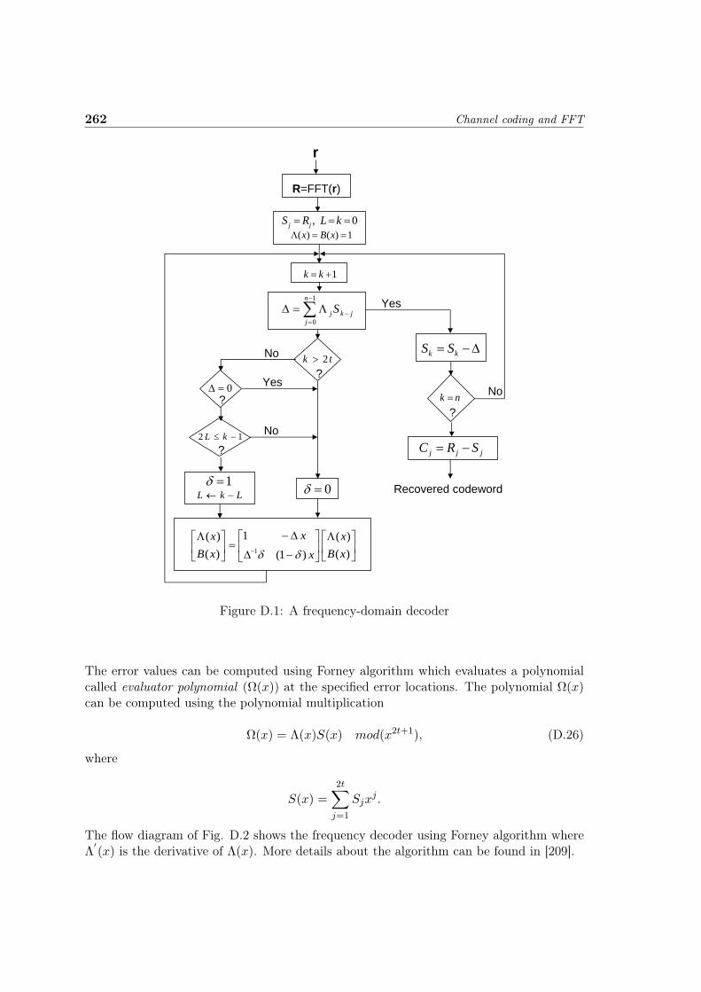
262 Channel coding and FFT
1
0
n
jjkj S
R=FFT(r)
r
)()(
)1(1
)()(
1 xBx
xx
xBx
1)()( xBx
?
??
0
?12 kL
kk SS
1
tk 2
LkL 0
jjj SRC
No
Yes
No
Yes
No
0, kLRS jj
Recovered codeword
1kk
nk
Figure D.1: A frequency-domain decoder
The error values can be computed using Forney algorithm which evaluates a polynomialcalled evaluator polynomial (Ω(x)) at the specified error locations. The polynomial Ω(x)can be computed using the polynomial multiplication
Ω(x) = Λ(x)S(x) mod(x2t+1), (D.26)
where
S(x) =2t∑
j=1
Sjxj .
The flow diagram of Fig. D.2 shows the frequency decoder using Forney algorithm whereΛ
′(x) is the derivative of Λ(x). More details about the algorithm can be found in [209].

D.1 The Fourier transform over finite fields 263
Chien searchWith FFT
1
0
n
jjkj S
R=FFT(r)
)()(
)1(1
)()(
1 xBx
xx
xBx
1)()( xBx
?0
?12 kL
1LkL 0
)(mod)()()( 12txxxSx
No
No
0, kLRS jj
?tk 2
No
Yes
jj
j xx 1' )(
0)()(
)('
ii
ii
ii Ifrc
0)( iii Ifrc
Yes
Yes
r
Recovered codeword
1kk
Figure D.2: A frequency-domain decoder using the Forney algorithm
We note that there are other important algorithms known in the literature used in thedecoding of RS codes. Among these algorithms, we find Sugiyama, Euclide, Gao and otheralgorithms. The study of these various algorithms is not the subject of our work. The goalis to highlight the role of the FFT in the encoding and decoding processes by reviewingthe most important algorithms adapted to the frequency processing of RS codes.
D.1.3 Comparison between time and frequency domain decoding of RScodes
In this section we give a comparison between frequency domain and time domain decodingof RS codes. All the notations for time domain decoding and details of time domain RSdecoder can be found in [216]. For the frequency domain approach, the matrix update, i.e.update of Λ(x) and B(x), requires at most 2t multiplications per iteration and the calcu-lation of ∆k requires at most t multiplications per iteration. There are 2t iterations and sono more than 6t2 multiplications are required to compute the error locater polynomial. Inthe other hand, the time domain approach works directly on the raw data word as receivedwithout any transform. The frequency-domain vectors of Berlekamp-Massey algorithm oflength t are replaced by time-domain vectors of length n. Then the time domain decoderhas a computation complexity proportional to n2 while the one of the frequency domain

264 Channel coding and FFT
decoder is proportional to t2.
The time domain decoder can be attractive because there is no syndrome computation orChien search. This means that the decoder has a very simple structure, but the penalty isa longer running time. As for the frequency domain decoder, its structure is more complexbut this drawback is largely compensated by its major advantage that is a shorter runningtime. For this latest reason, the frequency domain decoders are more attractive and havefound their use in various applications and specifically in applications that require highthroughput rates.
D.2 Fermat Transform Based RS Codes
In this section we describe RS codes defined over GF (Ft) and we show that these codeshave almost the same performances in terms of Bit Error Rate (BER) and Frame ErrorRate (FER) compared to the classical RS codes defined over GF (2m). We are interestedin RS codes defined over GF (Ft) because of the fact that their hardware implementationcan be partially performed with the aid of pre-implemented FFT where the building of aSR system is considered.
D.2.1 Encoding of RS codes defined over GF (Ft)
The principles of RS encoding as described in section D.1.1, can be applied to the RScodes defined over GF (Ft) with the only difference that the arithmetic operations aredone modulo Ft rather than modulo 2. The encoding in the time domain uses a generatorpolynomial to calculate the parity check symbols. In the frequency domain, the encodingconsists in constraining some specified spectral components to zero and filling the uncon-strained components of the spectrum with data symbols of GF (Ft). Then, the inverseFermat transform generates a non systematic codeword.
D.2.2 Decoding of RS codes defined over GF (Ft)
Different algorithms used for the decoding of RS codes defined over GF (2m) as explainedin section D.1.2 can be applied to decode the RS codes defined over GF (Ft). However,the highly used RS decoding procedure in actual applications is that composed of theBerlekamp-Massey algorithm, Chien algorithm and Forney algorithm (see Fig. D.2).
D.2.3 Performances comparison between RS over GF (Ft) and RS overGF (2m)
In this subsection, we give simulation results in terms of BER and FER vs EbN0
(Eb isthe energy per bit and N0 the power spectral density of the channel noise) for differentRS coding schemes with correcting capacity tc equal to 2. In this simulation, randomdata with a BPSK modulation are transmitted over an Additive White Gaussian Noise(AWGN) channel. In Fig. D.3 and Fig. D.4, we have a set of five BER and FER curves:(i) uncoded; (ii) RS(16,12) over GF (17) with frequency encoding and frequency decodingusing the Berlekamp-Massey algorithm and the recursive extension, the codeword symbols

D.2 Fermat Transform Based RS Codes 265
are represented by 5 bits each; (iii) RS(16,12) over GF (17) with time domain encoding andfrequency domain decoding using the algorithms indicated in Figure 6.4, the informationsymbols and the parity check symbols are represented by 4 bits (4-4); (iv) it is the samecase of (iii) with the only difference that each parity check symbol is transmitted over 5bits (5-4); (v) RS(15,11) over GF (16).
We start this analysis with curve (ii) of Fig. D.3. In this case, for low EbN0
values, theBER is high compared to other coding schemes. This phenomena can be explained by thefollowing: firstly, the loss of useful data rate by transmitting each symbol over 2t + 1 bitsincreases the channel error probability and consequently the BER. Secondly, if the numberof erroneous symbols is higher than the correcting capacity, the decoding fails and sincethe symbols of code words are generated by the Fermat transform, the symbols will beall erroneous resulting in an high BER. Curve (iii) also indicates a high BER due to thefact that the symbol 22t
= 16 is set to zero knowing that its probability occurrence is notequal to zero. We have calculated this probability for different Eb
N0values to be around 5.8
%, which in turn degrades the code performances. This degradation is clearly illustratedin Fig. D.4 where we observe that at high (Eb/N0), the performances in terms of FERof curve (iii) worsen as compared to curves (ii). This can be explain by the fact that theprobability of occurrence of symbol 22t (estimated to be around 5.8 %) and that does notdepend on the energy of signal, deliberately decreases the code’s error correcting capability.
0 2 4 6 8 10 1210
−7
10−6
10−5
10−4
10−3
10−2
10−1
100
Eb/N0
Bit
Err
or R
ate
(BE
R)
(i) Uncoded(ii) RS(16,12)(F.E)(iii) RS(16,12)(4−4)(iv) RS(16,12)(5−4)(v) RS(15,11)
0.16 dB
Figure D.3: Performances of RS(16,12) over GF (17) and RS(15,11) over GF (16) withBPSK modulation on AWGN channel. (F.E: Frequency Encoding))

266 Channel coding and FFT
The influence of this pre-committed error becomes more evident at high (Eb/N0) wherethe RS codes represented by curve (ii) of Fig. D.4 begin to be more efficient.
0 2 4 6 8 10 1210
−7
10−6
10−5
10−4
10−3
10−2
10−1
100
Eb/N0
Fra
me
Err
or R
ate
(FE
R)
(i) uncoded
(ii) RS(16,12)(F.E)
(iii) RS(16,12)(4−4)
(iv) RS(16,12)(5−4)
(v) RS(15,11)
Figure D.4: FER of RS(16,12) over GF (17) and RS(15,11) over GF (16) with BPSKmodulation on AWGN channel.
Now, let us consider the two curves (iv) and (v) of Fig. D.3. To solve the problem of thesymbol ”22t
”, we have transmitted each information symbol over 2t bits and each paritycheck symbol over 2t + 1 bits. In this way, the symbol ”22t
” is correctly represented.Fig. D.3 shows that the performances of the RS(16,12) defined over GF (17), using thetime domain encoding and the frequency domain decoding according to the algorithmspresented in Fig. 6.4, has similar performances as RS(15,11) defined over GF (16). Theasymptotic difference is 0.16 dB and can be expressed by the expression (in dB):
∆ = 10log(1/R1)− 10log(1/R2), (D.27)
where R1 and R2 are the code rates of RS(15,11) and RS(16,12) respectively. Here,∆ = 10log(15/11) − 10log(68/48) = 0.16 dB. This difference decreases with the codelength. To justify this, let us consider the two RS codes: RS(255,223) over GF(256) andRS(256,224) over GF(257), where the codes of each pair have the same error correctingcapability (tc). The associated code rates R1 and R2 are equal to 0.87 and 0.86 respectively.Applying equation D.27, ∆ in this case is equal to 0.05 dB. This drop of ∆ can be explainedalso by evaluating, for each RS code, the channel error probability
Pi =12erfc
√Ri
Eb
N0, i = 1, 2. (D.28)

D.3 DMFFT architecture 267
Fig. D.5 shows the channel error probability of each RS code. It is to be noticed that thedifference between the two curves of channel error probability in the case of RS(255,223)and RS(256,224) is very low compared to that of the RS(15,11) and RS(16,12). Theo-retically, the RS codes over GF (Ft) have the same error correcting capability, the smalldifference in terms of BER is due to the difference between the channel error probabili-ties. In turn, the channel error probability varies according to the code rate. The lowerthe difference between the code rates, the lower the difference between the channel errorprobabilities. Consequently, for long RS codes the difference in term of BER becomesnegligible.
0 1 2 3 4 5 6 7 810
−4
10−3
10−2
10−1
100
Eb/N0 (dB)
Ch
ann
el e
rro
r p
rob
abili
ty
RS(15,11)RS(16,12)RS(255,223)RS(256,224)
Figure D.5: The channel error probability for different RS codes.
D.3 DMFFT architecture
There are many different ways of implementing DMFFT operator. There can be twoextreme architectures:
1. Perform the transform computations by using only a single memory unit and oneRBPE. This method leads to a very simple circuit in terms of area, but the penaltyis the very high computation time required to execute the transform.
2. Perform the transform computations by implementing the entire FFT structure com-posed of log2N stages and N
2 RBPE units in each stage, where N is the transformlength. For this method, no RAM blocks are needed between two consecutive stagessince the entire sequence is processed in parallel. This method leads to a very highspeed computation at a very large area.

268 Channel coding and FFT
We can find an architecture between two extremes. To compute transform length N , thestrategy adopted is to implement log2N computation stages where each stage is composedof one processing element (known as RBPE), a stage control unit and some memory blocks.With this implementation strategy, the DMFFT and the Velcro operators are implementedand compared. Based on this choice, let us consider the proposed block diagram of theDMFFT operator as shown in Fig. D.6. This block diagram contains a Global ControlUnit (GCU) and log2N stages.
1
log N stages
Global Control Unit (GCU)
Global Control Unit (GCU)
Stage 1 Stage 2 Stage (log N)Data input Data output
Figure D.6: The DMFFT architecture
The GCU is composed of the following individual circuits:
1. FFT/FNT operation selection: there is a control signal DM which determines theoperating mode. The values 1, 0 of DM indicate that the complex Fourier transformand Fermat transform are performed respectively.
2. Transform size selection: the DMFFT operator is designed to perform variouslengths of FFT and FNT computations. The parameter m determines the num-ber of stages to be implemented and then the transform size N = 2m.
3. Word-length size: to provide the system designer with maximum flexibility, the in-put/output data and the twiddle factor’s word-length has been designed in a way tovary by a simple adjustment of corresponding parameters. A parameter nc deter-mines the complex word-length, nw determines the twiddle factor word-length andt determines the desired Fermat number and subsequently the length n = 2t + 1 ofthe GF (Ft) valued symbols.
This GCU is also responsible for the initialization of the entire DMFFT architecture andfor the control of the data input and data output and the synchronization between twoconsecutive input frames.

D.3 DMFFT architecture 269
D.3.1 Stage architecture
The proposed FFT architecture is a pipeline architecture where a pipeline level is em-ployed between two consecutive stages. The internal structure of each stage except stage1 is illustrated in Fig. D.7. As shown, the stage architecture is composed of the follow-ing design units: SCU (Stage Control Unit), AGU (Address Generating Unit), memoryblocks (RAM and ROM) and RBPE. As for stage 1, its architecture is similar to the onepresented in Fig. D.7 with some modifications.
RPE
Data out
Stage Architecture
1
0
Stage Control Unit(SCU)
iB
AGU
RAMs
rW iWiαROMs
AGU
Data in
Figure D.7: The general architecture of a DMFFT stage
In this stage, no multipliers nor ROM blocks are needed since the corresponding twiddlefactors are equal to 1. The RBPE as shown in Fig. D.8. represents the core of the DMFFToperator. RBPE is implemented in each stage and its operating mode is controlled by theGCU. The data stream acquisition of a RBPE employed in stage i is controlled by theSCU of stage i − 1. The RBPE acquires the data and applies the multiplication of thetwiddle factors with the corresponding symbols and the intermediate results continue theway to the adders and subtracters to undergo the corresponding operations. The storageof the RBPE computation results in the RAM blocks is handled by the SCU. Details ofthe internal blocks of RBPE can be found in [43].
D.3.2 RBPE complexity study
Table D.1 shows some measures of the implementation on Stratix II of the reconfigurableand Velcro butterflies for different nc and n values that represent the C and GF (Ft) sym-bol word-lengths respectively. The values n = 9 and n = 17 are the required bits numberto map the symbols in GF (Ft = 28 +1 = 257) and GF (Ft = 216 +1 = 65537) respectively.

270 Channel coding and FFT
X
X
X+
+-Ft-1
+
+
Ft-1
+
Wr
Wi
Pipeline stage
nc bits
nc bits
nc bits
X
DM
nc bits
n+1=2t +1 bits
n
n
nc
"i
1
0
01
1
0
0
1
1
001
10
10
01
01
01
10
10
Bi
Br
Ai
Ar
1rP1
iP
2rP2
iP
mux 1
Figure D.8: The reconfigurable butterfly architecture
Table D.1: Comparison between the reconfigurable butterfly and the Velcro butterflies ona STRATIX II, EP2S15F484C3 device.
circuitnc=9 nc=12 nc=17n=9 n=9 n=17
Velcro butterfly403ALUTs
629ALUTs
1062 ALUTs
4.20ns
5.07ns
5.60 ns
Re-configurablebutterfly
326ALUTs
514ALUTs
875 ALUTs
4.3 ns 5.18ns
5.64 ns
ALUT’s gain 19.1 % 18.2 % 17.6 %Delay’s excess 2.18 % 2.16 % 0.7 %
η = 1TC ∗ 106 ηV = 590 ηV = 313 ηV = 168
ηR = 713 ηR = 375 ηR = 202Performance-to-cost ratio gain
20.8% 19.8% 20.2%
Now let us discuss the figures given in Table D.1. For the reconfigurable butterfly, there isa small delay excess of around 2% compared to the Velcro solution. This time penalty iswidely balanced by complexity gain values (in term of Adaptive Lookup Tables (ALUTs))around 18% in favor of the common butterfly operator. Moreover, the performance-to-cost

D.4 Altera’s Stratix-II FPGA family 271
ratio ηR has always the highest value compared to ηV . The associated gains are 20.8, 19.8and 20.2 % for nc equal to 9, 12 and 17 respectively. These performance figures clearlyjustify once again the interest of using a common and reconfigurable operator instead ofVelcro operator.
D.4 Altera’s Stratix-II FPGA family
This section gives a brief overview of useful features of Altera’s Stratix-II FPGA family.Stratix II presents an efficient logic structure that maximizes the performance and enablesdevice densities approaching 180,000 equivalent Logic Elements (LEs). Stratix II devicesoffer up to 9 Mbits of on chip, TriMatrix memory and has up to 96 DSP (Digital SignalProcessing) blocks with up to 384 (18− bit× 18− bit) multipliers for efficient implemen-tation of high performance filters and other DSP functions. Depending on the device, upto 1,170 I/O user pins can be supported.
The architecture of Stratix II devices is based on two-dimensional row and column thatprovides signal interconnects between Logic Array Blocks (LAB), memory block struc-tures and DSP blocks. Each LAB consists of eight Adaptive Logic Modules (ALMs), carrychains, LAB control signals, local interconnects and register connection chain lines. AnALM is the Stratix II device family’s building block of logic providing efficient implemen-tation of user logic functions. The local interconnect transfers signals between ALMs inthe same LAB. Register chain connections transfer the output of an ALM register to theadjacent ALM register in an LAB.
One ALM contains a variety of Look Up Tables (LUT)-based resources that can be dividedbetween two Adaptive LUTs (ALUTs) as shown in Fig. D.9. With up to eight inputs tothe combinatorial logic, one ALM can implement various combinations of two functions.In addition to the adaptive LUT-based ressources, each ALM contains two programmableregisters, two dedicated full adders, a carry chain, a shared arithmetic chain and a registerchain. The ALUT is the cell used in the Quartus II software for logic synthesis. Thus, thenumber of ALUTs are used throughout in this work as a metric to evaluate the FPGA-based circuit complexity and then the parameter η as defined in [44].

272 Channel coding and FFT
Carry_inShared_arith_in reg_chain_in
carry_out
Shared_arith_outReg_chain_out
Combinatorial Output
Register Output
Combinatorial Output
Register Output
Full Adder
Full Adder
CombinatorialLogicr
Reg 0
Reg 1
D Q
D Q
ALUT 1
ALUT 2
The combinatorial logic is adaptively divided between the two ALUTs
ALM
Figure D.9: High-Level block diagram of the Stratix II ALM and its relationship with theALUTs

Appendix E
LFSR architectures
E.1 Linear feedback shift register basics and its architectures
A linear feedback shift register is a shift register whose input bit is a linear function ofits previous state. The only linear functions of single bits are exclusive-OR (XOR) andexclusive-NOR (XNOR); thus it is a shift register whose input bit is driven by the XOR ofsome bits of the overall shift register value. The value of the inner state s of each registerelement Z−1 could be seen as a recursive linear series, where ak are the feedback multipliercoefficients:
st+n = anst + an−1st+1 + ... + a1st+n−1 (E.1)
The operation of the register is deterministic and the sequence of values produced by theregister is completely determined by its current (or previous) state. Likewise, because theregister has a finite number of possible states, it must eventually enter a repeating cycle.However, an LFSR with a well-chosen feedback function can produce a sequence of bitswhich appears random (pseudo random in nature) and which has a very long cycle.
Two families of LFSR are clearly discriminated in the literature [119]:
• Fibonacci LFSRs and
• Galois LFSRs
These two types are able to carry out dissimilar functionalities and as a consequence, wedesign two distinct COs, called Reconfigurable Fibonacci LFSR as shown in Fig. E.1 andReconfigurable Galois LFSR as shown in Fig. E.2.
E.1.1 RF-LFSR architecture
In the Fibonacci representation as shown in Fig. E.1, the value of each register is given bythe linear recurrence (ak are the feedback multiplier coefficients). The output of FibonacciLFSR is given by S0:
Sr−1 =r∑1
akSr−k and Sk = Sk+1, ∀k ∈ [0 : r − 1] (E.2)
273

274 LFSR architectures
+
1−Z 1−Z
ra
0SSS
1−ra1a
1−Z1−Z 1−Z
ra
0S1S1−rS
1−ra1a
1−Z
Figure E.1: Fibonacci LFSR
+ + +1−Z 1−Z
0S1SS
1−ra 1ara
1−Z1−Z 1−Z
0S1S1−rS
1−ra 1ara
1−Z
Figure E.2: Galois LFSR
E.1.2 RG-LFSR architecture
In the Galois representation as shown in Fig. E.2 the output of the last cell S0 is introducedinto each of the tapped cells simultaneously, where it is added to the contents of thepreceding cell. The value of the current state S
′0 of a register n is given by the value of the
preceding state Si+1 of register n− 1. The output of Galois LFSR is given by S0. Takingak as the feedback multiplier coefficients, the equation is:
S′i = Si+1 + ai+1S0 ∀k ∈ [0 : r − 1] (E.3)
The Galois architecture of LFSRs was designed to operate in a Galois Field (GF). A GaloisLFSR can generate all the non zero elements of GF: successive shifts of the register willgenerate the vector representations of the successive powers of α (the primitive element ofGF) [217]. In its simplest form, i.e with single bit value, the addition is ensured by XORand Inverse-XOR.
In practical terms, we first identify an architecture, maximize its executable operationsand then define a parameterizable CO. In order to enlarge these workable operations, weundergo the second step of the pragmatic approach and design step by step two NEWCO; the Reconfigurable LFSR (R-LFSR) as in Fig. E.3 and the Extended ReconfigurableLFSR (ER-LFSR) as in Fig. E.4.
E.1.3 R-LFSR architecture
The architecture of the R-LFSR operator is shown in Fig. E.3. This structure is a singlebit value operator. In consequence, the parameterizable coefficient is a logical binary AND
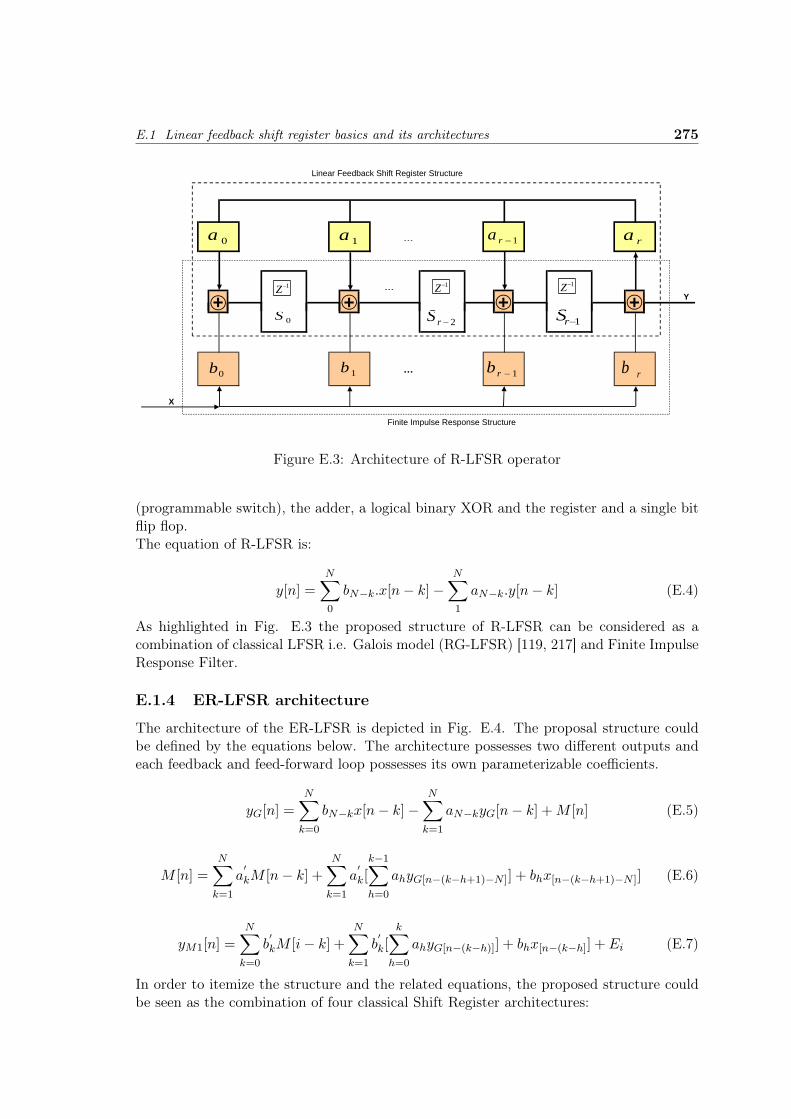
E.1 Linear feedback shift register basics and its architectures 275
…
…Y
Linear Feedback Shift Register Structure
++ + +1−Z 1−Z
S S
1−ra1a ra0a
S
1−Z
…
X
Finite Impulse Response Structure
0S 1−rS
0b 1b
2−rS
1−rb rb
Figure E.3: Architecture of R-LFSR operator
(programmable switch), the adder, a logical binary XOR and the register and a single bitflip flop.The equation of R-LFSR is:
y[n] =N∑0
bN−k.x[n− k]−N∑1
aN−k.y[n− k] (E.4)
As highlighted in Fig. E.3 the proposed structure of R-LFSR can be considered as acombination of classical LFSR i.e. Galois model (RG-LFSR) [119, 217] and Finite ImpulseResponse Filter.
E.1.4 ER-LFSR architecture
The architecture of the ER-LFSR is depicted in Fig. E.4. The proposal structure couldbe defined by the equations below. The architecture possesses two different outputs andeach feedback and feed-forward loop possesses its own parameterizable coefficients.
yG[n] =N∑
k=0
bN−kx[n− k]−N∑
k=1
aN−kyG[n− k] + M [n] (E.5)
M [n] =N∑
k=1
a′kM [n− k] +
N∑k=1
a′k[
k−1∑h=0
ahyG[n−(k−h+1)−N ]] + bhx[n−(k−h+1)−N ]] (E.6)
yM1[n] =N∑
k=0
b′kM [i− k] +
N∑k=1
b′k[
k∑h=0
ahyG[n−(k−h)]] + bhx[n−(k−h]] + Ei (E.7)
In order to itemize the structure and the related equations, the proposed structure couldbe seen as the combination of four classical Shift Register architectures:

276 LFSR architectures
++
++ + +
+ +
1−ZGyM
1'a1a
1' −Na Na'
0'b 1'b 1' −Nb Nb'0b 1b
1−Z 1−Z
0a 1−Na
Nb1−Nb
+
ER-LFSR Structure
+ + +x MY
Figure E.4: Architecture of ER-LFSR operator
1. Coefficients ak specify the linear feedback loop of a Galois LFSR [119, 217].
2. Coefficients a′k qualify the linear feedback loop of a Fibonacci LFSR [119].
3. Coefficients bk corresponds to the coefficients a Transposed form Finite-Impulse Re-sponse Filter.
4. Coefficients b′k correspond to the coefficients a Direct form Finite-Impulse Response
Filter.
The combination of architecture 1 and 3 gives the former R-LFSR, already presented in[46] and the combination of 2 and 4 gives the classical structure of an Infinite ImpulseResponse Filter.
E.2 Preeminent functions of LFSR COs
In this section, we give a brief summary of the operations obtainable by the four COs asin Fig. E.5 (taking the ER-LFSR as a reference). Each LFSR is devoted to a specificperimeter defining four nested operational perimeters. Since the perimeters are nested,LFSR are called Matriochkas LFSRs and define four degree of factoring from the smallestwith RF-LFSR to the largest with ER-LFSR. Operations of standards replaced by ourLFSRs are listed in Table E.1.

E.2 Preeminent functions of LFSR COs 277
Table E.1: Operations of standards replaced by our LFSRsStandards Function name Polynomial degreeIEEE 802.11g Scrambler 7IEEE 802.11g Descrambler 7IEEE 802.11g CCIT CRC-16 Coder 16IEEE 802.11g CCIT CRC-16 Decoder 16IEEE 802.11g Convolutional Coder PBCC 2×63GPP LTE CRC-24 Coder 243GPP LTE CRC-16 Coder 163GPP LTE CRC-12 Coder 123GPP LTE CRC-8 Coder 83GPP LTE CRC-24 Decoder 243GPP LTE CRC-16 Decoder 163GPP LTE CRC-12 Decoder 123GPP LTE CRC-8 Decoder 83GPP LTE Convolutional Coder, Rate 1/2 2×83GPP LTE Convolutional Coder, Rate 1/3 3×83GPP LTE Turbo Coder 2×4IEEE 802.16 Scrambler 15IEEE 802.16 Scrambler Spreading BPSK 22IEEE 802.16 Scrambler Pilot Modulation 11IEEE 802.16 Convolutional Coder 6IEEE 802.16 CRC-32 Coder 32IEEE 802.16 CRC-16 Coder 16IEEE 802.16 CRC-32 Decoder 32IEEE 802.16 CRC-16 Decoder 16

278 LFSR architectures
E.5ER-LFSR R-LFSR RG-LFSR RF-LFSR
Generic Structures:PN Sequences Generator X X X X
Scrambler X X X XCRC Coder X X X
CRC Decoder X X X
Non Systematic Convolutional Coder X XRecursive Systematic Convolutional Coder X X
Turbo Coder X XError Correcting Coder X X X
Error Correcting Decoder X XGalois Field Generator X XReed Solomon Coder X X
Reed Solomon Decoder X X"Unconventional" Structures:802.11g: Convolutional Coder ERP-PBCC 22/33
Mbits/s X802.16: Turbo Coderr (Rate 1/2 et 1/3) X
3 GPP LTE: Scrambler Code Generator (Uplink et Downlink) X
ER-LFSR R-LFSR RG-LFSR RF-LFSRBinary Operations
Addition X X X XDivision X X X
Multiplication X XComparison X X
Figure E.5: Nested functional perimeter of LFSR

List of Figures
1 Emetteur/récepteur super-hétérodyne . . . . . . . . . . . . . . . . . . . . . 62 Une architecture réaliste d’une radio logicielle . . . . . . . . . . . . . . . . . 63 Une architecture de récepteur réalisable . . . . . . . . . . . . . . . . . . . . 74 Taches d’un émetteur multi-standards . . . . . . . . . . . . . . . . . . . . . 105 Les deux approches de paramétrisation, par fonction ou opérateur com-
muns . . . . . . . . . . . . . . . . . . . . . . . . . . . . . . . . . . . . . . . 116 Diagrame généralisé de la décomposition de plusieurs standards . . . . . . . 127 Chemin optimal pour la "channelization", l’égalisation et la démodulation
OFDM . . . . . . . . . . . . . . . . . . . . . . . . . . . . . . . . . . . . . . 138 Exemple de graphe . . . . . . . . . . . . . . . . . . . . . . . . . . . . . . . . 189 Hyperarc OU . . . . . . . . . . . . . . . . . . . . . . . . . . . . . . . . . . 2010 Hyperarc ET . . . . . . . . . . . . . . . . . . . . . . . . . . . . . . . . . . . 2011 Graphe généralisé correspondant à un équipement de radio logicielle tri-
standards . . . . . . . . . . . . . . . . . . . . . . . . . . . . . . . . . . . . . 2112 Structure d’un graphe pour le cas d’un équipement de radio logicielle tri-
standards (émetteur simplifié) . . . . . . . . . . . . . . . . . . . . . . . . . 2213 Exemple d’un graphe partiel . . . . . . . . . . . . . . . . . . . . . . . . . . 2314 Exemple de graphe avec les coûts associés aux noeuds et aux arcs . . . . . 2615 Capture d’écran de l’interface graphique développée pour contruire les
graphes . . . . . . . . . . . . . . . . . . . . . . . . . . . . . . . . . . . . . . 3116 Approches d’optimisation [35] . . . . . . . . . . . . . . . . . . . . . . . . . 3217 Algorithme de la méthode par recherche exhaustive . . . . . . . . . . . . . 3318 Exemple de graphe avec les coûts associés . . . . . . . . . . . . . . . . . . . 3419 Algorithme du recuit simulé . . . . . . . . . . . . . . . . . . . . . . . . . . . 3720 Schéma simplifié d’un algorithme génétique . . . . . . . . . . . . . . . . . . 3821 Représentation simplifiée d’une population . . . . . . . . . . . . . . . . . . 3822 Croisements . . . . . . . . . . . . . . . . . . . . . . . . . . . . . . . . . . . 3823 Mutations . . . . . . . . . . . . . . . . . . . . . . . . . . . . . . . . . . . . . 3924 Equipment SDR générique . . . . . . . . . . . . . . . . . . . . . . . . . . . 4025 Resultats de la recherche exhaustive sur l’exemple générique . . . . . . . . 4126 Resultats du recuit simulé sur l’exemple générique . . . . . . . . . . . . . . 4227 Resultats d’un algorithme génétique sur l’exemple générique . . . . . . . . 4328 Elements retenus aux différentes itérations . . . . . . . . . . . . . . . . . . 4429 Exemple d’une FFT partagée entre un démodulateur OFDM et un dé-
codeur RS dans GF (Ft). . . . . . . . . . . . . . . . . . . . . . . . . . . . . 4830 Architecture du papillon reconfigurable . . . . . . . . . . . . . . . . . . . . 49
279

280 list of figures
31 Graphe d’un équipement tri-standards en utilisant GF (Ft) pour le codageRS . . . . . . . . . . . . . . . . . . . . . . . . . . . . . . . . . . . . . . . . . 51
32 Décomposition possible de la DMFFT . . . . . . . . . . . . . . . . . . . . . 5233 Banque d’opérateurs communs (COB) . . . . . . . . . . . . . . . . . . . . . 5734 LFSRs Combinés . . . . . . . . . . . . . . . . . . . . . . . . . . . . . . . . . 5935 Equipement tri-standards avec l’opérateur commun LFSR . . . . . . . . . . 6136 Décomposition de l’opérateur 22ER en opérateurs plus petits . . . . . . . . 6237 FIR filter architecture based on FRM technique . . . . . . . . . . . . . . . 6438 Canaliseurs pour un équipement SDR multi-standards . . . . . . . . . . . . 6439 An generalized view of common operators . . . . . . . . . . . . . . . . . . . 6740 Copie d’écran du graphe dans l’interface graphique . . . . . . . . . . . . . . 6841 Version en gros plan de la Fig. 40 . . . . . . . . . . . . . . . . . . . . . . . 6942 Number of operators kept at different number of iterations . . . . . . . . . 70
1.1 Classification of functions and their consequences on hardware cluster . . . 921.2 A top level view of wireless equipment architecture . . . . . . . . . . . . . . 931.3 Block diagram of a digital radio system . . . . . . . . . . . . . . . . . . . . 941.4 Superheterodyne transmitter/receiver . . . . . . . . . . . . . . . . . . . . . 951.5 a) SR transceiver architecture b) A more realistic SR architecture . . . . . 961.6 Trade-offs and limitations of converter performance . . . . . . . . . . . . . 971.7 Direct conversion architecture . . . . . . . . . . . . . . . . . . . . . . . . . 981.8 Simplified sub-sampling receiver architecture . . . . . . . . . . . . . . . . . 981.9 The feasible software radio receiver architecture . . . . . . . . . . . . . . . 99
2.1 Multi-standards transmitter data processing tasks . . . . . . . . . . . . . . 1112.2 Generalized parameterizable modulator [15] . . . . . . . . . . . . . . . . . . 1132.3 Generalized block diagram showing the breakdown of several standards . . 1152.4 Two techniques of parametrisation . . . . . . . . . . . . . . . . . . . . . . 1162.5 Optimal path for the channelization, equalization and OFDM demodulation120
3.1 A graph . . . . . . . . . . . . . . . . . . . . . . . . . . . . . . . . . . . . . . 1293.2 A corporate hierarchy . . . . . . . . . . . . . . . . . . . . . . . . . . . . . . 1303.3 An example of SynDEx software application graph . . . . . . . . . . . . . 1333.4 An example of SynDEx hardware platform graph . . . . . . . . . . . . . . 1333.5 An example of SynDEx partitioning and scheduling . . . . . . . . . . . . . 1353.6 OR hyperarc . . . . . . . . . . . . . . . . . . . . . . . . . . . . . . . . . . . 1373.7 AND hyperarc . . . . . . . . . . . . . . . . . . . . . . . . . . . . . . . . . . 1373.8 Generalized graph corresponding to a conceivable tri-standard SDR . . . . 1383.9 Global structure of the graph for tri-standard SDR system (transmitter
side), simplified version . . . . . . . . . . . . . . . . . . . . . . . . . . . . . 1393.10 An example of partial hypergraph . . . . . . . . . . . . . . . . . . . . . . . 1403.11 A simple single-source network design problem . . . . . . . . . . . . . . . . 1423.12 The network-design version of section of partial hypergraph . . . . . . . . . 1433.13 A network view of partial hypergraph given in 3.10 . . . . . . . . . . . . . . 143
4.1 Graph model with associated costs; PEs tagged with BC/CC and arrowstagged with NoC . . . . . . . . . . . . . . . . . . . . . . . . . . . . . . . . 150

list of figures 281
4.2 Solution space of cost function . . . . . . . . . . . . . . . . . . . . . . . . . 1604.3 Screen shot of GUI for drawing graph models . . . . . . . . . . . . . . . . . 1614.4 GUI with parameters’ adjustment window . . . . . . . . . . . . . . . . . . . 162
5.1 Global optimization approaches [35] . . . . . . . . . . . . . . . . . . . . . . 1675.2 Principal of SA for the selection of new states . . . . . . . . . . . . . . . . . 1695.3 Flow diagram of exhaustive search algorithm . . . . . . . . . . . . . . . . . 1715.4 Graph model with associated costs . . . . . . . . . . . . . . . . . . . . . . . 1725.5 Flow diagram of simulated annealing algorithm . . . . . . . . . . . . . . . . 1755.6 Canonical genetic algorithm . . . . . . . . . . . . . . . . . . . . . . . . . . . 1785.7 A simplified representation of population of chromosomes . . . . . . . . . . 1795.8 Crossover rule in CGA . . . . . . . . . . . . . . . . . . . . . . . . . . . . . 1795.9 Mutation rule in CGA . . . . . . . . . . . . . . . . . . . . . . . . . . . . . . 1805.10 A generic view of SDR equipment . . . . . . . . . . . . . . . . . . . . . . . 1815.11 Results of running ES on generic design example . . . . . . . . . . . . . . . 1835.12 Results of running ES on generic design example with good solutions . . . 1845.13 Results of running SA on generic design example . . . . . . . . . . . . . . . 1855.14 Results of running CGA on generic design example . . . . . . . . . . . . . . 1865.15 Processing elements retained at different iterations . . . . . . . . . . . . . . 187
6.1 An example of FFT sharing between OFDM demodulation and RS decod-ing over GF (Ft). . . . . . . . . . . . . . . . . . . . . . . . . . . . . . . . . . 194
6.2 A time-domain encoder and frequency-domain decoder for RS codes . . . . 1966.3 A frequency-domain encoder and frequency-domain decoder for RS codes . 1966.4 The three phases of RS decoding process over GF (Ft) . . . . . . . . . . . 1986.5 Graph of tri-standard system if RS coding in GF (Ft) had been used . . . . 2016.6 Building block of DMFFT . . . . . . . . . . . . . . . . . . . . . . . . . . . 202
7.1 Common operator bank . . . . . . . . . . . . . . . . . . . . . . . . . . . . . 2107.2 Combined LFSRs . . . . . . . . . . . . . . . . . . . . . . . . . . . . . . . . 2127.3 Implementation of a tri-standard systems with COs . . . . . . . . . . . . . 2157.4 Decomposition of 22ER into smaller/basic operators . . . . . . . . . . . . . 217
8.1 FIR filter architecture based on FRM technique . . . . . . . . . . . . . . . 2238.2 Channelizers for single/multi-standard SDR . . . . . . . . . . . . . . . . . . 2248.3 GSM channel distribution . . . . . . . . . . . . . . . . . . . . . . . . . . . . 2258.4 WCDMA channel distribution . . . . . . . . . . . . . . . . . . . . . . . . . 2258.5 Architecture of FRMFB - Design-1 . . . . . . . . . . . . . . . . . . . . . . . 2268.6 Architecture of FRMFB - Design-2 . . . . . . . . . . . . . . . . . . . . . . . 227
9.1 An generalized view of common operators . . . . . . . . . . . . . . . . . . . 2329.2 Screen shot of graph drawn in GUI . . . . . . . . . . . . . . . . . . . . . . . 2339.3 Zoomed version of graph in Fig. 9.2 . . . . . . . . . . . . . . . . . . . . . . 2349.4 Number of operators kept at different number of iterations . . . . . . . . . 236
D.1 A frequency-domain decoder . . . . . . . . . . . . . . . . . . . . . . . . . . 262D.2 A frequency-domain decoder using the Forney algorithm . . . . . . . . . . . 263

282 list of figures
D.3 Performances of RS(16,12) over GF (17) and RS(15,11) over GF (16) withBPSK modulation on AWGN channel. (F.E: Frequency Encoding)) . . . . 265
D.4 FER of RS(16,12) over GF (17) and RS(15,11) over GF (16) with BPSKmodulation on AWGN channel. . . . . . . . . . . . . . . . . . . . . . . . . . 266
D.5 The channel error probability for different RS codes. . . . . . . . . . . . . . 267D.6 The DMFFT architecture . . . . . . . . . . . . . . . . . . . . . . . . . . . . 268D.7 The general architecture of a DMFFT stage . . . . . . . . . . . . . . . . . . 269D.8 The reconfigurable butterfly architecture . . . . . . . . . . . . . . . . . . . 270D.9 High-Level block diagram of the Stratix II ALM and its relationship with
the ALUTs . . . . . . . . . . . . . . . . . . . . . . . . . . . . . . . . . . . . 272
E.1 Fibonacci LFSR . . . . . . . . . . . . . . . . . . . . . . . . . . . . . . . . . 274E.2 Galois LFSR . . . . . . . . . . . . . . . . . . . . . . . . . . . . . . . . . . . 274E.3 Architecture of R-LFSR operator . . . . . . . . . . . . . . . . . . . . . . . . 275E.4 Architecture of ER-LFSR operator . . . . . . . . . . . . . . . . . . . . . . . 276E.5 Nested functional perimeter of LFSR . . . . . . . . . . . . . . . . . . . . . 278

List of Tables
1 IEEE 802.11a and IEEE 802.16 implementation on FPGA . . . . . . . . . . 282 Comparaison entre la DMFFT-64 et la FFT/FNT-64 Velcro sur un Stratix-
II, EP2S15F484C3 . . . . . . . . . . . . . . . . . . . . . . . . . . . . . . . . 503 Comparaison entre la DMFFT-256 et la FFT/FNT-256 Velcro sur un
Stratix-II, EP2S15F484C3 . . . . . . . . . . . . . . . . . . . . . . . . . . . . 504 Nombre d’appels du bloc DMFFT . . . . . . . . . . . . . . . . . . . . . . . 525 Nombre d’appels en termes de multiplications et additions pour le décodage
RS classique pour t=8 et N=256 . . . . . . . . . . . . . . . . . . . . . . . . 526 Décomposition en LFSR Indépendants . . . . . . . . . . . . . . . . . . . . . 567 Opérations de WiFi/WiMAX/3GPP-LTE et nombre de LFSRs . . . . . . . 588 LFSRs combinés . . . . . . . . . . . . . . . . . . . . . . . . . . . . . . . . . 609 Complexité du FRMFB pour l’extraction de 5 canaux GSM et 5 canaux
WCDMA . . . . . . . . . . . . . . . . . . . . . . . . . . . . . . . . . . . . . 6510 Cost parameters for different blocks of Fig. 41 . . . . . . . . . . . . . . . . 68
1.1 Levels of SDR . . . . . . . . . . . . . . . . . . . . . . . . . . . . . . . . . . 90
4.1 IEEE 802.11a and IEEE 802.16 implementation on FPGA . . . . . . . . . . 1534.2 DSP Blackfin processor performance on DSP functions . . . . . . . . . . . . 1544.3 Algorithm partitioning of typical baseband processing tasks . . . . . . . . . 156
5.1 Results of SA at certain temperatures . . . . . . . . . . . . . . . . . . . . . 176
6.1 Comparison between the DMFFT-64 and the Velcro FFT/FNT-64 operatoron a Stratix II, EP2S15F484C3 . . . . . . . . . . . . . . . . . . . . . . . . . 199
6.2 Comparison between the DMFFT-256 and the Velcro FFT/FNT-256 op-erator on a Stratix II, EP2S15F484C3 . . . . . . . . . . . . . . . . . . . . . 200
6.3 No. of call of individual blocks of DMFFT . . . . . . . . . . . . . . . . . . 2036.4 No. of calls of multiplications and additions for classical RS decoding for
t=8 and N=256 . . . . . . . . . . . . . . . . . . . . . . . . . . . . . . . . . 203
7.1 Independent LFSR decomposition . . . . . . . . . . . . . . . . . . . . . . . 2107.2 Operations of WiFi/WiMAX/3GPP LTE and Number of LFSRs . . . . . . 2137.3 Combined LFSR decomposition . . . . . . . . . . . . . . . . . . . . . . . . 214
8.1 Computational complexity of FRMFB for the extraction of 5 GSM and 5WCDMA Channels - Design-1 . . . . . . . . . . . . . . . . . . . . . . . . . 226
283

284 list of tables
8.2 Computational complexity of FRMFB for the extraction of 5 GSM and 5WCDMA Channels - Design-2 . . . . . . . . . . . . . . . . . . . . . . . . . 227
9.1 Cost parameters for different blocks of Fig. 9.3 . . . . . . . . . . . . . . . . 235
B.1 Computational complexity of IEEE 802.11a transmitter tasks . . . . . . . . 250B.2 Computational complexity of IEEE 802.11a receiver tasks . . . . . . . . . . 251B.3 Computational complexity of UMTS, FDD UL Tx Blocks (CCTrCH and
TrCH decoding, 1 Frame) . . . . . . . . . . . . . . . . . . . . . . . . . . . . 252B.4 Computational complexity of UMTS, FDD DL Rx Blocks (CCTrCH and
TrCH decoding, 1 Frame) . . . . . . . . . . . . . . . . . . . . . . . . . . . . 253
D.1 Comparison between the reconfigurable butterfly and the Velcro butterflieson a STRATIX II, EP2S15F484C3 device. . . . . . . . . . . . . . . . . . . . 270
E.1 Operations of standards replaced by our LFSRs . . . . . . . . . . . . . . . 277

Bibliography
[1] F. M. Torre, “Speakeasy-a new direction in tactical communications for the 21stcentury,” in Proc. Tactical Communications Conference Vol. 1 Tactical Communi-cations: Technology in Transition, pp. 139–142 vol.1, 1992.
[2] J. H. Reed, Software Radio: A Modern Approach to Radio Engineering. PrenticeHall PTR, 2002.
[3] J. P. Cummings, “Software radios for airborne platforms,” IEEE Journal on SelectedAreas in Communications, vol. 17, no. 4, pp. 732–747, 1999.
[4] B. Tarver, E. Christensen, A. Miller, and E. R. Wing, “Digital modular radio (DMR)as a maritime/fixed Joint Tactical Radio System (JTRS),” in Proc. Communicationsfor Network-Centric Operations: Creating the Information Force. IEEE MilitaryCommunications Conference MILCOM 2001, vol. 1, pp. 163–167 vol.1, 2001.
[5] N. Hayes, “The JTRS SCA specification-the past, the present, and the future,” inProc. IEEE Military Communications Conference MILCOM 2005, pp. 2713–2719Vol. 5, 2005.
[6] D. L. Tennenhouse, T. Turletti, and V. G. Bose, “The SpectrumWare testbed forATM-based software radios,” in Proc. 5th IEEE International Conference on Uni-versal Personal Communications Record, vol. 2, pp. 915–917 vol.2, 1996.
[7] “GNU Radio - The GNU Software Radio,” http://www.gnu.org/software/gnuradio.
[8] M. Raulet, Optimisations Mémoire dans la Méthodologie AAA pour Code Embarquésur Architectures Parallèles. PhD thesis, Institut National des Sciences Appliquées(INSA) de Rennes, 2006.
[9] C. Moy, M. Raulet, S. Rouxel, J. P. Diguet, G. Gogniat, P. Desfray, N. Bulteau, J. E.Goubard, and Y. Denef, “UML Profiles for Waveform Signal Processing SystemsAbstraction,” in SDR Forum Technical Conference, 2004.
[10] A. Koudri, D. Aulagnier, D. Vojtisek, P. Soulard, C. Moy, J. Champeau, J. Vidal,and S. Lecomte, “RTL Code Generation from MARTE Models, in Proc. of Modelingand Analysis of Real-Time and Embedded Systems with the MARTE UML profile,”in Design, Automation, and Test in Europe (DATE’08), 2008.
[11] “SCARI OPEN - Software Communications Architecture - Reference Implementa-tion,” http://www.crc.gc.ca/en/html/crc/home/research/satcom/rars/sdr/products/scari_open/scari_open.
285

286 BIBLIOGRAPHY
[12] M. Hermeling, J. Hogg, and F. Bordeleau, “Developing SCA Compliant Systems,”http://www.zeligsoft.com/Technology/Resources.asp, 2005.
[13] “PrismTech Spectra SDR Power Tools,” http://www.prismtech.com/section-item.asp?snum=3&sid=152.
[14] W. H. W. Tuttlebee, Software Defined Radio: Enabling Technologies. John Wiley &Sons Ltd. UK, 2002.
[15] F. Jondral, Parameterization; A technique for SDR Implementation. John Wiley &Sons Inc., London, UK, 2002.
[16] A. R. Rhiemeier, “Benefits and Limits of Parameterized Channel Coding for SoftwareRadio,” in Proc. 2nd Karlsruhe Workshop on Software Radios, pp. 107–112, March2002.
[17] J. Palicot and C. Roland, “FFT: a Basic Function for a Reconfigurable Receiver,” in10th International Conference on Telecommunications, ICT’03, vol. 1, pp. 898–902,March 2003.
[18] L. Alaus, D. Noguet, and J. Palicot, “Extended Reconfigurable Linear FeedBack ShiftRegister Operators for Software Defined Radio,” in Proc. IEEE 10th InternationalSymposium on Spread Spectrum Techniques and Applications ISSSTA ’08, pp. 677–681, 25–28 Aug. 2008.
[19] A. Al Ghouwayel, Y. Louet, and J. Palicot, “A Reconfigurable Butterfly Architecturefor Fourier and Fermat transform,” in Proc. 4th Karlsruhe Workshop on SoftwareRadios, pp. 146–151, 17–19 Oct. 2006.
[20] V. Rodriguez, C. Moy, and J. Palicot, “Install or invoke?: The optimal trade-offbetween performance and cost in the design of multi-standard reconfigurable ra-dios,” Wiley InterScience, Wireless Communications and Mobile Computing Journal,vol. 7, pp. 1143–1156, November 2007.
[21] J. L. Gross and J. Yellen, Handbook of Graph Theory (Discrete Mathematics and ItsApplications). CRC Press, New York, USA., 2004.
[22] E. L. Lawler, J. K. Lenstra, A. H. G. R. Kan, and D. B. Schmoys, The TravelingSalesman Problem: A Guided Tour through Combinatorial Optimization. John Wiley& Sons Inc., 1985.
[23] G. B. Dantzig, D. R. Fulkerson, and S. M. Johnson, “Solution of a large-scaletraveling-salesman problem,” Oper. Res., vol. 2, pp. 393–410, 1954.
[24] M. W. Padberg and G. Rinaldi, “Optimization of a 532-city symmetric travelingsalesman problem by branch and cut,” Oper. Res. Lett., vol. 6, pp. 1–7, 1987.
[25] E. W. Dijkstra, “A note on two problems in connexion with graphs,” Numer. Math,vol. 1, pp. 269–271, 1959.
[26] J. R. Edmonds, “Paths, trees and flowers,” Canad. J. Math, vol. 17, pp. 449–467,1965.

BIBLIOGRAPHY 287
[27] S. A. Cook, “The complexity of theorem-proving procedures,” Proc. 3rd Annual ACMSymp. Theory of Computing, ACM, New York, pp. 151–158, 1971.
[28] R. M. Karp, Reducibility among combinatorial problems. Plenum Press, 1972.
[29] Y. Sorel, “Real-time embedded image processing applications using the A method-ology,” in Proc. International Conference on Image Processing, vol. 1, pp. 145–148,16–19 Sept. 1996.
[30] M. Raulet, F. Urban, J. F. Nezan, C. Moy, O. Deforges, and S. Y., “SynDEx Exec-utive Kernels for Fast Developments of Applications Over Heterogeneous Architec-tures,” in European Signal Processing Conference (EUSIPCO’05), 2005.
[31] J. P. Delahaye, P. Leray, C. Moy, and J. Palicot, “Managing Dynamic Partial Re-configuration on Heterogeneous SDR Platforms,” in SDR Forum Technical Confer-ence’05, 2005.
[32] J. P. Delahaye, J. Palicot, C. Moy, and P. Leray, “Partial Reconfiguration of FPGAsfor Dynamical Reconfiguration of a Software Radio Platform,” in IST Mobile andWireless Communications Summit’07, 2007.
[33] M. Cummings and S. Haruyama, “FPGA in the software radio,” IEEE Communica-tions Magazine, vol. 37, pp. 108–112, Feb. 1999.
[34] Lotze, Jorg, Fahmy, A. Suhaib, Noguera, Juanjo, Doyle, Linda, Esser and Robert,“An FPGA-based cognitive radio framework,” in Proc. IET Irish Signals and SystemsConference (ISSC 2008), pp. 138–143, 18–19 June 2008.
[35] C. A. Coello Coello, D. A. Van Veldhuizen, and G. B. Lamont, Evolutionary Algo-rithms for Solving Multi-Objective Problems. Kluwer Academic/ Plenum Publishers,New York, 2002.
[36] K. S. R. R. Kondapalli and C. K. Chew, “Optimal Design and Analysis of a DC-DC Synchronous Converter using Genetic Algorithm and Simulated Annealing,”International Journal of Modelling and Simulation, vol. 3, pp. 4823–4840, 2009.
[37] J. T. Alander, ed., Proceedings of the Second Nordic Workshop on Genetic Algorithmsand their Applications. Department of Information Technology and Production Eco-nomics, University of Vaasa, 1996.
[38] U. B. Nallamottu, T. L. Chambers, and W. Simon, “Comparison of the GeneticAlgorithm to Simulated Annealing Algorithm in Solving Transportation Location-allocation Problems With Euclidean Distances,” in Proc. American Society for En-gineering Education (ASEE) Gulf-Southwest Annual Conference, 2002.
[39] L. Ingber, “Adaptive simulated annealing (ASA): Lessons learned,” Journal of Con-trol and Cybernetics: Special issue on Simulated Annealing Applied to CombinatorialOptimization, 1995.
[40] C. Ortiz-Alemán, R. Martin, J. C. Gamio, and A. Nicolas, “Application of SimulatedAnnealing and Genetic Algorithms to the Reconstruction of Electrical Permittivity

288 BIBLIOGRAPHY
Images in Capacitance Tomography,” in 3rd World Congress on Industrial ProcessTomography, 2003.
[41] J. Fourier, Théorie Analytique de la Chaleur/The Analytical Theory of Heat, trans-lated by Alexander Freeman. Dover Publications, 1822, translated 1878, re-released2003.
[42] J. W. Cooley and J. W. Tukey, “An algorithm for the machine calculation of complexFourier series,” Mathematics Computation, vol. 19, pp. 297–301, April 1965.
[43] A. Al Ghouwayel, Y. Louet, and J. Palicot, “A reconfigurable architecture for theFFT operator in a software radio context,” in Proc. IEEE International Symposiumon Circuits and Systems ISCAS 2006, p. 4pp., 2006.
[44] W. W. Yu and S. Xing, “Fixed-Point Multiplier Evaluation and Design with FPGA,”in Proc. Society of Photographic Instrumentation Engineers (SPIE), 1999.
[45] S. T. Gul, A. Al Ghouwayel, C. Moy, and Y. Louët, “A Novel Design of Reconfig-urable Fourier Transform Operator Over C and GF (Ft) for Future Multi-standardsSDR Equipments,” International Journal of Communication Networks and Dis-tributed Systems-IJCNDS, Accepted in June 2009 for publication by the end of 2009.
[46] L. Alaus, D. Noguet, and J. Palicot, “A reconfigurable linear feedback shift registeroperator for software defined radio terminal,” in Proc. 3rd International Symposiumon Wireless Pervasive Computing ISWPC 2008, pp. 319–323, 7–9 May 2008.
[47] S. T. Gul, L. Alaus, C. Moy, J. Palicot, and D. Noguet, “Optimal set of LFSRCommon Operators for Multi-Standards Cognitive Radio Terminals,” InternationalJournal of Autonomous and Adaptive Communications-IJAACS, Special Issue onCognitive Radio Systems, Accpeted in July 2009 for publication in 2010.
[48] R. Mahesh and A. P. Vinod, “Reconfigurable Frequency Response Masking Filtersfor Software Radio Channelization,” IEEE Transactions on Circuits and Systems II:Express Briefs, vol. 55, pp. 274–278, March 2008.
[49] T. Hentschel, “Channelization for software defined base-stations,” Annales desTelecommunications, vol. 57, pp. 386–420, May-June 2002.
[50] L. Pucker, “Channelization techniques for software defined radio,” in Proc. SpectrumSignal Processing Inc., pp. 17–19, November 2003.
[51] C. Kim, S. Y., S. Im, and W. Lee, “SDR-based digital channelizer/de-channelizerfor multiple CDMA signals,” in Proc. 52nd Vehicular Technology Conference IEEEVTS-Fall VTC 2000, vol. 6, pp. 2862–2869, 24–28 Sept. 2000.
[52] Y. C. Lim, “Frequency-response masking approach for the synthesis of sharp linearphase digital filters,” IEEE Transactions on Circuits and Systems, vol. 33, pp. 357–364, Apr 1986.
[53] IEEE Communications Magazine, Special Issue on Software Radio, vol. 37. 1999.

BIBLIOGRAPHY 289
[54] J. Mitola III, “The software radio architecture,” IEEE Communications Magazine,vol. 33, pp. 26–38, May 1995.
[55] M. Woh, S. Seo, H. Lee, Y. Lin, S. Mahlke, T. Mudge, C. Chakrabarti, andF. K., “The Next Generation Challenge for Software Defined Radio,” Springer-VerlagBerlin Heidelberg, vol. LNCS 4599, pp. 343–354, 2007.
[56] J. Mitola III, Software Radio Architecture: Object Oriented Approaches to WirelessSystems Engineering. John Wiley & Sons, Inc., 2000.
[57] J. Mitola III, “Software radios-survey, critical evaluation and future directions,” inProc. National Telesystems Conference NTC-92, pp. 13/15–13/23, 19–20 May 1992.
[58] J. Mitola III, “Software radios: Survey, critical evaluation and future directions,”IEEE Aerospace and Electronic Systems Magazine, vol. 8, pp. 25–36, Apr. 1993.
[59] R. I. Lackey and D. W. Upmal, “Speakeasy: the military software radio,” IEEECommunications Magazine, vol. 33, no. 5, pp. 56–61, 1995.
[60] R. Baines, “The DSP bottleneck,” IEEE Communications Magazine, vol. 33, pp. 46–54, May 1995.
[61] IEEE Journal on Selected Areas in Communications, Special Issue on Software Ra-dio, vol. 17. 1999.
[62] W. H. W. Tuttlebee, “Software Defined Radio - Baseband Technology for 3G Hand-sets and Basestations [Book Review],” Communications Engineer, vol. 2, pp. 46–47,April–May 2004.
[63] A. Ivers and D. Smith, “A practical approach to the implementation of multipleradio configurations utilizing reconfigurable hardware and software building blocks,”in Proc. MILCOM 97, vol. 3, pp. 1327–1332, 2–5 Nov. 1997.
[64] A. A. Kountouris, C. Moy, L. Rambaud, and P. Le Corre, “A reconfigurable radiocase study: a software based multi-standard transceiver for UMTS, GSM, EDGEand Bluetooth,” in Proc. VTC 2001 Fall Vehicular Technology Conference IEEEVTS 54th, vol. 2, pp. 1196–1200, 7–11 Oct. 2001.
[65] O. Faust, B. Sputh, D. Nathan, S. Rezgui, A. Weisensee, and A. Allen, “A single-chip supervised partial self-reconfigurable architecture for software defined radio,” inProc. International Parallel and Distributed Processing Symposium, p. 7pp., 22–26April 2003.
[66] H. C. Miranda, P. C. Pinto, and S. B. Silva, “A self-reconfigurable receiver architec-ture for software radio systems,” in Proc. Radio and Wireless Conference RAWCON’03, pp. 241–244, 10–13 Aug. 2003.
[67] A. Pacifici, C. Vendetti, F. Frescura, and S. Cacopardi, “A reconfigurable channelcodec coprocessor for software radio multimedia applications,” in Proc. InternationalSymposium on Circuits and Systems ISCAS ’03, vol. 2, pp. II–41–II–44, 25–28 May2003.

290 BIBLIOGRAPHY
[68] T. Hentschel and G. Fettweis, “Sample rate conversion for software radio,” IEEECommunications Magazine, vol. 38, pp. 142–150, Aug. 2000.
[69] W. A. Abu-Al-Saud and G. L. Stuber, “Efficient sample rate conversion for softwareradio systems,” IEEE Transactions on Signal Processing, vol. 54, pp. 932–939, March2006.
[70] W. A. Abu-Al-Saud and G. L. Stuber, “Modified CIC filter for sample rate conversionin software radio systems,” IEEE Signal Processing Letters, vol. 10, pp. 152–154, May2003.
[71] J. A. García, Z. Gulobicic, F. Díaz, J. Alonso, J. Macleod, M. Beach, P. Warr,and D. Jennings, “A TRUST Approach to Software Defined Radio : RF Considera-tions,” tech. rep., TTI (Tecnolgias de Telecomunicaciones y de la Informacion) andUniversity of Bristol., 2001.
[72] M. Mehta, N. Drew, G. Vardoulias, N. Greco, and C. Niedermeier, “Reconfigurableterminals: an overview of architectural solutions,” IEEE Communications Magazine,vol. 39, pp. 82–89, 2001.
[73] M. Jian, W. H. Yung, and B. Songrong, “An efficient IF architecture for dual-modeGSM/W-CDMA receiver of a software radio,” in Proc. IEEE International Workshopon Mobile Multimedia Communications (MoMuC ’99), pp. 21–24, 15–17 Nov. 1999.
[74] J. P. Dodley, R. H. Erving, and C. W. Rice, “In-building software radio architecture,design and analysis,” in Proc. 11th IEEE International Symposium on Personal,Indoor and Mobile Radio Communications PIMRC-2000, vol. 1, pp. 479–483, 18–21Sept. 2000.
[75] W. Schacherbauer, A. Springer, T. Ostertag, C. C. W. Ruppel, and R. Weigel, “Aflexible multiband frontend for software radios using high IF and active interferencecancellation,” in Proc. IEEE MTT-S International Microwave Symposium Digest,vol. 2, pp. 1085–1088, 20–25 May 2001.
[76] A. Wiesler, Parametergesteuertes Software Radio für Mobilfunksysteme. PhD the-sis, Ph.D. dissertation, Forschungsberichte aus dem Institut für Nachrichtentechnik,Universität Karlsruhe (TH), May Karlsruhe, Germany, 2001.
[77] J. Beach, M. MacLeod and P. Warr, Radio frequency translation for software de-fined radios in Software Defined Radio: Enabling Technologies. John Wiley & Sons,London, UK, 2002.
[78] P. B. Kenington and L. Astier, “Power consumption of A/D converters for softwareradio applications,” IEEE Transactions on Vehicular Technology, vol. 49, pp. 643–650, March 2000.
[79] J. Singh, “High speed analog-to-digital converter for software radio applications,” inProc. 11th IEEE International Symposium on Personal, Indoor and Mobile RadioCommunications PIMRC 2000, vol. 1, pp. 39–42, 18–21 Sept. 2000.

BIBLIOGRAPHY 291
[80] J. P. Delahaye, J. Palicot, and P. Leray, “A hierarchical modeling approach in soft-ware defined radio system design,” in Proc. IEEE Workshop on Signal ProcessingSystems Design and Implementation, pp. 42–47, 2–4 Nov. 2005.
[81] G. C. Ahlquist, M. Rice, and B. Nelson, “Error control coding in software radios: anfpga approach,” IEEE Personal Communications, vol. 6, pp. 35–39, Aug. 1999.
[82] M. C. Valenti, “An efficient software radio implementation of the UMTS turbocodec,” in Proc. 12th IEEE International Symposium on Personal, Indoor and MobileRadio Communications, vol. 2, pp. G–108–G–113, 30 Sept.–3 Oct. 2001.
[83] V. B. B. M. Thara and M. U. Siddiqi, “Power efficiency of software radio basedturbo codec,” in Proc. IEEE Region 10 Conference on Computers, CommunicationsControl and Power Engineering TENCON ’02, vol. 2, pp. 1060–1063, 28–31 Oct.2002.
[84] A. Wiesler and F. K. Jondral, “A software radio for second- and third-generationmobile systems,” IEEE Transactions on Vehicular Technology, vol. 51, pp. 738–748,July 2002.
[85] J. Mitola III, “Software radio architecture: a mathematical perspective,” IEEE Jour-nal on Selected Areas in Communications, vol. 17, pp. 514–538, April 1999.
[86] R. H. Walden, “Performance trends for analog to digital converters,” IEEE Commu-nications Magazine, vol. 37, pp. 96–101, Feb. 1999.
[87] H. Tsurumi and Y. Suzuki, “Broadband RF stage architecture for software-definedradio in handheld terminal applications,” IEEE Communications Magazine, vol. 37,pp. 90–95, Feb. 1999.
[88] C. A. DeVries and R. D. Mason, “Subsampling Architecture for Low Power Re-ceivers,” IEEE Transactions on Circuits and Systems II: Express Briefs, vol. 55,pp. 304–308, April 2008.
[89] T. Hentschel, M. Henker, and G. Fettweis, “The digital front-end of software radioterminals,” IEEE Personal Communications, vol. 6, pp. 40–46, Aug. 1999.
[90] E. Newman and D. M. Climek, “Multiband multimode radio (MBMMR) technologyapplications in the military, civil, and commercial sectors,” in Proc. MILCOM 97,vol. 3, pp. 1192–1196 vol.3, 1997.
[91] P. G. Cook and W. Bonser, “Architectural overview of the SPEAKeasy system,”IEEE Journal on Selected Areas in Communications, vol. 17, pp. 650–661, April1999.
[92] R. Vidano, “SPEAKeasy II-an IPT approach to software programmable radio devel-opment,” in Proc. MILCOM 97, vol. 3, pp. 1212–1215 vol.3, 1997.
[93] P. A. Eyermann and M. A. Powell, “Maturing the software communications architec-ture for JTRS,” in Proc. Communications for Network-Centric Operations: Creatingthe Information Force. IEEE Military Communications Conference MILCOM 2001,vol. 1, pp. 158–162, 28–31 Oct. 2001.

292 BIBLIOGRAPHY
[94] M. S. Hasan, M. LaMacchia, L. Muzzelo, R. Gunsaulis, L. R. Housewright, andJ. Miller, “Designing the Joint Tactical Radio System (JTRS) Handheld, Manpack,and Small form Fit (HMS) Radios for Interoperable Networking and Waveform Ap-plications,” in Proc. IEEE Military Communications Conference MILCOM 2007,pp. 1–6, 2007.
[95] Chen, Yong, Yuan, Tanya, Le Tourneau and CDR Matt, “Joint Tactical Radio Sys-tem Common Network Services,” in Proc. IEEE Military Communications Confer-ence MILCOM 2007, pp. 1–8, 2007.
[96] B. Tarver, E. Christensen, and A. Miller, “The Wireless Information Transfer System(WITS) architecture for the Digital Modular Radio (DMR) software defined radio(SDR),” in Proc. 21st Century Military Communications MILCOM 2000, vol. 1,pp. 226–230, 22–25 Oct. 2000.
[97] “SDR Forum - Software Defined Radio Forum,” http://www.sdrforum.org.
[98] “End-to-End Reconfigurability,” www.e2r2.motlabs.com.
[99] “E2R at a glance,” ftp://ftp.cordis.europa.eu/pub/ist/docs/directorate_d/cnt/e2rii_en.pdf.
[100] M. Muck, D. Bourse, K. Moessner, N. Alonistioti, P. Demestichas, E. Nicollet, E. Bu-racchini, D. Bateman, Z. Boufidis, E. Patouni, V. Stavroulaki, A. Trogolo, andP. Goria, “End-to-End Reconfigurability in Heterogeneous Wireless Systems - Soft-ware and Cognitive Radio Solutions enriched by Policy- and Context-based DecisionMaking,” in Proc. 16th IST Mobile and Wireless Communications Summit, pp. 1–5,2007.
[101] F. Charot, M. Nyamsi, P. Quinton, and C. Wagner, “Architecture Exploration for 3GTelephony Applications Using aHardware-Software Prototyping Platform,” in Proc.Computer Systems: Architectures, Modeling and Simulation, 2003.
[102] R. Rabineau, D. Lattard, Y. Durand, L. M., and J. P. Rossi, “Flexible Test-Bed forB3G Systems,” in Proc. IST Mobile and Wireless Communications Summit, 2006.
[103] V. Bose, Design and Implementation of Software Radio Using a General PurposeProcessor. PhD thesis, Massachusetts Institute of Technology (MIT), 1999.
[104] A. Hoffmann, H. Meyr, and R. Leupers, Architecture Exploration for Embedded Pro-cessors with LISA. Kluwer Academic Publishers, 2002.
[105] C. Chavet, P. Coussy, P. Bomel, D. Heller, E. Senn, and E. Martin, GAUT : a High-Level synthesis tool for DSP applications, In High level Synthesis: from Algorithmto Digital Circuit. Springer-Verlag, 2006.
[106] S. Rouxel, J. P. Diguet, N. Bulteau, J. Carre-Gourdin, J. E. Goubard, and C. Moy,“UML Framework for PIM and PSM Verification of SDR Systems,” in Proc. SDRForum Technical Conference, 2005.

BIBLIOGRAPHY 293
[107] S. Rouxel, G. Gogniat, J. P. Diguet, J. L. Philippe, and C. Moy, From MDD Conceptsto Experiments and Illustrations, In Schedulability Analysis and MDD. InternationalScientific and Technical Encyclopedia, 2006.
[108] “PrismTech OpenFusion CORBA Products,” http://www.prismtech.com/section-item.asp?snum=3&sid=251.
[109] V. Blaschke, F. K. Jondral, S. Nagel, E. Nicollet, and D. Ragot, “Wireless Interop-erability for Security - WINTSEC,” in SDR Forum Technical Conference’07, 2007.
[110] S. Haykin, “Cognitive radio: brain-empowered wireless communications,” IEEEJournal on Selected Areas in Communications, vol. 23, pp. 201–220, Feb 2005.
[111] C. Moy, J. Palicot, V. Rodriguez, and D. Giri, “Optimal Determination of CommonOperators for Multi-standards SDR,” in Proc. 4th Karlsruhe Workshop on SoftwareRadios, March 2006.
[112] L. Alaus, J. Palicot, C. Roland, Y. Louët, and D. Noguet, “Promising Techniqueof Parametrisation For Reconfigurable Radio, the Common Operators Technique:Fundamentals and Examples,” Springer Science + Business Media LLC, 2009.
[113] F. Jondral, A. Wiesler, and R. Machauer, “A software defined radio structure for2nd and 3rd generation mobile communications standards,” in Proc. 6th IEEE In-ternational Symposium on Spread Spectrum Techniques and Applications, vol. 2,pp. 637–640, 6–8 Sept. 2000.
[114] C. Heegard and S. B. Wicker, eds., Turbo Coding. Kluwer Academic Publishers,1999.
[115] A. Wiesler, H. Schober, R. Machauer, and F. Jondral, “Software radio structure forUMTS and second generation mobile communication systems,” in Proc. VTC 1999- Fall Vehicular Technology Conference IEEE VTS 50th, vol. 2, pp. 939–942, Sept.19–22, 1999.
[116] J. R. Cavallaro and M. Vaya, “Viturbo: a reconfigurable architecture for Viterbi andturbo decoding,” in Proc. IEEE International Conference on Acoustics, Speech, andSignal Processing (ICASSP ’03), vol. 2, pp. II–497–500, 6–10 April 2003.
[117] V. Rodriguez, C. Moy, and J. Palicot, “An optimal architecture for a multi-standardreconfigurable radio: Cost-minimising common operators under latency constraints,”in 15th European Information Society Technologies (IST) Summit, June 2006.
[118] S. T. Gul, C. Moy, and J. Palicot, “Two Scenarios of Flexible Multi-Standard Archi-tecture Designs using a Multi-Granularity Exploration,” in Proc. IEEE 18th Interna-tional Symposium on Personal, Indoor and Mobile Radio Communications PIMRC2007, pp. 1–5, 3–7 Sept. 2007.
[119] M. Goresky and A. M. Klapper, “Fibonacci and Galois representations of feedback-with-carry shift registers,” IEEE Transactions on Information Theory, vol. 48,pp. 2826–2836, Nov. 2002.

294 BIBLIOGRAPHY
[120] E. R. Ferrara, C. F. N. Cowan, and P. M. Grant, Frequency Domain Adaptive Fil-tering. Prentice Hall, 1995.
[121] D. Mansour and J. Gray, A., “Unconstrained frequency-domain adaptive filter,”IEEE Transactions on Acoustics, Speech and Signal Processing, vol. 30, pp. 726–734, Oct 1982.
[122] T. Schirtzinger, X. Li, and W. K. Jenkins, “A comparison of three algorithms forblind equalization based on the constant modulus error criterion,” in Proc. Interna-tional Conference on Acoustics, Speech, and Signal Processing ICASSP-95, vol. 2,pp. 1049–1052, 9–12 May 1995.
[123] K. Berberidis and J. Palicot, “A block quasi-Newton algorithm implemented in thefrequency domain,” in Proc. IEEE International Conference on Acoustics, Speech,and Signal Processing ICASSP-96, vol. 3, pp. 1731–1734, 7–10 May 1996.
[124] K. Berberidis and J. Palicot, “A frequency-domain decision feedback equalizer formultipath echo cancellation,” in Proc. IEEE Global Telecommunications ConferenceGLOBECOM ’95, vol. 1, pp. 98–102, 13–17 Nov. 1995.
[125] K. Berberidis, A. Marava, P. Karaivazoglou, and J. Palicot, “Robust and fast con-verging decision feedback equalizer based on a new adaptive semi-blind channel esti-mation algorithm,” in Proc. IEEE Global Telecommunications Conference GLOBE-COM ’01, vol. 1, pp. 269–273, 25–29 Nov. 2001.
[126] T. Hentschel, G. Fettweis, and M. Bronzel, “Channelization and Sample Rate Adap-tation in Software Radio Terminals,” in 3rd ACTS Mobile Communications Summit,pp. 121–126, June 1998.
[127] E. Bidet, J. M. Cardin, M. D. Kouam, C. Joanblanq, and J. Palicot, “FDF, a 512-TAP FIR filter using a mixed temporal-frequential approach,” in Proc. IEEE CustomIntegrated Circuits Conference, pp. 173–176, 1–4 May 1995.
[128] E. Bidet, D. Castelain, C. Joanblanq, and P. Senn, “A fast single-chip implemen-tation of 8192 complex point FFT,” IEEE Journal of Solid-State Circuits, vol. 30,pp. 300–305, March 1995.
[129] G. Meigu, “Graphic programming using odd or even points,” Acta Math. Sinica(Chinese Math.), vol. 10(1), pp. 263–266/, 1962.
[130] P. Hall, “On representatives of subsets,” J. London Math. Soc., vol. 10, pp. 26–30,1935.
[131] P. R. Halmos and H. E. Vaughan, “The marriage problem,” Amer. J. Math, vol. 72,pp. 214–215, 1950.
[132] N. Deo, Graph Theory with Applications to Engineering and Computer Science(Prentice Hall Series in Automatic Computation). Prentice-Hall, Inc, 1974.
[133] R. Tanner, “A recursive approach to low complexity codes,” IEEE Transactions onInformation Theory, vol. 27, pp. 533–547, Sep 1981.

BIBLIOGRAPHY 295
[134] F. Kienle and N. Wehn, “Joint graph-decoder design of IRA codes on scalable ar-chitectures [LDPC codes],” in Proc. IEEE International Conference on Acoustics,Speech, and Signal Processing (ICASSP ’04), vol. 4, pp. iv–673–iv–676, 17–21 May2004.
[135] O. Boruvka, “O jistém problému minimalnim,” Acta Soc. Sci. Natur. Moravicae,vol. 3, pp. 37–58, 1926.
[136] J. B. Kruskal, “On the shortest spanning subtree of a graph and the traveling sales-man problem,” Proc. Amer. Math. Soc., vol. 7, pp. 48–50, 1956.
[137] R. E. Gomory and T. C. Hu, “Multi-terminal network flows,” SIAM J. Appl. Math.,vol. 9, pp. 551–556, 1961.
[138] T. C. Hu, “Parallel Sequencing and Assembly Line Problems,” Operations Research,vol. 9, pp. 841–848, 1961.
[139] M. Garey and D. Johnson, Computers and Intractablity: A Guide to the Theory ofNP-Completeness. Freeman, 1979.
[140] A. R. Rhiemeier and F. K. Jondral, “A software partitioning algorithm for modularsoftware defined radio,” in Proc. 6th International Symposium on Wireless PersonalMultimedia Communications (WPMC’03), pp. 42–46, 2003.
[141] A. R. Rhiemeier and F. K. Jondral, “Mathematical modeling of the software radiodesign problem,” IEICE Transactions on Communications: Special Issue on SoftwareDefined Radio Technology and Its Applications, vol. E86-B, pp. 3456–3467, 2003.
[142] “IEEE Standard 802.11b-1999/Cor 1-2001,” 2001.
[143] “IEEE Standard 802.11g: Wireless LAN Medium Access Control (MAC) and Phys-ical Layer (PHY) specifications,” 2003.
[144] “IEEE Standard 802.16: Air Interface for Fixed Broadband Wireless Access Sys-tems,” 2004.
[145] “3GPP Technical Specification TS25.101 (Release 5), User Equipment (UE) radiotransmission and reception (FDD), International Telecommunication Union (ITU)Standard,” 2005.
[146] “3GPP Technical Specification TS25.102 (Release 5), User Equipment (UE) radiotransmission and reception (TDD), International Telecommunication Union (ITU)Standard,” 2005.
[147] T. Magnanti and R. Wong, “Network design and transportation planning: modelsand algorithms,” Transportation Science, vol. 18, no. 1, pp. 1–56, 1984.
[148] A. Meyerson, K. Munagala, and S. Plotkin, “Cost-distance: Two metric networkdesign,” Foundations of Computer Science. 41st Annual Symposium, pp. 624–630,2000.

296 BIBLIOGRAPHY
[149] C. Chekuri, S. Khanna, and J. Naor, “A deterministic algorithm for the cost-distanceproblem,” 12th Annual ACM-SIAM symposium on discrete algorithms, pp. 232–233,2001.
[150] M. V. Marathe, R. Ravi, R. Sundaram, S. S. Ravi, R. D. J., and H. H. B., “Bicriterianetwork design problems,” Journal of Algorithms, vol. 28, pp. 142–171, 1998.
[151] “IEEE Standard 802.11a: Wireless LAN Medium Access Control (MAC) and Phys-ical Layer (PHY) specifications: high speed physical layer in the 5 GHz band ,”1999.
[152] K. Masselos, S. Blionas, and T. Rautio, “Reconfigurability requirements of wire-less communication systems,” in IEEE Workshop on Heterogeneous ReconfigurableSystems on Chip, Chances, Application, Trends, 2002.
[153] K. Masselos, A. Pelkonen, M. Cupak, and S. Blionas, “Realization of wireless mul-timedia communication systems on reconfigurable platforms,” Eelsevier, Journal ofSystems Architecture, vol. 49, pp. 155–175, 2003.
[154] Nokia, UNIS and LETI, “Hardware/Software Partitioning,” tech. rep., IST and MU-MOR, 2003.
[155] “Blackfin 16/32-bit embedded processors,” http://www.analog.com/en/embedded-processing-dsp/blackfin/content/index.html, 2009.
[156] C. A. Coello, “An updated survey of ga-based multiobjective optimization tech-niques,” ACM Computing Surveys (CSUR), vol. 32, pp. 109–143, 2000.
[157] V. Pareto, Cours D’Economie Politique. F. Rouge, Lausanne, Volume I and II, 1896.
[158] G. Syswerda and J. Palmucci, “The Applications of Genetic Algorithms to ResourceScheduling,” in Proc. 4th International Conference on Genetic Algorithms, pp. 502–508, Morgan Kaufmann Publishers, 1991.
[159] P. B. Wilson and M. D. Macleod, “Low implementation cost IIR digital filter designusing genetic algorithms,” in IEE/IEEE Workshop on Natural Algorithms in SignalProcessing, (Chelmsford, U. K.), pp. 4/1–4/8, 1993.
[160] W. Jakob, M. Gorges-Schleuter, and C. Blume, “Applications of Genetic Algorithmsto Task Planning and Learning,” in Parallel Problem Solving from Nature, 2nd Work-shop, Lecture Notes in Computer Science, (Amsterdam), pp. 291–300, North-HollandPublishing Company, 1992.
[161] G. Jones, R. D. Brown, D. E. Clark, P. Willett, and R. C. Glen, “Searching Databasesof Two-Dimensional and Three-Dimensional Chemical Structures using Genetic Al-gorithms,” in Proc. 5th International Conference on Genetic Algorithms, (San Mateo,California, USA), pp. 597–602, Morgan Kaufmann Publishers, 1993.
[162] X. Liu, D. W. Begg, and R. J. Fishwick, “Genetic Approach to Optimal Topol-ogy/ Controller Design of Adaptive Structures,” International Journal of NumericalMethods in Engineering, vol. 41, pp. 815–830, 1998.

BIBLIOGRAPHY 297
[163] M. Gen and R. Cheng, Genetic Algorithms and Engineering Design. New York:John Wiley & Sons Inc., 1997.
[164] J. Pearl, Heuristics. Addison-Wesley Publishing Company, Reading, Massachusetts,1989.
[165] R. Neapolitan and K. Naimipour, Foundations of Algorithms. D.C. Heath and Com-pany, Lexington, Massachusetts, 1996.
[166] G. Brassard and P. Bratley, Algorithmics: Theory and Practice. Prentice Hall En-glewood Cliffs, 1st Edition, New Jersey, 1988.
[167] P. Husbands, Genetic Algorithms in Optimization and Adaptation. Halsted Press,1992.
[168] S. Russell and P. Norvig, Artificial Intelligence: A Modern Approach. Prentice Hall,Upper Saddle River, New Jersey, 1995.
[169] M. R. Garey and D. S. Johnson, Computers and Intractability: A Guide to theTheory of NP-Completeness. W. H. Freeman and Co., 1979.
[170] H. Anton, Calculus with Analytic Geometryl. John Wiley & Sons, 2nd Edition, NewYork, 1984.
[171] D. E. Goldberg, Genetic Algorithms in Search, Optimization and Machine Learning.Addison-Wesley Publishing Company, Reading, Massachusetts, 1989.
[172] G. B. Lamont, Compendium of Parallel Programs for the Intel iPSC Computers. AirForce Institute of Technology, Wright Patterson AFB, 1993.
[173] S. Kirkpatrick, C. D. Gelatt, and M. P. Vecchi, “Optimization by Simulated Anneal-ing,” SCIENCE Journal, vol. 220, pp. 671–680, May 1983.
[174] A. Osyczka, Multicriterion Optimization in Engineering with FORTRAN Programs.Ellis Horwood Limited, 1984.
[175] F. Glover and M. Laguna, Tabu Search. Kluwer Academic Publishersn, Bostan,Massachusetts, 1997.
[176] Z. Michalewicz, Genetic Algorithms + Data Structures = Evolution Programs.Springer-Verlag, 3rd Edition, 1996.
[177] T. Bäck, Evolutionay Algorithms in Theory and Practice. Oxford University Press,New York, 1996.
[178] N. Metropolis, A. W. Rosenbluth, M. N. Rosenbluth, A. H. Teller, and E. Teller,“Equations of state calculations by fast computing machines,” Journal of ChemicalPhysics, vol. 21, pp. 1087–1092, 1953.
[179] A. Vicini and D. Quagliarella, “Multipoint transonic airfoil design by means of mul-tiobjective genetic algorithms,” in 35th AIAA Aerospace Sciences Meeting and Ex-hibition, 1997.

298 BIBLIOGRAPHY
[180] H. P. Schwefel, Evolution and Optimum Seeking. John Wiley & Sons, Inc., 1995.
[181] M. Pincus, “A Monte Carlo method for the approximate solution of certain typesof constrained optimization problems,” Operations Research, vol. 18, pp. 1225–1228,1970.
[182] J. H. Holland, “Adaptation in Natural and Artificial Systems,” tech. rep., Universityof Michigan Press, Ann Arbor, MI, 1975.
[183] B. L. Miller and D. E. Goldberg, “Genetic Algorithms, Tournament Selection, andthe Effects of Noise,” tech. rep., Department of General Engineering University ofIllinois at Urbana-Champaign Urbana, USA, 1995.
[184] S. Reddy and J. Robinson, “Random error and burst correction by iterated codes,”IEEE Transactions on Information Theory, vol. 18, pp. 182–185, Jan 1972.
[185] S. B. Wicker and V. K. Bhargava, “Reed-Solomon codes and their applications,” inIEEE Press, New York, 1994.
[186] C. Basile, A. P. Cavallerano, M. S. Deiss, R. Keeler, J. S. Lim, W. C. Luplow, W. H.Paik, E. Petajan, R. Rast, G. Reitmeier, T. R. Smith, and C. Todd, “The US HDTVstandard the grand,” IEEE Spectrum, vol. 32, pp. 36–45, April 1995.
[187] J. M. Pollard, “The fast Fourier transform in a finite field,” IEEE Transactions onComputations, vol. 25, pp. 365–374, April 1971.
[188] R. C. Agarwal and C. S. Burrus, “Fast digital convolution using Fermat transforms,”in Southwest IEEE Conference Rec., Houston, Texas, pp. 538–543, April 1973.
[189] C. Rader, “The number theoretic DFT and exact discrete convolution,” in IEEEArden House Workshop on Digital Signal Processing, January 1972.
[190] J. Justesen, “On the complexity of decoding Reed-Solomon codes (Corresp.),” IEEETransactions on Information Theory, vol. 22, pp. 237–238, Mar 1976.
[191] C. Y. Fung and S. C. Chan, “A multistage filterbank-based channelizer and itsmultiplier-less realization,” in Proc. IEEE International Symposium on Circuits andSystems ISCAS 2002, vol. 3, pp. III–429–III–432, 26–29 May 2002.
[192] W. A. Abu-Al-Saud and G. L. Stuber, “Efficient wideband channelizer for softwareradio systems using modulated PR filterbanks,” IEEE Transactions on Signal Pro-cessing, vol. 52, pp. 2807–2820, Oct. 2004.
[193] A. Russo, “TPFT-Tunable Pipelined Frequency Transform,” in RF Engines LimitedWhite Paper, 2002.
[194] A. P. Vinod, E. M. K. Lai, A. B. Premkumar, and C. T. Lau, “A reconfigurablemulti-standard channelizer using QMF trees for software radio receivers,” in Proc.14th IEEE on Personal, Indoor and Mobile Radio Communications PIMRC 2003,vol. 1, pp. 119–123, 7–10 Sept. 2003.

BIBLIOGRAPHY 299
[195] R. Mahesh and A. P. Vinod, “Frequency Response Masking based ReconfigurableChannel Filters for Software Radio Receivers,” in Proc. IEEE International Sympo-sium on Circuits and Systems ISCAS 2007, pp. 2518–2521, 27–30 May 2007.
[196] Y. C. Lim and Y. Lian, “Frequency-response masking approach for digital filterdesign: complexity reduction via masking filter factorization,” IEEE Transactionson Circuits and Systems II: Analog and Digital Signal Processing, vol. 41, pp. 518–525, Aug. 1994.
[197] S. T. Gul, C. Moy, and J. Palicot, “Graphical modeling and optimization of air inter-face standards for Software Defined Radios,” in Proc. IEEE International MultitopicConference INMIC 2008, pp. 473–479, 23–24 Dec. 2008.
[198] M. Bellanger, “On computational complexity in digital filters,” in Proc. EuropeanConference on Circuit Theory and Design, (Hague, Netherlands), pp. 58–63, August1981.
[199] M. Van Der Schaar, S. Krishnamachari, S. Choi, and X. Xu, “Adaptive cross-layerprotection strategies for robust scalable video transmission over 802.11 WLANs,”IEEE Journal on Selected Areas in Communications, vol. 21, pp. 1752–1763, Dec.2003.
[200] Y. S. Chan, Y. Pei, Q. Qu, and J. W. Modestino, “On cross-layer adaptivity andoptimization for multimedia CDMA mobile wireless networks,” in 1st InternationalSymposium on Control, Communications and Signal Processing, pp. 579–582, 2004.
[201] Q. Wang and M. A. Abu-Rgheff, “Cross-layer signalling for next-generation wirelesssystems,” in Proc. IEEE Wireless Communications and Networking WCNC 2003,vol. 2, pp. 1084–1089, 20–20 March 2003.
[202] W. H. W. Tuttlebee, “Software radio technology: a European perspective,” IEEECommunications Magazine, vol. 37, pp. 118–123, Feb. 1999.
[203] D. Ikonomou, J. M. Pereira, and J. da Silva, “EU funded R-D on Re-configurableRadio Systems and Networks: The story so Far,” in Infowin Thematic Issue MobileCommunications, ACTS, 2000.
[204] W. C. Gore, “Transmitting Binary Symbols with Reed-Solomon Codes,” in Proc.Princeton Conference on Information Sciences and Systems, pp. 495–497, 1973.
[205] A. Michelson, “A Fast Transform in Some Galois Field and an application to De-coding Reed-Solomon Codes,” in IEEE International Symposium on InformationTheory, 1976.
[206] A. Lempel and S. Winograd, “A New Approach of Error Correcting Codes,” IEEETransactions on Information Theory, vol. 23, pp. 503–508, 1977.
[207] R. Chien and D. Choy, “Algebraic generalization of BCH-Goppa-Helgert codes,”IEEE Transactions on Information Theory, vol. 21, pp. 70–79, Jan 1975.
[208] R. E. Blahut, “Transform Decoding without Transform,” in 10th IEEE Communica-tion Theory Workshop, Cypress Gardens, FL, 1980.

300 BIBLIOGRAPHY
[209] R. E. Blahut, Algebraic Codes for Data Transmission. Cambridge University Press,2003.
[210] W. Peterson, “Encoding and error-correction procedures for the Bose-Chaudhuricodes,” IRE Transactions on Information Theory, vol. 6, pp. 459–470, September1960.
[211] D. C. Gorenstein and N. Zierler, “A Class of Error-Correcting Codes in pm Symbols,”Journal of the Society of Industrial and Applied Mathematics, vol. 9, pp. 207–214,1961.
[212] R. E. Berlekamp, Algebraic coding theory. McGraw-Hill Book Company, Incorpora-tion, New York, 1986.
[213] J. L. Massey, “Shift Register Synthesis and BCH decoding,” IEEE Transactions onInformation Theory, vol. IT-15, pp. 122–127, 1972.
[214] R. T. Chien, “Cyclic Decoding Procedure for the Bose-Chaudhuri-HocquenghemCodes,” IEEE Transactions on Information Theory, vol. IT-10, pp. 357–363, October1964.
[215] G. D. Forney, “On Decoding BCH Codes,” IEEE Transactions on Information The-ory, vol. IT-11, pp. 549–557, 1965.
[216] R. E. Blahut, “A universal Reed-Solomon decoder,” IEEE Transactions on Compu-tations, vol. C-34, pp. 150–158, March 1984.
[217] P. Kitsos, T. G., and O. Koufopavlou, “An efficient Reconfigurable Multiplier Ar-chitecture for Galois Field,” Microelectronics Journal, 2003.

Publications
International Journal Papers
1. S. T. Gul, Ali Al-Ghouwayel, C. Moy and Y. Louët, “A Novel Design of Reconfig-urable Fourier Transform Operator Over C and GF (Ft) for Future Multi-standardsSDR Equipments,” International Journal of Communication Networks and Dis-tributed Systems-IJCNDS, Accepted in June 2009 for publication by the end of 2009.
2. S. T. Gul, L. Alaus, C. Moy, J. Palicot and D. Noguet, “Optimal set of LFSRCommon Operators for Multi-Standards Cognitive Radio Terminals,” InternationalJournal of Autonomous and Adaptive Communications-IJAACS, Special Issue onCognitive Radio Systems, Accepted in July 2009 for publication in 2010.
3. S. T. Gul, R. Mahesh, C. Moy, J. Palicot and A. P. Vinod “Filter Bank Techniquesfor SDR Channelizers and their Optimization using Graph Theoretical Approach,”EURASIP Journal on Advances in Signal Processing, Special Issue on Filter Banksfor Next Generation Multicarrier Wireless Communications, Submitted, June, 2009.
International Conference Papers
1. S. T. Gul, C. Moy and J. Palicot, “Graphical Modeling and Optimization of Air In-terface Standards for Software Defined Radios,” 12th IEEE International MultitopicConference-INMIC2008, Karachi, Pakistan, pp. 473-479, December 2008.
2. S. T. Gul, R. Mahesh, C. Moy, A. P. Vinod and J. Palicot, “A Graphical Approachfor the Optimization of SDR Channelizers,” International Union of Radio Science(Union Radio Scientifique Internationale-URSI); XXIX General Assembly, Chicago,Illinois, USA, August 2008.
3. S. T. Gul, C. Moy and J. Palicot, “Two scenarios of flexible multi-standard ar-chitecture designs using a multi-granularity exploration,” The 18th Annual IEEEInternational Symposium on Personal, Indoor and Mobile Radio Communication-PIMRC’07, Athens, Greece, pp. 1-5, September 2007.
International Conference Workshops
1. S. T. Gul, L. Alaus, D. Noguet, C. Moy and J. Palicot “The Common Operator Tech-nique: An Optimization Process to Identify and Design a Set of Common Operators
301

302 BIBLIOGRAPHY
to Perform SDR Equipment (project NEWCOM++),” Dynamic Spectrum Man-agement in Cognitive Radio Networks, ICT-MobileSummit 2009, Santander, Spain,June 2009.
Oral Communications
1. S. T. Gul, “A Multi-granularity Design Exploration for Multi-standard SDR Ter-minals,” Ecole Supérieure d’Électricité (Supélec), Séminaire SCEE, Rennes, France,November 2008.
2. S. T. Gul, “Designing Multi-standard SDR Terminals using Common Operators,”Doctoriales de Bretagne, Brest, France, November 2008.