
Hacking the Wireless World with Software Defined Radio – 2.0
282
Hacking the Wireless World with Software Defined Radio – 2.0 Balint Seeber (Applications Specialist & SDR Evangelist) [email protected] [email protected] @spenchdotnet
-
Upload
khangminh22 -
Category
Documents
-
view
0 -
download
0
Transcript of Hacking the Wireless World with Software Defined Radio – 2.0

Hacking the Wireless World with Software Defined Radio – 2.0Balint Seeber (Applications Specialist & SDR Evangelist)
[email protected]@spench.net@spenchdotnet
Presenter
Presentation Notes
For the latest version, visit: http://wiki.spench.net/wiki/Presentations

Presenter
Presentation Notes
http://wireless.ictp.it/school_2014/

Presenter
Presentation Notes
http://wireless.ictp.it/school_2014/pictures/


ISEE‐3
• International Sun/Earth Explorer 3
• Launched: August 12, 1978
• Heliocentric Orbit
• Study interaction between solar wind and Earth’s magnetic field
Presenter
Presentation Notes
http://en.wikipedia.org/wiki/International_Cometary_Explorer

ISEE‐3
• Renamed ICE: International Cometary Explorer
• First spacecraft in halo orbit at an Earth‐Sun L1 (Lagrange point)
• First spacecraft to pass through tail of a comet (Giacobini‐Zinner)
Presenter
Presentation Notes
http://en.wikipedia.org/wiki/Lagrangian_point http://en.wikipedia.org/wiki/21P/Giacobini-Zinner

Presenter
Presentation Notes
http://denniswingo.wordpress.com/2014/05/15/isee-3-reboot-project-aiming-for-first-contact/

Presenter
Presentation Notes
By Mike Loucks https://www.youtube.com/watch?v=GMqBRqVFztc

Presenter
Presentation Notes
http://denniswingo.wordpress.com/2014/05/04/isee-3-reboot-project-near-term-objectives/

Old Telemetry Screen

Presenter
Presentation Notes
http://en.wikipedia.org/wiki/File:ISEE-3_%28ICE%29_Revisits_Earth.ogg

Overview
• Restaurant Pagers• RDS TMC
• Primary Surveillance RADAR
• RFID• ISEE‐3

Presenter
Presentation Notes
Waterfall of the cellular band in baudline. Strong GSM control channel in the middle with frequency correction bursts visible. Just to the left is bursty GSM traffic. Wideband cell signals on LHS and RHS.

50 MHz BW
Presenter
Presentation Notes
USRP B200 streaming at 50 Msps with Kitchen Sink into baudline (http://baudline.com/) Kitchen Sink: https://github.com/EttusResearch/uhd/tree/master/tools/kitchen_sink

GSM BCCH & Traffic
Presenter
Presentation Notes
Zooming in to GSM control channels. Frequency correction bursts (effectively unmodulated carrier) clearly visible on RHS.

Dialplan
• 101 – Registration– Text back 4‐to‐10 digit number to register
• 411 – Info
• 600 – Echo Test
• 777 – Time
• 778 – ANI
• 2103 – Me
Presenter
Presentation Notes
My Asterisk dialplan when running the OpenBTS demo

Presenter
Presentation Notes
Identifying cell signals using Fast Auto-correlation

400 MHz Band
Presenter
Presentation Notes
USRP X300 with WBX-120 streaming at 100 Msps with Kitchen Sink into baudline

50 MHz – 250 MHz (200 Msps, 120 MHz RF BW)
Presenter
Presentation Notes
USRP X300 with WBX-120 streaming at 200 Msps using rx_ascii_art_dft (https://github.com/EttusResearch/uhd/tree/master/host/examples)

Spectrum Monitoring
Presenter
Presentation Notes
GPS log of signal capture locations https://github.com/balint256/cyberspectrum

Spot the Antennas

Spot the Antennas

Spot the Antennas

Spot the USRPs
Presenter
Presentation Notes
USRP B210 and X310 with GPSDOs being controlled by: https://github.com/balint256/cyberspectrum

Stitched FFTs
Presenter
Presentation Notes
Multiple capture files of cell bands are stitched and displayed with ‘spectrum viewer’ from: https://github.com/balint256/cyberspectrum (Red: bin max, blue: bin ave, green: bin min, black line: individual band centre, grey line: individual band edge)

Stitched FFTs
Presenter
Presentation Notes
Multiple capture files of ISM bands are stitched and displayed with ‘spectrum viewer’ from https://github.com/balint256/cyberspectrum (Red: bin max, blue: bin ave, green: bin min, black line: individual band centre, grey line: individual band edge)

USRP B200 & B210
USB 3.0 (bus powered!)56 MHz bandwidth
70 MHz – 6 GHz2x2 MIMO
Presenter
Presentation Notes
http://b200.ettus.com/ http://b210.ettus.com/

Restaurant Pagers
@spenchdotnetHacking the Wireless World with #sdr

Your food is ready?
• Pagers inform waiting customer they can collect their order– Assuming their order is ready
• Order & collection rate should be ~same– Unless everyone is paged at once
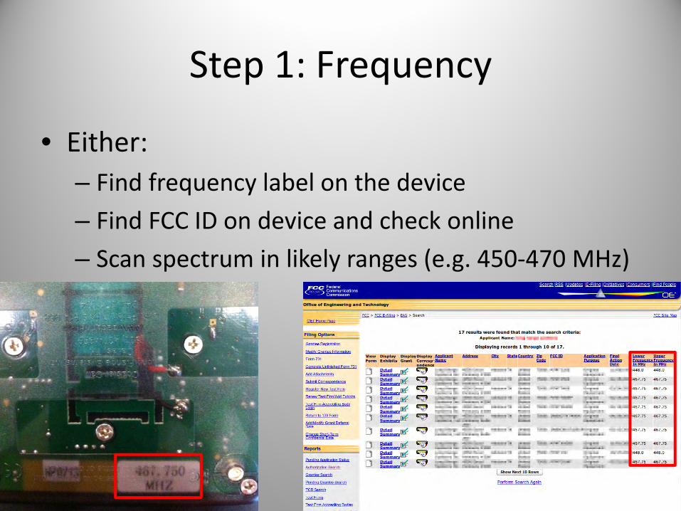
Step 1: Frequency
• Either:– Find frequency label on the device
– Find FCC ID on device and check online
– Scan spectrum in likely ranges (e.g. 450‐470 MHz)

Step 1: Frequency

Step 1: Frequency
Note how often transitions occur(no long runs of ‘0’ or ‘1’).Implies line encoding is in use(helps clock recovery at receiver).

Flowgraph

Step 2: Channel Selection

Step 3: FSK Deviation

Step 4: Quadrature Demod

Step 5: Baud Rate

Step 5: Clock Recovery

Step 6: Line Encoding

Manchester Encoding

Manchester Violation
Presenter
Presentation Notes
Red bits have resulted from an invalid Manchester pair (caused here by offsetting the bit stream by one bit)

Step 7: Compare Changing Bits

Step 8: Finding the ID

Modulator
• Reverse the decoding process:1. Construct packet
a) Preamble (wake up receiver)b) Magic header (sync & system ID)c) Pager numberd) Checksum
2. Interpolate (choose samples per bit)3. Frequency Modulate4. Apply pulse‐shaping filter (ideally)5. Resample for transmitter


Modulator

Modulator Output
Presenter
Presentation Notes
Note: pulse-shaping filter has not been applied yet!

Modulator

Remote Control

Slider

POCSAG
• Other restaurant pager systems adopt a standard
• Decode with gr‐pocsag– Modified to end frame decoding when squelch closes


POCSAG Decode

POCSAG Frames----[00] Address: 001dc168 function: 00000000[01] (001dc168) Data: 05[5] 0c[ ] 03[3] 03[3] 03[3][02] (001dc168) Idle=== SQUELCHED (residue: 5) ===----[00] (ffffffff) Idle[01] (ffffffff) Idle[02] (ffffffff) Idle[03] (ffffffff) Idle[04] (ffffffff) Idle[05] (ffffffff) Idle[06] Address: 001dc15b function: 00000000[07] (001dc15b) Data: 05[5] 0c[ ] 03[3] 03[3] 03[3][08] (001dc15b) Idle=== SQUELCHED (residue: 5) ===----[00] (ffffffff) Idle[01] (ffffffff) Idle[02] (ffffffff) Idle[03] (ffffffff) Idle[04] (ffffffff) Idle[05] (ffffffff) Idle[06] Address: 001dc15b function: 00000000[07] (001dc15b) Data: 05[5] 0c[ ] 03[3] 03[3] 03[3][08] (001dc15b) Idle=== SQUELCHED (residue: 5) ===

POCSAG Frame
----[00] (ffffffff) Idle[01] (ffffffff) Idle[02] (ffffffff) Idle[03] (ffffffff) Idle[04] (ffffffff) Idle[05] (ffffffff) Idle[06] Address: 001dc15b function: 00000000[07] (001dc15b) Data: 05[5] 0c[ ] 03[3] 03[3] 03[3][08] (001dc15b) Idle=== SQUELCHED (residue: 5) ===
5b = 01011011
Presenter
Presentation Notes
Least-significant three address bits = slot # / 2 http://en.wikipedia.org/wiki/POCSAG

Pager Frame Construction
• Preamble• SYNC• Address: System & Pager
– Schedule address to appear in correct slot– Pad with IDLEs beforehand
• Pager action• Trailing IDLE• Apply BCH(31,21) ECC to each slot

POCASG Modulator

ZigBee
• Roles reversed: pager unit transmits
• Pager unit has integrated RFID reader
• RFID chip stuck on underside of each table
• Placing pager unit on table transmits pager number and table number
• 2.4 GHz ISM band
• Decode with gr‐ieee802‐15‐4

ZigBee Transceiver
Presenter
Presentation Notes
http://www.ccs-labs.org/software/gr-ieee802-15-4/


Decoded ZigBee
Presenter
Presentation Notes
http://www.ccs-labs.org/software/gr-ieee802-15-4/

Decoded Pager
38 = 0x26
54 = 0x36
36 = 0x24
Pagers:
Table:

Hostage Pager
• Pagers get angry when system broadcast (beacon) is not heard within timeout– Flash & vibrate until they are returned within range
• Take a pager hostage by broadcasting beacon

RDS TMC
@spenchdotnetHacking the Wireless World with #sdr

FM Broadcast Band

FM Broadcast Band


Radio Data Service
• Subcarrier on commercial FM stations
• Not audible (filtered out)
• BPSK @ 1187.5 bps
• Listen & decode with gr‐rds

Stereo FM with RDS: Receiver

Radio Data Service
Presenter
Presentation Notes
https://github.com/balint256/gr-rds


Traffic Message Channel
• Type 8A RDS group message• Compact representation via look‐up table:
– Event– Location– Duration
• Examples:– Congestion– Accidents– Road work

Traffic Message Channel
Presenter
Presentation Notes
Happens to flow via Sirius terrestrial repeater. Blanked FM band and Sirius bands to find which.

Traffic Message Channel

Encrypted Location Codes
• Location codes: 16‐bit for a given geographical area
• Encryption keys: 16‐bit
• Schedule: One randomly chosen each day from 31 standard keys
• Receiver update: Key ID broadcast constantly

Daily Key ID

Patterns
• Always three unique temperature reports– Key: Event ID– Value: Location
• Group of three Event IDs always the ‘same’• Encrypted Location IDs always the same for given Enc ID
• Event IDs identical for period of days/weeks– Can vary after some time, but ‘hidden’ (unobserved) value is always the same

‘Temperatures’

Patterns
Key ID (randomeach day)
K1 K2 K2 K3 …
Group Period P1 P1 P2 P2 …
Hidden Plain ‘Location’
L1 evt(P1, L1) : enc(K1, L1) evt(P1, L1) : enc(K2, L1) evt(P2, L1) : enc(K2, L1) evt(P2, L1) : enc(K3, L1) …
L2 evt(P1, L2) : enc(K1, L2) evt(P1, L2) : enc(K2, L2) evt(P2, L2) : enc(K2, L2) evt(P2, L2) : enc(K3, L2) …
L3 evt(P1, L3) : enc(K1, L3) evt(P1, L3) : enc(K2, L3) evt(P2, L3) : enc(K2, L3) evt(P2, L3) : enc(K3, L3) …
Transmitted over the air:Event = evt(period, plain location)Location = enc(key of the day, plain location)
Days

Security Analysis
• 16‐bit is very short
• Identical group of ‘location codes’ are broadcast on a daily basis– Unknown but re‐used plaintext
• ‘Singular’ events can be correlated from a trusted source– Known plaintext

Singular Event from Trusted Source

Input Data
Plain ‘Location’ L1 L2 L3Key ID
K1 enc(K1, L1) enc(K1, L2) enc(K1, L3)
K2 enc(K2, L1) enc(K2, L2) enc(K2, L3)
K3 enc(K3, L1) enc(K3, L2) enc(K3, L3)
K4 enc(K4, L1) enc(K4, L2) enc(K4, L3)
K5 enc(K5, L1) enc(K5, L2) enc(K5, L3)
… … … …
1. Bootstrap: find all possible plain locations & keys that result in enc(K1, L1)2. Given those keys, find all possible plain locations recorded with that Key K1 (i.e. L2, L3)
• Remember pool of possible plain locations for each L & pool of possible keys for K3. For each remaining K, repeat maintaining pool of possible keys for each K:
• Find all possible keys given pool of possible plain locations for each L• Repeat, filtering pools until only one match remains
Remove item from pool when enc(K, L) ≠ input data

AlgorithmPossible Plain Location Pools
Plain ‘Location’
L1 L2 L3
Key ID
K1 enc(K1, L1) enc(K1, L2) enc(K1, L3)
K2 enc(K2, L1) enc(K2, L2) enc(K2, L3)
K3 enc(K3, L1) enc(K3, L2) enc(K3, L3)
K4 enc(K4, L1) enc(K4, L2) enc(K4, L3)
K5 enc(K5, L1) enc(K5, L2) enc(K5, L3)
… … … …
L1 L2
L3
Possible Key Pools
K1K2
K3K4 K5
Iterate & Filter
Despite 16 bits, many potential keys/plain locations are generated at the start due to nature of enc(K, L)

Results

Results
• Convergence expedited by addition of ‘singular’ events– “vehicle fire(s)”– “flooding”– “object(s) on roadway {something that does not neccessarily block the road or part of it}”
• Even though multiple keys exist for a Key ID, with enough data plain location search yields one match!
Aviation RADAR
@spenchdotnetHacking the Wireless World with #sdr

ATCRBS, PSR & SSR
• Air Traffic Control Radar Beacon System– Primary Surveillance Radar
– Secondary Surveillance Radar
Primary:• Traditional RADAR• ‘Paints skins’ and listens for return• Identifies and tracks primary targets, while ignoring ‘ground clutter’• Range limited by RADAR equation ( )4
1d
Presenter
Presentation Notes
B&W photo: http://www.faa.gov/about/history/photo_album/air_traffic_control/index.cfm?cid=radar&print=go

ATCRBS, PSR & SSR
• Air Traffic Control Radar Beacon System– Primary Surveillance Radar
– Secondary Surveillance Radar
Secondary:• Directional radio• Requires transponder• Interrogates transponders, which reply with squawk code, altitude, etc.• Increased range ( )2
1d
Presenter
Presentation Notes
SSR scope: http://cmh.natca.net/tracon.htm

Presenter
Presentation Notes
http://maps.spench.net/rf/#pos=-33.9500387,151.1810595&zoom=17&type=hybrid&auto_fetch=true&clustering=true&cluster_level=16&site=16189

Presenter
Presentation Notes
Not simultaneously covering area; rotating beam that sweeps out circle. Comparative only!

Primary Surveillance RADAR
• Transmits a ‘bang’ (the main pulse)
• Listens for returns (echoes)
‘Bang’
Presenter
Presentation Notes
http://en.wikipedia.org/wiki/Radar_signal_characteristics

The Modes
• A: reply with squawk code• C: reply with altitude• S: enables Automatic Dependant Surveillance‐Broadcast (ADS‐B), and the Aircraft/Traffic Collision Avoidance System (ACAS/TCAS)
SSR
Presenter
Presentation Notes
More modes (military, IFF)

The Modes
• A: reply with squawk code• C: reply with altitude• S: enables Automatic Dependant Surveillance‐Broadcast (ADS‐B), and the Aircraft/Traffic Collision Avoidance System (ACAS/TCAS)
• Mode S not part of ATCRBS, but uses same radio hardware (same frequencies)– Increasing problem of channel congestion
SSR
Presenter
Presentation Notes
More modes (military, IFF)

ADS‐BPosition
Heading
Altitude
Vertical rate
Flight ID
Squawk code

A Typical 747 has…
• 2 x 400 W voice HF• 3 x 25 W voice/data VHF• 2 x 100 W 9GHz RADARs• 2 x GPS, 1.5GHz 60 W voice/data SATCOM• 2 x 75MHz marker beacons• 3 x VHF LOC localiser• 3 x UHF glide slope• 2 x LF ADF automatic direction finder• 2 x VOR VHF omni‐directional range• 2 x 1GHz 600 W transponders• 2 x 1GHz 700 W DME distance measuring equipment• 3 x 500mW 4.3GHz radar altimeters• 3 x 406MHz EPIRB
31 radios

TCASHigh gainSATCOM
Low‐gainVHFXpndr
VHF
DMEADFEPIRBMarkerRADAR Altimeter
HF
Presenter
Presentation Notes
Some of the antenna positions are guesses! HF in vertical stabilizer Distance Measuring Equipment Automatic Direction Finder Emergency Position Indicating Radio Beacon

Mode S Response Encoding
• Data block is created & bits control position of pulses sent by transmitter
Pulse Position Modulation (AM)
Early chipLate chip
Used to differentiate against other Modes
Presenter
Presentation Notes
In reality, pulses won’t be perfect square shapes Manchester encoding

Pulse Position Modulation
• Pulse lasts 0.0000005 seconds (0.5 µs)• Need to sample signal at a minimum of 2 MHz(assuming you start sampling at precisely the right moment and stay synchronised)
• Requires high‐bandwidth hardware and increased processing power
• Ideally, oversample to increase accuracy
Presenter
Presentation Notes
This is a bit faster than what a soundcard can do!
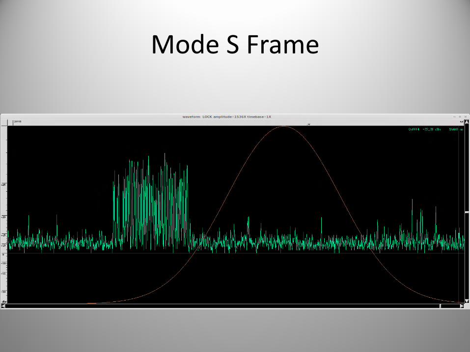
Mode S Frame

Mode S Response: AM signal
Presenter
Presentation Notes
https://www.youtube.com/watch?v=DpNmq7lVpTc&list=PLPmwwVknVIiVReNlEhQ-cBIE7gklFef8_&index=9

Presenter
Presentation Notes
NorCal https://www.youtube.com/watch?v=TTWvlLfdYSg&index=21&list=PLPmwwVknVIiVReNlEhQ-cBIE7gklFef8_

Presenter
Presentation Notes
Bay Area. Trails are altitude colour-coded.

Presenter
Presentation Notes
SFO

Presenter
Presentation Notes
Parallel landing. VRD357 (photo left) has touched down, 102 (photo right) is about to. https://www.youtube.com/watch?v=wP_ILcrHAPw&index=23&list=PLPmwwVknVIiVReNlEhQ-cBIE7gklFef8_

Presenter
Presentation Notes
Parallel landing. VRD357 (photo left) has touched down, 102 (photo right) is about to. https://www.youtube.com/watch?v=wP_ILcrHAPw&index=23&list=PLPmwwVknVIiVReNlEhQ-cBIE7gklFef8_

Presenter
Presentation Notes
VRD034 has just taken off https://www.youtube.com/watch?v=dvOEdaEqgdw&index=24&list=PLPmwwVknVIiVReNlEhQ-cBIE7gklFef8_

Presenter
Presentation Notes
VRD034 has just taken off https://www.youtube.com/watch?v=dvOEdaEqgdw&index=24&list=PLPmwwVknVIiVReNlEhQ-cBIE7gklFef8_

Presenter
Presentation Notes
3D side view of VRD034 takeoff & ascent https://www.youtube.com/watch?v=eKOxQACMb7k&index=25&list=PLPmwwVknVIiVReNlEhQ-cBIE7gklFef8_

Presenter
Presentation Notes
Virtual cockpit view during VRD034 takeoff (during rotate) https://www.youtube.com/watch?v=fbZM2B8xf9k&index=26&list=PLPmwwVknVIiVReNlEhQ-cBIE7gklFef8_

Presenter
Presentation Notes
Virtual cockpit view during VRD034 takeoff (during rotate) https://www.youtube.com/watch?v=fbZM2B8xf9k&index=26&list=PLPmwwVknVIiVReNlEhQ-cBIE7gklFef8_

Presenter
Presentation Notes
Virtual cockpit view during late final approach of UA 1703 at SFO https://www.youtube.com/watch?v=kZy-hRBRu4E&index=22&list=PLPmwwVknVIiVReNlEhQ-cBIE7gklFef8_

Presenter
Presentation Notes
Virtual cockpit view during late final approach of UA 1703 at SFO https://www.youtube.com/watch?v=kZy-hRBRu4E&index=22&list=PLPmwwVknVIiVReNlEhQ-cBIE7gklFef8_

Presenter
Presentation Notes
Bay Area https://www.youtube.com/watch?v=-T4He3PL85I&index=20&list=PLPmwwVknVIiVReNlEhQ-cBIE7gklFef8_

Presenter
Presentation Notes
ACARS messages shown spatially around Sydney, Australia https://www.youtube.com/watch?v=wPUuYjm6TCg&list=PLPmwwVknVIiVReNlEhQ-cBIE7gklFef8_&index=19

Presenter
Presentation Notes
Many ACARS messages are exchanged before/during takeoff, and during/after landing https://www.youtube.com/watch?v=I9krFG3llA4&list=PLPmwwVknVIiVReNlEhQ-cBIE7gklFef8_&index=18

Presenter
Presentation Notes
Easter Egg

Presenter
Presentation Notes
Long-haul flights into Asia

Primary Surveillance RADAR
@spenchdotnetHacking the Wireless World with #sdr
Presenter
Presentation Notes
Waterfall of primary RADAR pulses

Moffett Field ASR‐9

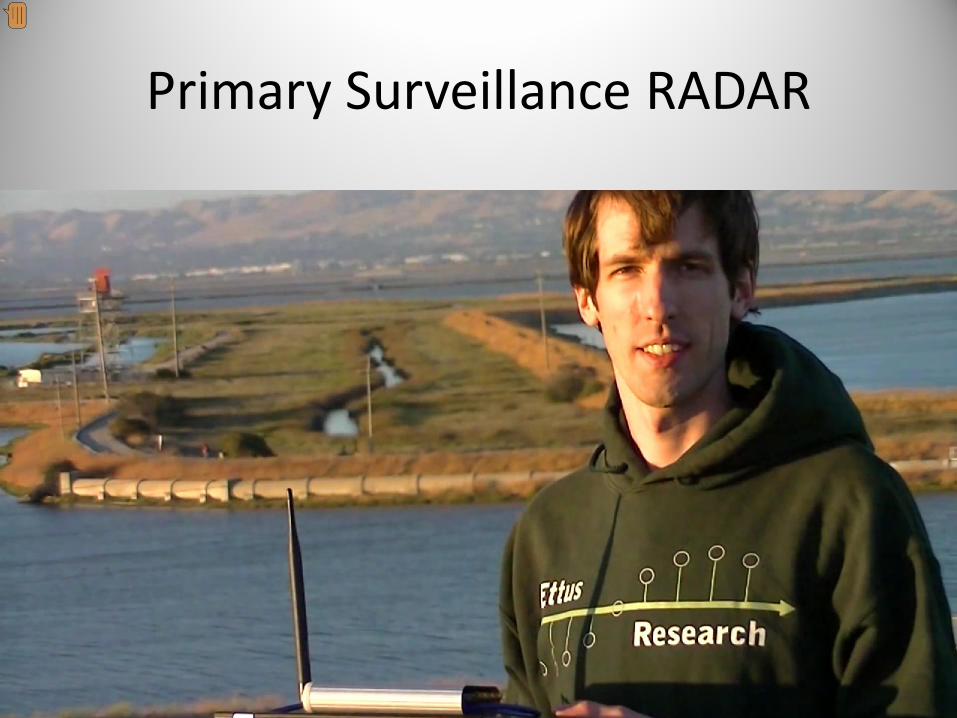
Primary Surveillance RADAR
Presenter
Presentation Notes
All signals shown here were captured with a USRP B210 and a VERT2450 whip antenna (nothing directional!)

Primary Surveillance RADAR
Presenter
Presentation Notes
https://www.youtube.com/watch?v=pRzd_x2Yt5Y&index=37&list=PLPmwwVknVIiVReNlEhQ-cBIE7gklFef8_ Uses RADAR Detector block from: https://github.com/balint256/gr-baz

Primary Surveillance RADAR
Presenter
Presentation Notes
https://www.youtube.com/watch?v=OLVcoZo22TI&index=36&list=PLPmwwVknVIiVReNlEhQ-cBIE7gklFef8_ http://wiki.spench.net/wiki/RADAR

Dual PRF Mode: Weather
Presenter
Presentation Notes
http://www.ufosnw.com/sighting_reports/2006/chicagoohare11072006/narcap_18_radar-section.doc Cho: https://www.ll.mit.edu/mission/aviation/publications/publication-files/atc-reports/Cho_2006_ATC-328_WW-14418.pdf Newell: http://www.ll.mit.edu/mission/aviation/publications/publication-files/atc-reports/Newell_2000_ATC-264_WW-15318.pdf

RADAR Returns‘Bang’
Presenter
Presentation Notes
http://en.wikipedia.org/wiki/Radar_signal_characteristics

Presenter
Presentation Notes
A beautiful view at sunset

Presenter
Presentation Notes
Alfredo Muniz & Austin Epps helping with signal acquisition (unfortunately didn’t actually end up using these captures for various reasons – just used those captured on the USRP B210 with the whip antenna)

Presenter
Presentation Notes
Alfredo Muniz helping with signal acquisition (unfortunately didn’t actually end up using these captures for various reasons – just used those captured on the USRP B210 with the whip antenna)

Presenter
Presentation Notes
Like old times in Sydney Park with mah BOR!

Magnitude Histogram
Presenter
Presentation Notes
Histogram of the magnitude of all recorded samples (linear count)

Magnitude Histogram
Presenter
Presentation Notes
Histogram of the magnitude of all recorded samples (logarithmic count). Pick a reasonable noise floor threshold.

Above Noise Floor
Presenter
Presentation Notes
Histogram of all sample magnitudes that exceed noise floor (linear counts)

Above Noise Floor
Presenter
Presentation Notes
Histogram of all sample magnitudes that exceed noise floor (logarithmic counts). Pick a ‘strong pulse’ threshold level.

Pulse Length Histogram
Presenter
Presentation Notes
Histogram of length (in samples) of continuous series of samples that exceed the strong pulse threshold. Pick reasonable length of RADAR’s ‘bang’ (transmit pulse).

Pulse Envelope
Presenter
Presentation Notes
With levels and ‘bang’ length set, analyser can begin tracking and visualising the bangs and samples that follow

Pulse Envelope
Presenter
Presentation Notes
Letting the analyser run for longer and accumulate (overlay) more detected ‘bangs’ (linear magnitude scale)

Pulse Envelope
Presenter
Presentation Notes
Bang envelope as before, but logarithmic magnitude scale

Strong Pulse Separation
Presenter
Presentation Notes
Graph of distance (in samples) between detected ‘bangs’, which will indicate the RADAR’s Pulse Repetition Frequency (PRF). Here there appear to be two distinct PRFs.

PRF Histogram
Presenter
Presentation Notes
Showing the previous result as a histogram of the inverse of the distance (in seconds) between detected bangs, the two Pulse Repetition Frequencies are clearly discernable

Strong Pulses vs. Time
Presenter
Presentation Notes
Time-series graph of strong pulses revealing regularity of signal as RADAR rotates and points at receiver’s antenna (blank periods when RADAR is facing away from receiver)

Strong Pulses vs. Time (zoomed)
Presenter
Presentation Notes
Zooming into one of the ‘strong pulse’ groups

Pulse Power vs. Time
Presenter
Presentation Notes
Once full tracking is enabled (PRFs are set), the blank areas are filled with the RADAR signal (weaker, while it’s pointed away from the receiver)

Pulse Power vs. Time (zoomed)
Presenter
Presentation Notes
Zooming into the peak of a group (while the RADAR’s beam is passing through the receiver’s antenna) reveals fluctuations in the signal magnitude

Distance Between Pulses
Presenter
Presentation Notes
Once full tracking is enabled, it is possible to graph the (sample) distance between detected ‘bangs’, showing some drift in timing (the diagonal arrangement of points) as well a seemingly random switching back-and-forth between the two PRFs

Pulse and echo power over time
Presenter
Presentation Notes
All detected pulses can be visualised showing how the intensity of the ‘bang’, as well as the close-in returns (clutter), changes as the RADAR rotates. https://www.youtube.com/watch?v=ymD27ePLD1o&index=38&list=PLPmwwVknVIiVReNlEhQ-cBIE7gklFef8_

Raw RADAR Return Plot
Each scanline is synchronised to an emitted pulse
Scanline is amplitude of samples over time (also range of the return)
Presenter
Presentation Notes
Taking each ‘frame’ (or pulse-triggered group of samples) from the last sequence, and stacking them vertically produces this raster plot of the sample magnitudes where each scanline is triggered by a pulse

Presenter
Presentation Notes
Interesting shapes emerge

Presenter
Presentation Notes
Interesting patterns can be seen

Presenter
Presentation Notes
Some features appear particularly interesting

Presenter
Presentation Notes
Close-up of the distant, strong return

Virtual RADAR Scope
RADAR
Presenter
Presentation Notes
The raster plot can undergo a polar-coordinate transformation and be unwrapped onto the map (with the image centred on the RADAR’s position). The ‘interesting features’ now line up with real physical features of the area.

Presenter
Presentation Notes
The curved, dotted feature now becomes a series of straight lines (inside the red polygon), which are in fact power line pylons

Presenter
Presentation Notes
The pylons cross the Bay

Presenter
Presentation Notes
Looking further north-west at the bridges

Presenter
Presentation Notes
The raster plot can be rendered for the entire capture, which shows multiple RADAR rotations (the same patterns being repeated)

Presenter
Presentation Notes
Rendering each rotation in greyscale, and creating a composite RGB image where each colour channel is one of the individual rotations (e.g. R: first, G: middle, B: last), can be used to detect a moving target. In this image, everything is ‘white’, since all the pixels from each channel align (spatially within the image, which implies in terms of time).

Presenter
Presentation Notes
In this image, the R-G-B separation caused by moving target can be seen (each rotation will have that cluster of pixels move, so the pixels will no longer line up on top of each other in each colour channel)

Presenter
Presentation Notes
Close-up of moving target

Presenter
Presentation Notes
Another moving target, this time further out

Presenter
Presentation Notes
Close-up of moving target

Presenter
Presentation Notes
Polar un-wrap of moving-target plot

Presenter
Presentation Notes
Adding map underlay to moving-target plot

Presenter
Presentation Notes
Close-up of moving target on map. Probably a large truck (good RADAR Cross-Section) driving along a road in front of the Bay (speed, which is about that of a moving vehicle, can be inferred from RADAR rotation rate)

Presenter
Presentation Notes
Recording RADAR pulses while in Las Vegas (LAS McCarran International Airport is just off to the left, as is the ASR-9)

LAS ASR‐9
Presenter
Presentation Notes
Position of the RADAR and the receiver. Having the airport (i.e. moving targets) between the two is a highly non-ideal configuration.

Distortion MapMon
ostatic
Bistatic
Angle Distance 2D Offset
Presenter
Presentation Notes
Since the transmitter (RADAR) and receiver are actually in different positions (more a bistatic setup), technically you need to ‘undistort’ the polar unwrapping of the RADAR returns (e.g. with a distortion map). If the receiver is close to the RADAR (like on the hill where the signals were recorded) the offset is negligible, and doesn’t need to be corrected. Nevertheless to perform correction, a distortion map needs to be generated using the spatial offset of the transmitter and receiver. Such a map can be visualised (like in this slide) to see how spatial points will get adjusted. The ‘2D Offset’ images show the magnitude of the horizontal (red) and vertical (blue) displacement of pixels in the distortion map.

Presenter
Presentation Notes
Potential moving target at LAS

Presenter
Presentation Notes
Close-up of potential moving target at LAS

Presenter
Presentation Notes
Odd clutter returns on only one rotation at LAS

Presenter
Presentation Notes
Close-up of odd clutter returns on only one rotation at LAS

Multipath
@spenchdotnetHacking the Wireless World with #sdr
Presenter
Presentation Notes
Waterfall of FasTrak interrogation

ATSC
Presenter
Presentation Notes
Spectrum of ATSC (digital TV in the US)

PN511
Presenter
Presentation Notes
PN511 is inserted into the transmitted stream to serve as field synchronisation pattern that receivers can detect. Modulated waveform shown.

Correlation Peaks
Presenter
Presentation Notes
Correlation response of a real ATSC signal with the PN511 waveform showing regularity of sync pattern (X axis is time in samples)

Presenter
Presentation Notes
Consecutive PN511 correlation responses overlaid on top of one-another (sync’d around each one’s peak, X axis is time in samples zoomed around each peak)

Presenter
Presentation Notes
Each horizontal scanline is a PN511 correlation response (centred on peak response, X axis is time in samples zoomed around each peak). Like looking at the previous image from above so it is now possible to see time (vertically).

Presenter
Presentation Notes
View from directional antenna reception position. Antenna starts by pointing at closer hill on the right and is rotated slowly to point toward distant hill on the left. ATSC transmitter is behind scene’s virutal camera, on the other side of the hill from which we see this view (so there is no direct path to transmitter).

Presenter
Presentation Notes
Visualisation of multipath signal propagation. Correlation response over time as antenna is rotated from pointing at closer hill to distant one. Strongest initial correlation peak in centre is from the signal traversing the shorter ‘initial primary’ path (off the closer hill). The other strong responses to the right of centre are the longer propagation paths (those signals are delayed, so appear further to the right of the initial primary since the X-axis is time). As antenna is rotated the initial primary signal becomes weaker, and the right-most response becomes the strongest as the antenna is now pointing at the distant hill.

Presenter
Presentation Notes
Running the experiment while the receiver is covering a large distance. Composite of signal captured & processed at regular intervals (image is of vertically stacked chunks). SNR changes dramatically in certain areas. Captured with: https://github.com/balint256/cyberspectrum

Presenter
Presentation Notes
Zooming into previous image, correlation peak is tilted, which could suggest that the path of signal is changing in length. The receiver is sync’d with a GPSDO, so the analysis software operates in ‘unlocked’ mode where the correlation peak synchronisation only happens once at the beginning. After that, the correlation response is sampled at a regular interval (instead of the peak search being done).

RFID
@spenchdotnetHacking the Wireless World with #sdr
Presenter
Presentation Notes
Waterfall of FasTrak interrogation

Presenter
Presentation Notes
http://en.wikipedia.org/wiki/FasTrak

FasTrak
• Traffic toll tag– Contains your ID
• Interrogation signal in 900 MHz ISM band– ‘Wake up’ signal activates tag
– Pulse‐Position Modulated payload
• Tag replies with backscatter modulation– Reflects transmitter’s RF energy (tiny amount)
– Modulates reflection with Frequency Shift Keying

Presenter
Presentation Notes
Excellent source of info & hardware-level security analysis http://rdist.root.org/2008/08/07/fastrak-talk-summary-and-slides/

Presenter
Presentation Notes
Yagi antennas pointed into each lane. This is not a toll point! This is traffic ‘monitoring’.

Presenter
Presentation Notes
One of the yagi antennas

Presenter
Presentation Notes
The interrogator’s signal in the frequency domain

Presenter
Presentation Notes
Drive-through toll implementation

Interrogation Signal
Payload
Backscatter carrierWake up
Preamble

Wake Up/Preamble

Interrogation Payload

Backscatter Carrier

RF Circulation
1
2
3TX
ANT
RX
Presenter
Presentation Notes
http://en.wikipedia.org/wiki/Circulator

Interrogation Signal
Presenter
Presentation Notes
This is transmitted constantly

Received Signal
Interrogation
CW
Presenter
Presentation Notes
This is what the radio hears (due to signal leakage in the RF front end, and lack of perfect circulator signal isolation) https://www.youtube.com/watch?v=Z814WybtY5g&list=PLPmwwVknVIiVReNlEhQ-cBIE7gklFef8_&index=40

Received Signal
Response
Presenter
Presentation Notes
Received signal while tag is replying https://www.youtube.com/watch?v=Z814WybtY5g&list=PLPmwwVknVIiVReNlEhQ-cBIE7gklFef8_&index=40

Received Signal
Response
Presenter
Presentation Notes
Received signal while tag is replying https://www.youtube.com/watch?v=Z814WybtY5g&list=PLPmwwVknVIiVReNlEhQ-cBIE7gklFef8_&index=40

Title 21 Specification
Presenter
Presentation Notes
CA DOT’s open specification

Preamble Detection
Presenter
Presentation Notes
https://www.youtube.com/watch?v=Z814WybtY5g&list=PLPmwwVknVIiVReNlEhQ-cBIE7gklFef8_&index=40

Preamble Detection
Matched Preamble Filter Response
Presenter
Presentation Notes
Maximal filter response from tag response’s preamble https://www.youtube.com/watch?v=Z814WybtY5g&list=PLPmwwVknVIiVReNlEhQ-cBIE7gklFef8_&index=40

Slicer Time!
Sample bits
Presenter
Presentation Notes
Perform slicing to extract bits, just like with POCSAG at the very beginning of this slide deck https://www.youtube.com/watch?v=Z814WybtY5g&list=PLPmwwVknVIiVReNlEhQ-cBIE7gklFef8_&index=40

Reading a Tag Outside
Presenter
Presentation Notes
https://www.youtube.com/watch?v=tAkujpOP4XI&index=39&list=PLPmwwVknVIiVReNlEhQ-cBIE7gklFef8_

Presenter
Presentation Notes
The FasTrak tag reader flowgraph FasTrak Decoder block in: https://github.com/balint256/gr-baz/

Presenter
Presentation Notes
USRP X310 used to do simultaneous dual-channel recording with an LFRX (car) and WBX (remote)

Presenter
Presentation Notes
WBX is used to receive UHF transmission from remote control, which is triggered by LF challenge from car

Frequency‐domain Amplitude (LF)
Presenter
Presentation Notes
Challenge

Time‐domain Amplitude (LF)
Presenter
Presentation Notes
Challenge

Time‐domain Amplitude (LF)
Presenter
Presentation Notes
Response

Frequency‐domain Amplitude (UHF)
Presenter
Presentation Notes
Response

Time‐domain Amplitude (UHF)

baudline Dual FFT
LF
UHF

GNU Radio baudline
Presenter
Presentation Notes
https://www.youtube.com/watch?v=kIxYxKAJdiI&list=PLPmwwVknVIiVReNlEhQ-cBIE7gklFef8_&index=41

GNU Radio + baudline
Presenter
Presentation Notes
Dual-channel RX stream is combined into interleaved sample stream, which is sent to baudline


Building Security Badge Auth

Time‐domain Amplitude

Time‐domain Amplitude
Reader Badge

Time‐domain Amplitude
Reader Badge

ISEE‐3 Reboot Project
@spenchdotnetHacking the Wireless World with #sdr
Presenter
Presentation Notes
Waterfall of ISEE-3 telemetry For more detailed information, see the separate presentation: http://wiki.spench.net/wiki/Presentations#ISEE-3_Reboot_Project


Delta V Limit
Presenter
Presentation Notes
http://denniswingo.wordpress.com/2014/05/01/isee-3-reboot-project-technical-update-and-discussion/

Presenter
Presentation Notes
http://en.wikipedia.org/wiki/Arecibo_Observatory http://www.naic.edu/

Arecibo Radio Observatory
Fun
Presenter
Presentation Notes
View from the 12m dish

View from above
Ionospheric heaters
Presenter
Presentation Notes
Heaters are not yet operational

Still a good start…

Weak Signal Low RBW
Presenter
Presentation Notes
Barely above the noise floor (< 1 Hz RBW)

numpy & matplotlib
Presenter
Presentation Notes
There are 3 high-side mixers in the receive chain, so this spectrum is reversed

After Improving Pointing
• ~45 dB C/N
• Moving peak below due to Doppler shift
Presenter
Presentation Notes
Much better SNR

Verifying Transmitted Signal
B200 receiving ‘leakage’ from dish
Presenter
Presentation Notes
While the commands were being transmitted, a USRP B200 was used to verify that the commands (RF energy) were actually leaving the dish (the B200’s antenna is receiving a fraction of total radiated energy – the fraction that happens to fall over the side of the dish).

Moment of First Contact
Happy Dance
Presenter
Presentation Notes
The moment when the unmodulated carrier suddenly became modulated with telemetry after we sent the command to re-enable it (round-trip time: ~105s) Happy Dance GIF: http://imgur.com/oIDnVxs Happy Dance video: Happy Dance GIF: http://imgur.com/oIDnVxs Happy Dance video: https://www.youtube.com/watch?v=CLPG15HXkv8&list=PLPmwwVknVIiUlPbkfBUY1ebP_8hA_4q8j&index=11

Dual Channel Recording
Presenter
Presentation Notes
https://www.youtube.com/watch?v=LX67p5i8nwI&list=PLPmwwVknVIiUlPbkfBUY1ebP_8hA_4q8j&index=13

Raw Captured Baseband
PLL tracking carrier
Presenter
Presentation Notes
Green line indicates the frequency at which the tracker is operating (i.e. should indicate the carrier that is being tracked and mixed down to baseband)

PLL Lock
Presenter
Presentation Notes
Carrier is tracked and signal is centred (mixed down to baseband)

Propulsion System
Presenter
Presentation Notes
Output of ‘tlm’ from: https://github.com/balint256/ice/

Telemetry: 16 bps
Presenter
Presentation Notes
https://www.youtube.com/watch?v=sFXphMnRjKk&list=PLPmwwVknVIiUW9FXfhryeB0BWtba62Igu&index=1

Telemetry: 64 bps
Presenter
Presentation Notes
https://www.youtube.com/watch?v=fKPBvf2hRrw&list=PLPmwwVknVIiUW9FXfhryeB0BWtba62Igu&index=2

Telemetry: 512 bps
Presenter
Presentation Notes
https://www.youtube.com/watch?v=Zr2WUQZMtyI&index=3&list=PLPmwwVknVIiUW9FXfhryeB0BWtba62Igu

Telemetry: 2048 bps
Presenter
Presentation Notes
https://www.youtube.com/watch?v=Y68xdvErQHo&list=PLPmwwVknVIiUW9FXfhryeB0BWtba62Igu&index=4

Telemetry During Thruster Firing
Presenter
Presentation Notes
Graphed with ‘tlm_graph’ from: https://github.com/balint256/ice/

No Thrust
Presenter
Presentation Notes
Each attempt would produce only one (or no) pulse on the real-time accelerometer data. Expectation was to see a large pulse for each firing of the selected thrusters.

Hydrazine Propulsion System
Presenter
Presentation Notes
Nitrogen (pressurant) might have leaked out of both sets of tanks.

New Orbit
Presenter
Presentation Notes
From Cameron Woodman: “So with the failure to perform a trajectory maneuver before the lunar flyby, we passed the Moon at an altitude of 13,000 km instead of the 50 km we needed to bring the s/c back Here is it’s new orbit and it’s now mostly outside Earth’s orbit Brings new challenges, the spacecraft will be farther away from the sun than it was ever designed to be ~20% farther at it’s furthest point: Less power generated by the solar arrays, it’s also going to be a lot colder. It will come back again in 15 years. After the failure of the propulsion system we quickly shifted gears, turned on the data from the science experiments and powered up some of the remaining experiments.”

Presenter
Presentation Notes
http://spacecraftforall.com/

www.spacecraftforall.com
Presenter
Presentation Notes
http://spacecraftforall.com/

Presenter
Presentation Notes
The team outside McMoons

#cyberspectrum
Presenter
Presentation Notes
SDR Meetup: http://www.meetup.com/Cyberspectrum/

Other Applications
@spenchdotnetHacking the Wireless World with #sdr

Blind Signal Analysis

What you need
Dish + LNB + power injector + USRP + GNU Radio(set‐top box with LNB‐thru)
Presenter
Presentation Notes
http://en.wikipedia.org/wiki/Low-noise_block_downconverter

D1 TLM1: 12243.25 MHzMirror of RHS*
Beacon with Phase Modulation* (PM): 1PPS and two telemetry streams (sidebands)
Constant carrier power*
TLM sidebands
Constant sub‐carrier
1PPS
Presenter
Presentation Notes
Mirrored sidebands due to Phase Modulation Constant carrier power useful for determining downlink signal strength

Visualisation
Presenter
Presentation Notes
Highlighted areas are integers (i.e. their binary bits) being incremented on each successive scan line of data

Let’s try one…
• Feed entire baseband spectrum into GR• Perform ‘channel selection’ to isolate stream of interest (create new baseband
centred on stream)
Presenter
Presentation Notes
Eleven narrowband downlinks and one broad(er)band one

Frame analysis
• Header– SYN SYN SYN (EBCDIC)
• Character‐oriented encoding:– SOH– STX– ETX– CRC (CCITT‐16)
• Numbers of fixed‐length messages– Each contains an ID

Un‐pack & find patterns
0001 [20 049 200] (1/1) ff 18 80 70 01 24 e9 ae ed 26 1a 07 31 90 19 fa 00 00 03 02 00 72 e9 2e
0034 [20 051 161] (1/1) ff 18 80 70 01 24 e9 c7 ed 24 1a 07 31 90 19 fa 00 00 03 02 00 72 e9 2d
0067 [20 053 121] (1/1) ff 18 80 70 01 24 e9 d9 ed 2c 1a 07 31 90 19 fa 00 00 03 02 00 71 e9 2d
0101 [20 055 082] (1/1) ff 18 80 70 01 24 e9 ee ed 2f 1a 07 31 90 19 fa 00 00 03 02 00 71 e9 2d
0134 [20 057 043] (1/1) ff 18 80 70 01 24 e9 ff ed 36 1a 07 31 90 19 fa 00 00 03 03 00 72 e9 2e
0167 [20 059 004] (1/1) ff 18 80 70 01 24 ea 10 ed 40 1a 07 31 90 19 fa 00 00 03 02 00 72 e9 2d
0200 [20 060 221] (1/1) ff 18 80 70 01 24 ea 24 ed 43 1a 07 31 90 19 fa 00 00 03 02 00 73 e9 2d
0233 [20 062 182] (1/1) ff 18 80 70 01 24 ea 3b ed 44 1a 07 31 90 19 fa 00 00 03 02 00 72 e9 2d
0266 [20 064 142] (1/1) ff 18 80 70 01 24 ea 4d ed 4c 1a 07 31 90 19 fa 00 00 03 03 00 74 e9 2c
0299 [20 066 103] (1/1) ff 18 80 70 01 24 ea 62 ed 4f 1a 07 31 90 19 fa 00 00 03 03 00 71 e9 2c
0332 [20 068 064] (1/1) ff 18 80 70 01 24 ea 75 ed 54 1a 07 31 90 19 fa 00 00 03 04 00 70 e9 2c
0365 [20 070 025] (1/1) ff 18 80 70 01 24 ea 80 ed 62 1a 07 31 90 19 fa 00 00 03 03 00 6d e9 2d
0398 [20 071 242] (1/1) ff 18 80 70 01 24 ea 98 ed 64 1a 07 31 90 19 fa 00 00 03 02 00 6b e9 2d
0431 [20 073 203] (1/1) ff 18 80 70 01 24 ea a7 ed 6e 1a 08 31 90 19 fa 00 00 03 00 00 6c e9 2d
0464 [20 075 164] (1/1) ff 18 80 70 01 24 ea bc ed 71 1a 08 31 90 19 fa 00 00 03 00 00 6c e9 2d
0497 [20 077 125] (1/1) ff 18 80 70 01 24 ea cf ed 76 1a 08 31 90 19 fa 00 00 02 99 00 6d e9 2d
0530 [20 079 086] (1/1) ff 18 80 70 01 24 ea e8 ed 76 1a 08 31 90 19 fa 00 00 03 00 00 6b e9 2b
0563 [20 081 047] (1/1) ff 18 80 70 01 24 ea f7 ed 80 1a 08 31 90 19 fa 00 00 03 01 00 69 e9 2b
0596 [20 083 008] (1/1) ff 18 80 70 01 24 eb 06 ed 8a 1a 08 31 90 19 fa 00 00 03 01 00 66 e9 2b
0630 [20 084 225] (1/1) ff 18 80 70 01 24 eb 1b ed 8e 1a 08 31 90 19 fa 00 00 03 01 00 67 e9 2b
0663 [20 086 187] (1/1) ff 18 80 70 01 24 eb 30 ed 92 1a 08 31 90 19 fa 00 00 03 01 00 6a e9 2c
0696 [20 088 148] (1/1) ff 18 80 70 01 24 eb 45 ed 95 1a 08 31 90 19 fa 00 00 03 01 00 70 e9 2c
0729 [20 090 109] (1/1) ff 18 80 70 01 24 eb 59 ed 99 1a 08 31 90 19 fa 00 00 03 03 00 73 e9 2c
0762 [20 092 069] (1/1) ff 18 80 70 01 24 eb 6b ed a1 1a 08 31 90 19 fa 00 00 03 03 00 75 e9 2b
0795 [20 094 030] (1/1) ff 18 80 70 01 24 eb 7b ed a9 1a 08 31 90 19 fa 00 00 03 03 00 76 e9 2b
0828 [20 095 247] (1/1) ff 18 80 70 01 24 eb 8e ed af 1a 08 31 90 19 fa 00 00 03 03 00 75 e9 2b
0861 [20 097 208] (1/1) ff 18 80 70 01 24 eb a2 ed b3 1a 08 31 90 19 fa 00 00 03 02 00 74 e9 2b
0894 [20 099 169] (1/1) ff 18 80 70 01 24 eb b7 ed b6 1a 08 31 90 19 fa 00 00 03 03 00 72 e9 2b
0927 [20 101 130] (1/1) ff 18 80 70 01 24 eb ca ed bd 1a 08 31 90 19 fa 00 00 03 03 00 71 e9 2b
0960 [20 103 091] (1/1) ff 18 80 70 01 24 eb da ed c4 1a 08 31 90 19 fa 00 00 03 03 00 70 e9 2b
0993 [20 105 052] (1/1) ff 18 80 70 01 24 eb ef ed c9 1a 08 31 90 19 fa 00 00 03 03 00 70 e9 2b
1026 [20 107 013] (1/1) ff 18 80 70 01 24 ec 03 ed cd 1a 08 31 90 19 fa 00 00 03 03 00 71 e9 2b
#
Message header
16‐bit signed
BCD
8‐bit signed
Presenter
Presentation Notes
Sequence of frames and data analysis

Graphing the Data
1540
1560
1580
1600
1620
1640
1660
‐980 ‐970 ‐960 ‐950 ‐940 ‐930 ‐920
‐8
‐6
‐4
‐2
0
2
4
6
0 5 10 15 20 25 30 35
0
20
40
60
80
100
120
0 5 10 15 20 25 30 35
Presenter
Presentation Notes
Left-hand graph is XY plot of 16-bit signed integer pairs Right graphs are two of the 8-bit signed streams

Software DefinedRadio Direction Finding

SDR Direction Finding
Presenter
Presentation Notes
http://wiki.spench.net/wiki/SDRDF

Presenter
Presentation Notes
MUSIC algorithm-based DOA GUI https://www.youtube.com/watch?v=sGKDsszdMCI&index=3&list=PLPmwwVknVIiVReNlEhQ-cBIE7gklFef8_ MUSIC and compass blocks: https://github.com/balint256/gr-baz

Presenter
Presentation Notes
Video of Direction Finding lab test with four-element Uniform Linear Array antenna configuration https://www.youtube.com/watch?v=usiO6urG73c&index=2&list=PLPmwwVknVIiVReNlEhQ-cBIE7gklFef8_

Presenter
Presentation Notes
Video of Direction-Of-Arrival being plotted during drive https://www.youtube.com/watch?v=DwJUSmD4D3c&index=5&list=PLPmwwVknVIiVReNlEhQ-cBIE7gklFef8_

Two WiFi channels, and then some…
Presenter
Presentation Notes
Demonstrating wide bandwidth of the USRP B2x0 https://www.youtube.com/watch?v=-OwIhPD4tLU&index=34&list=PLPmwwVknVIiVReNlEhQ-cBIE7gklFef8_

FLEX Pagers & Baudline
Presenter
Presentation Notes
https://www.youtube.com/watch?v=3qrwGiw2QJo&index=33&list=PLPmwwVknVIiVReNlEhQ-cBIE7gklFef8_ Visualised with http://www.baudline.com/

900 MHz ISM – Smart Meters
Presenter
Presentation Notes
Smart meter transmissions are the thin wide bursts sitting in well-defined channels https://www.youtube.com/watch?v=a0zGb0nnr8k&index=32&list=PLPmwwVknVIiVReNlEhQ-cBIE7gklFef8_ Received with HDSDR (http://www.hdsdr.de/) and ExtIO_USRP (http://spench.net/r/USRP_Interfaces)

3G W‐CDMA
Signature of UMTS: repeating data in CPICH at 10 ms intervals
Presenter
Presentation Notes
Common Pilot Channel http://wiki.spench.net/wiki/W-CDMA http://wiki.spench.net/wiki/Fast_Auto-correlation

No apparent signal
Cyclic 1023 bit code @ 1.023 MHz chip rate
1 ms
Presenter
Presentation Notes
https://sites.google.com/site/radiorausch/USRPFastAutocorrelation.html Frank says: “It is well known that the (inverse) Fourier transform of a signal's power spectrum is the auto-correlation function (Wiener Khinchin theorem). Therefore if we run a signal through an FFT, calculate the magnitude, and run a final FFT we have a particularly fast way of calculating auto-correlations.” “No signal is apparent in the FFT window while the auto correlation window clearly indicates the presence of something with a 1 ms periodicity. And indeed GPS C/A signals are in fact spread at a 1.023 MHz chip rate with cyclic 1023 bit long codes resulting in 1 ms cycles.”

gnss‐sdr: Decoding L1
Ettus HQ
Presenter
Presentation Notes
Received with a USRP B200 (and N210), bias tee and active GPS antenna http://gnss-sdr.org/

TETRA
Frequency correction burst
Repeating idle pattern
Presenter
Presentation Notes
One slot (of four): 14.175ms http://wiki.spench.net/wiki/TETRA

Presenter
Presentation Notes
The BORs

The Entire HAM Band
Presenter
Presentation Notes
HDSDR with ExtIO_USRP sampling from a USRP N210 (WBX + upconverter) http://spench.net/r/USRP_Interfaces

OpenBTS
• Open‐source 2G GSM stack– Asterix softswitch (PBX)
– VoIP backhaul
Presenter
Presentation Notes
Original implementation with USRP 1 requires special FPGA code (for signal timing constraints) Supports SMS-ing and now GPRS http://openbts.org/ https://wush.net/trac/rangepublic

Presenter
Presentation Notes
LTE eNodeB implemented entirely in host code http://www.amarisoft.com/ https://www.youtube.com/watch?v=7vnz0S52hM0

802.11agp (OFDM) Decoding
Presenter
Presentation Notes
Using gr-ieee-802-11: 802.11agp OFDM transceiver http://www.ccs-labs.org/software/gr-ieee802-11/

Presenter
Presentation Notes
APT reception with a USRP B200 as satellite passes overhead

Automatic Picture Transmission
Presenter
Presentation Notes
http://en.wikipedia.org/wiki/Automatic_Picture_Transmission http://www.wxtoimg.com/

Presenter
Presentation Notes
False Colour

Presenter
Presentation Notes
Sea surface temp

Automatic Identification System
Presenter
Presentation Notes
https://www.youtube.com/watch?v=kU13FuV7IGI&index=31&list=PLPmwwVknVIiVReNlEhQ-cBIE7gklFef8_ Will be found as new repo in https://github.com/balint256/

Presenter
Presentation Notes
Whatever the situation…
Presenter
Presentation Notes
…there’s always SDR.