Optimization of cooperative spectrum sensing and implementation on software defined radios

IEEE TRANSACTIONS ON VEHICULAR TECHNOLOGY, VOL. XX, NO. XX, XX 2011 1

Optimization of Cooperative Spectrum Sensing inCognitive Radio

Tao Cui, Feifei Gao, and A. Nallanathan, Senior Member, IEEE

Abstract— In this paper, we consider cooperative spectrumsensing when two secondary users (SU) collaborate via relayingscheme. We investigate two cooperative sensing strategies, i.e.,SUs exchange data information locally and SUs relay informationto a central controller. The relaying scheme at each SU isoptimized via functional analysis with either the average- or thepeak-power constraints. For local cooperative sensing strategy,the optimal relaying schemes looks like amplify-and-forward (AF)in low signal-to-noise ratio (SNR) region, while behaves likedecode-and-forward (DF) in high SNR region. The fundamentalperformance limit using local cooperative sensing is discussed.For global cooperative sensing strategy, we propose both coher-ent and non-coherent sensing, depending on whether SUs aresynchronized. In the coherent case, a decentralized approach isdesigned and each SU optimizes its relaying function locally. Inthe non-coherent case, we use linear energy combination detectorto decouple the relaying function from the weight coefficientsoptimization. Simulation results demonstrate that the proposedprotocols achieve much better performance over the existing ones.

Index Terms— Cooperative Spectrum Sensing, Cognitive Ra-dio, Optimal Strategy, Wireless Relay Networks.

I. INTRODUCTION

In traditional spectrum management, frequency bands areexclusively allocated to licensed users, which induces spec-trum scarcity due to the emergence of new wireless services.According to the Federal Communications Commission (FCC)[1], the current utilization of the licensed spectrum varies from15% to 85%, whereas only 2% of spectrum would be usedin US at any given moment. The concept of cognitive radio(CR) was introduced in [2] to remedy the spectrum scarcityproblem. In CR, the unlicensed users could opportunisticallyaccess the spectrum assigned to the licensed users providedthat no harmful interference is caused to incumbent services.For example, the IEEE 802.22 standard for cognitive wire-less regional area networks [3] aims at sharing the unusedspectrums that have been allocated to the television broadcastservice to bring broadband access to hard-to-reach areas.

Paper approved by Prof. Bechir Hamdaoui. Manuscript received July 15,2010; revised November 24, 2010; accepted January 22, 2011.

This work was supported in part by EPSRC under Grant EP/I000054/1. Thispaper has been presented in part in the tenth IEEE International Workshopon Signal Processing Advances for Wireless Communications, Perugia, Italy,June 2009.

T. Cui is with the Department of Electrical Engineering, California Instituteof Technology, Pasadena, CA 91125, USA (Email: [email protected]).

F. Gao is with the Department of Automation, Tsinghua University, China(Email: [email protected]).

A. Nallanathan is with the Department of Electronic Engineering, King’sCollege London, London, WC2R 2LS, United Kingdom (Email: [email protected]).

The key technology for CR is the spectrum sensing that canfind the vacant frequency band that is not currently occupiedby the primary users (PU). Existing spectrum sensing tech-niques include energy detection, matched filter, and variousothers that can be found from [4] and the reference therein.The sensing performance with a single cognitive user degradesgreatly with channel fading and shadowing. To enhance thesensing reliability, cooperative spectrum sensing has beenstudied in [5]. Normally, the cooperative sensing involves twosuccessive stages: sensing and reporting. In the sensing stage,the techniques in [4] can be used by each secondary user (SU).In the reporting stage, all local sensing decisions are reportedto a central controller through a control channel. Finally thecentral controller makes the decision and informs it to all SUs.The above described scheme requires a control channel andcan be characterized as a centralized scheme.

On the other hand, distributed cooperative sensing protocolwas proposed in [6], where SUs exchange the sensing informa-tion by relaying a properly designed signal to each other. Animproved technology over [6] was reported in [9] by allowingSU to choose to relay or not based on the first sensing decision.Unfortunately, both [6] and [9] are based on intuitive relayingfunctions and no optimal criterion is examined. Cooperativesensing with optimal criterion has been designed in many CRscenarios [7], [8], [10]–[13]. In [7], the channel throughput ismaximized under the interference constraints to cognitive radionetwork. Energy detection with the optimal detection thresholdis derived in [8], [10]. Soft combination of the observedenergies from different cognitive radio users is investigatedin [11] based on the Neyman-Pearson criterion.

In this paper, we propose a different way to optimize theperformance of cooperative spectrum sensing by designing therelaying function. We consider two cooperative sensing strate-gies: local cooperative sensing and global cooperative sensing.In local cooperative sensing, we derive the optimal relayingfunction at SUs by optimizing the sensing performance underboth average and peak power constraints. Interestingly, theoptimal function with the average power constraint agreeswith the amplify-and-forwad (AF)-like scheme in [6] at lowsignal-to-noise (SNR) region, while it reduces to decode-and-forward (DF)-like scheme at high SNR region. Moreover, wedesign an estimate-and-forward (EF) relaying function, whoseperformance is close to the optimal function. In global coop-erative sensing, SUs first observe the signal from the primaryuser (PU) and then transmit processed signals to a centralcontroller to get the final decision. We discuss over bothcoherent cooperation (synchronized SUs) and non-coherentcooperation (unsynchronized SUs). The former cooperationutilized a decentralized approach, where each SU optimizes

2 IEEE TRANSACTIONS ON VEHICULAR TECHNOLOGY, VOL. XX, NO. XX, XX 2011

its relaying function locally while the latter refers to a linearenergy detector. Simulation results show that the proposedstrategies achieve superior performance over the existing ones.

The rest of the paper is organized as follows. Section IIprovides the background. Section III presents the local coop-erative sensing and Section IV discusses the global cooperativesensing. Simulation results are demonstrated in Section V.Finally, conclusions are drawn in Section VI.

II. SYSTEM MODEL

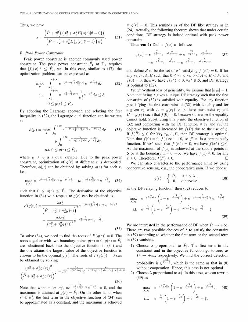
Consider a simple network with two SUs U1 and U2, and asingle PU P. When SUs listen to the environment, the receivedsignal at Ui is

yi = θxphpi + wi, i = 1, 2, (1)

where θ ∈ {0, 1} is the PU indicator, xp belongs to the signalconstellation C, hpi is the channel gain between P and Ui

which is complex Gaussian with unit variance, and wi is theadditive white Gaussian noise with variance σ2

i . All yi, xp,hpi, and wi are complex random variables. We further assumethat the transmission power of PU is P and θ remains staticover the spectrum sensing period.

The probability density function (pdf) of the received yi is

f(yi|θ = 0) =1

πσ2i

e− |yi|2

σ2i , (2)

f(yi|θ = 1) =∑

x∈C

1π(|x|2 + σ2

i )e− |yi|2|x|2+σ2

i Pr(x), (3)

where Pr(x) denotes the probability of x being sent from PU.The optimal detector can be derived from the likelihood ratiotest (LRT):

Λ(y)=f(y|θ = 1)f(y|θ = 0)

=∑

x∈C

Pr(x)σ2i

|x|2 + σ2i

exp( |x|2|y|2

(|x|2 + σ2i )σ2

i

). (4)

SU decides the existence of PU if Λ(y) is greater than athreshold, and not otherwise. Since Λ(y) is a strictly increasingfunction of |y|2, the optimal decision problem is equivalent tocomparing |y|2 with a threshold λ, i.e., If |y|2 > λ, the SUdecides θ = 1; otherwise, θ = 0. Therefore, energy detectoris proved optimal.

The key measurements in spectrum sensing are the proba-bility of correct detection and the probability of false alarm,defined as

Pd = Pr(θ = 1|θ = 1), Pf = Pr(θ = 1|θ = 0). (5)

With the optimal energy detector, it can be calculated that

Pf (λ) =∫ +∞

λ

1σ2

exp(− t

σ2

)dt = exp

(− λ

σ2

), (6)

and

Pd(λ) =∫ +∞

λ

∑

x∈C

1|x|2 + σ2

exp(− t

|x|2 + σ2

)Pr(x)dt

=∑

x∈Cexp

(− λ

|x|2 + σ2

)Pr(x).

(7)

(a) (b)

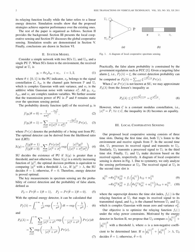
Fig. 1. A diagram of local cooperative spectrum sensing.

Practically, the false alarm probability is constrained by thegovernment regulation such as FCC [1]. Given a targeting falsealarm ξ, i.e., Pf (λ) = ξ, the correct detection probability can

be computed as Pd(λ) =∑

x∈C ξσ2

|x|2+σ2 Pr(x).When C or Pr(x) is not known at SU, we may approximate

Pd(λ) from the Jensen’s inequality as

Pd(λ) ≤ ξσ2

E{|x|2}+σ2 = ξσ2

P+σ2 , (8)

However, when C is a constant modulus constellation, i.e.,|x|2 = P , ∀x ∈ C, the inequality in (8) becomes an equality.

III. LOCAL COOPERATIVE SENSING

Our proposed local cooperative sensing consists of threetime slots. During the first time slot, both Ui’s listen to theenvironment and receive signals from P. In the second timeslot, U1 processes its received signal and transmits to U2.Similarly, U2 transmits a processed signal to U1 in the thirdtime slot. Finally, U1 and U2 make decision based on thereceived signals, respectively. A diagram of local cooperativesensing is shown in Fig. 1. Due to symmetry, we only analyzethe sensing performance at U2. The received signal at U2 inthe second time slot is

y(2)2 =θx(2)

p h(2)p2 + f1

(y(1)1

)h12 + w

(2)2 (9)

=θx(2)p h

(2)p2 + f1

(θx(1)

p h(1)p1 + w

(1)1

)h12 + w

(2)2 , (10)

where the superscript denotes the time slot index, f1(·) is therelaying function at U1 that maps its received signal to itstransmitted signal, and h12 is the channel between U1 and U2

which is complex Gaussian with mean zero and variance σ2h.

Our objective is to optimize the relaying function f1(·)under the relay power constraints. Motivated by the energy

detector in Section II, we propose that U2 compare α∣∣∣y(1)

2

∣∣∣2

+∣∣∣y(2)

2

∣∣∣2

with a threshold λ, where α is a non-negative coeffi-

cient to be determined later. If α∣∣∣y(1)

2

∣∣∣2

+∣∣∣y(2)

2

∣∣∣2

> λ, U2

decides θ = 1; otherwise, θ = 0.

CUI et al.: OPTIMIZATION OF COOPERATIVE SPECTRUM SENSING IN COGNITIVE RADIO 3

A. Average Power Constraint

We first consider the average power constraint P1 at U1.The optimization problem can be expressed

maxf1,α

Pd(f1, α, λ), (11)

s.t. Pf (f1, α, λ) = ξ, E

{∣∣∣f1

(y(1)1

)∣∣∣2∣∣∣∣ θ

}≤ P1, θ = 0, 1.

Given θ we approximate θx(1)p h

(1)p1 +w

(1)1 and θx

(2)p h

(2)p2 +w

(2)2

as Gaussian random variables with zero mean and varianceω2

1 = θP +σ21 and ω2

2 = θP +σ22 , respectively. If x

(1)p and x

(2)p

are from a constant modulus constellation, the approximationis exact. We can rewrite (9) as

y(2)2 = x2 + h12f (x1) , (12)

where x1 and x2 are two independent Gaussian random vari-ables with zero mean and variances ω2

1 and ω22 , respectively.

As an energy detector is applied at SUs, we assume that f(x1)is only a function of |x1|, i.e., f (x1) =

√g (|x1|2) =

√g (r),

where r is chi-square distributed with two degrees of freedom.Assuming that E{|h12|2} = σ2

h is known at U1 and U2,conditioned on a given r, y is a Gaussian random variable withmean zero and variance ω2

2 + σ2hg (r), and v = |y|2 is a chi-

square random variable with two degrees of freedom. From the

characteristic function approach [14], z = α∣∣∣y(1)

2

∣∣∣2

+∣∣∣y(2)

2

∣∣∣2

is a non-central chi-square random variable given r = |x1|2with pdf

p(z|r) =

e− z

(θP+σ22)+σ2

hg(r)−e

− zα(θP+σ2

2)

(1−α)(θP+σ22)+σ2

hg(r),

if (1− α)(θP + σ22) + σ2

hg (r) 6= 0,z

α2(θP+σ22)2

e− z

α(θP+σ22) , otherwise.

(13)

The pdf of z is computed as

p(z) =∫

p(z|r)p(r)dr =∫ +∞

0

p(z|r) 1ω2

1

e− r

ω21 dr. (14)

Given the threshold λ, we find that

P (λ, θ) =∫ +∞

λ

p(z)dz (15)

=∫ +∞

0

((θP + σ2

2) + σ2hg (r)

(1− α)(θP + σ22) + σ2

hg (r)e− λ

(θP+σ22)+σ2

hg(r)

− α(θP + σ22)

(1− α)(θP + σ22) + σ2

hg (r)e− λ

α(θP+σ22)

)1ω2

1

e− r

ω21 dr.

Hence, the optimization problem (11) can be rewritten as

maxg,α

P (λ, 1) (16)

s.t. P (λ, 0) ≤ ξ,

∫ +∞

0

g(r)θP + σ2

1

e− r

θP+σ21 dr ≤ P1,

θ = 0, 1, g(r) ≥ 0, ∀r ≥ 0.

From (16), we know that considering θ = 0 in the averagepower constraint is redundant if g(r) is a non-decreasingfunction, which is a reasonable assumption in practice.

The optimal way to solve (16) is to find the optimal gfor each α and then to perform a line search to find theα that achieves the best performance. In the following, weconsider the case α = 0, whose solution can provide sufficientinsight on how the optimal relay function looks like. We thensubstitute the derived relay functions into (16) and perform aline search to find the best α. When α = 0, (16) simplifies to

maxg

∫ +∞

0

e− λ

(P+σ22)+σ2

hg(r) e

− r

P+σ21 dr (17)

s.t.∫ +∞

0

e− λ

σ22+σ2

hg(r) 1

σ21

e− r

σ21 dr ≤ ξ,

∫ +∞

0

g(r)P + σ2

1

e− r

P+σ21 dr ≤ P1, g(r) ≥ 0, ∀r ≥ 0.

1) Lagrange Approach: Lagrange method is a conventionalway to solve optimization problem [15]. Using this method,the optimal relaying function g(r) can be found by maximizingthe Lagrange dual function:

L(g, µ1, µ2) =∫ +∞

0

e− λ

(P+σ22)+σ2

hg(r) e

− r

P+σ21 dr

−µ1

(∫ +∞

0

e− λ

σ22+σ2

hg(r) e

− r

σ21 dr − σ2

1ξ

)

−µ2

(∫ +∞

0

g(r)e− r

P+σ21 dr − (P + σ2

1)P1

),

(18)

where µ1, µ2 ≥ 0 are dual variables. To find the optimal g(r)for each r, we take the derivative of L(g, µ1, µ2) with respectto g(r), which can be obtained as

F (g(r)) =∂L(g, µ1, µ2)

∂g

=λσ2

h(P + σ2

2 + σ2hg (r)

)2 e− λ

(P+σ22)+σ2

hg(r) e

− r

P+σ21

− µ1λσ2h

(σ22 + σ2

hg (r))2e− λ

σ22+σ2

hg(r) e

− r

σ21 − µ2e

− r

P+σ21 .

(19)

To solve (17) numerically, we consider two cases:i) If F (g(r)) < 0 for all g(r) ≥ 0, then it is clear that

we should choose g(r) = 0 to maximize L(g, µ1, µ2), whichcorresponds to the boundary solution;

ii) If there exists a g(r) such that F (g(r)) > 0, then theremust exist a g(r) such that F (g(r)) = 0, because F (∞) < 0and F (g(r)) is a continuous function in g(r). In this case,by solving F (g(r)) = 0, we obtain an implicit function g(r)depending on λ, µ1, µ2.

We then fix one of λ, µ1, µ2 (for example µ2) and substituteg(r) obtained from the two cases into (17). By making thetwo constraints in (17) attain equality, we can obtain theother two parameters (for example λ, µ1) as a function of thefixed parameter µ2. Finally, substituting g(r) into the objectivefunction of (17) and optimizing over the remaining parameterµ2, we obtain the optimal g(r).

To gain insights on the structure of the optimal relayingfunction, we consider several important limiting scenarios inthe following.


i) r À σ21 : Since e

− r

σ21 ≈ 0 when r À σ2

1 , (19) reduces to

λσ2h(

P + σ22 + σ2

hg (r))2 e

− λ

(P+σ22)+σ2

hg(r) = µ2, (20)

which indicates that g(r) = C when r À σ21 and C is a

constant.ii) 0 ≤ r ¿ σ2

1 and σ21 , σ2

2 À P : When 0 ≤ r ¿ σ21 ,

e− r

P+σ21 ≈ 1. With σ2

1 , σ22 À P (corresponding to low SNR

case), (19) can then be simplified to

(1− µ1)λσ2h(

P + σ22 + σ2

hg (r))2 e

− λ

(P+σ22)+σ2

hg(r) = µ2e

P r

σ21(P+σ2

1) , (21)

which gives

g(r) = − λ

2σ2hW

(−Ae

P r

2σ21(P+σ2

1)

) − P + σ22

σ2h

, (22)

where W (·) denotes Lambert’s W function defined asW (x)eW (x) = x. Since rP ¿ (P + σ2

1)σ21 , g(r) can be

linearized to be g(r) = Ar + B by using first order Taylorseries expansion, where A and B are two constants.

Combining both cases, the optimized relaying function canbe approximated by a piecewise linear function as

g(r) =

C, if r > λ1,0, if r ≤ λ2,

Cr − λ2

λ1 − λ2, if λ2 < r ≤ λ1,

(23)

where C > 0, λ1 ≥ λ2 ≥ 0 and λ1, λ2 are two detectionthresholds at U1. To find C, λ1, λ2, we need to substitute (23)into (17). By making the two constraints in (17) attain equality,two variables out of C, λ1, λ2 can be eliminated. The objectivefunction of (17) now only depends on the only remainingvariable, which can be maximized by performing a line search.Finally, substituting the optimized C, λ1, λ2 into (23) gives theoptimized g(r). From the simulation results in Fig. 4, we cansee that when σ2

1 = σ22 = 100.5 the mis-detection probability

1− η by using (23) is twice as that by solving (19) directly.Interestingly, the function (23) contains several special cases

illustrated as follows:i) Decode-and-forward: In (23), if we choose λ1 = λ2, we

obtain

g(r) ={

C, if r > λ1,0, otherwise, (24)

which is similar to the DF strategy in conventional relaychannels. Substituting (24) into (17), we obtain

maxC,λ,λ1

e− λ

P+σ22

(1− e

− λ1P+σ2

1

)+ e

− λ

(P+σ22)+Cσ2

h e− λ1

P+σ21

s.t. e− λ

σ22

(1− e

−λ1σ21

)+ e

− λ

σ22+Cσ2

h e−λ1

σ21 ≤ ξ,

Ce− λ1

P+σ21 ≤ P1.

(25)

We can then convert the DF optimization problem (25) intoa single parameter optimization problem by solving C and λ

from the two constraints for a given λ1 and maximizing theobjective function over λ1.

ii) Amplify-and-forward: In (23), if we choose λ1 = +∞,C/λ1 = A and λ2 = 0, we obtain the AF-like function. Tosatisfy the average power constraint, we should choose A =

P1

P+σ21

, i.e., g(r) = P1rP+σ2

1, which agrees with the AF scheme

in [6].iii) Hybrid: Since (23) can be considered as a combination

of AF and DF, we name it as hybrid strategy in the rest of thepaper.

2) Minimum Mean Square Error Approach: So far we havediscussed how to obtain the relaying function at U1 via theLagrangian function L(g, µ1, µ2). We next consider anotherclass of g(r) by minimizing the average mean square error(MSE) at U1. The detection at U1 incurs false detection.Sending the detection at U1 directly to U2 will cause errorprorogation. Though spectrum sensing is a detection problem,U1 can estimate θ rather than making a hard decision, whichcan be considered as sending soft detection information. Wethus consider the function g(r) to minimize the MSE betweenθ and g(r), i.e.,

g(r) = arg ming′

E{|θ − g′(r)|2

∣∣∣ r}

. (26)

Assuming that the a priori probability of Pr(θ = 0) is knownto be ζ, the objective function in (26) can be written as

E{|θ − g(r)|2

∣∣∣ r}

=∑

θ∈{0,1}

Pr(r|θ)Pr(θ)Pr(r)

|θ − g(r)|2. (27)

Note that Pr(r) is a common factor. Therefore, minimizing(27) is equivalent to minimizing

∑

θ∈{0,1}p(r|θ)Pr(θ) |θ − g(r)|2 (28)

=ζ

σ21

e− r

σ21 g2(r) +

1− ζ

P + σ21

e− r

P+σ21 (1− g(r))2 .

which gives the result

g(r) =1−ζ

P+σ21e− r

P+σ21

1−ζ

P+σ21e− r

P+σ21 + ζ

σ21e− r

σ21

. (29)

Finally, we set g(r) = Cg(r), where C is a constant to keepthe average power constraint at U1. We can compute C and λfrom the last two constraints and the first constraint in (17),respectively. When ζ is unknown, we can substitute g(r) =Cg(r) into (17) and optimize over C, ζ, λ to maximize thecorrect detection probability. This strategy is called estimate-and-forward (EF) in this paper.

3) Determination of α: After obtaining g(r) with α = 0,we can approximate y

(2)2 as Gaussian and the log-likelihood

ratio (LLR) is

lnp(y(1)

2 |θ = 1)p(y(2)2 |θ = 1)

p(y(1)2 |θ = 0)p(y(2)

2 |θ = 0)(30)

=P + σ2

2

σ22

|y(1)2 |2 +

P + σ22 + σ2

hE{g(r)|θ = 1}σ2

2 + σ2hE{g(r)|θ = 0} |y(2)

2 |2.


Thus, we have

α =

(P + σ2

2

) (σ2

2 + σ2hE{g(r)|θ = 0})

(P + σ2

2 + σ2hE{g(r)|θ = 1}

)σ2

2

. (31)

B. Peak Power Constraint

Peak power constraint is another commonly used powerconstraint. The peak power constraint P1 at U1 requiresthat |f1(x)|2 ≤ P1, ∀x. In this case, similar to (17), theoptimization problem can be expressed as

maxg

∫ +∞

0

e− λ

(P+σ22)+σ2

hg(r) e

− r

P+σ21 dr (32)

s.t.∫ +∞

0

e− λ

σ22+σ2

hg(r) 1

σ21

e− r

σ21 dx ≤ ξ,

0 ≤ g(r) ≤ P1.

By adopting the Lagrange approach and relaxing the firstinequality in (32), the Lagrange dual function can be writtenas

φ(µ) = maxg

∫ +∞

0

e− λ

(P+σ22)+σ2

hg(r) e

− r

P+σ21 dr (33)

− µ

∫ +∞

0

e− λ

σ22+σ2

hg(r) e

− r

σ21 dr,

s.t. 0 ≤ g(r) ≤ P1,

where µ ≥ 0 is a dual variable. Due to the peak powerconstraint, optimization of g(r) at different r is decoupled.Therefore, φ(µ) can be obtained by solving g(r) for each r,i.e.,

maxg(r)

e− λ

(P+σ22)+σ2

hg(r) e

− r

P+σ21 − µe

− λ

σ22+σ2

hg(r) e

− r

σ21 , (34)

such that 0 ≤ g(r) ≤ P1. The derivative of the objectivefunction in (34) with respect to g(r) can be obtained as

F (g(r)) =λσ2

h(P + σ2

2 + σ2hg (r)

)2 e− λ

(P+σ22)+σ2

hg(r) e

− r

P+σ21

− µλσ2h

(σ22 + σ2

hg (r))2e− λ

σ22+σ2

hg(r) e

− r

σ21 .

(35)

To solve (34), we need to find the roots of F (g(r)) = 0. Theroots together with two boundary points g(r) = 0, g(r) = P1

are substituted back into the objective function in (34) andthe one attains the largest value of the objective function ischosen to be the optimal g(r). The roots of F (g(r)) = 0 canbe obtained by solving

(σ2

2 + σ2hg (r)

)2

(P + σ2

2 + σ2hg (r)

)2 = µe− P r

σ21(P+σ2

1) e− P λ

(P+σ22+σ2

hg(r))(σ2

2+σ2h

g(r)) .

(36)

Note that when r À σ21 , µe

− λ

σ22+σ2

hg(r) e

− r

σ21 ≈ 0, and the

maximum is attained at g(r) = P1. On the other hand, whenr ¿ σ2

1 , the first term in the objective function of (34) canbe approximated as a constant, and the maximum is achieved

at g(r) = 0. This reminds us of the DF like strategy as in(24). Actually, the following theorem shows that under certainconditions, DF strategy is indeed optimal with peak powerconstraint.

Theorem 1: Define f(x) as follows:

f(x) = e− r1

σ21+x e

− λ

σ22+A+x + e

− r2σ21+x e

− λ

σ22+B+x (37)

−e− r1

σ21+x e

− λ

σ22+x − e

− r2σ21+x e

− λ

σ22+P1+x ,

and define S to be the set of x∗ satisfying f ′(x∗) = 0. If forany r1, r2, A, B such that 0 ≤ r1 < r2, 0 < A < B < P , andf(0) = 0, then we have f(x∗) < 0, ∀x∗ ∈ S, and DF strategyis optimal to (32).

Proof: Without loss of generality, we assume that |h12| = 1.Note that fixing λ gives a unique DF strategy such that the firstconstraint of (32) is satisfied with equality. For any functiong satisfying the first constraint of (32) with equality and fora given r1 with A = g(r1) > 0, there must exist r2 andB = g(r2) such that f(0) = 0, because otherwise the equalitycannot hold. Substituting this g into the objective function of(32) and comparing with the DF function at r1 and r2, theobjective function is increased by f(P ) due to the use of g.If f(P ) ≤ 0 for ∀r1, r2, A, B, then DF strategy is optimal.Note that f(0) = 0, f(+∞) → 0, so f ′(x) is a continuouslyfunction. If ∀x∗ such that f ′(x∗) = 0, we have f(x∗) ≤ 0.As the maximum of f(x) is achieved at the saddle points inS or at the boundary x = 0,+∞, we have f(x) ≤ 0, for anyx ≥ 0. Therefore, f(P ) ≤ 0. ¤

We can also characterize the performance limit by usingcooperative sensing, e.g., the cooperative gain. If we choose

g(r) ={

P1, if r > λ1,0, otherwise,

(38)

as the DF relaying function, then (32) reduces to

maxλ,λ1

e− λ

(P+σ22)

(1− e

− λ1P+σ2

1

)+ e

− λ

(P+σ22)+σ2

hP1 e

− λ1P+σ2

1

s.t. e− λ

σ22

(1− e

−λ1σ21

)+ e

− λ

σ22+σ2

hP1 e

−λ1σ21 = ξ.

(39)

We are interested in the performance of DF when P1 → +∞.There are two possible choices of λ to satisfy the constraintin (39) according to whether the first term or the second termin (39) vanishes.

1) Choose λ proportional to P1. The first term in theconstraint and in the objective function go to zero asP1 → +∞, respectively. We find the correct detection

probability is ξσ22

P+σ22 , which is the same as that in (8)

without cooperation. Hence, this case is not optimal.2) Choose λ proportional to σ2

2 . In this case, we can rewrite(39) as

maxλ,λ1

e− λ

(P+σ22)

(1− e

− λ1P+σ2

1

)+ e

− λ1P+σ2

1 , (40)

s.t. e− λ

σ22

(1− e

−λ1σ21

)+ e

−λ1σ21 = ξ.


(a) (b)

and

Non-coherent Cooperation

Coherent Cooperation

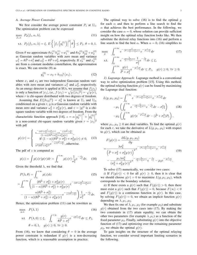
Fig. 2. A diagram of global cooperative spectrum sensing.

Therefore, the maximum correct detection probability is

η∗ = maxλ1≥0

ξ − e

−λ1σ21

1− e−λ1

σ21

σ22

P+σ22

+ e− λ1

P+σ21 . (41)

If λ1 → +∞, (41) reduces to (8). Therefore, η∗ is alwaysgreater than or equal to (8) without cooperation, and thedifference between η∗ and (8) is the cooperative gain. Notethat η∗ does not depend on P1 and thus η∗ is the fundamentallimit of local cooperative sensing, which cannot be improvedby increasing SUs’ transmission power. The fundamental limitalso holds for average power constraint.

Remarks:• Since (17) is not a convex optimization problem, the

solution from solving the Lagrange dual problem may notbe optimal. Nevertheless, we find the solution works wellin most practical scenarios from the simulation results inSection V.

• The hybrid processing function in (23) can be furtherextended to

g(r) =

C, if r > λ1,0, if r ≤ λ2,

Cr − λ3

λ1 − λ2, if λ2 < r ≤ λ1,

(42)

where C, λ1, λ2 are defined the same as in (23) and λ3 ≥λ2 is an additional parameter. By choosing λ3 = λ2,(42) reduces to (23). Thus, (42) is expected to achieve abetter performance than (23) due to an extra degree offreedom. However, using (42) requires more parametersto be optimized.

• Different from [6], where only the signal in the co-operative time slot is used for sensing detection, theproposed protocol makes use of signals received in boththe first and the second time slots, which requires thatthe primary user’s activity remains unchanged during thesensing period.

IV. OPTIMIZATION OF GLOBAL COOPERATIVE SENSING

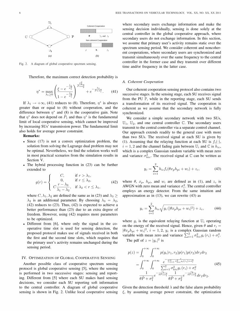
Another possible class of cooperative spectrum sensingprotocol is global cooperative sensing [5], where the sensingis performed in two successive stages: sensing and report-ing. Different from [5] where each SU makes hard sensingdecisions, we consider each SU reporting soft informationto the central controller. A diagram of global cooperativesensing is shown in Fig. 2. Unlike local cooperative sensing

where secondary users exchange information and make thesensing decision individually, sensing is done solely at thecentral controller in the global cooperative approach, wheresecondary users do not exchange information. In this section,we assume that primary user’s activity remains static over thespectrum sensing period. We consider coherent and noncoher-ent cooperations, where secondary users are synchronized andtransmit simultaneously over the same frequency to the centralcontroller in the former case and they transmit over differenttime and/or frequency in the latter case.

A. Coherent Cooperation

Our coherent cooperation sensing protocol also contains twosuccessive stages. In the sensing stage, each SU receives signalfrom the PU P, while in the reporting stage, each SU sendsa transformation of its received signal. The cooperation iscoherent as we assume that the secondary network is fullysynchronized.

We consider a simple secondary network with two SUs,U1, U2, and one central controller C. The secondary userstransmit to the central controller via a separate control channel.Our approach extends readily to the general case with morethan two SUs. The received signal at each SU is given by(1). Assuming that the relaying function at each SU is fi(·),i = 1, 2 and the channel fading gain between Ui and C is hic,which is a complex Gaussian random variable with mean zeroand variance σ2

hic. The received signal at C can be written as

yc =2∑

i=1

hicfi(θxphpi + wi) + zc, (43)

where θ, xp, hpi, and wi are defined as in (1), and zc isAWGN with zero mean and variance σ2

c . The central controlleremploys an energy detector. From the same intuition andapproximation as in (13), we can rewrite (43) as

yc =2∑

i=1

hic

√gi (|θxphpi + wi|2) + zc, (44)

where gi is the equivalent relaying function at Ui operatingon the energy of the received signal. Hence, given θ and ri =|θxphpi + wi|2, i = 1, 2, yc is a complex Gaussian randomvariable with mean zero and variance

∑2i=1 σ2

hicgi (ri) + σ2c .

The pdf of z = |yc|2 is

p(z) =∫ +∞

0

∫ +∞

0

p(yc|r1, r2)p(r1)p(r2)dr1dr2

=∫ +∞

0

∫ +∞

0

e− zP2

i=1 σ2hic

gi(ri)+σ2c

∑2i=1 σ2

hicgi (ri) + σ2c

1θP + σ2

1

e− r1

θP+σ21

1θP + σ2

2

e− r2

θP+σ22 dr1dr2.

(45)

Given the detection threshold λ and the false alarm probabilityξ, by assuming average power constraint, the optimization


problem becomes

maxg

∫ ∫ +∞

0

e− λP2

i=1 σ2hic

gi(ri)+σ2c e− r1

P+σ21 e− r2

P+σ22 dr1dr2

s.t.∫ ∫ +∞

0

e− λP2

i=1 σ2hic

gi(ri)+σ2c

1σ2

1σ22

e− r1

σ21− r2

σ22 dr1dr2 ≤ ξ,

∫ +∞

0

gi(ri)e− ri

P+σ2i

P + σ2i

dri ≤ Pi,

∫ +∞

0

gi(ri)e− ri

σ2i

σ2i

dri ≤ Pi,

(46)

i = 1, 2. Since g1 (r1) and g2 (r2) can be separated, (46)is hard to solve even with a central controller. We insteadconsider two suboptimal approaches. The first approach isa parametric and centralized approach. We can assume thatgi (ri) attains a specific form such as AF, DF, and EF. Wethen optimize over the relevant parameters in each strategy.This approach requires that the optimization is performed atthe central controller and it then informs all the SUs about theoptimized functions that they should use. The second approachis a decentralized approach, where each SU optimizes itsrelaying function by assuming other SUs experiencing thesame noise variance σ2

i , channel fading variance σ2hic, and

power Pi. By using the DF strategy and considering thegeneral case with N SUs, the i-th SU needs to solve

maxg

∑

b∈{0,1}N

e− λPN

j=1 bjσ2hic

Ci+σ2c

N∏

j=1

(bj − (2bj − 1)e

− λiP+σ2

i

)

s.t.∑

b∈{0,1}N

e− λPN

j=1 bjσ2hic

Ci+σ2c

N∏

j=1

(bj − (2bj − 1)e

− λiσ2

i

)= ξ,

Ci = eλi

P+σ2i Pi.

(47)

Note that (47) can be simplified to contain only a singleparameter which is easy to solve at each SU. Optimizationunder peak power constraint can be performed similarly.

B. Non-Coherent CooperationIn non-coherent cooperation, each SU sends its signal to

the central controller asynchronously at different time orfrequency. Thus, the central controller receives N differentsignals from N secondary users, i.e.,

yic = hicfi(θxphpi + wi) + zic, i = 1, 2, . . . , N, (48)

where hic, θ, xp, and hpi, are defined as before, and wi and zic

are AWGN with zero mean and variance σ2iw, σ2

c , respectively.The problem is how we can combine yic’s to achieve the bestsensing performance. Motivated by the energy detector, weconsider using the test statistic

z =N∑

i=1

αi|yic|2 =N∑

i=1

αiui, (49)

where ui = |yic|2 and αi ≥ 0 is the weighting coefficient.Applying the same approximation as in (13), yic is a com-plex Gaussian random variable with mean zero and variance

σ2hicgi (ri) + σ2

c given θ and ri = |θxphpi + wi|2, i = 1, 2.We thus obtain the mean of ui as

mi,θ = Eri|θ{σ2

hicgi (ri) + σ2c

}, (50)

and the variance of ui is

ω2i,θ = Eri|θ

{(σ2

hicgi (ri) + σ2c

)2}−m2

i,θ. (51)

According to Lyapunov’s central limit theorem [16], if Nis large, the test statistic z is asymptotically normally dis-tributed with mean mθ =

∑Ni=1 αimi,θ and variance ω2

θ =∑Ni=1 α2

i ω2i,θ. Given the false alarm probability ξ, we deter-

mine the threshold from

Pf (λ) = Q

(λ−m0

ω0

)= ξ ⇒ λ = Q−1(ξ)ω0 + m0, (52)

where Q(·) is the Q-function. The correct detection probabilityis

Pd(α, g) = Q

(λ−m1

ω1

)= Q

(Q−1(ξ)ω0 + m0 −m1

ω1

).

(53)Therefore, we need to solve

minα,g

δω0 + m0 −m1

ω1, (54)

subject to the power constraint, where δ = Q−1(ξ). To solve(54), we decouple the optimization over α and g. Like in thecoherent case, each SU assumes that all the other SUs have thesame noise variance σ2

i , channel fading variance σ2hic, power

Pi, and weight αi. SU i thus needs to compute gi from

mingi

δωi,0 +√

N (mi,0 −mi,1)ωi,1

. (55)

Instead of solving (55) directly, we consider the followingproblem

mingi

δωi,0 +√

N (mi,0 −mi,1)− βωi,1, (56)

where β ≥ 0 is a parameter. By using the same Lagrangianapproach, we find that the optimal solution to (56) has theform

gi(ri) =1 + Ae

− riP

σ2iw

(P+σ2iw

)

B + Ce− riP

σ2iw

(P+σ2iw

)

− σ2c

σ2hic

. (57)

Given B and C, A can be determined by the average powerconstraint. Therefore, a suboptimal solution to (56) can befound by substituting (57) into (56) and performing a twodimensional search. Note that (55) can be solved locally ateach SU.

To compute αi, let αi = αiωi,0. Given mi,θ, ω2i,θ, we can

rewrite (54) as

minα

δ√∑N

i=1 α2i +

∑Ni=1 αi

mi,0−mi,1ωi,0∑N

i=1 α2i

ω2i,1

ω2i,0

. (58)

Define x = [α1, . . . , αN ]T , a =[m1,1−m1,0

ω1,0, . . . ,

mN,1−mN,0ωN,0

]T , and


Λ =diag{

ω21,1

ω21,0

, . . . ,ω2

N,1

ω2N,0

}. Since the value of (58) is

invariant to scaling αi by a constant, (58) is equivalent to

minx

δ − aT x√xT Λx

, s.t. xT x = 1. (59)

In practice, the correct detection probability is usually greaterthan 0.5. By the property of Q-function, we know δ−aT x < 0.Therefore, (59) is equivalent to

minx

δ − aT xε

s.t. xT x = 1, xT Λx ≤ ε2, δ−aT x < 0.

(60)Defining x = x/ε, we obtain

minx

δ‖x‖2 − aT x s.t. xT Λx ≤ 1, δ‖x‖2 − aT x < 0.

(61)It can be easily verified that (61) is a convex optimizationproblem, which can be solved efficiently using interior pointmethod [15]. If (61) is infeasible, then the correct detectionprobability is less than 0.5. In this case, δ−aT x ≥ 0 and (59)is equivalent to

minx

(δ − aT x)2

xT Λxs.t. xT x = 1. (62)

Since (δ − aT x)2 ≤ 2(δ2 + (aT x)2), instead of dealing with(62), we take

minx

xT (δ2IN + aaT )xxT Λx

s.t. xT x = 1, (63)

which can be readily solved using Rayleigh quotient [17], i.e.,the solution is the eigenvector corresponding to the minimumeigenvalue of Λ

12 (δ2IN + aaT )Λ

12 . After obtaining x from

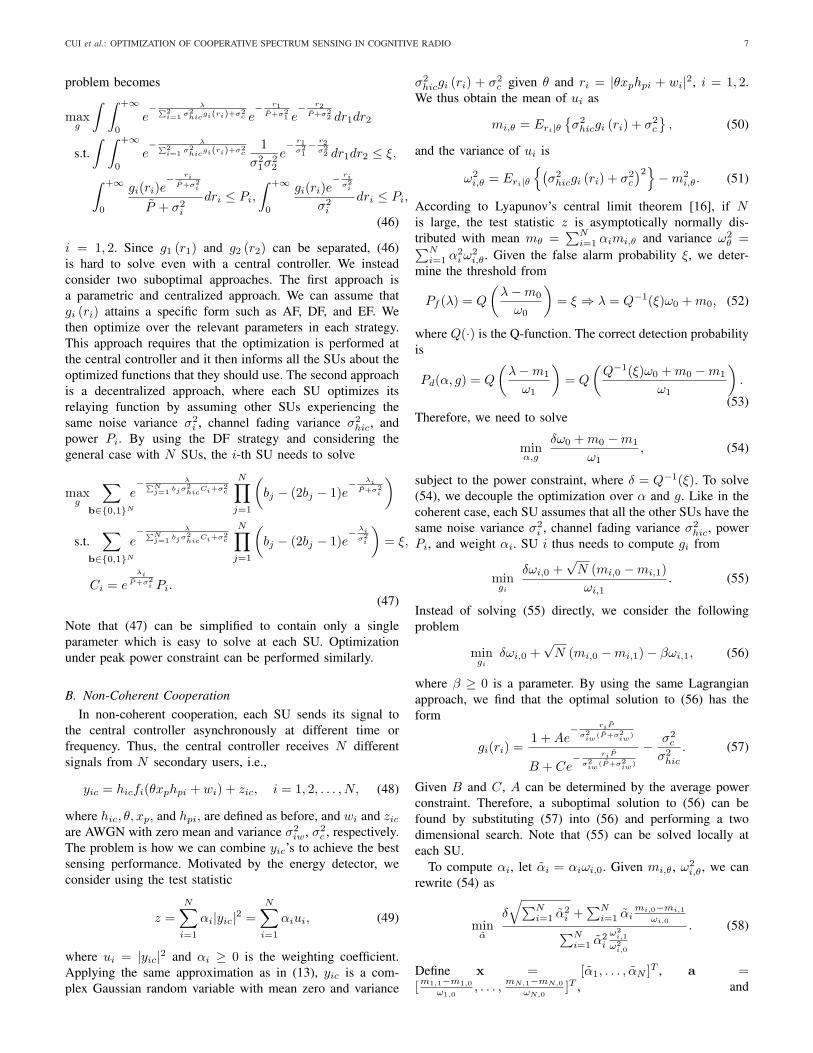
(63), we substitute it into (59) and compare its value with thatobtained from an all-one x. Finally, the approximate solutionis the one that attains a larger value in (59). To evaluatethe performance of the proposed algorithm, 1000 randominstances are generated such that δ − aT x ≥ 0. The solutionusing the approximation (63) is compared with both that fromsolving (59) locally around the approximation and that fromthe all-one vector. Finally, the candidate that attains a largervalue of (59) will be selected. We can see from Fig. 3 thatwith probability greater than 85%, the approximate solutionattains a value less than twice of that by local search.

V. SIMULATION RESULTS

In this section, simulation results are provided to corroboratethe proposed theoretical results. Unless otherwise mentioned,we choose the received PU’s power P = 1 at each SU.

A. Local Cooperative Sensing

In the local cooperative sensing, we choose σ2h = E{σ2

h} =1. We compare with the cooperative spectrum sensing strate-gies in [6] and [9] because the former strategy is similar toAF schme while the latter one is close to DF.

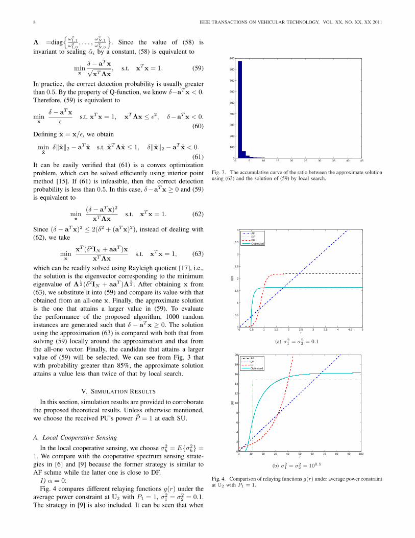
1) α = 0:Fig. 4 compares different relaying functions g(r) under the

average power constraint at U2 with P1 = 1, σ21 = σ2

2 = 0.1.The strategy in [9] is also included. It can be seen that when

0 5 10 15 20 25 30 35 40 450

100

200

300

400

500

600

700

800

900

Fig. 3. The accumulative curve of the ratio between the approximate solutionusing (63) and the solution of (59) by local search.

0 0.5 1 1.5 2 2.5 3 3.5 4 4.5 50

0.5

1

1.5

2

2.5

3

3.5

4

r

g(r)

AFDFEFOptimized

(a) σ21 = σ2

2 = 0.1

0 10 20 30 40 50 60 70 80 90 1000

2

4

6

8

10

12

14

16

18

20

r

g(r)

AFDFEFOptimized

(b) σ21 = σ2

2 = 100.5

Fig. 4. Comparison of relaying functions g(r) under average power constraintat U2 with P1 = 1.


0 0.1 0.2 0.3 0.4 0.5 0.6 0.7 0.8 0.9 110

−4

10−3

10−2

10−1

100

False alarm probability α

Mis

−de

tect

ion

prob

abili

ty 1

−η

AFDFHybridEFAlgorithm in [9]OptimizedNo Cooperation

(a) σ21 = σ2

2 = 0.1

0 0.1 0.2 0.3 0.4 0.5 0.6 0.7 0.8 0.9 10

0.1

0.2

0.3

0.4

0.5

0.6

0.7

0.8

0.9

1


Mis

−de

tect

ion

prob

abili

ty 1

−η

AFDFHybridEFAlgorithm in [9]OptimizedNo Cooperation

0.3 0.35 0.4 0.45 0.5 0.55 0.60.3

0.35

0.4

0.45

0.5

0.55

0.6

(b) σ21 = σ2

2 = 100.5

Fig. 5. Comparison of mis-detection probability 1− η at U2 with differentfalse alarm probability α under the average power constraint under the averagepower constraint at U2 with P1 = 1.

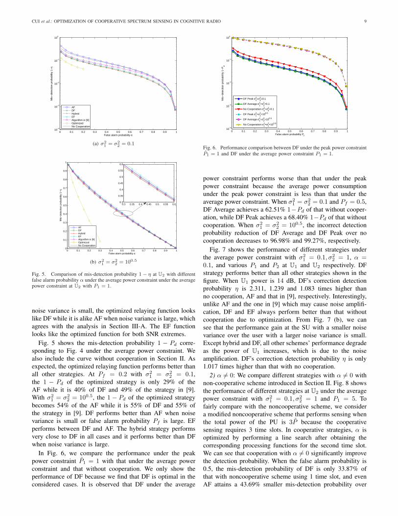
noise variance is small, the optimized relaying function lookslike DF while it is alike AF when noise variance is large, whichagrees with the analysis in Section III-A. The EF functionlooks like the optimized function for both SNR extremes.

Fig. 5 shows the mis-detection probability 1 − Pd corre-sponding to Fig. 4 under the average power constraint. Wealso include the curve without cooperation in Section II. Asexpected, the optimized relaying function performs better thanall other strategies. At Pf = 0.2 with σ2

1 = σ22 = 0.1,

the 1 − Pd of the optimized strategy is only 29% of theAF while it is 40% of DF and 49% of the strategy in [9].With σ2

1 = σ22 = 100.5, the 1 − Pd of the optimized strategy

becomes 54% of the AF while it is 55% of DF and 55% ofthe strategy in [9]. DF performs better than AF when noisevariance is small or false alarm probability Pf is large. EFperforms between DF and AF. The hybrid strategy performsvery close to DF in all cases and it performs better than DFwhen noise variance is large.

In Fig. 6, we compare the performance under the peakpower constraint P1 = 1 with that under the average powerconstraint and that without cooperation. We only show theperformance of DF because we find that DF is optimal in theconsidered cases. It is observed that DF under the average

0 0.1 0.2 0.3 0.4 0.5 0.6 0.7 0.8 0.9 110

−4

10−3

10−2

10−1

100

False alarm probability Pf

Mis

−de

tect

ion

prob

abili

ty 1

−P

d

DF Peak σ12=σ

22=0.1

DF Average σ12=σ

22=0.1

No Cooperation σ12=σ

22=0.1

DF Peak σ12=σ

22=100.5

DF Average σ12=σ

22=100.5

No Cooperation σ12=σ

22=100.5

Fig. 6. Performance comparison between DF under the peak power constraintP1 = 1 and DF under the average power constraint P1 = 1.

power constraint performs worse than that under the peakpower constraint because the average power consumptionunder the peak power constraint is less than that under theaverage power constraint. When σ2

1 = σ22 = 0.1 and Pf = 0.5,

DF Average achieves a 62.51% 1−Pd of that without cooper-ation, while DF Peak achieves a 68.40% 1−Pd of that withoutcooperation. When σ2

1 = σ22 = 100.5, the incorrect detection

probability reduction of DF Average and DF Peak over nocooperation decreases to 96.98% and 99.27%, respectively.

Fig. 7 shows the performance of different strategies underthe average power constraint with σ2

1 = 0.1, σ22 = 1, α =

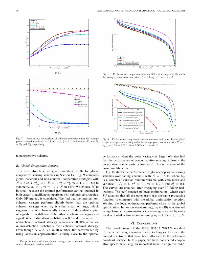
0.1, and various P1 and P2 at U1 and U2 respectively. DFstrategy performs better than all other strategies shown in thefigure. When U1 power is 14 dB, DF’s correction detectionprobability η is 2.311, 1.239 and 1.083 times higher thanno cooperation, AF and that in [9], respectively. Interestingly,unlike AF and the one in [9] which may cause noise amplifi-cation, DF and EF always perform better than that withoutcooperation due to optimization. From Fig. 7 (b), we cansee that the performance gain at the SU with a smaller noisevariance over the user with a larger noise variance is small.Except hybrid and DF, all other schemes’ performance degradeas the power of U1 increases, which is due to the noiseamplification. DF’s correction detection probability η is only1.017 times higher than that with no cooperation.

2) α 6= 0: We compare different strategies with α 6= 0 withnon-cooperative scheme introduced in Section II. Fig. 8 showsthe performance of different strategies at U2 under the averagepower constraint with σ2

1 = 0.1, σ22 = 1 and P1 = 5. To

fairly compare with the noncooperative scheme, we considera modified noncooperative scheme that performs sensing whenthe total power of the PU is 3P because the cooperativesensing requires 3 time slots. In cooperative strategies, α isoptimized by performing a line search after obtaining thecorresponding processing functions for the second time slot.We can see that cooperation with α 6= 0 significantly improvethe detection probability. When the false alarm probability is0.5, the mis-detection probability of DF is only 33.87% ofthat with noncooperative scheme using 1 time slot, and evenAF attains a 43.69% smaller mis-detection probability over


0 5 10 15 20 25 30

0.4

0.5

0.6

0.7

0.8

0.9

1

Transmission power of U1 (dB)

Cor

rect

det

ectio

n η

AFDFHybridEFAlgorithm in [9]No Cooperation

(a) U2

0 5 10 15 20 25 300.2

0.3

0.4

0.5

0.6

0.7

0.8

0.9

1

Transmission power of U2 (dB)

Cor

rect

det

ectio

n η

AFDFHybridEFAlgorithm in [9]No Cooperation

(b) U1

Fig. 7. Performance comparison of different strategies under the averagepower constraint with σ2

1 = 0.1, σ22 = 1, ξ = 0.1, and various P1 and P2

at U1 and U2 respectively.

noncooperative scheme.

B. Global Cooperative Sensing

In this subsection, we give simulation results for globalcooperative sensing schemes in Section IV. Fig. 9 comparesglobal coherent and non-coherent cooperative strategies withN = 3 SUs, σ2

hic = 1, Pi = 1, σ2i = σ2

1 , ∀i = 1, 2, 3. Due tosymmetry, αi = 1, ∀i = 1, . . . , N in (49). We choose N tobe small because the optimal performance can be obtained inboth cases1 to facilitate comparison with suboptimal strategies.Only DF strategy is considered. We find that the optimal non-coherent strategy performs slightly better than the optimalcoherent strategy when σ2

1 is either small or large, whichsuggests that it is beneficially to obtain independent copiesof signals from different SUs rather to obtain an aggregatedsignal. When false alarm probability is 0.5 and σi = σc = 0.1,non-coherent optimal strategy achieves a 60.60% reductionin mis-detection probability over coherent optimal strategy.Even though N = 3 is a small number, the performance byusing Gaussian approximation is fairly close to the optimal

1The performance of non-coherent strategy can be obtained from a non-central chi-square random variable.

0 0.1 0.2 0.3 0.4 0.5 0.6 0.7 0.8 0.9 110

−3

10−2

10−1

100


Mis

−de

tect

ion

prob

abili

ty 1

−η

AFDFEFNo Cooperation 3 time slotsNo Cooperation 1 time slot

Fig. 8. Performance comparison between different strategies at U2 underthe average power constraint with σ2

1 = 0.1, σ22 = 1 and P1 = 5.

0 0.1 0.2 0.3 0.4 0.5 0.6 0.7 0.8 0.9 110

−4

10−3

10−2

10−1

100


Mis

−de

tect

ion

prob

abili

ty 1

−η

Coherent optimal σi2=σ

c2=0.1

Non−coherent optimal σi2=σ

c2=0.1

Non−coherent Gaussian σi2=σ

c2=0.1

No Cooperation σi2=σ

c2=0.1

Coherent optimal σi2=σ

c2=100.5

Non−coherent optimal σi2=σ

c2=100.5

Non−coherent Gaussian σi2=σ

c2=100.5

No Cooperation σi2=σ

c2=100.5

Fig. 9. Performance comparison between coherent and non-coherent globalcooperative spectrum sensing under the average power constraint with Pi = 1,σ2

hic = 1, ∀i = 1, 2, 3. N = 3 SUs are considered.

performance when the noise variance is large. We also findthat the performance of noncooperative sensing is close to thecooperative counterparts in low SNR. This is because of thenoise amplification.

Fig. 10 shows the performance of global cooperative sensingschemes over fading channels with N = 3 SUs, where hic

is a complex Gaussian random variable with zero mean andvariance 1. Pi = 1, σ2

i = 0.1, ∀i = 1, 2, 3 and σ2c = 0.1.

The curves are obtained after averaging over 30 fading real-izations. The performance of local optimization, where eachSU assumes that all the other users use the same processingfunction, is compared with the global optimization solution.We find the local optimization performs close to the globaloptimization. In non-coherent strategy, αi in (49) is optimizedusing Gaussian approximation (53) where gi is solved by usinglocal or global optimization assuming αi = 1, ∀i = 1, . . . , N .

VI. CONCLUSIONS

The development of the IEEE 802.22 WRAN standard[3] aims at using cognitive radio techniques to share theunused spectrums that have been allocated to the televisionbroadcast service. In this paper, we have considered cooper-ative spectrum sensing, an important issue in cognitive radio.


0.1 0.15 0.2 0.25 0.3 0.35 0.4 0.45 0.5

0.02

0.04

0.06

0.08

0.1

0.12

0.14

0.16

0.18

0.2


Mis

−de

tect

ion

prob

abili

ty 1

−η

Coherent globalCoherent localNon−coherent global α

i=1

Non−coherent global optimized αi

Non−coherent local αi=1

Non−coherent local optimized αi

Fig. 10. Performance comparison between coherent and non-coherent globalcooperative spectrum sensing over Rayleigh fading channels under the averagepower constraint with Pi = 1, σ2

i = 0.1, ∀i = 1, 2, 3, ∀i = 1, 2, 3 andσ2

c = 0.1. N = 3 secondary users are considered.

Different from existing works where each SU transmits itslocal sensing decision, we consider SU transmitting a functionof its received signal from the PU. We optimized the relayingfunction at each SU via functional analysis for both averageand peak power constraints. We have discussed optimization oflocal spectrum sensing with two SUs. The proposed spectrumsensing algorithms have a significant performance improve-ment over existing ones. It is interesting to investigate how topair nodes in a large network and what is the best strategy formore than two users cooperation. Also considering multiplePUs simultaneously is in place.

REFERENCES

[1] Federal Communications Commission, “Spectrum policy task force,”http://www.fcc.gov/sptf/.

[2] J. Mitola and G. Maguire, “Cognitive radio: making software radiosmore personal,” IEEE Personal Communications, vol. 6, no. 4, pp. 13–18, Aug. 1999.

[3] “IEEE P802.22/D1.0 Draft Standard for Wireless Regional Area Net-works Part 22: Cognitive Wireless RAN Medium Access Control (MAC)and Physical Layer (PHY) Specifications: Policies and Procedures forOperation in the TV Bands, Apr. 2008.

[4] Y.-C. Liang, Y. Zeng, E. C. Y. Peh, and A. T. Hoang, “Sensing-throughput tradeoff for cognitive radio networks,” IEEE Trans. WirelessCommun., vol. 7, no. 4, pp. 1326–1377, Apr. 2008.

[5] A. Ghasemi and E. Sousa, “Collaborative spectrum sensing for oppor-tunistic. access in fading environments,” in Proc. of IEEE DySPAN, Nov.2005, pp. 8–11.

[6] G. Ghurumuruhan and Y. Li, “Cooperative spectrum sensing in cognitiveradio, part I: two user networks,” IEEE Trans. Wireless Commun., vol. 6,no. 6, pp. 2204–2213, June 2007.

[7] J. Shen, T. Jiang, S. Liu, and Z. Zhang, “Maximum channel throughputvia cooperative spectrum sensing in cognitive radio networks,” IEEETrans. Wireless Commun., vol. 8, no. 10, pp. 5166–5175, Oct. 2009.

[8] W. Zhang and K. B. Letaief, “Cooperative spectrum sensing withtransmit and relay diversity in cognitive radio networks,” IEEE Trans.Wireless Commun., vol. 7, no. 12, pp. 4761–4766, Dec. 2008.

[9] Q. Chen, F. Gao, A. Nallanathan, and Y. Xin, “Improved cooperativespectrum sensing in cognitive radio,” in Proc. of IEEE VTC, 2008.

[10] W. Zhang, R. K. Mallik, and K. B. Letaief, “Optimization of cooperativespectrum sensing with energy detection in cognitive radio networks,”IEEE Trans. Wireless Commun., vol. 8, no. 12, pp. 5761–5766, Dec.2009.

[11] J. Ma, G. Zhao, and Y. Li, “Soft combination and detection forcooperative spectrum sensing in cognitive radio networks,” IEEE Trans.Wireless Commun., vol. 7, no. 11, pp. 4502–4507, Nov. 2008.

[12] J. Unnikrishnan and V. Veeravalli, “Cooperative spectrum sensing anddetection for cognitive radio,” in Proc. of IEEE GLOBECOM, Nov. 2007,pp. 2972–2976.

[13] L. Cardoso, M. Debbah, P. Bianchi, and J. Najim, “Cooperative spec-trum sensing using random matrix theory,” in Proc. of InternationalSymposium on Wireless Pervasive Computing, May 2008, pp. 334–338.

[14] J. G. Proakis, Digital Communications, 4th ed., 2001.[15] S. Boyd and L. Vandenberghe, Convex Optimization. Cambridge

University Press, 2004.[16] O. Kallenberg, Foundations of Modern Probability. New York:

Springer-Verlag, 1997.[17] G. H. Golub and C. F. V. Loan, Matrix Computations, 3rd ed. Johns

Hopkins University Press, 1996.

Tao Cui (S’04) received the M.Sc. degree in theDepartment of Electrical and Computer Engineering,University of Alberta, Edmonton, AB, Canada, in2005, and the M.S. degree from the Department ofElectrical Engineering, California Institute of Tech-nology, Pasadena, USA, in 2006. He is currentlyworking toward the Ph.D. degree at the Departmentof Electrical Engineering, California Institute ofTechnology, Pasadena. His research interests are inthe interactions between networking theory, commu-nication theory, and information theory.

Feifei Gao (S’05−M’09) Feifei Gao received theB.Eng. degree from Xi’an Jiaotong University,Xi’an, Shaanxi China in 2002, the M.Sc. degreefrom McMaster University, Hamilton, ON, Canadain 2004, and the Ph.D degree from National Univer-sity of Singapore in 2007. He was a Research Fel-low at Institute for Infocomm Research, A*STAR,Singapore in 2008, and was an Assistant Professorof the School of Engineering and Science at JacobsUniversity, Bremen, Germany from 2009 to 2010.He joined the Department of Automation, Tsinghua

University, China in 2011, where he is currently an Associate Professor. Healso serves as an Adjunct Professor of the School of Engineering and Scienceat Jacobs University now. His research interests are in communication theory,broadband wireless communications, signal processing, MIMO systems, andarray signal processing. Mr. Gao has co-authored more than 70 refereed IEEEjournal and conference papers and has served as a TPC member for IEEE ICC,IEEE GLOBECOM, IEEE VTC and IEEE PIMRC.

Arumugam Nallanathan (S’97−M’00−SM’05) isa Senior Lecturer in the Department of ElectronicEngineering at King’s College London, United King-dom. He was an Assistant Professor in the De-partment of Electrical and Computer Engineering,National University of Singapore, Singapore fromAugust 2000 to December 2007. His research in-terests include smart grid, cognitive radio and relaynetworks. In these areas, he has published over 160journal and conference papers. He is a co-recipientof the Best Paper Award presented at 2007 IEEE

International Conference on Ultra-Wideband (ICUWB’2007).He currently serves on the Editorial Board of IEEE TRANSACTIONS ON

WIRELESS COMMUNICATIONS, IEEE TRANSACTIONS ON VEHICU-LAR TECHNOLOGY and IEEE SIGNAL PROCESSING LETTERS as anAssociate Editor. He served as a Guest Editor for EURASIP JOURNAL OFWIRELESS COMMUNICATIONS AND NETWORKING: Special issue onUWB Communication Systems- Technology and Applications. He served asthe General Track Chair for the IEEE VTC’2008-Spring, Co-Chair for theIEEE GLOBECOM’2008 Signal Processing for Communications Symposiumand IEEE ICC’2009 Wireless Communications Symposium. He currentlyserves as Co- Chair for the IEEE GLOBECOM’2011 and IEEE ICC’2012Signal Processing for Communications Symposium and Technical programCo-Chair for IEEE International Conference on Ultra-Wideband’2011 (IEEEICUWB’2011). He also currently serves as the Vice-Chair for the SignalProcessing for Communication Electronics Technical Committee of IEEECommunications Society.

Optimization of cooperative spectrum sensing and implementation on software defined radios

Documents

Transcript of Optimization of cooperative spectrum sensing and implementation on software defined radios