
optimal tundish design methodology - University of Pretoria
193
OPTIMAL TUNDISH DESIGN METHODOLOGY IN A CONTINUOUS CASTING PROCESS Daniël Johannes de Kock Presented as partial fulfilment for the degree Philosophiae Doctor in the Faculty Engineering, Built Environment and Information Technology University of Pretoria February 2005 University of Pretoria etd – De Kock, D J (2005)
-
Upload
khangminh22 -
Category
Documents
-
view
6 -
download
0
Transcript of optimal tundish design methodology - University of Pretoria
OPTIMAL TUNDISH DESIGN METHODOLOGY IN A
CONTINUOUS CASTING PROCESS
Daniël Johannes de Kock
Presented as partial fulfilment for the degree
Philosophiae Doctor
in the
Faculty Engineering, Built Environment and Information Technology
University of Pretoria
February 2005
UUnniivveerrssiittyy ooff PPrreettoorriiaa eettdd –– DDee KKoocckk,, DD JJ ((22000055))
ii
ABSTRACT
Title: Optimal Tundish Design Methodology in a Continuous Casting
Process
Author: D.J. de Kock
Promoter: Prof. K.J. Craig
Department: Mechanical and Aeronautical Engineering
University: University of Pretoria
Degree: Philosophiae Doctor (Mechanical Engineering)
The demand for higher quality steel and higher production rates in the production of
steel slabs is ever increasing. These slabs are produced using a continuous casting
process. The molten steel flow patterns inside the components of the caster play an
important role in the quality of these products. A simple yet effective design method
that yields optimum designs is required to design the systems influencing the flow
patterns in the caster. The tundish is one of these systems. Traditionally,
experimental methods were used in the design of these tundishes, making use of plant
trials or water modelling. These methods are both costly and time consuming. More
recently, Computational Fluid Dynamics (CFD) has established itself as a viable
alternative to reduce the number of experimentation required, resulting in a reduction
in the time scales and cost of the design process. Furthermore, CFD provides more
insight into the flow process that is not available through experimentation only. The
CFD process is usually based on a trial-and-error basis and relies heavily on the
insight and experience of the designer to improve designs. Even an experienced
designer will only be able to improve the design and does not necessarily guarantee
optimum results. In this thesis, a more efficient design methodology is proposed.
This methodology involves the combination of a mathematical optimiser with CFD to
automate the design process. The methodology is tested on a four different industrial
test cases. The first case involves the optimisation of a simple dam-weir configuration
of a single strand caster. The position of the dam and weir relative to inlet region is
optimised to reduce the dead volume and increase the inclusion removal. The second
UUnniivveerrssiittyy ooff PPrreettoorriiaa eettdd –– DDee KKoocckk,, DD JJ ((22000055))
Abstract
iii
case involves the optimisation of a pouring box and baffle of a two-strand caster. In
this case, the pouring box and baffle geometry is optimised to maximise the minimum
residence time at operating level and a typical transition level. The third case deals
with the geometry optimisation of an impact pad to reduce the surface turbulence that
should result in a reduction in the particle entrainment from the slag layer. The last
case continues from the third case where a dam position and height is optimised in
conjunction with the optimised impact pad to maximise the inclusion removal on the
slag layer. The cases studies show that a mathematical optimiser combined with CFD
is a superior alternative compared to traditional design methods, in that it yields
optimum designs for a tundish in a continuous casting system.
Keywords: tundish, continuous casting, computational fluid dynamics, mathematical
optimisation, computational flow optimisation, design methodology,
steelmaking, inclusion removal, tundish design
UUnniivveerrssiittyy ooff PPrreettoorriiaa eettdd –– DDee KKoocckk,, DD JJ ((22000055))
iv
SAMEVATTING
Titel: Optimale Gietbak Ontwerpsmetodiek van‘n Kontinue-gietproses
Outeur: D.J. de Kock
Promotor: Prof. K.J. Craig
Universiteit: Universiteit van Pretoria
Departement: Meganiese en Lugvaartkundige Ingenieurswese
Graad: Philosophiae Doctor (Meganiese Ingenieurswese)
Daar bestaan ’n alomtoenemende aanvraag vir hoër kwaliteit staalplate wat teen ’n
hoër tempo geproduseer word. Die plate word geproduseer deur ’n kontinue
gietproses. Die vloeistaal patrone in die proses speel ’n belangrike rol in die
kwaliteit van die produkte. ’n Eenvoudige maar tog effektiewe ontwerpsmetode word
verlang wat optimum ontwerpe lewer van die sisteme wat die vloeipatrone beïnvloed.
Die gietbak is een van die sisteme. Histories is eksperimentele metodes gebruik in die
ontwerp van die gietbakke, met gebruikmaking van aanlegtoetse of water modellering,
Meer onlangs is Berekenings Vloei Dinamika (BVD) gebruik as ’n alternatief om die
aantal eksperimentele toetse te verminder en om sodoende die tydskaal en kostes van
die ontwerpsproses te verminder. Verder verskaf BVD baie meer insig in die vloei
proses wat nie beskikbaar is met tradisionele eksperimentele metodes nie. Die BVD
proses is gewoonlik gebaseer op ’n tref-of-fouteer basis en steun sterk op die
ontwerper se insig en ondervinding om die ontwerp te verbeter. Selfs ’n ontwerper
met baie ondervinding sal slegs die ontwerp kan verbeter en sal nie noodwendig ’n
optimum ontwerp kan gee nie. In die tesis word ’n meer effektiewe ontwerpsmetodiek
voorgestel. Die metodiek behels die kombinering van ’n wiskundige optimerings
program met BVD om die ontwerpsproses te outomatiseer. Die metodiek word
getoets op vier verskillende toetsgevalle. Die eerste geval is die optimering van ’n
eenvoudige dam-keermuur konfigurasie vir ’n enkelstring gietproses. Die posisie van
die dam en keermuur relatief tot die inlaat area is geoptimeer om die dooie volume
verminder en die inklusie verwydering te vermeerder. Die tweede geval beskryf die
optimering van die gietboks en skermplaat van ’n tweestring gietbak. In die geval
UUnniivveerrssiittyy ooff PPrreettoorriiaa eettdd –– DDee KKoocckk,, DD JJ ((22000055))

Samevatting
v
word die gietboks en skermplaat geometrie geoptimeer om die minimum residensie
tyd te maksimeer by die bedryfsvlak en by ’n tipiese transisievlak. Die derde geval
beskou die geometrie optimering van ’n impakstuk om die oppervlak turbulensie te
verlaag, wat veroorsaak dat minder partikels in die vloei ingetrek sal word vanaf die
slaklaag. Die laaste geval volg op geval drie waar ’n dam se posisie en hoogte
geoptimeer word saam met die geoptimeerde impakstuk om die inklusie verwydering
op die slaklaag te maksimeer. Die toetsgevalle wys dat ’n wiskundige optimeerder
gekombineerd met BVD ’n beter alternatief is as tradisionele ontwerpsmetodes, om
sodoende optimum ontwerpe van ’n gietbak van ’n kontinue stringgiet proses te lewer.
Sleutelwoorde: gietbak, stringgiet, berekenings vloei dinamika, wiskundige
optimering, berekenings vloei optimering, ontwerpsmetodiek,
staalmaak, inklusieverwydering, gietbak ontwerp
UUnniivveerrssiittyy ooff PPrreettoorriiaa eettdd –– DDee KKoocckk,, DD JJ ((22000055))

vi
ACKNOWLEDGEMENTS
I wish to express my sincere appreciation to the following persons and organisations
that made this thesis possible:
• Prof Ken Craig and Prof Jan Snyman from the University of Pretoria, for their
guidance, support and friendship.
• Pieter Venter and Willem Orban (Columbus Stainless) for the experimental
water model results.
• Columbus Stainless, Middelburg, South-Africa, especially Johan Ackerman
for his assistance and guidance.
• ISCOR, Flat Steel Products, Vanderbijlpark, South Africa, especially Chris
Pretorius for the plant trial results.
• Technology and Human Resource for Industry Programme (THRIP) funded by
the Department of Trade and Industry (DTI) and managed by the National
Research Foundation for their financial support.
UUnniivveerrssiittyy ooff PPrreettoorriiaa eettdd –– DDee KKoocckk,, DD JJ ((22000055))

vii
TABLE OF CONTENTS
LIST OF FIGURES ....................................................................................................xi
LIST OF TABLES ....................................................................................................xiv
NOMENCLATURE................................................................................................... xv
CHAPTER 1: INTRODUCTION ...........................................................................1
1-1 BACKGROUND.................................................................................................1
1-2 EXISTING KNOWLEDGE...................................................................................4
1-3 RESEARCH OBJECTIVES ..................................................................................5
1-4 SCOPE OF THE STUDY......................................................................................5
1-5 ORGANISATION OF THE THESIS .......................................................................5
CHAPTER 2: LITERATURE STUDY ..................................................................7
2-1 INTRODUCTION ...............................................................................................7
2-2 TUNDISH MODELLING AND DESIGN ................................................................7
2-2.1 The Continuous Casting Process....................................................... 7
2-2.2 Physical Modelling ............................................................................ 8
2-2.3 Plant Trials ...................................................................................... 12
2-2.4 Numerical Modelling....................................................................... 13
2-2.4.1 Grid Generation .................................................................13
2-2.4.2 Conservation Equations.....................................................14
2-2.4.3 Turbulence Modelling .......................................................17
2-2.4.4 Inclusion modelling ...........................................................22
2-2.4.5 Solution Algorithm............................................................25
2-3 MATHEMATICAL OPTIMISATION ...................................................................27
2-3.1 Definition of Mathematical Optimisation........................................ 27
2-3.2 The Non-Linear Optimisation Problem........................................... 27
2-3.3 Optimisation Algorithms.................................................................. 28
UUnniivveerrssiittyy ooff PPrreettoorriiaa eettdd –– DDee KKoocckk,, DD JJ ((22000055))
Table of Contents
viii
2-3.3.1 Snyman’s Leap-Frog Optimisation Program (LFOP)
Adapted to Handle Constrained Optimisation Problems
(LFOPC) ............................................................................29
2-3.3.2 Snyman’s DYNAMIC-Q Method .....................................31
2-3.3.3 Successive Response Surface Method (SRSM) ................37
2-3.4 Gradient Approximation of Objective and Constraint Functions ... 37
2-3.5 Effect of Noise Associated with CFD Solutions on the Gradient
Approximation ................................................................................. 39
2-3.5.1 Source of Noise in CFD Solutions ....................................39
2-3.5.2 Influence of Noise on the Finite Differencing Scheme .....39
2-4 CONCLUSION.................................................................................................42
CHAPTER 3: TUNDISH DESIGN OPTIMISATION METHODOLOGY .....43
3-1 INTRODUCTION .............................................................................................43
3-2 VALIDATION OF CFD MODEL .......................................................................44
3-2.1 Validation Case 1 ............................................................................ 44
3-2.2 Validation Case 2 ............................................................................ 45
3-3 FORMULATION OF OPTIMISATION PROBLEM .................................................47
3-3.1 Candidate design variables ............................................................. 47
3-3.2 Candidate Objective Functions and Constraints from CFD
analysis ............................................................................................ 47
3-3.2.1 RTD Curve ........................................................................48
3-3.2.2 Inclusion removal ..............................................................49
3-3.2.3 Mixed-grade length ...........................................................49
3-3.2.4 Temperature.......................................................................50
3-3.2.5 Slag layer ...........................................................................50
3-3.2.6 Cascading ..........................................................................50
3-3.3 Other Constraints ............................................................................ 51
3-4 AUTOMATION OF OPTIMISATION PROBLEM...................................................51
3-5 CONCLUSION.................................................................................................52
CHAPTER 4: APPLICATION OF TUNDISH DESIGN METHODOLOGY
TO CASE STUDIES .............................................................................................54
4-1 INTRODUCTION .............................................................................................54
UUnniivveerrssiittyy ooff PPrreettoorriiaa eettdd –– DDee KKoocckk,, DD JJ ((22000055))
Table of Contents
ix
4-2 CASE STUDY 1: OPTIMISATION OF 1-DAM-1-WEIR CONFIGURATION ...........54
4-2.1 Case 1a: Dead Volume Minimisation.............................................. 56
4-2.2 Case 1b: Inclusion Removal Optimisation ...................................... 60
4-2.3 Conclusion ....................................................................................... 64
4-3 CASE STUDY 2: BAFFLE OPTIMISATION ........................................................65
4-3.1 Flow Modelling................................................................................ 68
4-3.2 Flow Simulation Results .................................................................. 72
4-3.3 Optimisation Results (DYNAMIC-Q) .............................................. 76
4-3.4 Optimisation Results (LS-OPT) ....................................................... 78
4-3.5 Conclusion ....................................................................................... 82
4-4 CASE STUDY 3: IMPACT PAD OPTIMISATION.................................................83
4-4.1 Parameterisation of Geometry ........................................................ 83
4-4.2 Definition of Optimisation Problem ................................................ 85
4-4.3 CFD Modelling................................................................................ 85
4-4.4 Optimisation Results........................................................................ 88
4-4.5 Chosen design.................................................................................. 96
4-4.5.1 Flow Results of Chosen Design ........................................97
4-4.6 Water Model and Plant Implementation ......................................... 98
4-4.7 Conclusions ..................................................................................... 99
4-5 CASE STUDY 4: DAM OPTIMISATION WITH IMPACT PAD.............................100
4-5.1 Parameterisation of Geometry ...................................................... 100
4-5.2 Definition of Optimisation Problem .............................................. 101
4-5.3 Inclusion Particle Modelling Approach ........................................ 101
4-5.4 Optimisation Results...................................................................... 102
4-5.5 Flow Results .................................................................................. 104
4-5.6 Conclusion ..................................................................................... 105
4-6 CONCLUSION...............................................................................................106
CHAPTER 5: CONCLUSION ............................................................................107
CHAPTER 6: RECOMMENDATIONS AND FUTURE WORK ...................110
6-1 APPLICATION OF METHODOLOGY TO OTHER ELEMENTS OF THE
CONTINUOUS CASTING PROCESS................................................................110
6-2 TRANSIENT COMPUTATIONAL FLUID DYNAMICS MODEL ...........................110
UUnniivveerrssiittyy ooff PPrreettoorriiaa eettdd –– DDee KKoocckk,, DD JJ ((22000055))
Table of Contents
x
6-3 TESTING OF OPTIMISATION FORMULATIONS ...............................................111
6-4 EXTENSION AND VALIDATION OF INCLUSION MODELLING .........................111
REFERENCES.........................................................................................................113
APPENDICES..........................................................................................................121
APPENDIX A: WATER MODEL VALIDATION STUDY.........................................A-1
APPENDIX B: PLANT TRIAL VALIDATION STUDY ............................................B-1
APPENDIX C: MODIFIED DYNAMIC-Q PROGRAM.............................................C-1
APPENDIX D: GAMBIT JOURNAL FILES FOR IMPACT PAD CREATION AND
MESH GENERATION ...................................................................D-1
APPENDIX E: FLUENT JOURNAL FILE FOR SIMULATION OF TUNDISH WITH
IMPACT PAD AND EXTRACTION OF RESULTS.............................. E-1
APPENDIX F: FORTRAN PROGRAM TO EXTRACT DATA ................................... F-1
APPENDIX G: STEADY FLOW RESULTS OF CHOSEN IMPACT PAD DESIGN........G-1
APPENDIX H: PARTICLE TRAPPING USER DEFINED FUNCTION ........................H-1
UUnniivveerrssiittyy ooff PPrreettoorriiaa eettdd –– DDee KKoocckk,, DD JJ ((22000055))
xi
LIST OF FIGURES
Figure 1-1: Schematic representation of the continuous casting process [3]................. 2
Figure 2-1: Typical measured RTD curve in a water model of a single strand slab
casting tundish system at various values of the dimensionless tundish width
[23]....................................................................................................................... 10
Figure 2-2: Typical time variation of the ui-velocity component in a flow field [33] . 18
Figure 2-3: Overview of the Segregated Solution Method [35] .................................. 27
Figure 2-4: Influence of a too small step size on the finite difference approximation
of the gradients of a “noisy” function in 1-D....................................................... 40
Figure 2-5: Influence of too large step size on the finite difference approximation of
the gradients of a function in 1-D ........................................................................ 40
Figure 2-6: Rocking motion of one design variable near the optimum caused by the
forward differencing scheme ............................................................................... 41
Figure 3-1: Comparison of RTD curves of the water model and CFD model............. 45
Figure 3-2: Comparison of RTD curves of the plant trial and CFD model ................. 46
Figure 3-3: Flow diagram of FLUENT coupled to optimiser...................................... 52
Figure 4-1: Side view of tundish showing dam, weir, stopper, SEN and shroud ........ 55
Figure 4-2: Concentration profile of starting configuration (x1 = 0.9, x2 = 1.5) ......... 57
Figure 4-3: RTD curve of starting configuration (x1 = 0.9, x2 = 1.5)........................... 58
Figure 4-4: Optimisation history of objective function (Case 1a) ............................... 59
Figure 4-5: Optimisation history of design variables (Case 1a) .................................. 59
Figure 4-6: Particle tracks for a) 0.207mm b) 0.024mm size inclusions released at
one specific location only (Starting configuration: x1 = 0.9, x2 = 1.5)................. 61
Figure 4-7: Optimisation history of the objective function (Case 1b) ......................... 63
Figure 4-8: Optimisation history of the design variables (Case 1b) ............................ 63
Figure 4-9: Graphical depiction of the design variables (1/4 symmetrical model)
(Case 2) ................................................................................................................ 66
Figure 4-10: Fixed parameters for optimisation of tundish (1/4 symmetrical model)
(Case 2) ................................................................................................................ 67
Figure 4-11: Typical grid at operating level (Case 2).................................................. 69
UUnniivveerrssiittyy ooff PPrreettoorriiaa eettdd –– DDee KKoocckk,, DD JJ ((22000055))

List of Figures
xii
Figure 4-12: Typical grid at transition level (Case 2)................................................. 70
Figure 4-13: Boundary conditions used in tundish model (Case 2)............................. 71
Figure 4-14: RTD obtained from CFD simulation for starting design at operating
level ( ( )T0,70,100,70,100,300=x and MRT=0.189) (Case 2) ............................ 73
Figure 4-15: RTD obtained from CFD simulation for starting design at transition
level ( ( )T0,70,100,70,100,300=x and MRT=0.283) (Case 2) ............................ 73
Figure 4-16: Path lines coloured by velocity magnitude [m.s-1] from CFD
simulation at full operating level for starting design
( ( )T0,70,100,70,100,300=x ) (Case 2) ................................................................ 74
Figure 4-17: Typical temperature contours [K] at full operating level
( ( )T0,70,100,70,100,300=x ) (Case 2) ................................................................ 75
Figure 4-18: Optimisation history of objective function (DYNAMIC-Q) (Case 2) .... 77
Figure 4-19: Optimisation history of design variables (DYNAMIC-Q) (Case 2) ....... 78
Figure 4-20: Optimisation history of objective function (LS-OPT) (Case 2).............. 79
Figure 4-21: Optimisation history of design variables (LS-OPT) (Case 2)................. 80
Figure 4-22: Starting and final designs (DYNAMIC-Q and LS-OPT) (Case 2) ......... 81
Figure 4-23: Comparison of turbulent kinetic energy on slag layer for the starting
and final designs (DYNAMIC-Q and LS-OPT) (Case 2).................................... 82
Figure 4-24: Schematic representation of impact pad with the design variables and
fixed parameters (Case 3) .................................................................................... 84
Figure 4-25: Graphical representation of impact pad inside tundish (Case 3) ............ 84
Figure 4-26: Typical grid of tundish with impact pad (Case 3)................................... 86
Figure 4-27: Boundary conditions (Case 3)................................................................. 87
Figure 4-28: Optimisation history of objective function (Case 3) ............................... 89
Figure 4-29: Turbulent kinetic energy on slag layer for different designs in
optimisation history compared to the TurbostopTM and baffle configuration
(Case 3) ................................................................................................................ 90
Figure 4-30: Optimisation history of design variables (Case 3) .................................. 91
Figure 4-31: Optimisation history of design (Case 3) ................................................. 92
Figure 4-32: Size distribution of inclusion at inlet of tundish (Case 3)....................... 93
Figure 4-33: Optimisation history of monitoring functions (particle removal)
(Case 3) ................................................................................................................ 94
Figure 4-34: Optimisation history of monitoring functions (volumes) (Case 3) ......... 95
UUnniivveerrssiittyy ooff PPrreettoorriiaa eettdd –– DDee KKoocckk,, DD JJ ((22000055))

List of Figures
xiii
Figure 4-35: Design variables of dam (Case 4) ......................................................... 100
Figure 4-36: Optimisation history of objective function (Case 4) ............................. 103
Figure 4-37: Optimisation history of design variables (Case 4) ................................ 104
Figure 4-38: Turbulent kinetic energy without dam (a) and with initial dam (b) and
with optimised dam (c) (Case 4)........................................................................ 105
UUnniivveerrssiittyy ooff PPrreettoorriiaa eettdd –– DDee KKoocckk,, DD JJ ((22000055))
xiv
LIST OF TABLES
Table 2-1: Physical properties of water at 20°C and steel at 1600°C [15] .................... 8
Table 3-1: Comparison of RTD data of the water model and CFD model.................. 45
Table 3-2: Comparison of RTD data of the plant trial and CFD model ...................... 46
Table 4-1: Parameters used in the numerical model .................................................... 56
Table 4-2: Upper and lower limits and move limits on the design variables .............. 57
Table 4-3: Inclusions size distribution obtained from image analyser ........................ 60
Table 4-4: Fixed parameters of optimisation problem (Case 2) .................................. 67
Table 4-5: Minimum and maximum values of design variables (Case 2) ................... 68
Table 4-6: Thermal properties of tundish (Case 2) ...................................................... 71
Table 4-7: Properties of liquid steel (Case 2) .............................................................. 72
Table 4-8: RTD data for starting design ( ( )T0,70,100,70,100,300=x )(Case 2) ......... 74
Table 4-9: Minimum, maximum and initial subregion of design variables (Case 3) .. 85
Table 4-10: Fluid and thermal properties of steel used for Case 3 .............................. 87
Table 4-11: Optimisation history of objective and selected monitoring functions
(Case 3) ................................................................................................................ 96
Table 4-12: Rounded variable values – Design 3a (Case 3) ........................................ 97
Table 4-13: RTD-related data (Case 3)........................................................................ 98
Table 4-14: Visual observation of surface and dye flow patterns [75]........................ 98
Table 4-15: Minimum, maximum and initial subregion of design variables (Case 4)101
UUnniivveerrssiittyy ooff PPrreettoorriiaa eettdd –– DDee KKoocckk,, DD JJ ((22000055))
xv
NOMENCLATURE
Symbols:
Variable Description Unit
1a , 2a , 3a Constants for particle drag law -
A Approximated Hessian matrix -
a Approximated curvature -
DC Particle drag coefficient -
LC Constant for eddy lifetime -
Cµ Empirical constant for k-ε turbulence model -
C1 Empirical constant for k-ε turbulence model -
C2 Empirical constant for k-ε turbulence model -
cp Specific heat at constant pressure J/kg·K
effD Local effective diffusion coefficient m2/s
0D Laminar diffusion coefficient m2/s
D/Dt Substantial derivative -
dp Particle diameter M
E Empirical constant for the wall function in turbulent flow -
f Objective function ♦
Fr Froude number -
g Gravitational acceleration m/s2
gj j-th inequality constraint ♦
H Fluid enthalpy J/kg
H Hessian matrix -
hk k-th inequality constraint ♦
I Identity matrix -
K Thermal conductivity W/m·K
♦ Problem dependant
UUnniivveerrssiittyy ooff PPrreettoorriiaa eettdd –– DDee KKoocckk,, DD JJ ((22000055))
Nomenclature
xvi
Variable Description Unit
k Turbulent kinetic energy m2/s2
kP Turbulent kinetic energy at point P m2/s2
L Reference length m
Turbulent length scale m
Le Eddy length scale m
m Number of inequality constraints -
n Number of design variables - p Time-averaged pressure equations Pa
p Pressure Pa
Penalty function -
Number of equality constraints -
Re Reynolds Number -
tSc Turbulent Schmitt number -
Sm Mass source kg/m3·s
t Time s
crosst Particle eddy crossing time s
T Temperature K
T0 Reference temperature K
U Reference velocity m/s
u Velocity in x-direction m/s
U* Dimensionless velocity -
ui Instantaneous velocity in the i-th direction m/s
Ui Mean velocity in the i-th direction m/s
ui’ Fluctuating part of velocity in the i-th direction m/s
UP Mean velocity of the fluid at point P m/s
up Particle velocity m/s
V Time-averaged velocity vector m/s
V Velocity vector m/s
v Velocity in y-direction m/s
Vdpv Dispersed plug volume -
Vdv Dead volume -
Vmv Well-mixed volume -
UUnniivveerrssiittyy ooff PPrreettoorriiaa eettdd –– DDee KKoocckk,, DD JJ ((22000055))
Nomenclature
xvii
Variable Description Unit
Vpv Plug flow volume -
vt Eddy viscosity m2/s
w Velocity in z-direction m/s
x Distance in x-direction m
x Design variable vector ♦
x* Optimum design variable vector ♦
xi Spatial co-ordinate in the i-direction m
i-th design variable ♦
y Distance in y-direction m
Y Inclusion mass fraction -
y* Dimensionless distance fro the wall -
yP Distance from point P to the wall m
z Distance in z-direction m
α Penalty function parameter for inequality constraint -
β Thermal expansion coefficient 1/K
Penalty function parameter for equality constraint -
γ Penalty function parameter for objective function -
δi Move limit on i-th design variable ♦
δij Kronecker delta function -
ε Turbulent dissipation rate m2/s3
ζ Normally distributed random number -
θav Average residence time -
θmin Minimum break-through time -
θpeak Time to reach peak concentration -
κ Von Kármán constant -
λ Bulk viscosity m/s2
µ Kinematic viscosity m2/s
Large positive number -
ρ Density kg/m3
Penalty function parameter -
♦ Problem dependant
UUnniivveerrssiittyy ooff PPrreettoorriiaa eettdd –– DDee KKoocckk,, DD JJ ((22000055))
Nomenclature
xviii
Variable Description Unit
ρ0 Reference density kg/m3
ρp Particle density kg/m3
σε, Empirical constant for k-ε turbulence model -
σk, Empirical constant for k-ε turbulence model -
τ Theoretical residence time -
Particle relaxation time -
τe Characteristic lifetime of an eddy s
ω Turbulent vorticity 1/s
normx∆ Normalized step size -
normf∆ normalized change in function value -
ix∆ Step size for i-th design variable ♦
Φ Viscous dissipation W/m3
Abbreviations:
CFD Computational Fluid Dynamics
RANS Reynolds Averaged Navier-Stokes equation
RTD Residence time distribution
MRT Minimum residence time
RSM Reynolds Stress Models
ASM Algebraic Stress Models
LES Large-Eddy Simulation
DNS Direct Numerical Simulation
SEN Submerged Entry Nozzle
♦ Problem dependant
UUnniivveerrssiittyy ooff PPrreettoorriiaa eettdd –– DDee KKoocckk,, DD JJ ((22000055))
1
1 CHAPTER 1: INTRODUCTION
1-1 BACKGROUND The continuous casting of metals is not a very old process in the manufacturing
process. The continuous strip casting process was conceived by Henry Bessemer in
1858 but only became widespread in the 1960s [1]. The continuous casting process
however increased significantly since then and now, most basic metals are mass-
produced using a continuous casting process. In 1992, continuous casting was used to
produce over 90% of steel in the world, including carbon, alloy and stainless steel
grades [2]. In 2001 over 500 million tons of steel, 20 million tons of aluminium and 1
million tons of copper, nickel and other metals were produced in a continuous casting
process [1]. It is estimated that the total world production of crude steel will increase
to over 900 million tons per year in 2010 with steel produced by continuous casting
still making up 90% of this production [2].
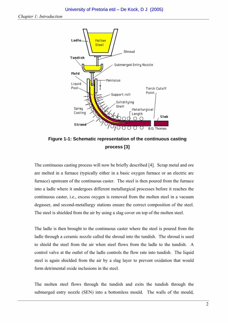
A graphic representation of the continuous casting process is given in Figure 1-1 [3].
This figure shows the different entities of the continuous casting process. These
entities are:
the ladle and shroud,
the tundish,
the submerged entry nozzle (SEN) and mould and
the solidifying strand and slab.
UUnniivveerrssiittyy ooff PPrreettoorriiaa eettdd –– DDee KKoocckk,, DD JJ ((22000055))
Chapter 1: Introduction
2
Figure 1-1: Schematic representation of the continuous casting process [3]
The continuous casting process will now be briefly described [4]. Scrap metal and ore
are melted in a furnace (typically either in a basic oxygen furnace or an electric arc
furnace) upstream of the continuous caster. The steel is then poured from the furnace
into a ladle where it undergoes different metallurgical processes before it reaches the
continuous caster, i.e., excess oxygen is removed from the molten steel in a vacuum
degasser, and second-metallurgy stations ensure the correct composition of the steel.
The steel is shielded from the air by using a slag cover on top of the molten steel.
The ladle is then brought to the continuous caster where the steel is poured from the
ladle through a ceramic nozzle called the shroud into the tundish. The shroud is used
to shield the steel from the air when steel flows from the ladle to the tundish. A
control valve at the outlet of the ladle controls the flow rate into tundish. The liquid
steel is again shielded from the air by a slag layer to prevent oxidation that would
form detrimental oxide inclusions in the steel.
The molten steel flows through the tundish and exits the tundish through the
submerged entry nozzle (SEN) into a bottomless mould. The walls of the mould,
Shroud
UUnniivveerrssiittyy ooff PPrreettoorriiaa eettdd –– DDee KKoocckk,, DD JJ ((22000055))
Chapter 1: Introduction
3
usually made of copper, are water-cooled, which causes the steel to solidify on the
sides. The sides of the mould are usually oscillating to prevent “sticking” of the steel
to the sides of the mould.
Drive rollers lower in the casting machine continuously withdraw the solidifying shell
from the mould. The speed of the rollers is set so that the material exiting the mould
matches that of the incoming flow into the tundish so that the caster runs in steady
state most of the time. Water jets sprayed on the strand, as it exits the mould, cools
the strand further, causing the solidifying shell to grow to the core of the strand. The
supporting rollers hold the strand in place as the core of the strand solidifies. The core
of the strand continues to solidify for a significant length after exiting the mould. The
point where the whole slab is fully solidified can be in the order of tenths of meters
downstream of the mould.
The solidified strand at the end of the rollers is then cut into slabs by a torch. These
slabs are then processed further, e.g., the slabs are hot and cold rolled into sheets,
bars, rails and other shapes.
Because of the nature of the continuous casting process, the tundish has traditionally
acted purely as a reservoir when one ladle is emptied and when a new ladle is brought
into place. In the last couple of decades, the role of the tundish in the continuous
casting process has evolved from that of a reservoir between the ladle and mould to
being a grade separator, an inclusion removal device and a metallurgical reactor. For
both grade separation and inclusion removal, the flow patterns inside the tundish play
an important role. For the former, the flow patterns determine the amount of mixing
that occurs, while for the latter, the paths of inclusion particles are influenced by the
flow field. Several tundish designs and tundish devices or furniture exist that have as
their aim the modification of tundish flow patterns, to either minimize mixed-grade
length during transition, and/or to increase inclusion particle removal by the slag
layer.
At the initiation of this study, steel producing plants in South Africa are experiencing
difficulties with more economical and higher quality steel production in the
UUnniivveerrssiittyy ooff PPrreettoorriiaa eettdd –– DDee KKoocckk,, DD JJ ((22000055))
Chapter 1: Introduction
4
continuous casting process. Tons of steel are downgraded or scrapped at continuous
casting plants. The typical difficulties of these plants are:
downgrading or scrapping of steel due to inclusions and slag entrainment in
the ladle, tundish and mould,
downgrading or scrapping of mixed-grade sections during grade transitions,
downgrading or scrapping of first section of new cast,
break-outs of the strand,
nozzle clogging due to solidifying steel,
low yield levels in the tundish when draining the tundish at the end of a
sequence due to slag entrainment and vortex formation.
1-2 EXISTING KNOWLEDGE Tundish design is traditionally performed through experimental plant trials or water
modelling. For the former, due to the nature of the process, it is difficult to have an
exact knowledge of the flow field. Indirect measurements such as copper traces and
oxygen sensing give an indication of the residence time and inclusion particles present
in the tundish. Water modelling on the other hand, provided that Reynolds number
and Froude number similarity for steady-state conditions can be achieved [5,6,7,8],
can provide more insight into the mixing characteristics. In order to include thermal
effects however, water models require significant modification to address cases where
buoyancy effects and natural convection plays a measurable role [9,10].
With the advent of powerful computers and fluid flow modelling software,
Computational Fluid Dynamics (CFD) has become an alternative tool with which to
assess different tundish designs [11,12,13,14]. Not only can the thermal effects be
incorporated, but also every detail of the flow field becomes available for extracting
measures of performance.
UUnniivveerrssiittyy ooff PPrreettoorriiaa eettdd –– DDee KKoocckk,, DD JJ ((22000055))
Chapter 1: Introduction
5
1-3 RESEARCH OBJECTIVES The objectives of this study are to:
develop a methodology for the design optimisation of tundish and tundish
furniture,
apply the methodology to the design of specific products used in the tundish in
the South African continuous casting industry.
1-4 SCOPE OF THE STUDY In this study, the focus is placed on the design of a tundish and the tundish furniture to
improve the molten steel flow patterns. The method developed in this study will be
applied to a single strand caster of Columbus Stainless Steel as well as the two strand
continuous caster of ISCOR Vanderbijlpark. The optimisation methodology can
however be extended to other areas of the continuous casting process as well as other
fluid flow and heat transfer applications where CFD is used to analyse the design.
CFD as analysis tool only, has limitations in that the variation of many parameters
require trial-and-error simulations of which the interpretation relies heavily on the
insight of the modeller. This usually leads to non-optimal solutions and furthermore
requires a lot of manual labour by the engineer doing the modelling. In this study, a
more efficient method is developed which combines CFD with mathematical
optimisation. This means that the design parameters become design variables and that
the performance trends with respect to these variables are taken into account
automatically by the optimisation algorithm. Using this method, an optimum design
for the tundish and its furniture can be found.
1-5 ORGANISATION OF THE THESIS The thesis consists of the following chapters:
Chapter 2 gives the appropriate literature pertaining the modelling of tundishes
and optimisation tools. This chapter describes the relevant theory behind
physical modelling and numerical modelling of tundishes. The chapter also
UUnniivveerrssiittyy ooff PPrreettoorriiaa eettdd –– DDee KKoocckk,, DD JJ ((22000055))
Chapter 1: Introduction
6
gives the theory of two mathematical optimisation methods that will be used in
the rest of the study.
Chapter 3 then develops the methodology for optimising tundish furniture.
This chapter looks at the different important aspects in the tundish and tundish
furniture design using a mathematical optimisation method. The different
steps involved in a mathematical optimisation study is given and it is shown
how an optimisation method links with a commercial CFD code.
Chapter 4 applies this methodology to four different case studies. The
methodology developed in Chapter 3 is applied to these case studies to show
that the optimisation methodology is a viable alternative in the design of
tundish and tundish furniture.
Chapter 5 gives the conclusions drawn form this study.
Chapter 6 give recommendations and possibility of future research in this
field.
UUnniivveerrssiittyy ooff PPrreettoorriiaa eettdd –– DDee KKoocckk,, DD JJ ((22000055))

7
2 CHAPTER 2: LITERATURE STUDY
2-1 INTRODUCTION This chapter gives the literature pertaining to this thesis. The literature study is
divided into two main parts. The first part is on the modelling and design of the
tundish and tundish furniture. The second part provides a background to
mathematical optimisation. The modelling and design section is divided into three
main parts, i.e., physical modelling, plant trials and numerical modelling. The
mathematical optimisation section describes the theory behind mathematical
optimisation and a description of the different optimisers used in this thesis.
2-2 TUNDISH MODELLING AND DESIGN
2-2.1 The Continuous Casting Process
In the last couple of decades, the role of the tundish in the continuous casting
process has evolved from that of a reservoir between the ladle and mould to
being a grade separator, an inclusion removal device and a metallurgical
reactor. For both grade separation and inclusion removal, the flow patterns
inside the tundish play an important role. For the former, the flow patterns
determine the amount of mixing that occurs, while for the latter, the paths of
inclusion particles are influenced by the flow field. Several tundish designs
and tundish devices or furniture exist that have as their aim the modification of
tundish flow patterns, to either minimise mixed-grade length during transition,
and/or to increase inclusion particle removal by the slag layer.
UUnniivveerrssiittyy ooff PPrreettoorriiaa eettdd –– DDee KKoocckk,, DD JJ ((22000055))
Chapter 2: Literature Study
8
The modelling and design of the tundish and tundish furniture can be divided
into three main categories, i.e., physical modelling, plant trials and
mathematical modelling. These three categories will now be described in
more detail.
2-2.2 Physical Modelling
Physical modelling has great benefits over doing plant trials, i.e.:
• It does not operate under such harsh environments under which the
tundish operates in the plant (e.g., extreme high temperatures and
almost no visual observations possible).
• It does not interfere with the production of the plant.
• It can be a lot more repeatable due to the more stringent control one
has in the laboratory whereas in the plant there are other variables that
cannot be controlled.
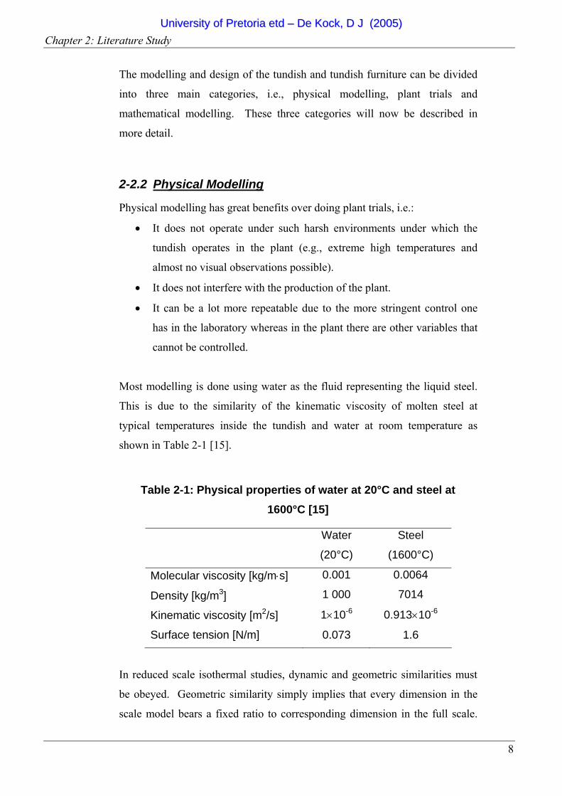
Most modelling is done using water as the fluid representing the liquid steel.
This is due to the similarity of the kinematic viscosity of molten steel at
typical temperatures inside the tundish and water at room temperature as
shown in Table 2-1 [15].
Table 2-1: Physical properties of water at 20°C and steel at 1600°C [15]
Water
(20°C)
Steel
(1600°C)
Molecular viscosity [kg/m⋅s]
Density [kg/m3]
Kinematic viscosity [m2/s]
Surface tension [N/m]
0.001
1 000
1×10⁻⁶
0.073
0.0064
7014
0.913×10⁻⁶
1.6
In reduced scale isothermal studies, dynamic and geometric similarities must
be obeyed. Geometric similarity simply implies that every dimension in the
scale model bears a fixed ratio to corresponding dimension in the full scale.
UUnniivveerrssiittyy ooff PPrreettoorriiaa eettdd –– DDee KKoocckk,, DD JJ ((22000055))
Chapter 2: Literature Study
9
Dynamic similarity implies that the ratio of the different forces acting on a
small fluid element must be the same in the scale model and in the full-scale
version [16].
Considering dynamic similarity, the inertial, viscous and gravitational forces
are of importance in tundish flows. These forces are characterised by two
dimensionless numbers. The first is the Reynolds ⎟⎟⎠
⎞⎜⎜⎝
⎛=
µρULRe number that
gives the ratio of the inertia forces to the viscous forces. The second is the
Froude number ⎟⎟⎠
⎞⎜⎜⎝
⎛=
gLU 2
Fr that gives the ratio of the inertia forces to
gravitational forces. When water at room temperature is used as the modelling
fluid, matching of both Reynolds and Froude numbers is only possible using
full-scale models. In reduced-scale models, either Reynolds or Froude
numbers can be satisfied, but not both [17].
Full scale, as well as reduced scale, water modelling has been performed
extensively [5,14,18,19,20]. In order to include thermal effects however,
water models require significant modification to address cases where
buoyancy effects and natural convection plays a measurable role [10, 21].
This makes the use of numerical modelling as discussed later, an attractive
alternative.
To quantify the performance of the tundish, two different types of approaches
have been commonly applied by researchers [16]:
1. the measurement of residence time distribution (RTD)
2. direct measurement of inclusion separation through aqueous
simulation.
The residence time of fluid within a rector is defined as the time a single fluid
element spends in the reactor vessel. The theoretical residence time is defined
as:
UUnniivveerrssiittyy ooff PPrreettoorriiaa eettdd –– DDee KKoocckk,, DD JJ ((22000055))

Chapter 2: Literature Study
10
tundish theinto steel of rate flow Volumetric tundish theof Volume Filled
≡τ (2-1)
Usually flow in any tundish is accompanied by a distribution of residence
times for different fluid elements (i.e., some fluid elements stay longer while
others spend shorter times within the tundish with respect to the theoretical
residence time) [16]. These residence time distributions can be experimentally
measured by injecting a tracer (pulse or continuous) at the inlet of the tundish
and then dynamically measuring the concentration at the outlet using
colourimetry, conductimetry, or spectrophotometry.
When injecting a pulse injection at time t = 0, a typical concentration profile at
the outlet, also called the C curve [22], is obtained as shown in Figure 2-1
[23]. Typical C curves or Residence Time Distribution (RTD) for different
dimensionless tundish widths are shown in this figure.
Figure 2-1: Typical measured RTD curve in a water model of a single strand slab casting tundish system at various values of
the dimensionless tundish width [23]
UUnniivveerrssiittyy ooff PPrreettoorriiaa eettdd –– DDee KKoocckk,, DD JJ ((22000055))

Chapter 2: Literature Study
11
From a typical RTD curve, different performance-related criteria for the
tundish can be extracted. The values of the minimum break-through time
( minθ in dimensionless form), time to attain the peak concentration ( peakθ ), and
the average residence time ( avθ ) can be incorporated into an appropriate flow
model to estimate the proportions of dead ( dvV ,) plug ( pvV ), and well-mixed
volumes ( mvV ). The minimum break through time is also referenced to as the
Minimum Residence Time (MRT). Kemeny et al. [15] proposed the various
fractional volumes as:
peakmv
peakpv
avdv
CV
VV
1
1
min
=
==−=
θθθ
(2-2)
As pointed out by Sahai and Ahuja [6] this model has two shortcomings:
1. Considerable axial or longitudinal diffusion is present in tundish
systems, causing the minimum break-through time and the time to
reach the peak concentration not to be equal.
2. The three volume fractions do not add up to unity, which is a
requirement for the mixed model.
Sahai and Ahuja [6] proposed a modified mixed model for tundish systems.
Instead of dividing the tundish into a dead volume, plug-flow volume and
well-mixed volume, they defined a dead volume, dispersed plug-flow volume
( dpvV ) and a well-mixed volume as follows:
( )
dpvdvmv
peakdpv
avdv
VVV
V
V
−−=
+=
−=
12
1
min θθθ
(2-3)
Several investigators have also carried out direct measurement of particle
removal in water models [24,25,26]. In these studies, hollow glass spheres
were introduced into the tundish via the shroud. The exit particle
UUnniivveerrssiittyy ooff PPrreettoorriiaa eettdd –– DDee KKoocckk,, DD JJ ((22000055))
Chapter 2: Literature Study
12
concentration was monitored with various techniques. Nakajama et al. [24]
showed that any increase in the plug flow volume leads to an increase in the
separation efficiency. This type of measurements however needs considerable
hardware upgrades to an existing water model.
2-2.3 Plant Trials
The high temperature associated with the continuous casting process makes it
very difficult to do on-site plant trials. Typical plant operations take a few
discrete temperature measurements at regular intervals. Some tundishes have
been instrumented to give on-line tundish wall temperatures [27]
A RTD curve can also be constructed by doing a copper trace trial. A copper
dosage is introduced near the shroud of the tundish. Samples are then taken
from the mould at regular intervals. These samples are then analysed for the
copper concentration using a photo-spectrometer [28]. The principle of the
analysis method is optical emission spectroscopy [29]. The sample material is
vaporised by an arc. The atoms and ions contained in the atomic vapour are
excited into emission of radiation. The radiation emitted is passed to the
spectrometer optics via an optical fibre, where it is dispersed into its spectral
components. From the range of wavelengths emitted by each element, the
composition of the steel can be determined.
The last common practice to be used in plant trials is taking samples at the
shroud and SEN to determine the number of inclusions present in the steel.
Many measurement techniques exist to evaluate the steel cleanliness as given
by Zhang et al [30]. The steel cleanliness at the shroud and SEN are then
compared to each other to determine the efficiency of tundish in terms of
particle removal.
As mentioned earlier, there are two major drawbacks of doing plant trials.
Firstly, it interferes with production of the plant. Secondly, due to a large
number of other uncontrollable parameters on the plant, the trials are
UUnniivveerrssiittyy ooff PPrreettoorriiaa eettdd –– DDee KKoocckk,, DD JJ ((22000055))
Chapter 2: Literature Study
13
unrepeatable and therefore it is difficult to isolate the influence of certain
parameters on the performance of the tundish.
2-2.4 Numerical Modelling
Computational Fluid Dynamics (CFD) is a numerical modelling technique that
solves the Navier-Stokes equations on a discretised domain of the geometry of
interest with the appropriate flow boundary conditions supplied. The Navier-
Stokes equations are a complex non-linear set of partial differential equations
that describes the mass and momentum conservation of a fluid. Additional
physics can also be resolved by solving additional conservation equations,
e.g., heat transfer, multi-phase flow, and combustion. A CFD analysis
consists of the following steps [31]:
• Problem Identification and Pre-Processing
o Define your modelling goals
o Identify the domain you will model
o Design and create the grid
• Solver Execution
o Set up the numerical model
o Compute and monitor the solution
• Post-Processing
o Examine the results
o Consider revisions to the model
Some of these steps will now be discussed in more detail.
2-2.4.1 Grid Generation
The grid generation process deals with the division of the domain
under consideration into small control volumes on which the disretised
governing equations will be solved.
The grid generation forms a large part in terms of person-hour time of
the CFD analysis. A large amount of time has gone into and is
currently going into the development of commercial automated grid
UUnniivveerrssiittyy ooff PPrreettoorriiaa eettdd –– DDee KKoocckk,, DD JJ ((22000055))
Chapter 2: Literature Study
14
generators. Once such product is GAMBIT (Geometry and Mesh
Building Intelligent Toolkit) [32]. GAMBIT uses solid modelling
techniques to create a virtual model of the geometry under
consideration. Various grid generation tools are available to create a
grid in this geometry. The gird generation tools are available to create
hexahedron, tetrahedron, prism and pyramid cells.
GAMBIT makes use of a Graphical User Interface (GUI) where the
user is able to give commands to manipulate and generate the grid via
the input of values and appropriate mouse clicks. An important aspect
of GAMBIT with respect to mathematical optimisation is the
parameterisation and automation of the set-up of the model and grid
generation using journal files. A journal file is a text file that contains
text commands that give the instructions to GAMBIT to generate a
model without the use of the GUI.
2-2.4.2 Conservation Equations
The governing equations that describe the flow field are a set of
non-linear partial differential equations. The equations are derived
from mass, momentum and energy conservation. These three different
governing equations will now be discussed briefly.
Conservation of Mass
The conservation of mass in Eulerian terms in its most common
general form for fluids is given in the following [33]:
mSt
=+∂∂ Vρρ div (2-4)
where ρ is the density, t is the time, V is the velocity vector of the fluid
and Sm is a mass source. For a constant density, equation (2-4) simply
reduces to the following:
0div =V (2-5)
The constant density assumption can be made for tundishes when the
temperature differences are not too large. The effect of the buoyancy
UUnniivveerrssiittyy ooff PPrreettoorriiaa eettdd –– DDee KKoocckk,, DD JJ ((22000055))

Chapter 2: Literature Study
15
of the higher temperature steel is then treated through the Boussinesq
model in the momentum transport equation. More detail on this model
is given below.
Transport of Momentum
The Navier-Stokes equations are derived from the conservation of
momentum (Newton’s second law). The set of equations can be
written in Eulerian terms as a single vector equation using the indicial
notation [33]:
⎥⎥⎦
⎤
⎢⎢⎣
⎡+⎟
⎟⎠
⎞⎜⎜⎝
⎛
∂
∂+
∂∂
∂∂
+∇−= VgV divλδµρρ iji
j
j
i
j xv
xv
xp
DtD (2-6)
where g is the gravitation vector, xi is the spatial co-ordinate, vi is the
i-component of the velocity vector, µ is the ordinary coefficient of
viscosity, λ is the coefficient of bulk viscosity, δij is the Kronecker
delta function (δij=1 if i=j and δij=0 of i≠j) and DtD the total or
substantial derivative. The relation between the ordinary viscosity and
bulk viscosity is given by Stokes’ hypothesis [34]:
032
=+ µλ (2-7)
As an example, equation (2-6) is written out in full for the i-direction
in the following equation:
⎥⎦
⎤⎢⎣
⎡⎟⎠⎞
⎜⎝⎛
∂∂
+∂∂
∂∂
+
⎥⎦
⎤⎢⎣
⎡⎟⎟⎠
⎞⎜⎜⎝
⎛∂∂
+∂∂
∂∂
+⎟⎠⎞
⎜⎝⎛ +
∂∂
∂∂
+∂∂
−=
xw
zu
z
xv
yu
yxu
xxpg
DtDu
x
µ
µλµρρ Vdiv2 (2-8)
When assuming incompressible flow with a constant viscosity,
equation (2-6) reduces considerably to the following:
VgV 2∇+∇−= µρρ pDtD (2-9)
UUnniivveerrssiittyy ooff PPrreettoorriiaa eettdd –– DDee KKoocckk,, DD JJ ((22000055))
Chapter 2: Literature Study
16
For many natural-convection flows, you can get faster convergence
with the Boussinesq model (originally published in [35] as cited in
[36]) than you can get by setting up the problem with fluid density as a
function of temperature. This model treats density as a constant value
in all solved equations, except for a momentum source term in the
momentum equation:
( ) ( )gTTg 000 −−≈− βρρρ (2-10)
where 0ρ is the (constant) density of the fluid, 0T is the operating
temperature, and β is the thermal expansion coefficient. Equation
(2-10) is obtained by using the Boussinesq approximation
( )T∆−= βρρ 10 to eliminate ρ from the buoyancy term. This
approximation is accurate as long as changes in actual density are
small; specifically, the Boussinesq approximation is valid when
( ) 10 <<− TTβ [37]. The term on the left of this equation ( )( )0TT −β
is the fraction of the change in density relative to the reference density,
implying that the change in density should be small relative to the
reference density.
Transport of Energy
The energy equation is derived from the first law of thermodynamics.
The energy relation in Eulerian terms is given by the following if it is
assumed that the conduction heat fluxes are given by Fourier’s Law
and that radiative effects are negligible [33]:
( ) Φ+∇+= TkDtDp
DtDh divρ (2-11)
where h is the fluid enthalpy, k is the thermal conductivity, T is the
temperature of the fluid and Φ is the viscous dissipation and is given
by:
22
22222
222
⎟⎟⎠
⎞⎜⎜⎝
⎛∂∂
+∂∂
+∂∂
+⎥⎥⎦
⎤⎟⎠⎞
⎜⎝⎛
∂∂
+∂∂
+
⎢⎢⎣
⎡⎟⎟⎠
⎞⎜⎜⎝
⎛∂∂
+∂∂
+⎟⎟⎠
⎞⎜⎜⎝
⎛∂∂
+∂∂
+⎟⎠⎞
⎜⎝⎛
∂∂
+⎟⎟⎠
⎞⎜⎜⎝
⎛∂∂
+⎟⎠⎞
⎜⎝⎛
∂∂
=Φ
zw
yv
xu
xw
zu
zv
yw
yu
xv
zw
yv
xu
λ
µ
(2-12)
UUnniivveerrssiittyy ooff PPrreettoorriiaa eettdd –– DDee KKoocckk,, DD JJ ((22000055))
Chapter 2: Literature Study
17
Again assuming incompressible flow as well as a constant thermal
conductivity and low-velocity flow where the viscous-dissipation (Φ)
is zero, equation (2-11) reduces considerably to the following:
TkDtDTcp
2∇=ρ (2-13)
2-2.4.3 Turbulence Modelling
Turbulence models are used in CFD because of the fact that the
small-scale fluctuations of the flow field cannot be resolved when
solving the above-mentioned governing equations on an ordinary grid.
Instead, the ensemble average of the basic conservation equations is
taken to give the Reynolds-Averaged Navier-Stokes (RANS)
formulation. The RANS formulation is derived from the assumption
that every solved for quantity consists of a mean part as given and a
fluctuating part. For instance, the ui velocity component is
decomposed into a mean part and a fluctuating part as given in
equation (2-14).
( ) ( ) ( )txutxUtxu iii ,,, rrr ′+= (2-14)
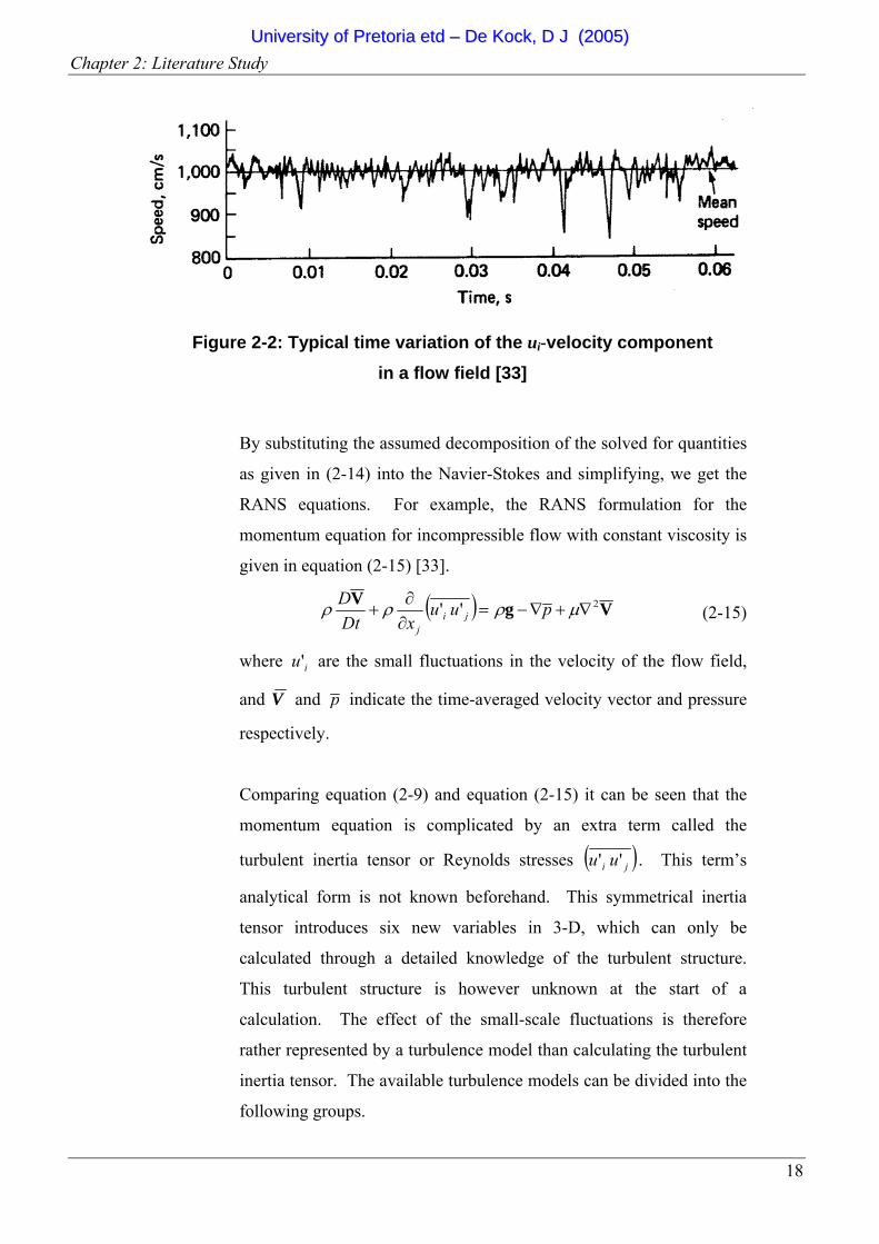
Figure 2-2 shows a typical behaviour for the ui velocity component but
all the flow quantities that are solved for are assumed to be of a similar
form.
UUnniivveerrssiittyy ooff PPrreettoorriiaa eettdd –– DDee KKoocckk,, DD JJ ((22000055))
Chapter 2: Literature Study
18
Figure 2-2: Typical time variation of the ui-velocity component in a flow field [33]
By substituting the assumed decomposition of the solved for quantities
as given in (2-14) into the Navier-Stokes and simplifying, we get the
RANS equations. For example, the RANS formulation for the
momentum equation for incompressible flow with constant viscosity is
given in equation (2-15) [33].
( ) VgV 2'' ∇+∇−=∂∂
+ µρρρ puuxDt
Dji
j
(2-15)
where iu' are the small fluctuations in the velocity of the flow field,
and V and p indicate the time-averaged velocity vector and pressure
respectively.
Comparing equation (2-9) and equation (2-15) it can be seen that the
momentum equation is complicated by an extra term called the
turbulent inertia tensor or Reynolds stresses ( )ji uu '' . This term’s
analytical form is not known beforehand. This symmetrical inertia
tensor introduces six new variables in 3-D, which can only be
calculated through a detailed knowledge of the turbulent structure.
This turbulent structure is however unknown at the start of a
calculation. The effect of the small-scale fluctuations is therefore
rather represented by a turbulence model than calculating the turbulent
inertia tensor. The available turbulence models can be divided into the
following groups.
UUnniivveerrssiittyy ooff PPrreettoorriiaa eettdd –– DDee KKoocckk,, DD JJ ((22000055))
Chapter 2: Literature Study
19
Zero-equation models
These models are simple algebraic models and are computationally
inexpensive. The accuracy obtained with these types of models is
sometimes not sufficient especially in very complex flow, due to the
fact that no information from the surrounding flow field is used. Some
examples of these types of turbulence models are the mixing-length
model and the Baldwin-Lomax model [38].
One-equation models
One-equation turbulence models model the turbulent kinetic energy (k)
equation. These models satisfy the transport of the turbulent kinetic
energy. The turbulent length scales in these models are correlated with
algebraic equations [39]. The results obtained with these types of
models are satisfactory but no better than the zero-equation models
resulting in the fact that these models are not very popular. An
exception is the Spallart-Almaras model that has been developed for
high speed external flow applications.
Two-equation models
In two-equation turbulence models, a second equation is coupled with
the turbulent kinetic energy equation used in the one-equation models.
The second equation models for example the rate of change of either
dissipation (ε), turbulent length scale (L) or vorticity (ω).
The most popular scheme is probably the standard k-ε model
[40,41,42] or some derivative of it like the renormalisation group
(RNG) k-ε model [43]. This model is also used throughout this study.
The two equations that describe the turbulent kinetic energy (k) and
turbulent dissipation (ε) are given in the following two equations.
UUnniivveerrssiittyy ooff PPrreettoorriiaa eettdd –– DDee KKoocckk,, DD JJ ((22000055))
Chapter 2: Literature Study
20
ενσν
−⎟⎟⎠
⎞⎜⎜⎝
⎛
∂∂
+∂∂
∂∂
+⎟⎟⎠
⎞⎜⎜⎝
⎛
∂∂
∂∂
=i
j
j
i
j
it
jk
t
j xu
xu
xu
xk
xDtDk (2-16)
kC
xu
xu
xu
kC
xxDtD
i
j
j
i
j
it
j
t
j
2
21εενε
σνε
ε
−⎟⎟⎠
⎞⎜⎜⎝
⎛
∂∂
+∂∂
∂∂
+⎟⎟⎠
⎞⎜⎜⎝
⎛
∂∂
∂∂
= (2-17)
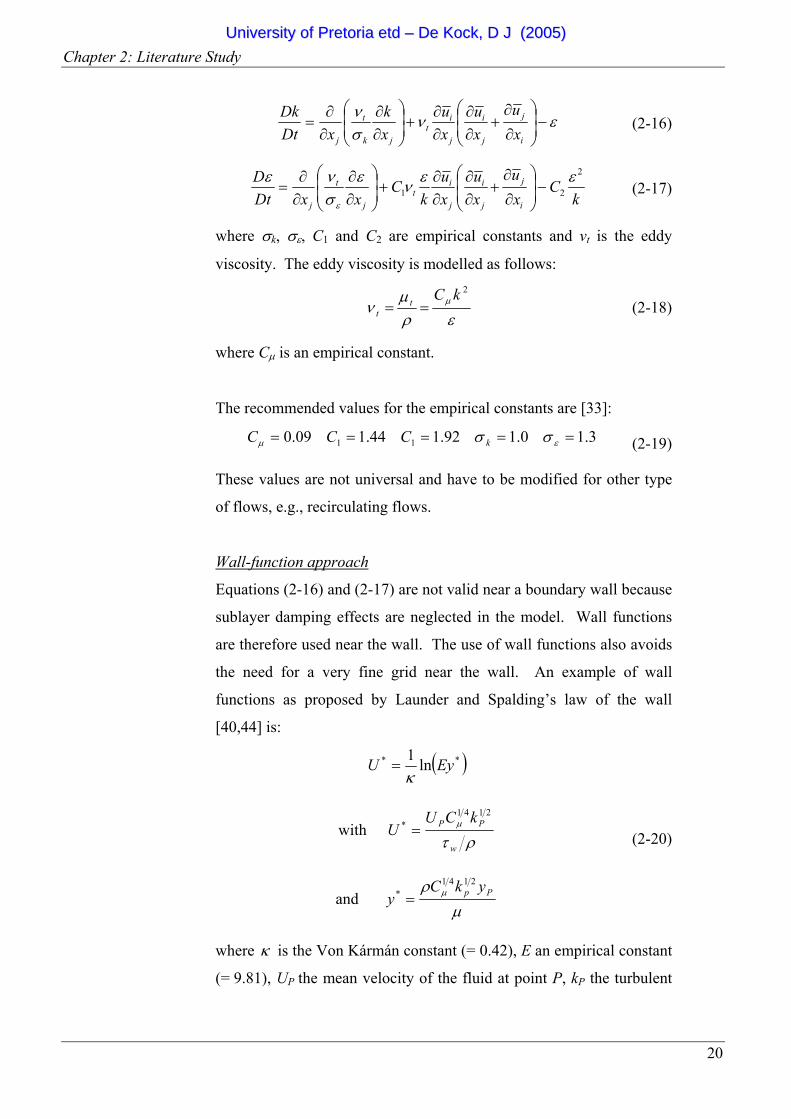
where σk, σε, C1 and C2 are empirical constants and vt is the eddy
viscosity. The eddy viscosity is modelled as follows:
ερµ
ν µ2kCt
t == (2-18)
where Cµ is an empirical constant.
The recommended values for the empirical constants are [33]:
3.10.192.144.109.0 11 ===== εµ σσ kCCC (2-19)
These values are not universal and have to be modified for other type
of flows, e.g., recirculating flows.
Wall-function approach
Equations (2-16) and (2-17) are not valid near a boundary wall because
sublayer damping effects are neglected in the model. Wall functions
are therefore used near the wall. The use of wall functions also avoids
the need for a very fine grid near the wall. An example of wall
functions as proposed by Launder and Spalding’s law of the wall
[40,44] is:
( )** ln1 EyUκ
=
with ρτ
µ
w
PP kCUU
2141* =
and µ
ρ µ Pp ykCy
2141* =
(2-20)
where κ is the Von Kármán constant (= 0.42), E an empirical constant
(= 9.81), UP the mean velocity of the fluid at point P, kP the turbulent
UUnniivveerrssiittyy ooff PPrreettoorriiaa eettdd –– DDee KKoocckk,, DD JJ ((22000055))
Chapter 2: Literature Study
21
kinetic energy at point P, yP the distance from point P to the wall, and
µ the dynamic viscosity of the fluid.
The effect of turbulence in all the above-mentioned models is modelled
as an increase in the viscosity. This is called the eddy-viscosity
concept. The dynamic viscosity (µ) used in equations (2-6) and (2-12)
is the total viscosity and is expressed as the sum of the molecular
viscosity of the fluid plus the turbulent viscosity (µt). The turbulent
viscosity is directly calculated from the turbulent kinetic energy and
turbulent dissipation rate. For the standard k-ε model this relationship
is given in equation (2-18).
Other Methods
Another approach in turbulence modelling is to model the Reynolds
stresses ( )''jiuuρ− using partial differential equations [45]. These are
called the Reynolds Stress Models (RSM). The RSM model is at a
level higher than the previous schemes and therefore provides
second-order turbulent closure at the cost of computational complexity.
Another method to reduce the complexity of the RSM approach, is to
model the Reynolds stresses by a purely algebraic equation with the
same characteristics than the differential equations [46]. These
methods are called the Algebraic Stress Models (ASM). Both these
Reynolds stress models, RSM and ASM, have the potential for greater
accuracy, mainly because the turbulence in the flow is not assumed to
be isotropic as the previous methods (i.e., the zero-, one and two-
equation models).
Currently a lot of research is conducted on Large-Eddy Simulation
(LES) in which only the smallest fluctuations (or sub-grid scales) are
modelled using a simple turbulence model (e.g., k-ε turbulence model).
Modelling the turbulence in this way requires an unsteady simulation
with a very fine grid distribution, making this model computational
UUnniivveerrssiittyy ooff PPrreettoorriiaa eettdd –– DDee KKoocckk,, DD JJ ((22000055))
Chapter 2: Literature Study
22
very expensive. For industrial applications, like the tundish, this
model is computationally too expensive.
Currently another active research topic is that of Direct Numerical
Simulation (DNS). This method for calculating turbulent flow is direct
in that it does not use turbulence models. Consequently, a very fine
grid and small time step are required. The method is even more
computationally expensive than the LES model. This method is
currently considered as the state-of-the-art method for turbulent flow
calculations but is restricted to very simple flow cases with a low
Reynolds number making it impractical for industrial applications of
CFD.
2-2.4.4 Inclusion modelling
Modelling of the non-metallic inclusion in steel melt can be done in a
number of ways [47]. The different methods will now be briefly
discussed.
Lagrangian particle tracking
The trajectory of a discrete phase particle (or inclusion) can be
predicted by integrating the force balance on the particle, which is
written in a Lagrangian reference frame. This force balance equates
the particle inertia with the forces acting on the particle, and can be
written (for the x-direction in Cartesian coordinates) as [37]:
( ) ( )Fx
guuF
dtdu
p
pxpD
p +−
+−=ρ
ρρ (2-21)
where ( )pD uuF − is the drag force per unit particle mass and
24Re18
2D
pPD
Cd
Fρ
µ= (2-22)
Here, u is the fluid phase velocity, pu is the particle velocity, µ is the
molecular viscosity of the fluid, ρ is the fluid density, pρ is the density
UUnniivveerrssiittyy ooff PPrreettoorriiaa eettdd –– DDee KKoocckk,, DD JJ ((22000055))

Chapter 2: Literature Study
23
of the particle, and pd is the particle diameter. Re is the relative
Reynolds number, which is defined as
µ
ρ uud pp −=Re (2-23)
The drag coefficient, DC , is taken from:
232
1 ReReaaaCD ++= (2-24)
where 1a , 2a , and 3a are constants that apply for smooth spherical
particles over several ranges of Reynolds number given by Morsi and
Alexander [48].
The effect of a turbulent flow field in the above-mentioned method
does not include the effect of turbulence on the particle trajectory. One
approach to include the effect of turbulence is through stochastic
tracking. This approach predicts the turbulent dispersion of particles
by integrating the trajectory equations for individual particles, using
the instantaneous fluid velocity, e.g., for the x-direction ( )tuu '+ ,
along the particle path during the integration. By computing the
trajectory in this manner for a sufficient number of representative
particles, the random effects of turbulence on the particle dispersion
may be accounted for [37]. The velocity fluctuations that prevail
during the lifetime of the turbulent eddy are sampled by assuming that
they obey a Gaussian probability distribution. This results in the
fluctuation velocity in the x-direction to be:
2'' uu ζ= (2-25)
where ζ is a normally distributed random number and 2'u is the
local RMS value of the velocity fluctuations. Since the kinetic energy
of turbulence is known at each point in the flow (from the appropriate
turbulence model), these values of the RMS fluctuating components
can be obtained (assuming isotropy) as:
UUnniivveerrssiittyy ooff PPrreettoorriiaa eettdd –– DDee KKoocckk,, DD JJ ((22000055))
Chapter 2: Literature Study
24
32'2 ku = (2-26)
The characteristic lifetime of the eddy is best calculated by assuming a
random variation about LT :
( )rTLe log−=τ (2-27)
where r is a uniform random number between 0 and 1, LT is given by
εkCL with 15.0≈LC when used in conjunction with the k-ε
turbulence model [49].
The particle eddy crossing time is defined as
⎥⎥⎦
⎤
⎢⎢⎣
⎡
⎟⎟
⎠
⎞
⎜⎜
⎝
⎛
−−−=
p
ecross uu
Ltτ
τ 1ln (2-28)
where τ is the particle relaxation time, eL is the eddy length scale,
and puu − is the magnitude of the relative velocity.
The particle is assumed to interact with the fluid phase eddy over the
smaller of the eddy lifetime and the eddy crossing time. When this
time is reached, a new value of the instantaneous velocity is obtained
by applying a new value of ζ in (2-25) [31].
Inclusion diffusion model
The second method makes use of a species diffusion model to calculate
the distribution of small inclusions [47]. This method solves the
convection-diffusion equation of a species inside the tundish as given
in equation (2-29) to give the time evolution of the inclusion mass
fraction, Y:
UUnniivveerrssiittyy ooff PPrreettoorriiaa eettdd –– DDee KKoocckk,, DD JJ ((22000055))
Chapter 2: Literature Study
25
( ) ( ) 0=⎟⎟⎠
⎞⎜⎜⎝
⎛∂∂
∂∂
+∂∂
+∂∂
ieff
ii
i xYD
xYu
xY
tρρρ (2-29)
where effD is the local effective diffusion coefficient and is dependent
on the local turbulence and dissipation levels as calculated from the
turbulence model as given in (2-30):
t
teff DD
Sc0 ρµ
+= (2-30)
where 0D is the laminar diffusion coefficient and tSc is the turbulent
Schmitt number.
The flotation of inclusions, reoxidation, and collision agglomeration
are ignored in this model which is only used to investigate general
transient mixing behaviour.
Lumped inclusion removal model with size function
The last model calculates the evolution of the inclusion size
distribution for the duration of its residence time in the tundish
(developed by Miki et al [50]). This model considers the collision of
particles due to both turbulence and differences in flotation removal
rate of each inclusion size. This is a lumped model based on uniform
average properties within the tundish. The collision rate due to
turbulent eddy motion is governed by the mean turbulent dissipation
level, ε, and the cluster size of the inclusion. Details of this model can
be found in [47,50].
2-2.4.5 Solution Algorithm
The finite volume approach as implemented in the commercial CFD
solver, FLUENT [37] is used in this study. In this method, the
governing equations are first integrated on the individual control
volumes that were created in the grid generation phase, to construct
algebraic equations for the discrete dependent variables such as
velocities, pressure, temperature, and conserved scalars. Secondly, the
UUnniivveerrssiittyy ooff PPrreettoorriiaa eettdd –– DDee KKoocckk,, DD JJ ((22000055))
Chapter 2: Literature Study
26
discretised equations are linearised and the resulting linear equation
system is solved to yield updated values of the dependent variables.
In this study, the segregated solution method of FLUENT is used. In
this approach, the governing equations are solved sequentially (i.e.,
segregated from one another). Because the governing equations are
non-linear (and coupled), several iterations of the solution loop must
be performed before a converged solution is obtained. Each iteration
consists of the steps illustrated in Figure 2-3 and outlined below [37]:
• Fluid properties are updated, based on the current solution. (If
the calculation has just begun, the fluid properties will be
updated based on the initialised solution.)
• The u, v and w momentum equations are each solved in turn
using current values for pressure and face mass fluxes, in order
to update the velocity field.
• Since the velocities obtained in the previous step may not
satisfy the continuity equation locally, a ‘Poisson-type’
equation for the pressure correction is derived from the
continuity equation and the linearised momentum equations.
This pressure correction equation is then solved to obtain the
necessary corrections to the pressure and velocity fields and
face mass fluxes such that continuity is satisfied.
• Equations for scalars such as turbulence, energy and species are
solved using the previously updated values of the other
variables.
• A check for convergence of the equation set is made.
These steps are continued until the convergence criteria are met.
UUnniivveerrssiittyy ooff PPrreettoorriiaa eettdd –– DDee KKoocckk,, DD JJ ((22000055))
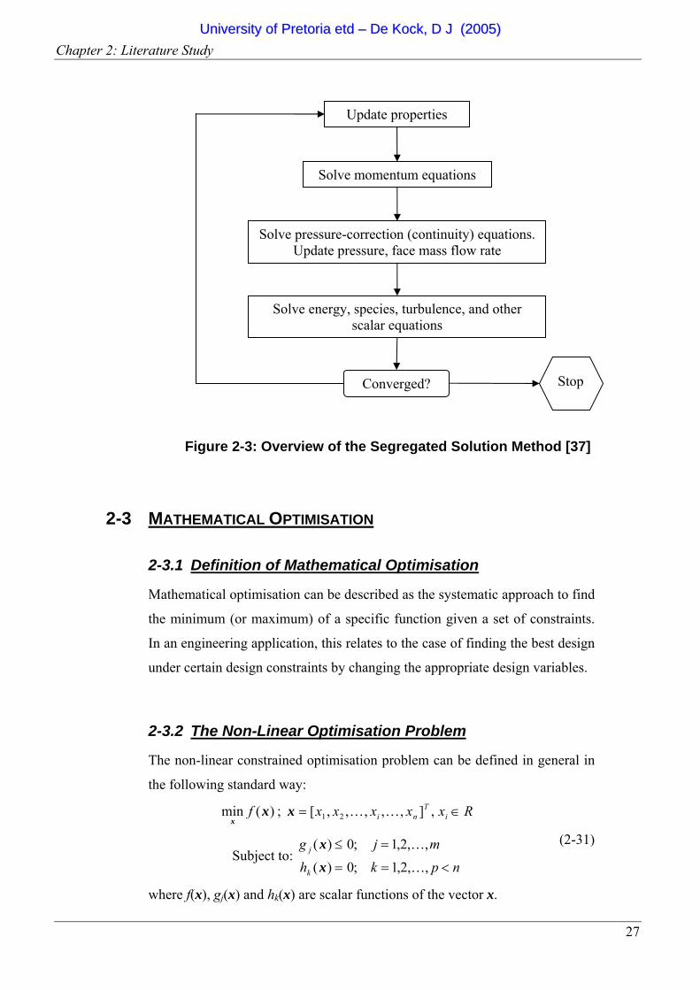
Chapter 2: Literature Study
27
Figure 2-3: Overview of the Segregated Solution Method [37]
2-3 MATHEMATICAL OPTIMISATION
2-3.1 Definition of Mathematical Optimisation
Mathematical optimisation can be described as the systematic approach to find
the minimum (or maximum) of a specific function given a set of constraints.
In an engineering application, this relates to the case of finding the best design
under certain design constraints by changing the appropriate design variables.
2-3.2 The Non-Linear Optimisation Problem
The non-linear constrained optimisation problem can be defined in general in
the following standard way:
)(min xx
f ; Rxxxxx iT
ni ∈= ,],,,,,[ 21 KKx
Subject to: npkh
mjg
k
j
<==
=≤
,,2,1;0)(,,2,1;0)(
K
K
xx
(2-31)
where f(x), gj(x) and hk(x) are scalar functions of the vector x.
Update properties
Converged?
Solve momentum equations
Solve pressure-correction (continuity) equations. Update pressure, face mass flow rate
Solve energy, species, turbulence, and other scalar equations
Stop
UUnniivveerrssiittyy ooff PPrreettoorriiaa eettdd –– DDee KKoocckk,, DD JJ ((22000055))
Chapter 2: Literature Study
28
The function f(x) is the objective function (or sometimes called the cost
function) that is being minimised. The functions gj(x) and hk(x) are the
inequality and equality constraints respectively. The variable n is called the
dimension of the optimisation problem. The components of the vector x are
called the design variables. The solution to problem (2-31) is given by the
vector x*:
[ ]T**2
*1
* ;;; nxxx K=x (2-32)
and gives the lowest value for f(x) subject to the specified inequality and
equality constraints. The solution x* may however be non-unique.
If there are no equality or inequality constraints, the optimisation problem
becomes an unconstrained optimisation problem. The unconstrained
optimisation problem can be more easily solved because the optimisation
simply consists of finding the minimum of f(x). For a constrained
optimisation problem, the optimisation becomes much more complex and the
constraints have to be treated in some sort of special way. The most popular
way to treat these constraints is by introducing a penalty function, as will be
described in the following paragraphs.
A large number of algorithms have been developed to solve the optimisation
problem given in equation (2-31). Some of the state-of-the-art methods
include multiplier methods and sequential quadratic programming [51, 52].
This chapter will only discuss the optimisation algorithms that were used in
this study. The choice of these specific algorithms is guided the way in which
each algorithm is suited for problems with computationally expensive function
evaluations as well as the robustness of the algorithms. The success of the
choices becomes evident in the rest of this study.
2-3.3 Optimisation Algorithms
Two optimisation algorithms are investigated in this study. The first is a
gradient-based optimisation algorithm of Snyman called DYNAMIC-Q, while
UUnniivveerrssiittyy ooff PPrreettoorriiaa eettdd –– DDee KKoocckk,, DD JJ ((22000055))
Chapter 2: Literature Study
29
the second is the Successive Response Surface Method (SRSM) algorithm
incorporated into the commercial optimisation program LS-OPT. Both these
optimisation algorithms make use internally of another optimisation algorithm,
the Leap Frog Optimisation Program (LFOPC), to optimise an approximation
to the original optimisation problem. DYNAMIC-Q, SRSM and LFOPC will
now be discussed in detail.
2-3.3.1 Snyman’s Leap-Frog Optimisation Program (LFOP)
Adapted to Handle Constrained Optimisation Problems
(LFOPC)
The original LFOP of Snyman [53,54] was subsequently adapted to
handle constrained optimisation problems [55,56,57]. This is achieved
by applying the original LFOP to a penalty function formulation of the
original problem. The appropriate penalty function formulation is
given in equation (2-33).
∑∑==
++=p
kkk
m
jjj hgfp
1
2
1
2 )()()()( xxxx βαγ (2-33)
where ⎩⎨⎧
>≤
=0)(if
0)(if0x
x
jj
jj g
gρ
α , ρj and βk are large positive numbers
and 1=γ (unless otherwise stated).
For simplicity, the penalty parameters, mjj ,,2,1, K=ρ and
pkk ,,2,1, K=β take on the same positive value, µβρ == kj . The
unconstrained minimum of p(x) tends to the constrained minimum of
problem (2-31) as µ tends to infinity. The choice of µ has received a
lot of attention. For µ very large, high accuracy is obtained, although
the unconstrained minimisation problem can become ill-conditioned.
For this reason, the penalty is usually increased gradually, thereby
allowing a controlled approach to the solution with limited violation of
the inequality constraints in the initial design steps.
UUnniivveerrssiittyy ooff PPrreettoorriiaa eettdd –– DDee KKoocckk,, DD JJ ((22000055))
Chapter 2: Literature Study
30
The LFOPC applies the LFOP algorithm to the penalty function
formulation (as given in (2-33)) in three phases. The three phases are
executed in the following way [57]:
Phase 0:
In the first phase, the penalty parameter is introduced at a moderately
low value. The penalty function is then minimised using the LFOP. In
this phase, the value of µ is set to µ0=102. This initial value of µ was
used throughout this study. This is possible because the LFOP
automatically scales the constraints ensuring that the spatial violation
of a constraint on the penalty function gradient is approximately the
same for all the constraints. On convergence, this gives an
approximate optimum point. The active inequality constraints are then
identified. An active inequality constraint is one that is violated. In
the standard formulation (2-31), this implies that the particular
inequality constraint gj is greater than or equal to zero. If no active
inequality constraints are found and there are no equality constraints,
the algorithm is terminated and the minimum is found. The minimum
of the constrained problem in (2-31) is then the same as the minimum
of the unconstrained problem. If the computational time of the
optimisation program becomes significant, the following phase is
sometimes skipped if the number of active constraint plus the number
of equality constraint are equal to the number of design variables. The
computational time associated with CFD is however, a few orders
larger than the computational time of the optimisation program and
therefore the following phase has never been skipped in this study.
Phase 1:
In this phase, the penalty parameter is increased. Here a value of
µ = 104 is used. The LFOP is again used to minimise the penalty
function but using the approximate design point from Phase 0 as a
starting point. On convergence, a more accurate approximate solution
point of the original problem given in (2-31) is found. The active set
UUnniivveerrssiittyy ooff PPrreettoorriiaa eettdd –– DDee KKoocckk,, DD JJ ((22000055))
Chapter 2: Literature Study
31
of inequality constraints is again identified. This set might not be
identical to the set identified in Phase 0.
Phase 2:
In the last phase, the LFOP is used to minimise the penalty function,
again using the approximate solution of the previous phase as the
starting point but with γ set to zero in the penalty function. This
implies that LFOP seeks a solution to the intersection of the active
constraints. The constrained minimum of the optimisation problem is
at the minimum of the intersection of the active constraints. If the
active constraints do not intersect, this algorithm will find the best
possible solution by giving a compromised solution. The
compromised solution usually violates the active constraints by a small
amount. This ability to obtain a compromised solution makes LFOPC
a very robust algorithm as will be shown in the optimisation cases
investigated in the following chapters.
The dynamic trajectory method described above is applied to a
sequence of approximate subproblems until convergence is obtained.
The subproblems are constructed due to the fact that is very
computationally expensive to evaluate the penalty function due to the
required CFD simulations. If the subproblems are not constructed, the
function value will have to be evaluated at each iteration of the LFOPC
algorithm. Successive subproblems are constructed at relatively high
computational cost, but these subproblems are solved economically
using the LFOPC algorithm. The construction of the approximate
subproblems is described below.
2-3.3.2 Snyman’s DYNAMIC-Q Method
In a complex problem where the objective function is unknown and/or
is computationally expensive, the successive approximation scheme
developed by Snyman et al [55,58,59,60] is used. This approach
involves the application of the above-mentioned dynamic trajectory
UUnniivveerrssiittyy ooff PPrreettoorriiaa eettdd –– DDee KKoocckk,, DD JJ ((22000055))
Chapter 2: Literature Study
32
method for unconstrained optimisation adapted to handle constrained
problems through penalty formulations as follows. The DYNAMIC
method is applied to successive approximate Quadratic subproblems of
the original problem, hence the name, DYNAMIC-Q. The successive
subproblems are constructed by sampling at relatively high
computational expense, the behaviour of the optimisation problem at
successive approximate solution points in the design space. These
subproblems are approximated using the quadratic approximation of a
function as discussed in the following paragraph. These subproblems,
which are analytically simple, are solved quickly and economically
using the LFOPC discussed above.
Successive quadratic subproblems, P[l]:l=1,2,…, are formed at
successive design points x(l). Spherically quadratic approximations are
used to approximate the objective function and/or constraints, if these
functions are not analytically known or computationally expensive.
The approximation of the subproblems will be discussed in detail in
the following paragraph.
These spherical quadratic subproblems have favourable characteristics
for the optimisation program, e.g., the quadratic subproblem is smooth
with no discontinuities and the subproblem usually has only one global
optimum.
The application of the DYNAMIC-Q method requires the use of move
limits. This is an added feature used to control convergence of the
optimisation process. Essentially, it implies the placing of additional
constraints that limit the movement of each of the design variables
from one design point to the next design point. This is helpful in the
initial steps of the optimisation run when the spherical quadratic
approximation may have a large error. This implies that the next
design point is not allowed to move too far from the current design
point.
UUnniivveerrssiittyy ooff PPrreettoorriiaa eettdd –– DDee KKoocckk,, DD JJ ((22000055))
Chapter 2: Literature Study
33
The move limits are implemented as additional inequality constraints
in the following way:
nixxxx
il
ii
il
ii ,,2,1;00
)(
)(
K=≤−+−≤−−
δδ
(2-34)
where in general the δi are different move limits for each design
variable and )(lix is the design variable at the current design point.
The DYNAMIC-Q method has the potential to be applied to any
engineering optimisation problem in which the numerical simulation is
computationally expensive. The only two requirements are that the
engineer has confidence in the answer obtained by the numerical
analysis and that the engineer can define his/her problem as an
optimisation problem. This study will apply the DYNAMIC-Q
algorithm to CFD.
Constructing the Successive Approximate Spherical Quadratic
Subproblems
The spherical quadratic approximation of a function is used in this
study to approximate the functions that are not analytically known
and/or computationally expensive to evaluate, to construct the
subproblem at design iteration l. These functions may be the objective
function or one of the constraints, depending on the optimisation
problem investigated. By approximating these computationally
expensive functions, the computational time is drastically reduced
because only a few function evaluations are necessary to obtain the
approximation. The way these successive subproblems are constructed
will now be discussed in detail [55,58].
The Taylor expansion of a function )(xf in the region of the current
design point x(l) is given by:
UUnniivveerrssiittyy ooff PPrreettoorriiaa eettdd –– DDee KKoocckk,, DD JJ ((22000055))
Chapter 2: Literature Study
34
H.O.T))(H()(21
))(()()(
)()(T)(
)()(T)(
+−−
+−∇+=
lll
lll fff
xxxxx
xxxxx (2-35)
where )(H )(lx is the Hessian matrix at point x(l) and H.O.T are the
higher order terms in the expansion. The vector x(l) is the current
design point. The Hessian matrix is defined in equation (2-36).
( ) )()H( 2
2
2
2
2
1
2
2
2
22
2
12
21
2
21
2
21
2
xxx f
xf
xxf
xxf
xxf
xf
xxf
xxf
xxf
xf
nnn
n
n
∇=
⎥⎥⎥⎥⎥⎥⎥⎥
⎦
⎤
⎢⎢⎢⎢⎢⎢⎢⎢
⎣
⎡
∂∂
∂∂∂
∂∂∂
∂∂∂
∂∂
∂∂∂
∂∂∂
∂∂∂
∂∂
=
K
MM
K
K
(2-36)
Note the symmetry of this matrix because ijji xx
fxxf
∂∂∂
=∂∂
∂ 22
.
If the higher order terms are ignored, the value of f at a point x in the
region of x(l) is given approximately by:
( ) ( )( )( ) ( ))()(T)(
)()(T)(
)(H21
)(
lll
lll fff
xxxxx
xxxxx
−−
+−∇+≈ (2-37)
The gradient vector ( ))(lf x∇ in equation (2-37), is approximated using
a first-order forward differencing scheme. This first-order gradient
approximation needs some special consideration and will be discussed
in the following paragraphs.
Because the function f, or its derivatives, is not analytically known, the
second-order derivatives need also to be calculated using a
finite-difference approximation, e.g., a forward-differencing scheme.
Furthermore, if the calculation of the function is computationally
expensive to evaluate (as is the case with CFD), the calculation of the
Hessian matrix becomes extremely expensive computationally. The
Hessian matrix is therefore approximated. The way the Hessian matrix
is approximated now follows.
UUnniivveerrssiittyy ooff PPrreettoorriiaa eettdd –– DDee KKoocckk,, DD JJ ((22000055))
Chapter 2: Literature Study
35
Taking A(l) as the approximation of the Hessian matrix, the
approximation )(~ xf to the function, )(xf is given by:
( ) ( )( )( ) ( ))()(T)(
)()(T)(
21
)(~
lkl
lll fff
xxAxx
xxxxx
−−
+−∇+= (2-38)
where the approximation of the Hessian matrix (A(l)) is given by
( ) IA )()()()()( ,,,diag lllll aaaa == K (2-39)
and I is the identity matrix.
The appropriate constant )(la used in the construction of the
approximate Hessian matrix is calculated by using function and
gradient information at the design point x(l) and at a previous design
point, say at point x(l-1). The value of )(la defines the amount of
curvature of the spherical quadratic approximation. During an
optimisation run the point x(l-1) is the previous design point where the
gradient and function values of the function are already known. The
initial value, )1(a , depends on the specific optimisation problem being
considered. In this study, a value of zero was chosen for the
construction of the first subproblem. This implies that the first
approximation has no curvature.
If it is specified that )(~ xf interpolates )(xf at x(l) and x(l-1) and that
the gradient of )(~ xf matches that of )(xf at x(l), equation (2-38) can
be rewritten to give a(l) as follows:
( ) ( ) ( )( ){ }21
1T1)( 2
)(l-(l)
(l))(l-(l)(l))(l-l fffa
xx
xxxxx
−
−∇−−= (2-40)
This may be called the backward interpolating spherical approximation
to )(xf at x(l).
UUnniivveerrssiittyy ooff PPrreettoorriiaa eettdd –– DDee KKoocckk,, DD JJ ((22000055))

Chapter 2: Literature Study
36
Another way to calculate a(l) is to specify that )(~ xf interpolates )(xf
at x(l) and x(l-1) and that the gradient of )(~ xf matches that of )(xf at
x(l-1) and not at x(l) as above. This may be called the forward
interpolating spherical approximation. This gives an expression for a(l)
as follows:
( ) ( ) ( )( ){ }21
11T1)( 2
)(l-(l)
)(l(l))(l)(l(l)l fffa
xx
xxxxx
−
−∇−−=
−−−
(2-41)
By averaging the curvature of the backward interpolating quadratic
function as in (2-40), and forward interpolating quadratic
approximation as in (2-41), an averaged expression for a(l) can be
obtained [61] and is given in (2-42).
( ) ( )( )( )21
1T1T)(
)(l-(l)
(l))(l-(l))(ll ffa
xx
xxxx
−
−∇−∇=
−
(2-42)
Expression (2-42) may be called the backward-forward interpolating
spherical approximation and gives more stable values for the curvature.
In the following chapters, it will be shown that this results in smoother
convergence of the optimisation run. It must be noted that constructing
)(~ xf using the averaged value of a(l) means that it no longer
necessarily interpolates )(xf at point x(l-1).
The DYNAMIC-Q method is terminated when either the normalized
step size ( ) ( )
( )l
ll
xx
xx
+
−=∆
−
1
1
norm (2-43)
or if the normalized change in function value ( )
best
bestnorm 1 f
fff
l
+
−=∆ (2-44)
are below specified tolerances. The DYNAMIC-Q method does not
guarantee a global minimum and typically, a multi-start approach (i.e.
starting the optimizer from different starting designs) should be used to
ensure that a global optimum is obtained.
UUnniivveerrssiittyy ooff PPrreettoorriiaa eettdd –– DDee KKoocckk,, DD JJ ((22000055))
Chapter 2: Literature Study
37
2-3.3.3 Successive Response Surface Method (SRSM)
The last optimisation method used is the Successive Response Surface
Method (SRSM) [62] as implemented in LS-OPT [63]. LS-OPT is a
commercial package available as part of the LS-DYNA software suite.
This algorithm uses a Response Surface Methodology (RSM) [64], i.e.,
a meta-modelling or surrogate technique, to construct linear response
surfaces on a subregion from a D-optimal subset of experiments. The
D-optimality criterion is implemented using a genetic algorithm and a
50% over-sampling is typically used. Successive subproblems are
solved using a multi-start variant of the Leap-Frog dynamic trajectory
method of Snyman [57]. The multi-start locations are selected as the
subset of experimental designs, and the best optimum is selected as the
optimum of the subproblem. The size of successive subregions is
adapted based on contraction and panning parameters designed to
prevent oscillation and premature termination [62]. Infeasibility is
handled automatically when it occurs through the construction and
solution of an auxiliary problem to bring the design within the
subregion if possible. As the optimum is approached, the subregion is
contracted automatically, implying that inaccuracies in the sensitivity
information do not cause large departures from the previous design.
Therefore, this handling of the step-size dilemma also provides an
inherent move limit to the algorithm.
2-3.4 Gradient Approximation of Objective and Constraint
Functions
The Dynamic-Q method of Snyman needs first-order gradients of the objective
and constraint functions with respect to each of the design variables. There
are different methods available when calculating these gradients. These
different methods have certain advantages and disadvantages when using CFD
to construct the gradient, as explained in the next section.
UUnniivveerrssiittyy ooff PPrreettoorriiaa eettdd –– DDee KKoocckk,, DD JJ ((22000055))

Chapter 2: Literature Study
38
Forward-Differencing Scheme
A forward-differencing scheme is used to approximate the gradient vector of
the objective function ( )( ))(lf x∇ when the function is approximated using the
spherical quadratic approximation discussed in 2-3.3.2. The first-order
gradients are calculated as follows:
( ) ( ) ( )ni
xff
xf
ii
,,2,1 K=∆
−∆+=
∂∂ xxxx i (2-45)
where
[ ]Tii x 0,,,,0,0 KK ∆=∆x
The first-order gradients of the inequality and equality constraints, when these
constraints are approximated using the spherical quadratic approximation, are
approximated in a similar fashion and are given in (2-46).
( ) ( ) ( )
( ) ( ) ( )pk
xhh
xh
mjx
ggx
g
i
kk
i
k
i
jj
i
j
K
K
,1
,1
=∆
−∆+=
∂∂
=∆
−∆+=
∂
∂
xxxx
xxxx
i
i
(2-46)
again with
[ ]Tii x 0,,,,0,0 KK ∆=∆x
A new CFD simulation is required to approximate each of the gradients. A
number of 1+n CFD simulations have therefore to be performed at each
optimisation iteration. The restart feature of the CFD package can be used to
reduce the computation time required to obtain the CFD solution. In some
cases, the amount of iterations to obtain a converged CFD solution can be
reduced by a factor of ten when using the restart feature of the CFD package.
UUnniivveerrssiittyy ooff PPrreettoorriiaa eettdd –– DDee KKoocckk,, DD JJ ((22000055))
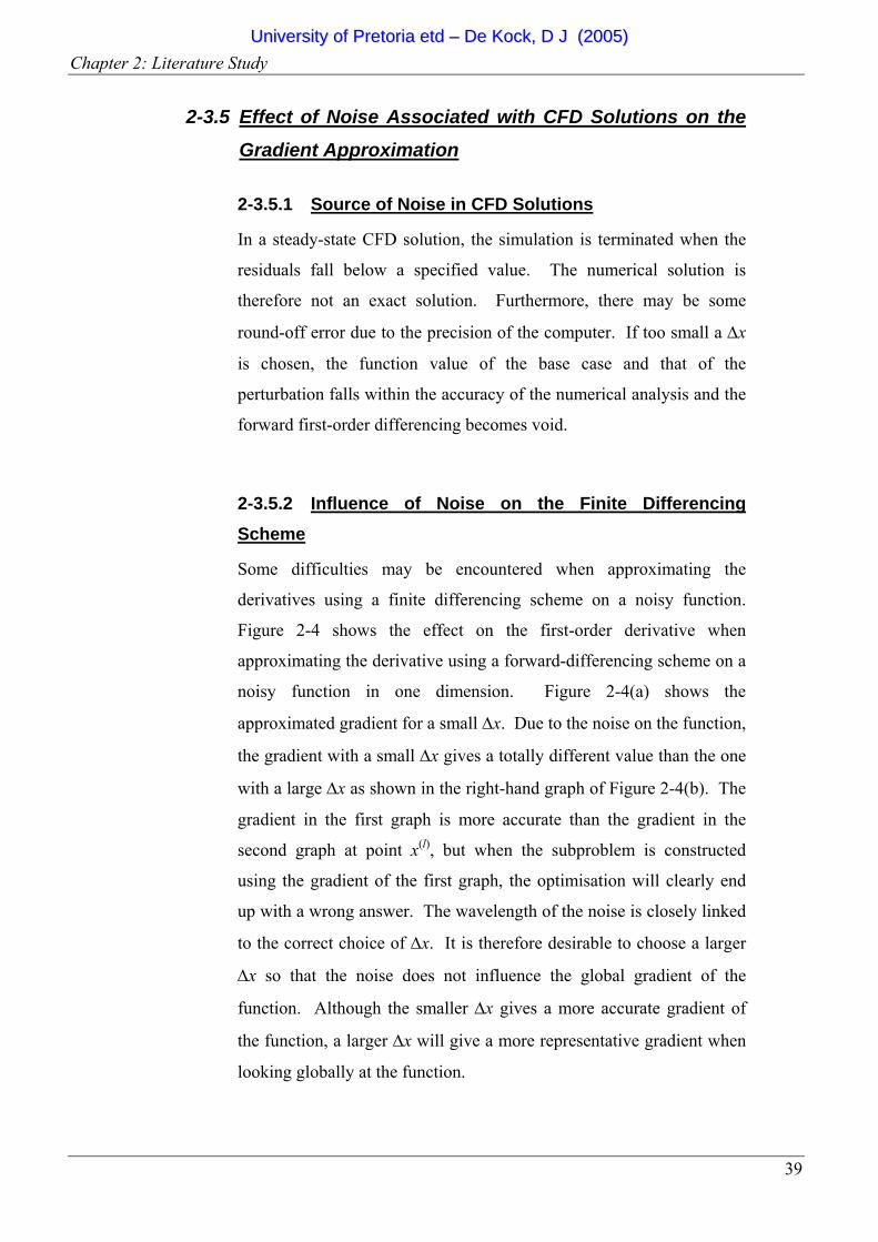
Chapter 2: Literature Study
39
2-3.5 Effect of Noise Associated with CFD Solutions on the
Gradient Approximation
2-3.5.1 Source of Noise in CFD Solutions
In a steady-state CFD solution, the simulation is terminated when the
residuals fall below a specified value. The numerical solution is
therefore not an exact solution. Furthermore, there may be some
round-off error due to the precision of the computer. If too small a ∆x
is chosen, the function value of the base case and that of the
perturbation falls within the accuracy of the numerical analysis and the
forward first-order differencing becomes void.
2-3.5.2 Influence of Noise on the Finite Differencing Scheme
Some difficulties may be encountered when approximating the
derivatives using a finite differencing scheme on a noisy function.
Figure 2-4 shows the effect on the first-order derivative when
approximating the derivative using a forward-differencing scheme on a
noisy function in one dimension. Figure 2-4(a) shows the
approximated gradient for a small ∆x. Due to the noise on the function,
the gradient with a small ∆x gives a totally different value than the one
with a large ∆x as shown in the right-hand graph of Figure 2-4(b). The
gradient in the first graph is more accurate than the gradient in the
second graph at point x(l), but when the subproblem is constructed
using the gradient of the first graph, the optimisation will clearly end
up with a wrong answer. The wavelength of the noise is closely linked
to the correct choice of ∆x. It is therefore desirable to choose a larger
∆x so that the noise does not influence the global gradient of the
function. Although the smaller ∆x gives a more accurate gradient of
the function, a larger ∆x will give a more representative gradient when
looking globally at the function.
UUnniivveerrssiittyy ooff PPrreettoorriiaa eettdd –– DDee KKoocckk,, DD JJ ((22000055))
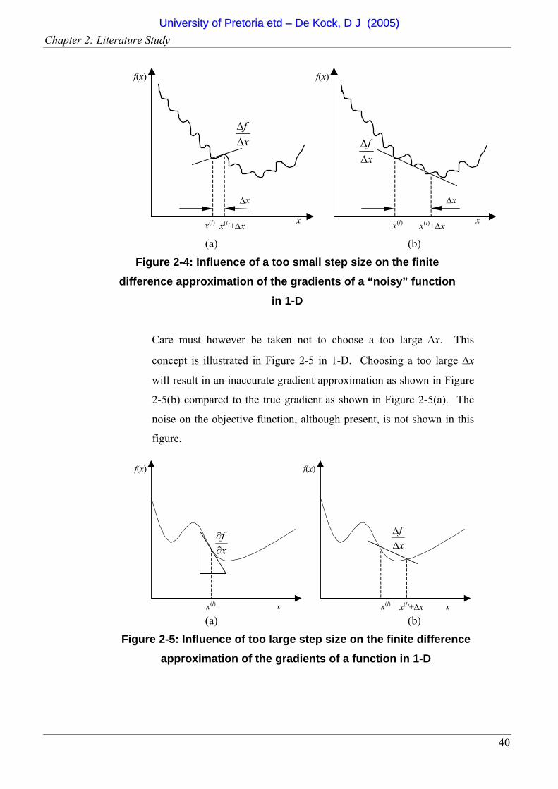
Chapter 2: Literature Study
40
f(x) f(x)
x x
∆x ∆x
x(l) x(l)+∆x x(l) x(l)+∆x
xf
∆∆
xf
∆∆
(a) (b)
Figure 2-4: Influence of a too small step size on the finite difference approximation of the gradients of a “noisy” function
in 1-D
Care must however be taken not to choose a too large ∆x. This
concept is illustrated in Figure 2-5 in 1-D. Choosing a too large ∆x
will result in an inaccurate gradient approximation as shown in Figure
2-5(b) compared to the true gradient as shown in Figure 2-5(a). The
noise on the objective function, although present, is not shown in this
figure.
f(x) f(x)
x xx(l)+∆xx(l)
xf
∂∂
xf
∆∆
x(l)
(a) (b)
Figure 2-5: Influence of too large step size on the finite difference approximation of the gradients of a function in 1-D
UUnniivveerrssiittyy ooff PPrreettoorriiaa eettdd –– DDee KKoocckk,, DD JJ ((22000055))
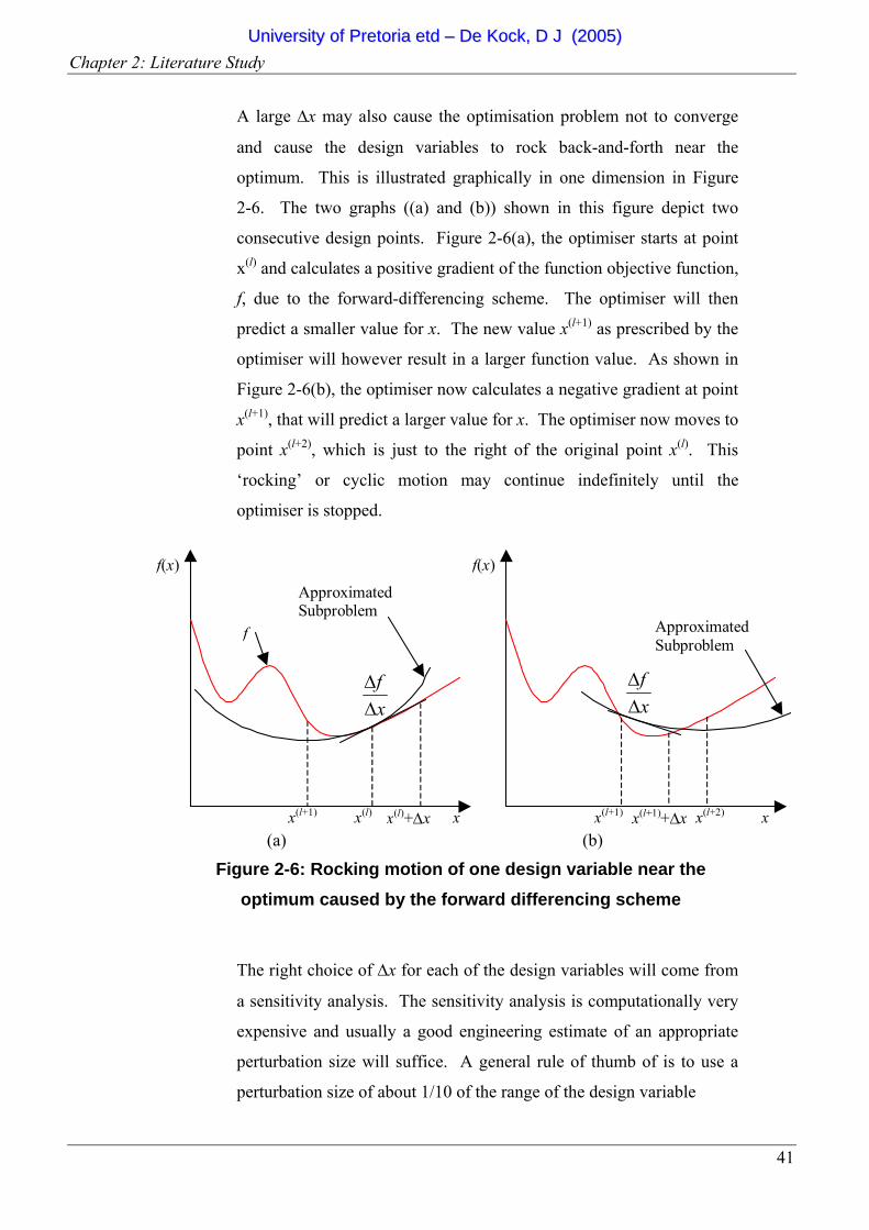
Chapter 2: Literature Study
41
A large ∆x may also cause the optimisation problem not to converge
and cause the design variables to rock back-and-forth near the
optimum. This is illustrated graphically in one dimension in Figure
2-6. The two graphs ((a) and (b)) shown in this figure depict two
consecutive design points. Figure 2-6(a), the optimiser starts at point
x(l) and calculates a positive gradient of the function objective function,
f, due to the forward-differencing scheme. The optimiser will then
predict a smaller value for x. The new value x(l+1) as prescribed by the
optimiser will however result in a larger function value. As shown in
Figure 2-6(b), the optimiser now calculates a negative gradient at point
x(l+1), that will predict a larger value for x. The optimiser now moves to
point x(l+2), which is just to the right of the original point x(l). This
‘rocking’ or cyclic motion may continue indefinitely until the
optimiser is stopped.
f(x) f(x)
x xx(l+1)+∆x x(l+2)
xf
∆∆
xf
∆∆
x(l) x(l+1)x(l)+∆xx(l+1)
ApproximatedSubproblem
f ApproximatedSubproblem
(a) (b)
Figure 2-6: Rocking motion of one design variable near the optimum caused by the forward differencing scheme
The right choice of ∆x for each of the design variables will come from
a sensitivity analysis. The sensitivity analysis is computationally very
expensive and usually a good engineering estimate of an appropriate
perturbation size will suffice. A general rule of thumb of is to use a
perturbation size of about 1/10 of the range of the design variable
UUnniivveerrssiittyy ooff PPrreettoorriiaa eettdd –– DDee KKoocckk,, DD JJ ((22000055))
Chapter 2: Literature Study
42
There may be a variety of sources that cause the noise in the CFD
solutions. This noise may be due to grid changes, convergence,
numerical accuracy of the computer etc. This noise and the source of
the noise still need some further investigation and falls outside the
scope of this study. The better resolved the CFD analysis are, i.e., the
finer the mesh, the higher the convergence of the residuals, and the
more accurate the models used, the less contribution of noise is
expected to be.
2-4 CONCLUSION The first part of this chapter described the current available literature on tundish and
tundish furniture design. A large amount of research has been done on improving the
design of tundish and tundish furniture. These improvements are achieved by using
two different types of modelling techniques. The modelling is either through physical
modelling or through numerical modelling. In the physical modelling, either plant
trials or water models are used. Numerical modelling makes use of Computational
Fluid Dynamics (CFD). The chapter looked in detail at the techniques, methods and
procedures used in CFD to model different aspects of the tundish like turbulence, heat
transfer and inclusion removal. All the cases in the literature in which new tundish or
tundish furniture have been designed used a trial-and-error method to improve the
design using either of the modelling techniques mentioned above.
The second part of the chapter focussed on mathematical optimisation. Mathematical
optimisation was formally defined and then three optimisation algorithms were
discussed. The effect of numerical noise inherent to a CFD analysis and its effect on
gradient-based optimisation algorithms were also shown.
UUnniivveerrssiittyy ooff PPrreettoorriiaa eettdd –– DDee KKoocckk,, DD JJ ((22000055))
43
3 CHAPTER 3: TUNDISH DESIGN OPTIMISATION
METHODOLOGY
3-1 INTRODUCTION This chapter describes the methodology developed to optimise tundish and tundish
furniture designs. This chapter’s aim is also to serve as a guide for the setup of an
optimisation problem involving tundishes.
In order to optimise, one must first be confident that the modelling techniques used
accurately predict the physical process being modelled. The first section of this
chapter describes the validation of the modelling techniques that are going to be used
to predict the physical process.
The next step is to formulate the optimisation problem. This is the most important
step in the optimisation process. For the complex flow phenomena that exist inside a
tundish, a wide range of candidate objective functions and constraints are available
for possible use. It is up to the design engineer to decide which criteria and
constraints are important and/or essential for his/her specific application.
The last section of the chapter describes the automisation of the optimisation
procedure. This forms an essential part of the optimisation process. It is necessary
for the optimisation procedure to be executed without any human intervention. This
involves the automated setup of the problem being solved, solving the problem and
then post-processing the results needed by the optimiser.
UUnniivveerrssiittyy ooff PPrreettoorriiaa eettdd –– DDee KKoocckk,, DD JJ ((22000055))

Chapter 3: Tundish Design Optimisation Methodology
44
3-2 VALIDATION OF CFD MODEL A crucial prerequisite before an optimisation run can be started is to have confidence
in the accuracy of the modelling tool used in the evaluation of the objective and
constraint functions. The optimisation results can only be as good as the accuracy of
the modelling. For this reason, two validation cases were undertaken to validate the
CFD models. These two validation cases are described below.
3-2.1 Validation Case 1
The first validation study undertaken was the validation against a full-scale
single-strand water model of the Columbus Stainless Steel Caster. The details
of this validation are given in Appendix A [65,66]. In this study a tracer was
injected into the tundish at the shroud (refer Figure 1-1) and the concentration
was measured at the outlet with a spectrophotometer [67]. The resulting
Residence Time Distribution (RTD) curve was then compared with the
numerical model as shown in Figure 3-1 (a repeat of Figure A-3, for ease of
reference).
From the RTD curve, the relevant RTD data were extracted to compare with
the experimental and CFD data. These data are given in Table 3-1 (repeated
from Table A-1). Generally, good agreement is found between the
experimental and CFD data with the minimum residence time (MRT) being
the only value that is not predicted to within 15%. This MRT is however very
sensitive to the duration of the injection and the sensitivity of the
spectrophotometer (refer Appendix A).
UUnniivveerrssiittyy ooff PPrreettoorriiaa eettdd –– DDee KKoocckk,, DD JJ ((22000055))
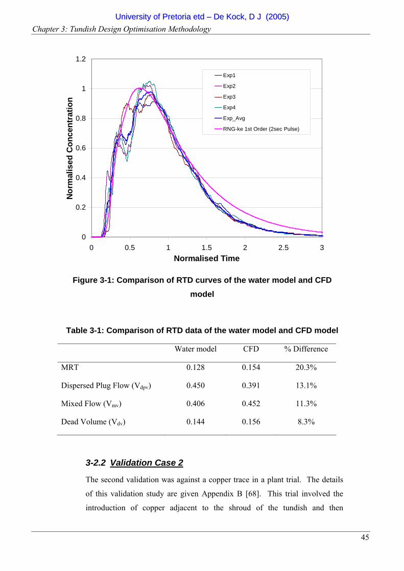
Chapter 3: Tundish Design Optimisation Methodology
45
0
0.2
0.4
0.6
0.8
1
1.2
0 0.5 1 1.5 2 2.5 3Normalised Time
Nor
mal
ised
Con
cent
ratio
nExp1
Exp2
Exp3
Exp4
Exp_Avg
RNG-ke 1st Order (2sec Pulse)
Figure 3-1: Comparison of RTD curves of the water model and CFD model
Table 3-1: Comparison of RTD data of the water model and CFD model
Water model CFD % Difference
MRT
Dispersed Plug Flow (Vdpv)
Mixed Flow (Vmv)
Dead Volume (Vdv)
0.128
0.450
0.406
0.144
0.154
0.391
0.452
0.156
20.3%
13.1%
11.3%
8.3%
3-2.2 Validation Case 2
The second validation was against a copper trace in a plant trial. The details
of this validation study are given Appendix B [68]. This trial involved the
introduction of copper adjacent to the shroud of the tundish and then
UUnniivveerrssiittyy ooff PPrreettoorriiaa eettdd –– DDee KKoocckk,, DD JJ ((22000055))
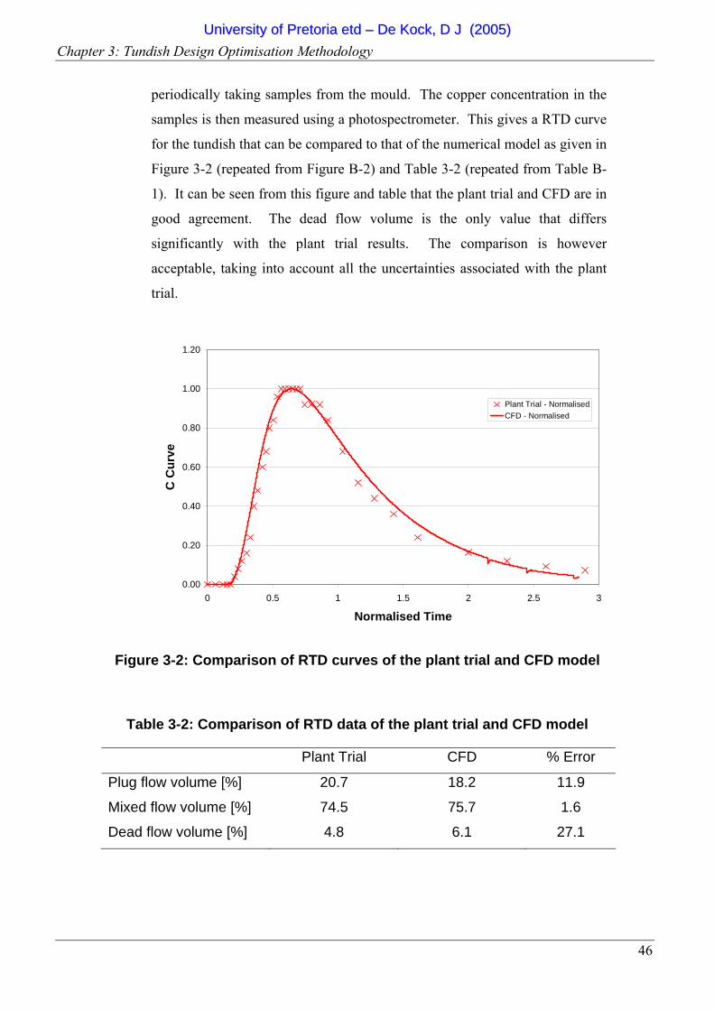
Chapter 3: Tundish Design Optimisation Methodology
46
periodically taking samples from the mould. The copper concentration in the
samples is then measured using a photospectrometer. This gives a RTD curve
for the tundish that can be compared to that of the numerical model as given in
Figure 3-2 (repeated from Figure B-2) and Table 3-2 (repeated from Table B-
1). It can be seen from this figure and table that the plant trial and CFD are in
good agreement. The dead flow volume is the only value that differs
significantly with the plant trial results. The comparison is however
acceptable, taking into account all the uncertainties associated with the plant
trial.
0.00
0.20
0.40
0.60
0.80
1.00
1.20
0 0.5 1 1.5 2 2.5 3
Normalised Time
C C
urve
Plant Trial - NormalisedCFD - Normalised
Figure 3-2: Comparison of RTD curves of the plant trial and CFD model
Table 3-2: Comparison of RTD data of the plant trial and CFD model
Plant Trial CFD % Error
Plug flow volume [%] 20.7 18.2 11.9
Mixed flow volume [%] 74.5 75.7 1.6
Dead flow volume [%] 4.8 6.1 27.1
UUnniivveerrssiittyy ooff PPrreettoorriiaa eettdd –– DDee KKoocckk,, DD JJ ((22000055))
Chapter 3: Tundish Design Optimisation Methodology
47
3-3 FORMULATION OF OPTIMISATION PROBLEM The correct formulation of the optimisation problem is the most important step in any
optimisation study. This section shows the different design variables, objective
functions and constraints that can be chosen by the design engineer when optimising a
tundish and tundish furniture.
3-3.1 Candidate design variables
The design variables are usually the easiest for the design engineer to choose.
The variables are usually the design parameters that the engineer can and want
to change to improve the design. Design variables for a tundish can be
divided into two main categories, i.e., process variables and geometric
variables.
The process variables include parameters like flow rate, inlet temperature, etc.
Process variables are usually not as easy to change as these are dictated by the
operation of the plant. For example, the molten steel inlet temperature is
usually a function of the holding time of the ladle and the amount of time the
ladle spent at the secondary metallurgy station.
Geometric variables include parameters like the position and height of a dam,
or the shape and size of an impact pad or even the total size and shape of a
tundish. The geometric variables, especially those linked to refractory
components, are parameters that are easier to change and control than the
process parameters.
3-3.2 Candidate Objective Functions and Constraints from
CFD analysis
A number of candidate objective functions are available when optimising the
tundish and tundish furniture design. A list of possible functions and their
effect on the performance of the tundish are given below.
UUnniivveerrssiittyy ooff PPrreettoorriiaa eettdd –– DDee KKoocckk,, DD JJ ((22000055))
Chapter 3: Tundish Design Optimisation Methodology
48
3-3.2.1 RTD Curve
As shown in section 2-2.2, various quantities can be extracted from a
RTD curve to determine the performance of the tundish. The different
quantities and their possible use in an optimisation formulation are
given below.
Minimum Residence Time (MRT)
The MRT or minimum break-through time, one typically wants as long
a possible. A long MRT indicates a large plug flow volume and
therefore smaller mixed volume and dead volume compared to a
tundish with a short MRT. This in turn will result in a short mixed-
grade length in the slab when casting different grades due to the lower
mixed and dead volumes. Therefore, for the design of a tundish that
will undergo many grade changes, the design engineer would want to
maximise MRT.
Well-mixed volume
The well-mixed volume gives an indication to how much mixing takes
place within the tundish. For inclusion particle removal, it is desirable
to have a large amount of mixing as this give the particle the
opportunity to reach the slag surface. Conversely, for a short mixed-
grade length in the slab it is desirable to have a small amount of
mixing. Therefore, for the design of a tundish where the quality is of
high importance, the design engineer will want to maximise the well-
mixed volume.
Dead volume
The dead volume gives an indication of stagnant or recirculating
regions. These regions want to be kept as small as possible as this will
negatively influence the length of the mixed-grade slab. The
optimisation formulation would therefore be to minimise the dead
volume.
UUnniivveerrssiittyy ooff PPrreettoorriiaa eettdd –– DDee KKoocckk,, DD JJ ((22000055))
Chapter 3: Tundish Design Optimisation Methodology
49
Usually a trade-off has to be made between the MRT, well-mixed volume and
dead volume. A tundish with very little mixing (i.e., a high MRT, low dead
volume) gives a short mixed-grade length but low inclusion removal
capabilities. On the contrary, a tundish with high mixing (i.e., a high well-
mixed volume) will give good inclusion removal capabilities but a long
mixed-grade length. It is the design engineer’s responsibility to decide which
is the most important in his/her specific application and choose the appropriate
RTD related quantity.
3-3.2.2 Inclusion removal
For higher quality steel and less defects, the design engineer will opt to
maximise the inclusion removal on the slag layer. The inclusion
removal modelling can be performed using the methods discussed in
section 2-2.4.4. In some cases only the larger sized inclusions’
(typically larger than 50micron) removal can be chosen to be
maximised as the smaller inclusion (typically smaller than 50micron)
will not adversely affect the quality of the steel. The inclusions are
removed by sticking to the refractories and absorption into and reaction
with the slag layer.
3-3.2.3 Mixed-grade length
The mixed-grade length can be modelled explicitly by doing a transient
multi-phase CFD analysis to capture the free surface between the air,
slag layer and steel. This must be done to capture the effect of wave
formation on the free surface and mixing of the inlet stream with the
remaining steel as the tundish is filled with a different steel grade from
a new ladle. As the multi-phase analysis is a computationally
expensive, an indication of the mixed grade length can however be
obtained from a RTD curve (discussed in section 3-3.2.1 above)
obtained for a full level or using quasi-steady solutions at various fixed
fill levels. This will not be as accurate as doing a multi-phase analysis.
UUnniivveerrssiittyy ooff PPrreettoorriiaa eettdd –– DDee KKoocckk,, DD JJ ((22000055))
Chapter 3: Tundish Design Optimisation Methodology
50
The mixed-grade length will obviously be minimised to reduce the
amount of steel that will be downgraded.
3-3.2.4 Temperature
The minimum temperature in the tundish is required to stay above a
specified lower value. This is required so that the steel does not
solidify inside the tundish. Furthermore, the tundish outlet temperature
is required to be within a specified temperature range to carry a certain
amount of super heat into the mould. These temperatures will typically
be constraint functions that will be specified in the optimisation
formulation.
3-3.2.5 Slag layer
It is required that the slag layer is stagnant and that turbulence levels on
the slag layer are low. High velocities and turbulence levels on the
slag layer might cause slag entrainment into the steel and adversely
affect the quality of the steel. Another two possible objective functions
would therefore be to minimise the turbulence levels on the slag layer
or to minimise the velocities on the slag layer.
3-3.2.6 Cascading
Cascading happens during the first cast when the steel enters the
tundish for the first time. During this time, there is no slag cover
present and at these high temperatures, significant oxidation occurs.
This oxidation results in a poor quality first slab. A possible
optimisation formulation would therefore be to minimise the area of
steel exposed to the atmosphere. This requires a transient multi-phase
flow analysis of the filling that is computationally very expensive and
probably not a viable formulation due to the excessive computational
effort that will be required.
UUnniivveerrssiittyy ooff PPrreettoorriiaa eettdd –– DDee KKoocckk,, DD JJ ((22000055))
Chapter 3: Tundish Design Optimisation Methodology
51
3-3.3 Other Constraints
Other constraint functions also exist that are not related to the CFD simulation.
These constraints are typical geometric constraints as well as manufacturing
constraints. A typical manufacturing constraint would be the minimum
thickness that a piece of tundish furniture could be. A geometrical constraint
can also be derived from the required strength of the specific furniture piece,
e.g., what is the minimum thickness that will withstand the ferrostatic head.
Another type of constraint that can be important is the yield that can be
achieved by the tundish (i.e., minimising the liquid steel that remains in the
tundish when drained). This can be based on a purely geometrical
consideration or it can be based on the fact that a vortex forms at the end of a
cast when the tundish level drops. The vortex then entrains slag that goes
directly into the mould.
3-4 AUTOMATION OF OPTIMISATION PROBLEM The automation of the optimisation problem forms an important part of the whole
optimisation procedure. The automation is done so that no human intervention is
required once the optimisation process has started. The optimisation process is shown
in the flow diagram given in Figure 3-3. For a given starting design (x), the
mathematical optimiser generates a set of k designs that need to be evaluated. The
number k and the exact values of the design vector to be evaluated (xi) are a function
of the specific optimiser to be used. A journal file for the specific design is then
generated and is passed to GAMBIT (gambit.jou) to generate the geometry and the
mesh to be used in FLUENT. The mesh is exported to FLUENT where another
journal file (fluent.jou) controls the setting up, running and writing of the necessary
files for the post-processing of the design. As an example in this flow diagram, a file
called conc.out is written to the hard disk containing the outlet concentration. The
output file(s) are then processed to yield the objective and constraint functions of the
specific design. The mathematical optimiser gathers all these data and predicts a new
optimum design. The process is repeated until the optimisation converges to specified
criteria.
UUnniivveerrssiittyy ooff PPrreettoorriiaa eettdd –– DDee KKoocckk,, DD JJ ((22000055))
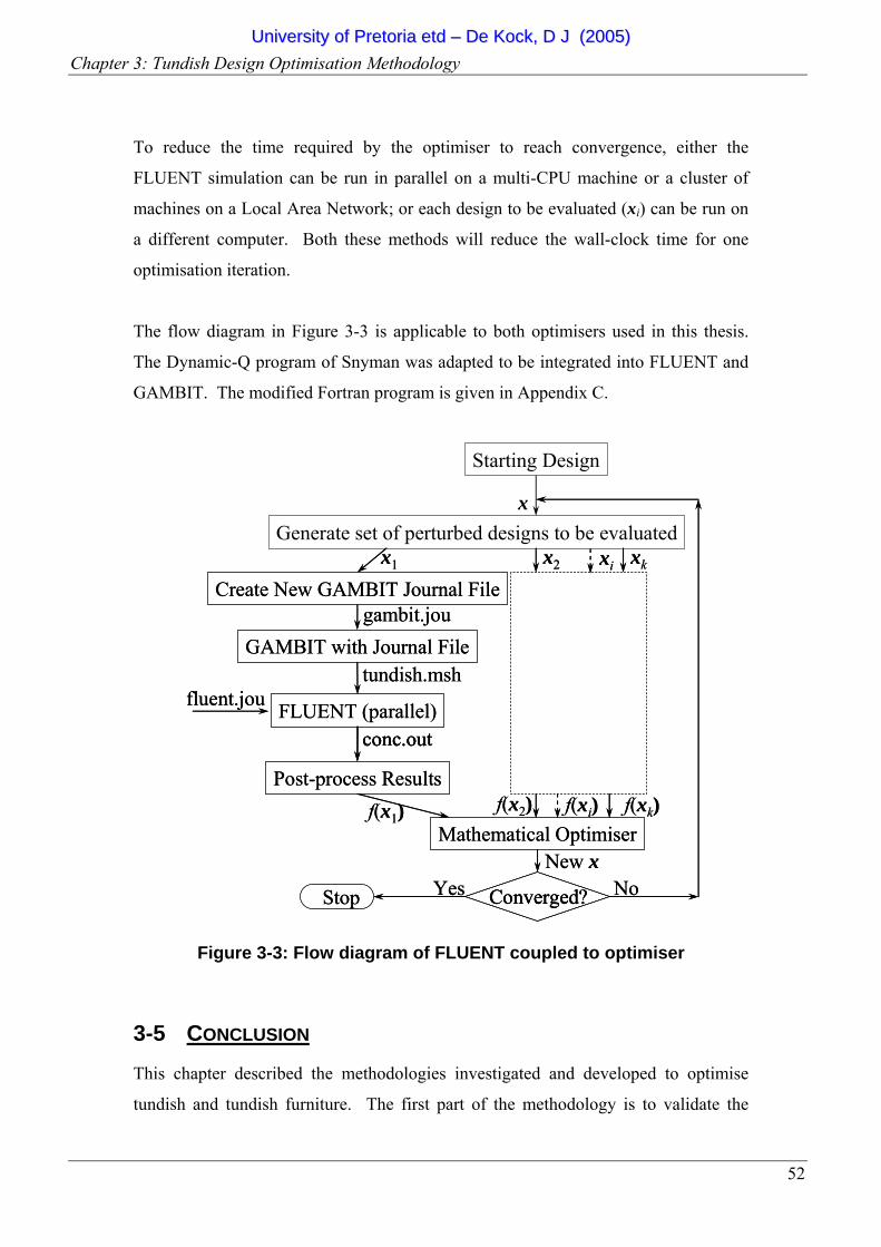
Chapter 3: Tundish Design Optimisation Methodology
52
To reduce the time required by the optimiser to reach convergence, either the
FLUENT simulation can be run in parallel on a multi-CPU machine or a cluster of
machines on a Local Area Network; or each design to be evaluated (xi) can be run on
a different computer. Both these methods will reduce the wall-clock time for one
optimisation iteration.
The flow diagram in Figure 3-3 is applicable to both optimisers used in this thesis.
The Dynamic-Q program of Snyman was adapted to be integrated into FLUENT and
GAMBIT. The modified Fortran program is given in Appendix C.
Starting Design
Generate set of perturbed designs to be evaluated
Create New GAMBIT Journal Filegambit.jou
Create New GAMBIT Journal Filegambit.jou
Post-process Results
conc.out
Post-process Results
conc.outconc.out
New xNew x
x1 x2 xkxix1 x2 xkxi
NoNoConverged?YesStop Converged?Converged?YesStop
x
GAMBIT with Journal Filetundish.msh
GAMBIT with Journal Filetundish.msh
f(xi)Mathematical Optimiser
f(x1) f(x2) f(xk)f(xi)Mathematical Optimiser
f(x1) f(x2) f(xk)
fluent.jou FLUENT (parallel)fluent.jou FLUENT (parallel)
Figure 3-3: Flow diagram of FLUENT coupled to optimiser
3-5 CONCLUSION This chapter described the methodologies investigated and developed to optimise
tundish and tundish furniture. The first part of the methodology is to validate the
UUnniivveerrssiittyy ooff PPrreettoorriiaa eettdd –– DDee KKoocckk,, DD JJ ((22000055))

Chapter 3: Tundish Design Optimisation Methodology
53
numerical model that will be used in the optimisation study. Secondly and the most
important, is formulating the optimisation problem. This involves choosing the
design variables and the appropriate object function and constraints. Typical design
variables, objective function and constraint functions for tundish design were given
and discussed. Lastly, the automation of the numerical set-up, solving and extraction
of data were described. The following chapter will describe the application of this
methodology to different case studies.
UUnniivveerrssiittyy ooff PPrreettoorriiaa eettdd –– DDee KKoocckk,, DD JJ ((22000055))
54
4 CHAPTER 4: APPLICATION OF TUNDISH DESIGN
METHODOLOGY TO CASE STUDIES
4-1 INTRODUCTION The design optimisation methodology developed in Chapter 3 has been tested on a
number of different case studies. These case studies are given in detail in this chapter.
The chapter starts with the optimisation of a simple 1-dam-1-weir configuration. The
optimisation of a baffle follows next, with the optimisation of an impact pad and an
impact pad with a dam forming the last two test cases.
4-2 CASE STUDY 1: OPTIMISATION OF 1-DAM-1-WEIR
CONFIGURATION The first case study involves the single-strand stainless steel continuous caster in
operation at the Middelburg plant of Columbus Stainless. The work of this case study
has been published in the Journal of Iron and Steel Institute of Japan International
[69] and presented at the 20th International Congress of Theoretical and Applied
Mechanics [70].
The tundish geometry considered is shown in Figure 4-1. The flow rate is controlled
by the position of the stopper. When injecting a tracer element at the shroud (inlet),
this tracer is detected at the SEN (outlet) after a certain amount of time. The
concentration at the outlet increases to a maximum where after it decreases. The time
history of the tracer concentration as measured at the outlet is called the Residence
Time Distribution (RTD) in 2-2.2. The rate of decay is of interest since it correlates
with the ratio of plug flow versus mixed flow in the tundish. The amount of tracer left
in the tundish after 2 t (twice the mean residence time) is defined in this study as the
UUnniivveerrssiittyy ooff PPrreettoorriiaa eettdd –– DDee KKoocckk,, DD JJ ((22000055))
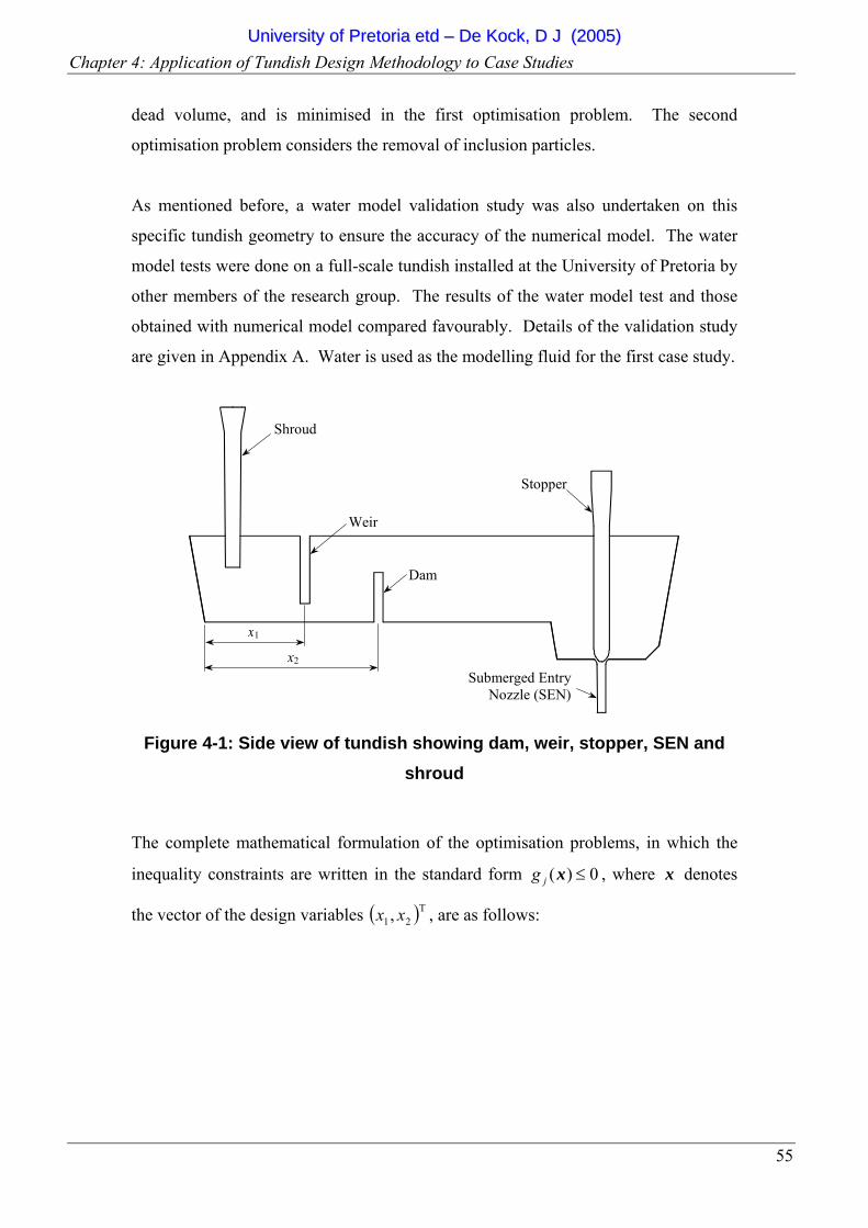
Chapter 4: Application of Tundish Design Methodology to Case Studies
55
dead volume, and is minimised in the first optimisation problem. The second
optimisation problem considers the removal of inclusion particles.
As mentioned before, a water model validation study was also undertaken on this
specific tundish geometry to ensure the accuracy of the numerical model. The water
model tests were done on a full-scale tundish installed at the University of Pretoria by
other members of the research group. The results of the water model test and those
obtained with numerical model compared favourably. Details of the validation study
are given in Appendix A. Water is used as the modelling fluid for the first case study.
Shroud
Weir
Dam
Stopper
Submerged EntryNozzle (SEN)
x1
x2
Figure 4-1: Side view of tundish showing dam, weir, stopper, SEN and shroud
The complete mathematical formulation of the optimisation problems, in which the
inequality constraints are written in the standard form 0)( ≤xjg , where x denotes
the vector of the design variables ( )T21, xx , are as follows:
UUnniivveerrssiittyy ooff PPrreettoorriiaa eettdd –– DDee KKoocckk,, DD JJ ((22000055))
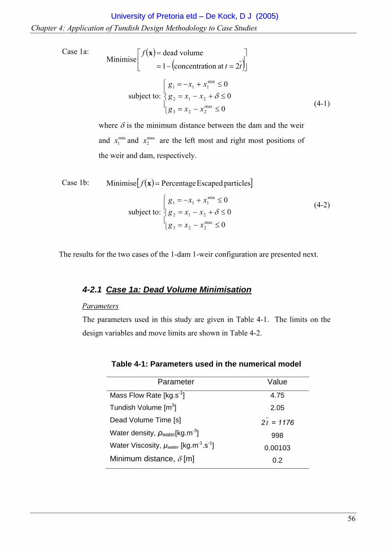
Chapter 4: Application of Tundish Design Methodology to Case Studies
56
Case 1a: ( )( )⎥⎦
⎤⎢⎣
⎡
=−=
=
tt
f
2at ion concentrat1
volumedead Minimise
x
subject to: ⎪⎩
⎪⎨
⎧
≤−=
≤+−=≤+−=
0
00
max223
212
min111
xxg
xxgxxg
δ
where δ is the minimum distance between the dam and the weir
and min1x and max
2x are the left most and right most positions of
the weir and dam, respectively.
(4-1)
Case 1b: ( )[ ]particles Escaped Percentage Minimise =xf
subject to: ⎪⎩
⎪⎨
⎧
≤−=
≤+−=≤+−=
00
0
max223
212
min111
xxgxxgxxg
δ (4-2)
The results for the two cases of the 1-dam 1-weir configuration are presented next.
4-2.1 Case 1a: Dead Volume Minimisation
Parameters
The parameters used in this study are given in Table 4-1. The limits on the
design variables and move limits are shown in Table 4-2.
Table 4-1: Parameters used in the numerical model
Parameter Value
Mass Flow Rate [kg.s-1] Tundish Volume [m3]
Dead Volume Time [s]
Water density, ρwater[kg.m-3]
Water Viscosity, µwater [kg.m-1.s-1]
Minimum distance, δ [m]
4.75 2.05
2 t = 1176
998
0.00103
0.2
UUnniivveerrssiittyy ooff PPrreettoorriiaa eettdd –– DDee KKoocckk,, DD JJ ((22000055))
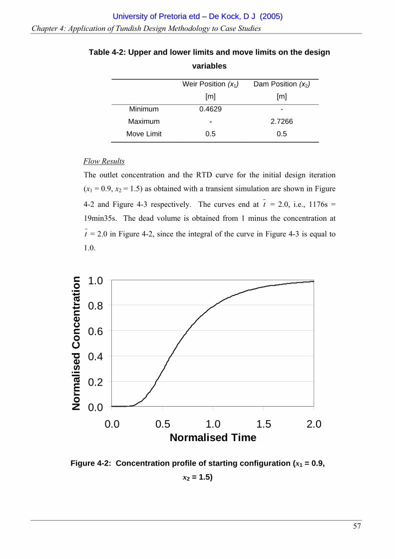
Chapter 4: Application of Tundish Design Methodology to Case Studies
57
Table 4-2: Upper and lower limits and move limits on the design variables
Weir Position (x1)
[m]
Dam Position (x2)
[m]
Minimum
Maximum
Move Limit
0.4629
-
0.5
-
2.7266
0.5
Flow Results
The outlet concentration and the RTD curve for the initial design iteration
(x1 = 0.9, x2 = 1.5) as obtained with a transient simulation are shown in Figure
4-2 and Figure 4-3 respectively. The curves end at t = 2.0, i.e., 1176s =
19min35s. The dead volume is obtained from 1 minus the concentration at
t = 2.0 in Figure 4-2, since the integral of the curve in Figure 4-3 is equal to
1.0.
0.0
0.2
0.4
0.6
0.8
1.0
0.0 0.5 1.0 1.5 2.0Normalised Time
Nor
mal
ised
Con
cent
ratio
n
Figure 4-2: Concentration profile of starting configuration (x1 = 0.9, x2 = 1.5)
UUnniivveerrssiittyy ooff PPrreettoorriiaa eettdd –– DDee KKoocckk,, DD JJ ((22000055))
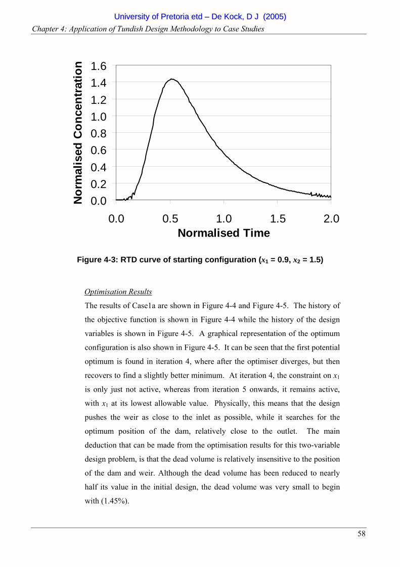
Chapter 4: Application of Tundish Design Methodology to Case Studies
58
0.00.20.40.60.81.01.21.41.6
0.0 0.5 1.0 1.5 2.0Normalised Time
Nor
mal
ised
Con
cent
ratio
n
Figure 4-3: RTD curve of starting configuration (x1 = 0.9, x2 = 1.5)
Optimisation Results
The results of Case1a are shown in Figure 4-4 and Figure 4-5. The history of
the objective function is shown in Figure 4-4 while the history of the design
variables is shown in Figure 4-5. A graphical representation of the optimum
configuration is also shown in Figure 4-5. It can be seen that the first potential
optimum is found in iteration 4, where after the optimiser diverges, but then
recovers to find a slightly better minimum. At iteration 4, the constraint on x1
is only just not active, whereas from iteration 5 onwards, it remains active,
with x1 at its lowest allowable value. Physically, this means that the design
pushes the weir as close to the inlet as possible, while it searches for the
optimum position of the dam, relatively close to the outlet. The main
deduction that can be made from the optimisation results for this two-variable
design problem, is that the dead volume is relatively insensitive to the position
of the dam and weir. Although the dead volume has been reduced to nearly
half its value in the initial design, the dead volume was very small to begin
with (1.45%).
UUnniivveerrssiittyy ooff PPrreettoorriiaa eettdd –– DDee KKoocckk,, DD JJ ((22000055))
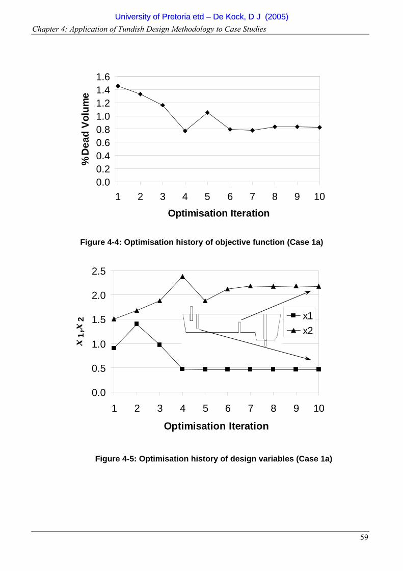
Chapter 4: Application of Tundish Design Methodology to Case Studies
59
0.00.20.40.60.81.01.21.41.6
1 2 3 4 5 6 7 8 9 10
Optimisation Iteration
% D
ead
Volu
me
Figure 4-4: Optimisation history of objective function (Case 1a)
0.0
0.5
1.0
1.5
2.0
2.5
1 2 3 4 5 6 7 8 9 10
Optimisation Iteration
x1,x
2 x1x2
Figure 4-5: Optimisation history of design variables (Case 1a)
UUnniivveerrssiittyy ooff PPrreettoorriiaa eettdd –– DDee KKoocckk,, DD JJ ((22000055))

Chapter 4: Application of Tundish Design Methodology to Case Studies
60
4-2.2 Case 1b: Inclusion Removal Optimisation
Parameters
The same parameters and limits on the design variables are used as in Case 1a.
The only additional parameters considered is the inclusion size distribution,
inclusion particle mass flow and density. The inclusion size distribution is
given in Table 4-3. These data were acquired from taking a sample of the
steel at the shroud on the plant and then using an image analyser to determine
the size distribution. This information was obtained from ISCOR
Vanderbijlpark Works [71]. The mass flow is determined from the total
percentage of inclusions in the sample and was calculated as 0.469g.s-1 for the
whole tundish. The density of the inclusions was taken as 456kg.m-3 which is
2.2 times smaller than the density of the water (the modelling fluid used).
This represents the same density ratio of the alumina inclusions relative to the
molten steel in the plant. A total of 2700 inclusions with the same size
distribution as in Table 4-3 are released in the CFD simulation.
Table 4-3: Inclusions size distribution obtained from image analyser [71]
Size
[mm] Number of particles
0.024
0.093
0.207
0.366
0.571
113 37.75
4.5 0.5
0.25
Inclusion Tracks
The inclusion tracks for the starting design are shown in Figure 4-6 for two of
the inclusion sizes considered (i.e. 0.024mm and 0.207mm), released at one
specific location for illustration purposes. It can be seen that the all the larger
inclusion are trapped at the slag layer before the weir due to their larger
buoyancy forces (Figure 4-6a). The smaller inclusions tend to follow the flow
stream and exit at the SEN (Figure 4-6b).
UUnniivveerrssiittyy ooff PPrreettoorriiaa eettdd –– DDee KKoocckk,, DD JJ ((22000055))

Chapter 4: Application of Tundish Design Methodology to Case Studies
61
Figure 4-6: Particle tracks for a) 0.207mm b) 0.024mm size inclusions released at one specific location only (Starting configuration: x1 = 0.9,
x2 = 1.5)
a)
b)
UUnniivveerrssiittyy ooff PPrreettoorriiaa eettdd –– DDee KKoocckk,, DD JJ ((22000055))

Chapter 4: Application of Tundish Design Methodology to Case Studies
62
Optimisation Results
The history of the inclusion optimisation is shown in Figure 4-7 and Figure
4-8. The history of the objective function is shown in Figure 4-8, while the
history of the design variables is shown in Figure 4-8. It can be seen from
Figure 4-8 that the optimiser tends to hit the constraint of minimum distance
(δ) between the dam and the weir, and then moves the dam and weir together
as a pair. A graphical representation of the optimum configuration is also
shown in Figure 4-8. This small distance between the dam and the weir
creates a jet with a high velocity directed towards the surface providing a
mechanism for particle trapping. This may however cause some entrainment
of the slag layer, which was not modelled in this case due to the absence of a
free surface in the CFD model.
The reduction in the objective function is quite small as can be seen in Figure
4-7. This shows that the inclusion removal capability of this tundish with
these given tundish furniture and constraints are not very good. Also, the
improvements that can be made to the design to increase the inclusion removal
capability are not great.
It can also be seen that this optimum differs completely from the optimum in
Case 1a. The main reason for this is that the two objective functions represent
two opposing design criteria.
UUnniivveerrssiittyy ooff PPrreettoorriiaa eettdd –– DDee KKoocckk,, DD JJ ((22000055))

Chapter 4: Application of Tundish Design Methodology to Case Studies
63
0.0
1.0
2.0
3.0
4.0
5.0
6.0
7.0
8.0
9.0
10.0
1 2 3 4 5 6 7
Optimization Iteration
% E
scap
ed P
artic
les
Figure 4-7: Optimisation history of the objective function (Case 1b)
0.0
0.5
1.0
1.5
2.0
2.5
1 2 3 4 5 6 7Optimization Iteration
x1, x
2
x1x2
Figure 4-8: Optimisation history of the design variables (Case 1b)
UUnniivveerrssiittyy ooff PPrreettoorriiaa eettdd –– DDee KKoocckk,, DD JJ ((22000055))

Chapter 4: Application of Tundish Design Methodology to Case Studies
64
4-2.3 Conclusion
A simple dam and weir configuration was optimised for the single-strand
continuous caster of Columbus Stainless Steel. Two different objective
functions were defined for two different cases under investigation. It was
shown that different optima exist for these different objective functions.
UUnniivveerrssiittyy ooff PPrreettoorriiaa eettdd –– DDee KKoocckk,, DD JJ ((22000055))
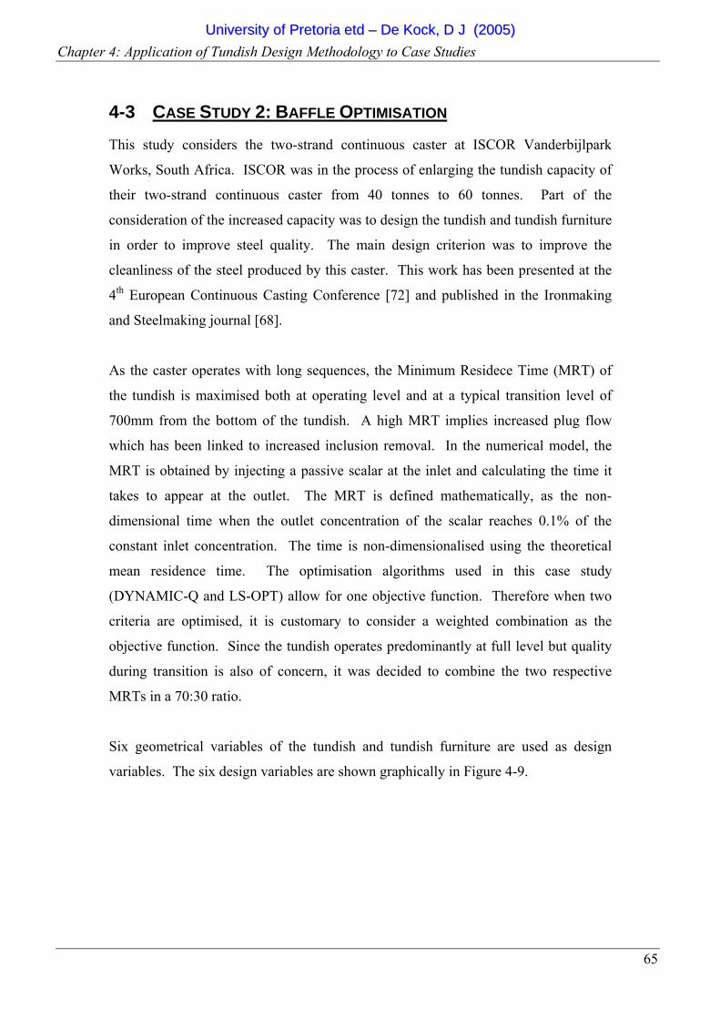
Chapter 4: Application of Tundish Design Methodology to Case Studies
65
4-3 CASE STUDY 2: BAFFLE OPTIMISATION This study considers the two-strand continuous caster at ISCOR Vanderbijlpark
Works, South Africa. ISCOR was in the process of enlarging the tundish capacity of
their two-strand continuous caster from 40 tonnes to 60 tonnes. Part of the
consideration of the increased capacity was to design the tundish and tundish furniture
in order to improve steel quality. The main design criterion was to improve the
cleanliness of the steel produced by this caster. This work has been presented at the
4th European Continuous Casting Conference [72] and published in the Ironmaking
and Steelmaking journal [68].
As the caster operates with long sequences, the Minimum Residece Time (MRT) of
the tundish is maximised both at operating level and at a typical transition level of
700mm from the bottom of the tundish. A high MRT implies increased plug flow
which has been linked to increased inclusion removal. In the numerical model, the
MRT is obtained by injecting a passive scalar at the inlet and calculating the time it
takes to appear at the outlet. The MRT is defined mathematically, as the non-
dimensional time when the outlet concentration of the scalar reaches 0.1% of the
constant inlet concentration. The time is non-dimensionalised using the theoretical
mean residence time. The optimisation algorithms used in this case study
(DYNAMIC-Q and LS-OPT) allow for one objective function. Therefore when two
criteria are optimised, it is customary to consider a weighted combination as the
objective function. Since the tundish operates predominantly at full level but quality
during transition is also of concern, it was decided to combine the two respective
MRTs in a 70:30 ratio.
Six geometrical variables of the tundish and tundish furniture are used as design
variables. The six design variables are shown graphically in Figure 4-9.
UUnniivveerrssiittyy ooff PPrreettoorriiaa eettdd –– DDee KKoocckk,, DD JJ ((22000055))
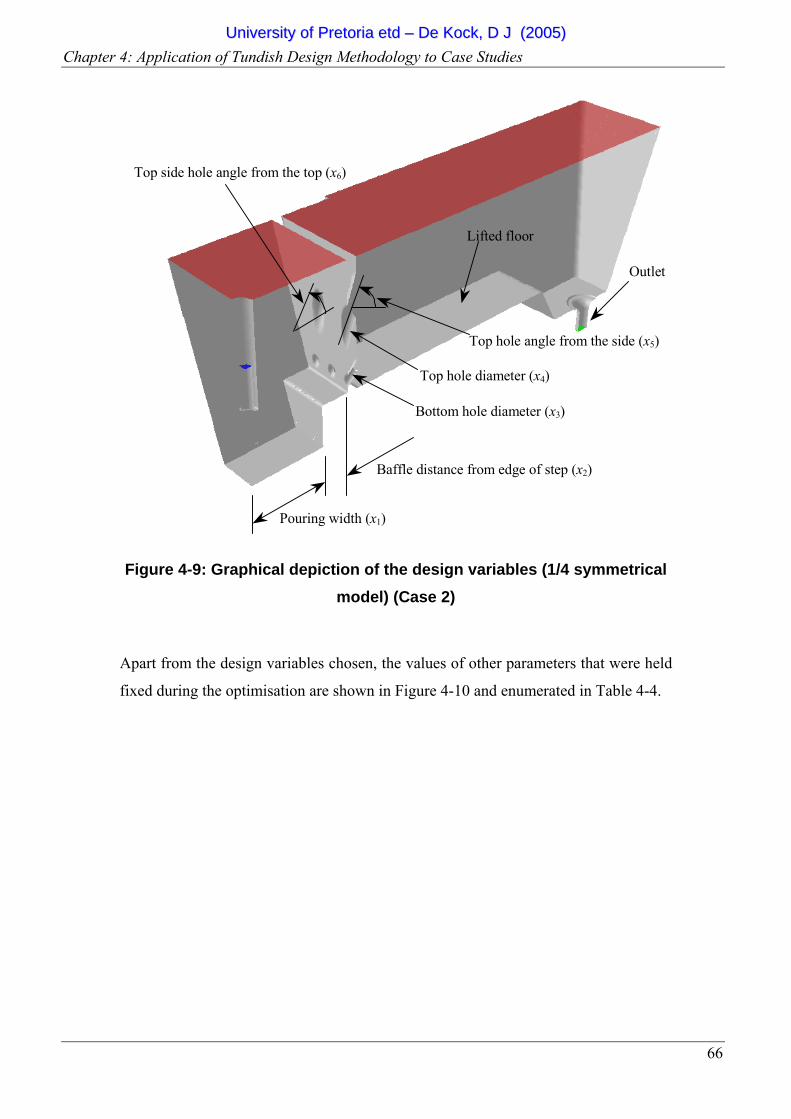
Chapter 4: Application of Tundish Design Methodology to Case Studies
66
Pouring width (x1)
Baffle distance from edge of step (x2)
Bottom hole diameter (x3)
Top hole diameter (x4)
Top hole angle from the side (x5)
Top side hole angle from the top (x6)
Lifted floor
Outlet
Figure 4-9: Graphical depiction of the design variables (1/4 symmetrical model) (Case 2)
Apart from the design variables chosen, the values of other parameters that were held
fixed during the optimisation are shown in Figure 4-10 and enumerated in Table 4-4.
UUnniivveerrssiittyy ooff PPrreettoorriiaa eettdd –– DDee KKoocckk,, DD JJ ((22000055))
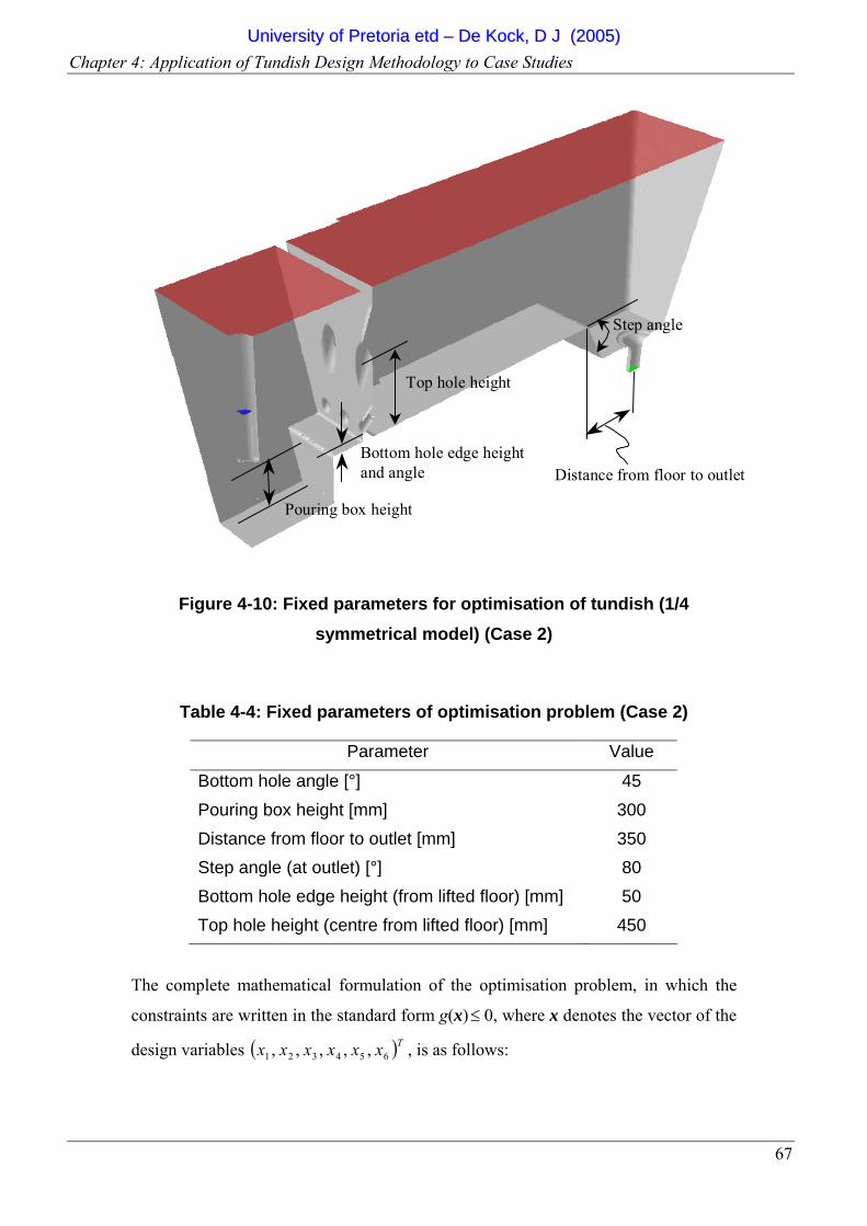
Chapter 4: Application of Tundish Design Methodology to Case Studies
67
Pouring box height
Distance from floor to outletBottom hole edge height and angle
Top hole height
Step angle
Figure 4-10: Fixed parameters for optimisation of tundish (1/4 symmetrical model) (Case 2)
Table 4-4: Fixed parameters of optimisation problem (Case 2)
Parameter Value
Bottom hole angle [°] 45 Pouring box height [mm] 300 Distance from floor to outlet [mm] 350 Step angle (at outlet) [°] 80 Bottom hole edge height (from lifted floor) [mm] 50 Top hole height (centre from lifted floor) [mm] 450
The complete mathematical formulation of the optimisation problem, in which the
constraints are written in the standard form g(x) ≤ 0, where x denotes the vector of the
design variables ( )Txxxxxx 654321 ,,,,, , is as follows:
UUnniivveerrssiittyy ooff PPrreettoorriiaa eettdd –– DDee KKoocckk,, DD JJ ((22000055))
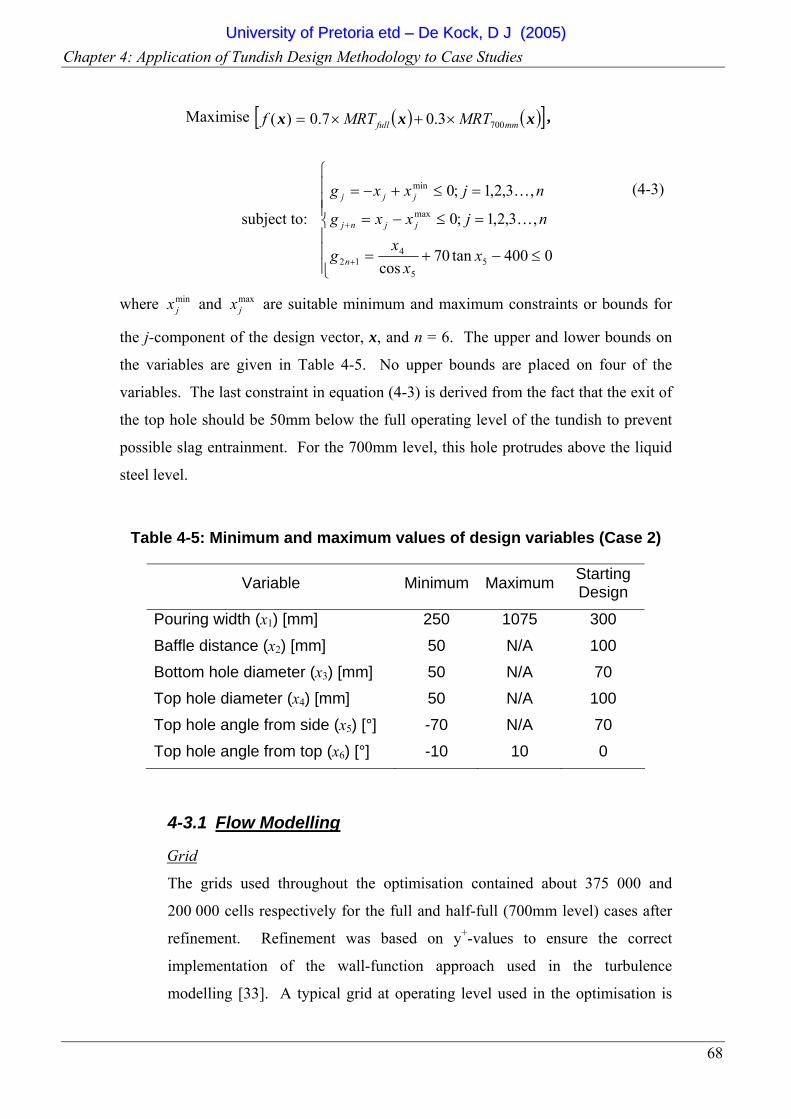
Chapter 4: Application of Tundish Design Methodology to Case Studies
68
Maximise ( ) ( )[ ]xxx mmfull MRTMRTf 7003.07.0)( ×+×= ,
subject to:
⎪⎪⎪
⎩
⎪⎪⎪
⎨
⎧
≤−+=
=≤−=
=≤+−=
+
+
0400tan70cos
,3,2,1;0
,3,2,1;0
55
412
max
min
xx
xg
njxxg
njxxg
n
jjnj
jjj
K
K
(4-3)
where minjx and max
jx are suitable minimum and maximum constraints or bounds for
the j-component of the design vector, x, and n = 6. The upper and lower bounds on
the variables are given in Table 4-5. No upper bounds are placed on four of the
variables. The last constraint in equation (4-3) is derived from the fact that the exit of
the top hole should be 50mm below the full operating level of the tundish to prevent
possible slag entrainment. For the 700mm level, this hole protrudes above the liquid
steel level.
Table 4-5: Minimum and maximum values of design variables (Case 2)
Variable Minimum Maximum Starting Design
Pouring width (x1) [mm] 250 1075 300 Baffle distance (x2) [mm] 50 N/A 100 Bottom hole diameter (x3) [mm] 50 N/A 70 Top hole diameter (x4) [mm] 50 N/A 100 Top hole angle from side (x5) [°] -70 N/A 70 Top hole angle from top (x6) [°] -10 10 0
4-3.1 Flow Modelling
Grid
The grids used throughout the optimisation contained about 375 000 and
200 000 cells respectively for the full and half-full (700mm level) cases after
refinement. Refinement was based on y+-values to ensure the correct
implementation of the wall-function approach used in the turbulence
modelling [33]. A typical grid at operating level used in the optimisation is
UUnniivveerrssiittyy ooff PPrreettoorriiaa eettdd –– DDee KKoocckk,, DD JJ ((22000055))
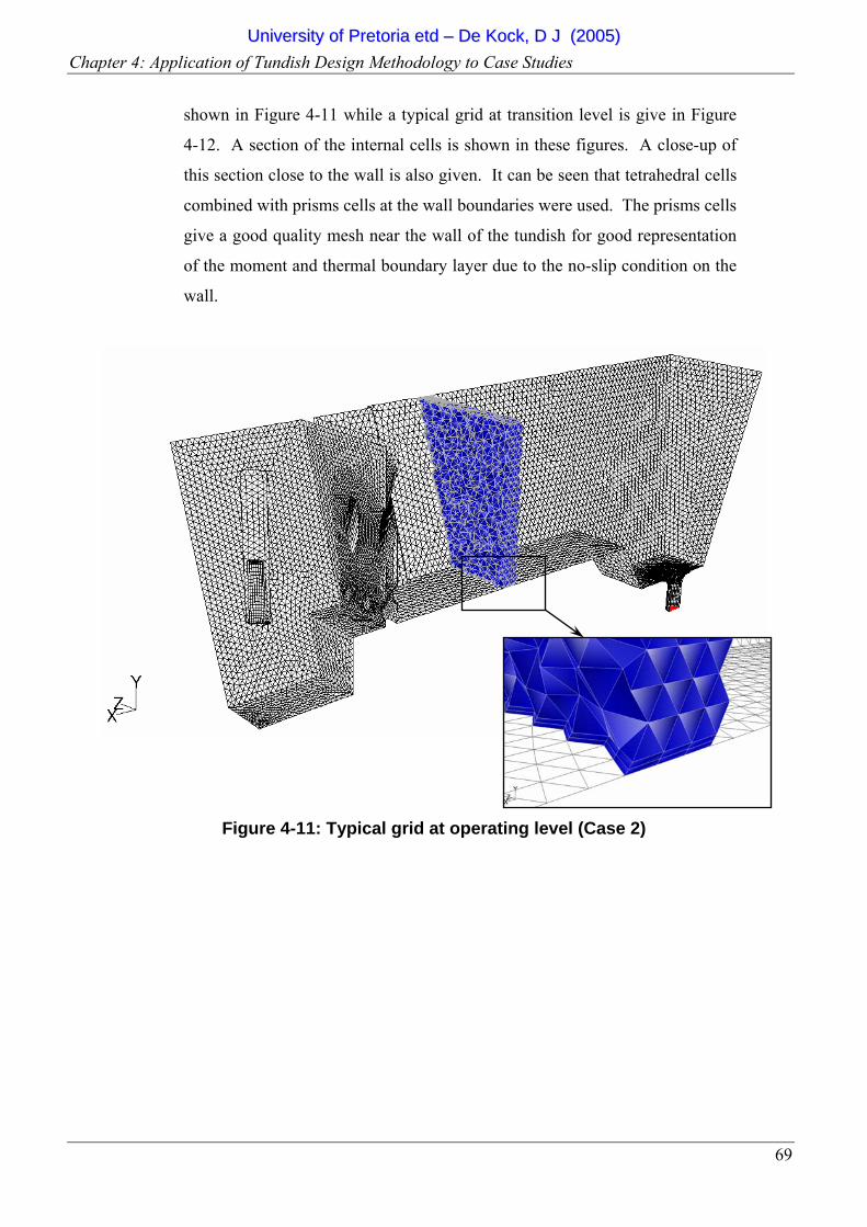
Chapter 4: Application of Tundish Design Methodology to Case Studies
69
shown in Figure 4-11 while a typical grid at transition level is give in Figure
4-12. A section of the internal cells is shown in these figures. A close-up of
this section close to the wall is also given. It can be seen that tetrahedral cells
combined with prisms cells at the wall boundaries were used. The prisms cells
give a good quality mesh near the wall of the tundish for good representation
of the moment and thermal boundary layer due to the no-slip condition on the
wall.
Figure 4-11: Typical grid at operating level (Case 2)
UUnniivveerrssiittyy ooff PPrreettoorriiaa eettdd –– DDee KKoocckk,, DD JJ ((22000055))
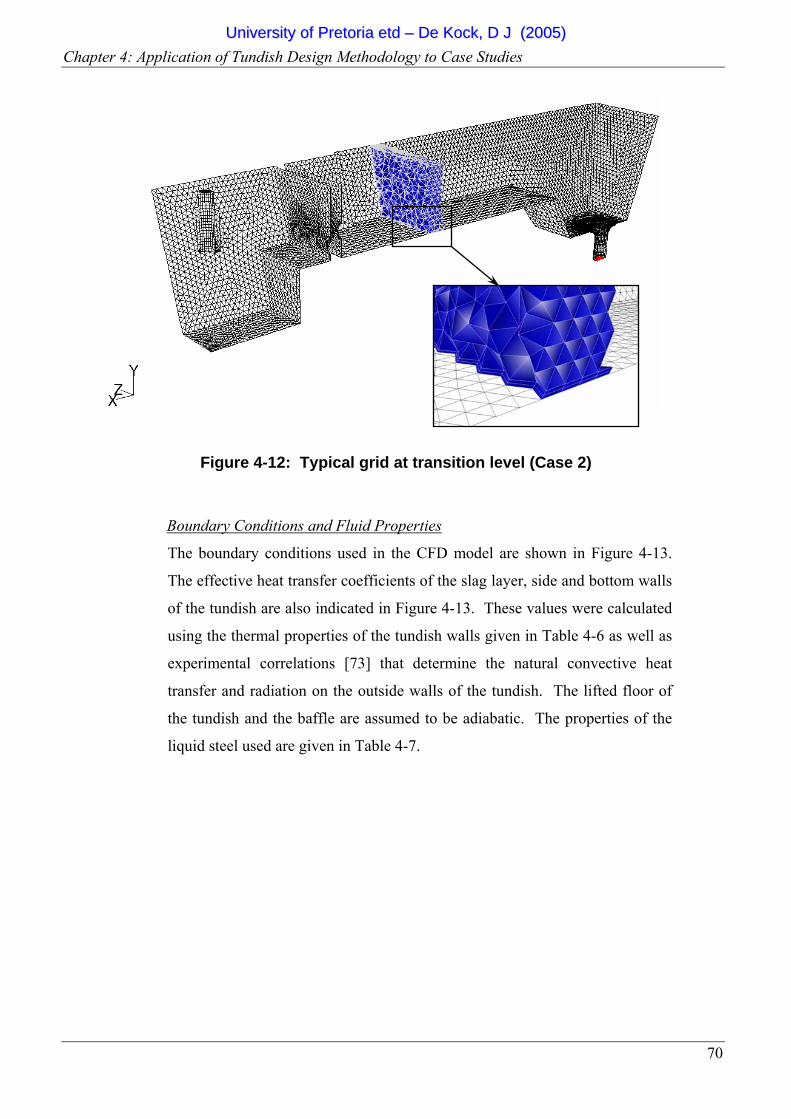
Chapter 4: Application of Tundish Design Methodology to Case Studies
70
Figure 4-12: Typical grid at transition level (Case 2)
Boundary Conditions and Fluid Properties
The boundary conditions used in the CFD model are shown in Figure 4-13.
The effective heat transfer coefficients of the slag layer, side and bottom walls
of the tundish are also indicated in Figure 4-13. These values were calculated
using the thermal properties of the tundish walls given in Table 4-6 as well as
experimental correlations [73] that determine the natural convective heat
transfer and radiation on the outside walls of the tundish. The lifted floor of
the tundish and the baffle are assumed to be adiabatic. The properties of the
liquid steel used are given in Table 4-7.
UUnniivveerrssiittyy ooff PPrreettoorriiaa eettdd –– DDee KKoocckk,, DD JJ ((22000055))
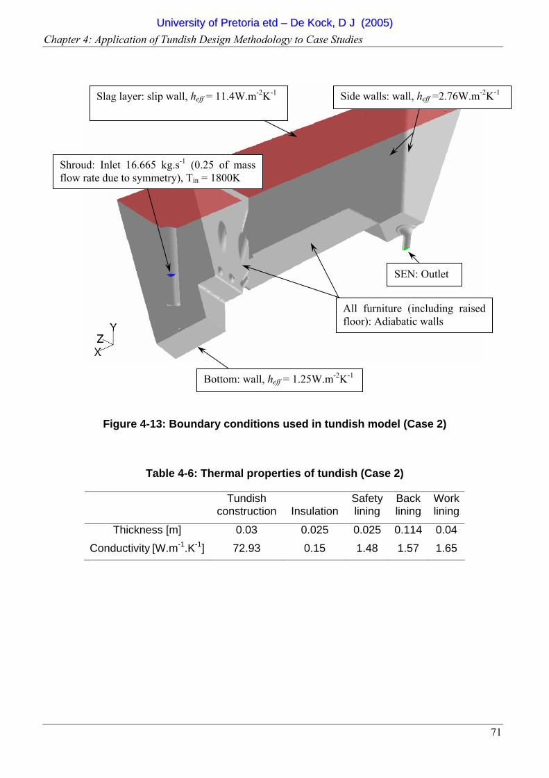
Chapter 4: Application of Tundish Design Methodology to Case Studies
71
Figure 4-13: Boundary conditions used in tundish model (Case 2)
Table 4-6: Thermal properties of tundish (Case 2)
Tundish
construction Insulation Safety lining
Back lining
Work lining
Thickness [m] 0.03 0.025 0.025 0.114 0.04 Conductivity [W.m-1.K-1] 72.93 0.15 1.48 1.57 1.65
Slag layer: slip wall, heff = 11.4W.m-2K-1
Shroud: Inlet 16.665 kg.s-1 (0.25 of mass flow rate due to symmetry), Tin = 1800K
SEN: Outlet
Side walls: wall, heff =2.76W.m-2K-1
All furniture (including raised floor): Adiabatic walls
Bottom: wall, heff = 1.25W.m-2K-1
UUnniivveerrssiittyy ooff PPrreettoorriiaa eettdd –– DDee KKoocckk,, DD JJ ((22000055))
Chapter 4: Application of Tundish Design Methodology to Case Studies
72
Table 4-7: Properties of liquid steel (Case 2)
Property Value
Thermal expansion coefficient [K-1] 1.1970×10⁻⁴ Reference density [kg.m-3] 7026.8 Reference temperature [K] 1800 Specific heat coefficient of steel [J.kg-1.K-1] 822 Conductivity of liquid steel [W.m-1.K-1] 52.535
Dynamic viscosity of steel [Pa.s] 5.3×10⁻³
Solver
For the simulations presented in this study, the Reynolds-Averaged Navier-
Stokes equations are solved using the segregated solver available in FLUENT.
The standard k-ε turbulence model is used to provide turbulent closure.
Second-order discretisation is used for all the flow equations while a three-
order drop in the sum of the scaled residuals was considered to constitute a
converged solution.
4-3.2 Flow Simulation Results
Typical results obtained from the CFD simulations are given in this section.
The starting design RTD curves for the operating level and transition level are
given in Figure 4-14 and Figure 4-15 respectively. The spikes in the RTD
curve are indicative of possible short-circuiting in the tundish. The RTD data
for the starting design for the operating level and transition level are given in
Table 4-8.
UUnniivveerrssiittyy ooff PPrreettoorriiaa eettdd –– DDee KKoocckk,, DD JJ ((22000055))

Chapter 4: Application of Tundish Design Methodology to Case Studies
73
Figure 4-14: RTD obtained from CFD simulation for starting design at
operating level ( ( )T0,70,100,70,100,300=x and MRT=0.189) (Case 2)
Figure 4-15: RTD obtained from CFD simulation for starting design at
transition level ( ( )T0,70,100,70,100,300=x and MRT=0.283) (Case 2)
0.00
0.10
0.20
0.30
0.40
0.50
0.60
0.70
0 0.5 1 1.5 2 2.5 3
Normalised Time
C C
urve
0.00
0.10
0.20
0.30
0.40
0.50
0.60
0.70
0 0.5 1 1.5 2 2.5 3
Normalised Time
C C
urve
UUnniivveerrssiittyy ooff PPrreettoorriiaa eettdd –– DDee KKoocckk,, DD JJ ((22000055))

Chapter 4: Application of Tundish Design Methodology to Case Studies
74
Table 4-8: RTD data for starting design ( ( )T0,70,100,70,100,300=x )(Case 2)
Full 700mm Level
Dispersed Plug Flow [%]
Dead Volume [%]
Mixed Volume [%]
MRT (non-dimensionalised)
PRT (non-dimensionalised)
AMRT (non-dimensionalised)
21.2
23.2
55.7
0.189
0.234
0.768
34.2
19.9
46.0
0.283
0.400
0.801
Path lines for the starting design are given in Figure 4-16 for the full operating
level. Figure 4-16 shows that the tundish flow exhibits a large recirculation
zone behind the baffle. Temperature contours for the operating level are given
in Figure 4-17. As expected, the steel is the hottest in the pouring box region,
with the coolest regimes being in the cornets above the tundish outlet. The hot
jet of steel that is caused by the baffle holes can also be clearly seen in Figure
4-17.
Figure 4-16: Path lines coloured by velocity magnitude [m.s-1] from CFD simulation at full operating level for starting design
( ( )T0,70,100,70,100,300=x ) (Case 2)
UUnniivveerrssiittyy ooff PPrreettoorriiaa eettdd –– DDee KKoocckk,, DD JJ ((22000055))
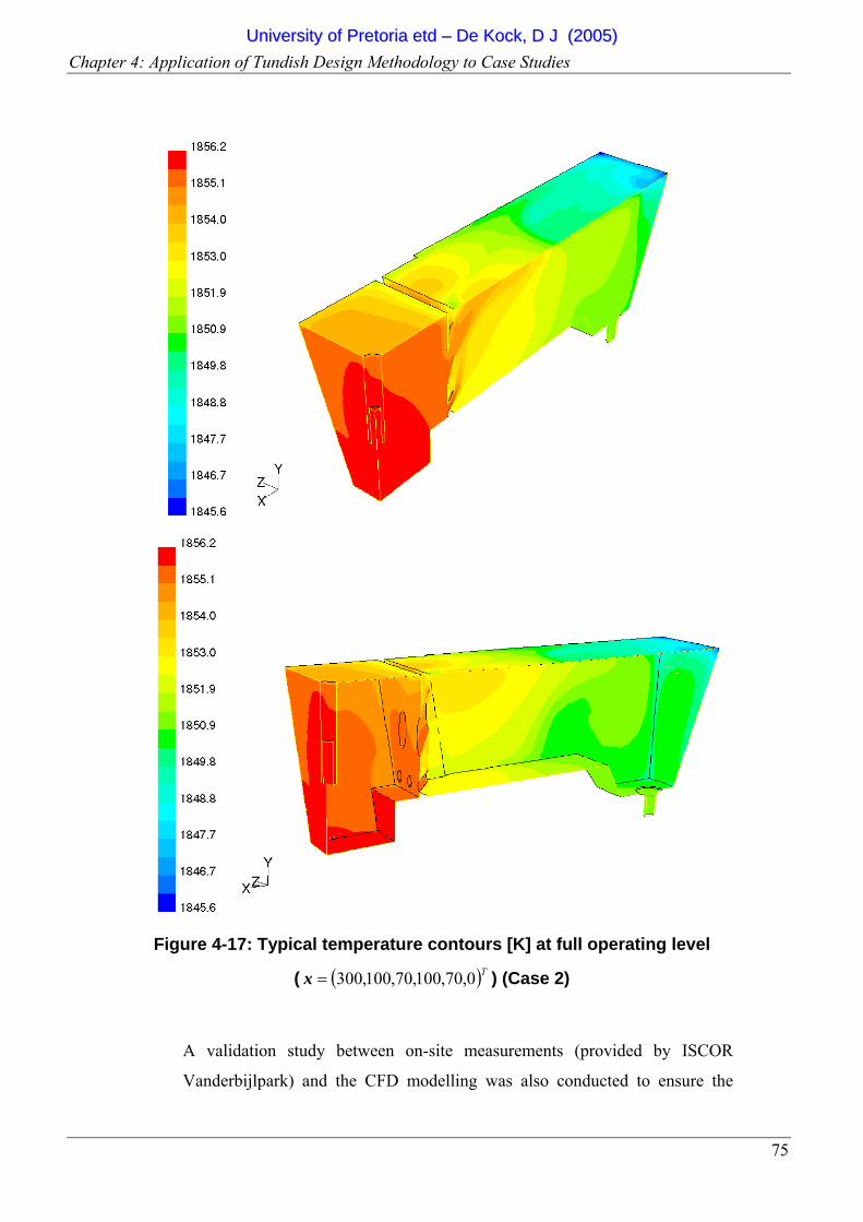
Chapter 4: Application of Tundish Design Methodology to Case Studies
75
Figure 4-17: Typical temperature contours [K] at full operating level
( ( )T0,70,100,70,100,300=x ) (Case 2)
A validation study between on-site measurements (provided by ISCOR
Vanderbijlpark) and the CFD modelling was also conducted to ensure the
UUnniivveerrssiittyy ooff PPrreettoorriiaa eettdd –– DDee KKoocckk,, DD JJ ((22000055))

Chapter 4: Application of Tundish Design Methodology to Case Studies
76
validity of the CFD model. The results from this study are given in
Appendix B.
4-3.3 Optimisation Results (DYNAMIC-Q)
The results of the optimisation run obtained using the DYNAMIC-Q algorithm
are given and discussed in this section. Figure 4-18 shows the optimisation
history of the objective function as well as the MRT for operating level and at
700mm level. It can be seen that the objective function essentially levels out
after 4 design iterations showing that the objective function has converged.
The MRT for the operating level increased from 0.18 to 0.43 which represents
an increase of 138%, while the MRT for the 700mm level increased from 0.29
to 0.31 which is an increase of 6.9%. The weighted combination of these two
values (the objective function) can be seen to be dominated by the full
operating level value. This relative insensitivity of the transition level MRT
with respect to the design variables, is partly due to the fact that only 3 of the 6
variables influence the performance at the lower level, due to the fact that the
upper hole in the baffle protrudes above the liquid steel at this level.
UUnniivveerrssiittyy ooff PPrreettoorriiaa eettdd –– DDee KKoocckk,, DD JJ ((22000055))
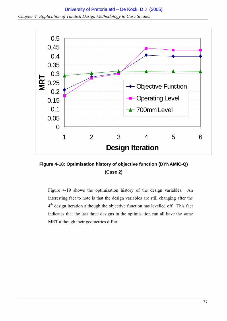
Chapter 4: Application of Tundish Design Methodology to Case Studies
77
Figure 4-18: Optimisation history of objective function (DYNAMIC-Q) (Case 2)
Figure 4-19 shows the optimisation history of the design variables. An
interesting fact to note is that the design variables are still changing after the
4th design iteration although the objective function has levelled off. This fact
indicates that the last three designs in the optimisation run all have the same
MRT although their geometries differ.
00.050.1
0.150.2
0.250.3
0.350.4
0.450.5
1 2 3 4 5 6Design Iteration
MR
T
Objective Function
Operating Level
700mm Level
UUnniivveerrssiittyy ooff PPrreettoorriiaa eettdd –– DDee KKoocckk,, DD JJ ((22000055))
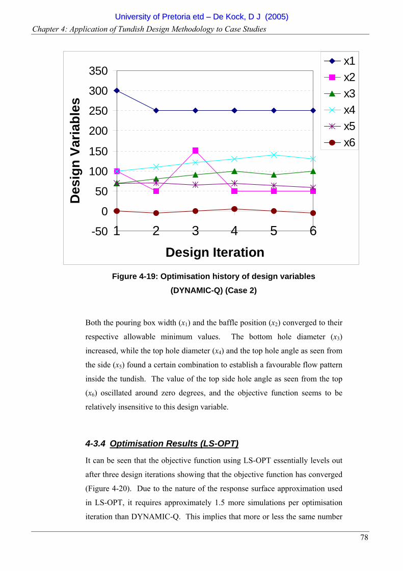
Chapter 4: Application of Tundish Design Methodology to Case Studies
78
Figure 4-19: Optimisation history of design variables
(DYNAMIC-Q) (Case 2)
Both the pouring box width (x1) and the baffle position (x2) converged to their
respective allowable minimum values. The bottom hole diameter (x3)
increased, while the top hole diameter (x4) and the top hole angle as seen from
the side (x5) found a certain combination to establish a favourable flow pattern
inside the tundish. The value of the top side hole angle as seen from the top
(x6) oscillated around zero degrees, and the objective function seems to be
relatively insensitive to this design variable.
4-3.4 Optimisation Results (LS-OPT)
It can be seen that the objective function using LS-OPT essentially levels out
after three design iterations showing that the objective function has converged
(Figure 4-20). Due to the nature of the response surface approximation used
in LS-OPT, it requires approximately 1.5 more simulations per optimisation
iteration than DYNAMIC-Q. This implies that more or less the same number
-50
0
50
100
150
200
250
300
350
1 2 3 4 5 6Design Iteration
Des
ign
Varia
bles
x1x2x3x4x5x6
UUnniivveerrssiittyy ooff PPrreettoorriiaa eettdd –– DDee KKoocckk,, DD JJ ((22000055))

Chapter 4: Application of Tundish Design Methodology to Case Studies
79
of function evaluations (or CFD simulations) was performed for both
DYNAMIC-Q and LS-OPT to achieve their respective optima.
Figure 4-20: Optimisation history of objective function (LS-OPT) (Case 2)
The MRT for the operating level increased from 0.18 to 0.48, which represents
an increase of 167%, while the MRT for the 700mm level again proved
insensitive to the design changes. When using LS-OPT, x3, x4 and x5 converge
to different values, while x1 and x2 again reached their respective minimum
values (Figure 4-21).
00.05
0.10.15
0.20.25
0.30.35
0.40.45
0.5
1 2 3 4 5 6Design Iteration
MR
T
Objective Function
Operating Level
700mm Level
UUnniivveerrssiittyy ooff PPrreettoorriiaa eettdd –– DDee KKoocckk,, DD JJ ((22000055))
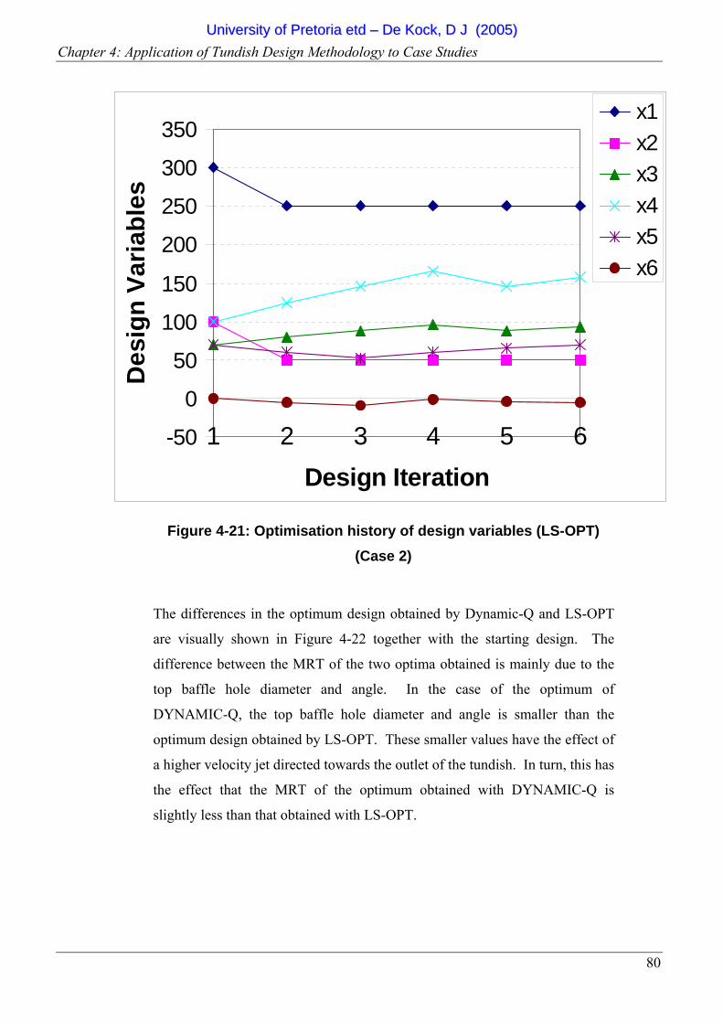
Chapter 4: Application of Tundish Design Methodology to Case Studies
80
Figure 4-21: Optimisation history of design variables (LS-OPT) (Case 2)
The differences in the optimum design obtained by Dynamic-Q and LS-OPT
are visually shown in Figure 4-22 together with the starting design. The
difference between the MRT of the two optima obtained is mainly due to the
top baffle hole diameter and angle. In the case of the optimum of
DYNAMIC-Q, the top baffle hole diameter and angle is smaller than the
optimum design obtained by LS-OPT. These smaller values have the effect of
a higher velocity jet directed towards the outlet of the tundish. In turn, this has
the effect that the MRT of the optimum obtained with DYNAMIC-Q is
slightly less than that obtained with LS-OPT.
-50
0
50
100
150
200
250
300
350
1 2 3 4 5 6Design Iteration
Des
ign
Varia
bles
x1x2x3x4x5x6
UUnniivveerrssiittyy ooff PPrreettoorriiaa eettdd –– DDee KKoocckk,, DD JJ ((22000055))
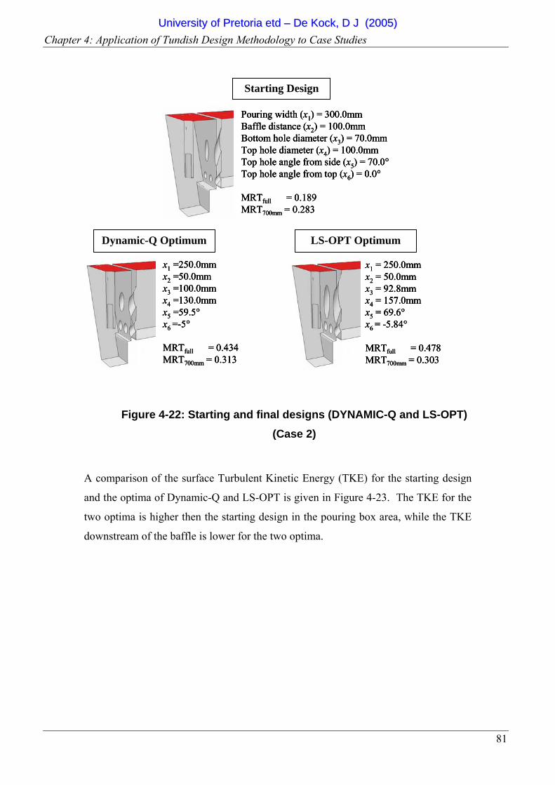
Chapter 4: Application of Tundish Design Methodology to Case Studies
81
Pouring width (x1) = 300.0mmBaffle distance (x2) = 100.0mmBottom hole diameter (x3) = 70.0mmTop hole diameter (x4) = 100.0mmTop hole angle from side (x5) = 70.0°Top hole angle from top (x6) = 0.0°
MRTfull = 0.189MRT700mm = 0.283
Pouring width (x1) = 300.0mmBaffle distance (x2) = 100.0mmBottom hole diameter (x3) = 70.0mmTop hole diameter (x4) = 100.0mmTop hole angle from side (x5) = 70.0°Top hole angle from top (x6) = 0.0°
MRTfull = 0.189MRT700mm = 0.283
Pouring width (x1) = 300.0mmBaffle distance (x2) = 100.0mmBottom hole diameter (x3) = 70.0mmTop hole diameter (x4) = 100.0mmTop hole angle from side (x5) = 70.0°Top hole angle from top (x6) = 0.0°
MRTfull = 0.189MRT700mm = 0.283
x1 =250.0mmx2 =50.0mmx3 =100.0mmx4 =130.0mmx5 =59.5°x6 =-5°
MRTfull = 0.434MRT700mm = 0.313
x1 =250.0mmx2 =50.0mmx3 =100.0mmx4 =130.0mmx5 =59.5°x6 =-5°
MRTfull = 0.434MRT700mm = 0.313
x1 =250.0mmx2 =50.0mmx3 =100.0mmx4 =130.0mmx5 =59.5°x6 =-5°
MRTfull = 0.434MRT700mm = 0.313
x1 = 250.0mmx2 = 50.0mmx3 = 92.8mmx4 = 157.0mmx5 = 69.6°x6 = -5.84°
MRTfull = 0.478MRT700mm = 0.303
x1 = 250.0mmx2 = 50.0mmx3 = 92.8mmx4 = 157.0mmx5 = 69.6°x6 = -5.84°
MRTfull = 0.478MRT700mm = 0.303
x1 = 250.0mmx2 = 50.0mmx3 = 92.8mmx4 = 157.0mmx5 = 69.6°x6 = -5.84°
MRTfull = 0.478MRT700mm = 0.303
Figure 4-22: Starting and final designs (DYNAMIC-Q and LS-OPT) (Case 2)
A comparison of the surface Turbulent Kinetic Energy (TKE) for the starting design
and the optima of Dynamic-Q and LS-OPT is given in Figure 4-23. The TKE for the
two optima is higher then the starting design in the pouring box area, while the TKE
downstream of the baffle is lower for the two optima.
Starting Design
Dynamic-Q Optimum LS-OPT Optimum
UUnniivveerrssiittyy ooff PPrreettoorriiaa eettdd –– DDee KKoocckk,, DD JJ ((22000055))
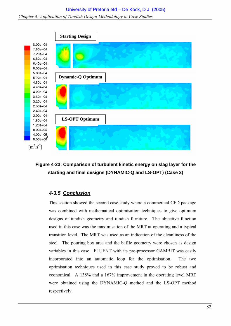
Chapter 4: Application of Tundish Design Methodology to Case Studies
82
Figure 4-23: Comparison of turbulent kinetic energy on slag layer for the starting and final designs (DYNAMIC-Q and LS-OPT) (Case 2)
4-3.5 Conclusion
This section showed the second case study where a commercial CFD package
was combined with mathematical optimisation techniques to give optimum
designs of tundish geometry and tundish furniture. The objective function
used in this case was the maximisation of the MRT at operating and a typical
transition level. The MRT was used as an indication of the cleanliness of the
steel. The pouring box area and the baffle geometry were chosen as design
variables in this case. FLUENT with its pre-processor GAMBIT was easily
incorporated into an automatic loop for the optimisation. The two
optimisation techniques used in this case study proved to be robust and
economical. A 138% and a 167% improvement in the operating level MRT
were obtained using the DYNAMIC-Q method and the LS-OPT method
respectively.
Starting Design
Dynamic-Q Optimum
LS-OPT Optimum
[m2.s-2]
UUnniivveerrssiittyy ooff PPrreettoorriiaa eettdd –– DDee KKoocckk,, DD JJ ((22000055))

Chapter 4: Application of Tundish Design Methodology to Case Studies
83
4-4 CASE STUDY 3: IMPACT PAD OPTIMISATION The third case study is on a new impact pad design. Impact pads in tundishes have as
their aim the reduction in the turbulence levels in the tundish. For this specific impact
pad, the aim was to reduce the free-surface turbulence levels [74]. The design of the
impact pad is also such that the flow is angled upwards toward the free-surface to
improve the inclusion removal of the tundish. The impact pad is designed to be used
in the single-strand stainless steel continuous caster in operation at the Middelburg
plant of Columbus Stainless. This is the same tundish used in the first case study.
4-4.1 Parameterisation of Geometry
The impact pad geometry is shown Figure 4-24. The characteristics of the
impact pad implies that it resorts under the Turbostop® [75] patent. The aim
of the pad is to suppress turbulence through the creation of a recirculation
zone within the pad through two overhead wings. As can be seen from the
location of the impact pad in the tundish in Figure 4-25, the jet emanating
from the shroud would impact the pad and then bend over on itself to flow
towards the outlet. The pad has to suppress the turbulence of the jet so that it
does not reach the surface above the pad with sufficient energy that could
entrain slag. The lip on the pad has the function of angling the flow in the
pouring box area upwards, much as a baffle with angled holes would do.
In order to optimise the impact pad, its geometry needs to be parameterised.
The parameters chosen are shown in Figure 4-24. Initially, eight variables
were chosen of which the values of two were fixed to the values shown in the
figure. The value of w1 is assumed to be the full width of the tundish (refer
Figure 4-25), while the value of w2 is such that the gap between the wings
accommodates the possible motion of and uncertainty of the shroud position
during casting. The three curvatures (d1 through d3) are parameterised as
control points of Nonuniform Rational B-Splines (NURBS) used to define the
geometry. A GAMBIT journal file that creates the impact pad given the of
design variables and parameters is given in Appendix D.
UUnniivveerrssiittyy ooff PPrreettoorriiaa eettdd –– DDee KKoocckk,, DD JJ ((22000055))
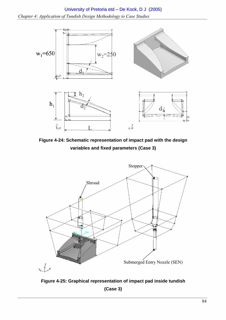
Chapter 4: Application of Tundish Design Methodology to Case Studies
84
L
w2=250
d1
h2
d2 d3h1
w1=650
L
w2=250
d1
h2
d2 d3h1
w1=650
L
w2=250
d1
h2
d2 d3h1
w1=650
Figure 4-24: Schematic representation of impact pad with the design variables and fixed parameters (Case 3)
Figure 4-25: Graphical representation of impact pad inside tundish (Case 3)
Shroud
Stopper
Submerged Entry Nozzle (SEN)
UUnniivveerrssiittyy ooff PPrreettoorriiaa eettdd –– DDee KKoocckk,, DD JJ ((22000055))
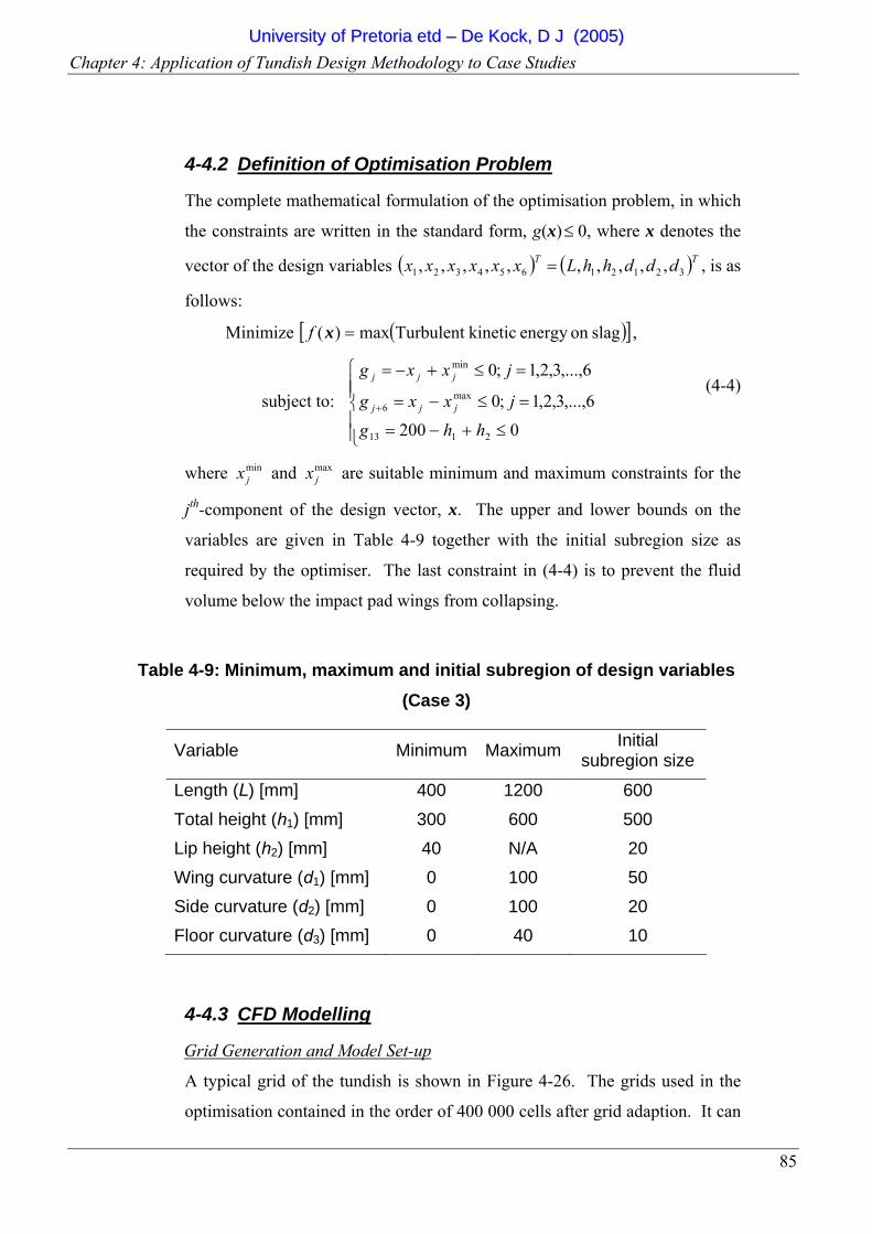
Chapter 4: Application of Tundish Design Methodology to Case Studies
85
4-4.2 Definition of Optimisation Problem
The complete mathematical formulation of the optimisation problem, in which
the constraints are written in the standard form, g(x) ≤ 0, where x denotes the
vector of the design variables ( ) ( )TT dddhhLxxxxxx 32121654321 ,,,,,,,,,, = , is as
follows:
Minimize ( )[ ]slagon energy kineticTurbulent max)( =xf ,
subject to:
⎪⎪⎩
⎪⎪⎨
⎧
≤+−=
=≤−=
=≤+−=
+
02006,...,3,2,1;0
6,...,3,2,1;0
2113
max6
min
hhgjxxg
jxxg
jjj
jjj
(4-4)
where minjx and max
jx are suitable minimum and maximum constraints for the
jth-component of the design vector, x. The upper and lower bounds on the
variables are given in Table 4-9 together with the initial subregion size as
required by the optimiser. The last constraint in (4-4) is to prevent the fluid
volume below the impact pad wings from collapsing.
Table 4-9: Minimum, maximum and initial subregion of design variables (Case 3)
Variable Minimum Maximum Initial subregion size
Length (L) [mm] 400 1200 600 Total height (h1) [mm] 300 600 500 Lip height (h2) [mm] 40 N/A 20 Wing curvature (d1) [mm] 0 100 50 Side curvature (d2) [mm] 0 100 20 Floor curvature (d3) [mm] 0 40 10
4-4.3 CFD Modelling
Grid Generation and Model Set-up
A typical grid of the tundish is shown in Figure 4-26. The grids used in the
optimisation contained in the order of 400 000 cells after grid adaption. It can
UUnniivveerrssiittyy ooff PPrreettoorriiaa eettdd –– DDee KKoocckk,, DD JJ ((22000055))
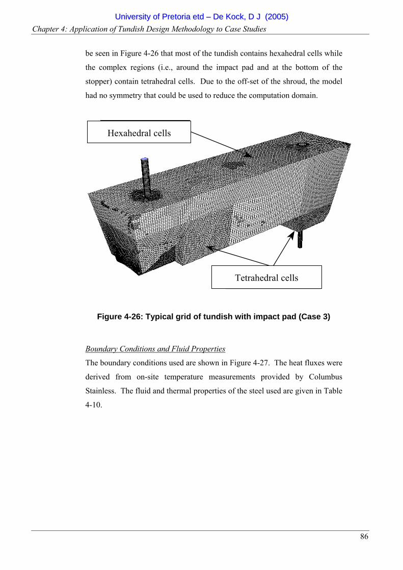
Chapter 4: Application of Tundish Design Methodology to Case Studies
86
be seen in Figure 4-26 that most of the tundish contains hexahedral cells while
the complex regions (i.e., around the impact pad and at the bottom of the
stopper) contain tetrahedral cells. Due to the off-set of the shroud, the model
had no symmetry that could be used to reduce the computation domain.
Hexahedron cells
Tetrahedron cells
Figure 4-26: Typical grid of tundish with impact pad (Case 3)
Boundary Conditions and Fluid Properties
The boundary conditions used are shown in Figure 4-27. The heat fluxes were
derived from on-site temperature measurements provided by Columbus
Stainless. The fluid and thermal properties of the steel used are given in Table
4-10.
Tetrahedral cells
Hexahedral cells
UUnniivveerrssiittyy ooff PPrreettoorriiaa eettdd –– DDee KKoocckk,, DD JJ ((22000055))
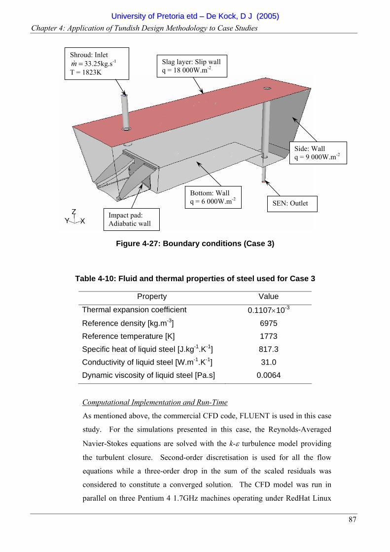
Chapter 4: Application of Tundish Design Methodology to Case Studies
87
Figure 4-27: Boundary conditions (Case 3)
Table 4-10: Fluid and thermal properties of steel used for Case 3
Property Value
Thermal expansion coefficient 0.1107×10⁻³
Reference density [kg.m-3] 6975 Reference temperature [K] 1773 Specific heat of liquid steel [J.kg-1.K-1] 817.3 Conductivity of liquid steel [W.m-1.K-1] 31.0 Dynamic viscosity of liquid steel [Pa.s] 0.0064
Computational Implementation and Run-Time
As mentioned above, the commercial CFD code, FLUENT is used in this case
study. For the simulations presented in this case, the Reynolds-Averaged
Navier-Stokes equations are solved with the k-ε turbulence model providing
the turbulent closure. Second-order discretisation is used for all the flow
equations while a three-order drop in the sum of the scaled residuals was
considered to constitute a converged solution. The CFD model was run in
parallel on three Pentium 4 1.7GHz machines operating under RedHat Linux
Shroud: Inlet =m& 33.25kg.s-1
T = 1823K Slag layer: Slip wall q = 18 000W.m-2
Bottom: Wall q = 6 000W.m-2
Side: Wall q = 9 000W.m-2
SEN: Outlet
Impact pad: Adiabatic wall
UUnniivveerrssiittyy ooff PPrreettoorriiaa eettdd –– DDee KKoocckk,, DD JJ ((22000055))
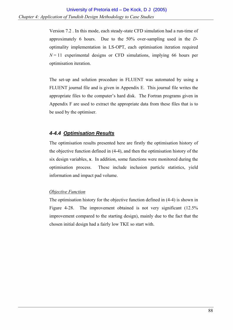
Chapter 4: Application of Tundish Design Methodology to Case Studies
88
Version 7.2 . In this mode, each steady-state CFD simulation had a run-time of
approximately 6 hours. Due to the 50% over-sampling used in the D-
optimality implementation in LS-OPT, each optimisation iteration required
N = 11 experimental designs or CFD simulations, implying 66 hours per
optimisation iteration.
The set-up and solution procedure in FLUENT was automated by using a
FLUENT journal file and is given in Appendix E. This journal file writes the
appropriate files to the computer’s hard disk. The Fortran programs given in
Appendix F are used to extract the appropriate data from these files that is to
be used by the optimiser.
4-4.4 Optimisation Results
The optimisation results presented here are firstly the optimisation history of
the objective function defined in (4-4), and then the optimisation history of the
six design variables, x. In addition, some functions were monitored during the
optimisation process. These include inclusion particle statistics, yield
information and impact pad volume.
Objective Function
The optimisation history for the objective function defined in (4-4) is shown in
Figure 4-28. The improvement obtained is not very significant (12.5%
improvement compared to the starting design), mainly due to the fact that the
chosen initial design had a fairly low TKE so start with.
UUnniivveerrssiittyy ooff PPrreettoorriiaa eettdd –– DDee KKoocckk,, DD JJ ((22000055))
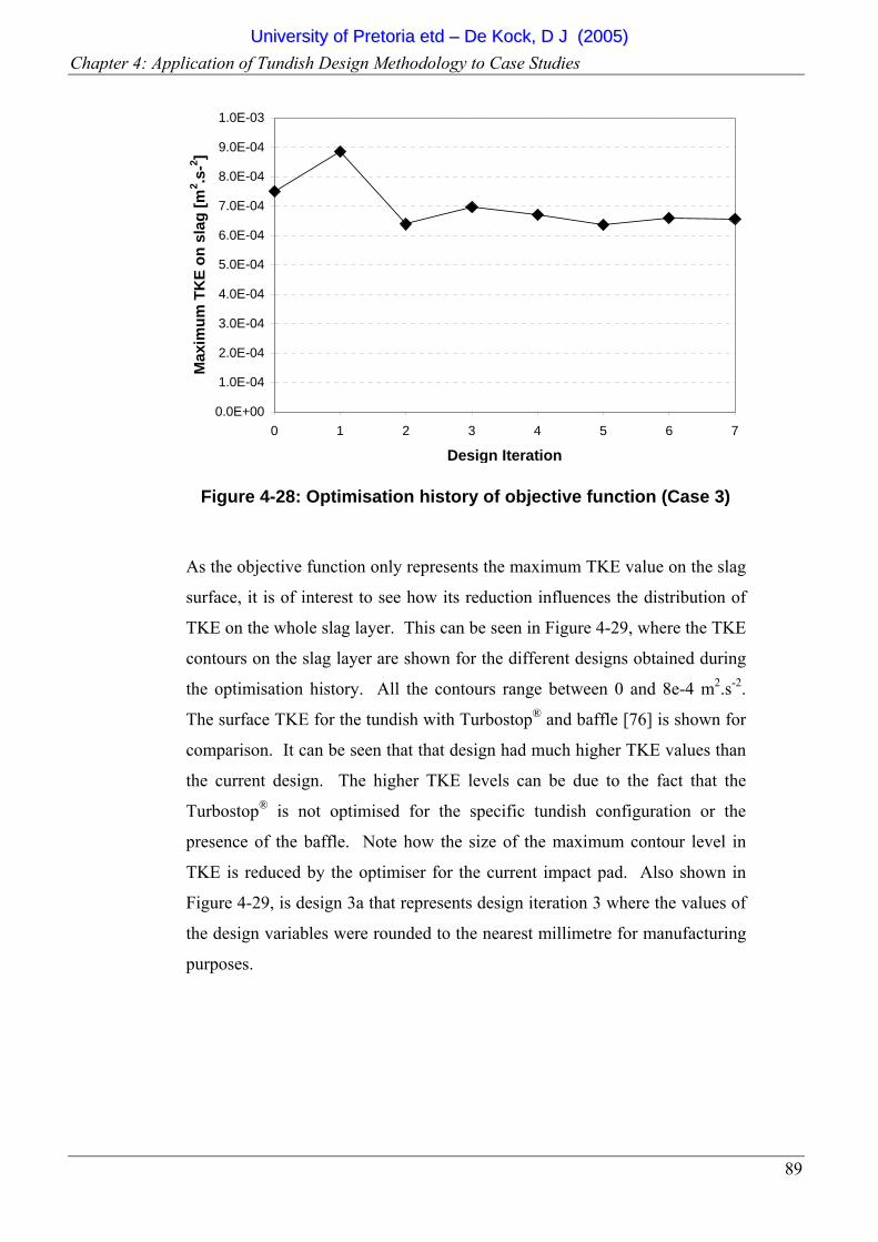
Chapter 4: Application of Tundish Design Methodology to Case Studies
89
0.0E+00
1.0E-04
2.0E-04
3.0E-04
4.0E-04
5.0E-04
6.0E-04
7.0E-04
8.0E-04
9.0E-04
1.0E-03
0 1 2 3 4 5 6 7
Design Iteration
Max
imum
TK
E on
sla
g [m
2 .s-2 ]
Figure 4-28: Optimisation history of objective function (Case 3)
As the objective function only represents the maximum TKE value on the slag
surface, it is of interest to see how its reduction influences the distribution of
TKE on the whole slag layer. This can be seen in Figure 4-29, where the TKE
contours on the slag layer are shown for the different designs obtained during
the optimisation history. All the contours range between 0 and 8e-4 m2.s-2.
The surface TKE for the tundish with Turbostop® and baffle [76] is shown for
comparison. It can be seen that that design had much higher TKE values than
the current design. The higher TKE levels can be due to the fact that the
Turbostop® is not optimised for the specific tundish configuration or the
presence of the baffle. Note how the size of the maximum contour level in
TKE is reduced by the optimiser for the current impact pad. Also shown in
Figure 4-29, is design 3a that represents design iteration 3 where the values of
the design variables were rounded to the nearest millimetre for manufacturing
purposes.
UUnniivveerrssiittyy ooff PPrreettoorriiaa eettdd –– DDee KKoocckk,, DD JJ ((22000055))
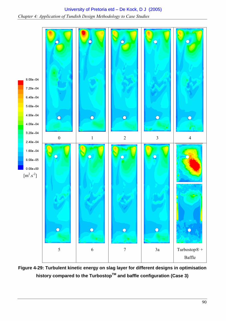
Chapter 4: Application of Tundish Design Methodology to Case Studies
90
0 1 2 3 4
5 6 7 3a Turbostop® +
Baffle
Figure 4-29: Turbulent kinetic energy on slag layer for different designs in optimisation history compared to the TurbostopTM and baffle configuration (Case 3)
[m2.s-2]
UUnniivveerrssiittyy ooff PPrreettoorriiaa eettdd –– DDee KKoocckk,, DD JJ ((22000055))
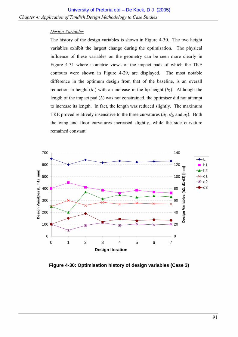
Chapter 4: Application of Tundish Design Methodology to Case Studies
91
Design Variables
The history of the design variables is shown in Figure 4-30. The two height
variables exhibit the largest change during the optimisation. The physical
influence of these variables on the geometry can be seen more clearly in
Figure 4-31 where isometric views of the impact pads of which the TKE
contours were shown in Figure 4-29, are displayed. The most notable
difference in the optimum design from that of the baseline, is an overall
reduction in height (h1) with an increase in the lip height (h2). Although the
length of the impact pad (L) was not constrained, the optimiser did not attempt
to increase its length. In fact, the length was reduced slightly. The maximum
TKE proved relatively insensitive to the three curvatures (d1, d2, and d3). Both
the wing and floor curvatures increased slightly, while the side curvature
remained constant.
0
100
200
300
400
500
600
700
0 1 2 3 4 5 6 7
Design Iteration
Des
ign
Varia
bles
(L, h
1) [m
m]
0
20
40
60
80
100
120
140
Des
ign
Varia
bles
(h2,
d1-
d3) [
mm
]
Lh1h2d1d2d3
Figure 4-30: Optimisation history of design variables (Case 3)
UUnniivveerrssiittyy ooff PPrreettoorriiaa eettdd –– DDee KKoocckk,, DD JJ ((22000055))
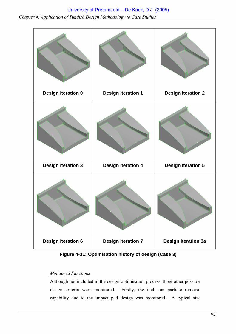
Chapter 4: Application of Tundish Design Methodology to Case Studies
92
Design Iteration 0 Design Iteration 1 Design Iteration 2
Design Iteration 3 Design Iteration 4 Design Iteration 5
Design Iteration 6 Design Iteration 7 Design Iteration 3a
Figure 4-31: Optimisation history of design (Case 3)
Monitored Functions
Although not included in the design optimisation process, three other possible
design criteria were monitored. Firstly, the inclusion particle removal
capability due to the impact pad design was monitored. A typical size
UUnniivveerrssiittyy ooff PPrreettoorriiaa eettdd –– DDee KKoocckk,, DD JJ ((22000055))
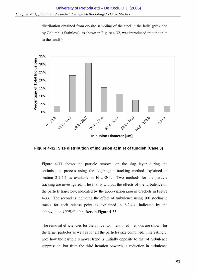
Chapter 4: Application of Tundish Design Methodology to Case Studies
93
distribution obtained from on-site sampling of the steel in the ladle (provided
by Columbus Stainless), as shown in Figure 4-32, was introduced into the inlet
to the tundish.
0%
5%
10%
15%
20%
25%
30%
35%
0 - 13
.8
13.8
- 19.2
19.2
- 26.7
26.7
- 37.4
37.4
- 52.9
52.9
- 74.8
74.8
- 108
.8
>105
.8
Inlcusion Diameter [µm]
Perc
enta
ge o
f Tot
al In
clus
ions
Figure 4-32: Size distribution of inclusion at inlet of tundish (Case 3)
Figure 4-33 shows the particle removal on the slag layer during the
optimisation process using the Lagrangian tracking method explained in
section 2-2.4.4 as available in FLUENT. Two methods for the particle
tracking are investigated. The first is without the effects of the turbulence on
the particle trajectory, indicated by the abbreviation Lam in brackets in Figure
4-33. The second is including the effect of turbulence using 100 stochastic
tracks for each release point as explained in 2-2.4.4, indicated by the
abbreviation 100RW in brackets in Figure 4-33.
The removal efficiencies for the above two mentioned methods are shown for
the larger particles as well as for all the particles size combined. Interestingly,
note how the particle removal trend is initially opposite to that of turbulence
suppression, but from the third iteration onwards, a reduction in turbulence
UUnniivveerrssiittyy ooff PPrreettoorriiaa eettdd –– DDee KKoocckk,, DD JJ ((22000055))
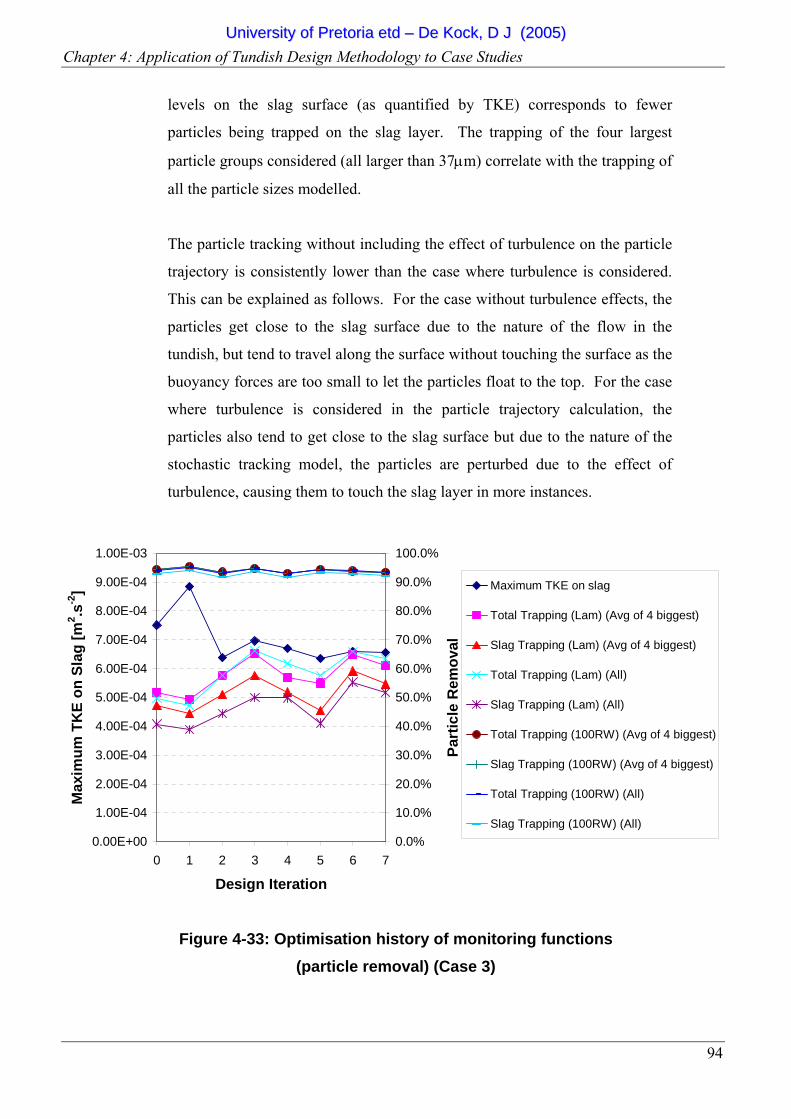
Chapter 4: Application of Tundish Design Methodology to Case Studies
94
levels on the slag surface (as quantified by TKE) corresponds to fewer
particles being trapped on the slag layer. The trapping of the four largest
particle groups considered (all larger than 37µm) correlate with the trapping of
all the particle sizes modelled.
The particle tracking without including the effect of turbulence on the particle
trajectory is consistently lower than the case where turbulence is considered.
This can be explained as follows. For the case without turbulence effects, the
particles get close to the slag surface due to the nature of the flow in the
tundish, but tend to travel along the surface without touching the surface as the
buoyancy forces are too small to let the particles float to the top. For the case
where turbulence is considered in the particle trajectory calculation, the
particles also tend to get close to the slag surface but due to the nature of the
stochastic tracking model, the particles are perturbed due to the effect of
turbulence, causing them to touch the slag layer in more instances.
0.00E+00
1.00E-04
2.00E-04
3.00E-04
4.00E-04
5.00E-04
6.00E-04
7.00E-04
8.00E-04
9.00E-04
1.00E-03
0 1 2 3 4 5 6 7
Design Iteration
Max
imum
TK
E on
Sla
g [m
2 .s-2
]
0.0%
10.0%
20.0%
30.0%
40.0%
50.0%
60.0%
70.0%
80.0%
90.0%
100.0%
Part
icle
Rem
oval
Maximum TKE on slag
Total Trapping (Lam) (Avg of 4 biggest)
Slag Trapping (Lam) (Avg of 4 biggest)
Total Trapping (Lam) (All)
Slag Trapping (Lam) (All)
Total Trapping (100RW) (Avg of 4 biggest)
Slag Trapping (100RW) (Avg of 4 biggest)
Total Trapping (100RW) (All)
Slag Trapping (100RW) (All)
Figure 4-33: Optimisation history of monitoring functions (particle removal) (Case 3)
UUnniivveerrssiittyy ooff PPrreettoorriiaa eettdd –– DDee KKoocckk,, DD JJ ((22000055))
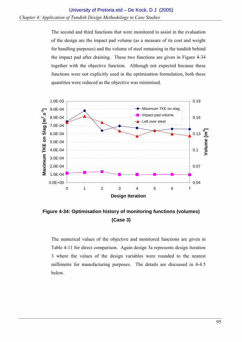
Chapter 4: Application of Tundish Design Methodology to Case Studies
95
The second and third functions that were monitored to assist in the evaluation
of the design are the impact pad volume (as a measure of its cost and weight
for handling purposes) and the volume of steel remaining in the tundish behind
the impact pad after draining. These two functions are given in Figure 4-34
together with the objective function. Although not expected because these
functions were not explicitly used in the optimisation formulation, both these
quantities were reduced as the objective was minimised.
0.0E+00
1.0E-04
2.0E-04
3.0E-04
4.0E-04
5.0E-04
6.0E-04
7.0E-04
8.0E-04
9.0E-04
1.0E-03
0 1 2 3 4 5 6 7
Design Iteration
Max
imum
TK
E on
Sla
g [m
2 .s-2
]
0.04
0.07
0.1
0.13
0.16
0.19
Volu
me
[m3 ]
Maximum TKE on slag
Impact pad volume
Left over steel
Figure 4-34: Optimisation history of monitoring functions (volumes) (Case 3)
The numerical values of the objective and monitored functions are given in
Table 4-11 for direct comparison. Again design 3a represents design iteration
3 where the values of the design variables were rounded to the nearest
millimetre for manufacturing purposes. The details are discussed in 4-4.5
below.
UUnniivveerrssiittyy ooff PPrreettoorriiaa eettdd –– DDee KKoocckk,, DD JJ ((22000055))
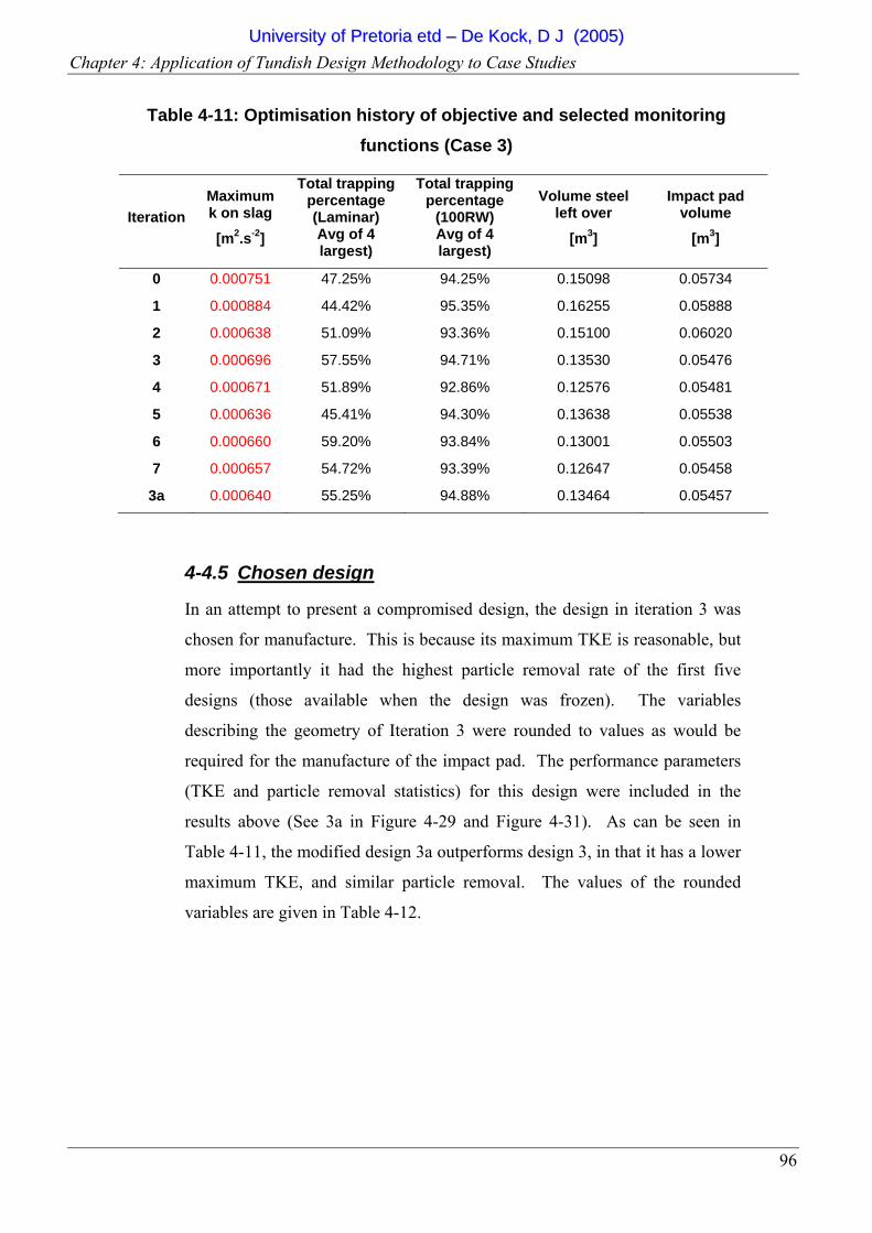
Chapter 4: Application of Tundish Design Methodology to Case Studies
96
Table 4-11: Optimisation history of objective and selected monitoring functions (Case 3)
Iteration Maximum k on slag
[m2.s-2]
Total trapping percentage (Laminar) Avg of 4 largest)
Total trapping percentage
(100RW) Avg of 4 largest)
Volume steel left over
[m3]
Impact pad volume
[m3]
0 0.000751 47.25% 94.25% 0.15098 0.05734
1 0.000884 44.42% 95.35% 0.16255 0.05888
2 0.000638 51.09% 93.36% 0.15100 0.06020
3 0.000696 57.55% 94.71% 0.13530 0.05476
4 0.000671 51.89% 92.86% 0.12576 0.05481
5 0.000636 45.41% 94.30% 0.13638 0.05538
6 0.000660 59.20% 93.84% 0.13001 0.05503
7 0.000657 54.72% 93.39% 0.12647 0.05458
3a 0.000640 55.25% 94.88% 0.13464 0.05457
4-4.5 Chosen design
In an attempt to present a compromised design, the design in iteration 3 was
chosen for manufacture. This is because its maximum TKE is reasonable, but
more importantly it had the highest particle removal rate of the first five
designs (those available when the design was frozen). The variables
describing the geometry of Iteration 3 were rounded to values as would be
required for the manufacture of the impact pad. The performance parameters
(TKE and particle removal statistics) for this design were included in the
results above (See 3a in Figure 4-29 and Figure 4-31). As can be seen in
Table 4-11, the modified design 3a outperforms design 3, in that it has a lower
maximum TKE, and similar particle removal. The values of the rounded
variables are given in Table 4-12.
UUnniivveerrssiittyy ooff PPrreettoorriiaa eettdd –– DDee KKoocckk,, DD JJ ((22000055))
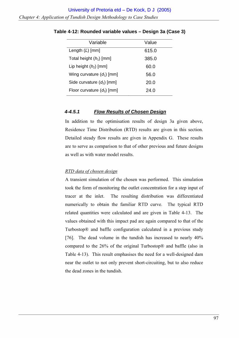
Chapter 4: Application of Tundish Design Methodology to Case Studies
97
Table 4-12: Rounded variable values – Design 3a (Case 3)
Variable Value Length (L) [mm] 615.0 Total height (h1) [mm] 385.0 Lip height (h2) [mm] 60.0 Wing curvature (d1) [mm] 56.0 Side curvature (d2) [mm] 20.0 Floor curvature (d3) [mm] 24.0
4-4.5.1 Flow Results of Chosen Design
In addition to the optimisation results of design 3a given above,
Residence Time Distribution (RTD) results are given in this section.
Detailed steady flow results are given in Appendix G. These results
are to serve as comparison to that of other previous and future designs
as well as with water model results.
RTD data of chosen design
A transient simulation of the chosen was performed. This simulation
took the form of monitoring the outlet concentration for a step input of
tracer at the inlet. The resulting distribution was differentiated
numerically to obtain the familiar RTD curve. The typical RTD
related quantities were calculated and are given in Table 4-13. The
values obtained with this impact pad are again compared to that of the
Turbostop® and baffle configuration calculated in a previous study
[76]. The dead volume in the tundish has increased to nearly 40%
compared to the 26% of the original Turbostop® and baffle (also in
Table 4-13). This result emphasises the need for a well-designed dam
near the outlet to not only prevent short-circuiting, but to also reduce
the dead zones in the tundish.
UUnniivveerrssiittyy ooff PPrreettoorriiaa eettdd –– DDee KKoocckk,, DD JJ ((22000055))
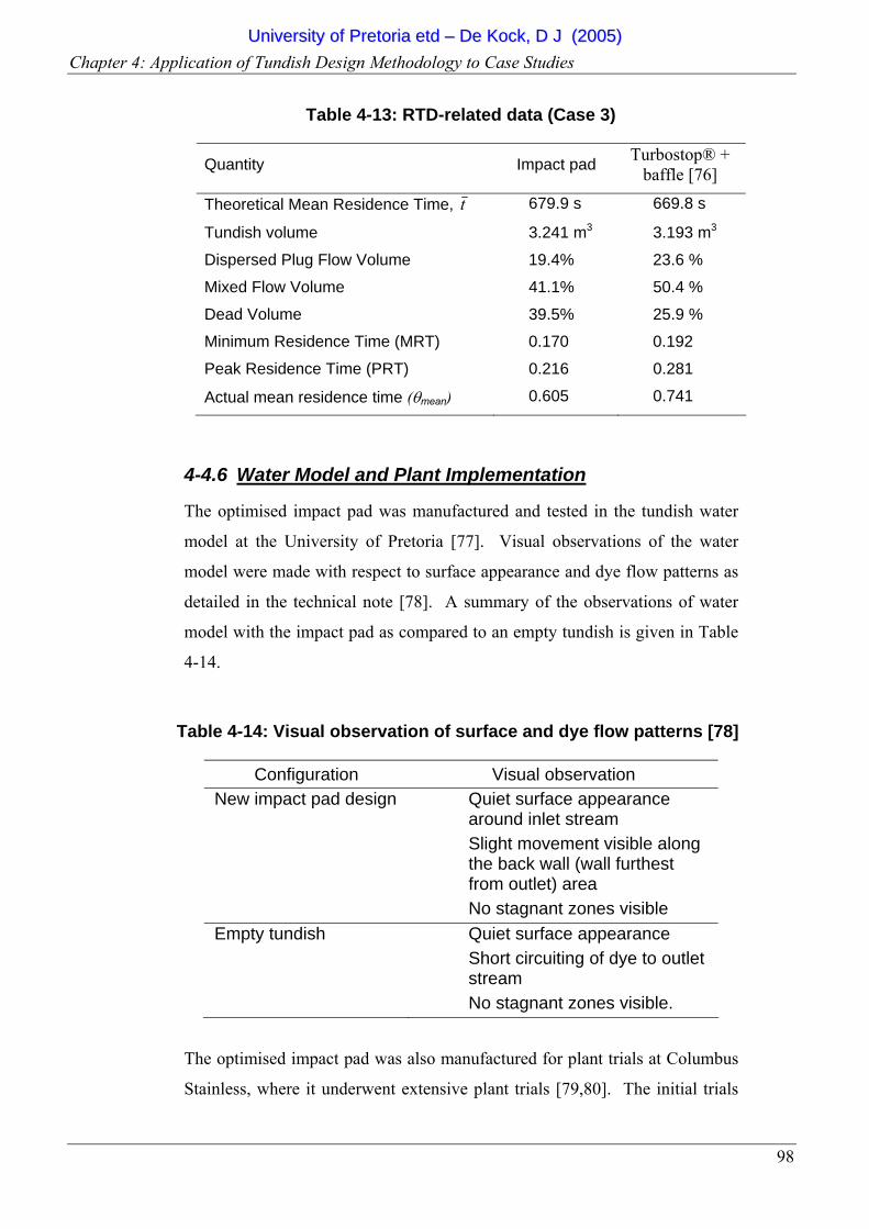
Chapter 4: Application of Tundish Design Methodology to Case Studies
98
Table 4-13: RTD-related data (Case 3)
Quantity Impact pad Turbostop® + baffle [76]
Theoretical Mean Residence Time, t 679.9 s 669.8 s
Tundish volume 3.241 m3 3.193 m3
Dispersed Plug Flow Volume 19.4% 23.6 %
Mixed Flow Volume 41.1% 50.4 %
Dead Volume 39.5% 25.9 %
Minimum Residence Time (MRT) 0.170 0.192
Peak Residence Time (PRT) 0.216 0.281
Actual mean residence time (θmean) 0.605 0.741
4-4.6 Water Model and Plant Implementation
The optimised impact pad was manufactured and tested in the tundish water
model at the University of Pretoria [77]. Visual observations of the water
model were made with respect to surface appearance and dye flow patterns as
detailed in the technical note [78]. A summary of the observations of water
model with the impact pad as compared to an empty tundish is given in Table
4-14.
Table 4-14: Visual observation of surface and dye flow patterns [78]
Configuration Visual observation New impact pad design
Quiet surface appearance around inlet stream Slight movement visible along the back wall (wall furthest from outlet) area No stagnant zones visible
Empty tundish
Quiet surface appearance Short circuiting of dye to outlet stream No stagnant zones visible.
The optimised impact pad was also manufactured for plant trials at Columbus
Stainless, where it underwent extensive plant trials [79,80]. The initial trials
UUnniivveerrssiittyy ooff PPrreettoorriiaa eettdd –– DDee KKoocckk,, DD JJ ((22000055))
Chapter 4: Application of Tundish Design Methodology to Case Studies
99
[79] indicated that the 304 stainless steel grade showed a reduction in defects
with the new impact pad compared to the case without any furniture. The 409
stainless steel grade however showed an increase in the number of defects
when using the new impact pad compared to Columbus Stainless’ current
furniture. The results from the initial trial motivated a long-term trial for the
new impact pad [80]. The long-term trial indicated that the impact pad
decreased the defects in the austenitic material (e.g., 304, 316), while
increasing the defects in the ferritic material (e.g, 409). From this, it was
recommended that the new impact pad should be implemented on a long-term
basis on the 304 steel grade. The difference in performance for the ferritic and
austenitic material in the plant trials highlighted the current challenge for CFD
to model the detailed metallurgical reactions that occur in different steel
grades (e.g., inclusion formation and the interaction with the slag layer) to
explain why there is difference in the impact pad performance of these two
grades.
4-4.7 Conclusions
This section described the optimisation of an impact pad for the single-strand
tundish of Columbus Stainless. The techniques of CFD coupled with
mathematical optimisation were used in the form of the commercial solver
FLUENT, its pre-processor GAMBIT and the commercial optimiser, LS-OPT.
The objective function used was the maximum turbulent kinetic energy on the
slag surface. Six design variables describing the impact pad geometry were
used. A 12.5% reduction in maximum surface turbulent kinetic energy was
obtained during the optimisation. During the optimisation process, the
inclusion particle removal capability of the design was monitored as well as
impact pad volume and liquid steel yield.
UUnniivveerrssiittyy ooff PPrreettoorriiaa eettdd –– DDee KKoocckk,, DD JJ ((22000055))
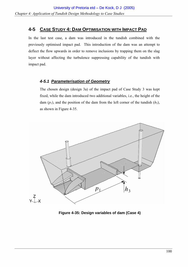
Chapter 4: Application of Tundish Design Methodology to Case Studies
100
4-5 CASE STUDY 4: DAM OPTIMISATION WITH IMPACT PAD In the last test case, a dam was introduced in the tundish combined with the
previously optimised impact pad. This introduction of the dam was an attempt to
deflect the flow upwards in order to remove inclusions by trapping them on the slag
layer without affecting the turbulence suppressing capability of the tundish with
impact pad.
4-5.1 Parameterisation of Geometry
The chosen design (design 3a) of the impact pad of Case Study 3 was kept
fixed, while the dam introduced two additional variables, i.e., the height of the
dam (p1), and the position of the dam from the left corner of the tundish (h3),
as shown in Figure 4-35.
Figure 4-35: Design variables of dam (Case 4)
p1 h3p1 h3
UUnniivveerrssiittyy ooff PPrreettoorriiaa eettdd –– DDee KKoocckk,, DD JJ ((22000055))
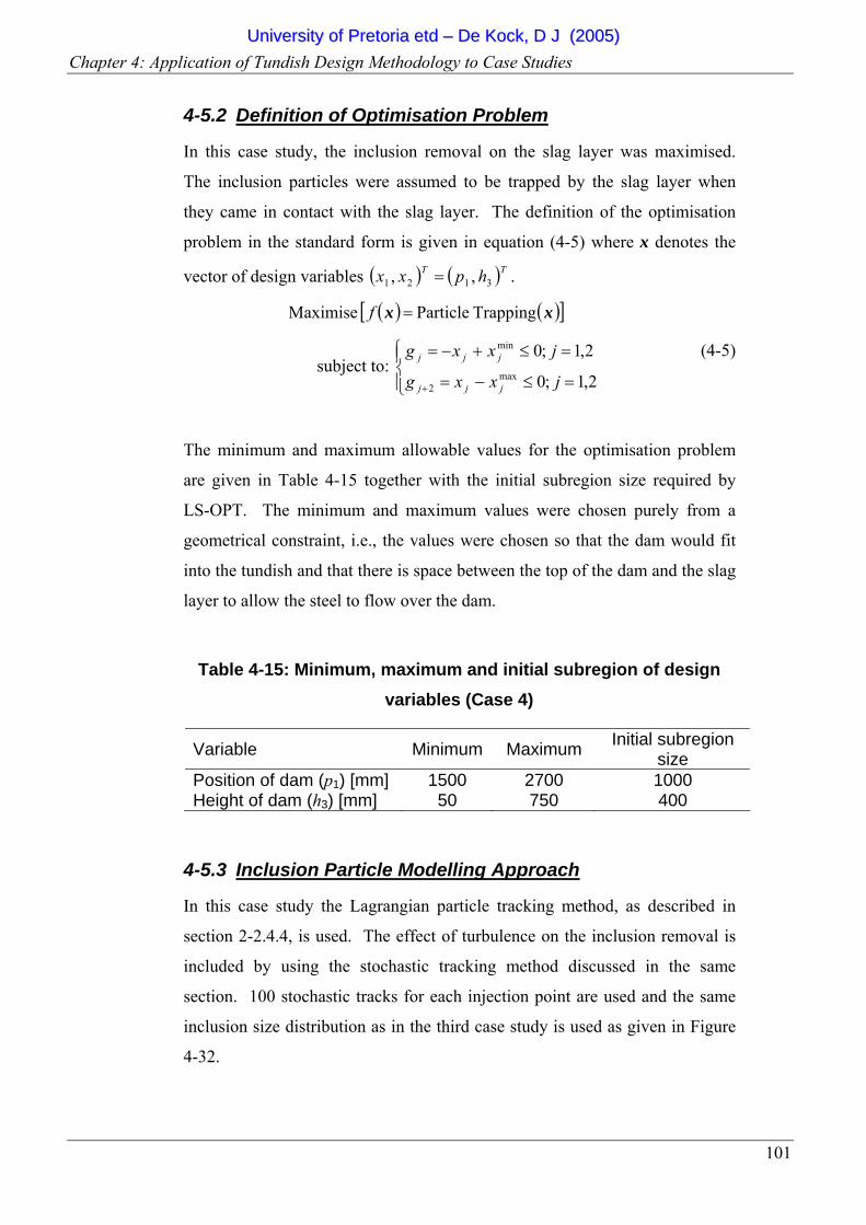
Chapter 4: Application of Tundish Design Methodology to Case Studies
101
4-5.2 Definition of Optimisation Problem
In this case study, the inclusion removal on the slag layer was maximised.
The inclusion particles were assumed to be trapped by the slag layer when
they came in contact with the slag layer. The definition of the optimisation
problem in the standard form is given in equation (4-5) where x denotes the
vector of design variables ( ) ( )TT hpxx 3121 ,, = .
( ) ( )[ ]xx Trapping Particle Maximise =f
subject to: ⎪⎩
⎪⎨⎧
=≤−=
=≤+−=
+ 2,1;0
2,1;0max
2
min
jxxg
jxxg
jjj
jjj (4-5)
The minimum and maximum allowable values for the optimisation problem
are given in Table 4-15 together with the initial subregion size required by
LS-OPT. The minimum and maximum values were chosen purely from a
geometrical constraint, i.e., the values were chosen so that the dam would fit
into the tundish and that there is space between the top of the dam and the slag
layer to allow the steel to flow over the dam.
Table 4-15: Minimum, maximum and initial subregion of design variables (Case 4)
Variable Minimum Maximum Initial subregion size
Position of dam (p1) [mm] 1500 2700 1000 Height of dam (h3) [mm] 50 750 400
4-5.3 Inclusion Particle Modelling Approach
In this case study the Lagrangian particle tracking method, as described in
section 2-2.4.4, is used. The effect of turbulence on the inclusion removal is
included by using the stochastic tracking method discussed in the same
section. 100 stochastic tracks for each injection point are used and the same
inclusion size distribution as in the third case study is used as given in Figure
4-32.
UUnniivveerrssiittyy ooff PPrreettoorriiaa eettdd –– DDee KKoocckk,, DD JJ ((22000055))

Chapter 4: Application of Tundish Design Methodology to Case Studies
102
Particles touching the sides and bottom of the tundish and the tundish furniture
are assumed to be reflected back into the molten steel flow.
4-5.4 Optimisation Results
Objective function and monitoring function
The history of the objective and monitored function is given in Figure 4-36.
As shown, the particle removal increased from just under 95% removal to
above 97% removal by the slag layer. Although the maximum turbulent
kinetic energy on the slag layer did not form part of the optimisation problem,
it was monitored to see what the effect of the introduction of the dam would
have on the turbulence of the slag surface. In this case, the maximum
turbulent kinetic energy proved to be insensitive to the introduction of the dam
and the optimised case even had a slightly lower value. This can be explained
by the fact that the maximum values on the slag surface occur close to the
shroud and the dam does not introduce higher levels of turbulence in the slow-
moving liquid in the area of the dam.
If it were found that the turbulent kinetic energy was higher than the starting
design, it could explicitly form part of the optimisation through the
introduction of a constraint function limiting the maximum turbulent kinetic
energy on the slag layer to be below the value of the case without a dam.
UUnniivveerrssiittyy ooff PPrreettoorriiaa eettdd –– DDee KKoocckk,, DD JJ ((22000055))

Chapter 4: Application of Tundish Design Methodology to Case Studies
103
94%
95%
96%
97%
98%
99%
100%
0 1 2 3 4
Design Iteration
Part
icle
Rem
oval
6.5E-04
6.7E-04
6.9E-04
7.1E-04
7.3E-04
7.5E-04
Turb
ulen
t k o
n Sl
ag[m
2 .s-2
]Partical removal
Turbulent kinetic energy
Figure 4-36: Optimisation history of objective function (Case 4)
Design Variables
The history of the design variables is shown in Figure 4-37. As can be seen in
this figure, the optimum dam configuration for particle removal is the highest
allowable dam as close to the shroud as allowed. The result makes intuitive
sense as the flow is deflected upwards and the chance of a particle reaching
the slag layer is improved. This optimum design is however impractical
looking at it from a yield prospective unless draining holes are inserted into
the dam. This shows how important the initial formulation of the optimisation
problem is. The yield can also form part of the optimisation problem as a
constraint and then the optimiser will find an optimum within the prescribed
yield limit.
UUnniivveerrssiittyy ooff PPrreettoorriiaa eettdd –– DDee KKoocckk,, DD JJ ((22000055))
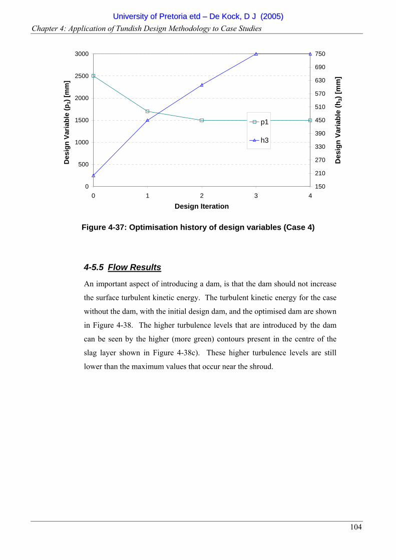
Chapter 4: Application of Tundish Design Methodology to Case Studies
104
0
500
1000
1500
2000
2500
3000
0 1 2 3 4
Design Iteration
Des
ign
Varia
ble
(p1)
[mm
]
150
210
270
330
390
450
510
570
630
690
750
Des
ign
Varia
ble
(h3)
[mm
]
p1
h3
Figure 4-37: Optimisation history of design variables (Case 4)
4-5.5 Flow Results
An important aspect of introducing a dam, is that the dam should not increase
the surface turbulent kinetic energy. The turbulent kinetic energy for the case
without the dam, with the initial design dam, and the optimised dam are shown
in Figure 4-38. The higher turbulence levels that are introduced by the dam
can be seen by the higher (more green) contours present in the centre of the
slag layer shown in Figure 4-38c). These higher turbulence levels are still
lower than the maximum values that occur near the shroud.
UUnniivveerrssiittyy ooff PPrreettoorriiaa eettdd –– DDee KKoocckk,, DD JJ ((22000055))
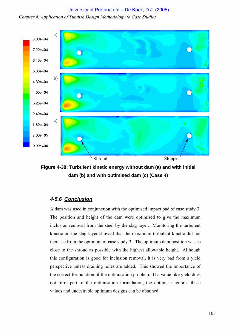
Chapter 4: Application of Tundish Design Methodology to Case Studies
105
Figure 4-38: Turbulent kinetic energy without dam (a) and with initial dam (b) and with optimised dam (c) (Case 4)
4-5.6 Conclusion
A dam was used in conjunction with the optimised impact pad of case study 3.
The position and height of the dam were optimised to give the maximum
inclusion removal from the steel by the slag layer. Monitoring the turbulent
kinetic on the slag layer showed that the maximum turbulent kinetic did not
increase from the optimum of case study 3. The optimum dam position was as
close to the shroud as possible with the highest allowable height. Although
this configuration is good for inclusion removal, it is very bad from a yield
perspective unless draining holes are added. This showed the importance of
the correct formulation of the optimisation problem. If a value like yield does
not form part of the optimisation formulation, the optimiser ignores these
values and undesirable optimum designs can be obtained.
a)
b)
c)
Shroud Stopper
UUnniivveerrssiittyy ooff PPrreettoorriiaa eettdd –– DDee KKoocckk,, DD JJ ((22000055))
Chapter 4: Application of Tundish Design Methodology to Case Studies
106
4-6 CONCLUSION This chapter applied the methodology developed in Chapter 3 to different test cases.
The first case optimised the position of a dam and a weir of a single-strand tundish.
Two optimisation formulations were considered in this case, the first was the
minimisation of the dead volume in the tundish and the second the maximisation of
the inclusion removal of the tundish. Two different optima were obtained for the two
different formulations, highlighting the importance of the correct formulation of the
optimisation problem.
The second case optimised the baffle and pouring box area of a two-strand continuous
caster. In this case, the minimum residence time was maximised by changing the
geometry of the pouring box and baffle area. In this optimisation formulation a
weighted value of the minimum residence time at the operating condition and that of
the minimum residence time at a transition level were used. Significant
improvements, in excess of 130%, were made to the design compared to the starting
design.
The third case investigated the design of a new impact pad. An impact pad in a
tundish has as its aim the reduction of turbulence in the tundish. For this reason the
surface turbulent kinetic energy was minimised by changing the geometry of the
impact pad.
The inclusion removal capabilities of the impact pad on its own, as optimised in the
third test case, are not very good. The last case optimised a dam height and position
in conjunction with the previously designed impact pad. The dam improved the
particle removal capabilities of the tundish without increasing the turbulent kinetic
energy on the free surface, but the suggested design seems to be impractical. This
again highlights the importance of the correct formulation of the optimisation
problem.
UUnniivveerrssiittyy ooff PPrreettoorriiaa eettdd –– DDee KKoocckk,, DD JJ ((22000055))
107
5 CHAPTER 5: CONCLUSION
The continuous casting process is not a very old manufacturing process, but in the last
four decades, it became the most common process for producing most basic metals.
One of the particular important components in this system is the tundish.
Traditionally, the tundish acted as a reservoir between the ladle and the mould but
more recently it has been used a grade separator, an inclusion removal device and a
metallurgical reactor. A continuous drive to understand the molten metal flow
patterns inside the tundish has led to many research papers being published in the
modelling of the flow patterns, through either water modelling or numerical
modelling. Included in these papers, researchers changed the design of the tundish by
adding tundish furniture or changing the dimensions of the tundish. They showed that
these changes can improve the flow patterns that ultimately improve the performance
of the tundish. These changes were however based on trial-and-error experimentation
or relied on the experience of the modeller to propose the design changes. This type
of design methodology can lead to non-optimal solutions.
In this thesis, a methodology has been developed to optimise the molten steel flow
patterns in a tundish by changing the tundish and tundish furniture. The methodology
makes use of mathematical optimisation and Computational Fluid Dynamics (CFD) to
give an optimum tundish and tundish furniture design based on certain design criteria
as specified by the engineer. A literature survey that describes CFD modelling of a
tundish and the optimisation algorithms used in this work were presented in Chapter
2.
The proposed methodology (as outlined in Chapter 3) consists of a number of steps.
The first step is the validation the numerical (CFD) mode. This can be achieved by
UUnniivveerrssiittyy ooff PPrreettoorriiaa eettdd –– DDee KKoocckk,, DD JJ ((22000055))
Chapter 5: Conclusion
108
either comparing the numerical results to a water model or to a plant trial. The second
and most important step is the formulation of the optimisation problem. This step
involves deciding on the design variables, objective function and constraint
function(s). The last step before running the optimisation involves the automisation
of the optimisation process. This involves the creation of appropriate files and scripts
so that the CFD model can be created, solved and data extracted for a specific set of
design variables without user intervention.
The methodology developed in the thesis was tested on four cases as described in
Chapter 4. The first case optimised a simple dam-weir configuration for the lowest
dead volume and for high inclusion removal on the slag layer. The second case
optimised the baffle and pouring-box area in order to maximise the minimum
residence time. In the third case, the methodology was used to design a new impact
pad to reduce the slag layer turbulence. The newly designed impact pad was built and
tested in the full-scale water model at the University of Pretoria. The new impact pad
has also undergone trials in the single-strand continuous caster of Columbus Stainless
Steel. The fourth and last case, described the optimisation of the position and height
if a dam to be used with the impact pad developed in the third case, in order to
increase the trapping of inclusion by the slag layer.
The methodology proved to work extremely well in all cases. The results show good
improvements in the performance of the tundishes under investigation. From this, it
is concluded that this methodology provides an improved alternative over the
traditional design methods of developing and redesigning tundish and tundish
furniture.
An important aspect that was highlighted by the study is that the correct formulation
of the optimisation problem is crucial for the success of the optimisation procedure.
This correct formulation is reliant on the understanding and skill of the design
engineer. The resulting optimum is sensitive to the formulation of the optimisation
problem.
One drawback of this methodology is the computational time that the optimisation
procedure takes. This time can be reduced by using multiple computers to run the
UUnniivveerrssiittyy ooff PPrreettoorriiaa eettdd –– DDee KKoocckk,, DD JJ ((22000055))

Chapter 5: Conclusion
109
simulations in parallel. The continued growth of computer power is leading to a
reduction in the required optimisation time, but at the same time allowing more
detailed CFD model to be constructed. This drawback is however offset by the fact
that an optimum design is obtained which would not be possible or highly unlikely
using traditional experimental modelling (water modelling or plant trials) or trial-and-
error numerical modelling.
The methodology developed can now be applied in general to other tundishes with
other tundish furniture, providing that the design engineer formulates the optimisation
problem correctly.
UUnniivveerrssiittyy ooff PPrreettoorriiaa eettdd –– DDee KKoocckk,, DD JJ ((22000055))
110
6 CHAPTER 6: RECOMMENDATIONS AND FUTURE
WORK
A number of new areas that can follow on this current research have been identified
and are given below.
6-1 APPLICATION OF METHODOLOGY TO OTHER ELEMENTS OF
THE CONTINUOUS CASTING PROCESS The optimisation methodology developed in this study should be applied to the
Submerged Entry Nozzle (SEN), mould design and other components downstream of
the tundish in the continuous casting process. It is important to have favourable flow
patterns in the mould as poor flow patterns can result in slag entrainment that will
render all the improvements made in the tundish useless. If electromagnetic stirring is
used in the mould, the operating parameters of the stirrer could be optimised.
The optimisation methodology should also be applied to components upstream of the
tundish, e.g., the ladle. This could include the optimum design of gas sparging in the
ladle to reduce temperature stratification, or the design of the refractory to minimise
the heat losses from the ladle.
6-2 TRANSIENT COMPUTATIONAL FLUID DYNAMICS MODEL The cases in the thesis were all steady state. As the actual tundish and ladle operation
involves transient periods as well, especially during mixed grade transition, the
optimisation of the transient performance can also be treated with this methodology as
computing power allows.
UUnniivveerrssiittyy ooff PPrreettoorriiaa eettdd –– DDee KKoocckk,, DD JJ ((22000055))
Chapter 6: Recommendations and Future Work
111
The cascading that corresponds to high oxidation of the steel also occurs during the
initial filling (first heat) of the tundish. This transient filling phenomenon and design
of the furniture to reduce this effect can also be treated with this methodology.
6-3 TESTING OF OPTIMISATION FORMULATIONS Additional tundish and tundish furniture designs can be optimised and the
methodology can be tested on some of the other optimisation formulations given in
Chapter 3. Some of the optimisation formulations at the time of this study were
computationally too expensive, but with the rapid growth in computational power,
these formulations could soon be investigated.
6-4 EXTENSION AND VALIDATION OF INCLUSION MODELLING Validation of the inclusion modelling should be undertaken to validate the accuracy of
the models when using stochastic tracking. There remains some uncertainty as to the
accuracy of the CFD model of the small inclusions in a turbulent flow field.
A model should also be developed to include the detailed chemistry of the inclusions
in the CFD analysis. This model should include aspects such as inclusion generation,
amalgamation, and reaction with the slag layer. In this study, a particle touching the
free surface was assumed to be trapped which is not the case in a physical tundish. A
first attempt was made to improve the modelling of the capturing of a particle on the
slag surface. For this purpose, a FLUENT User Defined Function was developed and
is given in Appendix H. This first attempt is a simple model and calculates the
maximum continuous time that a particle spends in a user-defined region close to the
slag layer. A correlation is then used that relates the probability of a particle being
trapped, to the size of the particle and the time it spent near the slag layer. Other
possible correlations should also be investigated and the detailed reaction of the
particle on the slag surface can be included. One of the anticipated difficulties for this
future work is to get quantative data from the plant operations to validate the
numerical model.
UUnniivveerrssiittyy ooff PPrreettoorriiaa eettdd –– DDee KKoocckk,, DD JJ ((22000055))

Chapter 6: Recommendations and Future Work
112
The erosion of the tundish furniture is a further source of inclusions. A model
describing the erosion rate of the furniture and the corresponding size and chemical
composition of the inclusions that are introduced into the steel should be developed.
The movement of these inclusions and interaction with the slag layer should then be
modelled in a similar manner as described in the paragraph above.
UUnniivveerrssiittyy ooff PPrreettoorriiaa eettdd –– DDee KKoocckk,, DD JJ ((22000055))
113
REFERENCES
[1] Thomas, BG, ‘Continuous Casting’, The Encyclopedia of Materials: Science and Technology, K.H. J. Buschow, R. Cahn, M. Flemings, B. Ilschner, E. J. Kramer, S. Mahajan.(D. Apelian, subject ed.) Elsevier Science Ltd., Oxford, United Kingdom, Vol. 2, pp. 1595-1599, 2001.
[2] Wolf MM, ‘History of Continuous Casting’, Steelmaking Conference Proceedings, Iron & Steel Society, Warrendale, PA, pp. 83-137, 1992.
[3] Thomas BG, ‘Introduction to Continuous Casting’, Continuous Casting Consortium, URL: http://bgtibm1.me.uiuc.edu, 1999.
[4] Thomas BG, ‘Continuous Casting of Steel’, Chapter 15 in Modeling for Casting and Solidification Processing, O. Yu, editor, Marcel,Dekker, New York, NY, pp. 499-540, 2001.
[5] Mazumdar D, Yamanoglu G, Shankarnarayanan R, Guthrie RIL, ‘Similarity Considerations in the Physical Modelling of Steel Making Tundish Systems’, Steel Research, Vol. 66, No. 1, 14-19, 1995.
[6] Sahai Y, Ahuja R, ‘Fluid Flow and Mixing of Melt in Steelmaking Tundishes’, Ironmaking & Steelmaking, Vol. 13, No. 5, pp. 241-247, 1986.
[7] López-Ramirez S, De J Barreto J, Palafox-Ramos J, Morales RD, Zacharias D, ‘Modeling Study of the Influence of Turbulence Inhibitors on the Molten Steel Flow, Tracer Dispersion, and Inclusion Trajectoris in Tundishes’, Metallurgical and Materials Transactions B, Vol. 32B, pp. 615-627, 2001.
[8] Koria SC, Singh S, ‘Physical Modeling of the Effects of the Flow Modifier on the Dynamics of Molten Steel Flowing in a Tundish’, Iron and Steel Institute of Japan Int., Vol. 34, No. 10, pp. 784-793, 1994.
[9] Sheng DY, Jonsson L, ‘Investigation of Transient Fluid-Flow and Heat-Transfer in a Continuous-Casting Tundish by Numerical-Analysis Verified with Nonisothermal Water Model Experiments’, Metallurgical and Materials Transactions B, Vol. 30B, No. 5, pp. 979-985, 1999.
UUnniivveerrssiittyy ooff PPrreettoorriiaa eettdd –– DDee KKoocckk,, DD JJ ((22000055))

References
114
[10] Sinha AK, Vassilicos A, ‘Physical Modelling of Thermal Effects on Steel Flow and Mixing in Tundish’, Ironmaking & Steelmaking, Vol. 25, No. 5, pp. 387-393, 1998.
[11] He Y, Sahai Y, ‘The Effect of Tundish Wall Inclination on the Fluid Flow and Mixing: A Modeling Study’, Metallurgical Transactions B, Vol. 18, pp. 81-92, 1987.
[12] Joo S, Han JW, Guthrie RIL, ‘Inclusion Behavior and Heat-Transfer Phenomena in Steelmaking Tundish Operations’, Metallurgical and Materials Transactions B, Vol. 24B, pp. 767-777, 1993.
[13] Chakraborty S, Sahai Y,’ Mathematical Modelling of Transport Phenomena in Continuous Casting Tundishes’ Ironmaking & Steelmaking, Vol. 19, (6), pp. 479, 1992.
[14] Sahai Y, Ahuja R, ‘Fluid Flow and Mixing of Melt in Steelmaking tundishes’, Ironmaking & Steelmaking, Vol. 13, No. 5, pp. 241-247, 1986.
[15] Kemeny F, Harris DJ, McLean A, Meadowcroft TR, Young JD, ‘Fluid Flow Studies in the Tundish of a Slab Caster’, Proceedings of the 2nd Process Technology Conf., Warrendale, PA, 1981.
[16] Mazumdar D, Guthrie RIL, ‘The Physical and Mathematical Modelling of Continuous Casting Tundish Systems’, Iron and Steel Institute of Japan Int., Vol. 39, No. 6, pp. 524-547, 1999.
[17] Sahai Y, Burval M, ‘Validity of Reynolds and Froude similarity criteria for water modeling of melt flow in tundishes’, Proc. Electric Furnace Conference, ISS-AIME, Vol. 50, pp.469-474, 1992.
[18] Morales RD, Lopez-Ramirez S, Palafox-Ramos J, Zacharias D, ‘Numerical and Modeling Analysis of Fluid Flow and Heat Transfer of Liquid Steel in a Tundish with Different Flow Control Devices’, Iron and Steel Institute of Japan Int., Vol. 39, No. 5, pp. 455-462, 1999.
[19] López-Ramirez S, De J Barreto J, Palafox-Ramos J, Morales RD, Zacharias D, ‘Modeling Study of the Influence of Turbulence Inhibitors on the Molten Steel Flow, Tracer Dispersion, and Inclusion Trajectories in Tundishes’, Metallurgical and Materials Transactions B, Vol. 32B, pp. 615-627, 2001.
UUnniivveerrssiittyy ooff PPrreettoorriiaa eettdd –– DDee KKoocckk,, DD JJ ((22000055))
References
115
[20] Koria SC, Singh S, ‘Physical Modeling of the Effects of the Flow Modifier on the Dynamics of Molten Steel Flowing in a Tundish’, Iron and Steel Institute of Japan Int., Vol. 34, No. 10, pp. 784-793, 1994.
[21] Sheng DY, Jonsson L, ‘Investigation of Transient Fluid-Flow and Heat-Transfer in a Continuous-Casting Tundish by Numerical-Analysis Verified with Nonisothermal Water Model Experiments’, Metallurgical and Materials Transactions B, Vol. 30B, No. 5, pp. 979-985, 1999.
[22] Lievenspiel O, Chemical Reaction Engineering – An Introduction to the Design of Chemical Rectors, John Wiley and Sons Inc., New York, 1967.
[23] Singh S, Koria SC, ‘Model Study of the Dynamics of Flow of Steel Melt in the Tundish’, Iron and Steel Institute of Japan Int., Vol. 33, No. 12, pp. 1228-1237, 1993
[24] Nakajima H, Sebo F, Tanaka S, Dumitru I, Harris DJ Guthrie RIL, Proc. of the 2nd Process Technology Conference, TMS, Warrendale, PA, pp232, 1981.
[25] Martinez E, Maeda M, Heaslip LJ, Rodriquez G, McLean A, ‘Effects of Fluid Flow on the Inclusion Separation in Continuous Casting Tundish’, Trans. Iron Steel Jpn., Vol. 26, No. 9, pp. 724-731, 1986.
[26] Collur MM, Love DB, Patil BV, Proc. of the Steelmaking Conf., TMS, Warrendale, PA, pp. 629, 1995.
[27] Ackerman J, Personal Communication, Columbus Stainless Steel, Middelburg, South Africa, 2002.
[28] Pretorius CA, Personal Communication, ISCOR Vanderbijlpark, South Africa, 2002.
[29] Spectro Analytical Instruments Inc., www.spectro.com, 2002.
[30] Zhang L, Thomas BG, ‘State of the Art in Evaluation and Control of Steel Cleanliness’, Iron and Steel Institute of Japan Int., Vol. 43, No. 3, pp. 271-291, 2003.
[31] Fluent Inc., ‘Fluent 6 Introductory Training Notes’, 2003.
[32[ Fluent Inc., Gambit Version 2 Manuals, Centerra Resource Park, 10 Cavendish Court, Lebanon, New Hampshire, USA, 2001 (www.fluent.com).
UUnniivveerrssiittyy ooff PPrreettoorriiaa eettdd –– DDee KKoocckk,, DD JJ ((22000055))
References
116
[33] White FM, Viscous Fluid Flow, 2nd Edition, McGraw-Hill International, New York, 1991.
[34] Stokes GG, ‘On the Theories of Internal Friction of Fluids in Motion’, Trans. Cambridge Phil. Soc., Vol. 8, pp. 287-305, 1845.
[35] Bousinessq J, Théorie Analytique de la Chaleur, Vol. II, Gauthier-Villars, Paris, 1903.
[36] Zeytounian RKh, ‘Joseph Boussinesq and his approximation: a contemporary view’, C.R. Mecanique, Vol 331, pp. 575-586, 2003.
[37] Fluent Inc., Fluent Version 6 Manuals, Centerra Resource Park, 10 Cavendish Court, Lebanon, New Hampshire, USA, 2001 (www.fluent.com).
[38] Baldwin BS, Lomax H, ‘Thin Layer and Approximation and Algebraic Model for Separated Turbulent Flow’, AIAA Paper 78-257, 1978.
[39] Kline SJ, Morkovin MV, Sovran G, Cockrell D J, ‘Computation of Turbulent Boundary Layers – 1968 AFOSR-IFP Stanford Conference’, Proceedings 1968 Conference, Vol. 1, Stanford University, Stanford, California, 1968.
[40] Launder BE, Spalding DB, ‘The Numerical Computation of Turbulent Flow’, Comp. Meth. in Appl. Mech. & Eng., Vol. 3, pp. 269-289, North-Holland Publishing Co., 1974.
[41] Rodi W, ‘Influence of Boyancy and Rotation on Equations for Turbulent Length scale’, Proceedings of the 2nd Symposium on Turbulent Shear Flows, 1979.
[42] El Thary SH, ‘k-ε Equation for Compressible Reciprocating Engine Flows’, AIAA J. Energy, Vol. 7, No. 4, pp. 345-353, 1983.
[43] Choudhury D, ‘Introduction to the Renormalization Group Method and Turbulence Modeling’, Technical Memorandum TM-107, Fluent Inc., 1993.
[44] Spalding DB, ‘A Single Formula for the Law of the Wall’, Journal of Applied Mechanics, Vol. 28, pp. 455-457, 1961.
[45] Launder BE, Reece BJ, Rodi W, ‘Progress in the Development of a Reynolds Stress Turbulent Closure’, Journal of Fliud Mechanics, Vol. 68, pp. 537-566, 1975.
UUnniivveerrssiittyy ooff PPrreettoorriiaa eettdd –– DDee KKoocckk,, DD JJ ((22000055))
References
117
[46] Kline S, Cantwell BJ, Liley GM, ‘The 1980-1981 ASFOSR-HTTM Stanford Conference on Complex Turbulent Flows: Comparison of Computation and Experiment’, Vols. 1-3, Mech. Engineering Dept., Stanford University, Stanford, California, 1982.
[47] Miki Y, Thomas BG, ‘Modeling of Inclusion Removal in a Tundish’, Metallurgical and Materials Transactions B, Vol. 30B, pp. 639-654, August 1999.
[48] Morsi SA, Alexander AJ, ‘An Investigation of Particle Trajectories in Two-Phase Flow Systems’, Journal of Fluid Mechanics, Vol. 55, No. 2, pp. 193-208, September 1972.
[49] Daly BJ, Harlow FH. ‘Transport Equations in Turbulence’, Phys. Fluids, Vol. 13, pp. 2634-2649, 1970.
[50] Miki Y, Thomas BG, Dennisov A, Shimanda Y, ‘Model of Inclusion Removal During RH Degassing of Steel’, Iron and Steelmaker, Vol. 24, No. 8, pp. 31-39, 1997.
[51] Snyman JA, Introduction to Mathematical Optimisation, Post-graduate course, Department of Mechanical and Aeronautical Engineering, University of Pretoria, South Africa, 1994.
[52] Snyman JA, Practical Mathematical Optimization: An Introduction to Basic Optimization Theory and Classical and New Gradient-Based Algorithms, Springer, New York, New York, 2005.
[53] Snyman JA, ‘A New Dynamic Method for Unconstrained Minimization’, Applied Mathematical Modelling, Vol. 6, pp. 449-462, 1982.
[54] Snyman JA, ‘An Improved Version of the Original Leap-Frog Dynamic Method for Unconstrained Minimization LFOP1(b)’, Applied Mathematical Modelling, Vol. 7, pp. 216-218, 1983.
[55] Snyman JA, Stander N, Roux W J, ‘A Dynamic Penalty Function Method for the Solution of Structural Optimization Problems’, Applied Mathematical Modelling, Vol. 18, pp. 453-460, August 1994.
UUnniivveerrssiittyy ooff PPrreettoorriiaa eettdd –– DDee KKoocckk,, DD JJ ((22000055))
References
118
[56] Snyman JA, Frangos C, Yavin Y, ‘Penalty Function Solutions to Optimal Control Problems with General Constraints via a Dynamic Optimisation Method’, Computer & Mathematics with Applications, Vol. 23, pp. 46-47, 1992.
[57] Snyman JA, ‘The LFOPCV3 Leap-Frog Algorithm for Constrained Optimisation’, Computers & Mathematics with Applications, Vol. 40, pp. 1085-1096, 2000.
[58] Snyman JA, Stander N, ‘A New Successive Approximation Method for Optimum Structural Design’, AIAA Journal, Vol. 32, pp. 1310-1315, 1994.
[59] Snyman JA, Stander N, ‘Feasible Descent Cone Methods for Inequality Constrained Optimisation Methods in Engineering’, International Journal for Numerical Methods in Engineering, Vol. 38, pp. 119-135, 1995.
[60] Snyman JA, Hay AM, ‘The Dynamic-Q Optimization Method: An alternative to SQP?’, Computers & Mathematics with Application, Vol. 44, No. 14, pp. 1589-1598, 2002.
[61] Snyman JA, Private Communication, Department of Mechanical and Aeronuatical Engineering, University of Pretoria, Pretoria, South Africa, 1998.
[62] Stander N, Craig KJ, ‘On the robustness of a simple domain reduction scheme for simulation based optimization’, Engineering Computations, Vol. 19, No. 4, pp. 431-450, 2002.
[63] Stander N, Eggleston TA, Craig KJ, Roux W, LS-OPT User’s Manual Version 2, Livermore Software Technology Corporation, Livermore, CA, (October 2003).
[64] Myers RH, Montgomery DC, Response Surface Methodology, Wiley, New York, 1995.
[65] Venter PJ, Craig KJ, Hasse GW, De Kock DJ, Ackerman J, ‘Comparison of Water Model and CFD Results for a Single-Strand Continuous Caster’, Mechanical Technology, April 2000.
[66] Hasse G.W., Design, Construction, Commissioning & Initial Experimental Tests for a Full Scale Tundish Water Model, Technical report, Gübau cc., July 1999.
UUnniivveerrssiittyy ooff PPrreettoorriiaa eettdd –– DDee KKoocckk,, DD JJ ((22000055))
References
119
[67] UFM 600 User Manual, Krohne Altosonic, The Netherlands, 1990.
[68] De Kock DJ, Craig KJ, Pretorius CA. ‘Mathematical Maximisation of the Minimum Residence Time for a Two-Strand Continuous Caster’, Ironmaking and Steelmaking, Vol. 30, No. 3. pp. 229- 234, 2003.
[69] Craig KJ, De Kock DJ, Makgata KW, De Wet GJ, ‘Design Optimization of a Single-strand Continuous Caster Tundish Using Residence Time Distribution Data’, Iron and Steel Institute of Japan Int., Vol. 31, No. 10, pp. 1194-1200, 2001.
[70] Craig KJ, De Kock DJ, Snyman JA, ‘Continuous Casting Optimization using CFD and Dynamic-Q’, 20th International Congress of Theoretical and Applied Mechanics, Chicago, 27 August – 2 September 2000.
[71] Pretorius CA, Personal Communication, ISCOR Vanderbijlpark Works, South Africa , 2000.
[72] De Kock DJ, Craig KJ, Pretorius CA. ‘Mathematical Maximisation of the Minimum Residence Time for a Two-Strand Continuous Caster’, Proceedings of the 4th European Continuous Casting Conference, Birmingham, United Kingdom, pp. 84-93, 14-16 October 2002.
[73] Mills AF, Basic Heat and Mass Transfer, 2nd Edition, New Jersey, Prentice-Hall Inc., 1999.
[74] Craig KJ, De Kock DJ, De Wet GJ, Haarhoff LJ, Pretorius CA, ‘Design Optimization of Continuous Caster Refractory Components’, submitted, ASME 2005 International Design Engineering Technical Conferences and Computers and Information in Engineering Conference, Long Beach, California, USA, September 2005.
[75] US Patent Number 6159418, ‘Tundish Impact Pad’, Foseco International Ltd., Wiltshire, United Kingdom, 12 December 2000.
[76] Craig KJ, De Kock DJ & De Wet GJ, ‘CFD Analysis of the Single-strand Tundish of Columbus Stainless – Modelling of New Tundish (with 150mm lining) with Existing Turbostop and Baffle’, Internal Report to Columbus Stainless, 2002.
UUnniivveerrssiittyy ooff PPrreettoorriiaa eettdd –– DDee KKoocckk,, DD JJ ((22000055))

References
120
[77] Venter PJ, Craig KJ, Hasse GW, De Kock DJ, Ackerman J, ‘Comparison Of Water Model and CFD Results for a Single-Strand Continuous Caster’, Proceedings of International Conference on Applied Mechanics, Durban, South Africa, 2000.
[78] Orban W, Technical Note, Columbus Stainless (Pty) Ltd, 2004.
[79] De Beer G, ‘Trial 155: Trial on “Cash Register” tundish furniture’, Columbus Stainless (Pty) Ltd, Internal Report, January 2004.
[80] De Beer G, ‘Trial 155: Trial on “Cash Register” tundish furniture (Progress report 1)’, Columbus Stainless (Pty) Ltd, Internal Report, June 2004.
UUnniivveerrssiittyy ooff PPrreettoorriiaa eettdd –– DDee KKoocckk,, DD JJ ((22000055))
A-1
A APPENDIX A: WATER MODEL VALIDATION STUDY
A-1 INTRODUCTION
An important part of the optimisation is to trust the accuracy of the numerical model.
For this purpose a water model validation study was done. This work was published
in Mechanical Technology [65]. The details of this study are given in this appendix.
In physical modelling, water is normally used to simulate molten steel in perspex
models of tundishes. In this modelling, emphasis has been placed on the matching of
Reynolds (Re) and Froude (Fr) similarity criteria [17]. When water at room
temperature is used as the modelling fluid, matching of both Reynolds and Froude
numbers require the use of full-scale models. In reduced-scale models, either
Reynolds or Froude numbers can be satisfied. A full-scale water model of the
Columbus Stainless Steel tundish was commissioned at the University of Pretoria in
1999 [66] therefore having the advantage of having both Reynolds and Froude
number similarity satisfied. The tundish model is constructed from 10mm-thick
perspex sheets and supported by a steel frame. The water flow network provides the
option to recirculate the water from the tundish outlet to the reservoir, or to divert it to
a drain (see Figure A-1).
UUnniivveerrssiittyy ooff PPrreettoorriiaa eettdd –– DDee KKoocckk,, DD JJ ((22000055))
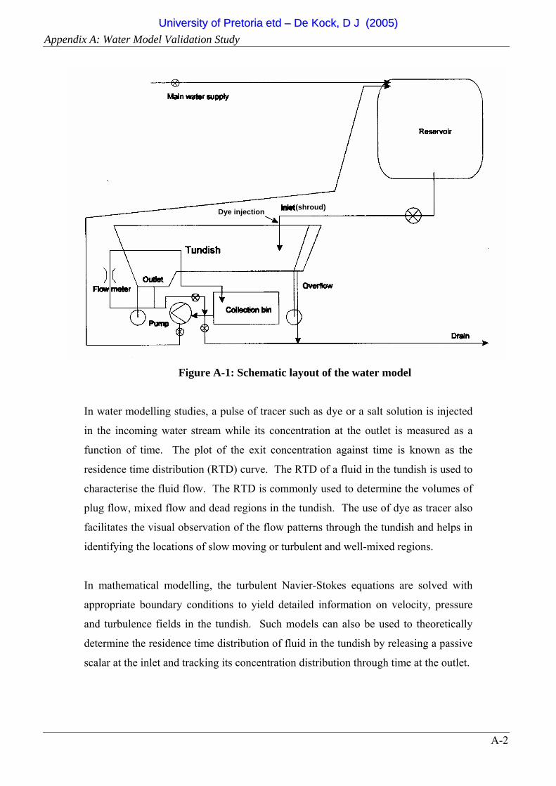
Appendix A: Water Model Validation Study
A-2
Figure A-1: Schematic layout of the water model
In water modelling studies, a pulse of tracer such as dye or a salt solution is injected
in the incoming water stream while its concentration at the outlet is measured as a
function of time. The plot of the exit concentration against time is known as the
residence time distribution (RTD) curve. The RTD of a fluid in the tundish is used to
characterise the fluid flow. The RTD is commonly used to determine the volumes of
plug flow, mixed flow and dead regions in the tundish. The use of dye as tracer also
facilitates the visual observation of the flow patterns through the tundish and helps in
identifying the locations of slow moving or turbulent and well-mixed regions.
In mathematical modelling, the turbulent Navier-Stokes equations are solved with
appropriate boundary conditions to yield detailed information on velocity, pressure
and turbulence fields in the tundish. Such models can also be used to theoretically
determine the residence time distribution of fluid in the tundish by releasing a passive
scalar at the inlet and tracking its concentration distribution through time at the outlet.
Dye injection (shroud)
UUnniivveerrssiittyy ooff PPrreettoorriiaa eettdd –– DDee KKoocckk,, DD JJ ((22000055))
Appendix A: Water Model Validation Study
A-3
A-2 EXPERIMENTAL SETUP
The experimental process involves achieving a stable operating level in the tundish
for a period which is at least 3 times the average residence time before an experiment
is initiated by injecting the dye. A water sample is obtained from a sampling tube
inside the outlet pipe. The water sample is fed through a spectrophotometer where the
absorbance at a specified wavelength is measured. The absorbance of the sample is
referenced to the absorbance of clean water. A pre-measured amount of the dye
solution is injected into the shroud (inlet to the tundish) as a pulse over three to five
seconds. The dye input is called the tracer and the mixing of the tracer in the water
changes the absorbance of the water.
A-2.1 SPECTROPHOTOMETER
A Novaspec II visible spectrophotometer [67] was used to determine the
residence time distribution curve of the tracer at the outlet of the water model.
The spectrophotometer provides measurement of both light absorbance and
light transmission in the visible wavelength range (325–900nm). The diagram
in Figure A-2 shows in simplified form the optical system of the instrument.
The light output from the lamp passes through a slit into the monochromator
where a collimating mirror converts the light into a parallel beam. The light
then passes to the diffraction grating to produce light of the selected
wavelength. This monochromatic light then passes through the stray light
filters and the monochromator outlet slit and then through the cuvette with the
water sample to the solid-state detector unit.
UUnniivveerrssiittyy ooff PPrreettoorriiaa eettdd –– DDee KKoocckk,, DD JJ ((22000055))
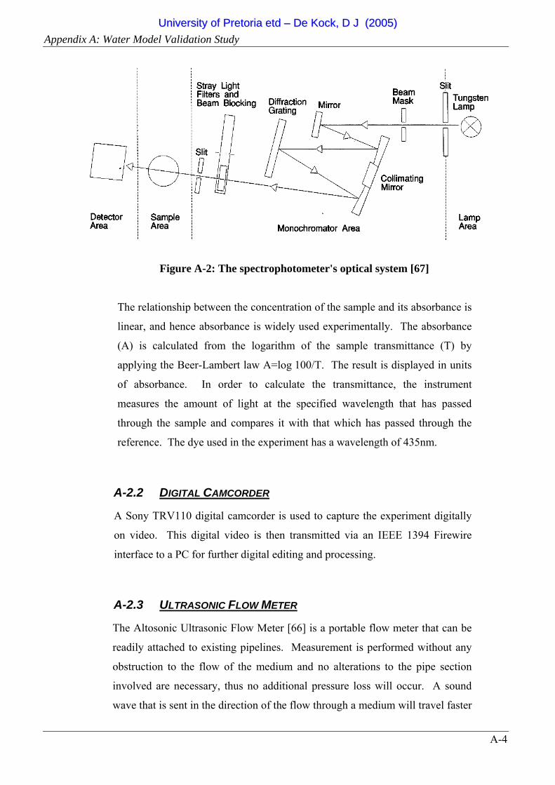
Appendix A: Water Model Validation Study
A-4
Figure A-2: The spectrophotometer's optical system [67]
The relationship between the concentration of the sample and its absorbance is
linear, and hence absorbance is widely used experimentally. The absorbance
(A) is calculated from the logarithm of the sample transmittance (T) by
applying the Beer-Lambert law A=log 100/T. The result is displayed in units
of absorbance. In order to calculate the transmittance, the instrument
measures the amount of light at the specified wavelength that has passed
through the sample and compares it with that which has passed through the
reference. The dye used in the experiment has a wavelength of 435nm.
A-2.2 DIGITAL CAMCORDER
A Sony TRV110 digital camcorder is used to capture the experiment digitally
on video. This digital video is then transmitted via an IEEE 1394 Firewire
interface to a PC for further digital editing and processing.
A-2.3 ULTRASONIC FLOW METER
The Altosonic Ultrasonic Flow Meter [66] is a portable flow meter that can be
readily attached to existing pipelines. Measurement is performed without any
obstruction to the flow of the medium and no alterations to the pipe section
involved are necessary, thus no additional pressure loss will occur. A sound
wave that is sent in the direction of the flow through a medium will travel faster
UUnniivveerrssiittyy ooff PPrreettoorriiaa eettdd –– DDee KKoocckk,, DD JJ ((22000055))

Appendix A: Water Model Validation Study
A-5
than one that is sent in the opposite direction. This principle is used in the
ultrasonic transit time flow meter.
A-3 RESULTS
A-3.1 RESIDENCE TIME DISTRIBUTION (RTD)
The RTD curve of the experiment (repeated four times) is compared to the
RTD curves obtained by the CFD code in Figure A-3 for an empty tundish.
Different turbulence modelling options were tested in the CFD model and the
one shown (RNG k-ε turbulence model) gave the best results. The
experimental set-up was emulated by a 2 sec pulse injection in the CFD model
to obtain the RTD.
0
0.2
0.4
0.6
0.8
1
1.2
0 0.5 1 1.5 2 2.5 3Normalised Time
Nor
mal
ised
Con
cent
ratio
n
Exp1
Exp2
Exp3
Exp4
Exp_Avg
RNG-ke 1st Order (2sec Pulse)
Figure A-3: Comparison of RTD curves
UUnniivveerrssiittyy ooff PPrreettoorriiaa eettdd –– DDee KKoocckk,, DD JJ ((22000055))
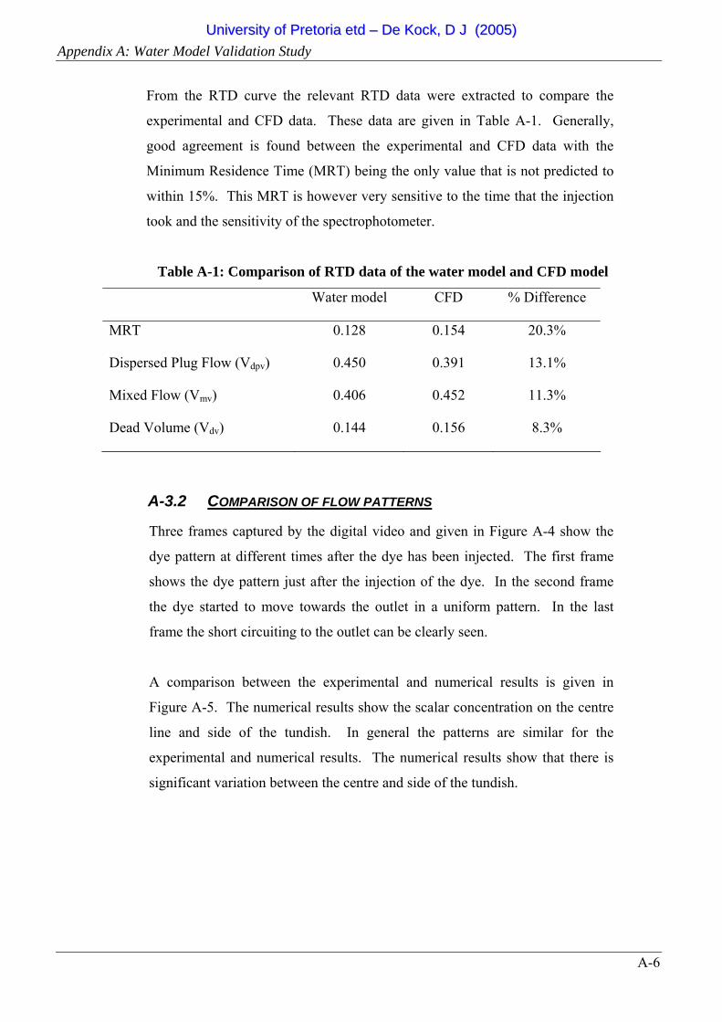
Appendix A: Water Model Validation Study
A-6
From the RTD curve the relevant RTD data were extracted to compare the
experimental and CFD data. These data are given in Table A-1. Generally,
good agreement is found between the experimental and CFD data with the
Minimum Residence Time (MRT) being the only value that is not predicted to
within 15%. This MRT is however very sensitive to the time that the injection
took and the sensitivity of the spectrophotometer.
Table A-1: Comparison of RTD data of the water model and CFD model
Water model CFD % Difference
MRT
Dispersed Plug Flow (Vdpv)
Mixed Flow (Vmv)
Dead Volume (Vdv)
0.128
0.450
0.406
0.144
0.154
0.391
0.452
0.156
20.3%
13.1%
11.3%
8.3%
A-3.2 COMPARISON OF FLOW PATTERNS
Three frames captured by the digital video and given in Figure A-4 show the
dye pattern at different times after the dye has been injected. The first frame
shows the dye pattern just after the injection of the dye. In the second frame
the dye started to move towards the outlet in a uniform pattern. In the last
frame the short circuiting to the outlet can be clearly seen.
A comparison between the experimental and numerical results is given in
Figure A-5. The numerical results show the scalar concentration on the centre
line and side of the tundish. In general the patterns are similar for the
experimental and numerical results. The numerical results show that there is
significant variation between the centre and side of the tundish.
UUnniivveerrssiittyy ooff PPrreettoorriiaa eettdd –– DDee KKoocckk,, DD JJ ((22000055))
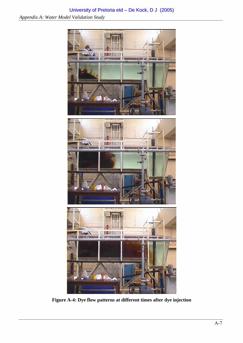
Appendix A: Water Model Validation Study
A-7
Figure A-4: Dye flow patterns at different times after dye injection
UUnniivveerrssiittyy ooff PPrreettoorriiaa eettdd –– DDee KKoocckk,, DD JJ ((22000055))
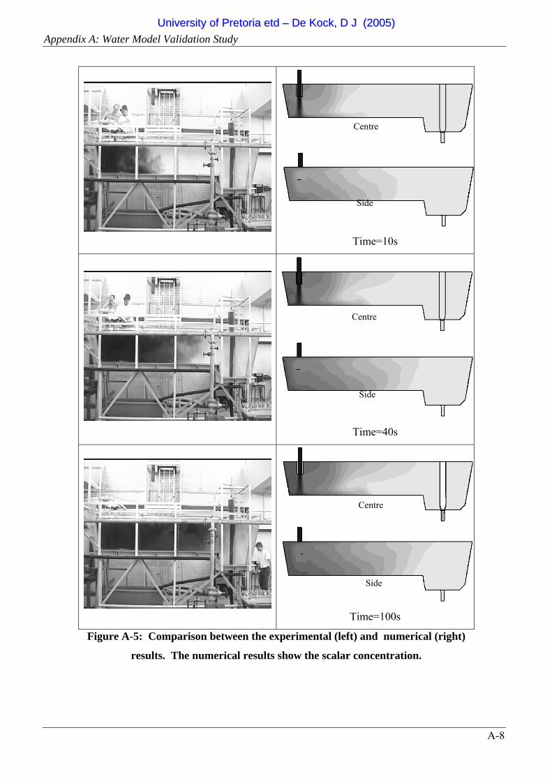
Appendix A: Water Model Validation Study
A-8
Time=10s
Time=40s
Time=100s
Figure A-5: Comparison between the experimental (left) and numerical (right)
results. The numerical results show the scalar concentration.
Centre
Side
Centre
Side
Centre
Side
UUnniivveerrssiittyy ooff PPrreettoorriiaa eettdd –– DDee KKoocckk,, DD JJ ((22000055))

Appendix A: Water Model Validation Study
A-9
A-4 CONCLUSION AND FUTURE WORK
There appears to be a good correlation between the experimental results and the CFD
results for this simple set-up. The diffusion of the tracer during the experiment could
also not be quantified.
UUnniivveerrssiittyy ooff PPrreettoorriiaa eettdd –– DDee KKoocckk,, DD JJ ((22000055))
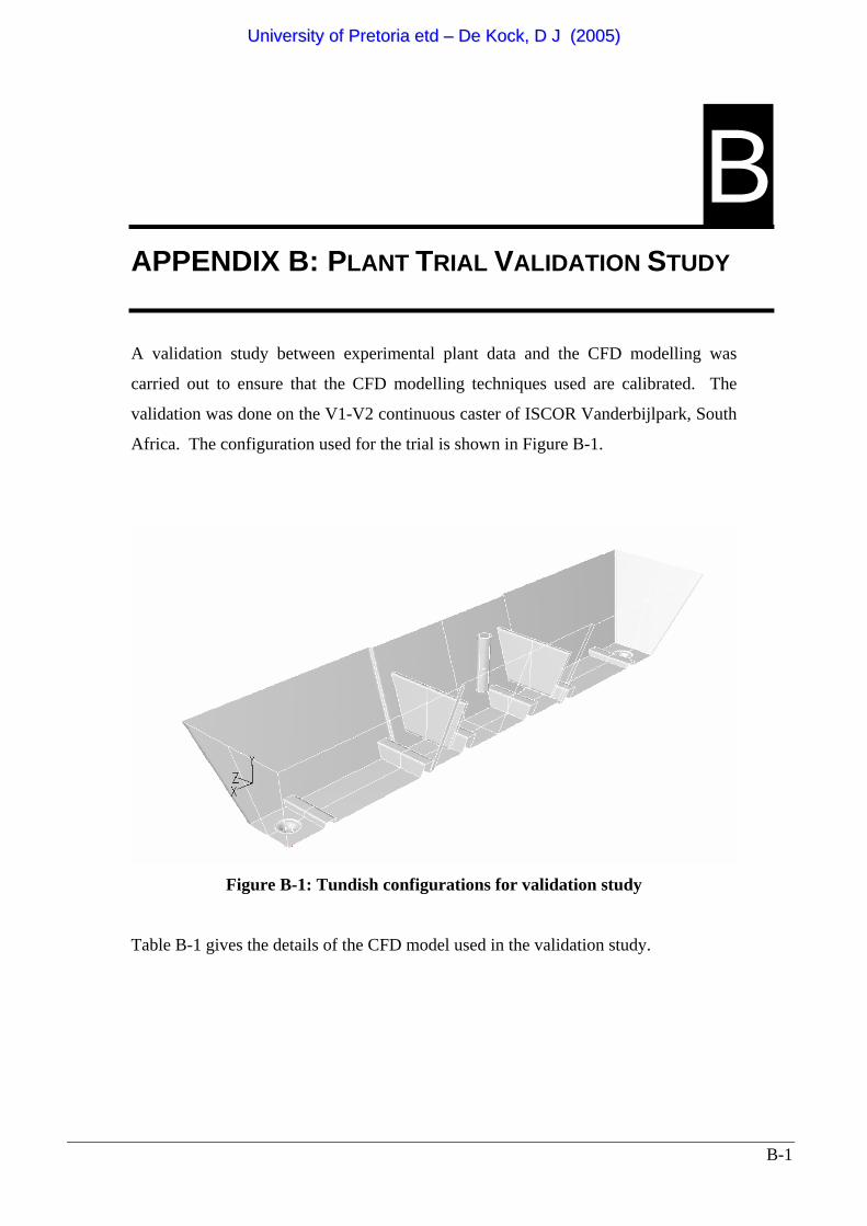
B-1
B APPENDIX B: PLANT TRIAL VALIDATION STUDY
A validation study between experimental plant data and the CFD modelling was
carried out to ensure that the CFD modelling techniques used are calibrated. The
validation was done on the V1-V2 continuous caster of ISCOR Vanderbijlpark, South
Africa. The configuration used for the trial is shown in Figure B-1.
Figure B-1: Tundish configurations for validation study
Table B-1 gives the details of the CFD model used in the validation study.
UUnniivveerrssiittyy ooff PPrreettoorriiaa eettdd –– DDee KKoocckk,, DD JJ ((22000055))
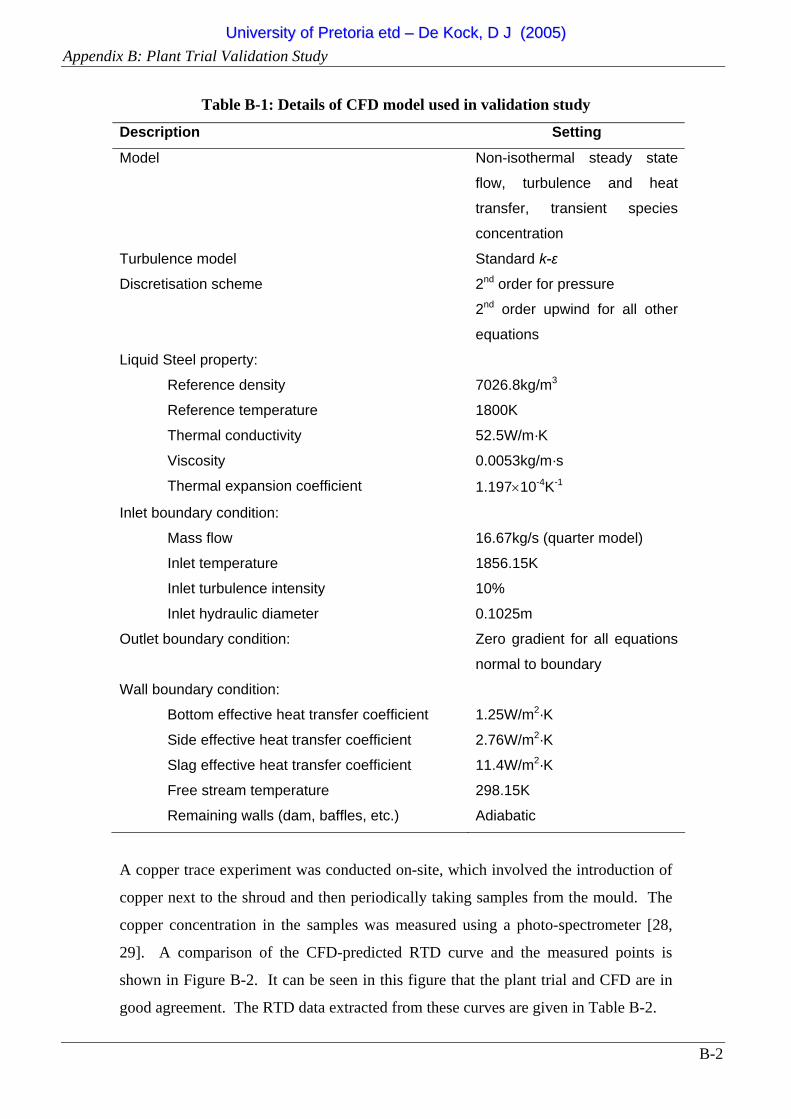
Appendix B: Plant Trial Validation Study
B-2
Table B-1: Details of CFD model used in validation study
Description Setting
Model Non-isothermal steady state
flow, turbulence and heat
transfer, transient species
concentration
Turbulence model Standard k-ε
Discretisation scheme 2nd order for pressure
2nd order upwind for all other
equations
Liquid Steel property:
Reference density
Reference temperature
Thermal conductivity
Viscosity
Thermal expansion coefficient
7026.8kg/m3
1800K
52.5W/m·K
0.0053kg/m·s
1.197×10⁻⁴K-1
Inlet boundary condition:
Mass flow
Inlet temperature
Inlet turbulence intensity
Inlet hydraulic diameter
16.67kg/s (quarter model)
1856.15K
10%
0.1025m
Outlet boundary condition:
Zero gradient for all equations
normal to boundary
Wall boundary condition:
Bottom effective heat transfer coefficient
Side effective heat transfer coefficient
Slag effective heat transfer coefficient
Free stream temperature
Remaining walls (dam, baffles, etc.)
1.25W/m2·K
2.76W/m2·K
11.4W/m2·K
298.15K
Adiabatic
A copper trace experiment was conducted on-site, which involved the introduction of
copper next to the shroud and then periodically taking samples from the mould. The
copper concentration in the samples was measured using a photo-spectrometer [28,
29]. A comparison of the CFD-predicted RTD curve and the measured points is
shown in Figure B-2. It can be seen in this figure that the plant trial and CFD are in
good agreement. The RTD data extracted from these curves are given in Table B-2.
UUnniivveerrssiittyy ooff PPrreettoorriiaa eettdd –– DDee KKoocckk,, DD JJ ((22000055))
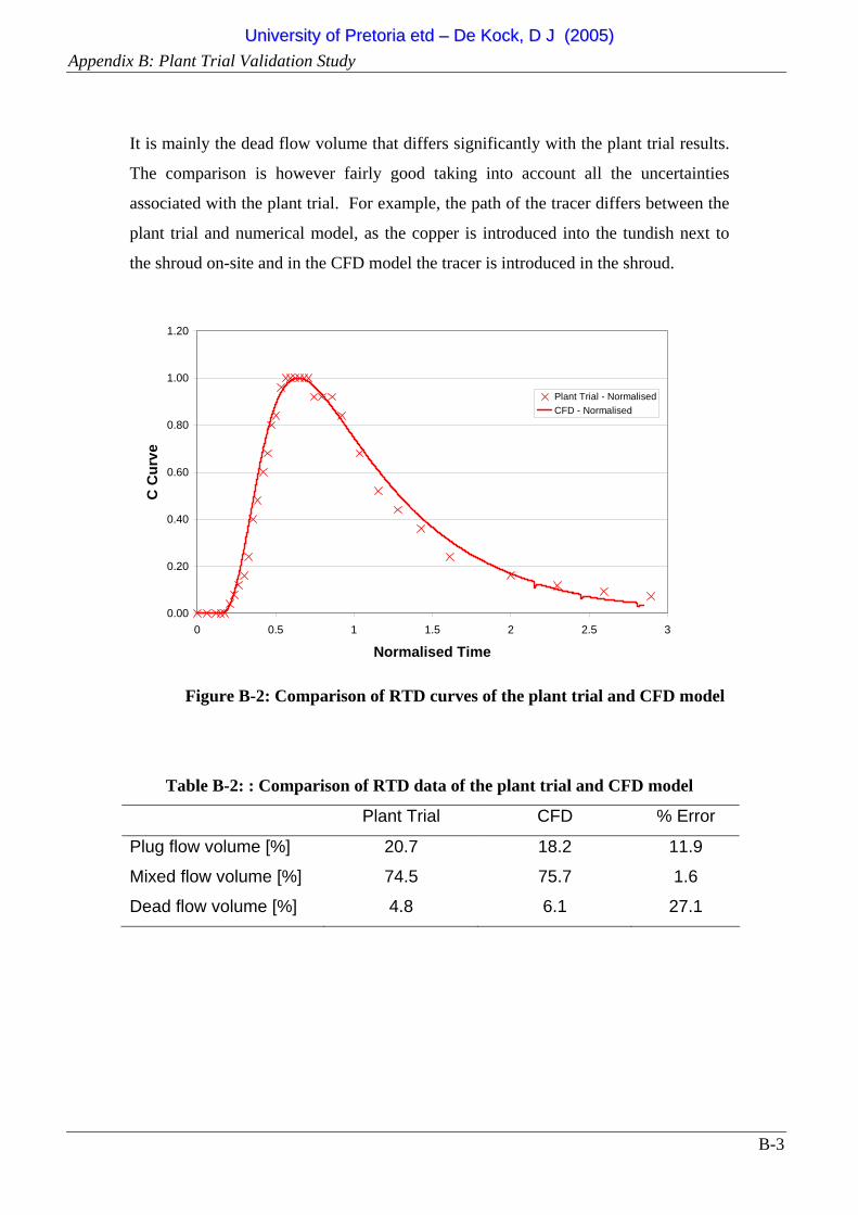
Appendix B: Plant Trial Validation Study
B-3
It is mainly the dead flow volume that differs significantly with the plant trial results.
The comparison is however fairly good taking into account all the uncertainties
associated with the plant trial. For example, the path of the tracer differs between the
plant trial and numerical model, as the copper is introduced into the tundish next to
the shroud on-site and in the CFD model the tracer is introduced in the shroud.
0.00
0.20
0.40
0.60
0.80
1.00
1.20
0 0.5 1 1.5 2 2.5 3
Normalised Time
C C
urve
Plant Trial - NormalisedCFD - Normalised
Figure B-2: Comparison of RTD curves of the plant trial and CFD model
Table B-2: : Comparison of RTD data of the plant trial and CFD model
Plant Trial CFD % Error
Plug flow volume [%] 20.7 18.2 11.9
Mixed flow volume [%] 74.5 75.7 1.6
Dead flow volume [%] 4.8 6.1 27.1
UUnniivveerrssiittyy ooff PPrreettoorriiaa eettdd –– DDee KKoocckk,, DD JJ ((22000055))
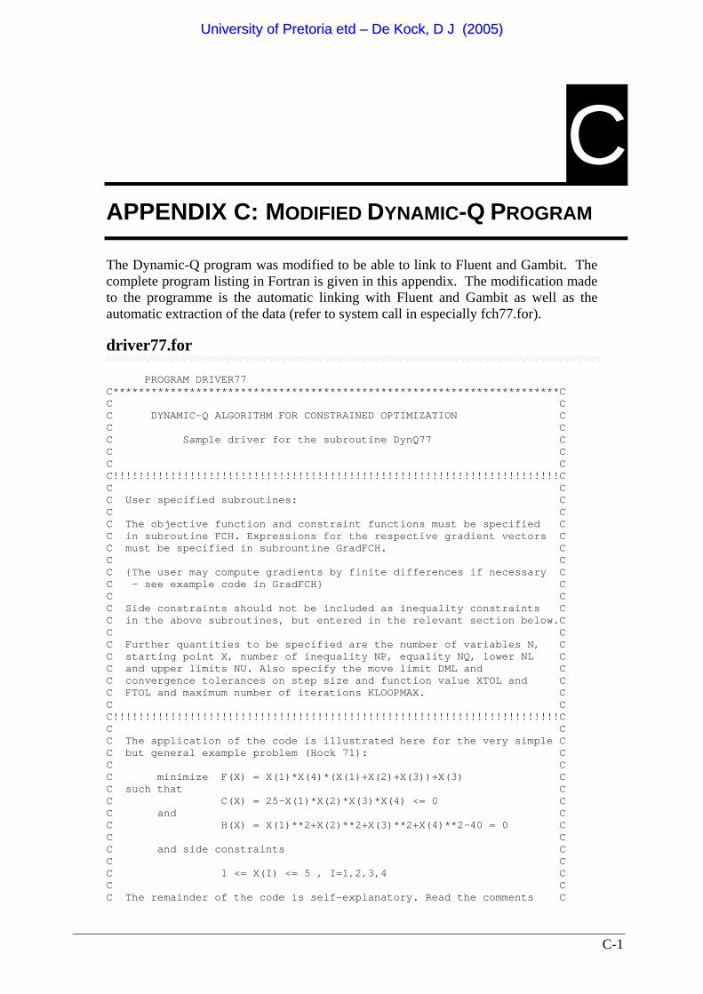
C-1
C APPENDIX C: MODIFIED DYNAMIC-Q PROGRAM The Dynamic-Q program was modified to be able to link to Fluent and Gambit. The complete program listing in Fortran is given in this appendix. The modification made to the programme is the automatic linking with Fluent and Gambit as well as the automatic extraction of the data (refer to system call in especially fch77.for).
driver77.for PROGRAM DRIVER77 C**********************************************************************C C C C DYNAMIC-Q ALGORITHM FOR CONSTRAINED OPTIMIZATION C C C C Sample driver for the subroutine DynQ77 C C C C C C!!!!!!!!!!!!!!!!!!!!!!!!!!!!!!!!!!!!!!!!!!!!!!!!!!!!!!!!!!!!!!!!!!!!!!C C C C User specified subroutines: C C C C The objective function and constraint functions must be specified C C in subroutine FCH. Expressions for the respective gradient vectors C C must be specified in subrountine GradFCH. C C C C {The user may compute gradients by finite differences if necessary C C - see example code in GradFCH} C C C C Side constraints should not be included as inequality constraints C C in the above subroutines, but entered in the relevant section below.C C C C Further quantities to be specified are the number of variables N, C C starting point X, number of inequality NP, equality NQ, lower NL C C and upper limits NU. Also specify the move limit DML and C C convergence tolerances on step size and function value XTOL and C C FTOL and maximum number of iterations KLOOPMAX. C C C C!!!!!!!!!!!!!!!!!!!!!!!!!!!!!!!!!!!!!!!!!!!!!!!!!!!!!!!!!!!!!!!!!!!!!!C C C C The application of the code is illustrated here for the very simple C C but general example problem (Hock 71): C C C C minimize F(X) = X(1)*X(4)*(X(1)+X(2)+X(3))+X(3) C C such that C C C(X) = 25-X(1)*X(2)*X(3)*X(4) <= 0 C C and C C H(X) = X(1)**2+X(2)**2+X(3)**2+X(4)**2-40 = 0 C C C C and side constraints C C C C 1 <= X(I) <= 5 , I=1,2,3,4 C C C C The remainder of the code is self-explanatory. Read the comments C
UUnniivveerrssiittyy ooff PPrreettoorriiaa eettdd –– DDee KKoocckk,, DD JJ ((22000055))
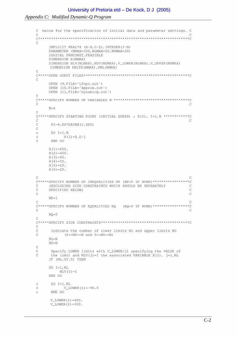
Appendix C: Modified Dynamic-Q Program
C-2
C below for the specification of initial data and parameter settings. C C C C**********************************************************************C C IMPLICIT REAL*8 (A-H,O-Z),INTEGER(I-N) PARAMETER (NMAX=300,NLMAX=50,NUMAX=50) LOGICAL PRNCONST,FEASIBLE DIMENSION X(NMAX) DIMENSION NLV(NLMAX),NUV(NUMAX),V_LOWER(NLMAX),V_UPPER(NUMAX) DIMENSION DELTX(NMAX),DML(NMAX) C C*****OPEN OUPUT FILES*************************************************C C OPEN (9,FILE='Lfopc.out') OPEN (10,FILE='Approx.out') OPEN (11,FILE='DynamicQ.out') C C*****SPECIFY NUMBER OF VARIABLES N ***********************************C C C N=6 C C*****SPECIFY STARTING POINT (INITIAL GUESS) : X(I), I=1,N ************C C C C PI=4.D0*DATAN(1.0D0) C c DO I=1,N c X(I)=8.D-1 c END DO X(1)=650. X(2)=400. X(3)=50. X(4)=50. X(5)=20. X(6)=20. C C C*****SPECIFY NUMBER OF INEQUALITIES NP (NP=0 IF NONE)*****************C C (EXCLUDING SIDE CONSTRAINTS WHICH SHOULD BE SEPARATELY C C SPECIFIED BELOW) C C C NP=1 C C C*****SPECIFY NUMBER OF EQUALITIES NQ (NQ=0 IF NONE)*****************C C C NQ=0 C C*****SPECIFY SIDE CONSTRAINTS*****************************************C C C Indicate the number of lower limits NL and upper limits NU C (0<=NU<=N and 0<=NU<=N) NL=N NU=N C C Specify LOWER limits with V_LOWER(j) specifying the VALUE of C the limit and NLV(j)=I the associated VARIABLE X(I), j=1,NL IF (NL.GT.0) THEN DO I=1,NL NLV(I)=I END DO c DO I=1,NL c V_LOWER(I)=-90.0 c END DO V_LOWER(1)=400. V_LOWER(2)=300.
UUnniivveerrssiittyy ooff PPrreettoorriiaa eettdd –– DDee KKoocckk,, DD JJ ((22000055))

Appendix C: Modified Dynamic-Q Program
C-3
V_LOWER(3)=40. V_LOWER(4)=0. V_LOWER(5)=0. V_LOWER(6)=0. END IF C Specify UPPER limits with V_UPPER(j) specifying the VALUE of C the limit and NUV(j)=I the associated VARIABLE X(I), j=1,NU IF (NU.GT.0) THEN DO I=1,NU NUV(I)=I END DO c DO I=1,NU c V_UPPER(I)=0.0 c END DO V_UPPER(1)=1200. V_UPPER(2)=600. V_UPPER(3)=10000. V_UPPER(4)=100. V_UPPER(5)=100. V_UPPER(6)=40. END IF C C*****GIVE THE CONVERGENCE TOLERANCES ON FUNC AND STEPNORM VALUES******C C FTOL=1.D-8 XTOL=1.D-5 C C*****SPECIFY THE MOVE LIMIT DML***************************************C C c DO I=1,N c DML(I)=30.0 c END DO DML(1)=200. DML(2)=100. DML(3)=10. DML(4)=25. DML(5)=25. DML(6)=10. C C*****GIVE THE MAXIMUM NUMBER OF ITERATIONS****************************C C KLOOPMAX=99 C C*****PRINT CONSTRAINTS TO SCREEN AT END OF PROGRAM?*******************C C YES: .TRUE. OR NO: .FALSE. C PRNCONST=.TRUE. C C*****SPECIFY SIZE OF FINITE DIFFERENCE STEP SIZE**********************C C c DO I=1,N c DELTX(I)=10.0 c END DO DELTX(1)=100. DELTX(2)=50. DELTX(3)=5. DELTX(4)=12. DELTX(5)=12.
UUnniivveerrssiittyy ooff PPrreettoorriiaa eettdd –– DDee KKoocckk,, DD JJ ((22000055))
Appendix C: Modified Dynamic-Q Program
C-4
DELTX(6)=5. C C*****FEASABLE LIMIT TO CHECK CONVERGENCE******************************C C (AMOUNT AN CONSTRAINT CAN BE VOILATED C FEASLIM=1.D-1 C C C*****CALL SUBROUTINE DYNQ77*******************************************C CALL DYNQ77(N,X,NP,NQ,NL,NU,NLV,NUV,V_LOWER,V_UPPER, * FTOL,XTOL,DML,KLOOPMAX,PRNCONST,DELTX,FEASLIM) STOP END PROGRAM DRIVER77
DynQ77.for SUBROUTINE DYNQ77(N,X,NP,NQ,NL,NU,NLV,NUV,V_LOWER,V_UPPER, * FTOL,XTOL,DML,KLOOPMAX,PRNCONST,DELTX,FEASLIM) C**********************************************************************C C C C DYNAMIC-Q ALGORITHM FOR CONSTRAINED OPTIMIZATION C C GENERAL MATHEMATICAL PROGRAMMING CODE (FORTRAN 77) C C ------------------------------------- C C C C Programmed by A.M. HAY C C Multidisciplinary Design Optimization Group (MDOG) C C Department of Mechanical Engineering, University of Pretoria C C June 2000 C C C C UPDATED : 18 August 2000 C C C C Specific modification made to code for implementation into C C Fluent by DJ de Kock 2003 C C C C This code is based on the Dynamic-Q method of Snyman documented C C in the paper "THE DYNAMIC-Q OPTIMIZATION METHOD: AN ALTERNATIVE C C TO SQP?" by J.A. Snyman and A.M. Hay. Technical Report, Dept Mech. C C Eng., UP. C C C C BRIEF DESCRIPTION C C ----------------- C C C C Dynamic-Q solves inequality and equality constrained optimization C C problems of the form: C C C C minimize F(X) , X={X(1),X(2),...,X(N)} C C such that C C Cj(X) <= 0 j=1,2,...,NP C C and C C Hj(X) = 0 j=1,2,...,NQ C C with lower bounds C C CLj(X) = V_LOWER(j)-X(NLV(j)) <= 0 j=1,2,...,NL C C and upper bounds C C CUj(X) = X(NUV(j))-V_UPPER(j) <= 0 j=1,2,...,NU C C C C This is a completely general code - the objective function and the C C constraints may be linear or non-linear. The code therefore solves C C LP, QP and NLP problems. C C C C!!!!!!!!!!!!!!!!!!!!!!!!!!!!!!!!!!!!!!!!!!!!!!!!!!!!!!!!!!!!!!!!!!!!!!C C C C Arguments of DynQ77 subroutine: C
UUnniivveerrssiittyy ooff PPrreettoorriiaa eettdd –– DDee KKoocckk,, DD JJ ((22000055))
Appendix C: Modified Dynamic-Q Program
C-5
C C C NAME DIMENSION TYPE DESCRIPTION C C N INTEGER Number of variables C C X X(N) DBL PREC Starting point C C NP INTEGER Number of inequality constraints C C NQ INTEGER Number of equality constraints C C NL INTEGER Number of lower bounds C C NU INTEGER Number of upper bounds C C NLV NLV(NL) INTEGER See description below C C NUV NUV(NU) INTEGER See description below C C V_LOWER V_LOWER(NL) DBL PREC See description below C C V_UPPER V_UPPER(NL) DBL PREC See description below C C FTOL DBL PREC Termination tolerance on func. value C C XTOL DBL PREC Termination tolerance on step size C C DML DBL PREC Move limit C C KLOOPMAX INTEGER Maximum number of iterations C C PRNCONST LOGICAL Controls printing of constraints to C C screen at end of program C C DELTX DELTX(N) DBL PREC Size of finite difference C C DML DML(N) DBL PREC Move limit for each variable C C FEASLIM DBL PREC Amount a constraint can be violated C C C C!!!!!!!!!!!!!!!!!!!!!!!!!!!!!!!!!!!!!!!!!!!!!!!!!!!!!!!!!!!!!!!!!!!!!!C C C C Specify LOWER limits with V_LOWER(j) specifying the VALUE of C C the limit and NLV(j)=I the associated VARIABLE X(I), j=1,NL C C Specify UPPER limits with V_UPPER(j) specifying the VALUE of C C the limit and NUV(j)=I the associated VARIABLE X(I), j=1,NU C C C C!!!!!!!!!!!!!!!!!!!!!!!!!!!!!!!!!!!!!!!!!!!!!!!!!!!!!!!!!!!!!!!!!!!!!!C C C C The application of the code is illustrated here for the very simple C C but general example problem (Hock 71): C C C C minimize F(X) = X(1)*X(4)*(X(1)+X(2)+X(3))+X(3) C C such that C C C(X) = 25-X(1)*X(2)*X(3)*X(4) <= 0 C C and C C H(X) = X(1)**2+X(2)**2+X(3)**2+X(4)**2-40 = 0 C C C C and side constraints C C C C 1 <= X(I) <= 5 , I=1,2,3,4 C C C C C C The remainder of the code is self-explanatory. Read the comments C C below for the specification of initial data and parameter settings. C C C C**********************************************************************C C IMPLICIT REAL*8 (A-H,O-Z),INTEGER(I-N) DIMENSION X(N),DELX(N),GF(N),GC_V(N),GH_V(N) DIMENSION C(NP),GC(NP,N),BCURV(NP) DIMENSION H(NQ),H_A(NQ),GH(NQ,N),CCURV(NQ) DIMENSION NLV(NL),NUV(NU),V_LOWER(NL),V_UPPER(NU) DIMENSION C_A(NP+NL+NU+N) DIMENSION X_H(0:KLOOPMAX,N),F_H(0:KLOOPMAX) DIMENSION C_H(0:KLOOPMAX,NP+NL+NU+N),H_H(0:KLOOPMAX,NQ) LOGICAL PRNCONST,FEASIBLE DIMENSION DELTX(N),DML(N) C C######################################################################C C**********************************************************************C C MAIN PROGRAM FOLLOWS: C**********************************************************************C C######################################################################C C
UUnniivveerrssiittyy ooff PPrreettoorriiaa eettdd –– DDee KKoocckk,, DD JJ ((22000055))
Appendix C: Modified Dynamic-Q Program
C-6
C*****INITIALIZE OUTPUT************************************************C WRITE (10,'(/1X,"DYNAMICQ OUTPUT FILE")') WRITE (10,'(1X,"--------------------")') WRITE (10,'(/1X,"Number of variables [N]=",I3)'), N WRITE (10,'(1X,"Number of inequality constraints [NP]=",I3)'),NP WRITE (10,'(1X,"Number of equality constraints [NQ]=",I3)'),NQ WRITE (10,'(/1X,"Move limit=",5F12.8)'), (DML(I),I=1,N) WRITE (*,'(1X,"DYNAMICQ OPTIMIZATION ALGORITHM")') WRITE (*,'(1X,"-------------------------------")') WRITE (*,'(/1X,A))') 'Iter Function value ? XNORM RFD' WRITE (*,'(1X,A)') '-------------------------------------------' WRITE (11,'(1X,"DYNAMICQ OPTIMIZATION ALGORITHM")') WRITE (11,'(1X,"-------------------------------")') WRITE (11,'(/1X,A)') * 'Iter Function value ? XNORM RFD' WRITE (11,'(5(1X,A,I2,A,8X))') ('X(',I,')',I=1,N) C Initialize outer loop counter KLOOP=0 C Arbitrary large values to prevent premature termination F_LOW=1.D6 RFD=1.D6 RELXNORM=1.D6 DO I=1,(NP+NL+NU+N) C_A(I)=0.D0 END DO C Specify initial approximation curvatures ACURV=0.D0 DO I=1,NP BCURV(I)=0.d0 END DO DO I=1,NQ CCURV(I)=0.D0 END DO C*****START OF OUTER OPTIMIZATION LOOP*********************************C DO WHILE (KLOOP.LE.KLOOPMAX) C*****APPROXIMATE FUNCTIONS********************************************C C Determine function values CALL FCH(N,NP,NQ,X,F,C,H,KLOOP,0) C Calculate relative step size IF (KLOOP.GT.0) THEN DELXNORM=0.D0 XNORM=0.D0 DO I=1,N DELXNORM=DELXNORM+(X_H(KLOOP-1,I)-X(I))**2 XNORM=XNORM+X(I)**2 END DO DELXNORM=DSQRT(DELXNORM) XNORM=DSQRT(XNORM) RELXNORM=DELXNORM/(1.D0+XNORM) END IF C Determine lowest feasible function value so far C FEASLIM=1.D-6 IF (KLOOP.GT.0) THEN FEASIBLE=.TRUE. DO I=1,NP IF (C(I).GT.FEASLIM) THEN FEASIBLE=.FALSE.
UUnniivveerrssiittyy ooff PPrreettoorriiaa eettdd –– DDee KKoocckk,, DD JJ ((22000055))
Appendix C: Modified Dynamic-Q Program
C-7
END IF END DO DO I=1,NQ IF (DABS(H(I)).GT.FEASLIM) THEN FEASIBLE=.FALSE. END IF END DO DO I=1,NL IF (C_A(I+NP).GT.FEASLIM) THEN FEASIBLE=.FALSE. END IF END DO DO I=1,NU IF (C_A(I+NP+NL).GT.FEASLIM) THEN FEASIBLE=.FALSE. END IF END DO END IF C Calculate relative function difference IF (F_LOW.NE.1.D6.AND.FEASIBLE) THEN RFD=DABS(F-F_LOW)/(1+DABS(F)) END IF IF (FEASIBLE.AND.F.LT.F_LOW) THEN F_LOW=F END IF C Store function values DO I=1,N X_H(KLOOP,I)=X(I) END DO F_H(KLOOP)=F DO I=1,NP C_H(KLOOP,I)=C(I) END DO DO I=1,NL C_H(KLOOP,NP+I)=C_A(NP+I) END DO DO I=1,NU C_H(KLOOP,NP+NL+I)=C_A(NP+NL+I) END DO DO I=1,N C_H(KLOOP,NP+NL+NU+I)=C_A(NP+NL+NU+I) END DO ! C_H(KLOOP,NP+NL+NU+1)=C_A(NP+NL+NU+1) DO I=1,NQ H_H(KLOOP,I)=H(I) END DO C Determine gradients CALL GRADFCH(N,X,NP,NQ,GF,GC,GH,F,C,H,DELTX,KLOOP) C Calculate curvatures IF (KLOOP.GE.1) THEN DELXNORM=0.D0 DO I=1,N DELX(I)=X_H(KLOOP-1,I)-X_H(KLOOP,I) DELXNORM=DELXNORM+DELX(I)**2 END DO C Dot product of GF and DELX DP=0.D0 DO I=1,N DP=DP+GF(I)*DELX(I) END DO
UUnniivveerrssiittyy ooff PPrreettoorriiaa eettdd –– DDee KKoocckk,, DD JJ ((22000055))
Appendix C: Modified Dynamic-Q Program
C-8
ACURV=2.*(F_H(KLOOP-1)-F_H(KLOOP)-DP) * /DELXNORM DO J=1,NP C Extract relevant vector from GC DO I=1,N GC_V(I)=GC(J,I) END DO C Dot product of GC_V and DELX DP=0.D0 DO I=1,N DP=DP+GC_V(I)*DELX(I) END DO C Calculate corresponding cuvature BCURV(J) BCURV(J)=2.*(C_H(KLOOP-1,J)-C_H(KLOOP,J) * -DP)/DELXNORM END DO DO J=1,NQ C Extract relevant vector from GC DO I=1,N GH_V(I)=GH(J,I) END DO C Dot product of GH_V and DELX DP=0.D0 DO I=1,N DP=DP+GH_V(I)*DELX(I) END DO C Calculate corresponding curvature CCURV(J) CCURV(J)=2.*(H_H(KLOOP-1,J)-H_H(KLOOP,J) * -DP)/DELXNORM END DO END IF C*****RECORD PARAMETERS FOR THE ITERATION******************************C C Write approximation constants to Approx.out WRITE (10,'(/1X,A,I3)') 'Iteration ',KLOOP WRITE (10,'(1X,A)') '--------------' WRITE (10,'(1X,A)') 'X=' WRITE (10,'(1X,5(F12.8))') (X(I), I=1,N) WRITE (10,'(/1X,A,D15.8)') 'F=',F DO I=1,NP WRITE (10,'(1X,A,I2,A,D15.8)') 'C(',I,')=',C(I) END DO DO I=1,NQ WRITE (10,'(1X,A,I2,A,D15.8)') 'H(',I,')=',H(I) END DO WRITE (10,'(/1X,A,D15.8)') 'Acurv=',ACURV DO I=1,NP WRITE (10,'(1X,A,I2,A,D15.8)') 'Bcurv(',I,')=',BCURV(I) END DO DO I=1,NQ WRITE (10,'(1X,A,I2,A,D15.8)') 'Ccurv(',I,')=',CCURV(I) END DO C Write solution to file IF (KLOOP.EQ.0) THEN WRITE (11,'(1X,I4,1X,D19.12,1X,L1)') * KLOOP,F,FEASIBLE WRITE (11,'(5(1X,D13.6))') (X(I),I=1,N) ELSE IF (RFD.NE.1.D6) THEN
UUnniivveerrssiittyy ooff PPrreettoorriiaa eettdd –– DDee KKoocckk,, DD JJ ((22000055))
Appendix C: Modified Dynamic-Q Program
C-9
WRITE (11,'(1X,I4,1X,D19.12,1X,L1,1X,D9.3,1X,D9.3)') * KLOOP,F,FEASIBLE,RELXNORM,RFD WRITE (11,'(5(1X,D13.6))') (X(I),I=1,N) ELSE WRITE (11,'(1X,I4,1X,D19.12,1X,L1,1X,D9.3,10X)') * KLOOP,F,FEASIBLE,RELXNORM WRITE (11,'(5(1X,D13.6))') (X(I),I=1,N) END IF END IF C Write solution to screen IF (KLOOP.EQ.0) THEN WRITE (*,'(1X,I4,1X,D14.7,1X,L1)') KLOOP,F,FEASIBLE ELSE IF (RFD.NE.1.D6.AND.FEASIBLE) THEN WRITE (*,'(1X,I4,1X,D15.8,1X,L1,1X,D9.3,1X,D9.3)') * KLOOP,F,FEASIBLE,RELXNORM,RFD ELSE WRITE (*,'(1X,I4,1X,D15.8,1X,L1,1X,D9.3)') * KLOOP,F,FEASIBLE,RELXNORM END IF END IF C Exit do loop here on final iteration IF (KLOOP.EQ.KLOOPMAX.OR.RFD.LT.FTOL.OR.RELXNORM.LT.XTOL) THEN IF (KLOOP.EQ.KLOOPMAX) THEN WRITE(*,'(1X,A)') 'Terminated on max number of steps' WRITE(11,'(1X,A)') 'Terminated on max number of steps' END IF IF (RFD.LT.FTOL) THEN WRITE(*,'(1X,A)') 'Terminated on function value' WRITE(11,'(1X,A)') 'Terminated on function value' END IF IF (RELXNORM.LT.XTOL) THEN WRITE(*,'(1X,A)') 'Terminated on step size' WRITE(11,'(1X,A)') 'Terminated on step size' END IF WRITE(*,'(1X,A)') ' ' WRITE(11,'(1X,A)') ' ' EXIT END IF C*****SOLVE THE APPROXIMATED SUBPROBLEM********************************C CALL LFOPC77(N,X,NP,NQ,F,C,H,GF,GC,GH,ACURV,BCURV,CCURV,DML, * F_A,C_A,H_A,NL,NU,NLV,NUV,V_LOWER,V_UPPER,xtol,KLOOP) C Record solution to approximated problem WRITE (10,'(/A)') 'Solution of approximated problem:' WRITE (10,'(/1X,A)') 'X=' WRITE (10,'(1X,5(F12.8))') (X(I), I=1,N) WRITE (10,'(/1X,A,D15.8)') 'F_A=',F_A DO I=1,NP+NL+NU+N WRITE (10,'(1X,A,I2,A,D15.8)') 'C_A(',I,')=',C_A(I) END DO DO I=1,NQ WRITE (10,'(1X,A,I2,A,D15.8)') 'H_A(',I,')=',H_A(I) END DO C Increment outer loop counter KLOOP=KLOOP+1 END DO C Write final constraint values to file WRITE (11,'(/1X,A)') 'Final function value:' WRITE (11,'(1X,A,D19.12)') 'F=',F
UUnniivveerrssiittyy ooff PPrreettoorriiaa eettdd –– DDee KKoocckk,, DD JJ ((22000055))

Appendix C: Modified Dynamic-Q Program
C-10
IF (NP.GT.0) THEN WRITE (11,'(/1X,A)') 'Final inequality constraint * function values:' DO I=1,NP WRITE (11,'(1X,A,I2,A,D15.8)') 'C(',I,')=',C(I) END DO END IF IF (NQ.GT.0) THEN WRITE (11,'(/1X,A)') 'Final * equality constraint function values:' DO I=1,NQ WRITE (11,'(1X,A,I2,A,D15.8)') 'H(',I,')=',H(I) END DO END IF IF (NL.GT.0) THEN WRITE (11,'(/1X,A)') 'Final side (lower) * constraint function values:' DO I=1,NL WRITE (11,'(1X,A,I2,A,D15.8)') 'C(X(',NLV(I),'))=' * ,C_A(NP+I) END DO END IF IF (NU.GT.0) THEN WRITE (11,'(/1X,A)') 'Final side (upper) * constraint function values:' DO I=1,NU WRITE (11,'(1X,A,I2,A,D15.8)') 'C(X(',NUV(I),'))=' * ,C_A(NP+NL+I) END DO END IF C Write final X values to screen (DDK 23/11/2000) WRITE (*,'(1/X,A)') 'Final design variables values:' DO I=1,N WRITE (*,'(1X,A,I2,A,D15.8)') 'X(',I,')=',X(I) ENDDO WRITE (*,*) C Write final constraint values to screen IF (PRNCONST) THEN PAUSE 'Constraint values follow: Press enter to continue' IF (NP.GT.0) THEN WRITE (*,'(/1X,A)') 'Final inequality constraint * function values:' DO I=1,NP WRITE (*,'(1X,A,I2,A,D15.8)') 'C(',I,')=',C(I) END DO END IF IF (NQ.GT.0) THEN WRITE (*,'(/1X,A)') 'Final * equality constraint function values:' DO I=1,NQ WRITE (*,'(1X,A,I2,A,D15.8)') 'H(',I,')=',H(I) END DO END IF IF (NL.GT.0) THEN WRITE (*,'(/1X,A)') 'Final side (lower) * constraint function values:' DO I=1,NL WRITE (*,'(1X,A,I2,A,D15.8)') 'C(X(',NLV(I),'))=' * ,C_A(NP+I) END DO END IF IF (NU.GT.0) THEN WRITE (*,'(/1X,A)') 'Final side (upper) * constraint function values:' DO I=1,NU WRITE (*,'(1X,A,I2,A,D15.8)') 'C(X(',NUV(I),'))='
UUnniivveerrssiittyy ooff PPrreettoorriiaa eettdd –– DDee KKoocckk,, DD JJ ((22000055))
Appendix C: Modified Dynamic-Q Program
C-11
* ,C_A(NP+NL+I) END DO END IF END IF RETURN END SUBROUTINE DYNQ77
gradfch77.for C**********************************************************************C C USER SPECIFIED SUBROUTINE C C C SUBROUTINE GRADFCH(N,X,NP,NQ,GF,GC,GH,F_X,C_X,H_X,DELTX,KLOOP) C C C COMPUTE THE GRADIENT VECTORS OF THE OBJECTIVE FUNCTION F, C C INEQUALITY CONSTRAINTS C, AND EQUALITY CONSTRAINTS H C C W.R.T. THE VARIABLES X(I): C C GF(I),I=1,N C C GC(J,I), J=1,NP I=1,N C C GH(J,I), J=1,NQ I=1,N C C C C**********************************************************************C IMPLICIT REAL*8 (A-H,O-Z),INTEGER(I-N) DIMENSION X(N),GF(N),GC(NP,N),GH(NQ,N) DIMENSION DX(N),C_X(NP),H_X(NQ),C_D(NP),H_D(NQ) DIMENSION DELTX(N) C Determine gradients by finite difference ! DELTX=1.D-5 ! Finite difference interval ! CALL FCH(N,NP,NQ,X,F_X,C_X,H_X) DO I=1,N DO J=1,N IF (I.EQ.J) THEN DX(J)=X(J)+DELTX(J) ELSE DX(J)=X(J) END IF END DO CALL FCH(N,NP,NQ,DX,F_D,C_D,H_D,KLOOP,I) GF(I)=(F_D-F_X)/DELTX(I) DO J=1,NP GC(J,I)=(C_D(J)-C_X(J))/DELTX(J) END DO DO J=1,NQ GH(J,I)=(H_D(J)-H_X(J))/DELTX(J) END DO END DO RETURN END SUBROUTINE GRADFCH
fch77.for C**********************************************************************C C USER SPECIFIED SUBROUTINE C C C SUBROUTINE FCH(N,NP,NQ,X,F,C,H,KLOOP,NLOOP)
UUnniivveerrssiittyy ooff PPrreettoorriiaa eettdd –– DDee KKoocckk,, DD JJ ((22000055))
Appendix C: Modified Dynamic-Q Program
C-12
C C C COMPUTE OBJECTIVE FUNCTION : F C C INEQUALITY CONSTRAINT FUNCTIONS : C C C EQUALITY CONSTRAINT FUNCTIONS : H C C C C C C**********************************************************************C IMPLICIT REAL*8 (A-H,O-Z),INTEGER(I-N) DIMENSION X(N),C(NP),H(NQ) integer ios,node real time,maktke,tke C Fluent Simulation (running on lnx86 DDK - 2002) C Call Pre-processor OPEN (33,FILE='parameterset.jou') DO i=1,N WRITE (33,'(A,I1,A,D20.8)') '$x',i,' = ',X(i) END DO CLOSE(33) C Call Gambit CALL SYSTEM('gambit_script') ! For windows use the file command below ! CALL SYSTEM('gambit_script.bat') C Call Fluent CALL SYSTEM('fluent_script') ! For windows use the file command below ! CALL SYSTEM('fluent_script.bat') ! Example of what should be in script: fluent 3d -g -wait -i input.jou C Call Post maxtke = 0. ! Extract maximum tke from file open(99,file='tke.out') read(99,*) read(99,*) read(99,*) read(99,*) ios=0 READ (99, *,iostat=ios) time,tke DO WHILE (ios.eq.0) ! Check maximum if (tke.gt.maxtke) maxtke=tke READ (99, *,iostat=ios) time,tke END DO close(99) F = maxtke ! Move case, data etc. to new file name OPEN (33,FILE='move_script') WRITE (33,'(A, I2.2, A, I2.2, A)') # 'mv groot_impact.cas.gz groot_impact',KLOOP,'_',NLOOP,'.cas.gz' WRITE (33,'(A,I2.2,A,I2.2,A)') # 'mv groot_impact.dat.gz groot_impact',KLOOP,'_',NLOOP,'.dat.gz' WRITE (33,'(A,I2.2,A,I2.2,A)') # 'mv tke.out tke',KLOOP,'_',NLOOP,'.out' CLOSE(33) CALL SYSTEM('chmod u+x move_script') CALL SYSTEM('./move_script') CALL SYSTEM('rm move_script') ! Constraint C(1) = 200. - x(2) + x(3) RETURN END SUBROUTINE FCH
UUnniivveerrssiittyy ooff PPrreettoorriiaa eettdd –– DDee KKoocckk,, DD JJ ((22000055))

D-1
D APPENDIX D: GAMBIT JOURNAL FILES FOR IMPACT PAD CREATION AND MESH
GENERATION This appendix contains the two Gambit journal files that were used to automatically create the impact pad and mesh the geometry used in Case study 3 of Chapter 4. The first file (gambitsetup.jou) creates the impact pad according to the supplied design variables. The design variables are defined as variables at the start of the journal (e.g. $l, $h1 etc). The second file (groot_opt.jou) imports the impact pad created by the previous file into an existing model of the tundish. The journal file then moves the impact pad to the correct location and does the necessary operations on it, after which the geometry is meshed. gambitsetup.jou / Impact pad creation / DdK 19/2/2002 / DdK 13/2/2002 - Added dam at outlet / Define paramaters $w1 = 650. $w2 = 250. $l = <<l>> $h1 = <<h1>> $h2 = <<h2>> $d1 = <<d1>>
UUnniivveerrssiittyy ooff PPrreettoorriiaa eettdd –– DDee KKoocckk,, DD JJ ((22000055))
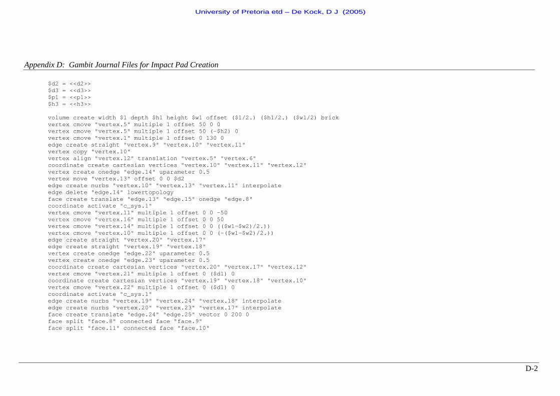
Appendix D: Gambit Journal Files for Impact Pad Creation
D-2
$d2 = <<d2>> $d3 = <<d3>> $p1 = <<p1>> $h3 = <<h3>> volume create width $l depth $h1 height $w1 offset ($l/2.) ($h1/2.) ($w1/2) brick vertex cmove "vertex.5" multiple 1 offset 50 0 0 vertex cmove "vertex.5" multiple 1 offset 50 (-$h2) 0 vertex cmove "vertex.1" multiple 1 offset 0 130 0 edge create straight "vertex.9" "vertex.10" "vertex.11" vertex copy "vertex.10" vertex align "vertex.12" translation "vertex.5" "vertex.6" coordinate create cartesian vertices "vertex.10" "vertex.11" "vertex.12" vertex create onedge "edge.14" uparameter 0.5 vertex move "vertex.13" offset 0 0 $d2 edge create nurbs "vertex.10" "vertex.13" "vertex.11" interpolate edge delete "edge.14" lowertopology face create translate "edge.13" "edge.15" onedge "edge.8" coordinate activate "c_sys.1" vertex cmove "vertex.11" multiple 1 offset 0 0 -50 vertex cmove "vertex.16" multiple 1 offset 0 0 50 vertex cmove "vertex.14" multiple 1 offset 0 0 (($w1-$w2)/2.)) vertex cmove "vertex.10" multiple 1 offset 0 0 (-($w1-$w2)/2.)) edge create straight "vertex.20" "vertex.17" edge create straight "vertex.19" "vertex.18" vertex create onedge "edge.22" uparameter 0.5 vertex create onedge "edge.23" uparameter 0.5 coordinate create cartesian vertices "vertex.20" "vertex.17" "vertex.12" vertex cmove "vertex.21" multiple 1 offset 0 ($d1) 0 coordinate create cartesian vertices "vertex.19" "vertex.18" "vertex.10" vertex cmove "vertex.22" multiple 1 offset 0 ($d1) 0 coordinate activate "c_sys.1" edge create nurbs "vertex.19" "vertex.24" "vertex.18" interpolate edge create nurbs "vertex.20" "vertex.23" "vertex.17" interpolate face create translate "edge.24" "edge.25" vector 0 200 0 face split "face.8" connected face "face.9" face split "face.11" connected face "face.10"
UUnniivveerrssiittyy ooff PPrreettoorriiaa eettdd –– DDee KKoocckk,, DD JJ ((22000055))
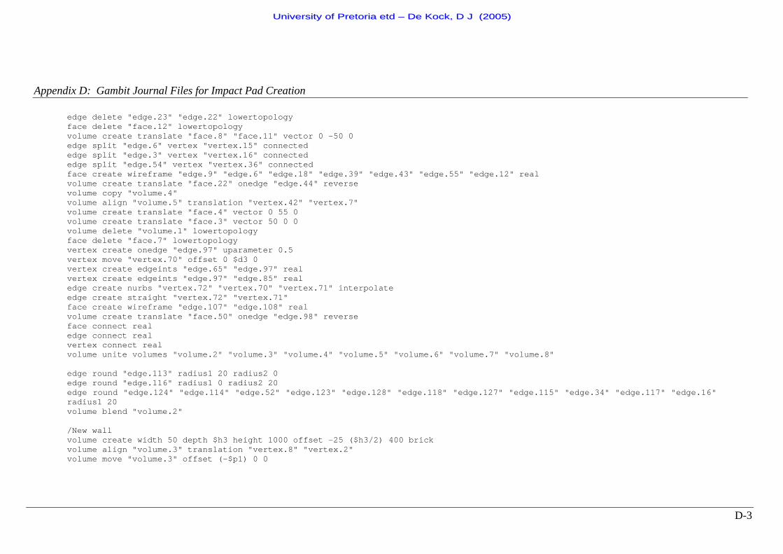
Appendix D: Gambit Journal Files for Impact Pad Creation
D-3
edge delete "edge.23" "edge.22" lowertopology face delete "face.12" lowertopology volume create translate "face.8" "face.11" vector 0 -50 0 edge split "edge.6" vertex "vertex.15" connected edge split "edge.3" vertex "vertex.16" connected edge split "edge.54" vertex "vertex.36" connected face create wireframe "edge.9" "edge.6" "edge.18" "edge.39" "edge.43" "edge.55" "edge.12" real volume create translate "face.22" onedge "edge.44" reverse volume copy "volume.4" volume align "volume.5" translation "vertex.42" "vertex.7" volume create translate "face.4" vector 0 55 0 volume create translate "face.3" vector 50 0 0 volume delete "volume.1" lowertopology face delete "face.7" lowertopology vertex create onedge "edge.97" uparameter 0.5 vertex move "vertex.70" offset 0 $d3 0 vertex create edgeints "edge.65" "edge.97" real vertex create edgeints "edge.97" "edge.85" real edge create nurbs "vertex.72" "vertex.70" "vertex.71" interpolate edge create straight "vertex.72" "vertex.71" face create wireframe "edge.107" "edge.108" real volume create translate "face.50" onedge "edge.98" reverse face connect real edge connect real vertex connect real volume unite volumes "volume.2" "volume.3" "volume.4" "volume.5" "volume.6" "volume.7" "volume.8" edge round "edge.113" radius1 20 radius2 0 edge round "edge.116" radius1 0 radius2 20 edge round "edge.124" "edge.114" "edge.52" "edge.123" "edge.128" "edge.118" "edge.127" "edge.115" "edge.34" "edge.117" "edge.16" radius1 20 volume blend "volume.2" /New wall volume create width 50 depth $h3 height 1000 offset -25 ($h3/2) 400 brick volume align "volume.3" translation "vertex.8" "vertex.2" volume move "volume.3" offset (-$p1) 0 0
UUnniivveerrssiittyy ooff PPrreettoorriiaa eettdd –– DDee KKoocckk,, DD JJ ((22000055))
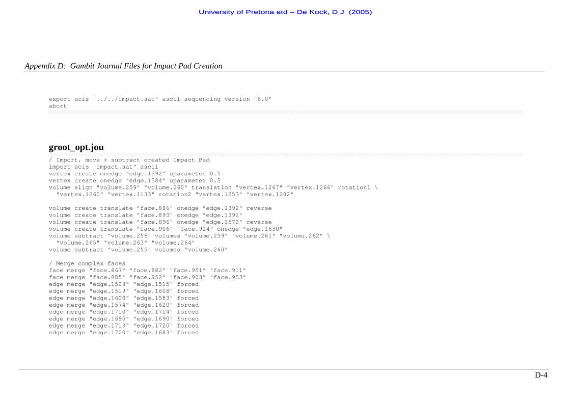
Appendix D: Gambit Journal Files for Impact Pad Creation
D-4
export acis "../../impact.sat" ascii sequencing version "6.0" abort
groot_opt.jou / Import, move + subtract created Impact Pad import acis "impact.sat" ascii vertex create onedge "edge.1392" uparameter 0.5 vertex create onedge "edge.1584" uparameter 0.5 volume align "volume.259" "volume.260" translation "vertex.1267" "vertex.1266" rotation1 \ "vertex.1260" "vertex.1133" rotation2 "vertex.1253" "vertex.1202" volume create translate "face.886" onedge "edge.1392" reverse volume create translate "face.893" onedge "edge.1392" volume create translate "face.896" onedge "edge.1572" reverse volume create translate "face.906" "face.914" onedge "edge.1630" volume subtract "volume.256" volumes "volume.259" "volume.261" "volume.262" \ "volume.265" "volume.263" "volume.264" volume subtract "volume.255" volumes "volume.260" / Merge complex faces face merge "face.867" "face.882" "face.951" "face.911" face merge "face.885" "face.952" "face.903" "face.953" edge merge "edge.1528" "edge.1515" forced edge merge "edge.1519" "edge.1608" forced edge merge "edge.1600" "edge.1583" forced edge merge "edge.1574" "edge.1620" forced edge merge "edge.1710" "edge.1714" forced edge merge "edge.1695" "edge.1690" forced edge merge "edge.1719" "edge.1720" forced edge merge "edge.1700" "edge.1683" forced
UUnniivveerrssiittyy ooff PPrreettoorriiaa eettdd –– DDee KKoocckk,, DD JJ ((22000055))
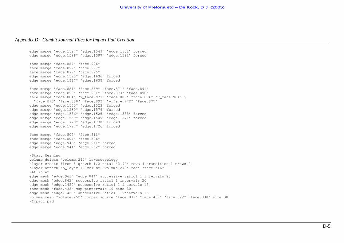
Appendix D: Gambit Journal Files for Impact Pad Creation
D-5
edge merge "edge.1527" "edge.1543" "edge.1551" forced edge merge "edge.1586" "edge.1597" "edge.1592" forced face merge "face.887" "face.926" face merge "face.897" "face.927" face merge "face.877" "face.925" edge merge "edge.1590" "edge.1636" forced edge merge "edge.1567" "edge.1635" forced face merge "face.881" "face.869" "face.871" "face.891" face merge "face.899" "face.901" "face.873" "face.890" face merge "face.884" "v_face.971" "face.889" "face.894" "v_face.964" \ "face.898" "face.880" "face.892" "v_face.972" "face.875" edge merge "edge.1545" "edge.1523" forced edge merge "edge.1580" "edge.1579" forced edge merge "edge.1536" "edge.1525" "edge.1538" forced edge merge "edge.1559" "edge.1549" "edge.1571" forced edge merge "edge.1729" "edge.1730" forced edge merge "edge.1727" "edge.1726" forced face merge "face.507" "face.511" face merge "face.504" "face.506" edge merge "edge.946" "edge.941" forced edge merge "edge.944" "edge.952" forced /Start Meshing volume delete "volume.247" lowertopology blayer create first 8 growth 1.2 total 42.944 rows 4 transition 1 trows 0 blayer attach "b_layer.1" volume "volume.248" face "face.516" /At inlet edge mesh "edge.961" "edge.844" successive ratio1 1 intervals 28 edge mesh "edge.842" successive ratio1 1 intervals 20 edge mesh "edge.1450" successive ratio1 1 intervals 15 face mesh "face.438" map pintervals 10 size 30 edge mesh "edge.1450" successive ratio1 1 intervals 15 volume mesh "volume.252" cooper source "face.831" "face.437" "face.522" "face.838" size 30 /Impact pad
UUnniivveerrssiittyy ooff PPrreettoorriiaa eettdd –– DDee KKoocckk,, DD JJ ((22000055))
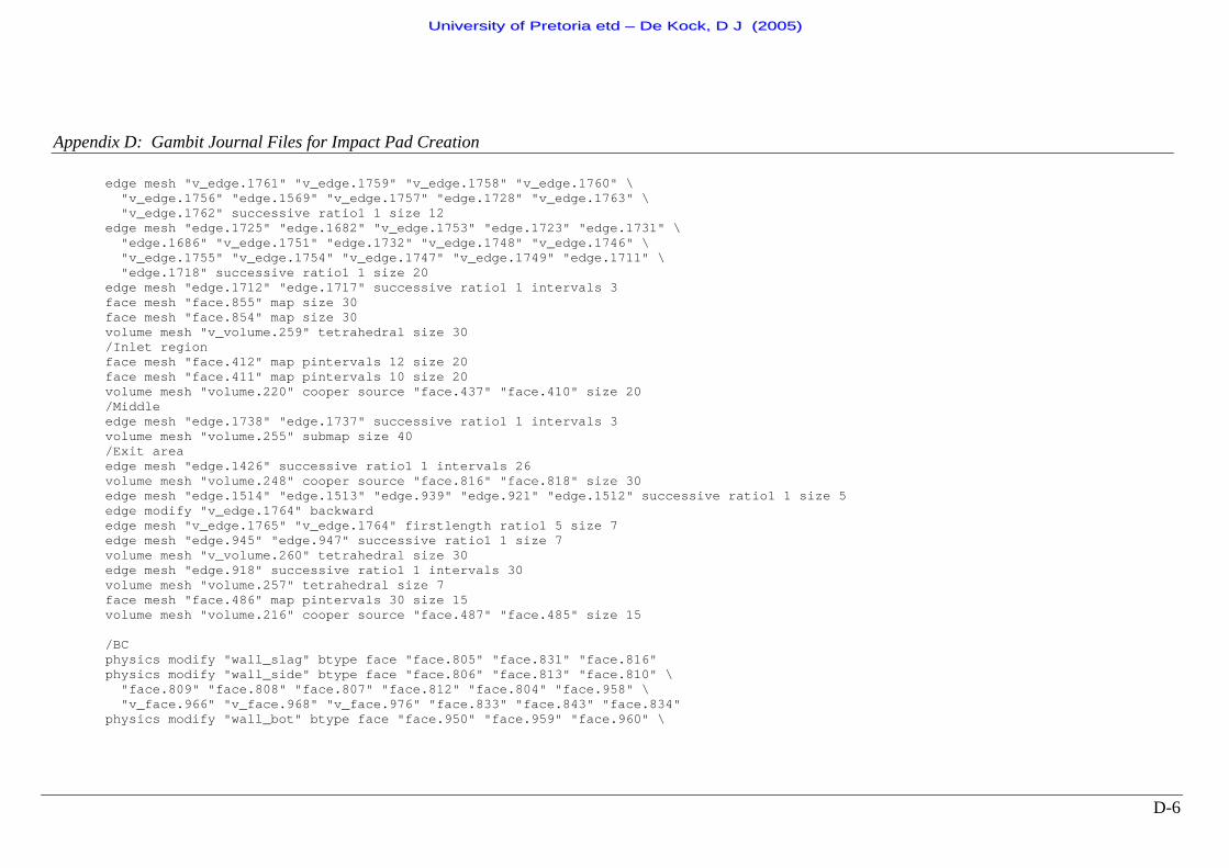
Appendix D: Gambit Journal Files for Impact Pad Creation
D-6
edge mesh "v_edge.1761" "v_edge.1759" "v_edge.1758" "v_edge.1760" \ "v_edge.1756" "edge.1569" "v_edge.1757" "edge.1728" "v_edge.1763" \ "v_edge.1762" successive ratio1 1 size 12 edge mesh "edge.1725" "edge.1682" "v_edge.1753" "edge.1723" "edge.1731" \ "edge.1686" "v_edge.1751" "edge.1732" "v_edge.1748" "v_edge.1746" \ "v_edge.1755" "v_edge.1754" "v_edge.1747" "v_edge.1749" "edge.1711" \ "edge.1718" successive ratio1 1 size 20 edge mesh "edge.1712" "edge.1717" successive ratio1 1 intervals 3 face mesh "face.855" map size 30 face mesh "face.854" map size 30 volume mesh "v_volume.259" tetrahedral size 30 /Inlet region face mesh "face.412" map pintervals 12 size 20 face mesh "face.411" map pintervals 10 size 20 volume mesh "volume.220" cooper source "face.437" "face.410" size 20 /Middle edge mesh "edge.1738" "edge.1737" successive ratio1 1 intervals 3 volume mesh "volume.255" submap size 40 /Exit area edge mesh "edge.1426" successive ratio1 1 intervals 26 volume mesh "volume.248" cooper source "face.816" "face.818" size 30 edge mesh "edge.1514" "edge.1513" "edge.939" "edge.921" "edge.1512" successive ratio1 1 size 5 edge modify "v_edge.1764" backward edge mesh "v_edge.1765" "v_edge.1764" firstlength ratio1 5 size 7 edge mesh "edge.945" "edge.947" successive ratio1 1 size 7 volume mesh "v_volume.260" tetrahedral size 30 edge mesh "edge.918" successive ratio1 1 intervals 30 volume mesh "volume.257" tetrahedral size 7 face mesh "face.486" map pintervals 30 size 15 volume mesh "volume.216" cooper source "face.487" "face.485" size 15 /BC physics modify "wall_slag" btype face "face.805" "face.831" "face.816" physics modify "wall_side" btype face "face.806" "face.813" "face.810" \ "face.809" "face.808" "face.807" "face.812" "face.804" "face.958" \ "v_face.966" "v_face.968" "v_face.976" "face.833" "face.843" "face.834" physics modify "wall_bot" btype face "face.950" "face.959" "face.960" \
UUnniivveerrssiittyy ooff PPrreettoorriiaa eettdd –– DDee KKoocckk,, DD JJ ((22000055))
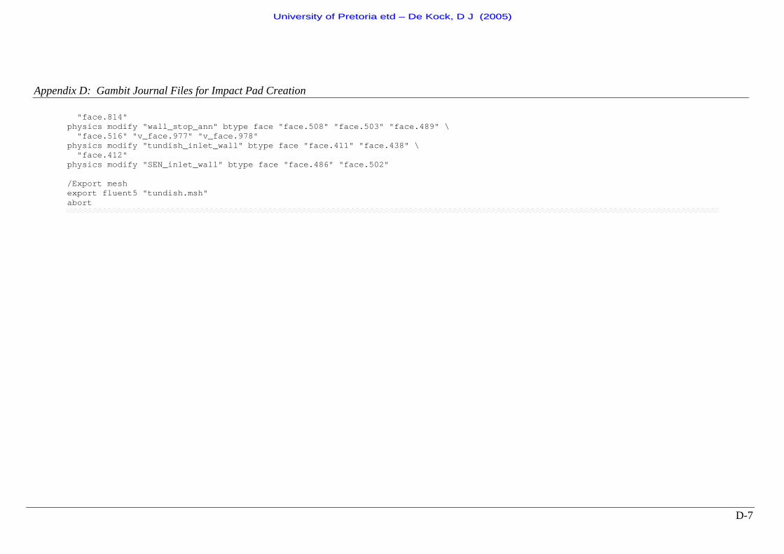
Appendix D: Gambit Journal Files for Impact Pad Creation
D-7
"face.814" physics modify "wall_stop_ann" btype face "face.508" "face.503" "face.489" \ "face.516" "v_face.977" "v_face.978" physics modify "tundish_inlet_wall" btype face "face.411" "face.438" \ "face.412" physics modify "SEN_inlet_wall" btype face "face.486" "face.502" /Export mesh export fluent5 "tundish.msh" abort
UUnniivveerrssiittyy ooff PPrreettoorriiaa eettdd –– DDee KKoocckk,, DD JJ ((22000055))
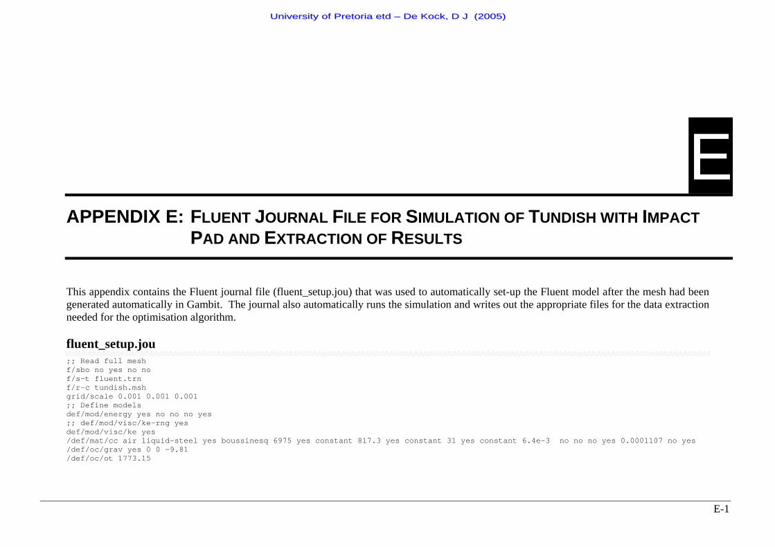
E-1
E APPENDIX E: FLUENT JOURNAL FILE FOR SIMULATION OF TUNDISH WITH IMPACT
PAD AND EXTRACTION OF RESULTS This appendix contains the Fluent journal file (fluent_setup.jou) that was used to automatically set-up the Fluent model after the mesh had been generated automatically in Gambit. The journal also automatically runs the simulation and writes out the appropriate files for the data extraction needed for the optimisation algorithm. fluent_setup.jou ;; Read full mesh f/sbo no yes no no f/s-t fluent.trn f/r-c tundish.msh grid/scale 0.001 0.001 0.001 ;; Define models def/mod/energy yes no no no yes ;; def/mod/visc/ke-rng yes def/mod/visc/ke yes /def/mat/cc air liquid-steel yes boussinesq 6975 yes constant 817.3 yes constant 31 yes constant 6.4e-3 no no no yes 0.0001107 no yes /def/oc/grav yes 0 0 -9.81 /def/oc/ot 1773.15
UUnniivveerrssiittyy ooff PPrreettoorriiaa eettdd –– DDee KKoocckk,, DD JJ ((22000055))
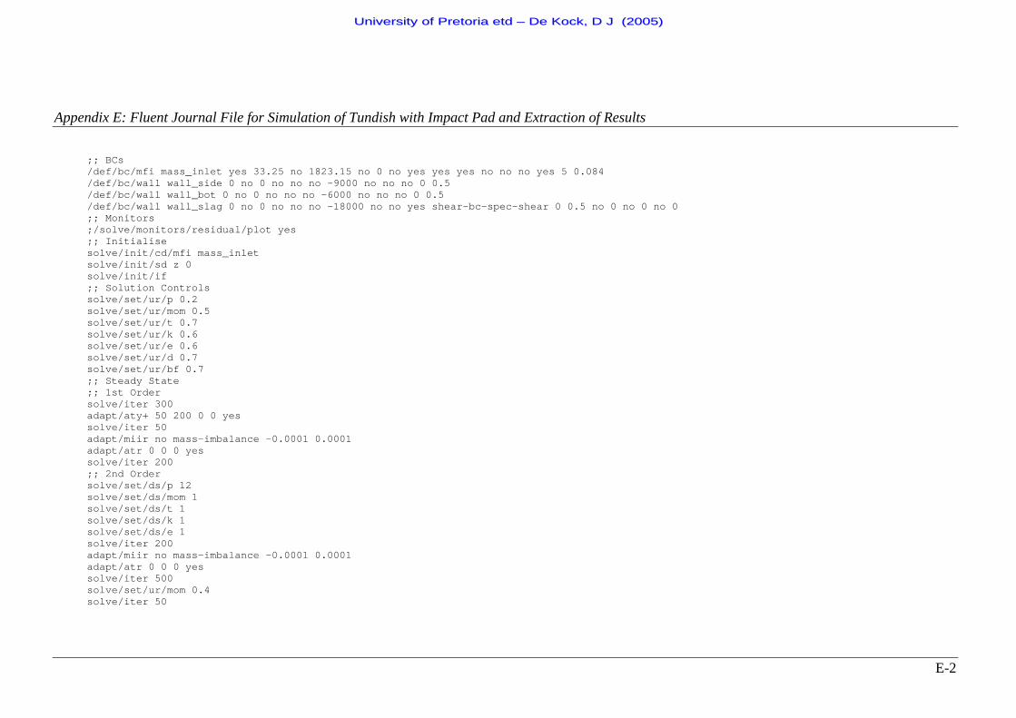
Appendix E: Fluent Journal File for Simulation of Tundish with Impact Pad and Extraction of Results
E-2
;; BCs /def/bc/mfi mass_inlet yes 33.25 no 1823.15 no 0 no yes yes yes no no no yes 5 0.084 /def/bc/wall wall_side 0 no 0 no no no -9000 no no no 0 0.5 /def/bc/wall wall_bot 0 no 0 no no no -6000 no no no 0 0.5 /def/bc/wall wall_slag 0 no 0 no no no -18000 no no yes shear-bc-spec-shear 0 0.5 no 0 no 0 no 0 ;; Monitors ;/solve/monitors/residual/plot yes ;; Initialise solve/init/cd/mfi mass_inlet solve/init/sd z 0 solve/init/if ;; Solution Controls solve/set/ur/p 0.2 solve/set/ur/mom 0.5 solve/set/ur/t 0.7 solve/set/ur/k 0.6 solve/set/ur/e 0.6 solve/set/ur/d 0.7 solve/set/ur/bf 0.7 ;; Steady State ;; 1st Order solve/iter 300 adapt/aty+ 50 200 0 0 yes solve/iter 50 adapt/miir no mass-imbalance -0.0001 0.0001 adapt/atr 0 0 0 yes solve/iter 200 ;; 2nd Order solve/set/ds/p 12 solve/set/ds/mom 1 solve/set/ds/t 1 solve/set/ds/k 1 solve/set/ds/e 1 solve/iter 200 adapt/miir no mass-imbalance -0.0001 0.0001 adapt/atr 0 0 0 yes solve/iter 500 solve/set/ur/mom 0.4 solve/iter 50
UUnniivveerrssiittyy ooff PPrreettoorriiaa eettdd –– DDee KKoocckk,, DD JJ ((22000055))
Appendix E: Fluent Journal File for Simulation of Tundish with Impact Pad and Extraction of Results
E-3
;; Post /plot/plot yes tke.out yes no no tke yes 1 0 0 wall_slag () ;; Set-up particles ; random_eddy num_tries diam /def/inj/ci injection-0 no yes surface no mass_inlet no yes no 100 0.15 no no no 0 0 -0.7692084 6.9e-6 1823.15 0 /def/mat/cc anthracite alumina yes 3200 yes constant 1680 yes 31 yes /def/inj/ci injection-1 no yes surface no mass_inlet no yes no 100 0.15 no no no 0 0 -0.7692084 1.65e-5 1823.15 0 /def/inj/ci injection-2 no yes surface no mass_inlet no yes no 100 0.15 no no no 0 0 -0.7692084 2.30e-5 1823.15 0 /def/inj/ci injection-3 no yes surface no mass_inlet no yes no 100 0.15 no no no 0 0 -0.7692084 3.21e-5 1823.15 0 /def/inj/ci injection-4 no yes surface no mass_inlet no yes no 100 0.15 no no no 0 0 -0.7692084 4.52e-5 1823.15 0 /def/inj/ci injection-5 no yes surface no mass_inlet no yes no 100 0.15 no no no 0 0 -0.7692084 6.39e-5 1823.15 0 /def/inj/ci injection-6 no yes surface no mass_inlet no yes no 100 0.15 no no no 0 0 -0.7692084 9.03e-5 1823.15 0 /def/inj/ci injection-7 no yes surface no mass_inlet no yes no 100 0.15 no no no 0 0 -0.7692084 0.000137 1823.15 0 ; #steps /define/models/dpm/tracking/max-steps 100000 ; Trap on slag layer /define/bc/wall wall_slag 0 no 0 no no no -18000 no no no 0 0.5 yes trap no 0 no 0 no 0 ; Run particles /file/stop-t /file/s-t part.trn /report/dpm-sample-report injection-7 injection-6 injection-5 injection-4 () outflow () () no /file/stop-t ;; Write case and data file/wcd groot_impact.cas.gz exit
UUnniivveerrssiittyy ooff PPrreettoorriiaa eettdd –– DDee KKoocckk,, DD JJ ((22000055))
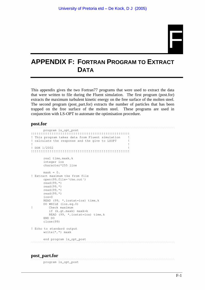
F-1
F APPENDIX F: FORTRAN PROGRAM TO EXTRACT
DATA This appendix gives the two Fortran77 programs that were used to extract the data that were written to file during the Fluent simulation. The first program (post.for) extracts the maximum turbulent kinetic energy on the free surface of the molten steel. The second program (post_part.for) extracts the number of particles that has been trapped on the free surface of the molten steel. These programs are used in conjunction with LS-OPT to automate the optimisation procedure. post.for program ls_opt_post !!!!!!!!!!!!!!!!!!!!!!!!!!!!!!!!!!!!!!!!!!!!!!!!!!!!! ! This program takes data from Fluent simulation ! ! calculate the response and the give to LSOPT ! ! ! ! DDK 1/2002 ! !!!!!!!!!!!!!!!!!!!!!!!!!!!!!!!!!!!!!!!!!!!!!!!!!!!!! real time,maxk,k integer ios character*255 line maxk = 0. ! Extract maximum tke from file open(99,file='tke.out') read(99,*) read(99,*) read(99,*) read(99,*) ios=0 READ (99, *,iostat=ios) time,k DO WHILE (ios.eq.0) ! Check maximum if (k.gt.maxk) maxk=k READ (99, *,iostat=ios) time,k END DO close(99) ! Echo to standard output write(*,*) maxk end program ls_opt_post
post_part.for program ls_opt_post
UUnniivveerrssiittyy ooff PPrreettoorriiaa eettdd –– DDee KKoocckk,, DD JJ ((22000055))
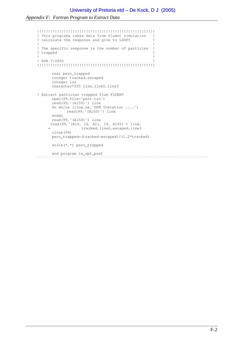
Appendix F: Fortran Program to Extract Data
F-2
!!!!!!!!!!!!!!!!!!!!!!!!!!!!!!!!!!!!!!!!!!!!!!!!!!!!! ! This programs takes data from Fluent simulation ! ! calculate the response and give to LSOPT ! ! ! ! The specific response is the number of particles ! ! trapped ! ! ! ! DDK 7/2002 ! !!!!!!!!!!!!!!!!!!!!!!!!!!!!!!!!!!!!!!!!!!!!!!!!!!!!! real perc_trapped integer tracked,escaped integer ios character*255 line,line2,line3 ! Extract particles trapped from FLUENT open(99,file='part.trn') read(99,'(A150)') line do while (line.ne.'DPM Iteration ....') read(99,'(A150)') line enddo read(99,'(A150)') line read(99,'(A16, I4, A11, I4, A150)') line, + tracked,line2,escaped,line3 close(99) perc_trapped=(tracked-escaped)/(1.0*tracked) write(*,*) perc_trapped end program ls_opt_post
UUnniivveerrssiittyy ooff PPrreettoorriiaa eettdd –– DDee KKoocckk,, DD JJ ((22000055))
G-1
G APPENDIX G: STEADY FLOW RESULTS OF
CHOSEN IMPACT PAD DESIGN
G-1 INTRODUCTION
This appendix gives the detail flow results of the optimised impact pad obtained from
case study 3. The appendix shows the temperature, flow distribution and turbulence
levels in the tundish.
G-2 TEMPERATURE CONTOURS
The temperature contours in the tundish are first shown on the walls (Figure G-1 and
Figure G-2) and then on vertical planes throughout the tundish width (Figure G-3
through Figure G-7). In Figure G-8, the temperature contours are shown on the slag
layer (note that this figure has a reduced scale compared to the other temperature
plots, all of which have the same scale). Starting with this last figure, the contours can
be seen to be remarkably symmetrical on the slag surface even though the shroud is
offset. At the bottom, especially inside the impact pad (Figure G-2), the side wing of
the pad nearest the shroud position is notably hotter than the other wing. From the
vertical planes (Figure G-3 through Figure G-7), it can be seen that a cold dead zone
extends across the whole tundish width in the wake of the impact pad.
UUnniivveerrssiittyy ooff PPrreettoorriiaa eettdd –– DDee KKoocckk,, DD JJ ((22000055))
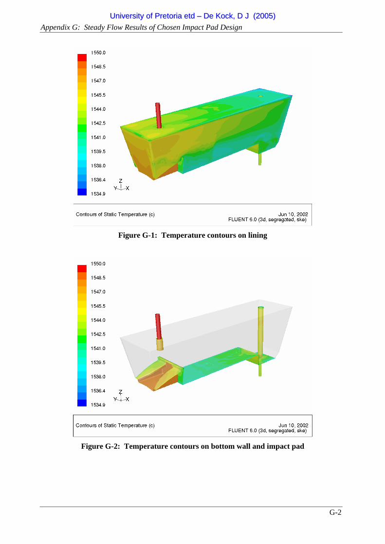
Appendix G: Steady Flow Results of Chosen Impact Pad Design
G-2
Figure G-1: Temperature contours on lining
Figure G-2: Temperature contours on bottom wall and impact pad
UUnniivveerrssiittyy ooff PPrreettoorriiaa eettdd –– DDee KKoocckk,, DD JJ ((22000055))
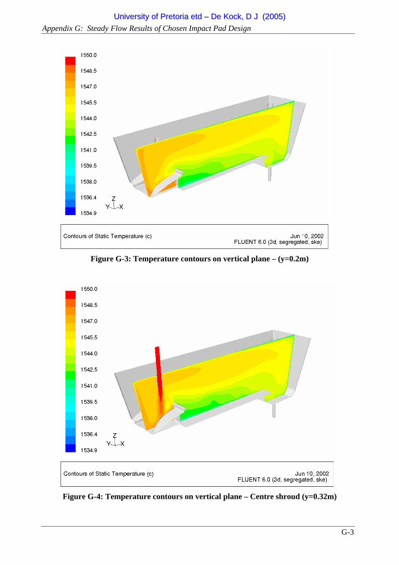
Appendix G: Steady Flow Results of Chosen Impact Pad Design
G-3
Figure G-3: Temperature contours on vertical plane – (y=0.2m)
Figure G-4: Temperature contours on vertical plane – Centre shroud (y=0.32m)
UUnniivveerrssiittyy ooff PPrreettoorriiaa eettdd –– DDee KKoocckk,, DD JJ ((22000055))
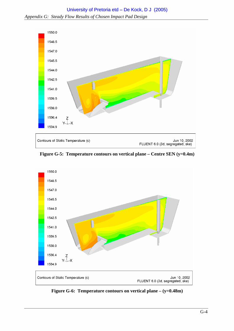
Appendix G: Steady Flow Results of Chosen Impact Pad Design
G-4
Figure G-5: Temperature contours on vertical plane – Centre SEN (y=0.4m)
Figure G-6: Temperature contours on vertical plane – (y=0.48m)
UUnniivveerrssiittyy ooff PPrreettoorriiaa eettdd –– DDee KKoocckk,, DD JJ ((22000055))
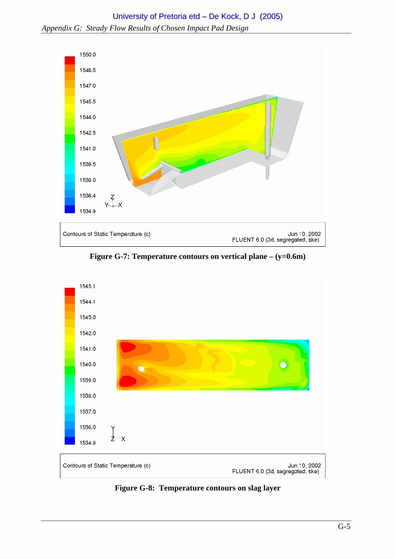
Appendix G: Steady Flow Results of Chosen Impact Pad Design
G-5
Figure G-7: Temperature contours on vertical plane – (y=0.6m)
Figure G-8: Temperature contours on slag layer
UUnniivveerrssiittyy ooff PPrreettoorriiaa eettdd –– DDee KKoocckk,, DD JJ ((22000055))
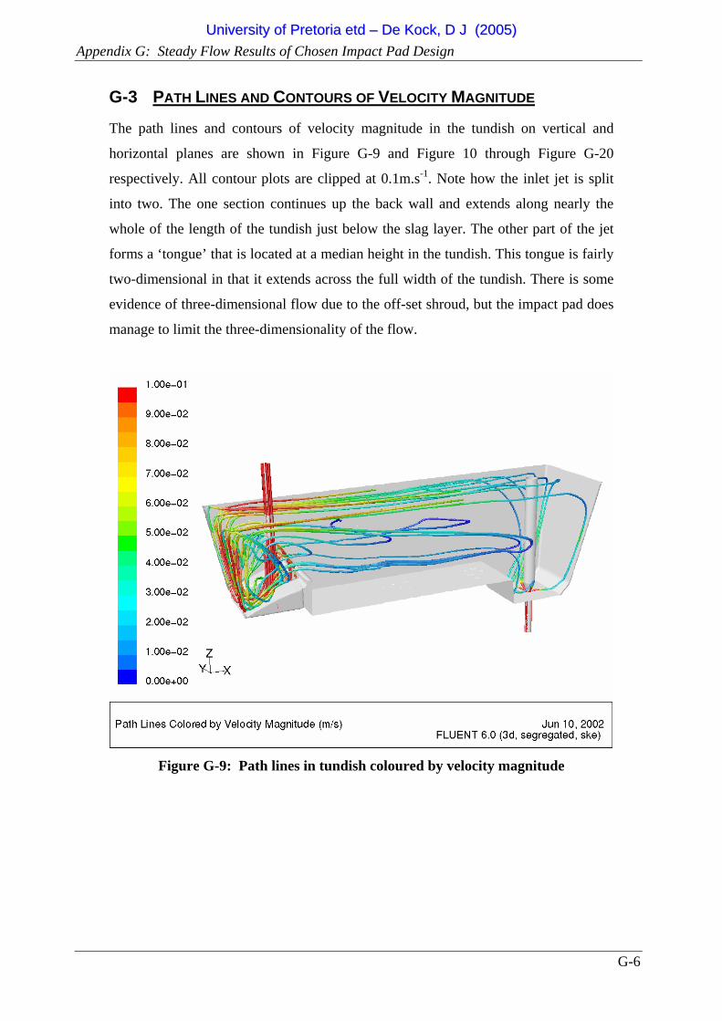
Appendix G: Steady Flow Results of Chosen Impact Pad Design
G-6
G-3 PATH LINES AND CONTOURS OF VELOCITY MAGNITUDE
The path lines and contours of velocity magnitude in the tundish on vertical and
horizontal planes are shown in Figure G-9 and Figure 10 through Figure G-20
respectively. All contour plots are clipped at 0.1m.s-1. Note how the inlet jet is split
into two. The one section continues up the back wall and extends along nearly the
whole of the length of the tundish just below the slag layer. The other part of the jet
forms a ‘tongue’ that is located at a median height in the tundish. This tongue is fairly
two-dimensional in that it extends across the full width of the tundish. There is some
evidence of three-dimensional flow due to the off-set shroud, but the impact pad does
manage to limit the three-dimensionality of the flow.
Figure G-9: Path lines in tundish coloured by velocity magnitude
UUnniivveerrssiittyy ooff PPrreettoorriiaa eettdd –– DDee KKoocckk,, DD JJ ((22000055))
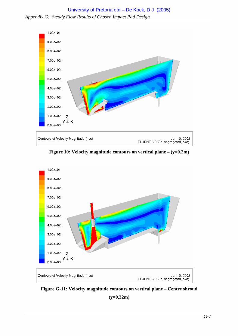
Appendix G: Steady Flow Results of Chosen Impact Pad Design
G-7
Figure 10: Velocity magnitude contours on vertical plane – (y=0.2m)
Figure G-11: Velocity magnitude contours on vertical plane – Centre shroud
(y=0.32m)
UUnniivveerrssiittyy ooff PPrreettoorriiaa eettdd –– DDee KKoocckk,, DD JJ ((22000055))
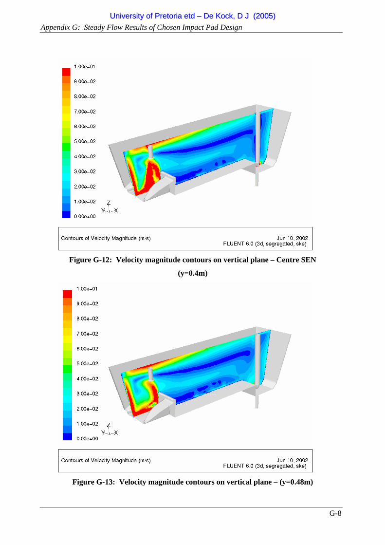
Appendix G: Steady Flow Results of Chosen Impact Pad Design
G-8
Figure G-12: Velocity magnitude contours on vertical plane – Centre SEN
(y=0.4m)
Figure G-13: Velocity magnitude contours on vertical plane – (y=0.48m)
UUnniivveerrssiittyy ooff PPrreettoorriiaa eettdd –– DDee KKoocckk,, DD JJ ((22000055))

Appendix G: Steady Flow Results of Chosen Impact Pad Design
G-9
Figure G-14: Velocity magnitude contours on vertical plane – (y=0.6m)
Figure G-15: Velocity magnitude contours on horizontal plane – (z=-0.6m)
UUnniivveerrssiittyy ooff PPrreettoorriiaa eettdd –– DDee KKoocckk,, DD JJ ((22000055))
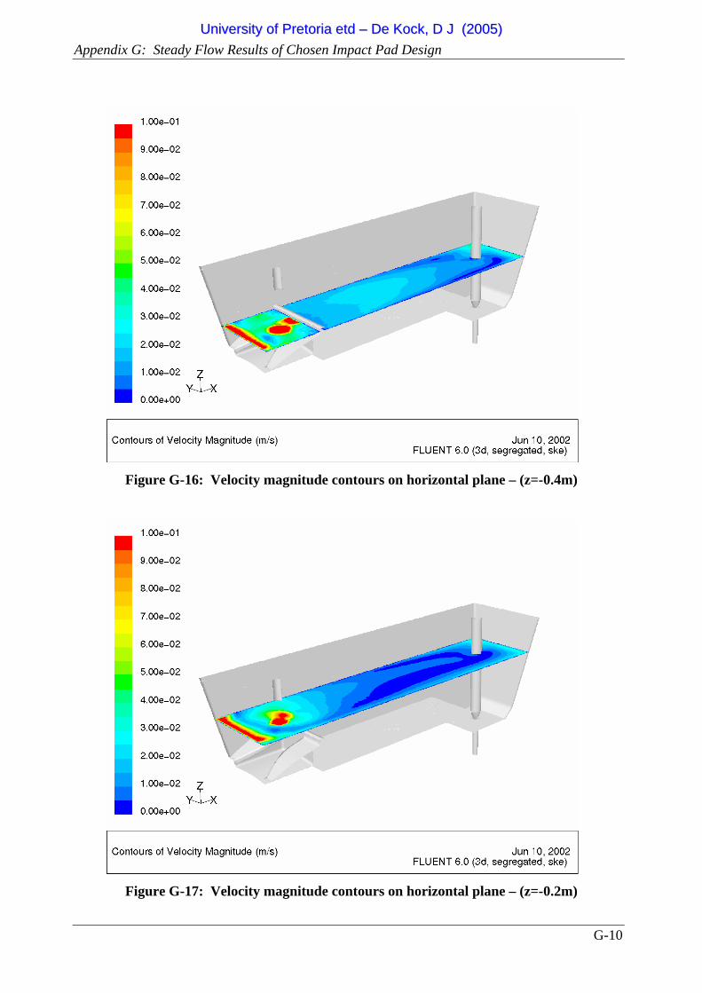
Appendix G: Steady Flow Results of Chosen Impact Pad Design
G-10
Figure G-16: Velocity magnitude contours on horizontal plane – (z=-0.4m)
Figure G-17: Velocity magnitude contours on horizontal plane – (z=-0.2m)
UUnniivveerrssiittyy ooff PPrreettoorriiaa eettdd –– DDee KKoocckk,, DD JJ ((22000055))
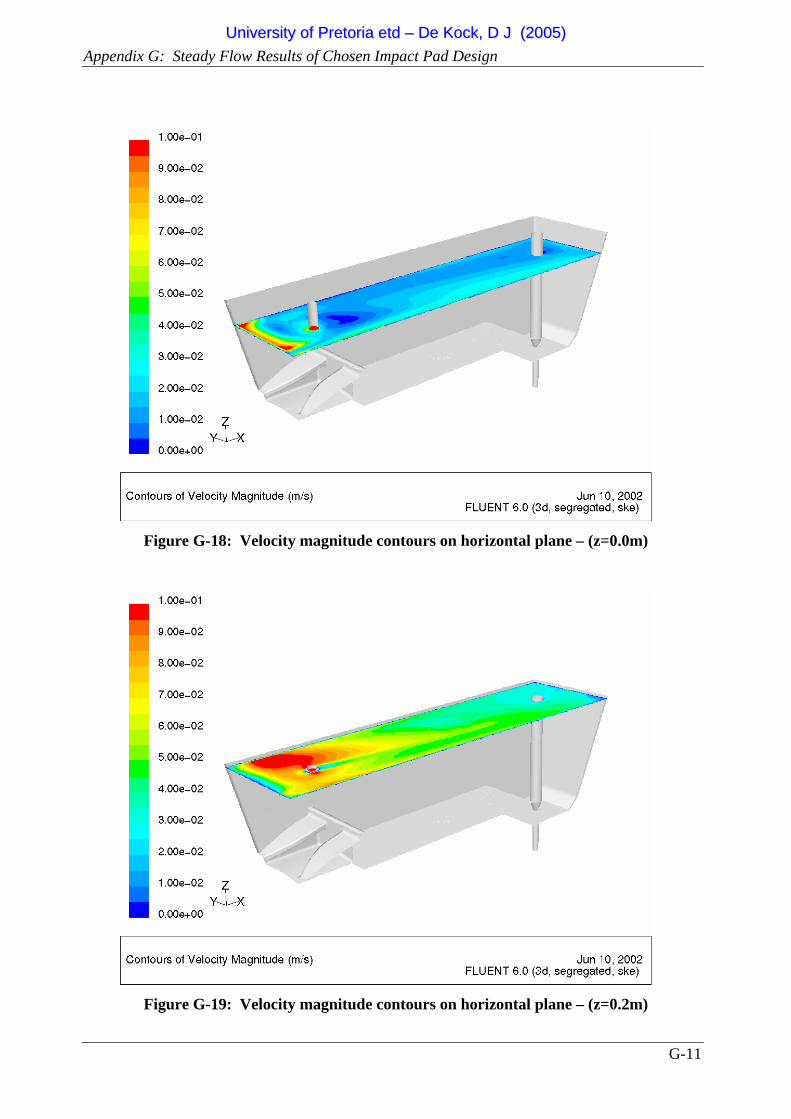
Appendix G: Steady Flow Results of Chosen Impact Pad Design
G-11
Figure G-18: Velocity magnitude contours on horizontal plane – (z=0.0m)
Figure G-19: Velocity magnitude contours on horizontal plane – (z=0.2m)
UUnniivveerrssiittyy ooff PPrreettoorriiaa eettdd –– DDee KKoocckk,, DD JJ ((22000055))
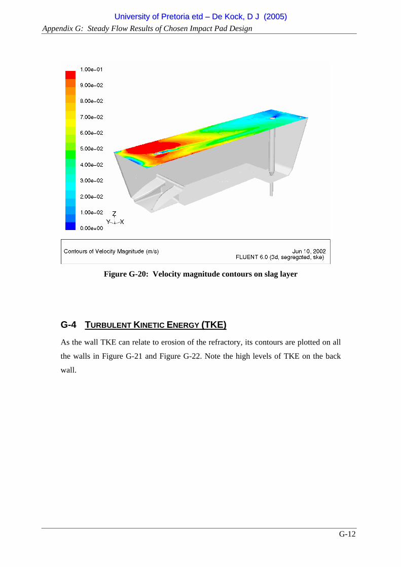
Appendix G: Steady Flow Results of Chosen Impact Pad Design
G-12
Figure G-20: Velocity magnitude contours on slag layer
G-4 TURBULENT KINETIC ENERGY (TKE)
As the wall TKE can relate to erosion of the refractory, its contours are plotted on all
the walls in Figure G-21 and Figure G-22. Note the high levels of TKE on the back
wall.
UUnniivveerrssiittyy ooff PPrreettoorriiaa eettdd –– DDee KKoocckk,, DD JJ ((22000055))
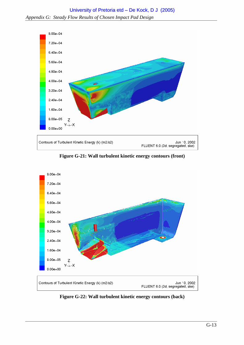
Appendix G: Steady Flow Results of Chosen Impact Pad Design
G-13
Figure G-21: Wall turbulent kinetic energy contours (front)
Figure G-22: Wall turbulent kinetic energy contours (back)
UUnniivveerrssiittyy ooff PPrreettoorriiaa eettdd –– DDee KKoocckk,, DD JJ ((22000055))
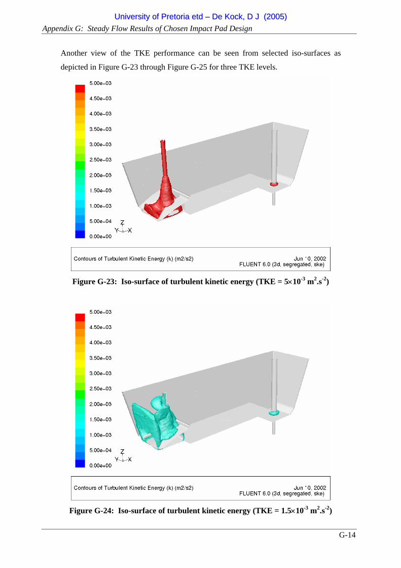
Appendix G: Steady Flow Results of Chosen Impact Pad Design
G-14
Another view of the TKE performance can be seen from selected iso-surfaces as
depicted in Figure G-23 through Figure G-25 for three TKE levels.
Figure G-23: Iso-surface of turbulent kinetic energy (TKE = 5×10⁻³ m2.s-2)
Figure G-24: Iso-surface of turbulent kinetic energy (TKE = 1.5×10⁻³ m2.s-2)
UUnniivveerrssiittyy ooff PPrreettoorriiaa eettdd –– DDee KKoocckk,, DD JJ ((22000055))
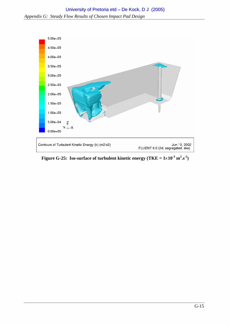
Appendix G: Steady Flow Results of Chosen Impact Pad Design
G-15
Figure G-25: Iso-surface of turbulent kinetic energy (TKE = 1×10⁻³ m2.s-2)
UUnniivveerrssiittyy ooff PPrreettoorriiaa eettdd –– DDee KKoocckk,, DD JJ ((22000055))
H-1
H APPENDIX H: PARTICLE TRAPPING USER DEFINED FUNCTION This appendix contained the first attempt of a more advanced model for the trapping of a particle on the slag layer. This is a C-program that is compiled as a User Defined Function in Fluent. The model calculates the maximum continuous time that a particle spends in a user defined region close to the slag layer. A simple correlation is then used that relates the probability of a particle being trapped to the size of the particle and the time it spent near the slag layer. /**************************************************************************/ /*UDF for computing the maximum cont. time spent by a particle in the */ /* region close to the slag layer */ /* This model assumes: */ /* z is pointing upwards */ /* Model inputs: */ /* thickness of trapping zone */ /* z-position of slag layer */ /* */ /* File History: */ /* DdK 12/2001 */ /* DdK 4/2002 Automating output of number trapped */ /* */ /**************************************************************************/
UUnniivveerrssiittyy ooff PPrreettoorriiaa eettdd –– DDee KKoocckk,, DD JJ ((22000055))
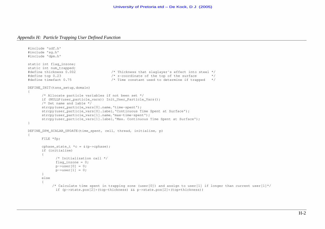
Appendix H: Particle Trapping User Defined Function
H-2
#include "udf.h" #include "sg.h" #include "dpm.h" static int flag_inzone; static int num_trapped; #define thickness 0.002 /* Thickness that slaglayer's effect into steel */ #define top 0.23 /* z-coordinate of the top of the surface */ #define timefact 0.75 /* Time constant used to determine if trapped */ DEFINE_INIT(tsns_setup,domain) { /* Allocate particle variables if not been set */ if (NULLP(user_particle_vars)) Init_User_Particle_Vars(); /* Set name and lable */ strcpy(user_particle_vars[0].name,"time-spent"); strcpy(user_particle_vars[0].label,"Continuous Time Spent at Surface"); strcpy(user_particle_vars[1].name,"max-time-spent"); strcpy(user_particle_vars[1].label,"Max. Continuous Time Spent at Surface"); } DEFINE_DPM_SCALAR_UPDATE(time_spent, cell, thread, initialise, p) { FILE *fp; cphase_state_t *c = &(p->cphase); if (initialise) { /* Initialization call */ flag_inzone = 0; p->user[0] = 0; p->user[1] = 0; } else { /* Calculate time spent in trapping zone (user[0]) and assign to user[1] if longer than current user[1]*/ if (p->state.pos[2]>(top-thickness) && p->state.pos[2]<(top+thickness))
UUnniivveerrssiittyy ooff PPrreettoorriiaa eettdd –– DDee KKoocckk,, DD JJ ((22000055))
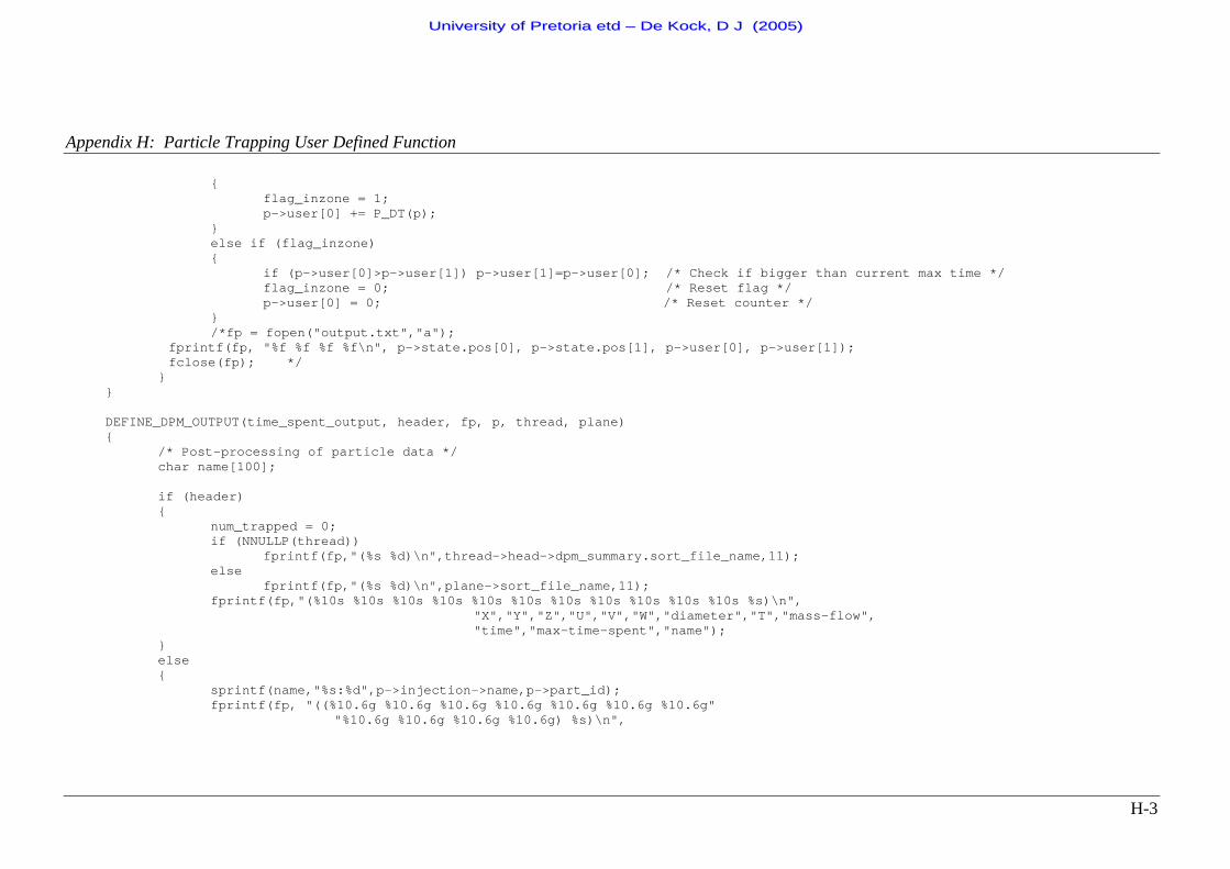
Appendix H: Particle Trapping User Defined Function
H-3
{ flag_inzone = 1; p->user[0] += P_DT(p); } else if (flag_inzone) { if (p->user[0]>p->user[1]) p->user[1]=p->user[0]; /* Check if bigger than current max time */ flag_inzone = 0; /* Reset flag */ p->user[0] = 0; /* Reset counter */ } /*fp = fopen("output.txt","a"); fprintf(fp, "%f %f %f %f\n", p->state.pos[0], p->state.pos[1], p->user[0], p->user[1]); fclose(fp); */ } } DEFINE_DPM_OUTPUT(time_spent_output, header, fp, p, thread, plane) { /* Post-processing of particle data */
char name[100]; if (header) { num_trapped = 0; if (NNULLP(thread)) fprintf(fp,"(%s %d)\n",thread->head->dpm_summary.sort_file_name,11); else fprintf(fp,"(%s %d)\n",plane->sort_file_name,11); fprintf(fp,"(%10s %10s %10s %10s %10s %10s %10s %10s %10s %10s %10s %s)\n", "X","Y","Z","U","V","W","diameter","T","mass-flow", "time","max-time-spent","name"); } else { sprintf(name,"%s:%d",p->injection->name,p->part_id); fprintf(fp, "((%10.6g %10.6g %10.6g %10.6g %10.6g %10.6g %10.6g" "%10.6g %10.6g %10.6g %10.6g) %s)\n",
UUnniivveerrssiittyy ooff PPrreettoorriiaa eettdd –– DDee KKoocckk,, DD JJ ((22000055))
Appendix H: Particle Trapping User Defined Function
H-4
p->state.pos[0], p->state.pos[1], p->state.pos[2], p->state.V[0], p->state.V[1], p->state.V[2], p->state.diam, p->state.temp, p->flow_rate, p->state.time, p->user[1], name); if (p->user[1] >(timefact*p->state.diam*1e6)) { num_trapped = num_trapped + 1; printf("Particle %s leaving %s would have been trapped \n", name,thread->head->dpm_summary.sort_file_name); printf("Total number trapped in trapping zone = %d \n",num_trapped); } } }
UUnniivveerrssiittyy ooff PPrreettoorriiaa eettdd –– DDee KKoocckk,, DD JJ ((22000055))