Optimal Team Time Trial Strategy in Road Cycling
83
Optimal Team Time Trial Strategy in Road Cycling Optimisation of Changing Strategy using a Mathemati- cal Performance model M. W. B. Overtoom
-
Upload
khangminh22 -
Category
Documents
-
view
1 -
download
0
Transcript of Optimal Team Time Trial Strategy in Road Cycling
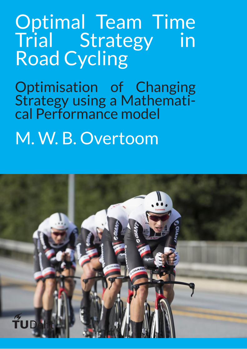
Optimal Team TimeTrial Strategy inRoad CyclingOptimisation of ChangingStrategy using a Mathemati-cal PerformancemodelM.W. B. Overtoom

Optimal TeamTime TrialStrategy in
Road CyclingOptimisation of Changing Strategy using a
Mathematical Performance modelby
M. W. B. Overtoomto obtain the degree of Master of Science
at the Delft University of Technology,to be defended publicly on Tuesday January 1, 2013 at 10:00 AM.
Student number: 4178777Project duration: March 1, 2012 – January 1, 2013Thesis committee: Dr. ir. A. L. Schwab, TU Delft, supervisor
Dr. D. J. J. Bregman, TU Delft, supervisorDr. A. Sciacchitano, TU DelftMSc. T. Van Erp, Team Sunweb
This thesis is confidential and cannot be made public until October 31, 2020.
An electronic version of this thesis is available at http://repository.tudelft.nl/.

Abstract
During team time trials in road cycling changing schemes are used to spread the workload over the cyclistsin the team. Models that provide predictions of race performance already exist for individual time trials. It isproposed that with a performance model for team time trials, the performance of different strategies can becompared and optimised.
In literature combinations of mechanical resistance models and physiological models are used to deter-mine the performance of individual time trials. The aerodynamic interaction between cyclists is very impor-tant to the effectiveness of a strategy. Coefficients of drag reduction between cyclists in a team time trial arepresented in several studies, however most studies use groups of only four cyclists, which is not useful for ateam time trial with eight cyclists. Only two studies report data for groups up to eight cyclists. These two mod-els show different behaviour and are both used to asses the performance of strategies. Also two physiologicalmodels were used.
In the model provided in this study the resistances are calculated from the kinematics resulting from theevaluated strategy. The mechanical resistance model, including the aerodynamic interaction model calcu-lates the power required to perform the strategy. The physiological model calculates the physiology duringthe race, which determines if the cyclists are able to sustain the prescribed strategy.
Genetic algorithm optimisation is used to optimise the strategy parameters, such as initial position andtimes spend in first position. The velocity is optimised for each evaluated strategy configuration. A con-vergence test was performed to determine the parameters for the genetic algorithm, which are used in theoptimisation of strategy.
Using the standard strategy, where cyclists only change from first to last position, different orders are com-pared. From this study it was determined that the mean velocity over a 30 km team time trial could be raisedby a maximum of 0.228 m/s by improving the order, depending on the model configuration. It was foundthat the best performing orders were those where the mean performance difference of following cyclists waslowest.
Two different strategies have been assessed where cyclists still always change from first, but not necessarilylast position have been assessed on their performance. With those more complex strategies the mean velocitycould be increased with 0.358 m/s over a 30 km team time trial.
The model still lacks validity, but gives a relevant insight in the performance of different team time trialstrategies. The validity can either improved by using track test to validate the drag reduction coefficients orby using power data from a team time trial to show that the model predicts realistic physiology. Of those twomethods the last is preferred.
iii

Preface
This document contains the research results for the final research (thesis) for the Master Mechanical Engi-neering, Track Biomechanical Design and specialisation Sports Engineering, part of the faculty of Mechan-ical, Maritime and Materials Engineering, Delft Technical University. The project has been performed incollaboration with Cycling Team, Team Sunweb
This reports will present a mathematical model to estimate the performance of strategies in a team timetrial in road cycling, as well as the analysis of several suggested strategies for a team time trial.I would like to thank my university committee: Dr. ir. A. L. Schwab, Dr. D. J. J. Bregman, Dr. A. Sciacchitanoand company mentor Msc. T Van Erp for their academic support, my friends family and study mates for theirdaily support during the period of this research.
M. W. B. OvertoomDelft, October 2018
v

Contents
Abstract iii1 Introduction 1
1.1 List of symbols . . . . . . . . . . . . . . . . . . . . . . . . . . . . . . . . . . . . . . . . . . 3
2 Modelling of the team time trial performance 52.1 Introduction . . . . . . . . . . . . . . . . . . . . . . . . . . . . . . . . . . . . . . . . . . . 52.2 Mechanical model . . . . . . . . . . . . . . . . . . . . . . . . . . . . . . . . . . . . . . . . 5
2.2.1 Equation of motion of the individual cyclist . . . . . . . . . . . . . . . . . . . . . . . . 52.3 Physiological model. . . . . . . . . . . . . . . . . . . . . . . . . . . . . . . . . . . . . . . . 7
2.3.1 Critical power . . . . . . . . . . . . . . . . . . . . . . . . . . . . . . . . . . . . . . . 72.3.2 From critical power to critical velocity . . . . . . . . . . . . . . . . . . . . . . . . . . . 82.3.3 Margaria-Morton Physiological Models . . . . . . . . . . . . . . . . . . . . . . . . . . 8
2.4 Aerodynamic interaction model . . . . . . . . . . . . . . . . . . . . . . . . . . . . . . . . . 102.4.1 implementation of drafting . . . . . . . . . . . . . . . . . . . . . . . . . . . . . . . . 102.4.2 Comparison of Aerodynamic interaction studies. . . . . . . . . . . . . . . . . . . . . . 10
2.5 Simulation framework . . . . . . . . . . . . . . . . . . . . . . . . . . . . . . . . . . . . . . 122.5.1 constraints . . . . . . . . . . . . . . . . . . . . . . . . . . . . . . . . . . . . . . . . . 122.5.2 Strategies . . . . . . . . . . . . . . . . . . . . . . . . . . . . . . . . . . . . . . . . . 132.5.3 Differential equations . . . . . . . . . . . . . . . . . . . . . . . . . . . . . . . . . . . 142.5.4 Solving of differential equations . . . . . . . . . . . . . . . . . . . . . . . . . . . . . . 14
2.6 Cyclists standardisation . . . . . . . . . . . . . . . . . . . . . . . . . . . . . . . . . . . . . . 142.6.1 Parameters. . . . . . . . . . . . . . . . . . . . . . . . . . . . . . . . . . . . . . . . . 14
2.7 Model Sensitivity . . . . . . . . . . . . . . . . . . . . . . . . . . . . . . . . . . . . . . . . . 152.7.1 Mechanical and aerodynamic interaction . . . . . . . . . . . . . . . . . . . . . . . . . 162.7.2 Physiological . . . . . . . . . . . . . . . . . . . . . . . . . . . . . . . . . . . . . . . . 17
2.8 Validity . . . . . . . . . . . . . . . . . . . . . . . . . . . . . . . . . . . . . . . . . . . . . . 17
3 Optimising Strategy 193.1 Strategies . . . . . . . . . . . . . . . . . . . . . . . . . . . . . . . . . . . . . . . . . . . . . 19
3.1.1 Regular strategy . . . . . . . . . . . . . . . . . . . . . . . . . . . . . . . . . . . . . . 193.2 Optimisation . . . . . . . . . . . . . . . . . . . . . . . . . . . . . . . . . . . . . . . . . . . 21
3.2.1 Objective Function. . . . . . . . . . . . . . . . . . . . . . . . . . . . . . . . . . . . . 213.2.2 Separating the Problem . . . . . . . . . . . . . . . . . . . . . . . . . . . . . . . . . . 213.2.3 Velocity Optimisation . . . . . . . . . . . . . . . . . . . . . . . . . . . . . . . . . . . 213.2.4 Strategy Optimisation . . . . . . . . . . . . . . . . . . . . . . . . . . . . . . . . . . . 21
3.3 Convergence . . . . . . . . . . . . . . . . . . . . . . . . . . . . . . . . . . . . . . . . . . . 233.3.1 Elite, mutation and crossover ratio. . . . . . . . . . . . . . . . . . . . . . . . . . . . . 233.3.2 Population size. . . . . . . . . . . . . . . . . . . . . . . . . . . . . . . . . . . . . . . 25
3.4 Conclusion . . . . . . . . . . . . . . . . . . . . . . . . . . . . . . . . . . . . . . . . . . . . 27
4 Analysis of a standard team time trial 294.1 Analysis of the regular strategy without workload balancing . . . . . . . . . . . . . . . . . . . 294.2 Head time optimisation . . . . . . . . . . . . . . . . . . . . . . . . . . . . . . . . . . . . . . 304.3 Head time optimisation with dropping . . . . . . . . . . . . . . . . . . . . . . . . . . . . . . 304.4 Discussion . . . . . . . . . . . . . . . . . . . . . . . . . . . . . . . . . . . . . . . . . . . . 304.5 Conclusion . . . . . . . . . . . . . . . . . . . . . . . . . . . . . . . . . . . . . . . . . . . . 32
5 Order optimisation 335.1 Results . . . . . . . . . . . . . . . . . . . . . . . . . . . . . . . . . . . . . . . . . . . . . . 355.2 Discussion . . . . . . . . . . . . . . . . . . . . . . . . . . . . . . . . . . . . . . . . . . . . 355.3 Conclusion . . . . . . . . . . . . . . . . . . . . . . . . . . . . . . . . . . . . . . . . . . . . 37
vii
viii Contents
6 Adjusted Return Positions Strategy 396.1 Selected return positions . . . . . . . . . . . . . . . . . . . . . . . . . . . . . . . . . . . . . 42
6.1.1 hypotheses. . . . . . . . . . . . . . . . . . . . . . . . . . . . . . . . . . . . . . . . . 436.2 Results . . . . . . . . . . . . . . . . . . . . . . . . . . . . . . . . . . . . . . . . . . . . . . 436.3 Discussion . . . . . . . . . . . . . . . . . . . . . . . . . . . . . . . . . . . . . . . . . . . . 456.4 Conclusion . . . . . . . . . . . . . . . . . . . . . . . . . . . . . . . . . . . . . . . . . . . . 45
7 Skipping Strategy 477.1 hypothesis . . . . . . . . . . . . . . . . . . . . . . . . . . . . . . . . . . . . . . . . . . . . 477.2 Results . . . . . . . . . . . . . . . . . . . . . . . . . . . . . . . . . . . . . . . . . . . . . . 477.3 Discussion . . . . . . . . . . . . . . . . . . . . . . . . . . . . . . . . . . . . . . . . . . . . 487.4 Conclusion . . . . . . . . . . . . . . . . . . . . . . . . . . . . . . . . . . . . . . . . . . . . 48
8 Conclusion 518.1 Model . . . . . . . . . . . . . . . . . . . . . . . . . . . . . . . . . . . . . . . . . . . . . . . 518.2 Strategy . . . . . . . . . . . . . . . . . . . . . . . . . . . . . . . . . . . . . . . . . . . . . . 51
9 Recomendations 539.1 Model . . . . . . . . . . . . . . . . . . . . . . . . . . . . . . . . . . . . . . . . . . . . . . . 53
9.1.1 Validation of the aerodynamic interaction . . . . . . . . . . . . . . . . . . . . . . . . . 539.1.2 Individual aerodynamic characteristics . . . . . . . . . . . . . . . . . . . . . . . . . . 539.1.3 Additional aerodynamic improvements . . . . . . . . . . . . . . . . . . . . . . . . . . 539.1.4 Overall performance validation . . . . . . . . . . . . . . . . . . . . . . . . . . . . . . 54
9.2 Studies using the existing model . . . . . . . . . . . . . . . . . . . . . . . . . . . . . . . . . 549.2.1 Performance difference on different slopes . . . . . . . . . . . . . . . . . . . . . . . . 54
A Interpolation of cyclist drafting coefficient 55A.1 Method . . . . . . . . . . . . . . . . . . . . . . . . . . . . . . . . . . . . . . . . . . . . . . 56
A.1.1 Framework. . . . . . . . . . . . . . . . . . . . . . . . . . . . . . . . . . . . . . . . . 56A.1.2 Least squares estimation . . . . . . . . . . . . . . . . . . . . . . . . . . . . . . . . . . 57
A.2 Results . . . . . . . . . . . . . . . . . . . . . . . . . . . . . . . . . . . . . . . . . . . . . . 58A.2.1 interpolation in groups up to eight. . . . . . . . . . . . . . . . . . . . . . . . . . . . . 58A.2.2 Extrapolation from a group of four cyclists . . . . . . . . . . . . . . . . . . . . . . . . . 60
A.3 Discussion . . . . . . . . . . . . . . . . . . . . . . . . . . . . . . . . . . . . . . . . . . . . 61A.4 conclusion . . . . . . . . . . . . . . . . . . . . . . . . . . . . . . . . . . . . . . . . . . . . 61
B Fitting theMargaria-Mortonmodels 63B.1 Introduction . . . . . . . . . . . . . . . . . . . . . . . . . . . . . . . . . . . . . . . . . . . 63B.2 The MM-model . . . . . . . . . . . . . . . . . . . . . . . . . . . . . . . . . . . . . . . . . . 63
B.2.1 Differential equations . . . . . . . . . . . . . . . . . . . . . . . . . . . . . . . . . . . 63B.2.2 Sizing . . . . . . . . . . . . . . . . . . . . . . . . . . . . . . . . . . . . . . . . . . . 65
B.3 Method . . . . . . . . . . . . . . . . . . . . . . . . . . . . . . . . . . . . . . . . . . . . . . 66B.3.1 constraints . . . . . . . . . . . . . . . . . . . . . . . . . . . . . . . . . . . . . . . . . 66B.3.2 Tests . . . . . . . . . . . . . . . . . . . . . . . . . . . . . . . . . . . . . . . . . . . . 66B.3.3 Optimisation. . . . . . . . . . . . . . . . . . . . . . . . . . . . . . . . . . . . . . . . 66
B.4 Results and discussion . . . . . . . . . . . . . . . . . . . . . . . . . . . . . . . . . . . . . . 67B.5 conclusion . . . . . . . . . . . . . . . . . . . . . . . . . . . . . . . . . . . . . . . . . . . . 68
Bibliography 71
1Introduction
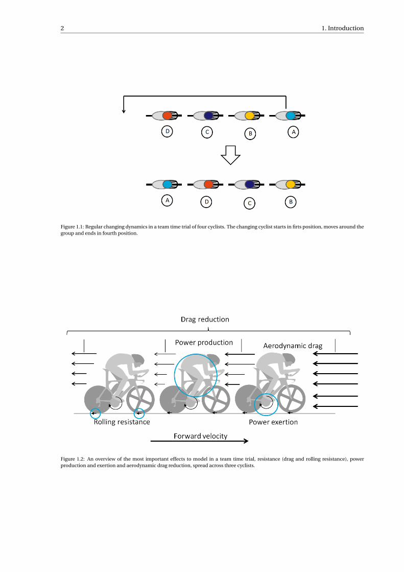
This report is a study on the optimisation of team time trial strategy, this first paragraph will explain thebasics of team time trials in road cycling, after which the details and modelling is described. Team time trialsare races in which a team of cyclists compete to finish a predefined course in the lowest amount of timepossible. Within the race the cyclists interact with each other, but not with the other teams or other vehicleson the road, thereby making it a team effort. The cyclists are usually with six to eight and drive close after eachother to reduce the drag of the cyclists in the tail of the line, this is commonly known as drafting or straying.The cyclists are not allowed to push each other and the drafting effect does not have the same effect in everyposition in the group, the cyclists change their position throughout the race. A common way to do this is tospend some time in first position, than steer to the side of the group and reduce the power output to move tothe tail of the group where, the speed is brought up to the that of the other cyclists until it is possible to pickin to the last position, as demonstrated in figure 1.1. As this repeats each cyclist moves into the front relativeto the others, until it reaches the first position and it changes to the last position. It is possible and allowed touse another method to change positions however it is very uncommon.
The full rules of team time trials can e found in the regulation of the ICU [26]. A lot of specific rules can bedetermined by the organiser of the event. However it is stated that a team time trial should be with at leasttwo and no more than 10 cyclists. The distance of the race should not exceed 100 km, for elite men and 50 kmfor elite women. The members of the team may use the aerodynamic advantages by drafting from each other,but not from vehicles from the organisation or team support. Neither are teams allowed to draft from othercompeting teams that are on the same course. There are more rules regarding courses and organisation, butthis roughly sketches the outlines of the regulations that affect the strategy.
The goal of this study is to determine performance for different team time trial strategies with respectto each other, in order to try a large amount of strategies a model for simulations is required. This modelshould model the behaviour of the aerodynamic and physiological behaviour accurately in order to asses thedifferences between strategies, however it does not necessarily need to exactly match real performance. Amathematical model for the team time trial needs three components: a mechanical of resistance model, aphysiological model and an aerodynamic interaction model as illustrated in figure 1.2. The resistances howthe power requirements are related to the velocity additionally, it should also include the effects of acceler-ation and slopes. The physiology should describe the ability of power production, including endurance andintermittent exercise. The modelling of aerodynamic interaction will describe the reductions in aerodynamicresistance, this is important, because the changing of position is a result of the aerodynamic dissimilaritiesbetween positions.
The mechanical model links the kinematics to the forces and thereby power output by the cyclist. Manyconfigurations have been used in publications,[3, 12, 14, 15, 18, 23, 24, 36, 38–40, 42, 45, 46] of which «nearly»all of them contain aerodynamic drag and rolling resistance, which are two largest sources of resistance. Someinclude the forces generated by gravity on sloped roads [18, 23, 24, 36, 40, 45, 46]. Only two studies report theeffects of lean on the forward dynamics of the bicycle [39, 45] and the mechanical efficiency of the bicycle isonly mentioned in one study [45].
1
2 1. Introduction
Figure 1.1: Regular changing dynamics in a team time trial of four cyclists. The changing cyclist starts in firts position, moves around thegroup and ends in fourth position.
Figure 1.2: An overview of the most important effects to model in a team time trial, resistance (drag and rolling resistance), powerproduction and exertion and aerodynamic drag reduction, spread across three cyclists.

1.1. List of symbols 3
The physiology should provide a mathematical description with on the ability of the cyclist to producepower output over time. Eventually the physiological model should lead to a form in which it can determineweather or not a certain power is producible by the cyclist. The theory of Monod and Scherrer (1965) [30]defines a power to time relationship, more commonly known as the Critical Power Theory. This determinesthe maximum time a constant power can be delivered by a cyclist. This theory is extended by recovery modelsof Skiba et al. (2012) [43] and Bartram (2017) [5], creating a model which can model a physiological state (an-earobic work) throughout an exercise, from this state it can be determined if it was possible for the athlete toperform this exercise. Another model is the bioenergetic model by MArgaria and Morton [33, 41] (Margaria-Morton model). This model is more based on the bio-chemistry inside the body and also models two physio-logical states of an athlete, which can determine weather the exercise was possible. The critical power modelis easier to determine for a cyclist, with only two variables, the Margaria-Morton model is harder to fit witheight free variables, but is capable of describing a more detailed physiological behaviour of the cyclist.
As mentioned earlier in team time trials drafting is used to increase performance. In order to implementthis effect in the team time trial model, the drafting of the cyclists has to be quantified. Several studies havebeen performed on the drafting effect, when cycling in groups [4, 8, 10, 16–18, 22, 27, 29]. Of these studiesfour are dedicated to the team pursuit in track cycling and provide data for four cyclists [4, 10, 16, 22] andonly two provide data to group seizes up to eight [8, 27]. The discussed studies can also be differentiated bythe method of assessment, these are distinguished in three categories: computational flow dynamics (CFD)[8, 16, 27], wind tunnel tests [4, 10] and field tests [10, 17, 22, 29]. These studies describe the drag reductionfor every position in the group.
In this study a model will be used in an optimisation to determine optimal strategy in team time trials.As presented in figure 1.1 the strategy that is currently most used is to have a fixed order where every cyclistdrives roughly ten to thirty seconds in first position and then changes to last position. In first position the dragis the highest, thus is the required power output is high. Depending on the capability of the cyclist and it’sstate at the moment the cyclist will adjust the time spend in that position, shorter if weaker or tired and longerif stronger or in a more energetic state. Cyclists that are much weaker than the others, are often dropped outof the group during the race.
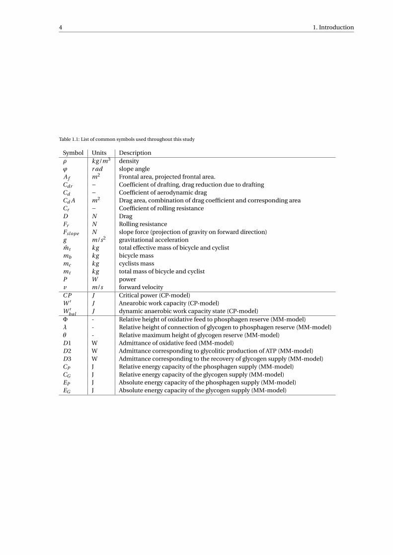
1.1. List of symbolsIn table 1.1 a list of symbols used throughout this study is provided.
4 1. Introduction
Table 1.1: List of common symbols used throughout this study
Symbol Units Descriptionρ kg /m3 densityϕ r ad slope angleA f m2 Frontal area, projected frontal area.Cdr − Coefficient of drafting, drag reduction due to draftingCd − Coefficient of aerodynamic dragCd A m2 Drag area, combination of drag coefficient and corresponding areaCr − Coefficient of rolling resistanceD N DragFr N Rolling resistanceFsl ope N slope force (projection of gravity on forward direction)g m/s2 gravitational accelerationm̂t kg total effective mass of bicycle and cyclistmb kg bicycle massmc kg cyclists massmt kg total mass of bicycle and cyclistP W powerv m/s forward velocityC P J Critical power (CP-model)W ′ J Anearobic work capacity (CP-model)W ′
bal J dynamic anaerobic work capacity state (CP-model)Φ - Relative height of oxidative feed to phosphagen reserve (MM-model)λ - Relative height of connection of glycogen to phosphagen reserve (MM-model)θ - Relative maximum height of glycogen reserve (MM-model)D1 W Admittance of oxidative feed (MM-model)D2 W Admittance corresponding to glycolitic production of ATP (MM-model)D3 W Admittance corresponding to the recovery of glycogen supply (MM-model)CP J Relative energy capacity of the phosphagen supply (MM-model)CG J Relative energy capacity of the glycogen supply (MM-model)EP J Absolute energy capacity of the phosphagen supply (MM-model)EG J Absolute energy capacity of the glycogen supply (MM-model)
2Modelling of the team time trial
performance
2.1. IntroductionA mathematical model is used to model the physiology of the cyclists during a team time trial. The model is acombination of three models, which are the mechanical, physiological and aerodynamic interaction model.The mechanical model is defined by the equation of motion of the cyclist. The physiological model uses thethe cyclists power, from the equation of motion to model the cyclist’s physiological state(s). The aerodynamicinteraction model is modelled by a constant of drag reduction, this constant can be calculated using the cy-clists group positions and aerodynamic drag areas of the cyclists. In this chapter explanations the model, howit is used in simulations, physiological models and aerodynamic models that can be used with this model. Aschematic overview is provided in figure 2.1
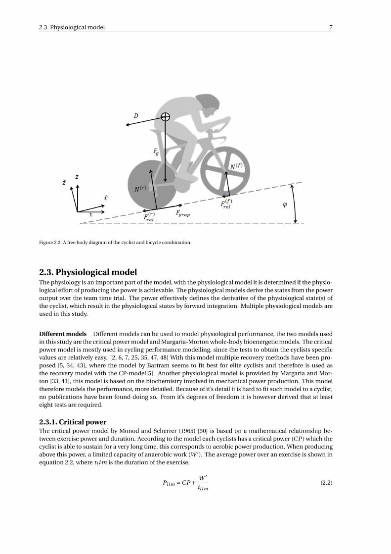
2.2. Mechanical modelThe mechanical model can be described by the equation of motion. In figure 2.2 the free body diagram ofthe cyclist is considered. Out of plane forces and lean are neglected. The motion of the cyclist is restrictedin the vertical direction due to the ground contacts. The equation of motion is defined in this direction. Theequation of motion has terms related to slope related forces, rolling resistance, aerodynamic drag and powerproduction by the cyclist. Those last two terms have interaction with the aerodynamic interaction modelsand physiological models.
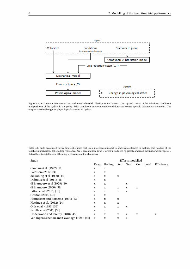
A lot of studies have provided a mechanical model that is used to model forces acting on a cyclist. In ta-ble 2.1. It is shown that all considdered researches consider rolling resistance and aerodynamic drag. Somestudies performed an analysis at constant velocity and did not include acceleration. Also a fair amount ofstudies performed an analysis without road incline and therefore did not include forces as a result of inclina-tion in the road surface. centrifugal forces are not considered much, nor is the chain efficiency.
2.2.1. Equation of motion of the individual cyclistThe equations of motion for the individual cyclist corresponding to figure 2.2. The equation is shown in equa-tion 2.1, the physiological model calculates the time derivative from the current state and the cyclist’s poweroutput and the aerodynamic drag reduction coefficient is defined by the aerodynamic interaction model as afunction of a cyclist’s group position.
Pi
vi= m̂i ·ai +
(mgCr
)i +
(1
2ρCd Av2
)i+mi g tan
(ϕ(xi )
)(2.1)
5
6 2. Modelling of the team time trial performance
Figure 2.1: A schematic overview of the mathematical model. The inputs are shown at the top and consist of the velocities, conditionsand positions of the cyclists in the group. With conditions environmental conditions and course specific parameters are meant. Theoutputs are the changes in physiological states of all cyclists.
Table 2.1: parts accounted for by different studies that use a mechanical model to address resistances in cycling. The headers of thetabel are abbriviated, Rol = rolling resistance, Acc = acceleration, Grad = forces introduced by gravity and road inclination, Centripetal =(lateral) centripetal forces, Efficiency = efficiency of the chaindrive
Study Effects modelledDrag Rolling Acc Grad Centripetal Efficiency
Candau et al. (1997) [11] x xBaldisera (2017) [3] x xde Koning et al (1999) [14] x x xDebraux et al (2011) [15] x xdi Prampero et al (1979) [40] x x xdi Prampero (2000) [39] x x x x xFitton et al. (2018) [18] x x x xGordon (2005) [42] x xHennekam and Botsema (1991) [23] x x xHettinga et al. (2012) [24] x x xOlds et al. (1993) [36] x x x xPadilla et al (2000) [38] x xUnderwood and Jeremy (2010) [45] x x x x x xVan Ingen Schenau and Cavanagh (1990) [46] x x x x
2.3. Physiological model 7
Figure 2.2: A free body diagram of the cyclist and bicycle combination.
2.3. Physiological modelThe physiology is an important part of the model, with the physiological model it is determined if the physio-logical effort of producing the power is achievable. The physiological models derive the states from the poweroutput over the team time trial. The power effectively defines the derivative of the physiological state(s) ofthe cyclist, which result in the physiological states by forward integration. Multiple physiological models areused in this study.
Different models Different models can be used to model physiological performance, the two models usedin this study are the critical power model and Margaria-Morton whole-body bioenergetic models. The criticalpower model is mostly used in cycling performance modelling, since the tests to obtain the cyclists specificvalues are relatively easy. [2, 6, 7, 25, 35, 47, 48] With this model multiple recovery methods have been pro-posed [5, 34, 43], where the model by Bartram seems to fit best for elite cyclists and therefore is used asthe recovery model with the CP-model[5]. Another physiological model is provided by Margaria and Mor-ton [33, 41], this model is based on the biochemistry involved in mechanical power production. This modeltherefore models the performance, more detailed. Because of it’s detail it is hard to fit such model to a cyclist,no publications have been found doing so. From it’s degrees of freedom it is however derived that at leasteight tests are required.
2.3.1. Critical powerThe critical power model by Monod and Scherrer (1965) [30] is based on a mathematical relationship be-tween exercise power and duration. According to the model each cyclists has a critical power (C P ) which thecyclist is able to sustain for a very long time, this corresponds to aerobic power production. When producingabove this power, a limited capacity of anaerobic work (W ′). The average power over an exercise is shown inequation 2.2, where tl i m is the duration of the exercise.
Pl i m =C P + W ′
tl i m(2.2)
8 2. Modelling of the team time trial performance
Wmax =C P · tl i m +W ′ (2.3)
The dynamical state of the anaerobic work capacity is defined by W ′bal , during a depletion of the anaerobic
reserve the change of the state of anaerobic work capacity is the amount of power delivered above the criticalpower, see equation 2.4. By integrating this over an exercise duration (tl i m) using any power (Pl i m) largerthan CP, the original relation from equation 2.3 is obtained, thus this equation satisfies the original model.The original model only models the expenditure and not the recovery. [30, 32]
dW ′bal
d t=C P −P P >C P (2.4)
Bartram’s recovery model [5] The recovery of Bartram’s model is modelled as a first order differential equa-tion, based on the theories of Skiba et al (2012) [43] and Morton and Billat (2004) [34]. This first order dif-ferential equation equation 2.5a has one parameter corresponding to the refill rate (τ), this time constant ismodelled as a function of recovery power Dcp = C P −P , see equation 2.5b. This equation is fitted to testsperformed by elite cyclists.
dW ′bal
d t= W ′−W ′
bal
τC P > P (2.5a)
τ= 2287.2 · (C P −P )−0.688 (2.5b)
Skiba’s recovery model [43] The recovery model by Skiba is most standard in physiological modelling, how-ever there are some conflicting things on this model. First of all the recovery equation reported by Skiba etal (2012) [43] contains an equation where it’s units mismatch and also does not correspond to the behaviourshown, this equation is slightly altered, such that the behaviour corresponds and the units match. An addi-tional point is that when the power output approaches critical power, the recovery rate does not approachzero, which result in that a slightly varying power output around CP has a much higher performance, thusalso resulting that the accuracy of determining the CP is corrupted. At last the model is not fitted to a cyclingtest or tested with elite athletes, which makes it less useful with respect to the Bartram Model.The model itself is based on the recovery kinetics proposed by Morton and Billat (2004) [34], with the equationshown in equation 2.6a. Just as in Bartram’s model the time constant τ is fitted as a function of the recoverypower: equation 2.6b.
dW ′bal
d t= W ′−W ′
bal
τC P > P (2.6a)
τ= 546e−0.01·(C P−P ) +316 (2.6b)
2.3.2. From critical power to critical velocityUsing the mechanical model the critical power can directly be linked to a velocity, at critical power this valueis defined as the critical velocity (CV). The critical velocity is, a velocity that can be maintained for a long time.This variable is influenced by environmental parameters (ρ, ϕ) and cyclist or bicycle parameters (Cr , Cd A).The critical velocity can be useful in determining the group velocity during a team time trial.
2.3.3. Margaria-Morton Physiological ModelsThe Margaria-Morton models are based on physiological processes in the body rather than mathematicalrelations found in tests. These models are mostly used to explain phenomena in exercises. [33, 41] Thesemodels could also be fitted to athletes.
Instead of one aerobic capacity as described in the critical power model, this model has two anaerobiccapacities. The first anaerobic capacity is related to the bodies capacity of phosphates, used in the produc-tion of ATP, which is directly used in production of mechanical work by the muscles. The second anaerobiccapacity is related to the supply of sugars in the form of lactate or glycogen, this reacts much slower thanthe phosphates. Another component in this process is the aerobic feed of energy, which contributes to thecontinues refilling of both anaerobic capacities.
2.3. Physiological model 9
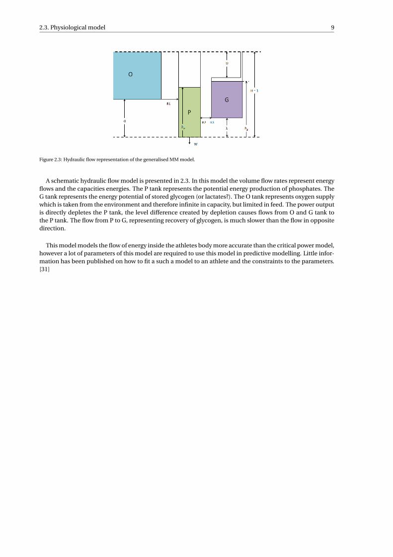
Figure 2.3: Hydraulic flow representation of the generalised MM model.
A schematic hydraulic flow model is presented in 2.3. In this model the volume flow rates represent energyflows and the capacities energies. The P tank represents the potential energy production of phosphates. TheG tank represents the energy potential of stored glycogen (or lactates?). The O tank represents oxygen supplywhich is taken from the environment and therefore infinite in capacity, but limited in feed. The power outputis directly depletes the P tank, the level difference created by depletion causes flows from O and G tank tothe P tank. The flow from P to G, representing recovery of glycogen, is much slower than the flow in oppositedirection.
This model models the flow of energy inside the athletes body more accurate than the critical power model,however a lot of parameters of this model are required to use this model in predictive modelling. Little infor-mation has been published on how to fit a such a model to an athlete and the constraints to the parameters.[31]
10 2. Modelling of the team time trial performance
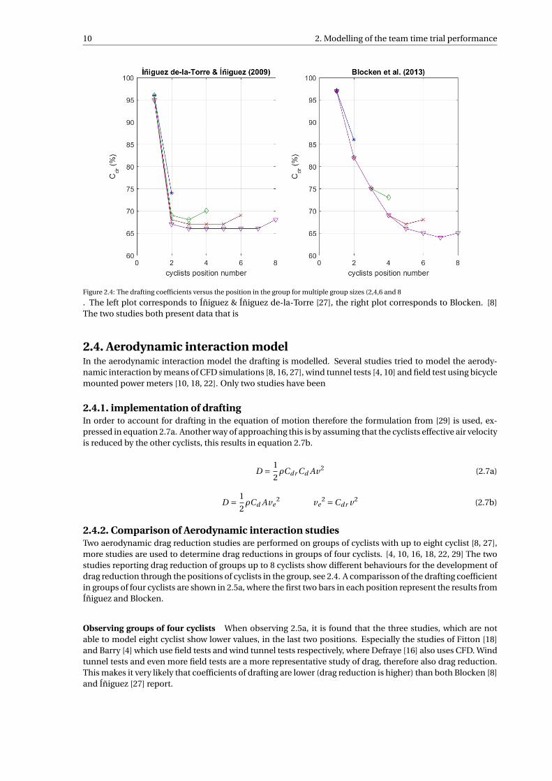
Figure 2.4: The drafting coefficients versus the position in the group for multiple group sizes (2,4,6 and 8
. The left plot corresponds to Íñiguez & Íñiguez de-la-Torre [27], the right plot corresponds to Blocken. [8]The two studies both present data that is
2.4. Aerodynamic interaction modelIn the aerodynamic interaction model the drafting is modelled. Several studies tried to model the aerody-namic interaction by means of CFD simulations [8, 16, 27], wind tunnel tests [4, 10] and field test using bicyclemounted power meters [10, 18, 22]. Only two studies have been
2.4.1. implementation of draftingIn order to account for drafting in the equation of motion therefore the formulation from [29] is used, ex-pressed in equation 2.7a. Another way of approaching this is by assuming that the cyclists effective air velocityis reduced by the other cyclists, this results in equation 2.7b.
D = 1
2ρCdr Cd Av2 (2.7a)
D = 1
2ρCd Ave
2 ve2 =Cdr v2 (2.7b)
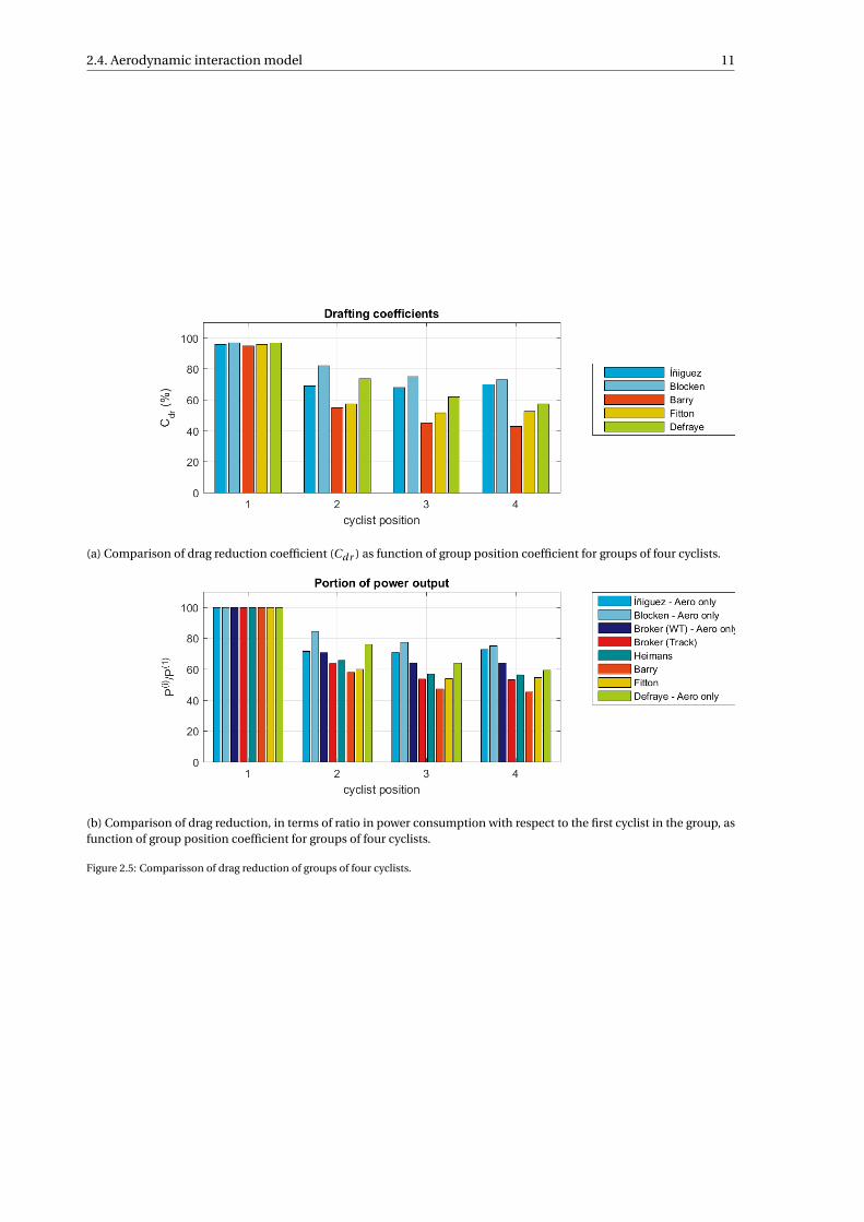
2.4.2. Comparison of Aerodynamic interaction studiesTwo aerodynamic drag reduction studies are performed on groups of cyclists with up to eight cyclist [8, 27],more studies are used to determine drag reductions in groups of four cyclists. [4, 10, 16, 18, 22, 29] The twostudies reporting drag reduction of groups up to 8 cyclists show different behaviours for the development ofdrag reduction through the positions of cyclists in the group, see 2.4. A comparisson of the drafting coefficientin groups of four cyclists are shown in 2.5a, where the first two bars in each position represent the results fromÍñiguez and Blocken.
Observing groups of four cyclists When observing 2.5a, it is found that the three studies, which are notable to model eight cyclist show lower values, in the last two positions. Especially the studies of Fitton [18]and Barry [4] which use field tests and wind tunnel tests respectively, where Defraye [16] also uses CFD. Windtunnel tests and even more field tests are a more representative study of drag, therefore also drag reduction.This makes it very likely that coefficients of drafting are lower (drag reduction is higher) than both Blocken [8]and Íñiguez [27] report.
2.4. Aerodynamic interaction model 11
(a) Comparison of drag reduction coefficient (Cdr ) as function of group position coefficient for groups of four cyclists.
(b) Comparison of drag reduction, in terms of ratio in power consumption with respect to the first cyclist in the group, asfunction of group position coefficient for groups of four cyclists.
Figure 2.5: Comparisson of drag reduction of groups of four cyclists.
12 2. Modelling of the team time trial performance
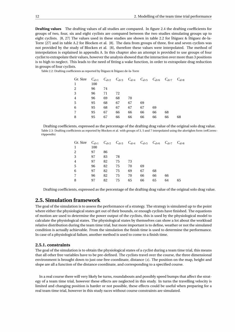
Drafting values The drafting values of all studies are compared. In figure 2.4 the drafting coefficients forgroups of two, four, six and eight cyclists are compared between the two studies simulating groups up toeight cyclists. [8, 27] The values used in these studies are shown in table 2.2 for Íñiguez & Íñiguez de-la-Torre [27] and in table A.2 for Blocken et al. [8]. The data from groups of three, five and seven cyclists wasnot provided by the study of Blocken et al. [8], therefore these values were interpolated. The method ofinterpolation is explained in appendix A. In this chapter also an attempt is provided to use groups of fourcyclist to extrapolate their values, however the analysis showed that the interaction over more than 3 positionsis to high to neglect. This leads to the need of fitting a wake function, in order to extrapolate drag reductionin groups of four cyclists.
Table 2.2: Drafting coefficients as reported by Íñiguez & Íñiguez de-la-Torre
Gr. Size Cdr 1 Cdr 2 Cdr 3 Cdr 4 Cdr 5 Cdr 6 Cdr 7 Cdr 8
1 1002 96 743 96 71 724 96 69 68 705 95 68 67 67 696 95 68 67 67 67 697 95 67 66 66 66 66 688 95 67 66 66 66 66 66 68
Drafting coefficients, expressed as the percentage of the drafting drag value of the original solo drag value.Table 2.3: Drafting coefficients as reported by Blocken et al. with groups of 3, 5 and 7 interpolated using the alortighm form (refCorrec-tAppendix)
Gr. Size Cdr 1 Cdr 2 Cdr 3 Cdr 4 Cdr 5 Cdr 6 Cdr 7 Cdr 8
1 1002 97 863 97 83 784 97 82 75 735 96 82 75 70 696 97 82 75 69 67 687 96 82 75 70 66 66 668 97 82 75 65 66 65 64 65
Drafting coefficients, expressed as the percentage of the drafting drag value of the original solo drag value.
2.5. Simulation frameworkThe goal of the simulation is to assess the performance of a strategy. The strategy is simulated up to the pointwhere either the physiological states get out of their bounds, or enough cyclists have finished. The equationsof motion are used to determine the power output of the cyclists, this is used by the physiological model tocalculate the physiological states. The physiological states by themselves can show a lot about the workloadrelative distribution during the team time trial, but more important is to define, weather or not the simulatedcondition is actually achievable. From the simulation the finish time is used to determine the performance.In case of a physiological failure, another method is used to come to a finish time.
2.5.1. constraintsThe goal of the simulation is to obtain the physiological states of a cyclist during a team time trial, this meansthat all other free variables have to be pre-defined. The cyclists travel over the course, the three dimensionalenvironment is brought down to just one free coordinate, distance (s). The position on the map, height andslope are all a function of the distance coordinate, and corresponding to a specified course.
In a real course there will very likely be turns, roundabouts and possibly speed bumps that affect the strat-egy of a team time trial, however these effects are neglected in this study. In turns the travelling velocity islimited and changing position is harder or not possible, these effects could be useful when preparing for areal team time trial, however in this study races without course constraints are simulated.
2.5. Simulation framework 13
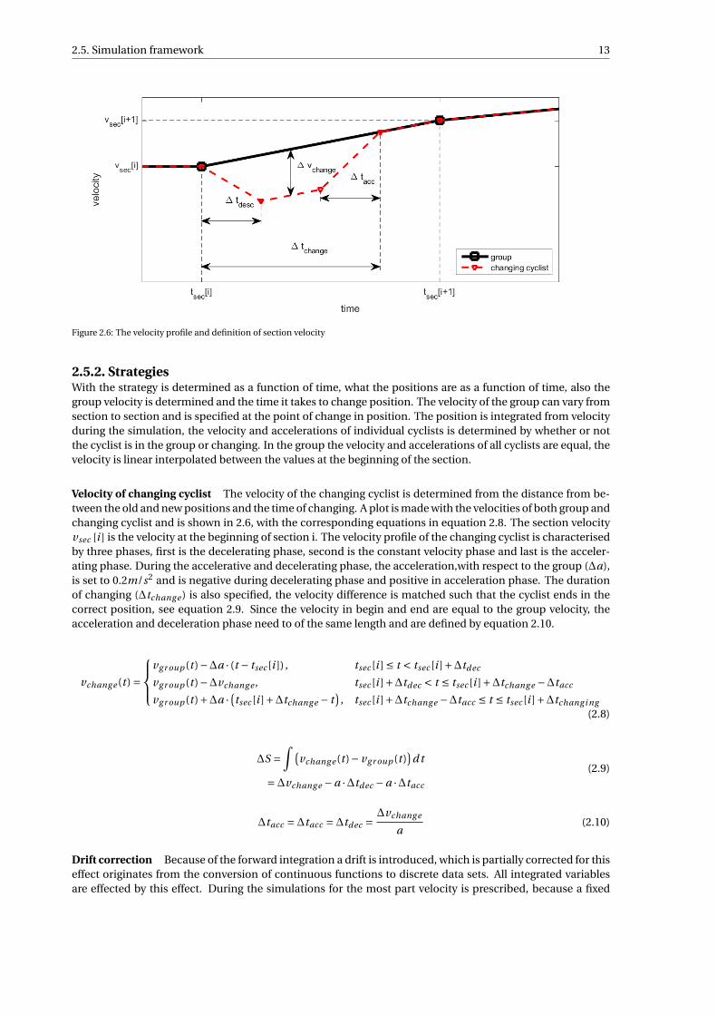
Figure 2.6: The velocity profile and definition of section velocity
2.5.2. StrategiesWith the strategy is determined as a function of time, what the positions are as a function of time, also thegroup velocity is determined and the time it takes to change position. The velocity of the group can vary fromsection to section and is specified at the point of change in position. The position is integrated from velocityduring the simulation, the velocity and accelerations of individual cyclists is determined by whether or notthe cyclist is in the group or changing. In the group the velocity and accelerations of all cyclists are equal, thevelocity is linear interpolated between the values at the beginning of the section.
Velocity of changing cyclist The velocity of the changing cyclist is determined from the distance from be-tween the old and new positions and the time of changing. A plot is made with the velocities of both group andchanging cyclist and is shown in 2.6, with the corresponding equations in equation 2.8. The section velocityvsec [i ] is the velocity at the beginning of section i. The velocity profile of the changing cyclist is characterisedby three phases, first is the decelerating phase, second is the constant velocity phase and last is the acceler-ating phase. During the accelerative and decelerating phase, the acceleration,with respect to the group (∆a),is set to 0.2m/s2 and is negative during decelerating phase and positive in acceleration phase. The durationof changing (∆tchang e ) is also specified, the velocity difference is matched such that the cyclist ends in thecorrect position, see equation 2.9. Since the velocity in begin and end are equal to the group velocity, theacceleration and deceleration phase need to of the same length and are defined by equation 2.10.
vchang e (t ) =
vg r oup (t )−∆a · (t − tsec [i ]) , tsec [i ] ≤ t < tsec [i ]+∆tdec
vg r oup (t )−∆vchang e , tsec [i ]+∆tdec < t ≤ tsec [i ]+∆tchang e −∆tacc
vg r oup (t )+∆a · (tsec [i ]+∆tchang e − t)
, tsec [i ]+∆tchang e −∆tacc ≤ t ≤ tsec [i ]+∆tchang i ng
(2.8)
∆S =∫ (
vchang e (t )− vg r oup (t ))
d t
=∆vchang e −a ·∆tdec −a ·∆tacc
(2.9)
∆tacc =∆tacc =∆tdec =∆vchang e
a(2.10)
Drift correction Because of the forward integration a drift is introduced, which is partially corrected for thiseffect originates from the conversion of continuous functions to discrete data sets. All integrated variablesare effected by this effect. During the simulations for the most part velocity is prescribed, because a fixed
14 2. Modelling of the team time trial performance
time step was used the accelerations can be calculated from this prescribed velocity. The velocity only devi-ates from the prescribed velocity, when cyclists are dropped out of the group. The velocity integrated fromthe acceleration is used rather than the prescribed velocity because this is will effect the energy balance, be-tween mechanical work performed by the cyclist and the kinetic energy. The accelerating and de-acceleratingphases in the changing procedure will be exactly of exactly the same duration and therefore the velocity willnot have any drift due to this procedure, the distance is slightly effected. Therefore the cyclist will be of fromthe aimed position after changing. Since the spacing between cyclist should be fixed, when in formation, thedrift can be corrected for the cyclists right after the changing procedure is performed. This is done by addinga peak in the velocity profile, which corrects the distance with respect to the others.
2.5.3. Differential equationsThe set differential equations can be defined as a function that calculates the state derivative with respect totime as a function of the state and the time. The state contains all the variables which are integrated. Since thesimulation contains multiple cyclists the states of all cyclist. The mechanical model has the travelled distance(s) and velocity (v) as states. The critical power model has the dynamic anaerobic work capacity (W ′
bal ) andthe Margaria-Morton model has the two energy levels (hP and hG ) as states.
2.5.4. Solving of differential equationsThe differential equation is solved using an euler integration scheme. The state denoted with X containsposition data as well as the physiological states. The physiological states, velocity and position of all cyclists.Only the group velocity is predefined, so not individual velocities and acceleration, those are calculated in thesame process as the physiological state differences. The difference in physiological state, acceleration andvelocity are de state derivatives. The states are determined by numerical integration using Euler integrationscheme as shown in equation 2.11. Here Xi is the current state, Xi+1 the next state and ∆ti the time step.
Xi+1 = Xi + dXi
d t·∆ti (2.11)
The usage of more accurate and complex solvers were considered. For example a fourth order Runge-Kuttasolver is likely to give a much more accurate integration. The simulation as it is, has lots of logical stageswitches which are harder to implement while using higher order solvers. The way it is programmed is thatthere are numerous variables called from the integration loop that are not stored in the states, therefore thestate derivatives are not a function of only time and state, which makes it harder to use higher order solvers.It must also be noted that between the compared simulations the changing behaviour is more or less equal,accelerations and durations of changing are kept equal between simulations, therefore a small integrationerror will be present in both of the compared simulations and thereby not influence the results.
2.6. Cyclists standardisationDuring this report standardised cyclists will be representing varying cyclists performance characteristics ina team. Team time trials are often a part of a multiple stage event meaning that, the cyclists selected willlikely vary in performance characteristics. The results of this study are generated by using parameters forstandardised cyclists. The parameters associated with these standards as well as a performance comparisonis discussed.
2.6.1. ParametersThe standardisation of cyclists is split up into two categories, the mechanical standards and the physiologicalstandard. Within the physiological standards there are of course two types, corresponding to critical powerand Margaria-Morton models. The mechanical standards are the masses and coefficients of resistance. Thestandardisation for mechanical coefficients is done per weight class (heavy, medium or light). The physiolog-ical parameters are split into classes of power output (super strong, strong, medium, weak).
Mechanical standardsWithin the mechanical constants some vary per class and others are independent, the varying parametersare cyclist mass and drag area, the others are the same for all cyclists. The three classes correspond to a body
2.7. Model Sensitivity 15
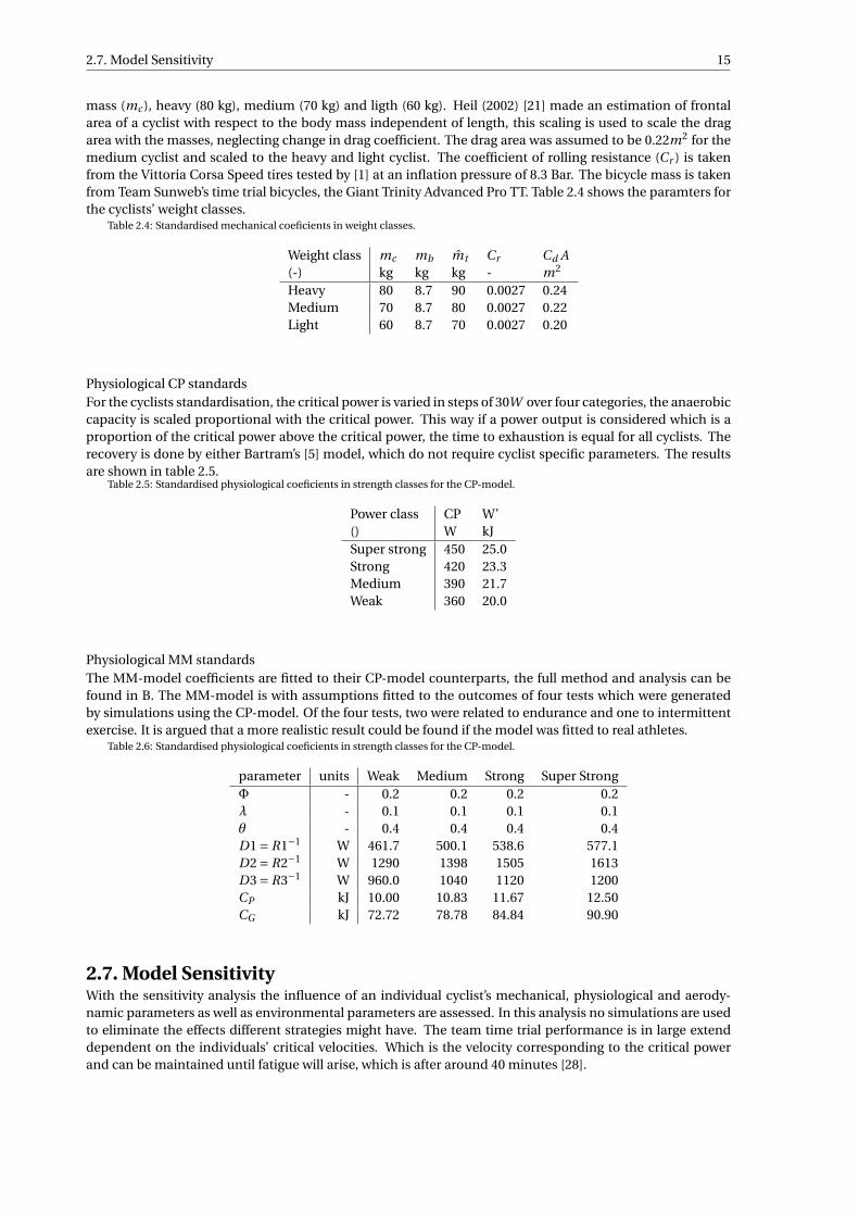
mass (mc ), heavy (80 kg), medium (70 kg) and ligth (60 kg). Heil (2002) [21] made an estimation of frontalarea of a cyclist with respect to the body mass independent of length, this scaling is used to scale the dragarea with the masses, neglecting change in drag coefficient. The drag area was assumed to be 0.22m2 for themedium cyclist and scaled to the heavy and light cyclist. The coefficient of rolling resistance (Cr ) is takenfrom the Vittoria Corsa Speed tires tested by [1] at an inflation pressure of 8.3 Bar. The bicycle mass is takenfrom Team Sunweb’s time trial bicycles, the Giant Trinity Advanced Pro TT. Table 2.4 shows the paramters forthe cyclists’ weight classes.
Table 2.4: Standardised mechanical coeficients in weight classes.
Weight class mc mb m̂t Cr Cd A(-) kg kg kg - m2
Heavy 80 8.7 90 0.0027 0.24Medium 70 8.7 80 0.0027 0.22Light 60 8.7 70 0.0027 0.20
Physiological CP standardsFor the cyclists standardisation, the critical power is varied in steps of 30W over four categories, the anaerobiccapacity is scaled proportional with the critical power. This way if a power output is considered which is aproportion of the critical power above the critical power, the time to exhaustion is equal for all cyclists. Therecovery is done by either Bartram’s [5] model, which do not require cyclist specific parameters. The resultsare shown in table 2.5.
Table 2.5: Standardised physiological coeficients in strength classes for the CP-model.
Power class CP W’() W kJSuper strong 450 25.0Strong 420 23.3Medium 390 21.7Weak 360 20.0
Physiological MM standardsThe MM-model coefficients are fitted to their CP-model counterparts, the full method and analysis can befound in B. The MM-model is with assumptions fitted to the outcomes of four tests which were generatedby simulations using the CP-model. Of the four tests, two were related to endurance and one to intermittentexercise. It is argued that a more realistic result could be found if the model was fitted to real athletes.
Table 2.6: Standardised physiological coeficients in strength classes for the CP-model.
parameter units Weak Medium Strong Super StrongΦ - 0.2 0.2 0.2 0.2λ - 0.1 0.1 0.1 0.1θ - 0.4 0.4 0.4 0.4D1 = R1−1 W 461.7 500.1 538.6 577.1D2 = R2−1 W 1290 1398 1505 1613D3 = R3−1 W 960.0 1040 1120 1200CP kJ 10.00 10.83 11.67 12.50CG kJ 72.72 78.78 84.84 90.90
2.7. Model SensitivityWith the sensitivity analysis the influence of an individual cyclist’s mechanical, physiological and aerody-namic parameters as well as environmental parameters are assessed. In this analysis no simulations are usedto eliminate the effects different strategies might have. The team time trial performance is in large extenddependent on the individuals’ critical velocities. Which is the velocity corresponding to the critical powerand can be maintained until fatigue will arise, which is after around 40 minutes [28].
16 2. Modelling of the team time trial performance
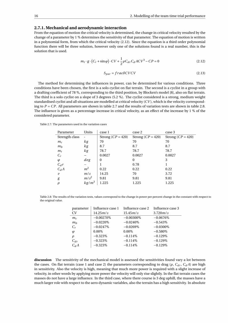
2.7.1. Mechanical and aerodynamic interactionFrom the equation of motion the critical velocity is determined, the change in critical velocity resulted by thechange of a parameter by 1 % determines the sensitivity of that parameter. The equation of motion is writtenin a polynomial form, from which the critical velocity (2.12). Since the equation is a third order polynomialfunction there will be three solution, however only one of the solutions found is a real number, this is thesolution that is used.
mt · g · (Cr + sinϕ) ·CV + 1
2ρCdr Cd ACV 3 −C P = 0 (2.12)
Spar = f r acδCV CV (2.13)
The method for determining the influences in power, can be determined for various conditions. Threeconditions have been chosen, the first is a solo cyclist on flat terrain. The second is a cyclist in a group witha drafting coefficient of 78 %, corresponding to the third position, by Blocken’s model [8], also on flat terrain.The third is a solo cyclist on a slope of 3 degrees (5.2 %). The cyclist considered is a strong, medium weightstandardised cyclist and all situations are modelled at critical velocity (CV ), which is the velocity correspond-ing to P =C P . All parameters are shown in table 2.7 and the results of variation tests are shown in table 2.8.The influence is given as a percentage increase in critical velocity, as an effect of the increase by 1 % of theconsidered parameter.
Table 2.7: The parameters used in the variation cases
Parameter Units case 1 case 2 case 3Strength class - Strong (C P = 420) Strong (C P = 420) Strong (C P = 420)mc kg 70 70 70mb kg 8.7 8.7 8.7mt kg 78.7 78.7 78.7Cr − 0.0027 0.0027 0.0027ϕ deg 0 0 3Cd r − 1 0.78 1Cd A m2 0.22 0.22 0.22v m/s 14.25 70 3.72g m/s2 9.81 9.81 9.81ρ kg /m3 1.225 1.225 1.225
Table 2.8: The results of the variation tests, values correspond to the change in power per percent change in the constant with respect tothe original value.
parameter Influence case 1 Influence case 2 Influence case 3CV 14.25m/s 15.45m/s 3.720m/smc −0.00270% −0.00300% −0.0676%mb −0.0220% −0.0240% −0.543%Cr −0.0247% −0.0269% −0.0300%ϕ 0.00% 0.00% −0.580%ρ −0.323% −0.114% −0.129%Cdr −0.323% −0.114% −0.129%Cd A −0.323% −0.114% −0.129%
discussion The sensitivity of the mechanical model is assessed the sensitivities found vary a lot betweenthe cases. On flat terrain (case 1 and case 2) the parameters corresponding to drag (ρ, Cdr , Cd A) are highin sensitivity. Also the velocity is high, meaning that much more power is required with a slight increase ofvelocity, in other words by applying more power the velocity will only rise slightly. In the flat terrain cases themasses do not have a large influence. In the third case, where there course is 3 deg uphill, the masses have amuch larger role with respect to the aero dynamic variables, also the terrain has a high sensitivity. In absolute
2.8. Validity 17
values the slope angle has an equal sensitivity in both cases, only the rise of one percent of the original valueis zero for the first two cases (since the value is zero). The rolling resistance does not have a high sensitivity inany of these cases.
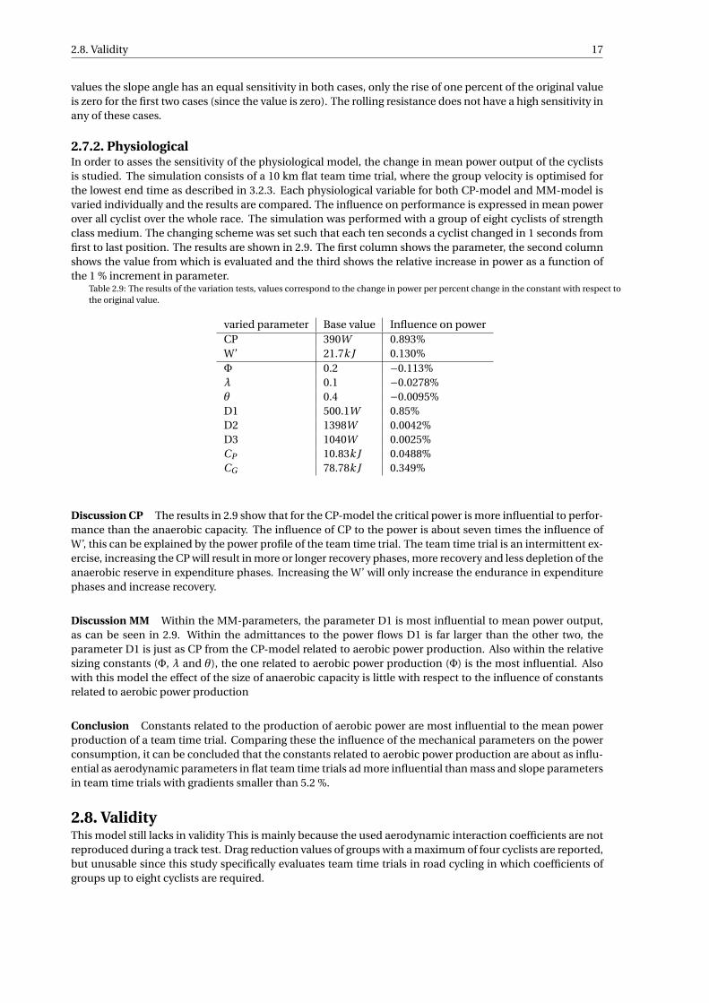
2.7.2. PhysiologicalIn order to asses the sensitivity of the physiological model, the change in mean power output of the cyclistsis studied. The simulation consists of a 10 km flat team time trial, where the group velocity is optimised forthe lowest end time as described in 3.2.3. Each physiological variable for both CP-model and MM-model isvaried individually and the results are compared. The influence on performance is expressed in mean powerover all cyclist over the whole race. The simulation was performed with a group of eight cyclists of strengthclass medium. The changing scheme was set such that each ten seconds a cyclist changed in 1 seconds fromfirst to last position. The results are shown in 2.9. The first column shows the parameter, the second columnshows the value from which is evaluated and the third shows the relative increase in power as a function ofthe 1 % increment in parameter.
Table 2.9: The results of the variation tests, values correspond to the change in power per percent change in the constant with respect tothe original value.
varied parameter Base value Influence on powerCP 390W 0.893%W’ 21.7k J 0.130%Φ 0.2 −0.113%λ 0.1 −0.0278%θ 0.4 −0.0095%D1 500.1W 0.85%D2 1398W 0.0042%D3 1040W 0.0025%CP 10.83k J 0.0488%CG 78.78k J 0.349%
Discussion CP The results in 2.9 show that for the CP-model the critical power is more influential to perfor-mance than the anaerobic capacity. The influence of CP to the power is about seven times the influence ofW’, this can be explained by the power profile of the team time trial. The team time trial is an intermittent ex-ercise, increasing the CP will result in more or longer recovery phases, more recovery and less depletion of theanaerobic reserve in expenditure phases. Increasing the W’ will only increase the endurance in expenditurephases and increase recovery.
Discussion MM Within the MM-parameters, the parameter D1 is most influential to mean power output,as can be seen in 2.9. Within the admittances to the power flows D1 is far larger than the other two, theparameter D1 is just as CP from the CP-model related to aerobic power production. Also within the relativesizing constants (Φ, λ and θ), the one related to aerobic power production (Φ) is the most influential. Alsowith this model the effect of the size of anaerobic capacity is little with respect to the influence of constantsrelated to aerobic power production
Conclusion Constants related to the production of aerobic power are most influential to the mean powerproduction of a team time trial. Comparing these the influence of the mechanical parameters on the powerconsumption, it can be concluded that the constants related to aerobic power production are about as influ-ential as aerodynamic parameters in flat team time trials ad more influential than mass and slope parametersin team time trials with gradients smaller than 5.2 %.
2.8. ValidityThis model still lacks in validity This is mainly because the used aerodynamic interaction coefficients are notreproduced during a track test. Drag reduction values of groups with a maximum of four cyclists are reported,but unusable since this study specifically evaluates team time trials in road cycling in which coefficients ofgroups up to eight cyclists are required.
18 2. Modelling of the team time trial performance
One way to improve the validity of the model presented in this study is to improve the validity drag re-duction coefficients. This can be done by reproducing the values from the CFD tests in a track test, as areperformed on groups of four cyclists [10, 18, 22].
Another way to increase the validity is to simulate a strategy that was performed in a real race. For examplethe velocity could be optimised while maintaining the same changing scheme in order to assess the bestachievable finish time given the strategy and compare this to the performed result. However in order to dothis, for a group of cyclists both a physiological model has to be fitted and aerodynamic drag area of all cyclistshas to be determined accurately.
3Optimising Strategy
The strategy of a team time trial can be described by a lot of parameters. The most defining are the timesspend in positions and the positions of cyclists over time. Different less important parameters are the changeduration and the acceleration and deceleration while changing. Alternatively the wheel gaps and lateral de-viations can be modelled, however the current model is unfit to do so since there is no data on the change ofaerodynamic drafting coefficients as a function of these parameters is undefined. In this study only the mainparameters, cyclists positions and times spend in positions are assessed in later studies it is also possible tovary the other parameters.
3.1. StrategiesAs explained in chapter 2 the strategy is the description of the cyclists position in the group, change duration,velocity during the race. For each different section, where the cyclists have the same position in the group,including the part where the cyclists change their position; the strategy contains their velocity, the time itshould take to perform the change their position, and the positions of all cyclists and the time the start timeof this configuration. For a 40 minute race with eight cyclist where the cyclists keep their formation over 20 sthis yields 120 formations, leading to 1320 free variables. In real races strategies are simplified by a set of rulesto make the strategy less complex, for example always change from first to last position, or when tired reducetime in first position. In this section the strategies will be explained and how they are optimised.
3.1.1. Regular strategyThe most regular strategy is used as the baseline in this study, it is performed by many teams in professionalroad cycling. The team starts in a predefined order. Changing happens from first to last position, where allother cyclist effectively shift one position forward, due to the absence of the previously first cyclist in group,see figure 3.2. To differ the workload between cyclists in a team, the time for each cyclist in first position (headtime) is varied among the cyclists.
Using the regular strategy the number of free variables is reduced. Using the previous example of a 40minute race, the positioning options has been reduced by a factor 120 (8 ·120 to 8) and the time of changingoptions by a factor 15 (120 to 8). The group velocity can be defined by sections of the course, or made as afunction of the courses slope. This leads to a strategy that has two free parameters per cyclist with additionalvelocity parameters.
19

20 3. Optimising Strategy
Figure 3.1: A position change according to the regular strategy, the circled numbers denote the group position of the cyclists. The cyclistin first position changes to the last position, therefore all other cyclists shift to one position in front.
Figure 3.2: A position change according to the variable return position strategy, the circled numbers denote the group position of thecyclists. In this case the cyclist first position goes to the third position, the cyclist in position four remains in position four, but will haveto make room for to let the cyclist in third position, the cyclist in position two and three become the cyclists in position one and tworespectively, but keep their velocity constant.
3.2. Optimisation 21
3.2. OptimisationOptimisations can be performed to estimate the optimal inputs to a strategy. For each strategy inputs canbe defined, such as initial positions, head times or velocity. The optimisation uses an objective function todetermine a score, this score is minimised by altering the inputs to the objective function, such that the scorewill be lowest. In the optimisations in this study the score is the finish time of a team time trial, which isthe time in which four cyclists pass the finish line. For applicability the values are presented as the averagevelocity over the race, which is computed by dividing the race distance by the finish time.
3.2.1. Objective FunctionTo optimise performance an objective function is used, this function gives a score to the strategy, which isminimised. The objective function is the simulation, the finish time is used as the objective value, therefore anperformance optimisation will always optimise towards a lower finish time, if the optimisation is convergent.It could be that one of the cyclists fails to execute prescribed strategy, in this case the simulation is terminated.To compute the finish time in cases of physiological failure, it is assumed that the cyclists are able to completethe race by cycling at a velocity of 30 km/h. This velocity is used to compute the time required to completethe maintaining distance and added to the time of failure. This "motivates" the optimisation to move themoment of failure towards the finish, for a better convergence.
3.2.2. Separating the ProblemThe free variables of a strategy are composed of two types, the continuous variables and the integer constraintvariables. The continuous variables in this problem are the velocities of sections of the race. The integerconstraint variables are the initial positions, the return positions and the head times. The head times couldalso be presented as continuous numbers, however they are set in steps of 10 seconds to reduce the size ofthe problem. To asses a strategy the velocities are not provided as inputs, but optimised at each iteration ofthe strategy optimisation. This is done to improve the convergence of the problem.
3.2.3. Velocity OptimisationFor each strategy in the optimisation, the velocity is optimised to give maximum result over the simulation,given the specified strategy. The strategy could contain multiple velocities, for example when the slope variesalong the course, different sections will have most likely have different ideal velocities, therefore the velocityis a multiple input, single output optimisation.
The algorithm used for the velocity optimisation is the derivative free method. This method is chosenbecause the velocity optimisation has both continuous input (velocity) and continuous output, from whicha gradient can be computed. The algorithm is set to optimise until the input velocity difference is lower than0.005 m/s.
3.2.4. Strategy OptimisationGenetic algorithm is used to optimise strategy since it is able to handle problems with many local minimaand integer constraints and is still able to find the global minimum. The strategy parameters that were variedin this study are, initial positions, times spend in first position, and «return position», of which only the timesspend in first position are continuous. Since the interest is in the global optimum and not the local optima,the are also discretized to steps of 10 seconds.
The genetic algorithm uses an evolution inspired method of crossing and mutating bit strings that containthe inputs of the objective function. The population size determines how many sets of bit strings are con-sidered in each generation. The input of the genetic algorithm is converted to a bit string, the length of thebit string defines the complexity of the problem. The higher the complexity the lower the convergence rate,meaning a larger population size and/or number of generations is needed to achieve the same accuracy. Theoptimisation of different strategies require different inputs. These inputs are if necessary discretized. Thecomplexity of the inputs are listed below. Note that all numbers have to be rounded upwards.
• Order: The order is selected from a list of all possible orders depending on the number of cyclists (nc )the complexity depends on the length of the list, the list has nc ! inputs, meaning the complexity isc = log2 nc ! bits.
22 3. Optimising Strategy
• Head times: the head times are discretized in steps of 10 seconds, with a maximum of 60 s. meaningthere are six options, this results in three bits per cyclist. If multiple routines are used, the amountneeds to be multiplied by the number of routines nr , hence: c = 3 ·nc bits.
• dropping distance: The dropping distance can be defined in parts of a fifteenth of the total courselength. Therefore the complexity is four bits per cyclists: c = nc ·4 bits.
The maximum number of generations was set to 200, however during the convergence tests, this was neverexceeded. The rest of the parameters was set to the default settings of MATLAB’s built in genetic algorithmoptimisation.

3.3. Convergence 23
3.3. ConvergenceIt is determined that a genetic optimisation will be used to generate the results, however the accuracy of opti-misation depends on the problem as well as the parameters of the genetic algorithm. The genetic algorithm isperformed with use of the optimisation toolbox in MATLAB. This toolbox has a function for genetic algorithm[13], which is used. Four parameters (three independent) are varied to asses their influence on accuracy andcomputational costs. The population size is closely related to the computational costs. The population sizedetermines the number of function evaluations per generation. If the population size causes better conver-gence, the amount of generations required reach a required accuracy is lower. Elite ratio, mutation ratio andcrossover ratio influence the convergence, and thereby also the computational costs, but the influence on thecomputational costs is not as high as that from the population size. Therefore using a low complexity problemthe convergence of different combinations of the Elite-, Mutation- and crossover-ratio are compared.
First a case with lower complexity is used to determine the cross-over ratio, mutation ratio and elite ratio ofthe genetic algorithm in a strategy optimisation of low complexity. This test simulated a group of four cyclistsover a race of five kilometres. A second test, with higher complexity was used to determine the populationsize, for the best convergence. This test was with eight cyclists over a race of kilometres.
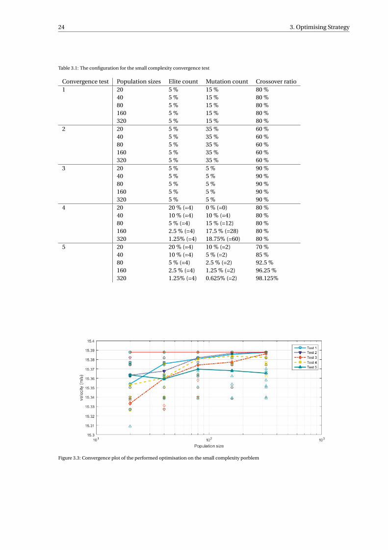
3.3.1. Elite, mutation and crossover ratiomultiple configurations of elite, mutation and crossover ratio are compared using a small complexity prob-lem. The population is split in three categories to produce the next generation, these three categories areelite, mutation and crossover; it is therefore that the sum of the elite-, mutation- and crossover-ratio needs tobe 100 %. In this problem from a 5 km team time trial with four cyclists, the order and head times are opti-mised. This results in 17 bit complexity. For every population size in every test the optimisation is performed20 times, to provide enough data points. The configurations are based on [20], not all parameters are indi-vidually varied to reduce computational costs, the objective is a well converging combination rather than theoptimum since the convergence tests will be far more computationally expensive with respect to the actualoptimisations. For all configurations the test are performed on populations sizes 20, 40, 80, 160, 320 in orderto be able to detect their convergence over population size. Later the population size will be selected. Theused configurations are presented in table 3.1. in the first three configurations the elite count was set to 5 %and the mutation ratio was varied, test 1 is according to the standard options from MATLAB’s genetic algo-rithm. In [20] it was said that for small population (4, 8) sizes a mutation ratio of 15 % was preferred and forlarger population sizes (64, 128) 1 % or 2 % performed better. This lead to the hypothesis that a fixed numberof elites and mutations (throughout the population sizes) would perform well, therefore in test 4 the numberof elites and the crossover ratio are kept constant and in test 5 the both the number of elites and number ofmutated are kept constant.
The results are presented in figure 3.3 in terms of the average velocity. The red line is the value of themaximum velocity of all data sets, the error is defined as the difference of a data point to that value. In thisgraph it is shown that the two tests with a fixed number of elites (4, 5) did not perform well with respect to therest, with the largest error with the largest population size. The third test with a low mutation rate took verylong to get good convergence, with a large error at a population size of 160. Test 1 and 2 both performed well.
From this little tests it cannot be concluded that a fixed number of elites is not preferred, however given theresults presented results it does not seem better. There is no test where the number of mutated is fixed andthe number of elite is varied along the population sizes, however the results with the fixed number of elitesdo not motivate to do so. As test 1 were the standard MATLAB configurations it was no surprise that theypreformed so well. Test two shows a better convergence with both population sizes 80 and 160, with respectto test 1.
It is chosen to proceed with the configuration from test 2 with an equal elite ratio and a higher mutationratio and a lower crossover ratio with respect to the MATLAB’s standard (test 1). With these settings the testswill be repeated for an optimisation with higher complexity and all considered model configurations.
24 3. Optimising Strategy
Table 3.1: The configuration for the small complexity convergence test
Convergence test Population sizes Elite count Mutation count Crossover ratio1 20 5 % 15 % 80 %
40 5 % 15 % 80 %80 5 % 15 % 80 %160 5 % 15 % 80 %320 5 % 15 % 80 %
2 20 5 % 35 % 60 %40 5 % 35 % 60 %80 5 % 35 % 60 %160 5 % 35 % 60 %320 5 % 35 % 60 %
3 20 5 % 5 % 90 %40 5 % 5 % 90 %80 5 % 5 % 90 %160 5 % 5 % 90 %320 5 % 5 % 90 %
4 20 20 % (=4) 0 % (=0) 80 %40 10 % (=4) 10 % (=4) 80 %80 5 % (=4) 15 % (=12) 80 %160 2.5 % (=4) 17.5 % (=28) 80 %320 1.25% (=4) 18.75% (=60) 80 %
5 20 20 % (=4) 10 % (=2) 70 %40 10 % (=4) 5 % (=2) 85 %80 5 % (=4) 2.5 % (=2) 92.5 %160 2.5 % (=4) 1.25 % (=2) 96.25 %320 1.25% (=4) 0.625% (=2) 98.125%
Figure 3.3: Convergence plot of the performed optimisation on the small complexity porblem

3.3. Convergence 25
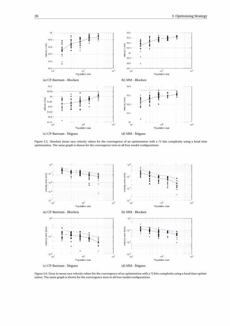
3.3.2. Population sizeWith the configurations from the small complexity test, the convergence tests are performed again on a prob-lem of larger complexity, that is the same size as those used later in the study. From these convergence test notonly the population for further optimisation is selected, but also the standard deviations are defined, whichare used in the statistics of the results. As the standard deviations are expected to be different for the differentmodel configurations, the convergence test is performed for all four model configurations used to obtain theresults later. It is therefore also important that an optimisation is performed that results in high standarddeviations. The optimisation that is preformed is a order and head times optimisation, with dropping. Thisresults in a 72 bit complexity optimisation. In order to drive the optimisation results to a high standard de-viation a very different group was selected, containing two super strong, two strong, two medium and twoweak cyclists. In order to obtain a decent amount of head turns the simulation was performed over a 10 kmflat road. As with the small complexity test, for each population size 20 optimisations were performed.
The results for the larger complexity test are presented in figure 3.5 and the errors in figure 3.6. From thevelocity results it is shown that the means rise towards the estimated maximum velocity, defined as the largestmean velocity found in the data set an plotted as the red horizontal line. Also the standard deviation shrinkswith the population size, as is plotted in figure 3.4. It is shown that generally the convergence up to populationsizes 80 or 160 is significant and from there it begins to flatten out. Taking in consideration the convergenceof both means, standard deviation and the computational costs it is selected to continue with a populationsize of 160. In cases where more accurate results are required it can be decided to run more optimisations.
Figure 3.4: The standard deviation on the velocity of the results from the genetic algorithm optimisation against population size.
26 3. Optimising Strategy
(a) CP-Bartram - Blocken (b) MM - Blocken
(c) CP-Bartram - Íñiguez (d) MM - Íñiguez
Figure 3.5: Absolute mean race velocity values for the convergence of an optimisation with a 72 bits complexity using a head timeoptimisation. The same graph is shown for the convergence tests in all four model configurations
(a) CP-Bartram - Blocken (b) MM - Blocken
(c) CP-Bartram - Íñiguez (d) MM - Íñiguez
Figure 3.6: Error in mean race velocity values for the convergence of an optimisation with a 72 bits complexity using a head time optimi-sation. The same graph is shown for the convergence tests in all four model configurations
3.4. Conclusion 27
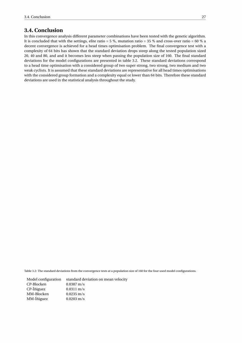
3.4. ConclusionIn this convergence analysis different parameter combinations have been tested with the genetic algorithm.It is concluded that with the settings, elite ratio = 5 %, mutation ratio = 35 % and cross-over ratio = 60 % adecent convergence is achieved for a head times optimisation problem. The final convergence test with acomplexity of 64 bits has shown that the standard deviation drops steep along the tested population sized20, 40 and 80, and and it becomes less steep when passing the population size of 160. The final standarddeviations for the model configurations are presented in table 3.2. These standard deviations correspondto a head time optimisation with a considered group of two super strong, two strong, two medium and twoweak cyclists. It is assumed that these standard deviations are representative for all head times optimisationswith the considered group formation and a complexity equal or lower than 64 bits. Therefore these standarddeviations are used in the statistical analysis throughout the study.
Table 3.2: The standard deviations from the convergence tests at a population size of 160 for the four used model configurations.
Model configuration standard deviation on mean velocityCP-Blocken 0.0387 m/sCP-Íñiguez 0.0311 m/sMM-Blocken 0.0235 m/sMM-Íñiguez 0.0203 m/s

4Analysis of a standard team time trial
Before diving into optimising different strategies, an evaluation of a standard strategy team time trial isperformed. The analysis will be in three steps, at first the analysis will be made on a team time trial withoutany balancing. Secondly the performance is improved by performing workload balance by means of adjustingthe times spend in first position for different cyclists. In the third case, cyclists are also dropped from thegroup during the race, to further balance the workload.
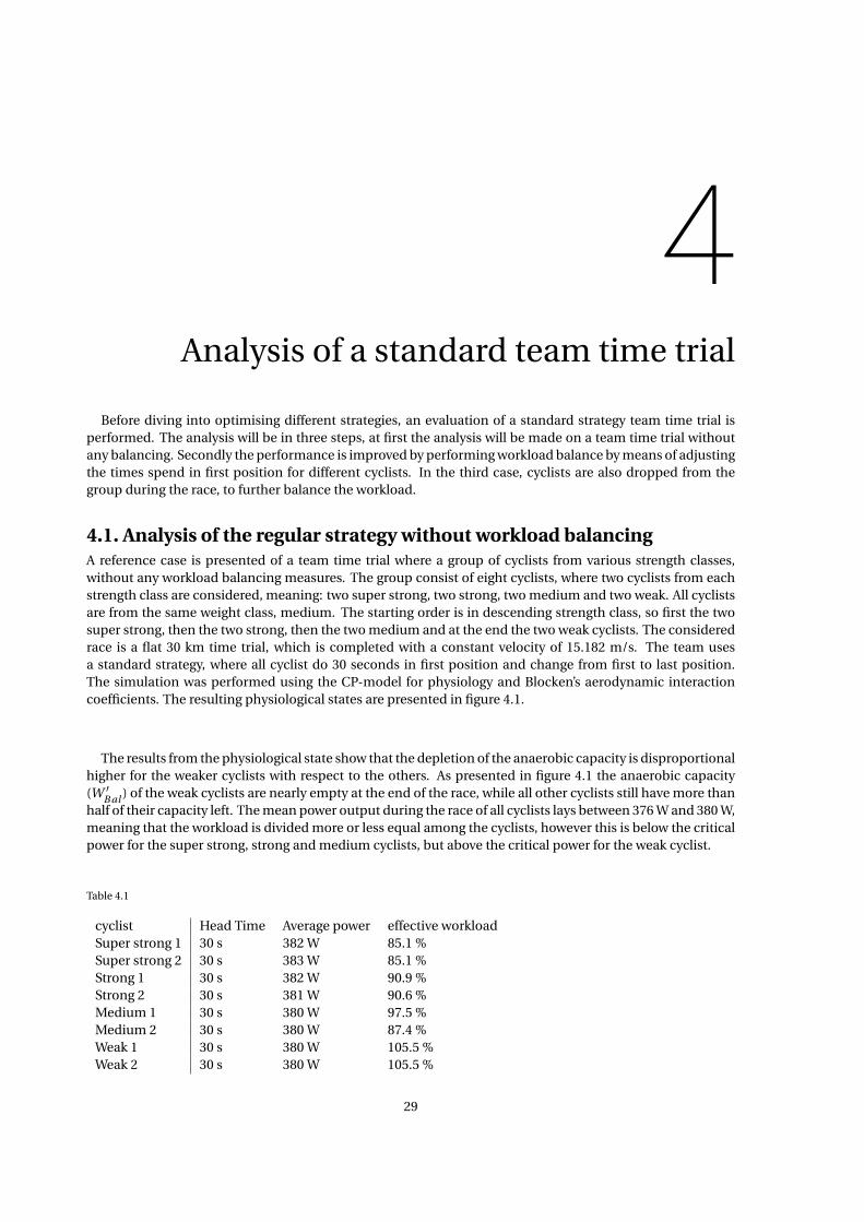
4.1. Analysis of the regular strategy without workload balancingA reference case is presented of a team time trial where a group of cyclists from various strength classes,without any workload balancing measures. The group consist of eight cyclists, where two cyclists from eachstrength class are considered, meaning: two super strong, two strong, two medium and two weak. All cyclistsare from the same weight class, medium. The starting order is in descending strength class, so first the twosuper strong, then the two strong, then the two medium and at the end the two weak cyclists. The consideredrace is a flat 30 km time trial, which is completed with a constant velocity of 15.182 m/s. The team usesa standard strategy, where all cyclist do 30 seconds in first position and change from first to last position.The simulation was performed using the CP-model for physiology and Blocken’s aerodynamic interactioncoefficients. The resulting physiological states are presented in figure 4.1.
The results from the physiological state show that the depletion of the anaerobic capacity is disproportionalhigher for the weaker cyclists with respect to the others. As presented in figure 4.1 the anaerobic capacity(W ′
B al ) of the weak cyclists are nearly empty at the end of the race, while all other cyclists still have more thanhalf of their capacity left. The mean power output during the race of all cyclists lays between 376 W and 380 W,meaning that the workload is divided more or less equal among the cyclists, however this is below the criticalpower for the super strong, strong and medium cyclists, but above the critical power for the weak cyclist.
Table 4.1
cyclist Head Time Average power effective workloadSuper strong 1 30 s 382 W 85.1 %Super strong 2 30 s 383 W 85.1 %Strong 1 30 s 382 W 90.9 %Strong 2 30 s 381 W 90.6 %Medium 1 30 s 380 W 97.5 %Medium 2 30 s 380 W 87.4 %Weak 1 30 s 380 W 105.5 %Weak 2 30 s 380 W 105.5 %
29
30 4. Analysis of a standard team time trial
Figure 4.1: An example of the W ′B al states of cyclists during a team time trial. The top two lines represent the super strong cyclist, the
two lines below that, the strong cyclists, followed by two medium cyclists, and the bottom lines represent two weak cyclists. The headtimes of the cyclists are equal with 30 s in this example.
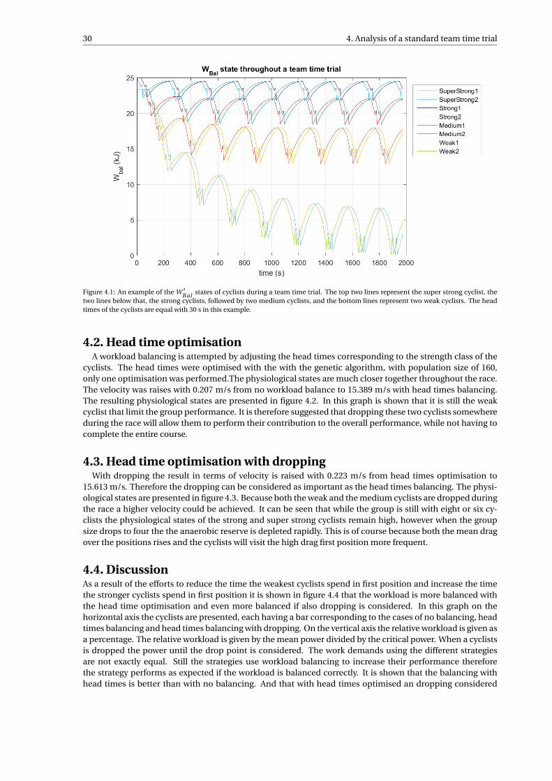
4.2. Head time optimisationA workload balancing is attempted by adjusting the head times corresponding to the strength class of the
cyclists. The head times were optimised with the with the genetic algorithm, with population size of 160,only one optimisation was performed.The physiological states are much closer together throughout the race.The velocity was raises with 0.207 m/s from no workload balance to 15.389 m/s with head times balancing.The resulting physiological states are presented in figure 4.2. In this graph is shown that it is still the weakcyclist that limit the group performance. It is therefore suggested that dropping these two cyclists somewhereduring the race will allow them to perform their contribution to the overall performance, while not having tocomplete the entire course.
4.3. Head time optimisation with droppingWith dropping the result in terms of velocity is raised with 0.223 m/s from head times optimisation to
15.613 m/s. Therefore the dropping can be considered as important as the head times balancing. The physi-ological states are presented in figure 4.3. Because both the weak and the medium cyclists are dropped duringthe race a higher velocity could be achieved. It can be seen that while the group is still with eight or six cy-clists the physiological states of the strong and super strong cyclists remain high, however when the groupsize drops to four the the anaerobic reserve is depleted rapidly. This is of course because both the mean dragover the positions rises and the cyclists will visit the high drag first position more frequent.
4.4. DiscussionAs a result of the efforts to reduce the time the weakest cyclists spend in first position and increase the timethe stronger cyclists spend in first position it is shown in figure 4.4 that the workload is more balanced withthe head time optimisation and even more balanced if also dropping is considered. In this graph on thehorizontal axis the cyclists are presented, each having a bar corresponding to the cases of no balancing, headtimes balancing and head times balancing with dropping. On the vertical axis the relative workload is given asa percentage. The relative workload is given by the mean power divided by the critical power. When a cyclistsis dropped the power until the drop point is considered. The work demands using the different strategiesare not exactly equal. Still the strategies use workload balancing to increase their performance thereforethe strategy performs as expected if the workload is balanced correctly. It is shown that the balancing withhead times is better than with no balancing. And that with head times optimised an dropping considered
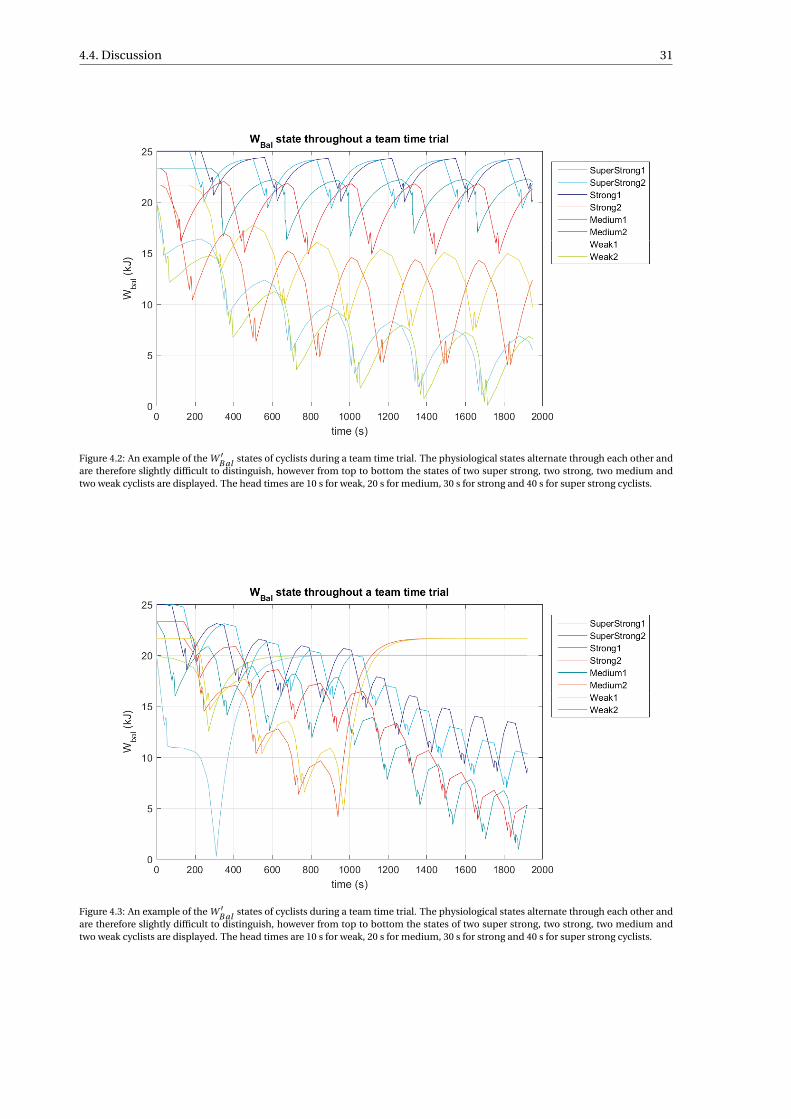
4.4. Discussion 31
Figure 4.2: An example of the W ′B al states of cyclists during a team time trial. The physiological states alternate through each other and
are therefore slightly difficult to distinguish, however from top to bottom the states of two super strong, two strong, two medium andtwo weak cyclists are displayed. The head times are 10 s for weak, 20 s for medium, 30 s for strong and 40 s for super strong cyclists.
Figure 4.3: An example of the W ′B al states of cyclists during a team time trial. The physiological states alternate through each other and
are therefore slightly difficult to distinguish, however from top to bottom the states of two super strong, two strong, two medium andtwo weak cyclists are displayed. The head times are 10 s for weak, 20 s for medium, 30 s for strong and 40 s for super strong cyclists.
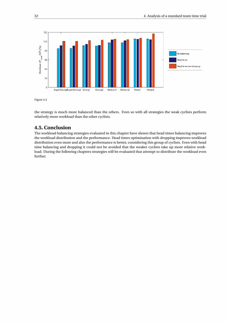
32 4. Analysis of a standard team time trial
Figure 4.4
the strategy is much more balanced than the others. Even so with all strategies the weak cyclists performrelatively more workload than the other cyclists.
4.5. ConclusionThe workload balancing strategies evaluated in this chapter have shown that head times balancing improvesthe workload distribution and the performance. Head times optimisation with dropping improves workloaddistribution even more and also the performance is better, considering this group of cyclists. Even with headtime balancing and dropping it could not be avoided that the weaker cyclists take up more relative work-load. During the following chapters strategies will be evaluated that attempt to distribute the workload evenfurther.
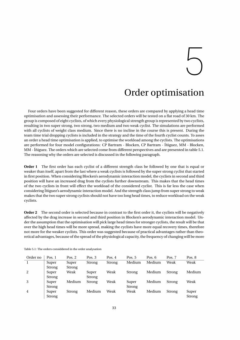
5Order optimisation
Four orders have been suggested for different reason, these orders are compared by applying a head timeoptimisation and assessing their performance. The selected orders will be tested on a flat road of 30 km. Thegroup is composed of eight cyclists, of which every physiological strength group is represented by two cyclists,resulting in two super strong, two strong, two medium and two weak cyclist. The simulations are performedwith all cyclists of weight class medium. Since there is no incline in the course this is present. During theteam time trial dropping cyclists is included in the strategy and the time of the fourth cyclist counts. To assesan order a head time optimisation is applied, to optimise the workload among the cyclists. The optimisationsare performed for four model configurations: CP Bartram - Blocken, CP Bartram - Íñiguez, MM - Blocken,MM - Íñiguez. The orders which are selected come from different perspectives and are presented in table 5.1.The reasoning why the orders are selected is discussed in the following paragraph.
Order 1 The first order has each cyclist of a different strength class be followed by one that is equal orweaker than itself, apart from the last where a weak cyclists is followed by the super strong cyclist that startedin first position. When considering Blocken’s aerodynamic interaction model, the cyclists in second and thirdposition will have an increased drag from the cyclists further downstream. This makes that the head timesof the two cyclists in front will effect the workload of the considered cyclist. This is far less the case whenconsidering Íñiguez’s aerodynamic interaction model. And the strength class jump from super strong to weakmakes that the two super strong cyclists should not have too long head times, to reduce workload on the weakcyclists.
Order 2 The second order is selected because in contrast to the first order it, the cyclists will be negativelyaffected by the drag increase in second and third position in Blocken’s aerodynamic interaction model. Un-der the assumption that the optimisation will pick large head times for stronger cyclists, the result will be thatover the high head times will be more spread, making the cyclists have more equal recovery times, thereforenot more for the weaker cyclists. This order was suggested because of practical advantages rather than theo-retical advantages, because of the spread of the physiological capacity, the frequency of changing will be more
Table 5.1: The orders considdered in the order analysation
Order no Pos. 1 Pos. 2 Pos. 3 Pos. 4 Pos. 5 Pos. 6 Pos. 7 Pos. 81 Super
StrongSuperStrong
Strong Strong Medium Medium Weak Weak
2 SuperStrong
Weak SuperStrong
Weak Strong Medium Strong Medium
3 SuperStrong
Medium Strong Weak SuperStrong
Medium Strong Weak
4 SuperStrong
Strong Medium Weak Weak Medium Strong SuperStrong
33
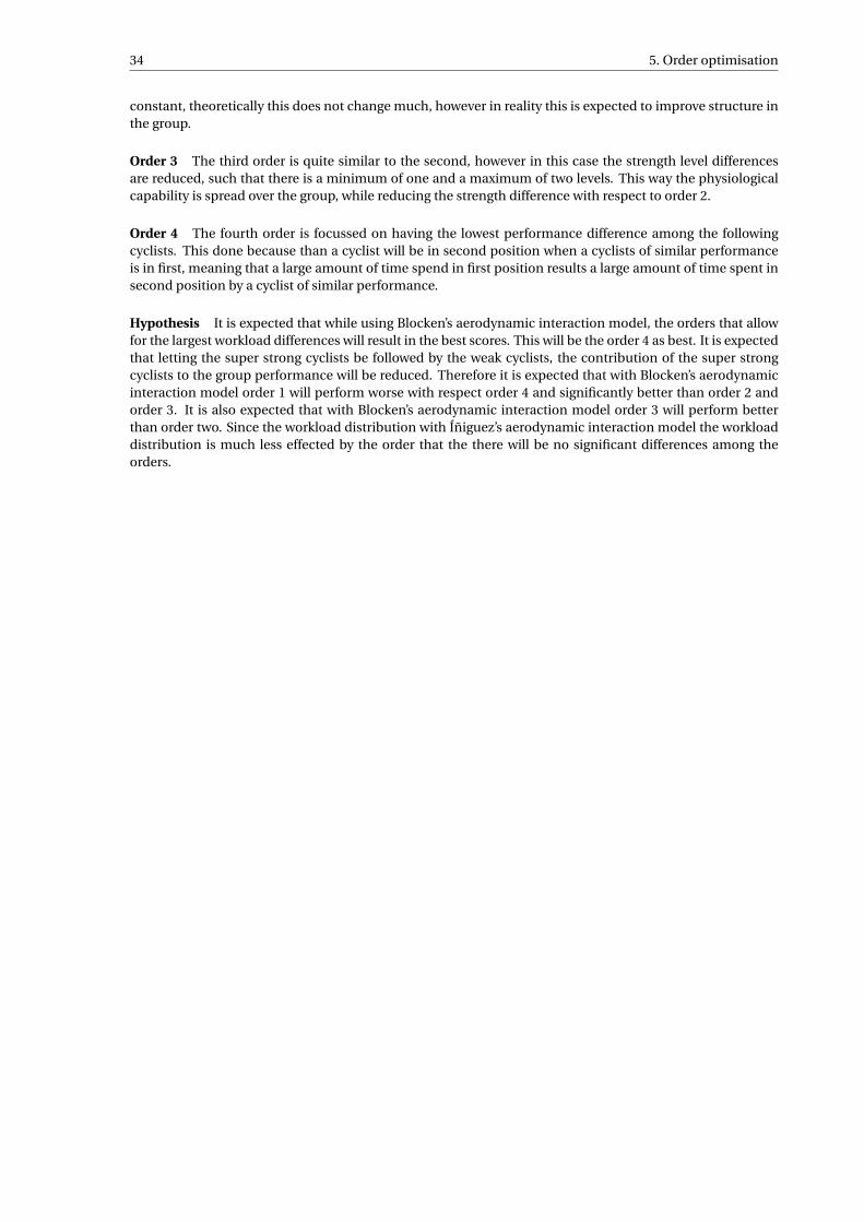
34 5. Order optimisation
constant, theoretically this does not change much, however in reality this is expected to improve structure inthe group.
Order 3 The third order is quite similar to the second, however in this case the strength level differencesare reduced, such that there is a minimum of one and a maximum of two levels. This way the physiologicalcapability is spread over the group, while reducing the strength difference with respect to order 2.
Order 4 The fourth order is focussed on having the lowest performance difference among the followingcyclists. This done because than a cyclist will be in second position when a cyclists of similar performanceis in first, meaning that a large amount of time spend in first position results a large amount of time spent insecond position by a cyclist of similar performance.
Hypothesis It is expected that while using Blocken’s aerodynamic interaction model, the orders that allowfor the largest workload differences will result in the best scores. This will be the order 4 as best. It is expectedthat letting the super strong cyclists be followed by the weak cyclists, the contribution of the super strongcyclists to the group performance will be reduced. Therefore it is expected that with Blocken’s aerodynamicinteraction model order 1 will perform worse with respect order 4 and significantly better than order 2 andorder 3. It is also expected that with Blocken’s aerodynamic interaction model order 3 will perform betterthan order two. Since the workload distribution with Íñiguez’s aerodynamic interaction model the workloaddistribution is much less effected by the order that the there will be no significant differences among theorders.
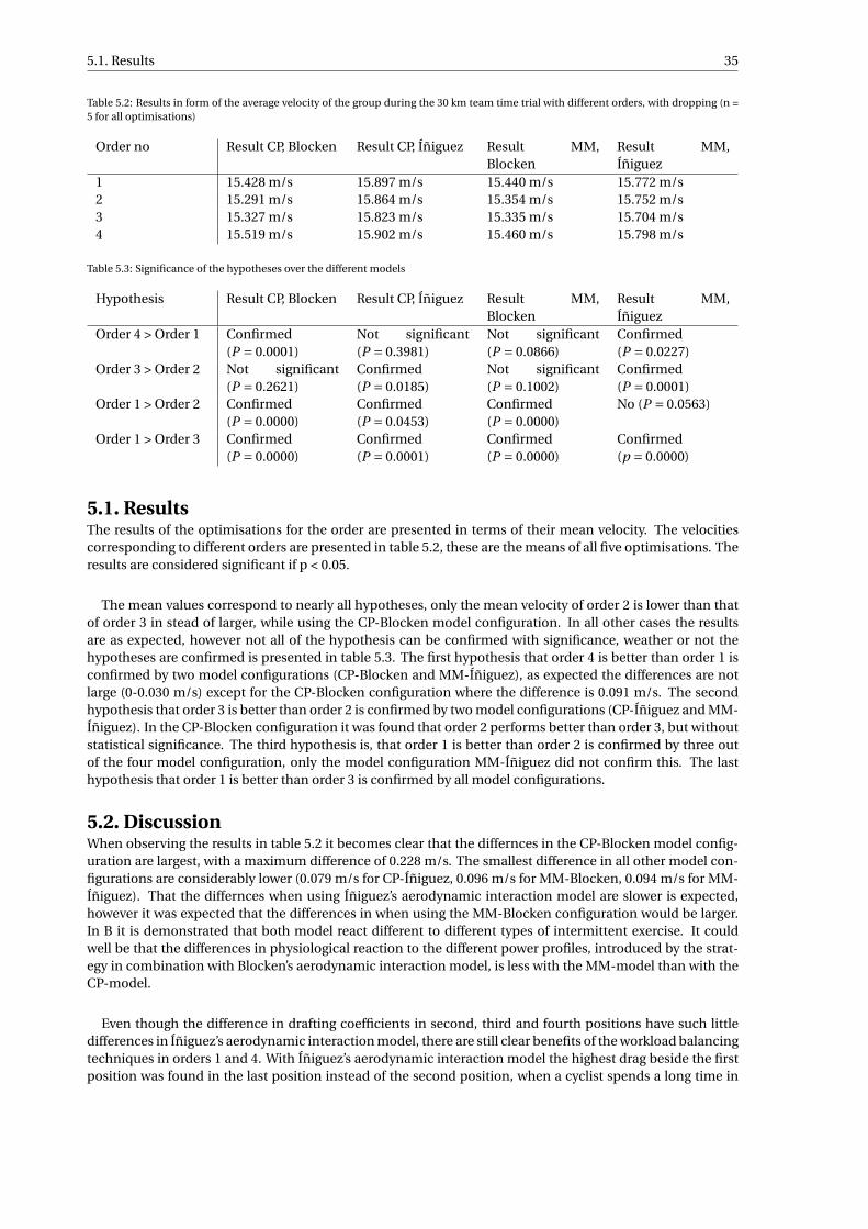
5.1. Results 35
Table 5.2: Results in form of the average velocity of the group during the 30 km team time trial with different orders, with dropping (n =5 for all optimisations)
Order no Result CP, Blocken Result CP, Íñiguez Result MM,Blocken
Result MM,Íñiguez
1 15.428 m/s 15.897 m/s 15.440 m/s 15.772 m/s2 15.291 m/s 15.864 m/s 15.354 m/s 15.752 m/s3 15.327 m/s 15.823 m/s 15.335 m/s 15.704 m/s4 15.519 m/s 15.902 m/s 15.460 m/s 15.798 m/s
Table 5.3: Significance of the hypotheses over the different models
Hypothesis Result CP, Blocken Result CP, Íñiguez Result MM,Blocken
Result MM,Íñiguez
Order 4 > Order 1 Confirmed(P = 0.0001)
Not significant(P = 0.3981)
Not significant(P = 0.0866)
Confirmed(P = 0.0227)
Order 3 > Order 2 Not significant(P = 0.2621)
Confirmed(P = 0.0185)
Not significant(P = 0.1002)
Confirmed(P = 0.0001)
Order 1 > Order 2 Confirmed(P = 0.0000)
Confirmed(P = 0.0453)
Confirmed(P = 0.0000)
No (P = 0.0563)
Order 1 > Order 3 Confirmed(P = 0.0000)
Confirmed(P = 0.0001)
Confirmed(P = 0.0000)
Confirmed(p = 0.0000)
5.1. ResultsThe results of the optimisations for the order are presented in terms of their mean velocity. The velocitiescorresponding to different orders are presented in table 5.2, these are the means of all five optimisations. Theresults are considered significant if p < 0.05.
The mean values correspond to nearly all hypotheses, only the mean velocity of order 2 is lower than thatof order 3 in stead of larger, while using the CP-Blocken model configuration. In all other cases the resultsare as expected, however not all of the hypothesis can be confirmed with significance, weather or not thehypotheses are confirmed is presented in table 5.3. The first hypothesis that order 4 is better than order 1 isconfirmed by two model configurations (CP-Blocken and MM-Íñiguez), as expected the differences are notlarge (0-0.030 m/s) except for the CP-Blocken configuration where the difference is 0.091 m/s. The secondhypothesis that order 3 is better than order 2 is confirmed by two model configurations (CP-Íñiguez and MM-Íñiguez). In the CP-Blocken configuration it was found that order 2 performs better than order 3, but withoutstatistical significance. The third hypothesis is, that order 1 is better than order 2 is confirmed by three outof the four model configuration, only the model configuration MM-Íñiguez did not confirm this. The lasthypothesis that order 1 is better than order 3 is confirmed by all model configurations.
5.2. DiscussionWhen observing the results in table 5.2 it becomes clear that the differnces in the CP-Blocken model config-uration are largest, with a maximum difference of 0.228 m/s. The smallest difference in all other model con-figurations are considerably lower (0.079 m/s for CP-Íñiguez, 0.096 m/s for MM-Blocken, 0.094 m/s for MM-Íñiguez). That the differnces when using Íñiguez’s aerodynamic interaction model are slower is expected,however it was expected that the differences in when using the MM-Blocken configuration would be larger.In B it is demonstrated that both model react different to different types of intermittent exercise. It couldwell be that the differences in physiological reaction to the different power profiles, introduced by the strat-egy in combination with Blocken’s aerodynamic interaction model, is less with the MM-model than with theCP-model.
Even though the difference in drafting coefficients in second, third and fourth positions have such littledifferences in Íñiguez’s aerodynamic interaction model, there are still clear benefits of the workload balancingtechniques in orders 1 and 4. With Íñiguez’s aerodynamic interaction model the highest drag beside the firstposition was found in the last position instead of the second position, when a cyclist spends a long time in
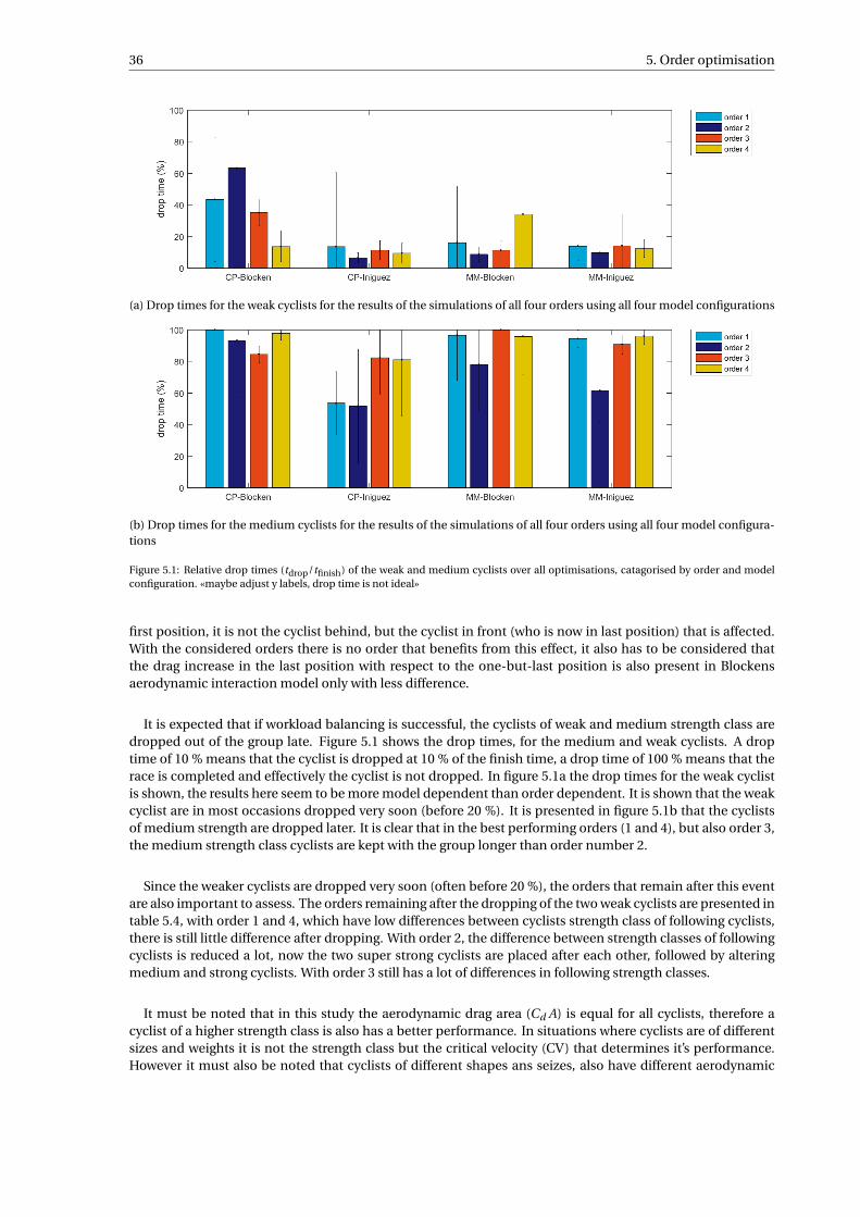
36 5. Order optimisation
(a) Drop times for the weak cyclists for the results of the simulations of all four orders using all four model configurations
(b) Drop times for the medium cyclists for the results of the simulations of all four orders using all four model configura-tions
Figure 5.1: Relative drop times (tdrop/tfinish) of the weak and medium cyclists over all optimisations, catagorised by order and modelconfiguration. «maybe adjust y labels, drop time is not ideal»
first position, it is not the cyclist behind, but the cyclist in front (who is now in last position) that is affected.With the considered orders there is no order that benefits from this effect, it also has to be considered thatthe drag increase in the last position with respect to the one-but-last position is also present in Blockensaerodynamic interaction model only with less difference.
It is expected that if workload balancing is successful, the cyclists of weak and medium strength class aredropped out of the group late. Figure 5.1 shows the drop times, for the medium and weak cyclists. A droptime of 10 % means that the cyclist is dropped at 10 % of the finish time, a drop time of 100 % means that therace is completed and effectively the cyclist is not dropped. In figure 5.1a the drop times for the weak cyclistis shown, the results here seem to be more model dependent than order dependent. It is shown that the weakcyclist are in most occasions dropped very soon (before 20 %). It is presented in figure 5.1b that the cyclistsof medium strength are dropped later. It is clear that in the best performing orders (1 and 4), but also order 3,the medium strength class cyclists are kept with the group longer than order number 2.
Since the weaker cyclists are dropped very soon (often before 20 %), the orders that remain after this eventare also important to assess. The orders remaining after the dropping of the two weak cyclists are presented intable 5.4, with order 1 and 4, which have low differences between cyclists strength class of following cyclists,there is still little difference after dropping. With order 2, the difference between strength classes of followingcyclists is reduced a lot, now the two super strong cyclists are placed after each other, followed by alteringmedium and strong cyclists. With order 3 still has a lot of differences in following strength classes.
It must be noted that in this study the aerodynamic drag area (Cd A) is equal for all cyclists, therefore acyclist of a higher strength class is also has a better performance. In situations where cyclists are of differentsizes and weights it is not the strength class but the critical velocity (CV) that determines it’s performance.However it must also be noted that cyclists of different shapes ans seizes, also have different aerodynamic
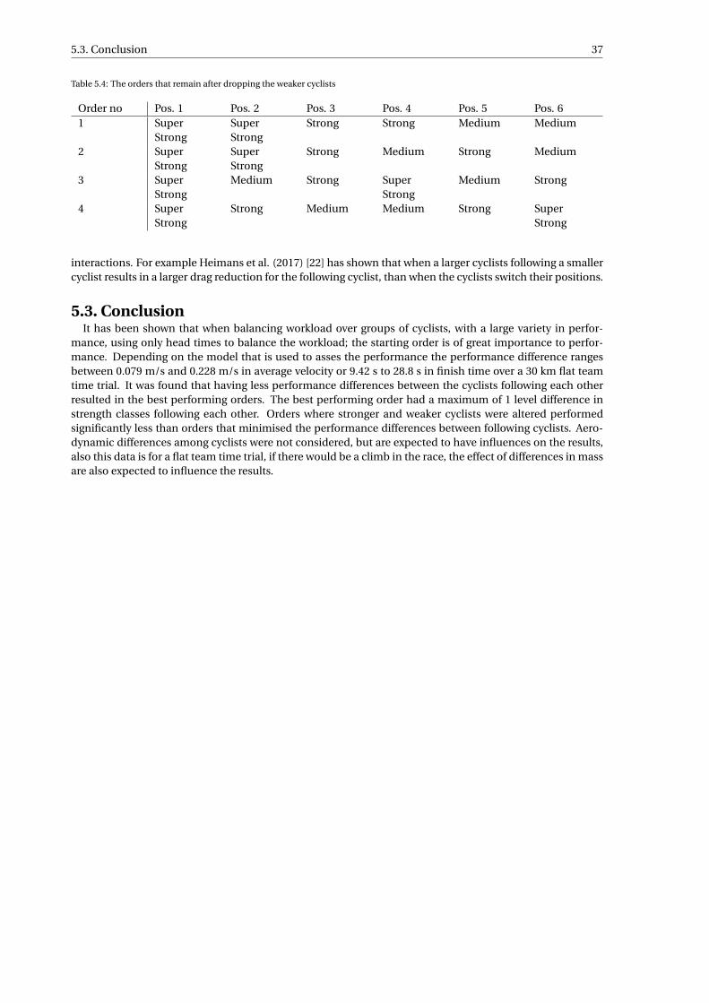
5.3. Conclusion 37
Table 5.4: The orders that remain after dropping the weaker cyclists
Order no Pos. 1 Pos. 2 Pos. 3 Pos. 4 Pos. 5 Pos. 61 Super
StrongSuperStrong
Strong Strong Medium Medium
2 SuperStrong
SuperStrong
Strong Medium Strong Medium
3 SuperStrong
Medium Strong SuperStrong
Medium Strong
4 SuperStrong
Strong Medium Medium Strong SuperStrong
interactions. For example Heimans et al. (2017) [22] has shown that when a larger cyclists following a smallercyclist results in a larger drag reduction for the following cyclist, than when the cyclists switch their positions.
5.3. ConclusionIt has been shown that when balancing workload over groups of cyclists, with a large variety in perfor-
mance, using only head times to balance the workload; the starting order is of great importance to perfor-mance. Depending on the model that is used to asses the performance the performance difference rangesbetween 0.079 m/s and 0.228 m/s in average velocity or 9.42 s to 28.8 s in finish time over a 30 km flat teamtime trial. It was found that having less performance differences between the cyclists following each otherresulted in the best performing orders. The best performing order had a maximum of 1 level difference instrength classes following each other. Orders where stronger and weaker cyclists were altered performedsignificantly less than orders that minimised the performance differences between following cyclists. Aero-dynamic differences among cyclists were not considered, but are expected to have influences on the results,also this data is for a flat team time trial, if there would be a climb in the race, the effect of differences in massare also expected to influence the results.

6Adjusted Return Positions Strategy
The workload balancing is performed by adjusting the ratio between time spend in different positions.With the standard strategy, the amount of times a cyclists is in a specific position is equal over the cyclists,considering that no cyclists is dropped. The times are balanced by adjusting the time of the cyclist in firstposition. It is shown in chapter 4 that without dropping, this does not create enough balance in the presentedgroup (2 x super strong, 2 x strong, 2 x medium and 2 x weak). It is shown that the balancing error is reducedseverely by dropping weaker cyclists, however by doing so this increases the mean drag among cyclists andtherefore requiring more power to reach the same velocity. In this chapter a workload balancing method willbe presented that adjust the frequency that a cyclists is in different positions.
Instead of adjusting the amount of time spend in a position during a race by adjusting the duration of eachtime the cyclist reaches that position; the amount of time can also be adjusted by changing the amount oftimes a cyclist reaches that position. This strategy aims to do this by letting the cyclists change from firstposition not only to last but any position. Each cyclist will have its own position to return to. An example ofa group of four cyclists is shown in figure 6.1. This means that the order is changing as the cyclists changeposition. Also depending on the start order the changing with different return positions may turn out in adifferent pattern. The aim is that by letting stronger cyclists return to positions in front of the last, the weakerwill get more time to recover from their workload contribution in the front positions. A difference betweenthe two aerodynamic interaction models is expected to be large and will be discussed in the next paragraph.
Using this strategy it is important to know which positions a cyclist recovers and which positions it expends.The border between these physiological phases is described by the critical velocity. This critical velocity repre-sents the velocity above which anaerobic energy is expended and above which anaerobic energy is recovered,this is defined per position per cyclist. For both aerodynamic interaction models and different cyclists thisis visualised in figure 6.2, the two graphs represent the two aerodynamic studies. On the horizontal axis thepositions are noted, at each position there is a bar reaching to a critical velocity that belongs to the cyclisttype as is noted in the legend. As a short recap it is noted that if the velocity exceeds the critical velocity thecyclist will not recover in this position. For both Blocken’s and Íñiguez’s models the highest critical velocityfor the weak cyclist is about 15.5 m/s (Blocken: 15.60 m/s, Íñiguez: 15.45 m/s). As this corresponds to themaximum value found in the order optimisation, it is expected that the weak cyclist will not recover at all.Even so the medium cyclists peak at around 16 m/s (Blocken: 16.05 m/s, Íñiguez: 15.895 m/s) Therefore alsothey will need a lot of recovery time.
39
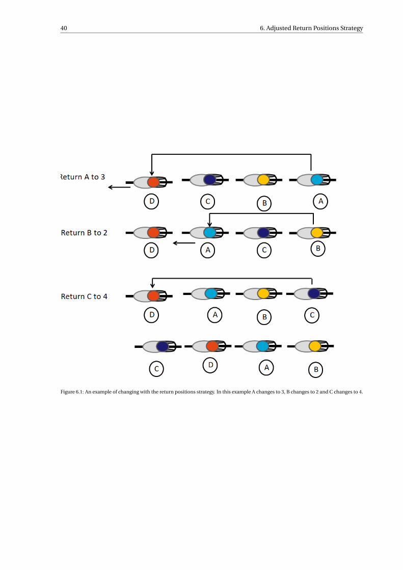
40 6. Adjusted Return Positions Strategy
Figure 6.1: An example of changing with the return positions strategy. In this example A changes to 3, B changes to 2 and C changes to 4.
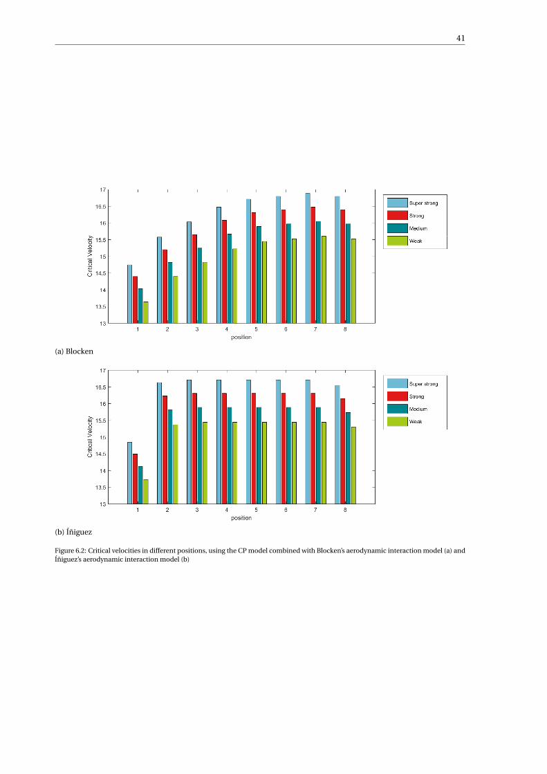
41
(a) Blocken
(b) Íñiguez
Figure 6.2: Critical velocities in different positions, using the CP model combined with Blocken’s aerodynamic interaction model (a) andÍñiguez’s aerodynamic interaction model (b)
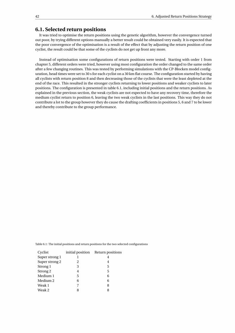
42 6. Adjusted Return Positions Strategy
6.1. Selected return positionsIt was tried to optimise the return positions using the genetic algorithm, however the convergence turned
out poor, by trying different options manually a better result could be obtained very easily. It is expected thatthe poor convergence of the optimisation is a result of the effect that by adjusting the return position of onecyclist, the result could be that some of the cyclists do not get up front any more.
Instead of optimisation some configurations of return positions were tested. Starting with order 1 fromchapter 5, different orders were tried, however using most configuration the order changed to the same orderafter a few changing routines. This was tested by performing simulations with the CP-Blocken model config-uration, head times were set to 30 s for each cyclist on a 30 km flat course. The configuration started by havingall cyclists with return position 8 and then decreasing those of the cyclists that were the least depleted at theend of the race. This resulted in the stronger cyclists returning to lower positions and weaker cyclists to laterpositions. The configuration is presented in table 6.1, including initial positions and the return positions. Asexplained in the previous section, the weak cyclists are not expected to have any recovery time, therefore themedium cyclist return to position 6, leaving the two weak cyclists in the last positions. This way they do notcontribute a lot to the group however they do cause the drafting coefficients in positions 5, 6 and 7 to be lowerand thereby contribute to the group performance.
Table 6.1: The initial positions and return positions for the two selected configurations
Cyclist initial position Return positionsSuper strong 1 1 4Super strong 2 2 4Strong 1 3 5Strong 2 4 5Medium 1 5 6Medium 2 6 6Weak 1 7 8Weak 2 8 8
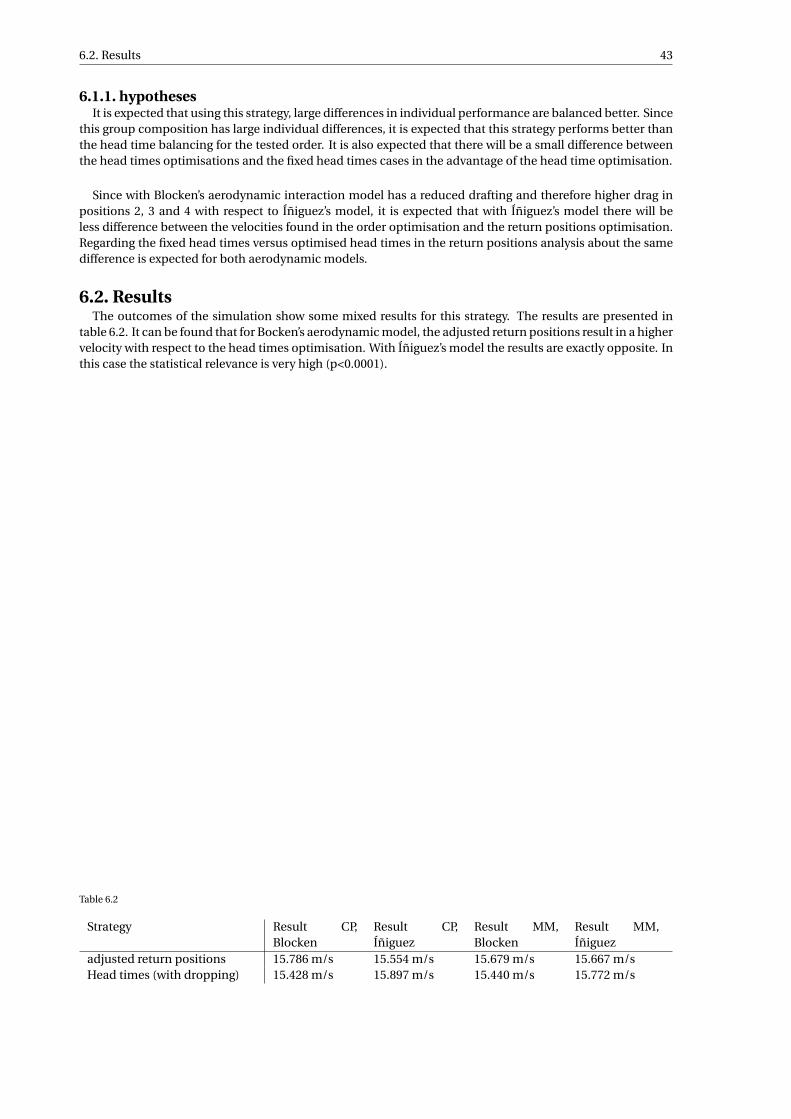
6.2. Results 43
6.1.1. hypothesesIt is expected that using this strategy, large differences in individual performance are balanced better. Since
this group composition has large individual differences, it is expected that this strategy performs better thanthe head time balancing for the tested order. It is also expected that there will be a small difference betweenthe head times optimisations and the fixed head times cases in the advantage of the head time optimisation.
Since with Blocken’s aerodynamic interaction model has a reduced drafting and therefore higher drag inpositions 2, 3 and 4 with respect to Íñiguez’s model, it is expected that with Íñiguez’s model there will beless difference between the velocities found in the order optimisation and the return positions optimisation.Regarding the fixed head times versus optimised head times in the return positions analysis about the samedifference is expected for both aerodynamic models.
6.2. ResultsThe outcomes of the simulation show some mixed results for this strategy. The results are presented in
table 6.2. It can be found that for Bocken’s aerodynamic model, the adjusted return positions result in a highervelocity with respect to the head times optimisation. With Íñiguez’s model the results are exactly opposite. Inthis case the statistical relevance is very high (p<0.0001).
Table 6.2
Strategy Result CP,Blocken
Result CP,Íñiguez
Result MM,Blocken
Result MM,Íñiguez
adjusted return positions 15.786 m/s 15.554 m/s 15.679 m/s 15.667 m/sHead times (with dropping) 15.428 m/s 15.897 m/s 15.440 m/s 15.772 m/s
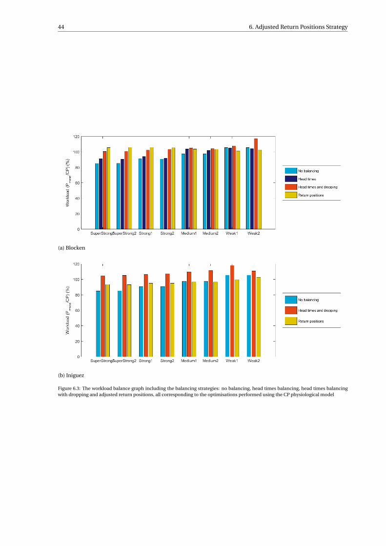
44 6. Adjusted Return Positions Strategy
(a) Blocken
(b) Iniguez
Figure 6.3: The workload balance graph including the balancing strategies: no balancing, head times balancing, head times balancingwith dropping and adjusted return positions, all corresponding to the optimisations performed using the CP physiological model
6.3. Discussion 45
6.3. DiscussionConsidering the mean velocities in these results with respect to the critical velocities it is shown that in case
of the Íñiguez aerodynamic model the velocities get so high that the weaker cyclists need to be dropped inorder to achieve a higher velocity. The concept of this strategy is to let the weaker cyclists make a contributionto the group performance. This is not achieved with Íñiguez’s model, however it is likely that in a differentgroup composition this strategy will have also have a positive effect. It is also because the tested configu-ration was optimised on Blocken’s model that it is more likely to be not the best performing configurationconsidering Iñiguez’s model.
In figure 7.1 it is presented that the workload is best distributed with Blocken’s aerodynamic model usingthe return positions adjustment strategy, this is because in this case the mean power to critical power ratio ishigh and about equal over all cyclists. When considering Íñiguez’s aerodynamic model the same strategy isabout as well distributed as no balancing strategy at al. This implies that the low velocities in the results withthis aerodynamic model are indeed because the workload is not well balanced.
Considering Blocken’s aerodynamic model a remarkable increase in velocity is achieved, with 0.358 m/sfor the CP physiological model and 0.239 m/s for the MM physiological model. It is shown in figure 7.1 thatthe workload balancing worked at least using the CP physiological model. This figure shows the relativeperformance a cyclist was able to deliver, it is shown in this figure that from the head times optimisation withdropping, the stronger cyclist (strong and super strong) have now a higher relative workload with respect tothe weaker cyclists (medium and weak). Ideally this would be exactly equal for all cyclists it is expected thatif the head times would be optimised for this strategy the workload would be even more spread.
6.4. ConclusionThe concept of balancing workload through the adjustment of return positions has proven to have potential.With Blocken’s areodynamic model depending on the considered physiological model an improvement of0.358 m/s (CP) or 0.239 m/s (MM) is made. Using the considered group of cyclists and configuration noimprovement was found by using Íñiguez’s aerodynamic model. In this study it is only demonstrated thatthis method of balancing has potential, but further study is required to define the properties of a case inwhich this workload balancing technique can be advantageous. It must also be noted that this strategy showsthat the aerodynamic interaction model has a large influence on the effectiveness of the workload balancingstrategy.

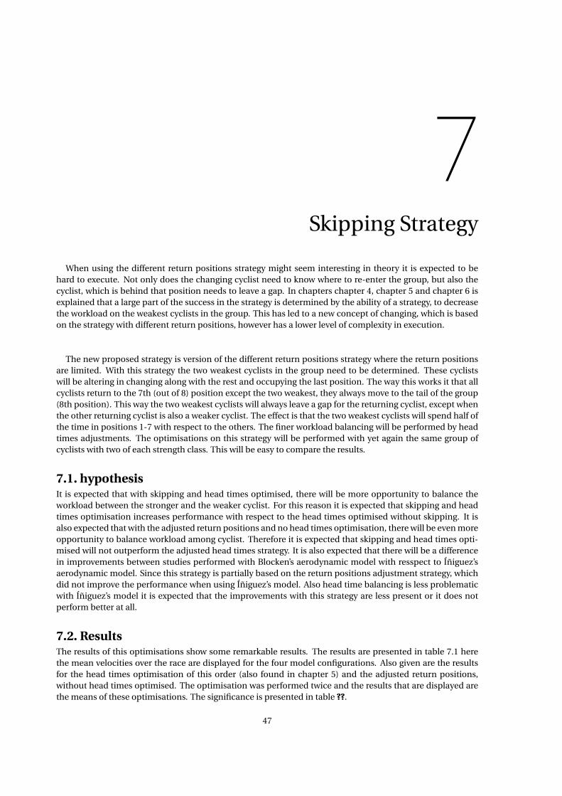
7Skipping Strategy
When using the different return positions strategy might seem interesting in theory it is expected to behard to execute. Not only does the changing cyclist need to know where to re-enter the group, but also thecyclist, which is behind that position needs to leave a gap. In chapters chapter 4, chapter 5 and chapter 6 isexplained that a large part of the success in the strategy is determined by the ability of a strategy, to decreasethe workload on the weakest cyclists in the group. This has led to a new concept of changing, which is basedon the strategy with different return positions, however has a lower level of complexity in execution.
The new proposed strategy is version of the different return positions strategy where the return positionsare limited. With this strategy the two weakest cyclists in the group need to be determined. These cyclistswill be altering in changing along with the rest and occupying the last position. The way this works it that allcyclists return to the 7th (out of 8) position except the two weakest, they always move to the tail of the group(8th position). This way the two weakest cyclists will always leave a gap for the returning cyclist, except whenthe other returning cyclist is also a weaker cyclist. The effect is that the two weakest cyclists will spend half ofthe time in positions 1-7 with respect to the others. The finer workload balancing will be performed by headtimes adjustments. The optimisations on this strategy will be performed with yet again the same group ofcyclists with two of each strength class. This will be easy to compare the results.
7.1. hypothesisIt is expected that with skipping and head times optimised, there will be more opportunity to balance theworkload between the stronger and the weaker cyclist. For this reason it is expected that skipping and headtimes optimisation increases performance with respect to the head times optimised without skipping. It isalso expected that with the adjusted return positions and no head times optimisation, there will be even moreopportunity to balance workload among cyclist. Therefore it is expected that skipping and head times opti-mised will not outperform the adjusted head times strategy. It is also expected that there will be a differencein improvements between studies performed with Blocken’s aerodynamic model with resspect to Íñiguez’saerodynamic model. Since this strategy is partially based on the return positions adjustment strategy, whichdid not improve the performance when using Íñiguez’s model. Also head time balancing is less problematicwith Íñiguez’s model it is expected that the improvements with this strategy are less present or it does notperform better at all.
7.2. ResultsThe results of this optimisations show some remarkable results. The results are presented in table 7.1 herethe mean velocities over the race are displayed for the four model configurations. Also given are the resultsfor the head times optimisation of this order (also found in chapter 5) and the adjusted return positions,without head times optimised. The optimisation was performed twice and the results that are displayed arethe means of these optimisations. The significance is presented in table ??.
47
48 7. Skipping Strategy
Table 7.1: The results in terms of mean velocity of the head times optimisation regarding using the skipping strategy (top row). The resultsare compared to the results of the head times optimisation of the same order without skipping (= order 1 from order optimisation) andthe Adjusted return positions.
Configuration CP-Blocken CP-Íñiguez MM-Blocken MM-ÍñiguezHead times optimised withskipping (n = 7)
15.628 m/s 16.069 m/s 15.549 m/s 15.975 m/s
Head times optimised withoutskipping (n = 5)
15.428 m/s 15.897 m/s 15.440 m/s 15.772 m/s
Adjusted return positions (n =1)
15.786 m/s 15.554 m/s 15.679 m/s 15.667 m/s
Table 7.2: The significance corresponding to the results and hypotheses fo rthe skipping strategy
Configuration CP-Blocken CP-Íñiguez MM-Blocken MM-ÍñiguezHead times optimised withskipping performs better thanwithout skipping
Confirmed(P = 0.0000)
Confirmed(P = 0.0000)
Confirmed(P = 0.0000)
Confirmed(P = 0.0000)
Head times optimised withskipping performs better thanthe adjusted return positions
Denied(P = 0.0001)
Confirmed(P = 0.0000)
Denied(P = 0.0000)
Confirmed(P = 0.0000)
7.3. DiscussionIt is surprising that with this strategy the results with Íñiguez’s aerodynamic interaction model perform betterthan the in the head times optimisation, since with the adjusted return positions all results simulated withÍñiguez’s model performed worse. However when the results are further analysed it was found that in bothoptimisation performed with the CP-Íñiguez model it was found that the two weakest cyclists were droppedbefore the first 25 % of the race. However this does mean that the contribution of the two weak cyclists withinthis first section was effective enough to improve the result from the head times optimisation. With Blocken’saerodynamic model the results of the skipping strategy perform better than in the head time optimisationand worse with respect to the adjusted return positions optimisation, just as expected.
When considering the workload distribution graphs as presented in figure 7.1 the first thing that mightsurprise is the high relative workload of the weak and medium cyclists, this is explained by the fact that be-cause they are dropped soon in the race they deplete their anaerobic work capacity in a shorter time and aretherefore able to produce a higher power according to the critical power theory [30]. Considering the graphcorresponding to Íñiguez’s aerodynamic model the relative workload for both skipping is about equal to thatof head times with dropping and does therefore provide no explanation to why the skipping strategy worksbetter than the head times balancing with dropping strategy. When observing the graph corresponding toBlocken’s aerodynamic interaction model the strongest four cyclists have a lower relative workload with re-spect to those of the adjusted return positions, which does explain why it is not performing better, howeverjust as with Íñiguez’s aerodynamic model the relative workload results of the four strongest cyclists with theskipping strategy are more or less equal to those with the head times balancing strategy.
7.4. ConclusionThis strategy provides an attempt at better workload distribution while being less complex to execute withrespect to the adjusted return positions strategy. The results show that it causes an increment of 0.088 m/sto 0.210 m/s with respect to the head times balancing, depending on the model configuration. Because theresults show that the weaker cyclists are still dropped soon in the race it is unclear why this method performsthis much better.
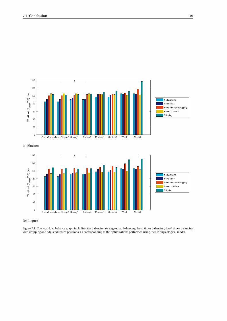
7.4. Conclusion 49
(a) Blocken
(b) Iniguez
Figure 7.1: The workload balance graph including the balancing strategies: no balancing, head times balancing, head times balancingwith dropping and adjusted return positions, all corresponding to the optimisations performed using the CP physiological model

8Conclusion
8.1. ModelIn the analysis of the standard strategy and the optimisation of the new proposed strategies the model
has shown that it gives good insights in the physiological states and power requirements during a team timetrial. These power requirements and physiological states have been used to identify the cyclists in that arewithholding the team from reaching higher mean velocities. The workload balances have been proven agood measure for how well the work is distributed in the group, which turns out to have a large influence onperformance.
The differences in performance of cyclists that are simulated has a large influence on the optimal strategy.During this analysis standardised cyclists are used, however when real cyclists are tested it is important thatthe combination of their physiology and aerodynamics, resulting in the critical velocity is determined withaccuracy.
The model lacks in validation, the combination of the mechanical and physiological model have beenwidely used in simulations of individual time trials[19, 24, 42, 45]. It is therefore that the only undeterminedpart of the model is the aerodynamic interaction. A lot of studies doing so with groups of four cyclists havebeen published[4, 10, 16, 18, 22, 29]. However the only two studies that have been published on the aerody-namic interaction in groups of up to eight cyclists have used poorly validated computational flow dynamicsstudies to do so. Since different strategies cause different results when using different aerodynamic models itis important that the aerodynamic interaction models are validated.
Even better then improving the validity of the aerodynamic interaction is to validate the models capabilityof estimating performance of a strategy. This could be done by comparing race results to the simulated result.This simulated result can be performed with the changing scheme that was used in the actual race.
Two physiological models have been used in this study however the different behaviour of the two modelshas not lead to a lot of differences in outcomes of strategies. The Margaria-Morton (MM) model could model acyclist in more detail than the Critical Power (CP) model, however in this study it is not demonstrated that thedifferent behaviour also resulted in different conclusions. It cannot be concluded that there is no advantageof using the MM model over the CP model since in this study the MM model is not fit to real cyclists, howeverwhen continuing with the standardised cyclists as presented in this model there is no advantage of using theMM model.
8.2. StrategyDuring this study it is determined that the performance of the team time trial relies on the distribution
of workload over the cyclists in the team. In this study the strategy was optimised for a group with largephysiological differences among the team members. It is determined that when simulating with Blocken’saerodynamic model, the strategy can be improved such that the mean velocity over a team time trial is raised
51

52 8. Conclusion
by 0.358 m/s or 0.239 m/s for the CP and MM physiological models respectively. This is done by alteringthe return positions, such that every cyclists has it’s own designated position to return to instead of letting alcyclists return to the last positions, when changing from first. When simulating with Íñiguez’s aerodynamicmodel, it was found that skipping worked best and was able to improve the mean velocity over the team timetrial by 0.521 m/s simulated with the CP physiological model.
While remaining in the standard changing strategy, the order has proven to be of great influence to theresults. When only using head times to balance a team during a team time trial the workload distribution isvery dependent on the order that is used. It is found that between the best and the worst simulated ordersthe results expressed in mean velocity over a 30 km race ranges between 0.079 m/s and 0.228 m/s. The lowestimprovement was found while simulating with the MM-Íñiguez configuration and the highest improvementwas found while using the CP-Blocken combination.
9Recomendations
The developed model is used to gain insights in the strategies used during team time trials ans also toimprove the strategies. The model has provided information regarding the workload among different cyclistsin a team during the race and has helped develop new strategies that could potentially improve team time trialperformances. However the model remains invalidated in this study. The model has been used to evaluate asingle case, which is a flat time trial of 30 km with a single configuration of cyclists. The model has potentialto evaluate a wide range of different cases. In this chapter will be explained both how the model could beimproved and how the existing or improved model could be used to optimise more situations.
9.1. ModelA model of a team time trial was developed but it still lacks validity, also the model could be improved tosimulate with higher detail. The aerodynamic models that are used in the different configurations of thismodel have shown very different behaviour. It is essential to determine which model suits the consideredreality best.
9.1.1. Validation of the aerodynamic interactionSince the two aerodynamic models show such a different behaviour and have lead to different conclusion inthis study, a validation of the aerodynamic interaction has to be made. It is advised to do this in a field testwhile using power meters, since this method of assessment lies close to the use case in application. Alterna-tively a wind tunnel test could be done. It has been shown in A that it is also essential to do this with a largergroups size, at least five, but more preferable eight cyclists.
9.1.2. Individual aerodynamic characteristicsRecent studies [4, 18, 22] have also shown that the aerodynamic characteristics of the cyclists in the grouphave an influence on the coefficient of drafting that applies to the cyclists. During this study the consideredcyclists where equal in size, however when a real time of different individuals is considered this will be impor-tant. The study of Heimans et al. (2017) provided a good framework that could be used to include the effectof different individual aerodynamic characteristics into the teams drafting model.
9.1.3. Additional aerodynamic improvementsThe world of aerodynamics is more complex than drag areas and drafting coefficients, the applicability of themodel would increase by including these details into the model. Winds are not included in this situation, theeffects of head and tail winds can be included relatively easily, by separating forward velocity and air velocity.However when side winds are being considered this becomes more complex. When side winds occur in teamtime trials cyclists tend to introduce a lateral offset in their position in the group in order to remain drafting.It would be interesting to also include these effects in the model, such that the strategic decisions could beadapted to the weather conditions.
53
54 9. Recomendations
9.1.4. Overall performance validationThe aerodynamic interaction seems to be the least validated component of the model. However togetherwith the physiology and resistance models it determines the time trial performance. The highest level ofvalidation would be if it could be determined that the performance of this model would be accurate. Thisrequires a fits of the desired physiological modes to a real team of cyclists, also the aerodynamic drag areaand rolling resistances of these cyclists should be determined. This way a strategy of a real performed teamtime trial can be fed into the model and the performance can be compared to asses the model validity.
Relative validity With such large amount of parameters to determine, which in their way have inaccuraciesthe exact finish time will likely not match very accurate, however when multiple time trials are performedusing different changing strategies. The differences in finish time or mean velocity can be compared to thoseof the model predictions. This way it could be ensured that the strategy optimisations by making use of themodel will result in an improvement of performance in reality without predicting accurate finish times.
9.2. Studies using the existing modelThis study focusses on the development of a model to predict and compare performances in team time trialsas well as optimising performance of the team time trial. Since this study contains much information aboutdifferent model types and variation in strategies and group composition is decreased. A follow up study couldprovide much more information about the performance of strategies and different strategy concepts. In thissection some ideas, which are currently labeled as interesting, are explained.
9.2.1. Performance difference on different slopesIn this study a few strategies have been analysed on a 30 km flat team time trial using only one group forma-tion. There are still a lot of variation possible. In this section a few examples are given of additional cases thatare expected to enrich this study with interesting results.
Order and inclination In the order optimisation no variation is made in cyclists weigh class or road incli-nation. It will be interesting to see how the optimal orders change with the inclination of the course. This canbe done by taking the order that is now considered, which consists of two super strong cyclists, two strongcyclists, two medium and two weak and altering their weight. Specifically if the super strong cyclists becomeof the heavy weight class and the weak cyclists of light. This way depending on the road inclination the crit-ical velocity of the cyclists change in the advantage of the weak cyclists and at the disadvantage of the superstrong cyclists. This could even be performed with a course that has both a flat and inclining part.
More balanced groups The current considered group has a lot of variation between cyclists, which makethe workload distribution important. It would be interesting to place in contrast to that a group where thecyclists are more balanced, for example six strong and two medium cyclists. It is expected that the strategiesproposed to balance the workload have less effect in these cases, but it is unknown if they will perform worse,it could be that in cases that need less workload balancing these strategies may not have a large advantage,they still perform well.
AInterpolation of cyclist drafting coefficient
This chapter describes the method of interpolation of drag reduction on cyclists in groups of various sizes,where the goal is to get drag reductions for a group of any number of cyclists. Two studies have been per-formed where the aerodynamic interaction of groups of eight cyclists have been tested, both lack validity.The study of Íñiguez and Íñiguez de-la-Torre (2009) [27] tested the drafting coefficients of all group sizes upto nine. The study of Blocken et al. (2013) [9] tested only with group sizes 1, 2, 4, 6 and 8 More studies havebeen performed on configurations with four cyclists also varying individual drag areas and postures. In orderto use both studies for up to eight cyclists an interpolation has to be performed use all cyclists configurations.Possibly the same method of interpolation could be used to extrapolate the drag reduction in groups of fourcyclists to groups of eight cyclists. This study attempts to describe the drafting coefficients of a group, but of-ten the drag reduction is mentioned. With the drafting coefficient (Cdr ), the drag in the group with respect tothe solo drag value is meant. The relative drag reduction (R) is the ratio between drag difference between soloand in group and the solo drag value and is related to the drafting coefficient as described in equation A.1.
R = 1−Cdr (A.1)
55
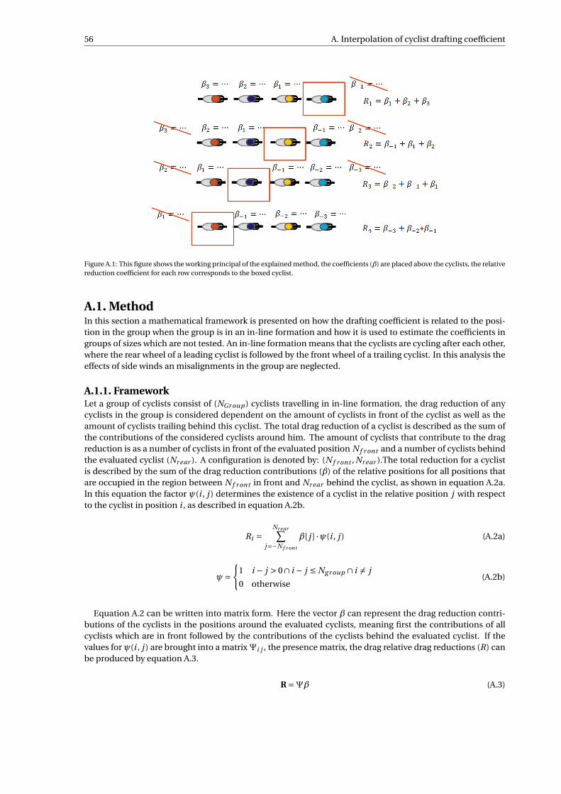
56 A. Interpolation of cyclist drafting coefficient
Figure A.1: This figure shows the working principal of the explained method, the coefficients (β) are placed above the cyclists, the relativereduction coefficient for each row corresponds to the boxed cyclist.
A.1. MethodIn this section a mathematical framework is presented on how the drafting coefficient is related to the posi-tion in the group when the group is in an in-line formation and how it is used to estimate the coefficients ingroups of sizes which are not tested. An in-line formation means that the cyclists are cycling after each other,where the rear wheel of a leading cyclist is followed by the front wheel of a trailing cyclist. In this analysis theeffects of side winds an misalignments in the group are neglected.
A.1.1. FrameworkLet a group of cyclists consist of (NGr oup ) cyclists travelling in in-line formation, the drag reduction of anycyclists in the group is considered dependent on the amount of cyclists in front of the cyclist as well as theamount of cyclists trailing behind this cyclist. The total drag reduction of a cyclist is described as the sum ofthe contributions of the considered cyclists around him. The amount of cyclists that contribute to the dragreduction is as a number of cyclists in front of the evaluated position N f r ont and a number of cyclists behindthe evaluated cyclist (Nr ear ). A configuration is denoted by: (N f r ont , Nr ear ).The total reduction for a cyclistis described by the sum of the drag reduction contributions (β) of the relative positions for all positions thatare occupied in the region between N f r ont in front and Nr ear behind the cyclist, as shown in equation A.2a.In this equation the factor ψ(i , j ) determines the existence of a cyclist in the relative position j with respectto the cyclist in position i , as described in equation A.2b.
Ri =Nr ear∑
j=−N f r ont
β[ j ] ·ψ(i , j ) (A.2a)
ψ={
1 i − j > 0∩ i − j ≤ Ng r oup ∩ i 6= j
0 otherwise(A.2b)
Equation A.2 can be written into matrix form. Here the vector β can represent the drag reduction contri-butions of the cyclists in the positions around the evaluated cyclists, meaning first the contributions of allcyclists which are in front followed by the contributions of the cyclists behind the evaluated cyclist. If thevalues for ψ(i , j ) are brought into a matrixΨi j , the presence matrix, the drag relative drag reductions (R) canbe produced by equation A.3.
R =Ψβ (A.3)
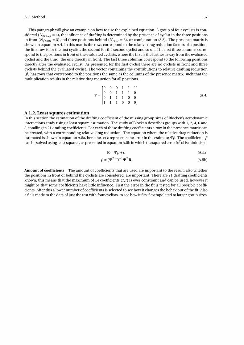
A.1. Method 57
This paragraph will give an example on how to use the explained equation. A group of four cyclists is con-sidered (Ng r oup = 4), the influence of drafting is determined by the presence of cyclist in the three positionsin front (N f r ont = 3) and three positions behind (Nr ear = 3), or configuration (3,3). The presence matrix isshown in equation A.4. In this matrix the rows correspond to the relative drag reduction factors of a position,the first row is for the first cyclist, the second for the second cyclist and so on. The first three columns corre-spond to the positions in front of the evaluated cyclists, where the first is the furthest away from the evaluatedcyclist and the third, the one directly in front. The last three columns correspond to the following positionsdirectly after the evaluated cyclist. As presented for the first cyclist there are no cyclists in front and threecyclists behind the evaluated cyclist. The vector containing the contributions to relative drafting reduction(β) has rows that correspond to the positions the same as the columns of the presence matrix, such that themultiplication results in the relative drag reduction for all positions.
Ψ=
0 0 0 1 1 10 0 1 1 1 00 1 1 1 0 01 1 1 0 0 0
(A.4)
A.1.2. Least squares estimationIn this section the estimation of the drafting coefficient of the missing group sizes of Blocken’s aerodynamicinteractions study using a least square estimation. The study of Blocken describes groups with 1, 2, 4, 6 and8, totalling in 21 drafting coefficients. For each of these drafting coefficients a row in the presence matrix canbe created, with a corresponding relative drag reduction. The equation where the relative drag reduction isestimated is shown in equation A.5a, here the set ε represents the error in the estimateΨβ. The coefficients βcan be solved using least squares, as presented in equation A.5b in which the squared error (εT ε) is minimised.
R =Ψβ+ε (A.5a)
β= (ΨTΨ)−1ΨT R (A.5b)
Amount of coefficients The amount of coefficients that are used are important to the result, also whetherthe positions in front or behind the cyclists are considered, are important. There are 21 drafting coefficientsknown, this means that the maximum of 14 coefficients (7,7) is over constraint and can be used, however itmight be that some coefficients have little influence. First the error in the fit is tested for all possible coeffi-cients. After this a lower number of coefficients is selected to see how it changes the behaviour of the fit. Alsoa fit is made to the data of just the test with four cyclists, to see how it fits if extrapolated to larger group sizes.
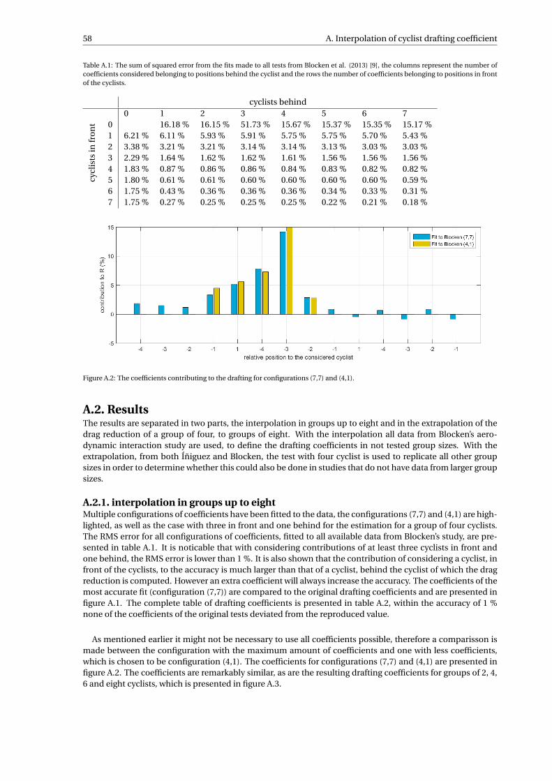
58 A. Interpolation of cyclist drafting coefficient
Table A.1: The sum of squared error from the fits made to all tests from Blocken et al. (2013) [9], the columns represent the number ofcoefficients considered belonging to positions behind the cyclist and the rows the number of coefficients belonging to positions in frontof the cyclists.
cyclists behindcy
clis
tsin
fro
nt
0 1 2 3 4 5 6 70 16.18 % 16.15 % 51.73 % 15.67 % 15.37 % 15.35 % 15.17 %1 6.21 % 6.11 % 5.93 % 5.91 % 5.75 % 5.75 % 5.70 % 5.43 %2 3.38 % 3.21 % 3.21 % 3.14 % 3.14 % 3.13 % 3.03 % 3.03 %3 2.29 % 1.64 % 1.62 % 1.62 % 1.61 % 1.56 % 1.56 % 1.56 %4 1.83 % 0.87 % 0.86 % 0.86 % 0.84 % 0.83 % 0.82 % 0.82 %5 1.80 % 0.61 % 0.61 % 0.60 % 0.60 % 0.60 % 0.60 % 0.59 %6 1.75 % 0.43 % 0.36 % 0.36 % 0.36 % 0.34 % 0.33 % 0.31 %7 1.75 % 0.27 % 0.25 % 0.25 % 0.25 % 0.22 % 0.21 % 0.18 %
Figure A.2: The coefficients contributing to the drafting for configurations (7,7) and (4,1).
A.2. ResultsThe results are separated in two parts, the interpolation in groups up to eight and in the extrapolation of thedrag reduction of a group of four, to groups of eight. With the interpolation all data from Blocken’s aero-dynamic interaction study are used, to define the drafting coefficients in not tested group sizes. With theextrapolation, from both Íñiguez and Blocken, the test with four cyclist is used to replicate all other groupsizes in order to determine whether this could also be done in studies that do not have data from larger groupsizes.
A.2.1. interpolation in groups up to eightMultiple configurations of coefficients have been fitted to the data, the configurations (7,7) and (4,1) are high-lighted, as well as the case with three in front and one behind for the estimation for a group of four cyclists.The RMS error for all configurations of coefficients, fitted to all available data from Blocken’s study, are pre-sented in table A.1. It is noticable that with considering contributions of at least three cyclists in front andone behind, the RMS error is lower than 1 %. It is also shown that the contribution of considering a cyclist, infront of the cyclists, to the accuracy is much larger than that of a cyclist, behind the cyclist of which the dragreduction is computed. However an extra coefficient will always increase the accuracy. The coefficients of themost accurate fit (configuration (7,7)) are compared to the original drafting coefficients and are presented infigure A.1. The complete table of drafting coefficients is presented in table A.2, within the accuracy of 1 %none of the coefficients of the original tests deviated from the reproduced value.
As mentioned earlier it might not be necessary to use all coefficients possible, therefore a comparisson ismade between the configuration with the maximum amount of coefficients and one with less coefficients,which is chosen to be configuration (4,1). The coefficients for configurations (7,7) and (4,1) are presented infigure A.2. The coefficients are remarkably similar, as are the resulting drafting coefficients for groups of 2, 4,6 and eight cyclists, which is presented in figure A.3.
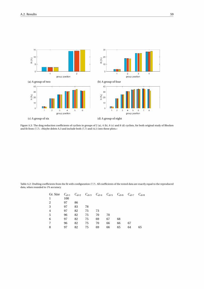
A.2. Results 59
(a) A group of two (b) A group of four
(c) A group of six (d) A group of eight
Figure A.3: The drag reduction coefficients of cyclists in groups of 2 (a), 4 (b), 6 (c) and 8 (d) cyclists, for both original study of Blockenand fit from (7,7). «Maybe delete A.3 and include both (7,7) and (4,1) into these plots.»
Table A.2: Drafting coefficients from the fit with configuration (7,7). All coefficients of the tested data are exactly equal to the reproduceddata, when rounded to 1% accuracy.
Gr. Size Cdr 1 Cdr 2 Cdr 3 Cdr 4 Cdr 5 Cdr 6 Cdr 7 Cdr 8
1 1002 97 863 97 83 784 97 82 75 735 96 82 75 70 706 97 82 75 69 67 687 96 82 75 70 66 66 678 97 82 75 69 66 65 64 65
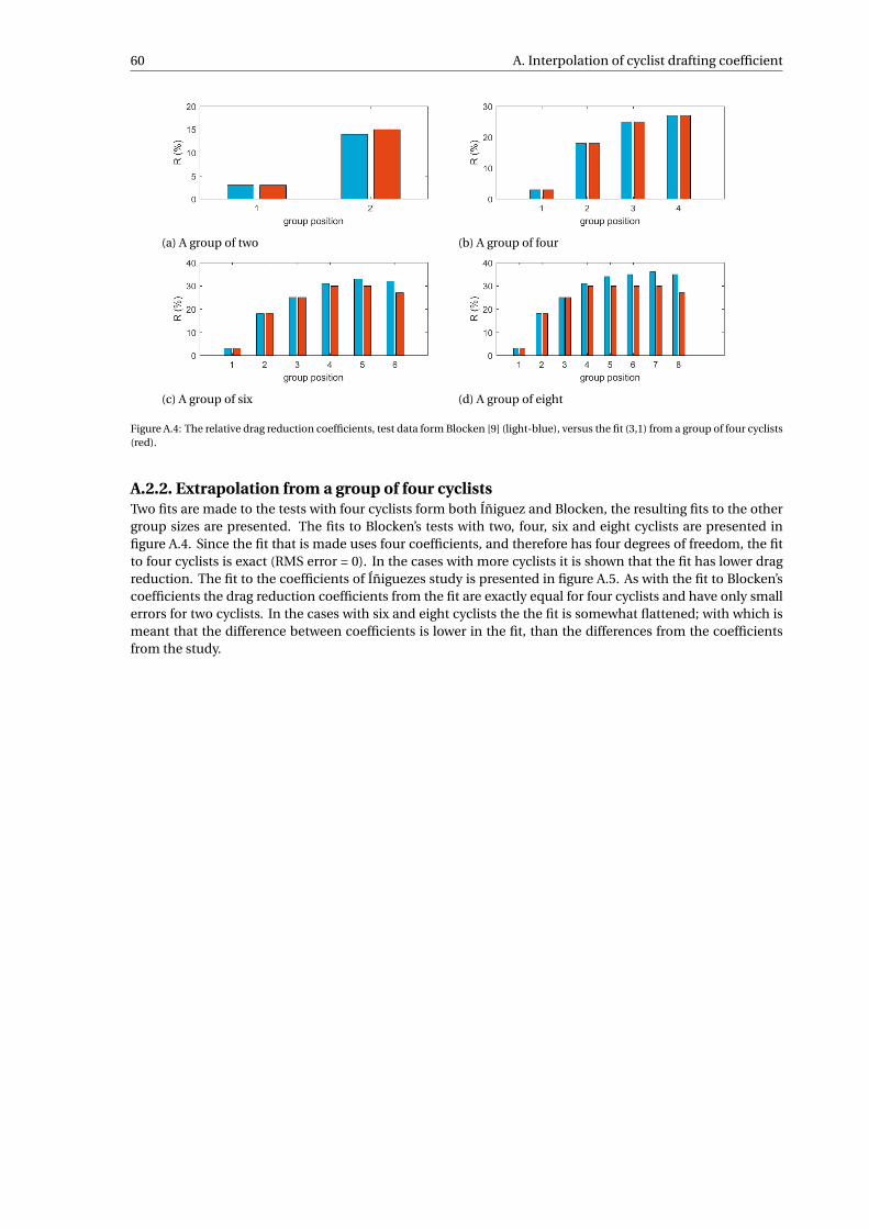
60 A. Interpolation of cyclist drafting coefficient
(a) A group of two (b) A group of four
(c) A group of six (d) A group of eight
Figure A.4: The relative drag reduction coefficients, test data form Blocken [9] (light-blue), versus the fit (3,1) from a group of four cyclists(red).
A.2.2. Extrapolation from a group of four cyclistsTwo fits are made to the tests with four cyclists form both Íñiguez and Blocken, the resulting fits to the othergroup sizes are presented. The fits to Blocken’s tests with two, four, six and eight cyclists are presented infigure A.4. Since the fit that is made uses four coefficients, and therefore has four degrees of freedom, the fitto four cyclists is exact (RMS error = 0). In the cases with more cyclists it is shown that the fit has lower dragreduction. The fit to the coefficients of Íñiguezes study is presented in figure A.5. As with the fit to Blocken’scoefficients the drag reduction coefficients from the fit are exactly equal for four cyclists and have only smallerrors for two cyclists. In the cases with six and eight cyclists the the fit is somewhat flattened; with which ismeant that the difference between coefficients is lower in the fit, than the differences from the coefficientsfrom the study.
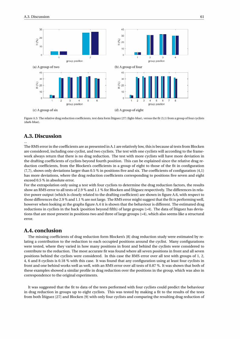
A.3. Discussion 61
(a) A group of two (b) A group of four
(c) A group of six (d) A group of eight
Figure A.5: The relative drag reduction coefficients, test data form Íñiguez [27] (light-blue), versus the fit (3,1) from a group of four cyclists(dark-blue).
A.3. Discussion...The RMS error in the coefficients are as presented in A.1 are relatively low, this is because al tests from Blockenare considered, including one cyclist, and two cyclists. The test with one cyclists will according to the frame-work always return that there is no drag reduction. The test with more cyclists will have more deviation inthe drafting coefficients of cyclists beyond fourth position. This can be explained since the relative drag re-duction coefficients, from the Blocken’s coefficients in a group of eight to those of the fit in configuration(7,7), shows only deviations larger than 0.5 % in positions five and six. The coefficients of configuration (4,1)has more deviations, where the drag reduction coefficients corresponding to positions five seven and eightexceed 0.5 % in absolute error.For the extrapolation only using a test with four cyclists to determine the drag reduction factors, the resultsshow an RMS error to all tests of 2.9 % and 1.1 % for Blocken and Íñiguez respectively. The differences in rela-tive power output (which is closely related to the drafting coefficient) are shown in figure A.6, with respect tothose differences the 2.9 % and 1.1 % are not large. The RMS error might suggest that the fit is performing well,however when looking at the graphs figure A.4 it is shown that the behaviour is different. The estimated dragreductions in cyclists in the back (position beyond fifth) of large groups (>4). The data of Íñiguez has devia-tions that are most present in positions two and three of large groups (>4), which also seems like a structuralerror.
A.4. conclusionThe missing coefficients of drag reduction form Blocken’s [8] drag reduction study were estimated by re-
lating a contribution to the reduction to each occupied positions around the cyclist. Many configurationswere tested, where they varied in how many positions in front and behind the cyclists were considered tocontribute to the reduction. The most accurate fit was found where all seven positions in front and all sevenpositions behind the cyclists were considered. In this case the RMS error over all test with groups of 1, 2,4, 6 and 8 cyclists is 0.18 % with this case. It was found that any configuration using at least four cyclists infront and one behind works well as well, with an RMS error over all tests of 0.87 %. It was shown that both ofthese examples showed a similar profile in drag reduction over the positions in the group, which was also incorrespondence to the original experiments.
It was suggested that the fit to data of the tests performed with four cyclists could predict the behaviourin drag reduction in groups up to eight cyclists. This was tested by making a fit to the results of the testsfrom both Íñiguez [27] and Blocken [9] with only four cyclists and comparing the resulting drag reduction of

62 A. Interpolation of cyclist drafting coefficient
Figure A.6: Comparison of drag reduction, in terms of ratio in power consumption with respect to the first cyclist in the group, as functionof group position coefficient for groups of four cyclists.
all group sizes to the tests. The RMS errors in the drafting coefficients were 2.9 % and 1.1 % respectively. Itwas found that the errors were largest in the positions beyond fourth for groups larger than four for Blocken’sstudy. In the case of the fit to Íñiguez’s coefficients the errors were largest in positions two and three in groupslarger than four. It is shown in A.4 that the profile of drag reduction over positions in the group is altered wheninterpolating from a group of four cyclists, and it is therefore concluded that it cannot be guaranteed that thisgives a representative result. The profile of drag reduction and thereby drafting coefficient over the positionsis important when comparing different strategies, disturbing this profile might induce advantage of certainstrategies.
BFitting the Margaria-Morton models
B.1. IntroductionIn the literature the critical power model (CP-model) [30] is often used to model physiology, while the Margaria-Morton model (MM-model) [33, 41] could give more detail than the critical power model. The reason that theCP-model is so popular with respect to the MM-model is because it only uses two parameters, which is farless than the eight used in the MM-model. Because the MM-model, describes the physiology in more detailwith respect to the CP-model it has potential to describe the complex physiology in team time trails betterthan the CP-model.
The critical power model is often used in the modelling of individual time trials [14, 42], however in thesestudies, no recovery of anaerobic capacity is required. Since team time trials are an intermitted exercise,meaning that the power output of a cyclist fluctuates around the critical power, the model has to model re-covery. The accuracy of the CP-model decreases when using a recovery model. [5, 44] It is therefore suggestedthat the hard to fit MM-model could provide a better description of the cyclists ability to produce power.
B.2. The MM-modelThe MM-model is a whole body bio-energetic model, where processes leading to power production are de-scribed based on bio-chemical processes. The MM-model is often represented in a hydraulic flow model,where flows represent power and volumes represent energy. The hydraulic flow model representation isshown in figure B.1, where the three tanks are noted with O, P and G. The O-tank represents the oxidativeproduction of phosphates, which are used in the production of mechanical power. The O tank is infinite insize, representing the oxygen in the environment. The P-tank represents the storage of ATP, and the G tankrepresents the storage of carbohydrates, which supply energy to tank P through the glycolysis process. Duringthe glycolysis process, lactate is converted to lactic acid.
B.2.1. Differential equationsThe MM-model is, in literature, described as a hydraulic flow model, however the result of this model areonly differential equations. The main differential equations are the two equations related to the change ofheight in the tanks, shown in B.1a and B.1b. In these equations, there is a reference to powers P1 refers to thepower through R1 from tank (O to P), P2 is the power through R2 (G to P), P3 is the power through R3 (P toG). The athletes power output is represented by Pout . These powers are dependent on resistances and hightdifference, but only under certain conditions and are therefore defined in B.1.
Cp · dhP
d t=−Pout +P1+P2−P3 (B.1a)
Cg ·dhg
d t=−P2+P3 (B.1b)
63
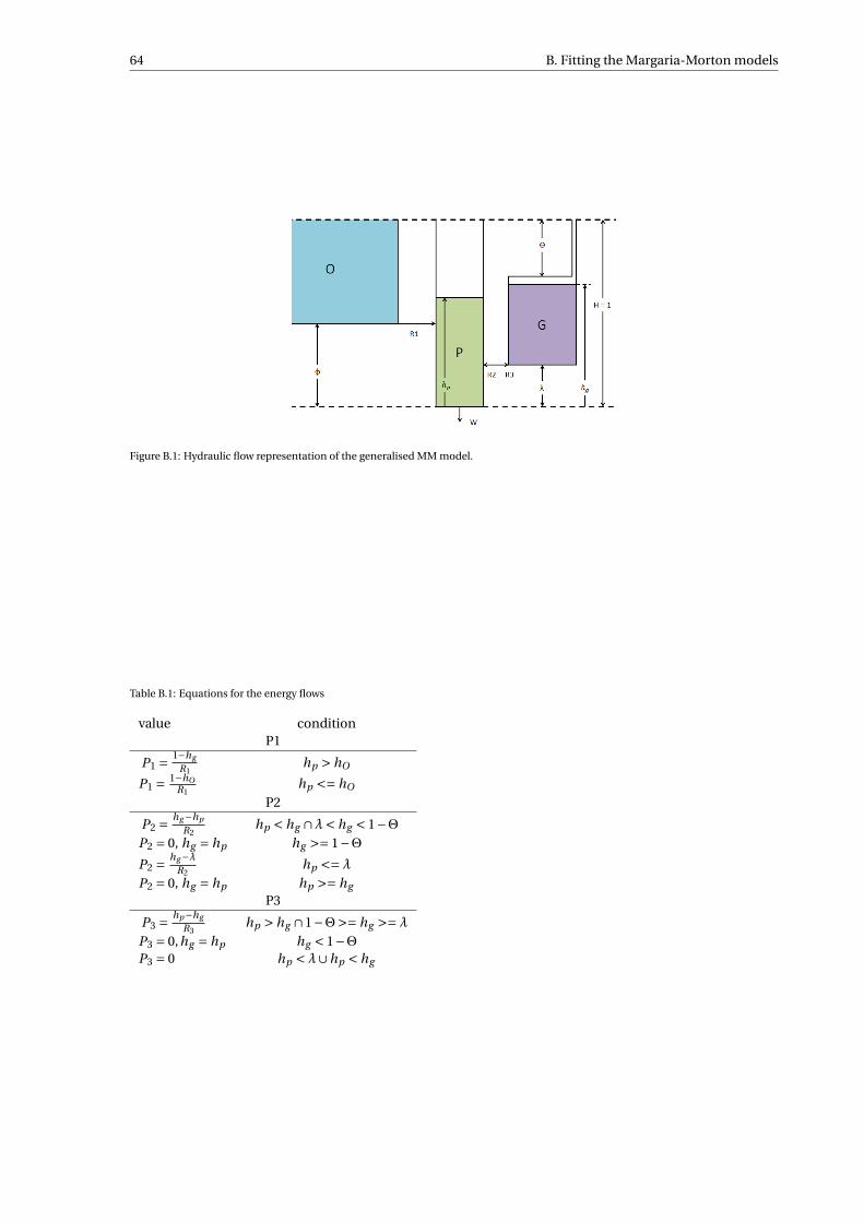
64 B. Fitting the Margaria-Morton models
Figure B.1: Hydraulic flow representation of the generalised MM model.
Table B.1: Equations for the energy flows
value conditionP1
P1 = 1−hg
R1hp > hO
P1 = 1−hOR1
hp <= hO
P2
P2 = hg −hp
R2hp < hg ∩λ< hg < 1−Θ
P2 = 0, hg = hp hg >= 1−ΘP2 = hg −λ
R2hp <=λ
P2 = 0, hg = hp hp >= hg
P3
P3 = hp−hg
R3hp > hg ∩1−Θ>= hg >=λ
P3 = 0,hg = hp hg < 1−ΘP3 = 0 hp <λ∪hp < hg
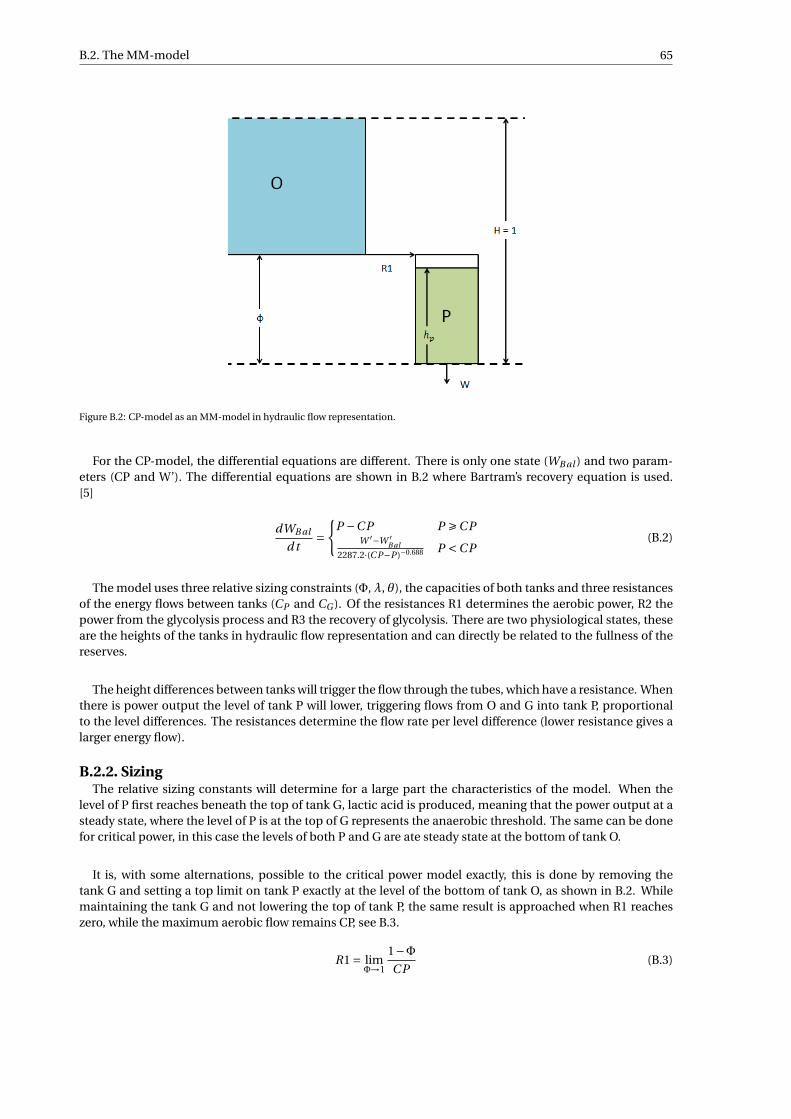
B.2. The MM-model 65
Figure B.2: CP-model as an MM-model in hydraulic flow representation.
For the CP-model, the differential equations are different. There is only one state (WB al ) and two param-eters (CP and W’). The differential equations are shown in B.2 where Bartram’s recovery equation is used.[5]
dWB al
d t=
{P −C P P ÊC P
W ′−W ′B al
2287.2·(C P−P )−0.688 P <C P(B.2)
The model uses three relative sizing constraints (Φ, λ, θ), the capacities of both tanks and three resistancesof the energy flows between tanks (CP and CG ). Of the resistances R1 determines the aerobic power, R2 thepower from the glycolysis process and R3 the recovery of glycolysis. There are two physiological states, theseare the heights of the tanks in hydraulic flow representation and can directly be related to the fullness of thereserves.
The height differences between tanks will trigger the flow through the tubes, which have a resistance. Whenthere is power output the level of tank P will lower, triggering flows from O and G into tank P, proportionalto the level differences. The resistances determine the flow rate per level difference (lower resistance gives alarger energy flow).
B.2.2. SizingThe relative sizing constants will determine for a large part the characteristics of the model. When the
level of P first reaches beneath the top of tank G, lactic acid is produced, meaning that the power output at asteady state, where the level of P is at the top of G represents the anaerobic threshold. The same can be donefor critical power, in this case the levels of both P and G are ate steady state at the bottom of tank O.
It is, with some alternations, possible to the critical power model exactly, this is done by removing thetank G and setting a top limit on tank P exactly at the level of the bottom of tank O, as shown in B.2. Whilemaintaining the tank G and not lowering the top of tank P, the same result is approached when R1 reacheszero, while the maximum aerobic flow remains CP, see B.3.
R1 = limΦ→1
1−ΦC P
(B.3)

66 B. Fitting the Margaria-Morton models
B.3. MethodIn literature there is a lack of information and standardisation on how to fit a MM-model to an athlete. Thatcombined with the lack of resources to perform the required test to do so, makes for an easy decision toprovide parameters for fictional cyclists. A combination of tests that could also be used to fit the criticalpower model are combined with a test that of intermittent exercise, to determine the recovery kinetics.
In this study, standardised cyclists are used, the parameters of the critical power model, for the standard-ised cyclists, are used to generate those for the MM-models of the same fictional cyclists. The two constantsof the CP-model are, critical power and anaerobic work capacity. Those two are proportionally scaled alongthe standardised cyclists, which are shown in equation B.2.
Table B.2: Standardised physiological coeficients in strength classes for the CP-model.
Power class CP W’W kJ
Super strong 450 25.0Strong 420 23.3Medium 390 21.7Weak 360 20.0
B.3.1. constraintsThe MM-model can be configured in various configurations, the desired configuration is such that it showsa different behaviour with respect the the CP-model. Having two models that have different characteristics,different optima in strategies might be found according to the model which is used. To make the modeldifferent from the CP-model the relative sizing coefficient Φ is chosen to be low (0.2). It is assumed that theanaerobic threshold for this athlete is at half of the critical power leading to θ = 0.4. The coefficient λ is setto 0.1. In order to model that the G reserve is actually used, the size of the P tank is set to exactly half of theW’ reserve in the corresponding CP-model. This leaves four constants undefined, which could be fitted witha minimum of four tests.
B.3.2. TestsBecause using the constraints, four constants of the MM-model are undefined, four tests are done to fit theMM-model to the CP-model. The CP-model can be fitted to cyclists using a series of three self paced allout tests. [6] The duration of these tests are set to one, three and twenty minute tests. The last test is anintermittent test as performed in the study from Bartram’s recovery model. [5] Using these tests, the modelparameters are fitted such as they would in a test to determine the parameters for the critical power model.The power profiles of the tests are shown along with the results in B.3
B.3.3. OptimisationThe parameters were adjusted manually, after which a gradient optimisation was performed to find the localminimum to this problem. Optimisation was performed using the ’trust-region-reflection’ algorithm. Theoptimisation was performed in MATLAB using default settings of the ’fmincon’ function.
The objective is that the at all tests the tank is first empty exactly at the end of the test. The scores of thetests are combined by taking the root mean square of the individual test errors, as defined in equation B.4b.The individual test are simulated with a fixed time step simulation. If the value for hP would reach below zero,the simulation is terminated and the time of failure (t f ai l ) is computed, the error in time between failure andobjective is the objective score. If the simulation is valid the remaining level in the tank P (hP [end ]) is theobjective score, as shown in equation B.4a.
eri ={
hP [end ] mi n(hP (t )) Ê 0tob j ect i ve−t f ai l
tob j ect i vemi n(hP (t )) < 0
(B.4a)
J =√√√√ 4∑
i=1er 2
i (B.4b)

B.4. Results and discussion 67
The relative sizing parameters (Φ,λ and θ) are not scaled for the other strength classes, all other parametersare scaled proportional to the critical power of the CP-model of the same strength class. This way only onestrength class is optimised. In case of the possibility of multiple optima, this makes sure that all strengthclasses use the same optimum. The optimisation is performed on the strength class ’Strong’.
B.4. Results and discussionUsing the optimisation the results are produced ans shwon in table B.3, in this table the resistances are con-verted to an admittance (D, D = R−1), which represents the energy flow per tank level difference. What sur-prises is the value for D1, in strength class Super Strong it has a value of 577.1 W, multiplying this with thelevel difference between top of tank P (1) and the bottom of tank O (Phi = 0.2), this results in the maximumaerobic power and is equal to 461.7 W, see B.6. The maximum aerobic power of the MM-model is thereby 11.7W (2.6 %) higher than the critical power of the same strength class. The higher maximal aerobic power can beexplained by the fact that when the athlete is at steady state power output at maximal aerobic power, usingthe relative sizing parameters chosen, very little anaerobic capacity is left. The additional bit of aerobic powercompensates for the lack of anaerobic work beyond this point, in longer endurance tasks such as the twentyminute test or the intermittent test. Also the total anaerobic work capacity is over four times as large as theW’ of the CP-model (103 kJ for MM and 25 kJ for CP). The reason for this effect is that a large part of the Greserve is consumed when aerobic power is low, meaning that the with the MM-model a lot of the anaerobicenergy is consumed while the aerobic power is below maximal aerobic power. With the CP model when thepower output is below maximum aerobic power, the whole power output is considered aerobic.
PO2,max = D1 · (1−Φ) (B.5)
Wan,M M =CP +CG · (1−λ−θ) (B.6)
Table B.3: Standardised physiological coeficients in strength classes for the CP-model.
parameter units Weak Medium Strong Super StrongΦ - 0.2 0.2 0.2 0.2λ - 0.1 0.1 0.1 0.1θ - 0.4 0.4 0.4 0.4D1 = R1−1 W 461.7 500.1 538.6 577.1D2 = R2−1 W 1290 1398 1505 1613D3 = R3−1 W 960.0 1040 1120 1200CP kJ 10.00 10833 11.67 12.50CG kJ 72.72 78.78 84.84 90.90
The errors of the four test and the resulting objective value are shown in table B.4, the values are low andsurprisingly similar between strength classes. The low values mean that the optimisation yielded a goodoutcome that fits al four tests well. The similarity among strength classes means that fitting just one strengthclass and scaling up and down to the other strength classes was a successful choice, now all strength classescontain the same error as the fitted class.
Table B.4: Standardised physiological coeficients in strength classes for the CP-model.
Error values er1 er2 er3 er4 JWeak 2.10 ·10−5 9.89 ·10−4 1.80 ·10−2 7.93 ·10−5 9.84 ·10−3
Medium 1.90 ·10−5 9.75 ·10−4 1.79 ·10−2 3.18 ·10−3 9.10 ·10−3
Strong 1.70 ·10−5 9.63 ·10−4 1.78 ·10−2 6.82 ·10−4 3.88 ·10−3
Super Strong 3.88 ·10−5 9.53 ·10−4 1.78 ·10−2 4.23 ·10−5 8.90 ·10−3
The results of a simulation are the physiological states, for al test were the fit is optimised to the physiologi-cal states are plotted against time. This is done considering a cyclist of strength class ’Strong’, where the massis not influential. In the figure, the plots on each row represent a test, where on the left (plots a, c, e and g) thereference is plotted, this consists of the power profile and the WB al (physiological stat of the CP model). On
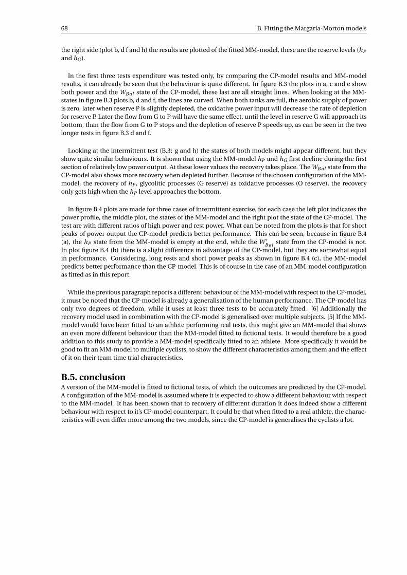
68 B. Fitting the Margaria-Morton models
the right side (plot b, d f and h) the results are plotted of the fitted MM-model, these are the reserve levels (hP
and hG ).
In the first three tests expenditure was tested only, by comparing the CP-model results and MM-modelresults, it can already be seen that the behaviour is quite different. In figure B.3 the plots in a, c and e showboth power and the WB al state of the CP-model, these last are all straight lines. When looking at the MM-states in figure B.3 plots b, d and f, the lines are curved. When both tanks are full, the aerobic supply of poweris zero, later when reserve P is slightly depleted, the oxidative power input will decrease the rate of depletionfor reserve P. Later the flow from G to P will have the same effect, until the level in reserve G will approach itsbottom, than the flow from G to P stops and the depletion of reserve P speeds up, as can be seen in the twolonger tests in figure B.3 d and f.
Looking at the intermittent test (B.3: g and h) the states of both models might appear different, but theyshow quite similar behaviours. It is shown that using the MM-model hP and hG first decline during the firstsection of relatively low power output. At these lower values the recovery takes place. The WB al state from theCP-model also shows more recovery when depleted further. Because of the chosen configuration of the MM-model, the recovery of hP , glycolitic processes (G reserve) as oxidative processes (O reserve), the recoveryonly gets high when the hP level approaches the bottom.
In figure B.4 plots are made for three cases of intermittent exercise, for each case the left plot indicates thepower profile, the middle plot, the states of the MM-model and the right plot the state of the CP-model. Thetest are with different ratios of high power and rest power. What can be noted from the plots is that for shortpeaks of power output the CP-model predicts better performance. This can be seen, because in figure B.4(a), the hP state from the MM-model is empty at the end, while the W ′
B al state from the CP-model is not.In plot figure B.4 (b) there is a slight difference in advantage of the CP-model, but they are somewhat equalin performance. Considering, long rests and short power peaks as shown in figure B.4 (c), the MM-modelpredicts better performance than the CP-model. This is of course in the case of an MM-model configurationas fitted as in this report.
While the previous paragraph reports a different behaviour of the MM-model with respect to the CP-model,it must be noted that the CP-model is already a generalisation of the human performance. The CP-model hasonly two degrees of freedom, while it uses at least three tests to be accurately fitted. [6] Additionally therecovery model used in combination with the CP-model is generalised over multiple subjects. [5] If the MM-model would have been fitted to an athlete performing real tests, this might give an MM-model that showsan even more different behaviour than the MM-model fitted to fictional tests. It would therefore be a goodaddition to this study to provide a MM-model specifically fitted to an athlete. More specifically it would begood to fit an MM-model to multiple cyclists, to show the different characteristics among them and the effectof it on their team time trial characteristics.
B.5. conclusionA version of the MM-model is fitted to fictional tests, of which the outcomes are predicted by the CP-model.A configuration of the MM-model is assumed where it is expected to show a different behaviour with respectto the MM-model. It has been shown that to recovery of different duration it does indeed show a differentbehaviour with respect to it’s CP-model counterpart. It could be that when fitted to a real athlete, the charac-teristics will even differ more among the two models, since the CP-model is generalises the cyclists a lot.

B.5. conclusion 69
(a) (b)
(c) (d)
(e) (f)
(g) (h)
Figure B.3: The fitted MM-model for the standardised strength of the strong cyclist. in the left plots the power output of the test is shown(solid) along with the WB al state of the simulated CP-model. In the right plot the physiological states in form of the tank levels are showncorresponding to the simulated test with the MM-model. Plots a and b are fromt the one-minute test, c and d are from the three minutetest, e and f are from the twenty minute test and g and h are from the intermittent test.
70 B. Fitting the Margaria-Morton models
(a) Intermittent exercise with short power and long recovery while Ppeak = 1020W .
(b) Intermittent exercise with medium power and medium recovery while Ppeak = 670W .
(c) Intermittent exercise with long power and short recovery while Ppeak = 520W .
Figure B.4: Plots of physiological states of both models in three different intermittent exercises, the ratio between power and recovery
time are varied. The power ratio RP = Pr estPpeak
is 0.2. In the plots shown in (a) rest is long (100 s) and power is short (20 s), in (b) power and
rest phase are of medium duration (60 s), in (c) the rest is short (20 s) and power is long (100 s). For each cases the left plot is the poweroutput (solid line is power output, the dashed is critical power), the center plot are the states of the MM-model and the right plot showsthe state of the CP-model.
Bibliography
[1] Bicycle rolling resistance: The test. https://www.bicyclerollingresistance.com/the-test. Accessed: 20-07-2018.
[2] p Astrand. Quantification of exercise capability and evaluation of physical capacity in man. Progress inCardiovascular Diseases, 19:154–163, 1976.
[3] P Baldissera. Proposal of a coast-down model including speed-dependent coefficients for the retardingforces. Journal of Sports Engineering and Technology, 231:154–163, 2017.
[4] N Barry, T Burton, J Sheridan, M Thomson, and A T Brown. Aerodynamic drag interactions betweencyclists in a team pursuit. Sports Engineering, 18:93–103, 2015.
[5] J C Bartram, D Thewlis, D T Martin, and K I Norton. Accuracy of w’ recovery kinetics in high perfor-mance cyclists - modelling intermittet work capacity. International Journal of Sports Physiology andPerformance, 0:0, 2016.
[6] J C Bartram, D Thewlis, D T Martin, and K I Norton. Predicting critical power in elite cyclists: Questioningvalidity of the 3-min all-out test. Journal of Sport Physiology and Performance, IN PRESS.
[7] H C Bergstrom, J M Housh T J and, Zuniga, D A Traylor, R W Lewis, C L Camic, R J Schmit, and G OJohnson. Differences among estimates of critical power and anearobic work capacity derived from fivemathematical models and the three minute all-out test. Journal of Strength and Conditioning Research,28:592–600, 2014.
[8] B Blocken, T Defraye, E Konincks, J Carmeliet, and P Hespel. Cfd simulations of the aerodynamic dragof two drafting cyclists. Computers & Fluids, 71:435–445, 2013.
[9] B Blocken, T Defraye, E Konincks, J Carmeliet, and P Hespel. Surprices in cycling aerodynamics. EuroPhysics News, 44:20–23, 2013.
[10] J P Broker, C R Kyle, and Burke E R. Racing cyclist power requirements in the 4000-m individual andteam persuits. Medicine and Science in Sports and Exercise, 31:1677–1685, 1999.
[11] R Candau, F Grappe, M Ménard, B Barbier, G Y Millet, M D Hoffman, A R Belli, and J D Roullion. Sim-plified deceleration method for assessment of resistive forces in cycling. Medicine and Science in Sportsand Exercise, 31:1441–1447, 1999.
[12] R Candau, F Grappe, M Ménard, B Barbier, G Y Millet, M D Hoffman, A R Belli, and J D Roullion. Sim-plified deceleration method for assessment of resistive forces in cycling. Medicine and Science in Sportsand Exercise, 31:1441–1447, 1999.
[13] A J Chipperfield, P Fleming, and H Pohlheim. A genetic algorithm toolbox for matlab. In Proc. TenthInternational Conference on Systems Engineering (ICSE, Coventry, UK, September 1994), pages 200–207,Coventry, UK, 1994. Research Gate.
[14] Jos J De Koning, Maarten F Bobbert, and Carl Foster. Determination of optimal pacing strategy in trackcycling with an energy flow model. Journal of Medicine in Sport, 2:266–277, 1999.
[15] P Debraux, F Grappe, A V Manolova, and W Bertucci. Aerodynamic drag in cycling: methods of asses-ment. Sports Biomechanics, 10:197–218, 2011.
[16] T Defraye, B Blocken, E Konincks, P Hespel, P Verboven, B Nicolai, and J Carmeliet. Cyclist drag in teampursuit: Influence of cyclist sequence stature, and arm spacing. Journal of Biomechanical Engineering,136:011005–1–011005–9, 2014.
71
72 Bibliography
[17] W. C. Edwards, A. G. & Byrnes. Aerodynamic characteristics as determinants of the drafting effect incycling. Med. Sci. Sports Exerc., 39:170–176, 2007.
[18] B Fitton, O Caddy, and D Symons. The impact of relative athlete characteristics on te drag reductionscaused by draftin when cycling in a velodrome. Journal of Sports Engineering and Technology, 232:39–49,2018.
[19] C Foster, J J De Koning, F Hettinga, J Lampen, K L La Clair, C Dodge, M Bobbert, and J P Porcari. Patternof energy expenditure during simulated competition. Medicine and Sciency in Sports and Exercise, 35:826–831, 2003.
[20] R. L. Haupt. Optimum population size and mutation rate for a simple real genetic algorithm that opti-mizes array factors. In IEEE Antennas and Propagation Society International Symposium. TransmittingWaves of Progress to the Next Millennium. 2000 Digest. Held in conjunction with: USNC/URSI NationalRadio Science Meeting (C, volume 2, pages 1034–1037 vol.2, July 2000. doi: 10.1109/APS.2000.875398.
[21] D P Heil. Body mass scaling of frontal area in competetive cyclists not using aero-handlebars. EuropeanJournal of Physiology, 87:520–528, 2002.
[22] L Heimans, W R Dijkshoorn, M J M Hoozemans, and J J De Koning. Optimizing the team for requiredpower during track cycling team pursuit. International Journal of Sports Physiology and Performance,12:1385–1391, 2017.
[23] W Hennekam and J Bontsema. Determination of fr and kd from the solution of the equation of motionof a cyclist. European Journal of Physics, 12:59–63, 1999.
[24] F J Hettinga, J J de Koning, and Foster C. Relative importance of pacing strategy and mean power outputin 1500-m self-paced cycling. British Journal of Sports Medicine, 46:30–35, 2012.
[25] D J Housh, T J Housh, and S M Bauge. A methodological consideration for the determination of criticalpower and anaerobic work capacity. Exercise and Sport, 61(4):406–409, 1990.
[26] ICU. Icu cycling regulations - part 2 road races. online http://www.uci.ch/inside-uci/rules-and-regulations/regulations/, October 2017.
[27] A Íñiguez de-la Torre and J Íñiguez. Aerodynamics of a cycling team in a time trial: does the cyclist at thefront benefit? European Journal of Physics, 30:1365, 2009.
[28] D Jenkins, K Kretek, and D Bishop. The duration of predicting trial influences time to fatique at criticalpower. Journal of Science and Medicin in Sports, 1(4):213–218, 1998.
[29] C R Kyle. Reduction of wind resistance and power output of racing cyclists and runners traveling ingroups. Ergonomics, 22:387–397, 1979.
[30] H. Monod and J. Scherrer. The work capacity of a synergic muscular group. Ergonomics, 8:329–338, 1965.
[31] H R Morton. Modeling human power endurance. Journal of Mathematical Biology, 28:49–64, 1990.
[32] H R Morton. The critical power and related whole-body bioenergetic models. European Journal of Ap-plied Physiology, 96:339–354, 2006.
[33] R H Morton. A three component model of human bioenergetics. Journal of Mathematical Biology, 24:451–466, 2004.
[34] R H Morton and L V Billat. The critical power model for intermittent exercise. European Journal ofApplied Physiology, 91:303–307, 2004.
[35] D A Noordhof, Skiba P F, and J J de Koning. Determining anaerobic capcity in sporting activities. Inter-national Journal of Sports Physiology and Performance, 8:475–482, 2013.
[36] T S Olds, K I Norton, and N P Craig. Mathematicle model of cycling performance. Journal of AppliedPhysiology, 75:730–737, 1993.
Bibliography 73
[37] T S Olds, K I Norton, E L A Lowe, F Olive, and S Ly. Modeling road cycling performance. Journal ofApplied Physiology, 78:1596–1611, 1995.
[38] S Padilla, I Mujika, F Angulo, and Goiriena J J. Scientific approach to the 1-h cycling world record: a casestudy. Journal of Applied Physiology, 89:1522–1527, 2000.
[39] P. E. Prampero, di. Cycling on earth, in space, on the moon. European Journal of Applied Physiology, 82:345–360, 2000.
[40] P. E. Prampero, di, Gortili G., P. Mognoni, and F. Saibene. Equations of motion of a cyclist. Journal ofApplied Physiology, 47:201–206, 1979.
[41] Margaria R. Biomechanics and energetics of muscular exercise. Oxford university press, 1976.
[42] Gordon S. Optimising distribution of power during a cycling time trial. Sports Engineering, 8:81–90,2005.
[43] F. P. Skiba, W Chidnok, A Vanhatalo, and A. M. Jones. Modeling the expendature and reconstruction ofwork capacity above critical power. American college of sports medicine, 44:1526–1532, 2012.
[44] V S Sreedhara, G M Mocko, and R E Hutchison. An experimental protocol to model recovery of anaerobicwork. Proceedings, 2:208, 2018.
[45] L Underwood and M Jeremy. Mathematical model of track ccling: the individual pursuit. Procidia engi-neering, 2:3217–3222, 2010.
[46] G. J. Van Ingen Schenau and P. R. Cavanagh. Power equations in endurance sports. Journal of Biomedics,23:865–881, 1990.
[47] H Vandewalle. Critical power test for ramp exercise. Journal of Applied Physiology, 71:285–286, 1995.
[48] A Vanhatalo, J H Doust, and Burnley M. Determination of critical power using a 3-min all-out cyclingtest. Medicien in Sports and Exercise, 39(3):548–555, 2007.