Water Resources Management 17: 409–428, 2003.© 2003 Kluwer Academic Publishers. Printed in the Netherlands.

409

Optimal Groundwater Management in DeltaicRegions using Simulated Annealing and NeuralNetworks

S. V. N. RAO1∗, B. S. THANDAVESWARA2, S. MURTY BHALLAMUDI2 andV. SRINIVASULU1

1 National Institute of Hydrology, Kakinada, AP India; 2 Indian Institute of Technology, Chennai,TN, India(∗ author for correspondence, e-mail: shedimbi@yahoo.com)

(Received: 26 November 2002; in final form: 24 June 2003)

Abstract. This study deals with the optimal management of groundwater in deltaic aquifer systemswith some reference to east coastal hydro-geo-climatic conditions of India. A system of cooperativewells is proposed to supplement surface water sources to meet the demand during the non-monsoonseason, without inducing excessive saltwater intrusion. The management models are solved as non-linear, non-convex, combinatorial problems. The management models are solved by interfacingsimulated annealing (SA) algorithm with an existing SHARP interface flow model to determine anoptimal policy for location and pumpages of cooperative wells. Computational burden arising fromSA algorithm is managed within practical timeframes by replacing the simulator with an artificialneural network (ANN).

Key words: artificial neural network, combinatorial, sharp interface model, simulated annealing

1. Introduction

The objective of groundwater management in deltaic regions, with only a moderateavailability of surface water, is to evolve appropriate operational strategies to sup-plement the surface water with the groundwater to meet the water demand for irrig-ation and other uses, while controlling the aquifer salinity. Excessive groundwaterextraction in these regions, particularly in the lower deltaic plains, may lead tosignificant seawater intrusion, and hence excessive salinity. Therefore, groundwa-ter management models for deltaic regions should combine the process model forseawater intrusion with an appropriate technique for solving the optimization prob-lem. In the present study, a nonlinear-optimization based model is developed forthe management of groundwater in deltaic regions. The motivation for this studyhas come from the hydro-geo-climatic conditions and water deficit problems, es-pecially during the non-monsoon season, prevailing in large deltaic systems alongthe east coast of India.

410 S. V. N. RAO ET AL.

The Delta systems in general evolved with the deposition of silt and sedimentfrom river basins over geologic time. In India several delta systems exist along theeastern coast. The groundwater recharge here is largely influenced by monsoonrainfall (July–December). The spatial variability in fresh groundwater availabilitydepends on hydro-geologic setting, paleo channels and sea/river boundary condi-tions. The delta systems are often irrigated from surface water diversion systems.While adequate amount of surface water is normally available during the monsoonseason from the diversion system, the situation is not the same during the non-monsoon season, even for large deltas with perennial flows. The problem is acutein the tail end reaches of the irrigation canal system in lower deltaic plains that areadjacent to the sea. Therefore, groundwater pumping becomes necessary in theseregions in order to meet the irrigation demand.

In general, the fresh water and saltwater zones within an aquifer are separatedby a transition zone, in which there is a gradual change in density. Two generalmodels have been used to describe the seawater intrusion phenomenon. The mis-cible interface flow model explicitly represents the presence of this zone throughan advection-dispersion equation. Although, miscible density dependent flow andtransport models (Voss, 1984; Huyakorn et al., 1987; Das and Datta, 1999a) arepresently available their use in management models has been somewhat limitedbecause of high computational burden. The second approach to the analysis of sea-water intrusion problems is based on the simplifying assumption that the transitionzone can be represented by a sharp interface (Bear and Dagan, 1964; Shamir andDagan, 1974; Bear and Moulem, 1974; Wilson and Costa, 1982; Essaid, 1990).

Coupled simulation-optimization (S/O) models (Gorelick, 1983) have beenwidely used to address the management issues. Willis and Finney (1988), Hallajiand Yazicigil (1996), Emch and Yeh (1998), Das and Datta (1999a, b), Cheng et al.(2000), among others, have proposed a number of groundwater management mod-els applicable for coastal aquifers. Although a number of studies have been reportedon management issues related to coastal aquifers in general, not much attention hasbeen paid to the issues unique to groundwater management in deltaic regions. Alsoas has been stated by Emch and Yeh (1998), the objectives and the constraints in acoastal or deltaic aquifer management model are typically nonlinear, and therefore,use of gradient based methods for solving the optimization problem is beset withdifficulties. Gradient search methods cannot be applied directly if some of thedecision variables in the management model, such as the locations of the pumpingwells, are discrete. In the last 15 yr, heuristic and evolutionary methods have beendeveloped for this purpose. Among these, the Simulated Annealing (Doughertyand Marryott, 1991) and the Genetic Algorithms (Goldberg, 1989) are the twomost popular methods. More recently Wang and Zheng (1998) and Cunha (1999)have demonstrated the application of SA to hypothetical groundwater managementproblems in non-coastal regions.

In this study, a management model is developed within S/O framework, for de-termining the optimal groundwater extraction in a hypothetical deltaic region with

OPTIMAL GROUNDWATER MANAGEMENT IN DELTAIC REGIONS 411

Figure 1. Definition sketch of a hypothetical deltaic system.

some reference to Indian conditions. The groundwater is extracted through a sys-tem of cooperative wells, and is assumed to supplement the surface water supply,so as to meet the irrigation demand during the non-monsoon season. The objectiveof the management model is to determine an optimal configuration of rates ofpumpages and their location in lower deltaic plains such that the seawater intrusionvolume is minimized. The management model is formulated as a combinatorialproblem since the locations of wells form part of the decision vector. The com-binatorial problem is solved using the Simulated Annealing (SA) algorithm. Thecomputational burden is kept within practical timeframes by replacing the SHARPmodel with ANN, a universal approximator (ASCE Task Committee, 2000).

2. Model Formulation

A hypothetical deltaic system is conceptualized as shown in Figure 1. In this delta,irrigation requirements are wholly met from a diversion structure during the mon-soon season, while the surface water is supplemented with groundwater during thenon-monsoon season. It is required to determine the optimal location and ground-water pumpages of co-operative wells in the lower deltaic plain to augment surfacewater supplies during the nonmonsoon season. The aquifer system is assumed to beunconfined with freshwater and saltwater separated by a sharp interface. The wellscreens are assumed to be above the interface through out the operation, such thatonly fresh water is utilized. Higher values of porosity and hydraulic conductivityare used for nodes representing paleo channels resulting in non-homogeneity inthe aquifer system. Pumpages are assigned to a few nodes in the upper deltaicplain to represent existing pumpages in a partially developed aquifer system. Two

412 S. V. N. RAO ET AL.

single objective management models are separately formulated as combinatorialproblems subject to a set of constraints.

2.1. MANAGEMENT MODEL-I

The Management Model-I (MM1) determines the maximum amount of ground-water that can be extracted during the non-monsoon season, through a system ofco-operative wells in the region of interest. Thus this model evaluates the maximumgroundwater potential in the region of interest, in the non-monsoon season. In thismodel, only two time steps are considered over a period of one year. The two timesteps correspond to monsoon and non-monsoon seasons consisting of 183 dayseach. A known uniform recharge (based on the rainfall) is assumed during the first(monsoon) season.

It is required to determine the location of cooperative pumping wells in lowerdelta plains and their corresponding pumping rates at these wells such that thetotal amount of groundwater withdrawn during the second season (non-monsoon)is a maximum. The model, formulated as a combinatorial problem, determineslocations for K (K is specified) number of pumping wells out of a possible Kmax

locations (Ex: Kmax = 10 in Figure 1) and the corresponding pumping rate ateach of these K pumping wells. The objective function and the constraints forthe optimization problem can be written in terms of decision and state variables asfollows.

max F1 =K∑

k=1

Qgk . (1)

Subject to the following constraints:

(1) Interface elevation constraint for coastal nodes: Elevation of the interface atspecified locations close to the coast line should be lower than a maximumspecified interface elevation so that the sea water intrusion is limited.

z(i, j)≤Zmax(i, j) , (2)

at specified (i, j) locations adjacent to the coast line.(2) Draw down elevation constraint at prescribed nodes: This constraint is import-

ant from the point of view of having some reserves for future usage, besidesavoiding reversal of hydraulic gradients.

hf (i, j)≥Hmin(i, j) , (3)

at specified (i, j) locations in the region.

OPTIMAL GROUNDWATER MANAGEMENT IN DELTAIC REGIONS 413

(3) Hydraulic response equations (continuity): This is implemented in the presentstudy by using the SHARP simulation model for coastal aquifers.

(4) Not more than one well at the same location. This constraint is imposed tomeet demand that is distributed in space.

In Equation (1) Qgk = volume of groundwater pumpage (decision variable) atthe kth pumping location during the nonmonsoon season. The freshwater headsand interface elevations are represented by hf (i, j) and z(i, j), respectively, at node(i, j). Hmin(i, j) and Zmax(i, j) are the limits set on freshwater heads and the inter-face elevations.

2.2. MANAGEMENT MODEL-II

The Management Model-II (MM2) seeks to determine the optimal locations andcorresponding pumpages from a system of co-operative wells to meet a targetgroundwater extraction during the non-monsoon season, while minimizing the in-truded saltwater volume. The Management Model-I (MM1) provides the maximumpotential that could be exploited and enables the Decision Maker (DM) to fix thetarget groundwater extraction for MM2. The MM2 is also formulated as a com-binatorial problem i.e., it determines locations for K (K is specified) number ofpumping wells out of a possible Kmax locations (Ex: Kmax = 10 in Figure 1) andthe corresponding pumping rate at each of these K pumping wells. The objectivefunction and the constraints in this model can be written as follows.

min F2 =I∑

i=1

J∑j=1

[(zi, j − B

)A

]. (4)

Subject to the following constraints:

(1) Total pumpage meets the target groundwater demand

K∑k=1

Qgk≥Qd . (5)

(2) Draw down elevation constraint at prescribed nodes as in MM1

hf (i, j)≥Hmin(i, j) (6)

at specified (i, j) locations in the region.(3) Hydraulic response equations (continuity) of the simulator as in MM1.

414 S. V. N. RAO ET AL.

(4) Not more than one well at the same location as in MM1.

Where, Qd = the minimum target demand to be met (specified by the decisionmaker), A = area of each grid in the model, and B = the constant bottom elevationof aquifer. I and J represent the total number of rows and columns in the grid(active cells are within delta). It may be noted here that Qd is decided based on theresult from the MM1. It should be less than the maximum value of total pumpagegiven by the MM1.

3. Solution Methodology

The methodology adapted in this study uses a coupled S/O approach. A codewas developed, by interfacing the simulated annealing (SA) algorithm (optimizer),with the SHARP simulation model (Essaid 1990), as a subroutine. The SHARPsimulator is subsequently replaced with ANN model to reduce the computationalburden. The simulator (SHARP model), the optimizer (SA algorithm) and theneural network (ANN) are briefly discussed below.

3.1. SHARP SIMULATION MODEL

The two fluid SHARP – interface simulator (Essaid 1990) used in this study isan established model tested for both benchmark and field problems. SHARP is amulti-layer quasi-3D finite difference model that simulates flow in a coastal aquifersystem. The coupled, nonlinear partial differential equations are as under.

[Sf Bf + n (α + δ)

] ∂hf

∂t− n (1 + δ)

∂hs

∂t=

∂

∂x

(Bf xKf x

∂hf

∂x

)+ ∂

∂y

(BfyKfy

∂hf

∂y

)+ Qf

(7)

[SsBs + n (1 + δ)]∂hs

∂t− nδ

∂hf

∂t=

∂

∂x

(BsxKsx

∂hs

∂x

)+ ∂

∂y

(BsyKsy

∂hs

∂y

)+ Qs

(8)

Zi = (1 + δ) hs − δhf , (9)

where

OPTIMAL GROUNDWATER MANAGEMENT IN DELTAIC REGIONS 415

hf , hs = fresh and salt water hydraulic heads, respectively (L);

Sf , Ss = fresh and salt water specific storage (L−1);

Kf x , Ksx = fresh and salt water hydraulic conductivity in x direction(LT−1);

Kfy , Ksy = fresh and salt water hydraulic conductivity in y direction(LT−1);

Bf , Bs = fresh and salt water saturated thickness (L);

Qf , Qs = fresh and saltwater source/sink terms (pumpage, recharge)(LT−1);

n = effective porosity;

δ = γf /(γs − γf );

γf , γs = fresh water and salt water specific weights (ML−2 T−2);

α = 1 for an unconfined aquifer, 0 for confined aquifer;

Zi = interface elevation (L).

3.2. SIMULATED ANNEALING ALGORITHM

Simulated annealing (SA) technique was developed by Kirkpatrick et al. (1983) tofind near optimum solutions for combinatorial problems. In this algorithm, each de-cision variable can only take a discrete value from a specified set of possible values.Each combination of decision variables is called a configuration. The method gen-erates a random configuration (trial point) within the configuration space throughperturbation, makes a function call to the simulator to determine the state variables,and then evaluates the objective function and the constraints. If the trial pointresults in constraint violation, it is rejected and a new point is generated. If thetrial point is feasible and the objective function value is better than the previousbest record then the point is accepted and the record for the best value is updated.If the trial point results in feasibility but the objective function is worse than thecurrent best value, then the trial point is either accepted or rejected based on theMetropolis criterion (Metropolis, 1953). For this purpose, a random deviate, whichis uniformly distributed on the interval (0, 1), is generated. If this random deviateis smaller than the acceptance probability, then the worse move is accepted. Theprobability for the acceptance of a worse move is equal to exp(−�C/T ), where�C = difference in the objective function values corresponding to the present andprevious best configurations, and T is a parameter called ‘temperature’. Initially alarge value of temperature is selected so that a large percentage of downhill/uphillmoves are accepted. The value of T is progressively reduced as the trials proceed,and the acceptance probability of uphill moves steadily decreases to zero. This iscalled ‘cooling schedule’, and the worse configurations are almost always rejectedin the final stages. The entire process is terminated after a fairly large number oftrials. This strategy avoids getting trapped in a local minimum, a problem common

416 S. V. N. RAO ET AL.

to gradient-based algorithms. The algorithmic representation of the SA along withthe SHARP simulation model is shown in Figure 2. The code for SA algorithmdeveloped here incorporates a perturbation procedure called genetic rearrangement(Dougherty et al., 1991) for generating a new configuration.

3.3. ARTIFICIAL NEURAL NETWORK (ANN)

In the management model, the SHARP simulator is called several thousands oftimes to verify the constraints for each trial point, resulting in significant com-putational burden. Therefore the computational time of the simulator needs to bereduced. This is achieved in the present study by replacing the SHARP simulatorwith ANN.

ANN is discussed in detail in ASCE Task Committee paper (2000), Aly andPeralta (1999) and in ANN toolbox of MATLAB (2000). In this study a 3 layer,feed forward, error back propagation network is used. The training of the networkconsists of a forward pass and a backward pass. In the forward pass, the effect of anapplied activity pattern at the input layer is propagated through the network layerby layer. The activation value at ith neuron in nth layer an

i is given by the followingequation.

ani =

m∑j=1

WnjiO

n−1j + bn

i , (10)

in which, Wnji = weight of the link between ith neuron in nth layer and j neuron in

(n − 1) layer; On−1j = output of j th neuron in the (n − 1)th layer; bn

i = bias of theith neuron in nth layer; and m = number of neurons in j layer. The activation valueof a neuron is used to obtain the output value of that neuron through the transferfunction. The commonly used transfer function (sigmoidal) is given by:

f (t) = 1/(1 + exp(−t)) . (11)

The function value of each neuron in the output layer is obtained by propagatingthe effect of input through layers. The goal of ANN here is to establish a relationof the form as under:

(Y m) = f (Xn) , (12)

where, Xn is an n dimensional input vector consisting of x1, x2, . . .xn; and Y m is anm dimensional output or target vector consisting of resulting variables of interesty1, y2, . . ., yn. The network is trained generally, using a back propagation algorithmthat will adjust the weights and biases so as to minimize the error function givenby,

E =∑P

∑p

(yi − ti)2 , (13)

OPTIMAL GROUNDWATER MANAGEMENT IN DELTAIC REGIONS 417

Figure 2. Scheme of solution procedure using simulated annealing.

418 S. V. N. RAO ET AL.

Figure 3. Sketch of a simplified hypothetical delta system.

where yi , is the ANN output and ti , is the desired output; p is the number of outputneurons and P is the number of training patterns or data sets.

4. Illustrative Application of Management Models

Management models developed in this study are applicable for the groundwatermanagement of deltaic aquifers subjected to seasonal rainfall, which is typical ofdeltas on the east coast of India. Illustrative applications of management mod-els presented in this study are intended to test the feasibility, applicability andevaluation of the methodology under representative conditions. The evaluationand interpretation are however subject to the limitations and assumptions built insimulation model, optimization procedure and the hypothetical data used in thestudy.

4.1. DESCRIPTION OF STUDY AREA AND DATA

In the course of developing and testing the methodology, a hypothetical data setrepresenting the unconfined deltaic aquifer system is used. The idealized homo-geneous, isotropic unconfined aquifer system is represented in the form of a delta(isosceles triangle) of uniform thickness (Figure 3). The delta is 10 km long alongthe coast and extends up to 10 km normal to the coastline. The aquifer propertiesconsidered in the study are presented in Table I. The sea face is assumed vertical.A constant head (zero) is assigned to the nodes along the coast and a specifiedhead boundary condition is assumed along the two sides of the delta representingriver boundary conditions. The problem geometry, the boundary conditions and thepossible locations of 10 cooperative wells were made symmetrical about the axisAB (see Figure 3), so that a qualitative analysis of the results was possible, and theperformance of the models could be evaluated. However, several other alternativearrangements for possible location of wells could be considered.

For illustration purposes, the problem of determining locations for five co-operative wells out of ten possible locations is examined. The pumpage at each of

OPTIMAL GROUNDWATER MANAGEMENT IN DELTAIC REGIONS 419

Table I. Aquifer properties used as input to SHARP flow model

Parameter Value

1. Area 50 km2

2. Hydraulic conductivity 1.777E-04 m/s

3. Specific storage of fresh/saltwater domains 1.0E-07/m

4. Porosity 0.15

5. Grid spacing (�x = �y) 1000 m

6. Time step (�t) 183 days (6 months)

7. Specific gravity of sea water 1.025

8. Aquifer thickness 100 m

9. Average (monsoon rainfall) 1000 mm

Table II. Discrete values of pumpages

Pumpages 1 2 3 4 5 6 7 8 9 10

(105 m3/season)

these five wells during the non-monsoon season needs to be determined out of 10possible discrete values (Table II). The discrete values of groundwater pumpages(in terms of volume) for real cases must be arrived from practical considerationsand should be based on available data. In the present study these are chosen withdue regard to the scale of the problem, and to represent near-realistic conditions. Itis also assumed that pump capacities are consistent with discrete values of ground-water pumpage. The combinatorial problem with 1010 possible configurations issolved for the two management objectives subject to the constraints discussedearlier.

The time horizon of the model is one year, which is divided into two time steps:monsoon season, and non-monsoon season (6 months each). Uniform recharge(10% of average rainfall) is assumed during the monsoon season, and the pumpingis carried out only during the non-monsoon season. Although pumpages do existin reality during the monsoon season also, these are small compared to the amountof recharge and hence ignored. During the non-monsoon season, discharge occursthrough cooperative wells, in addition to some existing pumpages. No recharge isassumed during the nonmonsoon season. The constraint for draw down elevation isset at 1 m above msl. and the constraint for interface elevation is set at 50 m belowmsl. for both MM1 and MM2 models. These constraints apply to locations in thecoastal nodes adjacent to sea. The initial groundwater levels were set at steadystate conditions to represent initial conditions at the beginning of simulation i.e.monsoon season.

420 S. V. N. RAO ET AL.

In the present study, the two management models are applied in a sequentialmanner. The MM1 is used first to determine the maximum possible withdrawalduring the non-monsoon season, for a specified recharge during the monsoon sea-son. Based on the results from this model, the target groundwater extraction, Qd

in the model MM2 is fixed. The model MM2 is then used to determine the optimallocation and pumpages to meet the objective of minimizing the total seawater in-truded volume. Results for two cases A and B are presented in this section. CaseA represents an undeveloped, symmetrical and homogeneous aquifer system. CaseB represents a near real, partially developed (with some existing pumpages in theupper deltaic region) and non-homogeneous (due to a paleo channel) system.

4.2. CASE A: SYMMETRICAL AQUIFER SYSTEM

The case of a simple homogeneous aquifer system, for which the solution is obvi-ous, is chosen here as a proof of concept test to evaluate the management modelperformance. The solution for the symmetrical case can be determined intuitivelyfrom trial configurations by (i) inspecting the range of input over which the de-cision variables vary in Table II, (ii) evaluating the objective function, and (iii) veri-fying the constraints using the SHARP model. For example, the case of determin-ation of locations for five wells and the corresponding pumpages, when the targetdemand, Qd = 25 units (1 unit = 105 m3), is considered. As mentioned earlier, it isassumed that (i) the aquifer system is homogeneous (no paleo channels), (ii) thereare no existing pumpages in the upper deltaic region, and (iii) the river boundarycondition on either side of the delta are same, resulting in symmetry. Solutionfor this case, corresponding to the globally minimum saltwater intruded volume,should obviously be symmetrical and the wells should be located as far away fromthe coast as possible. Also, pumpage at a well located farther from the coastlineshould be more than the pumpage at a well located nearer to the coastline, andthe pumpage at any well cannot exceed 10 units (see Table II). Thus the optimalsolution configuration for MM2 could be (i) the wells are located at locations 1, 2,3, 4, and 5 as shown in Figure 4a, and (ii) the corresponding pumpages are 10, 10,1, 3, and 1 unit, respectively. The SHARP simulation model was run for the abovescenario and it is found that none of the constraints are violated. Also, the objectivefunction value for this case = 380 092 952 m3 of seawater intruded volume.

The models MM1 and MM2 were applied to the symmetrical case using thealgorithm presented in Figure 2. The annealing parameters were chosen based onthe guidelines defined by Dougherty et al. (1991) and Cunha (1999). The initialtemperature (50 for MM1 and 4 × 105 for MM2) and cooling factors were set suchthat more than 80% of the configurations are accepted in the beginning. The chainlength was set at 100 times the number of decision variables (i.e., 1000 for MM1and MM2) and cooling factor (rate of reducing temperature) was set at 0.4 (forMM1 and MM2). The SA procedure was terminated when four successive temper-ature reductions, did not yield improvement in the solution (termination criterion

OPTIMAL GROUNDWATER MANAGEMENT IN DELTAIC REGIONS 421

Figure 4. Pumpages (×105 m3) for a hypothetical symmetrical aquifer. (a) Optimal solution(b) MM2 solution (Case A).

Figure 5. Evolution of solution (Model MM2 – Case A).

for MM1 and MM2). With these annealing parameters the solution takes severalhours (5–6 hr) on a microcomputer. Modification of annealing parameters and in-creasing chain lengths improved the solution only marginally but with additionalcomputational burden. Further the solutions were sub-optimal compared to thesolution obtained through intuition (Figure 4a). Therefore a bias was introduced to-wards first 5 locations away from the coast (see Figure 1), while generating randomconfigurations. This drastically reduces the configuration space to less than 5% ofthe original configuration space. As such longer chain lengths (2500 iterations)could be used and the solution is obtained in a few minutes. It is important to notethat introduction of this simple bias is justified only for a symmetrical system, andnot for real systems.

The results for the above symmetrical case obtained using the MM1 and theMM2 are presented in Table III. It may be noted from Table III that the solutionobtained using the MM1 is symmetric. In this case, the objective function value of44 units indicates that it is possible to extract a total of 44 × 105 m3 of groundwa-

422 S. V. N. RAO ET AL.

Table III. Optimal solution for locations and pumpages:Case A

Location MM1 model MM2 model

(See Figure 1) (Target = 25 units)

1 10 10

2 9 10

3 10 2

4 5 2

5 10 1

6 – –

7 – –

8 – –

9 – –

10 – –

O.F.a 44 unitsb 380 092 972 m3c

a Objective function value.b One unit = 105 m3.c Seawater intruded volume.

ter during the non-monsoon season without violating the constraints on the drawdown, and the interface elevation. This means a solution using MM2 is feasibleonly if the target extraction in MM2 i.e., Qd is less than 44 units. Therefore, thetarget extraction value in MM2 was set at 25 units for illustration purposes. Theobjective now is to extract 25 units while minimizing the intruded seawater volume.The model MM2 is used for this purpose, and the results are shown in Table III.The solution configuration (see Figure 4b) obtained using the MM2 is 10, 10, 2, 2,and 1 units of pumpage at wells 1, 2, 3, 4, and 5, respectively (near symmetrical).The corresponding objective function (OF) value is 380 092 972 m3. This is closeto the optimal solution of 10, 10, 1, 3, 1 units with an objective function value =380 092 952 m3 as found earlier from intuition. Therefore, it can be concludedthat the model performance is along expected lines. The evolution of solution bythe SA algorithm is illustrated in Figures 5 and 6. Figure 5 shows the evolutionof the objective function in MM2 as the solution progresses or as the number oftrials increases. Figure 6 shows the percentage of acceptance of solution as thetemperature is reduced.

The solution in the present case of symmetrical, homogeneous aquifer system,without any groundwater development (i.e. without existing pumpages) is trivial,and can be intuitively guessed without the aid of management models presentedhere. However, it is not so in the case of near-real deltaic aquifer systems.

OPTIMAL GROUNDWATER MANAGEMENT IN DELTAIC REGIONS 423

Figure 6. Evolution of percentage of acceptance with temperature (Model MM2 – Case A).

4.3. CASE B: NEAR-REAL AQUIFER SYSTEMS

The symmetrical aquifer system discussed in the previous section is converted toa near-real system by introducing nonhomogenity (a paleo channel) and by addingsome pumpages at a few locations (to represent existing pumpages in a partiallydeveloped aquifer system). The porosity and hydraulic conductivity at the nodesalong the paleo channel were assumed to be significantly higher (30% more) rel-ative to the surrounding areas and connected to the river/stream boundary at somepoint upstream. Also, one of the locations of well (location-3 in Figure 1) waschosen over a paleo channel.

It is difficult to apply bias as discussed in previous section to real aquifer sys-tems. This is because real aquifer systems are generally partially developed, het-erogeneous, unsymmetrical (boundary conditions and stresses) and complex. Thecomputational burden is much more, as the number of infeasible guesses increasesdue to interference of existing pumpages with the new pumpages arising from trialconfigurations. The location and pumpages have no definite pattern and there isno way to verify the optimal solution obtained. However, as the model performswell for Case A discussed in the previous section, it is expected to perform wellfor Case B. Also, longer chain lengths and termination criterion in SA procedurecould ensure better and high-quality solutions. Since longer chain lengths increasecomputational burden, the SHARP simulation model was replaced with neuralnetworks (ANN) as discussed before.

A three layer feed-forward network (Figure 7) was trained using ANN toolboxof MATLAB (2000). For this purpose, 5000 datasets (patterns) of input/output weregenerated using SHARP simulation model. The input included randomly generatedfeasible configurations of pumpages at any 5 of the possible 10 locations as shownin Figure 1 (remaining are assigned zero values). The output included SHARPresponses in terms of drawdown elevation (freshwater heads), interface depth andthe resulting saltwater intruded volume in the delta system at the end of the non-

424 S. V. N. RAO ET AL.

Figure 7. Architecture of a typical 3-layer feed-forward network of ANN for simulation ofheads.

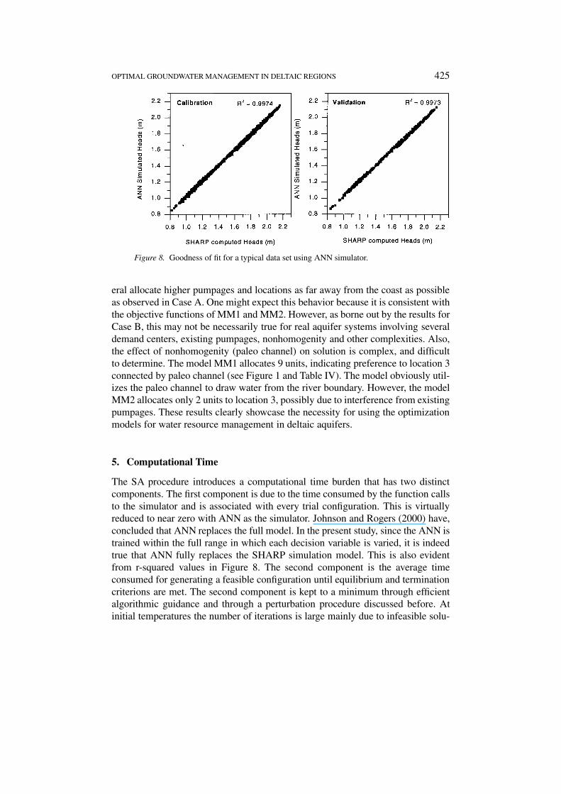
monsoon season. In all, 16 output values: freshwater heads at all 10 locations,interface depth for coastal nodes adjacent to sea i.e., last 5 locations and onevalue of seawater intruded volume for each configuration, were considered. Dueto memory constraints, the 16 output responses of SHARP were trained in threeseparate sets. The first set included head responses at first five locations (1 through5), the second set included head responses for the second 5 locations (6 through10), and the last set included the interface response at last 5 locations (6 through10) and one value for seawater intruded volume, respectively. The interface anddrawdown constraints were relaxed so as to permit decision variables to assume allpossible values within the maximum range listed in Table II. A typical ANN fortraining heads is shown in Figure 7. The training takes about 1 hr, with less than 25epochs. After training, the optimal values of ANN weights and biases connectingthe network were obtained. The goodness of fit for calibration and validation for atypical dataset is shown in Figure 8.

The original SA code with SHARP simulator was modified to include a sub-routine that computes the SHARP responses using ANN weights and biases. Theannealing parameters were set as in previous case. Several trial runs were madewith different random seed numbers to ensure that best solutions were found. Theresults for the near-real aquifer system with same constraints as in Case A wereobtained for models MM1 and MM2 and are listed in Table IV. The models in gen-

OPTIMAL GROUNDWATER MANAGEMENT IN DELTAIC REGIONS 425

Figure 8. Goodness of fit for a typical data set using ANN simulator.

eral allocate higher pumpages and locations as far away from the coast as possibleas observed in Case A. One might expect this behavior because it is consistent withthe objective functions of MM1 and MM2. However, as borne out by the results forCase B, this may not be necessarily true for real aquifer systems involving severaldemand centers, existing pumpages, nonhomogenity and other complexities. Also,the effect of nonhomogenity (paleo channel) on solution is complex, and difficultto determine. The model MM1 allocates 9 units, indicating preference to location 3connected by paleo channel (see Figure 1 and Table IV). The model obviously util-izes the paleo channel to draw water from the river boundary. However, the modelMM2 allocates only 2 units to location 3, possibly due to interference from existingpumpages. These results clearly showcase the necessity for using the optimizationmodels for water resource management in deltaic aquifers.

5. Computational Time

The SA procedure introduces a computational time burden that has two distinctcomponents. The first component is due to the time consumed by the function callsto the simulator and is associated with every trial configuration. This is virtuallyreduced to near zero with ANN as the simulator. Johnson and Rogers (2000) have,concluded that ANN replaces the full model. In the present study, since the ANN istrained within the full range in which each decision variable is varied, it is indeedtrue that ANN fully replaces the SHARP simulation model. This is also evidentfrom r-squared values in Figure 8. The second component is the average timeconsumed for generating a feasible configuration until equilibrium and terminationcriterions are met. The second component is kept to a minimum through efficientalgorithmic guidance and through a perturbation procedure discussed before. Atinitial temperatures the number of iterations is large mainly due to infeasible solu-

426 S. V. N. RAO ET AL.

Table IV. Optimal solution for locations and pumpages:Case B

Location MM1 model MM2 model

(See Figure 1) (Target = 25 units)

1 8 10

2 10 10

3 9 2

4 7 –

5 5 2

6 – –

7 – –

8 – 1

9 – –

10 – –

O.F.a 39 unitsb 380217100 m3c

a Objective function value.b One unit = 105 m3.c Seawater intruded volume.

tions. At final temperatures the rejected uphill moves are too many. The total CPUtime is determined by sum of the two components multiplied by the total number ofiterations or chains. The total number of iterations is problem specific and thereforedetermined only after actual model run.

The total CPU time on a microcomputer for models MM1 and MM2 were 15and 110 min, respectively. The MM2 has an additional constraint to meet a targetdemand leading to more number of infeasible guesses. Further the interference ofexisting pumpages add to the number of infeasible guesses and hence more timefor MM2. Although the time consumed by the ANN simulator is reduced to nearzero, the computational burden arising from SA procedure involving equilibriumand termination criteria, cannot be reduced. Also an increase in areal extent ofdelta does not increase the computational burden with ANN as the simulator. Theburden however, comes from the increase in the number of decision variables andthe constraints that are implied to large delta systems.

6. Summary and Conclusions

The study presented here deals with management of groundwater in delta sys-tems in general with some reference to Indian deltaic conditions. The manage-ment objective is to meet the demand (supplement surface sources) during thenon-monsoon season through pumping from a system of co-operative wells, withleast amount of seawater intrusion. The methodology uses simulated annealing

OPTIMAL GROUNDWATER MANAGEMENT IN DELTAIC REGIONS 427

algorithm and a sharp interface flow model within a simulation-optimisation frame-work. The computational burden is managed within practical timeframes for near-real aquifer systems by replacing the SHARP simulator with ANN model andthrough efficient algorithmic guidance.

The methodology is limited by the assumptions inherent to sharp interfacemodel besides the hypothetical data sets used to illustrate the methodology. Nev-ertheless, the model provides near optimal solutions of practical importance. Themodel takes about a couple of hours of CPU time on a microcomputer for thenear-real hypothetical cases presented here. However, for real world problems thenumber of co-operative wells could be much higher besides other complexities,leading to greater computational burden. While the proposed methodology is notlimited by the areal extent of real delta systems due to ANN replacing the simulator,the restriction comes in terms of the number of decision variables and constraintsimplied in these large aquifer systems. Such problems could to be solved usingparallel-simulated annealing techniques.

Acknowledgements

The authors are grateful to Dr K.S. Ramasastri, Director, National Institute of Hy-drology, Roorkee, India for the support and encouragement to publish this work.The authors are thankful to the anonymous reviewers for their useful suggestionsin improving the paper. The authors are also thankful to Sri D. M. Rangan, at NIHKakinada (AP) for the neat figures and tables.

References

Aly, A. H. and Peralta, R. C.: 1999, ‘Optimal design of aquifer cleanup systems using a neuralnetwork and a genetic algorithm’, J. WRR 35(8), 2523–2532.

ASCE, Task Committee on Application of Artificial neural networks in Hydrology: 2000, ‘Arti-ficial Neural Networks in Hydrology. I: Preliminary Concepts’. II: Hydrologic Applications’,by the ASCE task committee on application of artificial neural networks in Hydrology, underchairmanship of Prof. Rao S. Govindraju Jr. of Hydrologic Engineering, ASCE 5(2), 115–137.

Bear J. and Dagan, G.: 1964, ‘Moving interface in coastal aquifers’. J. Hydraul., ASCE HY-4, 193–216.

Bear, Jacob and Maulem, Y.: 1974. ‘The shape of the interface in steady flow in a stratified aquifer’,Water Resour. Res. 10(6), 1207–1215.

Cunha, M. D. C.: 1999, ‘On solving aquifer management problems with simulated annealingalgorithms’, J. Water Res. Manage. 13, 153–169.

Cheng, A. H.-D., Halhal, D., Naji, A. and Ouazar, D.: 2000, ‘Pumping optimisation in saltwater-intruded coastal aquifers’, WRR 36(8), 2155–2165.

Das, A. and Datta, B.: 1999a, ‘Development of multi objective management models for coastalaquifers’, J. Irrigat. Drain., ASCE 125(3), 112–121.

Das, A. and Datta, B.: 1999b, ‘Development of management models for sustainable use of coastalaquifers’, J. WRPM ASCE 125(2), 76–87.

Dougherty, D. E. and Maryott, R. A.: 1991, ‘Optimal groundwater management. 1. Simulatedannealing’, Water Resour. Res. 27(10), 2493–2508.

428 S. V. N. RAO ET AL.

Emch, P. G. and Yeh, W. G.: 1998, ‘Management model for conjunctive use of coastal surface waterand groundwater’, J. WRPM ASCE 124(3), 129–139.

Essaid, H. I.: 1990, ‘A multilayered sharp interface model of coupled freshwater and saltwater flowin coastal systems: Model development and application’, Water Resour. Res. 26(7), 1431–1454.

Gorelick, S. M.: 1983, ‘A review of distributed parameter groundwater management modelingmethods’, Water Resour. Res. 19(2), 305–319.

Goldberg, David E.: 1989, Genetic Algorithms in Search Optimization and Machine Learning,Addison Wesley Longman Inc., Mexico City, p. 3.

Huyakorn, P. S., Anderson, P. F., Mercer, J. W. and White Jr., W. O.: 1987, ‘Saltwater intrusionin aquifers. Development and testing of a three dimensional finite-element model’, WRR 23(2),293–312.

Hallaji, K. and Yazicigil, H.: 1996, ‘Optimal management of a coastal aquifer in southern Turkey’,J. Water Res. Plann. Manage. ASCE 122(4), 233–244.

Johnson, V. M. and Rogers, L. L.: 2000, ‘Accuracy of neural network approximators in simulation-optimization’, J. Water Res. Plann. Manage. ASCE 126(2), 48–56.

Kirkpatrick, S., Gelatt Jr., C. D. and Vecchi, M. P.: 1983, ‘Optimization by simulated annealing’,Science 220(4598), 671–680.

MATLAB: 2000, Neural Network Tool Box for use with Matlab, User Guide. Ver. 4. The Mathwork,Inc. 3, Apple Hill Drive, MA, U.S.A.

Metropolis, N., Rosenbluth, A. W. and Teller, A. H.: 1953, ‘Equation of state calculations by fastcomputing machines’, J. Chem. Phys. 21(6), 1087–1092.

Shamir, U. and Dagan, G.: 1971, ‘Motion of seawater interface in coastal aquifer-a numericalsolution’, WRR 12, 644–657.

Voss, C. I.: 1984 ‘SUTRA: Saturated Unsaturated Transport – A Finite Element Simulation Model forSaturated and Unsaturated Fluid-density-dependent Ground Water Flow with Energy Transportor Chemically Reactive Single Species Solute Transport’, USGS Water Res. Invest. Rep. 84-4369.

Wilson, J. L. and Sa Da Costa, A.: 1982, ‘Finite element simulation of a saltwater/freshwater interfacewith indirect toe tracking’, Water Resour. Res. 8(4), 1069–1080.

Wang, M. and Zheng, M.: 1998, ‘Groundwater management optimization using genetic algorithmsand simulated annealing: Formulation and comparison’, J. Amer. Water Res. Assoc. 34(3), 519–530.

Willis, R. and Finney, W. A.: 1988, ‘Planning model for optimal control of saltwater intrusion’, J.Water Res. Plann. Manage. ASCE 114(2), 163–177.