arX

iv:h

ep-p

h/96

0546

5v2

2 J

ul 1

996

Theoretical Physics Institute

University of Minnesota

TPI-MINN-96/05-TUMN-TH-1426-96CERN-TH/96-113

hep-ph/9605465

Operator Product Expansion, Heavy Quarks,QCD Duality and its Violations

Boris Chibisov, R. David Dikeman, M. Shifman

Theoretical Physics Institute, Univ. of Minnesota, Minneapolis, MN 55455

and

N.G. Uraltsev

TH Division, CERN, CH 1211 Geneva 23, Switzerlandand

St.Petersburg Nuclear Physics Institute, Gatchina, St.Petersburg 188350, Russia

Abstract

The quark (gluon)-hadron duality constitutes a basis for the theoreticaltreatment of a wide range of inclusive processes – from hadronic τ decays andRe+e− , to semileptonic and nonleptonic decay rates of heavy flavor hadrons.A theoretical analysis of these processes is carried out by using the operatorproduct expansion (OPE) in the Euclidean domain, with subsequent analyticcontinuation to the Minkowski domain. We formulate the notion of the quark(gluon)-hadron duality in quantitative terms, then classify various contribu-tions leading to violations of duality. A prominent role in the violations ofduality seems to belong to the so called exponential terms which, conceptually,may represent the (truncated) tail of the power series. A qualitative model,relying on an instanton background field, is developed, allowing one to get anestimate of the exponential terms. We then discuss a number of applications,mostly from heavy quark physics.

CERN-TH/96-113April 1996

1 Introduction

Nonperturbative effects have been analyzed in QCD in the framework of the operatorproduct expansion (OPE) [1, 2] since the inception of QCD. Recently a remarkableprogress has been achieved along these lines in the heavy quark theory (for reviewssee Ref. [3]). A large number of applications of OPE in heavy quark theory referto quantities of the essentially Minkowski nature, e.g. calculations of the inclusivedecay widths, spectra and so on. Wilson’s operator product expansion per se isformulated in the Euclidean domain. The expansion built in the Euclidean domainand by necessity truncated, is translated in the language of the observables throughan analytic continuation. An indispensable element of this procedure, the so calledquark-hadron duality, is always assumed, most often tacitly. This paper is devotedto the discussion of quark-hadron duality and deviations from it. Although the issuewill be considered primarily in the context of heavy quark theory, the problems wewill deal with are quite general and are by no means confined to heavy quark theory.For instance, determination of αs from the hadronic width of τ – a problem ofparamount importance now under intense scrutiny [4] – falls into this category. It isknown [5] that deviations from duality may be conceptually related to the behaviorof the operators of high dimension in OPE. Unfortunately, very little is knownabout this behavior in the quantitative sense, beyond the fact that the expansion isasymptotic [5]. Therefore we are forced to approach the problem from the other side– engineering a model which allows us to start discussing deviations from duality.The model is based on instantons, but by no means is derivable in QCD. Moreover, itdoes not exhaust all mechanisms which might lead, in principle, to deviations fromduality, focusing, rather, on one specific contribution – the so called exponentialterms. Nevertheless, it seems to be physically motivated and can serve for qualitativeanalysis at present, and as a guideline for future refinements.

Indeed, the (fixed size) instanton contribution to correlation functions with largemomentum transfers can be interpreted as a mechanism in which the large externalmomentum is transmitted through a soft coherent field configuration. Speakinggraphically, the large external momentum is shared by a very large number of quantaso that each quantum is still relatively soft. It is clear that this mechanism is notrepresented in the practical version of OPE [2], and, thus, gives an idea of howstrong deviations from duality might be.

One of the most interesting aspects revealed in this model is the distinct natureof exponential contributions absent in practical OPE, both in the Euclidean and theMinkowski domains. If in the former the exponential effects die off fast enough, inthe latter, deviations from duality are suppressed to a lesser extent – the exponentialfall off is milder, and it is modulated by oscillations. These features seem to be sogeneral that most certainly they will survive in future treatments which, hopefully,will be significantly closer to fundamental QCD than our present consideration.

If one accepts this model, at least for orientation, many interesting technicalproblems arise. Instanton contributions in heavy quark theory were previously dis-

1

cussed more than once [6, 7]. Although the corresponding analysis seemed ratherstraightforward at first sight, it resulted in some apparent paradoxes; for instance,the instanton contribution to the spectrum of the inclusive heavy quark decaysseemingly turned out to be parametrically larger than the very same contributionto the total decay rate [7, 8]. The puzzle is readily solvable, however: one observesthat the problem lies in the separation of the exponentially small terms from the“background” of the power terms of OPE; this is a subtle and, generally speaking,ambiguous procedure, particularly in the Minkowski domain, and depends on thespecific quantity under consideration. We will dwell on this issue at length in thepresent paper.

We begin, however, with a brief formulation of the very notion of duality (Sect.2). Quantifying this notion is an important task by itself. In modeling deviationsfrom duality, the adoption of the following attitude is made so as to stay on safeground: we will try to develop a model yielding a conservative estimate on the upperbound for deviations from duality. In other words, given the prediction for this orthat quantity based on duality (i.e. spectra, total inclusive widths and so on), oneestablishes the accuracy with which this prediction is expected to be valid. In thisway one sets the lower limit on the energy release needed to achieve the requiredaccuracy. For this limited purpose even a crude model, such as the instanton modelto be discussed below, may be sufficient, perhaps, after some minor refinements.

Why is this attitude logical? If we knew in detail some specific mechanismomitted in the theoretical calculations – whether associated with the truncationof practical OPE, or due to other sources – we could include it in the theoreticalprediction for the cross sections and say that the actual hadronic cross section isdual to this new improved prediction. Thus, paradoxically, the very nature of dualityimplies that deviations from it are always estimated roughly. Analyzing deviationsfrom duality at each given stage of development of QCD is equivalent to analyzingour ignorance, rather than our knowledge. At the present stage, as was alreadymentioned, our knowledge is, more or less, limited to practical OPE.

A much more ambitious goal is developing a framework suitable for actual cal-culation of extra contributions not seen in practical OPE. Although the instantonmodel is sometimes used for this purpose as well, one should clearly realize thatquantitatively reliable results are not expected to emerge in this way. This is aspeculative procedure intended only for qualitative orientation. We will occasion-ally resort to it only due to the absence of better ideas. One may hope that auniversal qualitative picture will be revealed en route, which will be robust enoughto survive future developments of the issue.

Although this problem – estimates of deviations from duality – is obviously ofparamount practical importance, surprisingly little has been said about this subjectin the literature. Apart from some general remarks presented in Ref. [5], an attemptto discuss the issue in a different (exclusive) context was made in [9].

Our paper is organized below as follows: In Sect. 2 we outline the generalprinciples behind duality and its violation. Sect. 3 is devoted to general features of

2

the exponential terms believed to be responsible for duality violation. In particular,the distinction between their patterns in the Euclidean and Minkowski domains isexplained here. In Sect. 4 we outline the instanton model we use as a framework togenerate exponential terms. Sect. 5 illustrates our main points in what is, probably,the most transparent example: e+e− annihilation and the hadronic decays of theτ lepton. In Sect. 6 we discuss the general features of heavy quark decays in theinstanton background. In Sect. 7, we begin the business of actual calculation – towarm up, we consider a toy model where the spins of all relevant fields are discardedto avoid technicalities. Section 8 is devoted to actual heavy quark decays in QCD.The exponential contributions are estimated, both in the spectra, and in the inclusivedecay rates, for the transitions of the heavy quark into a massless one. In section 9 weaddress the applied, but practically important, problem of deviations from dualityin the semileptonic decays of D and B mesons. There are good phenomenologicalreasons to believe that in D decays these deviations are significant, of order 0.5.Adjusting parameters of the model in such a way as to explain these deviations, weconclude that deviations from duality in the B decays are expected to be negligiblysmall (in the total semileptonic decay rate and in the similar radiative processes).The effect seems to be larger – perhaps even detectable – in the inclusive nonleptonicrates. The drawbacks and deficiencies of the model we use for the estimates of theexponential terms are summarized in Sect. 10. We present some comments onthe vast literature treating the processes under discussion in Sect. 11. Section 12summarizes our results and outlines problems for future exploration.

2 Duality and the OPE

Wilson’s OPE is the basis of virtually all calculations of nonperturbative effects inanalytical QCD. Since the very definition of duality relies heavily on Wilson’s OPE,we first briefly review its main elements. For the sake of definiteness, we will speakof the heavy quark expansion, although one should keep in mind that the procedureis quite general; in other processes (e.g. the hadronic τ decays) the wording mustbe somewhat changed, but the essence remains intact.

The original QCD Lagrangian is formulated at very short distances. Startingfrom this Lagrangian, one evolves it down, integrating out all fluctuations withfrequencies µ < ω < M0 where M0 is the original normalization point, and µ willbe treated, for the time being, as a current parameter. In this way we get theLagrangian which has the form

L =∑

n

Cn(M0;µ)On(µ) . (1)

The coefficient functions, Cn, represent the contribution of virtual momenta fromµ to M0. The operators, On, enjoy the full rights of Heisenberg operators withrespect to all field fluctuations with frequencies less than µ. The sum in Eq. (1) isinfinite – it runs over all possible Lorentz singlet gauge invariant operators which

3

possess the appropriate quantum numbers. The operators can be ordered accordingto their dimension; moreover, we can use the equations of motion, stemming fromthe original QCD Lagrangian, to get rid of some of the operators in the sum. Thoseoperators that are reducible to full derivatives give vanishing contributions to thephysical (on mass shell) matrix elements, and can thus be discarded as well.

Speaking abstractly, one is free to take any value of µ in Eq. (1); in particular,µ = 0 would mean that everything is calculated and we have the full S matrix, allconceivable amplitudes, at our disposal. Nothing is left to be done. In this caseEq. (1) is just a sum of all possible amplitudes. This sum then must be writtenin terms of physical hadronic states, of course, not in terms of the quark and gluonoperators since the latter degrees of freedom simply do not survive scales below someµhad ∼ ΛQCD.

Needless to say, present-day QCD does not allow the explicit evolution down toµ = 0. Calculating the coefficient functions we have to stop somewhere, at suchvirtualities that the quark and gluon degrees of freedom are still relevant, and thecoefficient functions Cn(M0, µ) are still explicitly calculable. On the other hand, forobvious reasons, it is highly desirable to have µ as low as possible. In the heavyquark theory there is an additional requirement that µ must be much less than mQ.

Let us assume that µ is large enough so that αs(µ)/π ≪ 1 on the one hand, andsmall enough so that there is no large gap between ΛQCD and µ. The possibilityto make such a choice of µ could not be anticipated a priori and is an extremelyfortunate feature of QCD. Quarks and gluons with offshellness larger than µ chosenin this way will be referred to as hard.

All observable amplitudes must be µ independent, of course. The µ dependenceof the coefficient functions Cn must conspire with that of the matrix elements ofthe operators On in such a way as to ensure this µ independence of the physicalamplitudes.

What can be said about the calculation of the coefficients Cn? Since µ is suffi-ciently large, the main contribution comes from perturbation theory. We just drawall relevant Feynman graphs and calculate them, generating an expansion in αs(µ)

Cn =∑

l

alαls(µ) . (2)

(Sometimes some graphs will contain not only the powers of αs(µ) but also powersof αs ln(mQ/µ). This happens if the anomalous dimension of the operator On isnonvanishing, or if a part of a contribution to Cn comes from characteristic momentaof order mQ and is, thus, expressible in terms of αs(mQ), and we rewrite it in termsof αs(µ).)

As a matter of fact expression (2) is not quite accurate theoretically. One shouldnot forget that, in doing the loop integrations in Cn, we must discard the domainof virtual momenta below µ, by definition of Cn(µ). Subtracting this domain fromthe perturbative loop integrals, we introduce in Cn power corrections of the type(µ/mQ)n by hand. In principle, one should recognize the existence of such corrections

4

and deal with them. The fact that they are actually present was realized long ago [2].Neglecting them, at the theoretical level, results in countless paradoxes which stillsurface from time to time in the literature. If it is possible to choose µ sufficientlysmall, these corrections may be insignificant numerically, and can be omitted. Thisis what is actually done in practice. This is one of the elements of a simplification ofthe Wilson operator product expansion. The simplified version is called the practicalversion of the OPE, or practical OPE [2].

Even if perturbation theory may dominate the coefficient functions, they stillalso contain nonperturbative terms coming from short distances. Sometimes theyare referred to as noncondensate nonperturbative terms. An example is providedby direct instantons [10], with sizes of order m−1

Q . These contributions fall off ashigh powers of ΛQCD/mQ (or ΛQCD/E where E is a characteristic energy release inthe process under consideration), and are very poorly controlled theoretically. Sincethe fall off of the noncondensate nonperturbative corrections is extremely steep,basically the only thing we can say about them is that there is a critical value ofmQ (or E). For lower values of mQ (or E) no reliable theoretical predictions arepossible at present. For higher values of mQ one can ignore the noncondensatenonperturbative contributions. The noncondensate nonperturbative contributionsare neglected in the practical OPE. In what follows, we will not touch upon thesetype of effects which are associated with the (small-size) instanton contributionsto the coefficient functions. There is another, technical, reason why we choosenot to consider these effects. Since the small-size instantons represent hard fieldfluctuations, all heavy quark expansions carried out in the spirit of HQET [11]become invalid; the corresponding theory has to be developed anew. In particular,the standard HQET decomposition of the heavy quark field in the form Q(x) =exp{imQvµxµ}Q(x) becomes inapplicable, as well as the statement that all heavyquark spin effects are suppressed by 1/mQ, and so on. This circumstance is not fullyrecognized in the literature. Due to these reasons, we instead focus on effects dueto large-size instantons. This will provide a workable framework for visualizing theexponential term.

At very large mQ (or E), the exponential terms are parametrically smaller (in theEuclidean domain) than the power-like non-condensate nonperturbative correctionsin the coefficient functions. One can argue, however, that this natural hierarchysets in at such large values of momentum transfer where both effects are practicallyunimportant. At intermediate values of the momentum transfers – most interestingfrom the point of view of applications – an inverse hierarchy may take place, wherethe exponential terms are numerically more important.

Ignoring the nonperturbative contributions in the coefficient functions is not theonly simplification in the practical OPE. The series of operators appearing in L(the condensate series) is infinite. Practically we truncate it in some finite order, sothat the sum in the expansion we deal with approximates the exact result, but byno means coincides with it. The truncation of the expansion is a key point. Thecondensate expansion is asymptotic [5]. Therefore, expanding it to higher orders

5

indefinitely does not mean that the accuracy of the approximation to the exactresult becomes better. On the contrary, as in any asymptotic series, there exists anoptimal order. Truncating the series at this order, we get the best accuracy. Thedifference between the exact result and the series truncated at the optimal order isexponential. Large-size instantons, treated in an appropriate way will, in a sense,represent the high-order tail omitted in the truncated series.

The essence of the phenomenon – occurrence of the exponential terms – is similarto the emergence of the condensates at a previous stage. Indeed, let us consider, first,the standard Feynman perturbation theory. At any finite order the perturbativecontribution is well-defined. At the same time, the coefficients of the αs series growfactorially with n, and this means that the αs series must be, somehow, cut off, i.e.regularized. The proper way of handling this factorial divergence is by introducingthe normalization point µ and the condensate corrections which tempers the factorialdivergence of the Feynman perturbative series in high orders and, simultaneously,bring in terms of order exp (−C/αs(mQ)) where C is some positive constant. Looselyspeaking, one may say that contributions of this type are related to the high-ordertails of the αs series. Similarly, the high-order tails of the condensate (power) seriescorrespond to the occurrence of the exponential terms. Correspondingly, the OPE,even optimally truncated, approximates the exact result up to exponential terms.

The exponential terms not seen in the practical OPE appear both in Euclidean,and Minkowski quantities. Their particular roles and behaviors are quite different,however. Technically, the rate of fall off is much faster in the Euclidean domainthan in the Minkowski domain, as we will see later. Conceptually, the exponentialterms in the Minkowski domain determine deviations from duality.

Let us now describe what we mean by duality in somewhat more detail. Assumethat the effective Lagrangian we work with includes external sources, so that theexpectation value of this Lagrangian actually yields the complete set of physicalamplitudes. The physically observable Minkowski quantities (i.e. spectra, totalhadronic widths and so on) are given by the imaginary parts of certain terms in theeffective Lagrangian. These terms are calculated as an expansion in the Euclideandomain. This is a practical necessity – since our theoretical tools are based onthe expansions phrased in terms of quarks and gluons, we have to operate in theEuclidean domain. We then analytically continue in relevant momentum transfers tothe Minkowski domain. Of course, if we could find the exact result in the Euclideandomain, its analytic continuation to the Minkowski domain would yield the exactspectra, etc., – there would be no need in introducing duality at all. In reality,the calculation is done using the practical OPE. Both, the perturbative series inthe coefficient functions and the condensate series are truncated at a certain order.We then analytically continue each individual term in the expansion thus obtained,term by term, from the deep Euclidean domain to the Minkowski one, and take theimaginary part. The corresponding prediction, which can be interpreted in termsof quarks and gluons, is declared to be dual to physically measurable quantities interms of hadrons provided that the energy release is large. In this context dual means

6

approximately equal. The discrepancy between the exact (hadronic) result and thequark-gluon prediction based on the practical OPE is referred to as a deviation from(local) duality.

Reiterating, in defining duality, we first do a straightforward analytical continu-ation, term by term. Defining the analytic continuation to the Minkowski domainin this way, it is not difficult to see, diagrammatically, that those lines which werefar off shell in the Euclidean calculation remain hard in the sense that now they areeither still far off shell, or on shell, but carry large components of the four-momenta,scaling like mQ, or large energy release. The sum of the imaginary parts obtainedin this way is the so called the quark-gluon cross section. This quantity serves asa reference quantity in formulating the duality relations. When one says that thehadron cross section is dual to the quark-gluon one, the latter must be calculatedby virtue of the procedure described above.

The contributions left aside in the above procedure are related, at least at aconceptual level, to the high-order tail of the power (condensate) series. They can bevisualized with large-size instantons. A subtle point is that the large-size instantonscontribute not only to the exponential terms, but also to the condensate (power)expansion. Our task is to single out the exponential contribution, since we have nointention to use the instanton model to imitate the low-order terms of the powerexpansion. Our instanton model is far too crude for that. In the next sectionwe proceed to formulating the instanton model, making special emphasis on thisparticular element – isolating exponential contributions.

Beyond the simplest one-variable problems, like the correlation function of twovector currents related to Re+e− or Rτ , very often one encounters a more complicatedsituation when the amplitudes have several separated kinematical cuts associatedwith physically different channels of the given amplitude, and one is interested onlyin one specific channel. This situation is typical for the inclusive heavy quark decays[12, 13]. The OPE-based predictions in this case require – additionally – a differenttype of duality: one needs to assume that a particular cut of interest in the hadronicamplitude is in one-to-one correspondence with the given quark-gluon cut. In otherwords, it is assumed that different channels (in terms of the hadronic processes andin terms of the quark-gluon processes) do not contaminate each other [13]. This wascalled “global duality” 1. In the practical OPE the cuts of the perturbative coefficientfunctions carry clear identity, and the above assumption of “global duality” is easilyimplementable. The above assumption can actually be proven in the frameworkof the practical OPE at any finite order, as was shown in [13]. However, mostprobably, this “global duality” fails at the level of the exponential terms. In thepresent paper we do not address the issue of “global duality” violations althoughinstantons can model this phenomenon as well. Such effects are probably smallerthan the deviations from local duality; in any case they deserve a dedicated analysis.It is worth noting that for one-variable problems (e.g. the total e+e− annihilation

1 Warning: the term global duality is often used in the literature in a different context.

7

cross section), duality for various integrals over the cross section over a finite energyrange is still local duality, as will be discussed in Sect. 5.

3 Abstracting General Aspects

Before submerging into details of the instanton calculations, we outline the practicalmotivation for inclusion of the corresponding effects from the general perspective ofthe short distance expansion. It will also enable us to illustrate in a simple waythe divergence of the power expansion. Consider a generic two-point correlationfunction Π(Q2), say, the polarization operator for vector currents:

Π(Q) =∫

d4x eiqxΠ(x) = −∫

d4x eiqx 〈G(x, 0)G(0, x) 〉0 (3)

where G are the quark Green functions in an external gauge field and averaging overthe field configurations is implied; we do not explicitly show the Lorentz indices.Equation (3), and all considerations in this section, refer to Euclidean space.

The power expansion of Π(Q) in 1/Q is the expansion of the correlation functionΠ(x) in singularities near the origin. (This statement is not quite accurate in theWilson’s OPE; it is correct, however, in the practical OPE). Thus, one is interestedin the small-x behavior of Π(x) or, equivalently, of G(x). In the leading, deep Eu-clidean approximation, Green’s functions are the free ones, xγ/x4, plus perturbativecorrections arranged in powers of αs(1/x

2):

Gpt(x) =1

2π2

xγ

x4

(

1 + a1αs(1/x2) + ...

)

; xγ = xµγµ (4)

(a particular invariant gauge is assumed here; the correlator is gauge-invariant any-way, and similar series can be written directly for the product of the two Greenfunctions). All terms in the perturbative expansion (4) have the same power ofx, and differ only by powers of log x2. Logarithms emerge due to the singularity1/x2 of the gluon interaction near x2 = 0. Upon making the Fourier transform, theperturbative corrections in Eq. (4) are converted into powers of logQ2.

Power corrections, 1/Qn, emerge from the expansion of Green’s functions nearx = 0: for example, in the Fock–Schwinger gauge

G(x) =1

2π2

xγ

x4+

1

8π2

xα

x2Gαβ(0)γβγ5 + ... (5)

where higher order terms contain higher powers of the gluon field, Gαβ, or its deriva-tives at x = 0 (for a review see [14]). Since the additional terms in the expansioncontain extra powers of x (generically accompanied by log x2), it is clear that, re-turning to the momentum representation, one gets additional powers of Q in thedenominator for extra powers of x in the expansion of Π(x). (The positive powersof x in Π(x) are accompanied by log x2.) Thus, the 1/Q expansion obtained in the

8

practical OPE is in one-to-one correspondence, in the coordinate space, with theexpansion of Green’s function near the point x = 0. (This fact is absolutely explicitin ordinary quantum mechanics, where the dynamics are described by a potential.In QCD the power corrections to the inclusive heavy quark decay rates, for exam-ple, have a similar interpretation: the leading 1/mQ correction, due to the Coulombpotential at the position of the heavy quark, is absent because of a cancellationbetween the initial binding energy and the similar charge interaction with the de-cay products in the final state. Physically, the reason is conservation of color flow.Moreover, the chromomagnetic term is determined by the magnetic interaction atthe origin, and so on.)

The question that naturally comes to one’s mind is whether the above expansionin the x space is, in a sense, convergent. At best, it can have a finite radius ofconvergence which, for the given external field, is determined by the distance tothe closest (apart from the origin) singularity in the complex x2 plane. On theother hand, evaluating the Fourier transform (3) converting Π(x) into Π(Q), oneperforms the integration over all x. Therefore, even for arbitrarily large Q, onehas to integrate Π(x) in the region where the expansion of the Green’s functions isdivergent. Although any particular power term 1/Qn can be calculated and is finite,this leads to the factorial growth of the coefficients in the 1/Q expansion, and thusexplains its asymptotic nature.

Let us illustrate this purely mathematical fact in a simplified setting. Let usconsider the “OPE expansion” of a modified Fourier transform (the one-dimensionalintegral runs from zero to infinity; such transforms are relevant in heavy quarktheory, see [5]):

f(Q) =∫ ∞

0dx

1

x2 + ρ2eiQx =

=π

2ρe−Qρ +

1

2ρ[e−QρEi(Qρ) − eQρEi(−Qρ)] , (6)

where Ei is the exponential-integral function. The integrand has a singularity in thecomplex plane, at x = ±iρ and is perfectly expandable at x = 0. Expanding the“propagator”, 1/(x2 + ρ2), in x2 we get the “OPE series”

f(Q) =∫ ∞

0dx

∞∑

k=0

(−1)k x2k

ρ2k+2eiQx =

i

ρ

∞∑

k=0

(2k)!

(Qρ)2k+1. (7)

First of all note, that the “OPE series” has only odd powers of 1/Q. Comparing withthe exact expression (6) we see that the function f(Q) is not fully represented byits expansion (7), which is obviously asymptotic. The exponential term is missing.This exponential term comes from the finite-distance singularities of the integrand.Indeed, one can deform the contour of integration over x into the complex plane; theintegral remains the same as long as the integration contour does not wind aroundthe singularity at x = ±iρ, whose contribution is

δf(Q) =π

ρe−Qρ . (8)

9

This is precisely the uncertainty in defining the value of the asymptotic 1/Q series(7).

Since f(Q) is expanded only in odd powers of 1/Q, the symmetric combinationg(Q) = f(Q) + f(−Q) has no power expansion at all. The function g(Q) does notvanish, however:

g(Q) = f(Q) + f(−Q) =∫ ∞

−∞dx

1

x2 + ρ2eiQx = π

e−Qρ

ρ. (9)

This expression is in agreement with the above estimate of the uncertainty of thepower expansion per se and demonstrates that the exponential terms are present.

The appearance of the terms exponential in Q in the example above bears someresemblance to the renormalon issue – the factorial growth of the coefficients inthe perturbative expansions in QCD [15]. The Feynman graphs contain integrationover all gluon momenta k2; on the other hand, the expansion of αs(k

2) in termsof αs(Q

2) is convergent only for k2 between some minimal and maximal scales,Λ2

QCD<∼ k2 <∼ Q4/Λ2

QCD. Although each particular term in the expansion can beintegrated from k2 = 0 to ∞, yielding a finite number, the problem of divergence ofthe original expansion of αs(k

2) is resurrected as the factorial growth of the resultingcoefficients.

We conclude, therefore, that the divergence of the power expansion within thepractical OPE, and the presence of the exponential terms is a rather general phe-nomenon, and is related, conceptually, to the singularities of Green’s functions inthe coordinate space at complex Euclidean values of x2 located at finite distancesfrom the origin. The question of the possible role of these finite distance singularitieswas first raised in Refs. [16, 17] (see also [18]).

The analogy with renormalons in the αs perturbative expansions can be contin-ued. In the renormalon problem, the proper inclusion of the condensates, within theframework of the OPE, eliminates the infrared renormalons altogether and makesthe infrared-related perturbative series well defined and, presumably, convergent.One may hope that a consistent explicit account for the finite-x2 singularities wouldalso make the infinite power series well defined. From the theoretical perspective,though, this problem has not been investigated so far.

Addressing practical applications, there are two general reasons to expect thatthe inclusion of the exponential terms in the analysis can be important – even thoughthe power series analysis accounts, at best, for only a few leading terms in the1/Q expansion. First, there exists some phenomenological evidence, to be discussedbelow, indicating that the impact of the exponential terms in the Minkowski domainmay be more important numerically than that of the omitted condensate terms forintermediate values of the momentum transfers. This statement is illustrated by theτ example, see Sect. 5. Second, historically, this is not the first case where we haveencountered such a perverted hierarchy in QCD. It is quite typical that in the QCDsum rules, the contribution of the (omitted) higher order αs terms, which formallydominate over the condensates, is far less significant numerically than that of the

10

condensates. This point is crucial – while the exponential terms die out fast in theEuclidean domain, they decrease much more slowly in the physical cross sectionsand, thus, often dominate over the condensate effects, the more so that the latteroften are concentrated at the end points, and are not seen at all outside the end pointregion. This observation was emphasized in Ref. [17]. Indeed, the terms ∼ e −Qρ

oscillate, rather than decrease, when analytically continued from the Euclidean tothe Minkowski domain, Q→ iE.

Leaving aside such subtle theoretical questions as the summation of the infinitecondensate series, one may hope that including the principal singularities at theorigin and at finite x2 will lead to a description of the correlation functions at handwhich is good numerically. Indeed, the leading singularity at x2 = 0 is given by theperturbative expansion, and subleading terms near x2 = 0 are given by the practicalOPE. Adding the dominant singularity at x2 ∼ Λ−2

QCD in the complex plane wecapture enough information to describe the main properties of the function, andthus provide a suitable approximation to the exact result, which may work wellenough for a wide range of x2, thus yielding the proper behavior of the correlationfunction, Π(Q), down to low enough Q2. One should clearly realize, however, thatthis procedure is justified only if we do not raise the subtle question formulatedabove and keep just a few of the first terms in both the perturbative and condensateexpansions. Summing more and more condensate terms within this – rather eclectic– procedure may not only stop improving the accuracy, but even lead to double-counting of certain field configurations. Being fully aware of all deficiencies of thisapproach at present, we still accept it for estimating possible violations of localduality in a few cases of practical interest. Eventually, this approach may developinto a systematic, and self-consistent phenomenology of the exponential terms, muchin the same way as the QCD sum rules represent a systematic phenomenology ofthe condensate terms.

Technically, Green’s functions are obtained by solving the equations of motion inthe given background gauge field; in particular, quark Green’s functions are obtainedby solving the Dirac equation. Henceforth, the singularities outside the origin emergeonly at such (complex) values of x2 = 0 where the gauge field is singular. Instantonsprovide an explicit example of such fields which are, of course, regular at real x2,but have a singularity in the complex x2 plane 2. The singularities of the instantonfields are passed to the Green’s functions, e.g. the singular terms in the spin-0 andspin-1/2 Green’s function have the structure

Gs(x, y) ∼1

((x− z)2 + ρ2)1/2,

1

((y − z)2 + ρ2)1/2,

Gf(x, y) ∼1

((x− z)2 + ρ2)ℓ ,1

((y − z)2 + ρ2)ℓ , ℓ =1

2,3

2, (10)

where z is the center of the instanton, and ρ is its radius. The actual nature ofthe singularity changes when one integrates over the position of the instanton, and

2The gauge potential itself may have singularities at real x2, but these are purely gauge artefacts.

11

over its orientation and size. The poles in Π(x) may change into more complicatedsingularities (say, cuts). Interactions of different instantons will also affect the natureof the singularities. One does not expect, however, the finite-distance singularitiesto disappear. The precise position of the singularities, and their nature, depend onthe details of the strong dynamics.

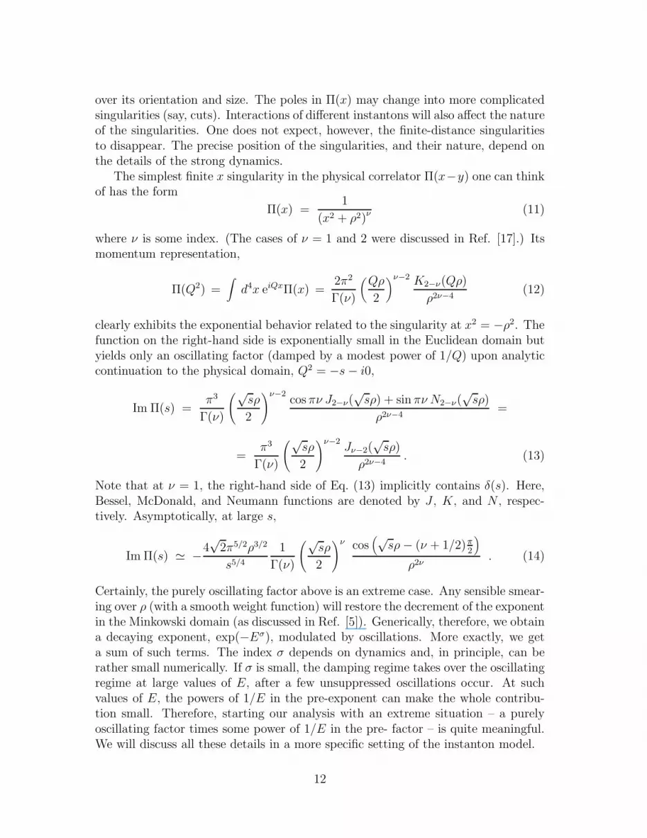
The simplest finite x singularity in the physical correlator Π(x−y) one can thinkof has the form

Π(x) =1

(x2 + ρ2)ν (11)

where ν is some index. (The cases of ν = 1 and 2 were discussed in Ref. [17].) Itsmomentum representation,

Π(Q2) =∫

d4x eiQxΠ(x) =2π2

Γ(ν)

(

Qρ

2

)ν−2 K2−ν(Qρ)

ρ2ν−4(12)

clearly exhibits the exponential behavior related to the singularity at x2 = −ρ2. Thefunction on the right-hand side is exponentially small in the Euclidean domain butyields only an oscillating factor (damped by a modest power of 1/Q) upon analyticcontinuation to the physical domain, Q2 = −s− i0,

Im Π(s) =π3

Γ(ν)

(√sρ

2

)ν−2cosπν J2−ν(

√sρ) + sin πν N2−ν(

√sρ)

ρ2ν−4=

=π3

Γ(ν)

(√sρ

2

)ν−2Jν−2(

√sρ)

ρ2ν−4. (13)

Note that at ν = 1, the right-hand side of Eq. (13) implicitly contains δ(s). Here,Bessel, McDonald, and Neumann functions are denoted by J , K, and N , respec-tively. Asymptotically, at large s,

Im Π(s) ≃ −4√

2π5/2ρ3/2

s5/4

1

Γ(ν)

(√sρ

2

)ν cos(√

sρ− (ν + 1/2)π2

)

ρ2ν. (14)

Certainly, the purely oscillating factor above is an extreme case. Any sensible smear-ing over ρ (with a smooth weight function) will restore the decrement of the exponentin the Minkowski domain (as discussed in Ref. [5]). Generically, therefore, we obtaina decaying exponent, exp(−Eσ), modulated by oscillations. More exactly, we geta sum of such terms. The index σ depends on dynamics and, in principle, can berather small numerically. If σ is small, the damping regime takes over the oscillatingregime at large values of E, after a few unsuppressed oscillations occur. At suchvalues of E, the powers of 1/E in the pre-exponent can make the whole contribu-tion small. Therefore, starting our analysis with an extreme situation – a purelyoscillating factor times some power of 1/E in the pre- factor – is quite meaningful.We will discuss all these details in a more specific setting of the instanton model.

12

It is easy to see that causality requires singularities of Π(x2) to lie either on thenegative real axis of x2, or at larger arguments of x2, on the unphysical sheet; Π(x2)must be analytic at | arg x2| < π. In the instanton model the singularities are onthe negative x2 axis. Smearing the instanton sizes with a smooth function weakensthe strength of the singularity near the purely imaginary

√x2 and thus effectively

moves it further into the complex plane.To summarize, we argued that the violations of local duality are conceptually re-

lated to the divergence of the condensate expansion (practical OPE) in high orders.Technically, they may occur due to the singularities of Green’s functions at complexEuclidean values of x at finite distances from the origin. Accounting for such singu-larities, in addition to the perturbative and the condensate expansion, is a naturalfirst step beyond the framework of the practical OPE. In the next section we willproceed to a specific model for this phenomenon based on instantons. Since theyare not necessarily the dominant vacuum component we try to limit our reliance oninstantons to the absolute minimum. In particular, their topological properties areinessential for us, and even lead to certain superfluous complications.

4 Instanton Model

Here we will formulate our rules of the game. To get an idea of possible violations ofduality we will consider a set of physically interesting processes (two-point functionsof various currents built from light quarks, the transition operators relevant for theinclusive heavy quark decays and so on). Our primary goal is isolating the finite-distance singularities in x2, which will eventually be converted into the exponentialterms in the momentum plane. To this end it will be assumed that the quark Green’sfunctions in the amplitudes under consideration are Green’s functions in the givenone-instanton background. The one-instanton field is selected to represent coherentgluon field fluctuations for technical reasons – in this background Green’s functionsfor the massless quarks are exactly known.

The instanton field depends on the collective coordinates – its center, color spaceorientations, and its radius. Integration over all coordinates except the radius istrivial, and will be done automatically. Integration over the instanton radius ρrequires additional comments.

First of all, in all expressions given below, integration over ρ is not indicated ex-plicitly unless stated otherwise. Any expression F (ρ) should be actually understoodas follows

F (ρ) →∫

dρ

ρd(ρ)F (ρ) (15)

where d(ρ) is a weight function and integration over instanton position, d4z/ρ4, isincluded in the definition of F (ρ).

If we were building a dynamical model of the QCD vacuum based on instantons,we could have tried to calculate this weight function. As a matter of fact, for an

13

isolated instanton the instanton density, d(ρ), was found in the pioneering work [19];for pure gluodynamics,

d(ρ)0 = const (ρΛQCD)b, (16)

where b is the first coefficient in the Gell-Mann-Low function (b = 11/3 Nc for theSU(3) gauge group). Of course, the approximation of the instanton gas [20] is totallyinadequate for many reasons – one of them is the fact that inclusion of the masslessquarks completely suppresses the isolated instantons [19]. This particular drawbackcan be eliminated if one takes into account the quark condensate, 〈qq〉 6= 0. Thenthe instanton density takes the form [21]

d(ρ) = const (〈qq〉ρ3)nfd0(ρ) (17)

where nf is the number of the massless quarks, and now b = 11/3Nc − 2/3nf . Notethe extremely steep ρ dependence of the instanton density at small ρ. The impactof the quark condensates is not the end of the story, however, since for physicallyinteresting values of ρ, the vacuum field fluctuations form a rather dense mediumwhere each instanton feels the presence of all other fluctuations. In principle, onecould try to build a model of the QCD vacuum in this way, for instance, that is whatis done in the so called instanton liquid model (see [22, 23] and references therein).The main idea is that the instanton density is sharply peaked at ρ ≈ 1.6 (GeV)−1,where the classical action is still large, i.e. we can still consider individual instantons.On the other hand, the interaction between instantons is also large, but still not largeenough so that the instantons melt. The extremely steep growth of the instantondensity at small ρ is cut off abruptly at larger ρ, due to interactions in the instantonliquid. The proposed model density which captures these features is just a plateauat ρ = ρc with the width δ ≪ ρc.

We would like to avoid addressing dynamical issues of the QCD vacuum in thepresent paper. Our task is to rely on general features, rather than on specific details,and the instanton field, for us, is merely representative of a strong coherent fieldfluctuation. For this limited purpose, we can ignore the problems of the calculationof the instanton density, and just postulate the weight function d(ρ) in the simplestform possible. The most extreme assumption is to approximate d(ρ) by a deltafunction,

d(ρ) = d0 ρ0δ(ρ− ρ0), (18)

where d0 and ρ0 are appropriately chosen constants. In a very crude approxima-tion this weight function is suitable, in principle, although it has an obvious draw-back. If ρ is fixed, as in Eq. (18), the instanton exponential in the Euclideandomain becomes cosine in the Minkowski domain, with no decrement. For instance,(Qρ)−1K1(Qρ) → E−3/2 cos (Eρ− phase), where the arrow denotes continuing tothe Minkowski domain, taking the imaginary part, and keeping the leading term inthe expansion for large Eρ. If one wants to be more realistic, one should introducea finite width. A reasonable choice might be

w(ρ) = (ρ)−1N exp{−αρ− βρ} (19)

14

where N is a normalization constant,

α =ρ3

0

∆2, β =

ρ0

∆2, (20)

ρ0 is the center of the distribution, and ∆ is its width. Convoluting (Qρ)−1K1(Qρ)with this weight function, one smears the cosine, which results in the exponentialfall off in the Minkowski domain,

(Qρ)−1K1(Qρ) → N 2E−1J1{√

2α[√

β2 + E2 − β]1/2}K1{√

2α[√

β2 + E2 + β]1/2}(21)

where the meaning of the arrow is the same as above.If

E ≫ 1

∆

ρ0

∆, (22)

the imaginary part reduces to

2NE−1J1(√

2Eρ0ρ0

∆)K1(

√

2Eρ0ρ0

∆) , (23)

and falls off exponentially. If the weight function is narrow, (∆ ≪ ρ0), this exponen-tial suppression starts at high energies, see Eq. (22). In the limit when ∆ → 0, withE fixed, the exponential suppression disappears from Eq. (21), and we return tothe original oscillating imaginary part. Note also that the exponent at E ≫ 1

∆ρ0

∆is

different from the one in the Euclidean domain (√E versus Q). In Sect. 5.2 we will

introduce the corresponding index, σ, characterizing the degree of the exponentialfall off in the Minkowski domain at asymptotically large energies.

Concluding this section, we pause here to make two remarks of general character.The fact that smearing the scale with smooth functions of the type (19) producesexponential fall off is not specific to the instanton-induced spectral density. Evenmuch rougher spectral densities (with appropriate properties), being smeared withthe weight function (19), become exponential. An instructive example is provided bya model spectral density suggested in Ref. [5]. Consider the following “polarizationoperator”

“Π” ∝ β

(

Q2 + Λ2

2Λ2

)

where β is the special beta function related to Euler’s ψ function,

β(x) =1

2

[

ψ(

x+ 1

2

)

− ψ(

x

2

)]

=∞∑

k=0

(−1)k

x+ k. (24)

This fake polarization operator mimics, in very gross features, say, the differencebetween the vector-vector and axial-axial two-point functions 3. At positive Q2, it isexpandable in an asymptotic series in 1/Q2, plus exponential terms. At negative Q2,

3In Ref. [5] the model spectral density (24) was suggested in the context of the heavy-light

15

(positive s), it develops an imaginary part. The imaginary part obviously consistsof two infinite combs of equidistant delta functions – half of them enter with thecoefficient 1, the other half with the coefficient −1. Literally speaking, there is nolocal (point-by-point) duality at any energies.

Let us smear the combs of the delta functions with the weight function (19).Now, the imaginary part at negative x is smooth, exponentially suppressed, andoscillating,

Im∫ ∞

0dρ w(ρ) β(ρx) =

π

x

∞∑

k=1

(−1)kw (k/|x|) ∝ Im e −√

π/2 (1−i)√

α|x| +const . (25)

Indeed, one can represent the sign alternating sum, (−1)kw(k/|x|), as the integralof the function i/(2 sin(πz)w(z/|x|)), with complex variable z, over the contourembedding the positive real axis [1,+∞). At large |x|, its value is determined by

large z; the integrand has two complex conjugated saddle points, z =√

α|x|π

e±iπ/4,whose steepest descents lead to z = 0 and z = ±i∞. Evaluating the saddle pointintegrals, one arrives at the above asymptotics.

Returning to the instanton model, we note that the weight function, (19), is con-venient, because the contribution of the small-size instantons (which affect the OPEcoefficients and are not discussed in the present paper) are naturally suppressed.The absence of these small-size instantons allows for a sensible expansion param-eter, 1/(mQρ), which can be used in calculations with heavy quarks. It is worthemphasizing again that at very large momentum transfers (energies, heavy quarkmasses, etc.), the small-size instantons will always dominate over the exponentialterms. Thus, our model is applicable, if at all, only to intermediate scales.

In QCD, the instanton field configuration does not constitute any closed ap-proximation. Therefore, one may question practically every aspect of the model wesuggest. Developing phenomenology of the exponential terms will help us under-stand whether this approach has grounds. From the purely theoretical standpoint itmight be instructive to consider a formulation of the problem where the instantonscan be studied in a clean environment, rather than in the complex world of QCD.Such an analysis was already outlined in the literature [25]. Let us assume that in-stead of QCD, we study the Higgs phase, i.e. we introduce scalar colored fields whichdevelop a vacuum expectation value, and break color symmetry spontaneously. Thegluon fields acquire masses. If their masses are much larger than ΛQCD, we are in theweak coupling regime, and the semiclassical approximation becomes fully justified.

two-point functions, and, accordingly, x was related to E, not Q2. In the heavy-light systems,the model does not reproduce fine features either; in particular, the equidistant spectrum it yieldsis not realistic. The separation between the highly excited states should fall off as 1/E. Such abehavior immediately follows from the semiclassical quantization condition

∫

(E − Λ2r)dr ∝ n .

Previously this pattern was noted in the two-dimensional ’t Hooft model [24].

16

The instanton contribution to various amplitudes is well-defined now, and subtlequestions, which could not be reliably answered in QCD, can be addressed.

The pattern of the instanton contribution as a function of energy in this case wasstudied in Ref. [25]. It is quite remarkable that the pattern obtained bears a closeresemblance to what we have in QCD, in particular, oscillations in the Minkowskidomain.

5 Deviations from duality in Re+e− or hadronic τ

decays

5.1 Instanton estimates

The peculiar details of local duality violations are more transparent in the simplecases of e+e− annihilation cross section and inclusive hadronic τ decays. Severalrather sophisticated analyses of the instanton effects in these problems were carriedout recently [26, 27, 28, 29]. A more general consideration, rather close in ideologyto our approach, was given in [17] (in a sense the spirit of the suggestion of Ref. [17]is more extreme). We further comment on these works in Sect.11. To see typicalfeatures of the instanton-like effects we consider, for simplicity, the correlator of theflavor-nonsinglet vector currents relevant to Re+e−; a similar correlation functionappears in the hadronic τ decays, alongside with its axial-vector counterpart. Forsimplicity, we will mainly ignore the latter contribution and discuss the vector partas a concrete example.

Let us define (Q2 = −q2 − i0)

Πµν(q2) =

∫

d4x eiqx 〈 iT{

J+µ (x) Jν(0)

}

〉 =1

4π2(q2δµν − qµqν)Π(q2) ,

Π(Q2) = logQ2

µ2+ ... , (26)

R(s) = −1

πIm Π(Q2 = −s− i0) = 1 + ... .

For the purpose of our discussion the average 〈...〉 is not yet understood as averagingover the physical vacuum; we, rather, calculate the correlation function in a partic-ular external field, and average over certain parameters of this field (the invarianttensor decomposition is appropriate in the latter case). The second equation showsΠ(Q2) in the absence of any field. In a given field, Πµν(x, y) is merely a trace of theproduct of the two Green functions which are explicitly known for massless quarksin the field of one instanton. Upon averaging over the positions and orientations ofthe instanton of the fixed size ρ, one arrives at the known expression (integrationover ρ is shown explicitly) [30, 16]

Π(Q) = Π0(Q) + ΠI(Q) =

17

= logQ2

µ2+ 16π2

∫

dρ

ρd(ρ)

[

1

3(Qρ)4− 1

(Qρ)2

∫ 1

0dt K2

(

2Qρ√1 − t2

)]

(27)

where K2 is a McDonald function, and∫

(d(ρ)/ρ5)dρ is to be identified with thenumber of instantons per unit volume. The superscript I marks the instanton con-tribution. The first term in the square brackets is “a condensate”, the second one,on the contrary, does not produce any 1/Qn expansion. Considering Eq.(27) in theMinkowski domain one has (E =

√s)

R(E) = R0(E) + RI(E) =

1 + 8π2∫

dρ

ρd(ρ)

[

1

2ρ2δ(E2) +

1

(Eρ)2

∫ 1

0dt J2

(

2Eρ√1 − t2

)]

, (28)

where J2 is a Bessel function. Violation of local duality at finite E is given by thelast term. Expanding the Bessel function at large Eρ, and performing the saddlepoint evaluation of the inner integral, we see that it oscillates, but decreases inmagnitude only as 1/E3:

RI(E)|fixed ρ ≃ − 4π2 1

(Eρ)3cos (2Eρ) , (29)

(we remind the reader that the true power corrections from the OPE appear in theimaginary part at large E only at the level α2

s/E4 provided that the quarks are

massless, as we assume here). After averaging this result over ρ with a smoothenough weight, the resulting RI decreases exponentially at E → ∞; the decrementis determined by the analytic properties of d(ρ). The behavior of the “exponential”contribution, given by the last term in Eq.(28) at small E, is relatively smooth,

RI(E) ∼ −4π2 log (Eρ) . (30)

To visualize the above expressions, we plot in Fig.1 the value of R(E) stemmingfrom Eq. (28) in the real scale E using the instanton density (18), with some ratherad hoc overall normalization 4 d0, and ρ0 = 1.15 GeV−1.

Figure 2 represents experimental values extracted from the CLEO data [31].Although our theoretical curve does not literally coincide with the actual data,it is definite that the general feature of the experimental curve – the presence ofoscillations, and a moderate falloff of their magnitude with energy – is capturedcorrectly. The fact that our model is not accurate enough to ensure the point-by-point coincidence was to be anticipated. Obvious deficiencies of the model will bediscussed in Sect. 10. Some additional remarks concerning duality violations in thehadronic τ decays are given in Sect. 9.1, see Eq.(105).

4In Sect. 9.1 we discuss our choice for d0. Our motivation is based on phenomenological analysisof the duality violations in the semileptonic D decays, which may be as large as ∼ 50% .

18

0.8

0.9

1

1.1

1.2

1.3

1.4

1.5

1.5 2 2.5 3 3.5 4 4.5GeV

Figure 1: R(E), taking into account the instanton contribution. The perturbativeresult is normalized to unity.

0.8

0.9

1

1.1

1.2

1.3

1.4

1.5

0.5 1 1.5 2 2.5 3GeV^2

Figure 2: Experimental value of R(E).

19

5.2 Three zones

A single glance at experimental data (a part of the data is presented on Fig. 2)reveals a striking regularity of the inclusive cross section. We believe that thisregularity is a general phenomenon, and its discussion is very pertinent to the issueof the duality violations. The same pattern of behavior is expected, say, in thespectra of the radiative decays B → Xs + γ, and so on.

One can single out three distinct zones in the physical inclusive hadronic crosssections, governed by different dynamical regimes. If we proceed from the low in-variant masses of the inclusive hadronic state to high masses, the first zone we see isa “narrow resonance” zone. It includes one, or at most two, conspicuous resonances.It stretches up to a first boundary – call it s0. Crossing this first boundary, we findourselves in the second zone – the oscillation zone. The cross section here is alreadysmooth, and the point-by-point violations of the quark (gluon) hadron duality arenot violent. Still, these violations are quite noticeable (they may constitute a fewdozen percent), and have a very clear pattern – several clearly visible oscillations,with relatively mild suppression,

R = ROPE + (const/Ek) sin(2Eρ+ φ) .

The upper boundary of this zone will be referred to as s1. Finally, above this secondboundary, there lies a third domain – the asymptotic zone, where

R = ROPE + exp[−(2Eρ)σ] sin ((2Eρ′)σ + φ) or (1/E)γ , σ < 1 , γ ≫ 1 .

Here ROPE is a smooth (practical) OPE prediction, k is an integer, σ and γ areindices. Our model is intended for applications in the second (oscillation) zone.

It is worth noting that the precise values of the boundaries s0 and s1 are verysensitive to dynamical details. For instance, in the imaginary world with infinitenumber of colors, s0, is believed to go to infinity, and the regime of the second zonenever occurs.

5.3 Smearing and local duality.

In this section, we discuss another general, and crucial feature of the “exponential”terms. What happens if, instead of considering the imaginary parts point-by-point,we choose to analyze some integrals over a finite energy interval, with some weight?Intuitively, it is clear that violations of the quark (gluon) – hadron duality areexpected to become smaller if the weight function is smooth enough and the energyinterval over which we integrate is large. The case when one integrates with apolynomial weight (polynomial in s = E2) is of a particular practical interest. Letus consider the finite-energy moments

Mn(s) = (n+ 1)∫ s

0RI(t) tn dt . (31)

20

The deviations from duality are smallest at the upper edge of the integrationdomain, and largest at the lower edge. Intuitively, it is clear that the deviationsfrom duality in the integral (31) are determined by deviations at the upper edgeof the integration domain. This result, however, is obtained only if one makes fulluse of the analytic properties of the exponential contributions at hand. If one triesto directly integrate the asymptotic instanton formulae over t, in a straightforwardmanner, one gets a huge contribution determined by the lower end. This is theessence of the so called “a part larger than the whole” paradox, observed in theinstanton calculations, say, in Refs. [7, 8], where the instanton contribution to thedecay spectrum turned out to be parametrically larger than that to the total decayrate.

Let us elucidate the point in more detail. The moments, Mn(s), get contribu-tions both from the usual OPE terms, which are located at small s ∼ Λ2

QCD (inour case it is δ′(s) from the term 1/Q4 in Eq.(27) which survives only for n = 1),and from the exponential part going beyond the practical OPE. We are interestedhere only in the latter piece and, therefore, subtract the condensate part. Using thelarge-s expansion for R, one is literally in trouble: the integral over the imaginarypart (29) seemingly diverges at small s where this expression is not applicable, andmust be cut off at s0

<∼ 1/ρ2. At first sight, it then seems the result completelydepends on the lower limit s0, and on the precise way of implementing the cut offat s0. The fact that we integrate over a large interval stretching up to s seems tobe of no help in suppressing the duality violations.

It is easy to see, however, that the large result above is obtained only becausewe have used a wrong expression at small s. The asymptotic instanton formula isdefinitely invalid at small s. If ρ is fixed, we could use, of course, the exact instantonexpression at small s which is (almost) not singular (see Eqs. (30) and (28)). Wewould not trust the instanton result at small s anyway. Therefore, the prediction forthe moments, Mn(s), should be obtained without relying on the expicit expressionsat small s. To this end one invokes dispersion relations.

Whatever the origin of the exponential contribution under consideration is, itmust obey the dispersion relations. Take Π(Q) − ΠOPE(Q), where the “practicalOPE” piece, ΠOPE(Q), in our example is given explicitly by the single term

ΠOPE(Q) ≡ 16π2

3ρ4

1

Q4. (32)

(we omit the subscript I, since, in what follows we consider only instanton inducedcontributions). Since Π(Q) − ΠOPE(Q) exponentially decreases at large EuclideanQ2, one has an infinite number of constraints

limQ2→∞

Q2n (Π(Q) − ΠOPE(Q)) = (−1)n∫ ∞

0(R(s) −ROPE(s)) sn−1 ds = 0 .

(33)In other words, all moments considered in the full s range from 0 to ∞, Mn(∞), aregiven completely by their OPE values, and the extra contribution from the non-dual

21

piece is absent. (To define Mn ≡ Mn(∞) in the particular example one may needto regularize integrals in (31), (33) by, say, introducing a damping exponent e−ǫ

√s

with an infinitesimal ǫ.)Using this property, one immediately concludes that the violation of duality in

the moments, Mn(s), is determined, parametrically, by the upper limit of integrations :

Mn(s) = MOPEn (s) − (n+ 1)

∫ ∞

sR(t) tn dt . (34)

This is, clearly, the most general property of the “exponential” terms which doesnot depend on any details of a particular ansatz.

Formally, the relations of the type (33) and (34) for the imaginary part (obtainedby the analytic continuation of the Euclidean exponential terms) can be written asfollows:

R(s) − ROPE(s) =∫ ∞

0dt Φ(t)

[

δ(t− s) − e −t ∂∂s δ(s)

]

, (35)

where Φ(t) vanishes at t ≤ 0 and coincides with the asymptotic instanton expressionat positive t,

Φ(s) = −4 π2 1

(ρ√s)3

cos (2ρ√s) + O

(

s−2)

. (36)

In other words, to do the smearing integrals properly one must substitute R(s) byR(s) plus the whole tower of terms presented on the right-hand side of Eq. (35).

The representation (35) is convenient since it explicitly ensures the property (34),which is the fact that the corresponding contribution to the correlator dies out fasterthan any power in the deep Euclidean domain. It shows that any particular spectraldensity generated at large s as a violation of local duality, must be necessarily accom-panied by the corresponding OPE-looking terms located at small s; disconnectingthese seemingly different contributions is not consistent with analyticity.

Let us parenthetically note that similar relations, with delta functions at theend point, must be used in the instanton calculations of the semileptonic spectrain the heavy quark decays. The occurrence of the end-point delta functions in theinstanton expressions is reminiscent of what happens with the regular (OPE) powercorrections to the semileptonic widths [32]. The interaction with the final quarkmagnetic moment does contribute to the inclusive lepton spectrum with a definitesign in its regular part. And, yet, it is known to be absent in the total width. Thecancellation occurs due to the terms located at the end point of the spectrum which– in the naive approach – are not seen in the 1/mQ expansion.

Loosely speaking, the part referring to low t in the integral (31) is eaten up bythe “condensates”.

Eq.(34) demonstrates that the deviations from duality in the finite-energy mo-ments, Mn(s), are generically given by the accuracy of local duality at the maximalenergy scale covered, s. More exactly, the error is approximately given by the inte-gral over the last half-period of oscillations. For the sign-alternating combination of

22

the moments, similar to the one determining the hadronic width of the τ lepton,

Γhad(τ) ∼ 2M0(m2τ )/m

2τ − 2M2(m

2τ )/m

6τ + M3(m

2τ )/m

8τ ,

it is likely to be larger and can be governed by a lower scale. Indeed, the resultingweight function

wτ (s) = 2 ϑ(m2τ − s) ·

(

1 + 2s

m2τ

)(

1 − s

m2τ

)2

(37)

is saturated mainly at s <∼ m2τ/3. Therefore, s ∼ m2

τ/3 can be viewed as the actualmass scale governing the duality violation in this problem. Numerically it is closeto the first pronounced resonance in the axial channel.

An obvious reservation is in order here. In real QCD, where the series of thepower corrections in the OPE is infinite, and presumably factorially divergent, un-tangling the exponential terms from the high-order tail of the series remains obscure.There is no answer to the question “what is the summed infinite OPE series?”, evenin the Euclidean domain. Our approach to this issue is purely operational, and isclearly formulated in simple problems: pick up the contribution of the finite x gular-ity in the saddle point approximation. It is motivated by the general considerationof Sect. 3.

6 Soft instantons in the 1/mQ expansion.

In this section, we briefly outline the generalities of the instanton induced expo-nential corrections of heavy quark decays. The goal of this section is a “back ofthe envelope” calculation presenting the functional dependence on the heavy quarkmass. More detailed calculations, which will provide us with all coefficients in thepre-exponential factors, are deferred until Sects. 7 and 8.

The main feature of the problems at hand is the presence of a large parameter,mQρ, which allows us to obtain sensible analytic expressions. As we have alreadydiscussed in a general context, there are three types of contributions associated withinstantons: (i) Small size instantons affect the coefficient functions of the OPE. Weare not interested in these terms. They will not appear in our calculations, sinceinstantons of small size are, by definition, excluded from our model density functiond(ρ), and we always assume that mQρ≫ 1. Technically, as was already mentioned,small size instantons cannot be taken into account using the standard methodsof HQET. (ii) The terms proportional to powers of 1/(mQρ). They represent theinstanton contributions to the matrix elements of various finite-dimension operatorsthat are present in the OPE. (In the present context these terms are actually purecontamination, and so we will discuss only how to get rid of them). (iii) Finally,there are exponential terms, of the form exp (−2mQρ). These terms are our focus.

23

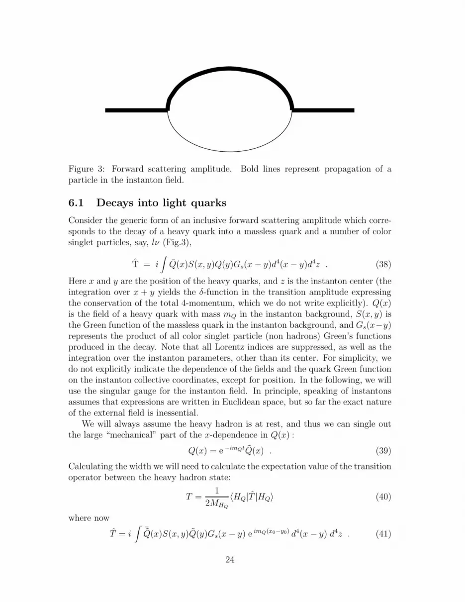
Figure 3: Forward scattering amplitude. Bold lines represent propagation of aparticle in the instanton field.

6.1 Decays into light quarks

Consider the generic form of an inclusive forward scattering amplitude which corre-sponds to the decay of a heavy quark into a massless quark and a number of colorsinglet particles, say, lν (Fig.3),

T = i∫

Q(x)S(x, y)Q(y)Gs(x− y)d4(x− y)d4z . (38)

Here x and y are the position of the heavy quarks, and z is the instanton center (theintegration over x + y yields the δ-function in the transition amplitude expressingthe conservation of the total 4-momentum, which we do not write explicitly). Q(x)is the field of a heavy quark with mass mQ in the instanton background, S(x, y) isthe Green function of the massless quark in the instanton background, and Gs(x−y)represents the product of all color singlet particle (non hadrons) Green’s functionsproduced in the decay. Note that all Lorentz indices are suppressed, as well as theintegration over the instanton parameters, other than its center. For simplicity, wedo not explicitly indicate the dependence of the fields and the quark Green functionon the instanton collective coordinates, except for position. In the following, we willuse the singular gauge for the instanton field. In principle, speaking of instantonsassumes that expressions are written in Euclidean space, but so far the exact natureof the external field is inessential.

We will always assume the heavy hadron is at rest, and thus we can single outthe large “mechanical” part of the x-dependence in Q(x) :

Q(x) = e −imQtQ(x) . (39)

Calculating the width we will need to calculate the expectation value of the transitionoperator between the heavy hadron state:

T =1

2MHQ

〈HQ|T |HQ〉 (40)

where now

T = i∫

¯Q(x)S(x, y)Q(y)Gs(x− y) e imQ(x0−y0) d4(x− y) d4z . (41)

24

Since the product of the quark Green functions and nonrelativistic Q fields does nothave an explicit strong dependence on mQ, we clearly deal with a hard (momentum∼ mQ) Fourier transform of a certain hadronic correlator which is soft in whatconcerns nonperturbative effects. Note that mQ can now be considered an externalparameter in the problem, for example, as an arbitrary, and even complex, number.We are not yet formally ready, however, to consider the Euclidean theory since westill have initial and final states. We shall address this issue a bit later, and nowproceed as if we deal with free heavy quarks, which are transferred to the Euclideandomain without problems.

Let us examine the propagator of the massless quark in the instanton back-ground, which is calculated exactly for the case of spin 0, 1/2, 1 particles [33]. This(Euclidean) Green function S(x, y) has a generic form

S(x, y) =1

[(x− y)2]n1

[(x− z)2 + ρ2]k1/2 [(y − z)2 + ρ2]k2/2× S (42)

where S has no singularities at complex xα or yα (a polynomial). Using the Feynmanparametrization, we rewrite it as

S(x, y) =Γ(k)

Γ(k1/2)Γ(k2/2)

1

[(x− y)2]nS ×

∫ 1

0dξ ξk1/2−1(1 − ξ)k2/2−1 1

[ξ(1 − ξ)(x− y)2 + (ρ2 + z2)]k, (43)

k =k1 + k2

2, z = z − ξx− (1 − ξ)y .

For the propagator of a spin 0 or 1/2 particle, the value of k is eventually 1 and 2,respectively, and n = 1, 2. The large-momentum behavior of the Fourier transformof the correlator, Eq.(41), depends on the analytic properties of the integratedfunction. Let us first consider the analytic properties of S(x, y) in the complex(x0 − y0) plane (Fig.4) - it has two different singularities. One singularity is on thereal axis, and corresponds to two quarks being at the same point. This is the samesingularity occuring in the Green function of free quarks, but upon integration, theresidue is softly modified by the instanton field. Picking up this pole and calculatingthe amplitude, we will get instanton contributions to the usual power (1/mQρ)

n

terms in the OPE, which we are not interested in. Indeed, making a Taylor expansionin (x−y)/ρ around this pole, we obtain a series of corrections ((x−y)/ρ)k/(x−y)2n,which, integrated with the exponent, result in the above terms.

Another singularity lies on the imaginary (x0 − y0) axis. It comes from the finitequark separation

(x− y)2 = [ξ(1 − ξ)]−1(ρ2 + z2) . (44)

In contrast to the perturbative or OPE pieces, this separation does not scale like1/mQ, but stays finite in the heavy quark limit. Upon integration over d4z d4(x −

25

Im xo

i

Re x o

ρ

Figure 4: Finite distance singularity of the Green function of a massless particle inthe instanton background.

y) dξ this singularity, together with the factor eimQ(x0−y0) from the heavy fields,produces the e −const mQρ terms in the (Euclidean) amplitude that we are lookingfor. We then only need to determine the constant that enters the exponent, and thepre-exponential factor.

Now with this general strategy in mind, let us outline the machinery in moredetail. We want to abstract from the complicated questions of the interrelationof the instanton configurations to the particular heavy hadron structure, i.e. toconsider the simplest possible state similar to a quasifree heavy quark instead of areal B or D meson or heavy baryon. On the other hand, the heavy quark,a priori,cannot be taken as free since the field Q(x) must obey the QCD equation of motion,in particular, in the instanton field. It is clear that such a program can be carriedout consistently if the instanton size is small enough compared to the typical size ofthe hadron ∼ ΛQCD, but still is much larger than m−1

Q . Having this choice in mind,we neglect, in what follows, the fact that the heavy quark is actually bound in thehadron although, eventually, the values of ρ will not be parametrically smaller thanthe hadronic scale.

Thus we merely solve the equation of motion for the heavy quark in the instantonfield, as one would do for an isolated particle. The role of the initial hadronic state,HQ, in Eq.(40) is played by the single heavy quark spread in space and evolvingin time according to the solution of the heavy quark Dirac equation analyticallycontinued from Euclidean to Minkowski space. In our actual calculations we, ofcourse, go in reverse: both the heavy quark field and the transition operator are

26

calculated in the Euclidean domain; the subsequent continuation to the Minkowskispace is performed in the final expression for the forward amplitude T . Technically,we are able to solve the equation of motion for the heavy quark field since theparameter mQρ≫ 1.

The heavy field Q(x0, ~x) can be written in the leading order as

Q(x0, ~x) = T e i∫ x0

0A0(τ,~x)dτ Q(0, ~x) + O (1/(mQρ)) ≡

U(x) Q(0, ~x) + O (1/(mQρ)) . (45)

The expression is written in Euclidean space, although we use Minkowski notations.Using the explicit solution for the SU(2) instanton in the singular gauge, Eq.(62),one gets the matrices U in the following cumbersome form:

U(x) = exp

{

i ~τ~n

[(

arctan

(

z0|~z − ~x |

)

− arctan

(

z0 − x0

|~z − ~x |

))

−

− |~z − ~x|√

(~z − ~x )2 + ρ2

arctan

z0√

(~z − ~x )2 + ρ2

− arctan

z0 − x0√

(~z − ~x )2 + ρ2

(46)

where ~n = (~x − ~z)/√

(~x− ~z )2, z is the coordinate of the instanton’s center and

~τ/2 are the color SU(2) generators. The integration is simplified since along theintegration path ~x − ~z = const in Eq.(45), A0 is proportional to one and the samecolor matrix ~τ (~x−~z ) and, therefore, the path-ordered exponent reduces to the usualexponent of the integral of A0.

It is important that the expression for Q(x) is only valid in the leading orderin the expansion parameter 1/mQρ. If one considers the contribution of small sizeinstantons (as in Ref. [7]), then no legitimate expansion parameter is available. Theexpansion in the heavy quark mass can only be obtained if instantons of size ρ < ρc

(where ρc is some parameter ≫ 1/mQ) are absent. Otherwise, the correspondingequations of motion need to be solved exactly.

Even though we managed to solve the equations of motion for the heavy quarksin the leading approximation, the solution governed by the color matrices U is notanalytic. The apparent singularities at x = z or y = z are, in fact, spurious andmerely an artifact of using the singular gauge for the instanton field; since theamplitude we calculate is manifestly gauge invariant (it is nothing but the lightquark Green functions times the path exponent 5), this singularity is absent in thefull expression, being canceled by similar terms in the light quark Green functions.

5Since the path exponent over the straight line is unity in the Fock-Schwinger gauge, theproducts we calculate are nothing else than the quark Green functions in the instanton field in theFock- Schwinger gauge. However, the fixed point of the gauge does not lie at the center of theinstanton, but, rather, at the external current point, x or y. For a review of the Schwinger gaugesee Ref. [14].

27

However, in general, the propagation matrix U introduces additional exponentialcorrections, since

arctan

(

t√~x 2 + ρ 2

)

has a (cut) singularity at t = i√~x 2 + ρ2, which is a point where the singularity in

the potential is not of the gauge type. The fortunate simplification which arises,in the leading approximation in 1/(mQρ), is that the two factors U(y) and U−1(x)are unity at the saddle point. This happens due to the fact that the saddle pointcorresponds to the configuration where the instanton is situated right on the line (inthree-dimensional coordinate space) connecting ~x and ~y and thus ~x− ~z = ~y− ~z = 0Eq.(48) Finally, picking up the pole in the complex (x0−y0) plane in the light quarkpropagator in Eq.(43),

[((x− y)2 + [ξ(1 − ξ)]−1(ρ2 + z2)]−k , (47)

we get an exponential factor

exp(

−mQ

√

(ρ2 + z2)/(ξ(1 − ξ)) + (~x− ~y )2

)

in the transition amplitude. The expression in the exponent has a sharp minimumat

z = 0, ξ = 1/2, (~x− ~y)2 = 0 . (48)

Evaluating it at this point we get the exponential factor

e −2mQρ .

The power of mQ in the pre exponent can be determined without actual calcula-tions as well. The residue of the k-th order pole of the propagator yields the factormk−1

Q upon integration over x0 − y0. The Gaussian integrals over (~x− ~y), x0 − y0, z,

and ξ around their saddle points give m−4Q ; on the contrary, all “free” propagators

(those of the color singlet final particles and the bare propagators of the quarksproduced) enter at a fixed separation ∼ −ρ2, and are mQ-independent. We thus get

T ∝ const ·mk−5Q e −2mQρ . (49)

For example, the large size instanton corrections to the transition amplitude for thesemileptonic decays of heavy quarks has the form

Tsl ∝ e −2mQρ

m3Q

. (50)

The pre exponent can be easily calculated in the same way and will be given for afew cases of interest in the subsequent sections.

28

0.6

0.8

1

1.2

1.4

1.6

1.5 2 2.5 3 3.5 4 4.5GeV

Figure 5: Exact (solid line) and asymptotic (dashed line) behavior of R(E).

The same counting rules apply for the case when more quarks are present inthe final state. In the case of the vector correlator of the light quarks we have theproduct of two light quark propagators instead of one, and eventually k = 4. SinceΠµν(Q) ∼ Q2Π(Q2), we get for Π(Q2) defined in Eq.(27)

Π(Q2) = 4π3 e −2√

Q2ρ

( Q ρ )3, (51)

in accordance with the explicit calculation of Eq.(27). In fact, the asymptoticexpression works accurately enough even in the Minkowski domain already at

√sρ ≃

3; the corresponding approximate expression for 1πIm Π is plotted as a dashed curve

in Fig.5. It is clear that the main effect of the subleading in 1/(Qρ) terms is a phaseshift in the oscillations.

Using the same counting techniques, one concludes that the non-OPE soft in-stanton contribution to the forward amplitude describing nonleptonic decays of theheavy quark (we have three light quarks in the final state i.e. k = 6) scales like

Tnl ∝ mQ e −2mQρ . (52)

In the next section, we give a more detailed calculation, and discuss total widthsand differential distributions.

A qualifying comment is in order here. So far, in calculating the exponentialterms, we assumed the heavy initial quark to be static (at rest). In this approxi-mation the presence of the initial heavy quark does not affect our result at all; it

29

is the final quarks that fully determine the exponential terms. We know for sure,however, that the initial heavy quark experiences a “Fermi” motion inside the heavyhadron. In the practical OPE, the first correction due to this Fermi motion comesfrom the operator Q~π2Q. In other words, the accuracy of the static initial quarkapproximation is 1/m2

Q. An important question is how the exponential terms of thetype we focus on show up in those subleading effects proportional to 〈~π2〉 (and othersimilar subleading effects).

The expansion of the heavy quark propagator in 1/mQ leads, generally speaking,to terms of the type (1/m2

Q)1/(x2 + ρ2), i.e. we get an extra singularity in theamplitude due to the initial heavy quark. This extra factor enhances the overallsingularity of the amplitude in the complex plane and, thus, leads to a higher powerof mQ in the preexponent. The additional denominator, (x2+ρ2), generates only thefirst power of mQ, however, so the overall effect is suppressed by the small parameter1/(mQρ).

In the Minkowski domain, inside the oscillation zone, the exponential factor isnot a suppression at all, so we must count only the pre-exponential factors. We seethat deviations from duality are parametrically relatively stronger in the 〈~π2〉 piece.Still the original suppression of the 〈~π2〉 piece by 1/m2

Q is not completely lifted. Welose one power of 1/mQ, but retain the other power. Thus, our approximation ofthe static initial quark in the analysis of the exponential deviations from duality isjustified. Nevertheless, it is interesting to note that the initial-state 1/mQ effectsare less suppressed in the exponential terms. This seems to be a general feature.

6.2 Decays into massive quarks

The case of the massive final state quark (e.g. b→ clν) does not differ conceptuallyif treated in the 1/(Qρ) expansion, although a technical complication arises due tothe unknown explicit expression for the massive propagator in the instanton field.Still, this is not a stumbling block in the analysis: the relevant singularity of thec quark Green function can again only be at (x − z)2 = −ρ2 or (y − z)2 = −ρ2,and the corresponding power of the displacements can be determined analyticallykeeping trace of the singular terms in the massive Dirac equation. Only the exactconstant in front of this singular term constitutes a problem, and it can be evaluatednumerically. We shall address this case in detail elsewhere, and here only considera few limiting cases.

(i) Heavy and light quarks in the final state, e.g. b→ cdu

It is possible to see that, in this case, the exponential terms, in the leadingapproximation, are associated with the light quark, and the presence of the heavyquark in the final state has no impact apart from changing kinematics. Indeed,we saw that the Green functions of the final state particles enter at large distances|x| ∼ ρ (it will be also illustrated in more detail in the next section). In thissituation the interaction of the final heavy quark with the soft background field

30

reduces to the ordered exponential of i∫

Aµ(ξ)dξµ along the heavy quark trajectory.We have already calculated it and found to be unity (the exponent to vanish) in thesaddle point configuration. Therefore the final heavy quark can be taken as non-interacting. The propagator of the non-interacting final c quark ∝ e−imc|x| (e−mc|x|

in the Euclidean time) will be multiplied by the light quark Green function, whichdevelops a pole in the complex x2 plane. This means that as far as the exponentialterms are concerned, the effect of the final heavy quark is the replacement of mQ inthe Fourier transform by mQ −mc,

mQ → ∆ = mQ −mfin (53)

(in the general case, with a few heavy particles in the final state, ∆ = mQ −∑mfin ,with the sum running over all heavy final state particles). Calculating the width, onethus has, at the saddle point, the exponent of the form e−2∆ρ rather than e−2mQρ. Itis worth emphasizing that this result holds as long as the mass of the final state quarkinvolved exceeds 1/ρ, i.e. mfin ρ≫ 1, regardless of the actual hierarchy between mQ

and mfin. The very same kinematic change refers, of course, also to the case whenmassive leptons (or other color-singlet particles) are present in the final state.

Such a result might seem counter-intuitive to the reader who would compareit, say, with the free quark answer for the total width, where the final quark massappears only as a quadratic correction ∝ m2

fin/m2Q if mfin/mQ ≪ 1, and the final

heavy quark is typically fast. As a matter of fact, there is no mystery – the oc-currence of e−2∆ρ, instead of e−2mQρ, is a manifestation of a remarkable propertyof the exponential terms discussed in Sect. 5. These terms are determined by thehighest possible invariant mass of the light quark system. In the case at hand this isachieved when the final c quark is at rest, i.e. we are in the SV limit [34]. With thispicture, it is then no surprise that the exponential terms are determined by e−2∆ρ.

Since this result is rather unusual, we reiterate. In calculating the exponentialterms in the transitions of the type b → cud we find ourselves in the situation ofthe heavy quark symmetry [34, 35]. It is an extended symmetry, however, since itapplies to arbitrary color structure of the weak vertices, e.g. even when color flows,say, from Q to the light quark q rather than from Q to the heavy final quark c(the standard heavy quark symmetry works only for the color singlet bc currents).Similar consideration applies even to the decays like b→ ccs.

(ii) SV limit.

In the SV limit, when the final heavy quark is slow, we can calculate the ex-ponential terms analytically in a wider class of processes, e.g. in the nonleptonictransition b→ cud.

This case can be treated as follows. The final heavy quark Green function isgiven by the P exponent together with the “mechanical” phase factor (we write ithere in the Euclidean space):

GSV(x, 0) = m31 + ixγ

|x|2

e−m|x|

(2πm|x|)3/2T e i

∫ x

0Aµ(ξ)dξµ ≃

31

≃ m31 + ixγ

|x|2

e−m|x|

(2πm|x|)3/2U+(x)U(0) . (54)

The path exponent is again given by the U matrix presented in Eq.(46) 6. At thesaddle point when the instanton is on the line (~x, ~y ) the final heavy quark pathexponent equals to unity, and, therefore, the heavy quarks appear to be “sterile” –they do not feel the instanton field at all. Thus, in nonleptonic decays in the SVlimit the appearance of exponential corrections is due - in the leading order - only tothe light quark interaction with the instanton. (Note also, in the semileptonic decayin the SV limit the exponential terms are absent in the approximation accepted inthe present paper. To see them we have to go beyond the leading approximationnear the saddle point approximation. )

It is worth noting that, outside the exponential factor, in the pre-exponent, themasses enter in a more complicated way than is indicated in Eq. (53). For example,

the integration over d3x near the saddle point produces m−3/2Q rather than the power

of the energy release.

6.3 Summary

Now we are ready to incorporate the effect of both massive and massless quarks inthe final state.

1) Each light (massless) quark contains a second order pole in its propagator(43) and brings in two powers of energy release in the numerator.

2) Each heavy (static) quark propagator contains factor m3/2fin

3) The scale of energy release in the exponent is set up by the masses of theheavy quarks,

mQ −∑

mfin

Exploiting Eq.(49) and discussion above it we obtain

T ∝ const ·(

mQ −∑

mfin

)2nl−7/2m

−3/2Q e−2ρ(mQ−

∑

mfin)∏

m3

2

fin (55)

where nl is the number of massless quarks; mQ is the mass of the initial quark andmfin are the masses of the final heavy particles (both quarks and leptons). If thereare no heavy particles in the final state we return to Eq.(49).

7 Heavy quarks – a toy model

Before proceeding to the actual calculation of the instanton contribution to heavyquark decays, we will first perform the same analysis in the simple toy model of

6Here, we can first deform the integration contour over x0 into the complex plane and then usethe 1/mfin expansion for the quark propagator. Another clarifying remark: for massive particles,the propagator entering at the saddle (effectively Minkowski) point is complex. In doing the saddlepoint calculations, one should take its values at the “bottom” of the cut; we shall dwell on thispoint elsewhere.

32

scalar chromodynamics. Without any loss of physical content, we can simplify ourconsideration by neglecting the spin degrees of freedom, as was suggested in Ref.[36]. We also assume the SU(2) color group here.

The weak Lagrangian,LW = h Qq φ+ h.c., (56)

describes the decay of a heavy scalar quark, Q, into a light (massless) quark, q,, anda scalar “photon”, φ ; the coupling, h, has dimensions of mass. Both quarks are inthe spinor representation of the color group.

The basic strategy of our semiclassical calculation of the transition amplitudehas been outlined in the previous section; here we work out details. We calculatethe transition operator in Euclidean space using the semiclassical approximation,considering scalar quarks in the background of an instanton field. Upon returningto the Minkowski space, T will acquire an imaginary part related to the instantoncorrection to the total decay width.

7.1 Inclusive width

Consider the transition amplitude,

T (r) =1

2MHQ

〈HQ|T (r)|HQ〉 =1

2MHQ

〈HQ|∫

d4x e −irx iT{LW (x)LW (0)}|HQ〉(57)

where r is an arbitrary external momentum. Denote the 4-velocity of the heavyhadron by vµ (~v = 0). Proceeding to the nonrelativistic fields, Q, and using Eq.(38),we have

T (r) = i∫

¯Q(x)S(x, 0)Q(0)Gφ(x2) e i(mQv−r)x d4x d4z , (58)

where Gφ is the propagator of the scalar photon, and S(x, y) is the propagator of themassless scalar quark in the external (instanton) field. We put y = 0. Addressingthe total width, we will only consider ~r = 0 and r0 arbitrary (and complex); themore general case is relevant for differential distributions. For heavy quarks thetransition amplitude depends only on the combination mQ − r0 :

T (r) = T(mQ − r0) .

Choosing an appropriate r0, we select deep Euclidean kinematics and calculate theamplitude in the presence of an instanton. To this end we write

mQ − r0 = ik0 , (x0, z0) → −i(x0, z0), (59)

andT(k0) =

∫

¯Q(x)S(x, 0)Q(0) Gφ(x) e ikx d4x d4z, (60)

where now everything is in Euclidean space; in what follows it is assumed thatk0 ∼ mQ.

33

The propagator of the massless scalar particle in the instanton background isknown exactly, and in the singular gauge takes the following form [33]

S(x, y) =1

4π2(x− y)2(1 + ρ2/x2)−1/2

(

1 +ρ2(τ+x)(τy)

x2y2

)

(

1 + ρ2/y2)−1/2

(61)

where, to simplify the expression, we have assumed that the instanton is centeredat z = 0 and lies in a particular SU(2) color subgroup,

Aµa(x) =2ηµνa(x− z)νρ

2

(x− z)2((x− z)2 + ρ2)(62)

andτ = (~τ, i) τ+ = (~τ ,−i) τ+

α τβ = δαβ + ηαβcτc , (63)

where ~τ are the Pauli matrices acting in the color subgroup.The heavy quark field, Q(x), is the solution of the equation of motion in the

instanton background

iD0Q(x) =1

2mQ(iD)2Q(x)

which, in the leading order in 1/mQ, yields Eq.(45) with the matrices U given byEq.(46). For the heavy scalar quarks one has

1

2MHQ

〈HQ | QQ | HQ〉 =1

2mQ. (64)

Now we take a closer look at the final state quark propagator, rewriting it usingthe Feynman parametrization:

S(x, y) =1

π

∫ 1

0dξ [ξ(1 − ξ)]−1/2 1

ξ(1 − ξ)(x− y)2 + ρ2 + z2×

1

4π2(x− y)2

(

1 +ρ2τ+(x− z)τ(y − z)

(x− z)2(y − z)2

)

√

(x− z)2√

(y − z)2 (65)

wherez = z − xξ − (1 − ξ)y .

Integrating in Eq.(60) over x0 we only pick up the pole at

x2 =ρ2 + z2

ξ(1 − ξ)

which yields the following exponential factor:

e −k0

√(ρ2+z2)/(ξ(1−ξ))+~x2

. (66)

34

At k0ρ ∼ mQρ ≫ 1, the remaining integrations are nearly Gaussian, and run overnarrow intervals,

~x2 ∼ ρ

mQ

,(

ξ − 1

2

)2

∼ 1

mQρ,(

z − x

2

)2

∼ ρ

mQ

. (67)

Thus, one performs the remaining integrations by merely evaluating all pre expo-nential factors at the saddle point. In particular, this refers to the matrix U−1(x),coming from the heavy quark propagation, which is now the path exponent fromthe point (x0, 0 ) to (0, 0 ) . U−1(x) evaluated at the saddle point and is just the unitmatrix, and the color part of the light quark Green function Eq.(61) . The heavy

quark field, ¯Q(0, ~x ), according to Eq.(67), enters at distances ~x ∼√

ρ/mQ ≪ ρ and,

therefore, the transition operator is finally proportional to Q(0)Q(0) .Collecting all remaining factors, one has

T(k0) = h2 Q(0)

{

Gφ(−4ρ2)

2π2ρ

∫

dξ d3~x d4z e −k0

√(ρ2+z2)/(ξ(1−ξ))+~x2)

}

Q(0) , (68)

where

Gφ(x2) =

1

4π2x2,

is the free scalar propagator. Performing the Gaussian integrations (which yield thefactor 4π4ρ3k−4

0 · e−2k0ρ), and using Eq.(64), we finally arrive at

T (q0) = − h2

16mQ

e −2k0ρ

k40

= −h2 e 2i(mQ−r0)ρ

16mQ(mQ − r0)4. (69)

Let us note that the above equation shows the correct pre-exponential power of mQ.The propagator of the scalar particle in the instanton background has a first orderpole, unlike the second order one of the spin-half quark, and matrix element (64)has an additional power of m−1

Q . This leads to a result with two powers of mQρ lessthen predicted in Eq.(50).

Now, we are interested in the decay width, which is given by the imaginary partof T (r) at the physical Minkowski point r = 0. Since the singularity of the amplitudewe calculated is located far enough away, at r0 ≃ mQ, we perform a straightforwardanalytic continuation by merely setting r0 = 0 and, thus, get

ΓIscal = −h2 sin (2mQρ)

8m5Q ρ4

. (70)

In accordance with the general analysis of Sect. 3 the instanton contribution in thewidth decreases only as a power of mQ and oscillates.

35

7.2 Decay distribution

Here we address the calculation of the instanton-induced corrections to the “photon”spectrum. The corrections blow up near the tree-level endpoint, where the semi-classical approach is not applicable. On the other hand, the total width is given bythe integral over the whole spectrum and is calculable. The situation here is similarto the one we discussed in the Sect. 5 for the finite energy moment integrals in thee+e− cross section, and we closely follow this analogy in our analysis.

Let us denote the photon momentum by q, with q0 = Eγ . To find dΓ/dEγ, onemust consider the transition operator similar to the total width, but without thephoton propagator Gφ :

dT (r, q) =1

2MHQ

〈HQ|dT (q, r)|HQ〉 (71)

withdT (q, r) = i

∫

¯Q(x)S(x, 0)Q(0) e i(mQv−q−r)x d4x d4z . (72)

The transition operator then clearly depends only on the sum of the four-momentaq + r, but since calculating the differential decay rate we need to keep q2 = 0 andq0 = Eγ > 0, such a temporary proliferation formally allows us to use the momentumr for analytic continuation and is appropriate. In particular, we will keep ~q fixed,say, directed along the z axis, assume ~r = 0, and again use the variable r0 tomake calculations in the Euclidean domain. Kinematically, the amplitude dT (r, q)depends on two invariants, (r + q)2 and (r + q)0, or any two combinations thereof.

Technically, the calculation of the transition operator does not differ from thecase of the total width except for the fact that now the Euclidean momentum k

mQ − q0 − r0 = ik0 , ~q + ~r = ~k

has not only the zeroth, but also spacelike components. The saddle point calcu-

lation goes exactly in the same way if one replaces k0 by√k2 =

√

k20 + ~k 2, the

main contribution comes from the singularity of the light quark propagator and theheavy quark matrix U still equals unity at the saddle point. For this reason, in theleading approximation the amplitude dT (r, q) appears to depend, in fact, only onone kinematic variable (mQv − r − q)2 = (p− q)2, and one has

dT (q, r) = π2h2ρ2

mQ

e −2ρ√

k2

k4= π2 h

2ρ2

mQ

e 2iρ√

(mQv−q)2

(mQv − q)4 ρ4. (73)

In the last equation, we continued the result to the physical domain setting r = 0;to be far enough from the singularity and ensure the applicability of the calculationswe must assume that (mQv − q)2ρ2 ≫ 1.

The differential decay rate for the massless φ is given by

dΓ

dq0=

1

2π2q0 ϑ(q0) Im dT (q) =

36

=h2ρ2

2mQq0 ϑ(q0) · ϑ(mQ − 2q0)

sin(

2ρ√

(mQv − q)2)

(mQv − q)4 ρ4(74)

(remember, we fixed |~q | = q0). Eq.(73) (and (74) for the imaginary part), in fact, arenothing but the soft instanton contribution to the massless (scalar) quark propagator(in the Fock-Schwinger gauge, or dressed with the path exponent to make it gauge-invariant in the general case).

In the approximation of free quark decay, the photon spectrum is monochromatic,∝ δ(Eγ − mQ/2). Equation (74) yields a decay spectrum below the end point,at Eγ < (mQ/2). The result for the spectrum is, as expected, oscillating (sign-alternating). This does not lead to any physical problems, of course, because thiscontribution is to be considered on the background of “normal” OPE corrections(as well as the perturbative ones) which populate the spectrum below the two-bodyendpoint. The main OPE contribution near the end point is related to certain initial-state interactions of the heavy quark, and is interpreted as Fermi motion [32, 36, 37].It produces a decay distribution which is unsuppressed, of order unity, in the interval|Eγ −mQ/2| ∼ ΛQCD, and decreases fast only when mQ/2−Eγ becomes larger thana hadronic scale. At (mQ/2) − Eγ ≫ ΛQCD the perturbative tail of the spectrumdensity takes over. In this domain our instanton calculations are already legitimate,

since there√

(mQv − q)2 ∼ √mQρ if ρ ∼ ΛQCD. However, we emphasize that the

corrections (73), (74) are not related to the Fermi motion: the instanton effects inthe latter appear in subleading orders in mQρ.

Equation (74), far enough from the end point, represents, in a sense, a purely“exponential” effect. This is not the case anymore, however, if one attempts tointegrate over Eγ and find the contribution to the total decay width. This factis clearly revealed at the technical level when one compares the above calculationwith the preceeding calculation of the total width: in the case of Γtot one effectivelyuses the x-independent photon propagator Gφ(x

2) = −1/(16π2ρ2), whereas Eq.(74),according to Cutkowski’s rules, corresponds to the propagator Gφ(q) = −1/q2, i.e.Gφ(x

2) = 1/(4π2x2). They differ explicitly by the presence of the singularity atx = 0, which generates the normal OPE terms in Γtot. Of course, a thoughtfulinstanton calculation of the integrated spectrum yields the same result as the directcalculation of the total width. Starting from the differential spectrum one has toresort to a special treatment of the OPE domain near the end point.

A straightforward attempt to calculate the total width by integrating the spec-trum (74) seemingly faces a surprising problem: the correction grows fast towardthe end point [7, 8] where the light quark is soft (though carrying large energy), andthe integral seems to saturate at mQ/2 − Eγ ∼ 1/(mQρ

2), where the expansion in1/Qρ fails, and the overall result completely depends on an ad hoc cutoff procedure;the total contribution then would allegedly be governed by this soft scale, ratherthan by mQ. This is similar to the apparent paradox in the finite energy momentsof R in the e+e− annihilation addressed in Sect. 5. The resolution of the paradox isessentially the same: any exponential contribution in the hard part of the spectrum

37

is automatically accompanied by the corresponding OPE-like “counterterms” in theend point region, which are superficially invisible. Although the exact spectrum inthe latter cannot be calculated, certain integrals are defined unambiguously. As aresult, the non-zero total width effect emerges only from the explicit (non analytic)constraint on the photon energy at Eγ = 0, i.e. at small q, and, thus, the instanton(exponential) contribution to the total width is indeed determined by the hard scalemQ.

To reveal this conspiracy explicitly, we again exploit the fact that dT exponen-tially decreases in the Euclidean domain. In our concrete case, there is a technicalsimplification: dT (q) depends only on one kinematic variable κ2 = (mQv − q)2, the“invariant mass squared” of the light final state quark. One can write the dispersionrelation over κ2,

dT (κ2) =1

π

∫ ∞

0

Im dT (κ′2)

κ′2 − κ2dκ′2 . (75)

The fact that dT (κ2) falls off exponentially in the Euclidean domain, dT (κ2) ∼e−2

√−κ2ρ, means that all moments of Im dT (κ2) vanish:

∫ ∞

0κ2n Im dT (κ2) dκ2 = 0 . (76)

On the other hand, ImdT (κ2) differs from dΓ/dq0 by only a simple kinematic factor.For a massless φ, for example,

dΓ

dq0=

1

2π2q0 ϑ(q0) Im dT (q) , (77)

q0 =m2

Q − κ2

2mQ, |~q | = q0 .

Therefore,

∫ MHQ/2

Edq0 q

n0

dΓ

dq0= − 1

4π2mQ

∫ ∞

m2Q−2mQE

(

m2Q − κ2

2mQ

)n+1

Im dT (κ2) dκ2 . (78)

We see that the instanton correction to the spectrum integrated from the very endpoint down to some Emin is determined, not by the end point effects, but by the

lowest energy included, and one has in this case 2ρQ→ 2ρ√

m2Q − 2mQEmin . If one

integrates over the whole spectrum, the correction is parametrically minimal, andreproduces the correction for the total width. Clearly, it is the most general featureof the “exponential” effects which does not depend on the particular decay. As wasmentioned in Sect. 5, the constraints (76) can be written in the following compactform

Im dT (κ2) =∫ ∞

0ds χ(s)

[

δ(s− κ2) − e −s ∂

∂κ2 δ(κ2)]

, (79)

38

where χ(s) is some smooth function vanishing at s ≤ 0. This expression automati-cally satisfies the relation

∫ κ2

0Im dT (κ2)P (κ2) dκ2 = −

∫ ∞

κ2

Im dT (κ2)P (κ2) dκ2 (80)

for any appropriate analytic P (κ2). The saddle point instanton calculation carriedout above determins the asymptotics of the function χ(s) at s≫ 1/ρ2 :

χ(s) ≃ π2h2 ρ2

mQ

sin (2√s ρ)

s2. (81)

In such a saddle point way we cannot calculate Im dT (κ2) at κρ <∼ 1. Accordingto Eq.(79), however, we know certain integrals over the small virtuality domain.For any particular “exact” χ(s) they are obtained as a series of δ functions andderivatives of δ functions located at the end point, which, when summed, give acertain more or less smooth function in the whole range, whose asymptotics aregiven by Eq.(81).

For example, one can calculate the instanton contribution to the total width byintegrating the spectrum. We use the general relation of the type (76) or (78) towrite the total width as minus the integral of the right- hand side of Eq.(74) (withoutstep-functions) from q0 = −∞ to 0. In the leading order in mQρ, the integral iseasily performed by parts, and is determined near the vicinity of the point q0 = 0,immediately yielding, exactly, the total width (70).

It is not difficult to see how this works in the most general case. Suppose westudy, for example, the “semileptonic decays” Q → q + ℓ + ν. If we can measuremomenta of both ℓ and ν, pℓ,ν, the differential distribution is merely given by

d2Γ = Φ(pℓ, pν) · Im dT (mQv − (pℓ + pν)) . (82)

Now we want to integrate over the momentum of neutrino and determine the in-stanton contribution to the charged lepton spectrum. We then keep pℓ fixed andintegrate Im dT with the phase space, Φ, depending on pν . If the phase space fac-tor were an analytic function of pν , the constraints (76) or (79) would ensure thevanishing of the integral.

However, the phase space contains a step-function at Eν = 0, and only for thisreason does one get a nonvanishing integrated width due to exponential terms. Thenthe relation (80) can be used to represent the integrated effect as the effect from thekinematic boundary and above (i.e., over the domain where neutrino “carries away”negative energy), which is a hard domain where the expansion is applicable 7. Since

7The same reasoning equally applies, of course, to the case of the massive final particles as well.In this case it is convenient to phrase this consideration in the frame where mQv − pℓ has only atimelike component. The phase space integral is not a polynomial anymore when mν 6= 0, but isthe step-function at Eν = mν multiplying a fractional power function. Then one merely must putthe corresponding phase space factor P in Eq.(80) under the sign of Im in the right hand side.This does not change the general reasoning presented here.

39

in this domain Im dT (κ2) is a rapidly oscillating function ∼ sin (2κρ), the integralis determined by its lower limit; the expansion in 1/Q is obtained by integratingby parts, and in the leading approximation given by the corresponding derivativeof Im dT (κ2), from which we must keep only the derivatives of sin (2κρ). Theexact coefficients combine to yield just the value of the neutrino propagator at thepoint which enters in the direct calculation of the lepton spectrum, i.e. Gν(x) atx = 2ρ(mQv − pℓ)/|mQv − pℓ| .

To illustrate the last assertion, we must remember that to get the total width inthe leading approximation, we need to integrate the differential width near pν = 0keeping trace of only the non-analytic part due to the neutrino phase space, and

the oscillating part, sin (2ρ√

(mQv − pℓ − pν)2), in the differential distribution. Allother constituents of the amplitude can be approximated by their values at pν = 0.

To see that this integration automatically yields the proper factor, we can usethe following trick: compare this integral with the calculation of the neutrino Greenfunction in the coordinate space by taking the Fourier transform of its momentumrepresentation. Let us take the Fourier integral by closing the contour of integrationover k0 by its physical residue (we assume here that the zeroth coordinate coincideswith the direction of the vector mQv − pℓ):

Gν(x) =∫ d4k

(2π)4iGν(k) e ikx =

∫ d3k

(2π)32k0Gν(~k) e ikx . (83)

The large-x asymptotics of the last integral is determined by the behavior of thephase space factor d3k/k0 at small |k| where it is non analytic. This factor, on theother hand, is exactly the same as in the double distribution if one identifies k inthe above calculation with pν (both are nothing but d4k δ+(k2 −m2

ν)/(2π4)). If one

chooses the coordinate x in such a way as to have the same oscillating exponent

e ikx on the right hand side of Eq.(83) as in dT ∼ e 2iρ√

(mQv−pℓ−pν)2 , identifyingk with pν , the values of the integrals will also coincide. The last condition justfixes the above stated value of the coordinate. This matching is rather obvioussince the oscillating factor in dT came originally from evaluating the exponentiale i(mQv−pℓ−pν)x at the saddle point x, which enters the neutrino Green function.

Therefore, integrating over the neutrino momentum in the decay, we recoveredour direct recipe of calculating the lepton spectrum, namely considering the problemas a two-body one, but using dT given by the product of the quark propagator in theinstanton field, and the neutrino propagator at the saddle point x2 = −4ρ2. Sincethe integrated effect comes from the zero momentum of neutrino, it is governed bythe same exponential (oscillating) factor determined by mQ and p, | mQv− pℓ|. Wecan repeat the very same consideration once more integrating now over the energy ofthe charged lepton; the leading term in the integral again comes from pℓ = 0, wherethe phase space of the lepton is non-analytic, the nearby integration reproducesGℓ(−2iρ, 0), the argument of the neutrino Green function becomes the same, andwe arrive at the total width obtained in the direct way in the preceeding subsection.

40

8 Instanton Contribution to Heavy Quark Decay

Rates – Real QCD

We now proceed to the case of actual b and c quarks; the modification required hereis accounting for the quark spins. In principle, the analysis goes along the samelines as for the scalar quarks. However, since we deal with instantons – topologically-nontrivial configurations of the gauge field – the massless quarks acquire zero modes.They manifest the intervention of the infrared, long-distance effects in the presenceof the instantons. This is an obvious defect of our simplified one-instanton ansatz. Ifwe used the topologically trivial (but nonperturbative) configurations, the problemswith the zero modes would be absent.

Technically, this problem emerges already at the very first step: the Green func-tion of the massless quark is not defined in the field of one instanton since the Diracoperator has a zero mode. In order to perform estimates similar to the ones de-scribed in the previous sections, we need to regularize the massless quark Greenfunctions in the infrared. We do it in the most naive way: introducing a small massterm mq. Now, the Green functions are well-defined but they have terms whichbehave like 1/mq, which show up wherever the chirality-flip quark amplitudes oc-cur. However, when the weak interactions of the quarks are purely left-handed, theproblem disappears since the zero modes do not contribute, and we can put mq = 0in the end. We are aware, of course, that this procedure is not fully self-consistent,but, hopefully, it works satisfactorily for our limited purposes – revealing the correctexponential dependence, as well as the power of mQ, in the pre-exponent. It seemsquite plausible that only the overall numerical coefficient will be modified in a moreaccurate analysis.

Otherwise, the calculations go with minimal modifications. Let us outline thetreatment of the semileptonic width. Once again, we write the transition operator(the integration over ρ will be restored at the very end)

T (r0) =G2

F |VQq|22

∫

¯Q(x)ΓµS(x, 0)ΓνQ(0)Lµν(x) e i(mQv−r)x d4x d4z (84)

where the weak polarization tensor for the lepton pair Lµν and the weak vertices are

Lµν(x) = − 2

π4

1

x8(2xµxν − x2δµν) , Γµ = γµ(1 − γ5) . (85)

The heavy quark fields, Q, are nonrelativistic as in Eq.(39), and are originallybispinors. However, solving the Dirac equation of motion in the limit mQρ ≫ 1 weget the fields in the form of Eq.(45). The color matrix U has the same form as inEq.(46).

The Green function of the light quark in the instanton background, S(x, y), isexpanded in mq and has the following form [33, 30]:

S(x, y) = − 1

mqP0(x, y) +G(x, y) +mq∆(x, y) +O(m2

q)

41

where P0 is the projector on the zero modes (P0 does not contribute to Eq.(84) sinceit flips chirality.) Therefore, we can merely put mq = 0 to arrive at

1 − γ5

2S(x, y)

1 + γ5

2=

1 − γ5

2G(x, y)

1 + γ5

2=

1 − γ5

2

{

−∆γ

2π2∆4(1 + ρ2/ζ2)−1/2

(

1 + ρ2/η2)−1/2 ·

(

1 +ρ2(τ+ζ)(τη)

ξ2η2

)

+

−1

4π2∆2ζ2η2(1 + ρ2/ζ2)−1/2(1 + ρ2/η2)−1/2

(

ρ2

ρ2 + η2(τ+ζ)(τ∆)(τ+γ)(τη)

)}

(86)

whereζ = x− z , η = y − z , ∆ = x− y .

Now, the calculation differs from the case of the scalar quarks in minor technicaldetails, namely, the different power of (x2+ρ2) in the denominator, and the presenceof the γ matrices in the numerator. At the saddle point, U = 1 , the heavy quarkfields enter at the origin, the leptonic tensor must be evaluated at x∗ = (2iρ,~0), andthe final result is

T (r0) = − G2F |VQq|2

4π2ρ8 (i(mQ − r0))3 e 2i(mQ−r0)ρ Q(0) iγ0 P Q(0) (87)

where P is the projector onto the instanton color SU(2) subgroup, P = (1, 1, 0)diag.Since

〈HQ|Q γ0Q|HQ〉 = 2MHQ

we finally obtain

ΓIsl = −2

3

G2F |VQq|2

2π2ρ8 m3Q

sin (2mQρ) . (88)

In terms of the free quark semileptonic width,

Γ0 =G2

Fm5Q|VQq|2

192π3,

we get

ΓIsl = −Γ0

2

3

96π

(mQρ)8sin (2mQρ) . (89)

In a similar manner it is easy to find the expression for the differential distribu-tions in the semileptonic decays. We quote here the expression for the instanton-induced lepton spectrum (in its hard part, i.e. far enough from the end point) inthe same approximation,

mb

2Γ0

dΓI(b→ uℓν)

dEℓ= −2

3

48π

(mbρ)5ǫ2(

1 − ǫ

2

) cos(

2mbρ√

1 − ǫ)

(1 − ǫ)5/2,

42

mc

2Γ0

dΓI(c→ s(d)ℓν)

dEℓ= −2

3

48π

(mcρ)5ǫ2(1 − ǫ)2

cos(

2mcρ√

1 − ǫ)

(1 − ǫ)5/2. (90)

Here ǫ = 2Eℓ/mb or ǫ = 2Eℓ/mc for the two decays, respectively. It is immediatelyseen explicitly, using the technique described in Sect. 7.2, that the integral over thespectrum reproduces the total semileptonic width (88).

Now let us proceed to the nonleptonic decays with the massless quarks in thefinal state. Repeating the derivation above we get the non-leptonic width 8

ΓInl =

2

3c2− Γ0

256π

15(mQρ)4sin (2mQρ) (91)

where c± are the standard color factors due to the hard gluons in the weak vertex[38].

For completeness we also give the instanton contribution to the inclusive radiativerate of the type b→ s+ γ,

ΓIγ ≃ 2

3Γ0

γ

12π

(mQρ)6sin (2mQρ) . (92)

The above estimate refers to the yield of photons with all energies. In experiment onecuts off the low-energy photons, however. According to the previous discussion, theintroduction of the lower cut off can change the estimate of the duality deviations.We will not submerge into further details regarding this effect here.

9 Numerical estimates

In this section, we present numerical estimates of the possible violations of the localduality in our model. The effects rapidly decrease with the energy release. They canbe quite noticeable at intermediate energies, however. The inclusive decay width ofthe D meson, and is expected to be one of the prime suspects. Indeed, with themass of the c quark only slightly over 1 GeV, one can expect sizable violations ofduality. Another case of potential concern is the hadronic width of τ . This width isalso saturated at a similar mass scale. In these two cases, there exists at least some(quite incomplete, though) empiric information. It is natural to treat one of themas a reference point, in order to adjust the parameters of the model. Basically, wehave only one such parameter, the overall normalization of the instanton density d0,see Eq. (18). We will use the semileptonic D decays for this purpose. Then thesecond problem (τ decays) can be used as a check that the model is qualitativelyreasonable and does not lead to gross inaccuracies. As a matter of fact, this wasalready demonstrated in Sect. 5.1. Encouraged by this success we then take the riskto use the model for numerical estimates of the duality violating effects in variousB decays. Although our model is admittedly imperfect, the numbers obtained canhopefully be viewed as valid order-of-magnitude estimates.

8We should note that here the subleading effects are probably significant: even within our simplesaddle point calculation we formally had to discard, e.g. terms of the type 9!!/(2Qρ)5 ≃ (4/(2Qρ))5.

43

9.1 Γsl(D)

This decay was numerically analyzed in the heavy quark expansion more than once[39]–[45], with quite controversial conclusions. We will summarize here our currentpoint of view [46], deferring a brief discussion of the literature until Sect. 11.

The parton semileptonic D decay width is given by

Γ0(D → lνXs,d) =G2

Fm5c

192π3≃ 1.03 · 10−13 GeV at mc = 1.35 GeV , (93)

where the strange quark mass is neglected. The comparison with the experimentalvalue

Γexp(D → lνX) ≃ 1.06 · 10−13 GeV (94)

seems to be very good. However, there are corrections to the free quark estimate(93); both the perturbative and nonperturbative corrections calculated within 1/mc

expansion work together to noticeably decrease the theoretical prediction.

(i) Perturbative corrections

The one-loop perturbative correction to the width in the four-fermion decay isknown since the mid-fifties [47]; for QCD one gets the factor ηpert multiplying thetheoretical formula for the width (i.e. Γ → Γ0ηpert),

ηpert = 1 − 2

3

(

π2 − 25

4

)

αs

π. (95)

This factor obviously decreases the theoretical prediction for the width, the questionis how much. The answer for ηpert is not as obvious as it might seem, and dependson how mc is defined.

Equation (95) implies that one uses the (one-loop) pole mass of the c quark in theinclusive rate. (As well-known, the notion of the pole mass is ill-defined theoretically[48, 49, 50]. It is safer to use the Euclidean mass, which also pumps away some of theαs corrections from the explicit correction factor ηpert . This decreases the mass andthe coefficient in the correction simultaneously. The product m5

cηpert is numericallystable, however, and for our limited purposes we can stick to Eq. (95) and theone-loop pole mass.) The one-loop pole mass was numerically evaluated, say, inthe charmonium sum rules, yielding [51] the number 1.35 GeV quoted above. Thisnumber is also in a good agreement with the heavy quark expansion for the differencemb −mc [52],

mb −mc = MB − MD + µ2π

(

1

2mc− 1

2mb

)

+ O(

1

m2Q

)

(96)

where

MB,D =MB,D +MB∗,D∗

4.

44

Here, and in what follows, we use the notations

µ2G =

〈B| b i2σµνG

µν b |B〉2MB

≈ 3

4(M2

B∗ −M2B) ,

and

µ2π =

〈B| b(i ~D )2 b |B〉2MB

. (97)

Substituting mpoleb ≃ 4.83 ± .03 GeV [53], and a reasonable value of µ2

π (see below),in Eq. (96), we again end up with mpole

c ≃ 1.35 GeV.Controversial statements can be found in the literature concerning the value of

µ2π, (associated mainly with its different understanding) but the issue appears to be

numerically unimportant for our purposes.Now, one has to establish the normalization point of αs in Eq. (95). Luke et

al. suggested [54] exploiting the BLM prescription [55] for this purpose; it must bedone in strict accord with the treatment of the mass. This leads to

ηpert ≈ (1 − 0.25) (98)

(for further details see Ref. [45]). This number turns out to be stable against theinclusion of the O(α2

s), and higher order corrections estimated in a certain approxi-mation [56].

(ii) Nonperturbative corrections

Now let us examine the nonperturbative corrections. There are no correctionsto the width that scale like 1/mc , and the leading ones are given by the 1/m2

c terms

Γsl(D) = Γ0ηpert

(

1 − 3µ2G

2m2c

− µ2π

2m2c

)

. (99)

While µ2G is known, see above, µ2

π is not yet measured in experiment. We have torely on theoretical arguments, which, unfortunately, are not completely settled yet.

The original QCD sum rules estimate [57] yielded

µ2π = (0.5 ± 0.1) GeV2 . (100)

We believe that the value µ2π ≈ 0.5 GeV2 is the most reasonable estimate available

at present. It matches a general inequality, [36, 58, 59]

µ2π > µ2

G ≃ 0.36 GeV2 , (101)

and a more phenomenological estimate of Ref. [60]. Moreover, Eq. (100) ismarginally consistent with the first attempt of extracting µ2

π directly from data[61], keeping in mind the theoretical uncertainties encountered there (other analyses

45

are in progress now). In any case, the effect of the kinetic operator on the semilep-tonic D width is modest, so that the impact of the uncertainties debated in theliterature can lead to at most ∼ 5% change in Γsl(D).

Assembling all pieces together, numerically we get

Γslth(D) ≃ Γ0 (1 − 0.25 − 0.3 − 0.15) (102)

where the corrections in the parentheses stand for the perturbative correction, thechromomagnetic and the kinetic energy terms, respectively. Thus, one is left withless than a half of the experimental width. According to Ref. [46], the next ordernonperturbative O(1/m3

c) effects apparently do not cure – and possibly deepen –the discrepancy.

Pushing the numerical values of the parameters above, within uncertainties, totheir extremes (but still, within acceptable limits), one can somewhat narrow thegap, but it is certainly impossible to eliminate it completely. Therefore, it is naturalto conclude that the observed discrepancy in Γsl(D), at the level of several dozenpercent, is due to duality violations.

We will make this bold assumption. The instanton contribution to Γsl(D), Eq.(89), is then convoluted with the instanton density (18) to yield

ΓIsl(D) = −Γ0

2

3d0

96π

(mcρ0)8sin (2mcρ0) . (103)

Ignoring the sine on the right-hand side 9, and requiring this contribution to be0.5 Γ0, we obtain

d0 ≈ 9 × 10−2 (104)

(the values ρ = 1.15 GeV−1 and mc = 1.35 GeV are used). We will consistentlyexploit the above values of d0 and ρ0 in all numerical estimates in Sect. 9.2.

If our approach is applied to the hadronic τ width, deviation from duality comesout to be

ΓI(τ → hadrons)

Γ0 (τ → hadrons)∼ d0

4π2

(mτρ0)6≈ 5 × 10−2, (105)

i.e. quite reasonable. The fact that the numbers come out qualitatively reasonablein this case is also demonstrated by Fig. 1. Let us note in passing that the 5%uncertainty in Γ(τ → hadrons) translates into ∼ 30% uncertainty in the value ofαs(mτ ).

9.2 Duality violation in b decays

What is the magnitude of the anticipated effects in other situations where they arenot yet determined experimentally, say, in beauty decays? Within our model the

9The value of sin (2mcρ0) is sensitive to how close the argument is to kπ. This proximity is avery model-dependent feature, sensitive to small variations of parameters. Since we are aimed atconservative estimates all sine factors here and below will be consistently put equal to unity.

46

answer can be given. In what follows we will use expressions obtained in Sect. 8,convoluted with the instanton density (18), ignoring sines and cosines in numericalestimates. In this way we expect to get an upper bound on the duality violatingcontributions. This expectation is based on the following: (i) smearing with amore realistic finite-width instanton density will inevitably result in some extra(exponential) suppression, compared to the delta-function density; if the instantondensity is distributed rather narrowly, the above suppression plays no role in D andτ but will presumably show up at high energy releases characteristic to B decays;(ii) replacing sines and cosines by unity we increase the estimated value of the dualityviolations.

Let us first address the simplest case, b → u ℓν semileptonic width, where theenergy release is the largest. To abstract as much as possible from the untrustworthydetails of the instanton model, we can merely use the scaling behavior Eq.(89). Inother words, in all expressions below we keep only the pre-exponential factors. Then

|ΓI(b→ u ℓν)|Γ0(b→ u ℓν)

∼ 2

3d0

96π

(mbρ0)8≈ 2 × 10−5 . (106)

A similar estimate for the radiative transition, b → s + γ, based on Eq.(92),yields

|ΓI(b→ s+ γ)|Γ0(b→ s+ γ)

∼ 2

3d0

12π

(mbρ0)6≈ 8 × 10−5 . (107)

Next, we move on to processes with a heavy quark in the final state. Of partic-ular interest are duality violating effects in the Kobayashi-Maskawa allowed b → ctransitions. Consider first the semileptonic decays B → Xc ℓν. As was discussed inSect. 6.2, the instanton result for this process vanishes in the leading saddle-pointapproximation, while the subleading terms near the saddle point have not been cal-culated. To get an upper bound on the duality violations in the b→ c transition, ina rough approximation, we neglect all these subtleties and merely use our expressionfor the b→ u replacing mb by mb −mc,

|ΓI(B → c ℓν)|Γ0(B → c ℓν)

∼ 2

3d0

96π

ρ80(mb −mc)8

≈ 3 × 10−4 . (108)

Summarizing, the duality violating corrections are expected to be negligible inthe semileptonic and radiative B decays, even in the b→ c transitions.

Let us proceed now to nonleptonic decays. Here, according to our model, thesituation may somewhat change: deviations from duality jump up. Intuitively it isclear that the smallest effect is expected in the channel b → uud where the energyrelease is the largest. Specifically,

|ΓI(b→ uud)|Γ0(b→ uud)

∼ 2

3d0 c

2−

256π

45(mb ρ0)4≈ 10−3 , (109)

47

where

Γ0(b→ uud) = 3 Γ0 =G2

F m5b |Vub|2

64π3

andc− = c−2

+ = {αs(mb)/αs(MW )}12/23 ≈ 1.3.

The effect further increases in the case of Kobayashi-Maskawa allowed nonlep-tonic transitions b→ cud.

Considering the c quark as a static heavy quark which, according to section 6.2,does not interact with the instanton field at the saddle point, we obtain the followingexpression:

|ΓI(b→ cud)|Γ0(b→ cud)

∼ 2d07c2+ + 3c2− + 2c+c−

12×

16 π5/2 (mb −mc)1/2

m5b ρ

9/20

(

mc

mb

)3/2

≈ 3 × 10−3 . (110)

Here

Γ0(b→ cud) ≃ 3 Γ0 · 0.5 = 0.5G2

F |Vcb|2 m5b

64π3,

with the factor 0.5 due to the kinematical suppression in the phase space associatedwith the c quark mass. The peculiar expression with the c± factors above emergesfrom the color matrices in the weak Lagrangian and in the quark Green functionsafter averaging over orientations of the SU(2) instanton over the color SU(3) group.

However, one may worry that the c quark is not heavy enough since the parametermcρ ∼ 2 is rather close to unity. Then, we may also try to consider another limitingcase, and treat the c quark as massless, keeping mc only in the energy release. Thenapplying the technique from Sect. 6.1, we obtain

|ΓI(b→ cud)|Γ0(b→ cud)

∼ 22

3d0 c

2−

256π

45ρ40(mb −mc)4

≈ 8 × 10−3 , (111)

which is close, numerically, to the previous estimate. Note, the coefficients in frontof c+ and c− are different since the heavy quark does not have color structure in thepropagator while the massless quark does.

The instanton contribution is enhanced by an order of magnitude due to thefact that the energy release is by a factor, (mb −mc)/mb ≈ 0.7, smaller then in thechannel with massless quarks, and due to the kinematical suppresion in the partonicwidth.

Finally, let us discuss the duality violating contributions in the transition withtwo heavy quarks in the final state, b → ccs, where they are believed to be thelargest, for an obvious reason: the energy release is the smallest 10. This naturalexpectation does not contradict our model, although the enhancement we literally

10Phenomenological analyses of the b → ccs channel are presented, e.g. in recent works [62].

48

get is rather modest, cf. Eqs. (110) and (113). The SV approximation for the cquarks in the transition b → ccs is justified; the simplest saddle point evaluationyields a non-vanishing effect due to the presence of the s quark in the final state.Performing the saddle point evaluation, one obtains

ΓI(b→ ccs (d)) ∼ d02c2+ + c2−

3

G2F |Vcb|2 |Vcs|2m3

c

πm3/2b (mb − 2mc)3/2ρ5

0

sin (2ρ0(mb − 2mc)) ,

(112)with

Γ0(b→ ccs) ≃ 3 Γ0 · 0.15 = 0.15G2 |Vcb|2 |Vcs|2 m5

b

64π3,

and 0.15 coming from phase space suppression due to two c quarks in the final state.Numerically,

|ΓI(b→ ccs)|Γ0(b→ ccs)

∼ 7 d02c2+ + c2−

3

64 π2

(mbρ0)5

m3c

(mb(mb − 2mc))3/2≈ 6 × 10−3 . (113)

Concluding this section, let us reiterate our numerical findings. Using the saddlepoint approximation, and the instanton model to determine the nature of the sin-gularities in the quark propagators, in the complex (Euclidean) plane, we are ableto derive some scaling relations for the duality violating effects induced by “softbackground” fields. Keeping track of only the powers of relevant energies in thepre-exponent and neglecting the rest, we observe the following hierarchy:

∆ΓI

Γ0(b → ccs) ∼ 2

∆ΓI

Γ0(b→ cud) ∼ 5

∆ΓI

Γ0(b→ uud)

∼ 16∆ΓI

Γ0(b→ clν) ∼ 75

∆ΓI

Γ0(b→ sγ) ∼ 300

∆ΓI

Γ0(b→ ulν) .

Our numerical estimates are expected to be upper bounds within the particularmechanism of duality violations considered in the present paper. We hasten toadd, though, that there exist physically distinct mechanisms, e.g. due to hard non-perturbative fluctuations, or those which may be somehow related to the spectatorlight quarks in the initial state, and so on. They deserve a special investigation.

10 Drawbacks and Deficiencies of the Model

Our instanton model of duality violations has obvious shortcomings. Although qual-itatively it correctly captures the essence of the phenomenon we want to model –transmission of a large external momentum through a soft background gluon field– the one-instanton ansatz itself is too rigid to be fully realistic. It has virtuallyone free parameter, the instanton size, and this is obviously not enough for perfectlysuccessful phenomenology. The value of ρ we use is even somewhat smaller than that

49

usually accepted in the instanton liquid model [23]. Correspondingly, the oscillationperiod comes out too large. For instance, in R(s), Eq.(28), the oscillation period isalmost four times as large as one observes experimentally. Figure 2 suggests thatthe typical oscillation length in R(s)exp is

√s ∼ 0.6 GeV while from Fig.1 we get√

s ∼ 2.7 GeV . Even if we used the instanton liquid value, this would not narrowthe discrepancy in any significant way. Moreover, the data seems to suggest thatthe oscillation length slowly varies as we move to higher energies. Our one-instantonansatz is certainly incapable of reproducing this feature. The lesson we learn is thatthe soft background field has to be larger in scale and more sophisticated in shape.

Another manifestation of the unwanted rigidity of the one-instanton backgroundis the occurrence of zero modes for massless quarks. This phenomenon also leads tosome inconsistencies in our treatment. For instance, the two-point function of theaxial currents would not possess the necessary transversality properties. We essen-tially ignored this problem, keeping in mind the emphasis we place on qualitativeaspects of duality violations. After all, our model is semi-quantitative, at best.

The soft gluon fluctuations crucial in the duality violations are definitely not theones constituting the dominant component of the vacuum. Indeed, if we used theinstanton weight (18), with d0 fitted to reproduce the duality violations in the Dmeson semileptonic decay, as the instanton density in the liquid model we wouldrender this model disastrous. With our density in the instanton liquid model wewould get the value of the gluon condensate ∼ 25 times larger than it actually is.

In addition to the above negative features, the model obviously misses othermechanisms which might also lead to violations of duality. The most noticeable isthe absence of the impact of the initial light quarks in b decays. At the very least,one could suspect that they play a role in the formation of the soft gluon mediumwhich, after the decay, has to transmit a large energy release. The influence of theinitial light quarks would make the duality violating effects non-universal (they willbe different, say, in mesons and baryons). At the moment we have no idea howto take into account this effect, nor we have any idea of how essential it might benumerically.

On the positive side, we would like to stress again, that the model is generalenough. One considers instantons only as a source of finite distance singularitiesin the quark Green functions, and for that purpose they may serve satisfactorily.Our procedure has very little to do with the full-scale instanton calculations of thetype presented in Refs. [27] – [30]. In this sense, our calculations are much lessvulnerable than the standard instanton exercises. The finite-distance singularitiesmerely represent the mechanism of transmitting a large momentum through a largenumber of soft “lines”, with no hard lines involved (so that this mechanism does notappear in the practical OPE). Our point of view is pragmatic: experimental dataclearly indicate duality violations, with an oscillating pattern, and so we reproducethis physical effect through fixed-size instantons. Eventually, comparison with datawill lead to a better understanding of the relevant gluon field configurations andemergence of a model free from the drawbacks summarized above.

50

11 Comments on the Literature

The present work intertwines many aspects of QCD – purely theoretical and phe-nomenological – in one junction; some of these aspects are quite controversial andcause heated debates. Therefore, it is in order to briefly review the literature inwhich the relevant issues were discussed previously.

We have already mentioned previous instanton calculations in Re+e− and τ decays[30, 26, 27, 28, 29]. Technically, they are very instructive and advanced. There arehardly any doubts, however, that the solitary instantons considered in these exercisesdo not represent, in the dynamical sense, typical relevant vacuum fluctuations. Thefact that the corresponding estimates fell short of the experimentally observed effectsis neither surprising nor frustrating. At the same time, the provocative suggestion ofRef. [17] to use instantons for abstracting finite-distance singularities in the quarkGreen functions, was largely ignored. We try to develop this idea to its logical limits.

Recently, the impact of the small-size instantons was analyzed in the spectraldistributions of the inclusive heavy quark decays, within the formalism of HQET[7, 8]. The “part larger than the whole” paradox was first detected in these works:the instanton contribution to the spectra was found to be parametrically largerthan the very same contribution to the decay rate. (The result was divergent at theboundaries of the phase space. This divergence is due to the fact that the isolatedinstanton density badly diverges at large ρ, and the instanton size is regulated bythe external energy release, which vanishes at the end points.) The solution of thisparadox was discussed at length above. The spectra near the boundaries of thephase space can not be calculated point-by-point in the present-day QCD. Still,the integrals over the spectra over a finite energy range touching the end-point arecalculable. Integrating the instanton contribution, taking into account its peculiaranalytical properties, automatically yields the effect which is determined by thefar side of the smearing interval, rather than by the end point domain. The mainsubtlety lies in the process of separation of a “genuine” instanton contribution fromthe regular OPE. Our procedure automatically avoids double counting, an obviousvirtue which is hard to achieve otherwise.

The question of whether or not the semileptonic D decays are subject to no-ticeable duality violations is more controversial and is debated in the literature.Sometimes it is claimed that the OPE result (99) is compatible with experimentaldata, with no additional terms. The price paid is rather high, however: the massof the c quark is then pushed up beyond 1.55 GeV (the value of µ2

π is pushed downalmost to zero). If the value of mc was that high, one would be in trouble in manyother problems, e.g. the charmonium sum rules [51], the analysis of the bb thresholdregion [53], and so on. Moreover, using a calculational scheme, which relies on largemc, leads to poor control of the perturbative series – a fact noted in Ref. [54]. Webelieve that the value of the product m5

cηpert used above is realistic, which inevitablyentails violations of duality in the D meson semileptonic decays in the ballpark ofseveral units times 10−1. Let us emphasize that our standpoint is testable experi-

51

mentally. One of possible tests is analyzing, say, the average lepton energy in theD meson semileptonic decays. This quantity is much less sensitive to the value ofmc than the total width. Therefore, the task of detecting deviations from the OPEbecomes much easier. An indirect proof may be provided by confirmation of dualityviolations in the τ lepton rate in the ballpark of several units times 10−2.

12 Conclusions and outlook

At high energies the inclusive decay rates (e.g. τ → ν+ hadrons, or B → Xu + ℓν,or nonleptonic B decays) are represented by the sum of the transition probabilitiesinto a very large number of possible final states. It looks like a miracle that thesecomplicated sums, with various threshold factors, final state interactions and so on,reproduce a smooth quark (gluon) curve. This duality is explained by QCD. If thequark (gluon) cross section is calculated by virtue of the procedure known as thepractical OPE, one expects that the inclusive hadronic cross section coincides withthe quark (gluon) curve at large energy releases up to terms which are exponential inthe Euclidean domain, and have a very peculiar oscillating pattern in the Minkowskidomain, where they fall off relatively slowly, at least in the oscillation zone (Sect.5.2). Physically these exponential terms are associated with the transmission of largeexternal momenta through the soft gluon medium.

To model this mechanism mentioned above we suggest instanton-motivated es-timates. The instantons are used to abstract general features of the phenomenonand, to some extent, to gauge our expectations. We associate duality violations withthe finite distance singularities in the quark Green functions due to soft backgroundfield configurations. The instanton-induced finite distance singularities produce apattern of duality violations which closely resembles the indications (rather scarce,though) provided by current experimental data on e+e− and τ decays. The freeparameters of the model are calibrated using these data.

Let us examine, for instance, Fig. 2. which presents the differential hadronicmass distribution in τ decays. From the first glance it is clear that significant (up to∼ 20÷30%) violations of local duality are present in the whole accessible range. Asa matter of fact, the “oscillating”, duality-violating part of the effective V−A× V−Across section, δRV −A, is well approximated, in the region 0.8 GeV2 − 3 GeV2, by thefunction

δRV −A ≃ 5

(

J1(7.5√s)

7.5√s

− 2

7.52δ(s)

)

( s in GeV2 ) . (114)

The right-hand side is about −0.1 at s = 2.5 GeV2. If we take this function literallyat all s, and reconstruct the corresponding correlator δΠ in the complex plane, wewill find that it has no 1/Q2 expansion at all and, hence, would be omitted in anycalculation based on the practical OPE. In the Euclidean domain, the corresponding

52

0.6

0.7

0.8

0.9

1

1.1

1.2

1.3

1.4

-1 -0.5 0 0.5 1 1.5 2 2.5 3

s, GeV^2-Q^2 = s

R(s)D(Q^2)

Experiment

Euclid Minkowski

Figure 6: Experimental data for RV −A(s); the solid line at s > 0 is a Bessel function(see text) drawn to guide the eye through the data points. The curve at the Eu-clidean Q2 is the corresponding McDonald function. D(Q2) = 1

π(Q2d/dQ2)Π(Q2).

Π(Q2) decreases exponentially,

− δΠ(Q2) ≃ 10K1(7.5

√Q2)

7.5√Q2

. (115)

We plot R(s) corresponding to Eqs.(114) and 115 in Fig. 6. The value of δΠ(Q2) isextraordinarily small, ∼ 3×10−4, already at Q2 = 1 GeV2. It reaches a “noticeable”30% level only at Q2 = 0.1 GeV2, at the mass of the two pion threshold. And it isstill (at least) as important as the usual perturbative corrections in the Minkowskidomain, in the physical cross section, at as large of values of s as s ≃ 2.5 GeV2! Withsome reservations we can say that in the e+e− annihilation and in the τ decays wealready have direct experimental evidence that such effects are significant.

Less direct – but still quite convincing – arguments show that semileptonic charmdecays also exhibit a similar phenomenon. There are good reasons to believe thatsuch a situation is not exceptional. We argued that these effects represent a typicalbehavior of the strongly confining interacting theory in Minkowski space.

Accepting our model, with all its drawbacks, for qualitative orientation we wereable to achieve certain progress in relating various pieces of phenomenology to eachother. First, we found that the observed 20 to 30% deviations in e+e− annihilationand in the spectra of the τ decays are consistent with significant corrections to theinclusive semileptonic D decay rate. At the same time, our estimates of dualityviolations rapidly decrease with increase of the energy scale, and produce seemingly

53

negligible effects in the inclusive decays of beauty.The strongest duality violations are expected to occur in the non-leptonic decays

of B mesons, especially in those which contain two charmed quarks in the final state.In the transitions b → ccs they are of order of 1%, while in the semileptonic andradiative decay rates deviations from duality fall off in magnitude to several units×10−4.

Although our estimates are universal – they do not distinguish, say, between Bmesons and Λb baryons – the model per se, taken seriously actually carries seedsof “spectator-dependency”. Indeed, the presence of extra light quarks in the initialstate (baryons of the type Λb) can help lift the chiral suppression of instantons,enhancing their weight compared to the meson case. In the case of Λb the spectatorquarks can naturally saturate the instanton zero modes for u and d quarks in thediagram incorporating both “Pauli Interference” and “Weak Scattering”-type pro-cesses. Then it is natural to expect stronger violations of duality. The argumentis quite speculative, of course. This issue has not been investigated in detail. Adedicated analysis is clearly in order.

The instanton model we suggest for estimating duality violations relies only onthe most general features of instanton calculus, deliberately leaving aside concretedetails. Instantons are taken merely as representatives of a strong coherent fieldconfiguration which have fixed size ρ ≫ 1/Q, providing the quark Green functionswith finite-distance singularities. In this situation we get a transparent pictureof the corresponding duality violating phenomena. Technically, in the Minkowskikinematics the effect of the finite-x singularities can be viewed as an additionalemission of a spurious particle, a “ghost”, with an arbitrary mass κ. The mass ofthe fictitious ghost has a smooth distribution, decreasing as some power of 1/κ, butoscillating in a more or less universal way. Equation (114), with 7.5

√s replaced by

2ρκ, is an example. The peculiarity of the κ distribution is a remarkable fact that theoverall decay rate, with emission of the “ghost”, is always saturated at the maximalinvariant mass of the ghost available in the process at hand. This qualitative picturecan actually be converted into a kind of special diagrammatic technique for theghost propagation. The instanton-motivated estimate of the strength of the “ghostcoupling” is probably too crude. However, we think that such an approach, in ageneralized form, may prove to be useful in describing violations of duality.

Exploring duality violations is a notoriously difficult task. This field practicallyremains terra incognito, over the two decades since the advent of QCD. Our presentattempt is only the first step. The model itself has an obvious potential for im-provement. Getting rid of the rigidity of the one-instanton ansatz, one may hopeto achieve phenomenological success in describing fine structure of the duality vio-lating effects: the length of the oscillations and its modulations, and so on. (Thepattern of experimental data suggests, perhaps, the presence of more than one scaleof oscillations in the duality violating component. More accurate data that couldprovide more definite guidelines, are still absent.)

To this end, it is necessary to consider as a background field a more generic

54

configuration, with more free parameters, say, an instanton molecule, or liquid typeconfigurations. It is clear that the configurations relevant to the phenomenon underconsideration 11 have at least two scales built in, and one of them is significantlylower than 1 GeV. Such a project will require a lot of numerical work, however – anelement we wanted to avoid at the first stage.

Two other promising directions for explorations of duality violations are two-dimensional models and weakly coupled QCD in the Higgs phase. Both directionsare much simpler than the actual QCD, and still the phenomenon is complicatedenough so that the answer is not immediately clear. The first attempt of usingthe ’t Hooft model for this purpose was made in Ref. [24], which contains someinitial observations. The potential of the model is clearly far from being exhausted.As for gauge theories with the spontaneous breaking of symmetry, calculation ofthe inclusive two-particle scattering near the sphaleron mass, revealing the typicalpattern of the cross section, would be extremely instructive for QCD proper [25].

Let us note in this respect that lattice QCD, unfortunately, can add very lit-tle, if at all, to the solution of the problem of duality violations. The reason isquite obvious: all lattice simulations are done in the Euclidean domain, where all“exponential” terms are indeed exponentially small. Physically interesting and nu-merically important are these effects at large energies, deeply inside the Minkowskidomain, and very far from the Euclidean domain where the lattice simulations areformulated.

ACKNOWLEDGMENTS: The authors are grateful to A. Vainshtein andM. Voloshin for useful discussions, and to S. Sanghera for assistance with the CLEOexperimental data on τ decays. N.U. also benefited from numerous discussions withYu. Dokshitzer. This work was supported in part by DOE under the grant numberDE-FG02-94ER40823.

11Remember, these configurations definitely have very little to do with those determining themost essential features of the QCD vacuum.

55

References

[1] K. Wilson, Phys. Rev. 179 (1969) 1499;K. Wilson and J. Kogut, Phys. Reports 12 (1974) 75.

[2] V. Novikov, M. Shifman, A. Vainshtein and V. Zakharov, Nucl. Phys. B249

(1985) 445.

[3] N. Isgur and M.B. Wise, in B Decays, Ed. B Stone (World Scientific, Singa-pore, 1992); H. Georgi, in Perspectives in the Standard Model, Proceedings ofthe Theoretical Advanced Study Instituite, Boulder, Colorado, 1991, Ed. R.K.Ellis, C.T. Hill, and J. D. Lykken (World Scientific, Singapore, 1992); T. Man-nel, Heavy Quark Mass Expansions in QCD, in Proc. of the Workshop QCD– 20 Years Later, Eds. P. M. Zerwas and H.A. Kastrup (World Scientific, Sin-gapore, 1993), vol. 2, page 634; B. Grinstein, Ann. Rev. Nucl. Part. Sci. 42

(1992) 101; M. Neubert, Phys. Reports 245 (1994) 259; M. Shifman, Lectureson Heavy Quarks in Quantum Chromodynamics, Preprint TPI-MINN-95-31-T[hep-ph/9510377].

[4] E. Braaten, S. Narison and A. Pich, Nucl. Phys. B373 (1992) 581; F. LeDiberder and A. Pich, Phys. Lett., B286 (1992) 147;A. Pich, Nucl. Phys. Proc. Suppl. 39BC (1995) 326;G. Altarelli, P. Nason and G. Ridolfi, Z. Phys. C68 (1995) 257;P. Ball, M. Beneke, and V.M. Braun, Nucl. Phys. B452 (1995) 563;M. Neubert, Nucl. Phys. B463 (1996) 511;M. Shifman, Int. Journ. Mod. Phys. A11 (1996) 3195 [hep-ph/9511469].

[5] M. Shifman, Theory of Preasymptotic Effects in Weak Inclusive Decays, in Proc.of the Workshop Continuous Advances in QCD, ed. A. Smilga, (World Scien-tific, Singapore, 1994), page 249 [hep-ph/9405246]; Recent Progress in the HeavyQuark Theory, Talk at the V Int. Symp. on Particles, Strings and Cosmology– PASCOS – March 1995, Preprint TPI-MINN-95/15-T [hep-ph/9505289].

[6] H. Georgi and S. Osofsky, Nucl. Phys. B420 (1994) 94.

[7] J. Chay and Soo-Jong Rey, Z. Phys. C68 (1995) 425; Z. Phys. C68 (1995) 431.

[8] A. Falk and A. Kyatkin, Phys. Rev. D52 (1995) 5049.

[9] B. Blok and T. Mannel, Preprint TTP-95-22 [hep-ph/9505288].

[10] V. Novikov, M. Shifman, A. Vainshtein and V. Zakharov, Nucl. Phys. B191

(1981) 301.

[11] E. Eichten and B. Hill, Phys. Lett. B234 (1990) 511;H. Georgi, Phys. Lett. B240 (1990) 447.

56

[12] J. Chay, H. Georgi, B. Grinstein, Phys. Lett. B247 (1990) 399.

[13] I. Bigi, M. Shifman, N.G. Uraltsev, and A. Vainshtein, Phys. Rev. D52 (1995)196.

[14] V. Novikov, M. Shifman, A. Vainshtein, and V. Zakharov, Fortsch. Phys. 32

(1984) 585.

[15] G. ’t Hooft, in The Whys Of Subnuclear Physics, Erice 1977, ed. A. Zichichi(Plenum, New York, 1977), p. 943;B. Lautrup, Phys. Lett. 69B (1977) 109;G. Parisi, Phys. Lett. 76B (1978) 65; Nucl. Phys. B150 (1979) 163;A. Mueller, Nucl. Phys. B250 (1985) 327;for a recent review see A. H. Mueller, in Proc. Int. Conf. “QCD – 20 YearsLater”, Aachen 1992, eds. P. Zerwas and H. Kastrup, (World Scientific, Singa-pore, 1993), vol. 1, page 162.

[16] M.S. Dubovikov and A.V. Smilga, Nucl. Phys. B185 (1981) 109

[17] M.S. Dubovikov and A.V. Smilga, Yad. Fiz. 37 ( 1983) 984 [Sov. J. Nucl. Phys.37 (1983) 585].

[18] I. I. Balitsky and V. M. Braun, Phys. Rev. D47 (1993) 1879.

[19] G. ’t Hooft, Phys. Rev. D14 (1976) 3432.

[20] C.G. Callan, R. Dashen, and D. Gross, Phys. Rev. D17 (1978) 2717.

[21] M. Shifman, A. Vainshtein, and V. Zakharov, Nucl. Phys. B163 (1980) 46.

[22] E. Shuryak, Nucl. Phys. B203 (1982) 93, 117;D. Dyakonov and V. Petrov, Nucl. Phys. B245 (1984) 259; ZhETF 89 (1985)361 [Sov. Phys. JETP 62 (1985) 204];E. Shuryak, Nucl. Phys. B328 (1989) 102.

[23] E. Shuryak, The QCD Vacuum, Hadrons and the Superdense Matter, (WorldScientific, Singapore, 1988).

[24] A. Zhitnitsky, Phys. Rev. D53 (1996) 5821.

[25] M. Maggiore and M. Shifman, in Baryon Number Violation at the ElectroweakScale, Eds. L. Krauss and S.J. Rey, (World Scientific, Singapore, 1992), page153.

[26] I.I. Balitsky, Phys. Lett. B273 (1991) 282.

[27] I.I. Balitsky, M. Beneke, and V.M. Braun Phys. Lett. B318 (1993) 371.

57

[28] P. Nason and M. Porrati, Nucl. Phys. B421 (1994) 518.

[29] S.V. Faleev and P.G. Silvestrov, Preprint Budker INP 95-73 [hep-ph/9509231].

[30] R. Carlitz and C. Lee, Phys. Rev. D17 (1978) 3238;N. Andrei and D. Gross, Phys. Rev. D18, (1978) 469;C. Baulieu et al. Phys. Lett. B77 (1978) 290;T. Appelquist and R. Shankar, Phys. Rev. D18 (1978) 2952.

[31] T. Coan et al., (CLEO Collaboration), Phys. Lett. B365 (1995) 580.

[32] I. Bigi, M. Shifman, N. Uraltsev and A. Vainshtein, Phys. Rev. Lett. 71 (1993)496;I. Bigi, B. Blok, M. Shifman, N. Uraltsev and A. Vainshtein, The FermilabMeeting Proc. of the 1992 DPF meeting of APS, Eds. C. H. Albright , P.Kasper, R. Raja and J. Yoh, (World Scientific, Singapore, 1993), vol. 1, page610.

[33] L.S. Brown et al., Phys. Rev. D17 (1978) 1583.

[34] M. Voloshin and M. Shifman, Yad. Fiz. 47 (1988) 801 [Sov. J. Nucl. Phys. 47

(1988) 511].

[35] N. Isgur and M. Wise, Phys. Lett. B232 (1989) 113; Phys. Lett. B237 (1990)527.

[36] I. Bigi, M. Shifman, N.G. Uraltsev and A. Vainshtein, Int. Journ. Mod. Phys.,A9 (1994) 2467.

[37] M. Neubert, Phys. Rev. D49 (1994) 4623.

[38] M.K. Gaillard and B.W. Lee, Phys. Rev. Lett. 33 (1974) 108;G. Altarelli and L. Maiani, Phys. Rev. B52 (1974) 351;for definitions see e.g. Fayyazuddin and Riazuddin, A Modern Introduction toParticle Physics, (World Scientific, Singapore, 1992), Sect. 15.3.4.

[39] M. Luke and M. Savage, Phys. Lett. B321 (1994) 88.

[40] I. Bigi and N. Uraltsev, Z. Phys. C62 (1994) 623.

[41] Z. Ligetti and Y. Nir, Phys. Rev. D49 (1994) 4331.

[42] V. Chernyak, Nucl. Phys. B457 (1996) 96.

[43] A. F. Falk, M. Luke, and M. J. Savage, Phys. Rev. D53 (1996) 6316.

[44] M. Shifman and N.G. Uraltsev, Int. Journ. Mod. Phys. A10 (1995) 4705.

[45] N.G. Uraltsev, Int. Journ. Mod. Phys. A11 (1996) 515.

58

[46] B. Blok, R.D. Dikeman, and M. Shifman, Phys. Rev. D51 (1995) 6167.

[47] R.E. Behrends, R.J. Finkelstein, and A. Sirlin, Phys Rev. 101, (1956) 866;S. Berman, ibid 112, (1958) 267 .

[48] I. Bigi, M. Shifman, N.G. Uraltsev and A. Vainshtein, Phys. Rev. D50 (1994)2234.

[49] I. Bigi and N.G. Uraltsev, Phys. Lett. B 321 (1994) 412.

[50] M. Beneke and V. Braun, Nucl. Phys. B426 (1994) 301.

[51] V. Novikov et al., Phys. Reports 41 (1978) 1.

[52] A. Falk and M. Neubert, Phys. Rev. D47 (1993) 2965; 2982.

[53] M.B. Voloshin, Int. Journ. Mod. Phys. A10 (1995) 2865.

[54] M. Luke, M. Savage, and M. Wise, Phys. Lett. B345 (1995) 301.

[55] S. Brodsky, G. Lepage and P. Mackenzie, Phys. Rev. D28 (1983) 228.

[56] P. Ball, M. Beneke, and V. Braun, Phys. Rev. D52 (1995) 3929.

[57] P. Ball and V. Braun, Phys. Rev. D49 (1994) 2472; for an update see E.Bagan, P. Ball, V. Braun and P. Gosdzinsky, Phys. Lett. B342 (1995) 362;earlier estimates can be found in M. Neubert, Phys. Rev. D46 (1992) 1076; E.Bagan, P. Ball, V. Braun, and H. Dosch, Phys. Lett. B278 (1992) 457.

[58] M. Voloshin, Surv. High En. Phys. 8 (1995) 27.

[59] M. Shifman, N.G. Uraltsev and A. Vainshtein, Phys. Rev. D51 (1995) 2217.

[60] I. Bigi, A. Grozin, M. Shifman, N.G. Uraltsev, and A. Vainshtein, Phys. Lett.,B339 (1994) 160.

[61] M. Gremm, A. Kapustin, Z. Ligeti, and M. B. Wise, Preprint CALT-68-2043[hep-ph/9603314];V. Chernyak, Preprint Budker INP-96-23 [hep-ph/9604376].

[62] A. Falk, M. Wise and I. Dunietz, Phys. Rev. D51 (1995) 1183;G. Buchalla, I. Dunietz, and H. Yamamoto, Phys. Lett. B364 (1995) 188.

59