open stope hangingwall design based on general ... - HARVEST
300
OPEN STOPE HANGINGWALL DESIGN BASED ON GENERAL AND DETAILED DATA COLLECTION IN ROCK MASSES WITH UNFAVOURABLE HANGINGWALL CONDITIONS A Thesis Submitted to the College of Graduate Studies and Research In Partial Fulfilment of the Requirements For the Degree of Doctor of Philosophy In the Department of Geological and Civil Engineering University of Saskatchewan Saskatoon By GEOFFREY WILLIAM CAPES © Copyright Geoffrey William Capes, April, 2009. All rights reserved.
-
Upload
khangminh22 -
Category
Documents
-
view
0 -
download
0
Transcript of open stope hangingwall design based on general ... - HARVEST

OPEN STOPE HANGINGWALL DESIGN BASED ON GENERAL AND DETAILED DATA
COLLECTION IN ROCK MASSES WITH UNFAVOURABLE HANGINGWALL
CONDITIONS
A Thesis Submitted to the College of
Graduate Studies and Research
In Partial Fulfilment of the Requirements
For the Degree of Doctor of Philosophy
In the Department of Geological and Civil Engineering
University of Saskatchewan
Saskatoon
By
GEOFFREY WILLIAM CAPES
© Copyright Geoffrey William Capes, April, 2009. All rights reserved.

i
Permission to Use
In presenting this thesis in partial fulfilment of the requirements for a Postgraduate degree from
the University of Saskatchewan, I agree that the Libraries of this University may make it freely
available for inspection. I further agree that permission for copying of this thesis in any manner,
in whole or in part, for scholarly purposes may be granted by the professor or professors who
supervised my thesis work or, in their absence, by the Head of the Department or the Dean of the
College in which my thesis work was done. It is understood that any copying or publication or
use of this thesis or parts thereof for financial gain shall not be allowed without my written
permission. It is also understood that due recognition shall be given to me and to the University
of Saskatchewan in any scholarly use which may be made of any material in my thesis.
Requests for permission to copy or to make other use of material in this thesis in whole or
part should be addressed to:
Head of the Department of Civil Engineering
University of Saskatchewan
Saskatoon, Saskatchewan (S7N 5A9)

ii
ABSTRACT
This thesis presents new methods to improve open stope hangingwall (HW) design based on
knowledge gained from site visits, observations, and data collection at underground mines in
Canada, Australia, and Kazakhstan. The data for analysis was collected during 2 months of
research at the Hudson Bay Mining and Smelting Ltd. Callinan Mine in Flin Flon, Manitoba, a
few trips to the Cameco Rabbit Lake mine in northern Saskatchewan, and 3 years of research and
employment at the Xstrata Zinc George Fisher mine near Mount Isa, Queensland, Australia.
Other sites visited, where substantial stope stability knowledge was accessed include the Inco
Thompson mines in northern Manitoba; BHP Cannington mine, Xstrata Zinc Lead Mine, and
Xstrata Copper Enterprise Mine, in Queensland, Australia; and the Kazzinc Maleevskiy Mine in
north-eastern Kazakhstan.
An improved understanding of stability and design of open stope HWs was developed based
on:
1) Three years of data collection from various rock masses and mining geometries to
develop new sets of design lines for an existing HW stability assessment method;
2) The consideration of various scales of domains to examine HW rock mass behaviour and
development of a new HW stability assessment method;
3) The investigation of the HW failure mechanism using analytical and numerical methods;
4) An examination of the effects of stress, undercutting, faulting, and time on stope HW
stability through the presentation of observations and case histories; and
5) Innovative stope design techniques to manage predicted stope HW instability.

iii
An observational approach was used for the formulation of the new stope design
methodology. To improve mine performance by reducing and/or controlling the HW rock from
diluting the ore with non-economic material, the individual stope design methodology included
creating vertical HWs, leaving ore skins or chocks where appropriate, and rock mass
management. The work contributed to a reduction in annual dilution from 14.4% (2003) to 6.3%
(2005), an increase in zinc grade from 7.4% to 8.7%, and increasing production tonnes from 2.1
to 2.6 Mt (Capes et al., 2006).

iv
ACKNOWLEDGMENTS
The initial support for this research project by Hudson Bay Mining and Smelting (HBMS),
Cameco and the Natural Sciences and Engineering Research Council of Canada is greatly
appreciated. Special thanks to HBMS: Brent Christensen, Ken Pawliuk; Cameco: Dave
Neuberger; Xstrata Zinc: Leigh Neindorf, Don Grant, and Jeremy Doolan; and Denis Usmanov
for his aid as a translator through Kazakhstan. Additional thanks to Doug Milne for showing
great patience and guidance through the duration of the thesis. Special thanks to my mother for
showing me the importance of advanced education but reminding me to stop and smell the
flowers along the way. A final acknowledgement to my wife Georgie for her patience,
generosity, and support throughout my research.

v
Dedication
This thesis is dedicated in honour to the late Dorothy Joan Gowda for inspiring me through many tales of past adventures and who praised the benefits of being footloose and fancy free and to the late William Gowda for showing me the importance of simple observations.

vi
TABLE OF CONTENTS
page
ABSTRACT.................................................................................................................................... ii
ACKNOWLEDGMENTS ............................................................................................................. iv
LIST OF TABLES......................................................................................................................... ix
LIST OF FIGURES ....................................................................................................................... xi
INTRODUCTION ...........................................................................................................................1
1.1 Background........................................................................................................................... 2 1.1.1 Open Stope Mining Method.........................................................................................4 1.1.2 Dilution and its Cost ....................................................................................................7 1.1.3 Defining HW Overbreak and dilution..........................................................................8
1.2 Problem Definition.............................................................................................................. 10 1.3 Research Objectives............................................................................................................ 14 1.4 Thesis Layout Overview..................................................................................................... 15
LITERATURE REVIEW: ROCK MASS DATA COLLECTION...............................................19
2.1 Rock Mass Domains ........................................................................................................... 19 2.2 Rock Mass Classification Systems ..................................................................................... 24
2.2.1 Rock Quality Designation (RQD)..............................................................................26 2.2.2 NGI (Q) Classification ...............................................................................................28 2.2.3 RMR (Rock Mass Rating)..........................................................................................32
2.3 Summary ............................................................................................................................. 34
LITERATURE REVIEW: ANALYSIS OF STRESS AROUND UNDERGROUND OPENINGS....................................................................................................................................35
3.1 Constitutive Material Behaviour......................................................................................... 38 3.2 Conceptual Stress Flow around an Opening....................................................................... 40 3.3 Analytical Solution for Induced Stress Estimation............................................................. 43 3.4 Numerical Approximations for Induced Stress Estimation ................................................ 43
3.4.1 Boundary Element Approximations for Elastic Behaviour .......................................45 3.4.2 Finite Element and Difference Approximations for Elasto-plastic Behaviour ..........45 3.4.3 Consideration of Discontinuities in Domain and Boundary Element Solutions........46

vii
3.4.4 Distinct Element Modelling for Discontinuum..........................................................47 3.5 Literature Review Summary ............................................................................................... 47
LITERATURE REVIEW: STABILITY ASSESSMENT METHODS FOR UNDERGROUND OPENINGS....................................................................................................49
4.1 Analytical Design Methods................................................................................................. 51 4.1.1 Kinematic Analysis ....................................................................................................52 4.1.2 Beam Failure and Plate Buckling Analysis................................................................52 4.1.3 Voussoir Beam Analysis ............................................................................................54 4.1.4 Rock Mass Failure Criterion ......................................................................................57 4.1.5 Estimating HW stability from the Modelled Stresses around an Opening ................64
4.2 Empirical Methods for Stope Design.................................................................................. 65 4.2.1 Qualitative design tools for open stope design ..........................................................65 4.2.2 Quantitative design approaches for open stope design ..............................................77 4.2.3 Additional Influencing Factors ..................................................................................80
4.3 Statistical Analysis for Empirical Design ........................................................................... 82 4.4 Summary ............................................................................................................................. 87
GENERAL AND DETAILED DATA COLLECTION ................................................................89
5.1 Domain Definitions in Open Stope Mining ........................................................................ 90 5.2 Data Collection Overview................................................................................................... 94 5.3 General Data Collection..................................................................................................... 97
5.3.1 Clark (1998) Database: 39 HW Cases .......................................................................97 5.3.2 Callinan Mine: 27 Cases ............................................................................................98 5.3.3 Rabbit Lake Sutton (1998) Revised Database: 11cases...........................................101
5.4 General and Detailed Data Collection .............................................................................. 105 5.4.1 George Fisher Mine Background.............................................................................106 5.4.2 HW Domains at the George Fisher Mine.................................................................108 5.4.3 George Fisher Mine Data Collection for the Dilution Graph: 131 cases.................109 5.4.5 Rock Categories within the 5m HW Domains.........................................................129
5.5 Summary ........................................................................................................................... 132
STABILITY LIMITS FOR OPEN STOPE HW DESIGN..........................................................133
6.1 Preliminary Revision of Dilution Graph Lines................................................................. 134 6.2 Use of Statistical Methods to define Stability Lines......................................................... 140 6.3 Limitations of Modified Dilution Graph........................................................................... 151
6.3.1 Rock Mass Conditions .............................................................................................152 6.3.2 Mining Factors .........................................................................................................152
6.4 Observations and Potential Effects of some Site Specific Factors ................................... 154 6.4.1 Consideration of Hydraulic Radius and ELOS Calculation.....................................154 6.4.2 Effect of Time ..........................................................................................................157 6.4.3 Effect of Blasting .....................................................................................................159

viii
6.4.4 Effect of Faulting .....................................................................................................160 6.4.5 Empirical Analysis of the Effect of Undercutting and Stress ..................................164
6.5 Summary ........................................................................................................................... 169
EFFECT OF STRUCTURAL DOMAIN REVISIONS ..............................................................171
7.1 Observations and Case Histories ...................................................................................... 171 7.2 Observed HW Failure Mechanism.................................................................................... 184 7.3 Revised HW Domains to Estimate Empirical HW Stability Limits ................................. 185 7.4 Voussoir Beam Analysis................................................................................................... 193 7.5 Summary ........................................................................................................................... 196
EFFECT OF STRESS ON STOPE HW PERFORMANCE .......................................................198
8.1 Historical Stope Performance based on Stress Category.................................................. 199 8.2 Inputs for the Elastic Model.............................................................................................. 205 8.3 Relating an Elastic Model to Actual Rock Mass Behaviour............................................. 207 8.4 Numerical Analysis........................................................................................................... 209
8.4.1 Boundary Element Analysis.....................................................................................209 8.4.2 Finite element analysis.............................................................................................216 8.4.3 Discussion on the A-factor for the Dilution Graph..................................................219
8.5 Summary ........................................................................................................................... 222
STOPE DESIGN INNOVATIONS AT THE GEORGE FISHER MINE...................................223
9.1 Use of Ore Skins ............................................................................................................... 225 9.2 Use of Cablebolted and Non-Cablebolted Ore Chocks .................................................... 227 9.3 Use of Vertical HWs......................................................................................................... 229 9.4 Summary ........................................................................................................................... 232
CONCLUSIONS..........................................................................................................................233
10.1 Establishment of HW Stability Knowledge and a Comprehensive Database................234 10.2 Revised Design Lines for the Dilution Graph................................................................235 10.3 Effect of Time, Blasting, Faulting, Stress and Undercutting on HW Overbreak ..........236 10.4 Revised Structural Domains to improve Stope HW Overbreak Prediction...................237 10.5 Numerical Modelling for Open Stope HW design ........................................................240 10.6 Innovative Open Stope Design Methodology................................................................240 10.7 Recommendations for Future Research .........................................................................241
LIST OF REFERENCES.............................................................................................................241
APPENDIX A - RQD Data, plots, and stope profiles for george fisher stopes...........................249
APPENDIX B - GEORGE FISHER DATABASE and other collected data ..............................250

ix
LIST OF TABLES
Table page Table 2.1: Classification of individual parameters used in the NGI Q classification
system (From Hoek & Brown (1980) after Barton et al. (1974)) ......................................29
Table 2.2: Classifications of rock mass quality based on Q (Barton et al., 1974).........................32
Table 2.3: Physical Measurements of Q joint condition parameters (After Milne et al., 1992) ..................................................................................................................................32
Table 2.4: Description of RMR inputs (After Bienawski, 1976)...................................................33
Table 5.1: Summary of Data from Callinan Mine “777” Orebody..............................................100
Table 5.2: Geological rock mass assessment (After Sutton, 1998) ........................................... 102
Table 5.3: Correlation between the R1 / R3 and A1 / A7 geology system and Q’ classification systems (After Sutton, 1998) .....................................................................102
Table 5.4: Rabbit Lake Database modified from Sutton (1998).................................................103
Table 5.5: George Fisher Mine D-Orebody Dilution Graph Inputs from data in Capes et al., 2005 and 2007............................................................................................................119
Table 5.6: George Fisher Mine C-Orebody Dilution Graph Inputs from data in Capes et al., 2005 and 2007............................................................................................................124
Table 6.1: Compiled Data Percentage Correct in relation to the Original Dilution Graph (DG) and the Modified Stability Graph (MSG)...............................................................137
Table 6.2: Compiled Data, Percentage Correct in relation to Preliminary Revision of the Dilution Graph Design Lines ...........................................................................................138
Table 6.3: Compiled Data, Percentage Correct in relation to Preliminary Revision of the Dilution Graph Design Lines with undefined cases removed 140
Table 6.4: Coefficients for H.R., N’, and Intercept from SPSS computations for each ELOS line.........................................................................................................................142
Table 6.5: Logistic Regression Model Classification Results (Modelled vs Actual) ..................146
Table 7.1: Data for Category 1 rock analysis ..............................................................................186
Table 7.2: Data for N’ Comparison .............................................................................................190
Table 8.1: Rock categories and corresponding strength parameters............................................207

x
Table 8.2: Maximum Depth of Failure for the case of σ1 Perpendicular to the HW ...................214
Table 8.3: Maximum Depth of Failure for the case of σ1 Parallel to the HW .............................215
Table 9.1: Comparison of Design Methodologies in the GF Database for D-orebody ...............224

xi
LIST OF FIGURES
Figure page
Figure 1.1: Photo of Open Stope with blasted material removed....................................................3
Figure 1.2: Open stope mining method plan view (top) and cross section (bottom) down the centreline of a crosscut.........................................................................................5
Figure 1.3: Example of the Open Stope Mining Method shown in long section view (From Neindorf and Karunatillake, 2000) ...........................................................................6
Figure 1.4: Dilution Definitions (After Scoble & Moss, 1994).......................................................8
Figure 1.5: Cross section view of the CMS profile from an open stope........................................10
Figure 1.6: Areas of further data collection required for the Dilution Graph (After Clark, 1998). ......................................................................................................................12
Figure 1.7: Open stope design problem definition.........................................................................13
Figure 2.1: Typically collected rock mass information relative to opening geometry and scale....................................................................................................................................20
Figure 2.2: Comparison of rock mass characteristics, testing methods, and theoretical understanding (From Hoek et al., 1995) ............................................................................22
Figure 2.3: Structural Data Collection (After Hutchison and Diederichs, 1996, From Nedin and Potvin 2003) .....................................................................................................23
Figure 2.4: RQD measurement (After Hutchison and Diederichs, 1996, From Nedin and Potvin, 2003)......................................................................................................................27
Figure 2.5: Relationship between joint spacing and RQD (after Bienawski, 1989)......................27
Figure 2.6: Suggested Relationship between RMR(1976) and Q (From Bienawski, 1976) ..................................................................................................................................34
Figure 3.1: Observed Failure Modes and Numerical Model Behaviour........................................36
Figure 3.2: Potential Stress paths around underground openings (From Martin et al., 2000) ..................................................................................................................................37

xii
Figure 3.3: Simplified material relationships (From Hoek and Brown, 1988)..............................39
Figure 3.4: Conceptual stress flow (From Hoek and Brown, 1980)..............................................42
Figure 3.5 Definition of stresses in polar coordinates used in Kirsch’s equations (After Brady and Brown, 1993)....................................................................................................44
Figure 4.1: General information required for stability assessment of an open stope ....................50
Figure 4.2: Discontinuities forming a wedge above the entrance to an underground mine....................................................................................................................................53
Figure 4.3: Compression arch in a deflecting beam (From Diederichs and Kaiser, 1999)............55
Figure 4.4: Voussoir beam failure modes (From Hutchinson and Diederichs, 1996) ...................55
Figure 4.5: Voussoir Plate and Beam Analysis (From Hutchinson and Diederichs, 1996)...........56
Figure 4.6: Mohr-Coulomb Criterion shown with comparative Hoek-Brown Criterion (After Goodman, 1989)......................................................................................................59
Figure 4.7: Hoek-Brown Criterion (curved) shown with Mohr-Coulomb Criterion (linear) (From Hoek et al., 2002) .......................................................................................60
Figure 4.8: m and s parameters related to RMR and Q (From Hoek and Brown, 1988)...............61
Figure 4.9: GSI index from Hoek and Marinos (2000) .................................................................63
Figure 4.10: Determination of Stability Graph Factor A ( After Potvin, 1988, from Hutchinson and Diederichs 1996)......................................................................................67
Figure 4.11: Determination of Stability Graph Factor B (After Potvin, 1988, from Hutchinson and Diederichs 1996)......................................................................................68
Figure 4.12: Determination of Stability Graph Factor C ( After Potvin, 1988, from Hutchinson and Diederichs 1996)......................................................................................68
Figure 4.13: Stability Graph (After Mathews et al., 1981, From Potvin and Hadjigeorgiou, 2001) .........................................................................................................70
Figure 4.14: Modified Stability Graph (After Potvin, 1988, From Potvin and Hadjigeorgiou, 2001) .........................................................................................................71
Figure 4.15: Modified Stability Graph with Support (After Nickson, 1992, From Potvin and Hadjigeorgiou, 2001) ..................................................................................................72
Figure 4.16: Modified Stability Graph (After Stewart and Forsyth, 1993, From Potvin and Hadjigeorgiou, 2001) ..................................................................................................73

xiii
Figure 4.17: Modified Stability Graph (After Hadjigeorgiou et al. (1995), From Potvin and Hadjigeorgiou, 2001) ..................................................................................................74
Figure 4.18: Hanging Wall Stability Rating (From Villaescusa, 1996) ........................................76
Figure 4.19: Dilution vs RMR (From Pakalnis, 1986) ..................................................................78
Figure 4.20: Dilution Graph (From Clark, 1998) ..........................................................................79
Figure 4.21: Logistic S-shaped distribution after Cohen and Cohen (2003) .................................84
Figure 4.22: Logistic Function for Dichotomous data after Cohen and Cohen (2003) .................84
Figure 4.23: Example of a classification plot from SPSS Inc. (2005)...........................................86
Figure 4.24: Example of classification tables from SPSS Inc. (2005)...........................................86
Figure 5.1: Approximate position of Modified Stability Graph Transition Zone (after Potvin, 1988) and Dilution Graph outer ELOS Lines, (after Clark, 1998), with Clark (1998) HW data (39 cases with H.R. < 10 m). ........................................................90
Figure 5.2: Geologist’s Domains ...................................................................................................91
Figure 5.3: Planning Engineer’s Domains .....................................................................................91
Figure 5.4: Structural domains for Rock Mechanics Engineers ....................................................93
Figure 5.5: Clark HW Data below H.R. < 10: 39 cases.................................................................97
Figure 5.6: Callinan mine “777 orebody” data plotted in terms of ELOS category from database in Capes et al. (2005): 27 cases...........................................................................99
Figure 5.7: Data modified from Sutton (1998) Rabbit Lake Data: 11 Cases ..............................103
Figure 5.8: Nevada weak rock mass data from Brady et al. (2005): 47 cases .............................105
Figure 5.9: George Fisher Mine long section (From Neindorf and Karunatillake, 2000) ...........107
Figure 5.10: George Fisher Mine Cross section looking North (From Capes et al., 2006).........107
Figure 5.11: George Fisher Mine Data from Capes et al. 2005 and 2007: 131 cases..................110
Figure 5.12: RQD Long Section with RQD 5m Averages given at drillhole locations, as well as faults and RQD contours after Capes et al. (2007)..............................................112
Figure 5.13: RQD Long Section with Stope Outline, RQD 5m Average values representing drillhole locations, faults, and RQD contours after Capes et al. (2007). For a sense of scale, stope outlines representing a 35 m vertical height are shown in orange. ........................................................................................................113

xiv
Figure 5.14: RQD plot and data for 716D 12C-11L....................................................................114
Figure 5.15: RQD plot and data for 732D 12L-12C....................................................................115
Figure 5.16: RQD Plot for DN75 12C-11L .................................................................................116
Figure 5.17: Stope HW Exposures( Upper: End of a crosscut showing HW/Ore Contact; Lower: Graphitic alteration in HW at the end of a stope crosscut) .................................126
Figure 5.18: Carpenter’s Comb tool used for estimating Jr-joint roughness...............................127
Figure 5.19: 3 Rock Categories defined within the HW Domain................................................131
Figure 6.1: Preliminary revision of the Dilution Graph lines shown with collected data (169 cases) and Clark (1998) HW data (39 cases)...........................................................135
Figure 6.2: Preliminary revision of the Dilution Graph lines alongside the original Dilution Graph lines and Modified Stability Graph lines................................................135
Figure 6.3: Data shown with MSG and DG Design lines............................................................137
Figure 6.4: Preliminary Design Lines shown on the DG template with 255 cases .....................138
Figure 6.5: Use of Logistic Regression to define P=0.2, 0.5, 0.8, and 0.99 design lines for ELOS <0.5 (255 cases) ..............................................................................................144
Figure 6.6: Use of Logistic Regression to define P=0.8 design lines (255 cases).......................145
Figure 6.7: Logistic Regression Classification for 255 case database.........................................146
Figure 6.8: Dilution Graph based on highest percentage correct classification: 255 case database............................................................................................................................147
Figure 6.9: Use of Logistic Regression to define P=0.99 design lines for 255 case database............................................................................................................................148
Figure 6.10: Flin Flon, Canada area data from Wang (2004): 148 cases ....................................150
Figure 6.11: Use of Logistic Regression to define P=0.8 design lines for 403 cases..................150
Figure 6.12: Comparison of the P=0.8 design lines for 255 cases (dashed) and 403 cases (solid) ...............................................................................................................................151
Figure 6.13: Three potential measurement to calculate the H.R. of a stope from Forster et al. (2007) ......................................................................................................................156
Figure 6.14: Effect of stage of extraction on ELOS calculation from Capes et al. (2006)..........158
Figure 6.15: Effect of poor drill and blast recovery from Capes et al (2006)..............................160

xv
Figure 6.16: Faulting Related to RQD at the GF Mine (RQD-Fault Trends Highlighted) after Capes et al. (2007) ...................................................................................................162
Figure 6.17: Faulting in relation to stope performance after Capes et al. (2007) ........................163
Figure 6.18: Effect of Undercutting on relaxation zone (From Wang, 2004) .............................165
Figure 6.19: Comparison between maximum depth of failure and ELOS definition..................166
Figure 6.20: Empirical relationship between maximum depth of failure and ELOS values ...............................................................................................................................167
Figure 6.21: Effect of Stress and Undercutting on Stope HW performance ...............................168
Figure 7.1: 716D 12C-11L RQD plot and domain adjacent to the stope profile. This is a secondary stope where a major failure was expected using predicted stress conditions from a boundary element model (Section 8.4.1). Faults and shears are shown as thick lines oblique to the orebody. Geological Domains are shown as thick lines parallel to the orebody. Local rock mass conditions limited depth of failure to 2–3 m as stope failed through Category 3 rock to the Category 1 domain (February 2004). .................................................................................................173
Figure 7.2a: 742D 12C-11L RQD plot and domain overlain on stope profile: The first thickness of Category 1 domain was stable under H.R =4.3 m, but failed under a H.R =5.6 m, failing through the Category 2 and 3 rock to the next Category 1 domain (May 2004)..........................................................................................................174
Figure 7.2b: 742D 12C-11L Photo: As shown in Figure 7.2a, the first thickness of Category 1 domain was stable under H.R =4.3 m (11.m span), but failed under a H.R =5.6 m (17m span) through the Category 1 domain and Category 2 domain to the next Category 1 domain (May 2004). Note the reference dot in both photos representing the Category 1 domain which failed................................................175
Figure 7.3: STOPE PHOTO: Looking west through the open stope. The photo shows failure through category 3 to category 1 rocks. ...............................................................176
Figure 7.4: STOPE PHOTO 721D 11L-11C: Looking west from the FW side of the stope crosscut into the open stope. Photo shows failure through category 3 rock. Note the non-recovered Category 1 rock providing support for the Category 3 rock that hasn’t failed into the stope on the left side of the void. ....................................177
Figure 7.5: STOPE PHOTO 746D 11L-11C: Looking west into the open stope. The photo shows Category 1 rock holding back Category 3 rock. As the stope was emptied of ore and the HW became fully exposed, the category 1 rock failed. As a result the Category 3 rock also failed. Stability did not occur until the next Category 1 structural domain was intersected. ................................................................178

xvi
Figure 7.6: STOPE PHOTO 746D 12L-12C: Looking North along the HW of the open stope. Photo shows high grade sulphides as the Category 1 domain providing stability for the given stope H.R. .....................................................................................179
Figure 7.7: Looking North along a failed HW showing evidence of failure profile bound by bedding planes, existing joint surfaces (planar-wavy), and new fractures (irregular surface)..............................................................................................180
Figure 7.8: Looking down the mid-span of a HW of a nearly backfilled stope. This shows potential evidence of snap-thru failure mechanism. Refer to voussoir arch section (Section 7.4) for snap-through failure definition.................................................181
Figure 7.9: Looking West through an open stope at the HW from the FW drill and blast access. Evidence of the drill and blast HW design oblique to bedding result in a true HW of stacked, bedded ore not recovered. This observation resulted in the development of a stability control method discussed in Chapter 10. ..............................182
Figure 7.10: Looking at the NW upper corner of an open stope HW. Category 1 rock left against the HW is inhibiting the Category 3 rock from failing into the stope. A stope design stability control method was developed based on observations like this discussed in Chapter 10......................................................................................183
Figure 7.11: Plan view of failure profile types ............................................................................188
Figure 7.12: Stability Chart for Category 1 Domain ...................................................................189
Figure 7.13: Simplified Relationship between Q’ and Rock Mass Modulus (From Diederichs and Kaiser, 1999)...........................................................................................195
Figure 7.14: Snap-Thru limits for George Fisher Mine Category 1 Domain with possible lamination thicknesses of 0.1-1.8 m (After Hutchinson and Diederichs, 1996) ................................................................................................................................195
Figure 7.15: Use of refined structural domains to explain HW behaviour (cross section –looking North)................................................................................................................197
Figure 8.1: Comparison of all Primary and Secondary Stopes from Capes et al., 2007..............201
Figure 8.2: Comparison of Primary and Secondary Stopes with no design modifications .........201
Figure 8.3: Measured Performance of Primary and Secondary Stopes in Category 3 rock with no design modifications to the HW (41 Cases) ...............................................203
Figure 8.4: Measured Performance of Primary and Secondary Stopes in Category 2 rock with no design modifications to the HW (40 Cases) ...............................................203
Figure 8.5: A sample plan view through primary and secondary stopes at mid-sublevel height................................................................................................................................204
xvii
Figure 8.6: Two different stress field assumptions for the GF mine after Sharrock and Robinson (2002): Top (σ1 parallel to the HW), Bottom (σ1 perpendicular to the HW) . Note: HW dips to the West ...................................................................................206
Figure 8.7: Modelled mining steps and sections from Map3D. The secondary stope section is shown in Figures 8.8, 8.9, 8.10, 8.11. ..............................................................210
Figure 8.8: Sigma 1 and Sigma 3 contours for Secondary Stope with the Major Principal Stress Perpendicular to the HW from Map3D..................................................212
Figure 8.9: Sigma 1 and Sigma 3 contours for Secondary stopes with the Major Principal Stress Parallel to the HW..................................................................................212
Figure 8.10: Examples of SF = 1 Contour for primary and secondary stopes in Category 2 rock with major principal stress perpendicular to the HW ...........................................213
Figure 8.11: Examples of SF = 1 Contour for primary and secondary stopes in Category 2 rock with major principal stress parallel to the HW .....................................................213
Figure 8.12: Final stress state 2m out from the HW contact for all modelled cases ...................214
Figure 8.13: Effect of Rock Category on Strength Factor Calculation from Rocsience (2005)...............................................................................................................................219
Figure 8.14: A-factor comparison for primary stopes .................................................................221
Figure 8.15: A-factor comparison for secondary stopes..............................................................221
Figure 9.1: George Fisher North Dilution% over time from Capes et al. (2006) ........................224
Figure 9.2: Use of Ore Skins (Category 1 rock) to reduce ELOS ...............................................226
Figure 9.3: Use of Cabled or Non-Cabled Ore Chocks to reduce ELOS. ...................................228
Figure 9.4: Creation of a vertical HW where major HW failure was expected...........................230
Figure 9.5: Sequence of selective extraction in a stope with a vertical HW ...............................230
Figure 9.6: Effect of Vertical HW on H.R. and N’ calculations..................................................232
Figure 10.1: Dilution Graph based on highest percentage correct classification: 255 case database....................................................................................................................236
Figure 10.2: Empirical Design tool for Category 1 rock .............................................................238
Figure 10.3: Position of Stable Domain shown for two stopes with similar average rock mass conditions and opening geometry. ..........................................................................239

CHAPTER 1 INTRODUCTION
This thesis presents new methods to understand, control, and reduce hangingwall (HW)
overbreak for the open stope mining method based on the detailed analysis of case histories from
underground mines. Open stope mining is a bulk mining method used to extract ore from an
underground mine. From 2003 - 2007, experience was gained in the application of the open stope
mining method through discussions at industry short courses, site visits, employment,
discussions with visiting consultants, and data collection at underground mines in Canada,
Australia, and Kazakhstan. The main database was collected during 2 months of research at the
Hudson Bay Mining and Smelting Ltd. Callinan Mine in Flin Flon, Manitoba (MB) and Cameco
Rabbit Lake Mine in Northern Saskatchewan (SK), Canada and 3 years of research and
employment at the Xstrata Zinc George Fisher Mine near Mount Isa, Queensland (QLD),
Australia. These mines were available as data collection sites based on contacts established in
industry by the student’s supervisor (Doug Milne) over the past 20 years.
From a mine design viewpoint, the objectives are to maximize ore extraction within a planned
open stope while maintaining stability in the surrounding rock such that the economics and
safety of the area remain at an acceptable level. To help achieve these objectives, 3 years and 2
months of field research was undertaken at the mine sites to examine open stope HW behaviour
under a variety of rock mass and mining conditions. The observational approach was followed
which allows for an unbiased assessment of site specific factors which influence open stope HW
design. A basic introduction of open stope mining is presented in this chapter along with the
definition and cost of stope HW overbreak (dilution) which is fundamental to the description of

2
the thesis problem definition. The research objectives and thesis layout are presented to
demonstrate the methodology required to meet the open stope mining objectives.
1.1 Background
Open stope mining is a method where a large block of ore, often the size of a house or
apartment building, is extracted using a drill and blast method from previously mined access
drives in an underground orebody (Figure 1.1). It is a common non-entry, bulk underground
mining method in Canada (Pakalnis et al., 1995). Sites visited where the author observed the
application of open stope mining include the former Inco Thompson operations near Thompson,
Manitoba, Cameco Rabbit Lake Mine in Northern Saskatchewan, and HBMS Callinan mine near
Flin Flon, Manitoba, Canada; BHP Cannington mine, Xstrata Zinc Lead Mine, and Xstrata
Copper Enterprise Mine, in Queensland, Australia; and the Kazzinc Maleevskiy Mine in north-
eastern Kazakhstan.
The extraction of the blasted material using heavy machinery leaves behind an open void or
stope, surrounded by walls of rock, which is usually then backfilled (Figure 1.1). The backfilling
of the primary stopes allows the extraction of the adjacent ore commonly called secondary
stopes. The walls surrounding the stope vary in orientation depending upon the local geology and
mining equipment constraints. An inclined wall overhanging the stope is typically referred to as
a hangingwall (HW). The orientation and geometry of a stope HW with respect to the open void,
usually causes it to be less stable than the other stope walls. Overbreak is the term used to
describe the volume of unstable rock, attributed to a particular wall, which falls into the stope
from outside the design shape. The overbreak can be economic or non-economic depending upon
its source. Dilution is the term used to define the amount of overbreak that is removed from the
stope by the heavy machinery and enters the ore processing stream. HW overbreak and dilution
can be directly related when the majority of overbreak from the stope walls typically comes from

3
the non-economic material in the HW. Unplanned hanging wall dilution is a significant cost for
many open stope mining operations. Mines may suffer significant operating costs if they are not
able to overcome the economic consequences associated with their dilution problems. An
adequate understanding of the open stope mining method, the cost of dilution, and how dilution
can be accounted for are required in a study on open stope HW stability.
Figure 1.1: Photo of Open Stope with blasted material removed
Drill and Blast Level
Hangingwall
30 m
Extraction Level
15 m
HW
Plan view
Photo

4
1.1.1 Open Stope Mining Method
The open stope mining method can be conducted in a variety of ways depending upon
direction of access to the orebody, the relationship between orebody geometry and HW stability,
and mine economics and safety requirements. An example from the Xstrata Zinc George Fisher
D-orebody, that is mined using a transverse open-stope mining method where the ore bodies are
greater than 10 m in thickness, is shown in Figure 1.2. Access to the orebody is typically along
stope crosscuts from a footwall drive offset from the orebody. The stopes are mined either on a
30- or 60-m vertical sublevel spacing, giving consideration to the local rock mass quality and
stope geometry relationship. Stopes are mined using drill and blast methodology and designated
as primary or secondary stopes depending upon the mining sequence (Figure 1.3). Primary
stopes are mined first and then filled with either a cement aggregate fill or a paste fill material. A
secondary stope is typically mined once the adjacent primaries have been mined to one 30-m
sublevel above the secondary stope elevation and the fill has been allowed to sit for 28 days to
gain sufficient strength to act as a sidewall during extraction. Typical strike spans of the stopes
are 10-20 m depending upon the local rock mass conditions, geometry, fill constraints, and many
other factors influencing the individual stope design and regional stability. Overbreak, the
sloughing of rock from outside the planned design shape, can occur from any of the stope walls,
but the HW is usually the key contributor due to its combined orientation and shape relative to
the void.

5
Figure 1.2: Open stope mining method plan view (top) and cross section (bottom) down the centreline of a crosscut
HW
FW
N
Orebody
FW drive
Primary Crosscut
Primary Crosscut
Secondary Crosscut
25 m
Stope Outlines
HWFW
Drillholes30 m
Drill and Blast Level
Extraction Level
W

Figure 1.3: Example of the Open Stope Mining Method shown in long section view (From Neindorf and Karunatillake, 2000)
1
3 4 3 4 3 4
4 S
EC
ON
DA
RY
6 S
EC
ON
DA
RY
8 S
EC
ON
DA
RY
10
SEC
ON
DA
RY
12
SEC
ON
DA
RY
1 P
RIM
AR
Y
2 1 12 2
3 P
RIM
AR
Y
2 S
EC
ON
DA
RY
5 P
RIM
AR
Y
7 P
RIM
AR
Y
9 P
RIM
AR
Y
11 P
RIM
AR
Y
12C
11L
12L
13C
13L
Primary Lift 2
Secondary Lift 2
Secondary Lift 1
Primary Lift 1
Stope Number
Extract Stopes 1, 5, 9
Fill Stopes 1, 5, 9 & Extract 3, 7, 11
Fill & Cure Stopes 1, 3, 5, 9 & Extract 2, 6, 10
Fill Stopes 2, 6, 10 & Extract 4, 8, 12.
3
1
4
2
D OREBODY 1, 5, 9 SEQUENCE
NORTH
Sequence No.
5
7 8
56
6

7
1.1.2 Dilution and its Cost
Pakalnis (1986) showed there are many definitions of dilution used in Canadian practice. For
mine accounting purposes, unplanned dilution is any waste material that enters the ore stream
that is outside a planned extraction shape. Due to orebody demarcation, there is often waste
material outside the orebody that is mined as planned dilution due to drill and blast constraints
(Figure 1.4). The effect of unplanned dilution on the mining cycle includes direct and indirect
costs. Direct costs are associated with the physical handling of the materials while indirect costs
are related to the downstream effects of the instability. Direct Costs include mucking, hauling,
crushing, hoisting and milling of the waste rock and the additional material needed for
backfilling. The indirect costs of dilution can include stope cycle delay, loss or damage of
equipment, lower mill grade recovery, increased tailings, morale drops, sterilisation of adjacent
orebodies, creation of rehabilitation requirements, loss of access and additional mining, reduction
in mine efficiencies, and increased mucking and backfilling risks. Controlling dilution is
extremely important in times of decline in metal prices and is dependent upon a number of mine
specific factors.
Estimating the total indirect and direct monetary costs of dilution cannot be quantified with
any degree of accuracy. An approximation can be made with the use of a typical mine’s
operating cost to mine, move, and process a tonne of material. Costs for mining, milling and
administration to handle the waste materials have been estimated to be $30-40/tonne based on
values from Anderson and Grebence (1995) and Dunne et al. (1996). Using an average cost of
$30/tonne, a 10% drop in dilution in a mine which produces 2,000,000 tonnes/year would result
in an approximate saving of $6 million. This savings is due to a reduction of waste material for
movement and processing. This savings also creates the potential for the additional production of
200,000 tonnes of ore capacity.

8
Extraction
Geological Mining
Planned Dilution
Mining Line
Unplanned Dilution
Ore Body
Figure 1.4: Dilution Definitions (After Scoble & Moss, 1994)
1.1.3 Defining HW Overbreak and dilution
The ability to measure the amount of HW failure is a fundamental step in understanding the
rock mass behaviour. Prior to 1991, failure was crudely estimated; the design tonnage for a
stope was subtracted from the total tonnage mucked from the stope. The total tonnage mucked
was estimated by counting scoop loads of combined ore and waste. Potvin and Hadjigeorgiou
(2001) discuss HW behaviour subjectively as:
• Stable (< 5% dilution but depends on operational economics)
• Caved (Excessive dilution or unmanageable stability problems which can have significant
impact on the economics)
• Transition zone between the areas

9
A more accurate estimation of dilution was made possible due to the development of the CMS
(Cavity Monitoring Survey) by Miller et al. (1991). The CMS permits a quantitative analysis of
stope stability from the determination of volumes for dilution from open stope walls as opposed
to estimations of scoop loads of ore and waste removed from the stope compared to the total
design volume or tonnage of the stope. A typical CMS operation involves suspending the CMS
scanning unit into an underground opening, the scanning of the open void with the CMS laser,
and data processing in the office. This data can be entered into mine design software to produce
sections or views of any orientation. These views and sections can be overlaid on the planned
stope shape to identify areas of overbreak (Figure 1.5). These sections demonstrate the shape and
depth of failure into a stope wall. With the use of CMS data, Clark and Pakalnis (1997) presented
the ELOS term (Equivalent Linear Overbreak/Slough) for quantifying stope HW overbreak. The
volume of the stope HW overbreak is divided by the stope HW surface area to create the ELOS
value or average depth of failure. It is a term beneficial for mine planning purposes. Maximum
depth of failure is also a term used in the definition of stope HW failure.

10
Figure 1.5: Cross section view of the CMS profile from an open stope
1.2 Problem Definition
The ability to quantify dilution and assess its cost has created the ability and need for in-depth
studies on stope HW behaviour (Pakalnis, 1986; Potvin, 1988; Nickson, 1992; Stewart and
Forsyth, 1993; Clark, 1998; Sourineni, 1998; Milne, 1997; and Wang, 2004). The studies have
created empirical design charts incorporating the key factors in HW stability and have included
mine specific studies on faulting, stress, and undercutting. The key factors include rock quality,
stope geometry, joint orientation, ground support, and the intact rock compressive strength in
relation to stope HW boundary stress after mining. Other factors such as drill and blast
parameters, faulting, stress, and undercutting are not directly accounted for in the empirical
charts. The existing design methods also have limitations in that they lack data in poor quality
HWFW
30 m
Drill and Blast Level
Extraction Level
W
CMS Profile
ELOS
Max. D
epth
of Fa
ilure
Planned Shape

11
rock masses (Stewart and Forsyth (1993) and Clark (1998)). For example, the quantitative
Dilution Graph (Clark, 1998) shown in Figure 1.6 has areas which require further study and data
collection to verify the position of the existing design lines. There has been some recent work
done that has increased case history data for weak rock masses by (Brady et al. (2005)) but a
revised set of design lines has not been proposed.
In addition to the lack of quantitative case history data in the existing design methods, an
example from the George Fisher mine with variable quality HWs demonstrates that stope HW
behaviour is not easily understood (Figure 1.7). The two stopes have similar average rock mass
conditions and geometry. Intuition and experience would suggest that the upper stope, which was
undercut, had a major fault running through its HW, and a shallower dip, should have
experienced more HW overbreak than the lower stope with a steeper dip and no fault through its
HW. However, the CMS profile demonstrates the contrary. Existing design methods are unable
to provide a rigorous explanation for this example. Further study on the factors influencing
dilution in variable rock masses will allow the development of effective open stope HW stability
design methodology.

12
Figure 1.6: Areas of further data collection required for the Dilution Graph (After Clark, 1998).
Zone of Interest

13
Figure 1.7: Open stope design problem definition
0m 5m 10m
StopeHW andFW
Faults
Cross cut
Cross cut
Cross cut
Stope B
Stope A

14
1.3 Research Objectives
The objective of the research is to use an observational approach to improve open stope HW
design by creating new empirical design tools with the aid of numerical analysis and statistical
methods based on comprehensive, on-site, long term collection of case histories from different
rock masses in Canada and Australia. Initial short term data collection in Canada provided a
broad framework for the thesis content while 3 years of on-site data collection in Australia
allowed for further development of new design tools. The following steps were undertaken to
meet the objective:
• Make underground observations and collect comprehensive case history data for
the existing design tools in areas lacking data such as mines with poor quality
rock masses and shallow dipping HWs;
• Use statistical methods to assist in the revision of the Dilution Graph design lines
based on the existing and collected data;
• Use the observational approach to develop an understanding of the effect of the
factors influencing stope HW overbreak such as variable rock mass quality, stope
geometry, faulting, stress, undercutting, blasting, time, and any other observed
site-specific influencing factors;
• Use analytical and numerical design methodology to reconcile observations with
existing theory;
• Develop and trial new stope design methodology to control and reduce HW
dilution based on obtaining a reasonable understanding of the factors influencing
stope HW behaviour.

15
1.4 Thesis Layout Overview
This thesis is organised into ten chapters which step through the methodology used to meet
the research objectives. The following is an overview of the thesis:
Chapter 1 provides background information on the open stope mining method, the importance
of controlling HW overbreak, the current lack of understanding of HW behaviour, the research
objectives, and thesis layout.
Chapters 2 and 3 provide a discussion on rock mass data collection and behaviour. Various
aspects of these chapters are used as inputs into the stability assessment methods discussed in
chapter 4. Figure 1.8 shows a summary of the type of input data required for stability assessment
methods. Chapter 2 focuses on the rock mass data collection while chapter 3 focuses on the
analysis of stress around underground openings using a variety of numerical modelling tools.
Chapter 4 is a discussion of methods typically used to assess open stope HW stability.
Chapter 5 is a discussion of the data collection that was carried out with various levels of
detail from 2003-2007 in Canada, Australia, and Kazakhstan. During this time, the author acted
as a researcher, consultant, and employee at various underground mines. The collected data and
data from literature, are presented together in this chapter to provide an improved database of
quantitative empirical data to enable the determination of a revised set of design lines for the
Dilution Graph in Chapter 6.
Chapter 6 provides discussion on revised design lines for the Dilution Graph. Preliminary
design lines, created using a limited database and engineering judgment, are refined with
additional data and the use of logistic regression models. Statistical classification analysis is used
to examine how well the logistic regression models fit the data and to define a set of design lines
which provide the highest percentage of correctly predicted cases. A discussion is also presented

Figure 1.8 Inputs for stability assessment methods
16
Combination of input from and relationships between all categories to come up with a reliable correlation to stability
Scale Geometry
Discontinuities
Rock Type
Compressive Strength
Tensile Strength
Elastic Modulus
In-situ Stress
Spacing
Persistence
Alteration
Condition
Water
Roughness
Orientation
Shear Strength
Intact Rock
35 m
Openings
Rock Mass Data Collection
Observed Failure Modes
Discontinuum
Shear failure along joints due to stress change leading to detachment of block from the rock mass
Crushing/Buckling of intact rock then gravity failure
Separation of joints due to gravity and lack of confining stress leading to detachment of block from the rock mass
Continuum
Case History Data Collection
Numerical Model Material Behaviour
Elastic Inelastic
Rock is allowed to overstress. Interpreted yielding does not change stress flow.
Rock cannot overstress, yielding occurs and stress is redistributed based on residual rock mass property and dilation assumptions
Discontinuum
Blocks can deform as either elastic or inelastic materials and rotate or slide along discontinuities. Peak and residual intact rock and joint property assumptions are required.
Ubiquitous Joints can be added to the models and stresses transformed to an assigned plane to compare to the joint shear strength
Continuous

17
on the limitations of the design method which can be broadly described as difficulties in defining
rock mass conditions and the influence of mining factors. Some site based empirical correction
factors are also discussed.
Chapter 7 examines the influence of the rock categories, defined in the detailed data collection
section in Chapter 5, on stope HW overbreak prediction. Some observations during site visits and
data collection suggested that a 5m average value used to estimate the HW domain could lead to
erroneous overbreak prediction. Thus, structural domains were defined to coincide with the rock
categories as opposed to the 5m average and they were compared to open stope survey profiles.
The observations and case histories are presented and described in terms of the revised structural
domains. Based on the observations, potential failure mechanisms are discussed. Empirical data
is then presented to develop a more rigorous design method based on the revised structural
domains.
Chapter 8 presents numerical modelling and interpretation of the modelled results for primary
and secondary stopes. The modelled results are compared to field data. Estimation of depth of
relaxation and strength factors are compared for 3 rock categories over a range of stress
conditions. A discussion on the stress based input into the Dilution Graph is included to verify
assumptions made in the computation of the Stability Number.
Chapter 9 discusses the innovative stope design methods which were developed and tested
during research and employment at the Xstrata Zinc George Fisher mine. These methods were
developed as a result of the understanding of the effect of domain size in relation to the open
stope geometry presented in Chapter 7. Through the research, innovative stope design methods
including vertical HWs, ore skins, and cablebolted and non-cablebolted ore chocks were
developed, tested, and applied under specified rock mass conditions. Papers on the use of these

18
methods were presented at the ARMA, Alaska Rocks 2005 (Capes et al., 2005) and at the
Australian Centre for Geomechanics Strategical and Tactical Mine Planning Conference in Perth
(Capes et al., 2006).
Chapter 10 summarises the key findings of the thesis and identifies areas of design which
require future improvements.

19
CHAPTER 2 LITERATURE REVIEW: ROCK MASS DATA COLLECTION
The methods of assessing the stability of underground openings require observations of rock
mass failure, the opening geometry, collection of characteristic rock mass properties, and rock
mass failure mode assumptions. Key parameters collected about the rock mass and environment
typically include intact rock properties, characteristics of the discontinuities, opening geometry
and scale, and in-situ stress field estimations (Figure 2.1). Rock mass domains are used to help
define the rock mass behaviour relative to the loading conditions, opening geometry, and rock
mass characteristics. Stacey (2003) suggested that you cannot define a rock mass structure
explicitly as you can for man made structures. This creates the need for rock mass classification
systems to implicitly account for the key parameters influencing rock mass stability. Parker
(1973) emphasized the importance of underground observation because mines are the best of all
possible laboratories containing the real conditions on a full scale. Since explicit data is difficult
to determine, observation and rock mass classification form the best available input data for
many design methods. This chapter discusses rock mass domains and commonly used rock mass
classification systems for underground mining.
2.1 Rock Mass Domains
Key information about the rock mass is collected from core recovered from drill holes and
observations from underground and surface mapping. The gathered information often includes
rock type, mineralogy, and characteristics of the breaks or cracks, commonly referred to as
discontinuities or joints, in the rock mass. The rock type and mineralogy can represent the

Figure 2.1: Typically collected rock mass information relative to opening geometry and scale.
Scale Geometry
Discontinuities
Rock Type
Compressive Strength
Tensile Strength
Elastic Modulus
In-situ Stress
Spacing
Persistence
Alteration
Condition
Water
Roughness
Orientation
Shear Strength
Intact Rock
35 m
Openings
20

21
strength of individual pieces within a rock mass. The characteristics of the discontinuities are
required to define the overall strength of the rock mass. There are many lab index tests available
to estimate intact tensile rock strength, intact compressive rock strength, and the shear strength of
a single joint as described in Goodman (1989). However, it is difficult if not impossible to
conduct tests on representative sized samples of common conditions found in underground mines
such as heavily jointed rock masses. This makes the response of some rock masses to loading
conditions poorly understood (Figure 2.2).
The rock mass can be divided into different domains based on any collected characteristic
information. An example of the collection of structural information is shown in Figure 2.3. This
information is commonly categorized into structural domains to lump areas having similar
characteristics. The term structural domain was initially applied to open pit stability where
extensive zones of rock surrounding open pits were divided into structural domains with average
rock mass properties for design in the early 1970s (Coates, 1977). A method of breaking a rock
mass into structural domains is taken from Nicholas and Sims (2000) and is given in the
following paragraphs.
“The first level of structure domain division is to separate the deposit into regions with
different engineering rock types based on rock shear strength and fracture shear-strength
properties. Rocks with similar strength values, regardless of petrogenesis, are considered to be
unique engineering rock types, and the engineering rock-type boundaries act as the primary
structure domain boundaries. Usually, the rock strength is related to the primary lithology or to
secondary alteration; therefore, engineering rock types can be directly related to either lithology
or alteration.”

22
Figure 2.2: Comparison of rock mass characteristics, testing methods, and theoretical understanding (From Hoek et al., 1995)

23
Figure 2.3: Structural Data Collection (After Hutchison and Diederichs, 1996, From Nedin and Potvin 2003)

24
“The second level of division for structure domains is regional structures. Fracture and
intermediate structure orientations may vary significantly on either side of a regional fault. Fold
axes are almost always structure domain boundaries because they define a boundary between
areas where bedding and bedding-related fractures change in orientation.”
This general approach for breaking the rock mass into structural domains is ideally suited for
very large engineering structures such as open pit slope walls. The approach has also been
extensively applied to open stopes in the Canadian Shield and can be described as an industry
standard. For open stope design, structural domains are commonly delineated based on rock type
such as hanging wall rock, footwall rock and ore for each lens. If warranted, the hanging wall
rock may be broken into an immediate hanging wall rock adjacent to the ore and a main hanging
wall zone. Separate structural domains would be delineated corresponding to fault zones and
minor faults and shears would be assessed as discrete weakness planes for kinematic analysis.
The joints in the rock mass define the structural data which is typically collected on a major and
minor scale. Major structures, defined as faults, tend to offset the orebodies and may be
reactivated during mining activities. Minor structures, defined as discontinuities, often repeating
in a similar orientation as more major features, may interact to create local instability.
Rock mass classification systems, discussed in the next section, are used to incorporate the
various descriptive characteristics of the gathered rock mass data into a single value. The values
derived from the classification systems are used to define different domains and are a key input
parameter in stability assessment methods.
2.2 Rock Mass Classification Systems
There are many common classification systems that have been developed over time for
characterizing rock masses for use as input data in methods for assessing the stability of
underground openings. They provide a systematic, quantitative, repeatable approach to assess the

25
rock mass conditions for a design method. Each classification system has its own weighting of
parameters and may include a representation of the effect of block size, joint strength, stress and
ground water. These parameters are represented as an index which can be empirically related to
engineering design requirements such as excavation span and ground support requirements.
Though, the systems are not without their flaws. Palmstrom et al. (2000) identified the following
key points on the use of classification systems with the thought that the systems don’t apply to
all rock masses:
• The database from which a system was derived must be well known to be able to
apply the system to a specific site;
• The limitations to the systems and sensitivity of the input parameters should be
well known; and
• It is important to ensure site characterization precedes rock mass classification to
understand the key parameters.
Of the many classification systems developed, in recent years, only the “Rock Mass Rating”
(RMR) developed by Bieniawski (1976) and “Tunnelling Quality Index” (Q) developed by
Barton et al. (1974) or variations of these two systems are commonly used in Australian hard
rock mines (Nedin and Potvin, 2003). RQD is a fundamental parameter in each system and will
also be described. A variation of the Q system is an input in the widely used Modified Stability
Graph Method (Potvin, 1988). The RMR (1976) is used to look at back stability using the Span
Graph Method (Lang et al.,1991) and as a stope HW dilution estimation method (Pakalnis,
1986).

26
2.2.1 Rock Quality Designation (RQD)
RQD is a relatively simple rock mass classification tool which was developed by Deere
(1964) to quantify the competence of 54mm diamond drill core. It is a fundamental parameter
within many classification systems. The Rock Quality Designation (RQD) is defined as the sum
of the length of intact core pieces greater than 10 cm in length, divided by the total length of the
core drilled over a set interval (Figure 2.4). Local core logging techniques will determine the
interval over which RQD is calculated. A percentage rating is assigned between 0-100% to
assess the rock mass competency. In Australia, smaller diameter boreholes 36.5-40.7 mm or
47.6-50.5 mm core are often used (Nedin and Potvin, 2003). Work completed by Priest and
Hudson (1976) provide an estimate of RQD for line mapping data as follows:
RQD = 100e-.1λ (.1λ+1) (2.2)
where λ = 1/joint frequency (2.3)
Based on the work by Priest and Hudson(1976), Bienawski linked average joint spacing (1/joint
frequency) to RQD (Figure 2.5). Note that the line labelled RQDmax is incorrectly labelled and
is actually the expected RQD based on equation 2.2. Another common method, developed by
Palmstrom (1982), estimated RQD for clay free rocks, from rock exposures with the following
formula:
RQD= 115 - 3.3 (Jv) (2.4)
where Jv = SUM (1/ joint set spacing) (2.5)
The methodology allows for determination of RQD from area mapping where multidirectional
joint spacing data is available. Each joint set contributes to the Jv value. For the thesis, the RQD
data was calculated from core data using the methodology shown in Figure 2.4.

27
Figure 2.4: RQD measurement (After Hutchison and Diederichs, 1996, From Nedin and Potvin, 2003)
Figure 2.5: Relationship between joint spacing and RQD (after Bienawski, 1989)

28
2.2.2 NGI (Q) Classification
The NGI rock mass classification system (Q) (Barton et al., 1974) is a function of 6
independent variables defining a constant. Each quotient in the equation represents a physical
characteristic (shown in parentheses) of the rock mass:
Q = RQD/Jn (Block Size) x Jr/Ja (Shear Strength) x Jw/SRF (Effective Stress) (2.6)
RQD = Rock Quality Designation
Jn = Joint set number
Jr = Joint set roughness
Ja = Joint set alteration number
Jw = Joint water reduction factor
SRF = Stress reduction factor
A description of the Q parameters is shown in Table 2.1. The range of values and subjective
definitions for which Q can be assigned is shown in Table 2.2. The system has been modified for
input into stope stability assessment methods in mining and is referred to as Q’. The variables for
Q’ include RQD, number of joint sets, joint alteration, and joint roughness and water so that the
effect of stress is not taken into account more than once for a particular design method (Potvin,
1988). For example, the stability number (N’) used in the dilution graph is based on Q’ and has a
factor to account for the effect of stress. Attempts were made by Noranda to better quantify some
of these parameters (Milne et al., 1991 and Milne et al., 1992). This included performing tests on
joint surfaces to directly measure joint condition and relating these measurements to the
parameters in the Q system. Table 2.3 shows some of these useful relationships.

29
Table 2.1: Classification of individual parameters used in the NGI Q classification system (From Hoek & Brown (1980) after Barton et al. (1974))
Description Value Note 1. ROCK QUALITY DESIGNATION RQD
A. Very poor 0 – 25 B. Poor 25 – 50 C. Fair 50 – 75 D. Good 75 – 90 E. Excellent 90 – 100
1. Where RQD is reported or measured as ≤ 10 (including 0), a nominal value of 10 is used to evaluate Q.
2. RQD intervals of 5, i.e. 100,
95, 90 etc are sufficiently accurate
2. JOINT SET NUMBER Jn A. Massive, no or few joints 0.5 – 1.0 B. One joint set 2 C. One joint set plus random 3 D. Two joint sets 4 E. Two joint sets plus random 6 F. Three joint sets 9 G. Three joint set plus random 12 H. Four or more joint sets, random,
heavily jointed ‘sugar cube’, etc 15
J. Crushed rock, earthlike 20
1. For intersections use (3.0 × Jn) 2. For portals use (2.0 × Jn)
3. JOINT ROUGHNESS NUMBER Jr
a. Rock wall contact and b. Rock wall contact before 10 cms shear
A. Discontinuous joints 4 B. Rough and irregular, undulating 3 C. Smooth, undulating 2 D. Slickensided, undulating 1.5 E. Rough or irregular, planar 1.5 F. Smooth, planar 1.0 G. Slickensided, planar 0.5
c. No rock contact when sheared. H. Zone containing clay minerals
thick enough to prevent rock wall contact
1.0
J. Sandy gravelly or crushed zone thick enough to prevent rock wall contact
1.0
Add 1.0 if the mean spacing of the relevant joint set is greater than 3m.
Jr = 0.5 can be used for planar,
slickensided joints having lineations, provided the lineations are orientated for minimum strength.

30
4. JOINT ALTERATION NUMBER Ja φr (Approx.)
a. Rock wall contact A. Tightly healed, hard, non-softening,
impermeable 0.75 -
B. Unaltered joint walls, surface staining only 1.0 (25° - 35°)
C. Slightly altered joint walls non-softening mineral coatings, sandy particles, clay-free disintegrated rock, etc
2.0 (25° - 30°)
D. Silty-, or sandy-clay coatings, small clay-fraction (non-softening)
3.0 (20° - 25°)
E. Softening or low friction clay mineral coatings, i.e. kaolinite, mica. Also chlorite, talc, gypsum and graphite etc., and small quantities of swelling clays. (Discontinuous coatings, 1-2mm or less in thickness)
4.0 (8° - 16°)
b. Rock wall contact before 10 cms shear.
F. Sandy particles, clay-free disintegrated rock etc
4.0 (25° - 30°)
G. Strongly over-consolidated, non- softening clay mineral fillings (continuous, < 5mm thick)
6.0 (16° - 24°)
H. Medium or low over-consolidation, softening, clay mineral fillings, (continuous, < 5mm thick)
8.0 (12° - 16°)
J. Swelling clay fillings, i.e. montmorillonite (continuous, <5mm thick). Values of Ja depend on percent of swelling clay-size particles, and access to water
8.0 – 12.0 (6° - 12°)
c. No rock wall contact when sheared.
K. Zones or bands of disintegrated 6.0
L. or crushed rock and clay (see 8.0
M. G,H and J for clay conditions) 8.0 – 12.0 (6° - 24°)
N. Zones or bands of silty or sandy clay, small clay fraction, (non-softening) 5.0
Q. Thick, continuous zones or
P. bands of clay ( see G, H and (6° - 24°)
R. J for clay conditions)
10.0 – 13.0
13.0 – 20.0
1. Values of φr, the residual friction angle, are intended as an approximate guide to the mineralogical properties of the alteration products, if present.

31
5. JOINT WATER REDUCTION FACTOR Jw Approx. water pressure (kgf/cm2)
A. Dry excavations or minor inflow, i.e. < 5 lit/min, locally 1.0 <1.0
B. Medium inflow or pressure, occasional outwash of joint fillings 0.66 1.0 - 2.5
C. Large inflow or high pressure in competent rock with unfilled joints 0.5 2.5 – 10.0
D. Large inflow or high pressure, considerable outwash of fillings 0.33 2.5 – 10.0
E. Exceptionally high inflow or pressure at blasting, decaying with time 0.2 – 0.1 >10
F. Exceptionally high inflow or pressure continuing without decay 0.1 – 0.05 >10
1. Factors C to F are
crude estimates. Increase Jw if drainage measures are installed.
2. Special problems
caused by ice formation are not considered.
6. STRESS REDUCTION FACTOR SRF
a. Weakness zones intersecting excavation, which may cause loosening of rock mass when tunnel is excavated.
A. Multiple occurrences of weakness zones containing clay or chemically disintegrated rock, very loose surrounding rock (any depth)
10.0
B. Single weakness zones containing clay, or chemically disintegrated rock (excavation depth < 50m)
5.0
C. Single weakness zones containing clay, or chemically disintegrated rock (excavation depth > 50m)
2.5
D. Multiple shear zones in competent rock (clay free), loose surrounding rock (any depth )
7.5
E. Single shear zones in competent rock (clay free), (depth of excavation < 50m)
5.0
F. Single shear zones in competent rock (clay free), (depth of excavation > 50m)
2.5
G. Loose open joints, heavily jointed or 'sugar cube' (any depth) 5.0
b. Competent rock, rock stress problems σc/σ1 σt/σ1 H. Low stress, near surface >200 >13 2.5 J. Medium stress 200 - 10 13-0.66 1.0 K. High stress, very tight structure
(usually favorable to stability, may be unfavorable for wall stability)
10-5 0.66-0.33 0.5-2
L. Mild rock burst (massive rock) 5-2.5 0.33-0.16 5-10 M. Heavy rock burst (massive rock) <2.5 <0.16 10-20
c. Squeezing rock, plastic flow of incompetent rock under the influence of high rock pressure N. Mild squeezing rock pressure 5-10 O. Heavy squeezing rock pressure 10-20
d. Swelling rock, chemical swelling activity depending upon presence of water P. Mild swelling rock pressure 5-10 R. Heavy swelling rock pressure 10-20

32
Table 2.2: Classifications of rock mass quality based on Q (Barton et al., 1974)
Tunnelling Quality Index Q Rock Mass Description
0.001 – 0.01 Exceptionally Poor 0.01 – 0.1 Extremely Poor
0.1 – 1 Very Poor 1 – 4 Poor 4 – 10 Fair 10 – 40 Good 40 – 100 Very Good 100 – 400 Extremely Good 400 – 1000 Exceptionally Good
Table 2.3: Physical Measurements of Q joint condition parameters (After Milne et al., 1992)
Physical Description Joint Alteration (Ja)
Surface can be scratched 1 to 1.5 with a knife
Surface can be scratched 2 with a fingernail – feels slippery
Surface can be dented 4 with a fingernail – feels slippery
2.2.3 RMR (Rock Mass Rating)
The Geomechanics Classification or Rock Mass Rating (RMR) system, created by Bieniawski
(1976), was originally developed for estimating support requirements for civil engineering
tunnelling work. The RMR index is the sum of 5 parameters over a range of 8-100 with an
adjustment parameter to account for joint orientation. The parameters include intact material
strength, RQD, joint spacing, joint condition, and groundwater. The system was modified by
Bienawski (1989) to include a larger weighting for joint condition values and smaller weighting
for joint spacing values relative to the initial system. Table 2.4 shows a description of possible
values for the individual variables from the 1976 classification system as it is commonly used

33
with empirical design charts. The RMR(1976) and Q systems have been related as RMR = 9lnQ
+ 44 shown in Figure 2.6. It is a relationship which should be used only as an assessment to
examine why the two systems differ from the best-fit line, in any potential case, due to the
difference in weightings applied to the similar parameters in each system. RMR assesses rock
strength & joint orientation. Q assesses the number of joint sets, but not rock strength or joint
orientation.
Table 2.4: Description of RMR inputs (After Bienawski, 1976)
Rock Strength (R1) Groundwater (R5) Description MPA Rating Description Inflow Rating Very low 1-25 0-2 Dry 0 10 Low 25-50 4 Moist >25L/min 7 Medium 50-100 7 under moderate High 100-200 12 water pressure 25-125L/min 4 Very high >200 15 sever water problems >125L/min 0 Joint Density (R2) Joint Spacing (R3) RQD Joints/m3 Rating Description Distance Rating 90-100% 0-8 20 very wide >3m 30 75-90% 8-12 17 wide 1-3m 25 50-75% 12-20 13 moderately close .3-1m 20 25-50% 20-27 8 close .05-.3m 10 <25% >27 3 very close <.05m 5 Joint Condition (R4) Description Rating
• Very Rough, not continuous, no separation 25 hard joint wall rock
• Slightly rough surfaces, separation <1mm 20 hard joint wall rock
• Slightly rough surfaces, separation < 1mm 12 soft joint wall rock
• Slickensided or gouge, <5mm thick or 6 Joints open 1 – 5mm
• Soft gouge > 5mm thick or 0 Joints open > 5mm

34
Figure 2.6: Suggested Relationship between RMR(1976) and Q (From Bienawski, 1976)
2.3 Summary
Dividing rock masses into domains of similar characteristics and the use of rock mass
classification systems are useful tools to categorise material behaviour in a mass which cannot be
explicitly described. Collecting information on the intact rock properties and joint conditions is
the first step in defining geomechanical domains. This base data can be used to define rock mass
domains based on rock type, mineralogy, and joint conditions. Rock mass classification systems
take the data a step further and implicitly describe key parameters such as block size and shear
strength which influence rock mass stability. The classification systems coupled with opening
geometry and stress conditions, form key inputs for assessing the stability of underground
openings.

35
CHAPTER 3 LITERATURE REVIEW: ANALYSIS OF STRESS AROUND UNDERGROUND OPENINGS
Numerical models are used in mining to relate the modelled stress flow around underground
openings to observed rock mass behaviour. During many site visits, a common method of
assessing stability was observed to be the correlation of a variety of the components of induced
stress from numerical models to observations of rock mass behaviour. Allowable material
behaviour within numerical models and typical observations of rock mass damage to which the
models are correlated are described in Figure 3.1. The type of model used depends upon the rock
mass constitutive behaviour assumptions. Typical numerical modelling tools can analyse elastic,
inelastic (elasto-plastic), and discontinuum material behaviour. Discontinuum models provide
the most sophisticated analysis. However, the author’s experience suggests the most commonly
used models in underground open stope mining operations are elastic and inelastic models.
Though, Wiles (2006) suggests it is unclear whether the increase in certainty anticipated by using
a model that can handle inelastic behaviour outweighs the uncertainty introduced with additional
input parameters. Thus, an elastic modelling tool is used in the thesis.
Regardless of the material behaviour assumption, the first step in estimating induced stresses
around underground opening is to define the in-situ stress conditions. Brady and Brown (1993)
discuss many methods to determine the in-situ stresses from underground measurements. The
influence of opening geometry on the in-situ stress state can then be estimated using one of many
modelling tools which cater to different material behaviours. The models will estimate the
amount of induced relaxation or compression at different areas around openings.

Figure 3.1: Observed Failure Modes and Numerical Model Behaviour
36
Observed Failure Modes
Discontinuum
Shear failure along joints due to stress change leading to detachment of block from the rock mass
Crushing/Buckling of intact rock then gravity failure
Separation of joints due to gravity and lack of confining stress leading to detachment of block from the rock mass
Continuum
Numerical Model Material Behaviour
Elastic Inelastic
Rock is allowed to overstress. Interpreted yielding does not change stress flow.
Rock cannot overstress, yielding occurs and stress is redistributed based on residual rock mass property and dilation assumptions
Discontinuum
Blocks can deform as either elastic or inelastic materials and rotate or slide along discontinuities. Peak and residual intact rock and joint property assumptions are required.
Ubiquitous Joints can be added to the models and stresses transformed to an assigned plane to compare to the joint shear strength
Continuous

37
Board et al., (2001) discuss that the output (stress and deformation) from a numerical model is
of little use unless it is calibrated against a database of experience from the mine. This can be
accomplished by comparing observed rock mass damage to modelled stress levels relative to the
rock mass strength. This correlation is used as a tool to predict future rock mass behaviour under
changing stress conditions. Changes in stress can be correlated to failure modes around
underground openings as shown in Figure 3.2 for the case of an elastic model. The various
methods commonly used in industry for correlating modelled stress change to observed rock
mass behaviour are discussed in Chapter 4 and applied in Chapter 8. These methods can involve
correlating observed discontinuous, inelastic rock mass behaviour to the results of a numerical
model which assumes elastic, continuous conditions. This chapter presents a discussion on
commonly assumed material behaviours and the types of numerical models used to estimate the
stress flow around underground openings within the different materials.
Figure 3.2: Potential Stress paths around underground openings (From Martin et al., 2000)

38
3.1 Constitutive Material Behaviour
Rock masses are broadly characterised as continuous, having no discontinuities or
discontinuous having one or more sets of discontinuities. Constitutive material relationships
define the way in which stress and strain are related in the rock mass under load. The behaviour
of discrete blocks between discontinuities may be modelled with lab tests. As discussed in
section 2.1, the ability to examine rock mass behaviour in the lab with multiple discontinuities is
limited to individual sets.
Performing lab tests on the intact, continuous rock allows for the measurement of deformation
compared to the load applied and gives properties for elastic and post peak behaviour of intact
rock. When a continuous rock is loaded it will deform based on properties specific to that rock.
If the load is removed and the rock recovers from the deformation, it is said to behave elastically.
If the rock undergoes irrecoverable deformation it is said to have inelastic behaviour. Elastic
materials have a recoverable deformation until the yield strength is exceeded. At this point they
begin to exhibit plastic or inelastic behaviour with residual rock mass properties. Plastic
behaviour can be defined as softening, hardening, or perfectly plastic depending upon the stress
required to continue deformation. Figure 3.3 demonstrates simplified common elastic-plastic
behaviour of rocks encountered in underground applications. When the peak strength of a rock
mass is a exceeded, the transition from peak to residual properties can occur in a number of
ways. Some rock masses fail in a brittle manner where there is a switch directly from the peak to
residual parameters. Other rock masses fail with a softening mechanism such that there is a
transition from peak to residual properties. Hoek and Brown (1988) state that there are no
definite rules for assigning yield criterion (plastic behaviour) for use in the modelling of rock
mass behaviour. The elastic and inelastic behaviour assumptions used to represent the intact rock
mass will have an effect on the calculated stress redistribution. Thus, much experience and time

39
is required in calibrating a realistic elastic-plastic constitutive model to match observed rock
mass behaviour. This creates difficulties even in the simplest models. Nonetheless, including
discontinuities in the model is the next step in trying to create an improved model which can be
calibrated to observed behaviour.
Figure 3.3: Simplified material relationships (From Hoek and Brown, 1988)

40
Lab tests can be performed on a single discontinuity to obtain the friction and cohesion based
on various normal and shear loads. These tests result in the terms joint shear and joint normal
stiffness. The normal stiffness is the slope of the normal stress and normal closure relationship
while the shear stiffness is a function of the shear stress and shear displacement relationship.
Brady and Brown (1993) describe the methods to obtain these relationships. In a discontinuum
model, the rock mass is treated as a discrete blocks bounded by joints. The discrete blocks can
deform and slide against each under the loading conditions and assigned joint properties. There
is a lot of effort and time required to use discontinuities in many more sophisticated design tools
at mines. Common mining practice usually limits modelling discontinuities to the kinematic
analysis of wedge and planes under gravity loading. Information from continuous elastic and
inelastic models is combined with underground observations of failure modes in a discontinuum
and calibrated as a design tool without explicitly defining the discontinuities in the model. Areas
of stress concentration and extensive stress relaxation are often correlated with areas of
instability.
3.2 Conceptual Stress Flow around an Opening
When an opening is created underground, the in situ stress state will be disturbed such that
new magnitudes and directions of stress will be created around the opening. Hoek and Brown
(1980) present in-situ stress redistribution in response to a mined opening as conceptually similar
to water flowing around a rock in a stream. Zones of streamline crowding develop around the
sides of the rock and eddies or streamline separation zones develop downstream and upstream of
the rock as shown in Figure 3.4. It is helpful to put this concept in relation to tension and
compression of the rock mass. Where a zone of rock is identified as being subject to tensile stress
(streamline separation), the zone will be destressed and result in stress redistribution to adjacent
rock. Often, the tensile strength of a rock mass is almost negligible due to its jointed nature and

41
is even very low in intact rock. Thus, it is generally fair to assume that tensile stress cannot be
generated within a rock mass (Potvin, 1988). The zones of streamline crowding represent
compression. If there is enough streamline crowding, or in other words the compressive stresses
become too high, then the rock mass strength can be exceeded and yielding will occur.
There are both analytical solutions and numerical approximations for estimating induced
stress depending upon the complexity of the problem. The analytical solutions are often used as a
verification of the correctness of a numerical approximation by comparing both methods for a
case of simple geometry. The simplest case to model is to treat the rock mass as a linear elastic,
isotropic, homogeneous material and assess the rock mass as a continuum. The most difficult
case is to introduce discontinuities into the model, attempt to explicitly define their properties,
make assumptions regarding the yielding of the rock and assess the rock mass as a discontinuum.

Figure 3.4: Conceptual stress flow (From Hoek and Brown, 1980)
42

43
3.3 Analytical Solution for Induced Stress Estimation
Kirsch (1898) developed linear elastic solutions for the stress and displacement around
cylindrical openings limited to isotropic, homogeneous, linear elastic conditions. The Kirsch
equations state that the magnitude of stresses around openings are related to the ratio of vertical
to horizontal principal stress, the radius of the opening, the distance from the opening, and the
magnitude of the in situ stresses. Plane strain conditions are assumed meaning a tunnel in cross-
section is infinitely long such that there are no end effects, the displacements are the same for all
cross sections, and the strain perpendicular to the tunnel is zero though stress conditions can be
changed (plane strain). Kirsch’s equations shown in Figure 3.5 are expressed relative to a system
of polar co-ordinates with stresses acting on the faces of an element located at a radius r and a
polar angle θ counterclockwise from the Kσ principal stress direction (Hoek and Brown, 1980).
3.4 Numerical Approximations for Induced Stress Estimation
Closed-form solutions are an appropriate linear elastic solution for applications where a
cylindrical hole is created in the ground. However, for many mining applications, equipment
constraints make a circular geometry impractical. Numerical solutions may be required when the
problem geometry is irregular and/or the constitutive equation is non-linear, and/or the material
is inhomogeneous. Software is available to solve problems involving both continuous and
discontinuous rock masses. Some of the established numerical modelling methods which
include boundary, domain, and discontinuum solutions are discussed in this section.

where,
σrr is the radial stress,
σθθ is the tangential stress,
σrθ is the shear stress,
σv is the original vertical stress,
σh is the original horizontal stress,
K is the ratio of horizontal stress to vertical stress (K=σh/σv),
θ is the polar angle measured counter-clockwise from the kσ principal stress direction,
a is radius of the hole, and
r is the distance from the hole centre.
Figure 3.5 Definition of stresses in polar coordinates used in Kirsch’s equations (After Brady and Brown, 1993)
θσ
θσ
θσ
σθ
σθθ
σ
2sin)231)(1(
2cos)1)(1()1)(1(
2cos)1)(1()1)(1(
2
2
4
4
4
4
2
2
2
2
4
4
2
2
2
32
432
ra
ra
r
ra
ra
ra
ra
ra
rr
K
KK
KK
v
v
v
+−−=
⎥⎦⎤
⎢⎣⎡ +−+++=
⎥⎦⎤
⎢⎣⎡ −+−−−+=
θa
σvσ
rθ
r
σθθ σrr
Kσv
θa
σvσ
rθ
r
σθθ σrr
Kσv
44

45
3.4.1 Boundary Element Approximations for Elastic Behaviour
Boundary element modelling is one method to determine the stress state at the boundary of an
opening. Boundary element solutions are a type of mathematical solution where a region of
interest enclosed within a boundary is divided into elements only at the boundary. A simple
explanation is given in Hoek and Brown (1980).
A popular software application based on the boundary element method is Examine2D
(RocScience Inc., 2006) which is used for taking a first pass look at what stress conditions might
exist around different opening geometries in an elastic material. The boundary element analysis
used in Examine2D assumes plane strain conditions and that the material being modelled is
homogenous, isotropic, and linearly elastic. Elastic models (linear or non-linear) assume that
there is no failure load limit and stress concentrations are controlled by the geometry of the
excavations. They are good to use as an initial check to determine if induced stress exceeds the
material strength or where material behaviour is expected to remain elastic until the end of
extraction. The calculated stress values are independent of the materials elastic constants which
are used to determine the displacements. The method is also available for a simple analysis in
3D. Map3D (Wiles, 2005) is used widely at Canadian and Australian mining operations. Since
3D elastic models are a commonly used numerical open stope design tools (Henning and Mitri,
2007; Wiles, 2005; and Martin et al., 2000), they will be used for this thesis.
3.4.2 Finite Element and Difference Approximations for Elasto-plastic Behaviour
Finite element (FEM) and finite difference models (FDM) are methods which may be desired
as an analysis tool as available boundary element methods do not allow for inelastic material
behaviour. FEM and FDM divide the problem areas between boundaries into points and elements
respectively. There has been a lot of debate over the relative merits of FDM and FEM but they

46
may only be different in the way that the equations are formulated (Jaeger and Cook, 1979).
Either method is suited to problems of material heterogeneity and non-linearity. The inelastic
models assume that the rock mass around an opening may yield and the stress will be
redistributed away from the opening. A residual failure criterion is used to describe the rock
mass behaviour in the plastic zone. Wiles (2006) discusses that it is unclear whether the increase
in certainty anticipated by using a model that can handle inelastic behaviour outweighs the
uncertainty introduced with additional input parameters. The majority of published work on
numerical modelling in underground open stope design is based on boundary elements and
elastic material behaviour due to its ease of use. Phase2 (RocScience Inc., 2005) may be an
improved modelling approach over Boundary Element models, where plane strain conditions are
valid, because it can be used to model heterogeneous, elastic materials.
3.4.3 Consideration of Discontinuities in Domain and Boundary Element Solutions
Phase2 has an option called the ubiquitous joint criteria that can be used to assess
discontinuity behaviour based on the magnitude and orientations of modelled stresses relative to
the discontinuity orientation. This assessment on the discontinuities does not alter the modelled
induced stresses. In any orientation within the rock mass, the normal and shear stress can be
computed on a specified plane. The ubiquitous joints are used to determine whether the stresses
generated from the finite element analysis are sufficient to cause slip on a specified joint. Other
programs such as Map3D (Wiles, 2005) have the capability to back analyse the movement along
structures in a similar manner where the discontinuity failure criterion is adjusted by the user to
represent the observed failure.

47
3.4.4 Distinct Element Modelling for Discontinuum
Distinct element modelling packages such as UDEC from Itasca (2004) are available for
modelling discontinuous rock masses using 2-D plain strain assumptions. Further complexity
can be handled with a 3-D discontinuum model. The discrete blocks are divided into finite
elements which respond to an assigned rock mass constitutive behaviour, while the
discontinuities themselves are treated as boundaries between the blocks. Contact forces and
displacements at the edges are solved through a series of calculations tracing block movement
based on inputted shear and normal joint stiffnesses, continuity, and stresses. Joint properties can
be assigned separately to individual, or sets of discontinuities in a model. Suorineni et al.(1999)
stated that many difficulties such as the faithful reproduction of rock joint configuration and
spacing and testing of rock joint properties, except for a few joints, limits the inclusion of
discontinuities into routine design tools in mining. A significant amount of experience with the
software is required to adjust these parameters to make the results representative of field
conditions.
3.5 Literature Review Summary
This chapter provided a discussion on the common numerical methods used to determine
stress flow around underground openings. The type of model used depends on the assumption of
the rock mass constitutive behaviour. It is debatable whether or not a more complex model
provides a more accurate representation of field conditions given the uncertainty that exists with
the introduction of new parameters. The modelled stress flow around the opening and
observations of rock mass damage are correlated to predict future rock mass behaviour under
similar stress conditions. Information from continuous elastic and inelastic models can be
combined with underground observation of failure mode in a discontinuum and calibrated as a

48
design tool without explicitly defining the discontinuities in a model. Methods used in industry
to correlate stress conditions to rock mass response are discussed in Chapter 4.

49
CHAPTER 4 LITERATURE REVIEW: STABILITY ASSESSMENT METHODS FOR UNDERGROUND
OPENINGS
The assessment of the stability of open stopes requires a combination of data from rock mass
classification, numerical modelling, observations, and case histories (Figure 4.1). Due to the
inability to explicitly define rock masses, underground observations of rock mass behaviour are
correlated to parameters thought to influence the rock mass stability. These parameters are
inherent within analytical and empirical assessment methods. The analytical methods use theory
to show which explicit parameters influence opening stability. Empirical methods through rock
mass classification and experience use implicit parameters to define the explicit parameters in an
attempt to represent the factors influencing the opening stability. Underground observations
from many comprehensive case histories are compiled to create confidence in the correlation
between the empirical parameters and opening stability. Statistical methods can then be used to
assign probability estimates for the design lines defining various levels of HW stability. This
chapter discusses these various design methods available for open stope HW design.

Figure 4.1: General information required for stability assessment of an open stope
50
Combination of input from and relationships between all categories to come up with a reliable correlation to stability
Scale Geometry
Discontinuities
Rock Type
Compressive Strength
Tensile Strength
Elastic Modulus
In-situ Stress
Spacing
Persistence
Alteration
Condition
Water
Roughness
Orientation
Shear Strength
Intact Rock
35 m
Openings
Rock Mass Data Collection
Observed Failure Modes
Discontinuum
Shear failure along joints due to stress change leading to detachment of block from the rock mass
Crushing/Buckling of intact rock then gravity failure
Separation of joints due to gravity and lack of confining stress leading to detachment of block from the rock mass
Continuum
Case History Data Collection
Numerical Model Material Behaviour
Elastic Inelastic
Rock is allowed to overstress. Interpreted yielding does not change stress flow.
Rock cannot overstress, yielding occurs and stress is redistributed based on residual rock mass property and dilation assumptions
Discontinuum
Blocks can deform as either elastic or inelastic materials and rotate or slide along discontinuities. Peak and residual intact rock and joint property assumptions are required.
Ubiquitous Joints can be added to the models and stresses transformed to an assigned plane to compare to the joint shear strength
Continuous

51
4.1 Analytical Design Methods
Analytical design methods presented in this thesis include the consideration of stress driven
(non-dynamic) failure, gravity driven failure, or a combination of the two. An understanding of
the relationship between the stress conditions and the rock properties is a key component for
design. In the analysis of gravity-wedge failures, the shear strength along the joints related to the
normal stress clamping the wedge as well as the joint orientations are probably the most
important inputs for design. Whereas, in the case of determining intact rock behaviour under a
changing load condition, it is important to know the magnitude and orientation of the principal
stresses acting upon the rock and the strength of the rock. The assumptions required for some of
the analytical methods make them of limited value. The following sections provide an overview
of the analytical design methods with emphasis placed on the limiting assumptions. However,
the theory within these methods helps define the parameters which need to be accounted for
implicitly in other stability assessment methods.
As an excavation is made underground, stress will be released from the free face of the rock
and the rock near the opening will be in relaxation. Depending upon the local stress field, rock
mass classification, and orientation of bedding and structures in relation to the opening, a variety
of potential gravity driven failures of the rock may exist. The gravity driven failure analyses
include Kinematic Wedge Failure, Beam and Plate Buckling Analysis, and Voussoir Beam
Analysis. As an excavation is made underground, stress will also be concentrated in some areas
around the opening. The stress driven failure analyses use failure criteria such as Mohr-Coulomb
and Hoek-Brown to consider the relationship between rock mass strength and the induced stress
regime. The Hoek and Brown criterion has become more favourable for underground mining
applications as relationships are available between rock mass classification systems and the
parameters which define the criterion.

52
4.1.1 Kinematic Analysis
Kinematic failure analysis relies on structural mapping discussed in Section 2.1 to identify
potential wedge geometries that can form within an opening. Wedge type failures may exist
where the intersection of joints creates suitable conditions for a block of material to fall from a
stope wall if the effect of acting force (gravity) is greater than the resisting force (joint cohesion
and frictional strength). Major faults may act as one of the key structures for large scale failures
in stope walls, while the intersection of joints may lead to smaller failures as shown in Figure 4.2
where rock bolts are holding a wedge in place above the entrance to an underground tunnel. If
data is available for a stope wall, the analysis of wedge failure is used in open stope design.
4.1.2 Beam Failure and Plate Buckling Analysis
Beam failure and plate buckling analysis discussed by Obert and Duval (1967) have been
used in the past to examine the stability of tunnel roofs in laminated rock masses. The
assumption of continuous, homogeneous, isotropic, and linear elastic conditions makes the
method difficult to use in underground mines where discontinuities play a significant role in
opening stability. Equations exist to estimate the stability of the plate based on gravity loading,
thickness, length, width and elastic deformation coefficients. The assumption that the plate
mobilizes tensile stresses makes this approach inappropriate in a jointed rock mass. If joints are
located perpendicular to bedding, tensile strength cannot develop within the rock mass. For this
reason plate analysis is limited in its use for an open stope excavation design.

53
Figure 4.2: Discontinuities forming a wedge above the entrance to an underground mine

54
4.1.3 Voussoir Beam Analysis
The Voussoir beam model is an improvement over plate and beam analyses when there are
joints near perpendicular to the laminations. A model was proposed by Evans (1941) to account
for the stability of a jointed beam which involves the transmission of vertical gravity loading to a
near horizontal thrust through the individual blocks and onto the opening abutment. The
Voussoir beam model was modified by Beer and Meek (1982), Brady and Brown (1985), and
Diederichs and Kaiser (1999). When a jointed beam deflects, cracks dilate coinciding with the
areas of tension. A compression arch is created within the beam from the compression points at
the abutments to midspan (Figure 4.3). Assumptions on the thickness of a parabolic arch through
the beam and triangular loading distributions at the abutments and centre of the beam are
required to analyse the stability of the developed arch. Hutchinson and Diederichs (1996) present
a summary of the iterative solution required for this indeterminate problem with the assumption
of crushing and buckling failure (Figure 4.4). Beer and Meek (1982) identified shear failure, in
addition to crushing, and buckling, as possible failure modes for Voussoir beams.
Design graphs have been formulated from the theory for the stability analysis of plates and
beams. Figure 4.5 shows a theoretical beam and plate stability graph from Hutchinson and
Diederichs (1996). However the method has many limitations. The main limitations of the
method as discussed by Diederichs and Kaiser (1999) in regards to open stope design for poor
quality rock masses are:
• Not suitable for poor rock mass with > 3 joint sets and < 50% RQD
• Design charts invalid if low to mid-angle jointing is present
• Only the first lamination is considered

55
Figure 4.3: Compression arch in a deflecting beam (From Diederichs and Kaiser, 1999)
Figure 4.4: Voussoir beam failure modes (From Hutchinson and Diederichs, 1996)

56
Figure 4.5: Voussoir Plate and Beam Analysis (From Hutchinson and Diederichs, 1996)

57
4.1.4 Rock Mass Failure Criterion
An interpretation of the stability of an underground opening can be made based on a
comparison of the modelled induced stress levels to the rock mass strength. Numerical
modelling, discussed in chapter 3, is used to estimate the stress levels around an underground
opening. The rock mass strength can be defined in a number of ways, depending on the applied
stresses. Thus, failure criteria have been developed to define rock mass strength under variable
stress conditions. The change in stress conditions relative to the failure criteria for a particular
rock defines the resulting stability or instability. Martin et al. (2000) show the potential modes of
failure as the stress path moves from the undisturbed in-situ state to a final position in response
to the mining of underground openings (Figure 3.2). The failure envelope (failure criterion)
represents the upper limit of stability for the example rock mass. If there is loss of confinement
(σ3) then relaxation and gravity driven failures may occur while if σ3 remains high, then some
form of compressional damage may occur in the rock mass. Every rock mass will have a specific
failure criterion defining the amount of stress change required to create instability.
Commonly used failure criteria include the Mohr-Coulomb criterion as discussed by
Goodman (1989) and the Hoek-Brown criterion developed by Hoek and Brown (1980). The
Mohr-Coulomb criterion is primarily used to estimate intact rock failure or failure along one
discontinuity while Hoek and Brown has a set of empirically derived constants to attempt to
represent failure limits for continuous and a range of discontinuous rock masses.
The failure criteria are derived from empirical experience and the theoretical behaviour of
intact rock from lab testing. Correlations of the criteria to rock mass classification system values
have been developed and can be used to obtain estimates of the inputs for the failure criterion.
Numerical modelling approaches devote a lot of effort trying to link the fairly quantifiable rock

58
mass classification values to the empirical failure criterion inputs required for theoretical
calculations for design. The predictions from numerical analysis can be calibrated to observed
behaviour with the adjustment of the rock strength parameters used to describe the failure
criterion.
The Mohr-Coulomb criterion described by Goodman (1989) and shown in Figure 4.6 is the
simplest and best-known criterion of failure representing the critical combinations of principal
stresses. The criterion suggests failure occurs when the shear stress exceeds the combined
resistance of the cohesion and frictional resistance due to the normal stress on the failure plane.
There is a tensile cutoff as the criterion is linear and overestimates strength in the tensile zone.
Another limitation with the linearity of this equation is under very high confinements where the
curve should be flattened to better represent the maximum stress at failure. The following
equations show the Mohr-Coulomb criterion in terms of principal stresses to compare to the
Hoek-Brown criterion:
)sin1sin1(31 φ
φσσσ−+
+= c (4.1)
The failure criterion is also expressed as:
)2
sin()(21
31 φπσστ +−= or βσστ 2sin)(21
31 −= (4.2)
where,
τ = shear strength;
σ1 = maximum principal stress;
σ3 = minimum principal stress; and
φ = angle of internal friction.
β = 45o + φ/2

59
Figure 4.6: Mohr-Coulomb Criterion shown with comparative Hoek-Brown Criterion (After Goodman, 1989)
An empirical failure criterion was developed by Hoek and Brown(1980) using many lab tests
as it was thought the classical theories did not represent observed rock behaviour over the range
of expected stress conditions. The Hoek Brown criterion (Figure 4.7) is defined as follows:
σ1 = σ3+ (mσ3σUCS + sσUCS2)a (4.3)
where,
σCI = Unconfined compressive strength of intact rock
σ1 and σ3 are the major and minor effective principal stresses at failure
m is a constant similar to the friction angle in the Mohr-Coulomb criterion
s is a constant similar to cohesion in the Mohr-Coulomb criterion
a is typically set to 0.5 for mining purposes and controls the curvature of the failure envelope
at low confining stress to ensure a tension cutoff
The constants defining the criterion shown in Figure 4.8 were originally based on a limited
database but are continually being updated and related to rock mass classification systems
Hoek-Brown Crite
rion

60
attempting to account for the jointed nature of rock as described by Hoek and Marinos (2006).
The 1988 version of the constants are shown in Figure 4.8 correlated to Q and RMR rock mass
classification values. The criterion is purely empirical with no regards to fundamental theory
though Hoek and Marinos (2006) discuss that rock mass failure by translation and rotation of
individual rock pieces, separated by numerous joint surfaces, is the inherent failure mode within
the criterion. The criterion is often used to define peak and residual constants for estimation of
elastic and inelastic material behaviour in numerical modelling tools. However, Hoek and Brown
(1988) stated that there are no definite rules for dealing with assigning yield criterion (inelastic
behaviour) in terms of the Hoek-Brown failure criterion. Thus, experience and use of the
Figure 4.7: Hoek-Brown Criterion (curved) shown with Mohr-Coulomb Criterion (linear) (From Hoek et al., 2002)

61
Figure 4.8: m and s parameters related to RMR and Q (From Hoek and Brown, 1988)

62
criterion is key for its successful application. Hoek and Marinos (2006) discuss that the method
became used for poor quality rock masses due to lack of alternatives. In addition, the GSI index
(Hoek, 1994) shown in Figure 4.9 was developed to more adequately describe the rockmass,
especially in poor quality rock masses. The GSI index is a value assigned to a rock mass based
on field observations and also used to establish the Hoek-Brown criterion constants.

63
Figure 4.9: GSI index from Hoek and Marinos (2000)

64
4.1.5 Estimating HW stability from the Modelled Stresses around an Opening
As shown in Figure 4.5, the creation of an opening in a rock mass may lead to relaxation or a
destressed zone in which gravity failure of discrete blocks may occur. Within the destressed area,
a zone of tensile stress may exist. Potvin (1988) described the failure mode as follows: “Since
intact rock has a very low tensile strength and joints have no strength in tension, tensile stress is
not likely to build up in a rock mass. Instead, tensile stresses will open existing joints or induce
new cracks through intact rock, creating a zone of relaxation. Inside this zone of relaxation,
individual rock blocks have more freedom of movement and become more sensitive to the action
of gravity, because they are unconfined”. There have been many studies which show that
instability in an underground excavation is closely related to the zone of relaxation (Clark, 1998;
Diederichs and Kaiser, 1999; Kaiser et al., 1997; Martin et al., 2000; Henning and Mitri, 2007).
Martin et al. (2000) suggested that dilution in Canadian hard rock mines can be estimated
using the confining stress (σ3) contours. Using an elastic model the zero confining stress contour
was shown to match one case of surveyed HW overbreak. Henning and Mitri (2007) suggested a
similar approach, though they assumed that rock has some tensile strength to pick the contours
which represent the zone of overbreak.
Board et al. (2001) discuss that the output (stress and deformation) from a numerical model is
of little use unless it is calibrated against a database of experience from the mine. The
interpretation of what the modelled stress states represent, in terms of depth of failure for open
stope design application, is a key limitation to using stress contours to estimate stability. This can
be accomplished by comparing rock mass damage with stress levels compared to the rock mass
strength. A term called the “strength factor” is used in the Map3D software to estimate failure
based on a comparison between the modelled induced stresses and one of the previously

65
mentioned failure criteria. The strength factor can be used as an indication of where the material
strength is exceeded or when a more in depth plastic analysis may be desired.
4.2 Empirical Methods for Stope Design
Over the past 2 decades, significant work has been completed on the development and use of
empirical open stope design methods by rock mechanics professionals from the University of
British Columbia such as Milne (1997), Potvin (1988), Pakalnis (1986), Nickson (1992) and
Clark (1998). The methods use the variables observed to be the most critical for design based on
experience such as rock mass characterization data and opening geometry to compare results of
past outcomes. Data such as gravity, stress, rock strength, rock mass classification and joint
orientation are key factors for input into the design methods. Empirical methods are an important
part of rock mechanics as rock masses are not engineered materials with predetermined
properties on which standard theoretical analysis can be performed. The individual blocks and
joints can be assessed on a laboratory scale but the interaction of the blocks and many
discontinuities on a minewide scale is very difficult to assess. Colwell et al. (2003) suggested:
“Empirical analysis is leading the way in finding solutions to the clear benefit of the industries
we serve as engineers” and that good engineering design is a process, which combines
knowledge, observation, and judgment to safely meet production targets in an underground
environment. The open stope design empirical methods can be divided into stability (qualitative)
and dilution (quantitative) methods.
4.2.1 Qualitative design tools for open stope design
Over the past 20 years, a series of empirical design graphs have evolved as practical design
tools in industry. The design graphs compare a stability number which uses a relationship
between the opening geometry and the rock mass quality and loading conditions to estimate
stope wall stability. Rock mass classification systems for input into open stope stability design

66
methods do not directly incorporate the response of intact rock properties under different loading
conditions. This is due to the consideration that rock mechanics is a discipline where input
parameters such as loading conditions and material strength are very difficult to determine on a
minewide scale. The opening geometry is represented by a term called the shape factor or
hydraulic radius (H.R.) which is a measure of the opening area divided by its perimeter. The
modified stability number (N’) (Potvin, 1988) is based on the NGI (Q’) and three additional
factors as follows:
N’ = Q’x A x B x C (4.4)
Q’ = modified from the NGI (Q) rock quality index (Barton et al.,1974) with the stress
reduction factor set to 1 (Potvin, 1988).
The values of A, B, and C are described graphically in the Figures 4.10, 4.11, 4.12 and
described in the following paragraphs.
A = stress factor. The A-factor was modified by Potvin (1988) from a rule of thumb by
Mathews et al. (1981) to attempt to account for the effect of stress in open stope empirical
design. The A-factor is a relationship between intact rock compressive strength and induced
stress in the HW to account for any compressive failure. If the value of the A factor is 1, the HW
is assumed to be in relaxation. Clark (1998) suggested that more research is needed to fully
understand the effects of stress on stope HW stability and that there is little precedence for using
A values less than 1 for HWs and FWs as only 1 of the 106 HW and FW data points from the
Potvin (1988) database had an A value other than 1. Pakalnis and Vongpaisal (1998) also
emphasized the point and suggested that to apply an A value other than 1, numerical modelling
which shows a HW with a high state of induced stress compared to rock compressive strength
must be augmented with observation of the failure mechanism. Also, an extensive literature

67
review did not reveal any evidence showing that a quantitative analysis has been completed
which compares the effect of A=1 versus A<1 on stope stability prediction. Thus, the authors
have assumed A=1 for the study. The A factor is discussed in more detail in section 8.4.3;
B = rock defect factor representing the effect of joint orientation. This value is typically
assigned a value of 0.3 due to parallel jointing; and
C = stope orientation factor representing the effect of the dip is defined as C = 8 – (6 × cos φ
(HW dip)).
Factor AStrength/stress
Uniaxial Compressive Strength, UCSMax. Induced Compressive Stress, σmax.
0 2 4 6 8 10 12
0
0.2
0.4
0.6
0.8
1
Ratio:
Roc
k St
ress
fact
or A
σ Max.
Stope Face
Obtain σmax. from 2D or 3Dnumerical stress modelling
Figure 4.10: Determination of Stability Graph Factor A ( After Potvin, 1988, from Hutchinson and Diederichs 1996).

68
0 10 20 30 40 50 60 70 80 900
0.2
0.4
0.6
0.8
1.0Jo
int O
r ient
atio
n Fa
ctor
B
Factor B
α
Joint Pole Face
Pole
JointFace
True Angle Between Face and Joint(Angle α Between Poles)
Determination of the minimum or true angle between two planes = Angle α Between Poles
Figure 4.11: Determination of Stability Graph Factor B (After Potvin, 1988, from Hutchinson and Diederichs 1996).
0 10 20 30 40 50 60 70 80 900
2
4
6
8
10
Dip of Stope Face
Gra
vity
Adj
ustm
ent F
acto
r, C
C=8-6cos(Dip)
90Dip of Critical Joint
Factor CSliding
20
Gra
vity
Adj
ustm
ent F
acto
r, C
6
2
00 10
4
10
8
4030 50 60 70 80
Face Dip
Stop
eSt
ope
Joint Dip
Factor CGravity Fall &Slabbing
Figure 4.12: Determination of Stability Graph Factor C ( After Potvin, 1988, from Hutchinson and Diederichs 1996).

69
Mathews et al. (1981), with limited data, first plotted a stability number (N) against a shape
factor (hydraulic radius) defining zones of stability (Figure 4.13). The method gained greater
acceptance when Potvin (1988) compiled a more significant database and refined the input
factors to create a modified stability number (N’) and reduced the large transition zone between
stable and unstable behaviour (Figure 4.14). Nickson (1992) added a zone that shows stable
spans created if pattern cable bolting could be applied (Figure 4.15).
Stewart and Forsyth (1993) discussed rock mass classification systems available for use in the
mining industry. It was emphasized that each method had its own limitations and that they only
provide an indication of the correct path to follow. The use of sound engineering judgment was
stressed as the most significant input into underground design. It was suggested that Potvin’s
approach seemed to be too precise with only two zones of stability separated by a transition
zone. Based on their experience, they redefined the stability zones in a qualitative manner but
relative to percentage dilution estimates (Figure 4.16). At the same time as criticizing the
Modified Stability Graph for being too precise and potentially creating a false feeling of
confidence, they suggested there is a reasonably clear cut boundary between the newly defined
stable and unstable lines. One of the most emphatic points presented by Stewart and Forsyth
(1993) was that the design methods had very little data from mines with very weak or poor
quality rock masses. Most of the case histories were from steeply dipping, strong orebodies. It
was recommended that individual mines use similar methodology but create their own design
lines, realizing that significant deviation from prediction may be a result of ignored influencing
factors such as faults, weak inclusions, undercutting, and biasing of geotechnical data as a result
of drill hole orientation. Hadjigeorgiou et al. (1995) modified the graph to more accurately
represent the design of large HWs in good quality rock (Figure 4.17).

70
Figure 4.13: Stability Graph (After Mathews et al., 1981, From Potvin and Hadjigeorgiou, 2001)

71
Figure 4.14: Modified Stability Graph (After Potvin, 1988, From Potvin and Hadjigeorgiou, 2001)

72
Figure 4.15: Modified Stability Graph with Support (After Nickson, 1992, From Potvin and Hadjigeorgiou, 2001)

73
Figure 4.16: Modified Stability Graph (After Stewart and Forsyth, 1993, From Potvin and Hadjigeorgiou, 2001)

74
Figure 4.17: Modified Stability Graph (After Hadjigeorgiou et al. (1995), From Potvin and Hadjigeorgiou, 2001)

75
Hutchinson and Diederichs (1999) discussed the following limitations of the Modified
Stability Graph as a design approach:
• The method assumes the wall in question is fully bounded and thus the method
can not be used when adjacent stopes are not tightly filled or for intersections;
• Discrete wedges, shears, and delamination zones are not accounted for and are
more appropriately assessed by analytical methods; and
• Corners or bulges in the stope wall are not accounted for in the hydraulic radius
calculation and will dominate the stope stability.
Villaescusa (1996) developed a bench stability method (Figure 4.18) for the strongly
laminated stope HWs at the Lead mine in Mount Isa, Australia. The method has a similar design
principle to the Modified Stability Graph in that a stability rating is compared to a shape factor.
However, the input data for this rating was derived to suit local conditions. The input relies
mainly on the bedding plane breaks per meter and number and continuity of joint sets present
with a minor influence of stress normal to the orebody and blasting practice.
All of the graphs were developed to increase confidence in the prediction of HW behaviour
based on the influencing factors for the particular database. In general, the limitations of the
methods may include:
1) Using the graphs for design outside their limitations (specific to the mines and range of
data applied to develop the empirical system);
2) Limited database from weak rock masses;
3) Methods do not account for undercutting, stress, faulting, blasting, time, and other mine
specific factors;
4) Difficult to assess irregular opening geometry;

76
5) The failure to realise that the graphs are for one rock type rating and don’t include an
adjustment for rock contacts and structure.
Figure 4.18: Hanging Wall Stability Rating (From Villaescusa, 1996)

77
4.2.2 Quantitative design approaches for open stope design
Pakalnis (1986) took the first published approach towards attempting to express dilution in an
objective matter for different mine extraction scenarios. The RMR rock mass classification
system was compared to the shape factor of the stope. Case histories were plotted and
demonstrated an increase in %dilution with increased stope size or decreased rock quality
(Figure 4.19). Time or stress is accounted for in an indirect manner as a result of additional
extraction around the initial isolated stope.
In the late 1990’s the University of British Columbia completed significant research in the
area of quantifying HW overbreak (Clark and Pakalnis, 1997). The factor ELOS (Equivalent
Linear Overbreak\Slough) was introduced in an attempt to quantify overbreak regardless of stope
width. ELOS is the volume of the rock failed from the stope HW divided by the HW area which
creates an average depth of failure over the HW surface. The definition was developed to
eliminate the confusion arising from the various definitions of dilution in use in the industry. The
dilution graph (Figure 4.20) was developed by plotting ELOS values on the Modified Stability
Graph and then drafting in best fit design lines. Based on statistics (logistic regression and neural
networks) and mainly engineering judgment, the design lines were accepted. It was suggested
that logistic regression models could have been used to successfully determine ELOS design
zones if enough data was available. It is key to note that the graph included footwall cases and
was mainly derived from cases in good quality rock masses.
Clark (1998) attempted to use neural networks to identify factors as additional corrections to
the graph. The study identified that irregular wall geometry, blast hole diameter and length,
blasthole layout, and the stope life had strong influences on the estimation of ELOS when

ISOLATED ADJACENT RIB
ECHELON
HYDRAULIC RADIUS (m)
RO
CK
MA
SS R
A TIN
G (
%)
0 5 10 15 200
RO
CK
MA
SS R
ATIN
G (
%)
HYDRAULIC RADIUS (m)50
40
20
0
60
80
10 15 20
RO
CK
MAS
S R
A TIN
G (
%)
HYDRAULIC RADIUS (m)50
40
20
0
60
80
10 15 20
3 8 12
534 5 544 7
3
713 5
787
4
7
6
9
7
912
17
14
10121078 12
101210
12
14
16
15
DILUTIO
N = 0%
DILUTIO
N = 10%
DILUTIO
N = 20%
5
2
8
44
109
4
9910
12
12
3
16
12
30
19
151418
4
19
1617
19 19
DILUTION = 0%
DILUTION = 10%
DILUTION = 20%
ER = 0
2 3 65
6 67 8 89
910 103 1318 12 18
365
66
5
4
4
97
8
78
109
9
911
913
3
1413
12
14
14
15 15
16
18
ER = 0
DILUTI
ON = 0
%
DILUTI
ON = 10
%
DILUTI
ON = 20
%
ER = 0
80
60
40
20
100 100
100
ECHELON STOPE (44 obs)
STOPE CATEGORY - PLAN
ISOLATED STOPE (61 obs)
RIB STOPE (28 obs)
Figure 4.19: Dilution vs RMR (From Pakalnis, 1986)
78

Figure 4.20: Dilution Graph (From Clark, 1998)
79

80
assessed individually with H.R. and N’. From this data, there were no proposed modifications to
the design lines. The main limitations of the design approach were deemed as follows:
1) Limited number of HW case histories (47 stopes from 6 mines)
2) Relaxed stress conditions and parallel structure critical to stability
3) Biased towards mines with small diameter blastholes (< 65 mm)
4) Needs data from poor quality rock and large stopes
5) Stope support is not addressed
6) Only broad guidelines given from other influencing factors
4.2.3 Additional Influencing Factors
The Dilution Graph and Stability Graph methods are useful starting points for analysis.
However, many factors such as undercutting of the HW, faulting, structural changes in the HW,
blasting conditions, exposure time and stress conditions are not accounted for in this approach.
The empirical design method only incorporates average conditions for the site conditions of the
cases in the database. There have been various attempts to try and improve the prediction of the
methods by quantifying the influence of the additional factors.
Undercutting a stope HW with production development or the effect of failure from a stope
below can be a major cause of instability (Yao et al., 1999; and Wang et al., 2002). Wang et al.
(2002) developed an undercutting factor to try and account for its effect on the ELOS parameter.
The data shows a trend between unpredicted dilution and increased hanging wall undercutting;
however, there is a great deal of scatter in the database.
As discussed in section 4.1.4, stress change in relation to the rock mass failure criterion may
lead to different failure mechanisms. Kaiser et al. (1997) suggested that current design methods
do not take into account rock mass relaxation and degradation as a result of adjacent mining. As

81
the stress normal to a planned stope-hanging wall increases, the resulting zone of relaxation after
the stope has been mined will increase resulting in more actual dilution in excess of predicted
dilution. The other thought was that damage to a HW rock due to high stress levels prior to
mining should require a degraded stability number. Sprott et al. (1999) added a stress damage
factor to a site-specific stability graph analysis. This created a lower stability number to explain
the local stope instability in a high stress environment. Wang et al. (2007) attempted, with
limited success, to link average depth of relaxation to degree of HW overbreak.
Faulting can influence hanging wall stability in three general ways. A fault can change the
stresses in the stope HW which can result in an increase in the zone of HW relaxation. The
second way a fault influences instability is through a decrease in overall rock mass strength due
to an increase in fracturing and possible joint alteration near the fault plane. Finally, the fault
may form a part of a kinematic failure surface. Suorineni et al. (1999) proposed using a
numerical stress model to estimate the extent of HW overbreak caused by a fault. It was
suggested that faulting may be more of an influencing factor than any of the other factors used to
derive the Stability Number. The factor accounted for the angle between the fault and the stope
surface and intersection point with the HW.
The quantifications of the additional factors have only appeared as site specific correction
factors. There are many other factors that are even more difficult to quantify, but on an
individual stope basis may have a significant impact on HW overbreak. These may include
drillhole orientation, amount of drillhole and mapping data, blasting parameters relative to rock
mass conditions, time, planning/operational function errors, unknown geological structures,
extraneous operational events and a variety of other factors may lead to unplanned overbreak.
Trends have been determined for many of these additional factors which influence hanging wall

82
dilution. Additional data, in a wide variety of ground conditions and mining environments, is
needed to improve and confirm these observed trends.
4.3 Statistical Analysis for Empirical Design
Four types of variables are available to define the categories of collected data in a study.
These include nominal, ordinal, interval, and ratio variables (Norman and Steiner, 1997). A
variable may be defined in multiple categories. The following general definitions may be used to
describe the difference between the categories. A nominal variable classifies data into qualitative
categories which do not have an order. An ordinal variable classifies data into qualitative
categories which have an order. Ordinal variables become interval variables if they are
continuous and the intervals between the categories are the same. Ratio variables are continuous
and quantitative like interval variables but the ratio between any two measurements of a ratio
variable is meaningful. The type of variable collected in a study will lead to the type of
statistical analysis conducted. In regards to open stope mining, quantitative, independent, ratio
variables include rock quality and hydraulic radius. However, the data can be sorted into ordered
categories as qualitative, ordinal variables. If the dependent variable is ordinal a non-parametric
study will be conducted. Parametric statistics are used when the dependent variable is
quantitative. The ELOS parameter from the Dilution Graph can be considered as a quantitative
continuous variable as per Wang (2004) or as a qualitative ordinal variable if it is grouped into
categories as per Clark (1998). Mawdesley and Trueman (2003) also demonstrated the use of
logistic regression to create isoprobability contours defining the predicted probability of an event
occurrence for a stability class, as the stability boundaries in their dataset did not clearly separate
stable and unstable cases. Clark (1998) used logistic regression and engineering judgment to
model ELOS zones as a categorical variable grouped into categories of < 0.5m and > 0.5 m. The

83
logistic regression method will be used in the thesis to statistically delineate the ELOS
boundaries. Statistical classification analysis can then be used to examine the model fit and
quantify the correct and incorrect cases in the logistic regression models.
Logistic regression is a common non-parametric analysis used when an independent variable
(ELOS) is described as dichotomous; that is, having only two values. It is used to predict the
probability (P) of an occurrence with a categorical response such as a yes (P=1) or no (P=0)
answer rather than a continuous variable. For application in the thesis, the assumption is that the
data can be divided into categories such as ELOS < 0.5 (P=1) and ELOS > 0.5 (P=0). When the
dependent variable is defined in terms of occurring or not occurring ( 1’s and 0’s) an S-shape
results which can be expressed as a logistic distribution (Figure 4.21). The multiple logistic
regression equation is shown below after Cohen and Cohen (2003) in the form of probability (P),
odds (P/(1-P), and a logit function( ln(P/(1-P))):
Probability: )1/().....( ).....2211(2211
OBXBXBO eBXBXBeP
+++++= 1 > P > 0 (4.5)
Odds: ).....( 2211)1/( OBXBXBePP ++=− ∞ > P/(1-P) > 0 (4.6)
Logit: OBXBXBPP ++=− ....))1/(ln( 2211 ∞ > ln(P/(1-P)) > -∞ (4.7)
Where : P = probability
Bi = Coefficient
Xi = Variable
Bo = Constant
Figure 4.22 shows a graph of the logit function for the range of values for each equation. The
logit function forms a linear relationship with the predictor variables and is bounded between
zero and one which eliminate the possibility of getting illogical predicted probabilities. To

84
estimate the coefficients of the independent variables, a maximum likelihood estimation is used.
The estimation yields values for the unknown parameters which maximize the probability of
obtaining the observed set of data (Hosmer and Lemeshow, 2000).
Figure 4.21: Logistic S-shaped distribution after Cohen and Cohen (2003)
Figure 4.22: Logistic Function for Dichotomous data after Cohen and Cohen (2003)
logit = ln (P/(1-P)) Probability, P0.0 1.00.5
∞
-∞
P = 1
P = 0-∞ ∞

85
The adequacy of the logistic regression can be assessed in many ways. However, the
measures of overall model fit and regression diagnostics are not so well developed as for
ordinary least squares regression and no single agreed upon index of goodness of fit exists
(Cohen and Cohen, 2003). The SPSS (Statistical Package for the Social Sciences) (SPSS Inc.,
2005) manual suggests that the simplest and most easily used test is a classification plot (Figure
4.23) and classification table (Figure 4.24) which helps to assess the performance of your model
by cross-tabulating the observed response categories with the predicted response categories. A
cut-off value (probability) can be assigned and the number of correctly classified cases based on
this assumption are tabulated. Figure 4.24 shows the classification tables for the cutoff values of
0.2 and 0.8. Through iteration, a cutoff value can be determined which maximises the number of
correctly classified cases. The constant and coefficients for the variables (i.e., N’ and H.R.)
calculated from the maximum likelihood estimation and any cutoff value (probability) can be
inputted into the logistic regression equation (Equation 4.7). The inputs create a linear
relationship between the input variables, N’ and H.R which can be used to create a design line
for the Dilution Graph. This analysis is presented in Section 6.2.

86
Observed Groups and Predicted Probabilities
32 ô ô ó ó ó óF ó 1 óR 24 ô 1 ôE ó 1 1 óQ ó 1 1 óU ó 11 1 1 1 óE 16 ô 01011011 111 ôN ó 0 00010011 1111 óC ó 0 0000001010011 1 1 óY ó 0 0000000010010 1 1 1 1 ó 8 ô 1000000000001000010 1 0 1 1 ô ó 000000000000000001010 0 11 1 1 ó ó 0 00000000000000000001010010101 111 1 111 01 ó ó 000000000000000000000000000000000100110101 11011101101 1óPredicted òòòòòòòòòòòòòòôòòòòòòòòòòòòòòôòòòòòòòòòòòòòòôòòòòòòòòòòòòòòò Prob: 0 .25 .5 .75 1 Group: 000000000000111111111111111111111111111111111111111111111111 The Cut Value is .20 Group: 000000000000000000000000000000000000000000000000111111111111 The Cut Value is .80 Predicted Probability is of Membership for 1.00
Symbols: 0 - .00 1 - 1.00 Each Symbol Represents 2 Cases. Figure 4.23: Example of a classification plot from SPSS Inc. (2005)
0.00 1.000.00 42 202 17.21.00 4 157 97.5
49.1Overall Percentagea. The cut value is .200
Classification Table(a)
Observed
PredictedCAT Percentage
CorrectStep 1 CAT
0.00 1.000.00 238 6 97.51.00 141 20 12.4
63.7
Classification Table(a)
Observed
PredictedCAT Percentage
CorrectStep 1 CAT
Overall Percentagea. The cut value is .800
Figure 4.24: Example of classification tables from SPSS Inc. (2005)

87
4.4 Summary
Many methods were presented as options to assess the stability of underground openings. If
geometry and rock mass property simplifications and failure mode assumptions are made,
analytical design tools can be used to estimate rock mass stability. If numerical models are
available to estimate loading conditions from an in-situ stress estimate, opening geometry, and
constitutive behaviour then empirical failure criterion, based on lab testing, rock mass
classification and experience can be used to determine the rock mass response. Finally, if
historical performance of the stability of underground openings has been collected along with the
relevant rock mass classification and loading condition data, then empirical methods can be
developed to assess rock mass behaviour. Statistics can be used on any analysis to determine
variation within individual parameters, relationships between parameters, and create probabilistic
models demonstrating potential error and confidence in design.
Based on the amount of literature available, empirical and numerical design techniques appear
to be more commonly used in open stope design than analytical methods likely due to the
simplifications required in the analytical methods. Analytical methods can be used to assist in the
understanding of failure mechanism observations. Modelling techniques require a back analysis
procedure to calibrate input parameters to field conditions, which is not possible to do in all
cases. Empirical methods include aspects of the analytical and numerical methods. They are
based on a failure criterion derived from extensive experience such as the observation of failure
mechanisms and the resulting failed and stable cases. Rock mass characterization data and
opening geometry measurements are compared for the cases. These variables capture the key
elements influencing stability without using direct measurements. Empirical design techniques
have proven to be very effective tools requiring easily collected field data. Both empirical and
numerical design approaches have strengths and weaknesses and, if used together with

88
observation, both approaches can be improved. There is a significant lack of data from poor
quality rock masses, which makes predicting dilution levels quite difficult in this area. An
approach for rigorous design is needed. The quantification of additional influencing factors have
only appeared as site specific correction factors. Thus, a more in-depth study is of interest. This
can be achieved with an appropriate design philosophy focusing on observations to understand
the failure mode, rock mass classification, and potential impact of sight specific factors in areas
of the existing design graphs which have limited data.

89
CHAPTER 5 GENERAL AND DETAILED DATA COLLECTION
One of the objectives of this thesis was to address some of the limitations of the Dilution
Graph design method, discussed in Section 4.2.2. This required the collection of data from mines
whose rock mass and stoping conditions coincided with areas of the Dilution Graph which had
limited data (Figure 5.1). To collect data for the Dilution Graph, a single estimate of HW rock
mass conditions is required. However, guidelines do not exist to suggest an interval over which
the estimate should be derived. Thus, an introductory discussion is presented to demonstrate the
various domains (volumes of rock) from which the estimate can be derived. Observations and
data collection were carried out with various levels of detail from 2003-2007 in Canada,
Australia, and Kazakhstan. During this time, the author acted as a researcher, consultant, and
employee at various underground mines. Experience has suggested that a visiting researcher or
consultant will not likely be able to have the time or resource to define the rock mass conditions
and domains to the same level of detail as a mine employee. Thus, the data in this chapter is
presented as either general or detailed data to demonstrate the influence of the data collector. The
collected data and data from literature are presented together in this chapter to provide an
improved database of quantitative empirical data to enable the determination of a revised set of
design lines in Chapter 6.

90
Figure 5.1: Approximate position of Modified Stability Graph Transition Zone (after Potvin, 1988) and Dilution Graph outer ELOS Lines, (after Clark, 1998), with Clark (1998) HW data (39 cases with H.R. < 10 m).
5.1 Domain Definitions in Open Stope Mining
Rock mass properties are averaged over zones or domains to obtain a single estimate for input
into a design graph as proposed by Nicholas and Sims (2000) and discussed in Section 2.1. For
open stope mine design, domains are delineated for specific purposes by geologists, planning
engineers, and rock mechanics engineers. Geologists define domains based on the ore and waste
boundaries and ore grade to provide guidelines for drill and blast extraction (Figure 5.2). They
also define domains based on zones of rock between or within major fault zones. The other
mining disciplines base their domains on this initial geological interpretation. The Planning
Engineers define revised economic boundaries from the Geologist’s ore and waste boundaries
based on current metal prices (Figure 5.3). Rock mechanics engineers collect data within
0.1
1
10
100
0 5 10
Hydraulic Radius (m)
Stab
ility
Num
ber
N'
Clark < 0.5 m
Clark 0.5- 1.0 m
Clark 1.0- 2.0 m
Clark 2.0-4.0 m
Clark 4 -6 m
MSG: Stable
MSG: Caved
DG: 0.5m ELOS
DG: 2m ELOS
Zone of Interest

91
Figure 5.2: Geologist’s Domains
Figure 5.3: Planning Engineer’s Domains
FW / HWHW FW
Fault
Fault
OREORE
HW
FWORE
ORE
Sulph
ide S
tinge
rs
Pyrit
eSi
ltsto
ne
Shal
ePb
-Zn
Sulph
ides
Pb-Z
n Su
lphide
s
25 m25 m
HW
FWORE
ORE
Sulph
ide S
tinge
rs
Pyrit
eSi
ltsto
ne
Shal
ePb
-Zn
Sulph
ides
Pb-Z
n Su
lphide
s
FW
Econ
omic
Econ
omic
Non-
Econ
omic
HWMining HW Based on Current Metal Prices
25 m

92
domains which initially correlate with lithological boundaries defined by geologists, or that
correlate with economic domains defined by planning engineers defining the boundaries of the
planned stope extraction volume (Figure 5.4). The rock mechanics engineers base their estimate
of domain boundaries on average geotechnical rock mass properties. These domains,
representing different geotechnical properties, are referred to as structural domains. The scale of
these domains may change as the amount of data available increases from the feasibility stage of
the mine to ore extraction. Discrete zones of weakness, such as faults and shears, are analysed
separately to estimate their influence on design.
Standard guidelines do not exist for the size of the domain used to determine an average input
value for empirical or numerical design methods. Due to the lack of guidelines, the author has
observed many different ways in which a single estimate of the HW rock mass conditions can be
derived. The HW domain’s rock mass properties can be based on a predetermined volume of
rock such as 5m or 10m into a stope HW from which average rock mass properties are obtained.
Another approach for data analysis may consist of averaging rock mass properties to get a
domain size that would encompass most expected failures. If there is no experience with the
rock mass conditions, such as at the feasibility stage, then the average rock mass properties of the
geological HW domain, based on a predetermined volume of rock, may be used. With additional
data, sub-domains may be established. In a homogeneous rock mass, domain size is irrelevant.
However, in heterogeneous rock masses, the scale of the domain will have a major influence on
the averaged values. The following discussion on structural domains for underground mining
application is taken from Capes et al. (2005).

93
Figure 5.4: Structural domains for Rock Mechanics Engineers
The scale at which structural domains are delineated can have a significant impact on design.
The sizes of the structural domains where average rock mass properties are estimated are based
on the rock properties, as well as several other factors which include:
1. The size of the engineering structure for design
2. The availability of geotechnical data
3. The resources available for interpreting geotechnical data
4. The design method used for analysis
HW
FWORE
ORE
Sulph
ide S
tinge
rs
Pyrit
eSi
ltsto
ne
Shal
e
Pb-Z
n Su
lphide
s
Pb-Z
n Su
lphide
s
HW
D1D2
D3
D4D5
5m
Numerical(5, 10 m Average) Domain for Empirical Design. Note: Numerical domain crosses lithologies
Structural Domains established in Feasibility Study
10m
E3 E2 E1
Revised Structural Domainsbased on additional data
25 m
94
The first two factors influencing the size of structural domains are not controlled by the
engineer. In open pit applications, structural domains can easily be hundreds of metres in extent
due to the large engineering structures involved. For underground stope applications, structural
domains can be more finely delineated to correspond to the stope geometry. As mining
progresses, additional geotechnical data becomes available and new structural domains may
develop. Initial domain boundaries may be quite coarse approximations based on limited
exploration drilling.
The second two factors, available resources for gathering data and the design method used,
are influenced by the engineer and can also significantly influence design. The design method
used for analysis can create an interesting constraint on the creation and application of structural
domains. As the design techniques become more sophisticated and time consuming, fewer
variations in rock mass properties can be easily incorporated into the design process. The data
collection and interpretation is often tailored to the design method creating structural domains
that can easily be applied to the design method. The final constraint listed refers to the time
available for analysis. Consultants and other rock mechanics experts often emphasize the design
aspect of rock mechanics work, leaving less time for data collection and interpretation.
5.2 Data Collection Overview
From 2003 - 2007, experience was gained understanding open stope HW stability through
discussions at industry short courses, site visits, consultants’ visits, employment, and data
collection at underground mines in Canada, Australia, and Kazakhstan. Data collection was
focussed at mines whose rock mass conditions and mining environment were in or near the zone
of interest for the study shown in Figure 5.1. General data was collected from the Callinan and
Rabbit Lake Mines as a researcher, while detailed data was collected from the George Fisher

95
Mine as a researcher and employee. Data from literature is presented in the general data
collection section due to the uncertainty with the domain definitions used for estimating the HW
rock mass conditions. Other sites visited as a consultant or a visitor, where substantial stope
stability knowledge was accessed, include the former Inco Thompson operation in North-Central
Canada (now Xstrata); BHP Cannington Mine, Xstrata Zinc Lead Mine, and Xstrata Copper
Enterprise Mine, in Queensland, Australia; BHP Leinster Mine in Western Australia, Australia;
and the Kazzinc Maleevskiy Mine in north-eastern Kazakhstan.
To begin the research, two months during 2003 were spent on site at the former Hudson Bay
Mining and Smelting Ltd (HBMS) Callinan mine in Flin Flon, Canada for the collection of 27
cases in a rock mass with HWs having Q’ =2-6 and shallow dips. Subsequent trips were made to
the Cameco Rabbit Lake mine in Northern Saskatchewan, Canada which had HWs of variable
quality with Q’ = 0.4-11 and moderate dips. The site provided an opportunity to improve the
Sutton (1998) database (11 cases) which Forster et al. (2007) have since been expanding.
To obtain detailed data, three years (2003-2006) were spent on site at the Xstrata Zinc George
Fisher Mine in Mount Isa, Australia as a researcher and employee. 131 ELOS cases were
collected from a variable quality rock mass with Q’=0.1-7.2 and shallow to steep dipping HWs
discussed in Capes et al. (2005) and (2007).
Recent North American literature provides additional data near or within the zone of interest.
A weak rock mass database (Q < 1) consisting of openings mainly with vertical walls in Nevada,
USA from Brady et al. (2005) provided 47 additional relevant cases. A large database of 150
ELOS cases from mines near the Flin Flon, Canada area by Wang (2004) is also presented here
for discussion. A full analysis is not conducted with the Wang (2004) database as the majority of
cases are outside the zone of interest.

96
All of the databases are described independently such that a reader may select the dataset
most representative of their rock mass and mining situation to add to their own database if
desired. All the cases compiled except 10 had a H.R. of less than 10 m. Thus, for clarity, the
scale for the databases shown will be based on H.R. less than 10 m. The final database of 255
cases represents a combined 169 cases collected in Capes et al. (2005) and Capes et al. (2007),
47 cases compiled from Brady et al. (2005), and the 39 cases from the Clark (1998) database.
Each database provides valuable data in or near the zone of interest, as well as insight into
potential errors in the empirical method which led to the development of other techniques
(Chapter 7) to assess stability of the stope HW in conjunction with the existing approaches.
One of the key purposes of the Dilution Graph method is to provide planning engineers a
single estimate of HW overbreak for budgeting purposes. Thus, rock mass classification results
were given single values using RQD% from core logging averaged over a numerical domain
combined with observations of the most influential joint characteristics from window mapping of
HW exposures. The potential error associated with using a single value for the Dilution Graph
method is discussed in section 6.3. A discussion of the potential effect of the various intervals
within the domain used to create the single value is presented in chapter 7.

97
5.3 General Data Collection
5.3.1 Clark (1998) Database: 39 HW Cases
The original Dilution Graph database consists of 47 HW cases from 6 Canadian mines
including Lupin, Westmin (Myra Falls), Trout Lake, Detour Lake, Contact Lake, and Ruttan.
Thirty of the stopes were considered primary stopes and 17 were secondary stopes mined
adjacent to backfill. Other than the Trout Lake data, which had stope walls dipping on average of
55 degrees, cases were predominantly dipping 60-90 degrees with N’> 10. Additionally, the
majority of the HW cases collected had ELOS < 2 m (Figure 5.5). Data shown in the figure
represents only the 39 HW cases with an H.R. <10 to represent data closest to the zone of interest
for the study.
Figure 5.5: Clark HW Data below H.R. < 10: 39 cases
0.1
1
10
100
0 5 10
Hydraulic Radius (m)
Stab
ility
Num
ber
N'
Clark < 0.5 m
Clark 0.5- 1.0 m
Clark 1.0- 2.0 m
Clark 2.0-4.0 m
Clark 4 -6 m
MSG: Stable
MSG: Caved
DG: 0.5m ELOS
DG: 2m ELOS

98
5.3.2 Callinan Mine: 27 Cases
Two months during 2003 were spent on site at the former Hudson Bay Mining and Smelting
Ltd, (HBMS) Callinan mine in Flin Flon, Canada to study open stope HW behaviour. The study
resulted in the collection of 27 cases in a rock mass with shallow dipping HWs in a stoping area
which had significant future mining potential.
The Callinan mine is one of many mines in the Flin Flon, Manitoba area. The orebody was
discovered using diamond drilling from the nearby Flin Flon Mine in the early 1980s and
extended mine life in the area. The ore body is a typical volcanogenic massive sulphide-type
copper-zinc deposit (Syme and Bailes, 1993). Anon (1990) describes the orebody as consisting
of multiple lenses of massive sulphide in three distinct zones hosted in quartz phyric rhyolites
with a HW commonly exhibiting chlorite talc schist alteration. The key areas of the study were
the 777 #1 and # 2 lenses as they had significant potential for future extraction. The immediate
stope HW in the 777 #1 lens is described as fragmented quartz phyric, tuff, and sheared quartz
phyric while the 777 #2 lens HW is described as quartz phyric, chlorite, and schist (Wang, 2004).
The predominant mining method is longhole open stoping by longitudinal retreat with a
combination of paste filled stopes and pillars with backfill.
Geotechnical data collection for each stope was based on the average HW joint condition
values obtained from underground mapping and RQD data for each individual HW provided by
site personnel. The only rock classification value that varied between stopes were the RQD
values obtained from core logging. A summary of the compiled database input parameters is
provided for reference in Table 5.1. The rock quality ranged from Q’ 2 -6. Typical Modified
Stability numbers (N’) of 3-7 were observed due to the low value of the C factor related to the
shallow dipping HW (23-54 degrees). In a steeply dipping orebody, stopes in the specified range
of Q’ would have an N’>10-25 assuming all other factors remained the same. Hydraulic Radii

99
ranged from 3.7 to 7.5 m (strike lengths of 15-40 m) over the small sublevel height of 15 m with
the mining occurring at depths of 1040 to 1100m. HW overbreak data was collected based on the
ELOS parameter (Clark, 1998) and ranged from 0 to 3.4 m. The database is displayed on the
Dilution Graph template in Figure 5.6.
Some of the more specific quantitative data related to structure, drilling and blasting, and
undercutting was not collected. At that time, it was assumed that these factors would be hidden
in the average overbreak predicted from the empirical design tool. Some general observations
included that the primary stope HW behaviour was similar to secondary stope HW behaviour,
undercutting is a factor, and ore left behind on the HW provided additional HW stability in some
cases.
Figure 5.6: Callinan mine “777 orebody” data plotted in terms of ELOS category from database in Capes et al. (2005): 27 cases
0.1
1
10
100
0 5 10
Hydraulic Radius (m)
Stab
ility
Num
ber
N'
Callinan< 0.5 m
Callinan 0.5-1 m
Callinan 1.0-2.0 m
Callinan 2.0-4.0 m
MSG: Stable
MSG: Caved
DG: 0.5m ELOS
DG: 2m ELOS

100
Table 5.1: Summary of Data from Callinan Mine “777” Orebody
777 HW DILUTION DATA (data compiled with Brent Christensen (HBMS Employee)
STOPE H.R. STRIKE HW EXP. HW RQD Jn Jr Ja Q' A B C N' ELOSNAME LENGTH HEIGHT DIP %
(m) (m) (m) (DEG) (m)1100-2-7 6.7 26 28 32 72 12 1.5 2 4.5 1 0.3 2.9 3.9 1.21100-2-8 4.3 16 18 28 83 12 1.5 2 5.2 1 0.3 2.7 4.2 0.01100-2-9 5.9 26 21 35 69 12 1.5 2 4.3 1 0.3 3.1 4.0 1.01100-2-11 5.8 20 28 34 80 12 1.5 2 5.0 1 0.3 3.0 4.5 0.6
1080-2-1&2 7.5 34 27 38 60 12 1.5 2 3.8 1 0.3 3.3 3.7 3.31080-2-3 4.7 20 18 35 69 12 1.5 2 4.3 1 0.3 3.1 4.0 0.41080-2-4 4.8 20 19 30 75 12 1.5 2 4.7 1 0.3 2.8 3.9 0.0
1080-2-5&6 6.6 27 26 30 81 12 1.5 2 5.1 1 0.3 2.8 4.3 0.01080-2-7 7.5 32 28 39 72 12 1.5 2 4.5 1 0.3 3.3 4.5 3.41080-2-8 7.4 32 27 40 89 12 1.5 2 5.6 1 0.3 3.4 5.7 0.71080-2-9 4.9 14 31 35 95 12 1.5 2 5.9 1 0.3 3.1 5.5 0.11080-2-10 6.7 23 32 33 80 12 1.5 2 5.0 1 0.3 3.0 4.5 1.1
1070-3-2 4.8 20 19 31 50 12 1.5 2 3.1 1 0.3 2.9 2.7 1.01070-2-3 4.7 18 20 28 53 12 1.5 2 3.3 1 0.3 2.7 2.7 0.0
1070-2-3/4 5.4 39 15 25 57 12 1.5 2 3.6 1 0.3 2.6 2.7 2.41070-2-4 3.9 18 14 26 55 12 1.5 2 3.4 1 0.3 2.6 2.7 0.01070-2-5 5.2 22 20 23 54 12 1.5 2 3.4 1 0.3 2.5 2.5 0.01070-2-7a 5.5 18 28 33 60 12 1.5 2 3.8 1 0.3 3.0 3.3 0.21070-2-8 5.4 22 22 28 63 12 1.5 2 3.9 1 0.3 2.7 3.2 0.11070-2-9 5.5 20 25 37 60 12 1.5 2 3.8 1 0.3 3.2 3.6 1.41070-2-10 6.4 23 29 33 93 12 1.5 2 5.8 1 0.3 3.0 5.2 0.41070-2-11 5.6 18 29 40 37 12 1.5 2 2.3 1 0.3 3.4 2.4 2.4
1055-3-2 5.0 18 22 34 52 12 1.5 2 3.3 1 0.3 3.0 3.0 0.71055-2-9 6.7 21 38 29 67 12 1.5 2 4.2 1 0.3 2.8 3.5 2.21055-2-10 5.8 18 32 25 67 12 1.5 2 4.2 1 0.3 2.6 3.2 1.21055-2-11 4.1 20 14 30 67 12 1.5 2 4.2 1 0.3 2.8 3.5 0.0

101
5.3.3 Rabbit Lake Sutton (1998) Revised Database: 11cases
A few trips were made to the Cameco Rabbit Lake mine in Northern Saskatchewan after a
review of the Sutton (1998) database showed stope geometries and rock mass conditions near the
zone of interest for the study. The database is composed of data from 11 stope HWs of variable
rock quality. The following background discussion is taken from Sutton (1998).
The Rabbit Lake Mine is located on the eastern edge of the Athabasca Basin, close to
Wollaston Lake, 800km north of Saskatoon, Canada. The uranium mineralization at the Eagle
Point mine is structurally controlled, and typically occurs within the hanging wall of the Collins
Bay reverse fault within the basal unit of the Aphebian metasediments (Dishaw, 2005). During
this time (1997 – 1998) the Rabbit Lake Mine was producing in an ore zone dipping between 45
and 60 degrees mined using longhole open stoping with delayed backfill. The standard stope size
was 15 metres on strike and up to 15 metres wide. Hydraulic Radii ranged from 4.0 to 8.5 m over
a sublevel height of 30 m with the mining occurring at depths of between approximately 170m
and 260m below surface. In addition to the uraninite ore, many other types of alteration
assemblages are associated with the ore zone. The alteration is typically confined to within 5m in
the hanging wall of the ore zone, but can extend up to 20m into the hanging wall of high-grade
mineralization, localized around multiple fault intersections. The local rock mass classification
based on a combination of unconfined compressive strength and joint wall alteration (Table 5.2)
was correlated to Q’ which ranged between 0.4-11 to provide inputs for the empirical methods
(Table 5.3).
Since the Sutton (1998) thesis was completed at a time at which the ELOS parameter was in
the development stage, accurate ELOS calculations had not been made. Sutton made the
simplifying assumption that the cross sectional geometry of the HW dilution could be equated to
a triangular wedge based failure shape using the centre ring as a maximum depth of failure and

102
no failure at the limits of the HW strike length. Modifications were made to the original ELOS
data using multiple cross-sections for each stope to improve upon this simple assumption. The
database is displayed in Figure 5.7 and tabulated in Table 5.4. One of the key findings of the
study was that the hanging wall may fail through various zones of altered HW rock to a higher
quality rock. This demonstrated the error associated with the requirement of averaging the HW
rock mass quality to obtain a single input into the empirical design methods. Forster et al. (2007)
discuss a similar failure profile where the HW sloughs through a lower RQD to a higher RQD
geological contact.
Table 5.2: Geological rock mass assessment (After Sutton, 1998) Rock Strength Assessment
Alteration Assessment
Code Description Code Description % of rock mass altered R1 Very Weak Rock
Indents with thumbnail A1 Fresh 0%
R2 Weak Rock Peel with a knive
A3 Weakly Altered 0 – 5%
R3 Medium Strong Rock Several hammer blows to break
A5 Moderately Altered 5 – 25%
A7 Strongly Altered 25 – 100%
Table 5.3: Correlation between the R1 / R3 and A1 / A7 geology system and Q’ classification systems (After Sutton, 1998)
Rock Strength Alteration R1 R2 R3 A1 N/A N/A 22 A3 N/A 3.8 11 A5 1.2 2.5 8.3 A7 0.4 2 3.8

103
Table 5.4: Rabbit Lake Database modified from Sutton (1998)
Stope # Q' A B C N' H.R. ELOS
170-115 9.75 1 0.3 4 11.7 6.9 0.5
170-130 11.2 1 0.3 5 16.8 4 0.2
200-040A 1.5 1 0.3 5 2.3 6.1 1
200-965 2 1 0.3 5 3.0 8.5 4.5
200-995 2 1 0.3 4.5 2.7 7.8 5
230-055 1.2 1 0.3 4.6 1.7 5.1 5.5
260-025 5.2 1 0.3 5 7.8 5.8 0.4
260-070A 2.5 1 0.3 5 3.8 5 0.4
260-070B 0.4 1 0.3 5.3 0.6 4.1 2
260-085B 0.4 1 0.3 4.6 0.6 8 10
260-100B 2 1 0.3 5.7 3.4 4.7 0.7
Figure 5.7: Data modified from Sutton (1998) Rabbit Lake Data: 11 Cases
0.1
1
10
100
0 5 10
Hydraulic Radius (m)
Stab
ility
Num
ber
N'
Sutton < 0.5 m
Sutton 0.5- 1.0 m
Sutton 1.0- 2.0 m
Sutton 4 -6 m
Sutton > 6 m
MSG: Stable
MSG: Caved
DG: 0.5m ELOS
DG: 2m ELOS

104
5.3.4 Nevada Weak Rock Database from Brady, Pakalnis, and Clark (2005): 47 cases
The Nevada Weak Rock Mass Database was included from literature to complement the
collected data, particularly near the low end of the Dilution Graph. This database consists of data
from 5 mines in Nevada composed of weak rock masses. Weak rock masses were defined as
having a rock mass rating (RMR) (Bienawski, 1976) of less than 45% and/or a rock mass quality
rating (Q) under 1.0 (Brady et al. (2005)). The data was plotted alongside the original Clark
(1998) lines and the following comments from the paper suggest a need to adjust the lines at the
lower left end of the graph:
“An initial observation…is that the classical design curves (ELOS)… are inaccurate at
low N' and hydraulic radius values. If hydraulic radius is kept below 3.5 m in a weak
rock mass, the ELOS value should remain under 1 m. It appears a hydraulic radius under
3 m would not result in ELOS values much greater than 1 m. This result is being further
evaluated. (Brady et al., 2005)”
To comply with the format of the other databases presented in the thesis, the cases described
in the database as ELOS > 2m category were placed in the ELOS = 2-4 m. The database is
displayed in Figure 5.8.

105
Figure 5.8: Nevada weak rock mass data from Brady et al. (2005): 47 cases
5.4 General and Detailed Data Collection
Since it takes months to years to complete the mining cycle of a stope, significant time was
spent at the Xstrata Zinc George Fisher mine site from 2003-2006 to gather both general and
detailed data from many case histories. General information included the standard input
parameters for the Dilution Graph and collection of stope profiles to calculate the ELOS values.
During the 3 years at the mine, a new database evolved from an existing report which included
28 D-orebody stopes by Sharrock and Robinson (2002) to an extensive compilation of 143 stopes
(135 D-Orebody Stopes, 8 C-Orebody stopes) at the end of 2006. There was ELOS data
calculated for 131 of the 143 stopes. 123 of the ELOS cases were from D-orebody stopes while
the other 8 cases were obtained from C-orebody stopes. Maximum depth of failure data was
collected for 134 of the 135 D-Orebody stopes and is used for analysis in Chapters 6 and 8. An
observational approach to design led to the collection of more detailed data on the scale of the
rock mass domains in the HW. The analysis of this more detailed data is discussed in chapter 7.
0.1
1
10
100
0 5 10
Hydraulic Radius (m)
Stab
ility
Num
ber
N'
Nev < 0.5 m
Nev 0.5-1 m
Nev 1.0-2.0 m
Nev > 2 (2-4m)
Nev 4-6 m
MSG: Stable
MSG: Caved
DG: 0.5m ELOS
DG: 2m ELOS

106
5.4.1 George Fisher Mine Background
The Xstrata Zinc George Fisher lead, zinc, and silver ore bodies lie 2.6 km north of the Hilton
ore bodies which are 22 km north of Mount Isa, Queensland, Australia. The predominant mining
method is transverse open stope mining in a primary-secondary sequence using delayed backfill.
A long section of the mining area is shown in Figure 5.9 and a cross section is shown in Figure
5.10. The deposit consists of a sequence of stratiform, Middle Proterozoic, Ag-Pb-Zn orebodies
that occur entirely within the Urquhart Shale unit of the Mount Isa Group, and is located within
the Western Fold Belt of the Mount Isa Inlier (Grenfell and Haydon, 2006), an area which has an
extensive deformation history. The main host rocks in the area are thin to medium-bedded
dolomitic mudstones and shales and medium to coarsely-bedded siltstone varieties (Tolman et
al., 2002). The mineralisation is unequally distributed through the orebody including a high
grade massive sulphide layer sometimes defining the ore/HW contact. The ore body consists of a
series of parallel seams or zones of variable grade and thickness with the main zones, C through
H, shown in Fig. 5.10. The HW rocks of each zone consist of ‘packages’ or zones of variable
quality rock. The D zone was the primary zone mined during the course of this study. The
thickness and rock mass quality of each package or zone of rock in the HW of D-orebody, in the
direction towards the adjacent C-orebody, varies quite significantly along strike and dip due to
past faulting and folding events. The two main types of faults are cross-cutting NE trending
faults and bedding parallel faults having their own individual characteristics and zone of
influence.

107
Figure 5.9: George Fisher Mine long section (From Neindorf and Karunatillake, 2000)
Figure 5.10: George Fisher Mine Cross section looking North (From Capes et al., 2006)
Existing P49Hoisting
ShaftL72
VentilationShaft
K74 VentilationShaft
Limit ofproposed
development
GEORGEFISHER
HILTONMINE
Existingdeclineaccess
Ore Limit
Ore Limit
Proposedhaulage
* Some Hilton Mine development omitted for clarity
NorthSouth
0 500
(Metres)
250
7C
16L14L
10L12L
15C
6900
N
7800
N
13 Level
12 Level
11 Level
10 Level
60 m
Faults
Looking North
W E

108
5.4.2 HW Domains at the George Fisher Mine
From a geological domain viewpoint, the George Fisher mine deposit consists of a sequence
of stratiform orebodies within thin to medium-bedded dolomitic mudstones and shales and
medium to coarsely-bedded siltstone. Within this group of rocks, domains are defined to
represent zones of rock which can be economically mined or should be left behind. These
economic domains may include a combination of mineralised and non-mineralised rock through
a variety of rock types. For example, the uneconomic D-orebody HW rock is described from
Capes et al. (2006) as follows:
• A siltstone marker rib followed by a package of pyritic shales (5-20% fine
grained pyrite) and a series of very fissile black shales ( 8.6 m thick).
• A Lead-Zinc lens of variable thickness (2 m) too thin to mine unless siltstone and
shale packages are absent and it may be bulked with D-Orebody
• A section of siltstone (7 m thick)
• A massive pyrite marker and massive sulphides, which defines the start of C-
orebody (15 m thick).
An economic zone may also have zones of non-mineralised shales and siltstones between
lead-zinc lenses. The rock types within the economically defined domains may be further divided
into structural domains based on changing geotechnical characteristics. The scale of the
economical and structural domains varies along strike and dip making a consistent estimate of
the HW domain a difficult task. For rock mechanics design purposes, a standard value such as 3,
5 or 10 m has been observed in use to consistently define the scale of a HW domain. This
numerical domain may include more than one geological and structural domain depending on the
local geometry.

109
5.4.3 George Fisher Mine Data Collection for the Dilution Graph: 131 cases
The database is composed of 123 ELOS cases from D-orebody and 8 ELOS cases from the
more competent C-orebody. The D-orebody ELOS cases can be divided into 72 primary and 51
secondary stopes. The ELOS cases can also be divided into categories based on design. 53 of the
123 ELOS cases had some form of design modification made to the HW. These modifications
are briefly discussed in this section and elaborated upon in Chapter 9. The rock quality Q’ values
ranged from 0.1-7.2 with Modified Stability Numbers (N’) of 0.2-13.9. Stope HW dips varied
between 36-90 degrees. The stopes were mined at depths of 600-800m with Hydraulic Radii
ranging between 3.0 to 7.9 m (strike lengths of 7-25 m) over one or two sublevel heights of 30
m. Stope profile information and engineering judgment based on data acquired using the cavity
monitoring system (Miller et al., 1992) was used to calculate ELOS values which varied between
0 and 13 m. For consistency in the study, the stope shape, represented by the Hydraulic Radius
(H.R.), is defined over the stope’s expected up-dip length from the floor of the undercut to the
back of the overcut and the single estimate of rock mass conditions was initially based on a 5 m
average out from the mined HW contact. It is relevant to note that the mined HW may not
coincide with the geological HW / ore contact. The 131 case histories are displayed on the
Dilution Graph in Figure 5.11.
The data collection methodology and assumptions are discussed further in this section. The
general data presented in this section is used to update Dilution Graph lines in Chapter 6 while
some of the more detailed data will be used in Chapter 7 to discuss HW failure mechanisms and
an empirical relationship for HW design specific to the George Fisher mine.

110
Figure 5.11: George Fisher Mine Data from Capes et al. 2005 and 2007: 131 cases
The initial data at George Fisher (28 stopes) by Sharrock and Robinson (2002), was based on
a fixed 5m interval to average the rock mass properties in the HW domain. The determination of
RQD, Jn, Jr, and Ja for the calculation of the Q’ index had been based on a 5m value averaged
from geotechnical core logging and underground mapping. To create an unbiased interpretation
of data collection for each stope in the database of 131 ELOS cases, a similar standardized data
collection process was used and is discussed below.
RQD data was primarily obtained from geotechnical drillholes (BQ size) through the HW
rock due to a change in mining method which eliminated drives mined along the HW, which
provided HW exposure for following the ore HW contact. Three RQD drill holes from the
footwall drive were drilled at different angles through alternating stopes . This resulted in drill
holes which were near-perpendicular and (+/- 30 degrees) to the HW. The RQD values for the 5
m average calculation were not corrected for the effect of orientation as the difference would
0.1
1
10
100
0 5 10
Hydraulic Radius (m)
Stab
ility
Num
ber
N'
GF < 0.5 m
GF 0.5-1.0 m
GF 1.0-2.0 m
GF 2.0-4.0 m
GF 4.0-6.0 m
GF > 6.0 m
MSG: Stable
MSG: Caved
DG: 0.5m ELOS
DG: 2m ELOS

111
have been within the RQD rounding error.. A discussion of the potential effect of the range of
RQD values within the 5m domain used to create the average value is presented in chapter 7. The
RQD value was a regularly collected parameter by core logging geologists along with structure,
rock type, and ore grade. The RQD data was collected over intervals of typically 1-3 m. Core of
similar quality would be grouped together to create the intervals. To determine a 5 m average
RQD value, the drillhole data was tabulated by the rock mechanics engineer in an EXCEL
spreadsheet using the following equation.
length Core TotalRQDx Length Core∑=avgRQD (5.1)
For each drillhole, a weighted averaged of RQD was calculated for the first 5 m of rock into
the hanging wall and placed on a long section. The long section was contoured using the
Minesight (Mintec, 2006) software by creating topographic surfaces between RQD points and
joining equal elevation points as contours. The RQD long section is shown in Figure 5.12 with
RQD contours and 5m average RQD values representing the drillhole locations. CMS stope
profiles are added to the long section in Figure 5.13 for the purpose of reference and scale. A
comparison of the 5m average RQD data displayed on the long section to RQD values from each
logged intervals is shown in Figure 5.14-5.16 as RQD plots for three stopes. Each dot on the
graph represents the RQD over a core run or split interval,plotted at the centre of the interval;
the line connecting the dots is only added to aid in interpretation and does not represent the
variation in RQD. The position of these drillholes and related stopes are located on the long
sections in Figure 5.12 and 5.13. RQD plots for all of the other stopes are in Appendix A. Some
of the key observations from the long section and drillhole data includes:

Figure 5.12: RQD Long Section with RQD 5m Averages given at drillhole locations, as well as faults and RQD contours after Capes et al., (2007)
DN75 12C-11L716D 12C-11L 732D 12L-12C
112

Figure 5.13: RQD Long Section with Stope Outline, RQD 5m Average values representing drillhole locations, faults, and RQD contours (Aafter Capes et al. (2007). For a sense of scale, stope outlines representing a 35 m vertical height are shown in orange.
DN75 12C-11L716D 12C-11L 732D 12L-12C
113

Figure 5.14: RQD plot and data for 716D 12C-11L
HW5011.7
HW1010.9
HW010.1
HW259.3
HW258.1
HW156.9
HW405.7
HW404.5
HW453.7
HW602.8
HW202
HW201.1
ore20-1
ore60-2
ore55-2.9
ore50-3.7
ore40-4.5
ore20-5.5
ore20-6.7
ore40-7.7
ore20-8.7
ore0-10
DomainRQD
Distance from HW
(m)
HW5011.7
HW1010.9
HW010.1
HW259.3
HW258.1
HW156.9
HW405.7
HW404.5
HW453.7
HW602.8
HW202
HW201.1
ore20-1
ore60-2
ore55-2.9
ore50-3.7
ore40-4.5
ore20-5.5
ore20-6.7
ore40-7.7
ore20-8.7
ore0-10
DomainRQD
Distance from HW
(m)
5m Average RQD
114

Figure 5.15: RQD plot and data for 732D 12L-12C
HW010.2
HW309
HW107.8
HW256.6
HW605.4
HW454.6
HW03.4
HW102.2
HW351.2
ore10-1.2
ore70-2.4
ore25-3.6
ore30-4.8
ore35-6
ore25-7
ore50-8.2
ore70-9.4
ore25-10.5
DomainRQD
Distance from HW
(m)
HW010.2
HW309
HW107.8
HW256.6
HW605.4
HW454.6
HW03.4
HW102.2
HW351.2
ore10-1.2
ore70-2.4
ore25-3.6
ore30-4.8
ore35-6
ore25-7
ore50-8.2
ore70-9.4
ore25-10.5
DomainRQD
Distance from HW
(m)
5m Average RQD
115

Figure 5.16: RQD Plot for DN75 12C-11L
HW010.2
HW08.2
HW357
HW05.8
HW04.8
HW03.6
HW02.4
HW101.2
ore11-1.2
ore15-2
ore12-3
ore33-3.8
ore0-4.6
ore19-5.4
ore53-6.6
ore0-7.8
ore73-9
ore83-10.2
DomainRQD
Distance from HW
(m)
HW010.2
HW08.2
HW357
HW05.8
HW04.8
HW03.6
HW02.4
HW101.2
ore11-1.2
ore15-2
ore12-3
ore33-3.8
ore0-4.6
ore19-5.4
ore53-6.6
ore0-7.8
ore73-9
ore83-10.2
DomainRQD
Distance from HW
(m)
5m Average RQD5m Average RQD5m Average RQD5m Average RQD
116

117
• Variation in rock quality occurs along strike and elevation of the long section.
• Significant variation in RQD values exist within the 5m average interval shown
on the RQD plots
• There is a substantial increase in the frequency of RQD data above the 11 Level
elevation due to increased diamond drilling requirements.
• Some faulting follows zones of low RQD(<20%)
• Unmapped Bedding parallel faults may be responsible for some of the low RQD
N-S trends
Applying the raw RQD data from the long section to an estimation of the 5m average for a
15m x 40 m stope HW can be a difficult task if there are no drillholes going through a particular
stope, the data from multiple drillholes in a stope is contradictory, or the contour value differs
from the drillhole data. This complication in data collection and interpretation is often
overlooked in design. To maintain consistency within the analysis, a decision was made to use
average RQD based on the most representative contour line or drillhole points if they were
located within the stope.
However, it was also discovered that the designed HW of a particular stope may not follow
the geology. This would make the use of the RQD 5m HW average long section erroneous in
some instances. This was the case in 40 of the 123 D-orebody stopes which had an unblasted
skin of ore left inside the HW in an attempt to enhance the HW stability. Cases involving these
skins of ore (called profile types “os” (ore skin) or “aos” (arched ore skin)) are discussed further
in Chapters 7 and 9. RQD estimates for these 40 stopes were based on the 5 m average of rock
mass conditions measured from the approximate design HW contact as opposed to the geological
HW contact. Ten other cases having chocks (noted as profile type “c”) left in front of the base of

118
the HW for support and 4 cases having steepened (vertical) HWs (noted as profile type “v”) also
discussed further in Chapter 9 used the geological HW contact to determine the 5 m average rock
mass conditions. Cases without any major design modifications which also used the 5 m average
conditions measured out from the geological HW contact are noted as profile ”x”. The 5m
average RQD for each D-Orebody stope and other relevant information for the Dilution Graph
and further analysis are presented in Table 5.5. The C-orebody data is presented in Table 5.6.
The database is enclosed on disk in Appendix B.

Table 5.5: George Fisher Mine D-Orebody Dilution Graph Inputs from data in Capes et al., 2005 and 2007
STOPE Dip StrikeHW
Height H.R. RQD Joint Properties Q' Dilution Graph Factors N' ELOS
Max. Failure Depth
Design Code
Stress Cat.
Undercut Area
° m m m % Jn Jr Ja A B C (m) (m) m2
709D 13C 65 20 39 6.6 15 12.0 1.0 3.0 0.4 1 0.3 5.5 0.7 12.6 16.5 x s 136.0709D 13L 69 20 38 6.6 5 12.0 1.0 4.0 0.1 1 0.3 5.8 0.2 3.6 8.0 x s 0.0711D 11L 38 20 50 7.1 17 12.0 1.0 3.0 0.5 1 0.3 3.3 0.5 12.7 14.5 x s 100.0711D 12C 72 18 39 6.2 16 12.0 1.0 3.0 0.4 1 0.3 6.1 0.8 2.3 10.0 x p 10.0711D 12L 73 19 35 6.2 33 12.0 1.0 3.0 0.9 1 0.3 6.2 1.7 2.7 5.0 x p -13.0711D 13L 48 13 90 5.7 39 10.5 1.0 1.5 2.5 1 0.3 4.0 2.9 0.0 -2.0 os p 0.0712D 11C 70 10 80 4.4 32 12.0 1.0 2.0 1.3 1 0.3 5.9 2.4 0.0 0.0 x p 0.0712D 12C 60 16 41 5.8 22 10.5 1.0 1.5 1.4 1 0.3 5.0 2.1 0.4 1.0 os s NC712D 13L 51 11 78 4.7 35 10.5 1.0 1.5 2.2 1 0.3 4.2 2.8 0.0 -2.0 os s 0.0714D 10L 55 15 40 5.5 30 12.0 1.0 2.0 1.3 1 0.3 4.6 1.7 0.0 0.0 aos p 0.0714D 11C 70 10 38 4.0 25 12.0 1.0 2.0 1.0 1 0.3 5.9 1.9 0.4 1.0 x p 20.0714D 11L 38 10 45 4.1 35 10.5 1.0 1.5 2.2 1 0.3 3.3 2.2 0.0 -3.0 aos p 15.0714D 12L 65 15 80 6.3 33 12.0 1.2 2.5 1.3 1 0.3 5.5 2.2 1.5 10.0 x p 120.0714D 13L 49 15 80 6.3 30 12.0 1.2 2.5 1.2 1 0.3 4.1 1.5 2.0 12.0 x p 0.0716D 10C 48 15 45 5.6 19 12.0 1.0 2.0 0.8 1 0.3 4.0 0.9 0.5 2.0 x p 100.0
716D 11C L. 50 18 40 6.2 27 12.0 1.0 2.0 1.1 1 0.3 4.1 1.4 4.9 12.0 x s 320.0716D 11C U. 50 7 40 3.0 11 12.0 1.0 2.0 0.5 1 0.3 4.1 0.6 0.0 0.0 aos p 0.0
716D 11L 90 16 35 5.5 10 12.0 1.0 2.0 0.4 1 0.5 8.0 1.7 1.3 2.0 v s 54.0716D 12C 66 18 39 6.2 36 12.0 1.0 2.0 1.5 1 0.3 5.6 2.5 2.5 3.0 x s -34.0716D 12L 64 15 40 5.5 40 9.0 1.0 1.0 4.5 1 0.3 5.4 7.2 0.5 -4.0 aos s 180.0716D 13C 52 15 48 5.7 40 12.0 1.2 2.5 1.6 1 0.3 4.3 2.1 5.3 12.0 x s 0.0716D 13L 42 10 44 4.1 40 10.5 1.0 1.5 2.5 1 0.3 3.5 2.7 0.0 -3.0 aos s 0.0718D 10C 45 10 45 4.1 10 12.0 1.0 2.0 0.4 1 0.3 3.8 0.5 3.3 7.0 x p 70.0718D 10L 42 15 52 5.8 17 12.0 1.0 2.0 0.7 1 0.3 3.5 0.8 2.3 7.0 x p 0.0718D 11C 66 15 37 5.3 15 12.0 1.0 2.0 0.6 1 0.3 5.6 1.0 0.9 3.0 x p 49.0718D 12C 60 15 78 6.3 27 12.0 1.0 2.0 1.1 1 0.3 5.0 1.7 4.1 7.0 x p 0.0
119

STOPE Dip StrikeHW
Height H.R. RQD Joint Properties Q' Dilution Graph Factors N' ELOS
Max. Failure Depth
Design Code
Stress Cat.
Undercut Area
° m m m % Jn Jr Ja A B C (m) (m) m2
718D 12L 70 13 40 4.9 25 12.0 1.0 2.0 1.0 1 0.3 5.9 1.9 0.9 -3.0 os p -10.0718D 13L 43 14 88 6.0 35 12.0 1.0 2.0 1.5 1 0.3 3.6 1.6 8.0 12.0 x p 0.0719D 10L 45 15 54 5.9 19 12.0 1.0 2.0 0.8 1 0.3 3.8 0.9 NC 9.0 x s 45.0719D 11L 55 14 42 5.3 30 12.0 1.0 2.0 1.3 1 0.3 4.6 1.7 0.3 3.0 c s 0.0719D 12C 50 15 38 5.4 25 10.5 1.0 1.5 1.6 1 0.3 4.1 1.9 0.5 0.0 os-ANFO s 17.0719D 12L 60 17 45 6.2 49 9.0 1.0 1.0 5.4 1 0.3 5.0 8.2 0.0 -4.0 os s 300.0719D 13C 40 13 50 5.2 56 12.0 1.0 2.0 2.3 1 0.3 3.4 2.4 1.0 1.0 x s 104.0719D 13L 55 13 47 5.1 25 12.0 1.0 2.0 1.0 1 0.3 4.6 1.4 NC 8.0 x s 0.0721D 10C 45 15 49 5.7 17 12.0 1.0 2.0 0.7 1 0.2 3.8 0.5 0.8 2.5 x p 60.0721D 10L 45 15 51 5.8 39 10.5 1.0 1.5 2.5 1 0.2 3.8 1.9 1.4 7.0 x p 0.0721D 11C 50 12 38 4.6 35 12.0 1.0 2.0 1.5 1 0.3 4.1 1.8 0.0 -6.0 os p 20.0721D 11L 53 14 42 5.3 12 12.0 1.2 2.5 0.5 1 0.3 4.4 0.6 1.5 6.0 x p NC721D 12C 46 15 45 5.6 22 12.0 1.2 2.5 0.9 1 0.3 3.8 1.0 NC 4.0 x p 75.0721D 12L 47 15 47 5.7 20 12.0 1.2 2.5 0.8 1 0.3 3.9 0.9 2.2 7.0 x p -30.0721D 13L 45 15 85 6.4 40 10.5 1.0 1.5 2.5 1 0.3 3.8 2.9 0.0 -2.0 os p 0.0723D 10L 45 15 27 4.8 20 12.0 1.0 2.0 0.8 1 0.3 3.8 0.9 NC 9.0 x s 120.0723D 11C 60 15 38 5.4 10 12.0 1.0 2.0 0.4 1 0.3 5.0 0.6 4.2 8.0 x s 16.0723D 11L 50 16 41 5.8 23 10.5 1.0 1.5 1.5 1 0.3 4.1 1.8 0.3 0-2 c s NC723D 12C 90 20 35 6.4 15 12.0 1.0 2.0 0.6 1 0.5 8.0 2.5 >6 10.0 x s 78.0723D 12L 50 13 48 5.1 17 10.5 1.0 1.5 1.1 1 0.3 4.1 1.3 4.5 0-10 c s 56.0723D 13C 38 14 43 5.4 24 12.0 1.2 2.5 1.0 1 0.3 3.3 0.9 1.8 5.0 x s -14.0723D 13L 58 13 46 5.1 40 10.5 1.0 1.5 2.5 1 0.3 4.8 3.7 0.0 -3.0 aos s 0.0725D 10C 45 15 50 5.8 17 12.0 1.0 2.0 0.7 1 0.3 3.8 0.8 2.8 5.0 x p 15.0725D 10L 52 15 46 5.7 18 12.0 1.0 2.0 0.8 1 0.3 4.3 1.0 1.0 1.0 x p 48.0725D 11C 85 13 32 4.6 11 12.0 1.0 2.0 0.5 1 0.5 7.5 1.7 1.2 0* v p 8.0725D 11L 50 14 38 5.1 30 10.5 1.0 1.5 1.9 1 0.3 4.1 2.4 0.5 0.0 c p 375.0725D 12L 50 16 82 6.7 14 12.0 1.0 2.0 0.6 1 0.3 4.1 0.7 13.0 18.0 x p -32.0725D 13L 58 16 90 6.8 38 10.5 1.0 1.5 2.4 1 0.3 4.8 3.5 0.8 -1.5 aos p 0.0725D 9L 46 15 62 6.0 32 12.0 1.0 2.0 1.3 1 0.3 3.8 1.5 4.2 11.0 x p NC726D 10L 50 15 48 5.7 20 12.0 1.0 2.0 0.8 1 0.3 4.1 1.0 0.0 -4.0 os s 50.0726D 11C 55 18 45 6.4 37 10.5 1.0 1.5 2.3 1 0.3 4.6 3.2 0.6 0.0 aos s -13.0726D 11L 60 13 41 4.9 30 10.5 1.0 1.5 1.9 1 0.3 5.0 2.9 0.0 -2.0 aos s -200.0
120

STOPE Dip StrikeHW
Height H.R. RQD Joint Properties Q' Dilution Graph Factors N' ELOS
Max. Failure Depth
Profile Type
Stress Cat.
Undercut Area
° m m m % Jn Jr Ja A B C (m) (m) m2
726D 12C 52 10 39 4.0 55 9.0 1.0 1.0 6.1 1 0.3 4.3 7.9 0.0 -10.0 os s 64.0726D 12L 43 16 50 6.1 23 12.0 1.0 2.0 1.0 1 0.3 3.6 1.0 6.3 8.0 x s 144.0726D 13C 50 20 48 7.1 33 10.5 1.0 1.5 2.1 1 0.3 4.1 2.6 2.2 0.0 c s 0.0726D 13L 45 15 41 5.5 46 9.0 1.0 1.0 5.1 1 0.3 3.8 5.7 0.4 -1.0 aos s 0.0728D 10C 45 15 45 5.6 50 9.0 1.0 1.0 5.6 1 0.3 3.8 6.3 0.0 -5.0 os p 0.0728D 10L 45 10 47 4.1 25 12.0 1.0 2.0 1.0 1 0.3 3.8 1.2 0.0 -4.0 os p 0.0728D 11C 48 15 45 5.6 57 9.0 1.0 1.0 6.3 1 0.3 4.0 7.6 0.1 0.0 aos p 20.0728D 11L 50 10 46 4.1 13 12.0 1.0 2.0 0.5 1 0.3 4.1 0.7 2.0 7.0 x p 90.0728D 12C 40 16 49 6.0 35 12.0 1.0 2.0 1.5 1 0.3 3.4 1.5 3.0 10.0 x p -15.0728D 12L 40 15 52 5.8 31 10.5 1.0 1.5 2.0 1 0.3 3.4 2.0 0.5 -1.0 aos p 39.0728D 13L 57 16 80 6.7 36 10.5 1.0 1.5 2.3 1 0.3 4.7 3.2 1.4 0-4 os p 0.0730D 11L 41 15 51 5.8 18 12.0 1.0 2.0 0.8 1 0.3 3.5 0.8 2.9 6.0 x s 0.0730D 12C 39 17 49 6.3 37 10.5 1.0 1.5 2.3 1 0.3 3.3 2.3 0.0 -3.0 os s 216.0730D 12L 40 18 47 6.5 22 10.5 1.0 1.5 1.4 1 0.3 3.4 1.4 10.6 12.0 os s -55.0730D 13C 80 11 42 4.4 50 9.0 1.0 1.0 5.6 1 0.3 7.0 11.6 NC NC os s NC732D 10C 45 15 45 5.6 20 12.0 1.0 2.0 0.8 1 0.3 3.8 0.9 0.6 5.5 x p 72.0732D 10L 51 14 51 5.5 14 12.0 1.0 2.0 0.6 1 0.3 4.2 0.7 2.7 10.0 x p 40.0732D 11C 52 10 40 4.0 10 12.0 1.0 2.0 0.4 1 0.3 4.3 0.5 4.3 6.0 x p 72.0732D 11L 36 15 56 5.9 61 9.0 1.0 1.0 6.8 1 0.3 3.1 6.4 0.0 -6.0 os p 7.5732D 12C 45 15 47 5.7 50 9.0 1.0 1.0 5.6 1 0.3 3.8 6.3 0.6 1.5 aos p 80.0732D 12L 47 15 46 5.7 30 12.0 1.1 2.4 1.1 1 0.3 3.9 1.3 4.3 8.0 x p 24.0732D 13L 57 15 81 6.3 32 10.5 1.2 2.5 1.5 1 0.3 4.7 2.1 1.4 0-2 c p 0.0733D 12C 70 15 36 5.3 60 9.0 1.0 1.0 6.7 1 0.3 5.9 11.9 0.0 -10.0 os s 200.0733D 12L 50 20 46 7.0 30 12.0 1.0 2.0 1.3 1 0.3 4.1 1.6 >6 10.0 x s 0.0733D 13C 65 17 39 5.9 54 9.0 1.0 1.0 6.0 1 0.3 5.5 9.8 0.7 0.0 c s 0.0734D 11L 50 10 45 4.1 19 10.5 1.0 1.5 1.2 1 0.3 4.1 1.5 0.0 0.0 os s 0.0735D 10L 55 15 47 5.7 30 12.0 1.0 2.0 1.3 1 0.3 4.6 1.7 NC 10.0 x p 180.0735D 11C 55 18 45 6.4 39 10.5 1.0 1.5 2.5 1 0.3 4.6 3.4 NC 12.0 x p 0.0735D 11L 45 10 48 4.1 25 10.5 1.0 1.5 1.6 1 0.3 3.8 1.8 0.0 0.0 os p 0.0735D 12C 60 15 40 5.5 12 12.0 1.0 2.0 0.5 1 0.3 5.0 0.7 2.4 9.0 x p 48.0735D 12L 55 15 45 5.6 30 12.0 1.0 2.0 1.3 1 0.3 4.6 1.7 0.7 4.0 x p 60.0735D 13L 54 16 81 6.7 25 12.0 1.2 2.5 1.0 1 0.3 4.5 1.3 1.8 8.0 x p 0.0736D 11L 70 15 41 5.5 28 12.0 1.0 2.0 1.2 1 0.4 5.9 2.4 0.5 0-7 c p 80.0
121

STOPE Dip StrikeHW
Height H.R. RQD Joint Properties Q' Dilution Graph Factors N' ELOS
Max. Failure Depth
Profile Type
Stress Cat.
Undercut Area
° m m m % Jn Jr Ja A B C (m) (m) m2
737D 11L 45 15 31 5.1 28 12.0 1.0 2.0 1.2 1 0.3 3.8 1.3 NC 12.0 x s -60.0737D 12L 50 20 42 6.8 18 12.0 1.2 2.5 0.7 1 0.3 4.1 0.9 4.1 8.0 x s NC737D 13L 55 13 39 4.9 15 12.0 1.2 2.0 0.8 1 0.3 4.6 1.0 1.4 2.0 x s 0.0739D 11C 50 15 42 5.5 35 10.5 1.0 1.5 2.2 1 0.3 4.1 2.8 0.0 0-3 c p 21.0739D 11L 47 15 50 5.8 15 11.4 1.0 1.8 0.7 1 0.3 3.9 0.9 0.8 3.0 x p 0.0739D 12C 80 15 40 5.5 55 9.0 1.0 1.0 6.1 1 0.3 7.0 12.7 0.0 -5.0 os p 30.0739D 12L 40 15 48 5.7 35 12.0 1.2 2.5 1.4 1 0.3 3.4 1.4 1.8 4.0 x p 16.0739D 13L 57 15 81 6.3 15 12.0 1.2 2.5 0.6 1 0.3 4.7 0.9 2.1 4.0 x p 0.0740D 11C 82 15 32 5.1 18 12.0 1.0 2.0 0.8 1 0.4 7.2 2.1 0.0 0.0 v s 225.0740D 11L 66 12 40 4.6 3 12.0 1.0 2.0 0.1 1 0.3 5.6 0.2 NC 15.0 x s NC740D 12L 50 12 48 4.8 40 10.5 1.0 1.5 2.5 1 0.3 4.1 3.2 0.2 -2.0 os s 150.0740D 13C 60 20 45 6.9 28 12.0 1.0 2.0 1.2 1 0.3 5.0 1.7 2.7 6.0 x s 100.0740D 13L 55 20 42 6.8 15 12.0 1.0 2.0 0.6 1 0.3 4.6 0.9 2.0 5.0 x s 0.0741D 11C 56 12 40 4.6 4 12.0 1.0 2.0 0.2 1 0.3 4.6 0.2 2.5 6.0 x s NC742D 10L 62 15 33 5.2 12 12.0 1.0 2.0 0.5 1 0.3 5.1 0.8 4.6 10.0 x p 30.0742D 11C 75 15 38 5.4 17 12.0 1.0 2.0 0.7 1 0.3 6.4 1.4 NC 3.0 v,x p 0.0742D 12C 60 17 38 5.9 32 10.5 1.0 1.5 2.1 1 0.3 5.0 3.1 0.9 4.0 os p 75.0742D 12L 48 16 44 5.9 30 12.0 1.2 2.5 1.2 1 0.3 4.0 1.4 4.8 14.0 x p 180.0742D 13L 48 15 84 6.4 22 12.0 1.2 2.5 0.9 1 0.3 4.0 1.1 1.7 3.0 x p 0.0744D 11L 75 15 38 5.4 11 12.0 1.0 2.0 0.5 1 0.3 6.4 0.9 NC 7.0 x s 0.0744D 12C 80 19 35 6.2 25 10.5 1.0 1.5 1.6 1 0.3 7.0 3.3 0.0 0.0 c s 0.0744D 12L 80 10 35 3.9 50 9.0 1.0 1.0 5.6 1 0.3 7.0 11.6 0.0 0.0 os s 300.0744D 13C 50 19 42 6.5 10 12.0 1.2 2.5 0.4 1 0.3 4.1 0.5 6.3 15.0 x s 20.0744D 13L 51 19 39 6.4 15 12.0 1.2 2.5 0.6 1 0.3 4.2 0.8 0.4 0.0 x s 0.0746D 11C 60 15 40 5.5 15 12.0 1.0 2.0 0.6 1 0.3 5.0 0.9 0.0 0.0 v p 40.0746D 11L 55 12 42 4.7 35 10.5 1.0 1.5 2.2 1 0.3 4.6 3.1 4.1 5.5 os-ANFO p 75.0746D 12C 50 15 45 5.6 31 10.5 1.0 1.5 2.0 1 0.3 4.1 2.4 5.2 5.0 os p 0.0746D 12L 60 15 41 5.5 38 10.5 1.0 1.5 2.4 1 0.3 5.0 3.6 0.0 -1.0 os p 50.0746D 13L 56 15 84 6.4 15 9.0 1.2 2.0 1.0 1 0.3 4.6 1.4 0.6 3.5 x p 0.0
122
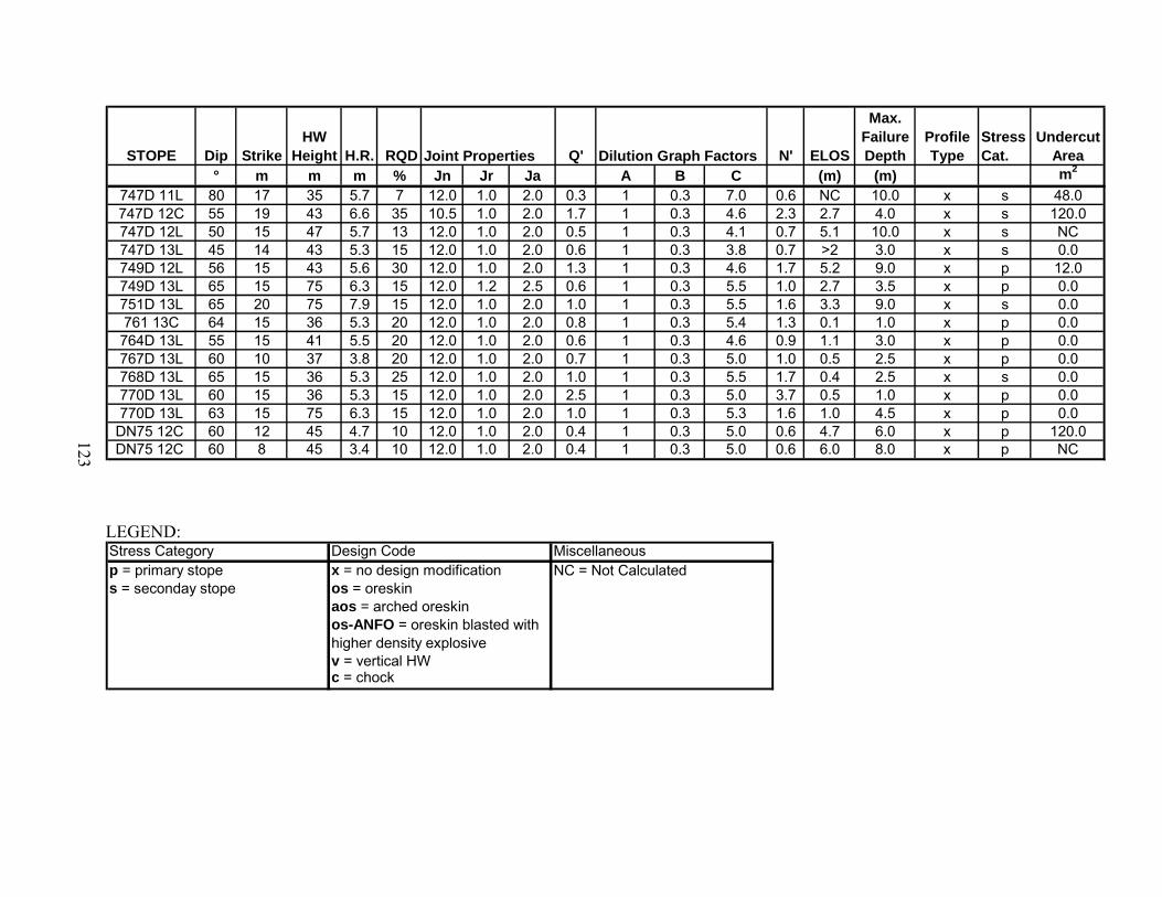
STOPE Dip StrikeHW
Height H.R. RQD Joint Properties Q' Dilution Graph Factors N' ELOS
Max. Failure Depth
Profile Type
Stress Cat.
Undercut Area
° m m m % Jn Jr Ja A B C (m) (m) m2
747D 11L 80 17 35 5.7 7 12.0 1.0 2.0 0.3 1 0.3 7.0 0.6 NC 10.0 x s 48.0747D 12C 55 19 43 6.6 35 10.5 1.0 2.0 1.7 1 0.3 4.6 2.3 2.7 4.0 x s 120.0747D 12L 50 15 47 5.7 13 12.0 1.0 2.0 0.5 1 0.3 4.1 0.7 5.1 10.0 x s NC747D 13L 45 14 43 5.3 15 12.0 1.0 2.0 0.6 1 0.3 3.8 0.7 >2 3.0 x s 0.0749D 12L 56 15 43 5.6 30 12.0 1.0 2.0 1.3 1 0.3 4.6 1.7 5.2 9.0 x p 12.0749D 13L 65 15 75 6.3 15 12.0 1.2 2.5 0.6 1 0.3 5.5 1.0 2.7 3.5 x p 0.0751D 13L 65 20 75 7.9 15 12.0 1.0 2.0 1.0 1 0.3 5.5 1.6 3.3 9.0 x s 0.0761 13C 64 15 36 5.3 20 12.0 1.0 2.0 0.8 1 0.3 5.4 1.3 0.1 1.0 x p 0.0764D 13L 55 15 41 5.5 20 12.0 1.0 2.0 0.6 1 0.3 4.6 0.9 1.1 3.0 x p 0.0767D 13L 60 10 37 3.8 20 12.0 1.0 2.0 0.7 1 0.3 5.0 1.0 0.5 2.5 x p 0.0768D 13L 65 15 36 5.3 25 12.0 1.0 2.0 1.0 1 0.3 5.5 1.7 0.4 2.5 x s 0.0770D 13L 60 15 36 5.3 15 12.0 1.0 2.0 2.5 1 0.3 5.0 3.7 0.5 1.0 x p 0.0770D 13L 63 15 75 6.3 15 12.0 1.0 2.0 1.0 1 0.3 5.3 1.6 1.0 4.5 x p 0.0
DN75 12C 60 12 45 4.7 10 12.0 1.0 2.0 0.4 1 0.3 5.0 0.6 4.7 6.0 x p 120.0DN75 12C 60 8 45 3.4 10 12.0 1.0 2.0 0.4 1 0.3 5.0 0.6 6.0 8.0 x p NC
LEGEND: Stress Category Design Code Miscellaneousp = primary stope x = no design modification NC = Not Calculateds = seconday stope os = oreskin
aos = arched oreskinos-ANFO = oreskin blasted with higher density explosivev = vertical HWc = chock
123

Table 5.6: George Fisher Mine C-Orebody Dilution Graph Inputs from data in Capes et al., 2005 and 2007
STOPE Dip StrikeHW
Height H.R. RQD Joint Properties Q' Dilution Graph Factors N' ELOS
Max. Failure Depth
Profile Type
Stress Cat.
Undercut Area
° m m m % Jn Jr Ja A B C (m) (m) m2
703CD 12C 70 23 39 7.2 30 10.5 1 1.5 1.7 1 0.3 5.9 3.4 1.6 NC x NC NC703CD 11L 80 23 36 7.0 18 12 1 2 1.0 1 0.3 7.0 1.6 2.0 NC x NC NC705CD 12C 79 19 36 6.2 39 9 1 1 4.3 1 0.3 6.9 8.9 0.0 NC x NC NCCN71 13C 55 25 42 7.8 18 12 1 2 0.8 1 0.3 4.6 1.0 5.0 NC x NC NCCN71 12L 65 15 39 5.4 40 9 1 2 2.2 1 0.3 5.5 3.6 0.0 NC x NC NC
CN71 12C P1 68 12 41 4.6 40 9 1 1 6.7 1 0.3 5.7 11.5 0.7 NC x NC NCCN71 12C P2 70 12 39 4.6 60 9 1 1 6.7 1 0.3 5.9 11.9 0.0 NC x NC NCCN71 12C P3 70 12 39 4.6 60 9 1 1 6.7 1 0.3 5.9 11.9 0.0 NC x NC NC
124

125
The Jn, Jr, Ja values were not regularly collected by the geologists and had to be determined
by the rock mechanics engineer from the core or from underground observations. The drill core
is only on the racks for a short period of time (days) and a long period of time (months to years)
passes prior to a stope for which the core data could be used is mined. This created a logistical
problem for the collection of the joint parameter data. Personnel shortages coupled with
problems with core storage and degradation made relogging the core unfeasible. Core photos
were available but it is difficult to determine Jr and Ja from photos as physical measurements are
required. Techniques used to obtain Jn, Jr, Ja data through underground mapping of HW
exposures are more suitable for the definition of these joint surface conditions parameters as
described in Milne et al. (1992). These techniques which provide simple, repeatable results were
described in section 2.2.2. Two examples of HW exposures from which joint parameter
information was obtained are shown in Figure 5.17. The tool used to measure joint roughness is
shown in Figure 5.18 along a joint plane. It was difficult to obtain a 5 m average of joint
conditions to input into the Q’ index as a 5 m exposure of the HW was not typically available for
underground mapping. Window mapping of the HW exposures was conducted to identify the
most typical joint condition parameters which would affect the stope instability. The properties
of the joint set most detrimental to stability were used for design. This set corresponds to the
joint set orientation giving the lowest B value with the Stability N’ calculation (section 4.2.1).
Underground observations made of D-orebody’s HW joint conditions indicated Jn = 12 (3 joint
sets plus random), Ja = 1-2 (surface staining-slightly altered, shiny slippery) and may increase to
Ja = 2-4 (graphitic infill is present). Observations made underground in D-orebody indicated
fewer observable joint sets Jn < 9 (~3 joint sets), and Ja =1 (surface staining only). Joint
roughness in the ore and HW was typically found to be related to the amount of shearing,
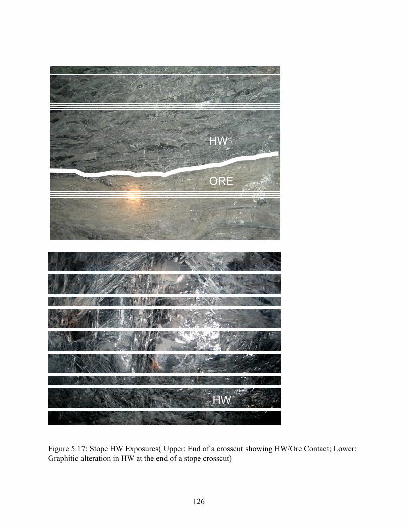
126
Figure 5.17: Stope HW Exposures( Upper: End of a crosscut showing HW/Ore Contact; Lower: Graphitic alteration in HW at the end of a stope crosscut)
ORE
HW
HW

127
Figure 5.18: Carpenter’s Comb tool used for estimating Jr-joint roughness

128
folding, or faulting through the orebody (Jr =1 – 2). Smoother, more altered joint surfaces tended
to coincide with areas of shearing, folding and faulting. These values were similar to the values
collected by Robinson and Sharrock (2002) which were determined between 13L-11L (Figure
5.12) from underground mapping as Jn =9-12, Jr =0.5-1.5, Ja = 1-3.0. The collected joint
condition data is also presented for each stope in Table 5.5 and is described as follows.
For the 40 cases where the ore was included with the HW in the 5m average RQD estimation,
the joint condition values were estimated to reflect the relative amount of HW and ore in the 5m
interval. If the 5m average RQD indicated a rock mass typical of the ore (i.e. RQD > 40%) then
the typical ore joint condition parameters were applied. If the RQD was 20- 40 %, more typical
of a mixture of the HW and ore rock mass, then an average of the ore and HW joint conditions
was used. The requirement to understand the variation of joint condition parameters in different
geological domains partially contributed to the development of three rock categories discussed in
the next section.

129
5.4.5 Rock Categories within the 5m HW Domains
During collection of rock mass data to define the 5 m average domains, variations in
geological and geotechnical characteristics were observed within this 5m wide domain. This was
particularly evident when RQD data was plotted against distance within the ore and HW domains
(Figure 5.15-5.17). The term Rock Categories is introduced to describe the geotechnical and
lithological changes that have been observed in the 5m HW domain chosen for design. Three
typical cases of Rock Categories were observed and often could be related to lithology. This
section introduces the 3 rock categories. It was thought that the variation of these categories
within the 5 m average could influence the HW response to mining. Chapter 7 assesses the
behaviour of these rock categories in more detail to see if they can be used to correct for the
effect of the single input (average) of rock mass quality required for the Dilution Graph.
The 3 rock categories could be defined in the HW and ore domains based on the logged drill
core runs which typically ranged between 1-3m. In relation to the definition of the geological
domains in 5.3.3, the sulphides would most commonly be found in the ore domains while the
siltstones and shales would predominantly exist in the HW domain. Category 1 rock was typical
in ore domains while Category 2 and 3 were both typical in the HW domain. The geotechnical
characteristics of each rock category are shown in Figure 5.19 and described below.
The category 1 rock would appear as pyritic shales, siltstone beds, or narrow mineralized
areas with RQD > 40%. The joint parameter observations suggested bedding and an additional 1-
2 joint sets with surfaces that could be scratched with a knife and had a smooth, planar character
(Fig. 5.19).
The category 2 domain shown appeared as a combination of shales and siltstones having
variable bedding thickness with an additional 2 joint sets plus random joints. RQD was typically

130
20-40%. The joint parameter observations suggested joint sets with surfaces that could be
scratched with a knife and had a smooth, planar to wavy character (Fig. 5.19).
The category 3 domain was similar to the category 2 domain in terms of rock type. However,
the effect of the shearing contributed to RQD < 20%, commonly < 10%. It was composed
predominantly of thinly bedded shales which often exhibited bedding parallel shears having a
smooth, planar to wavy character often with a graphitic infill. Bedding and an additional 3 joint
sets defined the block size (Figure 5.19).
Each rock category has unique RQD values with specific joint parameters. Thus, abundant
RQD drillhole data, especially above the 11L elevation (Figure 5.13), could be used as an
indicator of a structural domain if underground mapping of the joint parameters was not
available. RQD drillhole data was available on a 15 m spacing along strike and approximately
10m up dip with 3 holes per ring over 1 sublevel (30 m) for stopes above the 11L elevations. The
drillhole data below this elevation existed on a greater spacing but there were drives orientated
along the HW which provided opportunity for geotechnical data collection. Above 11L, drives
were only mined perpendicular to the HW which reduced the amount of near HW data which
could be observed during the development stage. However, on occasions for specific mine
design purposes, the crosscuts extended into the HW which allowed for observations of the
changing structural domains on a 5m x 5m scale to verify domains defined from the drillhole
data. The drillhole and mapping data enable the refinement of the HW domain into the 3
different categories.

131
Category 1
RQD > 40%Jn < 6-9Jr = 1Ja = 1Q’ = 4.4
Category 2
RQD = 20- 40%Jn = 12Jr = 1Ja = 2Q’ = 0.8-1.6
Category 3
RQD <10-20%Jn = 12-15Jr =1-2Ja = 2-4Q’ = 0.3-0.8
Figure 5.19: 3 Rock Categories defined within the HW Domain

132
5.5 Summary
With much support from industry, knowledge was gained and data was collected over a
period of 4 years through discussions at industry short courses, site visits, consultants’ visits,
employment, and research at underground mines in Canada, Australia, and Kazakhstan. Data
collection was focussed in areas of the Dilution Graph which previously lacked data. The level of
detail in data collection was enhanced when the author was an employee at a mine site as
opposed to a researcher or consultant. The data collection included a total of 255 HW cases of
which 169 were collected from mine sites and 86 were from literature. This data is analysed
using engineering judgment and statistical methods in Chapter 6 to determine new positions for
the empirical Dilution Graph design lines based on 255 HW cases, a significant improvement
upon the 47 HW and 41 FW cases used to create the original design lines.
During the collection of data at the Xstrata Zinc George Fisher mine, variations in the rock
quality were found within the average HW rock mass conditions which are required to define a
single input for the Dilution Graph. Observations of these variations defined three possible rock
categories with specific geotechnical and lithological characteristics. Chapter 7 assesses the
behaviour of these rock categories in more detail to see if they can be used to correct for the
effect of the single input (average) of rock mass quality required for the Dilution Graph.

133
CHAPTER 6 STABILITY LIMITS FOR OPEN STOPE HW DESIGN
This chapter presents a discussion on the development of new ELOS design lines for the
Dilution Graph based on different levels of detail for data collection and analysis. The databases
on which the lines are based were discussed in Chapter 5. Preliminary design lines, created using
a limited database and engineering judgment, are refined with additional data and the use of
logistic regression models. Statistical classification analysis is used to examine how well the
logistic regression models fit the data and to define a set of design lines which provide the
highest percentage of correctly predicted cases. A discussion is also presented on the limitations
of the design method which can be broadly described as difficulties in defining rock mass
conditions and the influence of mining factors. Empirical data and observations of some of these
mining factors at the George Fisher mine are discussed. Considerations of error in the
determination of H.R. and ELOS are presented along with observations and empirical data on the
influence of time, blasting, faulting, stress, and undercutting.
134
6.1 Preliminary Revision of Dilution Graph Lines
Initially, preliminary design lines were created using engineering judgment based on the
collected empirical data in Canada from the Callinan “777” mine and Rabbit Lake Mines and the
original Clark database. The collected databases, consisting of 27 and 11 case histories
respectively, were plotted on the Dilution Graph template at the end of 2003 (Figures 5.6 and
5.7). Trends were observed between Hydraulic Radius, Stability Number and amount of HW
overbreak which suggested the original dilution lines could be improved upon. A preliminary
revision to the ELOS lines, using the same values (0.5, 1, and 2 m) as the original ELOS lines,
were created using the compiled data and engineering judgment (Figure 6.1). The dataset was
then taken to the George Fisher mine in Australia to collect addition data and test the use of the
preliminary lines as a predictive design tool. George Fisher mine data (Figure 5.11) was added to
the new Dilution Graph database as it was collected and an ELOS = 4m line was created (Figure
6.1). The preliminary revision to the Dilution Graph lines are shown with the final number of
collected cases from the sites visited (169 cases) and Clark (1998) data (39 cases) in Figure 6.1
and alongside the original Dilution Graph and Modified Stability Graph lines in Figure 6.2. The
curvature of the revised lines was in agreement with the lines from the Modified Stability Graph,
which has significantly more case histories then the original Dilution Graph. The revised dilution
lines, however, varied significantly from the original dilution lines. The lines were truncated at
N’ =1 due to a lack of data. During this stage of analysis, a quantitative statistical assessment of
the graph’s predictive ability was not completed. The use of the revised lines at the mine had
proved successful enough such there were was no reason to change their position. However,
during the application of the method, many limitations were noted (Section 6.4) and additional
design tools were developed (Chapter 7) to improve upon some of these limitations.
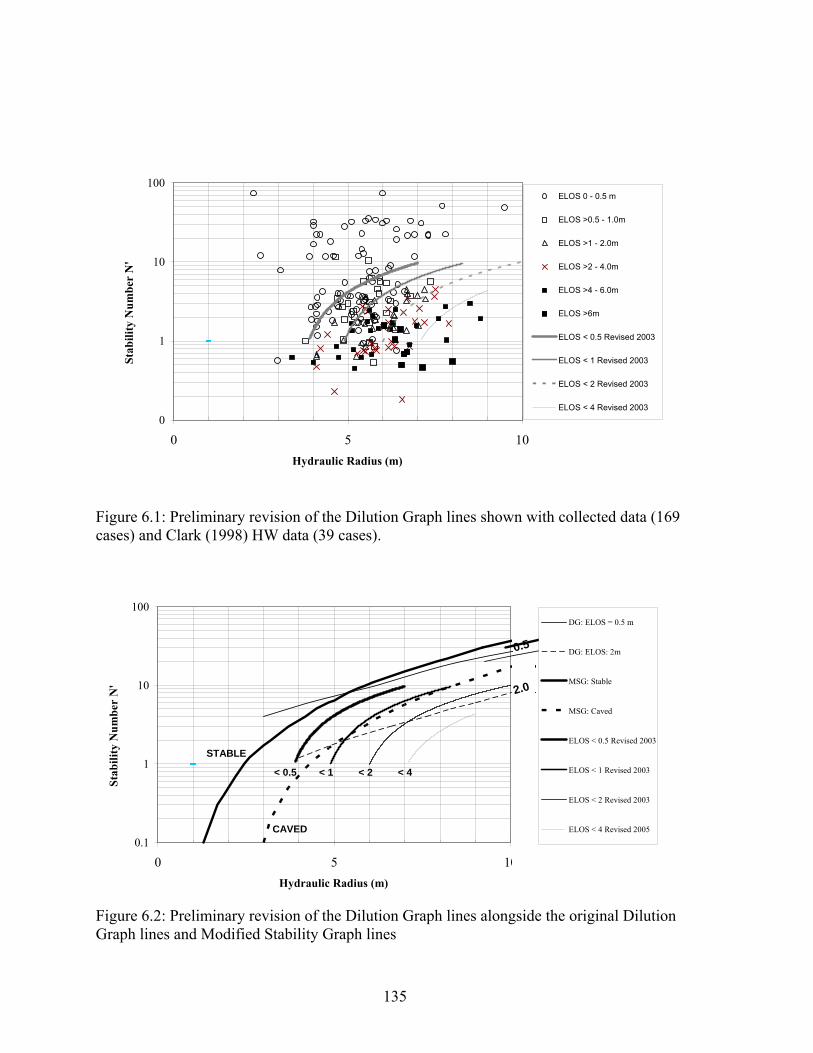
135
Figure 6.1: Preliminary revision of the Dilution Graph lines shown with collected data (169 cases) and Clark (1998) HW data (39 cases).
Figure 6.2: Preliminary revision of the Dilution Graph lines alongside the original Dilution Graph lines and Modified Stability Graph lines
0.1
1
10
100
0 5 10Hydraulic Radius (m)
Stab
ility
Num
ber
N'
< 0.5 < 1 < 2 < 4
CAVED
STABLE
0.5
2.0
DG: ELOS = 0.5 m
DG: ELOS: 2m
MSG: Stable
MSG: Caved
ELOS < 0.5 Revised 2003
ELOS < 1 Revised 2003
ELOS < 2 Revised 2003
ELOS < 4 Revised 2005
0
1
10
100
0 5 10Hydraulic Radius (m)
Stab
ility
Num
ber
N'
ELOS 0 - 0.5 m
ELOS >0.5 - 1.0m
ELOS >1 - 2.0m
ELOS >2 - 4.0m
ELOS >4 - 6.0m
ELOS >6m
ELOS < 0.5 Revised 2003
ELOS < 1 Revised 2003
ELOS < 2 Revised 2003
ELOS < 4 Revised 2003

136
At the end of data collection, the final GF database (131 cases), Rabbit Lake Database (11
cases), Callinan Database (27 cases), and the literature data from Clark (1998) (39 cases) and the
Nevada weak rock mass database (Brady et al., 2005) (47 cases) were compiled. The compilation
(255 cases) is shown in Figure 6.3 with the Modified Stability Graph and original Dilution Graph
stability lines and in Figure 6.4 with the revised ELOS lines. The number of cases from each
ELOS category plotting in the defined stability zones were counted to determine how well the
data agreed with the existing and revised lines. A summary of the results for each set of lines are
shown in Tables 6.1 and 6.2 and discussed in the following paragraphs.
The number of cases from each ELOS category were first compared to the stable, transition,
and caved zones of the Modified Stability Graph and to the ELOS = 0.5 m, ELOS 0.5-2m zone,
and ELOS = 2m zone of the Dilution Graph. The cases were classified as undefined where the
Dilution Graph lines are truncated. Table 6.1 describes the percentage of points from each ELOS
category plotting in the existing defined stability zones. For the compiled database of 255 cases,
the key observation from the existing lines is that no case with ELOS > 1 m plots in the stable
zone or above the ELOS < 0.5 m line. In addition, 80 and 90% of the ELOS > 2m cases
respectively plot below the ELOS > 2m line and in the caved zone. However, some ELOS data
points have a lower value than the zone in which they plot. It was an interesting exercise to
classify the data in relation to the original DG and MSG lines. The data in Table 6.1 can be
simply used to estimate quantitative values for the MSG stability lines.
The number of cases from each ELOS category were then compared to the preliminary
revision of the Dilution Graph lines. Table 6.2 describes the percentage of points from each
ELOS category plotting in the zones defined by these lines. There are a significant number of
undefined cases due to the truncation at N’ =1. There were no points with ELOS > 1 plotting

137
Figure 6.3: Data shown with MSG and DG Design lines
Table 6.1: Compiled Data Percentage Correct in relation to the Original Dilution Graph (DG) and the Modified Stability Graph (MSG) ELOS 0.0-0.5 m >0.5-1.0m >1-2.0m >2.0-4.0m >4m
StabilityZone # Cases % # Cases % # Cases % # Cases % # Cases %ELOS <0.5 33 31 2 5 0 0 0 0 0 0ELOS 0.5-2 52 49 20 51 9 23 4 11 1 3ELOS >2 13 12 8 21 26 67 29 81 33 94Undefined 8 8 9 23 4 10 3 8 1 3MSG upper 35 33 5 13 0 0 0 0 0 0Transition 56 53 22 56 6 15 3 8 1 3MSG lower 15 14 12 31 33 85 33 92 34 97
35 Cases106 Cases 39 Cases 39 Cases 36 Cases
0.1
1
10
100
0 5 10
Hydraulic Radius (m)
Stab
ility
Num
ber
N'
MSG: Stable
MSG: Caved
DG: 0.5 m ELOS
DG: 2m ELOS
ELOS 0 - 0.5 m
ELOS >0.5 - 1.0m
ELOS >1 - 2.0m
ELOS >2 - 4.0m
ELOS >4 - 6.0m
ELOS >6m

138
Figure 6.4: Preliminary Design Lines shown on the DG template with 255 cases
Table 6.2: Compiled Data, Percentage Correct in relation to Preliminary Revision of the Dilution Graph Design Lines ELOS 0.0-0.5 m >0.5-1.0m >1-2.0m >2.0-4.0m >4m
StabilityZone # Cases % # Cases % # Cases % # Cases % # Cases %ELOS < 0.5 57 54 10 26 0 0 0 0 0 0ELOS 0.5 - 1 23 22 13 33 4 10 3 8 1 3ELOS 1 - 2 16 15 5 13 14 36 6 17 10 29ELOS 2 - 4 0 0 1 3 5 13 6 17 5 14ELOS > 4 0 0 0 0 0 0 1 3 5 14Undefined 10 9 10 26 16 41 20 56 14 40
106 Cases 39 Cases 39 Cases 36 Cases 35 Cases
0.1
1.0
10.0
100.0
0 5 10
Hydraulic Radius (m)
Stab
ility
Num
ber
N'
ELOS 0 - 0.5 m
ELOS >0.5 - 1.0m
ELOS >1 - 2.0m
ELOS >2 - 4.0m
ELOS >4 - 6.0m
ELOS >6m
ELOS < 0.5 Revised 2003
ELOS < 1 Revised 2003
ELOS < 2 Revised 2003
ELOS < 4 Revised 2003

139
above the ELOS <0.5 m line. However, there was less than 20% correct classification for the
ELOS > 2-4m and ELOS > 4m cases for the revised lines compared to >80% correct
classification for the Modified Stability Graph and Dilution Graph lines. This is partially due to
the conservative definitions of the original design lines and partially due to the number of
undefined cases included in the analysis. Thus the analysis was repeated excluding the undefined
cases. The revised results are shown in Table 6.3. The revision increased the percentage of cases
but did not adequately classify the cases for the final database (255 cases).
The preliminary revised design lines for the Dilution Graph were based on engineering
judgment using an initial limited database collected in 2003. Upon further analysis with
additional data, the revised lines poorly classified the cases at the lower end of stability (i.e.
ELOS 2-4 m and ELOS >4 m). One of the objectives of the thesis was to create a new set of
design lines specific to the Dilution Graph which provided improved prediction over the
preliminary lines. Thus, the use of logistic regression, a statistical method commonly used to
delineate stability zones (for example Clark, 1998; and Mawdesley and Trueman, 2003) is
applied in the next section to determine a set of ELOS lines that provide the highest percentage
of correct classification.

140
Table 6.3: Compiled Data, Percentage Correct in relation to Preliminary Revision of the Dilution Graph Design Lines with undefined cases removed ELOS 0.0-0.5 m >0.5-1.0m >1-2.0m >2.0-4.0m >4m
StabilityZone # Cases % # Cases % # Cases % # Cases % # Cases %ELOS < 0.5 57 59 10 34 0 0 0 0 0 0ELOS 0.5 - 1 23 24 13 45 4 17 3 19 1 5ELOS 1 - 2 16 17 5 17 14 61 6 38 10 48ELOS 2 - 4 0 0 1 3 5 22 6 38 5 24ELOS > 4 0 0 0 0 0 0 1 6 5 24Total Defined 96 29 23 16 21Undefined 10 10 16 20 14
106 Cases 39 Cases 39 Cases 36 Cases 35 Cases
6.2 Use of Statistical Methods to define Stability Lines
Logistic regression models and classification analysis are presented in this section to develop
a quantifiable set of ELOS lines for the database composed of 255 cases. The logistic regression
method, described in section 4.3, is used to statistically delineate the ELOS boundaries.
Classification analysis can then be used to examine the model fit and quantify the number of
correct and incorrect cases in relation to the logistic regression models. An interpretation of the
classification analysis is used to determine the logistic regression models which maximise
correct classification for each particular design line. To show the effect of additional data on the
logistic regression models used to create design lines, the database compiled by Wang (2004) is
included.
Logistic regression methodology can be used to model design lines for the cases of ELOS <
0.5, <1, < 2 and < 4 m for different combinations of data. A set of ELOS lines can be modelled
for any level of probability. The model is based on the collected data and the local external
factors which created stability or instability. Depending on the database chosen and desired
probability of prediction, many different positions of design lines can be created.

141
Logistic regression models were computed for the combined database of the 255cases
using the SPSS (Statistical Package for the Social Sciences) (2005) software. To run the model
for each design line, it was necessary to divide the 255 cases into two categories (ELOS <
selected dilution line and ELOS ≥ selected dilution line). The models are used to predict the
probability (P) of an occurrence with a categorical response such as a yes (P=1) or no (P=0)
answer rather than as a continuous variable. For example, the data used to model the ELOS < 0.5
m line was divided into categories of actual ELOS < 0.5 m (P=1) and actual ELOS > 0.5 m
(P=0). With the use of the input variables (Xi) which are H.R. and N’ and the assigned
probability (P) for each case in the database, the software uses an estimation to generate
coefficients (Bi) for the input variables of equation 4.4 (the logit function: ln(P/(1-P)) = B1X1 +
B2X2….+ BO)) which maximize the probability of obtaining the inputted set of data.
The estimated values for the coefficients of the variables of the logit equation from the SPSS
analysis are shown in Table 6.4. Using the coefficients and intercept from Table 6.4 in equation
4.4 with an assumption of any value for P (probability of a case occurring), the equations can be
used to relate N’ and H.R. For all required values of H.R., the expected N’ can then be computed
for the particular probability assumption. A number of probability assumptions can be made to
create a set of design lines with different probabilities for each ELOS line. The probabilities can
also be expressed in terms of odds. A description of what the probability means in terms of the
odds of an ELOS case occurring are:
• For the probability of a case being 0.5, P = 0.5, ln(P/(1-P)) = 0; and the odds of being a
case to not being a case are equal to 1;
• For the probability of a case being 0.99, P = 0.99, ln(P/(1-P)) = 4.6; and the odds of
being a case to not being a case are equal to 99:1;

142
• For a the probability of a case being 0.8, P = 0.8, ln(P/(1-P)) = 1.4; and the odds of being
a case to not being a case are equal to 4:1.
Table 6.4: Coefficients for H.R., N’, and Intercept from SPSS computations for each ELOS line
ELOS H.R. N' Intercept< 0.5 -0.66 0.51 1.46< 1 -1.36 1.41 4.3< 2 -1.23 1.27 5.13< 4 -1.1 1.04 6.15
For ELOS< 0.5, the logit function: ln(P/(1-P)) = -0.66H.R. + 0.51N’+ 1.46
A series of logistic regression models was computed for each ELOS line (i.e. ELOS < 0.5 m).
The probability values of P =0.2, 0.5, 0.8, and 0.99 were used to create various sets of design
lines with the thought that P=0.99 would be a conservative design (99% of the cases that occur
above the 0.5m ELOS line would have ELOS < 0.5 m) and P= 0.2 would be an aggressive design
line. The probability values were chosen arbitrarily as a starting point to allow for an
interpolation of a set of probability lines which represented the highest number of correctly
classified cases. The ELOS < 0.5m line is shown for the 4 assigned probability values in Figure
6.5. Alternatively, all of the design lines (ELOS < 0.5, <1. <2, <4 m) for a single probability
assumption can be plotted as shown for P=0.8 in Figure 6.6. Classification analysis was then
used to determine the number of cases which plotted correctly on each side of the modelled
ELOS lines. The numbers of correct and incorrect predictions for each modelled ELOS lines at
each of the 4 probability assumptions are shown in Table 6.5. For example, consider ELOS <
0.5 m and the model with P=0.8. There are 145 points with ELOS > 0.5 m plotting below the
ELOS < 0.5 m modelled line (correct prediction) and 3 points with ELOS > 0.5 m plotting above
the ELOS < 0.5 m modelled line (incorrect prediction). There are 41 points with ELOS < 0.5 m

143
plotting above the ELOS = 0.5 m modelled line (correct prediction) and 67 points with ELOS >
0.5 m plotting below the ELOS < 0.5 m modelled line (incorrect prediction). The spread of the
data which influenced this particular modelled line creates a model which is very good at
predicting that a case with ELOS > 0.5 m only occurs incorrectly above the design line or less
stable than predicted 3 out of 148 times. Alternatively, 67 out of 108 cases which had ELOS <
0.5 plotted below the ELOS = 0.5 design line, or are more stable than predicted.
To determine the probability lines which represent the highest number of correct predictions
above and below each ELOS line, the values in Table 6.5 are plotted in Figure 6.7. Interpolation
can be used to approximate the probability line with the highest percentage of correct
classification. Iteration can then be used to maximise the prediction around the approximation.
The lines based on the maximised predictions are shown in Figure 6.8 and represent a division
where the largest number of correct classifications occurs for each category of data for a specific
ELOS line. For example, in consideration of the ELOS < 4 line, the P=0.86 logistic regression
line results in 28 of the 35 cases with ELOS > 4 plotting below the ELOS < 4 line and 172 of the
222 cases with ELOS < 4 plotting above the line. This results in a maximised 80% and 77%
correct classification respectively. From the data in Figure 6.7, it is observed that all the design
lines in Figure 6.8 have approximately 80% correct classification on either side of the respective
design line.
If the probability of having a stable HW is essential, a set of conservative design lines can be
determined from Table 6.5. The P=0.99 values represent the condition where the number of
cases with a value greater than the particular ELOS line value plotting above that line is
minimised (Figure 6.9). A limitation with this assumption is a decrease in the overall number of
cases with correct prediction.

0.1
1
10
100
0 5 10
Hydraulic Radius (m)
Stab
ility
Num
ber
N'
MSG: Stable
MSG: Caved
DG: 0.5 m ELOS
DG: 2m ELOS
ELOS < 0.5, P=0.8
ELOS <0.5, P=0.2
ELOS < 0.5, P=0.5
ELOS < 0.5, P =0.99
ELOS 0 - 0.5 m
ELOS >0.5 - 1.0m
ELOS >1 - 2.0m
ELOS >2 - 4.0m
ELOS >4 - 6.0m
ELOS >6m
P=0.99
P=0.80
P=0.50 P=0.20
Figure 6.5: Use of Logistic Regression to define P=0.2, 0.5, 0.8, and 0.99 design lines for ELOS <0.5 (255 cases)
144

0.1
1
10
100
0 5 10
Hydraulic Radius (m)
Stab
ility
Num
ber
N'
MSG: Stable
MSG: Caved
DG: 0.5 m ELOS
DG: 2m ELOS
P=0.8 ELOS < 0.5
P=0.8 ELOS <1
P=0.8 ELOS < 2
P=0.8 ELOS <4
ELOS 0 - 0.5 m
ELOS >0.5 - 1.0m
ELOS >1 - 2.0m
ELOS >2 - 4.0m
ELOS >4 - 6.0m
ELOS >6m
ELOS < 0.5EL
OS
< 2
ELO
S <
1
ELO
S <
4
Figure 6.6: Use of Logistic Regression to define P=0.8 design lines (For ELOS< 0.5, the logit function: ln(P/(1-P)) = -0.66H.R. +
0.51N’+ 1.46 (255 cases))
145

146
Table 6.5: Logistic Regression Model Classification Results (Modelled vs Actual) ELOS Probability Actual ELOS > ELOS line Actual ELOS < ELOS line Overall
Correct Incorrect % Incorrect Correct % % Correct0.5 0.2 66 82 45 4 104 96 660.5 0.5 132 16 89 44 64 59 770.5 0.8 145 3 98 67 41 38 730.5 0.99 147 1 99 75 33 31 701 0.2 55 55 50 8 138 95 751 0.5 90 20 82 21 125 86 841 0.8 108 2 98 45 101 69 821 0.99 110 0 100 96 50 34 632 0.2 18 53 25 3 182 98 782 0.5 45 26 63 18 167 90 832 0.8 66 5 93 51 134 72 782 0.99 71 0 100 127 58 31 504 0.2 4 31 11 0 221 100 884 0.5 11 24 31 5 216 98 894 0.8 25 10 71 38 183 83 814 0.99 35 0 100 155 66 30 39
Note: Correct refers to actual ELOS with a value > ELOS line under consideration plotting below the line or an actual ELOS with a value < ELOS line under consideration plotting above the line
Logisitic Regression Classification Results
0
20
40
60
80
100
120
0.2 0.3 0.4 0.5 0.6 0.7 0.8 0.9 1
Probability
Perc
enta
ge C
orre
ct
ELOS > 0.5
ELOS < 0.5
ELOS > 1
ELOS < 1
ELOS > 2
ELOS < 2
ELOS > 4
ELOS < 4
Figure 6.7: Logistic Regression Classification for 255 case database

0.1
1
10
100
0 5 10
Hydraulic Radius (m)
Stab
ility
Num
ber
N'
MSG: Stable
MSG: Caved
DG: 0.5 m ELOS
DG: 2m ELOS
P=0.37: ELOS < 0.5
P=0.53: ELOS <1
P=0.68 ELOS < 2
P=0.84 ELOS <4
ELOS 0 - 0.5 m
ELOS >0.5 - 1.0m
ELOS >1 - 2.0m
ELOS >2 - 4.0m
ELOS >4 - 6.0m
ELOS >6m
ELOS: <0.5 <1 <2 <4
Figure 6.8: Dilution Graph based on highest percentage correct classification: 255 case database
147

0.1
1
10
100
0 5 10
Hydraulic Radius (m)
Stab
ility
Num
ber
N'
MSG: Stable
MSG: Caved
DG: 0.5 m ELOS
DG: 2m ELOS
99:1 ELOS < 0.5
99:1 ELOS <1
99:1 ELOS < 2
99:1 ELOS <4
ELOS 0 - 0.5 m
ELOS >0.5 - 1.0m
ELOS >1 - 2.0m
ELOS >2 - 4.0m
ELOS >4 - 6.0m
ELOS >6m
ELOS < 0.5
ELOS < 4
ELOS < 2
ELOS < 1
Figure 6.9: Use of Logistic Regression to define P=0.99 design lines for 255 case database
148

Depending on the database chosen and desired probability of a conservative or unconservative
prediction, many different positions of design lines can be created. The model fit and
classification analysis is only based on the collected data and the local external factors which
created stability or instability. To test the effect of cases from a different database on the position
of the dilution lines using logistic regression methodology, the Wang (2004) database (Figure
6.10) was added to the 255 cases. The Wang (2004) database consists of 150 (148 with H.R. <
10) HW case histories, which include 45 cases from Callinan Mine, 8 cases from Ruttan Mine,
and 97 cases from Trout Lake Mine. Most of the cases had N’ > 10 which is outside the zone of
interest for the study. The resulting design lines for the P=0.8 logistic regression analysis are
shown in Figure 6.11. A comparison between the modelled P=0.8 design lines for the 255 and
403 cases shows the effect of the additional data (Figure 6.12). It is interesting to note that the
Wang data had cases with ELOS >2 and 4 which plotted above the original Dilution Graph
ELOS <0.5 line and in the Modified Stability Graph stable zone. These points either suggest the
influence of some extreme site specific factors relative to the other database or the points are
based on erroneous data. Stope undercutting was reported as a significant problem in the Wang
(2004) database which may have biased the results. This additional data was presented for
discussion only to show the effect of additional data on the method used to determine the ELOS
lines and is not examined further.

150
Figure 6.10: Flin Flon, Canada area data from Wang (2004): 148 cases
0.1
1
10
100
0 5 10
Hydraulic Radius (m)
Stab
ility
Num
ber
N'
MSG:Stable
MSG:Caved
DG: 0.5m ELOS
DG: 2m ELOS
P=0.8 ELOS < 0.5
P=0.8 ELOS <1
P=0.8 ELOS < 2
P=0.8 ELOS <4
ELOS 0 - 0.5 m
ELOS >0.5 - 1.0m
ELOS >1 - 2.0m
ELOS >2 - 4.0m
ELOS >4 - 6.0m
ELOS >6m
ELOS < 0.5
ELO
S <
4
ELO
S <
2
ELO
S <
1
Figure 6.11: Use of Logistic Regression to define P=0.8 design lines for 403 cases
0.1
1
10
100
0 5 10
Hydraulic Radius (m)
Stab
ility
Num
ber
N'
Wang < 0.5 m
Wang 0.5- 1.0 m
Wang 1.0- 2.0 m
Wang 2.0-4.0 m
Wang 4 -6 m
Wang > 6 m
MSG: Stable
MSG: Caved
DG: 0.5m ELOS
DG: 2m ELOS

0.1
1
10
100
0 5 10
Hydraulic Radius (m)
Stab
ility
Num
ber
N'
ELOS < 0.5 (255 cases)
ELOS <1 (255 cases)
ELOS < 2 (255 cases)
ELOS <4 (255 cases)
ELOS < 0.5(403 cases)
ELOS <1(403 cases)
ELOS < 2(403 cases)
ELOS <4(403 cases)
ELOS < 0 5
ELOS < 4
ELOS < 2
ELOS < 1
ELO
S <
1ELOS < 0 5
ELO
S <
2
ELO
S <
4
Figure 6.12: Comparison of the P=0.8 design lines for 255 cases (dashed) and 403 cases (solid)
6.3 Limitations of Modified Dilution Graph
The collected data, from which the new sets of design lines were created, represents a wide
range of mining and rock mass conditions. Inaccurate overbreak predictions could occur if the
new design lines were applied to a mine that had a significantly different mining environment
than the conditions which existed at the mines used for developing the lines. The effect of these
factors is inherent within the created design lines. The factors limiting the applicability of the
empirical Dilution Graph design method are derived from the difficulty assessing the influence
of the many factors affecting ore extraction (mining factors). The main challenge facing the
accuracy of the design technique comes from the difficulty in quantifying strength properties for
a rock mass (rock mass conditions). These 2 general categories influencing HW dilution and
factors specific to the collected databases are explained in more detail in the following sections.

152
6.3.1 Rock Mass Conditions
A major source of uncertainty in estimating dilution is in quantifying rock mass properties
based on the Q’ classification system. Milne et al. (1992) present a review of the variability in
N’ based on challenges in determining Q’. Based on the reported subjectivity in estimating Q’,
and using the Dilution Graphs presented in this thesis, a 2.0 metre range in ELOS values could
easily be predicted (Capes et al., 2008). Techniques exist for reducing the subjectivity in
estimating Q’, however, these methods are seldom applied in a mining environment (Milne et al.,
1998).
There are other significant problems associated with obtaining representative rock
classification values which include the following:
• Limited HW exposure
• Difficulty interpreting core data
• Defining Structural Domains/Variable HW rock quality
• Multiple zones of HW rock (layered)
• Difficulty interpreting discrete features such as shears and dykes
At both the Rabbit Lake and George Fisher mines, the HW could fail through various zones of
altered HW rock to a higher quality rock. Existing empirical design methods require a single
value or average of the HW rock mass conditions and do not cater for the variable rock mass
quality. The effect of the various categories of rock in the HW at the George Fisher mine is
discussed in more detail in Chapter 7.
6.3.2 Mining Factors
The Dilution Graph method only provides a relationship between the open stope geometry,
rock mass conditions, and stope wall stability based on empirical data. There are many mining

153
controlled practices that will act to increase or decrease dilution. One mine’s standard mining
procedure could easily produce less dilution than another mine’s practice. Factors which are
external to the input parameters of the method have been seen
to potentially influence stability at various mine sites. These factors may include faulting,
stress, undercutting, blasting, and other mine specific factors. The effect of these factors is not
explicitly accounted for in the empirical methods and a widely used, industry design criteria for
these factors does not exist. It is very difficult to include these mining influences on predicted
HW dilution, though several authors have tried to quantify some of these factors. A partial list of
these factors is given:
• Blast damage. A mines blasting practice can significantly increase or decrease actual
dilution relative to predicted dilution (Clark, 1998).
• Complex HW geometries. Attempting to create complex HW geometries by following a
complex ore grade limit can significantly increase dilution. Quantifying this influence is
difficult. (Germain et al., 1996)
• Defining the HW span, height, and dip based on the location of the overcut and undercut
drives has been identified as a potential error in the calculation of H.R. (Forster et al.,
2007)
• Undercutting the HW undercut and overcut can lead to increased dilution. (Wang et al.,
2004; Yao et al., 1999; Suorineni et al., 1999)
• Cable bolt support is often installed to try and control dilution. The effect of different
degrees of cable support and cable installation cannot easily be assessed (Nickson, 1995).
• Delayed mucking and exposure time are recognised factors influencing dilution. (Wang
et al., 2003)

154
Empirical data and observations of some of these mining factors at the George Fisher mine
are presented in the next section. Considerations of error in the determination of H.R. and ELOS
are presented along with observations and empirical data on the influence of faulting, time,
stress, and undercutting. Historic stress data is further examined in Chapter 8 where it is
compared to predictions of stope HW overbreak interpreted from numerical modelling.
6.4 Observations and Potential Effects of some Site Specific Factors
This chapter provided a discussion on the use of the Dilution Graph as an estimate of HW
overbreak based on the average condition of the external factors from the compiled databases. It
is quite difficult to quantify the effect of the external factors. This is reflected by the lack of an
industry wide design methodology for the corrections of the errors in prediction caused by these
factors. For the George Fisher mine, the external factors were examined with various levels of
detail. A general discussion is presented on the potential error in the definition of the H.R. and
ELOS parameters, the effect of time on stope HW performance, consideration of blasting effects,
and relationship of faulting to HW RQD and overbreak. Empirical data showing the effect of
stress and undercutting on stope HW overbreak from 80 cases with no major design
modifications is also presented. A more detailed assessment of the effect of stress on stope HW
performance is presented in Chapter 8.
6.4.1 Consideration of Hydraulic Radius and ELOS Calculation
There are many ways in which error can exist in the determination of H.R. and ELOS
variables. Stopes were considered unsupported with the H.R. computed along the dip of the HW
from the floor of the bottom crosscut to the back (roof) of the top crosscut. Observations have
been made in various reports and at minesites where different definitions for HW height exist

155
based on local experience. An example of these definitions is shown from Forster et al. (2007) in
Figure 6.13. For the collected database, the effect of cable support in the drives was not included
as it did not result in pattern support of the HW, as described with the MSG (Potvin, 1988). For
the majority of the cases, if the effect of cablebolting would have been assumed, it would have
resulted in a correction of approximately 0.4 m for the Hydraulic Radius. If that were the case,
the cable bolted drifts would be treated as if they were rock abutments.
The definition of the H.R. will define the area over which the ELOS is calculated. Since the
H.R. was consistently defined for the entire database, ELOS was also consistently defined. The
Hydraulic Radius which results after blasting and mucking can be much different than the
planned Hydraulic Radius. This can result in a much different actual ELOS than predicted as the
boundary conditions for analysis have changed. For example, poor drill and blast techniques
which leave some of the ore unblasted can create a reduced H.R. and increase stability. If this is
not noted, this can lead to confusion between the planning engineers and the rock mechanics
engineer for future design. A planning engineer may interpret stability in a stope from the
planned H.R. If drill and blast practices improve, the previous stable stope under the planned
H.R. may fail with the enhanced extraction. Thus, team stope reconciliation is important to
define why stability or failure occurs in each stope HW. Further discussion on errors within
H.R. and ELOS is conducted as related to the effect of the external factors in the following
sections.

156
Figure 6.13: Three potential measurement to calculate the H.R. of a stope from Forster et al. (2007)

157
6.4.2 Effect of Time
Time is one of the most difficult factors to quantify in stope HW overbreak prediction.
Limited work had been conducted on examining the effect of time on stope overbreak except by
Ran (2002) and Wang et al. (2003). One of the difficulties for examining time is the difficulty in
obtaining CMS data when there are many other more pressing jobs required to meet daily survey
requirements. Occasionally, multiple CMS measurements are available from a particular stope.
The other difficulty is trying to quantify all of the time related overbreak effects. The factor is
composed of time-dependent, gravity-related failure in the relaxed or damaged zone of a stope
HW related to mucking of the stope, change in local induced stress due to nearby mining, and
daily effects from mine blasting events. Due to these difficulties, no attempt was made to
quantify the time factor. However, important information regarding assumptions in the Dilution
Graph was revealed. The key assumption relates to the representation of the CMS data as the
actual depth of failure of the stope based on profiles obtained during different stages of stope
extraction. Fortuitously, four different CMS profiles were obtained for one stope at monthly
intervals. The profiles shown in Figure 6.14 demonstrate a reducing amount of broken rock
against the HW with an increasing amount of HW overbreak for each monthly interval. The
effect of time between initial stope extraction and conducting the CMS survey of the final stope
profile can cause a large error in the calculation of ELOS. Fortunately, for stope reconciliation
purposes, geologists communicate with the technical services team to ensure an optimum time to
obtain a CMS survey, which is usually when the stope is empty. This is particularly the case in
primary stopes which are mucked empty to be backfilled with a cement fill and potentially mined
through at a later date. However, in secondary stopes, if the remaining muck in the stope is
waste, then the stope is not mucked to empty as it will be backfilled with waste rock. The final

158
database, from which the design lines were created, represents a wide range of times at which the
CMS profile was taken from different mining conditions.
Figure 6.14: Effect of stage of extraction on ELOS calculation from Capes et al. (2006)
30 m
WEST
Ore Drawdown
HW
FW
MonthlyFailure Profiles

159
6.4.3 Effect of Blasting
At the George Fisher mine the effect of blasting was not analysed to the same degree as the
other factors due to the relatively minor effect blasting has on dilution in a 20-m-wide ore body.
In general, the HW failures occur to a depth much greater than the influence of the highest
density explosive used. Based on the local experience of using 89 mm diameter blast holes on
the hanging wall blasting ring, < 2 metres of back break is expected with high density explosives
and < 0.5 metres for low density explosives. The majority of HW rings were charged with low-
density explosives except for a few cases noted in the database. These cases are described in
Chapter 7 to show the effect of using high-density explosive near a category 1 rock mass where
the high density explosive appeared to play a role in instability. Poor drill and blast can lead to
incomplete recovery of stope toes or ore left as a skin on the HW resulting in increased stability.
For example, Figure 6.15 shows a case where the toes of the blastholes remained intact after the
blast. This would result in a smaller H.R. than planned and reduce the ore recovery, but could
lead to increased stability in the HW. Blasting practices can be a major factor in Stope HW
overbreak. Understanding the effect of the local blasting practices will enable better predictive
capability for a design method such as the Dilution Graph. A stope which is predicted to have a
certain amount of HW overbreak using the method may have no overbreak due to poor ore
recovery. This can lead to a misunderstanding of the predictive capability of the Dilution Graph
if the effect of blasting is not recognised. The final database, from which the design lines were
created, represents a wide range of the effect of blasting from different mining conditions.

160
Figure 6.15: Effect of poor drill and blast recovery from Capes et al (2006)
6.4.4 Effect of Faulting
As for the other external factors, an industry wide design method does not exist for
quantifying the effect of faulting on stope HW stability. This is probably appropriate given the
broad nature of rock mass characteristics which can exist within a fault that may influence
stability. It was suggested by Sourineni et al. (1999) that faulting may be more of an influencing
factor than any of the other factors used to derive the Stability Number. There are three general
ways in which faulting can influence hanging wall stability and dilution:
• Faulting may change the stresses in the stope HW which will usually result in an increase
in the zone of HW relaxation;
• The overall rock stability may decrease due to an increase in jointing and possible joint
alteration; and
• The fault surface may form a potential failure surface.
Unblasted Material

161
At the George Fisher mine, the dextral offsets of the orebody from the NE trending faults
create domains which are divided into fault blocks. Further complexity is added by NS, NW and
NNE striking fault orientations that can produce either a loss or repeat of stratigraphy, local drag
folding, orebody attenuation and block rotation (Grenfell and Haydon, 2006). Throughout the
deposit there are many small faults (<2m displacement) that offset the orebodies and are very
difficult to anticipate from the drilling and nearby development, and can only be accounted for
once intersected (Sharrock and Robinson, 2002).
The effect of faults at the GF mine was examined with a general comparison between fault
location, RQD, and stope HW overbreak. Some trends between faulting and lower RQD values
were evident, but were not consistent. Areas where the major faults can be related to poor RQD
are highlighted in Figure 6.16. A trend can only be established for the S73 fault and lower RQD
values. There has also been failure next to the S73 fault on the majority of levels where the
stopes have been mined to the north of the fault. These stopes are highlighted in Figure 6.17. A
link between fault location, low RQD, and major overbreak (represented as maximum depth of
failure from the HW) does not exist for all the major north-east trending faults. This agrees with
the geological descriptions from Grenfell and Haydon (2006) that the major faults show variable
dextral offset, displacement and features. However, some of these trends may be hidden where
stope HW design modifications were implemented (55 of 131 cases) to reduce expected HW
failure. These modified cases represent the majority of the stopes with <0 m maximum depth of
failure in Figure 6.17.

Figure 6.16: Faulting Related to RQD at the GF Mine (RQD-Fault Trends Highlighted) after Capes et al. (2007)
S73: Zone of Influence
162

Figure 6.17: Faulting in relation to stope performance after Capes et al. (2007)
S73: Zone of Influence
163

164
6.4.5 Empirical Analysis of the Effect of Undercutting and Stress
An industry wide design approach does not exist for the effect of undercutting on stope HW
overbreak, while numerical modelling is commonly used in industry to assess the effect of stress
on stope HW performance. As part of an attempt to develop a design approach for industry,
Wang (2004) performed a numerical model comparison of the stress distributions in the case
with and without stope HW undercutting. Undercutting of a stope HW occurs when either
development drifts or stopes mined from below the current stope have broken through the ore-
HW contact in an area which may affect the mining of the current stope. The modelling
conducted by Wang (2004) suggested an increase in the relaxation zone with undercutting,
resulting in a larger zone of potential instability or overbreak (Figure 6.18). Henning and Mitri
(2007) presented a paper showing that secondary stopes should have a greater amount of
overbreak than primary stopes with the major principal stress orientated perpendicular to the
HW. Wang (2004) also showed that secondary stopes should have a greater zone of relaxation
than primary stopes. An empirical analysis is conducted in this section with the George Fisher
mine D-orebody data to verify this interpretation of modelling results and attempt to quantify the
effect of undercutting on stope HW performance under different stress categories and rock mass
conditions.
The cases which had design modifications made to the HW were removed from the
comparison. These design modifications, which were made to increase stability and are discussed
in Chapter 9, could include oreskins, ore chocks, ribrock, and vertical HW’s. The overbreak data
for this analysis is expressed in terms of maximum depth of failure as it is more representative of
the depth of relaxation relative to the Wang (2004) modelling. There were also more cases which
had maximum depth of failure measurements than ELOS calculations from which to conduct an

165
Relaxation Zone without undercutting
Relaxation Zone with undercutting
Undercut Drift
Overcut Drift
Footwall
Hanging Wall
Stope
Additional Relaxation Zone due to undercutting
Possible unstable zone due to undercutting geometry
Figure 6.18: Effect of Undercutting on relaxation zone (From Wang, 2004)
empirical analysis. The difference in meaning between maximum depth of failure and ELOS is
shown in Figure 6.19. An empirical relationship between ELOS and maximum depth of failure
based on the George Fisher D-orebody data is shown in Figure 6.20. The stress category and
undercutting data was presented in Table 5.5. With the cases with design modifications removed
from the analysis and the use of maximum depth of failure, there were 80 stopes available for
analysis.
The database was divided into categories which were expected to have different amounts of
HW overbreak based on previous theoretical studies. The first division of categories was based
on the division between primary and secondary stopes . The second division was made based on
the degree of undercutting. Wang (2004) showed the theoretical effect of undercutting but the
undercutting factor developed to account for the effect of various degrees of undercutting on
stope overbreak did not provide any obvious trends. Without any guidelines to follow, the
George Fisher database was examined to select an amount of undercutting which appeared to

166
divide the database into different amounts of HW overbreak. The undercutting data was collected
at the floor level of each stope analysed. To determine an average undercut value for each stope,
the value was based on the average depth and length of the undercutting area. Undercutting was
assessed as either >50 m2 or < 50 m2 at the floor level of the stope. Stope strike lengths were
fairly constant so it was not necessary to express the undercutting in terms of average undercut
area per metre of stope strike length. These values, referred to as major and minor undercutting
in the subsequent text, were chosen after a few other attempts at dividing the stopes into 3
categories resulted in too few cases to analyse. The third division was based on H.R intervals
(i.e. 4-5m). An attempt was then made to divide the H.R. intervals into categories based on N’
but there were too few cases. Thus average N’ values were used for the combined number of
cases in each H.R. category. To eliminate the effect of some of the mining conditions, stopes
which had HW design modifications, as presented in Chapter 9, were removed from the
database.
Figure 6.19: Comparison between maximum depth of failure and ELOS definition
HWFW
30 m
Drill and Blast Level
Extraction Level
W
CMS Profile
ELOS
Max. D
epth
of Fa
ilure
Planned Shape

167
ELOS vs Depth of Failure
y = 1.25x + 2.24
R2 = 0.71
0
2
4
6
8
10
12
14
16
18
20
0 2 4 6 8 10 12 14 16
ELOS(m)
Dep
th o
f Fai
lure
(m)
Figure 6.20: Empirical relationship between maximum depth of failure and ELOS values
The first division based on stress category showed that on average, the secondary stopes had
approximately 1.3 times greater depth of failure then the primary stopes (Figure 6.21). The
second division examined the effect of undercutting within each stress category. On average, in
primary stopes, there was a 1.1 times increase in depth of failure for stopes in the higher
undercutting category versus the lower undercutting category, while in secondary stopes there
was a 1.4 times increase in depth of failure between minor and major undercutting categories. To
determine useful correction factors for the Dilution Graph, the effect of undercutting within
combinations of rock quality and hydraulic radius would be required. The data was divided into
Hydraulic Radius categories with the average rock quality and depth of failure computed for the
defined regions. For most cases, the number of cases becomes too low for comparison. However,
the two circled areas in Figure 6.21 may present the best comparison of cases for the

168
effect of undercutting in primary and secondary stopes under specific hydraulic radius and rock
quality categories. These intervals suggest there is approximately 1.2 times increase in depth of
failure with the effect of undercutting in each stress category. These relationships can be used to
assist in stope HW overbreak prediction.
Figure 6.21: Effect of Stress and Undercutting on Stope HW performance
No Design Mods(80 stopes)
Primary(48 stopes)
N’ = 1.3 (0.5-4.1)H.R. = 5.6 (3.8-6.7)
DF = 6.4 (0-18)
Secondary(32 stopes)
N’ = 1.1 (0.2-2.4)H.R. = 5.9 (4.8-7.9)
DF =8.0 (0-16.5)
Undercutting < 50 m233 Cases
N’ =1.4 (0.7-4.1)H.R.= 5.7 (3.8-6.7)
DF =6.2 (0-18)
Undercutting > 50 m212 cases
N’ =1.1 (0.5-2.2)H.R.= 5.3 (4.0-6.3)
DF = 6.5 (2-14)
Undercutting < 50 m219 cases
N’ =1.1 (0.2-2.5)H.R.= 5.9 (4.9-7.9)
DF = 7.1 (0-15)
Undercutting >50m29 cases
N’ =1.4 (0.7-2.4)H.R.=6.2 (4.8-7.1)DF =8.9 (1-16.5)
H.R. 4-53 cases
N’= 1.7 (1-2.4)H.R. = 4.1 (3.8-4.4)
DF=1.2 (0-2.5)
H.R. 5-616 cases
N’= 1.2 (0.7-3.7)H.R. = 5.6 (5.2-5.8)
DF=5.5 (1-10)
H.R. 4-54 cases
N’= 0.6 (0.5-0.7)H.R.= 4.2 (4-4.7)
DF =6.5 (6-7)
H.R. 5-67 cases
N’= 1.2 (0.5-1.7)H.R. = 5.7 (5.3-5.9)
DF=6.0 (2-10)
H.R. 4-51 caseN’= 1.0
H.R.= 4.9DF=2.0
H.R. 5-611 cases
N’= 1.1 (0.6-2.1)H.R. = 5.5 (5.1-5.9)
DF=7.5(2.5-12)
H.R. 4-51 caseN’= 0.9
H.R.=4.8DF = 9.0
H.R. 5-61 caseN’=1.5
H.R.= 5.4DF= 5.5
H.R. 6-814 cases
N’= 1.4 (0.7-4.1)H.R. = 6.3 (6.0-6.7)
DF=8.0 (3-18)
H.R. 6-81 case
N’= 2.2 H.R. = 6.3
DF=10
H.R. 6-87 cases
N’= 1.1 (0.2-2.5)H.R. = 6.8 (6.2-7.9)
DF=7.1 (0-15)
H.R. 6-87 cases
N’= 1.4 (0.7-2.5)H.R. = 6.6 (6.1-7.1)DF=10.1 (1-16.5)
x 1.3
x 1.4x 1.1
Note: 3 Primary stopes had no Undercutting data
Note: 4 Secondary stopes had no Undercutting data

169
6.5 Summary
Revised ELOS lines for the Dilution Graph method, created using a limited database and
engineering judgment, were initially presented to demonstrate the evolution of data collection
and analysis in the study. With additional data and the use of statistical models, a few sets of
quantifiable design lines were created. Logistic regression models and classification analysis
were used to propose a set of ELOS lines which represented 80% correct prediction for the 255
case database. Alternatively, a conservative set of design lines was created that minimised the
number of cases with greater failure than predicted for all of the design lines. There were many
improvements to the dilution graph made upon the recommendations from Clark (1998). These
included increasing the number of HW case histories (47 stopes from 6 mines) in mainly good
quality rock masses to now 255 HW cases from a diverse range of rock mass and mining
conditions. The data bases presented in the thesis represent different mining practices as well as
different availability of rock mass classification data. The variability in the design lines reflects
the effect of the external factors for the databases considered. Like any design method, empirical
methods are useful tools for prediction when used for conditions similar to those which existed
for the development of the design method.
Empirical data and observations of some of the external factors at the George Fisher mine
were discussed. Considerations of error in the determination of H.R. and ELOS were presented
along with observations and empirical data on the influence of time, blasting, faulting, stress, and
undercutting. The time at which data was collected was considered to affect the calculation of the
H.R. and ELOS variables. Poor drill and blast recovery was observed to reduce the H.R. and
predicted ELOS. Individual fault characteristics were observed to play a role in stope stability.
The George Fisher mine data suggested 1.3 times greater failure in secondary stopes than
primary stopes. Analysis of the undercutting data suggested 1.2 and 1.4 times greater failure

170
between the cases of minor and major undercutting in primary and secondary stopes respectively.
The observations and empirical data can be used to assist stope HW overbreak prediction.

171
CHAPTER 7 EFFECT OF STRUCTURAL DOMAIN REVISIONS
An improvement to the Dilution Graph was developed in Chapter 6 for an area of the Dilution
Graph which previously lacked data. To determine a single value for rock quality as an input
parameter for the method, a structural domain must be defined for the HW. Some observations
during site visits and data collection suggested that a single value used to estimate the HW
domain could lead to erroneous overbreak prediction. This chapter investigates the rock
categories introduced in the detailed data collection in Chapter 5 to determine if a more detailed
assessment of the rock mass condition can improve the empirical HW dilution prediction. The
George Fisher mine, having an abundance of HW geotechnical drillhole data for analysis, is the
focus of the discussion. The case histories are shown in section 7.1 to represent some of the
observations collected for the analysis. Based on these observations, the potential failure
mechanisms are discussed in section 7.2. Empirical data is then presented in 7.3 to develop a
more rigorous design method based on the revised structural domains. The empirical data which
provides a relationship between domain scale and HW stability is compared to the Dilution
Graph method to determine if the revised domains improve prediction. The voussoir beam
analysis is applied in section 7.4 to examine the failure mechanisms from a theoretical viewpoint.
7.1 Observations and Case Histories
Many observations of failed stope HWs and reconciliation of the stope profiles with drillhole
data after mining suggested that stability could often be related to the positions of the rock

172
categories within the HW. Stability seemed to occur at a point in the stope HW where the
Category 1 rocks were intersected. To understand the HW failures and assess the behaviour of
the rock categories in more detail, case histories for a variety of stope failure profiles were
collected. Figures 7.1 – 7.10 show some of these case histories involving the different rock
categories. The case histories are a combination of open stope photos and drillhole data overlain
on stope profiles. Mining conditions underground are unfavourable for taking photos due to dust,
humidity, and limited time to capture data. However, a discussion of observations from the
higher quality photos is provided with each case history.

173
Figure 7.1: 716D 12C-11L RQD plot and domain adjacent to the stope profile. This is a secondary stope where a major failure was expected using predicted stress conditions from a boundary element model (Section 8.4.1). Faults and shears are shown as thick lines oblique to the orebody. Geological Domains are shown as thick lines parallel to the orebody. Local rock mass conditions limited depth of failure to 2–3 m as stope failed through Category 3 rock to the Category 1 domain (February 2004).
RQD Plot 716D 12C-11L (7163N Central)
0
10
20
30
40
50
60
70
-10 -5 0 5 10Distance from HW Contact(m)
RQ
D%
HWORE
Cat. 3 Cat. 1
D-FW D-HW
Drillhole
Plan View West
Cat. 3 Cat. 1Cat. 3 Cat. 1Cat. 3 Cat. 1

174
Figure 7.2a: 742D 12C-11L RQD plot and domain overlain on stope profile: The first thickness of Category 1 domain was stable under H.R =4.3 m, but failed under a H.R =5.6 m, failing through the Category 2 and 3 rock to the next Category 1 domain (May 2004).
0
10
20
30
40
50
60
70
-10 -5 0 5 10
RQD%
Distance from HW(m)
RQD Plot 742D 12C-11L(7440N upper)HangingwalOrebody
First Cat.1 Second
Cat.1
D-FW
D-HW
Drillhole
Cat.1 Cat.3 Cat.2
1st Cat.12nd Cat.1
Plan View West

175
Figure 7.2b: 742D 12C-11L Photo: As shown in Figure 7.2a, the first thickness of Category 1 domain was stable under H.R =4.3 m (11.m span), but failed under a H.R =5.6 m (17m span) through the Category 1 domain and Category 2 domain to the next Category 1 domain (May 2004). Note the reference dot in both photos representing the Category 1 domain which failed.
17 m HW span
11 m HW span Note: Dot represents similar position under each span
Stope will extend in this direction to 17m span
Area that will fail with 17m span

176
Figure 7.3: STOPE PHOTO: Looking west through the open stope. The photo shows failure through category 3 to category 1 rocks.
Category 1
Category 3

177
Figure 7.4: STOPE PHOTO 721D 11L-11C: Looking west from the FW side of the stope crosscut into the open stope. Photo shows failure through category 3 rock. Note the non-recovered Category 1 rock providing support for the Category 3 rock that hasn’t failed into the stope on the left side of the void.
Category 1
Category 3

178
Figure 7.5: STOPE PHOTO 746D 11L-11C: Looking west into the open stope. The photo shows Category 1 rock holding back Category 3 rock. As the stope was emptied of ore and the HW became fully exposed, the category 1 rock failed. As a result the Category 3 rock also failed. Stability did not occur until the next Category 1 structural domain was intersected.
Category 1
Category 3
Dilation

179
Figure 7.6: STOPE PHOTO 746D 12L-12C: Looking North along the HW of the open stope. Photo shows high grade sulphides as the Category 1 domain providing stability for the given stope H.R.
Category 1

180
Figure 7.7: Looking North along a failed HW showing evidence of failure profile bound by bedding planes, existing joint surfaces (planar-wavy), and new fractures (irregular surface)
Bedding PlanesNew Fractures

181
Figure 7.8: Looking down the mid-span of a HW of a nearly backfilled stope. This shows potential evidence of snap-thru failure mechanism. Refer to voussoir arch section (Section 7.4) for snap-through failure definition

182
Figure 7.9: Looking West through an open stope at the HW from the FW drill and blast access. Evidence of the drill and blast HW design oblique to bedding result in a true HW of stacked, bedded ore not recovered. This observation resulted in the development of a stability control method discussed in Chapter 10.
Stacked Bedding Planes

183
Figure 7.10: Looking at the NW upper corner of an open stope HW. Category 1 rock left against the HW is inhibiting the Category 3 rock from failing into the stope. A stope design stability control method was developed based on observations like this discussed in Chapter 10.
Category 3 rock
Category 1 rock

184
7.2 Observed HW Failure Mechanism
The observations of HW behaviour provided data to interpret the HW failure mechanism. In
general, observations indicated that HW overbreak was a function of the geometry of the HW
exposure and the spacing of the bedding planes which were represented by the rock mass
domains. Each HW had a unique combination of the 3 revised structural domains, discussed as
rock categories in section 5.4.5. However, all of the HWs had bedding planes of variable
thickness orientated parallel to the opening. Depending on the effects of past structural
processes, the number of joint sets varied for each rock category, as shown in Figure 5.19. The
interpreted HW failure mechanism during stope extraction, based on the observations, is
discussed in the following paragraphs.
When the HW was exposed during stope extraction, it would deform towards the opening as
there was no longer any confinement provided by the orebody. During the deformation process,
the bedding planes and joint surfaces would dilate. At some stage of deformation, the blocks
would detach from the rock mass and fall into the opening. At this point, the exact failure
mechanism is difficult to ascertain, but post failure photos demonstrate resultant failure profiles
bound by existing joint surfaces, existing bedding planes, and some new breaks across the
bedding (Figure 7.7). Figure 7.5 shows evidence of dilation of the Category 1 in front of the
Category 3 rock. Figure 7.8 may be an example of snap-through failure in thin bedding. It is
important to note that photos are not a quantitative measure and can only be used to surmise a
potential failure mechanism. Unfortunately, there was not HW access to the stopes to enable the
recording of quantitative deformation data through the use of extensometers.
The collected data suggests that Category 2 and 3 rocks would be unstable under the same
stoping conditions where Category 1 rocks were stable. Based on RQD core logging intervals of
1 to 3 m long, the bedding thickness in the Category 3 domain (RQD typically <10%) could have

185
a range of intact core lengths between 0.1- 0.3 m while for Category 1 domains (RQD 40% -
80%) the bedding thickness could have a range of intact core lengths between 0.4-2.4 m. These
observations suggest that HW overbreak is a function of the geometry of the HW exposure and
the thickness of the bedding planes in the domains. Empirical data is presented in section 7.3 to
quantify the observations by defining empirical stability limits between the extent of the
Category 1 rock and the HW response. Observations also suggested that there may be a snap-thru
beam failure mechanism as a function of bedding thickness and HW geometry. The voussoir
beam analogue is used in section 7.4 to validate the observed failure mode and examine
theoretical stability limits.
7.3 Revised HW Domains to Estimate Empirical HW Stability Limits
Stope HW overbreak profiles composed of Category 2 and 3 rocks in the near HW commonly
showed failure until a Category 1 rock was intersected. Case histories were collected to verify if
there was a stability relationship between the Category 1 rock thickness (metres of BQ core
>40% RQD) and stope Hydraulic Radius. It was thought that the relatively thin zones (< 5 m) of
higher RQD rock could be used as revised rock categories or structural domains to define
stability under a design criterion relating the HW Hydraulic Radius to Category 1 domain
thickness. These stable domains were not always a consistent lithology, but could often be
defined as pyritic shales, siltstone beds, or narrow mineralized zones. If they could be used to
improve overbreak prediction, then a revision could be investigated for the 5 m fixed domain
used in the determination of N’ for the Dilution Graph.
Data collected from 32 cases (28 stopes) where the Category 1 domains could be identified in
drill core data and related to a stope HW profile are shown in Table 7.1. For the 5m average
domain analysis (Chapter 5), there were other stopes that were assumed to have category 1 rock
in the HW based on nearby drill core data including stopes. A list of the stopes and the number

186
Table 7.1: Data for Category 1 rock analysis
STOPE Domain Domain HW HW HW H.R. Stable Unstable Extraction ELOS
Thickness Location Span Dip Height Profile Cat.(m) (m) (m) (m)
714D 11L-11C 1.9 ORE 10 38 45 4.1 x aos < 0.5716D 12L-12C 2 ORE 15 64 40 5.5 x aos < 0.5723D 13L-13C 2.5 ORE 13 58 46 5.1 x aos < 0.5732D12C-11L 5 ORE 15 45 47 5.7 x aos <1725D 13L-12L 2 ORE 16 58 90 6.8 x aos <1712D12C-11L 1.3 ORE 16 60 41 5.8 x aos <0.5728D11C-10L 5 ORE 15 48 45 5.6 x aos <0.5726D 13L-13C 9 ORE+HW 15 45 41 5.5 x aos <0.5711D 13L-13C 2.2 ORE 11 48 45 4.4 x os < 0.5712D 13L-13C 2 ORE 11 51 40 4.3 x os < 0.5716D 13L-13C 1 ORE 10 42 44 4.1 x os < 0.5728D 10C-9L 5 ORE 15 45 45 5.6 x os <0.5
730D 12C-11L 1.7 ORE 17 39 49 6.3 x os <0.5732D 11L-11C 5 ORE 15 36 56 5.9 x os <0.5733D 12C-11L 10 ORE 15 70 36 5.3 x os <0.5739D 12C-11L 5 ORE 15 80 40 5.5 x os <0.5742D 12C-11L 1.3 ORE 11 60 38 4.3 x os <0.5746D 12L-12C 2 ORE 15 60 41 5.5 x os <0.5719D 12C-11L 1.2 D-HW 10 50 38 4.0 x os-x 0.5 to 1742D 12C-11L 2.3 CD 13 60 38 4.8 x os-x 0.5 to 1730D 12L-12C 4 C-FW 15 40 47 5.7 x os-x >6747D 12C-11L 1 CD 10 55 43 4.1 x x 2 to 4726D 12L-12C 2.3 C-FW 16 43 50 6.1 x x >6737 12L-12C 3.1 C-FW 20 50 42 6.8 x x 4 to 6
716D 12C-11L 3.7 D-HW 18 66 39 6.2 x x 2 to 4721D 10C-9L 1.3 D-HW 14 45 49 5.4 x x < 0.5
726D 11C-10L 1.1 ORE 18 55 45 6.4 x aos-x 0.5 to 1730D 12L-12C 1.3 ORE 18 40 47 6.5 x os-x >6742D 12C-11L 1.3 ORE 17 60 38 5.9 x os-x 0.5 to 1719D 12C-11L 0.9 D-HW 15 50 38 5.4 x os-ANFO 0.5 to 1746D 11L-11C 1.7 ORE 12 55 42 4.7 x os-ANFO 4 to 6721D 10C-10L 1.9 D-HW 15 45 51 5.8 x x 1 to 2
of drillholes intersecting each stope HW is included on disk in the expanded database in
Appendix B. These are some stopes that did not have core data within the stoping limits. Due to
the significant variability in rock quality, it was felt that assessing these stopes, in the
development of a new design method, would add too much uncertainty to the data base. The 32
cases assessed only included stopes which contained a cored hole with recorded RQD data.

187
These 32 cases were divided up into HW conditions described as “x”, “aos”, and “os” as
shown in Figure 7.11. Figure 7.11 shows three approaches for mining a stope where the
immediate HW consists of category 2 or 3 rock. The “x” profile refers to a stope that was mined
without any design modifications such that the geological HW was the mining HW. These stopes
would typically fail until a Category 1 domain was reached in the HW (such as siltstone or
pyritic shale in the immediate D-HW, the CD sulphide lens or C-Orebody). Figure 7.11 also
shows typical positions of these domains. The “os” and “aos” profiles refer to stopes where
various amounts of category 1 ore were left unblasted inside the geological HW in an attempt to
mitigate HW failure. The extraction profiles for each of the 32 cases is shown in Table 7.1, as
well as an assessment of whether or not the stope failed (>1.0m HW failure). Any stope with
greater than 1.0 m of HW failure was labelled with the planned geometry ( aos, os) and an x
(aos-x, os-x ). The “os-x” profile refers to cases where the oreskin(os) was unstable and the stope
failed to a stable domain or arched in the HW. The “os-ANFO” profile mentioned in Table 7.1
refers to stopes where high density explosive was used in the drillholes adjacent to the stope
HW, resulting in a failed rock mass in the immediate HW. Typically, the explosive density was
reduced by half in these drillholes to limit blast damage. If a stope was unstable under the
immediate Category 1 domain-H.R. relationship (os-x, aos-x) and failed to a secondary Category
1 stable domain, data was obtained for each case. These stopes include 742D 12C-11L, 719D
12C-11L, and 730D 12L-12C. Of the 32 cases, 21 had the Category 1 domain on the ore side of
the geological HW with “os” or “aos” type extraction profiles, while 11 cases had a second
Category 1 domain located at variable distances into the geological HW. The domain 1
thicknesses ranged from 0.9-9.0 m. The stope HWs dipped between 36-66° and H.R. ranged
from 3.8-6.8 m. There were 26 stable and 6 unstable domains interpreted from the stope

188
Figure 7.11: Plan view of failure profile types
overbreak profiles. A plot of H.R. vs. domain thickness for Category 1 rocks was created to
determine if stability was a function of these two parameters (Figure 7.12). The plot shows a
transition zone between stable and unstable cases. It is also noted from the plot that a stable
domain could be a zone of Category 1 rock as thin as 1 m if the span was small enough to
maintain stability. This empirical design graph became a valuable tool for stope design at the
mine (Capes et al., 2007).
D-HW
D-FW
CD Lens
C-Orebody
D-Orebody
W
C-FW
C-HW
os aos x
i.e. : 712D 13L-13C 716D 12L-12C 726D12L-12C
100% Extraction Shape
Min. and Max. stope profiles for stopes with no design modifications
16 m
os = oreskin
aos= arched oreskin
x = no design modification
10 m 16 m

189
Figure 7.12: Stability Chart for Category 1 Domain
To determine if the stability chart for the Category 1 domain provided an improved stability
prediction compared to the revised Dilution Graph (Figure 6.8), N’ values for the Category 1
rocks were calculated and used to predict ELOS values. The predicted ELOS values for the
revised domains and the fixed 5m domains are compared to the actual values in Table 7.2. For
this analysis, fixed 5m domains were only calculated for the cases with “aos” and “os” profiles.
The domain RQD data for the “aos” and “os” cases were previously averaged with the RQD data
collected for the HW domain to determine a fixed 5 m domain for analysis. For the cases which
failed to C-FW, and CD, or the siltstone in D-HW, RQD data this far from the HW was not
readily available to be averaged in a similar manner. Cases which had irregular blast damage to
the HW (“os-ANFO”) were also omitted.
Category 1 Domain Thickness vs Stope HW Hydraulic Radius
0
0.5
1
1.5
2
2.5
3
3.5
4
4.5
5
3.0 3.5 4.0 4.5 5.0 5.5 6.0 6.5 7.0 7.5 8.0
Hydraulic Radius ( m)
Cat
egor
y 1
Dom
ain
Thic
knes
s (m
)
FailedStable ("x")Stable ("aos")Stable ("os")
Stable
Failedos- ANFO
Transition

190
The ELOS values were compared subjectively to determine whether or not prediction
improved (Y), stayed the same (N), or the prediction became further away (W) from the actual
ELOS values with the use of the Category 1 domains. For all of the cases that plotted as stable on
the Category 1 domain stability chart, the revised N’ values led to the same prediction or
improved prediction compared to the 5m N’ values. For all of the cases that plotted as failed on
the Category 1 domain stability chart, the revised N’ values resulted in a worse prediction than
the 5m N’ values. The comparison suggests that the revised structural domains provide
improved HW overbreak prediction compared to the 5m N’ for cases in the stable area of the
Category 1 stability chart.
Table 7.2: Data for N’ Comparison
H.R. Failure Domain Domain ELOS 5 m ELOS Domain ELOS Pred.STOPE Type Location Stable Actual N' Pred. N' Pred. Improved
(m) (y/n) (m) (m) (m) Y/N/W711D 13L-13C 4.4 os ORE Y < 0.5 2.9 <0.5 8.6 < 0.5 N714D 11L-11C 4.1 aos ORE Y <0.5 2.2 < 0.5 6.0 < 0.5 N716D 12L-12C 5.7 aos ORE Y <0.5 7.2 < 0.5 11.3 <0.5 N716D 13L-13C 4.1 aos ORE Y <0.5 2.7 < 0.5 7.1 < 0.5 N723D 13L-13C 5.1 aos ORE Y < 0.5 3.7 <0.5 9.6 < 0.5 N726D 13L-13C 5.8 aos ORE+HW Y <0.5 5.7 < 0.5 7.1 < 0.5 N728D 10C-9L 5.6 os ORE Y <0.5 6.3 <0.5 6.3 < 0.5 N728D11C-10L 5.6 aos ORE Y <0.5 7.6 <0.5 7.6 <0.5 N732D 11L-11C 5.9 os ORE Y <0.5 6.4 <0.5 6.4 < 0.5 N732D12C-11L 5.7 aos ORE Y <0.5 6.3 <0.5 6.3 <1 N733D 12C-11L 5.3 os ORE Y <0.5 11.9 <0.5 11.9 < 0.5 N739D 12C-11L 5.5 os ORE Y <0.5 12.7 <0.5 12.7 < 0.5 N742D 12C-11L 4.3 os ORE Y <0.5 3.1 <0.5 11.7 < 0.5 N746D 12L-12C 5.5 os ORE Y <0.5 3.6 <0.5 12.8 <0.5 N712D 12C-11L 5.8 os ORE Y <0.5 2.1 <4 9.2 <0.5 Y712D 13L-13C 4.3 os ORE Y <0.5 2.8 <1 7.0 < 0.5 Y725D 13L-12L 6.8 aos ORE Y <0.5 3.5 <2 8.0 <1 Y730D 12C-11L 6.2 os ORE Y <0.5 2.3 <1 5.6 < 0.5 Y726D 11C-10L 6.4 aos ORE N <1 3.2 <1 9.1 < 0.5 W730D 12L-12C 5.7 os ORE N >6 1.4 <4 4.5 <0.5 W742D 12C-11L 5.9 os ORE N <1 3.1 <1 11.7 < 0.5 W

191
Considering the observations presented in Figures 7.1-7.10, the analyses presented in Tables
7.1 and 7.2 and the revised Dilution Graph lines presented in Chapter 6, there are a few possible
approaches for determining a representative rock mass domain for assessing the HW condition.
1. As a general approach, the mining HW can be averaged based on the RQD of the
first 5 m of the HW. The Dilution Graph design lines in Figure 6.8, based on an
approximate correct classification of 80% for 255 cases, can be used to predict
ELOS for stopes with similar mining and rock mass conditions to those in the
database.
2. The RQD in the immediate 5.0 m HW, whether or not it’s an ore skin or the
geological HW, can be examined to determine if there is a Category 1 domain
present. As long as the domain thickness is greater than the minimum core
logging interval of about 1m, plot the point corresponding to the stope H.R. and
domain thickness in Figure 7.12. If the point plots above the middle of the
transition zone (depending upon the confidence required for prediction), use the
average rock mass properties within the Category 1 rock thickness to estimate
ELOS from the revised Dilution Graph lines in Figure 6.8. If the point plots below
the transition zone, the data shown in Table 7.2 suggests that rock mass properties
based on the 5 m average HW conditions results in a more accurate prediction
using the revised Dilution Graph lines.
3. The H.R. = 5 m and Category 1 domain thickness of 1 m (minimum core logging
interval) define the lower limit of stability in Figure 7.12. Based on observations
and Figure 7.12, it can be interpreted that any category 2 or 3 rock mass at an
H.R. of > 5m will also be unstable and fail to a Category 1 domain that meets the

192
stability criteria. Thus, if a Category 1 domain is not present in the immediate
HW, then an approximation of stope maximum depth of failure can be made
based on the position of the first Category 1 domain in the HW for H.R. > 5 m at
the George Fisher Mine.

193
7.4 Voussoir Beam Analysis
A voussoir beam analysis was conducted, with consideration to the method’s limitations, to
examine the theoretical failure mode for the Category 1 domain and compare it to Figure 7.1.
One of the limitations, described by Diederichs and Kaiser (1999), is that the method is not
suitable for a poor rock mass with > 3 joint sets and < 50% RQD. Other key limitations are that
only the lowermost lamination of a composite beam structure (domain) can be analysed and that
the influence of the gravity load component parallel to the inclined lamination is ignored. For the
following discussion, the assumption is made that the Category 1 domain (RQD 40%-80%, < 3
joint sets) can be represented as a voussoir beam. The following steps for voussoir beam stability
after Diederichs and Kaiser (1999) were required to perform the analysis.
1) To examine snap-thru failure an estimation of the elastic modulus for the rock mass
(ERM) using the simplified relationship between Q’ and ERM presented by Diederichs and
Kaiser (1999) in Figure 7.13 was required. With an assumption of Q’= 4-8, the Category
1 domain has an ERM of approximately 10 GPa.;
2) To examine crushing type failure, an estimation of the unconfined compressive
strength (UCS) was required. Diederichs and Kaiser (1999) recommend 1/3 to 1/2 of the
UCS to be used in the analysis for crushing failure. The UCS values in the bedded ore
and shales at George Fisher mine were approximately 140 MPa (Sharrock and Robinson,
2002).;
3) To account for the effect of dip on HW stability, The UCS and ERM are
normalized using an effective specific gravity (S.G.) as suggested by Diederichs and
Kaiser (1999):
S.G.eff = S.G. * cos(HW dip) (7.1)

194
An S.G. of 3.0 was assumed and the average dip of the HW was taken as 50 degrees for
the calculation of effective specific gravity. This results in an effective S.G. of
approximately 2, a normalised UCS (UCS/S.G.eff) of approximately 25, and a normalized
ERM (ERM /S.G.eff) of approximately 5.
4) To estimate a lamination thickness for the Category 1 domains, the range of
RQD values was examined. The Category 1 domains had RQD values ranging from
approximately 40-80% and averaging approximately 60%. For a 1m drill core interval,
the 60% average could be made up of 6 – 10 cm sections of core with the remaining
pieces less than 10 cm which would create a minimum possible lamination thickness of
10 cm. As a maximum lamination thickness in a 1 m core interval, 1 -60 cm section of
core could exist with the remaining pieces less than 10 cm. Core logging intervals ranged
from 1-3 m which would suggest a possible range of lamination thicknesses between 0.1-
1.8 m
The analysis results for the snap-thru and crushing failure modes are shown in Figure 7.14.
For the snap-thru failure mode, over the range of possible lamination thicknesses, the defining
limit of stability varies between a 20 and 50 m square span . The square span can be converted to
a H.R.. A square span of 20 m has a H.R. = 5 m and a square span of 50 m has an H.R. = 12.5 m.
For the crushing failure mode with a UCS/S.G. eff = 25, the ratio is beyond the limits of the
graph. Though, the closest ratio (UCS/S.G. eff = 15) on the graph would suggest crushing only
occurs when square spans > 40 m or H.R. > 10 m. The range of stope Hydraulic Radius at the
George Fisher mine were from 3.0 to 7.9 which would suggest that snap-thru is the likely failure
mode. The voussoir beam graph supports the general failure mode observations made at the

195
mine, but is not a rigorous design approach. The empirical data is required to establish stability
limits which are viable for design.
Figure 7.13: Simplified Relationship between Q’ and Rock Mass Modulus (From Diederichs and Kaiser, 1999)
Figure 7.14: Snap-Thru limits for George Fisher Mine Category 1 Domain with possible lamination thicknesses of 0.1-1.8 m (After Hutchinson and Diederichs, 1996)
Snap-thru span range
GF mine range

196
7.5 Summary
During the collection of data to improve the design lines on the Dilution Graph at the Xstrata
Zinc George Fisher mine, interesting relationships were observed between stope failure profiles,
rock quality, and stope geometry. RQD plots had been created for individual stopes which
identified 3 different rock categories in the HW. Observations suggested that Category 2 and 3
rocks would be unstable under the same stoping conditions where Category 1 rocks were stable.
The rock categories were defined over intervals smaller than the typical averaged 5m fixed
domain size to determine revised structural domains. Empirical data was collected for stable and
unstable cases of these revised structural domains to create a new design graph for stope HW
stability where Category 1 domains could be identified. Observations combined with the
voussoir beam analysis suggested that the mode of failure was a snap-thru failure mechanism.
The voussoir beam analysis could only be used as an indication of failure mode while the
empirical data was used to create a rigorous design tool. The idea of using an observational
approach to identify variable domain sizes presents a methodology that others may follow. The
methodology can be applied after some mine specific knowledge has been gained to develop
rock mass domains which provide the most realistic rock properties influencing stability. There
are currently no standards which exist for the size of a fixed domain required for empirical stope
design methods. For this study, recognizing the changing rock mass condition with distance from
the HW contact enabled an improved, more accurate method of estimating HW overbreak.
In Chapter 1, a problem was defined in which two stopes having similar average rock mass
conditions and geometry had very different stope HW overbreak results. The developed
knowledge discussed in this chapter provides an explanation. Figure 7.15 is an illustrative
example demonstrating the position of the Category 1 domains for two stope HWs having the
same average HW rock mass conditions. The position of the Category 1 domain in the upper

197
stope is just inside the HW while the lower stope has the domain located approximately 4-5 m
into the HW. Observations and empirical data provided evidence that the stope would fail
through the Category 2 and 3 rocks until a Category 1 domain was intersected. Breaking the 5m
fixed domain in the HW into revised structural domains provided an improved understanding to
HW overbreak at the George Fisher mine.
Figure 7.15: Use of refined structural domains to explain HW behaviour (cross section –looking North)
StopeHW andFW
Faults
Cross cut
Cross cut
Cross cut
Stope B
Stope A
RQD > 40%
RQD > 40%
RQD = 0-20%
0m 5m 10m

198
CHAPTER 8 EFFECT OF STRESS ON STOPE HW PERFORMANCE
The previous chapters demonstrated methods to predict stope HW overbreak without the
explicit consideration of stress. Stress is only considered implicitly through the inclusion of the
geometry of the opening and the A-factor in the Dilution Graph method, or through an empirical
correction, as discussed in section 6.4.5. It has been shown that the volume of rock in relaxation
in a stope hanging wall increases with the stope H.R. and also increases as the pre-mining stress
normal to the orebody increases relative to the stresses parallel to the opening (Wang et al.,
2007). Simple elastic models are used to model open stope mining operations as a compromise to
attempting to replicate the rock mass characteristics and behaviour with a complex model. Since
3-D stress redistribution in response to an underground opening may not be intuitive, the elastic
models help engineers estimate the relative magnitude and direction of various components of
stress. Relationships are then sought between the modelled stress response and actual rock mass
behaviour. The main benefit observed with the elastic models is the ability to quickly analyse
various mining options at the mine site with an accurate representation of opening geometry.
More complex models, such as some 3-D Finite Element models, require exceptional computer
power (Beck, 2008) and others such as 3-D Discrete Element models are not commonly used due
to the difficulty in finding realistic input for these more complex models.
For open stope mining applications, the 3-D elastic models are used to attempt to find a
relationship between various components of stress and observed rock mass behaviour. This
chapter presents analyses which use some of these relationships discussed in Chapter 4. Elastic
modelling is also required to define the stress factor (A-factor) for the Dilution Graph method

199
(Potvin, 1988) (Section 4.2.1). The A-factor is based on a rule of thumb relationship between
intact rock compressive strength and induced stress (elastic behaviour) in the HW to account for
any compressive failure. Literature research suggested that there is no definitive evidence to use
an A-factor other than 1.0 for a stope HW, representing relaxation or a low confining stress.
Pakalnis and Vongpaisal (1998) also emphasized the point and suggested that to apply an A
value other than 1, numerical modelling which shows a HW with a high state of induced stress
compared to rock compressive strength must be augmented with observation of the failure
mechanism. Thus, it was initially assumed that the HW was in relaxation and had an A-factor
value of 1.0. Numerical modelling is used in this chapter to assess the effect of different stress
field magnitude and orientation assumptions on the A-factor value.
The focus is on the George Fisher mine which has a large number of cases of historical
primary and secondary stope performance for comparison. Empirical stress data discussed briefly
in section 6.4.5 is expanded in this chapter. In this chapter, the overbreak data is expressed in
terms of maximum depth of failure (Figure 6.19) instead of ELOS as it is easier to compare to
the depth of relaxation relative to the numerical modelling. Chapter 7 provided evidence
suggesting that the stability of the HW at the GF mine was related to the variation of the domains
in the HW. Thus, a 2-D Finite element model is also presented for an analysis of the effect of
heterogeneity.
8.1 Historical Stope Performance based on Stress Category
Prior to attempting to correlate a 3-D elastic model to actual rock mass behaviour, the stopes
at the GF mine were categorised in terms of a stress environment. Previous studies have involved
breaking the analysis of stopes into different stress categories (for example Wang (2004) and
Henning and Mitri (2007)). These studies suggest there should be a greater amount of HW

200
relaxation in secondary stopes than primary stopes and thus a greater amount of overbreak.
Similarly, for this study, stopes were separated into categories of primary and secondary stopes.
Initial analysis included data from the majority of D-orebody stopes (Figure 5.10) mined to
the end of 2006 at the George Fisher mine. The averaged maximum depth of failure was reported
by Capes et al. (2007) as 4.2 m for secondary stopes (58 samples) and 4.3 m for primary stopes
(76 samples). This averaged data suggests there was no major difference in performance of
stopes in the two stress categories. However, secondary stopes most often either performed in a
stable manner or had > 5-m depth failure, with significantly fewer cases in the 0- to 5-m depth of
failure category (Figure 8.1). This suggested that further data manipulation was required to
determine if any trends were being hidden in the average results.
Stopes which had significant design modifications were eliminated from the analysis in the
same manner as section 6.4.5. These design modifications, which were made to increase stability
and are discussed in Chapter 9, could include oreskins, ore chocks, ribrock, and vertical HW’s.
This separation allowed for a new comparison between primary and secondary stopes where the
mining HW was always the D-orebody ore-HW contact, without stope modifications. The
comparison of averaged maximum depth of failures showed 8.1 m for secondary stopes (32
samples) and 6.4 m for primary stopes (48 samples). The depth of failure ranged from 0-16.5 m
in secondary stopes and 0-18 m in primary stopes. This equates to approximately 1.3 times more
overbreak in the secondary stopes. The new analysis, without design modification cases,
removes all of the stopes with < 0 m overbreak (Figure 8.2). The data with design modifications
removed suggests a higher average depth of failure and that the average HW performance in
secondary stopes is worse than primary stopes. It should also be mentioned that the secondary
stopes are, on average, slightly larger than the primary stopes in this data set with average HR

201
Primary vs Secondary Stope Depth of Failure Comparison
0
5
10
15
20
25
30
< 0 m overbreak 0-5 m Depth of failure > 5 m depth of failure
Depth of Failure Category
Num
ber o
f Cas
es
PrimarySecondary
Figure 8.1: Comparison of all Primary and Secondary Stopes from Capes et al., 2007
Primary vs Secondary Stope Depth of Failure Comparison
0
2
4
6
8
10
12
14
16
18
20
< 0 m overbreak 0-5 m 5-10 m >10 m
Depth of Failure Category
Num
ber o
f Cas
es
PrimarySecondary
Figure 8.2: Comparison of Primary and Secondary Stopes with no design modifications

202
values of 5.9 m compared to 5.6m. This variation in average hanging wall HR is not sufficient to
account for the variation in hanging wall behaviour. It is also noted from Figure 8.2 that the
behaviour can be as poor in primaries as it is in secondaries if the range in depth of failures is
examined. Figure 8.3 also demonstrates the range in primary and secondary stope performance
with Hydraulic Radius for N’ =1-4 (Category 2 domain) while figure 8.4 shows the range for
stopes with N’ < 1 (Category 3 domain).The N’s under consideration were based on the 5 m
fixed average N’. The 5m average Category 1 domains only existed when stope design
modifications were carried out and are not presented here. The plots demonstrate that under a
similar Hydraulic Radius the maximum depth of failure in a stope can be as large in a primary as
it is in a secondary stope. The plan section in Figure 8.5 also demonstrates the lack of consistent
behaviour in primary and secondary stopes. There are primary and secondary stopes which
exhibit major failure and those which show a stable HW.
Capes et al. (2007) discuss the historical performance of secondary stopes and primary
stopes at the George Fisher mine. Secondary stopes extracted under sequencing rules have
performed well under larger HW spans than primary stopes where the HW RQD in the
secondary stope has been better than that of the primary. On the other hand, there have been
additional HW and back failures in secondary stopes where mining has been conducted out of
sequence, where cemented fill has failed in primaries, and some areas where primary stopes in
the lift above were not filled for up to 8 months, resulting in additional fall-off and a
subsequently worse stress condition for mining the secondaries.

203
Category 3 Rocks (N' < 1)
0
2
4
6
8
10
12
14
16
18
20
3.0 4.0 5.0 6.0 7.0 8.0
H.R.(m)
Dep
th O
f Fai
lure
(m)
Primary Secondary
Figure 8.3: Measured Performance of Primary and Secondary Stopes in Category 3 rock with no design modifications to the HW (41 Cases)
Category 2 Rocks (N' = 1-4)
0
2
4
6
8
10
12
14
16
3.0 4.0 5.0 6.0 7.0 8.0
H.R.(m)
Dep
th O
f Fai
lure
(m)
Primary Secondary
Figure 8.4: Measured Performance of Primary and Secondary Stopes in Category 2 rock with no design modifications to the HW (40 Cases)

204
Figure 8.5: A sample plan view through primary and secondary stopes at mid-sublevel height
P P
P
PP
20 m
Drillhole Data
SS
S
S
SS
Faults
D-FW
D-HW
P = Primary
S = Secondary
Stable Secondary Stope
Secondary Stope with Major Failure
Typical Drillhole Location
CMS of Final Stope Profile

205
8.2 Inputs for the Elastic Model
The first step in creating an elastic model is defining the input parameters which include stope
geometry, in-situ stress, and a rock strength criterion. The rock strength criterion is only used
post-analysis and does not affect the modelled stress redistribution in an elastic model. The
assumed orientation and magnitude of the principal stresses in relation to the HW surface, stope
geometry, constitutive material behaviour model, and the selected rock strength criterion, will
allow for an interpretation of the potential failure modes in a stope wall. The stope geometry is
an easily measured parameter. However, the determination of the in-situ stress and a rock
strength criterion is a difficult task.
Two different stress conditions have been suggested at the GF mine. Stress cell data has been
interpreted to suggest the major principal stress is parallel to the stope HW (Sharrock and
Robinson, 2002). However, a recent fault model suggesting East-West compression,
(Stonestreet, 2007) indicates that the major principal stress is perpendicular to the HW. Stress
cell data from the nearby Lead mine also had the major principal stress orientated perpendicular
to the HW (Sharrock and Robinson, 2002). Thus, the stopes were modelled using both stress
conditions. The stress field assumptions for a depth of 700 m are shown in Figure 8.6
Rock strength criterion parameters are also required to relate the induced stresses to rock mass
behaviour. Estimates of the strength criterion were based on rock mass classification values for
each rock category. The Hoek-Brown criterion was used for input into the numerical models.
The m and s values were obtained by a table from Hoek and Brown (1988) shown in Figure 4.8
which relates the rock mass classification systems to the strength parameters. This created three
different strength criteria based on poor, fair, and good quality rock for each model (Table 8.1).
UCS values in relation to the 3 rock mass categories were interpreted from local strength data for
various rock types described in a report by Sharrock and Robinson (2002).

206
Figure 8.6: Two different stress field assumptions for the GF mine after Sharrock and Robinson (2002): Top (σ1 parallel to the HW), Bottom (σ1 perpendicular to the HW) . Note: HW dips to the West
N
σ3
σ2
σ1
Stress Mag. (MPa) Trend Plungeσ1 34 180 45 σ2 28 360 45σ3 16 90 0
N
σ1
σ2
σ3
Stress Mag. (MPa) Trend Plungeσ1 33 90 45 σ2 23 270 45σ3 16 180 0

207
Table 8.1: Rock categories and corresponding strength parameters Rock Category m s UCS(MPa)
Category 1 2.9 0.02 150 Category 2 1.4 0.002 125 Category 3 0.7 0.0002 100
8.3 Relating an Elastic Model to Actual Rock Mass Behaviour
A general discussion on estimating the rock mass failure mode from the modelled stress path
at the boundary of an underground opening was presented in Chapter 4. Previous studies have
been completed on the HW rock mass response where the orientation of the major principal
stress is perpendicular to the HW (Wang et al., 2007; Clark, 1998; Henning and Mitri, 2007).
Martin et al. (2000) suggested that dilution in Canadian hard rock mines can be estimated using
the confining stress (σ3 = 0) contours. Henning and Mitri (2007) suggested a similar approach,
though they assumed that rock has some tensile strength to pick the contours which represent the
zone of overbreak. Martin et al. (1999) presented a methodology to reflect the potential modes of
failure as the stress path moves from the undisturbed in-situ state to a final position in response
to the mining of underground openings (Figure 3.2). The ratio of the rock mass strength as
estimated from rock mass classification to the stresses driving instability is called the Strength
Factor (SF). An SF of 1.0 divides stable and failed predicted conditions. When the SF is < 1, a
mode of failure shown in Figure 4.5 can be inferred from the induced stress conditions relative to
the failure criterion. The literature review did not reveal any explanations of open stope HW
behaviour where the major principal stress was orientated parallel to the HW. Both assumptions
for the major principal stress orientation will be modelled in the next section. A specific
explanation of the rock mass response to mining in a bedded rock mass with the major principal

208
stress orientated perpendicular to the HW follows and is related to observations of the failure
mechanism discussed in Chapter 7. These explanations are presented to aid in the interpretation
of the numerical modelling compared to observations of actual HW behaviour.
Beer et al. (1983) explained the phenomenon of HW failure in a bedded rock mass with the
principal in-situ stress being perpendicular to the HW. When the stope is opened, the HW will
deflect due to the release of stress at the free surface and pressure arches will form at the
abutments. This creates a destressed zone of tensile stresses parallel to the bedding and the stope
HW surface. Potvin (1988) stated that since intact rock has a very low tensile strength and
discontinuities have no strength in tension, tensile stress is not likely to build up in a rock mass
medium. Instead, tensile stresses will open existing joints or induce new cracks through the intact
rock, creating a zone of relaxation. The rock is then completely relaxed perpendicular to the
bedding/HW except at the corners where pressure arches will form. Bedding plane slippage may
result from the development of the high shear stresses in the stope corners. The stability of these
plates will additionally be affected by plate thickness, cross fracture frequency, ground support,
and stope dimensions. A stable or failed HW will result depending upon the relative influence of
all parameters. Failure propagates into the HW until a stable equilibrium is reached based on a
combination of plate thickness and reduction in span as underground observations indicated. The
concepts described above can be interpreted from observations presented in this thesis,
particularly in Figures 7.3 and 7.15. A study of the HW failure mechanism was presented in
Chapter 7 with the consideration of observations and voussoir beam theory. The Category 2 and
3 domains were observed to be unstable until the Category 1 domain was intersected. The
Category 1 domain had thicker bedding, a lower cross fracture frequency, and was stable under
HW spans where the Category 2 and 3 domains had failed.

209
8.4 Numerical Analysis
Map3D (Wiles, 2005), boundary element software, commonly used in industry, was used as a
starting point to examine the effect of stress on stope HW performance. Interpretation of the
modelling results for primary and secondary stopes is presented in this section and compared to
the empirical data. Depth of relaxation (σ3 =0) and strength factors are examined for the three
rock categories under the two in-situ stress assumptions. The maximum depth of relaxation can
be used to infer a maximum depth of failure (Figure 6.19) much more easily than calculating the
ELOS parameter. Thus the maximum depth of failure is used to compare the empirical data to
the numerical modelling interpretation. A discussion on the A-factor, the stress based input into
the Dilution Graph, is also presented for the 2 in-situ stress assumptions. A 2D Finite Element
analysis is also presented so that heterogeneity can be introduced into the model to attempt to
account for the observed failure profiles discussed in Chapter 7.
8.4.1 Boundary Element Analysis
A boundary element model using the Map3D software was built to examine the stress
conditions in the stope HW of typical primary and secondary stopes at the GF mine for the two
different in-situ stress assumptions. Primary and secondary stopes with Hydraulic Radius = 5.5
(Dip = 60, Ore thickness = 20 m, Strike Length = 15, Vertical Height (floor of undercut to back
of overcut) = 35 m) were examined to estimate the modelled induced stress in the HW from the
two sets of stress data. This stope geometry represents a common stope configuration at the GF
mine. Based on Figures 8.3 and 8.4, the example stope geometry is close to the average stope
H.R. observed in the field. The first analysis was based on the major principal stress
perpendicular to the orebody. The second analysis was based on the major principal stress
parallel to the orebody. The stopes were modelled using the mining steps and sections shown in

210
Figure 8.7. A discussion of the secondary stopes is presented below to explain the methodology
used to interpret stope HW overbreak from numerical modelling.
Figure 8.7: Modelled mining steps and sections from Map3D. The secondary stope section is shown in Figures 8.8, 8.9, 8.10, 8.11.
Mining Step
Secondary StopeSection
Primary StopeSection
N

211
The σ1 and σ3 contours are shown for a secondary stope in Figures 8.8 and 8.9 for both in-situ
stress assumptions. The Strength Factor (SF) contours for a secondary stope with the Category 2
strength parameters are shown in Figure 8.10 and 8.11 for both stress assumption. The σ1 and σ3
values from the near HW are shown plotted in σ1 - σ3 space in Figure 8.12 in comparison to the
in-situ stress state. Using the methodology shown in Figure 3.2, the likely failure mode is HW
overbreak due to relaxation. Guidelines do not exist which state the distance from the HW that
the stress values should be picked. Thus, the values were picked to correspond to the centre of
the 5 m average HW domain. To achieve this accuracy the AG control parameter, which controls
the amount of detailed accuracy in Map3D (Wiles, 2005) was set equal to 2 metres. For all of the
cases, the near HW σ3 is less than 0 at varying depths into the HW. The σ3=0 contour represents
the boundary of the zone where the confinement is reduced to zero and the rock mass is free to
dilate and unravel under gravity loading (Martin et al., 1999). If the combination of σ3 and σ1
results in a SF < 1 for the chosen failure criterion, then various forms of failure may occur as
previously shown in Figure 3.2. At a distance from the HW where the stress state and failure
criterion give a SF = 1, then stability should be achieved. The σ3 = 0 contour can be used to
estimate the zone of relaxation while the SF = 1 contour can be used to show the limit where the
HW should be stable for stress driven potential modes of failure. The interpreted results for the
primary and secondary stopes analysed with the three failure criteria and each in-situ stress
assumption are presented in Tables 8.2 and 8.3 along with the averaged historical maximum
depth of failure for each stress environment. The maximum depth of the σ3=0 contour was
measured perpendicular from the HW at mid-span for all of the cases. The SF = 1 contours were
also measured perpendicular from the HW at mid-span.

212
Figure 8.8: Sigma 1 and Sigma 3 contours for Secondary Stope with the Major Principal Stress Perpendicular to the HW from Map3D
Figure 8.9: Sigma 1 and Sigma 3 contours for Secondary stopes with the Major Principal Stress Parallel to the HW
σ3 σ1
σ1 σ3
Note: Grid Spacing = 2 mW
Colours represent σ(MPa)

213
Figure 8.10: Examples of SF = 1 Contour for primary and secondary stopes in Category 2 rock with major principal stress perpendicular to the HW
Figure 8.11: Examples of SF = 1 Contour for primary and secondary stopes in Category 2 rock with major principal stress parallel to the HW
Note: Grid Spacing = 2 mW
Colours represent Strength Factor (SF)

214
Figure 8.12: Final stress state 2m out from the HW contact for all modelled cases
Table 8.2: Maximum Depth of Failure for the case of σ1 Perpendicular to the HW Analysis Primary Stope Secondary Stope
Depth of Failure (m)
Depth of Failure (m)
SF < 1 Domain 1 0.5 3.5SF < 1 Domain 2 2 7SF < 1 Domain 3 3 14σ3 = 0 Contour 1 6Actual 5.7 7.7
Hoek-Brown Criteria and Modelled HW Stresses
0
25
50
75
-10 -5 0 5 10 15 20
σ3 (MPa)
σ1 (M
Pa)
Domain 1
Domain 2
Domain 3
Stress
Primary (Parallel)
Secondary (Parallel)
Primary (Perp)
Secondary (Perp)
In-Situ Stress
SF = 1
SF = 1
SF = 1

215
Table 8.3: Maximum Depth of Failure for the case of σ1 Parallel to the HW Analysis Primary Stope Secondary Stope
Depth of Failure (m)
Depth of Failure (m)
SF < 1 Domain 1 2.5 6.3SF < 1 Domain 2 5 17.5SF < 1 Domain 3 9 26σ3 = 0 Contour 1 6Actual 5.7 7.7
In consideration of the σ3 = 0 contour, the methodology does not account for different rock
domains. The σ3 = 0 contour is only based on stress redistribution and doesn’t take into account
the failure criterion. There is only a minor difference in the σ3 =0 contour in the near HW for the
two stress assumptions. The modelled σ3 =0 contours significantly underestimate stope HW
overbreak.
In consideration of the SF = 1 contour, modelled results show secondary stopes having 3-4
times more failure in secondary than primary stopes in all three rock categories. From the data
collection it was suggested that secondary stopes should have approximately 1.3 times more
overbreak than primary stopes. This comparison would suggest that boundary element models
may not be an appropriate tool to estimate stope HW overbreak in this discontinuous rock mass.
It should be noted that a simplified mining sequence was used to compare the relative overbreak
in primary and secondary stopes due to the significant uncertainty in stress field orientation. In
an extended mining sequence, the increase in modelled relaxation in subsequent secondary
stopes would be significantly greater than that for the subsequent primary stopes as shown by
Henning and Mitri (2007). The results of the simplified modelling show the smallest difference
between overbreak in primary stopes compared to secondary stopes. The actual difference

216
between primary and secondary stope overbreak was smaller than the difference in the simplified
model and thus.not within the range of any possible outcomes of the interpreted overbreak from
the model.
The discrepancy between actual and interpreted results from the model may be partially
accounted for in reality by the observation that in any particular stope, failure can stop at a more
competent domain. Observations and analysis in Chapter 7 showed that stopes failed through the
Category 2 and 3 Domains to the Category 1 Domain. Table 8.2 and 8.3 summarize the actual
and modelled depths of failure. For the case where the maximum stress is oriented perpendicular
to the HW, primary stopes had a maximum modelled depth of failure of about half the actual
depth of failure for the domain 1 rock category. This makes it unlikely that this stress condition
could have been representative of GF field conditions. With this consideration, it may be
possible that the case of the stress parallel to the HW provides the best modelling prediction.
This case suggests 5 m maximum depth of failure in primary stopes (Actual = 5.7 m) and 17.5 m
maximum depth of failure in the secondary stopes (Actual = 7.7). Observations in Chapter 7
showed that the CD lens was a possible Category 1 rock at which a failing HW would become
stable. On average, the CD lens was described in Chapter 5 as being 8.6 m from the HW which is
approximately equivalent to the empirical averaged maximum failure depth. Since heterogeneity
can’t easily be modelled using Boundary Element methods, a Finite Element Model is presented
in section 8.4.2 to demonstrate the effect of the position of the rock categories in the HW on the
resultant strength factor.
8.4.2 Finite element analysis
In Chapter 7, observations were presented which showed the effect of the Rock Category on
the final stope HW overbreak profile. The effect of multiple rock types in the HW cannot easily
be modelled with a boundary element model. This limitation may reflect the inability to interpret

217
a reasonable estimation of HW overbreak from the boundary element model. A more appropriate
approach for modelling the rock mass may be to use a 2-D finite element software package that
more easily accounts for heterogeneity. Finite element models can also be used to model
inelastic behaviour of a stope HW, though Martin et al. (1999) suggested they over predict stope
HW dilution. There is little work published on interpreting what the yielded zone means in terms
of depth of failure in stope HWs using inelastic material behaviour. There is also no established
procedure for relating rock mass properties to yielding properties for a rock mass. Another
limitation of the modelling is the inability to realistically represent the 3D mining geometry to
define primary and secondary stopes. This is due to the effect of the plane strain assumptions. A
long section view, shown in 2-D, models the stopes assuming an infinite ore thickness. A plan
view of the stopes assumes the primary / secondary pattern extends indefinitely with depth,
ignoring the fact the pattern is finite in extent. The final 2D view possible is a vertical cross
section, which may be realistic for secondary stopes but cannot represent primary stopes since it
assumes an infinite stope strike length. The objective of the 2-D Finite Element model is to
qualitatively represent the possible effect of the Category 1 failure criterion using the Strength
Factor methodology and the m & s failure criterion (Hoek and Brown, 1980) with the
understanding that the 2-D stress state is not a realistic reflection of the actual stress condition.
The 2D finite element software Phase2 (Rocscience, 2005) was used to introduce the effect of
the rock categories into the model. Before the different rock categories could be modelled, a 2-D
stress field had to be inferred. The stress assumption of σ1 parallel to the HW was used as it was
identified as a plausible assumption in section 8.4.1. From the cross-section view in the 3-D
model, σV = 32 MPa and σH = 16 MPa are stresses present in the hanging wall of the secondary
stopes before mining. These stresses occur about two stope diameters into the hanging wall from

218
the ore / hanging wall contact and were felt to be a reasonable estimate of far field pre-mining
stresses for secondary stopes. These values were entered into the 2-D model and a Category 2
rock mass was defined for the HW. A secondary stope was analysed in cross section view. The
resulting SF =1 contour had a greater maximum depth of failure than the 3-D model due to the 2-
D simulation of the mining geometry that gives the stope strike length an infinite length. Thus,
the stress field was manipulated such that the resultant SF=1 contours for the 3-D and 2-D
models were approximately equal. To achieve the desired SF=1 contour (approximate maximum
depth of failure = 17m) in the 2-D model, the vertical and horizontal 2 D stress values were
decreased and increased incrementally until the 2D and 3D failure profiles matched. σV was set
to 28 MPa and σH was set to 20 MPa. This equates to a 4 MPa reduction in the vertical stress and
a 4MPa increase in horizontal stress from the 3D modelled stress values. After a satisfactory
stress field was determined, the typical sequence of the 3 rock categories was input into the
model. The category 2 rock was placed closest to the HW, followed by the category 3 rock, and
finally the category 1 rock. The modelled SF contours for a secondary stope are shown in Figure
8.13. The SF contours are < 1 in the category 2 and 3 domains but the Category 1 domain has a
SF > 1. Based on the field observations presented in Table 7.1, the modelled results could be
interpreted to represent the actual HW behaviour where the stopes failed through the Category 2
and 3 domains to the Category 1 domain. However, in reality when each domain fails, the stress
will be shed to the adjacent domain. The model, as used in this work, does not consider this
stress redistribution. It only provides a comparison of the modelled stress at any point to the rock
strength criterion. There were limitations with the use of the 2-D Finite Element model but the
field observations could be correlated to the modelled results.

219
GoodPoor Fair
Ore
Case 1: HW rock Fair-Poor-Good
Figure 8.13: Effect of Rock Category on Strength Factor Calculation from Rocscience (2005)
8.4.3 Discussion on the A-factor for the Dilution Graph
Elastic modelling is required to define the stress factor (A-factor) for the Dilution Graph
method which was discussed in Chapter 4. Clark (1998) suggested that more research is needed
to fully understand the effects of stress on stope HW stability and that there is little precedence
for using A values less than 1.0 for HWs and FWs, as only 1 of the 106 HW and FW data points
from the Potvin (1988) database had an A value other than 1.0. The original assumption for the
Dilution Graph data presented in this thesis was that A =1 for a HW. Since there are two possible
stress regimes measured at the GF mine site, both stress regimes will be used to calculate A-
factor values on typical primary and secondary stope geometries. The effect of the two different
stress assumptions for the A-factor value and subsequent N’ values are presented in this section.

220
The calculated A-factor for the different stress assumptions and rock categories in primary
and secondary stopes are shown in Table 8.4. The A-factor was calculated based on the UCS of
the average rock category in the first 5 m of the HW. The assumed UCS values for each rock
category were shown in Table 8.1.
For the case where the maximum in-situ stress is parallel to the HW, the modelled stresses
suggest a significant reduction in the A-factor for all rock categories due to compression in the
HW. The A-factor is also lower in primary stopes than in secondary stopes which means a lower
N’ and greater predicted overbreak for the primary stopes compared to the secondary stopes.
This is in direct contrast to the historical stope performance which shows that secondary stopes
have 1.3 times more overbreak on average than primaries.
There is little difference between the assumed A-factor = 1.0 case and the calculated A-factor
values for the stress regime for the case where the maximum in-situ stress was perpendicular to
the ore body in the Category 1 HWs. However, there is a reduction in the A-factor for Category 2
and 3 HWs in primary stopes compared to the secondary stopes. This suggests the primary stopes
should be less stable than the secondary stopes. This also contradicts the empirical data which
showed 1.3 times more overbreak in the secondary stopes compared to the primary stopes.
A second assessment was conducted using the A-factor values in Table 8.4. For this assessment,
an assumption was made that the majority of the ELOS < 1 m cases should plot in the MSG
transition zone or in the stable zone for the correct A-factor assumption. All of the cases with
ELOS < 1 m were plotted on the MSG for the primary and secondary stopes using the different
A-factor assumptions. The plot for primary stopes is shown in Figure 8.14 and for secondary
stopes in 8.15. For the majority of ELOS < 1 m cases, the reduced A-factor (N’) changes the
predicted behaviour from stable or in the transition zone to the caved zone, especially for

221
Figure 8.14: A-factor comparison for primary stopes
Figure 8.15: A-factor comparison for secondary stopes
0.1
1
10
100
0 5 10 15 20Hydraulic Radius (m)
Stab
ility
Num
ber
N'
MSG Stable MSG Caved ELOS < 1 with A =1ELOS < 1 Parallel Sigma1 ELOS < 1 Perpendicular Sigma1 DG: ELOS < 0.5DG ELOS < 2
0.1
1
10
100
0 5 10 15 20Hydraulic Radius (m)
Stab
ility
Num
ber
N'
MSG Stable MSG Caved ELOS < 1 with A =1ELOS < 1 Parallel Sigma1 ELOS < 1 Perpendicular Sigma1 DG: ELOS < 0.5DG ELOS < 2
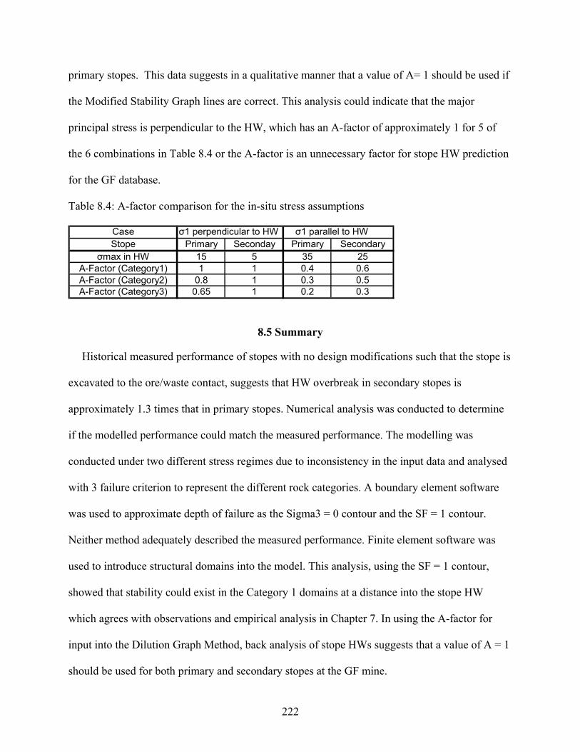
222
primary stopes. This data suggests in a qualitative manner that a value of A= 1 should be used if
the Modified Stability Graph lines are correct. This analysis could indicate that the major
principal stress is perpendicular to the HW, which has an A-factor of approximately 1 for 5 of
the 6 combinations in Table 8.4 or the A-factor is an unnecessary factor for stope HW prediction
for the GF database.
Table 8.4: A-factor comparison for the in-situ stress assumptions
Case σ1 perpendicular to HW σ1 parallel to HWStope Primary Seconday Primary Secondary
σmax in HW 15 5 35 25A-Factor (Category1) 1 1 0.4 0.6A-Factor (Category2) 0.8 1 0.3 0.5A-Factor (Category3) 0.65 1 0.2 0.3
8.5 Summary
Historical measured performance of stopes with no design modifications such that the stope is
excavated to the ore/waste contact, suggests that HW overbreak in secondary stopes is
approximately 1.3 times that in primary stopes. Numerical analysis was conducted to determine
if the modelled performance could match the measured performance. The modelling was
conducted under two different stress regimes due to inconsistency in the input data and analysed
with 3 failure criterion to represent the different rock categories. A boundary element software
was used to approximate depth of failure as the Sigma3 = 0 contour and the SF = 1 contour.
Neither method adequately described the measured performance. Finite element software was
used to introduce structural domains into the model. This analysis, using the SF = 1 contour,
showed that stability could exist in the Category 1 domains at a distance into the stope HW
which agrees with observations and empirical analysis in Chapter 7. In using the A-factor for
input into the Dilution Graph Method, back analysis of stope HWs suggests that a value of A = 1
should be used for both primary and secondary stopes at the GF mine.

223
CHAPTER 9 STOPE DESIGN INNOVATIONS AT THE GEORGE FISHER MINE
During data collection, a dilution study conducted as a researcher and employee at the Xstrata
Zinc George Fisher Mine, Australia contributed a large amount of data to the development of an
improved understanding of stope HW overbreak. From the mine’s viewpoint, it was also
important to develop controls to reduce the amount of dilution to go along with the
understanding of where, how, and why the dilution occurred. This chapter presents some of the
controls that were implemented as a response to the knowledge gained in the understanding of
stope HW overbreak. The controls were developed with the planning and operations team, to
achieve improved individual stope performance and also resulted in research and development
incentives. Through the research, innovative stope design methods including vertical HWs, ore
skins, and cablebolted and non-cablebolted ore chocks were developed, tested, and applied under
specified rock mass conditions. This was enabled due to the researcher’s position as a rock
mechanics engineer at the mine site. These stope design modifications, presented through three
papers at the ACG (Australia Centre for Geomechanics) Strategic and Tactical Mine Planning
Conference in Perth in April 2006, are described in this chapter. From the beginning of the study
in October 2003, the improved understanding of stope HW overbreak contributed to a change in
stoping methodology and a reduction in annual unplanned stope dilution from 14.4% in 2003 to
6.3% by the end of 2005 (Capes et al., 2006) as shown in Figure 9.1. A comparison of average
ELOS values for all of the applied stope design methodologies is shown in Table 9.1. The
fundamentals of these methodologies are described in the following sections.

224
Figure 9.1: George Fisher North Dilution% over time from Capes et al. (2006)
Table 9.1: Comparison of Design Methodologies in the GF Database for D-orebody
Stope Type Arched Ore
Skin Ore Skin Chock Vertical
No Mods
Database Code Aos os C V S #cases 13 26 10 4 70
ELOSave 0.3 0.9 1.0 0.6 3.1 ELOS Range 0-0.8 0-10.6 0-4.5 0-1.3 0-13
Total MineTonnes Hoisted and George Fisher Stope Dilution %
0
2
4
6
8
10
12
14
16
18
20
Jan-03
Mar-03
May-03
Jul-03
Sep-03
Nov-03
Jan-04
Mar-04
May-04
Jul-04
Sep-04
Nov-04
Jan-05
Mar-05
May-05
Jul-05
Sep-05
Nov-05
Time
Dilu
tion%
-
50,000
100,000
150,000
200,000
250,000
300,000
Tonn
es H
oist
ed
2005 Dilution(6.3%)
2003 Dilution(14.4%)
2004 Dilution(7.5%)
Dilution % = Tonnes Waste Tonnes Total

225
9.1 Use of Ore Skins
The empirical data in Chapter 7 provided a relationship between Category 1 domain thickness
and stope Hydraulic Radius. Using this data, a stope design methodology was developed. If a
stable domain didn’t exist at an acceptable distance into the HW domain, then the rock categories
in the ore domain would be defined. If there was a Category 1 rock in the ore at the ore/HW
contact, the extraction HW position could be redefined to achieve stability. An economic and
stability analysis would be conducted comparing the possible options. Prior to the dilution study,
the reason behind the effect of HW drillhole standoff (ore skin) for stability was not completely
understood. After the knowledge was developed, the stable domains could be picked with a
combination of drillhole data and underground observation. If the ore defining the Category 1
domain was of relatively high grade, the design could be optimised to place the domain at the
limit of stability such that the domain may fail and be partially recovered at the end of stope
production. The stability chart for the Category 1 domain was presented in Figure 7.12. If delays
in the mining cycle were expected to be long in duration, than a thicker domain would be left
inside the HW. Figure 9.2 shows a cross section of the design methodology. There were 27 cases
of oreskins and 13 cases of arched oreskins with 0.9 and 0.3 m of average ELOS respectively
(Table 9.1). There were a few cases of oreskins which had major HW overbreak and raised the
ELOS average from 0.2 to 0.9 m. The subtle difference between the oreskin and arched oreskin
methodology was described in Figure 7.11. Both of these methodologies provide a significant
improvement in stope HW stability compared to the case of no design modifications which had
3.1 m average ELOS from 70 cases. However, there is ore left unrecovered with the oreskin
options. The economics of ore recovery compared to HW stability was assessed on a stope by
stope basis in the design process at the mine. An indication of the amount of ore left in place for
this design technique can be inferred from Table 7.1. Individual stope economics are not

226
presented in the thesis. The economic analysis at the mine would compare the predicted stope
HW overbreak to the value of the ore, the position of adjacent orebodies which could be
sterilised by HW overbreak, the cost and time of placement of additional backfill, delays to the
overall mining cycle, and any other stope specific factors.
0m 5m 10m
Figure 9.2: Use of Ore Skins (Category 1 rock) to reduce ELOS
Ore Skin
Stope CMS Survey
HWFW
Very Po
or Roc
k Qua
lity
(Cate
gory
3) at
great
exten
t
into t
he H
W

227
9.2 Use of Cablebolted and Non-Cablebolted Ore Chocks
Another design option evolved from a tactical attempt to counter the effect of major
undercutting of the current stope from the stope below. A chock, shown in Figure 9.3, is a
triangular slab of ore, with the characteristics of Category 1 rock, left unmined at the base of the
HW. It has been applied to regain stability of a mining area where HW stability problems in
lower stoping areas were compromising new mining areas. There were 10 cases of chocks
observed in the database, 2 of these were reinforced with a dense pattern of cables. It is thought
that the chock reduces the H.R. by steepening the lower portion of the HW and improves the
average RQD of the stope, since the chock is category 1 rock. Due to the geometry of the chock,
though, it is difficult to quantify the domain over which rock mass classification should be
determined and also difficult to measure the H.R. The hanging wall is no longer a single plane
so the HR definition does not apply. The HW and chock could possibly be considered as two
surfaces separated by ~135o, instead of the conventional 90 o.
Dense, long cable-bolt patterns were installed in two areas where undercutting was severe, in
an attempt to confine the Category 2 and 3 HW rock between the ore (chock) and Category 1
rock at depth into the HW. Figure 9.3 shows an example of a successfully applied cable pattern
which was thought to aid the stability of the chock in the lower HW that had failed to a distance
of >15 metres from the ore contact in the lift below. A dense cable pattern consisting of 8 rows
of 15 m cables alternating 2 and 3 cables/row were installed dumped 30 degrees from vertical at
a 0.5m burden.
The average ELOS for the 10 cases, where chocks were used, was 1.0 m (Table 9.1). This
methodology is an improvement compared to the cases without design modifications which had
an average ELOS = 3.1m. However, like the ore skin modification, this methodology resulted in
loss of ore.

228
A summary of some possible reasons for the effectiveness of this approach are as follows:
• The chock reduces the effective H.R.of the HW by shortening the up dip height.
• The chock isolates the Domain 2/3 rock from the effect of the combined undercut
and open stope free faces.
• Applied support over the bottom third of the stope. The chock of Domain 1 ore
acts like a large plate for the 20-15m long cables installed.
0m 5m 10m
Figure 9.3: Use of Cabled or Non-Cabled Ore Chocks to reduce ELOS.
Chock CableSupport
Stope CMSSurveys
HWFW
Category 3 rock
Category 1 rock

229
9.3 Use of Vertical HWs
The previous design methodologies resulted in a reduction in stope HW overbreak but also
led to ore loss. An optimum methodology was sought which reduced HW overbreak but did not
result in ore loss. An observation presented in Figure 7.9 suggested that a stope with the HW
surface steeper than the bedding had minor overbreak. This observation led to a trial of mining
vertical HWs (Figure 9.4) as opposed to mining the stope HW along bedding. The operational
and design considerations of the methodology are discussed below.
From an operational perspective, the method required the development of extra metres of
development drive to extend the drill drive (overcut) and drill the vertical HW. Once the drilling
was completed, the objective was to selectively blast and extract low or zero grade ore to prevent
dilution from entering the ore stream. This would involve firing the material closest to the HW in
the early stages of the stope. This material, composed mainly as waste, would be selectively
mucked and a vertical HW would be created prior to firing the remaining drillholes in the stope.
The extraction sequence is shown in Figure 9.5.
From the design perspective, stability can be improved in 3 ways with the use of a vertical
HW:
1. A vertical wall is more stable then an inclined wall (Refer to the C-Factor in Figure
4.12);
2. The key joint orientation will become more favourable if the bedding angle to the
vertical wall becomes > 35 degrees (Refer to the B-Factor in Figure 4.11). The method is
most effective for stopes with HW’s dipping < 55 degrees;
3. The H.R. is reduced as the stope HW up dip height is reduced.

230
Cross Cut
Cross Cut
HangingWall andFootwall
Nearverticalblast holes
0m 5m 10m
Figure 9.4: Creation of a vertical HW where major HW failure was expected
0m 5m 10m Figure 9.5: Sequence of selective extraction in a stope with a vertical HW
Cross Cut
Cross Cut
HangingWall andFootwall
Nearverticalblast holes
1
2
3
4

231
For example, a stope HW dipping at 50 degrees with an initial N’ of 1, the mining of a
vertical HW results in an increase in the value of the B-Factor (0.3 to 0.5) and C factor (4.2 to 8).
The effect of these values increase N’ to 3.2. Assuming that the stope is mined over a vertical
height of 35 m and strike span = 15 m then the vertical HW would reduce the H.R. from 5.6 to
5.3. When the points are plotted on the revised Dilution Graph in Figure 9.6 there is a reduction
in ELOS from >4 m to < 1 m.
To create the vertical HW, development of the overcut extended into the HW which created
undercutting of the above stope. Undercutting was shown to increase stope HW overbreak in
section 6.4.5. However, the vertical HW could result in less of an undercut for the above stope
than if the stope would have been mined without a design modification, with subsequent HW
failure. Table 9.1 shows an average ELOS of 0.9 m for stopes with vertical HWs. However, the
ELOS measurement was measured from the vertical HW and not the ore/HW contact so the
value cannot be directly compared to the 3.1 m average ELOS from stopes without design
modifications. The methodology can be a good alternative when there is not a Category 1
domain within a reasonable distance of the HW for the application for the chock or ore skin
methodology, or if the material in the near HW cannot be sacrificed based on economic
tradeoffs. The effect of undercutting of the above lift can be controlled with the use of a chock or
oreskin.

232
Figure 9.6: Effect of Vertical HW on H.R. and N’ calculations
9.4 Summary
Dedicated research using a sound geological engineering approach of data collection,
communication, analysis and implementation resulted in a thorough understanding of HW
overbreak. This was achieved by creating a model for design, understanding why it worked and
why it did not work, appreciating it for the insights it provided and continually reanalysing as
more information became available. This understanding created the ability to develop innovative
empirical stope design methods (tactical) to control and reduce HW overbreak and dilution. The
combined effect of the design changes created a reduction in annual stope dilution from 14.4% in
2003 to 6.3% for the end of 2005 while increasing the production rate by 18% (Capes et al.,
2006).
0.1
1
10
100
0 5 10
Hydraulic Radius (m)
Stab
ility
Num
ber
N'
ELOS 0 - 0.5 m
ELOS >0.5 - 1.0m
ELOS >1 - 2.0m
ELOS >2 - 4.0m
ELOS >4 - 6.0m
ELOS >6m
ELOS < 0.5 <1 <2 <4
Typical HW
Vertical HW

233
CHAPTER 10 CONCLUSIONS
Unplanned open stope HW overbreak (dilution) is a major cost for many mining operations.
The objective of the research was to use an observational approach to improve open stope HW
design by creating new empirical design methods with the aid of numerical analysis and
statistical methods based on comprehensive, on-site, long term collection of case histories from
different rock masses in Canada and Australia. Initial short term data collection in Canada
provided a broad layout for the thesis content while 3 years of on-site data collection in Australia
combined with data from literature allowed for further development of new design tools. The
major achievements for this research include the following:
1) Establishing a comprehensive database of 255 ELOS cases (169 of these were
collected on site while 86 of these cases were from literature) with Hydraulic Radius less
than 10 m over a range of rock mass and mining conditions;
2) Development of new lines for the Dilution Graph method from the compiled database
using logistic regression and statistical classification analysis methodology;
3) Discussion and empirical assessment of the effect of time, blasting, faulting, stress and
undercutting on stope HW overbreak;
4) New approach for defining the size of structural domains used as inputs to stope
stability assessment methods to improve prediction in the Dilution Graph;
5) The use of numerical modelling to compare interpreted rock mass behaviour from the
model to empirical data (123 cases) and to examine different in-situ stress assumptions
on the value of the A-factor;

234
6) Implementation of innovative modifications to stope HW design resulting in improved
mine performance.
10.1 Establishment of Open Stope HW Stability Knowledge and a Comprehensive Database
From 2003 - 2007, experience was gained understanding open stope HW stability through
discussions at industry short courses, site visits, consultants’ visits, employment, and data
collection at underground mines in Canada, Australia, and Kazakhstan. Data collection was
focussed at mines whose rock mass conditions and mining environment were in or near the zone
of interest for the study shown in Figure 5.1. General data was collected over a period of 2
months from the Callinan and Rabbit Lake Mines as a researcher, while detailed data was
collected from the George Fisher Mine as a researcher and employee over a period of 3 years. A
comprehensive analysis of case studies was permitted due to the author’s long term on-site
exposure to the complete mining cycle. Other sites visited as a consultant or a visitor, where
substantial stope stability knowledge was accessed, include the former Inco Thompson operation
in North-Central Canada (now Xstrata); BHP Cannington Mine, Xstrata Zinc Lead Mine, and
Xstrata Copper Enterprise Mine, in Queensland, Australia; BHP Leinster Mine in Western
Australia, Australia; and the Kazzinc Maleevskiy Mine in north-eastern Kazakhstan.
Site geomechanics rock mass mapping and classification were conducted and case histories
were collected from Cavity Monitoring System (CMS) surveyed stopes. Based on stope mining
information, rock mass mapping and classification, as well as CMS survey data, a
comprehensive empirical database was established for the study. The database includes 161 HW
cases collected from mine sites and 94 HW cases from literature. The following information was
included in the database:

235
• General stope information
• Stope geometry
• Rock mass properties and classification
• Undercutting information
• Adjacent mining information
• CMS survey data and calculations.
The database is an importance resource for the dilution study. The comprehensive database is
presented in the Appendix B.
10.2 Revised Design Lines for the Dilution Graph
Logistic regression models and classification analysis were used to propose a set of ELOS
lines which represented 80% correct prediction for the compiled database of 255 cases (Figure
10.1). Alternatively, a conservative set of design lines was created that minimised the number of
cases with greater failure than predicted for all of the design lines. There were many
improvements to the dilution graph made upon the recommendations from Clark (1998). These
included increasing the number of HW case histories (47 stopes from 6 mines) in mainly good
quality rock masses to now 255 HW cases from a diverse range of rock mass and mining
conditions. The databases presented in the thesis represent different mining practices as well as
different availability of rock mass classification data. The variability in the design lines reflects
the effect of the external factors for the databases considered. Like any design method, empirical
methods are useful tools for prediction when used for conditions similar to those which existed
for the development of the design method.

236
0.1
1
10
100
0 5 10
Hydraulic Radius (m)
Stab
ility
Num
ber
N'
MSG: Stable
MSG: Caved
DG: 0.5 m ELOS
DG: 2m ELOS
P=0.37: ELOS < 0.5
P=0.53: ELOS <1
P=0.68 ELOS < 2
P=0.84 ELOS <4
ELOS 0 - 0.5 m
ELOS >0.5 - 1.0m
ELOS >1 - 2.0m
ELOS >2 - 4.0m
ELOS >4 - 6.0m
ELOS >6m
ELOS: <0.5 <1 <2 <4
Figure 10.1: Dilution Graph based on highest percentage correct classification: 255 case database
10.3 Effect of Time, Blasting, Faulting, Stress and Undercutting on Stope HW Overbreak
Empirical data and observations of some of the factors not included in the Dilution Graph
Method were examined. Cases were presented which showed error in the determination of H.R.
and ELOS. Observations and empirical data on the influence of time, blasting, faulting, stress,
and undercutting were also presented. The time at which data was collected was considered to
affect the calculation of the H.R. and ELOS variables. Poor drill and blast recovery was observed
to reduce the H.R. and the predicted ELOS. Individual fault characteristics were observed to play
a role in stope stability. The George Fisher mine data suggested 1.3 times greater failure in
secondary stopes than primary stopes. Analysis of the undercutting data suggested 1.1 and 1.4
times greater failure between the cases of minor and major undercutting in primary and
secondary stopes respectively. The observations and empirical data can be used to assist an
engineer’s judgement when using stope HW overbreak prediction methods.

237
10.4 Revised Structural Domains to improve Stope HW Overbreak Prediction
During the collection of data to improve the design lines on the Dilution Graph at the Xstrata
Zinc George Fisher mine, interesting relationships were observed between stope failure profiles,
rock quality, and stope geometry. RQD plots had been created for individual stopes which
identified 3 different rock categories in the HW. Observations suggested that Category 2 and 3
rocks would be unstable under the same stoping conditions where Category 1 rocks were stable.
The rock categories were defined over intervals smaller than the typical averaged 5m fixed
domain size required for the Dilution Graph method to determine revised structural domains.
Empirical data was collected for stable and unstable cases of these revised structural domains to
create a new design graph for stope HW stability where Category 1 domains could be identified.
Observations combined with the voussoir beam analysis suggested that the mode of failure was a
snap-thru failure mechanism. The voussoir beam analysis could only be used as an indication of
failure mode while the empirical data was used to create a rigorous design tool (Figure 10.2).
The idea of using an observational approach to identify variable domain sizes presents a
methodology that others may follow. The methodology can be applied after some mine specific
knowledge has been gained to develop rock mass domains which provide the most realistic rock
properties influencing stability. There are currently no standards which exist for the size of a
fixed domain required for empirical stope design methods. For this study, recognizing the
changing rock mass condition with distance from the HW contact enabled an improved, more
accurate method of estimating HW overbreak.

238
Figure 10.2: Empirical Design tool for Category 1 rock
In Chapter 1, a problem was defined in which two stopes having similar average rock mass
conditions and geometry had very different stope HW overbreak results. The developed
knowledge discussed in the thesis provides an explanation. Figure 10.3 is an illustrative example
demonstrating the position of the Category 1 domains for two stope HWs having the same
average HW rock mass conditions. The position of the Category 1 domain in the upper stope is
just inside the HW while the lower stope has the domain located approximately 4-5 m into the
HW. Observations and empirical data provided evidence that the stope would fail through the
Category 2 and 3 rocks until a Category 1 domain was intersected. Breaking the 5m fixed
domain in the HW into revised structural domains provided an improved understanding of HW
overbreak.
Category 1 Domain Thickness vs Stope HW Hydraulic Radius
0
0.5
1
1.5
2
2.5
3
3.5
4
4.5
5
3.0 3.5 4.0 4.5 5.0 5.5 6.0 6.5 7.0 7.5 8.0
Hydraulic Radius ( m)
Cat
egor
y 1
Dom
ain
Thic
knes
s (m
)
FailedStable ("x")Stable ("aos")Stable ("os")
Stable
Failedos- ANFO
Transition

239
StopeHW andFW
Faults
Cross cut
Cross cut
Cross cut
Stope B
Stope A
RQD > 40%
RQD > 40%
RQD = 0-20%
0m 5m 10m
(CAT1)
(CAT3)
(CAT1)
0m 5m 10m Figure 10.3: Position of Stable Domain shown for two stopes with similar average rock mass conditions and opening geometry.

240
10.5 Numerical Modelling for Open Stope HW design
Historical measured performance of stopes with no design modifications, such that the stope
is excavated to the ore/waste contact, suggested that HW overbreak in secondary stopes was
approximately 1.3 times that in primary stopes at the George Fisher mine. Numerical analysis
was conducted to determine if the modelled performance could match the measured
performance. The modelling was conducted under two different stress regimes due to
inconsistency in the input data and analysed with 3 failure criterion to represent the different
rock categories. A boundary element software was used to approximate depth of failure as the
Sigma3 = 0 contour and the SF = 1 contour. Neither method adequately described the measured
performance. Finite element software was used to introduce structural domains into the model.
This analysis, using the SF = 1 contour, showed that stability could exist in the Category 1
domains at a distance into the stope HW which agrees with observations and empirical analysis
in Chapter 7. In using the A-factor for input into the Dilution Graph Method, back analysis of
stope HWs suggests that a value of A = 1 should be used for both primary and secondary stopes
at the GF mine.
10.6 Innovative Open Stope Design Methodology
From a mine’s viewpoint, it is important to develop controls to reduce the amount of dilution
to go along with the understanding of HW overbreak. This thesis presented some of the controls
that were implemented as a response to the knowledge gained in the understanding of stope HW
overbreak. Through the research, innovative stope design methods including vertical HWs, ore
skins, and cablebolted and non-cablebolted ore chocks were developed, tested, and applied under
specified rock mass conditions. This was enabled due to the researcher’s position as a rock
mechanics engineer at the mine site. These stope design modifications, presented through 3
papers at the ACG (Australia Centre for Geomechanics) Strategic and Tactical Mine Planning

241
Conference in Perth in April 2006, are described in the thesis. From the beginning of the study in
October 2003, the improved understanding of stope HW overbreak contributed to a change in
stoping methodology and a reduction in annual stope dilution from 14.4% in 2003 to 6.3% by the
end of 2005 (Capes et al., 2006).
10.7 Recommendations for Future Research
This study has created a revised set of Dilution Graph design lines based on an improved
database of 255 cases. Empirical data was collected on factors external to the design method to
assist an engineer’s judgment in stope HW overbreak prediction. The observational approach led
to the creation of revised structural domains and an additional method for stope HW design.
Based on the understanding of stope HW overbreak from the structural domain revision,
innovative stope design methodology provided many improvements to stope design in mining
environments that experience major overbreak.
Further work should be conducted in the following areas:
• Case histories are required from other areas of the Dilution Graph lacking data.
• The revised structural domain methodology should be examined in other open stope
mining environments where the data is available to improve upon the predictive
capability of the Dilution Graph
• The innovative stope design methodology can be used in mining environments that
experience major overbreak
LIST OF REFERENCES
Anderson, B and Grebence, B., 1995. Controlling dilution at the Golden Giant Mine, 1995 CIM Operators Conference.
Anon, 1990. The geology of Callinan Mine. Internal Report, HBMS. Barton, N., Lien, R. and Lunde, J., 1974. Engineering classification of rock masses for the

242
242
design of tunnel support. Rock Mech. Vol. 6, pp. 189-236. Beck, D., 2008. Similitude, Model Sufficiency and Calibration for Mine-Scale Modelling,
Presentation from Australia Centre for Geomechanics Rock Mass to Rock Model Workshop at, SHIRMS 2008 Perth, Australia (15-9-2008).
Beer, G. and Meek, J.L., 1982. Design curves for roofs and hangingwalls in bedded rock based
on voussoir beam and plate solutions. Trans. Instn. Min. Metall. Vol. 91, pp. A18-22. Beer, G., Meek,J. and Cowling, R., 1983. Prediction of the behaviour of shale hangingwalls of
deep underground excavations. Proc. Fifth ISRM Congress, Melbourne Australia, 1983, D45-51.
Bienawski, Z.T., 1976. Rock Mass Classification in Rock Engineering. In Proceedings of the
Symposium on Exploration for Rock Engineering, Johannesburg, S. Africa, 1976, pp. 97-106.
Bienawski, Z.T., 1989. Engineering rock mass classification. John Wiley & Sons, New York. Board M, Brummer, R, Seldon S., 2001. Use of numerical modelling for mine design and
evaluation. In: Hustrulid WA, Bullock RL, editors. Underground mining methods: engineering fundamentals and international case studies. Littleton, Colo: Soc Mining Metall Explor; 2001. pp. 482-91.
Brady, B.H.G., and Brown, E.T., 1985. Rock mechanics for underground mining. London: Allen
and Unwin. Brady, B,H.G., and Brown, E.T., 1993. Rock mechanics for underground mining, 2nd edition.
Chapman & Hall. Brady, T., Pakalnis, R., and Clark, L., 2005 Design in Weak Rock Masses, Nevada Underground
Mining Operations, SME-AGM, Salt Lake City, 9 pp. Capes, G.W., Milne D.M., and Grant, D.R.,2005. Stope hangingwall design approaches at the
Xstrata Zinc, George Fisher Mine, North Queensland, Australia. In Proceedings of ARMA Alaska Rocks 2005: Rock Mechanics for Energy, Mineral, and Infrastructure Development in the Northern Regions, University of Alaska-Anchorage, USA, June, 2005.
Capes, G.W., Milne D.M., and Grant D.R., 2006 .Interpreting core data and rock quality
information for open stope design Paper 24. Rock Engineering. CIM Bulletin, Vol. 99, No 1097.
Capes, G.W., Grant, D.R., and Neindorf, L.B., 2006. George Fisher: Development of George
Fisher orebodies. At 2nd International Seminar Strategic versus Tactical Approaches in Mining, Perth, Australia, March, 2006.

243
243
Capes, G.W., Grant D.R., Neindorf L.B., 2006. George Fisher: Sustainable mine design. Paper presented at the Second International Seminar on Strategic Versus Tactical Approaches in Mining. Perth, Australia, March, 2006.
Capes, G.W., Grant, D.R., and Neindorf, L.B., 2006. George Fisher: Design issues for the future.
At 2nd International Seminar Strategic versus Tactical Approaches in Mining, Perth, Australia, March, 2006.
Capes, G.W., Doolan, J.P., and Neindorf, L., 2007. Stope design considerations using rock mass
classification tools at the Xstrata Zinc George Fisher mine, Proceedings of the International Workshop on Rock Mass Classification in Underground Mining, NIOSH, Information Circular 9498. May, 2007
Clark, L. and Pakalnis, R., 1997. An empirical design approach for estimating unplanned dilution
from open stope hangingwalls and footwalls. CIM AGM, Vancouver. Clark, L., 1998. Minimizing dilution in open stope mining with a focus on stope design and
narrow vein longhole blasting, Msc. Thesis, University of British Columbia, Canada, 316p Coates, D.F., 1977. Pit slope manual Chapter 2 – Structural Geology. CANMET (Canada Centre
for Mineral and Energy Technology), CANMET Report 77-5. Cohen, J., and Cohen, P., 2003. Applied multiple regression/correlation analysis for the
behavioural sciences. Lawrence Erlbaum Associates, Mahwah, New Jersey. pp.479 - 521. Colwell,M., Frith, R., Mark,C., 2003. Empirical solution best, Geomechanics & Ground Control,
AMM, pp.82-84. Deere, D.U., 1964. Technical description of rock cores for engineer-purposes. Rock Mech Eng
Geol 1(1). Diederichs, M.S., and Kaiser, P.K., 1999. Tensile strength and abutment relaxation as failure
control mechanisms in underground excavations. Int. Journal of Rock Mech. And Mining Sci. 36(1999) pp. 69-96.
Diederichs, M.S., and Kaiser, P.K., 1999. Stability of large excavations in laminated hard rock
masses: the voussoir analogue revisited. Int. Journal of Rock Mech. And Mining Sci. 36(1999) pp. 97-117.
Dishaw, G.R., 2005. Rabbit Lake Operation: Canada’s Longest Operating Uranium Mine – 30
Years and Still Glowing. CIM-AGM, Toronto, Canada. Dunne, K., Pakalnis, R., Vongpaisal, S., 1996. Design analysis of an open stope at the Detour
Lake Mine, 98th CIM AGM, Edmonton, Alberta. Evans, W.H., 1941. The strength of underground strata. Trans. Instn. Min. Metall., 50, pp. 475-

244
244
532. Forster, K., Milne, D., and Pop, A., 2007 Mining and Rock Mass Factors Influencing Hanging
Wall Dilution, 1st Annual Canada-US Rock Mechanics Symposium, Vancouver, Canada, May, 2007.
Germain, P., Hadjigeorgiou J., and Lessard, F.F., 1996. On the relationship between stability
prediction and observed stope overbreak, Proceedings of the 2nd North American Rock Mechanics Symposium, Montreal, Canada.
Goodman, R. E., 1989. Introduction to rock mechanics. 2nd edition, John Wiley & Sons. pp.257-
280. Grenfell K., and Haydon M., 2006. Challenges in modelling large complex orebodies at the
George Fisher north mine. In: Proceedings of the Sixth International Mining Geology Conference (Darwin, Northern Territory, Australia, August 21–23, 2006).
Hadjigeorgiou, J., Leclair, J.G., and Potvin, Y., 1995. An update of the stability graph method for
open stope design. 97th CIM-AGM, Rock Mechanics and Strata Control Session, Halifax, Nova Scotia.
Henning, J.G., and Mitri, H.S., 2007. Numerical modelling of ore dilution in blasthole stoping.
Int. Journal of Rock Mech. And Mining Sci. 44 (2007) pp. 692-703. Hoek, E., & Brown, E.T., 1980. Underground excavation in rock. The Institution of Mining and
Metallurgy. Hoek, E. and Brown E.T., 1988. The Hoek-Brown failure criterion - a 1988 update. Proc. 15th
Canadian Rock Mech. Symp. (ed. J.H. Curran), pp. 31-38. Toronto: Civil Engineering Dept., University of Toronto.
Hoek, E., 1994. Strength of rock and rock masses, ISRM News Journal, 2(2), 4-16. Hoek, E., P.K. Kaiser, and W.F. Bawden. 1995. Support of Underground Excavation in Hard
Rock, Rotterdam: Balkema. P. 215. Hoek, E. and Marinos, P., 2000. Predicting Tunnel Squeezing. Tunnels and Tunnelling
International. Part 1 – November 2000, Part 2 – December, 2000 Hoek, E., Carranza-Torres, C. and Corkum, B., 2002. Hoek-Brown criterion –2002 edition. Proc.
NARMS-TAC Conference, Toronto, 2002, 1, 267-273. Hoek, E., and Marinos P., 2006. A brief history of the development of the Hoek-Brown failure
criterion. November 2006, RocScience Website Hosmer, D., and Lemeshow, S., 2000. Applied Logistic Regression, 2nd ed. New York;

245
245
Chichester, Wiley. Hutchinson, D.J. and Diederichs, M.S., 1996. Cablebolting in underground mines. BiTech
Publishers Ltd. pp. 265-273. Itasca Consulting Group Inc., 2004. UDEC (Universal Distinct Element Code), Version 4.0.
Minneapolis: ICG (2004). Jaeger, J.C. and Cook, N.G.W., 1979. Fundamentals of Rock Mechanics, 3rd edn, Chapman &
Hall, London. Kaiser, P.K., Falmagne, V., Suorineni, F.T., Diederichs, M., Tannant, D.D., 1997. Incorporation
of rockmass relaxation and degradation into empirical stope design. CIM AGM 1997, Vancouver.
Lang, B., Pakalnis, R. and Vongpaisal S. 1991. Span design in wide cut and fill stopes at Detour
Lake Mine, 93rd AGM-CIMM, Calgary, Canada. Martin, C.D., Tannant, D.D., Yazici, S., Kaiser, P.K., 1999. Stress Path and instability around
mine openings. In : Vouille G, Berest P, editors, Proceedings of the 9th ISRM Cong Rock Mech, vol 1, Rotterdam: Balkema, 1999, p.311-315.
Martin, C.D., Yazici, S., Espley, S. and Tan, G., 2000. Using numerical models to quantify stope
dilution, Proc. Can. Inst. Min., AGM, Toronto. Mathews, K.E., Hoek, E., Wyllie, D., and Stewart, S.B., 1981. Prediction of stable excavation
spans for mining below 1000 metres in hard rock, Canada: CANMET, Dept. of Energy, Mines and Resources, DSS Serial No. OSQ80-00081, DSS File No. 17SQ.23440-0-9020.
Mawdesley, C. and Trueman, R., 2003. Predicting open stope stability and cavability using the
Extended Mathews stability graph, 1st AGCM Conference, Ground Control in Mining – Technology and Practice, November 2003.
Milne, Germain, P., Grant, D. and Noble, P., 1991. Systematic rock mass characterization for
underground mine design. International Congress on Rock Mechanics, A.A. Balkema Publishers, Aachen, Germany
Milne, D., Germain, P. and Potvin, Y., 1992. Measurement of Rock Mass Properties for Mine
Design, Proceeding of the ISRM-Eurock Symposium on Rock Characterization, A.A. Balkema Publishers, Chester, England.
Milne, D., 1997. Underground design and deformation based on surface geometry, Ph.D Thesis,
University of British Columbia, Vancouver, Canada. Milne, D., Hadjigeoriou, J., and Pakalnis, R., 1998. Rock mass characterization for underground
hard rock mines.” Tunnelling and Underground Space Technology, Oct. 1998, vol. 13, no

246
246
4, pp 383-391. Miller, F., Potvin, Y., Jacob, D., 1992. Laser measurement of open stope dilution, CIM Bull.,
Vol. 85, Jul. – Aug. Mintec Inc., 2006. Minesight Mine Planning Exploration and Design Software Nedin, P.R. and Potvin, Y., 2003. Management of Rockfall Risks in Underground Metalliferous
Mines, A Reference Manual, Minerals Council of Australia Neindorf, L.B. and Karunatillake, G.S.B., 2000. George Fisher Mine – Feasibility and
Construction, MassMin 2000, Brisbane Nicholas, D. and Sims D., 2000. Slope Stability in Surface Mining – Chapter 2 – Collecting and
Using Geologic Structure Data for Slope Design, Edited by Hustrulid, McCarter and Van Zyl. SME.
Nickson, S.D., 1992. Cable support guidelines for underground hard rock mine operations. M.Sc.
Thesis, University of British Columbia. Norman, G.R., and Steiner, D.L., 1997. PDQ Statistics. Mosby-Year Book, Inc. Obert, L., Duval, W., 1967. Rock mechanics and the design of structure in rock. John Wiley &
Sons, Inc. Pakalnis, R., 1986. Empirical stope design at the Ruttan Mine, Sherritt Gordon Mines Ltd.. Ph.D.
Thesis, University of British Columbia. Pakalnis, R., Poulin, R., and Vongpaisal, S., 1995. Quantifying dilution for underground mine
operations, CIM AGM, Halifax, N.S. Pakalnis, R. and Vongpaisal, S., 1998. Empirical design methods-UBC geomechanics, Proc.
Can. Inst. Min., AGM, Montreal. Palmström, A., 1982. Application of the volumetric joint count as a measure of rock mass
jointing. Int. symp. on Fundamentals of Rock Joints, Björkliden, Sweden. Palmström, A., Milne, D., Peck, W. 2000. The reliability of rock mass classification used in
underground excavation and support design, GeoEng Workshop, Melbourne, November 2000, AMC Reference Library.
Parker, J., 1973. Practical rock mechanics for miners.Reprint from Seven part series in
Engineering and Mining Journal, June 1973-February 1974, pp. 4-12. Potvin, Y.,1988. Empirical open stope design in Canada, Ph.D. thesis. The University of B.C.,
350p.

247
247
Potvin, Y., and Hadjigeorgiou, J., 2001. The stability graph method for open-stope design. In:
Hustrulid WA, Bullock RL, editors. Underground mining methods: engineering fundamentals and international case studies. Littleton, Colo: Soc Mining Metall Explor; 2001, p513-519.
Priest, S.D., and Hudson, J.A., 1976. Estimation of discontinuity spacing and trace length using
scan line surveys. Int. Journal of Rock Mech. And Mining Sci. 18(1976) pp. 183-197. Ran, J., 2002. Hanging wall sloughing mechanism in open stope mining, CIM Bulletin, Vol. 95,
No. 1064, pp. 74-77. Rocscience Inc., 2005. Phase Version 6.0 – 2. Finite Element Analysis for Excavations and
Slopes. www.rocscience.com, Toronto, Ontario, Canada. Rocscience Inc., 2006. Examine Version 7.0 - 2D. 2D Stress Analysis for Underground
Excavations. www.rocscience.com, Toronto, Ontario, Canada. Scoble, M.J., Moss, A., 1994. Dilution in underground bulk mining: Implications for production
management, mineral resource evaluation II, methods and case histories, Geological Society Publication No. 79, pp. 95-108.
Sharrock,G. and Robinson, J., 2002. The stability of stopes and development in D-Orebody.
Internal Report, George Fisher Mining Operation, Australia (2002-03-11). Sprott, D.L., Toppi M.A., Yi, X., Bawden W.F., 1999. The incorporation of stress damage factor
into Mathew’s Stability Graph, Canadian Institute of Mining Annual General Meeting, Calgary.
SPSS Inc., 2005. SPSS for Windows, Release 14.0. Chicago. Stacey, T.R. 2003. Presidential Address: Rock engineering-good design or good judgment?, The
journal of The South African Institute of Mining and Metallurgy, September 2003, pp. 411-421.
Stewart, S.B.V., and Forsyth W.W., 1995. The Mathews method for open stope design. CIM
Bull. Vol.88 (992), 1995, pp. 45-53. Stonestreet, P.G., 2007. Personal Communications. Suorineni, F.T., 1998. Effects of faults and stress on open stope design. PhD. Thesis, University
of Waterloo. Suorineni, F.T., Tannant D.D. and Kaiser P.K., 1999. Fault factor for the stability graph method
of open-stope. Trans. Instn Min. Metall. (Sect. A: Min. industry), 108, May-August.

248
248
Sutton, D., 1998. Use of the Modified Stability Graph to Predict Stope Instability and Dilution at Rabbit Lake Mine, Saskatchewan, University of Saskatchewan Design Project, Canada.
Syme, E.C., and Bailes, A.H., 1993. Stratigraphic and tectonic settings of early proterozoic
volcanogenic massive sulphide deposits, Flin Flon, Manitoba. Economic Geology, Vol. 88. Tolman, J, Shaw, A and Shannon, K, 2002. Stratigraphic relationships between stratiform
polymetallic base metal deposits within the Mt Isa Inlier, NW Queensland, Australia, in Proceedings 150 Years of Mining Conference (The Australasian Institute of Mining and Metallurgy: NZ Branch).
Villaescusa, E., 1996. Excavation design for bench stoping at Mount Isa., Transactions of the
Institute of Mining and Metallurgy, Section A Mining Industry, A1-A10. London. Wang, J., Milne, D., Yao, M. and Allen, G., 2002. Quantifying the effect of hanging wall
undercutting on stope dilution, CIM AGM, Vancouver, British Columbia. Wang, J., Milne, D., Yao, M., Allen, G. and Capes, G., 2003. Open stope exposure time and
stope dilution, CIM –AGM 2003, Montreal. Wang, J., 2004. Influence of stress, undercutting, blasting, and time on open stope stability and
dilution. PhD. Thesis, University of Saskatchewan. Wang, J., Milne,D., Wegner,L., and Reeves, M., 2007. Numerical Evaluation of the effects of
stress and excavation surface geometry on the zone of relaxation around open stope hanging walls. Int. Journal of Rock Mech. And Mining Sci. 44(2007) pp. 289-98.
Wiles, T., 2005. Map3D Version 51. A mining analysis program in three dimensions. Mine
Modelling Pty Ltd. Mt. Eliza, Victoria, Australia, 2005. http://www.map3d.com. Wiles, T., 2006. Reliability of Numerical Modelling Predictions. Int. Journal of Rock Mech. And
Mining Sci. 43(2006) pp. 454-472. Yao, X., Gary, A., and Willett, M., 1999. Dilution evaluation using Cavity Monitoring System at
HBMS – Trout Lake Mine. CIM AGM, Calgary, Alberta.

APPENDIX A APPENDIX A - RQD DATA, PLOTS, AND STOPE PROFILES FOR GEORGE
FISHER STOPES
Please refer to the attached CD in the folder named Appendix

13L 13C 2668
13C 12L 2698
12L 12C 2730
12C 11L 2761
11L 11C 2792
11C 10L 2822
10L 10C 2851
10C 9L 2880
Mid Stope Elevations

13L-13C 2668
709 711 712 714 716 718 719 721 723 725 726 728

13L-13C 2668
728 730 732 733 735 737 739 740 742 744 746 747 749 751

13C-12L 2698
709 711 712 714 716 718 719 721 723 725 726 728

13C-12L 2698728 730 732 733 735 737 739 740 742 744 746 747 749 751

12L-12C 2730
709 711 712 714 716 718 719 721 723 725 726 728 730

12L-12C 2730
709 711 712 714 716 718 719 721 723 725 726 728 730

12L-12C 2740
728 730 732 733 735 737 739 740 742 744 746 747 749 751

12C-11L 2761
709 711 712 714 716 718 719 721 723 725 726 728 730

12C-11L 2761728 730 732 733 735 737 739 740 742 744 746 747 749 751

11L-11C 2792
709 711 712 714 716 718 719 721 723 725 726 728 730

11L-11C 2792
728 730 732 734,735 736 737 739 740 741 742 744 746 747

11C-10L 2822
709 711 712 714 716 718 719 721 723 725 726 728 730 732

11C-10L 2822
728 730 732 733 735 736 737 739 740 741 742 744 746 747

10L-10C 2851
709 711 712 714 716 718 719 721 723 725 726 728 730 732

10L-10C 2851
728 730 732 733 735 736 737 739 740 741 742 744 746 747

10C-9L 2880709 711 712 714 716 718 719 721 723 725 726 728 730 732

RQD Plot 739 12C-11L(7400-midstope)
0
10
20
30
40
50
60
70
-10 -8 -6 -4 -2 0 2 4 6 8 10
Distance from HW(m)
RQ
D%
Series1
STABLE BEAM STABLE BEAM

GFM2108 02 H740 WI01 1 2C014 748.327210802 25.6 26.8 1.2 1.2 -10.2 0DM0U 46210802 26.8 27.5 0.7 0.7 -9 0DM0U 17210802 27.5 28.7 1.2 1.2 -8.3 0DM0U 53 shale plr210802 28.7 29.9 1.2 1.2 -7.1 Y 0DM0U 61210802 29.9 31.2 1.3 1.3 -5.9 0DM0U 17210802 31.2 32.2 1 1 -4.6 0DM0U 0 mnr cwt210802 32.2 33.2 1 1 -3.6 0DM0U 42 mnr cwt210802 33.2 34.5 1.3 1.3 -2.6 0DM0U 19210802 34.5 35.8 1.3 1.3 -1.3 0DM0U 50 fn lam cwt D
0210802 35.8 37.2 1.4 1.4 1.4 0DU0U 26210802 37.2 38.1 0.9 0.9 2.3 0DU0U 62 D upr210802 38.1 39.3 1.2 1.2 3.5 0DU0U 18 shale plr210802 39.3 40.5 1.2 1.2 4.7 0DU0U 34210802 40.5 41.5 1 1 5.7 0DU0U 40210802 41.5 42.5 1 1 6.7 0DU0U 13210802 42.5 43.5 1 1 7.7 0DU0U 11 end of plr210802 43.5 45.2 1.7 1.7 9.4 0CDMU 21 CD lns210802 45.2 46.4 1.2 1.2 10.6 0CDLU 12 brk grd plr210802 46.4 47.6 1.2 1.2 11.8 0CDLU 50 mnr sty msv210802 47.6 48.8 1.2 1.2 0CDLU 10

DHW
v

APPENDIX B APPENDIX B - GEORGE FISHER DATABASE, OTHER COLLECTED DATA, AND DATA
FROM LITERATURE
Please refer to the attached CD in the folder named Appendix B.

LegendStress Category Design Code Miscellaneousp = primary stope x = no design modification NC = Not Calculateds = seconday stope os = oreskin
aos = arched oreskios-ANFO = oreskin blasted with higher density explosivev = vertical HWc = chock

STOPE Dip StrikeHW
Height H.R. RQD Joint Properties Q' Dilution Graph Factors N' ELOS
Max. Failure Depth
Design Code
Stress Cat.
Undercut Area
° m m m % Jn Jr Ja A B C (m) (m) m2
709D 13C 65 20 39 6.6 15 12.0 1.0 3.0 0.4 1 0.3 5.5 0.7 12.6 16.5 x s 136.0709D 13L 69 20 38 6.6 5 12.0 1.0 4.0 0.1 1 0.3 5.8 0.2 3.6 8.0 x s 0.0711D 11L 38 20 50 7.1 17 12.0 1.0 3.0 0.5 1 0.3 3.3 0.5 12.7 14.5 x s 100.0711D 12C 72 18 39 6.2 16 12.0 1.0 3.0 0.4 1 0.3 6.1 0.8 2.3 10.0 x p 10.0711D 12L 73 19 35 6.2 33 12.0 1.0 3.0 0.9 1 0.3 6.2 1.7 2.7 5.0 x p -13.0711D 13L 48 13 90 5.7 39 10.5 1.0 1.5 2.5 1 0.3 4.0 2.9 0.0 -2.0 os p 0.0712D 11C 70 10 80 4.4 32 12.0 1.0 2.0 1.3 1 0.3 5.9 2.4 0.0 0.0 x p 0.0712D 12C 60 16 41 5.8 22 10.5 1.0 1.5 1.4 1 0.3 5.0 2.1 0.4 1.0 os s NC712D 13L 51 11 78 4.7 35 10.5 1.0 1.5 2.2 1 0.3 4.2 2.8 0.0 -2.0 os s 0.0714D 10L 55 15 40 5.5 30 12.0 1.0 2.0 1.3 1 0.3 4.6 1.7 0.0 0.0 aos p 0.0714D 11C 70 10 38 4.0 25 12.0 1.0 2.0 1.0 1 0.3 5.9 1.9 0.4 1.0 x p 20.0714D 11L 38 10 45 4.1 35 10.5 1.0 1.5 2.2 1 0.3 3.3 2.2 0.0 -3.0 aos p 15.0714D 12L 65 15 80 6.3 33 12.0 1.2 2.5 1.3 1 0.3 5.5 2.2 1.5 10.0 x p 120.0714D 13L 49 15 80 6.3 30 12.0 1.2 2.5 1.2 1 0.3 4.1 1.5 2.0 12.0 x p 0.0716D 10C 48 15 45 5.6 19 12.0 1.0 2.0 0.8 1 0.3 4.0 0.9 0.5 2.0 x p 100.0
716D 11C L. 50 18 40 6.2 27 12.0 1.0 2.0 1.1 1 0.3 4.1 1.4 4.9 12.0 x s 320.0716D 11C U. 50 7 40 3.0 11 12.0 1.0 2.0 0.5 1 0.3 4.1 0.6 0.0 0.0 aos p 0.0
716D 11L 90 16 35 5.5 10 12.0 1.0 2.0 0.4 1 0.5 8.0 1.7 1.3 2.0 v s 54.0716D 12C 66 18 39 6.2 36 12.0 1.0 2.0 1.5 1 0.3 5.6 2.5 2.5 3.0 x s -34.0716D 12L 64 15 40 5.5 40 9.0 1.0 1.0 4.5 1 0.3 5.4 7.2 0.5 -4.0 aos s 180.0716D 13C 52 15 48 5.7 40 12.0 1.2 2.5 1.6 1 0.3 4.3 2.1 5.3 12.0 x s 0.0716D 13L 42 10 44 4.1 40 10.5 1.0 1.5 2.5 1 0.3 3.5 2.7 0.0 -3.0 aos s 0.0718D 10C 45 10 45 4.1 10 12.0 1.0 2.0 0.4 1 0.3 3.8 0.5 3.3 7.0 x p 70.0718D 10L 42 15 52 5.8 17 12.0 1.0 2.0 0.7 1 0.3 3.5 0.8 2.3 7.0 x p 0.0718D 11C 66 15 37 5.3 15 12.0 1.0 2.0 0.6 1 0.3 5.6 1.0 0.9 3.0 x p 49.0718D 12C 60 15 78 6.3 27 12.0 1.0 2.0 1.1 1 0.3 5.0 1.7 4.1 7.0 x p 0.0
STOPE Dip StrikeHW
Height H.R. RQD Joint Properties Q' Dilution Graph Factors N' ELOS
Max. Failure Depth
Design Code
Stress Cat.
Undercut Area
° m m m % Jn Jr Ja A B C (m) (m) m2
718D 12L 70 13 40 4.9 25 12.0 1.0 2.0 1.0 1 0.3 5.9 1.9 0.9 -3.0 os p -10.0718D 13L 43 14 88 6.0 35 12.0 1.0 2.0 1.5 1 0.3 3.6 1.6 8.0 12.0 x p 0.0719D 10L 45 15 54 5.9 19 12.0 1.0 2.0 0.8 1 0.3 3.8 0.9 NC 9.0 x s 45.0

719D 11L 55 14 42 5.3 30 12.0 1.0 2.0 1.3 1 0.3 4.6 1.7 0.3 3.0 c s 0.0719D 12C 50 15 38 5.4 25 10.5 1.0 1.5 1.6 1 0.3 4.1 1.9 0.5 0.0 os-ANFO s 17.0719D 12L 60 17 45 6.2 49 9.0 1.0 1.0 5.4 1 0.3 5.0 8.2 0.0 -4.0 os s 300.0719D 13C 40 13 50 5.2 56 12.0 1.0 2.0 2.3 1 0.3 3.4 2.4 1.0 1.0 x s 104.0719D 13L 55 13 47 5.1 25 12.0 1.0 2.0 1.0 1 0.3 4.6 1.4 NC 8.0 x s 0.0721D 10C 45 15 49 5.7 17 12.0 1.0 2.0 0.7 1 0.2 3.8 0.5 0.8 2.5 x p 60.0721D 10L 45 15 51 5.8 39 10.5 1.0 1.5 2.5 1 0.2 3.8 1.9 1.4 7.0 x p 0.0721D 11C 50 12 38 4.6 35 12.0 1.0 2.0 1.5 1 0.3 4.1 1.8 0.0 -6.0 os p 20.0721D 11L 53 14 42 5.3 12 12.0 1.2 2.5 0.5 1 0.3 4.4 0.6 1.5 6.0 x p NC721D 12C 46 15 45 5.6 22 12.0 1.2 2.5 0.9 1 0.3 3.8 1.0 NC 4.0 x p 75.0721D 12L 47 15 47 5.7 20 12.0 1.2 2.5 0.8 1 0.3 3.9 0.9 2.2 7.0 x p -30.0721D 13L 45 15 85 6.4 40 10.5 1.0 1.5 2.5 1 0.3 3.8 2.9 0.0 -2.0 os p 0.0723D 10L 45 15 27 4.8 20 12.0 1.0 2.0 0.8 1 0.3 3.8 0.9 NC 9.0 x s 120.0723D 11C 60 15 38 5.4 10 12.0 1.0 2.0 0.4 1 0.3 5.0 0.6 4.2 8.0 x s 16.0723D 11L 50 16 41 5.8 23 10.5 1.0 1.5 1.5 1 0.3 4.1 1.8 0.3 0-2 c s NC723D 12C 90 20 35 6.4 15 12.0 1.0 2.0 0.6 1 0.5 8.0 2.5 >6 10.0 x s 78.0723D 12L 50 13 48 5.1 17 10.5 1.0 1.5 1.1 1 0.3 4.1 1.3 4.5 0-10 c s 56.0723D 13C 38 14 43 5.4 24 12.0 1.2 2.5 1.0 1 0.3 3.3 0.9 1.8 5.0 x s -14.0723D 13L 58 13 46 5.1 40 10.5 1.0 1.5 2.5 1 0.3 4.8 3.7 0.0 -3.0 aos s 0.0725D 10C 45 15 50 5.8 17 12.0 1.0 2.0 0.7 1 0.3 3.8 0.8 2.8 5.0 x p 15.0725D 10L 52 15 46 5.7 18 12.0 1.0 2.0 0.8 1 0.3 4.3 1.0 1.0 1.0 x p 48.0725D 11C 85 13 32 4.6 11 12.0 1.0 2.0 0.5 1 0.5 7.5 1.7 1.2 0* v p 8.0725D 11L 50 14 38 5.1 30 10.5 1.0 1.5 1.9 1 0.3 4.1 2.4 0.5 0.0 c p 375.0725D 12L 50 16 82 6.7 14 12.0 1.0 2.0 0.6 1 0.3 4.1 0.7 13.0 18.0 x p -32.0725D 13L 58 16 90 6.8 38 10.5 1.0 1.5 2.4 1 0.3 4.8 3.5 0.8 -1.5 aos p 0.0725D 9L 46 15 62 6.0 32 12.0 1.0 2.0 1.3 1 0.3 3.8 1.5 4.2 11.0 x p NC726D 10L 50 15 48 5.7 20 12.0 1.0 2.0 0.8 1 0.3 4.1 1.0 0.0 -4.0 os s 50.0726D 11C 55 18 45 6.4 37 10.5 1.0 1.5 2.3 1 0.3 4.6 3.2 0.6 0.0 aos s -13.0726D 11L 60 13 41 4.9 30 10.5 1.0 1.5 1.9 1 0.3 5.0 2.9 0.0 -2.0 aos s -200.0
STOPE Dip StrikeHW
Height H.R. RQD Joint Properties Q' Dilution Graph Factors N' ELOS
Max. Failure Depth
Design Code
Stress Cat.
Undercut Area
° m m m % Jn Jr Ja A B C (m) (m) m2
726D 12C 52 10 39 4.0 55 9.0 1.0 1.0 6.1 1 0.3 4.3 7.9 0.0 -10.0 os s 64.0726D 12L 43 16 50 6.1 23 12.0 1.0 2.0 1.0 1 0.3 3.6 1.0 6.3 8.0 x s 144.0726D 13C 50 20 48 7.1 33 10.5 1.0 1.5 2.1 1 0.3 4.1 2.6 2.2 0.0 c s 0.0726D 13L 45 15 41 5.5 46 9.0 1.0 1.0 5.1 1 0.3 3.8 5.7 0.4 -1.0 aos s 0.0

728D 10C 45 15 45 5.6 50 9.0 1.0 1.0 5.6 1 0.3 3.8 6.3 0.0 -5.0 os p 0.0728D 10L 45 10 47 4.1 25 12.0 1.0 2.0 1.0 1 0.3 3.8 1.2 0.0 -4.0 os p 0.0728D 11C 48 15 45 5.6 57 9.0 1.0 1.0 6.3 1 0.3 4.0 7.6 0.1 0.0 aos p 20.0728D 11L 50 10 46 4.1 13 12.0 1.0 2.0 0.5 1 0.3 4.1 0.7 2.0 7.0 x p 90.0728D 12C 40 16 49 6.0 35 12.0 1.0 2.0 1.5 1 0.3 3.4 1.5 3.0 10.0 x p -15.0728D 12L 40 15 52 5.8 31 10.5 1.0 1.5 2.0 1 0.3 3.4 2.0 0.5 -1.0 aos p 39.0728D 13L 57 16 80 6.7 36 10.5 1.0 1.5 2.3 1 0.3 4.7 3.2 1.4 0-4 os p 0.0730D 11L 41 15 51 5.8 18 12.0 1.0 2.0 0.8 1 0.3 3.5 0.8 2.9 6.0 x s 0.0730D 12C 39 17 49 6.3 37 10.5 1.0 1.5 2.3 1 0.3 3.3 2.3 0.0 -3.0 os s 216.0730D 12L 40 18 47 6.5 22 10.5 1.0 1.5 1.4 1 0.3 3.4 1.4 10.6 12.0 os s -55.0730D 13C 80 11 42 4.4 50 9.0 1.0 1.0 5.6 1 0.3 7.0 11.6 NC NC os s NC732D 10C 45 15 45 5.6 20 12.0 1.0 2.0 0.8 1 0.3 3.8 0.9 0.6 5.5 x p 72.0732D 10L 51 14 51 5.5 14 12.0 1.0 2.0 0.6 1 0.3 4.2 0.7 2.7 10.0 x p 40.0732D 11C 52 10 40 4.0 10 12.0 1.0 2.0 0.4 1 0.3 4.3 0.5 4.3 6.0 x p 72.0732D 11L 36 15 56 5.9 61 9.0 1.0 1.0 6.8 1 0.3 3.1 6.4 0.0 -6.0 os p 7.5732D 12C 45 15 47 5.7 50 9.0 1.0 1.0 5.6 1 0.3 3.8 6.3 0.6 1.5 aos p 80.0732D 12L 47 15 46 5.7 30 12.0 1.1 2.4 1.1 1 0.3 3.9 1.3 4.3 8.0 x p 24.0732D 13L 57 15 81 6.3 32 10.5 1.2 2.5 1.5 1 0.3 4.7 2.1 1.4 0-2 c p 0.0733D 12C 70 15 36 5.3 60 9.0 1.0 1.0 6.7 1 0.3 5.9 11.9 0.0 -10.0 os s 200.0733D 12L 50 20 46 7.0 30 12.0 1.0 2.0 1.3 1 0.3 4.1 1.6 >6 10.0 x s 0.0733D 13C 65 17 39 5.9 54 9.0 1.0 1.0 6.0 1 0.3 5.5 9.8 0.7 0.0 c s 0.0734D 11L 50 10 45 4.1 19 10.5 1.0 1.5 1.2 1 0.3 4.1 1.5 0.0 0.0 os s 0.0735D 10L 55 15 47 5.7 30 12.0 1.0 2.0 1.3 1 0.3 4.6 1.7 NC 10.0 x p 180.0735D 11C 55 18 45 6.4 39 10.5 1.0 1.5 2.5 1 0.3 4.6 3.4 NC 12.0 x p 0.0735D 11L 45 10 48 4.1 25 10.5 1.0 1.5 1.6 1 0.3 3.8 1.8 0.0 0.0 os p 0.0735D 12C 60 15 40 5.5 12 12.0 1.0 2.0 0.5 1 0.3 5.0 0.7 2.4 9.0 x p 48.0735D 12L 55 15 45 5.6 30 12.0 1.0 2.0 1.3 1 0.3 4.6 1.7 0.7 4.0 x p 60.0735D 13L 54 16 81 6.7 25 12.0 1.2 2.5 1.0 1 0.3 4.5 1.3 1.8 8.0 x p 0.0736D 11L 70 15 41 5.5 28 12.0 1.0 2.0 1.2 1 0.4 5.9 2.4 0.5 0-7 c p 80.0
STOPE Dip StrikeHW
Height H.R. RQD Joint Properties Q' Dilution Graph Factors N' ELOS
Max. Failure Depth
Design Code
Stress Cat.
Undercut Area
° m m m % Jn Jr Ja A B C (m) (m) m2
737D 11L 45 15 31 5.1 28 12.0 1.0 2.0 1.2 1 0.3 3.8 1.3 NC 12.0 x s -60.0737D 12L 50 20 42 6.8 18 12.0 1.2 2.5 0.7 1 0.3 4.1 0.9 4.1 8.0 x s NC737D 13L 55 13 39 4.9 15 12.0 1.2 2.0 0.8 1 0.3 4.6 1.0 1.4 2.0 x s 0.0739D 11C 50 15 42 5.5 35 10.5 1.0 1.5 2.2 1 0.3 4.1 2.8 0.0 0-3 c p 21.0

739D 11L 47 15 50 5.8 15 11.4 1.0 1.8 0.7 1 0.3 3.9 0.9 0.8 3.0 x p 0.0739D 12C 80 15 40 5.5 55 9.0 1.0 1.0 6.1 1 0.3 7.0 12.7 0.0 -5.0 os p 30.0739D 12L 40 15 48 5.7 35 12.0 1.2 2.5 1.4 1 0.3 3.4 1.4 1.8 4.0 x p 16.0739D 13L 57 15 81 6.3 15 12.0 1.2 2.5 0.6 1 0.3 4.7 0.9 2.1 4.0 x p 0.0740D 11C 82 15 32 5.1 18 12.0 1.0 2.0 0.8 1 0.4 7.2 2.1 0.0 0.0 v s 225.0740D 11L 66 12 40 4.6 3 12.0 1.0 2.0 0.1 1 0.3 5.6 0.2 NC 15.0 x s NC740D 12L 50 12 48 4.8 40 10.5 1.0 1.5 2.5 1 0.3 4.1 3.2 0.2 -2.0 os s 150.0740D 13C 60 20 45 6.9 28 12.0 1.0 2.0 1.2 1 0.3 5.0 1.7 2.7 6.0 x s 100.0740D 13L 55 20 42 6.8 15 12.0 1.0 2.0 0.6 1 0.3 4.6 0.9 2.0 5.0 x s 0.0741D 11C 56 12 40 4.6 4 12.0 1.0 2.0 0.2 1 0.3 4.6 0.2 2.5 6.0 x s NC742D 10L 62 15 33 5.2 12 12.0 1.0 2.0 0.5 1 0.3 5.1 0.8 4.6 10.0 x p 30.0742D 11C 75 15 38 5.4 17 12.0 1.0 2.0 0.7 1 0.3 6.4 1.4 NC 3.0 v,x p 0.0742D 12C 60 17 38 5.9 32 10.5 1.0 1.5 2.1 1 0.3 5.0 3.1 0.9 4.0 os p 75.0742D 12L 48 16 44 5.9 30 12.0 1.2 2.5 1.2 1 0.3 4.0 1.4 4.8 14.0 x p 180.0742D 13L 48 15 84 6.4 22 12.0 1.2 2.5 0.9 1 0.3 4.0 1.1 1.7 3.0 x p 0.0744D 11L 75 15 38 5.4 11 12.0 1.0 2.0 0.5 1 0.3 6.4 0.9 NC 7.0 x s 0.0744D 12C 80 19 35 6.2 25 10.5 1.0 1.5 1.6 1 0.3 7.0 3.3 0.0 0.0 c s 0.0744D 12L 80 10 35 3.9 50 9.0 1.0 1.0 5.6 1 0.3 7.0 11.6 0.0 0.0 os s 300.0744D 13C 50 19 42 6.5 10 12.0 1.2 2.5 0.4 1 0.3 4.1 0.5 6.3 15.0 x s 20.0744D 13L 51 19 39 6.4 15 12.0 1.2 2.5 0.6 1 0.3 4.2 0.8 0.4 0.0 x s 0.0746D 11C 60 15 40 5.5 15 12.0 1.0 2.0 0.6 1 0.3 5.0 0.9 0.0 0.0 v p 40.0746D 11L 55 12 42 4.7 35 10.5 1.0 1.5 2.2 1 0.3 4.6 3.1 4.1 5.5 os-ANFO p 75.0746D 12C 50 15 45 5.6 31 10.5 1.0 1.5 2.0 1 0.3 4.1 2.4 5.2 5.0 os p 0.0746D 12L 60 15 41 5.5 38 10.5 1.0 1.5 2.4 1 0.3 5.0 3.6 0.0 -1.0 os p 50.0746D 13L 56 15 84 6.4 15 9.0 1.2 2.0 1.0 1 0.3 4.6 1.4 0.6 3.5 x p 0.0
STOPE Dip StrikeHW
Height H.R. RQD Joint Properties Q' Dilution Graph Factors N' ELOS
Max. Failure Depth
Design Code
Stress Cat.
Undercut Area
° m m m % Jn Jr Ja A B C (m) (m) m2
747D 11L 80 17 35 5.7 7 12.0 1.0 2.0 0.3 1 0.3 7.0 0.6 NC 10.0 x s 48.0747D 12C 55 19 43 6.6 35 10.5 1.0 2.0 1.7 1 0.3 4.6 2.3 2.7 4.0 x s 120.0747D 12L 50 15 47 5.7 13 12.0 1.0 2.0 0.5 1 0.3 4.1 0.7 5.1 10.0 x s NC747D 13L 45 14 43 5.3 15 12.0 1.0 2.0 0.6 1 0.3 3.8 0.7 >2 3.0 x s 0.0749D 12L 56 15 43 5.6 30 12.0 1.0 2.0 1.3 1 0.3 4.6 1.7 5.2 9.0 x p 12.0749D 13L 65 15 75 6.3 15 12.0 1.2 2.5 0.6 1 0.3 5.5 1.0 2.7 3.5 x p 0.0751D 13L 65 20 75 7.9 15 12.0 1.0 2.0 1.0 1 0.3 5.5 1.6 3.3 9.0 x s 0.0761 13C 64 15 36 5.3 20 12.0 1.0 2.0 0.8 1 0.3 5.4 1.3 0.1 1.0 x p 0.0

764D 13L 55 15 41 5.5 20 12.0 1.0 2.0 0.6 1 0.3 4.6 0.9 1.1 3.0 x p 0.0767D 13L 60 10 37 3.8 20 12.0 1.0 2.0 0.7 1 0.3 5.0 1.0 0.5 2.5 x p 0.0768D 13L 65 15 36 5.3 25 12.0 1.0 2.0 1.0 1 0.3 5.5 1.7 0.4 2.5 x s 0.0770D 13L 60 15 36 5.3 15 12.0 1.0 2.0 2.5 1 0.3 5.0 3.7 0.5 1.0 x p 0.0770D 13L 63 15 75 6.3 15 12.0 1.0 2.0 1.0 1 0.3 5.3 1.6 1.0 4.5 x p 0.0
DN75 12C 60 12 45 4.7 10 12.0 1.0 2.0 0.4 1 0.3 5.0 0.6 4.7 6.0 x p 120.0DN75 12C 60 8 45 3.4 10 12.0 1.0 2.0 0.4 1 0.3 5.0 0.6 6.0 8.0 x p NC
STOPE Dip StrikeHW
Height H.R. RQD Joint Properties Q' Dilution Graph Factors N' ELOS
Max. Failure Depth
Design Code
Stress Cat.
Undercut Area
° m m m % Jn Jr Ja A B C (m) (m) m2
703CD 12C 70 23 39 7.2 30 10.5 1 1.5 1.7 1 0.3 5.9 3.4 1.6 NC x NC NC703CD 11L 80 23 36 7.0 18 12 1 2 1.0 1 0.3 7.0 1.6 2.0 NC x NC NC705CD 12C 79 19 36 6.2 39 9 1 1 4.3 1 0.3 6.9 8.9 0.0 NC x NC NCCN71 13C 55 25 42 7.8 18 12 1 2 0.8 1 0.3 4.6 1.0 5.0 NC x NC NCCN71 12L 65 15 39 5.4 40 9 1 2 2.2 1 0.3 5.5 3.6 0.0 NC x NC NC
CN71 12C P1 68 12 41 4.6 40 9 1 1 6.7 1 0.3 5.7 11.5 0.7 NC x NC NCCN71 12C P3 70 12 39 4.6 60 9 1 1 6.7 1 0.3 5.9 11.9 0.0 NC x NC NCCN71 12C P5 70 12 39 4.6 60 9 1 1 6.7 1 0.3 5.9 11.9 0.0 NC x NC NC

Nevada Weak Rock MassStope H.R. N' ELOSPAK 1 2.4 0.5 0.1PAK 2 3.5 0.5 0.1PAK 3 4.5 0.5 0.1PAK 4 7.0 7.2 0.1PAK 5 2.5 2.4 0.1PAK 6 3.5 2.4 0.1PAK 7 4.4 2.4 0.1PAK 8 2.5 0.2 0.3PAK 9 3.4 4.7 <0.5
PAK 10 2.4 2.4 0.5PAK 11 3.2 0.5 0.5PAK 12 2.5 0.5 0.5PAK 13 2.4 2.4 0.5PAK 14 2.5 0.5 0.5PAK 15 4.6 4.0 0.6PAK 16 2.3 0.5 0.6PAK 17 2.3 2.4 0.6PAK 18 2.3 0.5 0.6PAK 19 2.4 0.5 0.9PAK 20 4.6 2.7 <1PAK 21 1.8 0.3 <1PAK 22 3.4 0.3 <1PAK 23 2.8 0.3 <1PAK 24 3.4 1.5 <1PAK 25 6.6 8.1 1PAK 26 2.4 2.4 1PAK 27 3.5 0.5 1.5PAK 28 4.4 0.5 1.5PAK 29 4.4 0.5 1.5PAK 30 3.5 0.5 1.5PAK 31 4.3 0.5 1.5PAK 32 3.8 0.5 1.5PAK 33 3.0 0.5 1.5PAK 34 3.8 0.5 1.5PAK 35 4.4 0.5 1.5PAK 36 3.9 0.5 1.5PAK 37 3.8 0.5 1.5PAK 38 4.4 0.5 1.5PAK 39 4.4 1.5 2PAK 40 3.7 0.2 >2PAK 41 3.5 0.5 >2PAK 42 4.4 0.5 >2PAK 43 4.4 1.0 >2PAK 44 3.5 0.5 >2PAK 45 4.4 0.5 >2PAK 46 3.8 0.5 >2PAK 47 8.5 1.4 4.6
HBMS 777 dataStope H.R. N' ELOS

1055-2-11 4.1 3.5 0.01070-2-3 4.7 2.7 0.01070-2-4 3.9 2.7 0.01080-2-4 4.8 3.9 0.0
1080-2-5&6 6.6 4.3 0.01100-2-8 4.3 4.2 0.01070-2-5 5.2 2.5 0.01080-2-9 4.9 5.5 0.11070-2-8 5.4 3.2 0.1
1070-2-7a 5.5 3.3 0.21080-2-3 4.7 4.0 0.4
1055-2-12 5.3 3.1 0.41070-2-10 6.4 5.2 0.41100-2-11 5.8 4.5 0.61055-3-2 5.0 3.0 0.71080-2-8 7.4 5.7 0.71070-3-2 4.8 2.7 1.01100-2-9 5.9 4.0 1.0
1080-2-10 6.7 4.5 1.11055-2-10 5.8 3.2 1.21100-2-7 6.7 3.9 1.21070-2-9 5.5 3.6 1.41055-2-9 6.7 3.5 2.2
1070-2-11 5.6 2.4 2.41070-2-3/4 5.4 2.7 2.41080-2-1&2 7.5 3.7 3.3
1080-2-7 7.5 4.5 3.4Clark(1998) Data
Stope H.R. N' ELOS950 - 26J4 10.2 34.0 0.0
CZ 1010 S5-Feb24/96 4.0 29.0 0.0CZ 990-May19/96 6.4 26.0 0.0
WZN 1010 S2- Feb15/96 5.4 23.0 0.0WZN 750-Feb24/96 4.1 22.0 0.0WZN 750-Jun15/96 6.9 22.4 0.0WZN 750-Mar29/96 4.2 22.0 0.0
WZS 1010 S7-Jan15/96 5.8 34.0 0.0WZS 1010 S7-Mar22/96 4.0 32.0 0.0
WZS 1050-Sept19/96 6.8 33.0 0.0WZS 800-May2/96 5.1 32.0 0.0
K381-B3 6.7 21.6 0.0935 Q120 F6 2.3 74.0 0.0935 Q120 F8 7.7 51.0 0.0935 Q120 F7 6.0 74.0 0.1
CZ 890-May 19/96 4.9 28.0 0.1CZ 905-930-Jan.17/96 2.5 12.0 0.1
K381-B1 7.3 21.6 0.1WZN 770-May10/96 5.6 35.0 0.1WZS 1070-Aug7/96 5.5 33.0 0.1WZS 750-Sept2/96 6.1 33.0 0.1WZS 780-Jul30/96 7.1 31.0 0.1

CZ 890-Oct8/96 6.0 31.0 0.2K381-B5 4.5 18.2 0.2
WZN 800-Aug14/96 7.3 22.0 0.2885-PANELB-CE 7.8 22.5 0.2885-PANELB-CB 6.4 19.2 0.4
WZS 1010 S7-May9/96 5.4 14.5 0.47451 5.7 5.6 0.4
885-PANELB-CG 10.7 19.3 0.4885-PANELB-CH 14.7 21.0 0.5885-PANELB-CI 14.1 21.0 0.5935 Q120 F11 9.5 49.0 0.5825 PANELB 12.5 20.0 0.5
CZ 990-Jun22/96 5.2 2.0 0.86810T 6.1 5.4 1.0
WZN 1050-Jun18/96 5.6 10.5 1.07251 7.2 4.5 1.1
481-29 - Nov/95 20.0 22.5 1.2481-29 -July/95 15.0 22.5 1.7
7010T 7.0 3.8 1.9S351-B1 4.4 1.2 2.9740 - 5B 7.2 1.7 2.8S410-D3 4.2 0.8 3.1630 - 13B 8.8 1.9 4.3630 - 9B 7.6 1.9 5.2
885-PANELB-CJ 18.5 19.0 7.1Sutton(1998) Data
Stope H.R. N' ELOS170-130 4.0 16.8 0.2260-025 5.8 7.8 0.4
260-070A 5.0 3.8 0.4170-115 6.9 11.7 0.5
260-100B 4.7 3.4 0.7200-040A 6.1 2.3 1260-070B 4.1 0.6 2200-965 8.5 3.0 4.5200-995 7.8 2.7 5230-055 5.1 1.7 5.5
260-085B 8.0 0.6 10Wang Data(2004)
Stope H.R. N' ELOS910-1-3 7.3 51.3 0935-7-3 5.6 17.0 0935-7-4 4.6 23.3 0545-2 6.0 11.4 0
885-7-4 7.2 28.9 0440-1B2 6.9 5.0 0590-14B 8.3 36.2 0
810-N10-4 7.4 11.1 081103 6.6 12.2 084105 8.8 12.2 0
935-7-2 5.4 14.5 0.1

1100-2-4 3.0 3.8 0.1545-3 7.0 12.0 0.1
845-7-2 7.9 60.0 0.11070-W2-7 6.7 8.7 0.1840-M3-2 6.9 9.5 0.1980-N11-3 6.9 8.8 0.1840N9-2 6.7 6.7 0.110488 6.6 13.7 0.11048\5 5.0 11.8 0.11078\2 6.0 10.6 0.1
950N9-2 5.7 10.6 0.1935-1-1 6.8 48.8 0.2950-7-2 5.9 24.9 0.2865-7-3 7.0 38.7 0.2
540-12.5B 7.4 20.0 0.2950-W1-2 4.7 12.0 0.2
81102 5.4 14.1 0.2950-7-3 5.8 23.3 0.31095-6 7.0 18.9 0.3865-1-1 5.2 46.5 0.3101113 6.6 7.9 0.3
8792 6.0 9.2 0.37031 6.6 12.2 0.38753 5.5 11.2 0.3630-6 4.3 14.2 0.4630-7 4.3 14.2 0.4
865-1-2 5.7 39.4 0.4935-1-2 5.1 33.6 0.4920-7-4 6.8 14.2 0.4
870-N11-1 5.9 7.0 0.4980W1-6 9.5 13.2 0.41010N9 2 6.2 8.0 0.4865M3 3 6.5 7.4 0.4
8454 6.5 12.6 0.48412 5.5 12.2 0.4
8451\1 5.2 11.1 0.4950N5-1 6.4 11.6 0.4980N11 2 6.7 8.7 0.5
8433 5.9 9.8 0.510182 6.7 11.4 0.51048\2 5.0 11.1 0.57311 8.8 9.5 0.5
885-1-1 7.3 40.2 0.6920-7-3 6.4 17.7 0.61075-5 5.2 21.3 0.61095-2 8.4 22.1 0.6910-7-3 5.4 16.0 0.6910-7-4 6.2 16.3 0.6630-4B2 11.6 20.0 0.6840-N9-4 6.9 10.5 0.61070W2 6 7.2 7.3 0.6

9883 5.0 10.8 0.6101123 7.9 7.0 0.68791\4 8.1 7.1 0.68791\3 8.1 7.1 0.61078\1 6.5 11.6 0.6
1100-2-5 3.6 3.9 0.7865-1-1 5.2 35.4 0.798125 8.2 8.5 0.78410\3 6.3 12.0 0.710484 6.8 12.4 0.7
865-5-1 8.9 32.3 0.8885-1-3 8.3 35.2 0.8
777-1100-2-12 5.0 2.9 0.8950-N12-1 7.0 8.1 0.8
10186 6.9 12.6 0.810486 6.9 13.5 0.8
980N9-2 5.7 9.1 0.8920N12-3 5.7 9.9 0.81040-H1-4 6.5 9.3 0.9840M1 3 7.2 9.5 0.9101112 6.7 8.2 0.91018\5 5.6 13.5 0.91048\1 7.4 11.4 0.9935-5-1 6.0 33.6 1935-7-5 4.5 31.9 110183 5.0 10.4 187102 8.0 11.4 1
885-1-2 6.5 42.5 1.1910-1-2 7.2 54.7 1.1
980-N11-1 6.4 7.1 1.1950-N12-2 7.6 7.8 1.1980N12 4 7.5 7.5 1.1101114 7.1 6.7 1.1101122 7.3 6.7 1.184104 6.0 11.0 1.1
875C2F-8 6.0 8.2 1.1950W1-6 6.4 9.5 1.1910-7-1 4.3 16.6 1.21075-4 6.9 22.6 1.2
810-N10-5 6.5 9.3 1.2980W1 5 6.7 9.1 1.2810N5 1 4.7 8.5 1.210181 7.5 11.4 1.28152 7.2 8.0 1.2
1010H1-4 6.3 10.3 1.2950-W1-4 7.4 11.0 1.31010-N9-1 9.3 7.1 1.3980N12 3 7.5 6.8 1.3
6451b 7.5 10.0 1.310193 5.9 8.2 1.487112 9.1 9.9 1.4

980 W1 2 6.8 10.8 1.510783 7.5 9.8 1.5
765C2-1 5.6 7.7 1.5650-4 7.3 15.1 1.8
900 M3 3 6.9 10.7 1.88411 6.2 12.0 1.88452 6.8 10.3 1.8
10184 8.4 9.8 1.8580-2 5.4 16.4 1.9580-3 4.3 18.0 1.98491 6.9 7.8 1.9
920-7-1B 5.9 17.7 2440-0B2 8.7 20.1 21120-1 7.3 24.8 2.1
1050-29J6 8.7 15.0 2.1950-W1-3 7.3 11.0 2.11010N11 6 6.7 8.8 2.11010N11 5 8.4 8.2 2.1
8793 6.4 8.2 2.18410\2 7.4 11.1 2.1
980N11-6 5.3 12.8 2.18754 6.2 11.1 2.2
1075-2 7.4 20.1 2.3980-N12-2 8.8 7.0 2.31040H1-6/7 8.5 8.2 2.3810N10-7 6.9 10.4 2.3765C2-5 5.7 8.2 2.4545-#1 5.7 14.2 2.6
950-N12-3 8.3 6.8 2.66451 6.2 9.5 2.6605-3 5.0 14.2 2.9
9051#1 8.1 10.1 2.99884 7.5 9.1 3.3
550-28JS 12.6 12.9 3.41048\3 7.0 9.8 48791\E 8.0 6.3 5.6
440-5B2 6.8 14.6 10