Online Service Placement and Request Scheduling in MEC ...

1

Online Service Placement and Request

Scheduling in MEC Networks

Lina Su, Ne Wang, Ruiting Zhou, and Zongpeng Li

Abstract

Mobile edge computing (MEC) emerges as a promising solution for servicing delay-sensitive tasks

at the edge network. A body of recent literature started to focus on cost-efficient service placement

and request scheduling. This work investigates the joint optimization of service placement and request

scheduling in a dense MEC network, and develops an efficient online algorithm that achieves close-

to-optimal performance. Our online algorithm consists of two basic modules: (1) a regularization with

look-ahead approach from competitive online convex optimization, for decomposing the offline relaxed

minimization problem into multiple sub-problems, each of which can be efficiently solved in each

time slot; (2) a randomized rounding method to transform the fractional solution of offline relaxed

problem into integer solution of the original minimization problem, guaranteeing a low competitive

ratio. Both theoretical analysis and simulation studies corroborate the efficacy of our proposed online

MEC optimization algorithm.

Index Terms

MEC, service placement, request scheduling, online algorithm.

I. INTRODUCTION

A. Background and Motivations

Many intelligent applications including self-driving, augment reality, and virtual reality group

gaming have spurred a increasing demand of low-latency services that may not be solely

satisfied by today’s centralized cloud architecture. MEC [1], [2] emerges as a key technique

L. Su, Z. Li and N. Wang are with the School of Computer Science, Wuhan University, Wuhan 430072, China. E-mail:lina.su, ne.wang, [email protected].

R. Zhou is with the Key Laboratory of Aerospace Information Security and Trusted Computing, Ministry of Education, Schoolof Cyber Science and Engineering, Wuhan University, Wuhan 430072, China. E-mail: [email protected].

Manuscript received August 18, 2021.(Corresponding author: Zongpeng Li.)

arX

iv:2

108.

1163

3v1

[cs

.DC

] 2

6 A

ug 2

021

2

to accommodate the need by pushing substantial amounts of computational capabilities to the

network edge, in the vicinity of mobile users.

With MEC, services can be hosted at various types of small-cell base stations (SBSs), endowed

with storage resources for processing service requests. User requests for these services can

be completed by the local SBSs without duplicate transmission from a central server, helping

improve quality of service and reduce operational cost. Due to its limited capacity, each SBS

does not provide satisfactory services to all users. Therefore, this leads to the question of which

services to be hosted and where to execute each service in order to achieve economic efficiency

and meanwhile offer high-quality services.

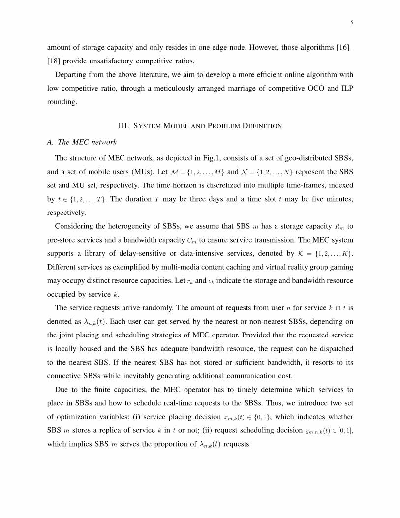
Fig.1 illustrates an example with five heterogeneous SBSs. Initially, each SBS places a subset

of services. If service k1 is already hosted in SBS S1, user u1 requesting service k1 can be

served locally. Otherwise, user may be served by non-nearest SBSs at the cost of additional

communication delay (as user u2 illustrated). With latest 5G technology, SBSs can communicate

with others beyond working individually. Furthermore, to better meet subsequent requests, each

SBS has to dynamically manage its services by removing or replacing the current services (as

SBS S3, S4, S5 illustrated).small base station (SBS)

SBS4 SBS!

SBS"

u1

u2

k3

k1

k2

k5

k2

k3

k2k3

k5

k1 k4

k5

k4

k1

k2k5

k3

SBS1

SBS3

network interconnection

Fig. 1: An illustration of the MEC system.

In addition to storage resources, modern innovative services also require data transmission,

which takes up a proportion of SBS bandwidth capacities and may even cause network conges-

tion. Moreover, under dense deployment of SBSs in 5G network [3], mobile users often reside in

the overlap coverage of SBSs. For the operator, bandwidth requirement and complicated multi-

SBSs scenario make placing and scheduling strategy more challenging. In this context, system

operator has a dynamic repertoire of service placing and scheduling alternatives. To minimize

overall operational cost, the operator should jointly optimize these strategies in an online fashion.

3

Previous studies examined the joint placing and routing problem for different objectives,

including minimizing service access latency [4]–[9] and maximizing the volume of served

requests [10]–[12]. A few recent approaches focus on cost-efficient placing and scheduling.

They suffer from limiting assumptions and lack of performance guarantee. Heuristic algorithms

without provable performance guarantee are proposed in [13]–[15]. Among those algorithms with

theoretical approximation guarantees [16]–[18], the performances are usually unsatisfactory.

Taking the above issue into account, the key challenges are:

How to dynamically adjust service placement in SBSs to satisfy the time-varying requests?

How to timely schedule user requests to appropriate SBSs?

How to jointly optimize these strategies in an online manner to minimize holistic operational

cost?

B. Methodology and Contributions

In this work, we establish a comprehensive model to address the above challenges, summarized

as follows.

• Online Framework. We formulate the joint placement and scheduling problem in MEC

networks, aiming to minimize holistic operational cost. We consider an MEC system with 1)

heterogeneous SBSs and diverse services, 2) stringent capacity limitations of SBSs, 3) time-

varying user requests, and 4) overlapping coverage regions of multi-SBSs.

• Regularization with look-Ahead Algorithm. We employ a regularization with look-ahead

approach from competitive online convex optimization (OCO) [19] to translate the offline relaxed

problem into a more tractable problem. The latter is then decomposed into multiple versions, each

of which partitions the time horizon into multiple episodes. Solving the problem of each episode

in each version, we obtain feasible fractional solutions to the offline relaxed problem by applying

Karush-Kuhn-Tucker (KKT) optimality conditions, while rigorously proving an upper-bound on

holistic operational cost relative to offline optimum.

• Rounding Algorithm. We devise a novel randomized rounding algorithm to transform frac-

tional solution of the offline relaxed problem into integer ones of the original problem. Working

in concert with the regularization with look-ahead algorithm, a low competitive ratio can be

realized.

4

• Evaluation Results. We carry out simulations in order to evaluate the effectiveness of the

proposed online framework. Compared with the latest related schemes, our proposed online

framework has a superior performance.

II. LITERATURE REVIEW

The problem of MEC service placement and scheduling has received increased attention in

recent years. The majority of previous works has been devoted to minimizing the latency [4]–[9]

or maximizing the volume of served requests [10]–[12].

Tran et al. [4] study how to minimize video access latency by leveraging the conditional

gradient method. Dehghan et al. [5] apply the greedy strategy and submodular optimization

to develop an approximation algorithm. Li et al. [6] present a distributed resilient caching

algorithm according to the concave relaxation of expected content access latency. Xu et al. [7]

define the joint problem as an integer linear programming (ILP) problem and develop a heuristic

algorithm. The works of [8], [9] both exploit Lyapunov optimization approach to study the time-

average latency, given diverse services and demands, and decentralized cooperation. Poularakis

et al. [10] investigate the joint optimization problem in dense MEC networks, and formulate

it as a submodular optimization problem respecting triple practical constraints. Considering the

sharable (storage) and non-sharable (computation, link bandwidth) resources, He et al. [11]

assume non-overlapped coverage region among multiple base stations and propose a greedy

algorithm.

While a few recent interesting studies focus on cost-efficient placing and scheduling, most of

them still has certain restrictions in the light of practicality and performance guarantee.

Taleb et al. [13] advocate content delivery network slicing, formulate cost optimization into

an ILP, and design computational-efficient heuristics. Yang et al. [14] utilize online request

prediction to regulate each round solution close to the optimum by a greedy algorithm. Ceselli

et al. [15] study the minimization of installation costs in network facilities, and design an

heuristic algorithm. The works of [13]–[15] fail to provide theoretical approximation guarantee.

Deep reinforcement learning has been adopted in [16], while their model confines service to

identically sized content, and only minimizes the traffic cost. Zeng et al. [17] utilize primal-dual

decomposition to translate the joint problem into bi-problems, and design an approximation al-

gorithm to solve each sub-problem. Zhao et al. [18] highlight the cost of forwarding requests and

downloading services in a homogeneous edge-cloud setting where all services consume the same

5

amount of storage capacity and only resides in one edge node. However, those algorithms [16]–

[18] provide unsatisfactory competitive ratios.

Departing from the above literature, we aim to develop a more efficient online algorithm with

low competitive ratio, through a meticulously arranged marriage of competitive OCO and ILP

rounding.

III. SYSTEM MODEL AND PROBLEM DEFINITION

A. The MEC network

The structure of MEC network, as depicted in Fig.1, consists of a set of geo-distributed SBSs,

and a set of mobile users (MUs). Let M = 1, 2, . . . ,M and N = 1, 2, . . . , N represent the SBS

set and MU set, respectively. The time horizon is discretized into multiple time-frames, indexed

by t ∈ 1, 2, . . . , T. The duration T may be three days and a time slot t may be five minutes,

respectively.

Considering the heterogeneity of SBSs, we assume that SBS m has a storage capacity Rm to

pre-store services and a bandwidth capacity Cm to ensure service transmission. The MEC system

supports a library of delay-sensitive or data-intensive services, denoted by K = 1, 2, . . . ,K.

Different services as exemplified by multi-media content caching and virtual reality group gaming

may occupy distinct resource capacities. Let rk and ck indicate the storage and bandwidth resource

occupied by service k.

The service requests arrive randomly. The amount of requests from user n for service k in t is

denoted as λn,k(t). Each user can get served by the nearest or non-nearest SBSs, depending on

the joint placing and scheduling strategies of MEC operator. Provided that the requested service

is locally housed and the SBS has adequate bandwidth resource, the request can be dispatched

to the nearest SBS. If the nearest SBS has not stored or sufficient bandwidth, it resorts to its

connective SBSs while inevitably generating additional communication cost.

Due to the finite capacities, the MEC operator has to timely determine which services to

place in SBSs and how to schedule real-time requests to the SBSs. Thus, we introduce two set

of optimization variables: (i) service placing decision xm,k(t) ∈ 0, 1, which indicates whether

SBS m stores a replica of service k in t or not; (ii) request scheduling decision ym,n,k(t) ∈ [0, 1],

which implies SBS m serves the proportion of λn,k(t) requests.

6

B. Cost Structure

The holistic cost of MEC system in its running time consists of three components.

Storage cost for storing service. The storage cost in t is computed as:

CR(t) =∑m

∑k

lm,kxm,k(t), (1)

where lm,k denote the unit storage cost to store service k in SBS m.

Service cost of SBSs. For each SBS, service cost mainly depends on MUs’ relative locations,

the number of served requests, and the proportion of services decided by the scheduling strategy.

In each time frame, let dm,n > 0 describe the communication parameter to weigh the location of

MUs. For example, when MUs locate in the boundary of the SBSs, serving such MUs consume

more communication power, which leads to higher cost. Accordingly, the service cost of SBSs

in t is:

CS(t) =∑m

∑n

∑k

dm,nλn,k(t)ym,n,k(t). (2)

Dynamic service placement cost. In addition to dispatch the real-time requests, the MEC

system has to dynamically manage the service placing of each SBS by removing current services

or placing newly service. To this end, we introduce a binary variable zm,k(t) to represent whether

SBS m stores newly service k in t or not, i.e., zm,k(t) = maxxm,k(t)−xm,k(t− 1), 0. The dynamic

service placing cost in t is

CD(t) =∑m

∑k

bm,kzm,k(t), (3)

where bm,k denote the unit placing cost of service k in SBS m.

C. Problem definition

We investigate the offline setting where all user requests are absolutely known, aiming at

minimizing the holistic cost. By adding Eq(1) to Eq(3) together, the offline problem, denoted

by Cost, can be formulated as follows

minimize∑t

(CR(t) + CS(t) + CD(t)

)(4)

subject to:

ym,n,k(t) ≤ xm,k(t),∀m,n, k, t, (4a)∑m

ym,n,k(t) ≥ 1,∀n, k, t, (4b)

7

zm,k(t) ≥ xm,k(t)− xm,k(t− 1),∀m, k, t, (4c)∑k

xm,k(t)rk ≤ Rm,∀m, t, (4d)

∑n

∑k

ym,n,k(t)λn,k(t)ck ≤ Cm,∀m, t, (4e)

ym,n,k(t) ∈ [0, 1] ,∀m,n, k, t, (4f)

xm,k(t) ∈ 0, 1,∀m, k, t, (4g)

zm,k(t) ∈ 0, 1,∀m, k, t, (4h)

where ∀m,n, k, t represent ∀m ∈M, n ∈ N , k ∈ K, t ∈ T .Constraint (4a) shows that a SBS should have already stored a replica of the requested service

before handling a request. Constraint (4b) indicates that the user request can be assigned to one

or multiple SBSs. Constraint (4d) and (4e) imply demand-supply balance conditions that SBS

m provided service can not exceed its capacities regarding storage and bandwidth resource.

Algorithmic challenges. The main challenges of minimization problem are two-fold. Firstly,

in realistic MEC system, it is not readily to make wise decisions timely due to the system

dynamics, such as newly arrived requests and placed services. Secondly, even within the offline

scenario where all the external inputs are absolutely provided, the original problem is still a

mixed-integer linear programming, which is NP-hard [20]. Then, without knowing all the future

information, how to online optimize holistic operational cost.

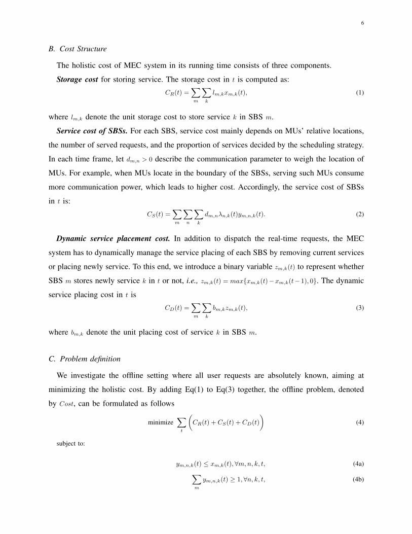
D. Basic idea

Enlightened by the competitive OCO [19], we devise an efficient online algorithm that lever-

ages the regularization with look-ahead approach and rounding technique, to tackle the above

challenges. The algorithmic idea, as illustrated in Fig.2, can be partitioned into two steps.

Step 1. In Sec. IV, we first obtain the fractional minimization problem P via relaxing the

integer decision variables. Then, by regularization with look-ahead, the fractional problem P

can be transformed into a more tractable problem PORA. The new problem PORA can be readily

decomposed into multiple versions, each of which partitions the time domain into a series of

episodes. And then, the dynamic service placing overhead of the beginning and last time-frame

in individual episode are substituted by two carefully-modified regularized terms in the objective

function. Solving the problem of each episode in each version, the fractional solution to relaxed

minimization problem is derived through online algorithm ORA.

8

Step 2. In Sec. V, considering the integral feature of decision variables, we design a randomized

dependent service placement algorithm RDSP , so as to round the fractional solution derived by

ORA into integer ones for the original problem.

Next, we discuss our online algorithm in details.

relax

Regularization with look-Ahead

Decompose L+1 versions

round

degrade

O R AP

( ) ( ) ( )(t : t )ORAP L

RDSPP

Cost

( ) ( ) ( )

0

1(t) P (t : t )

1

L

ORA ORAP OPT LL

map

1

1O R AP

r

1 2

1PRDSP

r r

Probability analysis

KKT analysis

Dual DP

Fig. 2: An illustration of our online algorithm

IV. ONLINE REGULARIZATION WITH LOOK-AHEAD ALGORITHM

A. Online Regularization with Look-Ahead Algorithm

1) Motivation

To conquer the challenge of NP-hardness in the offline minimization problem, we first relax

the integral variables, deriving the fractional minimization problem P as follows:

minimize∑t


)(5)

subject to: (4a) - (4f),

xm,k(t) ∈ [0, 1] ,∀m, k, t, (5g)

zm,k(t) ∈ [0, 1] ,∀m, k, t. (5h)

9

For the fractional minimization problem P , a straightforward solution is to greedily employ

the best control solutions in each time frame. However, such simple scheme would not certainly

guarantee the global optimal solution for the time span, and may even result in bad results [21].

Towards the competitive performance guarantee, we leverage the regularization technique and

finite look-ahead information to design a novel online algorithm, called Online Regularization

with look-Ahead (ORA). Here, look-ahead indicates that the system operator knows the current

information, and the information of consecutively following time (i.e., the look-ahead window

size). The key idea of algorithm ORA is to adopt two carefully-designed regularization terms

to approximate the dynamic service placing overhead of the beginning and last time-frame in

every episode.

More specifically, we first denote π as a non-negative integer from 0 to L. The algorithm ORA

executes L + 1 versions. Let ORA(π) represent the π-th version of ORA. ORA(π) partitions the

entire time into multiple episodes, each of which varies from t(π) to t(π)+L. And t(π) = π+(L+1)v,

where v = −1, 0, . . . , d TL+1e. In time t(π), the current information and the consecutively following L

time-slots’ information are provided. Thus, we further derive a formulation of ORA(π), denoted

by P(π)ORA:

minimizet(π)+L∑s=t(π)

∑m

∑k

lm,kxm,k(s)

+

t(π)+L∑s=t(π)

∑m

∑n

∑k

dm,nλn,k(s)ym,n,k(s)

+∑m

∑k

bm,kη

xm,k(t(π)) ln

(1 + ε

MK

x(π)m,k(t(π) − 1) + ε

MK

)

+

t(π)+L∑s=t(π)+1

∑m

∑k

bm,kzm,k(s)

+∑m

∑k

bm,kη

[(xm,k(t(π) + L) +

ε

MK

)· ln

(xm,k(t(π) + L) + ε

MK1 + ε

MK

)− xm,k(t(π) + L)

]

(6)

subject to:

ym,n,k(s) ≤ xm,k(s),∀m,n, k, s, (6a)∑m

ym,n,k(s) ≥ 1,∀n, k, s, (6b)

zm,k(s) ≥ xm,k(s)− xm,k(s− 1),∀m, k, s, (6c)

10

∑k

xm,k(s)rk ≤ Rm,∀m, s, (6d)

∑n

∑k

ym,n,k(s)λn,k(s)ck ≤ Cm,∀m, s, (6e)

xm,k(s), ym,n,k(s), zm,k(s) ∈ [0, 1] ,∀m,n, k, s, (6f)

where ∀m,n, k, s represent ∀m ∈M, n ∈ N , k ∈ K, and s ∈ [t(π), t(π)+L]. The notation η = ln(1+MKε ),

ε > 0 and control decision x(π)m,k(t(π) − 1) can be obtained by solving P

(π)ORA based on the previous

episodes from t(π) − L− 1 to t(π) − 1.

We should emphasize that, P (π)ORA approximates the dynamic service placing overhead of the

beginning time-frame t(π) and last time-frame t(π)+L in present episode by two regularized terms,

i.e., the third and fifth term in (6), which together guarantee the dynamic service placing overhead

at the boundary between the consecutive episodes cannot be arbitrarily large. Owing to the

convexity of regularization term, it has been widely adopted to approximate online optimization

problems in online learning [22].

2) Algorithm Design

Since ach problem P(π)ORA is a standard convex optimization problem comprising multiple

packing and covering constraints, it can be efficiently solved by invoking the interior point

method in convex optimization [23]. Then, in each time frame t, ORA gets the mean of X(π)(t)

and Y (π)(t) of all π as the control decision of ORA in t, i.e., XORA(t) and Y ORA(t). The details

of ORA are shown as Alg.1, which computes the fractional solution. Clearly, such fractional

solutions constitute a basis of solution to the original problem, and later are used as inputs in

next rounding algorithm.

B. Competitive Analysis

Next, we analyze the competitive performance of ORA according to an online primal-dual

framework [24]. Driven by this, we introduce the dual problem of fractional problem, denoted

by D, to bridge the offline minimization problem Cost and online minimization problem PORA

by constructing the following inequalities:

CORA(1 : T )(a)

≤ r1DORA(1 : T )

(b)

≤ r1Dopt(1 : T )

(c)

≤ r1Popt(1 : T )

(d)

≤ r1Costopt(1 : T ), (7)

where Costopt, P opt and Dopt denote the optimal objective function values of offline minimization

problem Cost, fractional primal problem P and fractional dual problem D. Let DORA be an

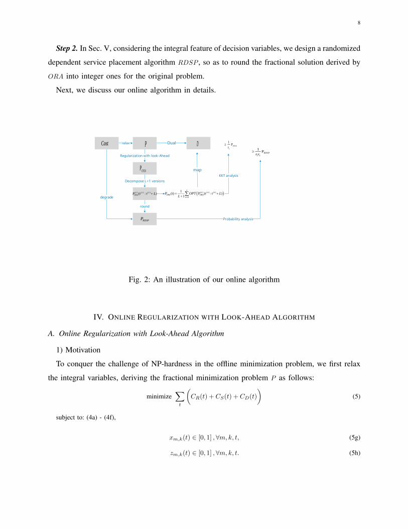
11

Algorithm 1 An Online Regularization with look-Ahead Algorithm (ORA)Input: η, ε, R, COutput: XORA(t), XORA(t)Initialize: XORA(t) = 0, Y ORA(t) = 0

1: for t = −(L+ 1), · · · , T do2: π ← t mod (L+ 1) and t(π) ← t3: if t(π) ≤ 0 then4: Remove the third term in (6)5: end if6: if t(π) + L ≥ T then7: Remove the fifth term in (6)8: end if9: Invoke the interior point method to solve P (π)

ORA and obtain X(π)(t(π) : t(π) +L) and Y (π)(t(π) : t(π) +L)10: while 1 ≤ t ≤ T do

11: XORA(t) = 1L+1

L∑π=0

X(π)(t)

12: Y ORA(t) = 1L+1

L∑π=0

Y (π)(t)

13: end while14: end for

objective function value of fractional dual problem D, obtained by a constructed solution mapped

from the fractional solution of online problem PORA. CORA is the objective function value of

online minimization problem PORA.

As P is obtained from Cost via relaxing its integral constraints, inequality (7d) holds. In

addition, inequality (7c) apparently follows from the Weak Duality Theorem [25]. Since the

fractional dual problem D is a maximization problem and the library of online dual solutions

obtained by ORA are feasible to problem D, we can consequently obtain inequality (7b).

The rest of this subsection presents how to establish inequality (7a). Specifically, we first

formulate the fractional dual problem D. Then, we construct a dual solution for problem DORA

and check the feasibility. Third, due to add two regularization terms in (6), the cost gap between

the online primal problem and online dual problem should be quantified. Finally, we obtain the

competitive performance of ORA.

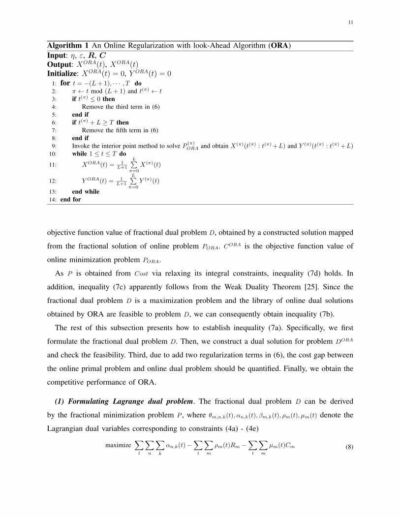
(1) Formulating Lagrange dual problem. The fractional dual problem D can be derived

by the fractional minimization problem P , where θm,n,k(t), αn,k(t), βm,k(t), ρm(t), µm(t) denote the

Lagrangian dual variables corresponding to constraints (4a) - (4e)

maximize∑t

∑n

∑k

αn,k(t)−∑t

∑m

ρm(t)Rm −∑t

∑m

µm(t)Cm (8)

12

subject to:

∑n

θm,n,k(t)− βm,k(t) + βm,k(t+ 1)− ρm(t)rk ≤ lm,k,∀m, k, t, (8a)

αn,k(t) ≤ dm,nλn,k(t) + θm,n,k(t) + µm(t)λn,k(t)ck,∀m,n, k, t, (8b)

βm,k(t) ≤ bm,k,∀m, k, t, (8c)

θm,n,k(t), αn,k(t), βj,k(t), ρm(t), µm(t) ≥ 0,∀m,n, k, t, (8d)

where ∀m,n, k, t represent ∀m ∈M, n ∈ N , k ∈ K, t ∈ T .

(2) Checking the fractional dual feasibility.

Now, we concentrate on one version of ORA and explain the decision solutions obtained by

all episodes of P (π)ORA are feasible to the fractional dual problem. Similar to (8), we can formulate

the online dual problem of (6) and let θ(π)m,n,k(t), α(π)n,k(t), β

(π)m,k(t), ρ

(π)m (t), µ

(π)m (t) denote the online dual

variables corresponding to constraints (6a) - (6e). The objective function of (6) has not contained

the dynamic service placing overhead in the beginning time-frame t(π). To this end, we define

the missing variables β(π)m,k(t(π)) as follows

β(π)m,k(t(π)) ,

bm,kη

ln

(1 + ε

MK

x(π)m,k(t(π) − 1) + ε

MK

). (9)

Lemma 1. The constructed solution θ(π)(t), α(π)(t), β(π)(t), ρ(π)(t), µ(π)(t) from the online dual

solution of P (π)ORA and (9) are also feasible for fractional dual problem D.

Proof. See Appendix A. ut

Lemma 1 can be proved by applying KKT optimality conditions [25] to P(π)ORA. In the following,

we list the Complementary slackness and Optimality conditions in a disjunctive form, where c ⊥ d

is equivalent to c, d ≥ 0 and cd = 0.

Complementary slackness : (10)

α(π)n,k(t) ⊥

[1−

∑m

y(π)m,n,k(t)

]= 0,∀m, k, t, (10a)

θ(π)m,n,k(t) ⊥

[x(π)m,k(t)− y(π)m,n,k(t)

]= 0,∀m,n, k, t, (10b)

β(π)m,k(t) ⊥

[x(π)m,k(t)− x(π)m,k(t− 1)− z(π)m,k(t)

]= 0,∀m, k, t, (10c)

ρ(π)m (t) ⊥

[∑k

rkx(π)m,k(t)−Rm

]= 0,∀m, t, (10d)

13

µ(π)m (t) ⊥

[∑k

∑n

ckλn,k(t)y(π)m,n,k(t)− Cm

]= 0,∀m, t. (10e)

Stationarity/Optimality : (11)

x(π)m,k(t(π)) ⊥

[lm,k + rkρ

(π)m (t(π))− β(π)

m,k(t(π) + 1)

−∑n

θ(π)m,n,k(t(π)) +

bm,kη

ln

(1 + ε

MK

x(π)m,k(t(π) − 1) + ε

MK

)]= 0,∀m, k, (11a)

x(π)m,k(t) ⊥

[lm,k + rkρ

(π)m (t)− β(π)

m,k(t+ 1)−∑n

θ(π)m,n,k(t) + β

(π)m,k(t)

]= 0,∀m, k, t ∈ [t(π) + 1, t(π) + L− 1],

(11b)x(π)m,k(t(π) + L) ⊥

[lm,k + rkρ

(π)m (t(π) + L) + β

(π)m,k(t(π) + L)

−∑n

θ(π)m,n,k(t(π) + L)− bm,k

ηln

(1 + ε

MK

x(π)m,k(t(π) + L) + ε

MK

)]= 0,∀m, k, (11c)

y(π)m,n,k(t)(t) ⊥

[θ(π)m,n,k(t) + ckλn,k(t)µ(π)

m (t)− α(π)n,k(t) + dm,nλn,k(t)

]= 0,∀m,n, k, t ∈ [t(π), t(π) + L], (11d)

z(π)m,k(t) ⊥

[β(π)m,k(t)− bm,k

]= 0,∀m,n, k, t ∈ [t(π) + 1, t(π) + L]. (11e)

(3) Gauging the cost gap.

Concentrating on a episode (i.e., from t(π) to t(π) + L) of P (π)ORA, we introduce online primal

overhead C(π)(t(π) : t(π) + L) and online dual cost D(π)(t(π) : t(π) + L) as follows

C(π)(t(π) : t(π) + L) ,t(π)+L∑t=t(π)


),

D(π)(t(π) : t(π) + L) ,t(π)+L∑t=t(π)

∑n

∑k

α(π)j,k (t)−

t(π)+L∑t=t(π)

∑m

ρ(π)m (t)Rm −t(π)+L∑t=t(π)

∑m

µ(π)m (t)Cm.

The objective function in P(π)ORA has involved two regularized items, there thus be certain gap

between online primal overhead and online dual overhead. In the following, we present the cost

gap.

Lemma 2. As for each ORA(π), we derive

14

C(π)(t(π) : t(π) + L) ≤ D(π)(t(π) : t(π) + L) +∑m

∑k

Ω(π)m,k(t(π)) +

∑m

∑k

φ(π)m,k(t(π)) +

∑m

∑k

ψ(π)m,k(t(π)),

(12)

where the dual tail-terms Ω(π)m,k(t(π)), φ(π)m,k(t(π)) and ψ

(π)m,k(t(π)) define as follows

Ω(π)m,k(t(π)) , bm,k

[x(π)m,k(t(π))− x(π)m,k(t(π) − 1)

]+, (12a)

φ(π)m,k(t(π)) , −bm,k

ηx(π)m,k(t(π)) ln

(1 + ε

MK

x(π)m,k(t(π) − 1) + ε

MK

), (12b)

ψ(π)m,k(t(π)) ,

bm,kη

x(π)m,k(t(π) + L) ln

(1 + ε

MK

x(π)m,k(t(π) + L) + ε

MK

). (12c)

Proof. See Appendix B. ut

Note that the online problem P(π)ORA has not optimize the dynamic service placing cost in the

first time-frame, which leads to dual tail-term Ω(π)m,k(t(π)). Since the online primal objective in

P(π)ORA includes two additional terms, the second and third tail-term are correspondingly obtained.

Bounding cost gap is the main challenge of establishing inequality (7a), we thus divide it into

bi-steps.

Step 3-1 Bounding the dual tail-terms.

Now, we are ready to bound three dual tail-terms, which originate from the same version

π of ORA. The upper-bound of tail-terms are well-chosen portions of the online dual cost. In

this context, we assume dre − 1 < L, where r , maxm,k

(bm,klm,k

). The proof is similar in the case of

dre − 1 ≥ L.Lemma 3. For each ORA(π), the following two inequalities hold.

d TL+1 e∑v=0

∑t(π)=π

+(L+1)v

∑m

∑k

Ω(π)m,k(t(π)) ≤ η(1 + ε)

d TL+1 e∑v=0

∑t(π)=π

+(L+1)v

D(π)(t(π) : t(π) + dre − 1), (13)

d TL+1 e∑v=−1

∑t(π)=π

+(L+1)v

∑m

∑k

[φ(π)m,k(t(π)) + ψ

(π)m,k(t(π))

]≤ η(1 + ε)

d TL+1 e∑v=−1

∑t(π)=π

+(L+1)v

D(π)(t(π) + L− dre+ 1 : t(π)), (14)

where D(π)(t) = 0 if t ≤ 0 or t > T .

Proof. See Appendix C. ut

Note that, according to (13), the upper-bound of first dual tail-term Ω(π)m,k is a partial summation

of online dual cost across intervals of size dre at the beginning time-slot of each episode.

The right-hand-side (RHS) of (14) has a analogous explanation, while the partial summation

15

is replaced by intervals in the finish of every episode.

Step 3-2 Bounding the online dual overhead.

The following lemma is to link the part of online dual overhead and the offline dual optimal

overhead.

Lemma 4. For each time interval [t1, t2], we derive

D(π)(t1 : t2) ≤Dopt(t1 : t2)−∑m

∑k

βoptm,k(t1)xoptm,k(t1 − 1)−∑m

∑k

β(π)m,k(t2 + 1)xoptm,k(t2)

+∑m

∑k

βoptm,k(t2 + 1)xoptm,k(t2) +∑m

∑k

β(π)m,k(t1)xoptm,k(t1 − 1),

(15)

where xoptm,k(t), βoptm,k(t), and β(π)m,k(t) denote the optimal offline primal solution, the optimal offline

dual solution, and the online dual solution.

Proof:For each time interval [t1, t2], by applying the complementary slackness conditions to (4), we

get

Costopt(t1 : t2) =

t2∑t=t1

∑m

∑k

lm,kxoptm,k(t) +

t2∑t=t1

∑m

∑n

∑k

dm,nλn,k(t)yoptm,n,k(t)

+

t2∑t=t1

∑m

∑k

bm,kzoptm,k(t) + αoptn,k(t)

[1−

∑m

yoptm,n,k(t)

]+ θoptm,n,k(t)

[xoptm,k(t)− yoptm,n,k(t)

]

+ βoptm,k(t)[xoptm,k(t)− xoptm,k(t− 1)− zoptm,k(t)

]+ ρoptm (t)

[∑k

rkxoptm,k(t)−Rm

]

+ µoptm (t)

[∑k

∑n

ckλn,k(t)yoptm,n,k(t)− Cm

].

(16)

By rearranging terms in (16), we have

Costopt(t1 : t2) =

t2∑t=t1

∑m

∑k

αoptn,k(t)−t2∑t=t1

∑m

ρoptm (t)Rm −t2∑t=t1

∑m

µoptm (t)Cm

−∑m

∑k

βoptm,k(t1)xoptm,k(t1 − 1) +∑m

∑k

βoptm,k(t2 + 1)xoptm,k(t2)

+

t2∑t=t1

∑m

∑k

xoptm,k(t)

[lm,k −

∑n

θoptm,n,k(t) + rkρoptm (t) + βoptm,k(t)− βoptm,k(t+ 1)

]

+

t2∑t=t1

∑m

∑n

∑k

yoptm,n,k(t) ·[θoptm,n,k(t) + ckλn,k(t)µoptm (t)− αoptn,k(t) + dm,nλn,k(t)

]

+

t2∑t=t1

∑m

∑k

zoptm,k(t)[βoptm,k(t)− bm,k

].

(17)

16

Utilizing the optimality conditions to (17), we get

Costopt(t1 : t2) =

t2∑t=t1

∑m

∑k


∑m

ρoptm (t)Rm +∑m

∑k

βoptm,k(t2 + 1)xoptm,k(t2)

−t2∑t=t1

∑m

µoptm (t)Cm −∑m

∑k

βoptm,k(t1)xoptm,k(t1 − 1).

(18)

Based on the primal constraints (4b) and (4c), we have

Costopt(t1 : t2) ≥t2∑t=t1

∑m

∑k

lm,kxoptm,k(t) +

t2∑t=t1

∑m

∑n

∑k

dm,nλn,k(t)yoptm,n,k(t) +

t2∑t=t1

∑m

∑k

bm,kzoptm,k(t)

+

t2∑t=t1

∑n

∑k

α(π)n,k(t)

[1−

∑m

yoptm,n,k(t)

]+

t2∑t=t1

∑m

∑n

∑k

θ(π)m,n,k(t)

[xoptm,k(t)− yoptm,n,k(t)

]

+

t2∑t=t1

∑m

∑k

β(π)m,k(t)

[xoptm,k(t)− xoptm,k(t− 1)− zoptm,k(t)

]+

t2∑t=t1

∑m

ρ(π)m (t)

[∑k

rkxoptm,k(t)−Rm

]

+

t2∑t=t1

∑m

µ(π)m (t)

[∑n

∑k


].

(19)

By rearranging the terms in (19), we have

Copt(t1 : t2) ≥t2∑t=t1

∑m

∑k

α(π)n,k(t)−

t2∑t=t1

∑m

ρ(π)m (t)Rm −t2∑t=t1

∑m

µ(π)m (t)Cm −

∑m

∑k

β(π)m,k(t1)xoptm,k(t1 − 1)

+∑m

∑k

β(π)m,k(t2 + 1)xoptm,k(t2) +

t2∑t=t1

∑m

∑k

zoptm,k(t)[β(π)m,k(t)− bm,k

]

+

t2∑t=t1

∑m

∑k

xoptm,k(t) ·

[lm,k −

∑n

θ(π)m,n,k(t) + rkρ

(π)m (t) + β

(π)m,k(t)− β(π)

m,k(t+ 1)

]

+

t2∑t=t1

∑m

∑n

∑k

yoptm,n,k(t) ·[θ(π)m,n,k(t) + ckλn,k(t)µ(π)


].

Note that xoptm,k(t) and yoptm,n,k(t) are non-negative. And, the optimality conditions indicate that, to

prevent the objective value of online dual problem from going down to minus infinity, constrains

(8a), (8b) and (8c) should be respected. Thus, we get

Costopt(t1 : t2) ≥t2∑t=t1

∑m

∑k

α(π)n,k(t)−

t2∑t=t1

∑m


∑m

µ(π)m (t)Cm

−∑m

∑k

β(π)m,k(t1)xoptm,k(t1 − 1) +

∑m

∑k

β(π)m,k(t2 + 1)xoptm,k(t2).

(20)

17

Based on (18) and (20), we get

t2∑t=t1

∑m

∑k

α(π)n,k(t)−

t2∑t=t1

∑m


∑m

µ(π)m (t)Cm

−∑m

∑k


∑m

∑k

β(π)m,k(t2 + 1)xoptm,k(t2)

≤t2∑t=t1

∑m

∑k


∑m

ρoptm (t)Rm −t2∑t=t1

∑m

µoptm (t)Cm

−∑m

∑k


∑m

∑k

β(π)m,k(t2 + 1)xoptm,k(t2).

ut(4) Obtaining the competitive ratio of ORA.

Next, we analyze the competitive performance of ORA.

Theorem 1. With L ≥ 1 and dre < L + 1, the competitive ratio of ORA can be computed as

follows

r1 = 1 +3η(1 + ε

MK )dreL+ 1

.

Before proving Theorem 1, we calculate the total cost of ORA as follows,

CORA(1 : T ) =

T∑t=1

∑m

∑k

lm,kxORAm,k (t) +

T∑t=1

∑m

∑n

∑k

dm,nλn,k(t)yORAm,n,k(t)

+

T∑t=1

∑m

∑k

bm,k[xORAm,k (t)− xORAm,k (t− 1)

]+,

(21)

where xORAm,k (t) and yORAm,n,k(t) can be obtained by Alg.1. By utilizing Jensen’s Inequality, we can

derive

CORA(1 : T ) ≤ 1

L+ 1

L∑π=0

C(π)(1 : T ). (22)

By applying Lemma 2 to (22), the upper-bound of ORA CORA(1 : T ) is

CORA(1 : T ) ≤ 1

L+ 1

N∑π=0

d TL+1 e∑v=−1

∑t(π)=π

+(L+1)v

D(π)(t(π) : t(π) + L)

+∑m

∑k

Ω(π)m,k(t(π)) +

∑m

∑k

φ(π)m,k(t(π)) +

∑m

∑k

ψ(π)m,k(t(π))

.

(23)

Based on Lemma 1, the online dual cost in (23) amounts to

1

L+ 1

L∑π=0

D(π)(1 : T ) ≤ Dopt(1 : T ). (24)

18

The RHS of (23) only remains three dual tail-terms that need to bound.

Recall that Lemma 3, we can deduce two important conclusions, and list as follows (the proof

is given by Appendix D).

(i) The upper-bound of∑m

∑k

Ω(π)m,k(t(π)) is

η(1 +ε

MK)

t(π)−1+dre∑t=t(π)

D(π)(t), t(π) ∈ [1, T − dre],

η(1 +ε

MK)

T∑t=t(π)

D(π)(t), t(π) ∈ [T − dre+ 1, T ],

(25)

where D(π)(t) =∑n

∑k

α(π)n,k(t) −

∑mρ(π)m (t)Rm −

∑mµ(π)m (t)Cm. For simplicity, we use D(π)(t) in the

following proof.

(ii) The upper-bound of∑m

∑k

[φ(π)m,k(t(π)) + ψ

(π)m,k(t(π))

]is

η(1 +ε

MK)

t(π)+L∑t=t(π)+L−dre+1

D(π)(t), t(π) ∈ [−L+ dre+ 1, T − L],

η(1 +ε

MK)

t(π)+L∑t=1

D(π)(t), t(π) ∈ [−L+ 1,−L+ dre].

(26)

Proof of Theorem 1.

Based on Lemma 4 and applying (25)-(26) to (13)-(14) in Lemma 3, we obtain

CORA(1 : T ) ≤ 1

L+ 1

L∑π=0

D(π)(1 : T )

+1

L+ 1η(1 +

ε

MK) · T−dre∑t(π)=1

D(π)(t(π) : t(π) + dre − 1) +

T∑t(π)=T−dre+1

D(π)(t(π) : T )

+

−L+dre∑t(π)=−(L+1)

D(π)(1 : t(π) + L) +

T−L∑t(π)=−L+dre+1

D(π)(t(π) + L− dre+ 1 : t(π) + L)

.

(27)

For each time-slot t, inequality D(π)(t) ≥ 0 holds. Therefore, from (27), we get

19

CORA(1 : T ) ≤ 1

L+ 1

L∑π=0

D(π)(1 : T ) +1

L+ 1η(1 +

ε

MK) · T−dre∑t(π)=1

D(π)(1 : t(π))

+

T−dre∑t(π)=1

D(π)(t(π) : t(π) + dre − 1) +

T∑t(π)=T−dre+1

D(π)(t(π) : T ) +

−L+dre∑t(π)=−L+1

D(π)(1 : t(π) + L)

+


D(π)(t(π) + L− dre+ 1 : t(π) + L) +

T∑t(π)=−L+dre+2

D(π)(t(π) : T )

.

(28)

According to Lemma 4, we derive

CORA(1 : T ) ≤ 1

L+ 1

L∑π=0

D(π)(1 : T ) +1

L+ 1η(1 +

ε

MK) ·

2dreDopt(1 : T )

+

T−dre∑t(π)=1

∑m

∑k

β(π)m,k(t(π))xoptm,k(t(π) − 1) +

T∑t(π)=T−dre+1

∑m

∑k

β(π)m,k(t(π))xoptm,k(t(π) − 1)

+


∑m

∑k

β(π)m,k(t(π) + L− dre+ 1) · xoptm,k(t(π) + L− dre) +

T∑t(π)=−L+dre+2

∑m

∑k


−dre−1∑t(π)=1

∑m

∑k

β(π)m,k(t(π) + 1)xoptm,k(t(π))−

T−dre∑t(π)=1

∑m

∑k

β(π)m,k(t(π) + dre)xoptm,k(t(π) + dre − 1)

−−L+dre∑

t(π)=−L+1

∑m

∑k

β(π)m,k(t(π) + L+ 1)xoptm,k(t(π) + L)

−T−L∑

t(π)=−L+dre+1

∑m

∑k

β(π)m,k(t(π) + L+ 1)xoptm,k(t(π) + L)

.

(29)

As constraint (8c) states 0 ≤ β(π)m,k(t) ≤ bm,k, we have

CORA(1 : T ) ≤ 1

L+ 1

L∑π=0

D(π)(1 : T ) +1

L+ 1η(1 +

ε

MK) ·

2dreDopt(1 : T )

+

T∑t(π)=1

∑m

∑k


+

T−dre∑t(π)=1

∑m

∑k

bm,kxoptm,k(t(π)) +

T−1∑t(π)=T−dre+1

∑m

∑k

bm,kxoptm,k(t(π))

−dre+1∑t(π)=2

∑m

∑k

β(π)m,k(t(π))xoptm,k(t(π) − 1)−

T∑t(π)=dre+2

∑m

∑k


.

(30)

As x(π)m,k(0) = 0 and xoptm,k(t) ≥ 0, from (30), we obtain

20

CORA(1 : T ) ≤ 1

L+ 1

L∑π=0

D(π)(1 : T ) +1

L+ 1η(1 +

ε

MK) ·

[2dreDopt(1 : T ) +

T∑t=1

∑m

∑k

lm,kxoptm,k(t)

].

(31)

Note that bm,kxoptm,k(t) ≤ drebm,kxoptm,k(t). Lastly, based on Lemma 1 and the duality theorem [25],

from (31), we derive

CORA(1 : T ) ≤ Copt(1 : T ) +1

L+ 1η(1 +

ε

MK) · 2dreCopt(1 : T ) + dreCopt(1 : T )

≤

1 +3η(1 + ε

MK )dreL+ 1

Copt(1 : T ).

ut

V. ONLINE DEPENDENT ROUNDING ALGORITHM

The online regularization with look-ahead algorithm calculates fractional solutions for frac-

tional minimization problem P in each time slot. When considering the integral constraints of

optimization variables, we should translate fractional solution x into integer ones x, which

simultaneously satisfies feasibility constraints (4a), (4d) and (4g).

A. Algorithm design

A natural approach is the independent rounding method [26] whose key idea is that each

control solution is rounded up or down individually. Yet, such simple solution may obtain a

infeasible solution or lead to a high cost and even system instability. To this end, we design a

randomized dependent service placing algorithm RDSP , enlightened by the dependent rounding

technique [27]. The online algorithm RDSP employs the interdependence of x , consisting of

the following step:

Step 1. We first construct a bipartite graph;

Step 2. We apply the dependent rounding method to calculate the rounded solution.

This algorithm executes a series of rounding iterations. Let xhm,k(t) denote solution xm,k(t) after

h-th rounding iteration.

We begin with the h+ 1 rounding iteration. If a service is fractionally allocated to more than

one SBS, we refer it as a floating service. Similarly, a SBS can be called as a floating SBS, if it

has more than one floating service dispatched to it in the current rounding iteration. Let Kf and

Mf denote the set of floating services and floating SBSs in the current iteration, respectively.

21

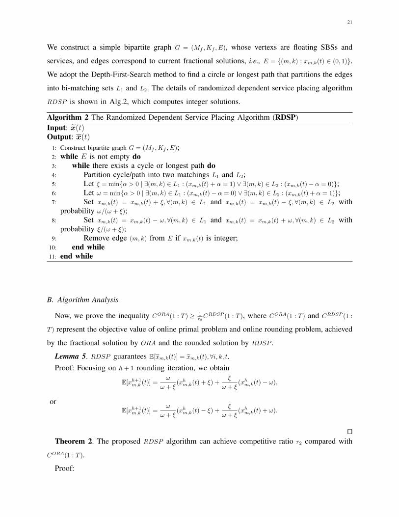
We construct a simple bipartite graph G = (Mf ,Kf , E), whose vertexs are floating SBSs and

services, and edges correspond to current fractional solutions, i.e., E = (m, k) : xm,k(t) ∈ (0, 1).

We adopt the Depth-First-Search method to find a circle or longest path that partitions the edges

into bi-matching sets L1 and L2. The details of randomized dependent service placing algorithm

RDSP is shown in Alg.2, which computes integer solutions.

Algorithm 2 The Randomized Dependent Service Placing Algorithm (RDSP)Input: x(t)Output: x(t)

1: Construct bipartite graph G = (Mf ,Kf , E);2: while E is not empty do3: while there exists a cycle or longest path do4: Partition cycle/path into two matchings L1 and L2;5: Let ξ = minα > 0 | ∃(m, k) ∈ L1 : (xm,k(t) + α = 1) ∨ ∃(m, k) ∈ L2 : (xm,k(t)− α = 0);6: Let ω = minα > 0 | ∃(m, k) ∈ L1 : (xm,k(t)− α = 0) ∨ ∃(m, k) ∈ L2 : (xm,k(t) + α = 1);7: Set xm,k(t) = xm,k(t) + ξ,∀(m, k) ∈ L1 and xm,k(t) = xm,k(t) − ξ,∀(m, k) ∈ L2 with

probability ω/(ω + ξ);8: Set xm,k(t) = xm,k(t) − ω,∀(m, k) ∈ L1 and xm,k(t) = xm,k(t) + ω,∀(m, k) ∈ L2 with

probability ξ/(ω + ξ);9: Remove edge (m, k) from E if xm,k(t) is integer;

10: end while11: end while

B. Algorithm Analysis

Now, we prove the inequality CORA(1 : T ) ≥ 1r2CRDSP (1 : T ), where CORA(1 : T ) and CRDSP (1 :

T ) represent the objective value of online primal problem and online rounding problem, achieved

by the fractional solution by ORA and the rounded solution by RDSP .

Lemma 5. RDSP guarantees E[xm,k(t)] = xm,k(t),∀i, k, t.Proof: Focusing on h+ 1 rounding iteration, we obtain

E[xh+1m,k (t)] =

ω

ω + ξ(xhm,k(t) + ξ) +

ξ

ω + ξ(xhm,k(t)− ω),

orE[xh+1

m,k (t)] =ω

ω + ξ(xhm,k(t)− ξ) +

ξ

ω + ξ(xhm,k(t) + ω).

utTheorem 2. The proposed RDSP algorithm can achieve competitive ratio r2 compared with

CORA(1 : T ).

Proof:

22

E[CRDSP (1 : T )

]= E

[∑t

∑m

∑k

lm,kxm,k(t) +∑t

∑m

∑n

∑k

dm,nλn,k(t)ym,n,k(t) +∑t

∑m

∑k

bm,kzm,k(t)

]

≤ CORA(1 : T ) + CORA(1 : T ) +∑t

∑m

∑k

maxm,k

(bm,klm,k

)lm,kxm,k(t)

≤ (2 + maxdre)CORA(1 : T ). (32)

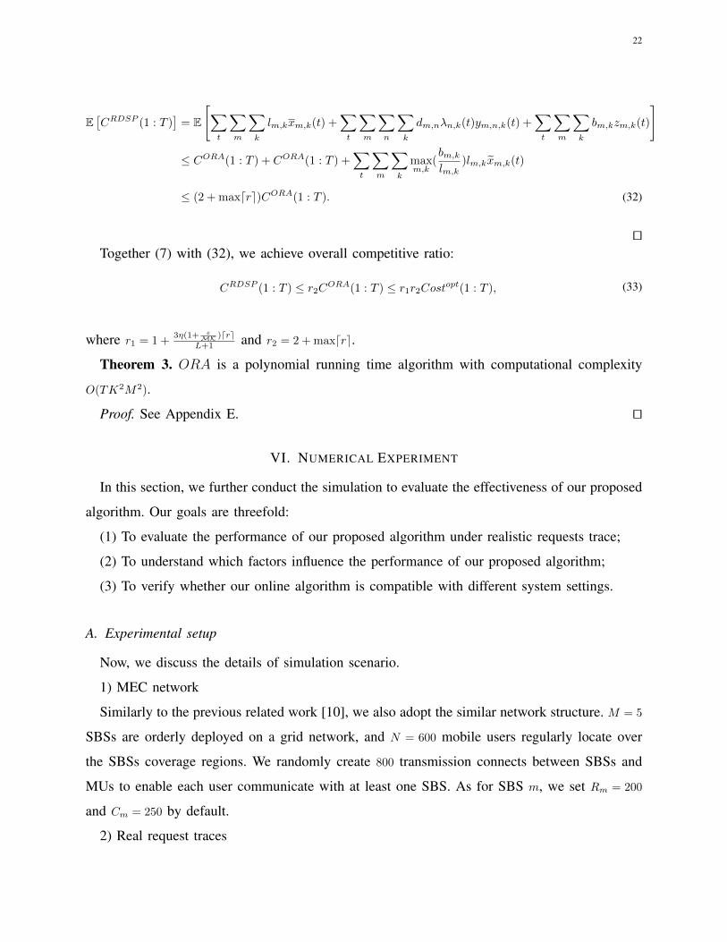
utTogether (7) with (32), we achieve overall competitive ratio:

CRDSP (1 : T ) ≤ r2CORA(1 : T ) ≤ r1r2Costopt(1 : T ), (33)

where r1 = 1 +3η(1+ ε

MK )dreL+1 and r2 = 2 + maxdre.

Theorem 3. ORA is a polynomial running time algorithm with computational complexity

O(TK2M2).

Proof. See Appendix E. ut

VI. NUMERICAL EXPERIMENT

In this section, we further conduct the simulation to evaluate the effectiveness of our proposed

algorithm. Our goals are threefold:

(1) To evaluate the performance of our proposed algorithm under realistic requests trace;

(2) To understand which factors influence the performance of our proposed algorithm;

(3) To verify whether our online algorithm is compatible with different system settings.

A. Experimental setup

Now, we discuss the details of simulation scenario.

1) MEC network

Similarly to the previous related work [10], we also adopt the similar network structure. M = 5

SBSs are orderly deployed on a grid network, and N = 600 mobile users regularly locate over

the SBSs coverage regions. We randomly create 800 transmission connects between SBSs and

MUs to enable each user communicate with at least one SBS. As for SBS m, we set Rm = 200

and Cm = 250 by default.

2) Real request traces

23

In each time slot, each user submits request for service drawn from a service set, K = 100. We

adopt the same service requirements in [10], and map services to three actual service, i.e., Video

streaming (VS), Augmented Reality (AR) and Network Gaming (NG). VS wants requirement

of storage and bandwidth within [1, 10] and [1, 25], respectively. The resource requirements of AR

are set within [2, 20] and [0.2, 2], respectively. The demand storage and bandwidth of NG are set

within [5, 40] and [1, 25], respectively. The service parameters are in accordance with real service

specifications [10].

3) Online algorithm description

As for the online algorithm, we set the default size of look-ahead window to be 5 and define the

number of time-slot as 300 . In terms of unit storage cost of a SBS, we adopt the similar pattern

in [28], where storage price is inversely proportion to the occupied capacity. The transmission

efficiency parameter dm,n is randomly distributed in [1, 5] due to short distance and low delay.

We set the dynamic placing cost bm,k randomly within [5, 10].

B. Comparison with offline algorithm

We introduce the algorithm competitive ratio, which can be obtained through its total cost

divided by the offline optimum that can be optimally solved by the MOSEK Optimizer.

100 150 200 250 300

Number of Services

0

0.5

1

1.5

2

2.5

3

Com

petitv

e R

atio

=0.1 =0.3 =0.5 =0.7 =0.9

Fig. 3: Competitive ratio with different K and ε.

600 700 800 900 1000

Number of MUs

1

1.5

2

2.5

3

Perf

orm

ance R

atio

=0.1 =0.3 =0.5 =0.7 =0.9

Fig. 4: Competitive ratio with different N and ε.

24

5 7 9 11 13

Number of SBSs

1

1.2

1.4

1.6

1.8

2

2.2

2.4

2.6

Perf

orm

ance R

atio

=0.1 =0.3 =0.5 =0.7 =0.9

Fig. 5: Competitive ratio with different M and ε.

Fig.3-Fig.5 exhibit that how the performance of online algorithm change. Globally, the in-

creasing number of total services, MUs and SBSs leads to a larger competitive ratio, which is

inline with the theoretical analysis. As we observe, Fig.3-Fig.5 also depict the impact of ε on

our performance. In the following evaluation, we set the default value of ε to be 0.3 instead of

the optimum ε to optimize the theoretical competitive ratio.

C. Comparison with other schemes

In this context, we compare with four algorithms in the latest related works.

Regularization-based algorithm (REG) [28]: it leverages regularization method to make the

joint placing and routing decision, in order to minimize the overall cost;

Primal-dual algorithm (PD) [17]: it resorts to primal-dual method to minimize the total cost;

Greedy algorithm (GA): it greedily make the joint decision to minimize the holistic cost;

Cache-only algorithm (CA) [29]: it places services on SBSs until all storage capacity are full

and tries to minimize the service placing cost.

100 150 200 250 300

Number of Services

1

1.5

2

2.5

3

Com

petitive R

atio

Ours REG PD GA CA

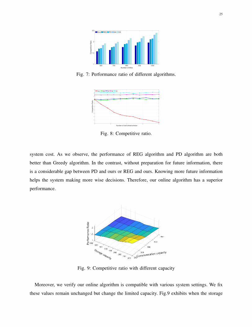
Fig. 6: Performance ratio of different algorithms.The results of Fig.6-Fig.8 present how the performance change with the increase of services,

MUs, and look-ahead window size. As expected, the performance of Cache-only algorithm is the

worst, since it stores as many services as possible, neglecting the transmission cost and dynamic

placing cost. Greedy algorithm performs better than Cache algorithm since it considers more

25

600 700 800 900 1000

Number of MUs

1

1.5

2

2.5

Com

petitive R

atio

Ours REG PD GA CA

Fig. 7: Performance ratio of different algorithms.

5 10 15 20 25

Number of look-ahead window

1

1.1

1.2

1.3

1.4

1.5

1.6

1.7

1.8

1.9

2

Co

mp

etitive

Ra

tio

Ours REG PD GA CA

Fig. 8: Competitive ratio.

system cost. As we observe, the performance of REG algorithm and PD algorithm are both

better than Greedy algorithm. In the contrast, without preparation for future information, there

is a considerable gap between PD and ours or REG and ours. Knowing more future information

helps the system making more wise decisions. Therefore, our online algorithm has a superior

performance.

Fig. 9: Competitive ratio with different capacity

Moreover, we verify our online algorithm is compatible with various system settings. We fix

these values remain unchanged but change the limited capacity. Fig.9 exhibits when the storage

26

and communication capacity increases, our algorithm persistently has a better performance since

it makes full use of system resources.

VII. CONCLUSION

In this context, we study the joint service placing and request scheduling problem in MEC

networks, and developed an efficient online framework, aiming to minimize holistic operational

cost. Our online algorithm employs the competitive OCO technique and rounding method to

solve the cost-minimization problem. The theoretical analysis and simulations have corroborated

the efficiency of our proposed online algorithm. We confirmed that our algorithm has a superior

performance over alternative benchmarks through large-scale evaluations. Next, we will further

concentrate on typical real-world scenarios and design more efficient online algorithm which

can accommodate more flexible user requests.

27

REFERENCES

[1] P. Mach and Z. Becvar, “Mobile edge computing: A survey on architecture and computation offloading,” IEEE

Communications Surveys Tutorials, vol. 19, no. 3, pp. 1628–1656, 2017.

[2] Y. Mao, C. You, J. Zhang, K. Huang, and K. B. Letaief, “A survey on mobile edge computing: The communication

perspective,” IEEE Communications Surveys Tutorials, vol. 19, no. 4, pp. 2322–2358, 2017.

[3] X. Ge, S. Tu, G. Mao, C.-X. Wang, and T. Han, “5g ultra-dense cellular networks,” IEEE Wireless Communications,

vol. 23, no. 1, pp. 72–79, 2016.

[4] T. X. Tran and D. Pompili, “Adaptive bitrate video caching and processing in mobile-edge computing networks,” IEEE

Transactions on Mobile Computing, vol. 18, no. 9, pp. 1965–1978, 2019.

[5] M. Dehghan, B. Jiang, A. Seetharam, T. He, T. Salonidis, J. Kurose, D. Towsley, and R. Sitaraman, “On the complexity of

optimal request routing and content caching in heterogeneous cache networks,” IEEE/ACM Transactions on Networking,

vol. 25, no. 3, pp. 1635–1648, 2017.

[6] J. Li, T. Khoa Phan, W. Koong Chai, D. Tuncer, G. Pavlou, D. Griffin, and M. Rio, “Dr-cache: Distributed resilient caching

with latency guarantees,” in IEEE INFOCOM 2018 - IEEE Conference on Computer Communications, 2018, pp. 441–449.

[7] Z. Xu, W. Liang, W. Xu, M. Jia, and S. Guo, “Efficient algorithms for capacitated cloudlet placements,” IEEE Transactions

on Parallel and Distributed Systems, vol. 27, no. 10, pp. 2866–2880, 2016.

[8] B. Gao, Z. Zhou, F. Liu, and F. Xu, “Winning at the starting line: Joint network selection and service placement for mobile

edge computing,” in IEEE INFOCOM 2019 - IEEE Conference on Computer Communications, 2019, pp. 1459–1467.

[9] J. Xu, L. Chen, and P. Zhou, “Joint service caching and task offloading for mobile edge computing in dense networks,”

in IEEE INFOCOM 2018 - IEEE Conference on Computer Communications, 2018, pp. 207–215.

[10] K. Poularakis, J. Llorca, A. M. Tulino, I. Taylor, and L. Tassiulas, “Service placement and request routing in mec networks

with storage, computation, and communication constraints,” IEEE/ACM Transactions on Networking, vol. 28, no. 3, pp.

1047–1060, 2020.

[11] T. He, H. Khamfroush, S. Wang, T. La Porta, and S. Stein, “It’s hard to share: Joint service placement and request

scheduling in edge clouds with sharable and non-sharable resources,” in 2018 IEEE 38th International Conference on

Distributed Computing Systems (ICDCS), 2018, pp. 365–375.

[12] K. Poularakis, G. Iosifidis, and L. Tassiulas, “Approximation algorithms for mobile data caching in small cell networks,”

IEEE Transactions on Communications, vol. 62, no. 10, pp. 3665–3677, 2014.

[13] T. Taleb, P. A. Frangoudis, I. Benkacem, and A. Ksentini, “Cdn slicing over a multi-domain edge cloud,” IEEE Transactions

on Mobile Computing, vol. 19, no. 9, pp. 2010–2027, 2020.

[14] L. Yang, J. Cao, G. Liang, and X. Han, “Cost aware service placement and load dispatching in mobile cloud systems,”

IEEE Transactions on Computers, vol. 65, no. 5, pp. 1440–1452, 2016.

[15] A. Ceselli, M. Premoli, and S. Secci, “Mobile edge cloud network design optimization,” IEEE/ACM Transactions on

Networking, vol. 25, no. 3, pp. 1818–1831, 2017.

[16] F. Wang, F. Wang, J. Liu, R. Shea, and L. Sun, “Intelligent video caching at network edge: A multi-agent deep reinforcement

learning approach,” in IEEE INFOCOM 2020 - IEEE Conference on Computer Communications, 2020.

[17] Y. Zeng, Y. Huang, Z. Liu, and Y. Yang, “Online distributed edge caching for mobile data offloading in 5g networks,” in

2020 IEEE/ACM 28th International Symposium on Quality of Service (IWQoS), 2020, pp. 1–10.

[18] T. Zhao, I. . Hou, S. Wang, and K. Chan, “Red/led: An asymptotically optimal and scalable online algorithm for service

caching at the edge,” IEEE Journal on Selected Areas in Communications, vol. 36, no. 8, pp. 1857–1870, 2018.

28

[19] X. L. M. Shi and L. Jiao, “Combining regularization with look-ahead for competitive online convex optimization,” purdue

University, Tech. Rep., 2021. Available at https://engineering.purdue.edu/%7elinx/papers.html.

[20] G. Gens and E. Levner, “Complexity of approximation algorithms for combinatorial problems: a survey,” ACM SIGACT

News, vol. 12, no. 3, pp. 52–65, 1980.

[21] Z. Zhou, Q. Wu, and X. Chen, “Online orchestration of cross-edge service function chaining for cost-efficient edge

computing,” IEEE Journal on Selected Areas in Communications, vol. 37, no. 8, pp. 1866–1880, 2019.

[22] N. Buchbinder, S. Chen, and J. S. Naor, Competitive Analysis via Regularization, 2014.

[23] A. Wachter and L. T. Biegler, “On the implementation of a primal-dual interior point filter line search algorithm for

large-scale nonlinear programming,” Mathematical Programming, vol. 106, no. 1, pp. 25–57, 2006.

[24] N. Buchbinder, S. Chen, J. Naor, and O. Shamir, “Unified algorithms for online learning and competitive analysis,”

Mathematics of Operations Research, vol. 41, pp. 5.1–5.18, 2016.

[25] S. Boyd and L. Vandenberghe, Convex Optimization, 2004.

[26] P. Raghavan and C. D. Tompson, Randomized rounding: a technique for provably good algorithms and algorithmic proofs.

Springer-Verlag New York, Inc., 1987.

[27] R. Gandhi, S. Khuller, S. Parthasarathy, and A. Srinivasan, “Dependent rounding and its applications to approximation

algorithms,” Journal of the ACM, vol. 53, no. 3, pp. 324–360, 2006.

[28] L. Pu, L. Jiao, X. Chen, L. Wang, Q. Xie, and J. Xu, “Online resource allocation, content placement and request routing for

cost-efficient edge caching in cloud radio access networks,” IEEE Journal on Selected Areas in Communications, vol. 36,

no. 8, pp. 1751–1767, 2018.

[29] A. Gharaibeh, A. Khreishah, B. Ji, and M. Ayyash, “A provably efficient online collaborative caching algorithm for

multicell-coordinated systems,” IEEE Transactions on Mobile Computing, vol. 15, no. 8, pp. 1863–1876, 2016.

Lina Su received her M.S. degree in 2011 from School of Computer Science, Chongqing University of

Posts and Telecommunications, China. Since September, 2019, she has been a Ph.D student in School of

Computer Science, Wuhan University. Her research includes online learning, online optimization, mobile

edge computing and Internet of Things.

Ne Wang received her B.E. and M.S. degrees in 2016 and 2019 from School of Computer Science,

Wuhan University Of Technology, China. Since September, 2019, she has been a Ph.D student in School

of Computer Science, Wuhan University, China. Her research interests is in the areas of cloud computing,

machine learning optimization, and online scheduling.

29

Ruiting Zhou has been an Associate Professor in the School of Cyber Science and Engineering at

Wuhan University since June 2018. She received her Ph.D. degree in 2018 from the Department of

Computer Science, University of Calgary, Canada. Her research interests include cloud computing, machine

learning and mobile network optimization. She has published research papers in top-tier computer science

conferences and journals, including IEEE INFOCOM, ACM Mobihoc, IEEE/ACM TON, IEEE JSAC,

IEEE TMC. She serves as the TPC chair for INFOCOM workshop-ICCN2019/2020/2021. She also serves

as a reviewer for international conferences and journals such us IEEE/ACM IWQoS, IEEE Globecom, IEEE JSAC, IEEE TON,

IEEE TMC, IEEE TCC and IEEE TWC.

Zongpeng Li received the BE degree in computer science from Tsinghua University, in 1999, and the

PhD degree from the University of Toronto, in 2005. He has been with the University of Calgary and then

Wuhan University. His research interests are in computer networks and cloud computing. He was named

an Edward S.Rogers Sr. Scholar, in 2004, won the Alberta Ingenuity New Faculty Award, in 2007, and

was nominated for the Alfred P. Sloan Research Fellow, in 2007. He co-authored papers that received Best

Paper Awards at the following conferences: PAM 2008, HotPOST 2012, and ACM e-Energy 2016. He

received the Department Excellence Award from the Department of Computer Science, University of Calgary, the Outstanding

Young Computer Science Researcher Prize from the Canadian Association of Computer Science, and the Research Excellence

Award from the Faculty of Science, University of Calgary. He is a senior member of the IEEE.

30

Appendix A

Proof of Lemma 1.

To prove Lemma 1, we start with proving one episode from t(π) to t(π) +L. The proof of other

episodes are similar.

Firstly, based onKKT Optimality Conditions (34)

of P (π)ORA, we derive

lm,k −∑n

θ(π)m,n,k(t(π)) + rkρ

(π)m (t(π))− β(π)

m,k(t(π) + 1) +bm,kη

ln

(1 + ε

MK

x(π)m,k(t(π) − 1) + ε

MK

)≥ 0,∀m, k, (34a)

lm,k −∑n


(π)m (t) + β


m,k(t+ 1) ≥ 0,∀m, k, t ∈ [t(π) + 1, t(π) + L− 1], (34b)

lm,k −∑n

θ(π)m,n,k(t(π) + L) + rkρ

(π)m (t(π) + L) + β

(π)m,k(t(π) + L)− bm,k

ηln

(1 + ε

MK

x(π)m,k(t(π) + L) + ε

MK

)≥ 0,∀m, k,

(34c)

dm,nλn,k(t)− α(π)n,k(t) + θ

(π)m,n,k(t) + ckλn,k(s)µ(π)

m (t) ≥ 0,∀m,n, k, t ∈ [t(π) + 1, t(π) + L], (34d)

bm,k ≥ β(π)m,k(t),∀m,n, k, t ∈ [t(π) + 1, t(π) + L]. (34e)

Therefore, constraint (8a) from t(π) +1 to t(π) +L−1 is satisfied. And constraint (8b), constraint

(8c), constraint θm,n,k(t) ≥ 0, αn,k(t) ≥ 0, ρm(t) ≥ 0, µm(t) ≥ 0 from t(π) to t(π) + L, and constraint

βm,k(t) ≥ 0 from t(π) + 1 to t(π) + L are satisfied. In addition, based on (9), we obtain β(π)m,k(t(π)) =

bm,kη ln(

1+ εMK

x(π)m,k(t

(π)−1)+ εMK

) and β(π)m,k(t(π) +L) =

bm,kη ln(

1+ εMK

x(π)m,k(t

(π)+L)+ εMK

). According to (34a) and (34c),

we can conduct that constraint (8a) at time t(π) and t(π) + L, and constraint βm,k(t) ≥ 0 at time

t(π) is satisfied. ut

Appendix B

Proof of Lemma 2.

As Alg.1 described, if t(π) ≤ 0, the third term in the objective function should be removed, and

if t(π) +L ≥ T , the fifth term should be removed. In the following, we reformulate Lemma 2 in a

precise manner by partitioning the time domain into three parts t(π)b ∈ [−(L+1), 0], t(π)m ∈ [1, T−L−1]

and t(π)e ∈ [T − L, T ], i.e., the beginning, middle and end segment.

Lemma 6. For each ORA(π), we derive

31

C(π)(1 : t(π)b + L) = D(π)(1 : t

(π)b + L) +

∑m

∑k

ψ(π)m,k(t

(π)b ),

C(π)(t(π)m : t(π)m + L) = D(π)(t(π)m : t(π)m + L) +∑m

∑k

Ω(π)m,k(t(π)m ) +

∑m

∑k

φ(π)m,k(t(π)m ) +

∑m

∑k

ψ(π)m,k(t(π)m ),

C(π)(t(π)e : T ) = D(π)(t(π)e : T ) +∑m

∑k

Ω(π)m,k(t(π)e ) +

∑m

∑k

φ(π)m,k(t(π)e ),

where t(π)b , t

(π)m , t

(π)e = π+(L+1)v; v = −1, 0, . . . , d T

L+1e, such that t(π)b ∈ [−(L+1), 0], t(π)m ∈ [1, T −L−1]

and t(π)e ∈ [T − L, T ].

Proof. Firstly, we prove the episode starting from time t(π)m ∈ [1, T −L−1]. And, we reformulate

P(π)ORA as follows

minimizet(π)m +L∑t=t

(π)m

∑m

∑k

lm,kxm,k(t) +

t(π)m +L∑t=t

(π)m

∑m

∑n

∑k

dm,nλn,k(t)ym,n,k(t)

+∑m

∑k

bm,kη

xm,k(t(π)m ) ln

(1 + ε

MK

x(π)m,k(t

(π)m − 1) + ε

MK

)+

t(π)m +L∑

t=t(π)m +1

∑m

∑k

bm,kzm,k(t)

+∑m

∑k

bm,kη

[(xm,k(t(π)m + L) +

ε

MK

)· ln

(xm,k(t

(π)m + L) + ε

MK1 + ε

MK

)− xm,k(t(π)m + L)

](35)

subject to:

ym,n,k(t) ≤ xm,k(t),∀m,n, k, t ∈ [t(π)m , t(π)m + L], (35a)∑m

ym,n,k(t) ≥ 1,∀n, k, t ∈ [t(π)m , t(π)m + L], (35b)

zm,k(t) ≥ xm,k(t)− xm,k(t− 1),∀m, k, t ∈ [t(π)m + 1, t(π)m + L], (35c)∑k

rkxm,k(t) ≤ Rm,∀m, t ∈ [t(π)m , t(π)m + L], (35d)

∑k

∑n

ym,n,k(t)λn,k(t)ck ≤ Cm,∀m, t ∈ [t(π)m , t(π)m + L], (35e)

ym,n,k(t) ∈ [0, 1] ,∀m,n, k, t ∈ [t(π)m , t(π)m + L], (35f)

xm,k(t) ∈ [0, 1] ,∀m, k, t ∈ [t(π)m , t(π)m + L], (35g)

zm,k(t) ∈ [0, 1] ,∀m, k, t ∈ [t(π)m + 1, t(π)m + L], (35h)

where η = ln(1 + MKε ), ε > 0 and decision x

(π)m,k(t

(π)m − 1) can be derived by solving ORA(π) based

on the previous episode from time t(π)m − L− 1 to t

(π)m − 1.

Then, by utilizing KKT conditions [25] to (35), we also acquire the Complementary slackness

and Stationarity conditions, whose forms are similar to the formulation of (10) and (11). Thirdly,

32

for each ORA(π), the overall cost from t(π)m to t

(π)m + L is

C(π)(t(π)m : t(π)m + L) =

t(π)m +L∑t=t

(π)m

∑m

∑k

lm,kx(π)m,k(t) +

t(π)m +L∑t=t

(π)m

∑m

∑n

∑k

dm,nλn,k(t)y(π)m,n,k(t)

+

t(π)m +L∑

t=t(π)m +1

∑m

∑k

bm,kz(π)m,k(t) +

∑m

∑k

bm,k

[x(π)m,k(t(π)m )− x(π)m,k(t(π)m − 1)

]+.

Then, adding the Complementary slackness equations to the RHS of (VII), we get

C(π)(t(π)m : t(π)m + L) =

t(π)m +L∑t=t

(π)m

D(π)(t)

+∑m

∑k

x(π)m,k(t(π)m )

[lm,k + rkρ

(π)m (t(π)m )− β(π)

m,k(t(π)m + 1)

−∑n

θ(π)m,n,k(t(π)m ) +

bm,kη

ln

(1 + ε

MK

x(π)m,k(t

(π)m − 1) + ε

MK

)]

+

t(π)m +L−1∑

t=t(π)m +1

∑m

∑n

∑k

x(π)m,k(t)

[lm,k −

∑n


(π)m (t) + β


m,k(t+ 1)

]

+∑m

∑k

x(π)m,k(t(π)m + L)

[rkρ

(π)m (t(π)m + L) + β

(π)m,k(t(π)m + L)

+lm,k −∑n

θ(π)m,n,k(t(π)m + L)− bm,k

ηln

(1 + ε

MK

x(π)m,k(t

(π)m + L) + ε

MK

)]

+

t(π)m +L∑t=t

(π)m

∑m

∑k

y(π)m,n,k(t)

[θ(π)m,n,k(t) + ckλn,k(t)µ(π)


]

+

t(π)m +L∑

t=t(π)m +1

∑m

∑k

z(π)m,k(t)


]+∑m

∑k

bm,k

[x(π)m,k(t(π)m )− x(π)m,k(t(π)m − 1)

]+

−∑m

∑k

bm,kη

x(π)m,k(t(π)m ) ln

(1 + ε

MK

x(π)m,k(t

(π)m − 1) + ε

MK

)

+∑m

∑k

bm,kη

x(π)m,k(t(π)m + L) ln

(1 + ε

MK

x(π)m,k(t

(π)m + L) + ε

MK

),

(36)

where D(π)(t) =∑n

∑k

α(π)n,k(t) −

∑mρ(π)m (t)Rm −

∑mµ(π)m (t)Cm. For simplicity, we use D(π)(t) in the

following proof.

Utilizing the Optimality condition to (36), we derive

33

C(π)(t(π)m : t(π)m + L) =

t(π)m +L∑t=t

(π)m

D(π)(t) +∑m

∑k

bm,k

[x(π)m,k(t(π)m )− x(π)m,k(t(π)m − 1)

]+

−∑m

∑k

bm,kη

x(π)m,k(t(π)m ) ln

(1 + ε

MK

x(π)m,k(t

(π)m − 1) + ε

MK

)

+∑m

∑k

bm,kη

x(π)m,k(t(π)m + L) ln

(1 + ε

MK

x(π)m,k(t

(π)m + L) + ε

MK

).

Thus, considering the episodes’ beginning time from t ∈ [1, T−L−1], Lemma 6 is true. Similarly,

we can also prove the episodes’ beginning time from t ∈ [−(L+ 1), 0] and t ∈ [T − L, T ]. ut

Appendix C

Proof of Lemma 3.

Next, we prove (13) and (14) one by one.

A. Proof of (13).

Firstly, let t(π)l↓ + 1 represent the first time frame when x(π)m,k(t) > x

(π)m,k(t + 1). And, we define

t(π)l,0 , min

t(π)l↓ , t

(π) + dre − 1, t(π) +K

.

To prove (13), we should prove

∑m

∑k

bm,k

[x(π)m,k(t(π))− x(π)m,k(t(π) − 1)

]+

≤ ηt(π)l,0∑

t=t(π)

[x(π)m,k(t) +

ε

MK

]D(π)(t)

+ bm,k

[x(π)m,k(t(π)) +

ε

MK

]ln

(1 + ε

MK

x(π)m,k(t

(π)l,0 ) + ε

MK

)

− bm,k[x(π)m,k(t(π)) +

ε

MK

]ln

(1 + ε

MK

x(π)m,k(t(π)) + ε

MK

)

≤ ηt(π)l,0∑

t=t(π)

[x(π)m,k(t) +

ε

MK

]D(π)(t).

(i) If x(π)m,k(t(π)) − x(π)m,k(t(π) − 1) ≤ 0, then

[x(π)m,k(t(π))− x(π)m,k(t(π) − 1)

]+= 0. The inequality (13)

holds as the RHS of (13) is greater than or equal to zero.

(ii) If x(π)m,k(t(π)) − x(π)m,k(t(π) − 1) > 0, then x(π)m,k(t(π)) > x

(π)m,k(t(π) − 1). As x

(π)m,k(t(π) − 1) > 0, then

x(π)m,k(t(π)) > 0. Therefore, inequality t

(π)l,0 ≤ t

(π)l↓ holds. And inequality x

(π)m,k(t) ≥ x(π)m,k(t(π) − 1) holds

when t ∈ [t(π), t(π)l,0 ]. Accordingly, x(π)m,k(t) > 0 holds for all t ∈ [t(π), t

(π)l,0 ]. According to the equation

of Optimality condition, we have

34

lm,k −∑n


(π)m (t) + β


m,k(t+ 1) = 0,∀m, k, t ∈ [t(π), t(π)l,0 ], (37)

where β(π)m,k(t(π)) =

bm,kη ln(

1+ εMK

x(π)m,k(t

(π)−1)+ εMK

). According to (37) and the Complementary slackness

conditions, we can conduct

t(π)l,0∑

t=t(π)

lm,k[x(π)m,k(t) +

ε

MK] +

t(π)l,0∑

t=t(π)

dm,nλn,k(t)y(π)m,n,k(t) +

t(π)l,0∑

t=t(π)+1

bm,kz(π)m,k(t)

+bm,kη

[x(π)m,k(t(π)) +

ε

MK

]ln

(1 + ε

MK

x(π)m,k(t(π) − 1) + ε

MK

)

=

t(π)l,0∑

t=t(π)

lm,k[x(π)m,k(t) +

ε

MK] +

t(π)l,0∑

t=t(π)


t(π)l,0∑

t=t(π)+1

bm,kz(π)m,k(t)

+bm,kη

[x(π)m,k(t(π)) +

ε

MK

]ln

(1 + ε

MK

x(π)m,k(t(π) − 1) + ε

MK

)

−[x(π)m,k(t(π)) +

ε

MK

] [lm,k −

∑n


(π)m (t) +

bm,kη

ln

(1 + ε

MK

x(π)m,k(t(π) − 1) + ε

MK

)− β(π)

m,k(t(π) + 1)

]

−t(π)l,0∑

t=t(π)+1

[x(π)m,k(t) +

ε

MK

] [lm,k −

∑n


(π)m (t) + β


m,k(t+ 1)

]

−t(π)l,0∑

t=t(π)+1

z(π)m,k(t)


]−

t(π)l,0∑

t=t(π)+1

β(π)m,k(t)

[x(π)m,k(t)− x(π)m,k(t− 1)− z(π)m,k(t)

]

−t(π)l,0∑

t=t(π)

µ(π)m (t)

[∑k

∑n


].

(38)

By rearranging the RHS of (38), we havet(π)l,0∑

t=t(π)

lm,k

[x(π)m,k(t) +

ε

MK

]+

t(π)l,0∑

t=t(π)


t(π)l,0∑

t=t(π)+1

bm,kz(π)m,k(t)

+bm,kη

[x(π)m,k(t(π)m ) +

ε

MK

]ln

(1 + ε

MK

x(π)m,k(t(π) − 1) + ε

MK

)

=

t(π)l,0∑

t=t(π)

[x(π)m,k(t) +

ε

MK

]D(π)(t) +

[x(π)m,k(t

(π)l,0 ) +

ε

MK

]β(π)m,k(t

(π)l,0 + 1).

(39)

By rearranging the terms of (39), we get

35

bm,kη

[x(π)m,k(t(π)) +

ε

MK

]ln

(1 + ε

MK

x(π)m,k(t(π) − 1) + ε

MK

)

=

t(π)l,0∑

t=t(π)

[x(π)m,k(t) +

ε

MK

]D(π)(t) +

[x(π)m,k(t

(π)l,0 ) +

ε

MK

]β(π)m,k(t

(π)l,0 + 1)

−t(π)l,0∑

t=t(π)

lm,k

[x(π)m,k(t) +

ε

MK

]−

t(π)l,0∑

t=t(π)

dm,nλn,k(t)y(π)m,n,k(t)−

t(π)l,0∑

t=t(π)+1

bm,kz(π)m,k(t).

Then, we confirm the final result by taking three cases into consideration, i.e., t(π)l,0 = t(π)l↓ ,

t(π)l,0 = t(π) + dre − 1, and t

(π)l,0 = t(π) + L. In the following, we only prove one case.

(a). If t(π) + L ≤ t(π)l↓ and t(π) + L ≤ t(π) + dre − 1, we obtain t

(π)l,0 = t(π) + L. And, based on the

definition of β(π)m,k(t(π)), we derive

β(π)m,k(t

(π)l,0 + 1) =

bm,kη

ln

(1 + ε

MK

x(π)m,k(t

(π)l,0 − 1) + ε

MK

).

Accordingly, we get∑m

∑k

bm,k

[x(π)m,k(t(π))− x(π)m,k(t(π) − 1)

]+≤∑m

∑k

bm,k

[x(π)m,k(t(π)) +

ε

MK

]ln

(x(π)m,k(t(π)) + ε

MK

x(π)m,k(t(π) − 1) + ε

MK

)

=∑m

∑k

bm,k

[x(π)m,k(t(π)) +

ε

MK

]ln

(1 + ε

MK

x(π)m,k(t(π) − 1) + ε

MK

)

−∑m

∑k

bm,k

[x(π)m,k(t(π)) +

ε

MK

]ln

(1 + ε

MK


MK

)

= η

t(π)l,0∑

t=t(π)

[x(π)m,k(t) +

ε

MK

]D(π)(t) +

[x(π)m,k(t

(π)l,0 ) +

ε

MK

]β(π)m,k(t

(π)l,0 − 1)

−t(π)l,0∑

t=t(π)

lm,k

[x(π)m,k(t) +

ε

MK

]−

t(π)l,0∑

t=t(π)

dm,nλn,k(t)y(π)m,n,k(t)−

t(π)l,0∑

t=t(π)+1

bm,kz(π)m,k(t)

− bm,k[x(π)m,k(t) +

ε

MK

]ln

(1 + ε

MK


MK

).

Finally, we can conduct

36

∑m

∑k

bm,k

[x(π)m,k(t(π))− x(π)m,k(t(π) − 1)

]+

≤ ηt(π)l,0∑

t=t(π)

[x(π)m,k(t) +

ε

MK

]D(π)(t)

+ bm,k

[x(π)m,k(t(π)) +

ε

MK

]ln

(1 + ε

MK

x(π)m,k(t

(π)l,0 ) + ε

MK

)

− bm,k[x(π)m,k(t(π)) +

ε

MK

]ln

(1 + ε

MK


MK

)

≤ ηt(π)l,0∑

t=t(π)

[x(π)m,k(t) +

ε

MK

]D(π)(t).

According to the complementary slackness conditions, we can conduct inequality (13) is true.

B. Proof of (14).

To prove (14), we leverage the conclusion of the following lemma.

Lemma 7. For each ORA(π), the sum of left-hand-side in (14) can be bounded as shows:∑m

∑k

ψ(π)m,k(t

(π)b ) +

∑m

∑k

φ(π)m,k(t(π)e ) +

∑0≤t(π)

m ≤T−L−1

∑m

∑k

[φ(π)m,k(t(π)m ) + ψ

(π)m,k(t(π)m )

]

≤∑

t(π)∈t(π)b ,t

(π)m ,t

(π)e

∑m

∑k

[x(π)m,k(t(π) + L)− x(π)m,k(t(π))

]· bm,kη

ln

(1 + ε

MK

x(π)m,k(t(π) − 1) + ε

MK

).

(40)

Let φ(π)m,k(t(π)m ) denote the RHS of (40), i.e.,

Φ(π)m,k(t(π)) =

[x(π)m,k(t(π) + L)− x(π)m,k(t(π))

]· bm,kη

ln

[1 + ε

MK

x(π)m,k(t(π) − 1) + ε

MK

].

Let t(π)l↑ + 1 represent the last time frame when x(π)m,k(t) increases. Furthermore, we define t

(π)l,1 =

max t(π)l↑ , t(π) + L− dre+ 1. To prove (14), we should prove that, at each t(π),

Φ(π)m,k(t(π)) ≤η

t(π)+L∑t=t

(π)l,1

[x(π)m,k(t) +

ε

MK

]D(π)(t). (41)

(i) If x(π)m,k(t(π) + L) − x(π)m,k(t(π)) ≤ 0, then Φ(π)m,k(t(π)) ≤ 0. The inequality (14) holds as the RHS

of (14) is greater than or equal to zero.(ii) If x

(π)m,k(t(π) + L) − x

(π)m,k(t(π)) > 0, then x

(π)m,k(t(π) + L) > x

(π)m,k(t(π)). As x

(π)m,k(t(π)) ≥ 0, then

x(π)m,k(t(π) + L) > 0. Thus,

Φ(π)m,k(t(π)) ≤ bm,k

[x(π)m,k(t(π) + L)− x(π)m,k(t(π))

]≤ bm,k · x(π)m,k(t(π) + L). (42)

37

Furthermore, as t(π)l,1 ≥ t(π)l↑ , the inequality x

(π)m,k(t) ≥ x(π)m,k(t(π) + L) holds for all t ∈ [t

(π)l,1 , t

(π) + L].

Thus, the inequality x(π)m,k(t) > 0 holds for all t ∈ [t

(π)l,1 , t

(π) + L]. According to the optimality

condition, we get

lm,k −∑n


(π)m (t) + β


m,k(t+ 1) = 0,∀t ∈ [t(π)l,1 , t

(π) + L], (43)

where β(π)m,k(t(π) + L + 1) =

bm,kη ln(

1+ εMK

x(π)m,k(t

(π)+L)+ εMK

). By adding (43) from time t(π)l,1 to t(π) + L, we

gett(π)+L∑t=t

(π)l,1

∑n

θ(π)m,n,k(t) = lm,k +

t(π)+L∑t=t

(π)l,1

rkρ(π)m (t) + β

(π)m,k(t

(π)l,1 )− bm,k

ηln

(1 + ε

MK

x(π)m,k(t(π) + L) + ε

MK

). (44)

Based on (44), we obtain

η

t(π)+L∑t=t

(π)l,1

[x(π)m,k(t) +

ε

MK

]D(π)(t) ≥ η

[x(π)m,k(t(π) + L) +

ε

MK

] t(π)+L∑t=t

(π)l,1

D(π)(t) ≥ bm,kx(π)m,k(t(π) + L). (45)

Therefore, (42) and (45) together indicate that (41) is true. According to the Complementary

slackness conditions, we can conduct (14) is true. ut

Appendix D

Important conclusions from Lemma 3.

Firstly, from (13), we have the following conclusions.

When dre < L+ 1, then t(π)l,0 = min

t(π)l↓ , t

(π) + dre − 1

. Therefore,

(i) If the episodes’ beginning time t(π) ∈ [1, T − dre], based on (13) and t(π)l,0 ≤ T − dre − 1, we

get

∑m

∑k

Ω(π)m,k(t(π)) ≤ η

t(π)+dre−1∑t=t(π)

[x(π)m,k(t) +

ε

MK

]D(π)(t) ≤ η(1 +

ε

MK)

t(π)+dre−1∑t=t(π)

D(π)(t).

The last inequality can follow from the complementary slackness condition.

(ii) If the episodes’ beginning time t(π) ∈ [T − dre + 1, T ], we have that t(π)l,0 ≤ T according to

t(π)l↓ ≤ T . Based on (13), we conduct

∑m

∑k

Ω(π)m,k(t(π)) ≤ η

T∑t=t(π)

[x(π)m,k(t) +

ε

MK

]D(π)(t) ≤ η(1 +

ε

MK)

T∑t=t(π)

D(π)(t).

38

Secondly, from (14), we conduct the following conclusions.

When dre < L+ 1, then t(π)l,1 = max

t(π)l↑ , t

(π) + L− dre+ 1

. Therefore,

(i) If the episodes’ beginning time t(π) ∈ [−L + dre + 1, T − L], according to (14) and t(π)l,1 ≥

t(π) + L− dre+ 1, we get

∑m

∑k

φ(π)m,k(t(π)) ≤ η


[x(π)m,k(t) +

ε

MK

]D(π)(t) ≤ η(1 +

ε

MK)


D(π)(t).

(ii) If the episodes’ beginning time t(π) ∈ [−L + 1,−L + dre], we obtain t(π)l,1 ≥ 1 according to

t(π)l↑ ≥ 1. Based on (14), we derive

∑m

∑k

φ(π)m,k(t(π)) ≤ η

t(π)+L∑t=1

[x(π)m,k(t) +

ε

MK

]D(π)(t) ≤ η(1 +

ε

MK)

t(π)+L∑t=1

D(π)(t).

ut

Appendix E

The mainly computational burden of algorithm ORA is the interior point method to solve

P(π)ORA. For algorithm RDSP , in each while loop in the outermost: line 4 − 9 iterate O(KM)

steps to terminate. Algorithm RDSP runs O(K2M2) steps. Hence, our proposed algorithm can

be completed in a polynominal running time. ut

Online Service Placement and Request Scheduling in MEC ...

Documents

Transcript of Online Service Placement and Request Scheduling in MEC ...