energies

Article

One-Dimensional Modelling of Marine CurrentTurbine Runaway Behaviour

Staffan Lundin *, Anders Goude and Mats Leijon

Division of Electricity, Department of Engineering Sciences, Uppsala University, P.O. Box 534,SE-751 21 Uppsala, Sweden; anders.goude@angstrom.uu.se (A.G.); mats.leijon@angstrom.uu.se (M.L.)* Correspondence: staffan.lundin@angstrom.uu.se; Tel.: +46-18-471-3396; Fax: +46-18-471-5810

Academic Editor: Stephen NashReceived: 12 February 2016; Accepted: 13 April 2016; Published: 25 April 2016

Abstract: If a turbine loses its electrical load, it will rotate freely and increase speed, eventuallyachieving that rotational speed which produces zero net torque. This is known as a runawaysituation. Unlike many other types of turbine, a marine current turbine will typically overshootthe final runaway speed before slowing down and settling at the runaway speed. Since thehydrodynamic forces acting on the turbine are dependent on rotational speed and acceleration,turbine behaviour during runaway becomes important for load analyses during turbine design.In this article, we consider analytical and numerical models of marine current turbine runawaybehaviour in one dimension. The analytical model is found not to capture the overshootphenomenon, while still providing useful estimates of acceleration at the onset of runaway. Thenumerical model incorporates turbine wake build-up and predicts a rotational speed overshoot.The predictions of the models are compared against measurements of runaway of a marine currentturbine. The models are also used to recreate previously-published results for a tidal turbine andapplied to a wind turbine. It is found that both models provide reasonable estimates of maximumaccelerations. The numerical model is found to capture the speed overshoot well.

Keywords: marine current turbines; tidal turbines; runaway speed

1. Introduction

If during the operation of a marine current turbine the electrical load is lost for any reason,the turbine will rotate freely and increase speed, eventually settling at the rotational speed thatproduces zero net torque. This is known as the runaway or no-load speed. The turbine will typicallyovershoot the runaway speed considerably, since the turbine captures more power from the waterflow before a wake has developed downstream. The hydrodynamic forces to which the turbine bladesare subjected are dependent on rotational speed and acceleration. It follows that rotational runawayspeed overshoot becomes an important consideration in fault handling for these turbines.

Runaway speed overshoot has been observed in simulations and scale model tests of horizontalaxis tidal turbines [1]. In wind turbines, whose greater inertia in comparison to that of the mediumin which they operate makes for a slower and less dynamic increase in rotational speed [2], thephenomenon of overshoot is not nearly as noticeable. Neither does overshoot of the no-load speedseem to be an issue in the case of a runaway hydropower turbine [3]. For a marine current turbine,however, the limiting case in terms of speeds and forces to which the turbine may be subjected willbe that of maximum runaway speed overshoot rather than the no-load speed itself.

In this article, we consider analytical and numerical models of marine current turbine runawaybehaviour in one dimension. The analytical model is found not to capture the overshootphenomenon, while still providing useful estimates of acceleration at the onset of runaway. The

Energies 2016, 9, 309; doi:10.3390/en9050309 www.mdpi.com/journal/energies

Energies 2016, 9, 309 2 of 16

numerical model incorporates turbine wake build-up and predicts a rotational speed overshoot. Thepredictions of the models are compared against measurements of turbine runaway.

2. Modelling

Consider a turbine runner with fixed-pitch blades, directly connected by a shaft to the rotor of agenerator. The rotational energy Erot of the turbine is:

Erot =Jω2

2(1)

where J is the mass moment of inertia of the rotating system (turbine runner, shaft and generatorrotor) and ω is the angular velocity at which the turbine is operating. The time derivative of Erot isthe power P:

P =∂Erot

∂t= Jω

∂ω

∂t(2)

However, power is also torque Q times angular velocity, so we get:

P = Jω∂ω

∂t= Qω =⇒ J

∂ω

∂t= Q (3)

The torque has a hydrodynamic component, a load component and a component due tomechanical and electrical losses:

Q = Qhydro + Qload + Qloss (4)

According to momentum theory (see, for instance, Chapter 3 in [4]), the hydrodynamic drivingtorque is proportional to the flow speed u and the angular velocity. Hydrodynamic drag causes atorque loss proportional to the angular velocity squared. We get:

Qhydro = k1uω− k2ω2 (5)

where k1 and k2 are constants.The load torque contribution is due to an electrical load being connected to the generator. It is

calculated as power dissipated in the load (including cabling) and in the generator (copper losses,where eddy current losses are neglected, since they can be expected to be small [5]) divided by theangular velocity:

Qload = −Pload + PCu

ω= −Pel

ω(6)

Here, the minus sign indicates that the load torque is negative in the sense that it causes powerto leave the rotating system.

The torque loss component is caused by friction in bearings and seals and by iron losses inthe generator. The frictional torque is constant. The iron losses in turn have several contributingcomponents, such as eddy currents and hysteresis effects in the stator [5]. Iron losses occur regardlessof whether any electrical load is connected or not. Due to the low rotational speeds typical ofdirect-driven generators, power losses other than those proportional to the electrical frequency(which in turn is proportional to the angular velocity of the rotor) are neglected. Consequently, thetorque contribution due to iron losses is constant. The torque loss then can be written:

Qloss = Qfric + QFe = −k3 (7)

Energies 2016, 9, 309 3 of 16

Altogether, we get:

J∂ω

∂t= k1uω− k2ω

2 − k3 −Pelω

(8)

which is the governing equation for turbine rotational speed when a load is connected. If the electricalload is disconnected, the load torque term disappears, and Equation (8) becomes:

J∂ω

∂t= k1uω− k2ω

2 − k3 (9)

This is the governing equation during runaway.

2.1. Analytical Model

To derive an analytical expression for the development of ω over time during runaway, weassume that the flow speed u seen by the turbine is constant. Then, Equation (9) is a separablefirst-order nonlinear ordinary differential equation with the solution:

ω(t) =

√4k2k3 − k2

1u2 tan(Cint −

√4k2k3 − k2

1u2

2Jt) + k1u

2k2(10)

where Cint is a constant of integration. If the initial condition is applied that operational angularvelocity isω = ω0 at time t = 0, we get:

Cint = arctan(2k2ω0 − k1u√4k2k3 − k2

1u2) (11)

The constants k1, k2 and k3 as well as the inertia of the rotating system J are determined byproperties of the actual turbine being modeled. Of these, J and k3 have to be measured (or calculated)directly. k1 and k2 can be determined from the governing equation. Suppose that the turbine operatesin a flow with freestream speed u∞ and that the electric power Pel delivered at an operational angularvelocity ωop is known, as well as the runaway angular velocity ωrwy in the same flow speed. Whenthe turbine runs at constant rotational speed, the left-hand sides of Equations (8) and (9) are 0,and we get:

k1u∞ωop − k2ω2op − k3 −

Pelωop

= 0 (12)

and:

k1u∞ωrwy − k2ω2rwy − k3 = 0 (13)

Solving for k1, Equation (13) yields:

k1 = k2ωrwy

u∞+

k3

u∞ωrwy(14)

which, when substituted into Equation (12), gives:

k2ωrwyωop +k3ωop

ωrwy− k2ω

2op − k3 −

Pelωop

= 0 (15)

which in turn can be solved for k2, yielding:

Energies 2016, 9, 309 4 of 16

k2 =

k3(1−ωop

ωrwy) +

Pelωop

(ωrwyωop −ω2op)

(16)

Since ωrwy > ωop, the constants are all positive. Typically, the numerical value of k3 will be atleast an order of magnitude lower than that of the other two. Consequently, the expression under theroot sign in Equation (10) will be negative and the argument of the arctan function in the expressionfor Cint imaginary. Cint will be complex in general, but its real part will be either 0 or ± 1

2π, and thesecond term of the tan argument in Equation (10) will be purely imaginary, so the value of the tanfunction will also be purely imaginary. In all, the expression forωwill be real-valued.

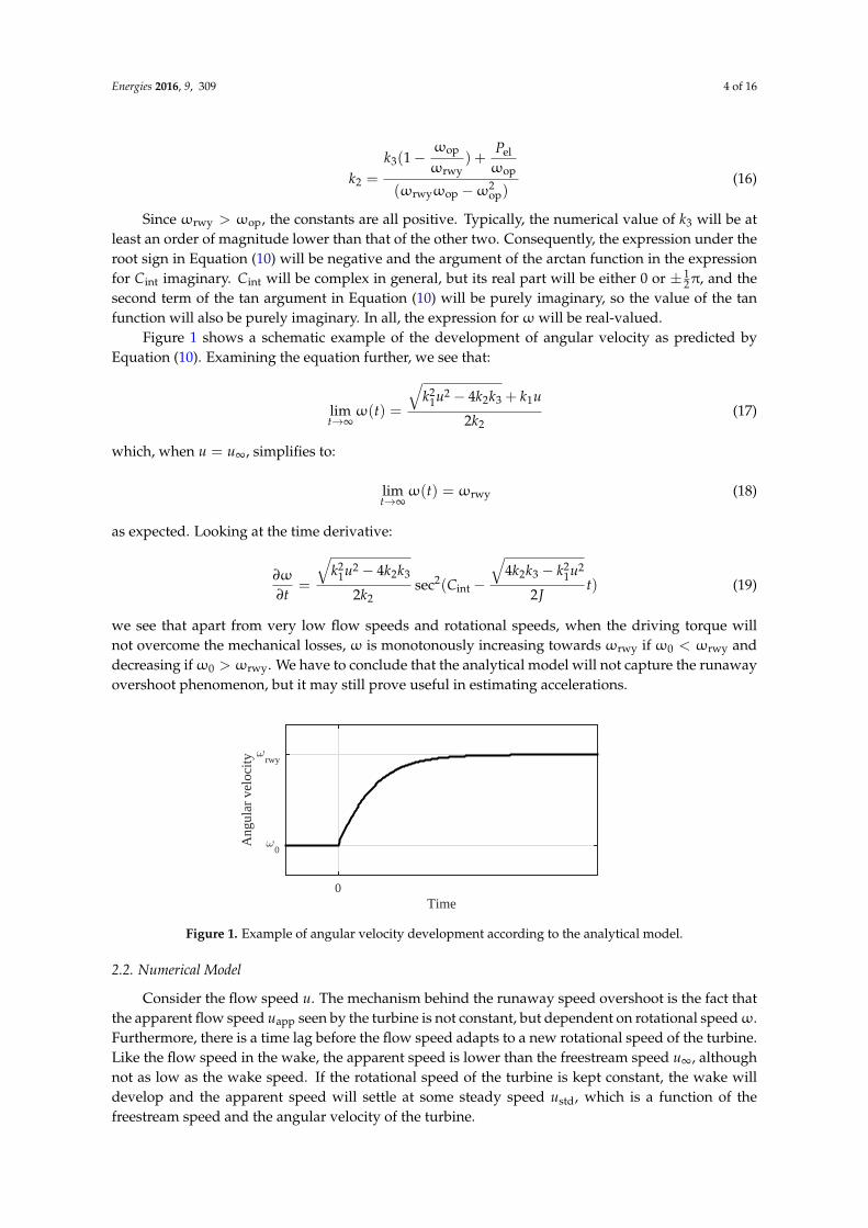
Figure 1 shows a schematic example of the development of angular velocity as predicted byEquation (10). Examining the equation further, we see that:

limt→∞

ω(t) =

√k2

1u2 − 4k2k3 + k1u

2k2(17)

which, when u = u∞, simplifies to:

limt→∞

ω(t) = ωrwy (18)

as expected. Looking at the time derivative:

∂ω

∂t=

√k2

1u2 − 4k2k3

2k2sec2(Cint −

√4k2k3 − k2

1u2

2Jt) (19)

we see that apart from very low flow speeds and rotational speeds, when the driving torque willnot overcome the mechanical losses, ω is monotonously increasing towards ωrwy if ω0 < ωrwy anddecreasing ifω0 > ωrwy. We have to conclude that the analytical model will not capture the runawayovershoot phenomenon, but it may still prove useful in estimating accelerations.

Time0

Ang

ular

vel

ocity

ω0

ωrwy

Figure 1. Example of angular velocity development according to the analytical model.

2.2. Numerical Model

Consider the flow speed u. The mechanism behind the runaway speed overshoot is the fact thatthe apparent flow speed uapp seen by the turbine is not constant, but dependent on rotational speedω.Furthermore, there is a time lag before the flow speed adapts to a new rotational speed of the turbine.Like the flow speed in the wake, the apparent speed is lower than the freestream speed u∞, althoughnot as low as the wake speed. If the rotational speed of the turbine is kept constant, the wake willdevelop and the apparent speed will settle at some steady speed ustd, which is a function of thefreestream speed and the angular velocity of the turbine.

Energies 2016, 9, 309 5 of 16

According to momentum theory [4], the flow speed at the turbine in steady-state operation canbe determined from the speed in the far wake. The flow speed deficit at the turbine is half the deficitin the downstream wake. Differently put, this means the speed at the turbine is the mean of the freestream speed and the wake speed:

ur

u∞=

u∞ + uw

2u∞(20)

where ur is the flow speed at the turbine runner and uw is the speed in the wake downstream.Measurements made of the wake downstream of a turbine (Section 3.4) suggest that the normalizedturbine flow speed as a function of tip speed ratio λ can be approximated as:

ur

u∞=

kk + λ2 (21)

where k is a constant. λ is defined as:

λ =ωRu∞

(22)

where R is the turbine radius. For our model, we assume that ustd can be taken as ur, which is then:

ustd(λ) = ur = u∞k4

k4 + λ2 (23)

where the constant k4 will have to be experimentally determined.Thus, we have:

u = uapp and uapp −→ ustd = ustd(λ) as t −→ ∞ (24)

This means the constants k1 and k2 will depend on ustd. If the (steady) apparent flow speedassociated with the operational angular velocityωop is uop and that associated withωrwy is urwy, weget the following expressions for k1 and k2 in the same manner as we derived Equations (14) and (16):

k1 = k2ωrwy

urwy+

k3

urwyωrwy(25)

and:

k2 =

k3(1−uopωop

urwyωrwy) +

Pelωop

(ωrwyωopuop

urwy−ω2

op)(26)

Now, our model has to handle the temporal development of both the rotational speed of theturbine and the apparent flow speed in which the turbine operates. In order to do this, we considerthe rotational energy of the turbine and the kinetic energy of the flow and how these quantities varywith time.

Suppose the turbine operates in a volume V of water of size:

V = k5DAt (27)

where D = 2R is the turbine diameter, At is the projected turbine cross-sectional area in the directionof flow, and k5 is a constant giving the length of the volume in turbine diameters. In this volume, theflow speed is assumed to be, in some average sense, uapp. Then, the kinetic energy in this volume is:

Energies 2016, 9, 309 6 of 16

EV = ρVu2

app

2(28)

During steady operation, when the wake is fully developed and u = ustd, ω is constant, and wecan solve Equation (8) for Pel to get:

Pstd = Pel = k1ustdω2 − k2ω

3 − k3ω (29)

This is the net power delivered by the turbine in steady operation, so we change the subscript to“steady”. Sinceω = λu∞/R, we can write Pstd as a function of the tip speed ratio:

Pstd(λ) = −k2u3

∞R3 λ

3 + k1ustd(λ)u2

∞R2 λ

2 − k3u∞

Rλ (30)

The momentaneous power P delivered by the turbine is:

P(ω, uapp) = −k2ω3 + k1uappω

2 − k3ω (31)

Due to the inertial properties of the turbine and of the flow, uapp will not always be equal to ustd.If the electrical load or the freestream flow speed is changed, ω and uapp will in time adapt to thenew premises.

During runaway, there is no electrical load connected to which the turbine can deliver capturedpower. Instead, the rotational energy and, thus, the rotational speed of the turbine will change.If P > 0, ω will increase. For high rotational speeds, however, hydrodynamic drag and mechanicallosses will slow the turbine down. Decreasingωmeans P < 0. For our model, we will conjecture thatthe turbine always captures Pstd from the freestream flow, but that the balance P− Pstd, whether moreor less than 0, comes from the operational volume V. This way, uapp will tend towards ustd in time.

The model then is a system of equations:

∂Erot

∂t= P(ω, uapp) (32)

∂EV∂t

= Pstd(λ)− P(ω, uapp) (33)

where Pstd and P are given by Equations (30) and (31), respectively, and ω and uapp are retrieved bythe relations:

ω =

√2Erot

Jand uapp =

√2EVρV

(34)

3. Measurements

3.1. The Söderfors Test Site

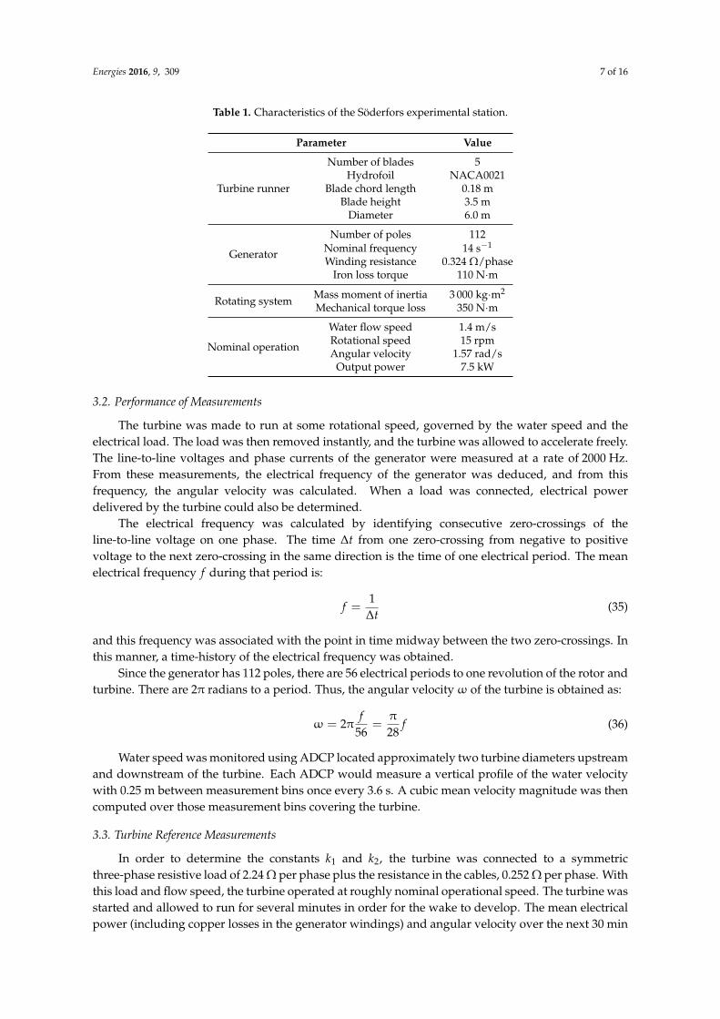
Experiments were carried out at the Söderfors experimental station operated by UppsalaUniversity (Uppsala, Sweden). A vertical axis turbine is located in a river downstream of aconventional hydro power plant. The turbine axis is directly connected to a permanent magnetsynchronous generator. Acoustic Doppler current profilers (ADCP) are mounted upstream anddownstream of the turbine. A measurement and control station is on shore. Details of theexperimental station can be found in [6,7]. Relevant characteristics are listed in Table 1.

Energies 2016, 9, 309 7 of 16

Table 1. Characteristics of the Söderfors experimental station.

Parameter Value

Turbine runner

Number of blades 5Hydrofoil NACA0021

Blade chord length 0.18 mBlade height 3.5 m

Diameter 6.0 m

Generator

Number of poles 112Nominal frequency 14 s−1

Winding resistance 0.324 Ω/phaseIron loss torque 110 N·m

Rotating system Mass moment of inertia 3 000 kg·m2

Mechanical torque loss 350 N·m

Nominal operation

Water flow speed 1.4 m/sRotational speed 15 rpmAngular velocity 1.57 rad/s

Output power 7.5 kW

3.2. Performance of Measurements

The turbine was made to run at some rotational speed, governed by the water speed and theelectrical load. The load was then removed instantly, and the turbine was allowed to accelerate freely.The line-to-line voltages and phase currents of the generator were measured at a rate of 2000 Hz.From these measurements, the electrical frequency of the generator was deduced, and from thisfrequency, the angular velocity was calculated. When a load was connected, electrical powerdelivered by the turbine could also be determined.

The electrical frequency was calculated by identifying consecutive zero-crossings of theline-to-line voltage on one phase. The time ∆t from one zero-crossing from negative to positivevoltage to the next zero-crossing in the same direction is the time of one electrical period. The meanelectrical frequency f during that period is:

f =1

∆t(35)

and this frequency was associated with the point in time midway between the two zero-crossings. Inthis manner, a time-history of the electrical frequency was obtained.

Since the generator has 112 poles, there are 56 electrical periods to one revolution of the rotor andturbine. There are 2π radians to a period. Thus, the angular velocityω of the turbine is obtained as:

ω = 2πf

56=π

28f (36)

Water speed was monitored using ADCP located approximately two turbine diameters upstreamand downstream of the turbine. Each ADCP would measure a vertical profile of the water velocitywith 0.25 m between measurement bins once every 3.6 s. A cubic mean velocity magnitude was thencomputed over those measurement bins covering the turbine.

3.3. Turbine Reference Measurements

In order to determine the constants k1 and k2, the turbine was connected to a symmetricthree-phase resistive load of 2.24 Ω per phase plus the resistance in the cables, 0.252 Ω per phase. Withthis load and flow speed, the turbine operated at roughly nominal operational speed. The turbine wasstarted and allowed to run for several minutes in order for the wake to develop. The mean electricalpower (including copper losses in the generator windings) and angular velocity over the next 30 min

Energies 2016, 9, 309 8 of 16

were calculated. The load was disconnected, and the mean runaway speed was similarly measuredover a 30-min period. For results, see Table 2.

Table 2. Mean results from 30-min measurements.

Quantity Value

Freestream flow speed u∞ 1.42 m/s

With load connected Power Pel 7 340 WAngular velocityωop 1.55 rad/s

Without load (runaway) Angular velocityωrwy 2.15 rad/s

3.4. Wake Speed

Measurements of the mean wake speed were taken by the downstream ADCP under variousconditions. The rotational speed of the turbine operating under different loads was recorded. Meanvalues over 30-min runs were computed. Furthermore, the undisturbed water speed (with stillstanding turbine) was recorded.

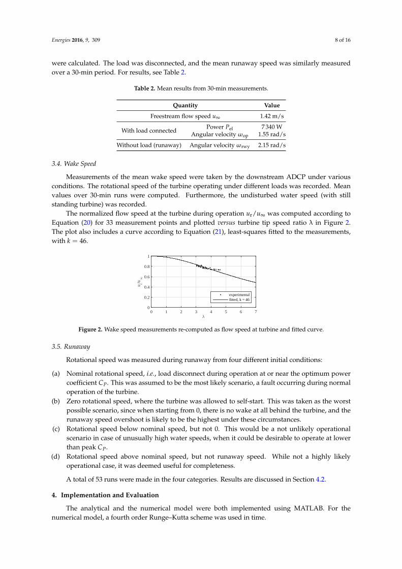
The normalized flow speed at the turbine during operation ur/u∞ was computed according toEquation (20) for 33 measurement points and plotted versus turbine tip speed ratio λ in Figure 2.The plot also includes a curve according to Equation (21), least-squares fitted to the measurements,with k = 46.

λ

0 1 2 3 4 5 6 7

u r/u∞

0

0.2

0.4

0.6

0.8

1

experimentalfitted, k = 46

Figure 2. Wake speed measurements re-computed as flow speed at turbine and fitted curve.

3.5. Runaway

Rotational speed was measured during runaway from four different initial conditions:

(a) Nominal rotational speed, i.e., load disconnect during operation at or near the optimum powercoefficient CP. This was assumed to be the most likely scenario, a fault occurring during normaloperation of the turbine.

(b) Zero rotational speed, where the turbine was allowed to self-start. This was taken as the worstpossible scenario, since when starting from 0, there is no wake at all behind the turbine, and therunaway speed overshoot is likely to be the highest under these circumstances.

(c) Rotational speed below nominal speed, but not 0. This would be a not unlikely operationalscenario in case of unusually high water speeds, when it could be desirable to operate at lowerthan peak CP.

(d) Rotational speed above nominal speed, but not runaway speed. While not a highly likelyoperational case, it was deemed useful for completeness.

A total of 53 runs were made in the four categories. Results are discussed in Section 4.2.

4. Implementation and Evaluation

The analytical and the numerical model were both implemented using MATLAB. For thenumerical model, a fourth order Runge–Kutta scheme was used in time.

Energies 2016, 9, 309 9 of 16

4.1. Calibration

For implementation of the analytical model, the constants k1 through k3 plus the radius R andinertia J of the turbine need to be determined. For the numerical model, constants k4 and k5 arealso required.

For the Söderfors turbine, R, k3 and J are known quantities (Table 1). Together with the referencemeasurements tabulated in Table 2, this is sufficient to establish k1 and k2 for the analytical model byway of Equations (14) and (16).

For the numerical model, k1 and k2 according to Equations (25) and (26) depend on uapp = ustdfor the operational and runaway rotational speeds. ustd is given by Equation (23) and depends on k4,and how quickly uapp changes depends on the size of V and consequently on k5. k4 was determinedby curve fitting as described in Section 3.4.

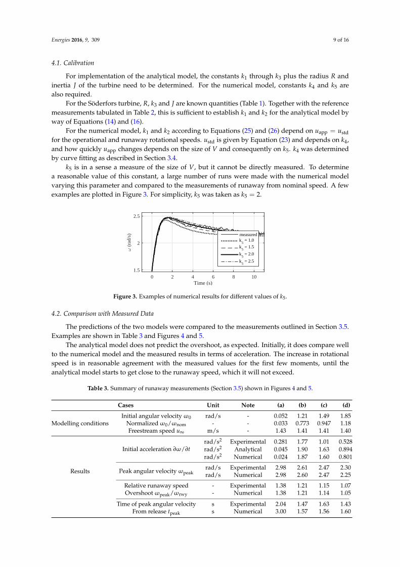
k5 is in a sense a measure of the size of V, but it cannot be directly measured. To determinea reasonable value of this constant, a large number of runs were made with the numerical modelvarying this parameter and compared to the measurements of runaway from nominal speed. A fewexamples are plotted in Figure 3. For simplicity, k5 was taken as k5 = 2.

Time (s)0 2 4 6 8 10

ω (

rad/

s)

1.5

2

2.5

measuredk

5 = 1.0

k5 = 1.5

k5 = 2.0

k5 = 2.5

Figure 3. Examples of numerical results for different values of k5.

4.2. Comparison with Measured Data

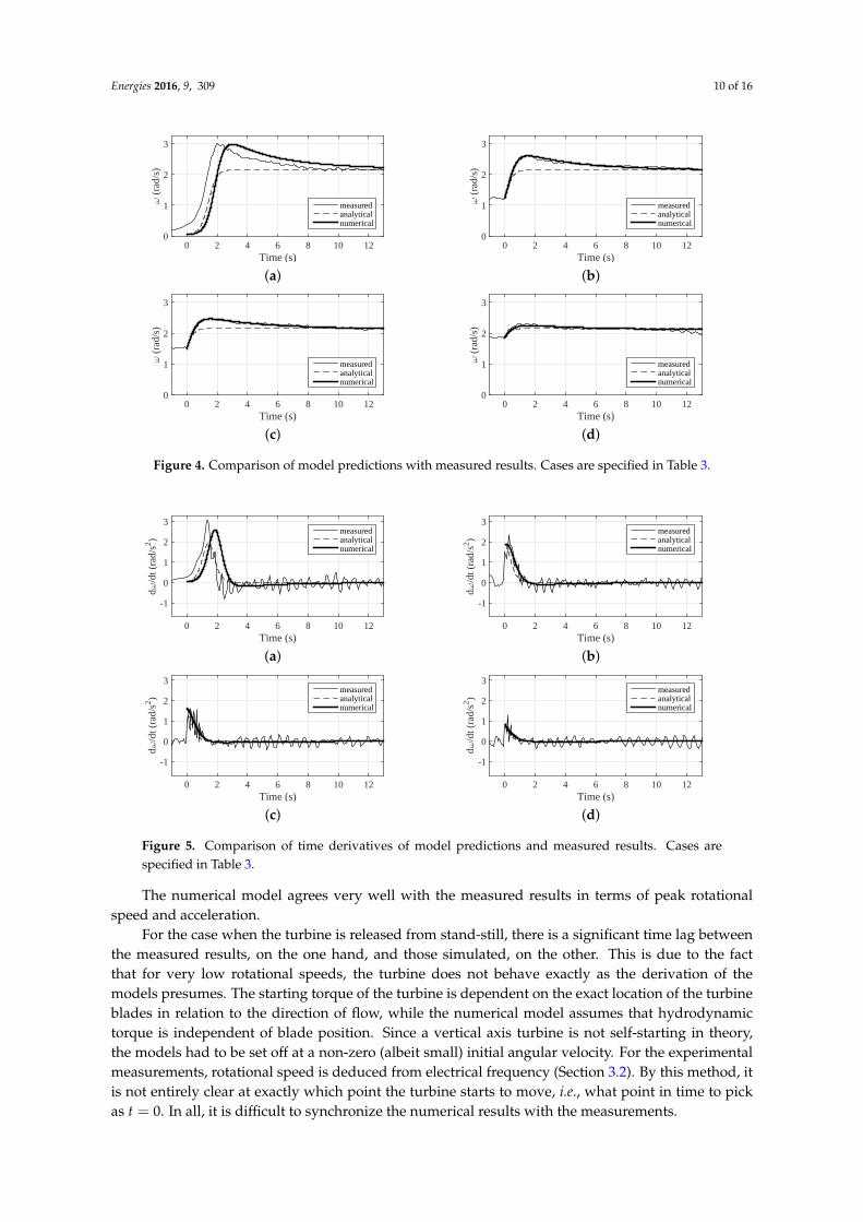
The predictions of the two models were compared to the measurements outlined in Section 3.5.Examples are shown in Table 3 and Figures 4 and 5.

The analytical model does not predict the overshoot, as expected. Initially, it does compare wellto the numerical model and the measured results in terms of acceleration. The increase in rotationalspeed is in reasonable agreement with the measured values for the first few moments, until theanalytical model starts to get close to the runaway speed, which it will not exceed.

Table 3. Summary of runaway measurements (Section 3.5) shown in Figures 4 and 5.

Cases Unit Note (a) (b) (c) (d)

Modelling conditionsInitial angular velocityω0 rad/s - 0.052 1.21 1.49 1.85

Normalizedω0/ωnom - - 0.033 0.773 0.947 1.18Freestream speed u∞ m/s - 1.43 1.41 1.41 1.40

Results

Initial acceleration ∂ω/∂trad/s2 Experimental 0.281 1.77 1.01 0.528rad/s2 Analytical 0.045 1.90 1.63 0.894rad/s2 Numerical 0.024 1.87 1.60 0.801

Peak angular velocityωpeakrad/s Experimental 2.98 2.61 2.47 2.30rad/s Numerical 2.98 2.60 2.47 2.25

Relative runaway speed - Experimental 1.38 1.21 1.15 1.07Overshootωpeak/ωrwy - Numerical 1.38 1.21 1.14 1.05

Time of peak angular velocity s Experimental 2.04 1.47 1.63 1.43From release tpeak s Numerical 3.00 1.57 1.56 1.60

Energies 2016, 9, 309 10 of 16

Time (s)0 2 4 6 8 10 12

ω (

rad/

s)

0

1

2

3

measuredanalyticalnumerical

(a)Time (s)

0 2 4 6 8 10 12

ω (

rad/

s)

0

1

2

3

measuredanalyticalnumerical

(b)

Time (s)0 2 4 6 8 10 12

ω (

rad/

s)

0

1

2

3

measuredanalyticalnumerical

(c)Time (s)

0 2 4 6 8 10 12

ω (

rad/

s)

0

1

2

3

measuredanalyticalnumerical

(d)

Figure 4. Comparison of model predictions with measured results. Cases are specified in Table 3.

Time (s)0 2 4 6 8 10 12

dω/d

t (ra

d/s2 )

-1

0

1

2

3measuredanalyticalnumerical

(a)Time (s)

0 2 4 6 8 10 12

dω/d

t (ra

d/s2 )

-1

0

1

2

3measuredanalyticalnumerical

(b)

Time (s)0 2 4 6 8 10 12

dω/d

t (ra

d/s2 )

-1

0

1

2

3measuredanalyticalnumerical

(c)Time (s)

0 2 4 6 8 10 12

dω/d

t (ra

d/s2 )

-1

0

1

2

3measuredanalyticalnumerical

(d)

Figure 5. Comparison of time derivatives of model predictions and measured results. Cases arespecified in Table 3.

The numerical model agrees very well with the measured results in terms of peak rotationalspeed and acceleration.

For the case when the turbine is released from stand-still, there is a significant time lag betweenthe measured results, on the one hand, and those simulated, on the other. This is due to the factthat for very low rotational speeds, the turbine does not behave exactly as the derivation of themodels presumes. The starting torque of the turbine is dependent on the exact location of the turbineblades in relation to the direction of flow, while the numerical model assumes that hydrodynamictorque is independent of blade position. Since a vertical axis turbine is not self-starting in theory,the models had to be set off at a non-zero (albeit small) initial angular velocity. For the experimentalmeasurements, rotational speed is deduced from electrical frequency (Section 3.2). By this method, itis not entirely clear at exactly which point the turbine starts to move, i.e., what point in time to pickas t = 0. In all, it is difficult to synchronize the numerical results with the measurements.

Energies 2016, 9, 309 11 of 16

Both models are dependent on the freestream water speed u∞. The constants k1 and k2 arecalculated from a reference run at some u∞, but if the free stream speed changes, this will affect otherruns. The value for u∞ applied in each case is listed in Table 3. It can be noted that the measuredrotational speed drops off towards the end of run (d). This is probably due to a decrease in u∞, whichthe model is not capable of emulating.

Figure 5 shows second-order numerical derivatives of the curves in Figure 4. The ‘ripple’ seenin the measured rotational speeds, due to the individual blades of the turbine, is enhanced in thederivative. Having said that, the numerical model catches the general temporal development of theaccelerations reasonably well.

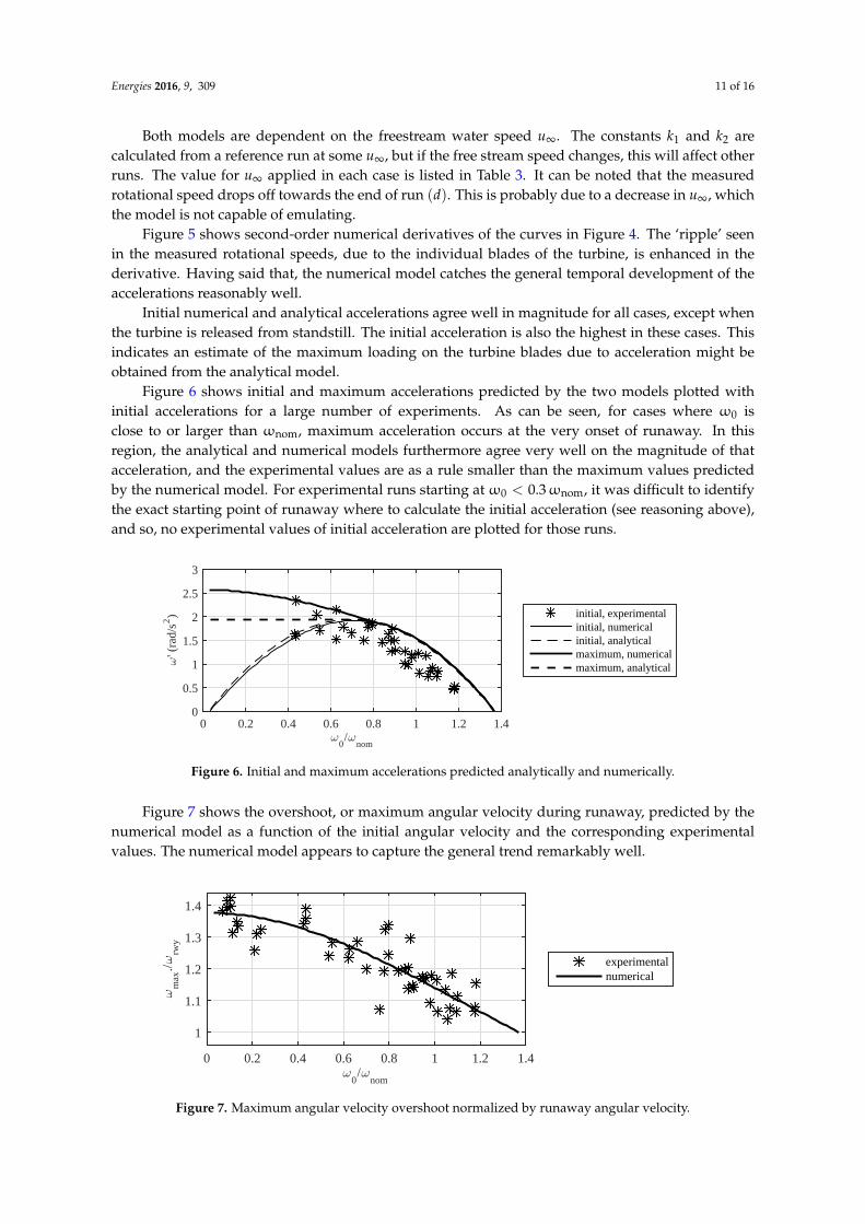
Initial numerical and analytical accelerations agree well in magnitude for all cases, except whenthe turbine is released from standstill. The initial acceleration is also the highest in these cases. Thisindicates an estimate of the maximum loading on the turbine blades due to acceleration might beobtained from the analytical model.

Figure 6 shows initial and maximum accelerations predicted by the two models plotted withinitial accelerations for a large number of experiments. As can be seen, for cases where ω0 isclose to or larger than ωnom, maximum acceleration occurs at the very onset of runaway. In thisregion, the analytical and numerical models furthermore agree very well on the magnitude of thatacceleration, and the experimental values are as a rule smaller than the maximum values predictedby the numerical model. For experimental runs starting at ω0 < 0.3ωnom, it was difficult to identifythe exact starting point of runaway where to calculate the initial acceleration (see reasoning above),and so, no experimental values of initial acceleration are plotted for those runs.

ω0/ω

nom

0 0.2 0.4 0.6 0.8 1 1.2 1.4

ω' (

rad/

s2 )

0

0.5

1

1.5

2

2.5

3

initial, experimentalinitial, numericalinitial, analyticalmaximum, numericalmaximum, analytical

Figure 6. Initial and maximum accelerations predicted analytically and numerically.

Figure 7 shows the overshoot, or maximum angular velocity during runaway, predicted by thenumerical model as a function of the initial angular velocity and the corresponding experimentalvalues. The numerical model appears to capture the general trend remarkably well.

ω0/ω

nom

0 0.2 0.4 0.6 0.8 1 1.2 1.4

ωm

ax./ω

rwy

1

1.1

1.2

1.3

1.4

experimentalnumerical

Figure 7. Maximum angular velocity overshoot normalized by runaway angular velocity.

Energies 2016, 9, 309 12 of 16

The time in seconds after release at which maximum speed occurs is plotted in Figure 8. Thenumerical model tends to overestimate the time taken to reach peak angular velocity. When runawayoccurs from low initial speeds, due to the difficulty in identifying a starting point on the experimentalruns, on the order of half a second should probably be added to the experimental values. Theseobservations are consistent with the examples shown in Figure 4.

ω0/ω

nom

0 0.2 0.4 0.6 0.8 1 1.2 1.4

t(ω

max

) (s

)

0

0.5

1

1.5

2

2.5

3

experimentalnumerical

Figure 8. Time of maximum overshoot in seconds from release.

4.3. Comparison with Published Results

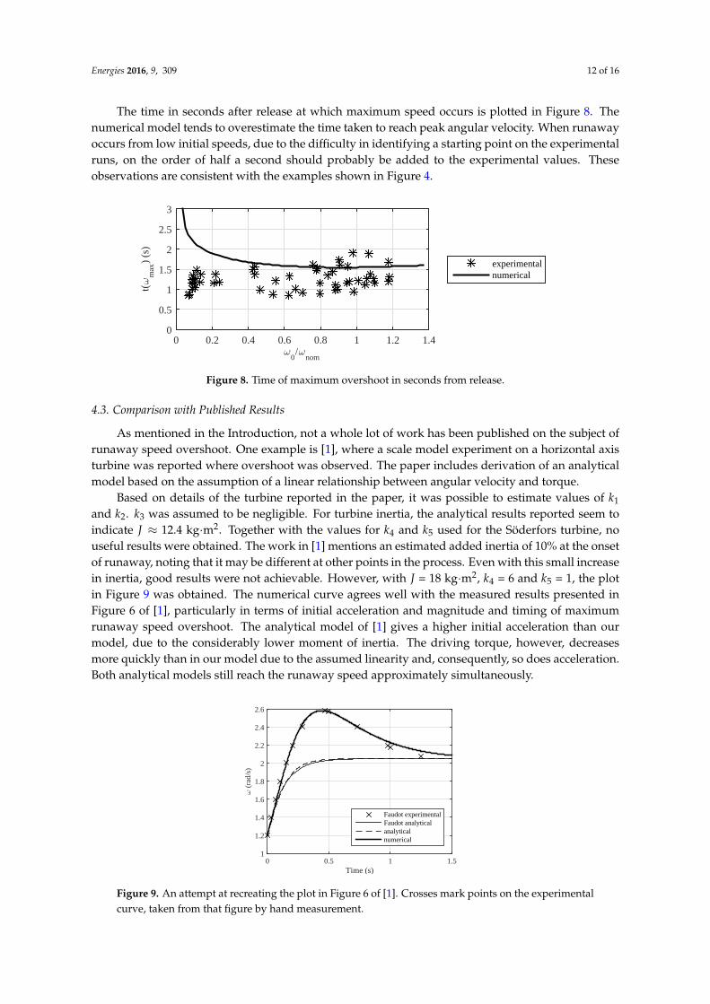
As mentioned in the Introduction, not a whole lot of work has been published on the subject ofrunaway speed overshoot. One example is [1], where a scale model experiment on a horizontal axisturbine was reported where overshoot was observed. The paper includes derivation of an analyticalmodel based on the assumption of a linear relationship between angular velocity and torque.

Based on details of the turbine reported in the paper, it was possible to estimate values of k1

and k2. k3 was assumed to be negligible. For turbine inertia, the analytical results reported seem toindicate J ≈ 12.4 kg·m2. Together with the values for k4 and k5 used for the Söderfors turbine, nouseful results were obtained. The work in [1] mentions an estimated added inertia of 10% at the onsetof runaway, noting that it may be different at other points in the process. Even with this small increasein inertia, good results were not achievable. However, with J = 18 kg·m2, k4 = 6 and k5 = 1, the plotin Figure 9 was obtained. The numerical curve agrees well with the measured results presented inFigure 6 of [1], particularly in terms of initial acceleration and magnitude and timing of maximumrunaway speed overshoot. The analytical model of [1] gives a higher initial acceleration than ourmodel, due to the considerably lower moment of inertia. The driving torque, however, decreasesmore quickly than in our model due to the assumed linearity and, consequently, so does acceleration.Both analytical models still reach the runaway speed approximately simultaneously.

Time (s)0 0.5 1 1.5

ω (

rad/

s)

1

1.2

1.4

1.6

1.8

2

2.2

2.4

2.6

Faudot experimentalFaudot analyticalanalyticalnumerical

Figure 9. An attempt at recreating the plot in Figure 6 of [1]. Crosses mark points on the experimentalcurve, taken from that figure by hand measurement.

Energies 2016, 9, 309 13 of 16

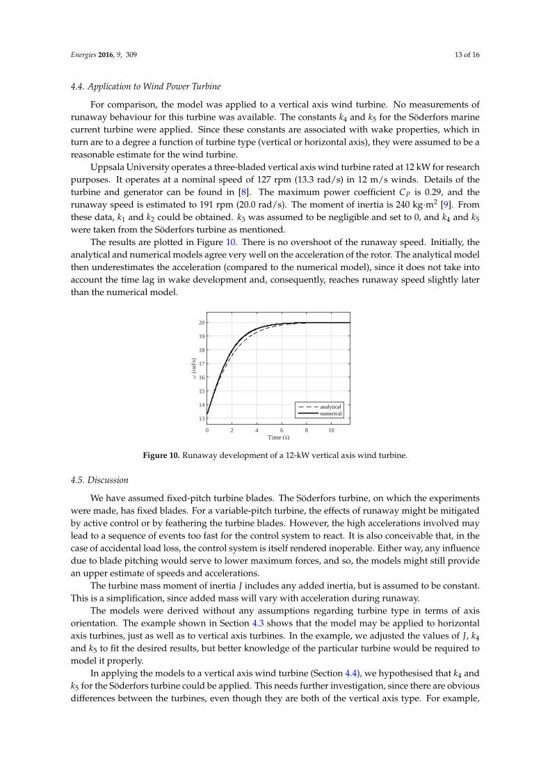
4.4. Application to Wind Power Turbine

For comparison, the model was applied to a vertical axis wind turbine. No measurements ofrunaway behaviour for this turbine was available. The constants k4 and k5 for the Söderfors marinecurrent turbine were applied. Since these constants are associated with wake properties, which inturn are to a degree a function of turbine type (vertical or horizontal axis), they were assumed to be areasonable estimate for the wind turbine.

Uppsala University operates a three-bladed vertical axis wind turbine rated at 12 kW for researchpurposes. It operates at a nominal speed of 127 rpm (13.3 rad/s) in 12 m/s winds. Details of theturbine and generator can be found in [8]. The maximum power coefficient CP is 0.29, and therunaway speed is estimated to 191 rpm (20.0 rad/s). The moment of inertia is 240 kg·m2 [9]. Fromthese data, k1 and k2 could be obtained. k3 was assumed to be negligible and set to 0, and k4 and k5

were taken from the Söderfors turbine as mentioned.The results are plotted in Figure 10. There is no overshoot of the runaway speed. Initially, the

analytical and numerical models agree very well on the acceleration of the rotor. The analytical modelthen underestimates the acceleration (compared to the numerical model), since it does not take intoaccount the time lag in wake development and, consequently, reaches runaway speed slightly laterthan the numerical model.

Time (s)0 2 4 6 8 10

ω (

rad/

s)

13

14

15

16

17

18

19

20

analyticalnumerical

Figure 10. Runaway development of a 12-kW vertical axis wind turbine.

4.5. Discussion

We have assumed fixed-pitch turbine blades. The Söderfors turbine, on which the experimentswere made, has fixed blades. For a variable-pitch turbine, the effects of runaway might be mitigatedby active control or by feathering the turbine blades. However, the high accelerations involved maylead to a sequence of events too fast for the control system to react. It is also conceivable that, in thecase of accidental load loss, the control system is itself rendered inoperable. Either way, any influencedue to blade pitching would serve to lower maximum forces, and so, the models might still providean upper estimate of speeds and accelerations.

The turbine mass moment of inertia J includes any added inertia, but is assumed to be constant.This is a simplification, since added mass will vary with acceleration during runaway.

The models were derived without any assumptions regarding turbine type in terms of axisorientation. The example shown in Section 4.3 shows that the model may be applied to horizontalaxis turbines, just as well as to vertical axis turbines. In the example, we adjusted the values of J, k4

and k5 to fit the desired results, but better knowledge of the particular turbine would be required tomodel it properly.

In applying the models to a vertical axis wind turbine (Section 4.4), we hypothesised that k4 andk5 for the Söderfors turbine could be applied. This needs further investigation, since there are obviousdifferences between the turbines, even though they are both of the vertical axis type. For example,

Energies 2016, 9, 309 14 of 16

the number of blades is different and so is the aspect ratio (proportion of turbine diameter to bladeheight). Both of these parameters, as well as others, may conceivably influence the values of k4 and k5.

The model constants also need further study in general. The experimental data available forcomparisons are limited in scope to one turbine and, essentially, one freestream flow speed. Ideally,it should be verified that the constants are in fact invariant under different operational conditions. Itwould also be interesting to obtain values of the constants for various turbines. Typical values fordifferent turbine types could possibly be determined in this manner.

The models are concerned with the development over time of angular velocity with no electricalload connected. With the experimental setup used, the simplifications outlined in Section 2 (nocopper losses and only constant iron losses) are valid. In principle, it would be easy to include aload term in Equations (32) and (33) in order to study turbine behaviour as the load is changed (butnot disconnected entirely). Depending on how big a change is made, and how quickly, a turbine mayor may not overshoot (or “undershoot”, if the load is increased) the new operational angular velocity.Similarly, it should be possible to model cases where the load is not disconnected so “cleanly” as inthe reported experiments.

The numerical model, supported by experimental results, indicates that on runaway fromstandstill the runaway speed overshoot may be well over 35% (Figure 7). This has to be takeninto account when designing the turbine runner and in fault analysis. If the final runaway speedis assumed to be the limiting case in terms of peak angular velocity, mechanical loads on the turbineare bound to be underestimated.

The point of predicting accelerations and peak angular velocities is to estimate forces to whichthe turbine is subjected. Better understanding of angular speed development may also aid in theanalysis of wake speed evolution. Calculation of these forces and wake velocity fields is beyond thescope of the current paper.

5. Conclusions

We have constructed two models of turbine runaway behaviour, one analytical and onenumerical. Comparisons with measured data from a vertical axis marine current turbine show thatboth models give reasonably accurate estimates of initial acceleration and that the numerical modelcaptures the phenomenon of runaway speed overshoot well in terms of magnitude and timing. Bycomparison with published data, we have also been able to indicate that the models should be ableto handle horizontal axis turbines just as well. A test run modelling a vertical axis wind turbine alsoproduced expected results in that no overshoot was observed for that turbine.

Turbine behaviour during runaway and, in particular, the phenomenon of runaway speedovershoot in marine current turbines, requires more attention than it has been getting so far. Themodels presented in this paper can be further developed for these purposes. Using the models toestimate forces on the turbine is a natural next step to study.

Acknowledgments: The work reported was financially supported by Vattenfall AB, the Swedish Research Council,the ÅForsk Foundation, StandUp for Energy, the Swedish Energy Agency (Swedish Centre for RenewableElectric Energy Conversion, CFE III), the J. Gust. Richert Memorial Fund and the Bixia Environmental Fund.

Author Contributions: Staffan Lundin developed the models, participated in the experiments and wrote themanuscript. Anders Goude initiated and participated in the experiments and contributed to the writing. Mats Leijonsupervised the work.

Conflicts of Interest: The authors declare no conflict of interest.

Abbreviations

ω rad/s Angular velocity of turbine

ω0 rad/s Initial angular velocity

Energies 2016, 9, 309 15 of 16

ωpeak rad/s Peak angular velocity

ωop rad/s Operational angular velocity

ωrwy rad/s Runaway angular velocity

ωnom rad/s Nominal angular velocity

u m/s Flow speed

u∞ m/s Freestream flow speed

uapp m/s Flow speed seen by turbine

ustd m/s uapp in steady operation

uw m/s Flow speed in the far wake

urwy m/s ustd when turbine is atωrwy

uop m/s ustd when turbine is atωop

ur m/s Flow speed at turbine runner

k1 kg·m Constant associated with hydrodynamic driving torque

k2 kg·m2 Constant associated with hydrodynamic torque loss

k3 N·m Torque loss constant

k4 - Steady speed constant

k5 - Operational volume size constant

tpeak s Time at whichωpeak occurs

∆t s Time between zero-crossings

f s−1 Electric frequency

E J Energy

EV J Kinetic energy of operational volume

Erot J Rotational energy of rotating system

Q N·m Torque

Qhydro N·m Hydrodynamic torque contribution

Qloss N·m Constant torque loss

Qload N·m Torque due to connected load

QFe N·m Torque due to iron losses in stator

P W Power

Pload W Power dissipated in load

PCu W Copper losses in generator windings

Pstd W Power delivered by turbine in steady operation

Pel W Electric power

CP - Power coefficient

J kg·m2 Inertia of rotating system

R m Turbine radius

D m Turbine diameter

At m2 Turbine cross-sectional area

V m3 Operational volume

ρ kg/m3 Mass density of flow

λ - Tip speed ratio

Cint - Constant of integration

Energies 2016, 9, 309 16 of 16

References

1. Faudot, C.; Dahlhaug, O.G.; Holst, M.A. Tidal Turbine Blades in Runaway Situation: Experimental andNumerical Approaches. In Proceedings of the 10th European Wave and Tidal Energy Conference (EWTEC13),Aalborg, Denmark, 2–5 September 2013.

2. Winter, A.I. Differences in Fundamental Design Drivers for Wind and Tidal Turbines. In Proceedings ofthe OCEANS 2011 IEEE-Spain, Santander, Spain, 6–9 June 2011; pp. 1–10.

3. Hosseinimanesh, H.; Devals, C.; Nennemann, B.; Guibault, F. Comparison of steady and unsteadysimulation methodologies for predicting no-load speed in Francis turbines. Int. J. Fluid Mach. Syst. 2015,8, 155–168.

4. Manwell, J.F.; McGowan, J.G.; Rogers, A.L. Wind Energy Explained: Theory, Design and Application, 2nd ed.;Wiley: Chichester, UK, 2009.

5. Eriksson, S.; Bernhoff, H. Loss evaluation and design optimisation for direct driven permanent magnetsynchronous generators for wind power. Appl. Energy 2011, 88, 265–271.

6. Yuen, K.; Lundin, S.; Grabbe, M.; Lalander, E.; Goude, A.; Leijon, M. The Söderfors Project: Construction ofan Experimental Hydrokinetic Power Station. In Proceedings of the 9th European Wave and Tidal EnergyConference (EWTEC11), Southampton, UK, 5–9 September 2011, pp. 1–5.

7. Lundin, S.; Forslund, J.; Carpman, N.; Grabbe, M.; Yuen, K.; Apelfröjd, S.; Goude, A.; Leijon, M. The SöderforsProject: Experimental Hydrokinetic Power Station Deployment and First Results. In Proceedings of the10th European Wave and Tidal Energy Conference (EWTEC13), Aalborg, Denmark, 2–5 September 2013.

8. Kjellin, J.; Bülow, F.; Eriksson, S.; Deglaire, P.; Leijon, M.; Bernhoff, H. Power coefficient measurement on a12 kW straight bladed vertical axis wind turbine. Renew. Energy 2011, 36, 3050–3053.

9. Deglaire, P.; Eriksson, S.; Kjellin, J.; Bernhoff, H. Experimental Results from a 12 kW Vertical Axis WindTurbine with a Direct Driven PM Synchronous Generator. In Proceedings of the European Wind EnergyConference & Exhibition (EWEC 2007), Milan, Italy, 7–10 May 2007.

© 2016 by the authors; licensee MDPI, Basel, Switzerland. This article is an open accessarticle distributed under the terms and conditions of the Creative Commons Attribution(CC-BY) license (http://creativecommons.org/licenses/by/4.0/).