One class classifiers for process monitoring illustrated by the application to online HPLC of a...

Special Issue Article

96

Received: 15 September 2009, Revised: 2 December 2009, Accepted: 3 December 2009, Published online in Wiley InterScience: 2 February 2010

(www.interscience.wiley.com) DOI: 10.1002/cem.1281

One class classifiers for process monitoringillustrated by the application to online HPLCof a continuous processSila Kittiwachanaa, Diana L. S. Ferreiraa, Gavin R. Lloyda, Louise A. Fidob,Duncan R. Thompsonb, Richard E. A. Escottc and Richard G. Breretona*

J. Chemom

In processmonitoring, a representative out-of-control class of samples cannot be generated. Here, it is assumed that itis possible to obtain a representative subset of samples from a single ‘in-control class’ and one class classifiers namelyQ and D statistics (respectively the residual distance to the disjoint PC model and the Mahalanobis distance to thecentre of the QDA model in the projected PC space), as well as support vector domain description (SVDD) are appliedto disjoint PCmodels of the normal operating conditions (NOC) region, to categorise whether the process is in-controlor out-of-control. To define the NOC region, the cumulative relative standard deviation (CRSD) and a test ofmultivariate normality are described and used as joint criteria. These calculations were based on the applicationof windowprincipal components analysis (WPCA) which can be used to define a NOC region. TheD andQ statistics andSVDDmodels were calculated for the NOC region and percentage predictive ability (%PA), percentage model stability(%MS) and percentage correctly classified (%CC) obtained to determine the quality of models from 100 training/testset splits. Q, D and SVDD control charts were obtained, and 90% confidence limits set up based on multivariatenormality (D and Q) or SVDD D value (which does not require assumptions of normality). We introduce a method forfinding an optimal radial basis function for the SVDDmodel and two new indices of percentage classification index (%CI)and percentage predictive index (%PI) for non-NOC samples are also defined. The methods in this paper are exemplifiedby a continuous process studied over 105.11h using online HPLC. Copyright � 2010 John Wiley & Sons, Ltd.

Keywords: control charts; multivariate statistical process control; one class classifiers; quadratic discriminant analysis;support vectors

* Correspondence to: R. G. Brereton, Centre for Chemometrics, School ofChemistry, University of Bristol, Cantocks Close, Bristol BS8 1TS, UK.E-mail: [email protected]

a S. Kittiwachana, D. L. S. Ferreira, G. R. Lloyd, R. G. Brereton

Centre for Chemometrics, School of Chemistry, University of Bristol, Cantocks

Close, Bristol BS8 1TS, UK

b L. A. Fido, D. R. Thompson

GlaxoSmithKline, Gunnels Wood Road, Stevenage, Hertfordshire SG1 2NY, UK

c R. E. A. Escott

GlaxoSmithKline, Old Powder Mills, Tonbridge, Kent TN11 9AN, UK

1. INTRODUCTION

Multivariate statistical process control (MSPC) [1–7] involves usingseveral variables to monitor the progress of a process, manyclassic examples involving the use of near infrared (NIR)spectroscopy [8,9]. These methods are complementary to thoseof univariate process control where the change in a singleparameter is studied as a process evolves, e.g. by using Shewhartcharts [10]. Most approaches to MSPC involve establishingcontrol charts that show the change in one or more multivariateparameter over time; multivariate control limits can beestablished, and if the value of the multivariate parameter isoutside these limits this is evidence that there is some problemwith the process. A variety of statistics have been proposed forthese control charts, including the D statistic based on Hotelling’sT2 for principal component models [6,7,11] and the Q statistic orsquare prediction error (SPE) [6,7,11–13]. Many of theseapproaches are based on SIMCA [2,14] and involve finding anormal operating conditions (NOC) region which is considered tobe a group of samples in-control and looking at future samples tosee whether they can be considered part of this group at one ormore predefined confidence limits.The problem of MSPC can be considered a classification

problem—involving setting up a model using the NOC regionand seeing whether other samples are classified into this region.However, unlike many classification problems we only know theorigins of samples in one class—the NOC region or in-group. Oneclass classifiers are a general way of defining these sort of

etrics 2010; 24: 96–110 Copyright � 201

problems [11,15], where a model is formed just using one groupof samples. Unknowns (or test samples) are then assigned to thisgroup according to a predefined confidence limit. If outside thelimit they are considered not to be part of this group. Whereasthis is compatible with the philosophy of SIMCA, in fact one classclassifiers are much more broadly based. SIMCA involves theapplication of Quadratic Discriminant Analysis (QDA) to disjointprincipal component models (that is PCs formed only usingin-group samples), and of course has the significant advantagethat no other samples are required for the model (i.e. samplesthat are not a member of the in-group are not needed providedthe NOC region is correctly defined, so it does not matter whetherthere is a defined out-group or whether these samples areoutliers or contain unexpected features for example). However,there are more flexible solutions and one is that most of the

0 John Wiley & Sons, Ltd.

One class classifiers for MSPC

commonly employed statistics from SIMCA require multinorm-ality, which is not always the case. Support vector domaindescription (SVDD) [15–17] involves a one-class support vectormodel, and allows for any distribution of data within the NOCregion, and so provides a complementary view to QDA/SIMCA,but by using the D parameter as discussed below, allows differentconfidence (or rejection) limits to be set up, just as for the Dstatistic.An additional limitation of some of the existing methods of

MSPC is that they do not take account of the rapid growth incomputer power. Whereas most methods for MSPC should beimplementable online, procedures such as the bootstrap [18–22]and repeated division into training and test sets [11,20–22] canusually be performed within seconds or minutes, makingcomputationally intensive approaches for online monitoringfeasible for real-time implementations.In this paper, we report an approach for MSPC that involves

using both QDA (or SIMCA) and SVDD based classifiers. Inaddition, we discuss approaches for determining the NOC regionthat involves both determining whether the samples arenormally distributed and looking at variation in sample charac-teristics over a window in time. We introduce a new method foroptimising the choice of parameters in SVDDwhen only one classis available, and also introduce new indices, the percentageclassification index (%CI) and percentage predictive index (%PI)that can be used to determine how often and how well unknownsamples are classified as in-control.The methods are illustrated by application to online HPLC for

monitoring of a continuous process where we hope the productquality will remain constant for several days, and samples are takenapproximately every 15min over the period of the process (105h).

9

2. EXPERIMENTAL

2.1. Process

This work is illustrated by the monitoring of the first stage of athree stage continuous process. More details have beendescribed elsewhere [23–25]. The first sample was taken fromthe process at 1.13 h after the reaction started. Subsequentsamples were taken from the process with 5–21min intervalsbetween each sample resulting in 309 samples overall. Thereaction was monitored over 105.11 h. Due to a detector fault,there were some gaps between 27.86 and 29.00 h, 66.35 and67.69 h, and 73.85 and 74.90 h when no samples were acquiredusing the methods described below.

2.2. Chromatography

Online high performance liquid chromatography (HPLC) wasused to monitor the continuous process. Although otherinformation such as spectroscopy and process variables werealso obtained, these are not discussed in this paper for brevity.The HPLC method involved three steps: a sampling mechanism, adilution device and a liquid chromatograph for online analysis. Allsystems were controlled by a personal computer. The samplingmechanism was connected to the chemical process. For eachanalysis, a sample volume of 365ml was obtained and thenpumped into the dilution device. 16.3ml of ethyl acetate (FisherScientific, Loughborough, UK) was used for dilution and thenpumped into an Agilent 1100 HPLC system controlled byChemstation, v10.02 (Agilent Technologies, Stockport, UK). The

J. Chemometrics 2010; 24: 96–110 Copyright � 2010 John Wile

HPLC consisted of a micro-degasser, binary pump, column heatercompartment and a variable wavelength UV detector-fitted witha standard 13ml flow cell. The HPLC system was programmed torun a reversed-phase gradient method, using acid modifiedeluent pumped at 2mlmin�1 through a Zorbax-SB-C18 HPLCcolumn (Agilent Technologies), controlled at 408C: the injectionvolume was 0.5ml. Between analyses, the dilution device wasprogrammed to flush itself with fresh diluent to preventcarry-over from previous samples. Each sample was analysedchromatographically using a single wavelength ultravioletspectrometer detector at 245nm, over an elution time of 2.5minsampled at the rate of 13.72 scan s�1 resulting in 2058 datapoints perchromatogram. Chromatographic data were exported to Matlabversion 7 (Matworks, Natick, MA, USA) for further analysis. Allsoftware was written in-house in Matlab. A data matrix of 309 rowscorresponding to the samples with time and 2058 columnscorresponding to the scans was obtained for further analysis.

3. METHODS

Although we had available all experimental data, software reportedbelow was designed so that chromatograms were sequentiallyinput with only historic information available to the algorithmsreported, to simulate real-time data acquisition. Hence whenanalysing, for example, chromatograms recorded over 50h, weassume that no information about future samples is available, sothat the methods reported in this paper can be implemented inreal-time online. An overview of the HPLC data analysis is presentedin Figure 1. Detailed steps are described below.

3.1. Data preparation

Several of the steps in data preparation have been described ingreater detail elsewhere [23], and only a summary is provided inthis section with differences described in more detail. Prior to thedata analysis, each chromatogram is baseline corrected. In ourprevious paper we discussed an approach for dynamicallychoosing the normal operating conditions (NOC) region, which isconsidered the benchmark for an in-control process. In this paper,we propose a modified method for determining the NOC region.Once this is found, chromatographic peaks are aligned accordingto a reference chromatogram found in this region as discussedpreviously [23]. After that peak picking (to determine how manydetectable peaks and what their elution times are) and peakmatching (to determine which peaks in each chromatogram orsample correspond to the same compound) are performed toobtain a peak table, whose rows consist of samples and whosecolumns consist of chromatographic peaks. The elements of thepeak table are square root transformed, to avoid large peaksunduly influencing the signal. Then, each row is scaled to aconstant value of 1. The motivation behind this procedure hasbeen described elsewhere [23–25]. After that, the peak table isstandardised to ensure that each peak has a similar influence onthe model. Note that when subsets of the data are used, e.g. foroptimisation (Sections 3.2.2 and 3.5.2) and validation (Section3.6), they are restandardised as appropriate. The chromato-graphic process data can be analysed in the form of either lockedor unlocked peak tables [23]; the former uses only peaks detectedin the NOC region for the model, and the latter allows new peaks(or chemicals detected) in future samples to be added to themodel to reflect the fact that not all peaks are detected in the

y & Sons, Ltd. www.interscience.wiley.com/journal/cem

7

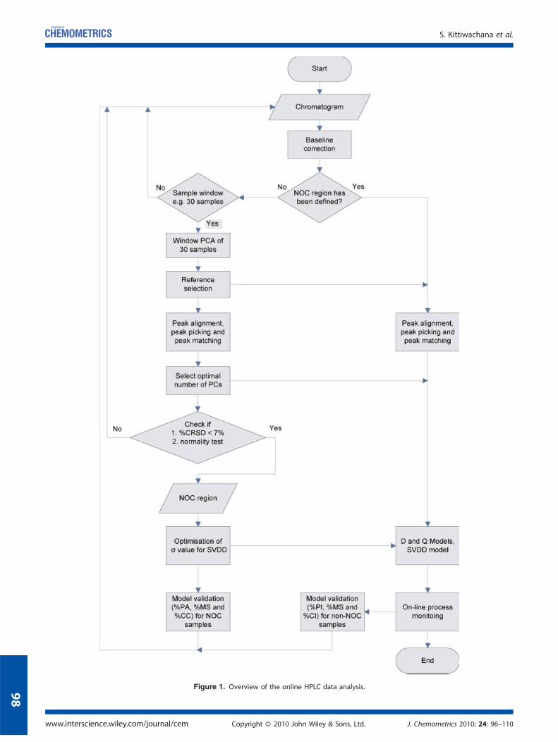
Figure 1. Overview of the online HPLC data analysis.

www.interscience.wiley.com/journal/cem Copyright � 2010 John Wiley & Sons, Ltd. J. Chemometrics 2010; 24: 96–110

S. Kittiwachana et al.

98

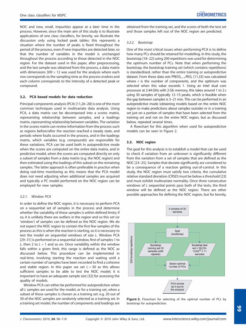
Figure 2. Flowchart for selecting of the optimal number of PCs by

bootstrap for autoprediction.


9

NOC and new, small, impurities appear at a later time in theprocess. However, since the main aim of this study is to illustrateapplications of one class classifiers, for brevity, we illustrate thediscussion only using locked peak tables: this represents asituation where the number of peaks is fixed throughout theperiod of the process, even if new impurities are detected later, sothat the number of variables in the model is unchangedthroughout the process according to those detected in the NOCregion. For the dataset used in this paper, after preprocessing,and the last sample was obtained from the process, a data matrixwith dimensions 309� 12 was used for the analysis where eachrow corresponds to the sampling time as the process evolves andeach column corresponds to the intensity of a detected peak orcompound.

3.2. PCA based models for data reduction

Principal components analysis (PCA) [11,26–28] is one of themostcommon techniques used in multivariate data analysis. UsingPCA, a data matrix can be decomposed into a scores matrix,representing relationship between samples, and a loadingsmatrix, representing relationship between variables. The variationin the scoresmatrix can review information from the process suchas regions before/after the reaction reached a steady state, andperiods where faults occurred in the process, and in the loadingsmatrix, which variables (e.g. compounds) are responsible forthese variations. PCA can be used both in autopredictive modewhen the scores are computed on the entire data matrix, and inpredictive model, when the scores are computed directly on onlya subset of samples from a data matrix (e.g. the NOC region) andthen estimated using the loadings of this subset on the remainingsamples. The latter approach is often preferable in practice whendoing real-time monitoring as this means that the PCA modeldoes not need adjusting when additional samples are acquiredand typically a PC model performed on the NOC region can beemployed for new samples.

3.2.1. Window PCA

In order to define the NOC region, it is necessary to perform PCAon a sequential set of samples in the process and determinewhether the variability of these samples is within defined limits; ifso, it is unlikely there are outliers in the region and so this set (or‘window’) of samples can be defined as the NOC region. We donot expect the NOC region to contain the first few samples of theprocess as this is when the reaction is starting, so it is necessary totest the model on sequential windows of size L. Window PCA[29–31] is performed on a sequential window, first of samples 1 toL, then 2 to Lþ 1 and so on. Once variability within the windowfalls within a given limit, this range is defined as the NOC asdiscussed below. This procedure can be implemented inreal-time, involving starting the reaction and waiting until acertain number of samples have been recorded to find a cohesiveand stable region. In this paper we set L¼ 30 as this allowssufficient samples to be able to test the NOC model; it isimportant to have an adequate sample size [32] for assessing thequality of models.Window PCA can either be performed for autoprediction when

all L samples are used for the model, or for a training set, when asubset of these samples is chosen as a training set: e.g. 20 out of30 of the NOC samples are randomly selected as a training set. Ina training set model, the number of components and loadings are


obtained from the training set, and the scores of both the test setand those samples left out of the NOC region are predicted.

3.2.2. Bootstrap

One of the most critical issues when performing PCA is to definehowmany PCs should be retained for modelling. In this study, thebootstrap [18–22] using 200 repetitions was used for determiningthe optimum number of PCs. Note that when performing thebootstrap, the bootstrap training set (which contains repetitions)is standardised, rather than the entire training or autopredictivedataset. From these data sets PRESSrþ1/RSSr [11,33] was calculatedwhere r is the number of components, and the optimum wasselected when this value exceeds 1. Using an Intel dual coreprocessor at 2.44GHz with 2Gb memory, this takes around 1 to 2 susing 30 samples of typically 12–15 peaks, which is feasible whenthe gap between samples is 5–21min. This can be performed in anautopredictive mode (obtaining models based on the entire NOCregion to make predictions about samples outside) or in a trainingset just on a portion of samples that have been selected from thetraining set and not on the entire NOC region, but as discussedbelow, repeated several times.A flowchart for this algorithm when used for autopredictive

models can be seen in Figure 2.

3.3. NOC region

The goal for this analysis is to establish a model that can be usedto check if variation from an unknown is significantly differentfrom the variation from a set of samples that are defined as theNOC [23–25]. Samples that deviate significantly are considered tobe a consequence of a reaction getting out-of-control. In thisstudy, the NOC region must satisfy two criteria, the cumulativerelative standard deviation (CRSD)must be below a threshold [23]and must exhibit multivariate normality. Once three consecutivewindows of L sequential points pass both of the tests, the thirdwindow will be defined as the NOC region. There are otherpossible approaches for defining the NOC region, but for brevity,


9


100

we use only these criteria in this paper. These criteria areevaluated in autopredictive mode as these can be completed in afew seconds, which is feasible when samples are recorded everyfew minutes, so that a full NOC assessment can be made soonafter samples are acquired.

3.3.1. Cumulative relative standard deviation

To determine whether a sample window exhibits low variation,the CRSD is calculated. The CRSD is a generalisation of thestandard deviation (SD) and relative standard deviation (RSD) ofthe scores from the rth component obtained using PCA for eachwindow which can be calculated as follows:

SDr ¼

ffiffiffiffiffiffiffiffiffiffiffiffiffiffiffiffiffiffiffiffiffiffiffiffiffiffiffiffiffiffiffiPL�1

l¼0

ðtrði�lÞ � trÞ2

L� 1

vuuut(1)

RSDr ¼ 100 SDr=tr (2)

where trði�lÞ is the score of PC r from the (i�l)th sequentialchromatogram in the window and tr is the average score of PC rfrom the L chromatograms. Finally, the CRSD is calculated asfollows:

CRSD ¼XRr¼1

grPRr¼1

gr

RSDr

��

��(3)

where gr is the rth eigenvalue. In this study, R is the optimumnumber of PCs which is determined as discussed in Section 3.2.2.It should be noted that, in this study, the CRSD is calculated fromeach sample window, which is different from the CRSD calculatedfrom expanding PCA [23]. An advantage of the calculation basedon using window PCA is that the relative variation in differentdata sets can be compared, providing that the size of the windowand the preprocessing method is the same. Based on ourexperience, we use 7% CRSD as the threshold for acceptance [23]which we find empirically is a good compromise that allows acandidate NOC region to be found close to the beginning of theprocess.

3.3.2. Test of normality

Several methods in the literature assume that samples areapproximated by a multinormal distribution in order to convertdistances or residuals into confidence levels. This is so with the D(or T2) statistic and the Q statistic (or Squared Prediction Error—SPE). Such tests may be misleading if samples deviatesignificantly from a normal distribution, which also may beindicative of outliers. Therefore, in order to find a good choice ofNOC region, each candidate window that has a CRSD below thethreshold is also checked if it exhibits normality. In this study, theDoornik–Hansen Omnibus test for normality was used [34]. Thisstatistic is a modified version of the omnibus test [35]. It is basedon the transformation of skewness and kurtosis to createstatistics which approximate to the x2 distribution [35,36].The p-value associated with the statistic is calculated where thehigher the p-value the more likely it is to be multivariatenormality. In this study, the test is performed on the optimumnumber of PCs and a threshold of p¼ 0.05 was employed. Note

www.interscience.wiley.com/journal/cem Copyright � 201

that there are several other tests of multivariate normality, but forbrevity we report just one approach.

3.4. Multivariate statistical process control

Multivariate statistical process control (MSPC) [1–7] involvescomputing statistics that can be used to monitor a process todetermine whether it is deviating from the NOC region. A samplecan be classified as an out-of-control sample if its variation issignificantly different from the variation of the NOC samples.Based on PCA decomposition of NOC samples X¼ TPR E,

variation in the NOC samples X can be divided into two parts; asystematic variation part TP and a residual part E which is notdescribed by the model. A single autopredictive model isobtained for the NOC region and used to determine whether thenon-NOC samples (outside the NOC region) are in-control orout-of-control, using the preprocessed locked peak tableobtained as discussed above.

3.4.1. D and Q statistics

D and Q statistics are commonly used methods for processmonitoring. The difference between these two methods is thatthey assess different aspects of the variation from the NOCregion. The D statistic is modelled on systematic variation in theNOC region, so it is used to determine whether a specific samplehas a large variation compared to the reference samples basedupon the PC projection into the NOC space. It is based onquadratic discriminant analysis (QDA) [11,37] of the scores of thePCs of the NOC region, and attempts to form a classificationmodel defined on the Mahalanobis distance [11,22] of a samplefrom the centre of a class. In contrast, the Q statistic looks at theresiduals from the PC model of the NOC region and sees howlarge this non-systematic variation is from the model. One of themost important considerations is to ensure that the model ofthe NOC has an appropriate number of PCs. In this study, thebootstrap, described in Section 3.2.2, was used to identify theoptimal number of PCs used to describe the NOC region.To categorise if a sample is in-control, D and Q values can be

calculated and compared with control limits, which can beestimated from the distribution of the reference systematicvariation (TP) for the D statistic, and from the distribution of thereference residual variation (E) for the Q statistic. The descriptionof how to calculate the D and Q values and their confidence levelis presented elsewhere [1–8,11,12,37,38]. Although there areseveral possible ways to calculate the confidence limits for the Qstatistic, in this paper, the approximation described by Jacksonet al. [12] was used; when there are sufficient number of samples,there is very little difference between the various equationsreported in the literature. When a process is in-control, the D andQ values should fall within predefined control limits. In this study,the value of the relevant statistic is calculated for each sample,and visualised together with the critical values in a bar chart. Inorder to determine the scores, the same data preprocessing usedfor Window PCA was used; test samples were pre-processedusing the mean and the standard deviation of the NOC samples.The 90 and 99% control limits for theD andQ statistics are used inthe paper and bar graphs are plotted on a logarithmic scale.

3.4.2. Contribution charts

In order to investigate which variable or peak contributes most tothe D and Q statistics, it is possible to plot the contribution values

0 John Wiley & Sons, Ltd. J. Chemometrics 2010; 24: 96–110


against each variable for each sample. On the other hand, thecontribution of each variable to process time can be reviewedwhen we plot the contribution values with time using sequentialsample numbers. These plots are commonly named as contributionplots and the equations for calculating this contribution arepresented elsewhere [23–25]. The contribution charts as all MSPCcharts are presented using a single autopredictive NOC model,assuming that samples outside the NOC region are test set samples.

3.5. Support vector domain description for MSPC

Support vector domain description (SVDD) [11,15–17,39–41] is amodified version of support vector machines (SVMs) [42–47]. Thedifference between SVDD and SVMs is that the latter methodcomputes a boundary between two or more classes, whereas, forSVDD, a boundary is drawn around each individual classseparately resulting in a separate (and different) model for eachclass; therefore, it is sometimes called a ‘one class classifier’. This isillustrated in Figure 3 in the case where there are two classes. Oneimportant advantage of using SVDD over D and Q statistics is thatthe classifier does not expect that the data follow a multivariatenormal distribution; therefore, the boundary drawn from a singleclass can be represented as a non-ellipsoidal shape if necessary.However, a disadvantage is that there are no straightforwardanalogies to contribution charts.

Figure 3. Difference between (a) a single SVM model separating two

classes and (b) two SVDD models for each class.


1

The mathematical basis of SVDD is well described elsewhere[11,15–17,39–41]. In this paper, a radial basis function (RBF) wasused for the kernel since it requires only one parameter to defineit [40–41]. Two parameters control the SVDD model, the samplerejection rate D [11,16,17] and the kernel width s for the RBF. Inthis paper, how these parameters are defined for processmonitoring is discussed below. Further detailed mathematicaldefinitions are provided in the references cited above.

3.5.1. Sample rejection rate (D)

For SVMs, the tolerance of the training error is controlled bypenalty term C [11,42–47]. The higher the value of C the smallerthe number of training set samples that will be rejected. ForSVDD, the penalty term is often best reformulated by the samplerejection rateDwhich is approximately equal to the proportion ofsamples misclassified in a training set and defined by

C ¼ 1

LD(5)

where L is the number of samples: this is because C for one classSVDD is not exactly analogous to C for two class SVMs, so weavoid this terminology below, preferring D although the equationabove shows the relationship with C. The sample rejection rate Dcan be compared to the confidence limit used in D and Qstatistics. For example,D¼ 0.1 is comparable to a 90% confidencelimit. In this work, the D parameter used for the modelling will befixed at 0.1 corresponding to a 90% confidence limit for D and Qstatistics for comparison.

3.5.2. Kernel width (s)

The other tuneable parameter to control the model boundary isthe kernel width s for RBF. A large s value can lead to a lesscomplicated boundary with a large radius. If this s value issufficiently large (larger than the maximum distance betweensamples in the training set), the decision boundary could bepresented as a rigid hypersphere in kernel space. It is thereforeimportant to find an optimal value of s.One possible procedure for selecting the optimal kernel width

s for SVDD is to use cross validation or bootstrapping tomaximisethe number of test set in-group samples correctly assigned to thein-group while minimising the number of out-group (orout-of-control) samples that are incorrectly assigned to thein-group (or in-control) samples. Another method proposed byTax et al. [48] is to evaluate the consistency of the classifier usingonly the error of the out-group class. However, these approachesassume that known out-group samples are available at the timeof modelling, which is unlikely to be valid in certaincircumstances, e.g. processing monitoring where it is not knownwhat types of fault may occur and therefore an out-group classcannot be generated. Maximising the number of correctlyclassified in-group samples from a test set is still a valid approach,but since there are no out-group samples available for the testset, there is nothing to prevent the classifier assigning all possiblespace to the in-group. While this results in extremely goodidentification of in-group samples, no sample is ever classified asthe out-group, which can cause problems, e.g. in process controlwhere no faults would ever be identified.To overcome the problem associated with the lack of a

representative set of out-group samples, the optimisation of s inthis paper is based on using the bootstrap applied to the full NOC


01


102

region (autopredictive mode) or a training set (Sections 3.6 and3.7), both involving the repeated formation of bootstrap trainingand test sets. This involves finding a compromise solution thatattempts to minimise the proportion of bootstrap test setsamples rejected as belonging to the in-group (defined by frej)whilst also minimising the radius of the hypersphere Rh thatsurrounds the bootstrap training set in kernel space, since thesmaller the radius of the hypersphere Rh the better the fit to thetraining set samples. Note that the volume of the hypersphere isproportional to nth power of radius, where n is a number ofhypersphere’s dimension, so byminimising the radius the volumeis also minimised. In order that the radius Rh is comparable inmagnitude to frej, the boundary radius can be scaled from 0 to 1 by:

k ¼ Rh � dmin

dmax � dmin(6)

where dmin is theminimumpairwise distance between samples in abootstrap training set and dmax is the maximum pairwise distancebetween these samples. Therefore, we define the optimum s by thevalue that results in theminimum of kþ frej. In this paper, by defaultthese two parameters are given equal importance; however, atradeoff parameter could be introduced if we want to change therelative influence of each parameter. Since frej is calculated using abootstrap test set, this will be dependent in part on which samplesare selected in the bootstrap test set. Hence this procedure isrepeated 100 times with different samples being selected eachtime for the bootstrap test and training sets. The average value of kover all 100 iterations is calculated for a range of s between thevalues of dmin and dmax for the NOC samples (which is usually widerthan for the bootstrap training set) and theminimum chosen as theoptimum. During this procedure, the sample rejection rateD is fixedat 0 (which should result in all samples being selected in thetraining set) although D¼ 0.1 was used for the next step of theanalysis: however, we find that the optimised s obtained from thismethod can performwell with awide range of the sample rejectionrateD. Note that s can be optimised either for a singlemodel basedon the NOC region (used for the SVDD chart, or repeatedly ontraining sets as discussed in Sections 3.6 and 3.7).

3.5.3. Distance in kernel space

Whether a sample is in-control or out-of-control is given bycalculating the distance in kernel space from the centre of themodel, and comparing it to the distance that is given by D¼ 0.1: ifbelow, then the sample is a member of the in-group (orin-control) with 90% confidence. Hence, an analogy to the Q andD chart can be obtained using SVDD.

3.6. Model validation

An important issue is to determine how well the NOC modelperforms. The conventional approach is to divide the data intotraining and test sets (or samples left out of the model, e.g. usingLOO cross-validation) and see how well training set modelspredict the test set samples. This is different to forming modelsusing the NOC region as the training set (which we callautopredictive models) and then predicting the class member-ship of samples outside the NOC region (as discussed in Sections3.4 and 3.5) and answers whether the NOC model is a suitableone. Since we know only about the NOC class, we can only findNOC models from the test and training sets. Since the approachdeveloped in this paper is aimed to be applied in real-time, and it


is not easy to obtain validation samples from the process, analternative solution is to split the NOC data and use some asvalidation samples. Here, it is assumed that all the NOC samplesare from a single class (in-control). To do the NOC assessment, theNOC samples are split into two subsets where 2/3 of the NOCsamples are randomly selected and used as a training set whilethe remaining samples are used as a test set: note that thisprocedure is different to the procedure in Section 3.5.2 used tooptimise s and should not be confused with the bootstrap. Thetraining set is standardised, as it has a different standarddeviation and mean to the overall NOC region. This training setcan be used to establish the models (D and Q statistics and SVDD)and test themselves in an autopredictive mode, or test set inpredictive mode. Note that procedures for determining theoptimum number of PCs and the optimum value of s by thebootstrap are repeated on each of the training sets, rather thanusing autopredictive models, to ensure that the procedures ofvalidation and optimisation are separated [32]. This algorithm isrepeated several times, in this work, 100, using iterative test andtraining set splits. An overview of model validation using thetraining/test set split can be seen in Figure 4. Note that thisapproach has some similarities with the recently reportedmethod of repeated double cross validation [49] but differs inthat it involves using the bootstrap. Several statistics such aspercentage predictive ability (%PA), percentage model stability(%MS) and percentage correctly classified (%CC) are computed todetermine model performance [11,20,22,50].

3.6.1. Percentage predictive ability (%PA)

This index is a percentage of times that a sample is correctlyclassified. For example, using 100 iterations, if a sample is picked60 times to be used as a test sample and from these 60 iterationsif there are 45 times that this sample is correctly classified (asin-control) this means that %PA for this sample is 75%. %PA canonly be computed for samples of known origins, in the case ofthis paper, in the NOC region. The average %PA over all samplescan also be calculated.

3.6.2. Percentage model stability (%MS)

The %MS is a measure of how stable the classification of a sampleis, and, when %A is available can be related as follows:

%MS ¼ 2ð %PA� 50j jÞ (6)

This index can be used to indicate the stability of a model whenit is used to predict a sample. %MS of a sample can be very high ifit is located far away from themodel boundaries even though it isclassified firmly into one group. On the other hand, if a sample islocated near the model boundary, there is more chance that thepredictive result could be uncertain as this sample could beclassified as in-control or out-of-control, therefore, the %MS forthis sample could be low. Note that for %MS, unlike %PA, it is notnecessary to know the true origin of a sample, and so this can beused for unknowns, and so samples outside the NOC region.

3.6.3. Percentage correctly classified (%CC)

The %CC is percentage correctly classified samples. In this paper,the %CC is obtained via majority vote which means that if over anumber of iterations a sample is classified more frequently asin-control (i.e. %PA >50%), it is assigned into the in-group. For


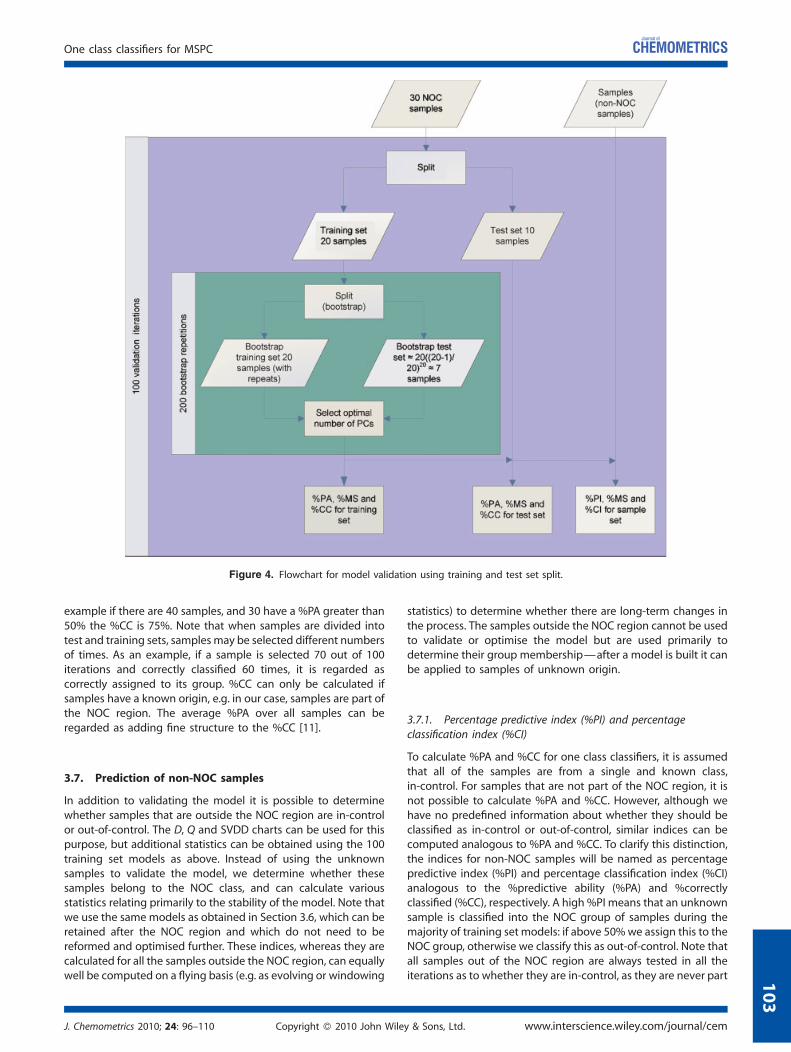
Figure 4. Flowchart for model validation using training and test set split.


example if there are 40 samples, and 30 have a %PA greater than50% the %CC is 75%. Note that when samples are divided intotest and training sets, samples may be selected different numbersof times. As an example, if a sample is selected 70 out of 100iterations and correctly classified 60 times, it is regarded ascorrectly assigned to its group. %CC can only be calculated ifsamples have a known origin, e.g. in our case, samples are part ofthe NOC region. The average %PA over all samples can beregarded as adding fine structure to the %CC [11].

1

3.7. Prediction of non-NOC samples

In addition to validating the model it is possible to determinewhether samples that are outside the NOC region are in-controlor out-of-control. The D, Q and SVDD charts can be used for thispurpose, but additional statistics can be obtained using the 100training set models as above. Instead of using the unknownsamples to validate the model, we determine whether thesesamples belong to the NOC class, and can calculate variousstatistics relating primarily to the stability of the model. Note thatwe use the same models as obtained in Section 3.6, which can beretained after the NOC region and which do not need to bereformed and optimised further. These indices, whereas they arecalculated for all the samples outside the NOC region, can equallywell be computed on a flying basis (e.g. as evolving or windowing


statistics) to determine whether there are long-term changes inthe process. The samples outside the NOC region cannot be usedto validate or optimise the model but are used primarily todetermine their group membership—after a model is built it canbe applied to samples of unknown origin.

3.7.1. Percentage predictive index (%PI) and percentageclassification index (%CI)

To calculate %PA and %CC for one class classifiers, it is assumedthat all of the samples are from a single and known class,in-control. For samples that are not part of the NOC region, it isnot possible to calculate %PA and %CC. However, although wehave no predefined information about whether they should beclassified as in-control or out-of-control, similar indices can becomputed analogous to %PA and %CC. To clarify this distinction,the indices for non-NOC samples will be named as percentagepredictive index (%PI) and percentage classification index (%CI)analogous to the %predictive ability (%PA) and %correctlyclassified (%CC), respectively. A high %PI means that an unknownsample is classified into the NOC group of samples during themajority of training set models: if above 50%we assign this to theNOC group, otherwise we classify this as out-of-control. Note thatall samples out of the NOC region are always tested in all theiterations as to whether they are in-control, as they are never part


03


104

of the model. A high %CI means that many samples have beenfound to be in-control, with only a few out-of-control samples.This statistic is an average of a range of samples. In this paper, wereport values of %CI for all samples that do not belong to the NOCregion, but in practice, this statistic could evolve, or be computedover a window of samples to provide a warning that there arelong-term problems with the process (rather than %PI whichcould be indicative of single outlying samples). It is interesting tonote that in this paper we use 90% confidence limits (or D¼ 0.1)to choose whether a sample is in-control, but of course, otherlimits could be employed to provide various warnings andactions as required. It is possible to compute %PA, %PI etc. for anypredefined confidence limit.

3.7.2. Percentage model stability (%MS)

Model stability can be calculated exactly analogous to the NOCregion. A high %MS usually suggests we are fairly certain of theorigins of the sample. We would expect misclassified samples inthe NOC region to have lower %MS than outside the NOC, asthere may be strong outliers that are very strongly classified asout-of-control, whereas any samples in the NOC region classifiedas out-of-control (remembering that we set 90% confidencelimits, so approximately 3 out of 30 will be out-of-control) may beclose to boundaries and so whether they are found to beout-of-control might be a consequence of which samples areused to establish the training set model, and as such will havemuch lower model stability.

4. RESULTS AND DISCUSSION

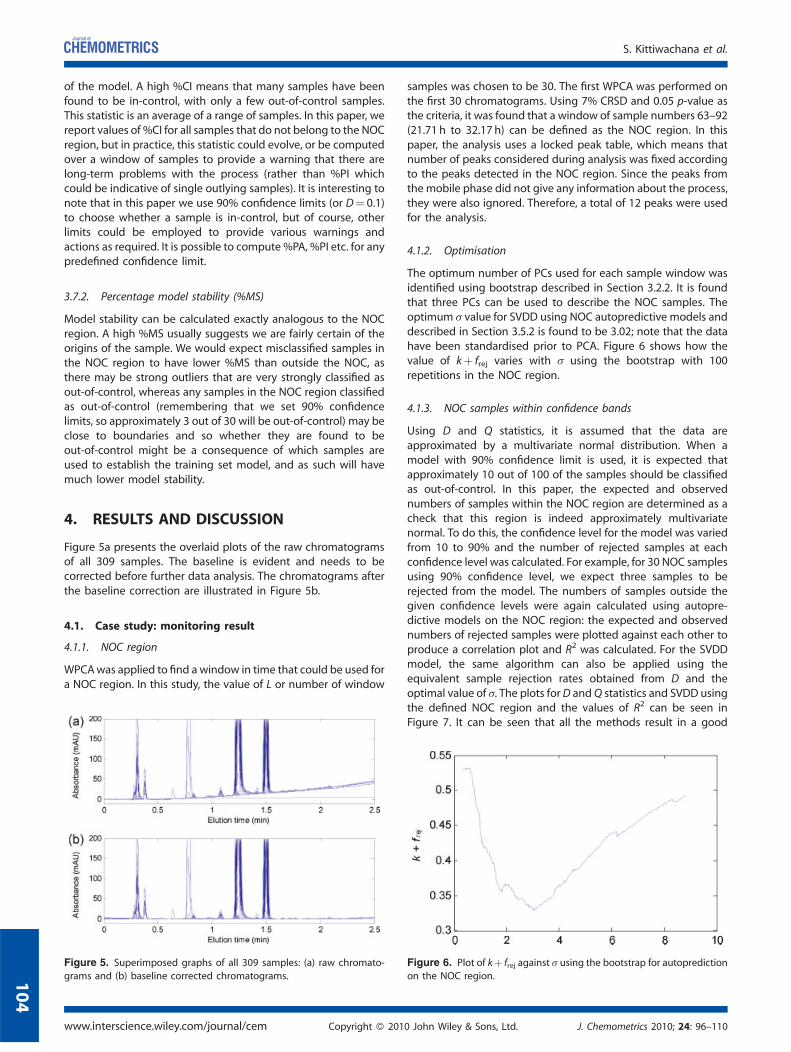
Figure 5a presents the overlaid plots of the raw chromatogramsof all 309 samples. The baseline is evident and needs to becorrected before further data analysis. The chromatograms afterthe baseline correction are illustrated in Figure 5b.

4.1. Case study: monitoring result

4.1.1. NOC region

WPCAwas applied to find awindow in time that could be used fora NOC region. In this study, the value of L or number of window

Figure 5. Superimposed graphs of all 309 samples: (a) raw chromato-

grams and (b) baseline corrected chromatograms.


samples was chosen to be 30. The first WPCA was performed onthe first 30 chromatograms. Using 7% CRSD and 0.05 p-value asthe criteria, it was found that a window of sample numbers 63–92(21.71 h to 32.17 h) can be defined as the NOC region. In thispaper, the analysis uses a locked peak table, which means thatnumber of peaks considered during analysis was fixed accordingto the peaks detected in the NOC region. Since the peaks fromthe mobile phase did not give any information about the process,they were also ignored. Therefore, a total of 12 peaks were usedfor the analysis.

4.1.2. Optimisation

The optimum number of PCs used for each sample window wasidentified using bootstrap described in Section 3.2.2. It is foundthat three PCs can be used to describe the NOC samples. Theoptimum s value for SVDD using NOC autopredictive models anddescribed in Section 3.5.2 is found to be 3.02; note that the datahave been standardised prior to PCA. Figure 6 shows how thevalue of kþ frej varies with s using the bootstrap with 100repetitions in the NOC region.

4.1.3. NOC samples within confidence bands

Using D and Q statistics, it is assumed that the data areapproximated by a multivariate normal distribution. When amodel with 90% confidence limit is used, it is expected thatapproximately 10 out of 100 of the samples should be classifiedas out-of-control. In this paper, the expected and observednumbers of samples within the NOC region are determined as acheck that this region is indeed approximately multivariatenormal. To do this, the confidence level for the model was variedfrom 10 to 90% and the number of rejected samples at eachconfidence level was calculated. For example, for 30 NOC samplesusing 90% confidence level, we expect three samples to berejected from the model. The numbers of samples outside thegiven confidence levels were again calculated using autopre-dictive models on the NOC region: the expected and observednumbers of rejected samples were plotted against each other toproduce a correlation plot and R2 was calculated. For the SVDDmodel, the same algorithm can also be applied using theequivalent sample rejection rates obtained from D and theoptimal value of s. The plots forD andQ statistics and SVDD usingthe defined NOC region and the values of R2 can be seen inFigure 7. It can be seen that all the methods result in a good

Figure 6. Plot of kþ frej against s using the bootstrap for autoprediction

on the NOC region.


Figure 7. Correlation plots for the NOC region. The confidence limits used were from 10 to 90% (equivalent to 0.9–0.1 sample rejection rateD for SVDD).


1

correlation (R2 more than 0.9). This confirms that the NOC regionfits a multi-normal model, and we regard it as good practice priorto applying statistical tests that assume normality, although this isa consequence of our choosing such a region. It alsodemonstrates that SVDD using our chosen parameters behavesin a similar fashion. Whilst SVDD may appear a more complexmethod to the D statistic, it provides an alternative insight, andhas the additional advantage that it can also cope with situationswhere the NOC region is not normally distributed.

4.2. Bulk predictions: model quality and predictionsof non-NOC samples

The next step is to determine how well the NOC model performs.For process monitoring, the only information available is for onegroup of samples (defined as in-control or the NOC) and it is notusually possible to define an out-group as one would have toknow about artificially induced faults in the process; therefore it isdifficult to obtain out-of-control validation samples. To validatethe models established from the defined NOC region, training/test set split assessment was applied. Indices for performance ofthemodels including%PA, %MS and%CC can be calculated usingthe NOC samples. Figures 8(a and b) to 10(a and b) show%PA and%MS for each sample for both training and test set models usingD and Q statistics as well as SVDD, respectively. %CC and theaverages of the %PA and %MS for training and test sets using allthemethods are presented in Table I. It has to be noted again thatfor D and Q statistics, the 90% confidence limit was used(equivalent to a sample rejection rate D¼ 0.1 used for SVDD).Using the training set, the %CC seems overly optimistic in all

cases. However, it is important to recognise that the models areperformed on different training sets each time and that


the average prediction is over 100 iterations. If most samplesare close to a boundary, then there will be different outlyingsamples in each model. If each sample were found to be outsidethe boundary 10% of the time but the samples outside thisboundary differed each time, then all samples would be classifiedas in-control, even though for each individual training set someare out of control as forced by the model. The average %PA is amore realistic measure. If each sample were randomly mis-classified 10% of the time, this measure would be close to 90%,which we find to be in good agreement for two of the measures.The D statistic seems somewhat over optimistic, but this may bebecause the data are not perfectly multinormal.Using the test set, the %PA from both the D statistic and SVDD

are close to 90%. This is a good sign that themodels are performingas expected, and also suggests that the %PA is a more realisticassessment of model performance than the %CC. However, theslightly lower %PA using SVDD could be because the SVDDboundary is optimised to fit the training data and is a sign of slightoverfitting. Figure 11 shows the boundaries drawn from the definedNOC samples. It can be seen that the boundary using SVDD fits theshape of the NOC region more closely: hence, the model can bemore sensitive and therefore, more samples are classified asout-of-control. For Q statistic, the assessment suggests that themodel is prone to be overfitting as%PA from test set is considerablylower than that from the training set. The solution could be toincrease the confidence limit used, such as 99.9% confidence limitas suggested by Nomikos [38], so more samples could be classifiedas under the control and this could avoid too many false alarms. Apossible problem with the Q statistic is that the number of trainingset samples is quite small, resulting in overfitting. TheD statistic andSVDD are both in the PC space and lose variability, e.g. due to smallsources of noise which may be due to the measurement process.


05

20 22 24 26 28 30 32 340

50

100(a)

(b)

(c)

Per

cent

age

(%)

Training set

20 22 24 26 28 30 32 340

50

100

Per

cent

age

(%)

Test set

0 10 20 30 40 50 60 70 80 90 1000

50

100

Sampling time (h)

Per

cent

age

(%)

Non-NOC samples

%PA%MS

%PA%MS

%PI%MS

65

76

76

83

83

5046

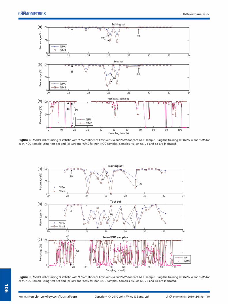
Figure 8. Model indices using D statistic with 90% confidence limit (a) %PA and %MS for each NOC sample using the training set (b) %PA and %MS foreach NOC sample using test set and (c) %PI and %MS for non-NOC samples. Samples 46, 50, 65, 76 and 83 are indicated.

20 22 24 26 28 30 32 340

50

100(a)

(b)

(c)

Per

cent

age

(%)

Training set

20 22 24 26 28 30 32 340

50

100

Per

cent

age

(%)

Test set

0 10 20 30 40 50 60 70 80 90 1000

50

100

Sampling time (h)

Per

cent

age

(%)

Non-NOC samples

%PA%MS

%PA%MS

%PI%MS

65

65

76

76

83

83

50

46

Figure 9. Model indices using Q statistic with 90% confidence limit (a) %PA and %MS for each NOC sample using the training set (b) %PA and %MS for

each NOC sample using test set and (c) %PI and %MS for non-NOC samples. Samples 46, 50, 65, 76 and 83 are indicated.

www.interscience.wiley.com/journal/cem Copyright � 2010 John Wiley & Sons, Ltd. J. Chemometrics 2010; 24: 96–110


106

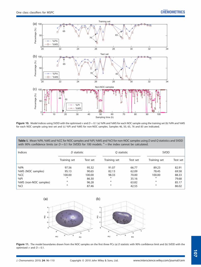
Table I. Mean%PA, %MS and %CC for NOC samples and %PI, %MS and %CI for non-NOC samples using D and Q statistics and SVDDwith 90% confidence limits (or D¼ 0.1 for SVDD) for 100 models. *¼ the index cannot be calculated.

Indices D statistic Q statistic SVDD

Training set Test set Training set Test set Training set Test set

%PA 97.56 95.32 91.07 66.77 89.23 82.91%MS (NOC samples) 95.13 90.65 82.13 62.09 78.45 69.58%CC 100.00 100.00 98.33 70.00 100.00 88.33%PI * 86.30 * 35.16 * 79.68%MS (non-NOC samples) * 96.28 * 63.82 * 85.17%CI * 87.46 * 42.55 * 86.02

Figure 11. The model boundaries drawn from the NOC samples on the first three PCs (a) D statistic with 90% confidence limit and (b) SVDD with the

optimised s and D¼ 0.1.

20 22 24 26 28 30 32 340

50

100(a)

(b)

(c)

Per

cent

age

(%)

Training set

20 22 24 26 28 30 32 340

50

100

Per

cent

age

(%)

Test set

0 10 20 30 40 50 60 70 80 90 1000

50

100

Sampling time (h)

Per

cent

age

(%)

Non-NOC samples

%PA%MS

%PA%MS

%PI%MS

65

65

76

76

83

83

5046

Figure 10. Model indices using SVDD with the optimised s and D¼ 0.1 (a) %PA and %MS for each NOC sample using the training set (b) %PA and %MS

for each NOC sample using test set and (c) %PI and %MS for non-NOC samples. Samples 46, 50, 65, 76 and 83 are indicated.

J. Chemometrics 2010; 24: 96–110 Copyright � 2010 John Wiley & Sons, Ltd. www.interscience.wiley.com/journal/cem


107

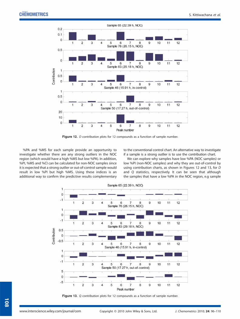
Figure 12. D contribution plots for 12 compounds as a function of sample number.


108

%PA and %MS for each sample provide an opportunity toinvestigate whether there are any strong outliers in the NOCregion (which would have a high %MS but low %PA). In addition,%PI, %MS and %CI can be calculated for non-NOC samples sinceit is expected that a strong outlier or out-of-control sample wouldresult in low %PI but high %MS. Using these indices is anadditional way to confirm the predictive results complementary

Figure 13. Q contribution plots for 12 com


to the conventional control chart. An alternative way to investigateif a sample is a strong outlier is to use the contribution chart.We can explore why samples have low %PA (NOC samples) or

low %PI (non-NOC samples) and why they are out-of-control byusing contribution charts, as shown in Figures 12 and 13, for Dand Q statistics, respectively. It can be seen that althoughthe samples that have a low %PA in the NOC region, e.g sample

pounds as a function of sample number.


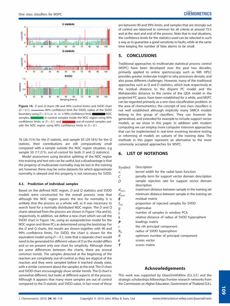
Figure 14. D and Q charts (90 and 99% control limits) and SVDD chart

(D¼ 0.1). 90% confidence limit (for SVDD, radius of the SVDD

boundary usingD¼ 0.1), 99% confidence limit, NOCsamples, in-control samples inside the NOC region using 90%

confidence limits or D¼ 0.1, and out-of-control samples out-

side the NOC region using 90% confidence limits or D¼ 0.1.


1

76 (26.15 h) for the D statistic, and sample 83 (29.18 h) for the Qstatistic, their contributions are still comparatively smallcompared with a sample outside the NOC region situation, e.gsample 50 (17.27 h, out-of-control for both D and Q statistics).Model assessment using iterative splitting of the NOC region

into training and test sets can be useful, but a disadvantage is thatthe property of multivariate normality may be lost in the trainingset; however, there may be some datasets for which approximatenormality is obeyed and this property is not necessary for SVDD.

4.3. Prediction of individual samples

Based on the defined NOC region, D and Q statistics and SVDDmodels were constructed for the overall process: note thatalthough the NOC region passes the test for normality it isunlikely that the process as a whole will, as it was necessary tosearch hard for a normally distributed NOC region. The D and Qcharts obtained from the process are shown in Figure 14(a and b),respectively. In addition, we define a new chart which we call theSVDD chart in Figure 14c, using an autopredictive model for theNOC region and three PCs as determined using the bootstrap. Forthe D and Q charts, the results are shown together with 90 and99% confidence limits. For SVDD, the chart is shown for theequivalent model using D¼ 0.1; note that a separate chart wouldneed to be generated for different values ofD as themodel differsand so we present only one chart for simplicity. Although thereare some differences between the charts, there are severalcommon trends. The samples detected at the beginning of thereaction are completely out-of-control as they are atypical of thereaction and they were sampled before it reached steady state,with a similar comment about the samples at the end. TheD chartand SVDD chart encouragingly show similar trends. TheQ chart issomewhat different, but looks at different aspects of the process.Although it appears that many more samples are out of controlcompared to the D statistic and SVDD value, in fact most of these


are between 90 and 99% limits, and samples that are strongly outof control are observed in common for all criteria at around 75hand at the start and end of the process. Note that in real situations,the confidence levels for the statistics used can be selected in sucha way as to guarantee a good sensitivity to faults, while at the sametime keeping the number of false alarms to be small.

5. CONCLUSIONS

Traditional approaches to multivariate statistical process control(MSPC) have been developed over the past two decades,primarily applied to online spectroscopy such as NIR. HPLCprovides greater molecular insight to why processes deviate, andalso poses different challenges. However, many of the traditionalapproaches such as Q and D statistics, which look respectively atthe residual distance to the disjoint PC model and theMahalanobis distance to the centre of the QDA model in theprojected PC space, have been established for a while, and MSPCcan be regarded primarily as a one class classification problem. Inthe area of chemometrics, the concept of one class classifiers isnot well established although implicitly many SIMCA modelsbelong to this group of classifiers. They can however begeneralised, and extended for example to include support vectormodels, as we show in this paper. In addition with moderncomputing we can employ more computer intensive approachesthat can be implemented in real-time involving iterative testingor reforming of models on subsets of the training data. Themethods in this paper represent an alternative to the morecommonly accepted approaches for MSPC.

6. LIST OF NOTATIONS

Symbol D

y & Sons, Ltd

escription

s k
ernel width for the radial basis function
C p
enalty term for support vector domain description
D s
ample rejection rate for support vector domaindescription
dmax m
aximum distance between sample in the training set
dmin m
inimum distance between sample in the training set
E r
esidual matrix
frej p
roportion of rejected samples for SVDD
g e
igenvalue
L n
umber of samples in window PCA
k r
elative distance of radius of SVDD hypersphere
P lo
adings matrix
r t
he rth principal component
Rh r
adius of SVDD hypersphere
R o
ptimum number of principal component
t s
cores vector
T s
cores matrix
Acknowledgements

This work was supported by GlaxoSmithKline (D.L.S.F.) and thestrategic scholarships fellowships frontier research networks fromthe Commission on Higher Education, Government of Thailand (S.K.).

. www.interscience.wiley.com/journal/cem

09

110


REFERENCES

1. Nomikos P, Macgregor JF. Monitoring batch processes using multiwayprincipal component analysis. AIChE J. 1994; 40: 1361–1375.

2. Nomikos P, MacGregor JF. Multivariate SPC charts for monitoringbatch processes. Technometrics 1995; 37: 41–59.

3. Kourti T, MacGregor JF. Process analysis, monitoring and diagnosis,sing multivariate projection methods. Chemometr. Intell. Lab. Syst.1995; 28: 3–21.

4. Westerhuis JA, Gurden SP, Smilde AK. Spectroscopic monitoring ofbatch reactions for on-line fault detection and diagnosis. Anal. Chem.2000; 72: 5322–5330.

5. Morud TE. Multivariate statistical process control: example from thechemical process industry. J. Chemometr. 1996; 10: 669–675.

6. Qin SJ. Statistical process monitoring: basics and beyond. J. Chemo-metr. 2003; 17: 480–502.

7. Chen Q, Kruger U, Meronk M, Leung AYT. Synthesis of T2 and Qstatistics for process monitoring. Control Eng. Pract. 2004; 12:745–755.

8. Gurden SP, Westerhuis JA, Smilde AK. Monitoring of batch processesusing spectroscopy. AIChE J. 2002; 48: 2283–2297.

9. Larrechi MS, Callao MP. Strategy for introducing NIR spectroscopy andmultivariate calibration techniques in industry. Trends Anal. Chem.2003; 10: 634–640.

10. NIST/SEMATECH e-Handbook of Statistical Methods. Available at:www.itl.nist.gov/div898/handbook/mpc/section2/mpc221.htm[2009-09-15].

11. Brereton RG. Chemometrics for Pattern Recognition. Wiley: Chichester,2009.

12. Jackson JE, Mudholkar GS. Control procedures for residuals associatedwith principal component analysis. Technometrics 1979; 21: 341–349.

13. Jackson JE. A User’s Guide to Principal Components. Wiley: New York,2003.

14. Wold S. Pattern_recognition by means of disjoint principal com-ponents models. Pattern Recognit. 1976; 8: 41–59.

15. Tax DMJ. One-class classification; concept-learning in the absence ofcounter-examples. PhD Thesis, Delft University of Technology (NL),2001. Available at: http://ict.ewi.tudelft.nl/�davidt/papers/thesis.pdf

16. Tax DMJ, Duin RPW. Support vector domain description. PatternRecognit. Lett. 1999; 20: 1119–1199.

17. Tax DMJ, Duin RPW. Support vector domain description. Mach. Learn.2004; 54: 45–66.

18. Efron B, Tibshirani R. An Introduction to the Bootstrap. Chapman & Hall:New York, 1993.

19. Hjorth JSU. Computer Intensive Statistical Methods: Validation, ModelSelection and Bootstrap. Chapman & Hall: New York, 1994.

20. Dixon SJ, Xu Y, Brereton RG, Soini HA, Novotny MV, Oberzaucher E,Grammer K, Penn DJ. Pattern recognition of gas chromatographymass spectrometry of human volatiles in sweat to distinguish the sexof subjects and determine potential discriminatory marker peaks.Chemometr. Intell. Lab. Syst. 2007; 87: 161–172.

21. Wongravee K, Heinrich N, Holmboe M, Schaefer ML, Reed RR, TrevejoJ, Brereton RG. Variable selection using iterative reformulation oftraining set models for discrimination of samples: application to gaschromatography/mass spectrometry of mouse urinary metabolites.Anal. Chem. 2009; 81: 5204–5217.

22. Dixon SJ, Brereton RG. Comparison of performance of five commonclassifiers represented as boundary methods: Euclidean distance tocentroids, linear discriminant analysis, quadratic discriminant analysis,learning vector quantization and support vector machines, as depen-dent on data structure. Chemometr. Intell. Lab. Syst. 2009; 95: 1–17.

23. Kittiwachana S, Ferreira DLS, Fido LA, Thompson DR, Escott REA,Brereton RG. Dynamic analysis of on-line high-performance liquidchromatography for multivariate statistical process control. J. Chro-matogr. A 2008; 1213: 130–144.

24. Zhu L, Brereton RG, Thompson DR, Hopkins PL, Escott REA. On-lineHPLC combined with multivariate statistical process control for themonitoring of reactions. Anal. Chim. Acta 2007; 584: 370–378.

25. Ferreira DLS, Kittiwachana S, Fido LA, Thompson DR, Escott REA,Brereton RG. Multilevel simultaneous component analysis for faultdetection in multicampaign process monitoring: application to


on-line high performance liquid chromatography of a continuousprocess. Analyst 2009; 134: 1571–1585.

26. Vandeginste BMG, Massart DL, Buydens LMC, De Jong S, Lewi PJ,Smeyers-Verbeke J. Handbook of Chemometrics and Qualimetrics PartB. Elsevier: Amsterdam, 1998.

27. Malinowski ER. Factor Analysis in Chemistry (3rd edn). Wiley: New York,2002.

28. Brereton RG. Chemometrics: Data Analysis for the Laboratory andChemical Plant. Wiley: Chichester, 2003.

29. Kavianpour K, Brereton RG. Chemometric methods for the determi-nation of selective regions in diode array detector high performanceliquid chromatography of mixtures: application to chlorophyll aallomers. Analyst 1998; 123: 2035–2042.

30. Wasim M, Hassan MS, Brereton RG. Evaluation of chemometricmethods for determining the number and position of componentsin high-performance liquid chromatography detected by diode arraydetector and on-flow 1H nuclear magnetic resonance spectroscopy.Analyst 2003; 128: 1082–1090.

31. Wasim M, Brereton RG. Determination of the number of significantcomponents in liquid chromatography nuclear magnetic resonancespectroscopy. Chemometr. Intell. Lab. Syst. 2004; 72: 133–151.

32. Brereton RG. Consequences of sample sizes, variable selection, modelvalidation and optimisation for predicting classification ability fromanalytical data. Trend Anal. Chem. 2006; 25: 1103–1111.

33. Wold S. Cross-validatory estimation of number of components infactor and principal components models. Technometrics 1978; 20:397–405.

34. Doornik JA, Hansen H. An omnibus test for univariate andmultivariatenormality. Oxf. Bull. Econ. Stat. 2008; 70: 927–939.

35. Bowman OK, Shenton LR. Omnibus test contours for departures fromnormality based on square-root Hb1 and b2. Biometrika 1975; 62:243–250.

36. Mardia KV. Measures of multivariate skewness and kurtosis withapplications. Biometrika 1970; 57: 519–530.

37. Maesschalck RD, Jouan-Rimbaud D, Massart DL. The Mahalanobisdistance. Chemometr. Intell. Lab. Syst. 2000; 50: 1–18.

38. Nomikos P. Detection and diagnosis of abnormal batch operationsbased on multi-way principal component analysis. ISATrans. 1996; 35:259–266.

39. Li D, Lloyd GR, Duncan JC, Brereton RG. Disjoint hard models forclassification. J. Chemometrics. DOI: 10.1002/cem.1288

40. Xu Y, Brereton RG. Diagnostic pattern recognition on gene expressionprofile data by using one-class classification. J. Chem. Inf. Model. 2005;45: 1392–1401.

41. Xu Y, Brereton RG. Automated single nucleotide polymorphismanalysis using fluorescence excitation-emission spectroscopy andone-class classifiers. Anal. Biochem. 2007; 388: 655–664.

42. Vapnik VN. The Nature of Statistical Learning Theory. Springer: NewYork, 2000.

43. Cortes C, Vapnik V. Support-vector networks. Mach. Learn. 1995; 20:273–295.

44. Cristianini N, Shawe-Taylor J. An Introduction to Support VectorMachines and Other Kernel-based Learning Methods. Cambridge, Uni-versity Press Cambridge: 2000.

45. Xu Y, Zomer S, Brereton RG. Support vector machines: a recentmethod for classification in chemometrics. Crit. Rev. Anal. Chem.2006; 36: 177–188.

46. Tay FEH, Cao LJ. Modified support vector machines in financial timeseries forecasting. Neurocomputing 2002; 48: 847–861.

47. Furey TS, Cristianini N, Duffy N, Bednarski DW, Schummer M, HausslerD. Support vector machine classification and validation of cancertissue samples using microarray data. Bioinformatics 2000; 16: 906–914.

48. Tax DMJ, Muller KR. A consistency-basedmodel selection for one-classclassification. In Proceedings of the 17th International Conference onPattern Recognition, IEEE Computer Society, Cambridge 2004; 3: 363–366.

49. Filzmoser P, Liebmann B, Varmuza K. Repeated double cross vali-dation. J. Chemometr. 2009; 23: 160–171.

50. Lloyd GR, Ahmad S, Wasim M, Brereton RG. Pattern recognition ofinductively coupled plasma atomic emission spectroscopy of humanscalp hair for discriminating between healthy and hepatitis C patients.Anal. Chim. Acta 2009; 649: 33–42.


One class classifiers for process monitoring illustrated by the application to online HPLC of a...

Documents

Transcript of One class classifiers for process monitoring illustrated by the application to online HPLC of a...