1

On the Use of the Transient Hot Strip Method for Measuring the Thermal Conductivity of High-Conducting Thin Bars

M Gustavsson1, H Wang2, R M Trejo2, E Lara-Curzio2, R B Dinwiddie2, S E Gustafsson3

Paper to be presented at the Seventeenth European Conference on Thermophysical Properties, September 5-

8, Bratislava, Slovak Republic, 2005.

1CIT Foundation, Chalmers University of Technology, SE-41288 Gothenburg, Sweden

Email: Gustavsson@cit.chalmers.se (corresponding author)

2Oak Ridge National Laboratory, Oak Ridge, TN, USA

3Department of Physics, Chalmers University of Technology, SE-41296 Gothenburg, Sweden

2

ABSTRACT

Thermal conductivity of thin, high-conducting ceramic and metal bars – commonly used in mechanical

tensile testing – is measured using a variant of the Short Transient Hot Strip technique. As with similar

contact transient methods, the influence from the thermal contact resistance between the sensor and the

sample is accurately recorded and filtered out from the analysis – a specific advantage that enables sensitive

measurements of the bulk properties of the sample material. The present concept requires sensors which are

square in shape with one side having the same width as the bar to be studied. As long as this requirement is

fulfilled the particular size of the thin bar can be selected at will.

This paper presents an application where the present technique is applied to study structural changes or

degradation in Reinforced Carbon-Carbon (RCC) bars exposed to thermal cycling. Simultaneously, tensile

testing and monitoring of mass loss are conducted. The results indicate that the present approach may be

utilized as a non-destructive quality control instrument to monitor local structural changes in RCC panels.

KEYWORDS Hot strip, non-destructive, quality control, reinforced carbon-carbon, thermal conductivity,

thermal degradation

3

1. INTRODUCTION

The Transient Plane Source (TPS)- [1-8], the Transient Hot Strip (THS)- [9-13] and the Pulse Transient Hot

Strip (PTHS) techniques [14-17] have been used for measuring thermal properties of materials, covering a

wide range of materials and sample geometries.

A sensor in the shape of a strip, strip pattern, disk or disk pattern is applied to a sample. It can be

sandwiched between two identical pieces of the sample – here referred to as a double-sided configuration –

or applied only to one sample piece – here referred to as a single-sided configuration. The sensor, having a

well-known temperature coefficient of resistivity, is used simultaneously as a resistance heater and a

resistance thermometer. Basically, a step-wise heating of the sensor is applied, which results in a transient

temperature increase of the near sample surroundings and the sensor itself. By recording the temperature

increase of the sensor element, typically of the order 1 K, the thermal transport properties of the sample can

be estimated.

The original analytical models used in model fitting to experimental data assume infinite sample geometry,

where the sensor is embedded in the sample. In practical experiments, the validity of this assumption is

maintained by controlling the duration of the experiment; by only considering the first part of the transient

response for which the thermal profile development around the sensor has not yet reached the lateral sample

surface boundary. In the following, this minimum distance between the sensor and the lateral sample surface

boundary is referred to as the available probing depth.

For most homogeneous samples having medium or low-conducting thermal transport properties, a sample

geometry of at least a couple of mm in thickness normally suffices for a straight-forward experimental setup

and measurement procedure. However, if the sample thickness is smaller, or the sample is a high-

conducting, the original approach may prove to be difficult, as the measurement time is significantly

reduced to a range which may be very difficult or impossible to attain with standard laboratory equipment.

4

This paper looks into the possibilities to extending the nominal measurement time considerably for high-

conducting metal and ceramic samples by adjusting the sample geometry configuration rather than

increasing the sample size. In particular, by utilizing thermal insulation, “mirroring” effects can be

accomplished which reduces the sample size considerably. When preparing a theoretical model to be used in

data analysis for such a geometrical configuration, the available probing depth will not be limited by any

mirroring surfaces. For instance, in [18, 19] – discussing a technique modification referred to as the Slab

technique in the following – it was shown that thin sheets (of the order 1 mm thickness) of high-conducting

metals can easily be thermally insulated, providing a theory where the available probing depth will be

defined by the minimum distance between the sensor and the lateral surface boundaries of the sides of the

sheets (in the same plane as the sensor itself). In this way, the experimental time was extended from the

range of milliseconds to several seconds. The reason this approach proved successful is that the loss of heat

to the surrounding thermal insulation – the mirroring surfaces – turns out to be practically negligible

compared to the input of power needed to increase the temperature of the Hot Disk sensor.

A different type of mirroring was previously applied for high-conducting samples, making it possible to

experimentally simulate the transient behavior of a much larger sensor and sample than is practically

available. With the Short Transient Hot Strip (STHS) technique [20], a symmetric 2D thermal profile in

accordance with the basic THS theory is achieved by thermally insulating a thin cut-out cross-section of the

imagined sample, where symmetry boundaries in the original configuration can be replaced by mirrored

surfaces. In this way, a comparatively small sample can be used to simulate a thermal conductivity

experiment of a much larger theoretical sample. Consequently, the experimental time is considerably

prolonged while the sample size is limited to a convenient size.

A combined STHS and Slab approach is here developed and utilized for the study of thermal conductivity of

high-conducting metal and ceramic bars of a well-defined geometry, which have been subject to thermal

5

cycling and tensile testing. The thermal conductivity equation is solved for the particular geometry and in

this way establishes the theoretical time dependence of the temperature increase as a result of a step-wise

heating. The THS solution is extended to a Slab-type geometry by implementing the method of images,

which is described in the Section 2.

It is well-accepted that the thermal conductivity is a highly-sensitive indicator of the structural constitution

of the sample [21], where very small structural changes can be closely monitored. Here, it is demonstrated

that the present measurement approach provides a sensitive measurement technique for high-conducting

bar-shaped samples. In Section 4, an application is presented where the downgrading of mechanical

properties in ceramic bars due to thermal cycling is discussed. With the Slab STHS technique presented

here, it is found that the weight-loss and degradation of mechanical properties of RCC bars due to thermal

cycling can be monitored and correlated with the corresponding changes in thermal conductivity.

2. THEORY

When performing thermal conductivity measurements with contact transient methods, it is often possible to

device the experimental setup so that one can measure and strictly eliminate the direct influence of any

thermal contact resistance between the sensor probe and the surface of the solid sample material. An

effective way is to device the measurement setup so that the temperature response of the sensor, T∆ , is the

sum of two clearly separable components – one component which is essentially constant [22], A ,

representing the total thermal contact resistance influence, and the second component a transient

component, ( )cBf τ , not influenced by any thermal contact resistance influence [5, 7, 22]:

( )cBfAT τ+=∆ (1)

where ( )lPBB B ⋅= λ0 , cf. [1, 6, 7, 19]. In Eq. (1), constant B incorporates the bulk thermal conductivity

Bλ of the sample, the heating power 0P and a characteristic length dimension l of the probe. The

dimensionless time function f is expressed in terms of the dimensionless time ( ) θτ cc tt −= , where t is

6

the real measurement time, ct is a time correction, al 2=θ represents the characteristic time of the

measurement, l is a characteristic length of the probe (e.g. strip width or sensor radius) and a is the thermal

diffusivity of the sample.

A large contacting area, typically the case for THS, PTHS and TPS techniques – in contrast to the similar

Transient Hot Wire (THW) technique – gives an improved thermal contact between the sensor and the

sample. This reduces the magnitude of component A . Also, a thin sensor, preferably as thin as possible,

reduces the specific heat capacity of the sensor itself, with additional improvements. To be more precise,

one can show that the component A may be varying a little bit due to imperfect electronics as well as due to

the specific heat capacity of the sensor itself [8]. A reformulation of Eq. (1) into a refined model having a

strictly constant A can be made, as demonstrated in [8].

The time function f depends on the probe design and size, as well as the sample geometry. If the sample is

assumed to be infinite in all directions – a common assumption for e.g. THS, PTHS, TPS and THW

technique – Equation (1) remains valid in the time interval from the beginning of the transient to the

instance in time, maxt , when the thermal penetration depth reaches the nearest lateral surface boundary. We

can express this time interval as ( )max,ttc , where

( ) 21max2 tap ⋅=∆ (2)

represents the minimum distance from any part of the heating area of the sensor to the lateral boundary of

the sample, i.e. the available probing depth.

Two issues limit the performance of this class of techniques. The first issue relates to the issue of

measurement time: The sample and probe size selected may give large variations in the possible time

interval, creating a problem if the maximum time maxt is very short. For instance, in a single-pulse

experiment with the THS, TPS or THW technique, it is difficult to arrange transient recordings over time

7

periods shorter than, say 0.5 seconds, with standard laboratory multimeters. The second issue relates to the

issue of measurement sensitivity, also governed by the selection of the probe and sample size configuration

as well as the measurement time. For the TPS and THS methods, the general rule-of-thumb is that the larger

the sensor, the greater the measurement sensitivity and accuracy. This however requires large sample sizes.

On the other hand, given a certain sample and sensor configuration, the theoretical optimal sensitivity in the

estimation of both thermal conductivity and thermal diffusivity properties can be analyzed with sensitivity

coefficients. When using a Hot Disk sensor, the optimal total measurement time meast should be selected

within the interval 133.0 meas << θt , provided the available probing depth does not limit the measurement

time, i.e. maxmeas tt < [23].

From Eq. (2), it is obvious that high-conducting samples which generally always have a large thermal

diffusivity a or samples which has a small available probing depth p∆ , results in very short maximum

times maxt – which adversely influences measurement performance and makes a measurement difficult or

impossible to perform if maxt is shorter than 0.5 seconds.

The PTHS technique was designed to enable a down-scaling of the measurement time, by inserting repeated

cycles of high-frequency pulses each representing a measurement time interval ( )FP,0 followed by a

cooling interval ( )PFP, , where 05.0=F is the duty cycle and P is the period. By repeating the

measurement in a series of pulses, measurement stability is obtained by averaging the result of many pulses.

The time behavior rendering the estimation of the thermal effusivity is obtained by varying the period P

[16, 17]. The measurement probe can in this way be down-scaled several orders of magnitude, enabling

measurements on samples with a sample thickness less than 1 micrometer, without altering the basic

principles of the theory as formulated in Eqs. (1)-(2), although the practical experimental setup, electrical

circuit, measurement procedure and analysis have been altered considerably.

8

3. EXPERIMENTAL ARRANGEMENTS

A measurement system incorporating a bridge circuit with automatic compensation for lead resistances, a

power supply and digital multimeter, as well as a data analysis module (supplied by Hot Disk Inc.) was used

in this study.

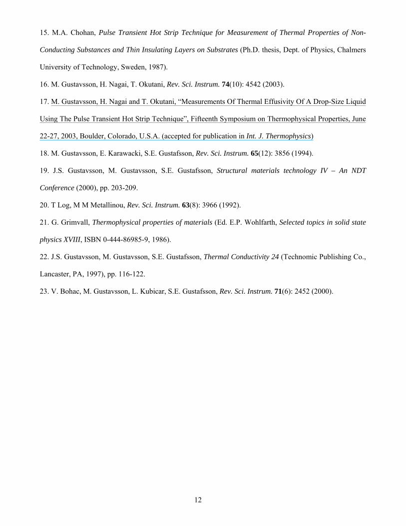
A Slab-based Short Transient Hot Strip configuration is obtained by cutting the samples into a shape that

directly resembles a metal bar, cf. Fig. 1, and insulate all sides of the bar. A double-sided setup may also be

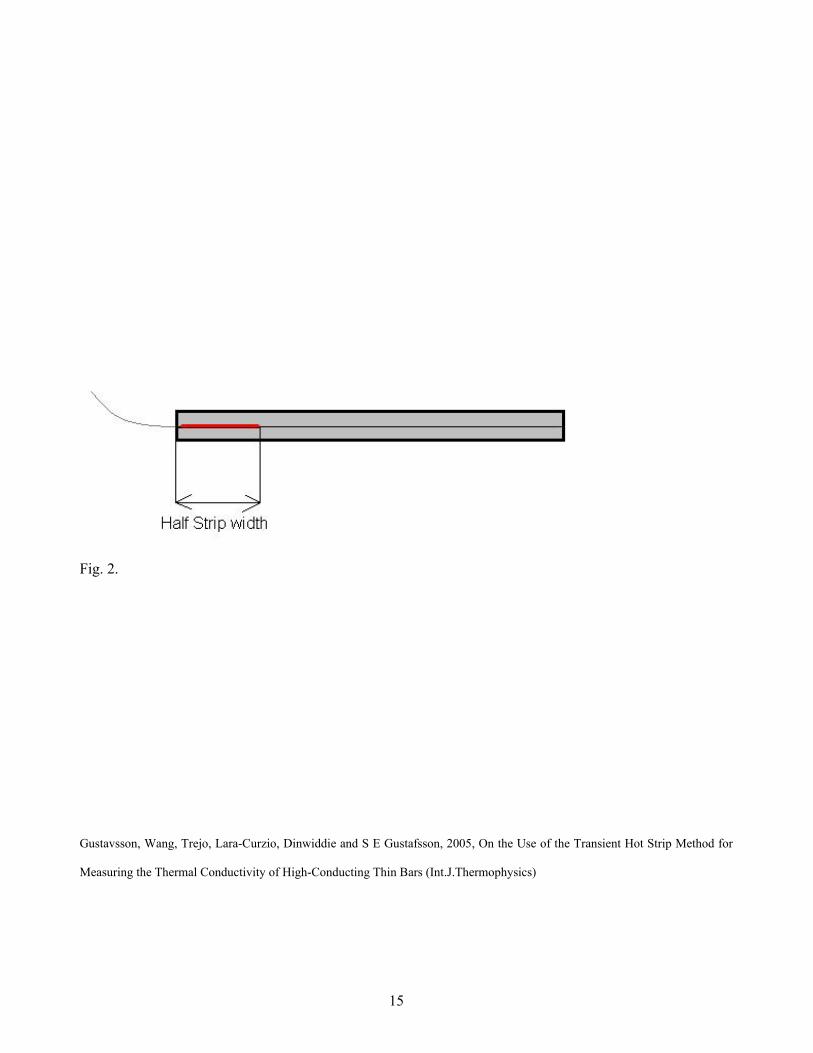
obtained in a similar way. The sensor can be placed in the center of the sample as in Fig. 1 or at one side of

the configuration, assuming a mirrored surface, cf. Fig. 2. The theoretical model to be used in accordance

with the principal model in Eq. (1) requires an adjustment of the time function f for this specific sample

and sensor geometry configuration.

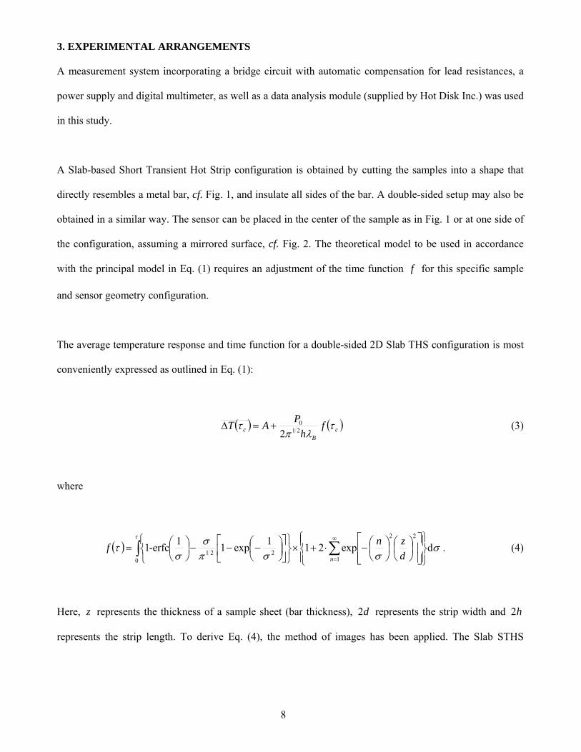
The average temperature response and time function for a double-sided 2D Slab THS configuration is most

conveniently expressed as outlined in Eq. (1):

( ) ( )cB

c fh

PAT τλπ

τ 210

2+=∆ (3)

where

( ) ∫ ∑⎪⎭

⎪⎬⎫

⎪⎩

⎪⎨⎧

⎥⎥⎦

⎤

⎢⎢⎣

⎡⎟⎠⎞

⎜⎝⎛

⎟⎠⎞

⎜⎝⎛−⋅+×

⎭⎬⎫

⎩⎨⎧

⎥⎦

⎤⎢⎣

⎡⎟⎠⎞

⎜⎝⎛−−−⎟

⎠⎞

⎜⎝⎛=

∞

=

τ

σσσπ

σσ

τ0 1

22

221 dexp211exp11erfc1n d

zn-f . (4)

Here, z represents the thickness of a sample sheet (bar thickness), d2 represents the strip width and h2

represents the strip length. To derive Eq. (4), the method of images has been applied. The Slab STHS

9

configuration in Figs 1-2 has a strip length h2 equal to the bar width. The strip width d2 is in this Slab-

STHS configuration equal to the length of the strip along the bar-length direction.

Function ( )τf in Eq. (4) describes a situation where the sample has a limited thickness perpendicular to the

Hot Strip sensor plane, while the sample is considered infinite in the plane of the sensor. Equations (3)-(4)

are identical to the expressions derived in [9] with the exception of the factor ( )( )[ ]∑∞

=−⋅

12222exp2

ndzn σ .

It is obvious that if z , the thickness of the Slab, tends to infinity one obtains the same function as that used

in the THS method, where the sample is considered infinite in all directions.

If additional mirroring of the sample setup is introduced, cf. e.g. Fig. 2 where the sensor is placed at the side

of the bar, the expression in Eq. (3) must be compensated for this. For instance, in Fig. 2 the settings of the

strip width d2 must be doubled to compensate for the symmetry boundary introduced. The assumed output

of power 0P must also be doubled. In Fig. 1, we note that the single-sided configuration assumes a perfect

mirroring – the symmetry boundary being the plane of the sensor – which requires us to assume a doubled

output of heating power 0P when analyzing data.

4. INFLUENCE FROM THERMAL TREATMENT ON CERAMIC BARS

A Reinforced Carbon-Carbon (RCC) consists of a carbon fiber/matrix composite (for rigidity and strength),

a silicon carbide fiber/matrix conversion coating for high-temperature oxide protection, and a TEOS

impregnation and a sodium silicate sealant for additional oxidation protection.

The present application investigates the TPS method as a non-destructive testing technique to evaluate

oxidation-induced mass-loss and sub-surface damage (sub-surface oxidation, void formation, delamination

etc.) in RCC panels through measurements of thermal conductivity.

10

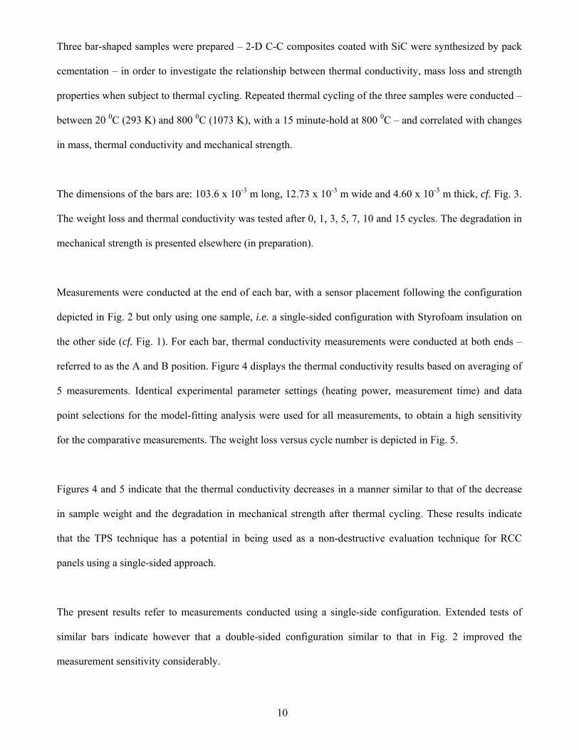
Three bar-shaped samples were prepared – 2-D C-C composites coated with SiC were synthesized by pack

cementation – in order to investigate the relationship between thermal conductivity, mass loss and strength

properties when subject to thermal cycling. Repeated thermal cycling of the three samples were conducted –

between 20 0C (293 K) and 800 0C (1073 K), with a 15 minute-hold at 800 0C – and correlated with changes

in mass, thermal conductivity and mechanical strength.

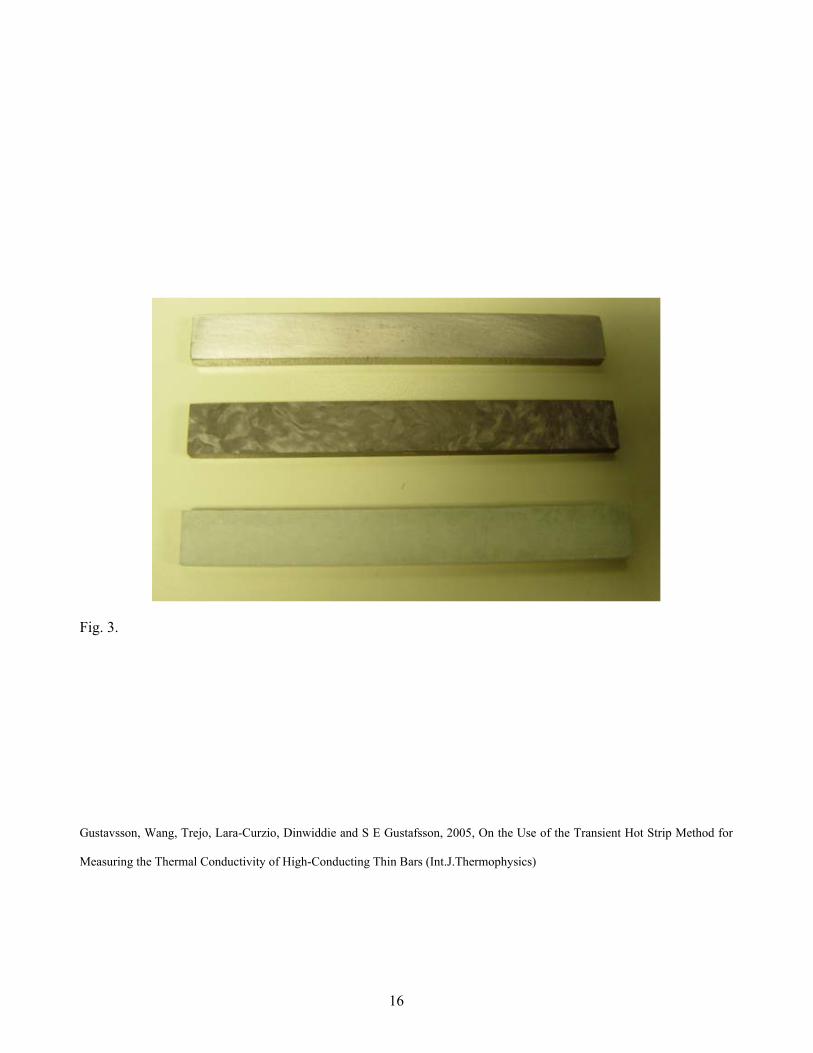
The dimensions of the bars are: 103.6 x 10-3 m long, 12.73 x 10-3 m wide and 4.60 x 10-3 m thick, cf. Fig. 3.

The weight loss and thermal conductivity was tested after 0, 1, 3, 5, 7, 10 and 15 cycles. The degradation in

mechanical strength is presented elsewhere (in preparation).

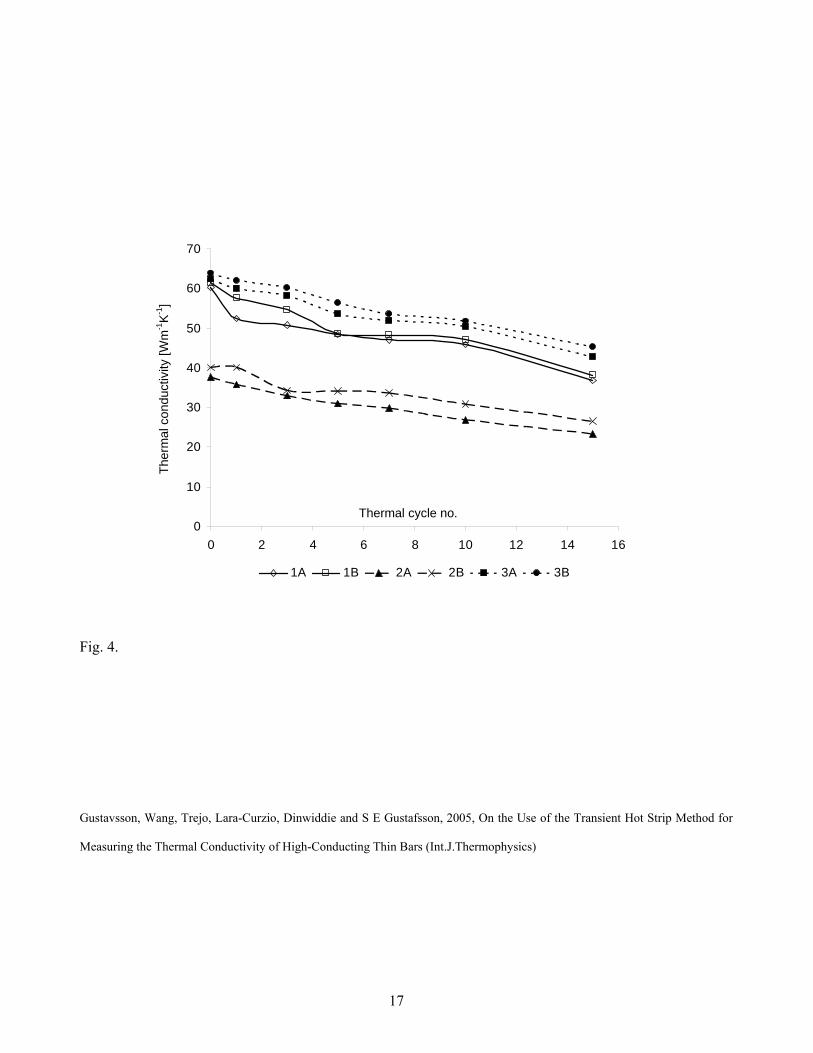
Measurements were conducted at the end of each bar, with a sensor placement following the configuration

depicted in Fig. 2 but only using one sample, i.e. a single-sided configuration with Styrofoam insulation on

the other side (cf. Fig. 1). For each bar, thermal conductivity measurements were conducted at both ends –

referred to as the A and B position. Figure 4 displays the thermal conductivity results based on averaging of

5 measurements. Identical experimental parameter settings (heating power, measurement time) and data

point selections for the model-fitting analysis were used for all measurements, to obtain a high sensitivity

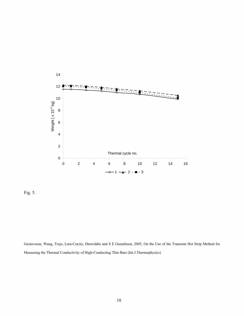
for the comparative measurements. The weight loss versus cycle number is depicted in Fig. 5.

Figures 4 and 5 indicate that the thermal conductivity decreases in a manner similar to that of the decrease

in sample weight and the degradation in mechanical strength after thermal cycling. These results indicate

that the TPS technique has a potential in being used as a non-destructive evaluation technique for RCC

panels using a single-sided approach.

The present results refer to measurements conducted using a single-side configuration. Extended tests of

similar bars indicate however that a double-sided configuration similar to that in Fig. 2 improved the

measurement sensitivity considerably.

11

5. ACKNOWLEDGEMENTS

This work is supported by the U.S. DOE, Assistant Secretary for Energy Efficiency and Renewable Energy,

Office of Office of Transportation Technologies, as part of the High Temperature Materials Laboratory

(HTML) User Program and Office of Industrial Technologies managed by the UT-Battelle LLC. for the

DOE under contract DE-AC05-000OR22725.

6. REFERENCES

1. S.E. Gustafsson, Rev. Sci. Instrum. 62(3): 797 (1991).

2. T. Log, S.E. Gustafsson, Fire and Materials 19: 43 (1995).

3. B.M. Suleiman, M. Gustavsson, E. Karawacki, A. Lundén, J. Phys. D: Appl. Phys. 30: 2553 (1997).

4. M. Gustavsson, J.S. Gustavsson, S.E. Gustafsson, L. Hälldahl, High Temp. High Press. 32: 47 (2000).

5. D. Lundström, B. Karlsson, M. Gustavsson, Z. Metallkd. 92: 1203 (2001).

6. Y. He, Proceedings of 30th NATAS Conference, (Pittsburgh, PA, 2002) pp. 499-504.

7. M. Gustavsson, S.E. Gustafsson, Thermal Conductivity 26, (DEStech Publications Inc., Lancaster, PA,

2001), pp. 367-377.

8. M.K. Gustavsson, S.E. Gustafsson, Thermal Conductivity 27, (DEStech Publications Inc., Lancaster, PA,

2003), pp. 338-346.

9. S.E. Gustafsson, E. Karawacki, M.N. Khan, J. Phys. D: Appl. Phys. 12: 1411 (1979).

10. S.E. Gustafsson, M.A. Chohan, K. Ahmed, A. Maqsood, J. Appl. Phys. 55(9): 3348 (1984).

11. S.E. Gustafsson, The Rigaku Journal (vol.4, n°1/2, 1987), pp. 16-28.

12. Y.W. Song, U. Groβ, E. Hahne, Fluid Phase equilibria 88: 291 (1993).

13. M.J. Lourenco, S.C.S. Rosa, C.A. Nieto de Castro, C. Albuquerque, B. Erdmann, J. Lang, R. Roitzsch,

Int. J. Thermophys. 21(2): 377 (2000).

14. S.E. Gustafsson, M.A. Chohan, M.N. Khan, High Temp. High Press. 17(1): 35 (1985).

12

15. M.A. Chohan, Pulse Transient Hot Strip Technique for Measurement of Thermal Properties of Non-

Conducting Substances and Thin Insulating Layers on Substrates (Ph.D. thesis, Dept. of Physics, Chalmers

University of Technology, Sweden, 1987).

16. M. Gustavsson, H. Nagai, T. Okutani, Rev. Sci. Instrum. 74(10): 4542 (2003).

17. M. Gustavsson, H. Nagai and T. Okutani, “Measurements Of Thermal Effusivity Of A Drop-Size Liquid

Using The Pulse Transient Hot Strip Technique”, Fifteenth Symposium on Thermophysical Properties, June

22-27, 2003, Boulder, Colorado, U.S.A. (accepted for publication in Int. J. Thermophysics)

18. M. Gustavsson, E. Karawacki, S.E. Gustafsson, Rev. Sci. Instrum. 65(12): 3856 (1994).

19. J.S. Gustavsson, M. Gustavsson, S.E. Gustafsson, Structural materials technology IV – An NDT

Conference (2000), pp. 203-209.

20. T Log, M M Metallinou, Rev. Sci. Instrum. 63(8): 3966 (1992).

21. G. Grimvall, Thermophysical properties of materials (Ed. E.P. Wohlfarth, Selected topics in solid state

physics XVIII, ISBN 0-444-86985-9, 1986).

22. J.S. Gustavsson, M. Gustavsson, S.E. Gustafsson, Thermal Conductivity 24 (Technomic Publishing Co.,

Lancaster, PA, 1997), pp. 116-122.

23. V. Bohac, M. Gustavsson, L. Kubicar, S.E. Gustafsson, Rev. Sci. Instrum. 71(6): 2452 (2000).

13

FIGURE CAPTIONS

Figure 1. Single-sided setup, centered strip sensor.

Figure 2. Double-sided setup.

Figure 3. Ceramic bars.

Figure 4. Thermal conductivity of ceramic bars versus thermal cycle number.

Figure 5. Weight of ceramic bars versus thermal cycle number.

Gustavsson, Wang, Trejo, Lara-Curzio, Dinwiddie and S E Gustafsson, 2005, On the Use of the Transient Hot Strip Method for

Measuring the Thermal Conductivity of High-Conducting Thin Bars (Int.J.Thermophysics)

14

Fig. 1.

Gustavsson, Wang, Trejo, Lara-Curzio, Dinwiddie and S E Gustafsson, 2005, On the Use of the Transient Hot Strip Method for

Measuring the Thermal Conductivity of High-Conducting Thin Bars (Int.J.Thermophysics)

15

Fig. 2.

Gustavsson, Wang, Trejo, Lara-Curzio, Dinwiddie and S E Gustafsson, 2005, On the Use of the Transient Hot Strip Method for

Measuring the Thermal Conductivity of High-Conducting Thin Bars (Int.J.Thermophysics)

16

Fig. 3.

Gustavsson, Wang, Trejo, Lara-Curzio, Dinwiddie and S E Gustafsson, 2005, On the Use of the Transient Hot Strip Method for

Measuring the Thermal Conductivity of High-Conducting Thin Bars (Int.J.Thermophysics)

17

0

10

20

30

40

50

60

70

0 2 4 6 8 10 12 14 16

1A 1B 2A 2B 3A 3B

Fig. 4.

Gustavsson, Wang, Trejo, Lara-Curzio, Dinwiddie and S E Gustafsson, 2005, On the Use of the Transient Hot Strip Method for

Measuring the Thermal Conductivity of High-Conducting Thin Bars (Int.J.Thermophysics)

Ther

mal

con

duct

ivity

[Wm

-1K

-1]

Thermal cycle no.

18

0

2

4

6

8

10

12

14

0 2 4 6 8 10 12 14 16

1 2 3

Fig. 5.

Gustavsson, Wang, Trejo, Lara-Curzio, Dinwiddie and S E Gustafsson, 2005, On the Use of the Transient Hot Strip Method for

Measuring the Thermal Conductivity of High-Conducting Thin Bars (Int.J.Thermophysics)

Wei

ght [

x 1

0-3 k

g]

Thermal cycle no.