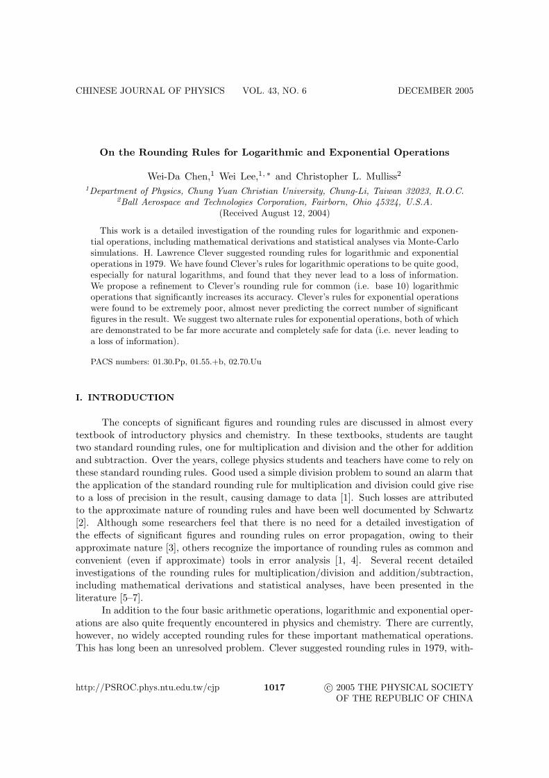
CHINESE JOURNAL OF PHYSICS VOL. 43, NO. 6 DECEMBER 2005

On the Rounding Rules for Logarithmic and Exponential Operations

Wei-Da Chen,1 Wei Lee,1, ∗ and Christopher L. Mulliss2

1Department of Physics, Chung Yuan Christian University, Chung-Li, Taiwan 32023, R.O.C.2Ball Aerospace and Technologies Corporation, Fairborn, Ohio 45324, U.S.A.

(Received August 12, 2004)

This work is a detailed investigation of the rounding rules for logarithmic and exponen-tial operations, including mathematical derivations and statistical analyses via Monte-Carlosimulations. H. Lawrence Clever suggested rounding rules for logarithmic and exponentialoperations in 1979. We have found Clever’s rules for logarithmic operations to be quite good,especially for natural logarithms, and found that they never lead to a loss of information.We propose a refinement to Clever’s rounding rule for common (i.e. base 10) logarithmicoperations that significantly increases its accuracy. Clever’s rules for exponential operationswere found to be extremely poor, almost never predicting the correct number of significantfigures in the result. We suggest two alternate rules for exponential operations, both of whichare demonstrated to be far more accurate and completely safe for data (i.e. never leading toa loss of information).

PACS numbers: 01.30.Pp, 01.55.+b, 02.70.Uu

I. INTRODUCTION

The concepts of significant figures and rounding rules are discussed in almost everytextbook of introductory physics and chemistry. In these textbooks, students are taughttwo standard rounding rules, one for multiplication and division and the other for additionand subtraction. Over the years, college physics students and teachers have come to rely onthese standard rounding rules. Good used a simple division problem to sound an alarm thatthe application of the standard rounding rule for multiplication and division could give riseto a loss of precision in the result, causing damage to data [1]. Such losses are attributedto the approximate nature of rounding rules and have been well documented by Schwartz[2]. Although some researchers feel that there is no need for a detailed investigation ofthe effects of significant figures and rounding rules on error propagation, owing to theirapproximate nature [3], others recognize the importance of rounding rules as common andconvenient (even if approximate) tools in error analysis [1, 4]. Several recent detailedinvestigations of the rounding rules for multiplication/division and addition/subtraction,including mathematical derivations and statistical analyses, have been presented in theliterature [5–7].

In addition to the four basic arithmetic operations, logarithmic and exponential oper-ations are also quite frequently encountered in physics and chemistry. There are currently,however, no widely accepted rounding rules for these important mathematical operations.This has long been an unresolved problem. Clever suggested rounding rules in 1979, with-

http://PSROC.phys.ntu.edu.tw/cjp 1017 c© 2005 THE PHYSICAL SOCIETYOF THE REPUBLIC OF CHINA

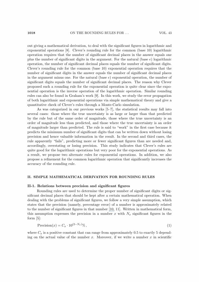
1018 ON THE ROUNDING RULES FOR . . . VOL. 43

out giving a mathematical derivation, to deal with the significant figures in logarithmic andexponential operations [8]. Clever’s rounding rule for the common (base 10) logarithmicoperation requires that the number of significant decimal places in the answer equals oneplus the number of significant digits in the argument. For the natural (base e) logarithmicoperation, the number of significant decimal places equals the number of significant digits.Clever’s rounding rule for the common (base 10) exponential operation requires that thenumber of significant digits in the answer equals the number of significant decimal placesin the argument minus one. For the natural (base e) exponential operation, the number ofsignificant digits equals the number of significant decimal places. The reason why Cleverproposed such a rounding rule for the exponential operation is quite clear since the expo-nential operation is the inverse operation of the logarithmic operation. Similar roundingrules can also be found in Graham’s work [9]. In this work, we study the error propagationof both logarithmic and exponential operations via simple mathematical theory and give aquantitative check of Clever’s rules through a Monte-Carlo simulation.

As was categorized in our previous works [5–7], the statistical results may fall intoseveral cases: those where the true uncertainty is as large or larger than that predictedby the rule but of the same order of magnitude, those where the true uncertainty is anorder of magnitude less than predicted, and those where the true uncertainty is an orderof magnitude larger than predicted. The rule is said to “work” in the first case because itpredicts the minimum number of significant digits that can be written down without losingprecision and hence valuable information in the result. In the second and third cases, therule apparently “fails”, predicting more or fewer significant figures than are needed and,accordingly, overstating or losing precision. This study indicates that Clever’s rules arequite good for the logarithmic operations but very poor for the exponential operations. Asa result, we propose two alternate rules for exponential operations. In addition, we alsopropose a refinement for the common logarithmic operation that significantly increases theaccuracy of the rounding rule.

II. SIMPLE MATHEMATICAL DERIVATION FOR ROUNDING RULES

II-1. Relations between precision and significant figures

Rounding rules are used to determine the proper number of significant digits or sig-nificant decimal places that should be kept after a certain mathematical operation. Whendealing with the problems of significant figures, we follow a very simple assumption, whichstates that the precision (namely, percentage error) of a number is approximately relatedto the number of significant figures in that number [10, 11]. Written in mathematical form,this assumption expresses the precision in a number x with Nx significant figures in theform [5]:

Precision(x) = Cx · 10(2−Nx)% , (1)

where Cx is a positive constant that can range from approximately 0.5 to exactly 5 depend-ing on the actual value of the number x. Moreover, if we write a number x in scientific

VOL. 43 WEI-DA CHEN, WEI LEE, AND CHRISTOPHER L. MULLISS 1019

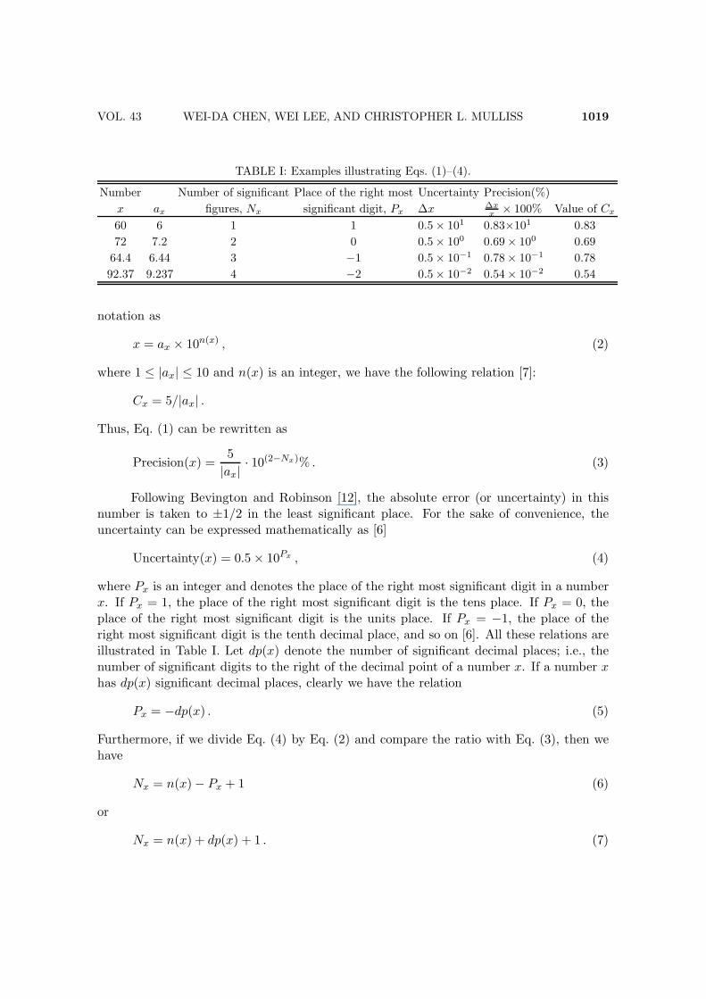
TABLE I: Examples illustrating Eqs. (1)–(4).

Number Number of significant Place of the right most Uncertainty Precision(%)

x ax figures, Nx significant digit, Px ∆x ∆xx

× 100% Value of Cx

60 6 1 1 0.5 × 101 0.83×101 0.83

72 7.2 2 0 0.5 × 100 0.69 × 100 0.69

64.4 6.44 3 −1 0.5 × 10−1 0.78 × 10−1 0.78

92.37 9.237 4 −2 0.5 × 10−2 0.54 × 10−2 0.54

notation as

x = ax × 10n(x) , (2)

where 1 ≤ |ax| ≤ 10 and n(x) is an integer, we have the following relation [7]:

Cx = 5/|ax| .

Thus, Eq. (1) can be rewritten as

Precision(x) =5

|ax|· 10(2−Nx)% . (3)

Following Bevington and Robinson [12], the absolute error (or uncertainty) in thisnumber is taken to ±1/2 in the least significant place. For the sake of convenience, theuncertainty can be expressed mathematically as [6]

Uncertainty(x) = 0.5 × 10Px , (4)

where Px is an integer and denotes the place of the right most significant digit in a numberx. If Px = 1, the place of the right most significant digit is the tens place. If Px = 0, theplace of the right most significant digit is the units place. If Px = −1, the place of theright most significant digit is the tenth decimal place, and so on [6]. All these relations areillustrated in Table I. Let dp(x) denote the number of significant decimal places; i.e., thenumber of significant digits to the right of the decimal point of a number x. If a number xhas dp(x) significant decimal places, clearly we have the relation

Px = −dp(x) . (5)

Furthermore, if we divide Eq. (4) by Eq. (2) and compare the ratio with Eq. (3), then wehave

Nx = n(x) − Px + 1 (6)

or

Nx = n(x) + dp(x) + 1 . (7)

1020 ON THE ROUNDING RULES FOR . . . VOL. 43

Eq. (7) has been presented and discussed previously in the literature, first by Graham, whoused the relationship to develop significant-figure rules for generic arithmetic functions [9],and then independently by Lee et al., who used the relationship to relate the rounding rulefor addition to the rule for multiplication [6].

Throughout this entire paper, Nx denotes the number of significant digits of a num-ber x, Px the least significant place, and dp(x) the number of significant decimal places.Moreover, we always use x, which is restricted to be a positive number, as the input of anoperation and y the output.

Finally, with the above notation, we can summarize Clever’s rules in the followingmathematical forms:

dp(y) = Nx + 1 or Py = −(Nx + 1) for common logarithmic operations ,

dp(y) = Nx or Py = −Nx for natural logarithmic operations ,

Ny = dp(x) − 1 or Ny = −Px − 1 for common exponential operations, and

Ny = dp(x) or Ny = −Px for natural exponential operations .

II-2. Rounding rules for logarithmic operations

Assume that the input x (> 0) has an uncertainty ∆x. We would like to calculatethe logarithm of x to the base b (> 0), where b 6= 0 or 1, and to know how this uncertaintypropagates into the output y under the logarithmic operation:

y = logb x . (8)

To achieve this goal, let us substitute x ± ∆x into Eq. (8) to get

y ± ∆y = logb(x ± ∆x)

=1

ln bln(x ± ∆x)

=1

ln bln

[

x

(

1 ±∆x

x

)]

=1

ln b

[

ln x + ln

(

1 ±∆x

x

)]

=ln x

ln b+

1

ln b

[

(

±∆x

x

)

−1

2

(

±∆x

x

)2

+1

3

(

±∆x

x

)3

− . . .

]

,

where we use the series expansion ln(1 + x) = x − x2/2 + x3/3 − x4/4 + . . .. Since theuncertainty of a number is smaller than that number, ∆x/x is smaller than 1, and we cantherefore neglect the terms of ∆x/x of higher orders, keeping just the first-order term; i.e.,

y ± ∆y ≈ln x

ln b±

1

ln b

(

∆x

x

)

= logb x ±1

ln b

(

∆x

x

)

.

Thus, we can easily recognize that

∆y ≈1

ln b

(

∆x

x

)

,

VOL. 43 WEI-DA CHEN, WEI LEE, AND CHRISTOPHER L. MULLISS 1021

which is equivalent to

Uncertainty(y) ≈ Precision(x)/ ln b . (9)

This is the error-propagation equation for logarithmic operations. Substitution of the rela-tions (i.e., Eqs. (3)–(5)) described above into Eq. (9) leads to the following formula:

dp(y) ≈ Nx + [log(ax) + log(ln b) − 1] . (10)

This is the formula we use to determine the number of significant decimal places in theoutput of logarithmic operations.

II-3. Rounding rules for exponential operations

As far as exponential operations are concerned, we consider the following exponentialoperation; i.e., the antilogarithm of x to the base b:

y = antilogb x = bx . (11)

In a similar way, we carry out the same procedure as we did for logarithmic operations toget

y ± ∆y = y ·

(

1 ±∆y

y

)

= bx±∆x

= exp [(x ± ∆x) · ln b]

= exp [x · ln b ± ∆x · ln b]

= exp(x · ln b) × exp(±∆x · ln b) .

Thus, with the recognition that y = bx = exp(x · ln b), we have

1 ±∆y

y= exp(±∆x · ln b)

= 1 + (±∆x · ln b) +1

2!(±∆x · ln b)2 +

1

3!(±∆x · ln b)3 + . . . ,

where we have expanded the exponential function in a Taylor series. We restrict our in-vestigation to a range where ∆x · ln b is less than 1 for both bases considered (b = 10 andb = e). This restriction requires that dp(x) ≥ 0. This allows us to neglect the terms oforders higher than 2 so that

1 ±∆y

y≈ 1 ± (∆x · ln b) .

Hence, we have

∆y

y≈ ∆x · ln b ,

1022 ON THE ROUNDING RULES FOR . . . VOL. 43

or

Precision(y) ≈ Uncertainty(x) × (ln b) . (12)

This is the error-propagation equation for exponential operations. Similarly, substitutingall the relations above into Eq. (12), we come to the following formula that determines thesignificant digits of the output of exponential operations:

Ny ≈ dp(x) − [log(ay) + log(ln b) − 1] . (13)

There is one thing worth noting. If we exchange x and y in Eq. (10) and rearrangethe terms, we will recover Eq. (13). This is expected, considering that the logarithmic andexponential functions are inverse functions of each other. The error-propagation equationscan be easily verified through differentiation, since we have the following relation for anyfunction y = f(x) [10]:

∆y ≈

(

df

dx

)

· ∆x .

III. A STATISTICAL STUDY OF THE ROUNDING RULES

III-1. The method

To investigate the statistical properties of the rounding rules, a Monte-Carlo pro-cedure was used. A computer code was written in Fortran 90 and run on a Pentium(R)4 PC equipped with a Compaq Visual Fortran complier (Version 6.5.0). The code usesa random number generator based on Ran2 [13] to create numbers. Each number has arandomly determined number of significant figures ranging from 1 to 5, and a randomlydetermined number of places to the left of the decimal point ranging from 0 to 5. Each digitin these numbers is randomly assigned a value from 0 to 9, except for the leading digit thatis randomly assigned a value from 1 to 9. We restrict the random numbers to the rangefrom 1 to 9.9999×105 for logarithmic operations and to the range from 0.01 to 9.9999 forexponential operations. The range of numbers investigated ensures that the assumptionsused to derive the error-propagation equations, given in Eqs. (9) and (12), are valid. Theprogram calculates the common and natural logarithms or exponentials of the generatednumbers, and determines the number of significant figures that should be kept accordingto each of the rounding rules. It uses Eq. (9) to directly compute the “true” absolute errorfor logarithmic operations. It uses Eq. (12) to compute the “true” precision for exponentialoperations, which is then converted to the “true” absolute error. The absolute error in theresult predicted by each rule is taken to ±1/2 in the least significant decimal place. Thetrue absolute error and the value predicted by each rule are compared, and the operationis counted as one of the cases described previously. The program repeats the calculationfor one million logarithmic and exponential problems and computes statistics.

VOL. 43 WEI-DA CHEN, WEI LEE, AND CHRISTOPHER L. MULLISS 1023

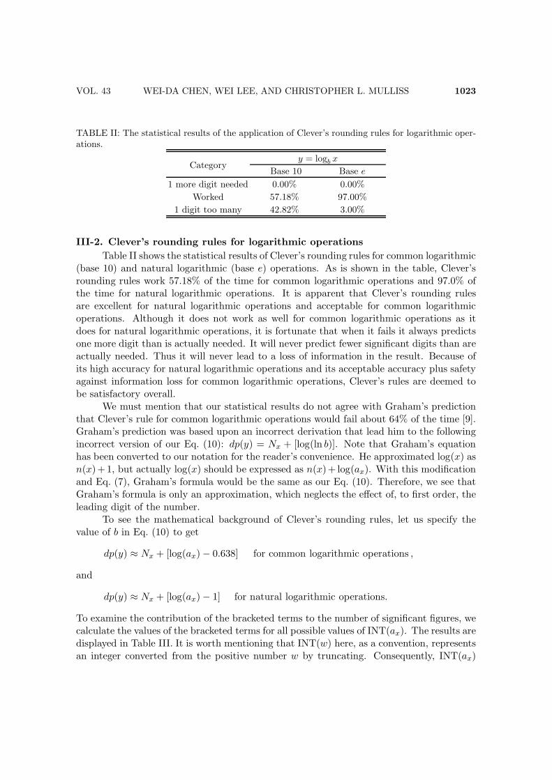
TABLE II: The statistical results of the application of Clever’s rounding rules for logarithmic oper-ations.

y = logb xCategory

Base 10 Base e

1 more digit needed 0.00% 0.00%

Worked 57.18% 97.00%

1 digit too many 42.82% 3.00%

III-2. Clever’s rounding rules for logarithmic operations

Table II shows the statistical results of Clever’s rounding rules for common logarithmic(base 10) and natural logarithmic (base e) operations. As is shown in the table, Clever’srounding rules work 57.18% of the time for common logarithmic operations and 97.0% ofthe time for natural logarithmic operations. It is apparent that Clever’s rounding rulesare excellent for natural logarithmic operations and acceptable for common logarithmicoperations. Although it does not work as well for common logarithmic operations as itdoes for natural logarithmic operations, it is fortunate that when it fails it always predictsone more digit than is actually needed. It will never predict fewer significant digits than areactually needed. Thus it will never lead to a loss of information in the result. Because ofits high accuracy for natural logarithmic operations and its acceptable accuracy plus safetyagainst information loss for common logarithmic operations, Clever’s rules are deemed tobe satisfactory overall.

We must mention that our statistical results do not agree with Graham’s predictionthat Clever’s rule for common logarithmic operations would fail about 64% of the time [9].Graham’s prediction was based upon an incorrect derivation that lead him to the followingincorrect version of our Eq. (10): dp(y) = Nx + [log(ln b)]. Note that Graham’s equationhas been converted to our notation for the reader’s convenience. He approximated log(x) asn(x)+1, but actually log(x) should be expressed as n(x)+ log(ax). With this modificationand Eq. (7), Graham’s formula would be the same as our Eq. (10). Therefore, we see thatGraham’s formula is only an approximation, which neglects the effect of, to first order, theleading digit of the number.

To see the mathematical background of Clever’s rounding rules, let us specify thevalue of b in Eq. (10) to get

dp(y) ≈ Nx + [log(ax) − 0.638] for common logarithmic operations ,

and

dp(y) ≈ Nx + [log(ax) − 1] for natural logarithmic operations.

To examine the contribution of the bracketed terms to the number of significant figures, wecalculate the values of the bracketed terms for all possible values of INT(ax). The results aredisplayed in Table III. It is worth mentioning that INT(w) here, as a convention, representsan integer converted from the positive number w by truncating. Consequently, INT(ax)

1024 ON THE ROUNDING RULES FOR . . . VOL. 43

TABLE III: Contribution of the leading digit of the input x = ax×10n(x) to the number of significantfigures in the output of logarithmic operations.

Base 10 Base e

INT(ax) Value of Proper choice of Value of Proper choice of

[log(INT(ax)) − 0.638] dp(y) [log(INT(ax)) − 1] dp(y)

1 −0.638 Nx −1.000 Nx − 1

2 −0.337 Nx −0.699 Nx

3 −0.161 Nx −0.523 Nx

4 −0.036 Nx −0.398 Nx

5 0.061 Nx + 1 −0.301 Nx

6 0.140 Nx + 1 −0.222 Nx

7 0.207 Nx + 1 −0.155 Nx

8 0.265 Nx + 1 −0.097 Nx

9 0.316 Nx + 1 −0.046 Nx

stands exactly for the leading digit (namely, the left-most significant digit) of the input x.Note that dp(y) listed in Table III must be a positive integer. The proper choice of dp(y)should be made in accordance with

dp(y) = RINT {Nx + [log(ax) + log(ln b) − 1]} ,

where RINT(w) denotes the smallest integer that is greater than or equal to w.For common logarithmic operations, Table III shows that there are two possible cases:

dp(y) = Nx (Py = −Nx) or dp(y) = Nx + 1 (Py = −(Nx + 1)). In order to avoid losingvaluable information carried by the digits, we would rather slightly overstate the precisionthan predict fewer digits than actually needed. That is to say, the most appropriate rulewhich is independent of ax is dp(y) = Nx+1 (Py = −(Nx+1)). This is just the mathematicalstatement of Clever’s rule for common logarithmic operations. The two possible cases inTable III (Nx and Nx + 1) ensure that Clever’s rule for common logarithmic operations(dp(y) = Nx + 1) can only predict one significant decimal place too many when it does fail.

As Table III shows, the transition from dp(y) = Nx (Py = −Nx) to dp(y) = Nx + 1(Py = −(Nx + 1)) happens somewhere between ax = 4 and ax = 5. Since ax can berepresented, to zeroth order, by the leading (significant) digit of the input x, we can refineClever’s rounding rule in order to attain a significantly higher probability of success. Weprovide the following rounding rule for common logarithmic operations, called the CLMrule for common logarithmic operations:

If the leading digit of the input x is greater than or equal to 4, report one moresignificant decimal place in the answer than there are significant digits in thenumber x; otherwise, keep the same number of significant decimal places inthe answer as there are significant digits in the number x.

The CLM rule for common logarithmic operations works very well, having a probability of

VOL. 43 WEI-DA CHEN, WEI LEE, AND CHRISTOPHER L. MULLISS 1025

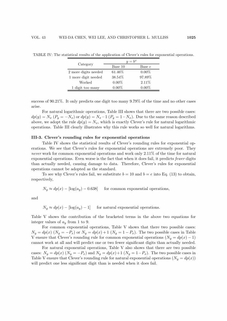
TABLE IV: The statistical results of the application of Clever’s rules for exponential operations.

y = bx

CategoryBase 10 Base e

2 more digits needed 61.46% 0.00%

1 more digit needed 38.54% 97.89%

Worked 0.00% 2.11%

1 digit too many 0.00% 0.00%

success of 90.21%. It only predicts one digit too many 9.79% of the time and no other casesarise.

For natural logarithmic operations, Table III shows that there are two possible cases:dp(y) = Nx (Py = −Nx) or dp(y) = Nx−1 (Py = 1−Nx). Due to the same reason describedabove, we adopt the rule dp(y) = Nx, which is exactly Clever’s rule for natural logarithmicoperations. Table III clearly illustrates why this rule works so well for natural logarithms.

III-3. Clever’s rounding rules for exponential operations

Table IV shows the statistical results of Clever’s rounding rules for exponential op-erations. We see that Clever’s rules for exponential operations are extremely poor. Theynever work for common exponential operations and work only 2.11% of the time for naturalexponential operations. Even worse is the fact that when it does fail, it predicts fewer digitsthan actually needed, causing damage to data. Therefore, Clever’s rules for exponentialoperations cannot be adopted as the standard.

To see why Clever’s rules fail, we substitute b = 10 and b = e into Eq. (13) to obtain,respectively,

Ny ≈ dp(x) − [log(ay) − 0.638] for common exponential operations,

and

Ny ≈ dp(x) − [log(ay) − 1] for natural exponential operations.

Table V shows the contribution of the bracketed terms in the above two equations forinteger values of ay from 1 to 9.

For common exponential operations, Table V shows that there two possible cases:Ny = dp(x) (Ny = −Px) or Ny = dp(x) + 1 (Ny = 1−Px). The two possible cases in TableV ensure that Clever’s rounding rule for common exponential operations (Ny = dp(x)− 1)cannot work at all and will predict one or two fewer significant digits than actually needed.

For natural exponential operations, Table V also shows that there are two possiblecases: Ny = dp(x) (Ny = −Px) and Ny = dp(x)+1 (Ny = 1−Px). The two possible cases inTable V ensure that Clever’s rounding rule for natural exponential operations (Ny = dp(x))will predict one less significant digit than is needed when it does fail.

1026 ON THE ROUNDING RULES FOR . . . VOL. 43

TABLE V: Contribution of the leading digit of the output y = ay ×10n(y) of exponential operationsto the number of significant figures in the output.

Base 10 Base e

INT(ay) Value of Proper choice of Value of Proper choice of

−[log(INT(ay)) − 0.638] Ny −[log(INT(ay)) − 1] Ny

1 0.638 dp(x) + 1 1 dp(x) + 1

2 0.337 dp(x) + 1 0.699 dp(x) + 1

3 0.161 dp(x) + 1 0.523 dp(x) + 1

4 0.036 dp(x) + 1 0.398 dp(x) + 1

5 −0.061 dp(x) 0.301 dp(x) + 1

6 −0.140 dp(x) 0.222 dp(x) + 1

7 −0.207 dp(x) 0.155 dp(x) + 1

8 −0.265 dp(x) 0.097 dp(x) + 1

9 −0.316 dp(x) 0.046 dp(x) + 1

III-4. Alternatives to Clever’s rounding rules for exponential operations

In addition to understanding why Clever’s rules for exponential operations fail, wecan propose an alternate rounding rule based upon the mathematical analysis. Because thepossible cases are Ny = dp(x) (Ny = −Px) and Ny = dp(x) + 1 (Ny = 1 − Px) for bothcommon and natural operations, we adopt the rule Ny = dp(x) + 1 (Ny = 1 − Px) for thesake of saving the important information carried by the digits. To put it into words, westate the rounding rule in the following way:

For both common and natural exponential operations, report one more signif-icant digit in the output y than there are significant digits decimal places inthe input x.

For convenience, we call this rule the CLM rule for exponential operations. We present thestatistical results of this rule in Table VI. It turns out that this CLM rule for exponen-tial operations is excellent for natural exponential operations and fairly good for commonexponential operations. It works 64.46% and 98.13% of the time for common and naturalexponential operations, respectively. Equally important, it never brings about a loss invaluable information carried by the digits. Although it will slightly overstate the precision,this is a minor shortcoming when compared with the risk of causing damage to data.

Note that the results in Tables V and VI may cause some readers concern. Seeingthat in Table V, 4 out of 10 rows have dp(x)+1 as the right answer for common exponentialoperations, some readers may expect the success rate of the CLM rule to be about 40%.This logic holds true for the results in Table II and Table III. This logic is, however, invalidfor the results in Table V and Table VI. Table III shows the contribution of the leadingdigit of the input which are generated as uniformly random numbers; i.e., the leading digithas a uniform frequency distribution. It is natural to expect the success rate in Table II tobe about 60% for common logarithmic operations, because there are 6 out 10 rows in Table

VOL. 43 WEI-DA CHEN, WEI LEE, AND CHRISTOPHER L. MULLISS 1027

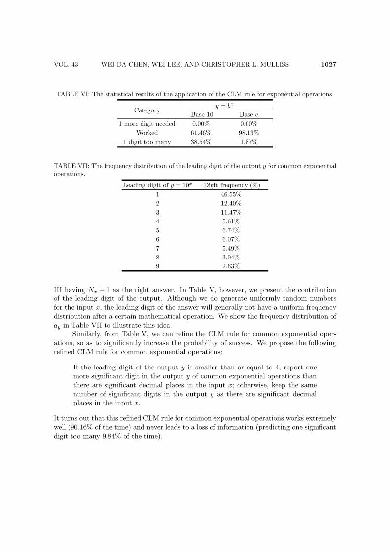
TABLE VI: The statistical results of the application of the CLM rule for exponential operations.

y = bx

CategoryBase 10 Base e

1 more digit needed 0.00% 0.00%

Worked 61.46% 98.13%

1 digit too many 38.54% 1.87%

TABLE VII: The frequency distribution of the leading digit of the output y for common exponentialoperations.

Leading digit of y = 10x Digit frequency (%)

1 46.55%

2 12.40%

3 11.47%

4 5.61%

5 6.74%

6 6.07%

7 5.49%

8 3.04%

9 2.63%

III having Nx + 1 as the right answer. In Table V, however, we present the contributionof the leading digit of the output. Although we do generate uniformly random numbersfor the input x, the leading digit of the answer will generally not have a uniform frequencydistribution after a certain mathematical operation. We show the frequency distribution ofay in Table VII to illustrate this idea.

Similarly, from Table V, we can refine the CLM rule for common exponential oper-ations, so as to significantly increase the probability of success. We propose the followingrefined CLM rule for common exponential operations:

If the leading digit of the output y is smaller than or equal to 4, report onemore significant digit in the output y of common exponential operations thanthere are significant decimal places in the input x; otherwise, keep the samenumber of significant digits in the output y as there are significant decimalplaces in the input x.

It turns out that this refined CLM rule for common exponential operations works extremelywell (90.16% of the time) and never leads to a loss of information (predicting one significantdigit too many 9.84% of the time).

1028 ON THE ROUNDING RULES FOR . . . VOL. 43

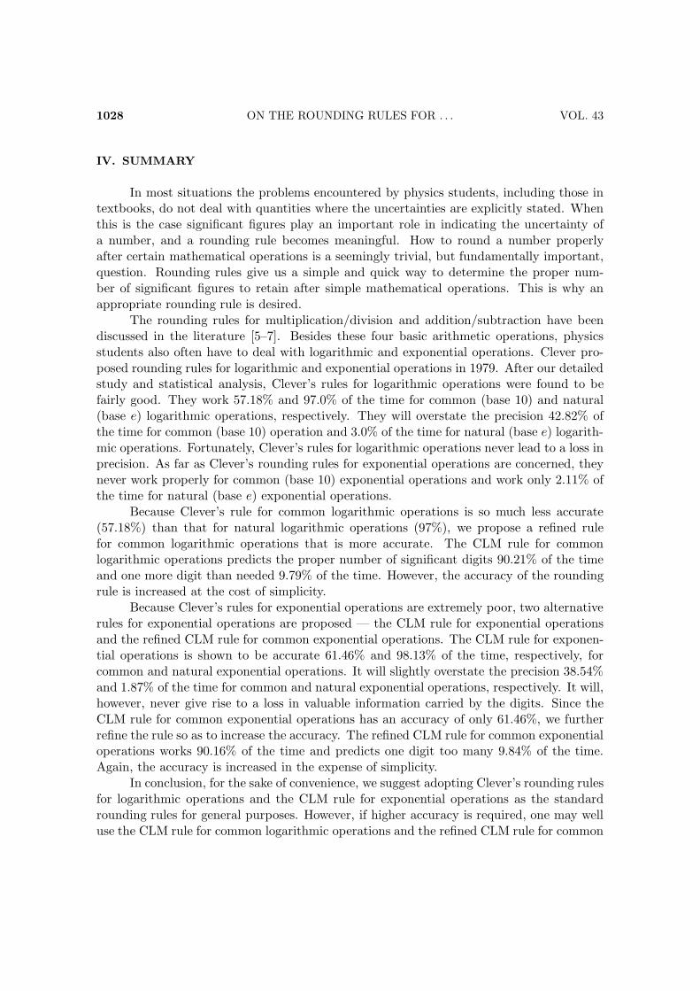
IV. SUMMARY

In most situations the problems encountered by physics students, including those intextbooks, do not deal with quantities where the uncertainties are explicitly stated. Whenthis is the case significant figures play an important role in indicating the uncertainty ofa number, and a rounding rule becomes meaningful. How to round a number properlyafter certain mathematical operations is a seemingly trivial, but fundamentally important,question. Rounding rules give us a simple and quick way to determine the proper num-ber of significant figures to retain after simple mathematical operations. This is why anappropriate rounding rule is desired.

The rounding rules for multiplication/division and addition/subtraction have beendiscussed in the literature [5–7]. Besides these four basic arithmetic operations, physicsstudents also often have to deal with logarithmic and exponential operations. Clever pro-posed rounding rules for logarithmic and exponential operations in 1979. After our detailedstudy and statistical analysis, Clever’s rules for logarithmic operations were found to befairly good. They work 57.18% and 97.0% of the time for common (base 10) and natural(base e) logarithmic operations, respectively. They will overstate the precision 42.82% ofthe time for common (base 10) operation and 3.0% of the time for natural (base e) logarith-mic operations. Fortunately, Clever’s rules for logarithmic operations never lead to a loss inprecision. As far as Clever’s rounding rules for exponential operations are concerned, theynever work properly for common (base 10) exponential operations and work only 2.11% ofthe time for natural (base e) exponential operations.

Because Clever’s rule for common logarithmic operations is so much less accurate(57.18%) than that for natural logarithmic operations (97%), we propose a refined rulefor common logarithmic operations that is more accurate. The CLM rule for commonlogarithmic operations predicts the proper number of significant digits 90.21% of the timeand one more digit than needed 9.79% of the time. However, the accuracy of the roundingrule is increased at the cost of simplicity.

Because Clever’s rules for exponential operations are extremely poor, two alternativerules for exponential operations are proposed — the CLM rule for exponential operationsand the refined CLM rule for common exponential operations. The CLM rule for exponen-tial operations is shown to be accurate 61.46% and 98.13% of the time, respectively, forcommon and natural exponential operations. It will slightly overstate the precision 38.54%and 1.87% of the time for common and natural exponential operations, respectively. It will,however, never give rise to a loss in valuable information carried by the digits. Since theCLM rule for common exponential operations has an accuracy of only 61.46%, we furtherrefine the rule so as to increase the accuracy. The refined CLM rule for common exponentialoperations works 90.16% of the time and predicts one digit too many 9.84% of the time.Again, the accuracy is increased in the expense of simplicity.

In conclusion, for the sake of convenience, we suggest adopting Clever’s rounding rulesfor logarithmic operations and the CLM rule for exponential operations as the standardrounding rules for general purposes. However, if higher accuracy is required, one may welluse the CLM rule for common logarithmic operations and the refined CLM rule for common

VOL. 43 WEI-DA CHEN, WEI LEE, AND CHRISTOPHER L. MULLISS 1029

TABLE VIII: Summary of the suggested rounding rules.

Operation Name of the rounding rule Rounding rule

Common logarithm Clever’s rule dp(y) = Nx + 1 Py = −(Nx + 1)

Natural logarithm Clever’s rule dp(y) = Nx Py = −Nx

Common exponential CLM rule Ny = dp(x) + 1 Ny = 1 − Px

Natural exponential CLM rule Ny = dp(x) + 1 Ny = 1 − Px

TABLE IX: Examples illustrating the usage of the rounding rules for logarithmic operations.

Number x Value of log(x) Rounded result by Rounded result by the

Clever’s rule CLM rule

34.5 1.53782 1.5378 1.538

358 2.55388 2.5539 2.554

853 2.93094 2.9309 2.9309

Number x Value of ln(x) Rounded result by Clever’s rule

34.5 3.5409 3.541

358 5.8805 5.881

853 6.7488 6.749

exponential operations. One should choose the appropriate rounding rule to use dependingon one’s own purpose and situation. To familiarize the readers with the rounding rules, wesummarize the suggested rounding rules in Table VIII and give some examples to illustratethe usage of the rounding rules in Tables IX and X.

TABLE X: Examples illustrating the usage of the rounding rules for exponential operations.

Number x Value of 10x Rounded result by the Rounded result by the

CLM rule refined CLM rule

2.856 717.79 717.8 717.8

3.258 1811.3 1811 1811

5.05 112200 112000 110000

Number x Value of ex Rounded result by the CLM rule

2.856 17.392 17.39

3.258 25.997 26.00

5.05 156.0 156

1030 ON THE ROUNDING RULES FOR . . . VOL. 43

Acknowledgments

Wei-Da Chen is currently pursuing his M.S. degree in the Graduate Institute of As-tronomy, National Central University. He acknowledges Chung Yuan Christian Universityfor supporting this study via an undergraduate research grant.

APPENDIX: TOWARDS A GENERAL PRINCIPLE OF ROUNDING RULES

Seeing that there are many other mathematical functions of one variable, we wouldlike to propose a general principle based on which one can determine the specific form ofthe rounding rule — which we consider the most proper one and should be adopted asa standard rule — for each function of one variable. To do so, we investigate in detailthe error propagation of uncertainty according to a more general statistical approach anddiscuss the validity of the general principle.

We note first that the result of any measurement of a quantity x is, in general, statedas

x = xbest + ∆x ,

where xbest is the best estimate value of x in the measurement and ∆x the uncertainty [10].We then consider the Taylor series expansion about xbest of an operation of the form ofy = f(x)

y = f(x) = f(xbest) + f ′(xbest)(x − xbest) +f ′′(xbest)

2!(x − xbest)

2 + . . . .

Moreover, the best estimate value of x can be proved to be the average of many measure-ments of x [10]; i.e.,

xbest = 〈x〉 ,

and for any symmetric error distribution function (such as the normal distribution) it canalso be shown that

∑

i

(xi − xbest) = 0 or 〈∆x〉 = 0 .

where xi denotes the result of the ith measurement. Hence, we have

y = f(x) = f(〈x〉) + f ′(〈x〉)(∆x) +f ′′(〈x〉)

2!(∆x)2 + . . . .

We will approximate the uncertainty (∆x) as the standard deviation σx [12]; i.e.,

(∆x)2 ≈ σ2x =

⟨

(x − 〈x〉)2⟩

= 〈x2〉 − 〈x〉2 . (A.1)

VOL. 43 WEI-DA CHEN, WEI LEE, AND CHRISTOPHER L. MULLISS 1031

If the uncertainty is small, the first-order approximation leads to

y = f(x) ≈ f(〈x〉) + f ′(〈x〉)(∆x) .

Thus the average of the outcome of the mathematical operation is

〈y〉 ≈ f(〈x〉) + 〈∆x〉f ′(〈x〉) ≈ f(〈x〉) .

We are now in a position to relate the uncertainty ∆y, which we will approximate as thestandard deviation σy, to the uncertainty ∆x:

(∆y)2 ≈ σ2y =

⟨

(y − 〈y〉)2⟩

=⟨

[

f ′(〈x〉)(∆x)]2

⟩

=[

f ′(〈x〉)]2

σ2x ≈

[

f ′(〈x〉)]2

(∆x)2 .

Substituting the relation between uncertainty and the place of least significance (Eq. (4))into the above equation, we arrive at, after some algebra,

Py ≈ Px + log f ′(〈x〉) . (A.2)

This is the equation on which the rounding rule for any arbitrary function of one variableis based; it is equivalent to Graham’s equation (Eq. (11)) [9].

To work out a specific form of the rounding rule for a specific function, one mustinvestigate the contribution of the logarithmic term in Eq. (A.2). In general, Py and Px arerequired to be integers whereas the logarithmic term, which depends on the value of 〈x〉, maynot be. This implies that there is no perfect rounding rule in most mathematical operations,as predicted by Mulliss and Lee [5] in an investigation of rounding rules for multiplicationand division. Nevertheless, we can propose a proper rounding rule following the principleof least damage. Significant figures can be used as a rough indication of the precisionof a number. Therefore, the significant figures cannot be overstated and rounding rulesare used to provide a quick and convenient way to determine the proper number of digitsthat should be kept after a certain mathematical operation. Since no perfect rule exists,the application of rounding rules can give rise to an overestimate or underestimate of thenumber of significant figures that the result of an operation should have. An overestimatemeans overstating the precision of the result, while an underestimate indicates a loss ofimportant information carried by the digits that are rounded off, implying damage to data.Accordingly, to strike a balance between overstating the precision and protecting the data,we must take into account the relative importance of overstating one or two more digitsand of losing important information. In our point of view, overstating only one or twomore digits is a minor defect compared with losing important information. This is whywe always choose the rounding rules in such a way that the rules never result in cases ofunderestimate, thus causing damage to data. In order not to lose the information carriedby the digits, obviously we should adopt the rule

Py = LINT[

Px + log f ′(〈x〉)]

, (A.3a)

1032 ON THE ROUNDING RULES FOR . . . VOL. 43

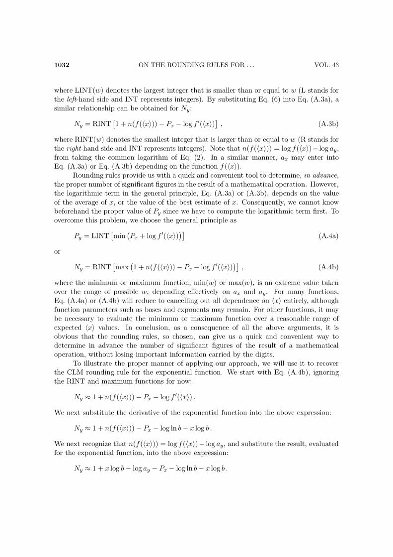
where LINT(w) denotes the largest integer that is smaller than or equal to w (L stands forthe left-hand side and INT represents integers). By substituting Eq. (6) into Eq. (A.3a), asimilar relationship can be obtained for Ny:

Ny = RINT[

1 + n(f(〈x〉)) − Px − log f ′(〈x〉)]

, (A.3b)

where RINT(w) denotes the smallest integer that is larger than or equal to w (R stands forthe right-hand side and INT represents integers). Note that n(f(〈x〉)) = log f(〈x〉)− log ay,from taking the common logarithm of Eq. (2). In a similar manner, ax may enter intoEq. (A.3a) or Eq. (A.3b) depending on the function f(〈x〉).

Rounding rules provide us with a quick and convenient tool to determine, in advance,the proper number of significant figures in the result of a mathematical operation. However,the logarithmic term in the general principle, Eq. (A.3a) or (A.3b), depends on the valueof the average of x, or the value of the best estimate of x. Consequently, we cannot knowbeforehand the proper value of Py since we have to compute the logarithmic term first. Toovercome this problem, we choose the general principle as

Py = LINT[

min(

Px + log f ′(〈x〉))]

(A.4a)

or

Ny = RINT[

max(

1 + n(f(〈x〉)) − Px − log f ′(〈x〉))]

, (A.4b)

where the minimum or maximum function, min(w) or max(w), is an extreme value takenover the range of possible w, depending effectively on ax and ay. For many functions,Eq. (A.4a) or (A.4b) will reduce to cancelling out all dependence on 〈x〉 entirely, althoughfunction parameters such as bases and exponents may remain. For other functions, it maybe necessary to evaluate the minimum or maximum function over a reasonable range ofexpected 〈x〉 values. In conclusion, as a consequence of all the above arguments, it isobvious that the rounding rules, so chosen, can give us a quick and convenient way todetermine in advance the number of significant figures of the result of a mathematicaloperation, without losing important information carried by the digits.

To illustrate the proper manner of applying our approach, we will use it to recoverthe CLM rounding rule for the exponential function. We start with Eq. (A.4b), ignoringthe RINT and maximum functions for now:

Ny ≈ 1 + n(f(〈x〉)) − Px − log f ′(〈x〉) .

We next substitute the derivative of the exponential function into the above expression:

Ny ≈ 1 + n(f(〈x〉)) − Px − log ln b − x log b .

We next recognize that n(f(〈x〉)) = log f(〈x〉)− log ay, and substitute the result, evaluatedfor the exponential function, into the above expression:

Ny ≈ 1 + x log b − log ay − Px − log ln b − x log b .

VOL. 43 WEI-DA CHEN, WEI LEE, AND CHRISTOPHER L. MULLISS 1033

We then simplify the expression and include the RINT and maximum functions to obtain:

Ny = RINT [max ((1 − Px) − (log ay − log ln b))] .

For both b = e and b = 10, and over the entire range of ay, the above expression reducesto Ny = 1 − Px, which is consistent with the results found by the more straightforwardmethod employed in the main body of this paper (refer to Table VIII). The general statisticapproach outlined in this appendix, and described by Eq. (A.4a) and Eq. (A.4b), appearsto be a plausible approach that may be applied to a wide class of single-variable functions.

Finally, there is one point to note. In arriving at Eq. (A.2), we made a first-orderapproximation. How good is this approximation? Or, how large is the domain of validity ofour general principle as expressed by Eq. (A.4a) or (A.4b)? To find the domain of validityof our general principle, we examine the condition that will make our approximation (tothe first order) a good one. Apparently, the condition imposed is

∣

∣

∣

∣

∣

f (n)(〈x〉)

n!(∆x)n

∣

∣

∣

∣

∣

>

∣

∣

∣

∣

∣

f (n+1)(〈x〉)

(n + 1)!(∆x)n+1

∣

∣

∣

∣

∣

or∣

∣

∣

∣

∣

f (n+1)(〈x〉)

f (n)(〈x〉)

∆x

n + 1

∣

∣

∣

∣

∣

< 1 ,

where f (n) denotes the nth derivative of the function f . We check the domain of validity forthe cases of the logarithmic and exponential operations. First, note that the nth derivativeof a logarithmic function of the form of Eq. (8) is

f (n) =1

ln b

1

xn,

which gives the relationship∣

∣

∣

∣

∣

f (n+1)

fn

∆x

n + 1

∣

∣

∣

∣

∣

=1

n + 1

∣

∣

∣

∣

∆x

x

∣

∣

∣

∣

< 1 .

The above inequality holds since n is a non-negative integer and (∆x/x) is smaller thanunity. This means that Clever’s rounding rules for logarithmic operations can be appliedto all real numbers. In this case, there is no restriction on the domain of validity. Next,let us check for the cases of exponential operations. The nth derivative of an exponentialfunction given by Eq. (11) is

f (n) = (ln b)nf ,

which leads to∣

∣

∣

∣

∣

f (n+1)

fn

∆x

n + 1

∣

∣

∣

∣

∣

=| ln b · ∆x|

n + 1.

1034 ON THE ROUNDING RULES FOR . . . VOL. 43

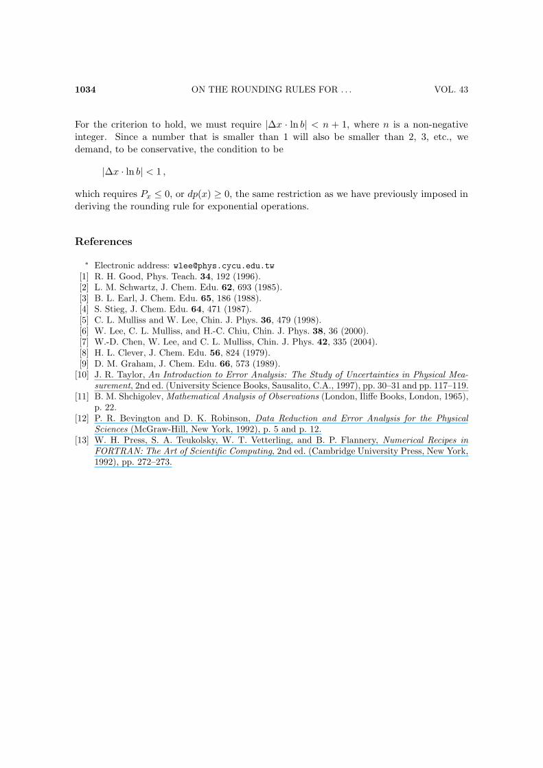
For the criterion to hold, we must require |∆x · ln b| < n + 1, where n is a non-negativeinteger. Since a number that is smaller than 1 will also be smaller than 2, 3, etc., wedemand, to be conservative, the condition to be

|∆x · ln b| < 1 ,

which requires Px ≤ 0, or dp(x) ≥ 0, the same restriction as we have previously imposed inderiving the rounding rule for exponential operations.

References

∗ Electronic address: wlee@phys.cycu.edu.tw[1] R. H. Good, Phys. Teach. 34, 192 (1996).[2] L. M. Schwartz, J. Chem. Edu. 62, 693 (1985).[3] B. L. Earl, J. Chem. Edu. 65, 186 (1988).[4] S. Stieg, J. Chem. Edu. 64, 471 (1987).[5] C. L. Mulliss and W. Lee, Chin. J. Phys. 36, 479 (1998).[6] W. Lee, C. L. Mulliss, and H.-C. Chiu, Chin. J. Phys. 38, 36 (2000).[7] W.-D. Chen, W. Lee, and C. L. Mulliss, Chin. J. Phys. 42, 335 (2004).[8] H. L. Clever, J. Chem. Edu. 56, 824 (1979).[9] D. M. Graham, J. Chem. Edu. 66, 573 (1989).

[10] J. R. Taylor, An Introduction to Error Analysis: The Study of Uncertainties in Physical Mea-

surement, 2nd ed. (University Science Books, Sausalito, C.A., 1997), pp. 30–31 and pp. 117–119.[11] B. M. Shchigolev, Mathematical Analysis of Observations (London, Iliffe Books, London, 1965),

p. 22.[12] P. R. Bevington and D. K. Robinson, Data Reduction and Error Analysis for the Physical

Sciences (McGraw-Hill, New York, 1992), p. 5 and p. 12.[13] W. H. Press, S. A. Teukolsky, W. T. Vetterling, and B. P. Flannery, Numerical Recipes in

FORTRAN: The Art of Scientific Computing, 2nd ed. (Cambridge University Press, New York,1992), pp. 272–273.