Logic Programming and Logarithmic Space

Clément Aubert1, Marc Bagnol1, Paolo Pistone1, and Thomas Seiller2 ∗

1 Aix Marseille Université, CNRS, I2M UMR 7373, 13453, Marseille, France2 I.H.É.S., Le Bois-Marie, 35, Route de Chartres, 91440 Bures-sur-Yvette, France

Abstract. We present an algebraic view on logic programming, related toproof theory and more specifically linear logic and geometry of interaction.Within this construction, a characterization of logspace (deterministicand non-deterministic) computation is given via a synctactic restriction,using an encoding of words that derives from proof theory.We show that the acceptance of a word by an observation (the counterpartof a program in the encoding) can be decided within logarithmic space, byreducing this problem to the acyclicity of a graph. We show moreover thatobservations are as expressive as two-ways multi-heads finite automata, akind of pointer machines that is a standard model of logarithmic spacecomputation.

Keywords: Implicit Complexity, Unification, Logic Programming, LogarithmicSpace, Proof Theory, Pointer Machines, Geometry of Interaction, Automata

1 IntroductionProof Theory and Implicit Complexity Theory Very generally, the aim ofimplicit complexity theory (ICC) is to describe complexity classes with no explicitreference to cost bounds: through a type system or a weakened recursion schemefor instance. The last two decades have seen numerous works relating prooftheory (more specifically linear logic [14]) and ICC, the basic idea being to lookfor restricted substructural logics [18] with an expressiveness that correspondsexactly to some complexity class.

This has been achieved by various syntactic restrictions, which entail a lesscomplex (any function provably total in second-order Peano Arithmetic [14] canbe encoded in second-order linear logic) cut-elimination procedure: control overthe modalities [29,9], type assignments [13] or stratification properties [5], toname a few.

Geometry of Interaction Over the recent years, the cut-elimination procedureand its mathematical modeling has become a central topic in proof theory. Theaim of the geometry of interaction research program [15] is to provide the toolsfor such a modeling [1,24,30].∗This work was partly supported by the ANR-10-BLAN-0213 Logoi and the ANR-

11-BS02-0010 Récré.

arX

iv:1

406.

2110

v1 [

cs.L

O]

9 J

un 2

014

As for complexity theory, these models allow for a more synthetic and abstractstudy of the resources needed to compute the normal form of a program, leadingto some complexity characterization results [6,19,2].

Unification The unification technique is one of the key-concepts of theoreticalcomputer science: it is a classical subject of study for complexity theory and atool with a wide range of applications, including logic programming and typeinference algorithms.

Unification has also been used to build syntactic models of geometryof interaction [17,6,20] where first-order terms with variables allow for amanipulation of infinite sets through a finite language.

Logic Programming After the work of Robinson on the resolution procedure,logic programming has emerged as a new computation paradigm with concreterealizations such as the languages Prolog and Datalog.

On the theoretical side, a lot of efforts has been made to clarify expressivenessand complexity issues [10]: most problems arising from logic programming areundecidable in their most general form and some restrictions must be introducedin order to make them tractable. For instance, the notion of finitely groundprogram [8] is related to our approach.

Pointer Machines Multi-heads finite automata provide an elegant character-ization of logspace computation, in terms of the (qualitative) type of memoryused rather than the (quantitative) amount of tape consumed. Since they canscan but not modify the input, they are usually called “pointer machines”.

This model was already at the heart of previous works relating geometry ofinteraction and complexity theory [19,3,2].

Contribution and Outline We begin by exposing the idea of relating geometryof interaction and logic programming, already evoked [17] but never reallydeveloped, and by recalling the basic notions on unification theory needed forthis article and some related complexity results.

We present in Sect. 2 the algebraic tools used later on to define the encodingof words and pointer machines. Section 2.2 and Sect. 2.3 introduce the syntacticalrestriction and associated tools that allow us to characterize logarithmic spacecomputation. Note that, compared to earlier work [2], we consider a much widerclass of programs while preserving bounded space evaluation.

The encoding of words enabling our results, which comes from the classical(Church) encoding of lists in proof theory, is given in Sect. 3. It allows to definethe counterpart of programs, and a notion of acceptance of a word by a program.

Finally, Sect. 4 makes use of the tools introduced earlier to state and proveour complexity results. While the expressiveness part is quite similar to earlierpresentations [3,2], the proof that acceptance can be decided within logarithmicspace has been made more modular by reducing it to cycle search in a graph.

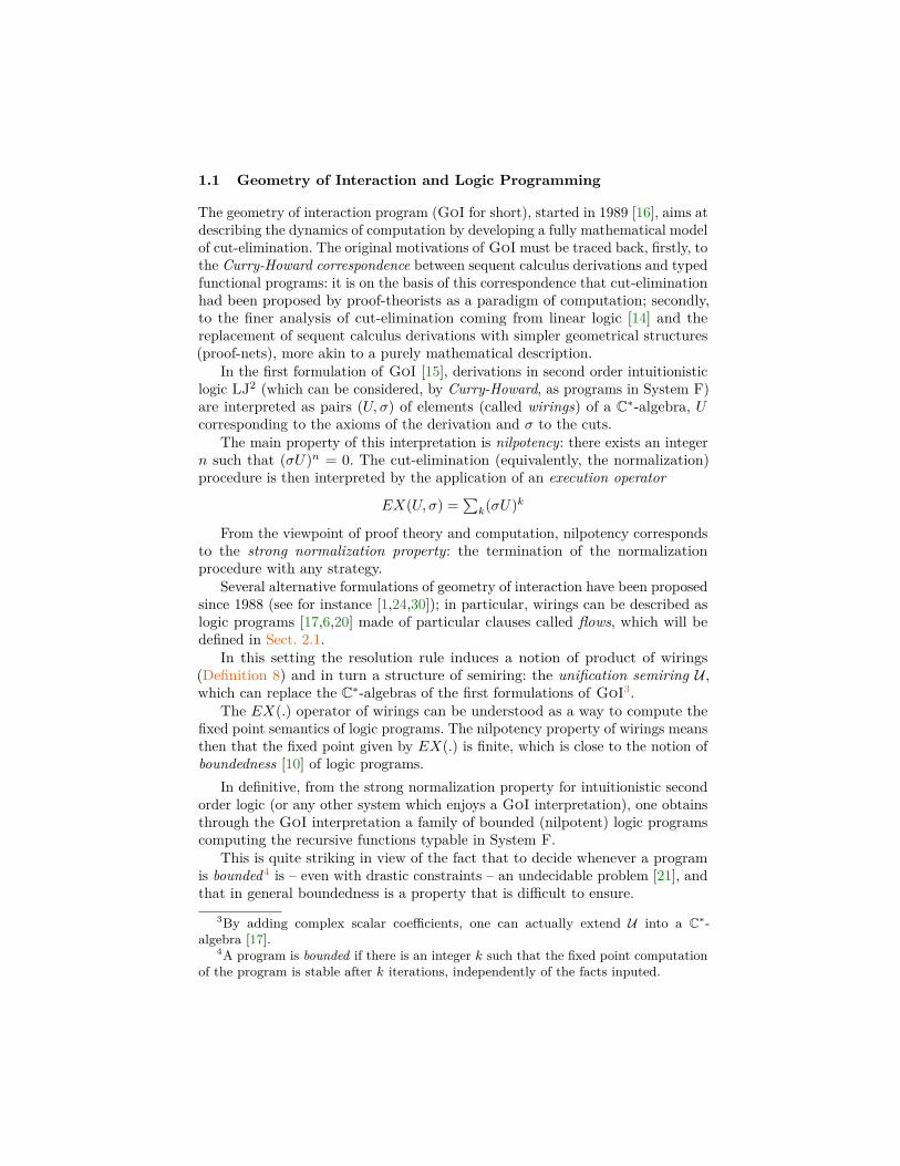
1.1 Geometry of Interaction and Logic Programming

The geometry of interaction program (GoI for short), started in 1989 [16], aims atdescribing the dynamics of computation by developing a fully mathematical modelof cut-elimination. The original motivations of GoI must be traced back, firstly, tothe Curry-Howard correspondence between sequent calculus derivations and typedfunctional programs: it is on the basis of this correspondence that cut-eliminationhad been proposed by proof-theorists as a paradigm of computation; secondly,to the finer analysis of cut-elimination coming from linear logic [14] and thereplacement of sequent calculus derivations with simpler geometrical structures(proof-nets), more akin to a purely mathematical description.

In the first formulation of GoI [15], derivations in second order intuitionisticlogic LJ2 (which can be considered, by Curry-Howard, as programs in System F)are interpreted as pairs (U, σ) of elements (called wirings) of a C∗-algebra, Ucorresponding to the axioms of the derivation and σ to the cuts.

The main property of this interpretation is nilpotency: there exists an integern such that (σU)n = 0. The cut-elimination (equivalently, the normalization)procedure is then interpreted by the application of an execution operator

EX(U, σ) =∑k(σU)k

From the viewpoint of proof theory and computation, nilpotency correspondsto the strong normalization property: the termination of the normalizationprocedure with any strategy.

Several alternative formulations of geometry of interaction have been proposedsince 1988 (see for instance [1,24,30]); in particular, wirings can be described aslogic programs [17,6,20] made of particular clauses called flows, which will bedefined in Sect. 2.1.

In this setting the resolution rule induces a notion of product of wirings(Definition 8) and in turn a structure of semiring: the unification semiring U ,which can replace the C∗-algebras of the first formulations of GoI3.

The EX(.) operator of wirings can be understood as a way to compute thefixed point semantics of logic programs. The nilpotency property of wirings meansthen that the fixed point given by EX(.) is finite, which is close to the notion ofboundedness [10] of logic programs.

In definitive, from the strong normalization property for intuitionistic secondorder logic (or any other system which enjoys a GoI interpretation), one obtainsthrough the GoI interpretation a family of bounded (nilpotent) logic programscomputing the recursive functions typable in System F.

This is quite striking in view of the fact that to decide whenever a programis bounded4 is – even with drastic constraints – an undecidable problem [21], andthat in general boundedness is a property that is difficult to ensure.

3By adding complex scalar coefficients, one can actually extend U into a C∗-algebra [17].

4A program is bounded if there is an integer k such that the fixed point computationof the program is stable after k iterations, independently of the facts inputed.

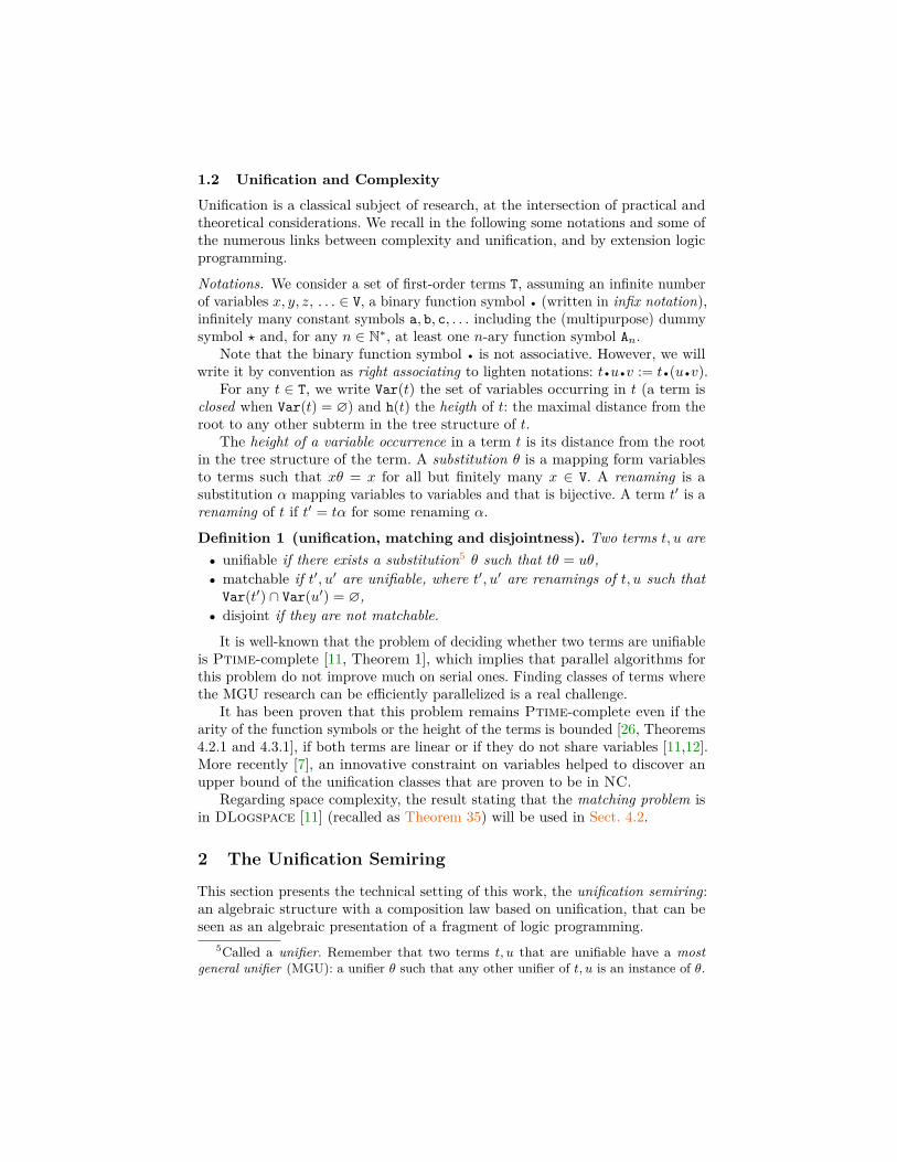
1.2 Unification and Complexity

Unification is a classical subject of research, at the intersection of practical andtheoretical considerations. We recall in the following some notations and some ofthe numerous links between complexity and unification, and by extension logicprogramming.

Notations. We consider a set of first-order terms T, assuming an infinite numberof variables x, y, z, . . . ∈ V, a binary function symbol • (written in infix notation),infinitely many constant symbols a, b, c, . . . including the (multipurpose) dummysymbol ? and, for any n ∈ N∗, at least one n-ary function symbol An.

Note that the binary function symbol • is not associative. However, we willwrite it by convention as right associating to lighten notations: t •u •v := t •(u •v).

For any t ∈ T, we write Var(t) the set of variables occurring in t (a term isclosed when Var(t) = ∅) and h(t) the heigth of t: the maximal distance from theroot to any other subterm in the tree structure of t.

The height of a variable occurrence in a term t is its distance from the rootin the tree structure of the term. A substitution θ is a mapping form variablesto terms such that xθ = x for all but finitely many x ∈ V. A renaming is asubstitution α mapping variables to variables and that is bijective. A term t′ is arenaming of t if t′ = tα for some renaming α.

Definition 1 (unification, matching and disjointness). Two terms t, u are• unifiable if there exists a substitution5 θ such that tθ = uθ,• matchable if t′, u′ are unifiable, where t′, u′ are renamings of t, u such that

Var(t′) ∩ Var(u′) = ∅,• disjoint if they are not matchable.

It is well-known that the problem of deciding whether two terms are unifiableis Ptime-complete [11, Theorem 1], which implies that parallel algorithms forthis problem do not improve much on serial ones. Finding classes of terms wherethe MGU research can be efficiently parallelized is a real challenge.

It has been proven that this problem remains Ptime-complete even if thearity of the function symbols or the height of the terms is bounded [26, Theorems4.2.1 and 4.3.1], if both terms are linear or if they do not share variables [11,12].More recently [7], an innovative constraint on variables helped to discover anupper bound of the unification classes that are proven to be in NC.

Regarding space complexity, the result stating that the matching problem isin DLogspace [11] (recalled as Theorem 35) will be used in Sect. 4.2.

2 The Unification Semiring

This section presents the technical setting of this work, the unification semiring:an algebraic structure with a composition law based on unification, that can beseen as an algebraic presentation of a fragment of logic programming.

5Called a unifier. Remember that two terms t, u that are unifiable have a mostgeneral unifier (MGU): a unifier θ such that any other unifier of t, u is an instance of θ.

2.1 Flows and Wirings

Flows can be thought of as very specific Horn clauses: safe (the variables of thehead must occur in the body) clauses with exactly one atom in the body.

As it is not relevant to this work, we make no difference between predicatesymbols and function symbols, for it makes the presentation easier.

Definition 2 (flows). A flow is a pair of terms t ↼ u with Var(t) ⊆ Var(u).Flows are considered up to renaming: for any renaming α, t ↼ u = tα ↼ uα.

Facts, that are usually defined as ground (using only closed terms) clauseswith an empty body, can still be represented as a special kind of flows.

Definition 3 (facts). A fact is a flow of the form t ↼ ?.

Remark 4. Note that this implies that t is closed.

The main interest of the restriction to flows is that it yields an algebraicstructure: a semigroup with a partially defined product.

Definition 5 (product of flows). Let u ↼ v and t ↼ w be two flows. Supposewe have representatives of the renaming classes such that Var(v) ∩ Var(w) = ∅.The product of u ↼ v and t ↼ w is defined if v, t are unifiable with MGU θ as(u ↼ v)(t ↼ w) := uθ ↼ wθ.

Remark 6. The condition on variables ensures that facts form a “left ideal” ofthe set of flows: if u is a fact and f a flow, then fu is a fact when it is defined.

Example 7.(f(x) ↼ x)(f(x) ↼ g(x)) = f(f(x)) ↼ g(x)(x •c ↼ (y •y) •x)((c •c) •x ↼ y •x) = x •c ↼ c •x(f(x •c) ↼ x •d)(d •d ↼ ?) = f(d •c) ↼ ?

The product of flows corresponds to the resolution rule in the following sense:given two flows f = u ↼ v and g = t ↼ w and a MGU θ of v and t, then theresolution rule applied to f and g would yield fg.

Wirings then correspond to logic programs (sets of clauses) and the nilpotencycondition can be seen as an algebraic variant of the notion of boundedness ofthese programs.

Definition 8 (wirings). Wirings are finite sets of flows. The product of wiringsis defined as FG := { fg | f ∈ F, g ∈ G, fg defined }.

We write U the set of wirings and refer to it as the unification semiring.

The set of wirings U has a structure of semiring. We use an additive notationfor sets of flows to stress this point:• The symbol + will be used in place of ∪.• We write sets as the sum of their elements: { f1, . . . , fn } := f1 + · · ·+ fn.• We write 0 for the empty set.

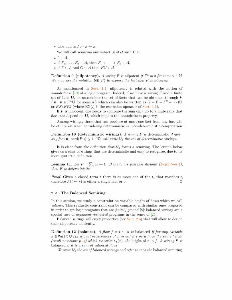
• The unit is I := x ↼ x.We will call semiring any subset A of U such that• 0 ∈ A,• if F1, . . . , Fn ∈ A, then F1 + · · · + Fn ∈ A,• if F ∈ A and G ∈ A then FG ∈ A.

Definition 9 (nilpotency). A wiring F is nilpotent if Fn = 0 for some n ∈ N.We may use the notation Nil(F ) to express the fact that F is nilpotent.

As mentionned in Sect. 1.1, nilpotency is related with the notion ofboundedness [10] of a logic program. Indeed, if we have a wiring F and a finiteset of facts U, let us consider the set of facts that can be obtained through F{ u | u ∈ FnU for some n } which can also be written as (I + F + F 2 + · · · )Uor EX(F )U (where EX(.) is the execution operator of Sect. 1.1).

If F is nilpotent, one needs to compute the sum only up to a finite rank thatdoes not depend on U, which implies the boundedness property.

Among wirings, those that can produce at most one fact from any fact willbe of interest when considering deterministic vs. non-deterministic computation.

Definition 10 (deterministic wirings). A wiring F is deterministic if givenany fact u, card(Fu) ≤ 1. We will write Ud the set of deterministic wirings.

It is clear from the definition that Ud forms a semiring. The lemma belowgives us a class of wirings that are deterministic and easy to recognize, due to itsmore syntactic definition.

Lemma 11. Let F =∑i ui ↼ ti. If the ti are pairwise disjoint (Definition 1),

then F is deterministic.

Proof. Given a closed term t there is at most one of the ti that matches t,therefore F (t ↼ ?) is either a single fact or 0. ut

2.2 The Balanced Semiring

In this section, we study a constraint on variable height of flows which we callbalance. This syntactic constraint can be compared with similar ones proposedin order to get logic programs that are finitely ground [8]: balanced wirings are aspecial case of argument-restricted programs in the sense of [25].

Balanced wirings will enjoy properties (see Sect. 2.3) that will allow to decidetheir nilpotency efficiently.

Definition 12 (balance). A flow f = t ↼ u is balanced if for any variablex ∈ Var(t) ∪ Var(u), all occurrences of x in either t or u have the same height(recall notations p. 4) which we write hf (x), the height of x in f . A wiring F isbalanced if it is a sum of balanced flows.

We write Ub the set of balanced wirings and refer to it as the balanced semiring.

Note that in Example 7, only the second line shows product of balanced flows.

Definition 13 (height). The height h(f) of a flow f = t ↼ u is max{h(t), h(u)}.The height h(F ) of a wiring F is the maximal height of flows in it.

The following lemma summarizes the properties that are preserved by theproduct of balanced flows. It implies in particular that Ub is indeed a semiring.

Lemma 14. When it is defined, the product fg of two balanced flows f and g isstill balanced and its height is at most max{h(f), h(g)}.

Proof (sketch). By showing that the variable height condition and the globalheight are both preserved by the basic steps of the unification procedure. ut

2.3 The Computation Graph

The main tool for a space-efficient treatment of balanced wirings is an associatednotion of graph. This section focuses on the algebraic aspects of this notion,proving various technical lemmas, and leaves the complexity issues to Sect. 4.2.

A separating space can be thought of as a finite subset of the Herbranduniverse associated with a logic program, containing enough information todecide the problem at hand.

Definition 15 (separating space). A separating space for a wiring F is a setof facts S such that• For all u ∈ S, Fu ⊆ S.• Fnu = 0 for all u ∈ S implies Fn = 0.

We can define such a space for balanced wirings with Lemma 14 in mind:balanced wirings behave well with respect to height of terms.

Definition 16 (computation space). Given a balanced wiring F , we defineits computation space Comp(F ) as the set of facts of height at most h(F ), builtusing only the symbols appearing in F and the constant symbol ?.

Lemma 17 (separation). If F is balanced, then Comp(F ) is separating for F .

Proof. By Lemma 14, F (u ↼ ?) is of height at most max{h(F ), h(u)} ≤ h(F )and it contains only symbols occurring in F and u, therefore if u ∈ Comp(F )we have Fu ⊆ Comp(F ).

By Lemma 14 again, Fn is still of height at most h(F ). If (Fn)u = 0 for allu ∈ Comp(F ), it means the flows of Fn do not match any closed term of heightat most h(F ) built with the symbols occurring in F (and eventually ?). This isonly possible if F contains no flow, ie. F = 0. ut

As F is a finite set, thus built with finitely many symbols, Comp(F ) is alsoa finite set. We can be a little more precise and give a bound to its cardinal.

Proposition 18 (cardinality). Let F be a balanced wiring, A the maximalarity of function symbols occurring in F and S the set of symbols occurring in F ,then card(Comp(F )) ≤ (card(S)+1)Ph(F )(A), where Pk(X) = 1+X+ · · ·+Xk.

Proof. The number of terms of height h(F ) built over the set of symbols S ∪ {?}of arity bounded by A is at most as large as the number of complete trees ofdegree A and height h(F ) (that is, trees where nodes of height less than h(F )have exactly A childs), with nodes labeled by elements of S ∪ {?}. ut

Then, we can encode in a directed graph6 the action of the wiring on itscomputation space.

Definition 19 (computation graph). If F is a balanced wiring, we define itscomputation graph G(F ) as the directed graph:• The vertices of G(F ) are the elements of Comp(F ).• There is an edge from u to v in G(F ) if v ∈ Fu.

We state finally that the computation graph of a wiring contains enoughinformation on the latter to determine its nilpotency. This is a key ingredientin the proof of Theorem 34, as the research of paths and cycles in graphs areproblems that are well-known to be solvable within logarithmic space.

Lemma 20. A balanced wiring F is nilpotent (Definition 9) iff G(F ) is acyclic.

Proof. Suppose there is a cycle of length n in G(F ), and let u be the label of avertex which is part of this cycle. By definition of G(F ), u ∈ (Fn)ku for all k,which means that (Fn)k 6= 0 for all k and therefore F cannot be nilpotent.

Conversely, suppose there is no cycle in G(F ). As it is a finite graph, thisentails a maximal length N of paths in G(F ). By definition of G(F ), this meansthat FN+1u = 0 for all u ∈ Comp(F ) and with Lemma 17 we get FN+1 = 0. ut

Moreover, the computation graph of a deterministic (Definition 10) wiringhas a specific shape, which in turn induces a deterministic procedure in this case.

Lemma 21. If F is a balanced and deterministic wiring, G(F ) has an out-degree(the maximal number of edges a vertex can be the source of) bounded by 1.

Proof. It is a direct consequence of the definitions of G(F ) and determinism. ut

2.4 Tensor product and other semirings

Finally, we list a few other semirings that will be used in the next section, wherewe define the notions of representation of a word and observation.

The binary function symbol • can be used to define an operation that issimilar to the algebraic notion of tensor product.

6Here by directed graph we mean a set of vertices V together with a set of edgesE ⊆ V × V . We say that there is an edge from e ∈ V to f ∈ V when (e, f) ∈ E.

Definition 22 (tensor product). Let u ↼ v and t ↼ w be two flows. Supposewe have chosen representatives of their renaming classes that have disjoint sets ofvariables. We define their tensor product as (u ↼ v) ⊗̇ (t ↼ w) := u •t ↼ v •w.The operation is extended to wirings by (

∑i fi) ⊗̇ (

∑j gj) :=

∑i,j fi ⊗̇ gj. Given

two semirings A,B, we define A⊗̇B := {∑i Fi ⊗̇Gi | Fi ∈ A , Gi ∈ B }.

The tensor product of two semirings is easily shown to be a semiring.

Example 23.(f(x) •y ↼ y •x) ⊗̇ (x ↼ g(x)) = (f(x) •y) •z ↼ (y •x) •g(z)

Notation. As the symbol • , the ⊗̇ operation is not associative. We carry on theconvention for • and write it as right associating: A⊗̇B ⊗̇ C := A⊗̇ (B ⊗̇ C).

Semirings can also naturally be associated to any set of closed terms or tothe restriction to a certain set of symbols.

Definition 24. Given a set of closed terms E, we define the following semiringE↼ := {

∑i ti ↼ ui | ti, ui ∈ E }. If S is a set of symbols and A a semiring, we

write A\S the semiring of wirings of A , that do not use the symbols in S.

This operation yields semirings because composition of flows made of closedterms involves no actual unification: it is just equality of terms and therefore onenever steps out of E↼.

Finally, the unit I = x ↼ x of U yields a semiring.

Definition 25 (unit semiring). We call unit semiring the semiring I := { I }.

3 Words and Observations

We define in this section the global framework that will be used later on to obtainthe characterization of logarithmic space computation. In order to discuss thecontents of this section, let us first define two specific semirings.

Definition 26 (word and observation semirings). We fix two (disjoint)infinite sets of constant symbols P and S, and a unary function symbol M. Wedenote by M(P) the set of terms M(p) with p ∈ P. We define the following twosemirings that are included in Ub:• The word semiring is the semiring W := I ⊗̇ I ⊗̇ M(P)↼.• The observation semiring is the semiring O := S↼ ⊗̇ Ub\P.

These two semirings will be used as parameters of a constructionMΣ (.) todefine the representation of words and a notion of abstract machine, that weshall call observations, on an alphabet Σ (we suppose ? 6∈ Σ).

Definition 27. We fix the set of constant symbols LR := {L, R}.Given a set of constant symbols Σ and a semiring A we define the semiring

MΣ (A) := (Σ ∪ {?})↼ ⊗̇ LR↼ ⊗̇A.

In the following of this section, we will show how to represent lists of elementsof Σ by wirings in the semiringMΣ (W). Then, we will explain how the semiringMΣ (O) captures a notion of abstract machine. In the last section of the paperwe will explain further how observations and words interact, and prove that thisinteraction captures logarithmic space computation.

3.1 Representation of Words

We now show how one can represent words by wirings in MΣ (W). We recallthis semiring is defined as

((Σ ∪ {?})↼ ⊗̇ LR↼

)⊗̇ I ⊗̇ I ⊗̇ M(P)↼.

The part (Σ ∪ {?})↼ ⊗̇ LR↼ deals with, and is dependent on, the alphabetΣ considered; this is where the integer and the observation will interact. Thetwo instances of the unit semiring I correspond to the fact that the word cannotaffect parts of the observation that correspond to internal configurations. Thelast part, namely the semiring M(P)↼, will contain the position constants of therepresentation of words.

Notation. We write t� u for t ↼ u+ u ↼ t.

Definition 28 (word representations). Let W = c1 . . . cn be a word over analphabet Σ and p = p0, p1, . . . , pn be pairwise distinct constant symbols.

Writing pn+1 = p0 and c0 = cn+1 = ?, we define the representation of Wassociated with p0, p1, . . . , pn as the following wiring:

W̄p =n∑i=0

ci •L •x •y •M(pi) � ci+1 •R •x •y •M(pi+1) (1)

We will write R(W ) the set of representations of a given word W .

To understand better this representation, consider that each symbol in thealphabet Σ comes in two “flavors”, left and right. Then, one can easily constructthe “context” W̄ =

∑ni=0 ci •L •x •y •M([ ]i) � ci+1 •R •x •y •M([ ]i+1) from the list

as the sums of the arrows in the following picture (where x and y are omitted):

? •R•LM([ ]0)

c1 •R•L(M[ ]1)

c2 •R•LM([ ]2)

. . . cn •R•LM([ ]n)

Then, choosing a set p = p0, . . . , pn of position constants, intuitively representingphysical memory addresses, the representation W̄p of a word associated with p isobtained by filling, for all i = 0, . . . , n, the hole [ ]i by the constant pi.

This abstract representation of words is not an arbitrary choice. It comesfrom the interpretation of lists in geometry of interaction.

Indeed, in System F, the type of binary lists corresponds to the formula∀X (X ⇒ X) ⇒ (X ⇒ X) ⇒ (X ⇒ X). Any lambda-term in normal formof this type can be written as λf0f1x. fc1fc2 · · · fck

x, where c1 · · · ck is a wordon {0, 1}. The GoI representation of such a lambda-term yields the abstract

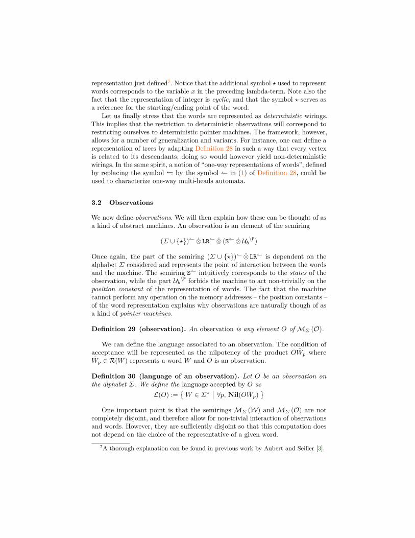
representation just defined7. Notice that the additional symbol ? used to representwords corresponds to the variable x in the preceding lambda-term. Note also thefact that the representation of integer is cyclic, and that the symbol ? serves asa reference for the starting/ending point of the word.

Let us finally stress that the words are represented as deterministic wirings.This implies that the restriction to deterministic observations will correspond torestricting ourselves to deterministic pointer machines. The framework, however,allows for a number of generalization and variants. For instance, one can define arepresentation of trees by adapting Definition 28 in such a way that every vertexis related to its descendants; doing so would however yield non-deterministicwirings. In the same spirit, a notion of “one-way representations of words”, definedby replacing the symbol � by the symbol ↼ in (1) of Definition 28, could beused to characterize one-way multi-heads automata.

3.2 Observations

We now define observations. We will then explain how these can be thought of asa kind of abstract machines. An observation is an element of the semiring

(Σ ∪ {?})↼ ⊗̇ LR↼ ⊗̇ (S↼ ⊗̇ Ub\P)

Once again, the part of the semiring (Σ ∪ {?})↼ ⊗̇ LR↼ is dependent on thealphabet Σ considered and represents the point of interaction between the wordsand the machine. The semiring S↼ intuitively corresponds to the states of theobservation, while the part Ub\P forbids the machine to act non-trivially on theposition constant of the representation of words. The fact that the machinecannot perform any operation on the memory addresses – the position constants –of the word representation explains why observations are naturally though of asa kind of pointer machines.

Definition 29 (observation). An observation is any element O ofMΣ (O).

We can define the language associated to an observation. The condition ofacceptance will be represented as the nilpotency of the product OW̄p whereW̄p ∈ R(W ) represents a word W and O is an observation.

Definition 30 (language of an observation). Let O be an observation onthe alphabet Σ. We define the language accepted by O as

L(O) :={W ∈ Σ∗

∣∣ ∀p, Nil(OW̄p)}

One important point is that the semirings MΣ (W) and MΣ (O) are notcompletely disjoint, and therefore allow for non-trivial interaction of observationsand words. However, they are sufficiently disjoint so that this computation doesnot depend on the choice of the representative of a given word.

7A thorough explanation can be found in previous work by Aubert and Seiller [3].

Lemma 31. Let W be a word, and W̄p, W̄q ∈ R(W ). For every observationO ∈MΣ (O), Nil(OW̄p) if and only if Nil(OW̄q).

Proof. As we pointed out, the observation cannot act on the position constantsof the representations W̄p and W̄q. This implies that for all integer k the wirings(OW̄p)k and (OW̄q)k are two instances of the same context, i.e. they are equalup to the interchange of the positions constants p0, . . . , pn and q0, . . . , qn. Thisimplies that (OW̄p)k = 0 if and only if (OW̄q)k = 0. ut

Corollary 32. Let O be an observation on the alphabet Σ. The set L(O) can beequivalently defined as the set

L(O) ={W ∈ Σ∗

∣∣ ∃p, Nil(OW̄p)}

This result implies that the notion of acceptance has the intended sense andis finitely verifyable: whether a word W is accepted by an observation O can bechecked without considering all representations of W .

This kind of situation where two semirings W and O are disjoint enoughto obtain Corollary 32 can be formalized through the notion of normative pairconsidered in earlier works [19,3,2].

4 Logarithmic Space

This section starts by explaining the computation one can perform with theobservations, and prove that it corresponds to logarithmic space computation byshowing how pointer machines can be simulated. Then, we will prove how thelanguage of an observation can be decided within logarithmic space.

This section uses the complexity classes DLogspace and coNLogspace, aswell as notions of completeness of a problem and reduction between problems.We use in Sect. 4.2 the classical theorem of coNLogspace-completeness of theacyclicity problem in directed graphs, and in Sect. 4.1 a convenient model ofcomputation, two-ways multi-heads finite automata, a generalization of automataalso called “pointer machine”. The reader who would like some reminders mayhave a look at any classical textbook [28]. Note that the non-deterministic part ofour results concerns coNLogspace, or equivalently NLogspace by the famousImmerman-Szelepcsényi theorem.

4.1 Completeness: Observations as Pointer Machines

This section describes the kind of computation one can model with observations.Let h0, x, y be variables, p0, p1, A0 constants and Σ = {0, 1}, the excerpt

of a dialogue in Figure 1 between an observation O = o1 + o2 + · · · and therepresentation of a word W̄p = w1 +w2 + · · · should help the reader to grasp themechanism.

We just depicted two transitions corresponding to an automata that reads thefirst bit of the word, and if this bit is a 1, goes back to the starting position, instate b. Remark that the answer of w1 differs from the one of w2: there is no need

? •L • init •A0 •M(h0) ↼ ? •R • init •A0 •M(h0) (o1)? •R •x •y •M(p0) ↼ 1 •L •x •y •M(p1) (w1)

1 •L • init •A0 •M(h0) ↼ 1 •L •b •A0 •M(h0) (o2)1 •L •x •y •M(p1) ↼ ? •R •x •y •M(p0) (w2)

By unification,? •L • init •A0 •M(p0) ↼ 1 •L • init •A0 •M(p1) (o1w1)? •L • init •A0 •M(p0) ↼ 1 •L •b •A0 •M(p1) (o1w1o2)? •L • init •A0 •M(p0) ↼ ? •R •b •A0 •M(p0) (o1w1o2w2)

This can be understood as the small following dialogue:

o1: [Is in state init] “I read ? from left to right, what do I read now?”w1: “Your position was p0, you are now in position p1 and read 1.”o2: [Change state to b] “I do an about-turn, what do I read now?”w2: “You are now in position p0 and read ?.”

Fig. 1. An example of dialogue between an observation and the representation of aword

to clarify the position (the variable argument of M), since h0 was already replacedby p1. Such an information is needed only in the first step of computation: afterthat, the updates of the position of the pointer take place on the word side.Remark that neither the state nor the constant A0 is an object of dialogue.

Note also that this excerpt corresponds to a deterministic computation. Ingeneral, several elements of the observation could get unified with the currentconfiguration, yielding non-deterministic transitions.

Multiple Pointers and Swapping We now add some computational powerto our observation by adding the possibility to handle several pointers. Theobservations will now use a k-ary function Ak that allows to “store” k positions.This part of the observation is not affected by the word, which means thatonly one head (the main pointer) can move. The observation can exchange theposition of the main pointer and the position stored in Ak: we therefore refer tothe arguments of Ak as auxiliary pointers that can become the main pointer atsome point of the computation. This is of course strictly equivalent to severalheads that have the ability to move.

Consider the following flow, that encodes the transition “if the observationreads 1 •R in state s, it stores the position of the main pointer (the variable h0)at the i-th position in Ak and start reading the input with a new pointer”:

1 •R •s •Ak(h1, . . . , hi, . . . , hk) •M(h0) ↼ ? •R •s′ •Ak(h1, . . . , h0, . . . , hk) •M(hi)

Suppose now we want to write an observation that, if it reads 0 •L in state r,then it restores the value that was stored in the i-th position of Ak, it stores the

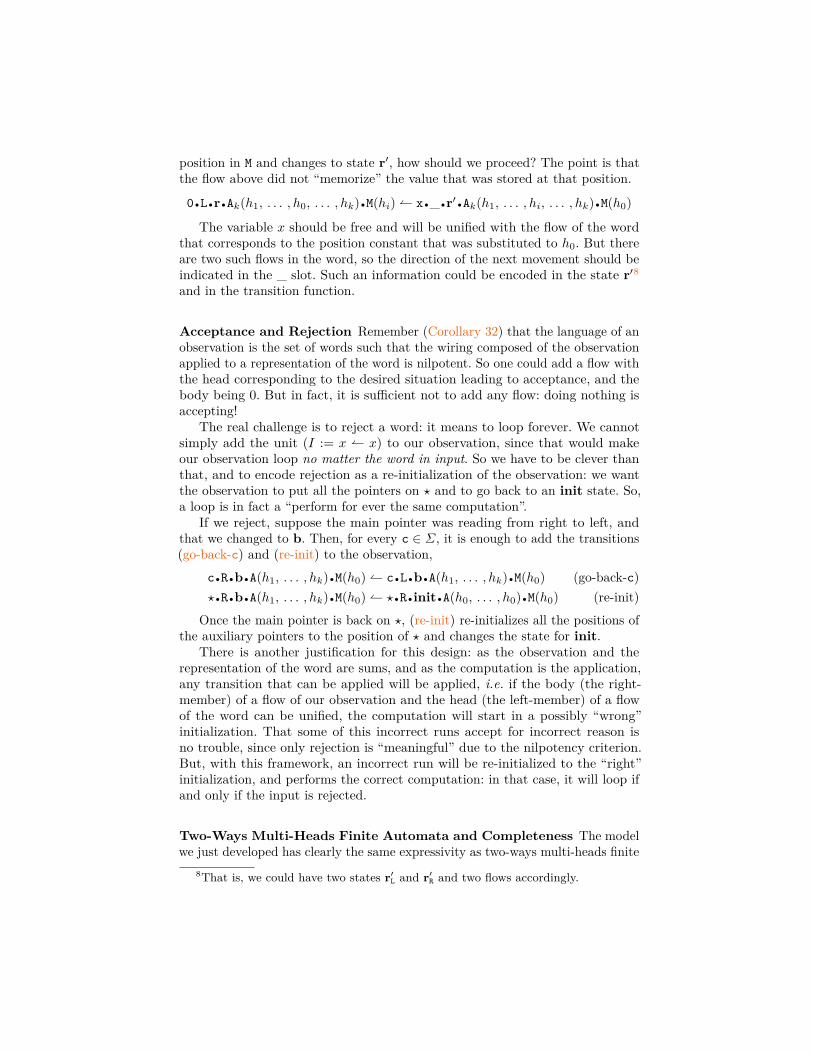
position in M and changes to state r′, how should we proceed? The point is thatthe flow above did not “memorize” the value that was stored at that position.

0 •L •r •Ak(h1, . . . , h0, . . . , hk) •M(hi) ↼ x •_ •r′ •Ak(h1, . . . , hi, . . . , hk) •M(h0)

The variable x should be free and will be unified with the flow of the wordthat corresponds to the position constant that was substituted to h0. But thereare two such flows in the word, so the direction of the next movement should beindicated in the _ slot. Such an information could be encoded in the state r′8and in the transition function.

Acceptance and Rejection Remember (Corollary 32) that the language of anobservation is the set of words such that the wiring composed of the observationapplied to a representation of the word is nilpotent. So one could add a flow withthe head corresponding to the desired situation leading to acceptance, and thebody being 0. But in fact, it is sufficient not to add any flow: doing nothing isaccepting!

The real challenge is to reject a word: it means to loop forever. We cannotsimply add the unit (I := x ↼ x) to our observation, since that would makeour observation loop no matter the word in input. So we have to be clever thanthat, and to encode rejection as a re-initialization of the observation: we wantthe observation to put all the pointers on ? and to go back to an init state. So,a loop is in fact a “perform for ever the same computation”.

If we reject, suppose the main pointer was reading from right to left, andthat we changed to b. Then, for every c ∈ Σ, it is enough to add the transitions(go-back-c) and (re-init) to the observation,

c •R •b •A(h1, . . . , hk) •M(h0) ↼ c •L •b •A(h1, . . . , hk) •M(h0) (go-back-c)? •R •b •A(h1, . . . , hk) •M(h0) ↼ ? •R • init •A(h0, . . . , h0) •M(h0) (re-init)

Once the main pointer is back on ?, (re-init) re-initializes all the positions ofthe auxiliary pointers to the position of ? and changes the state for init.

There is another justification for this design: as the observation and therepresentation of the word are sums, and as the computation is the application,any transition that can be applied will be applied, i.e. if the body (the right-member) of a flow of our observation and the head (the left-member) of a flowof the word can be unified, the computation will start in a possibly “wrong”initialization. That some of this incorrect runs accept for incorrect reason isno trouble, since only rejection is “meaningful” due to the nilpotency criterion.But, with this framework, an incorrect run will be re-initialized to the “right”initialization, and performs the correct computation: in that case, it will loop ifand only if the input is rejected.

Two-Ways Multi-Heads Finite Automata and Completeness The modelwe just developed has clearly the same expressivity as two-ways multi-heads finite

8That is, we could have two states r′L and r′R and two flows accordingly.

automata, a model of particular interest to us for it is well studied, tolerant toa lot of enhancements or restrictions9 and gives an elegant characterization ofDLogspace and NLogspace [22,27].

Then, by a plain and uniform encoding of two-ways multi-heads finiteautomata, we get Theorem 33. That acceptance and rejection in the non-deterministic case are “reversed” (i.e. all path have to accept for the computationto accepts) makes us characterize coNLogspace instead of NLogspace.

Note that encoding a deterministic automaton yields a wiring of the form ofLemma 11, which would be therefore a deterministic wiring.Theorem 33. If L ∈ coNLogspace, then there is an observation O such thatL(O) = L. Moreover, if L ∈ DLogspace, O can be chosen deterministic.

4.2 Soundness of Observations

We now use the results of Sect. 2.3 and Sect. 3.2 to design a procedure that decideswhether a word belongs to the language of an observation within logarithmicspace. This procedure will use the classical reduction from a problem to testingthe acyclicity of a graph, a problem well-known to be tractable with logarithmicspace resources.

First, we show how the computation graph of the product of the observationand the word representation can be constructed deterministically using onlylogarithmic space; then, we prove that testing the acyclicity of such a graph canbe done within the same bounds. Here, depending on the shape of the graph(which is dependent in itself of determinism of the wiring, recall Lemma 21), theprocedure will be deterministic or non-deterministic.

Finally, using classical composition of logspace algorithms10, Lemma 20 andCorollary 32, we will obtain the result expected, that is:

Theorem 34. If O is an observation, then L(O) ∈ coNLogspace. If moreoverO is deterministic, then L(O) ∈ DLogspace.

A Foreword on Word and Size Given a word W over Σ, to build arepresentation W̄p as in Definition 28 is clearly in DLogspace: it is a plain matterof encoding. By Lemma 31, it is sufficient to consider a single representation.So for the rest of this procedure, we consider given W̄p ∈ R(W ) and writeF := OW̄p. The size of Σ is a constant, and it is clear that the maximal arityand the height of the balanced wiring F remain fixed when W varies. The onlypoint that fluctuates is the cardinality of the set of symbols that occurs in F ,and it is linearly growing with the length of W , corresponding to the numberof positions constant. In the following, any mention to a logarithmic amount ofspace is to be completed by “relatively to the length of W”.

9In fact, most of the variations (the automata can be one-way, sweeping, rotating,oblivious, etc.) are studied in terms of number of states needed to simulate a variationwith another, but most of the time they characterize the same complexity classes.

10The reader unused to the mechanism of composition of logspace-algorithms mayhave a look at a classical textbook [28, Fig. 8.10].

Building the Computation Graph We need two main ingredients to buildthe computation graph (Definition 19) of F : to enumerate the computation spaceComp(F ) (recall Definition 16), and to determine whether there is an edgebetween two vertices.

By Proposition 18, card(Comp(F )) is polynomial in the size of W . Hence,given a balanced wiring F , a logarithmic amount of memory is enough toenumerate the members of Comp(F ), that is the vertices of G(F ).

Now the second part of the construction of G(F ) is to determine if there is anedge between two vertices. Remember that there is an edge from u = u ↼ ? tov = v ↼ ? in G(F ) if v ∈ Fu. So one has to scan the members of F = OW̄p: ifthere exists (t1 ↼ t2)(t′1 ↼ t′2) ∈ F such that (t1 ↼ t2)(t′1 ↼ t′2)(u ↼ ?) = v ↼ ?,then there is an edge from u to v. To list the members of F is in DLogspace,but unification in general is a difficult problem (see Sect. 1.2). The special caseof matching can be tested with a logarithmic amount of space:

Theorem 35 (Matching is in DLogspace [11, p. 49]). Given two termst and u such that either t or u is closed, deciding if they are matchable is inDLogspace.

Actually, this result relies on a subtle manipulation of the representation ofthe terms as simple directed acyclic graphs11, where the variables are “shared”.Translations between this representation of terms and the usual one can beperformed in logarithmic space [11, p. 38].

Deciding if G(F ) is Acyclic We know thanks to Lemma 20 that answeringthis question is equivalent to deciding if F is nilpotent. We may notice that G(F )is a directed, potentially unconnected graph of size card(Comp(F )).

It is well-know that testing for acyclicity of a directed graph is a coNLog-space [23, p. 83] problem. Moreover, if F is deterministic (which is the case whenO is), then G(F ) has out-degree bounded by 1 (Lemma 21) and one can testits acyclicity without being non-deterministic: it is enough to list the vertices ofComp(F ), and for each of them to follow card(Comp(F )) edges and to test forequality with the vertex picked at the beginning. If a loop is found, the algorithmrejects, otherwise it accepts after testing the last vertex. Only the starting vertexand the current vertex need to be stored, which fits within logarithmic space,and there is no need to do any non-deterministic transitions.

5 Conclusion

We presented the unification semiring, a construction that can be used both asan algebraic model of logic programming and as a setting for a dynamic modelof logic. Within this semiring, we were able to identify a class of wirings thathave the exact expressive power of logarithmic space computation.

11The reader willing to learn more about this may have a look at a classical chapter [4].

If we try to step back a little, we can notice that the main tool in the soundnessproof (Sect. 4.2) is the computation graph, defined in Sect. 2.3. More precisely,the properties of this graph, notably its cardinal (that turns out to be polynomialin the size of the input), allow to define a decision procedure that needs onlylogarithmic space. The technique is modular, hence not limited to logarithmicspace: identifying other conditions on wirings that ensure size bounds on thecomputation graph would be a first step towards the characterization of otherspace complexity classes.

Concerning completeness, the choice of encoding pointer machines (Sect. 4.1)rather than log-space bounded Turing machines was quite natural. Balancedwirings correspond to the idea of computing with pointers: manipulation of datawithout writing abilities, and thus with no capacity to store any informationother than a fixed number of positions on the input.

By considering other classes of wirings or by modifying the encoding it mightbe possible to capture other notions of machines characterizing some complexityclasses: we already mentioned that a modifcation of the representation of theinput that would model one-way finite automata.

The relation with proof theory needs to be explored further: the approach ofthis paper seems indeed to suggest a sort of “Curry-Howard” correspondance forlogic programming.

As Sect. 1.1 highlighted, there are many notions that might be transferablefrom one field to the other, thanks to a common setting provided by geometry ofinteraction and the unification semiring. Most notably, the notion of nilpotency(on the proof-theoretic side: strong normalization) corresponds to a variant ofboundedness of logic programs, a property that is usually hard to ensure.

Another direction could be to look for a proof-system counterpart of thiswork: a corresponding “balanced” logic of logarithmic space.

References1. Asperti, A., Danos, V., Laneve, C., Regnier, L.: Paths in the lambda-calculus. In:

LICS. pp. 426–436. IEEE Computer Society (1994)2. Aubert, C., Bagnol, M.: Unification and logarithmic space. In: Dowek, G. (ed.)

RTA-TLCA 2014. LNCS, vol. 8650, pp. 77––92. Springer (2014)3. Aubert, C., Seiller, T.: Characterizing co-nl by a group action. Arxiv preprint

abs/1209.3422 (2012)4. Baader, F., Snyder, W.: Unification theory. In: Robinson, J.A., Voronkov, A. (eds.)

Handbook of Automated Reasoning, pp. 445–532. Elsevier and MIT Press (2001)5. Baillot, P., Mazza, D.: Linear logic by levels and bounded time complexity. Theoret.

Comput. Sci. 411(2), 470–503 (2010)6. Baillot, P., Pedicini, M.: Elementary complexity and geometry of interaction. Fund.

Inform. 45(1–2), 1–31 (2001)7. Bellia, M., Occhiuto, M.E.: N-axioms parallel unification. Fund. Inform. 55(2),

115–128 (2003)8. Calimeri, F., Cozza, S., Ianni, G., Leone, N.: Computable functions in ASP: Theory

and implementation. In: Garcia de la Banda, M., Pontelli, E. (eds.) ICLP. LNCS,vol. 5366, pp. 407–424. Springer (2008)

9. Dal Lago, U., Hofmann, M.: Bounded linear logic, revisited. Log. Meth. Comput.Sci. 6(4) (2010)

10. Dantsin, E., Eiter, T., Gottlob, G., Voronkov, A.: Complexity and expressive powerof logic programming. ACM Comput. Surv. 33(3), 374–425 (2001)

11. Dwork, C., Kanellakis, P.C., Mitchell, J.C.: On the sequential nature of unification.J. Log. Program. 1(1), 35–50 (1984)

12. Dwork, C., Kanellakis, P.C., Stockmeyer, L.J.: Parallel algorithms for term matching.SIAM J. Comput. 17(4), 711–731 (1988)

13. Gaboardi, M., Marion, J.Y., Ronchi Della Rocca, S.: An implicit characterizationof pspace. ACM Trans. Comput. Log. 13(2), 18:1–18:36 (2012)

14. Girard, J.Y.: Linear logic. Theoret. Comput. Sci. 50(1), 1–101 (1987)15. Girard, J.Y.: Geometry of interaction 1: Interpretation of system F. Studies in

Logic and the Foundations of Mathematics 127, 221–260 (1989)16. Girard, J.Y.: Towards a geometry of interaction. In: Gray, J.W., Ščedrov, A. (eds.)

Proceedings of the AMS-IMS-SIAM Joint Summer Research Conference held June14-20, 1987. Categories in Computer Science and Logic, vol. 92, pp. 69–108. AMS(1989)

17. Girard, J.Y.: Geometry of interaction III: accommodating the additives. In: Girard,J.Y., Lafont, Y., Regnier, L. (eds.) Advances in Linear Logic, pp. 329–389. No. 222in London Math. Soc. Lecture Note Ser., CUP (Jun 1995)

18. Girard, J.Y.: Light linear logic. In: Leivant, D. (ed.) LCC, LNCS, vol. 960, pp.145–176. Springer (1995)

19. Girard, J.Y.: Normativity in logic. In: Dybjer, P., Lindström, S., Palmgren, E.,Sundholm, G. (eds.) Epistemology versus Ontology, Logic, Epistemology, and theUnity of Science, vol. 27, pp. 243–263. Springer (2012)

20. Girard, J.Y.: Three lightings of logic. In: Ronchi Della Rocca, S. (ed.) CSL. LIPIcs,vol. 23, pp. 11–23. Schloss Dagstuhl - Leibniz-Zentrum für Informatik (2013)

21. Hillebrand, G.G., Kanellakis, P.C., Mairson, H.G., Vardi, M.Y.: Undecidableboundedness problems for datalog programs. J. Log. Program. 25(2), 163–190(1995)

22. Holzer, M., Kutrib, M., Malcher, A.: Multi-head finite automata: Characterizations,concepts and open problems. In: Neary, T., Woods, D., Seda, A.K., Murphy, N.(eds.) CSP. EPTCS, vol. 1, pp. 93–107 (2008)

23. Jones, N.D.: Space-bounded reducibility among combinatorial problems. J. Comput.Syst. Sci. 11(1), 68–85 (1975)

24. Laurent, O.: A token machine for full geometry of interaction (extended abstract).In: Abramsky, S. (ed.) TLCA. LNCS, vol. 2044, pp. 283–297. Springer (May 2001)

25. Lierler, Y., Lifschitz, V.: One more decidable class of finitely ground programs.In: Hill, P.M., Warren, D.S. (eds.) ICLP. LNCS, vol. 5649, pp. 489–493. Springer(2009)

26. Ohkubo, M., Yasuura, H., Yajima, S.: On parallel computation time of unificationfor restricted terms. Tech. rep., Kyoto University (May 1987)

27. Pighizzini, G.: Two-way finite automata: Old and recent results. Fund. Inform.126(2–3), 225–246 (2013)

28. Savage, J.E.: Models of computation - exploring the power of computing. Addison-Wesley (1998)

29. Schöpp, U.: Stratified bounded affine logic for logarithmic space. In: LICS. pp.411–420. IEEE Computer Society (2007)

30. Seiller, T.: Interaction graphs: Multiplicatives. Ann. Pure Appl. Logic 163, 1808–1837 (Dec 2012)