Journal of Statistical Planning andInference 134 (2005) 194–205

www.elsevier.com/locate/jspi

On the difference between ML and REMLestimators in the modelling of multivariate

longitudinal data�

Vassilis G.S. Vasdekisa,∗, Ioannis G. VlachonikolisbaDepartment of Statistics, Athens University of Economics and Business, 76 Patission Street, 10434 Athens,

GreecebEuropean Institute of Health and Medical Sciences, University of Surrey, Guildford, Surrey GU2 5XH, UK

Received 13 January 2003; accepted 23 January 2004Available online 23 July 2004

Abstract

A random effects model is examined in themultivariate setting wheremore than one characteristicsare measured at each time point. ML and REML estimators are obtained under the restriction thatestimates of variance matrices being at least p.s.d. It is shown that REML has greater probabilityof giving full rank estimates of variance components matrices but as regards the efficiency in theestimation of the location parameter, correct specification of the number of random effects is needed.In general, REML provides larger estimates of variance of model parameters than ML.© 2004 Elsevier B.V. All rights reserved.

MSC:primary 62H12; secondary 62J10

Keywords:MANOVA; Longitudinal data; ML; REML; Random effects; Efficiency

1. Introduction

It is common practice in growth curve studies to measure one characteristic at a time. Inmore complex studies however, it is possible to encounter repeated measurements on sev-eral characteristics which are not independent or on one characteristic measured at different

� Professor Vlachonikolis passed away on September 2003. This paper was then at the revision stage. Theeditorial Board of JSPI takes this opportunity to honor the memory and contribution of Professor Vlachonikolis.

∗ Corresponding author. Tel.: +30-210-820-3529; fax: +30-210-820-3527.E-mail address:vasdekis@aueb.gr(V.G.S. Vasdekis).

0378-3758/$ - see front matter © 2004 Elsevier B.V. All rights reserved.doi:10.1016/j.jspi.2004.01.020

V.G.S. Vasdekis, I.G. Vlachonikolis / Journal of Statistical Planning and Inference 134 (2005) 194–205195

experimental conditions. Such examples can be met in clinical trials where measurementssuch as diastolic and systolic pressure are measured together on time. The fact that thesemeasurements are correlated not only on time but also on different characteristics or ex-perimental conditions makes the problem interesting. In the univariate setting, a modellingapproach would be to use a polynomial effect of time and linear effects of covariates rep-resenting measurements characteristics which possibly interact with time. Random effectson some explanatory variables (Laird and Ware, 1982) are also popular for modelling thevariance matrix of observations. In the multivariate setting this can be accomplished in asimilar way, the bulk however, of the data and the need for reduction of dimensionality, re-stricts us to be extremely careful in the datamodelling. Estimation of themean and varianceparameters in these models can use ML or REML. A problem however, which can arise isthat the estimated variance componentmatrix of the randomeffects, which take into accountthe variation within individuals, is not necessarily positive definite (Anderson et al., 1986).Considering modelling and estimation of multivariate observations on time, early refer-

ences include thework byReinsel (1982, 1984, 1985)with the last two publications devotedto prediction,Anderson et al. (1986)who considered ML estimation,Amemiya and Fuller(1984)andAmemiya (1985)who considered REML estimates under the restriction thatthe estimated variance matrix components are at least p.s.d. The model considered by theprevious authors was the usual MANOVA model with no interest in the location parameterand a simple form for the covariancematrix, generalizing the so-called ‘uniform correlation’model in the univariate case.Reinsel (1982)on the other hand, considered a generalizationof the model byRao (1965)by fitting explanatory variables for the location parameter andwith the same form of the covariance matrix of observations as that found inAndersonet al. (1986)andAmemiya (1985), but with no restriction about the positive definiteness ofthe covariance matrix components.In thepresent paper,we formamodelwhich, as regards themean, is a generalizationof the

classical growth curve model proposed byPotthoff and Roy (1964)and used byRao (1965,1967), Verbyla (1986), Diggle (1988), Lange and Laird (1989), Verbyla and Cullis (1990)and others and as regards the covariance matrix of observations is a generalization of themodel used byAnderson et al. (1986)providing a multivariate version of that ofLange andLaird (1989)by assuming an arbitrary number of randomeffects. Focus however here, is notgiven only in the estimation of the model parameters but mainly in the differences betweenMLandREMLestimators of variance componentmatrices under the restriction that they areall at least p.s.d. Themodel is formed (Section 2), ML and REML estimates of the unknownparameters of the covariance matrix of observations are found and a relationship betweenthem is noticed (Section 3). This relationship provides an interesting result on the differencebetween the two estimation methods which supports the idea of superiority researchershave about REML in the univariate case. In Section 4, the effect of wrong specification ofcovariance model is examined and ML and REML are compared for differences as regardsefficiency of estimated regression coefficients on the basis of a small simulation study.

2. Formulation of the model

Suppose that we havem treatment groups withnj individuals in each group. Each indi-vidual has a complete record of measurements onr characteristics at each ofq time-points.

196 V.G.S. Vasdekis, I.G. Vlachonikolis / Journal of Statistical Planning and Inference 134 (2005) 194–205

The experimental design is such that measurements for different individuals are indepen-dent.We denote byYij ther × q matrix of measurements consisting of measurements forr

characteristics takenonq timepoints, for individuali, i=1, . . . , nj in groupj , j=1, . . . , m.A model postulating orthogonal polynomials of orderp − 1 for the mean takes the form

Yij = �ijP + Uij ,

where�ij is ar×pmatrix of unknownparameters,P is ap×qmatrix of known (orthogonal)coefficients, of full row rankp�q, andUij a matrix of errors with

E(Uij )= 0 and Var(vec(Uij ))= Iq ⊗ �1,

where⊗ represents the well-known Kronecker product and�1 is a p.d. symmetric matrixrepresenting the variation betweenr characteristics.Random effects models, the wayLange and Laird (1989)have defined for univariate

observations, can be considered by assuming that�ij matrix consists of two parts. The firstpart is a random one, it refers tot polynomial (not necessarily thet terms of lowest order)coefficients and expresses that part of mean profile which is specific to each individualin each treatment group. The second part is considered to be constant and is the effect ofgroupj in the mean profile of the individual. Formalization of this idea uses the expansionP T= (P T1 , P T2 ) with P1(t × q) referring tot polynomial coefficients andP2 ((p− t)× q).Then, we are led to

Yij = �jP + VijP1+ Uij ,

where�j is a r × p matrix of unknown regression coefficients specific to each treatmentgroup andVij arer × t random matrices specific to each individual with

E(Vij )= 0 and Var(vec(Vij ))= It ⊗ �2,

where�2 is an at least p.s.d covariance matrix representing the random effects variation ofther characteristics. Therefore, its rank will be equal tos, 0�s�r.By vectorizing each individual’s response matrix and by arranging all vectors in matrix

Y , we end up with the following model:

Y = A�∗(P ⊗ Ir )+ V (P1⊗ Ir )+ U, (1)

whereY (n×rq) is the responsematrix withn the total number of observations,�∗(m×rp)is the matrix ofrp regression coefficients for each treatment group,A(n × m) is a designmatrix which assigns the appropriate mean coefficients to each individual andV andU are(n× rq) error matrices with

E(V )= 0 and Var(vec(V ))= (It ⊗ �2)⊗ In

and

E(U)= 0 and Var(vec(U))= (Iq ⊗ �1)⊗ In.

Such a structure is at-random effects one. In the case where each treatment group containsthe same number of individuals,n0= n/m, thenA= Im ⊗ 1n0 where1n0 = (1, . . . ,1)T isan0× 1 vector.

V.G.S. Vasdekis, I.G. Vlachonikolis / Journal of Statistical Planning and Inference 134 (2005) 194–205197

Under above assumptions the variance matrix of observations becomes

Var(vec(Y ))= (Iq ⊗ �1+ P T1 P1⊗ �2)⊗ In. (2)

Themodel considered in (1) and (2) is slightlymoregeneral than that usedbyReinsel (1982).This is easily seen since Reinsel considered only one random effect to explain the variationwithin individuals by settingP1 a 1× q orthogonal vector. Note also that by considering afew orthogonal polynomials as random effects, orthogonality ofP1 andP2 arises naturally.In all other cases this has to be postulated by the model (see alsoReinsel, 1982).Andersonet al. (1986)also considered a special case of the model above by assuming replicatedmeasurements for each individual representing this setting’s measurements on time, andwithout being interested in the modelling of the location parameter. Finally, they used onerandom effect to explain the possible variation between time points. Recently,Calvin andDykstra (1991a,b)andCalvin (1993), in a similar direction, provided a generalization ofthe model used byAnderson et al. (1986)giving a solution based on EM algorithm whichcan also handle unbalanced data.

3. ML and REML estimation

Assuming that error matricesV andU are normally distributed, the log-likelihood func-tion of observations can be written as

c − n

2log |Iq ⊗ �1+ P T1 P1⊗ �2|

− tr[Y − A�∗(P ⊗ Ir )](Iq ⊗ �1+ P T1 P1⊗ �2)−1[Y − A�∗(P ⊗ Ir )]T. (3)

In Appendix A the appropriate form of likelihood is obtained. There the form of the log-likelihood in (10) suggests thatG,H ,�AY (P

T1 P1⊗Ir ) and�AY (P

T2 P2⊗Ir ) are sufficient

statistics for�1+ �2, �1, �∗1 and�

∗2. Note that statisticsG andH coincide withS� andSe

of Section 3 inReinsel (1982)in the special case where one random effect is used.As regards the estimation,Reinsel (1982)used the fact that the sufficient statistics come

from independent transformations of the data and therefore are independent, andheobtainedunbiased estimates. However, for the case of�2, his estimate may not be positive definite.Theorems 1 and 2 below, provide ML and REML estimates of�2 under the restriction thatthey are at least positive semi-definite (p.s.d). The price however, we should pay for gettingan at least p.s.d solution of�2 is that this estimate will not necessarily be of full rank. Thus,the rank of�2 will depend on the data at hand and will have to be estimated, somethingwhich is noted byAnderson et al. (1986).Let us consider the followingdecompositions for�1,�2,H andGas�1=��T,�1+�2=

���T,H =BBT andG=BTBT, where� andBare non-singular matrices of ordersr× rand� andTare diagonal matrices containing the eigenvalues of�−1

1 (�1+�2) andH−1G,respectively. Note that the elements of� should satisfy�1� · · · ��s > �s+1=· · ·=�r =1for a value ofs, s = 0, · · · , r in order to get an at least p.s.d. solution for�2. The resultsthen, can be derived in a similar way as inAnderson et al. (1986)and are summarized inthe following theorem:

198 V.G.S. Vasdekis, I.G. Vlachonikolis / Journal of Statistical Planning and Inference 134 (2005) 194–205

Theorem 1. The maximum likelihood estimates of�1 and�2 under the assumption thatthey are both at least positive semidefinite are given by

�M

1 = BT 1/2D−2M T 1/2BT, (4)

�M

2 = BT 1/2D−1M (�M − Ir )D

−1M T 1/2BT, (5)

where

D−2M = 1

nq(T −1+ �

−1M ),

�M =( (q−t)

tT1 0

0 Ir−s∗M

)

with T1 the s∗M × s∗M part of T with s∗M the number ofi ’s, the diagonal elements ofT ,i = 1, . . . , r which satisfy

i >t

q − t.

Estimation with REML is accomplished by noting that the restricted likelihood in thiscase is Eq. (10) plus a function of the inverse covariance matrix of observations given by

− m

2log |(P ⊗ Ir )(Iq ⊗ �1+ P T1 P1⊗ �2)−1(P T ⊗ Ir )|

= −m2log |�1+ �2|−t |�1|−(p−t)

After maximization, one ends up with the following theorem:

Theorem 2. The restricted maximum likelihood estimates of�1 and�2 under the assump-tion that they are both at least positive semidefinite are given by

�R

1 = BT 1/2D−2R T 1/2BT, (6)

�R

2 = BT 1/2D−1R (�R − Ir )D

−1R T 1/2BT, (7)

where

D−2R = 1

nq −mp(T −1+ �

−1R )

�R =( [n(q−t)−m(p−t)]

(n−m)t T1 00 Ir−s∗R

)

with T1 the s∗R × s∗R part of T with s∗R the number ofi ’s, the diagonal elements ofT ,i = 1, . . . , r which satisfy

i >(n−m)t

n(q − t)−m(p − t).

V.G.S. Vasdekis, I.G. Vlachonikolis / Journal of Statistical Planning and Inference 134 (2005) 194–205199

Proof. This is presented in Appendix B.�It is obvious that the estimates of rank of�2 using ML and REML (s∗M, s∗R) will, in

general, be different for the two methods. Since(n−m)(q − t) < n(q − t)−m(p− t) wededuce that

(n−m)t

n(q − t)−m(p − t)<

t

q − t.

Thus,

Corollary 1. If the model defined in the previous section is assumed to be correct then,

s∗M�s∗R. (8)

The above corollary shows that the rank for�2 inferred using ML will always be lessor equal than that inferred by REML. This is an interesting result showing that REML hasgreater probability of giving a non-deficient estimate of�2 or a non-zero estimate. A zeroestimate is obtained whens∗R = 0 something which is likely to happen with real data. Theresult provides also a generalization of the univariate case in which matricesYij are 1× q

and for which Var(Yij )= 21Iq + 22PT1 P1. Then based onLange and Laird (1989)we can

show that

21M = 1

n(q − t)M1, 22M = 1

ntM2− 21M(P1P

T1 )

−1,

21R = 1

n(q − t)−m(p − t)M1, 22R = 1

(n−m)tM2− 2R1(P1P

T1 )

−1,

whereM1 = tr(Y − �AY�P )(In − �P1)(Y − �AY�P )T andM2 = tr(P1P T1 )−1P1Y T

(In−�A)YPT1(P1P

T1 )

−1. It is easy to see that22R > 22M and therefore theREMLestimatorof 2 has greater probability of being positive.The results of a small simulation study are shown inTable 1. These are frequencies of

values of estimated ranks of�2 under different number of random effects fitted to data. Thedata were generated for three characteristics using linear trend and two random effects forthe error structure and for three sample sizes (n=10,20,50). 1000 data setswere generated.REML, estimates a full rank�2 more frequently than ML as it was expected, while as thesample size increases, the differences in frequencies vanish.

4. Effects of wrongly specified models

It was seen in the previous section that as regards the estimated rank of�2, misspecifica-tion of the number of random effects can cause problems and that either in misspecificationor not, REML seems more stable than ML. In this section, differences in the estimationof �2 between ML and REML will be noted along with their implication into inferenceabout�∗.

200 V.G.S. Vasdekis, I.G. Vlachonikolis / Journal of Statistical Planning and Inference 134 (2005) 194–205

Table 1Frequencies of estimated ranks of�2 for one and two random effects error models (two random effects were usedfor data generation)

Sample size Random effects fitted Estimated rank of�2

REML ML

1 2 3 1 2 3

n= 10 1 24 520 456 31 564 4052 0 4 996 0 5 995

n= 20 1 0 172 828 0 200 8002 0 0 1000 0 0 1000

n= 50 1 0 6 994 0 8 9922 0 0 1000 0 0 1000

Efficiency will be defined using univariate measures of variance of the regression coeffi-cientsunder the trueand theassumedas truemodel for thecovariancematrix of observations.Two well-known univariate measures are given by the trace or the determinant of the vari-ance matrix of the estimated regression coefficients. The main question which concerns ushere is: What do we lose in efficiency and which method performs better if we wronglyspecify the number of random effects?The general form of the estimated regression coefficients is

�∗ = (ATA)−1ATY (P T ⊗ Ir ).

By vectorizing this matrix we get that its variance matrix is

(P ⊗ Ir ⊗ (ATA)−1AT)�(P T ⊗ Ir ⊗ A(ATA)−1), (9)

where� has a form seen just under Eq. (12). Suppose now that data were generated by amechanism with covariance matrix of the form specified by� assumingt0 random effects.Then substituting this form into (9), we get that

Var(vec(�))= Ip ⊗ �1⊗ (ATA)−1+ P(P T1 P1)PT ⊗ �2⊗ (ATA)−1,

whereP1 is at0× q matrix determining the random effects. Having in mind the expansionof matrixP in Section 2 and thatP is suborthogonal we see thatP(P T1 P1)P

T is actually adiagonalp× p matrix with units in the firstt0 entries and 0 elsewhere. It is seen that if weuse trace for defining a univariate measure of variance we get

tr(Var(vec(�)))= tr(ATA)−1(p tr�1+ t0 tr�2).

In the same way, if we use determinants we get

|Var(vec(�))| = |ATA|−1|�1+ �2|t0|�1|p−t0.

V.G.S. Vasdekis, I.G. Vlachonikolis / Journal of Statistical Planning and Inference 134 (2005) 194–205201

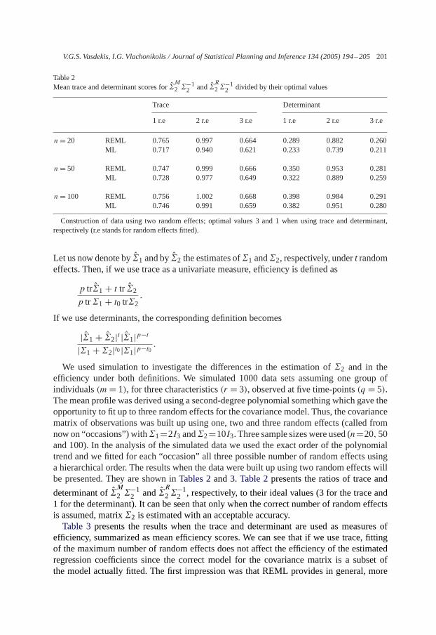
Table 2Mean trace and determinant scores for�

M2 �−1

2 and�R2 �−12 divided by their optimal values

Trace Determinant

1 r.e 2 r.e 3 r.e 1 r.e 2 r.e 3 r.e

n= 20 REML 0.765 0.997 0.664 0.289 0.882 0.260ML 0.717 0.940 0.621 0.233 0.739 0.211

n= 50 REML 0.747 0.999 0.666 0.350 0.953 0.281ML 0.728 0.977 0.649 0.322 0.889 0.259

n= 100 REML 0.756 1.002 0.668 0.398 0.984 0.291ML 0.746 0.991 0.659 0.382 0.951 0.280

Construction of data using two random effects; optimal values 3 and 1 when using trace and determinant,respectively (r.e stands for random effects fitted).

Let us now denote by�1 and by�2 the estimates of�1 and�2, respectively, undert randomeffects. Then, if we use trace as a univariate measure, efficiency is defined as

p tr�1+ t tr �2p tr�1+ t0 tr�2

.

If we use determinants, the corresponding definition becomes

|�1+ �2|t |�1|p−t

|�1+ �2|t0|�1|p−t0 .

We used simulation to investigate the differences in the estimation of�2 and in theefficiency under both definitions. We simulated 1000 data sets assuming one group ofindividuals(m= 1), for three characteristics(r = 3), observed at five time-points(q = 5).The mean profile was derived using a second-degree polynomial something which gave theopportunity to fit up to three random effects for the covariance model. Thus, the covariancematrix of observations was built up using one, two and three random effects (called fromnow on “occasions”) with�1=2I3 and�2=10I3. Three sample sizeswere used (n=20,50and 100). In the analysis of the simulated data we used the exact order of the polynomialtrend and we fitted for each “occasion” all three possible number of random effects usinga hierarchical order. The results when the data were built up using two random effects willbe presented. They are shown inTables 2and3. Table 2presents the ratios of trace and

determinant of�M

2 �−12 and�

R

2�−12 , respectively, to their ideal values (3 for the trace and

1 for the determinant). It can be seen that only when the correct number of random effectsis assumed, matrix�2 is estimated with an acceptable accuracy.Table 3presents the results when the trace and determinant are used as measures of

efficiency, summarized as mean efficiency scores. We can see that if we use trace, fittingof the maximum number of random effects does not affect the efficiency of the estimatedregression coefficients since the correct model for the covariance matrix is a subset ofthe model actually fitted. The first impression was that REML provides in general, more

202 V.G.S. Vasdekis, I.G. Vlachonikolis / Journal of Statistical Planning and Inference 134 (2005) 194–205

Table 3Mean efficiency scores using trace and determinant

Trace Determinant

1 r.e 2 r.e 3 r.e 1 r.e 2 r.e 3 r.e

n= 20 REML 0.803 0.998 0.998 0.474 0.950 14.300ML 0.771 0.950 0.948 0.350 0.664 9.013

n= 50 REML 0.805 1.000 0.999 0.546 0.979 12.372ML 0.792 0.981 0.979 0.484 0.850 10.315

n= 100 REML 0.809 1.002 1.002 0.579 1.005 12.193ML 0.802 0.993 0.992 0.545 0.937 11.138

Construction of data using two random effects (r.e stands for random effects fitted).

efficient estimators. Use of determinant however, must make us more cautious. The exactnumber of random effects must be specified otherwise the efficiency is completely lost (seefor example in fitting 3 random effects). A reason for the difference between these twounivariate measures is probably the linear and the exponential effects of misspecification ofrandom effects using traces and determinants respectively. On the other hand, it is knownthat REML provides an at least, larger determinant of the estimated variance matrix ofregression coefficients, than ML, in the univariate case without postulating that all variancecomponents are non-negative (Vasdekis, 1996).

Acknowledgements

The first author would like to thank all the referees for their valuable comments whichimproved the paper a lot. He would also like to express his sorrow for the loss of a dearestfriend last September.

Appendix A.

The form of the likelihood in (3) corresponds to that of the whole data space. For ourpurposes and in order to derive a convenient form similar toAnderson et al. (1986), weshall split the above log-likelihood into the sum of log-likelihoods corresponding to fiveuncorrelated random variables. These are found by multiplication of each of five possibleprojections of the data space with the data matrixY :

1. (�TP1⊗Ir ⊗ �A)vec(Y )=Y1,2. (�TP1⊗Ir ⊗ (In − �A))vec(Y )=Y2,3. ((�P⊗Ir − �P1⊗Ir )T ⊗ �A)vec(Y )=Y3,4. ((�P⊗Ir − �P1⊗Ir )T ⊗ (In − �A))vec(Y )=Y4,5. ((Iqr − �P⊗Ir )T ⊗ In)vec(Y )=Y5,

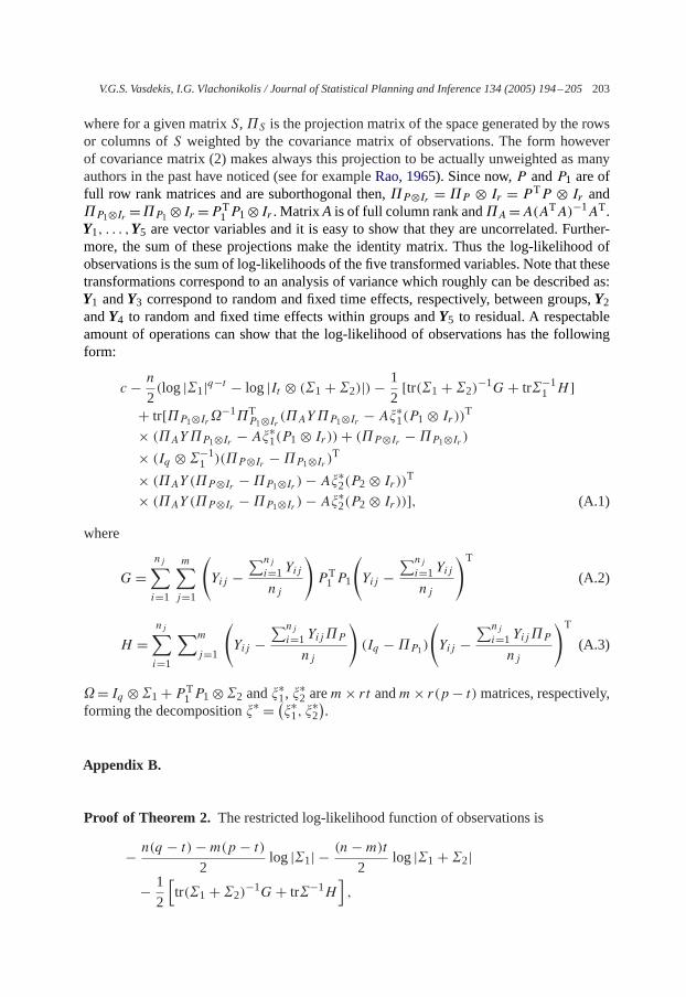
V.G.S. Vasdekis, I.G. Vlachonikolis / Journal of Statistical Planning and Inference 134 (2005) 194–205203

where for a given matrixS,�S is the projection matrix of the space generated by the rowsor columns ofS weighted by the covariance matrix of observations. The form howeverof covariance matrix (2) makes always this projection to be actually unweighted as manyauthors in the past have noticed (see for exampleRao, 1965). Since now,P andP1 are offull row rank matrices and are suborthogonal then,�P⊗Ir = �P ⊗ Ir = P TP ⊗ Ir and�P1⊗Ir =�P1⊗ Ir =P T1 P1⊗ Ir . MatrixA is of full column rank and�A=A(ATA)−1AT.Y1, . . . ,Y5 are vector variables and it is easy to show that they are uncorrelated. Further-more, the sum of these projections make the identity matrix. Thus the log-likelihood ofobservations is the sum of log-likelihoods of the five transformed variables. Note that thesetransformations correspond to an analysis of variance which roughly can be described as:Y1 andY3 correspond to random and fixed time effects, respectively, between groups,Y2andY4 to random and fixed time effects within groups andY5 to residual. A respectableamount of operations can show that the log-likelihood of observations has the followingform:

c − n

2(log |�1|q−t − log |It ⊗ (�1+ �2)|)− 1

2[tr(�1+ �2)−1G+ tr�−1

1 H ]+ tr[�P1⊗Ir�−1�TP1⊗Ir (�AY�P1⊗Ir − A�∗

1(P1⊗ Ir ))T

× (�AY�P1⊗Ir − A�∗1(P1⊗ Ir ))+ (�P⊗Ir − �P1⊗Ir )

× (Iq ⊗ �−11 )(�P⊗Ir − �P1⊗Ir )T

× (�AY (�P⊗Ir − �P1⊗Ir )− A�∗2(P2⊗ Ir ))

T

× (�AY (�P⊗Ir − �P1⊗Ir )− A�∗2(P2⊗ Ir ))], (A.1)

where

G=nj∑i=1

m∑j=1

(Yij −

∑nji=1 Yijnj

)P T1 P1

(Yij −

∑nji=1 Yijnj

)T(A.2)

H =nj∑i=1

∑m

j=1

(Yij −

∑nji=1 Yij�P

nj

)(Iq − �P1)

(Yij −

∑nji=1 Yij�P

nj

)T(A.3)

� = Iq ⊗ �1+P T1 P1⊗ �2 and�∗1, �

∗2 arem× rt andm× r(p− t)matrices, respectively,

forming the decomposition�∗ = (�∗1, �

∗2

).

Appendix B.

Proof of Theorem 2. The restricted log-likelihood function of observations is

− n(q − t)−m(p − t)

2log |�1| − (n−m)t

2log |�1+ �2|

− 1

2

[tr(�1+ �2)−1G+ tr�−1H

],

204 V.G.S. Vasdekis, I.G. Vlachonikolis / Journal of Statistical Planning and Inference 134 (2005) 194–205

whereG andH are given by (A.2) and (A.3), respectively. The proof now goes along thelines ofAnderson et al. (1986). Substituting the decompositions for�1,�1+ �2,H andG,defined before Theorem 1, we get the concentrated log-likelihood

− (nq −mp) log |�| − (n−m)t

2log |�|

− 1

2tr�−1(�−1BT 1/2)(�−1BT 1/2)T − 1

2tr(�−1BT 1/2)T −1(�−1BT 1/2)T.

This formhas to bemaximizedwith respect to�and�. Since�appears in the log-likelihoodin a complex form, we consider this form’s s.v.d to be�−1BT 1/2 = CDZ, whereC andZ are orthogonal andD diagonal. By applying von Neumann’s theorem (Anderson et al.,1986) we get that the maximum is given by

(nq −mp) log |D| − (n−m)t

2log |�| − 1

2tr D2T −1− 1

2tr�−1D2 (B.1)

and the maximizing value of� is

�R = BT 1/2D−1. (B.2)

However,D,� andT are diagonal matrices and form (B.1) is written as

1

2

r∑i=1

[2(nq −mp) log di − (n−m)t log�i − d2i

(1

i+ 1

�i

)]. (B.3)

Maximization with respect todi , i = 1, . . . , r gives

d−2i = 1

(nq −mp)

(1

i+ 1

�i

)

from which we takeD−2R of the theorem. Substitution now ofdi ’s to (B.3) gives

1

2

r∑i=1

[c − (nq −mp) log

(1

i+ 1

�i

)− (n−m)t log �i

].

Maximization with respect to�i , i = 1, . . . , r gives

�i = i[n(q − t)−m(p − t)]

(n−m)t.

It is evident that restriction�1� · · · ��s > �s+1= · · ·= �r =1 is satisfied for those�’s forwhich

i >(n−m)t

n(q − t)−m(p − t). (B.4)

Denoting this number bys∗R, the proof of the theorem is complete since direct substitutionof the estimate ofD provides an estimate of� which along with� provide the estimates of�1 and�2 shown in Theorem 2. �

V.G.S. Vasdekis, I.G. Vlachonikolis / Journal of Statistical Planning and Inference 134 (2005) 194–205205

References

Amemiya,Y., 1985.What should be done when an estimated between group covariance matrix in not nonnegativedefinite. Amer. Statist. 39, 112–117.

Amemiya, Y., Fuller, W., 1984. Estimation for the multivariate errors-in-variables model with estimated errorcovariance matrix. Ann. Statist. 12, 497–509.

Anderson, B.M., Anderson, T.W., Olkin, I., 1986. Maximum likelihood estimators and likelihood ratio criteria inmultivariate components of variance. Ann. Statist. 14, 405–417.

Calvin, J.A., 1993. REML estimation in unbalanced multivariate variance components models using an EMalgorithm. Biometrics 49, 691–701.

Calvin, J.A., Dykstra, R.L., 1991a. Maximum likelihood estimation of a set covariance matrices under Lownerorder restrictions with applications to balanced multivariate variance components models. Ann. Statist. 19,850–869.

Calvin, J.A., Dykstra, R.L., 1991b. Least squares estimation of covariance matrices in balanced multivariatevariance components models. J. Amer. Statist. Assoc. 86, 388–395.

Diggle, P.J., 1988. An approach to the analysis of repeated measurements. Biometrics 44, 959–971.Laird, N.M., Ware, J.H., 1982. Random effects models for longitudinal data. Biometrics 38, 963–974.Lange, N., Laird, N.M., 1989. The effect of covariance structure on variance estimation in balanced growth-curvemodels with random parameters. J. Amer. Statist. Assoc. 84, 241–247.

Potthoff, R.F., Roy, S.N., 1964. A generalized MANOVA model useful especially for growth curve problems.Biometrika 51, 313–326.

Rao, C.R., 1965. The theory of least squares when the parameters are stochastic and its application to the analysisof growth curves. Biometrika 52, 447–458.

Rao, C.R., 1967. Least squares theory using an estimated dispersion matrix and its application to measurement ofsignals. in: Le Cam, L.M., Neyman, J. (Eds.), Proceedings of the Fifth Berkeley Symposium on MathematicalStatistics and Probability. University of California Press, Berkeley, pp. 355–372.

Reinsel, G., 1982. Multivariate repeated-measurement or growth curve models with multivariate random-effectscovariance structure. J. Amer. Statist. Assoc. 77, 190–195.

Reinsel, G., 1984. Estimation and prediction in a multivariate random-effects generalized linear model. J. Amer.Statist. Assoc. 79, 406–414.

Reinsel, G., 1985. Mean squared error properties of empirical Bayes estimators in a multivariate random effectsgeneral linear model. J. Amer. Statist. Assoc. 80, 642–650.

Vasdekis,V.G.S., 1996.Anote on the differencebetween two likelihoodbasedmethods in growth curves.Commun.Statist. Theory Methods 25 (9), 2093–2100.

Verbyla, A.P., 1986. Conditioning in the growth curve model. Biometrika 75, 129–138.Verbyla, A.P., Cullis, B.R., 1990. Modelling in repeated measures experiments. Appl. Statist. 39, 341–356.