arX

iv:1

108.

1852

v1 [

mat

h.N

T]

9 A

ug 2

011

On the characterization of minimal value set

polynomials

Herivelto Borgesa, Ricardo Conceicaob

aUniversidade de Sao Paulo, Inst. de Ciencias Matematicas e de Computacao, Sao

Carlos, SP 13560-970, Brazil.bOxford College of Emory University. 100 Hamill Street, Oxford, Georgia 30054.

Abstract

We give an explicit characterization of all minimal value set polynomials inFq[x] whose set of values is a subfield Fq′ of Fq. We show that the set ofsuch polynomials, together with the constants of Fq′, is an Fq′-vector spaceof dimension 2[Fq:Fq′ ]. Our approach not only provides the exact number ofsuch polynomials, but also yields a construction of new examples of minimalvalue set polynomials for some other fixed value sets. In the latter case, wealso derive a non-trivial lower bound for the number of such polynomials.

Key words: Polynomials, Value set, Finite Field

1. Introduction

Let q be a power of a prime p, and for any non-constant polynomialF ∈ Fq[x], let VF = {F (α) : α ∈ Fq} be its value set. Since F has no morethan degF zeroes, one can easily show that VF satisfies

⌊

q − 1

deg F

⌋

+ 1 ≤ |VF | ≤ q, (1)

where ⌊t⌋ is the greatest integer ≤ t, and |S| denotes the cardinality of theset S. If |VF | attains the lower bound in (1), then F is called a minimalvalue set polynomial. Throughout this text, a polynomial of this kind will bereferred to by the abbreviation m. v. s. p..

In 1961, motivated by a generalization of the Waring’s problem modulop, the authors of [1] characterized m. v. s. p. ’s of degree < 2p+ 2. They alsoremarked that for any polynomial F ∈ Fqn[x], with 0 < deg F ≤ (qn−1)/(q−1) and VF ⊂ Fq, the polynomial G = F a, where a|(q − 1), is an m. v. s. p. inFqn [x] (see [1, Section 5]).

August 10, 2011

In 1963, W. Mills [5] provided additional results on m. v. s. p. ’s and man-aged to characterize all m. v. s. p. ’s in Fq[x] of degree ≤ √

q. Such polynomi-als (see Theorem 2.2) turned out to be part of a larger class of m. v. s. p. ’spreviously presented in [1]. Mills also provided a complete classification ofm. v. s. p. ’s in Fp2[x] and remarked that for q > p2, an m. v. s. p. differentfrom the ones already mentioned in [1] would be unlikely to exist.

In the first part of this paper (section 2), we extend the work of Mills intwo ways. First we characterize m. v. s. p. ’s over Fq of degree

√q+1; second

we show that, up to composition with degree one polynomials, there is aunique m. v. s. p. in Fq[x] of degree ≤ √

q for a given set of values.Despite the remarkable work of Mills in [5], which provides a great deal of

information on m. v. s. p. ’s, there exists no complete solution to the followingfundamental problem:

Problem 1. Given S ⊂ Fq, can we find an m. v. s. p. F ∈ Fq[x] with VF = S?If so, how many such polynomials are there? Can they be characterized?

The second part of this work is built around these questions and is or-ganized as follows: In Section 4 we will provide a complete solution to thisproblem in a special but very important case: when S = Fq′ is a subfield ofFq. The general case is treated in Section 3, where we show how the workof Mills imposes some very restrictive and necessary conditions on S. Forthe sets S satisfying such conditions, in Section 5 we will be able to providea partial answer to the question of the existence of m. v. s. p. ’s with S asits set of values and give a lower bound to the number of such polynomials.As a by-product of our constructions, we show that m. v. s. p. ’s other thanthe ones expected by Mills do exist: a simple example being the polynomialF = xq4+q − xq3+1 in Fq6 [x], which is addressed in Section 6.

The characterization of special classes of polynomials over finite fields,and the determination of its cardinal number are fundamental theoreticalproblems, which are not only worthy of study in their own right, but alsobecause of their applications. Our interest in investigating m. v. s. p. ’s isrelated to its potential application to the construction of new curves withmany rational points, the characterization of certain Frobenius non-classicalcurves and the construction of elliptic curves over Fq(t) with many integralpoints. The study connecting special aspects of such polynomials and theaforementioned applications is being handled in companion papers.

Notation: Throughout the text, q will denote a power of a prime p.

2

2. Preliminaries

The content of this section is mostly based on [5], from where a largeamount of notations and results are borrowed. Therefore, we believe thatsome familiarity with Sections 1 and 2 of that paper would be desirable forour reader.

We begin by pointing out that m. v. s. p. ’s F with |VF | ≤ 2 do not fit inthe general pattern and were handled separately in [1]. Mills [5] proved thefollowing important result that presents necessary conditions for a polynomialF ∈ Fq[x] with |VF | > 2 to be an m. v. s. p. and encloses other valuableinformation about such polynomials.

Theorem 2.1 (Mills). Let F ∈ Fq[x] be a polynomial of positive degree. LetVF = {γ0, γ1, · · · , γr} be its set of values, and let li be the number of distinctroots in Fq of the polynomial F − γi. Let γi be arranged in such way thatl0 ≤ li, 1 ≤ i ≤ r. Set L =

∏

(x − π) where the product is over the distinctroots of F − γ0 that lie in Fq.

Suppose that F is an m. v. s. p. and r > 1. Then there exist positiveintegers v,m, k; a polynomial N over Fq, and ω0, ω1, · · · , ωr in Fq such thatL ∤ N , v | (pk − 1), 1 + vr = pmk, L′ is a pmk-th power, ω0 6= 0, ωm = 1,

F = LvNpmk

+ γ0, (2)

r∏

i=1

(x− γi + γ0) =

m∑

i=0

ωix(pki−1)/v, (3)

m∑

i=0

ωiLpkiNpmk(pki−1)/v = −ω0(x

q − x)L′. (4)

Proof. See [5, Theorem 1].

As a consequence of this theorem, Mills presented the following charac-terization of all m. v. s. p. ’s over Fq of degree ≤ √

q.

Theorem 2.2 (Mills). Let F ∈ Fq[x] be a polynomial with 0 < degF ≤ √q.

Then F is an m. v. s. p. if and only if F is of the form

F = αLv + γ, (5)

where L is a polynomial that factors into distinct linear factors over Fq andthat has the form

L =

d∑

i=0

ϕixpki + β, (6)

3

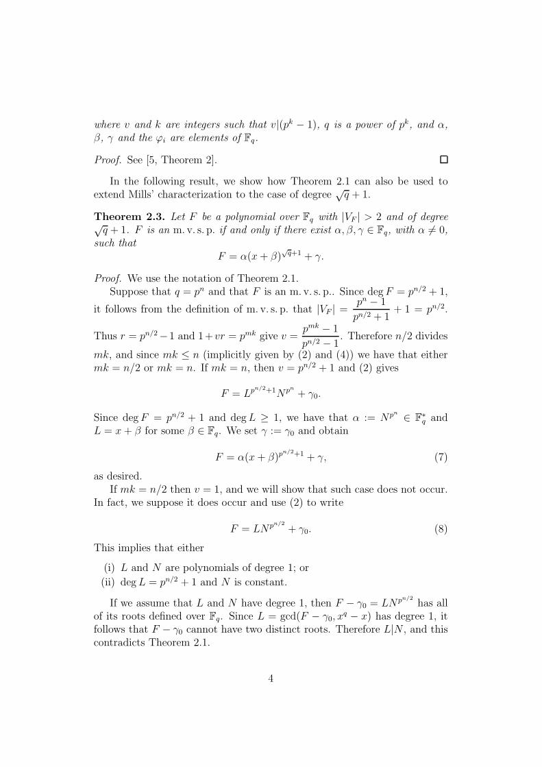
where v and k are integers such that v|(pk − 1), q is a power of pk, and α,β, γ and the ϕi are elements of Fq.

Proof. See [5, Theorem 2].

In the following result, we show how Theorem 2.1 can also be used toextend Mills’ characterization to the case of degree

√q + 1.

Theorem 2.3. Let F be a polynomial over Fq with |VF | > 2 and of degree√q + 1. F is an m. v. s. p. if and only if there exist α, β, γ ∈ Fq, with α 6= 0,

such thatF = α(x+ β)

√q+1 + γ.

Proof. We use the notation of Theorem 2.1.Suppose that q = pn and that F is an m. v. s. p.. Since degF = pn/2 + 1,

it follows from the definition of m. v. s. p. that |VF | =pn − 1

pn/2 + 1+ 1 = pn/2.

Thus r = pn/2−1 and 1+vr = pmk give v =pmk − 1

pn/2 − 1. Therefore n/2 divides

mk, and since mk ≤ n (implicitly given by (2) and (4)) we have that eithermk = n/2 or mk = n. If mk = n, then v = pn/2 + 1 and (2) gives

F = Lpn/2+1Npn + γ0.

Since degF = pn/2 + 1 and degL ≥ 1, we have that α := Npn ∈ F∗q and

L = x+ β for some β ∈ Fq. We set γ := γ0 and obtain

F = α(x+ β)pn/2+1 + γ, (7)

as desired.If mk = n/2 then v = 1, and we will show that such case does not occur.

In fact, we suppose it does occur and use (2) to write

F = LNpn/2

+ γ0. (8)

This implies that either

(i) L and N are polynomials of degree 1; or

(ii) degL = pn/2 + 1 and N is constant.

If we assume that L and N have degree 1, then F − γ0 = LNpn/2has all

of its roots defined over Fq. Since L = gcd(F − γ0, xq − x) has degree 1, it

follows that F − γ0 cannot have two distinct roots. Therefore L|N , and thiscontradicts Theorem 2.1.

4

If we assume that (ii) is true, then F − γ0 has pn/2 +1 distinct roots over

Fpn. For all 0 ≤ i ≤ r, recall that in Theorem 2.1 it is assumed that l0 ≤ li.Therefore, F − γi also has pn/2 + 1 distinct roots over Fpn. This implies that∏r

i=0(F − γi) is a polynomial over Fpn with (r + 1)(pn/2 + 1) = pn + pn/2

distinct roots defined over Fpn. This clear contradiction implies that neither(i) nor (ii) can hold and the result follows. The converse is trivial.

Observe that this result can be rephrased as follows: up to an affine com-position1, x

√q+1 is the only m. v. s. p. of degree

√q + 1. A similar statement

is true for m. v. s. p. ’s of degree ≤ √q with a given set of values: they are

also unique up to affine compositions. Our proof of this fact relies in part onthe following consequence of the results in [5].

Lemma 2.4. If F ∈ Fq[x] is an m. v. s. p. with VF = {γ0, γ1, · · · , γr} andr > 1, then

(i) A root of Fi = F − γi = 0 is not in Fq if and only if its multiplicity isdivisible by p.

(ii) F − γi = 0 has a simple root for at least r values γi ∈ VF .

Proof. This proof uses notations and results of [5]. Item (i) follows directlyfrom Lemmas 2 and 3 in [5]. In fact, since Fi = LiUi where Li = gcd(Fi, x

q−x), Lemma 2 in [5] implies Fi = Lwi+1

i Hpi , which proves the “only if” part of

(i). The other part of (i) follows from the fact that Fi is not a p-power; thatis F ′

i = F ′ 6= 0, which can be read off Theorem 2.1.Lemma 2 in [5] also gives Li ∤ Hi which, together with Lemma 3 in [5],

implies (ii).

As remarked in footnote 1, given a ∈ F∗q, b ∈ Fq and a non-constant

polynomial F , the polynomials F and G := F (ax + b) have the same setof values. In what follows, we will show that any two m. v. s. p. ’s of degree≤ √

q and with the same value set are related in this way.

Proposition 2.5. Let F ∈ Fq[x] be an m. v. s. p. such that |VF | > 2 anddeg F ≤ √

q. If G ∈ Fq[x] is an m. v. s. p. such that degG ≤ √q and VF = VG

then G = F (ax+ b) for some a, b ∈ Fq.

1 It is worth mentioning that if F ∈ Fq[x] is an m. v. s. p. and G = αx + β ∈ Fq[x] isnon-constant, then F1 = F (G(x)) and F2 = G(F (x)) are m. v. s. p. ’s with VF1

= VF andVF2

= αVF + β. The polynomials F1 and F2 will be referred to as affine compositions ofF .

5

Proof. Without loss of generality, we may assume d := degF ≥ degG.Suppose G(x) 6= F (ax + b) for all a, b ∈ Fq; that is, F (x) − G(y) hasno Fq-linear factors (in particular d ≥ 2). Since d ≤ √

q, Theorem 2.2implies F = αLv + γ0 and so F − γ = 0 has d distinct roots for allγ ∈ {γ1, γ2, · · · , γr} = VF\{γ0}, and by Lemma 2.4.(i), all such roots liein Fq. Therefore, if n is the number of times G(λ) assumes γ0 as λ rangesover Fq then the number N of Fq-solutions to F (y) = G(x) is given byN = d(q − n) + n · degL. But since 1 ≤ n ≤ d ≤ √

q we have

N = d(q − n) + n · degL ≥ d(q − d) + degL ≥ q(d− 1) + 1 (9)

Notice that if N = q(d − 1) + 1, then (9) gives 1 = n = d, contradictingd ≥ 2. Therefore we have

N > q(d− 1) + 1,

which contradicts the main result (Theorem 3.1) of [3]. This completes theproof.

The results in this section show that m. v. s. p. ’s with degree ≤ √q+1 are

unique (up to affine compositions) if their set of values are fixed. However,this is far from the truth in the general case. As we will see in the followingsections, the set of m. v. s. p. ’s with a fixed set of values S can be quite large.

3. On m.v.s.p.’s with a given set of values

Our discussion of Problem 1 starts with the following criterion to decidewhether or not a polynomial F is an m. v. s. p. with VF = S, for a given setS ⊂ Fq. The following theorem, which can be read off the work of [1] and [5],will be used to restate Problem 1 in terms of the polynomial T =

∏

γ∈S(x− γ)

of values of F .

Theorem 3.1. Let F be a polynomial in Fq[x], and let S be a subset of Fq.If |S| > 2 and T =

∏

γ∈S(x− γ), then the following are equivalent:

(A) F is an m. v. s. p. with VF = S.(B) There exists θ ∈ F∗

q such that

T (F ) = θ(xq − x)F ′. (10)

Moreover, θ = −T ′(γ) for some γ ∈ S.

6

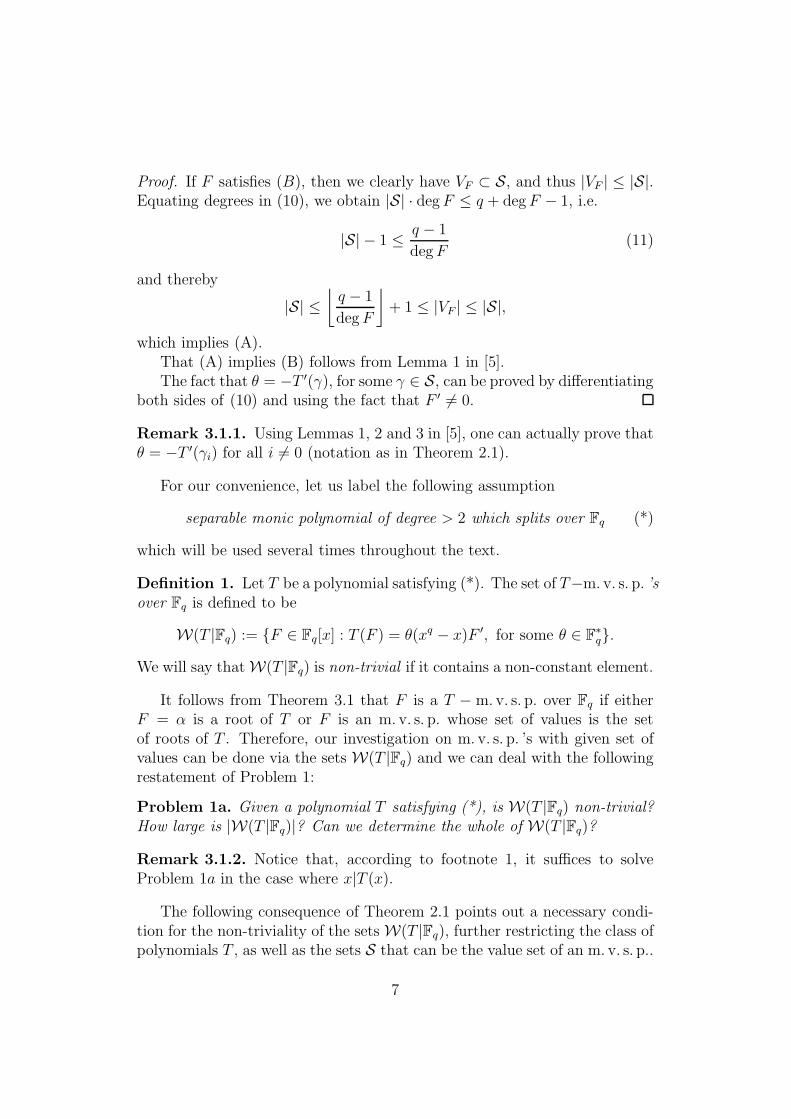
Proof. If F satisfies (B), then we clearly have VF ⊂ S, and thus |VF | ≤ |S|.Equating degrees in (10), we obtain |S| · degF ≤ q + degF − 1, i.e.

|S| − 1 ≤ q − 1

degF(11)

and thereby

|S| ≤⌊

q − 1

degF

⌋

+ 1 ≤ |VF | ≤ |S|,

which implies (A).That (A) implies (B) follows from Lemma 1 in [5].The fact that θ = −T ′(γ), for some γ ∈ S, can be proved by differentiating

both sides of (10) and using the fact that F ′ 6= 0.

Remark 3.1.1. Using Lemmas 1, 2 and 3 in [5], one can actually prove thatθ = −T ′(γi) for all i 6= 0 (notation as in Theorem 2.1).

For our convenience, let us label the following assumption

separable monic polynomial of degree > 2 which splits over Fq (*)

which will be used several times throughout the text.

Definition 1. Let T be a polynomial satisfying (*). The set of T−m. v. s. p. ’sover Fq is defined to be

W(T |Fq) := {F ∈ Fq[x] : T (F ) = θ(xq − x)F ′, for some θ ∈ F∗q}.

We will say that W(T |Fq) is non-trivial if it contains a non-constant element.

It follows from Theorem 3.1 that F is a T − m. v. s. p. over Fq if eitherF = α is a root of T or F is an m. v. s. p. whose set of values is the setof roots of T . Therefore, our investigation on m. v. s. p. ’s with given set ofvalues can be done via the sets W(T |Fq) and we can deal with the followingrestatement of Problem 1:

Problem 1a. Given a polynomial T satisfying (*), is W(T |Fq) non-trivial?How large is |W(T |Fq)|? Can we determine the whole of W(T |Fq)?

Remark 3.1.2. Notice that, according to footnote 1, it suffices to solveProblem 1a in the case where x|T (x).

The following consequence of Theorem 2.1 points out a necessary condi-tion for the non-triviality of the sets W(T |Fq), further restricting the class ofpolynomials T , as well as the sets S that can be the value set of an m. v. s. p..

7

Proposition 3.2. Let T be a polynomial satisfying (*). If W(T |Fq) is non-trivial, then there exist positive integers k, m and v, with v|(pk − 1), andelements γ, ω1, . . . , ωm ∈ Fq such that

A(x) := T (xv + γ)/xv−1 =m∑

i=0

ωixpki. (12)

Proof. Let {γ0, . . . , γr} be the set of roots of T . By Theorem 3.1, any non-constant F ∈ W(T |Fq) is an m. v. s. p. with VF = {γ0, . . . , γr} and r >1. Therefore, F satisfies the hypotheses of Theorem 2.1. In particular, wecan guarantee the existence of positive integers v, k and m, and elementsω1, . . . , ωm ∈ Fq such that (3) holds. Our conclusion is just a restatement of(3) with γ = γ0.

Polynomials given by the right-hand side of (12) are called pk-additivepolynomials and have been extensively studied (see [4, Section 3.4])2. Aswe will see, the class of additive polynomials plays a crucial role in the con-struction (and possibly in the complete characterization) of m. v. s. p. ’s witha given set of values. Most notably is the following result which is a first steptowards a proof of a partial converse to the previous proposition.

Proposition 3.3. Let v be a positive divisor of pk − 1 and T be a polyno-mial satisfying (*). Assume x|T (x) and A(x) = T (xv)/xv−1 is a pk-additivepolynomial satisfying (*). Then

W(A|Fq) −→ W(T |Fq)

F 7−→ F v

is a well-defined map. In particular,

|W(T |Fq)| ≥|W(A|Fq)| − 1

v+ 1.

Proof. For F ∈ W(A|Fq), we have

T (F v) = F v−1A(F ) = F v−1(−A′(xq − x)F ′) = −A′

v(xq − x)(F v)′.

Thus F v ∈ W(T |Fq), by definition.

2In [4], pk-additive polynomials are called pk-linearized polynomials.

8

Propositions 3.2 and 3.3 indicate that a solution to Problem 1a in theparticular case of pk-additive polynomials will provide a partial solution tothe general problem. It turns out that whenever A is pk-additive polynomialsatisfying (*), we are able to show that W(A|Fq) is non-trivial and find alower bound for its cardinal number. This is accomplished in the followingway:

For any pk-additive polynomial A satisfying (*), it is easily verified thatthe setW(A|Fq) is a finite Fpk-vector space. In Section 5 we will use this extra

structure to show that for any such A, there exist a polynomial xpkd − αx ∈Fq[x] satisfying (*) and a Fpk-linear map φ : W(xpkd − αx|Fq) −→ W(A|Fq)with ker φ ⊂ Fq. In particular, the non-triviality of W(A|Fq) and ultimately

W(T |Fq), for T as in Proposition 3.3, will follow from that ofW(xpkd−αx|Fq).

The next section will be used to show that not only the sets W(xpkd −αx|Fq)are non-trivial, but that they can be described very explicitly.

4. Characterization of W(xpkd

− αx|Fq)

Let us start our study of the vector spaces W(xpkd − αx|Fq) by noticing

that since xpkd − αx satisfies (*), it follows that q = (pkd)n for some integern ≥ 1 and that W(xpkd −αx|Fq) is isomorphic to W(xpkd −x|Fq). Therefore,it is sufficient to consider the set W(xq − x|Fqn). Observe that Theorem 3.1implies that

W(xq − x|Fqn) = {F ∈ Fqn [x] : Fq − F = (xqn − x)F ′}, (13)

since θ = −T ′(γ) = 1, for some γ ∈ Fq.Recall that deg T > 2 was required in the definition of W(T |Fq), and that

was motivated by the condition r > 2 in Theorem 3.1. However, we wantto stress that q = 2 will be allowed in (13), and the reason why this can bedone is just one of the facts given by the following Lemma.

Lemma 4.1. If F ∈ Fqn[x] is non-constant with VF ⊆ Fq, then the followingare equivalent:

(1) F is an m. v. s. p. with VF = Fq.

(2) F q − F = (xqn − x)F ′.

(3) qn−1 ≤ degF ≤ (qn − 1)/(q − 1).

(4) 0 < deg F ≤ (qn − 1)/(q − 1).

Proof. • (1) =⇒ (2): In the notation of Theorem 3.1 we have T = xq−x,and the result will follow if q > 2. Assuming q = 2, we have

F 2 − F = (x2n − x)G (14)

9

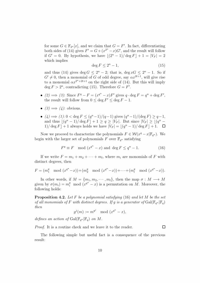
for some G ∈ F2n [x], and we claim that G = F ′. In fact, differentiatingboth sides of (14) gives F ′ = G+(x2n −x)G′, and the result will followif G′ = 0. By hypothesis, we have ⌊(2n − 1)/ degF ⌋ + 1 = |VF | = 2which implies

degF ≤ 2n − 1, (15)

and thus (14) gives degG ≤ 2n − 2; that is, deg xG ≤ 2n − 1. So ifG′ 6= 0, then a monomial of G of odd degree, say αx2t+1, will give riseto a monomial αx2n+2t+1 on the right side of (14). But this will implydeg F > 2n, contradicting (15). Therefore G = F ′.

• (2) =⇒ (3): Since F q − F = (xqn − x)F ′ gives q · deg F = qn + degF ′,the result will follow from 0 ≤ degF ′ ≤ degF − 1.

• (3) =⇒ (4): obvious.

• (4) =⇒ (1): 0 < degF ≤ (qn−1)/(q−1) gives (qn−1)/(degF ) ≥ q−1,and thus ⌊(qn − 1)/ degF ⌋ + 1 ≥ q ≥ |VF |. But since |VF | ≥ ⌊(qn −1)/ degF ⌋+ 1 always holds we have |VF | = ⌊(qn − 1)/ degF ⌋+ 1.

Now we proceed to characterize the polynomials F ∈ W(xq −x|Fqn). Webegin with the larger set of polynomials F over Fqn satisfying

F q ≡ F mod (xqn − x) and degF ≤ qn − 1. (16)

If we write F = m1 +m2 + · · ·+ml, where mi are monomials of F withdistinct degrees, then

F = (mq1 mod (xqn−x))+(mq

2 mod (xqn−x))+· · ·+(mql mod (xqn−x)).

In other words, if M = {m1, m2, · · · , ml}, then the map σ : M −→ Mgiven by σ(mi) = mq

i mod (xqn − x) is a permutation on M . Moreover, thefollowing holds:

Proposition 4.2. Let F be a polynomial satisfying (16) and let M be the setof all monomials of F with distinct degrees. If g is a generator of Gal(Fqn |Fq)then

gj(m) := mqj mod (xqn − x),

defines an action of Gal(Fqn|Fq) on M .

Proof. It is a routine check and we leave it to the reader.

The following simple but useful fact is a consequence of the previousresult:

10

Lemma 4.3. Let F be a polynomial satisfying (16). Then:

(a) If mq mod (xqn −x) is a monomial of F , then so is m mod (xqn −x).

(b) If m = αxkq+1 is a monomial of F , then so is m = α1/qxk+qn−1.

Proof. Both cases follow directly from that fact that if m is a monomial ofF , then so is mqn−1

mod (xqn − x).

Let Om denote the orbit of a monomial m = αxk of F by the action ofGal(Fqn|Fq). Let s(m) denote the size of Om. Then

(αxk)qs(m)

mod (xqn − x) = αxk,

implies that for any m0 ∈ Om, m0 is defined over Fqs(m) . This observationis the last ingredient in the characterization of the polynomials F over Fqn

satisfying F q ≡ F mod (xqn − x) and degF ≤ qn − 1.

Proposition 4.4. Every F satisfying (16) can be written as F =e∑

i=1

Fi,

whereFi =

∑

m∈Omi

m (17)

and m1, . . . , me are certain monomials of F . Moreover, for all 1 ≤ i ≤ e, Fi

is defined over Fqs(mi).

Proof. Pick a monomialm1 of F . The orbit Om1 is a set of distinct monomialsof F . Let F1 be the sum of all such monomials. If those are all the monomialsof F , then we are done; otherwise we can pick a monomial m2 of F not lyingon the set Om1 , and consider the polynomial F2, sum of the monomials in theorbit Om2 . We keep repeating this process, and it is clear that we will finish

it after a finite number of steps, let us say e steps. Now F =e∑

i=1

Fi follows

from the construction and from the fact that the sets Omi’s are mutually

disjoint.

Remark 4.4.1. Notice that a polynomial F satisfies F q ≡ F mod (xqn−x)if, and only if, VF ⊂ Fq. Therefore the previous result characterizes allpolynomials F over Fqn with VF ⊂ Fq and deg F ≤ qn − 1.

The complete description of F ∈ W(xq −x|Fqn) will follow once we knowwhat the monomials of such an F look like. The additional information,namely F q − F = (xqn − x)F ′, will answer this question.

11

Lemma 4.5. For all F ∈ W(xq − x|Fqn), there exist polynomials A and Bsuch that F = A+B and

F = x

(

A

xqn−1

)q

+Bq (18)

Proof. Let A,B ∈ Fqn[x] be such that F = A + B and A is formed by allthe monomials of F of degree at least qn−1. Note that Lemma 4.1.(3) impliesA 6= 0. Then Aq + Bq − F = xqnF ′ − xF ′, and after comparing degrees wehave

(a) Aq = xqnF ′, which gives F ′ =

(

A

xqn−1

)q

, and

(b) (Bq − F ) = −xF ′, which gives F = xF ′ +Bq.

Combining (a) and (b), we obtain the desired result.

Lemma 4.6. If αxk is a non-zero monomial of F ∈ W(xq − x|Fqn), then

k = an−1qn−1 + an−2q

n−2 + · · ·+ a1q + a0

where ai ∈ {0, 1}.

Proof. We can certainly write k =n∑

i=1

aiqi, where ai ∈ {0, 1, · · · , q − 1}.

From (18) we clearly have a0 ∈ {0, 1}. If a0 = 0 then Lemma 4.3 implies that

αqn−1x

kq is a term of F and then we fall into an equivalent problem with fewer

variables ai. Therefore, we may assume a0 = 1 and again Lemma 4.3 implies

that αxqn−1+ k−1q is a term of F . The new term αxqn−1+an−1qn−2+···+a2q+a1 gives

a1 ∈ {0, 1} and we repeat the process to reach a2. After at most n iterations,we find that all ai are either zero or one.

Before finishing the complete description of W(xq − x|Fqn), let us recallthat s(m) denotes the size of the orbit of the monomial m by the action ofGal(Fqn|Fq) as described in Proposition 4.2.

Theorem 4.7. A polynomial F lies in W(xq − x|Fqn) if, and only if, it canbe written as a sum of polynomials of the form

s(m)−1∑

i=0

[mqi mod (xqn − x)], (19)

where m ∈ Fqs(m)[x] is a monomial and degm = an−1qn−1 + an−2q

n−2+ · · ·+a1q + a0 with ai ∈ {0, 1}.

12

Proof. That such an F ∈ W(xq−x|Fqn) can be written as sum of polynomialsgiven by (19) is a consequence of Proposition 4.4 and Lemma 4.6. To provethe converse, we can use the fact that W(xq − x|Fqn) is an Fq-vector spaceand just prove that the polynomials given by (19) lie in W(xq − x|Fqn).

Let H be a polynomial given by (19). If degH = 0 then H ∈ Fq. Thuswe may assume that degH > 0. We know that H satisfies (16) and therebyVH ⊂ Fq. Moreover, 0 < degH ≤ 1 + q + q2 + . . .+ qn−1 = qn−1

q−1and Lemma

4.1.(4) implies H ∈ W(xq − x|Fqn).

4.1. The dimension of W(xq − x|Fqn)

Let g be a generator of Gal(Fqn|Fq) and (a0, . . . , an−1) ∈ {0, 1}n. Then themap given by g(a0, . . . , an−2, an−1) = (an−1, a0, . . . , an−2) defines an action ofGal(Fqn|Fq) on the set {0, 1}n. Let us identify the n-tuple (a0, . . . , an−2, an−1)with the q-ary expansion of an integer k = an−1q

n−1 + · · · + a1q + a0, andchoose representatives k1, . . . , kb on each orbit of the set {0, 1}n. For eachi ∈ {1, . . . , b}, let di be the size of the orbit Oki and

Vi :=

{

di−1∑

j=0

(αxki)qj

mod (xqn − x) : α ∈ Fqdi

}

.

Theorem 4.8. For i ∈ {1, · · · , b}, the set Vi is an Fq-vector subspace ofW(xq − x|Fqn) of dimension di. Moreover,

W(xq − x|Fqn) =b

⊕

i=1

Vi.

anddimFq W(xq − x|Fqn) = 2n.

Proof. Theorem 4.7 implies that each Vi ⊂ W(xq − x|Fqn). Also, it can beeasily verified that Vi is an Fq-vector space and that |Vi| = qdi. ConsequentlydimFq Vi = di.

Notice that if k = an−1qn−1+an−2q

n−2+ · · ·+a1q+a0 is identified with ann-tuple (a0, a1, . . . , an−1) ∈ {0, 1}n, then the degree of (αxk)q mod (xqn −x)is equal to anq

n−1 + a1qn−2 + . . .+ an−1; and, under the above identification,

it is given by the cyclic permutation (an−1, a0, a1, . . . , an−2).Therefore the set of exponents of monomials of elements in Vi is equal

to the orbit of ki (identified with an n-tuple) by the action of Gal(Fqn |Fq)on {0, 1}n. This implies that all elements of Vi will not share any monomialwith any element in a distinct Vj . Thus for all i,

Vi ∩ (V1 + . . .+ Vi−1 + Vi + . . .+ Vb) = 0.

13

Theorem 4.7 implies that every element of W(xq − x|Fqn) can be written as

sum of elements in distinct Vi’s. Therefore, W(xq − x|Fqn) =

b⊕

i=1

Vi.

Now, if we let o(d) denote the number of Vi’s of dimension d, then

dimFq W(xq − x|Fqn) =∑

d|nd · o(d).

Notice that by construction o(d) also counts the number of orbits of {0, 1}nof size d. Thus, d · o(d) is equal to the cardinality of the union of all orbitsof {0, 1}n with size d. Since {0, 1}n can be partitioned into orbits of size

dividing n, we conclude that∑

d|nd · o(d) = 2n.

Corollary 4.9. If xqd − αx satisfies (*) then

dimFq W(xqd − αx|Fqn) = d2n/d.

Proof. We leave the verification to the reader.

5. On the vector spaces W(A|Fq)

Let A be a pk-additive polynomial satisfying (*). The aim of this sectionis to provide a method to construct non-constant elements of W(A|Fq), com-pute a lower bound for its dimension, and point out cases where this boundis sharp. As before, it is enough to consider the Fq-vector spaces W(A|Fqn),where A is a q-additive polynomial.

The following two lemmas will be used to construct Fq-linear maps φ :

W(xqd − αx|Fqn) −→ W(A|Fqn). As discussed briefly in the end of Section

3, we will take advantage of our understanding of W(xqd − αx|Fqn) to giveinformation on W(A|Fqn).

Let R(A) denote the set of roots of a polynomial A. Then R(A) is an Fq-vector subspace of Fqn of dimension t, whenever A is a q-additive polynomialsatisfying (*) with degA = qt.

Lemma 5.1. Let A,L and M be q-additive polynomials. Suppose that Aand L satisfy (*) and that L = γA(M(x)), for some γ ∈ F∗

qn. Then the mapφM : W(L|Fqn) −→ W(A|Fqn) given by φM(F ) := M(F ) is Fq-linear withkernel R(M).

Proof. The assertions are simple and can be easily checked.

14

Lemma 5.2. Let A and xqd −αx be q-additive polynomials satisfying (*). IfA divides xqd −αx then there exists a q-additive polynomial M splitting overFqd and an element γ of F∗

qn such that

xqd − αx = γA(M(x)).

Proof. Suppose degA = qt, and assume α = 1. By assumption, the set R(A)is an Fq-vector subspace of codimension d−t in Fqd. Therefore, from Corollary2.5 of [2], there exists a unique monic q-additive polynomial M ∈ Fqd[x]splitting over Fqd and of degree qd−t, such that R(A) = {M(y) : y ∈ Fqn}.But this implies that A(M(x)) ∈ Fqd[x] is monic of degree qd and vanishesin Fqd. That is,

A(M(x)) = xqd − x.

For α 6= 1, we consider β ∈ F∗q such that α = βqd−1. Since A(x) divides

xqd − αx, we have that β−qtA(βx) is monic and divides xqd − x. As provedabove, there exists a unique monic q-additive polynomial L such that xqd −x = β−qtA(βL(x)). If we take M(x) = βL(β−1x) and γ = βqd−qt , then theresult follows.

We are ready to derive the main result of this section.

Theorem 5.3. Suppose A and xqd −αx are q-additive polynomials satisfying(*) and that degA = qt.

If A divides xqd − αx then there exists a q-additive polynomial M withdegM = qd−t such that the sequence

0 −→ R(M)ι−→ W(xqd − αx|Fqn)

φM−−→ W(A|Fqn) (20)

is exact, where ι is the inclusion map and φM is defined by φM(F ) = M(F ).Moreover,

dimFq W(A|Fqn) ≥ d2n/d − d+ t,

with equality if and only if φM is surjective.

Proof. Since A divides xqd − αx, Lemma 5.2 guarantees the existence of aq-additive polynomial M satisfying

xqd − αx = γA(M(x)),

for some γ ∈ F∗qd. Thus, Lemma 5.1 gives us the desired exact sequence.

The statement about the dimension follows from the Rank-nullity theo-rem and Corollary 4.9.

15

Let us recall that our study of the vector spaces W(A|Fqn) was motivatedby Problem 1. The previous result, footnote 1 and Theorem 3.1 show thatif S is any affine transformation of an Fq-vector space V, then we have apositive solution to part of Problem 1: there are m. v. s. p. ’s F over Fqn such

that VF = S. Moreover, these results provide the lower bound qd2n/d−d+t for

the number of such polynomials, where d > 0 is an integer depending onthe monic q-additive polynomial A of degree t > 2 such that V = R(A). Inmany cases this lower bound can be attained if, in Theorem 5.3, we choose theunique multiple of A of the form xqd − αx satisfying (*) and with minimaldegree. When A itself is of the form xqd − αx, this is a consequence ofCorollary 4.9. The next result shows that it also holds if dimFq V ≥ n/2.

Theorem 5.4. Suppose A and xqd −αx are q-additive polynomials satisfying(*) and that degA = qt ≥ qn/2.

If among all multiples of A of the form xqd − αx we choose the one withminimal degree, then the sequence given by Theorem 5.3 can be extended tothe exact sequence

0 −→ R(M)ι−→ W(xqd − αx|Fqn)

φM−−→ W(A|Fqn) −→ 0.

In particular,dimFq W(A|Fqn) = d2n/d − d+ t.

Proof. Let G ∈ W(A|Fqn). From (11) and degA ≥ qn/2, it follows thatdegG ≤ qn−1

degA−1≤ qn/2 + 1.

First assume that degG = qn/2 + 1 for some G ∈ W(A|Fqn). Theorem

2.3 implies that there exist α, β, γ ∈ Fqn such that G = α(x + β)qn/2+1 + γ.

Since R(A) = VG = αFqn/2 + γ is a vector space, we can conclude that γ = 0

and A = xqn/2 − αqn/2−1x. As observed above, for q-additive polynomials ofthis form the result is a consequence of Proposition 4.9.

Now suppose that degG < qn/2 + 1 for all G ∈ W(A|Fqn). The fact that

W(xqn/2 − αx|Fqn) is Fq-isomorphic to W(xqn/2 − x|Fqn) and Theorem 4.7

imply that A is not of the form xqn/2 −αx. Therefore xqn − x is the multipleof A of such form and with minimal degree. Theorem 5.3 guarantees theexistence of a q-linear polynomial M and an exact sequence

0 −→ R(M) −→ W(xqn − x|Fqn)φM−−→ W(A|Fqn).

We would like to show that the map φM(F ) := M(F ) is surjective. SinceW(xqn − x|Fqn) = {αx + β : α, β ∈ Fqn}, it follows that φM is surjective ifG ∈ W(A|Fqn) implies that G(x) = M(αx + β) for some α, β ∈ Fqn. Thislast assertion follows from Lemma 2.5.

16

6. Some Examples

As described in the introduction, the authors of [1] identified two classesof m. v. s. p. ’s over Fqn. Let G be one of the following polynomials over Fqn:

• a polynomial satisfying 0 < degG ≤ qn − 1

q − 1and VG ⊂ Fq; or

• a q-additive polynomial that splits over Fqn.

If v is a positive divisor of q − 1, α ∈ F∗q and β, γ ∈ Fq, then αG(x+ β)v + γ

is an m. v. s. p..At the end of [5], the author says that “it seems unlikely that there are

any more” m. v. s. p. ’s other than the ones above. In this section we show howthe previous results can be used to construct many examples of m. v. s. p. ’s;some of which are not of the form given above.

(1) Obtaining the elements of W(xq − x|Fqn) for n = 3.

Let us consider the action of Gal(Fq3 |Fq) on the set of 3-uples (a0, a1, a2) ∈{0, 1}3 via cyclic permutation. The orbits of this action are given by

• O0 := {(0, 0, 0)},• O1 := {(1, 0, 0), (0, 1, 0), (0, 0, 1)},• Oq+1 := {(1, 1, 0), (0, 1, 1), (1, 0, 1)},• Oq2+q+1 := {(1, 1, 1)}.

As discussed in Section 4.1, if we identify a 3-uple (a0, a1, a2) with theq-ary expansion of a number a2q

2+a1q+a0, then to each of these orbitswe associate the following Fq-vector spaces

• V0 := Fq,

• V1 := {αx+ (αx)q + (αx)q2: α ∈ Fq3},

• Vq+1 := {αxq+1 + αqxq2+q + αq2xq2+1 : α ∈ Fq3},• Vq2+q+1 := {αxq2+q+1 : α ∈ Fq}.

Theorem 4.8 implies that every element ofW(xq−x|Fq3) can be uniquelywritten as a sum of elements in distinct Vi’s. Notice that the sum ofthe Fq-dimensions of the Vi’s is given by 1+3+3+1 = 23 and is equalto the dimension of W(xq − x|Fq3).

17

(2) Constructing elements in W(A|Fq6) for A = xq2 + xq + x.

Observe that A = xq2 + xq + x is a q-additive polynomial dividingxq3 − x. By Theorem 5.3, we can find a q-additive polynomial Msatisfying A(M(x)) = xq3 − x, namely M = xq − x.This polynomial defines a linear map

W(xq3 − x|Fq6)φM−−→ W(xq2 + xq + x|Fq6)

given by φM(F ) = M(F ). In other words,

F q − F ∈ W(xq2 + xq + x|Fq6),

for all F ∈ W(xq3 − x|Fq6). Following the strategy of the previousexample, we can show that

W(xq3 − x|Fq6) = Fq3 ⊕ {αx+ (αx)q3 |α ∈ Fq6} ⊕ {αx1+q3 |α ∈ Fq3}.

In particular, dimFq W(xq3 − x|Fq6) = 12, and∣

∣

∣W(xq3 − x|Fq6)

∣

∣

∣= q12.

Since ker φA = Fq, we have that∣

∣

∣W(xq2 + xq + x|Fq6)

∣

∣

∣≥ q11.

(3) An m. v. s. p. different from the ones considered in [1, 5].

Take G = xq4+q − xq3+1. Notice that G = M(xq3+1) is an element ofW(xq2 + xq + x|Fq6). In particular, G is an m. v. s. p. with VG ⊂ Fq3

and degG > (q6 − 1)/(q3 − 1).Also it is not hard to see that for any q-additive polynomial L, Gis neither a power of L nor of the form α−degLL(αx) + β, for someα, β ∈ F∗

q6.

(4) Now assuming that q is odd, we use W(xq2 + xq + x|Fq6) to construct

elements of W(xq2+1

2 + xq+12 + x|Fq6).

For T = xq2+1

2 + xq+12 + x, we have xq2 + xq + x = T (x2)/x. Therefore,

Proposition 3.3 shows that F 2 ∈ W(xq2+1

2 + xq+12 + x|Fq6) for F ∈

W(xq2 + xq + x|Fq6). Using the results obtained in example (2), weconclude that

∣

∣

∣

∣

W(xq2+1

2 + xq+12 + x|Fq6)

∣

∣

∣

∣

≥ (q11 − 1)/2.

It is worth mentioning that a computer check for q ≤ 7 and q = 2n forn ≤ 11 shows that the lower bound obtained in example (2) is in fact theactual number of m. v. s. p. ’s in the corresponding set W(A|Fq6).

18

References

[1] Carlitz, L., Lewis, D. J., Mills, W. H., Straus, E. G., 1961. Polynomialsover finite fields with minimal value sets. Mathematika 8, 121–130.

[2] Garcia, A., Ozbudak, F., 2007. Some maximal function fields and additivepolynomials. Comm. Algebra 35 (5), 1553–1566.URL http://dx.doi.org/10.1080/00927870601169218

[3] Homma, M., Kim, S. J., 2010. Sziklai’s conjecture on the number of pointsof a plane curve over a finite field III. Finite Fields Appl. 16 (5), 315–319.URL http://dx.doi.org/10.1016/j.ffa.2010.05.001

[4] Lidl, R., Niederreiter, H., 1997. Finite fields, 2nd Edition. Vol. 20 ofEncyclopedia of Mathematics and its Applications. Cambridge UniversityPress, Cambridge, with a foreword by P. M. Cohn.

[5] Mills, W. H., 1964. Polynomials with minimal value sets. Pacific J. Math.14, 225–241.

19