Testing Low-Degree Polynomials over Prime Fields∗

Charanjit S. Jutla

IBM Thomas J. Watson Research Center,

Yorktown Heights, NY 10598

csjutla@watson.ibm.com

Anindya C. Patthak†

University of Texas at Austin

Austin, TX 78712

anindya@cs.utexas.edu

Atri Rudra‡

Dept. of Computer Science & Engineering

University of Washington

Seattle, WA 98915

atri@cs.washington.edu

David Zuckerman§

University of Texas at Austin

Austin, TX 78712

diz@cs.utexas.edu

August 17, 2006

Abstract

We present an efficient randomized algorithm to test if a given function f : Fn

p→ Fp (where

p is a prime) is a low-degree polynomial. This gives a local test for Generalized Reed-Mullercodes over prime fields. For a given integer t and a given real ǫ > 0, the algorithm queries f at

O(

1

ǫ+ t · p

2tp−1

+1)

points to determine whether f can be described by a polynomial of degree

at most t. If f is indeed a polynomial of degree at most t, our algorithm always accepts, and iff has a relative distance at least ǫ from every degree t polynomial, then our algorithm rejects fwith probability at least 1

2. Our result is almost optimal since any such algorithm must query

f on at least Ω(1

ǫ+ p

t+1

p−1 ) points.

keywords : Polynomials, Generalized Reed-Muller code, local testability, local correction.

∗A preliminary version of this paper appeared in 45th. Symposium on Foundations of Computer Science, 2004.†Supported in part by NSF Grant CCR-0310960.‡This work was done while the author was at the University of Texas at Austin.§Supported in part by NSF Grants CCR-9912428 and CCR-0310960 and a David and Lucile Packard Fellowship

for Science and Engineering.

1

1 Introduction

1.1 Background and Context

A low degree tester is a probabilistic algorithm, which given a degree parameter t and oracle accessto a function f on n arguments (which take values from some finite field F) has the followingbehavior. If f is the evaluation of a polynomial on n variables with total degree at most t then thelow degree tester must accept with probability one. On the other hand, if f is “far” from beingthe evaluation of some polynomial on n variables with degree at most t, then the tester must rejectwith constant probability. The tester can query the function f to obtain the evaluation of f at anypoint. However, the tester must accomplish its task by using as few probes as possible.

Low degree testers play an important part in the construction of Probabilistically Checkable Proofs(or PCPs)– in fact different parameters of low degree testers (for example, the number of probesand the amount of randomness used) directly affect the parameters of the corresponding PCPs aswell as various inapproximability results obtained from such PCPs ([11, 2]). Low degree testersalso form the core of the proof of MIP = NEXPTIME in [7].

Blum, Luby, and Rubinfeld designed the first low degree tester, which handled the linear case i.e.,t = 1 ([8]). This was followed by a series of work that gave low degree testers that worked for largervalues of the degree parameter ([17, 12, 4]). However, these subsequent works as well as otherswhich use low degree testers ([7, 13]) only work when the degree is larger than size of the fieldF. Alon et. al. proposed a low degree tester for any nontrivial degree parameter over F2 [1]. Anatural open problem was to give a low degree tester for all degrees for finite fields of size betweentwo and the degree parameter.

In this work we (partially) solve this problem by presenting a low degree test for multivariatepolynomials over any prime field Fp.

1.1.1 Connection to coding theory

A linear code C over a finite field F of dimension K and length N is a K-dimensional subspaceof F

N . The code C is said to be locally testable if there exists a local tester that can efficientlydistinguish between inputs in F

N that belong to C and inputs that differ from every codeword inC is a “large” fraction of positions.

The evaluations of polynomials in n variables of degree at most t are well known linear codes.In particular, the evaluation of polynomials in n variables of degree at most t over F2 is theReed-Muller code R(t, n) with parameters t and n. The corresponding code over general fields,called Generalized Reed-Muller code or GRMq(n, t) is the vector of (evaluations of) all polyno-mials in n variables of total degree at most t over Fq. These codes have length qn and dimension(n+t

n

)(see [9, 10, 5] for more details). Therefore, a function has degree t if and only if (the vector of

evaluations of) the function is a valid codeword in GRMq(n, t). In other words, low degree testingis equivalent to locally testing Generalized Reed-Muller codes.

2

1.2 Previous low degree testers

As was mentioned earlier, the study of low degree testing (along with self-correction) dates back tothe work of Blum, Luby and Rubinfeld ([8]), where an algorithm was given to test whether a givenfunction is linear. The approach in [8] later naturally extended to yield testers for low degreepolynomials over large fields. Roughly, the idea is to project the given function on to a random lineand then test if the projected univariate polynomial has low degree. Specifically, for a purporteddegree t function f : F

nq → Fq, the test works as follows. Pick vectors y and b from F

nq (uniformly

randomly), and distinct s1, · · · , st+1 from Fq arbitrarily. Query the oracle representing f at thet + 1 points b + siy and extrapolate to a degree t polynomial Pb,y in one variable s. Now test for arandom s ∈ Fp if

Pb,y(s) = f(b + sy)

(for details see [17],[12]). Similar ideas are also employed to test whether a given function is a lowdegree polynomial in each of its variable (see [11, 6, 3]).

Alon et al. give a tester over field F2 for any degree up to the number of inputs to the function (i.e.,for any non-trivial degree) [1]. In other words, their work shows that Reed-Muller codes are locallytestable. Under the coding theory interpretation, their tester picks a random minimum-weightcodeword from the dual code and checks if it is orthogonal to the input vector. It is important tonote that these minimum-weight code words generate the Reed-Muller code.

Specifically their test works as follows: given a function f : 0, 1n → 0, 1, to test if the givenfunction f has degree at most t, pick (t + 1)-vectors y1, · · · , yt+1 ∈ 0, 1n and test if

∑

∅6=S⊆[t+1]

f(∑

i∈S

yi) = 0.

1.3 Our Result

It is easier to define our tester over F3. To test if f has degree at most t, set k = ⌈ t+12 ⌉, and let

i = (t + 1) (mod 2). Pick k-vectors y1, · · · , yk and b from Fn3 , and test if1

∑

c∈Fk3 ;c=(c1,··· ,ck)

ci1f(b +

k∑

j=1

cjyj) = 0.

We remark here that a polynomial of degree at most t always passes the test, whereas a polynomial ofdegree greater than t gets caught with small probability. To obtain a constant rejection probabilitywe repeat the test.

The analysis of our test follows a similar general structure developed in [17] and borrows techniquesfrom [17, 1]. The presence of a doubly transitive group suffices for the analysis given in [17].Essentially we show that the presence of a doubly transitive group acting on the coordinates of thedual code does indeed allow us to randomize the test. However, this gives a weaker result. We usedtechniques developed in [1] for better results. However, the adoption is not immediate. Particularlythe interplay between the geometric objects described above and its polynomial representation playsa pivotal role in getting results which are only about a quadratic factor away from optimal querycomplexity.

1For notational convenience we use 00 = 1.

3

In coding theory terminology, we show that Generalized Reed-Muller codes (over prime fields)are locally testable. We further consider a new basis of Generalized Reed-Muller code over primefields that in general differs from the minimum weight basis. This allows us to present a novelexact characterization of the multivariate polynomial of degree t in n variables over prime fields.Our basis has a clean geometric structure in terms of flats [5], and unions of parallel flats (butwith different weights assigned to different parallel flats)2. Equivalent polynomial and geometricrepresentations allow us to provide an almost optimal test.

1.3.1 Main Result

Our results may be stated quantitatively as follows. For a given integer t ≥ (p−1) and a given real

ǫ > 0, our testing algorithm queries f at O(

1ǫ + t · p

2tp−1

+1)

points to determine whether f can be

described by a polynomial of degree at most t. If f is indeed a polynomial of degree at most t, ouralgorithm always accepts, and if f has a relative distance at least ǫ from every degree t polynomial,then our algorithm rejects f with probability at least 1

2 . (In the case t < (p − 1), our tester stillworks but more efficient testers are known). Our result is almost optimal since any such testing

algorithm must query f in at least Ω(1ǫ + p

t+1p−1 ) many points.

Our analysis also enables us to obtain a self-corrector (as defined in [8]) for f , in case the functionf is reasonably close to a degree t polynomial. Specifically, we show that the value of the functionf at any given point x ∈ F

np may be obtained with good probability by querying f on Θ(pt/p)

random points. Using pairwise-independence we can achieve even higher probability by queryingf on pO(t/p) random points and using majority logic decoding.

1.4 Related Work and Further Developments

Independently, Kaufman and Ron, generalizing a characterization result of [12], gave a tester forlow degree polynomials over general finite fields (see [16]). They show that a given polynomialis of degree at most t if and only if the restriction of the polynomial to every affine subspace ofsuitable dimension is of degree at most t. Following this idea, their tester chooses a random affinesubspace of a suitable dimension, computes the polynomial restricted to this subspace, and verifiesthat the coefficients of the higher degree terms are zero3. To obtain constant soundness, the testis repeated many times. An advantage of our approach is that in one round of the test (over theprime field) we test only one linear constraint, whereas their approach needs to test multiple linearconstraints.

A basis consisting of minimum-weight codewords was considered in [9, 10]. We extend their resultto obtain a different exact characterization for low-degree polynomials. Furthermore, it seems thattheir exact characterization can be turned into a robust characterization following analysis similarto our robust characterization, though we have not worked out the details. However, our basis iscleaner and yields a simpler analysis. We emphasize that we have not explicitly used duals of GRMcodes in our proof, and therefore our work also gives a direct elementary proof of the duality ofthe Generalized Reed-Muller code over prime fields. We point out that for degree smaller than the

2The natural basis given in [9, 10] assigns the same weight to each parallel flat.3Since the coefficients can be written as linear sums of the evaluations of the polynomial, this is equivalent to

check several linear constraints

4

field size, the exact characterization obtained from [9, 10] coincides with [8, 17, 12]. This providesan alternate proof to the exact characterization of [12] (for more details, see Remark 3.11 later and[12]).

Further Developments : In an attempt to generalize our result to more general fields, we obtainan exact characterization4 of low degree polynomials over general finite fields5[14]. This providesan alternate proof to the result of Kaufman and Ron [16] described earlier. Specifically the resultsays that a given polynomial is of degree at most t if and only if the restriction of the polynomialto every affine subspace of dimension ⌈ t+1

q−q/p⌉ (and higher) is of degree at most t.

1.5 Organization of the paper

The rest of the paper is organized as follows. In Section 2 we introduce notation and mention somepreliminary facts. Section 3 contains the exact characterization of the low degree polynomials overprime fields. In Section 4 we formally describe the tester and prove its correctness. In Section 5we sketch a lower bound that implies that the query complexity of our tester is almost optimal,and suggest how to self-correct a function which agrees with a low degree polynomial on most ofits input. Section 6 contains some concluding remarks.

2 Preliminaries

For any integer l, we denote the set 1, · · · , l by [l]. Throughout we use p to denote a prime andFp to denote a prime field of size p. We also use Fq to denote a finite field of size q, where q = ps

for some positive integer s. In this paper, we mostly deal with prime fields. We therefore restrictmost definitions to the prime field setting.

For any t ∈ [n(q − 1)], let Pt denote the family of all functions over Fnq which are polynomials of

total degree at most t (and individual degree at most q − 1) in n variables. In particular f ∈ Pt ifthere exists coefficients a(e1,··· ,en) ∈ Fq, for every i ∈ [n], ei ∈ 0, · · · , q − 1,

∑ni=1 ei ≤ t, such that

f =∑

(e1,··· ,en)∈0,··· ,q−1n;0≤Pn

i=1 ei≤t

a(e1,··· ,en)

n∏

i=1

xeii . (1)

The codeword corresponding to a function will refer naturally to the evaluation vector of f . Werecall the definition of the Generalized (Primitive) Reed-Muller code as described in [5, 10].

Definition 2.1 Let V = Fnq be the vector space of n-tuples, for n ≥ 1, over the field Fq. For any k

such that 0 ≤ k ≤ n(q− 1), the kth order Generalized Reed-Muller code GRMq(k, n) is the subspace

of F|V |q (with the basis as the characteristic functions of vectors in V ) of all n-variable polynomial

functions (reduced modulo xqi − xi) of degree at most k.

This implies that the code corresponding to the family of functions Pt is GRMq(t, n). Therefore, acharacterization for one will simply translate into a characterization for the other.

4Our alternate proof along with other omitted proofs will appear in the second author’s doctoral thesis.5We mention here that this can further be extended to a robust characterization using techniques we develop for

prime fields.

5

For any two functions f, g : Fnq → Fq, the relative distance δ(f, g) ∈ [0, 1] between f and g is defined

as δ(f, g)def= Prx∈Fn

q[f(x) 6= g(x)]. For a function g and a family of functions F (defined over the

same domain and range), we say g is ǫ-close to F , for some 0 < ǫ < 1, if, there exists an f ∈ F ,where δ(f, g) ≤ ǫ. Otherwise it is ǫ-far from F .

A one sided testing algorithm (one-sided tester) for Pt is a probabilistic algorithm that is givenquery access to a function f and a distance parameter ǫ, 0 < ǫ < 1. If f ∈ Pt, then the testershould always accept f (perfect completeness), and if f is ǫ-far from Pt, then with probability atleast 1

2 the tester should reject f (a two-sided tester may be defined analogously).

For vectors x, y ∈ Fnp , the dot (scalar) product of x and y, denoted x · y, is defined to be

∑ni=1 xiyi,

where wi denotes the ith co-ordinate of w.

To motivate the next notation which we will use frequently, we give a definition.

Definition 2.2 A k-flat (k ≥ 0)6 in Fnp is a k-dimensional affine subspace. Let y1, · · · , yk ∈ F

np be

linearly independent vectors and b ∈ Fnp be a point. Then the subset L =

∑ki=1 ciyi + b|∀i ∈ [k] ci ∈

Fp is a k-dimensional flat. We will say that L is generated by y1, · · · , yk at b. The incidencevector of the points in a given k-flat will be referred to as the codeword corresponding to the givenk-flat.

Given a function f : Fnp → Fp, for y1, · · · , yl, b ∈ F

np we define

Tf (y1, · · · , yl, b)def=

∑

c=(c1,··· ,cl)∈Flp

f(b +∑

i∈[l]

ciyi), (2)

which is the sum of the evaluations of function f over an l-flat generated by y1, · · · , yl, at b.Alternatively, this can also be interpreted as the dot product of the codeword corresponding to thel-flat generated by y1, · · · , yl at b and that corresponding to the function f (see Observation 3.5).

While k-flats are well-known, we define a new geometric object, called a pseudoflat. A k-pseudoflatis a union of (p−1) parallel (k−1)-flats. Also, a k-pseudoflat can have different exponents rangingfrom 1 to7 (p − 2). We stress that the point set of a k-pseudoflat remains the same irrespective ofits exponent. It is the value assigned to a point that changes with the exponents.

Definition 2.3 Let L1, L2, · · · , Lp−1 be parallel (k − 1)-flats (k ≥ 1), such that for some y ∈ Fnp

and all t ∈ [p − 2], Lt+1 = y + Lt.8 We define the points of k-pseudoflat L with any exponent

r (1 ≤ r ≤ p − 2) to be the union of the set of points L1 to Lp−1. Also, let Ij be the incidencevector of Lj for j ∈ [p− 1]. Then the evaluation vector of this k-pseudoflat with exponent r

is defined to be∑p−1

j=1 jrIj. The evaluation vector of a k-pseudoflat with exponent r will be referredas the codeword corresponding to the given k-pseudoflat with exponent r.

Let L be a k-pseudoflat with exponent r. Also, for j ∈ [p − 1], let Lj be the (k − 1)-flat generatedby y1, · · · , yk−1 at b + j · y, where y1, · · · , yk−1 are linearly independent. Then we say that L, ak-pseudoflat with exponent r, is generated by y, y1, · · · , yk−1 at b exponentiated along y.

6A zero-dimensional flat is just a point.7With slight abuse, a k-pseudoflat with exponent zero corresponds to a flat.8For a set S ⊆ F

np and y ∈ F

np , we define naturally y + S

def= x + y|x ∈ S.

6

Given a function f : Fnp → Fp, for y1, · · · , yl, b ∈ F

np , for all i ∈ [p − 2], we similarly define

T if (y1, · · · , yl, b)

def=

∑

c=(c1,··· ,cl)∈Flp

ci1 · f(b +

∑

j∈[l]

cjyj). (3)

The above can also be interpreted similarly as the dot product of the codeword corresponding tothe l-pseudoflat with exponent i generated by y1, · · · , yl at b and the codeword corresponding tothe function f (see Observation 3.9). With a slight abuse of notation9 we will use T 0

f (y1, · · · , yl, b)to denote Tf (y1, · · · , yl, b).

2.1 Facts from Finite Fields

In this section we spell out some facts from finite fields which will be used later. We denote themultiplicative group of Fq by F

∗q. We begin with a simple lemma.

Lemma 2.4 For any t ∈ [q − 1],∑

a∈Fqat 6= 0 if and only if t = q − 1.

Proof : First note that∑

a∈Fqat =

∑

a∈F∗qat. Observing that for any a ∈ F

∗q, aq−1 = 1, it follows

that∑

a∈F∗qaq−1 =

∑

a∈F∗q1 = −1 6= 0.

Next we show that for all t 6= q − 1,∑

a∈F∗qat = 0. Let α be a generator of F

∗q. The sum can be

re-written as∑q−2

i=0 αit = αt(q−1)−1αt−1 . The denominator is non-zero for t 6= q−1 and thus, the fraction

is well defined. The proof is complete by noting that αt(q−1) = 1.

This immediately implies the following lemma.

Lemma 2.5 Let t1, · · · , tl ∈ [q − 1]. Then

∑

(c1,··· ,cl)∈(Fq)l

ct11 ct2

2 · · · ctll 6= 0 if and only if t1 = t2 = · · · = tl = q − 1. (4)

Proof : Note that the left hand side can be rewritten as∏

i∈[l]

(∑

ci∈Fqcqii

)

.

We will need to transform products of variables to powers of linear functions in those variables.With this motivation, we present the following identity.

Lemma 2.6 For each k, s.t. 0 < k ≤ (p − 1) there exists ck ∈ F∗p such that

ck

k∏

i=1

xi =k∑

i=1

(−1)k−iSi where Si =∑

∅6=I⊆[k];|I|=i

∑

j∈I

xj

k

. (5)

Proof : Consider the right hand side of the Equation 5. Note that all the monomials are of degreeexactly k. Also note that

∏ki=1 xi appears only in the Sk and nowhere else. Now consider any

9We set 00 = 1, for notational convenience.

7

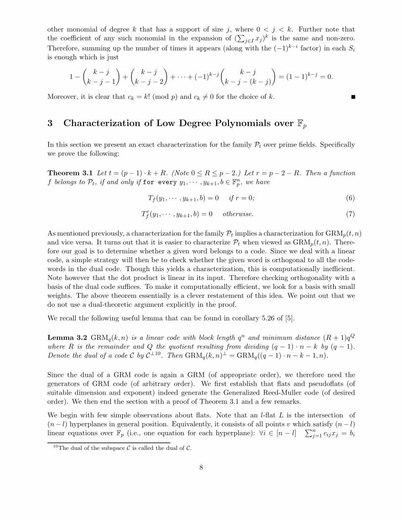
other monomial of degree k that has a support of size j, where 0 < j < k. Further note thatthe coefficient of any such monomial in the expansion of (

∑

j∈I xj)k is the same and non-zero.

Therefore, summing up the number of times it appears (along with the (−1)k−i factor) in each Si

is enough which is just

1 −

(k − j

k − j − 1

)

+

(k − j

k − j − 2

)

+ · · · + (−1)k−j

(k − j

k − j − (k − j)

)

= (1 − 1)k−j = 0.

Moreover, it is clear that ck = k! (mod p) and ck 6= 0 for the choice of k.

3 Characterization of Low Degree Polynomials over Fp

In this section we present an exact characterization for the family Pt over prime fields. Specificallywe prove the following:

Theorem 3.1 Let t = (p − 1) · k + R. (Note 0 ≤ R ≤ p − 2.) Let r = p − 2 − R. Then a functionf belongs to Pt, if and only if for every y1, · · · , yk+1, b ∈ F

np , we have

Tf (y1, · · · , yk+1, b) = 0 if r = 0; (6)

T rf (y1, · · · , yk+1, b) = 0 otherwise. (7)

As mentioned previously, a characterization for the family Pt implies a characterization for GRMp(t, n)and vice versa. It turns out that it is easier to characterize Pt when viewed as GRMp(t, n). There-fore our goal is to determine whether a given word belongs to a code. Since we deal with a linearcode, a simple strategy will then be to check whether the given word is orthogonal to all the code-words in the dual code. Though this yields a characterization, this is computationally inefficient.Note however that the dot product is linear in its input. Therefore checking orthogonality with abasis of the dual code suffices. To make it computationally efficient, we look for a basis with smallweights. The above theorem essentially is a clever restatement of this idea. We point out that wedo not use a dual-theoretic argument explicitly in the proof.

We recall the following useful lemma that can be found in corollary 5.26 of [5].

Lemma 3.2 GRMq(k, n) is a linear code with block length qn and minimum distance (R + 1)qQ

where R is the remainder and Q the quotient resulting from dividing (q − 1) · n − k by (q − 1).Denote the dual of a code C by C⊥10. Then GRMq(k, n)⊥ = GRMq((q − 1) · n − k − 1, n).

Since the dual of a GRM code is again a GRM (of appropriate order), we therefore need thegenerators of GRM code (of arbitrary order). We first establish that flats and pseudoflats (ofsuitable dimension and exponent) indeed generate the Generalized Reed-Muller code (of desiredorder). We then end the section with a proof of Theorem 3.1 and a few remarks.

We begin with few simple observations about flats. Note that an l-flat L is the intersection of(n− l) hyperplanes in general position. Equivalently, it consists of all points v which satisfy (n− l)linear equations over Fp (i.e., one equation for each hyperplane): ∀i ∈ [n − l]

∑nj=1 cijxj = bi

10The dual of the subspace C is called the dual of C.

8

where cij , bi defines the ith hyperplane (i.e., v satisfies∑n

j=1 cijvj = bi). General position meansthat the matrix cij has rank (n − l). Note that then the incidence vector of L can be written as

n−l∏

i=1

(1 − (

n∑

j=1

cijxj − bi)p−1) =

1 if (v1, · · · , vl) ∈ L

0 otherwise(8)

We record a lemma here that will be used later in this section. We leave the proof as a straightfor-ward exercise.

Lemma 3.3 For l ≥ k, the incidence vector of any l-flat is a linear sum of the incidence vectorsof k-flats.

As mentioned previously, we give an explicit basis for GRMp(r, n). For the special case of p = 3,our basis coincides with the min-weight basis given in [10].11 However, in general, our basis differsfrom the min-weight basis provided in [10].

The following Proposition shows that the incidence vectors of flats form a basis for the GeneralizedReed-Muller code of orders which are multiples of (p − 1).

Proposition 3.4 GRMp((p − 1)(n − l), n) is generated by the incidence vectors of the l-flats.

Proof : We first show that the incidence vectors of the l-flats are in GRMp((p−1)(n− l), n). Recallthat L is the intersection of (n− l) independent hyperplanes. Therefore using Equation 8, L can berepresented by a polynomial of degree at most (n− l)(p− 1) in x1, · · · , xn. Therefore the incidencevectors of l-flats are in GRMp((p − 1)(n − l), n).

We prove that GRMp((p−1)(n− l), n) is generated by l-flats by induction on n− l. When n− l = 0,the code consists of constants, which is clearly generated by n-flats i.e., the whole space.

To prove for an arbitrary (n− l) > 0, we show that any monomial of total degree d ≤ (p− 1)(n− l)can be written as a linear sum of the incidence vectors of l-flats. Let the monomial be xe1

1 · · · xett .

Rewrite the monomials as x1 · · · x1︸ ︷︷ ︸

e1 times

· · · xt · · · xt︸ ︷︷ ︸

et times

. Group into products of (p − 1) (not necessarily

distinct) variable as much as possible. Rewrite each group using Equation 5 setting k = (p − 1).For any incomplete group of size d′, use the same equation by setting the last (p− 1− d′) variablesto the constant 1. After expansion, the monomial can be seen to be a sum of product of at most

(n − l) degree (p − 1)th powered linear terms. We can add to it a polynomial of degree at most(p−1)(n−l−1) so as to represent the resulting polynomial as a sum of polynomials, each polynomialas in Equation 8. Each such non-zero polynomial is generated by a t flat, t ≥ l. By induction,the polynomial we added is generated by (l + 1) flats. Thus, by Lemma 3.3 our given monomial isgenerated by l-flats.

This leads to the following observation:

Observation 3.5 Consider an l-flat generated by y1, · · · , yl at b. Denote the incidence vector ofthis flat by I. Then the right hand side of Equation 2 may be identified as I · f , where I and fdenote the vector corresponding to respective codewords and · is the dot (scalar) product.

11The equations of the hyperplanes are slightly different in our case; nonetheless, both of them define the samebasis generated by the min-weight codewords.

9

To generate generalized Reed-Muller code of any arbitrary order, we need pseudoflats. Note thatthe points in a k-pseudoflat may alternatively be viewed as the space given by union of intersectionsof (n − k − 1) hyperplanes, where the union is parameterized by another hyperplane and whichdoes not take one particular value. Concretely, it is the set of points v which satisfy the followingconstraints over Fp:

∀i ∈ [n − k − 1]

n∑

j=1

cijxj = bi; and

n∑

j=1

cn−k,jxj 6= bn−k.

Thus the values taken by the points of a k-pseudoflat with exponent r is given by the polynomial

n−k−1∏

i=1

(1 − (

n∑

j=1

cijxj − bi)(p−1)) · (

n∑

j=1

cn−k,jxj − bn−k)r (9)

Remark 3.6 Note the difference between Equation 9 and the basis polynomial in [10] which (alongwith the action of the affine general linear group) yields the min-weight codewords:

h(x1, · · · , xm) =

k−1∏

i=1

(1 − (xi − wi)(p−1))

r∏

j=1

(xk − uj),

where w1, · · · , wk−1, u1, · · · , ur ∈ Fp.

The next lemma shows that the code generated by the incidence vectors of l-flats is a subcode ofthe code generated by the evaluation vectors of l-pseudoflats with exponent r.

Claim 3.7 The evaluation vectors of l-pseudoflats (l ≥ 1) with exponent r (r ∈ [p− 2]) generate acode containing the incidence vectors of l-flats.

Proof : Let W be the incidence vector of an l-flat generated by y1, · · · , yl at b. Clearly W =〈1, · · · , 1〉, where the ith (i ∈ [p−1]∪0) coordinate denotes the values taken by the characteristicfunctions of (l − 1)-flats generated by y2, · · · , yl at b + i · y1. Let this denote the standard basis.Let Lj be a pseudoflat with exponent r generated by y1, · · · , yl exponentiated along y1 at b+ j · y1,for each j ∈ Fp, and let Vj be the corresponding evaluation vector. Rewriting them in the standardbasis yields that Vj = 〈(p− j)r, (p− j +1)r, · · · , (p− j + i)r, · · · , (p− j− 1)r〉 ∈ F

pp. Let λj denote p

variables for t = 0, 1, · · · , (p− 1), each taking values in Fp. Then a solution to the following systemof equations

∀i ∈ [p − 1] ∪ 0 1 =∑

j∈Fp

λj(i − j)r

implies that W =∑p−1

j=0 λjVj, which suffices to establish the claim. Consider the identity

1 = (−1)∑

j∈Fp

(j + i)rjp−1−r

which may be verified by expanding and applying Lemma 2.4. Setting λj to (−1)(−j)p−1−r estab-lishes the claim.

10

The next Proposition complements Proposition 3.4. Together they say that by choosing dimensionand exponent appropriately, Generalized Reed-Muller code of any given order can be generated.This gives an equivalent representation of Generalized Reed-Muller code. An exact characterizationthen follows from this alternate representation.

Proposition 3.8 For every r ∈ [p − 2], the linear code generated by the evaluation vectors ofl-pseudoflats with exponent r is equivalent to GRMp((p − 1)(n − l) + r, n).

Proof : For the forward direction, consider an l-pseudoflat L with exponent r. Its evaluation vectoris given by an equation similar to Equation 9. Thus the codeword corresponding to the evaluationvector of this flat can be represented by a polynomial of degree at most (p − 1)(n − l) + r. Thiscompletes the forward direction.

To prove the other direction, we restrict our attention to monomials of degree at least (p−1)(n−l)+1and show that these monomials are generated by l-pseudoflats with exponent r. Since monomialsof degree at most (p−1)(n− l) is generated by l-flats, Claim 3.7 will establish the Proposition. Nowconsider any such monomial. Let the degree of the monomial be (p − 1)(n − l) + r′ (1 ≤ r′ ≤ r).Rewrite it as in Proposition 3.4. Since the degree of the monomial is (p− 1)(n− l) + r′, we will beleft with an incomplete group of degree r′. We make any incomplete group complete by adding 1’s(as necessary) to the product. We then use Lemma 2.6 to rewrite each (complete) group as a linearsum of rth powered terms. After expansion, the monomial can be seen to be a sum of product ofat most (n − l) degree (p − 1)th powered linear terms and a rth powered linear terms. Each suchpolynomial is generated either by an l-pseudoflat with exponent r or an l-flat. Claim 3.7 completesthe proof.

The following is analogous to Observation 3.5.

Observation 3.9 Consider an l-pseudoflat with exponent r, generated by y1, · · · , yl at b exponen-tiated along y1. Let E be the evaluation vector of this pseudoflat with exponent r. Then the righthand side of Equation 3 may be interpreted as E · f .

Now we prove the exact characterization.

Proof of Theorem 3.1: The proof directly follows from Lemma 3.2, Proposition 3.4, Claim 3.7and Observation 3.5 and Observation 3.9. Indeed by Observation 3.5 and Observation 3.9, Equa-tions 6 and 7 are essentially tests to determine whether the dot product of the function with everyvector in the dual space of GRM(t, n) evaluates to zero.

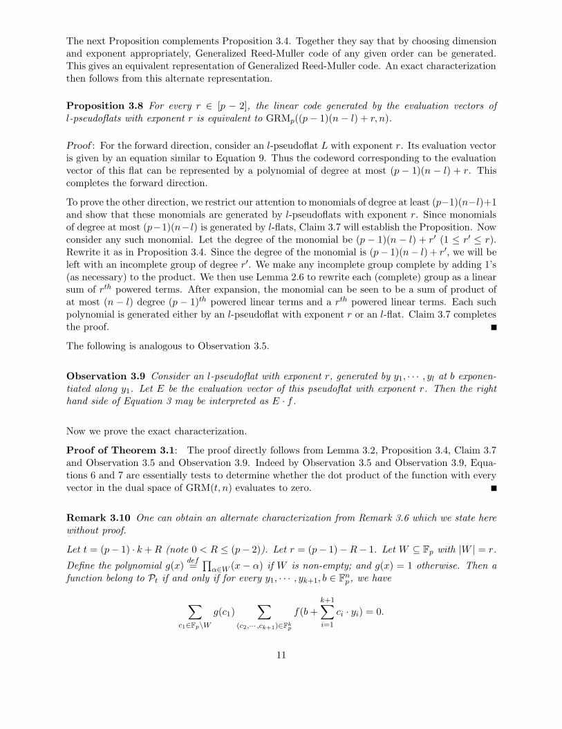
Remark 3.10 One can obtain an alternate characterization from Remark 3.6 which we state herewithout proof.

Let t = (p− 1) · k + R (note 0 < R ≤ (p − 2)). Let r = (p− 1)−R − 1. Let W ⊆ Fp with |W | = r.

Define the polynomial g(x)def=∏

α∈W (x − α) if W is non-empty; and g(x) = 1 otherwise. Then afunction belong to Pt if and only if for every y1, · · · , yk+1, b ∈ F

np , we have

∑

c1∈Fp\W

g(c1)∑

(c2,··· ,ck+1)∈Fkp

f(b +k+1∑

i=1

ci · yi) = 0.

11

Moreover, this characterization can also be extended to certain degrees for more general fields, i.e.,Fps (see the next remark).

Remark 3.11 The exact characterization of low degree polynomials as claimed in [12] may beproved using duality. Note that their proof works as long as the dual code has a min-weight basis(see [10]). Suppose that the polynomial has degree d ≤ q − q/p − 1, then the dual of GRMq(d, n)is GRMq((q − 1)n − d − 1, n) and therefore has a min-weight basis. Note that then the dual codehas min-weight (d+1). Therefore, assuming the minimum weight codewords constitute a basis, anyd + 1 evaluations of the original polynomial on a line are dependent and vice-versa. We leave thedetails as an exercise for the interested readers.

4 A Tester for Low Degree Polynomials over Fnp

In this section we present and analyze a one-sided tester for Pt. The analysis of the algorithmroughly follows the proof structure given in [17, 1]. We emphasize that the generalization from [1]to our case is not straightforward. As in [17, 1] we define a self-corrected version of the (possiblycorrupted) function being tested. The straightforward adoption of the analysis given in [17] givesreasonable bounds. However, the better bound is achieved by following the techniques developedin [1]. In there, they show that the self-corrector function can be interpolated with overwhelmingprobability. However their approach appears to use special properties of F2 and it is not clear howto generalize their technique for arbitrary prime fields. We give a clean formulation which relies onthe flats being represented through polynomials as described earlier. In particular, Claims 4.7, 4.9and their generalization appear to require our new polynomial based view.

4.1 Tester in Fp

In this subsection we describe the algorithm when underlying field is Fp.Algorithm Test-Pt in Fp

0. Let t = (p − 1) · k + R, 0 ≤ R < (p − 1). Denote r = p − 2 − R.1. Uniformly and independently at random select y1, · · · , yk+1, b ∈ F

np .

2. If T rf (y1, · · · , yk+1, b) 6= 0, then reject, else accept.

Theorem 4.1 The algorithm Test-Pt in Fp is a one-sided tester for Pt with a success probabilityat least min(Ω(pk+1ǫ), 1

2(k+7)pk+2 ).

Corollary 4.2 Repeating the algorithm Test-Pt in Fp Θ( 1pk+1ǫ

+ kpk) times, the probability of

error can be reduced to less than 1/2.

We will provide a general proof framework. However, we content ourselves by proving main technicallemmas for the case of F3. The proof idea in the general case is similar and the details are omitted.Therefore we will essentially prove the following.

Theorem 4.3 The algorithm Test-Pt in F3 is a one-sided tester for Pt with success probability atleast min(Ω(3k+1ǫ), 1

2(t+7)3t/2+1 ).

12

4.2 Analysis of Algorithm Test-Pt

In this subsection we analyze the algorithm described in Section 4.1. From Claim 3.1 it is clearthat if f ∈ Pt, then the tester accepts. Thus, the bulk of the proof is to show that if f is ǫ-farfrom Pt, then the tester rejects with significant probability. Our proof structure follows that ofthe analysis of the test in [1]. In what follows, we will denote Tf (y1, · · · , yl, b) by T 0

f (y1, · · · , yl, b)for the ease of exposition. In particular, let f be the function to be tested for membership inPt. Assume we perform Test T i

f for an appropriate i as required by the algorithm described inSection 4.1. For such an i, we define gi : F

np → Fp as follows: For y ∈ Fn

p , α ∈ Fp, denotepy,α = Pry1,··· ,yk+1

[f(y) − Tfi(y − y1, y2, · · · , yk+1, y1) = α]. Define gi(y) = α such that ∀β 6= α ∈

Fp, py,α ≥ py,β with ties broken arbitrarily. With this meaning of plurality, for all i ∈ [p − 2] ∪ 0,gi can be written as:

gi(y) = pluralityy1,··· ,yk+1

[f(y) − T i

f (y − y1, y2, · · · , yk+1, y1)]. (10)

Further we defineηi

def= Pry1,··· ,yk+1,b[T

if (y1, · · · , yk+1, b) 6= 0] (11)

The next lemma follows from a Markov-type argument.

Lemma 4.4 For a fixed f : Fnp → Fp, let gi, ηi are defined as above. Then, δ(f, gi) ≤ 2ηi.

Proof : Consider the set of elements y such that Pry1,··· ,yk+1[f(y) = f(y)−T i

f (y−y1, y2, · · · , yk+1, y1)] <1/2. If the fraction of such elements is more than 2ηi then that contradicts the condition that

ηi = Pry1,··· ,yk+1,b[Tif (y1, · · · , yk+1, b) 6= 0]

= Pry1,y2,··· ,yk+1,b[Tif (y1 − b, y2, · · · , yk+1, b) 6= 0]

= Pry,y1,··· ,yk+1[f(y) 6= f(y) − T i

f (y − y1, y2, · · · , yk+1, y1)].

Therefore, we obtain δ(f, gi) ≤ 2ηi.

Note that Pry1,··· ,yk+1[gi(y) = f(y) − T i

f (y − y1, y2, · · · , yk+1, y1)] ≥ 1p . We now show that this

probability is actually much higher. The next lemma (we omit its proof) gives a weak bound inthat direction following the analysis in [17].

Lemma 4.5 ∀y ∈ Fnp , Pry1,··· ,yk+1∈Fn

p[gi(y) = f(y) − T i

f (y − y1, y2, · · · , yk+1, y1)] ≥ 1 − 2pk+1ηi.

However, when the degree being tested is larger than the field size, we can improve the above lemmaconsiderably. The following lemma strengthens Lemma 4.5 when t ≥ (p− 1) or equivalently k ≥ 1.We now specialize to F3.

Lemma 4.6 ∀y ∈ Fn3 , Pry1,··· ,yk+1∈F

n3[gi(y) = f(y)− T i

f (y − y1, y2, · · · , yk+1, y1)] ≥ 1− (4k + 14)ηi.

Observe that the goal of the lemma is to show that at any fixed point y, if gi is interpolated outof a random hyperplane, then w.h.p. the interpolated value is the most popular vote. To ensurethis we show that the if gi is interpolated on two independently random hyperplanes, then the

13

probability that these interpolated values are same, that is the collision probability, is large. Toestimate this collision probability, we show that the difference of the interpolation values can berewritten as a sum of T i

f on small number of random hyperplanes. Thus if the test passes often

that is T if evaluates to zero w.h.p., then this sum (by a simple union bound) evaluates to zero often

and thus providing high collision.

The improvement will arise because we will express differences involving T if (· · · ) as a telescoping

series to essentially reduces the number of events in the union bound. To do this we will need thefollowing claims. They can easily be verified by expanding the terms on both sides like the proofof Claim 4 in [1]. However, this does not give much insight into the general case i.e., for Fp. Weprovide an alternate proof which can be generalized to get similar claims and has a much cleanerstructure based on the underlying geometric structure, i.e., flats or pseudoflats.

Claim 4.7 For every l ∈ 2, · · · , k+1, for every y(= y1), z, w, b, y2, · · · , yl−1, yl+1, · · · , yk+1 ∈ Fn3 ,

letSf (y, z)

def= Tf (y, y2, · · · , yl−1, z, yl+1, · · · , yk+1, b).

Then12 it holds that

Sf (y,w) − Sf (y, z) = Sf (y + w, z) + Sf (y − w, z) − Sf (y + z,w) − Sf (y − z,w).

Proof : Assume y, z, w are independent. Observe that it is enough to prove the result for k = 1and b = 0. This is because if k > 1, then we can expand the expression and regroup them with(possibly) different b’s, and we apply the above lemma and then again regroup in the right handside. Also, a linear transform (or renaming the co-ordinate system appropriately) settles the issuefor b 6= 0.

Now consider the space H generated by y, z and w at 0. Note that Sf (y,w) (with b = 0) is justf · 1L, where 1L is the incidence vector of the flat given by the equation z = 0. Therefore 1L isequivalent to the polynomial (1− z2). Similarly Sf (y, z) = f · 1L′ where L′ is given by the equation(1 − w2). We use the following polynomial identity (in F3)

w2 − z2 = [1 − (y − w)2 + 1 − (y + w)2] − [1 − (y + z)2 + 1 − (y − z)2].

Now observe that the equation (1− (y −w)2) is the incidence vector of the flat generated by y + wand z. Similar observations hold for other terms. Therefore, interpreting the above equation interms of incidence vectors of flats, we complete the proof with Observation 3.5.

We have the following analogue13 of Claim 4.7 in Fp:

Claim 4.8 For every l ∈ 2, · · · , k+1, for every y(= y1), z, w, b, y2, · · · , yl−1, yl+1, · · · , yk+1 ∈ Fnp ,

with notation used from the previous lemma, it holds that

Sf (y,w) − Sf (y, z) =∑

e∈F∗p

[Sf (y + ew, z) − Sf (y + ez,w)] .

12Note that Tf (·) is a symmetric function in all but its last input. Therefore to enhance readability, we omit thereference to index i.

13This claim can be extended over Fq in a straightforward manner. We mention here that this lemma over Fq

allows one to prove a similar version of Lemma 4.6 over Fq. That lemma along with versions of Lemma 4.15 andLemma 4.20 can be used to get a robust characterization as is done in [16].

14

Proof : (Sketch) Consider the following identity

w(p−1) − z(p−1) =∑

e∈F∗p

[

[1 − (ew + y)(p−1)] − [1 − (ez + y)(p−1)]]

(12)

then we can prove the claim along the same lines as the alternate proof of Claim 4.7. We completethe proof by proving Equation 12. Consider the sum:

∑

e∈F∗p(ew+y)(p−1). Expanding the terms and

rearranging the sums we get∑(p−1)

j=0

((p−1)j

)w(p−1)−jyj

∑

e∈F∗pej . By Lemma 2.4 the sum evaluates

to (−w(p−1)−y(p−1)). Similarly,∑

e∈F∗p(ez+y)(p−1) = (−z(p−1)−y(p−1)) which proves Equation 12.

Claim 4.9 For every l ∈ 2, · · · , k+1, for every y(= y1), z, w, b, y2, · · · , yl−1, yl+1, · · · , yk+1 ∈ Fn3 ,

denoteS1

f (y,w)def= T 1

f (y, y2, · · · , yl−1, w, yl+1, · · · , yk+1, b).

Then14 it holds that

S1f (y,w) − S1

f (y, z) = S1f (y + z,w) + S1

f (y − z,w) − S1f (y + w, z) − S1

f (y − w, z).

Proof : Note here that the defining equation of S1f (y, z) is y(1 − w2). Now consider the following

identity in F3:

y(z2 − w2) = (y + w)[1 − (y − w)2] + (y − w)[1 − (y + w)2]

−(y + z)[1 − (y − z)2] − (y − z)[1 − (y + z)2

for variables y, z, w ∈ F3. Rest of the proof is similar to the proof of Claim 4.7 (the proof replacesflats by pseudoflats) and is omitted.

We now prove the following analogue in Fp:

Claim 4.10 For every i ∈ 1, · · · , p − 2, for every l ∈ 2, · · · , k + 1 and for everyy(= y1), z, w, b, y2, · · · , yl−1, yl+1, · · · , yk+1 ∈ F

np , denote

Sif (y,w)

def= T i

f (y, y2, · · · , yl−1, w, yl+1, · · · , yk+1, b).

Then there exists ci such that

Sif (y,w) − Si

f (y, z) = ci

∑

e∈F∗p

[Si

f (y + ew, z) − Sif (y + ez,w)

].

Proof : Observe that T if (y, z) = f · ELi , where ELi denotes the evaluation vector of the pseudoflat

L with exponent i, generated by y, z at b exponentiated along y. Note that the polynomial definingELi is just yi(w(p−1) − 1). We now give an identity similar to that of Equation 12 that completesthe proof. We claim that the following identity holds

yi(w(p−1) − z(p−1)) = ci

∑

e∈F∗p

[

(y + ew)i[1 − (y − ew)(p−1)] − (y + ez)i[1 − (y − ez)(p−1)]]

. (13)

14Note that T if (·) is a symmetric function in its all but last and first input. Therefore to enhance readability, we

omit the reference to index l.

15

where ci = 2i. Before we prove the identity, note that (−1)j((p−1)

j

)= 1 in Fp. This is because for

1 ≤ m ≤ j, m = (−1)(p − m). Therefore j! = (−1)j (p−1)!(p−j−1)! holds in Fp. Substitution yields the

desired result. Also note that∑

e∈F∗p(y+ew)i = −yi (expand and apply Lemma 2.4). Now consider

the sum

∑

e∈F∗p

(y + ew)i(y − ew)(p−1) =∑

e∈F∗p

∑

0≤j≤i;0≤m≤(p−1)

(−1)m(

i

j

)(p − 1

m

)

y(p−1)+i−j−mwj+mej+m

=∑

0≤j≤i;0≤m≤(p−1)

(−1)m(

i

j

)(p − 1

m

)

y(p−1)+i−j−mwj+m∑

e∈F∗p

ej+m

= (−1)[y(p−1)+i + (−1)(p−1)i∑

j=0

(i

j

)(p − 1

j

)

(−1)j

︸ ︷︷ ︸

1

yiw(p−1)]

= (−1)[yi + yiw(p−1)2i] (14)

Similarly one has∑

e∈F∗p(y + ez)i(y− ez)(p−1) = (−1)[yi + yiz(p−1)2i]. Substituting and simplifying

one gets Equation 13.

We will also need the following claims.

Claim 4.11 For every l ∈ 2, · · · , k + 1, y(= yl), z, w, b, y2, · · · , yl−1, yl+1, · · · , yk+1 ∈ Fn3 , with

notation used in previous lemma, it holds that

S1f (w, y)−S1

f (z, y) = S1f (z+w, y−z)−S1

f (z+w, y−w)+S1f (y+z,w)+S1

f (y−z,w)−S1f (y+w, z)−S1

f (y−w, z).

Proof : The above follows from the identity

w(1 − z2) − z(1 − w2) = (z + w)[1 − (z + y)2 − 1 + (y + w)2] + y(w2 − z2)

Also we can expand y(w2 − z2) as in the proof of Claim 4.9.

Claim 4.12 For every i ∈ 1, · · · , p − 2, for every l ∈ 2, · · · , l + 1 and for everyy(= yl), z, w, b, y2, · · · , yl−1, yl+1, · · · , yk+1 ∈ F

np , there exists ci ∈ F

∗p such that

Sif (w, y) − Si

f (z, y) =∑

e∈F∗p

[Si

f (y + ew, y − ew) − Sif (w + ey,w − ey) + Si

f (z + ey, z − ey)

−Sif (y + ez, y − ez) + ci

[Si

f (y + ew, z) − Sif (y + ez,w)

]]

Proof : The above follows from the identity

wi(1− z(p−1))− zi(1−w(p−1)) = (wi − yi)(1− z(p−1))− (zi − yi)(1−w(p−1)) + yi(w(p−1) − z(p−1)).

We also use that∑

e∈F∗p(w + ey)i = −wi and Claim 4.10 to expand the last term. Note that ci = 2i

as before.

16

Proof of Lemma 4.6: We first prove the lemma for g0(y). We fix y ∈ Fn3 and let γ

def=

Pry1,··· ,yk+1∈Fn3[g0(y) = f(y) − Tf (y − y1, y2, · · · , yk+1, y1)]. Recall that we want to lower bound

γ by 1 − (4k + 14)η0. In that direction, we bound a slightly different but related probability. Let

µdef= Pry1,··· ,yk+1,z1,··· ,zk+1∈Fn

3[Tf (y − y1, y2, · · · , yk+1, y1) = Tf (y − z1, z2, · · · , zk+1, z1)]

Denote Y = 〈y1, · · · , yk+1〉 and similarly Z. Then by the definitions15 of µ and γ we have, γ ≥ µ.

We have µ = Pry1,··· ,yk+1,z1,··· ,zk+1∈Fn3[Tf (y − y1, y2, · · · , yk+1, y1) − Tf (y − z1, z2, · · · , zk+1, z1) = 0].

Now, for any choice of y1, · · · , yk+1 and z1, · · · , yk+1:Tf (y − y1, y2, · · · , yk+1, y1) − Tf (y − z1, z2, · · · , zk+1, z1) =Tf (y − y1, y2, · · · , yk+1, y1) − Tf (y − y1, y2, · · · , yk, zk+1, y1) +Tf (y − y1, y2, · · · , yk, zk+1, y1) − Tf (y − y1, y2, · · · , yk−1, zk, zk+1, y1) +Tf (y − y1, y2, · · · , yk−1, zk, zk+1, y1) − Tf (y − y1, y2, · · · , yk−2, zk−1, zk, zk+1, y1) +...Tf (y − y1, z2, z3, · · · , zk+1, y1) − Tf (y − z1, z2, · · · , zk+1, y1) +Tf (y − z1, z2, z3, · · · , zk+1, y1) − Tf (y − y1, z2, · · · , zk+1, z1) +Tf (y − y1, z2, z3, · · · , zk+1, z1) − Tf (y − z1, z2, · · · , zk+1, z1)

Consider any pair Tf (y − y1, y2, · · · , yl, zl+1, · · · , zk+1, y1)− Tf (y − y1, y2, · · · , yl−1, zl, · · · , zk+1, y1)that appears in the first k “rows” in the sum above. Note that Tf (y−y1, y2, · · · , yl, zl+1, · · · , zk+1, y1)and Tf (y − y1, y2, · · · , yl−1, zl, · · · , zk+1, y1) differ only in a single parameter. We apply Claim 4.7and obtain:Tf (y − y1, y2, · · · , yl, zl+1, · · · , zk+1, y1) − Tf (y − y1, y2, · · · , yl−1, zl, · · · , zk+1, y1) =Tf (y − y1 + yl, y2, · · · , yl−1, zl, · · · , zk+1, y1) + Tf (y − y1 − yl, y2, · · · , yl−1, zl, · · · , zk+1, y1)−Tf (y − y1 + zl, y2, · · · , yl, zl+1, · · · , zk+1, y1) − Tf (y − yl − zl, y2, · · · , yl, zl+1, · · · , zk+1, y1).

Recall that y is fixed and y2, · · · , yk+1, z2, · · · , zk+1 ∈ Fn3 are chosen uniformly at random, so all the

parameters on the right hand side of the equation are independent and uniformly distributed.Similarly one can expand the pairs Tf (y − y1, z2, z3, · · · , zk+1, y1) − Tf (y − z1, z2, · · · , zk+1, y1)and Tf (y − y1, z2, z3, · · · , zk+1, z1) − Tf (y − z1, z2, · · · , zk+1, z1) into four Tf with all parametersbeing independent and uniformly distributed16. Finally notice that the parameters in both Tf (y −z1, z2, z3, · · · , zk+1, y1) and Tf (y − z1, z2, · · · , zk+1, y1) are independent and uniformly distributed.Further recall that by the definition of η0, Prr1,··· ,rk+1

[Tf (r1, · · · , rk+1) 6= 0] ≤ η0 for independentand uniformly distributed ris. Thus, by the union bound, we have:

Pry1,··· ,yk+1,z1,··· ,zk+1∈Fn3[Tf (y1, · · · , yk+1)−Tf (z1, · · · , zk+1) 6= 0] ≤ (4k+10)η0 ≤ (4k+14)η0. (15)

Therefore γ ≥ µ ≥ 1 − (4k + 14)η0. A similar argument17 proves the Lemma for g1(y).

Remark 4.13 Analogously, in the case Fp we have: for every y ∈ Fnp , Pry1,y2,··· ,yk+1∈Fn

p[gi(y) =

f(y) − T if (y − y1, y2, · · · , yk+1, y1) + f(y)] ≥ 1 − 2((p − 1)k + 6(p − 1) + 1)ηi.

15Note for a probability vector v ∈ [0, 1]n, v

∞= Maxi∈[n]vi ≥ Maxi∈[n]vi · (

Pni=1 vi) =

Pni=1 vi ·

Maxi∈[n]vi ≥Pn

i=1 v2i =

v 2

2.

16Since Tf (·) is symmetric.17Tf1

(.) is not symmetric and needs some work. We use another identity as given in Lemma 4.11 to resolve theissue and get four extra terms than in the case of g0. The proof for g1(y) is same as the proof for g0(y) except it alsoneeds Lemma 4.11.

17

The proof is similar to that of Lemma 4.6 where it can be shown µi ≥ 1−2((p−1)k+6(p−1)+1)ηi,for each µi defined for gi(y).

Remark 4.14 Using Lemma 4.6, we can get a slightly stronger version of Lemma 4.4 followingthe proof of Lemma 2 in [1]. For a fixed function f : F

np → Fp, let gi, ηi are defined as in Equations

10 and 11. Then, δ(f, gi) ≤ min(2ηi,ηi

1−2((p−1)k+6(p−1)+1)ηi).

The next lemma shows that sufficiently small ηi implies that gi self-corrects the function f .

Lemma 4.15 Over F3, if ηi < 12(2k+7)3k+1 , then the function gi belongs to Pt (assuming k ≥ 1).

Proof : From Claim 3.1, it suffices to prove that if ηi < 12(2k+7)3k+1 then T i

gi(y1, · · · , yk+1, b) = 0

for every y1, · · · , yk+1, b ∈ Fn3 . Let fix the choice of y1, · · · , yk+1, b. Denote Y = 〈y1, · · · , yk+1〉. We

express T igi

(Y, b) as the sum of T if (·) with random arguments. Suppose we uniformly select (k +1)2

random variables zi,j over Fn3 for 1 ≤ i ≤ k + 1, and 1 ≤ j ≤ k + 1. Denote Zi = 〈zi,1, · · · , zi,k+1〉.

We also select uniformly (k + 1) random variables ri over Fn3 for 1 ≤ i ≤ k + 1. We use zi,j and

ri’s to set up the random arguments. Now by Lemma 4.6, for every I ∈ Fk+13 (i.e. think of I as an

ordered (k + 1)-tuple over 0, 1, 2), with probability at least 1− 2(2k + 7)ηi over the choice of zi,j

and ri,

gi(I ·Y + b) = f(I ·Y + b)−T if(I ·Y + b− I ·Z1−r1, I ·Z2 +r2, · · · , I ·Zk+1 +rk+1, I ·Z1 +r1), (16)

where I = 〈I1, · · · , Ik+1〉, Y · X =∑k+1

i=1 YiXi, holds.

Let E1 be the event that Equation 16 holds for all I ∈ Fk+13 . By the union bound:

Pr[E1] ≥ 1 − 3k+1 · 2(2k + 7)ηi. (17)

Assume that E1 holds. We now need the following claims. Let J = 〈J1, · · · , Jk+1〉 be a (k + 1)dimensional vector over F3, and denote J ′ = 〈J2, · · · , Jk+1〉.

Claim 4.16 If Equation 16 holds for all I ∈ Fk+13 , then

T 0g0

(Y, b) =∑

06=J ′∈Fk3

[

−Tf (y1 +

k+1∑

t=2

Jtzt,1, · · · , yk+1 +

k+1∑

t=2

Jtzt,(k+1), b +

k+1∑

t=2

Jtrt)

]

+∑

J ′∈Fk3

[

−Tf (2y1 − z1,1 +k+1∑

t=2

Jtzt,1, · · · , 2yk+1 − z1,(k+1) +k+1∑

t=2

Jtzt,(k+1), 2b − r1 +k+1∑

t=2

Jtrt)

+ Tf (z1,1 +k+1∑

t=2

Jtzt,1, · · · , z1,k+1 +k+1∑

t=2

Jtzt,(k+1), r1 +k+1∑

t=2

Jtrt)

]

(18)

,

18

Claim 4.17 If Equation 16 holds for all I ∈ Fk+13 , then

T 1g1

(Y, b) =∑

06=J ′∈Fk3

[

−T 1f (y1 +

k+1∑

t=2

Jtzt,1, · · · , yk+1 +k+1∑

t=2

Jtzt,(k+1), b +k+1∑

t=2

Jtrt)

]

+∑

J ′∈Fk3

[

T 1f (2y1 − z1,1 +

k+1∑

t=2

Jtzt,1, · · · , 2yk+1 − z1,(k+1) +k+1∑

t=2

Jtzt,(k+1), 2b − r1 +k+1∑

t=2

Jtrt)

]

.

(19)

The proofs of Claim 4.16 and Claim 4.17 are deferred to the appendix. Let E2 be the event thatfor every J ′ ∈ F

k3, T

if (y1 +

∑

t Jtzt,1, · · · , yk+1 +∑

t Jtzt,(k+1), b +∑

t=2 k + 1Jtrt) = 0

and T if (2y1 − z1,1 +

∑k+1t=2 Jtzt,1, · · · , 2yk+1 − z1,k+1 +

∑k+1t=2 Jtzt,(k+1), 2b − r1 +

∑k+1t=2 Jtrt) = 0,

and Tf (z1,1 +∑k+1

t=2 Jtzt,1, · · · , z1,k+1 +∑k+1

t=2 Jtzt,k+1, r1 +∑k+1

t=2 Jtrt) = 0. By Claim 4.16, and thedefinition of ηi we have:

Pr[E2] ≥ 1 − 3k+1ηi. (20)

Suppose that ηi ≤1

2(2k+7)3k+1 holds. Then by Equations 17 and 20, the probability that E1 and

E2 hold is strictly positive. In other words, there exists a choice of the zi,j ’s and ri’s for which allsummands in either Claim 4.16 or in Claim 4.17, whichever is appropriate, is 0. But this impliesthat T i

gi(y1, · · · , yk+1, b) = 0. We conclude that if ηi ≤

12(2k+7)3k+1 , then gi belongs to Pt.

Remark 4.18 Over Fp we have: if ηi < 12((p−1)k+6(p−1)+1)pk+1 , then gi belongs to Pt (if k ≥ 1).

In case of Fp, we can generalize Equation 16 straightforwardly. Let denote the probability that allsuch events holds. We can similarly obtain

Pr[E1] ≥ 1 − pk+1 · 2((p − 1)k + 6(p − 1) + 1)ηi. (21)

Claim 4.19 Assume equivalent of Equation 16 holds for all I ∈ Fk+1p , then18

T igi

(Y, b) =∑

06=J ′∈Fkp

[

−T if (y1 +

k+1∑

t=2

Jtzt,1, · · · , yk+1 +k+1∑

t=2

Jtzt,(k+1), b +k+1∑

t=2

Jtrt)

]

+∑

J ′∈Fkp

∑

J1∈Fp;J1 6=1

J i1

[

−T if (J1y1 − (J1 − 1)z1,1 +

k+1∑

t=2

Jtzt,1, · · · , J1yk+1 − (J1 − 1)z1,(k+1)

+

k+1∑

t=2

Jtzt,(k+1), J1b − (J1 − 1)r1 +

k+1∑

t=2

Jtrt)

]]

(22)

Let E2 be the analogous event. Then by the above claim and by Remark 4.13 we have

Pr[E2] ≥ 1 − 2pk+1ηi. (23)

18Recall that we are using the convention 00 = 1.

19

Then if we are given that ηi < 12((p−1)k+6(p−1)+1)pk+1 , then the probability that E1 and E2 holds is

strictly positive. Therefore, this implies T igi

(y1, · · · , yk+1, b) = 0.

By combining Lemma 4.4 and Lemma 4.15 we obtain that if f is Ω(1/(k3k))-far from Pt thenηi = Ω(1/(k3k)). We next consider the case in which ηi is small. By Lemma 4.4, in this case,the distance δ = δ(f, g) is small. The next lemma shows that in this case the test rejects f withprobability that is close to 3k+1δ. This follows from the fact that in this case, the probability overthe selection of y1, · · · , yk+1, b, that among the 3k+1 points

∑

i ciyi + b, the functions f and g differin precisely one point, is close to 3k+1 · δ. Observe that ff they do, then the test rejects.

Lemma 4.20 Suppose 0 ≤ ηi ≤1

2(2k+7)3k+1 . Let δ denote the relative distance between f and g,

ℓ = 3k+1, and Qdef= (1−ℓδ

1+ℓδ ) · ℓδ. Then, when y1, · · · , yk+1, b are chosen randomly, the probabilitythat for exactly one point v among the ℓ points

∑

i Ciyi + b, f(v) 6= g(v) is at least Q.

Observe that ηi = Ω(Q) = Ω(3k+1δ).Proof of Lemma 4.20: For each C ∈ F

k+13 , let XC be the indicator random variable whose value

is 1 if and only if f(C · Y + b) 6= g(C · Y + b). Clearly, Pr[XC = 1] = δ for every C. It followsthat the random variable X =

∑

C XC which counts the number of points v of the required formin which f(v) 6= g(v) has expectation E[X] = 3k+1δ = ℓ · δ. It is not difficult to check that therandom variables XC are pairwise independent, since for any two distinct C1 and C2, the sums∑k+1

i=1 C1,i + b and∑k+1

i=1 C2,i + b attain each pair of distinct values in Fn3 with equal probability

when the vectors are chosen randomly and independently. Since XC ’s are pairwise independent,Var[X] =

∑

C Var[XC ]. Since XC ’s are boolean random variables, we note

Var[XC ] = E[X2C ] − (E[XC ])2 = E[XC ] − (E[XC ])2 ≤ E[XC ].

Thus we obtain Var[X] ≤ E[X], so E[X2] ≤ E[X]2 + E[X]. Next we use the following inequalityfrom [1] which holds for a random variable X taking nonnegative, integer values,

Pr[X > 0] ≥(E[X])2

E[X2].

In our case, this implies

Pr[X > 0] ≥(E[X])2

E[X2]≥

(E[X])2

E[X] + (E[X])2=

E[X]

1 + E[X].

Therefore,

E[X] ≥ Pr[X = 1]+2Pr[X = 2] = Pr[X = 1]+2

(E[X]

1 + E[X]− Pr[X = 1]

)

=2E[X]

1 + E[X]− Pr[X = 1].

After simplification we obtain,

Pr[X = 1] ≥1 − E[X]

1 + E[X]· E[X].

Using the earlier bound obtained for E[X], the desired result follows.

20

Proof of Theorem 4.3: Clearly if f belongs to Pt, then by Claim 3.1 the tester accepts f withprobability 1.

Therefore let δ(f,Pt) ≥ ǫ. Let d = δ(f, gr), where r as in algorithm Test-Pt. If η < 12(2k+7)3k+1

then by Lemma 4.15 gr ∈ Pt and, by Lemma 4.20, ηi = Ω(3k+1 · d) = Ω(3k+1ǫ). Hence ηi ≥

min(

Ω(3k+1ǫ), 12(2k+7)3k+1

)

.

Remark 4.21 Analogously Theorem 4.1 follows.

5 A Lower Bound and Improved Self-correction

5.1 A Lower Bound

The next theorem is a simple modification of a theorem in [1] and essentially implies that our resultis almost optimal.

Proposition 5.1 Let F be any family of functions f : Fnp → Fp that corresponds to a linear code

C. Let d denote the minimum distance of the code C and let d denote the minimum distance of thedual code of C.Every one-sided testing algorithm for the family F must perform Ω(d) queries, and if the distanceparameter ǫ is at most d/pn+1, then Ω(1/ǫ) is also a lower bound for the necessary number ofqueries.

Lemma 3.2 and Proposition 5.1 gives us the following corollary.

Corollary 5.2 Every one-sided tester for testing Pt with distance parameter ǫ must perform Ω(max(1ǫ , (1+

((t + 1) mod (p − 1)))pt+1p−1 )) queries.

5.2 Improved Self-correction

From Lemmas 4.4, 4.6 and 4.15 the following corollary is immediate:

Corollary 5.3 Consider a function f : Fn3 → F3 that is ǫ-close to a degree-t polynomial g : F

n3 →

F3, where ǫ < 12(2k+7)3k+1 . (Assume k ≥ 1.) Then the function f can be self-corrected. That is,

for any given x ∈ Fn3 , it is possible to obtain the value g(x) with probability at least 1 − 3k+1ǫ by

querying f on 3k+1 points on Fn3 .

An analogous result may be obtained for the general case. We, however, improve the above corollaryslightly. The above corrector does not allow any errors in the 3k+1 points it queries. We obtain astronger result by querying on a slight larger flat H, but allowing some errors. Errors are handledby decoding the induced Generalized Reed-Muller code code on H.

Proposition 5.4 Consider a function f : Fnp → Fp that is ǫ-close to a degree-t polynomial g :

Fnp → Fp. Then the function f can be self-corrected. That is, assume K > (k + 1), then for any

21

given x ∈ Fnp , the value of g(x) can be obtained with probability at least 1 − ǫ

(1−ǫ·pk+1)2· p−(K−2k−3)

from queries to f .

Proof : Our goal is to correct the GRMp(t, n) at the point x. Assume t = (p−1) ·k +R, where 0 ≤R ≤ (p−2). Then the relative distance of the code δ is (1−R/p)p−k. Note that 2p−k−1 ≤ δ ≤ p−k.Recall that the local testability test requires a (k + 1)-flat, i.e., it tests

∑

c1,··· ,ck+1∈Fpcp−2−R1 f(y0 +

∑k+1i=1 ciyi) = 0, where yi ∈ F

np .

We choose a slightly larger flat, i.e., a K-flat with K > (k + 1) to be chosen later. We consider thecode restricted to this K-flat with point x being the origin. We query f on this K-flat. It is knownthat a majority logic decoding algorithm exists that can decode Generalized Reed-Muller code upto half the minimum distance for any choice of parameters (see [18]). Thus if the number of erroris small we can recover g(x).

Let the relative distance of f from the code be ǫ and let S be the set of points where it disagreeswith the closest codeword. Let the random K-flat be H = x +

∑Ki=1 tiui|ti ∈ F, ui ∈R F

np.

Let the random variable Y〈t1,··· ,tK〉 take the value 1 if x +∑K

i=1 uiti ∈ S and 0 otherwise. Let

D = FK \ 0 and U = 〈u1, · · · , uK〉. Define Y =

∑

〈t1,··· ,tK〉∈D Y〈t1,··· ,tK〉 and ℓ = (pK − 1). Wewould like to bound the probability

PrU [|Y − ǫℓ| ≥ (δ/2 − ǫ)ℓ].

Since PrU [Yt1,··· ,tK = 1] = ǫ, by linearity we get EU [Y ] = ǫℓ. Let T = 〈t1, · · · , tK〉. Now

V ar[Y ] =∑

T∈FK−0

V ar[YT ] +∑

T 6=T ′

Cov[YT , YT ′ ]

= ℓ(ǫ − ǫ2) +∑

T 6=λT ′

Cov[YT , YT ′ ]

+∑

T=λT ′;16=λ∈F∗

Cov[YT , YT ′ ]

≤ ℓ(ǫ − ǫ2) + ℓ · (p − 2)(ǫ − ǫ2)

= ℓ(ǫ − ǫ2)(p − 1)

The above follows from the fact that when T 6= λT ′ then the corresponding events YT and YT ′

are independent and therefore Cov[YT , YT ′ ] = 0. Also, when YT and YT ′ are dependent thenCov[YT , YT ′ ] = EU [YT YT ′ ] − EU [YT ]EU [YT ′ ] ≤ ǫ − ǫ2.Therefore, by Chebyshev’s inequality we have (assuming ǫ < p−(k+1))

PrU [|Y − ǫℓ| ≥ (δ/2 − ǫ)ℓ] ≤ℓǫ(1 − ǫ)(p − 1)

(δ/2 − ǫ)2ℓ2

Now note (δ/2 − ǫ) ≥ (p−k−1 − ǫ) = (1 − ǫ · pk+1)p−k−1. We thus have

PrU [|Y − ǫℓ| ≥ (δ/2 − ǫ)ℓ] ≤ǫ(1 − ǫ)(p − 1)

(1 − ǫ · pk+1)2p−2k−2ℓ

≤ǫp

(1 − ǫ · pk+1)2p−2k−2(ℓ + 1)

=ǫ

(1 − ǫ · pk+1)2· p−(K−2k−3).

22

6 Conclusions

The lower bound following Corollary 5.2 implies that our upper bound is almost tight. We resolvedthe question posed in [1] for all prime fields. Independently in [16] the question has been resolved forall fields. We mention that later we found an alternate proof to their characterization of polynomialsover general field.

Recently Kaufman and Litsyn ([15]) show that the dual of BCH codes are locally testable too.They also give a sufficient condition for a code to be locally testable. The condition roughly saysthat if the number of fixed length codewords in the dual to the union of the code and its ǫ-far cosetis suitably smaller than the same in the dual of the code, then the code is locally testable. Theirargument is more combinatorial in nature and needs the knowledge of weight-distribution of thecode and thus differs from the self-correction approach.

Therefore though they resolve another open question from Alon et. al. [1], the more general conjec-ture is still open. The conjecture claims that any linear code with small (constant) dual distance,having a doubly transitive group acting on the co-ordinates of the codewords mapping the dualcode to itself, is locally testable. It will be interesting to resolve the conjecture.

6.1 Acknowledgment

The second author wishes to thank Felipe Voloch for motivating discussions in an early stage ofthe work.

References

[1] N. Alon, T. Kaufman, M. Krivelevich, S. Litsyn, and D. Ron. Testing Low-Degree Ploynomialsover GF(2). In Proc. of RANDOM 03, 2003.

[2] S. Arora, C. Lund, R. Motwani, M. Sudan, and M. Szegedy. Proof verification and the in-tractability of approximation problems. In Proc. of IEEE Symposium of the Foundation ofComputer Science, pages 14–23, 1992.

[3] S. Arora and S. Safra. Probabilistic chekcing of proofs: A new characterization of np. In Proc.of IEEE Symposium of the Foundation of Computer Science, pages 2–13, 1992.

[4] S. Arora and M. Sudan. Improved low-degree testing and its application. In Proc. of Symposiumon the Theory of Computing, 1997.

[5] E. F. Assumus Jr. and J. D. Key. Polynomial codes and Finite Geometries in Handbook ofCoding Theory, Vol II , Edited by V. S. Pless Jr., and W. C. Huffman, chapter 16. Elsevier,1998.

[6] L. Babai, L. Fortnow, L. Levin, and M. Szegedy. Checking computations in polylogarithmictime. In Proc. of Symposium on the Theory of Computing, pages 21–31, 1991.

[7] L. Babai, L. Fortnow, and C. Lund. Non-deterministic exponential time has two prover inter-active protocols. In Computational Complexity, pages 3–40, 1991.

23

[8] M. Blum, M. Luby, and R. Rubinfeld. Self-testing/correcting with applications to numericalproblems. Journal of Computer and System Sciences, 47:549–595, 1993.

[9] P. Delsarte, J. M. Goethals, and F. J. MacWillams. On generalized reed-muller codes andtheir relatives. Information and Control, 16:403–442, 1970.

[10] P. Ding and J. D. Key. Minimum-weight codewords as generators of generalized reed-mullercodes. IEEE Trans. on Information Theory., 46:2152–2158, 2000.

[11] U. Fiege, S. Goldwasser, L. Lovasz, S. Safra, and M. Szegedy. Approximating clique is almostnp-complete. In Proc. of IEEE Symposium of the Foundation of Computer Science, pages2–12, 1991.

[12] K. Friedl and M. Sudan. Some improvements to total degree tests. In Proceedings of the3rd Annual Israel symposium on Theory of Computing and Systems, pages 190–198, 1995.Corrected version available at http://theory.lcs.mit.edu/∼madhu/papers/friedl.ps.

[13] P. Gemmell, R. Lipton, R. Rubinfeld, M. Sudan, and A. Wigderson. Self-testing/correctingfor polynomials and for approxiamte functions. In Proc. of Symposium on the Theory ofComputing, 1991.

[14] C. S. Jutla, A. C. Patthak, and A. Rudra. Testing polynomials over general fields. manuscript,2004.

[15] T. Kaufman and S. Litsyn. Almost orthogonal linear codes are locally testable. In To appearin Proc. of IEEE Symposium of the Foundation of Computer Science, 2005.

[16] T. Kaufman and D. Ron. Testing polynomials over general fields. In Proc. of IEEE Symposiumof the Foundation of Computer Science, 2004.

[17] R. Rubinfeld and M. Sudan. Robust characterizations of polynomials with applications toprogram testing. SIAM Journal on Computing, 25(2):252–271, 1996.

[18] M. Sudan. Lecture notes on algorithmic introduction to coding theory, Fall 2001. Lecture 15.

A Omitted Proofs from Section 4

Proof of Lemma 4.5: We will use I, J, I ′, J ′ to denote (k + 1) dimensional vectors over Fp. Nownote that

gi(y) = Pluralityy1,··· ,yk+1∈Fnp[−

∑

I∈Fk+1p ;I 6=〈1,0,··· ,0〉

Ii1f(I1(y − y1) +

k+1∑

t=2

Ityt + y1)]

= Pluralityy−y1,y2,··· ,yk+1∈Fnp[−

∑

I∈Fk+1p ;I 6=〈0,··· ,0〉

(I1 + 1)if(I1(y − y1) +k+1∑

t=2

Ityt + y)]

= Pluralityy1,··· ,yk+1∈Fnp[−

∑

I∈Fk+1p ;I 6=〈0,··· ,0〉

(I1 + 1)if(k+1∑

t=1

Ityt + y)] (24)

24

Let Y = 〈y1, · · · , yk+1〉 and Y ′ = 〈y′1, · · · , y′k+1〉. Also we will denote 〈0, · · · , 0〉 by ~0. Now notethat

1 − ηi ≤ Pry1,··· ,yk+1,b[Tif (y1, · · · , yk+1, b) = 0] (25)

= Pry1,··· ,yk+1,b[∑

I∈Fk+1p

Ii1f(b + I · Y ) = 0]

= Pry1,··· ,yk+1,b[f(b + y1) +∑

I∈Fk+1p ;I 6=〈1,0,··· ,0〉

Ii1f(b + I · Y ) = 0]

= Pry1,··· ,yk+1,y[f(y) +∑

I∈Fk+1p ;I 6=〈1,0,··· ,0〉

Ii1f(y − y1 + I · Y ) = 0]

= Pry1,··· ,yk+1,y[f(y) +∑

I∈Fk+1p ;I 6=〈0,··· ,0〉

(I1 + 1)if(y + I · Y ) = 0]

(26)

Therefore for any given I 6= ~0 we have the following:

PrY,Y ′ [f(y + I · Y ) =∑

J∈Fk+1p ;J 6=~0

−(J1 + 1)if(y + I · Y + J · Y ′)] ≥ 1 − ηi

and for any given J 6= ~0,

PrY,Y ′ [f(y + J · Y ′) =∑

I∈Fk+1p ;I 6=~0

−(I1 + 1)if(y + I · Y + J · Y ′)] ≥ 1 − ηi.

Combining the above two and using the union bound we get,

PrY,Y ′ [∑

I∈Fk+1p ;I 6=~0

(I1 + 1)if(y + I · Y ) =∑

I∈Fk+1p ;I 6=~0

∑

J∈Fk+1p ;J 6=~0

−(I1 + 1)i(J1 + 1)if(y + I · Y + J · Y ′)

=∑

J∈Fk+1p ;J 6=~0

(J1 + 1)if(y + J · Y ′)]

≥ 1 − 2(pk+1 − 1)η ≥ 1 − 2pk+1ηi (27)

The lemma now follows from the observation that the probability that the same object is drawnfrom a set in two independent trials lower bounds the probability of drawing the most likely objectin one trial: Suppose the objects are ordered so that pi is the probability of drawing object i, andp1 ≥ p2 ≥ · · · . Then the probability of drawing the same object twice is

∑

i p2i ≤

∑

i p1pi ≤ p1.

25

Proof of Claim 4.16:

Tg(Y, b) =∑

I∈Fk+13

g(I · Y + b)

=∑

I∈Fk+13

[−Tf (I · Y + b − I · Z1 − r1, I · Z2 + r2, · · · , I · Zk+1 + rk+1, I · Z1 + r1)

+f(I · Y + b)]

= −∑

I∈Fk+13

∑

∅6=J ′∈Fk3

f(I · Y + b +

k+1∑

t=2

JtI · Zt +

k+1∑

t=2

Jtrt)

+

∑

J ′∈F k3

(

f(2I · Y + 2b − I · Z1 − r1 +

k+1∑

t=2

JtI · Zt +

k+1∑

t=2

Jtrt)

+f(I · Z1 + r1 +

k+1∑

t=2

JtI · Zt +

k+1∑

t=2

Jtrt)

)]]

= −∑

06=J ′∈Fk3

∑

I∈Fk+13

f(I · Y + b +

k+1∑

t=2

Jtrt +

k+1∑

t=2

JtI · Zt)

−∑

J ′∈Fk3

∑

I∈Fk+13

f(2I · Y + 2b − I · Z1 − r1 +

k+1∑

t=2

JtI · Zt +

k+1∑

t=2

Jtrt)

+

∑

I∈Fk+13

f(I · Z1 + r1 +

k+1∑

t=2

JtI · Zt +

k+1∑

t=2

Jtrt)

=∑

06=J ′∈Fk3

[

−Tf (y1 +k+1∑

t=2

Jtzt,1, · · · , yk+1 +k+1∑

t=2

Jtzt,(k+1), b +k+1∑

t=2

Jtrt)

]

+∑

J ′∈Fk3

[

−Tf (2y1 − z1,1 +k+1∑

t=2

Jtzt,1, · · · , 2yk+1 − z1,(k+1) +k+1∑

t=2

Jtzt,(k+1), 2b − r1 +k+1∑

t=2

Jtrt)

+ Tf (z1,1 +k+1∑

t=2

Jtzt,1, · · · , z1,k+1 +k+1∑

t=2

Jtzt,(k+1), r1 +k+1∑

t=2

Jtrt)

]

(28)

26

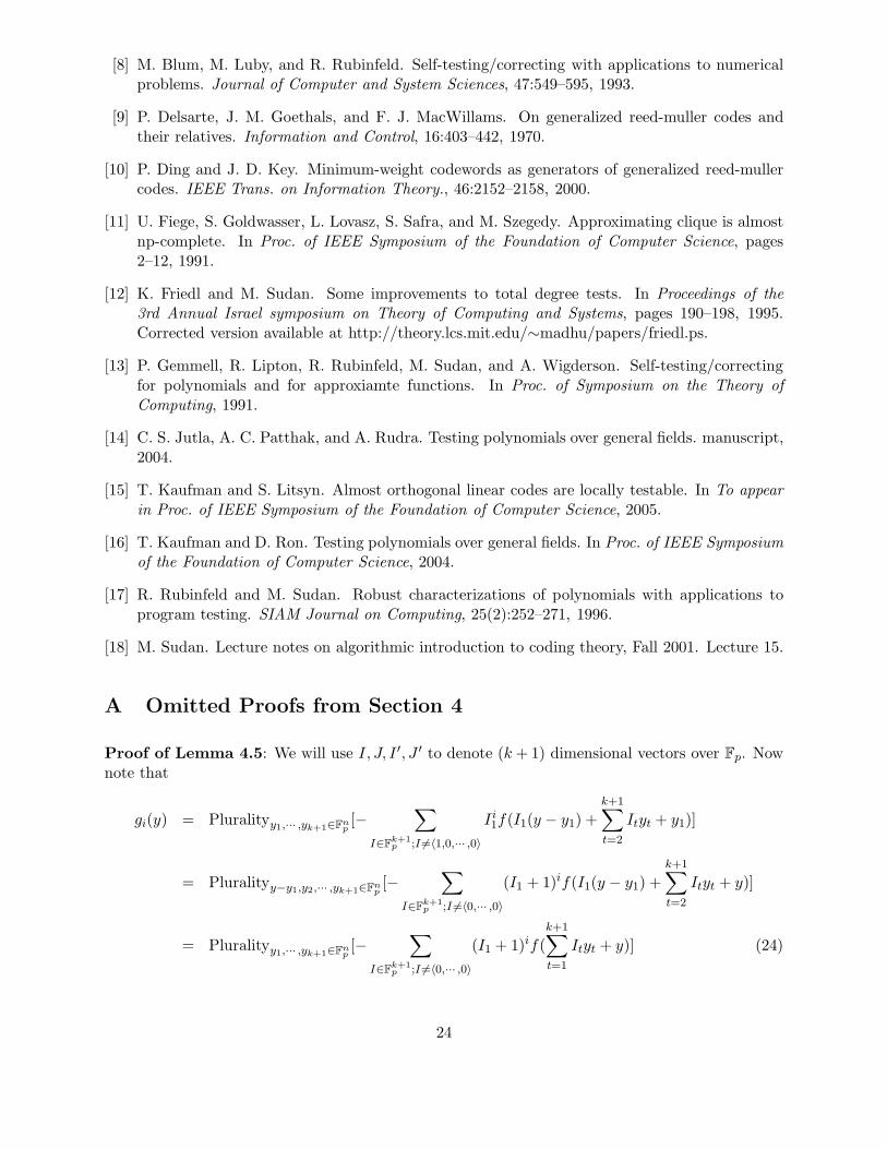
Proof of Claim 4.17:

T 1g1

(Y, b) =∑

I∈Fk+13

I1g1(I · Y + b)

=∑

I∈Fk+13

I1

[−T 1

f (I · Y + b − I · Z1 − r1, I · Z2 + r2, · · · , I · Zk+1 + rk+1, I · Z1 + r1)

+ f(I · Y + b)]

= −∑

I∈Fk+13

I1

∑

∅6=J ′∈Fk3

f(I · Y + b +

k+1∑

t=2

JtI · Zt +

k+1∑

t=2

Jtrt)

+

∑

J ′∈F k3

f(2I · Y + 2b − I · Z1 − r1 +

k+1∑

t=2

JtI · Zt +

k+1∑

t=2

Jtrt)

= −∑

06=J ′∈Fk3

∑

I∈Fk+13

I1f(I · Y + b +

k+1∑

t=2

Jtrt +

k+1∑

t=2

JtI · Zt)

−∑

J ′∈Fk3

∑

I∈Fk+13

I1f(2I · Y + 2b − I · Z1 − r1 +

k+1∑

t=2

JtI · Zt +

k+1∑

t=2

Jtrt)

=∑

06=J ′∈Fk3

[

−T 1f (y1 +

k+1∑

t=2

Jtzt,1, · · · , yk+1 +

k+1∑

t=2

Jtzt,(k+1), b +

k+1∑

t=2

Jtrt)

]

+∑

J ′∈Fk3

[

T 1f (2y1 − z1,1 +

k+1∑

t=2

Jtzt,1, · · · , 2yk+1 − z1,(k+1) +

k+1∑

t=2

Jtzt,(k+1), 2b − r1 +

k+1∑

t=2

Jtrt)

]

(29)

27

Proof of Claim 4.19:

T igi

(Y, b) =∑

I∈Fk+1p

Ii1gi(I · Y + b)

=∑

I∈Fk+1p

Ii1

[−T i

f (I · Y + b − I · Z1 − r1, I · Z2 + r2, · · · , I · Zk+1 + rk+1, I · Z1 + r1)

+ f(I · Y + b)]

= −∑

I∈Fk+1p

Ii1

∑

∅6=J ′∈Fkp

f(I · Y + b +

k+1∑

t=2

JtI · Zt +

k+1∑

t=2

Jtrt)

+

∑

J1∈Fp,J1 6=1

J i1

∑

J ′∈Fkp

f(J1I · Y + J1b − (J1 − 1)I · Z1 − (J1 − 1)r1 +k+1∑

t=2

JtI · Zt +k+1∑

t=2

Jtrt)

= −∑

06=J ′∈Fkp

∑

I∈Fk+1p

Ii1f(I · Y + b +

k+1∑

t=2

Jtrt +

k+1∑

t=2

JtI · Zt)

−∑

J ′∈Fkp

∑

J1∈Fp;J1 6=1

J i1

∑

I∈Fk+1p

Ii1f(J1I · Y + J1b − (J1 − 1)I · Z1 − (J1 − 1)r1

+

k+1∑

t=2

JtI · Zt +

k+1∑

t=2

Jtrt)

]]

=∑

06=J ′∈Fkp

[

−T if (y1 +

k+1∑

t=2

Jtzt,1, · · · , yk+1 +k+1∑

t=2

Jtzt,(k+1), b +k+1∑

t=2

Jtrt)

]

+∑

J ′∈Fkp

∑

J1∈Fp;J1 6=1

J i1

[

−T if (J1y1 − (J1 − 1)z1,1 +

k+1∑

t=2

Jtzt,1, · · · , J1yk+1 − (J1 − 1)z1,(k+1)

+

k+1∑

t=2

Jtzt,(k+1), J1b − (J1 − 1)r1 +

k+1∑

t=2

Jtrt)

]]

(30)

28