On the application of Large-Eddy simulations in engine ...
166
On the application of Large-Eddy simulations in engine-related problems Citation for published version (APA): Huijnen, V. (2007). On the application of Large-Eddy simulations in engine-related problems. Technische Universiteit Eindhoven. https://doi.org/10.6100/IR628798 DOI: 10.6100/IR628798 Document status and date: Published: 01/01/2007 Document Version: Publisher’s PDF, also known as Version of Record (includes final page, issue and volume numbers) Please check the document version of this publication: • A submitted manuscript is the version of the article upon submission and before peer-review. There can be important differences between the submitted version and the official published version of record. People interested in the research are advised to contact the author for the final version of the publication, or visit the DOI to the publisher's website. • The final author version and the galley proof are versions of the publication after peer review. • The final published version features the final layout of the paper including the volume, issue and page numbers. Link to publication General rights Copyright and moral rights for the publications made accessible in the public portal are retained by the authors and/or other copyright owners and it is a condition of accessing publications that users recognise and abide by the legal requirements associated with these rights. • Users may download and print one copy of any publication from the public portal for the purpose of private study or research. • You may not further distribute the material or use it for any profit-making activity or commercial gain • You may freely distribute the URL identifying the publication in the public portal. If the publication is distributed under the terms of Article 25fa of the Dutch Copyright Act, indicated by the “Taverne” license above, please follow below link for the End User Agreement: www.tue.nl/taverne Take down policy If you believe that this document breaches copyright please contact us at: [email protected] providing details and we will investigate your claim. Download date: 19. Mar. 2022
-
Upload
khangminh22 -
Category
Documents
-
view
0 -
download
0
Transcript of On the application of Large-Eddy simulations in engine ...

On the application of Large-Eddy simulations in engine-relatedproblemsCitation for published version (APA):Huijnen, V. (2007). On the application of Large-Eddy simulations in engine-related problems. TechnischeUniversiteit Eindhoven. https://doi.org/10.6100/IR628798
DOI:10.6100/IR628798
Document status and date:Published: 01/01/2007
Document Version:Publisher’s PDF, also known as Version of Record (includes final page, issue and volume numbers)
Please check the document version of this publication:
• A submitted manuscript is the version of the article upon submission and before peer-review. There can beimportant differences between the submitted version and the official published version of record. Peopleinterested in the research are advised to contact the author for the final version of the publication, or visit theDOI to the publisher's website.• The final author version and the galley proof are versions of the publication after peer review.• The final published version features the final layout of the paper including the volume, issue and pagenumbers.Link to publication
General rightsCopyright and moral rights for the publications made accessible in the public portal are retained by the authors and/or other copyright ownersand it is a condition of accessing publications that users recognise and abide by the legal requirements associated with these rights.
• Users may download and print one copy of any publication from the public portal for the purpose of private study or research. • You may not further distribute the material or use it for any profit-making activity or commercial gain • You may freely distribute the URL identifying the publication in the public portal.
If the publication is distributed under the terms of Article 25fa of the Dutch Copyright Act, indicated by the “Taverne” license above, pleasefollow below link for the End User Agreement:www.tue.nl/taverne
Take down policyIf you believe that this document breaches copyright please contact us at:[email protected] details and we will investigate your claim.
Download date: 19. Mar. 2022
On the Applicationof Large-Eddy Simulations
in Engine-related Problems
PROEFSCHRIFT
ter verkrijging van de graad van doctor aan deTechnische Universiteit Eindhoven, op gezag van deRector Magnificus, prof.dr.ir. C.J. van Duijn, voor een
commissie aangewezen door het College voorPromoties in het openbaar te verdedigen
op dinsdag 4 september 2007 om 16.00 uur
door
Vincent Huijnen
geboren te Enschede

Dit proefschrift is goedgekeurd door de promotoren:
prof.dr.ir. R.S.G. Baertenprof.dr. L.P.H. de Goey
Copromotor:dr.ir. L.M.T. Somers
Copyright c© 2007 by V. HuijnenAll rights reserved. No part of this publication may be reproduced, stored in a re-trieval system, or transmitted, in any form, or by any means, electronic, mechanical,photocopying, recording, or otherwise, without the prior permission of the author.
Cover design: Bregje Schoffelen, Oranje VormgeversA catalogue record is available from the Eindhoven University of TechnologyLibrary
ISBN: 978-90-386-1078-8


iv Contents

Contents
1 Introduction 1
1.1 Background . . . . . . . . . . . . . . . . . . . . . . . . . . . . . . . . . 11.2 Turbulence . . . . . . . . . . . . . . . . . . . . . . . . . . . . . . . . . . 31.3 This thesis . . . . . . . . . . . . . . . . . . . . . . . . . . . . . . . . . . 4
2 Theoretical background 7
2.1 Governing equations . . . . . . . . . . . . . . . . . . . . . . . . . . . . 72.1.1 Direct numerical simulations . . . . . . . . . . . . . . . . . . . 8
2.2 The phenomenology of Turbulence . . . . . . . . . . . . . . . . . . . . 92.2.1 RANS: Averaging the turbulence . . . . . . . . . . . . . . . . . 112.2.2 LES: Filtering the turbulence . . . . . . . . . . . . . . . . . . . 13
2.3 LES turbulence modeling . . . . . . . . . . . . . . . . . . . . . . . . . 132.3.1 Introduction to subgrid modeling . . . . . . . . . . . . . . . . 142.3.2 Subgrid-scale models . . . . . . . . . . . . . . . . . . . . . . . . 162.3.3 Near-wall modeling . . . . . . . . . . . . . . . . . . . . . . . . 202.3.4 Inflow conditions . . . . . . . . . . . . . . . . . . . . . . . . . . 21
2.4 Turbulence modeling for engine applications. . . . . . . . . . . . . . . 222.4.1 The phenomenology of engine turbulence . . . . . . . . . . . 222.4.2 Choice of the solver . . . . . . . . . . . . . . . . . . . . . . . . 23
3 LES in confined flow geometries 25
3.1 Introduction . . . . . . . . . . . . . . . . . . . . . . . . . . . . . . . . . 253.2 The numerical methods . . . . . . . . . . . . . . . . . . . . . . . . . . 29
3.2.1 Kiva-3V . . . . . . . . . . . . . . . . . . . . . . . . . . . . . . . 293.2.2 The convective scheme . . . . . . . . . . . . . . . . . . . . . . . 303.2.3 FASTEST-3D . . . . . . . . . . . . . . . . . . . . . . . . . . . . . 32
3.3 Square duct simulations . . . . . . . . . . . . . . . . . . . . . . . . . . 333.3.1 The numerical setup . . . . . . . . . . . . . . . . . . . . . . . . 343.3.2 Results . . . . . . . . . . . . . . . . . . . . . . . . . . . . . . . . 363.3.3 Discussion . . . . . . . . . . . . . . . . . . . . . . . . . . . . . . 40
3.4 A practical engine head simulation . . . . . . . . . . . . . . . . . . . . 413.4.1 The numerical setup . . . . . . . . . . . . . . . . . . . . . . . . 423.4.2 Results and discussions . . . . . . . . . . . . . . . . . . . . . . 453.4.3 Discussion . . . . . . . . . . . . . . . . . . . . . . . . . . . . . . 47
3.5 Conclusions . . . . . . . . . . . . . . . . . . . . . . . . . . . . . . . . . 49
vi Contents
4 Modeling the turbulent mixing of a gas jet 51
4.1 Introduction . . . . . . . . . . . . . . . . . . . . . . . . . . . . . . . . . 514.2 Phenomenology of liquid and gaseous fuel jets . . . . . . . . . . . . . 53
4.2.1 Liquid fuel jets . . . . . . . . . . . . . . . . . . . . . . . . . . . 534.2.2 Gaseous fuel jets . . . . . . . . . . . . . . . . . . . . . . . . . . 554.2.3 Modeling Diesel sprays using a gas jet . . . . . . . . . . . . . . 58
4.3 The mixing model . . . . . . . . . . . . . . . . . . . . . . . . . . . . . . 584.3.1 The mixture fraction . . . . . . . . . . . . . . . . . . . . . . . . 594.3.2 The numerical setup . . . . . . . . . . . . . . . . . . . . . . . . 60
4.4 Results . . . . . . . . . . . . . . . . . . . . . . . . . . . . . . . . . . . . 624.4.1 Steady state behaviour . . . . . . . . . . . . . . . . . . . . . . . 634.4.2 The unsteady behaviour of the turbulent gas jet . . . . . . . . 684.4.3 Comparison to a liquid jet model . . . . . . . . . . . . . . . . . 774.4.4 Global mixture composition . . . . . . . . . . . . . . . . . . . . 79
4.5 Conclusions . . . . . . . . . . . . . . . . . . . . . . . . . . . . . . . . . 81
5 Modeling finite-rate chemistry in turbulent diffusion flames 83
5.1 Introduction . . . . . . . . . . . . . . . . . . . . . . . . . . . . . . . . . 835.1.1 Combustion regimes encountered in engine flows . . . . . . . 835.1.2 Objectives . . . . . . . . . . . . . . . . . . . . . . . . . . . . . . 855.1.3 Chapter layout . . . . . . . . . . . . . . . . . . . . . . . . . . . 86
5.2 Non-premixed combustion modeling . . . . . . . . . . . . . . . . . . 865.2.1 Diffusion flamelet modeling . . . . . . . . . . . . . . . . . . . . 865.2.2 A progress variable method for non-premixed systems . . . . 88
5.3 Effects of turbulence . . . . . . . . . . . . . . . . . . . . . . . . . . . . 905.3.1 The LES filtered governing equations . . . . . . . . . . . . . . 915.3.2 The PDF Method . . . . . . . . . . . . . . . . . . . . . . . . . . 925.3.3 The numerical methodology . . . . . . . . . . . . . . . . . . . 93
5.4 LES of a piloted diffusion flame . . . . . . . . . . . . . . . . . . . . . . 935.4.1 The setup of the Sandia flame D . . . . . . . . . . . . . . . . . 945.4.2 Results . . . . . . . . . . . . . . . . . . . . . . . . . . . . . . . . 985.4.3 Analysis of the chemistry models . . . . . . . . . . . . . . . . . 1065.4.4 Concluding remarks . . . . . . . . . . . . . . . . . . . . . . . . 111
5.5 A sooting benzene diffusion flame . . . . . . . . . . . . . . . . . . . . 1115.5.1 The process of soot formation . . . . . . . . . . . . . . . . . . . 1125.5.2 Modeling soot in diffusion flames . . . . . . . . . . . . . . . . 1145.5.3 The setup for the Large-Eddy simulation . . . . . . . . . . . . 1195.5.4 Results . . . . . . . . . . . . . . . . . . . . . . . . . . . . . . . . 121
5.6 Conclusions . . . . . . . . . . . . . . . . . . . . . . . . . . . . . . . . . 127
6 General conclusions 129
A The numerical scheme of FASTEST-3D 133
A.1 Discretization . . . . . . . . . . . . . . . . . . . . . . . . . . . . . . . . 133A.2 The solution algorithm . . . . . . . . . . . . . . . . . . . . . . . . . . . 136
Bibliography 139

Contents vii
Abstract 151
Samenvatting 153
Curriculum Vitae 155
Dankwoord 157

viii Contents

Chapter
1Introduction
The work which is described in this thesis is a contribution to thedevelopment of the modeling of turbulent flows for engine-relatedproblems. The motivation to work on this problem lies in the de-mands from the community on an increased fuel efficiency and areduction of pollutants formation in internal combustion engines.The subject of this thesis is a combination of the validation of nu-merical methods and turbulence as well as turbulent combustionmodeling. In this chapter the proposed modeling methodology isbriefly introduced. Also an outline of this thesis is presented.
1.1 Background
Free to move
A main driving force for many developments in the human world is the need forfreedom, in the sense that one can decide personally what actions one is going totake and where one is heading for. An underlying aspect here is a freedom in thesense of thought and speech: one should decide personally what is best for him/her.This will generally result in a movement of thought: people will not stick to a sin-gle way of thinking. Similarly, there is a freedom to move, to get in contact withother people’s opinions, other habits, other atmospheres. However, this freedomin the more philosophical sense is not sufficient. It always needs to be realized bythe movement of products and of the people themselves, in cars, ships, airplanes.The need for transportation will remain necessary and will be growing in the nextdecades, notwithstanding that a growth in virtual transportation and communica-tion via modern electronic tools can be observed as well.
An increase in freedom will go in hand with an increase in mobility. The powersource and mechanical heart of this mobility is nowadays the Internal-Combustion(IC) engine. The IC engine is popular simply because this type of engine has beenproven to be the cheapest, most efficient and practical tool for energy conversioninto transportation. Moreover, this will remain to be true in the coming decadesas can be concluded from any of the main energy studies, for instance the WETOstudy [164]. But along with the benefits of free movement there will be a trendtowards higher fuel needs, more noise production, traffic accidents, queueing, andpollutant formation, which, in turn, will limit our freedom.
2 Introduction
A need to improve engines
Above limitations call for an improvement, mainly by means of engineering solu-tions. We do not necessarily need to live with the negative aspects of an internalcombustion engine. We are free to make developments. As a matter of fact, we areforced to develop our engines further, simply because in the aforementioned senseengines limit the total level of freedom. From a customer’s standpoint one of themain arguments is an increase in energy output for the lowest amount of fuel con-sumption, which calls for efficient combustion techniques. From a society point ofview reduced levels of soot and NOx exhaust are demanded, as pollutants reducethe health and vitality of a community, see, e.g., Avakian et al. [7].
Car manufacturers are forced to develop their engines to meet the regulationfrom the European government on the one hand and the local customer’s needs,in terms of fuel efficiency and traveling comfort on the other hand. Along withthe industrial drive, naturally there is an academic ambition to develop new engineconcepts, on a more fundamental basis. Here, new insights in the underlying pro-cesses with respect to the combustion inside an IC engine are expected to lead toimprovements in engine design.
The role of CFD
One type of engine, the Diesel engine, is efficient in terms of fuel consumption.Therefore this type of engine is mainly used for heavy duty transport purposes. Atthe same time these engines are more and more used in the personal car industry.However, the non-homogeneous fuel distribution during the combustion process inthe engine leads to relatively high levels of soot formation.
Diesel engine combustion is an extremely complex problem to model, Reitz andRutland [132]. When going through a typical combustion cycle of a Diesel enginewe start at the intake stroke. Fast valve and piston movement take place and sub-sequently large inflow velocities are present. As the valves are closed, the turbulentswirling air is compressed. Then fuel is injected as a spray. Droplets break up andvaporize and combustion starts at some critical location. The chemical energy isreleased and the gas expands, forcing the piston to move downwards. This is thepower stroke. Typical combustion products such as CO2 and H2O are produced,along with pollutants. During the exhaust phase most of the combustion productsleave the cylinder. In the next cycle a new air intake starts. Due to turbulence varia-tions, cycle to cycle variations occur, which may lead to different engine cycle char-acteristics for different cycles.
From the above it is clear that in modern Diesel engines both heat release rate andemissions formation are strongly influenced by the fuel-air mixing process which inturn is the outcome of the interaction between the injected fuel spray, the combus-tion and the in-cylinder flow field.
Through numerical modeling a better understanding can be gained of the detailsof in-cylinder combustion processes. This can lead to a design optimization in anearly stage of the development process. Therefore in the long term such a methodof investigation can be shorter and less expensive than is typically encountered inexperimental methods. This drives the development towards new modeling tools.

1.2 Turbulence 3
With the increase of computational power, the development of sophisticated nu-merical schemes and an increase in multi-disciplinary cooperation, new theoreticalmodeling approaches and modeling software become available. One aspect con-cerns a novel modeling of the turbulent fluid flow. Within this area of research thecurrent thesis is intended to give a new contribution.
1.2 Turbulence
The fluid flow inside cylinder geometries in actual engines is fully turbulent. Themain properties of the turbulence for any particular application depend basicallyon two aspects: the geometry and the mass flow. The Reynolds number is used tospecify the turbulence. It describes the ratio of the inertial forces compared to thefriction forces,
Re =ULν
. (1.1)
Here, U is a typical velocity scale, generally related to the global mass flow, L a typ-ical length scale of the geometry and ν a property of the fluid: the viscosity. Withincreasing Reynolds number, the flow becomes more turbulent. The modeling ofturbulent flows, which are inherently unsteady, fluctuating flows, is classically tack-led using an averaging technique. In this method all turbulent scales are modeledwhile only the mean flow is resolved. This is the Reynolds Averaged Navier Stokes(RANS) modeling technique.
RANS turbulence modeling
In RANS all turbulent properties are modeled using a limited number of turbulentquantities. In most industrial RANS codes, these are the turbulent kinetic energy kand the turbulent dissipation rate ε. For a critical discussion the reader is referred toHanjalic [58]. Focus of the RANS modeling is on predicting mean flow properties.Effects that take place on the smallest turbulent scales are not considered impor-tant as they have little direct impact on the mean fluid dynamics. Therefore, forprocesses that are dominated by an interplay with turbulence (such as mixing andcombustion) that mainly take place far from walls and that depend on relativelysmall scale vortical structures, a RANS approach will be less appropriate. RANSwill only reveal global information of the mixing.
LES turbulence modeling
In a Large Eddy Simulation (LES) more details of the flow are taken into account,compared to RANS. The turbulent flow is filtered in space, rather than averaged,as in RANS. Therefore all turbulent scales, up to a cutoff length are explicitly eval-uated. It can be argued that by performing a more detailed simulation a more ac-curate description of the processes can be expected. However, there are modellingissues related to this approach, which need to be accounted for. This makes the useof LES models not straightforward. Therefore an investigation with respect to theapplicability of this type of models for engine studies needs to be performed.
4 Introduction
1.3 This thesis
This thesis addresses the application of the LES technique to Diesel engines. Thereasons for applying LES are multiple. For future engine modeling and design it isimportant not only to consider the flow to be time-dependent, but also to explicitlyresolve the turbulence structures temporally as well as spatially. Time dependent,because the engine flow is highly unsteady, due to the movements of the valves,the injection and subsequent combustion. This can in principle be performed usingan Unsteady RANS formulation. However, in that case the turbulent structures arenot resolved. An accurate description of the interplay of turbulence with combus-tion processes is important, especially to account properly for chemical species thatare not in their equilibrium values. In particular, for the prediction of pollutants acorrect modeling of non-equilibrium effects is crucial, Navarro-Martinez and Kro-nenburg [101]. This means that not only the mean flow field needs to be describedaccurately, also the turbulence statistics is essential. In RANS the turbulence is typ-ically assumed to be homogeneous and global estimates for the mixing rates andreaction rates are based on this assumption. Therefore RANS models are less ap-propriate for the modeling of pollutant formation in engines. Instead, the LES ap-proach is designed to give more detailed information on the turbulence statistics,which makes it a more suitable modeling tool in this sense.
As simple as the LES method seems, its application is not straightforward. Boththe numerical method and the applied turbulence models can be a source of error,Meyers et al. [94]. First of all, any model implementation should be validated insufficient detail. Also, problems on the use of LES for practical applications needinvestigation. Additionally, any interaction with other physical effects, with spe-cial attention to the combustion process should be considered. But analysis of LESmodeling where the complete Diesel combustion process is modeled directly is verydifficult and will be obscured by the complexity of the system. Such an approachwill not reveal any of the issues that are related to separate aspects. Therefore arepresentative selection of key Diesel engine flow processes has been studied in thisthesis.
The outline of this thesis
As a start, the application of LES for a generic wall bounded shear flow is consi-dered, which is an important aspect in any turbulence model that is applied. Alsothe impact of the shear flow modeling on the modeling of the complex flow struc-tures as occurring in a typical engine geometry is studied. It is found that shearflows can not appropriately be modeled in the current formulation of the LES method.Therefore in the remainder no turbulence-wall interactions are considered. Anotheraspect that is examined is the mixing process of the fuel and air, which is a necessarytool for turbulent combustion modeling. Finally, the application of LES to the pre-diction of non-premixed combustion was studied, in particular considering finite-rate chemistry effects and the potential for the prediction of soot in such flames.
The results are presented in six chapters. Apart from this introduction and thefinal conclusions, the contents of this thesis can be described as follows. First of
1.3 This thesis 5
all, non-reactive turbulent flows are considered. The underlying physical laws areexplained in chapter 2. In chapter 3 it is shown how such a model can be translatedinto a working simulation code. The different turbulence LES sub-grid models areanalyzed and validated, as well as the impact of the numerical method on the flowsimulation. This is shown for a generic flow geometry: a square duct flow. Alsoa series of Large-Eddy simulations of the turbulent flow in an engine geometry ispresented: the flow in a steady engine head setup attached to a cylinder. This setupis representative to study typical flow properties of such a complex geometry, suchas wall shear, swirl and tumble. This chapter illustrates the difficulties of the LESapproach when simulating practical engine-related flow problems. It is shown thata poor resolution near the walls and numerical discretization errors will severelyinfluence the mean and turbulent flow properties in such a situation.
In chapter 4 LES is used to calculate a developing turbulent gaseous fuel jet. Thistype of flow is similar to the fuel/air mixing as takes place in direct injection (Diesel)engines. Here an LES modeling approach for turbulent mixing is introduced andvalidated. It is shown that the gaseous fuel jet follows well the similarity theorydeveloped for axisymmetrical turbulent jets. The gaseous fuel jet modeled usingLES is compared to a phenomenological liquid spray jet model. When corrected forthe difference in cone angle between the fuel spray and and the gas jet it is shownthat these models are exchangeable.
Combustion in Diesel engines can be considered mainly as non-premixed. Thistype of combustion problems is often tackled by so-called laminar flamelet methods.Here the main parameter that defines the mixing state is the mixture fraction. Butthe effect of turbulence on the chemistry cannot simply be accounted for with thissingle parameter. Other, more detailed methods are necessary. In chapter 5 modelsare presented that couple chemistry models to the turbulent flow field. The classicalmethod that uses a mixing-time scale (i.e., the scalar dissipation rate) is comparedto a newly developed method where reaction progress is tracked explicitly. Theapplicability of the different methods is validated using the well documented San-dia flame D. In the final sections of chapter 5 a sooting turbulent diffusion flameis modeled, where a crucial impact of non-equilibrium effects of the soot formationchemistry on the predicted soot production is illustrated. The methodology to ac-count for these effects is presented, as well as its application on a sooting turbulentbenzene flame.

6 Introduction

Chapter
2Theoretical background
In this chapter the theoretical background for the modeling of thefluid dynamics is introduced. The general conservation equationsfor turbulent transport of mass, momentum, energy and species,as used throughout this thesis, are given. The LES filtering opera-tion is presented, leading to the filtered transport equations. In thesecond part of this chapter the focus is on models that describe thesubgrid scale turbulence. This will serve as a basis for the simu-lations as presented in chapter 3. Finally, a brief classification isgiven of the approaches to solve fluid dynamical problems relatedto engine cases.
2.1 Governing equations
Modeling fluid dynamics starts with the definition of the underlying physical laws.The choice which models are used here defines the physical limitations of the prob-lems that can be solved. Here the laws of conservation of mass and momentum,known as the Navier-Stokes equations are introduced. These equations can be writ-ten as
∂ρ
∂t+
∂ρuj
∂xj
= 0, (2.1)
∂ρui
∂t+
∂ρujui
∂xj
=∂
∂xj
(ρσij) + ρgi −∂p
∂xi
. (2.2)
Here ρ is the density of the fluid, ui the velocity in xi-direction, p the pressure, σij
the stress tensor and gi the acceleration by gravity. For Newtonian fluids the stresstensor reads
σij = ν
[(∂ui
∂xj
+∂uj
∂xi
)− 2
3
∂uk
∂xk
δij
], (2.3)
with ν the kinematic molecular viscosity. These equations are the main conserva-tion equations that are required for fluid dynamics and turbulence modeling, andare therefore the heart of any fluid-dynamical solver. For the conservation of totalenergy an independent equation needs to be addressed. This equation is given here,in terms of temperature (see, e.g., Moin et al. [96]):
∂ρcvT
∂t+
∂ρujcvT
∂xj
=∂
∂xi
(λ
∂T
∂xi
)+ ωT . (2.4)
8 Theoretical background
Here λ and cv denote the thermal conductivity and specific heat at constant volumerespectively. ωT describes the total heat release rate, e.g., by chemical reactions,using an Arrhenius-like expression, see, e.g., Warnatz et al. [162]. In equation 2.4 theheating term due to internal friction has been neglected, as well as a term accountingfor acoustic interactions and pressure waves. This approximation is valid for lowMach number flows. Moreover, there is no ∂p
∂tterm in the above equation. This is
valid for constant pressure problems, such as in case of steady, open systems. Notethat this term should be retained in applications for reciprocating engines where thepiston movement induces a pressure rise.
When chemistry starts to play a role the modeling of additional quantities willbecome necessary. The conservation equations for the species mass fraction aregiven by
∂ρYi
∂t+
∂ρujYi
∂xj
=∂
∂xj
(ρDi
∂Yi
∂xj
)+ ωi. (2.5)
Here, Yi denotes the mass fraction of species i, and Di its diffusion coefficient. ωi isthe chemical source term. For species diffusion the diffusivity is often related to thethermal diffusivity λ
ρcp, given by the Lewis number
Lei =λ
ρDicp
. (2.6)
To close the above system of equations, a coupling between the pressure, densityand temperature needs to be provided. In the remainder of this work we will adoptthe ideal gas law
ρ =pM
RT, (2.7)
where R is the universal gas constant. This assumption is well-applicable for ICengine modeling, see Evlampiev [44]. This equation relates the local density ρ to themolar mass M and the temperature T at a specific working pressure.
2.1.1 Direct numerical simulations
When solving equations 2.1, 2.2, 2.4, 2.5 and 2.7 directly in some numerical methodone is applying the Direct Numerical Simulation (DNS) approach: all turbulentscales are resolved up to the Kolmogorov scale η, which is the smallest scale ofthe continuum. When only considering fluid dynamical scales, it can be shownthat the number of required grid points for such a simulation scales as Nt ∼ Re9/4,Sagaut [139]. This is untractable for typical practical simulations, where Re can eas-ily reach values of about 50.000, based on the cylinder diameter and the mass flowrates. Additionally the chemical length scales that should be accounted for are typ-ically of the size of 0.1 mm, for atmospheric flames, and decreasing with increasingpressure. Therefore the DNS approach cannot be used in practical applications. Thisimplies that modelling of the fluid dynamics as well as the chemistry is inevitable.In order to understand how the turbulence can be modelled it is necessary to under-stand some of its nature.

2.2 The phenomenology of Turbulence 9
E( )
κκκe d
κ-5/3
κ
Figure 2.1 : A typical energy spectrum of turbulence as a function of the wave number.Both scales are logarithmic
2.2 The phenomenology of Turbulence
Turbulence can be defined as the interplay of ordered, coherent structures. In gen-eral terms, these coherent structures can emerge from chaos at the smallest scalesunder the action of an external constraint. In these circumstances small perturba-tions have a chance to grow and become significant, Lesieur [85]. This is due to thenon-linear form of the system, as described by the Navier-Stokes equations. Theturbulent vortical structures range in size from the very small ones, defined by theKolmogorov scale η containing only a marginal amount of kinetic energy, up to thelarge-scale coherent structures. These large structures are responsible for a largefraction, up to 90 %, of the transport of the conserved properties such as species,mass, momentum and energy, Ferziger [45]. However, the appearance and evolu-tion of these coherent structures is difficult to predict. It is instructive to introducethe spectrum of the turbulent kinetic energy. In figure 2.1 the energy of the turbu-lence as a function of its wave number κ is presented, with κ the inverse of wavelength, κ = 2π/l. The turbulence spectrum can be divided into a macro-structure(small κ) and a micro-structure (large κ). In between a cascade process takes place.The macro-structure is dominated by the non-linear processes; viscous effects arenegligible. The kinetic energy of the turbulence scales with U2, with U the velocityscale of the macro-structure. These structures are the most dominant in the energy-domain. Here the turbulence is in general non-homogeneous and is strongly in-fluenced by the boundary conditions of the geometry. Its typical wave number is:κ ≈ κe = 2π/L with L the largest scale, a typical length scale of the geometry.
At the opposite side of the spectrum the small scale turbulence velocity andlength scale are defined by the Kolmogorov scales v (velocity scale) and η (lengthscale). Then κ ≈ κd = 2π/η. These are the smallest turbulent scales in the domain.These scales are assumed to depend only on local processes: viscosity (ν) and dissi-pation (ε). By dimensional analysis it can be derived that, Kolmogorov [76],
η =
(ν3
ε
)1/4
. (2.8)
This is the micro structure where the turbulence is dissipated by molecular viscosityeffects. The viscous term is now important, as the velocity gradients are large. In

10 Theoretical background
a) b)
Figure 2.2 : An illustration of the turbulent flow in a Diesel engine. (a) instantaneous, tur-bulent streamlines, (b) some streamlines of the average flow field.
case of a scale separation between the macro scales and the micro scales, the macro-scales U and L are not of direct importance in this regime: its non-homogeneousinformation is lost during the three-dimensional cascade process. This means thatthe structure of the microscale is universal, the turbulence is only indirectly coupledto the large scales. This universal behavior is valid for large Reynolds numbers, i.e.when the large scales and the small scales are completely separated: κd/κe ≫ 1.Consequently, close to the walls this universal behavior shifts to the smaller scales.The relation that connects the small scales to the large scales, in the case of homoge-neous isotropic turbulence is given by:
Lη
= Re3/4 (2.9)
with Re the bulk Reynolds number, based on the characteristic velocity scale U andlength scale L, see equation 1.1. The coupling of the large and the small scales isdominated by the processes in the so-called inertial subrange. In this regime, thespectrum is independent of the macro scale because κ ≫ κe. On the other hand thespectrum is independent of viscosity as well as κ ≪ κd. The only parameter leftresponsible for the energy cascade process, is the dissipation ε which is in equilib-rium with the injection of kinetic energy at the large scales. Based on dimensionalanalysis the shape of the spectrum in the inertial subrange can be found:
E(κ) = Ckε2/3κ−5/3 (2.10)
with Ck the Kolmogorov constant: Ck ≈ 1.6, as shown by Kolmogorov [76].The above considerations illustrate that it is artificial to make a strict distinction
between the different turbulent scales that are studied. Turbulence is an effect of thesum of all scales that appear in a system.
However, sometimes one is only interested in the mean flow properties, omittingturbulent statistics as unnecessary information. In terms of engine flows one can beinterested in the large-scale tumbling and swirling motions, which show a very reg-ular flow pattern on an average picture, see figure 2.2. In an instantaneous snapshot

2.2 The phenomenology of Turbulence 11
these flow patterns are very irregular and hard to recognize. This illustrates thatall instant turbulent eddies build up the mean picture, where only the largest-scaleflow patterns are retained. However, this also shows that just the knowledge of amean flow picture masks a lot of information of the actual fluid flow. Therefore,in fluid flow modeling not only the mean flow features are considered but also theturbulent statistics. Apart from the DNS method this modeling can be achieved bythe RANS and the LES approach.
2.2.1 RANS: Averaging the turbulence
In RANS, the full equations for any quantity φ are decomposed into a mean φ and afluctuating φ′ part:
φ = φ − φ′, (2.11)
φ = limn→∞
1
n
n∑
i=1
φi. (2.12)
This procedure is known as Reynolds ensemble averaging, over realizations i, andprovides equations for all mean quantities as a function of space and time. Withrespect to engines, the ensemble averaging procedure refers to averaging over cy-cles. For steady state problems, the ensemble averaging corresponds simply to time-averaging of the turbulence. In the frequency domain, only the lowest turbulentfrequencies, corresponding to wave numbers up to κe, are explicitly calculated, therest is modelled. If density varies generally the Favre-averaging procedure will beadopted. This is defined as
φ = ρφ/ρ. (2.13)
This substitution greatly simplifies all averaging and filtering procedures wherevariable density effects play a role. By applying above procedures to the Navier-Stokes equations and the energy equation the following set of equations can befound:
∂ρ
∂t+
∂ρuj
∂xj
= 0, (2.14)
∂ρui
∂t+
∂ρujui
∂xj
=∂
∂xj
(ρσij − ρτij) + ρgi −∂p
∂xi
, (2.15)
∂ρcvT
∂t+
∂ρujcvT
∂xj
=∂
∂xj
(λ
∂T
∂xj
− cvρqj
)+ ωT , (2.16)
∂ρYi
∂t+
∂ρujYi
∂xj
=∂
∂xj
(ρDi
∂Yi
∂xj
− ρJij
)+ ωi. (2.17)
In above equations the turbulent contribution in the diffusive terms of the energyand species concentration due to the averaging is neglected, as is generally accepted,Poinsot and Veynante [124]. Note that equations 2.14-2.17 closely resemble the orig-inal equations; only extra terms are found that are given in the diffusion part of the
12 Theoretical background
Table 2.1 : Modeling constants for the k − ε model
Cµ Cε1 Cε2 Cε3 σk σǫ
0.09 1.44 1.92 1.44 1.0 1.3
transport equations. These represent the influence of turbulent fluctuations from allfrequencies on the mean flow. These terms can be represented as:
τij = uiuj − uiuj, (2.18)
qj = ujT − ujT , (2.19)
Jij = ujYi − ujYi. (2.20)
The turbulent stress τij , the turbulent energy and species transport qj and Jij can beinterpreted as resulting mean rates of transport of momentum, energy and speciesdue to the turbulent movements of the fluid. The main contribution will come fromthe large scale fluctuations, as these are the most energetic. These additional terms(in the momentum equation it is the Reynolds stress and in the energy equation theturbulent heat flux) have to be modelled. In one of the simplest, and most widelyused models the Boussinesq hypothesis [20], assuming homogeneity of the turbu-lence, is adopted:
τij =2
3kδij − νt
(∂ui
∂xj
+∂uj
∂xi
)(2.21)
where νt denotes the turbulent viscosity, modeled as (e.g. Launder and Spalding[81])
νt = Cµk2
ε, (2.22)
with Cµ a modeling parameter. Here, transport equations for the total turbulentkinetic energy k = uiui/2 and dissipation ε come into play. The transport equationfor k is given by
ρ∂k
∂t+ ρuj
∂k
∂xj
= ρP +∂
∂xj
(νt
σk
∂k
∂xj
)− ρε, (2.23)
where P = −u′iu
′j
∂ui
∂xjdenotes the production term of turbulent kinetic energy. Un-
der the assumption of local isotropy the transport equation for the dissipation rate
ε = ν(
∂ui
∂xj
)2
is written as
ρ∂ε
∂t+ ρuj
∂ε
∂xj
= −(
2
3Cε1 − Cε3
)ρε
∂ui
∂xi
+∂
∂xj
(νt
σε
∂ε
∂xj
),
− ρε
k(Cε1P + Cε2ε) . (2.24)
The modeling constants are given in table 2.1.
2.3 LES turbulence modeling 13
Most industrial computational codes still rely on this type of k − ε models. Ad-vantages are the robustness, the relative simplicity, and the relatively low computa-tional costs. However, since long this model has been denounced in the academicworld for its failure in the modeling of anisotropic turbulence, which is occurring inpractically all industrial applications where complex geometries are present.
The RANS approach has been extended to Unsteady-RANS and models havebeen developed with second moment Reynolds Stress closures (RSM) and near-walltreatment, see, e.g., Pope [128] and references therein. Notwithstanding many re-ported successes on generic anisotropic turbulence cases (see e.g. Yang et al. [166,167]) these models have never become standard in industrial codes, see e.g. Han-jalic [58] and Laurence [82]. One reason is that the coupling of these turbulencemodels is less robust than in the case of an eddy viscosity closure. This implies afirm knowledge on turbulence theory and a large experience to handle simulationswhere these models are incorporated. Simplifications, by replacing the second mo-ment closure, where six transport equations for the Reynolds stress terms are solved,with Algebraic Stress Models (ASM) improve the stability and numerical efficiencyof the model. But this inherently decreases the modeling accuracy, as all ASM mod-els are based on simplifications of the full Reynolds Stress equations, as pointed outby Hanjalic [58].
2.2.2 LES: Filtering the turbulence
In the LES approach a spatial filtering procedure is applied to the governing equa-tions. All quantities are resolved up to some level of detail, at some location in theinertial subrange: κe < κC < κd with κC a cutoff frequency. This scales typically tothe mesh size. The details are filtered out spatially over a domain D:
Φ =
∫
D
G(x − x′)Φ(x′)dx′. (2.25)
Here, G is the convolution kernel, the definition of the adopted filter. Turbulencewith length scales larger than the filter size should be explicitly resolved. The struc-tures smaller than this size are in principle unknown. Therefore a subgrid scale (SGS)model has to be defined.
An argument for LES seems the clearness of the method: only the smallest scalesof the turbulence are modeled, whereas the rest is fully resolved. This is in contrastto the RANS approach, where all turbulent scales are modeled, which may requiremany scaling parameters. However, numerical accuracy as well as computationaldemands of the LES models pose limitations to the applicability. Therefore still theRANS approach remains most suitable for practical, industrial flow problems (Lau-rence [82]), whereas the LES approach still needs development on many aspects tobecome fully applicable for a wide range of problems.
2.3 LES turbulence modeling
Applying the spatial filter to the governing equations and adopting the Favre aver-aging procedure leads to the following set of equations, which are essentially iden-
14 Theoretical background
tical as the RANS averaged equations:
∂ρ
∂t+
∂ρuj
∂xj
= 0, (2.26)
∂ρui
∂t+
∂(ρujui)
∂xj
=∂ρσij
∂xj
− ∂ρτij
∂xj
+ ρgi −∂p
∂xi
, (2.27)
∂ρcvT
∂t+
∂ρujcvT
∂xj
=∂
∂xj
(λ
∂T
∂xj
− cvρqj
)+ ωT , (2.28)
∂ρYi
∂t+
∂ρujYi
∂xj
=∂
∂xj
(ρDi
∂Yi
∂xj
− ρJij
)+ ωi. (2.29)
The difference with the RANS counterpart is that in the above equation, τij , theturbulent stress, is responsible for the subgrid-scale velocity fluctuations insteadof the total turbulent stress. Similarly, qj is responsible for subgrid-scale energyfluctuations and Jij for the subgrid-scale fluctuations in species concentration Yi.In above equations the subscale contribution of the diffusive terms of the energyand species concentration due to the filtering is neglected, as is standard practise,Piomelli [119]. For the following discussion we will focus only on the modeling ofτij . It is standard practise to model qj and Jij analogous to τij . Some of these detailswill be discussed in chapter 4. Here, and for the following two chapters, predictingthe velocity field is of interest.
2.3.1 Introduction to subgrid modeling
Using a triple decomposition the subgrid stress tensor can be rewritten as, Sagaut[139],
τij = Lij + Cij + Rij, (2.30)
with Lij =(˜uiuj − uiuj
)the Leonard stresses accounting for the interaction of two
resolved eddies on the resolved scale, Cij = (˜uiu′j + ˜uju′
i) the cross terms, and
Rij = u′iu
′j the subgrid scale Reynolds stresses. The Leonard tensor represents the
SGS contribution from the resolved scales and can be computed explicitly; the crossterms represent the interactions of the resolved with the unresolved scales while theReynolds stresses represent the interaction of the unresolved scales, acting on theresolved scales.
With the velocity field divided into a resolved field and a subgrid scale field,also analogous to the RANS approach transport equations can be constructed forthe resolved kinetic energy q2
r = uiui/2 as well as for the subgrid scale kinetic en-
ergy q2sgs = u′
iu′i/2, see, e.g., Sagaut [139]. This will be helpful to understand the
2.3 LES turbulence modeling 15
mechanisms of energy transfer:
ρ∂q2
r
∂t+ ρuj
∂q2r
∂xj
= ρτij∂ui
∂xj︸ ︷︷ ︸I
− ρν∂ui
∂xj
∂ui
∂xj︸ ︷︷ ︸II
− ρ∂uip
∂xi︸ ︷︷ ︸III
+ ρ∂
∂xi
(ν∂q2
r
∂xi
)
︸ ︷︷ ︸IV
+ ρuiuj∂ui
∂xj︸ ︷︷ ︸V
− ρ∂uiτij
∂xj︸ ︷︷ ︸V I
(2.31)
Here, term I is the subgrid dissipation, II the dissipation by viscous effects, IIIthe diffusion by pressure effects, IV the diffusion by viscous effects, V the produc-tion term and V I the diffusion by interaction with subgrid modes. The transport
equation for the subgrid kinetic energy q2sgs = u′
iu′i/2 reads
ρ∂q2
sgs
∂t+ ρuj
∂q2sgs
∂xj
= −ρτijSij︸ ︷︷ ︸I
− ρν
2
∂u′i
∂xj
∂u′i
∂xj︸ ︷︷ ︸II
+ ρ∂
∂xj
(u′
jp +1
2u′
iu′iu
′j
)
︸ ︷︷ ︸III
+ ρ∂
∂xj
(ν∂q2
sgs
∂xj
)
︸ ︷︷ ︸IV
, (2.32)
where Sij = 1
2
(∂ui
∂xj+
∂uj
∂xi
). In the above equation, term I denotes the production
from the resolved scales, II is the turbulent dissipation. Term III consists of twoparts: the diffusion by pressure effects and the turbulent transport, and term IV isthe viscous diffusion term. For a subgrid scale model that is based on the transportequation of the subgrid scale energy it is necessary to solve above equation. Thenterms II and III need to be closed. The dissipation term ε is generally modeledusing dimensional reasoning, see Horiuti [51], leading to:
ε =ν
2
˜∂u′i
∂xj
∂u′i
∂xj
= Cd
(q2sgs)
3/2
∆, Cd = π
(2
3Ck
)3/2
, (2.33)
with Ck the Kolmogorov constant, usually set to Ck = 1.6. For term III the gradienthypothesis can be assumed, i.e. the non-linear term is proportional to the gradientof q2
sgs. This is referred to as the Kolmogorov-Prandtl relation:
ρ∂
∂xj
(u′
jp +1
2u′
iu′iu
′j
)= ρC2
∂
∂xj
(∆√
q2sgs
∂q2sgs
∂xj
). (2.34)
For the factor C2 generally the value of 0.1 is used. From equation 2.32 an estimatefor q2
sgs can be constructed, by relating this term to τij . This can be done by assuming

16 Theoretical background
a local equilibrium. Then, all terms in equation 2.32 vanish, except for the produc-tion and destruction term, terms I and II , which balance each other. This leads tothe expression
−τijSij = Cd
(q2sgs)
3/2
∆. (2.35)
The next step will be to find a way to treat the SGS stresses.
2.3.2 Subgrid-scale models
The first step towards the subgrid-scale modelling is in general to make the eddyviscosity assumption, Sagaut [139], which is known as the Boussinesq hypothesis.Here it is assumed that the energy transfer from the resolved to the subgrid scales isanalogous to molecular mechanisms. Then the stress term is written as:
τij = 2νtSij. (2.36)
Now an expression for the turbulent viscosity has to be provided. Such a model caneither be based on the resolved scales or on the subgrid scales. These models will bepresented in the following subsections. Additionally, the models can be improvedby evaluating the model constants dynamically. This procedure will be discussed inthe last part of this section.
The Smagorinsky model
The classical eddy-viscosity model was proposed by Smagorinsky [144]. It assumesan equilibrium between turbulence production and its dissipation. Then, the turbu-lent viscosity is proportional to the subgrid-scale characteristic length scale ∆ and
to a characteristic subgrid-scale turbulent velocity v∆ = ∆|S| with |S| =√
2SijSij ,
leading to:νt = (CS∆)2|S| (2.37)
with CS ≈ 0.18, Lilly [88]. However, in practice this constant is often adjustedto improve results, and thereby reducing the dissipation. This model is based onturbulence on the large scales. The advantage of this model is its simplicity. TheSmagorinsky model is suitable for isotropic homogeneous turbulence. In case of achannel flow the model constant is generally adapted, e.g. to CS = 0.1 in Dear-dorff [35]. However, due to the assumption of homogeneous turbulence the modelfails close to the wall as it is too dissipative. The model clearly does not work fortransitional flows in a boundary layer on a flat plate, starting with a laminar profileto which a small perturbation is added: the flow remains laminar, due to an exces-sive eddy viscosity coming from the mean shear, Germano et al. [53]. The turbulentviscosity is nonzero as soon as the velocity field exhibits spatial variations, even if itis laminar and all scales are resolved.
When a small value for CS is introduced, this will result into a proper dissipationin the laminar regime, allowing turbulence to grow. But in the turbulent regimes thedissipation now turns out to be too low, as CS is fixed to this low value, Vreman etal. [159].

2.3 LES turbulence modeling 17
The WALE model
The so-called Wall Adapting Local Eddy-viscosity (WALE) model as proposed byNicoud and Ducros [103] is based on γij , the traceless symmetric part of the squareof the velocity gradient tensor. It is constructed such that it will detect turbulentstructures with (large) strain rate, and/or rotation rate. When writing
aij =∂ui
∂xj
(2.38)
this tensor can be written as:
γij =1
2aimamj −
1
3δijaklakl. (2.39)
From this tensor the function G can be constructed:
G = γijγij. (2.40)
This function, which is based on the second invariant of the gradient tensor, van-ishes for pure shear flows, for instance close to walls. In this limiting case, wherethe distance to the wall y ≃ 0, G behaves like O(y2). However, a turbulent viscositythat would be based on this function directly does not show the correct behaviorclose to the walls, which should be νt = O(y3). In order to let the function fol-low this behavior, the turbulent diffusion should be proportional to G3/2. To matchthe dimensions G3/2 is scaled to (SijSij)
5/2. Notice that (SijSij) is O(1) close to thewalls. However, this ratio is not well conditioned numerically. Therefore, in thedenominator the term G5/4 is added. This term is negligible in the near-wall region.Concluding, the resulting model for the eddy-viscosity reads:
νt = (Cw∆)2 G3/2
(SijSij)5/2 + G5/4γ
. (2.41)
The constant Cw is set to 0.5, based on results from homogeneous isotropic turbu-lence, Nicoud and Ducros [103].
A generalized analytical subgrid-scale model
Another version of this approach for a SGS model is proposed by Vreman [160]. Justlike the WALE model this model needs only local filter information and first-ordervelocity derivatives. The eddy viscosity is based on the flow functional B:
B = b11b22 − b212 + b11b33 − b2
13 + b22b33 − b223, (2.42)
bij = ∆2mamiamj. (2.43)
Then, the subgrid dissipation reads
νt = CV
√B
aijaij
. (2.44)

18 Theoretical background
The subgrid dissipation is based on the flow functional B because this functionalB vanishes for the same (inhomogeneous) flow types as the theoretical subgrid dis-sipation, like in transitional flow and laminar shear flow at near-wall regions. Thetensor b is positive semidefinite, which implies B ≥ 0. B is an invariant of the matrixb while aijaij is an invariant of aT a. Notice that b = ∆2αT α in the case of identicalfilter width ∆m in any direction. Thus, νt will reduce to zero in case of vanishingaijaij .
The constant is chosen CV = 0.081, corresponding to CV ≈ 2.5C2S , with CS its
theoretical value of 0.18 for homogeneous isotropic turbulence. A lower value forthis constant would represent a smaller filter size.
Subgrid kinetic energy models
Different models have been developed based on the application of a transport equa-tion for the subgrid scale kinetic energy, e.g., Horiuti [51]. These are all of the form
νt = Cm∆√
q2sgs. (2.45)
Assumptions have to be made when modeling of the subgrid scale kinetic energyequation, equation 2.32. The structure of this model is similar to RANS modeling,which makes it easy to incorporate these models into an existing RANS code. Thismodel has been used by Sone and Menon [147] in the Kiva-3V code. The draw-back of this model is that an extra transport equation needs to be solved, requiringadditional computational efforts.
Dynamic subgrid-models
The Smagorinsky eddy viscosity model is able to represent the global, dissipativeeffects of the small scales in a satisfactory way in cases of homogeneous isotropicturbulence. However, in other cases of transitional flows, highly anisotropic flowsand under-resolved flows this SGS model will behave far less than appropriate. Alsoany transfer to and from the small scales cannot be represented.
In order to overcome these problems without modifying the structure of the sub-grid models strongly, dynamic models have been developed, Germano et al. [53]. Inthis approach the model coefficient is determined dynamically, and reacts locally onthe flow, based on the energy content of the smallest resolved scale, rather than apriori input as in the standard Smagorinsky model. The coefficient is determinedlocally in space and time, depending on the local flow characteristics. The main no-
tion of a dynamic adjustment of the model is the use of a test filter ∆ which is twice
the grid filter width ∆. The total stress tensor Tij at the test filter ∆ can be writtenas:
Tij = uiuj − uiuj (2.46)
and the subgrid-scale stresses τij defined as in equation 2.18:
τij = uiuj − uiuj. (2.47)

2.3 LES turbulence modeling 19
Figure 2.3 : A sketch of the dynamic procedure, showing the physical interpretation andrelation of the filtered turbulent stress Tij , describing the κ test filtered scaleturbulent stresses, to the subgrid-scale stresses τij , describing the κ subgridscale turbulent stresses, and the resolved stress tensor Lij
Now, when subtracting both terms it follows that [53]
Lij = Tij − τij, (2.48)
where the resolved turbulent stress tensor Lij for the test filter ∆ can be written as:
Lij = uiuj − uiuj. (2.49)
This is a remarkable result, which relates the resolved stresses to the filtered unre-solved stresses. From equation 2.49 it can be seen that Lij is known. The substractionin equation 2.48 can be interpreted as a kind of band-pass filter, see also figure 2.3.Physically this can be interpreted as follows: The tensor Tij that describes all stress
terms at the filtered ∆ level is equal to the sum of the resolved turbulent stresses Lij
and the subgrid tensor τij , that is filtered at the ∆ level.Now subgrid models for both stresses are introduced. The simplest approach is
to apply the Smagorinsky model for both τij and Tij :
τij −1
3τkkδij = 2C∆2|S|(Sij −
1
3Skkδij) = 2Cmsgs
ij , (2.50)
Tij −1
3Tkkδij = 2C∆2|S|(Sij −
1
3Skkδij) = 2Cmtest
ij . (2.51)
From these equations a local, dynamic equation for C can be constructed, usingequality 2.48. This system is overdetermined, as five independent equations areavailable for one model parameter C. Lilly [89] proposed to perform a minimizationprocedure in the least-squares sense. Then, writing
Mij = msgsij − mtest
ij (2.52)
it follows for the dynamic model coefficient:
C =MijLij
2MijMij
. (2.53)

20 Theoretical background
This parameter can show strong spatial and temporal variations. Some kind of av-eraging is necessary, otherwise unphysical fluctuations may occur that can lead toinstability problems. Germano et al. [53] proposed an averaging procedure of thenominator and denominator over homogeneous directions. However, this methodis clearly not applicable for flows in complex-geometries. It has been shown that bymeans of a temporal relaxation of the model parameter the stability is conserved,Wegner [163]. Also negative values of the model parameter can be encountered,which results in energy-backscattering. However, a physical argument that this ef-fect is correctly accounted for in this way is questionable, as the model is in principlebased on information on the resolved scales only. No information on the amount ofkinetic energy in the subgrid scales is available.
Discussion: Which model to choose
In the previous section a short overview of available LES subgrid scale models waspresented. By giving this overview it is not clear which model is preferred. The mostcomplicated model is not automatically the best performing one. Some considera-tions may be helpful in order to make a sound decision. The Smagorinsky modelis well known for its over-prediction of the turbulent stresses in regions where theturbulence is not homogeneous. Thus only for cases where the walls do not playany role this simple model may be sufficient. The problem of inhomogeneous tur-bulence is solved by applying a dynamic procedure. This method has been appliedon relatively simple geometries, Germano et al. [53], as well as complex geometries,e.g. Wegner [163]. However, the filtering approach leads to difficulties in practicalsimulations, especially on (coarse) unstructured meshes, Nicoud and Ducros [103].Moreover, one has to assure stability by an averaging procedure in space and/ortime. These issues have driven the search for easier to implement, more stable, localSGS models, such as presented by Nicoud and Ducros [103] and Vreman [160].
In chapter 3 the proposed subgrid-scale models will be compared to each otherfor the applied solver. Then the choice of the subgrid-scale model to be used in theremaining simulations in this thesis will be motivated in more detail.
2.3.3 Near-wall modeling
LES is well applicable for flows that are far away from walls. The small scales aremodelled, while the important, large scale energy-containing eddies are explicitlyevaluated.
However, the length scale of the energy-carrying, large structures depends onthe Reynolds number near the wall. As the energy-producing events, which scalewith the Reynolds number, should be captured, the resolution of the boundary layershould be increased considerably. This means that the grid spacing ∆ should besome fraction of the local inertial length scale, L = k3/2/ε. Normally, ∆/L ≈ 1/10is required for a good channel flow resolution, Bagget et al. [9]. Close to the wall,growth of the small scales is inhibited by the presence of the wall. Therefore Lscales directly with the distance from the wall. Secondly, the exchange mechanismsbetween the resolved and the unresolved scales are altered: in the near-wall re-

2.3 LES turbulence modeling 21
gion the subgrid scales may contain some significant Reynolds-stress producingevents, which in general the standard subgrid-scale stresses cannot account for:the Reynolds stresses are interactions on the subgrid scales, which produce stresseffects on the resolved scale. The mesh requirements to resolve these effects arecomputationally prohibitive. The ability of the previously presented subgrid scalemodels to properly account for the important physical effects near the walls is dif-ferent. Piomelli [118] showed that the dynamic Smagorinsky model is in principleable to model the shear stresses, turbulence intensities and mean velocity profilesproperly for high Reynolds number channel flow calculations. On the other hand,the Smagorinsky model was shown to fail dramatically due to its overprediction ofthe wall shear. The application of the WALE model on a coarse mesh was shownto over-predict the streamwise velocity magnitude, Temmerman et al. [153]. Im-provements can be made by the application of a wall modeling method. This canbe achieved by the application of a hybrid RANS-LES method. The general idea isto apply RANS methods for turbulence modeling at the near-wall regime, while theunsteady LES method is used inside the domain, where the inertial subrange is suf-ficiently resolved by the applied mesh, see e.g., Tessicini et al. [154] and de Langheet al. [79, 80].
An alternative solution lies in the application of dedicated wall models. Over-views have been given by Cabot and Moin [27] and Schmidt et al. [141]. In wallmodels the first grid point is typically located in the logarithmic layer. Then thewall model should provide information on the wall stresses and the wall-normalvelocity component at the first grid point.
2.3.4 Inflow conditions
In LES the presence of the large scale turbulent structures is of vital importance, asall statistics is based on these structures. A realistic time series of the velocity fieldat the inlet should be provided.
These inflow data should satisfy the Navier-Stokes equations, which in turn im-plies a separate simulation to produce this data. Effectively this means that theinflow boundary is shifted further upstream, and let all relevant fluctuations de-velop inside the computational domain. This is a good method in the case thatuncertainties exist on the exact flow conditions at the inlet boundary, as will be dis-cussed in chapter 3. However, this is a costly operation, which should be avoidedif possible. Methods to solve this problem have been discussed by Lund et al. [90].The first approximation would be to use a laminar profile with some random dis-turbances added. The natural transition to turbulence is then evaluated explicitly.However, simulating the transition in itself remains relatively costly. The amplitudeof the random fluctuations can easily be set to satisfy the size of the velocity fieldvariance. The problem lies in the mimicking of the phase relationships between thethree-dimensional velocity fluctuations, Klein [73]. This is important for simulatinga realistic turbulent structure.
Another approach is to extract the inflow boundary conditions from a dedicatedauxiliary simulation. Even the crudest of these kind of simulations will in general bemore accurate than the random fluctuation method. The advantage lies in the fact
22 Theoretical background
that no costly development section is obligatory in the main simulation. The sim-plest auxiliary simulation approach is simulating a parallel flow in which periodicboundary conditions are imposed in both the streamwise and spanwise directions,while extracting some velocity field from it. Still, a complete separate flow simu-lations needs to be performed.
Another method, as adopted in this work, is to create artificial turbulence that isbased on a prescribed mean flow as well as the Reynolds stress tensor. This turbu-lence is created by an appropriate filtering of random fluctuations using a Gaussiantwo-point correlation function. In this way instantaneous velocity fields that con-tain proper length scales can be reconstructed, see Klein [73]. This method will beadopted in some of the simulations.
2.4 Turbulence modeling for engine applications.
With the available models described globally, we need to focus on our particularapplication, i.e., turbulence and combustion modeling of in-cylinder engine flows.It is clear that direct injection (DI) Diesel and gasoline engines fluid dynamics playan important role in the process of fuel-air mixing and subsequent combustion.
It can be helpful, although artificial, to make a distinction between all processesthat take place in the engine, and to study these processes separately. When doingso these aspects can then be analyzed in more detail. In the following subsectionthese processes are briefly introduced. After that, one can decide which solver isadequate to use.
2.4.1 The phenomenology of engine turbulence
Typical flow features in an engine cylinder are the swirling and tumbling motions,arising from the jet-like flow due to the intake ports. A schematic representation of atypical Diesel engine setup is given in figure 2.4. The valve movement (the openingof the valve, and the subsequent downward/upward movement) defines the timingof the air intake, the piston movement has a decompressing and compressing effecton the flow. A typical phenomenon as taking place in in-cylinder engine flows isreferred to as squish, i.e. the final part of compression of the fluid flow, where thecompressed gasses are strongly forced to move into the piston bowl.
Turbulent structures arise from the jet-like flow at the intake ports. The size oftypical eddies will initially scale to the valve lift, about 0.01 m. After compressionthe length scale of the largest eddies relax to 0.1 m, proportional to the cylinderdiameter. The velocity scale U is about the velocity at the intake ports: up to 100m/s.
Near top dead center, where the piston is close to its maximum height, the in-jected fuel sprays induce new turbulence in the cylinder. The fuel will mix withthe air, and soon the combustion processes start. For Diesel engines this processcan be considered globally as non-premixed combustion, but details like soot andNOx production will strongly depend on local species concentrations, as well as lo-cal turbulence intensity. These engine processes can all be characterized in terms of

2.4 Turbulence modeling for engine applications. 23
a
b
cd
e
Figure 2.4 : Geometry of a direct injection combustion engine. (a) piston, (b) bowl, (c) re-gion where squish takes place, (d) valves, (e) fuel injector.
average flow fields, turbulent structures, free shear turbulence, turbulence-wall in-teractions and additionally mixing and combustion processes that strongly interactwith the turbulence.
2.4.2 Choice of the solver
In the previous section the most commonly used LES turbulence models have beendescribed, which can be used for studying in-cylinder flow aspects. Also the typicalfeatures of in-cylinder flows that should be modelled are outlined. Now the ques-tion can be reformulated at another, higher level, namely in terms of CFD codes:which code is best fitted to solve this problem? The main issue concerns the com-plexity of the physical processes that one wishes to study. Generally there is a trade-off in complexity of the code and its accuracy and computational efficiency. Forsimplicity computational codes can be divided into three groups. The first kind areaccurate solvers, dedicated to a special sub-process. This kind of solvers is gener-ally maintained and developed mainly by single research departments. DedicatedLES solvers can be developed for simple geometries, for instance to test subgrid-scale models [92] or designed to model turbulent jet flames [121]. Results achievedwith these types of codes are in this work used as a reference. The codes are gen-erally fully open source and can be adapted completely on the source code level, toinvestigate the (detailed) process of study.
The second kind of solvers are the complex CFD solvers that are available onopen source basis, mainly maintained by a larger scientific community. Examplesof these kind of solvers are the Kiva family [5], [157], the FASTEST code [93], [163],and the AVBP code [8].
Thirdly, there are several general purpose commercial solvers usable for a rel-atively wide range of applications. In this case many physical models can be in-

24 Theoretical background
cluded; the interaction of models can be studied in ’real’ situations. However, theaccuracy of all models is generally limited. Moreover, these commercial packagesusually use a closed source code. Also the computational efficiency may be re-duced in complex solvers, due to inefficient, but stable coding, for the sake of user-friendlyness. Examples of this kind of solvers are Fluent/CFX [47], STAR-CD [148]and Fire [46]. The applicability of this type of codes has been investigated for en-gine simulations by Smits [146], where RANS type simulations have been presentedusing the Fluent code. Promising results have been presented on flow simulationsusing complex, moving geometries. This type of simulation can in the near future beextended towards a more complete simulation, by including the modeling of moreprocesses that take place in an engine, and can be regarded optimal for parametrictype of studies.
Based on above considerations two different computational codes have been se-lected throughout this thesis, which were best suited for the chosen object of study,namely the Kiva-3V code and the FASTEST code. In the next chapter the Kiva-codeis used for the testing of the LES implementation in this type of codes. Also a com-parison on the applicability of the solver with respect to realistic engine geometrieswill be presented for the Kiva-3V code and the FASTEST code. In the remainingchapters, the FASTEST code has been chosen, because of its favorable numericaland meshing features, as will be explained in the next chapter.

Chapter
3LES in confined flowgeometries
In this chapter the application of the LES approach to the flow ina square duct and the flow in a realistic engine geometry is con-sidered. Also the numerical method used in Kiva-3V is describedwith focus on the convection scheme. It is shown that the accuracyof the numerical scheme as well as the resolution have a crucial im-pact on the LES prediction of the flow in a square duct. Next, oneURANS simulation and four Large-Eddy simulations of the turbu-lent flow in a cylinder, attached to a production-type heavy-dutyDiesel engine head have been performed, with two different flowsolvers. The results elucidate the multiple sensitivities of the tur-bulence prediction on the subgrid-scale model and the numerics.
3.1 Introduction
In internal-combustion engines the level of turbulence plays an important role in theoptimization of the efficiency. Turbulence will be highly anisotropic, due to swirlingand tumbling motions. Recently, several approaches and many different turbulencemodels have been developed to account for the turbulence effects in practical flows.The starting point in the numerical turbulence modeling originates from the classi-cal RANS k − ε model, as has been discussed in section 2.2.1.
Stimulated by the large increase in computational resources and the develop-ment of new CFD codes, the Large-Eddy Simulation (LES) has come within reachfor the use of more practical applications. As has been discussed in section 2.2.2only turbulence on the smallest scales is modeled. Especially for the modeling ofcombustion the application of an LES approach in the inner part of the cylinder ispreferable. The formation of pollutants like soot takes place under globally inhomo-geneous conditions. Additionally, the instantaneous chemical source terms are verysensitive to the local concentrations. RANS type of methods, where the turbulenceis averaged out are not suitable to give this type of information. LES can be morepreferable in this sense. The LES approach has been shown to be successful on abroad range of generic cases. An early overview of an LES approach for engineapplications has been given by Celik et al. [29], whereas Haworth and Jansen [60]

26 LES in confined flow geometries
presented computations on a simplified piston-cylinder assembly. However, the-oretical considerations make the use of the LES approach in practical applicationsquestionable.
Therefore in this chapter two types of simulations are performed. The first se-ries concerns a square duct flow, using the engine code Kiva-3V. This code has beenadapted in this thesis project for Large-Eddy simulations. Despite of the simple ge-ometry of the duct, the fluid dynamics already shows some complex features. More-over, contrary to typical engine geometries for such a geometry a well establishedamount of numerical and experimental data exists, so that a detailed comparison,analysis and validation is possible.
In the second part of this chapter a complex swirling and tumbling flow in aproduction-type heavy-duty Diesel engine head is simulated. The predictive qualityof two CFD codes is compared to each other and to experimental data for this flowsetup.
Kiva-3V
The Kiva code series is developed at the Los Alamos National Laboratory. It isprimarily written for simulating flows in reciprocating internal-combustion engines.From a relatively simple two dimensional compressible flow simulator with fuelsprays and combustion, it has been developed in the last twenty years to a three-dimensional, time-dependent solver, including the modeling of chemically reactiveflows, Reitz and Rutland [132].
In the latest version released in 2006, Torres and Trujillo [157], Kiva-4 can handleunstructured, body fitted grids. The Kiva-family has long been available for use inthe engine community, which resulted in many engine studies (e.g. Barths et al. [16],Celik et al. [28]), and the testing and development of new models, applicable forengine simulations (e.g. Tao et al. [152]).
Concerning the turbulence modeling, Kiva-3V has been developed for RANSsimulations of in-cylinder engine flow and combustion problems. However, as hasbeen described in the previous chapter, RANS turbulence modeling often leads toan over-simplification of the fluid flow in internal combustion engines. The assump-tion of isotropy, as is used in the two-equation k− ε model, does not generally hold.Therefore in this work the code is extended for the use of Large-Eddy simulationsof the turbulent flow. Previous studies on LES with Kiva-3V have been reportedin literature. Sone et al. [147] presented results using a subgrid-scale turbulent ki-netic energy model. However, the filter size remains relatively large. Celik et al. [28]has presented LES results in the Kiva-3V environment, using a Smagorinsky typeof model. The fluid flow in a compressed cylinder has been computed. However,some effects have not been fully cleared by the previously mentioned authors.
The modeling of the fluid dynamics in Kiva that needs investigation concernsthe influence of the accuracy of the applied numerical scheme, the influence of theresolution and the impact of the subgrid-scale (SGS) model.

3.1 Introduction 27
Problems of LES in Kiva-3V
The issue of the accuracy arises from the fact that engine codes like Kiva-3V, that areprimarily written for modeling multiphase reacting flows in complex geometries,generally use lower order finite volume schemes. When applying directly the LESapproach, by replacing the RANS turbulent viscosity with the LES counterpart, thenumerical diffusion caused by the truncation error can be of the same order of mag-nitude as the turbulent viscosity, especially in the case of upwind-biased schemes,Mittal and Moin [95]. Therefore the numerical scheme influences the effective filtersize, Geurts [54]. Moreover, in the inertial subrange the turbulent kinetic energycascades within scales that are of the same order of magnitude. Thus, the subgridmodel should be based on the lowest resolved turbulent scales. For any correctturbulence model this implies that these scales need to be evaluated correctly, i.e.the numerical dissipation should be much smaller than the modelled subgrid-scaledissipation, such that the modeling part is dominant, see e.g. Piomelli [119].
The question regarding the resolution is posed because for any quantitative LEScare needs to be taken that all scales up to the inertial subrange are sufficiently re-solved. But the isotropic turbulence in the near-wall region is restricted to very smallscales. This requires a very fine mesh with adapted meshing strategies, and addi-tionally large computational resources, see e.g. Sagaut [139] or Pope [128]. Yet, forpractical applications this is not achievable, the computational demands are simplynot affordable. The question that remains here is which impact an under-resolvedboundary layer will have on the overall flow structure.
Also the impact of the SGS model is critical in regions close to walls whereturbulence is inhomogeneous and shear plays a dominant role. In transition re-gions the flow is very sensitive to the presence of SGS dissipation. In this work theSmagorinsky model, that is based on the assumption of homogeneous turbulenceat the subgrid-scales, is compared to the WALE and Vreman models, which take in-homogeneous SGS turbulence into account. Also a dynamic model is tested. Finally,the turbulence model is switched off, to assess the impact of the applied numericalscheme.
LES for engine simulations
An additional problem related to engine simulations concerns the inflow boundarycondition. As mentioned in section 2.3.4 Lund et al. [90] showed that in case ofusing non-physical inflow boundary conditions, such as a constant velocity inflowor random fluctuations, a long development region is required to reproduce thecorrect mean and turbulence statistics. Also the initial conditions for LES in moreengine-like simulations are shown to significantly influence the flow characteristics,Devesa [39].
In figure 2.4 a schematic picture of a typical Diesel engine near top dead centerhas been illustrated. In a running engine with a moving piston the fluid flow iscompressed at the intake stroke. In the final phase, the squish, the fluid flow isstrongly forced to move towards the center of the cylinder, into the piston bowl.RANS results presented by Payri et al. [112] indicate a very strong impact of thesquish on the turbulence intensity of the flow field. The squish produces twice as
28 LES in confined flow geometries
much energy as remained from the tumble breakdown during compression. Thisindicates that not much of the preceding flow statistics remains after the squish. Theaverage flow patterns in these RANS simulations close to the injection phase differfrom one another, mainly due to different piston bowl geometries. But the resultingflow from the squish is not generally circle-symmetrical in all cases, especially notin cases of larger bowls. Then it is remarked that some of the initial flow featuressurvive, Payri [112] et al. In an LES setting Toledo et al. [156] shows fairly differentflow statistics of a tumbling flow after compression due to differences in the initialconditions. This can be associated to a precessing vortex core, which is one of theorigins of cycle-to-cycle variations. This gives arguments that the impact of theinlet stroke on the compression and ensuing combustion process cannot fully beneglected. The squish will strongly interfere with the remaining global swirlingflow, and also with the remaining turbulence. But while this generated turbulenceintensity itself will be very high on a global level, its character can be fairly differentfrom one case to the next, due to the initial conditions at the intake stroke.
The questions that are raised by the considerations mentioned above can now beformulated: What is the impact of the applied resolution, the accuracy of the schemeand the subgrid scale model, as investigated in detail on the square duct geometry,on the predictiveness of the LES method in a practical engine geometry? What is theimpact of the inflow conditions in the LES approach on the resulting flow phenom-ena? Also the differences between the RANS and LES methods will be elucidated.The location and magnitude of the global swirling and tumbling motions as well asthe modelled turbulence intensities are considered for both turbulence approaches.
This chapter
To cover all these issues from going from theory to a practical simulation, this chap-ter has the following structure. In the next section the numerical procedure as em-ployed in the Kiva-3V code will be outlined briefly. Special emphasis is put on theconvection scheme as this is of key importance when performing Large-Eddy simu-lations.
In section 3.3 square duct simulations are presented on two mesh types, to in-vestigate the impact of the resolution on the results. This information is necessary,as for typical engine calculations relatively coarse meshes are used. The differentturbulence models are also compared to each other on this setup.
In order to investigate the questions concerning a practical engine simulationthe flow in a steady state engine geometry is studied subsequently. For the numer-ical part two CFD codes have been used: Kiva-3V, and FASTEST-3D, see, e.g., Men-gler [93]. With Kiva-3V a URANS k−ε simulation and two coarse Large-Eddy simu-lations have been performed. With FASTEST two Large-Eddy simulations, withdifferent grid resolutions have been conducted, one on a relatively coarse mesh,comparable to the mesh in Kiva-3V, and one where the resolution has been ap-proximately doubled. Results are compared to PIV experiments performed by deLeeuw [83]. In section 3.4 the modeling and the numerical procedures for the en-gine flow simulations are briefly described, followed by a discussion of the results.Finally conclusions are drawn in section 3.5.

3.2 The numerical methods 29
3.2 The numerical methods
In this section first the numerical algorithm of Kiva-3V with respect to the fluid flowis briefly described. For a complete overview of all models available in Kiva-3V andfor its conversion into the numerical schemes, the reader is referred to Amsden [5].In the final part the FASTEST-3D code is briefly introduced.
3.2.1 Kiva-3V
The governing equations for the fluid dynamics are as listed in section 2.1. In thestandard version of Kiva-3V the Reynolds averaging procedure is applied to theseequations, leading to the RANS set of equations 2.14-2.16. Also the transport ofchemical species as well as separate transport equations for droplets can be solved.The governing equations in Kiva3-V are adapted to include these effects. For in-stance, the conservation of mass in the Kiva-3V environment is given by
∂ρ
∂t+
∂ (ρuj)
∂xj
= ˙ρs (3.1)
where ˙ρs =∑
m˙ρsm denotes the total mass source due to spray evaporation, where
the summation runs over all species concentrations. In this chapter the internalenergy remains constant as no chemical reactions, compression or expansion havebeen simulated. Therefore its description is omitted here. In the original version ofKiva-3V equations for the turbulent kinetic energy and the turbulent dissipation aresolved, according to equations 2.23 and 2.24.
The Kiva-3V code has been adapted for the LES approach. One major changeconcerns the implementation of different LES subgrid-scale models: the Smagorin-sky, WALE, Vreman and dynamic Smagorinsky SGS models, equations 2.37, 2.41,2.44 and 2.50, respectively. Thus, the equations that describe the average flow prop-erties in Kiva-3V are now used to evaluate the filtered quantities. But an importantdifference is that the LES filtering requires a higher accuracy of the numerical imple-mentation of these equations. The numerical scheme will be described below, withspecial attention to the adaptations that have been developed in this thesis.
The equations that describe the fluid dynamics are discretised and implementedinto a Fortran 77 code. In Kiva-3V the finite-volume concept is adopted. This meansthat the flow domain is divided into sub-domains; these are the computational cells,also referred to as finite volumes. These volumes are arbitrary hexahedrons, suchthat curved geometries can be meshed. For every computational cell in the domainthe conservation equations are solved.
Kiva-3V is based on the so-called Arbitrary Lagrangian-Eulerian (ALE) method.This method is chosen because the computational cells can move in an arbitrarilyprescribed manner, thereby in principle allowing a Lagrangian, Eulerian or mixedevolution of the mesh. In this method the mesh is in principle able to move andfollow the changes in the combustion chamber geometry, due to the movement ofthe valves and the piston.
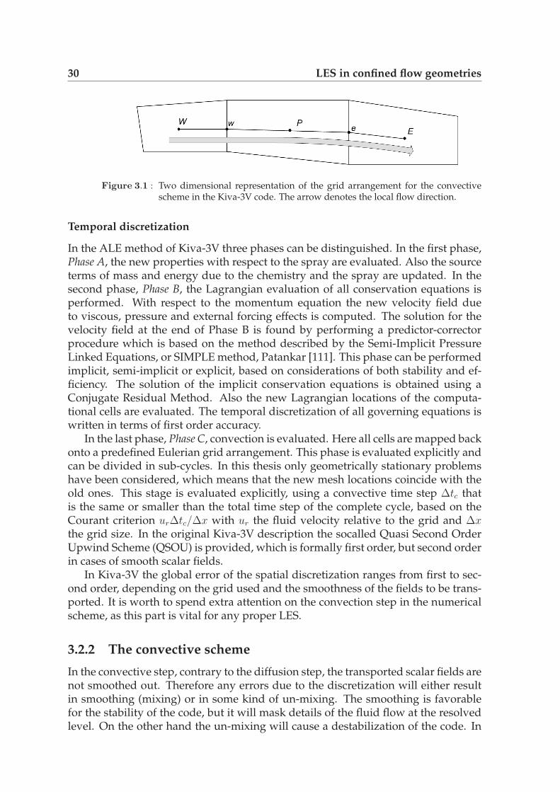
30 LES in confined flow geometries
Figure 3.1 : Two dimensional representation of the grid arrangement for the convectivescheme in the Kiva-3V code. The arrow denotes the local flow direction.
Temporal discretization
In the ALE method of Kiva-3V three phases can be distinguished. In the first phase,Phase A, the new properties with respect to the spray are evaluated. Also the sourceterms of mass and energy due to the chemistry and the spray are updated. In thesecond phase, Phase B, the Lagrangian evaluation of all conservation equations isperformed. With respect to the momentum equation the new velocity field dueto viscous, pressure and external forcing effects is computed. The solution for thevelocity field at the end of Phase B is found by performing a predictor-correctorprocedure which is based on the method described by the Semi-Implicit PressureLinked Equations, or SIMPLE method, Patankar [111]. This phase can be performedimplicit, semi-implicit or explicit, based on considerations of both stability and ef-ficiency. The solution of the implicit conservation equations is obtained using aConjugate Residual Method. Also the new Lagrangian locations of the computa-tional cells are evaluated. The temporal discretization of all governing equations iswritten in terms of first order accuracy.
In the last phase, Phase C, convection is evaluated. Here all cells are mapped backonto a predefined Eulerian grid arrangement. This phase is evaluated explicitly andcan be divided in sub-cycles. In this thesis only geometrically stationary problemshave been considered, which means that the new mesh locations coincide with theold ones. This stage is evaluated explicitly, using a convective time step ∆tc thatis the same or smaller than the total time step of the complete cycle, based on theCourant criterion ur∆tc/∆x with ur the fluid velocity relative to the grid and ∆xthe grid size. In the original Kiva-3V description the socalled Quasi Second OrderUpwind Scheme (QSOU) is provided, which is formally first order, but second orderin cases of smooth scalar fields.
In Kiva-3V the global error of the spatial discretization ranges from first to sec-ond order, depending on the grid used and the smoothness of the fields to be trans-ported. It is worth to spend extra attention on the convection step in the numericalscheme, as this part is vital for any proper LES.
3.2.2 The convective scheme
In the convective step, contrary to the diffusion step, the transported scalar fields arenot smoothed out. Therefore any errors due to the discretization will either resultin smoothing (mixing) or in some kind of un-mixing. The smoothing is favorablefor the stability of the code, but it will mask details of the fluid flow at the resolvedlevel. On the other hand the un-mixing will cause a destabilization of the code. In

3.2 The numerical methods 31
the convective phase the values of the scalar quantities φ (mass, momentum, speciesconcentrations) at the cell boundaries are essentially required, Amsden [5]. Thesevalues are interpolated in the following way:
φe = φP +xe − xP
xP − xW
Ψ(r)(φP − φW ). (3.2)
Here the subscripts e, E and W denote the cells relative to the center cell P , seefigure 3.1. Cell P is always located in the upwind direction of the local flow. Inthis equation the limiter function Ψ is introduced. This function comes from a TotalVariation Diminishing (TVD) procedure, that is introduced in the search for stable,but at the same time higher order schemes, see e.g. Hirsch [62]. For a first orderupwind scheme it can easily be seen that Ψ(r) = 1.
The motivation for using TVD schemes lies in their stability, which is importantfor simulations where destabilizing effects, such as highly curved meshes in combi-nation with high velocity gradients may appear. Standard second order schemes,such as the second order upwind or central scheme may cause serious stabilityproblems. The use of upwind schemes is necessary to keep the algorithm stable.However, lower order upwind schemes decrease the accuracy of the solver, andare thereby directly adding a numerical filter over the turbulent fluctuations. Thusit is of importance to reduce the level of upwinding as much as possible, but at thesame time keeping the algorithm bounded. For this goal TVD schemes are designed.In Kiva-3V a socalled Quasi Second Order Upwind (QSOU) differencing scheme isused. This can be qualified with the limiter function
Ψ(r) = max(0,min(r, 1)), (3.3)
where r is the ratio of the central- and the upwind gradient:
r =
(φE − φP
xE − xP
)/
(φP − φW
xP − xW
). (3.4)
Notice, that for Ψ(r) = r the interpolation scheme would be a second order accuratecentral scheme. The QSOU scheme can also be referred to as the minmod scheme,which is second order at locations where gradients remain small. The flux limiterfunction Ψ for the minmod scheme is the lower line in figure 3.2a: For r < 1 thefully second order central scheme is used, whereas for r > 1, i.e. large gradients ofΦE − ΦP , the first order upwind scheme is fully retained.
By replacing the limiter function with a less dissipative scheme we can reducethe impact of the algorithm on the numerical filtering. In this work with the Kiva-3Vcode the MUSCL scheme is applied. This limiter can be written as
Ψ(r) = max(0,min(2,3
4r +
1
4, 2r)) (3.5)
and follows a more curved line in the Ψ(r) space. In the flame simulations in theFASTEST-3D code, as will be presented in chapter 5, it appeared the most useful toapply the socalled Charm limiter function [163]. This is a smooth limiter function:
Ψ(r) = max
(0, r
3r + 1
(r + 1)2
). (3.6)
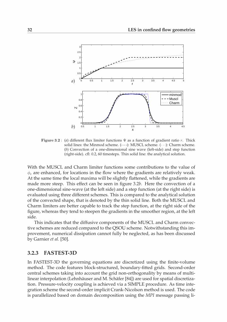
32 LES in confined flow geometries
0 0.5 1 1.5 2 2.5 3 3.5 4 4.5 50
0.5
1
1.5
2
2.5
3
r
Ψ
0.5 1 1.5 2 2.5 3 3.5 4 4.5
0
0.2
0.4
0.6
0.8
1
x
Z
minmodMusclCharm
a)
b)
Figure 3.2 : (a) different flux limiter functions Ψ as a function of gradient ratio r. Thicksolid lines: the Minmod scheme. (- - -): MUSCL scheme. (· · ·): Charm scheme.(b) Convection of a one-dimensional sine wave (left-side) and step function(right-side). cfl: 0.2, 60 timesteps. Thin solid line: the analytical solution.
With the MUSCL and Charm limiter functions some contributions to the value ofφe are enhanced, for locations in the flow where the gradients are relatively weak.At the same time the local maxima will be slightly flattened, while the gradients aremade more steep. This effect can be seen in figure 3.2b. Here the convection of aone-dimensional sine-wave (at the left side) and a step function (at the right side) isevaluated using three different schemes. This is compared to the analytical solutionof the convected shape, that is denoted by the thin solid line. Both the MUSCL andCharm limiters are better capable to track the step function, at the right side of thefigure, whereas they tend to steepen the gradients in the smoother region, at the leftside.
This indicates that the diffusive components of the MUSCL and Charm convec-tive schemes are reduced compared to the QSOU scheme. Notwithstanding this im-provement, numerical dissipation cannot fully be neglected, as has been discussedby Garnier et al. [50].
3.2.3 FASTEST-3D
In FASTEST-3D the governing equations are discretized using the finite-volumemethod. The code features block-structured, boundary-fitted grids. Second-ordercentral schemes taking into account the grid non-orthogonality by means of multi-linear interpolation (Lehnhauser and M. Schafer [84]) are used for spatial discretiza-tion. Pressure-velocity coupling is achieved via a SIMPLE procedure. As time inte-gration scheme the second-order implicit Crank-Nicolson method is used. The codeis parallelized based on domain decomposition using the MPI message passing li-

3.3 Square duct simulations 33
H
z
y
0 0.2 0.4 0.6 0.8 10
0.1
0.2
0.3
0.4
0.5
0.6
0.7
0.8
0.9
1
z/Hy/
H0 0.2 0.4 0.6 0.8 1
0
0.1
0.2
0.3
0.4
0.5
0.6
0.7
0.8
0.9
1
z/H
y/H
a) b) c)
Figure 3.3 : Geometry and orientation of the square duct. y and z denote the spanwiseflow directions. The dashed lines denote the locations where statistics is pre-sented: z = 0.25H and z = 0.5H , the arrows show the average, spanwise flowdirection. (b) Illustration of the coarse mesh (c) refined mesh.
brary. For details on the method we refer to Mengler [93], Durst and Schafer [42]or Wegner [163]. More details on the numerical method as used in FASTEST areoutlined in appendix A.
The dynamic formulation is employed for the subgrid scale stress-tensor τij , withLilly’s formulation of Germano’s dynamic procedure for the determination of themodel coefficient, Lilly [89]. No special wall treatment is used. Instead, the bound-ary layer is resolved and the dynamic procedure should be able to capture the cor-rect asymptotic behavior of the SGS model when approaching the wall, Lesieur andMetais [86].
3.3 Square duct simulations
For validation of the LES turbulence models numerical simulations of a turbulentflow in a square duct geometry with periodic boundary conditions for the stream-wise direction have been performed. This geometry is chosen for its simplicity. Yet,the fluid dynamics shows complex structures. This is a reflection of the anisotropyof the shear stress tensor. A characteristic of flow in square ducts is that it is accom-panied by turbulence driven secondary motions perpendicular to the streamwisedirection, figure 3.3. Although the magnitude of these motions may be as little as2% of the bulk velocity, they have an important effect on the overall flow structure.It is well known that simple RANS models such as the available k − ε model do notreveal any secondary flow.
Prediction of turbulence properties in regions of the flow domain where thesesecondary fluid motions occur are a test case for the LES method, as implementedin the Kiva-code. Furthermore, this geometry is well suited to study the turbulencebehavior and the predicted shear of the different models close to walls, which is ofbasic importance for confined situations, like internal combustion engines. Finally,for this situation well established literature results are available: numerical as wellas experimental [30, 37, 52, 57, 66, 92, 108]. Boundary layer flows are typically classi-fied using the friction velocity uτ . This velocity scale results from an applied force,
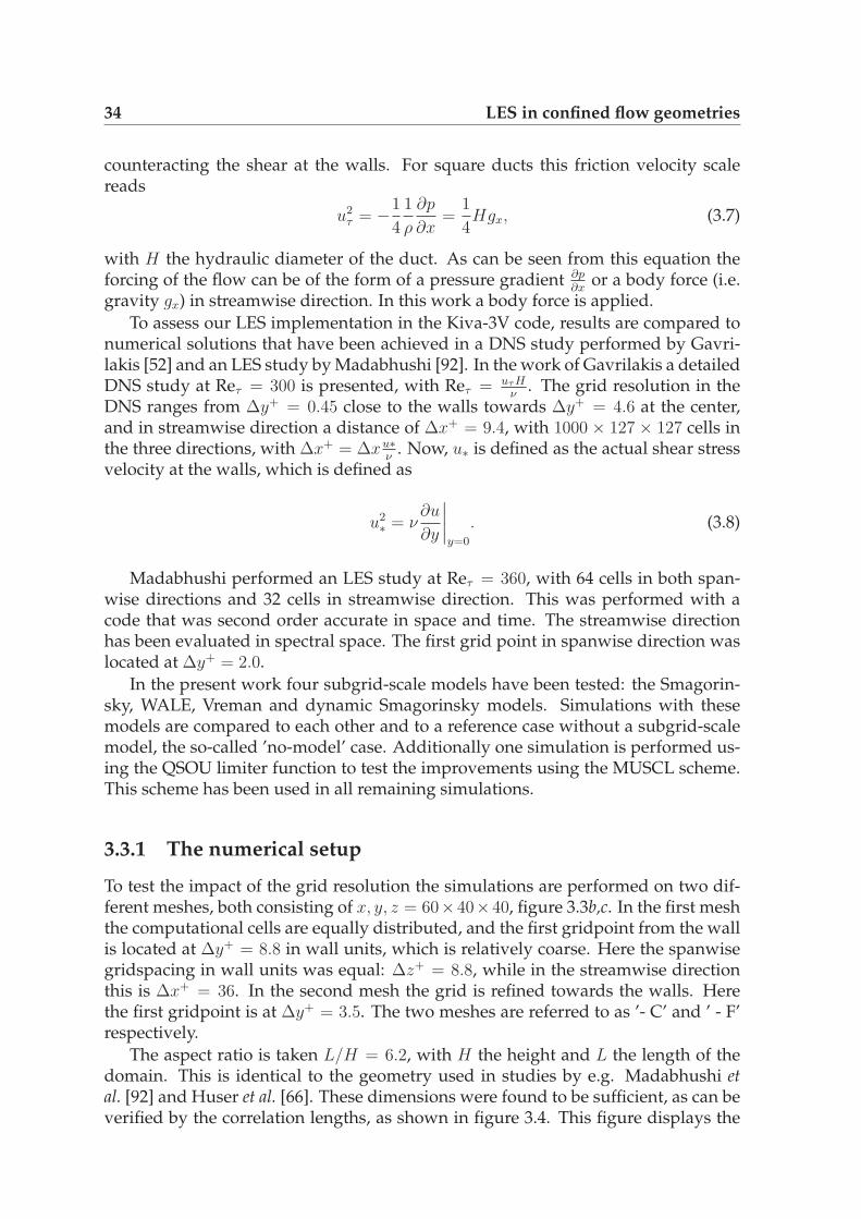
34 LES in confined flow geometries
counteracting the shear at the walls. For square ducts this friction velocity scalereads
u2τ = −1
4
1
ρ
∂p
∂x=
1
4Hgx, (3.7)
with H the hydraulic diameter of the duct. As can be seen from this equation theforcing of the flow can be of the form of a pressure gradient ∂p
∂xor a body force (i.e.
gravity gx) in streamwise direction. In this work a body force is applied.
To assess our LES implementation in the Kiva-3V code, results are compared tonumerical solutions that have been achieved in a DNS study performed by Gavri-lakis [52] and an LES study by Madabhushi [92]. In the work of Gavrilakis a detailedDNS study at Reτ = 300 is presented, with Reτ = uτ H
ν. The grid resolution in the
DNS ranges from ∆y+ = 0.45 close to the walls towards ∆y+ = 4.6 at the center,and in streamwise direction a distance of ∆x+ = 9.4, with 1000 × 127 × 127 cells inthe three directions, with ∆x+ = ∆xu∗
ν. Now, u∗ is defined as the actual shear stress
velocity at the walls, which is defined as
u2∗ = ν
∂u
∂y
∣∣∣∣y=0
. (3.8)
Madabhushi performed an LES study at Reτ = 360, with 64 cells in both span-wise directions and 32 cells in streamwise direction. This was performed with acode that was second order accurate in space and time. The streamwise directionhas been evaluated in spectral space. The first grid point in spanwise direction waslocated at ∆y+ = 2.0.
In the present work four subgrid-scale models have been tested: the Smagorin-sky, WALE, Vreman and dynamic Smagorinsky models. Simulations with thesemodels are compared to each other and to a reference case without a subgrid-scalemodel, the so-called ’no-model’ case. Additionally one simulation is performed us-ing the QSOU limiter function to test the improvements using the MUSCL scheme.This scheme has been used in all remaining simulations.
3.3.1 The numerical setup
To test the impact of the grid resolution the simulations are performed on two dif-ferent meshes, both consisting of x, y, z = 60×40×40, figure 3.3b,c. In the first meshthe computational cells are equally distributed, and the first gridpoint from the wallis located at ∆y+ = 8.8 in wall units, which is relatively coarse. Here the spanwisegridspacing in wall units was equal: ∆z+ = 8.8, while in the streamwise directionthis is ∆x+ = 36. In the second mesh the grid is refined towards the walls. Herethe first gridpoint is at ∆y+ = 3.5. The two meshes are referred to as ’- C’ and ’ - F’respectively.
The aspect ratio is taken L/H = 6.2, with H the height and L the length of thedomain. This is identical to the geometry used in studies by e.g. Madabhushi etal. [92] and Huser et al. [66]. These dimensions were found to be sufficient, as can beverified by the correlation lengths, as shown in figure 3.4. This figure displays the
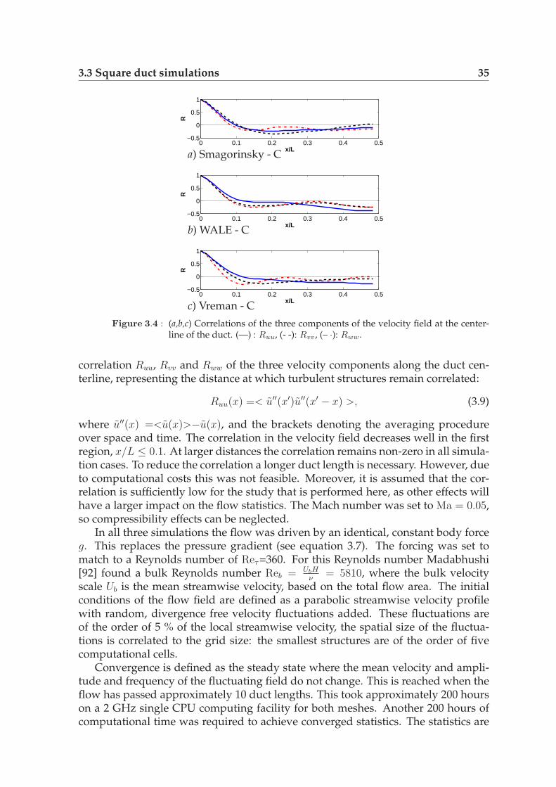
3.3 Square duct simulations 35
0 0.1 0.2 0.3 0.4 0.5−0.5
0
0.5
1
x/L
R
0 0.1 0.2 0.3 0.4 0.5−0.5
0
0.5
1
x/L
R
0 0.1 0.2 0.3 0.4 0.5−0.5
0
0.5
1
x/L
R
a) Smagorinsky - C
b) WALE - C
c) Vreman - C
Figure 3.4 : (a,b,c) Correlations of the three components of the velocity field at the center-line of the duct. (—) : Ruu, (- -): Rvv, (– ·): Rww.
correlation Ruu, Rvv and Rww of the three velocity components along the duct cen-terline, representing the distance at which turbulent structures remain correlated:
Ruu(x) =< u′′(x′)u′′(x′ − x) >, (3.9)
where u′′(x) =<u(x)>−u(x), and the brackets denoting the averaging procedureover space and time. The correlation in the velocity field decreases well in the firstregion, x/L ≤ 0.1. At larger distances the correlation remains non-zero in all simula-tion cases. To reduce the correlation a longer duct length is necessary. However, dueto computational costs this was not feasible. Moreover, it is assumed that the cor-relation is sufficiently low for the study that is performed here, as other effects willhave a larger impact on the flow statistics. The Mach number was set to Ma = 0.05,so compressibility effects can be neglected.
In all three simulations the flow was driven by an identical, constant body forceg. This replaces the pressure gradient (see equation 3.7). The forcing was set tomatch to a Reynolds number of Reτ =360. For this Reynolds number Madabhushi[92] found a bulk Reynolds number Reb = UbH
ν= 5810, where the bulk velocity
scale Ub is the mean streamwise velocity, based on the total flow area. The initialconditions of the flow field are defined as a parabolic streamwise velocity profilewith random, divergence free velocity fluctuations added. These fluctuations areof the order of 5 % of the local streamwise velocity, the spatial size of the fluctua-tions is correlated to the grid size: the smallest structures are of the order of fivecomputational cells.
Convergence is defined as the steady state where the mean velocity and ampli-tude and frequency of the fluctuating field do not change. This is reached when theflow has passed approximately 10 duct lengths. This took approximately 200 hourson a 2 GHz single CPU computing facility for both meshes. Another 200 hours ofcomputational time was required to achieve converged statistics. The statistics are

36 LES in confined flow geometries
Table 3.1 : Mean flow quantities Re∗ and Reb, based on the effective shear velocity u∗ andbulk velocity Ub respectively, and the ratio of the centerline velocity Uc overthe bulk velocity. ’C’ refers to the coarse resolution, ’F’ to the refined mesh.
Case Re∗ Reb Uc/Ub
Smagorinsky - C 244 6080 1.35WALE - C 317 7880 1.21
Vreman - C 332 7725 1.22Vreman - C - QSOU 330 8995 1.25
dynamic - C 311 7813 1.22no model - C 339 7665 1.20
Smagorinsky - F 257 5800 1.43WALE - F 318 7550 1.28
Vreman - F 324 7220 1.29no model - F 347 7490 1.29
Gavrilakis [52] 300 4410 1.33Madabhushi [92] 360 5810 1.28
evaluated based on two data planes perpendicular to the streamwise velocity field,0.5L apart from each other. The data was collected from t = 110 t∗ to 180 t∗ , witht∗ = L/Ub . The data is averaged over the four corners, as they are statisticallyidentical.
3.3.2 Results
The results of the simulations are analyzed on three different levels: the bulk flowquantities, the mean flow characteristics and the turbulent statistics.
Bulk flow quantities
In Table 3.1 the results of the bulk quantities for the different simulations are pre-sented. For every simulation a new Reb and Re∗ was evaluated, defined using thelocal shear stress velocity u∗ at the mid-wall location (z = 0.5H) of the duct. The re-sults all show a discrepancy with the work of Madabhushi and Gavrilakis: whereasRe∗ is relatively low, Reb exceeds the values found in literature. This indicates thatu∗ is underestimated in all simulations. Also notice that the simulations performedwith the Smagorinsky model show substantially smaller Reynolds numbers thanall other models, including the no model variant. The Vreman-QSOU model resultsin a larger bulk Reynolds number than the MUSCL variant. When comparing thecoarse mesh simulations with the simulations with refinement, Reτ increases, whileReb decreases.
A reason for the high values of Reb is the low resolution. This results in an in-ability to resolve steep mean gradients, which are encountered close to the walls.Moreover, the turbulent structures cannot properly be resolved. Then the flow willlaminarize and the bulk throughput increases, leading to an increase of Reb. It can

3.3 Square duct simulations 37
0 0.50
0.2
0.4
0.6
0.8
1
y/H
U/U
c
a) Coarse
0 0.50
0.2
0.4
0.6
0.8
1
y/H
U/U
c
b) Coarse
0 0.50
0.2
0.4
0.6
0.8
1
y/H
U/U
c
c) Refined
Figure 3.5 : Streamwise velocity field at z = 0.5H for the coarse and refined mesh simu-lations. Reference data: Gavrilakis [52] (- - -). For clearness the coarse meshresults are presented in two figures. (a) The models are ◦ Smagorinsky; ⋆dynamic model; (—) no model; (b) � WALE; △ Vreman model; (- - △ - -)Vreman - QSOU.
be seen that with increasing wall resolution these effects decrease. The steep gra-dients are better resolved and additionally more turbulent structures can grow inthe boundary layer. For the remainder of this study the velocity-scale Ub is consi-dered more appropriate for scaling the velocity, instead of the shear velocity uτ , asthe wall layer is not fully resolved. Also notice that the simulations including a sub-grid scale model and the no-model variants lead to very similar results (except forthe Smagorinsky model), indicating that the subgrid scale model is not very active.Other effects, as described above, are more crucial.
The ratio of the centerline velocity to the bulk velocity Uc/Ub is clearly the largestfor the Smagorinsky model, while all other models give similar low values around1.21 for the coarse mesh simulations and about 1.3 for the mesh with refinement.The Smagorinsky model is known to over-predict the turbulent dissipation in theshear flow close to the walls. With increasing Reynolds number the profiles of thestreamwise velocity should become flatter and gradients in the wall region steeper,which leads to a decrease in the ratio Uc/Ub. In case of the Smagorinsky model bothReynolds numbers decrease, due its large dissipation near the walls. This effect iswell visible in figure 3.5a,c.
Mean flow profiles
The mean streamwise profiles are shown in figure 3.5. The velocities are in this casescaled to the centerline velocity Uc, to focus on the shape of the profiles. All mod-els follow the reference profile reasonably accurately, except for the Smagorinskymodel, as discussed above.
The spanwise flow field is compared to the results obtained by Gavrilakis [52], asshown in figure 3.6a. Three representative cases are shown in figure 3.6: Smagorin-
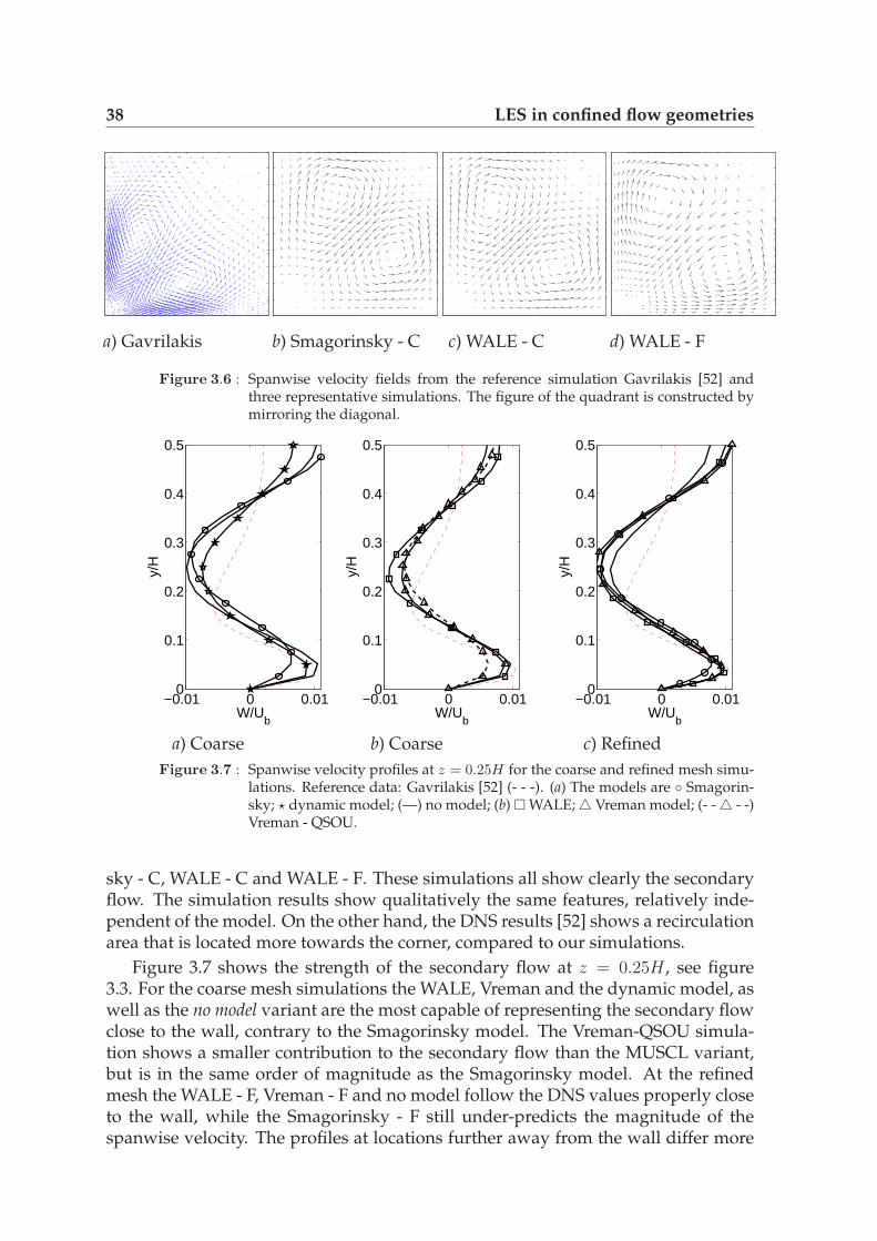
38 LES in confined flow geometries
a) Gavrilakis b) Smagorinsky - C c) WALE - C d) WALE - F
Figure 3.6 : Spanwise velocity fields from the reference simulation Gavrilakis [52] andthree representative simulations. The figure of the quadrant is constructed bymirroring the diagonal.
−0.01 0 0.010
0.1
0.2
0.3
0.4
0.5
y/H
W/Ub
a) Coarse
−0.01 0 0.010
0.1
0.2
0.3
0.4
0.5
y/H
W/Ub
b) Coarse
−0.01 0 0.010
0.1
0.2
0.3
0.4
0.5
y/H
W/Ub
c) Refined
Figure 3.7 : Spanwise velocity profiles at z = 0.25H for the coarse and refined mesh simu-lations. Reference data: Gavrilakis [52] (- - -). (a) The models are ◦ Smagorin-sky; ⋆ dynamic model; (—) no model; (b) � WALE; △ Vreman model; (- - △ - -)Vreman - QSOU.
sky - C, WALE - C and WALE - F. These simulations all show clearly the secondaryflow. The simulation results show qualitatively the same features, relatively inde-pendent of the model. On the other hand, the DNS results [52] shows a recirculationarea that is located more towards the corner, compared to our simulations.
Figure 3.7 shows the strength of the secondary flow at z = 0.25H , see figure3.3. For the coarse mesh simulations the WALE, Vreman and the dynamic model, aswell as the no model variant are the most capable of representing the secondary flowclose to the wall, contrary to the Smagorinsky model. The Vreman-QSOU simula-tion shows a smaller contribution to the secondary flow than the MUSCL variant,but is in the same order of magnitude as the Smagorinsky model. At the refinedmesh the WALE - F, Vreman - F and no model follow the DNS values properly closeto the wall, while the Smagorinsky - F still under-predicts the magnitude of thespanwise velocity. The profiles at locations further away from the wall differ more

3.3 Square duct simulations 39
0 0.1 0.2 0.3 0.4 0.50
0.005
0.01
0.015
0.02
0.025
y/H
k/U
b2
a) Coarse
0 0.1 0.2 0.3 0.4 0.50
0.005
0.01
0.015
0.02
0.025
y/H
k/U
b2
b) Refined
Figure 3.8 : Total resolved kinetic energy at z = 0.5H , compared to Gavrilakis [52] (- - -).(a) Coarse mesh, (b) Refined mesh. The models are ◦ Smagorinsky; � WALE; △Vreman model; (- - △ - -) Vreman - QSOU; ⋆ dynamic model, (—): no-model.
substantially from the DNS results, corresponding to the shift of the recirculationarea, visible from figure 3.6. An explanation for the observations can be providedby the impact of the numerical scheme, the subgrid model and the resolution. TheSmagorinsky model will dampen the secondary flow motion. The other subgridscale models will account better for anisotropic turbulence near the walls, and filterout the shear component. The subgrid scale models are now less active and lead tosimilar results as the no-model variant. Still the effect of the numerical scheme is im-portant, notwithstanding that the MUSCL variant leads to more appropriate resultsas the QSOU method. The refinement leads to a slight improvement, in particularfor the Smagorinsky model.
Turbulence statistics
The total resolved turbulent kinetic energy (k) at half the duct cross section (z = 0.5H),from the wall up to the duct centerline (y = 0.5H), is shown in figure 3.8. These pro-files are scaled to the bulk velocity. For the coarse mesh simulations the WALE,dynamic and no model variants show a similar level of turbulent kinetic energyas reported by Gavrilakis. The Vreman model overpredicts this value, whereas theVreman-QSOU model prediction for k is again reduced compared to the MUSCLvariant, but shows a broader profile. This can be attributed to the larger numer-ical diffusion that is inherent to this numerical scheme, and can explain the poorprediction of the secondary flow pattern close to the wall. The Smagorinsky modelshows a shift in its maximum value more towards the center of the domain. For therefined mesh simulations the Vreman model now shows a more accurate predictionof the turbulence intensity, which makes it more comparable with the other mod-els (WALE, no model) and the DNS. Still the Smagorinsky model remains shifted.When considering the different contributions to the turbulent kinetic energy it wasobserved that the streamwise turbulence profiles lead to similar behavior as k infigure 3.8. The simulations have more difficulties representing the smaller terms
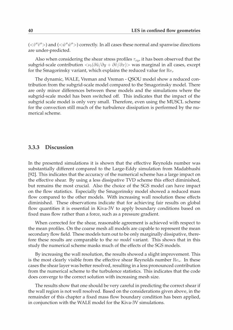
40 LES in confined flow geometries
(<v′′v′′>) and (<w′′w′′>) correctly. In all cases these normal and spanwise directionsare under-predicted.
Also when considering the shear stress profiles τxy, it has been observed that thesubgrid-scale contribution <νt(∂u/∂y + ∂v/∂x)> was marginal in all cases, exceptfor the Smagorinsky variant, which explains the reduced value for Reτ
The dynamic, WALE, Vreman and Vreman - QSOU model show a reduced con-tribution from the subgrid-scale model compared to the Smagorinsky model. Thereare only minor differences between these models and the simulations where thesubgrid-scale model has been switched off. This indicates that the impact of thesubgrid scale model is only very small. Therefore, even using the MUSCL schemefor the convection still much of the turbulence dissipation is performed by the nu-merical scheme.
3.3.3 Discussion
In the presented simulations it is shown that the effective Reynolds number wassubstantially different compared to the Large-Eddy simulation from Madabhushi[92]. This indicates that the accuracy of the numerical scheme has a large impact onthe effective shear. By using a less dissipative TVD scheme this effect diminished,but remains the most crucial. Also the choice of the SGS model can have impacton the flow statistics. Especially the Smagorinsky model showed a reduced massflow compared to the other models. With increasing wall resolution these effectsdiminished. These observations indicate that for achieving fair results on globalflow quantities it is essential in Kiva-3V to apply boundary conditions based onfixed mass flow rather than a force, such as a pressure gradient.
When corrected for the shear, reasonable agreement is achieved with respect tothe mean profiles. On the coarse mesh all models are capable to represent the meansecondary flow field. These models turn out to be only marginally dissipative, there-fore these results are comparable to the no model variant. This shows that in thisstudy the numerical scheme masks much of the effects of the SGS models.
By increasing the wall resolution, the results showed a slight improvement. Thisis the most clearly visible from the effective shear Reynolds number Re∗. In thesecases the shear layer was better resolved, resulting in a less pronounced contributionfrom the numerical scheme to the turbulence statistics. This indicates that the codedoes converge to the correct solution with increasing mesh size.
The results show that one should be very careful in predicting the correct shear ifthe wall region is not well resolved. Based on the considerations given above, in theremainder of this chapter a fixed mass flow boundary condition has been applied,in conjunction with the WALE model for the Kiva-3V simulations.
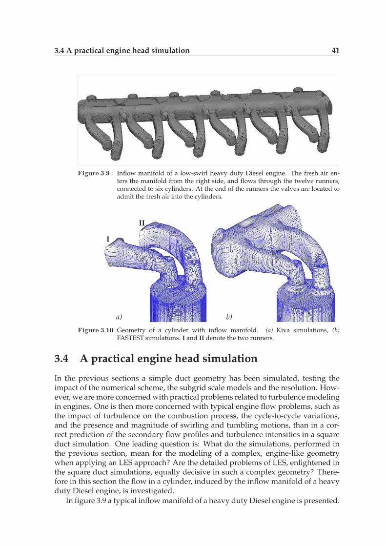
3.4 A practical engine head simulation 41
Figure 3.9 : Inflow manifold of a low-swirl heavy duty Diesel engine. The fresh air en-ters the manifold from the right side, and flows through the twelve runners,connected to six cylinders. At the end of the runners the valves are located toadmit the fresh air into the cylinders.
a) b)
I
II
Figure 3.10 :Geometry of a cylinder with inflow manifold. (a) Kiva simulations, (b)FASTEST simulations. I and II denote the two runners.
3.4 A practical engine head simulation
In the previous sections a simple duct geometry has been simulated, testing theimpact of the numerical scheme, the subgrid scale models and the resolution. How-ever, we are more concerned with practical problems related to turbulence modelingin engines. One is then more concerned with typical engine flow problems, such asthe impact of turbulence on the combustion process, the cycle-to-cycle variations,and the presence and magnitude of swirling and tumbling motions, than in a cor-rect prediction of the secondary flow profiles and turbulence intensities in a squareduct simulation. One leading question is: What do the simulations, performed inthe previous section, mean for the modeling of a complex, engine-like geometrywhen applying an LES approach? Are the detailed problems of LES, enlightened inthe square duct simulations, equally decisive in such a complex geometry? There-fore in this section the flow in a cylinder, induced by the inflow manifold of a heavyduty Diesel engine, is investigated.
In figure 3.9 a typical inflow manifold of a heavy duty Diesel engine is presented.

42 LES in confined flow geometries
The runners connect the inflow manifold with the cylinders. In this case there aresix cylinders connected to the runners. At the end of the runners the valves can beopened to control the flow of fresh gasses into the cylinder. The shape of the runnerswill have a large impact on the resulting flow dynamics down in the cylinder. In thiswork a so-called low swirl cylinder head is investigated.
Figure 3.10 shows in more detail the connection of the inlet runners to the cylin-der. In reality the cylinder head incorporates four valves: two inlet and two exhaustvalves. In the experiments as well as the simulations a steady state investigation ofthe flow is performed: only the flow due to the inlet runners is modeled. Thereforea constant valve lift of the inlet valves of 9 mm is applied, while the exhaust valvesare closed. This means that the piston at the bottom of the cylinder is removed, suchthat the fluid can flow steadily through the complete domain.
Such a steady flow setup is often used to characterize a production type cylinderhead experimentally. The bore diameter D is 130 mm. For the current simulationstudy a constant mass flow of 204 gr/s is applied through the cylinder. This corre-sponds approximately to the maximum flow rate occuring during the intake strokeof an engine running at full load. The corresponding Reynolds number Reinlet basedon the port diameter and the flow rate is around 2.2 · 105.
The numerical results are compared to particle image velocimetry (PIV) data,performed by de Leeuw [83]. Therefore the cylinder has been removed and replacedwith a dummy perspex cylinder, such that it is optically accessible.
3.4.1 The numerical setup
Kiva-3V simulations
Three simulations have been performed with Kiva-3V, see table 3.2. All simulationsused the same mesh, shown in figure 3.10a. This mesh consists of approximately400,000 cells, refined at the top of the cylinder. In the first simulation Kiva A theclassical URANS k − ε model is adopted. The other simulations are performed inthe LES mode. In the second simulation referred to as Kiva B the inflow boundarycondition is set based on simple considerations of equal mass flow through the tworunners. In the third simulation, simulation Kiva C, the actual space-dependent flowprofiles through the two runners is controlled in two inlet planes such that it equalsthe mean velocity profiles at these planes as found in the FASTEST results. In theKiva simulations a smaller domain is modelled than in the FASTEST simulations.This was because of the computational expenses: not only the computational timewas a limiting factor, also the available memory limited the size of the computation.Therefore, to keep sufficient resolution inside the cylinder, only a small upstreamregion was simulated additionally. This is standard practise in this type of simu-lations, e.g., Payri et al. [112], but the validity of this choice is unclear beforehand. Itis not obvious how the flow conditions in the two runners are related to each other.
In all simulations a zero-gradient outflow boundary is defined at the bottom, atz/D = 3. The influence of this downstream boundary is assumed to be sufficientlyreduced as the depth of the cylinder has been set to 3D, while performing the mainanalysis up to z = 1.75D.

3.4 A practical engine head simulation 43
Table 3.2 : List of performed simulations
Simulation number of cells turbulence Mass flow (I - II)[millions] model [kg/s]
Kiva A 0.4 URANS k-ε 0.102 - 0.102Kiva B 0.4 LES WALE 0.102 - 0.102Kiva C 0.4 LES WALE 0.110 - 0.094
FASTEST A 0.5 LES dynamic turbulent, 0.204FASTEST B 2.5 LES dynamic turbulent, 0.204
FASTEST-3D simulations
Two calculations have been carried out using the FASTEST code, see table 3.2. Thefirst computation had a relatively coarse resolution, this simulation is referred to asFASTEST A. The number of cells reaches 0.5 million cells. In the second simulationthe grid-cell size is reduced in every direction, which results in a total of 2.5 millioncells, referred to as simulation FASTEST B. As the FASTEST code applies a multi-block strategy, this implies that so-called O-grids can be used which will improvethe quality of the mesh, especially at all curved areas near the walls. In the cur-rent simulations the convective scheme has been blended with a first order upwindscheme, at a level of 10%, in order for the solver to remain stable at locations of veryskewed cells, especially near the valves. In the FASTEST simulations a larger partof the inflow manifold is simulated, compared to the Kiva simulations, see figure3.10b. Therefore the fluid is naturally distributed over the two inflow runners. Themass flow rates at the two runners, at the locations where the Kiva simulations start,has been evaluated. For both the coarse and the fine mesh simulations these valueswere 0.11 kg/s for runner I and 0.094 kg/s for runner II.
Moreover, at the inflow plane turbulent inflow conditions are provided consist-ing of a correlated inflow field with turbulent statistics based on pipe flow measure-ments, Eggels [43]. This procedure is based on the inflow generator developed byKlein et al. [73], and is adapted for arbitrary surfaces. At the bottom a zero-gradientoutflow boundary condition is defined.
Computational requirements
The computational time for both the Kiva-3V and FASTEST simulations was approx-imately 2 months on different high-performance computing facilities. The FASTESTA simulation is parallelized on two CPU’s where FASTEST B has used eight CPU’s.All Kiva-3V simulations ran on a single CPU. The simulated physical time equals0.15 sec, which is estimated to be sufficient to capture approximately 100 large-scaleturbulent time-scales in the upper part of the domain, where the fluctuations havea relatively short time scale.
For all simulations the y+ value is evaluated for the first grid point normal to thewall, as an indication of the resolution of the boundary layer by the applied grid,see table 3.3. For the Large-Eddy simulations with the FASTEST code y+ reachesvalues up to 6000 close to the valves, where instantaneous velocity magnitudes areextreme. Downward in the cylinder the average values decrease to 1000. Close

44 LES in confined flow geometries
Table 3.3 : Evaluation of y+ for the different simulations
Simulation max. y+ average y+ max. y+ average y+
at Z/D = 0.25 at Z/D=0.25 at Z/D = 1.75 at Z/D=1.75Kiva A 11000 2900 2150 410Kiva B 21500 4480 1950 530
FASTEST A 6330 2900 4300 1750FASTEST B 5850 1890 2700 960
I
II
I II
a) b)
Figure 3.11 :(a) Illustration of the two main vertical jets, arising from the two runners. Thesejets drive the mean swirling motion. (b) Streamlines illustrating the mean tum-bling flow by the recirculation areas below the valves. Simulation FASTESTB.
to the valves the y+ values for the Kiva-simulations exceed the levels from bothFASTEST simulations, due to the relatively coarse mesh. However, at the bottom ofthe cylinder the y+ values are much reduced compared to the FASTEST simulations,reflecting moderate velocities close to the walls.
It is acknowledged that these values indicate that the turbulent wall shear flowis completely not resolved in any case. For a good resolution of the shear flow at thewall in a pure LES, the value of y+ should be of the order unity. While a fixed massflow has been applied, the simulated Reynolds number was appropriate, but thelocal shear can have an important impact on the local flow behavior. This can haveconsequences on the average, global flow patterns that are induced by the shapeof the valves and cylinder wall, as well as the balancing of the imposed mass flowthrough the runners.
A more appropriate wall modeling method can be achieved by introducing ahybrid scheme, where the wall region is modeled using a RANS approach, and theregion far away with the LES approach. Recent efforts in this direction are reportedby Tessicini et al. [154], Temmerman et al. [153] and de Langhe et al. [79, 80].

3.4 A practical engine head simulation 45
I
II I
II
a) b)
Figure 3.12 :(a) Location of the plane where the data is evaluated, indicated by the blacksheet, crossing through the valves. (b) orientation for the figures at constantheight z.
3.4.2 Results and discussions
In this section the results from the simulations are presented and discussed. Themain features of the flow are illustrated in figure 3.11. Figure 3.11a illustrates theorigin and location of two large-scale jet-like structures. When following these struc-tures downwards along the cylinder walls a clear mean rotational flow is observed,referred to as a swirling motion. The right picture (figure 3.11b) shows the stream-lines of the mean velocity field on a cross-section in the domain. Two recirculationareas can be identified, which illustrate the second effect characteristic for enginegeometries: tumble. The size of the tumbling motion scales to the size of the valves.
By averaging the data over the performed simulation time mean and turbulentflow field data have been evaluated, which will be presented in the next subsec-tions. First the mean flow properties are considered, focussing on the tumble andthe swirling motion. Then the turbulent flow properties will be considered. Alldata is compared on several planes in the domain. A vertical plane is extractedsuch that it crosses the two valves, see figure 3.12a. Moreover at three locations,z = 0.25D, z = 1.25D and z = 1.75D below the cylinder head, with D being thecylinder diameter, horizontal cross sections are extracted. At the lower two levelsPIV data of the flowfield in spanwise direction is available.
Tumble
Figure 3.13 shows the contour levels of the mean vertical velocity fields for the fivedifferent cases. It is observed that in all simulations, except for the URANS simula-tion Kiva A, the flow is directed towards the right valve. This can be explained bythe inflow geometry, figure 3.12 . The runners induce a strong jet directed to the wallof the cylinder. The angle and strength of this jet will determine the strength of theswirling motion in the cylinder. The jet in Kiva C is more inclined towards the wallthan in Kiva B and FASTEST A,B. This indicates the impact of the mass balancing inthe two runners.
The resemblance of the two FASTEST simulations indicates that these simu-

46 LES in confined flow geometries0
−20
−20
0
−40−60
0
−20
−40
0
−20
−40
−80
20
0
−20
−40
0
00
−20
−40
−120
−80 −
80−4
0
0
20
−20
−40
−40
−40
−20
−20−40
−80
0
0
−40
0−20
−80
−40
-40
-20
-20
-40-2
0
-40
0
0
0
0
0
-20
00
-20-20
-8020
0
-60
00
-20
-20
0
-20
-20
20
-20
20
0-40
-20-80
-20
-40
0-2
0-6
0
-60
-40
-20
0
0
-60-40
0
20
-60
-40
-40
0
-20
-200
20 -20-40
-20
-60
Kiva A Kiva B Kiva C FASTEST A FASTEST B
Figure 3.13 :<w>-component velocity fields in the plane indicated in figure 3.12. Contourlevels are shown in steps of 20 m/s.
20
0
−20
−20−200
−40
−60
−40
−40
−40
−60 −40 −20 0 20 40 60
−60
−40
−20
0
20
40
60
−40
−20
0
−40
−40−20
0
−60
−80
−80
−60 0
−20
−20
−80
−60
−60 −40 −20 0 20 40 60
−60
−40
−20
0
20
40
60
20
0
−20
−40
−60
20
0
−20
−40
−60−20
−60−80
−80
−40
−60 −40 −20 0 20 40 60
−60
−40
−20
0
20
40
60
20
0
−20
−40
−60
−80
−40
−60
−40
−20
020
0
−20
−60 −40 −20 0 20 40 60
−60
−40
−20
0
20
40
60
200
−20−40
−60
−80
−200
−40
−40
−60 −40 −20 0 20 40 60
−60
−40
−20
0
20
40
60
Kiva A Kiva B Kiva C FASTEST A FASTEST B
Figure 3.14 :<w>- velocity fields at z = 0.25D below the cylinder head.
lations can be considered relatively grid-independent. The two jets emerging be-tween the valve and the cylinder walls do not penetrate deeply into the cylinder asthe shear at the walls is relatively large. These jets will be mainly responsible for thetumbling effects.
The tumble is best observed in figure 3.14. In case Kiva A the two tumblingregions are equally large, consistent with the <w>-contour plot from figure 3.13. Inthe other simulations the tumbling region at the right side of the cylinder is slightlysmaller than the left side, which is in correspondence with the centered jet in theprevious figure. The Kiva C simulation predicts a relatively large deviation betweenthe two tumbling regions.
Swirl
When looking at the mean spanwise velocity fields in figures 3.15 and 3.16, it isfound that the large-scale vortices are relatively weak for the URANS simulationKiva A. The Large-Eddy simulations show a stronger contribution to the vorticalmotions. In all cases two large-scale vortical structures are found at z/D = 1.25, incorrespondence with the PIV experimental data. In case Kiva B the vortical struc-tures are not equal in strength, just like the FASTEST results and experiments.
The mean spanwise velocity vector field from simulation FASTEST B changesfrom a complex flow structure near the valves to two counterrotating vortices, fig-ure 3.15. Lower in the cylinder the stronger counter-clockwise vortex still survives,figure 3.16. This is in contrast to the experiments and the simulations from Kiva-3V.
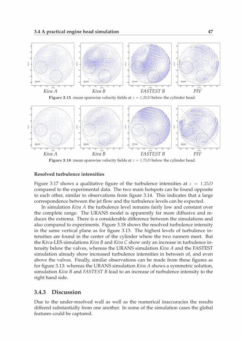
3.4 A practical engine head simulation 47
−60 −40 −20 0 20 40 60
−60
−40
−20
0
20
40
60
10 m/s
x [mm]
y [m
m]
−60 −40 −20 0 20 40 60
−60
−40
−20
0
20
40
60
10 m/s
x [mm]
y [m
m]
−60 −40 −20 0 20 40 60
−60
−40
−20
0
20
40
60
10 m/s
x [mm]
y [m
m]
−60 −40 −20 0 20 40 60
−60
−40
−20
0
20
40
60
10 m/s
x [mm]
y [m
m]
Kiva A Kiva B FASTEST B PIVFigure 3.15 :mean spanwise velocity fields at z = 1.25D below the cylinder head.
−60 −40 −20 0 20 40 60
−60
−40
−20
0
20
40
60
10 m/s
x [mm]
y [m
m]
−60 −40 −20 0 20 40 60
−60
−40
−20
0
20
40
60
10 m/s
x [mm]
y [m
m]
−60 −40 −20 0 20 40 60
−60
−40
−20
0
20
40
60
10 m/s
x [mm]
y [m
m]
−60 −40 −20 0 20 40 60
−60
−40
−20
0
20
40
60
10 m/s
x [mm]
y [m
m]
Kiva A Kiva B FASTEST B PIVFigure 3.16 :mean spanwise velocity fields at z = 1.75D below the cylinder head.
Resolved turbulence intensities
Figure 3.17 shows a qualitative figure of the turbulence intensities at z = 1.25Dcompared to the experimental data. The two main hotspots can be found oppositeto each other, similar to observations from figure 3.14. This indicates that a largecorrespondence between the jet flow and the turbulence levels can be expected.
In simulation Kiva A the turbulence level remains fairly low and constant overthe complete range. The URANS model is apparently far more diffusive and re-duces the extrema. There is a considerable difference between the simulations andalso compared to experiments. Figure 3.18 shows the resolved turbulence intensityin the same vertical plane as for figure 3.13. The highest levels of turbulence in-tensities are found in the center of the cylinder where the two runners meet. Butthe Kiva-LES simulations Kiva B and Kiva C show only an increase in turbulence in-tensity below the valves, whereas the URANS simulation Kiva A and the FASTESTsimulation already show increased turbulence intensities in between of, and evenabove the valves. Finally, similar observations can be made from these figures asfor figure 3.13: whereas the URANS simulation Kiva A shows a symmetric solution,simulation Kiva B and FASTEST B lead to an increase of turbulence intensity to theright hand side.
3.4.3 Discussion
Due to the under-resolved wall as well as the numerical inaccuracies the resultsdiffered substantially from one another. In some of the simulation cases the globalfeatures could be captured.
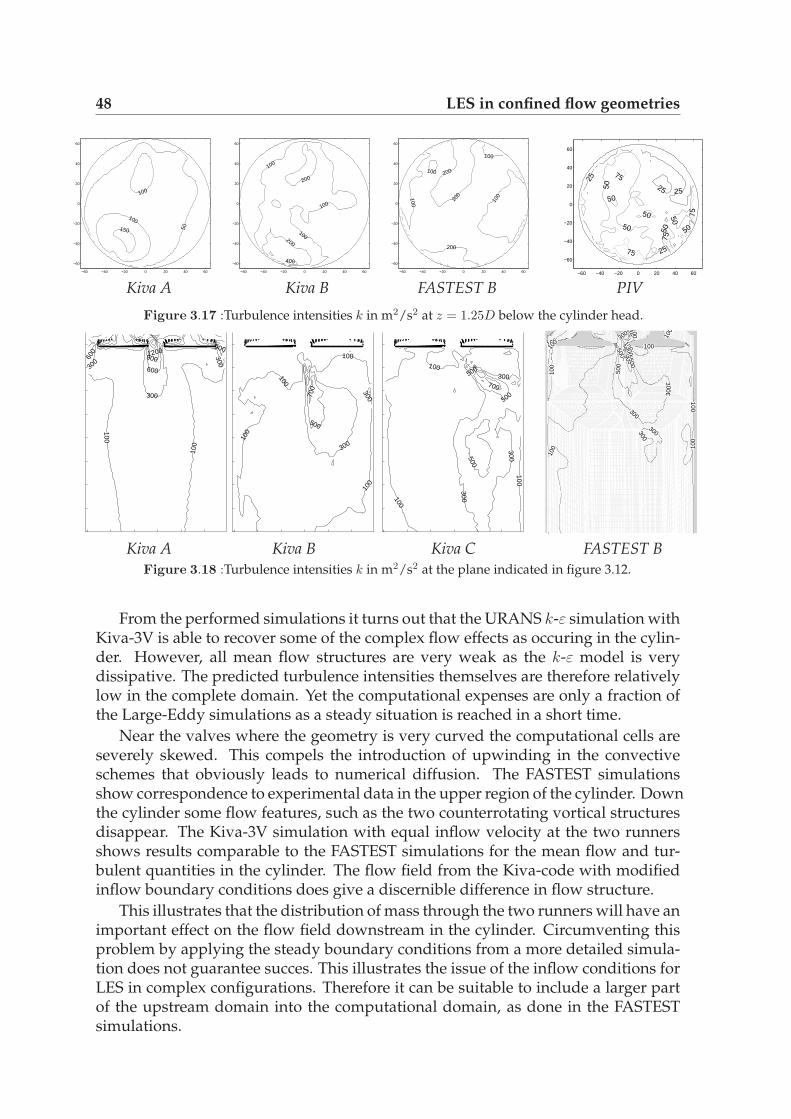
48 LES in confined flow geometries
150
100
100
50
−60 −40 −20 0 20 40 60
−60
−40
−20
0
20
40
60
400
200
100
100
200
100
−60 −40 −20 0 20 40 60
−60
−40
−20
0
20
40
60
100
200
200100
100
200
100
−60 −40 −20 0 20 40 60
−60
−40
−20
0
20
40
60
25
50
50
7525 25
50
5075
50
75
50
25
50
75
−60 −40 −20 0 20 40 60
−60
−40
−20
0
20
40
60
Kiva A Kiva B FASTEST B PIV
Figure 3.17 :Turbulence intensities k in m2/s2 at z = 1.25D below the cylinder head.
100
100
300
600
9001200
300
600 300
900
100
300
500
700
100
100
100
300
100
100
300500
500
700
500300
300100
100
100
100
100
500
500
300
900
900100300500500
300
300
100300300
100
300
300
100
300
300
100
100
Kiva A Kiva B Kiva C FASTEST BFigure 3.18 :Turbulence intensities k in m2/s2 at the plane indicated in figure 3.12.
From the performed simulations it turns out that the URANS k-ε simulation withKiva-3V is able to recover some of the complex flow effects as occuring in the cylin-der. However, all mean flow structures are very weak as the k-ε model is verydissipative. The predicted turbulence intensities themselves are therefore relativelylow in the complete domain. Yet the computational expenses are only a fraction ofthe Large-Eddy simulations as a steady situation is reached in a short time.
Near the valves where the geometry is very curved the computational cells areseverely skewed. This compels the introduction of upwinding in the convectiveschemes that obviously leads to numerical diffusion. The FASTEST simulationsshow correspondence to experimental data in the upper region of the cylinder. Downthe cylinder some flow features, such as the two counterrotating vortical structuresdisappear. The Kiva-3V simulation with equal inflow velocity at the two runnersshows results comparable to the FASTEST simulations for the mean flow and tur-bulent quantities in the cylinder. The flow field from the Kiva-code with modifiedinflow boundary conditions does give a discernible difference in flow structure.
This illustrates that the distribution of mass through the two runners will have animportant effect on the flow field downstream in the cylinder. Circumventing thisproblem by applying the steady boundary conditions from a more detailed simula-tion does not guarantee succes. This illustrates the issue of the inflow conditions forLES in complex configurations. Therefore it can be suitable to include a larger partof the upstream domain into the computational domain, as done in the FASTESTsimulations.

3.5 Conclusions 49
3.5 Conclusions
In this chapter the numerical procedure as applied in Kiva-3V has been sketched.The convective scheme of the Kiva-3V code has been adapted with a less dissipativeTVD scheme, in order to increase accuracy but at the same time keeping stability.
A number of subgrid scale models has been implemented in the Kiva-3V code.These were tested on the turbulent flow in a square duct geometry. Additionally,results are compared to a no model variant, where the SGS contribution is switchedoff. A general conclusion from the performed simulations is that global flow featuresare recovered, but if the wall region is not well resolved it is hard to quantitativelypredict the shear, as well as all other flow properties.
In the latter part of this chapter a more realistic engine geometry has been in-vestigated: a complex turbulent, swirling and tumbling flow in an engine cylinderthat is induced by the inlet manifold. A number of Large-Eddy simulations havebeen performed with the FASTEST and Kiva-3V code, and additionally one URANSsimulation. The effect of the poor wall resolution and the numerical scheme in theLarge-Eddy simulations on the flow field statistics was relatively large. Again, onlyglobal flow features could be captured appropriately. A detailed data analysis andcomparison of the different simulations with each other and with experiments isproblematic as small differences in the complex flow result in large differences ofspecific flow quantities at specific locations.
LES gives an indication of the unsteady, turbulent processes that take place inan engine. However, this study shows that for a quantitative predictive quality thenumerical scheme as well as the computational resolution have to be improved.
Recommendations
In this subsection some remarks will be presented to give an indication on futuremodeling approaches for complex (engine) setups. To gain more confidence in theunsteady flow behaviour, an Large-Eddy simulation can be more preferable to anURANS based calculation, on the condition that available computational power isnot a restriction. For the near wall regions, however, a hybrid approach woulddefinitely be more suitable, see, e.g., Tessicini et al. [154].
It appears that reasonable in-cylinder flow results can be achieved when onlymodeling a relatively small part of the upstream region, basically because the flowaround the valves will create the main flow structures. As pointed out above, thebest approach is to include a larger part of the upstream region into the computa-tional domain.
By showing the sensitivity of the inflow conditions on the flow pattern in asteady geometry it can be concluded that this will be very sensitive on any changesin inflow conditions as encountered in moving piston geometries: any erroneousvalve-motion modeling and grid-handling will lead to relatively large deviations inthe flow patterns. This is especially true for detailed flow information that, for ex-ample, can be extracted from experimental LDA methods. It can be expected that itremains very hard to make such a detailed prediction with any CFD method on thislevel. But interesting information from the simulations can be extracted on the level

50 LES in confined flow geometries
of global flow fields, as well as turbulence intensities. Best practice today concern-ing realistic engine geometries is to compare data from simulations to experimentaltechniques like PIV. In future more accurate, detailed measurements can serve as avalidating tool. Then, with increasing computational power sensitivity studies canmore easily be performed using LES.
In the introduction it has been remarked that the flow in an engine at real oper-ating conditions is strongly influenced by the squish at the end of the combustionphase. Concerning future work it is a challenging, and important question to inves-tigate its impact on the turbulent cylinder flow, induced by the inflow manifold, tostudy cycle-to-cycle variations.

Chapter
4Modeling the turbulentmixing of a gas jet
In this chapter the properties of a gaseous fuel jet have been studiedusing the LES method, for three different fuel to ambient gas den-sity ratios. The impact of the injected gas density on the resultingflow field is considered. The penetration depth and the cone angleare analyzed, and it is shown that the gaseous fuel jets follow wellthe similarity theory. By applying a virtual Schlieren postprocess-ing method to the simulation data problems related to this exper-imental technique could be enlightened. Also the correspondenceof the gas jet flow dynamics compared to those of a liquid spray isanalyzed. When corrected for the cone angle, the gas jet dynamicsfollows well the scaling laws proposed for the liquid fuel sprays.
4.1 Introduction
In the previous chapter the modeling of non-reacting fluid flow for engine appli-cations has been considered. The combustion process is of main concern in enginemodeling, and is governed by the chemical reactions that take place in a combustiblemixture. In Diesel engines, fuel is injected into the air near the end of the compres-sion stroke. The ensuing mixing process does influence the combustion parameters,such as ignition delay, location of ignition, heat production, reaction products for-mation and soot formation. Modeling of the mixing process in an engine is of keyimportance for the prediction of combustion in engines. Especially for future enginetypes, applying Homogeneous Charge Compression Ignition (HCCI) combustionconcepts, the mixing of the fuel and oxidizer is an important controlling variable ofthe combustion, Cook et al. [33].
Previous studies on Diesel injection have enabled a general understanding ofthe effect of high pressure direct injection systems on fuel-air mixing, Naber andSiebers [99]. Classical mixing models based on a RANS approach can be reasonablyaccurate for the use as a modeling tool; all physical effects that have been observedexperimentally can be represented, Abraham and Magi [2]. Only average, globalflow information had been available from experiments, which are the quantitiesthat are accounted for in the RANS modeling environment. Gas injection systems

52 Modeling the turbulent mixing of a gas jet
are generally studied based on RANS type methods, e.g. Ouellette and Hill [107]and references therein.
However, it has been argued in chapter 1 that for pollutants modeling like NOx
and soot it is very hard to predict concentration fields if only average flow quantitiesare available. Therefore a more accurate and detailed description of the processesthat govern this formation is required. This concerns both detailed experimentaldata as well as numerical studies on the mixing process in fuel gas jets and sprays.The LES approach is chosen, as it yields a more detailed, instantaneous flow andmixing information compared to RANS. Along with modeling the turbulent flowfield the transport of any representative scalar field can be evaluated. In princi-ple this scalar field can be used to define the chemical state of the fluid. For non-homogeneous mixtures like in Diesel engines, this scalar field is chosen such that itrepresents the fuel-to-air mixing ratio, given by the mixture fraction Z.
When the fuel is injected in the gas phase the modeling can be performed us-ing a single phase flow solver. The evolution of a gaseous mixture can be modelledby solving scalar transport equations for the different species separately. In Dieselengines, fuel is injected in the liquid phase and not in the gas phase. Therefore,droplet breakup, collisions and evaporation in a turbulent environment should inprinciple be accounted for. However, the quantitative optical diagnostics on dropletstatistics (size, speed, amount, location) is a tedious task, as has been discussed byBruneaux [24]. At the same time the simulation of two-phase flows in this field re-mains a challenge, and has -until now- been limited to very simple geometries, need-ing very specialized solvers. Moreover in most studies of two-phase flows only lowdroplet densities can be considered. Thus the modeling of dense sprays, as can befound in Diesel engine injection systems, remains a major challenge, Jay et al. [70].Most solvers that apply particle/droplet models are nowadays based on a RANSturbulence description, because for LES methods the computational demands aremuch larger. These limitations lead to the decision to study a gaseous fuel jet in-stead. This modeling simplification needs justification. Liquid jets can obviouslynot in all regions be simplified to gas jets. On the other hand, when all fuel dropletsare vaporized, finally the fuel spray flow resembles a gas jet structure.
An additional topic can be formulated regarding the data treatment. From exper-imental techniques difficulties remain in gathering and interpreting accurate mea-surement data, Klein-Douwel et al. [75]. Therefore a Large-Eddy simulation canhelp: a three-dimensional time-resolved dataset of all relevant flow parameters isprovided. Whereas in the experiments uncertainties with respect to measurementand visualization techniques are present, in simulations numerical inaccuracies andmodel limitations restrict the global predictability. Yet, the simulations can help toserve as a tool for validating experimental visualization techniques, and give in-formation on problems concerning numerical and experimental data treatment. Astandard practice in experimental methods is to use a Schlieren method, where lightrays are deflected due to density gradients in the gaseous jet. This can in principlebe simulated and applied to the numerical results.
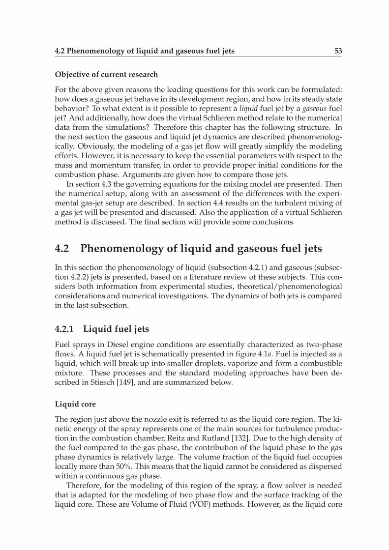
4.2 Phenomenology of liquid and gaseous fuel jets 53
Objective of current research
For the above given reasons the leading questions for this work can be formulated:how does a gaseous jet behave in its development region, and how in its steady statebehavior? To what extent is it possible to represent a liquid fuel jet by a gaseous fueljet? And additionally, how does the virtual Schlieren method relate to the numericaldata from the simulations? Therefore this chapter has the following structure. Inthe next section the gaseous and liquid jet dynamics are described phenomenolog-ically. Obviously, the modeling of a gas jet flow will greatly simplify the modelingefforts. However, it is necessary to keep the essential parameters with respect to themass and momentum transfer, in order to provide proper initial conditions for thecombustion phase. Arguments are given how to compare those jets.
In section 4.3 the governing equations for the mixing model are presented. Thenthe numerical setup, along with an assessment of the differences with the experi-mental gas-jet setup are described. In section 4.4 results on the turbulent mixing ofa gas jet will be presented and discussed. Also the application of a virtual Schlierenmethod is discussed. The final section will provide some conclusions.
4.2 Phenomenology of liquid and gaseous fuel jets
In this section the phenomenology of liquid (subsection 4.2.1) and gaseous (subsec-tion 4.2.2) jets is presented, based on a literature review of these subjects. This con-siders both information from experimental studies, theoretical/phenomenologicalconsiderations and numerical investigations. The dynamics of both jets is comparedin the last subsection.
4.2.1 Liquid fuel jets
Fuel sprays in Diesel engine conditions are essentially characterized as two-phaseflows. A liquid fuel jet is schematically presented in figure 4.1a. Fuel is injected as aliquid, which will break up into smaller droplets, vaporize and form a combustiblemixture. These processes and the standard modeling approaches have been de-scribed in Stiesch [149], and are summarized below.
Liquid core
The region just above the nozzle exit is referred to as the liquid core region. The ki-netic energy of the spray represents one of the main sources for turbulence produc-tion in the combustion chamber, Reitz and Rutland [132]. Due to the high density ofthe fuel compared to the gas phase, the contribution of the liquid phase to the gasphase dynamics is relatively large. The volume fraction of the liquid fuel occupieslocally more than 50%. This means that the liquid cannot be considered as dispersedwithin a continuous gas phase.
Therefore, for the modeling of this region of the spray, a flow solver is neededthat is adapted for the modeling of two phase flow and the surface tracking of theliquid core. These are Volume of Fluid (VOF) methods. However, as the liquid core
54 Modeling the turbulent mixing of a gas jet
region is normally very small and exists only close to the nozzle exit, this is usuallyneglected in typical spray simulation solvers, e.g. Amsden et al. [5], Naud [100].
Breakup region
In the next region separate fuel droplets can be identified in a continuous gas phase.The liquid core has now broken up into first ligaments and droplets. Three effectsdrive this primary breakup process: the turbulence within the liquid phase, the im-plosion of cavitation bubbles and aerodynamic forces acting on the liquid jet [149].Depending on injection parameters such as the relative velocity vrel between the liq-uid and the gas, the liquid density and gas density ρa, the droplet radius rd andsurface tension σ, the relative contribution of the different mechanisms to the spraybreakup varies, resulting in different breakup lengths and different droplet sizes.This is described by the characteristic Weber number:
We =ρardv
2rel
σ. (4.1)
This describes the strength of the aerodynamic forces, relative to the surface tensionof the droplets. For instance, with increasing relative velocity between liquid andgas phase, the aerodynamic forces acting on the liquid surface are intensified and thewavelength of the disturbances become shorter, resulting in smaller average dropletdiameters.
With the large-scale liquid fuel being transformed into droplets after the primarybreakup, the secondary breakup region is driven by aerodynamic forces acting onthe droplets by the surrounding gas phase. Droplets are distorted from their ini-tially spherical shape, and broken up into two (vibrational breakup) or many smalldroplets (catastrophic breakup) depending on the Weber number.
Particle interactions and evaporation
Another process that complicates the spray dynamics concerns the particle-particleinteractions. Collisions between particles have a strong impact on the mean dropletsize and its spatial distribution. The different regimes can be defined based on acollision Weber number. After collision the particles can bounce elastically, coalescepermanently or shatter into tiny droplets, depending on their relative velocity.
Finally, the evaporation takes place, which will provide a combustible mixture,when mixed with fresh air. Heat is transported into the droplet, while fuel vapormass is transferred from the boundary layer at the drop surface into the gas. Thepenetration depth of the spray is influenced by the evaporation rate. Naber andSiebers [99] show that for high ambient gas densities vaporizing sprays can be rep-resented by non-vaporizing liquid fuel sprays. Only with decreasing ambient airdensity, at a fuel-to-air density ratio of about 20 (for instance, using n-heptane at 684kg/m3 injecting in compressed air of about 35 kg/m3), the non-vaporizing fuel jetsshow an enhanced penetration depth up to 20% more, compared to the vaporizingjet. This is because the fuel droplets do not transfer momentum instantaneouslyfrom the injected fluid to entrained gas. Thus, depending on the rate of vaporiza-tion, a velocity difference may exist for some time, leading to a delayed entrainment

4.2 Phenomenology of liquid and gaseous fuel jets 55
Zt
a) b) c)Figure 4.1 : (a) Conceptual representation of a liquid fuel jet. (b) Concentration field and
entrainment pattern of a round turbulent jet. (c) Schematics of the self-similarconcentration profiles.
and enhanced penetration. Typically, poor evaporation will result in poor mixing,that will increase the soot production. Very rapid evaporation on the other handwill cause an increase in nitrogen oxides, due to a relatively large, hot premixedcombustion phase.
4.2.2 Gaseous fuel jets
For steady, round turbulent gas jets at moderate to high Reynolds number a widerange of experimental data exists. This type of jets is a standard test case when de-veloping turbulence models for practical applications. Olsson and Fuchs [106] haveshown LES results on a circular jet for three different Reynolds numbers rangingfrom 1 ·104 up to 50 ·104. Here the region close to the nozzle exit has been simulated.The main difference between a gas jet at engine operating conditions and standardexperimental turbulent jets as generally reported in the literature [41,67,109] are thephysical dimensions (tens of millimeters instead of centimeters / meters) and thedensity ratio. For fuel jets the density ratio of fuel to ambient air can be up to 100,whereas in most gas jet experiments only small variable density has been studied,with density ratios ranging from 0.5 to 5. The turbulent jet consists phenomenolog-ically by the core, the shear layer and the jet tip regions. In the remainder of thissection these aspects are described.
Potential core region
In the first region above the injector the gaseous fuel is not yet diluted with ambientair. This region is denoted as the potential core, and is comparable to the liquidcore for liquid jets. Lubbers et al. [91] note that the injection geometry does have animpact on the resulting jet dynamics. This will be discussed below.

56 Modeling the turbulent mixing of a gas jet
Shear layer
The injected jet momentum generates a high shear, which produces a wide rangeof turbulent structures, from small to large scale. Within this shear layer a largeentrainment of ambient gases can be expected.
The main mechanism of entrainment is by engulfment of ambient fluid alongthe edges of the large-scale turbulent jet structures, as depicted in figure 4.1b. Sub-sequently mixing takes place by stretching of the interface that is formed betweenthe entrained fluid and the jet fluid. Both jet and entrained fluid come into contactat ever smaller scales, until, at the Kolmogorov scale, the fluid from the two streamsbecomes fully mixed. This is well documented by Schefer et al. [140].
Jet Tip
The jet tip can be described as the top region of the visible, developing jet. In section4.4.2 a more detailed definition will be provided. Bruneaux [24] showed experi-mentally the existence of very steep gradients in the mean profiles near the jet tip.Compared to the mixing in the shear layer this indicates a lower turbulent mixingrate, which apparently is only involving the large scales. Due to this low mixing ratethe formation of uniformly distributed fuel pockets with steep gradients at the edgeis enhanced. Therefore large differences exist between independent instantaneousflow profiles. By averaging these profiles, an erroneous figure on the mixing mayappear, described by a gradually increasing level of fuel concentration. Bruneauxshowed that the fuel mass distribution function at the spray tip is represented by adouble-peak function, which illustrates these unmixed, uniformly distributed fuel/ air pockets with steep gradients in between.
Also the analysis by Schefer et al. [140] of instantaneous profiles in a turbulentjet has shown a close relationship between the fuel profile characteristics and thestructure of the turbulent velocity field. This can be characterized in terms of large-scale, quasi-periodic, and organized structures. There are significant departures ofthe instantaneous profiles from conventional time-averaged profiles. This showsthat a proper description of the mixing process at the trailing edge of the jet is notpossible when using a RANS-type model for the flow field. Here it is favorable toaccount for instantaneous flow field phenomena.
Additionally, as described by Pope [126], the standard k − ε model is not ade-quate to model jets: the mass entrainment rates are under-predicted. A solution isto include a second moment closure. Another modeling approach, keeping a two-equation RANS approach, is to adapt the turbulent modeling coefficients Cε1 andCε2 in equation 2.24 to better reproduce the mass entrainment rate in steady-statejets. However, this means giving up the idea that these established coefficients areuniversal, which leads to ad hoc assumptions for any changing geometrical case.
Self-similarity theory
The gaseous jet dynamics can be described phenomenologically using self-similaritytheory. This is very helpful for understanding the governing physics of a gaseousfuel jet. An important scaling parameter for injection systems is the momentum

4.2 Phenomenology of liquid and gaseous fuel jets 57
injection rate at the nozzle exit M0. This parameter is evaluated from
M0 =
∫
A
ρ0u20dA, (4.2)
with u0 the local injection velocity, ρ0 the density of the injected mass and A theinjection area. It has been generally accepted that a self-similarity solution doesexist for this type of problems, Dowling and Dimotakis [41]. For a discussion see,e.g., Lubbers et al. [91]. A similarity equation can be derived for a well developedturbulent jet, which is at Reynolds numbers larger than 3×10³ and distances largerthan 20 d0 (i.e., out of the potential core region). Then the mass entrainment ratecorrelation of Ricou and Spalding [136] is used. This relates the penetration depthzt of turbulent jets to a typical diameter deff :
zt
deff
= Γ(π
4
)1/4(
tu0
deff
)1/2
, (4.3)
with deff the equivalent, or effective diameter, defined as deff = d0(ρ0/ρa)1/2 and d0
being the nozzle diameter. In this equation ρa is the ambient air density. Further-more, Γ is a constant with a value of about 3.0 for turbulent jets with round nozzles.This equation can also be written in terms of the momentum injection rate:
zt = Γ(M0/ρa)1/4t1/2. (4.4)
Also the decrease of the mean velocity and mixture fraction along the centralaxis can be described using similarity theory. Generally, due to the conservation ofmomentum flux at each cross-section of the jet, the velocity decay rate will decreasefor increasing gas jet density. The impact of the ambient air entrainment on the jetdecay are written in decay correlations:
u0
u= Ku
z
deff
,Z0
Z= Kz
z
deff
, (4.5)
with Ku and Kz the entrainment rates for velocity and mixture fraction respectivelyand Z0 the mixture fraction at the nozzle exit. Thus, through the use of the effectivediameter the density effect is taken into account.
There is an ongoing debate whether self similarity theory is really valid, as thedecay-rate and other aspects depend considerably on the inlet conditions, e.g., Lub-bers et al. [91]. Carazzo et al. [26] discusses that complete self-similarity can onlybe found at very large distances from the nozzle exit. At intermediate distancesonly self-similarity can be found at increasing heights, for identical setups. Thisself-similarity is different for different setups. Also Ruffin et al. [137] write that forvariable density jets no exact self-similarity can be found, due to varying relativeinfluences of the inertial, gravitational and viscous forces as present in the jet dy-namics. On the other hand, the self-similarity model has proven its usability andglobal accuracy. Therefore it will be used in the discussion and analysis of the re-sults below.

58 Modeling the turbulent mixing of a gas jet
4.2.3 Modeling Diesel sprays using a gas jet
Due to the complications as given in subsection 4.2.1, it is tried to mimic the mixingprocess of a liquid fuel jet and the final state of the jet prior to ignition and com-bustion using a gas jet. One of the leading questions is how accurate such a jetsimulation can represent typical liquid Diesel sprays. Obviously, some importantphysics will be missing, especially at the regions of large liquid void fraction closeto the nozzle exit. On the other hand, further downstream where only a very dilutespray is present, it can be argued that the jet dynamics originating from a liquidspray follows the gas jet dynamics, Desantes [38].
For certain applications it has been argued that gaseous jets and Diesel sprayswith small droplet size (of the order of a few microns) mix at about the same rate,when injected into air of typical Diesel chamber density and with an equivalentmomentum injection rate, Ouellette and Hill [107]. Also Abraham and Magi [1]have investigated two RANS k− ε based models for gas jets to mimic Diesel sprays.There it was concluded that the numerical accuracy and resolution was far moredecisive than the applied modeling approach.
The question here is, which working point of a gas jet should be chosen such thatthe liquid fuel jet is well reproduced at the important regions where first ignitionand consequently combustion will take place. Typical working point variables forliquid Diesel jets are as follows (see, e.g. Naber and Siebers [99]). With respect tothe fuel: Diesel fuel density is ρ0 = 835 kg/m3; injection pressures range between∆pinj = 100 − 200 MPa and injection velocity v0 ≈ 350 m/s. The injector nozzleradius is usually d0 = 0.1-0.24 mm. The ambient density in the cylinder at injectionranges between ρa = 20-40 kg/m3.
For the simulations the injection velocity is subsonic; in this work an incompress-ible solver is used. For the ambient density a constant value of ρa =25 kg/m3 is ap-plied. The conservation equation for energy is not solved, therefore no heat releaseis accounted for. The jet density ρ0 ranged from 25 to 250 kg/m3, with an injec-tion velocity of about 180 m/s. However, by correcting for the applied momentuminjection rate and using the effective diameter it is assumed that the main parame-ters (spreading rate; turbulence intensity; jet penetration depth) can be corrected fortypical engine conditions, and compared to liquid jet data.
4.3 The mixing model
For the current investigation the FASTEST-3D code has been used. This code is aincompressible finite volume, code, validated for Large-Eddy simulations on coldflow engine setups. For a more detailed description of the code, see appendix A, ore.g. Wegner [163]. The standard LES equations on the mass and momentum conser-vation are solved. Additionally a mixing model is applied. This will be described inthe following. Then some details on the numerical setup will be provided.

4.3 The mixing model 59
4.3.1 The mixture fraction
In non-premixed combustion systems the mixture fraction Z can be used to definethe chemical composition of the fluid. This scalar field for this type of problems canbe written in the following way, Peters [114]:
Z =νstYF − YOx + YOx,2
νstYF,1 + YOx,2
, (4.6)
where the subscripts 1, 2 denote the fuel stream and air stream respectively, and YF
and YOx the local mass fractions of fuel and oxidizer respectively. In this equationνst refers to the stoichiometric oxidizer-to-fuel mass ratio, which can be written as(using subscript u to refer to the initial conditions in the unburnt mixture):
νst =YOx,u
YF,u
∣∣∣∣st
. (4.7)
Yet, for pure mixing problems, as presented in this chapter, Z simply correspondsto the injected fuel mass fraction. In the LES approach a transport equation for thefiltered mixture fraction field Z is solved:
ρ∂Z
∂t+ ρuj
∂Z
∂xj
=∂
∂xj
(ρ(DZ + Dt)
∂Z
∂xj
). (4.8)
The mixture fraction is bounded between zero and unity: Z equals 0 in the airstream, whereas Z = 1 in the injected fuel stream. The LES filtered molecular andturbulent diffusion of mixture fraction is correlated to the viscosity using a constantmolecular and turbulent Schmidt number:
Dz = ν/Sc, Dt = νt/Sct, (4.9)
where νt is modeled dynamically, using equation 2.50. In this work both Schmidtnumbers are set to 0.9. Similarly, for completeness we can write a transport equation
for the subgrid scale mixture fraction variance Z ′′2 as [114]
ρ∂Z ′′2
∂t+ ρuj
∂Z ′′2
∂xj
=∂
∂xj
(ρDt
∂Z ′′2
∂xj
)
︸ ︷︷ ︸I
+ 2ρDt
(∂Z
∂xj
)2
︸ ︷︷ ︸II
− 2ρDZ
˜(∂Z ′′
∂xj
)2
︸ ︷︷ ︸III
. (4.10)
The three terms in above equation denote I the turbulent transport, II the Z ′′2 pro-duction and III the filtered scalar dissipation rate, given by
χ = 2DZ
˜(∂Z ′′
∂xj
)2
. (4.11)
Notice that in the LES approach the mixture fraction variance transport equation isusually not solved. Instead an analytical model is used to describe the unresolvedpart. Then, to find an estimate of the mixture fraction variance, a similar procedure

60 Modeling the turbulent mixing of a gas jet
������������������������������������������������������������������������������������������������
������������������������������������������������������������������������������������������������
��������������������������������������������������������������������������������
��������������������������������������������������������������������������������
������������������������������������������������������������������������������������������������������������������
������������������������������������������������������������������������������������������������������������������
�������������������������������������������������������������������������������������������������������������������������������������
�������������������������������������������������������������������������������������������������������������������������������������
15mm
x
z
0.2mm
80mm
30mm
a) b)Figure 4.2 : (a) Schematics of the gas injection system. (b) Applied geometry for the per-
formed simulations
Table 4.1 : List of performed simulations. Subscript 0 denotes the values at the nozzle exitand ρa denotes the ambient density that is set to 25 kg/m3.
Simulation number of ρ0/ρa ρ0 ν0 M0 Re0
cells kg/m3 m2/s (kgm/s2)Jet 1A 50,000 1 25 2.68×10⁻⁵ 19.6×10⁻³ 1300Jet 1B 50,000 2 50 1.2×10⁻⁵ 39.3×10⁻³ 3000Jet 2A 400,000 1 25 2.68×10⁻⁵ 21.3×10⁻³ 1300Jet 2B 400,000 2 50 1.2×10⁻⁵ 42.3×10⁻³ 3000Jet 2C 400,000 10 250 1.05×10⁻⁵ 209×10−3 3400
as for the sgs turbulence intensity q2sgs can be followed, see section 2.3.1. By assum-
ing local equilibrium, the production balances the scalar dissipation rate. Then, by
scaling analysis this leads to a model for Z ′′2 of the form (Branley [22])
CZ
(∂Z
∂xj
)2
=Z ′′2
∆2. (4.12)
In this equation, for CZ the value of 0.15 is assumed, Wegner [163].
4.3.2 The numerical setup
A typical gas-injection system is characterized by a small nozzle (∼ 0.1 - 0.4 mm),that injects fuel at high speeds into a pressurized combustion chamber, as is schemat-ically shown in figure 4.2a. The gas enters the chamber perpendicular to the sur-rounding exit plane. The numerical setup is designed as shown in figure 4.2b. Thediameter of the injector orifice is d0 =0.2 mm. Mass is injected with a maximumvelocity speed of U0 = 180 m/s; the average jet velocity at the nozzle exit was about140 m/s. Then, a time scale can be defined: τ ∗ = d0/U0 = 4.5µs. For the jet cor-related inflow data has been generated with turbulent statistics corresponding to aturbulent pipe flow, Eggels [43]. In total five independent simulations have been

4.3 The mixing model 61
0 0.1 0.2 0.3 0.4 0.5 0.6 0.7 0.8 0.9 10
200
400
ρ [k
g/m
3 ]
Z0 0.1 0.2 0.3 0.4 0.5 0.6 0.7 0.8 0.9 1
1
2
3x 10
−5
ν [m
2 /s]
Figure 4.3 : Viscosity ν and density ρ as function of the mixture fraction Z, shown forJet 2C.
a) b)Figure 4.4 : (a) Sketch of the applied mesh. (b) Cross section around the nozzle for the fine
grid simulations.
performed, on two different meshes and applying three different density ratios, seetable 4.1.
The ambient density ρa in all simulations was set to 25 kg/m3, which is typicalfor the ambient air density in an engine around top dead center, and comparable tothe gasjet study performed by Desantes [38]. Three density ratios have been studied:one where the fuel injection density ρ0 was equal to the ambient gas density ρa,and an additional simulation with a density ratio ρ0/ρa = 2, which correspondsto a type of fuel with twice the density of air, e.g., ethane. The third density ratioreached a level of ρ0/ρa = 10, i.e., the injected fuel had a density of 250 kg/m3, whichcorresponds to a more practical engine fuel.
The viscosity has been computed from correlations provided by Evlampiev [44].Here, data from the ethane fuel for the specific conditions lead to values rangingfrom 2.68 ×10⁻⁵ m2/s for the ambient gas viscosity and 1.05 ×10⁻⁵m2/s for thefuel viscosity at 250 kg/m3. A linear dependence is applied for the laminar mixingof the fuel and ambient gas densities and viscosities, as is described in Evlampiev[44]. Then the applied mixing rules ν = ν(Z), ρ = ρ(Z) for simulation Jet 2C ispresented in figure 4.3. The Reynolds number based on the nozzle diameter, themaximum velocity and the fuel viscosity at the nozzle exit ranged between 1.3× 10³
and 3.5 × 10³.
The applied mesh is shown in figure 4.4. The height of the computational do-main was set to 8 cm, which corresponds to a scaled height of H = 400d0. For the
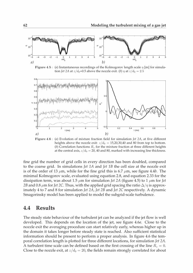
62 Modeling the turbulent mixing of a gas jet
−5 −4 −3 −2 −1 0 1 2 3 4 510
−6
10−5
10−4
x/d0
η
−5 −4 −3 −2 −1 0 1 2 3 4 510
−6
10−5
10−4
x/d0
η
a) b)Figure 4.5 : (a) Instantaneous recordings of the Kolmogorov length scale η [m] for simula-
tion Jet 2A at z/d0=0.5 above the nozzle exit. (b) η at z/d0 = 2.5
0 1 2 3 4 50
0.1
0.2
0.3
0.4
0.5
0.6
0.7
0.8
Z
t (ms)0 0.2 0.4 0.6 0.8 1
−0.5
0
0.5
1
Rz
τ (ms)
a) b)Figure 4.6 : (a) Evolution of mixture fraction field for simulation Jet 2A, at five different
heights above the nozzle exit: z/d0 = 15,20,30,40 and 80 from top to bottom.(b) Correlation functions Rz for the mixture fraction at three different heightsat the central axis, z/d0 = 20, 40 and 80, marked with increasing line thickness.
fine grid the number of grid cells in every direction has been doubled, comparedto the coarse grid. In simulations Jet 1A and Jet 1B the cell size at the nozzle exitis of the order of 13 µm, while for the fine grid this is 6.7 µm, see figure 4.4b. Theminimal Kolmogorov scale, evaluated using equation 2.8, and equation 2.33 for thedissipation term, was about 1.5 µm for simulation Jet 2A (figure 4.5) to 1 µm for Jet2B and 0.8 µm for Jet 2C. Thus, with the applied grid spacing the ratio ∆/η is approx-imately 4 to 7 and 8 for simulation Jet 2A, Jet 2B and Jet 2C respectively. A dynamicSmagorinsky model has been applied to model the subgrid-scale turbulence.
4.4 Results
The steady state behaviour of the turbulent jet can be analyzed if the jet flow is welldeveloped. This depends on the location of the jet, see figure 4.6a. Close to thenozzle exit the averaging procedure can start relatively early, whereas higher up inthe domain it takes longer before steady state is reached. Also sufficient statisticalinformation should be present to perform a proper analysis. In figure 4.6 the tem-poral correlation length is plotted for three different locations, for simulation Jet 2A.A turbulent time scale can be defined based on the first crossing of the line Rz = 0.Close to the nozzle exit, at z/d0 = 20, the fields remain strongly correlated for about

4.4 Results 63
0 10 20 30 40 500
1
2
3
4
5
6
7
8
9
10
11
z/d0
W0/W
c
Jet 2AJet 2BJet 2C
0 10 20 30 40 500
1
2
3
4
5
6
7
8
9
10
11
z/d0
1/Z
c
Jet 2AJet 2BJet 2C
a) b)Figure 4.7 : (a) Inverse velocity decay and (b) inverse mixture fraction decay at the center-
line, as a function of z/d0, for the two different density jets.
0 10 20 30 40 500
1
2
3
4
5
6
7
8
9
10
11
z/deff
W0/W
c
Jet 2AJet 2BJet 2C
0 5 10 15 20 25 30 35 40 45 500
1
2
3
4
5
6
7
8
9
10
11
z/deff
Z0/Z
Jet 2AJet 2BJet 2C
a) b)Figure 4.8 : (a) Inverse velocity decay and (b) inverse mixture fraction decay at the center-
line, as a function of z/deff , for the two different density jets
0.05 ms. This is similar at z/d0 = 40 and increases for z/d0 = 80 up to about 0.3 ms.The total simulation time was always 5 ms, which means that up to z/d0 = 40 about100 statistically independent realizations could be used. Therefore, up to this heightthe steady state behaviour will be examined, as presented in the first subsection. Inthe next subsection, results on the unsteady, developing behaviour is presented.
4.4.1 Steady state behaviour
The decay of the averaged inverse centerline velocity and mixture fraction is shownin figure 4.7. Here on the horizontal axis the depth is scaled to the nozzle diameterd0. Then, for both figures it can be seen that the velocity decay is reduced with in-creasing jet density. The unscaled core length remains constant for all three densitycases, as is visible from figure 4.7. This is in correspondence with numerical obser-vations from RANS calculations, Sanders et al. [138]. Here it was remarked that inthe far field, where the density across the jet is almost uniform, the similarity theoryapplies well. A more universal decay rate is found when scaling the depth with the
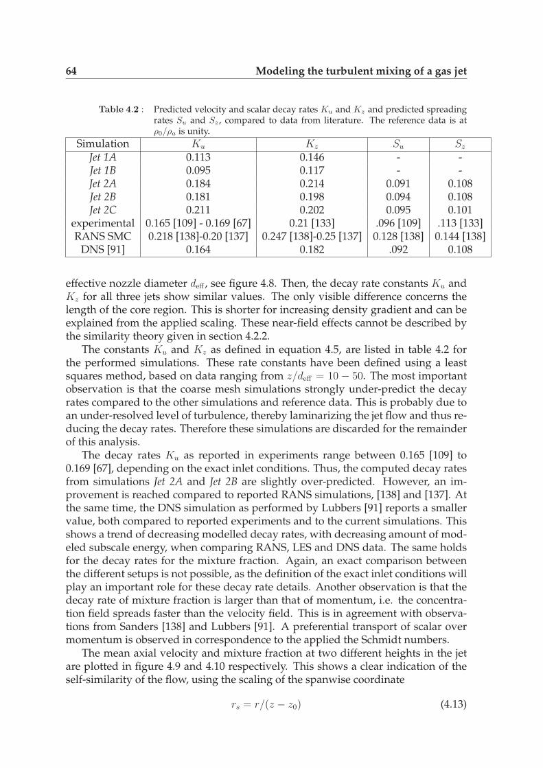
64 Modeling the turbulent mixing of a gas jet
Table 4.2 : Predicted velocity and scalar decay rates Ku and Kz and predicted spreadingrates Su and Sz , compared to data from literature. The reference data is atρ0/ρa is unity.
Simulation Ku Kz Su Sz
Jet 1A 0.113 0.146 - -Jet 1B 0.095 0.117 - -Jet 2A 0.184 0.214 0.091 0.108Jet 2B 0.181 0.198 0.094 0.108Jet 2C 0.211 0.202 0.095 0.101
experimental 0.165 [109] - 0.169 [67] 0.21 [133] .096 [109] .113 [133]RANS SMC 0.218 [138]-0.20 [137] 0.247 [138]-0.25 [137] 0.128 [138] 0.144 [138]
DNS [91] 0.164 0.182 .092 0.108
effective nozzle diameter deff , see figure 4.8. Then, the decay rate constants Ku andKz for all three jets show similar values. The only visible difference concerns thelength of the core region. This is shorter for increasing density gradient and can beexplained from the applied scaling. These near-field effects cannot be described bythe similarity theory given in section 4.2.2.
The constants Ku and Kz as defined in equation 4.5, are listed in table 4.2 forthe performed simulations. These rate constants have been defined using a leastsquares method, based on data ranging from z/deff = 10 − 50. The most importantobservation is that the coarse mesh simulations strongly under-predict the decayrates compared to the other simulations and reference data. This is probably due toan under-resolved level of turbulence, thereby laminarizing the jet flow and thus re-ducing the decay rates. Therefore these simulations are discarded for the remainderof this analysis.
The decay rates Ku as reported in experiments range between 0.165 [109] to0.169 [67], depending on the exact inlet conditions. Thus, the computed decay ratesfrom simulations Jet 2A and Jet 2B are slightly over-predicted. However, an im-provement is reached compared to reported RANS simulations, [138] and [137]. Atthe same time, the DNS simulation as performed by Lubbers [91] reports a smallervalue, both compared to reported experiments and to the current simulations. Thisshows a trend of decreasing modelled decay rates, with decreasing amount of mod-eled subscale energy, when comparing RANS, LES and DNS data. The same holdsfor the decay rates for the mixture fraction. Again, an exact comparison betweenthe different setups is not possible, as the definition of the exact inlet conditions willplay an important role for these decay rate details. Another observation is that thedecay rate of mixture fraction is larger than that of momentum, i.e. the concentra-tion field spreads faster than the velocity field. This is in agreement with observa-tions from Sanders [138] and Lubbers [91]. A preferential transport of scalar overmomentum is observed in correspondence to the applied the Schmidt numbers.
The mean axial velocity and mixture fraction at two different heights in the jetare plotted in figure 4.9 and 4.10 respectively. This shows a clear indication of theself-similarity of the flow, using the scaling of the spanwise coordinate
rs = r/(z − z0) (4.13)

4.4 Results 65
0 0.05 0.1 0.15 0.2 0.25 0.30
0.1
0.2
0.3
0.4
0.5
0.6
0.7
0.8
0.9
1
rs
W /
W0
z/d0= 10
z/d0= 40
0 0.05 0.1 0.15 0.2 0.25 0.30
0.1
0.2
0.3
0.4
0.5
0.6
0.7
0.8
0.9
1
rs
W /
W0
z/d0= 10
z/d0= 40
0 0.05 0.1 0.15 0.2 0.25 0.30
0.1
0.2
0.3
0.4
0.5
0.6
0.7
0.8
0.9
1
rs
W /
W0
z/d0= 10
z/d0= 40
a) Jet 2A b) Jet 2B c) Jet 2C
Figure 4.9 : Mean axial velocity as a function of the self-similarity coordinate rs for simu-lation Jet 2A, Jet 2B and Jet 2C, at two different heights above the nozzle exit.×: experiments by Panchapakesan [109].
0 0.05 0.1 0.15 0.2 0.25 0.30
0.1
0.2
0.3
0.4
0.5
0.6
0.7
0.8
0.9
1
rs
Z(r
s)/Z
c
z/d0= 10
z/d0= 40
0 0.05 0.1 0.15 0.2 0.25 0.30
0.1
0.2
0.3
0.4
0.5
0.6
0.7
0.8
0.9
1
rs
Z(r
s)/Z
c
z/d0= 10
z/d0= 40
0 0.05 0.1 0.15 0.2 0.25 0.30
0.1
0.2
0.3
0.4
0.5
0.6
0.7
0.8
0.9
1
rs
Z(r
s)/Z
c
z/d0= 10
z/d0= 40
a) Jet 2A b) Jet 2B c) Jet 2C
Figure 4.10 :Mean mixture fraction as a function of the self-similarity coordinate rs for sim-ulation Jet 2A, Jet 2B and Jet 2C, at two different heights above the nozzle exit.Symbols: experiments by Dowling [41].
with z0 the virtual origin of the jet. Still, there exists some difference between thesolution at the different heights. A better correspondence is found at z/d0 = 40.This can be due to the applied inlet conditions for this simulation, which are tunedto match engine conditions. The spreading rates Su and Sz, are given in table 4.2.These values are defined as the half-width values of rs, i.e. the scaled radial coordi-nate where the velocity and mixture fraction are half the centerline values: <w>=<wc>/2, <Z>=<Zc>/2 respectively. These values have been defined at the locationz = 40d0 above the nozzle, where the self-similar solution is well established. Com-pared to the experimental values and the DNS data, the spreading rates are verywell predicted. It is found that the spreading rate Sz is constantly larger than Su, inline with experiments and other simulations, and in line with the larger decay-rateKz, compared to Ku, indicating the more progressive transport of the scalar field.
Turbulence statistics
The Reynolds shear stress as a function of rs is presented in figure 4.11. The thinlines represent the resolved shear, < u′′w′′ >, while the thick lines in the figures are
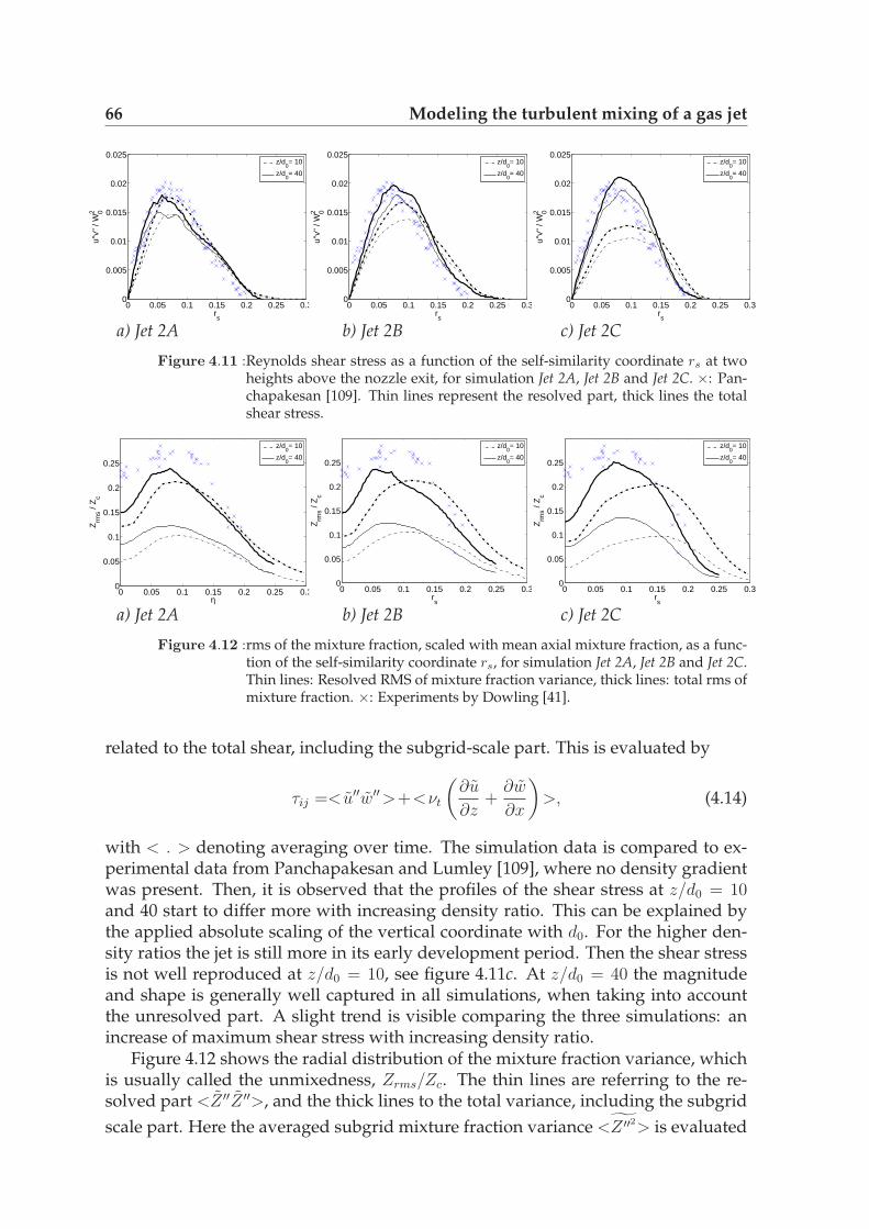
66 Modeling the turbulent mixing of a gas jet
0 0.05 0.1 0.15 0.2 0.25 0.30
0.005
0.01
0.015
0.02
0.025
rs
u"v"
/ W
02
z/d0= 10
z/d0= 40
0 0.05 0.1 0.15 0.2 0.25 0.30
0.005
0.01
0.015
0.02
0.025
rs
u"v"
/ W
02
z/d0= 10
z/d0= 40
0 0.05 0.1 0.15 0.2 0.25 0.30
0.005
0.01
0.015
0.02
0.025
rs
u"v"
/ W
02
z/d0= 10
z/d0= 40
a) Jet 2A b) Jet 2B c) Jet 2C
Figure 4.11 :Reynolds shear stress as a function of the self-similarity coordinate rs at twoheights above the nozzle exit, for simulation Jet 2A, Jet 2B and Jet 2C. ×: Pan-chapakesan [109]. Thin lines represent the resolved part, thick lines the totalshear stress.
0 0.05 0.1 0.15 0.2 0.25 0.30
0.05
0.1
0.15
0.2
0.25
η
Zrm
s / Z
c
z/d0= 10
z/d0= 40
0 0.05 0.1 0.15 0.2 0.25 0.30
0.05
0.1
0.15
0.2
0.25
rs
Zrm
s / Z
c
z/d0= 10
z/d0= 40
0 0.05 0.1 0.15 0.2 0.25 0.30
0.05
0.1
0.15
0.2
0.25
rs
Zrm
s / Z
c
z/d0= 10
z/d0= 40
a) Jet 2A b) Jet 2B c) Jet 2C
Figure 4.12 :rms of the mixture fraction, scaled with mean axial mixture fraction, as a func-tion of the self-similarity coordinate rs, for simulation Jet 2A, Jet 2B and Jet 2C.Thin lines: Resolved RMS of mixture fraction variance, thick lines: total rms ofmixture fraction. ×: Experiments by Dowling [41].
related to the total shear, including the subgrid-scale part. This is evaluated by
τij =<u′′w′′>+<νt
(∂u
∂z+
∂w
∂x
)>, (4.14)
with < . > denoting averaging over time. The simulation data is compared to ex-perimental data from Panchapakesan and Lumley [109], where no density gradientwas present. Then, it is observed that the profiles of the shear stress at z/d0 = 10and 40 start to differ more with increasing density ratio. This can be explained bythe applied absolute scaling of the vertical coordinate with d0. For the higher den-sity ratios the jet is still more in its early development period. Then the shear stressis not well reproduced at z/d0 = 10, see figure 4.11c. At z/d0 = 40 the magnitudeand shape is generally well captured in all simulations, when taking into accountthe unresolved part. A slight trend is visible comparing the three simulations: anincrease of maximum shear stress with increasing density ratio.
Figure 4.12 shows the radial distribution of the mixture fraction variance, whichis usually called the unmixedness, Zrms/Zc. The thin lines are referring to the re-solved part <Z ′′Z ′′>, and the thick lines to the total variance, including the subgrid
scale part. Here the averaged subgrid mixture fraction variance <Z ′′2> is evaluated

4.4 Results 67
0 10 20 30 40 500
0.05
0.1
0.15
0.2
0.25
0.3
0.35
0.4
0.45
0.5
z/d0
(2/3
k)1/
2 /Uc
Jet 2AJet 2BJet 2C
0 10 20 30 40 500
0.05
0.1
0.15
0.2
z/d0
Zrm
s/Zc
a) b)Figure 4.13 :(a) Scaled turbulent kinetic energy along the jet axis. Thin lines: resolved part
of turbulent kinetic energy k; thick lines: total k; ×: experiments [4]. (b) Meanaxial mixture fraction variance along the jet axis. Thin lines: Resolved RMS ofmixture fraction variance, thick lines: total Zrms. Experiments from Birch [18]:×, Dahm [34]: � and Dowling [41]: ◦.
using the equilibrium model, equation 4.12. The simulation data is compared toexperimental data from Dowling and Dimotakis [41]. In the present simulations asubstantial part of the total mixture fraction variance is in the subgrid scales: thesemagnitudes are approximately equal in size as the resolved scales. Still the total mix-ture fraction is relatively well predicted. This shows that the mixture fraction fieldcan be modelled adequately at this resolution. However, if the mixture fraction willhave a more drastic effect on the flow field than in these simulations it is advisedto increase the resolution, until about 80% of the turbulence intensity is resolved,Pope [129]. No large difference can be observed between the three simulations. Aswas also observed in the results of τij in figure 4.11, the profiles close to the nozzleexit, at z/d0 = 10, are spreading out more in radial direction. This effect increaseswith increasing density ratio.
Similarly as looking to the fluctuations in the mixture fraction field the turbu-lent kinetic energy k can be considered. Again, the contribution of the resolvedpart qres = 0.5<u′′
i u′′i > and a subgrid scale part q2
sgs can be considered. The latter isestimated using the formulation proposed by Lilly [88]:
q2sgs =
ν2t
(Cµ∆)2, (4.15)
with Cµ equal to 0.094. With this expression the q2sgs can be evaluated directly from
the local filtersize and turbulent viscosity. However, this model is known for itsoverprediction of the subgrid scale energy, Klein [74]. Also information on the dy-namic coefficient C in equation 2.53 has not been included. Figure 4.13a shows theturbulent kinetic energy along the central axis, scaled using the local centerline ve-locity. The results are compared to the air-air jet experiments from Amielh [4]. Itshows that the resolved turbulence intensities are lower than the experimental ones,suggesting that the subgrid-scale contribution should be included. However, withthis inclusion the total kinetic energy is over-estimated, specially in case Jet 2C. This
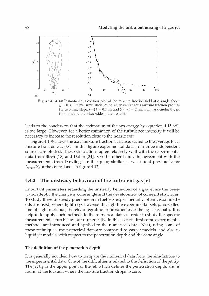
68 Modeling the turbulent mixing of a gas jet
x/d0
z/d 0
0.00
1
0.01
0.05
0.1
0.2
−20 0 200
20
40
60
80
100
0 20 40 60 80 1000
0.1
0.2
0.3
0.4
0.5
0.6
0.7
0.8
0.9
1
z/d0
Z
B
A
a) b)Figure 4.14 :(a) Instantaneous contour plot of the mixture fraction field at a single sheet,
y = 0, t = 2 ms, simulation Jet 2A (b) instantaneous mixture fraction profilesfor two time steps, (—) t = 0.5 ms and (- - -) t = 2 ms. Point A denotes the jetforefront and B the backside of the front jet.
leads to the conclusion that the estimation of the sgs energy by equation 4.15 stillis too large. However, for a better estimation of the turbulence intensity it will benecessary to increase the resolution close to the nozzle exit.
Figure 4.13b shows the axial mixture fraction variance, scaled to the average localmixture fraction Zrms/Zc. In this figure experimental data from three independentsources are plotted. These simulations agree relatively well with the experimentaldata from Birch [18] and Dahm [34]. On the other hand, the agreement with themeasurements from Dowling is rather poor, similar as was found previously forZrms/Zc at the central axis in figure 4.12.
4.4.2 The unsteady behaviour of the turbulent gas jet
Important parameters regarding the unsteady behaviour of a gas jet are the pene-tration depth, the change in cone angle and the development of coherent structures.To study these unsteady phenomena in fuel jets experimentally, often visual meth-ods are used, where light rays traverse through the experimental setup: so-calledline-of-sight methods, thereby integrating information over the light ray path. It ishelpful to apply such methods to the numerical data, in order to study the specificmeasurement setup behaviour numerically. In this section, first some experimentalmethods are introduced and applied to the numerical data. Next, using some ofthese techniques, the numerical data are compared to gas jet models, and also toliquid jet models, with respect to the penetration depth and the cone angle.
The definition of the penetration depth
It is generally not clear how to compare the numerical data from the simulations tothe experimental data. One of the difficulties is related to the definition of the jet tip.The jet tip is the upper point of the jet, which defines the penetration depth, and isfound at the location where the mixture fraction drops to zero.
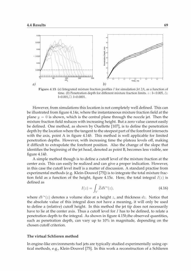
4.4 Results 69
0 50 100 150 2000
0.005
0.01
0.015
0.02
0.025
0.03
z/d0
I
0 0.5 1 1.5 2 2.5 3 3.5 4 4.5 50
5
10
15
20
25
30
35
40
Time, ms
Pen
etra
tion
Dep
th, m
m
a) b)Figure 4.15 :(a) Integrated mixture fraction profiles I for simulation Jet 2A, as a function of
time. (b) Penetration depth for different mixture fraction limits. ◦ : I= 0.005, △:I=0.001,�: I=0.0001.
However, from simulations this location is not completely well defined. This canbe illustrated from figure 4.14a, where the instantaneous mixture fraction field at theplane y = 0 is shown, which is the central plane through the nozzle jet. Then themixture fraction field reduces with increasing height. But a zero value cannot easilybe defined. One method, as shown by Ouellette [107], is to define the penetrationdepth by the location where the tangent to the steepest part of the forefront intersectswith the axis, point A in figure 4.14b. This method is well applicable for limitedpenetration depths. However, with increasing time the plateau levels off, makingit difficult to extrapolate the forefront position. Also the change of the slope thatidentifies the beginning of the jet head, denoted as point B, becomes less visible, seefigure 4.14b.
A simple method though is to define a cutoff level of the mixture fraction at thecenter axis. This can easily be realized and can give a proper indication. However,in this case the cutoff level itself is a matter of discussion. A standard practise fromexperimental methods (e.g. Klein-Douwel [75]) is to integrate the total mixture frac-tion field as a function of the height, figure 4.15a. Here, the total integral I(z) isdefined as
I(z) =
∫
V
ZdV ∗(z), (4.16)
where dV ∗(z) denotes a volume slice at a height z, and thickness dz. Notice thatthe absolute value of this integral does not have a meaning, it will only be usedto define a (relative) cutoff height. In this method the jet tip does not necessarilyhave to lie at the center axis. Thus a cutoff level for I has to be defined, to relate apenetration depth to the integral. As shown in figure 4.15b,the observed quantities,such as penetration depth, can vary up to 10% in magnitude, depending on thechosen cutoff criterion.
The virtual Schlieren method
In engine-like environments fuel jets are typically studied experimentally using op-tical methods, e.g., Klein-Douwel [75]. In this work a reconstruction of a Schlieren
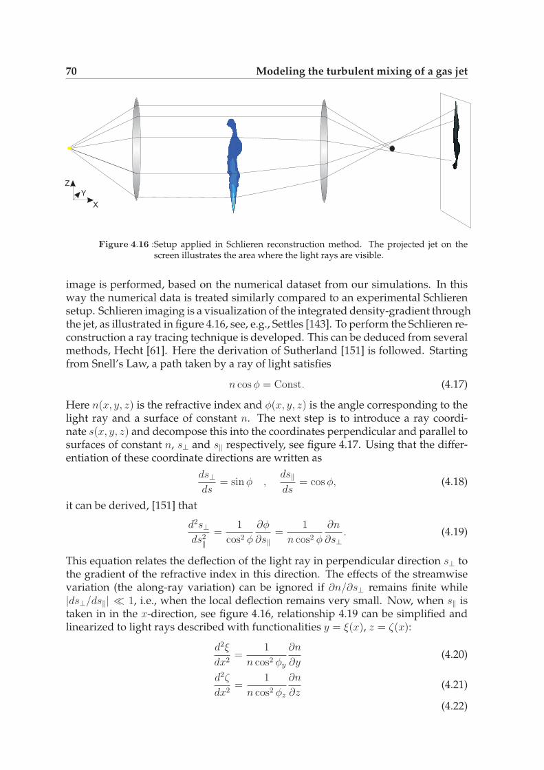
70 Modeling the turbulent mixing of a gas jet
Z
X
Y
Figure 4.16 :Setup applied in Schlieren reconstruction method. The projected jet on thescreen illustrates the area where the light rays are visible.
image is performed, based on the numerical dataset from our simulations. In thisway the numerical data is treated similarly compared to an experimental Schlierensetup. Schlieren imaging is a visualization of the integrated density-gradient throughthe jet, as illustrated in figure 4.16, see, e.g., Settles [143]. To perform the Schlieren re-construction a ray tracing technique is developed. This can be deduced from severalmethods, Hecht [61]. Here the derivation of Sutherland [151] is followed. Startingfrom Snell’s Law, a path taken by a ray of light satisfies
n cos φ = Const. (4.17)
Here n(x, y, z) is the refractive index and φ(x, y, z) is the angle corresponding to thelight ray and a surface of constant n. The next step is to introduce a ray coordi-nate s(x, y, z) and decompose this into the coordinates perpendicular and parallel tosurfaces of constant n, s⊥ and s‖ respectively, see figure 4.17. Using that the differ-entiation of these coordinate directions are written as
ds⊥ds
= sin φ ,ds‖ds
= cos φ, (4.18)
it can be derived, [151] that
d2s⊥ds2
‖
=1
cos2 φ
∂φ
∂s‖=
1
n cos2 φ
∂n
∂s⊥. (4.19)
This equation relates the deflection of the light ray in perpendicular direction s⊥ tothe gradient of the refractive index in this direction. The effects of the streamwisevariation (the along-ray variation) can be ignored if ∂n/∂s⊥ remains finite while|ds⊥/ds‖| ≪ 1, i.e., when the local deflection remains very small. Now, when s‖ istaken in in the x-direction, see figure 4.16, relationship 4.19 can be simplified andlinearized to light rays described with functionalities y = ξ(x), z = ζ(x):
d2ξ
dx2=
1
n cos2 φy
∂n
∂y(4.20)
d2ζ
dx2=
1
n cos2 φz
∂n
∂z(4.21)
(4.22)

4.4 Results 71
Figure 4.17 :Geometrical orientation of the deflection of the light rays.
where φy and φz represent the angles of the incident light ray related to the x-axis,in y- and z-directions respectively. For small angles, cos φ ≈ 1, such that this set ofequations can be simplified to
d2ξ
dx2=
1
n
∂n
∂y(4.23)
d2ζ
dx2=
1
n
∂n
∂z(4.24)
(4.25)
The integration of this equation then can be written, initially assuming the light raysto be parallel to the x-axis:
ξ(x) = y(0) +
∫ x
0
ǫy(x′)dx′ (4.26)
ζ(x) = z(0) +
∫ x
0
ǫz(x′)dx′ (4.27)
Here ǫy and ǫz denote the local light deflection, written as
ǫy(x) =
∫ x
0
1
n
∂n
∂ydx′, ǫz(x) =
∫ x
0
1
n
∂n
∂zdx′. (4.28)
These equations model the ray deflection ǫ in both perpendicular directions yand z, when traversing in x-direction. The relationship between the refractive indexand the density is assumed to be linear, Settles [143], which leads to
∂n
∂y=
dn
dρ
∂ρ
∂y= β
∂ρ
∂y, (4.29)
where β is a constant. Additionally, in our computations the density field for thismixing problem is linearly related to the mixture fraction. Therefore the mixturefraction and density are directly exchangeable for analysis. By filtering out the non-deflected rays using a stop at the focal point, as illustrated in figure 4.16, an imageof the integrated density gradient is recovered. This picture largely depends on thelocation of the rays at the focal point. The radial distance from the focal point Er isdefined as
Er =√
ξ2(xfp) + ζ2(xfp) (4.30)

72 Modeling the turbulent mixing of a gas jet
F
E
i y
i z
i r
i r
−5 −4 −3 −2 −1 0 1 2 3 4 5
x 10−9
−1.5
−1
−0.5
0
0.5
1
1.5x 10
−8
y
z
a) b)Figure 4.18 :(a) Classification of resulting Schlieren ray r(y, z), evaluated at the focal point.
This can be described with a total deflection angle Φr and deflection magnitudeEr. (b) Typical scatter plot of light rays at the focal point. The circle denotesthe filtering level EF .
and is compared to the focal point filter size EF . Also a deflection angle Φr can bereconstructed from the (y, z) coordinates at the focal point, see figure 4.18a. Thisis a measure of the total integrated deflection angle. Both the magnitude and theangle give information of the flow field that has been traversed. Notice that also aninverse figure can be generated, by filtering away all the deflected light rays. Theninstead of a stopper a pinhole should be used experimentally and numerically.
Equations 4.26, 4.27 are integrated numerically in the virtual Schlieren method.In order to get sufficient resolution a large number of rays is followed through thedomain. In present analysis a number of Ny × Nz = 70 × 100 rays are tracked. Atypical result of a scatter of the light rays at the focal is plotted in figure 4.18b. Asimplification to the ray tracing method is possible if it is assumed that the deflec-tion angle remains very small. Then the Schlieren image will directly scale to theintegrated transverse density gradients, because as a first order estimation the raysremain at their original (y, z) coordinates. Then the total deflection magnitude Ei
scales to
Ei =
∫ (∣∣∣∣∂ρ
∂y
∣∣∣∣2
+
∣∣∣∣∂ρ
∂z
∣∣∣∣2)1/2
dx. (4.31)
For this numerical method also a measure for the deflection angle can be defined:
Φi = arctan
∫ ∣∣∣∂ρ
∂y
∣∣∣ dx∫ ∣∣∂ρ
∂z
∣∣ dx
. (4.32)
Comparing visualisation methods
In the previous two subsections three visualization methods have been proposed.One is based on a single sheet mixture fraction field, using a cutoff mixture fractionlevel. This method is referred to as the direct field visualization. The next is basedon the virtual schlieren visualization technique, following the path of the light rays.The last method is a simplified variant of the previous method, referred to as theintegrated gradient visualization. The different integration methods are qualitativelycompared to each other in figure 4.19 for simulation Jet 2A, after 1 ms.
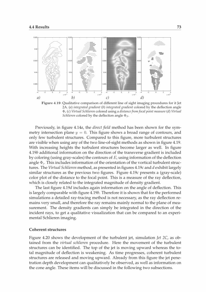
4.4 Results 73
−4 −2 0 2 4
x 10−3
0.005
0.01
0.015
0.02
0.025
−4 −2 0 2 4
x 10−3
0.005
0.01
0.015
0.02
0.025
−4 −2 0 2 4
x 10−3
0.005
0.01
0.015
0.02
0.025
−4 −2 0 2 4
x 10−3
0.005
0.01
0.015
0.02
0.025
a) b) c) d)Figure 4.19 :Qualitative comparison of different line of sight imaging procedures for it Jet
2A. (a) integrated gradient (b) integrated gradient colored by the deflection angleΦi (c) Virtual Schlieren colored using a distance from focal point measure (d) VirtualSchlieren colored by the deflection angle ΦS .
Previously, in figure 4.14a, the direct field method has been shown for the sym-metry intersection plane y = 0. This figure shows a broad range of contours, andonly few turbulent structures. Compared to this figure, more turbulent structuresare visible when using any of the two line-of-sight methods as shown in figure 4.19.With increasing heights the turbulent structures become larger as well. In figure4.19b additional information on the direction of the transverse gradient is includedby coloring (using gray-scales) the contours of Ei using information of the deflectionangle Φi. This includes information of the orientation of the vortical turbulent struc-tures. The Virtual Schlieren method, as presented in figures 4.19c and d exhibit largelysimilar structures as the previous two figures. Figure 4.19c presents a (gray-scale)color plot of the distance to the focal point. This is a measure of the ray deflection,which is closely related to the integrated magnitude of density gradient.
The last figure 4.19d includes again information on the angle of deflection. Thisis largely comparable with figure 4.19b. Therefore it is shown that for the performedsimulations a detailed ray-tracing method is not necessary, as the ray deflection re-mains very small, and therefore the ray remains mainly normal to the plane of mea-surement. The density gradients can simply be integrated in the direction of theincident rays, to get a qualitative visualization that can be compared to an experi-mental Schlieren imaging.
Coherent structures
Figure 4.20 shows the development of the turbulent jet, simulation Jet 2C, as ob-tained from the virtual schlieren procedure. Here the movement of the turbulentstructures can be identified. The top of the jet is moving upward whereas the to-tal magnitude of deflection is weakening. As time progresses, coherent turbulentstructures are released and moving upward. Already from this figure the jet pene-tration depth development can qualitatively be observed, as well as information onthe cone angle. These items will be discussed in the following two subsections.

74 Modeling the turbulent mixing of a gas jet
−4 −2 0 2 4
x 10−3
0.005
0.01
0.015
0.02
0.025
0.03
0.035
0.04
−4 −2 0 2 4
x 10−3
0.005
0.01
0.015
0.02
0.025
0.03
0.035
0.04
−4 −2 0 2 4
x 10−3
0.005
0.01
0.015
0.02
0.025
0.03
0.035
0.04
−4 −2 0 2 4
x 10−3
0.005
0.01
0.015
0.02
0.025
0.03
0.035
0.04
t = 0.6 ms t = 1.2 ms t = 1.8 ms t = 2.4 ms
Figure 4.20 :Development of Jet 2C for subsequent times separated by 0.6 ms, visualizedwith the virtual Schlieren method. The different color scales in the plots arerelated to the deflection angle Φr.
0 0.5 1 1.5 2 2.5 3 3.5 40
5
10
15
20
25
30
35
40
Time, ms
Pen
etra
tion
Dep
th, m
m
0 5 10 15 20 250
0.5
1
1.5
2
2.5
3
3.5
4
4.5
z(mm)
Tim
e (m
s)
a) b)
Figure 4.21 :(a) Penetration depths based on a Schlieren intensity (Solid lines), and inte-grated mixture fraction intensity (dash-dotted lines) for simulations Jet 2A (◦),Jet 2B (△) and Jet 2C (⋄) if a cutoff level of I = 10−4 is used, see figure 4.15a.(b) Time when steady state is reached, for simulation Jet 2A, based on data aspresented in figure 4.6a.
Penetration depth
For all three simulations the penetration depth is plotted in figure 4.21a. In thisfigure the definition of penetration depth is based on a virtual schlieren intensityas well as on an integrated intensity, where I < 10−4. The general trend is thatby increasing the density ratio the penetration depth is enhanced, simply due tothe increased jet momentum. This figure shows at what time the mixture fractiondeparts from its initial value Z = 0 for the first time. Now a typical jet structure willstart to develop. Globally the two methods lead to similar results, but the virtualSchlieren method mostly leads to a faster identification of the jet tip, notwithstandingthe stringent measure of the integration method, see figure 4.15.
It is more difficult to find a time instant when the steady state situation has beenreached at a specific location above the nozzle exit. Kuo [78] has shown an analysis

4.4 Results 75
0.01 0.015 0.02 0.025 0.03 0.035 0.04 0.045 0.05 0.055 0.06
0.04
0.06
0.08
0.1
0.12
0.14
0.16
0.18
0.2
T1/2, s1/2
z t/(M
0/ρa)1/
4 , s1/
2
0 0.5 1 1.5 2 2.5 3 3.5 40
2
4
6
8
10
12
14
16
18
T, ms
θ/2,
deg
Jet 2AJet 2BJet 2C
a) b)Figure 4.22 :Nondimensionalised penetration depths for all simulations. The solid lines
denote the results based on a Schlieren intensity, the dash-dotted lines the inte-grated mixture fraction intensity. the symbols denote simulation Jet 2A (◦); Jet2B (△) and Jet 2C (⋄). The dotted line represents the theoretical value, Γ = 3.0,Ricou [136]. (b) evaluated instantaneous half cone angles.
for RANS simulations, evaluating the time when steady state is reached. However,this method is more difficult to apply in the current (LES) problem formulation, asonly a single realization of the flow field is available. This is especially problem-atic when the fluctuations are of the order of magnitude of the absolute value forthe mean mixture fraction. In figure 4.21b the moment of reaching steady state isbased on the time-trace of the mixture fraction field along the central axis. The time-evolution data is shown in figure 4.6a. As only a single realization of the jet is usedfor gathering the data, there exists some scatter in the results, denoted by the sym-bols. The curve shows a least-squares fit of the results. As a general trend we cansee that figures 4.21b is the inverse of figure 4.21a, which is a logical result.
Scale similarity is shown in many of the previous figures on the steady state be-haviour. For the penetration depth as function of time the relationship 4.4, whichstates a square root dependency, is tested for the performed simulations, see figure4.22a. In this figure the data as presented in figure 4.21a is used, also adopting thetwo visualisation methods. Good agreement is observed independent of models,for all simulations. There is a small trend visible of a decreasing value for Γ with anincreasing density ratio: For simulations Jet 2A, Jet 2B and Jet 2C the constant Γ de-creases from 2.9 to 2.8 and 2.7 respectively, indicating a reduced -scaled- penetrationdepth velocity with increasing density ratio.
Cone Angle
In this work the jet angle θ is defined at half the jet penetration depth (see figure4.23):
θabs = tan−1
(Dzt/2
(zt/2)
), (4.33)
with Dzt/2 the diameter of the jet at half the penetration depth zt. This definitionrelates an angle to the outer boundary of the upstream portion of the jet, i.e. the

76 Modeling the turbulent mixing of a gas jet
qi
z /2
t
t
zz
z /2
qi
t
t
a) b)Figure 4.23 :(a) Schematics of an absolute value cone-angle definition, (b) Schematic repre-
sentation of a self-similar cone angle and penetration depth.
unsteady head of the jet does not influence this cone angle. The diameter Dzt/2 andspray penetration depth zt are defined based on the virtual Schlieren line-of-sightapproach, in order to follow the standard experimental method. Thus, an absolutecone angle definition is used, based on instantaneous, unscaled information fromthe mixture fraction field, as depicted in figure 4.23a.
Figure 4.22b shows the cone half angle for the three simulations as a function oftime. Two trends are visible: The cone angle decreases as a function of time, whichis the best visible for simulations Jet 2A and Jet 2B, and the absolute value increaseswith increasing density ratio. The cone angle for simulation Jet 2A is on averageθabs/2 =11.4 deg, whereas for Jet 2B and Jet 2C it is 12.2 deg and 13.1 deg, respectively.Both observations need some clarification. First, note that the used definition, basedon an experimental method, is not completely unambiguous. This can be explainedas follows. The sketch given in figure 4.23b, shows a cone angle that is related to aconstant value of the self-similarity mixture fraction Z(rs)/Zc. Using this definitionthe cone angle is independent of the height above the nozzle exit. Both definitions(based on the absolute mixture fraction and based on its relative value) are equalfor steep gradients of the mixture fraction, as appearing close to the nozzle exit.Higher up in the domain an absolute cone angle definition will lead to deviatingresults. Therefore in experimental studies using absolute values it is wise to use thedefinition of the spray angle at about half the penetration depth. Close to the nozzleexit the jet is not yet well developed, whereas above half the jet penetration depththe cone angle cannot be well defined due to low levels of mixture fraction. Thisleads to different cone angles defined at different locations above the nozzle exit.
Notice also that the found cone angles can be related to figure 4.10, i.e. the coneangle θ/2 can be given in terms of self-similarity coordinate rs = r/(z − z0), giventhat θs/2 = tan(rs), where the subscript s denotes the similarity-theory cone angle.This means that, for instance, a typical cone angle of θs/2 = 10 deg corresponds tors = 0.17.
Consequently rs corresponds to a relative mixture fraction. For rs = 0.17 it is

4.4 Results 77
found Z(rs)/Zc ≈ 0.2, see figure 4.10. However, a measure for the spreading ratehas already been introduced, namely Sz, as presented in table 4.2. Note, that thesespreading rates are defined at a constant height, z/d0 = 40, whereas here the anglesθabs/2 are defined on instant-time basis, and thus at increasing heights. For instance,at 4 ms, half the penetration depth zt/d0 is at about 30.
This means that the cone angle data, as presented in figure 4.22b are evaluated atlocations relatively close to the nozzle exit. For these early time instants the fully de-veloped self-similar region has not been reached. A similar observation has alreadybeen made with respect to figure 4.10b,c: the spreading of the mixture fraction closeto the nozzle (z/d0=10) is much wider than at z/d0=40. At the same time the spread-ing rates Sz at z/d0 = 40 are almost identical for all three simulations, see againtable 4.2. This indicates that with increasing density ratio the location of the self-similar region shifts in the down-stream direction. This is an additional problem inthe definition of the cone angle based on this type of flow field data.
Moreover, notice that if an experimental jet visualization technique would bebased on the absolute density levels, such as the Schlieren method, then an increas-ing jet density ratio will lead additionally to an increased value of the cone angleθabs/2, while the relative cone angle θs will remain constant.
To conclude: a cone angle definition that is related to the absolute value of themixture fraction depends on the operating conditions, and this definition itself doesnot show self-similar behaviour. This statement is similar to the discussion of theunscaled velocity and mixture fraction decay, figure 4.7. At the same time theseobservations concerning the cone angle show a similar difficulty as has been en-countered when analyzing the jet penetration depth.
4.4.3 Comparison to a liquid jet model
The gas jets can also more directly be compared to the experiments and modelsfor a liquid jet. The current simulations are compared to a study from Naber andSiebers [99]. A relationship for the penetration depth as function of time is derived,and validated on a set of vaporizing / non-vaporizing liquid fuel jet experiments.The proposed relationship reads
t =z
2+
z
4
√1 + 16z2 +
1
16ln(4z +
√1 + 16z2
), (4.34)
with t = t/t+ and z = zt/z+ a scaled time and penetration depth, based on
t+ =deff
a tan(θ/2)u0
, z+ =deff
a tan(θ/2). (4.35)
In the above equation a is a fitting parameter that defines the ratio of the modeljet cone angle to the practically observed jet angle. This parameter is introduced toaccount for ambiguities in the cone angle definition, as discussed in the previoussection. Naber proposes a = 0.66, which is also used in our scaling. In the rela-tionship 4.34 two limits can be defined. For small t the penetration depth followsa linear behaviour. Close to the nozzle exit fluid dynamics is then governed by theinjected fluid. For large t equation 4.34 follows a square root dependency. Here the

78 Modeling the turbulent mixing of a gas jet
10−1
100
101
102
103
10−1
100
101
t/t+
z t/z+
Naber & SiebersJet 2AJet 2BJet 2C
Figure 4.24 :A comparison of the simulation data to a correlation validated for liquid fuelsprays by Naber and Siebers [99]
entrainment of the surrounding gas plays an important role. The transition regionis around t = 1. Naber and Siebers show that except for some small deviations inthe transition region the non-vaporizing liquid spray experiments agree well withthe given correlation, for density ratios over nearly two orders of magnitude. Noticethat Naber shows vaporizing and non-vaporizing jet sprays over a range of densityratios from 250 to 10, while in this work the density ratios range from 10 to 1. Thismeans that care needs to be taken when extrapolating the given relationship.
For our simulations the scaling parameters s+ and t+ are 1.5 mm, 2.0 mm and 4.0mm and 8.5 µs, 11 µs and 23 µs for simulations Jet 2A, Jet 2B and Jet 2C respectively.The penetration depths, as presented in figure 4.21a, are rescaled accordingly andshown in figure 4.24. All simulations give good agreement for z > 2. This is at aboutthe location z/d0 = 20, where the self-similarity models start to be appropriate, seealso figures 4.8-4.12. This is reasonable, as further away from the nozzle exit all jetsshould behave similarly, according to similarity theory.
However, for short penetration times (t < 3) the penetration depth z is under-predicted. The correspondence gets worse with decreasing density ratio. A sim-ple explanation is that in our simulations a gas jet is modeled, where the entrain-ment rate close to the nozzle exit is relatively large. On the other hand in the liquidfuel jets the entrainment rate close to the nozzle remains relatively low, because alarge amount of liquid particles retain a strong momentum. Only at locations abovezt > 2z+, where the droplets are sufficiently small, the penetration depth of liquidnon-vaporizing fuel jets can be described by the similarity theory developed for gasjets.
Naber and Siebers [99] have observed a range of values for the spray cone angles.For the density ratio ρ0/ρa = 1 their estimate for the half cone angle ranges betweenθNS/2 = 12 − 16 deg while the cone angle is about θNS/2 = 11 − 14 deg for a densityratio of ρ0/ρa = 10. This range depends on the specific jet inlet geometry. Naberreports a decrease of cone angle with an increasing density ratio, in contrast to ourobservations, using the virtual Schlieren method. This difference in trend can beattributed to the difference in observation methods, and due to the different density

4.4 Results 79
gradient range. The gaseous fuel as simulated in this study has a larger spreadingrate with increasing density ratio, mainly due to the visualization method, as ex-plained in the previous section. In our simulations the spreading rate based on ascaled mixture fraction field remains constant, though. On the other hand, liquidfuel jets will show a delayed entrainment rate with increasing density ratio. The liq-uid fuel particles do not feel any large impact from the surrounding gas, until theyare sufficiently small that they start to behave as a gas with all mixing and spreadingrate consequences.
It is remarkable that the spray model fits so well to the jet simulation, and there-fore the similarity theory. To compare the similarity theory of the gas jet model tothe liquid fuel spray model of Naber, we can look at the similarity region of theliquid spray. Then, for large times, equation 4.34 collapses to
t = z2. (4.36)
This equation can be compared to the similarity model, given by equation 4.3. Then,by rewriting equation 4.36 to physical coordinates, we get
zt
deff
=1√
a tan(θ/2)
(tu0
deff
)1/2
. (4.37)
Therefore, the quantity Γ in equation 4.3 can be related to the cone angle through
ΓNS =1√
a tan(θ/2)
(π
4
)−1/4
. (4.38)
This implies for the found cone angles that the constants Γ are 2.9, 2.8 and 2.7 forsimulations Jet 2A, Jet 2B and Jet 2C respectively, see also figure 4.22.
This explains why the gas jet simulation data match so well to the liquid fueljet model, considering that in the present simulations the penetration depth in thegas jet is corrected using the found cone angles. This effect is accounted for by theconstant Γ, which is different for different (experimental) setups. For the typicalspray conditions, performed by Naber, Γ ranges from 2.3 to 2.8 for density ratiosρ0/ρa = 10 − 100. Therefore one should take this effect into account when using agas jet for the modeling of a turbulent liquid fuel spray.
4.4.4 Global mixture composition
One important parameter for ignition/combustion problems is the change of chem-ical energy content of the mixture, as a function of time. This defines wether amixture can be classified as highly reactive and explosive, or relatively un-mixed.Therefore it is interesting to study the distribution of gas as a function of equiva-lence ratio. This gives an indication on the global mixing of the total injected fuel, asa function of time. Depending on the total mass and mass-rate of the injected fuel,and the dynamics of the fuel jet, the composition of the mixture varies. By attribut-ing an energy content to every equivalence ratio, a measure for the energy contentcan be given.
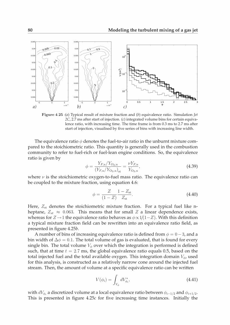
80 Modeling the turbulent mixing of a gas jet
0.005 0.02
0.0630.
1
0.1
0.2
−5 0 5
x 10−3
0.005
0.01
0.015
0.02
0.025
0.03
0.035
0.04
0.045
0.1 0.5
1
2
5
−5 0 5
x 10−3
0.005
0.01
0.015
0.02
0.025
0.03
0.035
0.04
0.045
0 0.5 1 1.5 2 2.5 3
10−2
10−1
100
φ
V [c
m3 ]
a) b) c)
Figure 4.25 :(a) Typical result of mixture fraction and (b) equivalence ratio. Simulation Jet2C, 2.7 ms after start of injection. (c) integrated volume bins for certain equiva-lence ratio, with increasing time. The time frame is from 0.3 ms to 2.7 ms afterstart of injection, visualised by five series of bins with increasing line width.
The equivalence ratio φ denotes the fuel-to-air ratio in the unburnt mixture com-pared to the stoichiometric ratio. This quantity is generally used in the combustioncommunity to refer to fuel-rich or fuel-lean engine conditions. So, the equivalenceratio is given by
φ =YF,u/YO2,u
(YF,u/YO2,u)st
=νYF,u
YO2,u
, (4.39)
where ν is the stoichiometric oxygen-to-fuel mass ratio. The equivalence ratio canbe coupled to the mixture fraction, using equation 4.6:
φ =Z
(1 − Z)
1 − Zst
Zst
. (4.40)
Here, Zst denotes the stoichiometric mixture fraction. For a typical fuel like n-heptane, Zst ≈ 0.063. This means that for small Z a linear dependence exists,whereas for Z→1 the equivalence ratio behaves as φ∝1/(1−Z). With this definitiona typical mixture fraction field can be rewritten into an equivalence ratio field, aspresented in figure 4.25b.
A number of bins of increasing equivalence ratio is defined from φ = 0−3, and abin width of ∆φ = 0.1. The total volume of gas is evaluated, that is found for everysingle bin. The total volume Vφ over which the integration is performed is definedsuch, that at time t = 2.7 ms, the global equivalence ratio equals 0.5, based on thetotal injected fuel and the total available oxygen. This integration domain Vφ, usedfor this analysis, is constructed as a relatively narrow cone around the injected fuelstream. Then, the amount of volume at a specific equivalence ratio can be written
V (φi) =
∫
Vφ
dV ∗φi
, (4.41)
with dVφia discretized volume at a local equivalence ratio between φi−1/2 and φi+1/2.
This is presented in figure 4.25c for five increasing time instances. Initially the

4.5 Conclusions 81
0 0.5 1 1.5 2 2.5 310
−4
10−3
10−2
10−1
φ
M [g
]
0 0.5 1 1.5 2 2.5 3
10−6
10−5
φ
E [M
J]
a) b)
Figure 4.26 :Integrated volume bins for certain equivalence ratio, with increasing time. Thetime frame is from 0.3 ms to 2.7 ms after start of injection. (a) Integrated mass,(b) integrated energy.
largest volume is related to the lowest equivalence ratio (φ = 0 − 0.1), whereasfor increasing times the volume at larger φ starts to increase, and the volume atφ = 0− 0.1 decreases accordingly. By multiplying the volume with the local densityM(φi) = ρ(φi)V (φi) the amount of mass in a specific range of equivalence ratios canbe retrieved, see figure 4.26a. This figure has a similar shape as figure 4.25c, exceptthat the slope M(φ) is less steep than in the previous figure. This is because the den-sity follows a linear dependence to the mixture fraction, and thus, (for small Z) toφ.
By multiplying the mass with the energy content of the fuel the total energyin a bin can be calculated: E(φi) = ∆HF YF (φ)M(φ), with ∆HF = 45 MJ/kg thereaction enthalpy, figure 4.26b. Because YF is linearly related to Z the total energy isproportional to the volume V (φi) and the equivalence ratio squared:
E(φi) ∝ φ2i V (φi). (4.42)
For early injection times the total energy is small: the energy content for small φ islittle due to the small local equivalence ratios, whereas for large φ the total amount ofV (φi) is limited. For increasing times, the maximum energy content shifts from therich side, φ > 1, towards stoichiometry, φ = 1, while the maximum value increasesone order of magnitude. With increasing times, the maximum can be expected to belocated more around φ = 0.5, because of the ongoing mixing with the surroundingair.
4.5 Conclusions
In this chapter the turbulent mixing process in gaseous jets has been studied usingthe LES method, for three different fuel to ambient air density ratios. This studywas focussed on three aspects. 1. The investigation of a turbulent jet for engine-relevant conditions, 2. To investigate an experimental visualization technique usingthe numerical simulation data 3. To compare the gaseous fuel jets to a phenomeno-logical liquid spray model and experiments on liquid jets. Finally, a global measure

82 Modeling the turbulent mixing of a gas jet
of the total mixture composition and its distribution of the energy content has beengiven, by expressing the mixture fraction field in terms of equivalence ratios. Infuture work such information can be used for injection-ignition studies of gaseousturbulent, burning fuel jets.
1. Concerning the steady state statistics of the fuel jet, it is shown that this followswell the similarity theory developed for turbulent gas jets. The fuel core lengthincreases with increasing density ratio, which means that this region is shiftedmore downstream in the fuel jet.
In the performed simulations it is observed that a substantial part of the turbu-lent kinetic energy and mixture fraction fluctuations is present in the subgridscales. Notwithstanding this observation, suitable results have been achieved,especially regarding the mixture fraction variance profiles. This gives confi-dence in the applied subgrid-scale model for the mixture fraction fluctuations.
Also the penetration depth as a function of time follows the self-similarity the-ory properly for a fuel-to-air density ratio of unity. With increasing densityratios, the scaled penetration depth decreases slightly.
2. A virtual Schlieren postprocessing method is developed in order to analyzethe results similarly as is typically done experimentally. The development ofseparate turbulent structures could be tracked when considering the turbulentjet at different time instances. When defining the penetration depth similarproblems are encountered as typically in experiments. These are related to thecutoff signal intensity of the post-processing method. Moreover, it is shownthat the virtual Schlieren ray-tracing method, based on an integration of thedensity gradients, leads to similar results when an integrating all density gra-dients in one direction.
3. When comparing the evolution of the penetration depth of a gaseous jet withmodels for liquid fuel sprays, the phenomenological models for both jets areexchangeable for larger penetration depths. This is because the penetrationrate from liquid sprays is governed by the entrainment rate, and thereforescales to
√t, which is similar as for gaseous jets. Only for very short distances
the simulation departs from the liquid jet experiment, due to the large liq-uid void fraction in liquid jets and accordingly the reduced entrainment rate.However, it remains questionable if gas jet models can simply be used to re-place the model for fuel sprays. The cone angle for gas jets deviates from thoseobserved in spray experiments. This corresponds to a different constant Γ inequation 4.3 for fuel sprays compared to gas jets. Whereas this quantity is uni-versal for relatively simple round turbulent gas jets, hardly depending on Re,the ratio ρ0/ρa or d0, for a fuel spray Γ strongly depends on the specific sprayconditions.

Chapter
5Modeling finite-ratechemistry in turbulentdiffusion flames
In this chapter, two non-premixed turbulent flames are consi-dered, where finite-rate chemistry plays a role. In the first flamethree flamelet-based methods are compared to account for finite-rate chemistry in a diffusion type of flame. These three methodsare the classical steady laminar flamelet method and two meth-ods based on a reaction progress variable. The test flame is a pi-loted methane/air flame (Sandia flame D). The second flame is aturbulent benzene diffusion flame. This flame is modeled using amodified flamelet method, where the PAH/soot source terms areextracted from a steady laminar flamelet database.
5.1 Introduction
Nowadays, the modeling of chemical processes that take place in Internal Com-bustion (IC) Engines is a major research topic, [44, 132]. As explained in the firstchapter, legislation puts more and more stringent rules on pollutant formation andCO2 emission. To keep up with the demands more detailed information about thephysics and chemistry of the combustion process in IC engines is required. Based onsuch knowledge, efficient modeling tools need to be developed that can be appliedfor predictive studies on future engine concepts, Evlampiev [44].
In the previous chapters the LES method for non-reactive flows, its applicationto an engine geometry and a mixing model have been discussed. Here, we turn toan additional step related to LES modeling of IC engines concerns the modeling ofturbulent combustion.
5.1.1 Combustion regimes encountered in engine flows
For typical combustion problems it is not feasible to solve the complete chemicalsystem within the CFD solver, just by evaluating transport equations for all species.For turbulent flows the large range of length and time scales present in this prob-
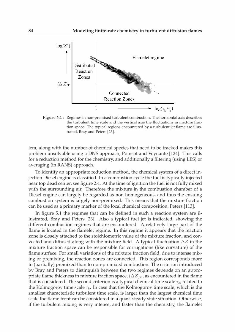
84 Modeling finite-rate chemistry in turbulent diffusion flames
Figure 5.1 : Regimes in non-premixed turbulent combustion. The horizontal axis describesthe turbulent time scale and the vertical axis the fluctuations in mixture frac-tion space. The typical regions encountered by a turbulent jet flame are illus-trated, Bray and Peters [23].
lem, along with the number of chemical species that need to be tracked makes thisproblem unsolvable using a DNS approach, Poinsot and Veynante [124]. This callsfor a reduction method for the chemistry, and additionally a filtering (using LES) oraveraging (in RANS) approach.
To identify an appropriate reduction method, the chemical system of a direct in-jection Diesel engine is classified. In a combustion cycle the fuel is typically injectednear top dead center, see figure 2.4. At the time of ignition the fuel is not fully mixedwith the surrounding air. Therefore the mixture in the combustion chamber of aDiesel engine can largely be regarded as non-homogeneous, and thus the ensuingcombustion system is largely non-premixed. This means that the mixture fractioncan be used as a primary marker of the local chemical composition, Peters [113].
In figure 5.1 the regimes that can be defined in such a reaction system are il-lustrated, Bray and Peters [23]. Also a typical fuel jet is indicated, showing thedifferent combustion regimes that are encountered. A relatively large part of theflame is located in the flamelet regime. In this regime it appears that the reactionzone is closely attached to the stoichiometric value of the mixture fraction, and con-vected and diffused along with the mixture field. A typical fluctuation ∆Z in themixture fraction space can be responsible for corrugations (like curvature) of theflame surface. For small variations of the mixture fraction field, due to intense mix-ing or premixing, the reaction zones are connected. This region corresponds moreto (partially) premixed than to non-premixed combustion. The criterion introducedby Bray and Peters to distinguish between the two regimes depends on an appro-priate flame thickness in mixture fraction space, (∆Z)F , as encountered in the flamethat is considered. The second criterion is a typical chemical time scale τc, related tothe Kolmogorov time scale τk. In case that the Kolmogorov time scale, which is thesmallest characteristic turbulent time scale, is larger than the largest chemical timescale the flame front can be considered in a quasi-steady state situation. Otherwise,if the turbulent mixing is very intense, and faster than the chemistry, the flamelet

5.1 Introduction 85
regime breaks down and regions of intense mixing and reaction will appear. This isreferred to as the distributed reaction zones regime. The main part of the combus-tion proces in the engine, concerning the heat release, can be modeled within theflamelet regime. Therefore, methods to model turbulent combustion in this regimeare primarily considered. On the other hand, chemical species as soot and NOx
cannot directly be described within this framework [6, 101].
Flamelet methods
The classical method to solve the problem of non-premixed chemistry in the flameletregime is the steady laminar flamelet method (SLF). It is based on a one-dimensionallaminar diffusion flame, Peters [113]. The application of the flamelet method toengine-related chemical problems has been investigated by Evlampiev [44]. In thecurrent thesis its application to fluid-dynamical problems is considered. The appli-cation of the classical method is problematic for several reasons, as will be explainedin section 5.2. Therefore there is a search for alternative approaches to the classi-cal flamelet method. In this thesis the application of a so-called progress variablemethod is investigated, and compared to the classical method.
Soot formation processes are relatively slow chemical processes, depending onresidence time, D’Anna et al. [6]. This is related to the connected reaction zonesregime where all main combustion reactants, such as CO2 and H2O have approachedtheir equilibrium values. It appears that also in this case a steady laminar flameletapproach will not be appropriate. A more suitable, time-dependent approach forthe modeling of soot formation in turbulent diffusion flames is required.
5.1.2 Objectives
In this chapter two non-premixed turbulent flames are studied, with a focus on themodeling of finite-rate chemistry. On the first flame a relatively new method fornon-premixed chemistry problems is investigated, where the appropriate flameletis defined based on an additional transport equation for a characteristic reactivespecies C. This variable accounts for the reaction progress, and plays a role wherefinite-rate chemistry takes place. Such a progress variable is used in a number ofpremixed chemistry problems. Three different methods are compared to each other:the classical flamelet method, Peters [113], where the chemistry is parameterizedusing the mixture fraction Z and the scalar dissipation rate χ; a progress variablemethod, where the same non-premixed flamelet database is parameterized withZ and a progress variable C, Pierce [116]; and finally the same progress variablemethod, but now based on a premixed chemical database, van Oijen [104]. Thesethree methods are compared to each other on a well documented test flame, theSandia flame D, [155]. The main concern in this flame is a correct prediction of thetemperature and major species.
To test the flamelet method for soot formation problems, in the second flamea sooting turbulent diffusion flame is investigated. Soot formation and oxidationtakes place mainly in the connected reaction zones regime, so the use of the classicalflamelet method is in principle not allowed. In the latter part of this chapter the state
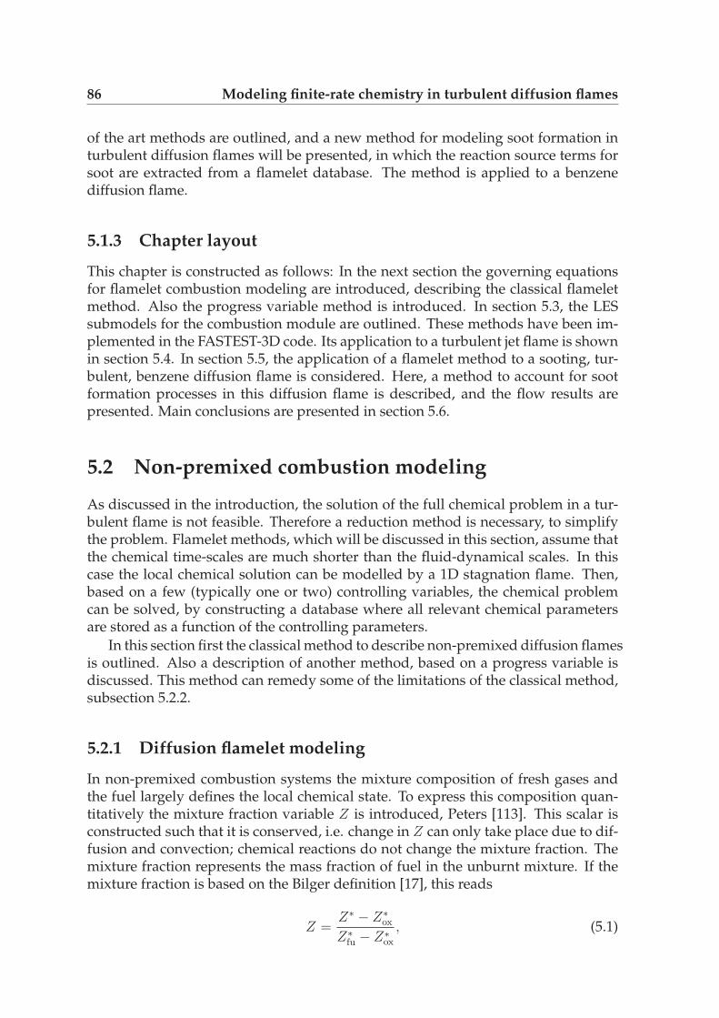
86 Modeling finite-rate chemistry in turbulent diffusion flames
of the art methods are outlined, and a new method for modeling soot formation inturbulent diffusion flames will be presented, in which the reaction source terms forsoot are extracted from a flamelet database. The method is applied to a benzenediffusion flame.
5.1.3 Chapter layout
This chapter is constructed as follows: In the next section the governing equationsfor flamelet combustion modeling are introduced, describing the classical flameletmethod. Also the progress variable method is introduced. In section 5.3, the LESsubmodels for the combustion module are outlined. These methods have been im-plemented in the FASTEST-3D code. Its application to a turbulent jet flame is shownin section 5.4. In section 5.5, the application of a flamelet method to a sooting, tur-bulent, benzene diffusion flame is considered. Here, a method to account for sootformation processes in this diffusion flame is described, and the flow results arepresented. Main conclusions are presented in section 5.6.
5.2 Non-premixed combustion modeling
As discussed in the introduction, the solution of the full chemical problem in a tur-bulent flame is not feasible. Therefore a reduction method is necessary, to simplifythe problem. Flamelet methods, which will be discussed in this section, assume thatthe chemical time-scales are much shorter than the fluid-dynamical scales. In thiscase the local chemical solution can be modelled by a 1D stagnation flame. Then,based on a few (typically one or two) controlling variables, the chemical problemcan be solved, by constructing a database where all relevant chemical parametersare stored as a function of the controlling parameters.
In this section first the classical method to describe non-premixed diffusion flamesis outlined. Also a description of another method, based on a progress variable isdiscussed. This method can remedy some of the limitations of the classical method,subsection 5.2.2.
5.2.1 Diffusion flamelet modeling
In non-premixed combustion systems the mixture composition of fresh gases andthe fuel largely defines the local chemical state. To express this composition quan-titatively the mixture fraction variable Z is introduced, Peters [113]. This scalar isconstructed such that it is conserved, i.e. change in Z can only take place due to dif-fusion and convection; chemical reactions do not change the mixture fraction. Themixture fraction represents the mass fraction of fuel in the unburnt mixture. If themixture fraction is based on the Bilger definition [17], this reads
Z =Z∗ − Z∗
ox
Z∗fu− Z∗
ox
, (5.1)

5.2 Non-premixed combustion modeling 87
a) b)Figure 5.2 : (a) Coordinate system attached to the surface of the stoichiometric mixture Zst
of a flame. (b) Geometry of a counterflow diffusion flame.
with
Z∗ = 2ZC
MC
+1
2
ZH
MC
− ZO
MO
. (5.2)
In this equation ZC , ZH and ZO are the element mass fractions and MC , MH andMO the element molar masses. The subscripts fu and ox denote the composition inthe pure fuel and oxidizer stream respectively. Then, a transport equation for themixture fraction can be constructed:
ρ∂Z
∂t+ ρuj
∂Z
∂xj
=∂
∂xj
(ρDZ
∂Z
∂xj
). (5.3)
A coordinate transformation can be performed around the vicinity of the surfaceof stoichiometric mixture, figure 5.2a, with the coordinates x2 and x3 the coordinatesalong the flame surface, x1 is the coordinate normal to it. Now the mixture fractionZ can replace the original coordinate x1, while x2 and x3 are retained. This leads toa transformed species transport equation, which in the original coordinate systemis given by equation 2.5, and now reads [113]
∂ρYi
∂t+
3∑
j=2
∂ρujYi
∂xj
= ρχ
2
∂2Yi
∂Z2+
3∑
j=2
∂
∂xj
(ρDi
∂Yi
∂xj
)+ 2ρDi
3∑
j=2
∂Z
∂xj
∂2Yi
∂Z∂xj
+ ωi. (5.4)
In this equation Yi is the mass fraction of species i, and ωi is the chemical source term.Here, the chemical source term is an Arrhenius-like expression, see, e.g., Warnatz etal. [162]. The scalar dissipation rate, χ, is defined as
χ = 2DZ∂Z
∂xk
∂Z
∂xk
. (5.5)
If the flame is thin in the Z-direction, asymptotic analysis shows that this equationcan be reduced to a purely one-dimensional flamelet, [113]. Subsequently all termsincluding x2 and x3 can be neglected, and equation 5.4 for the flamelet can be writtenin a steady state formulation as
ρχ
2
∂2Yi
∂Z2− ωi = 0. (5.6)

88 Modeling finite-rate chemistry in turbulent diffusion flames
In this equation, the diffusivities Di of all chemical species are assumed to be iden-tical. In this way we end up with a one-dimensional flame model. This problemformulation can be applied to a counterflow-diffusion flame, which is a well estab-lished numerical and experimental diffusion-flame setup, figure 5.2b. For this setupthe scalar dissipation rate may be approximated by [113]
χ(Z) =a
πexp
(−2[erfc−1(2Z)
]2). (5.7)
In this equation erfc−1 denotes the inverse complementary error function and a isthe so-called strain rate. This parameter is usually applied as a boundary conditionin the one-dimensional diffusion flame setup, and is defined as the velocity gradientin the oxidizer stream. This means that the chemical problem is in principle closed,as χ(Z) can be extracted from the flow field, using equation 5.5.
For the application of this one-dimensional flame formulation in practical, multi-dimensional (turbulent) flame simulations a steady laminar flamelet database isconstructed. This database is generated from the solutions of a number of flameletsat different strain rates. For every strain rate the scalar dissipation rate at stoichio-metry χst is defined, which is the lookup parameter in the CFD simulation, using
χst = χf(Zst)
f(Z), (5.8)
wheref(Z) = exp
(−2[erfc−1(2Z)]2
). (5.9)
This framework is shown to be successful on a wide range of applications, see, e.g.,Pitsch et al. [120].
5.2.2 A progress variable method for non-premixed systems
A relatively new approach to model finite-rate chemistry effects in non-premixedcombustion problems is proposed by Pierce [116]. Instead of using χ, a new scalarfield C is introduced additional to the mixture fraction. Key aspect here is thatthis variable is directly related to the reaction progress of a representative chemicalspecies that is considered, instead of relating the reaction progress to a mixing timescale χ. Contrary to the mixture fraction field, the transport equation for this vari-able is not conserved, but contains a source term, that changes the variable concen-tration depending on the local chemical composition. Then the transport equationfor this variable C reads
ρ∂C
∂t+ ρuj
∂C
∂xj
=∂
∂xj
(ρDC
∂C
∂xj
)+ ωC , (5.10)
where DC is the diffusion coefficient of C and ωC is the reaction source term. Whenusing this scalar field the chemical solution can be attributed to the combination ofZ and C. The chemical source term for the progress variable ωC can be extractedfrom a flamelet database. In contrast to the Z − χ method no direct assumption onthe shape of the scalar dissipation rate in the flamelet is necessary. Therefore, the

5.2 Non-premixed combustion modeling 89
a) b)Figure 5.3 : (a) Coordinate system attached to the progress variable C of a premixed flame.
(b) Geometry of a burner for a one-dimensional premixed flame.
progress variable method is by its nature a local method. The question remains,how this method then compares to the classical Z −χ parametrization, since in bothmethods the same chemical database generator is applied.
One main concern though is the choice of an appropriate progress variable. Aspointed out in [116], the progress variable should be an important controlling quan-tity that contains the essential features of the process it is supposed to represent.Moreover, it should provide a unique mapping of all of the chemical states in theflamelet library. Pierce and Moin [117] have applied this method to Large Eddysimulations using a steady diffusion flamelet database. There C = YH2O + YCO2
has been used as a progress variable. Improved predictions for mixture fractionand product mass fractions have been observed, especially close to the nozzle exit.However, further away, and for other quantities, there is room for improvement, asthe classical flamelet model casually outperforms the progress-variable approach.
The extra computational expenses in the Large-Eddy simulation are reasonablecompared to the Z − χ parametrization: one additional transport equation needsto be solved. Notice that this approach is easily extendible with additional reactivescalar fields, e.g. to account for ignition or for pollutant formation problems.
Another advantage of the Z − C method is that it is in principle independentfrom the flamelet generation method. The database can in principle also be basedon a premixed chemistry, van Oijen [104], as will be discussed below. In this waythe application of the progress variable method to non-premixed systems leads to amore general approach to turbulent combustion problems.
A premixed flamelet database for non-premixed systems
The flamelet methodology, assuming locally a one-dimensional flame structure, canin principle also be adopted for the modeling of a premixed flame, as shown by vanOijen [104]. Here, a reduction method for premixed flames has been developed. Themain difference now is that a progress variable is used to define a local coordinate,figure 5.3a. Then, in a one-dimensional flame system a mixture, at constant mixturefraction Z, is simulated which is unburnt on the one side of the domain and burnton the other side, figure 5.3b. By varying the initial mixture composition, a range offlamelets can then be evaluated, depending on the flamability limits of the studiedflame. By extrapolating these flames to Z = 0 and Z = 1, mimicking a diffusion
90 Modeling finite-rate chemistry in turbulent diffusion flames
Figure 5.4 : Flow chart of the coupling between the turbulent CFD problem and the lami-nar Flamelet solutions, using probability density functions (PDF).
process, the complete range in non-premixed chemistry can be constructed from thepremixed flame simulations. A (combination of) reactive species can be used to givean expression for the reaction progress.
However, a premixed flame simulation only accounts for diffusive transport pro-cesses in the direction of the progress variable. This is less appropriate in non-premixed diffusion flames where large gradients in Z are present. Only at locationsin the flame where premixing takes place, or when the flame is well mixed, suchthat relatively small gradients in Z-direction are not present, this is fully appropri-ate, Bongers [19].
The Flamelet Generated Manifolds (FGM) method developed by van Oijen [104]is originally used for the modeling of premixed flame systems. But it has been ap-plied successfully for the modeling of partially premixed laminar flames as well,van Oijen and de Goey [105]. It is also applicable in more practical combustionproblems, for instance, for turbulent swirl combustors, Wegner [163].
5.3 Effects of turbulence
The previously described chemical models are developed for laminar flames, butare applied to turbulent combustion problems, in a LES environment. This meansthat the mixture fraction, scalar dissipation rate and progress variable need to beexpressed in terms of filtered variables. Moreove, a coupling between the CFD andflamelet method needs to be provided using a probability density function (PDF)method, to reconstruct the filtered thermochemical data from the laminar flameletsolutions. This is illustrated in figure 5.4. In this section the governing filtered equa-tions in the applied combustion Large-Eddy simulations are discussed. Also thesubgrid-scale models and the PDF integration method are outlined.

5.3 Effects of turbulence 91
5.3.1 The LES filtered governing equations
The classical flamelet method
For the classical flamelet method, the chemistry is controlled by the mixture fractionZ and the scalar dissipation rate χ. These equations are filtered in LES. For themixture fraction field this generally leads to the filtered transport equation, as waspresented in section 4.3.1:
ρ∂Z
∂t+ ρuj
∂Z
∂xj
=∂
∂xj
(ρ(DZ + Dt)
∂Z
∂xj
). (5.11)
The filtered diffusion coefficient DZ is linked to the molecular viscosity using aSchmidt number relationship:
DZ = ν/ScZ , Dt = νt/Sct, (5.12)
where both the laminar and turbulent Schmidt numbers are set to 0.7. It was foundthat when changing from a constant turbulent Schmidt number to a dynamicallydetermined value this did not lead to very different results, Pitsch and Steiner [121].Therefore, a constant value is adopted here, as this is computationally more efficient.
The filtered mixture fraction variance Z ′′2 , is written as (Cook and Riley [32])
Z ′′2 = Z2 − Z2 (5.13)
and needs to be expressed based on the first moments. In literature several models
for the mixture fraction variance Z ′′2 have been presented. In the equilibrium model,it is assumed that the dissipation equals the production in the unresolved scales,while the production is proportional to the mean gradient of the mixture fraction.This leads to the following expression, Branley and Jones [22]:
Z ′′2 = CZ∆2
(∂Z
∂xk
)2
, (5.14)
where CZ is a model parameter which is set to CZ = 0.15, Wegner [163]. Pierce[115] has proposed a dynamic procedure for the prediction of CZ . A scale-similaritymethod has been proposed before by Cook and Riley [32]. This model assumes ascale similarity between the subgrid and the resolved distribution of the scalar:
Z ′′2 = Csim
((Z)2
−(Z)2
), (5.15)
where . denotes a filtering operation. It was remarked by Kempf [71] that the threemodels behave very similar in a practical CFD code. Therefore, the equilibriummodel is used, because of its numerical efficiency and numerical stability.
For the classical flamelet approach a model for the filtered scalar dissipation rateneeds to be provided. The unconditionally filtered scalar dissipation rate χ can be

92 Modeling finite-rate chemistry in turbulent diffusion flames
modeled as (Girimaji and Zhou [55])
χ = 2(Dm + Dt)
(∂Z
∂x
)2
. (5.16)
The progress variable method
In case of the progress variable method a model description for the filtered valuesof Z and C is required. A discussion on the mixture fraction field is given above, thetransport equation for C reads
ρ∂C
∂t+ ρvj
∂(C)
∂xj
=∂
∂xj
(ρ(DC + Dt)
∂C
∂xj
)+ ωC . (5.17)
Similarly to equation 5.11, the filtered diffusion coefficient DC is linked to the molec-ular viscosity using a constant Schmidt number relationship, where ScC is assumedequal to ScZ .
5.3.2 The PDF Method
In the LES method the species concentrations, their source terms, the density, tem-perature and viscosity from the laminar flame solution cannot be used directly inthe Large-Eddy simulation. Therefore these solutions need to be filtered. This isachieved by integrating these data over the joint PDF of the mixture fraction andthe scalar dissipation rate in the classical Z − χ method, or the mixture fraction andthe progress variable in the other method. For the two approaches a filtered scalarfield can then be written as
φ =
∫ ∞
0
∫ 1
0
φ(Z∗, χ∗)P ∗(Z, χ)dZ∗dχ∗ (5.18)
and
φ =
∫ 1
0
∫ 1
0
φ(Z∗, C∗)P ∗(Z,C)dZ∗dC∗, (5.19)
where P (Z, χ) and P (Z, c) denote the joint mass-averaged PDF. These functions arenot known a priori. Here Z, χ and Z, C are assumed to be statistically independent.Then, we have
P (Z, χ) = P (Z)P (χ); P (Z,C) = P (Z)P (C). (5.20)
Here it is assumed that both P (χ) and P (C) are Dirac delta functions. These as-sumptions are usually made in LES calculations, e.g., Kempf et al. [72], Pierce [116].Ihme et al. [68] have studied the effects of the above given assumptions in casesof extinction and re-ignition, and conclude that assuming a β-pdf for the progressvariable leads to improvements in case of RANS type of simulations. Yet, in LES themodel contribution is relatively small, compared to RANS, therefore the impact of

5.4 LES of a piloted diffusion flame 93
the assumption is reduced. Moreover, only few cases of extinction will be encoun-tered in the current study. Then, for the classical flamelet model the PDF reducesto
φ =
∫ 1
0
φ(Z∗, χ∗ = χ)P ∗(Z)dZ∗ (5.21)
φ =
∫ 1
0
φ(Z∗, C∗ = C)P ∗(Z)dZ∗. (5.22)
In this work a presumed function for the PDF is used, namely the standardβ−PDF function, Janicka and Kollman [69]. The PDF of a non-reactive scalar likethe mixture fraction can reasonably be approximated by a β distribution function,Cook and Riley [32]. This functionality reads
P ∗(Z) = P (Z∗, Z, Z ′′2) =Z∗α−1(1 − Z∗)β−1
∫ 1
0Z∗α−1(1 − Z∗)β−1dZ∗
(5.23)
with α and β related to the filtered mean and variance according to:
α = Zγ, β = (1 − Z)γ, γ =Z(1 − Z)
Z ′′2. (5.24)
5.3.3 The numerical methodology
As can be seen in figure 5.4 the impact of the chemistry on the fluid dynamics is onlythrough the filtered viscosity and filtered density fields. In the previous chapter themixing had a similar coupling with the fluid dynamics. However, in that case thedependency was only moderate. For typical combustion problems, however, thedensity is a strongly non-linear function of the mixture fraction, see also figure 5.8a.This poses more stringent requirements to the numerical code concerning mass andenergy conservation as well as stability, Pierce [116]. Here the FASTEST-3D code isapplied, as developed by Wegner [163]. Some details of the numerics are describedin appendix A, with special emphasis on the implications of the variable densityimplementation. In this code, extensions for the progress variable method havebeen implemented.
5.4 LES of a piloted diffusion flame
In this section, simulations of a turbulent non-premixed flame are presented. Here,a piloted methane/air flame, the Sandia flame D is chosen. This is a diffusion flame.The choice for this flame is motivated by the availability of a comprehensive amountof experimental data [155] and [14, 15, 142]. For reference numerical studies thereader is referred to, e.g., [25, 98, 121]. Three different methods to account for finite-rate effects, which have been described in section 5.2 are compared to each other forthis flame: the classical flamelet method and two progress variable methods, onebased on the non-premixed flamelet solutions and a second one based on premixedflamelet solutions. In the following subsection the geometrical and chemical detailsfor this flame are outlined. In subsection 5.4.2 the results are presented. A moredetailed discussion of the global observations is given in section 5.4.3.
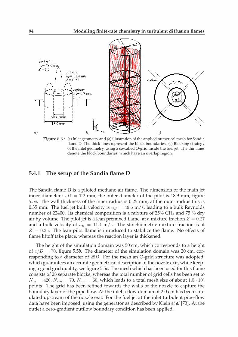
94 Modeling finite-rate chemistry in turbulent diffusion flames
a) b) c)Figure 5.5 : (a) Inlet geometry and (b) illustration of the applied numerical mesh for Sandia
flame D. The thick lines represent the block boundaries. (c) Blocking strategyof the inlet geometry, using a so-called O-grid inside the fuel jet. The thin linesdenote the block boundaries, which have an overlap region.
5.4.1 The setup of the Sandia flame D
The Sandia flame D is a piloted methane-air flame. The dimension of the main jetinner diameter is D = 7.2 mm, the outer diameter of the pilot is 18.9 mm, figure5.5a. The wall thickness of the inner radius is 0.25 mm, at the outer radius this is0.35 mm. The fuel jet bulk velocity is uB = 49.6 m/s, leading to a bulk Reynoldsnumber of 22400. Its chemical composition is a mixture of 25% CH4 and 75 % dryair by volume. The pilot jet is a lean premixed flame, at a mixture fraction Z = 0.27and a bulk velocity of uB = 11.4 m/s. The stoichiometric mixture fraction is atZ = 0.35. The lean pilot flame is introduced to stabilize the flame. No effects offlame liftoff take place, whereas the reaction layer is thickened.
The height of the simulation domain was 50 cm, which corresponds to a heightof z/D = 70, figure 5.5b. The diameter of the simulation domain was 20 cm, cor-responding to a diameter of 28D. For the mesh an O-grid structure was adopted,which guarantees an accurate geometrical description of the nozzle exit, while keep-ing a good grid quality, see figure 5.5c. The mesh which has been used for this flameconsists of 28 separate blocks, whereas the total number of grid cells has been set toNax = 420, Nrad = 70, Ntan = 60, which leads to a total mesh size of about 1.5 · 106
points. The grid has been refined towards the walls of the nozzle to capture theboundary layer of the pipe flow. At the inlet a flow domain of 2.0 cm has been sim-ulated upstream of the nozzle exit. For the fuel jet at the inlet turbulent pipe-flowdata have been imposed, using the generator as described by Klein et al [73]. At theoutlet a zero-gradient outflow boundary condition has been applied.

5.4 LES of a piloted diffusion flame 95
Table 5.1 : Definition of the three different parametrizations applied for the simulation ofthe Sandia flame D.
Case Chemical flamelet setup ParametrizationZχD Diffusion a(χ)ZCD Diffusion H2OZCP Premixed H2O
The chemical databases
The chemical databases that are used in this work are constructed from Steady Lam-inar Flamelet libraries. In case of the counterflow diffusion flame setup this libraryconsists of a set of flames with the strain rate a as the defining flame parameter.Unity Lewis numbers are assumed, while the flame geometry is flat. The mixturefraction is based on the Bilger definition [17], expression 5.1. Both the non-premixeddiffusion flames and the premixed flames are computed with the CHEM1D pack-age [31]. The reaction mechanism GRI-3.0 [145] has been applied. For the non-premixed flamelet database the strain rate in the database starts from the lower limita = 10s−1, which is close to equilibrium and is increased with steps of about 10% upto quenching, which is at a strain rate of a = 1250s−1.
In figure 5.6 the major species concentrations are plotted for this flame. The leftfigure shows the solution for a = 10 s−1, whereas the right figure shows the solutionnear quenching. The OH concentration, here shown with a magnification factor of50, shows its maximum at the location of the flame front. It can be seen that withdecreasing strain rate the species mass fractions for the reaction products appearat the fuel-rich side (Z > 0.35), whereas the CH4 and O2 mass fractions decrease.Now at the quenching strain rate the oxygen concentration remains present and themethane concentration penetrates far more deeply into the flame zone, leading toa decrease of H2O. The simulation that is based on this database, where the scalardissipation rate χ is used to determine the flamelet with the corresponding strainrate a (using equation 5.8) is referred to as the ZχD method, see table 5.1.
For the progress variable method that is based on the non-premixed chemistry,the mass fraction of H2O was chosen as the tracking variable. This variable showedthe required behavior of monotonicity over the complete range of mixture fractionspace: for every value of the mixture fraction the mass fraction of H2O was increas-ing with decreasing strain rate. For this method the non-premixed flamelet databasehas been reconstructed, based on increasing H2O mass fractions. This method is re-ferred to as the ZCD method.
For the premixed flamelet database a set of premixed flames with different chem-ical composition (different mixture fraction) has been generated, using the samemechanism and Lewis numbers. These flames are only evaluated between Z = 0.15and Z = 0.55, as these are the flamability limits of this setup, as can be seen from theOH profiles, figure 5.7. The values lower than Z = 0.15 and higher than Z = 0.55 areconstructed by interpolation with the boundary conditions at Z = 0 and 1. In factthis method represents a diffusion process in Z− space. In the premixed flamelet

96 Modeling finite-rate chemistry in turbulent diffusion flames
0 0.1 0.2 0.3 0.4 0.5 0.6 0.7 0.8 0.9 10
0.05
0.1
0.15
0.2
0.25
Z
Y
0 0.1 0.2 0.3 0.4 0.5 0.6 0.7 0.8 0.9 10
0.05
0.1
0.15
0.2
0.25
Z
Y
a) b)Figure 5.6 : Flamelet solutions for the non-premixed flame mass fractions of the major
species for the Sandia flame D. (a) strain rate a = 10 s−1, (b) a = 1250 s−1.(—): H2O, (- - -): CH4, (· · ·): CO2, � : O2, ◦: CO, △: OH, multiplied by a factor50.
0 0.1 0.2 0.3 0.4 0.5 0.6 0.7 0.8 0.9 10
0.05
0.1
0.15
0.2
0.25
Z
Y
0 0.1 0.2 0.3 0.4 0.5 0.6 0.7 0.8 0.9 10
0.05
0.1
0.15
0.2
0.25
Z
Y
a) b)Figure 5.7 : Flamelet solutions for the premixed flame mass fractions of the major species
for the Sandia flame D. (a) flame solution at maximum H2O concentration, (b)flame solution based on the H2O concentrations from the extinction flamelet infigure 5.6b. (—): H2O, (- - -): CH4, (· · ·): CO2, � : O2, ◦: CO, △: OH, multipliedby a factor 50.
database the H2O mass fraction does not show the required uniqueness outsidethese boundaries. Even at the rich premixed flames (0.5 < Z < 0.55) the massfraction of H2O did not show monotonicity. This non-uniqueness may call for theuse of another progress variable. However, in order to remain consistent with thenon-premixed approach, this option has not been chosen. Instead, the premixedflames have been cut off at the maximum H2O mass fraction, as the remaining re-gion in H2O space is expected not be encountered in the practical simulations of theflame. This is a similar reasoning as for the non-premixed flamelet database, thathas been cut off at a strain rate of 10 s−1. Below this strain rate only diffusive effectsat timescales larger than 0.1 s take place, which are expected not to be encounteredin this flame. This assumption will also be discussed based on the results. The sim-ulation that is performed with this database is referred to as ZCP , see also table5.1.

5.4 LES of a piloted diffusion flame 97
0 0.1 0.2 0.3 0.4 0.5 0.6 0.7 0.8 0.9 10.1
0.2
0.3
0.4
0.5
0.6
0.7
0.8
0.9
1
1.1
Z
ρ
a
0 0.1 0.2 0.3 0.4 0.5 0.6 0.7 0.8 0.9 1
400
600
800
1000
1200
1400
1600
1800
2000
2200
Z
T
a
a) b)Figure 5.8 : Non-premixed flamelet solutions of the density and temperature for increasing
strain rate a, for the Sandia flame D.
Z
H2O
1050100200
0 0.2 0.4 0.6 0.8 10
0.02
0.04
0.06
0.08
0.1
0.12
0.14
Z
H2O
10
10
50100
200
0 0.2 0.4 0.6 0.8 10
0.02
0.04
0.06
0.08
0.1
0.12
0.14
a) b)Figure 5.9 : Contour plots of the chemical source term for H2O, in kg/m3s as a function of
the H2O mass fraction and the mixture fraction. (a) The non-premixed flameletdatabase, (- - -) denote the flamelet solutions for H2O at strain rates 10 s−1
and 1250 s−1. (b) Premixed flamelet database. (- - -) is the maximum H2Oconcentration.
For the fluid dynamical problem the key parameter in the applied atmosphericflames is the local density. Its variation as a function of mixture fraction and strainrate is shown in figure 5.8a. Notice that this variation is very steep near the bound-aries of the mixture fraction field, but very moderate over a large range of mixturefraction, near the middle. The corresponding temperature profile is at its maximumaround stoichiometric mixture fraction, at Z = 0.35, figure 5.8b.
Figure 5.9 shows the flamelet solutions of the chemical source terms for the non-premixed and the premixed flames. In both cases the chemical source term decreaseswith increasing water concentration: with increasing H2O concentration the near-equilibrium value is reached. One difference between the two databases is that thenon-premixed flame database is defined only between the quenching flamelet andthe flamelet related to a = 10 s −1, while in case of the premixed flame databasethe manifold reaches far beyond this level, down to a mass fraction of H2O equal tozero. However, these locations of low concentration of H2O at intermediate mixturefraction are hardly encountered in the flame, as only few instances of extinction can
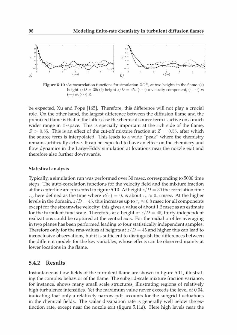
98 Modeling finite-rate chemistry in turbulent diffusion flames
0 1 2 3 4 5 6
−0.2
0
0.2
0.4
0.6
0.8
1
τ (ms)
R
0 1 2 3 4 5 6
−0.2
0
0.2
0.4
0.6
0.8
1
τ (ms)
R
a) b)
Figure 5.10 :Autocorrelation functions for simulation ZCD, at two heights in the flame. (a)height z/D = 30; (b) height z/D = 45. (- - -) u velocity component, (- · - ·) v;(—) w; (· · ·) Z.
be expected, Xu and Pope [165]. Therefore, this difference will not play a crucialrole. On the other hand, the largest difference between the diffusion flame and thepremixed flame is that in the latter case the chemical source term is active on a muchwider range in Z-space. This is specially important at the rich side of the flame,Z > 0.55. This is an effect of the cut-off mixture fraction at Z = 0.55, after whichthe source term is interpolated. This leads to a wide ”peak” where the chemistryremains artificially active. It can be expected to have an effect on the chemistry andflow dynamics in the Large-Eddy simulation at locations near the nozzle exit andtherefore also further downwards.
Statistical analysis
Typically, a simulation run was performed over 30 msec, corresponding to 5000 timesteps. The auto-correlation functions for the velocity field and the mixture fractionat the centerline are presented in figure 5.10. At height z/D = 30 the correlation timeτc, here defined as the time where R(τ) = 0, is about τc ≈ 0.5 msec. At the higherlevels in the domain, z/D = 45, this increases up to τc ≈ 0.8 msec for all componentsexcept for the streamwise velocity: this gives a value of about 1.2 msec as an estimatefor the turbulent time scale. Therefore, at a height of z/D = 45, thirty independentrealizations could be captured at the central axis. For the radial profiles averagingin two planes has been performed leading to four statistically independent samples.Therefore only for the rms-values at heights at z/D = 45 and higher this can lead toinconclusive observations, but it is sufficient to distinguish the differences betweenthe different models for the key variables, whose effects can be observed mainly atlower locations in the flame.
5.4.2 Results
Instantaneous flow fields of the turbulent flame are shown in figure 5.11, illustrat-ing the complex behavior of the flame. The subgrid-scale mixture fraction variance,for instance, shows many small scale structures, illustrating regions of relativelyhigh turbulence intensities. Yet the maximum value never exceeds the level of 0.04,indicating that only a relatively narrow pdf accounts for the subgrid fluctuationsin the chemical fields. The scalar dissipation rate is generally well below the ex-tinction rate, except near the nozzle exit (figure 5.11d). Here high levels near the
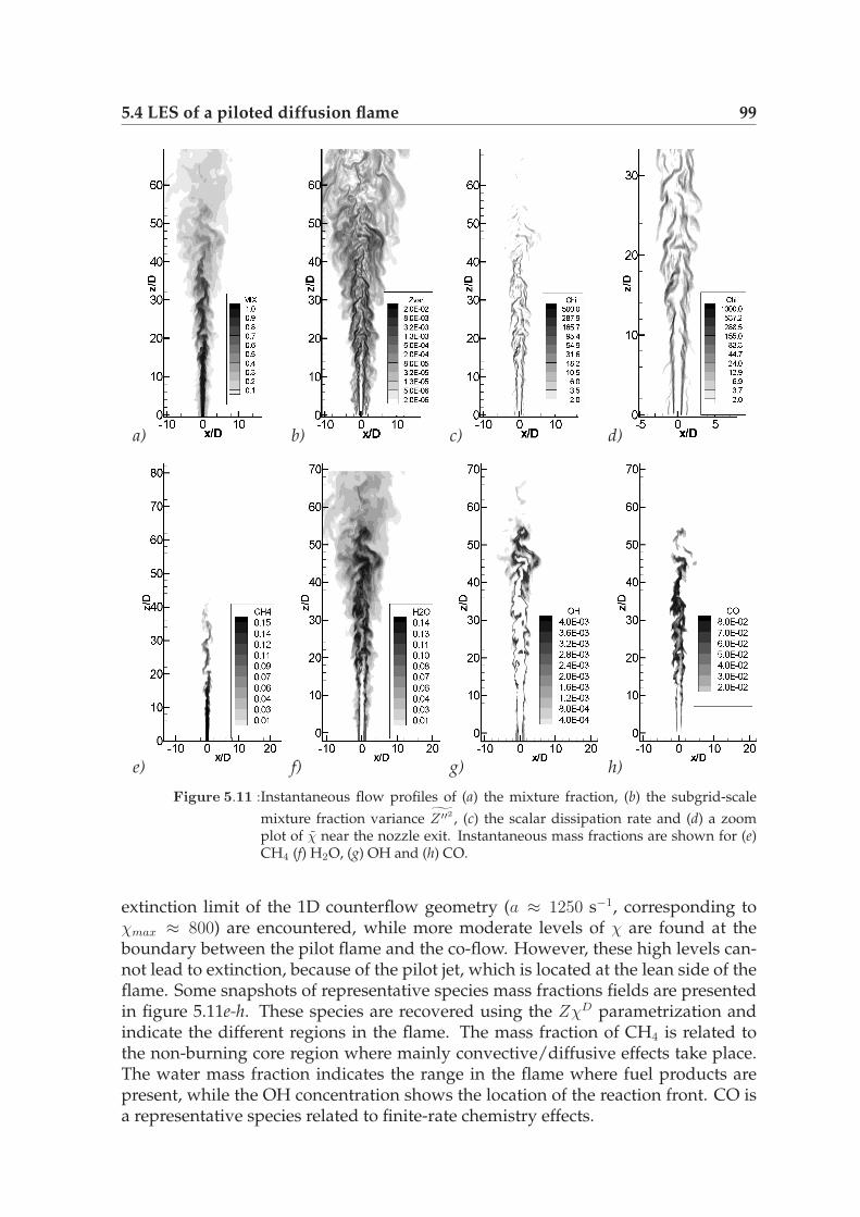
5.4 LES of a piloted diffusion flame 99
a) b) c) d)
e) f) g) h)
Figure 5.11 :Instantaneous flow profiles of (a) the mixture fraction, (b) the subgrid-scale
mixture fraction variance Z ′′2 , (c) the scalar dissipation rate and (d) a zoom
plot of χ near the nozzle exit. Instantaneous mass fractions are shown for (e)CH4 (f) H2O, (g) OH and (h) CO.
extinction limit of the 1D counterflow geometry (a ≈ 1250 s−1, corresponding toχmax ≈ 800) are encountered, while more moderate levels of χ are found at theboundary between the pilot flame and the co-flow. However, these high levels can-not lead to extinction, because of the pilot jet, which is located at the lean side of theflame. Some snapshots of representative species mass fractions fields are presentedin figure 5.11e-h. These species are recovered using the ZχD parametrization andindicate the different regions in the flame. The mass fraction of CH4 is related tothe non-burning core region where mainly convective/diffusive effects take place.The water mass fraction indicates the range in the flame where fuel products arepresent, while the OH concentration shows the location of the reaction front. CO isa representative species related to finite-rate chemistry effects.
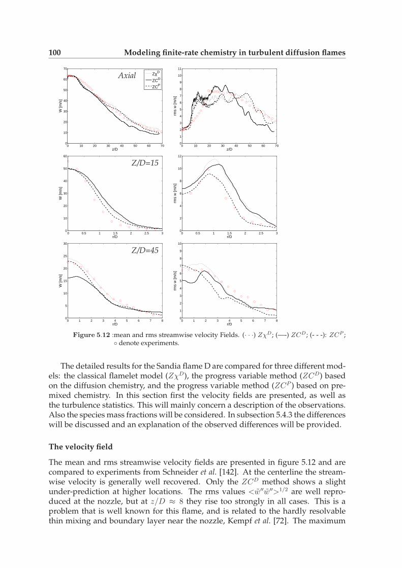
100 Modeling finite-rate chemistry in turbulent diffusion flames
0 10 20 30 40 50 60 700
10
20
30
40
50
60
70
z/D
W [m
/s]
ZχD
ZCD
ZCP
0 0.5 1 1.5 2 2.5 30
10
20
30
40
50
60
r/D
W [m
/s]
0 1 2 3 4 5 6 7 80
5
10
15
20
25
30
r/D
W [m
/s]
0 10 20 30 40 50 60 700
1
2
3
4
5
6
7
8
9
10
11
z/D
rms
w [m
/s]
0 0.5 1 1.5 2 2.5 30
2
4
6
8
10
12
r/D
rms
w [m
/s]
0 1 2 3 4 5 6 7 80
1
2
3
4
5
6
7
8
9
10
r/D
rms
w [m
/s]
Axial
Z/D=15
Z/D=45
Figure 5.12 :mean and rms streamwise velocity Fields. (· · ·) ZχD; (—-) ZCD; (- - -): ZCP ;◦ denote experiments.
The detailed results for the Sandia flame D are compared for three different mod-els: the classical flamelet model (ZχD), the progress variable method (ZCD) basedon the diffusion chemistry, and the progress variable method (ZCP ) based on pre-mixed chemistry. In this section first the velocity fields are presented, as well asthe turbulence statistics. This will mainly concern a description of the observations.Also the species mass fractions will be considered. In subsection 5.4.3 the differenceswill be discussed and an explanation of the observed differences will be provided.
The velocity field
The mean and rms streamwise velocity fields are presented in figure 5.12 and arecompared to experiments from Schneider et al. [142]. At the centerline the stream-wise velocity is generally well recovered. Only the ZCD method shows a slightunder-prediction at higher locations. The rms values <w′′w′′>1/2 are well repro-duced at the nozzle, but at z/D ≈ 8 they rise too strongly in all cases. This is aproblem that is well known for this flame, and is related to the hardly resolvablethin mixing and boundary layer near the nozzle, Kempf et al. [72]. The maximum
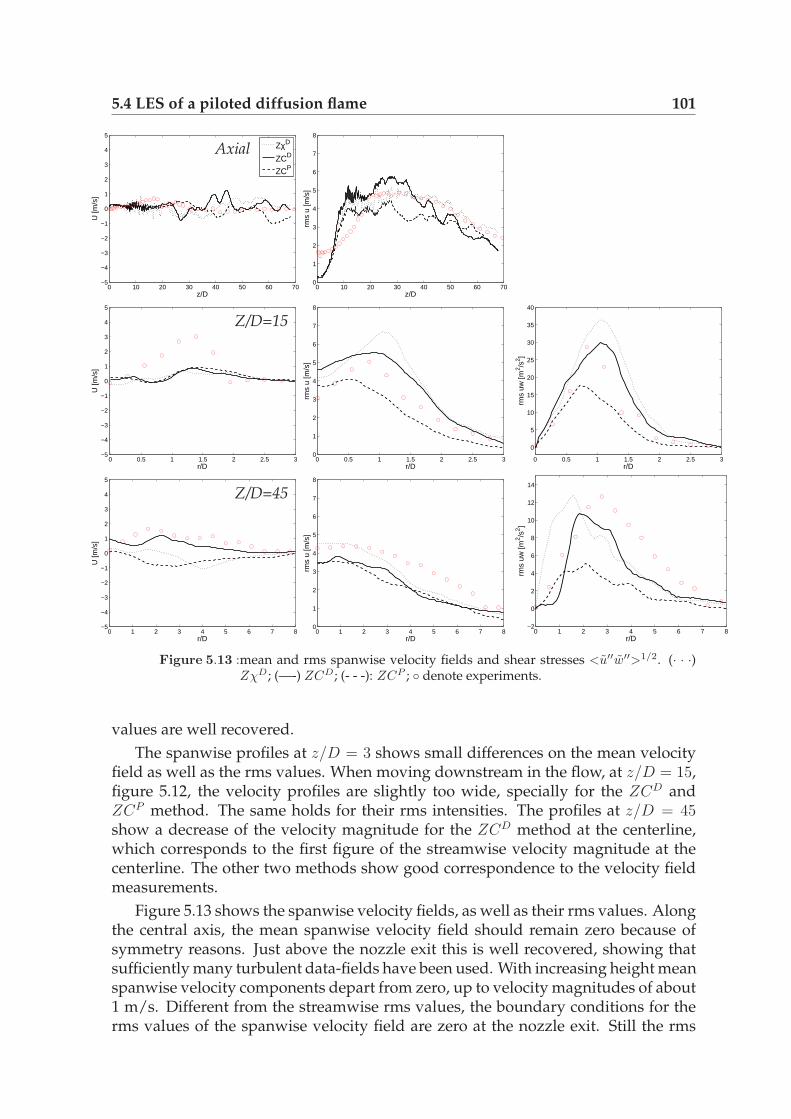
5.4 LES of a piloted diffusion flame 101
0 10 20 30 40 50 60 70−5
−4
−3
−2
−1
0
1
2
3
4
5
z/D
U [m
/s]
ZχD
ZCD
ZCP
0 0.5 1 1.5 2 2.5 3−5
−4
−3
−2
−1
0
1
2
3
4
5
r/D
U [m
/s]
0 1 2 3 4 5 6 7 8−5
−4
−3
−2
−1
0
1
2
3
4
5
r/D
U [m
/s]
0 10 20 30 40 50 60 700
1
2
3
4
5
6
7
8
z/D
rms
u [m
/s]
0 0.5 1 1.5 2 2.5 30
1
2
3
4
5
6
7
8
r/D
rms
u [m
/s]
0 1 2 3 4 5 6 7 80
1
2
3
4
5
6
7
8
r/D
rms
u [m
/s]
0 0.5 1 1.5 2 2.5 3
0
5
10
15
20
25
30
35
40
r/D
rms
uw [m
2 /s2 ]
0 1 2 3 4 5 6 7 8−2
0
2
4
6
8
10
12
14
r/D
rms
uw [m
2 /s2 ]
Axial
Z/D=15
Z/D=45
Figure 5.13 :mean and rms spanwise velocity fields and shear stresses <u′′w′′>1/2. (· · ·)ZχD; (—-) ZCD; (- - -): ZCP ; ◦ denote experiments.
values are well recovered.
The spanwise profiles at z/D = 3 shows small differences on the mean velocityfield as well as the rms values. When moving downstream in the flow, at z/D = 15,figure 5.12, the velocity profiles are slightly too wide, specially for the ZCD andZCP method. The same holds for their rms intensities. The profiles at z/D = 45show a decrease of the velocity magnitude for the ZCD method at the centerline,which corresponds to the first figure of the streamwise velocity magnitude at thecenterline. The other two methods show good correspondence to the velocity fieldmeasurements.
Figure 5.13 shows the spanwise velocity fields, as well as their rms values. Alongthe central axis, the mean spanwise velocity field should remain zero because ofsymmetry reasons. Just above the nozzle exit this is well recovered, showing thatsufficiently many turbulent data-fields have been used. With increasing height meanspanwise velocity components depart from zero, up to velocity magnitudes of about1 m/s. Different from the streamwise rms values, the boundary conditions for therms values of the spanwise velocity field are zero at the nozzle exit. Still the rms

102 Modeling finite-rate chemistry in turbulent diffusion flames
values of the u-velocity component at the centerline show a similar behavior as itsstreamwise counterparts. An abrupt increase is observed, followed by a steady levelat about 4 - 5.5 m/s. The ZCD method shows the largest values in the range up toheight z/D = 40.
The mean velocity field in radial direction has not been recovered very well. Onthe other hand, the absolute magnitude is very small and well below the turbulentfluctuations. The fluctuations themselves are on average reasonably well recovered,which is the most important. The < u′′w′′ >1/2 components are recovered relativelywell. Only the levels extracted from the ZCP method give a significant underpre-diction at all heights.
Concluding it can be stated that the mean velocity field and turbulence intensi-ties are well recovered in all simulations. There are minor differences visible, mainlyat larger heights above the nozzle. Then the mean streamwise velocity at the center-line for the ZCD method is lower than the other methods and the experiments. Inthe ZχD method the turbulence intensities just above the nozzle exit, near the pilotflame, are slightly over-estimated.
Species concentrations
Figure 5.14a shows the mixture fraction field along the central axis for the threedifferent models. While the ZCD model follows the experiments closely near thevicinity of the nozzle, it decreases relatively fast in magnitude at about z/D = 20. Onthe other hand in the ZCP and ZχD methods the mixture fraction field correspondsaccurately to the experiments, over the complete range. Yet the rms values are nowslightly over-predicted, figure 5.14b. Close to the nozzle exit, below z/D = 15 therms values from all models go to zero, while the fluctuations from the experimentsremain present. The observed fluctuations in the experiments can either be due toerrors in the experimental technique, such as previously suggested by Pitsch andSteiner [121] or due to preferential diffusion effects. In the latter case the averagemixture fraction field, that is based on the Bilger definition, Bilger [17] can be unity,while instantaneous values can exceed this level, due to increased concentrations ofhydrogen. When including preferential diffusion in the simulations in principle thiseffect can then be accounted for.
Because of the shift of mixture fraction field in the ZCD method, all chemicalspecies are shifted accordingly. This makes the analysis of the results, i.e. the im-pact of the parameterization unclear. To exclude the effect of the prediction of thechemistry as a function of the actual, spatial coordinates z/D and r/D, the speciesmass fractions will be presented as a function of the mixture fraction space. Thenhigh values of Z correspond to low values of z/D, which is physically located closeto the nozzle exit.
Figure 5.14c then shows the mass fraction of H2O. This quantity is evaluatedexplicitly in the ZCD and ZCP method, as this is the chosen progress variable,but naturally reconstructed using the steady laminar flamelet database in the ZχD
method. The ZCD method predicts the concentration globally well, while it is un-derpredicted by the ZCP method in the hot flame zone 0.3 < Z < 0.6. Near theend of the physical domain, for small Z, the correct levels are recovered in the ZCP

5.4 LES of a piloted diffusion flame 103
0 10 20 30 40 50 60 700
0.1
0.2
0.3
0.4
0.5
0.6
0.7
0.8
0.9
1
z/D
Z
ZχD
ZCD
ZCP
0 0.2 0.4 0.6 0.8 10
0.02
0.04
0.06
0.08
0.1
0.12
Z
H2O
ZχD
ZCD
ZCP
0 0.2 0.4 0.6 0.8 10
0.01
0.02
0.03
0.04
0.05
0.06
0.07
Z
CO
ZχD
ZCD
ZCP
0 10 20 30 40 50 60 700
0.02
0.04
0.06
0.08
0.1
0.12
0.14
0.16
0.18
0.2
z/D
rms
Z
0 0.2 0.4 0.6 0.8 10
0.005
0.01
0.015
0.02
0.025
0.03
0.035
Z
rms
H2O
0 0.2 0.4 0.6 0.8 10
0.005
0.01
0.015
0.02
0.025
0.03
0.035
Z
rms
CO
a) b)
c) d)
e) f)Figure 5.14 :Selected variables, and their rms values, along the center axis. (· · ·) ZχD; (—-)
ZCD; (- - -): ZCP ; ◦ denote experiments. The mixture fraction is given as afunction of the vertical coordinate z/D, the species mass fractions are given asa function of the mixture fraction Z.
method. The ZχD method shows an overprediction of the profiles at the rich side.
Concerning the variance, figure 5.14d, the first maximum is predicted too close tothe nozzle exit (z/D = 25; Z = 0.8) for all cases. The second maximum as found inthe experiments at Z ∼ 0.2, is poorly recovered in all cases. The temperature fieldsexhibit a similar trend as the H2O mass fractions, as these quantities are closelycoupled. Finally the CO concentration fields are shown, representing the finite-rate chemistry. A remarkable correspondence is visible for the ZCD method, whichfollows the experimental values closely. Both other methods give an overpredictionat the rich side. Only at decreasing Z, i.e. higher up in the flame, the ZχD andZCP methods get in line with the experiments. The reason for this behavior willbe discussed in more detail in the next subsection. The rms profiles show a correct
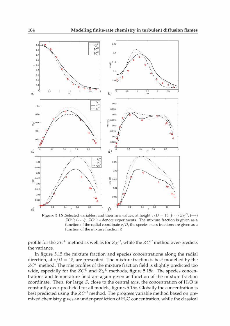
104 Modeling finite-rate chemistry in turbulent diffusion flames
0 0.5 1 1.5 2 2.5 30
0.1
0.2
0.3
0.4
0.5
0.6
0.7
0.8
0.9
r/D
Z
ZχD
ZCD
ZCP
0 0.2 0.4 0.6 0.8 10
0.02
0.04
0.06
0.08
0.1
Z
H2O
ZχD
ZCD
ZCP
0 0.2 0.4 0.6 0.8 10
0.005
0.01
0.015
0.02
0.025
0.03
0.035
0.04
0.045
Z
CO
ZχD
ZCD
ZCP
0 0.5 1 1.5 2 2.5 30
0.05
0.1
0.15
0.2
0.25
r/D
rms
Z
0 0.2 0.4 0.6 0.8 10
0.005
0.01
0.015
0.02
0.025
0.03
0.035
0.04
Z
rms
H2O
0 0.2 0.4 0.6 0.8 10
0.005
0.01
0.015
0.02
0.025
Z
rms
CO
a) b)
c) d)
e) f)Figure 5.15 :Selected variables, and their rms values, at height z/D = 15. (· · ·) ZχD; (—-)
ZCD; (- - -): ZCP ; ◦ denote experiments. The mixture fraction is given as afunction of the radial coordinate r/D, the species mass fractions are given as afunction of the mixture fraction Z.
profile for the ZCD method as well as for ZχD, while the ZCP method over-predictsthe variance.
In figure 5.15 the mixture fraction and species concentrations along the radialdirection, at z/D = 15, are presented. The mixture fraction is best modelled by theZCP method. The rms profiles of the mixture fraction field is slightly predicted toowide, especially for the ZCD and ZχD methods, figure 5.15b. The species concen-trations and temperature field are again given as function of the mixture fractioncoordinate. Then, for large Z, close to the central axis, the concentration of H2O isconstantly over-predicted for all models, figures 5.15c. Globally the concentration isbest predicted using the ZCD method. The progress variable method based on pre-mixed chemistry gives an under-prediction of H2O concentration, while the classical

5.4 LES of a piloted diffusion flame 105
0 1 2 3 4 5 6 7 80
0.05
0.1
0.15
0.2
0.25
0.3
0.35
r/D
Z
ZχD
ZCD
ZCP
0 0.2 0.4 0.6 0.8 10
0.02
0.04
0.06
0.08
0.1
Z
H2O
ZχD
ZCD
ZCP
0 0.2 0.4 0.6 0.8 10
0.005
0.01
0.015
0.02
0.025
0.03
0.035
0.04
Z
CO
ZχD
ZCD
ZCP
0 1 2 3 4 5 6 7 80
0.02
0.04
0.06
0.08
0.1
0.12
0.14
0.16
r/D
rms
Z
0 0.2 0.4 0.6 0.8 10
0.005
0.01
0.015
0.02
0.025
0.03
0.035
0.04
0.045
Z
rms
H2O
0 0.2 0.4 0.6 0.8 10
0.005
0.01
0.015
0.02
0.025
0.03
0.035
0.04
Z
rms
CO
a) b)
c) d)
e) f)Figure 5.16 :Selected variables, and their rms values, at height z/D = 45. (· · ·) ZχD; (—-)
ZCD; (- - -): ZCP ; ◦ denote experiments. The mixture fraction is given as afunction of the radial coordinate r/D, the species mass fractions are given as afunction of the mixture fraction Z.
flamelet method leads to an over-prediction. For small Z the results from the differ-ent models collapse again. Also concerning the rms profile the ZCD method is thebest performing, figure 5.15d, showing the dip in the rms value of H2O at the correctvalue of the mixture fraction. Concerning the CO mass fraction, the mean and rmsvalues for the ZχD and ZCP methods are overpredicted, figure 5.15g,h, while theZCD method shows a good correspondence to the experiments.
Higher up in the domain, at z/D = 45, figure 5.16, the ZCP and ZχD methodspredict the mixture fraction field correctly, but give a large overestimation of thefluctuating fields. At the same time the ZCD simulation underpredicts the center-line value, but shows correct magnitudes of the variance. The mean mass fractionof H2O are fairly equally predicted in all simulations, as are the rms values. The

106 Modeling finite-rate chemistry in turbulent diffusion flames
0 0.2 0.4 0.6 0.8 1
100
101
102
103
Z
χ
−4 −2 0 2 40
2
4
6
8
10
12
14
16
r/D
z/D
0.1
0.7
0.9
0.9
0.10.3
0.1
a) b)Figure 5.17 :(a) Scatter plot of the ZχD parametrization at z/D = 15. The two lines indicate
the scalar dissipation rate corresponding to a = 10 and 1250 s−1. (b) Recon-struction of the local flamelet structure, at one time instant. The contourplotshows the iso-lines of the mixture fraction field, the thick lines are the recon-structed flamelets.
ZCP method underpredicts the maximum H2O concentration, and overpredicts itsvariance at the larger values of Z. Concerning the CO profiles, figures 5.16e,f, theZχD method now gives slightly better results compared to the other two methods,but the tendencies are similar.
To conclude, the global trend is that the ZCP and ZχD methods predict the mix-ture fraction field better compared to the ZCD method. The prediction of Z is crucialfor the prediction of all remaining chemistry, therefore these methods show the bestcorrespondence to experiments, when looking at spatial coordinates. On the otherhand, to make a more fair comparison between the chemical models, the predic-tion of Z can be excluded. In that case on average a better correspondence betweenthe experiments and the ZCD method is achieved, especially for mixture fractionslarger than 0.2. Higher up in the domain, for smaller values of Z, the differencesbetween the models decrease. Thus, based on a chemical point of view, the ZCD
method performs the best, while when including the effect of the fluid dynamics,the other two methods are better.
5.4.3 Analysis of the chemistry models
The previous observations require an explanation. These cannot be extracted onlyfrom the presented observations alone, but are a result of a complex interplay ofseveral processes. The focus is on the interaction of the chemistry and the fluiddynamics. First we will focus on the ZχD method. Then, the two progress variablemethods will be discussed.
The classical flamelet method
In figure 5.11d the instantaneous scalar dissipation rate has been presented. This il-lustrates the presence of very high values of χ near the nozzle exit. When generatinga scatter plot of the scalar dissipation rate at height z/D = 15 the appropriateness of

5.4 LES of a piloted diffusion flame 107
0 0.2 0.4 0.6 0.8 10
50
100
150
200
250
300
Z
χ
0 0.5 1 1.5 2 2.50
50
100
150
200
250
r/D
χ
0 0.1 0.2 0.3 0.4 0.5 0.6 0.7 0.8 0.9 10
50
100
150
200
250
Z
χ
a)
b)
c)Figure 5.18 :(a) Examples of instantaneous χ(Z) profiles reconstructed from flamelets in the
ZχD simulation. Four flamelets at height z/D = 1, (—-): , z/D = 3, squares,z/D = 7, triangles, z/D = 15, (· · ··). (b): mean χ, as a function of radial coor-dinate, at three different heights. continuous line: z/D = 1, dashed: z/D = 3,dotted: z/D = 15. (c) conditional average of the mean scalar dissipation rateat the same heights.
the ZχD model can be checked in more general terms. This is shown in figure 5.17a.It is observed that a large amount of points are covered by the range of flamelets,from a = 10 s−1 to a = 1250 s−1. At these two strain rates the corresponding χprofiles are presented. A considerable amount of realizations can be found wherethe scalar dissipation rate is below its minimal value, mostly in the range close tostoichiometric conditions, 0.15 < Z < 0.5.
Figure 5.17b shows an example of the instantaneous, filtered flamelets in a planethat intersects the central axis in radial direction. To evaluate the flamelets a coor-dinate transformation, as depicted in figure 5.2a, has been performed for this two-dimensional plane, using the instantaneous LES results. It shows that in this rangez/D < 15 the flamelets are arranged mainly perpendicular to the vertical axis, i.e.at a constant height. The instantaneous χ(Z) profiles, as reconstructed from theseflamelets are presented in figure 5.18a. These profiles indicate that the assumptionof a bell-shape profile, described by equation 5.7, does not hold on an instantaneousbasis. Specially close to the nozzle exit this can lead to a wrong estimation of thestrainrate.
Figure 5.18b shows the average profiles along the radial coordinate at three dif-ferent heights above the nozzle exit. At z/D = 3 there are two peaks visible: a largeone, between the fuel jet and the pilot flame, and a smaller one between the pilotand the co-flow. Also when plotting the time-averaged <χ> as a function of themixture fraction this functionality does not show a bell-shape profile, especially notclose to the nozzle exit, figure 5.18c.
In the pilot flame, located at 0.5D < r < 1.3D, where (Z = 0.27), the scalardissipation rate is zero, as the pilot flame is in its chemical equilibrium. However,near the nozzle exit, close to the pilot, very high strain rates are encountered, thatcorrespond to highly finite-rate chemistry. Therefore the diffusion flame chemistryshould be described by a flamelet at high strain rate. But based on the applied para-

108 Modeling finite-rate chemistry in turbulent diffusion flames
0 0.2 0.4 0.6 0.8 10
0.02
0.04
0.06
0.08
0.1
0.12
0.14
Z
H2O
0 0.2 0.4 0.6 0.8 10
0.02
0.04
0.06
0.08
0.1
0.12
0.14
Z
H2O
a) b)
Figure 5.19 :(a) The scatter plot for the ZCD flame, at z/D = 15, the lines indicating theflamelets at strain rates a =10, 100 and 1250 s−1 (b) scatter plot for ZCP flameat z/D = 15. The line indicates the maximum H2O mass fraction in the FGM.
metrization, where a bell shape function for χ(Z) is assumed, a flamelet solutionat low strain rate is used. The effect of this difference is rather large, because thistakes place near stoichiometry. Here finite-rate chemistry effects on the density inthe applied chemical database are clearly visible, see figure 5.8.
Pitsch and Steiner [122] have reported on this effect before. There the stabilizingeffect of the pilot flame has been explained, by decreasing the scalar dissipation rateat stoichiometry. The difference on the chemical solution of a counterflow diffusionflame, between the scalar dissipation rate χ(Z), as found in this flame, and the pre-sumed shape, equation 5.7, was evaluated. A considerable shift of the temperatureprofile towards the lean side had been observed.
All these considerations indicate that in the ZχD method flamelet solutions closeto equilibrium, at low strain rates are used in the simulation. For the current simu-lations this leads to the results as presented in the previous section, showing reason-able prediction for the mixture fraction field, but less appropriate when consideringthe chemistry as a function of the mixture fraction coordinate.
The two progress variable methods
In the ZCD and ZCP methods the mass fraction of H2O is evaluated independentlyfrom the mixture fraction. By plotting the instantaneous values of H2O as a functionof Z the applicability of the H2O parametrization can be checked as well. This isshown in figure 5.19a for the ZCD method, at height z/D = 15. Also three flameletshave been included in this figure: a = 10 s−1, a = 100 s−1 and a = 1250 s−1. Here itcan be observed that for most points the instantaneous mass fraction of H2O is cov-ered by the domain defined by the non-premixed flamelets for strain rates smallerthan a = 100 s−1. Still in some instances H2O values are observed that are outsidethe range given by the flamelets, specially where lower concentrations of H2O areencountered. In this case the flamelet solution at the highest strainrate is used toevaluate the species concentrations and transport variables.
The ZCP model also parameterizes mixtures with low H2O concentration, figure

5.4 LES of a piloted diffusion flame 109
0 0.2 0.4 0.6 0.8 10
0.02
0.04
0.06
0.08
0.1
0.12
Z
C
0 0.2 0.4 0.6 0.8 10
0.02
0.04
0.06
0.08
0.1
0.12
Z
C
a) b)
Figure 5.20 :(a) Examples of instantaneous Z − C profiles reconstructed from flamelets inthe ZCD simulation. (—-): minimum and maximum H2O concentrations innon-premixed flamelet database. Four flamelets at height z/D = 1, squares,z/D = 7, triangles, z/D = 15, (· · ·). (b) The same, for the ZCP method. (—-):maximum H2O concentration from premixed chemistry table.
5.19b. Here the black line denotes the maximum H2O concentration. The minimumH2O concentration in the premixed database is naturally at 0. In this case all instan-taneous concentrations of H2O are covered.
Figure 5.20a shows a few examples of reconstructed flamelets at three differentheights close to the nozzle exit, for the ZCD simulation. The reconstruction is per-formed in a similar way as was done in figure 5.18. Also two reference flamelets,from the 1D counterflow diffusion flame are plotted, for a = 10 s−1 and a = 1250s−1. Then most flamelets are captured by the presumed shape, except for higher inthe domain. At z/D = 15 examples can be found where the flamelet departs fromthe 1-D configuration.
Figure 5.20b shows the same for the ZCP simulation. The maximum H2O con-centration is also shown. Compared to the ZCD method, at z/D = 1 the H2O con-centration is lower. This can be explained as an effect of the parametrization. As inthe premixed chemistry case, the H2O concentrations up to 0 are covered, leading tolow chemical source term. In case of the non-premixed chemistry, this source termis larger, as the quenching chemistry is used. This seems to be more appropriate, asin this flame no effects of lift off are present, i.e. the flame is directly burning. Again,higher in the domain, at z/D = 15 examples can be found where the flamelet showsstructures that depart from a typical non-premixed flamelet-like structure.
Modeling the mass fraction of CO
The scatter plots given in figure 5.17a and figure 5.19 indicate that at z/D = 15 finite-rate chemistry effects are encountered, and will be taken into account when evalu-ating the chemical species. Its impact along the central axis is studied in some moredetail in figure 5.21. Here the averaged H2O mass fraction is plotted as a function ofthe mixture fraction field, along the axial coordinate. In figures 5.21a,b the dashedlines indicate the minimal (near-extinction) and maximal (near-equilibrium) values,
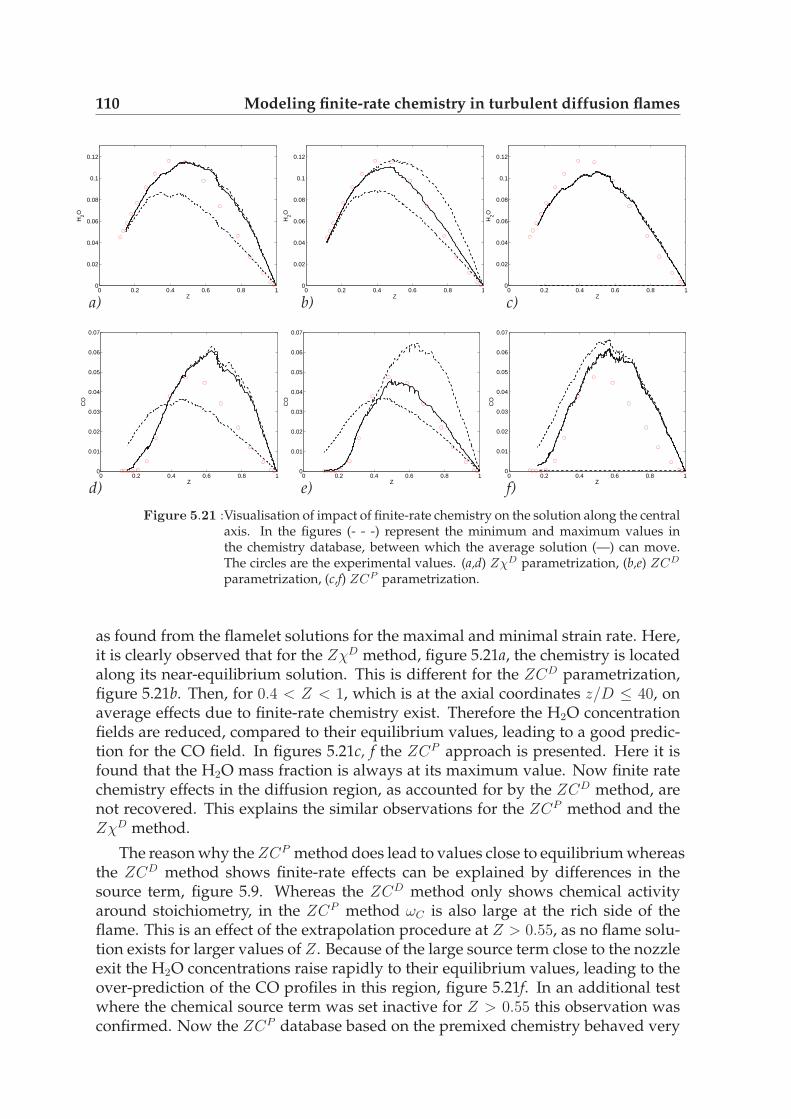
110 Modeling finite-rate chemistry in turbulent diffusion flames
0 0.2 0.4 0.6 0.8 10
0.02
0.04
0.06
0.08
0.1
0.12
Z
H2O
0 0.2 0.4 0.6 0.8 10
0.02
0.04
0.06
0.08
0.1
0.12
Z
H2O
0 0.2 0.4 0.6 0.8 10
0.02
0.04
0.06
0.08
0.1
0.12
Z
H2O
0 0.2 0.4 0.6 0.8 10
0.01
0.02
0.03
0.04
0.05
0.06
0.07
Z
CO
0 0.2 0.4 0.6 0.8 10
0.01
0.02
0.03
0.04
0.05
0.06
0.07
Z
CO
0 0.2 0.4 0.6 0.8 10
0.01
0.02
0.03
0.04
0.05
0.06
0.07
ZC
O
a) b) c)
d) e) f)
Figure 5.21 :Visualisation of impact of finite-rate chemistry on the solution along the centralaxis. In the figures (- - -) represent the minimum and maximum values inthe chemistry database, between which the average solution (—) can move.The circles are the experimental values. (a,d) ZχD parametrization, (b,e) ZCD
parametrization, (c,f) ZCP parametrization.
as found from the flamelet solutions for the maximal and minimal strain rate. Here,it is clearly observed that for the ZχD method, figure 5.21a, the chemistry is locatedalong its near-equilibrium solution. This is different for the ZCD parametrization,figure 5.21b. Then, for 0.4 < Z < 1, which is at the axial coordinates z/D ≤ 40, onaverage effects due to finite-rate chemistry exist. Therefore the H2O concentrationfields are reduced, compared to their equilibrium values, leading to a good predic-tion for the CO field. In figures 5.21c, f the ZCP approach is presented. Here it isfound that the H2O mass fraction is always at its maximum value. Now finite ratechemistry effects in the diffusion region, as accounted for by the ZCD method, arenot recovered. This explains the similar observations for the ZCP method and theZχD method.
The reason why the ZCP method does lead to values close to equilibrium whereasthe ZCD method shows finite-rate effects can be explained by differences in thesource term, figure 5.9. Whereas the ZCD method only shows chemical activityaround stoichiometry, in the ZCP method ωC is also large at the rich side of theflame. This is an effect of the extrapolation procedure at Z > 0.55, as no flame solu-tion exists for larger values of Z. Because of the large source term close to the nozzleexit the H2O concentrations raise rapidly to their equilibrium values, leading to theover-prediction of the CO profiles in this region, figure 5.21f. In an additional testwhere the chemical source term was set inactive for Z > 0.55 this observation wasconfirmed. Now the ZCP database based on the premixed chemistry behaved very

5.5 A sooting benzene diffusion flame 111
similar to the non-premixed chemistry for the mixture fraction field and the velocityfield.
Therefore, based on a chemical analysis the ZCD method leads to the best re-sults, especially for large values of the mixture fraction, close to the nozzle exit. Onthe other hand, the mixture fraction field remains the crucial parameter, which isinfluenced largely by the fluid dynamics.
5.4.4 Concluding remarks
By comparing the three parameterization methods it has been observed that the clas-sical flamelet method and the progress variable method based on premixed chem-istry give the most suitable results, based on the prediction of the mixture fractionfield. However, when showing the results as a function of the mixture fraction co-ordinate, the progress variable method based on non-premixed chemistry outper-forms the two other methods. This leads to the conclusion that the parameterizationof the chemistry, using this model, is better compared to the other two methods.
This indicates that the fluid dynamical part of the modeling problem needs im-provement. Possible effects can be an adjustment of the initial turbulence level at thenozzle exit, as this has an important effect on breakup of the core region, Kempf [71].Also an improved resolution of the shear layer close to the nozzle exit can lead tobetter results.
Improvements for the classical flamelet method can be achieved by applying aflamelet database that is better fitted to the current experimental setup. Especiallythe scalar dissipation rate as a function of the mixture fraction should be differentfrom the one encountered in the counterflow flame geometry. With respect to thedatabase of the premixed chemistry, a combination of species as progress variableshould be used in order to prevent problems of non-monotonicity in the completedomain of the chemical manifold.
5.5 A sooting benzene diffusion flame
In the previous section the flame structure itself in the sense of the velocity field, themixture fraction and their variances was of main concern. The impact of models forfinite-rate chemistry was mainly shown through these quantities. Also most chemi-cal species could well be described with the mixture fraction parameter solely, withan exception for the CO mass fraction. In this section we will focus on a turbulentflame where finite-rate chemistry has a large impact on the local chemical composi-tion within the flame. Also a fuel type is chosen that is more of relevance for engineconditions than methane.
In internal combustion engines the fuels that are used consist of a mixture oflarge hydrocarbon molecules. This implies a reaction process that is rather complex.Detailed reaction mechanisms of primary reference fuels, such as n-heptane and iso-octane involve about 1000 species and 4000 elementary reactions, Ranzi et al. [130].Also the total reaction path consists of a large number of steps. Apart from thecombustion process, where the large fuel particles are broken up into the typical
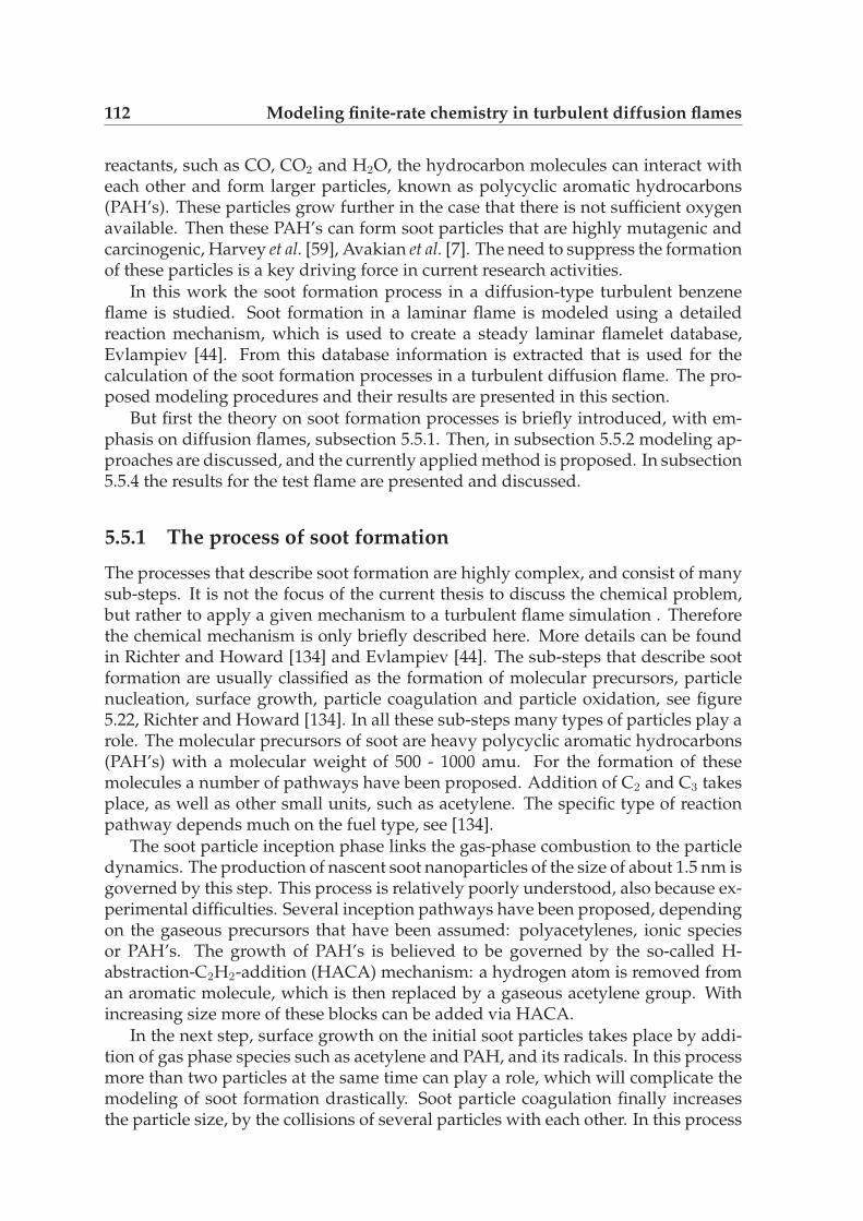
112 Modeling finite-rate chemistry in turbulent diffusion flames
reactants, such as CO, CO2 and H2O, the hydrocarbon molecules can interact witheach other and form larger particles, known as polycyclic aromatic hydrocarbons(PAH’s). These particles grow further in the case that there is not sufficient oxygenavailable. Then these PAH’s can form soot particles that are highly mutagenic andcarcinogenic, Harvey et al. [59], Avakian et al. [7]. The need to suppress the formationof these particles is a key driving force in current research activities.
In this work the soot formation process in a diffusion-type turbulent benzeneflame is studied. Soot formation in a laminar flame is modeled using a detailedreaction mechanism, which is used to create a steady laminar flamelet database,Evlampiev [44]. From this database information is extracted that is used for thecalculation of the soot formation processes in a turbulent diffusion flame. The pro-posed modeling procedures and their results are presented in this section.
But first the theory on soot formation processes is briefly introduced, with em-phasis on diffusion flames, subsection 5.5.1. Then, in subsection 5.5.2 modeling ap-proaches are discussed, and the currently applied method is proposed. In subsection5.5.4 the results for the test flame are presented and discussed.
5.5.1 The process of soot formation
The processes that describe soot formation are highly complex, and consist of manysub-steps. It is not the focus of the current thesis to discuss the chemical problem,but rather to apply a given mechanism to a turbulent flame simulation . Thereforethe chemical mechanism is only briefly described here. More details can be foundin Richter and Howard [134] and Evlampiev [44]. The sub-steps that describe sootformation are usually classified as the formation of molecular precursors, particlenucleation, surface growth, particle coagulation and particle oxidation, see figure5.22, Richter and Howard [134]. In all these sub-steps many types of particles play arole. The molecular precursors of soot are heavy polycyclic aromatic hydrocarbons(PAH’s) with a molecular weight of 500 - 1000 amu. For the formation of thesemolecules a number of pathways have been proposed. Addition of C2 and C3 takesplace, as well as other small units, such as acetylene. The specific type of reactionpathway depends much on the fuel type, see [134].
The soot particle inception phase links the gas-phase combustion to the particledynamics. The production of nascent soot nanoparticles of the size of about 1.5 nm isgoverned by this step. This process is relatively poorly understood, also because ex-perimental difficulties. Several inception pathways have been proposed, dependingon the gaseous precursors that have been assumed: polyacetylenes, ionic speciesor PAH’s. The growth of PAH’s is believed to be governed by the so-called H-abstraction-C2H2-addition (HACA) mechanism: a hydrogen atom is removed froman aromatic molecule, which is then replaced by a gaseous acetylene group. Withincreasing size more of these blocks can be added via HACA.
In the next step, surface growth on the initial soot particles takes place by addi-tion of gas phase species such as acetylene and PAH, and its radicals. In this processmore than two particles at the same time can play a role, which will complicate themodeling of soot formation drastically. Soot particle coagulation finally increasesthe particle size, by the collisions of several particles with each other. In this process
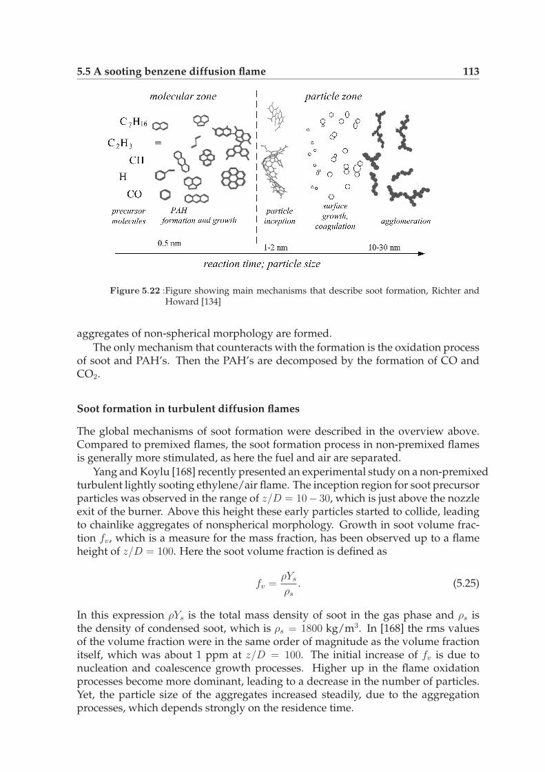
5.5 A sooting benzene diffusion flame 113
Figure 5.22 :Figure showing main mechanisms that describe soot formation, Richter andHoward [134]
aggregates of non-spherical morphology are formed.
The only mechanism that counteracts with the formation is the oxidation processof soot and PAH’s. Then the PAH’s are decomposed by the formation of CO andCO2.
Soot formation in turbulent diffusion flames
The global mechanisms of soot formation were described in the overview above.Compared to premixed flames, the soot formation process in non-premixed flamesis generally more stimulated, as here the fuel and air are separated.
Yang and Koylu [168] recently presented an experimental study on a non-premixedturbulent lightly sooting ethylene/air flame. The inception region for soot precursorparticles was observed in the range of z/D = 10− 30, which is just above the nozzleexit of the burner. Above this height these early particles started to collide, leadingto chainlike aggregates of nonspherical morphology. Growth in soot volume frac-tion fv, which is a measure for the mass fraction, has been observed up to a flameheight of z/D = 100. Here the soot volume fraction is defined as
fv =ρYs
ρs
. (5.25)
In this expression ρYs is the total mass density of soot in the gas phase and ρs isthe density of condensed soot, which is ρs = 1800 kg/m3. In [168] the rms valuesof the volume fraction were in the same order of magnitude as the volume fractionitself, which was about 1 ppm at z/D = 100. The initial increase of fv is due tonucleation and coalescence growth processes. Higher up in the flame oxidationprocesses become more dominant, leading to a decrease in the number of particles.Yet, the particle size of the aggregates increased steadily, due to the aggregationprocesses, which depends strongly on the residence time.

114 Modeling finite-rate chemistry in turbulent diffusion flames
For the modeling of diffusion flames a flamelet method is generally applied, Pe-ters [114]. However, it is well known that the soot concentrations cannot be corre-lated to the mixture fraction field directly, Balthasar et al. [12], Moss [97]. The sootcomposition depends strongly on the residence time as well as on the local gas com-position. However, recent observations show that this is mainly the case for thelarger soot particles. D’Anna et al. [6] studied a turbulent ethylene/air flame, andobserved two classes of particles. The first class are nanoparticles that consist oflarge poly-aromatic hydrocarbons, of the size of about 2 - 3 nm on average. Theseparticles are mainly found in the fuel rich region of the flame, close to the nozzle.The second class, the larger particles, are formed with increasing residence timesin the flame, as a result of the growth processes. These soot particles are dominantin the region of maximum flame temperature. D’Anna concludes that the concen-tration of the nanoparticles is not controlled by the chemical kinetics, but by theturbulent mixing, due to effects of inception and carbonization of precursor par-ticles. It is shown that these nanoparticles correlate strongly to the major speciesconcentration, and therefore the mixture fraction. A second flame with higher inletvelocity, that corresponds to a higher strain rate, shows lower concentrations of thistype of nanoparticles. This indicates that these species are simply depending on themixture fraction and the strain rate, but not directly on residence time. However,as mentioned, the larger soot particles cannot be correlated to the mixture fraction,but prevail in the regions close to the maximum flame temperature. The maximumconcentrations of larger soot particles have been observed just after the maximumof the nanoparticle concentration.
5.5.2 Modeling soot in diffusion flames
As can be understood from the previous section the formation of soot is a highlycomplex phenomenon, depending on many parameters, such as the type of fuel,pressure, residence time, the availability of oxygen. Amongst others this defines thedifferent paths of soot formation, and the final composition of the soot particles. Theparticle population can generally be defined by a particle size distribution function(PSDF): a continuous distribution of the number density N as a function of particlesize diameter d.
A standard application of a flamelet method to model the soot composition in aturbulent flame is not appropriate, [12], as the soot is not correlated to the mixturefraction and scalar dissipation rate only. This calls for a dedicated methodology,where the laminar flamelet solutions can be applied. In this subsection first the twomain approaches for the modeling of soot are discussed, that form the backgroundof the applied methodology in the current LES calculations. These are the method ofmoments and the sectional method, which are the most popular in the application toturbulent sooting flames. Then the laminar flamelet solutions are presented, whichare based on the sectional method. The analysis of the solutions will lead to theproposed flamelet method for the prediction of the total mass and number densities.

5.5 A sooting benzene diffusion flame 115
Method of Moments
In the method of moments (see Frenklach [48]) the soot particle distribution functionis divided into a number of particle sizes, with a corresponding mass
mi = i · m1, (5.26)
where index i refers to soot particles with a mass that corresponds to i times thesmallest mass unit, referred to as m1. Then the particle size distribution can bedescribed by the moments of this distribution, where the moment Mr is written as
Mr =∞∑
i=1
mri Ni. (5.27)
In this expression Ni denotes the number density of particles of size i, and mi themass corresponding to this particle size. It can be seen that in expression 5.27 thefirst two moments, M0 and M1 denote the number density and the mass density ofthe soot, respectively. In the CFD method conservation equations for these momentsare solved, using standard convection-diffusion transport equations:
∂Mr
∂t+ uj
∂Mr
∂xj
=∂
∂xj
((Dt + Dr)
∂Mr
∂xj
)+ Sr, (5.28)
with Dt the turbulent diffusion and Dr the diffusion coefficient corresponding tomoment Mr. Sr is the source term corresponding to moment r, due to nucleation,surface growth and oxidation. The complete set of moments, ranging from r = 0to r = ∞ defines the complete particle size distribution. In practical simulationsonly up to the second moment is being evaluated explicitly, e.g., Hong et al. [63].This means that an assumption on the shape of the PSDF has to be made, whichnormally is the log-normal distribution function.
Sectional method
Another approach that can be followed is to divide the complete range of the sootparticle size distribution into a number of sections, Pope and Howard [125], Hall etal. [56]. Then balance equations for every class of particles are composed which canbe solved in a way analogous to all other gas phase species. Therefore no assump-tion on the shape of the PSDF has to be made: the PSDF is a result of the solutionof the conservation equation for each section. Then the soot particle formation andoxidation processes can be expressed in terms of gas phase kinetics, using an ap-propriate reaction mechanism. This mechanism has to include aromatic growth,particle inception, surface reactions and coagulation.
Yet, this method is much more computationally demanding than the methodof moments. In the sectional method a large reaction mechanism has to be used,incorporating all relevant reactions between soot particles and gas phase, and be-tween soot particles themselves. The population balance equations are very stiffand highly non-linear, and therefore the problem cannot be solved by an explicitnumerical method. Therefore a specialized numerical solver has been developed totackle this problem, Evlampiev [44].

116 Modeling finite-rate chemistry in turbulent diffusion flames
The flamelet database of a benzene flame
In this work a steady laminar flamelet library from a counterflow diffusion flameis adopted, to model soot formation in a turbulent benzene diffusion flame. Thedatabase is can be described by a Z − χ parametrization, where the strain rate a iscoupled to the scalar dissipation rate χ using expression 5.7.
The reason to choose for this flame is that it is a highly sooting turbulent diffu-sion flame that resembles the situation in a conventional Diesel engine. Moreover,an extensive reaction mechanism exists for this fuel type, Richter et al. [135]. Thismechanism consists of 295 species, 1102 conventional gas phase reactions and 5552reactions describing particle growth and is based on the sectional method. On theother hand, no experimental data is available for this diffusion flame. The mech-anism developed by Richter is constructed for the modeling of soot formation inpremixed benzene/air combustion at low pressures, but it is here applied for themodeling of an atmospheric, turbulent non-premixed benzene flame, which is morerelevant for engine conditions. In the mechanism the PAH/soot is distributed over20 sections or bins, ranging from a particle size of 0.85 nm for bin 1 up to 67.8 nmfor bin 20. The masses in the bins are increasing on a logarithmic scale from one binto the next. The TROT-interpreter has been used to interpret and handle the mecha-nism, as well as all thermodynamic and transport property data, Evlampiev [44].
The steady laminar flamelet database for this flame has been constructed usingthe CFDF program, which is optimized for the treatment of this type of very largechemical problems, Evlampiev [44]. The temperature of the fuel stream was set to600 K, just above the critical value of 562.1 K, such that the benzene is gaseous.The air stream was set to 300 K. The strain rates a have been varied from 10 to 192s−1, which was near the quenching strain rate for this flame. Despite this preheat-ing the maximum temperature of the benzene flame (which was 2172 K) did notchange much, compared to a reference ethylene flame, Evlampiev [44], where thefuel stream was set to 300 K. This is because the stoichiometric condition is at lowmixture fraction, Z = 0.1, which means that the air stream contributes by 90% to themass at stoichiometric conditions. Moreover, the activation energies for both flamesare similar. The flamelet solutions for the major species are presented in figure 5.23for two different strain rates. Notice that at the lowest strain rate, a = 10 s−1 there isno overlap between the oxygen and the C2H2 mass fractions. This indicates that theconditions for soot formation are very strong, as C2H2 is the major precursor for theHACA mechanism.
Also the PAH/soot bins in the laminar flames at different strain rates can be visu-alized, figure 5.24. This shows the relative contribution of the different particle sizesto the total amount of soot. For large strain rates the smallest particles are dominant,whereas for smaller strain rates the largest particle size gives the largest contribu-tion to the total amount of soot mass. Notice also that the bins corresponding to thesmallest particle size are relatively insensitive to the strain rate, corresponding tothe observations of D’Anna [6].
In figure 5.25 the mass and mole fractions of the total PAH/soot, YS and XS ,which is the sum of all soot bins, are presented as a function of the mixture frac-tion, for increasing strain rates. It can be observed that these are very sensitive to

5.5 A sooting benzene diffusion flame 117
0 0.2 0.4 0.6 0.8 10
0.05
0.1
0.15
0.2
0.25
Z
Y
0 0.2 0.4 0.6 0.8 1
500
1000
1500
2000
T [K
]
0 0.2 0.4 0.6 0.8 10
0.05
0.1
0.15
0.2
0.25
Z
Y
0 0.2 0.4 0.6 0.8 1
500
1000
1500
2000
T [K
]
a) b)
Figure 5.23 :(a) Flamelet solutions of the main species and temperature field at strain rate10 s−1 (—) C6H6/10, (- - -) H2O, (· · ·) C2H2, � O2, ◦ CO, △ OH (b) The same ata = 190 s−1.
0 0.2 0.4 0.6 0.8 1
10−4
10−3
10−2
10−1
Z
Yi
bin 1
bin 4
bin 7
bin 10
bin 13
bin 17
bin 20
0 0.2 0.4 0.6 0.8 1
10−4
10−3
10−2
10−1
bin 1
bin 4bin 4
bin 7
bin 10
bin 13
bin 17
bin 20
Z
Yi
a) b)
Figure 5.24 :Flamelet solutions of the mass fraction of the PAH/soot bins at two strain rates,(a) a = 12 s−1 and (b) a = 120 s−1. The bins with increasing line width corre-spond to particle sizes of about 0.85, 1.7, 3.4, 6.7, 14, 34, and 68 nm.
the applied strain rate. The total mass fraction changes one order in magnitude withdecreasing strain rate by one order of magnitude. For the maximum PAH/soot massfraction an exponential dependency on the strain rate was found [44], similarly asfound by Decroix and Robert [36] for an experimental propane steady counterflowdiffusion flame. This leads to two problems. First, as discussed in subsection 5.2.1,it can be hard to reconstruct the strain rate a from the scalar dissipation rate which isprovided from the CFD calculations. A large sensitivity to the strain rate of the totalPAH/soot makes the method inherently additionally sensitive if a(χ) is not well de-fined. Secondly, for low strain rates the flamelet assumption (i.e. a one-dimensionalflame structure, where the chemical time scales are shorter than the turbulent timescales) does not hold anymore. This effect is visible from the flamelet database: themass/mole fractions do not indicate the presence of an equilibrium value at the low-est strain rate, which does not change when the strain rate is decreased. This can beseen as in figure 5.25 the PAH/soot concentrations do not converge to such a singleprofile with decreasing strain rates, but remain constantly rising. Also the chemical
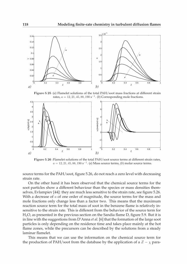
118 Modeling finite-rate chemistry in turbulent diffusion flames
0 0.2 0.4 0.6 0.8 10
0.02
0.04
0.06
0.08
0.1
0.12
0.14
0.16
Z
Y
a
0 0.2 0.4 0.6 0.8 10
0.5
1
1.5
2
2.5
3
3.5x 10
−3
Z
X
a
a) b)
Figure 5.25 :(a) Flamelet solutions of the total PAH/soot mass fractions at different strainrates, a = 12, 21, 45, 88, 190 s−1. (b) Corresponding mole fractions.
0 0.2 0.4 0.6 0.8 10
0.5
1
1.5
2
2.5
3
3.5
4
4.5
Z
ω [k
g/(m
3 s)
]
a
0 0.2 0.4 0.6 0.8 1−4
−2
0
2
4
6
8
Z
ω [m
ole/
(m3
s)]
a
a) b)
Figure 5.26 :Flamelet solutions of the total PAH/soot source terms at different strain rates,a = 12, 21, 45, 88, 190 s−1. (a) Mass source terms, (b) molar source terms.
source terms for the PAH/soot, figure 5.26, do not reach a zero level with decreasingstrain rate.
On the other hand it has been observed that the chemical source terms for thesoot particles show a different behaviour than the species or mass densities them-selves, Evlampiev [44]: they are much less sensitive to the strain rate, see figure 5.26.With a decrease of a of one order of magnitude, the source terms for the mass andmole fractions only change less than a factor two. This means that the maximumreaction source term for the total mass of soot in the benzene flame is relatively in-sensitive to the strain rate. This is different from the behavior of the source term forH2O, as presented in the previous section on the Sandia flame D, figure 5.9. But it isin line with the suggestions from D’Anna et al. [6] that the formation of the large sootparticles is only depending on the residence time and takes place mainly at the hotflame zones, while the precursors can be described by the solutions from a steadylaminar flamelet.
This means that we can use the information on the chemical source term forthe production of PAH/soot from the database by the application of a Z − χ para-

5.5 A sooting benzene diffusion flame 119
metrization, while the mass fractions of the PAH’s and the relatively small soot par-ticles can be retrieved reasonably well directly, from the same Z−χ parametrization.This analysis in fact corresponds to an analysis of the effective timescales of thechemistry. With increasing chemical time scales the flamelet assumption becomesless appropriate, whereas the flame regime starts to be located in the connected reac-tion zones regime, figure 5.1. Then it is better to solve transport equations retrievingsource terms from the steady laminar flamelet database.
A wide range of additional information is available from the flamelet solutions.Notice for instance, that for low strain rates the source term for the mole fraction be-comes negative, whereas the mass fraction remains mostly positive. This indicatesa shift of the soot particle size distribution from smaller, light particles to the largerones. Also information concerning typical particle size distribution functions andon the presence and growth rate of typical toxic species, such as benzo[a]pyreneis available, [44], which can be of practical relevance in the turbulent flame simu-lations.
5.5.3 The setup for the Large-Eddy simulation
In the previous subsection a steady laminar flamelet database has been describedwhere soot formation is modeled in a benzene flame, using the sectional method.Now a model needs to be provided in order to link the information of the SLFdatabase to the turbulent flame simulations. Different from observations on all rep-resentative species in the Sandia flame D, in section 5.4, It has been shown in theprevious section that even at the lowest strain rate, a=10 s−1 there is no evidence thatsoot is in its steady state value. This means that here it is certainly not appropriateto apply a progress variable method based on a typical soot concentration, and usethis to lookup all remaining soot species using results from a flamelet solution.
Also the use of a typical progress variable such as H2O is not expected to leadto improvements in the results. The chemical time scales of the soot formation pro-cess are in a completely different range as that of H2O: while H2O can be describedby the solution given by the lowest strain rate, the soot will continue to changedrastically. Moreover, in this flame no pilot flow is included. Therefore the Z − χparametrization for major species, density and viscosity is reasonable in this case.
Recently Netzell et al. [102] reported a study where a sooting turbulent diffu-sion flame was evaluated based on the sectional method. The flow field had beenevaluated based on a steady flamelet library incorporated into a standard RANSflame code, whereas the soot was reconstructed in a postprocessing step by using atime-dependent flamelet method. The representative flamelet was initialized by anextinguished flamelet at high strain rate. Then this flamelet traveled through the do-main, while mixing is governed by following the maximum scalar dissipation rate ata specific height, leading to soot formation results in this flamelet. However, as sootwas shown to be very sensitive on this scalar dissipation rate, the averaging proce-dure, where only a single representative flamelet is used that is subjected to a singleχ-profile, can be an over-simplification, leading to unrealistic soot predictions.
A more natural method would be to transport separately a representative selec-tion of soot bins. However, this method remains computationally rather expensive.

120 Modeling finite-rate chemistry in turbulent diffusion flames
Additionally, the source terms for the separate PAH/soot particle sizes are not di-rectly depending on the mixing rate, with only a mild sensitivity to the strain rate.The growth terms for separate PAH/soot particle sizes depend both on C2H2 con-tent and temperature (the flamelet parameters), as well as on the concentration ofthe smaller soot particles (due to particle coagulation/growth) and the concentra-tion of the larger soot particles (due to oxidation), Richter et al. [135]. The destructionterm due to oxidation was shown to depend mainly on the OH-radical content andtemperature, which are flamelet parameters.
Application of the SLF
With these considerations in mind we propose to base the soot chemistry on fourparameters. First of all the mixture fraction field Z, to define the global mixing stateof the turbulent diffusion flame. Secondly the scalar dissipation rate χ, to definethe global mixing time scale, which is used to find the strain rate a. Based on thesetwo parameters the temperature and the major species are retrieved, correspondingto the ZχD method, as described in the previous section on the simulation of theSandia flame D. In a similar manner the chemical source terms for the total numberdensity ωXS
(Z, a) and mass density ωYS(Z, a) are extracted from the steady laminar
flamelet database. The third and fourth parameters are therefore two additionaltracers that define the total number density of the soot XS , i.e. the mole fraction,as well as the mass density YS . These total mole and mass fractions are the sumof the mass and mole fraction of all PAH/soot particles, defined by bin 1 up to bin20. This methodology shows similarities to the work of Bai et al. [10]. There, anaxi-symmetric, turbulent ethylene diffusion flame has been modeled using a RANSapproach. The soot volume fraction was evaluated by extracting the source termsfor the total volume fraction from a steady laminar flamelet calculation.
As has been argued in the previous section this method can be used for evaluat-ing the total amount of PAH/soot, because these source terms are relatively insen-sitive to the strain rate, Balthasar et al. [12]. The method corresponds to a method ofmoments, in the sense that here the zeroth and first moment are evaluated explicitlyin the Large-Eddy simulations. An important difference, though, is that the sourceterms are here based on the flamelet solutions from a detailed reaction mechanismfor a benzene diffusion flame. Therefore no assumptions except for the rate con-stants and transport data in the chemical mechanism are necessary. Moreover, thismethod is naturally extendable, by introducing the transport of additional momentsor bins in the LES calculation.
Having information on the total amount of mass and the total amount of par-ticles is in general not sufficient to reconstruct all information on the separate sootparticles. Therefore a particle size distribution function has to be assumed. Typicallya log-normal shape is used, Hong et al. [63]. However, an increasing amount of evi-dence shows a bimodal size distribution of soot particles, with the first peak around2 nm and the second peak at 20-50 nm, due to primary soot particles, D’Alessio etal. [3]. This functionality has also been observed from the steady laminar flameletcalculations, Evlampiev [44]. Such a particle size distribution can be recovered byevaluating the transport of the representative bins separately.
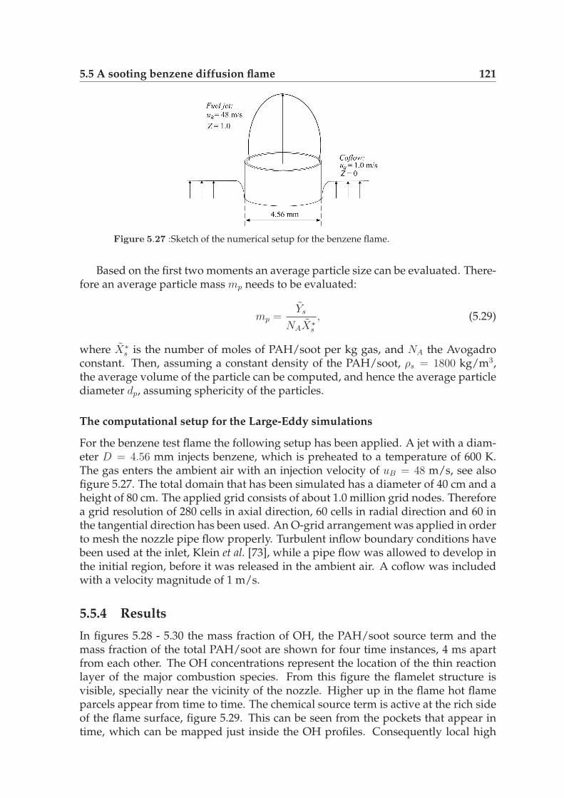
5.5 A sooting benzene diffusion flame 121
Figure 5.27 :Sketch of the numerical setup for the benzene flame.
Based on the first two moments an average particle size can be evaluated. There-fore an average particle mass mp needs to be evaluated:
mp =Ys
NAX∗s
, (5.29)
where X∗s is the number of moles of PAH/soot per kg gas, and NA the Avogadro
constant. Then, assuming a constant density of the PAH/soot, ρs = 1800 kg/m3,the average volume of the particle can be computed, and hence the average particlediameter dp, assuming sphericity of the particles.
The computational setup for the Large-Eddy simulations
For the benzene test flame the following setup has been applied. A jet with a diam-eter D = 4.56 mm injects benzene, which is preheated to a temperature of 600 K.The gas enters the ambient air with an injection velocity of uB = 48 m/s, see alsofigure 5.27. The total domain that has been simulated has a diameter of 40 cm and aheight of 80 cm. The applied grid consists of about 1.0 million grid nodes. Thereforea grid resolution of 280 cells in axial direction, 60 cells in radial direction and 60 inthe tangential direction has been used. An O-grid arrangement was applied in orderto mesh the nozzle pipe flow properly. Turbulent inflow boundary conditions havebeen used at the inlet, Klein et al. [73], while a pipe flow was allowed to develop inthe initial region, before it was released in the ambient air. A coflow was includedwith a velocity magnitude of 1 m/s.
5.5.4 Results
In figures 5.28 - 5.30 the mass fraction of OH, the PAH/soot source term and themass fraction of the total PAH/soot are shown for four time instances, 4 ms apartfrom each other. The OH concentrations represent the location of the thin reactionlayer of the major combustion species. From this figure the flamelet structure isvisible, specially near the vicinity of the nozzle. Higher up in the flame hot flameparcels appear from time to time. The chemical source term is active at the rich sideof the flame surface, figure 5.29. This can be seen from the pockets that appear intime, which can be mapped just inside the OH profiles. Consequently local high
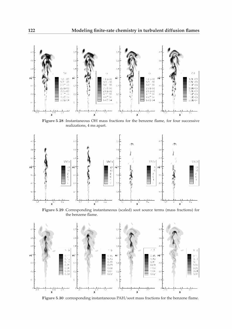
122 Modeling finite-rate chemistry in turbulent diffusion flames
Figure 5.28 :Instantaneous OH mass fractions for the benzene flame, for four successiverealizations, 4 ms apart.
Figure 5.29 :Corresponding instantaneous (scaled) soot source terms (mass fractions) forthe benzene flame.
Figure 5.30 :corresponding instantaneous PAH/soot mass fractions for the benzene flame.
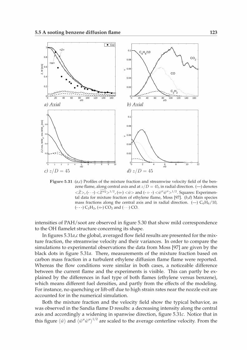
5.5 A sooting benzene diffusion flame 123
0 20 40 60 80 100 120 140 1600
0.2
0.4
0.6
0.8
1
z/D
Z, W
[m/s
]
<Z>
<w>
Exp
0 1 2 3 4 5 6 7 8 9 100
0.2
0.4
0.6
0.8
1
r/D
Z,Z
rm
s, W
/Wcl
, rm
s W
/Wcl
[m/s
]
0 20 40 60 80 100 120 140 1600
0.02
0.04
0.06
0.08
0.1
z/D
Y
C6H
6/10
CO2
CO
C2H
2
0 2 4 6 8 10 120
0.02
0.04
0.06
0.08
0.1
r/D
Y
a) Axial
c) z/D = 45
b) Axial
d) z/D = 45
Figure 5.31 :(a,c) Profiles of the mixture fraction and streamwise velocity field of the ben-zene flame, along central axis and at z/D = 45, in radial direction. (—) denotes
<Z>, (- · -) <Z ′′2>1/2, (-◦–) <w> and (- ◦· -) <w′′w′′>1/2. Squares: Experimen-tal data for mixture fraction of ethylene flame, Moss [97]. (b,d) Main speciesmass fractions along the central axis and in radial direction. (—) C6H6/10,(- - -) C2H2, (-◦–) CO2 and (· · ·) CO.
intensities of PAH/soot are observed in figure 5.30 that show mild correspondenceto the OH flamelet structure concerning its shape.
In figures 5.31a,c the global, averaged flow field results are presented for the mix-ture fraction, the streamwise velocity and their variances. In order to compare thesimulations to experimental observations the data from Moss [97] are given by theblack dots in figure 5.31a. There, measurements of the mixture fraction based oncarbon mass fraction in a turbulent ethylene diffusion flame flame were reported.Whereas the flow conditions were similar in both cases, a noticeable differencebetween the current flame and the experiments is visible. This can partly be ex-plained by the differences in fuel type of both flames (ethylene versus benzene),which means different fuel densities, and partly from the effects of the modeling.For instance, no quenching or lift-off due to high strain rates near the nozzle exit areaccounted for in the numerical simulation.
Both the mixture fraction and the velocity field show the typical behavior, aswas observed in the Sandia flame D results: a decreasing intensity along the centralaxis and accordingly a widening in spanwise direction, figure 5.31c. Notice that in
this figure 〈w〉 and 〈w′′w′′〉1/2 are scaled to the average centerline velocity. From the
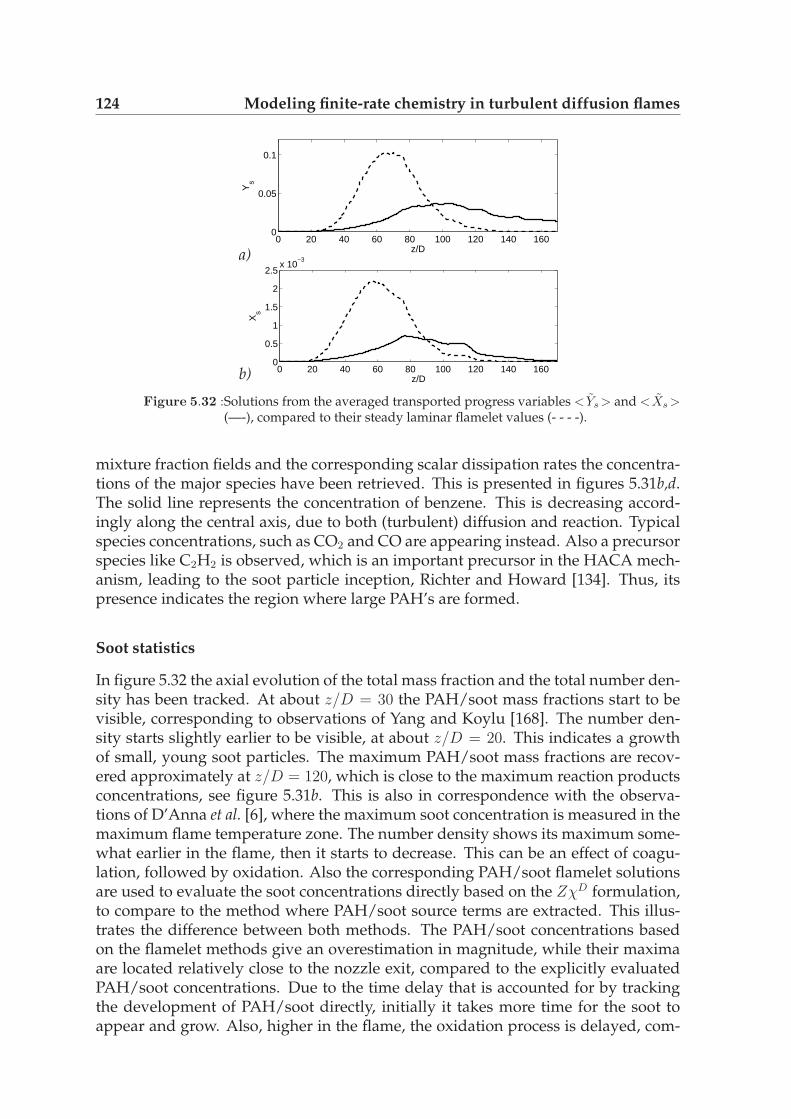
124 Modeling finite-rate chemistry in turbulent diffusion flames
0 20 40 60 80 100 120 140 1600
0.05
0.1
z/DY
s
0 20 40 60 80 100 120 140 1600
0.5
1
1.5
2
2.5x 10
−3
z/D
Xs
a)
b)
Figure 5.32 :Solutions from the averaged transported progress variables <Ys > and <Xs >(—-), compared to their steady laminar flamelet values (- - - -).
mixture fraction fields and the corresponding scalar dissipation rates the concentra-tions of the major species have been retrieved. This is presented in figures 5.31b,d.The solid line represents the concentration of benzene. This is decreasing accord-ingly along the central axis, due to both (turbulent) diffusion and reaction. Typicalspecies concentrations, such as CO2 and CO are appearing instead. Also a precursorspecies like C2H2 is observed, which is an important precursor in the HACA mech-anism, leading to the soot particle inception, Richter and Howard [134]. Thus, itspresence indicates the region where large PAH’s are formed.
Soot statistics
In figure 5.32 the axial evolution of the total mass fraction and the total number den-sity has been tracked. At about z/D = 30 the PAH/soot mass fractions start to bevisible, corresponding to observations of Yang and Koylu [168]. The number den-sity starts slightly earlier to be visible, at about z/D = 20. This indicates a growthof small, young soot particles. The maximum PAH/soot mass fractions are recov-ered approximately at z/D = 120, which is close to the maximum reaction productsconcentrations, see figure 5.31b. This is also in correspondence with the observa-tions of D’Anna et al. [6], where the maximum soot concentration is measured in themaximum flame temperature zone. The number density shows its maximum some-what earlier in the flame, then it starts to decrease. This can be an effect of coagu-lation, followed by oxidation. Also the corresponding PAH/soot flamelet solutionsare used to evaluate the soot concentrations directly based on the ZχD formulation,to compare to the method where PAH/soot source terms are extracted. This illus-trates the difference between both methods. The PAH/soot concentrations basedon the flamelet methods give an overestimation in magnitude, while their maximaare located relatively close to the nozzle exit, compared to the explicitly evaluatedPAH/soot concentrations. Due to the time delay that is accounted for by trackingthe development of PAH/soot directly, initially it takes more time for the soot toappear and grow. Also, higher in the flame, the oxidation process is delayed, com-
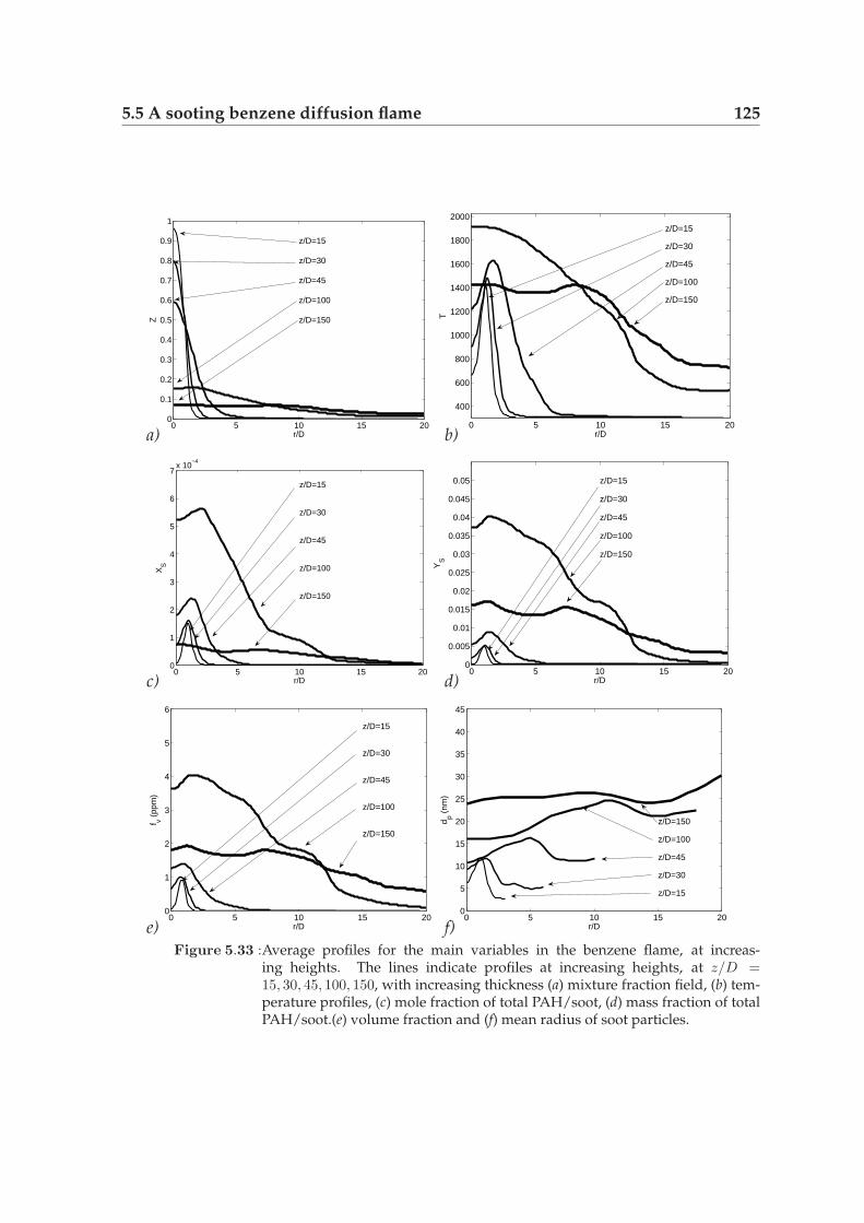
5.5 A sooting benzene diffusion flame 125
0 5 10 15 200
0.1
0.2
0.3
0.4
0.5
0.6
0.7
0.8
0.9
1
r/D
Z
z/D=15
z/D=30
z/D=45
z/D=100
z/D=150
0 5 10 15 20
400
600
800
1000
1200
1400
1600
1800
2000
r/DT
z/D=15
z/D=30
z/D=45
z/D=100
z/D=150
0 5 10 15 200
1
2
3
4
5
6
7x 10
−4
r/D
XS
z/D=15
z/D=30
z/D=45
z/D=100
z/D=150
0 5 10 15 200
0.005
0.01
0.015
0.02
0.025
0.03
0.035
0.04
0.045
0.05
r/D
YS
z/D=15
z/D=30
z/D=45
z/D=100
z/D=150
0 5 10 15 200
1
2
3
4
5
6
r/D
f v (pp
m)
z/D=15
z/D=30
z/D=45
z/D=100
z/D=150
0 5 10 15 200
5
10
15
20
25
30
35
40
45
r/D
d p (nm
)
z/D=150
z/D=100
z/D=45
z/D=30
z/D=15
a) b)
c) d)
e) f)Figure 5.33 :Average profiles for the main variables in the benzene flame, at increas-
ing heights. The lines indicate profiles at increasing heights, at z/D =15, 30, 45, 100, 150, with increasing thickness (a) mixture fraction field, (b) tem-perature profiles, (c) mole fraction of total PAH/soot, (d) mass fraction of totalPAH/soot.(e) volume fraction and (f) mean radius of soot particles.

126 Modeling finite-rate chemistry in turbulent diffusion flames
0 10 20 30 40 500
0.05
0.1
0.15
0.2
0.25
0.3
0.35
diameter (nm)
PD
F
z/D=50z/D=100z/D=150
Figure 5.34 :Probability density function of the mean particle size of the PAH/soot, as aresult of turbulent fluctuations, for three different heights along the centralaxis.
pared to results from the flamelet method.Figure 5.33a,b shows the average evolution of the mixture fraction field and the
corresponding temperature field. Especially the temperature field gives an indica-tion on the range where soot formation processes becomes more active. This is atthe rich side of the flame, Z > 0.1. Close to the nozzle exit, at z/D = 15, the moleand mass fractions of the total PAH/soot are only present at the flame zone, figure5.33c,d. Higher up in the flame these profiles are widening, leading to a smoothlydistributed averaged PAH/soot intensity. Despite the differences in magnitude, theshapes are very much comparable, showing an increase of total soot with increasingheight. Notice that the PAH/soot mass fractions are constantly wider compared tothe mole fraction. This is well visible at height z/D = 100, for r/D > 10. A reasonfor this is that the mole fraction has a negative source term at low strain rates. Thisleads to a reduced number of soot particles, whereas the mass fraction remains in-creasing. This indicates a shift of the particle size distribution to the larger particles.Higher up in the domain, z/D = 150 the intensities decrease again.
From these data the soot volume fraction has been reconstructed, using expres-sion 5.25. This is a quantity that is typically used in experimental techniques. Thevolume fraction is largely related to the mass fraction, see figure 5.33e. The maxi-mum volume fraction for the total PAH/soot that is reached for this benzene flameis about 5 ppm. Also a reconstruction of the average particle size diameter is per-formed, using both the information of the mass fractions and the mole fractions,expression 5.29. Here, it is assumed that the soot particles are spherical. The resultsare presented in figure 5.33f. Along the central axis, the average diameter increasesup to 25 nm, while at the side of the flame the average size can increase up to 40 nm.
Figure 5.34 shows a probability density function of the flame of the mean particlesizes that are encountered at three locations along the central axis. These resultingPDF’s are an effect of the turbulent fluctuations of the filtered mass fraction andmixture fraction of total PAH/soot only. Then, at z/D = 50 the mean particle size isabout 11 nm in diameter, with a rms of 1.5 nm. With increasing height the mean andrms values of the PDF increase: at z/D = 100 these are 19 nm and 5 nm respectively,and at z/D = 150 these are 26 and 6 nm. Notice the wide tail at the larger particlesizes. This can indicate the occasional presence of flow parcels containing large(average) soot particle sizes, as identified by figure 5.30.
5.6 Conclusions 127
5.6 Conclusions
In this chapter two turbulent diffusion flames have been investigated. The focuswas on modeling finite rate chemistry effects. Therefore, a progress variable ap-proach has been implemented in the FASTEST-3D code and applied to a standardturbulent diffusion flame, the Sandia flame D. The relatively new method, where aprogress variable is applied to non-premixed chemistry problems, is compared tothe classical flamelet method where the non-premixed chemistry is parameterizedusing a mixture fraction and the scalar dissipation rate.
In the progress variable method two different databases have been used: onebased on non-premixed flamelets and one based premixed flamelets. In both casesthe mass fraction of H2O is used as the progress variable. By comparing these threemethods it is found that differences are most visible from a different prediction of Z,which is the crucial parameter for the prediction of the chemical parameters in San-dia flame D. Therefore, based on the prediction of Z the classical flamelet methodand the progress variable method based on premixed chemistry give the most suit-able results. However, when correcting for the wrong prediction of the mixturefraction field, the progress variable method based on non-premixed chemistry out-performs the two other methods. This leads to the conclusion that the parameteriza-tion of the chemistry, using this model, is better compared to the other two methods.At the same time effects from the fluid-dynamics are now disturbing these results.Improvements can be achieved by adapting the inflow turbulence, and/or by a bet-ter resolution of the shear layer. This should lead to a more appropriate (reduced)model prediction of the jet breakup in the progress variable method.
In the last section of this chapter a sooting turbulent benzene diffusion flame hasbeen investigated. A steady laminar flamelet library has been used based on a verydetailed reaction mechanism. In the Large-Eddy simulations the total soot mass andmole fractions have been computed explicitly, based on a Z − χ parametrization forthe chemical source terms.
The regions of soot formation can be identified, showing distributed parcelswhere soot formation takes place. The results show a growth of soot volume frac-tion up to levels of about 4 ppm. The average particle sizes increase steadily in thisflame, up to about 30 nm.
This study can be considered illustrative in giving a methodology for the appli-cation of a flamelet method for soot prediction in turbulent diffusion flames. In thecurrent simulation one of the limitations is that up to today no chemical mechanismsexist for soot formation of more realistic fuel types, such as n-heptane. Nevertheless,it is believed that in future research this type of very large reaction mechanisms willbe at the chemical basis for the modeling of soot in practical engine applications.
Recommendations
Apart from a better resolution of the shear layer and better inflow conditions, thesimulation of the Sandia flame D can be improved by optimizing the flamelet database.Especially due to the pilot flame, the scalar dissipation rate is essentially differentfrom the one in the counterflow flame geometry. With respect to the database of

128 Modeling finite-rate chemistry in turbulent diffusion flames
the premixed chemistry, it is advised to use a combination of species as progressvariable, such that problems of non-monotonicity can be prevented.
It would be interesting to study the impact of the inclusion of extinquished/re-ignition flamelets into the non-premixed flamelet database. This is specially relevantfor the simulation of turbulent flames that depart more the chemical equilibrium so-lution than the Sandia flame D, such as the flames E and F. Then local extinction canhave a more drastic effect on the fluid dynamics. These type of chemical problemsare also more directly of interest for the modeling of turbulent combustion as takesplace in Diesel engines. Here combustion is highly turbulent, ignition delay andlift-off are phenomena that need attention.
Concerning the modeling of soot in diffusion flame type problems, a first ex-tension of the methodology as presented in this thesis, is to track an extra numberof soot variables in the Large-Eddy simulations, related to the different PAH/sootparticle sizes. Then less assumptions on the particle size distribution function hasto be made. This requires a more deep analysis of the contribution from differentchemical pathways to the growth/destruction rates for the different soot trackingvariables. This methodology suits very well to the sectional approach, based ona very detailed reaction mechanism. Then, this type of information is in principleavailable.
Moreover, it is interesting to study a prediction method based on a zero - dimen-sional, stirred reaction model, applied to stream-tracers of fluid moving away fromthe reaction front. While the heat release is close to its chemical equilibrium state,the soot parcels can be tracked in time explicitly, as a function of temperature andoxygen content that are encountered by these parcels, due to transport and mixing.
Additionally, it can be necessary to include an equation for the energy of thesystem, as for sooting flames radiative effects can become important. In the caseof the simulation of combustion in compressed cylinder, where additionally heatlosses at the walls can take place, the explicit tracking of the energy is of even moreimportance.

Chapter
6General conclusions
In this thesis the application of the Large-Eddy Simulation tech-nique is investigated as a tool for the modeling of turbulence andturbulent combustion problems that are relevant for engine condi-tions. It is found that its application to a complex engine geometryremains difficult, as the wall modeling and the accuracy of the nu-merical method can have a drastic impact on the flow statistics. Onthe other hand, a gaseous fuel jet and turbulent jet flames can wellbe modeled. Also the use of flamelet methods in turbulent diffu-sion flames and in models for soot formation in this type of flameshas been discussed.
This thesis reports on a study where the Large-Eddy simulation technique is ap-plied to model turbulent flow, mixing and combustion problems related to engines.Three subjects have been described: the turbulent flow in an engine-like geometry,the turbulent mixing of a gas jet system and the application of flamelet-based meth-ods to Large-Eddy simulations of two turbulent diffusion flames. Because of ourgoal to study engine-related flow problems, two relatively practical, ’engineering-like’ flow solvers have been selected for the simulations. This choice was motivatedby their ability to cope with complex geometries as encountered in realistic, engine-like geometries. However, the modeling of these type of realistic geometries canlead to the sacrifice of two aspects in the formulation of the current simulations: theaccuracy of the numerical schemes that can be applied and the grid resolution thatcan be achieved.
Modeling the turbulent flow in a confined engine-like geometry
In chapter three the impact of the numerical scheme of two flow solvers and the reso-lution has been investigated. It has been concluded from the performed simulationson a square duct flow that coherent structures can be detected and that global flowfeatures are well recovered. On the other hand, as the boundary layer is not well re-solved, the shear can not be predicted properly. Therefore the other flow properties,such as a typical secondary flow structure and the turbulence intensities, can onlybe captured qualitatively. Despite the improvements that have been implemented inthe Kiva-3V code, by the less dissipative convective scheme, the numerical dissipa-tion was shown to be obscuring most of the effects of the subgrid-scale models. This

130 General conclusions
is concluded by comparing the results from the simulations including the subgrid-scale models to two simulations where the subgrid-scale model was switched off.
The impact of an under-resolved shear layer and a dissipative numerical schemehave additionally been tested on a more realistic engine geometry: a complex tur-bulent, swirling and tumbling flow in an engine cylinder that is induced by the inletmanifold. For this geometry a number of LES simulations has been performed withthe FASTEST-3D code as well as the Kiva-3V code. Additionally one URANS simu-lation has been performed with Kiva-3V. The flow field statistics from the LES simu-lations deviated substantially between one case and the next. Again, only globalflow features could be captured appropriately, due to the previously mentionedshortcomings.
An additional sensitivity that has been observed, concerned the definition of theinflow conditions. Any uncertainty in the mass flow rates at the two runners, thatare connected the the cylinder head, can greatly influence the remaining flow pat-terns. To circumvent this problem, it can be mandatory to include a larger part ofthe upstream flow geometry into the computational domain.
Nevertheless, LES gives an indication of the unsteady, turbulent processes thattake place in an engine, whereas in the URANS simulations all mean flow structuresare very weak and the turbulence intensities are predicted to be relatively low in thecomplete domain. But this study does show that, for a predictive quality of this typeof LES on a quantitative level, the numerical scheme as well as the computationalresolution have to be improved.
In the remainder of this thesis the geometry has been kept relatively simple andsecond-order numerical schemes were applied, and sufficient resolution could bereached to perform relatively accurate LES simulations.
Modeling a turbulent gas jet
In chapter four the turbulent mixing process in gaseous jets has been studied forthree different fuel-to-air density ratios. This mimicked the injection of (heavy) fuelinto a pressurized chamber. It is shown that the three jets follow well the similaritytheory that was developed for turbulent gas jets. A main observation was that thefuel core length increases with increasing density ratio. Therefore the self-similarityregion is shifted more downstream in the fuel jet for heavy fuel jets. Also the pen-etration depth as a function of time follows the self-similarity theory properly for afuel-to-air density ratio of unity. In this case, an increase in density ratio leads to aslight decrease in the scaled penetration depth.
A virtual Schlieren postprocessing method has been developed, in order to an-alyze the results similarly as done experimentally, e.g., for the visualization of thedevelopment of turbulent structures. When defining the penetration depth based onthis method, similar difficulties are encountered as in Schlieren experiments, relatedto the definition of the cutoff signal intensity.
By comparing the evolution of the penetration depth of a gaseous jet with mod-els that have been developed for liquid fuel jets, it has been concluded that the phe-nomenological models for both jets are exchangeable for larger penetration depths.This is because the penetration rate from liquid sprays is governed by the entrain-

131
ment rate, which is similar as for gaseous jets. Only for very short distances the sim-ulation departs from the liquid jet experiment, due to the large impact of the liquidparticle dynamics on the entrainment rate, which is reduced accordingly. However,it remains questionable if gas jet models can simply be used to replace the modelfor fuel sprays. The cone angle for gas jets deviates strongly from those observedin spray experiments. Only when corrected for this effect, the penetration behaviorwas similar.
The application of flamelet-based chemistry to turbulent diffusion flames
In chapter five two turbulent diffusion flames have been investigated with a focuson the modeling of finite rate chemistry effects. For the first flame, the well knownSandia flame D, two methods have been compared to each other for the modeling ofthe main parameters of the turbulent flame, i.e. the main combustion products andheat release. The two methods are firstly the classical flamelet method where thenon-premixed chemistry is parameterized using a mixture fraction and the scalardissipation rate, and secondly a relatively new method, where a progress variablemethod is applied to non-premixed chemistry problems.
In the progress variable method two different databases have been compared:one based on non-premixed flamelets and one based premixed flamelets. It is foundthat the prediction of the mixture fraction field in the LES simulation of Sandia flameD is influenced by the different parameterizations. This is best predicted by boththe classical flamelet method, and the progress variable method that is based onpremixed chemistry, especially in the downstream region of the flow. In these casesthe solution of the chemical species in the flame is mostly predicted close to theirequilibrium values. When accounting for the shift of the mixture fraction field, theprogress variable method based on non-premixed chemistry leads to the most ap-propriate results, especially at locations where finite-rate chemistry is important.It can be concluded that the fluid dynamical part of the modeling problem needsimprovement.
In the last section of chapter five a sooting turbulent benzene diffusion flame hasbeen investigated. A steady laminar flamelet library is applied which is based on avery detailed reaction mechanism for premixed benzene flames. In the LES simu-lations the total PAH/soot mass and mole fractions are computed explicitly, whilethe source terms for these variables are based on a classical flamelet parametrization.The current study of a benzene flame can be considered as illustrative in giving amethodology for the application of flamelet methods for the prediction of soot inturbulent flames. The regions of PAH/soot formation have been identified, show-ing distributed parcels where PAH/soot formation takes place. The results showa growth of PAH/soot volume fraction up to levels of about 4 ppm. The averageparticle size increases steadily in this flame, up to about 30 nm.

132 General conclusions
Recommendations
To gain more confidence in the unsteady flow behavior, in future modeling attemptsof complex engine flows an LES simulation can be more preferable to URANS basedcalculations, on the condition that available computational power is not a restriction,and that stable and (second-order) accurate schemes are used. For the modeling ofthe near wall regions, however, a hybrid approach where RANS-like assumptionsfor the boundary layer are applied, would definitely be more suitable. This can leadto a correct prediction of the shear, which can result in a proper prediction of theinstantaneous, mean and turbulent flow features in an engine.
Yet, the flow and consequently the combustion in an engine at real operating con-ditions is not only influenced by the inlet geometry, as was studied in this thesis, butalso by the squish, that takes place at the end of the compression phase. Concerningfuture work it is a challenging question to investigate its impact on the turbulentin-cylinder flow field, using an LES approach, to study cycle-to-cycle variations.
In this thesis it is shown that for the modeling of a liquid fuel injection system,a gas jet system can be adopted. When accounting for the spreading rate of thejet, this can lead to a drastic simplification of the modeling efforts that are requiredfor practical simulations of (burning) fuel sprays. On the other hand, in the endthe inclusion of a droplet model is mandatory, as droplet breakup, collisions andevaporation can lead to different behavior of the burning fuel spray compared tothe one of a gas jet.
When discussing the simulation of the turbulent diffusion flames, one can thinkof improvements in many aspects of the problem formulation. This can involvethe turbulence and the chemical modeling, as well as with its interaction. Also thedevelopment of accurate, stable and efficient numerical discretization methods forall given models requires serious investigation.
Here we will confine ourselves to two examples of improvements that can bemade related to chemical aspects of the problem. The inclusion of extinquished/re-ignition flamelets into the non-premixed flamelet formulation is one of the morechallenging research questions, to study turbulent flames of practical relevance, forinstance at engine conditions. Under these circumstances drastic departures fromsolutions close to chemical equilibrium can be expected. Local flame extinction canhave a strong effect on the fluid dynamics.
Secondly, concerning the modeling of soot in diffusion flame type of problems,the introduction of an additional number of scalar fields can lead to better insightin the properties of the local PAH/soot in such a flame. In this way the contents ofthe different PAH/soot classes can be tracked in more detail. This will lead to animproved prediction of the soot particle size distribution.

Appendix
AThe numerical scheme ofFASTEST-3D
The numerical code FASTEST-3D is based on a boundary fitted, multi-block, finitevolume method. The governing fluid-dynamical equations in the non-premixedcombustion LES simulation consist of the conservation of mass, momentum, equa-tions 2.26, 2.27. Additionally, in case of mixing problems and combustion LES, thefiltered transport equations for the mixture fraction and the progress variable aresolved, equations 5.11, 5.17, depending on the applied chemical model. The dis-cretization of these transport equations is presented in this appendix.
A.1 Discretization
In the finite volume method the transport equations for the momentum and thescalar fields Φ are rewritten in the integral form:
∫
V
∂ρΦ
∂tdV +
∫
V
∂ρuiΦ
∂xi
dV =
∫
V
∂
∂xi
(ρD
∂Φ
∂xi
)dV +
∫
V
ρSΦdV (A.1)
Here, integration is performed over all control volumes V . These volumes are arbi-trary hexahedrons, see figure A.1 for a 2D representation. In above equation, andalso in the remainder of this section the LES filtering operators have been omittedfor simplicity. The different contributions to this equation are evaluated separately.These are the convective and diffusive fluxes and the source terms SΦ. Their dis-cretization will be presented in the following subsections.
W P e Ew
Figure A.1 : A sketch of the grid arrangement in the FASTEST-3D code.

134 The numerical scheme of FASTEST-3D
Spatial discretization
The convective fluxes Fc are evaluated using the identity
Fc =
∫
V
∂ρuiΦ
∂xi
dV =
∫
S
∂ρuiniΦ
∂xi
dS =∑
nb
∫
Snb
ρuiniΦdS (A.2)
Here, the Gauss theorem is applied, converting the volume integral over the controlvolume V into a surface integral. Here, ni denotes the normal vector on the controlvolume surface pointing outwards. This is then split up into a sum of the integralsover all neighbouring faces Snb of the computational cell. Now, the face integral isestimated by the mean value ()m, leaving
∑
nb
∫
Snb
ρuiniΦdS =∑
nb
(ρui)mni(Φ)mδSnb (A.3)
Finally this can be rewritten, using the expression for the mass flux at the cell bound-ary (m)nb = (ρui)nbδSnb:
∑
nb
(ρui)mni(Φ)mδSnb =∑
nb
(m)nb · (Φ)nb (A.4)
This means that both the mass flux and the value for Φ at the cell faces have to be de-fined, in terms of cell centered quantities. This can be achieved by several methods.A main concern is to keep the convective term stable, and at the same time accu-rate. One of the available schemes in the FASTEST-3D code which remains secondorder even on skewed grids is referred to as the multi-linear interpolation (MULI)procedure, Lehnhauser and Schafer [84]. This scheme is used for the evaluation ofthe momentum equations. On the other hand, for convection terms in the mixturefraction field a TVD scheme is adopted, to remedie strong oscillations in the densityfield, Wegner [163], Branley and Jones [21], Kempf [71]. In the current combustionsimulations the CHARM scheme has been applied, which formalism has been pre-sented in section 3.2.2. The CHARM limiter function has the advantage of beingsmooth, which aids to stabilize the code, Kempf [71].
Using a similar method as for the convective fluxes an expression for the diffu-sive fluxes Fd can be derived:
Fd =
∫
V
∂
∂xi
(ρD
∂Φ
∂xi
)dV =
∫
S
ρD∂φ
∂xi
dS =∑
nb
(ρD)nbδSnb∂φ
∂xi
∣∣∣∣nb
(A.5)
Now the diffusion coefficient (ρD)nb and the gradient of the variable ∂φ∂xi
∣∣nb
needto be evaluated at the cell boundaries. This is performed using a scheme whichis second order accurate, Lehnhauser and Schafer [84]. Finally, the source term issimply discretized as the multiplication of the cell volume with the cell center valueSφ,P :
Fs =
∫
V
ρSφdV = ρSφ,P δVP (A.6)
For the momentum equation the source term is described by the gravity Su = gx andfor the progress variable it is the chemical source term SC = ωC .

A.1 Discretization 135
Temporal Discretization
To discuss the temporal discretization, the convective and diffusive fluxes and thesource term are now referred to as the sum of all fluxes F (Φ, t):
F (Φ, t) = −Fc + Fd + Fs. (A.7)
This leads to the following form of the conservational equation:
∂ρΦ
∂tδV = F (Φ, t). (A.8)
The solution is integrated to yield the value for the new timestep:
[(ρΦ)n+1 − (ρΦ)n]δV =
∫ tn+1
tn
F (Φ, t)dt. (A.9)
In the FASTEST-3D code the Crank Nicolson scheme is adopted. This is an implicitscheme, which is favourable for numerical stability. This leads to the expression
[(ρΦ)n+1 − (ρΦ)n]δV = ∆t1
2[F (Φn, t) + F (Φn+1, t)]. (A.10)
The solution procedure of this linear system is performed by a 7-diagonal version ofthe strongly implicit procedure (SIP), Stone [150] and is based on an incomplete LUdecomposition that converges rapidly. Again, an exception is made for the transportof mixture fraction field and the progress variable. When solving the mixture frac-tion field using the Crank-Nicolson scheme the velocity field exhibits instabilities,probably due to the explicit contribution in the scheme, [163]. Oscillations in themixture fraction field lead to oscillations in the density field, and hence in all othertransported variables, such as momentum. Therefore it is chosen to use a fully im-plicit first order scheme. The reduction of the accuracy, both by introduction of theTVD scheme and by this first order time integration is argued to be allowed as thetransport of the passive variables are mostly driven trough convection. By treatingthe underlying velocity field to be second order accurate the mixture fraction fieldis remains well modelled, [116].
Pressure correction
The FASTEST-3D code adopts a Low Mach number approximation. The pressurecorrection takes place in order to fulfill the continuity constraint, using the so-calledSIMPLE method, Patankar [110]. Here, the key steps are presented. With the useof the estimated velocity field u∗ from the solution of the momentum equation themass conservation equation leads to a virtual source bm:
∂ρ
∂t+
∂(ρu∗i )
∂xi
= bm. (A.11)
Notice the extra ∂ρ∂t
-term which is absent in constant-density pressure correctionschemes. The virtual source bm can be related to the velocity correction u′
i = un+1i −u∗
i
and the pressure correction p′ = pn+1 − p∗ via
bm = −∂(ρu′i)
∂xi
= ∆t∂2p′
∂x2i
. (A.12)

136 The numerical scheme of FASTEST-3D
When this Poisson equation is solved to find the pressure correction p′, the velocityfield can be corrected accordingly, using
ρun+1i − ρu∗
i = −∆t∂p′
∂xi
. (A.13)
For the densities that appear in above formalism, the most recent values ρn+1 areconstantly used. The time derivative of the density field, which is needed in equa-tion A.11, is here approximated by
∂ρ
∂t=
ρn+1 − ρn
∆t, (A.14)
which is second-order accurate in the framework of the Crank-Nicolson scheme.Whereas, amongst others, Pierce [116] applies a spatial filtering of the time deriva-tive of the density field this appeared not necessary in the current formulation, dueto the first-order implicit formulation of the mixture fraction field [163].
A.2 The solution algorithm
The numerical scheme as presented above leads to the solution procedure as shownin figure A.2. For every time step first the new combustion variables are evaluated,using a fully implicit scheme. Then the density is updated using the chemistry table:
ρn+1 = ρ(Zn+1, ...). (A.15)
Also the other transport variables, such as the viscosity and diffusivities are updatedhere, as well as the density time derivative. Then the momentum equations aresolved leading to the predicted velocity field u∗, using the Crank Nicolson scheme.The Poisson equation is solved based on the predicted velocity field. Finally, thevelocity and pressure fields are corrected. Now, these steps are iterated, until a con-verged solution is achieved for the current time step. Then the algorithm proceedsto the next time step.
One inconsistency must be paid attention to [116]. The discretized transport ofmixture fraction that leads to a new density field does not necessarily correspondto the discretized transport of mass, derived from the continuity equation. In otherwords, the constraint equation which is used in the pressure correction stage de-pends on the combustion progress variables implicitly. Therefore, the evaluationof
∂ρΦ
∂tδV = F (Φ, t) (A.16)
followed by ρ = ρ(Φ), does not necessarily correspond to
∂ρ
∂tδV = F (ρ, t) (A.17)
Therefore it is of importance to use the same spatial discretization schemes in thePoisson equation as in the transport equation that drive the density via the scalarequations [163].

A.2 The solution algorithm 137
Figure A.2 : Flow chart of the applied solution procedure in FASTEST-3D.

138 The numerical scheme of FASTEST-3D

Bibliography
[1] J. Abraham, V. Magi, Computations of transient jets: RNG k-e model versusstandard k-e model. SAE Trans 106 (1997) 1442-1452.
[2] J. Abraham, V. Magi, A virtual liquid source (VLS) model for vaporizing dieselsprays. SAE Trans 108 (1999) 1363-1374.
[3] A. D’Alessio, A.C. Barone, R. Cau, A. D’Anna P. Minutolo, Surface depositionand coagulation efficiency of combustion generated nanoparticles in the sizerange from 1 to 10 nm. Proc. Comb. Inst. 30 (2005) 2595-2603.
[4] M. Amielh, T. Djeridane, F. Anselmet, L. Fulachier, Velocity near-field of variabledensity turbulent jets. Int. J. Heat Mass Transfer 39-10 (1996) 2149-2164.
[5] A.A. Amsden, P.J. O’Rourke, T.D. Butler, KIVA-II: A Computer Program forChemically Reactive Flows with Sprays. Technical Report LA-11560-MS LosAlamos National Laboratory (1989).
[6] A. D’Anna, M. Commodo, S. Violi, C. Allouis, J. Kent, Nano organic carbon andsoot in turbulent non-premixed ethylene flames. Proc. Comb. Inst. 31 (2007) 621-629.
[7] M.D. Avakian, B. Dellinger, H. Fiedler, B. Gullet, C.Koshland, et al., The origin,fate, and health effects of combustion by-products: a research framework. Envi-ronmental health perspectives 110 (2002) 1155-1162.
[8] http://www.cerfacs.fr/cfd/ (2007).
[9] J.S. Bagget, J. Jimenez, A.G. Kravchenko, Resolution requirements in large-eddysimulations of shear flows. Annual Research Briefs, Center for Turbulence ResearchStanford (1998) 267-277.
[10] X.S. Bai, M. Balthasar, F. Mauss, L. Fuchs, Detaled soot modeling in turbulentjet diffusion flames Proc. Combust. Inst. 27 (1998) 1623-1630.
[11] E. Balaras, C. Benocci, U. Piomelli, Two-layer approximate boundary condi-tions for large-eddy simulations. AIAA J. vol. 34 (1996) 1111–1119.
[12] M. Balthasar, A. Heyl, F. Mauss, F. Schmitt, H. Bockhorn, Flamelet modeling ofsoot formation in laminar ehtylene/air diffusion flames. Proc. Comb. Inst. (1996)2369-2377.
140 Bibliography
[13] J. Bardina, J.H. Ferziger W.C. Reynolds, Improved turbulence models based onLES of homogeneous incompressible turbulent flows. Rep. TF-19, Department ofMechanical engineering, Stanford (1984).
[14] R.S. Barlow, J.H. Frank, Effects of turbulence on species mass fractions onmethane/air jet flames. Proc. Combust. Inst. 27 (1998) 1087-1095.
[15] R.S. Barlow, J.H. Frank, and J.-Y. Chen, Scalar structure and transport effects inpiloted methane/air jet flames. Combustion and Flame 143 (2005) 433-449.
[16] H. Barths, C. Hasse, G. Bikas, N. Peters, Simulation of combustion in directinjection diesel engines using a eulerian particle flamelet model. Proc. Comb. Inst.28 (2000) 1161-1168.
[17] R.W. Bilger, The structure of nonpremixed turbulent flames. Proc. Combust. Inst.22 (1988) 475-488.
[18] A.D. Birch, D.R. Brown, M.D. Dodson, J.R. Thomas, The turbulent concentra-tion field of a methane jet. Journal of Fluid Mechanics 88 (1978) 431-449.
[19] H. Bongers, Analysis of flamelet-based methods to reduce chemical kinetics inflame computations. Ph.D Thesis, TU Eindhoven (2005).
[20] M.J. Boussinesq, Essay sur la theorie des eaux courantes. Memoires Presentes parDivers Savants Etrangers a l’Academie des Sciences, Gauthier-Villars, Paris (1877) 1.
[21] N. Branley, W.P. Jones, Large Eddy simulation of a turbulent non-premixedflame. Turbulent Shear Flows Conference II 21 (1997) 1-6.
[22] N. Branley, W.P. Jones, Large Eddy simulation of a turbulent non-premixedflame. Combustion and Flame 127 (2001) 1914-1934.
[23] K.N.C. Bray, N. Peters, Turbulent Reacting Flows Academic Press, London, eds.P.A. Libby and F.A. Williams (1994).
[24] G. Bruneaux, A study of mixture formation in direct injection diesel like con-ditions using quantitative fuel concentration visualizations in a gaseous fuel jet.SAE Trans. 2002-01-1632 (2002).
[25] R.R. Cao, S.B. Pope, The influence of chemical mechanisms on PDF calculationsof non-premixed piloted jet flames. Combustion and Flame 143 (2005) 450-470.
[26] G. Carazzo, E. Kaminski, S. Tait, The route to self-similarity in turbulent jetsand plumes. Journal of Fluid Mechanics 547 (2006) 137-148.
[27] W. Cabot, P. Moin, Approximate wall boundary conditions in the large-eddysimulation of high Reynolds number flow. Flow, Turbulence and Combustion 63(2000) 269-291.
[28] I. Celik, I. Yavuz, A. Smirnov, J. Smith, E. Amin, A. Gel, Prediction of in-cylinder turbulence for IC engines. Combustion Science and Technology 153 (2000)339-368.
141
[29] I. Celik, I. Yavuz, A. Smirnov, Large eddy simulations of in-cylinder turbulencefor internal combustion engines: a review. Int. J. Engine Research 2-2 (2001) 119-148.
[30] R. Cheesewright, G. McGrath, D.G. Petty, LDA measurements of turbulent flowin a duct of square cross section at low Reynolds number. Technical Report Aero-nautical Engineering Dept. Queen May Westfield College, University of London ER1011 (1990).
[31] CHEM1D. a one-dimensional laminar flame code. Eindhoven University of Tech-nology (2007). http://www.combustion.tue.nl.
[32] A.W. Cook, J. Riley, A subgrid model for equilibrium chemistry in turbulentflows. Physics of Fluids 6 (1994) 2868-2870.
[33] D. J. Cook, H. Pitsch, J. H. Chen, E. R. Hawkes, Flamelet-based modeling ofauto-ignition with thermal inhomogeneities for application to HCCI engines.Proc. Comb. Inst. 31 (2007) 2903-2911.
[34] W.J.A. Dahm, Experiments on entrainment, mixing and chemical reactions inturbulent jets at large Schmidt number. Ph.D Thesis Caltech, Pasadena (1987).
[35] J.W. Deardorff, A numerical study of three-dimensional turbulent channel flowat large Reynolds numbers. Journal of Fluid Mechanics 41 (1970) 453-465.
[36] M.E. Decroix, W.L. Roberts, Transient flow field effects on soot volume fractionin diffusion flames. Combustion Science and Technology 160 (2000) 165-189.
[37] J. Denev, T. Frank, K. Pachler, Large Eddy Simulation of Turbulent SquareChannel Flow using a PC-cluster architecture. Springer-Verlag Heidelberg, LectureNotes in Computer Science 2907 (2004) 363-370.
[38] J.M. Desantes, J. Arregle, J.J. Lopez, J.M. Garcıa, Turbulent gas jets and diesel-like sprays in a crossflow: A study on axis deflection and air entrainment. Fuel85 (2006) 2120-2132.
[39] A. Devesa, J. Moreau, J. Helie, V. Faivre, T. Poinsot, Initial conditions for LargeEddy Simulations of piston engine flows. Computers & Fluids 36 (2007) 701-713.
[40] E. Doosje, R.J.M. Bastiaans, R.S.G. Baert, Application of PIV to characterizethe flow-phenomena of a heavy-duty cylinder head on a stationary flow-bench.Proceedings of the EUROPIV 2 workshop (2004).
[41] D.R. Dowling, P.E. Dimotakis, Similarity of the concentration field of gas-phaseturbulent jets. Int. J. Fluid Mech. 218, (1990) 109-141.
[42] F. Durst, M. Schafer, A parallel blockstructured multigrid method for the pre-diction of incompressible flow. Int. J. Numer. Meth. Fluids 22, (1996) 549-565.

142 Bibliography
[43] J.G.M. Eggels, F. Unger, M.H. Weiss, J. Westerweel, R.J. Adrian, F.T.M. Nieuw-stadt, R. Friedrich, Fully developed pipe flow: A comparison between directnumerical simulation and experiment. Journal of Fluid Mechanics 268 (1994) 175-209.
[44] A. Evlampiev, Numerical Combustion Modeling for Complex Reaction Sys-tems, Ph.D Thesis, TU Eindhoven (2007).
[45] J.H. Ferziger, Introduction to Turbulence Modeling. Von Karman Institute forFluid Dynamics lecture notes (2004).
[46] http://www.avl.com/ (2007).
[47] http://www.fluent.com (2007).
[48] M. Frenklach, Method of moments with interpolative closure Chemical Engi-neering Science 57 (2002) 2229-2239.
[49] C. Fureby, G. Tabor, H.G. Weller, A.D. Gosman, A comparative study of subgridscale models in homogeneous isotropic turbulence. Physics of Fluids 9(5) (1997)1416-1429.
[50] E. Garnier, M. Mossi, P. Sagaut, P. Comte, M. Deville, On the use of Shock-capturing schemes for large-eddy simulation. Journal of computational physics 153(1999) 273-311.
[51] K. Horiuti, Large eddy simulation of turbulent channel flow by one-equationmodeling. J. Phys. Soc. Japan 54 (8) (1985) 2855-2865.
[52] S. Gavrilakis, Numerical simulation of low-Reynolds-number turbulent flowthrough a straight square duct. Journal of Fluid Mechanics 244 (1999) 101-129.
[53] M. Germano, U. Piomelli, P. Moin, W.H. Cabot, A dynamic subgrid-scale eddyviscosity model. Physics of Fluids A3 (7) (1991) 1760-1765.
[54] B.J. Geurts, Database-analysis of interacting errors in large-eddy simulation.Proceedings of the Quality Assessment of Unsteady Methods. (2005)
[55] S.S. Girimaji Y. Zhou, Analysis and modeling of subgrid scalar mixing usingnumerical data. Physics of Fluids 8 (1996) 1224-1236
[56] R.J. Hall, M.D. Smooke, M.B. Colket, F.L. Dryer, R.F. Sawyer (Ed.), Physicaland chemical aspects of combustion: a tribute to Irine Glasman. Gordon & Breach(1997).
[57] F.E. Ham, F.S. Lien, A.B. Strong, Large-Eddy Simulation of the square duct flowusing a parallel PC cluster. Proceedings of the 8th Annual Conference of the CFDsociety of Canada (2000).
[58] K. Hanjalic, Advanced turbulence closure models: a view of current status andfuture prospects. Int. J. Heat and Fluid Flow 15-3 (1994) 178-203.

143
[59] R.G. Harvey, Polycyclic aromatic hydrocarbons: chemistry and cancer, Cam-bridge University Press, Cambridge, UK (1991).
[60] D.C. Haworth, K. Jansen, Large-eddy simulation on unstructured deformingmeshes: towards reciprocating IC engines. Computers & Fluids 29 (2000) 493-524.
[61] E. Hecht, Optics, 4th edition. , MA: Addison-Wesley, Amsterdam (2002)
[62] C. Hirsch, Numerical computation of internal and external flows. Wiley: Chich-ester (1990).
[63] S. Hong, M.S. Wooldridge, H.G. Im, D.N. Assanis, H. Pitsch, Development andapplication of a comprehensive soot model for 3D CFD reacting flow studies ina diesel engine Combustion and Flame 143 (2005) 11-26.
[64] V. Huijnen, L.M.T. Somers, R.S.G. Baert, L.P.H. de Goey, Comparing differentturbulence modelling approaches for square duct simulations using the kivacode. Proc. ASME-PVP 491-2 (2004) 335-362.
[65] V. Huijnen, L.M.T. Somers, R.S.G. Baert, L.P.H. de Goey, Validation of the LESapproach in Kiva-3V on a square duct geometry. Int. J. Numer. Meth. Engineering64 (2005) 907-919.
[66] A. Huser, S. Biringen, Direct numerical simulation of turbulent flow in a squareduct. Journal of Fluid Mechanics 257 (1993) 65-95.
[67] H. J. Hussein, S. P. Capp, W. K. George, Velocity measurements in a high-Reynolds number, momentum-conserving, axisymmetric, turbulent jet.Journalof Fluid Mechanics 246 (1993) 197-223.
[68] M. Ihme, C.M. Cha, H. Pitsch, Prediction of local extinction and re-ignition ef-fects in non-premixed turbulent combustion using a flamelet/progress variableapproach. Proc. Comb. Inst. 30 (2005) 793-800.
[69] J. Janicka, W. Kollmann, A two-variables formailsm for the treatment of chem-ical reaction in turbulent H2-air diffusion flames Proc. Comb. Inst. 17 (1978) 421-430.
[70] S. Jay, F. Lacas, S. Candel, Combined surface density concepts for dense spraycombustion. Combustion and Flame 144 (2006) 558-577.
[71] A.M. Kempf, Large-Eddy Simulation of Non-Premixed Turbulent Flames. PhD-thesis, TU-Darmstadt (2003).
[72] A. Kempf, F. Flemming, J. Janicka, Investigation of lengthscales, scalar dissipa-tion, and flame orientation in a piloted diffusion flame by LES. Proc. Combust.Inst. 30 (2005) 557-565.
[73] M. Klein, A. Sadiki J. Janicka, A digital filter based generation of inflow data forspatially developing direct numerical or large eddy simulations. J. Comp. Physics186-2 (2003) 652-665.

144 Bibliography
[74] M. Klein, An attempt to assess the quality of large eddy simulations in thecontext of implicit filtering. Flow Turbulence and Combustion 75 (2005) 131-147.
[75] R.J.H. Klein-Douwel, P.J.M. Frijters, L.M.T. Somers, W.A. de Boer, R.S.G. Baert,Macroscopic diesel fuel spray shadowgraphy using high speed digital imagingin a high pressure cell. Fuel 87 (2007).
[76] A.N. Kolmogorov, The local structure of turbulence in incompressible viscousfluids for very large Reynolds number. Dokl Akad. Naul SSSR 30 (1941) 299-303.
[77] R.H. Kraichnan, Eddy viscosity in two and three dimensions. Journal of Atmo-spheric sciences 33 (1976) 1521-1536.
[78] T. -W. Kuo, On the scaling of imposively started incompressible turbulentround jets. Journal of Fluids Engineering 104 (1982) 191-197.
[79] C. de Langhe, B. Merci, E. Dick, Hybrid RANS/LES modelling with an approx-imate renormalization group. I: Model development. Journal of Turbulence 6 (13)(2005) 1-18.
[80] C. de Langhe, B. Merci, K. Lodefier, E. Dick, Hybrid RANS/LES modelling withan approximate renormalization group. II: Applications. Journal of Turbulence 6(14) (2005) 1-16.
[81] B.E. Launder, D.B. Spalding, Mathematical models of turbulence. AcademicPress (1972).
[82] D. Laurence, Applications of Reynolds Averaged Navier Stokes Equations toindustrial flows. Von Karman Institute for Fluid Dynamics lecture notes (2004).
[83] R. de Leeuw, Comparison of PIV and LDA on a stationary flow-bench of aheavy-duty cylinder-head. Master’s thesis, TU/e, Eindhoven, The Netherlands(2005).
[84] T. Lehnhauser and M. Schafer, Improved linear interpolation practice for finite-volume schemes on complex grids. Int. J. Numer. Meth. Fluids 38 (2002) 625-645.
[85] M. Lesieur, Turbulence in Fluids. Kluwer Academic Publishers (1997).
[86] M. Lesieur, O. Metais, New trends in Large Eddy Simulations of turbulence.Annual Review of Fluid Mechanics 28 (1996) 45-82.
[87] S. Liu, C. Meneveau, J. Katz, Experimental study of similarity subgrid-scalemodels as deduced from measurements in a turbulent jet. Journal of Fluid Me-chanics 275 (1994) 83-119.
[88] D. Lilly, The representation of small scale turbulence in numerical simulationexperiments. Proceedings of the IBM Scientific Computing Symposium on Environ-mental Sciences (1996) 195-210.
[89] D. Lilly, A proposed modification of the Germano subgrid-closure method.Physics of Fluids 4(3) (1992) 633-635.

145
[90] T. S. Lund, X. Wu K. D. Squires, Generation of turbulent inflow datafor spatially-developing boundary layer simulations. Journal of ComputationalPhysics 140 (1998) 233-258.
[91] C.L. Lubbers, G. Brethouwer, B.J. Boersma, Simulation of the mixing of a pas-sive scalar in a round turbulent jet. Fluid Dynamics Research 28 (2001) 189-208.
[92] R.K. Madabhushi, S.P. Vanka, Large eddy simulation of turbulence-driven sec-ondary flow in a square duct. Physics of Fluids A 1 (1991) 2734-2745.
[93] C. Mengler, Grobstruktursimulation der Stromungs- und Mischungsfelderkomplexer anwendungsnaher Konfigurationen. PhD-thesis, TU-Darmstadt(2001).
[94] J. Meyers, B. J. Geurts, M. Baelmans, Database analysis of errors in large-eddysimulation. Physics of Fluids 15 (2003) 2740-2755.
[95] R. Mittal, P. Moin, Suitability of upwind-biased finite difference schemes forLarge-Eddy simulation of turbulent flows. AIAA Journal 35 (8) (1997) 1415-1417.
[96] P. Moin, K. Squires, W. Cabot, S. Lee, A dynamic subgrid-scale model for com-pressible turbulence and scalar transport, Phys Fluids A3 (11) (1991) 2746-2757.
[97] B. Moss, in: H. Bockhorn (Ed.), Soot formation in combustion - Mechanismsand models, Lecture notes in physics. Springer New York (1994) 561-569.
[98] R. Mustata, L. Valino, C. Jimenez, W.P. Jones, S. Bondi, A probability densityfunction Eulerian Monte Carlo field method for large eddy simulations: appli-cation to a turbulent ploted methane/air diffusion flame (Sandia D). Combustionand Flame 145 (2006) 88-104.
[99] J.D. Naber, D.L. Siebers, Effects of gas density and vaporization on penetrationand dispersion of diesel sprays. SAE Trans 960034 (1996).
[100] B. Naud, PDF Modeling of turbulent sprays and flames using a particlestochastic approach. PhD-thesis, TU Delft (2003).
[101] S. Navarro-Martinez, A. Kronenburg, LES-CMC simulations of a turbulentbluff-body flame Proc. Comb. Inst. 31 (2007) 1721-1728.
[102] K. Netzell, H. Lehtiniemi, F. Mauss, Calculating the soot particle size distribu-tion function in turbulent diffusion flames using a sectional method. Proc. Comb.Inst. 31 (2007) 667-674.
[103] F. Nicoud, F. Ducros, Subgrid-scale stress modelling based on the square ofthe velocity gradient tensor. Flow, Turbulence and Combustion 62 (1999) 183-200.
[104] J.A. van Oijen, Flamelet-Generated Manifolds: development and applicationto premixed laminar flames. Ph.D Thesis, TU Eindhoven (2002).
146 Bibliography
[105] J.A. van Oijen, L.P.H. de Goey, A numerical study of confined triple flamesusing a flamelet-generated manifold. Combustion Theory and Modelling 8 (2004)141-163.
[106] M. Olsson, L. Fuchs, Large eddy simulation of the proximal region of a spa-tially developing circular jet. Physics of Fluids 8 (8) (1996) 2125-2137.
[107] P. Ouellette, P.G. Hill, Turbulent transient gas injections. Journal of Fluids engi-neering 122 (2000) 743-753.
[108] J. Pallares, L. Davidson, Large-eddy simulations of turbulent flows in sta-tionary and rotationg channels and in a stationary square duct. Technical ReportChalmers University of Technology (2000).
[109] N. R. Panchapakesan, J. L. Lumley, Turbulence measurements in axisymmetricjets of air and helium. Part 1. Air jet. Journal of Fluid Mechanics 246 (1993) 197-223.
[110] S.V. Patankar, D. Spalding, A calculation procedure for heat, mass and mo-mentum transfer in three dimensional parabolic flows. Int. J. of Heat and MassTransfer 15 (1972) 1787-1806.
[111] S.V Patankar, Numerical Heat Transfer and Fluid Flow. Hemisphere Washing-ton D.C., (1980).
[112] F. Payri, J. Benaljes, X. Margo, A. Gil, CFD modeling of the in-cylinder flow indirect-injection Diesel engines. Computers & Fluids 33 (2004) 995-1021.
[113] N. Peters, Laminar diffusion flamelet models in non-premixed combustion.Progress in Energy and Combustion Science 10 (1984) 319-339.
[114] N. Peters, Turbulent Combustion. Cambridge University Press (2000).
[115] C.D. Pierce, P. Moin, A dynamic model for subgrid-scale varinace and dissi-pation rate of a conserved scalar. Physics of Fluids 10 (1998) 3041-3044.
[116] C.D. Pierce, Progress-variable approach for large-eddy simulation of turbu-lent combustion. Ph.D Thesis Stanford University (2001).
[117] C.D. Pierce, P. Moin, Progress-variable approach for large-eddy simulation ofnon-premixed turbulent combustion. Journal of Fluid Mechanics 504 (2003) 73-97.
[118] U. Piomelli, High Reynolds number calculations using the dynamic subgrid-scale stress model. Physics of Fluids 5 (6) (1993) 1484-1490.
[119] U. Piomelli, Large-eddy simulation: achievements and challanges. Progress inAerospace Sciences 35 (1999) 335-362.
[120] H. Pitsch, H. Barths, N. Peters, Three-dimensional modeling of NOx and sootformation in DL-Diesel engines using detailed chemistry based on the interac-tive flamelet approach, SAE Trans 105 (1996) 2010-2024.

147
[121] H. Pitsch, H. Steiner, Large-eddy simulation of a turbulent pilotedmethane/air diffusion flame (Sandia flame D). Physics of Fluids 12 (10) (2000)2541-2554.
[122] H. Pitsch, H. Steiner, Scalar mixing and dissipation rate in Large-Eddy Simu-lations of non-premixed turbulent combustion. Proc. Comb. Inst. 28 (2000) 41-49.
[123] W.M. Pitts, Effects of global density ratio on the centerline mixing behavior ofaxisymmetric turbulent jets. Experiments in Fluids 11 (1991) 125-134.
[124] T. Poinsot, D. Veynante, Theoretical and numerical combustion. EdwardsPhiladelphia (2001).
[125] C.J. Pope, J.B. Howard, Simulationeous particle and molecule modeling(spamm): an approach for combining sectional aerosol equations and elemen-tary gas-phase reactions. Aerosol Sci. Technol. 27 (1997) 73-94.
[126] S.B. Pope, An explanation of the turbulent round jet/plane-jet anomaly, AIAAJ. 16-3 (1978) 279.
[127] S.B. Pope, Computations of turbulent combustion: Progress and challenges,Proc. Combust. Inst. 23 (1990) 591-612.
[128] S. B. Pope, Turbulent Flows. Cambridge University Press (2000)
[129] S.B. Pope Ten questions concerning the large-eddy-simulation of turbulentflows. New Journal of Physics 6(35), (2004).
[130] E. Ranzi, M. Dente, A. Goldaniga, G. Bozzano, T. Faravelli, Lumping proce-dures in detailed kinetic modeling of gasification, pyrolysis, partial oxidationand combustion of hydrocarbon mixtures, Progress in Energy and Combustion Sci-ence 27 (2000) 99-139.
[131] J.D. Ramshaw and P.J. O’Rourke, L.R. Stein, Pressure gradient scaling methodfor fluid flow with nearly uniform pressure. Journal of Computational Physics 58(1985) 361-376.
[132] R.D. Reitz, C.J. Rutland, Development and testing of diesel engine CFD mod-els, Progress in Energy and Combustion Science 21 (1995) 173-196.
[133] C.D. Richards, W.M. Pitts, Global density effects on the self-preservation ofturbulent free jets. Journal of Fluid Mechanics 254 (1993) 417-435.
[134] H. Richter, J.B. Howard, Formation of polycyclic aromatic hydrocarbons andtheir growth to soot - a review of chemical reaction pathways. Progress in Energyand Combustion Science 26 (2000) 565-608.
[135] H. Richter, S. Granata, W.H. Green, J.B. Howard, Detailed modeling of PAHand soot formation in a laminar premixed benzene/oxygen/argon low-pressureflame. Proc. Comb. Inst. 30 (2005) 1397-1405.
148 Bibliography
[136] F.P. Ricou, D.B. Spading, Measurements of entrainment by axisymmetricalturbulent jets. Journal of Fluid Mechanics 11 (1961) 21-32.
[137] E. Ruffin, R. Schiestel, F. Anselmet, M. Amielh, L. Fulachier, Investigationof characteristic scales in variable density turbulent jets using a second-ordermodel. Physics of Fluids 6-8 (1994) 2785-2799.
[138] J.P.H. Sanders, B. Sarh, I. Gokalp, Variable density effects in axisymmetricisothermal turbulent jets: a comparison between a first- and second-order tur-bulence model. Int. J. Heat Mass Transfer 40-4 (1997) 823-842.
[139] P. Sagaut, Large eddy simulation for incompressible flows. Springer (2002)
[140] R.W. Schefer, A. R. Kerstein, M. Namazian, J. Kelly, Role of large-scale struc-ture in a nonreacting turbulent CH4 jet. Physics of Fluids 6 (1994) 652-661.
[141] R.C. Schmidt, A. R. Kerstein, S. Wunsch, V. Nilsen, Near-wall LES closurebased on one-dimensional turbulence modeling. Journal of computational physics186 (2003) 317-355.
[142] C. Schneider, A. Dreizler, J. Janicka, Flow field measurements of stable andlocally extinguishing hydrocarbon-fuelled jet flames. Combustion and Flame 135(2003) 185-190.
[143] G.S. Settles, Schlieren and Shadowgraph Techniques: Visualizing phenomenain transparent media. Springer Verlag (2001)
[144] J. Smagorinsky, General circulation experiments with the primitive equations.Monthly Weather Review 91-3 (1963) 99-164.
[145] G. Smith, D. Golden, M. Frenklach, N. Moriarty, B. Eiteneer, M. Goldenberg,C. Bowman, R. Hanson, S. Song, W. Gardiner, V. Lissianski, Z. Qin, GRI-Mech3.0 - A Mechanism for the Combustion of Natural Gas, The Gas Research Institute(1999) http://www.me.berkeley.edu/gri mech/.
[146] J.J.M. Smits, Modeling of a fluid flow in an internal combustion engine. Mas-ter’s thesis, TU/e, Eindhoven, The Netherlands (2006).
[147] K. Sone, S. Menon, Effect of subgrid modeling on the in-cylinder unsteadymixing process in a direct injection engine. ASME Journal of Engineering for GasTurbines and Power 125-4 (2003) 765-781.
[148] http://www.cd-adapco.com/ (2007)
[149] G. Stiesch, Modeling Engine Spray and Combustion Processes. Springer Verlag(2003)
[150] H. Stone, Iterative solution of implicit approximations of multidimensionalpartial differential equations. SIAM Journal of Numerical Analysis 5 (1968) 530-558.

149
[151] B. R. Sutherland, S.B. Dalziel, G.O. Hughes, P.F. Linden, Visualization andmeasurement of internal waves by ’syntehtic schlieren’. Part 1. Vertically oscil-lating cylinder. Journal of Fluid Mechanics 390 (1999) 93-126.
[152] F. Tao, D.E. Foster, R.D. Reitz, Characterization of soot particle distribution inconventional, non-premixed DI diesel flame using a multi-step phenomenolog-ical soot model. Proc. Comb. Inst. 31 (2007) 2991.
[153] L. Temmerman, M. Hadziabdic, M.A. Leschziner and K. Hanjalic, A hybridtwo-layer URANS-LES approach for large eddy simulation at high Reynoldsnumbers. Int. J. Heat and Fluid Flow 26 (2005) 173-190.
[154] F. Tessicini, L. Temmerman, M.A. Leschziner, Approximate near-wall treat-ments based on zonal and hybrid RANS-LES methods for LES at high Reynoldsnumbers. Int. J. Heat and Fluid Flow 27 (2006) 789-799.
[155] http://www.ca.sandia.gov/TNF/DataArch/FlameD.html (2007).
[156] M.S. Toledo, L. Le Penven, M. Buffat, A. Cadiou, J. Padilla, Large eddy simu-lation of the generation and breakdown of a tumbling flow. Int. J. Heat and FluidFlow 28 (2007) 113-126.
[157] D. J. Torres, M. F. Trujillo, KIVA-4: An unstructured ALE code for compress-ible gas flow with sprays, Journal of Computational Physics 219 (2006) 943-975.
[158] S. Vedal, Ambient particles and health: lines that divide. Journal of Air andWaste Management Association 47 (1997) 551-581.
[159] B. Vreman, B. Geurts, H. Kuerten, Large-eddy simulation of the turbulent mix-ing layer. Journal of Fluid Mechanics 339 (1997) 357-390.
[160] A.W. Vreman, An eddy-viscosity subgrid-scale model for turbulent shearflow: Algebraic theory and applications. Physics of Fluids 16-10 (2004) 3670-3681.
[161] S. Wallin, A.V. Johansson, An explicit algebraic Reynolds stress model for in-compressible and compressible turbulent flows. Journal of Fluid Mechanics 403(2000) 89-132.
[162] J. Warnatz, U. Maas, R.W. Dibble, Combustion Springer Berlin Heidelberg,(1996).
[163] B. Wegner, A large-eddy simulation technique for the prediction of flow, mix-ing and combustion in gas turbine combustors. PhD-thesis, TU-Darmstadt (2006).
[164] World Energy, Technology and Climate Policy Outlook 2030. European Commi-sion, Directorate General for Research (2003)http://ec.europa.eu/research/energy/pdf/weto final report.pdf
[165] J. Xu, S.B. Pope, PDF calculations of turbulent nonpremixed flames with localextinction. Combustion and Flame 123 (2000) 281-307.

150 Bibliography
[166] S.L. Yang, B.D. Peschke, K. Hanjalic, Second-Moment Closure Model for ICEngine Flow Simulation Using Kiva Code. ASME Journal of Engineering for GasTurbines and Power 122 (2000) 355-363.
[167] S.L. Yang, Y.K. Siow, C.Y. Teo, K. Hanjalic, A KIVA code with Reynolds-stressmodel for engine flow simulation, Energy 30 (2005) 427-445.
[168] B. Yang, U.O. Koylu, Detailed soot field in a turbulent non-premixed ethy-lene/air flame from laster scattering and extinction experiments. Combustion andFlame 141 (2005) 55-65.

Abstract
On the Application of Large-Eddy Simulationsin Engine-related Problems
In internal combustion engines the combustion process and the pollutants for-mation are strongly influenced by the fuel-air mixing process. The modeling ofthe mixing and the underlying turbulent flow field is classically tackled using theReynolds Averaged Navier Stokes (RANS) modeling method. With the increase ofcomputational power and the development of sophisticated numerical methods theLarge Eddy Simulation (LES) method becomes within reach. In LES the turbulentflow is locally filtered in space, rather than fully averaged, as in RANS.
This thesis reports on a study where the LES technique is applied to model flowand combustion problems related to engines. Globally, three subjects have beendescribed: the turbulent flow in an engine-like geometry, the turbulent mixing of agas jet system and the application of flamelet-based methods to LES of two turbulentdiffusion flames. Because of our goal to study engine-related flow problems, tworelatively practical flow solvers have been selected for the simulations. This choicewas motivated by their ability to cope with complex geometries as encountered inrealistic, engine-like geometries.
A series of simulations of the complex turbulent, swirling and tumbling flowin an engine cylinder, that is induced by the inlet manifold, has been performedwith two different LES codes. Additionally one Unsteady RANS simulation hasbeen performed. The flow field statistics from the Large-Eddy simulations deviatedsubstantially between one case and the next. Only global flow features could becaptured appropriately. This is due to the impact of the under-resolved shear layerand the dissipative numerical scheme. Their effects have been examined on a squareduct flow simulation.
An additional sensitivity that was observed concerned the definition of the in-flow conditions. Any uncertainty in the mass flow rates at the two runners, thatare connected to the cylinder head, greatly influences the remaining flow patterns.To circumvent this problem, a larger part of the upstream flow geometry was in-cluded into the computational domain. Nevertheless, the Large-Eddy simulationsdo give an indication of the unsteady, turbulent processes that take place in an en-gine, whereas in the URANS simulations all mean flow structures are very weakand the turbulence intensities are predicted relatively low in the complete domain.
The turbulent mixing process in gaseous jets has been studied for three differentfuel-to-air density ratios. This mimicked the injection of (heavy) fuel into a pressur-ized chamber. It is shown that the three jets follow well the similarity theory that

152 Abstract
was developed for turbulent gas jets. A virtual Schlieren postprocessing method hasbeen developed in order to analyze the results similarly as can be done experimen-tally. By defining the penetration depth based on this method, problems as typicallyin Schlieren experiments, related to the definition of the cutoff signal intensity havebeen studied. Additionally it was shown that gaseous jet models can be used tosimulate liquid fuel jets, especially at larger penetration depths. This is because thepenetration rate from liquid sprays is governed by the entrainment rate, which issimilar as for gaseous jets. However, it remains questionable if gas jet models can inall cases replace the model for fuel sprays. The cone angle for gas jets can deviatestrongly from those observed in spray experiments. Only when corrected for thiseffect, the penetration behavior was similar.
Two turbulent diffusion flames have been investigated with a focus on the mod-eling of finite rate chemistry effects. Concerning the first flame, the well knownSandia flame D, two methods are compared to each other for the modeling of themain combustion products and heat release. These methods are described by theclassical flamelet method where the non-premixed chemistry is parameterized us-ing a mixture fraction and the scalar dissipation rate, and a relatively new method,where a progress variable is used in non-premixed combustion problems. In theprogress variable method two different databases have been compared: one basedon non-premixed flamelets and one based premixed flamelets.
It is found that the mixture fraction field in the Large-Eddy simulation of San-dia flame D is best predicted by both the classical flamelet method and the progressvariable method that is based on premixed chemistry. In these cases the flame so-lution was mostly located close to its equilibrium value. However, when correctingfor the prediction of the mixture fraction in the spatial coordinates, it is shown thatthe progress variable method based on non-premixed chemistry is better, comparedto experiments. Especially at locations where a flame solution near chemical equi-librium is not adequate this model is more appropriate.
Additionally a sooting turbulent benzene diffusion flame has been investigated.Therefore a steady laminar flamelet library has been applied which is based on avery detailed reaction mechanism for premixed benzene flames. In the Large-Eddysimulations the total PAH/soot mass and mole fractions have been computed ex-plicitly, while the source terms for these variables are based on a classical flameletparametrization. The regions of PAH/soot formation have been identified, show-ing distributed parcels where PAH/soot formation takes place. The results showa growth of PAH/soot volume fraction up to levels of about 4 ppm. The averageparticle size increases steadily in this flame, up to about 30 nm.

Samenvatting
In interne verbrandingsmotoren wordt het verbrandingsproces en de vorming vande uitlaatgassen sterk beınvloed door het meng-proces van de brandstof en de lucht.Het modelleren van de turbulente stroming en menging is tot nu toe vooral gebaseerdop de zogenaamde Reynolds Averaged Navier Stokes (RANS) methode. Door detoename van de beschikbare rekenkracht en de verdere ontwikkeling van verfijndenumerieke methodes komt het gebruik van de zogenaamde Large-Eddy Simulatie(LES) methode binnen handbereik voor motor-toepassingen. In LES wordt de tur-bulente stroming lokaal gefilterd, in plaats van volledig gemiddeld, zoals in deRANS aanpak.
Dit proefschrift beschrijft een studie waarin de LES techniek is toegepast op hetmodelleren van stromings- en verbrandingsprocessen die gerelateerd zijn aan prob-lemen in verbrandingsmotoren. Dit is opgesplitst in drie onderwerpen: de turbu-lente stroming in een motor-geometrie, het turbulente mengproces van een gas-jet systeem en de toepassing van zogenaamde flamelet-methodes in Large-Eddysimulaties van twee turbulente diffusie vlammen. Vanwege het doel om motor-gerelateerde stromingsproblemen te bestuderen zijn twee relatief praktische stromings-simulatie programma’s geselecteerd. Deze keuze is gemotiveerd door het vermogenvan deze programmatuur om de stroming in complexe (motor-)geometrieen te kun-nen beschrijven.
Als eerste is een serie simulaties uitgevoerd van de complexe turbulente stro-ming in een cylinder van een verbrandingsmotor. Hier treden grootschalige werve-lingen op, als gevolg van de vorm van het inlaat-spruitstuk. De voorspellingen vande turbulente stroming van de verschillende LES simulaties is behoorlijk verschil-lend. Alleen de globale aspecten van de stroming kunnen goed beschreven worden.Dit is te wijten aan de invloed van de niet-opgeloste schuiflaag aan de wanden,en aan het dissipatieve karakter van het numerieke schema. De effecten van dezeinvloeden zijn geanalyseerd op een simulatie van een relatief eenvoudige kanaal-stroming. Daarnaast is gebleken dat de stroming gevoelig is voor de opgelegdeinstroom-condities. Om dit probleem te omzeilen kan een groter deel van het stroom-opwaartse geometrie toegevoegd worden aan het rekendomein. Ondanks de gevon-den onzekerheden geven Large-Eddy simulaties een indicatie van de instationaireturbulente processen die plaatsvinden in de verbrandingsmotor. Een RANS simu-latie voorspelt hier alleen vrij zwakke stromings-profielen en turbulentie-intensiteiten.
Het turbulente mengproces van brandstof-gas-jets is bestudeerd voor drie ver-schillende brandstof/lucht dichtheids-verhoudingen. Dit kan gebruikt worden voorde modellering van de injectie van een (zware) brandstof in een hoge-druk kamer. In
154 Samenvatting
deze simulaties is het aangetoond dat de drie verschillende jets de gelijkvormigheids-theorie, zoals die was ontwikkeld voor turbulente gas-jets, goed volgen. Een zoge-naamde ”virtuele Schlieren” methode is ontwikkeld om de simulatie-resultaten vande gas-jets vergelijkbaar te behandelen als in een experimentele opstelling. Door demeting van de indring-diepte te baseren op deze methode konden problemen zoalsdie kunnen optreden in Schlieren-experimenten, gerelateerd aan de definitie van deafsnijd-intensiteit, bestudeerd worden.
Ook is aangetoond dat gas-jet modellen gebruikt kunnen worden om de injectievan vloeibare brandstoffen te modelleren, vooral bij grotere indringdieptes. Tochblijft het te betwijfelen of een gas-jet model in alle gevallen gebruikt kan wordenvoor het modelleren van een vloeibare brandstofstraal. De hoek van de gas-straalkan sterk afwijken van die van een vloeistof-straal, zoals die gemeten is in experi-menten. Alleen als hiervoor wordt gecorrigeerd zijn beide modellen uitwisselbaar.
Tot slot zijn twee turbulente diffusievlammen bestudeerd, met de nadruk op hetmodelleren van de relatief langzame chemie. Bij de eerste vlam, die bekend staatals de Sandia flame D, zijn twee methodes voor de modellering van de belangrijkstereactie-producten en warmte-productie met elkaar vergeleken. De eerste methode isde klassieke flamelet methode, waar de niet-voorgemengde chemie geparametriseerdis met de mengfractie en een diffusie-tijdschaal. In de tweede, relatief nieuwe me-thode wordt gebruik gemaakt van een reactie-voortgangsvariabele. In deze laatstemethode zijn de toepassing van twee verschillende databases met elkaar vergeleken:een die gebaseerd is op flamelets van diffusie-vlammen en een gebaseerd op flameletsuit voorgemengde vlammen.
Uit de resultaten blijkt dat de mengfractie in de Large-Eddy simulatie van deSandia flame D het best voorspeld wordt door zowel de klassieke flamelet-methodeen de voortgangsvariabele-methode gebaseerd op de voorgemengde chemie. Bijdeze simulaties was de voorspelling van de chemische compositie vooral dicht bijde evenwichts-situatie. Maar als wordt gecorrigeerd voor de voorspelling van demengfractie in de ruimtelijke coordinaten dan kan aangetoond worden dat de voort-gangsvariabele methode, gebaseerd op de diffusie-vlammen een beter resultaat geeftdan de andere twee, in vergelijking met de experimenten. Dit is vooral zichtbaar opplaatsen waar een vlamoplossing die dicht bij de evenwichts-concentratie zit nietterecht is.
Ook is een turbulente benzeen-diffusievlam gesimuleerd, met de nadruk op demodellering van de roetvorming. Hiervoor is gebruik gemaakt van stationaire lami-naire flamelets (SLF), die berekend zijn met behulp van een zeer gedetailleerd reac-tie mechanisme. In de Large-Eddy simulatie is de totale massafractie en molfractievan grote poly-aromatische koolwaterstoffen (PAK) en roet expliciet berekend, doorgebruik te maken van de brontermen voor deze variabelen, die gehaald zijn uit deSLF. De regio’s waar PAK/roet gevormd wordt in de vlam konden geıdentificeerdworden, vaak in afzonderlijke, losstaande gebiedjes. Uit de resultaten volgt dat dePAK/roet volume-fractie groeit tot een niveau van 4 ppm. De gemiddelde deeltjes-grootte neemt langzaam toe in deze vlam, tot waardes van rond de 30 nanometer.
Curriculum Vitae
Vincent Huijnen
19 october 1978 Born in Enschede, The Netherlands
1992-1997 Secondary school: VWO, Jacobus College, Enschede
1997-2002 Applied physics, Delft University of Technology
2002 Graduated at the Thermal and Fluids Sciences Section
2003-2007 Ph.D. research at the Section Combustion Technology,Department of Mechanical Engineering,Eindhoven University of Technology.

156 Curriculum Vitae

Dankwoord
”Het komt allemaal goed.” Hoe vaak heb ik dat niet gehoord van de mensen omme heen. Soms wist ik niet zeker of ze nu een grapje maakten of het echt meenden.Maar wat blijkt: ze hadden gelijk. Voor u ligt het bewijs. Maar het had er nooitkunnen zijn zonder de hulp van velen. Niet in de laatste plaats bijvoorbeeld hebik niks kunnen uitrichten zonder een goed werkend computer-systeem, waarvoordank aan Jan Hasker, en het NCF. En wat was ik zonder Marjan Dijk, hulp biedendbij administratieve, maar ook vele andersoortige zaken?
Maar in de eerste plaats is het meer dan gepast om mijn copromotor Bart Somerste danken, die altijd een luisterend oor had voor mijn problemen. Nadat ik weereens de weg kwijt was, wist hij me telkens weer motivatie op te wekken om er opeen andere manier naar te kijken, om een doorgang te bieden. Dit geldt zeker ookvoor Prof. Philip de Goey, die op belangrijke momenten zijn waardering voor mijnwerk over heeft gebracht, waarvoor meer dan dank. Prof. Rik Baert dank ik voorzijn vertrouwen in mijn werk, en voor zijn prikkelende vragen die hij me telkensweer wist te stellen, die me hielpen scherp te blijven. Ook dank aan prof. BernardGeurts, die mij, met zijn kritisch inzicht, heeft aangezet om het proefschrift aan tescherpen.
Special thanks go to Clemens Olbricht, who helped me a lot with realizing thefirst simulations using the FASTEST code, and for being very hospitable during mystays in Darmstadt. Thanks also go to Prof. Johannes Janicka and Prof. AmsiniSadiki, for being so kind to offer me a working facility at the TU Darmstadt. Bern-hard Wegner, thank you for providing me the basis of the working simulation soft-ware.
Natuurlijk ben ik ook grote dank verschuldigd aan Alexey Evlampiev, die meveel wist te leren over chemie en software-ontwikkeling, en, tussendoor, over poli-tiek en maatschappij, op grote en kleine schaal.
Dank aan mijn andere kamergenoten: Happy Bongers, die een bijzonder voor-beeld voor me is van iemand met een optimistische levensvisie. Voor het laatste jaarwil ik Liselotte Verhoeven en Giel Raemakers danken die het alledaagse werk leukmaakten. Stanley Delhaye en Jeroen van Oijen: dank voor de hulp bij het genererenen interpreteren van de flamelet data. En tot slot: Katrin, dank je voor al wat jeme geeft. Er is zoveel waardevols in de wereld dat zich niet laat vangen door eenwetenschappelijke benadering.
Vincent Huijnen, Eindhoven, juni 2007