506 IEEE TRANSACTIONS ON WIRELESS COMMUNICATIONS, VOL. 10, NO. 2, FEBRUARY 2011

On Optimal Cooperator Selection Policies forMulti-Hop Ad Hoc Networks

Michele Rossi, Member, IEEE, Cristiano Tapparello, and Stefano Tomasin, Member, IEEE

Abstract—In this paper we consider wireless cooperative multi-hop networks, where nodes that have decoded the message at theprevious hop cooperate in the transmission toward the next hop,realizing a distributed space-time coding scheme. Our objectiveis finding optimal cooperator selection policies for arbitrarytopologies with links affected by path loss and multipath fading.To this end, we model the network behavior through a suitableMarkov chain and we formulate the cooperator selection processas a stochastic shortest path problem (SSP). Further, we reducethe complexity of the SSP through a novel pruning techniquethat, starting from the original problem, obtains a reducedMarkov chain which is finally embedded into a solver basedon focused real time dynamic programming (FRTDP). Ouralgorithm can find cooperator selection policies for large statespaces and has a bounded (and small) additional cost withrespect to that of optimal solutions. Finally, for selected networktopologies, we show results which are relevant to the design ofpractical network protocols and discuss the impact of the set ofnodes that are allowed to cooperate at each hop, the optimizationcriterion and the maximum number of cooperating nodes.

Index Terms—Ad hoc wireless networks, automatic repeatrequest, cooperative communication, MIMO systems, multi-hopcommunication, optimal policies.

I. INTRODUCTION

COOPERATION among nodes of a wireless ad hoc net-work has been shown to be effective in improving the

efficiency of resource usage [1], e.g., increasing the networkthroughput or reducing the energy consumption. In recentyears, cooperation has been widely studied both from aninformation theoretic point of view and from an implemen-tation perspective. A significant amount of work has beendone either for the case of two nodes cooperating to transmittwo messages to a common destination [2], [3], or for thecase of a relay network where transmission from a singlesource is assisted by one or more cooperative nodes [4],[5]. When multiple nodes are available for cooperation, twomajor policies can be adopted: a) a single cooperator isselected to aid the transmission of a target node, or b) morenodes cooperate simultaneously with some coordination. Thenetwork performance is largely dictated by the cooperatorselection, both when only one node cooperates at any giventime (see [6] and references therein) and when multiple nodesoperate simultaneously [6], [7].

Most of the existing literature is focused on two hoptransmission topologies, where the source node transmits

Manuscript received October 20, 2009; revised September 16, 2010;accepted November 12, 2010. The associate editor coordinating the review ofthis paper and approving it for publication was R. Cheng.

The authors are with the Department of Information Engineering, DEI,University of Padova, via Gradenigo 6/B - 35131, Padova, Italy (e-mail:{Michele.Rossi, Cristiano.Tapparello, Stefano.Tomasin}@dei.unipd.it).

Digital Object Identifier 10.1109/TWC.2011.120810.091560

to the relays and then relays forward the message to thefinal destination. As an example of this, [8] presents a dis-tributed routing protocol that at each hop opportunisticallyselects the best relay node based on instantaneous channelmeasurements. However, cooperation can also be applied tomultihop transmissions with more than two hops, where ateach hop a set of nodes forwards data to another set ofnodes. A simple example of multihop transmission is providedin [9], where data are conveyed from the source to thedestination of a network by couples of nodes transmittingin cascade. For the case of two transmitting nodes at anyhop, in [10], [11], an Alamouti scheme is adopted for abroadband multihop transmission. The outage probability fora fixed rate transmission is analyzed in [12], for a multihoprelay network where nodes are organized in clusters andperfectly know the channel within each cluster, while onlypath-loss and shadowing are known among clusters. Powerallocation strategies for multihop multiple relay networks havebeen investigated in [13]. Under the assumption that relaycandidates know the channel conditions, a power efficientmultiple relay selection is proposed in [14], while capacitybounds are derived in [15], [16]. In the case of a singlenode transmitting at any time, power allocation is optimizedin [17] and [18]. In [19] the minimum energy consumptionis targeted for fixed nodes with no fading, an investigationwhich has also been conducted in [20], still with perfectchannel knowledge at the transmitter and with the constraintthat cooperating nodes are along the optimal non-cooperativeroute. [21] proposes a minimum power cooperative routingalgorithm in which, at any time, either a direct transmission ora single relay-aided transmission can occur. Clustered systemsare considered in [22] where both the number of nodes percluster and the clusters are determined to minimize energyconsumption in the absence of fading within the cluster, whilein [23] the clusters are optimized in order to minimize thetotal outage probability. In [24] the choice of the numberof cooperating transmitters and the cooperation strategy areinvestigated to exploit the diversity gain for an increase ineither the range or the rate of the links or both.

The analysis of this paper extends the work in the literatureas it applies to general multi-hop topologies where any numberof nodes can cooperate at each hop for the delivery of themessage. In detail, we consider a multihop wireless networkwith arbitrary topology where nodes decode the message andforward it to the next hop until it reaches the destination. In theenvisioned scenario nodes cooperate by simultaneously trans-mitting the message (implementing a distributed space-timecoding scheme with decode and forward, DF). The objectiveof our work is to analytically optimize multi-hop cooperative

1536-1276/11$25.00 c⃝ 2011 IEEE

ROSSI et al.: ON OPTIMAL COOPERATOR SELECTION POLICIES FOR MULTI-HOP AD HOC NETWORKS 507

transmission policies (along with their performance in termsof energy expenditure and delay) in the presence of channelimpairments and for general network topologies.

Transmission errors depend on path loss and multi-pathfading phenomena which dictate the packet error probabilityfor the transmission links. Note that, one may decide upon thecorrect reception of messages over a given link considering theinstantaneous value of its fading process. This would howeverentail a large complexity for the communicating nodes asthey should continuously exchange channel status information.In addition, since our objective in this paper is obtainingglobally optimal transmission policies, this knowledge shouldbe acquired for all links and for all time instants, which wouldbe impractical. Due to this, we adopt a different model, whichtakes into account the average channel status for each link, i.e.,path loss and fading are translated into outage probabilities.Note that this corresponds to a model with partial channelstate information where large scale channel effects (i.e., pathloss) are known, whereas small scale fading is modeled foreach link through its statistical description.

For the cost model, each transmission has an entangledcost, which is the weighted sum of normalized consumedenergy and delay. The goal of our optimization techniqueis determining which nodes should cooperate at each hopin order to minimize the expected cost over all possiblerealizations of the cooperative transmission process.

The main contributions of this paper are:∙ we model the network behavior through a Markov chain

and formulate the multihop cooperator selection processas a stochastic shortest path (SSP) problem. While thisSSP can be solved by an iterative procedure accordingto the framework of real time dynamic programming(RTDP) [25], [26], the complexity of this method growsexponentially with the number of nodes in the network.

∙ Hence, we derive an iterative solver that operates on areduced (pruned) Markov chain exploiting an originalstate pruning technique. This technique is thus inte-grated with a focused real time dynamic programming(FRTDP) solver [27]. We prove that, by tuning suitableparameters, the algorithm converges with a bounded (andsmall) additional cost with respect to that of the optimalsolution, while considerably reducing the computationalcomplexity.

∙ The performance bounds obtained in this paper can beuseful for the design of practical protocols. In fact, weshow results for selected network topologies, discussingthe impact of the set of nodes that are allowed tocooperate at each hop, the optimization criterion, i.e.,energy vs delay minimization and the maximum numberof cooperating nodes.

We stress that our analytical tool is meant for centralizedand off-line use and we can therefore afford higher com-plexities than techniques operating in real time. Nevertheless,thanks to our state pruning technique we obtain a problemsolver with moderate complexity, which can find optimalpolicies for large networks in a reasonable time. Note that ourobjective is obtaining optimal policies along with their perfor-mance and not deriving fully implementable solutions. Finally,we observe that our analytical tool works with any scenario

where outage probabilities can be obtained analytically andis thus applicable as well to different network optimizationproblems.

The paper is organized as follows. In Section II we presentthe system model. In Section III we formulate the cooperatorselection problem using stochastic dynamic programming andprove the technical results related to state pruning. In Sec-tion III-E we integrate our pruning technique with FRTDP.In Section IV we prove the effectiveness of our optimizationapproach and discuss relevant trade-offs in terms of energy,delay and complexity. Section V concludes the paper.

II. SYSTEM MODEL

Consider a wireless network consisting of a set 𝒯 of staticnodes spread out according to any distribution. Among the ∣𝒯 ∣nodes, a source node 𝑠 has a message to send to a terminationnode 𝑡.

A. Network Model

We deal with the transmission of a message from a sourcenode 𝑠 to a termination node 𝑡. Transmissions are performedas follows. At the beginning, the source node 𝑠 broadcaststhe message, according to the DF scheme; all the nodes thatnow decode the message (set ℛ0, including 𝑠) are eligiblefor transmitting it in the next hop. However, only nodes ina subset 𝑎1 ⊆ ℛ0 actually cooperate in the second hop,and they do so simultaneously transmitting the message witha distributed space-time code. The source node 𝑠 may beincluded in 𝑎1 or not, according to the cooperation policy.Decoding and cooperative retransmissions are iterated until thetermination node is reached. At the generic hop 𝑖, 𝑖 = 2, 3, . . .,nodes in the set 𝑎𝑖 cooperate (simultaneously transmitting themessage), and they are chosen from the set ℛ𝑖−1 of nodesthat know the message at the end of the previous hop. For afailed transmission the packet is discarded. In other words, weconsider a distributed automatic repeat request (ARQ), whilewe leave use of hybrid ARQ (H-ARQ) for future study.

B. Link Model

Each node is equipped with 𝑁A antennas, and when nodesin a set 𝑎 cooperatively transmit, the total number of transmitantennas is 𝑁T = ∣𝑎∣𝑁A. As nodes decode the incomingsignals separately, the number of receive antennas for eachnode is in any case 𝑁R = 𝑁A. We assume that nodes operatein half-duplex mode and that the same power is used atall transmit antennas. Furthermore, we assume no channelknowledge at the transmitter, i.e., transmit nodes are not awareof position and channel conditions of surrounding nodes.

The transmission channel from nodes in 𝑎 to a generic node𝑛, is described by the 𝑁R × 𝑁T matrix 𝑯𝑛(𝑎), having asentry [𝐻𝑛(𝑎)]𝑖,𝑗 , 𝑖 = 1, 2, . . . , 𝑁R, 𝑗 = 1, 2, . . . , 𝑁T, thechannel between the 𝑗th transmit antenna and the 𝑖th receiveantenna. For the statistics of 𝑯𝑛(𝑎) we consider two wirelesspropagation phenomena: path-loss and fading. According tothis scenario, 𝑯𝑛(𝑎) is circular symmetric complex Gaussianwith independent entries having zero mean. About the vari-ance, considering a distance 𝑑(𝑛)𝑖,𝑗 between transmit and receive

508 IEEE TRANSACTIONS ON WIRELESS COMMUNICATIONS, VOL. 10, NO. 2, FEBRUARY 2011

antennas 𝑗 and 𝑖, respectively, the power gain due to path lossis E[∣[𝐻𝑛(𝑎)]𝑖,𝑗 ∣2] = (𝑑

(𝑛)𝑖,𝑗 /𝑑0)

−𝜈 , where 𝑑0 is the distanceat which the average gain is unitary and 𝜈 is the path-lossexponent. For the sake of a simpler notation, we set 𝑑0 = 1in the following. Let 𝜌 be the average signal to noise ratio(SNR), defined as the ratio between the transmit power of asingle antenna and the noise power at each receive antenna.

C. Outage Probability

Cooperative transmission is performed by nodes througha distributed space-time code using ∣𝑎∣𝑁A transmit antennasin a synchronous manner. Moreover, in order to improve thetransmission reliability, forward error correction (FEC) codesare employed. In order to allow an analysis of the proposedarchitecture we consider that both the space-time codes andthe FEC codes are capacity-achieving, which is a reasonableassumption when advanced space-time coding techniques [28],[29] and low-density parity check codes [30] are employed.In any case, the following analysis provides a bound onthe performance that can be obtained with practical systems.We assume that nodes are not aware of the instantaneouschannel conditions, but only of their average gain, i.e., thepath-loss component. This is realistic when we observe thatchannel conditions may change, e.g., due to the mobilityof surrounding objects. Moreover, referring to our multi-hoproute optimization, channel conditions may change as thepackets go through the various hops.

As transmit nodes are not aware of instantaneous channelconditions, messages are encoded with a capacity-achievingcode having a data rate per unit frequency 𝑅. When thechannel capacity, normalized with respect to the bandwidth, isbelow rate 𝑅, outage occurs. In this case the message is notdecoded at the receiving node and is discarded. Let 𝐶(𝑛, 𝑎) bethe capacity of channel 𝑯𝑛(𝑎) with SNR 𝜌, normalized withrespect to the bandwidth. Then, the outage probability canbe computed from the characteristic function (cf) of capacity𝜙𝐶(𝑛,𝑎)(𝑧) as

𝑝out(𝑛, 𝑎) = P[𝐶(𝑛, 𝑎) < 𝑅] (1)

=

∫ ∞

−∞𝜙𝐶(𝑛,𝑎)(𝑧)

[1− 𝑒−𝑗2𝜋𝑧𝑅

𝑗2𝜋𝑧

]𝑑𝑧 .

In the following we derive the statistics of outage, that willbe used to determine the cooperator selection policy in the nextsection. First, the normalized capacity can be written as a func-tion of the ordered positive eigenvalues of 𝑯𝑛(𝑎)𝑯𝑛(𝑎)

𝐻 ,𝝀 = [𝜆1, 𝜆2, . . . , 𝜆𝑁min ], with 𝜆1 ≤ 𝜆2 ≤ . . . ≤ 𝜆𝑁min as

𝐶(𝑛, 𝑎) =

𝑁min∑𝑖=1

log2 (1 + 𝜌𝜆𝑖) , (2)

where 𝑁min = min{𝑁T, 𝑁R}. The cf of the capacity can bethen obtained from the statistics of the ordered eigenvalues.In particular, the joint probability density function (pdf) of𝝀, 𝑓(𝝀) has been studied in [31] for the case 𝑁T > 𝑁R

when the columns are independent and identically distributedwhile the elements within the same column are correlated. Theoutage capacity of the corresponding multiple input-multipleoutput (MIMO) system with correlation at the receive antennas

has been derived in [32]. However, in our scenario, even ifwe neglect the correlation due to under-spaced antennas, westill have different path-loss coefficients for each link betweentwo nodes. Indeed, this phenomenon can be modeled as asimple correlation among transmit antennas. By indicatingwith [𝑯𝑛(𝑎)]⋅,𝑚 the 𝑚th column of 𝑯𝑛(𝑎), the correlationmatrix among transmit antennas is the diagonal 𝑁max×𝑁max

matrix Σ with entries Σ𝑚 = E[[𝑯𝑛(𝑎)]𝐻⋅,𝑚[𝑯𝑛(𝑎)]⋅,𝑚],

𝑚 = 1, 2, . . . , 𝑁max. In the general case where the nodes havemultiple antennas, the characteristic function of the capacitycan be derived following the analyses in [32] and [33]. Forthe sake of completeness, in Appendix A we derive thesimplified expression of the outage probability 𝑝out(𝑛, 𝑎) forthe particular case of single antenna nodes, for which weobtain the results in this paper.

III. OPTIMAL COOPERATOR SELECTION POLICIES

The evolution of our cooperative multihop network canbe described by a Markov chain, where the generic state𝑥 is identified by all nodes that have correctly decoded themessage so far. The set of all states is instead denoted by 𝒮.In particular, we are interested in the state in which only node𝑠 knows the message and the termination states in which node𝑡 knows the message. Since many states may lead to a correctdecoding at node 𝑡, there are in general many terminationstates and we denote their set by 𝒟 = {𝑥 : node 𝑡 ∈ state 𝑥}.In what follows, with a slight abuse of notation, we refer to𝑠 and 𝑡 as the starting and termination states, respectively,where 𝑡 denotes in this case any state in 𝒟. We can nowaddress the problem of finding the stochastic shortest path(SSP) from state 𝑠 to state 𝑡. At each transmission hop thesystem is in a generic state 𝑥, representing the nodes that havedecoded the message so far. If 𝑥 ∕= 𝑡 we must select nodesin 𝑥 that will cooperate in the next hop. We denote the setof cooperating nodes as the action 𝑎, while set 𝒜(𝑥) collectsall states 𝑎 being a subset of nodes of state 𝑥. The dynamicsof the network is captured by transition probabilities 𝑝𝑥𝑦(𝑎),𝑥, 𝑦 ∈ 𝒮 and 𝑎 ∈ 𝒜(𝑥), describing the probability that nodesin state 𝑦 know the message after it has been transmitted bythe nodes in set 𝑎 when the network was in state 𝑥. From thedefinition of outage probability (2), we have

𝑝𝑥𝑦(𝑎) =∏

𝑛∈𝒯 s.t.𝑛∈𝑦,𝑛/∈𝑥

(1− 𝑝out(𝑛, 𝑎))∏

𝑘∈𝒯 s.t.𝑘/∈𝑦

𝑝out(𝑘, 𝑎) . (3)

The termination state 𝑡 is absorbing, i.e., 𝑝𝑡𝑡(𝑎) = 1, ∀ 𝑎 ∈𝒜(𝑡). Note that (3) holds in general for any outage probability,i.e. any channel/transmission model. As an important remark,note that according to our framework the transition probability𝑝𝑥𝑦(𝑎) depends on starting and ending states 𝑥 and 𝑦, i.e.,on the nodes having the message prior to and after thetransmission as well as on the nodes that transmit (i.e., action𝑎). Thus, the transition probabilities for the Markov chaindepend on the relative positions of the transmitting nodes andon the statistical description of channel effects. This modelcan be extended to accommodate the cases where multiplerates and/or powers are exploited at the physical layer. Thiswill only entail the definition of a wider action space (actionswill additionally include power and/or rate values), withoutaffecting the state space 𝒮.

ROSSI et al.: ON OPTIMAL COOPERATOR SELECTION POLICIES FOR MULTI-HOP AD HOC NETWORKS 509

Each transition has also an associated cost. In formulas, apositive cost 𝑐(𝑥, 𝑎, 𝑦) is incurred when the current state is𝑥 ∈ 𝒮, action 𝑎 ∈ 𝒜(𝑥) is selected and the system moves tostate 𝑦 ∈ 𝒮. In detail,

𝑐(𝑥, 𝑎, 𝑦) = 𝛼𝑐E(𝑥, 𝑎, 𝑦) + (1− 𝛼)𝑐D(𝑥, 𝑎, 𝑦) , (4)

where 𝑐E = ∣𝑎∣ + 𝜔(∣𝑦∣ − ∣𝑥∣) (energy cost) accounts forthe energy spent in transmitting and receiving the message,i.e., ∣𝑎∣ is the number of cooperating nodes, ∣𝑦∣ − ∣𝑥∣ is theadditional number of nodes that correctly receive the messageand 𝜔 ≥ 0 is a parameter taking into account the energyconsumed for reception at these nodes. 𝑐D(𝑥, 𝑎, 𝑦) = 1,∀𝑥, 𝑦 ∈ 𝒮, 𝑎 ∈ 𝒜(𝑥) (delay cost) accounts for the delay (innumber of hops) associated with a path from 𝑠 to 𝑡. 𝛼 ∈ [0, 1]is a parameter that we tune to drive the optimization. Note that,since our costs are additive, computing optimal cooperationpolicies with the cost model of (4) by varying 𝛼 in [0, 1]returns the Pareto efficient frontier in terms of consumedenergy vs delay, see [34, Section 3.2.4, p. 74]. In addition,observe that 𝑐𝐸 and 𝑐𝐷 are also related to other networkparameters. For example, as the delay increases the effectivenetwork throughput decreases, since more transmissions areneeded to convey the packet to the destination, thus reducingthe efficiency of frequency reuse.

The optimization problem P = (𝒮,𝒜, 𝑝, 𝑐, 𝑠, 𝑡) can then beseen as a stochastic shortest path search from state 𝑠 to state𝑡 on the modified chain with states 𝒮, probabilities {𝑝𝑥𝑦(𝑎)},𝑎 ∈ 𝒜(𝑥), and costs 𝑐(𝑥, 𝑎, 𝑦). Our objective is to find, foreach possible state 𝑥 ∈ 𝒮, an optimal action 𝑎∗(𝑥) so that thesystem will reach the termination state 𝑡 following the pathwith minimum average cost. A generic decision policy can bewritten as 𝜋 = {𝑎(𝑥) : 𝑥 ∈ 𝒮}. In general, optimal policiesare guaranteed to exist under the following assumptions [35]:

A1. for any starting state 𝑥 ∈ 𝒮, there exist at least onepolicy 𝜋 that eventually reaches the termination state 𝑡,i.e., lim𝑘→+∞

∑𝑘𝑟=1 𝑝

𝜋𝑥𝑡(𝑟) = 1, where 𝑝𝜋𝑥𝑡(𝑟) is the

probability, averaged over all possible paths followed by𝜋, that the message will reach state 𝑡 using this policy inexactly 𝑟 transmission hops;

A2. all costs are positive.In our scenario both assumptions hold true as costs are

positive by definition and we consider strongly connectedtopologies, i.e., there is a positive probability that any messagereaches its destination possibly through multi-hop transmis-sions.

A. Optimal Solution

Let 𝐽(𝑥) be the average cost incurred if the current state is𝑥 due to all possible paths, weighted by their probabilities, toreach the final state 𝑡. Note that ∀𝑥 ∈ 𝒟 we have 𝐽(𝑥) = 0.Let us define (𝑇𝐽)(𝑥), 𝑥 ∈ 𝒮, as

(𝑇𝐽)(𝑥) = min𝑎∈𝒜(𝑥)

[ ∑𝑦∈𝒩 (𝑥)

𝑝𝑥𝑦(𝑎)

(𝑐(𝑥, 𝑎, 𝑦) + 𝛾𝐽(𝑦)

)],

(5)where 𝛾 ∈ [0, 1) and 𝒩 (𝑥) is the neighborhood set of 𝑥,containing states 𝑦 ∈ 𝒮 such that 𝑝𝑥𝑦(𝑎) > 0 for at leastone action 𝑎. Let 𝐽∗(𝑥) be the optimal cost-to-go, i.e., the

minimum average cost incurred if the current state is 𝑥, andthe optimal policy is followed until we get to the terminationstate 𝑡. It is known [26] that the optimal policy 𝜋∗ obeys thefollowing Bellman’s optimality equation

𝐽∗(𝑥) = (𝑇𝐽∗)(𝑥) , 𝑥 ∈ 𝒮 . (6)

In (5) and (6) we consider a discounted version of the SSPproblem P , since costs incurred in future hops are multipliedby 𝛾 ∈ [0, 1). Note that 𝛾 = 0 captures the behavior ofa myopic decision maker which takes actions based on thecost incurred in the next hop only (immediate costs), whereasfurther future costs are ignored. Setting 𝛾 < 1 is suitedto a time varying network, where over a hop the status ofclosely located terminals remains relatively constant, whereasthe status of nodes placed a few hops away will be changedby the time the message will get in their proximity.

From [26, Proposition 2.1.2, p. 91], we know that map-ping 𝑇 (⋅) can be iteratively applied, i.e., (𝑇 (𝑇 𝑘−1𝐽𝑜))(𝑥) =(𝑇 𝑘𝐽𝑜)(𝑥), and the following properties hold: 1) uniqueness:𝐽∗(𝑥) is the unique solution of 𝐽∗(𝑥) = (𝑇𝐽∗)(𝑥), ∀𝑥 ∈ 𝒮and 2) value iteration: lim𝑘→+∞(𝑇 𝑘𝐽𝑜)(𝑥) = 𝐽∗(𝑥), ∀𝑥 ∈ 𝒮and for any initial guess of the cost-to-go from 𝑥, 𝐽𝑜(𝑥). Westress that these results also hold for 𝛾 = 1. From the aboveproperties, iterating the optimality equation over all states in𝒮 is a practical method to obtain the optimal policies. Thistechnique, however, in our case is impractical due to the largecardinality of 𝒮. Thus, we advocate the use of advanced RTDPtechniques [25], [36], where we decrease the number of statesto be visited through a suitable pruning strategy.

B. Reduced Complexity Techniques

Let 𝑥 ∈ 𝒮 be the system state in a generic transmissionhop. Our aim is to prune the action set 𝒜(𝑥) as well asthe neighborhood set 𝒩 (𝑥) to the most relevant actions andsystem transitions in order to reduce the number of states tobe visited.

In particular, we consider a new action set 𝒜′(𝑥) ⊆ 𝒜(𝑥)(𝒜′(𝑥) ∕= ∅) and a new neighborhood set 𝒩 ′(𝑥) ⊆ 𝒩 (𝑥)(𝒩 ′(𝑥) ∕= ∅). States pruned from 𝒩 (𝑥) are those for which𝑝𝑥𝑦(𝑎) is small, as detailed below. Similarly, we neglectactions which are unlikely to belong to the optimal policy.Then, indicating with J the vector of the current cost esti-mates, according to (5) the optimal action set for state 𝑥 is𝑎∗ = argmin𝑎∈𝒜′(𝑥)𝑄(𝑥, 𝑎,J) where

𝑄(𝑥, 𝑎,J)𝑑𝑒𝑓=

∑𝑦∈𝒩 ′(𝑥)

𝑝′𝑥𝑦(𝑎)(𝑐(𝑥, 𝑎, 𝑦) + 𝛾𝐽(𝑦)

),

𝑥 ∈ 𝒮, 𝑎 ∈ 𝒜′(𝑥) , (7)

𝑝′𝑥𝑦(𝑎) =𝑝𝑥𝑦(𝑎)∑

𝑦∈𝒩 ′(𝑥) 𝑝𝑥𝑦(𝑎). (8)

In this case (5) becomes

(𝑇𝑝𝐽)(𝑥) = min𝑎∈𝒜′(𝑥)

𝑄(𝑥, 𝑎,J) , 𝑥 ∈ 𝒮 , (9)

and (6) becomes

𝐽∗𝑝 (𝑥) = (𝑇𝑝𝐽

∗𝑝 )(𝑥) , 𝑥 ∈ 𝒮 , (10)

510 IEEE TRANSACTIONS ON WIRELESS COMMUNICATIONS, VOL. 10, NO. 2, FEBRUARY 2011

where 𝐽∗𝑝 (𝑥) is the optimal cost function for the new Markov

chain. The transition probabilities of this new problem 𝑝′𝑥𝑦(𝑎)are normalized so that they still provide a valid probabil-ity distribution on 𝒜′(𝑥). Note that, since the network isstrongly connected, assumption A1) still holds for problemP ′ = (𝒮,𝒜′, 𝑝′, 𝑐, 𝑠, 𝑡) as long as 𝒩 ′(𝑥) ∕= ∅; A2) stillholds since costs are unmodified. Consequently, properties ofuniqueness and value iteration still hold true for P ′ with thenew mapping 𝑇𝑝(⋅). For our optimizations, we assume that atmost 𝜒max nodes are allowed to transmit concurrently at eachhop, i.e., max𝑎∈𝒜′(𝑥) ∣𝑎∣ ≤ 𝜒max, ∀𝑥 ∈ 𝒮. The implicationsof this choice are discussed at the end of Section III-D.

C. Performance Bounds for State Pruning

We relate 𝐽∗(𝑥) to 𝐽∗𝑝 (𝑥) for arbitrary network topologies

through a number of technical results. We define as a properupper bound any function 𝐽(𝑥) such that 𝐽(𝑥) ≥ 𝐽∗(𝑥), ∀𝑥 ∈𝒮. A valid lower bound is defined analogously, i.e., 𝐽(𝑥) ≤𝐽∗(𝑥), ∀𝑥 ∈ 𝒮. Let us also define

𝑀(𝑥)𝑑𝑒𝑓= max

𝑎∈𝒜′(𝑥)

⎡⎣ ∑𝑦∈𝒩 (𝑥)∖𝒩 ′(𝑥)

𝑝𝑥𝑦(𝑎)

⎤⎦ . (11)

Lemma 3.1: Assume that at the generic hop 𝑖 ≥ 1 thesystem is in state 𝑥 ∈ 𝒮, while 𝑦 ∈ 𝒩 (𝑥) is the state athop 𝑖 + 1. Define 𝑐max = 𝛼(𝜒max + 𝜔(∣𝒯 ∣ − 1)) + 1− 𝛼and Δ(𝑥) =𝑀(𝑥)[𝑐max + 𝛾max𝑥∈𝒮 𝐽(𝑥)]. For any 𝐽(𝑥) ≤𝐽(𝑥), where 𝐽(𝑥) is any proper upper bound for P , we have:(𝑇𝐽)(𝑥) ≤ (𝑇𝑝𝐽)(𝑥) + Δ(𝑥) , ∀𝑥 ∈ 𝒮 .

Proof: See the Appendix.Lemma 3.2: Let 𝑥 ∈ 𝒮 be the system state, 𝜂 ∈ [0, 1) be

a constant, 𝑀(𝑥) be as defined in (11) with 𝑀(𝑥) ≤ 𝜂 anddefine:

𝑔(𝑥, 𝑎)𝑑𝑒𝑓=

∑𝑦∈𝒩 (𝑥)

𝑝𝑥𝑦(𝑎)

(𝑐(𝑥, 𝑎, 𝑦) + 𝛾𝐽(𝑦)

), (12)

for any 𝐽(𝑥). If the following equality holds

min𝑎∈𝒜(𝑥)

𝑔(𝑥, 𝑎) = min𝑎∈𝒜′(𝑥)

𝑔(𝑥, 𝑎) , ∀𝑥 ∈ 𝒮 (13)

we thus have that (𝑇𝐽)(𝑥) ≥ 𝛿(𝑇𝑝𝐽)(𝑥), where 𝛿 = 1−𝜂 forall 𝑥 ∈ 𝒮.

Proof: See the Appendix.Remark 3.3: Lemma 3.2 proves that if, for all states 𝑥 ∈ 𝒮,

we obtain set 𝒜′(𝑥) for problem P ′ by exclusively removingnon-optimal actions for problem P from 𝒜(𝑥), then we canlower bound (𝑇𝐽)(𝑥) by 𝛿(𝑇𝑝𝐽)(𝑥), where 𝛿 ∈ (0, 1] dependson the transition probabilities of the pruned states in 𝒩 (𝑥) ∖𝒩 ′(𝑥).

Theorem 3.4 (error bounds): Let 𝑥 ∈ 𝒮 be the systemstate, let Δ ≥ 0 be a constant and assume

𝑀(𝑥) ≤ Δ

𝑐max + 𝛾max𝑥∈𝒮 𝐽(𝑥), ∀𝑥 ∈ 𝒮 (14)

with 𝑐max = 𝛼(𝜒max + 𝜔(∣𝒯 ∣ − 1)) + 1− 𝛼. For any properupper bound 𝐽(𝑥) for problem P we have(i) For all 𝑥 ∈ 𝒮, 𝐽∗(𝑥) can be upper bounded as

𝐽∗(𝑥) ≤ 𝐽∗𝑝 (𝑥) +

Δ

1− 𝛾 , ∀𝑥 ∈ 𝒮 . (15)

(ii) In addition, if for any 𝑥 ∈ 𝒮 we never remove optimalactions from 𝒜(𝑥), i.e., condition (13) of Lemma 3.2holds and we have

𝛿𝐽∗𝑝 (𝑥) ≤ 𝐽∗(𝑥) ≤ 𝐽∗

𝑝 (𝑥) +Δ

1− 𝛾 , ∀𝑥 ∈ 𝒮 , (16)

where 𝐽∗𝑝 (𝑥) is the optimal cost function for problem

P ′ (see (10)) with the modified discount factor 𝛾 = 𝛾𝛿where 𝛿 is

𝛿 = 1− Δ

𝑐max + 𝛾max𝑥∈𝒮 𝐽(𝑥). (17)

Proof: See the Appendix.

D. Pruning Criteria

Next, we present an efficient state pruning technique forproblem P where, for a given sub-optimality thresholdΔ/(1 − 𝛾) and for any state 𝑥 ∈ 𝒮, set 𝒩 ′(𝑥) is chosensuch that (14) holds, i.e., result (i) of Theorem 3.4 holds.

Lemma 3.5 (monotonicity): Let 𝑖 ≥ 1 be the current trans-mission hop, 𝑥 ∈ 𝒮 the corresponding state and 𝒯 −(𝑥) =𝒯 ∖ 𝑥 be the set of nodes that still have to decode themessage. Let 𝒜′(𝑥) be the action set for P ′ and state 𝑥.Define 𝑝succ(𝑛, 𝑎) = 1 − 𝑝out(𝑛, 𝑎) as the probability that agiven node 𝑛 ∈ 𝒯 −(𝑥) correctly decodes the message in hop𝑖, conditioned on the set of nodes in 𝑥 that transmit in hop𝑖, which we refer to as 𝑎 ∈ 𝒜′(𝑥). This probability is alsoconditioned on system topology, channel model and related

parameters, see (21). We define 𝑎max𝑑𝑒𝑓= argmax𝑎∈𝒜′(𝑥) ∣𝑎∣.

It holds

𝑝succ(𝑛, 𝑎) ≤ 𝑝succ(𝑛, 𝑎max) , ∀𝑥 ∈ 𝒮 ,, ∀𝑛 ∈ 𝒯 −(𝑥) , ∀ 𝑎 ∈ 𝒜′(𝑥) . (18)

Proof: The result follows as, for any 𝑛 ∈ 𝒯 −(𝑥), forany system topology and channel/transmission models, thedecoding probability in hop 𝑖, 𝑝succ(𝑛, 𝑎), is non-increasingwhen the number of transmitting nodes goes from ∣𝑎max∣ to∣𝑎∣ < ∣𝑎max∣.

Let us now introduce some notation. Given a discountfactor 𝛾, set the sub-optimality threshold Δ/(1 − 𝛾), forgiven 𝑥 ∈ 𝒮 and 𝒜′(𝑥), for all nodes 𝑛 ∈ 𝒯 −(𝑥), store𝑝succ(𝑛, 𝑎max) in non-decreasing order into a vector v, withentries 𝑣(𝑗), 𝑗 = 1, 2, . . . , ∣𝒯 −(𝑥)∣. Let 𝑚(𝑗) ∈ 𝒯 −(𝑥)be a mapping associating 𝑣(𝑗) to the corresponding node𝑛 ∈ 𝒯 −(𝑥). For 𝜅 ≥ 1 define Ψ(𝑥) as the set of all sequences(𝜉(1), 𝜉(2), . . . , 𝜉(𝜅)) such that 1 ≤ ∑𝜅

𝑗=1 𝜉(𝑗) ≤ 𝜅, with𝜉(𝑗) ∈ {0, 1}.

Proposition 3.6 (state pruning): Consider the following se-quential node selection procedure. Initialize set 𝒱(𝑥) as empty.Evaluate one entry of v at a time, let 𝜅 ≥ 1 be the currentevaluation step. If 𝜅 < ∣𝒯 −(𝑥)∣ − 1 and∑Ψ(𝜅)

𝜅∏𝑗=1

𝑣(𝑗)𝜉(𝑗)(1− 𝑣(𝑗))1−𝜉(𝑗) ≤ Δ

𝑐max + 𝛾max𝑥∈𝒮 𝐽(𝑥)

then 1) 𝜅 ← 𝜅 + 1, 2) add 𝑚(𝜅) to 𝒱(𝑥), i.e., 𝒱(𝑥) ←𝒱(𝑥) ∪ {𝑚(𝜅)}, stop otherwise. This procedure returns set

ROSSI et al.: ON OPTIMAL COOPERATOR SELECTION POLICIES FOR MULTI-HOP AD HOC NETWORKS 511

𝒱(𝑥). If we prune from 𝒩 (𝑥) all states 𝑦 for which at leastone of the nodes in set 𝒱(𝑥) is successful, it holds

𝑀(𝑥) =∑

Ψ(∣𝒱(𝑥)∣)

∣𝒱(𝑥)∣∏𝑗=1

𝑣(𝑗)𝜉(𝑗)(1− 𝑣(𝑗))1−𝜉(𝑗)

≤ Δ

𝑐max + 𝛾max𝑥∈𝒮 𝐽(𝑥), ∀𝑥 ∈ 𝒮 . (19)

Proof: See the Appendix.Remark 3.7 (pruning in practice): The rationale behind

our pruning strategy is that, for any given 𝑥 ∈ 𝒮, there arestates 𝑦 ∈ 𝒩 (𝑥) having a very small transition probability𝑝𝑥𝑦(𝑎) for all possible actions 𝑎, i.e., nodes in 𝒯 −(𝑥) havinga small probability of successful decoding in the next hop.Theorem 3.4 can be used as a practical tool to obtain boundson the optimal policy when solving for P ′ and, at the sametime, to keep the error induced by state pruning negligible.Note that the complexity of the procedure in Proposition 3.6is linear in the size of 𝒯 −(𝑥), i.e., 𝑂(∣𝒯 −(𝑥)∣) as it sufficesto sequentially evaluate nodes in 𝒯 −(𝑥). The lower bound inTheorem 3.4 is generally very close to 𝐽∗

𝑝 (𝑥). This is becausein general Δ ≪ 𝑐max + 𝛾max𝑥∈𝒮 𝐽(𝑥), thus, 𝛿 ≈ 1 and𝛾 ≈ 𝛾. Lastly, we have the further approximation∑Ψ(𝜅)

𝜅∏𝑗=1

𝑣(𝑗)𝜉(𝑗)(1− 𝑣(𝑗))1−𝜉(𝑗) ≈𝜅∑

𝑗=1

𝑣(𝑗)

𝜅∏𝑧=1, ∕=𝑗

(1− 𝑣(𝑧))

(20)where we neglected higher order terms, which are𝑜(∑𝜅

𝑗=1 𝑣(𝑗)∏𝜅

𝑧=1, ∕=𝑗(1− 𝑣(𝑧))). The above approximation

is very accurate and is preferred in practice as it can becalculated in linear time.

Remark 3.8 (characterization of set 𝒜′(𝑥)): for eachtransmission hop we assume that at most 𝜒max nodes areallowed to transmit concurrently. For a given 𝜒max, 𝒜′(𝑥) isobtained from 𝒜(𝑥) by picking the 𝜒max nodes in 𝑥 that areclosest to 𝑡.1 This, for non-pathological topologies minimizesthe cost (averaged over fading) to reach the destinationnode 𝑡. Hence, in this way we never remove optimal actionsfrom 𝒜(𝑥) and, in turn, (16) of Theorem 3.4 holds for theselected 𝒜′(𝑥). Of course, optimizing for a given 𝜒max

returns the optimal policy 𝜋∗(𝜒max) over all policies thatdo not exceed 𝜒max transmitting nodes per hop. As a lastremark, observe that picking the nodes that are closest to𝑡 implies perfect knowledge of their geographical position.This is adequate for our analysis, as our objective is obtainingglobally optimal policies. Also, in certain networks exploitinggeographical routing, such as wireless sensor networks orvehicular networks this assumption may be realistic.

E. Focused Real Time Dynamic Programming with StatePruning

A well established method to solve a stochastic controlproblem is the value iteration method of Section III-A. This ishowever infeasible when the state space is very large, as in ourcase. Focused real time dynamic programming (FRTDP) [27]is a heuristic search algorithm to solve stochastic Markov

1𝒜′(𝑥) coincides with 𝒜(𝑥) in case the number of nodes in this set issmaller than or equal to 𝜒max.

Algorithm 1: Focused Real Time Dynamic Programming.Data: Initial state of the systemResult: Optimal policy and relative cost𝑠← initial state;1

D ← D0;2

while (𝐽(𝑠)− 𝐽(𝑠)) > 𝜖 do3

(𝑞𝑝𝑟𝑒𝑣, 𝑛𝑝𝑟𝑒𝑣, 𝑞𝑐𝑢𝑟𝑟, 𝑛𝑐𝑢𝑟𝑟)← (0, 0, 0, 0);4

trialRecurse(𝑠, W = 1, d = 0);5

if (𝑞𝑐𝑢𝑟𝑟/𝑛𝑐𝑢𝑟𝑟) ≥ (𝑞𝑝𝑟𝑒𝑣/𝑛𝑝𝑟𝑒𝑣) then D ← 𝑘𝐷D;6

end7

Algorithm 2: trialRecurse(x, W, d). This function recur-sively implements each trial of FRTDP.

(𝒩 ′(𝑥),𝒜′(𝑥))← Prune(𝑥);1

𝑎∗ ← argmin𝑎∈𝒜′(𝑥) {𝑄(𝑥, 𝑎,J)};2

lower ← 𝑄(𝑥, 𝑎∗,J);3

𝛿 ← ∣𝐽(𝑥)− lower∣;4

𝐽(𝑥)← lower;5

𝐽(𝑥)← min𝑎∈𝒜′(𝑥){𝑄(𝑥, 𝑎,J)

};6

𝑦∗ ← argmin𝑦∈𝒩 ′(𝑥){𝛾𝑝′𝑥𝑦(𝑎∗)𝑓(𝑦)

};7

𝑓 ← min𝑦∈𝒩 ′(𝑥){𝛾𝑝′𝑥𝑦(𝑎∗)𝑓(𝑦)

};8

𝑓(𝑥)← min(∣𝐽(𝑥)− 𝐽(𝑥)∣ − 𝜖/2, 𝑓);9

if d > D/k𝐷 then10

(𝑞𝑐𝑢𝑟𝑟, 𝑛𝑐𝑢𝑟𝑟)← (𝑞𝑐𝑢𝑟𝑟 + 𝛿W, 𝑛𝑐𝑢𝑟𝑟 + 1);else (𝑞𝑝𝑟𝑒𝑣 , 𝑛𝑝𝑟𝑒𝑣)← (𝑞𝑝𝑟𝑒𝑣 + 𝛿W, 𝑛𝑝𝑟𝑒𝑣 + 1);11

if(∣𝐽(𝑥) − 𝐽(𝑥)∣ ≤ 𝜖/2

)or (𝑑 ≥ 𝐷) then return;12

trialRecurse(𝑦∗, 𝛾𝑝′𝑥𝑦∗(𝑎∗)W, d+1);13

𝑎∗ ← argmin𝑎∈𝒜′(𝑥) {𝑄(𝑥, 𝑎,J)};14

𝐽(𝑥)← 𝑄(𝑥, 𝑎∗,J);15

𝐽(𝑥)← min𝑎∈𝒜′(𝑥){𝑄(𝑥, 𝑎,J)

};16

𝑓 ← min𝑦∈𝒩 ′(𝑠){𝛾𝑝′𝑥𝑦(𝑎

∗)𝑓(𝑦)};17

𝑓(𝑥)← min(∣𝐽(𝑥)− 𝐽(𝑥)∣ − 𝜖/2, 𝑓);18

decision processes having a large number of states. It involvessimulated greedy searches within the state space, where costestimates are updated in a dynamic programming fashion.That is, whenever state 𝑥 is reached, its new cost estimate𝐽new(𝑥) is updated as: 𝐽new(𝑥) ← 𝑄(𝑥, 𝑎∗,J), where J isthe vector of the current cost estimates and 𝑎∗ is the optimalaction based on this vector. We then integrate our pruningtechniques of Section III-D into FRTDP to obtain the modifiedalgorithms shown in Algorithms 1–3. The algorithm performsrepeated walks through the state space, all starting from 𝑠and terminating in 𝑡. Upper and lower bound estimates ofthe costs are updated for each visited state 𝑥; the lowerbound 𝐽(𝑥) is used to compute optimal policies, whereasthe upper bound 𝐽(𝑥) is used for the stopping criterion.Among other advantages, empirically, policies obtained fromlower bounds tend to perform better [27]. Trials terminatewhenever upper and lower bounds of the estimated policy costfrom 𝑠 → 𝑡 are sufficiently close. trialRecurse(𝑥,𝑊, 𝑑)is the recursive function implementing each trial, startingfrom node 𝑠 and performing actions until node 𝑡 is reached.𝑊 represents the probability (updated recursively) of beingin state 𝑥. We modified FRTDP adding the new function

512 IEEE TRANSACTIONS ON WIRELESS COMMUNICATIONS, VOL. 10, NO. 2, FEBRUARY 2011

Algorithm 3: Prune(𝑥). This function implements the statepruning technique of Section III-D.input : 𝑥 ∈ 𝒮output: sets 𝒩 ′(𝑥) and 𝒜′(𝑥)

𝑎max ← take the 𝜒max nodes in 𝑥 closest to 𝑡;1

obtain 𝒜′(𝑥) from 𝑎max;2

𝜅← 1; v← 0; 𝒱(𝑥)← ∅;3

forall elements 𝑛 in set 𝒯 −(𝑥) do4

remove element 𝑛 from 𝒯 −(𝑥);5

𝑣[𝜅]← 𝑝succ(𝑛, 𝑎max);6

𝜅← 𝜅+ 1;7

end8

SortNonDecreasingOrder(v, ∣𝒯 −(𝑥)∣);9

𝜅← 1; 𝑀 ← Δ𝑐max+𝛾max𝑥∈𝑆 𝐽(𝑥)

;10

𝑀(𝑥)← 0;11

repeat12

𝑀(𝑥) =𝑀(𝑥)(1 − 𝑣(𝜅)) + 𝑣(𝜅)∏𝜅−1

𝑧=1 (1− 𝑣(𝑧));13

if 𝑀(𝑥) ≤𝑀 then14

𝒱(𝑥)← 𝒱(𝑥) ∪ {𝑚(𝜅)};15

𝜅← 𝜅+ 1;16

end17

until (𝑀(𝑥) > 𝑀) or (𝜅 == ∣𝒯 −(𝑥)∣) ;18

obtain 𝒩 ′(𝑥) from 𝑥 and 𝒱(𝑥);19

return (𝒩 ′(𝑥),𝒜′(𝑥));20

Prune(𝑥). In detail, for each state 𝑥 in a path, according toProposition 3.6 we prune the neighborhood set. These stateshave a small probability of being visited and a negligibleimpact on the performance. Prune(𝑥) works as follows: weselect the 𝜒max nodes in 𝑥 that are closest to node 𝑡 (seeRemark 3.8) and obtain the action set from these. Hence, weuse the pruning algorithm of Proposition 3.6 considering allnodes 𝑛 ∈ 𝒯 that have not yet decoded the message andpruning those with smaller probability of being reached atthe next transmission. In particular, we add new nodes until𝑀(𝑥) > 𝑀 , as dictated by Proposition 3.6. In addition, for𝑀(𝑥) we consider the approximation of Remark 3.7. 𝒩 ′(𝑥),i.e., the neighborhood set, is finally obtained from the set ofselected nodes. The remainder of trialRecurse(𝑠,𝑊, 𝑑)is as specified in [27]. In short, the new optimal action𝑎∗ for state 𝑥 is selected according to the DP optimalequation using the latest cost estimates J. Upper and lowerbounds are updated according to the optimality equation as(𝐽new(𝑥), 𝐽new(𝑥)) ← (𝑄(𝑥, 𝑎∗,J),min𝑎∈𝒜′(𝑥)𝑄(𝑥, 𝑎,J))(lines 3 and 6). The next state to visit, 𝑦∗, is picked bymaximizing the occupancy times excess uncertainty metric,i.e., 𝑊 (𝑦)Δ(𝑦), where 𝑊 (𝑦) is the average probability ofvisiting the state and Δ(𝑦) = (𝐽(𝑦)−𝐽(𝑦))− 𝜖/2, representsthe accuracy of its cost estimates. This is implemented as inthe original algorithm [27] through a priority function 𝑓(𝑦),which is recursively computed for each state. The currenttrial terminates when the final state is reached (note that𝐽(𝑡) = 𝐽(𝑡) = 0), when a state 𝑥 having estimates sufficientlyclose to the optimum cost is reached, i.e., 𝐽(𝑥)−𝐽(𝑥) ≤ 𝜖/2

s td d d d

2 m

2 m

2 m

2 m

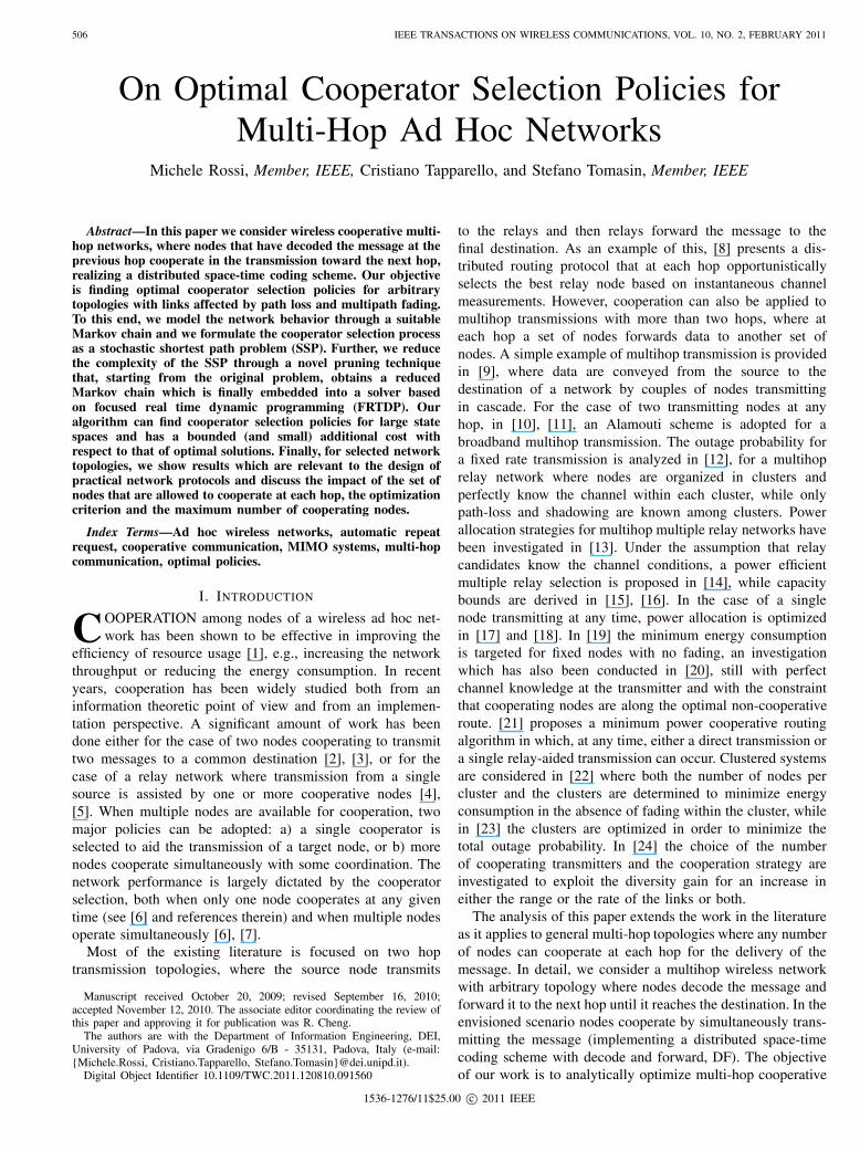
Fig. 1. Network topology for scenario A (4 columns, 21 nodes).

or when the current path is longer than 𝐷. Whenever thecurrent trial terminates, optimal actions, lower and upperbounds and priority are updated on the way back along thetraversed path from 𝑠 → 𝑡 (lines 14 − 18). For the checkon the path length, poor outcome selection early in a trialcould lead to traversing a large number of irrelevant states,which take a long time to escape. The check on the maximumhop length implements the adaptive maximum depth (AMD)trial termination of [27], which solves this problem by cuttingexcessively long paths.

IV. NUMERICAL RESULTS

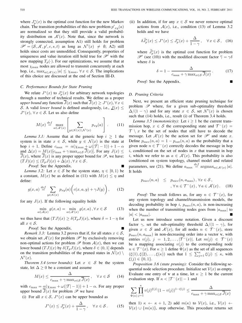
In this section we provide an example application of theproposed optimization techniques for cooperator selectionpolicies, showing numerical results and obtaining insights forpossible low-complexity implementations. We consider thenetwork topology of Fig. 1, where a source node 𝑠 transmits amessage to a destination node 𝑡 and the remaining nodes areavailable for cooperation. All nodes except the destination areorganized in a number of columns, each comprising five nodes.The inter-column distance 𝑑 is picked in the range 45÷80 m,while the distance between two adjacent nodes in a columnis 2 m. The path-loss exponent is 𝜈 = 3.5 and the referencedistance is 𝑑0 = 1 m. In what follows, two network scenariosare considered: scenario A) is the topology of Fig. 1 with fourcolumns and 21 nodes and scenario B) where we extendedthe number of columns to eight for a total of 41 nodes. Thetransmit data rate 𝑅 and the average SNR are set in order toobtain, for a single active link, an outage probability of 0.2at a distance of 30 m, while transmissions among adjacentnodes in a column have average outage probability 2 ⋅ 10−5.Each node is equipped with a single antenna (i.e., 𝑁A = 1).We evaluated the performance for various values of 𝜔 ≥ 0and we observed a straightforward behavior for the optimizedcost, which increases linearly with increasing 𝜔. Therefore, inwhat follows we only discuss the case 𝜔 = 0.

Our optimization is driven by the cost model of (4), whichreturns the cost over a single transmission hop taking intoaccount a weighted sum of energy (𝑐E) and delay (𝑐D), where𝛼 ∈ [0, 1] is the weighting factor. Analogously, the overallcooperator selection policy is characterized by the two costs𝐶E and 𝐶D that are respectively the expected normalizedenergy and the expected total delay of the optimal cooperator

ROSSI et al.: ON OPTIMAL COOPERATOR SELECTION POLICIES FOR MULTI-HOP AD HOC NETWORKS 513

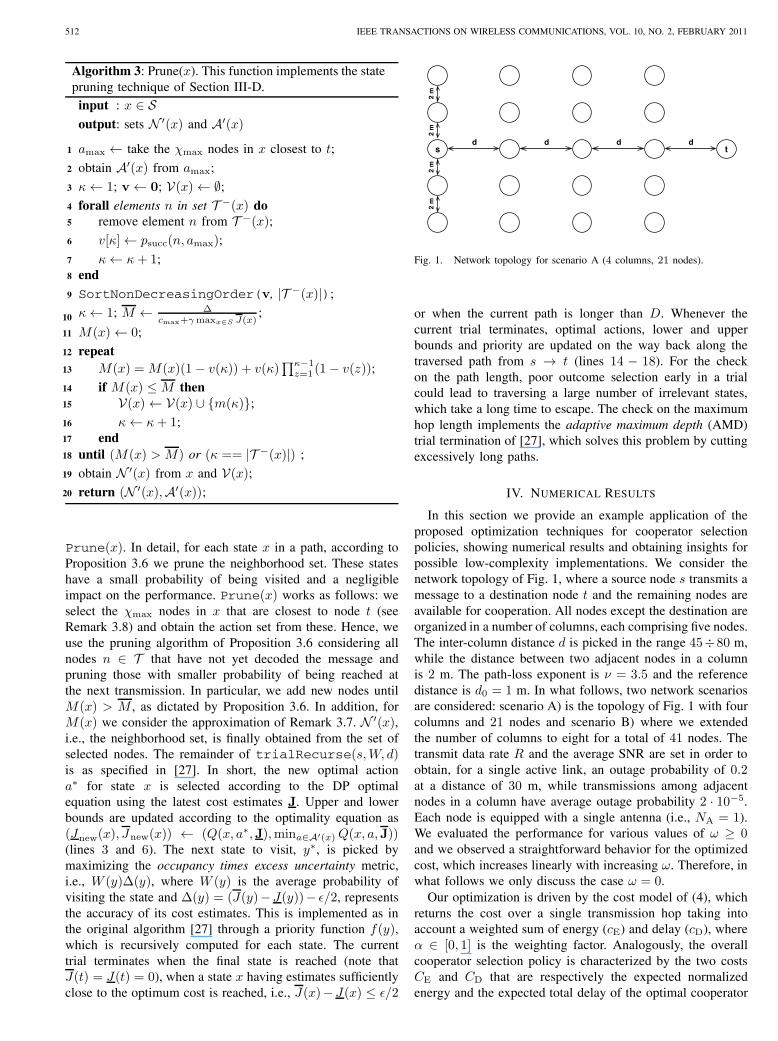
TABLE IPERFORMANCE OF THE MODIFIED FRTDP OPTIMIZER AS A FUNCTION OF Δ.

Scenario A: 21 nodes network Scenario B: 41 nodes networkΔ Visited Failure Δ𝐶 [%] Δ𝐶 [%] Visited Failure Δ𝐶 [%]

States Prob. 𝑝fail(Δ) Actual Predicted States Prob. 𝑝fail(Δ) Predicted

0 1.3 ⋅ 109 0 0.00 — — — —0.001 2.2 ⋅ 106 9.0 ⋅ 10−6 0.00 0.76 3.3 ⋅ 108 5.0 ⋅ 10−6 0.450.005 2.2 ⋅ 106 9.0 ⋅ 10−6 0.00 3.82 3.3 ⋅ 108 5.0 ⋅ 10−6 2.240.01 2.2 ⋅ 106 9.0 ⋅ 10−6 0.00 7.64 3.3 ⋅ 108 5.0 ⋅ 10−6 4.490.05 2.2 ⋅ 106 9.0 ⋅ 10−6 0.00 38.18 3.3 ⋅ 108 5.0 ⋅ 10−6 22.450.1 2.2 ⋅ 106 9.0 ⋅ 10−6 0.00 76.35 3.3 ⋅ 108 5.0 ⋅ 10−6 44.890.5 2.2 ⋅ 106 9.0 ⋅ 10−6 0.00 381.77 3.3 ⋅ 108 5.0 ⋅ 10−6 224.461 2.2 ⋅ 106 9.0 ⋅ 10−6 0.00 763.53 3.3 ⋅ 108 5.0 ⋅ 10−6 448.925 1.5 ⋅ 106 5.9 ⋅ 10−5 5.13 3631.35 2.9 ⋅ 108 1.3 ⋅ 10−5 2175.9510 7.0 ⋅ 105 3.6 ⋅ 10−4 13.88 6704.66 1.6 ⋅ 108 2.5 ⋅ 10−5 4293.26

selection policy used to route packets from 𝑠 to 𝑡.2 Picking𝛼 = 1 returns optimal policies in terms of 𝐶E, while 𝐶D isignored. Conversely, 𝛼 = 0 returns optimal policies in termsof 𝐶D, ignoring 𝐶E. Intermediate values of 𝛼 lead to suitabletrade-offs between energy and delay. In what follows, optimalpolicies are obtained setting 𝛾 = 0.99, which is adequate forstatic networks, see Section III-A. For our FRTDP techniquewe set 𝜖 = 10−3, 𝐽(𝑥) = 0, ∀𝑥 ∈ 𝒮, 𝐾𝐷 = 1.1 and 𝐷0 = 10.For the upper bound 𝐽(𝑥) we considered Δ = 0.001 and alarge initial 𝐽(𝑥) = 100, ∀𝑥 ∈ 𝒮 ∖ 𝑡. We obtained a firstpolicy and the corresponding cost 𝐽∗

𝑝 (𝑥), ∀𝑥 ∈ 𝒮 ∖ 𝑡 and thusset 𝐽(𝑥)← 𝐽∗

𝑝 (𝑥) + Δ/(1− 𝛾).The choice of parameter Δ is guided by the trade-off

between sub-optimality of the policy and its computationalcomplexity. In detail, when Δ = 0 our FRTDP optimizerdoes not cut any state and finds optimal policies as doneby RTDP [25], where 𝐽∗(𝑠) is their cost. When Δ > 0some states are instead pruned according to our techniquesof Section III-D and our optimizer returns an approximationof the optimal policy, with cost 𝐽∗

𝑝 (𝑠). Note that setting Δ > 0for any given state 𝑥 reduces the number of neighboring states𝑦 and, to a lesser extent, also reduces the number of statesfor which the policy is computed, as states hit with smallprobability are not considered. As a consequence, the optimalpolicy is not calculated for these states. Table I shows theperformance of our FRTDP algorithm as a function of Δ,for 𝑑 = 60 m and 𝛼 = 1 in terms of 1) computationalcomplexity, expressed in terms of number of visited states, 2)estimated failure probability 𝑝fail(Δ), i.e., the probability ofhitting a state for which our optimizer did not calculate optimalactions, 3) actual cost difference with respect to RTDP, i.e.,100∣𝐽∗

𝑝 (𝑠)−𝐽∗(𝑠)∣/𝐽∗(𝑠) and 4) the maximum cost differencebetween 𝐽∗

𝑝 (𝑠) and 𝐽∗(𝑠), as predicted by Theorem 3.4, i.e.,100Δ/[𝐽∗

𝑝 (𝑠)(1 − 𝛾)]. We discuss the results for scenarioA first. In this case, even a small Δ = 0.001 suffices todramatically reduce the number of visited states, which dropsfrom 1.3⋅109 to 2.2⋅106. For this Δ, our bounds would predicta maximum additional cost that is just 0.76% larger than𝐽∗𝑝 (𝑆). We note that, for this specific network topology, the

solver performance is better than that predicted by the bound.Also, there is a threshold effect on the number of pruned states

2These costs are the average of the costs obtained over all possiblerealizations of the cooperator selection process from 𝑠 to 𝑡 when the optimalpolicy is adopted.

0

10

20

30

40

50

60

70

45 50 55 60 65 70 75 80

Nor

mal

ized

Cos

t

Inter-column distance d [m]

CE, α=0CD, α=0CE, α=1CD, α=1

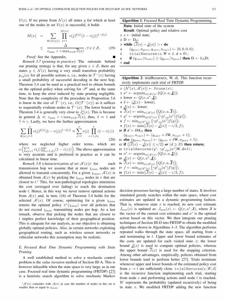
Fig. 2. Normalized costs 𝐶E and 𝐶D as a function of 𝑑 for 𝛼 = 0 and𝛼 = 1. 𝐶E and 𝐶D are normalized with respect to the energy spent totransmit a single packet and the message transmission delay, respectively.Other optimization parameters are: 𝜔 = 0, 𝛾 = 0.99, Δ = 0.001 and𝜒max = 5.

for increasing Δ, which is due to the specific topology underconsideration. For scenario B (41 nodes) the solver fails toobtain policies for Δ = 0, due to the excessively large numberof states. However, Δ = 0.001 already provides cooperationpolicies having a small bounded additional cost with respectto the unknown optimal performance. We shall observe thatthe bounds of Theorem 3.4 are asymptotically tight, i.e., theybecome more accurate as the path length increases. Finally, wenote that 𝑝fail(Δ) is very small in all cases. These results showthe effectiveness of our technique, which makes it possible tofind quasi-optimal policies for large networks at a reducedcomplexity.

Fig. 2 shows 𝐶E and 𝐶D as a function of the inter-columndistance 𝑑 for 𝛼 = 1 (minimum energy) and 𝛼 = 0 (minimumdelay). Costs are normalized with respect to the cost incurredfor a single packet transmission. We observe that for 𝛼 = 1the energy cost 𝐶E increases smoothly with 𝑑, while for𝛼 = 0 the delay cost 𝐶D increases smoothly with time, sincea larger distance 𝑑 between columns yields higher outageprobabilities which, in turn, lead to longer transmission delaysover single hops. In the figure, we also show non targetedcosts, i.e., 𝐶D when the optimization objective corresponds to

514 IEEE TRANSACTIONS ON WIRELESS COMMUNICATIONS, VOL. 10, NO. 2, FEBRUARY 2011

1

1.5

2

2.5

3

3.5

4

4.5

45 50 55 60 65 70 75 80

Con

curr

ent T

rans

mis

sion

s pe

r H

op

Inter-column distance d [m]

α = 1 α = 0.4 α = 0.2 α = 0.05α = 0

1

1.5

2

2.5

3

3.5

4

4.5

45 50 55 60 65 70 75 80

Con

curr

ent T

rans

mis

sion

s pe

r H

op

Inter-column distance d [m]

α = 1 α = 0.4 α = 0.2 α = 0.05α = 0

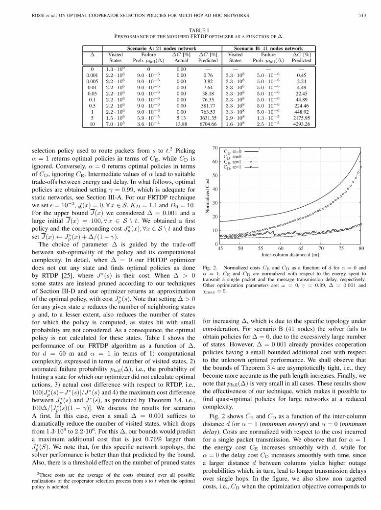
Fig. 3. Average number of cooperating nodes as a function of 𝑑 for differentvalues of 𝛼. Other optimization parameters are: 𝜔 = 0, 𝛾 = 0.99, Δ = 0.001and 𝜒max = 5.

minimizing the energy consumption (𝛼 = 1) and 𝐶E whenthe objective is the minimization of the delay (𝛼 = 0). Nontargeted costs generally increase with increasing 𝑑. However,the corresponding curves have an irregular behavior as insome cases non-targeted costs decrease with the inter-columndistance. This is due to the fact that the optimization isperformed on a discrete set of policies. For example, whenthe target cost is 𝐶E and 𝑑 is slightly increased, to counteractthe increased outage probability cooperation may start earlierand involve a larger number of nodes. The effect of this istwofold: 1) 𝐶E is kept as small as possible and 2) the delayis decreased as more nodes transmit at each hop. Overall, theresult is a slight increase in 𝐶E (thus the smooth curve for𝐶E) together with a sudden drop of 𝐶D due to the reducednumber of hops (thus the irregular curve for 𝐶D).

To better understand the impact of cooperation in a multi-hop scenario with optimized cooperator selection policies inFig. 3 we show the average number of nodes that transmitsimultaneously, as a function of 𝑑 and for various values of 𝛼.Note that, when the objective is to minimize the delay, optimalpolicies tend to maximize the number of cooperating nodes perhop as the cost in this case is solely given by the number ofhops traveled by the message, irrespective of the number oftransmitting nodes within each hop. When minimizing energy,the cost also depends on the number of cooperating nodeswithin each hop and, as a consequence, the optimal numberof cooperating nodes per hop is smaller. Also in this casewe observe an irregular behavior of the curves, which canbe explained considering the discrete nature of the problem.In general, the average number of simultaneous transmissionsdecreases with increasing 𝑑, as outages occur more often and,in such cases, fewer nodes are available for transmission.However, this is true until the cooperation policy changes, atwhich point cooperation is forced among a larger number ofnodes in order to minimize the targeted cost. Notably, we cansee a close relationship between Fig. 3 and the non-targetedcosts of Fig. 2: for example, when 𝛼 = 1 at 58.75 m theaverage number of simultaneous transmissions increases from1.45 to 1.86 (Fig. 3) and, at the same time, 𝐶D drops from8.53 to 6.56 (Fig. 2). This corresponds to a forced earlier

10

12

14

16

18

20

22

24

4.5 5 5.5 6 6.5 7 7.5 8 8.5 9

Nor

mal

ized

Ene

rgy

Cos

t, C

E

Normalized Delay Cost, CD

χmax = 2χmax = 3χmax = 4χmax = 5

10

12

14

16

18

20

22

24

4.5 5 5.5 6 6.5 7 7.5 8 8.5 9

Nor

mal

ized

Ene

rgy

Cos

t, C

E

Normalized Delay Cost, CD

χmax = 2χmax = 3χmax = 4χmax = 5χmax = 6

Fig. 4. 𝐶E vs 𝐶D for several values of 𝜒max. The curves are obtained for𝑑 = 55 m, varying 𝛼 ∈ [0, 1]. Other optimization parameters are: 𝜔 = 0,𝛾 = 0.99, Δ = 0.001 and 𝜒max ∈ {1, 2, 3, 4, 5, 6}.

cooperation among nodes which causes an increase in 𝐶E aswell as a subsequent reduction in the number of hops. Fig. 3also confirms that cooperation is advantageous when multihopis considered and minimization of energy consumption ratherthan delay or rate are targeted. As an example, for 𝛼 = 1the average number of simultaneous transmissions goes from20% (i.e., 1 transmitting node for 𝑑 = 45 m over a maximumof 𝜒𝑚𝑎𝑥 = 5 cooperating nodes) to 60% (i.e., 3 cooperatingnodes over 𝜒max = 5). In addition, we observe that the averagenumber of cooperating nodes is small with respect to the totalnumber of nodes in the network, thus it is meaningful toimpose a maximum 𝜒max ≪ ∣𝒯 ∣ on the number of cooperatingnodes, as discussed in Section III-D.

Fig. 4 shows the trade-off between 𝐶E and 𝐶D as a functionof 𝜒max for an inter-column distance of 𝑑 = 55 m. The curvesare obtained by varying the weighting factor 𝛼 in [0, 1] andprovide the delay-energy achievable regions, as for a given𝜒max no policy can obtain a trade-off point situated belowthe corresponding optimal curve, while any point above theoptimal curve is achieved by a suitable suboptimal policy.However, this figure provides even further insights on possibleimplementations of optimal policies. In fact, for 𝛼 > 0 setting𝜒max = 5 already provides most of the benefits of optimalpolicies in the unconstrained optimization case (𝜒max = +∞).This means that complexity of both policy optimization andnetwork coordination can be reduced at almost no expense interms of performance. On the other side, being too restrictiveon the number of cooperators yields some performance loss,as for example allowing at most 2 cooperating nodes leads toa delay increase of about 20% and to an increase of energyconsumption of about 10%. Note that if cooperation is notallowed (i.e., 𝜒max = 1) delay and energy consumption arecentered around point (𝑥, 𝑦) = (11.8, 11.8) (out of range inthe figure). Therefore, even a minimum level of cooperation,i.e., between two nodes (𝜒max = 2), provides a substantialperformance advantage. We finally observe that, if at everyhop the maximum admissible number of nodes cooperate, weobtain the delay optimal policy (𝛼 = 0). This however comesat the expense of a high energy consumption. A more judiciouschoice leads to considerable advantages, e.g., a delay just 4%

ROSSI et al.: ON OPTIMAL COOPERATOR SELECTION POLICIES FOR MULTI-HOP AD HOC NETWORKS 515

0

10

20

30

40

50

60

150 200 250 300 350

Nor

mal

ized

Cos

t

Source-destination distance d [m]

CE, α=0CD, α=0CE, α=1CD, α=1

0

10

20

30

40

50

60

150 200 250 300 350

Nor

mal

ized

Cos

t

Source-destination distance d [m]

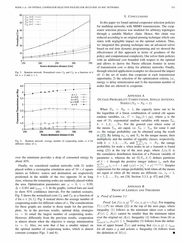
Fig. 5. Random network: Normalized costs 𝐶E and 𝐶D as a function of 𝑑for 𝛼 = 0 and 𝛼 = 1.

1

1.5

2

2.5

3

3.5

4

4.5

150 200 250 300 350

Con

curr

ent T

rans

mis

sion

s pe

r H

op

Source-destination distance d [m]

α = 1 α = 0.4 α = 0.2 α = 0.05α = 0

1

1.5

2

2.5

3

3.5

4

4.5

150 200 250 300 350

Con

curr

ent T

rans

mis

sion

s pe

r H

op

Source-destination distance d [m]

α = 1 α = 0.4 α = 0.2 α = 0.05α = 0

1

1.5

2

2.5

3

3.5

4

4.5

150 200 250 300 350

Con

curr

ent T

rans

mis

sion

s pe

r H

op

Source-destination distance d [m]

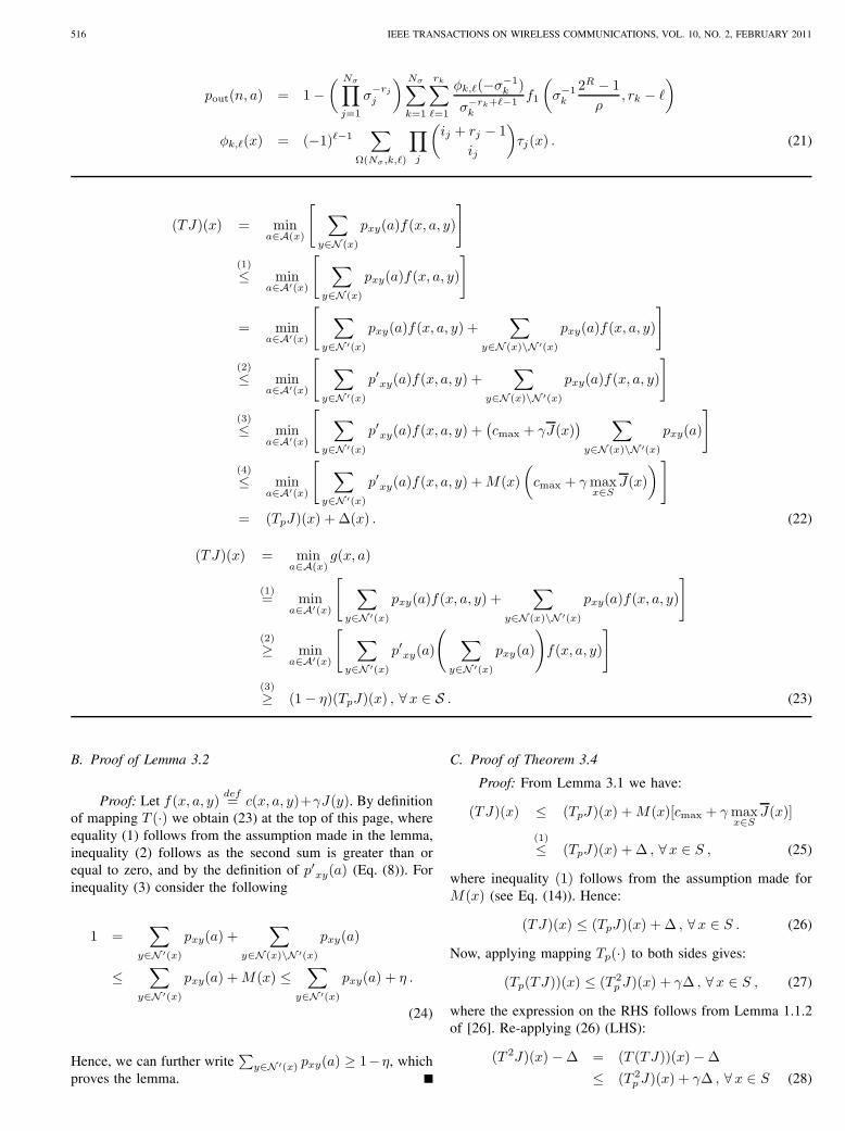
Fig. 6. Random network: average number of cooperating nodes vs 𝑑 fordifferent values of 𝛼.

over the minimum provides a drop of consumed energy byabout 30%.

Finally, we considered random networks with 21 nodesplaced within a rectangular simulation area of 50× 𝑑 squaremeters as follows: source and destination are respectivelypositioned in the middle of the two opposite 50 m longsizes, whereas the remaining nodes are randomly placed withinthe area. Optimization parameters are: 𝜔 = 0, 𝛾 = 0.99,Δ = 0.001 and 𝜒max = 5. In the graphs, vertical bars are usedto show 95% confidence intervals. For the random scenario,Fig. 5 shows the normalized costs 𝐶E and 𝐶D as a function of𝑑 for 𝛼 ∈ {0, 1}. Fig. 6 instead shows the average number ofcooperating nodes for different values of 𝛼. The considerationsfor these graphs are similar to those made for the previousplots. As in the previous results, optimal delay strategies(𝛼 = 0) entail the largest number of cooperating nodes.However, differently from the previous results, cooperationis almost absent when the objective is energy minimization(𝛼 = 1). Also, we note that 𝑑 has a smaller impact onthe optimal number of cooperating nodes, which is almostconstant (compare Figs. 3 and 6).

V. CONCLUSIONS

In this paper we found optimal cooperator selection policiesfor multihop networks with MIMO transmissions. The coop-erator selection process was modeled for arbitrary topologiesthrough a suitable Markov chain. Hence, this chain wasreduced according to an original pruning technique which cutsstates with negligible impact on the optimal solution. Thus,we integrated this pruning technique into an advanced solverbased on real time dynamic programming and we showed theeffectiveness of this approach in terms of goodness of thepolicy and computational complexity. Our solver finds policieswith an additional cost bounded with respect to the optimaland allows to derive the Pareto efficient frontier in termsof transmission cost vs delay for arbitrary networks. Finally,through selected application examples we discussed the impactof: 1) the set of nodes that cooperate at each transmissionopportunity, 2) the selection of the optimization criteria, i.e.,energy vs delay minimization and 3) the maximum number ofnodes that are allowed to cooperate.

APPENDIX AOUTAGE PROBABILITY COMPUTATION, SINGLE ANTENNA

NODES (𝑁A = 𝑁R = 1)

When 𝑁A = 𝑁R = 1, the capacity turns out to bethe logarithm of a linear combination of central chi squarerandom variables, i.e., 𝐶 = log2 (1 + 𝜌𝑦), where 𝑦 is thesum of 𝑁T exponential random variables with means Σ𝑘,𝑘 = 1, 2, . . . , 𝑁T. For the general case where some ofthe means Σ𝑚 are equal, i.e. Σ𝑘 = Σ𝑚 for some 𝑘 and𝑚, the outage probability can be obtained using the resultin [37]. By letting 𝜎𝑘, 𝑟𝑘 and 𝑁𝜎 be the unique means, theirmultiplicity and the number of equality classes, respectively,with 𝑘 = 1, 2, . . . , 𝑁𝜎 and

∑𝑁𝜎

𝑘=1 𝑟𝑘 = 𝑁T, the outageprobability for node 𝑛 when nodes in set 𝑎 transmit is foundusing (21) at the top of the next page, where 𝑓1(𝑎, 𝑏) isthe cumulative distribution function of a Poisson variable ofparameter 𝑎, whereas the set Ω(𝑁𝜎, 𝑘, ℓ) defines partitionsof ℓ − 1 through the positive integer indices 𝑖𝑗 , such that∑𝑁𝜎

𝑗=1, ∕=𝑘 𝑖𝑗 = ℓ − 1 and 𝜏𝑗(𝑥) = (𝜎−1𝑗 + 𝑥)−(𝑟𝑗+𝑖𝑗). Simpler

expressions for the outage probability hold when all the meansare equal or when all the means are different, i.e., 𝑟𝑘 = 1,𝑘 = 1, 2, . . . , 𝑁T, see [38, Section 3.3.1, p. 47] and [39].

APPENDIX BPROOF OF LEMMAS AND THEOREMS

A. Proof of Lemma 3.1

Proof: Let 𝑓(𝑥, 𝑎, 𝑦)𝑑𝑒𝑓= 𝑐(𝑥, 𝑎, 𝑦)+𝛾𝐽(𝑦). For mapping

𝑇 (⋅) (P) we obtain (22) at the top of the next page, whereinequality (1) follows as the minimum taken over a subset𝒜′(𝑥) ⊆ 𝒜(𝑥) cannot be smaller than the minimum takenover the original set 𝒜(𝑥). Inequality (2) follows from (8) as∑

𝑦∈𝒩 ′(𝑥) 𝑝𝑥𝑦(𝑎) ≤ 1. Inequality (3) follows from the defini-tion of upper bound 𝐽(𝑥) and noting that 𝑐(𝑥, 𝑎, 𝑦) ≤ 𝑐max

for all states 𝑥, 𝑦 and actions 𝑎. Inequality (4) follows fromthe definition of 𝑀(𝑥).

516 IEEE TRANSACTIONS ON WIRELESS COMMUNICATIONS, VOL. 10, NO. 2, FEBRUARY 2011

𝑝out(𝑛, 𝑎) = 1−( 𝑁𝜎∏

𝑗=1

𝜎−𝑟𝑗𝑗

) 𝑁𝜎∑𝑘=1

𝑟𝑘∑ℓ=1

𝜙𝑘,ℓ(−𝜎−1𝑘 )

𝜎−𝑟𝑘+ℓ−1𝑘

𝑓1

(𝜎−1𝑘

2𝑅 − 1

𝜌, 𝑟𝑘 − ℓ

)𝜙𝑘,ℓ(𝑥) = (−1)ℓ−1

∑Ω(𝑁𝜎,𝑘,ℓ)

∏𝑗

(𝑖𝑗 + 𝑟𝑗 − 1

𝑖𝑗

)𝜏𝑗(𝑥) . (21)

(𝑇𝐽)(𝑥) = min𝑎∈𝒜(𝑥)

[ ∑𝑦∈𝒩 (𝑥)

𝑝𝑥𝑦(𝑎)𝑓(𝑥, 𝑎, 𝑦)

](1)

≤ min𝑎∈𝒜′(𝑥)

[ ∑𝑦∈𝒩 (𝑥)

𝑝𝑥𝑦(𝑎)𝑓(𝑥, 𝑎, 𝑦)

]

= min𝑎∈𝒜′(𝑥)

[ ∑𝑦∈𝒩 ′(𝑥)

𝑝𝑥𝑦(𝑎)𝑓(𝑥, 𝑎, 𝑦) +∑

𝑦∈𝒩 (𝑥)∖𝒩 ′(𝑥)

𝑝𝑥𝑦(𝑎)𝑓(𝑥, 𝑎, 𝑦)

](2)

≤ min𝑎∈𝒜′(𝑥)

[ ∑𝑦∈𝒩 ′(𝑥)

𝑝′𝑥𝑦(𝑎)𝑓(𝑥, 𝑎, 𝑦) +∑

𝑦∈𝒩 (𝑥)∖𝒩 ′(𝑥)

𝑝𝑥𝑦(𝑎)𝑓(𝑥, 𝑎, 𝑦)

](3)

≤ min𝑎∈𝒜′(𝑥)

[ ∑𝑦∈𝒩 ′(𝑥)

𝑝′𝑥𝑦(𝑎)𝑓(𝑥, 𝑎, 𝑦) +(𝑐max + 𝛾𝐽(𝑥)

) ∑𝑦∈𝒩 (𝑥)∖𝒩 ′(𝑥)

𝑝𝑥𝑦(𝑎)

](4)

≤ min𝑎∈𝒜′(𝑥)

[ ∑𝑦∈𝒩 ′(𝑥)

𝑝′𝑥𝑦(𝑎)𝑓(𝑥, 𝑎, 𝑦) +𝑀(𝑥)

(𝑐max + 𝛾max

𝑥∈𝑆𝐽(𝑥)

)]= (𝑇𝑝𝐽)(𝑥) + Δ(𝑥) . (22)

(𝑇𝐽)(𝑥) = min𝑎∈𝒜(𝑥)

𝑔(𝑥, 𝑎)

(1)= min

𝑎∈𝒜′(𝑥)

[ ∑𝑦∈𝒩 ′(𝑥)

𝑝𝑥𝑦(𝑎)𝑓(𝑥, 𝑎, 𝑦) +∑

𝑦∈𝒩 (𝑥)∖𝒩 ′(𝑥)

𝑝𝑥𝑦(𝑎)𝑓(𝑥, 𝑎, 𝑦)

](2)

≥ min𝑎∈𝒜′(𝑥)

[ ∑𝑦∈𝒩 ′(𝑥)

𝑝′𝑥𝑦(𝑎)

( ∑𝑦∈𝒩 ′(𝑥)

𝑝𝑥𝑦(𝑎)

)𝑓(𝑥, 𝑎, 𝑦)

](3)

≥ (1− 𝜂)(𝑇𝑝𝐽)(𝑥) , ∀𝑥 ∈ 𝒮 . (23)

B. Proof of Lemma 3.2

Proof: Let 𝑓(𝑥, 𝑎, 𝑦)𝑑𝑒𝑓= 𝑐(𝑥, 𝑎, 𝑦)+𝛾𝐽(𝑦). By definition

of mapping 𝑇 (⋅) we obtain (23) at the top of this page, whereequality (1) follows from the assumption made in the lemma,inequality (2) follows as the second sum is greater than orequal to zero, and by the definition of 𝑝′𝑥𝑦(𝑎) (Eq. (8)). Forinequality (3) consider the following

1 =∑

𝑦∈𝒩 ′(𝑥)

𝑝𝑥𝑦(𝑎) +∑

𝑦∈𝒩 (𝑥)∖𝒩 ′(𝑥)

𝑝𝑥𝑦(𝑎)

≤∑

𝑦∈𝒩 ′(𝑥)

𝑝𝑥𝑦(𝑎) +𝑀(𝑥) ≤∑

𝑦∈𝒩 ′(𝑥)

𝑝𝑥𝑦(𝑎) + 𝜂 .

(24)

Hence, we can further write∑

𝑦∈𝒩 ′(𝑥) 𝑝𝑥𝑦(𝑎) ≥ 1−𝜂, whichproves the lemma.

C. Proof of Theorem 3.4

Proof: From Lemma 3.1 we have:

(𝑇𝐽)(𝑥) ≤ (𝑇𝑝𝐽)(𝑥) +𝑀(𝑥)[𝑐max + 𝛾max𝑥∈𝑆

𝐽(𝑥)]

(1)

≤ (𝑇𝑝𝐽)(𝑥) + Δ , ∀𝑥 ∈ 𝑆 , (25)

where inequality (1) follows from the assumption made for𝑀(𝑥) (see Eq. (14)). Hence:

(𝑇𝐽)(𝑥) ≤ (𝑇𝑝𝐽)(𝑥) + Δ , ∀𝑥 ∈ 𝑆 . (26)

Now, applying mapping 𝑇𝑝(⋅) to both sides gives:

(𝑇𝑝(𝑇𝐽))(𝑥) ≤ (𝑇 2𝑝 𝐽)(𝑥) + 𝛾Δ , ∀𝑥 ∈ 𝑆 , (27)

where the expression on the RHS follows from Lemma 1.1.2of [26]. Re-applying (26) (LHS):

(𝑇 2𝐽)(𝑥) −Δ = (𝑇 (𝑇𝐽))(𝑥)−Δ

≤ (𝑇 2𝑝 𝐽)(𝑥) + 𝛾Δ , ∀𝑥 ∈ 𝑆 (28)

ROSSI et al.: ON OPTIMAL COOPERATOR SELECTION POLICIES FOR MULTI-HOP AD HOC NETWORKS 517

and hence (𝑇 2𝐽)(𝑥) ≤ (𝑇 2𝑝 𝐽)(𝑥) + 𝛾Δ + Δ. Repeated

iterations of this procedure lead to:

(𝑇 𝑘𝐽)(𝑥) ≤ (𝑇 𝑘𝑝 𝐽)(𝑥) +

𝑘−1∑𝑗=0

𝛾𝑗Δ , ∀𝑥 ∈ 𝑆 . (29)

Now, taking the limit as 𝑘 → +∞ to both sides of (29) leadsto:

𝐽∗(𝑥) ≤ 𝐽∗𝑝 (𝑥) +

Δ

1− 𝛾 , ∀𝑥 ∈ 𝒮 , (30)

which proves (i). For (ii), from Lemma 3.2 we have(𝑇𝐽)(𝑥) ≥ 𝛿(𝑇𝑝𝐽)(𝑥), where 𝛿 is as in (17). Applying 𝑇𝑝(⋅)to both sides of this last inequality gives

(𝑇𝑝(𝑇𝐽))(𝑥) ≥ (𝑇𝑝𝛿(𝑇𝑝𝐽))(𝑥)𝑑𝑒𝑓= (𝑇𝑝(𝑇𝑝𝐽))(𝑥) , (31)

where 𝑇𝑝(⋅) is mapping 𝑇𝑝(⋅) (Eq. (10)) with discount factor𝛾 = 𝛾𝛿. Moreover, application of Lemma 3.2 to the LHS ofthe above inequality returns

(𝑇 2𝐽)(𝑥)𝛿−1 ≥ (𝑇𝑝(𝑇𝐽))(𝑥) ≥ (𝑇𝑝(𝑇𝑝𝐽))(𝑥) . (32)

Repeated iterations of this procedure lead to (𝑇 𝑘𝐽)(𝑥) ≥𝛿(𝑇 𝑘−1

𝑝 (𝑇𝑝𝐽))(𝑥). Now, taking the limit 𝑘 → +∞ to bothsides of the previous inequality gives 𝐽∗(𝑥) ≥ 𝛿𝐽∗

𝑝 (𝑥), where𝐽∗𝑝 (𝑥) is the optimal cost function for problem P ′ with

discount factor 𝛾 = 𝛾𝛿.

D. Proof of Proposition 3.6

Proof: Set 𝒩 (𝑥) ∖ 𝒩 ′(𝑥) contains the pruned states.These are states 𝑦 containing nodes with small proba-bility of receiving the message at the next hop 𝑖 + 1,given 𝑥. From Lemma 3.5 the maximizing action 𝑎′max =argmax𝑎∈𝒜′(𝑥)[

∑𝑦∈𝒩 (𝑥)∖𝒩 ′(𝑥) 𝑝𝑥𝑦(𝑎)] corresponds to the

case where the maximum number of nodes allowed by 𝒜′(𝑥)transmit, as all receiving nodes 𝑛 ∈ 𝒯 −(𝑥) maximize theirreception probability, namely 𝑝succ(𝑛, 𝑎), for this action. Thus,𝑎′max = 𝑎max, where 𝑎max was defined in Lemma 3.5. Thisimplies that 𝑀(𝑥) =

∑𝑦∈𝒩 (𝑥)∖𝒩 ′(𝑥) 𝑝𝑥𝑦(𝑎max) which is, by

definition, the probability that the system in hop 𝑖 + 1 willmove to state 𝑦 when action 𝑎max is selected. If we define𝑦 ∈ 𝒩 (𝑥) ∖ 𝒩 ′(𝑥) as any state for which: 1) all nodes thatwere successful in 𝑥 are still successful in 𝑦 and 2) at least onenode in 𝒱(𝑥) is successful, then by the way we constructed𝒱(𝑥) we have

𝑀(𝑥) =∑

𝑦∈𝒩 (𝑥)∖𝒩 ′(𝑥)

𝑝𝑥𝑦(𝑎max)

=∑

Ψ(∣𝒱(𝑥)∣)

∣𝒱(𝑥)∣∏𝑗=1

𝑣(𝑗)𝜉(𝑗)(1− 𝑣(𝑗))1−𝜉(𝑗)

(33)

and the inequality in (19) is granted by the constructionalgorithm.

REFERENCES

[1] T. M. Cover and A. A. El Gamal, “Capacity theorems for the relaychannel,” IEEE Trans. Inf. Theory, vol. 25, no. 5, pp. 572–584, Sep.1979.

[2] A. Sendonaris, E. Erkip, and B. Aazhang, “User cooperation diversity–part I: system description,” IEEE Trans. Commun., vol. 51, no. 11, pp.1927–1938, Nov. 2003.

[3] ——, “User cooperation diversity–part II: implementation aspects andperformance analysis,” IEEE Trans. Commun., vol. 51, no. 11, pp. 1939–1948, Nov. 2003.

[4] J. N. Laneman, D. N. C. Tse, and G. W. Wornell, “Cooperative diversityin wireless networks: efficient protocols and outage behavior,” IEEETrans. Inf. Theory, vol. 50, no. 12, pp. 3062–3080, Dec. 2004.

[5] J. N. Laneman and G. W. Wornell, “Distributed space-time-codedprototols for exploiting cooperative diversity in wireless networks,”IEEE Trans. Inf. Theory, vol. 49, no. 10, pp. 2415–2425, Oct. 2003.

[6] M. Chen, S. Serbetli, and A. Yener, “Distributed power allocationstrategies for parallel relay networks,” IEEE Trans. Wireless Commun.,vol. 7, no. 2, pp. 552–561, Feb. 2008.

[7] Y. Fan and J. Thompson, “MIMO configurations for relay channels:theory and practice,” IEEE Trans. Wireless Commun., vol. 6, no. 5, pp.1774–1780, May 2007.

[8] A. Bletsas, A. Khisti, D. P. Reed, and A. Lippman, “A simple cooper-ative diversity method based on network path selection,” IEEE J. Sel.Areas Commun., vol. 24, pp. 659–672, 2006.

[9] L. Liu and H. Ge, “Space-time coding for wireless sensor networks withcooperative routing diversity,” in Proc. Asilomar Conf. Signals, Systemsand Computers, vol. 1, Pacific Grove, CA, Nov. 2004, pp. 1271–1275.

[10] T. Miyano, H. Murata, and K. Araki, “Cooperative relaying scheme withspace time code for multihop communications among single antennaterminals,” in Proc. IEEE GLOBECOM, vol. 6, Dallas, TX, Nov.-Dec.2004.

[11] ——, “Space time coded cooperative relaying technique for multihopcommunications,” in Proc. IEEE VTC Fall, Los Angeles, CA, Sep. 2004.

[12] A. Del Coso, S. Savazzi, U. Spagnolini, and C. Ibars, “Virtual MIMOchannels in cooperative multi-hop wireless sensor networks,” in Proc.Annual Conf. Information Sciences and Systems, Princeton, NJ, Mar.2006, pp. 75–80.

[13] S. Savazzi and U. Spagnolini, “Energy aware power allocation strategiesfor multihop-cooperative transmission schemes,” IEEE J. Sel. AreasCommun., vol. 25, no. 2, pp. 318–327, Feb. 2007.

[14] L. Zhang and L. J. Cimini Jr., “Power-efficient relay selection incooperative networks using decentralized distributed space-time blockcoding,” EURASIP J. Advances in Signal Proc., vol. 2008, no. 1, 2008.

[15] L. Ong and M. Motani, “Optimal routing for the Gaussian multiple-relay channel with decode-and-forward,” in Proc. Int. Conf. InformationTheory (ISIT), Nice, France, June 2007.

[16] L. Ong, W. Wang, and M. Motani, “Achievable rates and optimalschedules for half duplex multiple-relay networks,” in Proc. AllertonConf., Monticello, IL, Sep. 2008.

[17] J. Si, Z. Li, Z. Liu, and X. Lu, “Joint route and power allocation incooperative-multihop networks,” in Proc. IEEE Int. Conf. Circuits andSystems for Commun., Shanghai, China, May 2008, pp. 114–118.

[18] Z. Yang and A. Høst-Madsen, “Routing and power allocation inasynchronous Gaussian multiple-relay channels,” EURASIP J. WirelessCommun. and Networking, vol. 2006, no. 2, pp. 1–11, Apr. 2006.

[19] F. Li, A. Lippman, and K. Wu, “Minimum energy cooperative pathrouting in wireless networks: an integer programming formulation,” inProc. IEEE VTC Spring, Melbourne, Australia, 2006.

[20] A. E. Khandani, J. Abounadi, E. Modiano, and L. Zheng, “Cooperativerouting in static wireless networks,” IEEE Trans. Commun., vol. 55,no. 11, pp. 2185–2192, Nov. 2007.

[21] A. S. Ibrahim, Z. Han, and K. J. Liu, “Distributed energy-efficient coop-erative routing in wireless networks,” IEEE Trans. Wireless Commun.,vol. 7, no. 10, pp. 3930–3941, Oct. 2008.

[22] Y. Yuan, M. Chen, and T. Kwon, “A novel cluster-based cooperativeMIMO scheme for multi-hop wireless sensor networks,” EURASIP J.Advances in Signal Proc., vol. 2006, no. 2, pp. 38–46, Apr. 2006.

[23] A. Del Coso, U. Spagnolini, and C. Ibars, “Cooperative distributedMIMO channels in wireless sensor networks,” IEEE J. Sel. AreasCommun., vol. 25, no. 2, pp. 402–414, Feb. 2007.

[24] S. Lakshmanan and R. Sivakumar, “Diversity routing for multi-hop wire-less networks with cooperative transmissions,” in Proc. IEEE SECON,Rome, Italy, 2009.

[25] A. G. Barto, S. J. Bradtke, and S. P. Singh, “Learning to act using realtime dynamic programming,” Artificial Intelligence, vol. 72, no. 1–2,pp. 81–138, Jan. 1995.

518 IEEE TRANSACTIONS ON WIRELESS COMMUNICATIONS, VOL. 10, NO. 2, FEBRUARY 2011

[26] D. P. Bertsekas, Dynamic Programming and Optimal Control: Vol. II,2nd edition. Athena Scientific, 2001.

[27] T. Smith and R. G. Simmons, “Focused real-time dynamic programmingfor MDPs: squeezing more out of a heuristic,” in Proc. Nat. Conf. onArtificial Intelligence, Boston, MA, July 2006.

[28] K. Lingkun, X. N. Soon, R. G. Maunder, and L. Hanzo, “Maximum-throughput irregular distributed space-time code for near-capacity coop-erative communications,” IEEE Trans. Veh. Technol., vol. 59, no. 3, pp.1511–1517, Mar. 2010.

[29] A. Sezgin and E. A. Jorswieck, “Capacity achieving high rate space-time block codes,” IEEE Commun. Lett., vol. 9, no. 5, pp. 435–437,May 2005.

[30] M. Franceschini, G. Ferrari, and R. Raheli, LDPC Coded Modulations.Springer Verlag, 2009.

[31] A. T. James, “Distributions of matrix variates and latent roots derivedfrom normal samples,” Ann. Math. Statist., vol. 35, pp. 475–501, 1964.

[32] M. Chiani, M. Z. Win, and A. Zanella, “On the capacity of spatiallycorrelated MIMO Rayleigh-fading channels,” IEEE Trans. Inf. Theory,vol. 49, no. 10, pp. 2363–2371, Oct. 2003.

[33] T. Ratnarajah and R. Vaillancourt, “Complex singular Wishart matricesand applications,” Computers & Mathematics with Applications, vol. 50,no. 3-4, pp. 399–411, Aug. 2005.

[34] R. L. Keeney and H. Raiffa, Decision with Multiple Objectives: Prefer-ences and Value Tradeoffs. Cambridge University Press, 1993.

[35] D. P. Bertsekas and J. N. Tsitsiklis, “An analysis of stochastic shortestpath problems,” Mathematics of Operations Research, vol. 16, pp. 580–595, Oct. 1991.

[36] H. B. McMahan, M. Likhachev, and G. J. Gordon, “Bounded real-time dynamic programming: RTDP with monotone upper bounds andperformance guarantees,” in Proc. International Conference on MachineLearning, Bonn, Germany, Oct. 2005.

[37] S. V. Amari and R. B. Misra, “Closed-form expressions for distributionof sum of exponential random variables,” IEEE Trans. Reliability,vol. 46, no. 4, pp. 519–522, Dec. 1997.

[38] P. V. Mieghem, Performance Analysis of Communications Networks andSystems. Cambridge University Press, 2006.

[39] M. Biswal, N. Biswal, and D. Li, “Probabilistic linear programmingproblems with exponential random variables: a technical note,” Euro-pean J. Operational Research, vol. 111, pp. 589–597, 1998.

Michele Rossi received the Laurea degree in Electri-cal Engineering (with honors) and the Ph.D. degreein Information Engineering from the University ofFerrara in 2000 and 2004, respectively. From March2000 to October 2005 he has been a Research Fellowat the Department of Engineering of the Universityof Ferrara. During 2003 he was on leave at theCenter for Wireless Communications (CWC) at theUniversity of California San Diego (UCSD), wherehe performed research on wireless sensor networks.In November 2005 he joined the Department of

Information Engineering of the University of Padova, Italy, where he is anAssistant Professor. Dr. Rossi is currently part of the EU-funded projectsSENSEI, IOT-A and SWAP, all on wireless sensor networks and Internetof Things. Broadly, his research interests are centered around the followingtopics: data dissemination in distributed ad hoc and wireless sensor networks,integrated MAC/routing schemes, application of compressive sensing for thereconstruction of signals in wireless sensor networks and cooperative routingpolicies for ad hoc networks. His current research activity also includes energyscavenging solutions for wireless sensor nodes and the utilization of sensingtechnology within smart buildings.

Cristiano Tapparello received the B.Sc. degreeand the M.Sc. degree (with honors) in ComputerEngineering from University of Padova, Italy, in2005 and 2008, respectively. Since January 2009 hehas been a Ph.D. student at the same University.His current research interests include cooperativerouting policies for ad hoc networks, interference-aware optimization of routing and scheduling andinformation-theoretic aspects of cognitive radiotechniques in ad hoc networks.

Stefano Tomasin (S’99, M’03) received the Laureadegree and the Ph.D. degree in TelecommunicationsEngineering from the University of Padova, Italy, in1999 and 2003, respectively. In the Academic year1999–2000 he was on leave at the IBM ResearchLaboratory, Zurich, Switzerland, doing research onsignal processing for magnetic recording systems.In the Academic year 2001–2002 he was on leaveat Philips Research, Eindhoven, the Netherlands,studying multicarrier transmission for mobile appli-cations. In the second half of 2004 he was visiting

at Qualcomm, San Diego (CA) doing research on receiver design for mobilecellular systems. Since 2005 he is assistant professor at University of Padova,Italy. In 2007 he has been visiting faculty at Polytechnic University ofBrooklyn, NY, working on cooperative communications. His current researchinterests include signal processing for wireless communications, access tech-nologies for multiuser/multiantenna systems and cross-layer protocol designand evaluation.