On k-Fibonacci sequences and polynomials and their derivatives

On k-Fibonacci sequences and polynomialsand their derivatives

Sergio Falcon *, Angel Plaza

Department of Mathematics, University of Las Palmas de Gran Canaria (ULPGC), 35017 Las Palmas de Gran Canaria, Spain

Accepted 30 March 2007

Abstract

The k-Fibonacci polynomials are the natural extension of the k-Fibonacci numbers and many of their propertiesadmit a straightforward proof. Here in particular, we present the derivatives of these polynomials in the form of con-volution of k-Fibonacci polynomials. This fact allows us to present in an easy form a family of integer sequences in anew and direct way. Many relations for the derivatives of Fibonacci polynomials are proven.� 2007 Elsevier Ltd. All rights reserved.

1. Introduction

There is a huge interest of modern science in the application of the Golden Section and Fibonacci numbers [1–10].The Fibonacci numbers Fn are the terms of the sequence f0; 1; 1; 2; 3; 5; . . .g wherein each term is the sum of the twoprevious terms, beginning with the values F0 = 0, and F1 = 1. On the other hand the ratio of two consecutive Fibonaccinumbers converges to the Golden Mean, or Golden Section, / ¼ 1þ

ffiffi5

p

2, which appears in modern research, particularly

physics of the high energy particles [11,12] or theoretical physics [13–19].The paper presented here was initially originated for the astonishing presence of the Golden Section in a recursive

partition of triangles in the context of the finite element method and triangular refinements. In [20] we showed the rela-tion between the 4-triangle longest-edge partition and the k-Fibonacci numbers, as another example of the relationbetween geometry and numbers. On the other hand in [21] the k-Fibonacci numbers were given in an explicit wayand, by easy arguments, many properties were proven. In particular the k-Fibonacci numbers were related with theso-called Pascal 2-triangle.

From this point on, the present paper is organized as follows. In Section 2 a brief summary of the previous resultsobtained in References [20–22] is given. Section 3 is focused on the k-Fibonacci polynomials which are the naturalextension of the k-Fibonacci numbers and many of their properties admit a straightforward proof. Here, in particularwe relate the Catalan’s numbers with the coefficients of the successive powers xn written as linear combination of Fibo-nacci polynomials. Section 4 presents many formulas and relations for the derivatives of the Fibonacci polynomials.For example, their derivatives are given as convolution of Fibonacci polynomials. This fact allows us to present a familyof integer sequences in a new and direct way.

0960-0779/$ - see front matter � 2007 Elsevier Ltd. All rights reserved.

doi:10.1016/j.chaos.2007.03.007

* Corresponding author. Tel.: +34 928 45 88 27; fax: +34 928 45 88 11.E-mail address: [email protected] (S. Falcon).

Chaos, Solitons and Fractals 39 (2009) 1005–1019

www.elsevier.com/locate/chaos

mailto:[email protected]

2. The k-Fibonacci numbers and properties

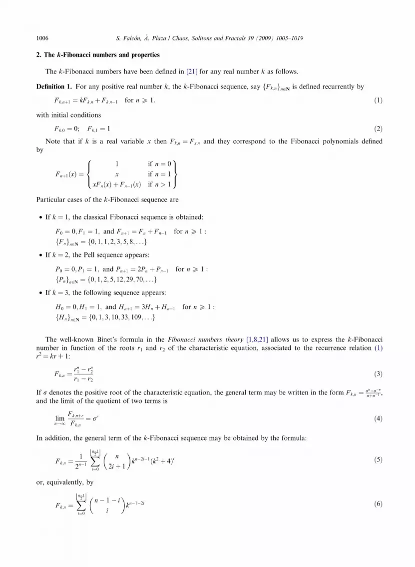
The k-Fibonacci numbers have been defined in [21] for any real number k as follows.

Definition 1. For any positive real number k, the k-Fibonacci sequence, say fF k;ngn2N is defined recurrently by

F k;nþ1 ¼ kF k;n þ F k;n�1 for nP 1: ð1Þ

with initial conditions

F k;0 ¼ 0; F k;1 ¼ 1 ð2ÞNote that if k is a real variable x then F k;n ¼ F x;n and they correspond to the Fibonacci polynomials defined

by

F nþ1ðxÞ ¼1 if n ¼ 0

x if n ¼ 1

xF nðxÞ þ F n�1ðxÞ if n > 1

8

><

>:

9

>=

>;

Particular cases of the k-Fibonacci sequence are

• If k = 1, the classical Fibonacci sequence is obtained:

F 0 ¼ 0; F 1 ¼ 1; and F nþ1 ¼ F n þ F n�1 for nP 1 :

fF ngn2N ¼ f0; 1; 1; 2; 3; 5; 8; . . .g

• If k = 2, the Pell sequence appears:

P 0 ¼ 0; P 1 ¼ 1; and P nþ1 ¼ 2P n þ P n�1 for nP 1 :

fP ngn2N ¼ f0; 1; 2; 5; 12; 29; 70; . . .g

• If k = 3, the following sequence appears:

H 0 ¼ 0;H 1 ¼ 1; and H nþ1 ¼ 3H n þ H n�1 for nP 1 :

fH ngn2N ¼ f0; 1; 3; 10; 33; 109; . . .g

The well-known Binet’s formula in the Fibonacci numbers theory [1,8,21] allows us to express the k-Fibonaccinumber in function of the roots r1 and r2 of the characteristic equation, associated to the recurrence relation (1)r2 = kr + 1:

F k;n ¼rn1 � rn2r1 � r2

ð3Þ

If r denotes the positive root of the characteristic equation, the general term may be written in the form F k;n ¼ rn�r�n

rþr�1 ,and the limit of the quotient of two terms is

limn!1

F k;nþr

F k;n

¼ rr ð4Þ

In addition, the general term of the k-Fibonacci sequence may be obtained by the formula:

F k;n ¼1

2n�1

Xn�12b c

i¼0

n

2iþ 1

� �

kn�2i�1ðk2 þ 4Þi ð5Þ

or, equivalently, by

F k;n ¼Xn�12b c

i¼0

n� 1� i

i

� �

kn�1�2i ð6Þ

1006 S. Falcon, A. Plaza / Chaos, Solitons and Fractals 39 (2009) 1005–1019

2.1. The k-Fibonacci numbers and the Pascal 2-triangle

From the definition of the k-Fibonacci numbers, the first of them are presented in Table 1. From these expressions,one may deduce the value of any k-Fibonacci number by simple substitution on the corresponding F k;n. For example,the seventh element of the 4-Fibonacci sequence, fF 4;ngn2N , is F 4;7 ¼ 46 þ 5 � 44þ 6 � 42 þ 1 ¼ 5473.

By doing k ¼ 1; 2; 3; . . . the respective k-Fibonacci sequences are obtained whose first elements are

fF 1;ngn2N ¼ f0; 1; 1; 2; 3; 5; 8; 13; 21; 34; 55 . . .gfF 2;ngn2N ¼ f0; 1; 2; 5; 12; 29; 70; 169; 408; 985; 2378 . . .gfF 3;ngn2N ¼ f0; 1; 3; 10; 33; 109; 360; 1189; 3927; 12970; 42837; . . .gfF 4;ngn2N ¼ f0; 1; 4; 17; 72; 305; 1292; 5473; 23184; 98209; 416020; . . .g

Sequence fF 1;ng is the classical Fibonacci sequence and fF 2;ng is the Pell sequence. It is worthy to be noted that only thefirst 11 k-Fibonacci sequences are referenced in The On-Line Encyclopedia of Integer Sequences [23] with the numbersgiven in Table 2. For k even with 12 6 k 6 62 sequences {Fk,n} are referenced without the first term Fk,0 = 0 in [23].

It is worthy to be noted that the coefficients arising in the previous list, see Table 1, can be written in triangular posi-tion, in such a way that every side of the triangle is double, and for this reason this triangle has been called Pascal 2-triangle [21]. See Table 3.

Table 1

The first k-Fibonacci numbers

F k;1 ¼ 1

F k;2 ¼ k

F k;3 ¼ k2 þ 1

F k;4 ¼ k3 þ 2k

F k;5 ¼ k4 þ 3k2 þ 1

F k;6 ¼ k5 þ 4k3 þ 3k

F k;7 ¼ k6 þ 5k4 þ 6k2 þ 1

F k;8 ¼ k7 þ 6k5 þ 10k3 þ 4k

Table 2

The first 11 k-Fibonacci sequences as numbered in The On-Line Encyclopedia of Integer Sequences [23]

fF 1;ng A000045 fF 7;ng A054413

fF 2;ng A000129 fF 8;ng A041025

fF 3;ng A006190 fF 9;ng A099371

fF 4;ng A001076 fF 10;ng A041041

fF 5;ng A052918 fF 11;ng A049666

fF 6;ng A005668

Table 3

The Pascal 2-triangle

1. 1

2. 1

3. 1 1

4. 1 2

5. 1 3 1

6. 1 4 3

7. 1 5 6 1

8. 1 6 10 4

9. 1 7 15 10 1

10. 1 8 21 20 5

11. 1 9 28 35 15 1

12. 1 10 36 56 35 6

13. 1 11 45 84 70 21 1

14. 1 12 55 120 126 56 7

S. Falcon, A. Plaza / Chaos, Solitons and Fractals 39 (2009) 1005–1019 1007

Note that the numbers belonging to the same row of the Pascal 2-triangle are the coefficients of F k;n as they areexpressed in Eq. (6). Also the elements belonging to the odd rows in inverse way build the Modified Numerical Triangle

(MNT) introduced by Trzaska in [24–26], and defined by the recurrence equation T nþ2ðxÞ ¼ ð2þ xÞT nþ1ðxÞ � T nðxÞ, forn ¼ 0; 1; 2; . . ., with initial values T0(x) = 1 and T1(x) = 1 + x. On the other hand, the even rows, written in inverse way,form the so-called (MNT2) triangle introduced by Trzaska in [26], and defined by the recurrence equationP nþ2ðxÞ ¼ ð2þ xÞP nþ1ðxÞ � P nðxÞ, for n ¼ 0; 1; 2; . . ., with initial values P0(x) = 1 and P1(x) = 1.

A simple explanation of the Pascal 2-triangle may be given by considering two sets of points in the coordinate axesX ¼ fx ¼ ðx; 0Þ=x 2 Ng and Y ¼ fy ¼ ð0; yÞ=y 2 Ng. A path between an x-point and a y-point is the not reversing pathin the first quadrant from x to y by horizontal and vertical unit segments. For example, from point x ¼ ð2; 0Þ to pointy ¼ ð0; 1Þ there are three paths: fð2; 0Þ; ð1; 0Þ; ð0; 0Þ; ð0; 1Þg, fð2; 0Þ; ð1; 0Þ; ð1; 1Þ; ð0; 1Þg, and fð2; 0Þ; ð2; 1Þ; ð1; 1Þ; ð0; 1Þg.Then, as it can be easily checked, the diagonals in the Pascal 2-triangle give the number of such paths between an x-point and an y-point.

Each one of the different lines of couples of adjacent numbers on the Pascal 2-triangle as shown in Table 3, fromright to left and from first row to bottom is called double diagonal [21]. For example, the third double diagonal isf1� 3; 6� 10; 15� 21; 28� 36; . . .g. These lines are also called antidiagonals. In addition, each line of numbers fromleft to right and from top to bottom is called simple diagonal. For example, the third simple diagonal is

f1; 3; 6; 10; 15; 21; 28; 36; . . .g:Note that the ith double diagonal is equal to the same order simple diagonal, and, therefore, they can be named diag-onal (simple) or antidiagonal (double).

For many properties of the Pascal 2-triangle see, for example [21].Writing down the diagonals of the classical Pascal 2-triangle in rows is obtained Table 4.Between the properties of this table, we emphasize the following ones. Each entrance of the row beginning with

f1; i; . . .g gives precisely the number of terms in the expansion of ða1 þ a2 þ a3 þ � � � þ aiÞn, for n ¼ 0; 1; 2; 3; . . ., and this

number isnþ i� 1

n

� �

. Each entrance in the diagonal beginning with f1; j; . . .g reports the number of terms in the

expansion of ða1 þ a2 þ a3 þ � � � þ anþ3�jÞn, for nP j� 2, and this number is2nþ j� 4

n� 2

� �

. For instance, diagonal

f1; 4; 15; 56; 210; . . .g means the number of terms in the expansion of ða1 þ a2 þ a3 þ � � � þ an�1Þn for nP 2, which is

2n� 2n� 2

� �

. In particular, by dividing each term of this diagonal respectively by 1; 2; 3; 4; . . . the sequence of Catalan’s

numbers is obtained.

The antidiagonals in Table 4 correspond to the rows of the classical Pascal triangle, which aren

i

� �

. Term ai;j of

Table 4 verifies ai;j ¼ ai�1;j þ ai;j�1. The square matrices obtained from term a1;1 have determinant equal to 1. Theyare also symmetric with respect to the diagonal f1; 2; 6; 20; 70; . . .g.

3. The Fibonacci polynomials

Note that if k is a real variable x then F k;n ¼ F x;n and they correspond to the Fibonacci polynomials defined by

F nþ1ðxÞ ¼1 if n ¼ 0

x if n ¼ 1

xF nðxÞ þ F n�1ðxÞ if nP 2

8

><

>:

9

>=

>;

ð7Þ

from where the first Fibonacci polynomials are

Table 4

New table from the Classical Pascal triangle

1 1 1 1 1 1 1 . . .

1 2 3 4 5 6 7 . . .

1 3 6 10 15 21 28 . . .

1 4 10 20 35 56 84 . . .

1 5 15 35 70 126 210 . . .

1 6 21 56 126 252 462 . . .

. . .


F 1ðxÞ ¼ 1

F 2ðxÞ ¼ x

F 3ðxÞ ¼ x2 þ 1

F 4ðxÞ ¼ x3 þ 2x

F 5ðxÞ ¼ x4 þ 3x2 þ 1

F 6ðxÞ ¼ x5 þ 4x3 þ 3x

F 7ðxÞ ¼ x6 þ 5x4 þ 6x2 þ 1

F 8ðxÞ ¼ x7 þ 6x5 þ 10x3 þ 4x

and from these expressions, as for the k-Fibonacci numbers we can write:

F nþ1ðxÞ ¼X

n2b c

i¼0

n� i

i

� �

xn�2i for nP 0 ð8Þ

Note that F2n(0) = 0 and x = 0 is the only real root, while F 2nþ1ð0Þ ¼ 1 with no real roots. Also for x = k 2 N we obtainthe elements of the k-Fibonacci sequences.

By iterating recurrence relation of Formula (7) the following property is straightforwardly deduced.

Proposition 2. For 1 6 r 6 n � 1 holds:

F nþ1ðxÞ ¼ F rðxÞF n�ðr�2ÞðxÞ þ F r�1ðxÞF n�ðr�1ÞðxÞ ð9Þ

Proposition 3 (Binet’s formula). The nth Fibonacci polynomial may be written as

F nðxÞ ¼rn � ð�rÞ�n

rþ r�1ð10Þ

being r ¼ xþffiffiffiffiffiffiffix2þ4

p2

.

Proof. Note that the characteristic equation for the k-Fibonacci polynomials is r2 � x � r � 1 ¼ 0 with roots

r1 ¼ r ¼ xþffiffiffiffiffiffiffix2þ4

p2

, and r2 ¼ �r�1, from where Formula (10) is deduced. h

From Binet’s formula, and in the same way that for the k-Fibonacci numbers [21] the following propositions may beproved:

Proposition 4 (Asymptotic behaviour of the quotient of consecutive terms).

If r ¼ xþffiffiffiffiffiffiffiffiffiffiffiffiffi

x2 þ 4p

2; then lim

n!1

F nþ1ðxÞF nðxÞ

¼ r �

As a consequence, the quotient between two consecutive terms of the k-Fibonacci sequence fF k;ng ¼ f0; 1; k; k2þ1; k3 þ 2k; . . .g tends to the positive characteristic root r = rk. For each integer k, r = rk is called the kth metallic ratio[10]: Golden Ratio, for k = 1, Silver Ratio, for k = 2, and Bronze Ratio for k = 3.

Proposition 5 (Honsberger’s formula). For n, m integers it holds:

F mþnðxÞ ¼ F mþ1ðxÞF nðxÞ þ F mðxÞF n�1ðxÞ ð11Þ

Proof. Eq. (11) follows by changing in Eq. (9) n � r + 2 by n and r by m + 1. h

In particular,

• For m = n � 1 an expression for the polynomial of even degree is obtained: F 2n�1ðxÞ ¼ F 2nðxÞ þ F 2

n�1ðxÞ.• For m = n it is obtained:

F 2nðxÞ ¼ F nþ1ðxÞF nðxÞ þ F nðxÞF n�1ðxÞ ¼ F nðxÞðF nþ1ðxÞ þ F n�1ðxÞÞor, equivalently: F 2nðxÞ ¼

F 2nþ1

ðxÞ�F 2n�1

ðxÞx

.Previous argument may be applied for m ¼ 2n; 3n; . . . from which it is deduced that the r Æ n order Fibonacci polynomialis multiple of the n order polynomial, and hence


• GCD½F mðxÞ; F nðxÞ� ¼ F GCD½m;n�ðxÞ

Proposition 6 (Catalan’s identity). For n, r integers and n > r, then

F n�rðxÞF nþrðxÞ � F 2nðxÞ ¼ ð�1Þn�r�1

F 2r ðxÞ

Proof. By applying Binet’s formula (10) to the left-hand side (LHS) results:

ðLHSÞ ¼ rn�r � ð�1Þn�rr�nþr

rþ r�1� r

nþr � ð�1Þnþrr�n�r

rþ r�1� rn � ð�1Þnr�n

rþ r�1

� �2

¼ r2n � ð�1Þnþrr�2r � ð�1Þn�r

r2r þ r�2n

ðrþ r�1Þ2� r2n � 2ð�1Þn þ r�2n

ðrþ r�1Þ2

¼ ð�1Þn�r�1r�2r þ ð�1Þn�r�1

r2r � 2ð�1Þn�1

ðrþ r�1Þ2¼ ð�1Þn�r�1 rr � r�r

rþ r�1

� �2

¼ ðRHSÞ �

Straightforward corollaries of Catalan’s identity are

• Cassini’s or Simson’s identity (by doing r = 1): F n�1ðxÞF nþ1ðxÞ � F 2nðxÞ ¼ ð�1Þn.

• By changing n by 4n and r by 2n, results: F 2nðxÞðF 2nðxÞ þ F 6nðxÞÞ ¼ F 24nðxÞ, and therefore the (LHS) is a perfect

square [27].• By changing n by 2n + r, results: F 2nðxÞF 2nþ2rðxÞ þ F 2

r ðxÞ ¼ F 22nþrðxÞ, and therefore the (LHS) is a perfect square.

If x = 1 we have F nðxÞ ¼ F n and hence F 1ð1Þ ¼ F 2ð1Þ ¼ 1, and the set fF 2n; F 2nþ2; F 2nþ4; 4F 2nþ1F 2nþ2F 2nþ3g is aDiophantine quadruple [28,29] which means that the product of two of them plus +1 is a perfect square. Forexample: F 2n � F 2nþ2 þ 1 ¼ F 2

2nþ1, F 2n � F 2nþ4 þ 1 ¼ F 22nþ2, F 2n � 4F 2nþ1F 2nþ2F 2nþ3 þ 1 ¼ ð2F 2nþ1F 2nþ2 � 1Þ2, F 2nþ2�

F 2nþ4 þ 1 ¼ F 22nþ3, F 2nþ2 � 4F 2nþ1F 2nþ2F 2nþ3 þ 1 ¼ ð2F 2

2nþ2 þ 1Þ2, and F 2nþ4 � 4F 2nþ1F 2nþ2F 2nþ3 þ 1 ¼ ð2F 2nþ2

F 2nþ3 þ 1Þ2.

Proposition 7 (General bilinear formula). For a, b, c, d and r integers, with a + b = c + d:

F aðxÞF bðxÞ � F cðxÞF dðxÞ ¼ ð�1ÞrðF a�rðxÞF b�rðxÞ � F c�rðxÞF d�rðxÞÞ ð12Þ

Proof. As it is well-known if Q is a square matrix and a, b, c and d are real numbers with a + b = c + d thenQaþb ¼ Qcþd . Let Q be the square matrix ðRk�1 � LÞn which was introduced in [20]. Matrix Q for Fibonacci polynomials

is of the form ðRk�1 � LÞn ¼ F nþ1ðxÞ � F nðxÞ F nðxÞxF nðxÞ F nðxÞ � F n�1ðxÞ

� �

.

By substituting this matrix in Qa � Qb�1 ¼ Qc � Qd�1, and considering (1,2) entrances of the result, it is obtained:

F aðxÞF bðxÞ � F cðxÞF dðxÞ ¼ ð�1Þ½F a�1ðxÞF b�1ðxÞ � F c�1ðxÞF d�1ðxÞ�

Now, by applying the same process r times, identity (12) is obtained. h

Corollary 8 (d’Ocagne’s identity). For n 6 m integers:

F nþ1ðxÞF mðxÞ � F nðxÞF mþ1ðxÞ ¼ ð�1Þn�1F m�nðxÞ

Proof. It is enough to do a = n + 1, b = m, c = n, d = m + 1 and r = n � 1 in Eq. (12). h

Binet’s formula (4) allows us to express the sum of the first n polynomials in an easy way. See [21, Proposition 8] fora proof.

Proposition 9 (Sum of the first n polynomials).

Xn

i¼1

F iðxÞ ¼F nþ1ðxÞ þ F nðxÞ � 1

x


3.1. Expression of xn as a function of the Fibonacci polynomials

Note first, that the equations for the Fibonacci polynomials may be written in matrix form as F = B Æ X, whereF ¼ ðF 1ðxÞ; F 2ðxÞ; F 3ðxÞ; . . . ÞT, X ¼ ð1; x; x2; x3; . . . ÞT, and B is the lower triangular matrix with entrances the coefficientsappearing in the expansion of the Fibonacci polynomials in increasing powers of x:

B ¼

1

0 1

1 0 1

0 2 0 1

1 0 3 0 1

0 3 0 4 0 1

1 0 6 0 5 0 1

0 4 0 10 0 6 0 1

0

BBBBBBBBBBBBB@

1

CCCCCCCCCCCCCA

Note that in matrix B the non-zero entrances build precisely the diagonals of the Pascal triangle and the sum of theelements in the same row gives the classical Fibonacci sequence. In addition, matrix B is invertible, and

B�1 ¼

1

0 1

�1 0 1

0 �2 0 1

2 0 �3 0 1

0 5 0 �4 0 1

�5 0 9 0 �5 0 1

0 �14 0 14 0 �6 0 1

0

BBBBBBBBBBBBB@

1

CCCCCCCCCCCCCA

and, therefore, xn may be written as linear combination of Fibonacci polynomials:

1 ¼ F 1ðxÞx ¼ F 2ðxÞx2 ¼ F 3ðxÞ � F 1ðxÞx3 ¼ F 4ðxÞ � 2F 2ðxÞx4 ¼ F 5ðxÞ � 3F 3ðxÞ þ 2F 1ðxÞx5 ¼ F 6ðxÞ � 4F 4ðxÞ þ 5F 2ðxÞx6 ¼ F 7ðxÞ � 5F 5ðxÞ þ 9F 3ðxÞ � 5F 1ðxÞx7 ¼ F 8ðxÞ � 6F 6ðxÞ þ 14F 4ðxÞ � 14F 2ðxÞ

These expansions are given in closed form in the following theorem, which is the version of the Zeckendorf’s theoremfor the Fibonacci polynomials. Zeckendorf’s theorem establishes that every integer may be written in a unique way assum of non-consecutive Fibonacci numbers: n ¼ Pr

i¼1eiF ðiÞ, where ei = 1, or ei = 0 and ei Æ ei+1 = 0 [30,31]. For theFibonacci polynomials we have the following result.

Theorem 10. For every integer nP 1, xn�1 may be written in a unique way as linear combination of the n first Fibonacci

polynomials as

xn�1 ¼X

n2b c

i¼0

ð�1Þin

i

� �

�n

i� 1

� ��

F n�2iðxÞ ð13Þ

wheren

�1

� �

¼ 0.


Proof. By induction. Eq. (13) is trivially true for n = 1. Let us suppose the Eq. (13) is true for every integer less or equalthan n � 1. Then

xn�2 ¼Xbn�1

2 c

i¼0

ð�1Þin� 1

i

� �

�n� 1

i� 1

� ��

F n�1�2iðxÞ

where by multiplying by x and having in mind that xF n�2i�1ðxÞ ¼ F n�2iðxÞ � F n�2i�2ðxÞ then from the second term all theterms cancel and Eq. (13) for n is obtained. h

Corollary 11. Every polynomial P nðxÞ ¼Pn

i¼0aixi may be written in a unique way as linear combination of Fibonacci

polynomials.

3.2. Fibonacci polynomials and Catalan’s triangle

The coefficients, in absolute value, of the successive powers xn written by increasing order of Fibonacci polynomialsmay be written in a 2-triangle, as the Pascal 2-triangle. See Table 5.

Note that in this 2-triangle the first double antidiagonal is of 1’s. Then each element of any row is the sum of the twoelements of the previous row: that on the same place on the row and the preceding one. That is, the recurrence law isanðiÞ ¼ an�1ðiÞ þ an�1ði� 1Þ. Finally for all even row, at the end is added the same last element of the previous row. Alsonote that if the diagonals of this 2-triangle are written as the rows of a new triangle we get the so-called Catalan’s tri-angle. See Table 6.

Catalan’s triangle shows many properties. Note, for example, that the sum of the elements in a row is equal to thelast element of the following row, and the first diagonal coincides with the second one and gives precisely the Catalan’ssequence: C1 ¼ f1; 1; 2; 5; 14; 42; 132; 429; . . .g. This sequence is the second column of matrix B-1 without consideringthe sings of the entrances.

Catalan’s numbers may be obtained by the following formulas: Cn ¼ 1nþ1

2nn

� �

or Cnþ1 ¼Pn

i¼0CiCn�i.

Table 5

Another Pascal 2-triangle

0. 1

1. 1

2. 1 1

3. 1 2

4. 1 3 2

5. 1 4 5

6. 1 5 9 5

7. 1 6 14 14

8. 1 7 20 28 14

9. 1 8 27 48 42

10. 1 9 35 75 90 42

11. 1 10 44 110 165 132

12. 1 11 54 154 275 297 132

13. 1 12 65 208 429 572 429

Table 6

Catalan’s triangle

0. 1

1. 1 1

2. 1 2 2

3. 1 3 5 5

4. 1 4 9 14 14

5. 1 5 14 28 42 42

6. 1 6 20 48 90 132 132


Since given two sequences {an} and {bn} their convolution is the new sequence {cn}, where cn ¼Pn

i¼0aibn�i [32], diag-onal Ci ¼ f1; i; . . .g is precisely the convolution of order i of Catalan’s sequence C1, so Ci ¼ �iC1. Also it is verifiedCi ¼ Ci�1 � C1.

Last formula for Catalan’s numbers says that each Catalan’s number is obtained by the convolution of the precedingterms.

A simple explanation of the Catalan’s numbers is that they give the number of possible partitions in triangles of aregular polygon, such that the triangles have their vertices in the polygon vertices. Also, Catalan’s numbers give thenumber of monotone paths in the plane between points (0,0) and ðn; nÞ. A path between points (0,0) and ðn; nÞ is mono-tone if consists on unitary segments from left to right and from bottom to top and never goes through the diagonal.

4. Derivative of the Fibonacci polynomials

In this section we shall study the sequences obtained by deriving the Fibonacci polynomials. Then by giving to var-iable x integer values x ¼ 1; 2; 3; . . . many integer sequences are generated. Several properties of these sequences, and therelations between the Fibonacci polynomials and their derivatives are proved.

4.1. Polynomials obtained by deriving the Fibonacci polynomials

By deriving the Fibonacci polynomials it is obtained:

F 01ðxÞ ¼ 0

F 02ðxÞ ¼ 1

F 03ðxÞ ¼ 2x

F 04ðxÞ ¼ 3x2 þ 2

F 05ðxÞ ¼ 4x3 þ 6x

F 06ðxÞ ¼ 5x4 þ 12x2 þ 3

F 07ðxÞ ¼ 6x5 þ 20x3 þ 12x

F 08ðxÞ ¼ 7x6 þ 30x4 þ 30x2 þ 4

Considering only the coefficients of the derivative polynomials, they may be written again in a double triangle, as shownin Table 7.

An interesting property of this triangle is that by summing up the elements of two alternate rows and dividing theresult by the order of the second row the Fibonacci number corresponding to that order is obtained. For example, by

Table 7

The derivative Pascal 2-triangle

1. 1

2. 2

3. 3 2

4. 4 6

5. 5 12 3

6. 6 20 12

7. 7 30 30 4

8. 8 42 60 20

9. 9 56 105 60 5

10. 10 72 168 140 30

Table 8

Triangle from the quasi-diagonals and the Pascal triangle

1. 1 1

2. 2 2 1 1

3. 3 6 3 ! 1 2 1

4. 4 12 12 4 1 3 3 1

5. 5 20 30 20 5 1 4 6 4 1


summing up the fifth row and the seventh row and dividing by 7 it is obtained F7(1) = 13. This result will be proved laterin Proposition 17.

Note that by rearranging the terms of the derivative Pascal 2-triangle writing down by rows the terms appearing inthe respective quasi-diagonal, a new triangle arises (see Table 8 (left)). If the ith file of this triangle is divided by i, againthe classical Pascal triangle appears (see Table 8 (right)).

Note also that by dividing by i each element of the ith antidiagonal in Table 7, the triangle obtained is shown inTable 9, which actually is the same Pascal 2-triangle after deleting the first antidiagonal (see Table 3).

If we derive again, we will get the second derivatives of the Fibonacci polynomials:

F 001ðxÞ ¼ 0

F 002ðxÞ ¼ 0

F 003ðxÞ ¼ 2

F 004ðxÞ ¼ 6x

F 005ðxÞ ¼ 12x2 þ 6

F 006ðxÞ ¼ 20x3 þ 24x

F 007ðxÞ ¼ 30x4 þ 60x2 þ 12

F 008ðxÞ ¼ 42x5 þ 120x3 þ 60x

From where we may write the coefficients again in triangular shape. See Table 10 (left). In this triangle, by dividing eachelement of the ith antidiagonal between i(i + 1) the triangle shown Table 10 (right) results. Note that this last triangle isprecisely the Pascal 2-triangle without its two first antidiagonals.

As before, by rearranging the terms of the second derivative Pascal 2-triangle in the same form as indicated previ-ously, we get again the classical Pascal triangle (see Table 11 (right)).

And this procedure follows for any successive derivative of Fibonacci polynomials.

Table 9

The derivative scaled by the antidiagonal Pascal 2-triangle

1. 1

2. 2

3. 3 1

4. 4 3

5. 5 6 1

6. 6 10 4

7. 7 15 10 1

8. 8 21 20 5

9. 9 28 35 15 1

10. 10 36 56 35 6

Table 10

The second derivative Pascal 2-triangle

1. 2 1

2. 6 3

3. 12 6 6 1

4. 20 24 ! 10 4

5. 30 60 12 15 10 1

6. 42 120 60 21 20 5

Table 11

Triangle from the 2nd-derivative triangle and the Pascal triangle

1. 2 1

2. 6 6 1 1

3. 12 24 12 ! 1 2 1

4. 20 60 60 20 1 3 3 1

5. 30 120 180 120 30 1 4 6 4 1


4.2. Numerical sequences obtained from the derivatives of Fibonacci polynomials

Different numerical sequences are obtained by simple substitution of variable x for an integer into the derivative ofFibonacci polynomials. For example, for the first derivative, we get

fF 0nð1Þg ¼ f0; 1; 2; 5; 10; 20; 38; 71; 130; 235; . . .g

fF 0nð2Þg ¼ f0; 1; 4; 14; 44; 131; 376; 1052; 2888; 7813; . . .g

fF 0nð3Þg ¼ f0; 1; 6; 29; 126; 516; 2034; 7807; 29382; . . .g

fF 0nð4Þg ¼ f0; 1; 8; 50; 280; 1475; 7472; 36836; 178000; . . .g

Sequence fF 0nð1Þg is studied in [23], in which it is numbered as sequence A001629. In that site is underlined that the kth

term of the sequence represents the number subsets of f1; 2; . . . ; k � 1g with no consecutive integers. For example:a(5) = 10 because there are 10 subsets of f1; 2; 3; 4g that have no consecutive elements:fg; f1g; f2g; f3g; f4g; f1; 3g; f1; 4g; f2; 4g; f1; 2; 4g; f1; 3; 4g (Emeric Deutsch ([email protected]), December 10,2003). Sequence fF 0

nð2Þg is also studied in [23], and numbered as sequence A006645. Sequences fF 0nð1Þg and fF 0

nð2Þgare the only ones appearing in [23]. It should be noted, however, that these two integer sequences, along with the otherin the list verify the general formulas and identities which we will show later on.

The same scheme followed with the list of polynomials fF 0nðxÞg can be observed in order to obtain other numerical

sequences from the list of mth derivative polynomial. So, for example, from the second derivative, follows:

fF 00nð1Þg ¼ f0; 0; 2; 6; 18; 44; 102; 222; 466; 948; . . .g

fF 00nð2Þg ¼ f0; 0; 2; 12; 54; 208; 732; 2424; 7684; 23568; . . .g

fF 00nð3Þg ¼ f0; 0; 2; 18; 114; 612; 2982; 13626; 59474; . . .g

fF 00nð4Þg ¼ f0; 0; 2; 24; 198; 1376; 8652; 50928; 286036; . . .g

While for the third derivative, we get

fF 000n ð1Þg ¼ f0; 0; 0; 6; 24; 84; 240; 630; 1536; 3564; . . .g

fF 000n ð2Þg ¼ f0; 0; 0; 6; 48; 264; 1200; 4860; 18192; . . .g

fF 000n ð3Þg ¼ f0; 0; 0; 6; 72; 564; 3600; 20310; 105408; . . .g

fF 000n ð4Þg ¼ f0; 0; 0; 6; 96; 984; 8160; 59580; 399264; . . .g

Proposition 12 (Asymptotic behaviour of the quotient of consecutive terms). If r ¼ kþffiffiffiffiffiffiffiffik2þ4

p2 , then

limn!1

F nþ1ðxÞF nðxÞ

¼ limn!1

F 0nþ1ðxÞF 0

nðxÞ¼ lim

n!1

F 00nþ1ðxÞF 00

nðxÞ¼ � � � ¼ r

However, the rate of convergence to the corresponding metallic mean decreases when the order of derivation increases.For example, for k = 3 and n = 9, and without considering the initial null terms is obtained: F 10ð3Þ

F 9ð3Þ ¼4283712970

¼ 3:3027,F 010ð3Þ

F 09ð3Þ ¼ 108923

29382¼ 3:7071,

F 0010ð3Þ

F 009ð3Þ ¼ 250812

59474¼ 4:2171,

F 00010ð3Þ

F 0009ð3Þ ¼ 514956

105408¼ 4:8853, when r3 ¼ 3þ

ffiffiffiffi13

p

2¼ 3:3027.

4.3. First relation between the derivative sequence and the Fibonacci sequence

Proposition 13.

F 0nðxÞ ¼

nF nþ1ðxÞ � xF nðxÞ þ nF n�1ðxÞx2 þ 4

ð14Þ

Proof. By deriving into the Binet’s formula (10) it is obtained:

F 0nðxÞ ¼ n

rn�1 � ð�rÞ�n�1

rþ r�1r0 � rn � ð�rÞ�n

ðrþ r�1Þ2ð1� r�2Þr0

being r ¼ xþffiffiffiffiffiffiffix2þ4

p2

, and therefore r0 ¼ rrþr�1, 1� r�2 ¼ x

r, and then

F 0nðxÞ ¼ n

rn þ ð�rÞ�n

ðrþ r�1Þ2� rn � ð�rÞ�n

rþ r�1� x

ðrþ r�1Þ2¼ n

rn þ ð�rÞ�n

ðrþ r�1Þ2� xF nðxÞðrþ r�1Þ2


On the other hand, F nþ1ðxÞ þ F n�1ðxÞ ¼ rnþ1�ð�rÞ�n�1

rþr�1 þ rn�1�ð�rÞ�nþ1

rþr�1 ¼ rr2þ1

½rn�1ðr2 þ 1Þ � ð�rÞ�n�1ð1þ r2Þ� ¼ rnþð�rÞ�n.

From where, after some algebra Eq. (14) is obtained. h

Since F nþ1ðxÞ ¼ xF nðxÞ þ F n�1ðxÞ Eq. (14) may be re-written as F 0nðxÞ ¼ xðn�1ÞF nðxÞþ2nF n�1ðxÞ

x2þ4.

In particular, if x = 1 results F 0nð1Þ ¼

ðn�1ÞF nþ2nF n�1

5[4].

4.4. Expression of the derivative of the Fibonacci polynomials

Deriving in Eq. (8) it is obtained:

F 0nþ1ðxÞ ¼

Xn�12b c

i¼0

ðn� 2iÞ n� i

i

� �

xn�1�2i for nP 1 ð15Þ

while F 01ðxÞ ¼ 0.

And, in the same way, an explicit formula for any derivative may be obtained. For example for the second derivativeof the Fibonacci polynomials we have

F 00nþ1ðxÞ ¼

Xn�22b c

i¼0

ðn� 2iÞðn� 1� 2iÞ n� i

i

� �

xn�2�2i for nP 2 ð16Þ

while F 00nðxÞ ¼ 0 for n ¼ 1; 2.

4.5. Second relation between the derivative sequence and the Fibonacci sequence

Sequence fF 0nðxÞgn2N may be obtained by the self-convolution of the x-Fibonacci sequence, as the following Prop-

osition establishes.

Proposition 14 (The derivative of the Fibonacci polynomials and the convolved Fibonacci polynomials).

F 01ðxÞ ¼ 0; and F 0

nðxÞ ¼Xn�1

i¼1

F iðxÞF n�iðxÞ for n > 1 ð17Þ

Proof (By induction). For n = 2 is trivial, since F 02ðxÞ ¼ F 1ðxÞF 1ðxÞ ¼ 1. Let us suppose that the formula is true for

every polynomial F 0kðxÞ with k 6 n. Then, F 0

n�1ðxÞ ¼Pn�2

i¼1 F iðxÞF n�1�iðxÞ; F 0nðxÞ ¼

Pn�1i¼1 F iðxÞF n�iðxÞ By deriving in equa-

tion: F nþ1ðxÞ ¼ xF nðxÞ þ F n�1ðxÞ and using previous expression it is obtained:

F 0nþ1ðxÞ ¼ F nðxÞ þ xF 0

nðxÞ þ F 0n�1ðxÞ ¼ F nðxÞ þ x

Xn�1

i¼1

F iðxÞF n�iðxÞ þXn�2

i¼1

F iðxÞF n�1�iðxÞ

¼ F nðxÞ þ xF n�1ðxÞF 1ðxÞ þXn�2

i¼1

xF iðxÞF n�iðxÞ þXn�2

i¼1

F iðxÞF n�1�iðxÞ

¼ F nðxÞ þ xF n�1ðxÞ þXn�2

i¼1

F iðxÞ½xF n�iðxÞ þ F n�1�iðxÞ� ¼ F nðxÞF 1ðxÞ þ F n�1ðxÞF 2ðxÞ þXn�2

i¼1

F iðxÞF nþ1�iðxÞ

¼Xn

i¼1

F iðxÞF nþ1�iðxÞ �

It should be noted the similarity between the expression (17) for the derivative of the Fibonacci polynomials and theconvolution formula for the Catalan’s numbers. Also by using Eq. (14) together with Eq. (17) yields

Xn�1

i¼1

F iðxÞF n�iðxÞ ¼xðn� 1ÞF nðxÞ þ 2nF n�1ðxÞ

x2 þ 4for n > 1

which for x = 1 gives the corresponding formula for the Fibonacci numbers, see [32, Eq. (7.61)].


4.6. Third relation between the derivative sequence and the Fibonacci sequence

Proposition 15.

F 0nþ1ðxÞ ¼

Xn�12b c

i¼0

ð�1Þiðn� 2iÞF n�2iðxÞ for nP 1 ð18Þ

Proof (By induction). For n = 1 the formula is true since F 02ðxÞ ¼

P0i¼0ð�1Þið1� 2iÞF 1�2iðxÞ ¼ 1. Let us suppose that

Eq. (18) is held till the derivative of the nth Fibonacci polynomial. Let us also suppose that n is an even integer, that

is n = 2p. Then F 02pþ1ðxÞ ¼

Pp�1i¼0 ð�1Þið2p � 2iÞF 2p�2iðxÞ and F 0

2pðxÞ ¼Pp�1

i¼0 ð�1Þið2p � 1� 2iÞF 2p�1�2iðxÞ ¼Pp�1

i¼0

ð�1Þið2p � 2iÞF 2p�1�2iðxÞ þPp�1

i¼0 ð�1Þiþ1F 2p�1�2iðxÞ. Now, since F 2pþ2ðxÞ ¼ xF 2pþ1ðxÞ þ F 2pðxÞ, F 0

2pþ2ðxÞ ¼ F 2pþ1ðxÞþxF 0

2pþ1ðxÞ þ F 02pðxÞ and Eq. (18) is verified for n = 2p + 2 after some algebra. The case for n an odd integer is analo-

gously checked. h

For instance, F 06ð2Þ is given by F 0

6ð2Þ ¼P2

i¼0ð�1Þið5� 2iÞF 5�2ið2Þ ¼ 5F 5ð2Þ � 3F 3ð2Þ þ F 1ð2Þ ¼ 5 � 29� 3 � 5þ1 ¼ 131.

4.7. Fourth relation between the derivative sequence and the Fibonacci sequence

In this section we shall establish a new relation between the Fibonacci polynomials and their derivatives.

Proposition 16.

F nðxÞ ¼1

n½F 0

nþ1ðxÞ þ F 0n�1ðxÞ� ð19Þ

Proof. By Eq. (8) F nþ1ðxÞ ¼Pbn2c

i¼0

n� i

i

� �

xn�2i, and F n�1ðxÞ ¼Pbn�2

2 ci¼0

n� 2� i

i

� �

xn�2�2i, and, hence their sumresults:

F nþ1ðxÞ þ F n�1ðxÞ ¼ xn þXbn2c

i¼1

n� i

i

� �

xn�2i þXbn�2

2 c

i¼0

n� 2� i

i

� �

xn�2�2i ¼ xn þXbn2c

i¼1

n� i

i

� �

þn� 1� i

i� 1

� ��

xn�2i

Now, taking into account that

n� i

i

� �

þn� 1� i

i� 1

� �

¼n� 1� i

i� 1

� �n� i

iþ 1

� �

¼n� 1� i

i� 1

� �

� ni

we can deduce that F nþ1ðxÞ þ F n�1ðxÞ ¼ xn þ nPbn2c

i¼1

n� 1� i

i� 1

� �

1ixn�2i, where by deriving it is obtained:

F 0nþ1ðxÞ þ F 0

n�1ðxÞ ¼ n � xn�1 þ nPbn2c

i¼1

n� 1� i

i� 1

� �

n�2iixn�1�2i and hence

F 0nþ1

ðxÞþF 0n�1

ðxÞn

¼ Pbn�12 c

i¼0

n� 1� i

i

� �

xn�1�2i ¼

F nðxÞ. h

Note that, from Eq. (19) F 0nþ1ðxÞ ¼ nF nðxÞ � F 0

n�1ðxÞ, and then, given the x-Fibonacci sequence fF nðxÞgn2N and hav-ing in mind that F 0

1ðxÞ ¼ 0 the derivative sequence fF 0nðxÞgn2N may be easily obtained.

4.8. Generating function for the derivative polynomials

Function fkðxÞ ¼ x1�kx�x2

is the generating function of the k-Fibonacci polynomials [20]. Therefore, a simple way forobtaining the generating function for the derivative of the Fibonacci polynomials is by deriving function fk(x) withrespect to variable k. In this form f

ðrÞk ðxÞ ¼ r!ð t

1�xt�t2Þrþ1

is the generating function of the rth derivative of the Fibonaccipolynomials.

Another equivalent way for obtaining the generating function of the Fibonacci polynomials consists in the use of theconvolution theorem, since the derivative Fibonacci polynomials may be seen as the self-convolution of the Fibonaccipolynomials [32]. So, the generating function of the derivative sequence fF 0

nþ1ðxÞg is the square of the generating func-tion of sequence fF nþ1ðxÞg, that is Gð1Þ

n ðxÞ ¼ G2nðxÞ. From where, by deriving, it can be obtained the generating function

of the sequence fF 00nþ1ðxÞgn2N , and so on.


4.9. A recurrence relation into the derivative sequence

Proposition 17.

FðrÞnþ1ðxÞ ¼

0; if n < r

r!; if n ¼ r

1n�r

½nx � F ðrÞn ðxÞ þ ðnþ rÞF ðrÞ

n�1ðxÞ�; if n > r

8

><

>:

9

>=

>;

ð20Þ

It should be noted that all non-null terms on the rth derivative are obtained from the first non-null term, which is r!,and therefore all the terms are multiple of r!. As a consequence, sequence fF ðrÞ

n ðkÞgn2N is of the form

fF ðrÞn ðkÞgn2N ¼ r!f0; � � � ; 0

zfflfflfflffl}|fflfflfflffl{r

; 1; ðr þ 1Þk; . . .g.

4.10. The integral of the Fibonacci polynomial

From Eq. (19) is straightforwardly obtained the following result.

Proposition 18.Z x

0

F nðxÞdx ¼1

nðF nþ1ðxÞ þ F n�1ðxÞ � F nþ1ð0Þ � F n�1ð0ÞÞ

If n is even, then F nþ1ð0Þ ¼ F n�1ð0Þ ¼ 1 and, in this caseR x

0F nðxÞdx ¼ 1

nðF nþ1ðxÞ þ F n�1ðxÞ � 2Þ. If n is odd, then

F nþ1ð0Þ ¼ F n�1ð0Þ ¼ 0 and, in this caseR x

0F nðxÞdx ¼ 1

nðF nþ1ðxÞ þ F n�1ðxÞÞ.

5. Conclusions

The k-Fibonacci polynomials are the natural extension of the k-Fibonacci numbers. Many of their properties havebeen straightforwardly proven. In particular, the derivatives of these polynomials have been presented as convolutionof the k-Fibonacci polynomials. This fact allows us to present in an easy way a family of integer sequences in a new anddirect form.

Acknowledgements

This work has been supported in part by CICYT Project number MTM2005-08441-C02-02 from Ministerio de Edu-cacion y Ciencia of Spain.

References

[1] Hoggat VE. Fibonacci and Lucas numbers. Palo Alto, CA: Houghton-Mifflin; 1969.

[2] Livio M. The Golden ratio: the story of phi, the world’s most astonishing number. New York: Broadway Books; 2002.

[3] Horadam AF. A generalized Fibonacci sequence. Math Mag 1961;68:455–9.

[4] Vajda S. Fibonacci & Lucas numbers, and the Golden section, theory and applications. Ellis Horwood Limited; 1989.

[5] Gould HW. A history of the Fibonacci Q-matrix and a higher-dimensional problem. Fibonacci Quart 1981;19:250–7.

[6] Kalman D, Mena R. The Fibonacci numbers – exposed. Math Mag 2003;76:167–81.

[7] Stakhov A, Rozin B. The Golden Shofar. Chaos, Solitons & Fractals 2005;26(3):677–84.

[8] Stakhov A, Rozin B. Theory of Binet formulas for Fibonacci and Lucas p-numbers. Chaos, Solitons & Fractals

2006;27(5):1162–77.

[9] Stakhov A, Rozin B. The Golden algebraic equations. Chaos, Solitons & Fractals 2006;27(5):1415–21.

[10] Spinadel VW. The metallic means family and forbidden symmetries. Int Math J 2002;2(3):279–88.

[11] El Naschie MS. Modular groups in Cantorian E(1) high-energy physics. Chaos, Solitons & Fractals 2003;16(2):353–66.

[12] El Naschie MS. Determining the number of Fermions and the number of Boson separately in an extended standard model. Chaos,

Solitons & Fractals 2007;32(3):1241–3.

[13] El Naschie MS. The Golden mean in quantum geometry, Knot theory and related topics. Chaos, Solitons, & Fractals

1999;10(8):1303–7.


[14] El Naschie MS. Notes on superstrings and the infinite sums of Fibonacci and Lucas numbers. Chaos, Solitons & Fractals

2001;12(10):1937–40.

[15] El Naschie MS. Non-Euclidean spacetime structure and the two-slit experiment. Chaos, Solitons & Fractals 2005;26(1):1–6.

[16] El Naschie MS. On the cohomology and instantons number in E-infinity Cantorian spacetime. Chaos, Solitons & Fractals

2005;26(1):13–7.

[17] El Naschie MS. Topics in the mathematical physics of E-infinity theory. Chaos, Solitons & Fractals 2006;30(3):656–63.

[18] El Naschie MS. Hilbert space, Poincare dodecahedron and Golden mean transfiniteness. Chaos, Solitons & Fractals

2007;31(4):787–93.

[19] Iovane G. Varying G, accelerating Universe, and other relevant consequences of stochastic self-similar and fractal Universe.

Chaos, Solitons & Fractals 2004;20(4):657–67.

[20] Falcon S, Plaza A. On the Fibonacci k-numbers. Chaos, Solitons & Fractals 2007;32(5):1615–24.

[21] Falcon S, Plaza A. The k-Fibonacci sequence and the Pascal 2-triangle. Chaos, Solitons & Fractals 2007;33(1):38–49.

[22] Falcon S, Plaza A. The k-Fibonacci hyperbolic functions. Chaos, Solitons & Fractals 2008; 38(2):409–20.

[23] Sloane NJA. The on-line encyclopedia of integer sequences, 2006. www.research.att.com/~njas/sequences/.

[24] Trzaska ZW. Modified numerical triangle and the Fibonacci sequence. Fibonacci Quart 1993;32(2):124–9.

[25] Trzaska ZW. Numerical triangle, Fibonacci sequence and ladder networks: some further results. Appl Math Lett 1993;6(4):55–61.

[26] Trzaska ZW. On Fibonacci hyperbolic trigonometry and modified numerical triangles. Fibonacci Quart 1996;34(2):129–38.

[27] Honsberger R. A second look at the fibonacci and Lucas numbers. In: Mathematical gems III. Washington, DC: Math Assoc

Amer; 1985 [chapter 8].

[28] Hoggatt VE, Bergum GE. A problem of Fermat and the Fibonacci sequence. Fibonacci Quart 1977;15:323–30.

[29] Dujella A. Diophantine quadruples and Fibonacci numbers. Bull Kerala Math Assoc 2004;1:133–47.

[30] Brown Jr JL. Zeckendorf’s theorem and some applications. Fibonacci Quart 1964;2:163–8.

[31] Keller TJ. Generalizations of Zeckendorf’s Theorem. Fibonacci Quart 1972;10:95–112.

[32] Graham RL, Knuth DE, Patashnik O. Concrete mathematics. Addison-Wesley Publishing Co.; 1998.


http://www.research.att.com/~njas/sequences/

On k-Fibonacci sequences and polynomials and their derivatives

Documents

Transcript of On k-Fibonacci sequences and polynomials and their derivatives