On improving the efficiency of tensor voting

Rodrigo Moreno, Miguel Angel Garcia, Domenec Puig, Luis Pizarro,

Bernhard Burgeth and Joachim Weickert

Linköping University Post Print

N.B.: When citing this work, cite the original article.

©2011 IEEE. Personal use of this material is permitted. However, permission to

reprint/republish this material for advertising or promotional purposes or for creating new

collective works for resale or redistribution to servers or lists, or to reuse any copyrighted

component of this work in other works must be obtained from the IEEE.

Rodrigo Moreno, Miguel Angel Garcia, Domenec Puig, Luis Pizarro, Bernhard Burgeth and

Joachim Weickert, On improving the efficiency of tensor voting, 2011, IEEE Transaction on

Pattern Analysis and Machine Intelligence, (33), 11, 2215-2228.

http://dx.doi.org/10.1109/TPAMI.2011.23

Postprint available at: Linköping University Electronic Press

http://urn.kb.se/resolve?urn=urn:nbn:se:liu:diva-70982

1

On Improving the Efficiency of Tensor VotingRodrigo Moreno, Miguel Angel Garcia, Domenec Puig, Luis Pizarro, Bernhard Burgeth, and Joachim Weickert

Abstract—This paper proposes two alternative formulationsto reduce the high computational complexity of tensor voting,a robust perceptual grouping technique used to extract salientinformation from noisy data. The first scheme consists of nu-merical approximations of the votes, which have been derivedfrom an in-depth analysis of the plate and ball voting processes.The second scheme simplifies the formulation while keepingthe same perceptual meaning of the original tensor voting: thestick tensor voting and the stick component of the plate tensorvoting must reinforce surfaceness, the plate components of boththe plate and ball tensor voting must boost curveness, whereasjunctionness must be strengthened by the ball component of theball tensor voting. Two new parameters have been proposedfor the second formulation in order to control the potentiallyconflictive influence of the stick component of the plate voteand the ball component of the ball vote. Results show thatthe proposed formulations can be used in applications whereefficiency is an issue, since they have a complexity of order O

(1).

Moreover, the second proposed formulation has been shown to bemore appropriate than the original tensor voting for estimatingsaliencies by appropriately setting the two new parameters.

Index Terms—Perceptual methods, tensor voting, perceptualgrouping, non-linear approximation, curveness and junctionnesspropagation.

I. INTRODUCTION

MEDIONI and colleagues [1], [2], [3] proposed tensorvoting as a robust technique for extracting perceptual

structures from a cloud of points. This technique has beenproven versatile, since it has successfully been adapted toproblems well beyond the ones to which it was originallyapplied with excellent results (e.g., [3], [4] and referencestherein).

Despite its effectiveness, tensor voting cannot be used inapplications where efficiency is an issue. This is mainly dueto the high computational cost of its classical implementation,especially regarding the plate and ball tensor voting.

R. Moreno is with the Center for Medical Image Science and Visualizationand the Dept. of Medical and Health Sciences, Linkoping University, CampusUS, 58185 Linkoping, Sweden. E-mail: rodrigo.moreno@liu.se.

M. A. Garcia is with the Dept. of Electronic and Communications Tech-nology, Autonomous University of Madrid, Francisco Tomas y Valiente 11,28049 Madrid, Spain. E-mail: miguelangel.garcia@uam.es.

D. Puig is with the Intelligent Robotics and Computer Vision Group, Rovirai Virgili University, Av. Paısos Catalans 26, 43007 Tarragona, Spain. E-mail:domenec.puig@urv.cat.

L. Pizarro is with the Dept. of Computing, Imperial College London, 180Queen’s Gate, SW7 2AZ London, UK. E-mail: l.pizarro@imperial.ac.uk. Heis also with the School of Informatics Engineering, University Diego Portales,Av. Ejercito 441, Santiago, Chile.

B. Burgeth is with the Faculty of Mathematics and Computer Sci-ence, Saarland University, Building E2 4, 66041 Saarbrucken, Germany. E-mail:burgeth@math.uni-sb.de.

J. Weickert is with the Mathematical Image Analysis Group, Faculty ofMathematics and Computer Science, Saarland University, Building E1 1,66041 Saarbrucken, Germany. E-mail: weickert@mia.uni-saarland.de.

This research has been partially supported by the Spanish Ministry ofScience and Technology (project DPI2007-66556-C03-03).

This paper proposes two different ways of implementingtensor voting efficiently. The first one is based on a numericalapproximation of the plate and ball tensor voting, which aremainly responsible for the complexity of the original method.The second one is based on a simplified formulation thatfulfills the same perceptual rules followed by tensor voting,although reducing its numerical complexity.

This paper is organized as follows. Section II summarizesthe original formulation of tensor voting. Section III presentsthe proposed numerical approach for implementing tensorvoting efficiently. Section IV proposes a simplified versionof tensor voting based on the perceptual meaning of the stick,plate, and ball tensor voting processes. Section V shows anexperimental comparison between the original tensor votingand the two proposed schemes. Finally, Section VI discussesthe obtained results and makes some final remarks.

II. TENSOR VOTING

The formulation of tensor voting presented in this section isdifferent from, although equivalent to, the original formulationin [3]. It has been chosen since it simplifies the descriptionsin the following sections.

In 3D, tensor voting estimates saliency measurements ofhow likely a point lies on a surface, a curve, a junction, or itis noisy. It is based on the propagation and aggregation of themost likely normal(s) encoded by means of tensors throughthe so-called stick, plate and ball tensor voting.

Tensor voting comprises three stages. In a first stage, atensor is initialized at every point of the given cloud of pointseither with a first estimation of its normal, or with a ball-shaped tensor if such a priori information is not available.Afterwards, every tensor is decomposed into its three compo-nents, namely: a stick, a plate and a ball component. Everycomponent casts votes to the neighboring points by takinginto account the information encoded by the voter in thatcomponent. Every vote is a tensor that encodes the most likelydirection(s) of the normal at a neighboring point. Finally,the votes are summed up and analyzed in order to estimatedegrees of surfaceness, curveness and junctionness at everypoint. Points with low surfaceness, curveness and junctionnessare assumed to be noisy observations.

More formally, the tensor voting at p, TV(p), is given by:

TV(p) =∑

q∈neigh(p)

( SV(v,Sq)+PV(v,Pq)+BV(v,Bq) ),

(1)where q represents each of the points in the neighborhood ofp, SV, PV and BV are the stick, plate and ball tensor votescast to p by every component of q , v = p− q, and Sq, Pq

and Bq are the stick, plate and ball components of the tensor

2

SV(v, Sq)

Sq

q

pv

θ l

2θ

Fig. 1. Stick tensor voting. A stick Sq casts a stick vote SV(v, Sq) to p,which corresponds to the most likely tensorized normal at p.

at q respectively:

Sq = (λ1 − λ2)(e1e

T1

), (2)

Pq = (λ2 − λ3)(e1e

T1 + e2e

T2

), (3)

Bq = λ3

(e1e

T1 + e2e

T2 + e3e

T3

), (4)

where λi and ei are the i-th largest eigenvalue and itscorresponding eigenvector of the tensor at q respectively.

Saliency measurements can be estimated from an analysisof the eigenvalues of the resulting tensors in (1). Thus,s1 = (λ1 − λ2), s2 = (λ2 − λ3), and s3 = λ3 can be usedas measurements of surfaceness, curveness and junctionnessrespectively. Points whose three eigenvalues are small areregarded as noise. In addition, eigenvector ±e1 represents themost likely normal for points lying on a surface, whereas±e3 represents the most likely tangent direction of a curvefor points belonging to that curve.

The next subsections describe the processes required tocalculate stick, plate and ball tensor votes.

A. Stick Tensor Voting

Stick tensors are used by tensor voting to encode the orienta-tion of the surface normal at a specific 3D point. Tensor votinghandles stick tensors through the so-called stick tensor voting,which aims at propagating surfaceness in a neighborhood byusing the perceptual principles of proximity, similarity andgood continuation borrowed from the Gestalt psychology [5].The stick tensor voting is based on the hypothesis that surfacesare usually smooth. Thus, tensor voting assumes that normalsof neighboring points lying on a surface change smoothly. Thisprocess is illustrated in Figure 1. Given a known orientationof the normal at a point q, which is encoded by Sq, theorientation of the normal at a neighboring point p can beinferred by tracking the change of the normal on a joiningsmooth curve. Although any smooth curve can be used tocalculate stick votes, a circumference is usually chosen. Adecaying function, s1s, is also used to weight the vote asdefined below.

For a circumference, it is not difficult to show from Figure1 that:

SV(v,Sq) = s1s

[R2θ Sq R

T2θ

], (5)

where θ is the angle shown in Figure 1 and R2θ is a rotationwith respect to the axis v × (Sq v), which is perpendicular

to the plane that contains both v and Sq. Let λSq be theeigenvalue of Sq greater than zero. The angle θ can becalculated as:

θ = arcsin

(√vT Sq v

λSqvTv

). (6)

A point q can only cast stick votes for θ ≤ π/4, since thehypothesis that both points p and q belong to the same surfacebecomes more unlikely for higher values of θ. On the otherhand, a weighting function, s1s, is used to reduce the strengthof the vote with the arc length, l, given by:

l =||v|| θsin(θ)

, (7)

and with its curvature, κ, given by:

κ =2 sin(θ)

||v||. (8)

Thus, s1s was defined in [3] as:

s1s(v,Sq) =

{e−

l2+bκ2

σ2 if θ ≤ π/40 otherwise,

(9)

where b and σ are parameters. In practice, l ranges from ||v||,when θ = 0, to π

2√

2||v|| ≈ 1.11 ||v||, when θ = π/4.

B. Plate Tensor Voting

Tensor voting utilizes plate tensors to encode curves in 3D.Ideally, if a point belongs to a curve, the third eigenvectorof its tensor must be aligned with the tangent to the curve atthat point, and λ3 must be zero. Tensor voting handles platetensors through the so-called plate tensor voting. Unlike thestick tensor voting, whose formulation derives from perceptualrules to propagate surfaceness, plate votes are computed in aconstructive way. Thus, the plate tensor voting uses the factthat any plate tensor, P, can be decomposed into all possiblestick tensors inside the plate. Let λiP and ei respectively be thei-th largest eigenvalue of P and its corresponding eigenvector,Rβ be a rotation with respect to an axis parallel to e3, whichis perpendicular to P, and SP(β) = Rβe1e1

TRTβ be a stickinside the plate P derived from e1. Thus, any plate tensor Pcan be written as:

P =λ1P + λ2P

2π

∫ 2π

0

SP(β) dβ. (10)

Taking into account that λ1P= λ2P

, and that SP(β) is a sticktensor, the plate vote is defined as the aggregation of stickvotes cast by all the stick tensors SPq(β) that constitute Pq.Thus, the plate vote is defined as:

PV(v,Pq) =λ1Pq

π

∫ 2π

0

SV(v,SPq(β)) dβ. (11)

3

C. Ball Tensor Voting

Ball tensors are utilized by tensor voting to encode junctionsor noise. The ball tensor voting is defined similarly to theplate tensor voting, that is, in a constructive way. Let SB(φ, ψ)be a unitary stick tensor oriented in the direction (1, φ, ψ) inspherical coordinates. Then, any ball tensor B can be writtenas:

B =λ1B

+ λ2B+ λ3B

4π

∫Γ

SB(φ, ψ) dΓ, (12)

where Γ represents the surface of the unitary sphere, and λiBare the eigenvalues of B. Taking into account that the threeeigenvalues λiB are equal, and using the same argument as inthe case of the plate tensor voting, the ball vote is defined as:

BV(v,Bq) =3λ1Bq

4π

∫Γ

SV(v,SBq(φ, ψ)) dΓ. (13)

III. EFFICIENT FORMULATION FOR Plate AND Ball VOTES

The evaluation of the stick tensor voting is inexpensive,since the rotations involved in that process can be easilyavoided by following the geometric constructions of Figure1. Actually, the complexity of the stick tensor voting mainlystems from the computation of an arcsine required to calculatel, and the exponential required by (9). In addition, thesecomputations are not necessary for θ > π/4.

Additional efforts have also been made to make the sticktensor voting even more efficient. For example, by applyingsteerable filters in 2D [6], and tensorial harmonics in 3D inorder to compute stick votes in the frequency domain [7].Unfortunately, extensions of these methods to calculate plateand ball votes have not been proposed so far, mainly due tothe difficulty to adapt the integrals in (11) and (13) to thefrequency domain.

On the other hand, computing plate and ball votes is highlytime consuming, since (11) and (13) cannot be analyticallysimplified. Thus, researchers usually interpolate precomputedtensor fields in order to reduce the complexity of the plate andball tensor voting. Unfortunately, the amount of precomputedinformation can grow rapidly if several values of parameterb are used, since the voting fields strongly vary with it. Inaddition, the shape of the voting fields also varies with σ, since(9) is not scale-invariant (cf. Subsection III-A). In practice, thisfact involves the use of complex systems for data access andmemory management, which are not always available in manyapplications.

Following a different strategy, [4], [8] and [9] discard part ofthe votes for the sake of efficiency. Moreover, [10] proposed anefficient implementation of tensor voting that avoids discardingsuch information through a parallel implementation on agraphics processing unit (GPU). However, the improvementis determined by the number of available processing units.More recently, [11] and [12] proposed a different weightingfactor to be used instead of (9) which aims at avoidingits discontinuity. The introduction of this weighting factorsimplifies the computations, but at a cost of yielding very

different values from those obtained through the original tensorvoting.

The following subsections present a numerical approach toimplement plate and ball votes efficiently. Instead of approx-imating the integrals of equations (11) and (13), the proposedapproach is based on the scale-invariant version of stick tensorvoting described in the following subsection.

A. Scale-Invariant Stick Tensor Voting

Although the formulation of stick tensor voting given inSection II is inexpensive, it is not scale-invariant. Scale in-variance, which can be thought of as invariance under changeof metric units, is a desirable property, since the same resultsat a particular scale can be obtained for one another by anappropriate scaling of parameters [13]. This property usuallyfollowed by physics laws, has been applied to different fields,such as fractal analysis [13], economy [14], and mathematics[15], among many others. Using scale-invariant formulationsof tensor voting is advantageous. On the one hand, a scale-invariant tensor voting reduces the complexity of the prepro-cessing step by only precomputing voting fields at a singlescale, since votes at a different scale can be interpolatedfrom the precomputed fields by appropriately scaling spatialdistances. On the other hand, a scale-invariant version of thestick tensor voting is essential for analyzing the propertiesof the plate and ball tensor voting, as shown in the nextsubsections.

Scale invariance can be defined as follows. Let g be afunction of a set of variables, x, which directly depend onthe spatial length. Function g is scale-invariant if [13]:

g(x) = g(hx), for any h ∈ <. (14)

This definition can be used to check the scale invarianceproperty of (9). Let us consider s1s in (9) as a function offour variables, namely l, κ, σ and b. Before checking the scaleinvariance of s1s, it is required to determine the dependency ofeach variable on the spatial length. First, l and κ directly andinversely depend on the spatial length respectively. Second,σ directly depends on the spatial length, since it is a scaleparameter. Finally, b has been chosen in the literature eitheras a dimensionless constant (e.g., [3], [16]) or as a variablethat (mainly) depends on the spatial length (e.g., [17], [4], [8]).It is easy to check that (9) is not scale-invariant under theseconditions.

One option to make (9) scale-invariant is by making bdependent on the fourth power of the spatial length, forinstance, with b being proportional to σ4, as proposed in [6].The main problem with this strategy is the difficulty to setthe parameters, since both b and σ determine the influence ofcurvature in the votes. This paper describes an alternative toassure the scale invariance of (9), keeping intuitive parametertuning.

In particular, the lack of scale invariance of the sticktensor voting is due to the exponent in (9). From dimensionalanalysis [18], that exponent must be dimensionless in orderto assure scale invariance. Thus, (9) can be converted into ascale-invariant equation by using the normalized curvature, κ,

4

0 10 20 30 400

0.2

0.4

0.6

0.8

1

θ [degrees]

s′ 1s

b = 0

b = 1

b = 5

b = 10

b = 25

b = 50

b = 100

b = 1000

Fig. 2. Evolution of s′1s with respect to θ for some values of b.

instead of the curvature κ. The normalized curvature is givenby [19]:

κ = κ||v||

2=

2 sin(θ)

||v||||v||

2= sin(θ), (15)

where θ and v are shown in Figure 1. Since the normalizedcurvature is dimensionless, it does not require to be weightedby 1/σ2. Thus, the stick tensor voting becomes scale-invariantif (9) is replaced by:

s1s(v,Sq) =

{e−

l2

σ2−bκ2

if θ ≤ π/40 otherwise.

(16)

This equation preserves the spirit of (9) in the sense of pe-nalizing stick votes by both distance and curvature. Moreover,plate and ball votes calculated by means of (16) also becomescale-invariant thanks to spatial symmetry. Therefore, (16) willbe used instead of (9) in the remaining of this work due to itsscale invariance.

Figure 2 shows the effect of parameter b on s1s. In this plot,s′1s models the factor of s1s that does not depend on the 3Dspace, which is given by:

s′1s = e−bκ2

. (17)

The figure shows that b can be used to increase the preferencefor flat surfaces over curved ones. As an example, stick votesare negligible when θ > 5◦ for b = 1000. This meansthat, in this case, higher values of θ will not be consideredto propagate surfaceness. This behavior could be useful todiscriminate between flat surfaces and curved ones.

There are many other alternatives of dimensionless measure-ments of curvature that can be used instead of the normalizedcurvature. For example, the degree of curvature, which is isgiven by 2θ, is common in engineering (e.g., [20], [21]) andmedical sciences (e.g., [22]). Also, the relative eccentricity,which is given by (1 − cos(θ))/(2 sin(θ)), has been usedin biomechanics [23]. However, the advantage of using thenormalized curvature in tensor voting is that its definition ismore closely related to the curvature and it is computationallyless expensive than the aforementioned measurements.

Pq

q

p1

p2

e1

e2

e3

ψ2

γ1γ2

Fig. 3. Examples of the plate tensor voting. A tensor Pq casts votes to itsneighbors with a shape that depends on the cone shown in the figure. Votesare close to sticks for points outside the cone (p1), or close to plates forpoints inside the cone (p2). Note that neither the stick component vanishesinside the cone (except for γ = 0) nor the plate component vanishes outsidethe cone.

B. Efficient Plate Tensor Voting

Scale invariance and spatial symmetry can be used toanalyze the plate votes. Besides parameters σ and b, theplate vote PV(v,Pq) depends on two variables: the distancebetween p and q, ||v||, and the angle γ between e3 and v.This angle can be calculated similarly to the angle θ of thestick tensor voting:

γ = arcsin

(√vT Pq v

λ1PqvTv

). (18)

with λ1Pqbeing the largest eigenvalue of Pq.

The shape of plate votes is shown in Figure 3. The first pointto remark is that symmetry makes vanish the ball componentof plate votes. This fact has been tested experimentally bychecking the coplanarity of the votes cast by every differentstick inside Pq. Thus, in general, a plate vote can be seen asthe summation of a stick and a plate tensor, each of them witha relative strength that depends on the location of the receiverwith respect to the cone of Figure 3.

As shown in that figure, plate votes are close to sticks forpoints outside the depicted cone and close to plates for pointsinside the cone (γ ≤ π/4). This observation stems from thefollowing reasoning. Recall that a plate vote is defined as thesummation of the stick votes cast by all sticks inside the votingplate. Let SPq(β) be the stick inside the plate Pq that formsan angle β with respect to Pqvv

TPq, which also lies insidePq. The angle θβ , which is the angle θ required in (5) to rotateSPq(β), can be derived from (6) as:

θβ = arcsin(| cos(β)| sin(γ)). (19)

Thus, θβ ranges from 0, when β = π/2, to γ when β = 0.Thus, all sticks in the plate cast non-null votes for γ ≤ π/4,while only those whose θβ ≤ π/4 cast non-null votes forγ > π/4. An extreme case is given for γ = π/2 where onlyhalf of the sticks in the plate cast non-null votes.

Now, let us consider the case of b = 0. In this case, thestrength of every stick vote is mainly determined by the arclength extended between p and q with respect to every votingstick SPq(β). For points inside the cone depicted in Figure3, all SPq(β) cast non-null votes with arc lengths, l, varyingfrom ||v|| and ||v||γ/ sin(γ). Thus, the maximum range of

5

l is attained for γ = π/4 when it ranges between ||v|| and1.11||v||. Thus, for γ ≤ π/4, the stick component of the platevote is small since the arc length varies in a relatively smallrange of values. Consequently, the plate vote is close to a plateinside the cone. For points outside the cone, only a fractionof SPq(β) cast non-null votes, since θβ can be higher thanπ/4. This makes some orientations more favored than others,leading to an increase in the stick component of the platevote. Thus, the plate vote becomes closer to a stick outsidethe cone, although the plate component does not completelyvanish, even for the extreme case of γ = π/2. This generalbehavior of the plate tensor voting can be modified by usinghigher values of b. In that case, the transition between the zonewhere mainly-plate and the zone where mainly-stick votes arecast is accelerated.

Thanks to scale invariance, the plate vote can be dividedinto two independent functions: a scalar decaying functionf , which mainly depends on the spatial distance between thevoter and the votee, and a tensorial function H, which doesnot depend on spatial distance. In practice, f not only dependson ||v|| and σ, but also has a slight influence from γ. Thus,(11) can be rewritten as:

PV(v,Pq) = λ1Pqf(v, γ, σ) H(γ, b). (20)

The scalar function f is given by:

f(v, γ, σ) = e−t2vT vσ2 , (21)

where t is a factor that takes into account the use of the arclength l instead of the Euclidean distance in (16). Althought cannot be derived analytically, good approximations can beobtained as follows. As mentioned above, l ranges between||v|| and ||v||γ/ sin(γ) for γ ≤ π/4. Thus, t is bound tothe range [1, γ/ sin(γ)]. Thanks to the fact that t varies in asmall range of values, the mean arc length, which is givenby ||v||(1 + γ/ sin(γ))/2, can be used to approximate t as(1+γ/ sin(γ))/2. Note that t varies in a relatively small range,since t ∈ [1, 1.055] in this case. On the other hand, if γ > π/4,only a fraction of SPq(β) cast non-null votes, which makes itmore difficult to find a close approximation for t. The factort can be experimentally estimated by comparing the trace ofplate votes computed with arc lengths, as in (9) and (16),to the one computed with Euclidean distances instead. Suchexperiments yielded that t can be approximated by 1.033 forγ > π/4.

On the other hand, H determines the shape of the plate vote.H can be decomposed into its stick and plate components,whose shapes are shown in Figure 4:

H(γ, b) = SH + PH. (22)

These components can be calculated as:

SH = s′1p(u1u1

T), (23)

PH = s′2p(u1u1

T + u2u2T), (24)

with s′1p and s′2p being functions of γ and b, and ui beingthe eigenvectors of H. Functions s′1p and s′2p capture most ofthe non-linearities involved in (11) and cannot be analytically

Pq

q

pe2 SH

e1

u1

±Pqv

θPq

q

pe2

PH ψ

e3

u3

v

γ

Fig. 4. Components of function H. Left: the stick component, SH, which isalways perpendicular to the projection of v on Pq, given by ±Pqv. Right:the plate component, PH, seen from profile. The circumference that joins qand p (depicted as a dashed arc) is tangent both to e3 at q and to u3 at p.

simplified. In turn, ui can be calculated as follows. Spatialsymmetry makes u1 perpendicular to e3 and v. Thus,

u1 =

{ e3×v||e3×v|| if e3 and v are not parallele1 otherwise

(25)

Spatial symmetry also makes u3 lie on the plane thatcontains e3 and v. The angle ψ between u3 and e3 is 2γfor γ < π/4, and π−2γ otherwise. Thus, u3 = Rψe3, whereR is a rotation with respect to axis u1. As in the case ofthe stick tensor voting, this rotation can be easily avoidedby following the geometry of Figure 4. Having calculatedu1 and u3, the remaining eigenvector u2 can be obtainedas u2 = u3 × u1. As stated before, symmetry makes platevotes not to have ball component. Consequently, H does notto have a ball component either, since it models the shape ofplate votes.

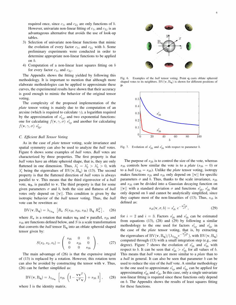
Functions s′1p and s′2p can be estimated from (20) by ex-tracting the eigenvalues of PV(v,Pq)/(λ1Pq

f(v, γ, σ)), withPV(v,Pq) computed through (11) with a small integrationstep (e.g., one degree). Figure 5 shows the curves of s′1pand s′2p vs. γ for different values of b. These curves havea discontinuity at γ = π/4. This was expected since the sticktensor voting also has a discontinuity at the same angle. Thecurves corresponding to s′1p and s′2p show that there are mainlytwo zones in the 3D space depending on which s′1p or s′2p isdominant, which is congruent with the observations made onFigure 3. The curves of s′1p and s′2p also show that b can beused to control the spread of the voting cone of Figure 3, sinceit becomes narrower as b is increased. These curves can beapproximated through any fitting method. As an example, sucha fitting can be done by applying two consecutive univariatenon-linear fittings as follows:

1) Selection of univariate non-linear functions that mimicthe shape of s′1p and s′2p for different fixed valuesof b. Some preliminary experiments were conductedwith different non-linear functions in order to determinesuitable non-linear functions to be applied to γ. Thesefunctions contain factors c1i and c2j , with i = 1, . . . , 6and j = 1, . . . , 4, which can be optimized by non-linearleast squares fitting.

2) Computation of a non-linear least squares fitting on γfor every different value of b. This process yields adifferent value of c1i and c2j for every different valueof b. At this point, these factors can be stored in orderto be queried as look-up tables. These queries are only

6

required once, since c1i and c2j are only functions of b.However, univariate non-linear fitting of c1i and c2j is anadvantageous alternative that avoids the use of look-uptables.

3) Selection of univariate non-linear functions that mimicthe evolution of every factor c1i and c2j with b. Somepreliminary experiments were conducted in order todetermine appropriate non-linear functions to be appliedon b.

4) Computation of a non-linear least squares fitting on bfor every factor c1i and c2j .

The Appendix shows the fitting yielded by following thismethodology. It is important to mention that although moreelaborate methodologies can be applied to approximate thesecurves, the experimental results have shown that their accuracyis good enough to mimic the behavior of the original tensorvoting.

The complexity of the proposed implementation of theplate tensor voting is mainly due to the computation of anarcsine (which is required to calculate γ), a logarithm requiredby the approximation of s′1p, and two exponential functions:one for calculating f(v, γ, σ) s′1p and another for calculatingf(v, γ, σ) s′2p.

C. Efficient Ball Tensor Voting

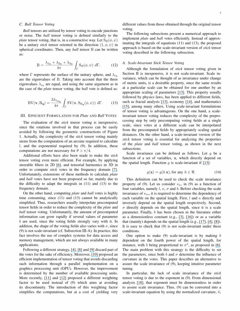
As in the case of plate tensor voting, scale invariance andspatial symmetry can also be used to analyze the ball votes.Figure 6 shows some examples of ball votes. Ball votes arecharacterized by three properties. The first property is thatball votes have an oblate spheroid shape, that is, they are onlyflattened in one dimension. Thus, λ′1 = λ′2 > λ′3 > 0, withλ′i being the eigenvalues of BV(v,Bq) in (13). The secondproperty is that the flattened direction of ball votes is alwaysparallel to v. This means that the third eigenvector of a ballvote, u3, is parallel to v. The third property is that for somegiven parameters σ and b, both the size and flatness of ballvotes only depend on ||v||. This condition is given by theisotropic behavior of the ball tensor voting. Thus, the ballvote can be rewritten as:

BV(v,Bq) = λ1Bq

[Rv S(s2b, s2b, s3b) Bq R

Tv

], (26)

where Rv is a rotation that makes u3 and v parallel, s2b ands3b are functions defined below, and S is a scale transformationthat converts the ball tensor Bq into an oblate spheroid shapedtensor given by:

S(s2, s2, s3) =

s2b 0 00 s2b 00 0 s3b

. (27)

The main advantage of (26) is that the expensive integralof (13) is replaced by a rotation. However, this rotation termcan also be avoided by constructing the tensor with v. Thus,(26) can be further simplified as:

BV(v,Bq) = λ1Bq

[s2b

(I− vvT

vTv

)+ s3b I

], (28)

where I is the identity matrix.

Bq

q z

yx

Fig. 6. Examples of the ball tensor voting. Point q casts oblate spheroidshaped votes to its neighbors. BV(v,Bq) is shown for different positions ofp.

0 20 40 60 80 1000

0.1

0.2

0.3

0.4

0.5

b

s′2b

s′3b

Fig. 7. Evolution of s′2b and s′3b with respect to parameter b.

The purpose of s2b is to control the size of the vote, whereass3b controls how similar the vote is to a plate (s3b = 0) orto a ball (s3b = s2b). Unlike the plate tensor voting, isotropymakes functions s2b and s3b only depend on ||v|| for specificparameters σ and b. Thus, thanks to the scale invariance, s2b

and s3b can be divided into a Gaussian decaying function on||v|| with a standard deviation σ and functions s′2b, s

′3b that

only depend on b and cannot be analytically simplified, sincethey capture most of the non-linearities of (13). Thus, sib isdefined as:

sib(v, σ, b) = s′ib e− vT v

σ2 , (29)

for i = 2 and i = 3. Factors s′2b and s′3b can be estimatedfrom equations (13), (28) and (29) by following a similarmethodology to the one used for factors s′1p and s′2p inthe case of the plate tensor voting, that is, by extractingthe eigenvalues of BV(v,Bq)/(λ1Bq

e−vT vσ2 ), with BV(v,Bq)

computed through (13) with a small integration step (e.g., onedegree). Figure 7 shows the evolution of s′2b and s′3b withrespect to b. It can be seen that s′2b > s′3b for all values of b.This means that ball votes are more similar to a plate than toa ball in general. It can also be seen that parameter b can beused to reduce the size of the ball vote. A similar methodologyto the one used to approximate s′1p and s′2p can be applied forapproximating s′2b and s′3b. In this case, only a single univariatenon-linear fitting is required since these functions only dependon b. The Appendix shows the results of least squares fittingfor these functions.

7

0 20 40 60 800

0.2

0.4

0.6

0.8

1

γ [degrees]

s′ 1p

0 20 40 60 800

0.2

0.4

0.6

0.8

1

γ [degrees]

s′ 2p

b = 0

b = 1

b = 5

b = 10

b = 25

b = 50

b = 100

b = 1000

Fig. 5. s′1p and s′2p as functions of γ for different values of parameter b.

The complexity of the proposed implementation of the balltensor voting is mainly due to the computation of a singleexponential (required in (29)), since the values of s′2b and s′3bare computed only once.

IV. SIMPLIFIED TENSOR VOTING

This section explores an alternative to the numerical ap-proach described in the previous section for calculating tensorvoting efficiently. This alternative is based on a simplifiedformulation that reduces the numerical complexity while keep-ing the same perceptual rules of tensor voting. The nextsubsections describe the proposed method to calculate stick,plate and ball tensor votes more efficiently.

A. Stick Tensor VotingThe original stick tensor voting can be further simplified

while keeping its perceptual meaning by redesigning theweighting function s1s defined in (16). This function has twoparameters: b that penalizes the curvature, and σ that penalizesboth the distance and curvature (the latter through the θ/ sin(θ)factor included in the computation of l in (7)). Thus, forexample, it is not possible to avoid the influence of curvatureon the calculations, even selecting b = 0, since σ not onlyaffects the distance but also the θ/ sin(θ) factor, which isrelated to curvature. For this reason, every parameter has asingle task: σ becomes a scale parameter, and b a curvatureparameter:

s1s(v,Sq) =

{e−

vT vσ2−b sin2(θ) if θ ≤ π/4

0 otherwise.(30)

This equation has the additional advantage that the arcsinerequired for calculating stick votes is no longer necessary. Notethat the only difference between (30) and (16) is the use ofthe squared Euclidean distance (vTv) instead of the squaredarc length (l2), since sin(θ) = κ. This simplification is alsobased on the fact that the difference between using Euclideandistances and arc lenghts is relatively small. The use of arclengths can be seen as spatial stretchings of at most 11%(attained at θ = π/4) and 5.5% (attained at γ = π/4) forstick and plate votes respectively. Thus, in general, the effectof the curvature on the votes can be better controlled throughb.

B. Plate Tensor Voting

Proposing simplified equations for the plate tensor votingrequires to understand the perceptual meaning of plate votes.From the analysis carried out in Subsection III-B, it can bestated that, from a perceptual point of view, a plate voteencodes two different hypotheses, one for every componentof the vote.

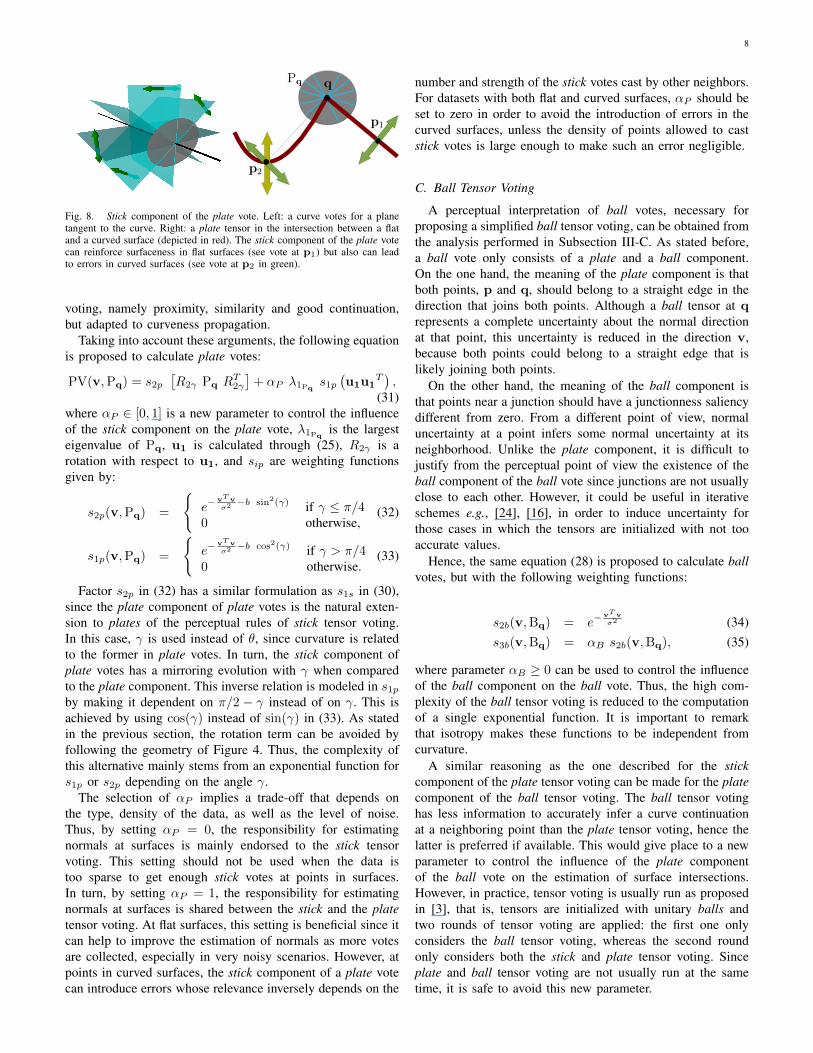
On the one hand, the hypothesis made by the stick compo-nent of the plate vote is that a neighboring point p of the voterq should belong to a surface that abuts the curve that crossesq. However, spatial symmetry makes such a surface be a plane,since the stick component is always tangent to the plate Pq

(see Figure 8). Thus, the stick component of the plate tensorvoting can be thought of as a stick tensor voting that makesa stronger hypothesis than the stick tensor voting itself, sincecurved surfaces are only encouraged in the latter. As seen inFigure 8, the stick component of the plate vote can lead toerrors in curved surfaces that must be corrected through stickvotes cast by other neighbors. This stick component mainlyappears outside the cone of Figure 3, since points inside thecone can either belong to the curve that crosses q or to anothersurface.

In other words, the plate tensor voting has less perceptualinformation to accurately infer a normal at a neighboring pointthan the stick tensor voting. Thus, it is more likely to estimatenormals more accurately with the stick tensor voting than withthe stick component of the plate tensor voting. However, ifno more information is available, for example, if the receiveronly gets votes cast by plates, the estimation computed by theplate tensor voting can be used as the most likely normal atthe receiver.

On the other hand, the hypothesis made by the platecomponent of the plate vote is that both points, p and q,should belong to the same curve. In that sense, p completesthe path of the curve that crosses q. This component mainlyappears inside the cone of Figure 3, since points outside thatcone are more unlikely to belong to the same curve. Thus,the plate component of the plate vote can be thought of as thenatural extension of the stick tensor voting in which curvenessinstead of surfaceness is smoothly propagated by followingsimilar rules. Hence, the plate component can be consideredto be based on the same Gestalt principles as the stick tensor

8

qPq

p1

p2

Fig. 8. Stick component of the plate vote. Left: a curve votes for a planetangent to the curve. Right: a plate tensor in the intersection between a flatand a curved surface (depicted in red). The stick component of the plate votecan reinforce surfaceness in flat surfaces (see vote at p1) but also can leadto errors in curved surfaces (see vote at p2 in green).

voting, namely proximity, similarity and good continuation,but adapted to curveness propagation.

Taking into account these arguments, the following equationis proposed to calculate plate votes:

PV(v,Pq) = s2p

[R2γ Pq R

T2γ

]+ αP λ1Pq

s1p

(u1u1

T),

(31)where αP ∈ [0, 1] is a new parameter to control the influenceof the stick component on the plate vote, λ1Pq

is the largesteigenvalue of Pq, u1 is calculated through (25), R2γ is arotation with respect to u1, and sip are weighting functionsgiven by:

s2p(v,Pq) =

{e−

vT vσ2−b sin2(γ) if γ ≤ π/4

0 otherwise,(32)

s1p(v,Pq) =

{e−

vT vσ2−b cos2(γ) if γ > π/4

0 otherwise.(33)

Factor s2p in (32) has a similar formulation as s1s in (30),since the plate component of plate votes is the natural exten-sion to plates of the perceptual rules of stick tensor voting.In this case, γ is used instead of θ, since curvature is relatedto the former in plate votes. In turn, the stick component ofplate votes has a mirroring evolution with γ when comparedto the plate component. This inverse relation is modeled in s1p

by making it dependent on π/2 − γ instead of on γ. This isachieved by using cos(γ) instead of sin(γ) in (33). As statedin the previous section, the rotation term can be avoided byfollowing the geometry of Figure 4. Thus, the complexity ofthis alternative mainly stems from an exponential function fors1p or s2p depending on the angle γ.

The selection of αP implies a trade-off that depends onthe type, density of the data, as well as the level of noise.Thus, by setting αP = 0, the responsibility for estimatingnormals at surfaces is mainly endorsed to the stick tensorvoting. This setting should not be used when the data istoo sparse to get enough stick votes at points in surfaces.In turn, by setting αP = 1, the responsibility for estimatingnormals at surfaces is shared between the stick and the platetensor voting. At flat surfaces, this setting is beneficial since itcan help to improve the estimation of normals as more votesare collected, especially in very noisy scenarios. However, atpoints in curved surfaces, the stick component of a plate votecan introduce errors whose relevance inversely depends on the

number and strength of the stick votes cast by other neighbors.For datasets with both flat and curved surfaces, αP should beset to zero in order to avoid the introduction of errors in thecurved surfaces, unless the density of points allowed to caststick votes is large enough to make such an error negligible.

C. Ball Tensor Voting

A perceptual interpretation of ball votes, necessary forproposing a simplified ball tensor voting, can be obtained fromthe analysis performed in Subsection III-C. As stated before,a ball vote only consists of a plate and a ball component.On the one hand, the meaning of the plate component is thatboth points, p and q, should belong to a straight edge in thedirection that joins both points. Although a ball tensor at qrepresents a complete uncertainty about the normal directionat that point, this uncertainty is reduced in the direction v,because both points could belong to a straight edge that islikely joining both points.

On the other hand, the meaning of the ball component isthat points near a junction should have a junctionness saliencydifferent from zero. From a different point of view, normaluncertainty at a point infers some normal uncertainty at itsneighborhood. Unlike the plate component, it is difficult tojustify from the perceptual point of view the existence of theball component of the ball vote since junctions are not usuallyclose to each other. However, it could be useful in iterativeschemes e.g., [24], [16], in order to induce uncertainty forthose cases in which the tensors are initialized with not tooaccurate values.

Hence, the same equation (28) is proposed to calculate ballvotes, but with the following weighting functions:

s2b(v,Bq) = e−vT vσ2 (34)

s3b(v,Bq) = αB s2b(v,Bq), (35)

where parameter αB ≥ 0 can be used to control the influenceof the ball component on the ball vote. Thus, the high com-plexity of the ball tensor voting is reduced to the computationof a single exponential function. It is important to remarkthat isotropy makes these functions to be independent fromcurvature.

A similar reasoning as the one described for the stickcomponent of the plate tensor voting can be made for the platecomponent of the ball tensor voting. The ball tensor votinghas less information to accurately infer a curve continuationat a neighboring point than the plate tensor voting, hence thelatter is preferred if available. This would give place to a newparameter to control the influence of the plate componentof the ball vote on the estimation of surface intersections.However, in practice, tensor voting is usually run as proposedin [3], that is, tensors are initialized with unitary balls andtwo rounds of tensor voting are applied: the first one onlyconsiders the ball tensor voting, whereas the second roundonly considers both the stick and plate tensor voting. Sinceplate and ball tensor voting are not usually run at the sametime, it is safe to avoid this new parameter.

9

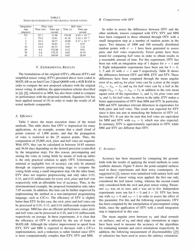
TABLE ISPEED MEASUREMENTS OF THE ORIGINAL TENSOR VOTING

Integration Plate votes Ball votesstep Time (ms) Votes per Time (s) Votes per

(degrees) second second0.5 87.1 11.48 124.48 8.03× 10−3

1 79.3 12.61 41.10 2.43× 10−2

2 32.5 30.77 10.90 9.17× 10−2

5 19.0 52.63 1.75 0.5710 12.0 83.33 0.45 2.2220 6.6 152.88 0.12 8.0130 5.6 178.25 0.05 19.1945 5.3 189.04 0.03 28.49

V. EXPERIMENTAL RESULTS

The formulations of the original (OTV), efficient (ETV) andsimplified tensor voting (STV) presented above were coded inMATLAB on an Intel Core 2 Quad Q6600 with a 4GB RAM inorder to compare the new proposed schemes with the originaltensor voting. In addition, the approximation scheme describedin [4], [8], referred to as MM, has also been coded to compareits performance with the proposed methods. Equation (16) hasbeen applied instead of (9) in order to make the results of alltested methods comparable.

A. Efficiency

Table I shows the mean execution times of the testedmethods. This table shows that OTV is impractical for manyapplications. As an example, assume that a small cloud ofpoints consists of 1,000 points, and that the propagationof votes is restricted to the 25 nearest points. Thus, thecomputation of 25,000 stick, plate and ball votes are required.With OTV, they can be calculated in between 16.85 minutesand 36.04 days depending on the desired precision (controlledby the integration step). For this reason, precomputing andstoring the votes in voting fields by means of look-up tablesis the only practical solution to apply OTV. Unfortunately,minimal or negligible loss of accuracy can only be attainedthrough an expensive preprocessing stage to compute thevoting fields using a small integration step. On the other hand,ETV does not requires preprocessing and only takes 0.05,0.18, and 0.05 milliseconds for every stick, plate and ball voterespectively with an affordable loss of accuracy. Thus, in theaforementioned example, the proposed formulation only takes7.05 seconds. In addition, this time can be further improved byimplementing the method in a non-interpreted programminglanguage, such as C/C++. The efficiency of STV is slightlybetter than ETV. In this case, the stick, plate and ball votes canbe processed in 0.05, 0.15, and 0.04 milliseconds respectivelyon average. MM has also an efficient performance, since plateand ball votes can be processed in 0.20, and 0.04 millisecondsrespectively on average. In these experiments, it is clear thatthe efficiency of OTV is affected by the use of loops inMATLAB. Although the relative improvement in speed fromETV, STV and MM is expected to decrease with a C/C++implementation, such a reduction is rather limited since OTVis more computationally complex than ETV, STV and MM.

B. Comparisons with OTV

In order to assess the differences between OTV and theother methods, tensors computed with ETV, STV and MMhave been compared to those obtained through OTV with asmall integration step at a number of random points in thespace. Two datasets of 1000 and 100 normally distributedrandom points with σ = 1 have been generated to assessplate and ball votes respectively. Fewer points have beentested for comparing ball votes in order to obtain results ina reasonable amount of time. For this experiment, OTV hasbeen run with an integration step of 1 degree for σ = 1 and5. Eight independent experiments have been run for b = 0,1, 5 and 10 with σ = 1 and 5 respectively. Table II showsthe differences between OTV and MM, ETV and STV. Thesedifferences have been computed through the mean angularerror of e1 and e3 for plate votes cast by a plate at the origin(λ1P

= λ2P= 1), and e3 for ball votes cast by a ball at the

origin (λ1B = λ2B = λ3B = 1), in addition to the root meansquare error of the eigenvalues λ1 and λ2 for plate votes andλ2 and λ3 for ball votes. As shown in the table, ETV makes abetter approximation of OTV than MM and STV. In particular,MM and STV introduce relevant diferences in eigenvalues forboth plate and ball votes. This result was expected for STVsince it does not aim at mimicking the behavior of OTV (cf.Section IV). It can also be seen that ball votes are equivalentfor MM and STV with αB = 0, which was also expected.In summary, ETV is approximately equivalent to OTV, whileMM and STV are different than OTV.

C. Accuracy

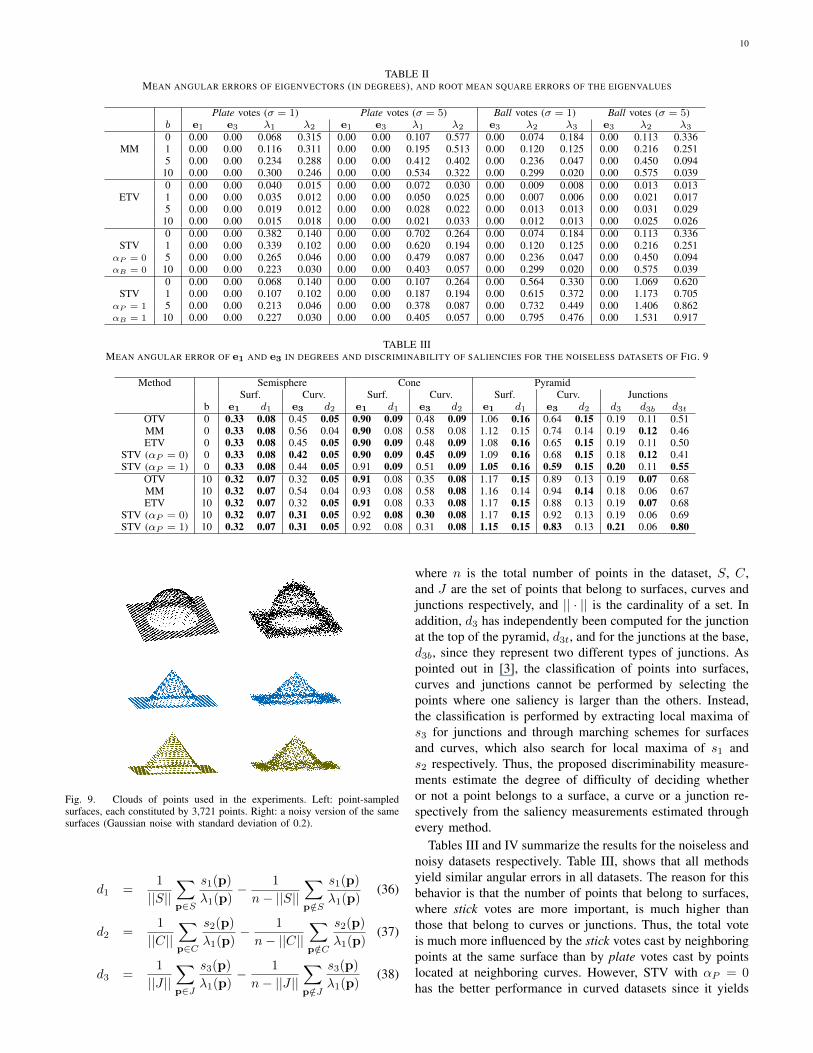
Accuracy has been measured by comparing the ground-truth with the results of applying the tested methods to somesynthetic datasets. Figure 9 shows the point-sampled surfacesused in these experiments and their noisy counterparts. Assuggested in [3], tensors were initialized with unitary balls andtwo rounds of tensor voting were applied: the first one onlyconsidered the ball tensor voting, whereas the second roundonly considered both the stick and plate tensor voting. Param-eter αB was set to zero, and σ was set to five. Independentexperiments were run for b = 0 and b = 10. STV has beenrun with αP = 0 and αP = 1 in order to assess the effect ofthis parameter. For this and the following experiments, OTVhas been computed by the interpolation of precomputed votingfields, since the application of OTV with a small integrationstep is impractical in this case.

The mean angular error between e1 and ideal normalson surfaces, and of e3 and ideal edge orientations at edgeshave been used to measure the accuracy of the algorithmsfor estimating normals and curve orientations respectively. Inaddition, the following measurement of discriminability [25]of saliencies has been used to assess the saliency estimation:

10

TABLE IIMEAN ANGULAR ERRORS OF EIGENVECTORS (IN DEGREES), AND ROOT MEAN SQUARE ERRORS OF THE EIGENVALUES

Plate votes (σ = 1) Plate votes (σ = 5) Ball votes (σ = 1) Ball votes (σ = 5)b e1 e3 λ1 λ2 e1 e3 λ1 λ2 e3 λ2 λ3 e3 λ2 λ3

MM0 0.00 0.00 0.068 0.315 0.00 0.00 0.107 0.577 0.00 0.074 0.184 0.00 0.113 0.3361 0.00 0.00 0.116 0.311 0.00 0.00 0.195 0.513 0.00 0.120 0.125 0.00 0.216 0.2515 0.00 0.00 0.234 0.288 0.00 0.00 0.412 0.402 0.00 0.236 0.047 0.00 0.450 0.094

10 0.00 0.00 0.300 0.246 0.00 0.00 0.534 0.322 0.00 0.299 0.020 0.00 0.575 0.039

ETV0 0.00 0.00 0.040 0.015 0.00 0.00 0.072 0.030 0.00 0.009 0.008 0.00 0.013 0.0131 0.00 0.00 0.035 0.012 0.00 0.00 0.050 0.025 0.00 0.007 0.006 0.00 0.021 0.0175 0.00 0.00 0.019 0.012 0.00 0.00 0.028 0.022 0.00 0.013 0.013 0.00 0.031 0.029

10 0.00 0.00 0.015 0.018 0.00 0.00 0.021 0.033 0.00 0.012 0.013 0.00 0.025 0.0260 0.00 0.00 0.382 0.140 0.00 0.00 0.702 0.264 0.00 0.074 0.184 0.00 0.113 0.336

STV 1 0.00 0.00 0.339 0.102 0.00 0.00 0.620 0.194 0.00 0.120 0.125 0.00 0.216 0.251αP = 0 5 0.00 0.00 0.265 0.046 0.00 0.00 0.479 0.087 0.00 0.236 0.047 0.00 0.450 0.094αB = 0 10 0.00 0.00 0.223 0.030 0.00 0.00 0.403 0.057 0.00 0.299 0.020 0.00 0.575 0.039

0 0.00 0.00 0.068 0.140 0.00 0.00 0.107 0.264 0.00 0.564 0.330 0.00 1.069 0.620STV 1 0.00 0.00 0.107 0.102 0.00 0.00 0.187 0.194 0.00 0.615 0.372 0.00 1.173 0.705αP = 1 5 0.00 0.00 0.213 0.046 0.00 0.00 0.378 0.087 0.00 0.732 0.449 0.00 1.406 0.862αB = 1 10 0.00 0.00 0.227 0.030 0.00 0.00 0.405 0.057 0.00 0.795 0.476 0.00 1.531 0.917

TABLE IIIMEAN ANGULAR ERROR OF e1 AND e3 IN DEGREES AND DISCRIMINABILITY OF SALIENCIES FOR THE NOISELESS DATASETS OF FIG. 9

Method Semisphere Cone PyramidSurf. Curv. Surf. Curv. Surf. Curv. Junctions

b e1 d1 e3 d2 e1 d1 e3 d2 e1 d1 e3 d2 d3 d3b d3tOTV 0 0.33 0.08 0.45 0.05 0.90 0.09 0.48 0.09 1.06 0.16 0.64 0.15 0.19 0.11 0.51MM 0 0.33 0.08 0.56 0.04 0.90 0.08 0.58 0.08 1.12 0.15 0.74 0.14 0.19 0.12 0.46ETV 0 0.33 0.08 0.45 0.05 0.90 0.09 0.48 0.09 1.08 0.16 0.65 0.15 0.19 0.11 0.50

STV (αP = 0) 0 0.33 0.08 0.42 0.05 0.90 0.09 0.45 0.09 1.09 0.16 0.68 0.15 0.18 0.12 0.41STV (αP = 1) 0 0.33 0.08 0.44 0.05 0.91 0.09 0.51 0.09 1.05 0.16 0.59 0.15 0.20 0.11 0.55

OTV 10 0.32 0.07 0.32 0.05 0.91 0.08 0.35 0.08 1.17 0.15 0.89 0.13 0.19 0.07 0.68MM 10 0.32 0.07 0.54 0.04 0.93 0.08 0.58 0.08 1.16 0.14 0.94 0.14 0.18 0.06 0.67ETV 10 0.32 0.07 0.32 0.05 0.91 0.08 0.33 0.08 1.17 0.15 0.88 0.13 0.19 0.07 0.68

STV (αP = 0) 10 0.32 0.07 0.31 0.05 0.92 0.08 0.30 0.08 1.17 0.15 0.92 0.13 0.19 0.06 0.69STV (αP = 1) 10 0.32 0.07 0.31 0.05 0.92 0.08 0.31 0.08 1.15 0.15 0.83 0.13 0.21 0.06 0.80

Fig. 9. Clouds of points used in the experiments. Left: point-sampledsurfaces, each constituted by 3,721 points. Right: a noisy version of the samesurfaces (Gaussian noise with standard deviation of 0.2).

d1 =1

||S||∑p∈S

s1(p)

λ1(p)− 1

n− ||S||∑p/∈S

s1(p)

λ1(p)(36)

d2 =1

||C||∑p∈C

s2(p)

λ1(p)− 1

n− ||C||∑p/∈C

s2(p)

λ1(p)(37)

d3 =1

||J ||∑p∈J

s3(p)

λ1(p)− 1

n− ||J ||∑p/∈J

s3(p)

λ1(p)(38)

where n is the total number of points in the dataset, S, C,and J are the set of points that belong to surfaces, curves andjunctions respectively, and || · || is the cardinality of a set. Inaddition, d3 has independently been computed for the junctionat the top of the pyramid, d3t, and for the junctions at the base,d3b, since they represent two different types of junctions. Aspointed out in [3], the classification of points into surfaces,curves and junctions cannot be performed by selecting thepoints where one saliency is larger than the others. Instead,the classification is performed by extracting local maxima ofs3 for junctions and through marching schemes for surfacesand curves, which also search for local maxima of s1 ands2 respectively. Thus, the proposed discriminability measure-ments estimate the degree of difficulty of deciding whetheror not a point belongs to a surface, a curve or a junction re-spectively from the saliency measurements estimated throughevery method.

Tables III and IV summarize the results for the noiseless andnoisy datasets respectively. Table III, shows that all methodsyield similar angular errors in all datasets. The reason for thisbehavior is that the number of points that belong to surfaces,where stick votes are more important, is much higher thanthose that belong to curves or junctions. Thus, the total voteis much more influenced by the stick votes cast by neighboringpoints at the same surface than by plate votes cast by pointslocated at neighboring curves. However, STV with αP = 0has the better performance in curved datasets since it yields

11

smaller angular errors for e3. In turn, STV with αP = 1 hasthe best performance for the pyramid according to the meanangular errors. That means that points in curves are actuallyaffected by plate votes cast from points located at neighboringsurfaces. Errors related to plate votes are mitigated at pointsbelonging to surfaces by the fact that they receive more stickvotes from other points in the same surface. It is also importantto note that parameter b barely influences angular errors and ittends to reduce the discriminability measurements in noiselessscenarios. Another observation with respect to this table isthat discriminability measurements are relatively small. Thisdoes not suppose a problem for detecting curves and junctions,since they are located at points where saliencies s2 and s3

attain local maxima values respectively. Alternatively, iterativeschemes can also be used to increase these discriminabilitymeasurements.

In turn, Table IV shows that, although the angular errorsare higher, the observations made for noiseless scenariosare also valid in noisy ones. That is, STV yields the bestresults for curved scenarios by setting αP = 0 and for thepyramid by setting αP = 1. An interesting observation is thatdiscriminability measurements d1 and d2 are similar to thosereported in Table III. That means that the detection of curves isalmost not influenced by noise. On the other hand, although thediscriminability measurement d3t is more affected by noise,the values are still high. In addition, the discriminability d3b

is less affected by noise. This means that junctions at the baseof the pyramid can also be extracted from a noisy scenario.

Regarding MM, this experiment confirms the observationmade in Table II in the sense that it is different from OTV,since both yield different results. In addition, the approxima-tion made by MM usually yields worse results than OTV. How-ever, it remains a good alternative to the methods proposed inthis paper. As for ETV, this experiments show that it succeedsin mimicking the behavior of OTV, since it yields almost theresult in all measurements.

D. Effect of Parameter αP of STV

The effect of the stick component of plate votes has been as-sessed by measuring the distortion introduced by the methodswhen the tensors are initialized with the ground-truth for thecloud of points shown in Figure 10. The same measurementsused in the previous experiment have been applied to thisexperiment and σ has been set to five. Table V shows thatSTV with αP = 0 is the method that less angular distortionintroduces both for b = 0 and b = 10. However, the differencesbetween STV and the other methods are reduced for b = 10.The reason of this behavior is that fewer points at curves areallowed to cast stick components, so their influence in the totalvote is reduced in such a case. Although STV with αP = 1is the method that induces less reductions in discriminabilityof saliencies, it has a bad performance in this dataset, since itintroduces higher angular errors. That means that that settingαP = 1 is not appropriate for curved datasets. An expectedresult was a reduction in the discriminability of saliencies,which are one in the ground-truth, for all tested methods. Sincethese reductions are relatively small, especially for b = 10,

Fig. 10. Cloud of points used to assess the effect of the stick component ofplate votes.

they can be thought of as the small price that tensor votinghas to pay for yielding robust results.

In addition, Table V shows the results on this datasetfor tensors initialized with unitary balls and two appliedrounds of tensor voting: one for ball votes and the otherfor stick and plate votes. For this dataset, angular errors anddiscriminabilities are larger than the values reported in TablesIII and IV for other datasets. This is mainly due to two factors.First, the surfaces are intersected in an angle of 90 degrees,which maximizes the saliency s2 in curves, leading to anincrease in d1 and d2. Second, the dataset is rather sparse,so fewer votes are received at every point. Thus, the effectof an erroneous vote cannot be effectively compensated withenough correct ones, leading to an increase in the angularerrors.

E. Effect of Parameter αB of STV

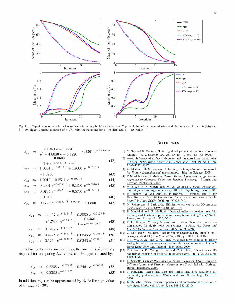
Values of αB greater than zero are only useful in iterativeschemes where tensors have been initialized with bad esti-mations of the normals. In order to test the effect of thisparameter, fifteen iterations of the stick, plate and ball tensorvoting have been run for a sampled flat surface. Tensors havebeen initialized with one of the worst possible scenarios, thatis, with tensors that are perpendicular to the normals in thesurface. In particular, tensors have been initialized with platetensors that are tangent to the surface. Thus, the angular errorof e1 is 90 degrees at the beginning of the process. In addition,a small ball component has also been added to the tensorsin order to force the application of the ball tensor voting inthe first iteration. Parameter αB has been set to ten for thefirst iteration and to zero for the subsequent iterations, sincebetter estimations of the tensors are then available. Parameterσ has been set to two, while αP has been set to zero. The arccosine of the normalized tensor scalar product has been usedto measure the tensor deviation, tdev, of the yielded tensorT(p) with respect to the ground-truth Tg(p) at every point ofthe dataset. This measure is given by [26], [27]:

tdev(p) = arccos

(〈T(p),Tg(p)〉

trace(T(p)) trace(Tg(p))

), (39)

where 〈A,B〉 = trace(ABT ) is the scalar product betweentensors A and B. This measurement has the advantage that itis able to assess differences in orientation and anisotropy ofthe tensors at the same time.

Figure 11 shows the evolution with the iterations of themean of tdev and the mean of the saliency s1 normalizedby the largest eigenvalue λ1. This figure shows that STV has

12

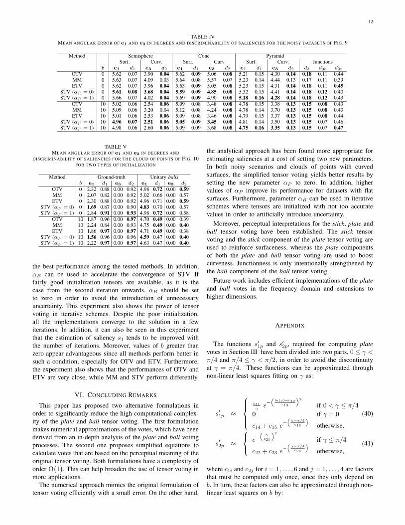
TABLE IVMEAN ANGULAR ERROR OF e1 AND e3 IN DEGREES AND DISCRIMINABILITY OF SALIENCIES FOR THE NOISY DATASETS OF FIG. 9

Method Semisphere Cone PyramidSurf. Curv. Surf. Curv. Surf. Curv. Junctions

b e1 d1 e3 d2 e1 d1 e3 d2 e1 d1 e3 d2 d3 d3b d3tOTV 0 5.62 0.07 3.90 0.04 5.62 0.09 5.06 0.08 5.21 0.15 4.30 0.14 0.18 0.11 0.44MM 0 5.63 0.07 4.09 0.03 5.64 0.08 5.57 0.07 5.23 0.14 4.44 0.13 0.17 0.11 0.39ETV 0 5.62 0.07 3.96 0.04 5.63 0.09 5.05 0.08 5.23 0.15 4.31 0.14 0.18 0.11 0.45

STV (αP = 0) 0 5.61 0.08 3.68 0.04 5.59 0.09 4.85 0.08 5.32 0.15 4.41 0.14 0.18 0.12 0.40STV (αP = 1) 0 5.66 0.07 4.02 0.04 5.69 0.09 4.90 0.08 5.18 0.16 4.28 0.14 0.18 0.12 0.43

OTV 10 5.02 0.06 2.54 0.06 5.09 0.08 3.48 0.08 4.78 0.15 3.38 0.13 0.15 0.08 0.43MM 10 5.09 0.06 3.20 0.04 5.12 0.08 4.24 0.08 4.78 0.14 3.70 0.13 0.15 0.08 0.43ETV 10 5.01 0.06 2.53 0.06 5.09 0.08 3.46 0.08 4.79 0.15 3.37 0.13 0.15 0.08 0.44

STV (αP = 0) 10 4.96 0.07 2.51 0.06 5.05 0.09 3.45 0.08 4.81 0.14 3.50 0.13 0.15 0.07 0.46STV (αP = 1) 10 4.98 0.06 2.60 0.06 5.09 0.09 3.68 0.08 4.75 0.16 3.35 0.13 0.15 0.07 0.47

TABLE VMEAN ANGULAR ERROR OF e1 AND e3 IN DEGREES AND

DISCRIMINABILITY OF SALIENCIES FOR THE CLOUD OF POINTS OF FIG. 10FOR TWO TYPES OF INITIALIZATION

Method Ground-truth Unitary ballsb e1 d1 e3 d2 e1 d1 e3 d2

OTV 0 2.32 0.88 0.00 0.92 4.98 0.72 0.00 0.59MM 0 2.07 0.82 0.00 0.92 5.02 0.66 0.00 0.57ETV 0 2.30 0.88 0.00 0.92 4.96 0.71 0.00 0.59

STV (αP = 0) 0 1.69 0.87 0.00 0.90 4.83 0.70 0.00 0.57STV (αP = 1) 0 2.84 0.91 0.00 0.93 4.98 0.72 0.00 0.58

OTV 10 1.87 0.96 0.00 0.97 4.70 0.49 0.00 0.39MM 10 2.24 0.84 0.00 0.93 4.75 0.49 0.00 0.40ETV 10 1.86 0.97 0.00 0.97 4.71 0.49 0.00 0.38

STV (αP = 0) 10 1.56 0.96 0.00 0.96 4.59 0.47 0.00 0.40STV (αP = 1) 10 2.22 0.97 0.00 0.97 4.63 0.47 0.00 0.40

the best performance among the tested methods. In addition,αB can be used to accelerate the convergence of STV. Iffairly good initialization tensors are available, as it is thecase from the second iteration onwards, αB should be setto zero in order to avoid the introduction of unnecessaryuncertainty. This experiment also shows the power of tensorvoting in iterative schemes. Despite the poor initialization,all the implementations converge to the solution in a fewiterations. In addition, it can also be seen in this experimentthat the estimation of saliency s1 tends to be improved withthe number of iterations. Moreover, values of b greater thanzero appear advantageous since all methods perform better insuch a condition, especially for OTV and ETV. Furthermore,the experiment also shows that the performances of OTV andETV are very close, while MM and STV perform differently.

VI. CONCLUDING REMARKS

This paper has proposed two alternative formulations inorder to significantly reduce the high computational complex-ity of the plate and ball tensor voting. The first formulationmakes numerical approximations of the votes, which have beenderived from an in-depth analysis of the plate and ball votingprocesses. The second one proposes simplified equations tocalculate votes that are based on the perceptual meaning of theoriginal tensor voting. Both formulations have a complexity oforder O

(1). This can help broaden the use of tensor voting in

more applications.The numerical approach mimics the original formulation of

tensor voting efficiently with a small error. On the other hand,

the analytical approach has been found more appropriate forestimating saliencies at a cost of setting two new parameters.In both noisy scenarios and clouds of points with curvedsurfaces, the simplified tensor voting yields better results bysetting the new parameter αP to zero. In addition, highervalues of αP improve its performance for datasets with flatsurfaces. Furthermore, parameter αB can be used in iterativeschemes where tensors are initialized with not too accuratevalues in order to artificially introduce uncertainty.

Moreover, perceptual interpretations for the stick, plate andball tensor voting have been established. The stick tensorvoting and the stick component of the plate tensor voting areused to reinforce surfaceness, whereas the plate componentsof both the plate and ball tensor voting are used to boostcurveness. Junctionness is only intentionally strengthened bythe ball component of the ball tensor voting.

Future work includes efficient implementations of the plateand ball votes in the frequency domain and extensions tohigher dimensions.

APPENDIX

The functions s′1p and s′2p, required for computing platevotes in Section III have been divided into two parts, 0 ≤ γ <π/4 and π/4 ≤ γ < π/2, in order to avoid the discontinuityat γ = π/4. These functions can be approximated throughnon-linear least squares fitting on γ as:

s′1p ≈

c11γ e

−(

ln(γ)−c12c13

)2

if 0 < γ ≤ π/40 if γ = 0

c14 + c15 e−(γ−π/4c16

)otherwise,

(40)

s′2p ≈

e−(γc21

)2

if γ ≤ π/4

c22 + c23 e−(γ−π/4c24

)otherwise,

(41)

where c1i and c2j for i = 1, . . . , 6 and j = 1, . . . , 4 are factorsthat must be computed only once, since they only depend onb. In turn, these factors can also be approximated through non-linear least squares on b by:

13

0 5 10 150

20

40

60

80

Iterations

Mea

noftdev

(deg

rees

)

0 5 10 150

20

40

60

80

Iterations

Mea

noftdev

(deg

rees

)

OTV

MM

ETV

STV (αB = 0)

STV (αB = 10)

0 5 10 150

0.2

0.4

0.6

0.8

1

Iterations

Mea

nofs 1/λ

1

0 5 10 150

0.2

0.4

0.6

0.8

1

Iterations

Mea

nofs 1/λ

1

OTV

MM

ETV

STV (αB = 0)

STV (αB = 10)

Fig. 11. Experiments on αB for a flat surface with wrong initialization tensors. Top: evolution of the mean of tdev with the iterations for b = 0 (left) andb = 10 (right). Bottom: evolution of s1/λ1 with the iterations for b = 0 (left) and b = 10 (right).

c11 ≈ 6.5360 b− 3.7920

b2 + 4.8680 b− 5.4220− 0.3301 e−0.1501 b

+0.0600

1 + e−0.0401 (b−25.0)(42)

c12 ≈ 1.9501 e−0.3010 b + 1.8001 e−0.0101 b

−1.5750 (43)c13 ≈ 1.2010− 0.2511 e−0.3001 b (44)c14 ≈ 0.4901 e−0.0801 b + 0.1301 e−0.0010 b (45)c15 ≈ 0.0785 e−0.0221 b − 0.5701 e−0.3501 b

+0.0466 (46)

c16 ≈ 0.1720 e−0.2501 (b−1.005)2 + 0.0550 (47)

c21 ≈ 1.1197 e−0.3114 b + 0.3552 e−0.0125 b

+1.7894 e−10.0 b +0.0450

1 + e−(b−100.0)(48)

c22 ≈ 0.1977 e−0.3101 b (49)c23 ≈ 0.4278 e−0.4051 b + 0.0836 e−0.0881 b (50)c24 ≈ 0.1294 e−0.0878 b + 0.0243 e0.0346 b (51)

Following the same methodology, the functions s′2b and s′3b,required for computing ball votes, can be approximated by:

s′2b ≈ 0.2838 e−0.0795b + 0.2461 e−0.0065b (52)s′3b ≈ 0.3380 e−0.3197b. (53)

In addition, s′3b can be approximated by s′2b/b for high valuesof b (e.g., b > 30).

REFERENCES

[1] G. Guy and G. Medioni, “Inferring global perceptual contours from localfeatures,” Int. J. Comput. Vis., vol. 20, no. 1-2, pp. 113–133, 1996.

[2] ——, “Inference of surfaces, 3D curves and junctions from sparse, noisy3D data,” IEEE Trans. Pattern Anal. Mach. Intell., vol. 19, no. 11, pp.1265–1277, 1997.

[3] G. Medioni, M. S. Lee, and C. K. Tang, A Computational Frameworkfor Feature Extraction and Segmentation. Elsevier Science, 2000.

[4] P. Mordohai and G. Medioni, Tensor Voting: A perceptual OrganizationApproach to Computer Vision and Machine Learning. Morgan andClaypool Publishers, 2006.

[5] V. Bruce, P. R. Green, and M. A. Georgeson, Visual Perception:physiology, psychology and ecology, 4th ed. Psychology Press, 2003.

[6] E. Franken, M. van Almsick, P. Rongen, L. Florack, and B. terHaar Romeny, “An efficient method for tensor voting using steerablefilters,” in Proc. ECCV, 2006, pp. IV:228–240.

[7] M. Reisert and H. Burkhardt, “Efficient tensor voting with 3D tensorialharmonics,” in Proc. CVPR, 2008, pp. 1–7.

[8] P. Mordohai and G. Medioni, “Dimensionality estimation, manifoldlearning and function approximation using tensor voting,” J. of Mach.Learn., vol. 11, pp. 411–450, 2010.

[9] D. Lu, H. Zhao, M. Jiang, S. Zhou, and T. Zhou, “A surface reconstruc-tion method for highly noisy point clouds,” in Proc. Var. Geom. andLev. Set Methods in Comput. Vis., 2005, pp. 283–294.

[10] C. Min and G. Medioni, “Tensor voting accelerated by graphics pro-cessing units (GPU),” in Proc. ICPR, 2006, pp. III:1103–1106.

[11] T.-P. Wu, J. Jia, and C.-K. Tang, “A closed-form solution to tensorvoting for robust parameter estimation via expectation-maximization,”Hong Kong Univ. Sci. Technol., Tech. Rep., 2009.

[12] T.-P. Wu, S.-K. Yeung, J. Jia, and C.-K. Tang, “Quasi-dense 3Dreconstruction using tensor-based multiview stereo,” in CVPR, 2010, pp.1482–1489.

[13] D. Sornette, Critical Phenomena in Natural Sciences. Chaos, Fractals,Selforganization and Disorder: Concepts and Tools, 2nd ed. SpringerBerlin Heidelberg, 2006.

[14] T. Marchant, “Scale invariance and similar invariance conditions forbankruptcy problems,” Soc. Choice Welf., vol. 31, no. 4, pp. 693–707,2008.

[15] K. Belbahri, “Scale invariant operators and combinatorial expansions,”Adv. Appl. Math., vol. 45, no. 4, pp. 548–563, 2010.

14

[16] L. Loss, G. Bebis, M. Nicolescu, and A. Skurikhin, “An iterative multi-scale tensor voting scheme for perceptual grouping of natural shapesin cluttered backgrounds,” Comput. Vis. and Image Underst., vol. 113,no. 1, pp. 126–149, 2009.

[17] W. S. Tong, C. K. Tang, P. Mordohai, and G. Medioni, “First orderaugmentation to tensor voting for boundary inference and multiscaleanalysis in 3D,” IEEE Trans. Pattern Anal. Mach. Intell., vol. 26, no. 5,pp. 594–611, 2004.

[18] P. W. Bridgman, Dimensional analysis. Yale University Press, 1922.[19] E. W. Andrews and L. J. Gibson, “The role of cellular structure in creep

of two-dimensional cellular solids,” Mater. Sci. Eng. A, vol. 303, no. 1-2,pp. 120–126, 2001.

[20] J. T. Ricketts, M. K. Loftin, and F. S. Merritt, Standard Handbook forCivil Engineers, 5th ed. McGraw-Hill Professional, 2003.

[21] F. Kreith and D. Y. Goswami, Eds., The CRC handbook of Mechanicalengineering, 2nd ed. CRC Press, 2005.

[22] D. J. Magee, Orthopedic Physical Assessment, 5th ed. Saunders, 2008.[23] Z. Miller and M. B. Fuchs, “Effect of trabecular curvature on the

stiffness of trabecular bone.” J. Biomech., vol. 38, no. 9, pp. 1855–1864,2005.

[24] S. Fischer, P. Bayerl, H. Neumann, G. Cristobal, and R. Redondo,“Iterated tensor voting and curvature improvement,” Signal Process.,vol. 87, no. 11, pp. 2503–2515, 2007.

[25] R. Moreno, D. Puig, C. Julia, and M. A. Garcia, “A new methodologyfor evaluation of edge detectors,” in Proc. ICIP, 2009, pp. 2157–2160.

[26] T. Peeters, P. Rodrigues, A. Vilanova, and B. ter Haar Romeny, Visu-alization and Processing of Tensor Fields: Advances and Perspectives.Springer, Berlin, 2009, ch. Analysis of distance/similarity measures forDiffusion Tensor Imaging, pp. 113–138.

[27] L. Jonasson, X. Bresson, P. Hagmann, O. Cuisenaire, R. Meuli, andJ. Thiran, “White matter fiber tract segmentation in DT-MRI usinggeometric flows,” Med. Image Anal., vol. 9, pp. 223–236, 2005.

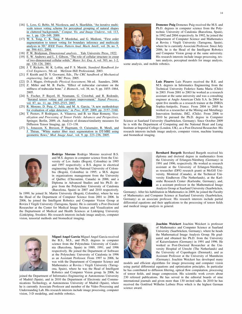
Rodrigo Moreno Rodrigo Moreno received B.S.and M.S. degrees in computer science from the Uni-versity of Los Andes (Bogota, Colombia) in 1995and 1997 respectively; a B.S. degree in electricalengineering from the National University of Colom-bia (Bogota, Colombia) in 1995; a M.S. degreein organizations management from the Universityof Quebec (Chicoutimi, Canada) in 2006; and aDiploma in Advanced Studies and his Ph.D. de-gree from the Polytechnic University of Catalonia(Barcelona, Spain) in 2007 and 2010 respectively.

In 1999, he joined St. Martin University (Bogota, Colombia), where he wasthe Head of the Department of Computer Science from 2001 to 2006. In2006, he joined the Intelligent Robotics and Computer Vision Group atRovira I Virgili University (Tarragona, Spain). He is currently a Post-DoctoralResearcher at the Center for Medical Image Science and Visualization andthe Deptartment of Medical and Health Sciences at Linkoping University(Linkoping, Sweden). His research interests include image analysis, computervision, tensorial methods and biomedical imaging.

Miguel Angel Garcia Miguel Angel Garcia receivedthe B.S., M.S., and Ph.D. degrees in computerscience from the Polytechnic University of Catalo-nia (Barcelona, Spain) in 1989, 1991, and 1996respectively. He joined the Department of Softwareat the Polytechnic University of Catalonia in 1996as an Assistant Professor. From 1997 to 2006, hewas with the Department of Computer Science andMathematics at Rovira i Virgili University (Tarrag-ona, Spain), where he was the Head of IntelligentRobotics and Computer Vision group. In 2006, he

joined the Department of Informatics Engineering at Autonomous Universityof Madrid (Spain), and in 2010 the Department of Electronic and Commu-nications Technology, at Autonomous University of Madrid (Spain), wherehe is currently Associate Professor and member of the Video Processing andUnderstanding Lab. His research interests include image processing, computervision, 3-D modeling, and mobile robotics.

Domenec Puig Domenec Puig received the M.S. andPh.D. degrees in computer science from the Poly-technic University of Catalonia (Barcelona, Spain),in 1992 and 2004 respectively. In 1992, he joined theDepartment of Computer Science and Mathematicsat Rovira i Virgili University (Tarragona, Spain),where he is currently Associate Professor. Since July2006, he is the Head of the Intelligent Roboticsand Computer Vision group at the same university.His research interests include image processing, tex-ture analysis, perceptual models for image analysis,

scene analysis, and mobile robotics.

Luis Pizarro Luis Pizarro received the B.E. andM.S. degrees in Informatics Engineering from theTechnical University Federico Santa Maria (Chile)in 2003. From 2001 to 2003 he worked as a researchassistant at the same university and was a consultingengineer at Anglo American Chile S.A. In 2004 hespent five months as a research trainee at the INRIASophia-Antipolis, France. From 2004 to 2005 heworked as a researcher at the Mining and MetallurgyInnovation Institute, IM2, (Chile). From 2006 to2010 he pursued the Ph.D. degree in Computer

Science at Saarland University (Saarbrucken, Germany). Since October 2009he is with the Department of Computing and the National Heart and LungInstitute at Imperial College (London, UK), as a Post-Doctoral Researcher. Hisresearch interests include image analysis, computer vision, machine learningand biomedical imaging.

Bernhard Burgeth Bernhard Burgeth received hisdiploma and doctoral degree in mathematics fromthe University of Erlangen-Nurnberg (Germany) in1991 and 1996, respectively. He worked as researchassistant at the University of Erlangen-Nurnberg,as researcher (DFG research grant) at McGill Uni-versity, Montreal (Canada), at the Technical Uni-versity Eindhoven (The Netherlands), at the Karl-sruhe Research Center (Karlsruhe, Germany), and,as a assistant professor in the Mathematical ImageAnalysis Group at Saarland University (Saarbrucken,

Germany). After his habilitation in Mathematics in 2009, he joined the Facultyof Mathematics and Computer Science at Saarland University (Saarbrucken,Germany) as an associate professor. His research interests include partialdifferential equations and their applications to the processing of tensor fieldsand medical image analysis in general.

Joachim Weickert Joachim Weickert is professorof Mathematics and Computer Science at SaarlandUniversity (Saarbrucken, Germany), where he headsthe Mathematical Image Analysis Group. He grad-uated and obtained his Ph.D. from the Universityof Kaiserslautern (Germany) in 1991 and 1996. Heworked as Post-Doctoral Researcher at the Uni-versity Hospital of Utrecht (The Netherlands) andthe University of Copenhagen (Denmark), and asAssistant Professor at the University of Mannheim(Germany). Joachim Weickert has developed many

models and efficient algorithms for image processing and computer visionusing partial differential equations and optimisation principles. In particularhe has contributed to diffusion filtering, optical flow computation, processingof tensor fields, and image compression. His scientific work covers about230 refereed publications. He has served in the editorial boards of nineinternational journals and given more than 130 invited talks. In 2010 he hasreceived the Gottfried Wilhelm Leibniz Prize which is the highest Germanscience award.