On Concise Set of Relative Candidate Keys

Shaoxu Song† Lei Chen‡ Hong Cheng§†KLiss, MoE; TNList; School of Software, Tsinghua University, China sxsong@tsinghua.edu.cn

‡The Hong Kong University of Science and Technology, China leichen@cse.ust.hk§The Chinese University of Hong Kong, China hcheng@se.cuhk.edu.hk

ABSTRACTMatching keys, specifying what attributes to compare andhow to compare them for identifying the same real-worldentities, are found to be useful in applications like recordmatching, blocking and windowing [7]. Owing to the com-plex redundant semantics among matching keys, capturinga proper set of matching keys is highly non-trivial. Anal-ogous to minimal/candidate keys w.r.t. functional depen-dencies, relative candidate keys (rcks [7], with a minimalnumber of compared attributes, see a more formal definitionin Section 2) can clear up redundant semantics w.r.t. “whatattributes to compare”. However, we note that redundancyissues may still exist among rcks on the same attributesabout “how to compare them”. In this paper, we proposeto find a concise set of matching keys, which has less redun-dancy and can still meet the requirements on coverage andvalidity. Specifically, we study approximation algorithms toefficiently discover a near optimal set. To ensure the qualityof matching keys, the returned results are guaranteed to bercks (minimal on compared attributes), and most impor-tantly, minimal w.r.t. distance restrictions (i.e., redundancyfree w.r.t. “how to compare the attributes”). The exper-imental evaluation demonstrates that our concise rck setis more effective than the existing rck choosing method.Moreover, the proposed pruning methods show up to 2 or-ders of magnitude improvement w.r.t. time costs on conciserck set discovery.

1. INTRODUCTIONFor matching records that denote the same real-world en-

tities, a variety of approaches have been proposed, suchas probabilistic matching [18], learning-based [2], distance-based [4], rule-based [11] (see [5] for a survey). As indicatedby Fan et al. [7], no matter what approaches to use, it is es-sential to decide “what attributes to compare” and “how tocompare them”, known as matching keys. While matchingkeys can typically assure high matching accuracy, the deter-mination and tuning of such matching rules is highly non-trivial, often requires extremely high manual effort from the

This work is licensed under the Creative Commons Attribution-NonCommercial-NoDerivs 3.0 Unported License. To view a copy of this li-cense, visit http://creativecommons.org/licenses/by-nc-nd/3.0/. Obtain per-mission prior to any use beyond those covered by the license. Contactcopyright holder by emailing info@vldb.org. Articles from this volumewere invited to present their results at the 40th International Conference onVery Large Data Bases, September 1st - 5th 2014, Hangzhou, China.Proceedings of the VLDB Endowment, Vol. 7, No. 12Copyright 2014 VLDB Endowment 2150-8097/14/08.

Table 1: An example instance of staff

ssn name address department

234*** Jason Smith Mark Road Social Science t12****3 J Smith Mark Rd Social Science t2862*** W J Smith Park St Social Science t3862*** Will J Smith Park Street Social Science t40****5 C Green Mark Road Computing t50****5 C Green Mark Rd Computing t6

human experts [5]. Recently, great efforts have been madeon enriching matching rules by reasoning over a given set ofmatching keys [7, 6]. Owing to the existence of possibly re-dundant semantics (as illustrated in the following Example1), analogous to conventional keys, a special group of match-ing keys are concerned where the number of compared at-tributes is minimized, namely relative candidate keys (rcks)[7]. However, redundancy issues exist not only w.r.t. “whatattributes to compare”, but also in “how to compare them”.We note that the distance comparisons could be redundantin different rcks on the same attributes as shown in thefollowing example.

Example 1. Consider a relation for collecting staff infor-mation in Table 1. Since different digits of ssn are hidden(denoted by *) for privacy issues from various data sources,we need to determine whether 234*** and 2****3 denote thesame ssn of a staff. Let

ψ1 : (name, address ‖ [0, 4], [0, 2])

be a matching key relative to ssn declared on attributes nameand address, where [0, 4] and [0, 2] denote the restrictions ofedit distances1 on attributes name and address, respectively.It states that for any tuples ti, tj in a relation instance ofstaff, if their distance on attribute name is in the range of[0, 4], i.e., ≥ 0 and ≤ 4, and the distance on address is in[0, 2], their ssn must be identified.

Consequently, the identification of 234*** in t1 and 2****3in t2 in Table 1 can be implied, since they have name dis-tance equal to 4 and address distance equal to 2, in the rangeof [0, 4] and [0, 2], respectively.

Similar to the demand of minimal keys, redundancy existsamong matching keys. A matching key ψ is said redundantw.r.t. a relation if all the tuple pairs that can be identified by

1Our proposed techniques below are independent to the se-lection of similarity/distance metrics (refer to [19] for selec-tion of best similarity functions). Without loss of generality,we use edit distance by default in the following examples.

1179

the matching key ψ can also be identified by another match-ing key ψ′. For example, given ψ1, the following ψ2 withadditional restrictions on department is unnecessary.

ψ2 : (name, address, department ‖ [0, 4], [0, 2], [0, 0])

For ψ1, since the number of compared attributes is mini-mized, i.e., not able to remove an attribute such that theremaining ones can still identify ssn, this ψ1 is an rck.

Owing to the presence of various distance restrictions,matching keys on the same attributes could be redundant aswell. For example, the following ψ3 with [0, 0] on name over-laps with ψ1 having [0, 4].

ψ3 : (name, address ‖ [0, 0], [0, 2])

Although ψ3 is an rck as well (i.e., minimal w.r.t. the num-ber of compared attributes), any tuple pair agreeing on ψ3

with name distance in [0, 0] (say t5, t6 in Table 1 for in-stance) will always satisfy [0, 4] of ψ1, i.e., redundancyamong matching keys on the same attributes.

Such redundancy obviously increases the overhead of recordmatching. It is not necessary to consider the redundantψ2, ψ3 to detect (t5, t6) again, since they have already beenidentified by ψ1.

In this study, rather than proposing a new record match-ing technique or another notation of matching rules, we em-ploy the existing matching keys [7] and focus on choosingconcise sets of matching keys with high quality and less re-dundancy. By providing a proper set of matching rules, itcomplements the existing record matching methods.

To evaluate the quality of matching keys, following thesame line of discovering data dependencies and keys fromdata [14], we consider a data instance where the same real-world entities in attribute Y are pre-identified, e.g., thematching tuple pairs (t1, t2), (t3, t4), (t5, t6) on ssn in Ta-ble 1. The support measure [3] evaluates the number oftuple pairs that can be covered by matching keys relative toY , and confidence indicates the proportion of covered tuplepairs that correspond to true identifications on Y (see moreexplanations in Example 4).

The concise set discovery problem is to find the optimalset of matching keys relative to a given Y , which has theminimum set size (less redundancy) and can still meet thequality requirements on support and confidence (refer to Ex-ample 5 for more details).

Contributions. While [7] focuses on deducing a set of rcksfrom a given set of matching keys, this paper is dedicatedto discover a concise set of matching keys from data. Ourmain contributions are summarized as follows.

(1) Recognizing the NP-hardness of discovering the optimalmatching key set, we devise approximation algorithms to ef-ficiently find near optimal solutions in Section 3. A boundof approximation ratio on the set size introduced by the ap-proximation is discussed (Proposition 1). Most importantly,we show that the matching keys discovered by the algorithmmust be relative candidate keys (rcks) [7] (Proposition 5)and minimal w.r.t. distance restrictions (Proposition 3).

(2) We develop advanced pruning strategies to further im-prove the efficiency in Section 4. Unqualified candidates ofmatching keys are filtered out during the set discovery com-putation (Propositions 6 and 8).

Table 2: Notations

Symbol Description

ψ matching key

Ψ matching key set

(t1, t2) � ψ Two tuples agree on a key

C1[A] l C2[A] Subsumption of distance restrictions

ψ1 ≺ ψ2 Dominating between keys

agree(ψ) Set of tuple pairs in r agreeing on a ψ

ηc Minimum requirement of confidence

ηs Minimum requirement of support

fds Functional dependencies [12]

rcks Relative candidate keys [7]

(3) We report an extensive experimental evaluation in Sec-tion 5. The experiments demonstrate the effectiveness ofchoosing concise rck sets for record matching, and the effi-ciency of the proposed discovery algorithms.

2. PRELIMINARIESIn this section, we introduce the formal syntax of match-

ing keys [7], and the corresponding statistical measures [3]over a given relation instance. Table 2 lists the frequentlyused notations in this paper.

2.1 SyntaxLet A be an attribute in a relation scheme R and dom(A)

denote a finite domain of A. We consider one distance met-ric dA for each attribute A, denoted by dA : dom(A) ×dom(A) → D, where D = {d1, . . . , d|D|} is a finite set ofdistance values. It satisfies non-negativity, dA(a, b) ≥ 0;identity of indiscernibles, dA(a, b) = 0 iff a = b; and symme-try, dA(a, b) = dA(b, a), where a, b ∈ dom(A). For example,we can use edit distance [15] or cosine similarity [4]. It isworth noting that the selection of best distance metrics isnot the focus of this study, please refer to [19] for a discus-sion. Our proposed techniques are fully compatible with anyother distance metrics having the aforesaid properties.

Matching Keys. A distance restriction is a range of met-ric distances in the form of [dv, du], where dv, du ∈ D anddv ≤ du. It specifies the restriction on distance between twovalues from A. We say two values a, b ∈ dom(A) satisfy therestriction [dv, du] if dv ≤ dA(a, b) ≤ du.

A matching key ψ relative to Y is in the form of (X ‖ C ),where X,Y are attribute sets in R, and C is a pattern ofdistance restrictions on X. Each C [A] denotes the distancerestriction on an attribute A ∈ X . It states that if the Xvalues of two tuples satisfy the distance restrictions C on X,their Y values should be identified, i.e., (X ‖ C )→ (Y ).

Let t1, t2 be two tuples from a relation instance r ofR. Wesay that t1, t2 agree on the matching key ψ : (X ‖ C ), de-noted by (t1, t2) � ψ, if their distances on attributes X sat-isfy the distance restrictions C. That is, for each attributeA ∈ X, the distance between t1[A] and t2[A] satisfies thecorresponding distance restriction C[A] = [dv, du], havingdv ≤ dA(t1[A], t2[A]) ≤ du or simply dv ≤ dA(t1, t2) ≤ du.

A dependency ψ → (Y ) requires that (t1, t2) � ψ im-plies t1[Y ] t2[Y ]. If they agree on ψ, their Y values shouldbe identified, i.e., denoting the same real-world entity.

1180

Example 2 (Example 1 continued). Consider the matchingkey ψ1 : (name, address ‖ [0, 4], [0, 2]) relative to ssn, denotedby ψ1 → (ssn ). According to ψ1, t1 and t2 in Table1 should have ssn values identified, referring to their namedistance 0 ≤ dname(t1, t2) = 4 ≤ 4, i.e., in the range of[0, 4], and address distance in the range of [0, 2] having 0 ≤daddress(t1, t2) = 2 ≤ 2.

Relative Candidate Keys. Key ψ : (X ‖ C ) is a relativecandidate key (rck) if there is no other key ψ′ : (X ′ ‖ C′)relative to Y such that (1) X ′ ⊂ X, and (2) for each A ∈ X ′,C′[A] of ψ′ is exactly C[A] of ψ. That is, no proper subsetof distance restrictions can still form a valid matching key.

Let d|D| = dmax be the maximum value of distances inD and d1 = 0 be the minimum distance value. We call[d1, d|D|] = [0, dmax] an unlimited distance restriction, sinceany distance values will always be in the range from 0 todmax. For the attributes not specified in an rck, it impli-cates unlimited distance restrictions. By appending unlim-ited restrictions, we can represent matching keys declared ondifferent attributes equivalently by a unified standard formwith the same attributes X = R \ Y .

Example 3 (Example 1 continued). We say that ψ1 is ina non-standard form, with X ⊂ R \ Y . There is no re-striction on attribute department specified by ψ1, i.e., un-limited on department. By appending the unlimited [0, dmax]on department, ψ1 is equivalent to

ψ∗1 : (name, address, department ‖ [0, 4], [0, 2], [0, dmax]).

This ψ∗1 :(X ‖ C ) with X = R \ Y is a standard form of ψ1.

In the following of this paper, matching keys are consid-ered in the standard form with X = R \ Y by default.

2.2 MeasuresSuppose that the same real-world entities are pre-identified

in a given data instance, e.g., Table 1 with all matching pairs(t1, t2), (t3, t4), (t5, t6) identified on ssn. To discover reason-able matching keys from the data instance, we first need toevaluate the quality of a key, i.e., how the matching key canidentify Y (ssn) values in the given data instance.

Evaluating a Single Matching Key. In light of coverageand validity in record matching, we study the following sup-port and confidence measures defined on tuple pairs [3].

supp(ψ) =|{t1, t2 ∈ r | (t1, t2) � ψ}|

|{t1, t2 ∈ r}| (1)

conf(ψ) =|{t1, t2 ∈ r | (t1, t2) � ψ, t1[Y ] t2[Y ]}|

|{t1, t2 ∈ r | (t1, t2) � ψ}| (2)

Intuitively, given a relation instance r of R, the supportof a ψ is the proportion of tuple pairs in r whose valuesagree on ψ. It denotes the “coverage” of the matching key.The confidence is the ratio of tuple pairs whose values agreeon ψ also having identified Y values, i.e., the “validity” ofidentifying Y by the matching key ψ. Matching keys withhigher support and confidence are preferred.

Evaluating a Set of Matching Keys. Let Ψ denote a setof matching keys relative to the same Y . As discussed inthe introduction, a tuple pair may agree on (be covered by)several keys ψ ∈ Ψ, i.e., redundancy in Ψ. If we simply add

supp(ψ) of all ψ ∈ Ψ as the support of the set Ψ, a tuplepair may be counted more than once due to the redundancy.To avoid duplicate counting, we should consider the distincttuple pairs that are covered by a set of matching keys.

We say that t1, t2 agree on a set Ψ of matching keys,denoted by (t1, t2) � Ψ, if there exists at least one ψ ∈ Ψsuch that (t1, t2) � ψ. The set support of a set Ψ is definedas the proportion of distinct tuple pairs that agree on atleast one of the matching keys in the set Ψ, i.e.,

supps(Ψ) =|{t1, t2 ∈ r | (t1, t2) � Ψ}|

|{t1, t2 ∈ r}| . (3)

Moreover, to evaluate the validity of a set Ψ, we needto justify the confidence of each individual key in Ψ. Intu-itively, in order to approach high accuracy in entity match-ing, it is expected that each applied matching key in the setshould have high confidence. The minimum confidence ofall the keys thus reflects the confidence of the set Ψ,

confs(Ψ) = minψ∈Ψ

conf(ψ). (4)

Example 4 (Example 2 continued). Given the data in-stance in Table 1 with truth matching (t1, t2), (t3, t4), (t5, t6),we consider ψ5 : (name, address ‖ [0, 4], [0, 4]) relative to ssn.There are four pairs of tuples (t1, t2), (t2, t3), (t3, t4), (t5, t6)agreeing on ψ2 and three pairs of tuples (t1, t2), (t3, t4), (t5, t6)with identified ssn. Considering all the 15 tuple pairs in Ta-ble 1, we have supp(ψ2) = 4/15 and conf(ψ2) = 3/4.

There are only two tuple pairs (t1, t2), (t5, t6) that can becovered by ψ1 : (name, address ‖ [0, 4], [0, 2]). Indeed, it isalready the key with the highest support, i.e., supp(ψ1) =2/15, when the confidence is required to be at least 1. Wecannot achieve a larger support by any individual key.

For a set Ψ1 = {ψ1, ψ4} relative to ssn, where (t3, t4) agreeon ψ4 : (name, address ‖ [0, 4], [4, 4]). We have supps(Ψ1) =3/15. Given conf(ψ1) = conf(ψ4) = 1, it follows confs(Ψ1) =1. That is, Ψ1 can correctly (with confidence 1) address all(a support of 3/15) the tuple pairs with identified Y .

2.3 Problem StatementIntuitively, we want to discover matching keys with high

quality (high confidence) and address identifications as manyas possible (high support). While a high confidence is alwayspreferred, maximizing the support is not necessary duringthe discovery, since it may “overfit” the data [10]. Followingthe same line, we propose to find a set Ψ of matching keysrelative to Y with the minimum requirements of support ηsand confidence ηc.

The selection of ηc for confidence is analogous to the re-quirement of matching accuracy. The support requirementηs could be chosen based on the user’s knowledge about howmany duplicates exit. If ηs and ηc are set too high, it maynot be able to find a feasible solution even when we considerall the possible matching keys as the answer set. Therefore,the first question is whether there exists a set Ψ such thatthe minimum requirements of support and confidence couldbe achieved. If yes, we find the minimum set Ψ∗o which hasless redundancy and can still satisfy ηs and ηc.

Problem 1. The matching key set determination problemis: given a relation instance r of R, a Y over R, a constantk, and the minimum requirements of support ηs and confi-dence ηc, to decide whether there exists a set Ψ of matchingkeys such that supps(Ψ) ≥ ηs, confs(Ψ) ≥ ηc, and the size ofthe set is |Ψ| ≤ k.

1181

This problem of deciding whether a feasible matching keyset exists is found to be NP-complete [1].

Considering possible redundant semantics among match-ing keys, it naturally leads us to discover the most conciseset of matching keys with less redundancy that can still meetthe measure requirements of support ηs and confidence ηc.

The corresponding optimization problem is to find theoptimal set Ψ∗o of matching keys such that the set size of Ψ∗ois minimized, and the set still satisfies supps(Ψ

∗o) ≥ ηs and

confs(Ψ∗o) ≥ ηc, if exists.

Example 5 (Example 4 continued). Given ηc = 1, ηs =3/15, a set Ψ2 = {ψ1, ψ3, ψ4} with conf(Ψ2) = 1, supp(Ψ2) =3/15 is feasible but not optimal, since Ψ1 = {ψ1, ψ4} is alsoa feasible solution that meets the ηc, ηs requirements but witha smaller size. Ψ1 is more concise without the redundant ψ3.

3. APPROXIMATION METHODIn this section, we present a greedy algorithm for effi-

ciently approximating the desired set. In particular, we showthat the discovered set of matching keys are always rcks,and most importantly, minimal w.r.t. distance restrictions.

3.1 Candidates of Matching KeysWe consider all the potential matching keys relative to

Y in standard form which specify distance restrictions onX = R \ Y . Recall that a finite set of all distance values Dis defined based on the dom(A) of an attribute A. With thisD, we can enumerate intervals of distance restrictions.

For each attribute A, we define CA to be the set of alldistance restrictions [dv, du] over A, i.e.,

CA ={[dv, du] | d1 ≤ dv ≤ du ≤ d|D|}={[d1, d1], . . . , [d1, d|D|−1], [d1, d|D|],

[d2, d2], . . . , [d2, d|D|],

. . . , [d|D|, d|D|]}

where d1, . . . , d|D| denote all the distance values inD (see the

following Figure 1 for instance). The size of CA is O(|D|2).Consider m attributes in X = R\Y = {A1, . . . , Am}. Let

Ψc be the set of all the potential matching keys,

Ψc = {(X ‖ C ) | C ∈ CA1 × · · · × CAm}. (5)

The size of Ψc is O(|D|2m). In the worst case, the numberof distinct distance values can be |D| = |dom(A)|2. Let cbe the size of dom(X), having c = |dom(A)|m. It follows|Ψc| = O(c4).

For any potential matching key ψ, let agree(ψ) denote theset of all the tuple pairs ti, tj ∈ r that agree on ψ, i.e.,

agree(ψ) = {(ti, tj) | (ti, tj) � ψ, ti, tj ∈ r}, (6)

which is utilized to compute

supp(ψ) =|agree(ψ)||{ti, tj ∈ r}| ,

conf(ψ) =|{(ti, tj) ∈ agree(ψ) | ti[Y ] tj [Y ]}|

|agree(ψ)| .

According to the set confidence in formula (4), the re-quirement of confs(Ψ) ≥ ηc for any set Ψ is equivalent toconf(ψ) ≥ ηc, ∀ψ ∈ Ψ. In other words, only those matchingkeys with confidence ≥ ηc can be considered as candidates.

Algorithm 1 presents the discovery of a set Ψ of potentialmatching keys from a relation instance r , whose confidences

are no less than ηc. Since the support and confidence mea-sures are defined on the pairs of tuples in a relation instance,the algorithm considers all the tuple pairs in r . Specifically,according to formula (5), Line 3 goes through the candidatesΨc for each tuple pair ti, tj ∈ r . Line 8/5 creates/maintainsagree(ψ) in formula (6), which is utilized to compute thesupport and confidence measures. Finally, those candidateswith confidence satisfying the minimum requirement ηc arereturned in Ψ.

Algorithm 1 Candidate set generation CS(r , ηc)

Input: data instance r , minimum confidence requirementηc

Output: A set Ψ of matching keys whose confidences areno less than ηc

1: Ψ := ∅2: for each tuple pair ti, tj ∈ r do3: for each candidate ψ ∈ Ψc s.t. (ti, tj) � ψ do4: if ψ ∈ Ψ then5: insert (ti, tj) to agree(ψ)6: update conf and supp of ψ to Ψ7: else8: agree(ψ) := {(ti, tj)}9: compute conf and supp of ψ, insert ψ to Ψ

10: return {ψ ∈ Ψ | conf(ψ) ≥ ηc}

Note that the for statement in Line 2 of Algorithm 1 addsa specific pair (ti, tj) to a certain agree(ψ) exactly once. Letn be the number of tuples in r . According to |Ψc| = O(c4),the generation algorithm runs in O(n2c4) time.

3.2 Greedy AlgorithmNow, we study the greedy algorithm for approximating a

near optimal matching key set in polynomial time.Let Ψ be a candidate set of matching keys (obtained in

the above candidate generation), and let Ψo denote the nearoptimal set to discover. Intuitively, the greedy algorithmremoves a candidate ψ with the maximum support from Ψin each iteration, adds it into Ψo, and does not stop untilthe minimum support requirement ηs is satisfied or all thevalid candidates in Ψ are added to Ψo.

Note that during the generation of candidates, a distincttuple pair (ti, tj) may be included in agree(ψ) of several ψin Ψ. However, according to formula (3), when we computethe support of a set Ψo, each tuple pair should be countedtowards supps(Ψo) only once. To follow this principle, ineach iteration of processing the current ψ, we need to removethe tuple pairs that agree on ψ (covered by ψ) from agree(ψ′)for all the remaining candidates ψ′ in Ψ. That is, we conductthe deduction operation,

agree(ψ′) = agree(ψ′) \ agree(ψ),

to avoid counting a tuple pair more than once.Algorithm 2 presents the discovery of a near optimal set

Ψo of matching keys from the candidate set Ψ. Line 7adds a ψ to Ψo in each iteration. The deduction opera-tion agree(ψ′) = agree(ψ′) \ agree(ψ) in Line 10 deducts allthe tuple pairs in agree(ψ) from agree(ψ′) of the remainingψ′ ∈ Ψ. Line 11 re-calculates the supp(ψ′) of ψ′ by using theupdated agree(ψ′). By ensuring that tuple pairs in agree(ψ)have not been counted towards supps(Ψo) in previous steps,we can directly add supp(ψ) to supps(Ψo) in Line 8.

1182

Algorithm 2 Greedy algorithm GA(Ψ, ηs)

Input: candidate set Ψ, minimum support requirement ηsOutput: a near optimal set Ψo

1: Ψo := ∅2: supps(Ψo) := 03: while Ψ 6= ∅ and supps(Ψo) < ηs do4: ψ := arg maxψ∈Ψ supp(ψ)5: if supp(ψ) = 0 then6: break7: move ψ from Ψ to Ψo

8: supps(Ψo) += supp(ψ)9: for each ψ′ ∈ Ψ do

10: agree(ψ′) := agree(ψ′) \ agree(ψ)11: update supp of ψ′ to Ψ12: if supps(Ψo) < ηs then13: return ∅14: else15: return Ψo

Proposition 1. The greedy algorithm is 1+2 ln |r | approxi-mation, having |Ψo|/|Ψ∗o| ≤ 1+2 ln |r |, where |Ψo| is the sizeof the returned result set and |Ψ∗o| is the optimal set size.

Proof. We employ the k-partial set cover problem: given aset of N elements E = {E1, E2, . . . , EN}, a collection S ofsubsets of E, S = {S1, S2, . . . , SM}, a cost function of S, anda k, to find a minimum cost sub-collection of S that covers atleast k elements of E. Our discovery problem can be mod-eled as the k-partial set cover problem as follows. Each Eidenotes a tuple pair and each Sj denotes a ψ in our prob-lem. The k corresponds to the minimum support ηs, andthe cost function counts the number of subsets, i.e., analo-gous to |Ψo|. Consequently, to find a set with the minimumsize, it is equivalent to find a minimum sub-collection of S.According to [8], the greedy algorithm is a lnN +1 approxi-mation for the partial covering problem, which equivalentlyholds for our discovery problem, where N = |r |2 is the totalnumber of tuple pairs.

Note that the for statement in Line 2 of Algorithm 1adds a specific tuple pair to a certain agree(ψ) exactly once(in Line 5 or 8), i.e., O(n2c4). Subsequently, the whilestatement in Line 3 of Algorithm 2 removes a specific tuplepair from a certain agree(ψ′) at most once (in Line 10).Therefore, the ga complexity is also O(n2c4), where n isthe number of tuples in r .

3.3 Redundancy Free ResultsIn the following, we show that the matching keys returned

by Algorithm 2 are redundancy free, i.e., rcks and minimalw.r.t. distance restrictions.

Definition 1. For any two distance restrictions [dv, du] and[dg, dh], if dv ≤ dg and dh ≤ du, we say that [dv, du] sub-sumes [dg, dh], denoted by [dv, du] l [dg, dh].

Consider two matching keys ψ1 and ψ2.

Definition 2. If Cψ1 [A]lCψ2 [A] for all attributes ∀A ∈ X,we say ψ1 dominates ψ2, denoted by ψ1 ≺ ψ2.If there exists one attribute ∃A ∈ X having Cψ1 [A]lCψ2 [A],we say ψ1 partially dominates ψ2, denoted by ψ1 ≺p ψ2.

Referring to the support definition, we derive the followingdominating relationships between matching keys.

Lemma 2. For any ψ1 dominating ψ2, i.e., ψ1 ≺ ψ2, wehave agree(ψ1) ⊇ agree(ψ2) and supp(ψ1) ≥ supp(ψ2).When agree(ψ1) = agree(ψ2), we say that ψ1 and ψ2 areequivalent, having supp(ψ1) = supp(ψ2).

Proof. For each attribute A ∈ X, let Cψ2 [A] = [dg, dh] andCψ1 [A] = [dv, du]. Consider a tuple pair (ti, tj) in agree(ψ2),i.e., having dg ≤ dA(ti, tj) ≤ dh for any attribute A ∈ X.According to ψ1 ≺ ψ2, we have dv ≤ dg ≤ dA(ti, tj) ≤ dh ≤du, that is, dA(t1, t2) satisfies Cψ1 [A] for each attribute A aswell. In other words, all the tuple pairs in agree(ψ2) are alsocontained in agree(ψ1), i.e., agree(ψ2) ⊆ agree(ψ1). Refer-ring to the support definition, we have supp(ψ1) ≥ supp(ψ2).

Moreover, since we always have agree(ψ2) ⊆ agree(ψ1),it follows supp(ψ1) = supp(ψ2) if and only if agree(ψ2) =agree(ψ1). That is, ψ1 and ψ2 cover exactly the same tuplepairs. Referring to the greedy algorithm, there is no differ-ence between the candidates ψ1 and ψ2, i.e., equivalent.

When both matching keys are valid (with confidences ≥ηc), we say that ψ2 is redundant w.r.t. ψ1, since any tupleswith Y values identified by ψ2 are identified by ψ1 as wellaccording to ψ1 ≺ ψ2.

A matching key ψ is minimal, if there does not exist anyψ′ such that ψ′ ≺ ψ and conf(ψ) ≥ ηc. That is, ψ is notredundant w.r.t. any other possible matching keys.

Proposition 3. The matching keys in Ψo discovered by GAalgorithm are always minimal, i.e., ∀ψ ∈ Ψo, there does notexist any ψ′ ∈ Ψc such that ψ′ ≺ ψ and conf(ψ) ≥ ηc.

Proof. According to Lemma 2, Algorithm 2 always selectsψ with higher support in Line 4. For the remaining ψ′, byconducting agree(ψ′) := agree(ψ′) \ agree(ψ) in Line 10, wehave agree(ψ′) = ∅ as agree(ψ) ⊇ agree(ψ′). Since there isno remaining support on ψ′, ψ′ will not contribute and thuscannot be selected into Ψo.

It is worth noting that the “minimal” definition is morestrict than the rck definition. While rcks require not exist-ing any other key with a subset of same distance restriction,the minimal matching keys ensure no other key with dis-tance restrictions dominating the minimal matching key.

Lemma 4. Minimal matching keys are always rcks.

Proof. Let ψ be a minimal matching key but not relativecandidate key. That is, there exists a ψ′ : (X ′ ‖ C′) relativeto Y such that X ′ ⊂ X, and for each A ∈ X ′, C′[A] of ψ′

is exactly C[A] of ψ. By representing both keys in standardform, we have C′[B] : [0, dmax] l C[B],∀B ∈ X \ X ′. Itfollows ψ′ ≺ ψ, according to the definition of dominating,i.e., ψ is not minimal.

Consequently, following the same line of Proposition 3, wecan show that the results are always rcks.

Proposition 5. The matching keys in Ψo discovered by GAalgorithm are always relative candidate keys (rcks).

Since equality is considered as a special case of distancerestriction, i.e., [0, 0], the relationship between traditionalsuper key and candidate key can also be interpreted by thedominating relationship (see examples below).

Example 6 (Example 5 continued). Consider ψ1 : (name,address ‖ [0, 4], [0, 2]) and ψ3 : (name, address ‖ [0, 0], [0, 2]),having [0, 4]l [0, 0] on name and consequently ψ1 ≺ ψ3. Forthe tuples in Table 1, we have agree(ψ1) = {(t1, t2), (t5, t6)},while ψ3 can only cover one of them, i.e., (t5, t6).

1183

Since both ψ1 and ψ3 can identify ssn of (t5, t6), ψ3 is re-dundant w.r.t. ψ1. GA algorithm first selects ψ1 with highersupport supp(ψ1) = 2/15. The deduction operation in Line10, i.e., agree(ψ3) = agree(ψ3)\agree(ψ1), eliminates (t5, t6)that has been addressed by ψ1 from agree(ψ3) and makes itempty. That is, there is no remaining tuples supporting ψ3.In other words, ψ3 cannot further contribute and will neverbe returned as results. By further processing ψ4, the returnedmatching keys {ψ1, ψ4} are minimal.

A super key {name, address, department} w.r.t. fds repre-sented by ψs : (name, address, department ‖ [0, 0], [0, 0], [0, 0])is not minimal, since there is a candidate key {name, address}with a subset of attributes, denoted by ψc : (name, address,department ‖ [0, 0], [0, 0], [0, dmax]). We have ψc ≺ ψs.

4. PRUNING APPROACHThe greedy discovery of a near optimal set is still very

costly. This is because the greedy step requires scanning allthe possible candidates of matching keys in Ψ. Remarkably,as introduced below, not all the possible matching keys arenecessary to be considered in candidate generation as Algo-rithm 1 does. Moreover, in the greedy step, after moving akey to Ψo, it is not necessary either to update the agree in-formation for all the remaining candidates in Ψ. In the restof this section, we propose several pruning strategies for thecandidate set generation and the greedy step, respectively.

4.1 Pruning in Candidate SetBased on the aforesaid subsumption/dominating relation-

ships among distance restrictions, we are already able to dis-cern some redundant matching keys in the candidate setΨ, without further evaluation on agree sets of tuple pairs.

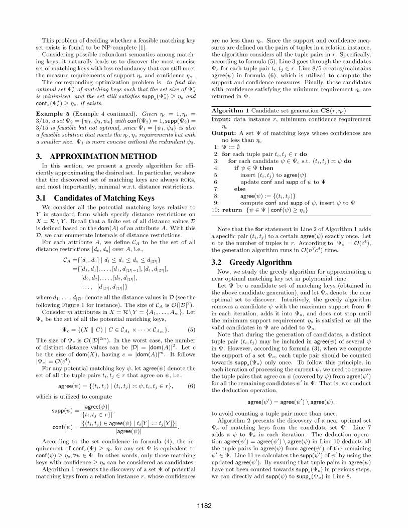
To understand the relationships more clearly, we representthe matching keys as follows. Based on the subsumptionrelationship, all the distance restrictions on an attribute canbe represented by a directed acyclic graph. For example,as shown in Figure 1(a), each dot node denotes a possibledistance restriction. An arrow from node a to b denotes alb.The transitivity relationship is naturally implied, in otherwords, alb and blc indicate alc as well. In the figure, weonly plot the most tight subsumption relationships, i.e., foreach al b there does not exist another c such that al cl b,and omit the subsumption that can be inferred.

Consequently, there is a triangle structure that specifiesall the possible distance restrictions corresponding to an at-tribute A, e.g., Figure 1(b) for attribute A2, Figure 1(c)for attribute A3, etc. The root node in the triangle struc-ture, [d1, d|D|], is the unlimited restriction. Recall that wehave X = R \ Y in the standard form. Thereby, each ψ (inthe standard form) consists of exactly one node (a distancerestriction) from each triangle (each attribute in X).

Identify Unqualified CandidatesNow, we study the pruning techniques for reducing the num-ber of candidates, before the greedy step is conducted. Re-call that distance values D of an attribute A are defined withrespect to the domain of A, dom(A). Therefore, some of thedistance values (say dv) in D of an attribute A may not ap-pear in a given relation instance r . However, according tothe candidate set generation algorithm, these distance valuesdv ∈ D are still considered as bounds in intervals of distancerestrictions in candidate matching keys. We study the prun-ing strategies based on these non-appearing distance values.

Figure 1: Relationship among distance restrictions

Intuitively, since the distance value dv does not appearin attribute A in the relation instance r , all the candidatesψ containing the distance restriction Cψ[A] = [dv, dv] onA should have an empty agree(ψ) set and can be ignored.Moreover, let us consider some other ψ with distance re-strictions like ψ[A] = [dv, dv+1] on A. We prove that therealways exists another ψ′ (such as ψ′[A] = [dv+1, dv+1] on A)having agree(ψ) = agree(ψ′). According to Lemma 2, ψ isequivalent to ψ′ and can be pruned. We define these prun-able candidates with certain distance restrictions below.

Proposition 6. Consider a distance value dv ∈ D of anattribute A ∈ X, which does not appear in the attribute Aof any tuple pairs in the relation instance r. Then all thecandidates ψ ∈ Ψ that contain the following distance restric-tions on attribute A, i.e., Cψ[A] ∈ (I1 ∪ I2), can be prunedfrom the candidate set Ψ.

I1 = {[dv, dv+u] | u = 0, 1, 2, . . . }I2 = {[dv−u, dv] | u = 0, 1, 2, . . . }

Proof sketch. For each candidate ψ having Cψ[A] ∈ I1, wecan always find a ψ2 with Cψ2 [A] = [dv+1, dv+u], which isequivalent to ψ, i.e., agree(ψ) = agree(ψ2). Thus, candidateψ can be pruned as redundancy. Similarly, for any ψ withCψ[A] ∈ I2, we can find a ψ1 with Cψ1 [A] = [dv−u, dv−1], asredundancy of ψ.

Example 7. Suppose that the distance value dv does not ap-pear in any tuple pair of r on attribute A1. Then, the sets ofdistance restrictions, I1 = {[dv, dv], [dv, dv+1], . . . , [dv, d|D|]}and I2 = {[d1, dv], [d2, dv], . . . , [dv, dv]} marked by shade ar-eas in Figure 1(a), can be ignored in attribute A1 duringthe candidate generation. That is, the candidate set prun-ing (csp) method removes all the candidates from Ψ whosedistance restrictions come from I1 or I2 on attribute A1.

4.2 Pruning in Greedy StepThe major cost of each greedy step originates from the

update of tuple pairs in agree(ψ′) after moving a ψ with thehighest support to Ψo. We propose pruning rules to reducethe number of updates, and remove redundant candidates.

Let ψ be the currently selected candidate in a greedy step.Let [dv, du] denote the distance restriction of ψ on attributeA, i.e., Cψ[A] = [dv, du]. For each attribute A, we divideall the distance restrictions into 6 blocks according to the

1184

subsumption relationship on [dv, du] as follows.

B1[A] = {C [A] | C [A] l [dv−1, du+1]}B2[A] = {C [A] | [d1, du] l C [A] l [dv−1, dv]}B3[A] = {C [A] | [dv, d|D|] l C [A] l [du, du+1]}B4[A] = {C [A] | [dv, du] l C [A]}B5[A] = {C [A] | [d1, dv−1] l C [A]}B6[A] = {C [A] | [du+1, d|D|] l C [A]}

Among the above 6 blocks, B1[A] represents the distancerestrictions on A that subsume Cψ[A]; B4[A] denotes all therestrictions on A that are subsumed by Cψ[A]; B5[A] andB6[A] are the restrictions that have no overlap with Cψ[A];B2[A] and B3[A] are the restrictions that have overlap withCψ[A]. For example, in Figure 1(b), we illustrate the 6blocks of all the distance restrictions in attribute A2 basedon Cψ[A2] of the current ψ.

Identify Qualified CandidatesWe first identify the set of candidates ψ′ whose agree set isnot updated by the deduction operation agree(ψ′) = agree(ψ′)\agree(ψ) even in the original greedy algorithm (Algorithm2). Intuitively, the deduction operation has no effect onthose distance restrictions, which do not subsume any otherrestrictions that are subsumed by Cψ[A], i.e., distance re-strictions in B5[A] and B6[A] having no overlap with Cψ[A].

Lemma 7. After inserting a ψ with the maximum supportinto Ψo, the following sets of candidates ψ′ are not updated.

K5 = {ψ′ | ∃A ∈ X,Cψ′ [A] ∈ B5[A]}K6 = {ψ′ | ∃A ∈ X,Cψ′ [A] ∈ B6[A]}

Proof sketch. For any ψ′ ∈ K5 or K6, we can prove that theintersection of agree sets of ψ and ψ′ is agree(ψ′)∩agree(ψ) =∅. The operation agree(ψ′) = agree(ψ′) \ agree(ψ) takes noeffect on candidate ψ′. Thus ψ′ is not updated.

According to Lemma 7, all the candidates with distancerestrictions from B5 or B6 on any attribute will not be up-dated in the current iteration. In other words, only thosecandidates will be updated, which have distance restrictionsfrom B1, B2, B3, B4 on all the attributes, i.e., Ψ\ (K5∪K6).

Identify Unqualified CandidatesNow, we study the pruning in Ψ \ (K5 ∪ K6) to avoid theupdates on unqualified candidates. Based on the subsump-tion and dominating relationships, we propose to filter outthe following two types of candidates:

(1) Those candidates ψ′ having agree(ψ′) = ∅ after theagree(ψ′) = agree(ψ′)\agree(ψ) operation. Candidates withempty agree set will have no contribution to the result, andthus can be pruned without conducting the updating opera-tion. Intuitively, those candidates with distance restrictionsin B4, i.e., subsumed by Cψ[A], may fall into this category.

(2) Those candidates ψ′ that always have another ψ1 in K5

or K6 having agree(ψ′) = agree(ψ1), i.e., equivalent, afterthe agree(ψ′) = agree(ψ′) \ agree(ψ) operation. For exam-ple, a candidate ψ′ with distance restrictions in B2 may beconsidered to find an equivalent ψ1 with distance restrictionin B5, such that Cψ′ [A] subsumes Cψ1 [A]. Since this ψ1 isreserved in Ψ without updating in the current iteration, theequivalent one ψ′ can be pruned as redundancy.

Formally, we define the candidates that can be directlypruned from the candidate set Ψ as follows.

Proposition 8. After inserting the current ψ with the max-imum support into Ψo, the following set of candidates Kp canbe pruned from Ψ.

Kp = {ψ′ | ∀A ∈ X,Cψ′ [A] ∈ (B2[A] ∪B3[A] ∪B4[A])}

Proof sketch. For a candidate ψ′ ∈ Kp, the distance restric-tion Cψ′ [A] of any attribute A comes from either B2[A],B3[A] or B4[A]. Let

K2 = {ψ′ | ∃A ∈ X,Cψ′ [A] ∈ B2[A], ψ′ ∈ Kp}K3 = {ψ′ | ∃A ∈ X,Cψ′ [A] ∈ B3[A], ψ′ ∈ Kp}K4 = {ψ′ | ∀A ∈ X,Cψ′ [A] ∈ B4[A], ψ′ ∈ Kp}

having Kp = K2 ∪K3 ∪K4.For any ψ′ ∈ K2 or K3, we prove that there always exists

a candidate in the remaining candidate sets (say ψ1 ∈ K5 orψ2 ∈ K6) which is equivalent to ψ′ after the current deduc-tion step. Thus, candidate ψ′ can be pruned as duplicates.

For any candidate ψ′ ∈ K4, by proving that agree(ψ′) = ∅after the current deduction step, ψ′ can be pruned.

According to the definition of Kp, ψ′ ∈ Kp contains only

distance restrictions from B2, B3, B4 on all the attributesA ∈ X. In other words, ψ′ ∈ Kp does not contain distancerestrictions from B1, B5, B6 on all the attributes. Let

K1 = {ψ′ | ∃A ∈ X,Cψ′ [A] ∈ B1[A]}.

Then, we can also represent Kp by Kp = Ψ\ (K1∪K5∪K6).

Definition 3. Let ψp1 , ψp5 , ψ

p6 be three pivot candidates such

that, ∀A ∈ X, Cψp1[A] = [dv−1, du+1], Cψp

5[A] = [d1, dv−1]

and Cψp6[A] = [du+1, d|D|], where Cψ[A] = [dv, du].

For instance, Cψp1[A2], Cψp

5[A2] and Cψp

6[A2] on attribute

A2 are illustrated in Figure 1(b) w.r.t. the current Cψ[A2].According to the partial dominating ≺p in Definition 2, werewrite K1 = {ψ′ | ψ′ ≺p ψp1}, K5 = {ψ′ | ψp5 ≺p ψ′} andK6 = {ψ′ | ψp6 ≺p ψ′} by ψp1 , ψ

p5 , ψ

p6 .

According to Proposition 8, we only need to update thecandidates ψ′ in K1 ∪ K5 ∪ K6, i.e., ψ′ ≺p ψp1 or ψp5 ≺pψ′ or ψp6 ≺p ψ′, while the remaining candidates Kp = Ψ \(K1 ∪K5 ∪K6) can be safely pruned.

Greedy Algorithm with PruningFinally, we present the greedy algorithm with pruning (namelygap). Rather than removing each tuple pair from possibleagree(ψ) exactly once in the original greedy algorithm, weprune the candidates that belong to the aforesaid Kp.

Algorithm 3 presents the pruning steps in the greedy com-putation. As illustrated in Line 4, we greedily select a can-didate ψ in each step. Line 9 computes the pruning pivotsψp1 , ψ

p5 , ψ

p6 in Definition 3. According to Proposition 8, those

candidates in Kp can be safely pruned, which are identifiedby using the pivots ψp1 , ψ

p5 , ψ

p6 . That is, we only conduct

the deduction operation (in Line 12) on those candidates ψ′

such that ψ′ ≺p ψp1 or ψp5 ≺p ψ′ or ψp6 ≺p ψ′, while theother candidates (belonging to Kp) are directly removed inLine 15. Finally, the greedy iteration terminates if either therequirement ηs of support is reached or all the candidateshave been evaluated (i.e., Ψ = ∅ in Line 3).

Example 8 (Example 6 continued). Suppose that ψ∗1 : (name,address, department ‖ [0, 4], [0, 2], [0, dmax]) is the currentlyselected candidate in Line 4 in Algorithm 3. We show thatψ∗3 : (name, address, department ‖ [0, 0], [0, 2], [0, dmax]) can

1185

Algorithm 3 Greedy algorithm with pruning GAP(Ψ, ηs)

Input: candidate set Ψ, minimum support requirement ηsOutput: a near optimal set Ψo

1: Ψo := ∅2: supps(Ψo) := 03: while Ψ 6= ∅ and supps(Ψo) < ηs do4: ψ := arg maxψ∈Ψ supp(ψ)5: if supp(ψ) = 0 then6: break7: move ψ from Ψ to Ψo

8: supps(Ψo) += supp(ψ)9: calculate ψp1 , ψ

p5 , ψ

p6 from ψ

10: for each candidate ψ′ ∈ Ψ do11: if ψ′ ≺p ψp1 or ψp5 ≺p ψ′or ψp6 ≺p ψ′ then12: agree(ψ′) := agree(ψ′) \ agree(ψ)13: update conf and supp of ψ′ to Ψ14: else15: remove ψ′ from Ψ16: if supps(Ψo) < ηs then17: return ∅18: else19: return Ψo

be safely pruned without further evaluation on its agree set(as it does in Example 6).

First, for the attribute name, we have Cψ∗1 [name] = [dv, du] =[0, 4]. Since dv = 0 is already the minimum distance value inD, blocks B1[name] and B5[name] are empty according to thedefinition. Referring to Definition 3, we have Cψp

6[name] =

[5, dmax]. That is, Cψ∗3 [name] does not belong to B6[name]either, and thus must be in blocks B2, B3 or B4.

For the other attributes with Cψ∗1 [address] = Cψ∗3 [address] =[0, 2] and Cψ∗1 [department] = Cψ∗3 [department] = [0, dmax],we directly conclude that Cψ∗3 [department] and Cψ∗3 [address]belong to B4 of ψ∗1 on department and address, respectively.

Finally, since none of Cψ∗3 [A] belong to B1, B5, B6, wehave all ψ∗3 ≺p ψp1 , ψ

p5 ≺p ψ∗3 , ψ

p6 ≺p ψ∗3 equal to false.

Let δ (0 ≤ δ ≤ 1) be the pruning rate on average, i.e.,δ percentage of candidates can be avoided to perform theagree(ψ′) = agree(ψ′) \ agree(ψ) operation. Calculating thepivot candidates ψp1 , ψ

p5 , ψ

p6 for Kp is in constant time. The

complexity of Algorithm 3 with pruning is O((1 − δ)n2c4),where n is the number of tuples in r . As illustrated in theexperiments, gap can always improve time performance inpractice. According to the results in Figures 7(f), 8(f) and9(f), the prune rate is greater than 0.8 (80%) in most tests.

Since the pruning methods do not affect the results, theconclusions about rcks and minimal matching keys of greedyalgorithm are still valid.

5. EXPERIMENTAL EVALUATIONWe report experiments on evaluating the proposed tech-

niques in two aspects. 1) Since this study is to complementthe existing record matching techniques by providing propermatching keys, we implement a rule-based matching method[11], and compare the matching effectiveness by using ourconcise rck set and the rcks return by the existing findR-CKs approach [7]. 2) We compare the efficiency of variousproposed techniques for finding the concise rck sets.

Benchmark datasets for evaluating record linkage are em-ployed,2 including two real datasets Cora (with 864 tuples)2http://www.cs.utexas.edu/users/ml/riddle/data.html

90 95 100 105 110 0.6 0.7

0.8 0.9

1 0 1 2 3 4 5 6

Set size

(a) Restaurant

ηs*372816ηc

Set size

490 530 570 610 650 0.6 0.7

0.8 0.9

1 0

2

4

6

8

10

Set size

(b) Cora

ηs*837865ηc

Set size

90 95 100 105 110 0.6

0.7 0.8

0.9 1

0 100 200 300 400 500 600

Time (ms)

(c) Restaurant

ηs*372816ηc

Time (ms)

490 530 570 610 650 0.6 0.7

0.8 0.9

1 500

1000 1500 2000 2500 3000 3500

Time (ms)

(d) Cora

ηs*837865ηc

Time (ms)

Figure 2: Concise RCK sets with various ηs and ηc

and Restaurant (with 1295 tuples) for evaluating the match-ing accuracy and a synthetic UIS database generator (with10,000 tuples generated) for efficiency evaluation. To studythe accuracy of record matching, we use the standard f-measure of precision and recall [17].

Exp1: Evaluating Concise RCK Sets. The first experi-ment, in Figure 2, observes the sizes of returned rck sets un-der various ηs and ηc settings. With the increase of the mini-mum support requirement ηs, we need to add more matchingkeys into the set Ψo in order to increase the support, andthus the Ψo size increases as well. On the other hand, if theminimum confidence requirement ηc is large, as mentioned,some candidates with high support but low confidence maybecome invalid. We have to seek some other second-highestsupport candidates to meet the ηs requirement, and the Ψo

set size increases consequently.When both ηs and ηc are too high, there does not exist

any matching key set with support and confidence greaterthan the requirements even by considering all the possiblecandidates, denoted by size 0. It is the worst case of con-sidering all the candidates, and thus the corresponding timecosts are extremely high (see more results in the followingexperiments on efficiency).

Exp2: Comparing RCKs in Record Matching. To eval-uate the quality of matching keys, we employ the existingrule-based matching method [11]. In particular, the experi-ments in Figure 3 compare the performance of using all thematching keys under certain confidence guarantees ηc, thetop five rcks by findRCKs as evaluated in [7], and the conciserck sets with various support commitment ηs (each line e.g.90 in Figure 3 denotes a ηs = 90/(864∗863/2) = 90/372816).

As shown in Figures 3(c) and (d), the recall is high by us-ing all the matching keys. However, many irrational match-ing keys are probably included that overfit the data, andthus the corresponding precision is relatively low as illus-trated in Figures 3(a) and (b). Indeed, owing to the largenumber of irrational matching keys, the time costs of usingall matching keys are extremely high in Figures 3(g) and(h). By choosing high quality matching keys, our conciserck sets (with various support guarantees) show compara-ble recall and higher precision compared with all matchingkeys. Generally, the higher the ηs is, the better the recall

1186

0

0.2

0.4

0.6

0.8

1

0.6 0.7 0.8 0.9 1.0

Pre

cis

ion

ηc

(a) Restaurant

90.095.0

100.0105.0110.0

findRCKsAll

0

0.2

0.4

0.6

0.8

1

0.6 0.7 0.8 0.9 1.0

Pre

cis

ion

ηc

(b) Cora

490.0530.0570.0610.0650.0

findRCKsAll

0

0.2

0.4

0.6

0.8

1

0.6 0.7 0.8 0.9 1.0

Recall

ηc

(c) Restaurant

90.095.0

100.0105.0110.0

findRCKsAll

0

0.2

0.4

0.6

0.8

1

0.6 0.7 0.8 0.9 1.0

Recall

ηc

(d) Cora

490.0530.0570.0610.0650.0

findRCKsAll

0

0.2

0.4

0.6

0.8

1

0.6 0.7 0.8 0.9 1.0

F-m

easure

ηc

(e) Restaurant

90.095.0

100.0105.0110.0

findRCKsAll

0

0.2

0.4

0.6

0.8

1

0.6 0.7 0.8 0.9 1.0

F-m

easure

ηc

(f) Cora

490.0530.0570.0610.0650.0

findRCKsAll

0.1

1

10

100

1000

0.6 0.7 0.8 0.9 1.0

Tim

e c

ost (s

)

ηc

(g) Restaurant

90.095.0

100.0105.0110.0

findRCKsAll

0.1

1

10

100

1000

0.6 0.7 0.8 0.9 1.0

Tim

e c

ost (s

)

ηc

(h) Cora

490.0530.0570.0610.0650.0

findRCKsAll

Figure 3: Record matching by various matching keys

will be. The corresponding time costs of concise rck setsare significantly lower than that of all matching keys, with3 orders of magnitude improvement.

The rcks returned by findRCKs [7] do not show stableaccuracy as illustrated in Figures 3(b), (d) and (f). The ra-tionale behind is that findRCKs considers only the numberof attributes and the lengths of attribute values in choosingmatching keys, while our approach investigates the moreprecise support evaluation. To demonstrate clearly the su-periority, we conduct another experiment in Figure 4 to com-pare the top-k rcks of findRCKs and the first k rcks of ourga algorithm. Both approaches achieve high precision inFigure 4(a), while the precision of our ga is higher in all thek tests in Figure 4(b). Although the recall of findRCKs in-creases (by finding matching keys similar to our concise set),no better results are reported compared with ga. These re-sults verify again the effectiveness of finding high qualityrcks by the proposed methods.

Exp3: Comparing Record Matching Methods. We re-port another group of experiments on comparing the pro-posed technique with other record matching approaches.

For machine learning approaches, we implement a logis-tic regression (LR)-based approach that performs recordmatching as classification [21] and a SVM-based approach[2] that uses SVM to learn how to merge the matching re-sults for individual fields of the records. For the constraintoptimization method [13], the rules should reflect absolute

0.5

0.6

0.7

0.8

0.9

1

1.1

1 2 3 4 5

Pre

cis

ion

Size of RCK sets

(a) Restaurant

GAfindRCKs

0.5

0.6

0.7

0.8

0.9

1

1.1

1 2 3 4 5

Pre

cis

ion

Size of RCK sets

(b) Cora

GAfindRCKs

0

0.2

0.4

0.6

0.8

1

1 2 3 4 5

Recall

Size of RCK sets

(c) Restaurant

GAfindRCKs

0

0.2

0.4

0.6

0.8

1

1 2 3 4 5

Recall

Size of RCK sets

(d) Cora

GAfindRCKs

Figure 4: Varying the number of RCKs in matching

truths and serve as functional dependencies (FD). We em-ploy the widely used level-wise algorithm [12] to discover theoptimal/minimal FDs. For the distance-based approach, weimplement [4] that treats a record as a long field and usesone distance metric to determine which records are similar.

Figure 5 illustrates the results given various sizes of train-ing data. As shown, the recall accuracy of our GA approachis significantly higher than SVM and Distance-based meth-ods, especially when the training size for learning/discoveringis quite limited. The rationale behind is that our GA al-gorithm can still discover a number of RCKs even over avery limited size of training data. Although FD and LRcan also achieve a relatively high recall, their correspondingprecision accuracies are much lower owing to the weaknessin expressing precise matching criteria. Consequently, theoverall f-measure accuracy of our GA approach is higher.

To further evaluate the performance on a limited size oftraining data, we evaluate the above approaches in the activelearning framework [16]. The idea of active learning is tointeractively identify challenging training pairs for labelingin each round, and thus the learned model is expected to begradually improved.

Figure 6 reports the results over various rounds of activelearning. The initial round 0 has 20 training pairs, and eachsucceeding round has 10 challenging pairs labeled that areidentified by the uncertainty [16]. Again, the accuracy ofGA is high even in the initial round 0, and keeps higher ac-curacy in succeeding rounds. Generally, the active learningmakes the training more efficient. For instance, for the GAapproach, round 4 (with total 20+10*4=60 labeled pairs) inFigure 6(f) already achieves an accuracy as high as that of200 training pairs in Figure 5(f).

Exp4: Efficiency of RCK Set Discovery. We study timeperformance of proposed algorithms, including the originalcandidate set generation (cs), the original greedy algorithm(ga), the candidate set generation with pruning (csp), andthe greedy algorithm with pruning (gap). Figures 7, 8 and9 show time performance over 2 real data sets Restaurant,Cora, and another larger synthetic data UIS, respectively.For each data set, e.g., Restaurant in Figures 7, we test 4experiments (a), (b), (c) and (d) with different ηs and ηcrequirements: test (a) with a large ηc, test (c) with a large

1187

0

0.2

0.4

0.6

0.8

1

20 40 60 80 100 120 140 160 180 200

Pre

cis

ion

Training size

(a) Restaurant

GAFDLR

SVMDistance

0

0.2

0.4

0.6

0.8

1

20 40 60 80 100 120 140 160 180 200

Pre

cis

ion

Training size

(b) Cora

GAFDLR

SVMDistance

0

0.2

0.4

0.6

0.8

1

20 40 60 80 100 120 140 160 180 200

Recall

Training size

(c) Restaurant

GAFDLR

SVMDistance

0

0.2

0.4

0.6

0.8

1

20 40 60 80 100 120 140 160 180 200

Recall

Training size

(d) Cora

GAFDLR

SVMDistance

0

0.2

0.4

0.6

0.8

1

20 40 60 80 100 120 140 160 180 200

F-m

easure

Training size

(e) Restaurant

GAFDLR

SVMDistance

0

0.2

0.4

0.6

0.8

1

20 40 60 80 100 120 140 160 180 200

F-m

easure

Training size

(f) Cora

GAFDLR

SVMDistance

Figure 5: Comparing record matching techniques

ηs, test (b) having both large ηs and ηc, and test (d) havingsmall ηs and ηc. The time costs of various tests are reportedin sub-figures (a), (b), (c) and (d).

First, as observed in Figure 2 as well, the time perfor-mance of greedy algorithms heavily relies on the size of thereturned set Ψo. If the size of the result set Ψo is large, weneed to search more candidates in order to assemble such alarge set and thus higher time costs. Since the confidencemeasure is not monotonic w.r.t. the size of data, the cor-responding Ψo sizes (given certain confidence requirements)may vary under different data sizes.

As mentioned, the returned set size is affected by the ηsand ηc requirements, and thereby the time performance ofapproaches is affected by different ηs and ηc. As shown inFigures 7(e), 8(e) and 9(e), test (d) with smaller ns andsmall nc yields smaller set sizes, compared with tests (a),(b) and (c). Consequently, it is not surprising that the cor-responding time costs are lower in test (d) in Figures 7(d),8(d) and 9(d). When both the support and confidence re-quirements are large, in tests (b), the algorithm needs toseek a large number of candidates in order to satisfy the ηsand ηc requirements. The corresponding Ψo sizes and timescosts of tests (b) are large. Recall that when both the ηs andηc requirements are set too large, there might not exist anyset that can achieve such high requirements, e.g., set size 0under 10k tuples of test (b) in Figure 9(e). It is the worstcase to traverse all the candidates. Thereby, as presented inFigure 9(b), the time cost on 10k is the highest.

Both the csp and gap techniques can improve the timeperformance compared with the original cs and ga respec-tively. In Figure 7, csp works well and keeps low time costeven when cs requires about 5 times larger cost in the sameenvironment, e.g., 900 tuples in Figure 7(b). Note that thepruning of csp relies on the distance values that do not ap-pear in the given data. When most possible values appear,

0

0.2

0.4

0.6

0.8

1

0 1 2 3 4 5 6 7 8 9 10

Pre

cis

ion

Round

(a) Restaurant

GAFDLR

SVMDistance

0

0.2

0.4

0.6

0.8

1

0 1 2 3 4 5 6 7 8 9 10

Pre

cis

ion

Round

(b) Cora

GAFDLR

SVMDistance

0

0.2

0.4

0.6

0.8

1

0 1 2 3 4 5 6 7 8 9 10

Recall

Round

(c) Restaurant

GAFDLR

SVMDistance

0

0.2

0.4

0.6

0.8

1

0 1 2 3 4 5 6 7 8 9 10

Recall

Round

(d) Cora

GAFDLR

SVMDistance

0

0.2

0.4

0.6

0.8

1

0 1 2 3 4 5 6 7 8 9 10F

-measure

Round

(e) Restaurant

GAFDLR

SVMDistance

0

0.2

0.4

0.6

0.8

1

0 1 2 3 4 5 6 7 8 9 10

F-m

easure

Round

(f) Cora

GAFDLR

SVMDistance

Figure 6: Comparison under active learning

e.g., in Figures 8 and 9, csp does not work. Nevertheless, thegap algorithm performs well (either with or without csp).The csp+gap approach always achieves the best time per-formance and shows up to 2 orders of magnitude improve-ment (e.g., test of 1100 tuples in Figure 8).

To illustrate whether the ratio is practical, we design agroup of new experiments on calculating the upper boundof approximation ratio in Figures 7(g), 8(g) and 9(g). Inparticular, although computing the exact minimum set isdifficult (NP-hard as shown in [1]), it is possible to effi-ciently identify a lower bound of the minimum set size. Theidea is to compute a set Ψu of matching keys with highestsupports, whose support summation is greater than ηs (thatis, exactly Algorithm 2 by ignoring Line 10 of reduction op-eration). Since the reduction operation is not considered,the set could be redundant and needs more matching keysto meet the support requirement ηs. In other words, thetrue minimum set Ψ∗o may be greater than the computedset Ψu. Let Ψo be the set computed by the Greedy algo-rithm. We have approximation ratio |Ψo|/|Ψ∗o| ≤ |Ψo|/|Ψu|,where |Ψo|/|Ψu| serves as an upper bound of approximationratio. As shown in Figures 7(g), 8(g) and 9(g), the upperbound of approximation ratio is no greater than 6 in all thetests, where the actual approximation could be lower thanthe upper bound. In particular, the bound of UIS with upto 10k records is no greater than 3 in Figure 9(g). These re-sults demonstrate that the approximation ratio is practicaland much lower than the theoretical bound.

6. RELATED WORK

Record Matching Technique. A variety of record match-ing methods have been devised (see [5] for a survey). Al-though matching keys [7] are not able to support more com-

1188

0

1

2

3

4

5

6

7

100 200 300 400 500 600 700 800 900

Tim

e c

ost (s

)

# tuples

(a) ηs = 90/372816, ηc = 1.0

CS+GACSP+GACS+GAP

CSP+GAP

0

5

10

15

20

25

30

35

100 200 300 400 500 600 700 800 900

Tim

e c

ost (s

)

# tuples

(b) ηs = 105/372816, ηc = 1.0

CS+GACSP+GACS+GAP

CSP+GAP

0

3

6

9

12

15

18

100 200 300 400 500 600 700 800 900

Tim

e c

ost (s

)

# tuples

(c) ηs = 105/372816, ηc = 0.8

CS+GACSP+GACS+GAP

CSP+GAP

0

0.5

1

1.5

2

100 200 300 400 500 600 700 800 900

Tim

e c

ost (s

)

# tuples

(d) ηs = 90/372816, ηc = 0.8

CS+GACSP+GACS+GAP

CSP+GAP

0

1

2

3

100 200 300 400 500 600 700 800 900

Set siz

e

# tuples

(e) Set size

(a) ηs = 90/372816, ηc = 1.0(b) ηs = 105/372816, ηc = 1.0(c) ηs = 105/372816, ηc = 0.8(d) ηs = 90/372816, ηc = 0.8

0

0.2

0.4

0.6

0.8

1

100 200 300 400 500 600 700 800 900

Pru

ne r

ate

# tuples

(f) Prune rate

(a) ηs = 90/372816, ηc = 1.0(b) ηs = 105/372816, ηc = 1.0(c) ηs = 105/372816, ηc = 0.8(d) ηs = 90/372816, ηc = 0.8

0

0.5

1

1.5

100 200 300 400 500 600 700 800 900

Ratio b

ound

# tuples

(g) Approximation ratio upper bound

(a) ηs = 90/372816, ηc = 1.0(b) ηs = 105/372816, ηc = 1.0(c) ηs = 105/372816, ηc = 0.8(d) ηs = 90/372816, ηc = 0.8

Figure 7: Discovery performance on Restaurant

plex Boolean expressions like disjunctions or negations, it isnot the focus of this work to propose another matching algo-rithm or invent another type of rules. Instead, following thesame line of [7], our study complements existing matchingalgorithms by providing proper matching keys. Neverthe-less, matching keys naturally support one distance functionfor multiple attributes. Indeed, when combining all the at-tributes together in a matching key with one single distancefunction, it is equivalent to the distance-based approach [4].We compare the Distance-based approach in Figures 5 and6. As shown, the GA approach of matching keys (concern-ing distances separately in different attributes) has higheraccuracy than the Distance one (with one distance functionfor multiple attributes).

Winkler [20] has shown that computerized record linkageprocedures can significantly reduce the resources needed foridentifying duplicates in comparison with methods that areprimarily manual. As one of the computerized record linkageapproach (see [5] for a survey), we believe that our approachalso benefits from the effort reduction. To illustrate theefficient manual effort reduction, we also add a new group ofexperiments on comparing the approaches under the activelearning framework in Figure 6, where the manual labelsare dynamically fed round by round. Nevertheless, besidesthe contribution of improving (recall/overall) accuracy inrecord matching, it is always promising to reduce the time

0

20

40

60

80

100

100 300 500 700 900 1100 1300

Tim

e c

ost (s

)

# tuples

(a) ηs = 500/837865, ηc = 1.0

CS+GACSP+GACS+GAP

CSP+GAP

0

40

80

120

160

100 300 500 700 900 1100 1300

Tim

e c

ost (s

)

# tuples

(b) ηs = 600/837865, ηc = 1.0

CS+GACSP+GACS+GAP

CSP+GAP

0

4

8

12

16

100 300 500 700 900 1100 1300

Tim

e c

ost (s

)

# tuples

(c) ηs = 600/837865, ηc = 0.8

CS+GACSP+GACS+GAP

CSP+GAP

0

1

2

3

4

100 300 500 700 900 1100 1300

Tim

e c

ost (s

)

# tuples

(d) ηs = 500/837865, ηc = 0.8

CS+GACSP+GACS+GAP

CSP+GAP

0

2

4

6

8

10

12

100 300 500 700 900 1100 1300S

et siz

e

# tuples

(e) Set size

(a) ηs = 500/837865, ηc = 1.0(b) ηs = 600/837865, ηc = 1.0(c) ηs = 600/837865, ηc = 0.8(d) ηs = 500/837865, ηc = 0.8

0

0.2

0.4

0.6

0.8

1

100 300 500 700 900 1100 1300

Pru

ne r

ate

# tuples

(f) Prune rate

(a) ηs = 500/837865, ηc = 1.0(b) ηs = 600/837865, ηc = 1.0(c) ηs = 600/837865, ηc = 0.8(d) ηs = 500/837865, ηc = 0.8

0

1

2

3

4

5

6

100 300 500 700 900 1100 1300

Ratio b

ound

# tuples

(g) Approximation ratio upper bound

(a) ηs = 500/837865, ηc = 1.0(b) ηs = 600/837865, ηc = 1.0(c) ηs = 600/837865, ηc = 0.8(d) ηs = 500/837865, ηc = 0.8

Figure 8: Discovery performance on Cora

costs of discovery/construction, without loss of quality ofthe returned matching keys. Figures 7–9 demonstrate ourcontribution in improving the time performance of discovery.

Constraint Optimization. In the constraint optimization-based record matching [13], the rules should reflect absolutetruths and serve as functional dependencies (FD). As one ofthe motivations of this study, the employed constraints areexpected to be optimal/minimal/concise. A variety of meth-ods have been proposed for discovering the optimal integrityconstraints from a given data instance (see [14] for a survey).To compare our proposed techniques with the constraintoptimization-based approach, we employ the widely usedlevel-wise algorithm [12] to discover the optimal/minimalFDs. Owing to the strict equality-based relationships ofconventional integrity constraints, the expressiveness is lim-ited compared with the matching keys [7] where more richmetric distance restrictions are considered. Consequently,as the experimental results reported in Figures 5 and 6, theaccuracy of our proposed GA (with matching keys) is higherthan that of constraint-based approach (FD).

7. CONCLUSIONSMatching keys specify what attributes to compare and how

to compare them for record matching. Owing to the exis-

1189

0

2

4

6

8

4k 5k 6k 7k 8k 9k 10k

Tim

e c

ost (s

)

# tuples

(a) ηs = 1000/4.9*107, ηc = 1.0

CS+GACSP+GACS+GAP

CSP+GAP

0

20

40

60

80

4k 5k 6k 7k 8k 9k 10k

Tim

e c

ost (s

)

# tuples

(b) ηs = 1500/4.9*107, ηc = 1.0

CS+GACSP+GACS+GAP

CSP+GAP

0

1

2

3

4

5

4k 5k 6k 7k 8k 9k 10k

Tim

e c

ost (s

)

# tuples

(c) ηs = 1500/4.9*107, ηc = 1.0

CS+GACSP+GACS+GAP

CSP+GAP

0

1

2

3

4

5

4k 5k 6k 7k 8k 9k 10k

Tim

e c

ost (s

)

# tuples

(d) ηs = 1000/4.9*107, ηc = 1.0

CS+GACSP+GACS+GAP

CSP+GAP

0

3

6

9

12

15

4k 5k 6k 7k 8k 9k 10k

Set siz

e

# tuples

(e) Set size

(a) ηs = 1000/4.9*107, ηc = 1.0

(b) ηs = 1500/4.9*107, ηc = 1.0

(c) ηs = 1500/4.9*107, ηc = 0.8

(d) ηs = 1000/4.9*107, ηc = 0.8

0

0.2

0.4

0.6

0.8

1

4k 5k 6k 7k 8k 9k 10k

Pru

ne r

ate

# tuples

(f) Prune rate

(a) ηs = 1000/4.9*107, ηc = 1.0

(b) ηs = 1500/4.9*107, ηc = 1.0

(c) ηs = 1500/4.9*107, ηc = 0.8

(d) ηs = 1000/4.9*107, ηc = 0.8

0

0.5

1

1.5

2

2.5

3

4k 5k 6k 7k 8k 9k 10k

Ratio b

ound

# tuples

(g) Approximation ratio upper bound

(a) ηs = 1000/4.9*107, ηc = 1.0

(b) ηs = 1500/4.9*107, ηc = 1.0

(c) ηs = 1500/4.9*107, ηc = 0.8

(d) ηs = 1000/4.9*107, ηc = 0.8

Figure 9: Discovery performance on UIS

tence of redundant semantics among matching keys, it ishighly demanded to explore the most concise set of match-ing keys with less redundancy. While relative candidate keys(rcks) can clear up redundant semantics w.r.t. “what at-tributes to compare” (minimal on the number of comparedattributes), redundancy issues may still exist among rckson the same attributes about “how to compare them”. Inthis paper, we introduce the greedy discovery algorithm witha bound on approximation ratio. To ensure the quality ofmatching keys, the return results are guaranteed to be rcks(minimal w.r.t. attributes), and also minimal w.r.t. distancerestrictions (i.e., redundancy free w.r.t. “how to comparethe attributes”). Experiment results demonstrate that ourconcise rck set is more effective in the evaluation over theexisting record matching methods. Moreover, the proposedpruning techniques can significantly improve the efficiencyof concise rck set discovery.

We believe that the proposed pruning technique can beapplied in solving other similar problems. For example, asequential dependency [9] SD: (date →[20,40] price) identi-fies stock prices that rapidly increase from day to day (byat least 20 points but no greater than 40). The interval[20,40] denotes a range of distance between two tuples onattribute price, which has the same meaning as the distanceinterval of matching keys studied in this paper. By adaptingthe algorithm for dealing with the order relationships on at-

tribute date, the proposed pruning technique can be appliedin determining the proper interval on price for SDs.

Acknowledgment. This work is supported in part by ChinaNSFC Grant No. 61202008, 61232018, 61370055, Hong KongRGC/NSFC Project No. N HKUST637/13, National GrandFundamental Research 973 Program of China Grant No.2012-CB316200, Microsoft Research Asia Gift Grant, GoogleFaculty Award 2013, Hong Kong RGC GRF Project No.CUHK 411211, 411310, CUHK Direct Grant No. 4055015.

8. REFERENCES[1] Full version.

http://ise.thss.tsinghua.edu.cn/sxsong/doc/mkey.pdf.[2] M. Bilenko, R. J. Mooney, W. W. Cohen, P. Ravikumar,

and S. E. Fienberg. Adaptive name matching in informationintegration. IEEE Intelligent Systems, 18(5):16–23, 2003.

[3] T. Calders, R. T. Ng, and J. Wijsen. Searching fordependencies at multiple abstraction levels. ACM Trans.Database Syst., 27(3):229–260, 2002.

[4] W. W. Cohen. Integration of heterogeneous databaseswithout common domains using queries based on textualsimilarity. In SIGMOD Conference, pages 201–212, 1998.

[5] A. K. Elmagarmid, P. G. Ipeirotis, and V. S. Verykios.Duplicate record detection: A survey. IEEE Trans. Knowl.Data Eng., 19(1):1–16, 2007.

[6] W. Fan, H. Gao, X. Jia, J. Li, and S. Ma. Dynamicconstraints for record matching. VLDB J., 20(4):495–520,2011.

[7] W. Fan, X. Jia, J. Li, and S. Ma. Reasoning about recordmatching rules. PVLDB, 2(1):407–418, 2009.

[8] R. Gandhi, S. Khuller, and A. Srinivasan. Approximationalgorithms for partial covering problems. J. Algorithms,53(1):55–84, 2004.

[9] L. Golab, H. J. Karloff, F. Korn, A. Saha, andD. Srivastava. Sequential dependencies. PVLDB,2(1):574–585, 2009.

[10] L. Golab, H. J. Karloff, F. Korn, D. Srivastava, and B. Yu.On generating near-optimal tableaux for conditionalfunctional dependencies. PVLDB, 1(1):376–390, 2008.

[11] M. A. Hernandez and S. J. Stolfo. The merge/purgeproblem for large databases. In SIGMOD Conference,pages 127–138, 1995.

[12] Y. Huhtala, J. Karkkainen, P. Porkka, and H. Toivonen.Efficient discovery of functional and approximatedependencies using partitions. In ICDE, pages 392–401,1998.

[13] E.-P. Lim, J. Srivastava, S. Prabhakar, and J. Richardson.Entity identification in database integration. In ICDE,pages 294–301, 1993.

[14] J. Liu, J. Li, C. Liu, and Y. Chen. Discover dependenciesfrom data - a review. IEEE Trans. Knowl. Data Eng.,24(2):251–264, 2012.

[15] G. Navarro. A guided tour to approximate string matching.ACM Comput. Surv., 33(1):31–88, 2001.

[16] S. Sarawagi and A. Bhamidipaty. Interactive deduplicationusing active learning. In KDD, pages 269–278, 2002.

[17] C. J. van Rijsbergen. Information Retrieval. Butterworth,1979.

[18] V. S. Verykios, G. V. Moustakides, and M. G. Elfeky. Abayesian decision model for cost optimal record matching.VLDB J., 12(1):28–40, 2003.

[19] J. Wang, G. Li, J. X. Yu, and J. Feng. Entity matching:How similar is similar. PVLDB, 4(10):622–633, 2011.

[20] W. E. Winkler. Matching and record linkage. In BusinessSurvey Methods, pages 355–384. Wiley, 1995.

[21] W. E. Winkler. Overview of record linkage and currentresearch directions. Technical report, BUREAU OF THECENSUS, 2006.

1190