ON A VARIANCE OF HECKE EIGENVALUES

IN ARITHMETIC PROGRESSIONS

YUK-KAM LAU, LILU ZHAO

Abstract. Let a(n) be the eigenvalue of a holomorphic Hecke eigenform f underthe nth Hecke operator. We derive asymptotic formulae for the variance

q∑b=1

∣∣ ∑n6X

n≡b (mod q)

a(n)∣∣2

when X1/4+ε 6 q 6 X1/2−ε or X1/2+ε 6 q 6 X1−ε, that exhibit distinct behavior.The analogous problem for the divisor function will be studied as well.

1. Introduction

There are numerous articles linked with the Barban-Davenport-Halberstam theo-rem, which is a study of the variance associated with the distribution of primes overan arithmetic progression. See, for example, [11], [22], [3] and the references therein.Amongst all, one gives the following nice asymptotic formula (1.1). Let Λ(n) be thevon Mangoldt function and

A∗(X, q; Λ) =∑b (q)

∗∣∣∣∣ ∑

n6xn≡b (q)

Λ(n)− x

φ(q)

∣∣∣∣2where the summation

∑b (q)∗ runs over 1 6 b 6 q with (b, q) = 1. Then for Q 6 x,∑

q6Q

A∗(X, q; Λ) = Qx logQ− cQx+O(Q5/4x3/4) +O(x2(log x)−A) (1.1)

for any constant A > 0, where c is a constant. The secondO-term may be replaced byO(x3/2+ε) under GRH. This result is due to Hooley [10]. An interesting consequence

is that under GRH, the size of A∗(X, q; Λ) is about x log q on average when x1/2+ε <q < x.

Motohashi [20] extended this investigation of variance to the divisor functionτ(n) =

∑d|n 1. The sum of τ(n) over an arithmetic progression

D(X, q, b) =∑n6X

n≡b (mod q)

τ(n)

January 17, 20122010 Mathematics Subject Classification: 11N30 (11N56)Keywords: Hecke eigenvalue, Fourier coefficient, Holomorphic cusp form, Divisor function,

Variance

1

2 YUK-KAM LAU, LILU ZHAO

is of its own importance and interest. The works of Selberg [21], Hooley [9] andHeath-Brown [8] are typical examples. Define

A(X, q; τ) =

q∑b=1

∣∣ ∑n6X

n≡b (mod q)

τ(n)− Tb(X, q)∣∣2 (1.2)

where

Tb(X, q) =1

q

∑r|(q,b)

φ(q/r)

q/rX(

logX + 2γ − 1− 2 log r)

− 2

q

∑r|(q,b)

∑d| q

r

µ(d) log d

dX. (1.3)

We know that D(X, q, b) can be well approximated as Tb(X, q) when q < X2/3

(essentially), thanking to the aforementioned works.

Motohashi [20] derived an asymptotic formula for∑

q6QA(Q, q; τ), which yields

an upper estimate for∑

q6QA(X, q; τ) for Q < X.1 Without the average over q,

Banks et al. [1] gave upper bounds to the mean value∑

b (q)∗ |D(X, q, b)− Tb(X, q)|,

enhancing the plausibility of good approximation in a wider range of q. Theseupper bounds were substantially improved in [2], where the variance A(X, q; τ) isevaluated instead of the mean value. Besides the investigation was carried over toHecke eigenvalues for a holomorphic primitive form.2 Although the divisor functionis always positive while the Hecke eigenvalues change signs, it is well-known thattheir mean values show similar oscillatory properties, governed by series of Voronoitype. A detailed exposition is Jutila [17]. Let us now turn to the case of Heckeeigenvalues with N = 1.

Suppose f is a normalized holomorphic Hecke eigenform of even weight k forthe full modular group. Let Tnf = af (n)f for each Hecke operator Tn. Then

af (n)n(k−1)/2 is the nth Fourier coefficient of f . Whenever no confusion arises, wewrite a(n) for af (n). Let

A(X, q; a) =

q∑b=1

∣∣ ∑n6X

n≡b (mod q)

a(n)∣∣2. (1.4)

It is shown in [2] that A(X, q; a)�f,ε X1+ε for q 6 X. Subsequently Lu [19] saved

ε in the exponent3, and further sharpened the estimate for q 6 X1/4 to

A(X, q; a)�f,ε q4/3X2/3+ε.

In this paper we refine the above estimate (cf. (1.5) and Remark 2 below) andderive asymptotic formulae for A(X, q; a) when q falls in certain ranges. One mayregard it as an analogue of (1.1) but here no average over q is taken. Above all, it

1In the review (MR0288087) of AMS MathSciNet, the reviewer H.L. Montgomery pointed outthat the argument in the paper would also provide an asymptotic formula in this case.

2The case of squarefree integers was also considered in [2].3We are confined to the case of full modular group.

3

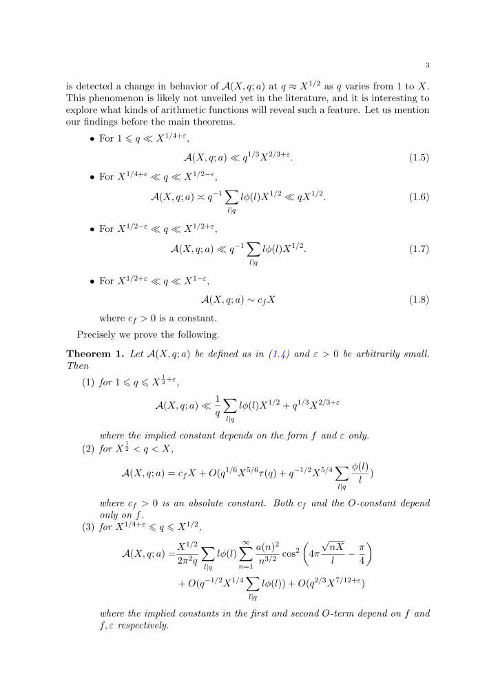
is detected a change in behavior of A(X, q; a) at q ≈ X1/2 as q varies from 1 to X.This phenomenon is likely not unveiled yet in the literature, and it is interesting toexplore what kinds of arithmetic functions will reveal such a feature. Let us mentionour findings before the main theorems.

• For 1 6 q � X1/4+ε,

A(X, q; a)� q1/3X2/3+ε. (1.5)

• For X1/4+ε � q � X1/2−ε,

A(X, q; a) � q−1∑l|q

lφ(l)X1/2 � qX1/2. (1.6)

• For X1/2−ε � q � X1/2+ε,

A(X, q; a)� q−1∑l|q

lφ(l)X1/2. (1.7)

• For X1/2+ε � q � X1−ε,

A(X, q; a) ∼ cfX (1.8)

where cf > 0 is a constant.

Precisely we prove the following.

Theorem 1. Let A(X, q; a) be defined as in (1.4) and ε > 0 be arbitrarily small.Then

(1) for 1 6 q 6 X12+ε,

A(X, q; a)� 1

q

∑l|q

lφ(l)X1/2 + q1/3X2/3+ε

where the implied constant depends on the form f and ε only.

(2) for X12 < q < X,

A(X, q; a) = cfX +O(q1/6X5/6τ(q) + q−1/2X5/4∑l|q

φ(l)

l)

where cf > 0 is an absolute constant. Both cf and the O-constant dependonly on f .

(3) for X1/4+ε 6 q 6 X1/2,

A(X, q; a) =X1/2

2π2q

∑l|q

lφ(l)∞∑n=1

a(n)2

n3/2cos2

(4π

√nX

l− π

4

)+O(q−1/2X1/4

∑l|q

lφ(l)) +O(q2/3X7/12+ε)

where the implied constants in the first and second O-term depend on f andf, ε respectively.

4 YUK-KAM LAU, LILU ZHAO

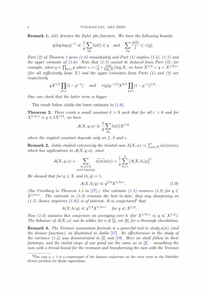
Remark 1. φ(l) denotes the Euler phi function. We have the following bounds:

q(log log q)−1 � 1

q

∑l|q

lφ(l) 6 q and∑l|q

φ(l)

l6 τ(q).

Part (2) of Theorem 1 gives (1.8) immediately and Part (1) implies (1.5), (1.7) andthe upper estimate of (1.6). Note that (1.7) cannot be deduced from Part (2); for

example, when q =∏p6z p where z = (12 + 0.01

log2X) logX, we have X1/2 < q < X1/2+ε

(for all sufficiently large X) and the upper estimates from Parts (1) and (2) arerespectively

qX1/2∏p6z

(1− p−1) and τ(q)q−1/2X5/4∏p6z

(1− p−1)1/2.

One can check that the latter term is bigger.

The result below yields the lower estimate in (1.6).

Theorem 2. There exists a small constant δ > 0 such that for all ε > 0 and forX1/4+ε 6 q 6 δX1/2, we have

A(X, q; a)� 1

q

∑l|q

lφ(l)X1/2

where the implied constant depends only on f , δ and ε.

Remark 2. Jutila studied extensively the twisted sum A(X,α) :=∑

n6X a(n)e(αn)which has applications to A(X, q; a), since

A(X, q; a) =∑

m,n6Xm≡n (mod q)

a(m)a(n) =1

q

q∑h=1

∣∣A(X,h/q)∣∣2.

He showed that for q 6 X and (h, q) = 1,

A(X,h/q)� q2/3X1/3+ε. (1.9)

(See Corollary to Theorem 1.1 in [17].) Our estimate (1.5) recovers (1.9) for q 6X1/4+ε. The estimate in (1.9) remains the best to-date, thus any sharpening on(1.5) (hence improves (1.9)) is of interest. It is conjectured4 that

A(X,h/q)� q1/2X1/4+ε for q � X1/2.

Now (1.6) sustains this conjecture on averaging over h (for X1/4+ε � q � X1/2).The behavior of A(X,α) can be wilder for α /∈ Q, see [6] for a thorough elucidation.

Remark 3. The Voronoi summation formula is a powerful tool to study a(n) (andthe divisor function), as illustrated in Jutila [17]. Its effectiveness in the study ofthe variance (1.4) was demonstrated in [2] and [19]. Here we shall follow in theirfootsteps, and the initial steps of our proof are the same as in [2] – smoothing thesum with a trivial bound for the remnant and transforming the sum with the Voronoi

4The case q = 1 is a counterpart of the famous conjecture on the error term in the Dirichletdivisor problem for Hecke eigenvalues.

5

formula. This process will turn (1.8) transparent (from technical point of view) ifone proceeds with the argument in [2, p.276]. Assume q is a prime. Then∑

n≡b (q)

a(n)w(n/X) =X

q2

∑n

a(n)S(n, b, q)w(nX/q2) + · · · .

Together with the following identity∑b (q)

∣∣∣∣∑n6x

α(n)S(n, b, q)

∣∣∣∣2 = q2∑n6x

|α(n)|2 − q∣∣∣∣∑n6x

α(n)

∣∣∣∣2for prime q and x < q, one infers A(X, q; a) ≈ (X/q2)2 ·q2 ·q2/X = X when q2/X is

not small, say� Xε or equivalently q � X1/2+ε, because w(x) decays rapidly. Then(1.8) is within expectation. Nevertheless there is technical complication, not only in

this case but also the case q 6 X1/2. To its end we need some asymptotic formulasof special functions. Section 2 is devoted to these formulas. In Section 3 we studyintegral transforms of a weight function. Then we provide a quite neat approximationto A(X, q;α) in Section 4. Sections 5-7 contain the proofs of theorems.

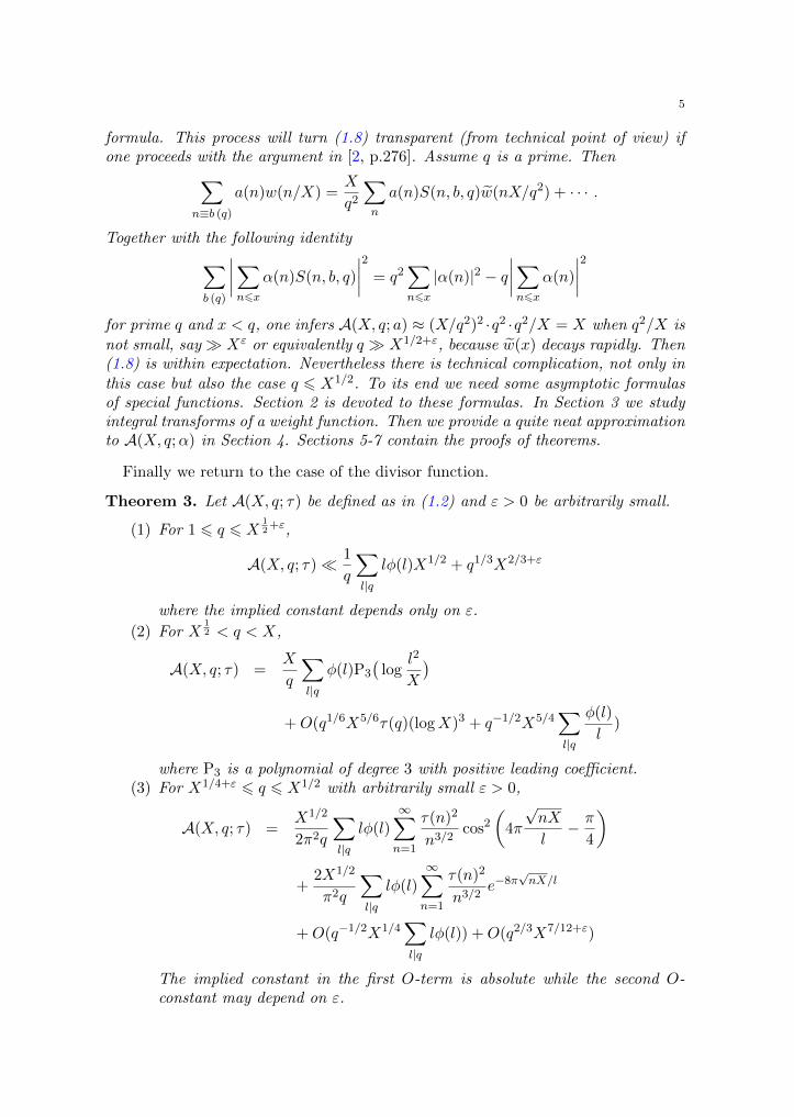
Finally we return to the case of the divisor function.

Theorem 3. Let A(X, q; τ) be defined as in (1.2) and ε > 0 be arbitrarily small.

(1) For 1 6 q 6 X12+ε,

A(X, q; τ)� 1

q

∑l|q

lφ(l)X1/2 + q1/3X2/3+ε

where the implied constant depends only on ε.

(2) For X12 < q < X,

A(X, q; τ) =X

q

∑l|q

φ(l)P3

(log

l2

X

)+O(q1/6X5/6τ(q)(logX)3 + q−1/2X5/4

∑l|q

φ(l)

l)

where P3 is a polynomial of degree 3 with positive leading coefficient.(3) For X1/4+ε 6 q 6 X1/2 with arbitrarily small ε > 0,

A(X, q; τ) =X1/2

2π2q

∑l|q

lφ(l)

∞∑n=1

τ(n)2

n3/2cos2

(4π

√nX

l− π

4

)

+2X1/2

π2q

∑l|q

lφ(l)

∞∑n=1

τ(n)2

n3/2e−8π

√nX/l

+O(q−1/2X1/4∑l|q

lφ(l)) +O(q2/3X7/12+ε)

The implied constant in the first O-term is absolute while the second O-constant may depend on ε.

6 YUK-KAM LAU, LILU ZHAO

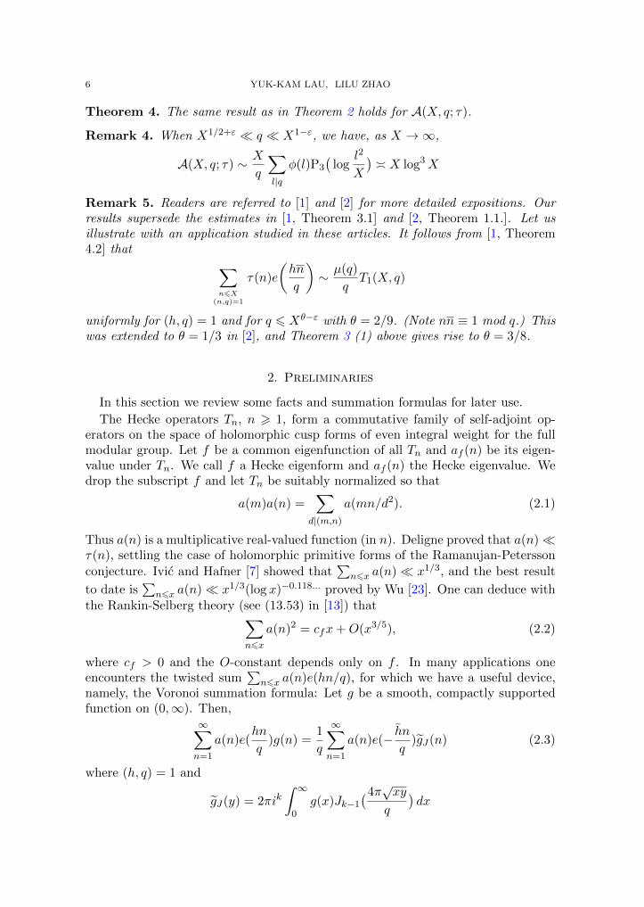
Theorem 4. The same result as in Theorem 2 holds for A(X, q; τ).

Remark 4. When X1/2+ε � q � X1−ε, we have, as X →∞,

A(X, q; τ) ∼ X

q

∑l|q

φ(l)P3

(log

l2

X

)� X log3X

Remark 5. Readers are referred to [1] and [2] for more detailed expositions. Ourresults supersede the estimates in [1, Theorem 3.1] and [2, Theorem 1.1.]. Let usillustrate with an application studied in these articles. It follows from [1, Theorem4.2] that ∑

n6X(n,q)=1

τ(n)e

(hn

q

)∼ µ(q)

qT1(X, q)

uniformly for (h, q) = 1 and for q 6 Xθ−ε with θ = 2/9. (Note nn ≡ 1 mod q.) Thiswas extended to θ = 1/3 in [2], and Theorem 3 (1) above gives rise to θ = 3/8.

2. Preliminaries

In this section we review some facts and summation formulas for later use.

The Hecke operators Tn, n > 1, form a commutative family of self-adjoint op-erators on the space of holomorphic cusp forms of even integral weight for the fullmodular group. Let f be a common eigenfunction of all Tn and af (n) be its eigen-value under Tn. We call f a Hecke eigenform and af (n) the Hecke eigenvalue. Wedrop the subscript f and let Tn be suitably normalized so that

a(m)a(n) =∑

d|(m,n)

a(mn/d2). (2.1)

Thus a(n) is a multiplicative real-valued function (in n). Deligne proved that a(n)�τ(n), settling the case of holomorphic primitive forms of the Ramanujan-Petersson

conjecture. Ivic and Hafner [7] showed that∑

n6x a(n)� x1/3, and the best result

to date is∑

n6x a(n)� x1/3(log x)−0.118... proved by Wu [23]. One can deduce withthe Rankin-Selberg theory (see (13.53) in [13]) that∑

n6x

a(n)2 = cfx+O(x3/5), (2.2)

where cf > 0 and the O-constant depends only on f . In many applications oneencounters the twisted sum

∑n6x a(n)e(hn/q), for which we have a useful device,

namely, the Voronoi summation formula: Let g be a smooth, compactly supportedfunction on (0,∞). Then,

∞∑n=1

a(n)e(hn

q)g(n) =

1

q

∞∑n=1

a(n)e(− hnq

)gJ(n) (2.3)

where (h, q) = 1 and

gJ(y) = 2πik∫ ∞0

g(x)Jk−1(4π√xy

q

)dx

7

and Jk−1 is a Bessel function.

The asymptotic formula for∑

n6x τ(n) is well-known. Besides we have (see [12,(14.30)]) ∑

n6x

τ(n)2 = xP3(log x) +O(x1/2+ε) (2.4)

where P3(x) is a cubic polynomial with positive leading coefficient. In this case theVoronoi summation formula is

∞∑n=1

τ(n)e(hn

q)g(n) =q−1

∫(log x+ 2γ − 2 log q)g(x)dx

+∞∑n=1

τ(n)e(− hnq

)gY (n) +∞∑n=1

τ(n)e(hn

q)gK(n) (2.5)

where

gY (y) = −2π

∫ ∞0

g(x)Y0(4π√xy

q

)dx, gK(y) = 4

∫ ∞0

g(x)K0

(4π√xy

q

)dx.

Here Y0 and K0 denote the standard Bessel functions. For the proof of the abovewell-known formulas, one may refer to, for example, Theorem 4 of Duke and Iwaniec[5] (see also Lemma 1 in [4]) and Theorem 4 of Jutila [16] (or Section 4.5 of Kowalskiand Iwaniec [15]).

3. Study of a weighting function

Let w(x) be a smooth function supported on [H,X] satisfying w(x) = 1 for all

x ∈ [2H,X −H] and w(j)(x)�j H−j , where q < H < X/3. Eventually we shall set

H = 13q

2/3X1/3. We need to study the integral transforms in (2.3) and (2.5). Let usbegin with the order of magnitude of the Bessel functions. We have for 0 < x� 1,

Jν(x) =1

Γ(ν + 1)

(x

2

)ν(1 +O(x)

)(ν > 0 real),

Y0(x) =2

πlog

x

2+O(1), K0(x) = log

2

x+O(1)

(3.1)

and Yν(x),Kν(x)�ν x−ν for real ν > 0. Let B denote the Bessel function J , Y or

K. If ν > 0 and x > 1 + ν2, then

Bν(x) =

√2

πx

(CS(x− νπ/2− π/4) +O(

1 + |ν|2

x)

),

Kν(x) =

√2

πxe−x(

1 +O(1 + |ν|2

x)

) (3.2)

where CS = cos if B = J and CS = sin if B = Y . In addition their derivatives fulfilrecurrence relations: for any ν > 0,

d

dx

(xν+1Bν+1(x)

)= εxν+1Bν(x) (3.3)

8 YUK-KAM LAU, LILU ZHAO

where ε = 1 for B = J, Y and ε = −1 for B = K. (See Chapter 5 of [18] for thebackground of Bessel functions.) In light of the Voronoi formulae, we introduce

$B(α) = cB

∫w(x)Bν(4πα

√x) dx (3.4)

where cB = 2πik,−2π, 4 and Bν = Jk−1, Y0,K0 for B = J, Y,K respectively.

Lemma 3.1. The following estimates hold: for α > 0,

(a) $B(α)� α−1/2X3/4,

(b) $B(α)�j α−j−1/2Xj/2−1/4H1−j (j = 1, 2, · · · ),

(c) $′B(α)� α−3/2X3/4

where B denotes J , Y or K. In fact,

(d) $K(α)� α−1/2X3/4e−α√H .

When α > 0 is small, we have

$J(α), α$J(α)� X

and for B = Y,K,

$B(α), α$B(α)� X(| logα|+ logX).

Proof. Let B = J or Y . Part (a) follows immediately from (3.2). By (3.3), wededuce

d

dx

(x(ν+1)/2Bν+1(4πα

√x)

)= ε2παxν/2Bν(4πα

√x). (3.5)

In view of the growth condition of w(j)(x), it follows that(x−ν/2w(x)

)(j) � x−ν/2−jχI(x) + x−ν/2H−jχJ(x)

where χS denotes the characteristic function over the set S with I = [H,X] andJ = [H, 2H] ∪ [X −H,X]. Thus for j > 1, integration by parts gives

$B(α) � α−j−1/2∫ X

Hx−j/2−1/4 dx+ α−j−1/2H−j

∫ X

X−Hxj/2−1/4 dx

� α−j−1/2Xj/2−1/4H−j .

Part (c) follows from an integration by parts and Part (a).

By (3.2) it is plain to get Part (d). The last estimates for small α are directconsequence of (3.1). �

Lemma 3.2. For α > 0, we have

$B(α) = − 1

π√

2α−3/2

∫x1/4w′(x) cos(4πα

√x− π

4) dx+O(α−2)

when B = J or Y , and

$K(α) =

√2

π2α−3/2

∫x1/4w′(x)e−4πα

√x dx+O(α−2).

9

Proof. By partial integration with (3.5), we have (for B = J , Y or K)

c−1B $B(α) =−1

2πεα

∫x1/2w′(x)Bν+1(4πα

√x) dx

+ν

4πεα

∫x−1/2w(x)Bν+1(4πα

√x) dx. (3.6)

The second term on the right side appears only for B = J , as ν = 0 for B = Yor K. If B = J , this term is � να−2 by (3.5) and Jν+2(x) � min(xν+2, x−1/2) �min(x, x−1/2).

Consider B = J or Y . We observe from (3.1) and (3.2) that for all x > 0,

Bν(x)−√

2

πxCS(x− νπ

2− π

4)� min(x−1/2, x−3/2)� x−1

where CS = cos if B = J and CS = sin if B = Y , and the implied constant dependson ν only. This yields the desired result with (3.6).

The case of B = K is similar. �

Lemma 3.3. We have for α > 0,

$B(α) =α−3/2

π√

2

{X1/4 cos(4πα

√X − π

4) +O(E1)

}if B = J or Y , and

$K(α) = −√

2

π2α−3/2

{X1/4e−4πα

√X +O(E1)

}where

E1 � α−1/2 +H1/4 + αX−1/4H.

Proof. We prove by the same argument, so only work out the first case. Considerthe integral in Lemma 3.2. Since w′(x) is supported on [H, 2H] ∪ [X −H,X], and

clearly the integral over [H, 2H] is � H1/4. We are led to handle

I =

∫ X

X−Hx1/4w′(x) cos

(4πα√x− π

4

)dx

As x1/4 = X1/4 +O(HX−3/4), we have, by partial integration,

I = −X1/4 cos(4πα√X − π

4

)+O(αX−1/4H +HX−3/4).

The result then follows, for HX−3/4 � H1/4. �

The next lemma is an exercise of Hankel transform (see [14, Appendix B.5]).

Lemma 3.4. We have ∫ ∞0

$J(√ξ)2 dξ = X +O(H).

10 YUK-KAM LAU, LILU ZHAO

Proof. It suffices to show

4π2∫ ∞0

(∫ ∞0

w(x)Jk−1(4π√ξx) dx

)2

dξ =

∫ ∞0

w(x)2 dx.

Changing variables (x = y2, ξ = (4π)−2η2), the left hand side is∫ ∞0

2w(y2)

(∫ ∞0

(∫ ∞0

w(x2)Jk−1(xη)x dx

)Jk−1(yη)η dη

)y dy.

By the Hankel inversion, the inner double integration is equal to w(y2). Hence theabove triple integration reduces to

∫w(y)2dy = X +O(H). �

Lemma 3.5. Let l > 1 and Q(ξ) be a polynomial in log ξ of degree m. Then forB = Y or K, we have∫ ∞

0Q(ξl2)$B(

√ξ)2 dξ = XQB

( l2X

)+O(X3/4H1/4(log(Xl))m)

where QB(ξ) is a polynomial in log ξ of degree m whose leading coefficient has thesame sign as Q.

Proof. Let us write

1XB(α) =

∫ X

0Bν(4πα

√x) dx.

We have the following estimates by (3.2), 1XB(α) � α−1/2X3/4 and α−3/2X1/4 byan integration by parts with (3.5). These bounds hold for $B(α) by Lemma 3.1.Besides we have

$B(α)− 1XB(α)�∫ X

0|w(x)− 1||Bν(4πα

√x)| dx� H3/4α−1/2

and consequently,

1XB(α)2 −$B(α)2 � min(α−1X3/2, α−8/3X5/12H1/4, α−3X1/2

).

(The middle bound makes use of a2 − b2 � |a − b|1/3(|a|5/3 + |b|5/3).) Cutting atξ = X−1 and ξ = X, we see that∫ ∞

0Q(ξl2)1XB(

√ξ)2 dξ −

∫ ∞0

Q(ξl2)$B(√ξ)2 dξ � X3/4H1/4(log(Xl))m.

It remains to evaluate the first integral on the left hand side. Note that 1XB(√ξ) =

ξ−11ξXB(1). If Q(ξ) =∑m

r=0 ar(log ξ)r, then this integral equals XQB(l2/X) with

QB(ξ) :=

m∑r=0

(log ξ)r∫ ∞0

Pm−r(log η) 1ηB(1)2η−2 dη,

where Pm−r is a polynomial of degree 6 m− r and P0 = am (so QB is of degree mand its leading coefficient is a positive scalar multiple of am). �

11

Lemma 3.6. Let κ > 1. Then we have∑n6κ

a(n)2$J

(√n

l

)2

= cf l2X +O(l2H)

+O(l3X1/2κ−1/2 + lX3/2 + l3/2X5/4),

and for B = Y or K,

∑n6κ

τ(n)2$B

(√n

l

)2

= l2XQ3B(l2/X) +O(l2X3/4H1/4(log(Xl))3)

+O(l3X1/2κ−1/2(log κ)3 + lX3/2 + l3/2X5/4),

where Q3B(ξ) is a polynomial in log ξ of degree 3 with a positive leading coefficient.

Proof. By partial summation with (2.2), we infer that

∑n6κ

a(n)2$J

(√n

l

)2

= cf

∫ κ

0+$J

(√t

l

)2

dt+ O(t3/5)$J

(√t

l

)2∣∣∣∣∣t=κ

t=0+

−∫ κ

0+O(t3/5)$J

(√t

l

)$′J

(√t

l

)dt

l√t.

In virtue of Lemma 3.4, the main term comes from the first summand on the rightside, which is,

cf l2

∫ ∞0

$J(√ξ)2 dξ +O(l3X1/2κ−1/2),

as $J(α) � α−3/2X1/4 by Lemma 3.1 (b). Also the second term on the right side

is � l3X1/2κ−9/10. Splitting the integral at t = 1, the last term is

� lX3/2

∫ 1

0+t

110−1 dt+ l3/2X5/4

∫ κ

1t

110− 5

4 dt

� lX3/2 + l3/2X5/4

by $′J(α)� α−3/2X3/4 with $J(α)� α−1/2X3/4 and

$J(α)�(α−1/2X3/4α−3/2X1/4

)1/2= α−1X1/2

respectively.

The proof for B = Y or K is similar, but the main term in this case is∫ ∞0

(P3(log t) + P ′3(log t))$B

(√t

l

)2

dt = l2∫ ∞0

Q3(ξl2)$B(

√ξ)2 dξ

by Lemma 3.5, where P3 is defined as in (2.4) and Q3(ξ) := P3(log ξ)+P ′3(log ξ). �

12 YUK-KAM LAU, LILU ZHAO

4. Approximations to A(X, q; a) & A(X, q; τ)

Define for Z > 0,

Sψ,B(Z;α) :=1

q

∑l|q

ψ(l)

l2

∑n6l2Z

α(n)2$B

(√n

l

)2

(4.1)

where ψ(l) denotes φ(l) or σ(l), α(n) = a(n) for B = J and α(n) = τ(n) forB = Y,K.

Proposition 4.1. Let H = 13q

2/3X1/3. We have

A(X, q; a) =Sφ,J(XH−2; a) + E

where the error term satisfies

E � Sσ,J(XH−2; a)1/2√q1/3X2/3

(√τ(q) +Xε

)+ q1/3X2/3(τ(q) +Xε).

The term Xε does not arise if q > X2/5, and Sφ,J ,Sσ,J are given by (4.1).

Proof. Installing the smooth weight function and squaring out, we have

A(X, q; a) =Aw(q; a) +O(Aw(q; a)1/2E1/21 + E1) (4.2)

where

Aw(q; a) =

q∑b=1

∣∣ ∑n≡b (mod q)

a(n)w(n)∣∣2

with w(x) selected as in Section 3, and E1 := A1−w(q; a). By Cauchy-Schwarz’sinequality we get, as H > q,

E1 �XεH2q−1 � q1/3X2/3Xε (4.3)

by Deligne’s bound or by (2.2). The factor Xε is removed when (2.2) is applicable,

i.e. H > X3/5 (or q > X2/5).

Replacing the congruence condition with additive characters, we have∑n≡b (mod q)

a(n)w(n) =1

q

∑r|q

∑h (r)

∗e(−bh

r)∑n

a(n)e(nh

r)w(n).

Applying Voronoi formula (2.3) to the last summation, it follows that∑n≡b (mod q)

a(n)w(n) =1

q

∑r|q

∑h (r)

∗e(−bh

r)Sa,J(∞,−h, r)

where

Sa,J(M,−h, r) =∑

16n<M

a(n)

re(−nh

r)$J

(√n

r

).

13

Let M(r) = r2XH−2 and M+(r) = M(r)Xε = r2XH−2Xε. We split the sumover n into two pieces according as n 6M+(r) or otherwise. Lemma 3.1 (b) yieldsthat for n > M+(r) = r2XH−2Xε,

$J

(√n

r

)�j (X1/2H−1Xε)−j−1/2Xj/2−1/4H1−j � X−2011

by selecting a sufficiently large j, whence we infer

Aw(q; a) =A′J(q; a) +O(X−100) (4.4)

where

A′J(q; a) =

q∑b=1

∣∣∣∣∣∣1q∑r|q

∑h (r)

∗e(−bh

r)Sa,J

(M+(r),−h, r

)∣∣∣∣∣∣2

.

Noting that for (h1, r1) = (h2, r2) = 1,

∑b (mod q)

e(−bh1r1

)e(−bh2r2

) =

q, if r1 = r2 = r and

h1 ≡ h2 (mod r),

0, otherwise,

we expand the square to obtain

A′J(q; a) =1

q

∑r|q

∑h (r)

∗ ∣∣Sa,J(M+(r),−h, r)∣∣2 . (4.5)

As usual, we apply the mobius formula∑

d|(h,r) µ(d) to substitute the constraint

(h, r) = 1. With the change of variables h by dh and r by dr, we deduce that

A′J(q; a) =1

q

∑d|q

µ(d)∑r| q

d

∑h (r)

∣∣Sa,J(M+(dr),−dh, dr)∣∣2 .

The next step is apparently squaring out and using the complete sum over h tosift out many non-diagonal terms. Indeed for 1 6 m,n < r/2, only diagonal termssurvive, which yield the initial section of Sφ,J(XH−2; a). However we need somecalculation by brute-force to control the non-diagonal terms and also the terms inthe segment between M(dr) and M+(dr).

Let us set M−(d, r) = min(r/2,M(dr)) and write

Bu,J(A,B) =1

q

∑d|q

u(d)∑r| q

d

∑h (r)

∣∣∣∣∣∣∑

A(d,r)6n<B(d,r)

e(−nhr

)a(n)

dr$J

(√n

dr

)∣∣∣∣∣∣2

for some functions A,B of d and r, where u(d) = µ(d) or |µ|(d) (:= |µ(d)|). Thenwe have

A′J(q; a) = Bµ,J(1,M−) + E2 (4.6)

where 1(d, r) denotes the constant function 1 and

E2 � B|µ|,J(1,M−)1/2(B|µ|,J(M−,M)1/2 + B|µ|,J(M,M+)1/2

)+B|µ|,J(M−,M) + B|µ|,J(M,M+). (4.7)

14 YUK-KAM LAU, LILU ZHAO

Here we take M+(d, r) = M+(dr) and M(d, r) = M(dr).

After squaring out and evaluating the sum over h, we deduce that

B|µ|,J(A,B)�1

q

∑d|q

∑r| q

d

1

d2r

∑A6m<B

a(m)2∣∣∣∣$J

(√m

dr

)∣∣∣∣ ∑A6n<B

m≡n (mod r)

∣∣∣∣$J

(√n

dr

)∣∣∣∣,as |a(m)a(n)| 6 a(m)2 + a(n)2.

Applying Lemma 3.1 (b) with j = 2, it follows that B|µ|,J(M,M+) is

� X3/2H−2

q

∑dr|q

d3r4∑

M(dr)6m<M+(dr)

|a(m)|2m−5/4∑

M(dr)6n<M+(dr)n≡m (mod r)

n−5/4.

For r 6 M(dr), the last sum over n is � 1rM(dr)−1/4, while for M(dr) < r, it is

�M(dr)−5/4. Hence the expression in the last line is

� X3/2H−2

q

∑dr|q

(dr)3M(dr)−1/2 +X3/2H−2

q

∑dr|q

d3r4M(dr)−3/2

� qXH−1τ(q) +Hτ(q)� q1/3X2/3τ(q),

for∑

dr|q(dr)2 � q2τ(q) and

∑dr|q r � qτ(q). Similarly, we apply Lemma 3.1 (b)

with j = 1 to get the same upper bound for B|µ|,J(M−,M).

Next we handle B|µ|,J(1,M−) and Bµ,J(1,M−) (in the same manner). One has

B|µ|,J(1,M−) =1

q

∑dr|q

|µ|(d)

d2r

∑16n<M(dr)

a(n)2$J

(√n

dr

)2

+ B′

where B′ accounts for the non-diagonal terms. For m,n 6 M−(d, r) (6 r/2), thecondition m ≡ n (mod r) forces m = n. With Lemma 3.1 (b), j = 1 again, it followsthat

B′ � X1/2

q

∑dr|q

dr2∑

r/26n<M(dr)

a(n)2

n3/2� q1/2X1/2τ(q).

Writing l = dr, the first summand is 6 Sσ,J(XH−2; a) as∑

dr=l r|µ|(d) 6 σ(l), andhence

B|µ|,J(1,M−) 6 Sσ,J(XH−2; a) +O(q1/2X1/2τ(q)). (4.8)

Proceeding with the same line of arguments, we deduce that

Bµ,J(1,M−) = Sφ,J(XH−2; a) +O(q1/2X1/2τ(q)) (4.9)

as∑

dr=l rµ(d) = φ(l). The O-term will be absorbed in O(q1/3X2/3τ(q)).

Plainly we get by (4.7)-(4.8) that

E2 � Sσ,J(XH−2; a)1/2√q1/3X2/3τ(q) + q1/3X2/3τ(q), (4.10)

as q1/2X1/2 � q1/3X2/3. Observing |Bµ,J | 6 B|µ|,J , it follows with (4.6) and (4.9)that

A′J(q; a) = Sφ,J(XH−2; a) + E2. (4.11)

15

On the other hand, with (4.2)-(4.4), we get that A(X, q; a)−A′J(q; a) is

� Sσ,J(XH−2; a)1/2√q1/3X2/3

(√τ(q) +Xε

)+ q1/3X2/3(τ(q) +Xε).

The term Xε appears only when q 6 X2/5. Our assertion follows after invoking(4.11). �

Proposition 4.2. Let H = 13q

2/3X1/3. We have

A(X, q; τ) =Sφ,Y (XH−2; τ) + Sφ,K(H−1Xε; τ) + E

where the error term satisfies

E �(Sσ,Y (XH−2; τ) + Sσ,K(H−1Xε; τ)

)1/2|E′|1/2 + |E′|and

E′ � q1/3X2/3(τ(q) log3X +Xε

).

When q > X1/4+ε, Xε is replaced by log3X.

Proof. The argument is the same as the proof of Proposition 4.1, so we give thesalient points only. We replace Tb(X, q) in (1.2) by

Tw(b, q) :=1

q

∑r|q

∑h (r)

∗e(−bh

r)1

r

∫(log x+ 2γ − 2 log r)w(x) dx

= Tb(X, q) +O(q−1τ(q)1/2τ(b)1/2H logX),

with the fact q−1∑

r|(q,b) rφ(q/r) 6 τ(q)1/2τ(b)1/2. As in (4.2), we have

A(X, q; τ) =Aw(q; τ) +O(Aw(q; τ)1/2E1/21 + E1) (4.12)

where

Aw(q; τ) =

q∑b=1

∣∣∣∣ ∑n≡b (mod q)

τ(n)w(n)− Tw(b, q)

∣∣∣∣2and

E1 �(Xε + τ(q) log3X

)H2q−1 � q1/3X2/3(τ(q) log3X +Xε) (4.13)

with Xε replaced by log3X if q > X1/4+ε.

We apply the Voronoi formula (2.5) and proceed with the argument in (4.4) and(4.5). Let M(r),M+(r),M−(r) be defined as therein. Then we have

Aw(q; τ) =A′Y,K(q; τ) +O(X−100) (4.14)

where

A′Y,K(q; τ) =1

q

∑r|q

∑h (r)

∗ ∣∣Sτ,Y (M+(r),−h, r)

+ Sτ,K(M+(r), h, r

)∣∣2 .Along the same argument in the proof of Proposition 4.1, we will complete the proofand let us remark that the condition 1 6 m,n 6 r/2 forces m + n 6≡ 0 (mod r).Thus, the cross term Sτ,Y Sτ,K is small and absorbed in E′. �

16 YUK-KAM LAU, LILU ZHAO

5. Proof of Theorem 1

We start with the evaluation of E in Proposition 4.1 and note H = 13q

2/3X1/3.Using the estimate in Lemma 3.1 (j = 1), we get from (4.1),

Sσ,J(XH−2; a)� X1/2

q

∑l|q

lσ(l)∑n

a(n)2n−3/2 � qX1/2σ−1(q) (5.1)

as∑

l|q lσ(l)� q2σ−1(q). On the other hand, by Lemma 3.6 with κ = l2XH−2, we

see that Sσ,J(XH−2; a) is

� 1

q

∑l|q

σ(l)X +1

q

∑l|q

σ(l)l−1X3/2 +1

q

∑l|q

σ(l)l−1/2X5/4

� τ(q)(X + σ−1(q)q

−1/2X5/4)

for q � X1/2. The second term dominates if X1/2 � q � X1/2σ−1(q)2. However,

in this case we may use (5.1) and the fact σ−1(q)n �n τ(q) (n > 0) to deduce that

Sσ,J(XH−2; a)� τ(q)X. Hence,

Sσ,J(XH−2; a)� τ(q) min(qX1/2, X) (5.2)

and the error term E in Proposition 4.1 is

� Xε(Sσ,J(XH−2; a)1/2q1/6X1/3

√τ(q) + q1/3X2/3τ(q)

)with 1 in place of Xε for q > X2/5, thus

E �

q1/3X2/3+ε if q 6 X1/4,

q2/3X7/12+ε if X1/4 < q 6 X1/2,

q1/6X5/6τ(q) if X1/2 < q 6 X(5.3)

where the implied constants in the first two cases depend on ε.

Now we handle the main term Sφ,J(XH−2; a) in Proposition 4.1 .

(1) Consider q 6 X1/2+ε. By Lemma 3.1 (b) (j = 1) again, we infer that

Sφ,J(XH−2; a)� X1/2

q

∑l|q

lφ(l)∑n

a(n)2

n3/2� X1/2

q

∑l|q

lφ(l) (5.4)

which leads to Part (1) with (5.3).

(2) Let q > X1/2. We apply Lemma 3.6 with κ = l2XH−2 to Sφ,J(XH−2; a).The main term is cfq

−1∑l|q φ(l)X and the O-term contributes a term

� H +X3/2

q

∑l|q

φ(l)l−1 +X5/4

q

∑l|q

φ(l)l−1/2,

which is absorbed in the error term of our desired result. Note that the term q2/3X1/3

is suppressed by q1/6X5/6 in E, and Part (2) is complete.

(3) We confine to X1/4+ε 6 q 6 X1/2. By Lemma 3.3, it follows that

$

(√n

l

)=

1

π√

2

l3/2

n3/4

{X1/4 cos

(4π

√nX

l− π

4

)+ E1

}

17

where E1 � l1/2n−1/4 +H1/4 + l−1n1/2X−1/4H. We insert this formula for $(√n/l)

into (4.1) and extend the range of summation from 1 6 n 6 l2L to n > 1 so as to

get the desired main term, where L = 9X1/3q−4/3. Next, we observe that

1

q

∑l|q

lφ(l)∑n6l2L

a(n)2

n3/2O(X1/4|E1|+ E21

)� q−1/2X1/4

∑l|q

lφ(l)

for X1/4+ε 6 q � X1/2, and

X1/2

q

∑l|q

lφ(l)∑n>l2L

a(n)2

n3/2� q2/3X1/3.

Together with (5.3), we conclude the result in Part (3).

6. Proof of Theorem 3

Let Z = XH−2 for B = Y and Z = H−1Xε for B = K. As in (5.2), we have

Sσ,B(Z; τ)� τ(q) min(qX1/2, X log3X).

This yields the following estimate for E in Proposition 4.2,

E�

q1/3X2/3+ε if q 6 X1/4,

q2/3X7/12+ε if X1/4 < q 6 X1/2,

q1/6X5/6τ(q)(logX)3 if X1/2 < q 6 X.(6.1)

Now we handle the main terms Sφ,B(Z; τ). Part (1) is clear, following the calcula-tion in (5.4) with (6.1). For Part (2) we apply Lemma 3.6 with B = Y , κ = l2XH−2

or B = K, κ = l2H−2Xε. The treatment of Part (3) is the same as in the proof ofTheorem 1. We omit the details.

7. Proof of Theorems 2 & 4

Consider the main term in Theorem 1 (3). By positivity, the main term is boundedbelow by

X1/2

2π2q

∑l|q

lφ(l)S(l) :=X1/2

2π2q

∑l|q

lφ(l)∑

m=1,2,4

a(m2)2

m3cos2

(mθ(l)− π

4

)(7.1)

where θ(l) := 4π√X/l. Our essential task is to show S(l)� 1. If | cos(θ(l)− π/4)|

is small, say less than 10−3, then | cos(mθ(l) − π/4)| > 0.5 for both m = 2 and 4.By (2.1) with m = n = 4, a(4) and a(16) cannot be simultaneously small. Ourassertion thus follows. In view of the O-term in Theorem 1 Part (3), we see that

(7.1) dominates when X1/4+ε 6 q 6 δX1/2 for a sufficiently small δ > 0.

Finally we turn to A(X, q; τ). We apply the above argument to handle the firstmultiple sum in Theorem 3 (3), which is in fact easier as τ(n) > 1. Note that thesecond multiple sum can be ignored by positivity. Theorem 4 follows immediately.

Acknowledgement. The authors wish to thank the referees for their readings,the explanatory viewpoint in Remark 3 and criticism. Lau is supported by a grant

18 YUK-KAM LAU, LILU ZHAO

from the Research Grants Council of the Hong Kong Special Adminstrative Region,China (HKU702308P).

References

[1] W.D. Banks, R. Heath-Brown, I.E. Shparlinski, On the average value of divisor sums inarithmetic progressions, Int. Math. Res. Not. 1 (2005), 1–25.

[2] V. Blomer, The average value of divisor sums in arithmetic progressions, Q. J. Math. 59(2008), 275–286.

[3] J. Brudern, T.D. Wooley, Sparse variance for primes in arithmetic progressions, Q. J. Math.62 (2011), 289–305.

[4] W. Duke, J. B. Friedlander, H. Iwaniec, Bounds for automorphic L-functions, Invent. Math.112 (1993), 1–8.

[5] W. Duke, H. Iwaniec, Bilinear forms in the Fourier coefficients of half-integral weight cuspfroms and sums over primes, Math. Ann. 286 (1990), 783–802.

[6] A.-M. Ernvall-Hytonen, K. Karppinen, On short exponential sums involving Fourier coeffi-cients of holomorphic cusp forms, IMRN 2008, Art. ID. rnn022, 44 pp.

[7] J.L. Hafner, A. Ivic, On sums of Fourier coefficients of cusp forms, Enseign. Math. 35 (1989),375–382.

[8] D.R. Heath-Brown, The fourth power moment of the Riemann zeta function, Proc. LondonMath. Soc. 38 (1979), 385–422.

[9] C. Hooley, An asymptotic formula in the theory of numbers, Proc. London Math. Soc. 7(1957), 396–413.

[10] C. Hooley, On the Barban-Davenport-Halberstam theorem I, J. Reine Angew. Math. 274/275(1975), 206–223.

[11] C. Hooley, On the Barban-Davenport-Halberstam theorem. XVIII, Illinois J. Math. 49 (2005),581–643.

[12] A. Ivic, The Riemann zeta-function. The theory of the Riemann zeta-function with applica-tions, John Wiley & Sons Inc. New York, 1985.

[13] H. Iwaniec, Topics in classical automorphic forms, AMS, 1997.[14] H. Iwaniec, Spectral methods of automorphic forms, Graduate Studies in Mathematics 53,

AMS, 2002.[15] H. Iwaniec, E. Kowalski, Analytic number theory, Amer. Math. Soc. Colloquium Publ. 53,

Amer. Math. Soc., Providence RI, 2004.[16] M. Jutila, On exponential sums involving the divisor function, J. Reine Angew. Math. 365

(1985), 173–190.[17] M. Jutila, Lectures on a method in the theory of exponential sums, Berlin Heidelberg New

York, 1987.[18] N.N. Lebedev, Special functions and their applications, Dover Publ. Inc., New York, 1972.[19] G. Lu, The average value of Fourier coefficients of cusp forms in arithmetic progressions, J.

Number Theory 129 (2009), 488–494.[20] Y. Motohashi, On the distribution of the divisor function in arithmetic progressions, Acta

Arith. 22 (1973), 175–199.[21] A. Selberg, Collected papers Vol. II, Springer-Verlag, Berlin, 1991.[22] R.C Vaughan, On a variance associated with the distribution of primes in arithmetic pro-

gressions, Proc. London Math. Soc. 82 (2001), 533–553.[23] J. Wu, Power sums of Hecke eigenvalues and applications, Acta Arith. 137 (2009), 333–344.

E-mail address: yklau@maths.hku.hk, zhaolilu@gmail.com

Department of Mathematics, The University of Hong Kong, Pokfulam Road, HongKong