Oil Production in the Lower 48 States: Economic, Geological, and Institutional Determinants

Robert K. Kau@ann and Cutler J. Cleveland*

In this paper, we establish an empirical model for oil production in the lower 48 states that represents its economic, physical, and institutional determinants. We estimate a vector error correction model for oil production in the lower 48 states that specifies real oil prices, average production costs, and prorationing by the Texas Railroad Commission. These modifications enable us to generate a model that accounts for most of the variation in oil production in the lower 48 states between 1938 and 1991. The result that oil production in the lower 48 states shares stochastic trends with real oil prices, average production costs, and prorationing indicates that accuracy of Hubbert’s bell shaped curve is fortuitous. The importance of these factors also indicates why the basic Hotelling model cannot replicate the production path for oil in the lower 48 states. i%is inability is critical. The negative economic effects associated with high prices and energy shortages imply that the importance of inconsistencies with the basic Hotelling model identified by this analysis may be st@icient to warrant a greater degree of government intervention in the transition from oil than is currently envisioned by most policy makers.

INTRODUCTION

The recent increase in real oil prices has generated concern about supply. Mirroring the debates of the 1960s and 197Os, attention is focused on extreme positions. On the optimistic side, Fisher (cited in Kerr, 1998) argues that global oil production won’t peak for another 30 or 40 years. At the other end of the spectrum, Campbell and Laherrere (1998) forecast that global production will peak and turn down within five years.

These and other contrasting forecasts are based on two approaches to modeling oil supply that have received considerable development and application. One is the standard economic model for the depletion of an exhaustible resource, the so-called Hotelling model (Hotelling, 1931). This

n2e Energy Journal, Vol. 22, No. 1. Copyright o 2001 by the IAEE. All rights reserved.

* Center for Energy and Environmental Studies, 675 Commonwealth Avenue, Boston University, Boston, MA 02215 USA. E-mail: Kaufmann@bu.edu, cutler@bu.edu

27

28 / The Energy Journal

model is derived from economic first principles and is used to describe dynamically consistent price and production paths that maximize the total social welfare (present value) of a nonrenewable resource. To generate these results, the basic Hotelling model makes some fairly restrictive assumptions about economic markets and the nature of the physical resource base. These restrictions often are not consistent with the operating conditions of the oil industry therefore, “there is strong empirical evidence that the basic Hotelling model of finite availability of nonrenewable resources does not adequately explain the observed behavior of nonrenewable resource prices and in situ values (Krautkraemer, 1998). W To overcome these difficulties, researchers have modified the basic model to incorporate the complexities of the exploration process, constraints on investment and capacity, ore quality, and a host of market imperfections. The modifications have improved the ability of the Hotelling model to account for the historical record of the US oil industry, but the resultant “variety of possible outcomes makes it difficult, if not impossible, to make any general predictions about . . . price and extraction paths (Krautkraemer, 1998).”

A second approach is the so-called Hubbert curve, named after the petroleum geologist M. King Hubbert (1962). The Hubbert model assumes that cumulative production can be described by a logistic function. Under these conditions, the annual rate of production is defined by the first difference of the logistic curve, which traces a symmetric bell-shaped curve over time. The Hubbert curve and its variants are popular because they have been used to generate accurate forecasts for the peak in regional oil production. For example, Hubbert (1956) correctly forecast the 1970 peak in production for the lower 48 states. Despite this success, the Hubbert model is undermined by the lack of a theoretical foundation. Hubbert (1982) admits that the bell-shaped curve is not based on theory or the principles of petroleum geology, geophysics, or petroleum geology. Several analysts modify the Hubbert model to include economic and institutional determinants of production and change the estimation procedures to improve its statistical properties (Uri, 1980; Kaufmann, 1991; Pesaran and Samiei, 1995; Moroney and Berg, 1999). Nonetheless, a significant fraction of the revised models’ explanatory power is generated by the bell-shaped curve, which has no explicit connection to real world variables.

In this paper, we relax the restrictive assumptions that underlie the basic economic model of production to estimate an empirical model for oil produa:ion in the lower 48 states. Although the model is not derived from first principles, it represents economic, physical, and institutional determinants of oil production in the lower 48 states. To do so, our model incorporates many of the modifications that have been made to the basic Hotelling model. To relax the assumption that oil producers operate in a competitive market, our model includes a variable that represents prorationing decisions by the Texas Railroad Commission. To relax the assumption that firms rank and produce their fields in order of increasing cost, our model includes a variable that represents the

Oil Production in the Lower 48 States ! 29

average cost of production. To relax the assumption of perfect price reversibility, our model specifies price in a way that differentiates the supply effects of price increases from price decreases. These modifications enable us to generate a model that accounts for most of the variation in oil production in the lower 48 states between 1938 and 1991.

II. METHODOLOGY

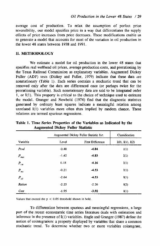
We estimate a model for oil production in the lower 48 states that specifies real wellhead oil prices, average production costs, and prorationing by the Texas Railroad Commission as explanatory variables. Augmented Dickey Fuller (ADF) tests (Dickey and Fuller, 1979) indicate that these data are nonstationary (Table 1). Each series contains a stochastic trend that can be removed only after the data are differenced once (or perhaps twice for the prorationing variable). Such nonstationary data are said to be integrated order 1, or I( 1). This property is critical to the choice of technique used to estimate the model. Granger and Newbold (1974) find that the diagnostic statistics generated by ordinary least squares indicate a meaningful relation among unrelated I(1) variables more often than implied by random chance. These relations are termed spurious regressions.

Table 1. Time Series Properties of the Variables as Indicated by the Augmented Dickey Fuller Statistic -

Augmented Dickey Fuller Statistic for: Classification

Variable

Prod

pm

Level First Difference

-0.40 -4.84

-1.42 -4.83

I(O), I(l), I(2) -

I(l)

I(l)

PC, I(l)

pm -0.21 -4.53

pd -2.64 -4.53

Ration -2.25 -2.26

cost -1.95 -3.92

Values that exceed the p < 0.05 threshold shown in bold.

I(1)

I(l)

I(2)

I(l) -

To differentiate between spurious and meaningful regressions, a large part of the recent econometric time series literature deals with estimation and inference in the presence of I( 1) variables. Engle and Granger (1987) define the notion of cointegration: a property displayed by variables that share a common stochastic trend. To determine whether two or more variables cointegrate,

30 / The Energy Journal

Johansen (1988) and Johansen and Juselius (1990) describe a full information maximum likelihood procedure based on the principle that variables which share the same stochastic trend can be combined linearly in a way that eliminates the stochastic trend. The coefficients that generate a stationary combination of nonstationary variables is termed a cointegrating vector (CV). The procedures to estimate the cointegrating vector(s) are derived from a vector autoregression (VAR) in levels, which is represented by equation 1:

y,=A,y,_,+...+Aky,_k+~+8t+Qjd,+~, ((1)

in which y is a vector of p variables whose behavior is being modeled, k is the number of lags, the A’s and 9 are matrices of regression coefficients, p and 6 are a vector of constants, and E, is a vector of error terms each of which is mid. d, is a vector of dummy variables and also possibly some stochastic variables that are found to be weakly exogenous.

To identify groups of variables that constitute a cointegrating relation from a vector of stochastic variables (y) which contain two or more I(1) variables, the cointegration procedure specifies the VAR as a vector error correction model (VECM):

Aj, = r,Ay,el +.. . +rk-,Ay,++, +I$-, +cpd, +p +E, c9

in which A is the first difference operator. Some variables may be weakly exogenous and therefore excluded from the LHS. As a result, the dimensions of the vector 9, may not be identical with y,. Equation 2 specifies the first difference of the nonstationary variables, which is stationary, as a linear function of lagged values of the first difference of the nonstationary variables, which also are stationary, and linear combinations of the nonstationary variables, which, are termed the cointegrating relations.

The term IIy,-, is the error correction mechanism (ECM). If there are one or more CVs, the ECM can be reformulated using equation 3:

HY,-, = 4’ [l 1 t, Y,-,‘I’ (3)

The term [ 1, t, y,.,‘]’ indicates that a constant and/or deterministic trend may be included in the cointegrating relation. The deterministic trend is intended to capture the behavior of trend stationary variables, i.e., variables that are stationary after removal of a deterministic trend rather than after differencing (Hansen and Juselius, 1995). /3’ is the matrix of coefficients that creates a stationary combination of nonstationary variables, i.e., the cointegration relation. This linear combination of variables is termed a cointegrating relation and represents the long-run equilibrium relation among the variables that are

Oil Production in the Lower 48 States / 31

included in the cointegrating relation. 01 is a matrix of coefficients that indicates whether a cointegrating relation (or ECM) affects a particular dependent variable. The number of cointegrating vectors, the variables that make up a cointegrating vector, the coefficients associated with these variables, and the relation between an ECM and the dependent variables all are evaluated from diagnostic statistics that are generated by the estimation process.

We specify a VECM (equation 2) to estimate the relation among oil production in the lower 48 states (Prod), the average real cost of oil production (Cost), real well head oil prices (P,J, and the fraction of capacity allowed to operate by the Texas Railroad Commissions (Ration) between 1938 and 1991. The sample period is determined the availability of data used to calculate average cost, which are not available before 19:36 or after 1991 (Cleveland, 1991). This variable represents the average cost of producing oil from fields in the lower 48 states. Including an explicit measure of cost relaxes the basic Hotelling model’s assumption that firms rank the quality of oil fields and recover them in order of increasing cost.

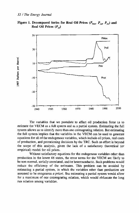
Previous studies of the oil industry hint at an asymmetric relation between real oil prices and production (Frankel, 1946). To evaluate this possibility, we use the method developed by Gately (1992) to decompose the red price data into three series. One series is the maximum real price of oil between 1936 and any given date (Pm). This series increases monotonically because Pm remains at the previous all-time high when real prices fall below this maximum (Figure 1). Real prices often decline following a new all-time high. Such declines are termed price cuts. These price cuts are accumulated to form a second series that decreases monotonically, which is termed P,,. Following such declines, real prices may rise towards, but not exceed, the previous maximum. These price recoveries are accumulated to form a third series that increases monotonically, which is termed Pr,. The three series contain a stochastic trend (Table 1). The sum of P-, P,,, and P,= at any time is the real price of oil.

We also include a variable (Ration) that represents the fraction of capacity allowed to operate by the Texas Railroad Commission (TRC). Adelman (1964) was among the first to qualitatively describe the effects of the TRC on prices, costs, and production. This relationship is quantified by Kaufmann (1991) and confirmed by Pesaran and Samiei (1995) and Moroney and Berg (1999). The TRC opened and closed capacity between 1935 and 1973 to damp the boom and bust cycle in oil production and prices (Prindle, 1981). By t‘tle early 1960’s, the TRC allowed owners to operate their wells at less than 30 percent of capacity. Texas was the largest producing state during the sample period, and the effect of prorationing decisions by the TRC was amplified by other state commissions that followed the TRC’s lead (e.g., the Kansas Commodity Corporation). Data for the fraction of operable capacity allowed to operate between 1938 and 1986 in Texas are obtained from the Texas Railroad Commission. Since 1973, the TRC allowed owners to operate at capacity and we extrapolate this value (1 .OO) through 1991.

32 / The Energy Journal

Figure 1. Decomposed Series for Real Oil Prices (Pm, PC,,, P,,) and Real Oil Prices (Po,l>

-50 ! I I 1

1940 1950 1960 1970 1980 1990 X00

The variables that we postulate to affect oil production force us to estimate the VECM as a full system and as a partial system. Estimating the full system allows us to identify more than one cointegrating relation. But estimating the full system implies that the variables in the VECM can be used to generate equations for all of the endogenous variables, which include oil prices, real costs of production, and prorationing decisions by the TRC. Such an effort is beyond the scope of this analysis, given the lack of a satisfactory theoretical (or empirical) model for oil prices.

Without satisfactory equations for the endogenous variables other than production in the lower 48 states, the error terms for the VECM are likely to be non-normal, serially correlated, and/or heteroscedactic. Such problems would reduce the efficiency of the estimates. This problem can be avoided by estimating a partial system, in which the variables other than production are assumed to be exogenous a priori. But estimating a partial system would allow for a maximum of one cointegrating relation, which would obfuscate the long run relation among variables.

Oil Production in the Lower 48 States / 33

34 / i%e Energy Journal

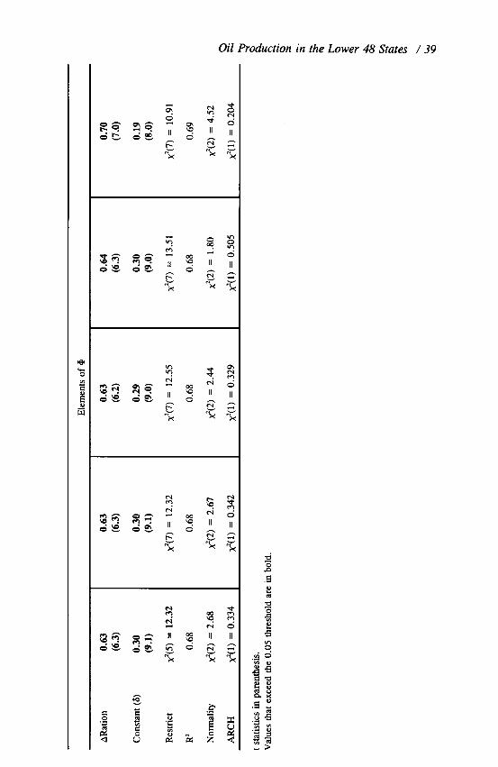
Because neither approach is fully satisfactory, we estimate both a full VECM and a partial system. For the full system, we focus on the equation for production. The degree to which the results for the production equation are robust is assessed by comparing it to results obtained for the partial system. Although the error terms estimated from the unrestricted full system are non- normal and serially correlated and the error terms from the unrestricted partial system are normal and not serially correlated (Table 2), the elements of 0 estimated from the full system (and the properties of the error term from this equation) are similar to those estimated from the partial system. This similarity implies that the inefficiencies associated with estimating the full system are not great and we can reliably interpret the individual cointegrating relations identified from the full system.

III. RESULTS

The inclusion of a time trend and/or constant in the cointegrating (equation 3) is chosen using a method developed by Pantula (1989). This method uses a rank test statistic to compare models ,that include/exclude a constant and/or a time trend in cointegration space and assumes various numbers of cointegrating relations. Using this method, we chose a model that includes a time trend in cointegration space (and three cointegrating vectors, which is consistent with the result described below). This specification also is the lleast restrictive, which implies we have not imposed any arbitrary restrictions on the VECM a priori.

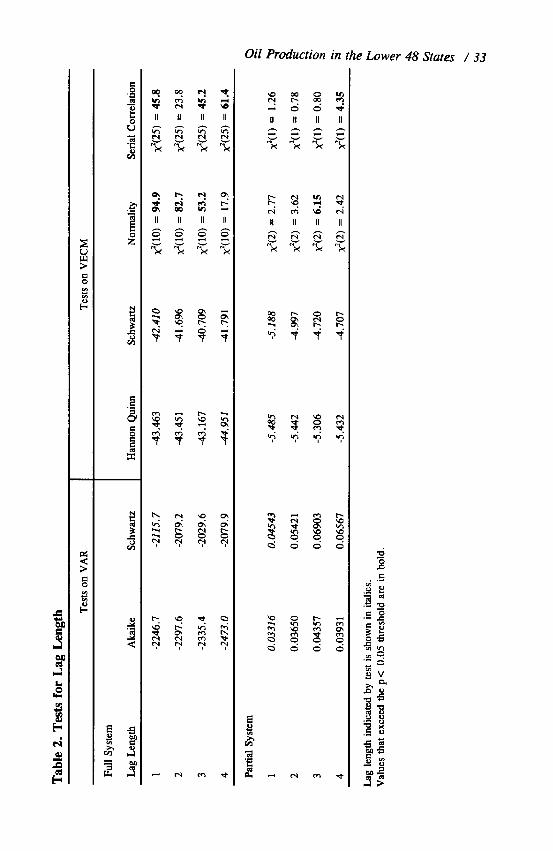
We choose the number of lagged first differences to include in equalion 2, which is given by k - 1, by comparing results generated by unrestricted VAR (eq. 1) and VECMs (eq. 2) that have k = 1 to 4, and are estimated over the same period, 1941-1991. The performance of the VAR is evaluated with a multivariate version of the Akaike (1971) and Schwartz information criterion. The Schwartz and Hannon Quinn information criterion (Hansen and Jusellius, 1995) are used to evaluate the VECM’s. Both sets of tests evaluate an increase in the lag length as measured by the decrease in the determinant of the residual covariance matrix of the model while making an adjustment for the decrease in the degrees of freedom. For the VAR and VECM, the Schwartz criterion indicates that the shortest lag length 1 cannot be rejected, while the Akaike and Harmon Quinn criterion indicates that the longest lag length 4 is appropriate. We choose the shorter lag length (l), which is indicated by the Schwartz criterion, consistent with the statistical preference for the most parsimonious model and the need to conserve degrees of freedom in the relatively short sample period. This choice is confirmed by the analysis of a partial system (section V Sensitivity Analysis). For the reasons discussed above, the error terms of the VECM’s generally are non-normal and serially correlated.

We choose the rank of II in equation 2, which corresponds to the number of cointegrating vectors-the number of columns in P-using the A,,,

Oil Production in the Lower 48 States / .35

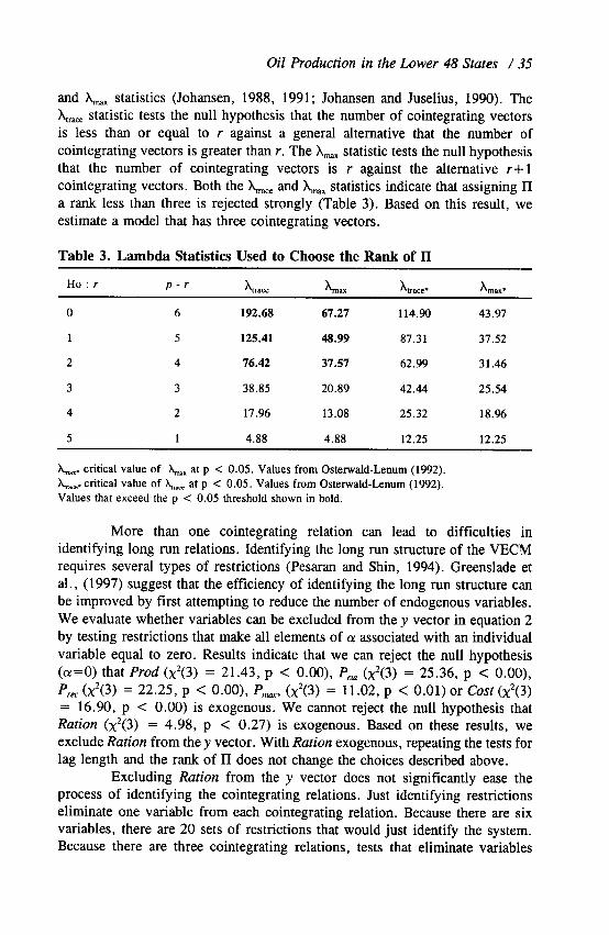
and Lax statistics (Johansen, 1988, 1991; Johansen and Juselius, 1990). The h,,,, statistic tests the null hypothesis that the number of cointegrating vectors is less than or equal to r against a general alternative that the number of cointegrating vectors is greater than r. The X, statistic tests the null hypothesis that the number of cointegrating vectors is r against the alternative r-k 1 cointegrating vectors. Both the &,,, and A,, statistics indicate that assigning II a rank less than three is rejected strongly (Table 3). Based on this result, we estimate a model that has three cointegrating vectors.

Table 3. Lambda Statistics Used to Choose the Rank of II -

0 6 192.68 67.27 114.90 43.97

1 5 125.41 48.99 87.31 37.52

2 4 76.42 37.57 62.99 31.46

3 3 38.85 20.89 42.44 25.54

4 2 17.96 13.08 25.32 18.96

5 1 4.88 4.88 12.25 12.25 -

L,,. critical value of L,, at p < 0.05. Values from Osterwald-Lenum (1992). a,.. critical value of A,,,,, at p < 0.05. Values from Osterwald-Lenum (1992). Values that exceed the p < 0.05 threshold shown in bold.

More than one cointegrating relation can lead to difficulties in identifying long run relations. Identifying the long run structure of the VECM requires several types of restrictions (Pesaran and Shin, 1994). Greenslade et al., (1997) suggest that the efficiency of identifying the long run structure c,an be improved by first attempting to reduce the number of endogenous variables. We evaluate whether variables can be excluded from the y vector in equation 2 by testing restrictions that make all elements of 01 associated with an individual variable equal to zero. Results indicate that we can reject the null hypothesis ((Y=O) that Prod (x’(3) = 21.43, p < O.OO), P,,, (x2(3) = 25.36, p < O.OO), P,, (x’(3) = 22.25, p < O.OO), Pm, (x2(3) = 11.02, p < 0.01) or Cost (x2(3) = 16.90, p < 0.00) is exogenous. We cannot reject the null hypothesis th.at

Ration (x’(3) = 4.98, p < 0.27) is exogenous. Based on these results, we exclude Ration from they vector. With Ration exogenous, repeating the tests for lag length and the rank of II does not change the choices described above.

Excluding Ration from the y vector does not significantly ease the process of identifying the cointegrating relations. Just identifying restrictions eliminate one variable from each cointegrating relation. Because there are six variables, there are 20 sets of restrictions that would just identify the system. Because there are three cointegrating relations, tests that eliminate variables

36 / The Energy Journal

from cointegration space are not definitive. As a result, we cannot use a mechanistic process to identify the most parsimonious model of the relation among oil prices, the decomposed price series, average cost of production, and pro-rationing decisions by the TRC. Instead, we use a priori theory and previous empirical results as a guide to identify model 1, which has the following form for the equation for the first difference in production (the first equation in the VECM):

AProd, = ?G,,(Prod,-, + FPcutm, P +“+p 4,

WC, _ ,

B ” +&,2(52Cost,_, +Ration,-,)

P 62

P P P +~,3(~Pcui-,+13P,~,_,+P3PNU-,+cost,_I)+E,y

0 53 f 053 P ’ 53

in which GI, = %@I,7 $2 = cq203,, and h13 = a,,lPS3. The degree to which the process used to identify model 1 affects the results is described in sectio:n V, which reports on the results of a sensitivity analysis.

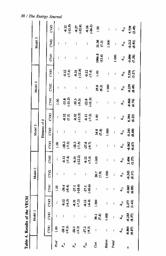
The restrictions that identify model 1 are rejected at the 5 percent level but not at the 1 percent level (x2(7) = 12.32, p < 0.03). Model 1 contains a cointegrating relation (CR #l) that includes Prod, P-, Pcuf, and P,,, a second cointegrating relation (CR #2) that includes Ration and Cost, and a third cointegrating relation (CR #3) that includes P-, PC,,,, Pr,,, and Cost (Tablt: 4).

The elements of (Y (L$, and i?&) indicate that only CR #l and CR #2 ‘load’ into the equation for the first difference of oil production (Table 4).

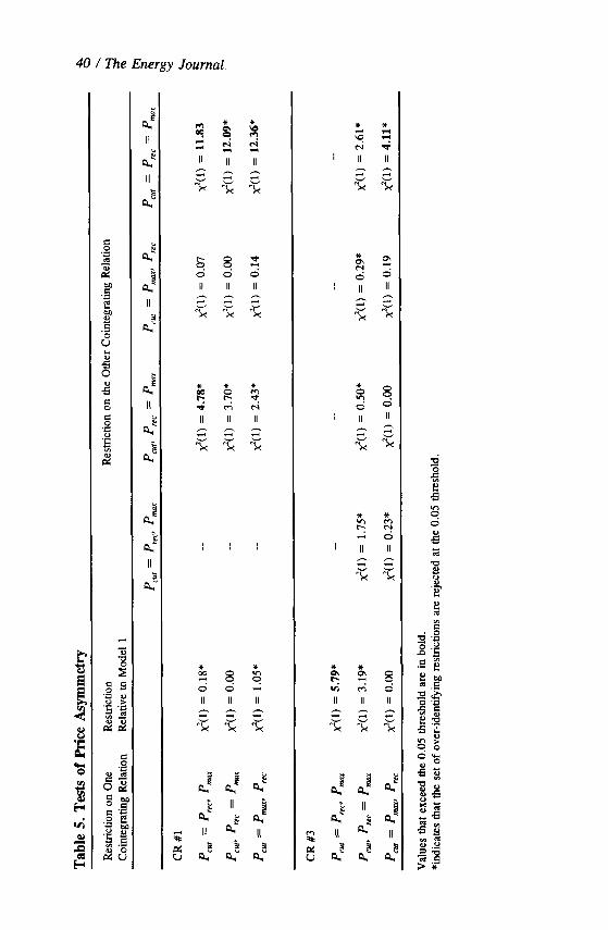
Next, we attempt to identify whether the price effects in CV #l and CV #3 are asymmetric and the nature of that asymmetry. The asymmetry can take many forms. The elements of fi associated with P-, PC,, and P,, in each of the cointegrating vectors may be different. Alternatively, two of the elements of fi associated with PM, P,,, and P,K may be equal. Wolffram (1971) describes an asymmetry in which a price increase to an all-time high has a greater effect Ithan a price cut or a price recovery. Trail et al., (1978) describe an asymmetry in which price increases, either an increase to an all-time high or a recovery back towards an all-time high, have a greater effect than a price cut.

To differentiate among these and other categories of price asymrneltry, we test restrictions on the elements of /3 associated with P-, Pcurr and P,, in two steps. In the first step, we impose restrictions on CV #l or CV #3 that equalize two of the three elements of 0 associated with P-, P,,, and Pr,,, Six sets of restrictions are possible-three for each cointegrating vector. Each of these restrictions is evaluated individually relative to model 1 using a likelihood ratio test. The results indicate that only one set of restrictions can be rejected (Table 5). The elements of /3 associated with P,, and P,, are not equal in CV #3.

Oil Production in the Lower 48 States / 37

Next, we test restrictions that equalize two elements of /3 associated with Pm, PC,,, and Pr,, in each of the cointegrating vectors. There are six combinations. The restriction on two of the three elements of /3 associated with P PC,,,, and PrC in the other cointegrating vector is evaluated two ways. We tez whether the individual restriction on the other cointegrating vector is rejected. We also evaluate whether the entire set of restrictions is rejected. The results indicate that three of the six possible restrictions cannot be rejected and generate three over-identified models (model 2, model 3, and model 4) that crumot be rejected at the 5 percent level (Table 4).

We also test whether the elements of /3 associated with Pm, PCp, and Pr,, are equal (perfect price reversibility) in CV #l or CV #3. Restrictions that equalize the elements of 0 associated with Pm, P,,, and P,,, in CV #3 are rejected relative to any set of restrictions that would equalize two of the elements of B associated with the decomposed price series in CV #3 (Table 5’). On the other hand, it is not possible to reject restrictions that equalize elements of /3 associated with Pm, PCW, and P,, in CV #l if the elements of p associated with P,,, and P,,,, are equal in CR #3. This model is not acceptable because the entire set of restrictions is rejected at the 5 percent level.

IV. DISCUSSION

Models 2 - 4 generally are similar. In these models, CR #l can be interpreted as the long run relation between price and the rate of oil production. This interpretation is consistent with the sign and statistical significance of CV #l. The elements of /3 associated with Pm, P,,, and P,,, are statistically significant and have the sign opposite that associated with Prod. These results indicate that production increases as the real price of oil: (1) rises to an all-time high; (2) recovers back towards that high; or (3) that production declines as oil prices fall way from a previous high. CR #l in. models 2 - 4 include every possible combination in which two of the elements of /3 associated with Pm,, P,,, and Pr, are equal. These results, along with our ability to reject restrictio:ns that equalize the elements of P associated with P,,, PC,, and Pr, indicate that the relation between price and production is asymmetric, but that the nature of the asymmetry is uncertain.

The element of CY associated with CR #l (&,, ) in models 2 - 4 indicates that disequilibrium in CR #l has a statistically significant effect on the annual change in oil production. The negative sign indicates that disequilibrium in the long run relation among Prod, Pm, PCW, and Pr,, has a self-correcting effect on production in the long run. For example, an increase in price reduces the value of CR #l. This reduction has a positive effect on production because c,, is negative, which increases production towards the long run value implied by CR #l. The rate of adjustment is slow. The estimates for Cr,, in models 2-4 implies that 6-7 percent of the disequilibrium in the long run relation among Prod and P f?UP PCur, and PTCC is eliminated each year. This slow rate of adjustment is

38 1 l%e Energy Journal

Oil Production in the Lower 48 States / 39

40 / The Energy Journal

6 8 2 6 d 6 II II II

P P a d m e-i II II II

II II II

Oil Production in the Lower 48 States / 411

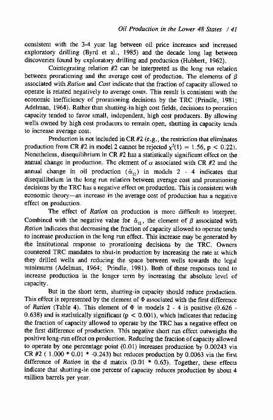
consistent with the 3-4 year lag between oil price increases and increased exploratory drilling (Byrd et al., 1985) and the decade long lag between discoveries found by exploratory drilling and production (Hubbert, 1962).

Cointegrating relation #2 can be interpreted as the long run relation between prorationing and the average cost of production. The elements of p associated with Ration and Cost indicate that the fraction of capacity allowed to operate is related negatively to average costs. This result is consistent with the economic inefficiency of prorationing decisions by the TRC (Prindle, 198.1; Adelman, 1964). Rather than shutting-in high cost fields, decisions to proration capacity tended to favor small, independent, high cost producers. By allowing wells owned by high cost producers to remain open, shutting in capacity tends to increase average cost.

Production is not included in CR #2 (e.g., the restriction that eliminates production from CR #2 in model 2 cannot be rejected x2( 1) = 1.56, p < 0.22). Nonetheless, disequilibrium in CR #2 has a statistically significant effect on the annual change in production. The element of (Y associated with CR #2 and the annual change in oil production ( G12) in models 2 - 4 indicates that disequilibrium in the long run relation between average cost and prorationing decisions by the TRC has a negative effect on production. This is consistent with economic theory-an increase in the average cost of production has a negative effect on production.

The effect of Ration on production is more difficult to interpret. Combined with the negative value for &,*, the element of p associated with Ration indicates that decreasing the fraction of capacity allowed to operate tends to increase production in the long run effect. This increase may be generated bsy the institutional response to prorationing decisions by the TRC. Owners countered TRC mandates to shut-in production by increasing the rate at which they drilled wells and reducing the space between wells towards the legal minimums (Adelman, 1964; Prindle, 1981). Both of these responses tend to increase production in the longer term by increasing the absolute level of capacity.

But in the short term, shutting-in capacity should reduce production. This effect is represented by the element of 9 associated with the first difference of Ration (Table 4). This element of @ in models 2 - 4 is positive (0.626 - 0.638) and is statistically significant (p < O.OOl), which indicates that reducin.g the fraction of capacity allowed to operate by the TRC has a negative effect on the first difference of production. This negative short run effect outweighs the positive long-run effect on production. Reducing the fraction of capacity allowed to operate by one percentage point (0.01) increases production by 0.00243 v:ia CR #2 ( 1.000 * 0.01 * -0.243) but reduces production by 0.0063 via the first difference of Ration in the d matrix (0.01 * 0.63). Together, these effects indicate that shutting-in one percent of capacity reduces production by about 4 million barrels per year.

42 / i’%e Energy Journal

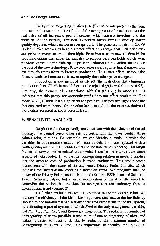
The third cointegrating relation (CR #3) can be interpreted as the long run relation between the price of oil and the average cost of production. As the real price of oil increases, profit increases, which attracts investment to the industry. At the margin, increased investment forces firms to develop lower quality deposits, which increases average costs. The price asymmetry in CR #3 is clear. Price recoveries have a greater effect on average cost than price cuts and price increases to an all-time high. Price increases to new all-time highs spur innovations that allow the industry to recover oil from fields which were previously uneconomic. Subsequent price reductions spur innovations that reduce the cost of the new technology. Price recoveries rarely spur technical innov,ation, but they do spur efforts to increase production. This latter effect, without the former, tends to increase costs more rapidly than other price changes.

Production is not included in CR #3 (the restriction that eliminates production from CR #3 in model 2 cannot be rejected x2( 1) = 0.01, p < 0.92). Similarly, the element of CY associated with CR #3 (&,3) in models 1 - 3 indicates that this proxy for economic profit does not affect production. For model 4, G13 is statistically significant and positive. The positive sign is opposite that expected from theory. On the other hand, model 4 is the most restrict:,ve of the models accepted at the 5 percent level.

V. SENSITIVITY ANALYSIS

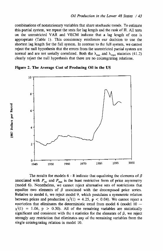
Despite results that generally are consistent with the behavior of the oil industry, we cannot reject other sets of restrictions that over-identify three cointegrating relations. For example, we can identify a model in which the variables in cointegrating relation #1 from models 1 - 4 are replaced with a cointegrating relation that includes Cost and the time trend (model 5). Although the set of restrictions associated with model 5 are less restrictive than those associated with models 1 - 4, the first cointegrating relation in model 5 implies that the average cost of production is trend stationary. This result seems inconsistent with the results of the augmented Dickey Fuller Statistic, which indicates that this variable contains a stochastic trend. We recognize that the power of the Dickey Fuller statistic is limited (Enders, 1995; Kim and Schmidt, 1990; Schwert, 1989), but a visual examination of the data also seems to contradict the notion that the data for average cost are stationary about a deterministic trend (Figure 2).

To further evaluate the results described in the previous section, we increase the efficiency of the identification process (and reduce the inefficiency implied by the non-normal and serially correlated error terms in the full system) by estimating a partial system in which Prod is the only endogenous variable, and P,, Pm P-2 Cost, and Ration are exogenous. This reduces the number of cointegrating relations possible, a maximum of one cointegrating relation, and makes it easier to identify it. But by reducing the maximum number of cointegrating relations to one, it is impossible to identify the individual

Oil Production in the Lower 48 States / 413

combinations of nonstationary variables that share stochastic trends. To estimate this partial system, we repeat the tests for lag length and the rank of II. All tests on the unrestricted VAR and VECM indicate that a lag length of one is appropriate (Table 1). This consistency reinforces our decision to use the shortest lag length for the full system. In contrast to the full system, we cannot reject the null hypothesis that the errors from the unrestricted partial system are normal and are not serially correlated. Both the A- and X,,, statistics (41.2) clearly reject the null hypothesis that there are not cointegrating relations.

Figure 2. The Average Cost of Producing Oil in the US

1940 1950 1960 1970 1980 1990 2000

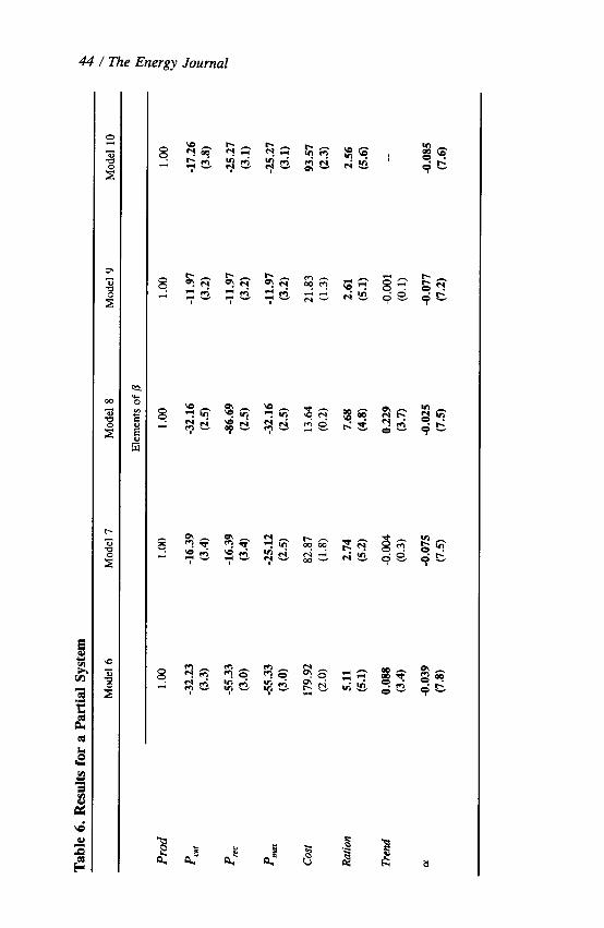
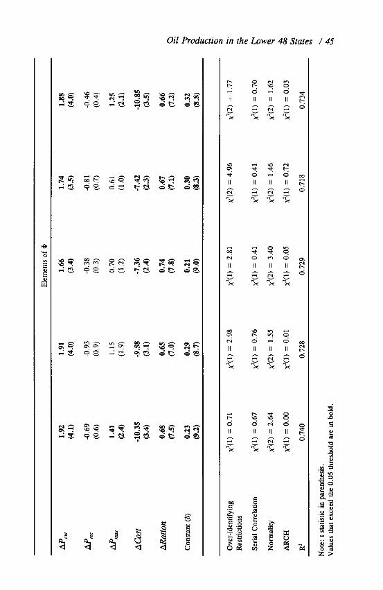
The results for models 6 - 8 indicate that equalizing the elements of /3 associated with P,,, and Pm is the least restrictive form of price asymmetry (model 6). Nonetheless, we cannot reject alternative sets of restrictions that equalize two elements of 0 associated with the decomposed price series. Relative to model 6, we reject model 9, which postulates a symmetric relation between prices and production (x2(1) = 4.25, p < 0.04). We cannot reject a restriction that eliminates the deterministic trend from model 6 (model 10 -- x2(l) = 1.06, p > 0.30). All of the remaining variables are statistically significant and consistent with the t statistics for the elements of p, we reject strongly any restriction that eliminates any of the remaining variables from the single cointegrating relation in model 10.

44 / The Energy Journal

Oil Production in the Lower 48 States / 45

46 / The Energy Journal

The results for model 10 generally are consistent with the results for the full system. The single cointegrating relation contains the same variables as three cointegrating relations in models 2 - 4. The variables in the single cointegrating relation in model 10 have the same sign and the same long run effect on production as the variables in CR #l & CR #2 in models 2 - 4. As in models 2 - 4, the relation between price and production is asymmetric. In model 10, price increases (Pm,, P,,,) have a greater effect on production than price reductions. Increases in average cost have a negative effect on production. Shutting in production by the TRC has a positive long run effect on production (via the cointegrating relation), but this effect is more than offset by the negative short run effect. The short run effects of the PcU, Pm, and Cost also are statistically significant, and their sign is consistent with the effect on production indicated by the cointegrating vectors for models 2- 4. The negative value for Q! indicates that disequilibrium in the single Icointegrating relation has a self- correcting effect on production in the long run and the magnitude of this ‘effect is similar to the results estimated for the full system. Together, these results indicate that the inefficiency of the estimation procedure associated with the structure of the error term for the full system and that the restrictions used to over-identify the three cointegrating relations in the full system may be a reasonable representation of the economic, technical, geological, and institutional determinants of oil production in the lower 48 states.

VI. CONCLUSIONS

Any lingering uncertainty about the efficiency of the estimation results or the identification of the cointegrating relations does not affect the conclusion that the accuracy of Hubbert’s original forecast for oil production in the lower 48 states is fortuitous (e.g., Ryan, 1965; Harris, 1977). The cointegration analysis indicates that oil production in the lower 48 states shares stochastic trends with the decomposed price series, average costs, and prorationing decisions by the TRC. These stochastic ,trends are not present in the deterministic bell-shaped curve, therefore the first difference of the bell-shaped curve drifts away from the annual change in oil production for extended periods (Figure 3). For example, production in the lower 48 states stabilizes in the late 1970’s and early 1980’s, which contradicts the steady decline forecast by the Hubbert model. Our results indicate that Hub’bert was able to predict the peak in US production accurately because real oil prices, average real cost of production, and decisions by the TRC co-evolved in a way that traced what appears to be a symmetric bell-shaped curve for production over time. A different evolutionary path for any of these variables could have produced a pattern of production that is significantly different from a bell-shaped curve. For example, if the TRC did not shut in production, or did not favor high cost producers, production may not have followed a bell-shaped curve for production and production may not have peaked in 1970. In effect, Hubbert got lucky. Thus, the ability of the Hubbert’s model (and its variants) to forecast production

Oil Production in the Lower 48 States / 47

in the lower 48 states accurately, probably cannot be extrapolated to other regions, as done by Campbell and Laherrere (1998).

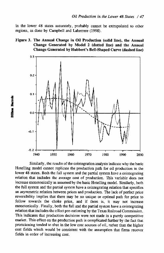
Figure 3. The Annual Change in Oil Production (solid line), the Annual Change Generated by Model 2 (dotted line) and the Annual Change Generated by Hubbert’s Bell-Shaped Curve (dashed line)

0.3

0.2

0.1

1

1 0.0

m

-0.1

-0.2

,

-i

I- 1 I , I I

1940 1950 1964I 1970 1980 1990 2030

Similarly, the results of the cointegration analysis indicate why the basic Hotelling model cannot replicate the production path for oil production in the lower 48 states. Both the full system and the partial system have a cointegrating relation that includes the average cost of production. This variable does not increase monotonically as assumed by the basic Hotelling model. Similarly, both the full system and the partial system have a cointegrating relation that specifies an asymmetric relation between prices and production. The lack of perfect price reversibility implies that there may be no unique or optimal path for price to follow towards the choke price, and if there is, it may not increase monotonically. Finally, both the full and the partial system have a cointegrating relation that includes the effect pro-rationing by the Texas Railroad Commission. This indicates that production decisions were not made in a purely competitive market. This effect on the production path is complicated further by the fact that prorationing tended to shut in the low cost sources of oil, rather than the higher cost fields which would be consistent with the assumption that firms recover fields in order of increasing cost.

48 / The Energy Journal

Because the behavior of oil producers and government regulators is not consistent with the assumptions that underlie the basic Hotelling model, the model loses its ability to make definitive statements about the production. path in the lower 48 states. The inability to make these statements undermines the de facto policy for managing the depletion of conventional oil supplies-a belief that the competitive market will generate a smooth transition from oil. The negative economic effects associated with high prices and energy shortages imply that the importance of inconsistencies with the basic Hotelling model identified by this analysis may be sufficient to warrant a greater degree of government intervention in the transition from oil than currently envisioned by most policy makers.

REFERENCES

Adelman, M. (1964). “Efficiency of resource use in crude petroleum.” Southern EconomicJournal 31: 101-122.

Byrd, L.T., R.M. Kumar, A.F. Williams, and D.L. Moore (1985). “US oil and gas finding and development costs, 1973-1982--lower 48 onshore and offshore.” Journal of Petroleum Technology 37: 2040-2048.

Cleveland, C.J. (1991). “Physical and economic aspects of resource quality: the cost of oil r,upply in the lower 48 United States, 19361988.” Resources and Energy 13: 163-188.

Cleveland, C.J. and R.K. Kaufmann (1991). “Forecasting ultimate oil recovery and its rate of production: Incorporating economic forces into the models of M. King Hubbert.” 77ze Energy Journal 12(2): 17-46.

Campbell, C.J. and J. H. Laherrere (1998). “The end of cheap oil.” ScienQic American. March: 78-83.

Cuthbertson K., S. G. Hall, and M. P. Taylor (1992). AppliedEconomerric Techniques. AM Arbor,

Michigan: University of Michigan Press. Dickey, D.A. and W.A. Fuller (1979). “Distribution of the estimators for auto regressive time series

with a unit root.” Journal of American Sratisrics Association 7: 427-431. Enders, W. (1995). Applied Econometric Time Series. New York, NY: John Wiley. Engle, R.E. and C.W.J. Granger (1987). “Cointegration and error correction: representation,

estimation, and testing.” Econometrica 55: 251-276. Fisher, A.C. (1981). Resource and Environmental Economics Cambridge, UK: Cambridge

University Press. Frankel, P.H. (1946). Essentials of Petroleum. London, UK: Frank Cass. Gately, D. (1992). “Imperfect price-reversibility of U.S. gasoline demand: Asymmetric responses

to price increases and declines. ” The Energy Journal 13(4): 179-207. Granger, C.W.J. and P. Newbold (1974). “Spurious regressions in econometrics.” Jourr!al of

Econometrics 2: 11 l-120. Greenslade, J.V. S.G. Hall, and S.G.B. Henry (1997). “Onthe identification of cointegrated sy.stems

in small samples: practical procedures with an application to UK wages and prices.” London Business School, Mimeo.

Hansen, J. and K. Juselius (1995). “CATS in RATS: Cointegration Analysis of Time Series.” Discussion paper, Estima, Evanston, Illinois.

Harris, D. (1977). “Conventional crude oil resources of the United States: recent estimates, methods, for estimation and policy considerations.” Muterials and Society 1: 263-286.

Hotelling, H. (1931). “The economics of exhaustible resources.” Journal of Political Economy 39(2): 137.

Hubbert, M. K. (1956). “Nuclear energy and the fossil fuels.” In: American Petroleum Institute (Editor), Drilling and Production Practice. New York: API.

Oil Production in the Lower 48 States / 49

Hubbert, M. K. (1962). “Energy Resources. A Report to the Committee on Natural Resources,” National Academy of Sciences. Government Printing Office. Publication No. 1000-D.

Hubbert, M.K. (1982). “Techniques of prediction as applied to the production of oil and gas.” In: Oil and Gas Supply Modelling. S. Gass (editor). National Bureau of Standards, Special publicati’on 631, Washington DC. p.l6-141.

Johansen, S. (1988). “Statistical analysis of cointegration vectors.” Journal ofEconomic Dynamrcs and Control 12: 231-254.

Johansen, S. and K. Juselius (1990). “Maximum likelihood estimation and inference on cointegrati’on with application to the demand for money.” Oxford Eulletin ofEconomics and Stufisfics 52: 169- 209.

Johansen, S. and K. Juselius (1994). “Identification of the long-run and the short run stmctnre: an application to the ISLM model.” Journal of Economefrics 63: 7-36.

Kaufmann, R.K. (1991). “Oil production in the lower 48 states: Reconciling curve fitting and econometric models.” Resources and Energy 13: 111-127.

Kerr, R. (1998). “The next oil crisis looms large--and perhaps close.” Science 281: 1128-1131. Kim, K. and P. Schmidt (1990). “Some evidence on the accuracy of Phillips-Perron tests using

alternative estimates of nuisance parameters.” Economics Letters 34: 345-350. Krautkraemer, J.A. (1998). “Nonrenewable resource scarcity.” Journal of Economic Literuture

36(4): 20652107. Menard, H.W. and G. Sharrnan (1975). “Scientific uses of random drilling models.” Science 190:

337-343. Gsterwald-Lennum, M. (1992). “A note with quantiles of the asymptotic distribution of the

maximum likelihood cointegration rank test statistics. ” Oxford Bulletin of Economics a.nd Statistics 54: 46 l-47 1.

Pantula, S.G. (1989). “Testing for unit roots in time series data.” Econometric Theory 5: 256-27 1. Pearce, D.W. and R.K. Turner (1990). Economics of Natural Resources and the Environment.

Baltimore, MD: The Johns Hopkins University Press. Pesaran, M.H. and H. Samiei (1995). “Forecasting ultimate resource recovery.” In?ernafior;al

Journal of Forecasting 1 l(4): 543-555. Pesaran, M.H. and Y. Shin (1994). “Long run structural modelling.” University of Cambridge,

Mimeo. Prindle, D.F. (1981). Petroleum Politics and the Texas Railroad Commission. Austin, TX:

University of Texas Press. Ryan, J.H. (1965). “National academy of sciences report on energy resources: discussion of

limitations on logistic projections,” Bulletin of theAmericun Association ofPetroleum Geologi.;ts 49(l): 1713-1720.

Schwert, G. W. (1989). “Tests for unit roots: a Monte Carlo investigation,” Journal of Business and Economic Statistics 7: 147-159.

Tietenberg, T. (2000). Environmental and Natural Resource Economics. Reading: Addison-Wesley. Trail], B., D. Colman, and T. Young (1978). “Estimating irreversible supply functions.” Ameriazn

Journal or Agricultural Economics 60: 528-53 1. Uri, N.D. (1980). “Crude oil appraisal of the United States.” The Energy Journal l(3): 65-75 Wolffram, R. (1971). “Positivistic measures of aggregate supply elasticities: Some new approache:;..

some critical notes.” American Journal of Agricultural Economics 53: 356-359.

All in-text references underlined in blue are linked to publications on ResearchGate, letting you access and read them immediately.