ODR Merged - CORE

1

NEW LIGHT SOURCE (NLS) PROJECT:

CONCEPTUAL DESIGN REPORT

PROJECT LEADER Jon Marangos (Imperial)

PROJECT MANAGER Gregory Diakun (STFC)

SOURCE MANAGER

Richard Walker (Diamond)

NLS SCIENCE TEAM

Andrea Cavalleri (Hamburg/Oxford) Condensed Matter Swapan Chattopadhyay (Cockcroft) Accelerator Concepts

Wendy Flavell (Manchester) Chemical Sciences Louise Johnson (Diamond/Oxford) Life Sciences

Jon Marangos (Imperial) Ultrafast electron dynamics/attosecond science Justin Wark (Oxford) High Energy Density Science

Peter Weightman (Liverpool) Life Sciences Jonathan Underwood (UCL) Chemical Sciences

PROJECT CUSTOMER Mike Dunne (STFC)

PROJECT SPONSOR

John Womersley (STFC)

May 2010

3

Contributors We are enormously grateful to all of those who contributed to the construction of this REPORT including many individuals both within and external to the working groups G. Aeppli1, R. Allemann2, A Almond3, D. Angal-Kalinin4,5, M. Ashfold6, V. Averbukh7, C. Bagshaw8, M. Barahona9, P. Barker1, R. Bartolini10,11, F. Baumberger12, C. Beard4,5, A. Beeby13, R. Bisby14, E. Blackburn15, N. Bliss5, P. Bonner10, P Booth16, M Bowler5, C. Bressler17, W. Brown18, W. Bryan19, F. Burge10, I. Carmichael20, C. Catlow18, A. Cavalleri21,22, H. Chapman21, S. Chattapadhyay4, M Chergui23, C. Christou10, J. Clarke4,5, R. Cogdell24, J. Collier25, P. Cook26, J. Costello27, J. Corlett28, M.-E. Couprie29, L. Cramer30, F. Currell31, I. Davis32, G. Diakun5, H. Dickinson33, C. Dougan34, R. Donovan35, M. Drescher36, A.M. Dunne25, D. Dunning4,5,37, H. Durr38, P. Emma39, J. Evans40, R. Evans41, R. Falcone28, J. Feldhaus42, B. Fell5, M. Ferenczi43, M Ferguson-Smith44, J. Fernandez-Hernando4,5, D. Fernig45, H.H. Fielding18, W. Flavell46, H. Fraser47, L.J. Frasinski41, C. Froud25, J. Gardiner48, M. Gensch42, M. George49, D. Gerricke50, A. Gleeson5, P Goddard22, I. Gould51, A. Goulden4,5, G. Gregori22, S. Griffiths5, J Hajdu39,52, B. Hamilton53, J.-H. Han10, M. Hanon54, S. Hasnain45, P. Hatton55, C. Hawes56, J. Herbert4,5, M. Heron10, D. Heyes3, G. Hirst25, M. Holbourn5, D. Holland5, M. Humphries57, C. Hunter58, M. Irving59, M. Ivanov41, F. Jackson4,5, S. Jamison4,5, D. Jaroszynski47, L. Johnson32, J. Jones4,5, M. Kadodwala60, A. Kalinin4,5, A. Kapanidis61, A. Kaplan15, J. Kay10, A. Kimel62, D. Klug51, B. Kuske38, D. Lammie63, R.W. Lee64, F. Maia65, J. Marangos41, K. Marinov4,5, M. Marsh66, I. Martin10,11, B. Martlew5, N. Mason67, G. Materlik10, J. McCombie49, M. McCoustra68, P. McIntosh4,5, J. McKenzie4,5, S. McKenzie69, H. McMahon70, M. McMahon71, B. McNeil47, K. Meek63, A. Michette72, B. Militsyn4,5, J. Molloy73, A. Moss4,5, A. Munro3, B. Muratori4,5, T. Nann74, C. Nave10, T. Ng59, L. Nicholson5, A. Nilsson39, P. O’Neill75, P. O’Shea76, H. Owen4,77, T. Parker25, F. Parmigiani78, S. Pattalwar4,5, R. Perutz79, C. Pickett74, S. Pimblott20,48, L.Poletto80, M. Poole4,5, I Powis49, G. Priebe5, H. Quiney81, F. Quinn5, P. Radaelli25, J. Raff26, G. Rehm10, S. Reiche82, P. Rich83, D. Riley31, B. Rimmer84, I. Robinson10,85, M. Roper5, S. Rose41, J. Rossbach42, J. Rowland10, G. Sankar86, H. Schlarb42, S. Schroeder87, N. Scrutton3, E. Seddon46, D. Segal41, T. Shintake88, J. Singleton89, A. Smith5, R. Smith4,5, S. Smith4,5, K. Sokolowski-Tinten90, M. Somekh91, E. Springate25, T. Stead92, M. Stringer93, M. Sutcliffe87, G. Tallents94, K. Taylor95, N. Thompson4,5,37, R. Thompson41, E. Towns-Andrews5, D. Townsend68, M. Towrie25, J. Tisch41, K. Ueda96, J. Underwood25,97, G. van der Laan10, R. van Grondelle98, J. van Thor99, A. Venkitaraman100, K. von Haeften101, M. Vrakking102, R. Walker10, I. Walmsley22, D. Wann35, J. Wark22, P. Weightman103, J. Weinstein58, T. Wess63, A. Wheelhouse4,5, P. Williams4,5, K. Willison104, M. Wilson10, J. Wishart105, A. Wolf106, J. Womersley25, P. Woodruff107, N. Woolsey94, S. Yaliraki51, E. Yates45, A. Zeitler108, M. Zepf31, A. Zholents28.

Affiliation

1 Department of Physics and Astronomy, University College London, Gower Street, London WC1E 6BT, UK.

2 School of Chemistry, Cardiff University, Main Building, Park Place, Cardiff CF10 3AT, UK. 3 Manchester Interdisciplinary Biocentre, 131 Princess Street, Manchester M1 7DN, UK. 4 Cockcroft Institute, STFC Daresbury Science and Innovation Campus, Keckwick Lane,

Daresbury, Warrington WA4 4AD, UK. 5 STFC Daresbury Laboratory, Keckwick Lane, Daresbury, Warrington WA4 4AD, UK. 6 School of Chemistry, University of Bristol, Bristol BS8 1TS, UK. 7 Max Planck Institute for the Physics of Complex Systems, Nöthnitzer Straße 38, 01187 Dresden,

Germany. 8 Department of Biochemistry, Leicester University, Henry Wellcome Building, Lancaster Road,

Leicester LE1 9HN, UK. 9 Department of Bioengineering, Imperial College London, South Kensington Campus, London

SW7 2AZ, UK.

4

10 Diamond Light Source Ltd, Diamond House, Harwell Science and Innovation Campus, Didcot, Oxfordshire OX11 0DE, UK.

11 John Adams Institute for Accelerator Science, Denys Wilkinson Building, Keble Road, Oxford OX1 3RH, UK

12 School of Physics and Astronomy, University of St. Andrews, North Haugh, St Andrews, Fife KY16 9SS, Scotland, UK.

13 University of Durham, Durham DH1 3HP, UK. 14 Biomedical Sciences Research Institute, University of Salford, Salford, Greater Manchester M5

4WT, UK 15 School of Physics and Astronomy, University of Birmingham, Edgbaston, Birmingham B15

2TT, UK. 16 Department of Biochemistry, School of Medical Sciences, University Walk, Bristol BS8 1TD,

UK. 17 European XFEL, Notkestraße 85, 22607 Hamburg, Germany 18 Department of Chemistry, University College London, 20 Gordon Street, London WC1H 0AJ,

UK. 19 Department of Physics, Swansea University, Singleton Park, Swansea SA2 8PP, UK. 20 Radiation Laboratory, University of Notre Dame, Notre Dame, IN 46556, USA 21 Centre for Free Electron Laser Science & Department of Physics University of Hamburg, DESY,

Geb 49, Notkestrasse 85, 22607 Hamburg, Germany. 22 Department of Physics, University of Oxford, Clarendon Laboratory, Parks Road, Oxford OX1

3PU, UK. 23 Laboratory of Ultrafast Spectroscopy, EPFL , 1015 Lausanne, Switzerland. 24 Glasgow Biomedical Research Centre, University of Glasgow, Glasgow G12 8QQ, UK. 25 STFC Rutherford Appleton Laboratory, Chilton, Didcot, Oxfordshire OX11 0QX, UK. 26 Sir William Dunn School of Pathology, University of Oxford, South Parks Road, Oxford OX1

3RE, UK. 27 School of Physical Sciences, Dublin City University, Dublin 9, Eire 28 Lawrence Berkeley National Lab, Berkeley, CA 94720, USA. 29 SOLEIL, L'Orme des Merisiers, Saint-Aubin - BP 48, 91192 Gif-sur-Yvette Cedex, France. 30 Research Department of Genetics, Evolution and Environment, University College London,

Gower Street, London WC1E 6BT, UK. 31 Department of Physics and Astronomy, Queen's University Belfast, University Road, Belfast

BT7 1NN, UK. 32 Department of Biochemistry, University of Oxford, South Parks Road, Oxford OX1 3QU, UK. 33 Department of Plant Sciences, University of Oxford, South Parks Road, Oxford OX1 3RB, UK 34 Knowledge Exchange, UK Astronomy Technology Centre, Royal Observatory, Blackford Hill,

Edinburgh EH9 3HJ, Scotland, UK. 35 School of Chemistry, University of Edinburgh, Joseph Black Building, West Mains Road,

Edinburgh EH9 3JJ, Scotland, UK 36 Institut für Experimentalphysik, Universität Hamburg, Luruper Chaussee 149, 22761 Hamburg,

Germany. 37 University of Strathclyde, Glasgow G4 0NG, Scotland, UK. 38 BESSY, Albert Einstein Str. 15, 12489 Berlin, Germany. 39 SLAC National Accelerator Laboratory, Menlo Park, CA, USA. 40 School of Chemistry, University of Southampton, Highfield, Southampton SO17 1BJ, UK. 41 Physics Department, Imperial College London, South Kensington campus, London, SW7 2AZ,

UK. 42 DESY, Notkestraße 85, 22607 Hamburg, Germany. 43 Molecular Medicine, NHLI, Imperial College London, Sir Alexander Fleming Building, South

Kensington Campus, London, SW7 2AZ, UK. 44 School of the Biological Sciences, University of Cambridge, 17 Mill Lane, Cambridge CB2

1RX, UK. 45 School of Biological Sciences, University of Liverpool, Liverpool L69 3BX, UK. 46 The Photon Science Institute, The University of Manchester, Alan Turing Building, Oxford

Road, Manchester M13 9PL, UK. 47 Department of Physics, University of Strathclyde, Glasgow G4 0NG, Scotland, UK 48 School of Chemistry, The University of Manchester, Oxford Road, Manchester M13 9PL, UK. 49 School of Chemistry, University of Nottingham, University Park, Nottingham NG7 2RD, UK. 50 Centre for Fusion, Space & Astrophysics, Department of Physics, University of Warwick,

Coventry CV4 7AL, UK.

5

51 Department of Chemistry, Imperial College London, South Kensington Campus, London SW7 2AZ, UK.

52 Laboratory of Molecular Physics, Box 596, SE-75124 Uppsala, Sweden. 53 School of Electrical & Electronic Engineering, The University of Manchester, Sackville Street,

Manchester M60 1QD, UK. 54 School of Chemistry, Edgbaston, University of Birmingham, Birmingham B15 2TT, UK. 55 Department of Physics, Durham University, South Road, Durham DH1 3LE, UK. 56 School of Life Sciences, Oxford Brookes University, Gipsy Lane, Headington, Oxford OX3

0BP, UK. 57 Faculty of Life Sciences, Michael Smith Building, Oxford Road, Manchester M13 9PT, UK. 58 Department of Chemistry, The University of Sheffield, Western Bank, Sheffield S10 2TN, UK. 59 Randall Division of Cell & Molecular Biophysics, New Hunt's House, King's College London,

Guy's Campus, London SE1 1UL, UK. 60 Department of Chemistry, University of Glasgow, Glasgow G12 8QQ, Scotland, UK. 61 Department of Physics, University of Oxford, Parks Road, Oxford OX1 3PU, UK. 62 Radboud University Nijmegen, 6500 HC Nijmegen, The Netherlands 63 School of Optometry and Vision Sciences, Cardiff University, Maindy Road, Cathays, Cardiff

CF24 4LU, UK. 64 Physics Division, Lawrence Livermore National Laboratory, 7000 East Avenue, Livermore, CA

94550, USA. 65 Department of Cell and Molecular Biology, Uppsala University, SE-751 05 Uppsala, Sweden. 66 Department of Developmental Biology, University College London, Gower Street, London

WC1E 6BT, UK. 67 Department of Physics and Astronomy, The Open University, Walton Hall, Milton Keynes MK7

6AA, UK. 68 School of EPS – Chemistry, Perkin Building, Heriot-Watt University, Edinburgh EH14 4AS,

UK 69 Physical and Theoretical Chemistry Laboratory, South Parks Road, Oxford OX1 3QZ, UK. 70 Neurobiology Division, Laboratory of Molecular Biology, Hills Road, Cambridge CB2 2QH,

UK. 71 School of Physics, CSEC, University of Edinburgh, Erskine Williamson Building, The King's

Buildings, Mayfield Road, Edinburgh EH9 3JZ, UK 72 Department of Physics, King's College London, Strand, London WC2R 2LS, UK. 73 National Institute for Medical Research, The Ridgeway, Mill Hill, London NW7 1AA, UK. 74 Chemical Sciences and Pharmacy, University of East Anglia, Norwich, NR4 7TJ, UK. 75 Department of Radiation Oncology Biology, University of Oxford, Old Road Campus Research

Building, Off Roosevelt Drive, Oxford, OX3 7DQ, UK. 76 Institute of Genetics, The School of Biology, The University of Nottingham, University Park,

Nottingham NG7 2RD, UK. 77 School of Physics and Astronomy, The University of Manchester, Oxford Road, Manchester

M13 9PL, UK. 78 FERMI@Elettra, Sincrotrone Trieste S.C.p.A. di interesse nazionale, AREA Science Park,

34149 Basovizza, Trieste, Italy. 79 Department of Chemistry, University of York, Heslington, York YO10 5DD, UK. 80 National Institute for the Physics of Matter, Laboratory for UV and X-Ray Optical Research,

Padova, Italy. 81 School of Physics, University of Melbourne, Australia. 82 UCLA, Department of Physics and Astronomy, Knudsen Hall 3-174A, Los Angeles CA 90095-

1547, USA. 83 Department of Genetics, Evolution and Environment, University College London, Gower Street,

London WC1E 6BT, UK. 84 Thomas Jefferson National Accelerator Facility, 12000 Jefferson Avenue, Newport News, VA

23606 Virginia, USA. 85 Centre for Materials Research, UCL, Torrington Place, London WC1E 7JC, UK. 86 The Royal Institution of Great Britain, 21 Albemarle Street, London W1S 4BS, UK. 87 School of Chemical Engineering and Analytical Science, The University of Manchester,

Sackville Street, Manchester M60 1QD, UK. 88 SPring-8, Hyogo, Japan 89 LANL, Bikini Atoll Rd., SM 30 Los Alamos, NM 87545 New Mexico, USA. 90 Institut für Experimentelle Physik, Universität Duisburg-Essen, Lotharstrasse 1, 47048

Duisburg, Germany.

6

91 School of Electrical and Electronic Engineering, University of Nottingham, University Park, Nottingham NG7 2RD, UK.

92 School of Biological Sciences, Royal Holloway University of London, Egham, Surrey TW20 0EX, UK.

93 School of Electronic and Electrical Engineering, University of Leeds, Leeds LS2 9JT, UK. 94 Department of Physics, University of York, Heslington, York YO10 5DD, UK. 95 Dept of Applied Mathematics and Theoretical Physics, Queen's University Belfast, Belfast BT7

1NN, Northern Ireland, U K. 96 Tohoku University, Sendai, Japan. 97 Physics and Astronomy, University College London, Gower Street, London WC1E 6BT, UK. 98 Department of Biophysics, Vrije University, Faculty of Sciences, 1081 HV Amsterdam, The

Netherlands. 99 Molecular Biosciences, Imperial College London, South Kensington Campus, London SW7

2AZ, UK. 100 Department of Oncology, University of Cambridge, Hutchison/MRC Research Centre, Hills

Road, Cambridge CB2 0XZ, UK. 101 Department of Physics and Astronomy, University of Leicester, University Road, Leicester LE1

7RH, UK. 102 FOM Institute for Atomic and Molecular Physics, Science Park 113, 1098 XG Amsterdam, The

Netherlands. 103 Physics Department & Surface Science Reasearch Centre, University of Liverpool, Oxford

Street, Liverpool L69 3BX, UK. 104 The Institute of Cancer Research, Chester Beatty Laboratories, 237 Fulham Road, London SW3

6JB, UK. 105 Brookhaven National Laboratory, Upton, NY 11973-5000, USA. 106 Max-Planck-Institut für Kernphysik, Saupfercheckweg 1, 69117 Heidelberg, Germany. 107 Department of Physics, University of Warwick, Coventry, CV4 7AL. 108 Department of Chemical Engineering and Biotechnology, University of Cambridge, Trinity

Lane, Cambridge CB2 1TN, UK.

7

Foreword

In the course of the last few years Free Electron Lasers (FELs) have emerged as an exceptionally exciting tool for science. New results from the first soft X-ray FEL, FLASH in Hamburg, on biological imaging, soft X-ray interaction physics and light source science have revealed prospects for remarkable future impact. The first hard X-ray FEL, LCLS at Stanford, is now operating and the first beam time late in 2009 yielded exciting new results on high brightness X-ray matter interaction and on X-ray imaging of the structure of matter. Other machines in Japan, Germany (Euro XFEL) and Italy are progressing rapidly towards first light and a number of other projects moving toward a formal go ahead (e.g. Max IV, SwissFEL). UK researchers are starting to establish a strong presence at these facilities. In response to the international developments STFC commissioned a project to examine the prospects for a UK FEL facility with unique capabilities and the NLS CDR is the outcome of that project.

The NLS project started in April 2008 and underwent two distinct phases. In the course of Phase 1 the project team undertook a broad based consultation on science (involving ~300 individuals) seeking to identify science drivers for a new UK light source with unique capability. The results of that consultation were distilled into a Science Case for a new light source that was formally presented in October 2008. We received STFC approval for that Science Case and the go ahead to proceed to Phase 2 with the aim of producing a facility conceptual design. About mid-way through Phase 2 an outline design report was presented for consideration alongside a further developed science case (summer 2009). That report received strong endorsement from reviewers and it was acknowledged by STFC that this was an important project with wide ranging scientific and technological impact. Due to the financial pressures, however, it was not possible to take the project forward at that time (December 2009) and so it was agreed that the Conceptual Design Report (CDR) would be completed and then the project would be parked for future consideration when the financial situation improved.

In the following CDR we map out a self-consistent design for a unique new high repetition rate light source that can, for example, produce highly controlled, high brightness, X-ray pulses over a wide photon energy range from 50 eV to 5 keV. Accompanying this we present the Science Case that defined the specification for that design.

This report begins with an Overview of the Case and the Facility (Part I) that serves to orientate the reader and make them aware of all the main points that are then explored in detail in the main material. As the report runs to many pages we appreciate the importance of this overview material but make no apology for including the full substance of the work achieved on NLS.

The continuing development of the Science Case is reflected in Part II of this report. Here we have been able to include significantly more detail as a consequence of the design work on the facility giving a concrete basis for the baseline specification. We also include discussions on the impact of NLS on scientific Grand Challenges of high priority to society and on the economic impact of NLS as a unique international facility based in the UK.

The NLS facility specification has been defined from the science drivers as described in Part II of the report. That science demands high repetition rate, ultra-short pulses, high brightness, high coherence X-rays and a suite of light sources tightly synchronised to these X-rays spanning the THz to vacuum UV range. To realise this goal a unique facility has been designed combining high repetition rate seeded soft X-ray FELs and advanced laser sources. Such FELs will require a superconducting linac continuously loaded with the accelerating RF field – an adventurous new technological direction in accelerator technology for light sources. Seeding too will push the state-of-the-art in photon science but will provide NLS with an unmatched capability for real time imaging of the processes that lie at the heart of chemistry, biology and physical systems. With this set of characteristics NLS will be different, and complementary, to any of the light

8

sources currently in operation or construction, and unique with its emphasis on combining laser and FEL sources.

In Part III of this report we report how this will be achieved to provide the UK with a world leading and unique science facility. We believe it is an important document which is not only a record of the impressive design developed by the NLS team but also a blueprint that will be of great value to other projects aspiring to develop a facility with similar scientific objectives.

The NLS project has been very positively endorsed by all those who reviewed it. The conclusion of the STFC review was “The NLS project would have very high impact, it would have a major lead in both a national and international context, it would be a unique world leading facility in the area of biological imaging and would open up exciting new research areas and develop new communities”. It is our hope that in the future we can move forward with a plan informed by the NLS design presented here. In the meantime we believe this CDR is an important and durable contribution to the international FEL community.

On behalf of the NLS team we would like to express our gratitude to the large number of scientists who have given their time and ideas to the project. The team is most grateful to the Technical Advisory Committee led by Professor Joerg Rossbach who provided invaluable advice to the project. We believe this is a project of exceptional promise that offers the prospects of exciting scientific discoveries and technological advances.

Prof Jon Marangos Imperial College London

Prof Richard Walker Diamond Light Source

May 2010

9

CONTENTS PART I – OVERVIEW ............................................................................................................... 13 EXECUTIVE SUMMARY ......................................................................................................... 15 1 Overview of Case ............................................................................................................... 17

1.1 Introduction .................................................................................................................... 17 1.2 Science Drivers .............................................................................................................. 18 1.3 Science Demands for Facility Capability ....................................................................... 21 1.4 Facility Overview ........................................................................................................... 26 1.5 NLS as a Leading Facility .............................................................................................. 29 1.6 Mapping to Societal Needs ............................................................................................ 32

PART II – SCIENCE CASE ....................................................................................................... 35 1 Science Drivers ................................................................................................................... 37

1.1 Imaging Nanoscale Structures ........................................................................................ 37 1.2 Capturing Fluctuating and Rapidly Evolving Systems .................................................. 45 1.3 Structural Dynamics Underlying Physical and Chemical Change ................................. 48 1.4 Ultrafast Electron Dynamics .......................................................................................... 56

2 Research Highlights ............................................................................................................ 63 2.1 Imaging Nanoscale Structures ........................................................................................ 63 2.2 Capturing Fluctuating and Rapidly Evolving Systems .................................................. 68 2.3 Structural Dynamics Underlying Physical and Chemical Changes ............................... 72 2.4 Ultrafast Electron Dynamics .......................................................................................... 85

3 Meeting Society’s Needs .................................................................................................... 93 3.1 Meeting Major Challenges ............................................................................................. 93 3.2 NLS Economic Impact ................................................................................................... 96

4 The Consultation Process ................................................................................................. 103 4.1 International Engagement ............................................................................................ 103 4.2 Research Council Engagement..................................................................................... 105 4.3 Industry Engagement ................................................................................................... 105

PART III – CONCEPTUAL DESIGN ...................................................................................... 107 1 Accelerator and FEL design ............................................................................................. 109

1.1 Choice of Electron Beam Energy ................................................................................. 109 1.2 Accelerator Design ....................................................................................................... 111 1.3 Design of Seeded Free-Electron Lasers ....................................................................... 123 1.4 Sensitivity and Tolerance Studies ................................................................................ 136 1.5 Generation of Sub-fs FEL Pulses ................................................................................. 142 1.6 Linac and FEL Operation with a High Repetition Rate Injector .................................. 150 1.7 Long Wavelength Sources ........................................................................................... 152

2 Injector .............................................................................................................................. 159 2.1 Baseline Injector ........................................................................................................... 159 2.2 High Repetition Rate Injector Options ......................................................................... 171

3 Superconducting Linac ..................................................................................................... 181 3.1 Choice of Technology .................................................................................................. 181 3.2 Operating Temperature ................................................................................................ 182

10

3.3 Frequency Choice ......................................................................................................... 182 3.4 Operating Gradient ....................................................................................................... 183 3.5 RF Operating Parameters ............................................................................................. 188 3.6 Cryomodule and Cavity Components .......................................................................... 190 3.7 Low Level RF Options for the NLS ............................................................................. 200 3.8 High Power RF System ................................................................................................ 204 3.9 RF Power Source .......................................................................................................... 205 3.10 DC Power Supply .................................................................................................... 207 3.11 Interlock Control System ......................................................................................... 208 3.12 RF Distribution System ........................................................................................... 209 3.13 Third Harmonic RF System ..................................................................................... 209

4 Electron Beam Transport .................................................................................................. 213 4.1 Injection Dogleg and Low Energy Diagnostics Section .............................................. 213 4.2 Bunch Compressors ..................................................................................................... 215 4.3 Collimation ................................................................................................................... 217 4.4 Beam Spreader ............................................................................................................. 222 4.5 High Energy Diagnostics Sections ............................................................................... 226 4.6 Beam Dumps ................................................................................................................ 228

5 Undulator Lines ................................................................................................................ 237 5.1 Requirements and Selection of Undulator Type .......................................................... 237 5.2 Outline Undulator Design ............................................................................................ 241 5.3 Vacuum Design ............................................................................................................ 244 5.4 Effect of Wakefields in the Vacuum Vessel ................................................................ 246 5.5 Inter-Undulator Sections .............................................................................................. 250 5.6 THz/IR Undulators ....................................................................................................... 251

6 Electron Beam Diagnostics .............................................................................................. 255 6.1 Requirements................................................................................................................ 255 6.2 Accelerator Diagnostics ............................................................................................... 256 6.3 Undulator Diagnostics .................................................................................................. 261 6.4 Machine Protection System .......................................................................................... 262 6.5 Beam Based Feedback Systems ................................................................................... 265

7 Photon Beam Transport and Diagnostics ......................................................................... 269 7.1 Introduction .................................................................................................................. 269 7.2 Reflectivity Considerations .......................................................................................... 269 7.3 Damage Considerations ............................................................................................... 271 7.4 Fundamental and Harmonic Attenuation ..................................................................... 277 7.5 Polarization .................................................................................................................. 282 7.6 Pulse Length Preservation in Photon Transport Systems ............................................. 283 7.7 FEL Beamline Suite ..................................................................................................... 286 7.8 THz and IR Beamlines ................................................................................................. 297 7.9 Electron and X-ray Pulses in Combination .................................................................. 305 7.10 Photon Diagnostics .................................................................................................. 306 7.11 Conclusion ............................................................................................................... 311

8 Experimental End-stations ................................................................................................ 315

11

8.1 Coherent Diffraction Imaging ...................................................................................... 315 8.2 High Energy Density .................................................................................................... 318 8.3 Pump-Probe .................................................................................................................. 320 8.4 Detector and Readout Requirements ............................................................................ 323

9 Timing and Synchronization ............................................................................................ 327 9.1 Timing .......................................................................................................................... 327 9.2 Synchronization ............................................................................................................ 329

10 Laser Systems ................................................................................................................... 339 10.1 Lasers for the Accelerator ........................................................................................ 339 10.2 FEL Seed Lasers ...................................................................................................... 344 10.3 Lasers for User Experiments .................................................................................... 353

11 Accelerator Systems ......................................................................................................... 361 11.1 Control System and Interlocks ................................................................................. 361 11.2 Kickers and Septum Magnets .................................................................................. 365 11.3 Vacuum .................................................................................................................... 367

12 Buildings and Services ..................................................................................................... 375 12.1 Conventional Facilities ............................................................................................ 375 12.2 Environmental Control ............................................................................................ 394 12.3 Stability and Alignment ........................................................................................... 396 12.4 Cryogenic Plant........................................................................................................ 403

13 Radiation Safety ............................................................................................................... 409 13.1 Dose Limits .............................................................................................................. 409 13.2 Shielding Calculations ............................................................................................. 409 13.3 Designation of Areas ............................................................................................... 411 13.4 Radiation Monitoring ............................................................................................... 411 13.5 Personnel Safety System .......................................................................................... 411

14 Recirculating Linac Option .............................................................................................. 413 14.1 Introduction .............................................................................................................. 413 14.2 Design Description .................................................................................................. 414 14.3 Longitudinal Optimisation & Results for 200 pC Bunch Charge ............................ 429 14.4 FEL-3 Performance at 1 keV Driven by the Recirculating Linac ............................ 434 14.5 Tolerance Studies ..................................................................................................... 436 14.6 Conclusion ............................................................................................................... 438

APPENDIX A ........................................................................................................................... 439 APPENDIX B ........................................................................................................................... 443 APPENDIX C ........................................................................................................................... 449 APPENDIX D ........................................................................................................................... 453

13

PART I – OVERVIEW

15

EXECUTIVE SUMMARY

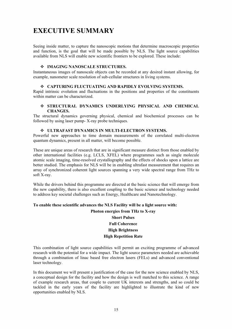
Seeing inside matter, to capture the nanoscopic motions that determine macroscopic properties and function, is the goal that will be made possible by NLS. The light source capabilities available from NLS will enable new scientific frontiers to be explored. These include:

IMAGING NANOSCALE STRUCTURES. Instantaneous images of nanoscale objects can be recorded at any desired instant allowing, for example, nanometer scale resolution of sub-cellular structures in living systems.

CAPTURING FLUCTUATING AND RAPIDLY EVOLVING SYSTEMS. Rapid intrinsic evolution and fluctuations in the positions and properties of the constituents within matter can be characterized.

STRUCTURAL DYNAMICS UNDERLYING PHYSICAL AND CHEMICAL CHANGES.

The structural dynamics governing physical, chemical and biochemical processes can be followed by using laser pump- X-ray probe techniques.

ULTRAFAST DYNAMICS IN MULTI-ELECTRON SYSTEMS. Powerful new approaches to time domain measurements of the correlated multi-electron quantum dynamics, present in all matter, will become possible.

These are unique areas of research that are in significant measure distinct from those enabled by other international facilities (e.g. LCLS, XFEL) where programmes such as single molecule atomic scale imaging, time-resolved crystallography and the effects of shocks upon a lattice are better studied. The emphasis for NLS will be in enabling ultrafast measurement that requires an array of synchronized coherent light sources spanning a very wide spectral range from THz to soft X-ray.

While the drivers behind this programme are directed at the basic science that will emerge from the new capability, there is also excellent coupling to the basic science and technology needed to address key societal challenges such as Energy, Healthcare and Nanotechnology.

To enable these scientific advances the NLS Facility will be a light source with: Photon energies from THz to X-ray

Short Pulses Full Coherence High Brightness

High Repetition Rate

This combination of light source capabilities will permit an exciting programme of advanced research with the potential for a wide impact. The light source parameters needed are achievable through a combination of linac based free electron lasers (FELs) and advanced conventional laser technology.

In this document we will present a justification of the case for the new science enabled by NLS, a conceptual design for the facility and how the design is well matched to this science. A range of example research areas, that couple to current UK interests and strengths, and so could be tackled in the early years of the facility are highlighted to illustrate the kind of new opportunities enabled by NLS.

17

1 Overview of Case

1.1 Introduction

Across a broad range of disciplines the scientific community is currently frustrated by its inability to dynamically image matter at the scale of nanometres and smaller. We can at present only observe relatively slow motion changes to structure, or infer dynamical effects via indirect measurements. In short, we are presently blind to structural changes occurring on the femtosecond timescale. Yet many critically important processes evolve on the femtosecond timescale and at the molecular and sub-cellular level requiring nanometre scale spatial resolution.

In this document we will discuss and present the scientific case and an outline design for a new light source facility that would permit us to see ultrafast dynamics on the nanoscale. The key to enable this breakthrough are to combine advanced conventional lasers and free electron lasers (FELs).

The potential breakthroughs to which NLS can lead include: • Nanometre scale imaging of arbitrary objects in their native state: Capturing a

living cell at nanometre resolution • Measuring the mechanisms of physical and chemical processes at the atomic

scale: Making molecular movies • Controlling electronic processes in matter: Directing attosecond dynamics

The properties of the light from the next generation of photon sources, i.e. free electron lasers, are dramatically different from those of storage rings and conventional lasers. Storage ring synchrotron radiation has enormous spectral coverage and can deliver a high photon fluence (photons per second) up to hard X-rays (10’s of keV). This has allowed these sources to be the dominant tool for crystallography, X-ray spectroscopy and many other areas of X-ray science for the last four decades. Nevertheless these sources have low peak brightness, especially if a narrow spectral bandwidth or a short pulse is selected. With advanced pulse slicing, these sources can provide sub-picosecond temporal resolution but only with tiny flux which severely limits the utility for measuring rapid changes. Conventional lasers have advanced hugely in recent years and can produce extremely short pulses (~5 fs) at very high brightness but these capabilities are limited to a restricted spectral range (0.5-5 eV).

FELs have the potential to deliver coherent radiation across an exceptional spectral range (<10 meV to multiple-keV) with narrow bandwidth (~0.1% of photon energy) and very energetic (millijoule) short pulses (~50 fs duration), and therefore exceptional brightness (1012 photons per pulse). A FEL undulator produces a very bright pulse at the fundamental frequency, but also bright pulses at three and five times that frequency (the harmonics) with photon number dropping by roughly a factor ~100 at each frequency step. This is a vastly larger spectral range than covered by conventional lasers and the pulses are typically a thousand times shorter and millions of times brighter than a storage ring can provide. FELs are likely to have a revolutionary impact on the science we do with light, potentially as profound as the revolutions created by the laser and synchrotron radiation.

We concentrate here on identifying and developing those scientific objectives for which a new UK facility with unique capabilities would be the optimal tool. This does not mean that some of these objectives are not possible, at least in part, using other international facilities (e.g. LCLS or XFEL). It would be unnecessarily limiting in planning a new UK based light source facility to consider solely that science that could not be done elsewhere. Nevertheless we believe that a high repetition rate seeded machine (key features of NLS) would lead to an exceptionally exciting programme ranging across the sciences that contains a major component of objectives

18

that are unique or simply better done there than anywhere else, and hence this would become an important international facility.

The science that is made possible by the availability of ultrashort, high brightness, coherent pulses in the THz to soft X-ray range is summarized in Figure 1-1. The processes of interest, i.e. valence/core electron dynamics, chemical dynamics, dynamics in condensed matter systems, and dense plasmas, are plotted in terms of the time and spatial resolution scales of the measurements required to capture them. Included also are the timescales in which high resolution “snapshots” must be recorded in order to ensure distortion free images from coherent diffraction imaging of nanoscale objects. The message is that to measure all of these fundamental processes, many for the first time, pulses as short as 20 fs or less are needed. The high spatial resolution is only possible if short wavelengths are used, in most cases utilising soft X-ray excitation near atomic absorption edges (in the 200 eV – 5 keV range) to capture local spatial relationships, but in some cases direct scattering (diffraction) signals can be used to obtain the spatial resolution.

Figure 1-1: The new science areas that will be enabled by an ultrafast, high brightness, soft X-ray to THz

light source

1.2 Science Drivers

We put forward the following major themes for the scientific impacts of NLS which we will then develop in more detail in the next Sections (Part II). They collectively encompass a new capability for seeing and controlling the nanoscale motions of the constituents of matter. We believe that the science and technology that will emerge from this capability will be revolutionary.

1.2.1 Imaging Nanoscale Structures

The high coherence and brightness of the FEL in the soft X-ray range will enable the exploitation of new imaging methodologies: e.g., coherent diffraction imaging and X-ray holography. The wavelength range of the FEL radiation will cover the “water window” (~4.36 - 2.38 nm), which is the wavelength range used to achieve penetration and contrast in “live” biological samples, and will extend to about 1 nm. Radiation damage by such high fluxes is a major problem with living systems, necessitating the use of flash imaging (made in a single shot using a pulse so short that no damage registers in the image that is captured). The longer wavelength FEL, FLASH at Hamburg has allowed important proof of principal studies in this field. It has been shown that images can be captured before the deleterious events of damage

19

occur provided the pulse is short enough and bright enough. Flash imaging has the potential for a new level of understanding of sub-cellular and macromolecule organization within cells, and should complement information obtained by optical and electron microscopy (EM). The gain compared to optical microscopy is improved spatial resolution (to 1 nm) and compared to EM the ability to make images with thicker specimens (to 2 μm). Moreover for non-biological objects, because the fundamental is bright enough to capture a full image in a single shot of <100 fs duration, the motion within nanoscale objects might be followed stroboscopically using either a sequence of mutually delayed pulses split from a common pulse or in a repetitive measurement following a sequence of identically prepared samples with increasing delay after the preparation step. The proposed NLS wavelength range also covers the most important edges for the study of complex condensed matter systems, i.e. the transition metal L edges, which access the physics of 3d valence electrons, and oxygen K edge for the physics of 2p shells. NLS would be ideally used to image complex electronic, magnetic and orbital structures, both statically and dynamically, down to 1 nm resolution. A key application will be to make stopwatch images of fluctuating magnetic, orbitally-ordered and electronic domains, polaronic states and even single Cooper pairs. Further, evolving structures around individual charge or spin carriers in functioning devices could be studied on an ultrafast timescale.

This theme is anticipated to have high impact in the following areas: life sciences, medicine, nanotechnology.

It requires a machine optimized for a fundamental in the soft X-rays, including the water window. The use of higher harmonics into the 5 keV region would allow imaging of the distribution of specific atoms at the nanoscale. Equal pulse spacing at a moderate repetition rate (>100 Hz) is suitable for getting the best from sample handling and detector technology.

In recent work from LCLS, the team of John Spence and colleagues from an international consortium have demonstrated diffraction from nano-crystals of a membrane protein with 2keV radiation. The results demonstrate that structure determination and time resolved studies on the 3-200 fs time scale is possible with crystals no more than 20 unit cells in dimensions, once higher energy radiation becomes available. The power of macromolecular crystallography can thus be applied for a range of biological complexes whose crystals (< 0.5 μm in length) previously had been considered too small for diffraction studies. Moreover the new results show that radiation damage is less severe than anticipated for these very small crystals with very short exposures (70fs).

1.2.2 Capturing Fluctuating and Rapidly Evolving Systems

Condensed matter and dense plasmas exhibit intrinsically fast structural fluctuations, which mediate all dynamic phenomena close to equilibrium.

Spontaneous fluctuations determine the physics and chemistry of liquids, the formation of glasses and alloys, magnetic properties of matter and complex phenomena in solids or in plasmas. In all these areas, our understanding of matter is then closely connected with our ability to experimentally capture time dependent correlation lengths and times between neighbouring particles.

Stimulated dynamics on the fast and ultrafast timescales is key to many technologies, e.g. from data transmission, switching and storage, materials processing. Understanding non-equilibrium phase changes in matter, which involve passage through short-lived states, can only be captured with the shortest exposure times.

A FEL with a short wavelength reach from 0.1 - 5 keV (including harmonics) and ultrafast bright pulses, will give access to dynamic physics of matter in new regimes. The wavelength will enable all forms of probing usually performed with soft X-rays and a great deal of new science using hard X-ray methods by using harmonics. For fluctuation physics, image

20

correlation spectroscopy, which is nowadays only possible down to microsecond timescales, will be transformed by the ability of having pairs or even trains of femtosecond X-ray pulses, and will be extended to arbitrarily short timescales. Non-equilibrium properties of matter will also become accessible on unprecedented timescales, with applications to condensed matter physics, materials, and chemistry but as well as plasma physics.

This theme is anticipated to have high impact in the following areas: nanotechnology, ultrafast solid state and magnetic devices, energy from fusion.

A wide spectral range and high transverse coherence are essential source requirements. A set of many repeated measurements is often required to obtain good signal to noise (S/N) so optimized pulse stability must be sought. High spectral resolution in inelastic X-ray scattering and for Thomson scattering to measure the ion acoustic feature is required.

1.2.3 Structural Dynamics Underlying Physical and Chemical Changes

Understanding the mechanism of physical, chemical and biological change at the microscopic scale is critical for a broad range of science and technology. A common goal is to develop this understanding to the point where it becomes possible to tailor functionality through material design, or by the application of electric, magnetic or optical fields. Chemical and physical changes involve the coupled flow of both charge and energy within the system due to electronic and nuclear motions. These processes may be triggered by e.g. the thermal fluctuations in the surrounding environment or by the absorption of light by a chromophore. Such processes, and the various processes which precede or compete with them, typically occur on the timescale of nuclear motion which is in the femtosecond regime. We anticipate a step function in our ability to directly monitor structural dynamics at the molecular level through the availability of femtosecond light pulses with X-ray wavelengths. The NLS will greatly extend the range of techniques we can use to both initiate and probe these processes. By use of visible/UV or IR/THz light of short pulse duration we can precisely trigger these events ourselves. Having triggered these events we can then follow them structurally using e.g. X-ray absorption spectroscopy (XAS) techniques or spectroscopically in the IR/visible. A combination of a tuneable soft X-ray FEL tightly synchronized to a IR/THz source or a UV/visible ultrafast laser will enable the structural changes to be followed in a vast range of physical and chemical processes. This will revolutionize our understanding of mechanisms in, for example, solution phase chemistry, in enzyme and surface catalysis and DNA photo-induced radiation damage. A variant of this method that would use a moderate energy electron beam to initiate “change” in non-photosensitive molecular samples and materials (radiolysis) can be readily combined with the soft X-ray probe capability. Moreover the moderate energy electrons may prove of great utility as a structural probe of laser or FEL induced changes in a new regime of time-resolved electron diffraction.

It is expected that this theme will have a high impact upon: materials technology, biochemistry, drug discovery, cancer/health, catalysis, sustainable use of resources.

A source providing tuneable high brightness soft X-ray to allow XAS across K and L edges of a majority of elements is essential as XAS is the primary tool for capturing the structural information. An adequate rep-rate is important to enable all measurements with good S/N and is essential to permit X-ray photoelectron spectroscopy (XPS) free from space-charge distortions. High spectral resolution is also very important in XPS. To achieve the best temporal resolution in pump-probe measurements a minimum jitter between lasers/electron beams and the FEL is needed.

1.2.4 Ultrafast Dynamics in Multi-Electron Systems

Electrons move very quickly within matter, often on timescales measured in 10’s of attoseconds (1 attosecond = 10-18 s) or quicker. Moreover in almost all matter the electrons are bound in very

21

close proximity to other electrons and so their dynamics are highly correlated through both the Coulomb interaction and quantum mechanical exchange effects (they are entangled). Although this may not be apparent in our everyday perception of matter it is of crucial importance if we are to understand or control the microscopic states of matter, goals which are at the core of many emerging 21st century technologies. We do not have the tools currently to adequately measure these ultrafast correlated electron processes, but NLS is set to provide them and so to revolutionize the science and technology of complex quantum processes.

Examples of the capabilities that are anticipated to be enabled by NLS are; (a) the measurement of hole dynamics in molecules and condensed matter (expected to happen in 10-15 to 10-17 s), (b) direct measurements of electron dynamics and damping in plasmons (collective electron resonances of increasing interest to frontier technological applications in nanoplasmonics), and (c) X-ray non-linear spectroscopy to provide full insight into the dynamical couplings between core and valence states. The newest aspect of NLS is the provision of very short X-ray pulses and the appearance of non-linear X-ray processes that open a new window on electron dynamics. The potential for measuring ultrafast electron dynamics through the non-linear response is only possible if high brightness femtosecond domain pulses are available. Ultrafast electron dynamics lie at the heart of material response to electromagnetic fields and so the outcomes of the proposed measurements will be a far more complete picture of the interaction of large complex quantum systems with light. Understanding ultrafast electron dynamics underpins new generations of technology for building and controlling; optical and electro-optical devices, ultrafast semiconductor and nanofabricated components.

This will have a high impact on areas such as: nanotechnology, quantum control, advanced materials, light harvesting.

The research needs appropriate ultrafast conventional lasers both for seeding of the X-ray pulses to ensure they are coherent and locked to an external IR laser for correlated electron studies, as well as pulse clicing for high brightness sub-fs for Xray pump-probe studies. Whilst we will have to await further technological developments at the NLS facility for pairs of sub-fs X-ray pulses to be available we can straightaway use seeding and phase locked lasers to achieve sub-fs domain measurements.

1.3 Science Demands for Facility Capability

1.3.1 Baseline and Upgrades

To satisfy the scientific objectives set out in Part II Sections 1 and 2 there are core capabilities that the facility must be able to deliver. These capabilities include:

Ultrashort pulses of photons in the spectral range from 0.01 eV to 5 keV High peak brightness pulses in the range 50 eV to 1 keV

A Stage 1 baseline specification that we envisage should be available from day one of the facility operation is:

♦ High brightness (more than 1011 photons/pulse) pulsed coherent light source coverage from THz to ~1 keV (with harmonics to ~5 keV)

♦ ~1 kHz repetition rate with even pulse spacing ♦ Photon source capable of smooth tuning across most of the spectral range ♦ Pulse durations down to ~20 fs ♦ Multi-colour capability for pump-probe experiments with synchronization jitter

better than 10 fs. For example, Colour 1: THz- IR (pump)/ Colour 2: 100 eV-5 keV (probe)

♦ High degree of temporal coherence of fundamental and harmonics through seeding of the FEL

22

♦ High degree of transverse coherence ♦ Synchronized to short pulsed lasers ♦ High degree of fully variable polarization

Further upgrade options are an essential part of the long term plan of the facility and the possibility to apply them at a future date is part of the outline design. It is envisaged that some additional capabilities, such as extending the seeding photon energy range, increasing repetition rate and implementing pulse slicing, could be implemented at an appropriate point within the routine facility development schedule. Other more extensive upgrades such as an increase in photon energy will require a more substantial investment.

There will need to be provision for a range of additional equipment and facilities that are essential to the NLS science. These include a suite of lasers synchronized to the FEL which form an integral part of the light source. Moreover, to realize the full potential of NLS, other critical equipment should be included in the facility such as a source for ultrafast relativistic electron diffraction (~5 MeV energy), high field magnets and a high power long pulse laser. Likewise essential facilities for sample preparation (e.g. tissue culture, crystal growth) and handling will need to be available from the start of operation. The selection and design of these would be part of the further planning process after approval of the baseline facility.

A stage 2 upgrade could then tackle the increase of the photon energy to a photon energy of 1.5 keV (i.e. up to 7.5 keV harmonics) and beyond, increased repetition rate (to 10 kHz and eventually still higher), and implementation of advanced pulse slicing techniques to achieve sub-femtosecond operation. An energy up-grade will be relatively costly as it entails adding additional accelerator modules to increase the electron beam energy. Provision of enough space in the facility site to accommodate an increase in the linac length is a requirement. Further extension of the long wavelength reach and performance would also be developed, potentially through the inclusion of an IR/THz FEL. Increasing the NLS repetition rate above 10 kHz would be feasible if a higher repetition rate gun is developed (not yet available but it is highly likely this technology will be available within the next 5 years).

The potential for a stage 3 up-grade to further enhance the facility should also be considered, perhaps waiting for technological advances that may make higher repetition rate or photon energy cheaper and more feasible than using current technology. Extending the spectral coverage of the FEL fundamental to higher photon energies (>2 keV) is a potential future aspiration. This would usually require either the increase of the linac energy (by adding acceleration modules) or a reduction in the undulator gap but future technology may offer alternative options (e.g. laser wakefield acceleration to boost the electron beam energy). It is desirable to retain the option of a potentially strategically important upgrade route to a UK hard X-ray (~8 keV) machine in the case that single macromolecular imaging were to become as successful as current protein crystallography.

1.3.2 Need for Seeding

To overcome the intrinsic jitter and fluctuations inherent to the self-amplified spontaneous emission (SASE) process seeding by the highly coherent short wavelength light produced by high harmonic generation has been identified, and recently demonstrated at SPring 8 in Japan [1], as the best strategy to radically improve the coherence, reproducibility and synchronization properties of a FEL (see Figure 1-2). It should be routine to achieve a few femtosecond jitter level using a seeded machine, allowing 20 fs pump-probe resolution to be realized with pulses of high coherence and reproducibility. In contrast a SASE machine will only achieve a jitter level of some tens of femtoseconds as well as the pulses being far from coherent and inherently noisy. Seeding will be essential to achieving the conditions needed for a wide range of the NLS science objectives.

23

Direct seeding to 1 keV will require relativistic high harmonic generation (RHHG) to ensure the photon energy and power needed but is not yet feasible due to the absence of high repetition rate high peak power lasers. With the likely improvement of high power ultrafast lasers anticipated to push the average power limit from 1 kW towards 10 kW over the next decade this may provide direct seeding capability across the entire energy range of the FEL. Instead we plan to adopt a hybrid scheme whereby direct seeding is used to 100 eV and 1 or 2 stages of harmonic up-conversion is employed in the FEL to reach 1 keV. This would correspond in the FEL harmonics to exceptional coherence and synchronization properties up to >5 keV.

Whilst this has yet to be demonstrated, and hence there are some technological risks associated with this approach, we believe that given the rapid progress being made in this field in general, together with some dedicated research and development (R&D), it will be able to be implemented at the start of facility operation. A fall-back option based on SASE operation for the higher energies will be feasible and would be adopted for a period if required. A seeded machine, operating at these high photon energies, would be a unique facility internationally.

An analysis of the importance of seeding is provided in Appendix B – The Importance of Seeding to the NLS Scientfic Mission.

Figure 1-2: The dramatic improvement in the temporal quality of the pulse is illustrated by comparing the results of a time dependent calculations for the SASE output for NLS (upper frame) compared to the

Seeded output (lower frame)

1.3.3 Need for High Repetition Rate

A very significant technical issue is related to the choice of repetition rate for the light source. The essence of this issue is that there is a technological difference between a source with a repetition rate of ~100 Hz and one in the 1 kHz – MHz range. For the lower repetition rate non superconducting (non-SC) accelerator modules can be employed in the electron linac. This technology is being used at LCLS, and in the Japanese and Swiss projects. For higher repetition rate it is essential to use superconducting (SC) accelerator modules in the linac. The latter are

24

either loaded with the accelerating radio-frequency field in a pulsed or continuous wave (CW) mode to achieve either a high repetition rate in a series of bursts (e.g. at FLASH or in the XFEL design) or an evenly spaced series of pulses at a repetition rate of 1-100 kHz (as in the BESSY, Arc-en-Ciel, LBNL, Wisconsin and NLS proposals).

The technological difference has a substantial effect upon cost. In summary SC technology modules are significantly more expensive per MV of acceleration, require a more expensive infrastructure (e.g. for cryo-cooling) and a larger building (in part to house the cryoplant and in part because the accelerator needs to be longer). Operating costs for the cryoplant and radio frequency (RF) power will also be higher. Nevertheless there are very significant scientific advantages of the higher repetition rate. Indeed the conclusion drawn from the science case is that a higher repetition rate is essential to extend the scientific reach for each given photon energy range. A higher repetition rate improves the signal to noise in most measurements. In a significant number of experiments use of a brighter pulse to boost the signal will not compensate for a lower repetition rate as sample damage limits the utility of higher brightness. Higher rep-rate does not, in itself, preclude any experiments (like flash imaging or some plasma related studies) that use only a single shot at a time and are unlikely to need the higher rep-rate themselves. Therefore more science is enabled by a higher rep-rate and so in constructing the science case the arrow on the choice of rep-rate logically points only in the direction of a higher rep-rate. High repetition rate even pulse spacing is a feature not offered by any of the existing FEL projects which therefore is another feature that will ensure the uniqueness and high international profile of the NLS project.

The versatility of a future up-grade route to higher repetition rate (> 10 kHz) is only an option if the SC technology is adopted from the start. Advantages of a higher rep-rate in terms of a future up-grade is that it could lead to a machine with many FEL beam-lines simultaneously running at different frequencies and so lead to much increased science productivity and cost effectiveness of the facility (a strategy being proposed for a new machine at Berkeley).

An analysis of the full science case to identify those elements for which a higher rep-rate is either beneficial or essential is given in Appendix C – Repetition Rate.

1.3.4 Mapping Science Needs to Capability

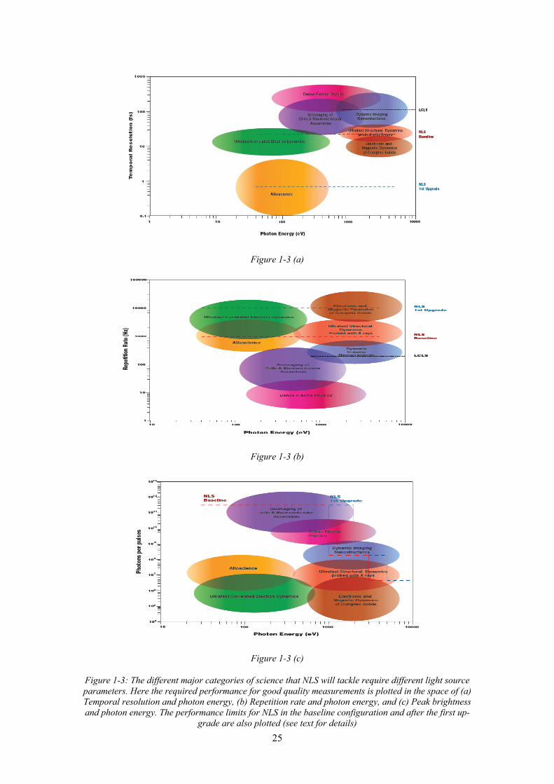
Figure 1-3 (a), (b) and (c) are graphical illustration of the demands on temporal resolution, repetition rate and peak brightness coming from key science areas: bioimaging of cells and macromolecular assemblies, dense plasma physics, dynamic imaging of nanostructures, ultrafast structural dynamics probed with X-rays, electronic and magnetic dynamics of complex solids, ultrafast correlated electron dynamics and attosecond science.

In Figure 1-3 (a) the temporal resolution and photon energy required for the various classes of science are plotted. The temporal resolution limits of LCLS, NLS (baseline) and NLS (first upgrade) are shown for the type of pump-probe configuration measurements typically needed. Any science above the respective lines should be accessible to that facility. Whilst LCLS will have difficulty reaching the required parameter space for much of the science considered here, NLS even in the baseline specification will be able to tackle the majority of the science and essentially all of it following the first up-grade. In Figure 1-3 (b) science classes are plotted in the space of the repetition rate required to make high quality (good S/N) measurements against photon energy. Again LCLS, NLS (baseline) and NLS (first upgrade) are shown, anything below the respective lines is science that can be captured with the facility. Once again we see NLS even in the baseline can capture most science and everything in the first upgrade whereas LCLS has more limited range. Figure 1-3 (c) shows the science classes plotted in the space of peak brightness versus photon energy, anything below the facility lines being accessible. We see that NLS in the baseline configuration is very able to capture most science and after an energy upgrade still more.

25

Figure 1-3 (a)

Figure 1-3 (b)

Figure 1-3 (c)

Figure 1-3: The different major categories of science that NLS will tackle require different light source parameters. Here the required performance for good quality measurements is plotted in the space of (a) Temporal resolution and photon energy, (b) Repetition rate and photon energy, and (c) Peak brightness and photon energy. The performance limits for NLS in the baseline configuration and after the first up-

grade are also plotted (see text for details)

26

1.4 Facility Overview

1.4.1 Facility Layout and Description

Figure 1-4: Overall layout of the NLS facility

Figure 1-4 shows the overall layout, main components and scale of the NLS facility. Such a layout has been chosen in order to leave the “straight-ahead” direction free, to provide an easy means of extending the facility as described in Section 1.4.2 below.

The baseline specification for the facility described in the above Sections will be met by three types of radiation source:

• A suite of three FELs will cover the range from 50 eV to 1 keV in the fundamental, with overlapping tuning ranges as follows:

FEL-1: 50-300 eV, FEL-2: 250-850 eV, FEL-3: 430-1000 eV. Harmonics will extend the output to 5 keV.

• Conventional laser sources, synchronized to the FEL sources, will cover the range from 60 meV (20 μm) to 50 eV.

• Coherent THz/IR radiation from 20–500 μm will be generated by the electron beams after passing through each FEL, for optimal synchronization between the FEL pulse envelope and THz/IR field for pump-probe experiments.

To meet the required FEL tuning ranges with realistic electron beam parameters, given the chosen undulator design, and without demanding excessive undulator lengths, requires a minimum electron beam energy of 2.25 GeV. A common electron energy for all three FELs, together with variable gap undulators, assures the required independent operation and easy tunability of the three FELs. The FEL undulators are based on the well developed APPLE-II scheme in order to provide the required fully variable polarization with the highest possible degree of polarization.

The high repetition rate of equally spaced pulses, initially 1 kHz and increasing in subsequent phases up to 1 MHz, demands superconducting technology for the linear accelerator (linac), operating in continuous wave (CW).

Figure 1-5: Schematic layout of the NLS facility

Figure 1-5 shows a schematic layout of the facility. The baseline electron gun is a modified version of the successful DESY FLASH/XFEL gun, optimized for 1 kHz operation. The linac

27

consists of a number of accelerating modules based on the well developed TESLA/XFEL design. These are however pulsed machines and although the cryomodule design provides a good starting point for meeting the NLS requirements, some re-engineering is needed to accommodate the higher dynamic head load, higher power couplers and HOM absorbers demanded by CW operation. The required engineering changes are considered in detail in Part III Section 3.6.6. Following a detailed analysis of associated capital and operational costs, as well as other relevant factors, the nominal accelerating gradient has been set at 15 MV/m (Part III Section 3.4), resulting in a requirement for 18 cryomodules (compared to 14 in the earlier design before the cost optimization had been carried out).

Three bunch compressors (BC1-3) are located at optimized locations (205 MeV, 460 MeV and 1.5 GeV) along the linac to compress the electron bunches while maintaining high beam quality. A 3rd harmonic cavity is included to optimize the beam dynamics by linearising the longitudinal phase space. A laser heater serves to introduce a controlled amount of energy spread in order to overcome the microbunching instability.

The linac is followed by a collimation section to remove unwanted beam halo before the beam enters the spreader region which directs successive electron bunches into different FEL lines by means of a set of kicker magnets. This arrangement was chosen for its flexibility. One of the lines parallel to the FELs is a diagnostic section which incorporates a transverse deflection cavity for full slice analysis of the electron beam. With this arrangement sophisticated beam diagnostics can be carried out on-line, by occasionally deflecting bunches into the diagnostics line. To provide the required temporal coherence of the FEL radiation, as well as the 20 fs pulse lengths, each FEL will be seeded with laser pulses obtained from High Harmonic Generation (HHG) in gases. Our current assessment, based on the rapid progress being made in this area, is that within the next ~5 years it will be possible to deliver HHG pulses with at least 400 kW peak power, with 1 kHz repetition rate, tunable over the range 50-100 eV. To obtain the required FEL output up to 1 keV, a one- or two-stage harmonic generation scheme is used, as shown schematically in Figure 1-6.

e‐ @ 2.25 GeV

APPLE‐II Radiatorλw = 32.2 mm

20fs FEL Pulse430 ‐ 1000eV

FEL3Modulator 1λw = 44 mm

Modulator 2λw = 44 mm400kW HHG 75‐100eV

Modulator 1λw = 44 mm


20fs FEL Pulse250‐850eV


e‐ @ 2.25 GeV

400kW HHG 75‐100eV



FEL1Modulatorλw = 49 mm

e‐ @ 2.25 GeV

400kW HHG 50‐100eV

Figure 1-6: Schematic of the harmonic cascade FEL scheme.

The expected output from the FELs is given in Table 1-1. Full start-to-end calculations have been performed to confirm the performance, using three linked computer codes: electrons are tracked from the gun through the first accelerating module (ASTRA), then through the linac, collimator and spreader (Elegant) and finally through the FEL (Genesis).

28

Table 1-1: Calculated output performance of the NLS FELs.

FEL Photon energy

(eV)

Output power (GW)

Energy per pulse (μJ)

Photons per pulse

Peak Brightness (photons/s/mm2/mrad2/0.1%bw)

FEL-1 50 7.1 142 1.8 1013 1.9 1030

300 5.3 106 2.2 1012 5.0 1031

FEL-2 250 5.3 106 2.7 1012 3.5 1031

850 2.9 59 4.3 1011 2.2 1032

FEL-3 500 4.2 84 1.1 1012 1.1 1032

1000 2.7 54 3.4 1011 2.8 1032

After exiting from each FEL and before being dumped, the electron beam passes through an undulator magnet to generate coherent undulator radiation in the 20-500 μm range. Broad-band radiation will also be generated using a bending magnet source.

Eight experimental stations are currently planned. Each FEL will have one with directly focussed beam and one with a grating monochromator to improve spectral resolution and/or filter out unwanted spectral components. In addition a time-preserving grating monochromator is foreseen on FEL-1, and a crystal monochromator on FEL-3 for accessing the harmonics in the range 2-5 keV. The photon beam transport region has been designed to avoid the optical components being damaged by the high peak power of the FEL radiation

1.4.2 Upgrade Paths

An important aspect of the design of NLS will be the possibility to extend its performance in future stages. The Science Case calls for the following options to be available for possible future development:

• Higher repetition rate, eventually up to 1 MHz. • Shorter FEL pulses, ranging from sub-fs at 1 keV to a few-fs at 100 eV. • Additional FELs and experimental stations. • Higher photon energies, at least 1.5 keV in the fundamental, and potentially in excess of

2 keV.

Higher repetition rates will require a different gun and several different types are under active consideration not only by NLS but by several laboratories world-wide (see Part III Section 2.2). Detailed simulations have now been carried out for one of these schemes which shows that it can be operated with the existing linac and bunch compression scheme producing a beam of sufficient quality to drive the FELs (see Part III Section 1.6). A corresponding upgrade of the photocathode, seed and experimental lasers will also be required. This is likely however given the timescales involved and the rapid progress being made in this area. To facilitate the development and commissioning of the second-stage gun, as well as for flexibility in future operations, a dogleg has been introduced between the injector and the linac which allows the linac to be operated easily with either gun (see Part III Section 4.1).

Various schemes have been put forward in the literature for generating sub-fs to fs FEL pulses. Start-to-end calculations have been carried out for three of the most promising schemes (Part III Section 1.4) demonstrating the feasibility and compatibility with the basic NLS design.

The proposed layout of the facility (Figure 1-4) and the choice of spreader scheme (Figure 1-5) lend themselves well to the future extension of the facility. The electron beam transport line can relatively easily be extended along the direction of the linac axis into a second spreader region

29

which then feeds a second FEL hall and experimental hall parallel to the first ones (see Part III Section 12.1.1). These could be of the same type as employed in the main linac, but if it is not essential for the higher energy beamlines to operate at high repetition rate, there are in principle alternative possibilities. The second linac could for example be a high gradient normal conducting system in order to reach the highest energy in the most efficient manner, at reduced repetition rate. The possibility of using plasma wakefield acceleration also deserves consideration.

1.5 NLS as a Leading Facility

1.5.1 Relationship to Other Facilities

It should be fully part of the UK strategy to use the other existing machines; a number of longer wavelength FELs (such as FELIX and the FLASH VUV FEL), several hard X-ray FELS in construction (e.g. LCLS, Stanford operational summer 2009; SCSS, Spring 8 operational 2011; and XFEL, Hamburg operational 2014) and a number of other projects in the planning/construction stage (e.g. PSI-XFEL, MAX IV, Fermi@Elettra, SPARX). The UK has strong links to FELIX, FLASH, XFEL and LCLS and it is hoped that these facilities will satisfy a significant range of national scientific objectives in this area. In particular LCLS and XFEL provide high brightness hard X-rays that may enable the exciting possibility of single molecule atomic scale diffractive imaging that will reveal the detailed structure of macromolecules not amenable to crystallization. LCLS became operational in 2009 and UK users have already participated in experiments here.

Exciting as hard X-ray science is, there are many other compelling scientific directions available for which a soft X-ray optimized facility is ideal. It is our belief that this is the scientific area where NLS should concentrate and which allow many original scientific opportunities. Moreover hard X-ray FELs are reliant on SASE which leads to a noisy output pulse whereas in the soft X-ray range seeding is feasible leading to a coherent output pulse that is highly advantageous in many applications. A soft X-ray facility with a multi-colour capability for pump-probe studies, possibilities of high temporal coherence and high repetition-rate trains of evenly spaced ultrashort pulses will be unique and optimal for tackling a wide range of new science which we discuss in detail below. Whilst FLASH (and the planned FLASH II) are also likely to develop two-colour and seeding capabilities the wavelength range of that facility will remain far more limited than NLS.

1.5.2 Unique Capabilities of NLS

We have concentrated on identifying and developing those scientific objectives that a new facility, with unique capabilities going beyond the existing array of international facilities, would be able to tackle. In particular multi-colour capability with IR/THz and visible sources tightly synchronized to a soft X-ray tuneable FEL (reaching up to >5 keV at the 5th harmonic) will be a powerful combination not matched by any existing source. The spectral coverage of this tuneable X-ray source will access all the K edges of the elements up to titanium (and to iron and cobalt with an energy up-grade) plus the L edges of the majority of atoms, which will permit dynamic structure determination for a vast range of solids, liquids and molecules inaccessible otherwise. Moreover femtosecond time-resolved X-ray diffraction for atom scale determination will be permitted at the highest photon energies still at a flux (~ 1010 photon/s) much higher than storage ring pulse slicing.

A further combination of capabilities that are exceptionally important to achieve a unique programme includes seeding (with HHG) and laser pulse slicing. Both require synchronized external lasers and with present technology this puts constraints on the time structure of the machine. LCLS will have a 120 Hz repetition rate and this readily permits laser slicing to be implemented, but a higher repetition rate is a significant advantage in a significant range of

30

experiments. XFEL will have a 10 Hz repetition rate of macro-pulses each containing up to 3000 pulses at a temporal separation of 200 ns. This makes it very hard to seed or slice the machine at the full repetition rate. In contrast a machine with even pulse spacing and a moderately high repetition rate (~100 Hz to 10 kHz) will be optimally suited to seeding and slicing and so will be ideal for applications where temporal coherence, tight synchronization to external lasers and sub-fs pulses are essential. Seeding will result in remarkable improvement in the X-ray coherence that will enable measurements with combined temporal and spectral resolutions that approach the transform limit that are inaccessible to any SASE machine.

There are a number of critical comparison criteria between available light sources that need to be considered to define the advantages of NLS for a given class of measurement. So for instance we can compare the projected capabilities of NLS with other sources in a number of ways (see Figure 1-7 (a)-(d)): temporal resolution variation with photon energy, peak and average brightness variation with photon energy, temporal resolution with repetition rate. It can be seen that the combination of excellent temporal resolution at uniquely high repetition rate and competitive average and peak brightness will provide NLS with excellent capability for ultrafast measurement and nanoscale imaging. Further it must be understood that the highest scientific impact is made possible by availability of near transform limited pulses (where energy and time spread are close to the uncertainty limit) that can be imposed only by seeding (SASE sources are very far from transform limited and inherently unpredictable in their temporal/spectral characteristics). There are also a broad class of measurements, which are currently not possible because sources with high spectral brightness don’t exist, where high energy resolution and somewhat lower temporal resolution are required it is anticipated that a combination of seeding alone or seeding and spectral selection can generate transform limited pulses of ~100 fs which is not possible with other sources.

1

10

100

1000

10000

0.001 0.01 0.1 1 10 100 1000 10000

Photon Energy (eV)

Bes

t Tem

pora

l Res

olut

ion

(fs)

FLASH

NLS

EU XFEL

LCLS

DLS

Figure 1-7 (a)

31

1.00E+20

1.00E+21

1.00E+22

1.00E+23

1.00E+24

1.00E+25

1.00E+26

1.00E+27

1.00E+28

1.00E+29

1.00E+30

1.00E+31

1.00E+32

1.00E+33

1.00E+34

10 100 1000 10000

Photon Energy (eV)

Peak

Brig

htne

ss (p

h/s/

mra

d2 /mm

2 /0.1

%bw

)

FLASH

EU XFEL

LCLS

NLS n=1 NLS n=3

NLS n=5

DLS U23

sFLASH

Figure 1-7 (b)

1.00E+18

1.00E+19

1.00E+20

1.00E+21

1.00E+22

1.00E+23

1.00E+24

1.00E+25

1.00E+26

10 100 1000 10000

Photon Energy (eV)

Ave

rage

Brig

htne

ss (p

h/s/

mra

d2 /mm

2 /0.1

%bw

EU XFEL

LCLS

NLS n=1

FLASH

DLS U23

NLS n=3

NLS n=5

Figure 1-7 (c)

32

1

10

100

1000

10000

1.00E+00 1.00E+01 1.00E+02 1.00E+03 1.00E+04 1.00E+05 1.00E+06 1.00E+07 1.00E+08 1.00E+09

Repetition Rate (Hz)

Bes

t Tem

pora

l Res

olut

ion

(fs)

DLS

NLS

LCLS

EU XFEL

FLASH

Figure 1-7 (d)

Figure 1-7: NLS compared with other leading facilities (FLASH and seeded-FLASH, Diamond Light Source (DLS), EU XFEL and LCLS) in terms of key performance parameters. (a) Temporal resolution (in pump-probe measurements accounting for jitter) versus photon energy, (b) Peak brightness versus photon energy, (c) Average brightness versus photon energy (note to compare with DLS operating at

sub-picosecond resolution where pulse slicing at lower rep-rate is needed the curve must be reduced by a fatcor >105). The data presented in the above Figure is best on the best information available from the

following sources [2, 3, 4, 5, 6, 7, 8]

1.6 Mapping to Societal Needs

There is a growing recognition that science and technology must rise to a number of pressing current societal challenges related, for example, to environmental sustainability, energy supply, healthcare and advanced information technology. NLS, although driven by the needs of the new basic science outlined above, is well suited to make major contributions to all these challenges by providing fundamental understanding of matter and processes that will lead directly to radical improvements through design and verification of, for example, better materials, drugs and catalysts. We discuss both the excellent coupling of NLS to recently identified research grand challenges and the potential for the facility to have a very high economic impact (Part II Section 3). NLS guarantees that the UK will establish a durable position of research leadership in many key areas of Science and Technology.

Although early in the process we can already identify a number of key technology areas where the science that NLS could produce will provide significant benefit. To measure mechanisms in physical, chemical and biological processes and to control electronic processes (that are invariably very quick) requires real time structural measurement capabilities in the sub-picosecond to sub-femtosecond range (see Sections 1 and 2). The potential technology benefits of NLS include:

Nanometre scale imaging of arbitrary objects in their native state Examples of imaging where this is vitally important are: following the interactions of sub-cellular systems and macromolecules in living cells to aid in development of drugs and medical technology, understanding the activity of nanostructures in physical and chemical processes to further the technological impact of nanotechnology.

33

Measuring the mechanisms of physical and chemical processes at the atomic scale Examples of where atom scale understanding of mechanism is vital include: understanding and improving catalysis and enzyme catalysis, elucidating and mitigating the mechanisms of radiation damage in matter, understanding the mechanisms of the complex chemistry occurring in the environment, and understanding and optimizing the limits to the speeds of switching in magnetic data storage. Controlling electronic processes in matter Examples of the impact of electron control are: improved efficiency in artificial photosynthesis, controlling superconductors, novel electronic and magnetic materials, new devices for optical and information technology. The NLS project can provide a direct coupling to economic activity in a number of ways. Firstly, as just elucidated, improved understanding of the fast structural changes that underpin high technology (nanotechnology, biotechnology, advanced materials, catalysis etc) will lead to long term benefits to UK industry. Secondly NLS will provide industry with access to advanced high brightness X-rays for myriad applications. Further NLS will provide a flow of highly trained manpower with skills in some of the most advanced areas of technology and measurement. As a major international facility located in the UK NLS will ensure significant inward investment.

REFERENCES [1] Lambert, G. et al., Injection of harmonics generated in gas in a FEL providing intense coherent

extreme-UV light Nature Physics 2008, 4(4), p. 296-300 [2] http://www-ssrl.slac.stanford.edu/htbin/rdbweb/LCLS_params_DB_public/ [3] http://xfel.desy.de/technical_information/photon_beam_parameter/ [4] Interim Report of the Scientific the Scientific and Technical Issues (XFEL-STI) Working Group on

a European XFEL Facility in Hamburg January 2005 [5] http://hasylab.desy.de/facilities/flash/facility_information/index_eng.html [6] http://hasylab.desy.de/facilities/flash/machine/parameter/index_eng.html [7] http://hasylab.desy.de/facilities/flash/facility_information/laser_and_fel_timing/index_eng.html [8] http://accelconf.web.cern.ch/AccelConf/e08/papers/mopc028.pdf

35

PART II – SCIENCE CASE

37

1 Science Drivers

In this Section we discuss the science drivers that were distilled from the NLS consultation process. These drivers define the facility capabilities that are required (see Part I Section 1.3). Together the new capabilities promise to open entirely new areas of research as well as offering profound advances in existing areas. We will try to explain how important scientific questions can be addressed by NLS. The underlying principles of the new types of measurement that NLS will allow will also be outlined. Later, in Section 2, we will present a range of specific research highlights that can be undertaken with NLS.

The choice of the four themes for the science drivers around which the case is organized is an effective way to explain the uniqueness of the science. The themes form an interlinked, and overlapping, set which conveniently encompasses almost all of the important new science accessible to NLS. We cannot predict all of the science that will emerge from NLS over the facilities lifetime. The facility offers a powerful, and upgradeable, platform for advanced photon science and it is probable many new opportunities will emerge. Here we attempt to capture some of the likely potential of the facility based upon our current state of knowledge.

Imaging of nanoscale structure with X-rays, whilst not an entirely new direction, will benefit hugely from the high coherence, brightness, repetition rate and short pulses of free electron lasers (FELs). Whilst hard X-ray single molecule imaging awaits the hard X-ray FEL machines for proof of principle experiments, there are already some very positive results supporting the concept of intense soft X-rays applied to imaging nanoscale objects. Nature is full of systems with a structure that rapidly evolves and/or fluctuates, e.g. condensed matter systems close to a phase change, liquids and dense plasmas. Hitherto it has not been possible to capture these over all the important timescales. NLS will provide a profound new insight into this aspect of matter. Directed change, e.g. chemical reactions or triggered phase changes, which involve dynamical structural changes over all possible timescales are another area of great importance. A unique capability of NLS is to provide two or more tightly synchronized and tuneable colours across the entire THz to soft X-ray range which will enable the structural dynamics to be fully elucidated for the first time in a multitude of physical, chemical and biochemical systems. Finally electron dynamics require soft X-ray pulses of sub-femtosecond timescale and so up to now have only been directly measured in a tiny set of systems. A combination of FEL and laser based sources will extend our understanding of the fundamentals of the electron dynamics across the whole range of matter.

1.1 Imaging Nanoscale Structures

‘Imaging is fundamental in all biological and biomedical research and the essence of cell biology’ [1]. The imaging methods now available cover spatial distances from the atomic to whole cell, but each has limitations. X-ray crystallography provides technology for the determination of atomic structures of macromolecular complexes, provided that the macromolecular complex can be crystallized. Electron microscopy (EM) allows imaging at the cellular, sub-cellular level and at the molecular level but demands thin specimens (< 0.2 μm thick). Optical microscopy has the powerful capacity to track the location and interactions of proteins in living cells using genetically encoded fluorescent proteins with ~100 nm resolution but it does not image the shapes of the macromolecular complexes, only the source of fluorescence. Soft X-ray microscopy using Fresnel zone plate lenses as objectives can deliver tomographic images to ~20 nm resolution of whole cells and the method is starting to be applied to monitor dynamic events in cells and cell responses to external stimuli. Because of the importance of visualization in biology, new imaging methods raise interest. There is a need to bridge the gap between the atomic and the whole cell imaging in order to observe macromolecular assemblies and their locations. The possibility of flash X-ray imaging to achieve resolutions of the order of 1-2 nm raises exciting possibilities when combined with

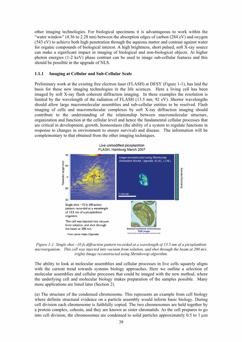
38

other imaging technologies. For biological specimens it is advantageous to work within the “water window” (4.36 to 2.28 nm) between the absorption edges of carbon (284 eV) and oxygen (543 eV) to achieve both high penetration through the aqueous matter and contrast against water for organic compounds of biological interest. A high brightness, short pulsed, soft X-ray source can make a significant impact in imaging of biological and non-biological objects. At higher photon energies (1-2 keV) phase contrast can be used to image sub-cellular features and this should be possible in the upgrade of NLS.

1.1.1 Imaging at Cellular and Sub-Cellular Scale

Preliminary work at the existing free electron laser (FLASH) at DESY (Figure 1-1), has laid the basis for these new imaging technologies in the life sciences. Here a living cell has been imaged by soft X-ray flash coherent diffraction imaging. In these examples the resolution is limited by the wavelength of the radiation of FLASH (13.5 nm; 92 eV). Shorter wavelengths should allow large macromolecular assemblies and sub-cellular entities to be resolved. Flash imaging of cells and macromolecular complexes by soft X-ray diffraction imaging should contribute to the understanding of the relationship between macromolecular structure, organization and function at the cellular level and hence the fundamental cellular processes that are critical in development, growth, homeostasis (the ability of a system to regulate functions in response to changes in environment to ensure survival) and disease. The information will be complementary to that obtained from the other imaging techniques.

Figure 1-1: Single shot ~10 fs diffraction pattern recorded at a wavelength of 13.5 nm of a picoplankton microorganism. This cell was injected into vacuum from solution, and shot through the beam at 200 m/s.

(right) Image reconstructed using Shrinkwrap algorithm.

The ability to look at molecular assemblies and cellular processes in live cells squarely aligns with the current trend towards systems biology approaches. Here we outline a selection of molecular assemblies and cellular processes that could be imaged with the new method, where the underlying cell and molecular biology makes preparation of the samples possible. Many more applications are listed later (Section 2).

(a) The structure of the condensed chromosome. This represents an example from cell biology where definite structural evidence on a particle assembly would inform basic biology. During cell division each chromosome is faithfully copied. The two chromosomes are held together by a protein complex, cohesin, and they are known as sister chromatids. As the cell prepares to go into cell division, the chromosomes are condensed to solid particles approximately 0.5 to 1 μm

39

in size that can be visualized by optical microscopy (Figure 1-2 (A)). The DNA in the chromosomes is organized into higher order structures by hierarchical compaction of the DNA. The DNA is first wound round a complex of eight histone proteins to form a nucleosome with 147 base pairs (bp) per nucleosome whose X-ray structure is known. The nucleosomal arrays are folded to form 30 nm fibers. Before the cell enters mitosis, these fibers are further condensed so that they form solid and robust units that can withstand the force when sister chromatids are pulled apart to deliver a complete chromosome to the daughter cell. Condensed chromosomes can be purified by flow cytometry. Information on the arrangement of a key protein, called condensin, in this process has come from immuno-stained thin sections examined by electron microscopy. In scanning electron micrographs distinct loops can be seen emanating from a central core. DNA hybridization experiments show that the order of visible features along a mitotic chromosome roughly reflects the order of genes along the DNA molecule. Condensed chromosomes are too thick to be examined intact by electron microscopy but they have been imaged using coherent diffraction imaging with a third generation light source at about 40-nm resolution. With flash imaging further structural details should become apparent that could inform on the organization of the DNA and proteins within the particle.

Figure 1-2: Assemblies important in the cell cycle. A) Top: A transmission electron micrograph of a thin section of a human metaphase chromosome from HeLa cells, which has been immunostained to reveal the condensin protein located on the axis of the chromosome arms. Below: A possible model for chromosome condensation. Only one chromatid is shown. Condensin subunit Smc2 occupies approximately one third

of the chromatid diameter, acting to stabilize the metaphase chromosome. (From Kireeva, N. et al., (2004) [2] ) B ) A simplified view of cell division showing condensation of DNA (blue) as the cell goes

from interphase (resting state) to prophase (start of cell division). Microtubules (green) are shown emanating from the centrosomes (small circles). The red dots on the chromosomes represent the

centromeric regions with attached kinetochores. (Adapted from Cheeseman IM, and Desai A (2008) [3]) C) An enlarged view of the chromosome centromeric region. On the right the kinetochore is attached to microtubules. On the left the kinetochore is not attached. D) A negatively stained electron micrograph of chromatin attached to kinetochore microtubules. (From McEwen BF, et al., (1998) [4]). E) A schematic

diagram of how the protein complexes that comprise the kinetochores might be arranged. (From Cheeseman IM., and Desai A., (2008) [3])

40

(b) The mitotic spindle. This represents an example where structural information on an assembly in situ in the cell would contribute to understanding a complex biological process. During cell division, the cell first duplicates the chromosomes to form the sister chromatids and then delivers one set of chromosomes to two identical daughter cells (Figure 1-2). The fidelity of the process is controlled by the mitotic spindle. In animal cells, the centrosomes (an assembly of two orthogonal protein complexes called centrioles) extend microtubule filaments that end in attachment to the chromosomes through a specialized complex called the kinetochore (an assembly of >60 proteins arranged into at least six major complexes). Kinetochores attach to specialized DNA regions, the centromeres, located on the chromosomes. Cell division does not take place until the sister chromatids are bi-oriented, that is each sister chromatid is attached via a microtubule to the opposite pole of the mitotic spindle. It is possible to arrest cells at different stages of cell division. Images of kinetochores have been obtained by EM from thin sections and the structures of some of the protein complexes obtained by protein crystallography. Analysis by flash imaging should provide detailed information on the whole assembly in situ to help understand this remarkable complex that is at the heart of regulating cell division.

(c) The nuclear pore complex – a further example of a sub-cellular assembly where information from flash imaging would contribute to what has already been observed with EM and protein crystallography. The nuclear envelope of all multi-cellular organisms is perforated by large multi-protein complexes known as nuclear pore complexes (NPC) (see Figure 1-3). The complexes form channels with eight-fold symmetry and in humans are composed of about 30 different proteins with an overall mass of about 125 MDa. They are the gateways for all molecular traffic between the nucleus and the cytoplasm. Their recent structural elucidation has come from a number of synergistic electron microscope imaging and reconstruction techniques and crystallographic studies on individual proteins. The traffic through the NPC is highly regulated utilising nuclear import and export target signals and associated receptors. There are hundreds of translocation events per second. A clear picture of the molecular organization and dynamics of the NPC is one of the basic requirements in order to understand the transport mechanism. Flash imaging with NLS would allow nm resolution imaging of the nuclear surface to visualize the NPCs in situ. Snap shot imaging of these large assemblies as they act as transporters should allow us to understand how and to what extent rearrangements of the NPC can modify its transport properties, in response to physiological requirements.

(d) Dynamic events in cells. Movement of particles and assemblies within cells is essential for many cellular processes. Kinesin is a widely studied molecular motor, which is composed of two 110 kDa proteins and two 70 kDa proteins to form an elongated molecule about 110 nm in length with an ATP-binding microtubule-binding unit at one end and a receptor binding unit for cargo at the other end. The active movement of the kinesin molecular motors supports several cellular functions including cell division and transport of cargo along nerve fibres. Structural, biochemical and biophysical evidence shows that kinesin-1 has just one binding site per tubulin dimer (the protein of the microtubule fibre), and that the motor takes 8 nm steps from one tubulin dimer to the adjacent one in a direction parallel to the protofilaments and towards the microtubule plus end. The isolated motor domain of kinesin-1 can hydrolyze up to 100 ATP molecules per second and each step corresponds to one cycle of the ATPase reaction. The step size of 8 nm corresponds to the axial distance between microtubule heterodimer subunits, and is independent of ATP concentration and load. The mechanical substeps should be amenable to direct imaging techniques available at NLS.

41

Figure 1-3: The nuclear pore complex. A) A model for the nuclear pore complex embedded in the nuclear envelope. B) A scanning electron micrograph of nuclear pore complexes seen from the nuclear sire side

of the nuclear membrane. C) An electron micrograph showing a side view of the nuclear pore complexes. D) Face on view of nuclear pore complexes showing eight fold symmetry. The membrane has been

removed by detergent extraction. (From Alberts, B. et al. (2008) [5]).

How is such imaging to be achieved? The NLS FEL source will provide X-rays with an exceptionally high peak brightness, ultrashort pulse duration and high repetition rate. Single-shot (flash) coherent diffraction imaging (CDI) relies on collecting a scattering pattern with a single high brightness short pulse of X-rays. The assumption, confirmed by the data from FLASH, is that the radiation damage will modify or destroy the sample on ps time scales but that the scattering pattern can be recorded on fs time scales before these events occur. Phases are retrieved from the over-sampled scattering pattern using algorithms that are still under development [6, 7] and hence the image reconstructed. Theoretical calculations by Neutze et al in 2000 [8] showed the possibility of these methods to image macromolecules and had a profound influence on the field. CDI is already practical with the coherence available from present-day 3rd generation sources of synchrotron radiation for imaging of the structure of nanoparticles and the strain fields within [9, 10] and imaging biological samples such as condensed chromosomes at 38 nm (2D) and 120 nm (3D) resolution [11] but is limited in resolution. Experimental verification of coherent flash-diffraction imaging has been achieved at FLASH, Hamburg [12] with a model object. This work has been followed by time-resolved studies with femtosecond time-delay X-ray holography [13]. Significantly it was shown that the photons are scattered before the shock wave of damage is propagated through the specimen, allowing faithful image formation from the scattering pattern.

In recent theoretical work, Bergh et al. [14] analysed the interactions of an intense X-ray pulse with a living cell, using a non-equilibrium population kinetics plasma code in which radiation transfer as a function of pulse length, wavelength and flux is incorporated, to model radiation damage and hydrodynamic expansion. The results (Figure 1-4) show that resolutions approaching 1 nm could be reached on micron sized living cells in diffraction-limited geometries at different wavelengths. Interestingly neither shortest wavelengths nor the highest intensities give the highest resolution on non-reproducible biological objects where averaging is not possible. These calculations suggest that a highly coherent source of soft X-ray wavelength

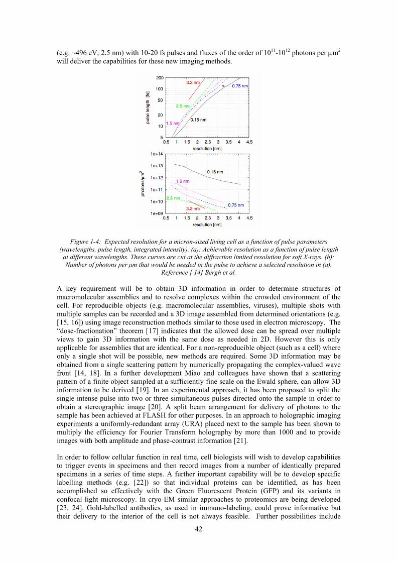
42

(e.g. ~496 eV; 2.5 nm) with 10-20 fs pulses and fluxes of the order of 1011-1012 photons per μm2 will deliver the capabilities for these new imaging methods.

Figure 1-4: Expected resolution for a micron-sized living cell as a function of pulse parameters (wavelengths, pulse length, integrated intensity). (a): Achievable resolution as a function of pulse length

at different wavelengths. These curves are cut at the diffraction limited resolution for soft X-rays. (b): Number of photons per μm that would be needed in the pulse to achieve a selected resolution in (a).

Reference [ 14] Bergh et al.

A key requirement will be to obtain 3D information in order to determine structures of macromolecular assemblies and to resolve complexes within the crowded environment of the cell. For reproducible objects (e.g. macromolecular assemblies, viruses), multiple shots with multiple samples can be recorded and a 3D image assembled from determined orientations (e.g. [15, 16]) using image reconstruction methods similar to those used in electron microscopy. The “dose-fractionation” theorem [17] indicates that the allowed dose can be spread over multiple views to gain 3D information with the same dose as needed in 2D. However this is only applicable for assemblies that are identical. For a non-reproducible object (such as a cell) where only a single shot will be possible, new methods are required. Some 3D information may be obtained from a single scattering pattern by numerically propagating the complex-valued wave front [14, 18]. In a further development Miao and colleagues have shown that a scattering pattern of a finite object sampled at a sufficiently fine scale on the Ewald sphere, can allow 3D information to be derived [19]. In an experimental approach, it has been proposed to split the single intense pulse into two or three simultaneous pulses directed onto the sample in order to obtain a stereographic image [20]. A split beam arrangement for delivery of photons to the sample has been achieved at FLASH for other purposes. In an approach to holographic imaging experiments a uniformly-redundant array (URA) placed next to the sample has been shown to multiply the efficiency for Fourier Transform holography by more than 1000 and to provide images with both amplitude and phase-contrast information [21].

In order to follow cellular function in real time, cell biologists will wish to develop capabilities to trigger events in specimens and then record images from a number of identically prepared specimens in a series of time steps. A further important capability will be to develop specific labelling methods (e.g. [22]) so that individual proteins can be identified, as has been accomplished so effectively with the Green Fluorescent Protein (GFP) and its variants in confocal light microscopy. In cryo-EM similar approaches to proteomics are being developed [23, 24]. Gold-labelled antibodies, as used in immuno-labeling, could prove informative but their delivery to the interior of the cell is not always feasible. Further possibilities include

43

expression of hexaHis tagged proteins and subsequent identification by NiNTA-gold labelled complexes [25]. More work is needed but the emerging field of nanomedicine is also developing similar technologies and there is considerable activity. For NLS it is proposed to have available on the beam line a high numerical aperture confocal light microscope to allow fluorescent-labelled molecules to be visualized and to provide correlated imaging with the flash images.

Presentation of the sample to the intense beam is being explored with a number of different strategies. These include mounting on a support film such as a silicon nitride substrate, injection by aerosol spray mechanisms similar to those used in mass spectrometry and a ‘serial crystallography’ method of creating a stream of droplets (~200 nm in diameter) synchronized with the X-ray beam, which may be ordered by external forces to provide a semi-crystalline of a hydrated specimen [26]

The NLS will have several unique features that will distinguish it from other FEL sources. The X-ray wavelengths produced by NLS at high peak brightness (including 280 eV- 1 keV; 4.4 nm - 1.24 nm) with a repetition rate of 1 kHz and pulse length of 20 fs will be optimal for cell flash imaging. The wavelengths produced by FLASH, where the machine has been so influential in proof of principle experiments, are too long (shortest wavelength 7 nm) for nm resolution. The wavelength range that will be produced by LCLS (energy range 800 eV-8 keV; 1.55 - 0.155 nm.) will not cover the 2-4 nm wavelength best suited for cell imaging. The XFEL, Hamburg, due to come on line in 2014, will cover the complete range (200 eV -12.4 keV; 6.2 nm – 0.1 nm). However the pulse structure (presently quoted) of 3000 pulses at 10 Hz and the pulse length 100 fs may not be optimal for cellular flash imaging.

1.1.2 Imaging of Nanoscale Systems for Science and Technology

The methods just outlined for biological imaging carry straight over to imaging non-biological condensed matter systems. One of the key challenges in X-ray scattering/spectroscopy in condensed matter is to be able to determine the structure and dynamics, either spontaneous or stimulated, of individual objects on nanometre scale. Typical questions to be answered are:

- How do bond lengths, coordination, electronic and magnetic structure vary between core and shell in a particular nanoparticle?

- Can we see polaronic states in general, or even an individual Cooper pair, and image the texture of lattice distortions, orbital and spin structure as well as the electronic properties?

- Can we image charge or spin carriers within individual electronic devices as they function at the nanoscale?

Continuous and quasi-continuous beams cannot be used for scattering from isolated objects. Over-illumination, necessary to collect sufficient number of scattered photons, results in damage. The concept of Flash Imaging with FELs, where a single, ultrashort scattering pulse captures the structure of an isolated object before this is destroyed, is of great interest for this set of problems.

Hard condensed matter is more radiation-resistant than biological matter, while heavier constituent atoms imply longer times for the structure to be destroyed (phonon frequencies and speeds of sound are lower). With the same “inertial confinement” concept, one could not only measure atomic structures, but also electronic and magnetic properties of isolated objects. Coherence has already been used fruitfully at third generation synchrotrons, to image strain fields in nano-crystals [27] and domain structures in magnetic materials [28].

The gains in peak brilliance and in coherent flux afforded by the NLS will make possible measurements of nanoscale order in new regimes. Nanoscale imaging will become possible in electronically ordered materials, extending the current capability of detecting electronic order in

44

spatially integrating experiments [29, 30, 31] to nanoscale objects. Soft X-rays from the NLS (0.5 -1 keV) are particularly advantageous, since they will directly probe transition metal and oxygen sites that constitute so many complex solids (e.g Cuprates and Manganites). The grand goal, which may revolutionize our ability to study strongly correlated electron physics, will be that of capturing a single polaron, or even a single Cooper pair, and holographically reconstructing its spin, orbital and atomic texture at one single point in time. Holographic measurements of microscopic ordered states may then afford similar insight as those done by using scanning tunnelling microscopy [32, 33], with the additional advantage of freezing out fluctuations, i.e. observing a single microstate of the system or a transient state during a non-equilibrium process.

To this end, one needs a source that emits pulses of few tens of femtosecond duration and that covers well the spectral region up to approximately 1 keV. In this area, the base design of the NLS, running at 1 kHz and seeded, will bring immediate benefits. As detector technology reaches higher readout rates, direct measurements at high repetition rates will become possible in sample-replacement or non-destructive regime. Currently some seed experiments are being performed at the FLASH facility in Hamburg [34], and a new generation of these will become possible with new sources. The anticipated capabilities of NLS would be a very good match to the requirements of such research and would significantly extend beyond the FLASH capability in terms of the wavelength reach. We see that the UK can be at the forefront in this area.

The non-destructive regime will be the mode of operation in the hard X-ray harmonics, allowing measurements of atomic texture to be made. In this area, other machines like LCLS, XFEL and SCSS will be where key complementary science is done.

1.1.3 IR and THz Studies of Living Tissue and Signatures for Disease

The availability of bright coherent IR and THz radiation alongside the soft X-rays is likely to provide a number of important additional science opportunities (see below for the pump-probe science). Here near field imaging techniques (SNOM) are looking promising achieving a resolution far better than the diffraction limit and so despite the long wavelength of the radiation it will be possible to obtain spatial resolutions in the 100’s of nanometre range or less. It has been possible using IR SNOM to locate single GluR2 receptors on neurons [35]. Direct use of THz radiation for imaging has already been developed towards commercial scanners for medical applications; however the basic science behind the contrast mechanism that provides useful medical information is not yet understood. Very bright THz radiation will permit essential quantitative studies to be carried out to establish a proper basis for the use of THz radiation in medical imaging.

There is a pressing need for fundamental work to establish the chemical origin of the THz fingerprint in intra-operative THz imaging of cancer patients since such imaging is used to examine excised tissue during surgery. However the relevant protocols are not well established e.g. range of frequencies for use in applications such as sentinel node mapping during cancer surgery. Although skin cancer is the obvious immediate application of THz technology it also has potential for diagnosis of other diseases by recording signals using endoscopic techniques. Commercial companies (Teraview) are already marketing instruments that can be used to diagnose skin cancers. However the current power levels available with laboratory sources do not make it possible to determine the origin of the contrast mechanism in these applications. The establishment of a THz signature of malignancy could lead to the development of low cost portable diagnostic instruments that would transform the diagnosis of skin cancers.

The unique combination of multiple THz/IR undulators at NLS providing high average and peak brightness and short pulses is an excellent platform for research into long wavelength imaging.

45

1.2 Capturing Fluctuating and Rapidly Evolving Systems

Many systems undergo intrinsic rapid structural evolution and fluctuations in the constituent parts, either at the atomic scale or larger scales e.g. of magnetic zones or grains. This is obvious when we consider matter in the liquid state where a non-static structure must be anticipated, but extends also to situations as diverse as domain fluctuations of correlated electron materials, dynamics in glass transitions and in high density plasmas. A variety of scattering techniques e.g. X-ray photon correlation spectroscopy (XPCS) and X-ray Thomson scattering are available. To capture the full fluctuation spectrum or to measure the properties of a rapidly evolving system requires high brightness, short pulses so the full scattering information can be gained in a single instant. NLS will have the temporal structure and wavelength range (1-5 keV) high coherence and brightness ideal for these studies in many different systems, accompanied by synchronization to other external sources (e.g. high magnetic fields).

1.2.1 Fluctuating Nanosystems

A variety of soft X-ray scattering techniques i.e. coherent speckle patterns/photon correlation/holography can be used to provide information on the spatial fluctuations of the structures within nano-particles or nanoscale texture in extended solids. The X-ray wavelengths provide access to dynamics at non-zero momentum transfer and thus at short length scales, and with tuneable sources, element specific information. Soft X-rays are particularly useful in that they can be tuned to important edges, providing chemical specificity and sensitivity to magnetism. Currently, fluctuations are studied in the time domain with time-resolved X-ray speckle techniques, limited by the readout times of area detectors and thus limited to resolutions of microseconds and longer. For fluctuations on very short timescales (attoseconds to hundreds of femtoseconds) the excitation spectrum of matter can be probed near equilibrium with inelastic scattering techniques (meV to eV energy resolutions).

Yet, we are blind to several regimes of paramount importance. For example, even near equilibrium, we cannot easily study fluctuations in the picosecond to nanosecond timescales, which determine the ground state properties of matter at low temperatures. This is because the spectral features of the relevant excitations are too narrow to detect, while their temporal rearrangements are too fast for detectors to be read out. Secondly, fluctuations that occur far from equilibrium, of importance in any driven process relevant to technology, are also difficult to study, because inelastic scattering techniques cannot be easily applied to transient state. A pulsed X-ray laser like the NLS would enhance coherence significantly. Methods for ultrafast XPCS have been proposed that split a pulse and introduce a delay to allow very short timescales (potentially as to ps timescales) to be measured. With this, dynamics could be measured in the same setup over the entire range of timescales (ps – ks). This would allow us to investigate the links between small atomic fluctuations and larger scale motions in e.g. proteins and polymer chains, something which to date can only be done by considering different time regimes in isolation.

In hard condensed matter, measurements of dynamics and correlation functions over many temporal and spatial scales would open new vistas. One could envisage correlations to be established between fluctuating order in different degrees of freedom of a solid (e.g. orbital and magnetic), which would require that one measured the scattering function at different times and at different wavevectors, since different degrees of freedom order on different spatial scales. Soft X-ray pulses of (1) ultrashort duration and (2) greatly enhanced coherent flux, would open the way to measurements of high order correlation functions S(Q1,t)* S(Q2,t+Δt). Similarly, access to correlation times in the nanosecond, picosecond and femtosecond timescales would permit measurements that test our understanding of phase transition physics, which in many cases do not follow simple softening dynamics (mode frequency vanishing at point of symmetry change) expected from Landau theory.

46

Furthermore, and possibly of greatest importance, the ability to measure correlation functions in the time domain with ultrashort pulses from the NLS would allow for experiments performed on metastable and non-equilibrium states, not possible in the frequency domain. The high repetition rate of the NLS would be greatly beneficial, since in these measurements the flux per pulse would have to be moderate not to damage the sample.

1.2.2 States of High Density Plasma

A diffuse plasma, like a gas, will display only weak correlations in the positions of the constituent charged particles (electrons and ions). However, at higher densities, approaching that of solids, the ions can become partially or fully ordered due to the stronger Coulombic interactions. Whilst the extreme situation of a cold solid is relatively well understood - as is the other extreme of a hot ideal gas where the thermal energy of particles dominates over any interparticle energies - the partially correlated state, often referred to as warm dense matter (WDM), remains a great challenge to theoretical description. This state is especially important as it is traversed by all plasmas created initially from heating solids (e.g. laser or X-ray produced plasmas) and moreover is a common constituent of many astrophysical objects. Furthermore, understanding the basic properties of WDM is of key relevance to Inertial Confinement Fusion (ICF) research, and thus has direct links with the energy agenda. This is potentially strategically important for the UK given the acute need for alternative energy sources and our central role in the HiPER project. Furthermore, High Energy Density Physics is an area of particular strength in the UK, with a very active research community, and we are well placed to exploit the novel capabilities that NLS will afford.

Warm dense matter (WDM) is thus an intriguing and largely unexplored state of matter that can be roughly described as midway between condensed and plasma states (see Figure 1-5). Matter in this regime is ‘strongly-coupled’, that is to say the Coulomb energies are comparable to the thermal energies. This makes WDM notoriously difficult to model, as the thermal component of the energy cannot be looked upon as a perturbation to the inter-atomic forces (as in a solid), or vice versa (as in a low density gas or plasma). As a result an accurate equations of state (EOS) – the relationship of density, temperature, pressure, and energy density for the system of interest – which normally permit prediction of the state of a system and its evolution, is largely unknown in this region (for example, at solid densities and temperatures of a few eV, several credible theories differ by up to a factor of two in their prediction of pressure).

Figure 1-5: A density – temperature plot shows the different regimes pertinent to high energy density matter. Condensed matter (CM) lies at the bottom centre (low temperature, solid density), whilst hot

dense plasmas (HDM) are at the top (high temperature, range of density). The region of greatest challenge to understanding in plasma physics, warm dense matter (WDM), lies at high density and

relatively low temperature

47

From the experimental point of view, several methods have been proposed for generating WDM (in particular optical laser or ion-beam heating) but, as a gross (yet reasonably accurate) generalization, success has remained elusive. Although generating some form of WDM with optical lasers poses few problems, generating uniform WDM, with the minimum of gradients in temperature and density, such that subsequent diagnosis of the plasma can yield meaningful results, has not yet been achieved – a similar situation exists with the manufacture of WDM with ion beams. To a great extent this is because, at least with laser generation, the frequency of optical light is far below the plasma frequency of conducting matter – a situation which is not true for XUV or X-radiation. Thus intense XUV and/or X-ray radiation holds significant advantages over other intense sources when it comes to generating warm dense uniform matter – the combination of high intensities yet relatively long absorption lengths affords the possibility of generating WDM with low gradients in temperature (owing to long absorption lengths) and also with low gradients in temperature. That said, in the context of NLS, it should be realized that the generation of matter in this WDM regime is to a large extent an inevitable consequence of any 4th generation light source, and in this sense, NLS will not necessarily be unique. Why is this? The simple answer is that the fluence, at almost any wavelength, of a 4th generation light source is so great that if the output of such a system, focussed or otherwise, is allowed to impinge upon a solid target, the amount and extent of energy deposition will be such that the target will invariably be heated (or, more precisely, on the timescale of the pulse, the electrons within the target will be heated) to temperatures of several eV up to hundreds of eV (the unit of temperature used by plasma physicists – eV, corresponds to a temperature of 1.1 x 104 K). As long as the electrons are not too energetic, the electron sub-system should thermalize on femtosecond timescales, and electron-ion (in condensed matter parlance the electron-phonon) equilibriation is expected to take place on the timescale of several picoseconds (such time-scales are predicted by density functional theory (DFT)).

Given that all 4th generation sources will inevitably produce WDM in some form, it behoves us to consider what particular advantages NLS may afford over alternative sources. NLS has the potential to be in a position to be a front-runner in this important area of research in a number of different, yet interlinked, set of ways. Firstly, NLS can access the 100 eV to 1 keV energy range with a high repetition rate of shot-to-shot reproducible pulses allowing new measurement methodologies to be implemented that go beyond the “single shot” measurements to which other FELs are confined. Secondly, we are proposing that NLS will be combined with a suite of optical lasers that will allow us to pre-compress matter to high densities, and so-to-do at repetition rates that will not be available elsewhere. It is difficult to over-emphasize this particular point – on their own 4th generation sources will be restricted to generating WDM at densities of the normal solid and below (e.g. with foam targets). However, much of the physics of interest (e.g. the EOS of the most direct relevance to ICF or so-called super-earths) necessitates an investigation of the properties of matter at densities significantly higher than that of normal solid density. These higher densities cannot be formed by a 4th generation source on its own - owing both to the brevity of the pulses, and to the penetration depth of the radiation. However, experience within the high power laser-community has shown that we know how to compress matter to densities significantly greater than solid for periods of nanoseconds (much longer than any of the relevant timescales that pertain to NLS). Somewhat ironically, such high compressions rely on the very fact that optical lasers cannot penetrate beyond the low electron densities corresponding to the critical surface, and thus high power optical lasers afford the possibility to pressurize targets to high densities whilst keeping them relatively cool. Indeed, it is this capability that has led to the emergence of the field of ‘isentropic compression’, where solids are compressed far beyond normal densities, yet remain well below the melt temperature. Our proposal for the uniqueness of NLS in this area is to have an optical laser alongside it of several nanosecond duration and operating at high repetition rate (which in this context is of order 10 Hz). Although the development of such systems is its infancy, these are precisely the laser parameters that are required for the HiPER project, and significant effort is being deployed towards their development, independently of 4th generation source research.

48

The most powerful probe of plasma state, including electron and ion temperature, electron density, velocity distribution and collisional damping rates come from light scattering (Thomson scattering). Examination of the optical scattered spectrum has been a powerful tool for diagnosis of lower density plasmas. As the density increases towards that of a solid, however, the plasma becomes opaque in the optical domain and the plasma will only be transparent in the X-ray range. Thus X-ray Thomson scattering is required to examine the detailed state of a high density plasma. For this a short pulse (sub-ps) of very bright X-rays are essential to capture the often very rapidly evolving plasma. A soft X-ray FEL is ideally suited for this purpose. Moreover the high longitudinal coherence of the beam will permit X-ray interferometry, phase contrast and holographic imaging measurements of fast evolving dense plasmas. This will contribute not only to our knowledge of the EOS in WDM but also allow the direct study of shocks, instabilities, jet formation and turbulence. It should also be noted that NLS will allow unique capabilities in this area owing to the proposal to have seeded output. The inherent bandwidth of current SASE sources is of order 0.2%, and this is too broad to enable Thomson scattering from the so-called ‘ion-features’ associated with scattering from the ion acoustic waves within the plasma. The significantly reduced bandwidth achieved via seeding (of the order of an order of magnitude improvement) will put NLS at a great advantage in this area.

Furthermore it has also been problematic in the past to produce WDM uniformly (i.e. with minimal gradients in temperature and density) in the laboratory. The soft X-rays have the potential to overcome these problems owing to the relatively long absorption length of the radiation compared with visible light – indeed it is important to note that WDM will inevitably be produced in many 4th generation light source experiments - the radiation is so intense that its interaction with solid matter will (unless undertaken at grazing angles of incidence) automatically produce WDM. For this reason alone WDM research will be an integral part of any new light source project, including the NLS. This ‘automatic’ WDM production will be isochoric, with energy initially deposited in the electrons, with subsequent thermalization via electron-ion coupling on picosecond time-scales.

Spectroscopy of plasmas on NLS, whether in the non-perturbing or perturbing mode, will be a key diagnostic of plasma parameters. Unique possibilities will exist which will both extend and complement the efforts on strongly coupled plasmas outlined above. In the non-perturbing mode (where we observe the WDM produced by the X-ray beam irradiating a solid, foam, or gas-phase target), the emission line intensity, position and shape of NLS-produced plasmas may be effected by strong coupling. Secondly, an intense X-ray source will act as a unique perturbing-pump for laser-produce plasmas which will test our understanding of several basic features of the radiative properties of strongly-coupled plasmas; for example, the capacity to model the full kinetics of even the simplest systems (i.e. bare, hydrogenic, and helium-like ions). Such experiments are impossible with current laser-plasma based soft X-ray lasers, as they do not have sufficient intensity for the pump rate to greatly exceed the spontaneous emission rates. Importantly, a monochromated intense soft X-ray source will be sufficiently narrow-band to pump within the line-width of a Stark-broadened bound-bound profile. Subsequent observation of the line shape of the emitted radiation will test the normal assumption of complete frequency re-distribution within the line. This assumption can be invalidated by ion-field fluctuations and inelastic collisions, and measuring the detailed redistribution of population after pumping can therefore provide crucial information on the rate of the relevant plasma processes.

1.3 Structural Dynamics Underlying Physical and Chemical Change

Ultrafast events in nature are often accompanied by equally fast structural and electronic changes. To understand the mechanism behind, e.g. chemical reactions, ultrafast magnetization, phonon triggered changes in electronic structure, photon induced processes in solids and at surfaces, we need to be able to measure these changes in real time. This requires us to make measurements in the 10 ps to 10 fs range in order to capture all the timescales of motion associated with changes in any complex matter system. To succeed in this new endeavour we

49

must be able to; (1) trigger the event of interest, (2) follow it with a probe sensitive to structural and electronic change. For most problems the dominant interest is in local changes around the active site and here soft X-ray methods (e.g. X-ray absorption and emission spectroscopy, and X-ray photoemission) provide an ideal tool. The trigger can be made via a variety of means e.g. controlled “thermal” excitation of lattice/vibrational modes with IR/THz pulses, photoexcitation of electronic states with a resonant laser, and electron beam excitation of system (radiolysis). Of critical importance is that the pump (event trigger) and probe pulses are sufficiently well synchronized to permit temporal resolution approaching the 10 fs limit. It is essential that any new light source will provide an array of pump-probe capabilities that will collectively resolve the ultrafast structure and dynamics in a wide range of processes.

1.3.1 THz-Visible Pump – X-ray Probe of Condensed Phase Systems

We consider first the measurement of ultrafast structural dynamics and photo-control in complex matter. Many solids of current interest, which unlike conventional semiconductors and metals exhibit ultra-strong interactions between electrons (eV energy scales), defy our understanding of the solid state. Strong electronic correlations result in exotic forms of ordering in spins, electrons, orbital structure as well as lattice properties, which compete to dictate macroscopic properties like conductivity, magnetism and optical response. What one is left with is a precarious equilibrium of forces that compete on the eV energy scale, enormous when compared to thermal fluctuations of few tens of meVs. This balance is extremely sensitive to very small perturbations, and spectacular, avalanching changes take place when even a subtle perturbation tips the balance between different degrees of freedom. This extreme sensitivity to boundary conditions, typical of chaotic or complex non-linear systems, brings ”complexity” to condensed matter. This is one of the frontiers of our understanding of the nature and at the same time will surely be conducive to all sorts of new applications where exotic states and their multistability will be put to good use. Beyond traditional forms of control with pressure, magnetic fields and other tools of experimental condensed matter physicists, the use of light [36] has recently emerged as a new approach to investigate the underlying ordering principles of complex solids (e.g. by measuring elementary interactions between various microscopic degrees of freedom) and develop new means of controlling the functionality of solids on the ultrafast timescale. Applications are many, from optical switching at Tbit rates to magnetization control on the ultrafast timescale.

• How do many degrees of freedom synchronize dynamically to bring about an ultrafast phase transition?

• How can we control this behaviour? • Can this be used for data processing and storage? • Can we control Magnetism in new ways? • Is it possible to photo-initiate new interesting functionalities? • Can we photo-induce superconductivity? • Can we use some of the exotic nanoscale excitation, like orbital or plasmon excitations

of complex matter, to transfer information over nanoscale lengths? All these questions are extremely difficult to tackle theoretically, since they involve highly non-equilibrium dynamical states, for which our understanding of even basic statistical mechanics is very limited. Two examples of possible experiments are presented in Section 2.3.1, demonstrating how the NLS, providing synchronized pulses of THz and soft X-ray radiation up to 1 keV, could break new ground in the study of driven dynamics of complex matter.

One wishes to extend the power of insight of X-rays, which have immensely contributed to our understanding of the static microscopic properties of condensed matter, to dynamic studies of solids. The past decade has seen step-like progress in this area, and some rudimentary X-ray techniques have already been extended to the ultrafast timescale, such as femtosecond X-ray diffraction [37, 38, 39, 40, 41] and femtosecond X-ray absorption [38, 42, 43]. Yet, these early experiments have used average fluxes some TEN (!) orders of magnitude below what is

50

available at third generation synchrotron facilities. One dreams of not only being able to measure the rearrangements in atomic positions or in spectroscopic properties, but also time resolving rearrangements in the excitation spectra with time-resolved inelastic X-ray scattering, or in the Fermi surface, with femtosecond angle resolved photo-emission (T-ARPES) and extending many flux hungry techniques that have only recently become possible with new generation storage rings.

The NLS will make it possible to measure femtosecond microscopic dynamics with the same average flux of a third generation synchrotron, a revolution in our experimental abilities that will open new vistas for the next generation of scientists.

Especially, the ability of having pairs of pulses, one in the THz/visible for the pump and a synchronized FEL pulse in the soft X-rays will be key. Many experiments will require excitation with visible pulses of few tens of femtosecond duration and stroboscopic soft X-ray scattering or X-ray spectroscopy probing. Alternatively, one will require a THz source (with carrier envelope phase stability) combined with soft X-ray scattering.

1.3.2 Observing Chemical Change with Ultrafast X-ray Spectroscopy

The development of new chemical processes relies upon the advancement of our mechanistic understanding of chemical change in complex systems. To achieve this goal it is necessary to measure the evolution of molecular structure on the timescales of importance to chemical change, and to be able to characterize key short lived intermediate species present in a complex mixture of reactants, products and intermediates. Since chemical change occurs on the timescales of nuclear motion, femtosecond time resolution is therefore a key requirement to meet these challenges. Furthermore, since chemical change is frequently mediated by the complex non-adiabatic couplings between electronic and nuclear motions that occur when the Born-Oppenheimer approximation fails, we require techniques which are sensitive to both nuclear and electronic configuration. The NLS will achieve these goals through the development of femtosecond soft X-ray spectroscopic probing of molecular processes. Due to the high degree of localization of core electrons, X-ray spectroscopy measurements are amenable to structure elucidation in complex systems and environments where valence spectroscopies would be unusable due to spectral congestion and complexity. The use of soft X-ray techniques for structural and electronic interrogation of matter in all phases is well established with conventional synchrotron sources, and their extension to ultrafast timescales will open entirely new windows into the realm of nuclear motion, electronic structure rearrangements and thereby chemical dynamics [44,45]. Key to these developments at the NLS will be the ability to initiate chemical change using a diverse range of synchronized ultrafast pump sources including optical pump fields from the THz to the UV, and pulsed radiolysis with electron beams.

Ultrafast soft X-ray probing of chemical processes with core level spectroscopies will allow femtosecond temporal resolution and simultaneous atomic scale structural resolution. In comparison with structural measurements via X-ray diffraction, where light of wavelengths on the atomic scale are required, probing via soft X-ray core level spectroscopies achieves atomic scale structural resolution by virtue of the short de Broglie wavelength of the core electron excited or ionized upon photon absorption, and so requires lower energy photons than X-ray diffraction.

Since much of chemistry occurs in complex systems, we require the ability to make such measurements on systems of varying complexity, for example, ranging from isolated gas phase molecules, nanoscale solvated clusters, species adsorbed at metal and liquid interfaces, through to large molecular systems in solution. The ability to make ultrafast measurements in such dilute and diverse samples requires both high photon numbers and high repetition rates.

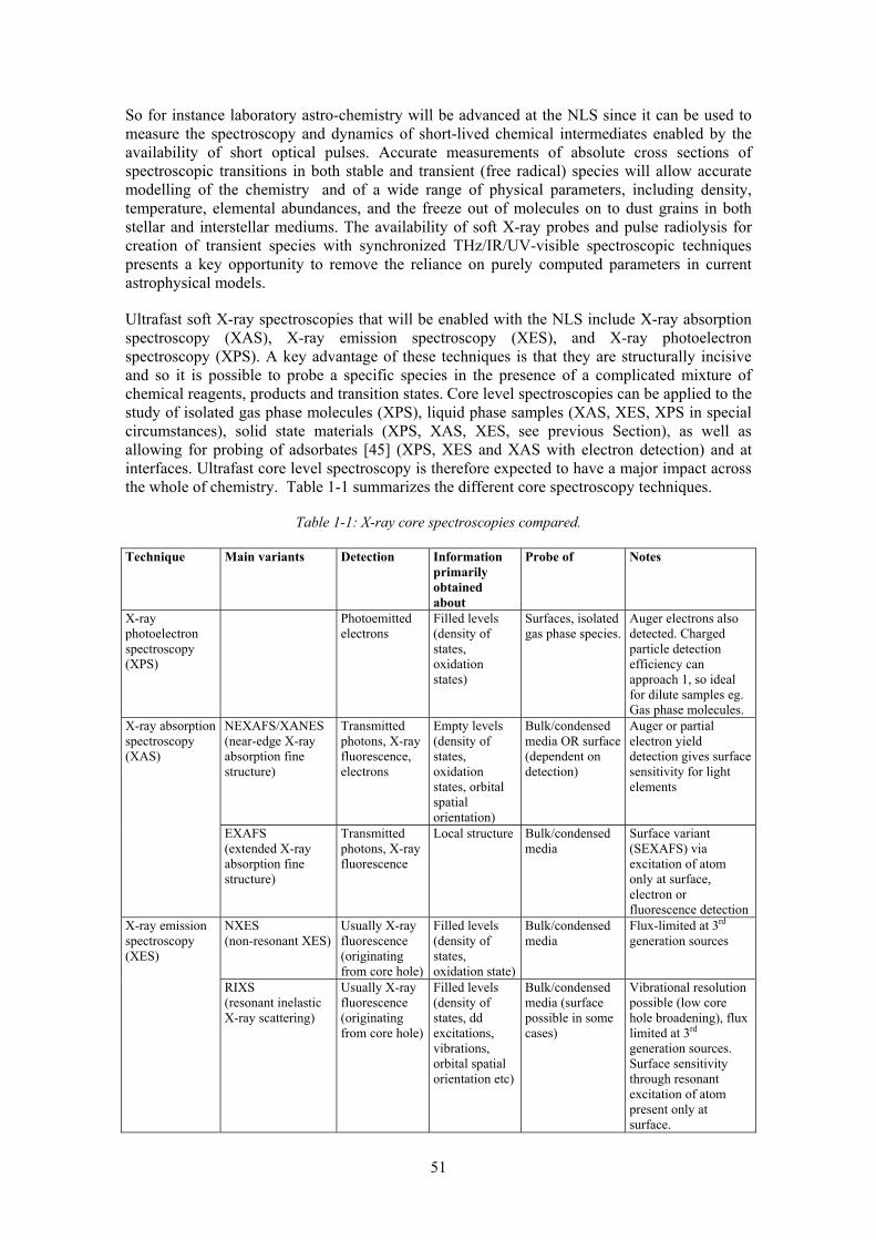
51

So for instance laboratory astro-chemistry will be advanced at the NLS since it can be used to measure the spectroscopy and dynamics of short-lived chemical intermediates enabled by the availability of short optical pulses. Accurate measurements of absolute cross sections of spectroscopic transitions in both stable and transient (free radical) species will allow accurate modelling of the chemistry and of a wide range of physical parameters, including density, temperature, elemental abundances, and the freeze out of molecules on to dust grains in both stellar and interstellar mediums. The availability of soft X-ray probes and pulse radiolysis for creation of transient species with synchronized THz/IR/UV-visible spectroscopic techniques presents a key opportunity to remove the reliance on purely computed parameters in current astrophysical models.

Ultrafast soft X-ray spectroscopies that will be enabled with the NLS include X-ray absorption spectroscopy (XAS), X-ray emission spectroscopy (XES), and X-ray photoelectron spectroscopy (XPS). A key advantage of these techniques is that they are structurally incisive and so it is possible to probe a specific species in the presence of a complicated mixture of chemical reagents, products and transition states. Core level spectroscopies can be applied to the study of isolated gas phase molecules (XPS), liquid phase samples (XAS, XES, XPS in special circumstances), solid state materials (XPS, XAS, XES, see previous Section), as well as allowing for probing of adsorbates [45] (XPS, XES and XAS with electron detection) and at interfaces. Ultrafast core level spectroscopy is therefore expected to have a major impact across the whole of chemistry. Table 1-1 summarizes the different core spectroscopy techniques.

Table 1-1: X-ray core spectroscopies compared.

Technique Main variants Detection Information primarily obtained about

Probe of Notes

X-ray photoelectron spectroscopy (XPS)

Photoemitted electrons

Filled levels (density of states, oxidation states)

Surfaces, isolated gas phase species.

Auger electrons also detected. Charged particle detection efficiency can approach 1, so ideal for dilute samples eg. Gas phase molecules.

X-ray absorption spectroscopy (XAS)

NEXAFS/XANES (near-edge X-ray absorption fine structure)

Transmitted photons, X-ray fluorescence, electrons

Empty levels (density of states, oxidation states, orbital spatial orientation)

Bulk/condensed media OR surface (dependent on detection)

Auger or partial electron yield detection gives surface sensitivity for light elements

EXAFS (extended X-ray absorption fine structure)

Transmitted photons, X-ray fluorescence

Local structure Bulk/condensed media

Surface variant (SEXAFS) via excitation of atom only at surface, electron or fluorescence detection

X-ray emission spectroscopy (XES)

NXES (non-resonant XES)

Usually X-ray fluorescence (originating from core hole)

Filled levels (density of states, oxidation state)

Bulk/condensed media

Flux-limited at 3rd generation sources

RIXS (resonant inelastic X-ray scattering)

Usually X-ray fluorescence (originating from core hole)

Filled levels (density of states, dd excitations, vibrations, orbital spatial orientation etc)

Bulk/condensed media (surface possible in some cases)

Vibrational resolution possible (low core hole broadening), flux limited at 3rd generation sources. Surface sensitivity through resonant excitation of atom present only at surface.

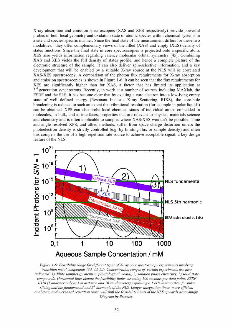
52

X-ray absorption and emission spectroscopies (XAS and XES respectively) provide powerful probes of both local geometry and oxidation state of atomic species within chemical systems in a site and species specific manner. Since the final state of the measurement differs for these two modalities, they offer complementary views of the filled (XAS) and empty (XES) density of states functions. Since the final state in core spectroscopies is projected onto a specific atom. XES also yields information regarding valence molecular orbital symmetry [45]. Combining XAS and XES yields the full density of states profile, and hence a complete picture of the electronic structure of the sample. It can also deliver spin-selective information, and a key development that will be enabled by a suitable X-ray source at the NLS will be correlated XAS-XES spectroscopy. A comparison of the photon flux requirements for X-ray absorption and emission spectroscopies is shown in Figure 1-6. It can be seen that the flux requirements for XES are significantly higher than for XAS, a factor that has limited its application at 3rd generation synchrotrons. Recently, in work at a number of sources including MAXlab, the ESRF and the SLS, it has become clear that by exciting a core electron into a low-lying empty state of well defined energy (Resonant Inelastic X-ray Scattering, RIXS), the core-hole broadening is reduced to such an extent that vibrational resolution (for example in polar liquids) can be obtained. XPS can also probe local chemical states of individual atoms embedded in molecules, in bulk, and at interfaces, properties that are relevant to physics, materials science and chemistry and is often applicable to samples where XAS/XES wouldn’t be possible. Time and angle resolved XPS, and allied methods, suffer from space charge distortion unless the photoelectron density is strictly controlled (e.g. by limiting flux or sample density) and often this compels the use of a high repetition rate source to achieve acceptable signal, a key design feature of the NLS.

Figure 1-6: Feasibility range for different types of X-ray core spectroscopy experiments involving transition metal compounds (3d, 4d, 5d). Concentration ranges of certain experiments are also

indicated: 1) dilute samples (proteins in physiological media), 2) solution phase chemistry, 3) solid state compounds. Horizontal lines denote the feasibility limits assuming 100 seconds per data point: ESRF ID26 (1 analyzer only at 1 m distance and 10 cm diameter) exploiting a 1 kHz laser system for pulse

slicing and the fundamental and 5th harmonic of the NLS. Longer integration times, more efficient analyzers, and increased repetition rates will shift the feasibility limits of the NLS upwards accordingly.

Diagram by Bressler.

53

Time-resolved XPS is a particularly appealing extension to the study of isolated gas phase molecules and clusters where time-resolved valence-shell photoelectron spectroscopy has emerged as a general tool for studying molecular processes [46] due to sensitivity to both electronic and nuclear motions. Extension of valence and core photoelectron spectroscopy to ultrafast timescales with few-fs X-ray pulses will enable very fast chemical events to be followed which are typically complicated by the breakdown of the Born-Oppenheimer picture as the flow of charge and energy in the molecule becomes strongly coupled at regions of configuration space such as conical intersections.

The means to controllably trigger (pump) the ultrafast events is vital to the success of the measurement and NLS will offer a powerful array of capabilities to achieve this. The use of precisely synthesized optical fields for the control of chemical [47] and even biological [48] systems has emerged as a powerful application of femtosecond laser technology. Despite the advances made in this field over the past decade, to date the precision with which these processes have been controlled has been limited by the available probing techniques provided by conventional lasers – our ability to control a chemical process is limited by the detail made available by the probing technique used to examine the process on which control is exerted. The combination of optical lasers with time-resolved X-ray probing will therefore open many new opportunities for highly efficient coherent control strategies by virtue of the enhanced detail offered by X-ray probe techniques. X-ray probing of control strategies in the solution phase is an as yet unexplored avenue, but once enabled by the NLS is expected to be a high impact area. It is also anticipated that the availability of high intensity IR radiation will allow for conformational selection and control of large molecular systems, as well as the control of molecular orientation and alignment of isolated gas phase molecules leading to enhancement of the information content of probing e.g. by electron or X-ray diffraction.

Pulse radiolysis as a trigger to accompany soft X-ray probes of structural change will also be an important avenue of research. A pulsed electron beam is a complementary and powerful method for the generation of chemical intermediates, excited states and free radicals which has made a major impact in areas as diverse as geochemistry [49], nanoscience [50], ionic liquids [51], and radiation damage of DNA [52]. Its major difference from laser initiation is that the primary excitation step involves interaction of electrons with the media and does not rely on the absorption by a chromophore of the laser light of a particular wavelength. A pulsed electron beam is often the method of choice to generate and determine the properties of radical ions, reactive oxygen species and initiate charge migration and proton transfer processes. The coupling of picosecond and sub-picosecond electron pulses (~ 5-10 MeV) as a trigger for chemical change with the X-ray probe techniques to monitor structural change in real time would represent a unique capability internationally. In particular, compared to existing pulse radiolysis facilities worldwide [53], this would give the NLS a leading edge in terms of both structural sensitivity and time resolution. The combination of XUV pulses and pulsed radiolysis at the same facility will also allow direct comparison of optically induced dynamics with those of radiolysis, another potential key international defining feature for the NLS. Example applications of this capability include determining the fundamental radiochemical processes occurring in media exposed to ionizing radiation through determination of kinetics in radiation tracks and how they influence the overall radiation chemical processes. The ability to generate charged species will allow studies of charge mobility in electronic devices and artificial solar cell systems, and also charge recombination processes leading to excited singlet/triplet states in light emitting devices and photovoltaic systems [54].

The development of ultrafast probing of chemical change requires the following key capabilities provided by the NLS:

1. A source of femtosecond X-ray pulses in the 0.1- 5 keV range for access to the X-ray absorption edges of a wide range of chemically important elements (see periodic table in Figure 1-7 for K and L edge energies). The use of EXAFS requires access to K edges of atoms, or L edges above 2 keV. While low lying edges (at around 0.5 – 1.5 keV) are good probes of geometric and electronic structure of light molecular species (for

54

example at the surface of a catalyst), XAS and XES above 2-5 keV also have the advantage of being good probes of bulk material.

2. Ultrafast X-ray spectroscopic approaches require scanability and tunability of the XUV photon energy which is a core capability of the NLS. This is a distinguishing feature of the NLS in comparison with hard X-ray sources such as XFEL where X-ray diffraction is the main modality of probing.

3. For the techniques described above, high photon fluxes (> 109 photons/s) are a key requirement, and this is particularly important for dilute samples such as single clusters, or molecules adsorbed on a surface. However, it is insufficient to deliver this photon flux with a high-intensity low repetition rate source (eg. XFEL, LCLS) since the high intensities may introduce unwanted sample damage as well as non-linear optical and space-charge effects. The high (kHz) repetition rate of the NLS is therefore a key enabling capability for these studies.

4. For ultrafast pump-probe studies of a broad range of chemical processes it is necessary to have a variety of synchronized sources available for the pump step. NLS provides the necessary optical sources, ranging from the UV to deep IR and THz, and also a pulsed electron beam source.

5. In order to follow the fastest processes relevant to chemical change, it is necessary to employ X-ray pulses with durations of 20 fs or less, and which are near transform limited in terms of their time-bandwidth product. Furthermore, it is necessary to have synchronization between the X-ray pulses and other pump sources to better than 10 fs jitter. These key capabilities at the NLS are met by seeding the FEL, and represent a major advantage over self amplified stimulated emission (SASE) sources.

Finally we note that with the high photon energy limit anticipated to reach ~7.5 keV in the second phase of NLS (e.g. 5th harmonic of a 1.5 keV FEL) time-resolved X-ray diffraction studies are also likely to be of importance.

Figure 1-7: Periodic table showing the energies of the K and L edges of the elements. We can see for instance that the K and L edges of Fe can be accessed if the 5th harmonic reaches above 7 keV, as is

planned for the second phase of the NLS.

55

1.3.3 THz, IR and Visible Vibrational Spectroscopy – Chemistry, Space Science and Life Sciences Applications

When combined with X-ray techniques, vibrational spectroscopy provides an important complementary probe of structural dynamics. Whilst the fine structure detected in XAS/XES provides geometrical information and is especially sensitive to heavy neighbouring atoms, infra-red (IR) and Raman vibrational spectroscopy can identify functional groups, light elements such as hydrogen, and, in some cases, the local symmetry.

A major challenge across chemical science is to understand molecular reorganization in complex environments in terms of both intra-molecular and environment dynamics. The reorganization of the environment of a molecule influences processes by solvation perturbations and outer-sphere molecular co-ordination and often dictates transition states, chemical outcomes, and product state distributions. However, these problems are technologically challenging. Current laser technology provides time-resolved IR capability [55], but with limited spectral coverage; currently the region below ~ 800 cm-1 is inaccessible. Extension of the spectral coverage to provide a full temporally resolved 4000 – 1 cm-1 spectrum would allow for example the study of large collective motions of proteins such as alpha helical stretches, also the hindered rotations or vibrational structure of solvent molecules which influence solvent reorganization dynamics in liquids, the direct probing of metal-carbon and metal-metal atom motions in surface science problems, and identification of key biologically active radical species during radical migration during DNA strand breaks. NLS in the baseline configuration will cover the majority of the range from 4000 cm-1 to 20 cm-1 using non-linear optics and undulators with the likelihood of filling all the range of interest following an upgrade. Accessing the complete vibrational spectrum and being able to relate mode-to-mode dynamics in multispectral and multi-time dimensions would open up a complete way of investigating molecular dynamics. Raman techniques, such as time-resolved resonance Raman and Electron-Vibration-Vibration 2DIR, offer a complementary and powerful probe of vibrational dynamics. A key requirement of the NLS is to be able to employ these techniques as the probe process in pump-probe measurements, and this will require synchronized deep IR sub-picosecond pulses.

The relevant frequencies for promoting motions of biological macromolecules lie in the far-IR/THz, so highly intense broadband IR/THz radiation should provide the ideal source for a new generation of non-damaging macromolecular dynamics experiments. Combinations of pump-probe studies (e.g. THz pump, IR or UV/visible probe) are required to assess the role of promoting motions in biological responses, such as catalysis. Near infrared and THz pump probe experiments will monitor the rate of relaxation and localization of energy within biological chromophores, the protein scaffold and between protein-protein complexes. The rate change can then be measured in the presence of pre-pumping or post probing THz radiation. Low temperatures will be used to obtain defined THz spectral features and pulse shaping will be investigated as a means to drive and optimize mode enhanced energy transfer in biological macromolecules. THz pump followed by UV/visible probing will address the role of promoting motions in biological catalysis through direct analysis of the chemical rate process.

Until recently, the far-IR (THz) was a spectral region which was opaque to astronomers. They knew of the potential importance of this region in terms of dust emission, observing coolant molecules in collapsing gas clump etc. but were restricted to ground based observations. ISO, IRAS and their worthy successors Akari and Herschel have removed this limitation by providing highly capable space-based observing platforms tuned to the mid- and far-IR regions. The observational goals of these platforms are tightly tied up with observing and understanding star forming regions through observations of icy dust, molecular line surveys of small molecular coolants (small hydrides, water etc.) linking through to the search for chemical complexity and identification of interstellar polycyclic aromatic hydrocarbons and their derivatives. These instruments acquire unprecedented amounts of data. To support the analysis of this flood of data, laboratory support is essential, and has been recognized as such by ASTRONET, in

56

several key areas; (i) Far-IR Spectroscopy of Ices and Grains, (ii) Far-IR Spectroscopy of Small Hydride species, and (iii) Far-IR Identification of Large Molecules and Biological Markers. NLS presents an excellent opportunity for impact in this area as it provides the synchronized THz/IR to XUV ultrafast light sources to e.g. create and probe the short lived radicals involved and mimic the conditions in interstellar environment. 1.4 Ultrafast Electron Dynamics

Electrons play an essential role in determining the structure and dynamics of matter by mediating the bonding between atoms and governing the optical, electrical and magnetic properties. The dynamics of bound state electrons in matter are tremendously fast with timescales from a few femtoseconds down to a few attoseconds duration. Electrons in valence, conduction or inner shell states are invariably strongly correlated to one another through the Coulomb interaction and spin statistics. Moreover inherently quantum properties, such as entanglement, play a vital role in the multi-electron states of all matter. Our present understanding of the dynamical response of multi-electron states to a rapid change (e.g. high frequency external field or the sudden removal of an electron) is very limited.

NLS will provide the bright and short wavelength radiation in the UV-X-ray range needed to drive new classes of simultaneously multi-electron and multi-photon non-linear interactions that will provide answers to key questions in the quantum coherence of electronic states. Non-linear X-ray interactions are essential to understand in all applications of high brightness short wavelength light with matter (e.g. in single shot diffractive imaging) but also offer to unlock a new understanding of multi-electron dynamics in complex matter. Key questions that might be answered include: How do electrons move within a large molecule undergoing a chemical change? How long does it take for an electron released in a solid to respond to the steady state band-structure? Can we follow and control the interaction of many-electron systems with an applied electromagnetic field?

Recently, measurement methods have begun to address the question of attosecond electron dynamics (see for example the recent review by Paul Corkum and Ferenc Krausz, [56]). These methods, based upon high harmonic generation (HHG) from lasers, are currently very limited by the spectral range (<100 eV) and photon flux (~107 photons/pulse and ~1010 photons/second) of these light sources. We need the capability to extend the current studies based upon HHG by using; (a) a seeded FEL to provide coherent near ~10fs pulses of high brightness soft X-rays phase locked to external lasers (see Part II Section 2), and (b) developing pulse slicing and/or single spike FEL methods to generate sub-fs soft X-ray pulses at high brightness. Using a seeded FEL will provide a greatly enhanced flux to > 1011 photons/pulse so making possible, for the first time, non-linear interactions in which two or more photons simultaneously interact with the matter. Also compared to HHG the photon fluence will be increased to > 1015 photons/second so permitting massive improvements in the measured signal. The wide spectral range will allow access to the states of interest in all matter not just a few test systems as is presently the case. Moreover with photon energies up to 5 keV the radiation can penetrate within condensed phase matter opening up the prospect of sub-femtosecond probing of processes within solids and liquids.

We outline the scientific opportunities opened up by NLS for ultrafast electron science and technology. First we consider the completely new interactions emerging due to the high brightness X-rays available and the implications this has for new measurements. Second we look at the ultrafast measurement of correlated electron dynamics that are possible. Third we speculate upon the long term technological impact of the ability to measure and control correlated electron dynamics at the fast timescale. In Part III there is discussion of the seeding technique and of methods for sub-femtosecond pulse generation (e.g. by operating the FELs in low bunch charge mode so as to allow only a single spike lase) that will provide the technological capability for the science.

57

1.4.1 Short pulse high intensity X-ray interaction physics

The interaction of matter with strong high frequency soft X-ray fields is a new physical regime which is fundamentally different to that accessed with strong visible/NIR fields (see Figure 1-8). This regime is currently poorly understood and involves highly correlated multi-electron multi-photon interactions. In part this arises because the frequency of the X-ray field is too high to be effectively screened by the outer electrons so the fields can couple with several electrons simultaneously. This is in contrast to interaction with visible light, where the interaction with the light field intrinsically only involves a single electron, and is well studied and understood [57]. All measurements made with high intensity short pulse soft X-ray FELs will encounter the complexities associated with this new regime of interaction, this includes the situations when coherent diffraction imaging with an intense X-ray pulse is being used, but this also offers new pathways to measure these complex multi-electron interactions.

An understanding of the fundamentals of high intensity soft X-ray-matter interaction physics will be crucial in all the FEL based measurements on complex systems of relevance to condensed matter, material, chemical, nano- and biosciences. The ideas of static and time-resolved imaging, where high peak brightness is essential, cannot be realized at the ultimate spatial resolution until we establish a full understanding of the ionization and fragmentation dynamics, electron heating and other ultrarapid damage processes caused by the linear and non-linear interactions of the intense X-rays. Similar studies on fragmentation dynamics are being undertaken on other light sources (e.g. FLASH, LCLS) and some questions may be resolved before NLS is available. NLS will, however, provide unique access to high brightness pulses in the 50 ev -1 keV photon energy range with high temporal coherence (through seeding) that is vital for any advanced quantitative studies that demand the temporal shape of the pulse to be well characterized and stable which is not available at any other facility. Moreover these interactions and their timescale will need to be fully understood for assemblies of matter ranging in size from isolated atoms/small molecules to extended solids. This is therefore a long term project and improvement in spatial resolution of snap-shot imaging methods towards the sub-nm scale will go hand in hand with the advances in our understanding of intense X-ray matter interaction.

The type of interactions facilitated by the high brightness X-rays are qualitatively new, including simultaneous 2-photon and 2-electron excitation, which allow entirely new investigations of matter. Moreover the flux will be sufficiently high to saturate hole formation or generate core holes with a high probability within a sample. High brightness X-rays thus begin to open new channels for probing. For instance they can excite 2-photon excitations of a single electron (this may be followed by ejection of secondary Auger electrons correlated with the first), the two photons can excite two core holes in the same atom and release two electrons (and then possibly further Auger electrons) or in a molecule or solid state system two core holes from neighbouring atoms that interact through the valence electrons. In all these cases new channels of information become available that reveal correlated as well as single electron properties.

58

Figure 1-8: Strong field physics enters a new regime for high frequency fields. There is special interest in the soft X-ray range (10 eV- 1 keV) where the fields couple efficiently to multi-electron – multi-photon

processes in matter (Up – ponderomotive energy is the mean kinetic energy of an electron oscillating in the field (scaling as λ2), α0 and a0 are the amplitude of electron oscillation and the Bohr radius

respectively and Ip- ionization potential of atom).

Besides the utility of these studies to CDI other new imaging methodologies enabled by intense short pulses of soft X-rays will arise from these investigations, e.g. Coulomb explosion imaging initiated by instantaneous removal of multiple core electrons. Most importantly it is anticipated that new ultrafast measurement techniques will emerge from understanding this regime – for example, coherent non-linear multi-dimensional X-ray spectroscopic techniques [58] and non-linear optical based X-ray temporal gating have been proposed [59].

1.4.2 Revealing Correlated Ultrafast Electron Dynamics

The key to studying ultrafast electron dynamics in matter is to follow the relaxation dynamics of a system after instantaneous removal of an electron, or in other words, observing the dynamics of the “hole” that is left behind in the still interacting electrons by the one removed electron. An electron is first rapidly removed from a bound valence or inner shell state (with a short duration X-ray pump pulse) and the evolution of the remaining electrons into new states observed using a photo-ionization or other probe that can be used to measure the correlated emission of multiple electrons and so retrieve the correlations in the bound system at the times the electrons were emitted. This requires either attosecond pulses as both pump and probe, or, alternatively, another fast event may be used as the pump (e.g. strong field ionization by a synchronized laser) or probe (e.g. laser field streaking of photoelectrons by a synchronized auxiliary laser [60]). All of these methodologies are anticipated within the lifetime of NLS but the methods utilizing an auxiliary laser are likely to be implemented first as they already lie within the realm that can be achieved within the baseline specification.

The use of strong field soft X-ray pulses as a pump of electronic dynamics will allow us to directly observe, for the first time, correlated electron dynamics. At present, our understanding of the way in which electron motions are correlated in matter is indirectly inferred through measurement of the single electron response of matter to light. The multi-electron nature of the response of matter to high intensity soft X-ray fields will allow an entirely new view of the way in which the ultrafast motions of electrons in matter are correlated. Since almost all matter involves multi-electron states, correlated electronic motion underpins the nature of matter at the quantum scale. It is possible to study such correlations if we measure the dynamics of the “hole” left following the removal of an electron as this includes all of the correlations of the remaining

59

electrons. Though there is a vast knowledge of equilibrium electronic structure, based on established theoretical tools (e.g. density functional theory (DFT)), our understanding of the dynamics of these systems is in its infancy, having only been studied through the response of individual electrons. The correlations of the many electrons induced by Coulomb interactions are strong and rapidly changing (on the sub-femtosecond timescale), and the role of quantum correlations (e.g. entanglement) is largely unexplored. The ability to study this fundamental feature of complex matter may underpin a new generation of optical, data storage and logic devices based upon ultrafast semiconductor and nanofabricated components, where the effects of correlation and entanglement will become an essential feature as the dimensions are shrunk into the quantum regime.

It is anticipated that NLS will provide the capability, through the intense ~10 fs X-ray source phase-locked to an external laser, auxiliary synchronized HHG sources and the possibility of intense sub-fs soft X-ray pulses from the FEL, to make completely new types of measurements that uncover ultrafast electron dynamics. Examples of what we hope to achieve through these new measurements of ultrafast electron correlation are:

• Fast changes of bound electronic structure (chemical reactions, phase changes in solids etc) that will require real time information to give a complete understanding at the electronic level

• Formation of band structure in real time, understanding this and the formation of other delocalized electronic properties will provide profound new insights in material science

• Quantum control – a frontier of 21st Century technology - concerns optical manipulation of electrons. For complex matter this will require an understanding and control over multi-electron correlations (we expand on this in the next Section).

The first phase of measurements will utilize two-photon excitation (X-ray + laser) to read out the ultrafast correlation. For this a seeded X-ray pulse of ~10 fs duration is sufficient (see Part II Section 2). Fully time domain measurements are also feasible but will require pulses as short as the temporal resolution that is required, e.g. <100 as, although not accessible within the baseline specification it is anticipated that NLS through future up-grades will ultimately give access to this possibility also.

1.4.3 Quantum Engineering

Quantum engineering and control is at the frontier of 21st Century technology, this is a logical progression in technology to controlling and fabricating devices of ever smaller size that has been happening in recent decades. The next generation of electronics, nanotechnology and logic components are inevitably going to be at a size scale where quantum effects dominate. Moreover if we wish to improve the efficiency of all kinds of physical and chemical processes, for instance light harvesting over and above that available from leaves [48], then we are certainly going to need to better build and control structures at these tiny scales. The technology for this will draw on synthetic chemistry, biology, nanotechnology and optical science. But we vitally need additional tools that can measure the very fast electronic processes going on within these tiny fabricated structures, and this is the first part of the contribution that NLS can make to improved quantum engineering.

Quantum control of material processes (physical and chemical) is a long term goal in quantum science as it can be seen as a frontier of our ability to engineer the world around us and so is at the cutting edge of future technology. It is clear that whilst we may be able to control very simple quantum systems [61] the more complex systems of interest in e.g. nanofabrication, quantum information processing and large molecule synthesis [62] are much harder to completely control. To understand why it is hard to control complex systems and to see where the road blocks may lie, and fix them if possible, we need to be able to uncover hitherto hidden information on the real-time evolution of the coherence and progress of decoherence within the system at each stage of the process. The limited control over mesoscopic quantum systems may

60

in part be due to our inability to measure all of the relevant parameters. One important such “hidden” parameter is electron correlation and so we need tools that can probe this. An ability to measure the multiple electron dynamics in a driven system will be a necessary precursor to efforts to control the dynamics of these systems. In current control experiments, where only one observable is monitored, it is not possible to uncover the real underlying limits to control.

If control of complex quantum systems is to have any hope of succeeding we assert that powerful new measurement techniques are needed that can monitor the electronic states of the complex quantum systems as they evolve under the influence of external electromagnetic fields. It is here that NLS can make a second unique contribution. Coherent control relies upon the generation and manipulation of electronic quantum coherence through interaction with electromagnetic fields. Since electronic excitation is typically used to mediate the control, even if the end result is control of a nuclear coordinate, future improvements in the engineering of coherent control schemes will require an ability to measure on timescales shorter than the optical oscillations (i.e. sub-fs). “Instantaneous” probes in the soft X-ray range, sensitive to electron correlations as well as single electron excitations, with pulse durations much shorter than the electron coherence periods (i.e. driving laser periods) will allow observation at any stage in the process of the evolving electronic coherence through ionization, or the measurement of scattered radiation. This will require sub-femtosecond soft X-ray pulses synchronized to shaped control laser fields with a precision of ~50 as. With such a capability we might see a step function change in our ability to design optimal laser fields for coherent control of complex quantum systems that would provide far ranging technological benefit.

REFERENCES [1] Parkinson, D.Y., et al., Quantitative 3-D imaging of eukaryotic cells using soft X-ray tomography. J.

Struct Biol, 2008. 162(3), 380-386. [2] Kireeva, N. et al., Visualization of early chromosome condensation: a hierarchical folding, axial

glue model of chromosome structure. J. Cell Biol. 2004. 166, 775-785. [3] Cheeseman I.M, and Desai A., Molecular architecture of the kinetochore-microtubule interface.

Nat Rev Mol Cell Biol 2008. 9, 33-46 [4] McEwen, BF., et. al., A new look at kinetochore structure in vertebrate somatic cells using high-

pressure freezing and freeze substitution Chromosoma 1998. 107 (6-7), 366-375 [5] Alberts, B. et al. The Molecular Biology of the Cell: Garland 2008 [6] Miao, J., et al., Extending the methodology of X-ray crystallography to allow imaging of

micrometre-sized non-crystalline specimens. Nature, 1999. 400, 342-344 [7] Sayre, D., Some implications of a theorm due to Shannon Acta Crystallographica, 1952, 5, 843-843 [8] Neutze, R., et al., Potential for biomolecular imaging with femtosecond X-ray pulses. Nature, 2000.

406(6797): p. 752-757. [9] Pfeifer, M.A., et al., Three-dimensional mapping of a deformation field inside a nanocrystal.

Nature, 2006. 442(7098), 63-66. [10] Williams, G., et al., Effectiveness of iterative algorithms in recovering phase in the presence of

noise. Acta Crystallogr A, 2007. 63(Pt 1), 36-42. [11] Nishino, T., et al., Three-dimensional visualization of a human chromosome using coherent X-ray

diffraction. Phys Rev Lett 2009. 102: 018101 [12] Chapman, H.N., et al., Femtosecond diffractive imaging with a soft X-ray free-electron laser. Nat.

Phys., 2006. 12, 839-843. [13] Chapman, H.N., et al., Femtosecond time-delay X-ray holography. Nature, 2007. 448(7154), 676-

679. [14] Bergh, M., et al., Feasibility of imaging live cells at high resolution by ultrafast cohernet X-ray

diffraction. Quarterly Reviews of Biophysics, 2008. 141, 181-204. [15] Duane Loh N-T and Elser, V., A reconstruction algorithm for single particle diffraction imaging

experiments. http://arXiv.org/0904.2581 2009. [16] Saldin, D., et al., Structure of isolated biomolecules obtained from ultrashort X-ray pulses:

exploting the symmetry of random orientations. J. Phys.: Condens Matter, 2009. 21: 134014 [17] McEwen, B F., et al., The relevance of dose-fractionation in tomography of radiation-sensitive

specimens. Ultramicroscopy 1995, 60: p. 357-373

61

REFERENCES [18] Chapman, H.N., et al., High-resolution ab initio three-dimensional X-ray diffraction microscopy. J.

Opt Soc Am A Opt Image Sci Vis, 2006, 23:p 1179-1200 [19] Raines, K., et al., Three dimensional structure determination from a single view. Nature 2009. 463

(7278), 214-217 [20] Schmidt, K.E., et al., Tomographic femtosecond X-ray diffractive imaging. Phys Rev Lett, 2008,

101: 115507 [21] Marchesini, S., et al., Ultrafast, ultrabright, X-ray holography using a uniformly-redundant array.

Nature Photonics. 2008, 2, 560-563 [22] Meyer-Ilse, W., et al., High resolution protein localization using soft X-ray microscopy. J. Microsc.

2001, 201, 395-403 [23] Nickell, S., et al., A visual approach to proteomics. Nat Rev Mol Cell Biol. 2006, 7, 225-230. [24] Nickell, S., et al., Structural analysis of the 26S proteasome by cryoelectron tomography. Biochem

Biophys Res Commun. 2007, 353, 115-120. [25] Passmore, LA., et al., Structural analysis of the anaphase-promoting complex reveals multiple

active sites and insights into polyubiquitylation. Mol Cell. 2005, 20, 855-866 [26] Starodub, D., et al., Dose, exposuretime and resolution in serial X-ray crystallography. J

Synchrotron Radiat. 2008, 15, 62-73 [27] Pfeifer, MA., et al., Three-dimensional mapping of a deformation field inside a nanocrystal. Nature

2005 442, 63-66 [28] Eisebitt, S., et al., Lensless imaging of magnetic nanostructures by X-ray spectro-holography.

Nature 2004 432, 885-888 [29] Wilkins, S., et al.,Direct observation of orbital ordering in La0.5Sr1..5MnO4 using soft X-ray

diffraction. Phys Rev Lett 2003, 91: 167205 [30] Dhesi, S., et al., Unraveling orbital ordering in La0.5Sr1..5MnO4. Phys Rev Lett 2004, 92: 056403 [31] Abbamonte, P., et al., Crystallisation of charge holes in the spin ladder of Sr14Cu24O41. Nature

2004, 431, 1078-1081 [32] Hoffmann, J E., et al., Imaging quasiparticle interference in Bi2Sr2CaCu2O8

+.δ Science 2002, 295, 466 – 469

[33] Lang, KM., Imaging the granular structure of high-Tc superconductivity in underdoped Bi2Sr2CaCu2O8

+δ. Nature, 2002 415, 412-416, [34] Barty, A. et al., Ultrafast single-shot diffraction imaging of nanoscale dynamics. Nature Photonics

2008, 2(7), p. 415-419 [35] Generosi, J., et al., Photobleaching-free infrared near-field microscopy localizes molecules in

neurons. J. App. Phys 2008 104, 106102 [36] Miyano, K., et al, Photoinduced Insulator-to-Metal Transition in a Perovskite Manganite. Phys.

Rev. Lett. 1997, 78(22), 4257-4260 [37] Rischel, C., et al., Femtosecond time-resolved X-ray diffraction from laser heated organic films.

Nature 1997 390, 490-492 [38] Cavalleri, A., et al., Femtosecond structural dynamics in VO2 during an ultrafast solid-solid phase

transition. Phys Rev Lett 2001 87, 237401 [39] Sokolowski-Tinten, K., et al., Femtosecond X-ray measurements of coherent lattice vibrations near

the Lindemann stability limit. Nature 2003 422, 287-289 [40] Lindenberg, AM et al., Atomic-scale visualisation of inertial dynamics. Science 2005 308, 392-395 [41] Fritz, DM., et al., Ultrafast bond softening in bismuth: Mapping a solid’s interatomic potential with

X-rays. Science 2007, 315, 633-636 [42] Stamm, C., et al., Femtosecond modification of electron localisation and transfer of angular

momentum in nickel. Nature Materials 2007 6, 740-743 [43] Bressler, C., et al., Femtosecond XANES study of the light-induced spin crossover dynamics in an

Iron(II) complex. Science 2009 323, 489-492 [44] E.g. Gawelda, W. et al., Electronic and Molecular Structure of Photoexcited [RuII(bpy)3]2+ Probed

by Picosecond X-ray Absorption Spectroscopy, J. Amer. Chem. Soc. 2006, 128(15), 5001-5009; W Gawelda, W. et al., Structural Determination of a Short-Lived Excited Iron(II) Complex by Picosecond X-ray Absorption Spectroscopy. Phys. Rev. Lett. 2007, 98(5), 057401.

[45] A. Nilsson, Applications of core level spectroscopy to adsorbates J. Electron Spectrosc. Rel. Phenom., 2002, 126(1-3), 3-42.

[46] Gessner, O. et al., Femtosecond Multi-dimensional Imaging of a Molecular Dissociation. Science 2006, 311(5758), 219-222.

[47] Assion, A. et al., Control of Chemical Reactions by Feedback-Optimized Phase-Shaped Femtosecond Laser Pulses. Science 1998, 282(5390), 919-922

62

REFERENCES [48] Prokhorenko, V. I. et al., Coherent Control of Retinal Isomerization in Bacteriorhodopsin Science

2006, 313(5791), 1257-1261 [49] Pasek, M. A., Rethinking early Earth phosphorus geochemistry, PNAS, 2008, 105(3) 853-858 [50] Adams D.M. et al, Charge Transfer on the Nanoscale: Current Status, J. Phys. Chem. B, 2003,

107(28), 6668-6697 [51] Justus, E., et al, Trialkylammoniododecaborates: Anions for ionic liquids with potassium, lithium

and protons as cations. Chem. – Eur. J., 2008, 14(6), 1918-1923 [52] Boussicault, F et al, The fate of C5 ' radicals of purine nucleosides under oxidative conditions J.

Amer. Chem. Soc., 2008, 130(7), 8377-8385 [53] e.g. Marignier, J-L. et al, Time-resolved spectroscopy at the picosecond laser-triggered electron

accelerator ELYSE. Radiat Phys Chem, 2006, 75(9), 1024-1033; Yang, J.F.. et al., Pulse radiolysis based on a femtosecond electron beam and a femtosecond laser light with double-pulse injection technique. Radiat Phys Chem 2006, 75(9), 1034-1040; Wishart, J. F. et al.. The LEAF picosecond pulse radiolysis facility at Brookhaven National Laboratory. Rev Sci Inst, 2004, 75(11), 4359-4366.

[54] Monkman, A.P. et al., Triplet Energies of π-Conjugated Polymers, Phys Rev Lett, 2001, 86(7) 1358-1361.

[55] Nibbering, E.T.J. et al. Ultrafast Chemistry: Using Time-Resolved Vibrational Spectroscopy for Interrogation of Structural Dynamics. Ehud Pines Annual Review of Physical Chemistry, 2005, 56, 337-367.

[56] Corkum P.B. and Krausz F., Attosecond Science Nature Physics 2008 3, 381-387 [57] “Strong Field Laser Physics”Editor Brabec T. Springer Series in Optical Science (2009) [58] Schweigert, I.V.and Mukamel, S., Coherent ultrafast core-hole correlation spectroscopy: X-ray

analogues of multi-dimensional NMR, Phys.Rev.Lett. 2007, 99(6), 163001. [59] Buth, C., et al., Electromagnetically Induced Transparency for X-rays Phys Rev Lett, 2007. 98,

253001 [60] Drescher M., et al, X-ray Pulses Approaching the Attosecond Frontier. Science, 2001. 291, 1923-

1927 [61] Meshulach D. and Silberberg Y., Coherent quantum control of two-photon transitions by a

femtosecond laser pulse. Nature, 1998. 396, 239-242 [62] Assion A., et al., Control of Chemical reactions by Feedback-Optimized Phase-Shaped

Femtosecond Laser Pulses. Science, 1998. 282, 919-922

63

2 Research Highlights

In this Section we propose a series of new research investigations that can be carried out by the machine operating at the baseline specification, or in a few cases following a period of routine source development (Part I Section 1.3). Not only are these new and exciting research topics that exploit the unique features of NLS, they also have behind them significant expertise within the UK scientific community which increases the probability of success. Now that a concrete outline design has been developed we can be more confident in what NLS will be able to deliver (compared to the Science Case presented late in 2008). For each research highlight we can identify the specific facility capability that will be utilized.

Of course much other science is possible with the machine at the baseline specification and we expect that demand will be substantial even from the outset. Indeed the breadth and depth of the research highlights identified here has grown significantly compared to the earlier version of the Science Case. The increase in material in this Section is in part due to the increased concreteness of the planned facility, and in part due to continuing and growing engagement of UK scientists. We feel that it is essential to capture that important science that has so far been identified whilst maintaining sight of the underlying science drivers (Part II Section 1). We have included only those topics that we see as gaining unique benefits from NLS compared to any other available light source.

2.1 Imaging Nanoscale Structures

2.1.1 Development of Sub-Cellular Imaging

Imaging of cells is an exciting opportunity for the NLS using radiation in the soft X-ray region. Recent calculations show that resolutions approaching 1-2 nm could be reached on micron sized living cells in diffraction-limited geometries with radiation wavelengths between 1.5 nm and 4.8 nm and intensities around 1010 – 1011 photons per μm2 and pulse length 20-50 fs [1] (Part II Section 1.1.1). It is anticipated that NLS will deliver these specifications (and superior). For non-reproducible particles such as living cells, uniformity cannot be assumed and radiation damage demands that information has to be obtained from a single shot. More work is needed to develop the methods to deliver high resolution and to deliver 3D images. The NLS is well matched to address the soft X-ray region for cellular imaging, while the other new sources (e.g. LCLS and XFEL) will have the capabilities for hard X-ray imaging at the atomic level.

Important proof of concept experiments to test X-ray imaging on the femtosecond timescale for biological specimens have been successfully completed in the work of Janos Hajdu (Uppsala) and Henry Chapman (DESY) and colleagues (Figure 1-1). Their work uses the principle that scattering can be recorded before X-ray damage occurs, provided that the X-ray pulse is short enough. The first biological specimen, photosynthetic picoplankton, mounted on a solid silicon nitride support had been imaged with a 10 fs pulse of wavelength 13.5 nm. The results from FLASH, operating in the VUV wavelength region, are an impressive start. The soft X-rays available from NLS will be of immediate utility in extending these concepts into the water window. Proof of concept studies of new imaging modalities (e.g. stereographic imaging) will be performed as an essential part of our programme. The quality of the studies, and the reliability of the findings, will gain greatly by the improved reproducibility of the temporal profiles of the pulse obtained from seeding.

NLS will be engaged initially in experiments with suitable biological objects fabricated to test these resolution predictions and to extend these investigations to interesting biological problems. There are a range of sub-cellular assemblies and processes of current biological interest that would be accessible to study (see Part II Section 1.1.1 for some examples).

64

Because the technology is not yet available it has not been possible to engage the UK biology community in proof of concept experiments. A survey of more than 20 senior scientists distributed throughout the UK gave a positive response for application of these methods, once the technology has become established (listed in Appendix D). Some of the biological applications from responders are indicated below. Prof Louise Johnson has been given access to shared beam time awarded to Janos Hajdu and Henry Chapman at FLASH. For the long wavelength limitation samples needed to be between 0.5 and 1 μ in size. Consultations with the community rapidly produced suitable samples to be flown into the X-ray beam. These included condensed isolated chromosomes; samples of Rhodobacter sphearoides, a widely studied bacterium especially for its mechanisms of response to different chemical environments in its search for nutrients; and Bdellvibrio bacteriovirus, where it was hoped to resolve the individual flagella of the bacteria.

Responses from the biological community for problems of interest for flash imaging

• Imaging assemblies

– Chromosomes

– Assemblies involved in cell cycle (kinetochores, centrosomes, mitotic spindle)

– Chromatin and DNA damage

– Macromolecular assemblies involved in sensing and repair of DNA damage

– Movement of lipids and proteins and changes in morphology of liposomes and vesicles

– Transcription/translation complexes

– Muscle: exact distribution of myosin heads; single myofibrils, cardiac myofibrils

• Imaging live cells:

- Correlation with light microscopy and electron microscopy for imaging cells, viruses and bacteria; direct imaging of cell shape, internal structure and dynamics, including responses of cells to environmental changes and to drugs.

- Photo-release of internal calcium to activate calcium dependent processes and subsequent observation of cell response

– Observation on structure and assembly of Golgi apparatus

– Actin cytoskeleton interactions; synapse formation

– Keratocytes in health and disease

– Stem cells –organization

– Responses of cells to stimuli (e.g. epidermal growth factor).

– Localization of individual chromosomes in the nucleus

– Plant cells and observation of programmed cell death in tapetal cells

One response received was:

“Most of those interested in cellular and sub-cellular tomography are users [of facilities] so won’t know what they might be able to do until someone [else] does it.”

65

This emphasizes the importance of building strong teams of life scientists, physicists and other specialists. NLS will provide an ideal environment to achieve this.

Optical microscopy has advanced spectacularly through the power of the fluorescence confocal microscope and recent developments to overcome the diffraction limit on resolution. In special circumstances resolutions of ~30 nm have been obtained with living cells but more commonly resolution is limited to 100 nm. These advances are having immediate applications to medicine. For example sites of protein interactions associated with cytoskeleton remodelling on specific membrane protrusion structures have been mapped in response to stimuli and correlated in real time as an immune cell probed a series of cancer cells. In vivo imaging has allowed the longitudinal tracking of cancer cells in the mouse and endoscopy imaging of many large complexes. The detection of image traits associated with cancer invasion, derived from patient cancer tissue microarrays, could provide a diagnostic marker for metastasis. In these studies there is a requirement to extend the resolution so as to be able to visualize the precise sub cellular location of the protein complexes. Combining high resolution X-ray images of cells (both flash-frozen and live) at defined time points with images from live cells using optical microscopy could provide detailed information on location and response in health and disease. This is an exciting early challenge for NLS that will harness the expertise in the UK biomedical imaging community.

We believe that the high repetition rate and even pulse spacing capability of NLS coupled to the optimized wavelength range and tuneability are very well suited to the demands of sub-cellular imaging. This research will require the following configuration of the NLS Facility and additional equipment:

(1) FEL-2 (250-850 eV) or FEL-3 (430-1000 eV) will be used as they provide the appropriate photon energy ranges. A direct beamline on each where the full (not spectrally filtered) pulse is focussed to a ~1μm spot would be located at each of these FELs. The weaker harmonics (3rd and 5th) may need to be filtered (e.g. by using appropriate mirror coatings) if they cause a loss of image quality.

(2) A sample delivery/handling system will be needed at each beam line to allow either samples on SiN substrates (requiring appropriate manipulators) or biological objects to be flown in a beam (using an aerodynamic lens flow system of the sort pioneered at LLNL).

(3) High resolution, large area and large dynamics range detectors are needed for capturing the coherent diffraction imaging (CDI) images. Much work is going into this technology as part of the XFEL and LCLS programmes and it is anticipated that suitable detectors with 100 frame per second readout rates will be available from the start of NLS operation. To fully utilize the high rep rate of NLS will require further detector technology to permit still higher frame rates.

(4) The facility will incorporate a wide range of equipment for life sciences research (e.g. laboratories for sample preparation). Advanced optical microscopy options will be available in situ on the beam line and electron microscopy (EM) facilities may also be available on site. Cell culture facilities and the ability to trigger co-ordinated cell responses prior to imaging.

2.1.1.1 Imaging Nanocrystals

Strain field and lattice deformation dynamics in nanocrystals can be studied with the NLS using a vacuum backscattering geometry with a direct-detection pixel detector surrounding the incident beam. For example, backscattering of the Au(111) Bragg reflection requires a photon energy of 2630 eV, which is achievable at NLS. Coherent diffraction patterns of Au or other nanocrystals, mounted as grown on a substrate, could be collected in a single shot and inverted to real-space images of the crystals using suitable iterative phasing methods. Focussing of the beam using a Fresnel zone plate would allow access to relatively small crystals in the range of

66

100 – 500 nm, where dynamical effects would not distort the diffraction pattern too seriously (although this would require testing).

As shown previously [2], the amplitude of such real-space images corresponds to the shape of the crystal, while the phase represents a projection of the internal displacements from the ideal lattice, which is highly sensitive to strain within the particle. Lattice displacements of a small fraction of an atomic spacing are routinely visible.

The new opportunity at NLS concerns pump-probe experiments of single-shot diffraction patterns following laser excitation of the nanocrystals. Laser-induced melt fronts could be followed comfortably as it would take 100 ps to traverse a 100 nm particle. The initial stages of the build-up of the melt front would be visualized as a strain field or a region of reduced density. Laser induced mixing, phase transitions and shape changes would all be accessible.

NLS will be especially well suited to developing time-resolved imaging of dynamics in nanocrystals due to the suite of ultrafast light sources synchronized to the X-ray pulses. Largely the facility requirements for this research are the same as for Part II Section 1.1.1, although additional synchronized high power lasers are required for the pump-probe work. Third harmonic radiation is required to be separated from the fundamental and delivered via a focussed beamline to the target. Scattering from the nanocrystals is anticipated to be strong so there will be sufficient photons in the 3rd harmonic of FEL-3 for a single shot image.

2.1.1.2 Ultrafast Electron Diffraction Probing of Structural Dynamics on the Atomic Scale

A complementary technique to X-ray diffraction for measuring structural dynamics may be offered by electron diffraction, and a femtosecond pulsed electron beam synchronized to the NLS light sources (as is required for radiolysis) would allow for substantial new progress to be made using time-resolved electron diffraction probing of structural change in matter. In comparison with X-ray diffraction, electron diffraction has several advantageous features: (1) scattering cross sections for electrons are typically 4-6 orders of magnitude larger due to the Coulombic interaction with both the nuclei and electrons in the target; (2) the inelastic: elastic scattering cross section for electrons is lower for electrons than for X-rays; and (3) the energy deposited into the target per inelastic collision is lower for electrons than X-ray photons [3, 4, 5]. The net result of these factors is that three orders of magnitude less energy is deposited per useful scattering event for electrons than for X-rays, significantly reducing the problem of sample damage. While the X-ray diffraction capability at the NLS will allow for nanoscale imaging, an ultrafast electron diffraction capability at the NLS could complement this by allowing atomic scale resolution without having to resort to the high photon energies and fluxes that would be required to extend the X-ray diffraction capability into this regime.

Time-resolved studies in which electron diffraction/microscopy is used as the structural probe are now well established, and typically employ electrons with non-relativistic energies of around 100 keV [6]. The temporal resolution is typically limited to ca. 1 ps by several factors: (1) the velocity mismatch between the laser and electron pulses as they traverse the sample; (2) the space-charge repulsion which acts to temporally broaden the electron bunch (and also may stochastically blur the observed image leading to reduced spatial resolution); and (3) the spread of initial electron velocities (corresponding to the energy spread of the electrons produced from the photocathode) which leads to broadening of the electron bunch as it travels to the sample. In addition, the space-charge repulsion also places an upper limit on the electron bunch charge.

The shortcomings and limitations of conventional pulsed electron diffraction may be alleviated by employing the ~5 MeV relativistic energy electrons already required in the case for radiolysis experiments, for which the space-charge repulsion can be significantly reduced allowing for significantly higher bunch charges and preservation of short bunch durations. In

67

fact, it is anticipated that bunch charges may be achieved that are sufficient to record single-shot images. In addition, relativistic electron bunches travel close to the speed of light removing issues of velocity mismatch with the pump laser pulse through the sample under study, and also removing pulse broadening due to the spread of initial electron energies in the photocathode. Electron diffraction with relativistic electrons therefore presents an opportunity to extend time-resolved electron diffraction and microscopy measurements into the < 100 fs domain, representing a step function in capability with application across the physical and life sciences. Recently, diffraction of relativistic electrons (5.4 MeV energy) from aluminium foil has been achieved at SLAC [7] demonstrating the feasibility of this approach. Further development of the technique is nonetheless required in order to implement fully time-resolved measurements, and the challenges associated with the small diffraction angles will need further work. Nonetheless, the provision of a relativistic electron beamline synchronized to the other light sources at the NLS will represent an internationally unique capability for ultrafast structural dynamics measurements for all phases of matter.

Initial experiments will focus on developing ultrafast electron probing of dynamics in gas phase molecules and solid targets with a longer term view of applying the technique to more complex samples of biological relevance. An example of initial experiments that would be carried out on solids targets include examining the melting dynamics of polycrystalline aluminium. The dynamics of this system have been recently examined by ultrafast (non-relativistic) electron diffraction with a time resolution of 600 fs [8]. By use of relativistic electrons we expect to be able to improve the time resolution to 50 fs. In addition, the range of pump sources available at the NLS will allow for the dependence of melting dynamics upon the photon energy to be examined. Such measurements will afford a more fundamental understanding of melt-zone nucleation and electron–phonon coupling under both highly excited thermal and athermal distributions of electrons. Other processes that would be amenable to study with optical-pump electron-diffraction-probe techniques include phase transformations, many phenomena in plasticity (such as dislocation—dislocation interactions or void nucleation in failure), solid-state chemical reactions, radiation damage, and shock propagation [5]. Furthermore, it will be possible to apply electron diffraction probing to the problems in catalysis detailed elsewhere in this document. For example, it will be possible to measure the structural changes of species adsorbed on metal substrates as they undergo chemical change.

Studies of chemical dynamics in isolated gas phase molecules and clusters will also be an important avenue of investigation with relativistic electron diffraction probing. A key feature of electron diffraction is that the electrons scatter off all atoms and atom-atom pairs in the molecular sample. In contrast to probing based upon spectroscopic methods where the probe is tuned to specific transitions, the electron probe is sensitive to all species in its path and can hence uncover structures that spectroscopic probing techniques may be blind to. Example systems that will initially be studied would be bond breaking in halobenzene molecules. For example, optical excitation of iodobenzene around 300 nm results in fragmentation of the bond between the benzene ring and the iodine atom via several mechanisms on the 400-700 fs timescale. Electron diffraction probing will allow for examination of the structural changes associated with the different channels to be examined. In particular the deformation of the benzene ring during this process, to date, has gone unexamined. Relatively simple systems such as this will allow for development of the technique with a view to extending it to study fast processes such as cis-trans isomerization, proton and electron transfer, and chemical reactions in clusters. In particular, by virtue of the synchronization of the electron source with the extreme ultra-violet (XUV) FELs at the NLS, it would be possible to examine structural changes that accompany core electron removal in molecules. Since the NLS also provides synchronized IR sources, it will be possible to use molecular axis alignment and orientation techniques to define the molecular direction and so remove the effects of orientational blurring of the diffraction pattern, potentially increasing the information content of the experiments significantly.

68

Time-resolved electron diffraction studies are uniquely suited to the NLS baseline specification as this will be the only facility which provides synchronized ultrafast X-ray and electron pulses. The work described here will require:

(1) A source of electron bunches with an energy of 5 MeV and pulse duration of ~100 fs. This electron source will need to have a low divergence (< 50 μrad) and a beam diameter of < 0.5 mm. This is likely to be located with the FEL-2 beamline.

(2) The electron source will need to be synchronized to optical pump sources with a jitter less than 10 fs. These optical pump sources should include FEL-2, the IR undulator, and conventional laser systems spanning the UV, visible, and IR regions.

(3) Gas phase studies will require a cooled molecular beam source.

(4) Electron imaging detection will be required for 5 MeV energies. In order to detect the small diffraction angles, an angular resolution of 75 μrad will be required.

2.2 Capturing Fluctuating and Rapidly Evolving Systems

2.2.1 Complex Correlations and Fluctuations in Solids

Some of the most difficult questions in modern condensed matter physics are related to the physics of complex solids. These are highly non-linear systems in which the choice of ground state is dictated by a subtle balance between the energetics of multiple degrees of freedom. The free energy landscape is then a very rugged terrain with multiple competing local minima, and an enormous degeneracy of states on similar energy scales. These are reminiscent of “glassy” or “liquid” states and exhibit very large sensitivity to external stimulation, leading to spectacular phenomena like colossal magneto-resistance, where a change in resistivity of nearly ten orders of magnitude may be triggered by the application of a moderate magnetic field. Some have compared this behaviour to the response of chaotic systems to even subtle changes of the boundary or initial conditions. Quantum mechanical coherence is also known to survive up to high temperatures in these systems, giving rise to superconductivity well above 100 K and indeed on a similar energy scale as room temperature. These are the problems that are very challenging to the physics community, and remain by and large unanswered.

Beyond academic interest, there is also true potential for a revolution in technology, leading to a world where magnetic storage would become orders of magnitudes denser and faster, where high critical magnetic fields from room-temperature superconductors would lead to frictionless mechanics, levitation transport and where energy transport without resistance would become possible.

In this context, it is imperative to understand the type of physics that stabilizes particular states, controls switching between competing ones, or which mediates condensation of Cooper pairs in high-Tc superconductors. One would like to know the type and size of ordering domains that form, their dynamics and the multiplicity of order parameters. Some example research that moves towards these goals is now outlined.

a) Manganites. In manganites, switching with magnetic [9] and electric fields [10], pressure [11], photo-excitation with X-rays [12] or visible radiation [13, 14] has been demonstrated in a number of landmark experiments. Recently, it has been shown that an insulator-metal transition can also be driven in Pr0.7Ca0.3MnO3 when a Mn-O stretching vibration is selectively excited with mid-infrared radiation [15]. A direct connection could then be drawn between this lattice distortion and the electronic phase of the solid. Such process was possible when the sample was excited with a small fraction of the energy (<1%) necessary to heat the sample to the transition temperature. This suggests that nonthermal coupling between lattice fluctuations and orbital texture is an important ingredient for the physics at hand.

69

A set of experiments of great impact would interrogate the microscopic pathways of orbitals directly with X-rays. Orbital ordering can be measured directly using soft X-ray scattering, as demonstrated statically in a number of recent studies [16]. One would measure the femtosecond dynamics of different peaks in the Resonant Soft X-ray scattering spectrum (e.g. at 643 eV and 650 eV), which are known to reflect in different ways the influence of the Jahn-Teller distortion and that of electronic correlations onto the orbital ordering [17]. One set of experiments would then rely on “photo-doping” with short visible pulses, and could differentiate between the slower dynamics of coherent lattice distortions from the faster response of coherent orbital excitations [18], provided that 15 fs temporal resolution was available. This would be a very general capability, and would enhance our ability to investigate complex order in matter, for example in many other systems that involve complex charge density waves, and in which the hierarchy between structural and electronic order is not understood. A second set of experiments would use direct excitation of the lattice at THz wavelengths [15,19], and could address the validity of a Jahn-Teller-driven ordering mechanism vs correlation-driven or Kugel-Khomskii picture [20] of orbital ordering.

b) Cuprates. In the Cuprates, one could use time-resolved, resonant X-ray scattering study the perturbed dynamics of electronic order. One-dimensional charge order, or stripe order, is found in these systems [21, 22], a peculiar microscopic arrangement of “rivers” of charge that separate regions of oppositely phased antiferromagnetism. Striped phases are of great interest in that their appearance depresses Tc, providing a form of microscopic organization that competes with superconductivity. It is also known that in systems where stripes are most stable, e.g. in the system La1.625Eu.2Sr.125CuO4, subtle distortions of the lattice, for example induced by pressure [23], can de-stabilize this phase and drive the system superconducting.

In the time domain, mid-infrared radiation could be used to perturb the striped phase, maybe de-stabilize it and seek to drive the system superconducting along a dynamic pathway. Scattering soft X-rays [24] has been especially successful to detect stripes statically. Experiments with short soft X-ray pulses from NLS will investigate the microscopic dynamic path that melts stripe order.

These investigations demand the high repetition rate, reproducible and tightly synchronized X-ray/laser pulses that NLS is best suited to provide. For these experiments one requires a facility with:

1) Visible and near lasers generating pulses of 10 fs duration synchronized to the FEL to the 10 fs level.

2) THz sources to stimulate materials 3) FEL pulses of ~10 fs duration tuneable between 500 eV and 1 keV, with a 1 kHz

repetition rate in the first instance, and not higher than approximately 20-50 kHz. 4) Circularly polarized radiation

2.2.2 High Energy Density Matter

a) Thomson scattering from X-ray produced plasmas

There is an early opportunity to use a soft X-ray FEL to create and probe the formation and properties of warm dense matter (WDM). Thin foils of solid density can be isochorically heated by the NLS beam to produce, warm (10 – 100 eV) matter. The possibility of uniform heating throughout the foil thickness and the very short time of the interaction will set up the ideal situation to track the plasma conditions as they evolve through the WDM state. This could then be probed by harmonics of the NLS beam of higher photon energy via Thomson scattering, to provide information on temperature, density, ionization state, and structure, as well as electron-ion equilibration times. Alternatively, the NLS fundamental pulse would be split into two different beams with different polarizations, one to produce the isochorically heated WDM, and the other to probe the system. By using polarization analysers, we will be able to collect the

70

scattering signal from the probe beam only. There is even the possibility of X-ray diffraction probing at the fifth harmonic. The thickness of foils amenable to isochoric heating in this way will depend strongly on material and the NLS wavelength - ideally, for uniform heating (as a function of distance), the foil should be less than of order 0.2 absorption depths of the radiation in question - e.g. for Al about 0.6 μm for 1.0 keV radiation (Al is a good material at modest temperatures, as up to 10 eV it has a constant number of free electrons at solid density). The 3-5 keV probe radiation (in 3rd and 5th harmonic) is particularly suited to scatter from coupled electron plasma modes, as the spatial scale-length of the plasmons is comparable to the X-ray wavelength. In an inelastic scattering experiments, plasmons as well as ion acoustic modes (phonons) exchange energy with the probe photons, and the scattered radiation shows characteristic resonances in its frequency spectrum. These indeed describe the full microscopic dielectric response of the WDM state. The UK already has world-leading capability to perform experiments in this area, albeit using the present, severely non-optimal sources [25, 26, 27, 28, 29, 30].

A powerful new approach to dense plasma measurements, use of a relativistic electron beam to probe a plasma created by the soft X-rays, can be pursued by NLS using the auxiliary ~5 MeV electron beam. Electrons scatter from charge fluctuations, thus the scattering signal is directly correlated to the charge-charge response function, which is different from the density-density correlation function probed with X-rays, and provides a means to investigate the dynamics of micro-field distribution in WDM. In addition, electron energy loss spectroscopy is a powerful technique to measure the stopping power and the integrated static structure in strongly coupled non ideal systems. This has particular relevance for the understanding of energy deposition in WDM states that occurs in inertial fusion energy experiments. The approach suggested for the NLS is a pump-probe experimental configuration where the X-ray FEL beam is used to produce the WDM state and the electron beam is employed as a probe. By using relativistic 1-10 MeV electrons generated in a RF photocathode gun and accelerated through compact linac optics, the spatial broadening of the pulse due to Coulomb repulsion can be minimized and time resolution <500 fs can be achieved. To achieve the highest contrast spatial resolution, the linac should be operated at ~1-2 kA in a focused ~50 μm diameter electron beam.

b) X-ray spectroscopy and opacity experiments

An important initial objective for soft X-ray spectroscopy with the NLS would be in the area of the creation and observation of hollow ions. These states are automatically produced when atoms are illuminated by intense X-rays and are an intrinsic feature when NLS interacts with matter. There will be considerable overlap here with the experimental goals of the atomic physics community, who wish to observe hollow atoms and ions produced in, for example, the interaction of the NLS beam with a gas-jet target. The interesting point here is to use hollow ions as a powerful new diagnostic of the conditions within dense plasmas. If the NLS irradiates a plasma (produced, for example, by optical laser-matter interactions), then the hollow-ion X-ray and XUV spectra provide a unique diagnostic of the ionic state and plasma conditions – the details of the complex recombination K-shell spectra depend on the occupancy (or otherwise) of the L, M (etc) shells, which of course is dictated by the temperature and density within the plasma [31].

Coupling of a 10 Hz optical system to the NLS will also allow us to obtain detailed opacity measurements of dense plasmas produced by the optical system. Such experiments have, in the past, produced limited information due to the technical difficulties in obtaining bright X-ray back-lighters to probe dense matter (that said, the information that has been gained has often proved invaluable - e.g. opacity measurements of hot-iron plasmas, made with laser-plasma sources, led to revisions in opacity tables and calculations that had an impact on the prediction of the behaviour of Cepheid variables, and in turn the Hubble constant). The high brightness monochromatic NLS beam should eliminate many of the problems normally encountered in such experiments.

71

c) Laser compressed matter

As well as isochoric heating, a further exploration of the parameter space of hot, dense plasmas could be achieved if the NLS is coupled with a high-power relatively high repetition rate nanosecond laser. Diode-pumped systems are now coming into existence that can produce 100 J, 1 ns output at 10 Hz. It is more than likely that 1 kJ modules of such systems - required for the HiPER project, will be available on the NLS construction time-scale. To our knowledge no other 4th generation source has plans to couple technologies in this way, and such a step would set the NLS apart from many of its competitors.

With such a nanosecond laser system one could pre-compress (by laser irradiation) foils, that are then probed with the NLS beam (with similar X-ray photon energies to those stated above). We note that a nanosecond optical laser is a requirement for such experiments, as the typical compression (shock) velocities in matter are on the 104 ms-1 timescale, requiring of order several hundred ps to traverse a few micron thick foil when shocking it, and longer if one wishes to keep it off-Hugoniot via ramp compression. At high laser irradiances, and fast rise times, (>1014 Wcm-2) highly compressed hot plasmas can be produced, which greatly extend the parameter space from those simply produced by isochoric heating. These can once more be probed with the NLS via Thomson scattering [29, 30].

Molecular-dissociation, partial ionization, strong coupling, non-linear transport, and indeterminate quantum statistics make the matter produced in this way very complicated but is a state that any solid must pass through en route to becoming a plasma. As noted above, matter of this type is of relevance to the physics of planetary interiors, being similar in nature (in terms of densities, temperatures, and coupling parameters) to those found towards the centre of the giant planets. Such conditions also prevail within inertial confinement fusion pellets during the implosion phase, and accurate prediction of capsule trajectories relies heavily on a detailed knowledge of the EOS in this regime. Thomson scattering allows direct measurement of the structure factor of such systems, which is closely related to the pressure. Details of the Thomson spectra (plasmon modes) are also sensitive to the electron-ion collision time - which is also not known in this regime owing to the difficulties in calculating Coulomb logarithms. Measurement of this time-scale is crucial for an understanding of all transport properties of such plasmas [32, 33, 34, 35].

The success of this work depends upon the availability of a high power ultrafast and a high energy nanosecond laser well synchronized with the X-ray source as is planned for the NLS facility. Because of their similarity we collect together the facility requirements for the work described in topics (a), (b) and (c). The baseline specification, plus some auxiliary equipment, is sufficient to conduct all this research.

(1) It will be necessary to focus the output of the fundamental of FEL-2 and FEL-3 to the highest intensities possible with reflective grazing incidence optics. It is envisaged that intensities in excess of 1017 Wcm-2 will be achievable, which for many materials will allow the highest temperatures of WDM to be achieved. That is because absorption will mainly take place via the creation of core holes, and, as recent experiments on FLASH have shown, at the highest intensities it is possible to saturate core-hole generation during the pulse (this of course depends in detail on the pulse length of the FEL compared with the Auger decay rate).

(2) Alongside the high intensity XUV radiation we will require the suite of optical lasers, and thus a target chamber arrangement akin to that provided at the Central Laser Facility with the VULCAN laser.

(3) Auxiliary equipment required will be XUV flatfield spectrometers, X-ray spectrometers (both high collection efficiency with highly reflecting mosaic crystals, as well as high resolution instruments based on perfect crystals such as quartz and Si). Furthermore, XUV and X-ray streak cameras with picosecond resolution will be a pre-requisite for several experiments – although the NLS pulse itself will be far shorter than the temporal

72

resolution of any streak-camera, the subsequent physics (electron-ion interactions, target disassembly and low density plasma formation etc.) will not.

(4) In order to fully exploit the high repetition rate (which will be dictated by NLS itself for isochoric heating experiments at normal density, and by the high power 10 Hz optical laser for other experiments) it will be necessary to develop a target handling system that can deliver targets accurately (micron precision) to known position. In most cases targets will be thin foils that can be translated at sufficiently high velocities to allow a fresh target to be placed in the beam at even the highest rep rates. Collections of such foils should be mounted on ‘carousel’ type systems that are already being explored at Rutherford Appleton Laboratory for use on higher repetition rate lasers such as Gemini.

2.3 Structural Dynamics Underlying Physical and Chemical Changes

2.3.1 New Probes of Electronic Structure and its Dynamics in Condensed Matter Systems: (ARPES and IXS)

In two areas, the laser-like properties of the machine, and the possibilities afforded by the narrow linewidth, seeded operation, either in the base design or with higher repetition rates, will bring great new abilities. We discuss these here with the caveat in mind that the baseline design will make possible an important subset of the interesting science but not all that might be contemplated. Still more will be possible following up-grades of repetition rate and further development of narrower bandwidth seeding. The examples provided will lay solid foundations for further development in the future as well as yielding significant science in their own right.

(a) Time-Resolved ARPES. Mapping the temporal evolution of the electronic structure of condensed matter systems is an exciting new possibility enabled by NLS. Angularly resolved photoelectron spectroscopy (ARPES) studies of the equilibrium near-surface electronic structure of complex materials such as the high-temperature superconductors have shaped our understanding of correlated electron systems. A new FEL source with sufficiently high flux per unit bandwidth in the near-keV region provides a prime opportunity for transforming ARPES toward

i) accessing bulk like properties (using keV photons) with unprecedented spectral flux (few meV linewidths). Bulk sensitivity would result from longer escape depth of energetic photo-electrons. The decrease in photoemission cross section could be compensated by gain in average flux. This application would require low-charge modes of operation and thus would benefit directly from the repetition rate. A 1 kHz initial repetition rate of the FEL would be sufficient for early studies, but future work will be extended if the repetition rate is increased to >10 kHz.

ii) accessing non-equilibrium electronic states with sensitivity to bulk properties of solids. This application would benefit directly from the short pulse duration and would allow for the study of the electronic structure at various points along a stimulated phase change. This offers exciting prospects for the study of relaxation phenomena, electronically driven phase transitions or novel photo-induced states. Time resolution would result from a pump-probe scheme exploiting the shorter pulse duration of FEL sources. Due to severe space charge distortion of the ARPES spectra only relatively small numbers of photoelectrons per shot are tolerable and so to accumulate good quality data a high repetition rate is needed.

(b) IXS. A powerful X-ray probe technique, available from a seeded FEL, is inelastic X-ray scattering (IXS) which probes the dynamics of condensed matter systems in the energy domain. A photon-in, photon-out technique, it offers a momentum-resolved, bulk-sensitive probe of excitations from 1 meV up to 10’s of eV and with momentum transfers from 0.1 Å-1 to 10 Å -1. In particular, it suffers from none of the limitations of ARPES, which is restricted in application to cleave-able conductors. Furthermore, IXS has a very clean, well-understood cross-section. At the best synchrotron sources today, the flux on the sample is 3 x 1010 photons s-1 in a band pass

73

of 6 meV. This is sufficient to measure phonons, which have relatively large cross-sections, but is inadequate for measuring any electronic excitations (at these resolutions). This is extremely unfortunate, since many of the most interesting questions in condensed matter revolve around understanding electronic response functions on these energy and momentum scales, and could in principle be addressed with this powerful technique.

A transform-limited, seeded FEL offers a tremendous gain for this field. Here, the energy bandpass is inversely related to the pulse duration. For a 100 fs pulse, it is ~10 meV. This would be sufficient for many experiments and would eliminate the need for any upstream optics. Time-averaged fluxes in excess of 1015 photons s-1 are needed for these measurements, which would represent a gain of five orders of magnitude over existing instruments. This would transform the applicability of the technique and would have enormous scientific impact.

Measurements of electronic excitations with these kind of resolutions (few meV, pulse lengths of >100 fs) would be transformative. Examples of excitations that one cannot currently study include electronic gaps (e.g. superconducting gaps, charge-density-wave gaps), collective excitations (so-called “orbitons”, particle-hole excitations, “holons”) and more exotic excitations (the pseudogap in high-Tc superconductors, new modes predicted for broken gauge symmetries in high-Tc superconductors [36]).

To take one example, measurements of the superconducting gap are in principle possible with this technique. However, at SPring-8 today, calculated cross-sections [37] translate into count rates of 10-3-10-2 cps – well below the observable threshold. Already the base design of the NLS, provided that seeding was available, these same experiments would have count rates of 102-103 cps, and become feasible for the first time. As the repetition rate is increased, a revolution in inelastic soft X-ray scattering could ensue.

Similarly, the pseudogap in high-Tc superconductors remains one of the great mysteries of these materials, with the general belief that it is an electronic continuum of some kind. IXS measurements at an FEL could probe the energy and momentum dependence of this continuum and reveal a great deal about its nature. Other fruitful areas of inelastic scattering study would include non-equilibrium dynamics, possibly interrogating transient intermediates of a system driven by external stimulation.

The transform limited bandwidth and the high repetition rate demanded by these investigations can only be satisfied at NLS due to the unique feature of seeding. For these experiments one requires a facility with

• Visible and near lasers synchronized to the FEL. • High repetition rate. The ARPES applications benefit from ~1 kHz or greater repetition

rates. The IXS experiments would require high average flux, so would benefit from higher rep rate.

• Seeding with longer pulses (>100 fs) will be part of the facility development programme, and will lead to pulses of bandwidth getting to 5 meV linewidths which would allow for measurements without monochromators at the level achieved at the best synchrotron facilities and so with any orders of magnitude more photons.

2.3.2 Time-resolved Structural Dynamics in Artificial Photosynthesis Using Light Harvesting Quantum Dots

A major solar energy challenge is the goal of artificial synthesis in which sunlight is used to generate fuels. Natural photosynthesis uses solar energy to generate dioxygen and carbohydrates from carbon dioxide and water, but the targets of artificial photosynthesis can be more diverse. The development of the NLS will provide unique mechanistic tools, which will help facilitate the step changes that are required to address this scientific Grand Challenge.

74

Figure 2-1: Illustration of a scheme for probing charge transfer dynamics in an artificial photosynthetic system comprising a semiconductor quantum dot and an iron porphyrin. (Courtesy of Thomas Nann

UEA)

There is diverse worldwide activity in this area and we highlight one such approach, as an example, which is trying to develop a solar nano-device that will drive the coupled photo-conversion of methane and carbon dioxide into methanol and carbon monoxide respectively. This challenging target differs fundamentally from the familiar one of splitting water into hydrogen and oxygen. The photocatalytic reduction of CO2 and oxidation of alkanes represent long-standing goals of great complexity. The initial oxidation of alkanes in the solar cell uses charge transfer processes induced through creation of carriers in light-harvesting quantum dots (see Figure 2-1). The scheme above shows an example where an iron-porphyrin is coupled to a semiconducting nanocrystal. The iron-centre is oxidized on illumination with visible light. The charge transfer needs to be optimized on the femtosecond timescale in order to produce an efficient device. Femtosecond time-resolved X-ray absorption spectroscopy (XAS) and extended X-ray absorption fine structure (EXAFS) will provide the electronic and structural sensitivity and the time-resolution to elucidate the dynamics of charge transfer directly. Such systems provide us with ideal models to explore the importance of non-adiabatic vibronic coupling in the dynamics, as very recently demonstrated by Bressler et al.[38] for [FeII(bpy)3]2+, where a relaxation between different spin states is shown to correspond with the period of the Fe-N vibration.

The baseline specification of NLS will allow measurement of the timescales for Fe oxidation using XAS at the Fe L2,3 edges. We note that the N K-edge is also accessible, which in core-hole clock measurements of related systems has been shown to be a sensitive probe of charge transfer across the porphyrin ligand [39]. The catalyst will be attached to semiconductor quantum dots (QDs) suspended in solution. The experiment is thus analogous to the solution XAS measurements made on Fe-containing complexes by Chergui et al. [38, 40] using pulse sliced SR, but makes use of the large flux gains of NLS to allow the dilute QD solution to be probed. For a typical 30 mM solution, the analysis in Figure 1-6 shows that both transmission XAS and valence X-ray emission spectroscopy (XES) are made feasible at the Fe L edges using NLS, assuming that NLS provides 1015 photons per 100 s in the fundamental (1010 photons per pulse at 1 kHz).

With Phase 2 of the NLS, the Fe K-edge will become accessible, allowing a direct EXAFS measurement of the structural dynamics associated with the charge-transfer process, analogous to [38]. This will use the 5th harmonic, assumed to deliver 1011 photons per 100 s, making transmission EXAFS and K-edge XES feasible (see Figure 1-6).

Other approaches to energy storage include polynuclear metal complexes, such as Mn-Ru clusters [41], and materials constructed from cascading electron transfer materials with dendrimeric materials [42]. These dendrimeric materials are constructed from molecular wires based on hybrid organic/inorganic modalities. Such systems have potential to generate high

75

charge density for energy storage on the nanoscale. In such materials investigating ultrafast electron and energy transfer properties initiated photons is clearly of high scientific value and will be a key application of the NLS. In addition, the availability of a synchronized electron beam source at the NLS provides additional capability to measure charge transfer state dynamics, since such a source can produce charge separated species with high efficiency. In particular, states which are of key importance to the operation of photosynthetic systems but which are not accessed directly through optical excitation become amenable to study using an electron beam pump source synchronized to the soft X-ray and IR sources for probing. This will be a unique capability at the NLS.

For all time-resolved X-ray spectroscopy the tuneability and high repetition rate provided by NLS will be essential features along with the tight temporal synchronization to other light sources. The work described here requires the following capabilities:

1. Access to the Fe L2,3 edges (~700 eV), the N K edge (~400 eV) which can be achieved using FEL-2 in the baseline machine. Photon energy scanability over ~200 eV above the edge in ~0.5 eV steps is required. Eventually we would like to probe this process using the Fe K edge (~7 keV) with femtosecond pulse duration which will require an energy up-grade.

2. Synchronized femtosecond visible and UV laser pulses with durations of 20 fs or better, and with a timing jitter of less than 10 fs. Ionization detectors before and after the sample may be needed for accurate determination of the absorption cross-section.

3. Synchronized femtosecond electron pulses with variable duration from < 100 fs to 1 ps. 2.3.3 Determination of Mechanism in Chemical Catalysis

Use of pump-probe techniques employing a range of IR/visible pump and high repetition rate transform limited X-ray probe pulses provided by NLS marks a step function change in ability to measure catalytic reaction dynamics. The use of X-ray techniques such as XAFS, XANES, XES and XPS will be the key enabling probe technologies of catalytic processes both in heterogeneous and homogeneous systems. Catalysis is one example of the application of NLS to complex chemical reactions, including solution phase chemical dynamics, where we believe it will have a very broad impact.

Over the past two decades, laser and synchrotron techniques have allowed for the measurement of static active site structures and atomic architectures under catalytic conditions. These measurements, when combined with computational models, have advanced understanding of catalysis significantly. However, while current computer models are able to offer predictions of key chemical intermediate and transition state structures, we currently lack the experimental ability to resolve the dynamic structural changes that occur on the ps and fs timescales associated with chemical reaction, and so only static pictures of structures averaged over a multitude of molecular processes are obtained. As a result we know little about the structure of transients, and virtually nothing about the charge and energy transfer occurring during the primary steps of catalytic reactions. In order to advance catalysis design further it is necessary to develop new techniques for probing catalytic reaction dynamics on the femtosecond timescale in order to allow for true mechanistic measurements to be made. Such advances, when combined with advanced models enabled by upcoming advances in Petascale computing, will allow for new models of catalytic mechanism and improved catalytic design.

A fundamental aspect of catalysis is that many reactions are thermally driven at around room temperature, and this motivates a desire to carry out pump-probe studies with a pump closely mimicking thermal activation. Short pulse radiation in the 1-20 THz region provides a potentially useful resource for mimicking thermal initiation of catalytic processes through broadband impulsive excitation. A deep IR/THz pump source tuned to excite the substrate phonons, metal-adsorbate modes or adsorbate internal modes could also be used in heterogeneous catalysis to allow direct investigation of the each region on the overall reaction

76

mechanism. This would enable rational catalyst design to be achieved by identifying which modes of a system promote a desired reaction, and by maximising the number of relevant active sites. Surface photoreactions can also be driven by a visible or near-infrared pulse to excite hot electrons in the substrate, which may thermalize and couple to the adsorbate within the first picosecond. Alternatively, the hot electron bath may excite phonons within a few picoseconds and these phonons, in turn, can couple to the adsorbate and initiate a reaction. Importantly, the pump-probe experiments will not just involve the use of structural/electronic probes such as EXAFS but also surface IR to detect adsorbed species and using the time resolutions available combined with gas phase measurements of the products formed provide information regarding spectators and reactive intermediates on the surface. The correlation of the transient timescales using a range of techniques is very powerful and the NLS has the potential to provide significant input and a step change in our understanding.

Present understanding of heterogeneous catalysis is largely based upon the use of computational techniques which allow for the calculation of potential energy surfaces (PES) with sufficient accuracy to allow direct comparison with experiment, at least for systems with low dimensionality. Such calculations provide reaction rates and dynamical features but assume adiabatic (Born-Oppenheimer) dynamics occurring on the ground PES. However, metals possess a continuous electronic spectrum allowing in principle electronic excitations of any quantum. Therefore there is a possibility that the adsorption or dissociation of a molecular species in the vicinity of the metal will result in excitation of the surface electronic system corresponding to non-adiabatic coupling between PESs of the system. Since reaching a chemical transition-state also involves large-amplitude vibrational motion and molecular charge redistribution, the question "Are electronically non-adiabatic couplings important at transition states of reactions at metal surfaces?" becomes important. In the past few years it has become increasingly clear that non-adiabatic processes play a key role in energy dissipation and hence chemistry at metal surfaces [43].This implies that theoretical approaches relying on the Born-Oppenheimer approximation may not accurately reflect the nature of transition-state traversal in reactions of catalytic importance. Developing a predictive understanding of surface reactivity beyond the Born-Oppenheimer approximation represents one of the most important challenges to current research in physical chemistry. The NLS will provide the key capability for addressing this problem by allowing for the surface reaction dynamics initiated by vibrational excitation with an IR pump pulse to be followed in real time using soft-X-ray and IR/THz probing, allowing for adiabatic and non-adiabatic processes to be disentangled.

This will allow for direct observation of processes where the reaction barrier to be surmounted is larger than the energies of the adsorbate fundamental vibrational modes and vibrational relaxation is significant, preventing rapid climbing of the adsorbate vibrational ladder by multiphoton excitation. Direct overtone excitation in this situation enhances electron-hole pair creation in the metal and generates a hot electron distribution in the conduction band that circumvents the barrier by accessing hot electron attachment reaction mechanisms on multiple PESs.

We briefly describe three examples where NLS can immediately applied to pressing problems in catalysis science.

(a) Dissociation of water on platinum surfaces, which has direct relevance to fuel cell technology based upon the electrolysis of water. Adsorption of water onto the Pt{111} and Pt{110} surfaces does not lead to dissociation of water molecules (although adsorption at defect sites causes dissociation). It has been demonstrated that irradiation with low energy (~100 eV) electrons gives rise to dissociation [44], and it is suggested that this involves a dissociative electron attachment mechanism involving hot Pt conduction band electrons. It is therefore anticipated that dissociation will be enhanced by vibrational excitation through the enhanced excitation of electron-hole pairs during optical pumping of the O-H stretching vibrations and their overtones. The NLS would allow this to be studied by using an IR pump pulse for vibrational excitation of the water molecules, and subsequent probing using time-resolved IR

77

absorption spectroscopy and O K-edge core spectroscopies (~500 eV) to monitor the evolution of the water molecular structure, and angle-resolved UV photoelectron spectroscopy to monitor the electron-hole pair evolution in the Pt substrate.

Homogeneous catalyst systems are typically single site materials and thus ideal molecules on which to probe reaction mechanisms in detail and, in this case, provide an understanding of the true active state of the catalyst by using spectroscopic probes with timescales shorter than that of a typical molecular vibration. Visible and UV pulses may be used to photoinitiate a process via electronic excitation, or by multi-photon excitation with IR radiation in the solvent transmission window. Direct monitoring of the products at high time resolutions in the liquid phase may not be possible in this case; however, X-ray and IR/Raman will be used to examine the changes in the coordination sphere as a function of time following the NLS pump.

(b) Au catalysis of low temperature oxidation reactions. There is a myriad of reactions in both heterogeneous and homogeneous catalysis where this information is of critical importance, but there is clearly a need to make a relatively simple initial choice of system for study. Supported Au catalysts have shown a remarkable activity in a variety of industrially-important low-temperature oxidation reactions, such as the oxidation of CO [45]. Despite extensive investigations of powder and model catalysts the mechanism by which molecular oxygen is activated in these reactions is not understood. Gold single crystals are inactive towards oxygen unless energy is provided to break the O-O double bond. Activation of O2 on the gold particles has been observed for TiO2 and Al2O3 supports. On the other hand, for reducible supports (such as TiO2) it has been suggested that this step proceeds on the support, which then provides active oxygen to the gold cluster. This view is supported by the low reactivity of bulk gold towards O2. Density Functional Theory (DFT) calculations [46] predict two oxygen activation pathways for gold supported on oxides: (i) an activation on the gold cluster and (ii) activation on the support oxide. However, experimental data elucidating O2 activation over these catalysts is scarce, and there is an urgent need to disentangle both the individual and cooperative roles played by gold, the adsorbates (including reactants and spectator species), and the support materials. Pump-probe spectroscopy with combined XAS and IR probes will allow the reaction mechanism to be established, distinguishing between the alternative proposed schemes illustrated in Figure 2-2.

Figure 2-2: Current mechanistic understanding of the reaction sequence leading from molecular O2 to its dissociation and/or reaction with CO to CO2 over supported Au. Note that the nature of the reactive

oxygen species remains unspecified as Ox,ads (2) Thermodynamically plausible, but experimentally unverified, sequence of elementary reactions leading from the adsorption of O2 to CO2 in the presence of

moisture. (3) Langmuir-Hinshelwood type reaction of O2 with CO. Experimentally not verified. (4) Alternative reaction scheme to (3) but involving a cationic Au species as the active site. Experimentally

not verified. Reproduced with the permission of Sven Schroeder.

78

(c) Nanoscale imaging could also be of significant benefit to heterogeneous catalysis, in particular where the imaging can be performed under reaction conditions. In-situ high resolution transmission electron microscopy has been pioneered by Haldor Topsøe and is very powerful but is limited to gas phase reactions and then only at low pressures. As stated for biological systems, if resolutions approaching 1-2 nm could be achieved in the X-ray region, this provides the possibility to image supported metal clusters under realistic pressures for gas phase reactions as well under liquid phase conditions for the first time. Metal particle sizes of this dimension are typical for many oxide and carbon supported materials but often the shape of the particle is not well understood. Given that the shape, as well as the size, determines the proportion and type of defect sites present, an understanding of the metal particle profile is of significant importance. Where this technique may be very powerful is for carbon supported materials utilized in organic solvents. These materials are often used for liquid phase fine and pharmaceutical chemical transformations, such as selective oxidation and hydrogenation reactions, and imaging would provide morphological changes of the metal with the support and the solvent being effectively invisible to the probe. Furthermore, in-situ spectroscopy, such as EXAFS, combined with the spatial resolution in this regime could provide important correlated information concerning the local and long range environment as a function of the reaction conditions and an in depth understanding of how catalysts work in both the liquid and gas phases.

As stated before NLS is the machine best matched for time-resolved X-ray spectroscopy due to the combination of tightly synchronized light sources, high repetition rate transform limited pulses and tuneability. The work described here will require the following capabilities of NLS:

1. Combined access to the Au M-edges (~2200 eV), the O K-edge (~500 eV) and the C K-edge (~300 eV) will be required to probe individual pathways within the network of elementary reactions (requiring a combination of FELs 2 and 3 and their harmonics). Photon energy scanability over ~200 eV above the edge in ~0.5 eV steps is required. Especially where putative “oxidized” Au species are proposed, the XANES-type information available at the Au M4,5 edges will be particularly important.

2. Initial activation of the physisorbed oxygen (which initiates reaction) can be achieved by either electron or VUV photon irradiation [47]. We anticipate a temporal resolution of some tens of ps will be achieved in initial experiments of this type, moving to some hundreds of fs as the experiments are optimized.

3. Synchronized IR and THz pump pulses allowing tuning to key molecular and substrate-molecule vibrational motions.

2.3.4 Chemical Dynamics in Isolated Molecules and Clusters

Understanding the structure and dynamics of isolated molecules has been key to developing an understanding of chemical reaction dynamics. Techniques for studying gas phase samples are appealing as it allows for the removal of environmental effects in order to study nascent molecular properties. Methods for producing molecular clusters then allow for the effects of intermolecular interactions and the environment to be systematically and selectively introduced. Examples of research highlights in this area include:

(a) Time-resolved inner shell photoelectron spectroscopy. Time-resolved photoelectron spectroscopy (TRPES) has emerged as a powerful and general technique for studying the flow of charge and energy in molecular systems [46], revealing important information regarding the non-Born-Oppenheimer coupling of nuclear and electronic motions governing excited state dynamics. The NLS will allow an important extension of this technique to allow the ejection of inner shell electrons which will provide critical new insight into molecular structural dynamics. In TRPES measurements performed to date, it is the valence electrons which are both implicated in the neutral dynamics following pump excitation, and also ionized in the probe step. As such, although valence ionization does carry the fingerprint of the nuclear dynamics, it is logical to also consider ionization of inner valence and core electrons which would be made possible by the availability of femtosecond probe pulses at > 100 eV. Such experiments would

79

yield complementary information regarding nuclear motion to conventional valence ionization, since the core level ionization thresholds of constituent atoms depend sensitively upon the chemical environment within the molecule. While chemical shifts are reflected in the binding energies of core electrons, far more detail about the molecular structure is available from the photoelectron angular distribution (PAD) following core level ionization. The photoelectron angular distribution is a diffraction pattern created by the electron wave as it leaves the molecule and scatters off the molecular potential – core electron ionization in a sense “illuminates the molecule from within”. Such techniques have also been shown to be sensitive to chirality [48], and provide a way of probing the dynamics of enantiomerically selective processes.

X-ray photoionization may also serve as the pump process, initiating a chemical rearrangement. For example carbon K shell ionization of acetylene at 310 eV triggers a fast rearrangement of the resulting acetylene ion to the vinylidene ion, which is expected to occur on a sub 100 fs timescale, and competes with Auger decay [49]. Time-resolved probing of such nuclear rearrangements upon core shell ionization is presently challenging, but is enabled by the NLS through the availability of femtosecond XUV pump and probe pulses. The potential of using X-ray ionization to probe the time evolution of electron correlation in molecular systems is also possible with the capabilities provided by the NLS (see Section 2.4).

(b) Probing of space fixed and conformationally controlled molecules. Measurements made on gas phase samples typically suffer a reduction in information due to averaging over the random orientations in the sample. In recent years, molecular axis alignment and orientation using strong non-resonant IR laser fields has been demonstrated, and offers a general route to avoiding the orientational averaging. The capability of NLS to deliver X-ray pulses tightly synchronized to the IR/visible pulses used for alignment and orientation is a unique feature of the facility. The extension of these techniques to larger molecular systems requires intense IR and THz radiation at wavelengths beyond those currently available from conventional lasers, and will require the ability to deliver polarization tuneable pulse sequences on target. The provision of this capability in conjunction with the X-ray capability of NLS offers exciting new prospects for highly refined structural measurements. Furthermore, the IR may be exploited for conformational control and selection in extended molecular systems which would otherwise be present in all thermally accessible conformations. In this regard IR double resonance and hole-burning are expected to be of great utility for conformational selection. The possibility of using high intensity deep IR fields to provide internal forces to molecules in order to control conformation is an exciting and largely unexplored area which will be enabled through the NLS capabilities.

(c) Probing of He droplet encapsulated clusters and complexes. Finally we note that with recent advances in cluster production, helium droplet encapsulation [50], and electrospray techniques it is now possible to systematically study intermolecular interactions in gas phase systems, and use size controlled clustering to mimic inner salvation shells. Also, advances in microjet and microfluidic technologies now allow for gas phase techniques to be applied to gas-liquid interfacial problems [51]. Such techniques will allow experiments to address the issue of structural and environmental complexity in chemistry by allowing samples with increasing size to be systematically studied. As an example, we focus here on the new scientific possibilities offered from coupling helium droplet production techniques with the NLS capabilities.

Helium droplets will as carriers for small molecular complexes, clusters or bio-molecules thereby providing continuous sample renewal, a requirement that will be crucial regarding the high-intensity laser fields that will change or even destroy samples under illumination. Furthermore, helium droplets provide a weakly interacting medium to (i) grow, (ii) host and (iii) cool foreign atomic and molecular complexes or clusters. In this way the use of helium droplet complements and bridges the gap between experiments in both the gas phase and the condensed phase. Their combined application with a soft X-ray free electron laser beam is new science: entirely new insight into the properties of condensed matter will be achieved, with

80

impact into the fields of nanoscience, astro-chemistry and physical chemistry. Helium droplet sources intrinsically produce very low number densities, and so require high photon fluxes for experiments. However, it is frequently the case that it is not possible to work with extremely high intensity pulses due to unwanted non-linear and strong field effects, and therefore a high repetition rate light source such as the NLS is ideal.

Helium droplets are always liquid and have a temperature of 0.4 K. Foreign atoms or molecules are embedded using the pick-up method: the droplets fly through a vacuum chamber that is filled with the gas of a particular substance. They collide with the gas particles which thereupon become cooled and trapped inside the droplets. Subsequent collisions lead to multiple trapping and agglomeration of the trapped particles inside the liquid droplets. The entire process depends on the collision cross section (the droplet diameter), the length of the collision region and the gas density and is governed by Poisson statistics. This gives control over the size of the embedded particles by variation of, for instance, the gas pressure in the collision cell. It is possible to use more than one pick-up chamber filled with different gases to produce doped or mixed clusters or molecular complexes. Below we briefly outline some example experiments that become possible through combination of the NLS and a helium droplet source.

(i) The NLS will allow for a systematic investigation of hydrogen bonding in water. In bulk water it is difficult to investigate the structure of the hydrogen bonding network because each molecule acts as a proton donor and acceptor. However, for dimers this distinction can be made and we expect to observe two separate peaks in the XPS spectrum after excitation of the 1s oxygen electrons. This XPS spectrum will be almost identical to that of free water dimers because it has already been demonstrated that fast electrons leave the helium environment without noticeable attenuation. The first XPS spectrum of water dimers (and trimers etc.) will provide an important benchmark for other hydrogen bonded systems. Extension to include more water molecules will then allow for a systematic building up of a mimic of bulk water. By embedding a molecule in this artificial water “solvent” mimic it will then be possible to measure the reorganization of the primary solvent shell upon photoexcitation of the embedded molecule.

(ii) Helium droplets will allow for controlled investigation of nanocatalysts since the active site on macroscopic scale catalysts frequently consists of metallic clusters consisting of less than 10 atoms on oxide substrates. We propose to investigate the electronic structure of complexes between small metal clusters and molecules relevant in catalysis research such as CO, NO, O2 and CH4 by XPS. The molecular complexes will be 'assembled' inside helium droplets and XAS and XPS spectra will be recorded. These spectra will provide detailed insight into the electronic structure such as the charge states as well as the coordination and bond lengths. Furthermore, dynamical processes will be investigated using time-resolved XPS probing following photo-excitation. For example, it will be possible to probe the evolution of CO molecules on metal clusters after photoexcitation in the visible and IR. Through selective control over the size of the metal cluster, the mechanisms active in bulk scale catalysis will be systematically investigated.

(iii) The investigation of point defects in crystalline and amorphous silica is of great technological importance in fibre optics and communications applications, in particular with regard to the degradation of SiO2-based electronic devices. By using helium droplets we will be able to 'assemble' such defects in almost any desired configuration, for instance, by doping SiO with Si it will be possible to synthesize Si-O-Si lone pair defects which, by further doping with hydrogen, can be passivated. We will investigate the electronic structure of these defects by XAS and XPS spectroscopy of the 1s electrons of oxygen. Furthermore, we will investigate the electron dynamics after electronic excitation using a UV fs laser as a pump source. Time resolved XPS spectroscopy will reveal a map of the energy transfer and electron trapping process.

(d) Exploring the mechanism behind biological chirality. A key question that the NLS will also be able to address is the origin of the primary asymmetry in biological molecules. All biologically relevant amino acids are left handed while the sugars that form the energy source

81

and constructional material in many biological systems are right handed. Numerous experiments have shown that photon- and low energy electron-induced processes in simple ice mixtures can result in the formation of pre-biotic molecules. But this chemistry is achiral – it does not introduce a handedness into the reaction products. A range of mechanisms have been suggested for the interstellar medium that could result in the necessary enantiomeric excess that include photodestruction of specific enantiomers by circularly polarized XUV in the gas phase or in the icy mantle, and the enantiospecific electron induced desorption from particles following irradiation with circularly polarized UV radiation to produce spin polarized electron emission from the substrate surface. Recently it has been demonstrated that low energy spin-polarized secondary electrons produced by irradiation of a magnetic substrate can induce chiral-selective chemistry [52]. The combination of X-ray, IR, and optical laser based probing with synchronized circularly polarized soft X-ray pumping available at the NLS will allow the chemical mechanisms giving rise to this primary chiral asymmetry to be elucidated. For example, the NLS would enable X-ray irradiation of a surface in the presence of a magnetic field to generate helical electrons, or the irradiation of a magnetic substrate with circularly polarized X-rays to produce spin-polarized electrons (in both cases tuning to an absorption edge). Time-resolved measurements of gaseous desorbates or materials left on the surface in such a way as to identify chiral excesses would then establish the key mechanisms and the lifetime of the chiral electrons.

The work described here will require the following capabilities which are all fully compatible with the NLS baseline specification and will especially benefit from ~20 fs transform limited X-ray pulses:

(1) Tuneable ultrashort (20 fs) VUV and soft X-ray pulses from 50 eV to 5 keV using FELs 1, 2 and 3 and also laser based High Harmonic Generation (HHG) for 10-50 eV.

(2) Synchronized ultrashort (<10 fs) pulses in the visible, UV and IR are needed for triggering of the processes of interest and sample preparation (e.g. molecular axis alignment and molecular conformation). Control over the duration, pulse shape of near IR, visible and UV laser pulses will be a required for optimized quantum control.

(3) High repetition rates (1 kHz and eventually higher) to enable coincidence detection techniques. This is also required to achieve sufficient photon fluxes (> 1011 photons/s) while maintaining peak intensities low enough to avoid sample damage, non-linear effects, and deleterious space charge broadening.

(4) Full control over the soft X-ray polarization state. In particular rotation of the linear polarization is required, and rapid (~0.1-0.01 Hz) switching between left and right circular polarization will be needed to enable circular dichroism measurements.

2.3.5 Pump-Probe Studies of the Dynamics in Biological Macromolecules

The following examples of research into biomolecule and biochemical ultrafast dynamics are all enabled by the capabilities of NLS to provide high brightness photons in the THz/FIR or X-ray range. There is a strong coupling of each example to activity within the UK research community, where research opportunities in many cases have been enhanced by access to the Central Laser Facility and to Diamond Light Source. The examples given below are based on ongoing work where the extension to a faster and brighter long wavelength source would require some innovation in instrumentation but could be implemented relatively easily based on existing technology.

(a) Electron-Vibration-Vibration multidimensional infrared spectroscopy (EVV 2DIR) for tissue imaging, proteomics and structural/molecular recognition analysis: Multidimensional coherent infrared spectroscopy measures vibration-vibration coupling and is analogous to 2D Nuclear Magnetic Resonance (NMR), which measures spin-spin coupling. 2DIR is many

82

orders of magnitude more sensitive than NMR and can provide structural analysis for extremely small or rare samples and can detect structural changes on a ps or fs timescale. NMR for structure determination and the analysis of complex samples was revolutionized by 2D methods and optical spectroscopy is passing through a similar revolution. Coherent multidimensional spectroscopy has considerable benefits and avoids the problems of peak overlap in the spectra of complex macromolecules [53]. With time-resolved multi-pulse coherent spectroscopy it has been possible to measure vibration/vibration cross-couplings on the ps timescale. At the Central Laser Facility, the ULTRA spectrometer has been developed to measure 2DIR using the double resonance and photon echo approaches and applied to the study of a hydrogenase enzyme [54]. These techniques have recently provided considerable insight into the dynamic processes that make photosynthesis so efficient [55, 56, 57. NLS will make it possible to extend these studies to longer wavelengths and to explore a much wide range of couplings between the normal vibrational modes of these important biological systems. Electron-Vibration-Vibration 2DIR is particularly well suited to biological problems and has evolved into a suite of new biological and biophysical tools. This includes whole protein top-down proteomics [58], imaging of histological sections [59], and the detection and geometric analysis of molecular complexation [60]. The proteomic approach for example has been applied to a range of coupled vibrations in protein molecules and has allowed identification of individual proteins based on their unique amino acid composition from signals of four amino acids. The method is not limited by protein size and it can detect post-translational modifications (e.g. phosphorylation), or protein responses such as light activated isomerization between the ground state and intermediate states of the photo-response cycle of bacteriorhodopsin.

NLS will make a unique contribution in two ways. Firstly table-top systems cannot go below a frequency of 800 cm-1 (26 THz) which means that long-range collective protein motions cannot be studied. Particularly important will be the study of hydrogen bond coupling (responsible for large sections of protein structure formation) to both local and collective motions and the interplay between local and collective motions. This can only be done through NLS and will open up a new set of phenomena that are central to protein behavior. A combination of wavelengths is particularly powerful for coherent two-dimensional methods allowing THz-THz mode couplings, THz-mid IR couplings and triply resonant (vibration-vibration-electron) couplings to be studied. The technique requires two independently tuneable IR sources coupled with a synchronized visible/UV tuneable laser source. EVV 2DIR can pick up the new couplings that occur when drugs bind in enzyme active sites, but these are often out of range of conventional tabletop sources. NLS will allow these molecular recognition events to be detected and the geometry of interaction determined.

With the higher repetition rate source on the NLS upgrade path, the method could be extended to time-resolved structural analysis to follow ligand/protein interactions through dipole/dipole coupling (r-3 dependence). This would extend the technique to allow measurement of coupling and geometry determination of short and long-range interactions from the present estimate of 4-5 Å limit ultimately to the 10-15 Å range. It will also provide greater sensitivity to pick up weak shorter-range interactions that could not be seen with tabletop systems. Finally the new wavelengths accessible via NLS will transform the ability of 2DIR to provide contrast when imaging tissue sections. This will allow the analysis of drug and metabolite distributions directly without the need to label. Resolution is maintained through use of the visible ‘probe-pulse’ and so IR information can be obtained far below the optical resolution limit if desired and potentially down to 0.5 microns.

The high repetition rate high intensity simple pulse structure of NLS means that it is able to be used very effectively for EVV 2DIR. It would be impossible for example to use either FELIX or FLASH for these experiments. This means NLS can have a significant impact in this important new area and enable biological research that could be done nowhere else.

(b) Enzyme catalysis Structural, kinetic and mutational data over the last 40 years have provided an understanding of enzyme catalysis for many systems based on transition state

83

theory. Chemists now seek a more detailed explanation, for example, of the time-resolved events by which a hydrogen or hydride ion may be transferred by tunnelling mechanisms at rates (~ 2 x 106 s-1) that seem faster than allowed by the current static structures of enzymes. There is a need for sub-ps high power THz radiation to promote molecular motions in macromolecules followed by probes in visible or IR to understand how conformational dynamics map to chemistry in enzyme catalysis [61]. Accurate measurements of spectra will provide information on the lifetime of promoting vibrations and yield insight into energy transfer processes. Careful synchronization of the THz pump with initiation of H-transfer catalysis, possibly through light activated catalysts as already used, would be required.

The ability to generate charged species will also allow for time-resolved studies of radiation damage in biomolecules, and of chemical and biological intermediates stemming from oxidation/reduction reactions. Some areas ripe for exploration are triggered enzymatic activity through heteroleptic bond cleavage [62] and resolving catalytic pathways in natural enzymes [63]. An electron beam for pulsed radiolysis opens new opportunities for studies of enzyme catalysis. Metalloenzymes are of particular interest since, although structures with atomic scale resolution are available, very little detail regarding the dynamics of these systems is available. Understanding of the structural changes occurring immediately after generating an active form of an enzyme are crucial for our understanding of its function. Yet presently little is known about electron density redistribution and geometrical changes on the ultrafast time scale. In particular many of this type of radical fall into the category of sigma radicals (R = aryl etc.) and therefore extremely difficult to generate photochemically. The plausibility of efficient activation of caged enzymes by pulse radiolysis has recently been demonstrated [62]. An opportunity to follow immediate structural changes in the active centre may provide a significant step forward in our understanding of enzymatic activity. Using caged enzymes which can be activated by pulse radiolysis will allow us to approach the earliest stages in enzymatic function, by mapping vibrational relaxation and structural changes in pulse-radiolitically generated active form of the enzyme experiments employing probes such as 2D vibrational correlation spectroscopy, and XAS probing. For example EXAFS will allow for studies of sulphur charge state and local geometry, and XES could be used to probe nitrogen and oxygen atoms in the active centre of the enzyme.

(c) Biological effects of free radicals. The formation of free radical induced strand breaks and base damage in cellular DNA are the major contributors to ionising radiation induced carcinogenesis and cell death [64]. A full understanding of these processes is vital to our knowledge of the effects of low level environmental radiation [65] and in the radiotherapy of cancer [66], and the provision of an electron beam pump source synchronized with ultrafast structural probing at the NLS will allow these processes to be examined. Radical migration in DNA contributes to the generation of damage complexity and potential signalling pathways. It is known to occur at two levels – within the ribose phosphates hydrogen atom transfer occurs too rapidly to be measured by ns measurements [67], so that the additional time resolution of a ps/fs apparatus will be vital in allowing processes such as proton transfer which influence charge migration to be characterized. Migration of electron/hole sites along the double stranded DNA molecule is slower, occurring in the ns to ms regime [68]. Similar radical transfer processes involving inter molecular H-atom transfer are increasing in prominence due to formation of tandem lesions [69]. However, here the observations are hampered by a lack of structural resolution based on UV-visible optical spectra that have been generally used to characterize radical sites on the different DNA bases. Time-resolved resonance Raman (TR3) and time-resolved infrared (TRIR) spectroscopic probes will allow stringent identification of the radical species and enable kinetic measurements of molecular processes leading to identification of DNA damage which may be mutagenic or lead to cell inactivation. Current research emphasis is focussing on identifying clusters of lesions which are a signature of ionising radiation formed against a background of endogenous DNA damage [70]; this was highlighted in a recent EU Marie Curie Research Training Network CLUSTOXDNA (http://clustoxdna.chem.uoa.gr/) which has pulse radiolysis as a central feature [71, 72]. However important structural confirmation of the intermediates would be a significant stride

84

forward in this field, and it will be possible to address this issue at the NLS using TR3, TRIR, and potentially RIXS spectroscopy. These ultrafast detection approaches in conjunction with pulse radiolysis opens up the potential to investigate the mechanisms of formation of DNA damage in a histone environment in order to address potential charge transfer processes between histone and DNA, a continuation of probing charge migration events in DNA.

The one-electron oxidation of certain organic molecules is of fundamental interest from a biochemical viewpoint. In particular organic free radicals are cofactors of several important enzymes including those utilising vitamin B12. In these enzymes, cobalamin generates a free radical of the organic substrate which undergoes a re-arrangement [73]. Similarly the one-electron oxidation of polyunsaturated fatty acyl groups in lipids of membranes and lipoproteins potentially generates different unsaturated radicals, the relative stability having recently been calculated [74]. Reactions of these radicals with oxygen leads to the chain reaction of lipid peroxidation and is the biochemical basis for heart disease [75]. In order to circumvent the diffusion problem, these species will be studied in molecular liquids. For example, the one-electron oxidized species of the fatty acid will be formed by direct ionization of methyl linoleate, a compound used in classical studies of oxygen uptake and peroxidisability [76]. The organic free radicals formed in such molecular liquids are ideally studied using TRIR. The organic peroxyl radicals expected to be formed in such systems are those species responsible for propagation of oxidative damage in biological systems. Free radical chain-breaking antioxidants (for example vitamins E and C) prevent such damage, and their effectiveness depends on stereo-electronic properties that are conveniently studied by TR3 (time-resolved resonance Raman) [77, 78]. (d) Probing the dynamics of cell membranes: The high quality pulsed THz of NLS and its synchronization with laser systems designed for processes such as using time-resolved stimulated emission depletion (STED) will dramatically improve the study of the dynamics of biomolecules. It has been shown recently [79] that the structures know as membrane rafts possess particular dipolar properties to which bound water contributes. It has also been shown [79] that modulation of these dipolar properties leads to changes in the activity of membrane proteins involved in receptor-mediated signalling processes. The latter appears to be a physiological process associated with the function of the membrane rafts. Thus modulation of bound-water by THz absorption could well lead also to changes of membrane raft-associated signalling systems. Moreover, it seems likely that the absorption bands for THz in water may be radically altered by hydration of biological macromolecules and macromolecular assemblies, ie proteins, nucleic acids (perhaps as chromosomes) and membranes (protein and lipids). This is borne out by the large differences observed in the THz absorption of different ionic solutions [80]. The long wavelength capabilities of NLS, with a number of high brightness IR/THz undulator sources available, is an ideal platform to extend this research.

It is anticipated that FEL-2 and FEL-3 will each also be furnished with a single THz undulator primarily for THz pump-X-ray probe work. The volume of demand for THz-THz and visible-THz experiments, especially in the life sciences area, leads to the need of provision of one FEL with two THz undulators (in addition to the X-ray capabilities) and associated with this a dedicated THz-visible end station.

(1) A visible-THz pump probe beamline is required for all of the work on biological/biochemical dynamics and on THz imaging. To satisfy this demand we propose positioning two THz undulator sections + bend magnet (to the dump) following the main FEL-1 undulator will furnish 4 synchronized fields: soft-X-rays + THz1 + THz2 + Broadband THz. Additionally all these pulses will be synchronized with external UV-Visible lasers. These combinations of wavelengths are unique compared to any existing sources. It is anticipated that high peak powers can be achieved as pulses of energy ~1 μJ delivered at the end station with ~1 ps duration up to 1 MW peak powers are achieved with 1 mW average power (rising to 10 mW and eventually 100 mW as the repetition rate is increased).

85

(2) Transport optics with suitable delay lines are then required to deliver the THz radiation to the end stations. In many experiments separation from the X-ray beam is required and a dedicated end-station optimized for THz + visible/UV light is desirable that can be run simultaneously with the X-ray end stations from the same FEL and so allow simultaneously two experiments to be performed from this FEL.

(3) The end station will need to be accessible to a broad suite of ultrafast lasers to enable the pump-probe and multi-dimensional experiments. Standard experimental set-ups in the end station include 2DFIR and SNOM.

2.3.6 Time Resolved Studies of Radiation Damage of Materials

Radiation damage of materials involved at all stages of the Nuclear power cycle are far from being understood on molecular or mechanistic level. This has direct implications for many areas - (1) Waste remediation and management; (2) Spent fuel processing; (3) Deep geological disposal; (4) continued power generation; (5) Next generation new build. Rational and safe long-term approaches of the above rely on our ability to predict the radiation effects for interfacial process, heterogeneous systems, humid and damp systems, hydrocarbons and organic polymers, and chlorinated materials in realistic environments under variable pressure and temperature. The boost of nuclear power has created an urgent need for fast kinetics techniques to develop understanding of such systems.

Corrosion is one of the key concerns in nuclear power plants; example materials include zirconia on fuel rod claddings and also iron oxides (and mixed Fe/Cr oxides) on various steel pipe work throughout the plants. Corrosion at high temperatures and in a radiation field is a serious problem in certain reactor design. Interfaces between solid oxides and water are commonplace in nuclear power systems and waste storage and management. It is commonly accepted that corrosion is caused by oxygen-containing species absorbed on the surface of solid oxides. This notion is supported by the lack of oxygen production observed upon radiolytic decomposition of water on oxides, whilst formation of hydrogen is being observed. Whilst considerable efforts have been invested into understanding radiolytic corrosion (NDRL, USA as well as other centres world-wide), the process is still neither predictable nor well understood. Identifying the key reactive oxygen species responsible for the corrosion is paramount for the future design of the nuclear plants. Pulse radiolysis with the proposed electron beam at the NLS to mimic the effects of the ionizing radiation coupled with synchronized probing with X-ray, visible and IR techniques will allow these issues to be addressed directly. The NLS will offer an increase by several orders of magnitude in sensitivity of vibrational spectroscopic detection on surfaces combined with time resolution superior to any existing systems world-wide. These features may enable detection of the key species which propagate corrosion and provide a breakthrough in this area.

The synchronized electron and X-ray pulses that NLS can provide are essential for this research and unique to this facility. This work requires the following capabilities that are available at the NLS:

1) The availability of a pulsed 5-10 MeV electron source with adjustable pulse duration from 50 fs to 1 ps.

2) Synchronized vibrational probing provided by techniques including time-resolved resonance Raman spectroscopy (visible), stimulated Raman spectroscopy (visible), and time-resolved and multidimensional IR spectroscopies.

3) Synchronized femtosecond soft X-ray pulses to 5 keV to enable XAS, XES and RIXS spectroscopies, and also direct comparison with X-ray initiated processes.

2.4 Ultrafast Electron Dynamics

NLS will provide a unique new tool for ultrafast science and here we stress the unique capability compared to other facilities and the research that it will immediately enable. An

86

X-ray free-electron laser operating in the Self Amplified Spontaneous Emission (SASE) mode of operation, as proposed at e.g. LCLS and XFEL, generates radiation pulses of limited temporal coherence consisting of a series of phase uncorrelated spikes within an envelope duration approximately that of the electron bunch (10-100 fs). The FLASH Free Electron Laser operating in the SASE high-gain amplifier regime is currently one of the world leaders in the field and is able to generate ~10 fs pulses of ~50 μJ at wavelength of 13.7 nm, and following a recent upgrade to a 1 GeV electron beam has achieved lasing to saturation at 6.5 nm. NLS is a soft X-ray FEL (50 eV to 1 keV - where we expect the electron correlation physics to be most interesting) with pulses of ~10 fs and because it is seeded we can be confident that it is already sufficient for new studies of non-linear interaction (Part II Section 1.4) and other time-resolved structural studies (see other Sections). To extract the maximum information on multi-electron dynamics we will need either attosecond pulses or full coherence with a probe laser as is inherent to the NLS design. Further a part of the science programme will involve developing the necessary pulse slicing/single spike techniques for 50 eV to few keV sub-femtosecond FELs. The availability of a high repetition rate CW linac synchronized to a wide array of lasers will equip NLS to be a unique test-bed for these future technology developments.

2.4.1 X-ray Interaction Physics

(a) Non-linear Ionization/ multi-hole dynamics

NLS has the ability to access the inner shells of a number of very important elements within the wavelength range of the fundamental radiation from its 3 FELS. This radiation can be focussed to high intensity so driving strong linear and non-linear excitation of these core states; it will access at high intensity the K shells of C, N, O, and L shells of Na, Mg, Al, Si, P, S, Cl, Ar, K, Ca, Ti, V, Cr, Mn, Fe, Co, Cu. For these the intensity will be high enough to cause efficient multi-electron ejection and multi-photon processes. Inner shells of many other elements will be accessible through linear excitation by the FEL harmonics (3rd and 5th) at lower intensity and this will be of utility for structural studies described elsewhere. Quantitative studies of the multi-photon electron emission in atoms, molecules and clusters containing these elements will constitute an early research goal for the seeded FELs that comprise NLS. The goal will be to determine the order of the dominant ionization process (e.g. one-, two-, three- photon) through X-ray intensity dependent scaling of yield and to obtain absolute cross-sections for the primary ionization events and secondary Auger emissions. NLS is essential for these quantitative studies as the yield depends not simply upon the pulse energy but the instantaneous intensity and so the pulse temporal structure must be near transform limited and reproducible as will be the case through seeding. Synchronized optical lasers will be used also to measure the time dependent effects of core removal upon evolution of the valence electron states in atoms and molecules so as to gain an improved understanding of the coupling between core and valence electrons.

(b) Quantitative fragmentation studies

Leading on from studies of inner shell electron emission from atoms the next task is to study quantitatively molecular and cluster fragmentation. Measurements of the fragmentation of matter in a strong X-ray field can be made with unprecedented precision and completeness due to the fully controlled nature of the X-ray radiation from the seeded FEL and the channels identified and the rates quantified for both electron, ion and neutral fragmentation in molecular and cluster systems exposed to intense X-rays. There are many unknown cross-sections that can be measured and the fragmentation mechanisms established using the baseline capabilities of NLS. This knowledge will be of use in establishing basic molecular and cluster X-ray science but also is very important for the nanoscale imaging part of the science mission of NLS and other FELs.

Developing an understanding of the ultrafast electronic dynamics occurring upon interaction with short-pulse high intensity X-ray pulses is a key area where the NLS will further international efforts towards the goal of single molecule and time-resolved measurement. There

87

is currently considerable international activity focussed towards the long-term and high profile goal of imaging the static and dynamic structure of single molecules via X-ray diffraction. Other methods to achieve the measurement of structural dynamics, including time-resolved photoelectron techniques and time-resolved X-ray absorption (e.g. EXAFS) are dealt with elsewhere in this report. To complement these powerful techniques for elucidating local structural dynamics of a part of a complex system it is anticipated that time-resolved X-ray diffraction will give global structural and dynamical information for large systems. For the successful realization of the single molecule X-ray imaging concept, freezing the motion of nuclei is critical since the high X-ray fluxes cause massive structural disruption. Currently it is posited that pulses less than 10 fs are sufficient to achieve this – but sub-femtosecond electron dynamics may also be critically important as X-rays must scatter from the bound electrons to provide the images. Indeed, since severe multi-electron ionization results in electrons with 100’s of eV energy, it is anticipated that electrons will leave the target on attosecond timescales. The subsequent decay dynamics of the remaining highly perturbed electrons (through e.g. Auger decay, autoionization) is poorly understood, but critically important for the realization of this technique. It is believed that the loss of bound electrons in the intense X-ray field must be controlled if the positions of relatively light atoms, e.g. carbon with only 6 bound electrons, are to be determined by X-ray scattering. This is a serious potential limit to single bio-molecule imaging where atomic scale resolution is required (although less severe for the nanometre resolution sought for biological systems imaging for NLS). Various approaches to mitigate this problem (e.g. confinement of the molecule of interest within electron donor tamping layers [81]) are being considered theoretically but these will require quantitative measurements to test and improve. The availability at NLS of a ~10 fs, 50 eV- 1 keV FEL sources will allow this problem to be addressed directly, through time-resolved studies of the photoelectrons and fragmentation of large molecules, clusters and nanostructures.

Cross sections for the non-linear response of matter to high intensity soft X-rays can be systematically measured by NLS in atoms, molecules and clusters. NLS can greatly improve on existing studies (e.g. at FLASH) by delivering a wider photon energy range (e.g. 50 eV- 1000 eV compared to a high photon energy limit ~300 eV from FLASH) and by improved shot to shot stability of energy and temporal profile through seeding across this energy range (not available in planned hard X-ray FELs). Moreover seeding leads to production of pulses of controlled temporal profile which is essential if systematic studies of intensity dependent (i.e. non-linear) phenomena are to be performed. Few femtosecond soft X-ray pulses will allow new understanding of the ultrafast response of many electron systems to high intensity high-frequency light.

For this research high repetition rate coherent pulses are essential and so NLS will be unique compared to all the SASE machines. NLS will provide the following capability essential to performing this research:

(1) Seeded FEL radiation in the range 50 eV-1 keV in the high brightness fundamental. It is anticipated that unique studies not possible at any other machine will be enabled by the full coherence imposed by seeding (i.e. the pulse will be close to transform limited), moreover in the energy range 250-800 eV provided by FEL-2 we will have truly unique access to new processes (including the inner shell ionization thresholds of C, N and O).

(2) Characterized pulses with well defined temporal shape (reproducible from shot to shot so detailed temporal measurements based upon cross-correlation can be carried out), pulse energy (intensity) will be varied by gas cell absorption to access the full intensity range needed for non-linear studies.

(3) Focal spots of 1 μm with the full beam energy. Harmonic suppression will be a critical aspect of this as it is important to capture the non-linear responses due to the intense fundamental without energetic electrons from linear processes driven by the harmonics.

88

(4) Primary tools will be high resolution electron and ion time-of-flight (TOF) spectrometers. Electron and ion velocity map imaging (VMI) is also likely to prove an invaluable tool in studying the many channels of excitation. For some measurements electron/ion fragment correlation will be required to unravel the many channels of excitation and so coincidence detection and full momentum retrieval techniques (such as COLTRIMS) will need to be adopted.

2.4.2 Measuring Multi-Electron Dynamics

Fundamental understanding of electron correlation can be gained by working in the soft X-ray regime, e.g. by looking at multi-photon, multiple-electron ionization induced by the field. Multi-photon as opposed to one-photon multi-electron ionization is particularly interesting, as it will allow one to time-resolve the interplay of correlated direct versus uncorrelated sequential ionization, as a function of the photon energy and intensity. Standard pump-probe attosecond-resolved measurements require attosecond pulses, which will not be initially available. However, there are no limits to time resolving attosecond photo-induced processes with femtosecond pulses, provided that both the amplitude and phase of the outgoing electronic wave packet are fully characterized. Conventional X-ray spectroscopy, performed at low intensity, cannot directly measure the multi-electron quantum dynamics: amplitude only measurements cannot reveal full time domain information without making additional assumptions about the spectral phase. Phase sensitive measurements of single electron wavepackets are presently an emerging tool, which uses high intensity visible lasers. Extension of phase-sensitive techniques to coincidence measurements will allow full characterization of the underlying correlated multi-electron dynamics for the first time [82]. The key ingredient is the capability to access the spectral phase of the two–electron wavepacket, with the electrons measured in coincidence. This capability allows one to recover full time domain information, with resolution in the attosecond domain accessible using pulses of femtosecond rather than attosecond duration [82]. The approach, dubbed CASTOR (Coherent Atto-Second Two-electron Optical Reconstruction), is similar to optical reconstruction techniques such as SPIDER (Spectral Phase Interferometry for Direct Electric field Reconstruction). It relies on the generation of spectrally shifted ‘replicas’ of the original photo-electron spectrum, which interfere with the original spectrum to record the spectral phase. NLS will build on this ability by combining short pulse XUV and conventional laser physics to achieve phase and amplitude measurement of two-electron wavepackets.

For example, an XUV pump can induce a multi-photon double ionization of an atom or a molecule, creating a two-electron wavepacket. In the first scheme, two spectrally shifted ‘replicas’ of this wavepacket are created in the presence of a dressing mid-IR field: one corresponds to the absorption of one mid-IR photon, one corresponding to its emission, see Figure 2-3.

Interference of the original wavepacket with the two replicas is controlled by controlling the time-delay of the XUV pump pulse relative to the carrier oscillations of the IR field. The spectral phase is extracted from the delay-dependence of the interference, yielding sub-10 as resolution for fs XUV pulses and ~100 as jitter between the XUV and the IR pulse. This scheme is best suited for weak IR fields, and can be applied as soon as the bandwidth of the XUV pulse is comparable to the IR photon energy.

In the second scheme, a stronger IR field is used in conjunction with an attosecond XUV pulse, the XUV bandwidth being much larger than the IR photon energy. In this regime, the two interfering wavepackets are created by using two slightly delayed replicas of the XUV pulses. The mid-IR field induces a controllable momentum shear between the wavepackets, modulating the wavepacket interference as a function of the XUV time-delay, from which the amplitudes and phases can be extracted. Standard coincidence techniques can be used to record phase and amplitude correlations on two-electron energy maps, although a high repetition rate (> 1 kHz) will be required to ensure good map statistics. Pump-probe coherence can be maintained by deriving the mid-IR beam from the laser used to modulate the electrons for the required pulse

89

slicing to produce the XUV pulse and controlling its stability relatively to the FEL radiation path.

Figure 2-3: Cartoon of the scheme, illustrated for single electron spectrum for simplicity. Top panel shows the original photo-electron spectrum with two sidebands (dashed lines) corresponding to the absorption and emission of one IR photon. The bottom panel shows the actual total spectrum, which includes the interference of all three wavepackets and encodes the spectral phase of the two-electron

wavefunction.

These methods will be a huge step in our ability to measure electronic dynamics and will provide unprecedented insights into complex systems, where there may be multiple states and couplings at play, indicating routes for their control. The capabilities required to implement this research is:

(1) X-ray pulses that are seeded and so correlated in time with the phase of the longer wavelength “streaking field” in CASTOR measurements where the X-ray interaction is linear. A seeded X-ray pulse duration of <10 fs is eventually anticipated with photon energy in the 50-300 eV range from FEL-1. The streaking field should have a cycle period exceeding by a significant factor the X-ray pulse duration, a field of around 5 μm (with an optical cycle time ~15 fs) can be generated at the required intensity using optical parametric conversion from a laser that also acts as the source for seeding of the FEL.

(2) Fully characterized (reproducible) pulses. Energy fluctuations only need be monitored on a shot-wise basis, whilst if good seeding is achieved the temporal profile of the X-ray pulses will vary only slightly.

(3) 1 kHz repetition rate is sufficient for preliminary studies, although the coincidence detection will work better once 10 kHz and higher are available and this will then really improve the S/N of these measurements.

(4) Tight focussing must be employed for two-electron/two-photon measurements that will be the extension of the CASTOR studies just described to non-linear interactions. The other aspects of the experiment are likely to remain the same.

(5) A suitable gas phase experimental station equipped for efficient electron/ion coincidence detection (e.g. COLTRIMS, although other configurations are possible) will be required.

REFERENCES [1] Bergh, M., et al., Feasibility of imaging live cells at high resolution by ultrafast coherent X-ray

diffraction. Quarterly Reviews of Biophysics, 2008. 141 181-204. [2] Pfeifer, M.A., et al., Three-dimensional mapping of a deformation field inside a nanocrystal.

Nature, 2006. 442(7098) 63-66. [3] Henderson, R., The potential and limitations of neutrons, electrons and X-rays for Atomic-

resolution microscopy of unstained biological molecules Q. Rev. Biophys. 1995 28, 171-193

90

REFERENCES [4] Jacobsen, C., et al., in X-ray Microscopy and Spectromicroscopy, edited by J. Thieme, G. Schmahl,

E. Umbach, and D. Rudolph (Springer-Verlag, Berlin, 1998). [5] King, W E., et al., Ultrafast electron microscopy in materials science, biology, and chemistry.

J. Appl. Phys. 2005 97, 111101 [6] Zewail, A. H., 4D Ultrafast electron diffraction, crystallography, and microscopy. Annu. Rev.

Phys. Chem. 2006, 57 65-103 [7] Hastings, J. B. et al., Ultrafast time-resolved electron diffraction with megavolt electron beams

Appl. Phys. Lett. 2006, 89(18), 184109. [8] Siwick, B J., et al., An atomic-level view of melting using femtosecond electron diffraction. Science

2003 302, 1382-1385 [9] Salamon, M B., & Jaime, M., The physics of manganites: Structure and transport. Rev. Mod. Phys.

2001 73, 583-628 [10] Asamitsu, A., et al., Current switching of resistive states in magnetoresistive manganites Nature

1997 388, 50-52 [11] Hwang, H Y., et al., Pressure effects on the magnestoresistance in doped manganese perovskites

Phys. Rev. B 1995 52 15046-15049 [12] Kiriukhin, V., et al., An X-ray-induced insulator-metal transition in a magnetoresistive manganite

Nature 1997 386, 813-815. [13] Miyano, K., et al., Photoinduced insulator-to-metal transition in a perovskite manganite Phys Rev

Lett 1997 78 4257-4260 [14] Fiebig, M., et al., Sub-picosecond photo-induced melting of a charge-ordered state in a perovskite

manganite Appl. Phys. B 2000 71, 211-215 [15] Rini, M., et al., Control of the electronic phase of a manganite by mode-selective vibrational

excitation Nature 2007 449, 72-74 [16] S. Dhesi, S., et al., Unraveling orbital ordering in La0.5Sr1.5MnO4 Phys. Rev. Lett. 2004 92 056403 [17] Castleton, C W M., & Altarelli, M., Orbital ordering in the manganites: Resonant X-ray scattering

predictions at the manganese L-II and L-III edges Phys. Rev. B 2000 62, 1033-1038 [18] Polli, D., et al., Coherent orbital waves in the phto-induced insulator-metal dynamics of a

magnetoresistive manganite Nature Materials 2007 6, 643-647 [19] Tobey, R I., et al., Ultrafast electronic phase transition in La0.5Sr1.5Mno4 by coherent vibrational

excitation: Evidence for nonthermal melting of orbital order Physical Review Letters 2008 101, 197404

[20] Kugel, K I., & Khomskii, D I., Crystal-structure and magnetic properties of substances with orbital degeneracy Zhurnal Eksperimentalonii Teoreticheskoi Fiziki 1973 64, 1429-1439

[21] Zaanen, J., & Gunnarson, O., Charged magnetic domain lines and the magnetism of high-TC oxides Phys. Rev. B 1989 40 7391-7394

[22] Low, U., et al., Study of an ising-model with competing long-range and short-range interactions Phys. Rev. Lett. 1994 72, 1918-1921

[23] T. Sasagawa, T., et al., Uniaxial pressure control of superconductivity via stripe instability in La1.64Eu0.2Sr0.16CuO4 crystals J Low Temp. Phys. 2003 131, 395-399

[24] Abbamonte, P., et al., Spatially modulated ‘Mottness’ in La2-xBaxCuO4 Nature Physics 2005 1 155-158

[25] Gregori, G., et al., Theoretical model of X-ray scattering as a dense matter probe Phys. Rev. E 2003 67, 026412

[26] Glenzer, S H., Demonstration of spectrally resolved X-ray scattering in dense plasmas Phys. Rev. Lett. 2003 90, 175002

[27] Glenzer, S H., et al., Observations of plasmons in warm dense matter Phys. Rev. Lett. 2007 98, 065002

[28] A. Ravasio, A., et al., Direct observation of strong ion coupling in laser-driven shock-compressed targets Phys. Rev. Lett. 2007 99, 135006

[29] García Saiz, E., et al., Evidence of short-range screening in shock-compressed aluminium plasma Phys. Rev. Lett. 2008 101, 075003

[30] Barbrel, B., et al., Measurement of short-range correlations in shock-compressed platic by short-pulse X-ray scattering Phys. Rev. Lett. 2009 102, 165004

[31] Nagler B., et al, Turning solid aluminium transparent by intense soft X-ray photoionization Nature Physics, 2009 5, 693-696

[32] Kalantar, D H., et al., Direct observation of the alpha-epsilon transition in shock-compressed iron via nanosecond X-ray diffraction Phys. Rev. Lett., 2005 95(7) 075502

[33] Hawreliak, J., et al., Analysis of the X-ray diffraction signal for the alpha-epsilon transition in shock-compressed iron: Simulation and experiment Phys. Rev. B, 2006 74(18) 184107

91

REFERENCES [34] Smith, R F., et al., Stiff response of aluminium under ultrafast shockless compression to 110 GPa

Phys. Rev. Lett, 2007 98, 065701/1-4 [35] Bradley, D K., et al., Diamond at 800 GPa Phys. Rev. Lett. 2009 102, 075503 [36] Johansson, P. et al., Theory of inelastic X-ray scattering in layered superconductors Phys. Rev. B.,

1996, 53(13) 8726-8732 [37] Lee, P A., & Nagaosa, N., Collective modes in the superconducting ground states in the gauge

theory description of the cuprates Phys.Rev.B., 2003, 68(2), 024516. [38] Bressler, C. et al., Femtosecond XANES Study of the Light-Induced Spin Crossover Dynamics in an

Iron (II) Complex. Science 2009 323, 489-492 [39] Schnadt, J., et al., Experimental evidence for sub-3-fs charge transfer from an aromatic adsorbate

to a semiconductor Nature 2002 418, 620-623 [40] Gawelda, W et al., Structural Determination of a Short-Lived Excited Iron(II) Complex by

Picosecond X-ray Absorption Spectroscopy Physical Review Letters 2007 98, 057401 [41] Borgstrom, M. et al., Light Induced Manganese Oxidation and Long-Lived Charge Separation in a

Mn2II,II-RuII(bpy)3-Acceptor Triad J Am. Chem. Soc. 2005 127, 17504-17515

[42] Ghaddar, T. H. et al., A Dendrimer-Based Electron Antenna: Paired Electron-Transfer Reactions in Dendrimers with a 4,4‘-Bipyridine Core and Naphthalene Peripheral Groups J Am. Chem. Soc. 2002 124, 8285-8289

[43] Hasselbrin, E., How non-adiabatic are surface dynamical processes?, Current Opinion in Solid State and Materials Science 2006 10, 192-204

[44] C. Clay, S. Haq, and A. Hodgson , Hydrogen Bonding in Mixed OH+H2O Overlayers on Pt(111)., Physical Review Letters 2004 92, 046102

[45] Weiher, N. et al., Activation of Oxygen by Metallic Gold in Au/TiO2 Catalysts J. Am. Chem. Soc. 2007, 129(8) 2240-2241.

[46] Remediakis, I. N. et al. CO oxidation on gold nanoparticles: Theoretical studies Applied Catalysis A - General, 2005, 291(1-2), 13-20

[47] Gottfried, J. M.. et al. Spontaneous and electron-induced adsorption of oxygen on Au(1 1 0)-(1×2), Surface Science, 2002, 51(1-3) 65-82.

[48] Powis, I., Photoelectron Circular Dichrosim in Chiral Molecules. In: J. C. Light, ed. Advances in Chemical Physics. 138. New York: Wiley, p. 267-329 (2008)

[49] Osipov, T. et al., Photoelectron-Photoion Momentum Spectroscopy as a Clock for Chemical Rearrangements: Isomerization of the Di-Cation of Acetylene to the Vinylidene Configuration, Phys. Rev. Lett. 2003, 90(23), 233002.

[50] Choi, M. Y. & Miller, R. E., Infrared Laser Spectroscopy of Uracil and Thymine in Helium Nanodroplets: Vibrational Transition Moment Angle Study. Journal of Physical Chemistry A 2007 111(13) 2475-2479.

[51] Winter, B. et al., Effect of bromide on the interfacial structure of aqueous tetrabutylammonium iodide: Photoelectron spectroscopy and molecular dynamics simulations, Chemical Physics Letters 2005, 410(4-6) 222-227.

[52] Rosenberg, R. A., et al.,, Chiral-Selective Chemistry Induced by Spin-Polarized Secondary Electrons from a Magnetic Substrate Phys. Rev. Lett.2008 101, 178301

[53] Fournier, F., et al., Optical fingerprinting of peptides using two-dimensional infrared spectroscopy: proof of principle. Anal Biochem, 2008. 374(2) 358-365.

[54] Stewart, AI., et al., Structure and vibrational dynamics of model compounds of the [FeFe]-hydrogenase enzyme system via ultrafast two-dimensional infrared spectroscopy. J Phys Chem B 2008, 112 10023-10032.

[55] Brixner, T., et al., Two-dimensional spectroscopy of electronic couplings in photosynthesis Nature 2005 434 625-628

[56] Lee. H., et al., Coherence dynamics in photosynthesis: Protein protection of excitonic coherence Science 2007 316 1462-1465

[57] Collini, E., et al., Coherently wired light-harvesting in photosynthetic marine algae at ambient temperature Nature 2010 463 644-648

[58] Fournier, F., et al., Protein Identification and Quantification by two-dimensional infrared spectroscopy: Implications for an all-optical proteomic platform, PNAS, 2008, 105(40) 15352-15357

[59] Fournier, F., et al. Biological and biomedical ppplications of two-dimensional vibrational spectroscopy: Proteomics, imaging and structural analysis. Accounts of Chemical Research 2009 42 1322-1331

92

REFERENCES [60] Guo, R., et al, Detection of complex formation and determination of intermolecular geometry

through electrical anharmonic coupling of molecular vibrations using electron-vibration-vibration two-dimensional infrared spectroscopy. PCCP Submitted

[61] Masgrau, L., et al., Atomic description of an enzyme reaction dominated by proton tunneling. Science, 2006. 312(5771). 237-241.

[62] Milanesi, L et al. A pulse-radiolysis approach to fast reductive cleavage of a disulfide bond to uncage enzyme activity. Free Rad.Biol. & Med. 2008 45, 1271-1278

[63] Schlichting, I, et al, The catalytic pathway of cytochrome P450cam at atomic resolution Science, 2000, 287(5458). 1615-1622

[64] von Sonntag , C., The chemical basis of radiation biology, Taylor and Francis (1987). [65] Lehnert, B E., & Iyer, R., Exposure to low-level chemicals and ionizing radiation: reactive oxygen

species and cellular pathwys Human Environ.Toxicol. 2002 21, 65-69 [66] Ward, J. F., The Yield of DNA Double-strand Breaks Produced Intracellularly by Ionizing

Radiation: A Review, International Journal of Radiation Biology 1990 57, 1141-1150 [67] Steenken, S., & Goldbergerova, L., Photoionization of Organic Phosphates by 193 nm Laser Light

in Aqueous Solution: Rapid Intramolecular H-Transfer to the Primarily Formed Phosphate Radical. A Model for Ionization-Induced Chain-Breakage in DNA?, Journal of the American Chemical Society 1998 120, 3928-3934

[68] Anderson, R. F., et al., Cytosine-Gated Hole Creation and Transfer in DNA in Aqueous Solution, Journal of the American Chemical Society, 2006 128, 15966-15967

[69] Chatgilialoglu, C., & O’Neill, P., Free Radicals Associated with DNA Damage, Experimental Gerontology 2001 36, 1459-1471

[70] O’Neill, P., & Wardman, P., Radiation Chemistry comes before Radiation Biology, International Journal of Radiation Biology 2009 85, 9-25

[71] Sharma, G. K., et al., Redox dependence of the Reaction of α-Alkoxyalky radicals with a series of oxidants, The Journal of Physical Chemistry B, 2009 113, 2207-2211

[72] D’Angelantonio, M. et al., Reaction of Hydrated Electrons with Guanine Derivatives: Tautomerism of Intermediate Species, Journal of Physical Chemistry B 2009 113, 2170-2176

[73] Toraya T., Radical catalysis in coenzyme B-12-dependent isomerisation (eliminating) reactions Chem Rev 2003 103 2095-2127

[74] Szori, M., et al., Allylic H-abstraction hydrogen abstraction from 1,4 type polyalkenes as a model for free radical trapping by polyunsaturated fatty acids (PUFAs) Phys Chem Chem Phys 2007, 9 1931-1940

[75] Pryor, W A., Vitamin E and heart disease: Basic science to clinical intervention trials. Free Radic Biol Med. 2000. 28 141-164

[76] Burton, G W., and Ingold KU., Vitamin-E-application of the principles of physical organic-chemistry to the exploration of its structure and function. Acc Chem Res 1986, 19 194-201

[77] Bisby, R H., & Parker AW., Reactions of excited triplet duroquinone with alpha-tocopherol and ascorbate – a nanosecond laser flash-photolysis and time-resolved resonance Raman investigation. JACS 1995, 117 5664-5670.

[78] Towrie, M., et al., Tunable picosecond optical pararmetric amplifiers for time resolved resonance Raman spectroscopy Laser Chem 1999 19 153-159

[79] Duggan, J., et al., Functional imaging of microdomains in cell membranes Eur Biophys J with Biophys Lett. 2008 37 1279-1289

[80] Masson, J B., et al., Direct observation of ligand transfer and bond formation in cytochrome c oxidase by using mid-infrared chirped-pulse upconversion. PNAS 103 4808 2006

[81] Gnodtke, C., et al., Ionization and charge migration through strong internal fields in clusters exposed to intense X-ray pulses, Phys Rev A 2009 79: 041201

[82] Smirnova O., et al., Use of Electron Correlation to Make Attosecond Measurements without Attosecond Pulses. Phys Rev Lett 2005 94: 213001

93

3 Meeting Society’s Needs

3.1 Meeting Major Challenges

RCUK has identified the following Grand Challenges for Research for the next 10-20 years [1]

Energy

Living with environmental change

Global Uncertainties: Security for all in a changing world

Ageing: lifelong health and wellbeing

Digital economy

Nanoscience through Engineering to Application

Each research council has adopted a strategy that reflects these priorities.

To address these challenges we need to develop tools that significantly extend our present capabilities for measurement and engineering of matter at the microscopic scale. This is because many aspects of the relevant systems, both living and non-living, of importance to these disparate challenges involve complex interaction at the nanoscopic scale, and indeed often at the quantum level. So, for instance, the intelligent design of better drug treatments for conditions of ageing needs a significant improvement of our ability to understand these conditions at the sub-cellular level. In the physical sciences an example is that if we can fully understand and control the operation of complex materials, ranging from high Tc super-conductors, complex magnets and novel thermoelectrics there would be enormous impact. The grand goal of reaching room temperature superconductivity, while conceptually formidable, would transform our economy, affording greatly improved energy transport and consumption, frictionless mechanics and many new applications.

Therefore from the RCUK Grand Challenges we can define a further set of Meta-Challenges for science and technology that address these nanoscopic and quantum scale measurement and engineering needs. These might be articulated as:

Nanometre scale imaging of arbitrary objects in their native state Examples of imaging where this is vitally important are: following the interactions of sub-cellular systems and macromolecules in living cells, understanding the activity of nanostructures in physical and chemical processes. Measuring the mechanisms of physical and chemical processes at the atomic scale Examples of where atom scale understanding of mechanism is vital include: understanding catalysis and enzyme catalysis, elucidating the mechanisms of radiation damage in matter, and understanding the limits to the speeds of switching in magnetic data storage. Controlling electronic processes in matter Examples of the impact of electron control are: improved efficiency in artificial photosynthesis, controlling superconductors, novel magnetic and other new materials, new devices for optical technology. To measure mechanisms in physical and chemical processes and to control electronic processes (that are invariably very quick) requires real time measurement capabilities in the sub-picosecond to sub-femtosecond range (see Sections 1 and 2).

94

We note that a similar conclusion has been drawn in the United States when considering the connection between new basic science and the sustainable energy agenda. In the 2007 Basic Energy Sciences Report for the Department of Energy in the USA (prepared by a team of eminent scientists) they captured the contribution that science must make to the long term Energy agenda in terms of five grand challenges:

How do we control material processes at the level of electrons? How do we design and perfect atom- and energy-efficient synthesis of revolutionary new forms of matter with tailored properties? How do remarkable properties of matter emerge from complex correlations of the atomic or electronic constituents and how can we control these properties? How can we master energy and information on the nanoscale to create new technologies with capabilities rivalling those of living things? How do we characterize and control matter away— especially very far away —from equilibrium?

The capabilities of the proposed NLS are an ideal match to the needs of Nanoscale Imaging, Atom scale measurement and Electron control encapsulated in the Meta-Challenges defined above. In the paragraphs that follow we provide examples as to how these couple to, and significantly advance, the RCUK Grand Challenges in many key areas. Of course no single research facility can hope to solve all the important problems within these Grand Challenges but NLS is remarkable in its potential for key advances and in the scope of problems that it can address.

3.1.1 Energy

The ability to measure mechanisms in complex systems at the atomic spatial and temporal scales will be essential to developing new technology and enhancing existing technology for controlling energy demand and energy generation.

In controlling energy demand, for example, we need improvements in the energy efficiency of all industrial processes and since NLS will enable the mechanisms of catalysis and other complex chemical processes to be more fully understood this will aid the intelligent development of improved processes that are not only more energy efficient but use more efficiently expensive reactants and reduce the amounts of unwanted by-product. A very important question that NLS would be able to address is to look at ways to improve the efficiency of combustion of hydrocarbons and so reduce the demand on the dwindling supply whilst also limiting the production of CO2.

The energy generation process remains a great conundrum; we simply do not yet know how best to generate energy in 50-100 years time. The capabilities of NLS for elucidating mechanisms of nanoscale processes may have major impact in a number of ways. There is presently a very active worldwide endeavour to develop our ability to harvest sunlight with high efficiency; the dream of the “artificial leaf” that might match or exceed the efficiency of the exquisitely designed natural leaf but would allow energy to be directly extracted without the need for conventional combustion is hugely appealing. To achieve these goals we must understand not only the photophysics of candidate materials but a wide range of accompanying physical and chemical processes that happen at fast time scales (we have still to fully elucidate the operation of natural photosynthesis despite many decades of effort). New ultrafast probes at X-ray and long wavelengths are vital for this task. In an entirely different sphere (but one that may be of increasing importance for future energy provision) the nuclear power industry requires a full understanding of radiation damage to materials involved in all parts of the nuclear cycle. The measurement of the fundamentals of radiation damage in many different materials is enabled by the space and time-resolved capabilities unique to NLS. For example, the availability of soft X-ray probes synchronized to a 5 MeV electron pulsed source will provide new understanding

95

of the fundamental processes occurring in radiation tracks in material exposed to ionizing radiation. This has direct application to changes during the nuclear reprocessing including waste remediation and management, spent fuel processing, deep geological disposal etc. This has strategic alignment with large scale commitment of many countries including the UK to development of Nuclear Power as a major player in non-carbon technologies which requires understanding of radiation effects in advanced materials and the development of good radiation monitors. A final example in this area concerns the NLS ability to create and probe warm dense plasmas and establish their fundamental thermodynamic properties (e.g. equation of state), since such matter is invariably produced en-route to achieving the conditions required for inertially confined fusion understanding this is an essential step in successful harnessing of that promising energy source.

A radical reduction in electricity needs would be hugely beneficial to global energy demand and were we able to crack the problem of robust and usable high Tc superconductors this could be achieved. To do so we must first understand the basic mechanisms of high Tc superconductivity and to do that we need real time measurement of electrical, magnetic and atomic structures, as well as the elementary excitations that underpin this process. Currently we are hampered in that task by a lack of an ability to measure these properties at the fast timescale that NLS would enable. Although demanding and not guaranteed were these breakthroughs to be made the impact upon the world economy would be measured in trillions of dollars.

3.1.2 Living with Environmental Change

Basic science has an important role to play in this arena by providing a clearer understanding of the complex interactions between solids, liquids and gases in the natural environment especially at the interfaces e.g. ocean-atmosphere, atmosphere-surface, and the role of liquid and solid nanoparticles in the atmosphere. The tools and capabilities that NLS will provide can provide profound new insights into these complex interaction mechanisms, an understanding that can help us better appreciate how these mechanisms can be modelled in the complex and highly variable conditions of the real environment. We highlight for instance development of efficient new processes for carbon sequestration that will benefit from NLS abilities to measure chemical mechanisms and for understanding the role of particulates and aerosols in the atmosphere (tools for obtaining a new level of understanding of chemical reactivity at surfaces and on nanoparticles and nanodroplets are an important part of the NLS Science Case).

3.1.3 Global Uncertainties: Security for All in a Changing World

Here again new imaging and ultrafast measurement techniques that NLS will enable can be a key element. For instance an improved understanding of the interaction of substances, such as narcotics and explosives, with electromagnetic fields at a wide range of wavelengths can lead to improved imaging and screening methods. Further development of THz screening technology, utilising the opportunities afforded by the high brightness THz sources that will accompany NLS, is another example of a direct coupling to this challenge.

3.1.4 Ageing: Lifelong Health and Wellbeing

NLS can address key parts of the required research agenda in this Grand Challenge through the potential for a unique new capability in nanometre scale imaging of “living” cells and through the improved understanding of the mechanisms underlying myriad biochemical processes. For instance the new imaging capabilities will permit a more detailed understanding of cell ageing and death as real live cells can be studied at resolutions approaching those of electron microscopy (where the processing of the sample often stands in the way of relating the image to the associated process in the living system) and potentially with functional information (using a variety of emerging nanotagging methods). In a similar vein new insights into the development of cell abnormalities and disease would be obtained. The direct imaging of the action of drugs

96

on sub-cellular activity may also be possible to image allowing new approaches to designing better drugs and therapies.

3.1.5 Digital Economy

If the UK is to be in a strong position to lead and adopt the future advances in digital technology to benefit the economy we must remain able to understand, pre-empt and lead the “disruptive” technologies that will inevitably continue to emerge and that have driven this sector forward at such a pace over the last 4 decades. NLS provides excellent opportunities for this as it enables new devices that approach the quantum scale of technology to be measured and improved. So for instance X-ray spectra have sensitivity to instantaneous electronic, magnetic and structure information. This will provide UK researchers and industry with unique additions to the tools they already have; e.g. the potential to measure the function of fast electronic devices of nanoscale dimension at timescales down to sub-femtoseconds (as devices shrink in size the electronic timescales also decrease). One key area is the study of ultrafast magnetic switching the limits of which are not at all understood, the temporal resolution of existing tools is insufficient but NLS will enable this to be measured to the few femtosecond limit and so real breakthroughs in switching speeds (e.g. enabled by half-cycle THz pulses) can be verified and optimized. This has the potential for massive technological impact.

3.1.6 Nanoscience Through Engineering to Applications

It is here that a combination of the two unique capabilities of NLS; nanometre scale imaging and ultrafast probing, may come together most effectively to deliver a revolutionary change in our ability to measure and control nanotechnology. NLS offers excellent prospects for development of time-resolved imaging methods such as holographic imaging combined with pump-probe methods. The wavelength scannability in the soft X-ray range will add to this chemical sensitivity and the ability to distinguish electronic and magnetic states. This will greatly improve our ability to measure and optimize the function of devices based upon current nanostructures. Moreover it will provide a powerful tool to guide us towards more optimized nanostructures for a wide variety of functions in the future.

3.1.7 Summary

These examples cannot be regarded as an exhaustive list and it is fully expected that a facility with the versatility of NLS will contribute to these Grand Challenges in any number of additional ways as yet unseen. Moreover it must be anticipated that other challenges and priorities will emerge for research as the future unfolds, here again the versatility and upgradability of NLS will position it to be a key part of the national research strategy for decades to come. Another aspect of NLS that should not be ignored is that it will be the focus of inherently interdisciplinary research teams. For example to achieve the full potential in nanometre scale imaging for the life sciences will require physicists, engineers, computer scientists as well as, of course, biologists and biomedical researchers. It is inevitable that this will promote the advance of interdisciplinary research in key areas such as the physical and life sciences interface that is likely to impact strongly upon the grand challenges even where the technical capabilities of NLS are not directly useful.

3.2 NLS Economic Impact

3.2.1 Introduction

The influence of NLS will go well beyond inspirational research outcomes, many of which will impact the research priorities currently defined by the UK government (see Part II Section 3.1 ). As a large scale international research facility, it will also produce economic impact through a variety of routes in addition to world class science.

97

There is a growing body of publications on the potential economic impact of future large scale facilities including the future ESS project in various potential locations[2, 3, 4, 5, 6] the Australian Light Source[7] and the Canadian Light Source[8]. In addition to potential economic reports, a study was undertaken by the OST [9] on the economic benefits of hosting large international scientific facilities, in order to develop a framework for appraising the benefits of such facilities. In addition, a similar study on the economic impact of the Synchrotron Radiation Source (SRS) at the Daresbury Laboratory has been undertaken by the STFC and is also referred to here.

3.2.2 Background

HMT Treasury defines economic impact[10] as:-

“An action or activity has an economic impact when it affects the welfare of consumers, the profits of firms and/or the revenue of government. Economic impacts range from those that are readily quantifiable, in terms of greater wealth, cheaper prices and more revenue, to those less easily quantifiable, such as effects on the environment, public health and quality of life”.

This definition highlights three interesting points:

• Economic impact is very wide ranging – not only financial impact as may be assumed. • The stakeholders who “receive” economic impact are also wide ranging and include

Government, industry and consumers. The general public and tax payers are amongst those who “receive” impact from research.

• Impacts can be both quantifiable and unquantifiable. Hallonsten et al [3] highlight the differences in impact from large scale facilities to be tangible such as employment and taxes, and intangible such as scientific outputs which are more difficult to measure.

In addition large scale scientific facilities impact at different levels [4, 6, 10, 11] and they include:-

• Direct, tangible and quantifiable economic impacts through the location of a facility in a particular area through the budget of the facility and its employees [4]. The Neutron Review [11] put the timescales of these impacts at the first 20 – 30 years in the life of the facility. These direct effects also produce induced and indirect benefits through the supply chain and employment effects.

• Indirect medium term impacts which are local to the facility are harder to quantify and can continue to impact after the closure of the facility. For example, the attraction of other science and commercial activities around the facility [11]. These secondary effects may be more significant than the direct benefits and could extend up to 50 years after the facility has closed [6].

• Globally distributed long term impacts that result from the scientific and technological outputs of the facility. These improve the science base of the host country and other contributors and some intangible impacts include the creation of global scientific networks and impacts on the national scientific prestige, credibility and performance.

3.2.3 Economic Impacts

3.2.3.1 International Influence and Scientific Prestige

The NLS will be a truly unique facility and the ambition and potential of the project is already recognized among our international peers. In feedback following the recently held Technical Advisory Committee (comprising leading scientists from Europe, USA and Japan) the chairperson, Prof Joerg Rossbach of the University of Hamburg, stated:

98

“NLS will be a fascinating and unique new radiation source. NLS will provide spectacular research opportunities to a wide range of users, featuring two clearly visible stand-alone properties:

• CW superconducting linac will provide large number of pulses with a maximum of flexibility in repetition rate.

• Consequent application of seeding technique for all FELs” We can therefore be confident that establishing the NLS in the UK will greatly enhance our international reputation in science and technology and that one of the benefits will be scientific prestige and leadership for the UK [9]. This also means that the world’s leading scientists will be attracted to the facility and scientific talent will be retained in the UK.

In addition, as evidenced with the SRS, influence on an international stage comes from the ability to collaborate with and provide advice to staff from other large facilities and universities in relevant areas. In the case of the SRS, the transfer of skills and technology through both formal and informal collaborations was vast. The ability to lead and influence international scientific networks, peer review and advisory bodies are examples of this.

3.2.3.2 The Generation of Skills

The skills agenda is one in which the NLS will have a significant role. One of its major outputs will be the creation of skilled and qualified people, both staff and users. A facility of the scale and scope of NLS will need large numbers of the most able engineers, technicians and scientists to achieve its scientific mission. These comprise the facility staff, the visiting users and employees of the companies supplying equipment and services - the annual numbers of which are anticipated to be high. For example, ca. 11000 individual users were registered on the SRS and staff numbers peaked at 325. The NLS will also be an important tool for the training of graduates, post graduates and apprentices and one would also expect studentship and training programmes to be on offer.

The process of designing, constructing and operating the facility will therefore necessarily create large numbers of highly trained people from PhD scientists up to electronics experts and mechanical technicians. Many of these will flow into the broader economy bringing their advanced skills and this is seen as a key impact. In the case of the SRS, evidence of over 100 staff members was found who went on to work at other facilities, industry, academia or the public sector.

Facilities such as the NLS retain scientific talent in particular countries and attract researchers to the local area. Valentin et al [4] see this establishment of a local talent pool as the creation of a “transit labour market of highly specialized PhD students, academics and professionals” which will then be recruited into science and technology based industries.

The final skills impact of large scale facilities is the ability to inspire young people to take up science & increase the public’s awareness of science. Many large scale facilities run activities which involve lectures, schools visits and work experience programmes.

3.2.3.3 Technology Development with Industry

To establish the NLS facility advanced technologies at, or indeed just beyond, their current state-of-the-art, must be assembled and developed. These include new technologies for CW superconducting RF accelerators, cryo-cooling, high power lasers, X-ray optics where there is a significant prospect of successful bidding by existing UK companies in e.g. the metallurgy, materials, optics and electrical engineering sectors. Existing business will therefore be stimulated to develop new products and processes.

99

Moreover the ongoing technical needs of such a facility will constantly be placing new demands on manufacturers to develop the required systems. It is well documented that this can lead to the development of new products and processes that can establish large new markets outside of the research sector. For example, there were several joint technology development projects between the SRS and industry. The challenging nature of these projects and their high specifications meant the industrial partner’s capabilities were improved, allowing them to win subsequent contracts and develop products for export. The study identified contracts worth nearly £300M which were won by UK industry as a direct result of working with the SRS.

The OST report [9] also agrees that there are several positive impacts on companies which supply to the facilities, which in effect provide a market for industry. In addition to those highlighted above, new skills are developed by the industrial partner which may also give them access to new technologies and/or markets. Kudos associated with supplying such technically demanding contracts may mean that the company can attract new contracts.

3.2.3.4 New Scientific Breakthroughs

Due to the unpredictable character of scientific discovery it is not possible to predict what science and technology breakthroughs will emerge from NLS. However, the facility may spearhead research that leads to practical high Tc superconductors, efficient devices for artificial photosynthesis or advances in treatment of common serious diseases. Any one such breakthrough could lead to the creation of markets worth billions of pounds per year.

When SRS was first proposed the case contained no protein crystallography beamlines, but in fact SRS played a leading role in developing synchrotron based protein crystallography to the point where it was the dominant scientific justification for the Diamond Light Source (DLS). The following quote highlights this impact [12], illustrating the somewhat serendipitous nature of basic science and that certain high impact developments cannot always be predicted -

“The UK owes its leading position in Structural Biology to SRS Daresbury. The pharmaceutical industry also places high value on access to SRS Daresbury”

3.2.3.5 Public Policy

Other discoveries may prove of direct benefit to government by informing the complex decisions needed in developing policy in many areas. So for instance policy in future energy technology, resource conservation and control of the spread of disease epidemics can be directly informed by the type of science under investigation at NLS. For example SRS played a pivotal role in developing vaccines for Foot-and-Mouth disease, had a mass vaccination programme begun in time it is estimated that £8 billion costs resulting from the last UK outbreak might have been avoided.

3.2.3.6 The Creation of New Companies

Emergence of new companies both in response to the procurement requirements of the facility and spinning out from new discoveries must be anticipated to be a key part of the economic impact of NLS. For example, skills, technology and knowledge gained on the SRS has helped in the creation of 9 new companies and one commercial service provider.

3.2.3.7 Inward Investment

The international nature of the facility is anticipated to lead to direct inward investment to the UK from overseas funding agencies wishing to contribute towards the costs of construction and running costs in order to play a fuller role in this prestigious facility. This will of course defray the costs of building and running the facility but it is likely that additional contributions will be

100

made by global organizations (including of course commercial ones) with an interest in using the facilities or needing a local base for supplying goods and services to the facility will establish substantial activities in the environs of the facility. The phenomenon of “clustering” of other research bodies and companies around scientific research establishments is well known. The cluster concept was made popular by Porter[13] who argued that clustering increases competition and productivity in the given area.

3.2.3.8 Improving the Performance of Industry

The NLS will have an industrial access programme in which UK and international industry will access the facility to solve pertinent industrial problems. For example, the SRS had 200 proprietary customers and the industrial users of the SRS included 11 out of the top 25 companies in the UK R&D Scoreboard [14] and included ICI, BP, Unilever, Shell, GSK, AstraZeneca and Pfizer.

3.2.3.9 Impacts to the Economy of the UK

The OST report and the SRS report both found that large scale facilities have significant impacts to the economies of the host regions in which they are situated. There will also be impacts to the UK economy although the majority are felt locally. It should be noted that it can be difficult to untangle regional and national impacts.

3.2.3.10 Impacting the National Economy

The NLS will impact on the national economy through direct employment creating benefits in the form of VAT and income tax. The benefits here come from creating additional jobs and attracting foreign nationals who will generate taxes. Benefits to the UK will also come from industries ability to supply to the facility and in some instances use of the facility.

3.2.3.11 Impacting the Local Economy

The NLS will impact the region in the UK in which it is situated through the generation of skills from the facility and the transfer of these skilled people to other parts of the economy. In addition, impacts will occur through expenditure from the facility budget and employment in the local area.

The NLS will also act as a purchaser of goods and services in the local area and wider UK. It will trade with local businesses, investing on small items such as consumables, small items of equipment and maintenance. This purchase of goods or services from suppliers leads to a further chain reaction of purchases from their supply chain and also has indirect effects on employment, spend and taxation. The direct employment of staff also creates indirect effects when their wages are spent in business in the area of facilities. Additionally visiting staff and users generate economic activity through spend in hotels, restaurants etc.

3.2.4 Summary

Whilst it is not possible to fully predict what the economic impact of the NLS will be in addition to the impact through the science it will produce, it is possible to indicate some of the areas in which impact will be felt. This list is by no means exhaustive but provides an indication of future impacts.

101

REFERENCES [1] http://www.rcuk.ac.uk/aboutrcuk/deliveryplan [2] Science at the Cutting Edge. The future of the Oresund Region, G. Tornqvist, Chapter 13,

Copenhagen Business School Press 2002 [3] Impacts of Large-Scale Research Facilities – A Socio-Economic Analysis, O Hallonsten et al.

School of Economic and Management, Lund University, August 2004. [4] Neutrons and innovations. “What benefits will Denmark obtain for its science, technology and

competitiveness by co-hosting an advanced large-scale research facility near Lund?” F Valentin et al. Copenhagen Business School, April 2005

[5] Assessment of the potential to locate the European Spallation Neutron in Sweden – Summary, discussion and recommendations, A. Larsson, July 2005

[6] The economic impact of a large-scale facility on Yorkshire and the Humber region, A. D. Little, November 2004

[7] National synchrotron light source; an economic impact study Centre for Strategic Economic Studies 1999 http://catalogue.nla.gov.au/

[8] The Economic Impact of the Proposed Light Source, Canada DRI/McGraw Hill 1996. [9] Economic Impacts of Hosting International Scientific Facilities, Cabinet Office, OST and Office of

Public Service and Science, April 1993 [10] HM Treasury’s “The Green Book: Appraisal and Evaluation in Central Government” (2003).

http://www.hm-treasury.gov.uk/d/green_book_complete.pdf [11] CCLRC, “Future access to neutron sources: A strategy for the UK” (2006)

http://www.neutrons.cclrc.ac.uk/home.aspx [12] BBSRC Review of UK Structural Biology, Polaris House (1996) [13] M Porter (1990) The competitive advantage of nations. The Free Press, New York [14] http://www.innovation.gov.uk/rd_scoreboard/?p=5

103

4 The Consultation Process

We have been successful in engaging a wide cross-section of the UK scientific community in constructing this case. A full account of this process may be found in APPENDIX D. Altogether more than 300 individuals have attended NLS meetings. Advice was sought from many who were unable to attend and was received from a good proportion. An e-mailing list of over 900 was used as the primary means for first contact. A dedicated website www.newlightsource.org was set up in March.

Additionally the NLS science team has taken the opportunity to contact, visit and discuss with a large number of scientists in the UK and internationally. Jon Marangos has visited LCLS, XFEL, FLASH, LBNL, SPRing8, BESSY, SOLEIL and MAX Lab (Lund) in the course of the consultation. Contacts with Italian and Japanese activities have also been developed. Further details of the international participation in workshops and working groups are given below.

An important early step was to ensure the engagement of the groups of people who had led the two earlier UK FEL activities; the 4GLS project and the Sapphire proposal. We believe we have successfully engaged with these groups through the composition of the NLS team and the working groups as well as through the participation in the workshops.

It is not possible to claim that all potentially interested parties have responded. During phase I we had to operate within tight time constraints imposed by STFC and this may have been a limit to engagement with some. In phase II (December 2008- present) contact was successfully widened to engage additional groups (e.g. biomedical researchers).

Below we give the list of meetings and workshops organized:

• NLS Launch, 11th April 2008, Royal Society London

• Electron Dynamics/Attosecond Science, 13th May 2008, Imperial College London

• High Energy Density Science, 20th May 2008, Rutherford Appleton Laboratory

• Condensed Matter, 21st May 2008, Rutherford Appleton Laboratory

• Chemical Science, 22-23rd May 2008, Daresbury Laboratory

• Advanced Photon Sources, 3rd-4th June 2008, Daresbury Laboratory

• Life Sciences, 19th June 2008, Diamond Light Source

• Photon Source Open Discussion, 2nd March 2009

• Discussion Meeting Royal Society 24th April 2009

• A series of NLS Roadshows were held at venues around the UK in the autumn of 2009.

4.1 International Engagement

NLS is at too early a stage to have sought yet any formal international partnerships. Collaboration and partnership with international bodies will strengthen and deepen if and when there is a concrete support from the UK.

104

Nevertheless we have been gratified by the enthusiasm and support received from many leading international experts who have participated in the consultation process including giving talks at the various meetings and participating in the working groups:

Roger Falcone (LBNL/Berkeley, USA) Paul Emma (LCLS/Stanford, USA) Marc Vrakking (AMOLF/ Netherlands) John Costello (DCU, Ireland) Richard Lee (LLNL, USA) John Singleton (Los Alamos, USA) Hermann Durr (BESSY, Germany) Alexey Kimel (Nijmegen, Netherlands) Fulvio Parmigiana (FERMI@Elettra, Italy) Michael Gensch (DESY, Germany) Andreas Wolf (MPI Kernphyik, Germany) Vitali Averbukh (MPIKS, Germany) Christian Bressler (Lausanne, Switzerland) Filipe Maia (Uppsala, Sweden) Bettina Kuske (BESSY, Germany) Josef Feldhaus (FLASH, Germany) Alexander Zholents (LBNL, USA) Sven Reiche (UCLA, USA) Holger Schlard (FLASH, Germany) Luca Poletto (Padova, Italy) Misha Ivanov (NRC, Canada) Janos Hajdu (Uppsala/Stanford) Marie-Emmanuelle Couprie (SOLEIL, France)

Additionally an International Technical Advisory Committee has been formed comprising distinguished international experts (Joerg Rossbach, Paul Emma, Marie-Emmanuelle Couprie, Tsumoru Shintake, Kiyoshi Ueda, Bob Rimmer, Joseph Feldhaus, Henry Chapman, Fulvio Parmigiani, John Corlett) who conducted their first review of the outline design (for which we received very positive feedback) over two days in early June and again in early December of 2009.

Our international colleagues have helped stimulate and develop the ideas expressed in this case and we look forward to a strong collaboration with these and other leading international experts.

We now turn to a brief survey of activities undertaken to strengthen relationships with major FEL laboratories around the world:

The NLS project was discussed with senior scientists at DESY (including the leaders of XFEL and FLASH) on June 24th 2009. As well as offering strong support to NLS a strategy of joint R & D on critical technologies was proposed by the DESY side and this will be developed over the coming months.

A visit to Japan by T Wess and J Marangos in late November 2008 initiated a discussion with Professor Ishikawa (the leader of the Spring 8 FEL project) which we hope will result in the signing of a MoU on NLS later this year.

The UK community has growing and close contacts with LCLS on multiple levels. The LCLS project leaders are fully briefed on NLS as are other important centres within USA (e.g. LBNL and JLab). The active involvement of a number of leading US accelerator scientists on the NLS TAC is reinforcing the contacts.

Contacts with the projects at both Trieste and Frascati were further developed in March 2009 during a series of joint workshops (IRUVX annual meeting in Trieste and a special meeting on Biomedical Impacts of New Light Sources hosted at the UK Ambassador’s residence in Rome).

There have been several contacts with the French FEL project (Arc-en-Ciel) where strong common cause with NLS has been recognized by both partners.

105

4.2 Research Council Engagement

In addition to STFC we have by now had the opportunity to discuss our plans and ideas with EPSRC, BBSRC and MRC. We have received constructive comment and general interest and support from all of these Research Councils. It can only be as the project advances to a more concrete form that we can expect to identify specific areas and mechanisms of deeper involvement with these bodies. At this stage we can report that a constructive engagement has begun and we look forward to developing this further in the coming months.

Engagement with other research councils (NERC), Research Charities (Wellcome, Cancer UK), learned societies has also begun at various levels of formality. It awaits the STFC to endorse the next phase of the project before these contacts can be fully developed.

4.3 Industry Engagement

It is likewise too soon to begin a full consultation with industry; this is anticipated to develop further over the next year. Certain interested parties (including participants in the Industrial Advisory Panel of 4GLS) have already been approached for their views and some useful feedback already received.

NLS was recently presented to the Diamond Industrial Science Committee (DISco) and useful advice was received on further engagement. This advice, which is now being implemented, was to set up one-to-one meetings with a number of important industrial players in the relevant sectors and to hold a small number of industry focussed workshops in key areas of industrial relevance such as Catalysis, Radiation Damage of Materials, Cell imaging these are planned for later in the year.

107

PART III – CONCEPTUAL DESIGN

109

1 Accelerator and FEL design

Single pass linacs have proven their ability to generate high brightness electron bunches capable of driving X-ray free electron lasers (FELs) down to the Angstrom wavelength range. It is therefore a natural choice for the NLS project to consider similar accelerator layouts to drive a FEL that satisfy the requirement of the Science Case, Part II. The Science Case requirements on the repetition rate (1 kHz and higher) have ruled out the normal conducting option for the linac and, given the present technological scenario, we have opted for superconducting radio frequency (RF) technology based on the TESLA modules (see Chapter 3). The Phase I high brightness injector described in Chapter 2, provides a beam of excellent quality for further acceleration and compression. The peak current required to drive the FEL is reached with a series of three magnetic compression stages. A careful control of the Coherent Synchrotron Radiation (CSR), wakefield and space charge contributions to the beam dynamics is necessary to guarantee sufficiently small slice emittance and slice energy spread at the beginning of the undulators in order to produce acceptable FEL gain.

The desired FEL output consisting of 20 fs long fully coherent pulses, is achieved with a cascaded harmonic generation scheme, where an initial seed based on laser High Harmonic Generation (HHG) in the range 50-100 eV, is amplified and up-converted to the required photon energy. The accelerator optimization has been tailored to the requirements of such a seeded operation. In this way the FEL can generate radiation pulses synchronized to the external laser pulse seed, retaining the temporal coherence of the seed laser. Such a performance is not achievable with the standard Self Amplified Stimulated Emission (SASE) operation.

In this Chapter we present the basic choice for the energy of the machine, followed by the layout and optimization of the accelerator and the FEL scheme.

1.1 Choice of Electron Beam Energy

1.1.1 Methodology

The electron beam energy was determined from the required tuning ranges of the three FELs and judgements made on the minimum and maximum operating gaps of the FEL undulators. The simultaneous operation of three FEL beamlines prevents the use of the energy to tune the wavelength of the FEL, therefore the required tunability has to be achieved by varying the gaps of the FEL undulators.

The FEL resonance condition defines the output wavelength λr as

( )22

12

ww

r a+=γ

λλ (1-1)

where λw is the period of the undulator, γ is the electron energy in units of the electron rest mass energy and wa is the RMS undulator parameter, a dimensionless magnetic field strength defined for a planar undulator by

cmBea

e

rmsww

w πλ2

= (1-2)

with rmswB the on-axis RMS value of the magnetic field and the other symbols having their usual

meanings.

110

From the resonance condition it is seen that the FEL wavelength is approximately the undulator period down-shifted by 2γ2, with tuning beyond this wavelength achieved by varying the magnetic gap and hence the on-axis field strength. To achieve resonance at a short wavelength, while minimising the electron beam energy, the undulator period must be made as short as possible. However, to maintain magnetic flux on axis over the whole tuning range as the gap is varied the period must not be smaller than about one and a half times the maximum operating gap. Consequently, pushing to short period, combined with the need to allow tuning over a reasonable range, requires making the minimum magnetic gap as small as possible. The internal aperture of the vacuum vessel is limited by the magnet gap and disruptive wakefields induced in the vessel walls are stronger for smaller apertures — it is this effect that ultimately defines the minimum gap, and the minimum gap which then subsequently drives the choice of electron beam energy. For NLS the minimum gap was defined as 8 mm as discussed in Chapter 5.

The maximum operating gap of the undulators, at which value the on-axis field is just sufficient to provide reasonable FEL coupling between electron beam and co-propagating radiation pulse, is coincident with the undulator parameter decaying to .7.0≈wa This was specified as a minimum acceptable value for NLS. With the minimum gap gmin defined, the minimum undulator parameter min,wa defined and the tuning range λr,min – λr,max of the FEL specified, the required electron beam energy and undulator period can be calculated unambiguously. From the resonance condition, with λr,min, λr,max and

min,wa all known,

1)1(min,

max,2min,max, −+=

r

rww aa

λλ

(1-3)

and the undulator period λw required to give max,wa at gap gmin can then be found by solving numerically

cmBea

e

rmsww

w πλ2max, = (1-4)

for λw and gmin, with rmswB given by the undulator field equation appropriate for the type of

undulator

).,F( gB wrmsw λ= (1-5)

Finally the energy can be determined by substituting λw, λr,min (or λr,max) and min,wa (or max,wa ) into the resonance condition.

1.1.2 Calculation of Required Electron Beam Energy

The previous method was applied to the three NLS FELs to calculate the required electron beam energy and undulator periods. The tuning ranges of the three NLS FELs are given in Table 1-1.

It should be noted that the modulator undulators do not require variable polarisation and tune only over lower photon energies so the electron beam energy choice is driven solely by the tuning range and polarisation of the radiator undulators. In order to achieve fully variable polarisation the radiator undulators will be APPLE-II designs, as discussed in Chapter 5. The undulator field equations, in linear, vertical and horizontal polarisation modes [1], were substituted in turn into Equ. 1-5. The result for FEL-3 is that to provide fully variable

111

polarisation over the complete photon energy range the electron beam energy must be 2.32 GeV and the period of the APPLE-II undulator 34.3 mm. However, by requiring that only circular and horizontal polarisations are required over the full photon energy range, the electron beam energy is reduced to 2.25 GeV with an undulator period of 32.2 mm. This was the choice made for NLS.

FEL-2 is not required to tune to such high photon energies as FEL-3, but its specified tuning range is wider. This results in the convenient conclusion that the required electron beam energy is the same as for FEL-3, with the required period for the APPLE-II radiator undulators found to be 38.6 mm.

The tuning range for FEL-1 is 50–300 eV. By setting the minimum undulator parameter to 7.0min, =wa , as for FEL-3 and FEL-2, the required electron beam energy is found to be

1.5 GeV. However it is advantageous to also operate FEL-1 at the full electron beam energy of 2.25 GeV as required for both FEL-2 and FEL-3. There are several reasons for this: first, the electron beam power Pbeam[W] = I[A]E[eV] is greater by a factor of 2.25/1.5 at the higher energy; second, the minimum undulator parameter at 300 eV is higher, at 4.1min, ≅wa giving better FEL coupling and enhanced efficiency in the conversion of electron beam power to FEL radiation power. Thus the FEL output power is increased both by the power source itself (the electron beam) being more powerful and by the enhanced conversion efficiency of electron beam power into radiation power. Furthermore, the fact that all three FELs operate at the same beam energy simplifies the design of the accelerator, beam transport and FEL beamlines—it is not necessary to extract electrons from the accelerator at a lower energy and the length of FEL beamline required to transport the lower energy, more diffracting photons to the NLS experimental areas is no longer than for the higher energy photons.

Table 1-1: Tuning ranges of the NLS FELs, with required APPLE-II radiator undulator periods.

FEL-1 FEL-2 FEL-3

eV nm eV nm eV nm

Tuning Range 50–300 24.8–4.13 250–850 4.96–1.46 430†–1000 2.88†–1.24

APPLE-II period λw 56.2 mm 38.6 mm 32.2 mm

†520 eV (2.38nm) for vertical polarisation

1.2 Accelerator Design

The electron beam from the high brightness injector has to be accelerated to the energy of 2.25 GeV while providing a transverse emittance, energy spread and peak current capable of driving the FELs and reach saturation within a reasonable undulator length. Following standard practice, the required peak current is obtained by means of a series of magnetic bunch compressors, preceded by accelerating sections which introduce a correlation between the energy and the longitudinal position along the bunch (energy chirp). This process is notoriously hampered by the onset of the microbunching instability driven by CSR and longitudinal space charge (LSC). A careful control of the collective effects is therefore mandatory in order to achieve a high peak current without spoiling the slice properties of the bunch from the injector or introducing significant modulations in the longitudinal current profile which affect the temporal output of the cascaded harmonic scheme (see Section 1.3). The beam dynamics are further complicated by the presence of wakefields in the accelerating structures. All of these effects were taken into account in the numerical simulations performed with the tracking code elegant [2].

112

Several layouts for the linac were considered with differing number and position of the bunch compressors. The design included the analysis of different RF gradient choices for the accelerating cavities dictated by the best trade off between capital and operating cost of the facility. The original choice of 20 MV/m of the Outline Facility Design [3] was in fact reduced to 15 MV/m and four more additional RF modules were inserted to reach the final energy of 2.25 GeV, making a total of 18 accelerating sections. The final design includes also a merger section after the injector that will allow the operation with two separate injectors. The solution which provided the best control of the beam qualities of the bunch delivered to the undulators consists of three compression stages as indicated in Figure 1-1.

Figure 1-1: Schematic linac layout with eighteen accelerating sections (A01-18), merger section (M), laser heater (LH), harmonic cavity (A39), three bunch compressors (BC1-3), beam spreader(SPDR) and

three FELs.

A laser heater (LH) is used to control the uncorrelated slice energy spread, a third harmonic cavity (A39) and a first accelerating module (A02) are located before the first compression (BC1) to better control the longitudinal phase space. The first compression occurs at 205 MeV, the electron beam is subsequently accelerated off-crest by two accelerating sections (A03-4) and reaches the second bunch compressors at 460 MeV. Eight accelerating modules (A05-12) bring the energy to 1.5 GeV where the last compression occurs. The beam is then accelerated on crest up to the final energy of 2.25 GeV by the remaining six modules (A13-18). A spreader distributes the beam to the three FEL lines. The details of the spreader optics and the pulsed magnetic elements are reported in Sections 4.4 and 11.2 respectively.

1.2.1 Linac Working Point Optimization

The linac working point was optimized with the aim of generating a bunch with low slice normalized emittance (< 1 μm), low slice relative energy spread (< 10–4) and sufficient peak current (> 1 kA). Special care was taken to provide a longitudinal current distribution with constant slice parameters over a length of about 100 fs to accommodate the seeding process. Various operating charges were considered. A reasonable management of the collective instabilities proved possible for charges below 200 pC. Assuming the undulator parameters of the radiator in FEL-3 described in Section 1.1.2, these beam parameters generate a FEL gain length sufficient to reach saturation within 50 m at 1 keV in the SASE operating mode. For the seeded cascaded scheme the slice parameters and the corresponding gain length have to be maintained over a portion of the bunch which is sufficiently long to accommodate the length of the laser seed pulse and the time jitter of the electron bunch, resulting from the small fluctuations in the gun and linac parameters (particularly voltage and phase). A detailed campaign of numerical simulations was set up to assess the effect of the main jitter sources in the gun and in the linac on the output beam parameters. The main results are reported in Sections 1.2.3 and 1.4.2 and show that relatively constant slice parameters exceeding the target mentioned above can be achieved over a portion of the bunch of about 100 fs. This value is sufficient to accommodate the timing jitter, which has been estimated to be close to 16fs rms.

The operating gradient of the TESLA module was chosen to be 15 MV/m, a figure well within the present capabilities of the technology (see Chapter 3). The gradient limit on the third harmonic cavity operating at 3.9 GHz, was chosen to be 15 MV/m. This value is justified by the latest advancement in the production of such cavities for the FLASH and XFEL projects (see Chapter 3). The module considered consists of an improved arrangement of eight cavities in one cryostat, as opposed to the four cavities in FLASH.

113

In the following we describe the general procedure that has been followed for the optimization of the linac working point with respect to the definition of the linear optics, the setting of the main RF and the third harmonic cavity, the strength of the bunch compressors and the power of the laser heater. The linear optics of the linac are characterized by a focussing system built along the RF accelerating modules with quadrupoles in-between each module. The merger section from the injector to the linac is a simple dogleg with four triplets of quadrupoles to control the optics functions (see Section 4.1). Triplets of quadrupoles are used also on either side of the bunch compressors to match to the linac channel and to minimize the horizontal beta function at the fourth dipole, a condition that minimizes the effect of CSR at the compressor. The optics functions over the whole linac, from the end of the injector including the spreader section, are reported in Figure 1-2.

Figure 1-2: Optics functions of the linac including the beam spreader section.

The injector is followed by a merger section which brings the electron beam on axis with the rest of the linac. The beam dynamics in the merger is considerably simplified if the electron beam coming from the injector has no energy chirp. In this way chromatic effects due to the large dispersion in the merger are greatly reduced. The energy chirp in the longitudinal phase space necessary for the compression in BC1 is imparted before BC1 by the second accelerating module (ACC2). A third harmonic cavity (ACC39) was introduced to linearize the longitudinal phase space before the compression to avoid any non-linear chirp which can generate local current density spikes with detrimental effects due to CSR. ACC39 actually precedes the second accelerating module (ACC2) so that the correction of the curvature in the longitudinal phase space is made before the energy chirp is actually imparted to the beam. No detrimental effects on the beam dynamics were found with this arrangement. An indication about the gradient and phase setting for the third harmonic cavity can be obtained by means of the analytical formulae reported below. A third harmonic cavity will remove the second order curvature if the electron bunch is sufficiently short with respect to the wavelength of the harmonic cavity. The acceleration in the injector can be summarized as

)ks3cos(U)kscos(U)kscos(U)s(U HC3HC3110 ϕϕ ++++= (1-6)

where k = 2π / λRF is the RF wave number for the 1.3 GHz linac, U0 is the voltage in the RF gun, U1 and U3HC is the voltage in the first accelerating section and third harmonic cavity

114

respectively. Zeroing the second order derivative at s = 0 will eliminate the quadratic chirp. This implies

HC3

110HC3 cos9

cosUUUϕ

ϕ+−= (1-7)

The amplitude and phase of the third harmonic cavity can be chosen in several ways to zero the second order curvature. Higher order effects neglected in the expansion and the higher order terms in the curvature introduced by the bunch compressors were dealt with numerically, since the tracking in elegant fully takes into account these effects. The analytical optimization requires a decelerating voltage of about 27 MV while the best numerical optimization provided 35 MV, corresponding to a gradient of 13.1 MV/m and a phase of -96.5 degrees for the 3.9 GHz module used, containing 8 cavities of nine cells each.

Concerning the compression, we have adopted a strategy whereby the first bunch compressor BC1, which acts at a relatively low energy of 205 MeV, produces only a moderate compression which is nevertheless sufficient to redistribute the task of the compression in a more relaxed way within the last two compressors. With the present design the compression ratio of the three bunch compressors is 2.0, 4.0 and 10.4 respectively. The bunch length from the injector is 15 ps full width half maximum (FWHM) and is reduced to 180 fs FWHM at the beginning of the undulators. Each compressor consists of four dipoles separated by drift spaces whose length has been varied in order to minimize the effect of the CSR while keeping a reasonable compressor length. During the course of the optimisation various types of magnetic compressors were considered: we found that the most effective control of CSR effects is obtained using C-type compressor in BC1 while we used S-type compressors in BC2 and BC3. The strength of the compressor and the overall R56 are optimized with the energy chirp of the beam. A preliminary analysis of the compression process has been made with the analytical microbunching gain curve given by [4]:

⎟⎟

⎠

⎞

⎜⎜

⎝

⎛−= 2

0

2256

22

0A0

056 RkC

21exp

Z|)k(Z|

II|R|CkG

γ

σγ

γ (1-8)

In Equ. 1-8 G(k) is defined as the ratio of the amplitudes of the current density modulation before and after the compressor, k is the wave number of the modulation, Z(k) is the LSC impedance, I0 is the peak current (assuming a Gaussian bunch), IA is the Alven current, σγ is the uncorrelated energy spread and

56hR11C

+= (1-9)

is the so called compression factor. For the NLS injector it is expected that the main source of modulation in the longitudinal current density occurs at a wavelength of 600 μm corresponding to the residual ripple in the longitudinal profile of the laser flat top. The energy chirp and the R56 of the first compressor have been chosen such that the maximum of the microbunching gain curve is far away from this critical modulation length, as shown in Figure 1-3.

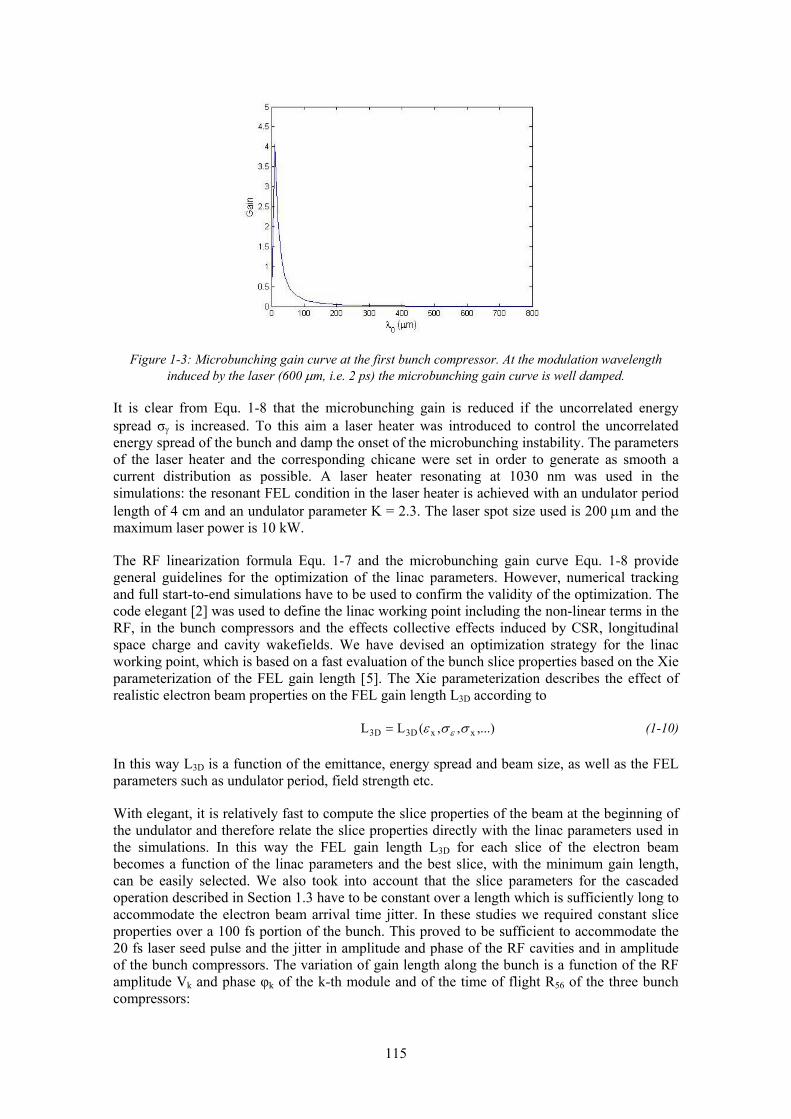
115

Figure 1-3: Microbunching gain curve at the first bunch compressor. At the modulation wavelength induced by the laser (600 μm, i.e. 2 ps) the microbunching gain curve is well damped.

It is clear from Equ. 1-8 that the microbunching gain is reduced if the uncorrelated energy spread σγ is increased. To this aim a laser heater was introduced to control the uncorrelated energy spread of the bunch and damp the onset of the microbunching instability. The parameters of the laser heater and the corresponding chicane were set in order to generate as smooth a current distribution as possible. A laser heater resonating at 1030 nm was used in the simulations: the resonant FEL condition in the laser heater is achieved with an undulator period length of 4 cm and an undulator parameter K = 2.3. The laser spot size used is 200 μm and the maximum laser power is 10 kW.

The RF linearization formula Equ. 1-7 and the microbunching gain curve Equ. 1-8 provide general guidelines for the optimization of the linac parameters. However, numerical tracking and full start-to-end simulations have to be used to confirm the validity of the optimization. The code elegant [2] was used to define the linac working point including the non-linear terms in the RF, in the bunch compressors and the effects collective effects induced by CSR, longitudinal space charge and cavity wakefields. We have devised an optimization strategy for the linac working point, which is based on a fast evaluation of the bunch slice properties based on the Xie parameterization of the FEL gain length [5]. The Xie parameterization describes the effect of realistic electron beam properties on the FEL gain length L3D according to

,...),,(LL xxD3D3 σσε ε= (1-10)

In this way L3D is a function of the emittance, energy spread and beam size, as well as the FEL parameters such as undulator period, field strength etc.

With elegant, it is relatively fast to compute the slice properties of the beam at the beginning of the undulator and therefore relate the slice properties directly with the linac parameters used in the simulations. In this way the FEL gain length L3D for each slice of the electron beam becomes a function of the linac parameters and the best slice, with the minimum gain length, can be easily selected. We also took into account that the slice parameters for the cascaded operation described in Section 1.3 have to be constant over a length which is sufficiently long to accommodate the electron beam arrival time jitter. In these studies we required constant slice properties over a 100 fs portion of the bunch. This proved to be sufficient to accommodate the 20 fs laser seed pulse and the jitter in amplitude and phase of the RF cavities and in amplitude of the bunch compressors. The variation of gain length along the bunch is a function of the RF amplitude Vk and phase φk of the k-th module and of the time of flight R56 of the three bunch compressors:

116

,...),,,...,,V,...,V(LL 21n1n1best

D3best

D3 θθφφ>>=<< (1-11)

We typically used a reduced number of parameters in the linac optimization:

• the phases of the accelerating section before the first compressor (including the harmonic cavity),

• the strength of the three compressors BC1, BC2 and BC3, • the phases of the accelerating sections before the second compressor.

The saturation power as predicted by the Xie parameterization and the flatness of the current pulse profile were also used in the optimization. The multi-objective multi-parameter optimizer for the analysis of the linac working point is based on a genetic algorithm implemented in the SPEA2 software package [6]. Figure 1-4 gives an example of the result of the optimization search performed with the optimizer. The best linac working points selected from Figure 1-4 are a trade off between the requirement of constant current profile (small y values) and small 3D Xie gain length averaged over 100 fs bunch length (small x values).

Figure 1-4: Example of the optimizer output. The dots on the top left correspond to linac working points with larger variation in the longitudinal current profile and lower average 3D Xie gain length. The blue

areas correspond to the Pareto optimal front at different number of iterations of the optimiser.

The final parameters obtained in the optimisation process are reported in Table 1-2 and the corresponding evolution of the longitudinal phase space is shown in Figure1-5 at various locations inside the linac.

117

Table 1-2: Linac operating parameters for the nominal working point (0.2nC case)

Voltage ACC2 15.1 MV/m

Phase ACC2 29 deg

Voltage 3HC 13.1 MV/m

Phase 3HC -96.5 deg

Voltage ACC3-4 15.5 MV/m

Phase ACC3-4 10 deg

Voltage ACC5-12 15.6 MV/m

Phase ACC5-12 0 deg

Votage ACC13-18 15.2 MV/m

Phase ACC13-18 0 deg

BC1 R56 7.4 cm

BC2 R56 9.2 cm

BC3 R56 8.7 cm

Figure 1-5: Longitudinal phase space at different locations in the linac: top left - after the 1st accelerating module; top right - after BC1; bottom left - after BC3; bottom right - at the end of the spreader.

Figure 1-6 reports the longitudinal current distribution, the normalized emittance, the relative energy spread and the corresponding 3D Xie gain length at the end of the spreader for the longitudinal slices in which the bunch was subdivided. It is shown that there is a relatively flat region of about 100 fs where the gain length is roughly constant. This region can accommodate

118

the laser seed pulse length of 20 fs and additional bunch time arrival jitter coming for the RF modules jitter and from the power supplies of the compression magnets. More details are presented in Section 1.2.3.

Figure 1-6: Beam parameters and corresponding 3D Xie gain length at the end of the spreader. The red arrow indicates the 100 fs portion with less than 10% variation in the 3D Xie gain length.

The final step in the accelerator optimization was to confirm that the electron beam characteristics described above are sufficient for FEL operation. This was done by transferring the actual electron beam distribution calculated with elegant into the well-known FEL simulation code, Genesis, and carrying out a full time-dependent analysis. These calculations, reported in the following Section, were carried out in the SASE mode in order to confirm the basic FEL gain length and saturation power. Once this preliminary assessment was successfully completed the same beam distribution was then used to perform simulations of the harmonic cascaded scheme described in Section 1.3.

1.2.2 SASE FEL Simulations

The results of the optimization were benchmarked with time-dependent SASE simulations with Genesis 1.3 on an undulator train of the type used for the FEL-3 radiator in the cascaded FEL scheme described in Section 1.3.

Figure 1-7 (upper) shows the growth of the radiation power along the undulator length. It is clear that 40 m are sufficient to reach saturation, confirming by means of full start-to-end simulations the high quality of the electron beam produced by the injector and linac. Figure 1-7 (lower) shows the temporal and spectral structure of the FEL pulse with many spikes, as is typical of the SASE mode of operation. The peak power reaches several GW with a time-bandwidth product of about 25.

119

Figure 1-7: Results of time-dependent simulations for the FEL-3 radiator at 1 keV in SASE mode, using the optimized 0.2 nC bunch of Section 1.2.1. Top – peak power as a function of the position along the

undulator, Bottom – temporal (left) and spectral (right) profiles at saturation (z = 40 m).

1.2.3 Linac Jitter Studies

The analysis of the effect of various jitter sources on the operation of the linac and the injector has been carried out numerically in order to assess the effect on the final electron beam qualities and to specify the tolerances required on the various linac subsystems. The jitter sources considered in our study are summarised in Tables 1-3 and 1-4. The beam dynamics has been analysed with full start-to-end simulations from the RF photocathode gun with ASTRA and through the linac with elegant. The parameters in the gun and in the linac were varied according to random Gaussian distribution. The rms of such distributions are defined on the basis of the operational experience at FLASH or modest improvement of these. In order to reduce the effect of the jitter on the arrival time it was assumed that each RF cavity in each module can be fed independently. In this way the effect of the random jitter adds in quadrature and the detrimental effect of correlated errors can be avoided.

Table 1-3: Jitter sources in the gun (rms values)

Solenoid field 0.01%

Gun phase 0.1o

Gun voltage 0.1%

Charge 1%

Laser spot offset 0.025 mm

120

Table 1-4: Jitter sources in the linac cavities and BC power supplies (rms values)

Cavity phase 0.01o

Cavity voltage 10-4

BC power supply 10-5

The jitter of all the relevant dynamical quantities are computed at the end of the spreader, before the FEL and the results are summarised in Tables 1-5 and 1-6.

Table 1-5: Arrival time jitter generated by the jitter sources listed in Tables 1-3 and 1-4

Jitter source Arrival time jitter (rms)

Gun 9 fs

Gun and ACC01 12 fs

Linac (excluding injector) 12 fs

ALL 16 fs

Table 1-6: Summary of jitter results for the case where all jitter sources listed in Tables 1-3 and 1-4 are included simultaneously. Results are computed over a slice of 100 fs centred around the seed.

Parameter Mean RMS

Energy 2.25 GeV 0.2 MeV

Emittance (normalised) 3 ⋅10–7 m rad 2.7 ⋅10–9 m rad

Energy spread 150 keV 15 keV

current 970 A 81 A

X position - 7 μm

Y position - 2 μm

X angle - 0.5 μrad

Y angle - 1.5 μrad

The longitudinal current profiles for 100 seeds are reported in Figure 1-8. The 3D Xie gain length plots show that the jitter leaves enough space for a 20 fs seed laser pulse to find an electron beam with constant slice parameters. This bunch was then used as nominal bunch for all subsequent FEL calculations.

121

Figure 1-8: Longitudinal profile of 100 jitter electron bunches (left) and corresponding 3D Xie gain length (right).

1.2.4 SASE Mode Operation at Lower Charge

The optimisation of the linac for the nominal working point was performed assuming that the electron beam from the injector has state of the art beam qualities (e.g. a normalised slice emittance below 0.4 μm). The whole optimisation process is further complicated by the requirement for constant slice parameters for seeded FEL operation which poses tight requirements on the jitters sources. As a fall-back option we also investigated the possibility of generating short radiation pulses in SASE mode, with a time duration of 20 fs FWHM.

To achieve 20 fs FWHM SASE pulse we need to shorten the electron bunch to about the same order. This mode of operation requires a strong compression of the electrons and correspondingly is more sensitive to CSR effects. It proved in fact rather difficult to compress a 200 pC bunch to 20 fs while keeping sufficient beam quality for SASE operation, therefore we have investigated the possibility of operating with lower charge. We have found that 50 pC is a good compromise for generating a 20 fs FWHM pulse with good peak power from the SASE FEL.

This optimisation of this operation point requires only minor changes to the setting of the bunch compressors and none at all to the RF cavities in the linac. The values of the bunch compressors are reported in Table 1-7. The 50 pC bunch from the injector is slightly shorter than the nominal 200 pC bunch and the optimal working point is reached with the same BC1 and BC2 and a slightly smaller R56 for BC3. Figure 1-9 shows the longitudinal current distribution of the electron bunch and the corresponding slice emittance at the end of the spreader.

Table 1-7: Bunch compressor settings for the optimisation of the SASE fall-back working point

Bunch Compressor R56

BC1 7.4 cm

BC2 9.2 cm

BC3 7.5 cm

122

Figure 1-9: Longitudinal beam distribution (left) and slice emittance (right) for the 50 pC bunch optimised for SASE operation

The corresponding SASE simulation in time-dependent mode was carried out with Genesis and shows (Figure 1-10) that the FEL driven by such a bunch can reach saturation within about 30 m and generate a few GW peak power with a pulse width of less than 20 fs FWHM. The time-bandwidth product is approximately 10.

Figure 1-10: Radiation power as a function of the distance along the undulators (top), pulse profile (bottom left) and spectrum (bottom right) in the lower charge (50 pC) SASE mode.

123

1.3 Design of Seeded Free-Electron Lasers

1.3.1 The Advantages of Seeding

The NLS Science Case specifies temporally coherent FEL pulses with durations of the order of 20 fs. Such a specification cannot be met by a Self Amplified Spontaneous Emission (SASE) FEL [7]. The theory of the spectral and temporal characteristics of SASE FEL output is well understood [8] and confirmed by experimental observation [9]. The device starts up from the spontaneous emission from the electron bunch, which is noisy due to sub-radiation-wavelength phase noise in the electron distribution (the shot noise), and this spontaneous emission is amplified in the FEL to saturation. The output pulse comprises a sequence of phase-uncorrelated spikes separated by at least 2πlc where lc = λr/4πρ is the FEL cooperation length defining the intrinsic coherence length of the FEL interaction and ρ is the FEL, or Pierce, parameter [7] with typical value 10-3 for soft X-Ray FELs. The temporal profile of the output pulse varies randomly shot-to-shot, and the spectrum is similarly noisy with bandwidth

ρλλ 2/ ≈Δ FWHM . Figures 1-7 and 1-10 show examples of the pulse shapes and spectra that would result from operating NLS in the SASE mode. The time-bandwidth product

zt ΔΔ=ΔΔ )/)(/1( λλλυ , where Δλ is the FWHM bandwidth and Δz is the FWHM pulse length, gives a quantitative measure of output pulse coherence. For these examples the time-bandwidth product varies between 10 and 25 depending on the pulse length, and hence deviates significantly from that of a transform limited Gaussian pulse with constant phase, for which

44.0=ΔΔ tυ .

If on the other hand a temporally coherent radiation pulse is injected into the FEL undulator to co-propagate with the electron bunch, with a wavelength matched to the resonant wavelength of the undulator, and with a power level greater than the spontaneous emission generated by the electron beam shot noise, then this coherent ‘seed’ pulse dominates the spontaneous emission and is amplified to saturation in the FEL while retaining its coherence. The time-bandwidth product is then much closer to that of a transform limited pulse. Furthermore, the pulse length of the amplified pulse is close to that of the injected seed pulse which can be considerably shorter than the electron bunch length. Finally, the shot-to-shot stability of the FEL output pulse is much improved, including its synchronisation to external laser sources. This is the principle of seeding which has been adopted by the NLS project in order to meet the requirements for pulse length, coherence and synchronisation stated in the Science Case.

Of course seeding of this type (direct seeding) is only possible if a seed source of sufficient power is available at the required wavelength. The NLS FELs are required to operate at up to 1 keV where no such seed source exists. In this case sub-harmonic seeding is possible—the FEL is seeded at a sub-harmonic of the required photon energy, then harmonic up-conversion is carried out within the FEL to reach the required output energy while retaining the temporal coherence of the seed. This is the choice made for NLS.

1.3.2 Review of Progress with Seeding

Research into the seeding of FELs is ongoing at many institutions worldwide. Seeding with lasers and the subsequent generation of higher harmonics in an FEL has been demonstrated, for example at Brookhaven [10] and more recently at the MAX-lab TEST FEL Facility [11] where coherent harmonic generation at 88 nm, the 3rd harmonic of a 263 nm Ti:Sapphire seed laser, was demonstrated in February 2010. Direct seeding of an FEL with a 160 nm HHG source has also been demonstrated at the SPring-8 Compact SASE Source [12].

The FERMI@Elettra project is currently under construction and will contain two FELs. FEL1 will reach 20 nm with a single HGHG stage, while to reach the shortest wavelength of 4 nm in FEL2 a two-stage HGHG cascade is proposed, seeded by a conventional laser at around

124

200 nm. As a facility due to come on-line in the near future, the FEL/seeding design choice has been strongly influenced by the present status of technology development, but also made flexible enough to exploit a future upgrade to HHG seeding [13].

Seeding experiments with an HHG source are planned at SPARC [14] where the FEL can be operated in both SASE and seeded modes. Characterisation of the SASE radiation is underway simultaneous with the setup for seeding. Two seed sources are planned, both obtained via harmonic generation, the first one in crystal (400 and 266 nm) and the second in rare gas (Argon). The ultimate intention is to demonstrate operation of a harmonic cascade seeded by HHG.

HHG seeding will also be tested soon at the FLASH user facility. The project is known as sFLASH [15] with the goal of studying the technical feasibility of seeding at short wavelengths (30 nm initially) and how to implement the technology for reliable user operation.

An experiment is also underway at SLAC to test the recently proposed scheme of Echo-Enabled Harmonic Generation (EEHG) [16].

The projects mentioned are some of those that are operational or under construction and which will provide valuable insight into the feasibility and reliability of seeding and harmonic generation at FEL user facilities. Their results over the next months and years will be invaluable in any future development of the NLS proposal. Other projects at the design stage, such as SwissFEL, WiFEL and the LBNL FEL facility, have also stated interests in seeding, specifically with HHG. Their progress and adopted strategies will also be informative.

1.3.3 Choice of Seed Source and FEL Scheme

Two options for a seed source are a conventional laser system or a source based on Higher Harmonic Generation (HHG) in gases. The assumptions made when choosing the FEL scheme for NLS were that the minimum wavelength accessible by a high power conventional laser system is 250 nm, based on design work for the FERMI@Elettra project [1], and that the available power at that wavelength is approximately 100 MW. For HHG systems, it was considered feasible to deliver 400 kW of power to the FEL undulator at a photon energy of 100 eV, or wavelength 12.4 nm. Further discussion of the design and performance of HHG sources is given in Section 10.2.

The decision was made to base the FEL design on an HHG seed source. In order to justify this decision the next Sections first present the principle and operation of an FEL scheme based on a High Gain Harmonic Generation (HGHG) Cascade seeded by a conventional laser (including discussion of a recent variation on laser-seeded HGHG referred to as Echo-Enabled Harmonic Generation (EEHG) [16]) and then present the alternative HHG-seeded approach that has been adopted for NLS.

1.3.3.1 Laser Seeded HGHG Cascade FEL

A FEL scheme based on harmonic up-conversion of a high power laser seed was proposed many years ago [17]. A subsequent variation of this scheme is known as High Gain Harmonic Generation (HGHG) [18, 19]. Single harmonic up-conversions using the HGHG principle have been successfully demonstrated [10]. The principle is that the high power seed laser interacts with the electron beam within a short modulator undulator tuned to be resonant with the laser seed. The interaction generates a sinusoidal energy modulation along the electron bunch with period equal to the seed laser wavelength. The electron bunch is then passed through a magnetic chicane which is longitudinally dispersive, such that electrons with a higher energy take a shorter path through the chicane and catch up with the lower energy electrons. The effect is that the initial sinusoidal energy modulation is converted into a periodic density modulation, or

125

bunching. As long as the initial energy modulation is greater than the natural RMS energy spread in the bunch by a factor n, i.e. satisfying

γσγ n>Δ (1-12)

then a Fourier transform of the bunch density shows that there is also strong bunching at higher harmonics of the seed laser wavelength, up to the nth harmonic. The bunch then propagates into a radiator undulator tuned to one of these higher harmonics and due to the pre-bunching in the beam at that higher harmonic the bunch radiates strongly and coherently at this harmonic. The initial growth of radiation power is initially quadratic with distance through the radiator undulator, with coherent power Pcoh over the first two gain lengths proportional to the square of the bunching parameter θieb −≡ :

2bPcoh ∝ (1-13)

where here θ is the relative phase between the electron transverse oscillation and the radiation field. If the total energy spread due to the initial energy spread and imposed energy modulation is small enough and satisfies

ργγσσ γγ <⎟⎟⎠

⎞⎜⎜⎝

⎛ Δ+=

22

total, 2 (1-14)

this initial coherent power burst is amplified exponentially to saturation.

To up-convert from the seed laser wavelength of 250 nm to a final output of 1.24 nm requires a total harmonic up-conversion of n ∼ 200, so assuming that each harmonic up-conversion has a harmonic factor of 5, as is typical for this type of FEL scheme, this would require a total of four harmonic up-conversions in series. Such a scheme, termed a harmonic cascade, was proposed for the BESSY-FEL [20] and an example is under construction at FERMI@Elettra [1]. In this scheme the radiator undulator of the first stage is made just long enough that the radiation power is sufficient to act as a seed pulse for the second stage, and the radiator output of the second stage is then used to seed the third stage, and so on, until the desired output wavelength is reached in the final radiator, which is made long enough for the FEL to reach saturation.

Due to the high gain FEL interaction in the first radiator however the energy spread in the electron bunch has grown significantly such that the condition of Equ. 1-12 cannot easily be satisfied in the modulator of the second stage. To counter this problem, the ‘fresh bunch’ scheme has been proposed [21] in which an additional chicane before the second stage modulator delays the electron bunch with respect to the radiation pulse such that in the second stage modulator the new seed pulse overlaps with a section of the bunch that did not interact with the seed in the first stage, and so consequently has not suffered the energy spread degradation of the seeded part of the bunch. An undesirable consequence of this ‘fresh bunch’ scheme is that the electron bunch must be made long enough that for each stage in the cascade there is a fresh part of the bunch available in front of the previously seeded part. For a given bunch charge, making the bunch longer reduces the peak current and because the FEL output power scales with peak current as P ∝ I4/3, and the gain length scales as Lg ∝ I-1/3, the performance of the FEL is degraded and the total length (and hence cost) increased.

A recently proposed variation of the laser seeded HGHG scheme is known as Echo-Enabled Harmonic Generation (EEHG) [16]. In this scheme the electron beam is modulated twice by two separate high-power seed lasers. Two dispersive chicanes are used, one after each modulator, with the first chicane being extremely strong. Such a scheme enables strong bunching to be produced at the start of the radiator at very high harmonic number, so that only one stage of

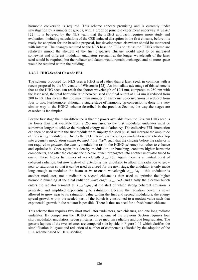
126

harmonic conversion is required. This scheme appears promising and is currently under investigation by a number of groups, with a proof of principle experiment underway at SLAC [22]. It is believed by the NLS team that the EEHG approach requires more study and evaluation, including calculations of the CSR induced disruption in the first chicane, before it is ready for adoption for the baseline proposal, but developments elsewhere should be monitored with interest. The changes required to the NLS baseline FELs to utilise the EEHG scheme are relatively minor: the strength of the first dispersive chicane would need to be increased somewhat and different modulator undulators resonant at the longer wavelength of the laser seed would be required, but the radiator undulators would remain unchanged and no more space would be required within the building.

1.3.3.2 HHG-Seeded Cascade FEL

The scheme proposed for NLS uses a HHG seed rather than a laser seed, in common with a recent proposal by the University of Wisconsin [23]. An immediate advantage of this scheme is that as the HHG seed can reach the shorter wavelength of 12.4 nm, compared to 250 nm with the laser seed, the total harmonic ratio between seed and final output at 1.24 nm is reduced from 200 to 10. This means that the maximum number of harmonic up-conversions is reduced from four to two. Furthermore, although a single stage of harmonic up-conversion is done in a very similar way to the HGHG scheme described in the previous Section, the way the stages are cascaded is far simpler.

For the first stage the main difference is that the power available from the 12.4 nm HHG seed is far lower than that available from a 250 nm laser, so the first modulator undulator must be somewhat longer to achieve the required energy modulation Δγ. The collective FEL interaction can then be used within the first modulator to amplify the seed pulse and increase the amplitude of the energy modulation. Due to the FEL interaction the energy modulation starts to develop into a density modulation within the modulator itself, such that the chicane before the radiator is not required to produce the density modulation (as in the HGHG scheme) but rather to enhance and optimise it. Once again this density modulation, or bunching, contains higher harmonic components, and after the chicane the electron bunch propagates into another undulator tuned to one of these higher harmonics of wavelength 1/ hseedλ . Again there is an initial burst of coherent radiation, but now instead of extending this undulator to allow this radiation to grow near to saturation so that it can be used as a seed for the next stage, the undulator is only made long enough to modulate the beam at its resonant wavelength 1/ hseedλ – this undulator is another modulator, not a radiator. A second chicane is then used to optimise the higher harmonic bunching at the final radiation wavelength 21/ hhseedλ and finally the electron bunch enters the radiator resonant at 21/ hhseedλ , at the start of which strong coherent emission is generated and amplified exponentially to saturation. Because the radiation power is never allowed to grow near to its saturation value within the first and second modulators, the energy spread growth within the seeded part of the bunch is constrained to a modest value such that exponential growth in the radiator is possible. There is thus no need for a fresh bunch chicane.

This scheme thus requires two short modulator undulators, two chicanes, and one long radiator undulator. By comparison the HGHG cascade scheme of the previous Section requires four short modulator undulators, seven chicanes, three medium radiators and one long radiator. The generic layouts of the two schemes are compared side by side in Figure 1-11 which clarifies the simplification in layout and reduction of number of components afforded by the adoption of the FEL scheme based on HHG seeding.

127

Modulator

Radiator

e‐

1/ hlaserλ

1/ hHHGλ 21/ hhHHGλ

21/ hhlaserλ

4321/ hhhhlaserλ321/ hhhlaserλe‐

Laser

Laser

HHG Seed

Gas Cell

Bunching Chicane

Fresh Bunch Chicane

HHG Seeded Cascade FEL

KEY

Laser Seeded HGHG Cascade FEL

Figure 1-11: Comparison of layouts for two generic FEL schemes: Laser-Seeded HGHG Cascade FEL and HHG Seeded Cascade FEL

1.3.4 Seed Power Requirement

For the seeding to be effective, such that the temporal coherence and pulse length of the seed are retained in the FEL output, the seed power Pseed must be much higher than Prad(0), the power of the spontaneous emission due to the electron beam shot noise (referred to hereafter as the shot noise power). If the output wavelength of the FEL is the same as the seed wavelength, so that no harmonic up-conversions are required, this is known as direct seeding. In this case simulations [24] and experiment [12] have shown that typically the seed power must satisfy

).0(100 radseed PP ×> (1-15)

For harmonic up-conversion schemes there is an additional factor of n2 required due to the degradation of the signal-to-noise ratio from input to final output [25]. In this case the requirement is

)0(100 2radseed PnP ××> (1-16)

where n is the harmonic ratio between seed and final output.

The shot noise power is given by the approximate expression [26]

beam2

rad P)/Nln(N

6)0(P ρρ

π

λλ

≈ (1-17)

where Nλ is the number of electrons per radiation wavelength. From this it is seen that at shorter wavelengths, where Nλ becomes smaller, the shot noise power increases placing greater demands on the seed source. This is illustrated in Figure 1-12 which shows the calculated shot noise power as a function of wavelength and peak current. The assumptions in these calculations are that the undulator parameter aw = 1.0, the undulator period λw = 30 mm, the normalised emittance εn = 1 mm-mrad and the average beta function β = 5 m. These are all typical values for the NLS FELs but by far the most dominant terms in the expression are the radiation wavelength and the electron beam peak current.

128

100

101

102

100

101

102

103

λ [nm]

P rad(0

) [W

]

I = 1kAI = 2kAI = 3kAI = 4kAI = 5kAI = 6kAI = 7kAI = 8kAI = 9kAI = 10kA

Figure 1-12: The approximate electron beam shot noise power as a function of wavelength and peak current.

At the minimum wavelength of the HHG seed, 12.4 nm, with peak current 2 kA, the shot noise power is seen to be approximately 35 W. From the previous discussion this means that the seed power required for direct seeding at 12.4 nm (100eV) is Pseed = 3.5 kW and for a harmonic FEL scheme seeded at 100 eV and up-converting to 1000 eV the required seed power is 350 kW. On this basis the 400 kW which is foreseen to be available from the HHG seed source at the FEL is therefore sufficient to assure longitudinal coherence of the FEL output.

1.3.5 Seed Tuning and Harmonic Conversions

In order to cover the entire tuning ranges of FEL-1, FEL-2 and FEL-3 the required tuning range of the HHG seed and the required combinations of harmonic up-conversions were studied. As before, the total harmonic ratio between seed and FEL output is n. For two harmonic up-conversions, with ratios [ ]5,4,3,2,11 =h and [ ]5,4,3,22 =h the total harmonic number must be

...]12,10,9,8,6,5,4,3,2[21 == hhn . The criterion was applied that h1 ≤ h2 because bunching develops more strongly at lower harmonics. This keeps the first modulator as short as possible and minimises energy spread growth before the first harmonic conversion.

The results of the study were that for uninterrupted wavelength coverage in FEL-3 and FEL-2 the HHG seed must tune from 75-100 eV, whereas for FEL-1 the seed must tune from 50-100 eV. For FEL-2 and FEL-3 the first modulator, Modulator 1, should also then tune over 75-100 eV, which assuming a planar undulator with 8 mm minimum gap gives a required period of 44 mm. The second modulator, Modulator 2, should tune to 200 eV for FEL-3 and to 300 eV for FEL-2. The period chosen for Modulator 2 for FEL-3 and FEL-2 was also 44 mm—in this way Modulator 2 can also tune down to 75 eV and be used as an extension to Modulator 1, giving operational flexibility, and simplification of design effort and manufacturing. The required harmonic up-conversions to give uninterrupted wavelength coverage over the design tuning ranges of the three FELs are illustrated schematically in Figure 1-13.

129

Figure 1-13: Undulator tunings and combinations of harmonic up-conversions to give uninterrupted wavelength coverage for FEL-3, FEL-2 and FEL-1.

1.3.6 Seeded FEL Design Optimisation

The FEL scheme has been simulated with the standard three-dimensional FEL code Genesis 1.3 [27]. In order to allow rapid progress in the optimisation of the design parameters the code was first used in ‘steady state’ mode. Here only a single slice of the electron beam, of length one radiation wavelength, is used in the simulation and the electron beam parameters for that slice are chosen to be representative of the average parameters within that part of the real electron bunch which will be aligned with the HHG seed pulse. In this mode of simulation the boundary conditions of the electron beam phase space are periodic over the wavelength slice—the effect is of simulating an infinitely long electron bunch and co-propagating radiation pulse and for this reason the steady-state simulation can give no information about the spectral properties of the FEL pulse (the Fourier transform of a constant is a delta function). Neither can any information about the growth of the shot noise emission be obtained because this grows from the slice-to-slice variation of sub-wavelength phase noise in the electron distribution so cannot be modelled using only a single slice. Information about the spectral and temporal properties of the output pulses can therefore only be obtained from time-dependent simulations in which the whole electron bunch is simulated but these simulations are thousands of times more CPU intensive and thus inappropriate for initial optimisation studies. Full start-to-end time-dependent simulations of FEL-3 operating at photon energy of 1000 eV have been done to provide a full analysis of the spectral and temporal properties of the output FEL pulses, and the results are presented in subsequent Sections.

The generic layout for a two stage harmonic up-conversion, such as that required to seed at 100 eV and produce output at 1000 eV, is shown in Figure 1-14. For the given seed laser power, the modulators were made long enough that condition Equ. 1-12 was satisfied, yet also short enough that condition Equ. 1-14 was simultaneously satisfied at the start of the radiator. The strength of the magnetic chicane before Modulator 2, the length of Modulator 2 and the strength of the chicane before the Radiator, were chosen to optimise the harmonic bunching at the end of Modulator 2, which of course is equivalent to optimising the bunching at the resonant wavelength of the final Radiator. The coherent emission over the first two gain lengths in the radiator is the signal which is amplified to saturation in the radiator. Because the power of this coherent signal is proportional to the square of the bunching parameter, the bunching must be strong enough that the coherent signal dominates the shot noise power ensuring good temporal

130

coherence in the output. The criterion applied was that |b| >1% is sufficient for retention of temporal coherence, and this was confirmed in later time-dependent simulations.

Modulator 1 Chicane + Radiator

e‐

SeedChicane + Modulator 2

Figure 1-14: The generic layout for a two stage harmonic up-conversion FEL scheme, such as that required to seed at 100 eV and produce output at 1000 eV

This optimisation was carried out for a number of different output wavelengths for FEL-3, FEL-2 and FEL-1. For the cases where only one harmonic up-conversion was required the optimisation followed a similar philosophy, but was of course somewhat more straightforward. In all cases the undulators are composed of 2.5 m sections and placed within a FODO focussing structure. The undulator section length has not yet been fully optimised; this work would form part of future NLS design studies. The gap between undulator sections is 1 m, a realistic space for the insertion of quadrupole, diagnostics station, phase shifter, corrector, BPM, vacuum pump and flanges.

The optimum electron beam β function within the radiator undulator, averaged over a FODO period, was found to be 5.8 m. In finding this optimum there is a trade off between maximising the output power and minimising the gain length: the chosen working point is a compromise position where the saturation length is only 0.5 m from its minimum and the saturation output power is less than 1% below its maximum.

Modulator 1: Resonant @ 100eV

bunching @ 200eV

Power @ 100eV

Modulator 2: Resonant @ 200eV

bunching @ 1000eV

Power @ 200eV

Radiator: Resonant @ 1000eV

bunching @ 1000eV

Power @ 1000eV

Figure 1-15: Steady-state Genesis 1.3 simulations for FEL-3 at 1 keV output energy. Also shown, in blue, is the equivalent SASE case where an unmodulated beam is injected directly into the radiator.

An example of the steady state simulation results is presented in Figure 1-15, for the 1000 eV photon output of FEL-3. The HHG seed, at photon energy 100 eV with peak power 400 kW, is injected into Modulator 1. The growth of the seed power and corresponding growth of bunching at the 2nd harmonic is shown. Modulator 2 is resonant at 200 eV. The strong emission of radiation at 200 eV due to the pre-bunching of the beam is clear, and this drives the development of bunching at the fifth harmonic of 200 eV. Finally in the Radiator the initial bunching at 1000 eV is 8% and the coherent power grows quickly to 30 MW within the first 2.5 m undulator section. This coherent power is then amplified exponentially to a saturation level of 2.7 GW at a saturation length of 18 m in the Radiator.

131

A comparison ‘equivalent’ SASE case is shown where the electron beam is not pre-bunched by modulators but injected directly into the radiator undulator. Here the initial power is set to the shot noise power level of just over 100 W. It is seen that there is no initial coherent power burst, but after a lethargy distance of around 3 m the FEL exponential growth regime is entered and the power saturates after 40 m. The growth rate of the SASE case is slightly greater than the seeded case—this is because of the energy spread growth within the modulators of the seeded scheme, although it is stressed that this energy spread growth is not sufficient to prohibit exponential amplification within the radiator.

Following this programme of design optimisation, and allowing contingency for alternative modes of operation (such as SASE, Section 1.2.4) or sub-optimal electron beam parameters (Section 1.4.1), it was possible to ascertain the required undulator lengths for the three NLS FELs. The resulting schematic layout is shown in Figure 1-16.

e‐ @ 2.25 GeV


20fs FEL Pulse430 ‐ 1000eV


Modulator 2λw = 44 mm400kW HHG 75‐100eV

Modulator 1λw = 44 mm




e‐ @ 2.25 GeV

400kW HHG 75‐100eV



FEL1Modulatorλw = 49 mm

e‐ @ 2.25 GeV

400kW HHG 50‐100eV

Figure 1-16: Schematic layout of the three NLS FELs. Each undulator section is 2.5 m long, with gaps between modules 1.0 m.

1.3.7 Seeded FEL Performance

1.3.7.1 Performance Summary

The performance estimates of the three NLS FELs over the full range of photon energies are shown in Figure 1-17. The results are based on time dependent and steady state Genesis 1.3 simulations at the highest photon energy of FEL-3 (1000eV) which have then been scaled to the other photon energies covered by FEL-3, FEL-2 and FEL-1 using the Xie formalism. The relative variation of output over the tuning ranges of the three FELs is in good agreement with a previous comprehensive set of steady Genesis 1.3 simulations for FEL-3, FEL-2 and FEL-1 [3] which were done using an earlier iteration of electron bunch parameters. The calculations for pulse energy and number of photons per pulse assume a 20 fs FWHM photon pulse. All values are for the APPLE-II undulators in horizontal polarisation. The power levels in circular polarisation mode will be somewhat higher.

132

0 200 400 600 800 10000

2

4

6

8

Photon Energy (eV)

Out

put P

ower

(GW

)

FEL-3 FEL-2 FEL-1

500 1000 1500 2000 2500 3000 3500 4000 4500 500010

4

106

108

Photon Energy (eV)

Out

put P

ower

(W)

FEL-3 3rd HarmonicFEL-3 5th HarmonicFEL-2 3rd HarmonicFEL-2 5th Harmonic

0 200 400 600 800 1000

50

100

150

Photon Energy (eV)

Puls

e En

ergy

(uJ)

0 200 400 600 800 100010

11

1012

1013

1014

Photon Energy (eV)

# ph

oton

s/pu

lse

Figure 1-17: Estimates of output power, pulse energy and number of photons per pulse for FEL-1, FEL-2 and FEL-3

1.3.7.2 FEL-3 at 1keV in the Fundamental

Earlier Sections presented the optimisation of the FEL design parameters using Genesis 1.3 in steady state mode. In this mode the radiation field and electron bunch are assumed to have no longitudinal variation and can therefore be modelled using a single slice of the radiation-electron interaction. Previous steady state results at different photon energies have been used to determine the relative scaling of output power as a function of photon energy for FEL-3, FEL-2 and FEL-1. In this Section FEL output estimates are made using time-dependent simulations, in which the relative slippage between electrons and radiation is modelled by using multiple slices. In this way longitudinal variations in the electron bunch and radiation field can be accounted for. These variations include the intrinsic variation in electron bunch properties arising from the

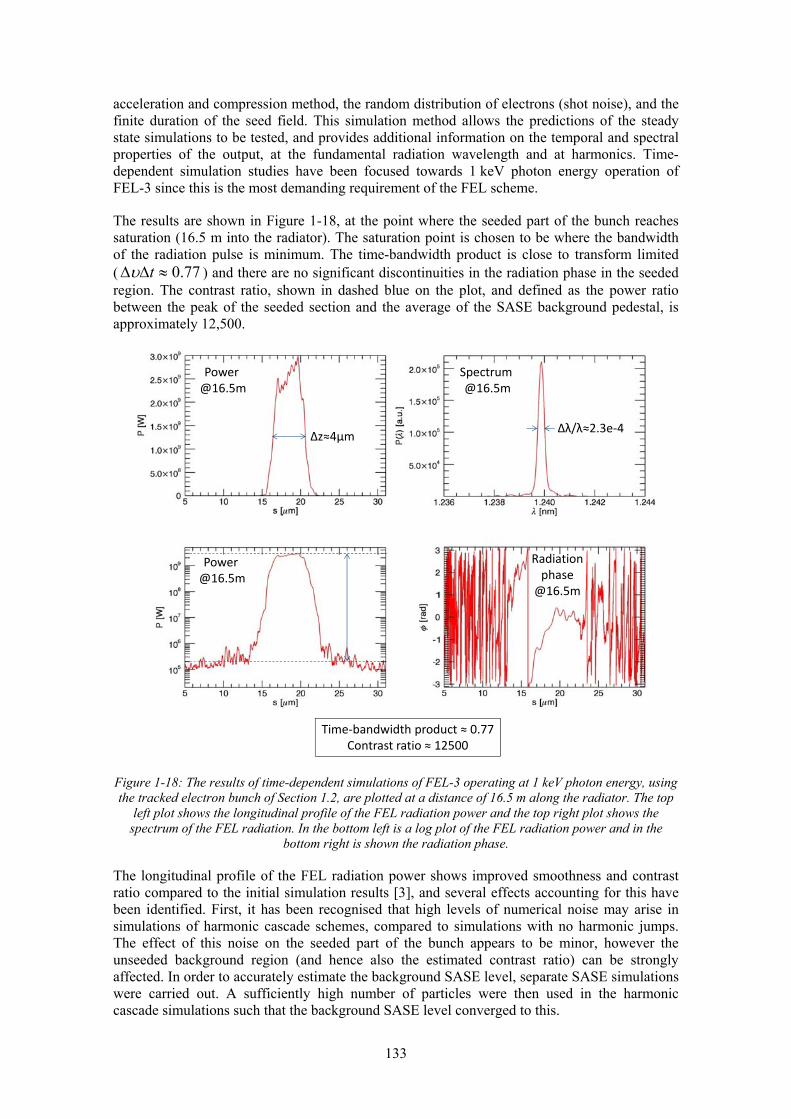
133

acceleration and compression method, the random distribution of electrons (shot noise), and the finite duration of the seed field. This simulation method allows the predictions of the steady state simulations to be tested, and provides additional information on the temporal and spectral properties of the output, at the fundamental radiation wavelength and at harmonics. Time-dependent simulation studies have been focused towards 1 keV photon energy operation of FEL-3 since this is the most demanding requirement of the FEL scheme.

The results are shown in Figure 1-18, at the point where the seeded part of the bunch reaches saturation (16.5 m into the radiator). The saturation point is chosen to be where the bandwidth of the radiation pulse is minimum. The time-bandwidth product is close to transform limited ( 77.0≈ΔΔ tυ ) and there are no significant discontinuities in the radiation phase in the seeded region. The contrast ratio, shown in dashed blue on the plot, and defined as the power ratio between the peak of the seeded section and the average of the SASE background pedestal, is approximately 12,500.

Power @16.5m

Spectrum @16.5m

Power @16.5m

∆z≈4μm∆λ/λ≈2.3e‐4

Time‐bandwidth product ≈ 0.77Contrast ratio ≈ 12500

Radiation phase

@16.5m

Figure 1-18: The results of time-dependent simulations of FEL-3 operating at 1 keV photon energy, using the tracked electron bunch of Section 1.2, are plotted at a distance of 16.5 m along the radiator. The top

left plot shows the longitudinal profile of the FEL radiation power and the top right plot shows the spectrum of the FEL radiation. In the bottom left is a log plot of the FEL radiation power and in the

bottom right is shown the radiation phase.

The longitudinal profile of the FEL radiation power shows improved smoothness and contrast ratio compared to the initial simulation results [3], and several effects accounting for this have been identified. First, it has been recognised that high levels of numerical noise may arise in simulations of harmonic cascade schemes, compared to simulations with no harmonic jumps. The effect of this noise on the seeded part of the bunch appears to be minor, however the unseeded background region (and hence also the estimated contrast ratio) can be strongly affected. In order to accurately estimate the background SASE level, separate SASE simulations were carried out. A sufficiently high number of particles were then used in the harmonic cascade simulations such that the background SASE level converged to this.

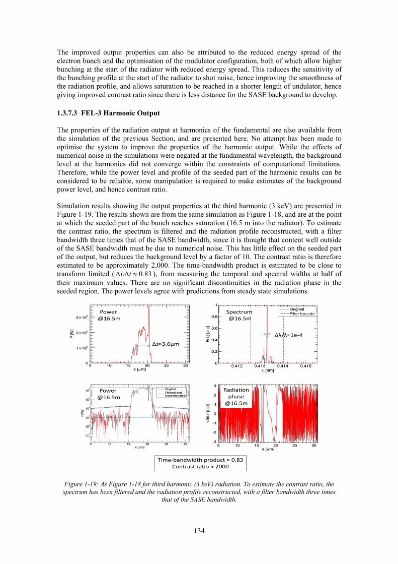
134

The improved output properties can also be attributed to the reduced energy spread of the electron bunch and the optimisation of the modulator configuration, both of which allow higher bunching at the start of the radiator with reduced energy spread. This reduces the sensitivity of the bunching profile at the start of the radiator to shot noise, hence improving the smoothness of the radiation profile, and allows saturation to be reached in a shorter length of undulator, hence giving improved contrast ratio since there is less distance for the SASE background to develop.

1.3.7.3 FEL-3 Harmonic Output

The properties of the radiation output at harmonics of the fundamental are also available from the simulation of the previous Section, and are presented here. No attempt has been made to optimise the system to improve the properties of the harmonic output. While the effects of numerical noise in the simulations were negated at the fundamental wavelength, the background level at the harmonics did not converge within the constraints of computational limitations. Therefore, while the power level and profile of the seeded part of the harmonic results can be considered to be reliable, some manipulation is required to make estimates of the background power level, and hence contrast ratio.

Simulation results showing the output properties at the third harmonic (3 keV) are presented in Figure 1-19. The results shown are from the same simulation as Figure 1-18, and are at the point at which the seeded part of the bunch reaches saturation (16.5 m into the radiator). To estimate the contrast ratio, the spectrum is filtered and the radiation profile reconstructed, with a filter bandwidth three times that of the SASE bandwidth, since it is thought that content well outside of the SASE bandwidth must be due to numerical noise. This has little effect on the seeded part of the output, but reduces the background level by a factor of 10. The contrast ratio is therefore estimated to be approximately 2,000. The time-bandwidth product is estimated to be close to transform limited ( 83.0≈ΔΔ tυ ), from measuring the temporal and spectral widths at half of their maximum values. There are no significant discontinuities in the radiation phase in the seeded region. The power levels agree with predictions from steady state simulations.

Power @16.5m

Spectrum @16.5m

Power @16.5m

∆λ/λ≈1e‐4


Radiation phase

@16.5m

∆z≈3.6μm

Figure 1-19: As Figure 1-18 for third harmonic (3 keV) radiation. To estimate the contrast ratio, the spectrum has been filtered and the radiation profile reconstructed, with a filter bandwidth three times

that of the SASE bandwidth.

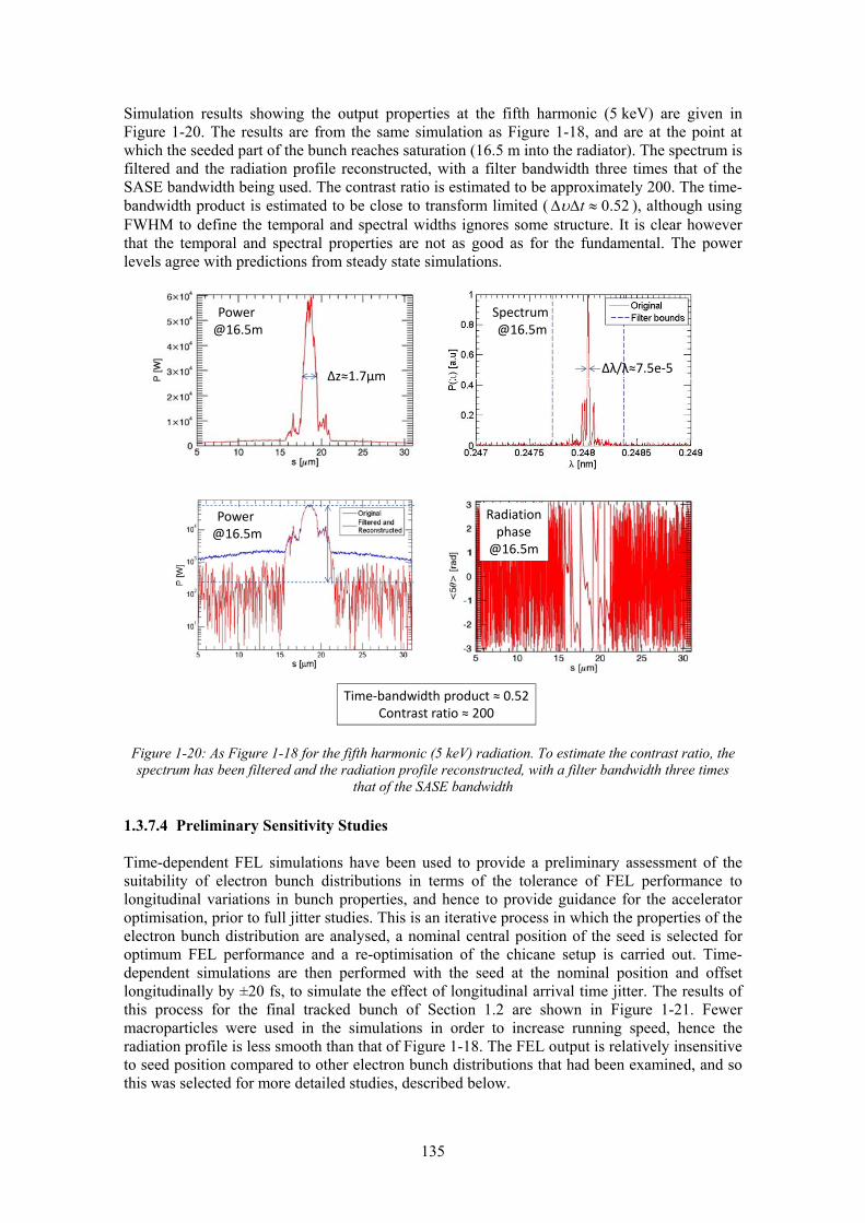
135

Simulation results showing the output properties at the fifth harmonic (5 keV) are given in Figure 1-20. The results are from the same simulation as Figure 1-18, and are at the point at which the seeded part of the bunch reaches saturation (16.5 m into the radiator). The spectrum is filtered and the radiation profile reconstructed, with a filter bandwidth three times that of the SASE bandwidth being used. The contrast ratio is estimated to be approximately 200. The time-bandwidth product is estimated to be close to transform limited ( 52.0≈ΔΔ tυ ), although using FWHM to define the temporal and spectral widths ignores some structure. It is clear however that the temporal and spectral properties are not as good as for the fundamental. The power levels agree with predictions from steady state simulations.

Power @16.5m

Spectrum @16.5m

Power @16.5m

∆z≈1.7μm ∆λ/λ≈7.5e‐5


Radiation phase

@16.5m

Figure 1-20: As Figure 1-18 for the fifth harmonic (5 keV) radiation. To estimate the contrast ratio, the spectrum has been filtered and the radiation profile reconstructed, with a filter bandwidth three times

that of the SASE bandwidth

1.3.7.4 Preliminary Sensitivity Studies

Time-dependent FEL simulations have been used to provide a preliminary assessment of the suitability of electron bunch distributions in terms of the tolerance of FEL performance to longitudinal variations in bunch properties, and hence to provide guidance for the accelerator optimisation, prior to full jitter studies. This is an iterative process in which the properties of the electron bunch distribution are analysed, a nominal central position of the seed is selected for optimum FEL performance and a re-optimisation of the chicane setup is carried out. Time-dependent simulations are then performed with the seed at the nominal position and offset longitudinally by ±20 fs, to simulate the effect of longitudinal arrival time jitter. The results of this process for the final tracked bunch of Section 1.2 are shown in Figure 1-21. Fewer macroparticles were used in the simulations in order to increase running speed, hence the radiation profile is less smooth than that of Figure 1-18. The FEL output is relatively insensitive to seed position compared to other electron bunch distributions that had been examined, and so this was selected for more detailed studies, described below.

136

Figure 1-21: The results of time-dependent simulations of FEL-3 at 1 keV photon energy, for three longitudinal positions of the seed relative to the electron bunch,“0 fs” being the nominal seed position.

Left - longitudinal profiles of the FEL radiation plotted at a distance of 16.5 m along the radiator, Right - variation of peak radiation power with distance through the radiator.

1.4 Sensitivity and Tolerance Studies

1.4.1 Sensitivity to Gun Performance

The sensitivity of the seeded FEL scheme to increased electron beam emittance has been studied taking the worst case of FEL-3 at 1 keV as an example. It was expected that some performance degradation would occur requiring an increase in undulator length to reach saturation, but the more important question was to confirm that the harmonic up-conversion process would still operate effectively.

A bunch with higher emittance from the gun was first produced by artificially increasing the thermal emittance until an arbitrarily high emittance of 0.6 mm mrad was produced. The bunch length was not significantly altered. Since the Twiss parameters of the beam from the injector were slightly different, the linear optics were re-matched to that of the linac using the matching section following ACC01. After this, the bunch could be transported and compressed with remarkably little change in the compression settings. The properties of the bunch at the exit of the spreader are shown in Figure 1-22, which shows that apart from the increased emittance, the bunch is very similar to the nominal 0.3 mm-mrad emittance case.

Figure 1-22: Comparison of the higher emittance bunch with 0.6 mm-mrad emittance with the nominal 0.3 mm mrad case, left - longitudinal current distribution, right - slice emittance analysis.

137

The higher emittance electron bunch was then used in steady-state Genesis 1.3 simulations to optimise the seeded FEL operation. To obtain the same level of harmonic bunching at the start of the radiator it was necessary to adjust the strength of the chicanes and adjust the strength of the radiator FODO lattice to obtain the optimum mean β-function, however no increase in the length of the modulators was needed. Figure 1-23 shows the power growth in the radiator for the baseline emittance of 0.3 mm-mrad and the increased emittance of 0.6 mm-mrad. It can be seen that for the increased emittance the saturation power reduces to ~0.62 of its baseline value and the saturation length increases by a factor of ~1.63. These relative changes are in extremely good agreement with the results of equivalent steady state simulations of the SASE power growth in the radiator only (i.e. no premodulation of the electron beam) for the two emittance values. The conclusion is thus made that the harmonic up-conversion still works effectively at the higher emittance and the reduction in performance is only due to decreased FEL coupling in the radiator undulator.

Figure 1-23: Genesis 1.3 steady state simulations of FEL-3 at 1 keV to illustrate the reduction in performance due to increased emittance. Blue - normalised radiator power growth for baseline emittance

of 0.3 mm-mrad, Green - re-optimised for increased emittance of 0.6 mm-mrad.

To confirm this result, calculations were then carried out using Genesis 1.3 in the time-dependent mode to assess the temporal and spectral properties of the radiation output. The FEL performance in the seeded region was found to agree well with the steady-state optimisation. The temporal and spectral profiles of the radiation at saturation (~29.0 m into the radiator) are shown in Figure 1-24; the profiles are not quite as smooth as the εn = 0.3 mm-mrad case but the seeding method is still effective.

These results therefore confirm the operation of the seeded FEL scheme within the currently assumed undulator length, even with an emittance much higher than predicted, and indeed significantly higher than already achieved at LCLS and PITZ/XFEL.

138

Power @29.0m

Spectrum @29.0m

Figure 1-24: Results of a Genesis 1.3 time dependent simulation for FEL-3 at 1 keV operating with an increased emittance of εn = 0.6 mm-mrad, at saturation (29 m into the radiator) showing the longitudinal

profile of the FEL radiation power (left) and spectrum (right).

1.4.2 Sensitivity to Gun and Linac Jitter

The effect of jitter sources in the RF gun and linac and the intrinsic jitter of the FEL interaction were studied in a full start-to-end computation where the electrons are extracted from the RF photocathode gun and transported to the FEL where the radiation is finally computed. In this way we can realistically estimate the stability properties of the seeded FEL radiation.

Using the electron bunch with jitter described in Section 1.2.3 we ran 100 FEL simulations including random shot noise to evaluate the characteristics of the FEL radiation. Figure 1-25 shows the behaviour of the peak power as a function of distance along the length of the radiator and the radiation pulse profile at an observation point at 23.2 m in the undulator, where saturation is reached for most seeds.

Figure 1-25: Power variation along the undulator and power profiles for the seeded harmonic generation scheme with a 20 fs seed laser pulse.

The results show that the peak power at 23.3 m is on average 1.4 GW with an rms of the 0.4 GW which corresponds to slightly less than 30 % variation.

1.4.3 HHG Seed Laser Tolerances

The performance of FEL-3 has been analysed with respect to fluctuations in the input HHG seed parameters. The parameters assessed are seed power, Rayleigh length, waist position within the modulator, and errors in transverse position and injection angle. The nominal Rayleigh length had previously been optimised at 1.0 m and the waist position set to 0.5 m downstream of the entrance to the first modulator undulator. The variation in normalised output power at the

139

nominal saturation point is shown as each parameter is varied independently. Also shown (in some cases) is the harmonic bunching at the entrance to the radiator. The results are based on Genesis 1.3 steady state simulations of the complete harmonic cascade, with the seed power, Rayleigh length and waist position varied directly within the Genesis input files. It is not possible to include errors in seed position and angle directly within Genesis 1.3, so to assess these errors appropriate input field files were created in an external code.

1.4.3.1 Seed Power, Rayleigh Length and Waist Position

Figure 1-26 shows the relative variation in output power and bunching parameter as a function of seed power, Rayleigh length and waist position; the nominal values of these parameters is also indicated. The corresponding tolerances on these parameters which are required to restrict the variation in output power to different amounts are summarised in Table 1-8.

200 250 300 350 400 450 500 550 6000.5

1

1.5

Nor

m. O

utpu

t Pow

er

Seed Power (kW)200 250 300 350 400 450 500 550 600

0

0.05

0.1

b 0

0 0.5 1 1.5 2 2.50.8

1

1.2

1.4

Nor

m. O

utpu

t Pow

er

Seed ZR (m)0 0.5 1 1.5 2 2.5

0.02

0.04

0.06

0.08

b 0

0 0.5 1 1.5 2 2.5 30.8

1

1.2

1.4

Nor

m. O

utpu

t Pow

er

Seed Waist Position (m)0 0.5 1 1.5 2 2.5 3

0.02

0.04

0.06

0.08

b 0

Nominal

Nominal

Nominal

Figure 1-26: Variation of FEL-3 normalised output power and bunching at radiator entrance, due to fluctuations in seed power, Rayleigh length and waist position.

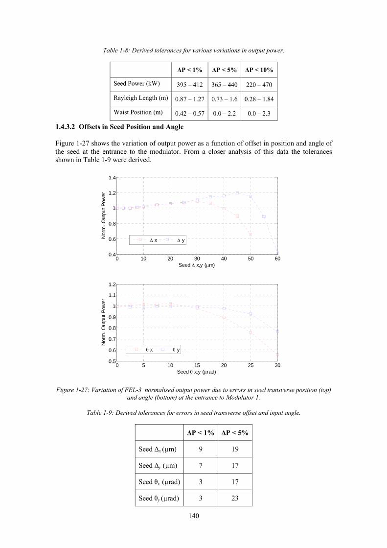
140

Table 1-8: Derived tolerances for various variations in output power.

ΔP < 1% ΔP < 5% ΔP < 10%

Seed Power (kW) 395 – 412 365 – 440 220 – 470

Rayleigh Length (m) 0.87 – 1.27 0.73 – 1.6 0.28 – 1.84

Waist Position (m) 0.42 – 0.57 0.0 – 2.2 0.0 – 2.3

1.4.3.2 Offsets in Seed Position and Angle

Figure 1-27 shows the variation of output power as a function of offset in position and angle of the seed at the entrance to the modulator. From a closer analysis of this data the tolerances shown in Table 1-9 were derived.

0 10 20 30 40 50 600.4

0.6

0.8

1

1.2

1.4

Seed Δ x,y (μm)

Nor

m. O

utpu

t Pow

er

0 5 10 15 20 25 300.5

0.6

0.7

0.8

0.9

1

1.1

1.2

Seed θ x,y (μrad)

Nor

m. O

utpu

t Pow

er

Δ x Δ y

θ x θ y

Figure 1-27: Variation of FEL-3 normalised output power due to errors in seed transverse position (top) and angle (bottom) at the entrance to Modulator 1.

Table 1-9: Derived tolerances for errors in seed transverse offset and input angle.

ΔP < 1% ΔP < 5%

Seed Δx (µm) 9 19

Seed Δy (µm) 7 17

Seed θx (µrad) 3 17

Seed θy (µrad) 3 23

141

1.4.4 Sensitivity to Electron Beam Alignment

The performance of FEL-3, operating at 1000 eV, has been assessed with respect to errors in the transverse position and angle of the electron beam at the entrance to Modulator 1, by means of Genesis 1.3 steady-state simulations. The normalised output power was calculated with electron beam position and angle varied separately and independently, and the results are shown in Figure 1-28. From analysis of these results the tolerances shown in Table 1-10 were derived.

It is notable that there is a marked difference in tolerance between the x-plane and the y-plane. This is due to the fact that the 1st quadrupole in the FODO lattice is focussing in x, which therefore counters any electron beam offset in x. For angular errors (because here the errors are applied independently) the offset at the 1st quadrupole is zero, but the beam is then offset in x at the 2nd quadrupole, which is defocussing and hence amplifies the trajectory error. Therefore, the offset tolerances are more relaxed in x, but the angular tolerances are tighter in x. Reversing the polarity of the FODO lattice is shown to reverse the tolerances between x and y.

0 10 20 30 40 50 60 700

0.2

0.4

0.6

0.8

1

Δx,y (μm)

Nor

m. O

utpu

t Pow

er

Δx Δy

0 0.5 1 1.5 2 2.5 3 3.5 40.5

0.6

0.7

0.8

0.9

1

θx,y (μrad)

Nor

m. O

utpu

t Pow

er

θx θy

Figure 1-28: Variation of FEL-3 normalised output power as a function of electron beam transverse position and angle at the entrance to Modulator 1.

Table 1-10: Derived tolerances for errors in electron beam transverse offset and angle at the entrance to Modulator 1.

ΔP < 1% ΔP < 5% ΔP < 10%

Δx (µm) 2.3 11.0 16.3

Δy (µm) 2.6 5.3 7.5

θx (µrad) 0.35 0.86 1.25

θy (µrad) 1.1 2.3 3.1

142

1.4.5 Undulator Tolerances

The required undulator field tolerances have been investigated, using Genesis 1.3 steady state calculations to analyse the output power of FEL-3 at 1 keV at the nominal saturation point. Random sets of undulator field errors have been applied to the radiator undulator, with the errors over each undulator module correlated to minimise first and second field integrals and hence minimise the trajectory error. The errors were specified as the σ of a Gaussian distribution in the relative variation in the undulator parameter aw, with five random seeds used for each increment. The results are shown in Figure 1-29 where the normalised output power is plotted as a function of increasing field error.

It can be seen that a relative variation in aw of up to 3×10-3 can be tolerated before any significant reduction in output power is observed. For field errors of 1.5% the output power drops to 70% of its nominal value. These results are in good agreement with similar analysis of other FEL proposals.

0 0.005 0.01 0.015 0.02

0.7

0.8

0.9

1

1.1

1.2

σaw/aw

Nor

m. O

utpu

t Pow

er

Figure 1-29: Normalised output power for FEL-3 as a function of applied undulator field errors.

1.5 Generation of Sub-fs FEL Pulses

Many different solutions have been proposed in the literature for the generation of sub–fs (attosecond) FEL pulses. Most of these schemes are based on the manipulation of the electron beam with an external laser (slicing techniques) or on the generation of electron beams with parameters, such as energy distribution or emittance or charge distribution, explicitly tailored to the generation of ultrashort radiation pulses. The most relevant schemes, listed here in chronological order, are based on:

• emittance spoiling [28,29] • slicing with wavelength selection [30,31] • slicing with current modulation [32,33] • slicing with angular separation [34] • slicing with chirped energy selection with a tapered undulator [35, 36] • single spike methods [8, 37] • mode-locking an FEL amplifier [38, 39] • a variation of the Echo-Enabled Harmonic Generation concept [40].

None of the above schemes have however been proven experimentally and in some cases the simulations are based on laser pulse seeds and few-cycle pulses based on OPA which have yet

143

to be demonstrated. The next phase of the NLS design study should include a comparison of the feasibility and predicted performance of these different methods. Consideration should be made of achievable pulse length, intensity, wavelength reach and tunability, repetition rate, feasibility of synchronization with an external laser for pump-probe experiments, contrast of the attosecond pulse with respect to the background, longitudinal coherence and shot-to-shot stability. This would enable identification of the techniques capable of matching the requirements of the NLS Science Case and therefore most appropriate for future research and possible implementation.

Some work has already been done on the implementation of selected schemes on NLS. In Sections 1.5.1 and 1.5.2 it will be seen that substantial progress has been made with the single-spike and one of the laser slicing techniques. In Section 1.5.3 some initial results of start-to-end simulations of the mode-locked amplifier schemer are also presented.

1.5.1 Single Spike Operation

Operation in the so-called “single spike” mode was recently proposed for the generation of ultra-short X-ray pulses with full temporal coherence [37], based on a concept put forward in 1994 by Bonifacio and co-workers [8]. To operate in this regime the RMS length of the electron bunch must be smaller than clπ2 , where

πρλ

4r

cl = (1-12)

is the cooperation length of the FEL, defined earlier. For FEL operation at 1 keV with 310−≈ρ the quantity clπ2 is about 2 fs. Thus in this case single spike operation requires a bunch with RMS length below 2 fs. This can be provided via a dedicated machine operating point at which the charge of the bunch delivered by the injector is reduced. Single spike operation is therefore very attractive since it could be implemented on NLS with no change to the accelerator hardware, beam transport system or FEL undulators.

Injector simulations with a charge of 2 pC show that an electron bunch with extremely good quality can be produced with a normalized emittance of 0.08 μm (Section 2.1). The compression in the linac is also enormously facilitated by the small charge and Figure 1-30 shows that a peak current larger than 1.5 kA is achievable with a bunch length of 1.5 fs FWHM after a very strong compression of the bunch with a compression ratio of about 8000. At such a small charge the degradation of the beam quality due to collective effects is not strong and the beam delivered to the undulator has still a high brightness.

Figure 1-30: Longitudinal current distribution (left) and longitudinal phase space (right) for single spike operation with a bunch charge of 2 pC.

144

Time-dependent SASE FEL simulations show that the saturation length of the FEL is about 30 m (see Figure 1-31) and is actually shorter than the SASE saturation length for the nominal bunch. The radiation pulse profile and the corresponding spectrum are reported in Figure 1-32.

0 5 10 15 20 25 30 35 4010-5

10-4

10-3

10-2

10-1

100

101

distance along undulator (m)

peak

pow

er (G

W)

Figure 1-31: SASE FEL power as a function of the position along the radiator

-2 -1.5 -1 -0.5 0 0.5 1 1.5 20

0.5

1

1.5

2

2.5

3

time (fs)

pow

er (G

W)

1.23 1.235 1.24 1.245 1.25 1.255 1.260

2

4

6

8

10

12

14

16x 104

wavelength (nm)

pow

er (a

rb.)

Figure 1-32: Temporal profile of the FEL SASE pulse in single spike regime (left) and corresponding spectrum (right)

The number of photons per pulse is about 1010 at 1 keV and the radiation pulse width is about 470 as FWHM. The time-bandwidth product is 0.53 showing that the radiation is very close to being fully coherent longitudinally.

While these figures seems to be very promising for potential application of this scheme to time resolved experiments, there are several more practical issues to be considered, not least the operation of beam diagnostics at such low charge. The stability of the single spike pulse with respect to RF amplitude and phase jitter and to the intrinsic fluctuation of the SASE process is also a matter of concern which has been carefully investigated with full jitter studies.

The jitter sources for this mode of operation were the same used for the nominal working point given in Tables 1-3 and 1-4. One hundred full start-to-end simulations from the RF gun to the FEL were performed to assess the effects of the jitter on the output electron bunch and on the FEL radiation. It turns out that this scheme is quite sensitive to the jitter sources: in particular jitter in the arrival time is significantly larger than the rms bunch length, as shown in Figure 1-33. This effect might prevent the effective use of this scheme for time resolved applications. However the possibility of time stamping the arrival time of the bunch by means of coherent radiation diagnostics has been put forward as a possible solution to this problem. The statistical parameters of the distribution of 100 seeds are reported in Table 1-11.

145

-20 -10 0 10 20 30 400

500

1000

1500

2000

2500

arrival time (fs)cu

rrent

(A)

Figure 1-33: Longitudinal current distributions of 100 electron bunches in the single spike operating mode.

Table 1-11: Statistical properties of the electron bunch distributions in single spike operation

Property Mean RMS

Peak current 1891 A 245 A

Arrival time - 11.2 fs

Electron bunch length 0.82 fs 0.22 fs

Not surprisingly the FEL performance also shows significant variation from shot to shot. The power as a function of distance along the radiator and the temporal and spectral pulse profiles are reported in Figures 1-34 and 1-35 for the 100 seeds. The average power at 17 m is 2 GW and the rms fluctuations are 0.9 GW which amounts to almost 50%. The time jitter of the FEL spikes is 11 fs rms and to a large extent corresponds to the time jitter of the electron bunches.

Figure 1-34: Power as a function of the distance along the radiator for 100 seeds in the single spike mode.

146

-25 -20 -15 -10 -5 0 5 10 15 20 250

1

2

3

4

5

6

7

time (fs)

pow

er (G

W)

1.23 1.235 1.24 1.245 1.25 1.255 1.260

0.5

1

1.5

2

2.5

3

3.5x 105

Wavelength (nm)

Pow

er (a

rb)

Figure 1-35: Single spike mode pulse profiles (left) and corresponding spectra (right)

1.5.2 Slicing Scheme for the Generation of Attosecond Pulses

A short-pulse scheme which can provide good synchronisation for pump-probe experiments and operates at the standard bunch charge was recently proposed by Saldin et al [35]. The scheme is based around using a few cycle laser to modulate the electron bunch energy at the laser wavelength, and compensates for the resulting time-dependant energy chirp by tapering the undulator gap in the main radiator. Since only a small part of the electron bunch will have the required gradient of energy chirp to be matched to the undulator taper, only this section of the bunch will experience high gain. The remainder of the bunch will suffer from strong gain degradation, resulting in an excellent contrast ratio between the short pulse radiation and radiation background. In this method, the FEL radiation pulse is naturally synchronised to the modulating laser pulse.

The main components of the scheme are summarised in Figure 1-36.

Figure 1-36: Layout of the slicing scheme for the generation of sub-fs radiation pulses proposed by Saldin et al [31].

The modulating laser is focussed in the centre of the short (two period) modulator resonant at the laser wavelength. If this laser pulse is timed to coincide with the arrival of the electron bunch, the electrons in the centre of the bunch will be modulated in energy. By setting the phase of the laser to π/2 (sine mode), a large approximately linear energy chirp can be applied to a short section of the bunch lasting less than 1 fs, as shown in Figure 1-37.

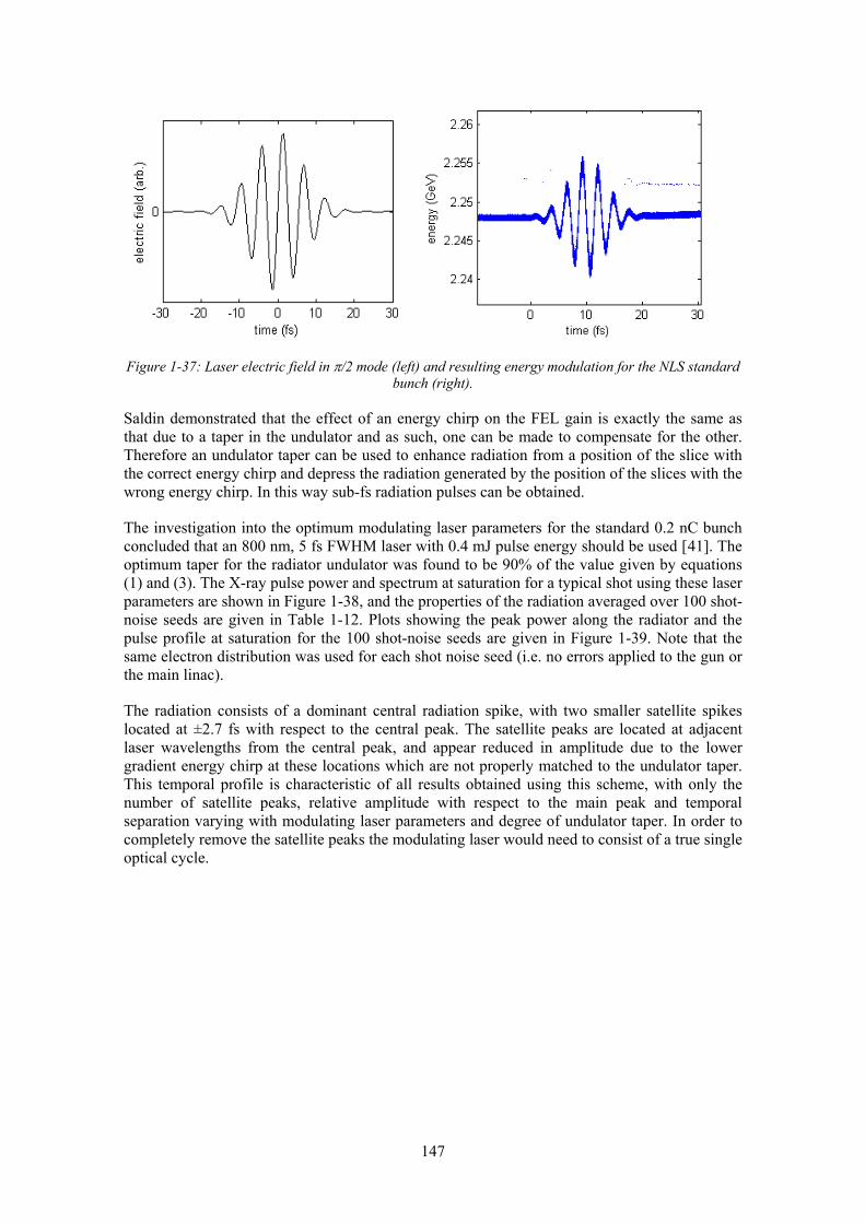
147

Figure 1-37: Laser electric field in π/2 mode (left) and resulting energy modulation for the NLS standard bunch (right).

Saldin demonstrated that the effect of an energy chirp on the FEL gain is exactly the same as that due to a taper in the undulator and as such, one can be made to compensate for the other. Therefore an undulator taper can be used to enhance radiation from a position of the slice with the correct energy chirp and depress the radiation generated by the position of the slices with the wrong energy chirp. In this way sub-fs radiation pulses can be obtained.

The investigation into the optimum modulating laser parameters for the standard 0.2 nC bunch concluded that an 800 nm, 5 fs FWHM laser with 0.4 mJ pulse energy should be used [41]. The optimum taper for the radiator undulator was found to be 90% of the value given by equations (1) and (3). The X-ray pulse power and spectrum at saturation for a typical shot using these laser parameters are shown in Figure 1-38, and the properties of the radiation averaged over 100 shot-noise seeds are given in Table 1-12. Plots showing the peak power along the radiator and the pulse profile at saturation for the 100 shot-noise seeds are given in Figure 1-39. Note that the same electron distribution was used for each shot noise seed (i.e. no errors applied to the gun or the main linac).

The radiation consists of a dominant central radiation spike, with two smaller satellite spikes located at ±2.7 fs with respect to the central peak. The satellite peaks are located at adjacent laser wavelengths from the central peak, and appear reduced in amplitude due to the lower gradient energy chirp at these locations which are not properly matched to the undulator taper. This temporal profile is characteristic of all results obtained using this scheme, with only the number of satellite peaks, relative amplitude with respect to the main peak and temporal separation varying with modulating laser parameters and degree of undulator taper. In order to completely remove the satellite peaks the modulating laser would need to consist of a true single optical cycle.

148

-8 -6 -4 -2 0 2 4 6 80

0.1

0.2

0.3

0.4

0.5

0.6

time (fs)

pow

er a

t sat

urat

ion

(GW

)

1.27 1.28 1.29 1.3 1.31 1.32 1.330

1000

2000

3000

4000

5000

6000

wavelength (nm)

spec

trum

at s

atur

atio

n (a

rb.)

Figure 1-38: Typical X-ray pulse power (left) and spectrum (right) at saturation assuming optimal laser and taper parameters.

Table 1-12: Summary of the FEL performance of the laser slicing scheme averaged over 100 seeds.

Parameter Mean Value RMS

Peak Power at Saturation (MW) 594 365

Average Power from Main Bunch (MW) 0.69 0.05

Pulse Energy in Central Peak (μJ) 0.35 0.25

Pulse FWHM (fs) 0.45 0.12

Pulse Line-Width (pm) 8.8 2.0

Time-Bandwidth Product 0.78 0.31

Contrast Ratio for Adjacent Spikes 11.6 11.3

Contrast Ratio to Main Bunch 870 542

Arrival Time Jitter (fs) - 0.06

0 5 10 15 20 25 30 35 40 4510-6

10-5

10-4

10-3

10-2

10-1

100

101

distance (m)

peak

pow

er (G

W)

-8 -6 -4 -2 0 2 4 6 80

0.5

1

1.5

time (fs)

pow

er a

t sat

urat

ion

(GW

)

Figure 1-39: X-ray pulse power along the undulator (left) and pulse profile spectrum (right) at saturation for 100 different shot-noise seeds. Dashed black lines show average values over the 100 seeds

1.5.3 Mode-Locked Amplifier FEL

In this scheme, described in some detail in [38], the electron bunch is repeatedly delayed with respect to the co-propagating radiation field using small magnetic chicanes. This synthesises a set of axial modes in the radiation field which are then phase-locked via a pre-applied energy

149

modulation along the electron bunch. This mechanism breaks down the FEL pulse into a train of evenly spaced spikes which in the XUV would have typical FWHM duration ~400 as and in the X-ray range are predicted to be as short as 24 as. Each spike is thus only a few optical cycles in duration yet the peak power is as high as could be obtained from a conventional FEL of the same electron beam parameters. The mode-locked FEL is thus the only short pulse FEL scheme predicted to generate few-cycle pulses of normal FEL intensity. Such a scheme, to operate at its best, requires short undulator modules of only a few periods each, interspersed with magnetic chicanes. Such a lattice structure is beyond the baseline design for NLS and therefore a mode-locked configuration would only be considered as a future development or upgrade. However, to test its feasibility for implementation simulations have been done in Genesis 1.3 using the full tracked electron bunch distribution. The resonant wavelength of the FEL is set to 12.4 nm (100 eV photon energy). Undulator modules of 8 periods are used and the slippage in the chicanes is set to 23 x λr (where λr is the resonant FEL wavelength). A sinusoidal electron energy modulation has been manually added to the tracked electron bunch distribution, with period equal to the total slippage in one undulator-chicane module, and amplitude of ±0.5%. The radiation power output close to saturation (49 undulator-chicane modules) is shown in Figure 1-40 for a ~200 fs region corresponding to the highest current region in the electron bunch. Peak powers of > 1 GW and pulse widths of 250 as FWHM (6 optical cycles) are predicted. The length of the pulse train is approximately that of the electron bunch. Methods of seeding the mode-locked FEL scheme to set the phase and envelope properties of the radiation output were proposed in [42], and could also be applied here. This preliminary study shows that the baseline NLS electron beam is capable of driving such an advanced FEL concept.

Figure 1-40: The results of time-dependent simulations of a mode-locked SASE FEL scheme operating at 100 eV photon energy, using the tracked electron bunch of Section 1.2, are shown near to saturation (49

undulator-chicane modules). Top left - longitudinal profile of the FEL radiation power, Bottom left - current profile of the simulated section of the electron bunch, Top right - detail of the radiation power

profile, Bottom right - electron beam energy in units of the electron rest mass energy.

150

1.6 Linac and FEL Operation with a High Repetition Rate Injector

It is intended that NLS will operate at a later stage at higher repetition rate and the possible options for the second stage injector are examined in Section 2.2. We choose for this preliminary investigation the most promising case, namely the superconducting RF gun, with an accelerating gradient of 50 MV/m. Despite being in its early stages, the optimization of the beam dynamics has produced an electron bunch with interesting quality. In particular, the transverse slice emittance is comparable with the one achieved in the Stage-1 normal conducting L-band gun, however at the expense of a significantly longer bunch length. We have performed preliminary studies using this bunch to check if the linac layout described so far is capable of compressing also this longer bunch with a sufficiently good control of the collective effects that it is suitable for driving the seeded FEL scheme.

The evolution of the phase space along the linac is reported in Figure 1-41 and the slice analysis of the bunch at the end of the spreader is reported in Figure 1-42. With the present preliminary optimization we obtain a flatness of the gain length within 20% over 200 fs. Despite the fact that this result is slightly worse than the corresponding one obtained for the nominal bunch (see Figures 1-5 and 1-6) it clearly shows that the bunch quality achieved with the second stage injector holds great promise for a successful seeded FEL operation.

Figure 1-41: Longitudinal phase space at different locations in the linac: top left - after the first accelerating module; top right - after BC1; bottom left - after BC3; bottom right - at the end of the

spreader.

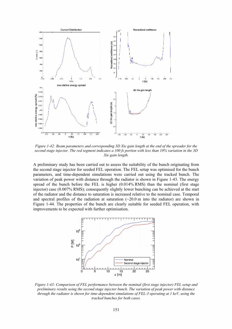
151

Figure 1-42: Beam parameters and corresponding 3D Xie gain length at the end of the spreader for the second stage injector. The red segment indicates a 100 fs portion with less than 10% variation in the 3D

Xie gain length.

A preliminary study has been carried out to assess the suitability of the bunch originating from the second stage injector for seeded FEL operation. The FEL setup was optimised for the bunch parameters, and time-dependent simulations were carried out using the tracked bunch. The variation of peak power with distance through the radiator is shown in Figure 1-43. The energy spread of the bunch before the FEL is higher (0.014% RMS) than the nominal (first stage injector) case (0.007% RMS); consequently slightly lower bunching can be achieved at the start of the radiator and the distance to saturation is increased relative to the nominal case. Temporal and spectral profiles of the radiation at saturation (~20.0 m into the radiator) are shown in Figure 1-44. The properties of the bunch are clearly suitable for seeded FEL operation, with improvements to be expected with further optimisation.

Figure 1-43: Comparison of FEL performance between the nominal (first stage injector) FEL setup and preliminary results using the second stage injector bunch. The variation of peak power with distance through the radiator is shown for time-dependent simulations of FEL-3 operating at 1 keV, using the

tracked bunches for both cases.

152

Power @20.0m

Spectrum @20.0m

Figure 1-44: Genesis 1.3 time-dependent simulation results for FEL-3 at 1 keV operating with the tracked second stage injector bunch. The left plot shows the longitudinal profile of the FEL radiation power at saturation (20.0m into the radiator) and the radiation spectrum at saturation is shown in the right plot

.

1.7 Long Wavelength Sources

A dramatic increase in radiation intensity occurs for wavelengths similar to and longer than the electron bunch, as the electrons in the bunch radiate coherently. For NLS, this will occur in the far infrared and THz regimes. Two complementary types of coherent long wavelength sources will be provided, broad-band coherent synchrotron radiation (CSR) from bending magnets and coherent undulator radiation (CUR) from long period undulators placed after each FEL.

The CSR flux as a function of wavelength is found from the single electron SR flux by multiplying by the form-factor of the electron bunch. The vertically integrated coherent flux is given by

)()( 2 λλ FNF eCSR Γ= (1-19)

where Ne is the number of electrons in the bunch and the vertically integrated flux F(λ) is usually given per horizontal mrad per 0.1% bandpass. The form factor Γ is the modulus squared of the Fourier Transform of the bunch profile, normalized to a value of 1 for infinitely long wavelength. F(λ) is found from (see for example [43])

( ) ydyKyyFy

′′= ∫∞

3/561023)( γα

π (1-20)

where y is the ratio of the critical wavelength to the required wavelength, K5/3 is a modified Bessel Function, α is the fine structure constant and γ the electron energy in terms of its rest mass.

A similar formula is used to estimate the energy in the central cone of an undulator

Γ= 2ecenCUR NEE (1-21)

where the energy radiated by a single electron into the central cone of undulator radiation Ecen can be approximated as [44]

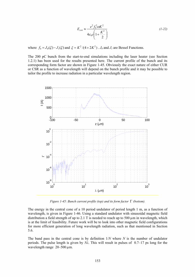
153

⎟⎟⎠

⎞⎜⎜⎝

⎛+

≈

214

2

0

222

Kc

KfeE bcen

ε

ω (1-22)

where )()( 10 ξξ JJfb −= and )24/( 22 KK +=ξ . J0 and J1 are Bessel Functions.

The 200 pC bunch from the start-to-end simulations including the laser heater (see Section 1.2.1) has been used for the results presented here. The current profile of the bunch and its corresponding form factor are shown in Figure 1-45. Obviously the exact nature of either CUR or CSR as a function of wavelength will depend on the bunch profile and it may be possible to tailor the profile to increase radiation in a particular wavelength region.

-100 -50 0 50 1000

500

1000

1500

z (μm)

I (A)

100

101

102

103

10-8

10-6

10-4

10-2

100

λ (μm)

Γ

Figure 1-45: Bunch current profile (top) and its form factor Γ (bottom).

The energy in the central cone of a 10 period undulator of period length 1 m, as a function of wavelength, is given in Figure 1-46. Using a standard undulator with sinusoidal magnetic field distribution a field strength of up to 2.1 T is needed to reach up to 500 μm in wavelength, which is at the limit of feasibility. Future work will be to look into other magnetic field configurations for more efficient generation of long wavelength radiation, such as that mentioned in Section 5.6.

The band pass in the central cone is by definition 1/N where N is the number of undulator periods. The pulse length is given by Nλ. This will result in pulses of 0.7–17 ps long for the wavelength range 20–500 μm.

154

100

101

102

103

10-4

10-3

10-2

10-1

100

101

102

λr (μm)

E CU

R (μ J

)

Figure 1-46: Energy ECUR in the central cone of a 10 period undulator of period length 1 m

CSR is generated at any bending magnet. However, the intensity of CSR increases with decreasing magnet strength, so it is preferable to insert special low field dipoles after the FELs to generate CSR. If we assume that these magnets should not be more than 2 m long and that we wish to extract 50 mrad horizontally, the minimum field is 0.1875 T; in the following we use a field strength of 0.2 T. Figure 1-47 gives the vertically integrated pulse energy per horizontal mrad per 0.1% bandpass as a function of wavelength. (Note that 0.1% bandpass is simply the standard unit for expressing spectral flux/energy, the uncertainty principle prevents small bandwidth being obtained for short pulses in this wavelength region).

Assuming 50 mrad can be extracted horizontally, the energy per pulse peaks at about 20 nJ/0.1%bw at a wavelengths around 150 μm. To compare with the pulse energy from the undulator, this is multiplied by a factor of 100 to allow for the different bandwidths, giving 2 μJ/pulse, an order of magnitude smaller than the pulse energy from the undulator at a similar wavelength.

155

100

101

102

103

10-4

10-3

10-2

10-1

100

λ (μm)

Puls

e En

ergy

(nJ/

mra

d/0.

1%bw

)

Figure 1-47: Energy per pulse, integrated over vertical angles, per mrad horizontal from a 0.2 T bending magnet.

The energy in the pulse integrated from 30–600 μm (0.5-10 THz) is given in Table 1-13 for two different vertical acceptance angles. The results show that a vertical acceptance angle of 30 mrad is sufficient to collect the majority of the flux. Integrating over 50 mrad horizontally would provide a pulse energy of over 30 μJ.

Table 1-13 also shows the flux integrated up to 1 cm in wavelength. The longest wavelength obtainable is however governed by the size of the vacuum vessel, and is given by [45]

ρλ bboffcut 2=− (1-23)

where b is the pipe diameter and ρ is the bending magnet radius. If we assume typical vessel dimensions of 2 cm, this would give a cut-off of wavelength of ~900 μm. To reach 1 cm wavelength would require a vessel of approximately 5 cm in dimension.

Table 1-13: Energy per pulse per horizontal mrad for different vertical apertures and different wavelength ranges.

Wavelength range (μm)

Vertically integrated (nJ/mrad)

50 mrad aperture (nJ/mrad)

30 mrad aperture (nJ/mrad)

30 - 600 640 640 610

30 - 10000 760 745 690

156

REFERENCES [1] FERMI@elettra Conceptual Design Report, Sincrotrone Trieste, 2007 [2] Borland, M., “elegant: a flexible SDDS compliant code for accelerator simulations”, APS report,

LS-287, ANL, Argonne, USA. [3] NLS Project: Science case & Outline Facility Design, STFC, UK, July 2009. [4] Saldin, E L., et al., Klystron instability of a relativistic electron beam in a bunch compressor NIM A

2002 490, 1-8 [5] M. Xie, “Design optimization for an X-Ray Free-Electron Laser driven by the SLAC LINAC”, PAC

1995, p. 183, (1995). [6] Giannakoglou, K., et al., “SPEA2: Improving the Strength Pareto Evolutionary Algorithm”,

Evolutionary Methods for Design, Optimization and Control [7] Bonifacio R., et al., Collective instabilities and high-gain regime in a free-electron laser Opt.

Commun., 1984. 50, 373-378 [8] Bonifacio R., et al., Spectrum, Temporal Structure, and Fluctuations in a High-Gain Free-Electron

Laser Starting from Noise, Phys. Rev. Lett., 1994. 73(1), 70-73 [9] O’Shea P. G. and Freund H. P., Laser technology – Free-electron lasers: Status and applications

Science, 2001. 292, 1853-1858 [10] Yu L. H. et al, High-Gain Harmonic Generation Free-Electron Laser, Science, 2000. 289, 932-934 [11] Werin, S, The Test FEL Facility at MAX-lab, Proceedings of the 31st International FEL Conference,

Liverpool, 2009 [12] Lambert G. et al, Injection of Harmonics Generated in Gas in a Free-Electron Laser Providing

Intense and Coherent Extreme-Ultraviolet Light, Nature Physics, 2008. 4, 296-300 [13] Allaria, E, The Second Stage of FERMI@Elettra: A seeded FEL in the Soft X-ray Spectral Range,

Proceedings of the 31st International FEL Conference, Liverpool, 2009 [14] Labat, M, Seeding Experiments at SPARC, Proceedings of the 31st International FEL Conference,

Liverpool, 2009 [15] Miltchev, V., Technical Design of the XUV Seeding Experiment at FLASH, Proceedings of the 31st

International FEL Conference, Liverpool, 2009 [16] Stupakov G, Using the beam-echo effect for generation of short-wavelength radiation Phys. Rev.

Lett. 2009 102, 074801 [17] Bonifacio R., et al., Generation of XUV Light by Resonant Frequency Tripling in a Two-Wiggler

FEL Amplifier, Nucl. Instrum. Methods in Phys. Res. A, 1990. 296, 787-790 [18] Ben-Zvi, I., et al., Proposed UV FEL user facility at BNL Nucl. Instrum. Methods in Phys. Res. A,

1991. 304, 181-186 [19] Yu, L H., Generation of intense UV-radiation by subharmonically seeded single-pass free-electron

lasers Phys. Rev. A, 1991. 44, 5178-5193 [20] Kramer D. et al, The BESSY Soft X-ray Free Electron Laser Technical Design Report, Berliner

Elektronenspeicherring-Gesellschaft für Synchrotronstrahlung m.b.H., 2004 [21] Ben-Zvi I., et al., The “fresh bunch” technique in FELs, Nucl. Instrum. Methods in Phys. Res. A,

1992. 318, 726-729 [22] Stupakov G., Beam Echo Effect for Generation of Short Wavelength Radiation, Proceedings of the

31st International FEL Conference, Liverpool, 2009 [23] Bisognano J. J., Conceptual Design Study and R&D for a VUV/Soft X-ray Free Electron Laser User

Facility, http://www.wifel.wisc.edu/WiFEL_R&D_Proposal.pdf, 2007 [24] McNeil B. W. J., et al., An XUV-FEL Amplifier Seeded Using High Harmonic Generation, New

Journal of Physics, 2007. 9, 82 [25] Saldin E. L., et al., Study of a noise degradation of amplification process in a multistage HGHG

FEL, Opt. Commun, 2002. 202, 169-187 [26] Kim, K.-J., 3-dimensional analysis of coherent amplification and self-amplified spontaneous

emission in free-electron lasers Phys. Rev. Lett., 1986. 57, 1871-1874 [27] Reiche S., GENESIS 1.3: afully 3D time dependent FEL simulation code Nucl. Instrum. Methods in

Phys. Res. A, 1999. 429, 243-248 [28] Emma P. et al., Femtosecond and Subfemtosecond X-ray Pulses from a Self-Amplified Spontaneous

Emission-Based Free-Electron Laser, Phys. Rev. Lett., 2004. 92, 074801. [29] Emma P. et al., Attosecond X-Ray Pulses in the LCLS Using the Slotted Foil Method, Proceedings of

FEL 2004, 2004. [30] Saldin E. L. et al., Terawatt-scale sub 10-fs Laser Technology – Key to Generation of GW-level

Attosecond Pulses in X-ray Free Electron Lasers, Opt. Comm., 2004, 237, 153-164.

157

REFERENCES [31] Saldin E. L. et al., A New Technique to Generate 100 GW-level Attosecond X-ray Pulses from the X-

ray SASE-FELs, Opt. Comm., 2004. 239, 161-172. [32] Penn G. and Zholents A. A., Techniques for the Generation of Attosecond X-ray Pulses Using an

FEL, LBNL-56726. [33] Zholents A. A. and Penn G., Obtaining Attosecond X-ray Pulses Using a SASE-FEL,

Phys. Rev. STAB, 8, 050704, (2004). [34] Zholents A. A. and Zolotorev M. S., Attosecond X-ray pulses produced by ultra short transverse

slicing via laser electron beam interaction, New Journal of Physics, 2008. 10, 025005. [35] Saldin E. L. et al., Self-amplified Spontaneous Emission FEL with Energy-Chirped Electron Beam

and its Application for the Generation of Attosecond Pulses, Phys. Rev. STAB, 2006. 9, 050702. [36] Fawley W. M, Use of few-cycle, optical energy modulation + undulator tapering to produce high

power, ultra-short FEL radiation pulses of soft X-ray and EUV wavelengths, FEL07 Frontiers, Elba Island, 2007.

[37] Rosenzweig J. et al., Generation of ultrashort high-brightness electron beams for single spike SASE FEL operation, Nucl. Inst. Meth. A, 2008. 593, 39

[38] Thompson N. R. and McNeil B. W. J, Mode-Locking in a Free Electron Laser Amplifier, Phys. Rev. Lett., 2008. 100, 203901.

[39] McNeil B. W. J. et al, Retention of Attosecond Pulse Structure in an HHG Seeded FEL Amplifier, Proceedings of the 30th International FEL Conference, Korea, 2008.

[40] D. Xiang et al., Generation of intense attosecond x-ray pulses using ultraviolet laser induced microbunching in electron beams, PRSTAB 12, 07070 (2009)

[41] Martin, I., “Short pulse radiation from energy-chirped electron bunches and tapered undulators: application to the NLS”, NLS-source-AP-REP-0007, May 2010

[42] Dunning D. J. et al, Start-To-End Simulations of SASE and HHG-Seeded Mode-Locked FEL, Proceedings of the 31st International FEL Conference, Liverpool, 2009

[43] Murphy J., Synchrotron Light Source Data Book, Version 4 (1996) [44] Geloni, G., at al., DESY-Report 03-031 (2003) [45] Murphy, J B., and S Krinsky, S., Millimeter-wave coherent synchrotron-radiation in the SXLS

phase-1 electron storage-ring. NIM A 1994 346 571-577.

159

2 Injector

The injector for the linac-based FEL must provide an electron beam of as high quality as possible because the normalized emittance cannot be improved during acceleration in the linac. A short bunch length before the main linac is also required because otherwise the beam is highly non-linear in the longitudinal phase space and difficult to be corrected by the high harmonic cavity. Minimization of the beam degradation due to space charge force is a critical issue for the generation of a small emittance beam. In a photocathode gun this can be achieved by increasing the accelerating field strength and optimising the laser pulse shape and size on the photocathode. The initial thermal emittance of the beam should also be minimized by proper choice of the photocathode material and the laser beam size at cathode. During beam transportation the phase space ellipses of the bunch slices should be aligned using a focusing system. The transverse emittance of the beam is frozen with further acceleration by the linac. For the 1st stage of the NSL facility, a FLASH/XFEL type injector based on a normal conducting L-band photocathode gun will be used for 1.1 kHz repetition operation. In the first part of this Chapter, the 1st stage injector will be described with beam dynamics simulation and technical issues. When the NLS facility is upgraded to higher repetition rate, eventually up to 1 MHz, we will need another type of injector. In the second part of this Chapter, possible options for the 2nd stage injector will be discussed. These two injectors will be housed in separate tunnels to allow the second one to be commissioned independently while the other one provides electron beams to the main linac.

2.1 Baseline Injector

The baseline injector will generate electron beams at a repetition rate of 1.1 kHz. This injector has the same layout as the FLASH/XFEL injector [1], consisting of a normal conducting gun and superconducting cavities, however the gun has been modified for high repetition rate operation. The NLS baseline gun will have a duty factor of 1.65%, which is higher than the European XFEL gun, 0.7%. The accelerating field of the NLS gun will therefore be lower than the European XFEL gun, 50 MV/m rather than 60 MV/m. The cell length of the gun cavity was optimized for low emittance beam generation for the lower RF field. The cooling water channels have also been improved for higher cooling capacity.

2.1.1 Layout

The proposed layout of the gun section is shown in Figure 2-1. The 1.5 cell gun cavity will operate at 1.3 GHz (L-band) resonant frequency. The RF power for electron beam acceleration will be fed through a coaxial coupler. With the coaxial coupler, the RF field in the gun cavity is perfectly axisymmetric and therefore no dipole or quadrupole component of the RF field exists. The coaxial coupler also allows an axisymmetric water-cooling channel distribution around the outer tube of the gun cavity and so the cavity deformation caused by RF power dissipation is also axisymmetric. At the back wall of the gun cavity a cathode slot will be located so that photocathodes are easily exchangeable as for the PITZ guns (see Figure 2-5).

A laser pulse for electron beam generation by photoemission will be guided by a mirror located inside the vacuum tube after the RF coupler. The incident angle of the laser to the cathode is about 1°. A main focusing solenoid keeps the beam emittance so that the beam slices are aligned in the transverse phase space. A bucking solenoid has a magnetic field which opposes the field configured by the main solenoid and makes the magnetic field zero at the cathode. Otherwise, an electron beam may have an angular momentum and the emittance increases. Three sets of steering magnets will be installed, each correcting in both the horizontal and vertical directions. To eliminate dark current from the gun section, collimators will be used. In the second diagnostic cross, three collimators will be installed in one actuator, with different opening diameters for different bunch charge operation. As discussed in Section 2.1.5 the optimum

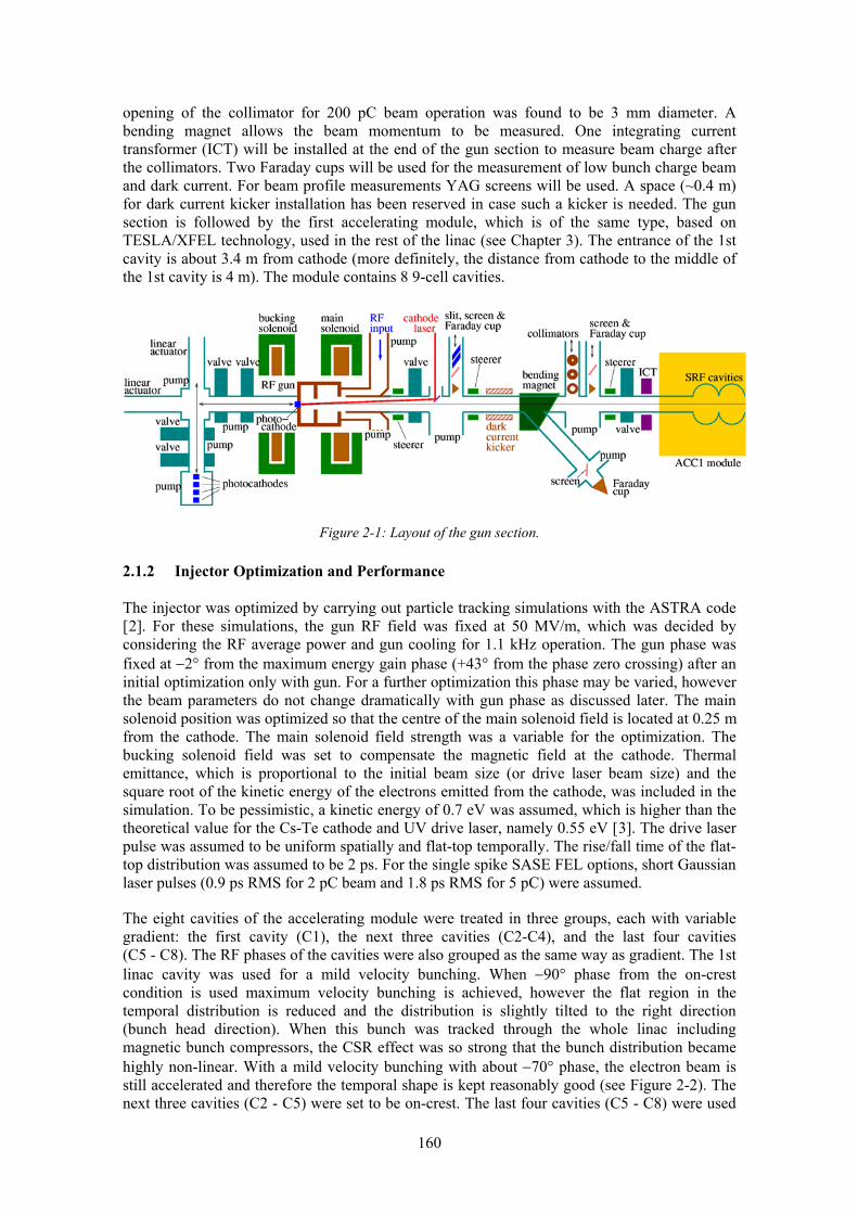
160

opening of the collimator for 200 pC beam operation was found to be 3 mm diameter. A bending magnet allows the beam momentum to be measured. One integrating current transformer (ICT) will be installed at the end of the gun section to measure beam charge after the collimators. Two Faraday cups will be used for the measurement of low bunch charge beam and dark current. For beam profile measurements YAG screens will be used. A space (~0.4 m) for dark current kicker installation has been reserved in case such a kicker is needed. The gun section is followed by the first accelerating module, which is of the same type, based on TESLA/XFEL technology, used in the rest of the linac (see Chapter 3). The entrance of the 1st cavity is about 3.4 m from cathode (more definitely, the distance from cathode to the middle of the 1st cavity is 4 m). The module contains 8 9-cell cavities.

Figure 2-1: Layout of the gun section.

2.1.2 Injector Optimization and Performance

The injector was optimized by carrying out particle tracking simulations with the ASTRA code [2]. For these simulations, the gun RF field was fixed at 50 MV/m, which was decided by considering the RF average power and gun cooling for 1.1 kHz operation. The gun phase was fixed at −2° from the maximum energy gain phase (+43° from the phase zero crossing) after an initial optimization only with gun. For a further optimization this phase may be varied, however the beam parameters do not change dramatically with gun phase as discussed later. The main solenoid position was optimized so that the centre of the main solenoid field is located at 0.25 m from the cathode. The main solenoid field strength was a variable for the optimization. The bucking solenoid field was set to compensate the magnetic field at the cathode. Thermal emittance, which is proportional to the initial beam size (or drive laser beam size) and the square root of the kinetic energy of the electrons emitted from the cathode, was included in the simulation. To be pessimistic, a kinetic energy of 0.7 eV was assumed, which is higher than the theoretical value for the Cs-Te cathode and UV drive laser, namely 0.55 eV [3]. The drive laser pulse was assumed to be uniform spatially and flat-top temporally. The rise/fall time of the flat-top distribution was assumed to be 2 ps. For the single spike SASE FEL options, short Gaussian laser pulses (0.9 ps RMS for 2 pC beam and 1.8 ps RMS for 5 pC) were assumed.

The eight cavities of the accelerating module were treated in three groups, each with variable gradient: the first cavity (C1), the next three cavities (C2-C4), and the last four cavities (C5 - C8). The RF phases of the cavities were also grouped as the same way as gradient. The 1st linac cavity was used for a mild velocity bunching. When −90° phase from the on-crest condition is used maximum velocity bunching is achieved, however the flat region in the temporal distribution is reduced and the distribution is slightly tilted to the right direction (bunch head direction). When this bunch was tracked through the whole linac including magnetic bunch compressors, the CSR effect was so strong that the bunch distribution became highly non-linear. With a mild velocity bunching with about −70° phase, the electron beam is still accelerated and therefore the temporal shape is kept reasonably good (see Figure 2-2). The next three cavities (C2 - C5) were set to be on-crest. The last four cavities (C5 - C8) were used

161

for compensating the energy chirp of the beam so that the beam would not suffer from the beam distortion in the horizontal direction caused by the dispersion in the injector merger.

The evolution of the beam size and normalized transverse emittance for the 50 pC and 200 pC cases is shown in Figure 2-3. The slice emittances are flat over a large region of the bunch (Figure 2-4), which is beneficial for lasing performance as well as stability. The injector optimization for bunch charges of 2 pC to 200 pC is summarized in Table 2-1. The beam parameters in the Table show the simulation results at 15 m from cathode, at the end of the 1st linac module. Final beam parameter optimization should however be carried out experimentally when the proposed injector is built and commissioned.

Figure 2-2: The temporal distributions of 200 pC beam at 15 m. The new optimized bunch distribution is compared with what was reported in the NLS Outline Facility Design and the case of the maximum

velocity bunching (VB) with −90° from the on-crest.

Figure 2-3: Transverse beam size and normalized emittance evolution of 50 pC and 200 pC beams.

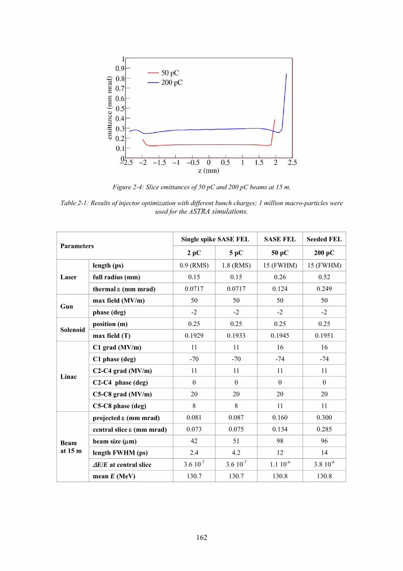
162

Figure 2-4: Slice emittances of 50 pC and 200 pC beams at 15 m.

Table 2-1: Results of injector optimization with different bunch charges; 1 million macro-particles were used for the ASTRA simulations.

Parameters Single spike SASE FEL SASE FEL Seeded FEL

2 pC 5 pC 50 pC 200 pC

Laser

length (ps) 0.9 (RMS) 1.8 (RMS) 15 (FWHM) 15 (FWHM)

full radius (mm) 0.15 0.15 0.26 0.52

thermal ε (mm mrad) 0.0717 0.0717 0.124 0.249

Gun max field (MV/m) 50 50 50 50

phase (deg) -2 -2 -2 -2

Solenoid position (m) 0.25 0.25 0.25 0.25

max field (T) 0.1929 0.1933 0.1945 0.1951

Linac

C1 grad (MV/m) 11 11 16 16

C1 phase (deg) -70 -70 -74 -74

C2-C4 grad (MV/m) 11 11 11 11

C2-C4 phase (deg) 0 0 0 0

C5-C8 grad (MV/m) 20 20 20 20

C5-C8 phase (deg) 8 8 11 11

Beam at 15 m

projected ε (mm mrad) 0.081 0.087 0.160 0.300

central slice ε (mm mrad) 0.073 0.075 0.134 0.285

beam size (μm) 42 51 98 96

length FWHM (ps) 2.4 4.2 12 14

ΔE/E at central slice 3.6 10-7 3.6 10-7 1.1 10-6 3.8 10-6

mean E (MeV) 130.7 130.7 130.8 130.8

163

2.1.3 Engineering Issues

2.1.3.1 RF Gun Cooling

The main cavity body will be made from oxygen-free high conductivity (OFHC) copper. The heat generated in the cavity due to the RF operation should be cooled by water in order to keep the cavity on resonance at 1.3 GHz. For 50 MV/m accelerating field at cathode, the gun must operate with 4.6 MW peak power. With a 15 μs pulse length and 1.1 kHz repetition rate the cavity will therefore operate with an average RF power of about 77 kW. This is higher than demonstrated at PITZ, 50 kW [4] with 7.2 MW peak power, 0.7 ms pulse length, and 10 Hz repetition rate. For the cooling of this high average power, an improvement of cooling water channel was made (see Figure 2-5). The cooling channels in the central iris and the cylindrical surface are the same as the PITZ gun4 [4], but the channels in both the end walls are improved to have the same channel shape as the central iris for higher cooling capacity.

(a) (b)

Figure 2-5: Gun cavity geometry and cooling-water channels. A section of cavity geometry (a) and cooling water channels in the central iris and both the end walls (b). Dark red - OFHC copper, pale

green – molybdenum, bright grey - stainless steel.

The RF power dissipation at the cavity inner surface was calculated with SUPERFISH [5]. For higher inner surface temperature, the conductivity decreases and the cavity quality factor also decreases by a few percent. In this case we need more RF power for a certain accelerating field and more power dissipates into the cavity inner surface (Table 2-2). For the cavity thermal analysis, an inner surface temperature of 60°C was assumed.

Table 2-2: The cavity temperature, the quality factor and the RF power required for 50 MV/m at cathode.

Temperature 20°C 30°C 40°C 50°C 60°C 70°C 80°C

Q 22965 22527 22113 21720 21348 21019 20682

Power (MW) 4.292 4.376 4.458 4.538 4.617 4.686 4.762

Temperature distributions were calculated numerically using ANSYS [6]. The cooling water temperature was set to be 30°C and the water speed through the channel was 2 m/s. Without RF power, the cavity temperature would be 30°C. The analysis shows a maximum temperature up to about 74°C, or 44°C rise from the water temperature, when 77 kW average RF power is applied (Figure 2-6). The extra temperature rise occurring during an RF pulse was also calculated with ANSYS. Simulations show that during the pulse a maximum temperature rise of

164

about 1.6°C takes place at the hottest area in the centre iris, which is sufficiently small not to produce material fatigue.

Figure 2-6: Temperature distribution over the cavity for 77 kW average RF power.

For gun RF phase stability within ± 0.35° peak-to-peak, the gun temperature must be controlled within ± 0.01°C [7]. For the temperature control, temperature sensors will be mounted in the cavity iris; holes for sensor installation are shown in Figure 2-6. A dedicated water cooling system with an accurate flow rate control of cold and warm water will be needed.

2.1.3.2 RF Source

A modulator which fully satisfies the NLS gun requirements is not currently available “off-the-shelf”. However, various combinations of the required peak power, repetition rate, and pulse length have been demonstrated using modern solid state modulators and at least three commercial companies have indicated their readiness to provide a modulator with the full NLS specification. The Thales TH 2104U klystron [8] fully satisfies the requirements of the peak RF power, average RF power and pulse length. The RF power will be transferred through one RF window into the gun cavity. The forward and reflected power will be monitored for the low level RF (LLRF) control. State-of-the-art performance is represented by what has been achieved at FLASH, namely 0.1% RMS in amplitude and 0.1 degree RMS in phase [1]. Beam dynamics simulations have been performed to determine the effect of such errors on the electron beam parameters and what tolerances would be needed. The result is discussed in Section 2.1.4. Simulation results indicate that gun RF errors of 0.1% RMS in amplitude and 0.1 degree RMS in phase would not affect beam parameters significantly.

2.1.3.3 Photocathode and Drive Laser

As a photocathode material either a metal or Cs-Te can be used. For 1.1 kHz operation a metal cathode would provide enough bunch charge (200 pC) with a commercially available laser system. However, Cs-Te allows more flexibility for higher repetition rate operation which will be discussed in Section 2.1.6. This material has shown a quantum efficiency (QE) higher than 1% for several months at FLASH and for several weeks at PITZ [9]. For the preservation of a good QE, the vacuum in the gun should be below 10-9 mbar. The thermal emittance of Cs2Te

165

was reported to be about 1 mm mrad for a laser beam size of 1 mm RMS [10] and this value was included in the simulations presented in Section 2.1.2. The response time of this cathode is about 0.1 ps [11], which is fast enough compared to the laser pulse length and rise/fall time (2 ps).

To generate an electron beam, a UV laser pulse of about 265 nm wavelength should be used for reasonably high cathode QE and low thermal emittance. Assuming 1% QE, a laser energy of 0.1 μJ will be needed for 200 pC beam generation. A requirement for low emittance is that the laser pulse should be uniform in the transverse direction and have flat-top temporal distribution. Such laser parameters are readily achievable (Section 10.1).

2.1.4 Effect of Errors

Misalignment of the accelerator components and jitter in machine parameters (laser, RF and solenoid field strength) may impair injector performance and so stable FEL operation requires that such errors are maintained within certain ranges. In this Section, we study the effect of such errors by means of ASTRA simulations and determine the required stability tolerances.

In photocathode RF guns, the cathode laser is a possible error source. At FLASH, the bunch charge drift was measured to be about 1% [1], which comes mainly from a variation in laser pulse energy of the same amount. Laser pulse arrival time jitter at the cathode and RF phase jitter, which together produce beam launch phase jitter, can also affect bunch charge however for achievable tolerances this is a much smaller effect. Simulations show that a variation of bunch charge by 1% increases the transverse emittance by only 0.1% (Table 2-3). For the minimization of transverse emittance degradation caused by space charge force, a flat-top laser pulse shape will be used for electron beam generation as discussed in Section 2.1.2. In practice, about 1-2% error in the rise/fall time of the temporal flat-top distribution and about 1% error in the laser pulse length are expected (see Chapter 10). However, even 10% error in the rise/fall time and 5% error in the pulse length will not affect the beam parameters significantly (Table 2-3). Errors in laser spot position and laser beam radius at the cathode do not affect the beam parameters. However, the beam position at the end of the injector would change with laser spot position jitter at the cathode (Table 2-4). Since the RMS beam size at the end of the injector is 96 μm, the laser spot position should be stabilized within 10 μm at the cathode in order for the beam position change to be smaller than one third of the beam size.

For calculating the thermal emittance in ASTRA, a kinetic energy of the emitted electrons of 0.7 eV was assumed, which includes a possible potential barrier decrease mainly caused by the RF field in addition to the theoretical value, 0.55 eV [3], without an external field. Table 2.1 shows that if the thermal emittance is higher, the total beam emittance increases by roughly the same factor.

Errors such as the main solenoid field and the gradient and phase of the gun and the 1st cavity of the first linac module would not affect the transverse emittance and bunch length of the beam as summarized in Table 2-3. Other cavities in the first linac module may not affect the beam performance even if the error range is about 20%. However, the beam arrival time, which is of critical importance for seeded lasing, is sensitively influenced by such jitters as discussed in Chapter 1.

166

Table 2-3: Effect of individual errors on the beam parameters at the end of the injector for the 200 pC case. Numbers in brackets indicate the nominal settings about which the parameter is varied.

Error source Error range εx change εy change length change

Laser

length (15 ps)

−5% +0.5% +0.4% −2.2% +5% −0.1% −0.1% 2.3%

rise/fall time (2 ps)

−10% −1.2% −1.2% −0.2% +10% +1.5% +1.3% 0.2%

position, Δx +30 μm 0.0% 0.0% 0.0% +50 μm 0.0% +0.1% 0.0% +100 μm 0.0% +0.4% 0.0%

bunch charge (200 pC)

−2% −0.2% −0.2% −0.6% −1% −0.1% −0.1% −0.3% +1% +0.1% +0.1% +0.3% +2% +0.2% +0.2% +0.6%

beam radius (0.52 mm)

−0.04 mm −6.3% −6.2% +2.6% −0.02 mm −3.3% −3.2% +1.2% +0.02 mm +3.6% +3.6% −1.0% +0.04 mm +7.8% +7.6% −2.0%

thermal ε (0.2485 mm mrad)

10% +7.6% +7.6% 0.0% 20% +17.8% +17.8% 0.0% 50% +32.7% +32.8% 0.0% 100% +79.3% +79.3% −0.1%

Solenoid max field (0.1951 T)

−0.02% 0.0% 0.0% 0.0% −0.01% 0.0% 0.0% 0.0% 0.01% 0.0% 0.0% 0.0% 0.02% 0.0% 0.0% 0.0%

Gun

phase (43° from phase zero crossing)

−0.2° +0.4% +0.4% −0.2% −0.1° +0.2% +0.2% −0.1% 0.1° −0.2% −0.2% +0.1% 0.2° −0.3% −0.3% +0.3%

peak field at cathode (50 MV/m)

−0.2% +2.1% +2.1% +0.1% −0.1% +0.5% +0.5% +0.1% +0.1% +0.4% +0.4% 0.0% +0.2% +1.5% +1.5% 0.0%

ACC01 Cavity1

phase (−76° from on crest)

−0.2° 0.0% 0.0% −0.3% −0.1° 0.0% 0.0% −0.1% 0.1° 0.0% 0.0% +0.1% 0.2° 0.0% 0.0% +0.3%

gradient (16 MV/m)

−0.2% 0.0% 0.0% +0.1% −0.1% 0.0% 0.0% 0.0% +0.1% 0.0% 0.0% 0.0% +0.2% +0.1% +0.1% 0.0%

167

Table 2-4: Variation in beam position at the end of the injector due to laser spot position drift at cathode.

Laser position, Δx Δx change Δy change +10 μm +10 μm +31 μm +30 μm +29 μm +94 μm +50 μm +49 μm +157 μm +100 μm +100 μm +313 μm

Alignment errors of the accelerator components may also affect the injector performance. Possible beam parameter changes caused by such errors have been studied with ASTRA simulations for the 200 pC case. The strongest beam parameter changes result from misalignment of the main solenoid. As summarized in Table 2-5, 100 μm transverse misalignment of the main solenoid would increase the transverse emittance by about 1%. For larger misalignments beam degradation as well as the beam position shift are significant. The main solenoid should therefore be carefully aligned to the beam by using a remotely controllable micro-mover [12] to within ±0.1 mm. Angular misalignments did not increase the transverse emittance or bunch length, but the transverse position of the beam was shifted. If the solenoid field does not drift, this can be corrected by steering magnets. However, if there is a magnetic field drift, possibly from the power supply, the beam position at the end of injector may drift transversely. Therefore, the angular misalignment should be corrected by the same procedure using the micro-mover within ±0.1 mrad. Longitudinal position errors of the main solenoid by 1 mm would increase the emittance by only 1%, which in fact can be recovered by a retuning of the solenoid field. In summary, these beam degradations are not at the level that might affect the FEL performance assuming beam-based alignment is performed. No effect on the temporal bunch profile was observed.

Table 2-5: Transverse emittance change due to gun main solenoid alignment errors.

Error source Error range εx change εy change Beam position, Δx

Beam position, Δy

position, Δx +20 μm +0.1% 0.0% −88 μm −143 μm +50 μm +0.3% +0.1% −217 μm −356 μm +100 μm +1.1% +0.5% −435 μm −714 μm +200 μm +4.0% +21.9% −868 μm −1428 μm

angle, Δθx +50 μrad +0.1% +0.1% −81 μm +115 μm +100 μrad +0.3% +0.5% −162 μm +130 μm +200 μrad +1.1% +2.0% −325 μm +459 μm

position, Δz −1 mm +0.9% +0.9% 0 μm 0 μm +1 mm +1.1% +1.1% 0 μm 0 μm

In summary, jitter in laser parameters will not affect the beam parameters except the beam position caused by laser position jitter at the cathode, which should be minimized by careful design of the laser beamline including temperature regulation. Since the injector beam dynamics has been tightly optimized, any thermal emittance increase will result in a transverse emittance increase. The most likely cause of thermal emittance increase is due to roughness of the cathode surface [13] which can be minimised by paying attention to the roughness of the substrate and the cathode deposition process. No serious beam quality degradation is expected from jitter in the RF parameters of the gun and the first linac module. A precise RF regulation is however

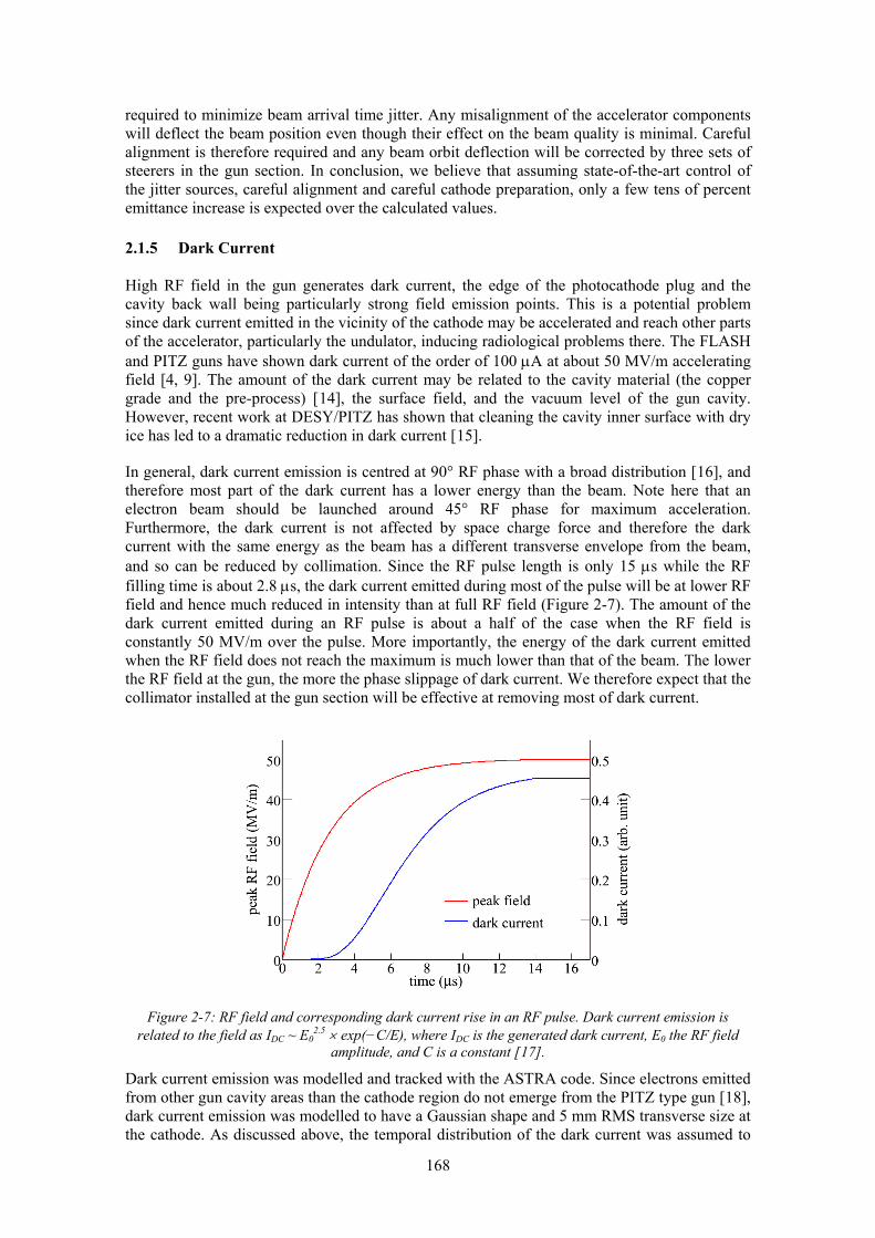
168

required to minimize beam arrival time jitter. Any misalignment of the accelerator components will deflect the beam position even though their effect on the beam quality is minimal. Careful alignment is therefore required and any beam orbit deflection will be corrected by three sets of steerers in the gun section. In conclusion, we believe that assuming state-of-the-art control of the jitter sources, careful alignment and careful cathode preparation, only a few tens of percent emittance increase is expected over the calculated values.

2.1.5 Dark Current

High RF field in the gun generates dark current, the edge of the photocathode plug and the cavity back wall being particularly strong field emission points. This is a potential problem since dark current emitted in the vicinity of the cathode may be accelerated and reach other parts of the accelerator, particularly the undulator, inducing radiological problems there. The FLASH and PITZ guns have shown dark current of the order of 100 μA at about 50 MV/m accelerating field [4, 9]. The amount of the dark current may be related to the cavity material (the copper grade and the pre-process) [14], the surface field, and the vacuum level of the gun cavity. However, recent work at DESY/PITZ has shown that cleaning the cavity inner surface with dry ice has led to a dramatic reduction in dark current [15].

In general, dark current emission is centred at 90° RF phase with a broad distribution [16], and therefore most part of the dark current has a lower energy than the beam. Note here that an electron beam should be launched around 45° RF phase for maximum acceleration. Furthermore, the dark current is not affected by space charge force and therefore the dark current with the same energy as the beam has a different transverse envelope from the beam, and so can be reduced by collimation. Since the RF pulse length is only 15 μs while the RF filling time is about 2.8 μs, the dark current emitted during most of the pulse will be at lower RF field and hence much reduced in intensity than at full RF field (Figure 2-7). The amount of the dark current emitted during an RF pulse is about a half of the case when the RF field is constantly 50 MV/m over the pulse. More importantly, the energy of the dark current emitted when the RF field does not reach the maximum is much lower than that of the beam. The lower the RF field at the gun, the more the phase slippage of dark current. We therefore expect that the collimator installed at the gun section will be effective at removing most of dark current.

Figure 2-7: RF field and corresponding dark current rise in an RF pulse. Dark current emission is related to the field as IDC ~ E0

2.5 × exp(−C/E), where IDC is the generated dark current, E0 the RF field amplitude, and C is a constant [17].

Dark current emission was modelled and tracked with the ASTRA code. Since electrons emitted from other gun cavity areas than the cathode region do not emerge from the PITZ type gun [18], dark current emission was modelled to have a Gaussian shape and 5 mm RMS transverse size at the cathode. As discussed above, the temporal distribution of the dark current was assumed to

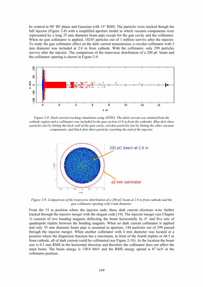
169

be centred at 90° RF phase and Gaussian with 15° RMS. The particles were tracked though the full injector (Figure 2-8) with a simplified aperture model in which vacuum components were represented by a long 35 mm diameter beam pipe except for the gun cavity and the collimator. When no gun collimator is applied, 10243 particles out of 1 million survive after the injector. To study the gun collimator effect on the dark current transmission, a circular collimator with 3 mm diameter was included at 2.8 m from cathode. With the collimator, only 299 particles survive after the injector. The comparison of the transverse distribution of a 200 pC beam and the collimator opening is shown in Figure 2-9.

Figure 2-8: Dark current tracking simulation using ASTRA. The dark current was emitted from the cathode region and a collimator was included in the gun section (2.8 m from the cathode). Blue dots show particles lost by hitting the back wall of the gun cavity, red dots particles lost by hitting the other vacuum

components, and black dots show particles reaching the end of the injector.

Figure 2-9: Comparison of the transverse distribution of a 200 pC beam at 2.8 m from cathode and the gun collimator opening with 3 mm diameter.

From the 15 m position where the injector ends, these dark current electrons were further tracked through the injector merger with the elegant code [19]. The injector merger (see Chapter 1) consists of two bending magnets deflecting the beam horizontally by 6° and five sets of quadrupole triplets between the bending magnets. When no dark current collimator is applied and only 35 mm diameter beam pipe is assumed as aperture, 144 particles out of 299 passed through the injector merger. When another collimator with 4 mm diameter was located at a position where the dispersion function has a maximum, in front of the fourth triplets or 48.5 m from cathode, all of dark current could be collimated (see Figure 2-10). At the location the beam size is 0.3 mm RMS in the horizontal direction and therefore the collimator does not affect the main beam. The beam energy is 130.8 MeV and the RMS energy spread is 87 keV at the collimator position.

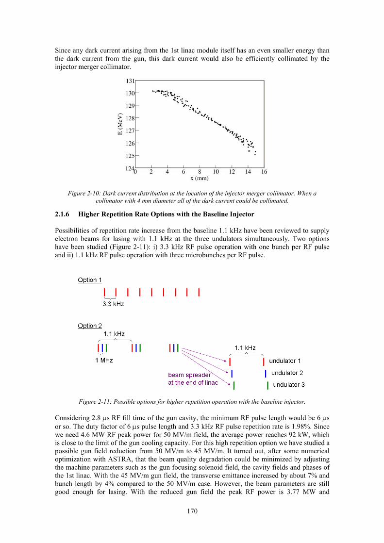
170

Since any dark current arising from the 1st linac module itself has an even smaller energy than the dark current from the gun, this dark current would also be efficiently collimated by the injector merger collimator.

Figure 2-10: Dark current distribution at the location of the injector merger collimator. When a collimator with 4 mm diameter all of the dark current could be collimated.

2.1.6 Higher Repetition Rate Options with the Baseline Injector

Possibilities of repetition rate increase from the baseline 1.1 kHz have been reviewed to supply electron beams for lasing with 1.1 kHz at the three undulators simultaneously. Two options have been studied (Figure 2-11): i) 3.3 kHz RF pulse operation with one bunch per RF pulse and ii) 1.1 kHz RF pulse operation with three microbunches per RF pulse.

Figure 2-11: Possible options for higher repetition operation with the baseline injector.

Considering 2.8 μs RF fill time of the gun cavity, the minimum RF pulse length would be 6 μs or so. The duty factor of 6 μs pulse length and 3.3 kHz RF pulse repetition rate is 1.98%. Since we need 4.6 MW RF peak power for 50 MV/m field, the average power reaches 92 kW, which is close to the limit of the gun cooling capacity. For this high repetition option we have studied a possible gun field reduction from 50 MV/m to 45 MV/m. It turned out, after some numerical optimization with ASTRA, that the beam quality degradation could be minimized by adjusting the machine parameters such as the gun focusing solenoid field, the cavity fields and phases of the 1st linac. With the 45 MV/m gun field, the transverse emittance increased by about 7% and bunch length by 4% compared to the 50 MV/m case. However, the beam parameters are still good enough for lasing. With the reduced gun field the peak RF power is 3.77 MW and

171

therefore the average RF power becomes 75 kW which is an acceptable level according to the gun heating simulation discussed above.

The second option, three microbunches with 1.1 kHz RF pulse repetition rate, would be achieved by increasing the pulse length only by twice of the microbunch spacing: If we assume 1 μs microbunching spacing, the pulse length should be about 17 μs instead of the originally assumed 15 μs. Then, the average RF power would be 87 kW. When the gun field is reduced from 50 MV/m to 45 MV/m, the average power is 71 kW. Technically, this second option is preferred from the gun point of view, because there is no high voltage pulse modulator available for 3.3 kHz at present. Distributing the three bunches to different FELs will however be more challenging, and will require the same fast rise- and fall-time kickers in the spreader that will be needed when the high repetition rate injector is brought on-steam. When Cs-Te cathodes are used, there will be no technical issue on the drive laser for either of the high repetition rate options (see Chapter 10).

2.2 High Repetition Rate Injector Options

2.2.1 Concepts for the NLS High Repetition Rate Injector

To go beyond the baseline design of 1 kHz repetition rate, eventually up to 1 MHz, will require a different type of injector. To provide a normalised emittance lower than 1 mm mrad in combination with high average current demands an injection system that is beyond the current state-of-the-art. Several laboratories are concentrating their efforts on the development of similar injection systems, though not all of them are designed for FEL applications. They utilise different approaches and technology and are at different stages of realisation.

The beam quality delivered from an electron injector is essentially defined by the gun where emitted electrons are accelerated to an energy of hundreds of keV or several MeV. To deliver a beam with small emittance, the main criterion is the electric field applied to the photocathode surface in the gun. The value of the cathode field, E, required for a bunch with charge, q, to achieve a minimum emittance, εmin, is defined by [20]

22min0

14 cm

TkqEe

B ⊥=επε

(2-1)

where ⊥TkB is the initial thermal energy. For the nominal NLS bunch charge of 200 pC, thermal energy of 0.7 eV, and a desired emittance of 0.5 mm mrad, this gives E as 9.85 MV/m. The requirements of high repetition rate demands that this field should be applied to the gun accelerating gap permanently or with a frequency of at least 1 MHz. RF guns are preferable as the time of application of maximum field is relatively small, resulting in significantly less parasitic field emission.

High repetition rate thermionic cathode based injectors have traditionally been used in IR FELs and successfully operate at high repetition rate in CW mode. They are simple to operate, do not require extra high vacuum conditions, the cathodes are very robust and have long operational lifetime. For example, the ELBE FEL injector delivers 1 mA average current through 77 pC bunches at a repetition rate of 13 MHz [21]. The major problems of applying thermionic cathodes in high brightness injectors for X-ray FELs are linked with their low emission density of 1-2 A/cm2 and difficulties in obtaining individual short beam pulses from the cathode. It is therefore necessary to generate relatively long beam pulses followed by a complicated bunch compression system. Traditional injection schemes with large diameter thermionic cathodes suffer from a significant increase of beam emittance following compression up to dozens of mm·mrad. Recent developments at SCSS in thermionic gun design in combination with a multistage bunch compression scheme have achieved an emittance of 0.6 mm·mrad although at a low repetition rate [22]. Further research of thermionic emitter based injectors towards

172

increasing their repetition rate is being carried out at Argonne National Laboratory [23]. Since this research is still in the initial stage, a high brightness, high repetition rate thermionic cathode based injector has currently been ruled out as serious candidate for the NLS injector.

Photocathode based electron guns are most popular in the FEL community. They are able to deliver high charge in very short pulses, which are relatively easily controllable through laser systems and may be implemented into both DC and RF accelerator environments. Two groups of photocathodes are used – metallic and semiconductors. Metallic photocathodes are very fast, very robust, do not require extra-high vacuum conditions and operate for a long time. However they have low quantum efficiency (QE, ratio of the number of emitted electrons to the number of incident photons), typically 10-5-10-3 and require an ultra-violet (UV) drive laser, typically 266 nm, which is limited to 1 W maximum average power. Although metallic photocathodes hold the world record for the emittance achieved so far the maximum average current achievable with metallic photocathodes only lies in the µA-region so rules out their usage in the NLS injector.

The second group of photocathodes which we consider here are alkali semiconductor photocathodes. Of them tellurium based Cs2Te is very popular. It has demonstrated a relatively high QE of 1-10% at a wavelength of 266 nm. The high robustness of Cs2Te allows it to be used in L-band and S-band pulsed RF guns. It is also used in the DC stage of combined DC-SRF gun at Peking University [24]. Cs2Te has demonstrated good performance in the PITZ [25] and FLASH [26] projects. At PITZ the photocathode delivers 1 nC bunches with a repetition rate of 1 MHz in relatively long 700 µs trains.

Another group of alkali photocathodes are antimonite based photocathodes such as Cs3Sb and K2CsSb. They have been used for years in photomultiplier tubes and vacuum photodiodes and have demonstrated exceptional QE of 15-20% in the visible range so may be operated at a wavelength of 532 nm. K2CsSb was used in the “Boeing gun” – a high duty factor electron injector that demonstrated the record average current extracted from the photocathode so far – 32 mA [27]. Unfortunately, antimonite based photocathodes are not widely used in accelerator injectors due to a complicated production and relatively low robustness. The modes of their degradation and maximum extracted charge are also not very well understood. These photocathodes are planned for use in the LBNL NCRF gun [28], BNL SRF gun [29] and other projects, where average currents of 1 mA or more are required. For NLS, where the requirement is only 0.2 mA (200 pC bunch charge at 1 MHz) Cs2Te is the photocathode of choice.

Three options of high repetition rate injectors based on photocathode guns were previously under consideration [ODR]- a high voltage DC gun, a superconducting L-band RF gun and a normal conducting VHF gun. Since a DC gun cannot achieve the required emittance due to the low cathode field strength of < 5 MV/m, we are no longer considering this option. In the following therefore we present schemes for VHF and SRF guns including new results of beam dynamics simulations. The VHF gun delivers relatively low energy (750 keV) beams and features a relatively high emittance in comparison with both normal and superconducting L-Band guns. However, the technology is more mature and less risky than the superconducting option. S-band normal conducting RF guns provide the highest field on the cathode and have the record of the lowest emittance reached so far, but they can not operate in high repetition rate mode as the extremely high RF power required makes cooling impossible. The same cooling problems exist for normal conducting L-band guns. The only solution which allows operating of an L-band gun in CW mode is utilising SRF technology.

Beam dynamics simulations have been carried out for the two guns using ASTRA [30] up to the end of the first module of the main linac where the beam reaches an energy of 120 MeV. Initial thermal energy of ⊥TkB = 0.7 eV was included in all of the simulations, assuming a Cs2Te photocathode as for the stage one injector. We also discuss other photocathodes which may be used in each gun.

173

2.2.2 Normal Conducting VHF Gun

A design of a high repetition rate normal conducting VHF gun has been proposed by LBNL [28]. A normal conducting copper cavity is driven with a frequency of 187 MHz and is able to deliver bunches over a broad range of repetition rates, varying from a few Hertz to the RF driving frequency. The cavity is based on mature normal conducting technology but demands a dedicated RF power supply. The total RF power required for acceleration of the beam to 750 keV is about 100 kW. This corresponds to a maximum field strength on the cathode of 20 MV/m. Operation at relatively low frequencies allows reduction of the power density dissipated in the gun walls to 10 W/cm2, which significantly simplifies the cooling system. The gun can use a broad range of photocathodes ranging from Cs2Te to K2CsSb or similar alkali-antimonide structures. Antimonide based photocathodes operate at a wavelength of 532 nm and require extra high vacuum, provided by a combined pumping system which comprises of an ion pump and an array of NEG strips installed on the periphery of the gun cavity. Use of Cs2Te photocathodes is also under consideration but its use is restricted by the maximum average laser power of 1 W available at present.

Figure 2-12: Schematic of the VHF gun based injector featuring a dedicated buncher cavity and second solenoid before injection into the main linac. The first of eight linac cavities is shown.

A design of a VHF gun based injector for NLS is shown in Figure 2-12. A solenoid after the gun is required for emittance compensation and transverse focusing, and a bucking coil is needed to zero the magnetic field on the cathode. Since the beam is expanding longitudinally after the gun, a dedicated buncher cavity can be used to reduce the bunch length. A second focusing solenoid is then needed to match the beam into the main linac. This arrangement is similar to that of DC photoguns; the low frequency of the gun RF means that the beam essentially sees a high gradient DC field.

Figure 2-13: Evolution of beam parameters for the VHF gun and buncher scheme.

174

Figure 2-14: Bunch properties at the end of the first linac module for the VHF gun and buncher scheme.

The beamline shown in Figure 2-12 up to the end of the first linac module was simulated in ASTRA with 100,000 particles, with the evolution of beam parameters shown in Figure 2-13 and the final profiles of the 200 pC bunch shown in Figure 2-14. A single-cell normal conducting buncher cavity operating at 1.3 GHz was used. These simulations use a laser pulse with a 2 mm diameter flat-top transverse profile and a 90 ps flat-top temporal profile with rise and fall times of 2 ps and initial thermal energy of 0.7 eV. The long laser pulse length was chosen in order to keep the slice emittance low, with an average of 0.64 mm mrad. The beam has been bunched from the initial 90 ps down to just under 30 ps full width, however, the temporal current profile is far from flat, with an rms of 7.8 ps. The final beam energy is 124 MeV with the gradients and phases in the first two cavities of the main linac chosen to minimise emittance whilst keeping a short bunch length. The remaining cavities are set to provide an average accelerating gradient of 15 MV/m and to leave no residual energy chirp.

As an alternative to using a buncher cavity, the beam from the gun can be directly injected into the first cavity of main linac, following a solenoid, as shown in Figure 2-15. Figure 2-17 shows the final distribution of the 200 pC bunch after being accelerated to 120 MeV, from an ASTRA simulation of 100,000 particles and Figure 2-16 shows how the beam parameters evolve along the beamline. Due to the lack of buncher cavity, the laser pulse duration was reduced to a 30 ps flat top (with 2 ps rise and fall times). Because the beam is not fully relativistic after the gun, the bunch length is still expanding. In order to compensate this lengthening, the first cavity of the linac is operated off-crest to restore the bunch length to the original 32 ps but with an rms of 7.9 ps due to a non-flat temporal profile. A phase of -40° is used in this simulation to keep the bunch length to that of the laser pulse. Operating even further from crest would cause the emittance to increase and the current profile to become highly peaked towards the head of the bunch. The slice emittance is higher than the case with a buncher cavity, at an average of 0.74 mm mrad. The rest of the bunch properties look similar, with a smoother current profile. The removal of the buncher and second solenoid remove elements introducing significant jitter and since the beam properties and time of flight are very sensitive to the buncher settings, the no buncher scheme is preferable, despite the increased emittance.

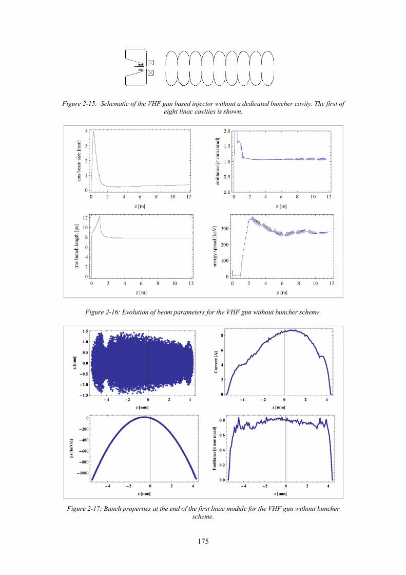
175

Figure 2-15: Schematic of the VHF gun based injector without a dedicated buncher cavity. The first of eight linac cavities is shown.

Figure 2-16: Evolution of beam parameters for the VHF gun without buncher scheme.

Figure 2-17: Bunch properties at the end of the first linac module for the VHF gun without buncher

scheme.

176

2.2.3 Superconducting RF Gun

The absence of parasitic Ohmic losses in SRF cavities provides an option for delivering high beam current with significantly less RF power than for an equivalent normal conducting gun. The hard limit is therefore the maximum power of CW RF source available at L-band. Klystrons are able to provide over 160 kW CW, with an IOT equivalent capable of rising to 30 kW.

Previous studies concentrated on a two cavity L-band gun with a 1½-cell launch cavity largely adopting the TESLA cavity shape, and an adapted Cornell 2-cell booster cavity. To reduce complexity of the gun, we focus here on a single cavity, 1½ Tesla cell design, as seen in Figure 2-18. Recently a 1½ cell cavity was vertically tested at TJNAF to 40 MV/m [31] and a gun with peak electric fields of 50 MV/m is potentially feasible, however, as this is pushing the state-of-the-art, simulations below have been carried out at both 40 and 50 MV/m.

Figure 2-18: A 1½ Tesla cell SRF gun cavity with the fields shown for the accelerating mode as simulated in CST Studio.

For a beam energy of 5 MeV and an average current of 0.2 mA and the proposed cavity design, the RF power required is easily achievable with a standard IOT amplifier that simplifies the RF input coupler scheme which often restricts the maximum beam power of SRF accelerating systems. If the gun operates at the frequency of the main linac, it easily integrates with the RF and cryogenic infrastructure and does not require non-standard RF power supplies.

As mentioned above, at 1 MHz, existing ultra-violet laser systems are not able to drive metallic photocathodes so alkali photocathodes have to be considered. A SRF gun using Cs2Te photocathodes is under commissioning at FZD [32] and a SRF gun using K2CsSb photocathodes is under development at BNL [29] to operate in CW mode with an average current of 50 mA.

A buncher cavity is also not required as the SRF gun alone provides bunches with length close to that of the initial laser pulse length. The laser pulse used in the ASTRA simulations has a 1 mm diameter flat-top transverse profile and a 30 ps flat-top temporal profile with rise and fall times of 2 ps. Initial thermal energy of 0.7 eV was included. Following the gun cavity is an emittance compensation solenoid which may be superconducting in order to be contained within the gun cryostat. At 50 MV/m peak field the gun accelerates the electron beam to 4.5 MeV. Operating at 40 MV/m this energy is reduced to 3.6 MeV. The beam is then injected into the first module of the main linac where it is further accelerated to 130 MeV. The standard linac module contains eight 9-cell Tesla cavities, operated at an average accelerating gradient of 15 MV/m. The first cavity is operated at a phase of -40° the remaining cavities are then operated at +4.5° in order to compensate the energy chirp.

177

Figure 2-19: Evolution of beam parameters for the SRF gun based injector with a gun peak field in the gun of 50 MV/m.

Figure 2-20: Bunch properties at the exit of the first linac module for the SRF gun based injector with the peak field in the gun of 50 MV/m.

178

Figure 2-21: Evolution of beam parameters for the SRF gun based injector with a reduced gun peak field of 40 MV/m.

Figure 2-22: Bunch properties at the exit of the first linac module for the SRF gun based injector with a

reduced gun peak field of 40 MV/m.

Figure 2-19 and Figure 2-21 show the evolution of beam parameters along the injector for the two cases. Figure 2-20 shows the final distribution of the 200 pC bunch at the exit of the first linac module for an ASTRA simulation of 100,000 particles. The flat current profile has a length of 35 ps and the slice emittance remains low, around 0.3-0.35 mm mrad, throughout the bunch. Figure 2-22 shows the bunch distribution with the gradient in the gun reduced from 50 to 40 MV/m. For the 40 MV/m case slice emittance increases up to an average of 0.39 mm mrad whilst other beam properties remain unchanged. The average kinetic energy of the bunch slightly drops from 129.7 to 129.0 MeV.

179

2.2.4 Summary

The results of beam dynamics simulations for the VHF gun based injector both with and without buncher and the SRF gun based injector with peak fields of 50 MV/m and 40 MV/m are summarised in Table 2-6. As may be seen the best beam parameters which may be delivered are by the SRF gun and regarding slice parameters are similar to those of the lower repetition rate injector described in Section 2.1. Even at the reduced peak gradient of 40 MV/m, the beam parameters are still superior to the normal conducting VHF gun design. The disadvantage however of the SRF gun is the greater complexity and risk. Since the high repetition rate gun is not required for the baseline configuration of NLS, the choice of technology can be made later, taking into account practical experience with these two types of injectors at LBNL [28] and FZD [32].

Table 2-6: Beam parameters at the exit of the injectors.

VHF with

buncher

VHF no

buncher

SRF 50MV/m

SRF 40MV/m

RMS projected emittance (mm·mrad) 1.239 1.081 0.602 0.686

Average slice emittance (mm·mrad) 0.642 0.736 0.302 0.387

Full bunch length (ps) 32.86 32.45 35.16 33.70

RMS bunch length (ps) 7.80 7.87 8.26 8.13

RMS longitudinal emittance (keV·mm) 662 611 686 662

RMS energy spread (keV) 295 278 277 272

Average kinetic energy (MeV) 124.1 123.1 129.7 129.0

REFERENCES [1] Schreiber, S., et al., Operation of FLASH at 6.5 nm Wavelength, EPAC’08, p. 133 (2008). [2] Floettmann, K., A Space Charge Tracking Algorithm (ASTRA); http://www.desy.de/~mpyflo. [3] Floettmann, K., Note on the Thermal Emittance of Electrons Emitted by Cesium Telluride Photo

Cathodes, TESLA FEL Report 1997-01,1997. [4] Rimjaem, S., et al., Tuning and Conditioning of a New High Gradient Gun Cavity at PITZ,

EPAC’08, p. 244 (2008). [5] Billen, J H., & Young, L M., Poisson Superfish, LAUR-96-1834. [6] ANSYS v.11, ANSYS, Inc., http://www.ansys.com. [7] H. Schlarb et al., Beam Based Measurements of RF Phase and Amplitude Stability at FLASH,

DIPAC’07, p. 307. [8] http://www.thalesgroup.com. [9] Lederer, S., et al., Investigations on the Increased Life Time of Photocathodes at FLASH and PITZ,

PAC’09, MO6RFP055. [10] Miltchev, V., et al., Measurements of Thermal Emittance for Cesium Telluride Photocathodes at

PITZ, FEL’05, p. 560. [11] Ferrini, G., et al., A Monte Carlo Simulation of Low Energy Photoelectron Scattering in Cs2Te,

Solid State Commun. 1998 106, 21-26 [12] Krasilnikov, M., et al., Beam-Based Procedures for RF Guns, PAC’05, p. 967. [13] Krasilnikov, M., Impact of the Cathode Roughness on the Emittance of an Electron Beam, FEL’06,

p. 583. [14] Matsumto, H., Dark Current, LINAC’96, p. 626. [15] Stephan, F., et al., New Experimental Results from PITZ, LINAC’08, p. 474. [16] Han, J-H., et al., Dark Current Measurements at the PITZ RF gun, DIPAC’03, p. 242.

180

REFERENCES [17] Wang, J., Some Problems on RF Breakdown in Room Temperature Accelerator Structure, a

Possible Criterion, SLAC/AP - 51 (1986). [18] Han, J-H., Dynamics of Electron Beam and Dark Current in the Photocathode RF Guns, PhD

Thesis, Universität Hamburg, 2005. [19] Borland, M., elegant: A Flexible SDDS-Compliant Code for Accelerator Simulation, Advanced

Photon Source LS-287, 2000. [20] Bazarov, I V., et al., Thermal emittance and response time measurements of negative electron

affinity photocathodes, J. App. Phys. 2008 103 054901 [21] Michel, P., et al., The Rossendorf IR-FEL ELBE, Proceedings of FEL2006, p. 488 [22] Togawa, K., et al., Emittance measurement on the CeB6 electron gun for the Spring8 compact SASE

source, Proceedings of FEL 2004 [23] Ostroumov, P N., et al., Development of ultra-low emittance injector for future X-Ray FEL

oscillator, Proceedings of LINAC 2008 [24] Xiang, R., et al., Experimental investigations of DC-SC photoinjector at Peking University, NIM A

2004 527 321-325. [25] Stephan, F., et al., New experimental results from PITZ, Proceedings of LINAC 2008 [26] Honkavaara, K., et al., Status of FLASH, Proceedings of FEL 2008. [27] Dowell, D H., et al., Results from the average power laser experiment photocathode injector test,

NIM A 1995 356 167-176 [28] Baptiste, K., et al., A CW normal-conductive RF gun for free electron laser and energy recovery

linac applications, Nucl. Instr. and Meth. A 2008 599 9-14 [29] Calaga, R., et al., High current superconducting gun at 703.75 MHz, Physica C 2006 441 159-172 [30] Flöttmann, K., ASTRA, http://www.desy.de/~mpyflo/ [31] Kamps, T., private communication. [32] Teichert, J., et al., First operation results of the superconducting photoinjector at ELBE,

Proceedings of EPAC’08, WEPP105

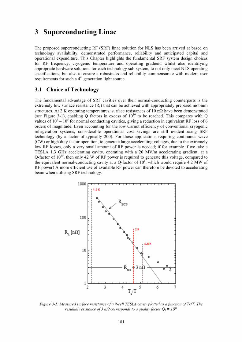
181

3 Superconducting Linac

The proposed superconducting RF (SRF) linac solution for NLS has been arrived at based on technology availability, demonstrated performance, reliability and anticipated capital and operational expenditure. This Chapter highlights the fundamental SRF system design choices for RF frequency, cryogenic temperature and operating gradient, whilst also identifying appropriate hardware solutions for each technology sub-system, to not only meet NLS operating specifications, but also to ensure a robustness and reliability commensurate with modern user requirements for such a 4th generation light source.

3.1 Choice of Technology

The fundamental advantage of SRF cavities over their normal-conducting counterparts is the extremely low surface resistance (Rs) that can be achieved with appropriately prepared niobium structures. At 2 K operating temperatures, surface resistances of 10 nΩ have been demonstrated (see Figure 3-1), enabling Q factors in excess of 1010 to be reached. This compares with Q values of 104 – 105 for normal conducting cavities, giving a reduction in equivalent RF loss of 6 orders of magnitude. Even accounting for the low Carnot efficiency of conventional cryogenic refrigeration systems, considerable operational cost savings are still evident using SRF technology (by a factor of typically 200). For those applications requiring continuous wave (CW) or high duty factor operation, to generate large accelerating voltages, due to the extremely low RF losses, only a very small amount of RF power is needed; if for example if we take a TESLA 1.3 GHz accelerating cavity, operating with a 20 MV/m accelerating gradient, at a Q-factor of 1010, then only 42 W of RF power is required to generate this voltage, compared to the equivalent normal-conducting cavity at a Q-factor of 105, which would require 4.2 MW of RF power! A more efficient use of available RF power can therefore be devoted to accelerating beam when utilising SRF technology.

Figure 3-1: Measured surface resistance of a 9-cell TESLA cavity plotted as a function of Tc/T. The residual resistance of 3 nΩ corresponds to a quality factor Q0 = 1011

182

Another major advantage of SRF technology relates to the cavity geometry optimisation, which owing to the significantly reduced RF losses, does not require the r/Qo to be maximised, resulting in larger, more open cavity beam-pipes. This has the benefit of reducing the trapped Higher Order Mode (HOM) impedances, such that beam instability and breakup thresholds can be increased compared to normal-conducting cavities. For a high energy linac application such as NLS, where emittance growth is a serious concern, the large beam-pipe apertures significantly reduce the short-range wakefield contributions.

The practical limitation of an SRF resonator is dictated by the requirement that the RF magnetic field on the cavity surface has to stay below the theoretical RF critical magnetic field (or superheating field, Hsh) of the superconductor which equals 200-240 mT for niobium. For TESLA 1.3 GHz cavities, this implies a maximum accelerating field of 50 - 60 MV/m. The Q factor should stay roughly constant when approaching this fundamental limit, but in practice the ‘Qo vs Eacc’ curve ends at considerably lower Q values at the highest achievable Eacc. The main reasons for this degradation are excessive heating due to impurities in the niobium material, field emission of electrons and multipactor breakdown. The SRF linac operating frequency is strongly defined by the achievable surface resistance (Rs) for the superconducting niobium (Nb) material. Minimising Rs for a given accelerating gradient (Eacc) ensures that the cryogenic plant capacity (and subsequent capital and operating costs) can also be reduced to affordable and acceptable levels.

3.2 Operating Temperature

At low temperatures (i.e. T<Tc, where Tc is the superconducting transition temperature, 9.2 K for Nb) Rs is small, but finite as the intrinsic Cooper pairs have an inherent inertia, where a small number of normal conducting electrons interact with the RF electric field and the subsequent electron flow induces a current which is dissipated in the Nb surface. The rate at which the surface resistance for Nb reduces as a function of T (for T < Tc/2 and f < 1012 Hz) is referred to as the Bardeen, Cooper and Schieffer resistance (RBCS) [1], which is derived from:

⎟⎠⎞

⎜⎝⎛−⎟

⎠⎞

⎜⎝⎛×= −

Tf

TRBCS

67.17exp5.1

11022

4 ( 3-1)

As can be seen from Figure 3-1 at a fixed frequency of 1.3 GHz, below a certain operating temperature (T), the observed surface resistance (Rs) is larger than the BCS resistance (RBCS) and is accounted for by the residual resistance (Rres), whereby:

resBCSs RTRR += )( ( 3-2)

A well prepared Nb surface can reach Rres = 10 nΩ, such that the operating temperature T is normally chosen so that RBCS is reduced to an economically acceptable value. By reducing the operating temperature, the BCS resistance can be lowered to below that of the residual resistance and as in the case of Figure 3-1, shows that a temperature < 2 K would be required. Assuming then that the SRF cavities for NLS are optimally processed and achieve the required performance, the cryogenic load will be dominated by Rres. At 4.2 K operating temperature the surface resistance is dominated by the BCS resistance, which rules this operating temperature out of consideration for NLS as the cryogenic power demand would be excessive. It is therefore proposed that the operating temperature for NLS be set at 1.8 K; evaluation of the cryogenic loads will be detailed in Section 3.6.3.

3.3 Frequency Choice

Although a Rres of 3 nΩ is identified in Figure 3-1 for TESLA structures which have been electro-polished, a more conservative limit of 10 nΩ is assumed for NLS using conventional

183

Buffered Chemical Polishing (BCP) which is predicated by the requirement to procure appropriate quality niobium material from industry. For the intrinsic losses associated with SRF accelerating structures, when RBCS >> Rres then Rs scales with frequency2, when RBCS << Rres then Rs is independent of frequency. At an operating temperature of 1.8 K the BCS term dominates above 1.93 GHz and hence the losses grow linearly with frequency, whereas for frequencies below 500 MHz the Rres dominates and the losses grow with 1/frequency (see Figure 3-2).

Figure 3-2: Preferred frequency band for an SRF cavity with Rres = 10 nΩ at an operating temperature of 1.8 K.

Longitudinal (W//) and transverse (W⊥) wakefields scale as f2 and f3 respectively and so beam emittance growth and beam-induced cryogenic losses are much larger at higher frequencies, which must be factored against the increased size and cost of lower frequency SRF cryomodules. The choice of frequency proposed for NLS is based upon technology availability within this frequency band, not only in terms of the accelerating structures and associated cryomodules, but also in terms of high power RF infrastructure to match the design requirements for NLS. For these reasons, L-band technology at 1.3 GHz has been adopted, taking advantage of the decades of development for the TESLA, ILC, TTF, FLASH and XFEL accelerator facilities, whilst also witnessing the implementation of TESLA technology for many other existing and proposed accelerator projects around the world, such as ALICE, ELBE, Cornell-ERL, JAERI ERL, BESSY-FEL and 4GLS.

3.4 Operating Gradient

The choice of gradient for NLS is dependent upon many factors; of primary consideration is the anticipated cavity performance and the associated effect on costs. As previously indicated, as Eacc is increased for a SRF cavity, invariably the Qo reduces and rolls off until a fundamental limitation is reached. Estimating the operational Qo for structures that have not yet been fabricated or integrated into complete cryomodules is a difficult task, as each cavity must follow extremely strict handling and preparation procedures to ensure its RF surfaces remain inclusion and particulate free, to guarantee (as best we can) optimum performance. For NLS we plan to utilise TESLA L-band structures processed using conventional BCP processing techniques. Figure 3-3 shows the predicted performance for such a cavity at 1.8 K, based on measured

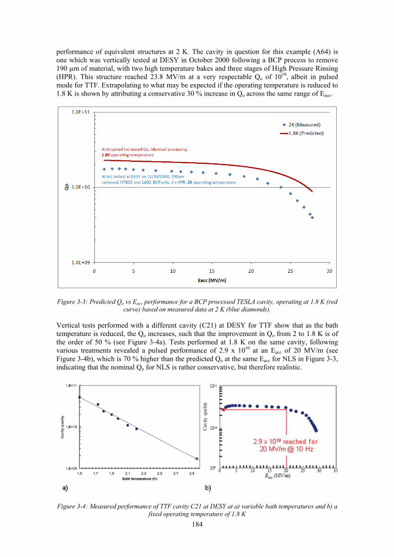
184

performance of equivalent structures at 2 K. The cavity in question for this example (A64) is one which was vertically tested at DESY in October 2000 following a BCP process to remove 190 µm of material, with two high temperature bakes and three stages of High Pressure Rinsing (HPR). This structure reached 23.8 MV/m at a very respectable Qo of 1010, albeit in pulsed mode for TTF. Extrapolating to what may be expected if the operating temperature is reduced to 1.8 K is shown by attributing a conservative 30 % increase in Qo across the same range of Eacc.

Figure 3-3: Predicted Qo vs Eacc performance for a BCP processed TESLA cavity, operating at 1.8 K (red curve) based on measured data at 2 K (blue diamonds).

Vertical tests performed with a different cavity (C21) at DESY for TTF show that as the bath temperature is reduced, the Qo increases, such that the improvement in Qo from 2 to 1.8 K is of the order of 50 % (see Figure 3-4a). Tests performed at 1.8 K on the same cavity, following various treatments revealed a pulsed performance of 2.9 x 1010 at an Eacc of 20 MV/m (see Figure 3-4b), which is 70 % higher than the predicted Qo at the same Eacc for NLS in Figure 3-3, indicating that the nominal Qo for NLS is rather conservative, but therefore realistic.

Figure 3-4: Measured performance of TTF cavity C21 at DESY at a) variable bath temperatures and b) a fixed operating temperature of 1.8 K

185

For this predicted variation in Qo, Figure 3-5 shows the relative reduction in total dynamic load at 1.8 K compared to 2 K, for NLS at its nominal operating energy of 2.25 GeV. It is apparent that up to Eacc ~ 15 MV/m the total dynamic load increases linearly for both temperatures and above this value the increase becomes more rapid.

Figure 3-5: NLS total 2 K and 1.8 K dynamic load variation for 2.25 GeV operation.

The ultimate choice of nominal operating gradient for NLS has been decided based upon anticipated total system costs (i.e. including cryomodules, RF amplifiers, cryoplant, tunnel installation and integrated system operational costs), coupled with best operational reliability. Figure 3-6a – f) show how the fundamental linac parameters vary as a function of Eacc in terms of linac length, RF power, number of cavities and cryomodules, cryomodule energy gain, AC power and cryogenic dynamic load respectively.

186

a) b)

c) d)

e) f)

Figure 3-6: a) Linac active and actual length, b) Total cavity and total linac RF power, c) Total number of cavities and cryomodules, d) Cryomodule energy gain, e) RF and cryogenic AC power and f) Total

cryogenic capacity including safety factor.

The relative major linac sub-system cost scalings have been determined based upon information sourced from industry and other national laboratories who have performed similar L-band technology assessments for their own respective accelerator designs (see Figure 3-7a). Accumulating these costs and adding linac operational costs over a 10 year period, Figure 3-7b shows that there is a broad Eacc minimum, centred at around 19 MV/m. This analysis however utilises energy costs at 2010 rates (£0.07/kWh) and assuming 6000 hrs/year of RF operation with 8400 hrs/year of cryoplant operation.

187

a) b)

Figure 3-7: a) Relative sub-system costs and b) Relative total capital and 10-year operational linac costs

Realistically however electricity costs are increasing and by the time NLS is ready for first operation no doubt energy costs will be much higher. Figure 3-8 shows how a doubling of the energy costs between now and then can significantly alter the optimum gradient, reducing it to around 17.5 MV/m.

Figure 3-8: Effect of increased energy cost on Eacc optimisation over 10 years

Assuming for the majority of the NLS linac that beam is being accelerated close to on crest, there will be discrete Eacc levels dependent upon the number of cryomodules employed. From Figure 3-8 it can be seen that 14 cryomodules operating at 19.35 MV/m would give a minimum total cost for a machine operating with today’s electricity costs, whereas 16 cryomodules operating at 16.9 MV/m would be closer to the optimum if electricity costs escalate to twice what they are now. The operational solution however for NLS has been determined not only by attempting to reduce capital and operational costs to a minimum, but also in reducing the technical risks associated in achieving the required accelerating gradient. It is therefore proposed to employ 18 cryomodules operating at a nominal gradient of 15.05 MV/m, for which the total linac cost is within 5 % of the cost optimum at today’s energy rates, 2 % for potentially doubled energy costs in the future. In reducing the operating Eacc to this level a number of associated benefits prevail:

• Reduced risk of poor cavity performance, especially field emission limitations • Cheaper cavity processing, using conventional BCP:HPR techniques • Increased reliability and availability • Increased intrinsic redundancy, as each cavity will have a larger operational

overhead capability • Increased production yield from industry

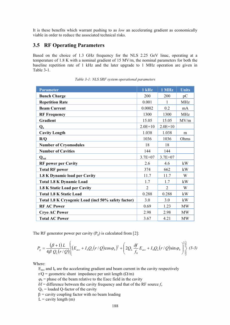
188

It is these benefits which warrant pushing to as low an accelerating gradient as economically viable in order to reduce the associated technical risks.

3.5 RF Operating Parameters

Based on the choice of 1.3 GHz frequency for the NLS 2.25 GeV linac, operating at a temperature of 1.8 K with a nominal gradient of 15 MV/m, the nominal parameters for both the baseline repetition rate of 1 kHz and the later upgrade to 1 MHz operation are given in Table 3-1.

Table 3-1: NLS SRF system operational parameters

Parameter 1 kHz 1 MHz Units Bunch Charge 200 200 pC Repetition Rate 0.001 1 MHz Beam Current 0.0002 0.2 mA RF Frequency 1300 1300 MHz Gradient 15.05 15.05 MV/m Qo 2.0E+10 2.0E+10 Cavity Length 1.038 1.038 m R/Q 1036 1036 Ohms Number of Cryomodules 18 18 Number of Cavities 144 144 Qext 3.7E+07 3.7E+07 RF power per Cavity 2.6 4.6 kW Total RF power 374 662 kW 1.8 K Dynamic load per Cavity 11.7 11.7 W Total 1.8 K Dynamic Load 1.7 1.7 kW 1.8 K Static Load per Cavity 2 2 W Total 1.8 K Static Load 0.288 0.288 kW Total 1.8 K Cryogenic Load (incl 50% safety factor) 3.0 3.0 kW RF AC Power 0.69 1.23 MW Cryo AC Power 2.98 2.98 MW Total AC Power 3.67 4.21 MW

The RF generator power per cavity (Pg) is calculated from [2]:

( )( ) ( )( ) ( )

⎪⎭

⎪⎬⎫

⎪⎩

⎪⎨⎧

⎟⎟⎠

⎞⎜⎜⎝

⎛+++

+=

2

00

2 sin/2cos//4

1bLaccLbLbacc

Lg QrQIE

ffQQrQIE

QrQLP ϕδϕ

ββ (3-3)

Where: Eacc and Ib are the accelerating gradient and beam current in the cavity respectively r/Q = geometric shunt impedance per unit length (Ω/m) ϕb = phase of the beam relative to the Eacc field in the cavity δf = difference between the cavity frequency and that of the RF source fo QL = loaded Q-factor of the cavity β = cavity coupling factor with no beam loading L = cavity length (m)

189

For NLS, assuming β >>1 and that beam is accelerated on-crest (ϕb = 0o) then equation 1-3 reduces to:

( ) ( )( )⎪⎭

⎪⎬⎫

⎪⎩

⎪⎨⎧

⎟⎟⎠

⎞⎜⎜⎝

⎛++=

2

0

2 2//4 accLLbacc

Lg E

ffQQrQIE

QrQLP δ

(3-4)

An optimum QL can be determined by defining the expected peak detuning (or microphonics) level (or δf) from the integrated cryomodule cavities, for which a minimum RF generator power is achieved. Figure 3-9 highlights for a relatively conservative microphonics level of 15 Hz, that an optimum QL = 3.7 x 107 is defined, giving an RF power of 4.6 kW/cavity for a 1 MHz repetition rate.

Figure 3-9: a) Relative sub-system costs and b) Relative total 10 year linac cost

This level of microphonics is comparable with measured data from a variety of SRF cryomodules in operation today; Table 3-2 highlights for those operating in CW-mode that 15 Hz peak detuning is a reasonably conservative value to use, especially as many of these cryomodules are operated typically at gradients comparable to NLS. A much larger detuning frequency is identified for the TTF cryomodule cavities, which operates in pulsed mode and at gradients in excess of 20 MV/m and so may not be directly analogous to what is required for NLS. What is also a little concerning about these figures is the scatter observed between cavities and even inside the same cryomodule, highlighting that a more conservative estimate for peak detuning is more appropriate.

Table 3-2: Operational detuning characteristics for SRF cryomodules

Machine σ (Hz) 6σ (Hz) Comments CEBAF 2.5 (average) 15 (average) Significant variation between cavities ELBE 1 (average) 6 (average) SNS 1 to 6 6 to 36 Significant variation between cavities TJNAF FEL 0.6 to 1.3 3.6 to 7.8 Central cavities quieter TTF 2 to 7 (pulsed) 12 to 42 (pulsed) Significant variation between cavities

190

3.6 Cryomodule and Cavity Components

The NLS cryomodule will be based upon the extensively developed TESLA/ILC/FLASH/XFEL cryomodule design, which employs 8 identical 1.3 GHz 9-cell RF cavities. To achieve the desired total acceleration of 2.25 GeV for NLS, 18 cryomodules will be utilised operating at a nominal Eacc of 15 MV/m with an initial electron bunch repetition rate of 1 kHz, with an upgrade requirement of up to 1 MHz. It is therefore essential to operate the cavities in CW mode, instead of the pulsed mode employed at FLASH/XFEL; the emphasis is to be able to operate at the highest Q0 level practically achievable, the NLS target being 2 x 1010.

3.6.1 The RF Cavity

The TESLA 9-cell cavity (see Figure 3-10) was designed to maximize the accelerating gradient whilst reducing the possibility for thermal breakdown and field emission [3]. Developments over the past 15 years in the manufacture of such structures, including all processing and handling of these high gradient cavities, has not only improved the fabrication yield from industry, but also the operational efficiency and reliability for successfully operating accelerator facilities, such as SCA, TTF, FLASH, ALICE and ELBE.

Figure 3-10: TESLA/XFEL cavity design

Although the TESLA 9-cell cavity was designed for pulsed operation, the same design can be easily adopted for CW operation on NLS due to the low average beam current. Higher order mode (HOM) couplers are designed that will couple strongly to the most resonant dipole modes in the cavity, and the orientation of these loops has been optimized to couple strongly to a number of these modes. The TESLA 9-cell cavity has the facility for HOM extraction through 3 individually placed HOM couplers [4].

191

3.6.1.1 Monopole Wakefield Contribution

A study of the HOM power generated by a 9-cell TESLA cavity is evaluated analytically using equations from Heifets and Kheifets’s [5] derivation of wakefields in periodic cavity arrays:

MgL

acgMZ

Z L2

2 20

ωππ= (3-5)

( )∫∞ −=

0

22

Re1 ωπ

ω deZLossFactor bunchLtL (3-6)

EnergyLost = bunchq *LossFactor (3-7)

PowerDeposition = EnergyLost*bunchreprate*bunchq (3-8)

For a TESLA cavity geometry, approximated here as step functions where the cavity length is L = λ/2, the flat iris length g is chosen as being the radius of the TESLA middle cell iris radius. The actual number chosen for g is actually irrelevant to the final result however as it cancels out in Eqtn (1-5).

The relevant parameters for the NLS case are shown in Table 3-3. The calculated power loss in a single 9-cell cavity is 1.44 W. In order to verify the calculation, the prediction is compared to the BESSY-FEL beam parameters. The value presented in the BESSY TDR for an 8-cavity cryomodule is 0.3 W/cavity [6], with a loss factor given as 15.4 V/pC per cavity. The value calculated with the method above is 0.27 W/cavity. The corresponding loss factor is 14.1 V/pC for a single cavity, which is close to the 15.4 V/pC identified in the BESSY TDR by alternative methods [7].

Table 3-3: Monopole HOM power determination compared to BESSY-FEL calculations

NLS BESSY-FEL

M 9 9 Number of cells

L 0.1154 m 0.1154 m Cell length

g 0.0914 m 0.0914 m Gap length

a 0.035 m 0.035 m Iris aperture

bunchq 200 pC 2.5 nC Bunch charge

bunchLt 150 fs 0.97 ps Bunch length (time)

bunchreprate 1 MHz 1 kHz Bunch repetition rate

Calculated

LossFactor 35.9 V/pC 14.1 V/pC Loss factor per cavity

PowerDeposition 1.44 W 0.27 W Power deposition per cavity

An additional verification has been made using the code Echo2D [8]. A 150 fs bunch has been simulated through a TESLA 9-cell structure (see Figure 3-11). The monopole mode has a loss factor of 39.4 V/pC which is equivalent to 1.52 W power deposition, comparable therefore with the analytical estimate above.

192

Figure 3-11: ECHO2D monopole result for a TESLA 9-cell structure with a 150 fs bunch.

3.6.1.2 Dipole Contribution to the Wakefields

The dipole contribution to the impedance can be written in terms of the longitudinal monopole impedance using [9].

LL Za

Z 2)1( 2

=

(3-9)

MgL

acgMZ

Z L2

2 20

ωππ= (3-10)

( )∫∞ −=

0

)1( 22

Re1 ωπ

ω deZLossFactor bunchLtL (3-11)

EnergyLost = bunchq *LossFactor

PowerDeposition = EnergyLost*bunchreprate*bunchq*bunchoffset2 (3-12)

Where (1) denotes the dipole component of the longitudinal impedance. Applying the same process as before, results in a deposited power of 0.23 W, for a 1 cm offset beam.

In order to verify these estimations a simulation was run using Echo2D, see Figure 3-12. The simulation gives a longitudinal loss factor of 6.422x104 V/pC/m2 which equates to a power deposition of 0.25 W for 1 cm bunch offset, in very good agreement with the analytical result.

193

Figure 3-12: ECHO2D dipole result for a TESLA 9-cell structure with a 150 fs bunch.

3.6.2 SRF Cryomodule

The purpose of the cryomodule is to support and sustain the cavities at the 1.8 K operating temperature. The cryomodule will contain the magnetic shielding to maximize the intrinsic Q of the cavities, this will minimize the RF power required should the structures be rigid enough with respect to microphonics. As well as minimising the cost of the RF power requirements, substantial savings can be achieved through appropriate thermal management for thermal jackets which are required to minimize the heat leak to the cryogenics.

Fundamental power couplers are used to transfer the RF power from the RF power source into the cavity. These provide large sources of heat leak from the cavities at 1.8 K to the outside environment and also have to provide a vacuum seal.

Figure 3-13: XFEL cryomodule layout

With regards to the design of the cryostat, consideration of each connection to the outside environment has to be understood and managed. The TESLA collaboration was largely responsible for the development of the XFEL cryomodule [10] (see Figure 3-13), with over 6 major institutes developing the design over 20 years, it is therefore believed that NLS can benefit from an already extensively validated, mature and proven cryomodule design.

In order to sustain CW RF power, increases in the diameter of the helium 2-phase line connections to the cavity helium jacket need to be evaluated, or the option of a secondary chimney must be considered. The orientation of the 2-phase line with respect to the cavity will also assist with the helium transfer and the reduction of microphonics.

194

3.6.3 Cryomodule Heat Load Estimates

The heat load or the refrigeration power required to maintain the temperature of SRF cavities at 1.8 K is the key parameter and the main cost driver for the design of the cryogenic system for NLS. Table 3-4 summarizes the estimated heat load of a typical cryomodule for the NLS linac at the nominal operating conditions at different temperature levels. XFEL data is also included for comparison. Note that the dynamic heat load is the dominant factor in the refrigeration budget of the cryomodule.

Table 3-4: The static and dynamic heat load (in W) of one cryomodule with 8 SRF cavities at an accelerating gradient of 15 MV/m, Q= 2 x 1010 operating in CW mode.

Source 1.8K static

1.8K dynamic

5K-8K static

5K-8K dynamic

40K-80K static

40K-80K dynamic

Static 16.0 96.2 13.5 8 63.9 88 Sum Static + dynamic 112.2 21.5 151.2 XFEL cryomodule data for comparison (*at 2K [11])

1.3 9.8* 11.0 17.1 71.0 42.9

3.6.4 Frequency Tuner

Several options of tuner would meet the design specification of the NLS. Since the packing factor of the cryomodule is of paramount importance to reduce the length of the accelerator, the preferred option is to adopt the blade tuner [12] which mounts to the helium jacket of the cavity and provides active compensation of microphonics through a number of piezo actuators (see Figure 3-14), without increasing the cryomodule active length.

Figure 3-14: Blade tuner implementation

Stiffening the cavity string reduces the maximum detune due to microphonics and allows operation at higher external Q in order to minimize the required overhead in RF power.

3.6.5 Input Power Coupler

The XFEL cryomodule RF power couplers were designed for low average power but high peak power [13]. For NLS a CW RF source of up to 10 kW CW is required, in order to provide a reasonable RF power overhead per cavity. With small modifications, the XFEL coupler has been tested to power levels approaching 10 kW CW [14]. Should the power demand be higher,

195

the Cornell injector coupler would be suitable [15], since this has been designed for >50 kW CW operation, and would require little modifications to fit into the XFEL cryomodule design.

a) b)

Figure 3-15: a) XFEL and b) Cornell ERL Input Couplers

Both options include a warm ceramic window as well as a cold ceramic window. This provides additional protection to the cryomodule in the event of a vacuum failure. This does however introduce additional cost in the manufacturing.

Both the XFEL and the Cornell Injector coupler have the capability of adjusting the cavity coupling and with an external 3-stub tuner, so that the Qext can be varied by greater than an order of magnitude. This would allow in-situ optimization of the cavity Qext, in order to minimize the RF power requirements in achieving a stable accelerating voltage. This internal adjustment capability also assists in RF conditioning of the input coupler assembly and in addition can be utilised to avoid multipactor bands during normal operation.

3.6.6 Reengineering of the XFEL Cryomodule for CW operation

The XFEL cryomodule design is chosen as a reference to develop a suitable cryomodule for the NLS linac. However, due to CW operation the dynamic heat load experienced by the NLS cryomodule will be about 10 times higher than for XFEL (see Section 12.4.1). Consequently the XFEL cryomodule must be modified to handle much higher mass flow with higher helium-gas pressure stability at the lower operating temperature of 1.8 K. Some of these requirements were analysed and identified during an industrial study [16] to develop a suitable cryomodule solution for the BESSY-FEL project, the requirements for which were similar to NLS. In order to address all of the related issues, a conceptual engineering design has been developed incorporating all of these changes as described below. Further work would however be required during a later technical design phase to guarantee optimum performance.

3.6.6.1 Larger Two Phase Line.

To allow heat transfer at 1 W/cm2 with a pressure drop of less than 0.1 mbar across the length of the cryomodule, the diameter of the two phase line and the pipe connecting it to the cavity reservoir have been increased from 88 mm to 100 mm (see Figure 3-16).

196

Figure 3-16: a) NLS cryomodule cut-away and b) XFEL cryomodule

3.6.6.2 Removing the 5 K Thermal Shield.

Increase in the two phase line conflicts with the 5 K shield and so this has been removed in order to maintain the same cryostat envelope. The absence of this shield will increase the static heat load for a cryomodule by approximately 3 W. This is only a fraction of the total dynamic load of 110 W and will have negligible impact on operation of the linac and the cryoplant. Similar approach has been proposed for BESSY-FEL, CORNELL-ERL [17] as well as for ILC [18]. This is also shown in Figure 3-16.

The 4 K – 8 K cooling circuit will however still be required for introducing thermal intercepts for RF couplers and several cryostat-support components. Primary reference designs of the additional thermal links have been developed although more work is needed to verify the performance.

3.6.6.3 Integrating Two Cold Valves for Each Cryomodule

In order to handle the increased mass flow (~10 g/s per cryomodule) at lower pressures, two valves will be introduced in every cryomodule, one as a Joule Thomson (JT) valve for 1.8 K operation and the other to aid the warm-up and cool-down of the cavities (see Figure 3-17).

197

Figure

Figure 3-17: NLS cryomodule with two cold valves

3.6.6.4 Liquid Helium Reservoir and Level Control Instrumentation

Each NLS cryomodule will require a liquid helium reservoir connected to the two phase line with level control instrumentation. Figure 3-18 shows that for proper flow control the control valve and the level control instrumentation are located at the two opposite ends of the cryomodule. This arrangement also requires that the two-phase line is terminated at both ends inside the cryostat.

Figure 3-18: Liquid Helium reservoir and level control instrumentation

3.6.6.5 Connections to the 300 mm Gas Return Pipe (GRP)

In the XFEL cryomodule the connection to the gas return pipe is achieved at the end of the cryomodule string. However, the termination of the two–phase line inside the cryomodule requires this connection to be introduced inside. This is now done at two places, one close to the JT valve and the other near the reservoir (see Figure 3-19).

198

Figure 3-19: Connection between the 2 phase line and the GRP

3.6.6.6 External Transfer Line Sections

Due to the layout of the NLS linac (see next sub-Section) it is necessary to introduce 7 jumper sections of cryogenic transfer lines to maintain the continuity of process lines along the length of the linac. From the cryogenic point of view a transfer line is basically a special cryostat and in the case of NLS its design will be more complex due to the accommodation of a variety of cryogenic process lines at differing temperatures and pressures. A conceptual design of these jumper sections has been developed (Figure 3-20) for modelling purposes.

Figure 3-20: Transfer line jumper section interconnecting the two cryomodules

3.6.7 Cryomodule Interconnections

A detailed study of the cryogenic distribution of some of the existing SRF linac installations was conducted. Cryogenic and vacuum sectarisation is a complex subject affecting several projects, for example Project X, XFEL, SPL, ILC etc. and no clear-cut universal approach or

199

guide lines have been established [19]. The choice is based on a compromise between the performance, cost and associated risks and varies widely from project to project.

CEBAF, the first CW linac [20] and SNS [21], employed two sets of external transfer lines running parallel to the linac (Figure 3-21). This design gives full flexibility in operating or isolating an individual cryomodule, but the cost as well as the risk of leakage through the innumerable joints with their associated (additional) heat leaks is significantly high.

Figure 3-21: Cryogenic distribution scheme for CEBAF (taken from CEBAF Report)

XFEL [22] and ILC [23] have taken the other extreme approach of not using any external transfer lines at all (see Figure 3-22). The whole length of the linac is considered to be single large cryostat and an individual cryomodule cannot be isolated or removed without warming the whole linac to room temperature. To safeguard against the failure or degradation of any individual cavity additional cryomodules have been added for redundancy. Reliable performance is achieved by introducing a very high level quality control measures at every stage from design to commissioning.

Figure 3-22: Cryogenic distribution scheme for XFEL (taken from XFEL TDR)

200

The NLS linac needs several warm sections for diagnostics and beam control. The cryomodules in the linac are distributed in 7 sections as shown in Figure 3-23. Cryogenically the cryomodules are connected in series and the continuity between individual sections is maintained through special jumper sections. This approach has the advantage that one can utilise the components of the XFEL linac as a design reference and introduce modifications wherever necessary. As in the case of XFEL this configuration has a disadvantage that there is no possibility of isolating or replacing a cryomodule in the case of failure or degradation in performance.

Figure 3-23: Cryogenic distribution scheme for NLS

3.7 Low Level RF Options for the NLS

3.7.1 RF Control Requirements

The task of the Low Level RF (LLRF) control system is to measure and regulate the field inside the RF cavities so as to promote high electron beam stability. Jitter and drift in the RF system phase and amplitude, if uncompensated, would lead to fluctuations in the position, angle and time of the electron beam entering the FELs, which subsequently cause variations in the FEL beam at the experiments. So far the LCLS [24] and FLASH [25] have achieved ~40 fs of timing jitter in their machines using in-house designed LLRF control systems. These systems have been developed over many years with huge amounts of in-house software design. 75% of the value of a LLRF control system such as this is in the coded software written by control system software engineers.

The jitter studies that have been carried out (see Section 1.2.3) indicate clearly that it is important that RF stability is maximized, in order to stabilise the arrival time of the linac beam with respect to the seed laser pulses in the FELs. The results obtained at FLASH and LCLS will not be good enough for the NLS. However, results obtained at Cornell on their energy recovery linac (ERL) injector of <0.01o in phase and 2 x 10-5 in amplitude offer the current state of the art [26] and are sufficient for NLS.

To improve upon this level of stability, emphasis must be placed on understanding beam feedback techniques to produce global feed-back and feed-forward for the entire machine. This means measuring and correcting the LLRF error tables from both the bunch compressors and the experiment to remove drift and repetitive errors.

3.7.2 Digital Control System Architecture

The electronic design of digital based LLRF control systems is broadly similar regardless of whether the accelerator is normal or super-conducting, pulsed or CW. The ADC’s and DAC’s used to measure and to provide control will only work up to ~120 MHz, and so all signals from

201

the amplifier and accelerating structure are down-converted to an intermediate frequency (IF) level, where they can be sampled. The sampled digital signals can then be put through control algorithms, be compared with setpoints and gain tables, modified by feed-forward controls before being up-converted back to control the amplifier system input.

Although not the most economic solution, the RF system architecture chosen for NLS is to use one amplifier for each cavity, in order to provide the highest stability and flexibility in terms of LLRF performance, control and machine availability (see Figure 3-24). Each cavity therefore has its own control loop with feedback and feedforward.

Figure 3-24: Independent amplifier LLRF architecture solution for NLS

3.7.3 Phase and Amplitude Stability

At Cornell, on their ERL injector test facility, a single amplifier is employed for each cavity, which promotes better field regulation as vector-sum errors (drift, calibration and compensation) are avoided. The system design encompasses high speed processing electronics, coupled with advanced feed-back and feed-forward control loops. The system latency is very low at <1 μs and it has demonstrated the ability to operate at high cavity Qext levels (>108) which significantly reduces RF power demand for low beam loading applications. To operate at this level, the control system has been designed to be able to cope with very large perturbations in amplitude and phase. Adoption of these same system attributes will be required for NLS, in order to achieve optimum performance.

One of the most significant limitations to the stability of SRF cavities is the microphonic sensitivity of the cryomodule. We are basing our expectations on measurements and experience at FLASH which indicate typical microphonics levels of 10 Hz [27]. Both FLASH/XFEL and Cornell systems utilize both stepper motor (slow frequency tuning) and piezo (fast perturbation and Lorentz force detuning) actuators to stabilize the cavity frequency, to ensure precise LLRF

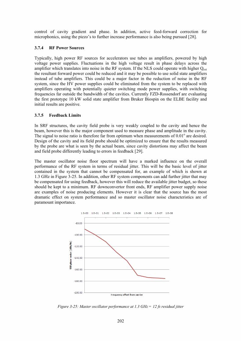
202

control of cavity gradient and phase. In addition, active feed-forward correction for microphonics, using the piezo’s to further increase performance is also being pursued [28].

3.7.4 RF Power Sources

Typically, high power RF sources for accelerators use tubes as amplifiers, powered by high voltage power supplies. Fluctuations in the high voltage result in phase delays across the amplifier which translates into noise in the RF system. If the NLS could operate with higher Qext the resultant forward power could be reduced and it may be possible to use solid state amplifiers instead of tube amplifiers. This could be a major factor in the reduction of noise in the RF system, since the HV power supplies could be eliminated from the system to be replaced with amplifiers operating with potentially quieter switching mode power supplies, with switching frequencies far outside the bandwidth of the cavities. Currently FZD-Rossendorf are evaluating the first prototype 10 kW solid state amplifier from Bruker Biospin on the ELBE facility and initial results are positive.

3.7.5 Feedback Limits

In SRF structures, the cavity field probe is very weakly coupled to the cavity and hence the beam, however this is the major component used to measure phase and amplitude in the cavity. The signal to noise ratio is therefore far from optimum when measurements of 0.01o are desired. Design of the cavity and its field probe should be optimized to ensure that the results measured by the probe are what is seen by the actual beam, since cavity distortions may affect the beam and field probe differently leading to errors in feedback [29].

The master oscillator noise floor spectrum will have a marked influence on the overall performance of the RF system in terms of residual jitter. This will be the basic level of jitter contained in the system that cannot be compensated for, an example of which is shown at 1.3 GHz in Figure 3-25. In addition, other RF system components can add further jitter that may be compensated for using feedback, however this will reduce the available jitter budget, so these should be kept to a minimum. RF downconvertor front ends, RF amplifier power supply noise are examples of noise producing elements. However it is clear that the source has the most dramatic effect on system performance and so master oscillator noise characteristics are of paramount importance.

Figure 3-25: Master oscillator performance at 1.3 GHz = 12 fs residual jitter

203

Experimental work and careful design is therefore required to understand and reduce the phase noise of components such as the RF down convertors, amplifiers and their power supplies and the master oscillator itself. Also the ADC sampling scheme needs to be optimised to possibly include high speed clocking of the digital systems at high IF speeds, this may help to reduce system noise of the field pickup components (see Figure 3-26). Further sources of noise that could limit the performance of the RF system include microphonics and environmental effects. Microphonic noise is created in the cryomodule, the cryogenic system; vacuum pumping systems and interfaces to the cavity itself. The design of these systems should be optimised to insure a high standard of decoupling for the cavity from environmental disturbances.

Figure 3-26: Noise floor of RF system components and the MO

3.7.6 Beam Feedback and Timing

Diagnostics have an important role to play in the RF feedback systems. Bunch Compression Monitors (BCM) are used to measure compression of the beam after the first bunch compressor, which is fedback onto the acceleration module phase control to maintain the desired phase set-point. Beam Arrival Monitors (BAM) are used to compare the electron arrival time against the laser timing system for the machine (see also Section 6.5). The output of the BAM updates the voltage setpoint of the acceleration module to maintain the set condition. For NLS, BCM and BAM monitors should be installed after each bunch compressor and at critical measurement points to feedback on the preceding acceleration module; this will stablise short (bunch-to-bunch) and long term drifting of the machine. This beam feedback system should also be applied to the gun. These developments will become essential to ensure stable photon output at the FELs. The beam feedback techniques described are being developed and implemented at both LCLS [30] and FLASH [31].

At FLASH a laser based synchronisation system is being installed using actively stabilised fibre links [32]. The system is phase locked to the 1.3 GHz RF master oscillator. Start to end sychronisation is then performed from the injection laser, RF, diagnostics, through to the FEL. The RF system is synchronised using laser to RF conversion using Sagnac loops. Direct usage

204

of the laser timing pulses is made for diagnostic and experiment purposes, energy BPMs, BAM and photon arrival time monitors.

Timing of the RF system must be driven by a machine timing system capable of synchronising the entire length of machine from gun to experiment. The jitter studies performed for NLS (see Section 1.2.3), indicate that the cavities in the first accelerating module dominate in terms of the overall linac jitter contribution. By feeding each cavity in ACC01 with its own laser synchronised master oscillator, amplifier system and LLRF controller, the noise contribution will become uncorrelated (see Figure 3-27). For this configuration one would expect to be able to replicate the Cornell demonstration of <0.01o and 2 x 10-5 stability response for phase and amplitude respectively. The other cavities give a smaller contribution to the overall jitter and so here a laser synchronised oscillator for each module can be used as the source of RF (see Section 9.2.3). For these systems, with an increased correlated error contribution, a nominal increase in jitter response is expected, however it is not expected to be significant and the aim will still be to maintain stability to 0.01o and 1 x 10-4 for these systems.

Figure 3-27: Uncorrelated master oscillator distribution for ACC01

3.8 High Power RF System

For an electron bunch charge of 200 pC at 1 MHz (200 µA) a CW RF power of 4.6 kW is required to provide 15 MV/m accelerating voltage in each cavity. However, the RF system will also need to account for micophonics, effects of beam loading and possible degradation of Q0 of the cavities with life, so will need to be capable of providing a CW RF power of the order of up to 10 kW. To deliver the RF power the baseline design for the RF system is to supply each of the cavities via individual Inductive Output Tubes (IOTs).

Each individual RF system will consist of an IOT, a solid state amplifier, a high voltage power supply with ancillary power supplies, a waveguide distribution system, and a low level RF (LLRF) control system. The IOT, solid state amplifier, and high voltage power supply with ancillary power supplier will all be positioned together and will be located in a separate hall above the linac tunnel to ensure that the electronic equipment is protected from any ionising

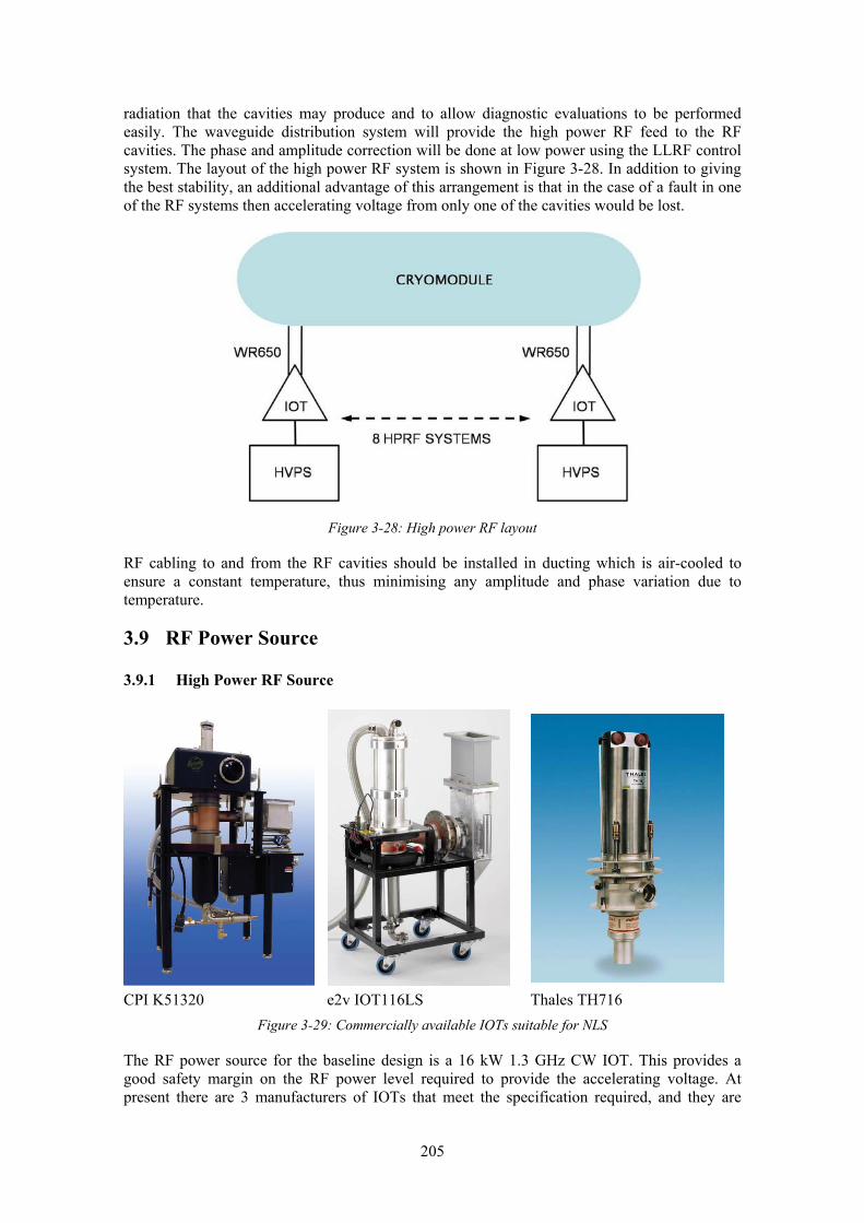
205

radiation that the cavities may produce and to allow diagnostic evaluations to be performed easily. The waveguide distribution system will provide the high power RF feed to the RF cavities. The phase and amplitude correction will be done at low power using the LLRF control system. The layout of the high power RF system is shown in Figure 3-28. In addition to giving the best stability, an additional advantage of this arrangement is that in the case of a fault in one of the RF systems then accelerating voltage from only one of the cavities would be lost.

Figure 3-28: High power RF layout

RF cabling to and from the RF cavities should be installed in ducting which is air-cooled to ensure a constant temperature, thus minimising any amplitude and phase variation due to temperature.

3.9 RF Power Source

3.9.1 High Power RF Source

CPI K51320

e2v IOT116LS

Thales TH716

Figure 3-29: Commercially available IOTs suitable for NLS

The RF power source for the baseline design is a 16 kW 1.3 GHz CW IOT. This provides a good safety margin on the RF power level required to provide the accelerating voltage. At present there are 3 manufacturers of IOTs that meet the specification required, and they are

206

CPI’s K51320W [33], e2v Technologies’ IOT116LS [34] and Thales Electronic Devices TH713 [35] as shown in Figure 3-29. The parameters for each of the IOTs are shown in Table 3-5.

Table 3-5: IOT parameters

CPI K51320W

e2v IOT116LS

Thales TH713

Frequency (GHz) 1.3 1.3 1.3 Max CW Power (kW) 30 16 20 Gain (dB) 21 >20 20.9 Beam Voltage (kV) 34 25 34 Bandwidth (MHz) 4.5 >4 >5 Efficiency (%) 63.8 >60 60.4

3.9.2 Low Power Solid State Amplifiers

The RF gain of the IOT is typically greater than 20 dB, thus to provide the required RF output power of 10 kW CW a solid state amplifier capable of providing greater than 150 W of linear drive power will be required for each of the IOTs. The phase and amplitude stability of the solid state amplifiers will need to be better than 1° and 1 %. There are numerous suppliers of RF amplifiers such as Microwave Amplifiers (AM83 Series) [36] and Bruker BioSpin [37] that are able to provide 200 W CW solid state amplifiers capable of meeting this specification.

3.9.3 High Power Solid State Amplifiers

Recently there have been improvements in LDMOS transistor technology, which has led to an increased power capability of solid state amplifiers. Bruker BioSpin have developed a high power solid state amplifier capable of producing around 10 kW CW (see Table 3-6). The solid state amplifier incorporates a 500 W pre-amplifier, which drives eight, 1.2 kW CW units each consisting of eight, 200W LDMOS transistors.

Table 3-6: Bruker Biospin Solid State Amplifier Parameters

Bruker Biospin Solid State Amplifier Frequency (GHz) 1.3 Max CW Power (kW) ~10 Gain (dB) 70 Power Supply Power (kW) 24 Power Supply Voltage (V) 28 Efficiency (%) 50

The typical operating efficiency for the system is around 50 %. The unit incorporates its own built-in 24 kW, 28 V power supply (see Figure 3-30). The high power solid state option appears to be the more cost effective option and further advances in efficiency are targeted. However, the technology is still being developed, so the reliability at present is still undefined.

207

Figure 3-30: Bruker Biospin 1.3 GHz Solid State Amplifier

3.10 DC Power Supply

A single high voltage power supply (HVPS) along with suitable ancillary power supplies and a solid state amplifier will be required for each of the individual IOTs. In the event of a HVPS fault then only one RF cavity will be lost. The specification for the HVPS and ancillary power supplies is defined in Table 3-7 and is based around the low power e2v IOT.

For tight control of phase and amplitude stability then tight requirements will be required on the noise and voltage ripple of both the HVPS and its ancillary power supplies. The synchronous ripple on the HVPS will produce an energy spread and jitter which will build up along the length of the linac section. This will have to be corrected by the LLRF system in the last RF cavity.

208

Table 3-7: High Voltage Power Supply Specification

Parameter Specification Note Voltage 30 kV Negative voltage Current 1.0 A Nominal efficiency (at full output) >80 % Recommended value Voltage stability (10% to 100%) ±0.1 % of full scale Voltage reproducibility ±0.25 % of Vmax Voltage accuracy ±1 % Voltage ripple ±0.1 %

<15 V RMS <30 V RMS

Overall 40 kHz to 100 kHz

Above 100 kHz Voltage ripple on ancillary PSUs <0.1 % Settling time <250 ms For 10% voltage change Voltage overshoot <5 % Nominal input voltage 400V 3-phase 50 Hz

Acoustic noise <75dBA At 1m with the doors closed Power Factor >0.9 Energy into tube arc <15 J Housing Full metal enclosure Rack or cubicle

3.11 Interlock Control System

The interlock control system has to protect both the accelerator and the RF system in the event of a fault. The RF system will have a dedicated PLC system which will provide the interface between the RF cavities and HVPS system to a high level control platform (e.g. EPICS [38], CORBA [39] etc). Cables will be used to interface from the RF cavities, the HVPS and the RF waveguide distribution system to individual PLC cavity nodes, which will be connected to the PLC in series using fibre optic connections. The PLC will then interface with the machine control system. The layout for the system is shown in Figure 3-31. The control for the RF system will use a state machine format which will enable easier operation and diagnosis of the system.

Protection for the IOT and the solid state amplifier will be provided by the control system for the HVPS, and should limit the energy dissipation within the IOT to less than 15 J in the event of an internal arc. For all other IOT fault conditions the RF power should be removed within 100 ms. Interlocks are required for each of the RF cavities to remove the RF power if a vacuum event occurs within the cavity in which the vacuum level increases above 1 x 10-8 Torr, or in the event of an arc at the cold window, which will be monitored using a photomultiplier. Additionally individual Helium pressure monitors will be incorporated for each of the 18 cryomodules, which will be capable of detecting a rapid increase in pressure during a quench event and provide an interlock which removes the RF power from each cavity.

209

Figure 3-31: Interlock Control System

Interlocks will also be required to remove the RF power in the event of an increase in the isolation vacuum above 1 x 10-6 Torr , in the event of a warm window arc (monitored using a photomultiplier), or in the event of a rapid increase in the temperature of the warm widow, which will be monitored using infrared detectors.

3.12 RF Distribution System

WR650 waveguide is to be used as the RF distribution system to channel the RF power from each of the IOTs to each of the RF cavities in the linac tunnel below. Circulators will be required on the output of each IOT to protect against reflected RF power. These will be contained within the housing for the power supply and the IOT. Forward and reflected power monitoring will be provided before and after each of the circulators which will be integrated into the LLRF system. Motorized stub tuners will be required between the cavities and the circulator to allow the adjustment of the Qext of each cavity.

3.13 Third Harmonic RF System

NLS bunches will require linearization which can be provided by a third harmonic cavity. Third harmonic cavities based on the FNAL 3.9 GHz superconducting RF cavity are being developed for the FLASH and XFEL projects. Unlike the FLASH/XFEL projects, NLS requires CW operation of the RF system. It is expected that a CW gradient of 15-17 MV/m is sustainable in the modules designed for FLASH/XFEL (see Figure 3-32) [40]. This means that a minimum of two 4-cavity cryomodules would be required in order to achieve the bunching required for NLS. The anticipated operating parameters are shown in Table 3-8.

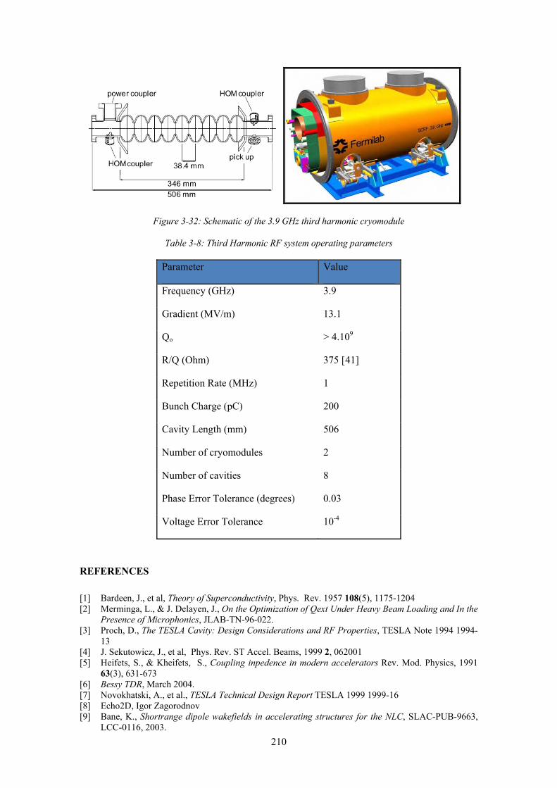
210

Figure 3-32: Schematic of the 3.9 GHz third harmonic cryomodule

Table 3-8: Third Harmonic RF system operating parameters

Parameter Value

Frequency (GHz) 3.9

Gradient (MV/m) 13.1

Qo > 4.109

R/Q (Ohm) 375 [41]

Repetition Rate (MHz) 1

Bunch Charge (pC) 200

Cavity Length (mm) 506

Number of cryomodules 2

Number of cavities 8

Phase Error Tolerance (degrees) 0.03

Voltage Error Tolerance 10-4

REFERENCES [1] Bardeen, J., et al, Theory of Superconductivity, Phys. Rev. 1957 108(5), 1175-1204 [2] Merminga, L., & J. Delayen, J., On the Optimization of Qext Under Heavy Beam Loading and In the

Presence of Microphonics, JLAB-TN-96-022. [3] Proch, D., The TESLA Cavity: Design Considerations and RF Properties, TESLA Note 1994 1994-

13 [4] J. Sekutowicz, J., et al, Phys. Rev. ST Accel. Beams, 1999 2, 062001 [5] Heifets, S., & Kheifets, S., Coupling inpedence in modern accelerators Rev. Mod. Physics, 1991

63(3), 631-673 [6] Bessy TDR, March 2004. [7] Novokhatski, A., et al., TESLA Technical Design Report TESLA 1999 1999-16 [8] Echo2D, Igor Zagorodnov [9] Bane, K., Shortrange dipole wakefields in accelerating structures for the NLC, SLAC-PUB-9663,

LCC-0116, 2003.

211

REFERENCES [10] ‘TESLA - The Superconducting Electron-Positron Linear Collider with an Integrated X-Ray Laser

Laboratory, Technical Design Report’, DESY, March 2001. [11] XFEL TDR, DESY 2006-097, July 2007 [12] Pagani, C., et al, Improvement of the Blade Tuner Design for Superconducting RF Cavities, PAC05,

Knoxville, 2005, pp. 3456 – 3458. [13] Kostin, D., et al, TESLA RF power couplers development at DESY, Proceedings of the SRF2001

Workshop, Tsukuba (Japan). [14] Knoblock, J., et al, CW Operation of the TTF-III Innput Coupler, PAC05, Knoxville, 2005,

3292 - 3294 [15] Belomestnykh, S., et al, Development of High RF Power Delivery System for 1300 MHz

Superconducting Cavities of Cornell ERL , Linac04, Lubeck, 2004 694 – 696. [16 ] BESSY-FEL industry study – DESY EV 010-04-S1 [17 ] Chojnacki, E., et al, Cryogenic heat load of the Cornell ERL main LINAC cryomodule, SRF2009,

Berlin, 2009. [18 ] Peterson, T., Course on Cryostat design at CEC-2009, Tucson, 2009. [19 ] Parma, V., Roadmap of the workshop, Workshop on cryogenic and vacuum sectorisations of the

SPL, CERN, November 10, 2009 [20] Chronis, W C., et al., The CEBAF cryogenic system, PAC89, Chicago, 1989, 592-594 [21 ] Rode, C., The SNS superconducting Linac systems, PAC01, Chicago, 2001, 619-623 [22] XFEL TDR, DESY 2006-097, July 2007 [23] Petersen, T., ILC Cryogenic System reference design, Advances in Cryogenic engineering, 2008 53

B, 1565-1572 [24] Akre, R., et al, LCLS LLRF Upgrades to the SLAC Linac, PAC07, Albuquerque, June 2007,

2421 - 2423 [25] Simrock, S., State of the art in RF control, Linac04, Lübeck, 2004, 523 – 527 [26] Liepe, M., Cornell ERL High Power Delivery and Low Level Control Systems, presented at ERL09,

Cornell University, June 2009 [27] Ayvazyan, V., et al, Digital RF Control System for the DESY FLASH Linear Accelerator, DESY,

Eurocon 2007 , Warsaw, Poland, September 2007 [28] Neumann, A., et al, Characterisation of a Piezo-Based Microphonics Compensation System AT

HoBiCaT, EPAC06, Edinburgh, 2006, 408 – 410 [29] Michel, P., et al, Experiences with the TESLA cavities in CW-operation at ELBE, ERL07,

Daresbury, May 2007 [30] Frisch, J., Diagnostics overview for the LCLS, presented at 48th ICFA FLS 2010, SLAC, USA,

February 2010. [31] Behrens, C., Simulations on beam monitor systems for longitudinal feedback schemes at FLASH,

presented at 48th ICFA FLS 2010, SLAC, USA, February 2010. [32] Schulz, S., Installation progress of the optical synchronization system at FLASH, presented at 48th

ICFA FLS 2010, SLAC, USA, February 2010. [33] ‘CPI IOT Data Sheet for CHK5-1320W Klystrode® IOT Amplifier’, CPI Inc, www.eimac.com [34] ‘IOT Data Sheet for IOT116LS: IOT Amplifier for CW Operation’, A1A-IOT116LS Issue 1, April

2006, e2v technologies (UK) Ltd, www.e2v.com [35] ‘Thales IOT Data Sheet for TH713 L Band IOT’, Thales Electron Devices,

www.thalesgroup.com/electrondevices [36] ‘Microwave Amplifier Catalogue’, pg 23, AM83 Series: 0.7 to 3.9GHz, Microwave Amps Ltd,

www.maltd.com [37] Bruker BioSpin, www.bruker-biospin.com/europe [38] ‘EPICS Experimental Physics and Industrial Control System’, Argonne National Laboratory,

www.aps.anl.gov/epics [39] Tanabe, T., et al, CORBA Based Control System with RTOS on VME/CPCI, International

Conference on Accelerator and Large Experimental Physics Control Systems, 1999, Trieste Italy, .588-560

[40] Vogel, E., et al, Considerations on the third harmonic RF of the European XFEL, Proc. SRF 2007, Beijing, China.

[41] Solyak, N., et al, Development of the 3rd Harmonic SC Cavity at Fermilab, Proc. PAC’03, Portland, Oregon

213

4 Electron Beam Transport

This Chapter describes the design choices for several important beam transport sections:

• an injection dogleg to permit the linac to be commissioned at a later stage with the high repetition rate gun without disturbing operations with the first stage gun.

• a dedicated diagnostics section placed after the laser heater for characterisation of the low energy beam.

• a three stage bunch compression scheme is used to achieve the required electron bunch length at the FELs. The optics designs of the bunch compressors have been optimised to minimise the CSR emittance growth.

• a dedicated transverse and longitudinal collimation system protects the undulators from beam halo.

• a spreader is required to switch the electron beam between the FELs. A design based on fast kicker magnets, similar to the LBNL proposal, has been chosen for its flexibility to include further FEL lines in the future as well as the possibility of diverting all of the bunches to any one FEL.

• a dedicated straight on high energy diagnostics section has been included for commissioning and tuning of the machine before sending the beam through the spreader.

• a dedicated tomography section for 6D characterisation of bunch properties has been included in the first branch of the beam spreader.

• a number of beam dumps to safely absorb the power of the electron beam.

4.1 Injection Dogleg and Low Energy Diagnostics Section

4.1.1 Optics Set-up of the Injection Dogleg

The injection dogleg is required to merge the high repetition rate gun at a later stage. This will allow the linac to be commissioned with high repetition rate without disturbing operations with the first gun. The dogleg design needs to provide a transverse off-set of ~2.8 m considering the requirements of the building including shielding constraints separating the two injectors. The dogleg design as shown in Figure 4-1 incorporates a first dipole bending the beam by +6° and a second dipole separated by ~26 m bending the beam by -6° to provide the required transverse off-set. The optics has been optimised using five quadrupole triplets located between these two dipoles with the aim of keeping the dispersion function as small as possible and the horizontal beta functions minimum at the two dipoles. The optics functions of the dogleg are shown in Figure 4-2. A quadrupole triplet located before the first dipole of the dogleg matches the Twiss parameters of the laser heater to the dogleg and a quadrupole triplet located after the second dipole of the dogleg matches the Twiss parameters to the third harmonic system.

4.1.2 Diagnostics Requirements and Optics Set-up of the Diagnostics Line

Satisfactory FEL operation relies on the low emittance bunch parameters from the injector. A dedicated diagnostics section is essential to make sure that the required parameters are achieved during the initial commissioning as well as normal running of the facility. The location of the low energy diagnostics section after the first dipole of the dogleg (see Figure 4-1) seems appropriate for two reasons: firstly, the straight on diagnostics line is available during initial commissioning of the low energy beam and by diverting a few bunches to this section for quality purposes during normal running of the machine and secondly, the location after the laser heater will also allow the laser heater settings to be monitored and tuned. The diagnostics section includes a deflecting cavity and tomography section which will allow the projected and slice emittances to be measured in both the transverse and longitudinal planes.

214

The 2.8 m transverse space between the dogleg and the straight on diagnostics section is sufficient to install the deflecting cavity and other components. The total length of the diagnostics line is ~25 m from the first dipole of the dogleg. The optics has been arranged independently of the settings required for the dogleg operation which will cause minimum disruption to the normal operation. The first dipole of the dogleg is switched off for the beam to enter the diagnostics section. Four matching quadrupoles located after this dipole match the beta function in both the transverse planes in the deflecting cavity to ~15 m and beam waists as shown in Figure 4-3. At this energy (~135 MeV), it seems possible do the measurements in both the planes using a single deflecting cavity. The deflecting cavity is then followed by four matching quadrupoles to match to the FODO incorporated with four OTR screens located with 45° phase advance between them. These will be used for slice as well as projected emittance measurements. The dipole and the screen at the end will be used to measure the energy spread of the bunch slices.

Figure 4-1: Layout of the dogleg and low energy beam diagnostics sections. The beam enters the diagnostics section when the first dipole of the injector dogleg merger is switched off.

Figure 4-2 : Optics of the injection dogleg

215

Figure 4-3: Optics of the low energy beam diagnostics section.

4.2 Bunch Compressors

4.2.1 Layout Considerations

The NLS design has to deliver ~200 fs FWHM electron bunch length at the end of the linac. This is achieved by gradual compression of the electron bunch from the gun of 20 ps FWHM to ~200 fs FWHM for the FEL operation. The accelerator design to achieve this requires three bunch compressors, BC1, BC2 and BC3 as described in Section 1.2. This Section describes the layouts and optics of these bunch compressors. The locations and strengths of the three bunch compressors have been optimised along with the beam chirps to achieve the required longitudinal bunch parameters at the entrance of the undulator. Detailed diagnostics such as beam arrival monitors, beam profile measurements and position monitors are planned to be included in and after each bunch compressor for compression control (Section 6.2).

4.2.2 Optics Optimisation

The first bunch compressor chicane is of the symmetric four-dipole type whereas the second and the third bunch compressor chicanes are of S-type. They are located at energies of 205 MeV, 459 MeV and 1493 MeV. The optimisation of the dipole bend angles is described in detail in Section 1.2. The derived optimal working point for NLS has bend angles of 11.84˚, 9.35˚ and 7.24˚ respectively. This optimised set-up gives the first order transport matrix element relating path length and energy deviation (R56) equal to 7.4, 9.2 and 8.7 cm for each compressor. For this optimal longitudinal set-up, the transverse optics has been matched using two quadrupole triplets per bunch compressor. A quadrupole triplet preceding each bunch compressor minimises the horizontal beta function and H-function at the fourth dipole of each bunch compressor. This suppresses coherent synchrotron radiation emission as the bunch becomes short and any consequent energy spread and transverse emittance increase [1]. A quadrupole triplet placed after each bunch compressor matches the lattice functions to the next part of the machine, thus keeping compressor settings independent from the optics of the rest of the machine. All four dipoles in each bunch compressor will be powered in series to avoid any beam offset/angle jitter in the beam. Table 4-1 summarises the bunch compressor parameters. Figure 4-4 shows the layout of bunch compressor 1 referring to distances listed in Table 4-1 for each compressor and Figure 4-5 shows the layout of bunch compressors 2 and 3. Figure 4-6 shows the optics and H-functions of each compressor.

216

Figure 4-4: Layout of the bunch compressor 1. Rectangular dipoles are shown in red, quadrupoles in green and correctors in blue. Details are given in Table 4-1.

Figure 4-5: Layout of the bunch compressors 2 & 3. Rectangular dipoles are shown in red, quadrupoles in green and correctors in blue. Details are given in Table 4-1.

Table 4-1: Bunch compressor details

BC1 BC2 BC3 Energy (MeV) 205 459 1493 Type C-type S-type S-type Dipole Length L1,L2 (m) 0.5,0.0 0.5, 1.0 0.5, 1.0 Dipole Angle θ1, θ2 (˚) 11.84 9.35 7.24 R56 (cm) 7.4 9.2 8.7 Bunch length (FW) (ps) 8.1 2.0 0.4 D1, D2 (m) 0.5, 0.96 0.5, 1.73 1.0, 4.69 Total length (m) 8.54 10.30 12.66

217

Figure 4-6: Optics and H-functions in BC1 (upper left), BC2 (upper right) and BC3 (lower)

To correct for magnet and alignment errors, correctors in both the transverse planes are included at the exit of each dipole. In order to trim electrons in the head and tail of the electron bunch which will reduce the peak current spikes at the bunch edges, it is planned to include a collimator in the centre of each bunch compressor as proposed in [2].

4.3 Collimation

4.3.1 Collimation Requirements

A collimation system is necessary in NLS to deal with the beam halo which will be generated due to dark current in the injector and in the accelerating modules, scattering from residual gas particles, off-energy beam tails caused by CSR in the bunch compressors and beam spreader. If not collimated, this beam halo can demagnetise the undulator magnet, cause Bremsstrahlung co-axial with the photon beam lines and can activate the components of the facility. Collimating the beam halo as near as possible to the various sources is preferred as this reduces the overall radiation levels in the machine.

The beam power of the NLS in the baseline will be ~450 W whereas in the upgrade scenario it will be ~450 kW. The research at FLASH has demonstrated that without halo collimation significant demagnetisation of the undulator magnets can occur very quickly for kW beam powers [3]. The post linac collimation scheme for NLS is dictated by the requirement of protecting the undulators.

In addition to removing the beam halo continuously, the collimation system must also provide protection against mis-steered or element failure scenarios.

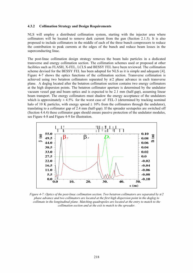
218

4.3.2 Collimation Strategy and Design Requirements

NLS will employ a distributed collimation system, starting with the injector area where collimators will be located to remove dark current from the gun (Section 2.1.5). It is also proposed to include collimators in the middle of each of the three bunch compressors to reduce the contribution to peak currents at the edges of the bunch and reduce beam losses in the superconducting linac.

The post-linac collimation design strategy removes the beam halo particles in a dedicated transverse and energy collimation section. The collimation schemes used or proposed at other facilities such as FLASH, X-FEL, LCLS and BESSY FEL have been reviewed. The collimation scheme devised for the BESSY FEL has been adopted for NLS as it is simple and adequate [4]. Figure 4-7 shows the optics functions of the collimation section. Transverse collimation is achieved using two betatron collimators separated by π/2 phase advance in each transverse plane. A dogleg located after the betatron collimation section contains two energy collimators at the high dispersion points. The betatron collimator aperture is determined by the undulator vacuum vessel gap and beam optics and is expected to be 2.1 mm (half-gap), assuming linear beam transport. The energy collimators must shadow the energy acceptance of the undulators which is approximately ± 4.5% for the worst case of FEL-3 (determined by tracking nominal halo of 10 K particles, with energy spread ± 10% from the collimators through the undulator), translating to a collimator gap of 2.4 mm (half-gap). If the spreader sextupoles are switched off (Section 4.4.4) these collimator gaps should ensure passive protection of the undulator modules, see Figure 4-8 and Figure 4-9 for illustration.

Figure 4-7: Optics of the post-linac collimation section. Two betatron collimators are separated by π/2 phase advance and two collimators are located at the first high dispersion point in the dogleg to

collimate in the longitudinal plane. Matching quadrupoles are located at the entry to match to the collimation section and at the exit to match to the spreader.

219

Figure 4-8: Post-linac betatron collimation simulations with spreader sextupoles off (s=0 m corresponds to first betatron collimator location). Particle loss distribution from halo tracking simulation without

(left) and with (right) betatron collimation. A nominal halo of 10 K particles, three times the transverse size of the undulator acceptance is tracked from the entrance to the collimation section through the

spreader (s = 36-120m) and the undulator (s = 120-165m). The betatron collimators are at s = 0 m and s =19.5 m. When betatron collimator apertures are set to 2.1 mm (half-gap) no particles are lost in the

undulator.

Figure 4-9: Post-linac energy collimation simulation with spreader sextupoles off (s=0 m corresponds to first betatron collimator location). Particle loss distribution from halo tracking simulation without (left)

and with (right) energy collimation. A nominal halo of 10 K particles, with energy spread ± 10 % is tracked from the entrance to the collimation section (s = 0m) through the spreader (s = 36-120m) and the

undulator (s = 120-165m). The energy collimators are located at s = 26 m and s = 28 m. When energy collimators are set to 2.4 mm (half-gap) (equivalent to approx ± 4.5 % energy spread) no particles are

lost in the undulator.

However, it may be required to switch on the sextupoles in the spreader as described in (Section 4.4.4), and the halo tracking in this case indicates that the collimator apertures may need to be reduced considerably due to non-linear beam transport. When the spreader sextupole magnets are included in the beam tracking simulation, the energy bandwidth of the system is reduced requiring tighter energy collimation; also the non-linearities in the transverse phase space transport demand smaller betatron collimator apertures. It was found from tracking simulations that betatron collimator apertures of 1.6 mm (half-gap) combined with an energy collimator gap of 1.0 mm (half-gap) gave nearly no losses in the undulator when a halo of transverse dimensions three times larger than the undulator aperture and energy spread of ±10 % was tracked from the entrance of the collimation section (see Figure 4-10).

220

Figure 4-10: Post-linac particle loss distribution from halo tracking simulation with spreader sextupoles on. A nominal halo of 100 K particles, three times the transverse size of the undulator acceptance and with energy spread ± 10 % is tracked from the entrance to the collimation section (s = 0m) through the spreader (s = 36-120m) and the undulator (s = 120-165m). The betatron collimators are at s = 0 m and s =19.5 m and are set to 1.6 mm (half-gap), the energy collimators are at s = 26 m and s = 28 m and are

set to 1.0 mm (half-gap). Nearly all losses are on the collimators, with a small loss (10-5 of the halo population) on the undulator.

4.3.3 Collimator Design

A copper block of 10 radiation lengths should be enough to absorb the beam halo particles. The betatron collimators will need adjustable gap in two transverse planes, whereas energy collimators will have jaws only in the horizontal plane. In order to minimise wakefields arising due to a step change of beam radius from ~25 mm to the required half gaps in the collimators of ~2 mm, a tapered design will be required for these collimators. In order to decide whether the collimators will need cooling during later operation at 1 MHz, beam halo was tracked through the collimator with half gap of 2 mm (no taper assumed in these simulations). Figure 4-11 shows the results from a FLUKA [5] simulation of the energy deposited by an annular halo distribution normalised per particle. Since the amount of beam halo is not known, we assume a pessimistic number of 10-3 of the beam particles.

Figure 4-11: Energy deposited by an annular halo distribution in the vertical and horizontal jaws of the collimator. Data is normalised by primary particle.

The FLUKA outputs were converted into a power density and introduced into ANSYS [6]. A steady state study of the thermal behaviour of the upper jaw was done to determine the need for cooling of the system. Even if the jaws will not need to be water cooled (preferred in order to avoid Tritium production) they will need to release the heat to a heat sink: a bigger radiative surface, with or without fins, that will help get rid of the excess heat. This surface will then

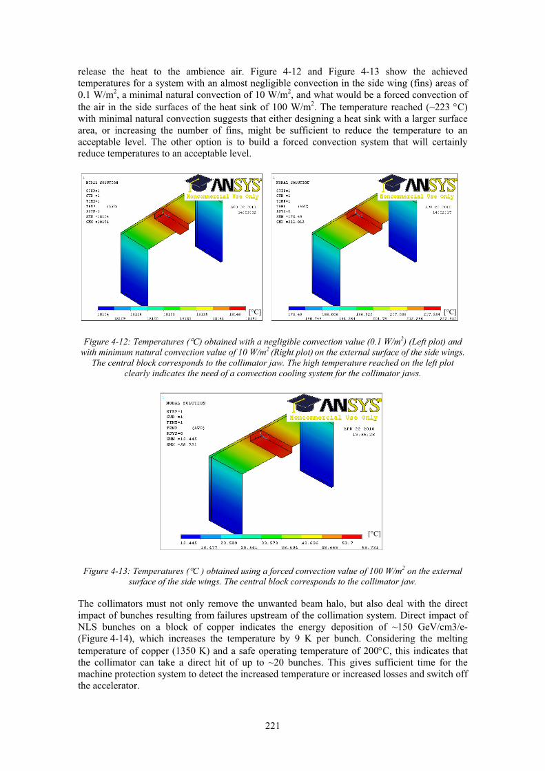
221

release the heat to the ambience air. Figure 4-12 and Figure 4-13 show the achieved temperatures for a system with an almost negligible convection in the side wing (fins) areas of 0.1 W/m2, a minimal natural convection of 10 W/m2, and what would be a forced convection of the air in the side surfaces of the heat sink of 100 W/m2. The temperature reached (~223 °C) with minimal natural convection suggests that either designing a heat sink with a larger surface area, or increasing the number of fins, might be sufficient to reduce the temperature to an acceptable level. The other option is to build a forced convection system that will certainly reduce temperatures to an acceptable level.

Figure 4-12: Temperatures (°C) obtained with a negligible convection value (0.1 W/m2) (Left plot) and with minimum natural convection value of 10 W/m2 (Right plot) on the external surface of the side wings.

The central block corresponds to the collimator jaw. The high temperature reached on the left plot clearly indicates the need of a convection cooling system for the collimator jaws.

Figure 4-13: Temperatures (°C ) obtained using a forced convection value of 100 W/m2 on the external surface of the side wings. The central block corresponds to the collimator jaw.

The collimators must not only remove the unwanted beam halo, but also deal with the direct impact of bunches resulting from failures upstream of the collimation system. Direct impact of NLS bunches on a block of copper indicates the energy deposition of ~150 GeV/cm3/e- (Figure 4-14), which increases the temperature by 9 K per bunch. Considering the melting temperature of copper (1350 K) and a safe operating temperature of 200°C, this indicates that the collimator can take a direct hit of up to ~20 bunches. This gives sufficient time for the machine protection system to detect the increased temperature or increased losses and switch off the accelerator.

[°C]

[°C] [°C]

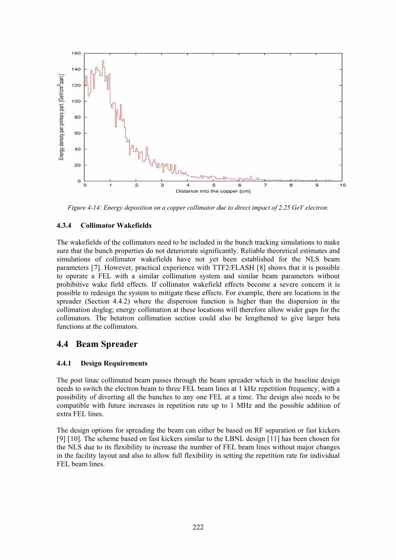
222

Figure 4-14: Energy deposition on a copper collimator due to direct impact of 2.25 GeV electron.

4.3.4 Collimator Wakefields

The wakefields of the collimators need to be included in the bunch tracking simulations to make sure that the bunch properties do not deteriorate significantly. Reliable theoretical estimates and simulations of collimator wakefields have not yet been established for the NLS beam parameters [7]. However, practical experience with TTF2/FLASH [8] shows that it is possible to operate a FEL with a similar collimation system and similar beam parameters without prohibitive wake field effects. If collimator wakefield effects become a severe concern it is possible to redesign the system to mitigate these effects. For example, there are locations in the spreader (Section 4.4.2) where the dispersion function is higher than the dispersion in the collimation dogleg; energy collimation at these locations will therefore allow wider gaps for the collimators. The betatron collimation section could also be lengthened to give larger beta functions at the collimators.

4.4 Beam Spreader

4.4.1 Design Requirements

The post linac collimated beam passes through the beam spreader which in the baseline design needs to switch the electron beam to three FEL beam lines at 1 kHz repetition frequency, with a possibility of diverting all the bunches to any one FEL at a time. The design also needs to be compatible with future increases in repetition rate up to 1 MHz and the possible addition of extra FEL lines.

The design options for spreading the beam can either be based on RF separation or fast kickers [9] [10]. The scheme based on fast kickers similar to the LBNL design [11] has been chosen for the NLS due to its flexibility to increase the number of FEL beam lines without major changes in the facility layout and also to allow full flexibility in setting the repetition rate for individual FEL beam lines.

223

4.4.2 Spreader Design

Figure 4-15: Layout of NLS spreader design based on LBNL design [11] with fast kicker and septum. The inset on the left hand corner shows the start of the different FEL beam lines and the main Figure shows

details of the complete lattice for one spreader line.

As shown in Figure 4-15, the spreader consists of a long FODO take-off section with a series of extraction points for various FEL lines. Bunches which are not diverted to the particular FEL line continue to pass on-axis through the FODO. Each extraction section consists of two Triple Bend Achromat (TBA) arcs, where the kicker and the septum replace the first dipole of the first TBA arc. A 2 meter long kicker placed between the first F and D quadrupole provides a kick of 3 mrad. The beam passes off-axis by ~4 mm in the centre of the D quadrupole immediately after the kicker and by ~16 mm in the centre of the F quadrupole before the septum. The beam is nearly parallel to the take-off axis at the entry of the septum. The septum kicks the beam by 27 mrad. The beam passes off-axis by ~53 mm through the D quadrupole after the septum giving an additional dipole kick of 17.5 mrad, thereby reducing the required strength of the septum magnet. The beam is finally separated from the incoming beam after the D magnet after the septum. The first TBA arc is then completed with two additional dipoles and seven quadrupoles. This section is followed by matching quadrupoles to match the beam into the second TBA arc. The NLS beam spreader optics is shown in Figure 4-16. The optics has been optimized to be achromatic and isochronous within each arc.

The spreader design used for the simulations (Section 1.2) uses the above described lattice with a large beam offset of ~53 mm in the quadrupole after the septum. However, achieving the required gradient in such a large bore quadrupole will be a problem and increasing the length of this magnet will affect the FODO take-off section layout. In addition to this, there may be some undesirable beam dynamics effects due to such a large beam offset. The proposed solution is to replace this quadrupole with a compact bore quadrupole for the take-off section and include an additional septum providing a kick of ~17.5 mrad after the 25 mrad septum. Optics studies show that the quadrupole term can be absorbed in the original lattice keeping the isochronous and achromaticity conditions as before. The lattice functions for this revised lattice are shown in Figure 4-17. The details of the compact quadrupole should be studied in the future.

224

Figure 4-16: Optics of one branch of NLS spreader. First 45 m section is first TBA arc and the second TBA arc starts at ~56m.

Figure 4-17: Optics of one branch of NLS spreader with replaced off-axis quadrupole after the septum with additional septum magnet (marked in blue).

4.4.3 Kicker Tolerances

To decide the tolerances on the kicker power supply, the kicker strength was changed by 10-4 and the position and angle offsets at the end of the spreader were estimated to be 1 μm and 0.23 μrad respectively. These numbers were then compared to the beam alignment tolerances defined by the FEL sensitivity studies (Section 1.4.4). To maintain the angle tolerance (θx) within 0.35 μrad for keeping output power variations less than 1% the required kicker stability needs to be better than 1.5 x 10-4. The details of the kicker power supply are discussed in (Section 11.2.1). If achieving the required kicker stability proves to be difficult, an option of including a second kicker which cancels the effect of the first and which is powered by the same power supply [12] has been investigated. This will considerably reduce the tolerance requirements on the kicker power supply. There is a suitable location with correct phase advance around 60 m in the spreader lattice but the horizontal beta function at that location is

225

~4 times larger than that at the first kicker. Thus the kicker strength needs to be half that of the first kicker. Detailed studies of the kicker and septum power supplies and the feasibility of this scheme should be investigated in the future.

To divert all bunches to any single FEL beamline; it is proposed to include a DC dipole magnet at the location of each kicker. A choice of DC septum (Section 11.2.2) allows this without any change.

4.4.4 Sextupoles in the Spreader

The second order terms in the spreader; namely the horizontal and vertical chromaticities and the second order dispersion are shown in Figure 4-18. These terms do not affect the standard operation but can adversely affect the performance of the single spike operation due to large energy spread. It was found to be effective to correct these higher order terms in order to remove the curvature in the longitudinal phase space and maintain a high current. Even though the single spike simulations presented in (Section 1.5.1) do not have significant effect of sextupoles, the earlier single spike optimisations did show significant improvement in the peak current when sextupoles were used. Taking this into consideration, it was decided to include sextupoles in the spreader as additional tuning knobs. As shown in Figure 4-18, without switching on the sextupoles, the T566 term is around 300 mm. In case of a beam energy error (i.e., δ ≠ 0, with respect to the spreader dipole magnet settings), this 300 mm T566 coefficient will generate a lower order feed-down, producing a non-zero value of R56 (= 2T566δ = ±0.6 mm for δ = ±0.1%, which may be a difficult level to detect). This possible R56 error should be studied in the future to determine if it causes any trouble for the FELs and/or if this can be used as an additional knob. If the sextupoles are switched on, this will not be an issue, however then the sextupole magnet position alignment tolerances should be checked since they can cause R56 errors and linear dispersion errors in both planes, as well as x-y coupling and beta-mismatch errors. This should be studied in detail in the future.

Figure 4-18: Horizontal and vertical chromaticities T162, T364 and second order dispersion T566 in the spreader. Plots on the left side are without sextupoles and plots on the right side are with optimised

sextupoles in the spreader.

226

4.5 High Energy Diagnostics Sections

4.5.1 Introduction

Two dedicated diagnostics sections, one located straight after the post linac collimation section and a second one located in the first branch of the spreader have been included to fully characterise the bunches during commissioning and normal operation. A dedicated straight on beam diagnostics section has been included after the post linac collimation section to enable initial commissioning and tuning of the machine without the spreader. A few bunches can be diverted to this diagnostics section for monitoring purposes during the normal operation to ensure tuning of the linac decoupled from the spreader. The dedicated diagnostics branch in the first branch of the spreader will characterise bunches including the effect of the spreader and thus measure equivalent bunches to those entering the FELs. This will allow the tuning and commissioning of the spreader magnets without having to send the beam through the undulators. Additionally, a few bunches can be diverted to this branch during normal operation for monitoring purposes. The proposed tomography beam diagnostics section in both these sections will fully characterise the beam in 6D phase space, which will provide knowledge of projected transverse emittances (& additionally tomography on slices for transverse emittances in the spreader branch), longitudinal bunch profile and bunch length and together with a spectrometer dipole, projected as well as slice energy spread. Some additional measurements may need to be included in each FEL branch which should complement the dedicated measurements in the first spreader branch and highlight the differences if any. 4.5.2 Diagnostics Line in First Branch of the Spreader

The tomography diagnostics section in first branch of the spreader shown in Figure 4-19 consists of a FODO lattice with four screens providing 45˚ phase advance per screen [13] [14] and is preceded by four matching quadrupoles to match to the FODO and two deflecting cavities (one for each transverse plane). The possibility of using just one deflecting cavity for both planes as is currently the case at JLab [15] should be investigated further. The deflecting cavities operate in TEM110 mode and at zero crossing, which allows streaking of the bunch to get the information of bunch length and slice emittance using one or more tomography screens. For effectiveness of the streak, the beam size at the location of the deflecting cavities needs to be reasonably large and the phase advance between the centre of the cavities and the first screen needs to be an odd integer multiple of π/2 or as close as possible to it. Four quadrupoles preceding the deflecting cavities are used to increase the beam sizes at the deflecting cavities. Depending on the direction of the streak, the head of the bunch is deflected downwards whereas the tail of a bunch is deflected upwards. Measurements without streak give the projected transverse profiles and emittances, whereas measurements with streak measure the slice emittances and the bunch length. This is more important since the effects of space charge and CSR vary along the bunch, and so only the slice emittances give the precise information about the part of the bunch which takes part in the lasing process. The required deflecting cavity parameters and details of the screens are described in (Section 6.2) respectively. Measurement of the projected and slice energy spread will be done using a spectrometer dipole and a screen at the end of the diagnostics line.

227

Figure 4-19: Possible layout of the tomography beam diagnostics line. TDC(x), TDC(y) are the Transverse Deflecting cavities and OTR is the screen/wire location. Matching quadrupoles are located

before and after the transverse deflecting cavities.

4.5.3 Straight on Diagnostics

A dedicated straight on beam diagnostics section has been included after the post linac collimation section to enable initial commissioning and tuning of the linac and the collimation system without the spreader (see Figure 4-20). The location after the post linac collimation section is most suited for this purpose as the FODO take-off section of the spreader can be used for emittance measurement. A final dipole and screen also allows energy spread to be measured. The phase advance of 90° in the FODO section for take-off optics can be changed to 45° by changing the strengths of the matching quadrupoles between the collimation and the spreader take-off section. More detailed studies should be done in the future considering the aperture limitations arising due to the kickers and proposed compact quadrupole to replace the large aperture quadrupole located after septum (Section 4.4.2).

TDC(x,y)

Post linac Collimation dogleg

OTR

Figure 4-20: Possible layout of the straight ahead tomography beam diagnostics line. Locations of OTR screen/wire are shown in light blue colour. Matching quadrupoles shown in green colour are located

before the spreader take-off FODO and before the transverse deflecting cavity(TDC).

From the preliminary estimates of the required dimensions of the Transverse Deflecting Cavity it looks difficult to install one TDC for both the planes or one TDC per plane within the drift space available between the FODO and thus it is proposed to install this cavity after the take-off section. However this set up will not allow tomography on slices for measuring slice emittances. It may be possible to get some information on slice emittances using the screen located after the TDC depending upon the TDC parameters and the distance of the OTR from it. This is a topic for future detailed studies. The dipole and the OTR placed after the dipole will measure the projected as well as slice energy spread of bunches. The required optics details in the TDC for optimum resolution should be included in the future detailed design stage.

228

4.6 Beam Dumps

4.6.1 Requirements

The 2.25 GeV energy electron beam needs to be dumped at several locations, after passing through the straight-through diagnostics/commissioning line, at the end of tomography/beam tuning section in first branch of the beam spreader and after each of the three FEL lines. Each beam dump has to absorb a power of ~450 W when operating at the baseline bunch repetition rate of 1 kHz and ~450 kW when upgraded to 1 MHz. The design requirements for both baseline and upgrade power levels need to be considered to understand the implications to the facility layout. For the baseline case, because of the modest power levels, five separate beam dumps each capable of absorbing 450 W are envisaged.

For later operation at up to 1 MHz repetition rate, it is proposed to transport beams to a single 450 kW beam dump as described in Section 4.6.3. A solid dump similar to that proposed for the European XFEL is considered. The beam power is entirely contained in solid materials in such a dump, minimising the problems associated with radioactive water handling in case of a water dump. In order to design a solid dump, careful choices on the dump material, beam size and its sweeping have to be made to keep the temperatures and stresses within acceptance limits.

4.6.2 450 kW Beam Dump Design

A solid beam dump similar to the XFEL beam dump with a graphite core embedded in a copper shell [16] is proposed. The XFEL beam dump absorbs 300 kW at a variable energy up to 25 GeV, which gives a maximum power density of ~2 kW/cm, whereas the NLS beam dump needs to absorb 450 kW power at 2.25 GeV, which gives a maximum power density of ~3.5 kW/cm. We describe below the choices made on the beam dump design to absorb a higher power by a factor of 1.75 compared to XFEL. Unlike the XFEL case where the impact of long bunch trains at 10 Hz is cyclic, the regular bunch pattern of NLS at 1 MHz implies less cyclic and instantaneous loading of all the involved materials and thus suggests that the proposed solution may be technically possible. Further work is required during a detailed design phase.

4.6.2.1 Material Choice Requisites

Heat extractions capabilities of the power deposited by the beam are the principal constraint in the dump design. We adopt a geometrical solution based on a cylindrical absorber. Around 90% of the beam power is dissipated near the shower axis within one Molière radius and flows radially towards the cooled circumference edge. We assumed in the calculations a cooling system which keeps the external surface of the cylinder at 40 °C. A material of low Z, with low power dissipation per unit length, together with high radial thermal conductivity will help reduce the equilibrium temperature (temperature in the steady state) inside the dump. To achieve high radial thermal conductivity we need to reduce the radial distance towards the cooled surface.

These constraints lead to a dump design of a low density core covered by a higher density shell with low thermal resistance and therefore, the materials we are interested in, and used widely in solid beam dump design, are graphite for the dump core and copper for the outer shell. The characteristics of graphite and copper used in the design presented here are shown in Table 4-2.

229

Table 4-2: Physical characteristics of graphite and copper used for dump design simulations

Graphite Copper Density [g/cm3] 1.71 8.96 Critical energy EC [MeV] 84.25 20.17 Radiation Length X0 [cm] 25.1 1.44 Molière radius RM [cm] 7 1.6 Melting Temp Tmelt [°C] 3800 1083 Operating Temp Top [°C] 500-600 <200 Static stress limit [MPa] 100-250 at compression

>40 at tension σ0.2≈150-400

(plasticity limit) Cyclic stress limit [MPa] 60 at compression

30 at tension 60-100

4.6.2.2 Beam Radius and Sweeping Requirements

The beam size at the entrance of the beam dump has to be large enough in order to reduce the deposited energy density and not damage the graphite. Figure 4-21 shows the peaks of energy density in the graphite depending on the beam size and number of bunches hitting the beam dump at the same location. The horizontal line, tol(dt/dm), fixes the limit of energy density for the material to avoid reaching the ultimate tensile strength limit and for graphite this value is 248 J/g [16]. However, this is a very conservative limit and excursions beyond it could be acceptable. The values below this line should be safe for the mechanical limits of the graphite.

Figure 4-21: Maximum deposited energy density in graphite for different numbers of bunches as a function of impinging radial beam size and comparison with the tolerable tensile limit.

It can be deduced from Figure 4-21 that we cannot continuously direct the beam to a fixed position in the dump core. For the energy that 100,000 bunches would deposit we are above tolerable tensile limit and therefore we will require to sweep the beam to different positions inside the dump. In this study we have selected a radial beam size of 2 mm as a starting point, which should be perfectly achievable in the beam line that transports the beam (Section 4.6.3) towards the dump and this beam size keeps us below the tensile limit for slightly less than

230

100,000 bunches as shown in Figure 4-21. A beam spot size of 2 mm or more is better from the temperature considerations as well. However, even with this beam size, the average beam power has to be diluted in the dump core by sweeping in order to keep the average temperature in the graphite core below its safe maximum operating temperature. The simulations shown in following Sections indicate that by sweeping the beam in twelve different spots both stress and temperature within the graphite core remain below acceptable levels.

The results presented here have been calculated using 2 mm radial beam size in FLUKA simulations and their output used in ANSYS for the twelve different sweep positions. To deal with the increase in the power density per length by a factor of 1.75 compared to XFEL, the radius of sweep circle is roughly scaled from 5 cm (XFEL) to ~9 cm [17]. This radius will be equivalent to having a bigger beam size and therefore thermal effects will also relax as heat will flow towards the centre of the core as well as towards the outer copper shell which will allow a rapid cool down of the dump.

4.6.2.3 Optimisation of Dump Radial Dimensions

The radial extension of an electromagnetic shower is characterised by the Molière radius (RM) and can be calculated by the following expression [16]:

02.21 XEMeVRc

M ≈

Where EC is the critical energy and X0 is the radiation length of the material. The radius needed to absorb 99% of the energy deposited radially by the electromagnetic showers is:

MRR .5%99 =

In our initial design we are using a sweep radius of 9 cm adding a thickness of 5 cm of graphite after that, which corresponds to 0.72 RM. Therefore the thickness of the copper shell needs to be 4.3 RM which corresponds to 7 cm thus giving a total radius of 21 cm (14 cm of graphite plus 7 cm of copper).

4.6.2.4 Optimisation of Dump Length

The length of material that is needed to avoid a leakage of beam energy bigger than 1% can be expressed as [16]:

00

%99 6.17ln.1.4ln.52.1 XMeV

EMeV

EL c⎟⎟⎠

⎞⎜⎜⎝

⎛+⎟

⎠⎞

⎜⎝⎛−⎟

⎠⎞

⎜⎝⎛=

E0 is the primary particle initial energy (2.25 GeV for NLS). For the graphite L99% corresponds to a total length of 280 cm. In order to reduce this length we can use copper as a backstopper (which has an L99% at 2.25 GeV of 17 cm) downstream of the graphite. We chose a combination of 200 cm of graphite and 10 cm of copper for our studies. This configuration, shown in Figure 4-22, absorbs 99.4% of the primary beam energy and is the one used in the ANSYS [6] calculations. Figure 4-23 shows an energy density profile for a beam of 2.25 GeV electrons hitting 200 cm of graphite and 10 cm of copper afterwards calculated using FLUKA [5]. The radius is considered to be large enough to not let escape any energy radially. The increment of temperature in the copper after 1 second of operation at 1 MHz is below 10 K in this case, therefore safe for the graphite-copper junction [16].

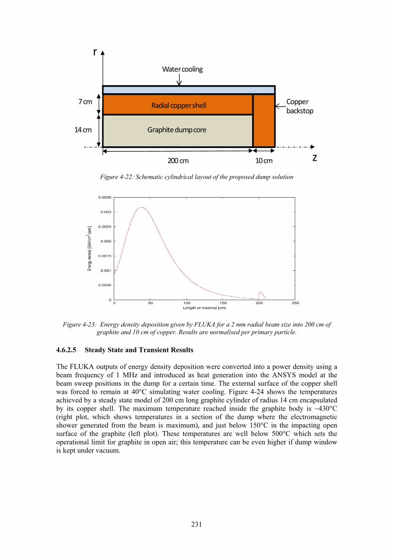
231

14 cm

7 cm

200 cm 10 cm

Copper backstop

Graphite dump core

Radial copper shell

Water cooling

r

z

Figure 4-22: Schematic cylindrical layout of the proposed dump solution

Figure 4-23: Energy density deposition given by FLUKA for a 2 mm radial beam size into 200 cm of graphite and 10 cm of copper. Results are normalised per primary particle.

4.6.2.5 Steady State and Transient Results

The FLUKA outputs of energy density deposition were converted into a power density using a beam frequency of 1 MHz and introduced as heat generation into the ANSYS model at the beam sweep positions in the dump for a certain time. The external surface of the copper shell was forced to remain at 40°C simulating water cooling. Figure 4-24 shows the temperatures achieved by a steady state model of 200 cm long graphite cylinder of radius 14 cm encapsulated by its copper shell. The maximum temperature reached inside the graphite body is ~430°C (right plot, which shows temperatures in a section of the dump where the electromagnetic shower generated from the beam is maximum), and just below 150°C in the impacting open surface of the graphite (left plot). These temperatures are well below 500°C which sets the operational limit for graphite in open air; this temperature can be even higher if dump window is kept under vacuum.

232

Figure 4-24: Left: Steady state calculation of the temperatures [° C], achieved in the impacting surface of the 200 cm graphite/Cu beam dump using a beam sweep radius of 9 cm with 12 spots. Right:

Temperatures achieved in the section of the dump where the electromagnetic shower generated by the beam is at maximum intensity.

A transient study was also performed to assess a proper sweeping frequency according to the stresses obtained. The results of the stress calculations in the graphite core and copper shell can be compared with the mechanical stress limits of the material by means of a certain failure criterion expressed by the equivalent stress value σeq, which can be defined as [16]:

213

232

221 )()()(

21 σσσσσσσ −+−+−=eq

At a given position σ 1, σ 2 and σ 3, the first, second and third components of stress, with σ1 > σ2 > σ3 are the stress components in the three main directions of the given coordinate system, which in our case is Cartesian with the origin in the centre of the circumference at the start of the dump cylinder. Since σeq is always a positive value it can be judged by the sign of the contributing stress components whether the material has to withstand a compressive or tensile load. Compression forces correspond to a negative sign in ANSYS results while tension forces correspond to a positive sign result.

The results reported here use a sweeping frequency of 10 Hz, which means staying in the same spot for 100 ms (100,000 bunches). This frequency sets the highest limit of consecutive bunches hitting the same spot in graphite, as was shown in Figure 4-21, and therefore it can be used as a reference.

Figure 4-25 shows the equivalent stress together with the first, second and third components of stress along the radius and in the position of maximum electromagnetic shower (55 cm) of the beam dump passing through one of the sweeping spots after 7.3 seconds, which means that the beam has done six full sweep cycles and returned to its start position. The first peak corresponds to the sweep spot position and we find compressive stress values reaching ~1.5 MPa. The second peak corresponds to the graphite and copper union and we observe a tensile stress of ~18 MPa. Figure 4-26 shows the first, second and third components of stress and the equivalent stress due to the beam doing a six full sweeps and returning to the start position. It takes 7.2 seconds for the beam to do a full sweep. These stresses are below the static and cyclic stress limits for graphite and copper. The sweeping strategy was to hit a position which was as far as possible to the previous location.

[°C] [°C]

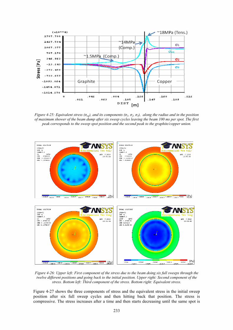
233

Figure 4-25: Equivalent stress (σeq), and its components (σ1, σ2, σ3), along the radius and in the position of maximum shower of the beam dump after six sweep cycles leaving the beam 100 ms per spot. The first

peak corresponds to the sweep spot position and the second peak to the graphite/copper union.

Figure 4-26: Upper left: First component of the stress due to the beam doing six full sweeps through the twelve different positions and going back to the initial position. Upper right: Second component of the

stress. Bottom left: Third component of the stress. Bottom right: Equivalent stress.

Figure 4-27 shows the three components of stress and the equivalent stress in the initial sweep position after six full sweep cycles and then hitting back that position. The stress is compressive. The stress increases after a time and then starts decreasing until the same spot is

[Pa] [Pa]

[Pa][Pa]

234

hit again by the beam adding up to the remaining compressive stress. Figure 4-28 shows a quadratic fit done to each peak of each cycle and the time and value when that stress stops increasing. The compressive stress value at equilibrium is just below 3 MPa and it is achieved after ~13 seconds.

Figure 4-27: First (σ1), second (σ2) and third (σ3) components of the stress and equivalent stress (σeq) in the initial hit position of the sweep with the beam doing six full sweep cycles through the twelve different

positions and going back to the initial position, stopping in each position 100 ms.

Figure 4-28:Equivalent stress (σeq) in the initial sweep spot position in the graphite core and a quadratic fit done to its peaks of stress showing how the stress stabilizes after a period of ~13 seconds at a value

nearing 3 MPa.

A compressive stress value of 3 MPa is well below the cyclic stress limit of the graphite. However, the peak of stress, tensile stress, happens in the graphite/copper union. Figure 4-29 shows the values of the equivalent stress in that union for a total of six sweep cycles and a quadratic fit done to these values which shows that the stress plateau is reached after ~33 seconds at a value of 27 MPa which is below the cyclic stress limit for copper and just under the cyclic stress limit in tension for graphite.

235

Figure 4-29:Equivalent stress (σeq) at the graphite/copper union and a quadratic fit done to it showing how the stress stabilizes after a period of ~33 seconds at a value nearing 27 MPa.

The cyclic stress behaviour showed in these calculations is mainly due to the low sweeping frequency chosen, which corresponds to the maximum time the beam can stay in a fixed position in graphite for the selected beam size of 2 mm. If we were to increase this frequency and instead of stopping in each sweep position 100 ms we would stop 20 or 10 ms the stress behaviour would approximate more to a quasi-static regime rather than a cyclic one. Therefore increasing the sweeping frequency could help avoid stress fatigue and using the static stress limit as a reference instead which is higher than the cyclic one. Nevertheless, the stress shown in these studies are between safety limits and make us think that the beam dump would survive with this configuration and this kind of sweeping/beam size strategy. These simulations indicate that it is possible to use the solid dump based on graphite for the NLS. The details of the dump window design and the dump region will need more technical details to be worked out. This work should be included in a future detailed design stage. Different beam sizes, sweeping strategies (i.e. sweeping radius, hitting time) and longer transient calculations that would allow us reaching a plateau in the stress would only benefit this study and the subsequent beam dump design.

4.6.3 Design of Beam Dump Regions at 1 MHz Repetition Rate

In principle, at 1 MHz repetition rate, five 450 kW beam dumps are needed at the end of the three FEL lines, the diagnostics line and the straight ahead direction. This is however impractical, considering the infrastructure, accessibility, radiation requirements and cost implications. It has been decided therefore that the first FEL diagnostics line will stay at the same beam power of 450 W as in the baseline i.e. limited to 1 kHz operation. The other four beams will be transported to a single 450 kW beam dump. The layout of the spreader and the facility in principle allows the possibility of transporting different beams to a single dump using suitable beam transport lines. In the FEL branches, this could be done by vertically bending the beam upwards at the end of undulators in each FEL line and then transporting them horizontally and combining the three beam lines from the FELs just before the beam dump using pulsed magnets. In addition to these three beam lines, it also seems possible to transport the beam from the straight through commissioning/tuning line to combine with this 450 kW beam dump. The section before the beam dump window will include only one set of sweeping magnets for the combined beams. Figure 4-30 shows a schematic of a possible layout to bring all the four

236

beams to a single beam dump. The optics design of these transport lines should be included in future detailed design stage.

Figure 4-30: Schematic of transporting electron beams to a common 450 kW beam dump

REFERENCES [1] Dohlus, M., & Limberg T., Impact of optics on CSR-related Emittance Growth in Bunch

Compressor Chicanes, PAC2005, Knoxville [2] Cornacchia, M., et al., FERMI & Elettra Accelerator Technical Optimization Final Report, LBNL-

60958, ST/F-TN-06/15, 2006 [3] Schlarb, H., Collimation System for the VUV Free-Electron Laser at the TESLA Test Facility. PhD

Thesis, University of Hamburg. 2001 [4] Kamps, T., Collimation System for the BESSY FEL. FEL 2004, Trieste, Italy [5 ] Fassò, A., et al., Electron-photon transport in FLUKA: status, Proceedings of the MonteCarlo 2000

Conference, Lisbon, October 23--26 2000, A.Kling, F.Barao, M.Nakagawa, L.Tavora, P.Vaz - eds., Springer-Verlag Berlin, p.159-164, 2001

[6] ANSYS® Academic Research [7] Zagorodnov, I.,Numerical Calculation of Small Angle Collimator Wakefields for Short Bunches.

TESLA-REPORT-2003-18, 2003 [8] Rossbach, J., Review of DESY FEL activities. EPAC 08, Genoa, Italy. [9] Douglas, D R., Design Considerations for Implementing Alternative RF Separator Schemes,

CEBAF-TN-91-072, 1991 [10] Brinkmann, R., Some Considerations on X-FEL Beam Distribution, DESY Internal presentation

2003 [11] Zholents, A A., et al., Design of the electron beam switch yard for an array of Free Electron Lasers,

CBP Tech Note 401, 2009 [12] Imai, T., et al., Double Kicker system in ATF, LINAC2000, Monterey, California [13] Löhl, F., Measurements of the Transverse Emittance at the VUV-FEL, Diploma Thesis, Hamburg,

DESY-THESIS 2005-014 and TESLA-FEL 2005-03, 2005 [14] Honkavaara, K., & Löhl, F., Personal Communication. 2005 [15] Krafft, G., Personal communication. 2007 [16] Maslov, M., et al., Layout Considerations on the 25GeV/300kW Beam Dump of the XFEL Project,

DESY, TESLA-FEL, 2006-05 [17 ] Schmitz, M., Personal communication, 2010

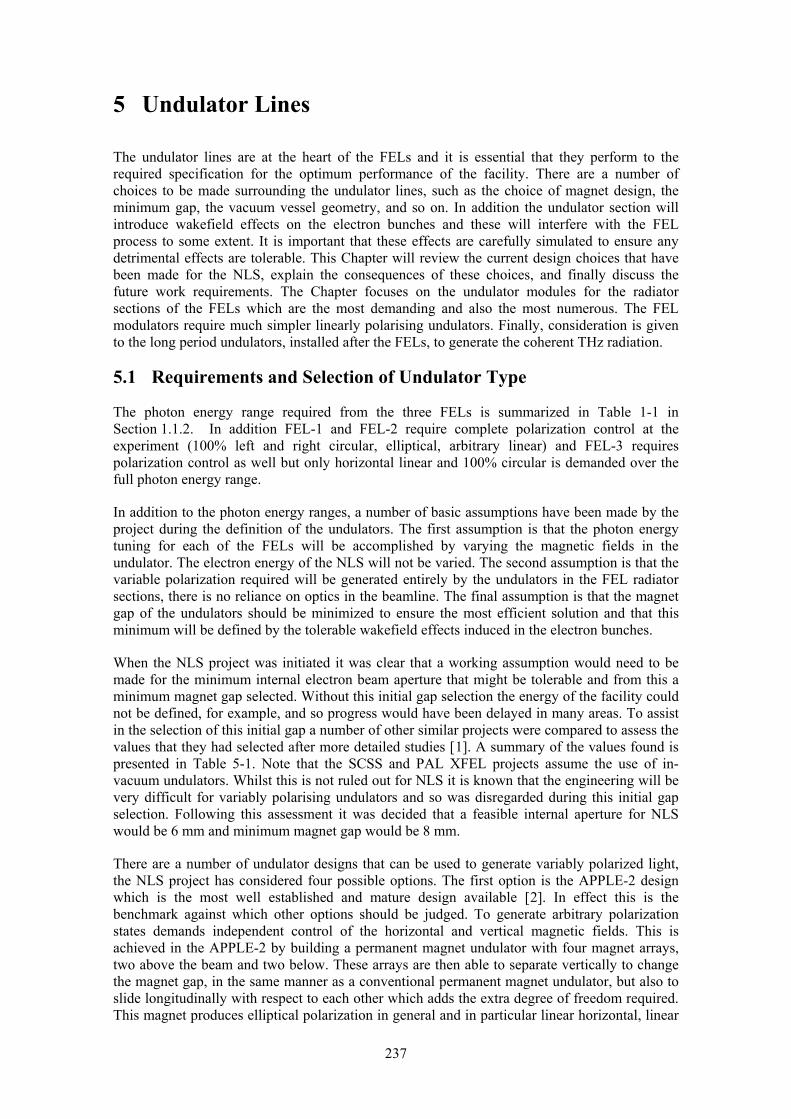
237

5 Undulator Lines

The undulator lines are at the heart of the FELs and it is essential that they perform to the required specification for the optimum performance of the facility. There are a number of choices to be made surrounding the undulator lines, such as the choice of magnet design, the minimum gap, the vacuum vessel geometry, and so on. In addition the undulator section will introduce wakefield effects on the electron bunches and these will interfere with the FEL process to some extent. It is important that these effects are carefully simulated to ensure any detrimental effects are tolerable. This Chapter will review the current design choices that have been made for the NLS, explain the consequences of these choices, and finally discuss the future work requirements. The Chapter focuses on the undulator modules for the radiator sections of the FELs which are the most demanding and also the most numerous. The FEL modulators require much simpler linearly polarising undulators. Finally, consideration is given to the long period undulators, installed after the FELs, to generate the coherent THz radiation.

5.1 Requirements and Selection of Undulator Type

The photon energy range required from the three FELs is summarized in Table 1-1 in Section 1.1.2. In addition FEL-1 and FEL-2 require complete polarization control at the experiment (100% left and right circular, elliptical, arbitrary linear) and FEL-3 requires polarization control as well but only horizontal linear and 100% circular is demanded over the full photon energy range.

In addition to the photon energy ranges, a number of basic assumptions have been made by the project during the definition of the undulators. The first assumption is that the photon energy tuning for each of the FELs will be accomplished by varying the magnetic fields in the undulator. The electron energy of the NLS will not be varied. The second assumption is that the variable polarization required will be generated entirely by the undulators in the FEL radiator sections, there is no reliance on optics in the beamline. The final assumption is that the magnet gap of the undulators should be minimized to ensure the most efficient solution and that this minimum will be defined by the tolerable wakefield effects induced in the electron bunches.

When the NLS project was initiated it was clear that a working assumption would need to be made for the minimum internal electron beam aperture that might be tolerable and from this a minimum magnet gap selected. Without this initial gap selection the energy of the facility could not be defined, for example, and so progress would have been delayed in many areas. To assist in the selection of this initial gap a number of other similar projects were compared to assess the values that they had selected after more detailed studies [1]. A summary of the values found is presented in Table 5-1. Note that the SCSS and PAL XFEL projects assume the use of in-vacuum undulators. Whilst this is not ruled out for NLS it is known that the engineering will be very difficult for variably polarising undulators and so was disregarded during this initial gap selection. Following this assessment it was decided that a feasible internal aperture for NLS would be 6 mm and minimum magnet gap would be 8 mm.

There are a number of undulator designs that can be used to generate variably polarized light, the NLS project has considered four possible options. The first option is the APPLE-2 design which is the most well established and mature design available [2]. In effect this is the benchmark against which other options should be judged. To generate arbitrary polarization states demands independent control of the horizontal and vertical magnetic fields. This is achieved in the APPLE-2 by building a permanent magnet undulator with four magnet arrays, two above the beam and two below. These arrays are then able to separate vertically to change the magnet gap, in the same manner as a conventional permanent magnet undulator, but also to slide longitudinally with respect to each other which adds the extra degree of freedom required. This magnet produces elliptical polarization in general and in particular linear horizontal, linear

238

vertical, left circular and right circular radiation. With control of the longitudinal position of all four arrays linear radiation of arbitrary inclination can also be generated.

Table 5-1: Summary of the vertical aperture available to the electron beam and the associated minimum magnet gap for various FEL projects

Project Vertical aperture for electron beam (mm) Minimum magnet gap (mm)

SCSS 4.0 nominal (in-vac) 4.0 nominal (in-vac)

PAL XFEL (2008) 5.0 nominal (in-vac) 5.0 nominal (in-vac)

European XFEL 7.6 10.0

LCLS 5.0 6.8

FERMI@ELETTRA 6.0 10.0

BESSY FEL 9.0 (diameter) 10.4 on-axis (circular pipe), 5.4 off-axis

FLASH 9.5 12.0

NLS (Working Assumption) 6.0 8.0

The second undulator design that has been considered is the APPLE-3 [3].This design produces a higher helical field by about a factor of 1.4 by partially surrounding a circular vacuum chamber with the permanent magnet blocks (see Figure 5-1). The permanent magnet blocks are chamfered so that they are better suited geometrically to a circular vacuum vessel. In addition, the magnetisation direction of the blocks is set to 45° to generate the highest possible field levels. A vertical gap between the upper and lower arrays is maintained so that the undulator can be measured magnetically using the standard method of traversing a Hall probe, supported from the side, along the beam axis. No practical examples of the APPLE-3 have been built as yet. Shimming of the APPLE-3 could be carried out using a combination of small, transverse block displacements, the addition of ferromagnetic shims, and the use of ‘magic fingers’ at the entrance and exit of the device.

Figure 5-1: Comparison of alternative variably polarising elliptical undulator designs that have been assessed by the NLS project. The designs are shown end on with the electron beam travelling into the

page.

The third possible undulator design that has been assessed is called the Delta undulator [4]. In this device a circular vacuum vessel is totally surrounded by magnet blocks (Figure 5-1). This

239

gives even higher field strengths, increasing the helical field by about a factor of 1.6 over the APPLE-2 device. In fact, the Delta can be considered to be magnetically identical to a more extreme version of the APPLE-3 (albeit rotated about the beam axis by 45° and with square blocks), as explained in Figure 5-2, and so will be referred to here as the APPLE-4 undulator. The use of square blocks will allow for the standard clamping arrangement to be implemented (at block corners, well away from the beam axis) rather than the Cornell approach, which is to rely on a novel soldering technique. The device, as proposed by Cornell, relies on longitudinal motion only for magnetic field control and is also designed to be an in-vacuum undulator. The NLS project has assumed that vertical gap control should be included and also that it would be an out of vacuum device. The vertical gap control then gives easy access to the vacuum vessel and also offers an alternative tuning mechanism which can allow the magnetic fields on the beam axis to be zero, which is not possible with longitudinal tuning alone. The vacuum vessel serves two purposes, the first is to support the beam vacuum, allowing the undulator to be fully out of the vacuum and the second is to provide a smooth, high electrical conductivity path close to the beam to mitigate against the resistive wall wakefield. Magnet measurement of this undulator is more difficult because the Hall probe has to be passed longitudinally through the magnet, rather than being supported from the side. This makes the position and angle control of the probe much more difficult. Additionally, shimming of this magnet would be more challenging, presumably relying on small block displacements, with each single array being shimmed individually perhaps before final assembly of the complete magnet. A short prototype has been constructed [5] and the magnetic measurement results look encouraging.

Figure 5-2: The Delta design is magnetically equivalent to a member of the APPLE family. A rotation by 45° and the use of square magnet blocks makes this clear.

The final option that has been considered is to use standard planar undulators in a so-called crossed-planar scheme [6]. In this scheme the electron bunches pass first through one long section of undulators with vertical field only. The FEL process is taken close to saturation and so micro-bunches are formed in the electron bunch. This bunch is then passed through a phase shifter and then a second, short, undulator with horizontal field only (see Figure 5-3a). Although this undulator is much shorter it still emits coherent radiation of similar intensity to the first undulator because of the pre-bunching of the electron beam. The coherent emission of the electron bunch ensures coherent addition of the radiation fields emitted by both undulator sections. The polarisation state of the final radiation observed depends on the phase shift between the horizontal and vertical electric fields (i.e. the phase between the two undulator sections). The phase shifter can be a small electromagnet and so relatively fast switching of the polarisation state (perhaps up to ~100 Hz) should be feasible. It is difficult in this scheme to keep the radiation from both undulators equal over a reasonable range of parameters and so a second scheme has been proposed to overcome this problem. In the second scheme (Figure 5-3b) the long undulator is used to bunch the electrons before they are transported

240

through two equal length short undulators with orthogonal magnetic fields. For this scheme it is essential that the bunching in the electron beam can be preserved whilst the electron beam is transported off-axis to the short undulators. As only standard undulators are used, the crossed-planar scheme can be considered as low risk magnetically. However, it relies upon a quite different FEL configuration and this introduces additional issues for the FEL operation [7, 8]. As well as fast switching, another advantage of this scheme is that circularly polarized higher harmonic radiation is also available, unlike in the helical undulator schemes.

(a)

(b)

Figure 5-3: Two variants of the crossed planar scheme [8].

In order to compare the magnetic field strengths that can be achieved in linear and circular operating modes for the four possible undulator options a RADIA model [9] of each type has been generated and the results of these simulations are given in Table 5-2. The minimum external magnet gap is assumed to be 8 mm (diameter). For the APPLE types the horizontal gap between adjacent arrays is assumed to be 1.0 mm. For the crossed-planar undulator an out of vacuum hybrid has been selected and the pole dimensions optimised for peak on-axis field. For all of the simulations the remanent field of the permanent magnet has been set to 1.3 T. Grades of NdFeB material are now available with this value of remanent field combined with very high intrinsic coercivity (at room temperature) which should be sufficient to cope with high reverse fields and also be resistant to radiation damage.

The modelling results show the expected field enhancements of the more advanced APPLE designs over the APPLE-2. Such field enhancements imply that either the wavelength coverage of the FELs can be increased by using such devices or the electron energy of the NLS can be reduced and the wavelength coverage maintained over the fixed range specified by the Science Case. This latter option of reduced energy of the facility is attractive economically as the savings made in having fewer linac cryomodules and additionally a shorter building will be much greater than the anticipated increased cost of the advanced undulators compared to the APPLE-2 types. However, the APPLE-3 and the APPLE-4 have yet to demonstrate that they can be built, shimmed, and measured, to meet the stringent requirements of a single pass FEL, such as the NLS. It would be a high risk strategy at this stage for the NLS project to adopt either of these promising designs without first building and testing a full scale prototype.

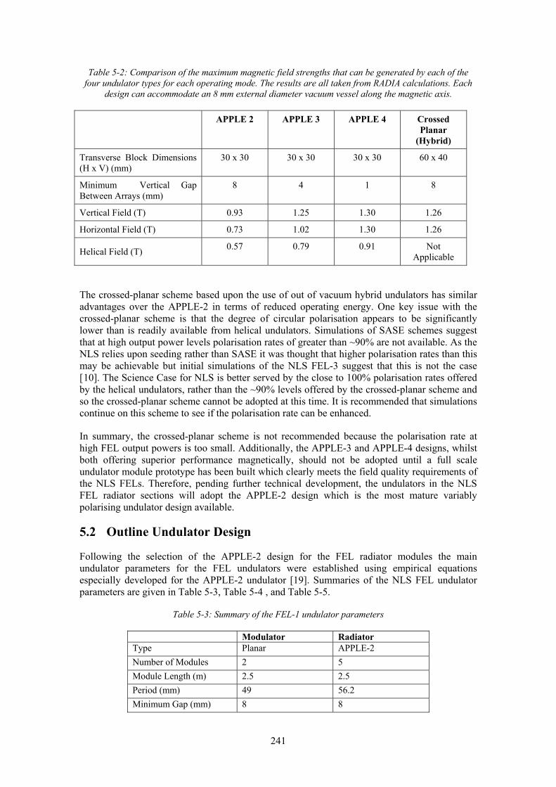
241

Table 5-2: Comparison of the maximum magnetic field strengths that can be generated by each of the four undulator types for each operating mode. The results are all taken from RADIA calculations. Each

design can accommodate an 8 mm external diameter vacuum vessel along the magnetic axis.

APPLE 2 APPLE 3 APPLE 4 Crossed Planar

(Hybrid)

Transverse Block Dimensions (H x V) (mm)

30 x 30 30 x 30 30 x 30 60 x 40

Minimum Vertical Gap Between Arrays (mm)

8 4 1 8

Vertical Field (T) 0.93 1.25 1.30 1.26

Horizontal Field (T) 0.73 1.02 1.30 1.26

Helical Field (T) 0.57 0.79 0.91 Not Applicable

The crossed-planar scheme based upon the use of out of vacuum hybrid undulators has similar advantages over the APPLE-2 in terms of reduced operating energy. One key issue with the crossed-planar scheme is that the degree of circular polarisation appears to be significantly lower than is readily available from helical undulators. Simulations of SASE schemes suggest that at high output power levels polarisation rates of greater than ~90% are not available. As the NLS relies upon seeding rather than SASE it was thought that higher polarisation rates than this may be achievable but initial simulations of the NLS FEL-3 suggest that this is not the case [10]. The Science Case for NLS is better served by the close to 100% polarisation rates offered by the helical undulators, rather than the ~90% levels offered by the crossed-planar scheme and so the crossed-planar scheme cannot be adopted at this time. It is recommended that simulations continue on this scheme to see if the polarisation rate can be enhanced.

In summary, the crossed-planar scheme is not recommended because the polarisation rate at high FEL output powers is too small. Additionally, the APPLE-3 and APPLE-4 designs, whilst both offering superior performance magnetically, should not be adopted until a full scale undulator module prototype has been built which clearly meets the field quality requirements of the NLS FELs. Therefore, pending further technical development, the undulators in the NLS FEL radiator sections will adopt the APPLE-2 design which is the most mature variably polarising undulator design available.

5.2 Outline Undulator Design

Following the selection of the APPLE-2 design for the FEL radiator modules the main undulator parameters for the FEL undulators were established using empirical equations especially developed for the APPLE-2 undulator [19]. Summaries of the NLS FEL undulator parameters are given in Table 5-3, Table 5-4 , and Table 5-5.

Table 5-3: Summary of the FEL-1 undulator parameters

Modulator Radiator Type Planar APPLE-2 Number of Modules 2 5 Module Length (m) 2.5 2.5 Period (mm) 49 56.2 Minimum Gap (mm) 8 8

242


Modulator 1 Modulator 2 Radiator Type Planar Planar APPLE-2 Number of Modules 2 1 7 Module Length (m) 2.5 2.5 2.5 Period (mm) 44 44 38.6 Minimum Gap (mm) 8 8 8


Modulator 1 Modulator 2 Radiator Type Planar Planar APPLE-2 Number of Modules 2 1 9 Module Length (m) 2.5 2.5 2.5 Period (mm) 44 44 32.2 Minimum Gap (mm) 8 8 8

Detailed magnetic modelling using RADIA has also been carried out to determine the permanent magnet block dimensions and the on-axis field levels, an example model is shown in Figure 5-4. A permanent magnet material with a remanent field of 1.3 T has been used in the calculations since such grades are now available with very high intrinsic coercivity (>1.5 MA/m) and so this NdFeB magnet should have good resistance to radiation damage [11] and any reverse fields. Other FEL projects have made use of permanent magnet materials with similar intrinsic coercivities where radiation damage has been a concern [12]. A summary of the 3D modelling and subsequent undulator parameters is given in Table 5-6. The field levels achieved are all sufficient to meet the photon energy range specified by the Science Case and summarised in Table 1-1 in Section 1.1.2.

Figure 5-4: Example RADIA model for the FEL-3 radiator. This model has 9 periods and is shown in circular polarisation mode. The red blocks are magnetised longitudinally and the blue blocks vertically.

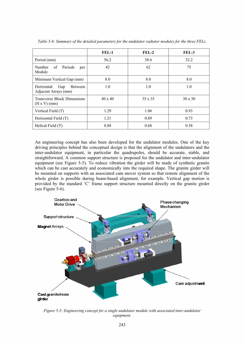
243

Table 5-6: Summary of the detailed parameters for the undulator radiator modules for the three FELs.

FEL-1 FEL-2 FEL-3

Period (mm) 56.2 38.6 32.2

Number of Periods per Module

42 62 75

Minimum Vertical Gap (mm) 8.0 8.0 8.0

Horizontal Gap Between Adjacent Arrays (mm)

1.0 1.0 1.0

Transverse Block Dimensions (H x V) (mm)

40 x 40 35 x 35 30 x 30

Vertical Field (T) 1.29 1.06 0.93

Horizontal Field (T) 1.21 0.89 0.73

Helical Field (T) 0.88 0.68 0.58

An engineering concept has also been developed for the undulator modules. One of the key driving principles behind the conceptual design is that the alignment of the undulators and the inter-undulator equipment, in particular the quadrupoles, should be accurate, stable, and straightforward. A common support structure is proposed for the undulator and inter-undulator equipment (see Figure 5-5). To reduce vibration the girder will be made of synthetic granite which can be cast accurately and economically into the required shape. The granite girder will be mounted on supports with an associated cam mover system so that remote alignment of the whole girder is possible during beam-based alignment, for example. Vertical gap motion is provided by the standard ‘C’ frame support structure mounted directly on the granite girder (see Figure 5-6).

Figure 5-5: Engineering concept for a single undulator module with associated inter-undulator equipment.

244

Figure 5-6: Engineering concept for a single undulator module showing undulator support structure.

For optimum operation of the FELs the electron beam trajectory through the undulator section must be very carefully controlled to within ~2 μm in both planes (see Table 1-11 in Section 1.4.4). This level will not be achieved through conventional survey and alignment techniques (although these will be used for the initial alignment) but rather through a beam-based alignment strategy equivalent to that developed elsewhere for similar FEL projects [12, 19]. The electron beam trajectory through the undulator system will be measured using Beam Position Monitors (BPMs), mounted between the undulator modules, over a wide range of electron beam energies. Subsequent analysis will provide information on BPM and quadrupole misalignment, as well as the initial launch conditions (position and angle) into the FEL. The quadrupoles will be mounted on remotely adjustable movers that will be able to be adjusted online. An iterative approach will be used to correct the errors initially but subsequently it is expected that a single iteration will be sufficient to control the trajectory straightness approximately once per month. Fine steering control between these gross corrections will be possible using the dipole correctors installed between undulator modules. Beam energy scanning is a more powerful technique than other options available, such as quadrupole strength scanning.

5.3 Vacuum Design

Calculations for similar FEL facilities to NLS suggest that an average pressure of 1 x 10-7 mbar in the undulator vacuum vessel should be sufficient, taking into account bremsstrahlung production [19] and emittance dilution effects [12]. Such a vacuum level is relatively easy to attain even with the poor conductance of the narrow gap undulator vessels. Figure 5-7 shows the pressure profile through a single 2.5 m vacuum vessel assuming that a small, 40 l/s pump (with an effective pumping speed of 20 l/s) is installed at either end. The vessel is here assumed to be stainless steel that has previously been baked at 250 °C for 24 hours. Similar profiles will be obtained for different materials, such as aluminium alloy or copper-coated stainless steel, which will have higher surface electrical conductivities and so be better suited to minimising wakefield effects. The average vacuum level generated in this case is far better than the specification. A similar calculation, this time showing the average pressure within the vessel as a function of the distance between the pumps, is shown in Figure 5-8. This result suggests that a pump could be installed every second undulator whilst still meeting the vacuum specification.

245

Figure 5-7: Pressure profile for a 2.5 m long, cylindrical, stainless steel, vacuum vessel with a 7 mm inner diameter and a 40 l/s pump installed at either end. The required vacuum level is 1 x 10-7 mbar.

Figure 5-8: Average pressure inside a variable length cylindrical stainless steel vacuum vessel with a 7 mm inner diameter and a 40 l/s pump installed at either end. The required vacuum level is

1 x 10-7 mbar.

The undulator vacuum vessel will have an elliptical cross-section with an internal height of 6 mm and an internal width of 18 mm. The minimum magnet gap of 8 mm required by the undulators implies that the external height of the vacuum vessel must be 7.5 mm, leaving adequate allowance for engineering tolerance build up in the vessel manufacture, alignment errors, and vessel straightness tolerance. The vacuum vessel could be made from extruded aluminium or from stainless steel coated with a thin layer of copper on the inner surface to mitigate resistive wall wakefield effects. Final selection of the material should also include the

246

requirement to achieve a sufficiently smooth surface finish to minimise surface roughness wakefield effects. An extruded aluminium chamber has been used successfully at a similar project [13] and so that is the preferred solution at present.

5.4 Effect of Wakefields in the Vacuum Vessel

There are three types of wakefield which need to be assessed for the undulator line. These are the resistive wall wake, the geometric wake, and the surface roughness wake. A review of other FEL projects [14] has confirmed that the resistive wake is the dominant of the three and so this has been studied in most detail. The other two wakes can, in principle, be reduced if they are found to be significant, as vacuum vessel taper sections can be made more gentle or surface finishes can be made smoother. In particular, significant efforts have been made elsewhere to successfully reduce undulator vessel surface roughness to acceptable levels [13].

The main impact of the resistive wake that is of concern is the variable energy change imparted longitudinally through the electron bunch and the overall average energy loss of the electron bunch. The wake effects can have significant impact on the FEL output power although it appears to be possible in some circumstances to counteract these by tapering the undulator though the FEL [15]. The vacuum chamber material selected to minimize the resistive wake will be either aluminium or copper. A stainless steel vessel coated with one of these materials should be equally as effective.

The APPLE-2 undulator design selected is compatible with an elliptically shaped vessel with internal height of 6 mm. We have studied how the resistive wake changes for a single particle as the aspect ratio of the elliptical vessel (see Figure 5-9) varies to find how wide the internal vessel aperture should be. A summary of the results is plotted in Figure 5-10. This shows that the wake does indeed reduce as the aspect ratio increases but also that there is little further reduction once the ratio has reached a value of about three.

Figure 5-9: Geometry of the elliptical vessel under study.

247

Figure 5-10: Graph showing how the resistive wake (AC conductivity model) due to a single particle (at z = 0) varies as the aspect ratio of the elliptical vessel varies. The vessel is assumed to be made of copper

and to have a fixed half height, b, of 3 mm.

Some example wakes for a 200 pC bunch at the end of the linac, which has a peak current of ~1.2 kA, are given in Figure 5-11 for both circular and elliptical vessels for two different apertures. For the bunch parameters of the NLS the difference between an elliptical vessel and a circular vessel appear to be relatively small. Our investigations have shown [16] that the relative difference in wake between elliptical and circular vessels is strongly correlated with the overall bunch length, or more precisely, the frequency content of the bunch. A very short bunch will excite very high frequencies and this favours elliptical vessels (i.e. elliptical vessels then have weaker wakefields for the same vertical aperture). It is for this reason that single electron wake functions show that elliptical vessels appear to have a significant advantage. However, as longer bunches are considered the apparent advantage is less clear and this is the case for the NLS. Note that the NLS generates, in absolute terms, a very short bunch with a FWHM of only ~150 fs.

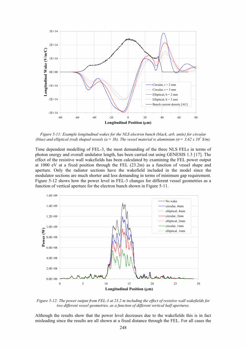
248

-3E+14

-2E+14

-1E+14

0E+00

1E+14

2E+14

3E+14

-80 -60 -40 -20 0 20 40 60 80

Longitudinal Position (μm)

Lon

gitu

dina

l Wak

e (V

/m/C

)

Circular, r = 2 mmCircular, r = 3 mmElliptical, b = 2 mmElliptical, b = 3 mmBunch current density [AU]

Figure 5-11: Example longitudinal wakes for the NLS electron bunch (black, arb. units) for circular (blue) and elliptical (red) shaped vessels (a = 3b). The vessel material is aluminium (σ = 3.62 x 107 S/m).

Time dependent modelling of FEL-3, the most demanding of the three NLS FELs in terms of photon energy and overall undulator length, has been carried out using GENESIS 1.3 [17]. The effect of the resistive wall wakefields has been calculated by examining the FEL power output at 1000 eV at a fixed position through the FEL (23.2m) as a function of vessel shape and aperture. Only the radiator sections have the wakefield included in the model since the modulator sections are much shorter and less demanding in terms of minimum gap requirement. Figure 5-12 shows how the power level in FEL-3 changes for different vessel geometries as a function of vertical aperture for the electron bunch shown in Figure 5-11.

0.0E+00

2.0E+08

4.0E+08

6.0E+08

8.0E+08

1.0E+09

1.2E+09

1.4E+09

1.6E+09

0 5 10 15 20 25 30

Longitudinal Position (μm)

Pow

er (W

)

No wakecircular, 4mmelliptical, 4mmcircular, 2mmelliptical, 2mmcircular, 1mmelliptical, 1mm

Figure 5-12: The power output from FEL-3 at 23.2 m including the effect of resistive wall wakefields for two different vessel geometries, as a function of different vertical half apertures.

Although the results show that the power level decreases due to the wakefields this is in fact misleading since the results are all shown at a fixed distance through the FEL. For all cases the

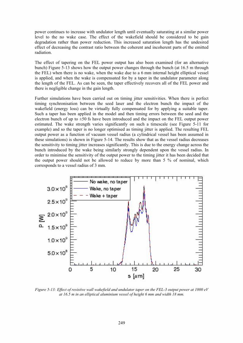
249

power continues to increase with undulator length until eventually saturating at a similar power level to the no wake case. The effect of the wakefield should be considered to be gain degradation rather than power reduction. This increased saturation length has the undesired effect of decreasing the contrast ratio between the coherent and incoherent parts of the emitted radiation.

The effect of tapering on the FEL power output has also been examined (for an alternative bunch) Figure 5-13 shows how the output power changes through the bunch (at 16.5 m through the FEL) when there is no wake, when the wake due to a 6 mm internal height elliptical vessel is applied, and when the wake is compensated for by a taper in the undulator parameter along the length of the FEL. As can be seen, the taper effectively recovers all of the FEL power and there is negligible change in the gain length.

Further simulations have been carried out on timing jitter sensitivities. When there is perfect timing synchronisation between the seed laser and the electron bunch the impact of the wakefield (energy loss) can be virtually fully compensated for by applying a suitable taper. Such a taper has been applied in the model and then timing errors between the seed and the electron bunch of up to ±50 fs have been introduced and the impact on the FEL output power estimated. The wake strength varies significantly on such a timescale (see Figure 5-11 for example) and so the taper is no longer optimised as timing jitter is applied. The resulting FEL output power as a function of vacuum vessel radius (a cylindrical vessel has been assumed in these simulations) is shown in Figure 5-14. The results show that as the vessel radius decreases the sensitivity to timing jitter increases significantly. This is due to the energy change across the bunch introduced by the wake being similarly strongly dependent upon the vessel radius. In order to minimise the sensitivity of the output power to the timing jitter it has been decided that the output power should not be allowed to reduce by more than 5 % of nominal, which corresponds to a vessel radius of 3 mm.

Figure 5-13: Effect of resistive wall wakefield and undulator taper on the FEL-3 output power at 1000 eV at 16.5 m in an elliptical aluminium vessel of height 6 mm and width 18 mm.

250

Figure 5-14: Minimum FEL output power (relative to the level with no timing error) as a function of vacuum vessel radius for timing synchronisation errors of up to ±50 fs between the seed laser and the

electron bunch.

5.5 Inter-Undulator Sections

The FEL radiators consist of a series of undulator modules (each assumed to be 2.5 m long at present) separated by the inter-undulator sections (Figure 5-15). These sections must contain several pieces of equipment to ensure the optimum operation of the FELs, the total space required for each section is presently assumed to be 1.0 m. Each section will contain a quadrupole to match the electron beam properties along the length of the FEL, a phasing unit to ensure the radiation from each module is correctly phased, horizontal and vertical steerers to maintain good electron beam orbit control, and a cavity BPM. Space must also be allowed for vacuum pumps and gauges, and additional beam diagnostics (OTR screens or wire scanners), although these items may not be present in every section. This space allowance is consistent with other, similar, projects [3, 18, 19].

251

Figure 5-15: View of the conceptual layout of the inter-undulator section.

5.6 THz/IR Undulators

The NLS Science Case requires coherent undulator radiation in the long wavelength range of up to 500 µm synchronised to the FEL output pulses. The electron bunches will pass through the FELs and will then pass through long undulators optimised to generate light in this THz/IR region. The electron bunches are short enough (typically 50 µm FWHM) that the whole bunch is shorter than the wavelengths required and so the bunch will emit coherently, enhancing the photon intensity by the square of the number of electrons.

The wavelength range required is not well suited to the electron energy of the NLS, being much longer than would normally be generated by an undulator with a period of a few cm, say. The solution is to build an insertion device with a very long period and a relatively high field strength. Such a device would normally be considered a wiggler, producing broadband radiation well into the X-ray region, but it will also generate harmonic undulator radiation at the long wavelength end of its range. A possible set of undulator parameters, assuming a standard sinusoidal magnetic field profile, is given in Table 5-7.

Table 5-7: A possible set of undulator parameters to cover the THz/IR wavelength range.

Period (mm) 1000

Number of Periods 10

Minimum Vertical Gap (mm) ~40

Maximum Vertical Field (T) 2.11

Maximum Wavelength (µm) 500

252

A potential issue with such a high strength undulator is the high photon beam power on axis. Alternative schemes are possible which use different periodic field shapes in order to reduce the power on axis whilst still maintaining the long wavelength performance. One example [20] has a magnetic field shape designed such that the emission directed along the axis is due to a low field region of the undulator rather than a high field one. This creates a relatively low power density on axis compared to the standard sinusoidal solution. An example of such a scheme that could be considered for the NLS is illustrated in Figure 5-16, which shows the magnetic field shape and electron beam trajectory through one period of the undulator. Note that in order to maintain the undulator harmonic output at 500 µm with the same magnetic peak field strength of 2.1 T, it is necessary to increase the period length to 1.6 m. In this case, if the length is limited to ~10 m the number of periods would have to reduce from ten to six, with the consequent reduction in intensity. Preliminary calculations show that with such a scheme the on-axis power density is more than a factor of twenty lower than from the conventional sinusoidal device, whereas the flux output is reduced by only a factor of three. Further studies of this and other alternative schemes should be investigated in the future and the parameters carefully selected in order to optimise the undulator output for each of the beamlines.

Figure 5-16: Magnetic field and trajectory of a 2.25 GeV electron through one period of a non-sinusoidal undulator designed to generate radiation with a wavelength of 500 µm with a reduced on-axis power

density.

REFERENCES [1] Clarke, J. A., Review of Undulator Options for NLS. NLS-Source-UND-REP-001 [2] Sasaki S., Analyses for a planar variably-polarizing undulator NIM A 1994 347 83-86 [3] The BESSY Soft X-ray Free Electron Laser Technical Design Report, March 2004. [4] Temnykh, A. B., Delta undulator for Cornell energy recovery linac. Phys. Rev. ST Accel. Beams

2008 11, 120702 [5] Temnykh, A., Delta undulator magnet for Cornell energy recovery linac, Proceedings of PAC

2009, Vancouver, Canada [6] Kim, K.-J., Circular polarization with crossed-planar undulators in high-gain FELs, NIM A 2000

445 329-332 [7] Ding, Y., & Huang, Z., Statistical analysis of crossed undulator for polarization control in a self-

amplified spontaneous emission free electron laser, PRST-AB 2008 11, 030702 [8] Li, Y., et.al., Polarization properties of a crossed planar undulator, NIM A 2010 613 163-168

253

REFERENCES [9] Chubar, O., et al., A 3D Magnetostatics Computer Code for Insertion devices, J. Synchrotron Rad.

1998 5, 481-484 [10] Huang, Z., Private Communication [11] Marechal, X., et al, 65 MeV neutron irradiation of Nd-Fe-B permanent magnets, Proceedings of

EPAC 2006, Edinburgh, Scotland, p3116 [12] Linac Coherent Light Source (LCLS) Conceptual Design Report, SLAC–R–593, April 2002 [13] Trakhtenberg, E., et al, LCLS extruded aluminum vacuum chamber – new approaches, to be

published in Proceedings of SRI 2008, Saskatoon, Canada (http://www.lightsource.ca/medsi-sri2008/pdf/papers/Paper-LCLS_extruded_aluminum_vacuum_chambers.pdf)

[14] Clarke, J. A., Review of Undulator Vessel Related Wakefields for NLS. NLS-Source-UND-REP-002 [15] Zagorodnov, I., et al., Impact of undulator wakefields and tapering on European X-ray FEL

performance, Proceedings of EPAC 2006, Edinburgh, Scotland, p83 [16] Clarke, J. A., et al, Selection of the Optimum Undulator Parameters for the NLS: A Holistic

Approach, Proceedings of FEL 2009, Liverpool, p722. [17] Reiche, S., GENESIS 1.3: a fully 3D time-dependent FEL simulation code, NIM A 1999 429 243-

248 [18] The European X-Ray Free-Electron Laser Technical Design Report, DESY 2006-097, July 2007 [19] FERMI@ELETTRA Conceptual Design Report, Jan 2007 [20] Khlebnikov, A. S., et al, VUV-Wiggler scheme with non-sinusoidal magnetic field profile for high

energy storage rings, Proceedings of EPAC 1996, Sitges, Spain, p2558

255

6 Electron Beam Diagnostics

The diagnostics proposed for NLS are designed to fulfil the functions of initial machine set up, regular operational monitoring and tuning of performance and longer-term facility development, as well as to provide the necessary sensors in feedback stabilization systems. Optical Transition Radiation (OTR) and wire scanner diagnostics are proposed for transverse measurements; stripline and cavity Beam Position Monitors (BPMs) for operational alignment and trajectory stabilization, with the cavity BPMs required for the precision alignment requirements of the undulator section; non-invasive beam arrival time and longitudinal profile monitors for the beam based longitudinal feedback systems; dedicated transverse tomography and deflecting cavity diagnostic sections for machine optimization and pre-FEL electron bunch characterization.

6.1 Requirements

In the first instance, the diagnostic requirements have been based on the baseline machine specification of 200 pC bunch charge, 1 kHz operation. Upgrades to the repetition rate, to 10 kHz and 100 kHz are not seen as introducing any significant additional challenges to the diagnostics systems. Further upgrade to 1 MHz operation will provide challenges to longitudinal feedback diagnostics, with far-IR to optical array detectors operating at these repition rates needing to be developed. A low charge mode for single-spike operation has also been proposed, and this presents additional challenges for the diagnostic systems. Operation at 20 pC would be within the capability of the majority of proposed diagnostics. An even lower charge of ~2 pC however is not within the current capabilities and will require significant additional R&D in order for this to be achieved.

The transverse diagnostics are targeted to achieve a transverse position tolerance of 30 μm throughout the majority of the machine, and a significantly lower tolerance of 3 μm in the undulator sections. These estimated tolerances should be refined with further design studies that include a full trajectory sensitivity and correction analysis. The undulator tolerances have been confirmed as reasonable from FEL simulations including trajectory position and angle offset, as discussed in Chapter 5. The baseline design charge of 200 pC is sufficiently large to allow standard or proven transverse position and profile diagnostics be used to meet the measurement specifications. Transverse beam position diagnostics systems have been developed which are expected to meet the requirements at 20 pC, while scintillation screens are able to operate at even lower charges.

Non-invasive longitudinal diagnostics requirements include sub-10 fs arrival time monitors and high resolution longitudinal profile measurements with resolution ranging from ps to 10 fs, depending on location within the machine and whether the diagnostic is intended for dedicated machine studies, or for real-time machine stabilisation.

Beam arrival time monitoring, using combined ultrafast optical measurement and high bandwidth beam electrical pickup has been demonstrated at the 10 fs level [1]. These demonstrated systems utilise pulsed optical timing distribution, and are consistent with the timing distribution system chosen for NLS. While the demonstrated performance of these systems has been restricted to relatively high bunch charges (1 nC), the NLS baseline charge of 200 pC is unlikely to require any significant further development. The low charge mode will require additional development of both the beam-pick and optical probe systems.

Non-invasive longitudinal profile monitoring is an area that has seen significant R&D effort over recent years, and techniques for characterising structure on a 100 fs (FWHM) time scale have been demonstrated. Further improvements to achieve resolutions approaching 50 fs FWHM can be envisaged in the near future with incremental improvements. Non-invasive

256

measurement with resolution beyond 50 fs FWHM will require significant future R&D. For feedback systems, a philosophy of accepting empirical information (such as information on the bunch spectral decomposition) rather than aiming for explicit temporal profile, is the most likely way forward. A number of single-shot spectral techniques aiming to this goal have been recently developed, and with further development are likely to meet the longitudinal profile feedback requirements for NLS. It is noted that the specific requirements of longitudinal profile and arrival monitoring for feedback applications require further analysis of the NLS beam dynamics and tolerances.

The NLS low charge mode is likely to present significant challenges to longitudinal profile feedback systems, with even a charge of 20 pC representing approximately an order of magnitude reduction in charge beyond that currently demonstrated.

Transverse deflecting cavities, together with dedicated diagnostic lines for tomography and slice energy measurements, will provide longitudinal diagnostics for machine-studies and tune-up.

6.2 Accelerator Diagnostics

Transverse diagnostics in the linac and beam transport section will comprise screen systems for machine tune-up (beta-function, emittance, dispersion), and stripline beam position monitors for operational measurements and feedback.

6.2.1 Optical Diagnostics – Screen Systems

Many screen systems will be employed throughout the accelerator and they will be used regularly to setup and test the accelerator optics. They will predominantly consist of simple pop-in devices where only one type of screen will be required. Any devices requiring two types of screen will be motorized to allow selection of the required screen desired at the time. The design of the screen carriage will typically include an RF cage structure.

Several types of screen material from scintillators to foils are available for mounting within these devices. For low energy imaging in areas such as the injector and gun, YAG:Ce crystals will be used. At higher energies and/or beam charge, OTR screens are the likely choice, although in the light of recent observations of optical micro-structure in the LCLS and FLASH their suitability has yet to be determined; this point is discussed further below. Choices of appropriate material for the location and task required will be made as the design of the NLS progresses.

The location and placing of the optical diagnostic devices will be made in conjunction with the accelerator designers and accelerator physicists who will define their requirements of what they wish to measure at various locations. Considerations of physically available space will also have to be made.

Beam Micro-bunching Issues: LCLS has encountered significant difficultly with the standard OTR diagnostics systems, with optical wavelength micro bunching structure giving rise to the emission of Coherent OTR (COTR) which obscures or destroys the imaging capability of the screens, and has led to the need to rely on wire scanners for beam transverse profile measurements. Similar effects have been observed at FLASH, particularly in measurements in the near infrared region of the spectrum. The origins of the micro bunching structure are not yet understood, although both FLASH and LCLS have carried out a number of investigations into its characteristics. The micro bunching is observed both at low energy (<150 MeV) and high energy (5 GeV) locations within the LCLS accelerator. Given the limited knowledge of the origins of the optical microbunching, it is not currently possible to predict whether NLS will suffer from the similar problems. It is likely that this situation will change before final decisions on screen systems are needed. However, in the event that screens need to be installed with remaining uncertainty on COTR effects, it is planned that wire scanners will also be installed in

257

a combined screen/wire scanner assembly, providing a fall-back beam profile measurement capability.

6.2.2 Electron Beam Position Monitors (EBPMs)

The EBPM system will be the predominant installed diagnostic system device to non-destructively measure transverse beam position. Due to the large range of bunch charge expected (2 pC to 200 pC), it will be necessary to install quarter wavelength shorted stripline type EBPM pickups. A single bunch positional resolution of 10 μm at 200 pC is achievable, and is currently seen as likely to meet the requirements of the NLS baseline 200 pC mode. This type of pickup within the accelerator module chain will provide sufficient signal across the range of expected operating charge to provide sufficient resolution of position. The variable repetition frequencies of 1 kHz to 1 MHz will still represent a single bunch operation mode to the pickup device, and hence it is possible to select a detection frequency that simplifies the demands on the detector electronics that will be attached. For this reason, the stripline EBPM pickup devices will be designed around a detection frequency of 800 MHz, which will have a consequence of slightly increasing the physical length of the overall device. Such EBPM pickups are standard mechanical devices in configuration and design, with dimensional modification to suit the actual installation point being the only challenge along the length of the accelerator. It will be necessary, at specific EBPM locations, to ensure that mechanically stable mountings are used, and positional feedback information is implemented, to ensure that accurate and reliable beam position measurements are made.

Each single bunch pulse signal produced by the pickup head must be detected and converted into a suitable DC value for digitization and passing to the control system to be recorded and displayed. The electronic detector for such an installation must be highly specialized and built for this purpose. No such commercial system is currently available, but one has been developed at DL for the EMMA FFAG demonstration accelerator, which with some minor modifications to its analogue detection stages will fit the NLS requirements. This detector is split into two major sections. Local to the BPM itself, and within the accelerator hall, specifically designed strip-line couplers and delay lines will separate out the two single plane (horizontal and vertical) signals into time separated and amplified signals. These are then transported down a single cable for each of the planes to a remotely located dual channel detector VME format card. Here the signal amplitudes are measured directly and the data from the ADC stored in a local memory buffer that can be read by the control system and the data interpreted.

6.2.3 Charge Monitoring

The monitoring of charge can be achieved in two ways. Commercially available integrating current transformers (ICTs) offer resolutions down to ~1 pC, and can be installed with a minimum of required length. Additionally, a new wideband wall current monitor (WCM) developed by FNAL and DL as part of the EMMA collaboration project could be used (see Figure 6-1). This would provide high frequency readings (> 10 GHz) of the bunches as they passed, and by the inclusion of a coupler network, could produce high resolution timing pulses for use in other areas of the facility.

258

Figure 6-1: EMMA type Wall Current Monitor currently under construction

6.2.4 Bunch Arrival Time Monitors (BAMs)

Stability of the bunch arrival time is required to ensure the reproducible overlap of the FEL seed laser and the electron bunch. Meeting this requirement imposes tight tolerances on the machine, particularly the RF system. It also follows that precision measurement of the arrival time can facilitate the stabilization of the RF systems.

The BAMs proposed are of the "DESY beam centroid" type [1]. The bunch arrival is sensed by a button BPM type pickup; the wide bandwidth signal from these pickups is fed locally into a fibre optic Mach-Zender modulator, which allows for sampling of the RF signal by ultrafast laser pulses derived directly from the optical fibre based timing distribution system (Section 9.1). The sampling of the waveform converts the (temporally sampled) RF signal into an optical intensity. The relative arrival time of the RF signal (and hence electron bunch) is directly related to the optical intensity output from the optical modulator. An accuracy in the arrival time of 7 fs, including fibre links, has been demonstrated [1]. The BAMs developed at DESY are able to operate at high (>1 MHz) repetition rate, providing a single valued output proportional to the time offset from a predefined set-point. Feedback systems that can use such rapid sensing are therefore possible.

The arrival time of a bunch provides important input into feedback systems, allowing the stability of the bunch parameters to be enhanced. The relationship between arrival time, and the bunch RF phase, and RF amplitude, will depend on the location of the diagnostic and on the electron beam optics; this is an area of ongoing investigation that is coupled to the accelerator machine design and optimization.

Precision bunch arrival time monitors (BAMs) will be located after the three bunch compressors and before the FELs (after the spreader). It is envisaged that the primary function of these BAMs is to provide an input for feedback onto the RF. For example, the arrival time after BC1 will be dependent on both the (off-crest) phase and amplitude of the preceding accelerating modules. In recent demonstration experiments at DESY [2] the arrival time after the first beam compressor at FLASH was shown to function as a sensitive indicator of the RF amplitude in the preceding modules. Including the arrival-time monitor into feedback for the RF amplitude provided an increased timing stability. The timing jitter was reduced from 250 fs RMS without feedback, to 40 fs RMS with arrival time feedback.

6.2.5 Beam Longitudinal Profile Monitors

Single shot electro-optic beam longitudinal profile monitors, and coherent synchrotron radiation (CSR) spectral detection will provide diagnostics for the compression. The diagnostics will be

259

available for RF feedback system input. Because of the intertwined nature of the beam arrival time and the compression/longitudinal profile, the feedback algorithm will be determined by the final machine optics, as will the final choice of the most suitable of the compression diagnostics.

It is currently envisaged that the Electro-Optic Spatial encoding concept will be the principle form of electro-optic (EO) diagnostics in NLS, when explicit temporal domain information is required. By sampling the Coulomb field with an ultrafast optical pulse obliquely incident to the EO crystal and the Coulomb field propagation direction, a spatial-to-temporal mapping is introduced for the relative delay of the laser arrival time at the crystal. Polarized imaging of the laser transmitted through the EO crystal provides Coulomb field (and hence charge density) temporal structure. This approach has been demonstrated at SLAC SPPS [3] and at DESY/FLASH [4]. At the FFTB EO signals of 270 fs FWHM were measured, while at FLASH ~300 fs FWHM signals have been obtained. A system is also under development for FERMI@Elettra. While this approach has yet to demonstrate the higher time resolution of 60 fs RMS that has been achieved in the alternative “temporal decoding” technique [5], EO spatial encoding is considered more amenable to low pulse energy, high repetition rate laser oscillator systems, and so can readily be scaled up from the initial 1 kHz bunch rate. The laser systems are relatively uncomplicated, and potentially could be derived directly from the laser timing distribution systems.

Figure 6-2: (Left) Example of high-time resolution, single-shot, longitudinal profile measurements at FLASH using Electro-optic Temporal Decoding [5]. (Right) The in-tunnel diagnostic station used to

obtain these measurements.

While it remains for this concept to demonstrate the high resolutions expected to be required, this situation will likely be rectified in the near future, with experiments planned by several laboratories. Refinements of temporal decoding are also being examined as possible alternatives in the event that the few remaining fundamental concerns of spatial encoding prove to be an obstacle to it achieving the required resolution.

It is noted that for feedback implementation, the longitudinal diagnostics do not necessarily need to provide an explicit determination of the longitudinal profile. They simply need to provide a measurable quantity that can be correlated to the beam profile, or possibly even directly to the final FEL lasing output. Single shot spectral characterization of coherent diffraction/synchrotron radiation (CDR/CSR) is a promising diagnostic approach. A system has been developed at FLASH that provides spectral coverage from 2-500 μm in a single shot. The correlation of spectrum with bunch compression, and to a lesser extent with SASE performance, has been demonstrated. A significant additional capability of this approach over EO techniques is the ability to infer information of structure on time scales <60 fs. Another particularly promising approach for high-repetition rate feedback systems is the recent development of “spectral-upconversion” [6]. Spectral up-conversion is closely related to the more widely explored EO diagnostics, but places significantly lower requirements on the laser system complexity and infrastructure. Through the use of non-linear optical processes, the technique converts the Far-infrared spectrum of the bunch Coulomb field into an easily measured optical

260

spectrum. In its approach of measuring the bunch spectrum, it is similar to diagnostics that measure CDR or CSR, but with an added advantage of being able to measure very long wavelength, highly diffracting, components of the field spectrum. It is intended that a spectral diagnostic will be included on the final bunch compressor. As well as providing non-invasive information on fast structure arising through intended compression, it will also be able to identify any short wavelength micro-bunching in the beam.

Many issues remain to be resolved in the fast-feedback longitudinal diagnostics. The feedback algorithm itself will be machine specific, and will also have to coordinate the BAM information into the feedback on the RF systems. While several prototype diagnostics have been developed and tested, there remains significant work to be done on the fast readout and analysis of the profile. The stability and robustness of the laser and optical systems will be an important requirement if they are to function as feedback sensors, and this also requires further development.

6.2.6 Low Energy Diagnostics Section

A dedicated diagnostics section located downstream of the first dipole of the injector dogleg will be used for characterising the beam after the injector and laser heater as described in Section 4.1. The section includes a deflecting cavity and tomography section, enabling the full suite of slice emittance, slice energy, and temporal profile to be characterised. Transporting the beam to the diagnostic section is through switching off a dipole, and hence the diagnostic section will receive the complete bunch train of the injector. For the required single-bunch diagnostics, the bunch selection will be achieved through gating of the optical cameras viewing the variation OTR or YAG screens. This mode of selection will be straight forward at the baseline 1 kHz repetition rate. The higher repetition rate upgrades are not seen to present any significant obstacle to this approach, although some care will be needed in achieving sufficient extinction ratio in the camera bunch selection.

6.2.7 High energy Transverse Tomography and Slice Diagnostics

To assess the quality of the beam before the FELs, a good knowledge of the complete (6D) phase space is highly desirable. To address this requirement, a diagnostic section is to be located after the spreader, in a dedicated diagnostic line adjacent to the FEL undulators. This location ensures that the diagnosed beam matches the beam injected into the FELs as closely as possible. The section will provide diagnostics for projected transverse emittance, longitudinal bunch profile and length, transverse slice emittance, energy spread and slice energy spread.

The diagnostic section contains a four screen tomography section, which is described in Section 4.5. The tomography section is preceded by one or two deflecting cavities (one for each plane) with three or four matching quadrupoles on either side. Measurement without streak gives the projected transverse beam profile, which allows a precise reconstruction of projected transverse emittance via tomographic methods. Measurement with streak gives the slice emittance measurement, with one dimension on the screen corresponding to time, and hence bunch length, whilst the other gives the emittance of a slice of the bunch in time. The possibility of using just one deflecting cavity for both planes remains to be investigated further.

For commissioning and tune up, tomography diagnostics of the full energy beam in the straight ahead direction will also be included. To minimise the additional machine length for such diagnostics, the tomography will use the sequence of spreader quadrupoles for the different beamlines. With the kickers off, the beam will be transported in the straight-through direction to a commissioning beam dump. The optics and beam physics of this tomography section are discussed in Section 4.5. A deflecting cavity will also be included in the straight-through diagnostics section, although space constraints have led to this being located after the straight though tomography section, and hence precluding slice tomography measurements with this diagnostic section.

261

The design of the deflecting structure has not yet been examined in any detail. However, consideration of the required time resolution and the current NLS beam parameters suggest that the deflecting structure requirements are feasible. As an initial design goal, a temporal structure with RMS width of σz = 7 μm (σt = 25 fs) is required to be resolved. To resolve this structure it is assumed that the transverse streak must exceed the RMS transverse diameter of the unstreaked beam by a factor of three. From these considerations, it can be shown that the effective deflecting voltage V0 = EcavLcav must satisfy

0

2 2

08

2 | sin cos |x x

z d s

pceVσ σλ

πσ μ ϕ β β−

=Δ

(6-1)

For the (conservatively) assumed NLS parameters of εn = 1 μm, βd = 50 m, pc =2.25 GeV, we obtain that the effective deflecting voltage V0 must be greater than 64 MV (21 MV) for a 1.3 GHz (3.9 GHz) cavity, respectively. It is proposed that the NLS deflecting cavity will be a travelling wave structure operating at the third harmonic, for which the required effective deflecting voltages are most easily achieved [7]. The cavity will be located after the spreader, which allows bunch selection to be done through the spreader kickers, rather than a cavity fill time. This allows both superconducting and normal conducting structures to be considered, and separates the deflecting cavity requirements from the machine repition rate.

6.3 Undulator Diagnostics

Analysis of the FEL performance with transverse offsets and angular misalignment of the beam path through the undulators is presented in Section 1.1.4. This analysis specfifies that a transverse positioning accuracy of 2-3um, is required to maintain FEL power stability within 1%. This tolerance specification is similar to that for LCLS, where the electron and photon beams within the undulator are required to be collinear to less than 10% of the transverse beam size over a minimum distance that is comparable to the FEL amplitude gain length [8, 9]. In order to facilitate beam alignment and trajectory correction to this precision, beam position monitor (BPMs) in the undulator section will need to provide single shot resolution of similar or better size. At the same time, small bunch charges are also foreseen for certain operational modes (as low as 2 pC). Cavity BPMs are able to meet the requirements outlined above and for this reason have been chosen in the past for similar projects such as LCLS [10, 11], SCSS [12], FERMI@Elettra [13] and the European XFEL [14]. NLS will therefore be equipped with one cavity BPM in each intra undulator location.

6.3.1 Tasks of BPMS in the Undulator Sections

The tasks of the BPMs in the undulator sections will be: • Commissioning of the Machine: Detect the beam position and the charge of the beam. The

goal is to get transmission through the undulator and so see where and how the beam might get lost. For this case high sensitivity for low charge operation and relaxed requirements on resolution are required.

• Beam Based Alignment (BBA) using one or a combination of methods based on ballistic trajectories, steering free quadrupoles and/or dispersion free steering. For these applications averaging over many shots can be used and the high repetition rates planned for NLS are beneficial to improve sensitivity of the position readout.

• Trajectory Reference: Deliver trajectory references for keeping, checking and restoring machine settings. This aspect requires small drifts of the BPMs (mechanically and electronically.

262

6.3.2 Pickup Cavities

The main advantage of cavity BPMs is that the signal in the dipolar cavity modes (which is coupled out for measurement) is intrinsically proportional to the beam offset (and the bunch charge), thus removing the need to subtract large signals to calculate the position. However, the bunch charge needs to be measured as well (using a reference cavity) to normalize the position signal. A further advantage of most cavity BPM designs is that they are largely rotationally symmetric devices which can be manufactured with high mechanical precision on a lathe. This leads to a very small offset between the mechanical and the electrical centre which means that after a careful mechanically straight alignment of the BPM pickups the straight path through the undulators is already tightly defined.

Mechanical dimensions of the cavity BPMs will have to be selected to choose the operating frequency of the BPM (which should be different from the linac frequency) and a suitable pipe diameter (which depends on the aperture in the undulator section). Currently, a C-band cavity with an inner free diameter of 20 mm is under consideration.

6.3.3 Processing Electronics

The signals produced by the cavity BPMs are damped oscillations at the cavity resonance frequency with a damping time (typically 500 ns) dependant on the quality factor (typically around 10,000) of the cavity. Processing electronics are thus typically based on down conversion followed by sampling and digital signal processing at a significantly lower intermediate frequency. This approach, while capable of reaching even X-band frequencies, requires a large number of RF components with their associated high cost and stability limitations (temperature drift etc). Alternatively, acquisition based on special ASICs DEFINE which facilitate analogue sampling and storage in capacitor arrays could provide similar performance while simplifying the design. Both technologies, which are being introduced in commercial products, will be evaluated. Using a down conversion receiver and C-band cavities, a standard deviation of shot-to-shot position measurements of around 20 nm has been measured for 1 nC bunches [15]. Even for the lower charges planned for NLS this illustrates that the required resolution can be achieved.

6.3.4 Mechanical Alignment

In principle, the mechanical alignment of the cavity BPM centres is of little importance, as a beam based alignment of the quadrupoles will reveal the offsets between magnetic quadrupole centres and electric BPM centres. However, as cavity BPMs have a limited range and larger drift at larger offset, a good mechanical alignment with the quadrupoles is desirable. A suitable mechanical support system to allow alignment of the BPMs while providing longer term stability is thus paramount.

6.4 Machine Protection System

The machine protection system provides primarily a twofold functionality. It will be required to quickly protect the accelerator components from damage should an uncontrolled or unintended situation occur with the beam. It will also provide information on the size and location of smaller losses, in order to diagnose problems and protect the delicate accelerator structures and the rare earth magnets of the FEL’s from a continuous integrated dose. Such systems are becoming common-place installations on high power accelerators, and all are bespoke systems, tailored to the specific requirements and operating modes of the accelerator. Many sensors, beam positions, inputs from plant and the control system must be interpreted and action taken at a fundamental point in beam production to ensure the integrity of the entire accelerator. Such a system is imperative for safe operation, but must intrinsically allow the accelerator to operate without spurious trips or obstacles. It is important to note that such a system, despite its importance, must still be considered as a secondary line of defence. Good engineering design,

263

with safety built in, being the primary mitigation against accidental damage by the powerful electron beam.

6.4.1 Active Machine Protection

The basic block diagram of a machine protection system is shown in Figure 6-3. Many different inputs from an array of detection devices must be dealt with and processed quickly in order to protect the accelerator.

Figure 6-3:Machine Protection Basic Block Diagram

There are many inputs into this system, not just those directly measured from the beam itself. Many conditions must be satisfied prior to even allowing the machine to run, and these must be constantly monitored by the system. Furthermore, the system must be flexible and allow many modes of machine operation in a safe manner, without being completely restrictive or tripping off the machine unduly, which will result in the system becoming poorly regarded. In implementing a system of direct beam related protection, a small number of fundamental questions must be answered. These are namely ones relating to the ‘time to damage‘ for components, both those for direct or total beam loss, and integrated beam loss. Then there is the issue, ultimately of what to switch off and how quickly the protection system can respond to prevent damage. This measurement to response time is critical and must be considered for the implementation of each detection system chosen. It also has a bearing on the location of the standalone data processing and control items of the system, as the ‘round trip time‘ due to the size of the accelerator make physical limits on the system’s ultimate ability to switch off the accelerator. This is put into context by calculations using FLUKA for a direct impact of the beam into a vessel wall. This shows a worst case temperature rise of 15 K/bunch at the impact point. A consideration of this temperature rise and the reaction time shows no great issues for the protection system speed during the initial operating phase of NLS, where a 1 kHz (1 ms between bunches) repetition rate will give time to react, but upgrades including increased repetition rates up to 1 MHz will require considerable upgrades to the system in order to mitigate against damage. It would therefore be prudent to make the system flexible, and also to

264

optimise it where possible with the most advanced detection available at the start, as this will assist greatly in future proofing the protection system as NLS evolves and is upgraded.

6.4.2 Beam Loss by Direct Detection and Active Interlocks

Beam loss can be detected by a number of devices, and it is certain that the majority of losses will occur during machine commissioning and after the installation of new components. During this period, a key safety feature will be a simple current difference system, which can employ current transformers or dedicated simple summing BPM pickups to provide a relative measurement of the beam current transported between sections as seen in Figure 6-4. This type of installation is inherently fast, being entirely analogue and can be used for all operating regimes. It is however important to minimise all losses by simple avoidance techniques where possible. The NLS will be equipped with many EBPMs down the accelerator and FEL sections of the machine. It is therefore possible to implement a scheme that allows measured position in a defined ‘safe window’ to allow beam transport to the final dump. Beam excursions outside of this region can trigger alarms and further transgressions can result in a trip, or the firing of a special kicker to switch the beam away from the FELs and into the beam dump.

Δ Δ Δ Δ Δ ΔΔ

PMT Tubes/Fibre Beam Loss Monitors

Emergency Dump Upgrade(higher rep rates)

Figure 6-4:Machine Protection System sensor scheme. Locations of paired current or charge monitors for differential current interlocks are shown separated by arrows labelled with Δ.

The BPM and differencing systems however are not able to provide the sensitivity to see very small beam losses, and by their very nature, the step size is such that it cannot pinpoint the loss point, as an aid to diagnosing a problem. This is especially the case for the long FEL and undulator sections where the mechanical structure prevents traditional diagnostics being used. Fibre-optic beam loss monitoring systems will be used in these regions.

6.4.3 Passive Protection Techniques

There can be no substitute for good engineering design, where high power beams are transported. All linac accelerating structures produce dark current and beam halo. Higher field devices produce greater amounts. Production of unwanted beam by-products at the early stages of acceleration will produce unwanted high energy electrons further down the accelerator, which in turn will cause cryogenic load and activate components unnecessarily. It is therefore essential to mitigate this by the addition of collimators and chicanes, and to ensure that vulnerable components such as bellows etc. are shielded appropriately. The collimation protection system is described in Section 4.3.

6.4.4 Undulator Protection – Optical Fibre Techniques

The permanent magnets of the undulator section are sensitive to radiation, with demagnetisation arising from the integrated radiation dose. The machine protection system will aim to track the long term exposure of the undulators, such as that coming from a low rate exposure to halo loss, as well as providing real time beam-loss monitoring. The accurate detection of radiation within the narrow gap structure of an undulator using traditional detection methods is impossible;

265

therefore, research into the use of optical fibre systems has been carried out throughout the FEL community.

Research at the Tesla Test Facility (TTF) [16] has shown that optical fibres can be used to accurately measure the integrated radiation dose. Radiation impacting on optical fibre, with an active 250 µm diameter, produces absorbing “colour centres” which attenuates the light from an LED source. This light attenuation can be measured with an optical power meter and displayed as a diagnostic tool for the operations team. This optical fibre system can be expanded to a multi-channel system to measure multiple positions along the undulator.

Developments at TTF have also shown that such optical fibres can also be used to measure the location of the radiation dose using Optical Time Domain Reflectometry (OTDR) techniques [17]. A short laser pulse is transmitted into a fibre which, when attenuated due to radiation, will give provide a refractive index change that produces a reflected optical signal. The propagation time of the transmitted and reflected pulse can be measured to give the location of the radiation dose.

In addition to integrated dose measurements, optical fibre techniques can be used for real-time monitoring of beam loss. This is achieved by monitoring Cerenkov radiation produced within the optical fibres [18]. Mis-steered or lost electrons hitting the vacuum chamber will create a shower of secondary electrons. These showers penetrate an optical fibre and generate Cerenkov radiation. By installing four parallel optical fibres radial to the vacuum vessel the electron loss can be located in transversal and longitudinal direction. The Cerenkov light is captured by a photomultiplier tube (PMT) to allow the dose to be calculated.

It is clear from current research that it is possible to detect, locate and measure radiation from an electron beam loss with optical fibre techniques. The Cerenkov radiation detection method is fast enough to be used within a machine protection system [16]. The main problem with all of these detection methods is that the induced radiation degrades the fibre over time; however it is possible to perform a level of in-situ regeneration [15]. This degradation, and the regeneration capability, should be investigated further to ensure suitable operational lifetime of such fibre systems. Operational lifetime is a particular issue for the higher repetition rate upgrades to the NLS facility.

6.5 Beam Based Feedback Systems

The RF stability requirements are discussed in Section 3.7. The RF amplitude and phase stability tolerances are sufficiently demanding that beam based feedback (BBFB) will be a necessary part of the LLRF system.

Experiments and operational experience at FLASH and LCLS have demonstrated the ability and importance of BBFB for improving stability in beam parameters. The system implemented at LCLS monitors bunch length and energy at several different locations within the machine, and uses this information to provide feedback signals for different sections of the accelerator. The feedback algorithm maintains 6 RF parameters using the 6x6 matrix of transfer coefficients [19]. FLASH routinely operates with bunch compression feedback on the first RF module, with the compression monitor based on Coherent Diffraction Radiation in the first bunch compressor. This feedback system does not attempt to correct for fast intra-train jitter, but rather is used to maintain the RF in a stable setpoint following operator setup of stable operation. There have also been very successful demonstrations at FLASH of intratrain fast feedback using laser based beam arrival time monitors (BAMs) suppressing intratrain timing jitter to 40fs rms [2].

For NLS it is envisaged that beam arrival time monitoring, bunch longitudinal profile, and energy diagnostics will all be available for feedback systems. Detailed analysis of the algorithm for the feedback systems remains to be undertaken. While this analysis will inevitably narrow the range of beam measurements that will be required or appropriate, because of the difficulty in

266

accurately predicting the sources of noise, and to allow for potential changes in the operating mode of the accelerator, the electron-beamline components of the accelerator will included the full range of diagnostic components; for both BAM and EO longitudinal profile diagnostics, the intra-beamline components of the diagnostics are relatively modest, with the majority of their complexity and infrastructure requirements lying outside the beamline. The extent to which the full range of longitudinal diagnostics are implemented will be determined by both further analysis and operational experience. A schematic of intended BBFB systems that will be included is given in Figure 6.5.

gun.FELFEL

accel accel accel accel

δtaρ(z)

δtaδtaρ(z)

δtaρ(z)

accel

3HC

δ

δ

δδ

Figure 6-5: Schematic of the longitudinal beam parameters to be monitored for BBFB, and their feedback onto RF systems.

6.5.1 Feedback Bandwidth and Noise Spectrum

Various sources of noise will couple to the accelerator systems either mechanically or electrically and lead to random longitudinal and transverse offsets of the electron bunch from its nominal position. Some of these sources (roughly in ascending order of frequency) are: ground movement and settlement, diurnal variations, temperature variations, tides, ground vibrations, mains interference, power supply drift and noise, vibrations from water cooling, shot-to-shot variation of pulsed magnets. Microphonics within the superconducting modules will also have an important effect on the RF stability, with the most significant contributions expected to occur in the frequencies below 100 Hz.

The baseline machine design operates at a bunch repetition frequency of 1 kHz, and hence any beam based feedback system can at best aim to suppress machine fluctuations or noise that occur at a fraction of this sampling frequency of all beam parameters. With a prudent assumption of feedback bandwidth being 10% of sampling frequency (it depends on many parameters such as latency and bandwidth of the control loop), we should be able to suppress or lower the influence of most of the sources above. With the increases of bunch repetition frequency in future upgrades, the capability of the feedback system to correct higher frequencies should increase, as long as it is not limited by latency in the feedback loop.

However, the efficiency of the feedback is also limited for long timescales due to the inherent limits of stability in the measurements. For instance, for a trajectory correction, the absolute physical alignment of all beam position monitors relative to each other has to be ensured either by continuous external monitoring or by reliance on the stability of the supports and foundations. Where this is not possible, beam based alignment techniques similar to those envisaged for initial commissioning will need to be re-executed whenever required.

REFERENCES [1] Loehl, F., et al.. Experimental Determination of the Timing Stability of the Optical Synchronization

System at FLASH. EPAC ‘08 [2] Loehl, F., et al., Measurement and Stabilization of the Bunch Arrival Time at FLASH, EPAC’08, [3] Cavalleri, A L., et al., Clocking Femtosecond Xrays. Phys. Rev Lett. 2005 94, 114801

267

REFERENCES [4] Azima, A., et al, Comparative Study of Bunch length and Arrival Time measurements at FLASH.

EPAC’06 [5] Berden, G., et al. Benchmarking of Electro-Optic Monitors for Femtosecond Electron Bunches,

Phys Rev Lett 99 164801 (2007); Berden, G., et al . Electro-Optic Technique with Improved Time Resolution for Real-Time, Nondestructive, Single-Shot Measurements of Femtosecond Electron Bunch Profiles. Phys Rev Lett 93 114802 (2004)

[6] Berden, G., et al., Longitudinal Electron Beam Diagnsostics via Upconversion of THz to Visible Radiation, FEL’09

[7] Alesini, D., et al., Sliced beam parameter measurements,DIPAC’09 [8] Hettel, R., et al., Investigation of beam alignment monitor technologies for the LCLS FEL

undulator, BIW1998 [9] Emma, P., & Wu, J., Trajectory Stability Modelling and Tolerances in the LCLS, EPAC 2006 [10] Lill, R., et.al. Design And Performance of the LCLS Cavity BPM System, PAC2007 [11] Krejcik, P., et al, Cavity Beam Position Monitors in the LCLS, FLS2006 [12] Otake, Y., et.al. Development Status of a Beam-Diagnostic System with a Spatial Resolution of Ten

Micron-Meters for XFEL, EPAC2008 [13] Craievich, P., et.al. Design of the Cavity BPM for FERMI@ELETTRA, FEL2006 [14] The European X-Ray Free-Electron Laser Technical Design Report, DESY 2006-097 [15] Walston, S., et.al., Performance of a High Resolution Cavity Beam Position Monitor System, Nucl.

Instr. and Meth. A 2007 578 1-22 [16] Henschel, H., et al., Optical Fibre Dosimeter for SASE FEL Undulators. DIPAC 2003 [17] Henschel, H., et al., Fibre Optical Radiation Sensing System for Tesla. DIPAC 2001 [18] Goettmann, W., et al., Beam Loss Position Monitor Using Cerenkov radiation In Optical Fibres.

DIPAC 2005 [19] Fairley, D., et. al., Beam Based Feedback for the LInac Cohenrente Light Source

SLAC-PUB-13834

269

7 Photon Beam Transport and Diagnostics

7.1 Introduction

The photon transport system is the key link that delivers the photons generated by the source to the experiment in a way that permits the experiments to be performed. As far as possible, the transport system should be designed with the requirements of the experiment in mind. It should aim to preserve those properties of the source that are required by the experiment, whilst modifying those properties that are not ideally matched to the needs of the experiment.

Since the experimental needs are not fully defined at this point in the NLS design process, the transport system design is necessarily at a very early stage. The starting point is thus to explore possibilities so that output predictions can be made and the designs iterated to a beamline that gives the best match to the experiment needs. There are however practical limits as to what can be achieved in a photon transport system, and these need to be explored so that the experimental needs can be tailored and the optimum balance of photon properties can be achieved.

Most of this Chapter will describe transport of photons in the XUV to X-ray range from 50 to 5000 eV, this being the energy range that the three “day one” FELs will cover between them in the fundamental and third and fifth harmonics. The breakdown of how this overall energy range will be exploited on “day one” beamlines is summarized in Table 7-1. Note that the fundamental range is the tuning range for all polarization states (horizontal and vertical linear and circular), except for FEL-3 where vertical linear polarization is only available above 520 eV. Horizontal linear polarization can be generated to lower photon energies, but may not be useable without attenuation to protect the optics and / or changes to mirror coatings. The minimum energy available in the harmonics depends on the polarization state. Only linear and elliptical polarization, not pure circular polarization, can be generated in the harmonics and the minimum energy will be a function of the degree of circular polarization achieved.

Table 7-1: Breakdown of day-one beamline exploitation of the photon energy ranges of the fundamental, third and fifth harmonics of the three FELs.

FEL Fundamental Third Harmonic Fifth Harmonic unit FEL-1 50 – 300 Not used Not used eV FEL-2 250 – 850 850 – 2000 Not used eV FEL-3 430 – 1000 2000 – 3000 3000 - 5000 eV

7.2 Reflectivity Considerations

The three baseline FELs cover a wide photon energy range from the XUV to X-ray in the fundamental and third and fifth harmonics, see Table 7-1. A first step in the design of the photon transport is thus to see which optical coatings give useful reflectivities over the operating range of each FEL. Whilst it is always possible to use multiple coatings on a plane mirror to cover a wide spectral range in stages, this is not practical with sagitally curved optical elements, which would thus have to be duplicated for each coating required. There is therefore a clear advantage in terms of operational convenience and cost if a single coating can be used over the entire energy range, and this is the target for the first stage designs.

The number of materials that are in general use for X-ray mirrors is actually quite limited. Materials that have been considered here are listed in Table 7-2 with the major absorption edges. The edges that have the most impact on reflectivity in the operating range of FELs 1 to 3 are marked in bold type.

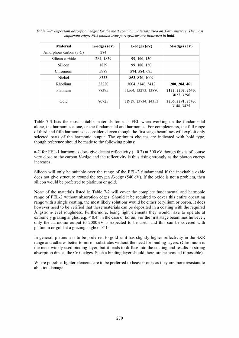
270

Table 7-2: Important absorption edges for the most common materials used on X-ray mirrors. The most important edges NLS photon transport systems are indicated in bold.

Material K-edges (eV) L-edges (eV) M-edges (eV) Amorphous carbon (a-C) 284

Silicon carbide 284, 1839 99, 100, 150 Silicon 1839 99, 100, 150

Chromium 5989 574, 584, 695 Nickel 8333 853, 870, 1009

Rhodium 23220 3004, 3146, 3412 280, 284, 461 Platinum 78395 11564, 13273, 13880 2122, 2202, 2645,

3027, 3296 Gold 80725 11919, 13734, 14353 2206, 2291, 2743,

3148, 3425

Table 7-3 lists the most suitable materials for each FEL when working on the fundamental alone, the harmonics alone, or the fundamental and harmonics. For completeness, the full range of third and fifth harmonics is considered even though the first stage beamlines will exploit only selected parts of the harmonic output. The optimum choices are indicated with bold type, though reference should be made to the following points:

a-C for FEL-1 harmonics does give decent reflectivity (~ 0.7) at 300 eV though this is of course very close to the carbon K-edge and the reflectivity is thus rising strongly as the photon energy increases.

Silicon will only be suitable over the range of the FEL-2 fundamental if the inevitable oxide does not give structure around the oxygen K-edge (540 eV). If the oxide is not a problem, then silicon would be preferred to platinum or gold.

None of the materials listed in Table 7-2 will cover the complete fundamental and harmonic range of FEL-2 without absorption edges. Should it be required to cover this entire operating range with a single coating, the most likely solutions would be either beryllium or boron. It does however need to be verified that these materials can be deposited in a coating with the required Ångstrom-level roughness. Furthermore, being light elements they would have to operate at extremely grazing angles, e.g. ≤ 0.4° in the case of boron. For the first stage beamlines however, only the harmonic output to 2000 eV is expected to be used, and this can be covered with platinum or gold at a grazing angle of ≤ 1°.

In general, platinum is to be preferred to gold as it has slightly higher reflectivity in the SXR range and adheres better to mirror substrates without the need for binding layers. (Chromium is the most widely used binding layer, but it tends to diffuse into the coating and results in strong absorption dips at the Cr L-edges. Such a binding layer should therefore be avoided if possible).

Where possible, lighter elements are to be preferred to heavier ones as they are more resistant to ablation damage.

271

Table 7-3: Possible coating materials that will give good reflectivity without strong absorption edges in the operating ranges of the FELs. The optimum choices are highlighted in bold

FEL Energy Range (eV)

Suitable materials

Usable grazing angles (°)

FEL-1 - Fundamental 50 – 300

Cr or Ni Pt or Au

≤ 6° ≤ 3°

FEL-1 - Harmonics 300 – 1500

a-C

Pt or Au ≤ 1.1° ≤ 2°

FEL-1 - Fundamental & harmonics

50 – 1500

Pt or Au ≤ 2°

FEL-2 - Fundamental 250 – 850 Pt or Au

Si ≤ 2° ≤ 1.8°

FEL-2 - Harmonics 850 – 4250 Cr or Ni ≤ 0.65° or ≤ 0.75°

FEL-2 - Fundamental & harmonics 250 – 4250

See text Pt or Au

≤ 1° for ≤ 2000 eV

FEL-3 - Fundamental 430 – 1000 a-C

Rh, Pt or Au ≤ 1° ≤ 2°

FEL-3 - Harmonics 1000 – 5000 a-C Ni

≤ 0.34° ≤ 0.83° for ≤ 2000 eV

≤ 0.6° FEL-3 - Fundamental &

harmonics 430 – 5000 a-C ≤ 0.34°

7.3 Damage Considerations

A critical factor in determining the layout of the photon transport systems is ensuring the optical elements will not be at risk from damage from the highly intense and ultra-short FEL pulses. Spatial dilution of the beam on the optical surface is the main method of preventing damage, and this is achieved by operating at increasingly grazing angles of incidence and by moving the elements further from the source. Although grazing angle operation is a necessity when working in the SXR range anyway, restrictions on the practical shapes of focusing mirrors means it can be essential to place the optical elements a considerable distance from the source. Preventing damage thus has big impact on the size of the transport system and it is necessary to derive estimates of these distances at an early stage so the overall scale of the facility can be judged.

A considerable amount of research has been undertaken over the past few years to understand the mechanisms and measure the thresholds for damage from short-wavelength laser pulses [1,2,3,4,5]. The picture that is emerging is complicated and not all damage mechanisms are fully understood. The following routes to damage must be considered in order to determine if an optical surface will be at risk in a FEL beam:

• Direct ablation, either through rapid melting or bond breaking, and the influence of the substrate in mirrors with thin coatings on the ablation threshold

• Photo-induced chemical or structural change, changing the optical surface without material removal

• Multi-shot accumulated damage at fluences insufficient to cause any visible damage with a single shot

7.3.1 Ablation Damage from Bulk Materials

Ablation caused by ultra-short photon pulses can be considered to be an essentially thermal process, but one in which the deposition of energy into the material is much more rapid than the

272

rate at which heat can be transported through the material. Consequently, the deposited energy does not have chance to dissipate into the bulk of the material and melting and evaporation at the surface can occur. A material is thus considered safe from ablation if the energy absorbed per atom is insufficient to cause melting. A safe level of 0.01 eV absorbed per atom has been suggested [6,7] and this same level is used here.

To calculate the energy absorbed (dose) per atom Da, the fraction of the incident pulse energy that is absorbed and the volume over which it is absorbed must be estimated. It is thus necessary to know the energy in the photon pulse EP, the footprint of the photon pulse on the optical element Aproj, the reflectivity of the optical element R at the wavelength of the photon pulse, the penetration depth de of the radiation into the surface, and the atom density na of the material. The absorbed dose per atom can then be written as:

(1 )Pa

proj e a

E RDA d n

−= (7-1)

The reflectivity and penetration depth are calculated from electromagnetic theory using tabulated values of the refractive index for the material. The energy contained within the pulse is obtained from simulations of the FEL output. The footprint on the optical element depends on the distance of the element from the source, the angle of incidence and the divergence of the source. Ideally, one would take the electric field of the simulated FEL output and propagate it to the position of the optical element to calculate the incident energy density at the surface. In practice, it is sufficient to use a simplified model as described below.

The radiation can safely be assumed to be transversely coherent and, since the transport systems will be essentially paraxial, the radiation will propagate according to Gaussian propagation theory. A beam quality, or M2, factor can be included in the propagation to account for the fact that the beam may not be pure Gaussian [8]. The beam width W (equal to twice the RMS beam size in intensity) thus propagates along the z-direction as:

( )2

22 2 40 0

0

( )W z W M z zWλ

π⎛ ⎞

= + −⎜ ⎟⎝ ⎠

(7-2)

where the beam waist W0 is the beam width at the source position z0. The beam waist can be approximated to twice the RMS electron beam size, i.e. 42 µm. A “worst case” scenario is modelled by taking M2 = 1. The pulse energies used, Table 7-4, are taken from Genesis 1.3 steady state simulations for an earlier linac and FEL configuration, but with the same 200 pC bunch charge. The latest results are slightly different from these, however the overall conclusions will not change substantially. Definitive calculations would in any case form part of a detailed design stage, taking into account also more realistic source position, size and M2 values. In addition, these calculations are for linear polarization; with circular polarization the output power should be slightly higher.

To illustrate how the distance of the first optical element varies with grazing angle, the incident energy density (fluence) required to give a dose of 0.01 eV absorbed per atom is calculated. For simplicity, the average of the Rs and Rp reflectivities is used, though they are very similar above 50 eV in any case. The distance from the source that gives this fluence is then calculated at a range of grazing angles. The results are a strong function of pulse energy, photon energy and optical element coating.

Figure 7-1 shows the result for the preferred option of a nickel-coated mirror on FEL-1. Whilst relatively high grazing angles can be used in this energy range, the consequence of using a large grazing angle is a significant increase in minimum distance. Therefore, a grazing angle 2° has been chosen for first stage design work, leading to a minimum distance of 38 m from the FEL-1

273

source. It is also noted that the minimum distance is determined by the highest photon energy. This is because, in the assumption of a diffraction-limited source of fixed size for all photon energies, the divergence scales inversely with photon energy and thus the footprint on the optic scales inversely as the square of the photon energy. Since the pulse energy does not decrease so rapidly with increasing photon energy, the absorbed dose thus increases with photon energy. The effect is compounded by the fact that the fluence to give the target dose also tends to fall as the photon energy increases.

Table 7-4: Pulse energies at selected photon energies for the three FELs derived from Genesis1.3 steady state simulations. These are the pulse energies for output in linear polarization.

FEL Photon Energy (eV) Pulse Energy (µJ)

FEL-1

50 252 100 161 200 143 300 121

FEL-2 250 93 500 70 850 34

FEL-3

500 80 666 44 800 41

1000 31

Figure 7-1 : The minimum distance of a nickel-coated mirror from the FEL-1 source as a function of

grazing angle of incidence for photon energies spanning the operating range of the FEL fundamental.

For FEL-2, the baseline assumption is that platinum coatings will need to be used for the fundamental. Being a heavier element, this has a much lower threshold fluence. The consequence is that the “safe” minimum distance is now much greater, as shown in Figure 7-2, where a minimum distance of 61 m at 1° grazing angle is needed.

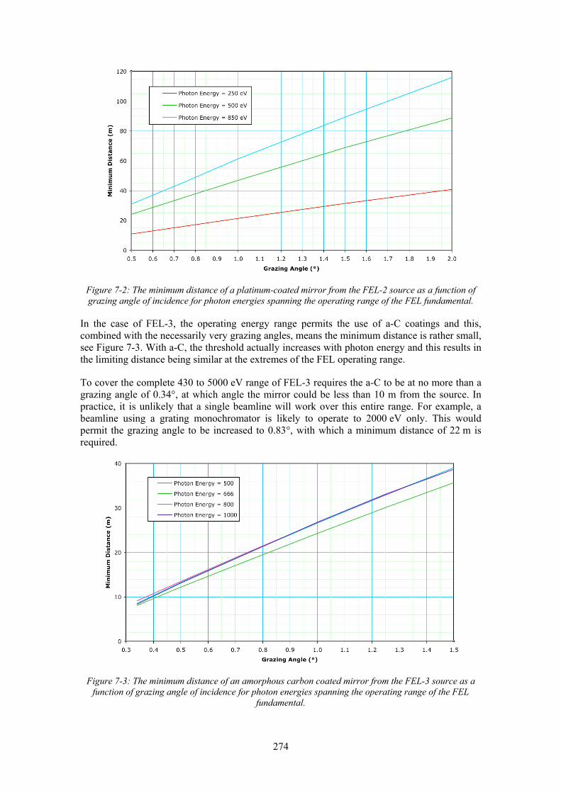
274

Figure 7-2: The minimum distance of a platinum-coated mirror from the FEL-2 source as a function of grazing angle of incidence for photon energies spanning the operating range of the FEL fundamental.

In the case of FEL-3, the operating energy range permits the use of a-C coatings and this, combined with the necessarily very grazing angles, means the minimum distance is rather small, see Figure 7-3. With a-C, the threshold actually increases with photon energy and this results in the limiting distance being similar at the extremes of the FEL operating range.

To cover the complete 430 to 5000 eV range of FEL-3 requires the a-C to be at no more than a grazing angle of 0.34°, at which angle the mirror could be less than 10 m from the source. In practice, it is unlikely that a single beamline will work over this entire range. For example, a beamline using a grating monochromator is likely to operate to 2000 eV only. This would permit the grazing angle to be increased to 0.83°, with which a minimum distance of 22 m is required.

Figure 7-3: The minimum distance of an amorphous carbon coated mirror from the FEL-3 source as a

function of grazing angle of incidence for photon energies spanning the operating range of the FEL fundamental.

275

7.3.1.1 The Influence of Mirrors with Thin Coatings

The above analysis of ablation damage made the assumption that the fraction of the energy contained in the photon pulses that is absorbed by the mirror surface is absorbed in a material depth equal to the penetration depth of the photon beam. Under conditions of total external reflection found with X-rays at grazing angles of incidence, the penetration depth is the extinction depth of the evanescent wave and is typically of order only one or two nanometres. The extinction depth is also fairly constant with photon energy (away from absorption edges) and so the absorption volume is small and decreases with photon energy (as the beam footprint falls). This accounts for the low threshold fluence and large distances that are required at short wavelengths.

However, it is not certain that this assumption is correct under all conditions. The energy absorbed from the photon pulse is deposited via coupling to the electrons in the material. If the material has a high electron mobility, then it is indeed possible for the energy to be carried into the bulk material before the damage can occur. This is naturally most likely to be the case when the mirror is coated with a metallic (and hence highly conducting) material. Since thin metallic coatings (typically only 40 nm thick) are the norm for X-ray mirrors, it is at least conceivable that the absorbed energy could be deposited even into the mirror substrate.

Accurately modelling these effects will be very tricky as a detailed knowledge of the electron transport in the coating and possibly also the substrate will be required. However, the likely effect of the deeper absorption volume is easy to model by simply replacing the penetration depth of the radiation in (0-1) with a fixed value, the effective absorption depth dA. Figure 7-4 shows the absorbed energy per atom in a Pt coated mirror at a grazing angle of 1° as a function of distance from the source for FEL-2 at 250 eV, 550 eV and 850 eV with dA = 5 nm. This value of dA is rather arbitrarily chosen, but is consistent with the mean free path of low energy electrons predicted by the “universal curve” of Seah and Dench [9]. As can be seen, the energy absorbed per atom is below 0.01 eV at distances above ~40 m even at 850 eV. The minimum safe operating distance is thus greatly reduced and is likely to be as close as permitted from a practical view of the space available.

Figure 7-4 : Absorbed dose per atom in a Pt coated mirror at a grazing angle of 1° as a function of

distance from the source of FEL-2 with a constant absorption depth of 5 nm. The pulse energies are given in Table 7-4

276

7.3.2 Damage without Material Removal

Removal of material from the mirror surface is not the only type of damage that affects the performance of the mirror. Any change in the surface quality can cause reflectivity loss through an increase in scattering and degrade image quality by an increase in local error in the surface form (i.e. shape). Even without physical change in the surface, the performance of the mirror can be affected through photon induced chemical changes that result in changes in the refractive index of the coating material. Even a simple expansion of the coating will change the reflectivity due to the change in atomic density in the coating. Studies made on amorphous carbon coatings [4] at 92 eV and 177 eV show that around the central ablation crater is a region of material expansion that has been attributed to graphitization of the carbon structure, giving both physical and chemical changes to the coating. Such damage occurs in the wings of the main photon pulses and thus occurs at fluences well below the threshold for ablation damage.

7.3.3 Multi-shot Damage

Another damage mode that must be considered is cumulative damage from multiple shots where each shot is below the threshold for causing any detectable damage on its own. Progressive erosion of amorphous carbon coatings at a fluence of half that required for single-shot ablation has been observed at a photon energy of 26 eV [5]. The damage mechanism is believed to be radiolytic cleavage of C-C bonds such that the coating is cut into small fragments that are able to leave the surface. There is thus material removal without the peripheral expansion observed in the single shot measurements referred to above.

7.3.4 Summary

Heavy metallic elements such as platinum or gold give a large absorbed dose per atom and thus the risk of damage is high. The absorbed dose depends on the depth to which the absorbed energy can diffuse into the coating material before bond breaking occurs. This depth is related to the electron mobility in the material and is difficult to predict. It may however be rather larger than the penetration depth of the X-rays under conditions of total external reflection and thus the threshold fluence for ablation may be higher than predicted from calculations of the type described in Section 7.3.1. This is welcome as the energy range of FEL-2 demands the use of platinum coatings and this makes the beamlines rather long.

However, caution must still be exercised since there are other damage modes that occur below the single shot threshold for ablation. It is therefore prudent to choose to operate the first mirrors with predicted fluences that are well below the single-shot ablation thresholds.

Table 7-5 summarizes the first mirror coatings, grazing angles and distances from the source that will be used in first stage beamline designs. For FEL-1 and FEL-3, the first optic distances have been determined by considerations of the practical machine layout rather than protection from radiation damage. Space is required for the THz undulators, the gas-cells, radiation shielding and a considerable amount of port hardware. The layout is also constrained by the electron transport to the common beam dump. Thus, it has been found that the first mirrors cannot be practically placed closer than about 50 m from the end of the FEL. This distance is more than sufficient for protection from radiation damage on FEL-1 and FEL-3. For FEL-2, a larger distance is adopted to allow for the greater risk associated with the heavy metallic coatings that will be used.

277

Table 7-5: Mirror coatings, grazing angles and distances from the source of the first mirror used for beamlines in the first stage design studies

FEL Mirror coating Grazing angle (°) Distance from source (m)

FEL-1 (≤ 800 eV) Ni 2 50 FEL-2 (≤ 2000 eV) Pt 1 60 FEL-3 (≤ 2000 eV) a-C 0.83 50 FEL-3 (> 2000 eV) a-C 0.34 50

7.4 Fundamental and Harmonic Attenuation

7.4.1 Attenuating the Fundamental

A requirement for some experiments is that the fundamental should be controllably attenuated by a factor of at least 100 and ideally 1000. The main reason is to deliver a controlled fluence at the sample and so the attenuation should be achieved without changing any other properties of the source. This makes selective defocusing of the beam unsuitable since this is accompanied by significant changes in the spatial distribution of the light, especially with coherent beams where intensity modulation in the beam is often visible away from the focus.

The standard approach to beam attenuation is to use a gas-cell to absorb some of the radiation. By passing the beam through a long column of gas at a relatively low (compared to atmospheric) pressure, the beam intensity can be controllably reduced. Since separating the gas column from the beamline vacuum by widows is impractical in the soft X-ray region (due to strong absorption and likely disruption of the coherent beam), differential pumping has to be used. The highest gas pressure is thus determined by the space allocated for the pumping and the diameter of the beam pipe into the gas cell. This latter cannot be too small as it is necessary to avoid diffraction at the aperture disrupting the beam.

A gas pressure of 0.1 Torr is considered feasible [10] and this has been used here. Calculations for a range of gases show that achieving a transmission of 0.1% from 50 to 1000 eV would require a gas column length of about 20 m. The total installed gas cell length, including differential pumping, would thus be ~25 m. The gases considered were neon, argon, krypton, xenon, nitrogen, oxygen, carbon dioxide and sulphur hexafluoride. Of these, argon, krypton, xenon and sulphur hexafluoride are the most effective. Figure 7-5 shows the gas pressure needed to achieve a transmission of 0.1% with a 20 m long column of these four gases. The limiting case is at ~676 eV, corresponding to the xenon MV-edge. The optimum gases are krypton and xenon, both of which are very expensive and so the gas cell would have to be equipped with a gas recovery system. However, argon and sulphur hexafluoride could be used, though a greater pressure (up to 0.2 Torr) would be needed between ~530 and 697 eV.

278

Figure 7-5: The gas pressure of a 20 m long column of gas required to give a transmission of 0.1%.

For FEL-1, a smaller gas cell is feasible. Using sulphur hexafluoride at 0.1 Torr, the gas column length would only need to be ~5 m. However, the more divergent beam at these lower photon energies would require a larger beam tube diameter through the differential pumping sections and so it is probably prudent to assume a cell length longer than this to allow lower pressure to be employed. In any case, there is likely to be sufficient space for a larger filter.

7.4.2 Attenuating the Harmonics

In photon flux terms, the third harmonic will be less than 1% of the fundamental intensity and the fifth harmonic will be less than 0.02%, see Table 7-8. Even order harmonics are strongly suppressed naturally and will be at an even lower level. Consequently, for many applications, the harmonic content is unlikely to be a serious problem.

One way to reduce the harmonic content further would be to operate the FEL in circularly polarized mode. Since the circularly polarized light is generated using helical undulators, all harmonics are naturally suppressed.

If linearly polarized light is required with very low harmonic content, than some additional means of reducing it is required. The gas attenuator will not be helpful in this application since the energy spacing between the fundamental and third harmonics is too large to give good contrast across an absorption edge.

If a monochromator is used in the beamline, then this will act to suppress higher harmonics to some extent. Whilst grating monochromators can have quite large higher order efficiencies, this is mainly an issue in the VUV to XUV part of the spectrum. Also, the main problem is second order and second harmonic light should not be present to any significant extent in the source anyway. Thus, a beamline with a grating monochromator will naturally suppress the harmonics without special design to achieve this. In the soft X-ray region, a third order efficiency of ~1% would be typical and this would give a third order contamination in the output beam of ~0.01%, which should be negligible. The fifth harmonic will be even more strongly suppressed.

For beamlines with no monochromator, the most practical way to achieve lower harmonic contamination will be by means of a mirror order sorter, which utilizes the high-energy cut-off in reflection that occurs in the X-ray region. Whilst good results can be achieved with just two reflections, the results of a 4-mirror order sorter are presented here. This is because such a

279

device can give zero overall deflection of the photon beam and so can be inserted or removed from the beam path as required, essentially without affecting the downstream optical layout. There will be a path-length difference, which could however affect downstream focusing optics, and would of course introduce a temporal shift. A three-mirror order sorter could also be used, but this requires one reflection to be a twice the grazing angle of the other two and so is less optimal.

Simulations on the performance of a four-mirror order sorter have demonstrated that it should be possible to attenuate the third harmonic by a factor of at least ten relative to the fundamental whilst still achieving at least 40% transmission in the fundamental over the energy range of the FELs. Table 7-6 shows the coatings and the grazing angles that would be needed to meet this requirement.

Table 7-6: The photon energy ranges over which a four-mirror order sorter with the specified coating and at the specified grazing angle will give a suppression of the third harmonic by at least a factor of ten

and give at least 40% transmission of the fundamental.

Photon energy range (eV) Coating material Grazing angle 50 – 88 SiC 5°

84 – 228 a-C 5° 92 – 250 a-C 3°

178 – 306 Cr 3° 278 – 732 Ni 2° 440 – 1000 SiC 1.6° 566 – 1000 a-C 1.3°

7.4.3 Suppressing the Fundamental

A key part of the science case involves exploiting the harmonics that are generated in the FELs. Since the harmonics have a relatively low power compared to the fundamental, a general requirement is to strongly suppress the fundamental to a level that is small compared with the harmonic. Table 7-7 shows the results of Genesis1.3 steady state simulations (for linear horizontal polarization) of the output in photons per pulse of FEL-2 and FEL-3 in the fundamental and harmonics. Table 7-8 shows the ratio of harmonic to fundamental intensity and the relative attenuation ratio of fundamental to harmonic required to bring the fundamental to 1% of the harmonic intensity. The required attenuation ratio is very high, varying between ~20,000 and ~5,500,000.

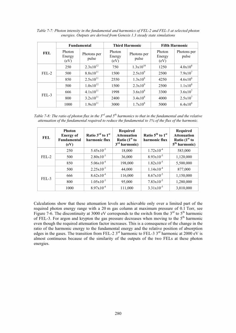
280

Table 7-7: Photon intensity in the fundamental and harmonics of FEL-2 and FEL-3 at selected photon energies. Outputs are derived from Genesis 1.3 steady state simulations

FEL

Fundamental Third Harmonic Fifth Harmonic Photon Energy

(eV)

Photons per pulse

Photon Energy

(eV)

Photons per pulse

Photon Energy

(eV)

Photons per pulse

FEL-2 250 2.3x1012 750 1.3x1010 1250 4.0x108 500 8.8x1011 1500 2.5x109 2500 7.9x107 850 2.5x1011 2550 1.3x108 4250 4.6x106

FEL-3

500 1.0x1012 1500 2.3x109 2500 1.1x108 666 4.1x1011 1998 3.6x108 3300 3.6x107 800 3.2x1011 2400 3.4x108 4000 2.5x107

1000 1.9x1011 3000 1.7x108 5000 6.4x106

Table 7-8: The ratio of photon flux in the 3rd and 5th harmonics to that in the fundamental and the relative attenuation of the fundamental required to reduce the fundamental to 1% of the flux of the harmonic.

FEL

Photon Energy of

Fundamental (eV)

Ratio 3rd to 1st harmonic flux

Required Attenuation Ratio (1st to

3rd harmonic)

Ratio 5th to 1st harmonic flux

Required Attenuation Ratio (1st to

5th harmonic)

FEL-2 250 5.45x10-3 18,000 1.72x10-4 583,000 500 2.80x10-3 36,000 8.93x10-5 1,120,000 850 5.06x10-4 198,000 1.82x10-5 5,500,000

FEL-3

500 2.25x10-3 44,000 1.14x10-4 877,000 666 8.62x10-4 116,000 8.67x10-5 1,150,000 800 1.05x10-3 95,000 7.83x10-5 1,280,000 1000 8.97x10-4 111,000 3.31x10-5 3,010,000

Calculations show that these attenuation levels are achievable only over a limited part of the required photon energy range with a 20 m gas column at maximum pressure of 0.1 Torr, see Figure 7-6. The discontinuity at 3000 eV corresponds to the switch from the 3rd to 5th harmonic of FEL-3. For argon and krypton the gas pressure decreases when moving to the 5th harmonic even though the required attenuation factor increases. This is a consequence of the change in the ratio of the harmonic energy to the fundamental energy and the relative position of absorption edges in the gases. The transition from FEL-2 3rd harmonic to FEL-3 3rd harmonic at 2000 eV is almost continuous because of the similarity of the outputs of the two FELs at these photon energies.

281

Figure 7-6: The calculated pressure in a 20 m gas cell required to attenuate the fundamental to 1% of the harmonic flux. The photon energy range 850 to 5000 eV is covered by FEL-2 with the 3rd harmonic and

FEL-3 with the 3rd and 5th harmonics in accordance with Table 7-1.

Krypton and xenon require the lowest pressure but neither gas has a very good transmission to the harmonic radiation at the required pressure, see Figure 7-7. The transmission is mostly less than 40%, and although the transmission of xenon is ~60% from 3400 to 4700 eV, both gases are effectively opaque between 1700 and 2000 eV. Sulphur hexafluoride has the best transmission, being greater than 50% from 1100 to 5000 eV. However, the required pressure is almost always above 0.1 Torr, and peaks at ~0.6 Torr, which might be impracticably high.

Figure 7-7: The transmission of the 20 m gas cell at the pressures needed to reduce the fundamental to

1% of the harmonic flux.

It should be noted that reducing the attenuation ratio to permit the fundamental to rise to ~10% of the harmonics will, in general, have only a modest effect on the gas pressure because the required attenuations are so high and the pressure scales as a the ratio of the logarithms of the attenuation ratios. For example, reducing the attenuation ratio from 1,000,000 to 100,000 reduces the gas pressure by just one sixth.

282

Consequently, for operation on the harmonics, the preferred method of removing the fundamental at this stage of the design process is to use a monochromator. Below ~2000 eV, this would be a grating monochromator and above 2000 eV a crystal monochromator would be used. The impact on the photon output will be discussed in later Sections, but it is worth noting that the gas filter will still be employed to attenuate the fundamental by a factor of ~10 in order to protect the optics (particularly the crystals) from ablation damage. This level of attenuation will of course be easy to achieve.

7.5 Polarization

Since the NLS FELs will be able to produce arbitrary linear and elliptical polarization states, the effect of the transport system on the polarization must be considered. For grazing angle reflections, there is a difference in reflectivity for light with the E-vector parallel (π state) or perpendicular (σ state) to the plane of incidence. There is also a phase shift between the two orthogonal polarizations.

These effects are not important if the light is purely linearly polarized and makes just s- or p-reflections from all the optics, but circular polarization will be converted to elliptical polarization. These effects can be very difficult to mange in the VUV, mainly because the phase shifts can be very large. In the soft X-ray range (> 100 eV) however, the polarising effects are usually very small since both the difference between the s- and p-reflectivities and the phase shifts are small. From ~50 eV to 100 eV, the polarising effects are stronger, but still not generally problematical and so, over the range of the fundamental radiation, polarising effects are not expected to be significant.

However, the use of crystal monochromators to isolate the harmonics above ~2000 eV will lead to significant polarising effects. The Darwin width is narrower for the π than it is for the σ state. Since the real part of the refractive index is very close to unity, the Darwin widths Γπ and Γσ are related to the Bragg angle θB by

cos2 Bπ σ θΓ = Γ (7-3)

Thus, the width for the π state is effectively zero at a Bragg angle of 45° (which is the Brewster angle) and the crystal acts as a linear polarizer. With Si(111), this occurs at a photon energy of 2796 eV.

Away from the Brewster angle, the Darwin width for the π state increases, but is always narrower than that for the σ state (except at normal incidence). Consequently, the polarising effect is different for the spectral components that lie within the narrower width than for the components that lie between the two widths. If the light is linearly polarized and makes an s-reflection, there is no change to the polarization. But if the incident light is circularly polarized, the spectral components that lie outside the π state Darwin width become linearly polarized. Since the π state has a very slightly lower reflectivity that the σ state (because the narrower Darwin width is the result of deeper penetration into the crystal and so there is higher absorption), those components that lie within the width of the π state become slightly elliptically polarized. The ellipse axis is also rotated because there is additionally a small phase shift between the two states. Because the polarising effect is different for the different spectral components of the beam, the overall effect is that the light becomes depolarized.

Clearly, these effects cannot be corrected by tuning the polarization of the source. The only way to maintain elliptically or circularly polarized light through the monochromator is to ensure the bandwidth of the light lies entirely within the narrower (i.e. π state) Darwin width. For NLS the pulses are expected to be close to transform limited with 20 fs FWHM duration and so the pulse bandwidth should be ~0.09 eV FWHM. Away from absorption edges, the Darwin widths have a near top-hat profile. Thus for 95% of the radiation to lie within the Darwin width, the π-state

283

width should be ~0.16 eV. With Si(111) this will be satisfied for photon energies below ~2300 eV and above ~3450 eV. The only practical way to preserve circular polarization within this energy range is to use a different crystal that places this energy range away from the Brewster angle and ideally has larger Darwin widths (meaning it has higher absorption and so is made from heavier atoms) to reduce the range over which the problem occurs. Both Ge(111) and InSb(111) are widely used at synchrotron sources, but neither have sufficiently bigger 2d-spacings to completely solve the problem. For example, the problem region with Ge(111) would span from ~2400 to ~2950 eV.

An alternative approach to producing circularly polarized light above 2000 eV would be to use a quarter-wave plate after the monochromator. The source would only need to produce linearly polarized light, where harmonic output is optimum, and the linear polarising effect of the monochromator would be an advantage. To maintain a wide operating range a method of retardation that does not rely on the large phase-shifts that can be produced near absorption edges is required.

It has long been known that crystals in Bragg geometry can act as nearly perfect quarter wave plates. The crystal is placed in the linearly polarized beam at an angle satisfying the Bragg condition at the wavelength of interest and with the E-vector at 45° to the plane of incidence. When the crystal is turned a very small angle (arcsecond level) from the Bragg condition, the required 90° phase shift can be generated for the forward-diffracted (i.e. transmitted) beam. The wavelength can be tuned by changing the angle of incidence on the crystal. The phase shift is sensitive to the deviation from the Bragg angle and also depends on the crystal thickness. The first practical demonstration [11] used a 62 µm thick Si(220) crystal in Bragg geometry to create X-rays in the range 6500 to 9500 eV with a degree of circular polarization greater than 0.98. Diamond has also been used and has the potential to work to lower photon energies due to the lower absorption, though available crystals have tended to be several hundred µm thick. Thus, operation has been limited to above ~5000 eV [12,13]. To give 50% transmission at 3000 eV, the diamond would need to be ~20 µm thick. Unfortunately, diamond cannot be used in the energy range required for FEL-3 since the lowest order reflection is (111) and, with a 2d-spacing of 4.12 Å, the lowest accessible energy is 3009 eV at a Bragg angle of 90°.

7.6 Pulse Length Preservation in Photon Transport Systems

To deliver a pulse from source to experiment whilst preserving the pulse length at the level of 20 fs FWHM will require a transport system that has a closely matched optical path length over the aperture of the system. In general, geometrical aberrations and the effect of manufacturing and thermally induced slope errors will have to be tightly controlled. However, the biggest factor affecting the pulse length will be the approach taken to modifying the spectral bandwidth, should this be required. If the FEL pulse is Gaussian and transform limited, then the RMS pulse length and RMS bandwidth will be related by the transform limit:

4rms rmshE τπ

Δ Δ = (7-4)

If the pulses are not fully longitudinally coherent or not Gaussian, then the time-bandwidth product will be greater than h/4π. This will be the case in practice since the pulses inevitably deviate from the Gaussian ideal even when fully longitudinally coherent.

A 20 fs FWHM pulse thus has a limiting bandwidth of 93 meV FWHM. Any attempt to reduce this bandwidth will lengthen the pulse. The bandpass of any monochromator used to condition the FEL beam, for example by removing the spontaneous and SASE background generated by the FEL undulator, must be no smaller than 93 meV if the pulse length is to be preserved.

284

7.6.1 Pulse Length Effects in Grating Monochromators

In the XUV and SXR up to ~2000 eV, reflection diffraction gratings at grazing angles of incidence are used as the dispersing elements in monochromators. When a beam passes across a diffraction grating, each illuminated groove gives a path length difference equal to the wavelength of the diffracted light λ times the order of diffraction m. This path length difference across the beam results in the output beam being longitudinally sheared and so temporally stretched.

Controlling the pulse stretch from a grating thus requires the number of illuminated grooves to be limited. The longer the wavelength of the radiation, the fewer the number of grooves that can be illuminated to give a certain pulse stretch. For example, 20 fs at 50 eV is equivalent to only ~240 wavelengths whereas at 1000 eV it is equivalent to ~4800 wavelengths. So maintaining a 20 fs pulse at 50 eV requires that less than 240 grooves be illuminated. This is very difficult to achieve with a grating in a conventional mount since the grazing angle of incidence spreads the beam out and impracticably low line densities would be required.

The task of reducing the number of illuminated grooves is eased by operating the grating in the so-called conical diffraction mount (also called the extreme off-plane mount). In this mount the grating is rotated by almost 90° about the grating normal when compared with the conventional mount so that the incident beam is almost parallel to the grooves [14]. Because the grooves are now almost parallel to the beam direction, the number of illuminated grooves is determined by the transverse footprint of the beam. At grazing angles of incidence, this is much smaller than the tangential footprint and so the inherent pulse stretch is potentially greatly reduced. The dispersion is also greatly reduced and so the line density may need to be increased, but it is possible to make a single grating monochromator work in the XUV with pulse stretch below 10 fs [15]. Higher diffraction efficiency is also possible with conical mounting. Another advantage is that the grating can be (and normally is) illuminated at a fixed altitude and thus the grazing angle of incidence at the grating is almost constant. This can be important in reducing the risk of ablation of the grating surface and is in contrast to the conventional mount in which the grazing angle will become larger at longer wavelengths and so make the FEL beam more concentrated on the grating surface.

Possibly the biggest disadvantage of the conical mount is that simple scanning of the grating is restricted to the “fixed altitude mode”. This mode permits scanning of the wavelength by a simple rotation of the grating about an axis in the grating surface and parallel to the grooves. Such a simple scanning mode is desirable as it allows for high quality mechanisms. It does, however, limit the flexibility in the way the grating is operated, and there is no easy way to achieve the equivalence of the variable-included-angle scanning modes possible with conventional mounting. For example, scanning the grating “on-blaze” in a conical mount requires a scan at fixed azimuth and this would require a very complicated mechanism with translation of the grating in a direction along its normal linked to rotating mirrors before and after the grating [16]. Such mechanisms are best avoided due to the difficulty in making them with the tolerance required to not introduce temporal and spatial jitter into the beam, and also their considerable cost. The total path length in such a mechanism would also vary as the wavelength is changed.

Another issue with the conical mount is the impact on the beam polarization. This is more complicated than with the conventional mount since the beam is deflected both horizontally and vertically. The grating can thus introduce a component of circularly polarized light in a linearly polarized incident beam [17].

When a single grating does not give satisfactory pulse length preservation, either in a conventional or conical mount, the only solution is to use a second grating that reverses the pulse stretch (spatial chirp) caused by the first grating. To do this, the optical path difference across the aperture of the beam must be equal and opposite for the two gratings. Figure 7-8

285

shows a so-called 4f configuration that achieves the required time compensation. This is an example of Fourier domain pulse shaping in which the time shaping occurs in the frequency domain.

Figure 7-8: Schema of a 4f system for pulse length preservation

The two focussing mirrors (shown as lenses for simplicity in the Figure) and the mirror-imaged grating pair are spaced at distances equal to the focal length f of the mirrors. The grating G1 disperses the light and M1 performs the Fourier transform, converting angle of dispersion into position at the slit plane between the two mirrors. M2 performs the inverse Fourier transform but maintains the dispersed spectrum. The grating G2 recombines the dispersed beam into a single collimated beam. G2 must work in the opposite order of diffraction to G1 in order for the path lengths to be correctly balanced. The slit is a simple spatial modulator; its purpose is to filter out the undesired spectral components but leave the required ones intact.

The main advantage of the double grating monochromator is that it can preserve the pulse length of the source to a very high level. Since the stretch caused by one grating is, in theory, completely reversed by the second grating, the only residual pulse stretch is that caused by aberrations and imperfect optics. These should be controllable down to the fs level if not lower. The main disadvantages are that the beamline is complicated (and so expensive) and that the transport efficiency is seriously reduced when compared to a single grating design.

7.6.2 Pulse Length Effects in Crystal Monochromators

Monochromators operating in the X-ray range above ~ 2 keV normally use Bragg reflections from crystals. In Bragg reflection, the amplitude of the incident wave is divided and reflected off successively deeper crystal planes. Because the photon beam must propagate through many layers of the crystal, there is an unavoidable stretching to the pulse. The penetration into the crystal is related to the rocking curve width and hence the spectral bandpass of the crystal since the more crystal planes that contribute to the reflection the narrower the rocking curve and bandpass. As the bandpass gets smaller, the pulse must get longer due to the transform limit. Away from absorption edges, the relative bandpass Δλ/λ is constant for a given crystal reflection; for example it is 1.4x10-4 for Si(111). The rocking curve is rather flat topped and so this approximates to the FWHM bandpass. So, at 4 keV, the approximate RMS bandpass is 0.24 eV and the RMS transform limited pulse length is approximately 1.4 fs. Since the relative bandwidth of the crystal is constant, at higher photon energies ΔE will be larger and the limiting pulse length will be shorter. Thus, crystal reflections are viable for short pulses as long as the optical system does not have too many separate crystal reflections and the pulses are not shorter than ~10 fs.

286

7.7 FEL Beamline Suite

Each FEL undulator will be followed by another undulator that will produce coherent THz radiation. THz radiation will be extracted after the undulator with a mirror at ~45° incidence angle and as close to the undulator exit as possible. The X-ray beam will propagate through the THz undulator and will pass through a hole in the THz extraction mirror. This hole (and the THz undulator gap) must be large enough not to cause diffractive disruption to the FEL beam. Conversely, the hole must be not so large as to reduce the THz extraction efficiency unnecessarily and excessively disrupt the THz beam. On FEL-1, a second THz undulator will be employed so that two synchronized THz sources are available. There will also be a bending magnet to give additional broadband coherent THz output. THz transport will be discussed in Section 7.8.

After the THz undulators will be the gas attenuators. On FELs 2 and 3 the attenuators will be about 25 m long in total, giving 20 m of gas length and 2.5 m at each end for the differential pumping. The pumping section will probably also include basic diagnostics such as intensity and beam position monitoring. On FEL-1, the gas cell can be much shorter and a total length of ~10 m is likely.

The first optical element will be positioned at a distance that ensures it will not be damaged by ablation, see Section 7.3. The primary function of the first optical element is to deflect the photon beam away from the axis of the FEL undulator and electron beam. This is essential to prevent high-energy radiation (e.g. gas-Brehmsstrahlung) from passing down the beamline and presenting a safety hazard. Whilst the first mirror can be a plane mirror, it may also be possible to make it a functional part of the beamline design.

In order to design a transport system for the FEL radiation it is essential to understand the properties of the FEL source. Most importantly, the source size and divergence must be known. Preliminary beamline modelling is performed by assuming the source behaves as an ideal coherent Gaussian beam with a source size taken to be the electron beam size (= 21 µm RMS). Thus, the RMS source size rσ and divergence rσ ′ are related by

4r rλσ σπ′ = (7-5)

The second stage is to use a more realistic model of the source that can be deduced from Genesis simulations of the FEL output. This approach is described in Section 7.7.1 below. Once a good design solution has been found, this will be checked by fully propagating the simulated FEL output from the FEL, through the optical system, and to the experiment. Wavefront propagation of this nature is computationally very intensive and so this approach will be used only for checking and final optimization of the transport system design.

High quality photon diagnostics are also essential to the experiments. An important design consideration is whether the diagnostics require an intermediate focus in the transport system to work. Since the provision of such a focus will in general be detrimental to the overall performance of the transport system, it will be assumed at this stage that the required diagnostics can be inserted non-invasively into the transport systems. Diagnostics are discussed in Section 7.10.

7.7.1 Source Properties of FEL-2 Deduced from M2 Analysis

The principal behind the M2 analysis is the fact that there is a quadratic propagation dependence of the second moment of the beam profile for any arbitrary real laser beam, whether it be Gaussian or non-Gaussian, fully coherent or partially incoherent, single mode or multiple transverse mode in character [8]. Thus the propagation can be described by (0-2) where M2 is a

287

beam “quality” factor that describes how far the actual beam is from the ideal Gaussian TEM00 mode.

As an example of this analysis, Genesis simulations of the electric field at the output of FEL-2 at 250 eV, 500 eV and 850 eV were propagated in free space using the Daresbury wavefront propagation code FOCUS [18]. The Genesis simulations used were steady state simulations, which is acceptable since the transverse beam properties do not require time-dependent simulations to be accurately modelled. The field files generated by Genesis were all taken at the end of the radiator module in which saturation occurred.

In principal, the M2 analysis requires the field to be propagated to just three different distances and this allows the source size, longitudinal source position and M2 factor to be determined [19]. In reality, because the calculation of the second moment of the beam profile is highly sensitive to noise in the generated field far from the optical axis, it is necessary to perform multiple propagations in the region where the beam expansion is not linear with distance in order to get a unique fit.

An example is shown in Figure 7-9. The graph shows the second moment of the horizontal and vertical beam profiles at a photon energy of 500 eV. Propagations were performed both forward and backward from the original field file (representing zero propagation distance). The points show the second moments calculated from the propagated field and the solid lines are the quadratic fits. The coefficients of the quadratic fit give the source parameters. The Figure shows that the quadratic propagation law is obeyed exactly. The horizontal and vertical sources are seen to be at different longitudinal positions before the “zero” position and have different source sizes and M2 factors. Table 7-9 summarises the results of the analysis at 250 eV, 500 eV and 850 eV. Note that because the source position is relative to the original field file, the deduced positions are not relative to the same absolute position for the different photon energies.

Figure 7-9 : Results of the propagation of Genesis simulation of the output of FEL-2 at 500 eV. The

points are the calculated second moments of the beam profiles and the solid lines are the quadratic fits.

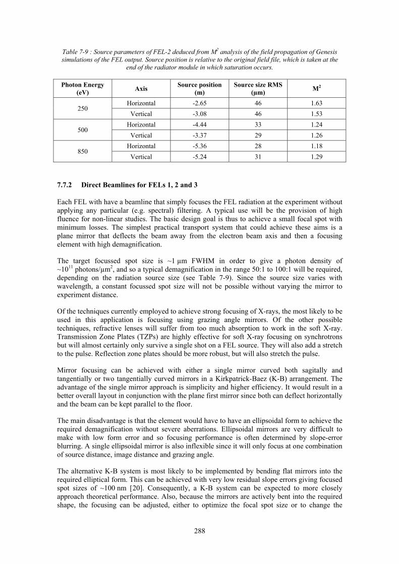
288

Table 7-9 : Source parameters of FEL-2 deduced from M2 analysis of the field propagation of Genesis simulations of the FEL output. Source position is relative to the original field file, which is taken at the

end of the radiator module in which saturation occurs.

Photon Energy (eV) Axis Source position

(m) Source size RMS

(µm) M2

250 Horizontal -2.65 46 1.63

Vertical -3.08 46 1.53

500 Horizontal -4.44 33 1.24

Vertical -3.37 29 1.26

850 Horizontal -5.36 28 1.18

Vertical -5.24 31 1.29

7.7.2 Direct Beamlines for FELs 1, 2 and 3

Each FEL with have a beamline that simply focuses the FEL radiation at the experiment without applying any particular (e.g. spectral) filtering. A typical use will be the provision of high fluence for non-linear studies. The basic design goal is thus to achieve a small focal spot with minimum losses. The simplest practical transport system that could achieve these aims is a plane mirror that deflects the beam away from the electron beam axis and then a focusing element with high demagnification.

The target focussed spot size is ~1 µm FWHM in order to give a photon density of ~1011 photons/µm2, and so a typical demagnification in the range 50:1 to 100:1 will be required, depending on the radiation source size (see Table 7-9). Since the source size varies with wavelength, a constant focussed spot size will not be possible without varying the mirror to experiment distance.

Of the techniques currently employed to achieve strong focusing of X-rays, the most likely to be used in this application is focusing using grazing angle mirrors. Of the other possible techniques, refractive lenses will suffer from too much absorption to work in the soft X-ray. Transmission Zone Plates (TZPs) are highly effective for soft X-ray focusing on synchrotrons but will almost certainly only survive a single shot on a FEL source. They will also add a stretch to the pulse. Reflection zone plates should be more robust, but will also stretch the pulse.

Mirror focusing can be achieved with either a single mirror curved both sagitally and tangentially or two tangentially curved mirrors in a Kirkpatrick-Baez (K-B) arrangement. The advantage of the single mirror approach is simplicity and higher efficiency. It would result in a better overall layout in conjunction with the plane first mirror since both can deflect horizontally and the beam can be kept parallel to the floor.

The main disadvantage is that the element would have to have an ellipsoidal form to achieve the required demagnification without severe aberrations. Ellipsoidal mirrors are very difficult to make with low form error and so focusing performance is often determined by slope-error blurring. A single ellipsoidal mirror is also inflexible since it will only focus at one combination of source distance, image distance and grazing angle.

The alternative K-B system is most likely to be implemented by bending flat mirrors into the required elliptical form. This can be achieved with very low residual slope errors giving focused spot sizes of ~100 nm [20]. Consequently, a K-B system can be expected to more closely approach theoretical performance. Also, because the mirrors are actively bent into the required shape, the focusing can be adjusted, either to optimize the focal spot size or to change the

289

demagnification. Changing the demagnification would, of course, be accompanied by a change in the longitudinal position of the focus.

Because the K-B system requires two orthogonal deflections, a beamline consisting of a horizontally deflecting first mirror and a K-B pair will result in the final beam pointing either upwards or downwards. This may not be a severe limitation however. The high demagnification requires a short image distance and so the overall rise or fall of the beam will be quite modest and the angle will probably be no more than 4° (likely 2° maximum grazing angle).

A more intractable limitation of the K-B approach is that the horizontal and vertical demagnifications must necessarily be different. This difference becomes more significant as the demagnification increases. Furthermore, with an average demagnification equal to that of the single mirror solution, the working distance after the K-B system is much smaller. This can result in the K-B system delivering lower demagnification than is possible with the single ellipsoid. This could however be offset by better quality focusing.

A point that must always be remembered when focusing coherent beams is the effect of diffraction at the aperture of the focusing system. With Gaussian illumination, the aperture should ideally be at least six times the RMS beam width to prevent significant diffractive effects.

Whilst the direct beamlines will provide by default a focusing mirror with either high or medium demagnification, they are intended to be flexible. Thus, the beam can be deflected into another branch where more complicated experiments in which the optical system forms part of the experiment can be performed. An example of this is where the X-ray pulse must be split and then recombined and focused at the experiment, see Figure 7-10. This is appropriate for coherent diffraction imaging or, with the addition of a variable delay between the split pulses, X-ray pump-probe measurements.

Figure 7-10: Concept of an X-ray beam splitter/ combiner for CDI experiments. A knife-edged mirror

splits the FEL pulse by wavefront division. The two pulses are brought to a common focus at the experiment at a relative angle of ~10°. Adjustment of one mirror will give temporal overlap. In practice,

the temporal and focusing functions will have to be separated and K-B rather than single mirrors as shown will probably be needed for the focusing.

7.7.3 Grating Beamlines for FEL-2

The first design concept for a grating beamline on FEL- 2 is for a beamline that operates in three modes to satisfy three different roles, viz

• Mode 1 - Spectrally isolate the fundamental from any background (e.g. SASE) radiation with minimal pulse stretch.

• Mode 2 - Improve the spectral resolving power in the fundamental from that determined by the transform limited pulse bandwidth. (It is assumed that above ~1000 eV, the

290

transform limited bandwidth of ~0.1 eV will be sufficient for most spectroscopic applications).

• Mode 3 - Spectrally isolate the harmonics in the range up to 2000 eV from the fundamental with minimal pulse stretch.

It is to be expected that a single beamline fulfilling such a wide range of roles will not achieve the ultimate performance in any one role. However, the advantage is that a wider range of scientific needs can be satisfied on “day one” of the facility and there is greater flexibility in the techniques that can be employed in a particular experiment without needing to move to another beamline. In any case, the objective of these first design concepts is more to see what is possible than to suggest a definite final design.

In order to meet this wide range of performance goals, a flexible monochromator design is required. The solution chosen for this design study is a variable-included-angle plane-grating monochromator operating in collimated light. The variation in included angle will be achieved by using the SX700 mount [21] in which a plane mirror (PM) before the plane grating (PG) rotates about a point outside its surface and can thus vary the angle at the grating without moving the beam along the grating. This mechanism, in conjunction with collimated light at the grating, allows a free choice of included angle at the grating whilst maintaining a monochromatic focus at an exit slit with a fixed longitudinal position. Before the plane mirror is a collimating mirror (CM), which is normally chosen to deflect horizontally and collimate in the vertical direction. The grating therefore disperses in the vertical direction. After the grating is a cylindrical focusing mirror (FM), which is also normally chosen to deflect horizontally and sagitally focus the dispersed light at the exit slit. The CM is set to focus at the exit slit in the non-dispersive direction so that a stigmatic image is formed at the slit and this can be refocused to the experiment with a post-focusing mirror (PFM). The CM therefore has a toroidal shape. The PFM can either be a single mirror (toroidal or ellipsoidal) or a pair of mirrors in a Kirkpatrick-Baez arrangement.

The following procedure is used to define the operating parameters of the monochromator for preserving the pulse length of the fundamental i.e. “Mode 1”. The spatial properties, i.e. RMS size and divergence, of the source with a beam quality factor of M2 are related by

2

4r r M λσ σπ′ = (7-6)

The longitudinal footprint of the beam on the grating determines the number of illuminated grooves and hence the pulse stretch added by the grating. As the source is close to Gaussian, it is a good approximation to consider the illuminated footprint as Gaussian and thus the pulse stretch is also Gaussian. We set a target for the pulse stretch to be a certain multiple (G) of the input pulse length thus,

G PGτ τΔ = Δ (7-7)

Such that the total pulse length after the grating is

21TOT P Gτ τΔ = Δ + (7-8)

In combination with the source divergence and distance of the grating from the source r, the required incidence angle at a grating of line density N in diffraction order m to give the target footprint is found to be:

2

72

1cos 4.08 10r P

Nm M rG E

ασ τ

−= × ⋅ ⋅Δ

(7-9)

291

where the photon energy E is in eV and the input pulse length is in femtoseconds. Strictly, this is only valid when the source divergence is constant, i.e. when the grating is in the far field. In the example given here, the large value of r ensures this is the case.

When the input pulse length is very short, as is the case with NLS, a very low line density grating is necessary to keep the pulse stretch factor G ≈ 1. The task becomes more difficult at lower photon energies since the source divergence is greater and the stretch per illuminated groove longer. A modelling tool is used to calculate the monochromator parameters in which the source is modelled with the source size and M2 deduced from the analysis described in Section 7.7.1 (in the absence of other simulations, a simple power law fit is used to calculate values at intermediate photon energies). The pulse stretch factor G can be varied linearly over the operating range of the grating to ensure the operating parameters of the monochromator are realistic.

Table 7-10 gives suitable parameters for operating over the fundamental range of FEL-2. The G-factor, which also changes the monochromatic magnification, was chosen to match the bandwidth of the pulse to the monochromatic image of the source at the exit slit in such a way that a slit set to pass six times the (assumed transform limited) RMS bandwidth of the pulse will also pass 95% of the intensity in the monochromatic image. Therefore, the monochromator does not change the pulse length by spectral narrowing and maintains very high geometrical transmission.

Table 7-10: Grating line densities and G factors for operation in pulse length preserving mode on FEL-2 fundamental. Also given are the grating profile parameters and the PM and PG coatings used in the

efficiency calculations.

Energy Range (eV) 250 – 500 425 - 850 Line Density (l/mm) 30 60

G at Emin / Emax 1.00 / 0.85 0.95 / 0.88 Output pulse length

(fs-RMS) at Emin / Emax 12.7 / 11.8 12.4 / 12.0

Exit slit (µm) at Emin / Emax 54 / 34 43 / 25 Groove Profile Trapezoidal with 10° base angle

Groove Width (µm) 18.0 9.0 Groove Depth (Å) 300 190

PG Coating Cr SiC PM Coating Cr SiC

The general layout of the beamline is shown in Figure 7-11 and Table 7-11 gives the essential parameters of the optical components. Note that the beam rises after the grating with an inclination angle of 1°. This increases the grazing angle at the plane mirror (by 0.5°) and is required to ensure the mirror length is realistic, though of course the reflectivity of the mirror is reduced. Another consequence is that providing a horizontal beam at the experiment requires a further vertical deflection downwards. This can be accomplished in one of three ways:

1. The PFM is a vertically deflecting toroid or ellipsoid with a grazing angle of 0.5° 2. A plane mirror at 0.5° grazing angle deflects the beam down followed by a horizontally

deflecting toroidal or ellipsoidal PFM 3. A Kirkpatrick-Baez PFM system is adopted in which one of the mirrors vertically

deflects downwards at 0.5° grazing angle. Because of the extreme grazing angle of just 0.5°, option one will give a poor result if a toroid is used due to excessive aberrations. An ellipsoid will give a good focus but is difficult to make. Therefore, a K-B system is used in this study with the advantage that bendable mirrors can be

292

used to tune the focused spot size whilst having only the same number of reflections as option two. It is assumed that the mirrors making up the K-B pair with have a plane-elliptical shape for optimum focusing.

Figure 7-11: Schematic diagram of a grating monochromator beamline for FEL-2.

Table 7-11: Optical elements for a multi-function grating monochromator on FEL-2

Element CM PM PG FM PFM-1 PFM-2 Shape Toroid Plane Plane Cylinder Ellipse Ellipse

Geometrical surface size (mm2) 300 x 40 310 x 30 150 x 30 160 x 40 200 x 40 200 x 40

Optical surface size (mm2) 280 x 20 300 x 20 140 x 20 140 x 20 180 x 20 180 x 20 Source distance (tangential /

sagittal) (m) 6 ∞ / ∞ ∞ / ∞ - / ∞ 4 / - 4.4 / -

Image distance (tangential / sagittal) (m) 27/ ∞ ∞ / ∞ ∞ / ∞ - / 20 2 / - 1.6 / -

Grazing angle of incidence (°) 1 variable variable 1 0.5 0.5

Curved mirror radius (tangential / sagittal) (m)

R = 2133 ρ = 2.09

- - ρ = 0.698 ellipse ellipse

Slope error RMS (tangential / sagittal) (µrad) 2 / 5 0.3 0.1 1.25 / 3 2 / 5 2 / 5

Coating Pt Cr / SiC Cr / SiC Pt Pt Pt

Figure 7-12 shows the calculated reflectivity of the beamline in pulse length preserving mode. The calculation is for linearly polarised light with the E-vector perpendicular to the plane of dispersion (i.e. horizontal linear polarisation). However, there is negligible difference between this and the reflectivity for the orthogonal polarisation. The maximum phase shift between orthogonal polarisation states is only 2° and so the beamline will have negligible impact on the polarisation state of the input light.

The entire spectral range of the fundamental can be covered with an efficiency of >10%, which is very good for a soft X-ray transport system with six optical elements. Since the exit slit is set to pass 95% of the monochromatic image, there are effectively no geometrical losses and these calculations represent the true overall transport efficiency for photons that lie in the transform limited bandwidth of the pulse.

293

Figure 7-12 : Beamline reflectivity in pulse length preserving mode over the range of the fundamental.

This is the combined reflectivity of the collimating mirror, plane mirror, plane grating, focusing mirror, and Kirkpatrick-Baez post focusing mirror pair.

In “Mode 3”, the beamline will operate in pulse length preserving mode over the range of the harmonics from 850 eV to 2000 eV. At the current time, a model of the source in the harmonics is not available and so equivalent calculations cannot be performed. However, earlier work [22] assuming a Gaussian source showed the monochromator reflectivity (i.e. excluding post-focusing mirrors) would peak at about 11% at ~1200 eV. An overall beamline reflectivity in the range 5% to 10% is therefore likely. The efficiency will be lower than in the fundamental because Pt must be used to cover this range.

The beamline is also required to operate in a high spectral resolving power mode (i.e. Mode 2). Since the monochromator has a free choice of included angle, this extra mode of operation is easy to implement. An 800 l/mm grating has been modelled over the fundamental range to illustrate the possible performance. Coverage of the harmonics will not be required as they are expected to have ~0.1 eV bandwidth and so there is an inherently high resolving power above ~1000 eV. The monochromator will operate in the so-called “fixed-focus” mode where the incident and diffraction angles are related to the fixed-focus constant Cff according to equation (7-10). In this study Cff = 2.5 has been used, but there is considerable scope to vary this and the line density depending on the resolving power (RP) required.

coscosffC β

α= (7-10)

The monochromator can work over the entire range of the fundamental with a Pt coated grating in conjunction with a Pt stripe on the plane mirror. However, the efficiency with Pt is not very high due to poor reflectivity of the plane mirror (45 to 55%). In consequence, most of the fundamental range should be covered using a Ni coated grating and a Ni stripe on the plane mirror. Furthermore, since the optimum groove depth decreases with increasing photon energy, advantage can be taken of developments in grating manufacturing that allow the groove depth to be varied across the grating – the so-called VGD (varied groove depth) grating [23]. The monochromator parameters are summarised in Table 7-12. The expected resolving power is almost constant with photon energy. This is due to the increase in source size at lower photon energies.

294

Table 7-12 : Monochromator parameters for operation in high spectral resolving power mode

Energy Range (eV) 250 – 500 350 – 750 600 – 850 Line Density (l/mm) 800

Groove Profile Trapezoidal with 10° base angle Groove Width (µm) 0.9 Groove Depth (Å) 160 120 100

PG Coating Ni Ni Pt PM Coating Ni Ni Pt RP at Emin 40,000 33,000 25,000 RP at Emax 28,000 23,000 21,000

Figure 7-13 shows the calculated reflectivities of the complete beamline for the different grating coatings and groove depths D. They are plotted over an extended energy range to illustrate the benefit of using the VGD grating. Using Ni gives a very good efficiency for a high RP monochromator and the VGD extends the upper photon energy before the switch to Pt must be made.

Figure 7-13 : Reflectivity of the beamline when working in high spectral resolving power mode. This is the combined reflectivity of the collimating mirror, plane mirror, plane grating, focusing mirror, and

Kirkpatrick-Baez post focusing mirror pair.

7.7.4 Grating Beamline for FEL-3

A multi-function monochromator with the same design goals as that described for FEL-2 is suggested, but with fundamental coverage from 430 to 1000 eV. Harmonic coverage to 2000 eV is not discussed because only linearly polarized light can be generated from ~1000 to ~1300 eV. However, covering this photon range is only a matter of adding another grating to the monochromator. At this time, an M2 analysis of source simulations for FEL-3 has not been performed and so a simpler model is used in which source is assumed to have a fixed M2 of 1.3 and source size of 30 µm RMS.

Because of the extreme grazing angles required with a-C coating, separating the beamlines on FEL-3 is more difficult, especially as there will be three beamlines. Therefore, the first mirror will be a plane, horizontally deflecting, turning mirror (TM) with a-C coating at 0.83° grazing angle. After that, the optical layout can be basically the same as for FEL-2. The collimating and focusing mirrors will also be a-C coated at a grazing angle of 0.83°.

295

For Mode 1, two gratings are required to cover the energy range whilst ensuring good reflectivity from the plane mirror. In the range 430 eV to 800 eV, a Ni coated grating of 60 l/mm and Ni coated stripe on the plane mirror is optimum. Ni cannot be used above ~820 eV due to the Ni L-edges, and so a SiC stripe on the plane mirror will be used in conjunction with a SiC grating with 80 l/mm in the range ~600 eV to 1000 eV (the SiC 80 l/mm grating will work down to 430 eV but the reflectivity will be much lower than the Ni 60 l/mm grating). For both gratings, a constant value of G = 0.8 gives the correct match of dispersion and magnification and so the output pulse length would be 27 fs FWHM.

In Mode 2, a single 800 l/mm grating operating with Cff = 2.5 would be sufficient, though it would be advantageous if it had coating stripes of Ni and Pt. This would give a maximum resolving power of about 30,000 at 430 eV and 20,000 at 1000 eV

7.7.5 Crystal Monochromator Beamline for FEL-3

The optimum choice of monochromator for harmonics from 2000 eV to 5000 eV on FEL-3 is a double crystal type monochromator. This will probably use Si(111) crystals, which will work to 2008 eV at a realistic maximum Bragg angle θB = 80°. Operation to lower energy would be desirable to overlap with the grating beamlines but this will require a crystal with a large 2d spacing. Both Ge(111) (1927 eV at θB = 80°) and InSb(111) (1683 eV at θB = 80°) are used on synchrotron sources, but consideration needs to be given to the effects of mosaic spread in the crystal on the FEL beam. With a beam that is fully transversely coherent, mosaic spread results in shifts in the diffraction angle and interference effects in the reflected beam. Crystals used on a FEL source thus need to be highly perfect, and this is most likely to be achieved with silicon. However, Ge(111) and InSb(111) would be able to preserve the source polarization over a wider energy range (see Section 7.5) and so should not be completely dismissed.

A conventional double crystal monochromator layout is suggested as a first design concept. The first mirror will be the plane turning mirror, horizontally deflecting, as required for radiation safety. Positioned at ~50 m from the source, it will have an a-C coating, and so must be at a very shallow grazing angle of 0.34° to reflect to 5000 eV. This will be followed by a horizontally deflecting mirror that collimates the light. Collimated light passes through the vertically deflecting monochromator and is focussed by another horizontally deflecting mirror to the experiment.

The advantage of collimating the light through the monochromator is that the transport efficiency is greatly increased. The crystals have essentially 100% reflectivity to light within the crystal rocking curve width, which for Si(111) is effectively constant at 1.4 x10-4 of the photon energy for S-reflection. Thus, across the entire operating range with linearly polarized light, the rocking curve width is greater than the transform limited pulse bandwidth. In collimated light, the monochromator has essentially 100% transmission of the harmonic radiation. The beamline efficiency will thus be very high, which is important considering the relatively low flux per pulse in the fifth harmonic. With a-C having a reflectivity of ~98% at 0.34°, the beamline transmission will be >90%.

When operating at high Bragg angles, the crystals are at risk of ablation from the fundamental radiation which will be 100% absorbed in the first crystal. However, even though the incidence angle is steep, the absorption volume is large because the radiation penetrates deeply into the crystal. Calculations show that it will only be necessary to attenuate the fundamental by a factor of ~10 to protect the crystals, and this can be easily achieved with the gas attenuator.

7.7.6 Grating Monochromator Beamlines for FEL-1

For FELs 2 and 3, multifunction grating beamlines were suggested that give the options of both high resolving power and spectral isolation of the fundamental with minimal stretching of the

296

pulse. Isolation of the harmonics from the fundamental is also delivered. These concepts were very successful except that preserving the pulse length at low photon energies requires very low line densities and rather large grazing angles at the plane mirror that compromise the reflectivity.

For the energy range of FEL-1, making a pulse length preserving monochromator of the type described for FEl-2 and FEL-3 is impractical. Even in conical diffraction, the number of illuminated groves will be too high due to the relatively high beam divergence at 50 eV and the necessity of putting the grating a large distance from the source. The only practical way to implement a pulse length preserving monochromator on FEL-1 is thus to use a double grating design. This could use gratings in either a conventional of conical mount. Figure 7-14 show a conceptual layout of a design based around two SX700 type mounts that is equivalent to the 4f design described in Section 7.6.1.

Figure 7-14: Schematic layout of a 4f pulse preserving monochromator based on two SX700 PGM systems

Since the transform limited bandwidth is ~0.1 eV, the effective resolving power offered by the raw pulse is not very high in the photon range of FEL-1 (RP ~500 to 3000). Therefore, a monochromator that gives high spectral resolving power will prove necessary. To reach 300 eV, a grazing incidence design will be necessary. There are a number of design approaches that will be studied such as:

• Variable included angle plane grating monochromator • Varied line-spacing plane grating monochromator • Variable included angle spherical grating monochromator

A detailed design study of the options will be necessary once a user specification is developed with a target resolving power. Another consideration is whether any part of the harmonic range should also be covered. Note, however, that nickel is the preferred mirror coating for FEL-1 and so operation beyond 800 eV will not be possible.

7.7.7 Effects of a Moving Source Position

An important consideration for the design of beamlines for FEL sources is the stability of the longitudinal source position. The saturation length will vary as the photon energy changes and this results in the position of the source moving along the undulator as the photon energy is tuned. The M2 analysis report in Section 7.7.1 showed that the radiation source is a considerable distance in front of the undulator module in which saturation occurs, and that the distance is not constant with wavelength. It is also evident that the horizontal and vertical positions generally differ.

Although the beamlines will be able to tolerate some source movement without causing excessive degradation of the performance, this tolerance will be quite limited. Ray-tracing

297

results for the FEL-2 monochromator beamline show that the permissible longitudinal shift would be only about ±50 cm.

Compensating for larger movements within the beamline optics will require the introduction of an adaptive element at the front of each beamline. This will produce a secondary image of the source (which could be real or virtual) that is stable in position and can be re-imaged by the beamline. In practice, such a system would have to be a Kirkpatrick-Baez pair of bendable mirrors and this will have profound implications for the beamline layouts because of the addition of a vertical deflection that must be compensated for elsewhere if the output beam is to be horizontal. The extra beamline length required to accommodate the adaptive system could also be considerable.

There are two types of source movement that must be considered: • The movement of the source as a function of wavelength • The stability of the source position (whether shot-by-shot or day-by-day) at any given

wavelength

It will clearly be very difficult to correct for source movement on a shot-by-shot basis since both the source position diagnostics and mirror benders will have to work at 1 kHz (and faster as the source repetition rate is increased). Furthermore, the correction signal will have to be generated and applied to the benders in the time taken for the photon pulse to propagate from the diagnostics to the mirrors (~100 ns or less). Indeed, any time-based source movement will require fast and high quality diagnostics of the source position if correction is to be implemented. There should therefore be a drive to understand the FEL process well enough such that the source position can be made constant at any given wavelength.

If the source position is a function of wavelength but is at least stable at a given wavelength, then correction can (potentially) be built into the optical design. For example, a known astigmatism of the source can be corrected for with small changes in the radii of a toroidal collimating mirror at the design stage. This correction would be fixed and thus there would still be a need to keep the source position constant with wavelength. It is clear that close cooperation between the FEL designers and beamline designers is required to ensure that these issues can be addressed during the detailed design.

7.8 THz and IR Beamlines

In order to provide combined X-ray and THz radiation, each FEL will be followed by an undulator designed to produce coherent THz output (Section 1.5). In addition, FEL-1 will have a second undulator and a dipole so that up to three independent THz sources are available, see Figure 7-15.

Figure 7-15: Conceptual layout showing how FEL-1 will have two THz undulators and a dipole for

producing coherent THz radiation

As will be described in Section 7.8.1, THz and IR radiation can only be transported long distances by means of a relay of alternating collimating and focusing elements. In practice, this will be implemented using mirrors at 45° angle of incidence. The consequence of this is that the

298

optical path length of the THz transport will be much longer than that of the X-ray transport, see Figure 7-16. Since the THz is also generated after the X-ray pulse by an amount related to the slippage through the THz undulator, the THz pulse will always arrive at the X-ray experiment after the X-ray pulse. This is the opposite of the general requirement.

Figure 7-16: Illustration showing how the THz pulse always arrives after the X-ray pulse at the

experiment

The only practical solution to this is to add a significant extra path length to the X-ray beamline. Since the additional path of the THz beam is likely to be at the metre level, this is not a trivial problem to address. A broadband X-ray delay line could use only grazing angle reflections and achieving such a large path length difference would require an unfeasibly large instrument. It will therefore be necessary to use multilayer mirrors, which will of course work at selected wavelengths only. The simplest approach is to propagate the X-ray beam beyond the experiment and reflect it back to the experiment with a single multilayer mirror at near-normal incidence. The relative timing of the pulses could be controlled by a longitudinal translation of the mirror.

The most practical way this can be implemented whilst maintaining co-propagation of the X-ray and THz beams is shown in Figure 7-17. The inherent path length difference between the X-ray and THz transports limits the maximum demagnification of the X-ray beam into the interaction region. Furthermore, the focusing will change if relative delay is tuned by translating the multilayer mirror unless the shape of the multilayer mirror can be changed.

Figure 7-17: Schema showing the use of a multilayer mirror to restore time synchronisation of the X-ray

and THz pulses

If greater flexibility in combining the beams at the experiment is required, then a more complicated delay line is needed in the X-ray transport. This could use two multilayer mirrors at

299

near-normal incidence, or four multilayer mirrors as shown in Figure 7-18. The advantage of using four mirrors with 90° deflections is that the angle of incidence is fixed as the delay is varied by a translation as shown. This is particularly important when using multilayer coatings, since the reflected wavelength and angle of incidence are coupled. However, the four-mirror system with 45° incidence angle will act as a linear polarizer. Whichever solution is adopted, the THz transport will also include a delay line for fine control of the pulse timing as this is easier to engineer in the THz region and eliminates any focus change of the X-ray beam.

Figure 7-18: An X-ray delay-line using multilayer mirrors allows the X-ray pulse to be delayed and synchronized to the THz pulse whilst maintaining co-propagation of the beams. In (a) a two mirror

system at near-normal incidence requires fewer reflections but a small adjustment to the mirror angles is necessary as the delay is varied, which may not be compatible with the use of multilayers. In (b) at four-

mirror system with 90° deflections keeps the angles fixed and requires only a translation to vary the delay, but the system will act as a linear polarizer.

7.8.1 Optical Relay for the THz Undulator Radiation

7.8.1.1 The THz Undulator Source

The THz undulators will be 10 m long with a period of 1 m and will be tuneable over the wavelength range 500 µm to 20 µm (2.5 meV to 62 meV) in the fundamental. At the longest wavelength, the undulator deflection parameter is nearly 200 and so the source contains a wide spread of harmonics.

SRW [24] was used to model the source. Note that SRW version 3.80 is required for calculations at sub-optical wavelengths. The following Figures show the simulated output of the undulator with a peak on-axis vertical field of 2.0 T (giving a fundamental of 450 µm, 2.76 meV). Figure 7-19a shows the spatial distribution of the electric field intensity of the horizontally linearly polarised radiation at 6.5 m from the centre of the undulator, plotted using a “rainbow” colour scale (red = low intensity, blue = high intensity). Figure 7-19b shows the vertical linear polarisation component with the colour scale enhanced by a factor of 5 since the intensity is, as expected, very low compared with the horizontal component. Plotted on the same scale as the horizontal polarisation, the yellow rings are not visible, and the most intense parts are yellow. All future calculations were performed using the total polarisation. The plot of the horizontal polarisation shows that the radiation is composed of two overlapping patterns, representing emission from the positive and negative poles of the undulator.

The single-electron spectrum from 2 meV to 60 meV into an aperture of 300 mm by 300 mm at 15 m from the centre of the undulator is shown in Figure 7-20. This shows that the undulator output will consist of a considerable number of harmonics and this should be bourn in mind in the following analysis, which considers a single wavelength only.

300

a) Horizontal linear polarisation b) Vertical linear polarisation (x5)

Figure 7-19 : Field intensity of THz undulator output at 450 µm wavelength at 6.5 m from the centre of the undulator.

Figure 7-20 : Spectrum of THz undulator into an aperture of 300 mm by 300 mm at 15 m from the centre of the undulator. The fundamental is at 2.76 meV (450 µm). The spectrum is shown to 60 meV only, but

the harmonics continue to much higher energies. However, as this is a single-electron spectrum, the effect of energy spread in the electron beam is not considered.

In all the SRW calculations, the “single-electron” option is used since the method by which SRW applies a finite electron emittance to the calculated output is inappropriate for coherent radiation generation [25]. In any case, at these wavelengths the electron beam emittance would have a negligible impact on the transverse radiation properties. It is not possible to simulate photon fluxes for coherent emission with SRW and thus all intensity calculations are in relative units only.

In order to design the undulator radiation transport system, it is necessary to know the source size, divergence and position. Because the radiation is transversely coherent, the focussing properties of the relay optics do not follow the normal geometrical optics formula. The modified focusing formula of Self [26] is thus used in the relay design. If the source distance is u and the

301

Rayleigh range of the source zR, then the image distance v for an optic of focal length f is given by (7-11).

( )2

1 1 1

Ru z u f v f+ =

+ − (7-11)

The source properties could be determined using the M2 analysis technique described in Section 7.7.1. However, the wide spread of field components produced by the undulator could make accurate calculation of the second moment difficult. Therefore a different approach was used here.

The calculated radiation field from the undulator was focused in SRW with two ideal lenses of differing focal lengths, the source distance u being kept fixed. The focus distance v was determined by propagating the field to various distances after the lens and finding the waist position. The focal length and focus distance of each lens (f1, v1) and (f2, v2) thus give the source distance and source Rayleigh range via rearrangement of (0-11):

( ) ( )( )( ) ( )( )

( )

2 21 1 2 2 2 2 1 1

1 1 1 2 2 2 2 2 1 1

22 2

2 2

2R

v f v f v f v fu

f v f v f f v f v f

uf v f vfz u

v f

− − −=

− − − − −

− −= −

−

(7-12)

The source size can be deduced from the size of the focused beam and the magnification of the lens, which is given by

( ) ( )1

2 2 21 Rm u f z f−

⎡ ⎤= − +⎣ ⎦ (7-13)

Table 7-13 summarises the source parameters that were thus deduced at 450 µm. The accuracy of these deduced parameters was tested by focusing the radiation with lenses of differing focal lengths and from different source positions. The lens formula (0-11) was found to predict the focus position and (0-13) the beam size to within the accuracy to which they could be determined. There was however some indication that the horizontal and vertical foci were not coincident. This could be the consequence of the horizontal and vertical sources being at a different longitudinal position, of them having different Rayleigh ranges, or a combination of both these factors. Future work should investigate this more thoroughly.

Table 7-13: Source parameters deduced for 450 µm radiation.

Source distance, relative to start of the undulator +1.05 m Source Rayleigh range zR 3.07 m Source size RMS, vertical 17.3 mm

Source size RMS, horizontal 11.0 mm

These results correspond well with analytical formulae for the RMS source size and divergence of the radiation from an undulator of length L at a wavelength λ [27]:

22 2r r

LL

λ λσ σπ ′= = (7-14)

302

which predict a radiation source size of 15 mm RMS at 450 µm wavelength. Also, the product of the size and divergence implies the source has M2 = 2 and a Rayleigh range zR = L/π, which is 3.18 m in this case.

7.8.1.2 The THz Relay

The basic concept of the optical relay is shown in Figure 7-21. This is drawn using lenses and showing only focusing elements for simplicity. In reality, toroidal mirrors, mainly at 45° incidence angle, will be used for focusing and plane mirrors will be used to correct for the beam deflections thus introduced.

Figure 7-21: Simplified layout of THz extraction and transport system

The long wavelength radiation is separated from the X-rays by an extraction mirror, which has a hole in it through which the X-rays pass undisturbed. The radiation is then focused onto a diamond window that allows the low vacuum system of the THz transport line to be separated from the machine vacuum. The extraction and first focusing system could be a single mirror or a plane mirror followed by a toroid.

After the diamond window, the radiation is allowed to diverge before it reaches the first collimating mirror. The footprint on this mirror should be as large as is practical to improve the collimation range at long wavelengths.

After collimation, the radiation is transported as far as is practical, i.e. without the beam size getting too large. It is then refocused by a toroidal focusing mirror to an intermediate focus, after which it diverges to an identical mirror that now acts the recollimate the beam. This process of collimation and focus is repeated until the radiation is near the experiment. Then the radiation can be conditioned (e.g. focused) as determined by the needs of the experiment.

To reduce flux loss and costs, the number of optical elements in the relay should be minimised and thus the radiation should be transported as far as possible at each stage. Note that the reflectivity of metals for THz radiation is very high; for example the reflectivity of aluminium has been measured to be >99% at 2.4 meV [28]. Transport losses are thus mainly caused by truncation of the beam at the mirrors, which also disrupts the wavefront through diffractive effects. The collimation range of the longest wavelengths and the largest practical size of the mirrors thus determine the distance between elements in the relay. In this design study, an optical aperture of 200 mm by 200 mm has been assumed, requiring mirrors of 200 mm width and 282 mm length at 45° angle of incidence. Whilst it is common to use standard circular mirrors in THz relays, giving an asymmetrical aperture, this is mainly a cost saving measure.

SRW was used to model the radiation field as it was propagated through the simplified system shown in Figure 7-21. Ideal lenses were used to test the layout without introducing aberrations. Table 7-14 gives the parameters of the relay. Note that the focal length of all but the first lens is set to be the same as the length that would be deduced from geometrical optics. These lenses are either collimating or focusing from infinity. The focal length shift caused by the wave nature of

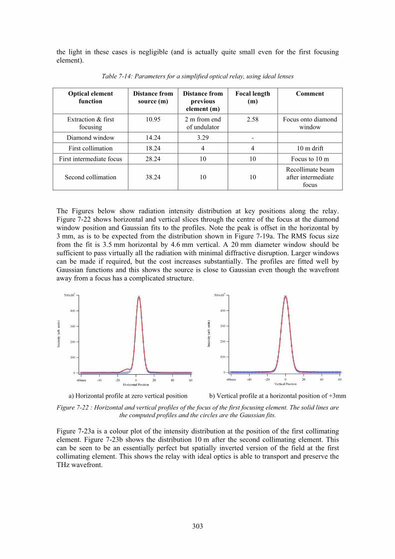
303

the light in these cases is negligible (and is actually quite small even for the first focusing element).

Table 7-14: Parameters for a simplified optical relay, using ideal lenses

Optical element function

Distance from source (m)

Distance from previous

element (m)

Focal length (m)

Comment

Extraction & first focusing

10.95 2 m from end of undulator

2.58 Focus onto diamond window

Diamond window 14.24 3.29 - First collimation 18.24 4 4 10 m drift

First intermediate focus 28.24 10 10 Focus to 10 m

Second collimation 38.24 10 10 Recollimate beam after intermediate

focus

The Figures below show radiation intensity distribution at key positions along the relay. Figure 7-22 shows horizontal and vertical slices through the centre of the focus at the diamond window position and Gaussian fits to the profiles. Note the peak is offset in the horizontal by 3 mm, as is to be expected from the distribution shown in Figure 7-19a. The RMS focus size from the fit is 3.5 mm horizontal by 4.6 mm vertical. A 20 mm diameter window should be sufficient to pass virtually all the radiation with minimal diffractive disruption. Larger windows can be made if required, but the cost increases substantially. The profiles are fitted well by Gaussian functions and this shows the source is close to Gaussian even though the wavefront away from a focus has a complicated structure.

a) Horizontal profile at zero vertical position b) Vertical profile at a horizontal position of +3mm

Figure 7-22 : Horizontal and vertical profiles of the focus of the first focusing element. The solid lines are the computed profiles and the circles are the Gaussian fits.

Figure 7-23a is a colour plot of the intensity distribution at the position of the first collimating element. Figure 7-23b shows the distribution 10 m after the second collimating element. This can be seen to be an essentially perfect but spatially inverted version of the field at the first collimating element. This shows the relay with ideal optics is able to transport and preserve the THz wavefront.

304

a) Intensity distribution at the position of the first collimating element

b) Intensity distribution 10 m after the second collimating element

Figure 7-23: Intensity distributions at the position of the first collimating element (left) and 10 m after the second collimating element (right), showing the relay with ideal optics is able to transport the THz and

preserve the wavefront

The horizontal and vertical profiles at the position of the intermediate focus are shown in Figure 7-24. The Gaussian fits have RMS widths of 8.7 mm horizontal by 11.4 mm vertical.

a) Horizontal profile at zero vertical position b) Vertical profile at a horizontal position of -7 mm

Figure 7-24: Horizontal and vertical profiles of the first intermediate focus. The solid lines are the computed profiles and the circles are the Gaussian fits.

Preliminary studies using toroidal mirrors instead of ideal lenses have been performed that indicate that performance should be close to that achievable with ideal lenses. The critical issue is to arrange the required horizontal and vertical reflections such that the overall path length for the “marginal rays” is the same otherwise the pulse wavefront will be severely distorted. This places constraints on how the relay can be laid out. Nevertheless, this work shows that the long wavelength radiation from a THz undulator can, at least in principle, be extracted and transported via an optical relay system with a basic unit length of 30 m. This would allow the radiation to be transported into the experimental hall in a single relay step, as is shown schematically in Figure 7-25. With 200 mm x 200 mm aperture mirrors and a 20 mm diameter window, losses with this system should be minimal even at the longest wavelengths.

305

Figure 7-25 : Schema of a possible THz relay to take long wavelength radiation out of the accelerator

hall. The radiation is taken over the main shield wall via a labyrinth for radiation safety reasons.

7.9 Electron and X-ray Pulses in Combination

Several areas of research in the Science Case require a combination of X-ray and electron pulses, for example, time-resolved radiation damage studies (Part II, Section 2.3.6) and time-resolved structural dynamics in artificial photosynthesis (Part II, Section 2.3.2). To meet these needs, a 5 MeV source based on the gun design for the FEL injector will be incorporated into an experimental end-station on the monochromatic beamline on FEL-2. Because the electrons cannot be transported easily whilst preserving the low emittance, the interaction region where the electrons and photons are brought together is “embedded” within the source. The only practical way to have co-linear X-rays and electrons is to use a multilayer mirror at 45° to deflect the X-rays whilst the electrons pass through a hole in the mirror, see Figure 7-26. This restricts operation to a single wavelength for any given multilayer.

Figure 7-26 : Schema showing that to achieve (near) colinear X-rays and electrons a multilayer mirror is

required to give the necessary large deflection of the X-ray beam

A potentially more satisfactory arrangement is to bring the X-rays at an angle to the electron beam. Figure 7-27 shows how this might be achieved and demonstrates that the smallest convergence angle will be ~25°.

306

Figure 7-27 : Schema showing how a 5 MeV electron source could be integrated with the FEL-2

monochromatic X-ray beamline

One concern with this layout is how it will fit in with experiments that do not require the electron source. It is clear that the spatial and shielding constraints imposed by the electron source will prevent many other types of experiment. Thus, the combined X-ray and electron experiments will need to be on a “branch line” of the FEL-2 beamline. Further work will be required during a future detailed design stage to determine the optimum layout.

7.10 Photon Diagnostics

The photon diagnostics can be broadly categorized as either measuring the particular property of each and every photon pulse or as giving the value of that property averaged over some integration period (number of pulses). Furthermore, the diagnostics can be either invasive in that they change the pulse they are measuring or non-invasive so that they can be permanently “on-line”.

It is expected that any FEL will give a sufficiently large pulse-to-pulse fluctuation in many key properties that the experiment will require knowledge on a pulse-by-pulse basis. This naturally also requires that the diagnostic technique must be non-invasive. This requirement will be essential for SASE operation of a FEL as the pulse-to-pulse fluctuations can be considerable. Nevertheless, invasive diagnostics are still important as they will be used during the commissioning and development of the sources.

7.10.1 Pulse Energy (photon flux)

The most basic information that an experiment will require is the number of photons contained in each photon pulse. For a pulsed source of limited bandwidth such as a FEL, this equates to a measurement of the energy contained in the pulse. Since the FEL will give fluctuations in pulse energy from shot to shot, an on-line measurement of the energy in each and every pulse is required. A non-invasive monitor with temporal resolution of better than 1 µs (to work with 1 MHz repletion rate source) will ultimately be required.

This can be achieved by measuring the photoionisation yield in a gas at low particle density. The gas can be almost (>99%) transparent to the beam and will not distort the pulse as it propagates through the gas. FLASH has developed the Gas Monitor Detector (GMD) [29] and

307

this is highly successful [30,31]. The instrument has a wide dynamic range, a temporal resolution of ~100 ns, and is effectively indestructible.

The key limitation is achieving sufficient ion yield to give the necessary uncertainty in the calculated pulse energy. This requires the photon energy to be above the ionization threshold of the gas. The preferred gas is xenon since its absorption cross-section is well characterized, but this will only work above 12.1 eV. For X-ray operation, the gas absorption is small and so the ion yield low. A X-GMD for use on XFEL is being developed [32] that increases the interaction path over which ions can be collected.

7.10.2 Beam Position

Maintaining good positional and angular stability of the FEL beam will be essential for the experiments. Knowledge of the position and angle will also be required for optimising the performance of the facility. A traditional type of blade position monitor that might be used on a third-generation synchrotron is not suitable for use with a FEL due to the disruption to the beam by diffraction and likely damage through ablation. A monitor based on photoionization of a low-pressure gas is the likely solution. A residual gas X-ray beam position monitor (RGXBPM) is being developed at HASYLAB [33]. Two such monitors placed at opposite ends of the gas absorption filter will give the required angular and spatial measurement. There is the need to improve the spatial resolution of the current instrument to achieve the necessary measurement accuracy.

7.10.3 Spectral Content

Whereas the spectral content is particularly variable for FEL operation in SASE mode, therefore requiring pulse-by-pulse measurement for some experiments, seeded operation will give a stable spectral output and so the diagnostic could be invasive.

A diagnostic spectrometer based on a varied-line-space (VLS) grating has been designed for use on FLASH [34]. The grating produces a flat-field dispersed spectrum on a CCD (position on the CCD equates to wavelength) in first order of diffraction whilst the zeroth order is reflected to the experiment. The grating profile can be chosen so that the zeroth order efficiency is very high (>95%) and so most of the light reaches the experiment. The spectrometer is thus effectively non-invasive and so can be left on-line. The same instrument concept can also be used for invasive measurements but with a simpler grating.

The grating based spectrometer will be suitable for use from the XUV to the SXR. Above ~2 keV, a crystal spectrometer would be required, but such an instrument could not be made effectively transparent and so is an invasive instrument only.

An alternative approach that has recently been proposed is based on photoionization and photoelectron spectroscopy from rare gases [35].

7.10.4 Coherence

Longitudinal coherence is given by the spectral content and the pulse temporal profile. A fully coherent pulse with ideal Gaussian temporal and spectral distributions will have time-bandwidth determined by the transform limit equation (7-4).

For non-Gaussian pulses or pulses that are not fully longitudinally coherent, then the time-bandwidth product will be greater than this. Only exact measurement of the spectral content and pulse length can determine the degree of longitudinal coherence. Measurement of these pulse properties is discussed elsewhere (Sections 7.10.3 and 7.10.8).

308

Transverse coherence is a measure of the wavefront quality, and this is critical for experiments that employ, for example, strong focusing or phase contrast imaging. The surface irregularities in the optical components within the transport system will all degrade the wavefront quality.

A measurement of the wavefront (see Section 7.10.7) will thus also give the transverse coherence. But the transverse coherence length can be more simply determined by measuring the diffraction pattern from a Young’s slit system [36,37]. Care must be taken with the incident fluence on the slits, and so the measurements may have to be performed after attenuating the beam. Alternatively, a Fresnel bi-mirror at a grazing angle can be used to give the same effect as a double slit [36]. The bi-mirror also has advantage that the effective slit separation is adjustable by rotating the mirror and so the coherence length is more easily probed. With suitable gating on the detector used to record the diffraction pattern and enough sensitivity, the measurement can be performed on individual pulses but is obviously invasive. The autocorrelator developed for FLASH has also been used to study spatial coherence by similarly splitting and then spatially overlapping the split beams [38].

7.10.5 Polarization

Pulse by pulse measurement of the full Stokes vector is not possible with current polarimetry techniques since it is necessary to subject the beam to a range of phase shifts and fully analyse the polarization components at each phase shift. Recent developments in multilayer polarimetry at Daresbury and BESSY have resulted in a wideband technique from ~400 to ~1000 eV [39]. The measurement at a given photon energy will usually take ~2 hours.

Although multilayer polarimetry can only give a time-averaged polarization, this should be sufficient for most needs as the polarization state will be largely determined by the tuning of the helical undulator arrays. As long as the tuning does not vary, the output polarization should be stable.

Another concern with multilayer polarimeters is that the multilayers, in particular the transmission multilayer that give the phase shifts, will not withstand the high beam fluence. Polarimetry measurements will therefore have to be performed at reduced intensity by using the gas attenuators. These devices should not affect the beam polarization when operating in the linear regime.

Other polarization determining techniques involve the measurement of some type of dichroism. For example, magnetic X-ray circular dichroism (MXCD) from well-characterized surfaces can be used to give the degree of circular polarization (but not the full Stokes vector). These are somewhat quicker than the multilayer polarimeter and can be added along the beam path to be inserted as required, but still will not give a pulse-by-pulse measurements as the photon energy needs to be scanned. They are also invasive techniques.

7.10.6 Focus Characterization

High-field physics experiments require the photon beam to be focused to a very small (micron level or below) spot. Characterization of the focused beam is essential not only for determining the achieved power density but also for setting up the focusing system. In general, shot by shot measurement will not be required and so the focus could be characterized by invasive techniques, though we have to be aware that source position fluctuations will result in movements of the spot and possibly also changes to its size and shape. However, techniques such as a scanning wire or knife-edge or a fluorescent screen cannot be used due to their limited spatial resolution and the certainty of ablation damage (though attenuating the beam with a gas attenuator should not affect the focus and would remove the ablation risk).

A technique that utilizes the saturation of the ion yield during photoionization of a rare gas is being developed [40,41]. As the photons in the pulse are compressed into a smaller and smaller

309

volume, the number of gas atoms they can interact with reduces and so the ion yield does not increase linearly with photon number. When combined with a measurement of the pulse energy (using a GMD, see Section 7.10.1), the ion yield can be used to infer the focus beam size.

7.10.7 Wavefront Measurement

There are two likely ways to directly measure the wavefront of a coherent beam in the VUV to X-ray region, viz. Shack-Hartmann sensors or interferometry.

Shack-Hartmann wavefront sensors are widely used in the visible part of the spectrum. An array of small lenses of the same focal length is illuminated by the wavefront and focus it as an array of spots onto a CCD sensor. Local tilt of the wavefront at any lens results in a deviation of the focal spot from the nominal position. By approximating the phase error of the wavefront to a set of local tilts, the measured tilts at all the lenses allow the actual wavefront to be determined. The main issue with extending this technique to work directly with X-rays is that it is not practical to make lenses with short enough focal lengths. The sensors thus have to work with just aperture arrays, and are thus strictly Hartmann sensors. Such an instrument, made by Imagine Optic [42], has been successfully used at FLASH [43].

Interferometric measurements are demanding since it is difficult to split the X-ray wavefront. Weitkamp et al. [44] used a Ronchi phase (transmission) grating to split an X-ray beam at 12.4 keV into two. The grating gives a small angular shear between the plus and minus orders of diffraction, which can then interfere. Careful control of the grating thickness (and hence phase shift) is necessary to eliminate the zeroth diffraction order. Fringe distortion in the interferogram is correlated to wavefront perturbation. At these wavelengths, the fringe spacing is very small and so cannot be measured directly. An additional absorption grating is thus placed in the plane of the interference fringes and tilted slightly so that it gives a Moiré pattern of sufficient spacing to be measurable with a CCD camera.

7.10.8 Time Domain Properties

The temporal properties of the pulse are a key part of the source performance and achieving the target specification will be crucial to the success of many experiments. The key temporal properties of the pulse that should be determined are:

• Pulse length - required to determine the pulse intensity (in conjunction with the measurement of the absolute energy in the pulse)

• Pulse profile - determines the ‘quality’ of the pulse (e.g. the length and height of the pedestal; the deviation from the transform limit for the measured spectral content) and is also related to the jitter (if the shape changes from pulse to pulse, then the centroid of the pulse can move and this is equivalent to a timing shift).

• Pulse jitter - The arrival time of the pulse must be measured relative to something and the time fluctuation relative to this something is the temporal jitter. The jitter is critical for time resolved and especially pump-probe experiments.

Since the pulse profile and timing will change on a pulse-by-pulse basis to some degree (especially for SASE operation of the FEL), then an on-line pulse profile and timing determination is essential.

A comprehensive review of the current state of temporal diagnostics for ultra-short XUV and X-ray pulses has been prepared for the EuroFEL consortium [45]. A brief summary is presented here, but the report should be referred to for more detail and references. The techniques can be broadly categorized as follows:

310

7.10.8.1 Autocorrelation Techniques

Intensity autocorrelation has been demonstrated at FLASH [38], but the main limitation of the technique is that no information is gained about the pulse shape and even the pulse length can only be deduced if the shape is assumed. At optical wavelengths, auto-correlation techniques have been extended to measure spectral and phase information so the pulse profile can be fully reconstructed. For example, Frequency Resolved Optical Gating (FROG) [46] measures the spectrum of a series of time slices whilst Spectral Phase Interferometry for Direct Electric-field Reconstruction (SPIDER) [47] uses spectral shearing interferometry. Extending these techniques to XUV and shorter wavelengths is dependent on finding non-linear processes that can mix the beams (FROG) or produce the spectral shear (SPIDER). Current research is concentrated around using photo-ionization techniques such as two-photon ionization, with one or two colours [48, 49], or single-photon multiple-ionization [50]. In all cases, the optical phase and spectral information is encoded into the photoelectrons and electron spectrometers are required, which tend to limit sensitivity and data rates.

In the SPIDER technique, two replicas of the input pulse are created, at a fixed time delay, and these two replicas are subsequently mixed with a chirped copy of the input pulse. The resulting two up-converted replicas are spectrally sheared with respect to each other and, upon recombination, interfere spectrally. Analysis of the wavelength resolved interference pattern allows the reconstruction of the spectral phase of the input pulse. To characterise short wavelength pulses, spectral shearing interferometry of photoelectron wave packets would be required. These wave packets would be produced by the photoionisation of atoms, in the presence of a laser field, by two delayed but otherwise identical replicas. The purpose of the laser field is to provide the energy shift (shear) between the wave packets. The interferogram that results from the interaction between these wave packets provides information about their relative phase. A successful application of this principle has already been demonstrated in the photoionisation of argon atoms at a photon energy of 46 eV [51].

7.10.8.2 Cross-correlation Techniques

The advantage of cross-correlation over auto-correlation is that timing jitter as well as the pulse length can be measured. Normally, an ultra-short IR laser is used and so the timing jitter is measured relative to that laser. This can derived from the same laser that drives the seeding or from an independent but synchronized laser.

The most common approach adopted in measuring XUV pulses is to use the IR laser to modulate the energy of photoelectrons emitted from a gas when it interacts with the XUV pulse. The photoelectrons can absorb or emit one or more IR photons and this leads to the production of sidebands on the photoelectron spectrum separated by the IR photon energy. The number and intensity of the sidebands is a measure of the intensity overlap of the IR and XUV pulses.

In the simplest implementation it is necessary to focus the XUV pulse onto the interaction region and scan the IR pulse delay. Such an arrangement [52, 53] has been used at FLASH to analyse the synchronisation between individual XUV pulses emitted by the FEL and an external laser. The photoelectron sideband intensity depends upon the relative time delay between the ionising and the dressing pulses. The experiment, carried out with helium and xenon, demonstrated that single-shot characterisation of the FEL pulses was feasible. A significant disadvantage of the experimental arrangement implemented in this study was the need to co-propagate the FEL and IR pulses to a common focus. This difficulty has been circumvented in the geometric configuration adopted by Cunovic et al [54] where the FEL and the IR beams intersect perpendicularly. Photoelectrons generated in an atomic gas (krypton in the experiment performed at FLASH) by laser-assisted photoionisation were used to create a two-dimensional image of the cross-correlation volume, thereby mapping time onto a space coordinate. Thus, information about pulse duration and relative timing between the pulses could be obtained without the need to scan an optical delay line. In principle this technique is non-invasive but its

311

general application to shot-to-shot characterisation will require further development of energetically resolved photoelectron imaging technology.

If these methods were to be extended to very short X-ray pulses, then it would be found that the spectral width of the X-ray pulse smeared out the sidebands. This can be overcome by observing the photoelectron spectra for electrons ejected at right angles to the polarisation of the laser. In this case, sideband formation is suppressed, thereby permitting the measurement of the red-shift in the electron kinetic energy due to the ponderomotive force exerted by the laser field. This has been achieved using 90 eV photons formed in an HHG source, co-focussed with the generating 770 nm laser pulses [55].

An alternative approach to cross-correlation utilises the fact that the XUV pulse can modify the reflectivity to visible light of a semiconductor surface such as GaAs [56, 57]. The XUV pulse strikes the GaAs surface at a grazing angle and a short-pulse visible laser illuminates the same area at near normal incidence. The reflected visible light will show an intensity change at the boundary of the XUV illumination as determined by the time at which the visible pulse hits the surface. Imaging the visible beam onto a CCD gives a time-to-space conversion and the relative arrival time of the XUV pulse can be monitored. Thus pulse-to-pulse jitter can be measured relative to the visible laser beam, which can be produced by frequency doubling from an IR laser synchronised to the master clock. The intensity profile of the reflected beam is also correlated to the XUV pulse intensity profile and so in principal the XUV pulse profile could be measured. In practice however, the relatively slow decay of the reflectivity change will distort and lengthen the perceived pulse profile.

Electro-optic techniques can be used to monitor the relative timing of an external laser to the electron bunch and this information can be used to improve the resolution of cross-correlation data [58].

7.10.8.3 Other Techniques

Streak cameras are a standard technique for measuring picosecond pulses and there is current activity in improving the achievable temporal resolution. Resolution of better than 300 fs at 4 kHz repetition rate has been demonstrated by the group at Lund. Development work is also being undertaken at the ALS and J-Lab. References are available in [45].

7.11 Conclusion

The design work undertaken so far has shown that a combination of beamlines can deliver photons over the range 50 to 5000 eV from the FELs with properties tailored to suit a wide range of potential applications.

Where the highest photon density at the experiment is required, the FEL output can be transported with a simple optical system consisting of a focusing element with high demagnification. A plane mirror at the shield wall is also necessary to deflect the photon beam away from the FEL axis for radiation safety and the focusing element can either by a single mirror of ellipsoidal form or a pair of plane-elliptical mirrors in a Kirkpatrick-Baez arrangement. With just two or three optical elements, the transport efficiency can be high (> 80%).

Some photon conditioning may be necessary with such a simple transport system, and a gas filter is positioned after each FEL to provide beam attenuation and to reduce the level of the fundamental when working on the harmonics.

Unfortunately, the gas filter cannot completely suppress the fundamental and nor can it do much to suppress the harmonics when working on the fundamental. Therefore, some experiments will

312

require a monochromator to improve the spectral filtering. This may also be desirable to remove SASE and spontaneous radiation that lies outside the bandwidth of the main pulse.

When short pulses are required simultaneously with spectral filtering, the monochromator design becomes challenging. Of course, the monochromator bandpass must not be smaller than the transform limited bandwidth of the short pulse, but there is an additional pulse stretch introduced when diffraction gratings are used as the dispersive element in soft X-ray beamlines. For FEL-1, achieving a monochromator with little or no pulse stretch requires a double grating system with a consequent low efficiency (~1%). For FEL-2 and FEL-3 a single grating design can be used that gives 40% or less pulse stretch and high transport efficiency (~10%).

For X-rays above ~2000 eV, a crystal monochromator will need to be used and this will give an unavoidable pulse stretch. However, in the context of pulses of a few femto-seconds duration, this stretch should not be significant. A more fundamental problem with a crystal monochromator is that it will act as a linear polariser near the Brewster angle. Since harder X-rays are only available on the harmonics where the generation of circularly polarised light is difficult, delivering spectrally-filtered, circularly-polarised light in the range ~2400 eV to ~3000 eV will be problematical.

Important complements to the X-ray FELs are the THz and IR sources. Each FEL will be followed by an undulator designed to coherently emit THz radiation in the wavelength range 20 µm to 500 µm. In addition, FEL-1 will have a second undulator and a dipole source for broadband THz output. Transport of long wavelength radiation over the considerable distance from source to experiment will be via a relay of alternating collimating and focusing elements based on toroidal mirrors of 200 mm clear aperture. Initial studies show that this can be achieved with minimal losses.

One consequence of the relay system is that the transport path of the THz is much longer than that of the X-rays. Thus, to use the THz as a “pump” in an experiment requires the X-ray beam to be significantly delayed. This is not easy to achieve and the only practical approach requires the use of multilayer mirrors that inevitably restrict the photon energy tunability at the experiment.

An essential part of all experiments will be accurate knowledge of the source properties. Since the FEL will inevitably have significant shot-to-shot variations in some output parameters, the diagnostics required should ideally measure every pulse individually. Achieving this over the broad range of photon properties that must be known is a significant challenge. A lot of progress has been made in recent years, but there its still much work to do.

Future work should concentrate on refining the details of the proposed transport systems and matching them to the specific scientific needs. Integration of the key diagnostics will also be required as this could impact significantly on the optical design. Better understanding of the source is also required as it obviously has a significant impact on the optical system design. It is critical to be able to predict with confidence the source size and divergence and how the longitudinal position of the source changes with photon energy. Tuning the FEL process to ensure the longitudinal source position is fixed as a function of wavelength will be critical if the need for complex adjustable focusing optics at the front of every beamline is to be avoided.

REFERENCES [1] Krzywinski, J., et al., Conductors, semiconductors, and insulators irradiated with short wavelength

free-electron laser. J Appl Phys, 2007. 101, 043107 [2] Mocek, T., et al., Surface modification of organic polymer by dual action of extreme

ultraviolet/visible-near infrared ultrashort pulses. J Appl Phys, 2009. 105, 026105 [3] Chalupský, J., et al., Non-thermal desorption/ablation of molecular solids induced by ultra-short

soft x-ray pulses. Opt Express, 2009. 17, 208-217

313

REFERENCES [4] Chalupský, J., et al., Damage of amorphous carbon induced by soft x-ray femtosecond pulses above

and below the critical angle, Appl Phys Lett 95, 2009. 031111 [5] Juha, L., et al., Radiation damage to amorphous carbon thin films irradiated by multiple 46.9 nm

laser shots below the single-shot damage threshold, J. Appl. Phys 2009. 105, 093117 [6] Arthur. J., et al., Linac Coherent Light Source (LCLS) - Conceptual Design Report section 9.1.2.2,

SLAC-R-593, SLAC, Stanford (2002). The same criteria is used in the XFEL Technical Design Report, Chapter 6, http://xfel.desy.de/tdr/tdr

[7] Tatchyn, R., et al., Focusing of undulator light at SPEAR with a lacquer-coated mirror to power densities of 109 watts/cm2. SPIE Proceedings 733, 1986. 368-376

[8] Siegman, A.E., How to (maybe) measure laser beam quality, a tutorial presentation to the OSA annual meeting 1997, http://www.stanford.edu/~siegman/beam_quality_tutorial_osa.pdf

[9] Seah, M.P. & Dench, W.A., Quantitative electron spectroscopy of surfaces: A standard data base for electron inelastic mean free paths in solids, Surf. Interface Anal., 1979, 1, 2-11

[10] Altarelli, M., et al., The European X-Ray Free-Electron Laser Technical Design Report. DESY 2006-097, 2007. Chapter 6

[11] Hirano, K., Tunable-Wavelength Production of Circularly Polarised X-rays with a Perfect-Crystal Quarter-Wave Plate. J Appl Cryst, 1992. 25, 531-535

[12] Giles, C., et al., Energy-Dispersive Phase Plate for Magnetic Circular Dichroism Experiments in the X-ray Range. J Appl Cryst, 1994. 27, 232-240

[13] Boada, R., et al., X-ray Magnetic Circular Dichroism (XMCD) measurements at BM25 SpLine (the Spanish CRG X-ray beamline for Absorption and Diffraction at the ESRF). 2008. http://www.unizar.es/icma/temasprevios/documents/HL.pdf

[14] Poletto, L. & Villoresi, P., Time-delay compensated monochromator in the off-plane mount for extreme-ultraviolet ultrashort pulses. Appl Opt, 2006. 45(34) 8577-8585

[15] Froud, C.A., et al., Artemis: a sub 10-fs XUV source for ultrafast time-resolved science. STFC Central Laser Facility Annual Report 2007/2008 http://www.clf.stfc.ac.uk/reports/2007-2008/pdfs/s7/ar07-08_s7_artemis_a_sub-10fs.pdf

[16] Werner, W. & Visser, H., X-ray monochromator designs based on extreme off-plane grating mounts. Appl Opt, 1981. 20(3) 487-492

[17] Vincent, P., et al., X-ray gratings: the GMS mount. Appl Opt, 1979. 18(11) 1780-1783 [18] Higgins, S.P. & Bowler, M.A. [19] Roper, M.D., Propagation of real laser beams and determination of beam waist from measured

beam profiles. 4GLS Technical Note, 2006. [20] Matsuyama, S. et al., Diffraction-limited two-dimensional hard x-ray focusing at the 100 nm level

using a Kirkpatrick-Baez mirror arrangement. Rev Sci Instrum, 2005. 76 083114 [21] Petersen, H., The plane grating and elliptical mirror: A new optical configuration fro

monochromators. Opt Comm, 1982. 40 402-406 [22] Roper, M.D., A Soft X-ray Monochromator For The UK New Light Source (NLS), Proc. of the

FEL2009 Conference (2009) [23] VGD Gratings made by Jobin Yvon Horiba, http://www.horiba.com/ [24] Chubar, O. & Elleaume, P., Accurate and Efficient Computation of Synchrotron Radiation in the

Near Field Region, Proc. of the EPAC98 Conference (1998) 1177-1179 [25] Bowler, M.A, personal communication [26] Self, S.A., Focusing of spherical Gaussian beams, Appl. Optics 1983, 22(5) 658 [27] Walker, R.P., Insertion devices: Undulators and wigglers, Elettra report ST/M-97/2 1997 [28] Gatesman, A.J, et al., High Precision reflectometer for sub-millimeter wavelengths, J. Opt. Soc.

Amer. 1995 B12 212 [29] Richter, M., Intensity Monitor for free-electron lasers.

http://www.ptb.de/en/publikationen/news042/artikel/04203.htm [30] Richter, M., et al., Measurement of gigawatt radiation pulses from a vacuum and extreme

ultraviolet free-electron laser. Appl Phys Lett, 2003. 83 2970 [31] Tiedtke, K., The SASE FEL at DESY: Photon Beam Diagnostics for the user facility. SRI-03: AIP

Conference Proceedings, 2004. 705(1) 588-592 [32] Tiedtke, K., et al., First test of the X-GMD prototype at the Sub-picosecond Pulse Source.

http://hasyweb.desy.de/science/annual_reports/2006_report/part1/contrib/30/18972.pdf [33] Ilinski, P., et al., Residual Gas X-ray Beam Position Monitor for PETRA III.

http://hasyweb.desy.de/science/annual_reports/2005_report/part1/contrib/28/15472.pdf

314

REFERENCES [34] Reininger, R., et al., Spectrometer based on a VLS Grating for Diagnostics of a Vacuum-Ultraviolet

Free Electron Laser. SRI-03: AIP Conference Proceedings, 2004. 705(1) 572-575 [35] Wellhöfer, M., et al., Photoelectron spectroscopy as a non-invasive method to monitor SASE-FEL

spectra. JINST, 2008. 3 , P02003 [36] Pietsch U., et al., Coherence experiments using white synchrotron radiation. Physica B, 2005. 357,

45–52 [37] Tran, C.Q., et al., Phase space density measurement of interfering X-rays. J Electr Spectr & Rel

Phenom, 2005. 144–147, 947–951 [38] Mitzner, R., et al., Spatio-temporal coherence of free electron laser pulses in the soft X-ray regime.

Optics Express, 2008. 16, 19909 [39] MacDonald, M.A. et al., A W:B4C multilayer phase retarder for broadband polarization analysis of

soft x-ray radiation. Rev Sci Instrum, 2008. 79, 025108 [40] Sorokin, A.A., et al., FLASH Focus Spot Size Measurement Based on atomic Photoionisation.

http://hasyweb.desy.de/science/annual_reports/2006_report/part1/contrib/40/17190.pdf [41] Richter, M., et al., Nonlinear photoionization in the soft X-ray regime. Appl Phys A, 2008. 92, 473-

478 [42] http://www.imagine-optic.com/iop_en_products_hasoxeuv_main.php [43] Kuhlmann, M. et al. Wave-front Observations at FLASH, Proc. FEL 2006 FRAAU03 [44] Weitkamp, et al., X-ray wavefront analysis and optics characterisation with a grating

interferometer. Appl Phys Lett, 2005. 86, 054101 [45] Bowler, M.A., et al., Survey of Diagnostics Techniques For Measuring The Temporal Properties of

Ultra-Short Photon Pulses, EuroFEL Work Package 7 Report, 2009. [46] Trebino, R., et al., Measuring ultashort laser pulses in the time-frequency domain using frequency-

resolved optical gating. Rev Sci Instrum, 1997. 68, 3277 [47] Iaconis, C. and Walmsley I. A., Spectral phase interferometry for direct electric-field reconstruction

of ultrashort optical pulses. Opt Lett, 1998. 23, 792 [48] Sekikawa, T., et al., Measurement of the intensity-dependent atomic dipole phase of a high

harmonic by frequency-resolved optical gating. Phys Rev Lett, 2002. 88, 193902 [49] Muller, H. G., Reconstruction of attosecond harmonic beating by interference of two-photon

transitions. Appl Phys B, 2002. 74, S17 [50] Nabekawa, Y., et al., Production of doubly charged helium ions by two-photon absorption of an

intense sub-10-fs soft X-ray pulse at 42 eV photon energy. Phys Rev Lett, 2005. 94, 043001 [51] Remetter, T., et al., Attosecond electron wave packet interferometry. Nat Phys, 2006. 2, 323 [52] Meyer, M., et al., Two-colour photoionization in xuv free-electron and visible laser fields. Phys

Rev, 2006. 74, 011401 [53] Radcliffe, P., et al., Single-shot characterization of independent femtosecond extreme ultraviolet

free electron and infrared laser pulses. Appl Phys Lett, 2007. 90, 131108 [54] Cunovic, S., et al., Time-to-space mapping in a gas medium for the temporal characterization of

vacuum-ultraviolet pulses. Appl Phys Lett, 2007. 90, 121112 [55] Drescher, M., et al., X-ray pulses approaching the attosecond frontier. Science, 2001. 291, 1923 [56] Gahl, C., et al., A femtosecond X-ray/optical cross-correlator. Nat Photonics, 2008. 2, 165 [57] Maltezopoulos, T., et al., Single-shot timing measurement of extreme-ultraviolet free-electron laser

pulses. New J Phys, 2008. 10, 033026 [58] Azima, A., et al., Time-resolved pump-probe experiments beyond the jitter limitations at FLASH.

Appl Phys Lett, 2009. 94, 144102

315

8 Experimental End-stations

The goals of a fourth generation light source such as NLS are to conduct science of a novel kind which goes beyond that possible on a conventional 3rd generation storage ring source. The NLS source properties are tailored to meet specific experimental objectives and the end-stations and photon transport systems will need to be designed with these particular requirements in mind. The number of individual sources will be limited on a FEL based machine (unlike the multi-port capability of a storage ring) and the number of experimental end stations will be initially restricted to a few, specifically designed to address the needs of the key science drivers.

At this early stage, there has been little effort to integrate the requirements of specific experiments with beamline design. This is particularly the case for those experiments where the instrument incorporates elements of beamline design, such as X-ray interferometry where the interferometer itself forms part of the beamline optics. This Chapter seeks to identify some of the issues that will arise in the integration of experiment and beamline.

Whilst it is anticipated that some experiments will solely utilise one FEL (such as coherent diffraction imaging which will benefit from the shorter wavelengths from FEL-3), others will be used on more than one FEL source (e.g. pump-probe experiments using laser-pump/FEL-probe). In these latter cases, further design work will be necessary to determine the conflicting practicalities of moving end-stations between different beamlines and leaving the end-stations fixed and ‘piping’ light from different FEL sources into them. Consideration will also need to be given to balance the advantages of facility provided experiments, which will become well characterised, well integrated to the source and well understood, against the scientific novelty of user provided instruments for which there will be less experience of operating them at NLS, but will be specifically tuned to particular experiments.

Three examples of possible end stations have been selected to provide a flavour of the issues confronting the design of experimental end stations on NLS. These have been selected as a representative cross section of the types of experiment outlined in the NLS Science Case and what is currently under development at existing FEL sources [1,2,3,4].

Ultrafast, ultra-intense, high repetition rate experiments at the fourth generation NLS source will impose many technological challenges on experimental design. End station experiments are anticipated to be complex and will involve considerable engineering design and fabrication effort. With the advent of a number of FEL sources coming on line in the next few years (e.g. LCLS, Fermi@Elettra, SPARX, SCSS/Spring8) it is envisaged that developments in FEL experiments will be very rapid in the near future.

It is noted that some of the instruments required for experimental measurement are the same as those needed in beamline diagnostics (e.g. optical auto-correlators). Particular experiments will demand knowledge of specific beam characteristics and hence particular sets of diagnostics. More work is needed to integrate these two sets of demands and to investigate whether in some cases the end-station experiment can simultaneously provide the beamline diagnostic measurement.

8.1 Coherent Diffraction Imaging

Coherent diffraction imaging (CDI) utilises the coherent properties of FEL radiation to overcome both difficulties imposed by the high power of the source and limitations on spatial imaging arising from limits in fabrication of X-ray micro-focussing optics.

The intensity and coherence of the photon pulse mean that a diffraction pattern can be recorded of the sample structure before it is destroyed by the intense power of the FEL pulse. An image can therefore be recorded without the need for a lens. This gives two advantages, there is no

316

lens to also be destroyed by the FEL pulse, and the image resolution is essentially diffraction limited to the photon wavelength, something which has still to be achieved in the SXR or harder photon range using optics.

For single viewpoint CDI, the beamline requirements are relatively modest. Apart from focussing the beam to the order of 20 μm, the FEL output will have sufficient temporal and spatial coherence so that further monochromisation of the beam is unnecessary. Coulomb explosion of a sample is anticipated to start to disrupt the atomic ordering within 5–10 fs, with larger scale disruption to structure occurring in some tens of femtoseconds [2,5]. The fundamental of FEL-3 is capable of delivering photons up to 1000 eV which corresponds to a diffraction limited resolution of the order of 1 nm allowing NLS to address structural determination on the sub-10 nm scale. This is an order of magnitude improvement over what is currently available using Fresnel zone plate soft X-ray microscopes, e.g. [6]. At this length scale, some atomic level (Å scale) disordering could be tolerated, permitting pulse stretching up to ~50 fs to be tolerated without significant loss of structural information.

Pioneering work in the development of CDI has been conducted in the XUV energy range at 32 nm (38 eV) at FLASH [7,8]. The instrument developed at FLASH comprises a graded multilayer mirror to collect the diffraction pattern and direct it onto a back illuminated CCD. This mirror has been manufactured with a central hole to allow the passage of the direct, un-diffracted, beam as the FEL intensity is sufficiently high to ablate a normal beam stop. The multilayer is designed to Bragg reflect the diffraction pattern and is graded to preserve the Bragg condition for the fixed wavelength of the FEL shot and the varying angle of incidence of the diverging diffraction pattern at the mirror. The manufacture of graded multilayers is challenging, and becomes increasing more difficult to achieve as the d-spacing of the multilayer reduces to reflect shorter wavelength radiation. CDI on NLS will use much shorter wavelengths than are available at FLASH, and so may have to dispense with the multi-layer optic and illuminate the imaging detector directly. In this case, the detector will need to be constructed around a central aperture of approximately 1 mm diameter in order to avoid damage from direct FEL radiation. Exploiting chip fabrication methods whereby the readout circuitry is confined to two adjacent edges of the imaging area, allowing the opposite sides to be butted against another imaging chip, would allow 4 such detectors to be assembled in a mosaic around a suitable aperture, see the schematic in Figure 8-1. A further requirement which will need to be considered in adopting this approach is the need to filter any plasma radiation from the sample from reaching the detector and providing unwanted background in the diffraction pattern. This is particularly the case for visible light in the case of optically sensitive CCD and CMOS imaging detectors. A similar system utilising two CCD chips with a gap between them is currently being tested by the Centre of FEL Science, DESY. A 4 chip design is being developed at LCLS in conjunction with Cornell. The prototype detector has 760x760 pixels, but an increase to 1520x1520 is envisaged, with the full detector being available for CDI experiments at LCLS in early 2011.

One specific experimental requirement is for the need to continuously replenish the sample as each FEL shot causes total sample loss. Some samples can be mounted on silicon nitride membranes and in such cases it will be possible in principle to deposit many samples onto a strip of Si3N4. This allows for good positional accuracy in placing the samples, although it is probably limited by the number of samples which can be so mounted. An alternative mechanism that has been developed uses aerodynamic lenses to project a continuous stream of particles into the path of the FEL beam [9] and is applicable to a wide range of nanoscale materials such as carbon nanotubes, biomolecules, viruses and cells. NLS will need to implement such a system and adapt it to make maximum use of the repetition rate of the source. Such a high frame rate will have implications on the data acquisition and storage systems, this will be touched on later in this Chapter. Electrostatic spraying of particles greater than 70 nm in diameter and at injection rates up to 3000 particles per second is being developed for single particle CDI at both FLASH and LCLS [10,11,12]. Alignment of the particle beam with the photon beam is being accomplished by shining laser light in two different colours through the particle sprayer and

317

along the optical path simultaneously. Work is in hand to synchronise the particle emission with the arrival of the FEL pulse. Achievement of this aim will allow reduction in the number of particles needed for each experiment, this is of interest to both biologists and nanotechnologists alike as production of the high numbers of samples needed can be problematical. Computational work is underway at FLASH/LCLS to determine the optimum number of samples needed for full reconstruction analysis [13]. Experimental determination of the ability to perform 2D reconstruction of reproducible crystals has been demonstrated at FLASH [14].

Figure 8-1 : Suggested scheme for using 4 overlapping CCD detectors in coherent diffraction imaging. Chip layout schemes which minimise the non-imaging area on 2 sides would allow effective overlapping of the CCDs to leave a small aperture in the centre through which the high intensity undiffracted beam

can pass.

8.1.1 Tomographic or Holographic Diffraction Imaging

In order to collect 3D image data, a further development has been proposed whereby a beam splitter is employed to direct two or more photon pulses simultaneously at a sample from different angles. Separate diffraction patterns are recorded which can then be recombined to form a 3D image of the original [15]. A schematic of this concept, modified to utilise grazing incidence optics in the SXR region, is shown in Figure 8-2. If used with CDI cameras of the type developed by Bajt et al [7], the incident beams need to be separated by at least 30 degrees to each other – the diffraction collection angle. To split and redirect a FEL pulse in the SXR energy range will require the use of multilayer or crystal reflecting optics due to the high angle of incidence necessary. It will also be necessary to recombine the separate ~20 fs photon pulses to within a few fs of each other. Although it is not necessary to record the two frames at the same instant, Coulomb explosion of the sample is expected to begin disrupting the structure within 5-10 fs of the first pulse arriving [5]. Recent studies at FLASH have suggested that encasing the sample in a thin sacrificial 'tamper' layer can increase this lifetime to several picoseconds [16]. Using the shortest wavelength available from the fundamental FEL beams, the target spatial resolution will be of the order of 1 nm. At these wavelengths, the motivation will be to study organisational structure, rather than atomic structure within nanoscale objects. The time delay before disruption of these large scale features will be longer and coincident timing of the two pulses could be relaxed to 10–20 fs for NLS multi-beam diffraction imaging. The path lengths of the two optical beams therefore need to be controlled to within a few micron, which it should be possible to achieve using nanometric positioners on the optical elements.

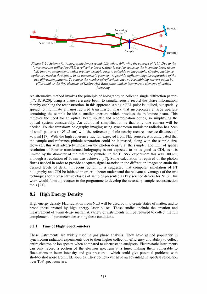
318

Figure 8-2 : Scheme for tomographic femtosecond diffraction, following the concept of [15]. Due to the lower energies utilised by NLS, a reflective beam splitter is used to separate the incoming beam (from left) into two components which are then brought back to coincide on the sample. Grazing incidence

optics are needed throughout in an asymmetric geometry to provide sufficient angular separation of the two diffraction patterns. To reduce the number of reflections, the two recombining mirrors could be

ellipsoidal or the first elements of Kirkpatrick-Baez pairs, and so incorporate elements of optical focussing.

An alternative method invokes the principle of holography to collect a single diffraction pattern [17,18,19,20], using a plane reference beam to simultaneously record the phase information, thereby enabling the reconstruction. In this approach, a single FEL pulse is utilised, but spatially spread to illuminate a nanostructured transmission mask that incorporates a large aperture containing the sample beside a smaller aperture which provides the reference beam. This removes the need for an optical beam splitter and recombination optics, so simplifying the optical system considerably. An additional simplification is that only one camera will be needed. Fourier transform holography imaging using synchrotron undulator radiation has been of small patterns (~ ∅1.5 μm) with the reference pinhole nearby (centre – centre distances of ~3 μm) [17]. With the high coherence fraction expected from FEL sources, it is anticipated that the sample and reference pinhole separation could be increased, along with the sample size. However, this will adversely impact on the photon density at the sample. The limit of spatial resolution of Fourier transformed holography is not expected to be as good as CDI, as it is limited by the diameter of the reference pinhole. In the BESSY experiment this was 100 nm, although a resolution of 50 nm was achieved [17]. Some calculation is required of the photon fluxes needed in order to provide adequate signal-to-noise in the diffraction images to attain the desired levels of detail in reconstruction. It is suggested that computer simulation of FT holography and CDI be initiated in order to better understand the relevant advantages of the two techniques for representative classes of samples presented as key science drivers for NLS. This work would form a precursor to the programme to develop the necessary sample reconstruction tools [21].

8.2 High Energy Density

High energy density FEL radiation from NLS will be used both to create states of matter, and to probe those created by high energy laser pulses. These studies include the creation and measurement of warm dense matter. A variety of instruments will be required to collect the full complement of parameters describing these conditions.

8.2.1 Time of Flight Spectrometers

These instruments are widely used in gas phase analysis. They have gained popularity in synchrotron radiation experiments due to their higher collection efficiency and ability to collect entire electron or ion spectra when compared to electrostatic analysers. Electrostatic instruments can only record a portion of the electron spectrum at a time, making them vulnerable to fluctuations in beam intensity and gas pressure – which could give potential problems with shot-to-shot noise from FEL sources. They do however have an advantage in spectral resolution over ToF spectrometers.

319

The basic ToF spectrometer is described by Wiley & McLaren [22]. The mass and charge of the particle determines its flight time in the instrument. For electrons these are of the order of a few hundred nanoseconds, whereas flight times for ions can be of the order of several microseconds. Ion ToF spectroscopy therefore places an upper limit on the maximum repetition rate that can be accommodated to 105-106 Hz. Rapid and continuous readout of the instrument is necessary to reconstruct the spectrum. ToF spectroscopy of molecular nitrogen has been demonstrated within the 1μs bunch spacing at FLASH [23,24,25]. Multiple electron spectrometer instruments are in use at storage ring sources [26] and proposed for use at LCLS. Basic ToF spectrometers can therefore be expected to play a role in NLS experiments.

Velocity Map Imaging (VMI) utilises a specific configuration of electric fields to map particles from an extended source region onto an imaging detector, their position on the detector being determined by their initial velocity [27]. VMI spectroscopy can also provide orientational and alignment information. They are best suited for measuring kinetic energies of a few eV, so will be constrained to studies where the FEL pulse is close to the ionisation energy of the species under investigation. A VMI instrument is already in use at FLASH [28].

Collecting both the electron and ion signals, such as in the Heidelberg Reaction Microscope also in use at FLASH [29,30,31], can provide a more complete picture of the created states. However, there is a need to operate these under UHV conditions of at least 10-10 Torr.

ToF spectrometers usually employ micro channel plate (MCP) detectors as image intensifying elements with either a single, plane anode for conventional spectrometers, or a 2D encoding anode – typically a RoentDek delay line – for VMI spectroscopy. Very intense FEL pulses could produce many charged particles per pulse. Under these conditions delay line detectors are not suitable and alternative imaging systems would need to be considered, such as using a phosphor screen coupled to a high frame rate camera [32]. The detectors have to be able to resolve more than one charged particle per pulse and some development is required to identify suitable candidate technologies. There is also a need to investigate whether VMI can be used for high kinetic energies, the resolution that can be achieved and how well multiphoton angular distributions can be measured.

8.2.2 X-ray Thomson Scattering

Measurement of FEL radiation inelastically scattered from plasmas of warm dense matter created within NLS provides information on a number of parameters including density, temperature and ionisation states [33,34]. To distinguish the inelastic from elastic component requires the use of a spectrometer. This spectrometer also needs to operate in a dispersive geometry to extract the spectrum of the inelastically scattered component. This can be achieved by using curved graphite, or mosaic focussing mode HOPG (Highly Ordered Pyrolytic Graphite) crystals [35]. Readout of Thomson scattering spectrometers is generally done using gated micro-channel plate (MCP) detectors [36], which will require similar investigations as required for ToF spectrometers.

8.2.3 Streak Cameras

For time resolved spectroscopy, there is a requirement for streak cameras offering suitable temporal resolution. Streak cameras direct the photon beam through the sample interaction region and onto a photocathode, the emerging photoelectrons are then swept in a time varying electric field before reaching an imaging detector. The photon beam is often spread in the orthogonal direction by a dispersive spectrometer to provide a 2D image of photon spectrum vs. time. The best temporal resolution reported to date is 280 fs in the UV [37], with the time limits due to the finite energy spread produced by the photocathode. A constraint on the maximum repetition rate is the speed at which the swept electric field can be reset. A 5 kHz repetition rate with sub-ps temporal resolution has been demonstrated at ALS [38].

320

To improve significantly upon this time resolution in the optical domain has led to the development of other techniques such as optical autocorrelation and frequency resolved optical gating (FROG). Development of these techniques to shorter wavelengths will be needed. These are techniques that will also be needed for photon beam diagnostics for NLS.

8.3 Pump-Probe

Pump-probe experiments will utilise a wide variety of instruments, depending upon the parameters that it is desired to study in probing the created excited state. Some of these methods have been covered in previous Sections such as diffraction imaging, ToF spectroscopy and X-ray Thomson scattering.

A prime requirement of pump-probe studies is to bring two photon beams from different sources into the same interaction region within a very short, highly controlled time interval. Whilst many experiments will use an optically driven laser to pump the excited state and the FEL radiation to probe it, there are some applications in which pump and probe will need to be derived from FEL sources with a suitable optical delay inserted into one beam path. This class of experiment probably places the most demands on beamline optics design.

For some studies the pump and probe pulses can be brought into the experiment in orthogonal directions, in others they will be required to be colinear – either co- or counter-propagating. For colinear beams, the experiment will need to include a focusing optic to accept a relatively broad beam and focus it into the interaction region. This optic will need to possess a central hole to allow passage of the second beam [39].

A number of structural probes are required, including X-ray interferometry, X-ray absorption spectroscopy, photoionisation studies, diffraction imaging and conventional optical microscopy (where the ‘probe’ is a visible laser pulse to illuminate the sample) [40]. For pump-probe experiments using lasers, the lasers will be housed in enclosures on the mezzanine level above the FEL experimental floor. There will be a desire from the user community to ensure sufficient levels of personnel safety system (PSS) interlocks to enable the laser beams to be 'called up' on demand, without the need for specialised laser training, in much the same way that PSS interlocked shutters and enclosures allow for 'on-demand' access to high intensity X-ray beams in experiments on storage ring SR sources.

8.3.1 X-ray Interferometers

X-ray interferometers allow for measurements of phenomena such as plasma emission from solid surfaces and the measurement of the shock wave that develops. The probe beam is split into two components, one of which is passed through the sample under study, before being recombined with the other, unperturbed portion. Upon recombination, an interference pattern is created and then recorded by an imaging detector.

X-ray interferometers have been built to work at 26 eV [41,42]. These utilise gratings as the beam splitting element, with the grating angle set to provide roughly equal intensities in first and zero orders. The grating angles need to be carefully set to achieve this and so is probably best suited to single energy applications with energy tuning being non-trivial. A further potential constraint with the use of gratings as a beam splitter is the inherent pulse stretch associated with them. This has an impact on the timing resolution achievable in pump-probe experiments. For pulse length preserving interferometers, use should be made of mirrors or multilayer optics throughout. DESY have demonstrated that suitably made knife edge mirrors can be used as beam splitters [43]. An X-ray interferometer will look superficially similar to the auto-correlator they have developed, although with both arms optically identical to keep both beams synchronised with each other. A schematic of the basic layout is shown in Figure 8-3. The use of grazing incidence mirrors as optical elements is expected to give a higher overall efficiency (due to higher reflectivity) compared to grating beam splitters and combiners.

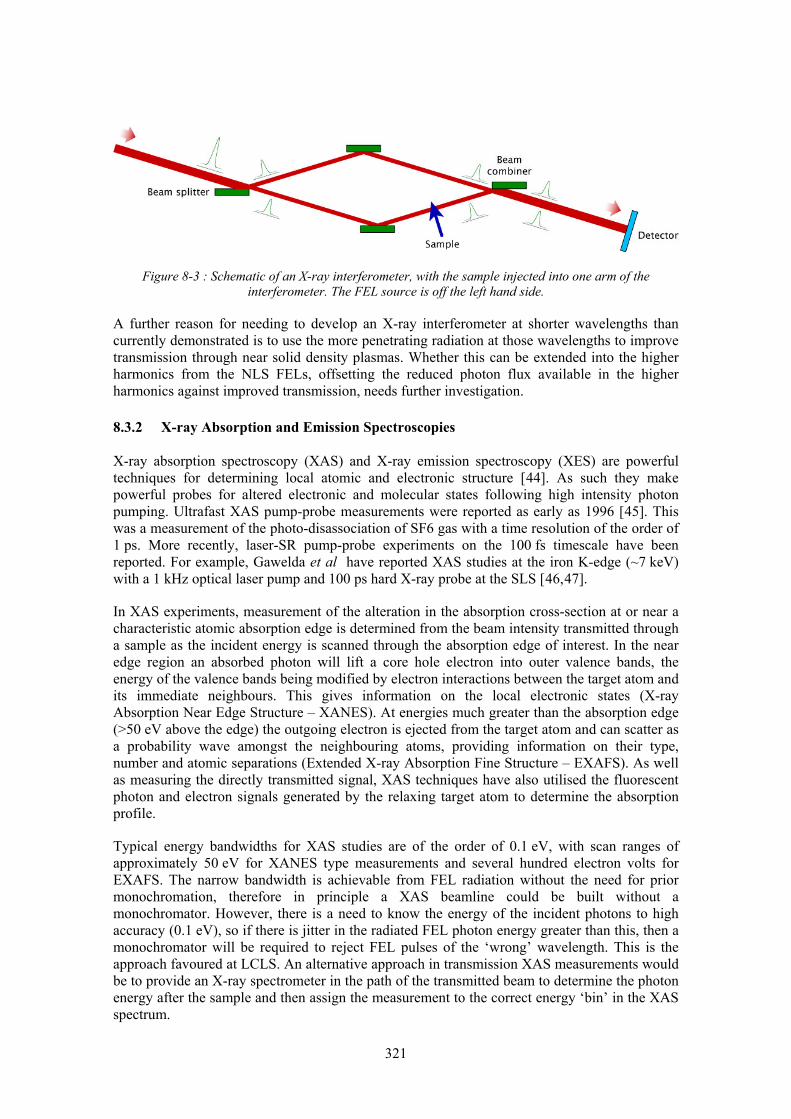
321

Figure 8-3 : Schematic of an X-ray interferometer, with the sample injected into one arm of the interferometer. The FEL source is off the left hand side.

A further reason for needing to develop an X-ray interferometer at shorter wavelengths than currently demonstrated is to use the more penetrating radiation at those wavelengths to improve transmission through near solid density plasmas. Whether this can be extended into the higher harmonics from the NLS FELs, offsetting the reduced photon flux available in the higher harmonics against improved transmission, needs further investigation.

8.3.2 X-ray Absorption and Emission Spectroscopies

X-ray absorption spectroscopy (XAS) and X-ray emission spectroscopy (XES) are powerful techniques for determining local atomic and electronic structure [44]. As such they make powerful probes for altered electronic and molecular states following high intensity photon pumping. Ultrafast XAS pump-probe measurements were reported as early as 1996 [45]. This was a measurement of the photo-disassociation of SF6 gas with a time resolution of the order of 1 ps. More recently, laser-SR pump-probe experiments on the 100 fs timescale have been reported. For example, Gawelda et al have reported XAS studies at the iron K-edge (~7 keV) with a 1 kHz optical laser pump and 100 ps hard X-ray probe at the SLS [46,47].

In XAS experiments, measurement of the alteration in the absorption cross-section at or near a characteristic atomic absorption edge is determined from the beam intensity transmitted through a sample as the incident energy is scanned through the absorption edge of interest. In the near edge region an absorbed photon will lift a core hole electron into outer valence bands, the energy of the valence bands being modified by electron interactions between the target atom and its immediate neighbours. This gives information on the local electronic states (X-ray Absorption Near Edge Structure – XANES). At energies much greater than the absorption edge (>50 eV above the edge) the outgoing electron is ejected from the target atom and can scatter as a probability wave amongst the neighbouring atoms, providing information on their type, number and atomic separations (Extended X-ray Absorption Fine Structure – EXAFS). As well as measuring the directly transmitted signal, XAS techniques have also utilised the fluorescent photon and electron signals generated by the relaxing target atom to determine the absorption profile.

Typical energy bandwidths for XAS studies are of the order of 0.1 eV, with scan ranges of approximately 50 eV for XANES type measurements and several hundred electron volts for EXAFS. The narrow bandwidth is achievable from FEL radiation without the need for prior monochromation, therefore in principle a XAS beamline could be built without a monochromator. However, there is a need to know the energy of the incident photons to high accuracy (0.1 eV), so if there is jitter in the radiated FEL photon energy greater than this, then a monochromator will be required to reject FEL pulses of the ‘wrong’ wavelength. This is the approach favoured at LCLS. An alternative approach in transmission XAS measurements would be to provide an X-ray spectrometer in the path of the transmitted beam to determine the photon energy after the sample and then assign the measurement to the correct energy ‘bin’ in the XAS spectrum.

322

To access the broad scan ranges, the FEL undulator gap will need to be scanned in much the same manner as is commonly used with undulator sources in third generation storage rings. NLS is specified to provide energy tuning by gap scanning at constant machine energy, offering a particular advantage for XAS experiments over current FEL sources with fixed gap undulator modules. The repeated measurements needed to build up an XAS spectrum will require continual replenishment of the sample using similar techniques as described for coherent diffraction imaging.

Conventional transmission or fluorescent XAS setups can be used as the critical timing is between the pump and probe pulses arriving at the sample, rather than in the signal detection. Therefore the time response of the detectors is less critical, provided that they can respond, be readout and reset within the time before the next event occurs. For a 1 kHz rep rate source, a total response and readout time within 1 ms is sufficient. However, the nature of FEL radiation, with many photons arriving in a very short time (a much higher instantaneous event rate compared to storage ring SR sources) means that pulse pileup will limit the application of conventional photon counting, energy discriminating detectors such as Si(Li), solid state Ge or Si, or gas proportional counters for fluorescent X-ray detection. Charge integrating detectors are expected be much more applicable to XAS measurements at NLS.

There is much interest currently in the synchrotron based XAS community in using X-ray Emission Spectroscopy (XES). The principles are described in e.g.[48,49], and involve using a high energy resolution spectrometer to extract fine structure relating to the radiative energy levels of the probed atom from the radiated fluorescence spectrum. The incident X-ray probe beam is tuned across the very near-edge region of the absorption edge of interest and used to excite core level electrons into the electronic levels produced by the photon pump. The spectra of de-excitation paths available to each excited state can then be recorded separately to allow 2D maps of spectral features to be produced, see e.g. [50]. This is sometimes also referred to photon-in photon-out spectroscopy. At softer X-ray energies the spectrometer can use a grating in a dispersive geometry, where sample, grating and (linear) detector all sit on a Rowland circle with the grating surface curved to a radius twice that of the Rowland circle. This geometry is applicable to NLS applications using FEL probe beams at fundamental and low harmonics up to approximately 2 keV. At harder energies, crystal spectrometers are required. As these are Bragg reflective and not dispersive they require modification to the Rowland geometry. A common geometry is the Johann one, where the crystal is curved to the same radius as the Rowland circle. Figure 8-4 shows the difference between the two geometries and the evolution of the latter to use multiple analysers to increase the solid angle of collection. Other modifications to the spectrometer geometry place the sample position inside the Rowland circle in order to increase the angular acceptance of the analyser crystal without seriously degrading the energy resolution. For higher energies, a more grazing incidence is required, leading some to adopt alternative geometries such as the von Hamos arrangement [51]. The energy range envisaged by NLS for XAS probe measurements (< 5 keV) is more appropriate for Rowland or Johann spectrometers rather than von Hamos instruments. For all crystal based analysers it is necessary to either spherically bend the crystals so that their crystal planes match the curvature of the Rowland circle [52], or create a mosaic crystal where the photon beam is only reflected by crystallites which happen to be orientated so as to meet the Bragg condition [53]. Suitable spectrometers utilising crystals have been developed in a variety of formats at a number of synchrotron beamlines, including BL19LXU at Spring8 [54], ID26 at ESRF [55], SuperXAS at SLS [56], ADRESS at SLS [57], beamline 9.3.1 at ALS [58]. A compact spectrometer for use at low energies has been developed at FLASH [59].

Energy dispersive XAS, whereby the sample is illuminated by a ‘pink’ beam of sufficient bandwidth to generate a whole XAS spectrum in one go, requires that the source have a bandwidth of 50 eV or more. The high monochromicity of the FEL output will preclude this. XES might therefore be expected to play a more significant role on fourth generation FEL sources than it traditionally has on previous generation storage ring sources.

323

(a) (b) (c)

Figure 8-4 : Optical geometries for X-ray emission spectrometers. (a) Rowland circle geometry for dispersive analyser elements (gratings) for use at softer X-ray energies, (b) modification for use with non-

dispersive analysers (Bragg reflecting crystals) – the Johann geometry, (c) development to use multiple analysers to increase the collection efficiency. To tune the spectrometer to another energy range (e.g. to

access a different absorption edge) requires that both sample and detector be moved around the Rowland circle.

8.4 Detector and Readout Requirements

The unique temporal output of FEL sources will impose their own demands on detector and readout systems. Very intense short pulses, with large numbers of photons arriving simultaneously at the detector means that individual photon counting devices or energy resolving detectors of the type routinely used at storage ring sources will not be exploitable at FEL sources. Detectors will therefore tend to be of the current integrating type, with the total charge produced per detector element per FEL pulse being read out between FEL pulses.

NLS will also operate at a high repetition rate, meaning that detector heads need to be readout and reset before the arrival of the next FEL pulse. The NLS baseline specification of 1 kHz repetition rate is unlikely to be challenging in this respect, however upgrade paths to increase this to 100 kHz – 1 MHz will require the readout times to be addressed. Data storage of large data frames, produced at high rate will impose demands on data acquisition and storage. For example, nanocrystal diffraction patterns from 30 particle/second streams at LCLS are generating data at the rate of 20 TB/day. Learning from similar problems encountered by the high energy physics community, automatic data quality assessment algorithms will need to be developed to ensure that space is not wasted on storing non-useful datasets (e.g. where the FEL or other source did not fire correctly or when the sample was not correctly coincident with the beam, leading to recording of incomplete or non-existent images or spectra). An example might use 2-d fast Fourier transformation of the recorded frame in a diffraction imaging experiment to identify the presence of high spatial frequencies originating from a diffraction pattern: frames which failed to record a diffraction pattern would only have low frequencies present and so could be identified and rejected. Due to the high frame capture rate, this decision making process can be most efficiently implemented in the detector front end electronics, one method of implementing the decision making process might be through the use of field programmable gate arrays (FPGAs) embedded within the camera [60].

For diffraction imaging experiments and in X-ray interferometers there is a need for imaging area detectors with pixel count of at least 1000 x 1000, sensitive to the UV, XUV and SXR energy ranges. These need to be capable of high frame rates (>1000 fps) to match the repetition rate of the FELs and to operate in current integrating, rather than pulse counting mode. Back illuminated CCDs have suitable sensitivity in the desired SXR range, however at high frame rates the data can be seriously degraded by readout noise. For diffraction imaging experiments with direct illumination, imaging area detectors need to have a hole in the direct line of the FEL beam as conventional beam stops will be ablated by the intense FEL radiation. A suitable aperture could be devised by edge-bumping 4 area detectors.

324

There are developments currently underway to provide 2D pixel detectors for the European XFEL source. These detectors are being designed for similar photon intensity per pulse and to store up to 100 frames at 5 MHz frame rate (with up to 0.1 s read out between pulse trains). These detector systems could be applied to lower energy X-rays as well. In addition, hybrid construction with separate detector and read-out chips may offer a solution at lower energies by replacing the detector chip with one more sensitive to the lower photon energies delivered by NLS.

Single dimension, linear detectors will also be required for photon and charge particle spectrometers. For experiments requiring spectral analysis of the experiment signal, dispersive spectrometers with a linear detector to readout the emitted or reflected spectrum will be needed. The requirements on 1D detectors are currently feasible, for example the XSTRIP X-ray detector can read 1K pixel strips at 100 kHz [61,62,63]. At lower energies, the ULTRA system is capable of operating at different wavelengths (Silicon head: 200 nm to 1100 nm; InGaAs head: 1100 nm to 2500 nm; Reverse Illuminated Silicon head: 0.25-0.07 nm (5–17 keV)) and at speeds of up to 1 MHz over 16 channels, allowing a detector with 512 channels to be read out at 20 kHz [64].

REFERENCES [1] Bostedt, C., et al., Experiments at FLASH. Nucl.Instrum.Meth.A. 2009 601 108–122 [2] Doniach, S., Studies of the structure of matter with photons from x-ray free-electron laser. J.

Synchrotron Rad. 1996 3 260–267 [3] Tiedtke, K., et al., The soft x-ray free-electron laser FLASH at DESY : beamlines, diagnostics and

end-stations. New J. Phys. 2009 11 023029 [4] Treusch, R & Feldhaus, J., FLASH: new opportunities for (time resolved) coherent imaging of

nanostructures. New J. Phys. 2010 12 035015 [5] Neutze, R., et al., Potential for biomolecular imaging with femtosecond X-ray pulses. Nature 2000

406 752–757 [6] Chao, W L., et al., Soft X-ray zone plate microscopy to 10nm resolution with XM-1 at the ALS. AIP

Conf. Proc. 2007 879 1269–1273 [7] Bajt, S., et al., Camera for coherent diffraction imaging and holography with a soft x-ray free

electron laser. Appl. Opt. 2008 47 1673–1683 [8] Chapman, H N., et al., Femtosecond diffractive imaging with a soft X-ray free electron laser. Nature

Phys. 2006 2 839–843 [9] Bogan, M J., et al., Single particle x-ray diffraction imaging. Nanoletters 2008 8 310–316 [10] Benner, W H., et al., Non-destructive characterisation and alignment of aerodynamically focused

particle beams using single particle charge detection. J. Aerosol Sci. 2008 39(11) 917–928. [11] Shapiro, D A., et al., Powder diffraction from a continuous microjet of submicrometer protein

crystals. J.Synchrotron Rad. 2008 15 593–599. [12] DePonte, D P., et al., Gas dynamic virtual nozzle for generation of microscopic droplet streams. J.

Phys. D:Appl. Phys. 2008 41 195505. [13] Kirian, R A., et al., Femtosecond protein nanocrystallography – data analysis methods. Opt. Exp.

2010 18 5713–5723 [14] Mancuso, A P., et al., Coherent-pulse 2D crystallography using a free electron laser X-ray source.

Phys. Rev. Lett. 2009 102 035502 [15] Schmidt, K E., et al., Tomographic femtosecond x-ray diffraction imaging. Phys. Rev. Lett. 2008

101 115507 [16] Hau-Riege. S P., et al., Sacrificial tamper slows down sample explosion in FLASH diffraction

experiments. Phys. Rev. Lett. 2010 104 064801, [17] Eisebitt, S., et al., Lensless imaging of magnetic nanostructures by X-ray spectro-holography.

Nature 2004 432 885–888 [18] McNulty, I., et al., High-resolution imaging by Fourier transform x-ray holography. Science 1992

256 1009–1012 [19] Rosenhahn, A., et al., Digital in-line holography with femtosecond VUV radiation provided by the

free-electron laser FLASH. Opt. Exp. 2009 17 8220–8228. [20] Mancuso, A P., et al., Coherent imaging of biological samples with femtosecond pulses at the free-

electron laser FLASH. New J. Phys. 2010 12 035003.

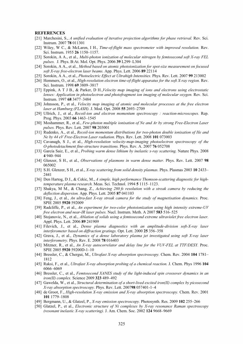
325

REFERENCES [21] Marchesini, S., A unified evaluation of iterative projection algorithms for phase retrieval. Rev. Sci.

Instrum. 2007 78 011301 [22] Wiley, W C., & McLaren, I H., Time-of-flight mass spectrometer with improved resolution. Rev.

Sci. Instrum. 1955 26 1150–1157. [23] Sorokin, A A., et al., Multi-photon ionization of molecular nitrogen by femtosecond soft X-ray FEL

pulses. J. Phys. B:At. Mol. Opt. Phys. 2006 39 L299–L304 [24] Sorokin, A A., et al., Method based on atomic photoionization for spot-size measurement on focused

soft X-ray free-electron laser beams. App. Phys. Lett. 2006 89 22114 [25] Sorokin, A A., et al., Photoelectric Effect at Ultrahigh Intensities. Phys. Rev. Lett. 2007 99 213002 [26] Hemmers, O., et al., High-resolution electron time-of-flight apparatus for the soft X-ray region. Rev.

Sci. Instrum. 1998 69 3809–3817 [27] Eppink, A T J B., & Parker, D H.,Velocity map imaging of ions and electrons using electrostatic

lenses: Application in photoelectron and photofragment ion imaging of molecular oxygen. Rev. Sci. Instrum. 1997 68 3477–3484

[28] Johnsson, P., et al., Velocity map imaging of atomic and molecular processes at the free electron laser at Hamburg (FLASH). J. Mod. Opt. 2008 55 2693–2709

[29] Ullrich, J., et al., Recoil-ion and electron momentum spectroscopy : reaction-microscopes. Rep. Prog. Phys. 2003 66 1463–1545

[30] Moshammer, R., et al., Few-photon multiple ionisation of Ne and Ar by strong Free-Electron Laser pulses. Phys. Rev. Lett. 2007 98 203001

[31] Rudenko, A., et al., Recoil-ion momentum distributions for two-photon double ionisation of He and Ne by 44 eV Free-Electron Laser radiation. Phys. Rev. Lett. 2008 101 073003

[32] Cavanagh, S J., et al., High-resolution velocity-map-imaging photoelectron spectroscopy of the O-photodetachment fine-structure transitions. Phys. Rev. A. 2007 76 052708

[33] García Saiz, E., et al., Probing warm dense lithium by inelastic x-ray scattering. Nature Phys. 2008 4 940–944

[34] Glenzer, S H., et al., Observations of plasmons in warm dense matter. Phys. Rev. Lett. 2007 98 065002

[35] S.H. Glenzer, S H., et al., X-ray scattering from solid density plasmas. Phys. Plasmas 2003 10 2433–2441

[36] Den Hartog, D J., & Cekic, M., A simple, high performance Thomson-scattering diagnostic for high-temperature plasma research. Meas. Sci. Technol. 1994 5 1115–1123.

[37] Shakya, M M., & Chang, Z., Achieving 280 fs resolution with a streak camera by reducing the deflection dispersion. App. Phys. Lett. 2005 87 041103

[38] Feng, J., et al., An ultra-fast X-ray streak camera for the study of magnetisation dynamics. Proc. SPIE 2005 5920 592009

[39] Radcliffe, P., et al., An experiment for two-color photoionization using high intensity extreme-UV free electron and near-IR laser pulses. Nucl. Instrum. Meth. A 2007 583 516–525

[40] Stojanovic, N., et al., Ablation of solids using a femtosecond extreme ultraviolet free electron laser. Appl. Phys. Lett. 2006 89 241909

[41] Filevich, J., et al., Dense plasma diagnostics with an amplitude-division soft-X-ray laser interferometer based on diffraction gratings. Opt. Lett. 2000 25 356–358

[42] Grava, J., et al., Dynamics of a dense laboratory plasma jet investigated using soft X-ray laser interferometry. Phys. Rev. E. 2008 78 016403

[43] Mitzner, R., et al., An X-ray autocorrelator and delay line for the VUV-FEL at TTF/DESY. Proc. SPIE 2005 5920 59200D-1–10

[44] Bressler, C., & Chergui, M., Ultrafast X-ray absorption spectroscopy. Chem. Rev. 2004 104 1781–1812

[45] Raksi, F., et al., Ultrafast X-ray absorption probing of a chemical reaction. J. Chem. Phys 1996 104 6066–6069

[46] Bressler, C., et al., Femtosecond XANES study of the light-induced spin crossover dynamics in an iron(II) complex. Science 2009 323 489–492

[47] Gawelda, W., et al., Structural determination of a short-lived excited iron(II) complex by picosecond X-ray absorption spectroscopy. Phys. Rev. Lett. 200798 057401-1–4

[48] de Groot, F., High-resolution X-ray emission and X-ray absorption spectroscopy. Chem. Rev. 2001 101 1779–1808

[49] Bergmann, U., & Glatzel, P., X-ray emission spectroscopy. Photosynth. Res. 2009 102 255–266 [50] Glatzel, P., et al., Electronic structure of Ni complexes by X-ray resonance Raman spectroscopy

(resonant inelastic X-ray scattering). J. Am. Chem. Soc. 2002 124 9668–9669

326

REFERENCES [51] Hoszowska, J., et al., High-resolution von Hamos crystal X-ray spectrometer. Nucl. Instrum. Meth.

A 1996 376 129–138 [52] Collart, E., et al., Spherically bent analysers for resonant inelastic X-ray scattering with intrinsic

resolution below 200 meV. J. Synchrotron Rad. 2005 12 473–478 [53] Legall, H., et al., An efficient X-ray spectrometer based on thin mosaic cystal films and its

application in various fields of X-ray spectroscopy. J. Appl. Crystal. 2009 42 572–579 [54] Higashiya, A., et al., Compact resonant inelastic x-ray scattering equipment at BL19LXU in

Spring-8. AIP. Conf. Proc.2007 879 1415–1418 [55] Glatzel, P., et al., Hard X-ray Photon-in Photon-Out Spectroscopy. S. R. News 2009 22(2) 12–16 [56] Kleimenov, E., et al., High-resolution hard-X-ray fluorescence spectrometer. J. Phys:Conf. Ser.

2009 190 012035. [57] Ghiringhelli, G., et al., SAXES, a high resolution spectrometer for resonant X-ray emission in the

400–1600 eV energy range. Rev. Sci. Instrum. 2006 77 113108 [58] Hudson, A C., et al., Design and performance of a curved-crystal x-ray emission spectrometer.

Rev.Sci.Instrum. 2007 78 053101 [59] Fäustlin, R R., et al., A compact soft X-ray spectrograph combining high efficiency and resolution. J.

Inst. 2010 5 02004. [60] Paindavoine, M., et al., High-speed camera with internal real-time image processing. Proc. SPIE

2005 5920 59200Y. [61] Headspith, J., et al., XSTRIP–a silicon micro strip-based x-ray detector for ultra-fast X-ray

spectroscopy studies. Nucl.Instrum.Meth.A 2003 512 239-244 [62] Headspith, J., et al., First experimental data from XH, a fine pitch germanium microstrip detector

for energy dispersive EXAFS (EDE). IEEE Nucl.Sci.Symposium 2007 NSS-07 2421–2428 [63] http://www.quantumdetectors.com/Datasheets/XSTRIPdatasheet.pdf [64] http://www.quantumdetectors.com/Datasheets/ULTRA_DAQ_datasheet.pdf

327

9 Timing and Synchronization

Many of the elements of the NLS science case depend on the delivery of multiple beams of very short photon pulses with extremely good synchronization between them. This area has developed very rapidly over the last 10-20 years and innovative and effective solutions have been found for the very challenging problems which have arisen. The field is still developing as users seek to exploit the source capabilities in the middle and lower decades of the femtosecond regime. However, while the technical achievements have been impressive, the community of specialists working in this area is quite small. This means that there is a strong need to collaborate on common solutions to the collective problems. The NLS team is committed to this and the schemes presented below reflect an approach which is being taken in many facilities. This sometimes means that a slightly more complex or over-specified solution has been adopted, but in each case this is justified by substantial benefits including reduced development costs, increased reliability (since solutions have been debugged in advance elsewhere) and increased prospect of commercialization, which has clear economic and operational advantages.

9.1 Timing

This Section covers the overall time structure of the NLS output pulse train, concentrating mostly on the factors which decide it. The mechanisms for achieving it are not technically challenging except in one critical respect: there is a very strong drive to deliver the pulses with the lowest possible timing jitter.

The output pulse time structure, set by the science requirements, is very simple. Pulses are equispaced with a nominal rate on Day 1 of 1 kHz. As the machine is developed this rate will increase, most probably in decade steps i.e. to 10 kHz then to 100 kHz with 1 MHz being the ultimate goal. The timing scheme has been designed to satisfy the Day 1 requirement and to allow for the upgrades with the minimum of change.

There are two other predetermined parameters which affect the timing. The main one is the choice of 1.3 GHz for the accelerator RF. Since the electron bunch timings obviously have to have a fixed relationship with the RF phase, the actual pulse rates will necessarily be sub-harmonics (integer submultiples) of 1.3 GHz. The second parameter relates to the way the system’s master clock is controlled (see below). To minimize jitter at the low-frequency end of the phase noise spectrum the clock will include a very stable RF reference. These are available commercially at a number of standard frequencies, with 10 MHz being one of the most common.

The choice of actual pulse rates has been made taking the above factors into account and including two more principles. The first is that the sub-harmonic ratios should have low-integer factors. This is justified on the basis that very low noise frequency dividers become increasingly difficult to make as the division ratio increases, and electronic noise is an unwelcome contributor to system jitter. In fact the division ratios used here are all products of powers of two and three. Such close integer relationships between rates make it easier to incorporate other equipment which operates resonantly at higher frequencies e.g. laser oscillators. A side effect of this choice is that that the machine rates cannot be exactly 1 kHz, 10 kHz etc since this would require a division of the RF at some stage by 13. The second principle is that the four planned rates (1 kHz-1 MHz) should be sub-harmonics of one another. This allows resonant systems to be deployed on Day 1 which are capable of operating at all of the planned rates without any upgrading. An example of this is the photoinjector drive laser system (see Section 10.1.1). It also allows low pulse rate items, e.g. users’ experimental equipment, to continue operating after an upgrade without having to be re-built to coincide with pulses from the higher-rate train.

328

0.846 MHz

105.8 kHz

8.816 kHz

1.102 kHz

650 MHz phase sensor

10 MHz RF reference

oscillator × 26

×3

PLL electronics

216.67 MHz fibre laser oscillator

÷ 28

÷ 23

÷ (22×3)

÷ 23

Figure 9-1: NLS master clock architecture showing pulse rate division and phase locking scheme

The first of the pulse rates to be fixed is that of the system’s master clock. For maximum flexibility this would be 1.3 GHz, the RF itself. But in practice this flexibility is not needed and a more convenient rate of the sixth sub-harmonic, 216.67 MHz, has been chosen. This rate is close to optimum for the particular kind of fibre laser which, with the 10 MHz reference described above, forms the clock. Indeed laser-based clocks operating at this rate have already been reported [1]. Selecting a clock rate reveals a conflict between the choices of RF and reference frequencies and the principle of low-integer division (or, in this case, multiplication). The chosen value is related in a simple way to the RF, but cannot be derived simply from the 10 MHz reference. The solution discussed in Section 9.2.2 and shown in Figure 9-1 appears to be the best. Here the laser and the reference are locked at their lowest common harmonic – 650 MHz. The problem of generating the 65th harmonic of the reference, which would otherwise involve an awkward ×13 multiplication, is resolved by using a chain of doublers to generate ×64 followed by a single low-noise mixer to reach ×65. The associated difference frequency component at 630 MHz is sufficiently far removed that it can be filtered out.

The remaining pulse rates are also shown in Figure 9-1. This choice of sub-harmonics gives the closest fit to the nominal values. The residual differences will not significantly affect the scientific capacity of the machine.

Under some circumstances it may be desirable to deliver different output pulse rates on the individual NLS beamlines. The kicker scheme which distributes the electron bunches into the separate FELs is based on non-resonant technology (see Section 11.2) which can operate with an arbitrary time structure, so this requirement can be satisfied straightforwardly. Alternatively it would also be possible to operate the whole machine at the highest required rate, using the kickers to switch the electron beam equally between the separate FELs, and then use optical choppers just before the experimental stations to reduce the individual rates as desired. Choppers are already available at rates beyond 105.8 kHz [2] which is the maximum planned for multiple beamline operation. This approach allows beam-based correction of timing jitter, which benefits from high pulse rates, to be extended along essentially the whole of the transport path.

329

Extensions of the baseline NLS system have been considered to allow simultaneous operation of each of the three FELs at 1.102 kHz. This could either involve operation of the accelerator at 3.306 kHz, achieved simply by removing a divide-by-three stage from the divider chain shown in Figure 9-1, or the basic pulse rate could be left at 1.102 kHz but three micropulses could be delivered with approximately 1 μs between them. The technology needed to generate this type of time structure from the photoinjector laser is described in Section 10.1.1.

9.2 Synchronization

The synchronization requirements can be split into three categories. The first, and most important, relates to the photon pulses arriving at the users’ experiments from the different NLS elements (FELs, conventional lasers etc). For multiphoton and time-resolved experiments these need to be delivered with low timing jitter and, in the time-resolved case, with controllable relative delay (note, it is not foreseen that any experiments will depend on absolute pulse-group arrival time defined, say, by a global time standard). Since the baseline pulse duration from the FELs is 20 fs FWHM a comparable figure for the relative timing jitter - 10 fs RMS – has been set as the design target.

The second requirement relates to the machine’s internal diagnostics. The properties of the electron bunches are actively controlled and one of the inputs to the control system is the bunch arrival time, measured at various points along the machine’s length (see Section 6.2). The arrival time monitors depend on a clock input from the synchronization system, against which the measurements are made. For the clock jitter not to degrade the measurements it must be significantly lower than the monitors’ resolution. A target for the clock jitter of 5 fs RMS has been set.

Three of the NLS’s accelerator subsystems are inherently time-varying – the RF fields in the accelerating cavities and the pulsed outputs of the photoinjector laser and the heater laser. The third requirement of the synchronization system is that these should be phase-locked. The first stage in this is to provide them with reference clock signals, similar to the diagnostics’ ones. The remainder of the control for the RF fields is discussed in Section 3.7. The control of the lasers is dealt with in this Chapter.

9.2.1 Principles

At the most basic level, synchronization is characterized by a single number – the timing jitter. This reflects the so-called “phase error” i.e. the extent to which a signal’s timing deviates from its reference. Phase error is a time-varying quantity. As the analysis becomes more sophisticated it moves out of the time domain and into the frequency domain. The phase error is then represented by its Fourier transform - a noise spectrum - and the timing jitter ΔtRMS can be shown to be proportional to the integral of the noise spectral density L(f)

∫=Δ 2

1

21

0

f

frms dffn

t )L(ω

( 9-1)

where ω0 is the frequency of the reference signal, n is the harmonic number (equal to one, unless the phase error is being sensed at a harmonic of the reference frequency) and f1 and f2 define the noise frequency range over which the jitter is being measured. The tendency for noise spectra to increase rapidly at low frequencies seems to be universal. In practice this means that, given long enough, any two free-running systems which start out in synchronism will eventually drift apart. There are two approaches to solving this problem, both of which are employed in the NLS. The first is to minimize drift and jitter passively through careful design and high-quality implementation. Examples include tight environmental control (e.g. stabilization of temperature,

330

humidity etc) and reduction of noise (e.g. vibration, electrical noise, acoustics etc). This can be very effective, particularly at higher frequencies, but is ultimately limited by cost.

Device under control

Actuator Output

Reference clock

PLL electronics

Phase sensor

Phase error

Figure 9-2: Layout of a generic feedback control system for locking a "device under control" to a reference clock signal

The second approach is the use of active feedback systems. The essential elements of such a system are sketched in Figure 9-2 . A phase sensor combines signals from the device under control and from a reference source and produces a phase error output. After processing and amplification this is used to drive an actuator which corrects the error. Optimized feedback systems can eliminate long-term drift completely and can reduce residual jitter, at least at low frequencies, by orders of magnitude. The impact is indicated qualitatively in Figure 9-3. Apart from the elimination of long-term drift the other characteristic of all real feedback systems is that they have a high-frequency roll-off. Above this the noise is unaffected and either has to be accepted or reduced using passive techniques. Feedback control is a mature subject area covered by a wide range of textbooks [3]. It is not discussed in any more detail here except to state a number of design principles which have practical consequences for the NLS.

L(f)

(dBc

/Hz)

Offset frequency (Hz)

Figure 9-3: Typical phase noise spectra: uncorrected (red) and after correction by a feedback control system (blue)

331

As far as possible, feedback control systems for NLS synchronization are designed so that: • Sensors are placed as close as possible to the point at which the signal they are sensing

is used. Actuators are placed as close as possible to the source of the noise that they are correcting;

• The parameters which are sensed and controlled are those which are actually of interest, rather than proxies;

• The paths of fast, low-amplitude signals (typically those from sensors) are kept as short as possible;

• The burden on the feedback control systems is minimized. These principles are applied to an example NLS subsystem in Section 9.2.4 below.

9.2.2 Clock Signals

The distribution of clock signals for the NLS, with the nominal jitter requirements for the separate machine subsystems, is shown in Figure-9-4. They need to be supplied along the whole length of the machine. The most stringent requirements are at the output, where the beams to the users’ experiments are synchronized to one another by synchronising them all to the clock. The most important of the bunch arrival diagnostics – the ones which time the bunches into the FEL undulators – are also close to the output end. This concentration of the most sensitive elements dictates the physical location of the clock, which is sited close to the user experimental area. This might seem an unusual choice. In many facilities the clock is found close to the gun. However the reason for this is often just historical. The gun is generally the first part of any system to be commissioned. If it is a photogun with RF acceleration then the first need for synchronization is to phase lock the cathode drive laser and the gun RF. So it is not surprising that embryonic synchronization systems are often built close to the gun. They remain there because once hardware is operational it becomes increasingly difficult to move it, even though its tasks get more and more challenging as the machine lengthens.

The jitter values listed in Figure-9-4 are derived either from the need to control photon pulse timing at the experiment or to ensure temporal overlap between the electron bunches and the laser photons (heater and FEL seed) as they travel through the machine. The value given for the acceptable photoinjector laser jitter may seem unusually large. The physical reason for this is that in a standard bunch compression scheme the effects of timing jitter at the start are simply reduced by the compression factor [4]. In the case of the NLS this factor is ~70.

Figure-9-4: Distribution of NLS clock signals for the NLS. Yellow-highlighted figures represent maximum rms jitter targets at subsystem inputs or outputs, measured relative to the mater clock (except for the 10 fs

output jitter which is measured between the FEL and laser pulses)

332

Under some circumstances this simple description is not appropriate. Timing jitter in the electron gun results in correlated low-level energy jitter as the electrons leave the accelerator. It is the correlation between timing and energy which allows the compressor to correct the timing jitter. But energy jitter can also arise elsewhere in the system and it may be that for operational reasons this is unacceptable. There are feedback schemes which can detect and correct it, but depending on the way they are implemented they may also eliminate the low-level energy jitter which enables the timing correction, inadvertently restoring the 1-to-1 relation between photoinjector laser timing and bunch arrival time after the compressor [5]. Schemes such as this are not currently implemented in the NLS design, but should they be then the photoinjector laser jitter specification will need to be revised.

The NLS clock is a hybrid RF-optical design, consisting of an Er-doped fibre laser oscillator, operating at the standard telecoms wavelength of 1.55 μm, locked to a low noise RF source (either a rubidium standard or a GPS-based system). Its architecture is shown in Figure 9-1. The roll-off frequency of the phase-locked loop is chosen to minimize the clock jitter. At low noise frequencies the RF source is quieter than the laser, so the laser is locked to it. At high frequencies the laser has the lower noise and is therefore allowed to free-run. The resulting noise spectrum reflects the best of both systems. Clocks like this have been in development for light source timing for some years and have achieved levels of jitter of ~10 fs [1]. Other advantages of this type of clock include:

SHORT OPTICAL PULSE OUTPUT: The shortness of the pulses from the laser (~100 fs) means they contain copious harmonics of the clock frequency. This improves electronic phase sensing at microwave frequencies. The most impressive electronic phase-locking of lasers has been achieved using this technique [6]. Likewise phase sensing based on all-optical approaches [7,8] benefits from having short optical clock pulses. In addition to being the most convenient way to lock one laser (the device under control) to another (the clock) all-optical phase sensors are relatively simple and are therefore less prone to problems of stability, especially drifting.

COMPATIBILITY WITH OPTICAL FIBRE DISTRIBUTION: Optical fibre itself is relatively inexpensive and is largely immune from electrical noise. Ultra-high bandwidth components, developed for the telecomms industry, are available off the shelf, also at relatively low cost. Most importantly, stabilization of fibre links over distances of many hundreds of metres has been achieved in an accelerator environment with a published jitter below 10 fs [8] and, more recently, unpublished results at the ~2 fs level [9]. This is at least an order of magnitude better than can be achieved with conventional coaxial cable.

The clock distribution scheme proposed here is based on the transmission of laser pulses over an optical fibre network, but this is not the only approach which can be taken. It is also possible to distribute a CW laser beam, with the clock signal carried as RF amplitude modulation [10]. Each scheme has its strengths and weaknesses, but both have been demonstrated in accelerator laboratory environments and it seems likely that, with sufficient development, both could deliver the required performance. For the NLS the choice between them does not need to be made yet. When it is made many factors will be involved, both technical and non-technical. The first and most obvious will be technical effectiveness. The chosen scheme will have to meet the baseline requirements and will also need to have the capacity for performance upgrading as the NLS’s capabilities develop. Operational factors will also be important. The system will need to work well for the facility’s scientific users. This will involve features such as ease of interfacing, reliability and diagnostic output, so the timing behaviour can be monitored and verified for example. Likewise the ease of installation, operation and maintenance will be important for the facility providers. An important factor will be the availability of support. This might be provided in-house and if it is the degree of overlap with other areas of machine expertise (RF systems, lasers, controls etc) could influence the technology choice. In any case the system’s outputs should be as compatible as possible with other machine elements. An alternative to in-house support would be to seek to use commercial components and to rely on support for these from the manufacturers. The potential for this will depend on the willingness

333

of businesses to become involved which, in turn, will depend on the potential for future exploitation, both in the field of clock provision for accelerators and more widely. And last, but probably not least, cost will also play a significant part in the choice.

At this stage it only needs to be confirmed that at least one of the two possible approaches can meet the specifications. Members of the NLS design team are currently working with colleagues at DESY Hamburg, Sincrotrone Trieste and elsewhere on the pulsed scheme as part of the IRUVX-PP programme, and the analysis in this Chapter is based on the pulsed approach.

There is no fundamental requirement for long-term stability from the RF source. It determines the noise spectrum of the clock only at frequencies below the roll-off of the phase-locked loop, which is 5-10 kHz. Some of the machine elements are responsive enough to follow the clock noise up to this limit. Others, for example the fields in the SCRF cavities, are not. So any clock noise which lies between the roll-off frequencies of the least and most responsive elements can cause timing jitter between those elements. But noise at lower frequencies can be “followed” by the whole machine and should, therefore, cause no relative jitter. However there are good reasons for minimising low-frequency noise. Firstly the RF must not drift, no matter how slowly, outside the range appropriate for the SCRF structures. These have extremely high Qs, so this range is extremely narrow. Secondly following a “noisy” clock requires all of the feedback control systems to work harder than they would otherwise need to. This contravenes the last of the principles in Section 9.2.1. Finally if the master clock is very stable then independent (e.g. portable) secondary clocks of comparable stability can be taken to any point on the machine and used to check the performance of local timing systems. This is a useful diagnostic feature. These reasons justify the choice of an RF source with good long-term stability.

Given the use of a low-noise clock and of extremely low-noise fibre links, the relative jitter between the distributed clock signals should be well below the limits shown in Figure 9-3 for the photoinjector and heater laser jitters. Its impact on the RF phase jitter should be small but perhaps not insignificant. Its effects are most important for the BAM diagnostics, the seed lasers and the endstation lasers. These are considered in more detail in Section 9.2.4.

9.2.3 Laser Synchronization

Laser oscillators which can be synchronized to external RF reference sources have been commercially available for some years. They all sample the laser pulse train with a photodiode and combine the signal from this with the reference RF in a low-noise mixer to generate the phase error signal. More sophisticated ones use harmonics of these signals to improve the sensitivity. The phase error is processed electronically and used to drive an actuator which changes the length of the laser’s optical cavity. Rather than altering the laser’s phase this actually alters its pulse frequency (the time derivative of the phase) but the result is the same – with a suitable choice of parameters in the phase-locked loop electronics the phase can be locked essentially indefinitely. The actuators are typically small mirrors on motor-driven (slow) and piezo-driven (fast) mounts and, for fibre lasers, piezo-driven fibre stretchers. Combinations of actuators spanning a broad frequency range are common. The best commercial laser oscillators, as supplied, can deliver timing jitters well below 100 fs RMS [11]. With customization, units which are still essentially commercial can be substantially improved. For example 20 fs RMS has been achieved in a working laboratory environment [12].

Jitter performance well beyond what is available commercially has been demonstrated in several laboratories. Fibre oscillators of the type used in the clock are locked at the sub-10 fs level (see above) without requiring particularly high levels of environmental or technical control (e.g. stabilization of the output from the pump diodes). With sufficient effort, lasers which are locked to one another using RF techniques only can have a relative jitter below 2 fs RMS even measured over noise bandwidths as large as 1 MHz [6]. Adding an all-optical sensor improves this and has allowed a jitter of 0.3 fs RMS, measured over the range from 10 mHz to 2.3 MHz, to be achieved [7].

334

The laser amplifiers which follow the oscillator can contribute additional timing jitter. The value of this will depend on the details of the design and operation. In a study of a fibre amplifier of a kind similar to the ones used in the photoinjector and heater laser chains (albeit doped with erbium rather than ytterbium) it has been shown [13] that the additional jitter can be reduced from 40 fs RMS, when the amplifier was seriously under-pumped, to less than 0.5 fs RMS when conditions were optimized. In the latter case the amplifier jitter is much smaller even than the very low value delivered by typical oscillators. Furthermore the performance may be improved by putting the amplifier chain and the passive optics which transport the beam to its point of use, inside the feedback control loop. The total length of this path can be many tens of metres, particularly if a regenerative amplifier stage is used, but the transit time is still just a few hundred nanoseconds and latency issues should not limit the performance.

A more significant problem may arise if the amplifiers are operated at reduced pulse rates. The phase sensor cannot unambiguously measure the phase noise spectrum at frequencies higher than half the sampling rate – the so-called Nyquist limit – and as this frequency is approached from below the sensitivity falls markedly. For laser oscillators this is not an issue. They all operate at rates which are sufficiently high that other factors (often the bandwidth of the actuator which corrects the timing) limit the feedback system’s performance. But for low pulse rate amplifiers this may not be the case. For example, baseline performance of the NLS requires that the photoinjector laser pulse rate be reduced to 1.102 kHz at some point before the beam enters the gun. If this happens before it is sampled for timing correction then the feedback loop cannot operate at all at noise frequencies higher than 550 Hz and in practice its performance is degraded at frequencies above ~100 Hz. This may lead to an unacceptably large level of uncorrected phase noise, in which case a more sophisticated feedback architecture will be required, probably involving sampling of the high pulse rate beam at a point early in the system and combining the result with the low-rate sample taken at the end.

9.2.4 Synchronization of an Example NLS Subsystem

To illustrate the approach taken to meeting the NLS synchronization specifications, in this Section the details of the scheme for one subsystem will be worked through. The one chosen is that which combines photon pulses from a FEL and from an endstation laser at a user experiment. This is one of the most demanding applications and is also relatively complex in terms of the number of machine elements involved.

Figure 9-5 shows a layout of the photon beams subsystem. The endstation laser and the FEL seed laser (see Chapter 10) are both based on tuneable Ti:S systems. In the case of the endstation laser the light from this may travel directly to the experiment or it may be converted on the way, using one of a wide range of non-linear optical processes, to a different photon energy. The FEL seed laser, which controls the timing of the FEL pulses, is sited close to the entrance to the undulator i.e. more than 100 m away from the endstation. Its output generates seed photons at the required energy in the HHG chamber. These are then fed into the FEL, the output of which travels, via the beamline optics, to the experiment. The two laser systems are synchronized by locking each of them to the master clock.

Since the laser systems are so similar, an alternative way to synchronize them would be to use a common oscillator. On the surface this is an attractive option since it removes the need to lock one of the lasers to the clock (the needs for the clock itself and for the locking of the other laser to it are not removed, since all of the machine subsystems still need to be synchronized). The fact that the lasers’ photon energies need to be independently tuned is not an issue since the tuning takes place after the oscillator, in the first amplifier stage. However there are at least two problems with a common oscillator scheme which, in the end, resulted in it being rejected in favour of the master clock option.

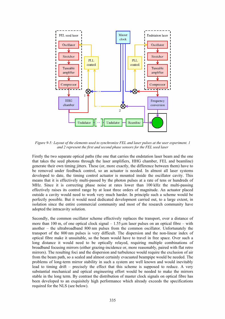
335

Figure 9-5: Layout of the elements used to synchronize FEL and laser pulses at the user experiment. 1 and 2 represent the first and second phase sensors for the FEL seed laser

Firstly the two separate optical paths (the one that carries the endstation laser beam and the one that takes the seed photons through the laser amplifiers, HHG chamber, FEL and beamline) generate their own timing jitters. These (or, more exactly, the difference between them) have to be removed under feedback control, so an actuator is needed. In almost all laser systems developed to date, the timing control actuator is mounted inside the oscillator cavity. This means that it is effectively multi-passed by the photon pulses at a rate of tens or hundreds of MHz. Since it is correcting phase noise at rates lower than 100 kHz the multi-passing effectively raises its control range by at least three orders of magnitude. An actuator placed outside a cavity would need to work very much harder. In principle such a scheme would be perfectly possible. But it would need dedicated development carried out, to a large extent, in isolation since the entire commercial community and most of the research community have adopted the intracavity solution.

Secondly, the common oscillator scheme effectively replaces the transport, over a distance of more than 100 m, of one optical clock signal – 1.55 μm laser pulses on an optical fibre – with another – the ultrabroadband 800 nm pulses from the common oscillator. Unfortunately the transport of the 800 nm pulses is very difficult. The dispersion and the non-linear index of optical fibre make it unsuitable, so the beam would have to travel in free space. Over such a long distance it would need to be optically relayed, requiring multiple combinations of broadband focusing mirrors (either grazing-incidence or, more reasonably, paired with flat retro mirrors). The resulting foci and the dispersion and turbulence would require the exclusion of air from the beam path, so a sealed and almost certainly evacuated beampipe would be needed. The problems of long-term mirror stability in such a system are well known and would inevitably lead to timing drift – precisely the effect that this scheme is supposed to reduce. A very substantial mechanical and optical engineering effort would be needed to make the mirrors stable in the long term. By contrast the distribution of master clock signals on optical fibre has been developed to an exquisitely high performance which already exceeds the specifications required for the NLS (see below).

336

The arrival time of the photons from the endstation laser is determined by the timing of the master clock and by the effectiveness with which the laser pulses, measured at the experiment, can be synchronized to it. The clock and the process of laser synchronization have been discussed in Sections 9.2.2 and 9.2.3. Since the clock is common to both the endstation laser and to the seeded FEL, its intrinsic noise does not contribute to their relative jitter. Although it is located close to the endstation laser, the signal from the clock still needs to be transported to the point where the final comparison with the laser pulses is made. The exact location of this point is a compromise between, on the one hand, the principles of measuring the signal of interest (the light delivered to the experiment) as close as possible to its point of use and, on the other, the practicality of making real-time measurements of a tuneable signal while it is being tuned, in an environment which has been transiently configured to suit a particular experiment. This compromise can be revisited at the experiment planning stage and for the most demanding experiments it may be decided to set the measurement point very close to the experiment itself. But in general it is proposed that the final timing measurement be made immediately before the non-linear conversion of Ti:S light to the photon energy needed by the user. Timing variation which arises after this point inevitably includes a jitter contribution. This needs to be controlled by designing the physical beam transport path for stability and by minimising the sources, which might include mechanical vibration, environmental changes, amplitude noise in the Ti:S laser beam (some non-linear processes can induce amplitude to phase noise conversion) etc. There can also be a contribution from systematic effects including, in particular, any tuning of the output photon energy. Fortunately systematic effects are, by definition, reproducible. So they can be measured in advance and corrected using feed forward techniques (this is consistent with the principle of minimising the burden on the feedback control system).

For the purposes of jitter budgeting, the element arising in the endstation laser beam path after the phase-locked Ti:S stage is perhaps the most difficult to estimate. A target value of 3 fs has been chosen. This is substantially worse than “interferometric” stability, which can be fairly straightforwardly achieved in the laboratory over distances of ~10 m (one quarter wave for 800 nm light corresponds to a time of 0.7 fs). The jitter of the Ti:S laser itself is easier to predict. The best results to date, using optical locking, have been sub-femtosecond for an oscillator [7]. It is known that the contribution from individual amplifier stages can be very small but in this case there are several of them and they may only be operating at 1.102 kHz, so Nyquist limits will apply. For this reason an allowance for laser locking of 5 fs has been made. The final contribution to the endstation laser timing is the distribution of the clock signal. An upper limit to this is the 2 fs value reported for a long fibre link [9].

Turning to the seeded FEL path in Figure 9-5 the first two elements are the same as those for the endstation laser – the clock distribution and the phase-locked Ti:S system. The clock is delivered to the first phase sensor which compares its timing with the residual infrared light leaving the HHG chamber. This can be accessed conveniently at the point where it is separated from the harmonics (see Section 10.2.5 ). An additional phase sensor is shown in Figure 9-5 and this has final control of the seed laser timing. However the first sensor is an operational requirement since laser locking sometimes needs to be established when the FEL itself is not being seeded.

The stage beyond the Ti:S laser is HHG conversion. The timing jitter between the drive beam and the harmonics is known to be negligible [14] so the only additional jitter before the FEL is seeded is that which appears in the seed beam transport path. This can be minimized by locating the first phase sensor as far as possible down that path. (The Ti:S light which is measured by the first phase sensor is only a proxy for the HHG signal, which conflicts with the principle of measuring signals, not proxies. But since it follows the same optical path it should be a good proxy and its use is consistent with the principle of measuring as close as possible to the point of use.)

Timing variations in the FEL amplification process itself can arise from a number of sources, generally driven by variations in the electron bunch properties. When these affect the coupling

337

between the electrons and the radiation field (as they do, for example, if the bunch energy spread changes or the trajectory moves off the undulator axis) then the point at which gain saturation is reached also moves. This, in turn, affects the time taken for the photon pulse to pass through the undulator. Timing can also be affected in the chicane which helps convert the initial bunch modulation into the density micro-bunching that drives the FEL process. Any fluctuations in the electron bunch’s mean energy affect the overall length of the path through the chicane and are converted into a timing variation. Quantification of any jitter which might arise from these processes will require detailed modelling. The results of this will drive refinement of the accelerator design to ensure that the electron bunch properties are kept sufficiently stable for the resulting timing jitter to be inconsequential.

Once the photon beam has left the FEL it propagates to the experiment via the beamline transport path. At the end of this, and close to the experiment, is the second phase sensor. Use of this sensor brings the FEL and the beamline transport optics inside the phase-locked loop and should therefore deliver the lowest level of timing jitter for the FEL radiation at the experiment. A number of issues remain to be resolved with the design of this sensor. In its simplest form it could consist of an X-ray photodiode [15] connected to a low-noise mixer in the standard configuration which, in the visible and near infrared, has been used so successfully with conventional lasers [7]. This has the advantage that it is not sharply sensitive to photon energy, so it could be used while the FEL is being tuned. Any sensitivity which does exist should be systematic and, therefore, compensatable. The X-ray equivalent of an “all optical” timing sensor has been demonstrated in at least two forms. The first, based on photoelectron spectroscopy, was effective [16] but may be difficult to develop into the real-time system capable of at least kHz operation which is needed for closed-loop feedback control. The second is much simpler and shows much more promise. Based on reflectivity modulation in GaAs this has already demonstrated 40 fs resolution in proof of principle experiments at FLASH [17]. The FLASH time structure has not allowed testing at high pulse rates but detectors capable of CW acquisition at tens of kHz already exist. The authors also believe that there are several ways in which the temporal resolution can be improved.

As well as finalising the choice of sensor technology, two other issues arise in the context of the second phase sensor. The first is the Nyquist limit referred to at the end of the previous Section. This applies to the 1.102 kHz radiation from the FEL in just the same way that it does to conventional lasers. Whether it is significant or not depends on the eventual noise spectrum of the FEL and the beamline transport system. In principle the HHG source can be operated at higher pulse rates than the FEL because the chicane between the first and second stages prevents any radiation from reaching the experiment in the absence of electron bunches. So any higher frequency phase noise present before the undulator should be correctable.

The second issue is that the long signal path from the phase sensor to the seed laser oscillator, through the seed laser system, via the HHG cell to the FEL and finally back to the experiment results in some latency in the control loop. It should be possible to keep the round-trip time for this path below 2 μs, which represents a manageable phase shift at the tens of kHz frequencies where laser feedback control loops currently roll off. So with sufficiently careful design and implementation this issue is not expected to degrade the performance significantly.

The additional jitter arising in the path from the HHG chamber to the second phase sensor can only be estimated, and as mentioned above simulations will influence the details of the system design to ensure that it is kept at an acceptable level. For the purposes of the jitter budget a figure of 5 fs has been assigned to it. An additional 3 fs is included, as with the endstation laser, to allow for the final short transport path from the second phase sensor to the experiment.

The overall jitter budget for the photon beams subsystem, based on the use of the second phase sensor to control the FEL seed laser, is shown in Table 9-1. As can be seen, the current design total meets the 10 fs target set at the start of this Section.

338

Table 9-1: Overall jitter budget for the photon beams subsystem.

Subsystem section Jitter (fs)

Clock distribution to phase sensor for endstation laser 2

Locking of endstation laser 5

Endstation laser beam path to experiment 3

Clock distribution to second (FEL output) phase sensor 2

Locking of FEL seed laser 5

Contribution for path from HHG chamber to second (FEL output) phase sensor 5

FEL output beam path to experiment 3

TOTAL (uncorrelated jitters combined in quadrature) 10

REFERENCES [1] Löhl F., et al, Experimental determination of the timing stability of the optical synchronization

system at FLASH, Proc EPAC08 2008. Paper TUPC135 [2] The 310CD chopper from Scitec Instruments Ltd, fitted with the 300D445 blade will chop at up to

120 kHz. With a custom blade design lower pulse-rate patterns can be selected from a pulse train running at this rate

[3] See e.g. Abramovici A. & Chapsky J., Feedback control systems – A fast-track guide for scientists and engineers, publ Kluwer Academic Publishers 2000. ISBN 0-7923-7935-7 or Best R. E., Phase-locked loops – Design, simulation and applications, publ McGraw-Hill 2003. ISBN 0-07-141201-8

[4] Rosenzweig J. B., et al, Pulse compression in radio frequency photoinjectors – Applications to advanced accelerators, IEEE Trans Plasma Sci, 1996. 24, 409-420

[5] Wu J., et al, Linac coherent light source longitudinal feedback model, Proc PAC 2005. 1-4, 911-913 [6] Shelton R. K., et al, Subfemtosecond timing jitter between two independent, actively synchronized,

mode-locked lasers, Opt Letts, 2000. 27, 312-314 [7] Schibli T. R., et al, Attosecond active synchronization of passively mode-locked lasers by balanced

cross-correlation, Opt Letts, 2003. 28, 947-949 [8] Löhl F., et al, Sub-10 femtosecond stabilization of a fiber link using a balanced optical

cross-correlator, Proc PAC 2007. 1-11, 16-18 [9] Schlarb H., private communication [10] Byrd J. M., et al, Timing distribution in accelerators via stabilized optical fiber links, Proc

LINAC06, 2006. 577-579 [11] Examples include the Micra Ti:S oscillator from Coherent Inc, and the FemtoFiber Er-fibre

oscillator from Toptica Photonics AG [12] Jones D. J., et al, Synchronization of two passively mode-locked, picosecond lasers within 20 fs for

coherent anti-Stokes Raman scattering microscopy, Rev Sci Instr 2002. 73, 2843-2848 [13] Löhl F., et al, Influence of erbium-doped fiber amplifiers on the timing stability of optical pulse

trains, Proc CLEO/QELS 2008. 1-9, 614-615 [14] Mairesse Y., et al, Attosecond synchronization of high-harmonic soft X-rays, Science, 2003. 302,

1540-1543 [15] Examples include the AXUV range from International Radiation Detectors Inc [16] Radcliffe P., et al, Single-shot characterization of independent femtosecond extreme ultraviolet free

electron and infrared laser pulses, Appl Phys Letts, 2007. 90, 113108 [17] Maltezopoulos T., et al, Single-shot timing measurement of extreme-ultraviolet free electron laser

pulses, New J Phys, 2008. 10, 033026.

339

10 Laser Systems

Conventional lasers play many roles in the NLS. They provide, directly, all of the photons for user experiments across the spectral range from 0.06 eV to 6 eV. They also cover the range from 6 eV to 50 eV through the high harmonic generation (HHG) process. Between 50 eV and 100 eV lasers supply the seed photons to FELs 1, 2 and 3, controlling the spectral and temporal properties of their output.

In addition to the provision of photons to users, lasers are also widely distributed along the machine itself. They generate the electron bunches in the gun, modify their properties through the laser heating process and diagnose their temporal behaviour along the full length of the beam transport path.

All of these roles are discussed elsewhere in this report. In this Chapter systems which deliver the required performance are described. Lasers are also an integral part of the timing and synchronization system which is described separately in Chapter 9.

Although the laser specifications differ widely, efforts have been made to share common system elements where practical. This generates significant benefits in terms of hardware (common spares, common interfaces to control and diagnostic systems, cost savings etc.) and of staffing (large parts of each subsystem are operable and serviceable by all of the laser specialists).

10.1 Lasers for the Accelerator

The lasers which form critical components of the accelerator are distinguished from the other systems by the need for the very highest levels of reliability and availability. Failure of a seed laser or of a system which directly serves an endstation brings the operation of one FEL or one experiment to a halt. Failure of, for example, the photocathode laser causes instant shutdown of the entire facility. Furthermore the other lasers are needed only when the related FEL is operating or when the users are setting up or taking data, which will not be the case for the whole of the time. On the other hand the accelerator itself will run 24 hours a day, 7 days a week for periods which might extend to months. This need for reliability strongly favours the use of diode-pumped lasers and, in particular, fibre lasers. These operate with the minimum number of mechanical parts and they are sealed, almost entirely, from the surrounding environment. Their reliability levels can be extremely high.

10.1.1 Photoinjector Laser

The specifications for the NLS photoinjector laser beam, measured at the photocathode, are derived in Section 2.1 and summarized in Table 10-1 below. They can be met by a laser system which uses the Yb3+ ion as the gain medium. This material has many desirable features. It can be directly pumped by laser diodes. Its quantum defect is small, so the lasing process is efficient and minimal waste heat is generated. It has sufficient gain bandwidth that it can deliver pulses with sub-picosecond rise-time. It is widely available in the form of Yb-doped fibre, and complete Yb-fibre laser systems have been in commercial production for some time. (Fibre lasers are the systems of choice when very low pulse timing jitter is required. They can also be scaled to high pulse repetition rate with high average power.) For these reasons and others the Yb system has already been adopted for one of the most recent photoinjector drive applications [1].

340

Table 10-1: Parameters of the photoinjector laser required to produce the nominal 200 pC electron bunch

Laser parameter Value (measured at the cathode)

Wavelength ~265 nm

Pulse energy 0.1 μJ

Pulse rate (baseline) 1.102 kHz

Temporal profile 15 ps FWHM, flat-topped, <2 ps rise- and fall-time

Spatial profile 0.52 mm radius, top-hat

A schematic of the laser system is shown in Figure 10-1. It consists of the Yb laser, which operates at an infrared wavelength of 1030 nm, a frequency quadrupler, which converts the infrared to 258 nm ultraviolet radiation, and a beam conditioning module which shapes the temporal and spatial profiles. The resulting pulses are delivered to the cathode using free-space optics which image-relay them from the output of the beam conditioning module. The numerical aperture (NA) of the transport optics sets the finest spatial detail which can be reproduced on the cathode. A NA of at least 0.01 is needed to reproduce sub-millimetre laser spots with sufficiently sharp edges. Beam transport in the ultraviolet presents significant problems (absorption, scattering and wavefront degradation are all worse at short wavelengths) so this section of the path is kept as simple as possible. However all of the components up to and including the beam conditioning module are located outside the radiation shield, in a controlled-environment enclosure. This allows access to the UV elements while the machine is running, which would not be possible if they are located in the tunnel. The resulting operational benefits outweigh the problems of the longer UV transport path.

Beam

conditioning

Frequency

quadrupler

Pockels cell driver

Yb-fibre laser system

Gun

Transverse profile monitor

Radiation shield

Timing monitor

Reference clock

Sampling optic

Figure 10-1: Schematic of the NLS photoinjector laser system

At the last possible point before the beam enters the gun it is sampled to allow measurement of the pulse timing and, in a plane equivalent to that of the cathode, the transverse profile. The

341

effects of variations in the path between the sampling point and the cathode cannot easily be corrected, so the separate paths after the sampling optic are made as short and stable as possible. This involves fixing the sampling optic relative to the photocathode using high quality optomechanics. Synchronization of the photoinjector laser is discussed in more detail in Section 9.2. Suffice it to say that a photodiode and a relatively simple electronic phase sensor are adequate for this purpose and these elements are shown mounted close to the sampling point. However given that UV photodiodes are rather insensitive and that they can also have long-term stability issues it may be necessary to replace this set-up with a more robust (probably all-optical) sensor. In any case the phase error signal resulting from the timing measurement is conditioned locally before being transported back to the laser oscillator where timing correction takes place.

The beam’s spatial and temporal profiles at the cathode are set by the beam conditioning module. The spatial profile is determined by an aspheric transmission optic which reshapes the intensity into a near top-hat distribution. The principle has already been demonstrated [2] although the details of the optic vary from case to case, dependent on the precise shape of the input beam. The output slightly overfills a fixed aperture, whose edges can be sharp or graded as desired. This aperture is the object which is image-relayed to the cathode. It will need to be changed, as will the demagnification factor of the telescope feeding it, when the machine parameters are reset for different bunch charges. The positional stability of the beam on the cathode derives from the physical stability of the aperture and of the transport optics. This approach eliminates any effect of beam-pointing variations earlier in the optical path, although in practice such variations should be very small. With careful engineering and, if necessary, a feedback control system positional stability at the sub-10 μm level should be practical.Normal SASE operation requires a 15 ps FWHM flat-topped temporal profile with a ~2 ps rise-time and fall-time. This is generated using a pulse stacking scheme. Compared with approaches based on the manipulation of spectral phase and amplitude at an early point in the laser system [3] this has the advantages of simplicity (all of the components are passive) and stability (the system has no powered components nor is there any dynamic adjustment). It is also compatible with a stable and relatively narrow spectral bandwidth, which makes the frequency multiplication stages easier to design and relatively efficient. Compared with schemes based on spectral shaping in the ultraviolet [4] it is very efficient since it does not require any of the pulse energy to be discarded. The simplest form of stacker [5] consists of a series of birefringent crystals which split the beam into two polarization components and delay one with respect to the other, the delay being proportional to the crystal length. Each crystal multiplies the number of stacked pulses by a factor of two.

The 15 ps pulse needed for the NLS is conveniently produced by a three-crystal arrangement which stacks 8 pulses, each with a FWHM duration of ~1.75 ps. The drawbacks with this scheme are that it is inflexible (only 2N pulses can be stacked), the stacking of discrete pulses results in ripple in the output pulse’s nominally flat top (interference effects prevent the individual pulses from being stacked arbitrarily close together) and the output beam has mixed polarization (which means that all of the downstream optics need to be polarization-insensitive). With the present design none of these issues causes a significant problem for the NLS. It does not need the pulse length to be variable in real time, and the much shorter pulses needed for single spike operation can be generated simply by reducing the number of stacking stages. The few-percent ripple amplitude is acceptably small and the transport path is optically simple. However if necessary the polarization mixing can be eliminated using an alternative stacking scheme [6] at the cost of substantially increased complexity. An attractive feature of stacking schemes is their inherent stability. When combined with the intrinsic stability of fibre lasers the result should be an output pulse whose duration and temporal shape is reproducible from shot to shot at the level of 1-2%.

The output pulse energy required from the laser itself is set by the specifications at the cathode and by the losses in the laser-to-cathode path. The loss budget includes figures of 15% for the image-relaying section (including sampling), 20% for the spatial reshaping and 15% for the

342

pulse stacker. So the combined throughput of these stages is 0.58, raising the required pulse energy from 0.1 μJ at the cathode to 0.175 μJ at the input to the beam conditioner. This is generated from the infrared output of the Yb laser by frequency quadrupling in a pair of non-linear crystals. Frequency multiplication is a well-established technique and conversion efficiencies of 8% to the fourth harmonic have been demonstrated in systems similar to the NLS one [7]. On this basis the pulse energy at the input to the quadrupler needs to be 2.2 μJ. This is well within reach of current Yb-fibre laser systems. In a research environment 8 μJ, sub-400 fs pulses have been delivered at a rate of 40 MHz [8]. At a 2 MHz rate, which is more than is needed even for the ultimate NLS upgrade, an Yb-fibre system delivering 10 μJ, 250 fs pulses is already a commercial product [9].

Neither of the systems reported in [8] and [9] includes an oscillator which can be synchronized. However such oscillators are readily available (see Chapter 9) and there is no reason why one cannot be used. As the NLS is developed the baseline bunch rate, 1.102 kHz, is expected to be raised in regular steps to a maximum of ~1 MHz. One approach would be to upgrade the photoinjector laser system each time the bunch rate is raised. But since MHz lasers are already available a less disruptive alternative would be to install a MHz system to begin with and then reduce its pulse rate to the required value.

Stable operation of the laser requires that all of the power amplifier stages are operated at their nominal pulse rate. So rate reduction must be carried out at the end of the amplification process. At this point the average laser power (a few watts) is low enough that a conventional Pockels cell switch can be used to “pick” the required pulses from the MHz train. Furthermore the fastest switching rate (~100 kHz) can be delivered using existing high-voltage drive technology. A solution based on a Pockels cell has the additional advantage that it does not disrupt the operation of the laser at all. This results in maximum stability and also allows feedback control systems, e.g. for stabilization of the pulse energy, to operate optimally. For these reasons it is the preferred option. However it does have the disadvantage of inflexibility. The drive electronics are likely to be tuned for the particular switching rate, making rate changes awkward and preventing any pulse structures other than the most regular. If other structures are ever required then an alternative switching scheme is available [10]. This maintains the required even loading of the amplifier chain by feeding it with pulses which differ only in their spectrum. The pulses which eventually reach the cathode will, immediately after the oscillator, have been spectrally narrowed as described above. The pulses which are to be dumped will have passed through a different filter whose transmission spectrum overlaps negligibly with the first one. However both spectra will lie under the Yb gain curve, so the laser population dynamics will be the same for both. At the end of the amplifier chain the pulses will automatically be separated in the bunch compressor which is inherently dispersive.

Whichever pulse switching scheme is adopted there will inevitably be a small amount (perhaps at the few tenths of a percent level) of cross-talk between the pulses which are switched to the cathode and the ones which are dumped. If this level of “ghost pulsing” were actually to reach the cathode then it could cause significant problems when the pulse rate is meant to be low. Fortunately the action of the frequency quadrupler tends to eliminate ghost pulses since its conversion efficiency is essentially proportional to the fourth power of the peak input intensity. This improves a 1% contrast ratio in the infrared to approximately 10-8 in the ultraviolet.

10.1.2 Laser Heater

A laser heater is installed after the injector, to suppress micro-bunching instabilities through a controlled increase in the energy spread (see Section 1.2). It imposes an energy modulation on the dispersed electron beam through the inverse FEL effect. The laser must deliver sufficient electric field strength to impose a suitably large modulation on the beam. The laser and electron beam transverse profiles must also be matched to provide a transversely varying magnitude to

343

the modulation. Without this transverse variation a residual peak in the density as a function of energy can remain at the end of the laser heater section.

The heater laser operates at a wavelength in the 1 μm region which can conveniently be delivered by an Yb system. The required pulse energy is the product of the peak power and the pulse duration. These are set by the need to overlap the electron bunch in all three dimensions. The cross-sectional area of the laser beam must be relatively large because it interacts with the electron bunch in a region where the latter is transversely broad. As a consequence the laser power is relatively high, ~10 MW. The heating occurs early in the accelerator, before any significant bunch compression, so the duration of the bunch is ~15 ps and for reasonable overlap the laser pulse should be at least equivalent to this. The pulse energy is thus ~150 μJ.

Off-the-shelf commercial Yb-fibre lasers cannot currently reach this energy. However a fibre system such as the one described for the photoinjector application could do so with the addition of just a small free-space final amplifier stage. Commercial versions of these can easily operate at the 1.102 kHz baseline pulse rate and rates up to ~25 kHz are offered [11]. Large mode area Yb-fibre lasers in research laboratories have already exceeded the required pulse energy by a factor of ~5 in the sub-picosecond regime [12]. They have been operated at pulse rates up to 100 kHz and the authors are confident that 1 MHz can be delivered. The system’s beam quality and spectrum are only marginally good enough for the laser heating application, but if the pulse energy is reduced these will certainly improve. It seems clear that a robust Yb-fibre based solution for the heater laser can be made available with appropriate development. Such systems may also become commercially available since there is demand from the laser micro-machining sector.

10.1.3 Diagnostic Lasers

Laser systems are used to diagnose the electron bunch timing through beam arrival monitors (BAMs) and electro-optic longitudinal profile monitors (see Chapter 6.2).

The BAMs couple directly to the laser based master clock and timing distribution system (see Section 9.2). They use commercial, telecoms-standard, electro-optic Mach-Zehnder inferometers to sample the RF waveforms from a stripline pickup. Each one requires an input from the optical clock which is boosted in a local Er-doped fibre amplifier (EDFA). Properly designed EDFAs have been shown to contribute negligible timing jitter to the signal they amplify [13].

The baseline design for the longitudinal profile monitors also takes 1.55 μm wavelength pulses from the optical clock. Again these are amplified in a local EDFA system, the output of which is now frequency doubled to 0.78 μm. While this is proven technology, care is needed to ensure that the system delivers sufficient optical bandwidth and pulse energy for the monitor (these, with the properties of the chosen sampling crystal, set the ultimate time resolution). Provided that the resolution requirement is met, this relatively simple approach offers the highest levels of robustness and reliability.

If the bandwidth of the directly amplified clock pulses is insufficient then an alternative, albeit more complex, solution exists. A local laser oscillator can be set up and locked to the optical clock. The oscillator can be configured to deliver the required bandwidth, either at 1.55 μm, using erbium as the gain medium, or directly at 0.8 μm using Ti:Sapphire. The oscillator pulses can then be amplified to higher energy and either fed to the profile monitor directly or, in the erbium case, via a frequency doubling stage. The profile monitor does not need to have the extremely low jitter that the BAMs do. So there are no significant timing issues associated with the independent oscillator scheme. Equally the technology is mature and not subject to any significant technical risk. However, as well as the reduced reliability which always comes with

344

complexity, there are also increases in cost and in space requirements. For these reasons the simpler design is the preferred one.

10.2 FEL Seed Lasers

The baseline requirements for seeding of the NLS are that the seed pulses (at the input to the FEL) should cover the energy range from 50 to 100 eV with a peak power of 400 kW and a 20 fs FWHM pulse length. They must be tuneable to provide continuous coverage over the full 50-100 eV range and this tuning must be rapid. These pulses are produced by high harmonic generation in rare gases in the ‘loose-focusing’ regime, driven by a high-power kHz laser system.

In this Section, a design for a suitable laser system, high harmonic source and beam transport to the FEL is presented. Continuous tuneability is achieved by varying the wavelength of the drive laser which is a 50 mJ, 1 kHz Ti:Sapphire system tuneable over ±25 nm from the 800 nm centre wavelength. The tuneability is obtained using a programmable gain control filter in the first amplifier stage.

10.2.1 Production of the HHG Seed Pulses

The requirement for a seed power of 400 kW per harmonic at the FEL modulator implies that 0.8-1.2 MW per harmonic must be generated at the source (assuming a global transport efficiency of 0.5-0.3, as discussed in Section 10.2.5). With the required 20 fs pulse length, this means that the energy per harmonic must be in the region of 16-24 nJ. The harmonics must also have good transverse coherence and sufficiently low jitter in timing, energy and pointing.

Pulses with the required energy have been reported across the full range from 50-100 eV, using a 50 mJ laser system focused into neon [14]. The energy and power produced in a sample of the harmonics is shown in Table 10-2.

Table 10-2: Measured pulse energy and calculated power for selected harmonics with a 50 mJ drive laser pulse [14].

Harmonic order Wavelength (nm)

Photon energy (eV) Pulse energy (nJ) Power (kW,

assuming 20 fs)

33 24.2 51.2 17 850

43 18.6 66.7 21 1050

53 15.1 82.1 24 1200

63 12.7 97.6 21 1050

The yield was optimized by loosely focusing the drive laser to ensure good phase-matching and by using high energy laser pulses with a large interaction volume. The laser and gas cell parameters reported in [14] and required for the NLS are summarized in Table 10-3.

345

Table 10-3: Parameters for optimized harmonic generation with 50 mJ laser energy from [14] and required for NLS.

Parameter Reported value [14] Required for NLS (baseline)

Laser wavelength 800 nm 800 ± 25 nm

Laser pulse energy 50 mJ 50 mJ

Laser repetition rate 10 Hz 1.102 kHz

Focused intensity 4×1014 Wcm-2 4×1014 Wcm-2

Laser pulse length 30 fs 30 fs

Focused spot size 360 μm 360 μm

Beam size at focusing optic 20 mm dia 20 mm dia

Focal length 5 m 5 m

f/# 250 250

Target Ne cell Ne cell

Medium length 5 cm 5 cm

Gas pressure 10 torr 10 torr

Absorption length at 100eV ~ 1 cm ~ 1 cm

The intensity is kept to ~4×1014 Wcm-2, where the ionization fraction is less than ~1%, to limit the phase mismatch arising from free-electron dispersion. As the harmonic yield is limited by absorption in these conditions, the optimal medium length, medL , has been shown to be a factor of ~3 greater than the absorption length, absL [15]. The number of photons in harmonic order q,

qN , then scales as

absq sAN ∝ (10-1)

where A is the cross-sectional area of the focal spot and abss is the absorption cross-section. For fixed laser intensity and pulse length, this means that harmonic photon yield scales linearly with laser energy. As the laser energy, LE , increases, the f-number of the focusing optic has to

scale as LEf ~# to keep the focused intensity constant. This imposes practical limits, with a focal length of ~ 5-10 m being the maximum for a single focusing optic.

The choice of target gas (non-linear medium) for HHG is determined by the balance between conversion efficiency and absorption length. The ionization potential, PI , also plays a role, determining the cut-off energy offcutE − through

PPoffcut UIE ⋅+=− 17.3 ( 10-2)

where PU is the ponderomotive energy. PI also governs the ionization fraction and hence the dispersion. Neon is the optimal choice for harmonics in the 50-100 eV range.

346

Figure 10-2: Layout for HHG in a long gas cell (after [14]). DM is a deformable mirror.

A conceptual diagram of the HHG layout is shown in Figure 10-2. A deformable mirror controlled by a wavefront sensor enables aberrations at the focus to be minimized and allows active optimization of the phase-matching [16]. The pulse is compressed to 30 fs using a grating compressor in vacuum, thereby avoiding the self-phase modulation that would occur if the compressed pulse was passed through a vacuum window. The beam is then focused using a 5 m focal length spherical mirror into a 5 cm long cell containing neon at 10 Torr. A translation stage allows the position of the focus within the cell to be optimized. The beam enters and exits the cell through pinholes that limit gas flow, so high vacuum can be maintained in the target chamber. Additional differential pumping stages can be added, if necessary, to ensure UHV conditions downstream.

10.2.1.1 Spatial Properties of the HHG Seed

The divergence of harmonics produced under these phase-matching conditions and with the long interaction length geometry has been found to be very low. The measured value in [14] was 0.35 mrad FWHM at 9 eV. The divergence scales with harmonic order, q, as q1 and

with medium length, medL , as medL1 . The expected divergence under the NLS conditions will vary from 0.3 mrad at 100 eV to 0.4 mrad at 50 eV. As shown in Section 10.2.5, this range is suitable for subsequent beam transport to the FEL undulator.

Laser high harmonics have been shown to have high spatial coherence. Young’s slits measurements of the intrinsic spatial coherence of the source show that the source size is of the order of four times that of the effective incoherent source size [17,18]. Tabletop lensless imaging experiments have shown a λλ Δ of 200 at a wavelength of 29 nm [19]. Harmonics have also been used as interferometric probes [20]. A key factor impacting the design of the beamline and focusing optics is the beam quality and focusability of the harmonics. Measurements of the spot size of the 27th harmonic (42 eV) focused with a toroidal mirror showed an M2 of 1.4 and a spot size of 1 μm [21]. Separate wavefront measurements of high harmonics at ~40 eV using point diffraction interferometry [22] have shown that the harmonic beam is a spherical wave to within a phase error of λ/15.

10.2.1.2 Temporal Properties of the HHG Seed

XUV pulses generated through harmonic generation are shorter than the generating laser pulse due to the non-linearity of the generating process. The intensity of the qth harmonic, qI , scales

with laser intensity, LI , as pLq II ∝ where p is the effective order of the non-linearity, typically

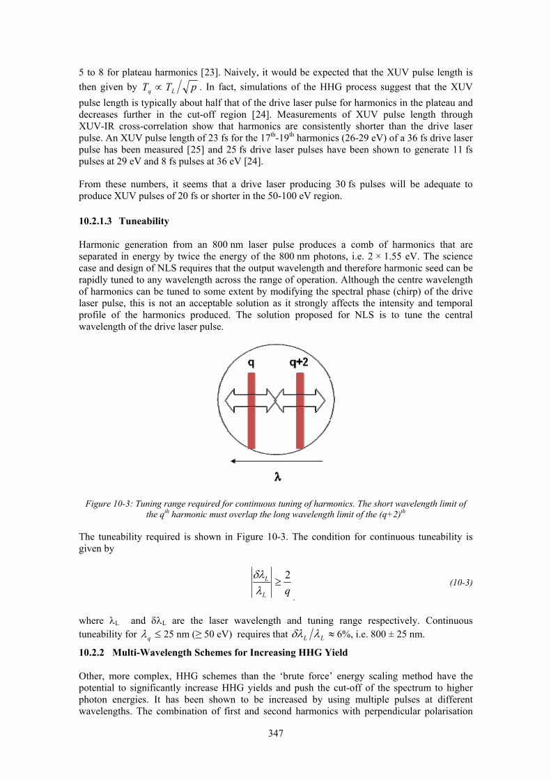
347

5 to 8 for plateau harmonics [23]. Naively, it would be expected that the XUV pulse length is then given by pTT Lq ∝ . In fact, simulations of the HHG process suggest that the XUV pulse length is typically about half that of the drive laser pulse for harmonics in the plateau and decreases further in the cut-off region [24]. Measurements of XUV pulse length through XUV-IR cross-correlation show that harmonics are consistently shorter than the drive laser pulse. An XUV pulse length of 23 fs for the 17th-19th harmonics (26-29 eV) of a 36 fs drive laser pulse has been measured [25] and 25 fs drive laser pulses have been shown to generate 11 fs pulses at 29 eV and 8 fs pulses at 36 eV [24].

From these numbers, it seems that a drive laser producing 30 fs pulses will be adequate to produce XUV pulses of 20 fs or shorter in the 50-100 eV region.

10.2.1.3 Tuneability

Harmonic generation from an 800 nm laser pulse produces a comb of harmonics that are separated in energy by twice the energy of the 800 nm photons, i.e. 2 × 1.55 eV. The science case and design of NLS requires that the output wavelength and therefore harmonic seed can be rapidly tuned to any wavelength across the range of operation. Although the centre wavelength of harmonics can be tuned to some extent by modifying the spectral phase (chirp) of the drive laser pulse, this is not an acceptable solution as it strongly affects the intensity and temporal profile of the harmonics produced. The solution proposed for NLS is to tune the central wavelength of the drive laser pulse.

Figure 10-3: Tuning range required for continuous tuning of harmonics. The short wavelength limit of the qth harmonic must overlap the long wavelength limit of the (q+2)th

The tuneability required is shown in Figure 10-3. The condition for continuous tuneability is given by

qL

L 2≥

λδλ

. (10-3)

where λL and δλL are the laser wavelength and tuning range respectively. Continuous tuneability for ≤qλ 25 nm (≥ 50 eV) requires that ≈LL λδλ 6%, i.e. 800 ± 25 nm.

10.2.2 Multi-Wavelength Schemes for Increasing HHG Yield

Other, more complex, HHG schemes than the ‘brute force’ energy scaling method have the potential to significantly increase HHG yields and push the cut-off of the spectrum to higher photon energies. It has been shown to be increased by using multiple pulses at different wavelengths. The combination of first and second harmonics with perpendicular polarisation

348

has been shown to give yields of up to 600 μJ at 57 eV, using just 3 mJ drive laser pulse energy [26]. Generating harmonics with a longer wavelength drive laser pulse can potentially increase the cut-off, with the cut-off frequency scaling as the square of the drive laser wavelength. However, the HHG yield in this case drops off by λ-5 to λ-6 [27].

Recent work has shown the addition of two non-harmonically related fields can significantly increase the yield of harmonics by up to two orders of magnitude compared to the yield from one of these two fields alone. Measurements on the Artemis facility at the Central Laser Facility (CLF) showed that the combination of 1290 nm pulses from an OPA with 800 nm pulses, both with intensities of mid-1013 Wcm-2 and with parallel polarisations, resulted in an enhancement of the yield of plateau harmonics by two orders of magnitude and an extension of the cut-off to higher frequencies [28]. The resulting harmonics are closely spaced in frequency (non-integer order harmonics appear between those due to each separate frequency), tuneable (because the OPA is tuneable) and robust to phase and timing jitter between the two pulses.

Further research is required to investigate whether these enhancements can be scaled to high laser pulse energies and the appropriate wavelength range required for seeding.

10.2.3 Laser System for Generation of Tuneable Harmonics

The baseline design for the NLS HHG seed lasers outlined in Section 10.2.1 uses proven Ti:Sapphire technology. Although gain-shifting and gain-narrowing make it difficult to tune the output of a Ti:Sapphire system solely by tuning the seed [29], tuneable systems using programmable gain filters in the amplifier are mature enough that they are becoming commercially available. The system architecture is shown in Figure 10-4. The layout is based on the Aurora system from Amplitude Technologies, which is a tuneable system delivering up to 15 mJ at 10 Hz.

Figure 10-4: Architecture of 50mJ, kHz tuneable Ti:Sapphire laser system. AOPDF is an acousto-optic programmable dispersion filter and AOPGCF is an acousto-optic programmable gain control filter.

349

Figure 10-5: Layout of the regenerative amplifier (after [31]).TFP are thin film polarizers. PC1 and PC2 are Pockels cells.

The initial pulses are produced in a commercial ultra-broadband oscillator (>100 nm) pumped by a continuous wave Nd:YVO4 laser at 532 nm. They are then stretched to ~200 ps in a grating-based stretcher. They pass through an acousto-optic programmable dispersion filter (AOPDF) [30], which enables fine control of the spectral phase. Next, the pulses are amplified up to the 1 mJ level in a regenerative amplifier containing an acousto-optic programmable gain control filter (AOPGCF) [31]. It is this which is the key to providing tuneable pulses. The layout of a similar regenerative amplifier is shown in Figure 10-5. The pulses pass through the AOPCGF ~20 times, experiencing the same spectral amplitude filtering each time. This configuration has a major advantage over designs where a single external filter is used as it means that the filter can be much softer, so the seed energy is higher. This improves energy stability and contrast at the output of the amplifier [31]. The effectiveness of the AOPGCF is shown in Figure 10-6 where 30 fs pulses have been tuned over a range of >50 nm.

A second amplifier stage takes the output of the regenerative amplifier up to the 80 mJ level. This stage is based on a multi-pass configuration, using a cryogenically-cooled Ti:Sapphire crystal. Cryogenic cooling is used as standard on kHz systems as, at low temperature, the thermal conductivity of Ti:Sapphire increases. Thermal lensing is also much reduced because at low temperatures the refractive index varies more slowly with temperature [32]. The current commercially available state-of-the-art for kHz Ti:Sapphire amplifiers is 20 mJ output energy (~30 mJ before compression) and 150 W of cooling power in the amplifier crystal. Some development work may be needed to scale up to the power level needed for the seed laser.

Currently available suitable pump lasers provide 30-50 mJ of green pump energy at 1 kHz in 100-200 ns pulses. These pump lasers can be readily multiplexed, with beams traversing the

Figure 10-6: Data from an Amplitude Technologies Aurora system showing a series of output spectra with central wavelengths spanning 55 nm.

350

fairly large pump crystal at a variety of angles. A typical kHz system delivering ~10 mJ would use two pump lasers on the final crystal. For the NLS system, up to 10 pump lasers are required. The reliability of the pump lasers is then a concern, so an appropriate number of spares (2-3 for 10 pump lasers) should be kept available.

The ~80 mJ, 200 ps output from the multipass amplifier is finally compressed back down to 30 fs in a grating compressor. These have typical throughputs of 65-75%. The compressor is in vacuum to avoid having to propagate the compressed pulse through a glass window into the harmonic generation chamber.

10.2.4 Seed Pulse Production at Higher Repetition Rates

The HHG seed scheme described above can be readily scaled to higher repetition rates, limited only by the availability of high-power high repetition rate laser systems. No fundamental repetition-rate limitations have yet been found when using gas-cell or continuous flow targets as a very low proportion of the laser energy is deposited into the gas (the ionisation fraction is less than ~1%). HHG has been demonstrated at 100 kHz [33] and at 10 MHz using a laser oscillator as the drive source [34]. We anticipate that some engineering issues will arise with high average power loading on mirrors and the entrance and exit pinholes of the HHG gas cell entrance/exit. High beam quality and low pointing jitter will thus be even more important to ensure reliable operation and active stabilisation beam pointing stabilisation will almost certainly be required.

The 1 kHz repetition rate tuneable laser system described above is commercially available now. Higher repetition rate lasers are being developed and will come on to the market over the next few years. We can expect that a 16 mJ, 40 fs, 5 kHz or 8 mJ, 40 fs, 10 kHz system will be available in the next two years. The 8 mJ system will however be borderline in terms of pulse energy to enable scaling of the ‘brute force’ approach to HHG to 10 kHz. Systems providing up to 20 mJ in 40 fs at 10 kHz will be coming on to the market in a timescale of three to four years [35] and these may provide enough energy to scale HHG to 10 kHz, although multi-wavelength generation techniques may be required.

10.2.5 Seed Beam Transport

A design for the beam transport from the HHG cell to the FEL undulator has been developed (Figure 10-7). The design uses a Kirkpatrick-Baez (K-B) focusing system to allow adjustment of the waist position in the undulator. The plane turning mirror allows the HHG cell and focusing optics to be located above the plane of the accelerator for ease of fit into the space envelope available. The current machine layout indicates that the plane mirror should be 13 m from the front of the undulator.

The centre of the K-B system is 9 m in front of the plane mirror pole. The pole to pole separation of the K-B pair is 0.5 m. This means that the maximum mirror length is ~40 cm. This is likely to be longer than needed to capture the radiation and so the separation of the K-B pair could probably be reduced. For 50 eV and 100 eV photons, the optimum focal positions are 1.2 m and 0.55 m inside the undulator respectively. The image distances from the K-B mirrors are thus 23.2 ± 0.25 m and 22.65 ± 0.25 m for 50 eV and 100 eV photons respectively.

The required Rayleigh ranges in the undulator have been calculated to be 0.7 m for 50 eV photons (with 0.6 – 0.9 m permissible) and 0.9 m for 100 eV photons (with 0.7 – 1.5 m permissible). The Rayleigh range of the XUV source has been calculated from the divergence (Section 10.2.1.1), assuming an M2 of 1.4 [21] and is shown in Table 10-4.

The Rayleigh range at the required position in the undulator has been calculated as the distance from the HHG source to the centre of the K-B mirror pair is varied (Figure 10-8). This gives two Rayleigh ranges for each photon energy, four Rayleigh ranges in total. The source distance has then been chosen to be in the centre of the region where the optimal Rayleigh ranges lie.

351

Figure 10-7: Layout of beam transport from HHG cell to FEL undulator.

Table 10-4: Calculated Rayleigh range of the XUV source

Photon energy (eV) Drive laser energy (mJ)

FWHM divergence of XUV (mrad)

Rayleigh range of XUV source (m)

50 50 0.4 0.0957

100 50 0.3 0.0851

For 50 mJ drive laser pulses, the optimum position of the HHG source is 7.8 m from the centre of the K-B mirror pair.

The overall efficiency of this design, with three reflections, is 0.88 at 50 eV and 0.90 at 100 eV with a 1º grazing angle on gold. With a 2º grazing angle, the efficiency would be 0.77 at 50 eV, and 0.82 at 100 eV.

Should the 800 nm radiation need to be stopped from propagating into the FEL, several options are possible. First, since the divergence of the harmonics is much smaller than the divergence of the drive laser beam (0.4 mrad at 50 eV compared to 4 mrad at 800 nm), a simple aperture of the appropriate size will block 95% of the IR energy while transmitting 99% of the XUV. Beam separators have also been developed for this wavelength region. Niobium nitride films used at Brewster’s angle for 800 nm have been shown to have a reflectivity of 0.75 to 0.55 across the 50 to 100 eV range, but a reflectivity of only 0.01 for 800 nm [36]. To allow for the possibility of adding beam separators or additional focusing optics, we have allowed for a total throughput of 0.3 to 0.5 in our calculation of the seed power required to be generated at the source (Section 10.2.1).

352

Figure 10-8: Calculated Rayleigh ranges of 50 eV and 100 eV photons at the focus in the undulator as the source distance is varied. The circles indicate the optimum Rayleigh ranges. The vertical line marks

the chosen source distance which gives Rayleigh ranges within the permissible range at both photon energies.

10.2.6 Spatial and Temporal Overlap of HHG Seed and Electron Bunch

Simulations have shown that the tolerable jitter on laser beam position and pointing for acceptable power fluctuations are <10 μm and <3 μrad for power fluctuations of <1% (Table 10-5). Measurements of single-shot energy and pointing fluctuations of HHG pulses have recently been carried out at Lund and data analysis is in progress [37].

Techniques for actively stabilising laser pointing are well-developed, with <1 μm rms pointing stability demonstrated on a 1 kHz, high power Ti:Sapphire laser using active stabilisation [38]. Fast fluctuations were dealt with using a 2D position sensitive detector with analogue feedback, enabling more rapid variations to be dealt with than systems relying on CCD cameras and PCs. Implementing this technique on a pair of mirrors enables stabilisation of both angle and position to the μm and μrad level. Stabilisation of the drive laser before the generating gas cell may be sufficient to stabilise the HHG seed beam. If it is not sufficient the seed beam can be stabilised after the cell This would be most straightforward to do by monitoring and stabilising the IR beam which co-propagates with the seed. This would require stable inline IR pick-offs, which could be annular IR mirrors as the divergence of the infrared is much greater than that of the seed. Reflections from foil filters used to attenuate the IR beam or IR scatter from XUV optics could also be used.

Table 10-5: Calculated tolerable jitter on laser beam position (Δx, Δy) and pointing (Θx, Θy) to keep power fluctuations (ΔP) within limits.

ΔP < 1% ΔP < 5% Δ x (µm) 9 19 Δ y (µm) 7 17 θ x (µrad) 3 17 θ y(µrad) 3 23

353

On-line diagnostics will also be required to monitor the overlap volume between the HHG seed and the electron bunch. Here, beamline apertures can be used to define the overlap volume. The co-propagating IR radiation can be imaged using standard CCD cameras and the HHG radiation can be visualised using techniques such as Ce:YAG fluorescence screens.

The temporal overlap between the HHG seed and electron bunch will require monitoring and control. The IR drive laser will be locked to the Master Clock and the HHG pulses will be intrinsically synchronised with sub-fs precision to the IR pulses. However, optical path instabilities could lead to jitter of the seed timing relative to the IR pulse. From experience with other long path length interferometers (for example at the Artemis facility in the CLF), we might pessimistically expect Δt ~20-50 fs rms. Interferometric stabilisation of the path length using piezo actuators can reduce this to the fs level [39]. Here, a typical response time would be ~100 Hz.

Suitable diagnostics for temporal overlap include streak cameras, which can establish timing to within a few ps. The temporal overlap between the IR and the electron bunch can be measured on a femtosecond time-scale using electro-optical sampling [40].

10.3 Lasers for User Experiments

The NLS Science Case calls for the provision of ultrafast light pulses tuneable from the far infrared to the soft X-ray, with the option of bringing several independent beams to bear simultaneously on individual experiments. In the baseline design accelerator-based light sources cover the extremes of the spectrum. Conventional lasers play a critical role in providing efficient, tuneable sources across the range from 0.06 eV to 6 eV. Additionally they can, using non-linear optical techniques, deliver outputs up to 50 eV, offering a realistic alternative to a FEL for this region. The lasers will be synchronized with the FELs and undulator sources (see Chapter 9) resulting in a versatile, tuneable pump-probe and multi-photon capability not presently available elsewhere. Furthermore, lasers provide a route to pulse durations of 10 fs or less. Exploiting the HHG process can reduce pulse lengths even further, into the attosecond regime.

10.3.1 Technology Overview

An obvious route for generating such a broad tuning range is to exploit the high intensities generated by chirped pulse amplification (CPA), a technique used in almost all ultrafast commercial and research lasers globally. Titanium-doped sapphire (Ti:S) crystals, pumped by readily available high power diode-pumped solid-state lasers, provide a high intensity tuneable source in the near infrared. This can be used to drive a variety of non-linear processes, generating a continuously tuneable output in spectral regions where direct laser action is difficult. This approach has been used with success on the new Artemis and ULTRA laser facilities at the STFC’s CLF. Figure 10-9 gives an overview of the techniques used to cover the full spectral range and Figure 10-10 shows a schematic of a typical laser system. Both the techniques and the laser technology are discussed in more detail in the following Sections.

The intention is to provide three laser systems based on identical components - one for each of the FELs. These will be located in environmentally controlled rooms above the beamline endstations. The use of common components reduces the risk of down time by minimising the spare parts requirements and simplifying the staff training. Where necessary, each laser can be optimized to meet the particular needs of its beamline. Experience from the CLF’s Astra laser system has shown that this is more effective than building a single large laser that is simultaneously optimized for several different tasks.

It is apparent from Figure 10-10 that the laser beam arriving at the experiment can have followed one of several alternative paths (and in fact those paths can themselves have sub-paths which make the arrangement even more complex). Effective use of the NLS requires that as far

354

as possible the manipulation of the beam along whichever of the paths is the relevant one must be automated. This is a complex task but a necessary one. As the optical path changes there is a tendency for the beam direction to change. Beam pointing variations obviously have undesirable effects at the endstation. Again as far as possible these will be eliminated using automatic alignment systems fed from laser beam position monitors and driving precision tip-tilt mirrors.

10-9

10-8

10-7

10-6

10-5

10-10

10-8

10-6

10-4

10-2

100

Nonlinear mediumcrystals(BBO, LBO)

gases(Ar, Ne, etc)

Ti:Sapphire

Pul

se e

nerg

y ./

J

50 eV 60 meV

White light OPA

10-9

10-8

10-7

10-6

10-5

Wavelength / m

HHG

Tuneable Ti:Sapphire

DifferenceFrequency Generation

SecondHarmonic /

Sum Frequency

Travelling waveOPA

HighHarmonic

Generation

6 eV

Figure 10-9: Overview of techniques used to cover the full spectral range; (top) state of the art pulse energies as a function of photon energy for a commercial tuneable Ti:S system (open rectangle), high harmonic generation (crosses) [41,42] and a white-light seeded OPA system [43] with a 6 mJ, 30 fs

pump pulse (lines); (bottom) limits of each technique to be used to span the full spectral range.

355

Ti:Sapphire CPA laser

Tuneable UV- IR0.06 eV– 6eV

OPA

Hollow fibrecompressor

Sub 10 fs

1.55 eV

End Stations

High harmonic

generation

XUV6 eV – 50 eV

80

0 n

m, 1

kH

z

Monochromator

Diagnostics

Figure 10-10: Schematic overview of one of the laser systems, showing the division of the main Ti:S drive laser to each of the wavelength conversion systems.

10.3.2 Ti:S Chirped Pulse System

A 1 kHz, 50 mJ, 20-30 fs, tuneable Ti:S laser, similar to the FEL seed laser described in Section 10.2.3, is used as the core of each of the NLS experimental systems. Given the similarity, the detailed description will not be repeated here. The significant differences from the FEL seed laser are:

• The tuning range is wider (see Section 10.3.4) • The carrier-envelope phase (CEP) is stabilized • The laser pulse arrival time is adjustable, allowing variation relative to the arrival time

of the FEL and undulator pulses (see Chapter 9) • The laser system’s adjustable parameters (photon energy, spectral profile, pulse energy,

pulse length, pulse arrival time etc) along with those of any operational non-linear stages are of direct interest to the facility’s users.

Control of the CEP is very important for processes, such as extreme non-linear optics, which have a strong dependence on the absolute phase of the optical electric field. Hardware for achieving it is now commercially available [44] but it is sufficiently novel that some discussion is merited. The process involves closed-loop feedback based on the output of a CEP sensor. The latter works by sampling the output of the oscillator at the start of the laser system and broadening the spectrum (without introducing phase noise) until it covers at least an octave. The low and high frequency parts of the spectrum are separated and a low frequency component (at frequency f) is frequency-doubled. This is then spatially overlapped with the corresponding high frequency component at 2f on a high-speed detector. The beat signal measured by the detector reveals the CEP offset. This is fed back to a correcting actuator which is a piezo-driven mirror controlling the length of the laser oscillator cavity. In addition to this “fast” loop which stabilizes the oscillator CEP there is also a “slow” loop which corrects for predominantly thermally-induced CEP-shifts arising in the Ti:S amplifier chain. The CEP is sensed at the end of the chain and is corrected by adjusting the position of one of the pulse compressor gratings.

The CEP is obviously indeterminate to within integer multiples of the optical period, so provided the loop is stable CEP corrections should only be being made on a scale smaller than this (i.e. sub-femtosecond). As such there should be no significant impact on the timing stabilization system which is concerned with fluctuations at the few-femtosecond level.

356

However it is important to ensure that the reverse is also true. In particular if the laser oscillator timing is being adjusted to correct for phase noise arising in a remote system, which might be relatively large, then this must be implemented in a way which does not compromise the CEP stabilization system.

The laser system performance has to be continuously monitored and logged both for operational control and also to provide source data for the experimental users. Comprehensive diagnostics suites of this kind have been implemented on systems such as the STFC CLF’s Astra Gemini laser. Likewise fast data acquisition systems, including elements of real-time processing and storage, are in place on the CLF’s 10 kHz ULTRA laser. These examples demonstrate that monitoring systems adequate for at least the NLS baseline performance already exist.

10.3.3 White-light Seeded OPA

The Ti:S laser provides a reliable source of highly energetic femtosecond pulses. But despite the tuneability offered by the system described in Section 10.2.3, the wavelength is limited to a narrow range around 800 nm. However, the high peak power allows the tuning range to be greatly extended by exploiting optical parametric amplification (OPA) processes. In a suitable non-linear crystal - β-barium borate (BBO) and lithium triborate (LBO) have ideal characteristics, including high non-linearity, low group velocity dispersion, broad transparency and high damage thresholds - a high frequency and high intensity beam (the pump at frequency ωp) can amplify a lower frequency, lower intensity beam (the signal at frequency ωs) with the generation of a third beam (the idler at frequency ωi) where ωi < ωs < ωp. Energy conservation requires that

isp ωωω hhh +=

and for the process to be efficient the momentum (phase-matching) condition

isp kkk hhh +=

should also be satisfied (kp, ks and ki are the wave vectors for the pump, signal and idler respectively). Clearly the signal frequency can vary from ωp/2 to ωp. In this way, the energy in a high-power, fixed-frequency pump beam can be transferred to a lower-power, variable frequency signal beam, creating a third idler beam to satisfy the above conservation laws. The low-power (seed) signal beam can be selected from a “white light” source generated by focusing an ultrashort laser pulse into a fused silica or sapphire plate (using materials with high thermal conductivity and low UV absorption such as sapphire avoids long-term degradation). Self-focusing and self-phase modulation processes take place in the high intensity focus and result in a large degree of spectral broadening. With 800 nm pump pulses the spectrum typically extends through the visible (from about 420 nm) into the near infra-red (to about 1500 nm) [43].

Practical OP systems are optimized in a number of ways. Beams are shaped to make their intensity as uniform as possible in both time and space. Pump intensities are chosen to achieve the maximum gain without causing damage to the crystal or inducing third-order non-linear effects such as self-focusing that would lead to beam distortions. The overall amplification can be staged through a series of crystals. It is usual to drive the later stages in saturation, both to deliver the maximum efficiency and also to minimize the effects of seed fluctuations which occur naturally in processes that are as non-linear as white light generation.

The white-light seeding scheme followed by multi-stage amplification is commonly employed in commercial OPA systems, for example the TOPAS series from Light Conversion Ltd. The HE (High Energy) TOPAS represents the current state-of-the-art. Using a combination of OPA and standard non-linear optical techniques its output is continuously tuneable from 6 eV

357

(200 nm) to 0.06 eV (20 μm). Table 10-6 summarizes its performance. It is clear from the Table that continuous tuneability requires beam switching between a large number of optical elements. The fact that a commercial system can achieve this is testament to the capability of modern process automation.

Table 10-6: Specification of a commercial white-light seeded OPA [43] showing the non-linear techniques used and including estimates of the pulse energy for a 10 mJ, 20 fs pump pulse

Range Technique Pulse energy (μJ) (10 mJ, 20 fs pump)

1600 – 2200 nm Idler 1000

1200 – 1600 nm Signal 1300

800 – 1200 nm Second harmonic idler (SHI) 100

600 – 800 nm Second harmonic signal (SHS) 400

533-600 nm Sum frequency idler 600

480 – 533 nm Sum frequency signal 700

300 – 480 nm Second harmonic of SHI or SHS 50

200 – 300 nm Second harmonic sum frequency 50

3 – 8 μm Difference frequency generation 50

5 – 12 μm Difference frequency generation 20 .

10.3.4 High Harmonic Generation

The white-light seeded OPA cannot operate at photon energies above ~6 eV because of absorption in the crystals. In this region high harmonics are the best tuneable source and they have been chosen for the baseline NLS design to span the region from 6 eV to 50 eV. Continuous coverage between these relatively low energy harmonics requires the fundamental to tune over a wider range than is necessary for the FEL seed laser. The current maximum edge-to-edge bandwidth of ±100 nm achievable with the Aurora-type system described in Section 10.2.3 is only sufficient to allow continuous tuneability above 12 eV. To provide continuous coverage down to 6 eV requires ≈LL λδλ 50%, i.e. 800 ± 200 nm. In principle a range this wide could be supported by Ti:S, since it has a gain bandwidth of 650-1100 nm, but even if sufficiently broadband optics and gratings could be manufactured, configuring a single setup to tune this far would be impractical. An easier solution for the 6-12 eV region is to scale the scheme which was proposed for seeding the 4GLS XUV-FEL [45] i.e. to use a high energy tuneable OPA system to generate the harmonics. Takahashi et al. have recently demonstrated an OPA operating between 1.25 μm and 1.55 μm with a peak output of 12 mJ, pumped by a 26 mJ, 10 Hz Ti:S laser i.e. with a maximum efficiency of ~45% [46]. Full tuning between the harmonics from 6 eV upwards can be achieved using the signal beam from an OPA which has a wavelength tuning range of 1200—1600 nm. OPAs in this region are fairly straightforward to design and operate and one can easily be pumped by the fundamental of the 50 mJ, 1 kHz Ti:S laser system. Low pump-signal and pump-idler group velocity mismatch in BBO allows the use of long crystals giving the possibility of high gain. Using an OPA to drive the HHG source requires an extra frequency conversion step and the atomic response for HHG scales as ~λ-5, so the efficiency might be expected to be low. However, as in all non-linear optics, HHG conversion depends not only on the atomic response but also the macroscopic effects of propagation and phase matching. Agostini et al. have suggested that, with optimization of the pump intensity, gas density and focusing geometry, harmonics can be generated using near-IR light with efficiency comparable to that generated at 800 nm [47].

358

The technique described in Section 10.2.1 of loosely focusing the drive laser and using high energy laser pulses with large interaction volumes is also used to make the harmonics for the experiments. Conversion efficiencies as high as 10-4 have been reported for the 15th harmonic of 800 nm (23 eV) generated in xenon [48] giving > 1012 photons per pulse with a 50 mJ pump laser. In general, conversion efficiency rises as the harmonic number and energy per harmonic photon fall, so at lower energies the number of photons per pulse should increase quickly. As the energy increases the HHG process moves towards the “plateau” region where conversion efficiencies are typically closer to 10-5.

10.3.5 Pulse Compression

Gain narrowing in the Ti:S amplifier chain and the limited bandwidth of the amplifier optics make direct production of high-energy ultrashort pulses difficult in a CPA system. The shortest pulse length obtainable from the Ti:S laser described here is 20 fs, and 30 fs is a more realistic limit when broad wavelength tuneability is required. To generate shorter pulses, for which significant user demand exists, the spectral broadening caused by self-phase modulation (SPM) in a hollow fibre can be exploited. After broadening, the pulse is recompressed using multiple bounces through a series of chirped dielectric mirrors. In this way it is possible to reach pulse lengths as short as 5 fs [49]. Suda et al have demonstrated sub-10 fs pulses with energies as high as 5 mJ and a conversion efficiency of ~50% [50]. The capillary dimensions were chosen to optimize the amount of SPM while remaining below the threshold for ionization. In principle, by scaling to larger capillaries with looser focusing geometry, the amount of energy produced can be increased, although this will require additional research.

REFERENCES [1] Ouzounov D. G., et al, The laser system for the ERL electron source at Cornell University,

Proc PAC07 2007. 530-532 [2] Zhang S., et al, Single-element laser beam shaper for uniform flat-top profiles, Opt Express, 2003.

11, 1942-1948 See also Refractive Beam Shaper, model no GBS-UV-H from Newport Corporation

[3] Cialdi S., et al, Rectangular pulse formation in a laser harmonic generation, Appl Phys B, 2006. 82, 383-389

[4] Cialdi S., et al, Simple scheme for ultraviolet time-pulse shaping, Appl Opt, 2007. 46, 4959-4962 [5] Power J. G. & Jing C. G., Temporal laser pulse shaping for RF photocathode guns: The cheap and

easy way using UV birefringent crystals, AIP Conf Proc, 2009. 1086, 689-694 [6] Will I. & Klemz G., Generation of flat-top picosecond pulses by coherent pulse stacking in a

multicrystal birefringent filter, Opt Express, 2008. 16, 14922-14937 [7] Csatari M. & Ross I. N., A diode-pumped photoinjector laser system for the CERN linear collider

(CLIC), Annual Report of the CCLRC Central Laser Facility 2003. 196-197 [8] Eidam T., et al, A 325W average power fiber CPA system delivering sub-400fs pulses,

IEEE J Selected Topics in Quantum Electronics, 2009. 15, 187-190 [9] Examples include the IMPULSE laser system from Clark MXR, Inc, and the Tangerine fs laser

system from Amplitude Systemes [10] Hirst G. J., 4GLS timing and synchronisation point design: photoinjectors and other conventional

laser applications, 4GLS Conceptual Design Report 2006. CCLRC Report 2006-4-5, 11, 27-29 [11] An example is the s-Pulse HP laser amplifier from Amplitude Systemes [12] Röser F., et al, Millijoule pulse energy high repetition rate femtosecond fiber chirped-pulse

amplification system, Opt Letts, 2007. 32, 3495-3497 [13] Löhl F., et al, Influence of erbium-doped fiber amplifiers on the timing stability of optical pulse

trains, Proc CLEO/QELS 2008. 1-9, 614-615 [14] Takahashi E. J., et al, Low-divergence coherent soft x-ray source at 13 nm by high-order harmonics,

Appl Phys Letts, 2004. 84, 4-6 [15] Constant E., et al, Optimizing high harmonic generation in absorbing gases: model and experiment,

Phys Rev Letts, 1999. 82, 1668 [16] Villoresi P., et al, Optimization of high-order harmonic generation by adaptive control of a sub-10-

fs pulse wave front, Opt Letts, 2004. 29, 207

359

REFERENCES [17] Ditmire T., et al, Spatial coherence measurement of soft X-ray radiation produced by high order

harmonic generation, Phys Rev Letts, 1996. 77, 4756 [18] Ditmire T., et al, Spatial coherence of short wavelength high-order harmonics, Appl Phys 1997. 65,

313 [19] Sandberg R. L., et al, Lensless diffractive imaging using tabletop coherent high-harmonic soft-X-ray

beams, Phys Rev Letts, 2007. 99, 098103 [20] Merdji H., et al, Coherence properties of high-order harmonics: Application to high-density laser–

plasma diagnostic, Laser & Part Beams, 2000. 18, 495 [21] Mashiko H., et al, Focusing coherent soft-x-ray radiation to a micrometer spot size with an intensity

of 1014 W/cm2, Opt Letts, 2004. 29, 1927-1929 [22] Lee D. G., et al, Wave-front phase measurements of high-order harmonic beams by use of point-

diffraction interferometry, Opt Letts, 2003. 28, 480 [23] L’Huillier A., et al, High order harmonic generation in rare gases pp 139-201,“Atoms in intense

laser fields” (M. Gavrila editor) Academic Press 1992 [24] Poletto L., et al, Intense femtosecond extreme ultraviolet pulses by using a time-delay-compensated

monochromator, Opt Letts, 2007. 19, 2897 [25] Lopez-Martens R., et al, Characterization of high-order harmonic radiation on femtosecond and

attosecond time scales, Appl Phys B, 2004. 78, 835 [26] Kim I. J. et al, Generation of submicrojoule high harmonics using a long gas jet in a two-color laser

field, Appl Phys Lett, 2008. 92, 021125. [27] Shiner, A. D. et al, Wavelength Scaling of High Harmonic Generation Efficiency, Phys Rev Lett,

2009. 103, 073902. [28] Siegel T., et al, High harmonic emission from a superposition of multiple unrelated frequency fields.

2010. Accepted for publication in Optics Express. [29] Le Blanc C., et al, Gain-narrowing and gain-shifting of ultra-short pulses in Ti:sapphire amplifiers,

Opt Comms 1996. 131, 391 [30] Verluise F., et al, Amplitude and phase control of ultrashort pulses by use of an acousto-optic

programmable dispersive filter: pulse compression and shaping, Opt Letts, 2000. 25, 575-577 [31] Oksenhendler T., et al, Intracavity acousto-optic programmable gain control for ultra-wide-band

regenerative amplifiers, Appl Phys B, 2006. 83, 491 [32] Backus S., et al, 0.2-TW laser system at 1 kHz, Opt Letts, 1997. 22, 1256 [33] Lindner F., et al. High-order harmonic generation at a repetition rate of 100 kHz, Phys Rev A, 2003.

68, 013814.. [34] Ozawa A., et al, High harmonic frequency combs for high resolution spectroscopy, Phys Rev Lett

2008. 100 253901. [35] Amplitude Technologies, private communication. [36] Nagata Y., et al, Development of high-throughput, high-damage-threshold beam separator for13 nm

high-order harmonics, Opt Letts, 2006. 31, 1316-1318 [37] Erik Mansten, private communication. [38] Kanai., et al, Development of a Pointing and Power Stabilization System for Intense Few-cycle

Lasers, Rev Laser Eng Suppl Vol 2008. 1109. [39] Lee K. F., et al., Unobtrusive interferometer tracking by path length oscillation for

multidimensional spectroscopy, Opt Express 2009. 17 12379. [40] Azima A., et al., Time-resolved pump-probe experiments beyond the jitter limitations at FLASH,

Appl Phys Lett 2009. 94 144102. [41] Takahashi E., et al, Generation of microjoule coherent extreme-ultraviolet light using high-order

harmonics, RIKEN Review, 2002. 49 14-18 [42] Hergott J.-F., et al, Extreme-ultraviolet high-order harmonic pulses in the microjoule range,

Phys Rev, 2002. 66, 021801 [43] HE-TOPAS white-light seeded OPA system from Light Conversion Ltd [44] XPS800 CEP stabilisation system from Menlo Systems GmbH [45] McNeil B. W. J., et al, An XUV-FEL amplifier seeded using high harmonic generation, New J Phys,

2007. 9, 82 [46] Takahashi E. J., et al, 10 mJ class femtosecond optical parametric amplifier for generating soft

X-ray harmonics, Appl Phys Letts, 2008. 93, 041111 [47] Agostini P., et al, Atoms in high intensity mid-infrared pulses, Contemporary Phys, 2008. 49, 179-

197 [48] Cerullo G. & de Silvestri S., Ultrafast optical parametric amplifiers, Rev Sci Instr, 2003. 74, 1-18 [49] Verhoef A. J., et al, Compression of the pulses of a Ti:sapphire laser system to 5 femtoseconds at

0.2 terawatt level, Appl Phys B, 2006. 82, 513-517

360

REFERENCES [50] Suda A., et al, Generation of sub-10 fs, 5 mJ optical pulses using a hollow fiber with a pressure

gradient, Appl Phys Letts, 2005. 86, 111116

361

11 Accelerator Systems

11.1 Control System and Interlocks

11.1.1 Introduction

The NLS control system will be a facility wide monitoring and control system integrating all parts of the NLS accelerator complex including experimental beamlines. The control system will extend from the interface of the equipment being controlled through to the operator, technical expert or beamline user. It will include all hardware and software between these bounds including: computer systems, networking, hardware interfaces, programmable logic controllers (PLCs) and programmable automation controllers (PACs).

The personnel safety interlock system will be interfaced to, and monitored by, the NLS control system. Timing and synchronization of the lasers, RF and experiments is covered in Chapter 9 and is not considered to be part of the control system. A separate event synchronization system will however be implemented as part of the control system to ensure synchronization of critical control operations and to provide a common high resolution time-stamping capability

The control system will not include data acquisition for the experimental stations and will only provide control of those beamline elements that are considered to be part of the fixed beamline rather than the experiments themselves.

Throughout this Section reference to specific hardware platforms and software toolkits has been largely avoided. This is deliberately done because of the speed at which developments are made in the fields of computing, electronics and software. Instead, a generic design is presented that details the overall architecture of the control system as well as describing the major requirements of the various sub-systems and software applications.

11.1.2 Control System Architecture

The control system will adopt the standard three layer client/server architecture. This is a well tried and tested approach that lends itself to incremental development and ease of future expansion. It will use a proven software toolkit with well defined interfaces at both the client and server to enable fast integration and development. It will support the use of commonly available hardware and provide an extensive collection of ready-to-use application software and device drivers.

The various elements of the control system will be connected to a high speed Ethernet local area network. This should be a private class B subnet connected to the main site network. Access will be provided to control system data via secure gateway systems

Whenever possible, wireless access will be provided in the accelerator and experimental areas to enable quick commissioning and maintenance to be carried out using laptops.

Standard commercial PCs will be used as operator consoles. A preferred operating system will be specified during the detailed design phase with an option being available to support specialized or commercial software solutions.

The interface layer of the control system will provide the connection to the underlying sub-systems. A modular hardware solution of embedded computers and a range of I/O types will be specified as part of the detailed design phase. This will possibly require an embeddable real time operating system if the preferred option is not suitable for critical systems.

362

Application software will be installed on central file servers rather than on the local hard disk of the console to ensure consistent operation from any console on the control system network.

11.1.3 Equipment Interfaces

In order to ensure uniformity of design across NLS it will be necessary to support a number of interface standards that should be used when interfacing plant into the control system. These standards should be used whenever possible although alternative arrangements may be considered in the case of specialized equipment.

Analogue – the preferred option will be ± 10 V high impedance inputs and ± 10 V voltage source outputs with 16 bit precision. Simple low pass anti-aliasing filters may be provided by the control system if required; more complex filtering or signal processing should be performed within the equipment;

Digital – optically isolated digital input and output signals at either TTL or 24 V logic level will be provided;

Serial – serial interfaces are often used to interface to devices with low data rate requirements such as power supplies and vacuum instrumentation. The NLS control system will support a number of physical standards including RS232, 422 and 485;

Field bus – field buses are widely used to connect intelligent instrumentation and devices to the control system. Ethernet is increasingly prevalent in this area and will be the preferred option;

Motion control – a number of alternatives are available for the control of motor systems including serial and Ethernet interface for intelligent systems or direct motor control from within the control system.

11.1.4 User Interface Software

The vast majority of the application software requirements for commissioning and operating NLS can be met by a limited number of generic applications:

Operator Menu Bar – provides single click access to all key operator facilities;

Graphical display manager – for designing and displaying graphical control panels used to produce a wide range of screens ranging from a high-level overview of the whole accelerator down to detailed engineering diagnostic information for a single device;

Plotting – a general purpose stripchart or trend plotting application will be available that will display one or more parameters plotted against time. This application should be capable of displaying both live and archived data;

Alarm management – a set of co-ordinated applications to detect, filter, categorize, display and log alarm and fault conditions from any part of the accelerator in a uniform manner;

Archiving – a series of tools to collect and archive the state and/or value of specified devices either at a regular interval (typically < 1 Hz) or whenever a significant change in state or value occurs. A corresponding set of tools will be available to retrieve and display the information;

Event capture – in addition to the slow archiving described above there is a need for a high speed (typically 1 Hz – a few kHz) “transient capture” mode of archiving that can be triggered by certain pre-defined events such a beam loss or a quench in the cryogenic system;

363

Logging – all significant control events should be recorded and archived by a central logging system. A suite of electronic logbooks will be available covering operations, accelerator physics and maintenance;

Data analysis – whenever possible, standard commercial packages should be used to provide data analysis and processing. Where this is not possible bespoke solutions will be provided.

11.1.5 Feedback Systems

Digital feedback will be required in a number of places on NLS. The primary requirements are:

Global Transverse Trajectory Stabilization – This will take transverse beam position information from the electron Beam Position Monitor system and derive correction settings to remove the effects of thermal drift, mechanical vibrations, electrical noise and other sources of disturbance. The achievable correction bandwidth is proportional to the beam repetition rate and so the detailed design should ensure that an upgrade path to repetition rates of up to 1 MHz is available.

Undulator Transverse Trajectory Stabilization – The stability requirements within the undulators are particularly demanding. Transverse beam position must be stabilized from bunch to bunch to the order of 3 μm in order to keep the FEL gain at an acceptable level. Cavity BPMs will be used to provide positional reference information. A low-latency system will be required to achieve good performance at repetition rates of 1 MHz.

Stabilization of the RF field within the accelerating structures – There are a wide range of processes that can affect stability of the amplitude and phase of the RF field within the superconducting accelerating structures of the linac. These fluctuations must be reduced to acceptable levels by the application of feedback. It is also intended to provide beam-based longitudinal feedback by correcting for the error in bunch arrival time at the bunch compressors. The necessary control loops will be implemented within the Low Level RF (LLRF) system and will be tightly integrated into the control system. (See Section 3.7)

11.1.6 Control Room

The NLS will be operated from a dedicated control room. The operator interface will be through a number of consoles attached to the control system network. There will also be a limited requirement for hard-wired connections to technical systems such as personnel safety lock-out keys and wide-band RF monitoring points.

An annex to the control room will house the central file servers and computer servers for the control system. This area will also contain the network distribution and monitoring equipment as well as the central components of the timing and event synchronization and machine protection systems.

The control room and adjacent computer room should have adequate heating, ventilation and air-conditioning (HVAC) facilities.

11.1.7 Signal Distribution

Due to the size of the facility it will neither be possible nor economically desirable to route the majority of diagnostic and test signals directly into the control room. Instead, signals should be digitized locally for remote display in the control room. This can be done by making use of network-enabled test instruments such as oscilloscopes and spectrum analysers, digital cameras and other specialized remote monitoring equipment.

364

11.1.8 Naming Convention

A compulsory device naming convention will be required to allow precise identification of accelerator components within the control system and to facilitate unambiguous communication between the various technical groups and specialists responsible for the design, construction and operation of NLS.

The naming convention adopted will provide a concise and consistent way of identifying components and should be used in all engineering drawings, design documents, software applications and in both formal and informal discussions. Device names will be constructed in a hierarchical manner and will provide an indication of both the location and function of the device or component.

11.1.9 Configuration Database

The control system of any large scientific facility contains hundreds of thousands of items of configuration data such as calibration factors, alarm limits, engineering units, hardware addresses etc. In order to efficiently manage this quantity of data and to be able to keep track of changes it is important that a central database of all configuration settings is maintained.

11.1.10 Timing and Synchronization Systems

One of the major challenges with a network distributed control system is the synchronization and accurate time-stamping of events spread across several physically and logically separated systems. An example of this is the simultaneous measurement of beam position along an entire beam transport system. This operation will typically involve collecting data from a number of front end server systems. Commercially available synchronization hardware, as used on Diamond, LCLS and other projects, is available for a number of platforms and provides timing outputs with a resolution of ~8 ns and an accuracy of ~10 ps. For NLS it will be important to ensure that the master clock used by the control system is locked to the RF and laser systems.

11.1.11 Interlock & Protection Systems

The control system will provide a comprehensive interlock and protection system ranging from the enforcement of sensible operating limits right through to protection of the whole accelerator from damage caused by excessive beam loss. This Section excludes the personnel safety system (PSS) which is described in Section 13.5 (Note: full monitoring of the PSS will be provided by the control system).

11.1.11.1 Equipment Protection

High Integrity – This will be used to provide high-speed and fail-safe local protection in situations where serious damage to equipment is likely to occur. It will use direct hard-wired logic and will not rely on any software components for safe operation. This system works independently of the Machine Protection System (see Sections 11.1.11.2 and 6.2). Typical examples will be protection of the vacuum system and protection of magnets from overheating.

Routine – This level of protection is intended to prevent minor damage to individual machine components or sub-systems. It is anticipated that this protection will be provided by a number of different solutions. Many intelligent commercial controllers provide a degree of internal protection with adequate reliability and fail-safe operation for direct use by the control system. Where no in-built protection is provided, or where for any reason the internal protection is not suitable, then the control system will provide its own interlock protection system.

365

Operating Limit Protection – This protection ensures that all devices are operated within safe working limits and that only set points that are appropriate to the operating mode of the facility can be applied. In general, there is a need to quickly and easily redefine these limits especially when performing maintenance or when investigating non-standard operating modes.

11.1.11.2 Machine Protection System

The Machine Protection System (MPS) (See Section 6.2) is designed to prevent vacuum contamination and damage to vital machine components in the event of a mis-steered beam or other excessive beam loss. The system must be able to detect a mis-aligned beam and trip the machine off before damage to the vacuum or machine hardware can occur. The system should be state based, taking into account the different operating modes of the accelerator e.g. bunch charge, repetition rate, etc. and setting trip levels, and defining the system response, accordingly.

There will be three primary sources of data feeding the MPS:

Optical Fibre Beam Loss Monitors – these will measure the average radiation levels throughout the accelerator. If the average radiation rises to a level where potential damage to machine components and/or systems could occur then the beam repetition rate will be automatically reduced.

Beam Loss Monitors – beam current will be measured at a number of key locations throughout the accelerator. Beam loss will be detected by performing a comparison between these current measurements. If the loss exceeds pre-defined values then the beam will be switched off or reduced in order to keep the beam loss at an acceptable level.

Beam Position Monitors - gross mis-alignment of the beam will also be detected directly by the electron beam position monitors.

Additional information from vacuum system instrumentation and vessel temperature monitors will also be used by the MPS to enhance the protection provided.

11.1.12 Conclusions

On the whole, the control system requirements for NLS do not differ significantly from those of a conventional 3rd generation light source and should not present any major difficulties in design and implementation. There are, however, a small number of areas that need to be better understood before a future detailed design stage can be completed. These areas are:

• Digital feedback and feed-forward systems for stabilization of the RF field in the accelerating structures;

• Digital feed-back systems for global stabilization of the electron beam position within the accelerator;

• The interaction between the control system and the timing and synchronization system. In addition, an assessment of suitable software toolkits and hardware sub-systems should be undertaken at the start of a future detailed design stage so that the correct choices can be made for the NLS control system.

11.2 Kickers and Septum Magnets

The requirement that the NLS electron bunches can be sent down any of the FEL lines on a bunch by bunch basis is a very demanding one. The NLS will initially operate at 1 kHz which means that there is 1 ms between bunches for the spreader system to respond. However, as there

366

are plans to upgrade to 1 MHz in the future, it is important that the design of the facility takes this requirement into account and establishes a feasible solution now for this scenario in case it has an impact on the overall layout of the facility. The design of the spreader system has been described in Section 4.4 and is based upon similar requirements for an FEL facility at LBNL [1]; this Section provides details of the proposed kicker and septum magnets and their power supplies.

11.2.1 Kickers

The specification for the kickers is that they need to provide a kick of 3 mrad to the 2.25 GeV electron beam with any arbitrary pulse pattern of up to 1 kHz in the first phase but later upgradeable to up to 1 MHz. This latter requirement implies that the kicker must switch from zero field to full field and back to zero field again in less than 1 μs. The kicker magnets are assumed to be 2 m long stripline systems [2]. A pair of striplines, with cross-section forming arcs of a circle and subtending an angle of 70° to the centre of the circle, separated by an 8 mm gap, will generate the required kick angle if there is a ±10 kV voltage applied across the striplines. The damping rings for the International Linear Collider require similar strength stripline kicker systems but with even more demanding rise and fall times (3 to 6 MHz repetition rate, rise and fall time 3 to 6 ns) and so several groups worldwide are actively prototyping the hardware required [3, 4]. The key difference with the NLS kickers is that they must operate continuously whereas the ILC kickers operate in a “burst mode” for ~1 ms every 200 ms. A simple DC magnet will be fitted around each of the kickers and this will be energized when the corresponding FEL requires every NLS bunch.

The amplitude stability requirement for the kickers has been determined (Section 4.4) by considering the position and angle tolerance at the entrance to the FELs. It has been found that a kicker amplitude stability of 1.5 x 10-4 should maintain the FEL output power variation to < 1%. The power supply will need to be carefully designed to ensure that it is robust, reliable, and stable. In order to make the spreader system passively more tolerant there is the option to install a second kicker in the spreader that is fed from the same supply in such a way that any kick errors introduced by the first kicker are compensated by the second kicker [5].

To make progress in understanding the power supply requirements the key performance criteria that are currently assumed are as follows:

• Voltage differential: 20 kV (+/-10 kV) • Capacitance between plates: <200 pF • Arbitrary pulse pattern: 1 kHz, upgradeable to 1 MHz • Pulse length: 1 μs (zero field to full field and back to zero field again) • Amplitude stability: 1.5 x 10-4

An investigation into the latest developments in pulsed power supply technology has revealed that FID GmbH [6] has achieved repetition rates up to 100 kHz, pulse amplitudes up to 15 kV and pulse lengths up to 10 ns. Alternatively Applied Pulse Power (APP) [7] have been developing a stripline kicker for TRIUMF and are currently well advanced with a prototype design which they are testing using a simple equivalent load. The system design parameters are voltage differential ±12.5 kV, 40 kHz repetition rate, pulse length 20 μs with rise times of 200 ns. On discussing the potential limitations of this power supply with APP they believe that 100 kHz repetition rate is probably achievable but 1 MHz will require a dedicated feasibility study. The equivalent load they had designed was double the predicted capacitance of the 1 m stripline kicker actual load. This was done to test the performance significantly beyond the required specification, as a higher capacitance of 200 pF increased the switching current and average power consumed.

The amplitude stability specification will mean that the power supply will have to be very carefully designed to minimise any sources of instability. A similar pulser has been designed

367

and prototyped which has demonstrated a stability of better than 5 x 10-5 [8], three times tighter than that required by the NLS. If a similar level can be demonstrated by the NLS kicker power supply then there will be no need to adopt the second kicker powered from the same supply.

In conclusion, it appears that major progress has been made in semiconductor technology and the initial pulse repetition rate of NLS of 1 kHz has already been demonstrated. To go much beyond 40 kHz will require R&D to advance the technology, specifically reviewing the switching losses of semiconductors devices, pulse to pulse jitter and peak voltage reproducibility.

11.2.2 Septum Magnets

The specification for the septum magnets is that they need to provide a kick of 27 mrad to the 2.25 GeV kicked electron beam, and zero deflection to any unkicked beam. The nominal separation between the kicked and unkicked beams at the septum is ~16 mm at their closest point. The septum magnets are also assumed to be 2 m long. To generate the required kick angle the septum needs to generate a dipole field of ~0.1 T. The stored energy and inductance of the septum magnets will be significant and so a pulsed septum solution would be very demanding. Instead a DC solution will be employed which will make the amplitude stability requirement easier to achieve, and also allow for higher electron bunch repetition rates in the future without any need for hardware changes. The main issue with the DC septum will be the necessarily high current density in the septum bar and the associated cooling problem. However, the magnet width and gap can be relatively small and this should help to reduce the total current to a manageable level. A DC septum with similar magnet parameters but with a much larger magnet gap than NLS will require has been shown to be feasible [9]. If the septum is found to be problematic then a Lambertson septum could be employed instead, which would avoid the need for high current densities completely, but this would then require vertical kickers and as a consequence a redesign of the spreader lattice. A study of the DC septum should be made in the future to assess the engineering issues in more detail.

The use of a second septum providing an additional kick of 17.5 mrad is proposed in Section 4.4 in order to avoid the use of a very wide bore quadrupole magnet. This additional septum appears to be less challenging than the main one but a similar design philosophy will be pursued. Indeed, it already seems likely that a single magnet could be used instead of two separate septa by either increasing the length or field strength of the main one. This should be studied in the future.

11.3 Vacuum

11.3.1 Introduction

In any accelerator based project, it is inevitable that detailed consideration of the vacuum system comes some way down the line of the design process. The major reason for this is that a relatively detailed understanding of the mechanical layout of the machine and of the design of individual vacuum vessels is required before any meaningful analysis of the pumping requirements can be made. Consequently, at this stage of the NLS project the vacuum design is concentrated on technological challenges and general considerations which are expected to be pertinent to the final design. Experience with ALICE, Diamond and other large accelerators will play a major role in influencing the final design of NLS.

Key vacuum challenges for NLS include:-

• Achieving localized eXtreme High Vacuum (XHV) in some parts of the machine. • Maintaining a contamination free environment within the vacuum system (critical in

some areas).

368

• Providing low particulate production vacuum system hardware and implementing strict particulate control procedures.

• Providing sufficient pumping for long inaccessible, narrow beam pipes. • Providing sufficient pumping for localized, very high gas desorption areas of the

machine. 11.3.2 General Design Objectives

The vacuum levels in an electron accelerator are such that it is not in fact pressure that is important per se, rather it is the number density of gas molecules inside the vacuum envelope. Number density plays an important role in two general types of process, viz. scattering and ionization, and impact rate on surfaces.

For the NLS the basic accelerator system can be considered as a single pass machine and therefore a modest number density of gas molecules inside the vacuum envelope can be tolerated. Typically pressures in the region of 1x10-8 mbar are expected to be sufficient to meet both the accelerator physics and engineering requirements.

11.3.3 Requirements for Specific Areas

11.3.3.1 Photo-cathode Gun

The baseline performance for the NLS will be met by using a modified version of the successful PITZ type gun, optimized for NLS requirements [10]. This type of gun uses a Caesium Telluride photocathode as the source of electrons for the accelerator. The lifetime of the photocathode is inversely proportional to the number density of gas molecules in the region of the gun and injector system. Cathode performance is also sensitive to the gas species present. This places stringent vacuum requirements on this region of the NLS machine.

To obtain reasonable cathode lifetimes, it is anticipated that total pressures below 1x10-9 mbar (ideally 1x10-10 mbar) and partial pressures of oxygen containing species bellow 1x10-12 mbar will be required. This implies that the gun must be in the good UHV range: at these pressure levels hydrogen is usually the dominant species present.

Good UHV cleaning techniques will therefore need to be applied to the gun cavity. This may include comprehensive chemical cleaning followed by an in-situ vacuum bake at around 150o C (or higher) for many hours. However, recent work at DESY using dry-ice cleaning has shown a significant reduction in the dark current from their gun and so this technique is likely to be adopted for the NLS. Brazing will be required for the gun cavity assembly, and DLS is currently gaining experience in this area.

In order to prove that the components of the gun, etc., are in fact sufficiently clean prior to final assembly, a high specification partial pressure analyser will need to be available.

11.3.3.2 Superconducting Linac

The linac will be based on XFEL-like superconducting RF accelerating modules (adapted for CW operation) [11]. When cold, they act as intrinsic pumps and the internal pressure will be very low. The main gas source will be gas flow from the warm bore sections on either side. These will need to be maintained at a sufficiently low pressure that beaming does not lead to build-up of cryosorbed layers of a thickness which affects the RF performance in reasonable operating times. This may require some measure of differential pumping at each end. Detailed modelling will be required to determine this once the layout and aperture sizes are fixed.

Initially, before cooling down, the accelerating modules will be pumped through the beam entry and exit ports. The pressure required before cool down will have to be such that only a small

369

amount of cryodeposition of gas takes place on the surface. Additionally the let-up and pump-down procedures for the modules will need to be carefully developed to minimize the risk of particulates migrating into the cavities. An ongoing programme of work is being carried out on the ALICE facility to develop the best particulate control strategy for the NLS.

Waveguides and cryostat insulating vacuum will operate at pressures between about 10-4 mbar and 10-5 mbar respectively, with no stringent cleanliness requirements.

11.3.3.3 FEL Undulator Vacuum

The major challenge in the design of the vacuum system for the FEL undulators is the provision of adequate pumping through a long narrow tube with low conductance to gas molecules. Vessel lengths are likely to be of the order of 2.5 m with internal vessel apertures of the order of 6 mm diameter. Conventional pumping at each end of the magnet vessel may not be sufficient and in this case other methods would need to be investigated. NEG coating could be the ideal solution providing the vessel could be baked to activate the NEG (baking of magnets is usually undesirable). Additionally, little is known about the potential wakefield effects caused by NEG coatings. Further consideration of these issues will be given during the detailed design stage of the project. Some further consideration will also be needed to determine the most effective method for vacuum and mechanical joints between the narrow bore vessels whilst maintaining a smooth internal surface. The choice of material for the vessels would have a bearing on this; it is likely that either extruded aluminium or copper alloy will be chosen to provide good electrical conductance. An alternative solution that may be considered is to use copper coated stainless steel. In any case the internal surface finish of the vessels will need to be smooth in order to meet the RF impedance requirements. Surface finish inside the vessel aperture better than 700 nm is likely to be required, which can be achieved using standard industrial processes developed for accelerator applications [12].

11.3.3.4 Beam Transfer Lines

This is taken to include all the other parts of the machine, including the spreader and lines to experimental stations and beam dumps.

The pressure level along the electron paths is essentially determined by ion effects on the beam and an average pressure of about 5 x 10-8 mbar is expected to be adequate. This value will be reassessed on the basis of detailed system modelling once key machine parameters are available. Although the pressure level is quite modest, cleanliness criteria will still be stringent and will follow standard UHV practice. It is recommended that all components receive a full UHV cleaning procedure followed by a vacuum bake to 250o C for 24 hours before installation.

Pressure levels in beam tubes not traversed by the electron beam (optical paths, etc.) will be determined individually, once the appropriate limitations are understood. It may, for example, be necessary to have a better pressure in the mirror chambers to prevent mirror degradation. Vacuum design for these sections is not expected to be particularly challenging with conventional pumping methods being used.

Differential pumping may be required to minimize gas transfer between various parts of the machine. This will be determined during the modelling stage of the project.

370

11.3.4 Vacuum System Design Principles

11.3.4.1 General

In general, the vacuum system design of NLS will be based on well tried and well understood design principles. It is not anticipated that it will be a particularly demanding design, except for those areas mentioned above (Photo-cathode gun, superconducting linac, FEL undulator).

The natural choice for the vacuum chamber material is stainless steel, because of its relative economy compared to aluminium for most of the vacuum vessels envisaged at present. This choice will be thoroughly reconsidered during the detailed design stage when a much more detailed understanding of the mechanical design of the machine is known. In the case of long, narrow gap FEL undulator vacuum vessels, the use of aluminium or copper alloy extrusions may be the "economical choice" but may well be mandatory for wakefield considerations. The 1st stage gun/coupler and waveguide will be manufactured from OFHC copper.

Knife edge sealing is the default standard for bakeable vacuum systems of the type required for NLS. However, in recent times, the reliability of VAT seals has been proven on a number of machines and it may be that their conformal inner surface geometry may be chosen to control the impedance characteristics of NLS.

11.3.4.2 Particulate Control

As noted above, parts of NLS will be sensitive to particulates. The standard to be aimed for inside the machine is that it should conform to ISO Class 4 [13][14]. To achieve this standard there are a number of things that can be done, these include the following:

• All items installed on the NLS will be processed following procedures designed to minimize particulates entering the machine with necessary machine components.

• Installation procedures will be developed to minimize particulate ingress during assembly (for example using laminar air flow hood systems).

• Components will be designed and selected to minimize particulate production during NLS operations.

• The location of let-up and pump-down valves as well as the rate of let-up and pump-down will be carefully selected to minimize turbulence and particulate transport.

Cleaning and processing techniques have been developed at STFC Daresbury Laboratory for the ALICE facility that minimize the possibility of particulates entering vacuum systems. The cleaning processes adopted for vacuum vessels and components, which involve rinsing with filtered high pressure clean water jets, help to remove particulates from vacuum components. To assist this process vessels are suspended in a way which maximizes the possibility of particulates being flushed out. A final gas flushing stage with particulate agitation has proven to be highly successful in removing troublesome particulates. Following cleaning, individual vessels are sealed off in a dust “free” atmosphere with cleaned plastic caps and smaller items are bagged under dry, dust free nitrogen. Foil was not used to seal ALICE vessels due to the high particulate shedding produced by a number of foils tested at Daresbury Laboratory. All vessels and subassemblies may need to be subjected to a particle count before being accepted as ready for installation.

During installation local cleanliness approaching ISO 5 or better can be achieved by erecting “tents” of clean plastic around work areas and using locally filtered, dry air flows. The requirement to achieve local cleanliness around installation areas will be determined by the engineering design team.

371

There are some design steps that can, and must, be taken to minimize particulate contamination. All moving pieces of equipment should be designed so as to minimize the rubbing of surfaces together – a major source of particulates. This applies to moveable beam screens, bellows and bellows screens, moveable impedance reduction tapers and screens, and vacuum gate valves for example. In the case of vacuum gate valves, Viton™ sealed valves (especially those with vulcanized seals) are, from the particulate generation point of view, preferable to metal sealed ones. This must be counterbalanced by two factors: (a) the degradation of Viton™ due to radiation exposure (the seals harden and particulate production is increased after a high radiation dose) and (b) the outgassing is too high for use in areas such as the gun, where, in any case, high temperature bakeout is required. In the mechanical design of vessels, etc., attention should be paid to ensuring that there are no nooks, crannies or crevices which can act as temporary particulate traps from which the particles can migrate in the course of time. Many of the design approaches required are, in fact, similar to those required for good ultra high vacuum practice and are therefore well understood. Ion pumps are known to be sources of particulates and it is likely that the machine will be pumped mainly by such pumps. To minimize the possibility of migration of particulates from these pumps, it is mandatory that they are installed below the machine plane so that the pump body forms a well to maximize particulate trapping. Pump ports should be screened by a discharge shield (a high transparency mesh electrically connected to the vessel walls) if there is no other form of RF screening installed for impedance reasons. Roughing pumps will be selected from those types known to minimize particulate generation. Again STFC Daresbury Laboratory has carried out extensive testing of these types of equipment for their performance in this regard.

It should be noted that it is not sufficient simply to ensure that initially the sensitive areas of the machine (gun and linac modules) are themselves particulate “free”. Experience shows that particulates readily migrate through machines of similar construction, so that if there is a source of particulates somewhere, undesirable particulates will eventually turn up where they are not wanted. To reduce the migration of particulates through the machine it is important that the location of let-up and pump-down ports is carefully selected, essentially setting up a gas flow away from the areas sensitive to particulates. Additionally the rate of gas flow during both let-up and pump-down should be restricted to prevent turbulence. Procedures have been developed for ALICE for this purpose [15].

11.3.4.3 Vacuum Pumping

It is expected that NLS will be conductance limited in most places, which will limit the pressures that can be achieved in the machine using a reasonable number of vacuum pumps. As usual, a number of iterations of machine layout and calculation of pressure distributions will be required before a satisfactory scheme of vacuum pumping can be determined. All the necessary vacuum design tools and skills for these tasks are available within Diamond and STFC.

Since the whole machine is sensitive to particulates and to hydrocarbon contamination to a greater or lesser degree, rough pumping will not use any oil-sealed pumps. Pre-pumping will use proven scroll pumps for a good balance of pumping throughput and costs, and high vacuum pumping will use clean turbomolecular pumps. These pump sets will be mounted on roughing carts that can be moved into position when required. A similar pumping scheme has been adopted for ALICE and has proven to be satisfactory.

In the case of the photocathode gun, however, where the possibility of hydrocarbon contamination must be minimized and UHV/XHV achieved, a dedicated magnetic bearing turbomolecular pump set will be used for roughing and baking through NW63 pipe work for increased conductance.

Main UHV pumping will be by sputter ion pumps, supplemented by NEG (non evaporable getter) cartridge pumps in the very low pressure areas. Following the detailed calculations of pressure distributions it may be that NEG coating of the inside of vacuum vessels will need to

372

be widely adopted. This would be particularly true for those parts of the machine which are severely conductance limited, for example in in-air FEL undulators, although wakefield effects will need to be considered. NEG coating may be adopted more widely as a cost effective solution as frequent vacuum interventions are not anticipated for NLS operation.

It should be noted that evaporable getters like titanium sublimation pumps are unacceptable from a particulate generation point of view.

11.3.4.4 Pressure Measurement

Adequate pressure measurement performance will be obtained by using Pirani gauges and Inverted Magnetron Gauges in most parts of the machine. However, in the XHV region around the gun, an extractor gauge or similar will be required to measure the very low pressures.

Residual Gas Analysers will be placed on or close to the gun, near the superconducting linear accelerator and at other strategic areas. Otherwise, RGA facilities will be mounted on the mobile roughing carts where they will be used mainly for leak testing and monitoring of initial cleanliness of the systems.

11.3.4.5 Valves

Gate valves are required to provide sectorization of the complete NLS vacuum system for practical reasons and for machine protection. Dividing up sections of the machine into sectors makes it easier to install and commission whilst at the same time simplifying maintenance and breakdown interventions. Additionally, some machine protection can be provided by fast-acting pneumatic gate valves, for example the protection of the accelerator complex from end user stations and the protection of the UHV/XHV gun from higher pressure exposure. There will be pressure to keep the number of gate valves at a minimum to reduce both costs and impedance. Thus a full evaluation of the requirement for gate valves will be carried out at the detailed design stage of the project.

In most circumstances gate valves will be Viton™ sealed, providing radiation exposure is sufficiently low, to minimize particulate production. An exception is the first valve after the gun, which may need to be all metal. It is anticipated that the gate valves will not require RF screening, although a proper impedance budget appraisal will be needed to confirm this. Roughing valves (right angled valves) and let-up valves will be situated at convenient points consistent with the requirements for minimising particulate transport mentioned earlier.

11.3.4.6 Bakeout

Most of the machine will not be baked in situ, although all warm-bore parts of the machine will be baked prior to installation as part of the conditioning and cleaning process. However, the gun system requires in situ bakeout to at least 150o C: suitable facilities will be installed for this.

For those parts of the machine using vacuum vessels which have been NEG coated bakeout to temperatures up to 200o C will be required. Suitable facilities, possibly removable, will be installed. Such areas may need to be isolated from the rest of the machine by vacuum valves.

11.3.4.7 Vacuum Control System

NLS will be a large vacuum system with a number of sectors and the provision of some flexibility for modification and upgrading. Therefore a full system of vacuum controls will be installed providing monitoring, automation, alarms and safety protection. Details of the specific requirements will be determined during the detailed design stage. For outline details of NLS control systems see the Section in this Chapter of this report ‘Control System and Interlocks’.

373

REFERENCES [1] Zholents, A. A., et al, Design of the electron beam switch yard for an array of Free Electron Lasers,

CBP Tech Note 401 [2] Synchrotron Radiation Sources: A Primer, edited by H. Winwick, published by World Scientific,

1995 [3] Naito, T., et al, Development of strip-line kicker system for ILC damping ring, PAC 2007. [4] Barnes, M.J. & Wait, G.D., Design and measurements of a damping ring kicker for the ILC, PAC

2007. [5] T. Imai et al, Double Kicker system in ATF, LINAC2000, Monterey, California [6] www.fidtechnology.com [7] www.appliedpulsedpower.com [8] Dressler, O., et al, Kicker pulser with high stability for the BESSY FEL, Proc. EPAC 2004, p1654. [9] Fan, K., et al, Design study of a thin-septum magnet for slow extraction system of J-PARC 50 GeV

ring, NIM A 565 (2006) 439–443 [10] Han, J.-H., Design of a Normal Conducting L-band Photoinjector. PAC’09, MO6RFP059. [11] Zapfe, K., et al., The vacuum system of the European X-ray free electron laser XFEL. Journal of

Physics: Conference Series 100 (2008) 092001 [12] Trakhtenberg, E., et al., LCLS Extruded Aluminium Vacuum Chamber – New Approaches.

MEDSI/Pan-American SRI, June 10-13, 2008, Saskatchewan, Canada. [13] Krupka, N., et al., Quality Control Update of the Cleanroom for Superconducting Multi Cell

Cavities at DESY. CARE Conf-05-032-SRF (2005). [14] Zapfe, K., et al., A new cleaning facility for particle-free UHV-components. Vacuum 73 (2004) 231-

235. [15] Middleman, K., Pumpdown Procedure for the Superconducting RF Cavities, Internal Document

(STFC).

375

12 Buildings and Services

The NLS building and services will require careful design, planning and implementation to ensure the facility delivers on its challenging science objectives and provides accommodation that inspires scientific output. The overall success of the facility requires an integrated approach for the accelerator, FELs, beamlines, laser systems, experimental stations, buildings and services, as well as staff and user needs such as offices, meeting and conference rooms, preparation laboratories and amenities that create a stimulating environment. To develop the design and planning to meet these needs all stakeholders must be involved from an early stage of the project to achieve the desired outcome. This Chapter describes the initial conceptual design of the NLS facility buildings, its environmental control, stability, alignment, services and cryogenics systems.

Particular attention will be required at all stages of the design and construction of the buildings and services to ensure that the very challenging performance of the facility is achieved. Stability issues in particular are of crucial importance. The need for stringent vibration control, floor stability and environment control in key areas will be essential.

Floor layouts, three dimensional views and architectural concepts are shown to illustrate how the facility will look and house the hardware and technical systems necessary to deliver an advanced research environment.

Consideration has also been given to ensure that the buildings have the flexibility to accommodate upgrades for advanced photoinjectors, higher electron beam energy and additional FEL beamlines. Adequate shielding for higher repetition rates will be included from day one operation due to the difficulty in adding additional shielding later.

An integrated approach to develop a flexible solution to pump-probe experiments is desired by providing ample space for conventional laser systems and the ability to port the laser beamlines to all experimental stations.

At this stage of the project no decision has been taken on the site location, although desirable features of the site as regards stability are discussed in Section 12.3.

12.1 Conventional Facilities

12.1.1 Layout

The overall facility layout shown in Figure 12-1 has been driven by the science and technology requirements of the NLS project.

Figure 12-1: Overall layout and scale of the 2.25GeV NLS facility

From the photo-injector source to the end of the linac is almost 400 m in length. The four spreader arcs that follow occupy almost another 100 m and angle the beam 27.2o away from the

Injector Hall

Ancilliary: Cryoplant & Services

Linac Tunnel

FEL Hall

Experimental Hall

700m

376

linac producing the characteristic ‘hockey stick’ shape. From the end of the spreader there is another approximate ~100 m of FEL hall before a common shield wall leads into the experimental area of ~75 m length. Overall, the facility by itself would occupy a land footprint of almost 700 x 125 m, although with access roads around the perimeter the land requirement increases to approximately 800 x 150 m.

The particular proposed layout of the facility lends itself well to potential future upgrade and expansion possibilities, as is shown by Figure 12-2. Increasing the beam energy can be achieved by extending the existing linac and adding a second spreader to accommodate a further suite of FEL beamlines, or alternatively, additional FEL beamlines at the same electron beam energy could be added without including additional accelerating modules.

Figure 12-2: Illustrating future upgrade potential of the NLS facility

12.1.2 Architectural Concept

The design of the proposed building structure is primarily driven by the facility layout but also strongly by other factors such as economic cost (such a large building is likely to represent a significant proportion of overall project cost) and also environmental, sustainability and decommissioning requirements as outlined in UK planning law and codes such as ISO 14000.

Figure 12-3: NLS facility architectural layout

Ancilliary Building: Cryoplant & Services

Accelerator Tunnel and Earth Mound Shielding

FEL Hall

Experimental Hall

Injector Hall

RF Services Building (Ground Floor)

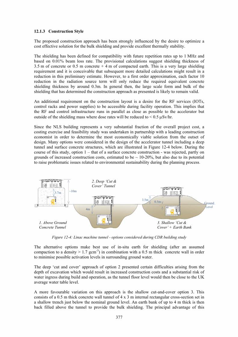
377

12.1.3 Construction Style

The proposed construction approach has been strongly influenced by the desire to optimize a cost effective solution for the bulk shielding and provide excellent thermally stability.

The shielding has been defined for compatibility with future repetition rates up to 1 MHz and based on 0.01% beam loss rate. The provisional calculations suggest shielding thickness of 3.5 m of concrete or 0.5 m concrete + 4 m of compacted earth. This is a very large shielding requirement and it is conceivable that subsequent more detailed calculations might result in a reduction in this preliminary estimate. However, to a first order approximation, each factor 10 reduction in the radiation source term will only reduce the required equivalent concrete shielding thickness by around 0.3m. In general then, the large scale form and bulk of the shielding that has determined the construction approach as presented is likely to remain valid.

An additional requirement on the construction layout is a desire for the RF services (IOTs, control racks and power supplies) to be accessible during facility operation. This implies that the RF and control infrastructure runs in parallel as close as possible to the accelerator but outside of the shielding mass where dose rates will be reduced to < 0.5 μSv/hr.

Since the NLS building represents a very substantial fraction of the overall project cost, a costing exercise and feasibility study was undertaken in partnership with a leading construction economist in order to determine the most economically viable solution from the outset of design. Many options were considered in the design of the accelerator tunnel including a deep tunnel and surface concrete structures, which are illustrated in Figure 12-4 below. During the course of this study, option 1 – that of a surface concrete construction - was rejected, partly on grounds of increased construction costs, estimated to be ~ 10-20%, but also due to its potential to raise problematic issues related to environmental sustainability during the planning process.

Figure 12-4: Linac machine tunnel - options considered during CDR building study

The alternative options make best use of in-situ earth for shielding (after an assumed compaction to a density > 1.7 gcm-3) in combination with a 0.5 m thick concrete wall in order to minimise possible activation levels in surrounding ground water.

The deep ‘cut and cover’ approach of option 2 presented certain difficulties arising from the depth of excavation which would result in increased construction costs and a substantial risk of water ingress during build and operation, as the tunnel floor level would then be close to the UK average water table level.

A more favourable variation on this approach is the shallow cut-and-cover option 3. This consists of a 0.5 m thick concrete wall tunnel of 4 x 3 m internal rectangular cross-section set in a shallow trench just below the nominal ground level. An earth bank of up to 4 m thick is then back filled above the tunnel to provide the bulk shielding. The principal advantage of this

1. Above Ground Concrete Tunnel

2. Deep ‘Cut & Cover’ Tunnel

3. Shallow ‘Cut & Cover’ + Earth Bank

~10m 3.7m

4m

3.5m 0.5m Ground Level

378

approach is that the ground excavations required where the tunnel emerges into the large areas formed by the experimental hall downstream, and the injector hall upstream, are then much less than if the tunnel had been a deep buried structure. Moreover, the earth from the excavations at either end can be used to provide the earth bank mounds that cover the linac and FEL hall tunnel (see later) so that the nett amount of earth moved on or off the site approaches zero. Since there is an estimated >60,000 m3 of earth displaced, which would attract a considerable disposal tax in the UK if taken off site, this represents a substantial cost saving. The earth cover also provides excellent thermal stability.

During the building feasibility study it became apparent that consolidation of the earth mound may produce significant settlement shifts in the level of 1st floor RF services building relative to the tunnel below of the order ~ 0.1m or more. A network of concrete pillars supporting the RF service building from the tunnel roof were envisaged to mitigate this. However, this solution presented it own construction problems of how to readily back fill the soil for the earth mound. After due consideration the preferred design for the linac tunnel construction was ultimately realised as a variation of the shallow ‘cut and cover’ option but with the RF services building at ground floor level and offset to the side as is illustrated as option 4 in Figure 12-5 below.

Figure 12-5: Linac machine tunnel – typical cross-section of option selected for building study

In this configuration, the personnel access labyrinth from the linac tunnel will pass under and emerge on the far side of the RF service building. Along the ‘pass-under’ only approximately 1.2 m of combined earth & concrete shielding separate the tunnel from the RF services above. However, this section does not ‘see’ the linac scatter directly as it emerges at a right angle from the chicane that exits from the tunnel. It is anticipated that the double 90º bend will reduce the scatter dose rates at this point to a level to ensure the reduced shielding bulk at the ‘pass under’ is sufficient, although calculations will be required to confirm this.

Note that none of the cross-sections of the machine tunnel indicate any form of pile foundations. Such supports may be required to reduce differential settlement of the tunnel to acceptable levels (<2 mm/year) following the build period and installation of the survey network. Although such an option has been costed and verified as entirely feasible, its implementation will depend very much on geotechnical aspects of the local site that is ultimately selected.

+3.5m

-4m

0m

+1.5m

Personnel access labyrinth

1.8m width keep clear access

Linac tunnel internal 3x4m

Waveguide labyrinth

Cryo, electrical & cooling services

RF Services building

4. Shallow ‘Cut & Cover’ w/ Ground Level RF Services

SECTION LOOKING ALONG BEAM

DIRECTION

IOT racksLEVEL

379

12.1.4 Linac Tunnel

The linac tunnel, approximately ~400 m in length, houses numbers 2 to 18 of the accelerator cryomodules which, along with associated beam transport systems (bunch compressors, collimators), comprise the linear accelerator. The first cryomodule in the overall linac transport is associated with the photo injector and is housed within the injector building.

A cross section of the linac tunnel is shown in Figure 12-5 above. In this view the electrical, cooling service runs are apparent mounted on the wall adjacent to the RF coupler side of the cryomodule, whilst HVAC (Heating/Ventilation/Air Con.) and other services run at high level on the labyrinth egress side of the tunnel. Interconnections between strings of cryomodule require that the cryo services run in a large diameter pipe. This is shown at the upper right hand corner of the tunnel cross section of Figure 12-5 and also in the 3D visualisation in Figure 12-6 below.

Personnel access and emergency exit from the tunnel will be via a stairwell labyrinth periodically located approximately every 90 m along the tunnel. Large radiation aperture services such as HVAC ducts will connect to outside air handling units along high levels routes in these labyrinths. At certain locations adjacent to the labyrinths, goods lifts can also be implemented for light equipment access (<1 T). All other large and heavy equipment including the estimated 6 Tonne accelerator modules will enter or exit at the injector hall end of the tunnel and be transported into place via skates or air pads down the access side of the tunnel length. For this reason one side of the tunnel must always be kept clear of obstruction or services.

Figure 12-6: Linac tunnel & RF services building – 3D cutaway visualization

12.1.5 RF & Services Building

The present design concept for RF power envisages the use of eight IOT units per accelerating module with each IOT requiring floor space for 3 x 19” full height rack units. Additional space for magnet power supplies, vacuum and control racks will also be required. All of these services will be located in a separate building at ground floor level immediately adjacent to the linac tunnel with always 4 m of earth shielding between them to facilitate access to RF services whilst the machine is running.

Within the RF service building, the IOT sources will be located directly adjacent to the corresponding accelerator modules. The intervening spaces between cryomodules,

Option for light goods lift shaft here

8 x WR650 waveguides grouped in pairs through 4 labyrinths. Only one cryomodule set shown for clarity. .

From photo‐injector & A02 BC1

BC2

Cryomodule A03

RF services building

Personel Access Labyrinth (spaced 90m apart)

HVAC ducts

IOTs & control racks

Cryomodule Interconnection pipe

380

corresponding to the locations of the laser heater and the bunch compressors…etc will be used to house laser rooms, magnet power supplies and control racks. Such an arrangement will minimize the length of waveguide and cable runs.

The design of the waveguide labyrinth is critical as they must be kept short as possible but also represent the largest open aperture for potential transmission of scattered radiation from the linac tunnel to the potentially occupied RF services building. There are 8 x WR650 type waveguides in 4 pairs per cryomodule, with each pair passing through a 1 x 0.25m labyrinth slot The labyrinths feed up from the cryomodule to the linac tunnel roof and through a 90° bend and then immediately horizontally across through the earth mound (housed in protective duct) to the RF service area. The single elbow joint will be made accessible for installation or maintenance from within the linac tunnel. Other electrical services for power and control will be dispersed between the waveguides. Overall there will be 18x4= 72 labyrinths for the cryomodules, plus a further 72 distributed downstream of the linac for all other electrical services required for the magnet, vacuum and control instrumentation in the spreader arcs and diagnostics downstream

Overall there are an estimated ~830 racks for vacuum, power supply and other control instrumentation. This includes the large contingent of (3x8x18)=432 racks that comprise the triplet sets providing control and RF power to the 8 x 16 kW IOT units at each of the 18 accelerator modules. The design of the RF services building includes a contingency overhead which allows space for a further 50% increase in the overall number of racks.

Apart from HVAC which exit via the personnel routes, other large aperture services such as the Ø200mm cooling water and Ø600mm cryo-service pipes will enter and exit the tunnel at a single point via a dedicated service tunnel to the ancillary cryoplant building (see later Section).

12.1.6 Injector Hall

The injector hall building houses the photo-injector gun and the first accelerating module for 1st phase (1 kHz) operation and a second photo-injector branch for the future 2nd phase high repetition rate (1 MHz) operation. The photo-injector branches run parallel for 40 m until angling at 6º to meet at a merge point located within the linac tunnel. This is shown in the plan and side elevation engineering layout of Figure 12-8 and also the 3D visualisation Figure 12-7 below.

Figure 12-7: Injector building – 3D visualisation section

PHOTO‐INJECTOR AREA WITH ROOF CUTAWAY

Cryo‐pipe labyrinths

Injector building work areas

Cryo‐pipe labyrinth from linac to injector area

2nd phase Photo‐injector

Gun klystron & cooling plant area

Cryomodule delivery & access

2m concrete (cutaway)

Linac tunnel & RF service building

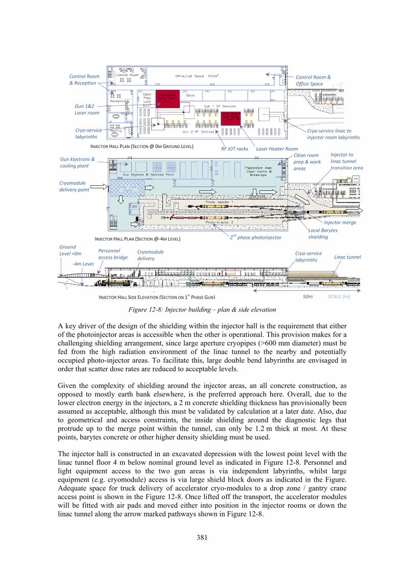
381

Figure 12-8: Injector building – plan & side elevation

A key driver of the design of the shielding within the injector hall is the requirement that either of the photoinjector areas is accessible when the other is operational. This provision makes for a challenging shielding arrangement, since large aperture cryopipes (>600 mm diameter) must be fed from the high radiation environment of the linac tunnel to the nearby and potentially occupied photo-injector areas. To facilitate this, large double bend labyrinths are envisaged in order that scatter dose rates are reduced to acceptable levels.

Given the complexity of shielding around the injector areas, an all concrete construction, as opposed to mostly earth bank elsewhere, is the preferred approach here. Overall, due to the lower electron energy in the injectors, a 2 m concrete shielding thickness has provisionally been assumed as acceptable, although this must be validated by calculation at a later date. Also, due to geometrical and access constraints, the inside shielding around the diagnostic legs that protrude up to the merge point within the tunnel, can only be 1.2 m thick at most. At these points, barytes concrete or other higher density shielding must be used.

The injector hall is constructed in an excavated depression with the lowest point level with the linac tunnel floor 4 m below nominal ground level as indicated in Figure 12-8. Personnel and light equipment access to the two gun areas is via independent labyrinths, whilst large equipment (e.g. cryomodule) access is via large shield block doors as indicated in the Figure. Adequate space for truck delivery of accelerator cryo-modules to a drop zone / gantry crane access point is shown in the Figure 12-8. Once lifted off the transport, the accelerator modules will be fitted with air pads and moved either into position in the injector rooms or down the linac tunnel along the arrow marked pathways shown in Figure 12-8.

2nd phase photoinjector

Injector merge

Cryomodule delivery point

Linac tunnel

Gun klystrons & cooling plant

Clean room prep & work areas

Cryo‐service labyrinths

Gun 1&2 Laser room

Laser Heater Room

Control Room & Office Space

RF IOT racks

SCALE (m)

Ground Level +0m

‐4m Level Cryo‐service labyrinths

Injector to linac tunnel transition area

Local Barytes shielding

Control Room & Reception

Cryo‐service linac to injector room labyrinths

50m INJECTOR HALL SIDE ELEVATION (SECTION ON 1ST PHASE GUN)

INJECTOR HALL PLAN (SECTION @‐4M LEVEL)

Personnel access bridge

Cryomodule delivery

INJECTOR HALL PLAN (SECTION @ 0M GROUND LEVEL)

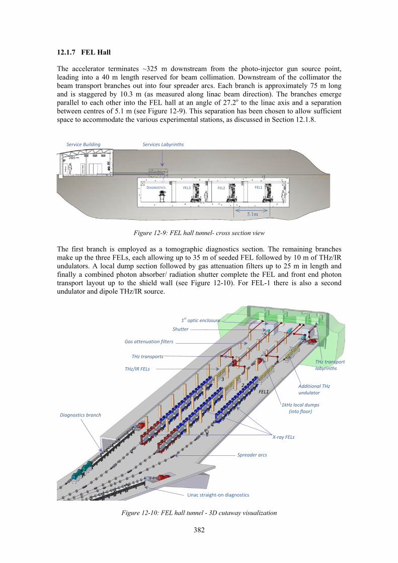
382

12.1.7 FEL Hall

The accelerator terminates ~325 m downstream from the photo-injector gun source point, leading into a 40 m length reserved for beam collimation. Downstream of the collimator the beam transport branches out into four spreader arcs. Each branch is approximately 75 m long and is staggered by 10.3 m (as measured along linac beam direction). The branches emerge parallel to each other into the FEL hall at an angle of 27.2o to the linac axis and a separation between centres of 5.1 m (see Figure 12-9). This separation has been chosen to allow sufficient space to accommodate the various experimental stations, as discussed in Section 12.1.8.

Figure 12-9: FEL hall tunnel- cross section view

The first branch is employed as a tomographic diagnostics section. The remaining branches make up the three FELs, each allowing up to 35 m of seeded FEL followed by 10 m of THz/IR undulators. A local dump section followed by gas attenuation filters up to 25 m in length and finally a combined photon absorber/ radiation shutter complete the FEL and front end photon transport layout up to the shield wall (see Figure 12-10). For FEL-1 there is also a second undulator and dipole THz/IR source.

Figure 12-10: FEL hall tunnel - 3D cutaway visualization

Diagnostics branch

X‐ray FELs

THz/IR FELs

Gas attenuation filters

THz transports

1kHz local dumps (into floor)

Linac straight‐on diagnostics

Spreader arcs

Additional THz undulator

1st optic enclosure

Shutter

THz transport labyrinths

3 2

FEL1

Services LabyrinthsService Building

DIAGNOSTICS FEL3 FEL2 FEL1

5.1m

383

FEL Radiation Transport: the positioning of each FEL in the hall primarily depends on the optimal placing of the ends of the FEL with respect to the 1st optic. This is driven by ablation thresholds. The current minimum distances have been specified (see Chapter 7) as ~38, 60 & 40m for FEL-1, 2, 3 respectively. Optimal placing with respect to the first optic must be balanced against the need to fit all other necessary equipment downstream of the FEL – including gas attenuators, e-beam transport & dump, photon transport (THz & X-ray) and shutters – and also by factors upstream of the FEL – such as maintaining optimum HHG transport lengths and a 10 m reserved space allowance for extra undulator length in case fallback SASE mode operation is required, or for other developments.

By a) placing FEL-1 & 3 first optics within the FEL hall, just upstream of the shield wall, b) staggering the FEL positions and c) placing the 10 m SASE contingency upstream for FEL 1 & 3, an optimal placing has been achieved as shown in Figure 12-11, which shows the ideal 1st optic distances in red. Even with this manipulation, it is evident from the layout that the necessary lengths of equipment downstream of FEL-3 determine that it is not possible to maintain the end at the optimum point from the 1st optic, but instead extends it ~5 m beyond. Minor adjustments to the beamline focal lengths downstream of the 1st optic will be required to accommodate this.

Figure 12-11: FEL hall – showing THz transport, FELs & relative optic positions

The concept design exercise highlights the importance of a ‘holistic’ approach to any future detailed design of the FEL hall. That is, the various design aspects of the facility – from the defining of minimum ablation distances based on predicted source parameters to the beamline /experimental layout and the HHG scheme – must all be comprehensively assessed in order to obtain an optimum building and engineering layout.

THz Radiation Transport: The THz transport concept is described in Section 7.8, but its implementation is significantly dependent on the local engineering and building layout. In the engineering concept as depicted for FEL-1 in Figure 12-12, diverging THz radiation is extracted via a periscope type mirror arrangement positioned very close to the end of the THz undulator.

10m SASE contigency

10m

10m

40m

38m

60m

FEL 3 430‐1000eV

FEL 2 250‐850eV

FEL 1 50‐300eV

FEL HALL PLAN SECTION VIEW

FEL2 SIDE ELEVATION SECTION

Ideal minimum 1st optic distance

INSET RIGHT ‐ THZ LABYRINTH SIDE ELEVATION SECTION

Undulators THz/IR undulator Beam dump

THz transport labyrinth

Gas attenuation filter

THz extraction mirror & periscope

Shutter

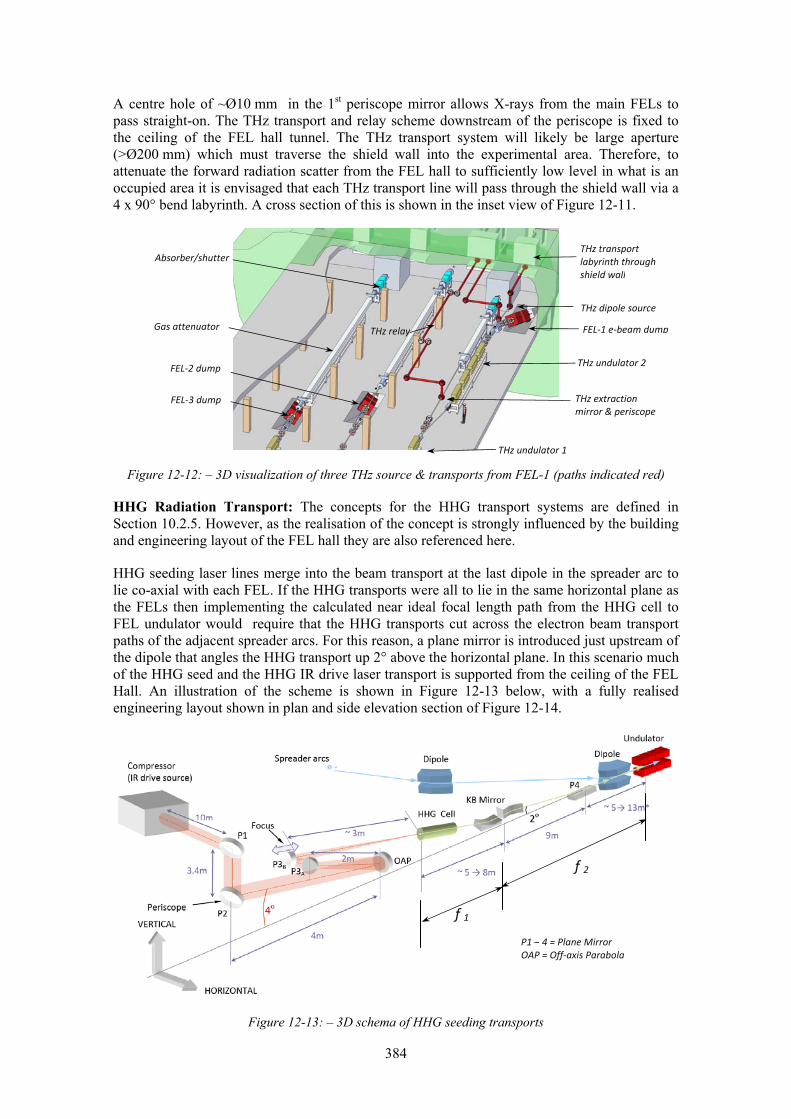
384

A centre hole of ~Ø10 mm in the 1st periscope mirror allows X-rays from the main FELs to pass straight-on. The THz transport and relay scheme downstream of the periscope is fixed to the ceiling of the FEL hall tunnel. The THz transport system will likely be large aperture (>Ø200 mm) which must traverse the shield wall into the experimental area. Therefore, to attenuate the forward radiation scatter from the FEL hall to sufficiently low level in what is an occupied area it is envisaged that each THz transport line will pass through the shield wall via a 4 x 90° bend labyrinth. A cross section of this is shown in the inset view of Figure 12-11.

Figure 12-12: – 3D visualization of three THz source & transports from FEL-1 (paths indicated red)

HHG Radiation Transport: The concepts for the HHG transport systems are defined in Section 10.2.5. However, as the realisation of the concept is strongly influenced by the building and engineering layout of the FEL hall they are also referenced here.

HHG seeding laser lines merge into the beam transport at the last dipole in the spreader arc to lie co-axial with each FEL. If the HHG transports were all to lie in the same horizontal plane as the FELs then implementing the calculated near ideal focal length path from the HHG cell to FEL undulator would require that the HHG transports cut across the electron beam transport paths of the adjacent spreader arcs. For this reason, a plane mirror is introduced just upstream of the dipole that angles the HHG transport up 2° above the horizontal plane. In this scenario much of the HHG seed and the HHG IR drive laser transport is supported from the ceiling of the FEL Hall. An illustration of the scheme is shown in Figure 12-13 below, with a fully realised engineering layout shown in plan and side elevation section of Figure 12-14.

Figure 12-13: – 3D schema of HHG seeding transports

THz relay

THz undulator 1

THz extraction mirror & periscope

THz undulator 2

THz dipole source

THz transport labyrinth through shield wall

FEL‐1 e‐beam dump

FEL‐2 dump

FEL‐3 dump

Gas attenuator

Absorber/shutter

P1 – 4 = Plane Mirror OAP = Off‐axis Parabola

f 1

f 2

385

A key optic parameter of the HHG transport is the ratio of focal lengths f1 / f2 - where f1 is the distance between the HHG gas cell and the KB focussing mirror pair and f2 between the KB mirror and FEL undulator - as these define the seeding source size and Rayleigh length. Because the FELs have been staggered in the FEL hall to optimise their positions relative to the first optic upstream, the distance between the undulator and the last dipole in the spreader varies according to the FEL. It is provisionally assumed that, dependent on the FEL, a range of installed focal lengths f2 from 14 to 22 m will be matched by variation in f1 from 5 to 8 m, thereby keeping the overall defocusing ratio f1/ f2 constant at around 0.35. This strategy requires a comprehensive review during detail design phase. A fallback position is to maintain uniform HHG transport paths and allow more flexibility in placing of the FELs relative to their optimum 1st optic positions.

Upstream of the HHG cell the light is infrared and therefore easier to transport using conventional optics. The focus into the cell is provided by an off-axis parabola (OAP) located 5m upstream and suspended from the ceiling. To maintain the required focal length to fit within the FEL hall and also allow for adjustment a precision slide retro-reflector arrangement (mirror set P3) is located immediately upstream.

Figure 12-14: HHG transport engineering layout

The three HHG IR drive lasers are provisionally located in the RF service building with the IR transported across the tunnel roof to feed into HHG cells located within the FEL tunnel at ceiling height via the periscope arrangement P1/P2. Alternatively, the laser rooms could be located in a purpose built ancillary building on the opposite side of the linac tunnel. This would be preferred from a shorter optical transport, and therefore timing synchronisation, point of view but adds additional building costs and problems extending services infrastructure. A cost benefit study of these options should be undertaken during the detailed design phase. The two alternative options for the HHG drive laser transports are indicated in Figure 12-15 below.

386

Figure 12-15: Showing possible alternative locations for HHG drive laser rooms.

Beam Dumps: For the first phase 1 kHz operation, electrons downstream of the FELs are diverted at a 20° angle down to beam dumps located in concrete ‘pits’ set into the FEL hall floor to minimise additional shielding. The proposed arrangement is similar to that of the DESY FLASH facility where the dump path is also angled in the horizontal so that the dumps are offset laterally to the FEL axis. In this way they can be readily be craned out vertically for maintenance or replacement, without disturbing photon transport lines. The layout of 1 kHz dumps can be seen in Figure 12-11 and Figure 12-12.

For 1 MHz operation the design of the beam dump becomes a far more challenging prospect. The engineering of 450 kW cooling systems within a high radiation activated environment has led to the decision that a single dump is the only viable option. The concept of the 1 MHz dump is reported in Section 4.6. The single dump will be positioned towards the shield wall end but just outside of the FEL hall, and located in a ‘bunker’ 6 m under ground level to provide sufficient bulk shielding. A concrete shaft covered by shield blocks will connect the bunker to ground level to provide vertical crane access for removal of the dump. The dump will be encased in shielding material thick enough to facilitate full extraction to a safe store by appropriate handling techniques and is therefore likely to mass more than 10 Tonne.

A preliminary layout (Section 4.6.3) shows how electron beam transport arcs could be engineered to take the electrons to be dumped from each branch vertically up and over the straight-on FEL and photon transport lines through to a common ceiling level beam dump path at the end of the FEL hall before being angled down towards the dump bunker outside. Although this outline design for a 1 MHz dump appears feasible, the study has revealed the complexities involved. Further detailed work is therefore needed to ensure full compatibility with the FEL hall from the outset.

12.1.8 Experimental Hall and Laser Mezzanine

The experimental hall is enclosed by a standard steel frame, highly insulated panel clad construction built onto foundations separated from the 0.5 m thick monolithic slab concrete that forms the experimental floor. This floor is level with the linac tunnel, and therefore constructed in an excavation 4 m below surrounding ground level.

An indicative layout of the proposed beamline schemes within the experimental hall is shown in Figure 12-16. Each shaded box represents experimental station enclosures or reserved floor

FEL HALL CROSS SECTION WITH HHG

DRIVE LASER TRANSPORTS

OPTION A) BASELINE – LOCATED IN RF SERVICE BUILDING OPTION B) DEDICATED HHG DRIVE LASER BUILDING

387

areas of 4 x 8 m. A 3D visualisation is shown in Figure 12-17. Photon transport is discussed in Chapter 7.

Figure 12-16: Experimental hall layout

Shielding: It is envisaged that straight-through penetrations through the shield wall by the X-ray transport lines will be as small an aperture as possible (~Ø10 mm). Nevertheless, it is still anticipated that shielded enclosures (indicated in red) will be required around the 1st or 2nd optic positions in to order reduce radiation doses to acceptable levels for general access within the experimental hall. The enclosure wall thickness – either in concrete or possibly lead - will be determined from detailed radiation scatter calculations.

In addition to the 1st /2nd optic enclosures, a shielded enclosure will be required around the end station of FEL-2, where a 5 MeV electron gun is envisaged for carrying out various experiments in combination with the FEL radiation. The layout and concept is described in Section 7.9.

The remaining experimental stations may require lightly shielded enclosures due to scatter from up to 5 keV harmonic FEL content, but otherwise the interaction chambers themselves may provide sufficient shielding. In this case then the shaded boxes indicated in the Figure may well just indicate standard air-conditioned cabin type rooms.

High Power Laser Mezzanine: The possibility of carrying out pump-probe experiments with FEL radiation in combination with high power conventional lasers is an essential requirement of the science case. The current proposal is that lasers will be located close to the experimental area on a substantial mezzanine 4 m above the experimental floor level (see Figure 12-16 and Figure 12-17). This arrangement has several distinct advantages in that it avoids the horizontal criss-cross of laser transport paths which restricts access on the experimental floor. In addition it allows maximum flexibility for the rearrangement of the beamline layout in the future, should the need arise.

75m

EXPERIMENTAL HALL AREA (@ ‐4M LEVEL)

Direct Focus

Grating Mono

DCM

Labs & work areas

Grating Mono

Direct Focus

Direct Focus

Pulse‐length Preserving Grating

Grating MonoExtension Space

3m Shield wall

‐4m Level

Control rack mezzanine

1std Optic enclosure

HPR Laser Mezzanine

EXPERIMENTAL HALL SIDE ELEVATION (SECTION ON FEL2)1st Optic enclosure

Laser Mezzanine

5MeV gun shielded enclosure

Cooling & HVAC services for experimental hall

FEL 3 430‐1000eV

FEL 2 250‐850eV

FEL 1 50‐300eV

388

For vibrational stability the mezzanine is envisaged to be a substantial construction, which for the building feasibility study was conceived as a 0.5 m thick concrete floor supported on a 7x4 matrix of 0.6 x 0.6 m2 columns. Further consideration will be given to this concept during the detailed design stage.

Figure 12-17: Experimental hall 3D visualization

Craneage of heavy equipment across beamlines will be by local jib type radial arms strategically positioned so that universal floor coverage on a point-to-point basis is achieved.

The experimental hall footprint is ~2450 m2. By considering the laser mezzanine as a stable ‘experimental quality’ floor, the available area increases by 800 m2 to 3250 m2. This compares very well with other facilities. For example, the total experimental floor space for three full insertion device beamlines of the Diamond synchrotron (& including all the bending magnet lines in between) totals ~1400m2. Thus, the size and scope of the proposed experimental hall allows considerable potential for extensions, additions or reconfigurations of the existing beamlines in the future.

12.1.9 Ancillary Building

The ancillary building is shown in Figure 12-18. It houses the cryogenics and general services plant at a central location along the length of the linac and offset to the accelerator tunnel by approximately 30m. This distance has been provisionally set as a compromise between maximising distance in order to attenuate ground-borne vibration from the plant compressors (which could adversely impact on the facility performance) and minimising cryogenic transport lengths, which add to cryogenic losses resulting in increased costs. Ref [1] has been used a guide in this regard but further studies should be conducted prior to detailed building design to confirm this as a reasonable operating distance. Additional measures will be taken to damp vibrations generated in the building and isolate the building foundation from the sub structure.

Up to 800m2 Lab & Prep space on 2 floors

~75m

Local control rack (100+) mezzanine located here (omitted for clarity)

CUTAWAY SECTION OF EXPERIMENTAL HALL

LOOKING TOWARD FELS

High Power Laser Mezzanine Floor 20x40m = 800m2

Experimental Area 2450m2

up to 500m2 auxillary floor space

Front end optic shielded enclosures

FELs

Shield wall

389

The 30m distance from the linac to the ancillary building should also be sufficient to ensure acceptable radiation scatter levels for anyone working in the ancillary plant near to the service tunnel access. However, as in the case above, this assumption should be subject to further study prior to detailed design. As a fallback, a simple chicane in the tunnel could be incorporated if this is required.

Figure 12-18: Ancillary building plan schematic layout & 3d visualisation cutaway

The building enclosure is 90 x 25 m, which includes sufficient space for cryoplant sized on the basis of an industrial study (see next Section), chiller heat exchangers and boiler rooms and also four part enclosed electrical transformer pens providing power to these services. Immediately adjacent to the building are large open compounds housing at one end 400m3 of He buffer tanks (stacked in two tiers) along with ~4 MW capacity air blast cooling units serving the cryoplant compressors, and at the other end approximately 5 – 6 MW capacity of air blast units sufficient for all other facility cooling requirements.

The size of the cryo-plant enclosure itself includes reserved space of 500 m2 for four helium compressors and adjacent rooms housing the oil removal system, helium refrigerator cold box and secondary heat exchange cold box plus a valve/control distribution room.

In addition to this ancillary building providing the main services to the facility there is an additional 200 m2 space reserved at the extreme downstream end of the RF services building to more locally provide HVAC & cooling services to the experimental area.

CUTAWAY LOOKING

ALONG BEAM DIRECTION

(RF SERVICE BUILDING REMOVED)

Cryo valve junction (TBD)

Service tunnel

Cryo service pipes – 2 legs

Cryoplant Building

PLAN VIEW ANCILLARY BUILDING (CRYOPLANT & SERVICES)

~90m

25m

~30m

Airblast compound sufficient for ~4MW cryoplant cooling

400m3 He Buffer Vessels

Airblast compound sufficient for all remaining 5MW facility cooling

Linac tunnel Beam Direction

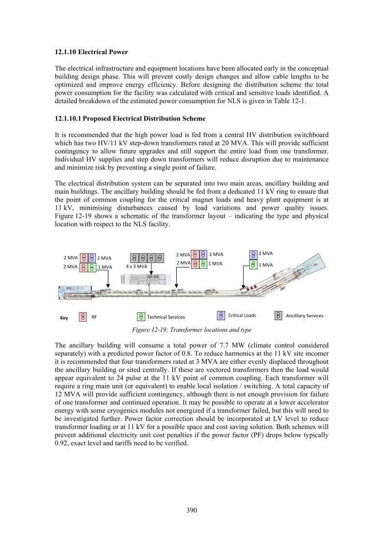
390

12.1.10 Electrical Power

The electrical infrastructure and equipment locations have been allocated early in the conceptual building design phase. This will prevent costly design changes and allow cable lengths to be optimized and improve energy efficiency. Before designing the distribution scheme the total power consumption for the facility was calculated with critical and sensitive loads identified. A detailed breakdown of the estimated power consumption for NLS is given in Table 12-1.

12.1.10.1 Proposed Electrical Distribution Scheme

It is recommended that the high power load is fed from a central HV distribution switchboard which has two HV/11 kV step-down transformers rated at 20 MVA. This will provide sufficient contingency to allow future upgrades and still support the entire load from one transformer. Individual HV supplies and step down transformers will reduce disruption due to maintenance and minimize risk by preventing a single point of failure.

The electrical distribution system can be separated into two main areas, ancillary building and main buildings. The ancillary building should be fed from a dedicated 11 kV ring to ensure that the point of common coupling for the critical magnet loads and heavy plant equipment is at 11 kV, minimising disturbances caused by load variations and power quality issues. Figure 12-19 shows a schematic of the transformer layout – indicating the type and physical location with respect to the NLS facility.

Figure 12-19: Transformer locations and type

The ancillary building will consume a total power of 7.7 MW (climate control considered separately) with a predicted power factor of 0.8. To reduce harmonics at the 11 kV site incomer it is recommended that four transformers rated at 3 MVA are either evenly displaced throughout the ancillary building or sited centrally. If these are vectored transformers then the load would appear equivalent to 24 pulse at the 11 kV point of common coupling. Each transformer will require a ring main unit (or equivalent) to enable local isolation / switching. A total capacity of 12 MVA will provide sufficient contingency, although there is not enough provision for failure of one transformer and continued operation. It may be possible to operate at a lower accelerator energy with some cryogenics modules not energized if a transformer failed, but this will need to be investigated further. Power factor correction should be incorporated at LV level to reduce transformer loading or at 11 kV for a possible space and cost saving solution. Both schemes will prevent additional electricity unit cost penalties if the power factor (PF) drops below typically 0.92, exact level and tariffs need to be verified.

2 MVA

2 MVA

2 MVA

1 MVA

2 MVA

1 MVA

2 MVA

2 MVA

2 MVA

1 MVA 4 x 3 MVA

RF Critical LoadsTechnical Services Ancilliary Services Key

391

Table 12-1: Estimated power consumption

A Technical Equipment No of racks

Power/rack

Total load

kW

1 Electron gun 620

2 RF Accelerator (IOT) 144 4267*

3 Power converters (magnets) 90 2300

4 Controls & Instrumentation:

5 Electron gun control (1KHz only) 10 2 20

6 Vacuum 70 4 280

7 Diagnostics 24 2 48

8 Personnel Safety 6 2 12

9 Network/control 28 2 56

10 Undulator - controls & Aux 62 2 124

11 RF Control & Auxiliaries 288 1 288

12 Motion control 10 2 20

13 Cryogenic system 15 3 45

14 Beamlines (3 beamlines at 20 kW each) 50 60

15 Laser – Photocathode / heater 3 40

16 Laser – 3 x HHG 15 150

17 Laser – 3 x HPR 15 300

Total No. of racks 830 Total machine kW 7932

B Services

1 Lighting 30

2 Climate Control Injector + accelerator tunnel area 500

(heating not required) Experimental and ancillary area 300

3 Chiller System Magnets, Cryo and RF 3350**

4 Cryogenics plant RF Modules 3040

5 Water Pumps Chilled, demin, inhib (Cryo) 250

6 Compressed Air 200

7 Offices/laboratories 50

Total ancillary load kW 7720

Total NLS operational electrical load 15652

Total NLS Electrical Infrastructure Requirement (10% contingency) 17217 * Note that maximum RF accelerator power is calculated for a peak 16 kW per IOT which is only required during commissioning tests. The calculation assumes 60% efficiency of IOT and 90% power supply efficiency. Therefore ‘plug power’= (16kW x 8 x 18)/(0.6x0.9) = 4267 kW. During normal operation only about ¼ of this is required. Therefore the Table indicates overall installed infrastructure requirements and the operational power consumption of the facility will be ~ 3MW less than this.

** Based on total heat load requirement – see Section -12.1.11 multiplied by assumed typical coefficient of performance of ~ 0.3

392

The main buildings should have two dedicated 11 kV rings. One should provide the necessary power to support the critical and power converter loads of the injector, accelerator, FEL Hall, and Experimental Hall with the other supporting the general loads and lighting, plus anything else that has load variations and can affect the facility operating stability. This can be the same ring main as that used for the ancillary building.

The predicted total power consumption for the main buildings is 7.7 MW (includes climate control) at 2.25 GeV. The RF system accounts for approximately 45% of the total power and consequently will be considered separately from the rest of the electrical distribution within the main buildings.

12.1.10.2 RF System

The maximum power requirement for the RF system is 4.27 MW at 2.25 GeV. The proposed configuration for the RF system comprises 144 low power amplifiers (IOTs). These relatively low power amplifiers will employ 6 pulse DC converters resulting in significant harmonic levels at the HV input supply.

Irrespective of the eventual choice of amplifiers the issue of harmonics will remain and needs to be addressed. Unfortunately passive harmonic correction has limited effect and although active harmonic correction is effective it is also expensive. The most cost effective and relatively simple solution to implement is the use of vectored transformers. If the RF load is separated into half or quarters, the transformers could be vectored to provide a 12 or 24 pulse load at 11 kV. Predicted harmonic levels will be calculated in more detail for the RF system as part of the detailed design.

To accommodate the predicted load four 2 MVA transformers would provide plenty of contingency in terms of power availability. These four vectored transformers would then provide the 24 pulse optimum load at 11kV. This over-rating of the transformers is recommended to compensate for the harmonics caused by the power converter loads feeding the amplifiers, which increase heating of the transformer. They should also be positioned and connected as dual transformers, normal operation would be independent, but during maintenance and failure one transformer could sustain the load of half the RF system.

Typical power factor for an RF system is between 0.8 and 0.9. It is recommended that power factor correction is provided at each of the four LV distribution boards. Again the cost and performance benefits of HV and LV PFC should be investigated. It is also possible that the power converters will be purchased with PFC included.

The power consumption breakdown figures for each IOT will require 16 kW of RF power. With an efficiency of 60%, this will equate to 27 kW of AC input power. The DC power converter will be 90% efficient and a total input ac power of ~30 kW is estimated for each IOT.

It is recommended that a main distribution board with a minimum of 8 fuse-switch outputs are installed for each transformer. Each of these transformers will supply a quarter of the RF system. Total load on each transformer will be at 2.25 GeV – 36 IOT x 30 kW ≈ 1.1MW, considerably under the 2 MVA rating.

12.1.10.3 Magnets, Critical Loads and General Distribution

The remaining electrical consumption for technical systems (excluding ancilliary building services) is predicted to be ~3.6 MW which is distributed throughout the main buildings. It is considered impractical to install one large transformer to support this wide variety of loads. The long cable lengths required for this solution would increase capital and running costs and as well as installation costs. The harmonics generated from the large quantity of low power DC magnet power converters will be high. A typical switch-mode design is likely to employ only

393

6-pulse or even 2-pulse operation. This combined with the vacuum ion pumps, auxiliary switch-mode power supplies and general electronic equipment will ensure that the G5/4 power quality levels are exceeded.

Again the most cost effective solution is to install vectored transformers to provide a minimum of a 12-pulse load to the 11 kV system. Detailed harmonic levels cannot be provided until further measurements and calculations are completed as part of a detailed design phase.

The facility consists of highly sensitive measuring and control equipment in both the accelerators and the experimental areas. There are also safety critical systems such as personnel safety, accelerator controls and an oxygen depletion system. It is important that the heavy power equipment and general electrical distribution are decoupled from this equipment.

The magnets and critical loads have an estimated load of ~3.1 MW and to provide a reliable and clean electrical supply to this critical equipment the point of common coupling should be set at 11 kV. This will minimize any mains disturbances caused by high power switching or faults within the general electrical distribution. It is recommended that four 2 MVA transformers are installed each supporting a quarter of the electrical consumption. Although this could be achieved with four 1 MVA transformers, over sizing the transformers allows the LV switch boards to be linked and will reduce facility downtime in case of a transformer failure. One transformer has enough capacity to support a half of the accelerator.

There are a number of reasons for employing this arrangement:

• Each quarter will have a dedicated transformer, supporting critical loads and the magnet power converters

• The critical loads can be fed via a 300 kVA UPS to maintain power during short disturbances with a hold-up time of about 5 to 10 minutes.

• The UPS will provide sufficient isolation between magnet loads and critical loads. • Each transformer has enough capacity to support a half of the total power consumption;

this will address issues such as maintenance and transformer failure. • Power factor correction should be included at each of the main LV distribution boards

with levels predicted at about 0.8. If this configuration is utilized then an allocation must include four 300 kVA UPS each with a bypass circuit to enable isolation during maintenance and system failure.

From each LV distribution board a power converter/general feed and a critical load (UPS backed) feed should be provided to switch-disconnectors at agreed locations throughout the building. These switch-disconnectors (isolators) should be of a type which can be fitted with trip coils so they can be operated by a remote power-off system (push-buttons in the machine tunnels) or other emergency system such as smoke detectors. Each switch-disconnector will supply a three-phase distribution board.

Power quality measuring equipment should be incorporated into the LV distribution boards. This will allow the effects of load changes to be monitored and electrical disturbances to be investigated. Otherwise such measurements will require internal access to a main LV distribution board necessitating a Live Working permit or isolation of the LV circuit; these need to be avoided.

A separate 11 kV ring main is required for general distribution such as offices, laboratories, lighting, cranes, mains sockets and localized compressed air and climate control. Again four vectored 1 MVA transformers would be sufficient evenly distributed along the building length to minimize voltage drop. LV switch boards could be linked to provide power in case of a transformer failure.

394

12.1.11 Cooling System

Table 12-2 shows the estimate of water cooling requirements for NLS. Temperature stability in the water supply is essential for many areas and especially for the magnet cooling in the beam transport system where control to at least ± 0.2 oC is desirable. This also applies to an even greater degree to the gun, where the cavity profile is controlled by individual control of multiple coolant channels to ± 0.1 oC is required. The overall heat load of the gun into a relatively small coolant volume will approach 100 kW.

Table 12-2: Estimated significant cooling water loads

System Cooling load (kW) Source

Gun RF & Magnets 410 1 kHz gun

Linac RF 3866 CW operation (RF IOT power less dump load)

Cryogenic plant 3040 Ref. electrical table & cryoplant section

Magnets 1800 Based on number count 260 quads & 60 dipoles

Dumps 400 Maximum at 1 MHz operation (at 1 kHz load 0.4 kW)

Vac Pumps & Racks - Assume 500kW heat lost in HVAC system – see below

Air compressors 200 Estimate based on other similar size facilities

Conventional Lasers 490 1xphotocathode, 1xlaser heater, 3xHHG, 3xHPR

HVAC 1100 HVAC cooling - see Section 12.2 for breakdown

Total 11306

Primary water cooling pumps and circuits will be specified to meet the cooling requirements of NLS. Primary chilled water circuits will supply the air conditioning systems as required to supplement the adiabatic air handling systems. Cooling water will also serve heat exchangers in secondary cooling circuits for de-ionized water. These secondary circuits will have water treatment, filtration, mixing valves and pump sets to achieve required pressure, temperature, volume flow and water quality. Conductivity of de-mineralized water will not exceed 0.1 µS/cm with 10 µm filtration. Circuits will have de-oxygenation to reduce copper corrosion.

Where possible, energy recovery options will be considered in order to make use of the waste heat, for example from the beam dumps.

12.2 Environmental Control

12.2.1 Heating, Ventilation and Air Conditioning (HVAC)

Packaged HVAC systems will be installed to satisfy both heating and cooling loads for the general accommodation areas and the more demanding technical areas of the accelerator tunnel and experimental hall. HVAC in the tunnel and experimental hall will be by direct gas-fired air handling induction systems for greater thermal control stability.

Only a very basic and highly provisional heating load has been calculated at this stage. Only a small proportion of the cooling load total as listed in the Table above will be accommodated by the packaged building HVAC cooling system. This will be dominated by perhaps a 5% overhead for magnets in the linac tunnel – amounting to ~165 kW and ventilation of the racks of around 500 kW. Alternatively racks could be enclosed in insulating rooms and ventilated by a separate system.

395

The system will be designed allowing for a minimum external temperature of -4 ºC and with 100 % saturation. Subject to suitable cooling and heating load profiles, CHP could be used to generate electricity and thermal energy for heating applications.

A breakdown of the HVAC loads in each of the provided areas is as follows:

• Injector hall including control rooms reception and general accommodation areas: approximate 150 kW capacity required – largely for make-up air as high insulative panelling is assumed.

• Linac and FEL tunnel: 200 kW capacity mostly all residual 5% venting from magnets. The thermal inertia of the tunnel means that even on the hottest day <50 kW is required for HVAC. This is chiefly to cool make-up air added from outside rather than any significant loss through direct heat transfer.

• RF & services building: 480 kW total capacity with the majority of this (400 kW) dominated by the ventilation of the racks*

• Experimental hall & beam line enclosures: 250 kW capacity. Highly insulative panel cladding and measures such as louvre windows to reduce solar gain fluctuations are assumed in building construction. Therefore total building environmental load is ~150 kW from make-up and heat transfer loss with the remaining load assumed to be from local beamline equipment and rack ventilation.

• Total ~1.1 MW Although the electrical tables indicated approx 850 kW of power is consumed by the racks – almost all of which is converted into heat , this is assumed to be a highly conservative figure used in order to size electrical infrastructure and likely to be only valid during short peak times during commissioning. For this reason we assume a lesser heat figure from the racks of 500 kW (400 kW within the RF service building and 100 kW in the experimental hall).

Thermal stability is a critical issue that will greatly affect NLS performance and is addressed in the next Section. Systems that provide temperature stability of ± 0.5 oC (stable stratified to >2 m from ground level) have been found economically viable at many other sites and often produce better performance over more local spans. This level of control is probably sufficient for the accelerator, FEL and Experimental Hall, but will need to be addressed further during a detail design phase (see also next Section on stability and alignment). The thermal inertia of the tunnel is so large that even extreme seasonal changes will produce negligible load (i.e. kWs) on the linac & FEL tunnel. A more relaxed conventional system can be used for offices and more conventional areas.

12.2.2 Gas, Liquid, Exhaust and COSHH Distribution Systems

The following conventional facilities will be required, and will be detailed at a later stage of the design process:

• COSHH exhaust systems. • Gas distribution including compressed air and possibly He & N2. Liquid Nitrogen may

also be required • Water main supplies will be required for make-up water to main heat exchange plant as

well as boilers and domestic local hot water heaters in toilets and fire hydrant systems. • Trade waste drainage system and bunds will be required.

12.2.3 Other Building Services Required

A non-exhaustive list of conventional building requirements to be expanded at a later stage of the design includes: artificial lighting, fire detection and alarm, telecommunications and data, security systems, safety alarm systems, building management system, lightning protection, public address system, information display systems, lifts.

396

12.3 Stability and Alignment

12.3.1 Stability

Successful operation of the NLS depends on maintaining electron and photon beam positions stable to the order of a few microns. It is therefore essential that a strategic approach is taken to control both mechanical and thermal stability. Both long and short term stability issues (from years to seconds) as well as high frequency motion must be addressed and suitably managed.

Even where active feedback can be employed to stabilize critical systems they rely on a passive background ‘noise’ environment that is quiet. For this reason the floor for the accelerating complex and photon transport must be very stable.

12.3.1.1 Ground Vibration

Figure 12-20 shows typical ground vibration power spectral densities (PSD) from various accelerator sites around the world [2] [3].

Figure 12-20: Generic ground noise spectrum of a typical quiet site

By integrating under the PSD profile one observes that >99% of all ground displacement lies below 1 Hz. This large motion at low frequency arises from powerful natural sources such as diurnal (0.001Hz) earth-moon interaction and the characteristic ocean swell at ~0.2 Hz. However, such very low frequencies have corresponding wavelengths of the order of many kilometres so that the movement across the facility site is correlated (i.e. all points move together) and therefore does not affect the operation of NLS. At frequencies near to and above 1 Hz, dependent on local site properties, the wavelength can approach the facility dimensions and start to have increasing effect (for example on synchronization over source to experiment distances). Until the ground properties are known at the NLS site we therefore follow the usual approach of disregarding all motion lower than 1 Hz. The PSD falls off strongly with frequency as 1/f4 so it is also reasonable to set 100 Hz as an upper limit.

The 1–100 Hz vibration spectrum is driven by ‘cultural noise’ – typically local, man-made noise arising from sources such as road traffic (often around 10 Hz), pumps, compressors etc. The

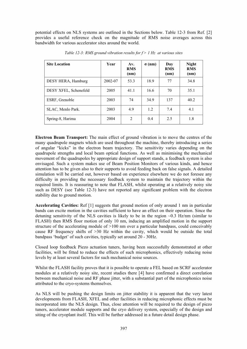
397

potential effects on NLS systems are outlined in the Sections below. Table 12-3 from Ref. [2] provides a useful reference check on the magnitude of RMS noise averages across this bandwidth for various accelerator sites around the world.

Table 12-3: RMS ground vibration results for f > 1 Hz at various sites

Site Location Year Av. RMS (nm)

σ (nm) Day RMS (nm)

Night RMS (nm)

DESY HERA, Hamburg 2002-07 53.3 18.9 77 34.8

DESY XFEL, Schenefeld 2005 41.1 16.6 70 35.1

ESRF, Grenoble 2003 74 34.9 137 40.2

SLAC, Menlo Park. 2003 4.9 1.2 7.4 4.1

Spring-8, Harima 2004 2 0.4 2.5 1.8

Electron Beam Transport: The main effect of ground vibration is to move the centres of the many quadrupole magnets which are used throughout the machine, thereby introducing a series of angular “kicks” in the electron beam trajectory. The sensitivity varies depending on the quadrupole strengths and local beam optical functions. As well as minimising the mechanical movement of the quadrupoles by appropriate design of support stands, a feedback system is also envisaged. Such a system makes use of Beam Position Monitors of various kinds, and hence attention has to be given also to their supports to avoid feeding back on false signals. A detailed simulation will be carried out, however based on experience elsewhere we do not foresee any difficulty in providing the necessary feedback system to maintain the trajectory within the required limits. It is reassuring to note that FLASH, whilst operating at a relatively noisy site such as DESY (see Table 12-3) have not reported any significant problem with the electron stability due to ground motion.

Accelerating Cavities: Ref [1] suggests that ground motion of only around 1 nm in particular bands can excite motion in the cavities sufficient to have an effect on their operation. Since the detuning sensitivity of the NLS cavities is likely to be in the region ~0.3 Hz/nm (similar to FLASH) then RMS floor motion of only 10 nm, inducing an amplified motion in the support structure of the accelerating module of >100 nm over a particular bandpass, could conceivably cause RF frequency shifts of >30 Hz within the cavity, which would be outside the total bandpass ‘budget’ of such cavities, typically set around 20 - 30Hz.

Closed loop feedback Piezo actuation tuners, having been successfully demonstrated at other facilities, will be fitted to reduce the effects of such microphonics, effectively reducing noise levels by at least several factors for such mechanical noise sources.

Whilst the FLASH facility proves that it is possible to operate a FEL based on SCRF accelerator modules at a relatively noisy site, recent studies there [4] have confirmed a direct correlation between mechanical noise and RF phase jitter, with a substantial part of the microphonics noise attributed to the cryo-systems themselves.

As NLS will be pushing the design limits on jitter stability it is apparent that the very latest developments from FLASH, XFEL and other facilities in reducing microphonic effects must be incorporated into the NLS design. Thus, close attention will be required to the design of piezo tuners, accelerator module supports and the cryo delivery system, especially of the design and siting of the cryoplant itself. This will be further addressed in a future detail design phase.

398

FELs: Studies for NLS [5] suggest that the electron beam trajectory must remain straight within 10% of the electron beam size, i.e. ~3μm to ensure FELs operate within 10% of optimum peak power. Whilst this represents a demanding challenge in terms of alignment and thermal stability (see later), incoherent ground vibrations (typical RMS around 20–30 nm above 1 Hz) are unlikely to produce this level of displacement as long as proper consideration is given to the design of the support mounts.

Photon Transport & Experimental Area: By applying best practice in current beamline design - e.g. decoupling optics from the vacuum envelope, good temperature control and thermal mount design with low noise response - photon transport systems should deliver the stability levels required for most experiments.

12.3.1.2 Diffuse Motion & Settlement

Over very long timescales and distance, Shiltsev [6] has shown that displacement can be described as being diffusive – a ‘random walk’ with limits governed by the ATL law. For the NLS site, ground displacements could potentially run into >mm over years to decades. In addition, for the first few years after construction another more critical but systematic motion exists due to concrete shrinkage and ground settlement. These relatively large displacements arise from the initial ground disturbance during excavation and re-compaction of the surrounding area over time and also from diurnal and seasonal changes in ground water.

To minimize settlement, suitable construction methods, already employed at other accelerator sites across the world, must be adopted for NLS – e.g. heavy vibro-compaction of disturbed earth, substantial piling for less supportive ground etc. A monolithic concrete construction for the linac & FEL tunnel and floor slab for the experimental hall is highly desirable but may not be possible due to crack formation during curing. This will be explored further during the detail design stage.

Correcting for diffuse motion & residual settlement (both defined by characteristically large displacements, hundreds of μm, over long periods) is best addressed by classifying them as alignment, rather than stability issues. These are examined in Section 12.3.2.

12.3.1.3 Thermal Stability

On the time scale of months to hours (sometimes minutes) another very important class of instability exists – that of thermally induced displacement.

The large bulk of earth bank shielding required for NLS has a side benefit in that it has a very high thermal inertia with an estimated time constant ~5 years. This means that diurnal changes have no measurable effect and even seasonal variations are unlikely to produce ambient temperature changes of more than 0.5 oC in the tunnel. The injector and experimental hall will be clad in super-insulative high ‘R’ rated panels in order to simulate the same effects there.

Within the tunnel and service areas themselves various localized heat sources (mostly from equipment such as vacuum pumps, magnets, certain instrumentation racks etc.) will give rise to temperature gradients unless adequately controlled. This control is achieved through the use of a distributed heating, air-conditioning and ventilation (HVAC) system (Section 12.2.1).

Electron Beam Transport: Temperature variations induce quadrupole magnet and BPM displacements, and hence trajectory changes, as described above for ground motion. Since a trajectory feedback system is envisaged in any case, the required temperature stability need not be very high, and a typical well-designed HVAC system providing of the order of ± 0.5oC stability should be adequate.

399

FELs: As well as the trajectory variations due to quadrupole and BPM displacements discussed above, a number of other effects arise specifically in the FEL undulators, the most important of which are:

• Change in magnet gap, and hence of undulator field strength. • Change in undulator field strength via the temperature dependence of the permanent

magnet material. The required temperature stability depends on the FEL gain parameter, ρ, and hence indirectly on the operating wavelength. In the case of XFEL at 0.1 nm, with ρ = 3 10−4, a stability of ±0.08 oC has been specified [7]. For NLS at 1.2 nm, with ρ = 2 10−3 we therefore expect the equivalent requirement to be of the order of ±0.7 oC, and therefore the same temperature stability as envisaged for the experimental area, ±0.5 oC, will be sufficient. A more detailed analysis will be carried in due course to confirm this point.

Photon Transport & Experimental Area: Some general aspects of stability in these areas (including thermal) were addressed under ground vibration above. It is envisaged that temperature control will be to ± 0.5 oC over the entire experimental hall, consistent with best practice at other facilities. Direct cooling for optics due to beam absorption is not required since only milli-Watts of power will be absorbed. However optics could be further thermally stabilized locally to ~ ± 0.05 oC by laminar flow precision control chiller units as a protection against ambient fluctuations. This will then also suffice as an optic cooling system for future operation at 1 MHz repetition rate.

12.3.1.4 Conclusions

Only a broad overview of NLS stability issues has been presented here which must be expanded during a later detail design stage. Overall, it is reassuring to note that many of the most challenging stability problems faced by NLS are of the same order or less than the tolerance requirements at other FEL facilities, which have either already been addressed, or are in the process of being so.

In general, the most challenging stability issues remaining for NLS can be summarized as:

• Ground and equipment vibration in the linear accelerating modules. • Thermal drift and other diffuse motion in the FEL and experimental hall pushing the

system out of spatial alignment and/or synchronization. Further attention will be given to these areas in the detailed design stage of the project.

12.3.2 Alignment

The alignment of an accelerator requires consideration of a number of stages, as illustrated in Figure 12-21.

There are two general types of equipment used for these stages: generic and integral. Generic survey equipment such as laser trackers, total stations, digital level, tiltmeters etc. can be used at any location across the facility and do not affect the design of the machine. They have various advantages and disadvantages depending on application and levels of accuracy required. For example, the best laser trackers can position any point to an average of within ~10 μm per metre, whilst the best levels (e.g. Trimble DiNi) have an angular accuracy of 1 μrad with a 10 μm resolution on height.

Integral systems, such as stretch wire systems, hydrostatic levelling etc. are often specifically designed to fit at pre-selected points on the machine to monitor position. Since the operational centres of the devices can often only be fiducialized to an external point to no better than 100 μm they are of limited use in establishing ab initio global or local positioning. However,

400

they often have sub-μm resolution and repeatability and so are able to track shifts in the beam to a high precision as part of a beam based alignment and/or feedback control system.

Figure 12-21: Flow chart for alignment operations.

12.3.2.1 Building: Primary Network

The civil engineering and construction phase depends on a building survey network (often termed primary network), consisting of a number of pillars firmly attached to the bedrock located outside the area occupied by the building. The survey monuments on the pillars generally allow for force-centring of theodolites and total stations to establish and maintain the network, while the building is being constructed. Required accuracy for dimensions taken from these pillars is in the order of a few millimetres over several hundred metres.

12.3.2.2 Machine Tunnel & Experimental Hall: Secondary Network

When the accelerator tunnel, FEL and experimental hall buildings are complete a second network of survey monuments can be established within these areas. This secondary network can be periodically referenced back to the external primary site network to check on gross settlement especially during first years of building stabilization. However, the secondary network main role will be to act as the reference for the precision alignment of the entire machine complex. In this regard it is mostly independent of, and more critical than, the primary network - increasingly so over time as the tunnel settles and thermally stabilizes.

For the secondary network it is proposed to establish the monuments based on a 3D ‘free-stationing’ approach using modern survey instruments such as laser tracker and total stations rather than ‘force-centred’ traditional based survey methods. The 3D approach uses laser trackers to measure all the fiducials on individual components or common girders with respect to a large reference network of points. This network of survey points consists of precision machined nests fixed very securely to a number of locations in the tunnel. The laser tracker retro-reflector ball mount can locate on any of these nests within a few μm repeatability. Precision location of the network of nests is not required as the laser tracker can ‘build’ a frame of reference system from a random placement. It is however important to produce a wide angle

401

distributed network with a substantial number of points running along the tunnel to reduce overall errors. Simulations using bespoke network analysis software will be performed to optimize the layout and minimize errors.

The network is established by moving along the tunnel and referencing a number of points at each stop, ensuring a large number of sampled points in each set always overlap with the set from the previous stop – see Figure 12-22. A double run levelling procedure down the length of the tunnel using a precision digital level (e.g. Trimble, Leica) will also be performed to improve vertical positioning.

The survey network in the tunnel complex will require linking with the service and experimental area network to ensure good integrity of these networks, and investigations will be made of the different approaches of relating the tunnel complex to these other areas.

Figure 12-22: Establishing a typical laser tracker survey network

Ultimately, a network will be established where any equipment installed can be positioned to a global accuracy better than ~150 - 200 μm with respect to the whole facility. Locally over any 1-50m diameter volume the relative error will be within approximately σ ~25–50 μm and in particular planes as low as ~20 μm.

Individual network points will inevitably drift via diffuse motion, settlement etc. but repeated periodic measurements (once every few months initially) should allow establishment of a reliable baseline coordinate system with low overall error. The laser tracker software automatically picks out aberrations above certain thresholds and identifies them as ‘outliers’ to be investigated further or discarded from the weighted average. Certain points along the tunnel complex, e.g. ‘golden’ BPM mounts, will be specifically targeted for improved error reduction.

12.3.2.3 Fiducialization and Pre-Alignment

The fiducialization process is used to determine where the survey reference points lie with respect to the critical datum of any component, these reference points are then called fiducials. It is important that fiducialization of accelerator components be done as accurately as possible as an error in fiducialization takes up part of the ‘error budget’ allowed for the components.

The fiducialization process will depend very much on the specific component or system - e.g the magnetic axis of quadrupoles can be measured on a pulsed wire system or rotating coil system and transferred to external fiducial posts using a coordinate measuring machine and/or laser tracker. In this manner fiducialization to an accuracy to around 20–50 μm to the magnet centre can be achieved.

402

Where appropriate, individual components such as BPMs, magnets etc. will be assembled into higher level sub-systems mounted on a common platform (e.g. motorized girder) to provide a stable single reference point. This assembly should be carried out in temperature controlled environments using a laser tracker, with each integrated system ready to be located in the machine only after a full QA certification process is complete and survey data securely logged and stored for reference.

12.3.2.4 Alignment in the Tunnel

The laser tracker is used to position components or common platform systems in the machine tunnel. Once the systems have been fixed down approximately within the tunnel, i.e. to within the ranges of any motorized or precision adjustment mechanism, then it is necessary to fine-tune them to their precise location. This can be done either via manual adjustment or remote motorized actuation. Remote adjustment including precision encoders on all drive axes is strongly preferred throughout as this greatly cuts down the manpower and time requirements for the initial and all subsequent re-alignments. For the FEL systems they are a prerequisite.

For the accelerator, once the components have been aligned to the limits of the fiducialization and network system (several 10s of μm) then the final alignment (a few μm) will be beam based in that the beam will be steered via horizontal or vertical corrector magnets to obtain optimum passage through the BPMs.

12.3.2.5 Beam Based FEL Alignment

Even using the most careful approach to survey and alignment of the FEL undulators and quadrupoles we cannot reasonably expect co-axial alignment errors to be < ~20μm over several gain lengths upon installation, which is significantly higher than the ~3 μm required for optimal FEL gain. For this reason it is anticipated that empirical beam based alignment procedures similar to those developed for the LCLS [8, 9] will be employed. In this method the beam energy is deliberately varied to detect and cancel error fields along the undulator line i.e., remove dispersion, by detecting the energy dependence of the trajectory using RF cavity BPMs. The quadrupoles are mounted on precision adjusters and are moved transversely so to use their off-axis fields for steering. An algorithm based control system using feedback from the principles described above is then used to adjust the entire quadrupole and undulator system to optimize FEL gain.

When the optimal beam position has been established it is important that the relative positions of the quadrupoles and undulators are continuously monitored thereafter to ensure that stability to within a few μm is maintained before the next survey and beam based re-alignment is carried out (which could be several months). To achieve this LCLS had adopted the use of a stretched wire system which involves a RF signal wire stretched between two points which can detect relative movements with a resolution of 0.1 μm along its length.

12.3.2.6 Long Term Drift

Over long timescales, diffuse motion, thermal drift and settlement will all cause the accelerator and FEL trajectory to be distorted sufficiently to impact the FEL gain, to the extent that it cannot be corrected by small isolated steering corrections. At this point a single iteration of the beam-based alignment procedure outlined above will need to be repeated. As per the LCLS the timescales for this action are envisaged to be every few months. Each re-alignment may reasonably be expected to result in a day’s downtime.

403

12.3.2.7 Conclusions

The alignment and monitoring process for both the accelerator and photon transport, whilst demanding, are expected to be in line with best practice for other light source facilities and therefore achievable with some measure of confidence. By contrast, the alignment of the FEL is expected to be considerably more difficult, requires greater precision monitoring and more frequent repeat iterations. The recent success in the start-up and initial operation of the LCLS demonstrates that while such challenges can be met, significant attention to detail in alignment strategy and QA of procedures and processes are an essential prerequisite to this.

12.4 Cryogenic Plant

12.4.1 Cryomodule Heat Load Estimates

The NLS LINAC consists of 144, 1.3GHz, 9 cell SRF cavities, operating at a temperature of 1.8K. [10] These cavities will be contained within 18 cryomodules, each of approx 12.2 m in length. The heat load (or the refrigeration power required to maintain the temperature) of SRF cavities at 1.8 K is the key parameter and the main cost driver for the design of the cryogenic system for NLS.

Table 12-4 summarises the distribution of the estimated heat load of a typical NLS LINAC cryomodule at the nominal operating conditions at the required different temperatures. As the design of XFEL cryomodule is used a reference, XFEL data is also included for comparison.

Table 12-4: The static and dynamic heat load (in W) of one cryomodule with 8 SRF cavities.

Source 1.8 K Static

1.8 K Dynamic

5-8 K Static

5-8 K Dynamic

40-80 K Static

40-80 K Dynamic

RF Load 0.0 94.3 0.0 0.0 0.0 0.0

Radiation 3.0 0.0 1.4 0.0 32.1 0.0

Supports 0.6 0.0 2.4 0.0 6.0 0.0

Input Coupler 0.2 0.2 2.6 4 18.0 40

HOM Coupler 0.01 0.4 4.3 2.4 1.7 8.0

HOM absorber 0.2 0.1 1.50 1.6 0.0 40

Beam tube bellows 0.0 0.3 0.00 0.0 0.0 0.0

HOM to structure 0.0 0.9 0.00 0.0 0.0 0.0

Cables 0.1 0.00 1.4 0.0 5.4 0.0

Sum 4.1 96.2 13.5 8 63.2 88

Static + Dynamic 100.3 21.6 151.2

Design 120.0 22.0 150.0

XFEL cryomodule data for comparison [11] 1.3 9.8* 11.0 17.1 71.0 113.8

* at 2K

404

12.4.2 Refrigeration Requirements

The heat loads stated in the Table 12-5 dictate the basic specification of the helium refrigerator. For safe and reliable operation the calculated heat load values have been multiplied by the normal “safety factor” of 1.5. The NLS refrigerator will have a capacity of 3.4 kW @ 1.8K. Large refrigerators with a capacity of 2.4 kW at 1.9K have been supplied by industry and are successfully operated by CERN for the LHC [12]. The XFEL refrigerator will also be of similar capacity as the LHC systems. The CEBAF [13] refrigerator, 4.8KW @ 2.1K is currently the world highest capacity system. The results of a recently commissioned industrial study, indicate that a single large refrigerator will be the optimum solution for NLS.

Table 12-5: Primary design parameters of NLS refrigerator

Parameter Value

Operating temperature 1.8 K

Eacc 15 MV/m

No of cavities per cryomodule 8

No of cryomodules 18

Overall dynamic heat load (including safety factor of 1.5) 3.4 kW

Length of a cryomodule 12 m

Overall length of the linac ~325 m

Cooling power at 40 K to 80 K 4 kW

Cooling Power for 5 K to 8 K 0.6 kW

Distance between the linac and Cryo-hall ~50 m

12.4.3 Process Description

Referring to the process diagram (Figure 12-23), the high pressure gas (HP) delivered from the warm compressor system is purified, firstly by three coalescing filters and one charcoal absorber that remove excess compressor oil; then a molecular sieve dryer bed removes moisture, before it enters coldbox 1. Within the coldbox 1, the gas stream is cooled in counter flow aluminium fin heat exchanges to the warming up low pressure streams LP1, LP2 and LP3. The heat exchangers are tagged with HX1 to HX4, all of them have sub-sections which are indicated by a letter A,B or C. The blocks HX1 and HX2 are mounted horizontally, HX3, HX4 and HX5 are mounted vertically. Refrigeration is performed by seven gas bearing turbines which are operating at different temperature levels. These turbines are tagged with Tu1 to Tu7. Six of the seven turbines work together as pairs serially connected. Tu7 is a single turbine.

The turbine string Tu1/Tu2 is fed by a gas flow which is split from the HP line between the heat exchangers sections HX1A and HX1B. The gas flow is mixed with the return flow from the 40-to-80K shield before entering the turbine1. The return flow from these turbines joins to pressure level LP3 between the heat exchangers HX1B and HX2A.

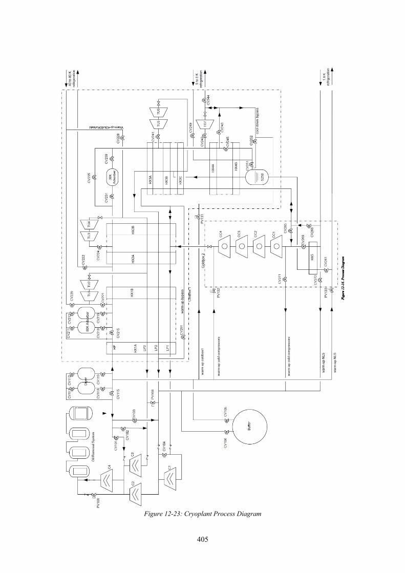
405

Figure 12-23: Cryoplant Process Diagram

406

The supply flow helium to the 40-to-80K radiation shields is also taken from the HP line between the heat-exchangers HX1B and HX2A.

The turbine strings Tu3/Tu4 and TU5/Tu6 receive gas flows which are taken from the HP line at lower temperatures. The string Tu3/Tu4 return flow also rejoins to pressure level LP3. The string Tu5/Tu6 return flow rejoins to pressure level LP2, this increases the pressure ratio and delivers a lower outlet temperature.

The turbine Tu7 is operating at the lowest temperature. Unlike the flows of the other turbine strings the discharge flow of Tu7is further cooled down by throttling. This flow is used, first for the 5-8 K radiation shield refrigeration and then for the 1.8 K refrigeration. The discharge pressure of Tu7 is 4.0 bar, the discharge temperature roughly 5.7 K at full load.

Vapor and liquid are separated in the vessel S250. The vapor returns through the LP2-line. The liquid is transferred to coldbox 2, where it becomes sub-cooled in the heat exchanger HX5 before it is supplied to the 1.8 K cryostat.

The gas returning from the 1.8 K evaporation is first warmed up in heat exchanger HX5 to approximately 3.8 K before being supplied to a 4 stage cold turbo compressor system. The discharge flow LP1 of this system is still sub-atmospheric. It becomes further compressed to LP2 pressure level at warm end by the compressor C1.

To protect against surge conditions, the cold turbo compressors have to be supplied with a fixed mass flow. To achieve this gas is by-passed in a closed loop from the discharge of the cold compressors to the suction side by re-cooling it in the heat exchangers HX3 and HX4 to 4.5 K. When in the 4.5 K stand-by mode the cold compressors are stopped, the same heat exchanger path is used with the gas flowing in the opposite direction for warming up. 12.4.4 Modes of Operation

There are three required operating modes, in which the helium liquefaction requirements differ greatly, due to the high ratio of dynamic (RF ON) to static heat loads (radiation losses) as shown in Table 12-6 and described further below.

Table 12-6: Helium Mass flow rates

Mode Helium Mass Flow (g/s)

Full Load at 1.8 K ~164

Stand-by at 1.8 K > 8.7

Stand-by at 4.5 K > 7.0

• Full load at 1.8 K: normal operating condition with full dynamic & static heat loads being applied.

• Stand-by at 1.8 K: SRF modules remain at normal operating temperature ready for use.Only the static heat loads are being applied. The system may remain in this mode for several days, during no cryogenic faults and normal accelerator operational requirements.

• Stand-by at 4.5 K: SRF modules are warmed up to 4.5K, only the static heat loads and no cold compression is required as the module pressure is above atmospheric. This is a accelerator shut-down mode, where it has been elected to keep the modules cold.

• Transient Modes & Cooldown: Changing from Stand-by at 4.5 K to Stand-by at 1.8 K will take approximately one hour and a further forty minutes to achieve stability at full

407

load. Cooldown from ambient temperature will take approximately four days; the cooldown capacity of the refrigerator is shown in Figure 12-24.

Figure 12-24: Cooldown capacity of refrigerator

12.4.5 Optimisation of Control

The compression system discharge pressure will be automatically adjusted to control the liquid level in the separator. As the heat load increases more refrigeration is required to maintain the liquid level in the separator. Thus the Compression system discharge pressure increases, which then results in an increase of helium mass flow. When the heat load drops, the discharge pressure decreases and control is maintained. The floating pressure control will ensure that the cryogenic system efficiently matches the actual load conditions being experienced.

12.4.6 Utility Consumption

Power and cooling consumption figures which are derived from the outcome of the industrial study for the different modes of operation as defined in Section 12.4.4 are shown in Table 12-7. The estimated operational load arises from calculations based on the expected actual power consumption – i.e. does not include the 50% safety factor assumed in the design study. The power input is then estimated as somewhat more than ‘Full Load’/1.5 because of a slight shift in the efficiency operational point when the system defined for the industrial study runs at less than its designed optimum (i.e. runs at 1/1.5 x specified 3.4 kW dynamic heat load)

Table 12-7: Utility Consumption

Full Load 1.8 K

Estimated Operational Load 1.8 K

Stand-by Load 1.8 K

Stand-by Load 4.5 K

Power Input (kW) 3040 ~2500 1320 562

Cooling Water (m3/h) ~270 ~270 ~125 ~55

Instrument Air (m3/h) 20 20 20 10

12.4.7 Redundancy

As the actual heat load is likely to be somewhat less than the maximum capacity of the refrigerator, some redundancy exists within the compression and oil recovery systems and if necessary further capacity could be added either initially or at a later date. However in other parts of the system, redundant capacity issues are more difficult. For example, there is only one coldbox, where any major failure would result in an enforced accelerator shut-down. The

408

mitigation for this is to hold sufficient moving part spares (valves & cold compressors), which should minimise fault durations to an acceptable level.

REFERENCES [1] Welch J, Ground Vibration and Siting of the Cryogenics Facility for Cornell ERL

Prototype, Proceedings ERL 02-03 [2] http://vibration.desy.de/overview [3] http://clic-stability.web.cern.ch/clic-stability/ see under literature [4] Amirikas R., et al., Effects of the Cryogenic Operational Conditions on the Mechanical Stability of

the FLASH Linear Accelerator Modules. [5] Internal communication; Presentation Report on Beam Offset, Tolerance Study for FEL-3, Seeded

Scheme, 1000eV, Neil Thompson, May 2009. [6] Shiltsev V., Space-Time Ground Diffusion: The ATL Law for Accelerators, 1995 [7] XFEL TDR Table 5.4.2 [8] LCLS-CDR SLAC_R_593 [9] Nuhn H D., et al, Electron Beam Alignment Strategy in the LCLS Undulators, SLCA-PUB-12098 [10] See Chapter 3 NLS CDR [11] XFEL TDR table 7.2.4 [12] Claudet, S., Recent progress in power refrigeration below 2K for supercondcuting accelerators.

CERN report CERN-AT-2005-12 [13] Chronis, W.C., et al., The CEBAF cryogenic system, proceedings of the1989 particle accelerator

Conference, pp 592-59

409

13 Radiation Safety

13.1 Dose Limits

NLS will be required to operate with due regard to all relevant radiation safety legislation. Currently, this requires, as a minimum, compliance with the Ionising Radiations Regulations 1999 (IRR99) and the Environmental Permitting Regulations 2007.

In keeping with the spirit of IRR99, doses to all staff, users and visitors must be kept as low as is reasonably practicable (ALARP). As a new facility, the dose limit of 1 milliSievert to any person in any year should be adopted. For staff, a derived working limit of 0.5 microSieverts per hour is usually adopted, based on 1 milliSievert over a 2000 hour working year. This criterion will be the most significant influence on the shielding design. Additional dose constraints [1] will apply at the NLS site boundary. If NLS is built on the site of an existing facility from which radioactive discharges are made, it must be designed in such a way that the total site boundary dose from all facilities must not exceed 0.5 milliSieverts per year. If it is built on a site from which no radioactive discharges are currently made, the dose constraint for NLS alone is 0.3 milliSieverts per year. These limits may therefore have further impact upon the shielding of the facility once the location has been determined.

13.2 Shielding Calculations

13.2.1 Prompt radiation

Preliminary shielding calculations [2] have been carried out using the SHIELD-11 code which considers bremsstrahlung and neutrons generated from beam loss on a thick target. These calculations indicate that, for the given operational parameters of:

• Energy 2.25 GeV • Charge 200 pC • Repetition rate 1 MHz • Beam loss 0.01 %

bulk shielding for the linac vault will need to be of the order of 3.8 metres of ordinary concrete, or 0.5 metres of concrete plus 4.3 metres of earth. These are based on reducing the dose outside the shielding to less than 0.5 microSieverts per hour. It has been shown [3] that doses arising from skyshine radiation can be a significant factor in determining shielding thickness for facilities which are located close to the site boundary, so these figures will need to be reviewed when the location of NLS has been determined. Further calculations will be required to specify the dimensions of entrance labyrinths and ducts.

The high energy electrons will interact with residual gas molecules within the vacuum pipe, generating gas bremsstrahlung. This high energy radiation will be primarily forward directed, and will require some specific shielding.

Gas bremsstrahlung will be generated at all points where there are high energy electrons within the accelerator vessel. This will be most intense at the end of long straights. Based on the above parameters, and the accelerator straight being of the order of 500 metres long, dose rates will be of the order of a few Grays per hour, requiring shielding of the equivalent of 35cm of lead or 300 cm of ordinary concrete. The existing vault shielding should provide adequate shielding for the forward directed bremsstrahlung, based on current machine parameters.

Each undulator straight will also generate gas bremsstrahlung. These straights are shorter, at around 80 metres long, so will generate less radiation, although dose rates will still be of the order 1 Gray per hour maximum, requiring up to 30 cm of lead shielding. Shielding this radiation will be more problematic, as it is coaxial with the output from the undulators. It is

410

suggested that a combination of in vault collimation is used with a bremsstrahlung stop placed downstream of the optical components in the first optics enclosures. Ray tracing must be used at the final design stage to determine lateral dimensions of these collimators and stops.

13.2.2 Induced activity

In addition to shielding the prompt radiation hazard, consideration will need to be given to management of induced activity, in machine components such as beam dumps, in air and in cooling water. Depending on the location and construction methods employed, the potential for activation of groundwater may also need to be assessed.

Since NLS will not be directing its electron beam onto solid targets for extended periods of time, it is likely that most of the activity induced in machine components will be due to short-lived isotopes. Whilst these components remain part of the machine they are relatively easy to control, although special arrangements are required if they need to be transported for repair whilst still radioactive, and also for their eventual consignment as waste.

Above the (γ,n) photoneutron reaction thresholds of 11 MeV in nitrogen and 16 MeV in oxygen, radioactive isotopes can be produced in air and water. These represent a potential environmental hazard if released, and a detailed environmental impact assessment would need to be carried out once a location for NLS has been agreed and the details of ventilation and drainage systems are known. It may be necessary to apply to the Environment Agency for an Authorisation to discharge liquid or gaseous radioactive waste unless it can be shown that the quantities discharged are truly below the level of regulatory concern.

The principal isotopes produced by air activation are H-3, Be-7, C-11, N-13, O-15, Cl-38 and Cl-39, produced by photoactivation, and Ar-41, produced by thermal neutron capture on Ar-40. Of these, H-3 and Be-7 are relatively long-lived and their yield is negligible in comparison with the other products. The longest-lived product which is produced in any quantity is Ar-41, with a half-life of 1.83 hours. These isotopes are removed from the air in the vault through ventilation and radioactive decay.

Table 13-1 shows production source terms in air of the principal products. A power loss of 450 kW is assumed into the beam dump, based on the operational parameters given at the start of this Section. For photoactivation products, a bremsstrahlung path length in air of 2 m is assumed. To calculate production of Ar-41 by thermal neutrons, the internal surface area of the concrete vault must be known, and is estimated as 3000 square metres.

Table 13-1 : Yields of principal isotopes produced by photoactivation and thermal neutron capture (Ar-41 only) in air

Isotope Half-life Parent elements Yield (with 450 kW power loss, 2 m air path length for photoactivation)

C-11 20.5 min C, N, O 9.7 108 Bq

N-13 10 min N 9.7 109 Bq

O-15 2.1 min O 4.9 109 Bq

Cl-38 37 min Ar 6.0 107 Bq

Cl-39 55 min Ar 7.5 108 Bq

Ar-41 1.83 hr Ar 1.6 109 Bq

The (γ,n) interaction in cooling water produces primarily O-15, N-13, C-11 and H-3, the longest lived of these being H-3 with a half-life of 12.3 years. The bremsstrahlung path length in a

411

cooling water circuit is likely to be only a few centimetres (as opposed to possibly several metres in air). Since the cooling water circuit is a closed system, the environmental implications for its routine operation are likely to be minimal, although the possibility of radioactive water released by leakage or accidental damage to the system should be considered.

Activation of groundwater has not proved a problem at other facilities, however it must be demonstrated that the design of NLS does not create possibilities for this to occur, either routinely or through a reasonably foreseeable accident. Although activity induced in shielding such as concrete is not easily transported, if the concrete is adjacent to earth shielding which is itself in contact with groundwater, there is a route by which radionuclides could enter water supplies. Additionally, any tunnel design below ground level with shielding provided mainly by earth opens up the possibility in principle for high energy neutrons to activate the earth directly, with consequent transfer of activity to groundwater. This should not be a problem with the proposed concrete shielding thickness, and expected losses, however further analysis should be carried out to verify this during the detailed design phase.

13.3 Designation of Areas

Regulation 16 of IRR99 requires an area to be designated as a Controlled radiation area if a person entering that area is likely to receive an annual dose in excess of 6 mSv, or if they are required to follow special procedures intended to restrict their radiation dose or the effects of an accident. As at synchrotron facilities, the radiation hazard inside the shielded enclosures of NLS will generally be negligible when they are not interlocked by the PSS (although consideration must be given to components such as beam dumps which have the potential for high levels of induced activity after the beam has been switched off).

Adopting the model used at the SRS and DLS in designating areas, the injector hall, linac tunnel, FEL hall and any shielded and interlocked experimental hutches within the experimental hall will be designated as Controlled radiation areas on a permanent basis.

IRR99 defines a Supervised radiation area as one where it is necessary to keep the conditions of the area under review to determine whether it should be designated as Controlled, or where a person is likely to receive an annual dose in excess of 1 mSv. It is therefore proposed that the surroundings of the experimental hall and the klystron gallery are designated as Supervised radiation areas, at least for an initial period whilst environmental dose measurements are taken in the area.

13.4 Radiation Monitoring

The installed (active) radiation monitors used at NLS will be commercially available monitors based on gamma and neutron sensitive ion chambers which are able to respond reliably in a 1 kHz – 1 MHz pulsed radiation field. They will be interlocked so that beam is tripped or shutters closed as appropriate when the radiation dose / dose rate limit outside the shielding is exceeded.

An environmental monitoring programme using thermoluminescent dosimeters (TLD) will be implemented in the Supervised radiation areas and areas outside the shielding which are not designated radiation areas.

13.5 Personnel Safety System

The Personnel Safety System will be similar to the existing DLS system in that it will be compliant with IRR99 and its ACOP and in accordance with EN61508 [4]. The architecture of the system will be subject to the analysis of the hazards and probabilistic modelling of safety to achieve the target safety levels for the facility. The design of the system will be advised by

412

current "best practice" for accelerator access control and key exchange systems, and will include the requirement for shielded areas to be searched prior to operation of the light source.

The processes necessary to comply with EN61508 include the following: • Identify the acceptable safety levels required for the facility • Identify the hazards using a technique such as HAZID including severity, initiating

event, frequency of occurrence, non-EEPE control measures and EEPE control measures. (HAZID: HAZard IDentification study; EEPE: Electrical, Electronic and Programmable Electronic safety system).

• Identify (from the HAZID) the functional requirements for EEPE • Model the safety requirements to generate probabilistic requirements for the safety

functions, leading to SIL rating. (SIL: Safety Integrity Level). • Undertake detailed design work • Review the design work with respect to functions • Build the Safety System • Test functional performance with respect to functional specification • Undertake proof tests to ensure continued correct operation. • Collect data and review performance against the assumptions in the safety model and

HAZID

A safety system that is compatible with IRR99 and the “generic prior authorisation” will include:

• Hierarchy of control measures • “Emergency Off” buttons • Search systems • Key transfer system, with the ability to leave the system disabled • “Fail safe” annunciators (signs) • Tests at suitable intervals • Maintenance

and is likely to include • PA announcements • Blue lights • Other warning signs • Redundancy and diversity of safety control measures • Redundancy and diversity of safety systems

REFERENCES [1] The Radioactive Substances (Basic Safety Standards) (England and Wales) Direction 2000. [2] M P Holbourn and L Nicholson. NLS Project Stage 1 Shielding Estimates NLS/HP/2008/01, 01

August 2008. [3] SCSS X-FEL Conceptual Design Report, Radiation Safety Issues. May 2005. [4] EN61508, "Functional safety of electrical/electronic/programmable electronic safety related

systems", BSI.

413

14 Recirculating Linac Option

This Chapter presents an alternative accelerator concept for the New Light Source, namely a two-pass recirculating linac. We discuss the motivation, advantages and disadvantages of a recirculating linac based facility in comparison to the single pass machine described in Chapter 1. We then describe in detail the layout and beam transport of a complete two-pass recirculating linac. We show the results of optimisation and tracking simulations of this machine up to and including FEL-3. These indicate a capability to fulfil the required beam properties to drive the NLS FELs. Finally, we present preliminary tolerance studies on the proposed design.

14.1 Introduction

14.1.1 Motivation: Advantages & Disadvantages of Recirculation

The New Light Source proposal is based on 1.3 GHz superconducting RF technology. This is principally to enable pulse repetition rates of up to 1 MHz as demanded by the science case. Superconducting infrastructure necessitates comparatively large capital outlay and running costs. A recirculating linac design mitigates this in that a lower energy linac is required when the beam is accelerated through it multiple times. Additionally, any tunnelling or shielded building above ground would be shorter in comparison to a single pass machine. However, in parts it would need to be wider. In principle, one is able to extract beams of different energies from one location, enabling FELs resonant at different wavelengths to operate efficiently. A final advantage is that a natural upgrade path is established without the need to add accelerating modules, instead additional recirculation paths can be constructed.

The recirculation design however needs to consider additional design issues compared to a single pass machine:

• combining and separating beams of different energies, leads to more complex optics • the bunch compression and linearisation scheme is restricted as the compression cannot

be done in sections with multiple beam energies • both incoherent and coherent synchrotron radiation (ISR and CSR) within the arcs will

lead to emittance degradation • all of the above make it more difficult to produce very short electron bunches for single

spike FEL operation • jitter tolerances will be more stringent due to the extra transport required.

It is the aim of this Chapter to address these issues, understand to what level they can be mitigated and make a comparison of the bunch properties from an optimised recirculating design with that from the baseline single pass machine.

An alternative philosophy would be to view recirculation as a way to extend the energy of a single pass 2.25 GeV machine. This scenario is not addressed in this report although this idea could be revisited in the context of a future upgrade of single pass machine.

14.1.2 Context: Recirculating Linacs Worldwide

The design of the NLS recirculating linac option is entirely novel, although it has been informed by other recirculation based facilities and design studies. The prime example of an operating facility based on a recirculating linac is the Continuous Electron Beam Accelerator Facility (CEBAF) at the Thomas Jefferson National Accelerator Facility (JLab) in the United States [1]. This is a nuclear physics facility and operates in a different parameter regime with low bunch charge and high energy. Though some of the design aspects of arcs, mergers, combiners and

414

extraction from this facility are educative, the requirement on NLS bunches to drive the FELs (high charge, short bunch length and extremely small emittances) need a new design approach.

There are currently three operating FEL based light source facilities that make use of a recirculating linac. These are as the JLab IR-FEL [2], the JAERI ERL-FEL [3] and the ALICE facility at Daresbury [4]. The JLab IR-FEL produces 14 kW CW at 1.6 microns from a 200 MeV beam. This facility is based on the same 1497 MHz superconducting technology as CEBAF, but the linacs are operated in energy recovery configuration in order to maximise accelerated beam power. A UV branch is currently under construction which will extend the capability of the machine down to 250 nm [5]. Currently being commissioned at Daresbury Laboratory is ALICE (Accelerators & Lasers in Combined Experiments) formerly known as the Energy Recovery Linac Prototype (ERLP). This is a 35 MeV IR-FEL based on recirculation in energy recovery mode using 1.3 GHz superconducting infrastructure. Output will be provided at 5-10 microns. Although these are low energy machines and are prototypes rather than full user orientated facilities, the arcs and merger sections have relevance to the NLS design.

There have also been a number of design studies that incorporated recirculation in the energy recovery configuration, chiefly Arc-en-Ciel [6], 4GLS [7] and LUX [8]. Elements of these designs have relevance to NLS, but to our knowledge none of these reached a stage where start-to-end simulations ensured the capability to drive the FELs. Of further relevance are designs that, while not recirculating, utilise complex transport of short, bright bunches. The most developed of these is the BESSY-FEL [9] design, which includes a 180° arc.

All these designs were reviewed in order to inform the configuration of the NLS recirculating linac and we thank the appropriate teams from whose work the present design has benefitted.

14.2 Design Description

14.2.1 Layout

We propose to achieve the nominal design energy of ~2.25 GeV through a ~200 MeV injector, followed by two recirculation passes of a ~1 GeV main linac (the energies quoted throughout this Chapter are necessarily approximate, due to the required longitudinal phase space tuning. This involves small changes in the phase of the linacs and in the gradient and phase of the linearising cavities). Other configurations that were considered and rejected include placing the linac in both legs and a dog-bone topology with a 360° arc; we concluded that these introduced additional issues without significant benefit.

Figure 14-1: Schematic layout of the recirculating linac option for NLS

Figure 14-1 shows a schematic layout of the chosen design. The injector part consists of a gun, two cryomodules, a third harmonic cavity, a laser heater and the first bunch compressor. The dogleg achromat followed by this merges the injected beam with the recirculated beam. The injected beam passes through 7 cryomodules of the same type as those proposed for the single pass linac (see Chapter 3). The beam then circulates through 360° using two arcs and a return FODO path, passes through a second bunch compressor, the merger section and enters the main linac a second time. The extracted high energy beam passes through the third bunch compressor, post linac collimation and finally through the spreader to the FELs. Such a design results in an operating gradient of 17.5 MV/m. This has not been cost optimized as for the single-pass case; if necessary one extra cryomodule could be added in the main linac to bring the gradient to the

415

same level as the single pass case (15 MV/m). The total number of cryomodules will then be 10 in the recirculation design compared to 18 in case of the single pass design.

In order to obtain maximal benefit from recirculation, one should inject into the main linac at as low energy as possible. However this aim must be traded off against considerations arising from the method of longitudinally compressing the electron bunches by means of off-crest RF acceleration and magnetic chicanes. With off-crest RF acceleration, the energy-time correlation is not linear, and the longer the bunch is on entering the main linac, the greater the amount of RF curvature seen by the bunch. This curvature impairs the ability to compress the bunch, thereby limiting peak current and subsequent lasing in the FELs. The standard method to mitigate this is to use a higher-harmonic RF cavity to linearise the longitudinal phase space. The achievable voltage of this higher-harmonic system then becomes the limiting factor, however this can be mitigated by utilising the second-order momentum compaction arising from placing sextupoles in the arcs as explained in Section 14.2.6. The bunch must be compressed enough on entry to the main linac that the curvature can be compensated within the design parameters of the third harmonic system. An additional consideration is that the injector must have a sufficiently high energy that space charge effects cannot significantly affect the beam during transport to the main linac. In performing this compression prior to injection into the main linac we utilise a defining property of superconducting machines, namely that longitudinal wakefields that would preclude entering a long warm accelerating section with a relatively short bunch are nearly absent.

One dimensional longitudinal phase space tracking was utilised to optimise the injection energy given the above constraints. This process lead to the proposed injector design; two accelerating cryomodules are positioned in the injector, followed by a third harmonic system. The injection energy is thus approximately 200 MeV. In order to reach the design energy, we therefore require a ~1 GeV main linac. The ratio of beam energies at injection and high energy beam after one pass is ~ 6 and that at high energies at the exit of linac is ~1.8. These ratios pose different optics and layout challenges for merging and separating the beams.

In the following Sections we describe in detail the individual parts of the recirculating linac scheme. The machine lattice and tracking simulations have been performed using Elegant [10]. For intensive optimisations this was interfaced with Mathematica. The hardware utilised was a number of clusters operated as North West (NW) accelerator grid. Optics design and matching was performed using Mad-8 and TRANSPORT. In referring to the bunch compression scheme the first order momentum compaction of a section (also referred to as longitudinal dispersion or transport matrix element R56) is negative if a negatively chirped bunch is compressed. In other words higher energy particles are at the back of the bunch and are allowed to catch up with the front. Thus a standard four dipole compression chicane has a negative R56. This is the sign convention used by Elegant.

14.2.2 Injection Straight & First Bunch Compressor

The gun is assumed to be identical to that in the single pass design described in Section 2.1. The first SC cryomodule has independent phase and voltage control for the first four cavities, with the final four having a single phase and voltage control. This arrangement is to enable particular emittance compensation schemes to be executed in conjunction with the gun parameters. A second SC cryomodule takes the energy from 135 MeV to 265 MeV, there is a single phase and voltage control for this module. A third harmonic cryomodule consisting of eight cavities then over-linearises the bunch to compensate for RF curvature imposed by both upstream and downstream off crest acceleration, this reduces the centroid energy to ~230 MeV.

At this point we should note a difference between the recirculating and single pass design. The above acceleration system is operated to produce a strongly chirped bunch with full width (FW) energy spread of ~3%. This is to enable significant magnetic compression prior to injection into the main linac for the reasons espoused in the previous Section. The gun optimisation used in

416

the recirculating linac design is thus different from that used in the single pass machine. The recirculating design necessitates that injection transport must be achromatic to at least second order as we wish to propagate a beam with a large energy spread without chromatically induced emittance increase. In the single pass machine, a dogleg section after the first cryomodule will be used to merge the second stage injector and the choice has been made to transport a beam without chirp from the injector in order to minimise chromatic emittance growth. The chirp is added in the accelerating section located after the dogleg but prior to compression. This option is not available to the recirculating design as we cannot have beams of two energies simultaneously traversing a magnetic compressor.

The recirculating design can also be modified to include an additional achromat for incorporation of a second gun, following a first cryomodule optimised for an unchirped beam. This should be considered in a future design phase, should the recirculating linac be pursued.

The two injector accelerating modules and third harmonic linearising module are situated in conjunction to provide efficient cryogenic interconnection design. Subsequent to these is a warm section with small chicane and laser system arranged to form a “laser heater”. As in the single pass design, this is intended to provide a method of increasing the uncorrelated slice energy spread within the bunch. Detailed microbunching studies should be undertaken in the future design stage to decide the requirements of the laser heater. For the results presented in this Chapter, the laser heater is switched off.

The beam now enters the first magnetic compression chicane. This is a four dipole C-type design. The dipoles are rectangular and of magnetic length 0.4 m. Figure 14-2 shows the optics and H-functions through the first bunch compressor. The four quadrupoles prior to the compressor ensure that the horizontal beta function and H-function is minimised in the final dipole to suppress any coherent as well as incoherent synchrotron radiation emission.

Figure 14-2: Optics in the first bunch compressor

14.2.3 Injection Achromat

To inject into the main linac we must transport the beam with a number of beam dynamics and layout restrictions. The transport must be achromatic and with small first order momentum compaction (R56) in order to not restrict the overall bunch compression scheme. In fact we choose to require R56 to be zero in the system. Necessarily the system shares the final dipole with the high energy returned beam in an energy ratio of six. Vertical focussing arising from the non-optimal edge angle of this dipole is therefore another restriction and must be dealt with carefully. In order to minimise the impact of this section on the building width, we make the choice that the injection system should be parallel to the linac, therefore the total angle of the system is zero. The system must be traversed by a beam with a large energy chirp which is thus sensitive to higher order transport matrix elements, for example chromaticity and second order

417

dispersion. These will cause emittance increase due to the imprinting of curvatures in the phase space of the relevant terms. Finally, the optics functions entering the linac must be such that control of them along the linac is possible using the same focussing elements that simultaneously affect the high energy beam.

In order to cope simultaneously with these restrictions, a carefully considered first order optics design has been employed with additional correction at second order. The high energy chicane needs to have a minimum dipole angle of -2° (at ~1.2 GeV) to allow to merge the injected beam. This angle then becomes -12° for the injected beam (~200 MeV). The symmetric achromatic system with two dipoles of opposite polarities is not suitable here due to the asymmetric edge angle of the second dipole, large optics functions and dispersion functions as well as the non-isochronicity of such a system. At large values of the optics functions the lattice becomes unacceptably sensitive to second order terms. In order to minimise these optics effects, the design chosen here uses two dipoles of opposite polarities (+11° and +1°) and 8 quadrupoles in the dispersive sections to make the overall system achromatic and isochronous with reasonable optical and dispersion functions. Five quadrupoles preceding the dispersive section are used to match the Twiss parameters to the linac. The floor layout of the injection achromat is shown in Figure 14-3 and the optics functions are shown in Figure 14-4.

Figure 14-3: Floor layout of the injection achromat, sextupoles are shown in blue

Figure 14-4: Optics & dispersion function in the injection achromat

On tracking a bunch through this system it is seen that chromatic aberrations are introduced and the emittance increases due to these nonlinearities. To analyse this we must look at the second order matrix elements involving energy, i.e. the Tij6 terms. Longitudinally, T566 is the relevant parameter, but transversely looking at all of the terms is not illustrative as they are not all independent. It is preferable to recast in terms of the variation of the Twiss parameters and dispersion with respect to energy. Thus, for the horizontal plane we define the chromatic amplitude functions.

418

and the chromatic derivative of dispersion

with analogous definitions for the vertical plane.

Figure 14-5 shows the chromatic amplitude functions. It can be seen that these become large by the end of the injection achromat, particularly in the horizontal plane. Figure 14-6 shows the chromatic derivative of dispersion, this is seen to diverge after the achromat. The second order longitudinal dispersion, T566 has a value of -1.13. This gives curvature to the bunch which is of opposite sign to that imposed by the third harmonic cavity. We therefore wish to reduce the T566 to minimise voltage demand on the third harmonic cavity.

Figure 14-5: Chromatic amplitude functions in the injection achromat before (black, red) and after (blue, green) correction

Figure 14-6: Chromatic derivative of dispersion in the injection achromat before (black) and after (red) correction

These terms can be reduced by the introduction of sextupoles into the lattice, however initially it was not obvious how this should be accomplished. We have therefore adopted a brute force method of chromatic correction; the lattice is defined in Mathematica and sextupoles are introduced in the drift spaces, both in the dispersive region and the preceding matching section. We then minimise the horizontal and vertical emittances and T566 using a Nelder-Mead simplex optimisation algorithm [11]. The variables for the minimisation are the number of sextupoles,

419

their strengths, and their positions within the drifts. An additional constraint is a ceiling on the sextupole strength.

It can be seen from Figure 14-3 that the optimisation has settled on six sextupoles with five in the dispersive region and one in the preceding matching section. The sextupoles in the dispersive region control the chromatic second order function, however in doing this some geometric second order terms become large; this is corrected by placing one sextupole in the dispersion free section.

Figure 14-7: Normalised emittances & dispersion function through the corrected injection achromat

As shown in Figure 14-5, the chromatic amplitude functions are reduced by a factor of ten in the horizontal plane although at the cost of a slight increase in the vertical plane. Figure 14-6 shows that the chromatic derivative of dispersion is fully corrected. The value of T566 after correction is -0.35, a fourfold reduction from the uncorrected value. Figure 14-8 shows the normalised emittances (less dispersive contributions) through the injection achromat. The horizontal emittance diverges from its initial value in the dispersive sections due to the non-Gaussian nature of the beam (when the normalised emittance less dispersive contributions is calculated, the formula assumes that the dispersive contributions are those followed by a Gaussian beam. In our case, the bunch is highly non-Gaussian), however it returns almost exactly to its initial value on leaving the dispersive region. The horizontal emittance increase in the injection achromat is from 0.34 mm mrad to 0.35 mm mrad. The vertical emittance is increased by a negligibly small amount.

14.2.4 Main Linac First Pass

We inject into the main linac at ~230 MeV and exit the main linac at ~1230 MeV. The main linac consists of seven cryomodules with a field gradient 17.5 MV/m. There is a quadrupole doublet between the linac modules to control the optics functions. These quadrupoles affect both the high and low energy beams and therefore strengths are determined by an optimisation procedure described in Section 14.2.8.

14.2.5 Achromat Matching Linac to Arc at 1.2 GeV

The dipole located at the exit of the main linac separates the ~1.2 GeV and ~2.2 GeV beams. We must therefore design two lines that transport each beam in an appropriate manner without conflicting with each other. The 1.2 GeV line must then match into arc 1. By reducing the strength of this dipole we are able to extract the 1.2 GeV beam should this be required. This dipole should separate these two different energy beams transversely in a sufficiently short distance to allow insertion of independent optics elements in the two transport lines. However the angle should not be too large as this would imply large optics functions and dispersion,

420

which in turn implies sensitivity to higher order terms. The optimum angle to allow this is 10° for the 1.2 GeV beam (and 5.45° for the 2.2 GeV beam).

The 2.2 GeV energy beam sees non-optimal exit edge angle and has been accounted in the design. The linac-to-arc section transports the 1.2 GeV beam to the arc. The energy spread is ~1.2% at this location and the same techniques of higher order corrections as described in Section 15.2.3 are applied for minimising the emittance growth.

Figure 14-8 shows the floor layout of the 1.2 GeV matching to the arc beam transport system and Figure 14-9 shows the optics and dispersion of this system. The optical functions are matched to the arc Twiss parameters and are kept below 80 m with maximum dispersion of 0.6 m using five quadrupoles each in the dispersive as well as the non-dispersive regions. The system is achromatic and though not isochronous it has been optimised to keep R56 small (+5 mm). This is sufficiently small in comparison to the bunch compressors that we can still consider the longitudinal tuning of the machine to be independent of the transverse transport.

Figure 14-8: Floor layout of the linac-to-arc matching achromat, sextupoles are shown in blue.

Figure 14-9: Optics and dispersion functions in linac-to-arc matching achromat at 1.2 GeV

As with the injection system, we require correction of the chromatically induced emittance growth. The same optimisation method was applied, varying the number, positions and strengths of sextupoles in order to minimise the emittance and T566. In this case four sextupoles are optimal in the configuration as shown in Figure 14-8. Figure 14-10 shows the chromatic amplitude functions before and after the sextupole correction. Horizontally, a reduction by a factor of approximately 5 is seen, this is made at the expense of the vertical plane where a commensurate increase is seen. Figure 14-11 shows the chromatic derivative of dispersion before and after correction. Although the correction is not as perfect as in the injector, there is nevertheless a reduction by over an order of magnitude.

421

Figure 14-10: Chromatic amplitude functions in linac-to-arc matching achromat before (black, red) and after (blue, green) correction

Figure 14-11: Chromatic derivative of dispersion through linac-to-arc matching achromat before (black) and after (red) correction

Figure 14-12: Normalised emittances & dispersion function through the corrected linac-to-arc matching achromat

Figure 14-12 shows the normalised emittances (less dispersive contributions) of the tracked bunch through the linac-to-arc matching achromat after chromatic correction. As with the injection system, there is virtually no emittance growth (from 0.35 mm mrad to 0.36 mm mrad horizontally and negligibly small vertically).

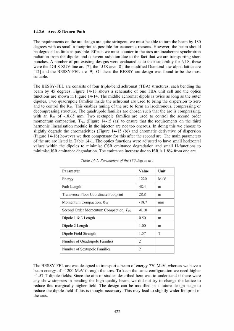
422

14.2.6 Arcs & Return Path

The requirements on the arc design are quite stringent, we must be able to turn the beam by 180 degrees with as small a footprint as possible for economic reasons. However, the beam should be degraded as little as possible. Effects we must counter in the arcs are incoherent synchrotron radiation from the dipoles and coherent radiation due to the fact that we are transporting short bunches. A number of pre-existing designs were evaluated as to their suitability for NLS, these were the 4GLS XUV line arc [7], the LUX arcs [8], the modified Diamond low-alpha lattice arc [12] and the BESSY-FEL arc [9]. Of these the BESSY arc design was found to be the most suitable.

The BESSY-FEL arc consists of four triple-bend achromat (TBA) structures, each bending the beam by 45 degrees. Figure 14-13 shows a schematic of one TBA unit cell and the optics functions are shown in Figure 14-14. The middle achromat dipole is twice as long as the outer dipoles. Two quadrupole families inside the achromat are used to bring the dispersion to zero and to control the R56. This enables tuning of the arc to form an isochronous, compressing or decompressing structure. The quadrupole families are chosen such that the arc is compressing, with an R56 of -18.65 mm. Two sextupole families are used to control the second order momentum compaction, T566 (Figure 14-15 (a)) to ensure that the requirements on the third harmonic linearisation module in the injector are not too onerous. In doing this we choose to slightly degrade the chromaticities (Figure 14-15 (b)) and chromatic derivative of dispersion (Figure 14-16) however we then compensate for this after the second arc. The main parameters of the arc are listed in Table 14-1. The optics functions were adjusted to have small horizontal values within the dipoles to minimise CSR emittance degradation and small H-functions to minimise ISR emittance degradation. The emittance increase due to ISR is 1.8% from one arc.

Table 14-1: Parameters of the 180 degree arc

Parameter Value Unit

Energy 1220 MeV

Path Length 48.4 m

Transverse Floor Coordinate Footprint 28.8 m

Momentum Compaction, R56 -18.7 mm

Second Order Momentum Compaction, T566 -0.10 m

Dipole 1 & 3 Length 0.50 m

Dipole 2 Length 1.00 m

Dipole Field Strength 1.57 T

Number of Quadrupole Families 2

Number of Sextupole Families 2

The BESSY-FEL arc was designed to transport a beam of energy 770 MeV, whereas we have a beam energy of ~1200 MeV through the arcs. To keep the same configuration we need higher ~1.57 T dipole fields. Since the aim of studies described here was to understand if there were any show stoppers in bending the high quality beam, we did not try to change the lattice to reduce this marginally higher field. The design can be modified in a future design stage to reduce the dipole field if this is thought necessary. This may lead to slightly wider footprint of the arcs.

423

Tracking investigations through the arc show that there is negligible CSR emittance degradation as long as the bunch is kept longer than 2 ps FW. As will be discussed in Section 14.3 this requirement is satisfied in the proposed bunch compression scheme.

Figure 14-13: Floor layout of triple bend achromat unit cell representing 45° of 180 degree arc

Figure 14-14 : Optics functions and dispersion through 180 degree arc

Figure 14-15: (a) T566 through 180 degree arc with and without sextupole correction, (b) Chromatic amplitude functions through arc before (black, red) and after (blue, green) sextupole correction

424

Figure 14-16: Chromatic derivative of dispersion through arc before and after sextupole correction

After the arc we match into a long transport line that brings the beam to the start of the second arc. We utilise a simple FODO channel with 45 degree phase advance. This phase advance was chosen with the intention of inserting a tomography diagnostics section to reconstruct the six dimensional phase space of the bunch after acceleration and turning in the arc. Since this FODO does not affect the beam dynamics, the phase advance can easily be reduced to decrease the number of components for cost benefit. Within this 140 m section it is intended to insert an additional path length correction system [13]. This will enable the total path length of the return transport to be varied over one complete RF wavelength (~23 cm). The system will comprise a pair of second order achromatic doglegs connected with a short bellows section. The path length variation will be achieved independently of all transverse beam properties, but will introduce a small (1-2 mm) R56 dependence as the path length is changed, this can be easily compensated for in the second bunch compressor. This has not yet been implemented in the simulated machine, though independent control of the linac phase in the second pass has been assumed.

The beam is then matched into the second 180 degree arc and emerges 2 m transversely displaced with respect to the main linac. It has been chosen to insert an exact reverse of the linac-to-arc matching achromat in order to bring the beam collinear to the linac. The reason for this is to ensure that there are identical magnets in the two arcs and matching to/from arcs enabling the number of independent power supplies to be reduced. If instead the second arc is widened, an arc-to-linac achromat is no longer required, but the inherent symmetry of the two identical structures is lost. Figure 14-17 shows the layout of this part and Figure 14-18 shows the optics through the arc-to-linac matching achromat. As before, a sextupole correction must be applied to the chromaticity, however this requires a separate optimisation from the one performed on the linac-to-arc system. The reason for this is the previously mentioned choice to correct for T566 in the arcs at the expense of the chromatic terms. When this is done we arrive at the layout shown in Figure 14-17 which has four sextupoles, three in the dispersive region and one in the preceding matching section to correct for geometric second order terms induced through the chromatic correction.

Figure 14-17: Floor layout of reverse extraction system, sextupoles are shown in blue.

425

Figure 14-18: Optics through the arc-to-linac matching achromat

14.2.7 Second Bunch Compressor and Re-injection

The second bunch compressor is located before re-injection into the main linac. As this is after the arcs we are now free to compress the bunch strongly. It is at this point that we must start to be mindful of CSR emittance growth as the bunch becomes shorter than 1 ps FW. Both C-type and S-type chicanes have been assessed for their suitability at this location, with the choice of S-type being due to the need to minimise CSR emittance growth. As with the first compressor, the horizontal beta function in the final dipole has been minimised to further suppress CSR emittance growth as shown in Figure 14-19. The beam is then passed through the high energy path of the injection merger. This is a weak C-type four dipole chicane with optimal edge angles for this 1.2 GeV beam (the non-optimal angle was chosen to be seen by the injected beam).

Figure 14-19: Optics functions through the second bunch compressor

14.2.8 Linac Second Pass

The optics in the second pass of the linac decides the Twiss parameters at the extraction of the 2.2 GeV beam. A dipole placed at the exit of the linac separates the 1.2 and 2.2 GeV beams. In order to minimise CSR induced emittance growth in this dipole on the second pass the horizontal beta function must be minimised. Failure to do this has been shown to increase the emittance by an order of magnitude. However this is not a simple task as the quadrupoles in the linac also focus the first pass beam, and obviously the same quadrupole gradient is seen by the lower energy beam as a higher k-value. To address this problem a dual optimisation of Twiss parameters was performed by the interfacing of Mad with Mathematica. A Nelder-Mead simplex optimisation algorithm was employed with variables being the linac quadrupole gradients. These were scaled to k-values for both passes of the linac and Twiss parameters found for both cases before constructing the optimisation penalty function. Constraints imposed were maximum and minimum acceptable beta function values, maximum acceptable alpha function values at the exit of the extraction dipole and a strong minimisation requirement on the horizontal beta function value at the exit of the extraction dipole in the 2.2 GeV case.

426

Figure 14-20 shows the optimised optics functions for the two energy beams simultaneously passing through the linac.

Figure 14-20: Simultaneous optics functions at 1.2GeV and 2.2 GeV through the main linac (red for horizontal, blue for vertical)

In performing the above optimisation care must be taken when implementing the results into the Elegant tracking simulation. Elegant and Mad use different approximations in the calculation of RF body focussing. This effect arises from the fact that we accelerate off crest and therefore the beam sees not only Ez but also Er; this is required in order to fulfil the Maxwell-Ampere relation

. Mad implements an approximate analytic solution of the resulting transverse equation of motion known as the Chambers model [14], but only does so on entry and exit of a cavity. Elegant uses the more sophisticated Rosenzweig-Serafini model, which directly gives the transfer matrix of an arbitrary standing wave mode including harmonic content [15], this reduces to the Chambers model for pure π-mode cavities. However, Elegant calculates this effect not just at entry and exit, but also through the entire cavity body. This leads to a small difference in the Twiss parameters at the end of the main linac between the two programs. Slight re-matching of 1.2 GeV parameters was done to cope with this difference.

14.2.9 Extraction at 2.2 GeV & Third Bunch Compressor

The requirements to be fulfilled for the 2.2 GeV extraction system are that the optics functions and dispersion should not become large and bends should be shallow; this will minimise the expected CSR induced emittance growth. The line should be achromatic and as close to isochronous as practicable. Chromatic considerations are not as important as the typical energy spread at this point is only 0.6%. Figure 14-21 shows the floor layout, this includes the linac-to-arc matching achromat in order to demonstrate that there is no clash. Figure 14-22 shows the optics functions through the extraction system. For completeness we include in Figure 14-23 the chromatic amplitude functions and chromatic derivative of dispersion, however it is not necessary to correct for these.

427

Figure 14-21: Floor layout of the extraction region

Figure 14-22: Optics functions and dispersion through the 2.2 GeV extraction system

Figure 14-23: Chromatic amplitude functions (left) and second order dispersion (right) through the 2.2 GeV extraction system

The third bunch compressor follows the extraction section, again an S-type design has been chosen in order to minimise CSR induced emittance growth. A preceding matching section ensures that the horizontal beta function is minimised in the final dipole. Figure 14-24 shows the optics functions, dispersion and H-function in the third compressor.

428

Figure 14-24: Optics functions, dispersion and H-function in third compressor

14.2.10 Collimation & Spreader to FELs

After the third bunch compressor, the recirculated beam is matched to the post linac collimation section. The design of the collimation and subsequent spreader sections assumed here is identical to the single pass design, described in Chapter 4.

14.2.11 Design Summary

As far as is possible, the design separates longitudinal beam dynamics from the layout and transverse beam dynamics. Figure 14-25 shows the optics for the entire machine from the second injection module to the end of the spreader. Figure 14-26 shows the overall layout and scale, and Figure 14-27 shows an architectural concept, for the recirculating linac option for NLS. The details of the parts common to the single pass linac are explained in Chapter 12.

Figure 14-25: Optics functions and dispersion for the recirculating linac including collimation and spreader

429

Figure 14-26: Overall layout and scale of the recirculation option for the NLS.

Figure 14-27: Architectural layout of the recirculation option for the NLS.

14.3 Longitudinal Optimisation & Results for 200 pC Bunch Charge

14.3.1 Optimisation Methodology

The longitudinal bunch compression scheme is predominantly governed by the strengths of the three bunch compressors, the off crest chirp imparted in the injector and first & second passes of the main linac, and the gradient and phase of the third harmonic linearising module. Tuning these to give the correct final bunch properties is thus an eight dimensional optimisation problem. Defining the constraints proved far from straightforward. As described in Chapter 1, there are additional constraints in the design of a seeded FEL facility such as NLS. In order to allow for jitter between the electron bunch and the laser seed, the slice properties of the bunch should be as constant as possible over some time window. As with the optics sections described above, an initial attempt was made to perform this optimisation using the Nelder-Mead simplex method however this was found to be inadequate. The Nelder-Mead simplex method operates by constructing an N-dimensional “derivative” in the optimisation variables by stepping up and down in each variable, then calculating a penalty function at each point. The new solution is then the point in variable space with the smallest penalty function. Thus it moves “downhill” until it reaches a minimum. However, with highly non-linear problems such as the one we are dealing with here, it tends to become stuck at a local minimum. It was therefore decided to abandon this method and utilise the Luus-Jaakola pseudo-random global minimum search algorithm [16]. In this procedure, a volume of variable space is defined and points selected

430

pseudo-randomly within it. The penalty function is calculated for each point and the volume of variable space is re-centred on that point. The volume is then reduced by some factor and the procedure repeated. The advantage of Luus-Jaakola over Nelder-Mead is the pseudo-random element, this ensures that the optimisation does not get stuck at a local minimum but rather explores the entire variable space to find the global minimum. Applying this to the NLS recirculating linac, each point corresponds to a specific machine. To calculate the penalty function we track the bunch through this machine and analyse the final bunch properties. Practically, we used the multiple node cluster dl1.nw-grid.ac.uk which is part of the UK NorthWest Grid Infrastructure. This machine consists of 96 nodes, each having two 2.4 GHz dual core CPUs (total 384 cores), each node having 16 Gb memory with communications between nodes provided by an InfiniPath high bandwidth interconnect. Each machine is submitted as a job, with each job being run in parallel on a number of computational cores. Typically, 50 machines were tracked simultaneously on four cores each. A typical 100,000 macroparticle track took 4 minutes to run. After each machine population had been tracked, the results were analysed using Mathematica. This calculates the penalty function, populates the new volume and submits to the cluster.

The definition of the penalty function is the crucial component in order to obtain a successful optimisation. A degree of trial and error was needed to specify a mutually consistent and suitably weighted set of constraints, these are:

1) Mean current (binned in 5 fs slices) over a contiguous 100 fs slice to be greater than 1 kA

2) Minimum current (binned in 5 fs slices) in that same 100 fs slice to be greater than 950 A

3) Standard deviation of current (binned in 5 fs slices) in that same 100 fs slice to be less than 50A

4) RMS bunch length to be less than 400 fs 5) Of the central 80% of the bunch binned by energy, the slice energy spread of all 5 fs

slices to be less then 1.2x10-4 6) The 5 fs current slices two away on either side of the central slice in time must be

such that the energy chirp ensures the back of the bunch has higher energy The combination of these ensures that we have a high peak current that is optimised to be as flat as possible in time over 100 fs, whilst keeping the bunch chirped in the correct direction to avoid passing through the minimum bunch length and “folding over” in longitudinal phase space. The solution found by this method is described below. It is important to note that the solution may be improved by further optimisation. Table 14-2 shows the final optimised values and also lists momentum compactions for all other fixed sections.

On completion of this optimisation a production run was carried out to produce 5 million macroparticles to inspect the properties of the bunch manually and provide input for the time dependent Genesis FEL simulations.

14.3.2 Description of Longitudinal Phase Space Solution

It is instructive to give detailed commentary on the evolution of the longitudinal phase space. Table 14-3 summarises the energy, bunch length and total energy spread at critical locations in the machine. From this we see that most compression occurs at bunch compressor 2, this gives us confidence that the optimisation procedure is working correctly. To minimize the degradation in emittance due to CSR, the choice has been made to keep the bunch relatively long when passing through the arcs and only then to approach full compression.

431

Figure 14-29 (a) illustrates the longitudinal phase space progressively in the injector part. The bunch emerges from the second accelerating cryomodule at 262 MeV with an energy spread of 6% FW and bunch length of 18 ps FW (black). After the third harmonic module its energy is lowered to 228 MeV with energy spread of 2.8% FW and the imprinted curvature has been reversed (red). After the first bunch compressor the FW bunch length has been reduced to 5 ps (blue). After the injection achromat the bunch length has increased slightly to 5.5 ps FW due to removal of some curvature from the T566 of this section (green). Figure 14-29 (b) illustrates the longitudinal phase space during the first pass of the machine. The bunch emerges from the linac-to-arc matching achromat at 1227 MeV with an energy spread of 1.5% FW and a bunch length of 6 ps FW (black). After both arcs and the transport between them the bunch length is 4.5 ps FW due to compression from the arcs (red). After the arc-to-linac matching achromat the bunch length is lengthened slightly to 5 ps FW (blue). After bunch compressor 2 the bunch length is 900 fs FW (green).

Table 14-2: Final variables from longitudinal optimisation together with momentum compactions for fixed sections

Optimised Section Variable Value 3 lineariser E 16.0 MV/m 3 lineariser φ +160.9° Injector φ -29.1° Main Linac 1st Pass φ -11.8° Main Linac 2nd Pass φ +2.3° Bunch Compressor 1 R56 -96.7 mm Bunch Compressor 2 R56 -80.9 mm Bunch Compressor 3 R56 -23.9 mm

Fixed Section Laser Heater Chicane R56 -4.9 mm Injection Achromat R56 0 mm Linac-to-Arc Matching R56 +5 mm Arc 1 R56 -18.65 mm Arc 2 R56 -18.65 mm Arc-to-Linac Matching R56 +5 mm Re-injection Chicane R56 -1.6 mm Extraction R56 -0.002 mm Collimation Spreader

R56

R56

+0.26 mm 0 mm

Table 14-3: Bunch properties at salient points in the recirculating linac

Section Energy Bunch Length (FW)

Energy Spread (FW)

Start of Elegant tracking (after 1st cryomodule) 136 MeV 18 ps 2.8 % After Bunch Compressor 1 228 MeV 5 ps 3.5 % Matching to Arc 1 1227 MeV 6 ps 1.5 % After Bunch Compressor 2 1227 MeV 900 fs 1.5 % After Bunch Compressor 3 2244 MeV 350 fs 0.6 %

432

Figure 14-29 illustrates the longitudinal phase space evolution in the second pass of the machine. The bunch emerges from the linac at 2244 MeV with an energy spread of 0.7% and bunch length of 900 fs (black). After the extraction section it is shortened to 850 fs due to the slight compression (red). After bunch compressor 3 the bunch length is reduced to 350 fs, additionally the energy spread is reduced to 0.6% by the CSR decreasing the energy of the back of the bunch (blue). After the spreader we again see that the energy spread is reduced to 0.5% due to CSR (green).

Figure 14-30 illustrates the horizontal coordinate profile along the bunch at few locations in the second pass of the machine. We see that the longitudinal compression and effects of CSR do not unduly disturb the transverse profile. This is reproduced when looking at horizontal angle and in both coordinates of the vertical plane (not shown).

Figure 14-28: (a) Longitudinal phase space at 228 MeV. Black - after second module, Red - after third harmonic cavity, Blue - after first bunch compressor, Green- after injection achromat. (b) Longitudinal phase space at 1227 MeV. Black - after linac-to-arc matching achromat, Red - at exit of arc 2, Blue -

after arc-to-linac matching achromat, Green - after bunch compressor 2

Figure 14-29: Longitudinal phase space at 2244 MeV. Black - after linac second pass, Red - after extraction, Blue - after bunch compressor 3, Green - after spreader and on entrance to FEL

433

Figure 14-30: Horizontal position along the bunch at 2244 MeV. Black - after linac second pass, Red - after extraction, Blue - after bunch compressor 3, Green - after spreader and on entrance to FEL

14.3.3 Final Bunch Properties

Figure 14-31 (left) shows the current profile and (right) shows the slice emittance profile of the bunch at the entrance to the FEL binned in 1 fs slices. It can be seen that 1 kA is achieved, but the current is not constant over 100 fs. The slice emittance is however quite constant, with all lasing slices having emittances less than 0.4 mm mrad. Figure 14-32 shows the slice energy spread profile of the bunch. For most of the lasing slices this is below 2 10-4, however at the end of the bunch this increases to 5 10-4. Figure 14-33 shows the projected normalised emittance (less dispersive contributions) through the entire machine. It can be seen that it is well controlled, remaining below 0.4 mm mrad vertically and 0.6 mm mrad horizontally right to the end of the spreader.

Figure 14-31: Current profile (left) and slice emittance (right) at the entrance to the FEL binned in 1 fs slices

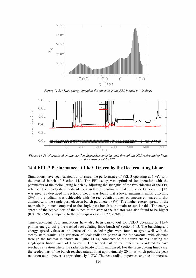
434

Figure 14-32: Slice energy spread at the entrance to the FEL binned in 1 fs slices

Figure 14-33: Normalised emittances (less dispersive contributions) through the NLS recirculating linac to the entrance of the FEL

14.4 FEL-3 Performance at 1 keV Driven by the Recirculating Linac

Simulations have been carried out to assess the performance of FEL-3 operating at 1 keV with the tracked bunch of Section 14.3. The FEL setup was optimised for operation with the parameters of the recirculating bunch by adjusting the strengths of the two chicanes of the FEL scheme. The steady-state mode of the standard three-dimensional FEL code Genesis 1.3 [17] was used, as described in Section 1.3.6. It was found that a lower maximum initial bunching (3%) in the radiator was achievable with the recirculating bunch parameters compared to that attained with the single-pass electron bunch parameters (8%). The higher energy spread of the recirculating bunch compared to the single-pass bunch is the main reason for this. The energy spread of the seeded part of the bunch at the start of the radiator was also found to be higher (0.036% RMS), compared to the single-pass case (0.027% RMS).

Time-dependent FEL simulations have also been carried out for FEL-3 operating at 1 keV photon energy, using the tracked recirculating linac bunch of Section 14.3. The bunching and energy spread values at the centre of the seeded region were found to agree well with the steady-state results. The variation of peak radiation power at the fundamental with distance through the radiator is shown in Figure 14-34, compared to the equivalent result using the single-pass linac bunch of Chapter 1. The seeded part of the bunch is considered to have reached saturation where the radiation bandwidth is minimised. For the recirculating linac case, the seeded part of the bunch reaches saturation at approximately 20 m, at which point the peak radiation output power is approximately 1 GW. The peak radiation power continues to increase

435

beyond this point but the temporal radiation profile quality becomes degraded. The properties of the radiation output at the fundamental wavelength at saturation are shown in Figure 14-35. The time-bandwidth product is close to transform limited ( 94.0≈ΔΔ tυ ) and there are no significant discontinuities in the radiation phase in the seeded region. The contrast ratio is approximately 3600. The FEL performance is thus slightly degraded compared to the results with the single-pass linac bunch but the properties of the radiation output are still good.

Figure 14-34: Variation of peak radiation power at the fundamental with distance through the radiator for time-dependent simulations of FEL-3 operating at 1 keV using the recirculating and single-pass

electron bunches

Figure 14-35: The results of time-dependent simulations of FEL-3 operating at 1 keV photon energy, using the tracked recirculating electron bunch of Section 14.3, are plotted at a distance of 20.0 m along the radiator. Top left - longitudinal profile of the FEL radiation power, Bottom left – the same on a log

scale, Top right - spectrum of the FEL radiation, Bottom right - the radiation phase.

Power @20.0m

Spectrum @20.0m

Power @20.0m

∆z≈4μm∆λ/λ≈2.9e‐4


Radiation phase

@20.0m

436

14.5 Tolerance Studies

The recirculating design incorporates a larger number of dipoles and quadrupole magnets in the main accelerator part compared to the single pass linac. In order to determine if this design is more sensitive to a range of common errors an analysis has been performed on the required tolerances on all magnets. These studies give us an idea whether the tolerances are within achievable bounds as well as an indication of sensitivity to beam jitter expected in this design.

The most common errors seen in accelerator components are displacements & rotations of the magnetic elements in the lattice and deviations from their design field. These errors lead to a change in the beam transport and can lead to degradation of the beam properties in certain sensitive sections of the machine such as the bunch compressors. This then leads to errors in the transmitted beam parameters at the FELs viz bunch length, energy spread, emittance and arrival time. To assess the effects of these errors in a qualitative manner, we split the analysis into two regimes viz, element-by-element tolerances and whole machine tolerances. These studies demonstrate how the final beam properties are sensitive to certain areas of the machine, or even individual magnets, and also how the machine as a whole is likely to behave when errors are present. In both these cases we are interested in the intrinsic lattice tolerances, and as such we do not include the effects of correction schemes (either of the beam trajectory, or of the beam transport) in the analysis. These correction regimes are expected to relax the tolerances significantly, and should be included in any future detailed design stage.

Initial analysis of the results of element-by-element errors shows that the most sensitive elements in the machine are located in the linac-to-arc and its mirror sections at ~1.2 GeV beam energy. These sections have a complicated transport with highly optimised magnet settings to mitigate the strong emittance dilution effects from the post-linac longitudinal transport, as well as CSR related effects in the extraction set-up. Other regions with tight tolerances include the injection magnets (which lead into the rest of the machine) and the arc magnets (which are located at high dispersion areas). Tolerances on quadrupole alignment and field strength are thus at their tightest in these regions. In these sensitive areas of the machine we calculate errors of less than a percent on the bunch length and less than 0.05% on the energy (at the charge centre of the bunch suitable for lasing) at field errors of up to 0.01% of the nominal strength. Change in arrival time at these magnitudes of errors is less than 1 fs rms. Errors on the horizontal position of the most sensitive magnetic elements of 100 μm, give ~25% change in bunch length and 0.02% in energy at the entrance to the beam spreader and in addition arrival time changes up to 70 fs rms. In the vertical plane, the same magnitude, 100 μm, of errors produces changes up to 4 times as large, suggesting tighter alignment requirements in these areas. This may partly be due to the sextupoles in the extraction region, which have a strong influence on the longitudinal beam properties. Tolerances on quadrupole roll errors show that a 10 mrad roll (as might be possible on a single magnet) leads to less than 10% change in the bunch length and ~15 fs change in the bunch arrival time. However, it does not have a strong effect on the charge-centre energy. The variations in the transverse emittance with roll errors, which are very large in the vertical plane, lead to a noticeable (~20%) change in the gain length, which has implications for the FEL output. However, these tolerances are well within reach of standard correction techniques. At significantly smaller errors (as would be normally be expected after mechanical survey) the effects on the gain length are much less than 1% for all magnets.

Position errors of the magnetic elements in both planes for the whole machine using 10 μm Gaussian distributed displacements gives an expected RMS error at the level of ~0.04% in energy at the charge centre and bunch length. Arrival time change is around 60 fs rms. As one example of these studies, Figure 14-36 shows the effect of these random position errors for 100 random seeds on the longitudinal phase space. The length of the bunches clearly changes over the 100 seeds. The charge distribution in the bunches, and the energy at which this charge occurs (highlighted as disks), can also be seen to vary in some of the seeds.

437

At 1 μm Gaussian distributed position errors, the expected RMS beam error is a few percent in the bunch length, and significantly less in energy, at less than 0.01%, with less than a 10 fs rms arrival time error. For magnetic field errors of less than 0.01%, there is very little effect on the machine. At 0.1% field errors (from an assumed mismatch in the machine) there is around 0.02% change in energy at the charge centre and a few percent change in the bunch length, whilst the arrival time change is less than 10 fs.

Although the numbers presented above are tight in terms of mechanical survey tolerance, it should be noted that they can be partly mitigated by beam orbit correction algorithms that will be present on the real machine. For individual errors the effect of each magnet is somewhat modified by the increase in the uncorrected trajectory in other magnets downstream of the magnet error. This amplifies the effects seen, and can easily be mitigated to a large extent by the introduction of a trajectory correction algorithm using either dipolar correction magnets and/or quadrupole magnets on linear movers. Individual magnet errors can also be corrected with Beam Based Alignment algorithms that can identify and minimise the displacement of a magnet relative to the beam position monitors around it, which reduces the offset of the magnet relative to the machine design trajectory. The expected accuracy of these algorithms is well within the 100 μm range shown here. In the global error sense, the effects can again be mitigated by the use of trajectory correction algorithms. In this case the correction algorithm, rather than minimising the effect of a single error, is used to minimise the average trajectory error (in a least-squares sense) along the machine. In theory this will minimise the effects on the beam. As has been noted, certain magnets are more sensitive than others to effects on the beam properties, and the trajectory correction algorithm can be used to preferentially correct the trajectory in those magnets with the largest effect, thus minimising the effects seen. Due to the complicated phasing between magnets and any correction elements, a full analysis of the tolerances including such a correction procedure, have not been completed, but would be an important next step in understanding the likely beam properties in the real machine.

Figure 14-36: Longitudinal phase space at the entrance to the beam spreader for 100 seeds of Gaussian distributed 10 μm position errors on all quadrupoles in both horizontal and vertical planes. The nominal phase space is shown in black in the centre of the image. The approximate charge center is illustrated by

the coloured disks.

438

14.6 Conclusion

An alternative recirculating linac design has been studied in detail for the NLS, motivated mainly by the potential cost savings on both construction and operation. The proposal developed here needed many novel design concepts as well as optimisation procedures to be developed in order to tackle the additional features in comparison to the single pass design, and to achieve the challenging bunch parameters for seeded FELs. The design optimisation is complex due to limitations arising from incoherent and coherent synchrotron radiation as well as the interplay of higher order chromatics with the energy chirp needed for bunch compression. A solution has been found which satisfies most of the design requirements for a bunch of nominal charge. Start-to-end simulations have been carried out taking the output from the gun, tracking through the recirculating linac, and then calculating the FEL radiation to demonstrate that it is possible to use such a design in principle. No major show stoppers have been found for such a concept, although such an option can never be as flexible as the single pass case. From the present design considerations and simulations, it seems difficult to reduce the energy chirp on the final bunch; however some ideas of using a higher harmonic cavity after the third bunch compressor could be explored to reduce the chirp. Should this option be considered in a future detailed design stage, the optimisations should continue to reduce the energy chirp, keeping other constraints on slice emittance, slice energy spread and peak current. Future work should also include start-to-end jitter simulations. The possibility of low charge, single spike FEL operation should also be studied.

REFERENCES [1] Leeman, C. W., et al., The Continuous Electron Beam Accelerator Facility at the Jefferson

Laboratory, Annu. Rev. Nucl. Part. Sci. 2001 51, 413-450. [2] Douglas, D., et al., A 10 kW IR FEL Design for Jefferson Lab, Chicago, Proceedings Particle

Accelerator Conference, 2001 [3] Minehara, E J., Development and operation of the JAERI superconducting energy recovery linacs,

Nuclear Instruments and Methods in Physics Research A 2006 557 (2006), 16–22 [4] Smith, S. et al, Current Status of the ALICE Facility, Proceedings 31st Free Electron Laser

Conference, Liverpool, 2009 [5] Hannon, F. et al, JLAMP: A Next Generation Photon Science Facility at JLab, Proceedings 31st

Free Electron Laser Conference , Liverpool, 2009 [6] Couprie, M. E. et al, The Arc-en-Ciel Fourth Generation Light Source Proposal, Proceedings 30th

Free Electron Laser Conference, Gyeongju, 2008. [7] Seddon, E.A. et al, 4GLS Conceptual Design Report,Daresbury Laboratory, 2006 [8] Zholents, A. et. al. Feasibility Study for a Recirculating Linac Based Facility for Femtosecond

Dynamics, LBNL-51766, 2002. [9] The BESSY Soft X-ray Free Electron Laser. Berliner Elektronenspeicherring Gesellschaft fuer

Synchrotronstrahlung m.b.H. Berlin , 2004, Technical Design. [10] Borland, M., Elegant: A flexible SDDS-complient code for accelerator simulation. Advanced Photon

Source LS-287. 2000 [11] Nelder, J.A. & Mead, R., A Simplex Method for Function Minimization. Computer Journal 7. 1965,

p. 308. [12 ] Martin, I P S., et al, A low momentum compaction lattice for the Diamond storage ring, Proceedings

of PAC09, Vancouver, BC, Canada, 2009 [13 ] Williams,P H. & Owen H.L., A path corrector for energy recovery at 4GLS, 4GLS report, 2007. [14] Chambers, E., Stanford High Energy Physics Laboratory, Unpublished, 1965. [15] Rosenzweig, J. & Serafini, L., Transverse particle motion in radio frequency linear accelerators

Phys. Rev. E. 1994, 49(2), 1599-1602 [16] Luus, R. & Jaakola, T H I., Optimization by Direct Search and Systematic Reduction of the Size of

Search Region, AIChE Journal 1973 19,. 760 [17] Reiche S., GENESIS 1.3: a fully 3D time dependent FEL simulation code Nucl. Instrum. Methods

in Phys. Res. A, 1999. 429, 243-248

439

APPENDIX A

Glossary and Common Abbreviations

ADC Analogue-to-Digital Converter ALS Advanced Light Source APPLE Advanced Planar Polarized Light Emitter ARPES Angularly Resolved Photoelectron Spectroscopy as Attosecond ASTRA A Space charge Tracking Algorithm ATP Adenosine triphosphate BAM Bunch Arrival time Monitor BCS resistance Bardeen, Cooper and Schieffer resistance BESSY Berliner Elektronenspeicherring-Gesellschaft für

Synchrotronstrahlung BPM Beam Position Monitor CASTOR Coherent Atto-Second Two-electron Optical Reconstruction CCD Charge Coupled Device CDI Coherent Diffraction Imaging CEBAF Continuous Electron Beam Acceleration Facility CM Condensed Matter CMOS Complementary Metal-Oxide-Semiconductor COTR Coherent Optical Transition Monitor CPA Chirped Pulse Amplification CSR Coherent Synchrotron Radiation CW Continuous Wave DAC Digital-to-Analogue Converter DC Direct Current DESY Deutsches Elektronen Synchrotron DFT Density Functional Theory DLS Diamond Light Source (Oxfordshire) EBPM Electron Beam Position Monitor EDFA Er-Doped Fibre Amplifier EM Electron Microscopy EMMA Electron Machine for Many Applications EO Electro-Optic EOS Equation of State EPICS Experimental Physics and Industrial Control System ERL Energy Recovery Linac EU XFEL European X-ray Free Electron Laser Project (Hamburg) eV/keV/MeV Electron volt/ kilo electron volt/Mega electron volt EXAFS Extended X-ray Absorption Fine Structure

440

FEL Free Electron Laser FFAG Fixed-Field Alternating Gradient FIR Far Infra-red FLASH Free electron LASer Hamburg FM Focusing Mirror FPGA Field Programmable Gate Array FODO Focus-Drift-Defocus-Drift lattice type FROG Frequency Resolved Optical Grating fs Femtosecond FWHM Full Width at Half Maximum GENESIS A particle tracking code GMD Gas Monitor Detector HDM Hot Dense Matter HGHG High Gain Harmonic Generation HHG High Harmonic Generation HiPER European High Power Laser Energy Research HOM Higher Order Mode HOPG Highly Ordered Pyrolytic Graphite HVAC Heating, Ventilation, Air-Conditioning HVPS High Voltage Power Supply ICF Inertial Confinement Fusion ICT Integrated Current Transformer IOT Inductive Output Tube IR Infra-red IXS Inelastic X-ray Scattering JLAB Jefferson Laboratory – See entry for TJNAL K-B Kirpatrick-Baez ks killosecond LBNL Lawrence Berkeley National Laboratory LCLS Linac Coherent Light Source (Stanford) linac Linear Accelerator LLRF Low Level Radio Frequency LSC Longitudinal Space Charge MCP Micro Channel Plate MXCD Magnetic X-ray Circular Dichroism NEG Non-Evaporable Getter NEXAFS Near Edge X-ray Absorption Fine Structure NLS New Light Source NPC Nuclear Pore Complexes NMR Nuclear Magnetic Resonance ns nanosecond OFHC Oxygen Free High Conductivity OPA Optical Parametric Amplifier

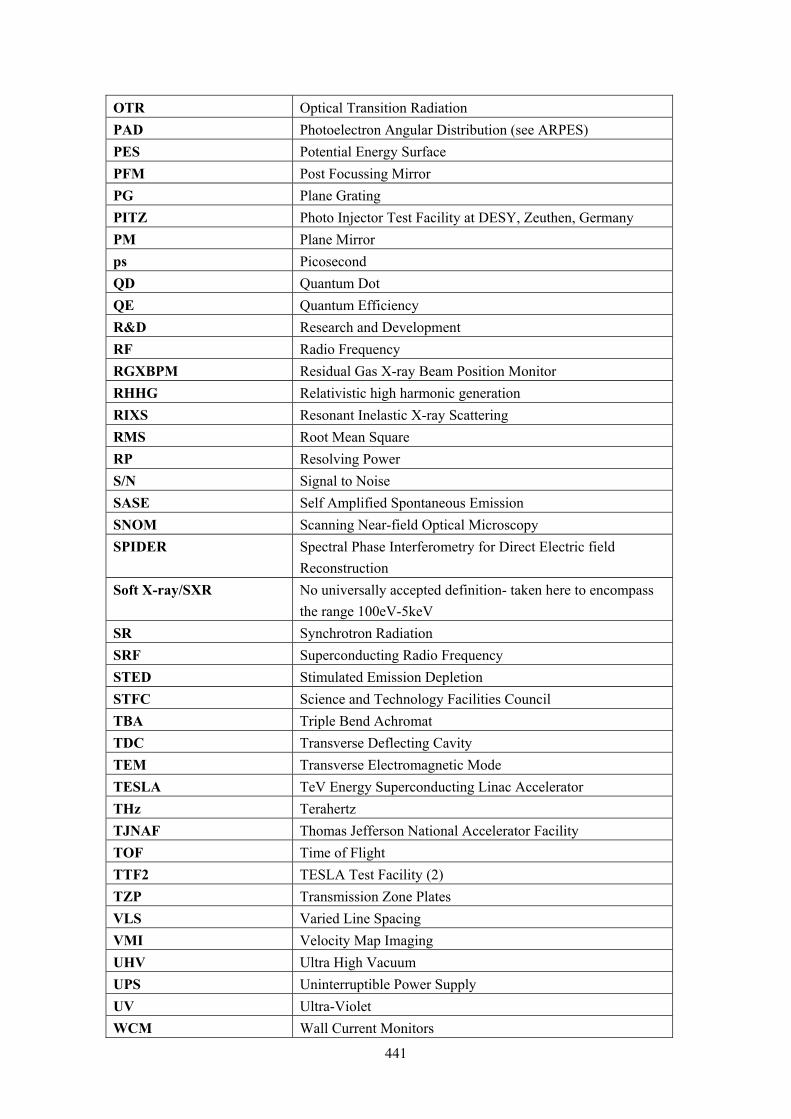
441

OTR Optical Transition Radiation PAD Photoelectron Angular Distribution (see ARPES) PES Potential Energy Surface PFM Post Focussing Mirror PG Plane Grating PITZ Photo Injector Test Facility at DESY, Zeuthen, Germany PM Plane Mirror ps Picosecond QD Quantum Dot QE Quantum Efficiency R&D Research and Development RF Radio Frequency RGXBPM Residual Gas X-ray Beam Position Monitor RHHG Relativistic high harmonic generation RIXS Resonant Inelastic X-ray Scattering RMS Root Mean Square RP Resolving Power S/N Signal to Noise SASE Self Amplified Spontaneous Emission SNOM Scanning Near-field Optical Microscopy SPIDER Spectral Phase Interferometry for Direct Electric field

Reconstruction Soft X-ray/SXR No universally accepted definition- taken here to encompass

the range 100eV-5keV SR Synchrotron Radiation SRF Superconducting Radio Frequency STED Stimulated Emission Depletion STFC Science and Technology Facilities Council TBA Triple Bend Achromat TDC Transverse Deflecting Cavity TEM Transverse Electromagnetic Mode TESLA TeV Energy Superconducting Linac Accelerator THz Terahertz TJNAF Thomas Jefferson National Accelerator Facility TOF Time of Flight TTF2 TESLA Test Facility (2) TZP Transmission Zone Plates VLS Varied Line Spacing VMI Velocity Map Imaging UHV Ultra High Vacuum UPS Uninterruptible Power Supply UV Ultra-Violet WCM Wall Current Monitors

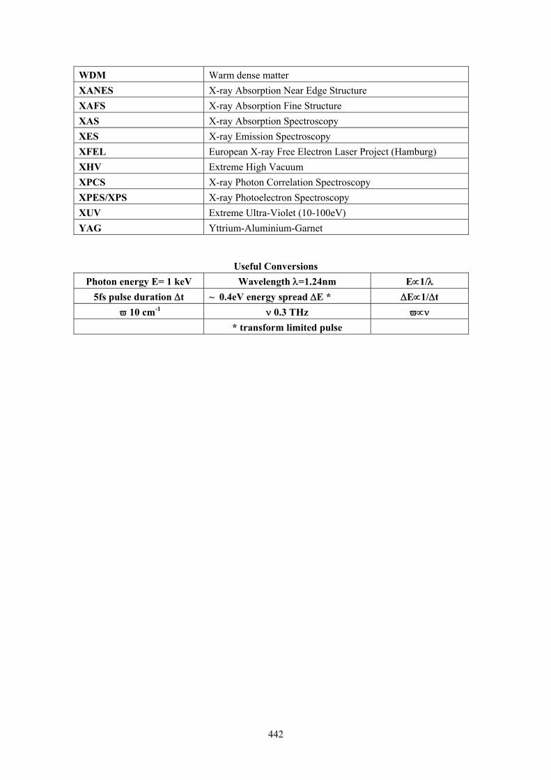
442

WDM Warm dense matter XANES X-ray Absorption Near Edge Structure XAFS X-ray Absorption Fine Structure XAS X-ray Absorption Spectroscopy XES X-ray Emission Spectroscopy XFEL European X-ray Free Electron Laser Project (Hamburg) XHV Extreme High Vacuum XPCS X-ray Photon Correlation Spectroscopy XPES/XPS X-ray Photoelectron Spectroscopy XUV Extreme Ultra-Violet (10-100eV) YAG Yttrium-Aluminium-Garnet

Useful Conversions Photon energy E= 1 keV Wavelength λ=1.24nm E∝1/λ

5fs pulse duration Δt ~ 0.4eV energy spread ΔE * ΔE∝1/Δt ϖ 10 cm-1 ν 0.3 THz ϖ∝ν

* transform limited pulse

443

APPENDIX B

The Importance of seeding to the NLS Scientific Mission

To understand the importance of seeding to the NLS scientific mission we must first of all review the present situation with non-seeded SASE machines. Self-amplified spontaneous emission (SASE) results from the high gain available in a well prepared FEL with a low emittance electron beam traversing an undulator of sufficient length and suitable period. In the undulator the periodic modulation of the electron bunch density necessary for coherent FEL emission comes about through the strong coupling between the emitted radiation and the electron bunch. In a SASE machine this is initiated by spontaneous emission which is a stochastic process so the phase of the modulation varies randomly along the bunch. The precise timing of the X-ray emission relative to the RF phase is also subject to temporal jitter due to uncertainties in the electron bunch position and the stochastic nature of lasing. In FLASH or LCLS without feedback stabilisation this is of the order of several hundred femtoseconds, although with feedback FLASH has reached a jitter as low as 40 fs with some room for further improvement.

Moreover in a high gain FEL the cooperation length (distance within the bunch over which the modulation is locked in phase) is typically shorter than the bunch length which allows a single bunch to emit several pulses (spikes) of X-ray radiation that have no defined phase relationship. The light is therefore only partially longitudinally coherent and will have a temporal and spectral structure that changes from shot to shot due to the stochastic nature of the process. Simulations, e.g. for LCLS [1] and NLS (see Part III Section 1.5.1), show that with very low bunch charges the electron bunch can be made so short that it can only support a single such "spike" that is coherent (close to transform limited). These FEL simulations indicate a single longitudinal spike of 2 fs at 1.5-nm wavelength. However, the timing jitter with respect to the RF phase remains, and will be many time larger than the bunch length. Thus in LCLS the X-ray pulse timing in low bunch charge mode has been found to have a FWHM jitter of ~ 200 fs even though the pulses are believed to be < 10 fs.

The implications of SASE operation are already limiting the time-resolved capabilities of the current generation of FELs. Since the intrinsic jitter is often much larger than the temporal resolution sought (recall that the full resolution of chemical dynamics requires ~ 10 fs temporal resolution) the approach adopted is time stamping of all the data using a shot by shot X-ray pulse arrival time monitor; it is asserted that this should result in a factor of 5-10 improvement of the temporal resolution. Pulse arrival monitors are based upon measuring the arrival of the electron bunch and so do not take into account the jitter between the bunch and the X-ray emission. The cost of that approach is potentially a lower useful repetition rate (as many shots may fall outside of a useful time window), the insertion of an extra uncertainty into the temporal resolution (the beam arrival time measurement is not error free and often involves making assumptions about the synchronisation of electrons and photons), and the problem of having to deal with an X-ray probe that often has a complex temporal structure that is changing from shot to shot (measurement of the full temporal profile on a single shot has not yet been achieved). If a split and delay approach is used to create two X-ray pulses from a single pulse then the arrival time synchronisation of the two pulses is not problematic and jitter no longer matters. There are many measurements, however, that require synchronisation with a conventional laser operating in UV – IR range. Further progress is expected but the ultimate limits of synchronisation in SASE machines remains uncertain.

It has long been the case in laser science that the full control of the field amplitude and phase is needed. This is because many of the most advanced measurements, e.g. non-linear spectroscopy, coherent control, laser driven particle acceleration and ultra-fast measurement, need either a transform limited pulse or a full knowledge of the phase and amplitude history of the pulse. A transform limited pulse is vitally important as it ensures the optimum matching of

444

the pulse duration and spectral bandwidth obtainable. Much of the impressive progress in laser science in recent years (e.g. attosecond science, frequency combs, multi-dimensional laser spectroscopy, laser particle acceleration) could not have happened without these capabilities. A transform limited Gaussian pulse follows a relation between pulse duration Δt and frequency bandwidth Δν that is 44.0≈ΔΔ νt , which means that for a given temporal duration the frequency bandwidth must be 0.44/Δt or larger. A non-transform limited pulse will have a larger bandwidth than needed to reach the given temporal resolution (this is the case with SASE pulses) and this can have a very a large implication for all temporal studies where a material excitation is involved as it is often required to have both the shortest pulse whilst having a spectral bandwidth which addresses only the excitation of interest and not other modes of excitation in the material. X-ray spectroscopy measurements will be hampered by the chaotic spectral distribution as well as chaotic temporal distribution of the X-ray pulse in a SASE machine.

To overcome the intrinsic jitter and fluctuations inherent to the SASE process seeding has been proposed. There are a number of such schemes where an externally applied field is used to pre-modulate the electron density fluctuation in the electron bunch. In that case the modulation is phase locked to the external field which overcomes the fluctuations inherent to SASE and leads to close to transform limited pulses. Moreover because the lasing is precisely locked to the modulating field derived from a master laser oscillator (rather than the machine RF) there is next to no jitter relative to the external laser. Various schemes are under consideration and we highlight only two; HHG seeding and EEHG, both of which are currently looking promising. EEHG employs a pair of phase locked fields to set up a density modulation with high frequency harmonic components resonant with the undulator that then leads to control of the X-ray emission [2]. Whilst there are currently promising predictions for EEHG and experiments to prove it are under development at SLAC at the time of writing these results have not yet been reported so in the current NLS design we have concentrated on HHG seeding where a body of experimental evidence already exists. In HHG seeding a modulating field already at X-ray wavelengths is applied to the electron bunch to directly impose the modulation. HHG seeding was recently demonstrated at the SCSS in Japan [3]. It is assumed to be a viable strategy to radically improve the coherence, reproducibility and synchronization properties of a FEL (see Figure A1). It should be routine to achieve a few femtosecond jitter level using a seeded machine, allowing 20 fs pump-probe resolution to be realised with pulses of high coherence and reproducibility. In contrast a SASE machine will only achieve a jitter level of some tens of femtoseconds as well as the pulses being far from coherent and inherently noisy. Seeding will be essential to achieving the conditions needed for a wide range of the NLS science objectives.

Direct seeding to 1 keV will require relativistic HHG or some other technological advance to ensure the photon energy and power needed but is not yet feasible due to the absence of high repetition rate high peak power lasers. With the likely improvement of high power ultra-fast lasers anticipated to push the average power limit from 1 kW towards 10 kW over the next decade this may provide direct seeding capability across the entire energy range of the FEL. Instead we plan to adopt a hybrid scheme whereby direct seeding is used to 100 eV and 1 or 2 stages of harmonic up-conversion is employed in the FEL to reach 1keV. This would correspond in the FEL harmonics to exceptional coherence and synchronization properties up to >5 keV.

Whilst this has yet to be demonstrated, and hence there are some technological risks associated with this approach, we believe that given the rapid progress being made in this field in general, together with some dedicated R&D, it will be able to be implemented at the start of facility operation. A fall-back option based on SASE operation for the higher energies will be feasible and would be adopted for a period if required. A seeded machine, operating at these high photon energies, would be a unique facility internationally.

445

Figure A1: The dramatic improvement in the temporal quality of the pulse is illustrated by comparing the results of a time dependent calculations for the SASE output for NLS (upper frame) compared to the

Seeded output (lower frame)

General Scientific Impact of Seeding

• There are a significant number of scientific directions for which a seeded, and therefore low temporal jitter and transform limited, X-ray pulse is essential:

• High resolution pump-probe studies with IR-UV pump and X-ray probe where a temporal resolution of better than 10 fs is required. This is likely to elude SASE based machines whereas in a seeded FEL it is likely that temporal resolution below a femtosecond will eventually be achieved.

• Sub-femtosecond experiments where the X-ray pulse must appear at exactly the correct phase relative to an optical field and be well characterized (although not necessarily of sub-femtosecond duration itself). The importance of this is that it will enable a variety of new laser dressing experiments (e.g. CASTOR discussed below) and so open the topic of coherent control of matter to probing by FELs

• Time resolved studies employing techniques such X-ray spectroscopy, inelastic X-ray scattering and X-ray photoelectron spectroscopy, where a single channel must be isolated with a resolution of < 1 eV (even down to 10 meV). Here the challenge is to be at the transform limit so that the best possible temporal and energy resolutions are simultaneously available. In such measurements the changes in the spectrum compared to the unexcited sample are at the level of a few percent or less, requiring high spectral and intensity stability.

• Coherent X-ray matter interactions where resonance or a precise detuning from resonance and smooth temporal pulses are essential (e.g. EIT, STIRAP, continuum state dressing, optical pumping). For this to be achieved both defined and reproducible timing and spectrum are required. It is well known in laser coherence experiments that

446

exceptional phase stability is required for these phenomena to be studied and this translates to a transform limited requirement for the FEL.

• High intensity X-ray – matter interaction studies where there is a non-linear dependence of the interaction on the intensity and so the temporal profile of the pulse must be stable and known. It is vital that a single peaked, near Gaussian, intensity envelope is available if the detailed intensity dependence of the myriad cross-sections of interest in strong X-ray field matter interaction are to be accurately measured.

• Implementations of X-ray non-linear spectroscopy. This is an experimental method that can only be implemented in a useful way if transform limited pulses are used. Phase locking between several pulses may also be required in the future, which also mandates seeding.

• Efficient image retrieval via CDI requires an iterative technique that needs to retrieve the structure from the scattered field distribution. If the initial field is unknown then the effectiveness of the retrieval is compromised. It is therefore hugely beneficial to have a seeded pulse (therefore well defined and reproducible field) so that the iterative retrieval can more efficiently find the structure.

Even where seeding is not essential it will never impede the effectiveness of a measurement and in most cases will lead to much improved signal to noise.

Specific Requirements for Seeding in Research Highlights

To illustrate the general importance of seeding we select below some of the NLS Research Highlights that require seeding.

Solid density plasma diagnostics: X-ray Thompson scattering from plasmas requires transform limited pulses; ideally ~ 100 fs with < 0.1 eV bandwidth in order to preserve the visibility and resolve the width of the ion acoustic feature from which the instantaneous plasma state can be determined. It is unlikely that a SASE machine will ever be able to resolve this feature in a near solid density plasma so a seeded FEL will have a unique impact on HED and WDM research.

Condensed phase time-resolved studies: Time resolved ARPES and IXS from condensed phase systems demands transform limited pulses so as to preserve the information on the evolution of the spectral features that are at the core of understanding the excitations in systems like high Tc superconductors. A transform-limited, seeded FEL offers a tremendous gain for this field. Here, the energy bandpass is inversely related to the pulse duration. For a 100 fs pulse, it is ~10 meV. This would be sufficient for many experiments and would eliminate the need for any upstream optics. In the case of inelastic X-ray scattering (IXS) time-averaged fluxes in excess of 1015 photons s-1 are needed for these measurements, which would require a gain of five orders of magnitude over existing instruments. This would transform the applicability of the technique and would have enormous scientific impact. Measurements of electronic excitations with these kind of resolutions (few meV, pulse lengths of >100 fs) would be transformative. Examples of excitations that one cannot currently study include electronic gaps (e.g. superconducting gaps, charge-density-wave gaps), collective excitations (so-called “orbitons”, particle-hole excitations, “holons”) and more exotic excitations (the pseudogap in high-Tc superconductors, new modes predicted for broken gauge symmetries in high-Tc superconductors [4]. Seeding with longer pulses (>100fs) will be part of the facility development programme, and will lead to pulses of bandwidth getting to 5 meV linewidths which would allow for measurements without monochromators at the level achieved at the best synchrotron facilities but with many orders of magnitude more photons and exceptional temporal resolution.

447

Time resolved X-ray spectroscopy of chemical dynamics: For all time-resolved X-ray spectroscopy (e.g. on catalysis, artificial light harvesting) in solid and liquid phase samples, tuneability and high repetition rate along with precise temporal synchronization with other light sources is essential. Moreover to perform X-ray absorption or emission spectroscopy the X-ray energy for each data point in a spectral scan must be well defined and the same from shot to shot. Any excess spectral bandwidth above the transform limit (typically a factor 10 excess bandwidth in SASE machines) can destroy the measurement. For instance in EXAFS spectral resolution ~ 1 eV is needed which is consistent with a 10 fs seeded machine but not with a SASE operation. Any attempt to overcome the spectral instability limitations of a SASE machine via monochromatization will transfer the spectral instability into an intensity instability, vastly reducing the signal-to-noise level of such measurements. In such measurements the changes in the spectrum compared to the unexcited sample are frequently at the level of a few percent or less, requiring both high spectral and intensity stability. The work described in the NLS case requires synchronized femtosecond visible and UV laser pulses with durations of 20 fs or better, and with a timing jitter of less than 10 fs.

X-ray interaction physics studies: Quantitative fragmentation studies of molecular and cluster fragmentation are essential to our understanding of X-ray matter interaction. This knowledge will be essential in establishing basic molecular and cluster X-ray science but also for the nanoscale imaging part of the science mission of NLS and other FELs. Seeding leads to production of pulses of controlled temporal profile which is essential if systematic studies of intensity dependent (i.e. non-linear) phenomena are to be performed. For this research high repetition rate coherent pulses are essential and so NLS will be unique compared to all the SASE machines. NLS will provide the following capability essential to performing this research. Seeded FEL radiation in the range 50eV-1keV in the high brightness fundamental is essential. It is anticipated that unique studies not possible at any other machine will be enabled by the full coherence imposed by seeding (i.e. the pulse will be close to transform limited), moreover in the energy range 250-800eV provided by FEL 2 we will have truly unique access to new processes (including the inner shell ionisation thresholds of C, N and O). Fully characterized pulses with well defined temporal shape (reproducible from shot to shot so detailed temporal measurements based upon cross-correlation can be carried out) are required.

Two colour probing of ultra-fast correlated electron dynamics: To measure attosecond correlated electron dynamics requires either attosecond pulses or temporally well defined X-ray pulses synchronised precisely to the phase of an optical dressing field (CASTOR). In the latter case X-ray pulses that are seeded and so phase correlated to longer wavelength “streaking” field in CASTOR measurements where the X-ray interaction is linear. A seeded X-ray pulse duration of <10fs is anticipated with photon energy in the 50-300eV range from FEL 1. The streaking field should have a cycle period exceeding by a significant factor the X-ray pulse duration, a field of around 5μm (with an optical cycle time ~15fs) can be generated at the required intensity using optical parametric conversion from a laser that also acts as the source for seeding of the FEL. Fully characterized (reproducible) X-ray pulses are required but these do not have to be sub-femtosecond to achieve attosecond temporal resolution in the measurement. Energy fluctuations only need be monitored on a shot-wise basis, whilst if good seeding is achieved the temporal profile of the X-ray pulses will vary only slightly.

REFERENCES [1] Ding, Y., et al., Measurement and simulations of ultralow emittance and ultrashort electron beams

in LCLS PRL 2009 102, 254801 [2] Stupakov, G., Using the beam-echo effect for generation of short wavelength radiation PRL, 2009

102, 074801 [3] Lambert, G., et al., Injection of harmonics generated in gas in a FEL providing intense coherent

extreme-UV light Nature Physics 2008, 4(4) 296-300 [4] Johansson, P., et al., Theory of inelastic X-ray scattering in layered superconductors Phys. Rev. B.,

1996, 53(13), 8726-8732

449

APPENDIX C

Repetition Rate

This issue is rather technical, and needs to be carefully considered for every individual experiment, and here we only analyse the situation rather generically.

The science outlined in the case is organized into the four categories:

1. IMAGING NANOSCALE STRUCTURES. 2. CAPTURING FLUCTUATING AND RAPIDLY EVOLVING SYSTEMS. 3. STRUCTURAL DYNAMICS UNDERLYING PHYSICAL AND CHEMICAL CHANGES. 4. ULTRAFAST DYNAMICS IN MULTI-ELECTRON SYSTEMS. In 1. Imaging nanoscale structures , the majority of the research falls into the category of single shot imaging where the chief requirement is that there are sufficient photons in a very short pulse. This therefore puts demands upon peak brightness but not on average brightness. Some variants on non-living samples involving two time images could be best achieved by splitting and delaying a single pulse – which again puts demands only on the peak rather than average brightness/rep-rate. We do not see any serious restrictions placed upon this work by constraining the machine to operate at a <500Hz repetition rate, indeed sample handling already may make higher repletion rates challenging to utilize.

For 2. Capturing fluctuating and rapidly evolving systems, the requirement is often to record scattering at two moments relatively close in time is critically dependent upon the properties of a single pulse and the possibility to split and delay. These measurements would benefit from a higher data acquisition rate but could probably still be done at 500Hz. However there is a potentially very important class of measurement where rare fluctuations are sought in isolated nanoscale objects, and for these an extended series of repeated measurements at 10-100kHz repetition frequency are required, this would only be possible using a high repetition rate machine. For high density plasma work the handling of high repetition rate (above 100Hz) is likely to prove more problematic and counter any signal advantages that might arise from a higher available repetition rate. For such measurements it is probably sufficient just to block the unwanted pulses from the beam so low or high rep-rate machines are equally effective.

In contrast much of the science in 3. Structural dynamics underlying physical and chemical changes, and in, 4. Ultrafast electron dynamics, will be benefit if a higher repetition rate is available, and for some experiments a higher repetition rate is essential. Most of these studies are by their nature repetitive measurements, typically utilising a pump-probe arrangement. At each pump-probe delay a good signal/noise needs to be acquired and then the measurement must be repeated at many delays, and to achieve this in a timescale before sample degradation or other changes occur is imperative. Thus in almost all conceivable measurements, whether they involve X-ray absorption, IR/THz non-linear optics/emission spectroscopy or photo-emission, best results are obtained by using a higher repetition rate with pulses of brightness below the threshold to cause sample damage. Moreover certain categories of experiment crucial to this part of the scientific mission - such as photoemission from solids and coincidence measurements probably demand >1kHz repetition rate to make them feasible. In these cases, because the count rates must necessarily be very low to avoid fatal distortion to the information content of the signal, it is not possible to compensate for a low repetition rate simply by increasing the single pulse brightness. Therefore we concentrate here upon these limits to indicate what science may become unfeasible unless a repetition rate >>1kHz is available.

450

The solution-phase XAS work depends on an overall fluence of around 1012 photons/s, but, mostly because the sample is refreshed continuously, and detection is by transmission (or possibly fluorescence in future), i.e. not electrons, to first order it is not critical how this is divided up. There would be clear advantages in a higher rep rate if this increases overall fluence, but the fs experiment is currently performed (although heroic) at 1 kHz rep rate on 3rd generation femtosecond-sliced sources, so it is clearly possible at 500 Hz on NLS. (Essentially the effect would be to pin the maximum benefit to the difference in numbers of useful photons/pulse between a 3rd generation and a 4th generation source which is very large in any event).

It is likely that for most of the longer wavelength vibrational and multi-dimensional spectroscopy a higher repetition rate would be beneficial as rather weak features in the spectrum are anticipated. Here it would be important to avoid exposing the samples to peak intensities that are too high to avoid exciting unwanted channels or promoting too rapid sample degradation.

For XPS in gas phase and from surfaces and in surface sensitive XAS (relying on Auger decay from surface sites) that is important in heterogeneous catalysis there will be more severe limits placed upon the distortion caused by a high peak brightness that produces too many photoelectrons simultaneously. In work on solid state samples involving electron detection, space charge effects have a severe effect for a low repetition rate, high intensity source. A number of studies of space-charge effects in photoemission for both ps and fs source (including FLASH) are available [1, 2, 3]. For example, we know that in core level photoemission of a metal at FLASH, space-charge experiments make the experiment untenable at fluences above around 109 photons per pulse. Basing an estimate on these numbers for a single spectrum from a bulk crystal in the FLASH experiment we can estimate that for a measurement from a more typical monolayer at low concentration ~1014 photons would be required to measure the emission at each photon energy with acceptable S/N. Assuming 100 different energies are recorded at each of 10 different time delays we infer ~1017 photons are needed to make a full time resolved measurement i.e. ~108 pulses. So whereas a 10 kHz rep-rate machine could complete the measurement in ~1 hour (a reasonable duration) on the order of 1 day would be required for a 500Hz machine, this would be more challenging once sample degradation and other experimental drifts are accounted for.

This consideration affects all condensed matter spectroscopies where electron detection is involved. This includes, for example, the ARPES photoemission outlined in Part II Section 2.3.1 (and as pointed out at the relevant workshop, because of this, a 10 – 100 kHz rep rate is desirable). However it is also critical to the XPS and XAS of surfaces discussed in the catalysis section. XPS is clearly affected, as it involves electron detection. In XAS, following absorption, the most likely process is electron emission. At surfaces, XAS of (in particular) of light elements generally uses surface-sensitive Auger electron yield detection (transmission is clearly not appropriate), and this will be subject to space-charge effects in a similar way to photoemission. In this experiment, the species probed will be dilute (as it is at the surface). Auger yield signals are normally comparable to transmission EXAFS, but (because of the low pathlength of the electrons) come mostly from the surface (typically around 90% of the signal comes from the first few tens of Å).

Very broadly this means the work in homogeneous catalysis is feasible at lower rep-rate, but for the work in heterogeneous catalysis higher rep rate is probably essential in many cases. Both categories of catalysis are very important, heterogeneous being at least as important to industrial chemical catalysis as homogeneous.

For applications in valence band photo-emission spectroscopy, which is used to measure electronic structures in complex solids and at surfaces, the possibility of having a high-repetition rate machine with a narrow transform limited energy spread would open new horizons. Both energy and temporally resolved measurements (limited only by the uncertainty

451

principle) would then be possible that address hitherto unresolved problems. A high average flux, spread over many pulses, is essential to ensure measurable signals that are not completely degraded by space charge effects. It is estimated that high resolution ARPES measurements require >1013 photons/s and since the number of photons per pulse incident upon the sample should be kept to <<109 to avoid severe space charge effects a repetition rate of ~10kHz appears to be a minimum requirement to satisfy these constraints.

The possibility of having ultra-narrow linewidths with a high average flux within that linewidth will impact inelastic scattering. Conventional light sources cannot provide this so here would be a new opportunity for NLS. The need is for a substantial average flux as the scattered signals are weak, but this flux needs to be delivered in many pulses so as to avoid significant sample damage. It is estimated that to obtain 10 counts per second in the scattered signal (the threshold where these experiments become feasible) requires a flux within the desired linewidth of ~1014 photon/sec. It is estimated that after spectral selection a 500Hz machine would deliver only ~1013 photons/second which is possibly insufficient whereas for a 10 kHz machine this rises to ~2 x 1014 photons/sec which is more acceptable. So we see this work too is best performed at a high repetition rate.

REFERENCES [1] Pietzsch, A., et al., Towards time resolved core level photoelectron spectroscopy with femto second

X-ray free-electron lasers New J Phys, 2008 10, 033004 [2] Passlack, S., et al., Space charge effects in photoemission with a low repetition, high intensity

femtosecond laser source J Appl Phys, 2006 100, 024912 [3] Zhou, X J., et al., Space charge effect and mirror charge effect in photoemission spectroscopy

J Electron Spectrosc Relat Phenom, 2005 142, 27-38

453

APPENDIX D

New Light Source Consultation Participation in Phase I

The first phase of the NLS project was to determine, through wide consultation, the key long-term scientific objectives for the UK light source strategy and establish the light source capability we need to implement that strategy.

This consultation aimed to reach existing users of UK light source facilities (DIAMOND, CLF, SRS), supporters of recent proposals (4GLS, Sapphire) and the science community in general.

Consultation Process The consultation process included the following:

• A project launch, 11th April 2008, Royal Society London, 113 attendees excluding meeting administration, advertised by email to STFC and DLS lists and on the STFC web

• A series of workshops in five key science areas during May and June 2008, convened by co-ordinators drawn from the science community, advertised by email to STFC and DLS lists, by flyers to university departments and on the STFC web. These were informal meetings with significant time for discussion and debate.

• Working groups in each of these science areas to further consult within their specialisms and to collate the community views, distilling key drivers and requirements (through June-August 2008). Membership was by invitation to leading UK scientists in each field and international experts

• Individual input was sought via an email invitation on STFC and DLS lists; this input could be either to the project leader, science area co-ordinators, or via a web-based form

• Meetings with Research Council representatives (July 2008) • Additionally, a workshop on Advanced Photon Sources, bringing together experts to

discuss the technological capabilities and limitations of both the conventional laser and accelerator based light sources on which it may be based

Analysis of input

Method Registrations Attendance at Launch (11th April 2008) 122 Registered general interest on web (available ~21st March 2008)

33

Attendance at workshops Ultrafast Electron Dynamics and Attosec Science; 13th May 2008

74

High Energy Density Science; 20th May 2008 69 Condensed Matter; 21st May 2008 50 Chemical Science, 22nd – 23rd May 2008 62 Advanced Photon Sources, 3rd – 4th June 2008 81 Life Sciences, 19th June 2008 51 Attendance at NLS Community Meeting 24th April 2009 123

454

Membership working groups

Condensed matter (co-ordinator Andrea Cavalleri) Andrea Cavalleri Oxford, STFC Ian Robinson UCL, DLS Gabriel Aeppli UCL Elizabeth Blackburn Birmingham Gerrit van der Laan STFC Paolo Radaelli STFC Felix Baumberger St, Andrews Peter Hatton Durham Chemical science (co-ordinators Jonathan Underwood and Wendy Flavell) Jonathan Underwood UCL Wendy Flavell Manchester Jon Marangos Imperial Justin Wark Oxford Peter Barker UCL Majed Chergui EPFL Anders Nilsson SLAC Helen Fielding UCL Ivan Powis Nottingham Gopinathan Sankar RI Martin McCoustra Heriot Watt Julia Weinstein Sheffield John Evans Southampton Sven Schroeder Manchester Christian Bressler EPFL Mike Towrie STFC Klaus von Haeften Leicester Stuart McKenzie Oxford Ultra fast (co-ordinator Jon Marangos) Jon Marangos Imperial Jonathan Underwood UCL John Tisch Imperial Matt Zepff QUB Will Bryan Swansea Leszek Frasinski Reading/Imperial Ian Walmsley Oxford Brian McNeil Strathclyde Riccardo Bartolini DLS Justin Wark Oxford Misha Ivanov Imperial Fred Currell QUB Nigel Mason Open University Emma Springate STFC Mark Roper STFC David Holland STFC HEDS (co-ordinator Justin Wark) Justin Wark Oxford Steve Rose Imperial Roger Evans Imperial Dave Riley QUB

455

Gianluca Gregori Oxford Malcolm McMahon Edinburgh Nigel Woolsey York Greg Tallents York Dirk Gerricke Warwick Dick Lee LLNL Life Science (co-ordinators Louise Johnson, Peter Weightman) Louise Johnson DLS/Oxford Peter Weightman Liverpool Tony Parker STFC David Klug Imperial Nigel Scrutton Manchester Tony Ng Kings Colin Nave STFC/Diamond Donna Lammie Cardiff Tim Wess Cardiff Alan Michette Kings

List of those who responded to inquiry on potential use of flash imaging

Clive Bagshaw (Leicester) Louise Cramer (University College London) Ilan Davis (Oxford) Hugh Dickinson (Oxford) Michael Ferenczi (Imperial College) Malcolm Ferguson-Smith (Cambridge) Mike Hanon (Birmingham) Samar Hasnain (Liverpool) Chris Hawes (Oxford Brooks) Martin Humphries (Manchester) Malcolm Irving (Kings College London) Achilles Kapanidis (Oxford) Mark Marsh (University College London) Keith Meek (Cardiff) Justin Molloy (NIMR, London) Harvey McMahon (Cambridge) Tony Ng (Kings College London) Peter O’Neil (Oxford) Nigel Scrutton (Manchester) Tony Stead (Royal Holloway College) Ashok Venkitaraman (Cambridge) Boris Vojnovic (Oxford) Peter Cook (Oxford) Jason Raff (Oxford)

456

UK distribution of involvement

ODR Merged - CORE

Documents

Transcript of ODR Merged - CORE