Obsidian Use-Wear Analysis and the 76 Draw

Site: A Medio Period, Casas Grandes Settlement in New

Mexico

Timothy Lambert-Law de Lauriston

Introduction:

The Casas Grandes region is a vast expanse of territory that covers much of the

Northwest corner of the modern day Mexican state of Chihuahua. The cultural center

of this region is the site that the region takes its name from, that is Casas Grandes, also

called Paquimé (Figure 1).

Figure 1: Location of the Casas Grandes site and region

(Mendez 2009:2)

This site is an extremely large adobe pueblo that sits is northwestern Chihuahua,

Mexico. Through ceramic studies conducted at Paquimé and in the surrounding regions

there is now an established chronology for the Casas Grandes culture spanning AD

1200-1450, also known as the Medio period. The Medio period can be split into two

parts, an early and late sequence (Whalen and Minnis 2009), but for the purposes of this

study this division in not necessary.

Paquimé:

The site of Paquimé is situated in a very unique environmental area, being

“located at the intersection of two major environmental zones” (Whalen and Minnis

2001:60). To the east of the site is the massive Chihuahuan Desert, exhibiting a basin-

and-range topography. This area of high desert covers elevations from 1200 m on its

eastern edge, near the modern day towns of El Paso, Texas and Ciudad Juárez, Mexico,

to around 1500 m on its west side, near the site. The other major environmental area is

the Sierra Madre Occidental a huge mountain range that runs over 500 km from the

Mexico/United States border south. The peaks of this mountain range from 2400 m to

3000 m in some areas. The confluence of these two very different zones provided

Paquimé and the Casas Grandes region in general, with a variety of economic zones to

take advantage of.

The Casas Grandes region, and indeed all of northwestern Mexico, has long been

an understudied area when it comes to the field of archaeology. About this

phenomenon, Whalen and Minnis (2001:25) state “[this area] has always been a sort of

archaeological vacuum, surrounded on both sides (i.e. to the north and south) by much

better studied areas”. A common sentiment in Mexican archaeology is that this

northern area is a relatively uninteresting place, which was a cultural backwater where

civilization did not penetrate. Many Mexican, and for that matter American,

archaeologists would much rather head south and study the Oaxaca Valley or the Valley

of Mexico, or even further south and investigate the Maya heartland. To the north of

the Casas Grandes region lies the vast area known as the American Southwest. This

culture area is one of the most heavily studied areas in North America, if not in the

western hemisphere. Thousands of sites have been dug, with thousands more having

been discovered but as of yet unexcavated. In addition to the massive amount of

archaeological studies that have been carried out in the American Southwest, there is a

very large and extensive ethnographic and ethnohistoric record as well. This can be said

the same of for the areas farther south of the Casas Grandes region, where we have

multiple Spanish chronicles, describing the lifestyle of the inhabitants upon contact.

This did not happen in the northwestern area of Mexico, and thus in the archaeological

and ethnographic record this area has a surprisingly small amount of data with which to

work. This has been changing in recent years, though with many new people coming

into northwestern Mexico and studying the cultures that existed there. But, as Whalen

and Minnis (2001:25) state “the neglect of generations will take long to undo”.

History of Casas Grandes Research:

Though the region has been largely understudied, the site of Paquimé has been

known for a relatively long period of time, and recognized as unique and beautiful since

it was first discovered by Europeans peoples. The first European to record the site was

Baltazar de Obregón in AD 1584, who marveled at Paquimé saying:

There are many houses of great size, strength, and height. They are of six and seven stories, with towers and walls like fortresses for protection and defense against the enemies who undoubtedly used to make war on the inhabitants. The houses contained large and magnificent patios paved with enormous and beautiful stones resembling jasper. There were knife-shaped stones which supported the wonderful and big pillars of heavy timbers brought from far away. The walls of the houses were whitewashed and painted in many colors and shades with pictures if the buildings. The structures had a kind of adobe wall.

However, it was mixed and interspersed with stone and wood, this combination being stronger and more durable than boards. (Hammond and Rey 1928:206)

Then, little mention was made of this impressive ruin and culture area for the next three

hundred years. Towards the end of the nineteenth century and the beginning of the

twentieth many explorers, scholars, and adventurers visited the area and made brief

descriptions of what they saw there. Some of these include the famous Hubert Bancroft

(1883), Adolf Bandelier (1890), and other names such as Carl Lumholtz (1901) and J,

Warren Weiseheimer (1917). The first extensive work done in the Casas Grandes region

was massive reconnaissance and field surveys carried out by Donald Brand and Edwin

Sayles both in the 1930’s and 1940’s. Through their work they collected large amounts

of artifactual data and provided an even larger amount of work on site descriptions and

locations. Although, it would not be until two decades later that any excavations took

place in this region.

In 1958 the Joint Casas Grandes Project was initiated as a cooperation between

the National Institute of Anthropology and History of Mexico (INAH) and the Amerind

Foundation of Dragoon, Arizona. The work carried out by this project has long been

considered one of the most important and influential excavations that have taken place

in the Casas Grandes region. The field director of this project was the now famous

Charles C. DiPeso, who oversaw all of the excavations that took place on the site. Work

spanned thirty-six months in which huge portions of Paquimé were excavated, a

number of smaller neighboring sites were excavated as well, and a small amount of

survey work was done. The project ended in 1961 yielding vast amounts of information

that would consume the next thirteen years of DiPeso’s life. In 1974 (DiPeso 1974, vols.

1-3; DiPeso, Rinaldo, and Fenner 1974 vols. 4-8) a massive eight volume publication was

finished that provided one of the most in depth studies ever done in the American

Southwest or Mesoamerica. It is from this work that many of the modern day

interpretations about the Casas Grandes culture have been drawn, being supplemented

by new work in and around the area.

Recent Work in the Casas Grandes Region:

Much of this new work has been focused on the smaller sites surrounding

Paquimé and establishing the different interactions between these sites and Paquimé

itself. A large portion of this work has been carried out by Dr. Michael E. Whalen of the

University of Tulsa and Dr. Paul E. Minnis of the University of Oklahoma. Their work

initiated with survey projects in 1989 and continued with more surveys and excavation

throughout the 1990’s and into the 2000’s, with some work still being conducted today.

Their work resulted in multiple publications (Whalen and Minnis 2009, 2001, and many

others) that gave much insight into how the peripheries of the Casas Grandes region

interacted with the core site of Paquimé. Another group of investigations have been

going on as well headed up by Drs. Todd and Christine VanPool of the University of

Missouri and Dr. Gordon Rakita of the University of North Florida. While each of these

authors have conducted individual research resulting in multiple publications (Raktia

2001; VanPool C. 2003a and 2003b; VanPool et al. 2000; VanPool and VanPool 2007),

more recently these three have teamed up and led investigations that included

excavations and survey work on the furthest areas of the Casas Grandes region.

One of these projects centers on the 76 Draw Site (LA 156980) (Figure 2) located

in Luna County, New Mexico, about 30 km south of the modern town of Deming and

180 km north of Paquimé. The work started with a field survey in 2008 that identified

the 76 Draw Site and concluded that further work should be done on the site. The

directors returned in the summers of 2009 and 2010 and carried out more survey work,

conducted an extensive ground penetrating radar survey, and excavated multiple pits.

Figure 2: 76 Draw Site in relation to Paquimé (Modified from Rakita et. al 2011)

I was involved in the excavations that took place during the 2010 field season and out of

my experience came the current project. The 2009 field season resulted in a report that

was submitted to the Bureau of Land Management in New Mexico as part of the site sits

on BLM land. The 2010 field season resulted in a paper presented at the Sixteenth

Biennial Jornada Mogollon Conference in Silver City, New Mexico (Rakita et al. 2011).

The site was reportedly first visited by Edwin Sayles in 1936, but the first documented

report of the site comes from Donald Brand (1943:132-133) who at the time indicated

that it was the northernmost Medio period site he had encountered. This is still true

today and this is one of many reasons that field work has taken place here, and will

continue into the future.

The 76 Draw Site:

The 76 Draw Site (Figure 3) is located north and east of a seasonally dry arroyo

from which the site takes its name. Its known extent covers an area of 350 m by 500 m

and is split between Bureau of Land Management Land (10%) and the privately owned

Inman Ranch (90%). The terrain of the area is typical desert scrubland with large

amounts of yucca plants, mesquite, creosote bushes, and a variety of grasses and small

bushes. The site has been disturbed in some locations by a dirt road that cuts through

the middle of the site, used by the rancher to get to his herds of cattle that currently

graze on the land, as well as by extensive alluvial erosion brought about by seasonal

rains, and the occasional breaching of a retaining dam. The site has also been disturbed

by pot hunters and looters that have been digging on the site for the last fifty years.

Even though there is a large amount of disturbance on the site “current excavations

demonstrate that over a meter of cultural deposits remain intact in many areas” (Rakita

et. al 2011:31). The surface of the site is characterized by a scatter of lithic artifacts,

animal bones, and pottery sherds. Also seen on the surface are several exposed adobe

walls, concentrations of burned adobe, two roasting pits, several possible effigy mounds

and plazas (Figure 3).

Figure 3: 76 Draw site map

(Modified from Rakita et al. 2011)

The site technically belongs in the Animas phase culture, which is defined as that part

of the Casas Grandes culture that lies north of the Mexican border.

Connections Between 76 Draw Site and Casas Grandes Sites South of the Border

Many archaeologists are of the opinion that sites this far north of Paquimé had

little or no interaction with the main hub at all. Through the ongoing work being

conducted on the site it is apparent that the inhabitants of the 76 Draw Site did have

some level of contact with the Medio period peoples farther to the south. This is

evidenced through the appearance of Ramos Polychrome and other ceramic types that

are characteristically Medio Period potteries. The connection is also evidenced through

a unique style of adobe wall construction known as “drop key” construction and also

called tongue and groove style (Figure 4).

Figure 4: Drop key style architecture shown in profile

This style of wall construction is uniquely Casas Grandes and is not found anywhere

outside of the region. The basic tenants of this construction technique is to form a

section of adobe wall several meters long and wait until is it just starting to dry out.

Then, one would cut a u-shaped groove from the top of the wall going into the middle of

the wall. Once this was completed, another layer of adobe wall would be built on top of

the pre-existing wall, with part of the new layer being connected to the first section by

way of the groove cut before the new layer was added. This provides a much stronger

wall and in fact this method is used in modern day buildings, but usually with wood or

concrete instead of adobe. A sourcing study conducted on the obsidian artifacts

(VanPool et al. in press) provides another line of evidence for connection with the Casas

Grandes culture region further to the south. Through this sourcing study it was

determined that a majority of the obsidian artifacts (65% of the flakes and 20% of the

retouched pieces) came from the Sierra Fresnal source located about 130 km south of

the 76 Draw Site, and well into the Casas Grandes region of northwestern Mexico. The

report concluded that by some means of procurement, either direct procurement,

indirect trading, or direct trading, obsidian from the northwestern Chihuahua desert

was definitely finding its way to the 76 Draw Site.

Goals for This Study:

While these three lines of evidence provide fairly conclusive evidence that the

peoples of the 76 Draw were interacting with their contemporaries farther to the south,

this study intends to add another aspect to support this conclusion. I intend to

accomplish this through a functional (or use-wear) analysis of an assemblage of obsidian

artifacts, in fact the same obsidian artifacts that were used in the sourcing study cited

above, excavated from the 76 Draw Site. This study is important is two ways, the first

being that this is only the second time a functional analysis has been performed on a

lithic assemblage from the Medio period and secondly because it is the first time that

this kind of analysis has been performed on a solely obsidian assemblage. After the

analysis is complete, I will take the results of this study and perform two kinds of

analysis. The first will be an inter-site analysis, in which I will compare the data gained

from the use-wear study to a similar study conducted on stone tools from Site 204 or La

Tinaja which is “one of the two largest neighbors of Paquimé…located about 17km west

of Paquimé in the Arroyo La Tinaja Valley” (Mendez 2009:16). Through this analysis I

hope to show that the peoples of the 76 Draw were using their stone tools for similar

motions and on similar materials as the inhabitants of La Tinaja were, providing yet

another connecting link between the Casas Grandes core region and the peripheral

regions. The second analysis will consist of an intra-site analysis in which I will attempt

to determine if there were specialized activity areas within the 76 Draw Site, and if so

what this might tell about the internal structure of the sight.

What is Use-Wear:

Before moving onto the results of the analysis, an overview of what a “use-

wear” study is and a brief outline of the history and theoretical frameworks of

functional analyses are in line. The most basic definition of what a use-wear analysis is,

was advanced by one of the pioneers of the field, Dr. George Odell. He states that a

functional study is “The analysis of the edges and surfaces of stone tools for the

purposes of ascertaining their patterns of damage” (Odell and Odell-Vereecken

1980:87). This is based on the theoretical notion that when used on a certain material

and in employed in certain motion, distinct and identifiable patterns of wear will appear

on the edges and surfaces of the tool that was used. Obviously, there are infinite

combinations of materials and motions that a tool can be employed for, but by

observing multiple factors, it is possible to decided what the tool was used on and how

it was used.

Variables Used in This Study and Their Definitions:

Generally there are four main categories of traces that one looks for. These are

striations, edge-rounding, polish, and scars. Striations are grooves, valleys, or scratches

cut into the surface of the tool, most likely by a fragment of the tool being dragged

across the surface while in use, or possibly from some component of the worked

material doing the same thing (Odell and Odell-Vereecken 1980; Semenov 1964). This

category is very important as it can provide a good indication of what direction the tool

was moving during its use. Following this line of thought, striations seen parallel to the

use edge would indicate the tool was used for slicing or sawing. Striations perpendicular

to the employed edge would indicate the tool had been used in a scraping or planning

motion and striations appearing diagonal to the used edge might indicate a whittling

motion, but diagonal striations are the most controversial ones and can indicate several

other motions as well. Edge-rounding refers to the amount of dulling or rounding of the

tool’s edge that has occurred during use. This is a relative variable, as the amount of

rounding is compared to the relatively sharp edge of an unused tool. The usual ways of

quantifying rounding are light, moderate, or heavy. Polish is perhaps one of the most

controversial variables and has spurred much debate among use-wear analysts. In

general polish “refers to a lustrous or reflective area of a tool surface which results from

any number of undetermined processes” (Mendez 2009:53). While polish is usually a

variable employed in most use-wear studies, it is most often excluded from obsidian

artifacts as obsidian is naturally lustrous and polish does not form well on this lithic

material.

The last variable of scar patterns deserves a more lengthy discussion as there are

several aspects to this variable and it generally plays the largest role in determining the

use of a tool. The two biggest variables within scar patterns are type (or termination)

and distribution. The termination variable has four possible states that are: feather,

step, hinge, and snap (Figure 5).

Figure 5: Scar termination types

(Modified from Hayden 1979) The definition of these termination states are taken from the Ho Ho Classification and

Nomenclature Report (Hayden 1979). A feather termination is one that ends in a

gradual slope resulting “in an edge with a minimal margin” (Crabtree 1972:64). A step

termination is a scar that ends in an abrupt way usually forming “a right angle break”

(Crabtree 1972:93). A hinge termination is difficult to define verbally so I will employ

the direct definition from the Ho Ho Classification and Nomenclature committee: “a

hinge fracture meets the surface at a steep angle or approximately right angles to the

longitudinal axis” (Hayden 1979:134). Snap fractures are definitely the easiest to

identify, but again pose a difficult problem when describing them in words. According

to the Ho Ho Committee, snap fractures “only occur with bending initiations and

continue in a relatively straight line to terminate nearly perpendicular to the opposite

face” (Hayden 1979:134). The variable of distribution refers to the intensity of the scars.

This has four states called dispersed, even, clustered, and compound in order of

increasing intensity. The patterns are best illustrated rather than described and figure 6

does the job adequately.

Figure 6: Scar distribution types

(Mendez 2009:55)

History of Use-Wear Analysis:

As mentioned above, the history of use-wear analysis and the development of

the associated theoretical frameworks should be discussed as well. The biggest and by

far the most influential piece of work published on use-wear analysis was the pioneering

Prehistoric Technology written by S.A. Semenov in 1964. This study laid the basic

groundwork for future analysts to build on for years to come. One of the most

important aspect of Semenov’s study was an experimental program to provide a

comparative collection to look at, so as to better understand the patterns that form

when a tool used for a particular function. This key tenant is employed in most every

functional analysis and any analyst worth his salt would not consider a use-wear study

to be valid without experimental replication. Of this technique Semenov states

“the experimental approach cannot serve as an independent method of study of the function of tools: precise evidence is required of what was the real purpose of the tool in each specific example “ (Semenov 1964:1). Using the experimental tools Semenov described the patterns of wear associated with

particular motions and worked material, then applied this to a vast array of

archaeological specimens to identify their use. This study is a seminal work which all

students of use-wear analysis should know and read as a good introduction to the field.

The Methodological Schism:

After Semenov published this pioneering work, there was an amazing response

by archaeologists concerning the theoretical and methodological aspects of use-wear.

The core of this debate revolved around two different analytic techniques and their

effectiveness of correctly identifying the use of the tool. One technique has become

commonly known as the high-power technique and the other the low-power technique,

though there is a much bigger difference in these two methods than the amount of

magnification employed when looking at the tools. The high-power technique’s most

commonly cited defenders were Lawrence Kelley and M.H. Newcomer. Though in

recent years others have taken this position, such as Dr. Marvin Kay at the University of

Arkansas. This technique makes use of magnifications above 100x and employs incident

or indirect lighting, as well as “metalizers” or metallic surface coatings (Keeley and

Newcomer 1977; Keeley 1980). They also employ a binocular microscope such as

Scanning Electron Microscopes (SEM) and/or Focused Ion Beam (FIB) systems instead of

the stereoscopic scopes used by the low-power analysts. The proponents of this

technique focus on polish, which at such high magnifications can be easily distinguished

between materials. Basically, these analysts can tell the difference between hide polish,

meat polish, bone polish, etc. As with all techniques there are some pros and cons of

using this framework. Some of the advantages are that many traces seen at such high

magnifications cannot be discerned at lower ones. As well as, the ability to distinguish

between polish types. I feel though, that this technique has a greater number of

disadvantages. For starters, the machines with which the microscopy is performed are

very expensive to purchase and to run. This technique is also very time consuming as

one must learn how to operate the scope before using it, so one does not break a piece

of equipment that regularly costs in excess of one million dollars. It also has the added

disadvantage of only being able to look at small pieces, areas of pieces, and small

assemblages at a time, consuming even more time. Although there seem to be many

disadvantages to this technique, many have successfully employed it in use-wear

studies.

The lower power technique, on the other hand, regularly employs magnifications

of 10x-100x. The main proponents of this technique were Ruth Tringham’s Harvard

group (Tringham et al. 1974) and Dr. George Odell (Odell 1975; Odell and Odell-

Vereecken 1980). This technique uses reflected lighting, or an external light source,

such as a lamp, and as stated above, the analysts use a stereoscopic microscope which

provides a more natural three-dimensional view, compared to the two-dimensional

view a binocular scope provides. Instead of solely focusing on polish, this technique

focuses on the scarring and the patterns of those scars along the used edge of the tool.

As with high-power there are some pros and cons of this technique as well. One of the

disadvantages is that when employing lower magnifications one might miss some of the

traces seen by high-power analysts. I personally feel that this technique overcomes

many of the disadvantages seen in the high-power methodology. It is not as costly as

the microscopes employed generally costs hundreds to a few thousands of dollars. It is

also less time consuming as one does not have to train as long to learn how to use these

microscopes. This technique also has the added advantage of being able to look at large

pieces, large areas, and thus large assemblages in a relatively short period of time, again

reducing the amount of time it takes to perform an analysis. This technique has also

successfully been used by many analysts over the years.

Methodology for This Study:

Given the above discussion it is probably not too difficult to discern which

technique I employed during this study. But, a brief description of the equipment used

and the way the data was recorded is definitely in order. For my study I employed a

Nikon SMZ-10 Stereomicroscope with a range capability of 10x to 80x. I recorded the

variables of scar patterns, edge rounding, and striations, and left out polish for the

reasons listed above. To help reduce ambiguity regarding the location of the observed

wear I used what is known as a “polar co-ordinate” system (Figure 7).

Figure 7: Polar co-ordinate system

(Mendez 2009:51)

With this system one basically draws the outline of the tool on a circle that is split evenly

into any given number of segments (I employed eight). This allows the analyst to

accurately record the position on the wear he/she is seeing. Thus, one can say “In polar

co-ordinate 1 there is such and such type of wear appearing” instead of using

ambiguous phrases like “wear occurs on the distal end on the left lateral margin”. This

simply helps to accurately pinpoint the wear so that future researchers, or even the

analyst himself, can go back to the data recording sheet and know exactly where on the

stone tool the observable wear patterns are occurring. For my study I also created an

experimental collection of tools (Figures 8 and 9) that I used on various materials and in

various ways. These tools included projectile points that were hafted in various ways, as

well as a variety of simple flake tools. I also had the added advantage of having access

to a large comparative collection housed in the archaeology laboratories at the

University of Tulsa.

Figure 8: Experimental tools utilized in this study

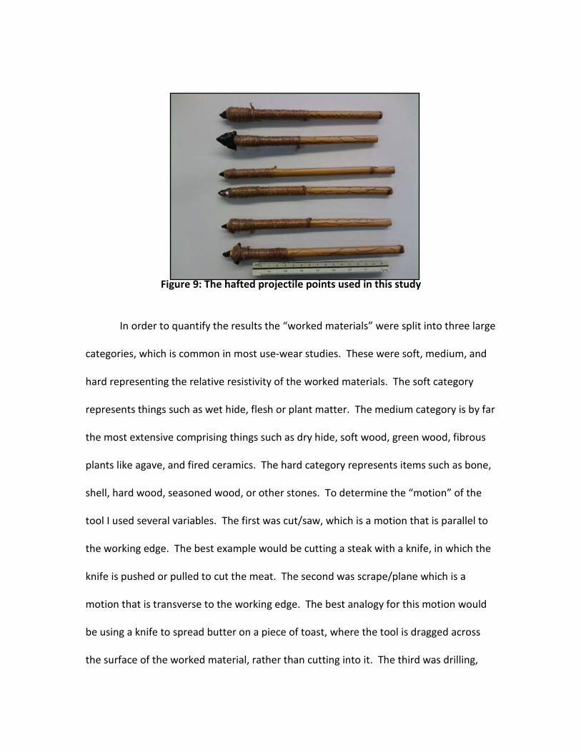
Figure 9: The hafted projectile points used in this study

In order to quantify the results the “worked materials” were split into three large

categories, which is common in most use-wear studies. These were soft, medium, and

hard representing the relative resistivity of the worked materials. The soft category

represents things such as wet hide, flesh or plant matter. The medium category is by far

the most extensive comprising things such as dry hide, soft wood, green wood, fibrous

plants like agave, and fired ceramics. The hard category represents items such as bone,

shell, hard wood, seasoned wood, or other stones. To determine the “motion” of the

tool I used several variables. The first was cut/saw, which is a motion that is parallel to

the working edge. The best example would be cutting a steak with a knife, in which the

knife is pushed or pulled to cut the meat. The second was scrape/plane which is a

motion that is transverse to the working edge. The best analogy for this motion would

be using a knife to spread butter on a piece of toast, where the tool is dragged across

the surface of the worked material, rather than cutting into it. The third was drilling,

which is pretty self-explanatory. A fourth was projectile point, which simply means that

the observed wear matched that expected to be seen on a piece that was actually

hafted, then shot with a bow or thrown like a dart. The last was punch/ream which is a

motion that employs the tool to poke a hole in the worked material for any given

reason. A depiction of these different motions is found in Figure 10. I also recorded the

metrics of the tools (length, width, and thickness all measured at the largest point) to

determine if there was any correlation between general tool size and tool activity.

Lastly, the tools were divided into five categories. These were broken flakes, broken

cores/nodules, projectile points, broken projectiles points, and whole flakes.

Figure 10: Tool motions

(Modified from Shea and Odell 1985)

The whole flakes category was then subdivided into primary flakes, those flakes showing

greater than 50% cortex, secondary flakes or those flakes showing less than 50% cortex,

and tertiary flakes or the flakes that exhibited no cortex at all.

Inter-Site Analysis

To start with, I will examine the similarities and differences found between the

76 Draw Site results and the data from the La Tinaja site. Table 1 gives a general

breakdown of the pieces and in what motion they were used. As evidenced by the

table, 58% (n=57) of the tools were not utilized and 42% (n=40) were. The table also

shows that drilling was by far the most common activity, with cutting being second, and

scraping and use as a projectile point tying for third. The La Tinaja site shows a similar

pattern where drill and cut/saw are the two most common motions, but with cut/saw

being the most common and drill being the second most common (Mendez 2009:78

table 4.14).

Table 1: Distribution of tool motion categories

Table 2 provides a similar look, but showing the worked materials category instead of

tool motion. The table shows that materials of a medium resistivity make up 80%

(n=32) of the total utilized pieces, with hard materials coming in second at 15% (n=6),

and lastly soft comprising only 5% (n=2). Comparing this data with the analysis at La

Tinaja the same exact pattern emerges, just with different percentages. At La Tinaja

medium materials comprise 60.6% of the utilized pieces, hard materials come in second

comprising 17.5%, and soft materials make up 16.3% of the assemblage (Mendez

2009:80 table 4.18). It should be noted that the reason the La Tinaja percentages do not

Drill Cut Scrape Projectile Punch Not

Used Broken Flakes 0 3 4 0 1 21

Broken Cores 0 1 2 0 0 14

Broken Projectile Points 4 2 0 5 0 7

Projectile Points 11 2 0 2 0 3 Primary Flakes 0 0 1 0 0 4 Secondary Flakes 0 1 0 0 0 3 Tertiary Flakes 0 1 0 0 0 5 Total 15 10 7 7 1 57 Percentage of Assemblage 15.46% 10.31% 7.22% 7.22% 1.03% 58.76%

add up to 100% is that the analyst included an “ambiguous” category, in which the

pieces he was unsure about were placed. This category constitutes the missing 5.6%.

Soft Medium Hard Broken Flakes 1 7 0

Broken Cores 1 2 0

Broken Projectile Points 0 10 1

Projectile Points 0 10 5 Primary Flakes 1 1 0 Secondary Flakes 0 1 0 Tertiary Flakes 0 1 0 Total 2 32 6 Percentage of Utilized Pieces 5% 80% 15%

Table 2: Distribution of worked material categories

Combining the two categories of worked material and tool motion create what is

called “tool function” or “tasks”. Some examples might include cut medium, drill hard,

scrape soft etc. These tool functions allow the analyst to look at what the most

common tasks are, instead of only comparing the most common motions and worked

materials. Table 3 displays the tool functions from this assemblage. At 76 Draw site the

Table 3: Distribution of tool functions,

three most common tool functions were drill medium representing 22.5% (n=9), cut

medium at 20% (n=8) and finally scrape medium and projectile point each represent

17.5% (n=7). At the La Tinaja site the top three tool functions were cut medium at

53.1%, cut soft making up 8.8%, and drill hard representing 8.1% (Mendez 2009:76 table

4.12). While the other two categories of data show similar trends between the two

sites, this one does not show as close of a connection. The only function that is

represented in both sites’ top three are cut medium. This task makes up 53% of the

utilized pieces at La Tinaja, with all the other tasks each represented by less than 9%.

This shows that for whatever reason, the peoples at the La Tinaja site were using a large

amount of their tools for cutting items of a medium substance, while all others were far

Drill Medium 9 22.50% Cut Medium 8 20% Scrape Medium 7 17.50% Projectile Point 7 17.50% Drill Hard 6 15% Cut Soft 2 5% Punch Medium 1 2.50% Total 40 100%

less represented. In contrast, the 76 Draw results show that the functions are more

equally spread out with five tasks each making up 15% or more of the used tools. This

discrepancy may represent that La Tinaja was a specialized site, focusing on working

medium materials, which they then provided to Paquimé for redistribution. If this was

the case, then the peoples at La Tinaja would have been receiving other goods from

Paquimé or through other trade, meaning that there would have been much less on site

processing of hard and soft materials. The 76 Draw Site, being much further away from

Paquimé, likely would not have been producing anything that they sent to Paquimé for

redistribution, so one would expect a more generalized and evenly balanced economy,

which seems to be the case, as represented by the tool function data.

Intra-Site Analysis Conclusions:

Through these comparisons it can been seen that the peoples at the 76 Draw

Site were using their tools most often on the same kinds of material and in the same

motions that the inhabitants at the La Tinaja site were most often using their tools for.

What is interesting though is when these two categories are combined to create the

“tool function” or “task” category the story changes markedly, with only one task out of

each sites’ top three overlapping. As well, La Tinaja’s functions are top heavy with

cutting medium making up 53% and the 76 Draw’s categories are evenly distributed

between multiple tasks. Again I believe this could show that La Tinaja was a specialized

production site, being close to Paquimé, and within the zone where they would have

been receiving redistributed goods from Paquimé. In contrast the 76 Draw Site being

much further away would have not received any kind of redistributive help from

Paquimé, meaning that they would have had to produce almost all of what they needed

on site, and this appears to be so when looking at the data presented. I believe that

data above presents a strong case for a connection between sites closer to Paquimé and

those farther away, by examining the materials their tools were used on and in what

motions there tools were used.

Inter-Site Analysis:

As for the intra-site analysis, there are several things that can be noted about

specialized areas within the 76 Draw Site. The first conclusion can be seen through the

data presented in table 4. Table 4 shows that of all the pieces in the assemblage, used

and unused, a very large number of these tools come from excavation unit one (XU-1).

In fact almost 63% (n=61) of all the obsidian tools come from this unit. This definitely

suggests that XU-1 was either a preferred place for the production of obsidian artifacts

or that it was a preferred place to use obsidian tools. The table also shows that XU-3

could have been a secondary location for obsidian tool usage or manufacture. The data

from table 4 tells us as well, that there doesn’t seem to be a particular location for

use/manufacture of a particular type category according to excavation unit. Basically all

of the units that had obsidian artifacts found in them, have a fairly spread out

distribution of lithic type categories represented in them. Looking at the data from

table 5, which show only those tools that have been used the same pattern emerges

with 67.5% (n=27) of the utilized pieces being in XU-1, and XU-3 again being the

secondary location. These tables show that either one or both of the conclusions stated

above about XU-1 and XU-3 have a high likelihood of being correct.

XU-1 XU-2 XU-3 XU-4 XU-5 XU-6 Surface Broken Flakes 20 0 4 1 0 3 1

Broken Cores 10 0 6 0 0 1 0

Broken Projectile Points 12 0 5 0 0 1 0

Projectile Points 12 0 5 0 0 1 0 Primary Flakes 2 0 1 0 0 2 0 Secondary Flakes 2 0 2 0 0 0 0 Tertiary Flakes 3 0 1 0 0 2 0 Total Artifacts 61 0 24 1 0 10 1 Percentage of Assemblage 62.89% 0% 24.74% 1.03% 0% 10.31% 1.03%

Table 4: Distribution of entire assemblage

Table 5: Distribution of tool motions by excavation unit

As far as the site having any kind of specialized area for a particular motion or a

particular worked material, tables 5 and 6 can provide this information. Looking at the

data in table 5 it does not appear that any given excavation unit favored one particular

tool motion over any other tool motion. Any excavation unit containing tools that were

utilized had a fairly equal distribution between all the different tool motions and no one

excavation unit was heavy in the direction of any given tool motion.

XU-1 XU-2 XU-3 XU-4 XU-5 XU-6 Cut 6 0 3 0 0 1 Scrape 6 0 1 0 0 0 Drill 10 0 4 0 0 1 Projectile 4 0 2 0 0 1 Punch 1 0 0 0 0 0 Total 27 0 10 0 0 3 Percentage of Used Pieces 67.50% 0% 25% 0% 0% 7.50%

XU-1 XU-2 XU-3 XU-4 XU-5 XU-6 Soft 1 0 1 0 0 0 Medium 22 0 7 0 0 3 Hard 4 0 2 0 0 0 Total 27 0 10 0 0 3 Percentage of Used Pieces 67.50% 0% 25% 0% 0% 7.50%

Table 6: Distribution of worked materials by excavation unit

Looking at the data contained in table 6, at first glance it would appear that XU-1 was

almost solely dedicated to the processing of medium materials. Medium materials

make up 81.5% (n=22) of the total utilized pieces from XU-1. But upon further

inspection it can be seen that about the same percentages are represented in the other

two excavation units that contained utilized pieces in them. This heavy bias towards

materials of medium resistivity is most likely due to the fact that medium worked

materials make up a large percentage of all utilized pieces, meaning that one would

expect to see them largely represented in each excavation unit, which is the case here.

Intra-Site Analysis Conclusion:

The intra-site analysis yields some information about the organization of space

at the 76 Draw Site. Excavation unit one seems to be the primary source for either

obsidian tool production or obsidian tool use, with 62% of all utilized pieces coming

from XU-1 and 67% of the total assemblage found in XU-1. Excavation unit three seems

to have been the secondary location for all things obsidian with about 25% each of the

utilized pieces and the total assemblage coming from this unit. As for any more

specialization than that, there does not appear to be any, with all motions, type

categories, and worked materials being spread out pretty evenly across the site. The

exception would be the medium category of worked materials, but I believe this to be

biased and inflated based on the reasons discussed above.

Metric Data:

The last bits of data that can be analyzed from the 76 Draw Site are the metrics

taken from each piece. First we can look at the data between each of the type

categories that is represented in table 7. This data reveals that the broken cores

category house the thickest pieces but not the longest or widest pieces. This is a bit

odd, as secondary flakes, on the average are longer and wider than the cores, which is a

bit of an oxy-moron. This is generally not expected as the reduction sequence begins

with the core and generally all subsequent flakes removed are smaller than their cores.

While this data appears to represent something that is impossible, I believe it simply is

the result of not having possession of the cores that these larger secondary flakes would

have come from. If the cores that the larger secondary flakes came from were found

and included in this study, the results would most definitely be that the cores are longer

than the secondary flakes. Comparing the projectile points’ data with the broken cores

and all categories of flakes, it would appear from the available data that projectile

points could have only been manufactured from secondary flakes or broken cores, as

these are the only categories that are larger than the projectile points in length, width,

and thickness. This is not too out of the ordinary, but one would expect primary flakes

to be larger than projectile points as well. I believe the cause of this to be the same

reason as stated above for the secondary flakes being longer and wider than the broken

cores. Using this same reasoning would also explain while primary flakes are smaller

than the secondary and tertiary flakes in all respects as well.

Mean Length

Mean Width

Mean Thickness

Broken Flakes 13.42 11.87 3.22

Broken Cores 18.14 13.62 6.36

Broken Projectile Points 14.69 10.46 2.57

Projectile Points 17.62 11.01 2.91 Primary Flakes 13.56 10.98 2.8 Secondary Flakes 19.2 18.98 4.83 Tertiary Flakes 16.05 13.7 3.1 All measurements taken at largest point and recorded in millimeters

Table 7: Metric data for lithic type categories

Two other sets of metric data can be used in this study as well. These are the metrics

according to tool motion (Table 8) and the metrics according to worked materials (Table

9). To start with table 8 shows a few correlations. The first being, that on the average

tools that were employed for drilling about 3 mm longer than all other utilized tools.

This would be logical since tools used for drilling usually exhibit a “bit” on one end from

where they were used to make the hole go all the way through whatever material it was

they were utilized on. The second correlation is that tools used for scraping are wider

and thicker than all other utilized pieces. This also makes logical sense as having a sharp

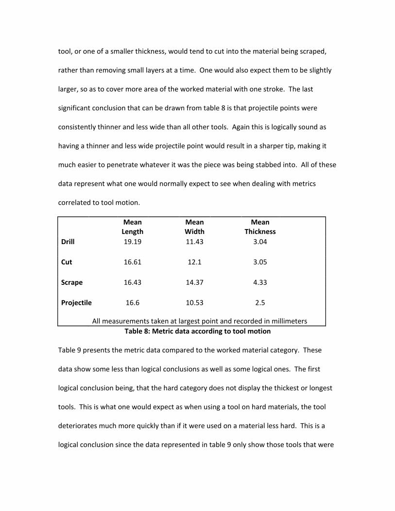
tool, or one of a smaller thickness, would tend to cut into the material being scraped,

rather than removing small layers at a time. One would also expect them to be slightly

larger, so as to cover more area of the worked material with one stroke. The last

significant conclusion that can be drawn from table 8 is that projectile points were

consistently thinner and less wide than all other tools. Again this is logically sound as

having a thinner and less wide projectile point would result in a sharper tip, making it

much easier to penetrate whatever it was the piece was being stabbed into. All of these

data represent what one would normally expect to see when dealing with metrics

correlated to tool motion.

Mean Length

Mean Width

Mean Thickness

Drill 19.19 11.43 3.04 Cut 16.61 12.1 3.05 Scrape 16.43 14.37 4.33 Projectile 16.6 10.53 2.5 All measurements taken at largest point and recorded in millimeters

Table 8: Metric data according to tool motion

Table 9 presents the metric data compared to the worked material category. These

data show some less than logical conclusions as well as some logical ones. The first

logical conclusion being, that the hard category does not display the thickest or longest

tools. This is what one would expect as when using a tool on hard materials, the tool

deteriorates much more quickly than if it were used on a material less hard. This is a

logical conclusion since the data represented in table 9 only show those tools that were

utilized, so we only see the end result of the tool after use. One not-so-logical

correlation is that the hard category shows the widest tools. Following the logic that

tools used on hard materials tend to deteriorate more quickly than the same tool used

on a soft or medium material, one would expect tools used on a hard material to

consistently be less wide than all other tools. This could be due to the fact that tools

used to process hard materials were only used for drilling, and since I measured all tools

at their widest point, it is likely that the widest point of the tools used on hard materials

were not actually those areas that made contact with the worked material. Another

illogical conclusion is that tolls utilized on soft materials are the thickest of the group.

One would expect to find that these tools were thinner than others, as it is much harder

to cut soft material with a thick edge than it is with a thinner edge. As both tools

utilized on soft materials were used for cutting, I can see no logical reason why they

would be thicker than all other tools. The only other conclusion that I could draw from

the available data was that the tools used on medium materials appear to be “just

right”. Their metric data appear, to me, to be of the proper size in all categories

Mean Length

Mean Width

Mean Thickness

Soft 23.3 11.3 4.8 Medium 16.29 11.67 2.99 Hard 21.75 13.42 3.42 All measurements taken at largest point and recorded in millimeters

Table 9: Metric data according to worked material

Metric Data Conclusions:

The data from tables 7, 8, and 9 present mostly logical conclusions. Table 8

represents the norm that one would expect to encounter when cross comparing metric

data with tool motion. The data from table 7 posed a few problems in that secondary

flakes were longer and wider than the broken cores, but I believe this could be

rationalized by the arguments present in the discussion about table 7. This same

reasoning can be used to describe why primary flakes were on the average smaller than

secondary flakes, projectile points, and tertiary flakes. Lastly table 9 presented more

illogical data than anything else. Many of the tools were too large to be able to

successfully process the worked materials they were used on, but I believe I presented

arguments to describe why this would occur, except in the case of the tool used on a

soft material, which I currently have no explanation for. The only logical conclusions

that were drawn was that medium tools appeared to be the proper size to work that

material, and tools utilized on hard materials were generally not the thinnest or longest

tools.

Conclusions

In the end this study provided many of the results that I was hoping to find when

the analysis was done. The first is that the people living at the 76 Draw Site were most

frequently utilizing their tools on the same materials and in the same motions as the

inhabitants of the La Tinaja site, showing another line of evidence for connection with

the Casas Grandes sites south of the border. The only discrepancy was that when the

two categories were combine to create “tool function” there was only one task that

appeared in the three most common functions at both sites. I believe this to be directly

correlated to the distance from Paquimé, meaning that the La Tinaja site was closer and

possibly a specialized production site, which would have received goods through

redistribution from Paquimé. This in turn, would result in many materials not being

processed at La Tinaja that would have been worked at the 76 Draw Site, which would

have received no redistributed goods from Paquimé, causing them to have to process a

wider range of materials on site. It should be noted though, that this represents the

results of an inter-site analysis between two sites, and to further prove this theory more

functional studies should be done at other sites in the Casas Grandes region, which

could then be compared to the sites of La Tinaja and the 76 Draw Site.

The intra-site analysis revealed that while there did not seem to be specialized

areas at 76 Draw to process a given material or areas that were used for a particular

function. However, it did show that XU-1 seemed to be the hotspot for anything dealing

with obsidian, evidenced by the large majority of all tools, used or not used, being found

in this unit. In addition to this, XU-3 seems to have been a secondary location for using

obsidian, as seen through the percentages of utilized and non-utilized tools found at this

location. While these seem to me to be fairly solid conclusions, more work at the site

will reveal whether or not they are correct. The metric data also provided some

interesting and thought provoking conclusions especially when it came to some

inconsistencies in the size of broken cores compared to secondary flakes, and

comparisons between primary, secondary, and tertiary flakes. Overall, I feel that this

project was a success as it proved many of the preliminary hypotheses to be true. In

addition, I feel it was a success in general as it provided only the second functional

analysis to be conducted on tools from the Casas Grandes region and the first to be

carried out on obsidian tools only.

Works Cited Bancroft, H. (1883). The Native Races in Antiquities 4:604-14 Bandelier, A. (1890). The Ruins of Casas Grandes in Nation 51:185-87 Brand, D. (1943). The Chihuahua Culture Area in New Mexico Anthropologist 6:115-58 Crabtree, D. (1972). An Introduction to Flintworking. Occasional Papers of the Idaho State University Museum, no. 28. Pocatello DiPeso, C. (1974). Casas Grandes: A Fallen Trading Center of the Gran Chichimeca, vols. 1,2, and 3. Amerind Foundation, Dragoon, Arizona DiPeso, C., J. Rinaldo, and G. Fenner (1974). Casas Grandes: A Fallen Trading Center of The Gran Chichimeca, vols. 4,5,6,7, and 8. Amerind Foundation Dragoon, Arizona Hammond, G., and A. Rey, (1928). Translators, Editors, and Annotators. Obregon’s History of Sixteenth Century Explorations in Western North America Entitled: Chronicle, Commentary, or Relation of the Ancient and Modern Discoveries in New Spain, New Mexico, and Mexico. 1584 Wetzel. Los Angeles Hayden, B. (1979) Editor. Lithic Use-Wear Analysis: Proceedings of the Conference on Lithic Use-Wear, Simon Frasier University, Burnaby (Vancouver), British Columbia, March 1977. Academic Press. New York Keeley, L. (1980). Experimental Determination of Stone Tool Uses. University of Chicago Press, Chicago Keeley, L., and M. Newcommer (1977). Microwear Analysis of Experimental Flint Tools: a Test Case in Journal of Archaeological Science 4:29-62

Lumhotlz, C. (1901) Unknown Mexico 2 vols. Charles Scribner’s Sons, New York. Mendez, K. (2009). Stone Tool use in the Casas Grandes Region: Use-Wear Analysis of a Medio Period Chipped Stone Assemblage from Site 204, Chihuahua, Mexico. Masters thesis, The University of Tulsa, Oklahoma Odell, G. (1975). Microwear in Perspective: a Sympathetic Response to Lawrence H. Keeley in World Archaeology 7:226-40 Odell, G. and F. Odell-Vereecken (1980). Verifying the Reliability of Lithic Use-Wear Assessments by “Blind Tests”: The Low-Power Approach in Journal of Field Archaeology 7:87-120 Rakita, G. (2001). Social Complexity, Religious Organization, and Mortuary Ritual in the Casas Grandes Region of Chihuahua, Mexico. Ph.D. dissertation, Southern Illinois University, Carbondale Rakita, G., C. VanPool, T. VanPool, and S. Sterling (2011). An Introduction to the 76 Draw Site, Luna County, New Mexico in Patterns in Transition: Papers from the 16th Biennial Jornada Mogollon Conference. ed. Melinda Landreth, El Paso Museum of Archaeology. El Paso Semenov, S.A. (1964) Prehistoric Technology: An experimental Study of the Oldest Tools and Artifacts from Traces of Manufacture and Wear. Redwood Press, Towbridge, Wiltshire Shea, J. and G. Odell (1985) Functional Experiments in Belizean Sand Hill Chert. Manuscript in possession of author. Tringham et al. (1974). Experiments in the Formation of Edge Damage: A New Approach to Lithic Analysis in Journal of Field Archaeology 1:171-96 VanPool, C. (2003a). The Symbolism of Casas Grandes. Ph.D. dissertation, University of New Mexico, Albuquerque

VanPool, C. (2003b). The Shaman Priests of the Casas Grandes Region of Northern Chihuahua, Mexico in American Antiquity 67(4):710-30 VanPool, C., and T. VanPool (2007). Signs of the Casas Grandes Shaman. University of Utah Press, Salt Lake City VanPool, T., C. Oswald, J. Christy, J. Ferguson, G. Rakita, and C. VanPool (in press). Provenance Studies of Obsidian at 76 Draw VanPool, T., C. VanPool, R. Cruz, R. Leonard, and M. Harmon (2001). Flaked Stone and Social Interaction in the Casas Grandes Region, Chihuahua, Mexico in Latin American Antiquity 11(2):163-74 Weiseheimer, W. (1917). Archaeological Researches in the San Joaquin Valley. Manuscript. Smithsonian Institute, Washington, D.C Whalen, M., and P. Minnis (2001). Casas Grandes and its Hinterland. The University of Arizona Press, Tucson. Whalen, M. and P. Minnis (2009). The Neighbors of Casas Grandes. The University of Arizona Press, Tucson.