Observations and Implications of the Star Formation History of the Large Magellanic Cloud

arX

iv:a

stro

-ph/

9907

259v

1 2

0 Ju

l 199

9

Observations and Implications of the Star Formation History of

the LMC 1

Jon A. Holtzman2, John S. Gallagher III3, Andrew A. Cole3,

Jeremy R. Mould4, Carl J. Grillmair5, Gilda E. Ballester6, Christopher J. Burrows7,

John T. Clarke6, David Crisp8, Robin W. Evans8, Richard E. Griffiths9,

J. Jeff Hester10, John G. Hoessel3, Paul A. Scowen10,

Karl R. Stapelfeldt8, John T. Trauger8, and Alan M. Watson11

1Based on observations with the NASA/ESA Hubble Space Telescope, obtained at the Space Telescope

Science Institute, operated by AURA Inc under contract to NASA

2Department of Astronomy, New Mexico State University, Dept 4500 Box 30001, Las Cruces, NM 88003,

[email protected]

3Department of Astronomy, University of Wisconsin – Madison, 475 N. Charter St., Madison, WI 53706,

[email protected],[email protected],hoessel@jth. astro.wisc.edu

4Mount Stromlo and Siding Spring Observatories, Australian National University, Private Bag, Weston

Creek Post Office, ACT 2611, Australia, [email protected]

5SIRTF Science Center, Caltech, MS 100-22, Pasadena, CA 91125, [email protected]

6Department of Atmospheric, Oceanic, and Space Sciences, University of Michigan, 2455 Hayward, Ann

Arbor, MI 48109, [email protected], [email protected]

7Astrophysics Division, Space Science Department, ESA & Space Telescope Science Institute, 3700 San

Martin Drive, Baltimore, MD 21218, [email protected]

8Jet Propulsion Laboratory, 4800 Oak Grove Drive, Pasadena, CA 91109, [email protected],

dc@cov, [email protected], [email protected], [email protected]

9Department of Physics, Carnegie Mellon University, 5000 Forbes Ave, Pittsburgh, PA 15213

10Department of Physics and Astronomy, Arizona State University, Tyler Mall, Tempe, AZ 85287,

[email protected], [email protected]

11Instituto de Astronomıa UNAM, J. J. Tablada 1006, Col. Lomas de Santa Maria, 58090 Morelia,

Michoacan, Mexico, [email protected]

http://arxiv.org/abs/astro-ph/9907259v1

– 2 –

ABSTRACT

We present derivations of star formation histories based on color-magnitude

diagrams of three fields in the LMC from HST/WFPC2 observations. One

field is located in the LMC bar and the other two are in the outer disk. We

find that a significant component of stars older than 4 Gyr is required to

match the observed color-magnitude diagrams. Models with a dispersion-free

age-metallicity relation are unable to reproduce the width of the observed main

sequence; models with a range of metallicity at a given age provide a much

better fit. Such models allow us to construct complete “population boxes”

for the LMC based entirely on color-magnitude diagrams; remarkably, these

qualitatively reproduce the age-metallicity relation observed in LMC clusters.

We discuss some of the uncertainties in deriving star formation histories by our

method and suggest that improvements and confidence in the method will be

obtained by independent metallicity determinations. We find, independently of

the models, that the LMC bar field has a larger relative component of older

stars than the outer fields. The main implications suggested by this study

are: 1) the star formation history of field stars appears to differ from the age

distribution of clusters, 2) there is no obvious evidence for bursty star formation,

but our ability to measure bursts shorter in duration than ∼ 25% of any given

age is limited by the statistics of the observed number of stars, 3) there may be

some correlation of the star formation rate with the last close passage of the

LMC/SMC/Milky Way, but there is no dramatic effect, and 4) the derived star

formation history is probably consistent with observed abundances, based on

recent chemical evolution models.

1. INTRODUCTION

Recent improvements in data quality and analysis tools have opened up the possibility

of deriving detailed star formation histories for Local Group galaxies based on observed

colors and brightnesses of individual stars. Results have been somewhat surprising,

indicating a wide diversity of star formation histories among galaxies of the Local Group,

even for galaxies of a given morphological type (e.g., the dwarf spheroidals); some recent

reviews have been presented by Mateo (1998), Grebel (1998), and Da Costa (1998).

The Large Magellanic Cloud occupies a special role in these studies. As our nearest

neighbor (apart from the Sagittarius dwarf), it allows observations of faint stars which

include essentially unevolved stars that are fainter than the turnoff corresponding to the

– 3 –

age of the universe. Such stars contain information about the initial mass function and

also about the earliest stages of the star formation history of a galaxy. In addition, we

can obtain accurate photometry of stars down to the oldest main sequence turnoff. It

is critical that information derived from these stars agrees with star formation histories

derived from brighter, more evolved stars if we are to believe the results on star formation

histories derived for more distant galaxies, where only the brighter stars are observable.

This is especially true given that uncertainties in our understanding of stellar evolution are

generally larger for stars in their later stages of evolution, when they are brighter.

In addition, the LMC provides a unique opportunity to compare the star formation

history of its field population with that of its star clusters, since the LMC has a rich

population of the latter. This has implications for understanding whether clusters form in a

different mode of star formation than field stars, and is important to understand the degree

to which one can trace the global star formation history of a galaxy from its constituent

star clusters.

Several studies have suggested star formation histories for the field population in the

LMC. Early studies by Butcher (1977) and Stryker (1984) suggested that the LMC might

be composed primarily of younger stars. Using ground-based observations which did not

quite reach to the oldest main sequence turnoff, Bertelli et al. (1992) and Vallenari et al.

(1996a,b) suggested that the LMC field population was composed primarily of younger

stars with ages less than a typical burst age of 4 Gyr, with some indication that the burst

age varied across the galaxy. Deeper observations with the HST have not confirmed this

picture, instead suggesting that star formation has been more continuous over the lifetime

of the LMC, although almost certainly with an increase in star formation rate in the past

several Gyr (Holtzman et al. 1997, Geha et al. 1998). All of these studies were for regions

outside the LMC bar. Inside the bar, Olsen (1999) suggests that the star formation rate

has also been more continuous, possibly extending back for a longer period at a roughly

constant rate than the outer fields; this differs from the conclusions of Elson et al (1997),

who suggest that the bar formed relatively recently and has an age of ∼ 1 Gyr.

In this paper, we present derivation of the star formation history for a field in the

LMC bar observed with the HST/WFPC2, as well as for several previously published outer

fields, using a more detailed analysis of the color-magnitude diagram. Along with this, we

discuss some of the problems and limitations of the techniques (including ours) which are

being used to extract star formation histories. We attempt to present a summary of some

of the main implications of recent results on the star formation history of the LMC: the

relation between the field and cluster star formation history, differences between the outer

regions and the bar, the relationship of the star formation history to the dynamical history

– 4 –

of the LMC, and the relation between the star formation history derived from studies of

color-magnitude diagrams with that derived from chemical evolution studies.

2. OBSERVATIONS

All of the data discussed in this paper were obtained with the Wide Field/Planetary

Camera 2 (WFPC2) on the Hubble Space Telescope (HST) as part of Guaranteed Time

Observations granted to the WFPC2 Investigation Definition Team. Three separate fields

were observed, with two located several degrees from the LMC center, and one located

within the LMC bar; details are given in Table 1 (for a map of the locations of the outer

fields, see Geha et al. 1998) In all fields, observations were made through the F555W and

F814W filters. Standard reduction procedures were applied to all of the frames, as discussed

by Holtzman et al (1995a).

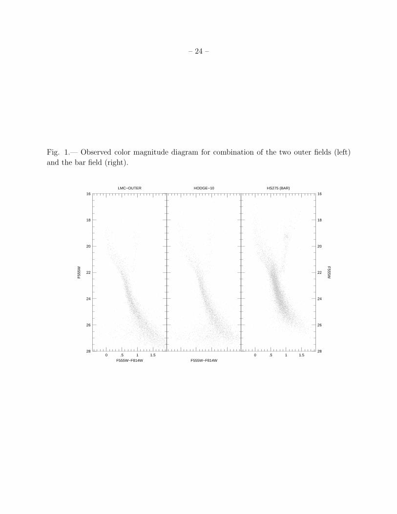
The two outer fields are relatively uncrowded. In contrast, the bar field is fairly

crowded, so stars cannot be seen as faint as in the outer field. This problem is exacerbated

by the fact the the PSF in the bar exposures is significantly broader than in the other fields.

This presumably occurred because of a large focus excursion (the so-called “breathing” of

the HST secondary); to our knowledge, these frames represent one of the largest examples

of this behavior. These exposures serve as a distinct warning to those who assume that the

HST PSF is temporally stable.

3. ANALYSIS

3.1. Photometry

Photometry in each of the fields was done using profile-fitting photometry as described

by Holtzman et al. (1997). To summarize, we performed the photometry simultaneously

on the entire stack of frames taken in each field, solving for the brightnesses in the two

colors, the relative positions of the stars, and the frame-to-frame positional shifts (and scale

changes between the filters), using an individual custom model PSF for each frame. The

model PSFs used a separate focus for each frame as derived using phase retrieval of a few

stars in the frame; the models also incorporate the field dependence of the pupil function

as specified by the WFPC2 optical prescription, and the field dependence of aberrations as

derived from phase retrieval from some other stellar fields. Instrumental magnitudes were

placed on the WFPC2 standard system using the calibration of Holtzman et al. (1995b).

No correction was made for the possible effect of charge transfer efficiency problems, since

– 5 –

these are expected to be relatively small for the background levels in our frames, especially

for the relatively bright stars on which most of our analysis is based. The software for all

of the PSF modelling and photometry was implemented in the XVISTA image processing

package.

Figure 1 shows the derived color-magnitude diagrams for the three fields.

We investigated errors in the photometry and its completeness using a series of artificial

star tests, in which artificial stars were placed into each image at a range of brightnesses

and the photometry was redone. The individual errors for all of the artificial stars (observed

vs. input brightness) were tabulated for use in the construction of artificial color-magnitude

diagrams, as discussed below.

3.2. Derivation of star formation histories

Various groups in the past several years have published descriptions of techniques used

to infer star formation histories based on the distribution of stars in a color-magnitude

diagram, or, more generally, for observations of stars in multiple colors (e.g., Tolstoy and

Saha 1996; Dolphin 1997; Hurley-Keller, Mateo, & Nemec 1998; Ng 1998; Olsen 1999;

Gallart et al. 1999; Han, in prep.). These are all similar in concept, in that a set of

observations is fit using some combination of individual simple stellar populations in an

effort to derive the relative importance of different simple stellar populations and thus a

star formation history. The techniques differ in detail, using different metrics against which

one measures how well a given model matches the observations (e.g., maximum likelihood,

minimum χ2 for different bins in color-magnitude space, etc.), different techniques with

which the best fit is sought (e.g., linear least squares, genetic algorithm, trial and error),

and different input stellar models.

For several years, we have also been doing fits for star formation histories. Our

technique bins stars in a color-magnitude diagram, and searches for a best fit by minimizing

the χ2 between the number of observed and model stars in the different bins. The search

for the best fit is automated, using nonlinear least squares to solve for the the relative

amplitudes of each simple stellar population, and optionally for the distance, reddening,

and metallicity; the fit is nonlinear because the problem is formulated to insure that only

positive amplitudes for each simple stellar population are allowed.

For our input stellar models, we use the isochrones from the Padova group (Bertelli et

al. 1994), and recently have also experimented with a preliminary version of the newest

isochrones from this group (Girardi, private communication). We find that the isochrones

– 6 –

from Girardi provide a significantly better match to the observed giant branches, as they

predict hotter temperatures for the giants; around the main sequence, where most of our

stars are located, the Girardi isochrones are similar to the original Padova set. In all of our

subsequent analysis, we use the Girardi isochrones which were available to us (Z=0.001,

0.004, and 0.008) in conjunction with Padova isochrones for other metallicities (Z=0.0004,

0.02, 0.05). The isochrones are used in conjunction with Kurucz (1993) model atmospheres

to derive colors and brightnesses in the WFPC2 photometric system.

We allow for arbitrary ages and metallicities by interpolating within the isochrones

using a set of equivalent evolutionary points to preserve the correct isochrone shape. Our

basis simple stellar populations are either discrete bursts or are constructed assuming

continuous star formation within specified epochs. Typically, we use epochs with equal

widths in the logarithm of the age, to account for the fact that isochrones at a fixed age

difference become more similar as a population ages. For the current work, we have assumed

a Salpeter initial mass function (dN/dM ∝ Mα, with α = −2.35) for most of our models,

although we have tried some other IMFs as well, as discussed briefly below. Uncertainty

about the IMF is probably responsible for one of the largest sources of potential errors in

our results.

Given model predictions for the number of stars as a function of color and magnitude

for any given star formation history, along with a distance and extinction, we account for

observational errors and incompleteness by smearing the model results with the errors

derived from our artificial star tests. We use the exact tabulations of measured errors

for our artificial stars to do this smearing, and thus make no assumption that the errors

are distributed normally (which they are often not, in particular, because of errors from

crowding which are correlated for each color). The fraction of detected artificial stars is

included in the smearing, so incompleteness is automatically taken into account.

Previous usages of this software (Holtzman et al. 1997, Geha et al. 1998) have used it

in a mode where the bins are very wide in color, effectively making this perform a fit to

the luminosity function. Fits to the luminosity function are less sensitive to possible errors

in reddening, photometric calibration, and color errors in the stellar models. Of course,

throwing away color information lowers the ability to discriminate among different models.

Fits to the full color-magnitude diagram using narrower color bins, along with a discussion

of possible problems with interpreting these, are presented next.

4. DISCUSSION

– 7 –

4.1. Derivation of star formation histories from model fits

We derived two separate star formation histories, one for the “outer” fields and one for

the bar. For the outer fields, we combined the data from the two observed fields because

there is no strong evidence that the star formation history of these fields differs (Geha et al.

1998) and because the relatively smaller number of stars in these fields limits the accuracy

of the derived star formation histories.

It is possible to attempt to determine the distance modulus and/or the extinction by

allowing these to be free parameters in the fit or by comparing the residuals for various

choices of these parameters. We do this below in an effort to estimate some of uncertainties

in our results. However, we believe that it is important, when possible, to use additional

constraints on these quantities rather than simply allowing them to be free parameters.

There are many methods for estimate distances and/or extinctions which do not depend on

interpretation of a color-magnitude diagram, for example, the use of variable stars or HI

column densities. As we will argue below, it seems prudent to use independent information

when possible to constrain the star formation histories.

For the LMC, however, there is significant debate about the distance and some

uncertainty about the extinction. For our initial fits, we decided to fix the distance to the

LMC at a (extinction-free) distance modulus of 18.5 and initially chose an extinction of

E(B-V)=0.10 based on the maps of Schwering and Israel (1991) which suggest a foreground

reddening of E(B-V)=0.07; we included an additional 0.03 mag as an estimate for internal

reddening. However, with these choices we found that the model main sequences were too

red, which, as discussed below, affected the derived star formation histories in systematic

ways. The only way we could match the color of the main sequence was to adopt lower

extinctions; we adopted E(B-V)=0.04 for the outer fields and E(B-V)=0.07 for the bar field.

Interestingly, ground-based studies of the LMC have been yielding relatively low reddenings

for fields away from young associations (Zaritsky, private communication), although we

do not have any direct estimates from these studies for our fields at this time. A possible

alternative to errors in our assumed reddening is errors in our photometric zeropoints;

in fact, a small color change of ∼ 0.02 mag in F555W-F814W relative to our adopted

calibration is suggested by Stetson (1998). In any case, we find that our derived results are

relatively insensitive to the source of the problem, and have chosen to use the empirical

lower reddenings.

In a subsequent section, we will present star formation histories derived from a variety

of choices of distance and extinction, in an effort to understand the uncertainties in our

results. Here, we note that our adopted choices for these quantities actually are those for

which the best-fitting star formation histories give relatively low χ2 values; there is some

– 8 –

variation in which distance and extinction give the absolutely lowest χ2 depending the field

being fit and assumptions about the age-metallicity relation.

For our initial fits, we constrained the basis stellar populations to have the age-

metallicity relation presented by Pagel and Tautvaisiene (1998), who derived it from a

chemical evolution model designed to to fit a variety of observations of LMC clusters

and field stars. For our initial models, we assumed that the age-metallicity relation is

dispersion-free; the cluster data (e.g., Olszewski 1993), however, suggest that there may be

a range of metallicities at any given age. To obtain isochrones at the appropriate ages and

metallicities, we interpolated among the Padova isochrones. We used age bins with a width

of 0.1 in log(age), assuming constant star formation within each age bin. We binned the

data in the color-magnitude diagrams with bin widths of 0.04 mag in color and 0.06 mag in

brightness; these were compromise values given the observed number of stars.

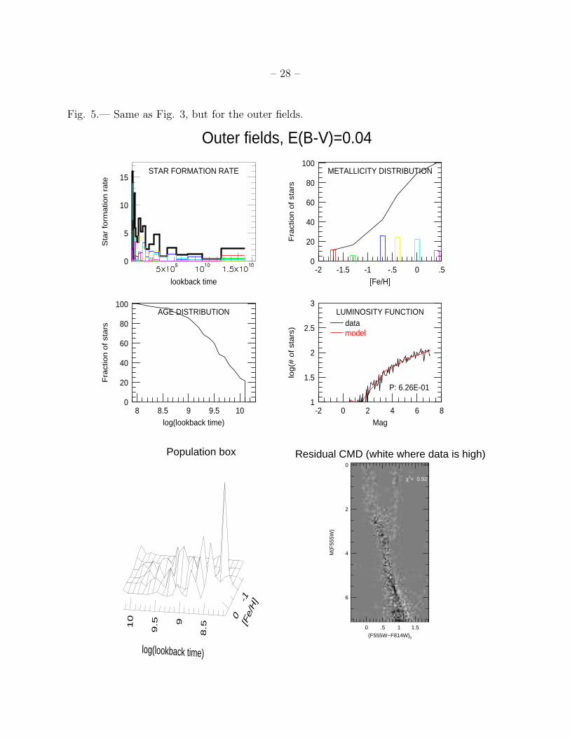
Figures 2 and 3 show a summary of the derived star formation history information

for the two fields with the constrained age-metallicity relation. The upper left plot shows

the derived star formation rate as a function of time (abscissa is linear in lookback time),

the lower left shows the cumulative number of stars formed as a function of log(lookback

time), the upper right plot shows the differential and cumulative metallicity distribution

functions, and the lower right shows the observed and model F555W luminosity functions

(corrected for reddening). The 3D diagram at the lower left shows the “population box”

(Hodge 1989) which gives the star formation rate as a function of log(lookback time) and

metallicity; older ages are at the left side of the plot, and lower metallicities are at the back.

The greyscale at the lower right shows the difference between the model and the observed

Hess diagrams divided by the square root of the data. Thus, the greyscale diagram gives

the deviation between the data and the model in units of the deviation expected from

counting statistics. The greyscale is in the sense that bright areas are regions where the

observed number of stars is larger than the model; the full range from black to white is −3σ

to +3σ. The quality of the fits is estimated by a reduced χ2 statistic which is shown in the

greyscale diagram, and also by the probability (given in the luminosity function panel) that

the observed and the model luminosity functions are drawn from the same population, as

inferred from a Kolmogorov-Smirnov test.

These model fits suggest that star formation has been ongoing in the LMC over its

entire history, with fluctuations of a factor of a few in star formation rate and a higher star

formation rate in the past few Gyr. In the outer fields, there is evidence for an increasing

star formation rate over the past few Gyr, whereas in the bar, the star formation rate seems

to have been more constant recently. More generally, these fits suggest, as did previous

studies (Holtzman et al. 1997, Geha et al. 1998, Olsen 1999), that a significant fraction (∼

– 9 –

50%) of the stars in the LMC are relatively old, i.e. older than ∼ 4 Gyr.

However, if one inspects the residual greyscale Hess diagrams, one one can clearly see

some systematic problems with the model fits. In particular, the model main sequences are

much narrower than the observed main sequences. A similar effect, although at a reduced

level, can be seen in the residuals shown in Olsen (1999); the apparently smaller effect in

those data is plausibly explained by the fact that their exposure times were shorter (by a

factor of ∼ 4), leading to larger photometric errors and hence broader observed and model

sequences.

There are several possible explanations:

1. The LMC has stars with a range of metallicities at any given age.

2. A significant number of stars in the LMC are unresolved binary stars.

3. There is a spread in distances and/or extinctions. This is unlikely given the inclination

of the LMC and the relatively low total extinction towards our fields.

4. Our observational errors have been significantly underestimated; we believe this is

unlikely given our careful analysis of photometric errors.

We discuss the first two possibilities in the next sections.

4.1.1. Metallicity dispersion

We feel that the mostly likely source of the broad main sequence is that the LMC

has stars with a range of metallicities at any given age. Certainly, the Milky Way has

a very significant dispersion in its age-metallicity relation. To test whether a spread in

metallicities can account for the observed broad main sequence, we performed the fits

allowing for multiple combinations of age and metallicity. We used the same age bins as

before, but at each age, allowed populations with discrete metallicities of Z=0.0004, 0.001,

0.004, and 0.008 , 0.02, and 0.05. The choice of these six metallicities was motivated by the

fact that these were available without any interpolation in metallicity. We allowed for all

combinations of age with these metallicities.

Figures 4 and 5 show the results using these models. Similar star formation histories

are derived, but the resulting residuals show substantially smaller systematic deviations.

Remarkably, the model fits qualitatively recover the mean age-metallicity relation observed

in LMC clusters, despite the fact that no assumptions were made about this relation at

– 10 –

all. This is demonstrated by comparing the “population boxes” for these models with

those using the constrained age-metallicity relation. Although the derived relation is not

especially quantitative since we only included six discrete metallicities, Figure 6 shows a

representation of the derived age-metallicity relation for the bar field; squares give the

metallicity of the population with the highest star formation rate at each age bin, while

crosses give the mean star-formation weighted metallicity from the six metallicity bins.

The solid line shows the relationship from Pagel and Tautvaisiene (1998), which does

a reasonable job of matching observations of LMC clusters (e.g., Olszewski 1993). Our

derived relation is similar to the model which was designed to fit the cluster observations;

the width of our relation at fixed age is also qualitatively similar to that seen in the cluster

distribution.

While the fits are significantly better using a range of metallicities at a given age,

the derived star formation histories are qualitatively similar to those derived using the

constrained dispersion-free age-metallicity relation. As with the constrained age-metallicity

fits, we find evidence that the bar field contains a larger relative number of older stars than

the outer fields. We find it encouraging that the results on the star formation appear to be

reasonably robust against assumptions made about the metallicity distribution.

Since our models allow for multiple combinations of age and metallicity, the results

actually make a crude prediction for the metallicity distribution of LMC stars; the

prediction is crude since we are only using six discrete metallicities in our models rather

than a continuous distribution. Figures 4 and 5 suggest that the LMC has a relatively

broad metallicity distribution. Low metallicity stars ([Fe/H] <∼ -1) comprise 15 and 30%

of the stars in the outer and bar fields, respectively. However, one needs to beware of

directly comparing these numbers to observations of giant star metallicities. Our models

give the relative numbers of stars of all stellar masses at different metallicities, while giants

sample only a small range of stellar masses. Because older, more metal-poor, populations

feed stars to the giant branch slower than young populations, the relative number of lower

metallicity giants will be lower than the true relative fraction of lower metallicity stars

which is predicted by the models. This effect can be substantial; for the bar model, we

estimate that that low metallicity giants will be undersampled by nearly a factor of two in

a pure giant sample as compared with the true metallicity distribution. Thus relatively few

metal-poor giants are predicted by these models.

Our models do have a reasonable component of relatively metal-rich (solar or greater)

stars, which are included to fit the reddest sections of the main sequence. It is possible that

the contribution of these stars is overestimated by our models because of some contribution

from unresolved binaries, as discussed next.

– 11 –

4.1.2. Unresolved binaries

Unresolved binary stars can significantly affect the distribution of objects in a

color-magnitude diagram. Although a variety of evidence suggests that a significant fraction

of all stars are in binary systems, it is less clear whether the masses of stars in such systems

are correlated or are drawn from the same initial mass function. If stellar masses of binaries

are uncorrelated and the mass function rises towards lower masses, then the effect of

unresolved binaries is mainly significant only for rather low mass stars at the bottom of

the main sequence; for more massive stars, a binary companion is much more likely to be

significantly fainter and thus have little influence on the total system luminosity and color.

As a result, the only way to get a broadening of the main sequence for stars similar to

those observed by us in the LMC (∼ 1M⊙) is to require that the masses of the components

of binary systems are correlated. Such a scenario has been suggested by Gallart et al.

(1999) to explain the color-magnitude diagram of the Leo I dwarf spheroidal; they find

significantly better fits using a large fraction of binary stars which are constrained to have

mass ratios greater than 0.6. However, we find that models using such a scenario still do

not accurately reproduce our observed color-magnitude diagram using a dispersion-free

age-metallicity relation. The problem arises because the width of the observed sequence is

broadest compared to the models at intermediate luminosities. If there is any range of mass

ratios in binaries at all, the effect of binaries grows with decreasing luminosity. Thus, any

model which matches the width of the main sequence at intermediate luminosities using a

binary component predicts too broad of a sequence at lower luminosities.

To further check the binary star hypotheses, we performed fits with multiple

combinations of age and metallicity, but using an assumed binary fraction of 0.5; binary

masses were drawn from the same initial mass function as the parent population but with

binary mass ratios constrained to be larger than 0.5. These fits are significantly worse than

fits without binaries. However, as mentioned above, if all mass ratios were allowed, then

the models would allow for a significant component of binaries since their effect is small for

the stars in our observations.

Although we find that metallicity spread is a more likely explanation than unresolved

binaries for the observed width of the main sequence, it is likely that both effects play

some role. The existence of some unresolved binaries would probably reduce some of the

spread in our derived age-metallicity relation; in particular, we expect it would reduce the

contribution of stars at the highest metallicities at any given age.

– 12 –

4.2. Accuracy of derived star formation histories from model fits

Before one reads too much into these derived star formation histories, however, one

should consider some of the limitations and problems of fitting star formation histories.

There are numerous assumptions that are made in the models:

• The stellar models accurately predict the observed properties of stars as a function of

age and metallicity,

• A unique initial mass function exists which is independent of age and metallicity, and

is represented (in this case) by a power law with dN/dM ∝ M−2.35,

• All stars are found at a common distance and extinction,

• The observational data are calibrated to the same system as the models, and the

observational errors can be accurately measured,

• The basis stellar populations used in the fits represent all populations present in the

galaxy.

All of these assumptions are likely to be in error at some level. Consequently, the

question is the degree to which deviations from the assumptions affect the derived star

formation histories. Unfortunately, this is very difficult to assess given the unknown nature

of the possible errors in the assumptions.

As a result of these problems, it is likely that no solution will actually matches the

observed distribution of stars within the errors expected from Poisson statistics alone. This

is certainly the case for the best models here; given the number of independent regions

in the color-magnitude diagrams being fit, one would expect a reduced χ2 much closer to

unity than the values we obtain. Sometimes the fits produce model luminosity functions

which are consistent with the data, but other times they are formally ruled out with a KS

test. Review of the various papers which derive star formation histories for various systems

suggest the same quality of matches is obtained for most other derived star formation

histories. Given the known problems with the assumptions, this is usually not considered

to be a major problem; instead, one makes the assumption that the “best-fitting” model

represents the closest approximation to the truth, even if it is statistically inconsistent with

the data. We make the same assumption, but feel the need to explicitly state it; one could

certainly imagine situations in which this assumption might not be true.

Because one is just choosing the best-fitting model averaged over the entire color-

magnitude diagram, our method inherently weights areas where there are more stars and

– 13 –

where the photometric errors are low. As a result the model does not give extra weight

to regions which carry more unique information about stellar ages. For example, if upper

main sequence stars exist, there must be a young population, but if these stars are vastly

outnumbered by older stars, the model will do its best to fit the older stars even if it means

sacrificing a good match to the younger stars. One could certainly devise a scheme where

certain regions of the color-magnitude diagram carry extra weight, and perhaps this is the

direction we should take in the future.

In addition, different assumptions can lead to systematic errors in the derived star

formation histories. For example, we found that changing the assumed reddening led to

systematic differences in the derived star formation history. At a higher reddening, more

metal-poor stars are required to fit the observed data. If the age-metallicity relation is

constrained, then this in turn leads to a higher derived number of older stars. Errors in the

assumed initial mass function can lead to similar systematic effects.

To demonstrate the effect of varying reddenings, distances, and IMF slopes, we ran a

set of solutions allowing for a range in reddening from 0.04 < E(B − V ) < 0.10, a range

of distance from 18.2 < m − M < 18.7, and two different IMF slopes with α = −2.35 and

α = −2.95; each of these was varied independently with the other two quantities at our

preferred values. For each different parameter, we derived a star formation history along

with a χ2 for the each fit. Figure 7 shows the derived values of χ2 for different choices of

reddening and distance modulus; in each panel, results are shown both for the constrained

age-metallicity relation as well as for multiple combinations of age and metallicity. If

the age-metallicity relation is constrained, the quality of the fit changes significantly for

different choices of reddening and distance modulus; minimum χ2 are reached around our

preferred values of m − M = 18.5 and E(B − V ) = 0.07 and 0.04 for the bar and outer

fields. However, if multiple combinations of age and metallicity are allowed, the quality of

the fits are relatively insensitive to the choice of reddening and distance modulus, indicating

there is some degeneracy in the sensitivity to different parameters.

This supports our assertion that it is better to use additional independent observational

constraints on parameters relevant to the star formation fit rather than to include these

parameters in the fitting process. For many systems, information about distance and

reddening are readily available. We suggest that perhaps the greatest improvement in

the confidence in our derived star formation histories will come from the observations

of observed metallicity distributions against which one could compare the derived star

formation histories. The derivation of metallicities is feasible in nearby stellar systems given

current multi-object spectroscopic capabilities and/or using multi-band photometry, and,

in fact, such studies are underway by several groups (e.g., Olszewski, Suntzeff, & Mateo

– 14 –

1996, Smecker-Hane et al., private communication). However, we reiterate that caution

must be used to compare observations with model predictions; one must take into account

the metallicity distribution biases which are introduced by the observational selection of

stars used for metallicity determinations.

Given the limited external constraints we have about the distance modulus to the LMC,

the extinction, the IMF, and the metallicity distributions, we must consider how possible

uncertainties in these affect our derived star formation histories. Figure 8 shows derived

star formation histories for the ensemble of models comprising 18.2 < (m − M) < 18.7,

0.04 < E(B − V ) < 0.10, and IMF slopes of -2.35 and -2.95; the bold line shows the results

from previous figures for our preferred quantities. One can see that the star formation

history is qualitatively similar independent of the parameters, but quantitatively, the star

formation rate at any given time can be in error by a factor of a few. The largest qualitative

difference comes for different choices of IMF slope; as the IMF becomes steeper (dashed

line in Figure 8), the observations require a larger relative number of younger stars, exactly

as expected (Holtzman et al. 1997). To the extent to which our parameter choices span

the full range of values expected for the LMC, Figure 8 can be used to give a reasonable

estimate of the uncertainties in our results, although these results do not consider the

possible effect of errors in the stellar models.

In addition to the systematic errors, there are random errors in our results because of

the limited number of stars observed. These random errors are larger for the outer fields

than for the bar field because they have fewer observed stars. However, simulations of

color-magnitude diagrams suggest that the magnitude of the random errors, even for the

more sparse outer fields, are smaller than those which arise because of potential systematic

errors.

4.3. Differential comparison of color-magnitude diagrams

To avoid potential problems with fitting star formation histories, it is possible to derive

differences in the star formation history from one field to another by a direct comparison

of the observed color-magnitude diagrams. Such differences lead to systematic residuals

when comparing the Hess diagrams of different fields. Differential comparisons of fields with

similar metallicities are relatively straightforward to interpret in terms of age differences,

although a quantitative association of a difference with an age requires the use of stellar

models. Differential comparisons may be more problematic for fields with significantly

different metallicities.

– 15 –

As an application, we consider the differences in star formation history between the

LMC outer fields and the bar field. Our model-dependent derived star formation history

suggested that there has been a greater relative contribution of the youngest stars in the

outer fields than in the bar, in agreement with the results derived by Olsen (1999) based on

similar fits, but in qualitative disagreement with the results of Elson et al. (1997) which

were based on a visual inspection of the color magnitude diagram in a bar field.

Figure 9 shows the difference in the Hess diagrams between the two fields, where white

areas represent locations where there are more outer field stars, and darker areas regions

where there are more bar stars. The Hess diagrams were normalized to have the same total

number of stars between MV ∼ 4 − 4.5 where the photometry in both fields is reasonably

complete and where stellar evolution effects are minimal; the difference between the Hess

diagrams was smoothed to suppress the noise from counting statistics. One can clearly

see a darker band in the lower parts of the residual Hess diagram which suggests that the

bar contains a relatively larger number of intermediate age stars than the outer field; the

difference is made up by a relatively larger number of upper main sequence (younger) stars

in the outer fields. The bar field also has a relatively larger number of red clump stars

which represent stars of intermediate age. Consequently, the differential, model-independent

comparison supports the results derived by fitting stellar models, namely that the bar,

although it contains a significant population of young stars, is relatively older than the

outer fields.

Although the bar field shows an apparently significant sequence which one might

associate with a several Gyr old burst (as seen in Figure 1 and shown in cross-section plots in

Elson et al. 1997), which shows up in contrast to the outer field color-magnitude diagrams,

such a feature turns out to be a generic feature of models even with a continuous star

formation rate. This arises because upper main sequence stars (those with convective cores)

evolve to cooler temperatures and higher luminosities over most of their main-sequence

lifetimes, but then retreat to higher temperatures, creating a jag in the evolutionary path in

a color-magnitude diagram. Since the star spends proportionally more time at the coolest

effective temperature, a secondary sequence which is offset from the main sequence exists

for a continuous star formation history. Although this is true even for a population of fixed

metallicity, an age-metallicity relation makes the secondary sequence even more pronounced.

The effect is demonstrated in Figure 10, where we show a synthetic Hess diagram of a

population with a constant star formation rate over the past 12 Gyr, using our adopted

age-metallicity relation for the LMC. One sees a clear sequence which might be confused

with an increase in the star formation rate at some time in the past, despite the fact that

it is a color-magnitude diagram for a constant star formation rate. This clearly shows the

peril of interpreting color-magnitude diagrams purely visually; an apparent concentration

– 16 –

of points does not necessarily imply a burst or even a significant enhancement in the star

formation rate.

This observation leads to an understanding of the difference between the interpretation

of Elson et al. (1997) and the results of this paper and Olsen (1999) regarding the relative

age of the LMC bar. Elson et al. (1997) suggest that the LMC bar is younger than the

rest of the LMC because they observe a bimodal distribution of color in the upper main

sequence of their LMC bar field. They associate the blue peak with the formation of the

LMC bar (∼ 1 Gyr ago) and the red peak with the formation of the bulk of LMC field stars

(∼ 4 Gyr ago). Instead, we find that the red peak is a generic prediction of the models even

for roughly constant star formation rate, and the blue peak represents a recent increase

in the star formation rate which is seen in both the outer fields and the bar (in fact, it is

stronger in the outer fields than in the bar).

4.4. Field vs. cluster star formation history

Perhaps the most notable conclusion which can be drawn from our derived star

formation histories is that the field star formation history in both the bar and the outer

fields appears to differ from the star formation as suggested by the age distribution of

LMC clusters. LMC clusters show a significant age gap between lookback times of 4 and

12 Gyr (e.g., van den Bergh 1991, Girardi et al. 1995), with 14 old clusters (which have

ages comparable to those of the Galactic globulars, see Olsen et al. 1998), numerous young

clusters, and only one cluster, ESO 121-SC03, at an intermediate age. In contrast, the

derived star formation histories of Figures 2-5 suggest that star formation has been more

continuous in the field of the LMC. Here we consider the robustness of that conclusion.

Geha et al. (1998) showed that the observed luminosity function in the outer fields was

strongly inconsistent with a star formation history which corresponds to the current number

distribution of clusters as a function of lookback time. However, this comparison is perhaps

unfair, as the older clusters are generally more massive than the younger ones, so weighting

by mass would allow for a larger older component. In addition, one might consider that

some fraction of clusters which were formed at an early epoch might be disrupted during

the subsequent evolution of the LMC; although many of the young clusters are massive and

appear tightly bound and unlikely to disrupt anytime soon, many others have lower masses

and larger sizes and might plausibly disrupt.

As a result, we consider the more general question of whether any star formation

history with a gap in star formation between 4 and 10 Gyr is capable of reproducing the

– 17 –

observed properties of the LMC field stars. To address this, we performed fits for the

star formation history again without allowing for any component stellar populations with

ages between 4 and 10 Gyr. Figures 11 and 12 show the results for the bar field for the

constrained age-metallicity relation and arbitrary combinations of age and metallicity.

The fit with the constrained age-metallicity relation is notably worse than allowing for

intermediate age stars. This is easily explained; the existence of a broad band of subgiants

around the oldest turnoff suggests that multiple ages are present. However, it is possible

to get such a continuous band with different combinations of age and metallicity, since

older, lower metallicity stars can blend smoothly into younger, higher metallicity stars

without necessarily leaving a gap in the color-magnitude diagram. This is confirmed by

Figure 12, which shows that a moderately good match to the observed Hess diagram can

be made even with an age gap in the star formation history. However, one can see that the

model produces too many subgiants at M(F555W ) ∼ 2.5; this can be seen in both the

residual Hess diagrams as well as in the luminosity function. The χ2 for the star formation

history is only slightly worse with an age gap than without it, but the probability that

the luminosity function is consistent with that of the data can be ruled out at a much

higher confidence level than for models without a gap. In addition, the existence of a gap

would require a relatively larger population of older, metal-poor stars; with a gap, we find

that approximately 40% of all of the LMC field stars would have to be older than 10 Gyr

and more metal-poor than [Fe/H] ∼ -1. This may not be consistent with observations of

metallicity distributions (e.g. Olszewski 1993) and the lack of a strong horizontal branch

in the color-magnitude diagrams; however, the possibility exists that the LMC has an

extended, low density, older stellar halo which becomes more dominant over the young and

intermediate age population as one moves farther from the center of the LMC.

Consequently, we feel that it is unlikely that the field star formation history, as sampled

by the location of our fields, has a gap in star formation between 4 and 10 Gyr ago.

4.5. Burstiness of star formation

Another outstanding question is the degree to which star formation is “bursty” in

the LMC. The degree to which we can distinguish between bursty and continuous star

formation depends on several factors. For older populations, the distribution of stars in

the color-magnitude diagrams changes very slowly with age, so it is difficult to get much

age resolution. For younger populations, the separation between ages is larger, but the

observed number of stars is smaller, so sensitivity to different distributions of star formation

is limited by counting statistics.

– 18 –

Our fits for star formation history have been performed assuming constant star

formation within epochs spaced by 0.1 in log(age). This value for the width of each epoch

was determined by finding the narrowest age bin which gave statistically distinguishable

fits, as measured by χ2.

To measure the sensitivity of the technique to burstiness in the star formation rate,

we performed the star formation fits in which single age bins were given a duration of

∆(log(age)) = 0.01, while preserving the 0.1 spacing in log(age). We did this for each age

bin in turn for lookback times from 1 to 4 Gyr. We found that we obtained nearly identical

quality fits using the 0.01 width epochs as we did with the 0.1 width epochs, although the

fits would have been worse if we had required more than one bin to be ”bursty” at a time.

The basic reason we could not discriminate the duration of a star formation epoch is small

number statistics in the number of stars observed on the upper main sequence; without the

counting statistics, the models are straightforward to distinguish. This was true even for

the bar field, which is the densest field one could observe in the LMC. We estimate that

increasing the number of stars by a factor of 5-10 would allow burstiness to be distinguished,

suggesting that a program with multiple pointings with WFPC2 (e.g., Smecker-Hane et

al., in progress) and/or the Advanced Camera would be useful. At ages older than 4 Gyr,

burstiness becomes extremely difficult to measure without exquisitely accurate photometry.

4.6. Star formation and the interaction history of the LMC

It has been suggested that star formation in the LMC is triggered by tidal interactions

with the Milky Way and the SMC. As a result, it is of interest to see whether there is any

evidence for an enhanced star formation rate around the time of the last closest passage.

Since the full orbits of the Magellanic Clouds are still unknown, the time of last close

passage is somewhat uncertain, but the latest models place it around 2.5 Gyr ago (Zhao,

private communication). Inspection of our derived star formation histories (for example,

Figure 8) show a general tendency for the star formation to increase by a mild amount

around this time, but no dramatic effect is seen. However, as discussed in the last section,

we cannot constrain the burstiness of the star formation rate very accurately from the

current data, so some correlation of star formation with orbit is not necessarily ruled out.

One might expect that triggered star formation would not occur in all regions of the

galaxy at the same time. If star formation were triggered in different regions at different

times, subsequent mixing arising from the stellar velocity dispersion and differential rotation

would smooth the bursty nature of the triggered star formation on a timescale given by the

mixing. Given an approximate velocity dispersion of 50 km/s, it would take only ∼ 500

– 19 –

Myr for stars at a radius of 4 kpc to mix azimuthally.

4.7. Chemical evolution and star formation history of the LMC

Pagel and Tautvaisiene (1998) have recently published a model for the chemical

evolution of the LMC and compared it with previous models. Such models attempt

to match the observed abundance distributions of different elements as a function of

metallicity. In general, these models allow to star formation rate to be a free parameter.

Models differ in the adopted yields, IMF, the presence of inflow and/or outflow, and the

degree to which outflow is selectively enhanced in heavy elements.

The best fitting model of Pagel & Tautvaisiene for the LMC favors a star formation

history which, although they call it a “bursty” model, has an underlying constant star

formation rate over the history of the LMC, with an enhancement in the star formation rate

3 Gyr ago. However, they also have a model with a smoothly varying star formation rate

which also provides a reasonable match with observational data. We suspect that using a

star formation history derived from our color-magnitude diagrams would be able to provide

a reasonable match to the abundance data as well, as it is intermediate between the two

models presented in Pagel and Tautvaisiene.

We suggest that the next logical step in modeling star formation histories is to

couple the derived star formation rates with chemical evolution models and simultaneously

attempt to match both color-magnitude diagram data and abundance data. In principle,

this might allow one to more uniquely determine the importance of mass inflow/outflow.

Unfortunately, such attempts will be complicated if the star formation history is a strong

function of location in the galaxy. However, from the few fields considered to date, it

appears that the variation with position may not be so large as to make such an attempt

futile; once data on more fields, particularly at large radii become available, we suspect a

simple model with a small number of radial zones might be sufficiently accurate.

5. CONCLUSIONS

We have derived star formation histories from the distribution of stars in deep color-

magnitude diagrams obtained using HST. These data suggest that there is a significant

component of stars older than 4 Gyr in both outer fields and the bar of the LMC. Models in

which there is a dispersion-free age-metallicity relation cannot reproduce the width of the

main sequence in our high accuracy photometric data. As a result, we have fit models which

– 20 –

allow for multiple combinations of age and metallicity and find we can obtain accurate

matches to the observed data. These fits allow us to fully construct “population boxes”

from our data which are derived solely from color-magnitude diagrams. Such diagrams

qualitatively reproduce the mean age-metallicity relation observed in LMC clusters as well

as the spread around this relation. These derived models produce crude predictions for the

abundance distribution the LMC; new observations which provide such distributions will be

extremely useful in constraining the star formation histories and confirming the validity of

the models.

Both the model fits as well as a differential comparison between the observed

color-magnitude diagrams suggest that the bar of the LMC contains a relatively larger

number of older stars than the outer fields. This is consistent with the conclusions of

Olsen (1999) but different from those of Elson et al. (1998), although we have presented a

plausible explanation for why the latter study reached their conclusions.

One main implication of the derived star formation histories is that the field star

formation history appears to differ from that suggested by the LMC clusters, in that there

does not appear to be an age gap in the field star age distribution. However, we note that it

is actually rather difficult to constrain the star formation history for lookback times greater

than 4 Gyr given the age-metallicity degeneracy in the location of isochrones; observations

of larger samples of subgiants, ideally with metallicity determinations, would be desirable

to confirm that field stars fill the cluster age gap.

We find that it is quite difficult to constrain the degree to which star formation is

bursty in the LMC on time scales less than about 25% in age with the observed number

of stars even in the WFPC2 bar field. Larger samples will be required to address this

issue. However, sequential star formation across the LMC followed by mixing may erase the

signatures of bursty star formation even if it occurs.

Future progress will be made with larger samples of stars; with accurate photometry

down to the oldest main sequence turnoff, one can further constrain burstiness and the

star formation history. In addition, we suggest that metallicity determinations for a large

number of stars will be crucial in constraining and testing derivations of star formation

histories. Coupled with chemical evolution models, we may be able to get constraints on

the importance of inflow/outflow in the LMC, and begin to fully understand the nature of

the star formation history in one of our nearest neighbors.

This work was supported in part by NASA under contract NAS7-918 to JPL.

– 21 –

REFERENCES

Bertelli, G., Bressan, A., Chiosi, C., Fagotto, F. & Nasi, E. 1994, A&AS, 106,275

Bertelli, G., Mateo, M., Chiosi, C., & Bressan, A. 1992, ApJ, 388, 400

Butcher, H. 1977, ApJ, 216, 372

Da Costa, G.S., 1998, in Stellar Astrophysics for the Local Group, A. Aparacio, A. Herrero,

& F. Sanchez eds, Cambridge: Cambridge University Press

Dolphin, A., 1997, New Astronomy 2, 397

Elson, R., Gilmore, G. & Santiago, B. 1997, MNRAS, 289, 157

Gallart, C., Freedman, W.L, Aparicio, A., Bertelli, G., Chiosi, C., 1999, AJ, in press

Geha, M.C., Holtzman, J.A., Mould, J.R., Gallagher, J.S., Watson, A.M., Cole, A.A.,

Grillmair, C.J, Stapelfeldt, K.R., & the WFPC2 IDT, 1998, AJ, 115, 1045

Girardi, L. et al. 1995, A&A, 298, 87

Grebel, E. K. 1998, in ASP Conf Series, The Stellar Content of the Local Group, eds. P.

Whitelock & R. Cannon, in press

Hodge, P., 1989, ARAA 27, 139

Holtzman, J. A. et al. 1995a, PASP, 107, 156

Holtzman, J. A. et al. 1995b, PASP, 107, 1065

Holtzman, J. A. et al. 1997, AJ, 113, 656

Hurley-Keller, D., Mateo, M., & Nemec, J. 1998, AJ, 115, 1840

Kurucz, R. L., 1993, ATLAS9 Stellar Atmosphere Programs and 2 km/s grid, CDROM 13,

Smithsonian Astrophysical Observatory

Mateo, M. L, 1998, ARAA 36, 435

Ng, Y.K. 1998, A&AS 132, 133

Olsen, K., 1999, AJ in press

Olsen, K., Hodge, P.W, Mateo, M., Olszewski, E.W., Schommer, R., Suntzeff, N.B, &

Walker, A.R., 1998, NMRAS, 300, 6650

Olszewski, E.W. 1993, in ASP Conf. Proc. 48, The Globular Cluster-Galaxy Connection,

ed. G. Smith & J. Brodie (San Francisco:ASP), 351

Olszewski, E.W., Suntzeff, N., & Mateo, M., 1996, ARAA, 34, 511

Pagel, B. E. J. & Tautvaisiene, G. 1998, MNRAS 299, 535

– 22 –

Schwering, P. G., & Israel, F. P. 1991, A&A, 246, 231

Stetson, P. B., 1998, PASP 110, 1448

Stryker, L. 1984, ApJS, 55, 127

Tolstoy, E. & Saha, A. 1996, ApJ 462, 672

Vallenari, A., Chiosi, C. Bertelli, G., & Ortolani, S. 1996a, A&A, 309, 358

Vallenari, A., Chiosi, C. Bertelli, G., Aparicio, A., & Ortolani, S. 1996b, A&A, 309, 367

van den Bergh, S. 1991, ApJ, 369, 1

This preprint was prepared with the AAS LATEX macros v4.0.

– 23 –

Table 1.

Summary of Observations

Field α2000 δ2000 Exposure time STScI filenames

LMC-OUTER 5h14m44s−65◦17′43′′ 4000s u2c5010[1-8]t

HODGE-10 5 58 21 -68 21 19 2500s u2o9020[1-6]t

HS-275 (BAR) 5 24 21 -69 46 27 3700s u2o9010[1-8]t

– 24 –

Fig. 1.— Observed color magnitude diagram for combination of the two outer fields (left)

and the bar field (right).

LMC−OUTER

0 .5 1 1.528

26

24

22

20

18

16

F555W−F814W

F55

5W

HODGE−10

F555W−F814W

HS275 (BAR)

0 .5 1 1.528

26

24

22

20

18

16

F555W

– 25 –

Fig. 2.— Derived star formation history for bar field, assuming an age-metallicity relation

for the LMC. See text for description of the various panels.

0-1

8.5

9

9.510 [Fe/

H]

log(lookback time)

0 .5 1 1.5

6

5

4

3

2

1

0

(F555W−F814W)0

M(F

555W

)

χ2= 2.46

Bar field, E(B-V)=0.07, constrained age-metallicity

STAR FORMATION RATE

0

5

10

15

20

25

lookback time

Sta

r fo

rmatio

n r

ate

AGE DISTRIBUTION

8 8.5 9 9.5 100

20

40

60

80

100

log(lookback time)

Fra

ctio

n o

f st

ars

METALLICITY DISTRIBUTION

-2 -1.5 -1 -.5 0 .50

20

40

60

80

100

[Fe/H]F

ract

ion o

f st

ars

LUMINOSITY FUNCTION data model

-2 0 2 4 6 81

1.5

2

2.5

3

Mag

log(#

of st

ars

)

P: 6.39E-01

Population box Residual CMD (white where data is high)

– 26 –

Fig. 3.— Same as Fig. 1, but for the outer fields.

0-1

8.5

9

9.510 [Fe/

H]

log(lookback time)

0 .5 1 1.5

6

5

4

3

2

1

0

(F555W−F814W)0

M(F

555W

)

χ2= 1.58

Outer fields, E(B-V)=0.04, constrained age-metallicity

STAR FORMATION RATE

0

5

10

15

20

25

lookback time

Sta

r fo

rmatio

n r

ate

AGE DISTRIBUTION

8 8.5 9 9.5 100

20

40

60

80

100

log(lookback time)

Fra

ctio

n o

f st

ars


-2 -1.5 -1 -.5 0 .50

20

40

60

80

100

[Fe/H]F

ract

ion o

f st

ars


-2 0 2 4 6 81

1.5

2

2.5

3

Mag

log(#

of st

ars

)

P: 2.08E-02


– 27 –

Fig. 4.— Derived star formation history for bar field, allowing for multiple combinations of

age and metallicity.

0-1

8.5

9

9.510 [Fe/

H]

log(lookback time)

0 .5 1 1.5

6

5

4

3

2

1

0

(F555W−F814W)0

M(F

555W

)

χ2= 1.31

Bar field, E(B-V)=0.07

STAR FORMATION RATE

0

5

10

15

lookback time

Sta

r fo

rmatio

n r

ate

AGE DISTRIBUTION

8 8.5 9 9.5 100

20

40

60

80

100

log(lookback time)

Fra

ctio

n o

f st

ars


-2 -1.5 -1 -.5 0 .50

20

40

60

80

100

[Fe/H]F

ract

ion o

f st

ars


-2 0 2 4 6 81

1.5

2

2.5

3

Mag

log(#

of st

ars

)

P: 3.39E-03


– 28 –

Fig. 5.— Same as Fig. 3, but for the outer fields.

0-1

8.5

9

9.510 [Fe/

H]

log(lookback time)

0 .5 1 1.5

6

4

2

0

(F555W−F814W)0

M(F

555W

)

χ2= 0.92

Outer fields, E(B-V)=0.04

STAR FORMATION RATE

0

5

10

15

lookback time

Sta

r fo

rmatio

n r

ate

AGE DISTRIBUTION

8 8.5 9 9.5 100

20

40

60

80

100

log(lookback time)

Fra

ctio

n o

f st

ars


-2 -1.5 -1 -.5 0 .50

20

40

60

80

100

[Fe/H]F

ract

ion o

f st

ars


-2 0 2 4 6 81

1.5

2

2.5

3

Mag

log(#

of st

ars

)

P: 6.26E-01


– 29 –

Fig. 6.— Our derived age-metallicity relation for the bar field. Squares represent the peak

metallicity seen at each age, while crosses represent the mean metallicity. The solid line

gives the relation of Pagel and Tautvaisiene (1998).

0 2×109 4×109 6×109 8×109 1010 1.2×1010 1.4×1010−2

−1.5

−1

−.5

0

.5

1

– 30 –

Fig. 7.— Values of χ2 for best-fitting models for different values of reddening (left) and

distance modulus (right). Top panels are for bar field, while bottom panels are for outer

fields. The two different lines in each panel correspond to fits with a fixed age-metallicity

relation and those will multiple combinations of age and metallicity.

Bar field

Outer fields

Bar field

Outer fields

0

1

2

3

χ2

.04 .06 .08 .10

1

2

3

E(B−V)

χ2

0

1

2

3

χ2

18.1 18.2 18.3 18.4 18.5 18.6 18.70

1

2

3

m−M

χ2

– 31 –

Fig. 8.— Derived star formation histories for a variety of choices of m − M , E(B − V ),

and IMF slope, as described in the text. Top panels are for outer fields and the bottom

panels are for bar field. Left panels show results with a constrained age-metallicity relation,

while right panels allow for multiple combinations of age and metallicity. Bold line indicates

results for our preferred set of parameters; dashed line shows the results for a steeper IMF.

Outer fields, constrained age−metallicity Outer fields

Bar field, constrained age−metallicity Bar field

0

5

10

15

20

25

Sta

r fo

rmat

ion

rate

0

5

10

15

20

25

Star form

ation rate

0 2×109 4×109 6×109 8×109 1010 1.2×1010 1.4×10100

5

10

15

20

25

lookback time

Sta

r fo

rmat

ion

rate

0 2×109 4×109 6×109 8×109 1010 1.2×1010 1.4×10100

5

10

15

20

25

lookback time

Star form

ation rate

– 32 –

Fig. 9.— Difference of the Hess diagrams between the bar and the outer fields, smoothed to

reduce noise from counting statistics.

– 33 –

Fig. 10.— Synthetic Hess diagrams for a continuous star formation rate over 12 Gyr with

our adopted age-metallicity relation for the LMC.

– 34 –

Fig. 11.— Derived star formation history for bar field, assuming an age-metallicity relation

for the LMC, but constraining the fit to have no star formation between 4 and 10 Gyr ago.

0-1

8.5

9

9.510 [Fe/

H]

log(lookback time)

0 .5 1 1.5

6

5

4

3

2

1

0

(F555W−F814W)0

M(F

555W

)

χ2= 2.88

Bar field

STAR FORMATION RATE

0

5

10

15

20

25

lookback time

Sta

r fo

rmatio

n r

ate

AGE DISTRIBUTION

8 8.5 9 9.5 100

20

40

60

80

100

log(lookback time)

Fra

ctio

n o

f st

ars


-2 -1.5 -1 -.5 0 .50

20

40

60

80

100

[Fe/H]F

ract

ion o

f st

ars


-2 0 2 4 6 81

1.5

2

2.5

3

Mag

log(#

of st

ars

)

P: 9.96E-04


– 35 –

Fig. 12.— Derived star formation history for bar field, allowing for multiple combinations

of age and metallicity, but constraining the fit to have no star formation between 4 and 10

Gyr ago.

0-1

8.5

9

9.510 [Fe/

H]

log(lookback time)

0 .5 1 1.5

6

5

4

3

2

1

0

(F555W−F814W)0

M(F

555W

)

χ2= 1.44

Bar field

STAR FORMATION RATE

0

5

10

15

lookback time

Sta

r fo

rmatio

n r

ate

AGE DISTRIBUTION

8 8.5 9 9.5 100

20

40

60

80

100

log(lookback time)

Fra

ctio

n o

f st

ars


-2 -1.5 -1 -.5 0 .50

20

40

60

80

100

[Fe/H]

Fra

ctio

n o

f st

ars


-2 0 2 4 6 81

1.5

2

2.5

3

Mag

log(#

of st

ars

)

P: 4.14E-05


Observations and Implications of the Star Formation History of the Large Magellanic Cloud

Documents

Transcript of Observations and Implications of the Star Formation History of the Large Magellanic Cloud