arX

iv:a

stro

-ph/

0408

099v

1 4

Aug

200

4

Obscured AGN and the X-ray, Optical and Far-Infrared Number

Counts of AGN in the GOODS Fields

Ezequiel Treister1,2, C. Megan Urry1, Eleni Chatzichristou1, Franz Bauer3, David M.

Alexander3, Anton Koekemoer4, Jeffrey Van Duyne1, William N. Brandt5, Jacqueline

Bergeron6, Daniel Stern7, Leonidas A. Moustakas4, Ranga-Ram Chary8, Christopher

Conselice9, Stefano Cristiani10, Norman Grogin11

treister@astro.yale.edu

ABSTRACT

The deep X-ray, optical, and far-infrared fields that constitute GOODS are

sensitive to obscured AGN (NH & 1022 cm−2) at the quasar epoch (z ∼ 2 − 3),

as well as to unobscured AGN as distant as z∼7. Luminous X-ray emission is a

sign of accretion onto a supermassive black hole and thus reveals all but the most

heavily obscured AGN. We combine X-ray luminosity functions with appropriate

spectral energy distributions for AGN to model the X-ray, optical and far-infrared

flux distributions of the X-ray sources in the GOODS fields. A simple model

based on the unified paradigm for AGN, with ∼ 3 times as many obscured AGN

as unobscured, successfully reproduces the z-band flux distributions measured in

1Yale Center for Astronomy & Astrophysics, Yale University, P.O. Box 208121, New Haven, CT 06520

2Departamento de Astronomıa, Universidad de Chile, Casilla 36-D, Santiago, Chile.

3Institute of Astronomy, Madingley Road, Cambridge CB3 0HA, UK.

4Space Telescope Science Institute, 3700 San Martin Drive, Baltimore, MD 21218.

5Department of Astronomy and Astrophysics, Pennsylvania State University, 525 Davey Laboratory,

University Park, PA 16802.

6Institut d’Astrophysique de Paris, 98bis Boulevard Arago, F-75014 Paris, France.

7Jet Propulsion Laboratory, California Institute of Technology, Mail Stop 169-506, Pasadena, CA 91109.

8SIRTF Science Center, California Institute of Technology, MS 220-6, Pasadena, CA 91125.

9California Institute of Technology, Pasadena, CA 91125.

10INAF-Osservatorio Astronomico, Via Tiepolo 11, I-34131 Trieste, Italy.

11Department of Physics and Astronomy, Johns Hopkins University, 3400 North Charles St., Baltimore,

MD, 21218.

– 2 –

the deep HST ACS observations on the GOODS North and South fields. This

model is also consistent with the observed spectroscopic and photometric red-

shift distributions once selection effects are considered. The previously reported

discrepancy between observed spectroscopic redshift distributions and the predic-

tions of population synthesis models for the X-ray background can be explained

by bias against the most heavily obscured AGN generated both by X-ray obser-

vations and the identification of sources via optical spectroscopy. We predict the

AGN number counts for Spitzer MIPS 24 µm and IRAC 3.6-8 µm observations

in the GOODS fields, which will verify whether most AGN in the early Universe

are obscured in the optical. Such AGN should be very bright far-infrared sources

and include some obscured AGN missed even by X-ray observations.

Subject headings: galaxies: active, quasars: general, X-rays: diffuse background

1. Introduction

Extensive studies of local Active Galactic Nuclei (AGN) have led to a unification

paradigm wherein continuum and broad-line emission from the active nucleus are hidden

from some lines of sight by an optically thick medium(Antonucci 1993). At such orienta-

tions, AGN lack broad emission lines or a bright continuum and are called Type 2 AGN (e.g.,

Seyfert 2 galaxies); usually they have strongly absorbed X-ray spectra as well. A population

of these obscured AGN out to redshift 2-3 has been invoked to explain the X-ray “back-

ground” (Madau, Ghisellini, & Fabian 1994; Comastri et al. 1995). Recent deep surveys

with Chandra and XMM have resolved most or all of this background, and thus must con-

tain high-redshift, obscured AGN (Brandt et al. 2001; Rosati et al. 2002). Obscured AGN

are needed to explain the spectral shape of the X-ray background (Setti & Woltjer 1989)

since the average observed AGN spectrum (Gruber 1992) is much harder than the typical

X-ray spectrum of an unobscured AGN (Mushotzky et al. 1993). Because strong absorption

of the ultraviolet and soft X-ray emission dramatically hardens the observed spectrum of

obscured AGN, population synthesis models involving large numbers of obscured AGN have

been very successful at matching the X-ray background intensity and spectrum (e.g., Madau,

Ghisellini, & Fabian 1994; Comastri et al. 1995; Gilli et al. 1999, 2001).

The main prediction of population synthesis models, namely that a combination of

obscured and unobscured AGN constitute the X-ray background, has been borne out by

deep X-ray observations (Gilli 2003; Perola et al. 2004). However, the observed redshift

distribution of X-ray sources in deep surveys is peaked at lower redshift than these models

require. Specifically, Gilli et al. (2001) predict a peak in the redshift distribution at z ∼ 1.4,

– 3 –

and a ratio of obscured to unobscured AGN that rises from 4:1 locally to 10:1 at z ≃

1.3. However, optical spectroscopy of X-ray sources in the Chandra Deep Fields and the

Lockman Hole indicates a redshift peak at z ≃ 0.7, and only twice as many obscured AGN

as unobscured (Hasinger 2002; Barger et al. 2003).

Because few Type 2 AGN are known at redshifts z ∼ 2 − 3, where AGN are most

numerous, it had been suggested that they do not exist, perhaps because the obscuring

torus of gas and dust evaporates at high luminosity (Lawrence 1987). Now, with deep X-ray

surveys, a few such objects have clearly been found (e.g., Norman et al. 2002; Stern et al.

2002; Dawson et al. 2003). It is important to note that UV-excess or optical emission-line

surveys would not have found most obscured AGN, nor would soft X-ray surveys such as the

ROSAT All-Sky (Voges et al. 1999) or the White, Giommi & Angelini (WGA; Singh et al.

1995) surveys. Instead, one needs to look at hard X-rays, where the absorption is smaller,

or in the far infrared, where the absorbed energy is re-radiated.

Discovering a previously undiscovered population of obscured AGN — a population

suggested by the hardness of the X-ray background — was a strong motivation for the Great

Observatories Origins Deep Survey. GOODS consists of deep imaging in the far infrared with

the Spitzer Space Telescope (Dickinson & Giavalisco 2002) and in the optical with the Hub-

ble Space Telescope (Giavalisco et al. 2004) on the footprints of the two deepest Chandra

fields (Giacconi et al. 2001; Brandt et al. 2001;Alexander et al. 2003, hereafter A03). The

total area is roughly 60 times larger than the original Hubble Deep Field (Williams et al.

1996) and nearly as deep in the optical. The Great Observatories data were augmented

with ground-based imaging and spectroscopy1. With extensive coverage over 5 decades in

energy from 24 µm to 8 keV (λ = 1.55 A ), this survey is well suited to find a high-redshift

population of obscured AGN if they exist. A complementary approach, given the relatively

low surface density of AGN (compared to normal galaxies), is to target higher luminosity

AGN over a wider area of the sky, an approach followed by, for example, the Chandra Mul-

tiwavelength Project (ChaMP; Green et al. 2004), Calan-Yale Deep Extragalactic Research

(CYDER; Castander et al. 2003), Serendipitous Extragalactic X-ray source identification

program (SEXSI; Harrison et al. 2003) and the High-Energy Large-Area Survey 2 (HEL-

LAS2XMM; Baldi et al. 2002) surveys.

In this paper we discuss the AGN populations detected in the X-ray and optical in the

GOODS North and South fields. Assuming a simple unification scheme, in which roughly

three-quarters of all AGN are obscured at all redshifts, we explain the optical magnitude,

hard X-ray flux, and redshift distributions of GOODS AGN. This model is compatible with

1Observations are summarized at http://www.stsci.edu/science/goods/

– 4 –

previous population syntheses models for the X-ray background. We also use this model

to predict the number counts and redshift distribution of AGN that will be detected with

Spitzer in the GOODS fields. These predictions differ from similar calculations by Andreani

et al. (2003) in that we include AGN evolution, which has a very strong effect, changing the

counts by 2 orders of magnitude at the wavelengths of interest.

In § 2 we outline the procedure used to derive the number counts and redshift distribu-

tions at various wavelengths, and specify the AGN luminosity function and Spectral Energy

Distributions used, which are appropriate to the unification paradigm and are based on a

combination of observation and theory. Results are discussed in § 3, and compared to obser-

vations in the GOODS fields. In § 4 we present predictions for the Spitzer observations at

24, 8 and 3.6 microns and discuss definitive tests for the obscured population. Conclusions

are given in § 5. Throughout this paper we assume H0 = 70 km s −1 Mpc−1, Ωm = 0.3 and

ΩΛ = 0.7.

2. Calculation of Multiwavelength Number Counts

2.1. Overview of Inputs and Procedure

To derive the number counts at any wavelength we start with a hard X-ray luminosity

function, an assumed cosmic evolution, and a library of spectral energy distributions. We use

the hard X-rays as a starting point because observations at 2-10 keV in the rest frame are less

affected by obscuration and therefore provide a less biased view of the AGN population, al-

though they are still biased against detection of heavily absorbed sources (NH & 1023 cm−2).

The intrinsic X-ray luminosity of each AGN is then related to its observed X-ray flux via its

NH value and intrinsic X-ray spectral index.

Hard X-ray surveys are heavily dominated by AGN and thus make AGN very easy to

identify. Although far-infrared emission can be even less biased, since the optical depth of the

obscuring matter is low and the dust emission is quasi-isotropic (Pier & Krolik 1992), such

surveys have a very low yield of AGN because normal galaxies are also strong far-infrared

sources and are far more numerous.

Hard X-ray luminosity functions based on compilations of deep Chandra, ROSAT,

HEAO-1 and ASCA observations have been published recently by Ueda et al. (2003;U03 in

what follows) and Steffen et al. (2003). We use the work of U03, based on 247 AGN selected

in the hard X-ray band in deep fields like the Lockman Hole and the Chandra Deep Field

North. This sample covers the X-ray flux range from 10−10 to 3.8×10−15 erg cm−2 s−1 in the

2−10 keV band. The luminosity function refers to the rest-frame absorption-corrected X-ray

– 5 –

luminosity. The dependence of the luminosity function on the column density is calculated

separately using an “NH function” presented in Equation 6 of U03, which is based on the

relative number of sources at each NH observed in their sample.

The number of sources per unit volume per unit of log LX and per unit of log NH is

(U03):

d3N(NH , LX , z)

dNHdLxdz= f(LX , z; NH)

dΦ(LX , z)

d log LX

V (z), (1)

where Φ is the luminosity function, which also includes evolution with redshift, f is the

observed neutral hydrogen column density distribution and V (z) is the co-moving volume

as a function of redshift, which depends on the adopted cosmology. We also adopt the

luminosity-dependent density evolution model of U03, in which low-luminosity sources peak

at lower redshift than high-luminosity AGN. This is compatible with evolution calculated in

the optical bands by Boyle et al. (2000), which peaks at redshift z ∼ 2 (but includes only

high luminosity objects). We refer the reader to U03 for more details about the hard X-ray

luminosity function.

The Spectral Energy Distributions (SEDs) described in § 2.2 give the AGN luminosity

at any wavelength. We use the number density in Eqn. (1) to generate a population of

objects spanning the following ranges of LX and NH : NH = 1020 − 1024 cm−2 and LX =

1042 − 1048 ergs s−1. We calculate the number counts at any given wavelength by summing

sources of the same observed flux at that wavelength, and scaling the result to the total area.

We book keep this calculation separately for different populations, for example, unobscured

and obscured AGN, adopting NH = 1022 cm−2 as the dividing point between the two classes

(as do U03).

The combination of the U03 luminosity function (version appropriate for our cosmology;

see Table 3 in U03), NH function, and the AGN SEDs described in the next section will be

called Model A in what follows.

2.2. AGN Spectral Energy Distributions

The rest-frame spectrum of an AGN depends strongly on the intrinsic luminosity of the

central engine and the amount of obscuration along the line of sight. In the simple unification

model considered here, the obscuring matter is distributed in an axially symmetric geometry

which, assuming random orientations of the symmetry axis, dictates the distribution of

neutral hydrogen column density, NH . The obscuring gas and dust both absorbs and emits

– 6 –

radiation (Nenkova et al. 2002; Elitzur et al. 2003; see also Pier & Krolik 1992, 1993; Granato

& Danese 1994), conserving energy when integrated over all angles.

We construct AGN SEDs from X-rays to the far infrared as a function of two parameters,

namely the intrinsic X-ray luminosity in the 2-10 keV band and the line-of-sight column

density of neutral hydrogen, NH . We consider three separate wavelength regions — X-rays,

optical/UV, and infrared — then merge the components with appropriate normalizations.

Specifically the SEDs are constructed as follows:

• The intrinsic relation between X-ray and UV luminosity (Vignali et al. 2003) was used

to normalize the unobscured optical AGN spectrum, which is taken from the SDSS

composite quasar spectrum (Vanden Berk et al. 2001).

• Absorption was then added to both the X-ray and UV/optical parts of the spectrum.

In X-rays photoelectric absorption was assumed, while in the UV/optical Milky-Way

type reddening laws were used, with a standard galactic dust-to-gas ratio to convert

NH into optical extinction (see § 2.2.1 and 2.2.2 for details).

• An L∗ (MB = −20.47 mag) elliptical host galaxy was added to the optical AGN

spectrum. In the most obscured sources, the host galaxy dominates the rest-frame

optical-near-IR spectrum. See § 2.2.2 for details.

• The value of NH for the infrared dust emission models of Nenkova et al. (2002); Elitzur

et al. (2003) was related to the angle between the equatorial plane of the AGN and

the line of sight for a simple torus geometry (§ 2.2.3).

• The infrared spectra for different angles are normalized at 100µm, where the emission

from the AGN is roughly isotropic (Pier & Krolik 1992), and the infrared spectrum

for the appropriate angle (i.e., NH value) is added to the AGN spectrum. Details are

presented in § 2.2.3.

This composite spectrum is shifted to the desired redshift and the change in the SED of the

host galaxy caused by passive stellar evolution is included (see § 2.2.2).

Examples of the final composite SEDs for some of the X-ray luminosities and NH val-

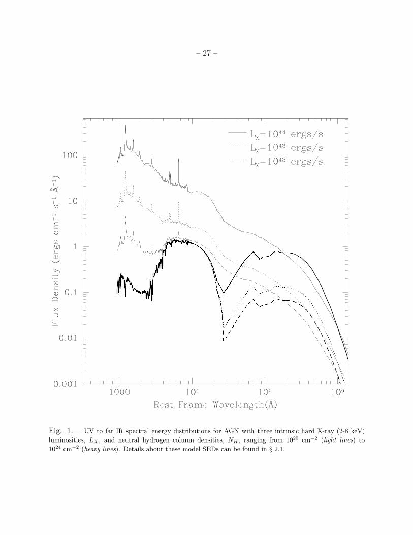
ues used in this calculation are shown in Figure 1. Two known AGN, the Type 1 quasar

PG0804+761 (z = 0.1, NH = 3.1 × 1020 cm−2; Elvis et al. 1994) and the Seyfert 2 galaxy

NGC 7582 (z = 0.00525,NH = 1.24 × 1023 cm−2; Bassani et al. 1999) agree well with the

appropriate model SEDs, as shown in Figure 2. Note that once NH and redshift (and thus

luminosity) are specified, there are no free parameters to adjust the fit to the data.

– 7 –

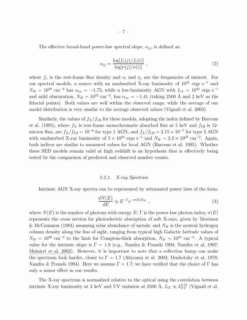
The effective broad-band power-law spectral slope, αij, is defined as:

αij =log[fν(j)/fν(i)]

log[ν(j)/ν(i)], (2)

where fν is the rest-frame flux density and νi and νj are the frequencies of interest. For

our spectral models, a source with an unabsorbed X-ray luminosity of 1045 ergs s−1 and

NH = 1020 cm−2 has αox = −1.73, while a low-luminosity AGN with LX = 1042 ergs s−1

and mild obscuration, NH = 1022 cm−2, has αox = −1.41 (taking 2500 A and 2 keV as the

fiducial points). Both values are well within the observed range, while the average of our

model distribution is very similar to the average observed values (Vignali et al. 2003).

Similarly, the values of fX/fIR for these models, adopting the index defined by Barcons

et al. (1995), where fX is rest-frame monochromatic absorbed flux at 5 keV and fIR is 12-

micron flux, are fX/fIR = 10−6 for type 1 AGN, and fX/fIR = 2.15× 10−7 for type 2 AGN

with unabsorbed X-ray luminosity of 5 × 1044 ergs s−1 and NH = 3.2 × 1023 cm−2. Again,

both indices are similar to measured values for local AGN (Barcons et al. 1995). Whether

these SED models remain valid at high redshift is an hypothesis that is effectively being

tested by the comparison of predicted and observed number counts.

2.2.1. X-ray Spectrum

Intrinsic AGN X-ray spectra can be represented by attenuated power laws of the form:

dN(E)

dE∝ E−Γe−σ(E)NH , (3)

where N(E) is the number of photons with energy E; Γ is the power-law photon index; σ(E)

represents the cross section for photoelectric absorption of soft X-rays, given by Morrison

& McCammon (1983) assuming solar abundance of metals; and NH is the neutral hydrogen

column density along the line of sight, ranging from typical high Galactic latitude values of

NH = 1020 cm−2 to the limit for Compton-thick absorption, NH ∼ 1024 cm−2. A typical

value for the intrinsic slope is Γ = 1.9 (e.g., Nandra & Pounds 1994; Nandra et al. 1997;

Mainieri et al. 2002). However, it is important to note that a reflection hump can make

the spectrum look harder, closer to Γ = 1.7 (Akiyama et al. 2003; Mushotzky et al. 1978;

Nandra & Pounds 1994). Here we assume Γ = 1.7; we have verified that the choice of Γ has

only a minor effect in our results.

The X-ray spectrum is normalized relative to the optical using the correlation between

intrinsic X-ray luminosity at 2 keV and UV emission at 2500 A, LX ∝ L0.75UV (Vignali et al.

– 8 –

2003). This relation has a dispersion of ±0.06 in the exponent and is significant at the 7.9σ

level when BALQSOs are excluded (they are in any case rare).

2.2.2. Optical Spectrum

From 1000 A to ∼ 1 µm we use the Sloan Digital Sky Survey (SDSS) composite quasar

spectrum (Vanden Berk et al. 2001), which represents an average of over 2000 SDSS quasars

with a median redshift z = 1.253, covering rest-frame wavelengths from 800 A to 8555 A at

a resolution of ∼ 1 A . The intrinsic luminosity of quasars in this sample spans the range from

Mr′ = −18 mag to Mr′ = −26.5 mag. This spectrum well represents unobscured (type 1)

AGN, in which the optical light from the central engine is not absorbed by the dust or gas

torus. Given that the SDSS quasar composite includes AGN brighter than the average AGN

observed in X-rays, the use of the SDSS composite spectrum may not be realistic; however,

it is completely appropriate to our very simple model which assumes the obscuring torus

is independent of luminosity or redshift. Furthermore, there are good indications that the

optical spectrum of faint quasars is very similar to the spectrum of the average SDSS quasar

(Steidel et al. 2002).

To calculate the effects of absorption on the optical and UV spectrum we use the ex-

tinction coefficients of Cardelli et al. (1989), obtained from absorption measurements on

Milky Way stars. A standard Milky Way dust-to-gas ratio was assumed to convert neutral

hydrogen column density into optical extinction: NH = 1.96 × 1021AV (Bohlin et al. 1978).

Some studies of the dust-to-gas ratio in AGN point out that this ratio is on average signif-

icantly smaller than the value obtained for the Milky Way (Maiolino et al. 2001b,a), but

this picture has been questioned (Weingartner & Murray 2002). Here we assume the more

conservative position and use the standard dust-to-gas ratio value. If in fact this ratio is

two orders of magnitude lower for AGN (Maiolino et al. 2001b), marginally obscured AGN

(with NH ∼ 1022 cm−2) will be significantly brighter in the optical. For example, a source

with LX = 1043 ergs s−1 and NH = 1022 cm−2 at z = 1 will be ∼1 magnitude brighter in the

z-band if the dust-to-gas ratio is two orders of magnitude smaller than in the Milky Way.

For more luminous sources this effect is larger, reaching ∼ 5 magnitudes in the z-band for a

source with LX = 1045 ergs s−1 and NH = 1022 cm−2 at z = 1. However, this is about the

maximum discrepancy for the sample studied in this paper, since sources with column densi-

ties larger than ∼ 5× 1022 cm−2 or lower than 1021 cm−2 are not significantly affected in the

optical bands since they are already too obscured (and thus dominated by the host galaxy)

or the obscuration is too low to make a significant change. Also, the infrared bands are not

greatly affected by a change in the dust-to-gas ratio assumed. Therefore, our conclusions

– 9 –

should not be greatly affected by a different choice of dust-to-gas ratio.

Given the small GOODS volume, the contribution of very high redshift sources (z > 5)

to the total sample is negligible. For these sources, z-band observations (λeff ∼ 8800 A )

effectively correspond to λ > 1460A in the rest frame, and therefore absorption from the

intergalactic medium (Madau 1995) can safely be ignored in the whole sample.

To the AGN spectrum we add optical light from a host galaxy, for which we assume an L∗

elliptical with spectrum given by Fioc & Rocca-Volmerange (1997). In order to account for

the evolution of the host galaxy, caused mainly by star formation, we adopt the evolutionary

correction of Poggianti (1997), assuming an elliptical galaxy with an e-folding time of the

star formation rate of 1 Gyr. This model predicts an increase in the z-band luminosity of

∼ 1.2 magnitudes at redshift ∼ 1. Preliminary results using GOODS optical data (Simmons

et al 2004, in prep) show that a large fraction of the AGN host galaxies in the survey are

luminous elliptical, justifying our assumption. The host galaxy dominates the optical light

for obscured sources with NH > 1022 cm−2. As an example, for a source with intrinsic hard

X-ray luminosity LX = 1043 ergs s−1 and NH = 1022 cm−2 the AGN contribution to the total

optical light is only ∼ 4% at z = 0.

2.2.3. Infrared Spectrum

Optical, UV, and soft X-ray light absorbed by dust within the AGN is re-radiated as

thermal emission in the far infrared. Instead of using observed infrared spectra we use the

dust-re-emission models of Nenkova et al. (2002); Elitzur et al. (2003) in order to construct

a grid of infrared spectra as a function of the X-ray luminosity of the AGN and observed

NH value (related to the line-of-sight angle in these physically-motivated models). These

models provide a better fit for recent infrared observations, as well as other advantages over

older torus models (e.g. Pier & Krolik 1992, 1993; Granato & Danese 1994); for a detailed

discussion of this point see Elitzur et al. (2003).

The Nenkova et al. (2002) models postulate a random distribution of clumps inside a

dusty torus. Each clump is optically thick, and the radial distribution is confined between an

inner radius Ri and an outer radius Ro (see Figure 2 of Elitzur et al. 2003). The mean free

path between clumps is given by a power law of the form rq where r is the radial distance

from the central engine, while the angular dependence of the number of clumps is a Gaussian

distribution with dispersion σ, so that the number of clouds as a function of viewing angle

β is given by

NT (β) = NT (0) exp

(

−β2

σ2

)

, (4)

– 10 –

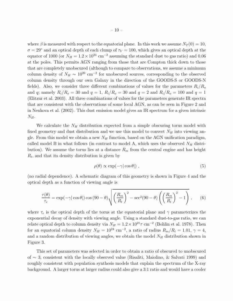
where β is measured with respect to the equatorial plane. In this work we assume NT (0) = 10,

σ = 29 and an optical depth of each clump of τV = 100, which gives an optical depth at the

equator of 1000 (or NH = 1.2×1024 cm−2 assuming the standard dust to gas ratio) and 0.06

at the poles. This permits AGN ranging from those that are Compton thick down to those

that are completely unobscured (although to compare to observations, we assume a minimum

column density of NH ∼ 1020 cm−2 for unobscured sources, corresponding to the observed

column density through our own Galaxy in the direction of the GOODS-S or GOODS-N

fields). Also, we consider three different combinations of values for the parameters Ri/Ro

and q; namely Ri/Ro = 30 and q = 1, Ri/Ro = 30 and q = 2 and Ri/Ro = 100 and q = 1

(Elitzur et al. 2003). All three combinations of values for the parameters generate IR spectra

that are consistent with the observations of some local AGN, as can be seen in Figure 2 and

in Nenkova et al. (2002). This dust emission model gives an IR spectrum for a given intrinsic

NH .

We calculate the NH distribution expected from a simple obscuring torus model with

fixed geometry and dust distribution and we use this model to convert NH into viewing an-

gle. From this model we obtain a new NH function, based on the AGN unification paradigm,

called model B in what follows (in contrast to model A, which uses the observed NH distri-

bution). We assume the torus lies at a distance Rm from the central engine and has height

Rt, and that its density distribution is given by

ρ(θ) ∝ exp(−γ| cos θ|) , (5)

(no radial dependence). A schematic diagram of this geometry is shown in Figure 4 and the

optical depth as a function of viewing angle is

τ(θ)

τe

= exp(−γ| cos θ|) cos (90 − θ)

√

√

√

√

(

Rm

Rt

)2

− sec2(90 − θ)

(

(

Rm

Rt

)2

− 1

)

, (6)

where τe is the optical depth of the torus at the equatorial plane and γ parameterizes the

exponential decay of density with viewing angle. Using a standard dust-to-gas ratio, we can

relate optical depth to column density via NH = 1.2×1021τ cm−2 (Bohlin et al. 1978). Then

for an equatorial column density NH = 1024 cm−2, a ratio of radius Rm/Rt = 1.01, γ = 4,

and a random distribution of viewing angles, we obtain the model NH distribution shown in

Figure 3.

This set of parameters was selected in order to obtain a ratio of obscured to unobscured

of ∼ 3, consistent with the locally observed value (Risaliti, Maiolino, & Salvati 1999) and

roughly consistent with population synthesis models that explain the spectrum of the X-ray

background. A larger torus at larger radius could also give a 3:1 ratio and would have a cooler

– 11 –

far-infrared spectrum, but until we get the Spitzer infrared data, we cannot constrain the

far-infrared emission. This distribution is very similar to that observed in the GOODS fields

(solid line in Figure 3), except for NH > 1023 cm−2 sources. For such high column densities,

the discrepancy, of the order of 10-15% in the fractional distribution, is probably caused by

incompleteness in the Chandra samples, since the amount of obscuration is large enough to

hide even the hard X-ray emission. In particular, for NH ≃ 3×1023 cm−2 the incompleteness

of the Chandra observations in the Chandra Deep Fields is ∼ 25%, increasing to ∼ 70% for

NH > 1024 cm−2, using the U03 luminosity function and calculating the number of sources

below the X-ray flux limit as a function of NH . Overall, for our model, roughly 50% of the

AGN are not detected in the Chandra Deep Fields (see § 4.3 for details).

Model B thus comprises the U03 luminosity function (including its redshift evolution),

the AGN SEDs described in section §2.2, and the NH function given by equation 6. Implicit

in this model is that the ratio of obscured to unobscured AGN is constant with redshift, and

that the geometry of the torus does not change with redshift or luminosity.

For a given luminosity, spectra for different orientation angles are normalized at 100 µm,

where the optical depth is low and thus the re-processed emission from the torus is roughly

isotropic. The infrared spectrum is then joined smoothly to the optical spectrum at 1 µm

so that the resulting spectrum is continuous. Infrared emission from star formation is not

considered in this model.

3. Observed and Predicted AGN Number Counts

3.1. The GOODS Data

We compare the number counts calculated above to the optical and X-ray flux distri-

butions for AGN in the two GOODS fields, based on Chandra and HST ACS multi-band

data. The two GOODS fields, each 10′ × 16′, were imaged with ACS in the B,V ,i and z

bands, for a total of 13 orbits per pointing, reaching AB magnitude 27.4 (5σ) in the z band2.

The GOODS fields have also been imaged extensively from the ground in UBVRIzJHK, and

spectroscopy is ongoing. Details of these observations can be found in Giavalisco et al. (2004)

and at http://www.stsci.edu/science/goods.

GOODS-N and GOODS-S fields have published deep X-ray observations: the 2 Ms

2Observations taken with the NASA/ESA Hubble Space Telescope (HST), which is operated by the As-

sociation of Universities for Research in Astronomy, Inc., under NASA contract NAS5-26555.

– 12 –

Chandra Deep Field-North (A03) and the 1 Ms Chandra Deep Field-South (Giacconi et al.

2002, hereafter G02). These two ultra-deep X-ray surveys provide the deepest views of the

Universe in the 0.5–8.0 keV band. The CDF-N is ≈ 2 times more sensitive at the aim

point than the CDF-S, with 0.5–2.0 keV and 2–8 keV flux limits (S/N= 3) of ≈ 2.5 ×

10−17 erg cm−2 s−1 and ≈ 1.4×10−16 erg cm−2 s−1, respectively (A03). The CDF-N remains

& 1.8 times and & 1.5 times deeper than the CDF-S over ≈ 50% (≈ 90 arcmin2) and ≈ 75%

(≈ 135 arcmin2) of the area of GOODS fields, respectively. Point-source Chandra catalogs

have been produced by A03 for the CDF-N and CDF-S and by G02 for the CDF-S. In this

study we use the Chandra catalogs of A03 which were generated using the same methods for

both fields. These catalogs include 326 sources detected in the CDF-S and 503 in the CDF-

N. 223 of the X-ray sources in the CDF-S are located in the GOODS-S region, while 324 of

the sources in the CDF-N were found in the GOODS-N region. If only the sources detected

in the hard band are included, the sample is reduced to 141 sources in the GOODS-S field

and 210 sources in the GOODS-N region.

The GOODS fields will be observed with the Spitzer IRAC instrument in all four bands

(3.6 to 8 µm), with expected sensitivity of 0.6µJy in the 3.6µm band. Both fields will also

be observed with the Spitzer MIPS instrument at 24 microns, to a flux limit that depends

somewhat on the as-yet unknown source density (and hence confusion limit), but which we

take to be roughly 22 µJy (5σ).

There are 168 published spectroscopic redshifts for X-ray sources in the CDF-S, all of

them measured using the FORS1 and FORS2 cameras at the VLT telescopes (Szokoly et al.

2004). Photometric redshifts have been calculated for all the sources detected in the optical

bands in the GOODS South field (see Mobasher et al. 2004 for details), which account

for ∼ 90% of the observed X-ray sources. Properties of some of the remaining sources

not detected in the ACS observations are described in detail by Koekemoer et al. (2004).

Spectroscopic redshifts were used when available.

Spectroscopic redshifts for 284 X-ray sources in the CDF-N were obtained by Barger

et al. (2003) using the Low-Resolution Imaging Spectrograph and the Deep Extragalactic

Imaging Multi-Object Spectrograph on the Keck 10-m telescopes and the HYDRA spectro-

graph on the WIYN 3.5-m telescope. Photometric redshifts were used when spectroscopic

redshifts were not available (see Barger et al. 2003). Spectroscopic redshifts were obtained

for 54% of the sources, while if photometric redshifts are added the completeness level rises to

∼ 75%. Sources without spectroscopic or photometric redshifts are very faint in the optical,

with all but two having z > 24.0 mag. Given the very faint magnitudes of the sources with-

out redshifts in the GOODS-N region, they are likely at redshift z > 1.0 and lack the strong

broad emission lines normally used to identify unobscured AGN at high redshift. That is,

– 13 –

most are probably obscured AGN at z > 1 (e.g., Alexander et al. 2001; Koekemoer et al.

2002).

3.2. The AGN Sample

Almost all the X-ray sources detected in the GOODS fields are AGN, with the exception

of a few nearby starburst galaxies (Alexander et al. 2003). Sources in the X-ray catalogs

were matched to the ACS images of the GOODS North and South fields by Bauer et al.

(2004, in prep) using the likelihood method described in Bauer et al. (2000). Using only

X-ray sources that were detected in the hard band and were unambiguously identified in the

optical images (i.e., only one optical counterpart within ∼ 1 arcsecond of the X-ray centroid),

the final sample includes 128 sources in the GOODS South region and 178 in the GOODS

North field. It is important to note that reducing the analysis to the unambiguously matched

sources eliminates ∼ 10% of the hard X-ray sources in the GOODS regions. Roughly half of

these sources in the GOODS-S field have counterparts in deep K-band imaging and thus may

be obscured AGN at high redshift (Koekemoer et al. 2004). Optically faint X-ray sources

detected in near-infrared bands in other fields were also discussed by Mainieri et al. (2002)

and Mignoli et al. (2004).

3.3. Deriving the NH Distribution from the Chandra Data

The hardness ratio, which we calculate for each source, is defined as (H − S)/(H + S),

where S is the number of counts detected in the 0.5 − 2 keV band and H is the number of

counts in the 2 − 8 keV band. The neutral hydrogen column density was calculated from

the hardness ratio assuming an intrinsic power-law X-ray spectrum with photon indices

Γ = 1.7 or Γ = 1.9. We generated a conversion table using XSPEC (Arnaud 1996) to

calculate hardness ratios for a range of NH and redshift values; this program incorporates

the Chandra ACIS instrumental response matrix. We added Galactic absorption column

densities (Stark et al. 1992) at z = 0 of NH = 8 × 1019 cm−2 for the GOODS-S field and

NH = 1.6 × 1020 cm−2 in the GOODS-N field to each NH -z pair stored in the table, since

all X-rays pass through the interstellar medium of our galaxy. Using the table, the hardness

ratio of each source with a spectroscopic redshift (photometric redshifts are too uncertain

for this purpose) can be converted to a value of NH . The distribution of derived NH values

for 82 sources with spectroscopic redshifts in the GOODS-S field and 103 sources in the

GOODS-N field is shown in Figure 3. Note that for individual sources, our method of

deriving NH may not be very accurate, as some will have soft excess emission or intrinsically

– 14 –

soft spectra (indeed, these may be the reasons why there is an excess of apparently low

column density objects) or will have intrinsically steeper spectra (and thus have spuriously

high NH) and therefore our resulting distribution can be affected by systematic errors. In

order to minimize these effects, the value of NH determined for each source is only used

to calculate the distribution of the sample and not for other purposes (e.g. to correct the

observed X-ray flux).

The predicted NH distributions for the sources in the GOODS N+S fields in models

A and B are compared in Figure 3. Model B provides a better fit to the observed data;

a K-S test on both models compared to the observations revealed that the null hypothesis

(that the model and observed distributions are drawn from the same parent distribution) is

acceptable at the 75.3% confidence level for model B and at the 58.5% confidence level for

model A. This is not surprising since model B uses an NH function with parameters chosen

to be consistent with the observations; however, it is important to note that this model

is motivated by the unification paradigm, which clearly can account for the observed NH

distribution.

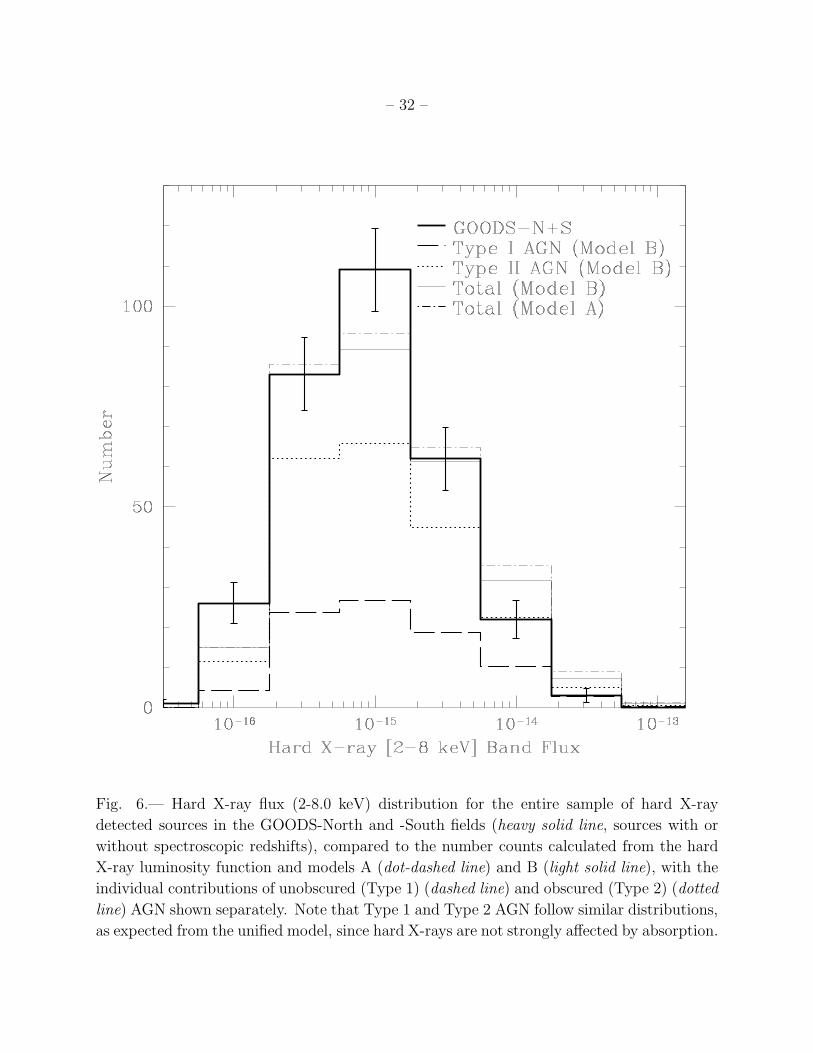
3.4. X-ray Number Counts

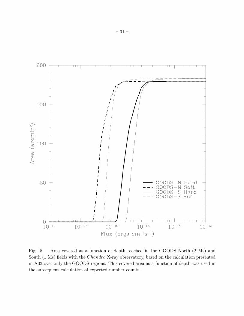
The total area covered as a function of X-ray flux limit for each GOODS field was

calculated based on the results presented in A03 and is shown in Figure 5. These curves

are needed to normalize the hard X-ray flux distributions for sources in the GOODS fields,

shown in Figure 6. We also plot the X-ray distributions calculated from the hard X-ray

luminosity function U03 for both models A (U03 observed NH function) and B (our NH

function based on a simple unified model). The agreement is very good for both models;

a K-S test shows that the null hypothesis is acceptable at > 90% confidence when either

model was tested against the observed distribution. Although the U03 sample includes the

CDF-N, this is not a circular argument since in that work only the brightest CDF-N sources

(with fX > 3 × 10−15 ergs cm−2 s−1 in the hard band) were considered, and therefore our

calculation tests the extrapolation to much fainter fluxes. In the hard X-ray flux distribution

both unobscured (type 1) and obscured (type 2) AGN are well represented (dotted and

dashed lines in Figure 6).

– 15 –

3.5. Optical Number Counts

In deep optical imaging with the HST ACS camera the vast majority of the X-ray

sources in the GOODS fields are detected. Figure 7 shows the distribution of observed z-

band magnitudes for the X-ray sources in the two fields combined (solid line), along with

the model predictions (dashed line). The agreement between the observed and predicted

distributions is very good; a K-S test comparing the observed distribution to the prediction

of model B gives a confidence level for the null hypothesis of 71%, while for model A the

confidence level is 53%. The observed distribution is very broad, with the brightest objects

at z ∼ 17 mag and the faintest below z ∼ 28 mag. Unobscured AGN (dashed line) fail to

account for the faintest optical counterparts. Given their large X-ray to optical flux ratios,

the fainter optical sources (z > 23.5 mag) may be obscured AGN at redshifts z ∼ 1 − 3

(Alexander et al. 2001; Koekemoer et al. 2002). Indeed in our models most obscured AGN

(dotted line) have faint optical magnitudes, while the unobscured AGN are responsible for

the peak at brighter magnitudes. For z > 23.5 mag, the approximate limit for ground-based

spectroscopy, obscured AGN are the dominant population.

3.6. Redshift Distribution

Figure 8 shows the redshift distributions for the sources in the GOODS-North and South

fields (thick solid lines) compared to the expected redshift distributions from our model B

(dashed lines). Using photometric redshifts (Mobasher et al. 2004), our GOODS-S sample of

hard X-ray sources is 100% complete. However, in the GOODS-N field, combining spectro-

scopic and photometric redshifts (Barger et al. 2003), the sample is only ∼ 75% complete3.

Spectroscopic redshifts are shown by the hatched regions. At redshifts above z ∼ 1, there is

a clear discrepancy between the spectroscopic redshifts and either the photometric redshift

or the model predictions, in the sense that there are fewer AGN with high spectroscopic

redshifts. This is explained at least in part by the effective brightness limit for spectroscopy,

R < 24 mag, for even the largest ground-based telescopes. Imposing this optical limit on

the GOODS AGN model (long dashed line in Figure 8) does match the observed spectro-

scopic redshift distribution very well. Obscured AGN at z > 1, in particular, are fainter

than this limit and thus are not included in the spectroscopic samples. This likely accounts

for the discrepancy between the observed redshift distribution of X-ray sources (Hasinger

2002; Szokoly et al. 2004) and the distribution predicted from population synthesis models

for the X-ray background (Gilli et al. 1999, 2001), as well as the low number of Type 2 AGN

3We expect the photometric redshifts to be 100% complete once the GOODS ACS data are fully analyzed.

– 16 –

identifications.

The agreement between the model and the observations is good, with a K-S test giving

63% confidence for the null hypothesis in the GOODS-S field and 21% confidence in the

GOODS-N field. This slightly lower level arises because the model predicts still more high

redshift AGN than are observed in the GOODS fields. This is because some high-redshift

obscured AGN are too faint even for the HST images (see Koekemoer et al. 2004) and because

the most obscured AGN are not detected in the Chandra deep fields. Also, an excess of

observed sources at z < 1 can be seen. This is explained by the presence of clusters and

large scale structure in both fields (e.g. Gilli et al. 2003).

Figure 8 shows the difference between the North and South fields, in the sense that

there is a larger discrepancy between the photometric redshifts and the model in the North.

This must be due to incompleteness since again the missing 25% of the AGN (those without

photometric or spectroscopic redshifts) are preferentially fainter.

The model redshift distribution is therefore in agreement with the data once these

selection effects are considered. It is also compatible with the kind of distribution predicted

from population synthesis (Gilli et al. 2001), in the sense that it peaks at a higher redshift

than previously reported distributions, with the same caveat about selection effects. This

better agreement between models and observations is explained also in part by the use of the

U03 luminosity function, that includes a redshift distribution that peaks at lower redshifts

than existing optical quasar luminosity functions (e.g. Boyle et al. 2000).

4. Discussion

Hard X-ray surveys find obscured sources that are largely missed in deep optical/UV

surveys. Deriving a hard X-ray luminosity function or a redshift distribution imposes an

effective optical cut at R < 24 mag, since optical spectroscopy is required to obtain redshifts.

Thus published redshift distributions can be missing optically faint sources. These sources

can be either low-luminosity unobscured AGN or obscured AGN, depending on their central

engine luminosity, and in general, the spectroscopic incompleteness increases with redshift.

This selection effect explains the discrepancy between the photometric and spectroscopic

redshift distributions (Fig. 8).

Evidence for the existence of a significant number of obscured AGN at z > 1 was

previously given by Fiore et al. (2003), who found a correlation between X-ray luminosity

and X-ray-to-optical flux ratio in obscured AGN. Such a correlation can be explained by our

models since for obscured AGN the optical light is dominated by the host galaxy, which is

– 17 –

independent of the AGN luminosity. Therefore, for an obscured AGN the optical emission is

roughly constant, while the X-ray emission scales directly with the AGN luminosity. Using

this correlation, Fiore et al. (2003) estimated source redshifts using just the X-ray-to-optical

flux ratio, thus including sources too faint for optical spectroscopy. They concluded there is

a significant number of obscured AGN at z > 1, and that these sources will be missed by

surveys that rely on optical spectroscopy. We arrive at the same conclusion from a different

direction, based on the comparison of our model with multiwavelength observations of X-ray

sources.

4.1. Optically Faint X-ray Sources

The GOODS HST data reveal an appreciable number of optically faint, X-ray-selected

AGN. While unobscured sources are bright in the optical bands, the vast majority of them

brighter than the spectroscopic limit, obscured sources will be optically fainter and therefore

missed preferentially by surveys that depend on spectroscopic identifications. Most obscured

AGN are bright enough in hard X-rays to be detected in the Chandra observations. There-

fore, given the large X-ray-to-optical flux ratios of the optically faint sample, their hardness

ratio and their red colors, they are very likely to be obscured AGN at z > 1 (Alexander et al.

2001; Koekemoer et al. 2002). Sources with high X-ray-to-optical flux ratio in other fields

were discussed previously in the literature (e.g., Fiore et al. 2003; Mignoli et al. 2004; Gandhi,

Crawford, Fabian, & Johnstone 2004), and in most cases these sources can be identified as

obscured AGN at high redshift.

4.2. NH Distribution

Both models for the NH distribution fit the observed flux distributions well (Figs 6,7).

Model A assumed the empirical NH function described in U03, which is based on observations

from several X-ray surveys and did not go as deep as the GOODS sample, while model B uses

an NH function based on a simple unified model, with the idea of a dust torus covering the

central engine. It is important to note that model B predicts a larger number of sources with

NH ∼ 1023 cm−2 than is observed, commensurate with the large number of very obscured

sources needed to explain the X-ray background spectrum (Gilli et al. 2001,U03). The

observed ratio of obscured to unobscured sources in the GOODS fields is ∼2.5 when the

division point is set at NH = 1021 cm−2 as assumed by Gilli et al. (2001), less than the

intrinsic value of 4 required by the X-ray background models. That is, the observed ratio is

affected by incompleteness in the X-ray samples at high column densities. Based on the U03

– 18 –

luminosity function and our torus model to calculate the NH distribution we calculate that

the completeness level of the Chandra observations in the GOODS fields drops to ∼ 75%

for NH = 1023 cm−2 and ∼ 30% for NH = 1024 cm−2. This is caused by absorption of the

X-ray emission which makes harder to detect sources with higher column densities in a flux-

limited survey. Therefore, if there are heavily obscured AGN in the field, the intrinsic ratio

of obscured to unobscured sources is larger than the observed ratio, and can even be ∼ 4, as

suggested by population synthesis models for the X-ray background. The relation between

the observed X-ray sources in the GOODS fields and the models for the X-ray background

will be analyzed in more detail in a later paper (Treister et al. 2004, in prep.).

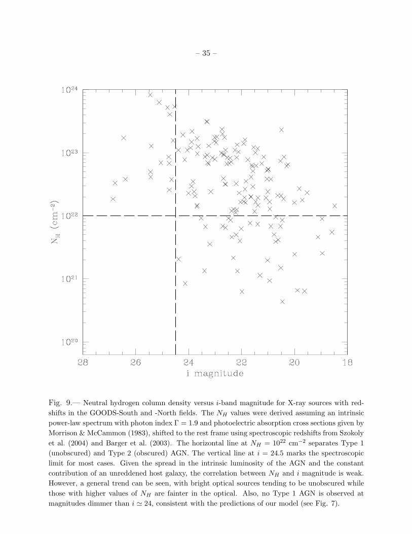
We can ask whether the X-ray absorption correlates with the optical dimming; that

is, is obscuration making bright hard X-ray sources optically faint? The relation between

optical magnitude and amount of obscuration is shown in Figure 9. Sources that present

large amounts of obscuration in the X-ray spectrum are in general the fainter sources in the

optical, as expected. There is no strong correlation present in Figure 9 — both obscured

and unobscured AGN appear at bright magnitudes — but the highest column densities do

correspond to the faintest magnitudes. In particular, it is important to note that there are no

unobscured sources at magnitudes i > 24.5, which is consistent with our model predictions

of a very low number of unobscured AGN at faint magnitudes. There is no strong correlation

because the optical emission from obscured AGN is dominated by the host galaxy; once the

optical emission of the AGN is absorbed, the i-band magnitude becomes insensitive to the

amount of obscuration or to the intrinsic luminosity of the AGN.

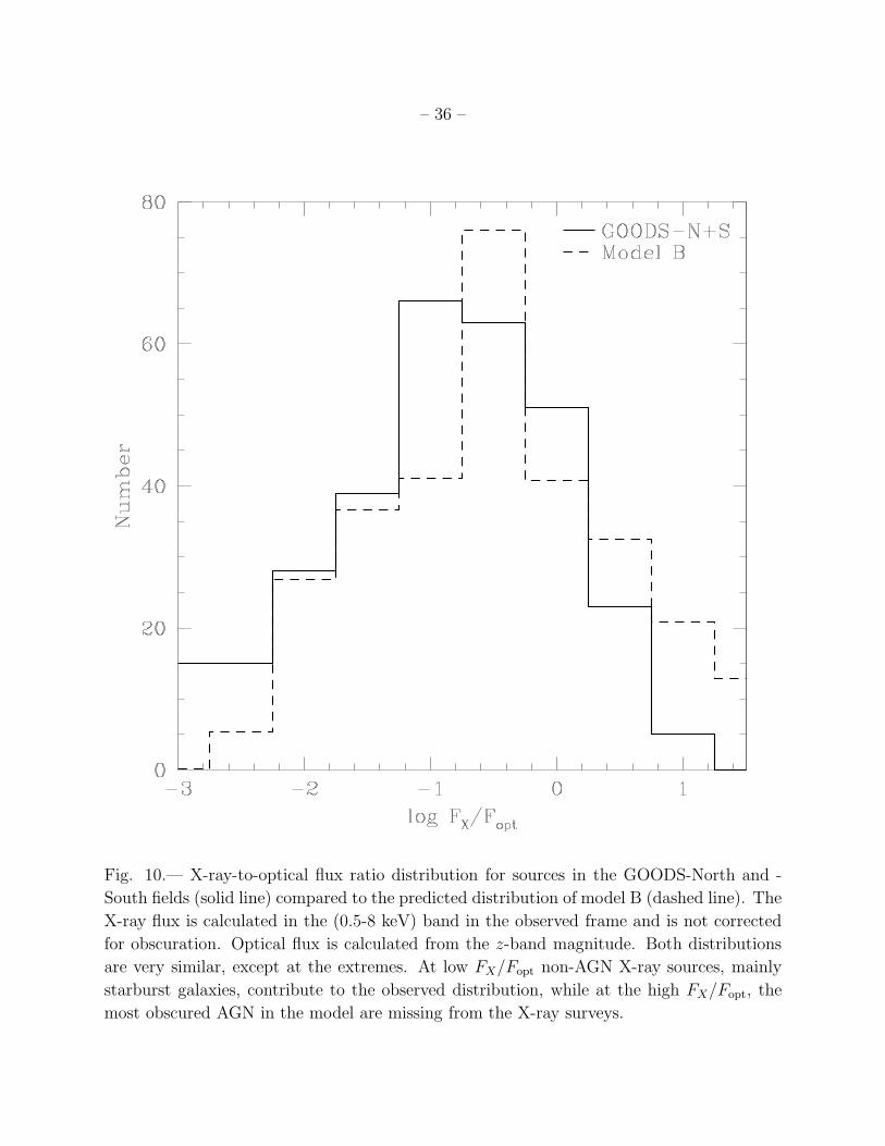
The full X-ray (0.5-8 keV) to optical (z-band) flux ratio4 for GOODS AGN is shown in

Figure 10, together with the ratio obtained from our model. The agreement between these

two distributions is very good, with a K-S confidence level of ∼ 92% for the null hypothesis,

except for a small discrepancy at log FX/Fopt > 0.5, which is consistent with the previously

calculated incompleteness of the X-ray samples for NH > 1023 cm−2. A second discrepancy

appears at the low FX/Fopt end, which can be explained by the presence of a few starburst

galaxy and other non-AGN X-ray sources in the Chandra Deep Fields observations (e.g.,

Hornschemeier et al. 2001; Alexander et al. 2002; Bauer et al. 2002). These sources, around

10% of the total sample, are not accounted in our model and therefore increase the number

of observed X-ray sources with log FX/Fopt < −2. This number of non-AGN X-ray sources

is in agreement with the values reported by A03.

4Defined as log FX/Fopt = log FX +0.4×mz +4.934, where FX is the X-ray flux in units of ergs cm−2 s−1

and mz is the optical magnitude in the z band in the AB system.

– 19 –

4.3. Predictions for the Infrared Number Counts

The Spitzer Space Telescope was launched in August 2003 and the GOODS fields

are scheduled to be observed in 2004. AGN are luminous infrared sources (Sanders et al.

1989), so the ratio of obscured to unobscured AGN will be strongly constrained by the

observed Spitzer number counts of X-ray sources. These two classes can be separated using

a combination of IRAC 4.5 and 8 microns bands and MIPS 24 microns data (Andreani et al.

2003). Furthermore, the infrared spectrum is sensitive to parameters of the dust emission

model, so will help refine the present simple spectral models.

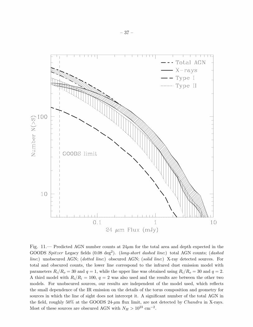
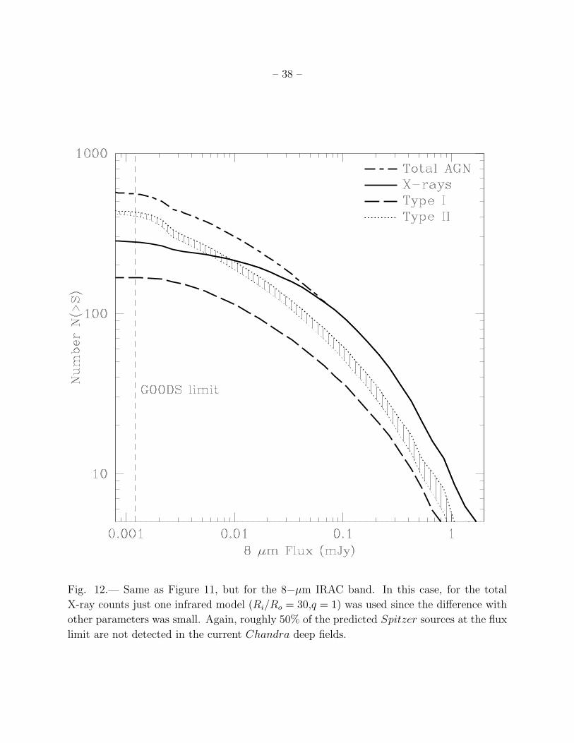
The AGN number counts at 24 µm calculated according to § 2 assuming the appropriate

hard X-ray flux limit for each Chandra deep field separately, and normalized to the total

GOODS area (0.08 deg2), are shown in Figure 11; the number counts at 8 µm and 3.6 µm

are presented in Figures 12 and 13. Contributions from obscured and unobscured AGN

were calculated from hard X-ray luminosity functions using model B. For the infrared part

of the SED, we assumed three different sets of parameters, as is described in §2.2; each

shaded region for the total and obscured number of sources corresponds to the extremes

that these values can have. For unobscured sources, the shape of the infrared SED is almost

independent of the assumed parameters, so only one line is plotted.

One important conclusion from this calculation is that all the AGN detected in the

Chandra deep fields should be detected in the Spitzer observations. The contrary is not

the case since some obscured AGN are missed by X-ray observations. This difference is

shown by the top two curves in Figure 11. Indeed, obscured AGN with NH > 1023 cm−2

should all be detected with Spitzer, in principle allowing for a complete study of the AGN

population in this field and providing a test for both the unified model of AGN and the

population synthesis models used to explain the X-ray background. However, to identify

obscured AGN not detected in X-rays and to separate them from luminous starburst galaxies

will not be easy. In fact, Andreani et al. (2003) reported that is not possible to separate

very obscured AGN activity from a burst of star formation just on the basis of infrared

photometry, even if information in the MIPS 70-micron band is included. This problem

is even more serious since typically there is overlap between the two populations, and a

starbust galaxy can harbor a very obscured AGN. In order to solve this problem, we can

take advantage of GOODS multiwavelength coverage, ranging from 0.4 to 24 microns, which

allows us to calculate accurate photometric redshifts and bolometric luminosities for even

very faint sources. Then, to first order, we can use bolometric luminosity in order to separate

AGN activity from starburst galaxies, since all AGN should have Lbol > 1042 ergs s−1, while

starbursts typically have much lower luminosities.

Similar calculations of the AGN number counts in the infrared were performed recently

– 20 –

by Andreani et al. (2003). For ΩΛ = 0.7 and Ωm = 0.3, they found a total of ∼ 3 × 105

sources per square degree with a 24 µm flux higher than 550 µJy, ∼ 10% of them Seyfert 2s.

We predict a much lower number of sources, ∼ 103 sources per square degree at the same

flux limit in the 24 µm band, with ∼ 70% of them being Seyfert 2s. This large discrepancy

of 2 orders of magnitude can be explained by the difference in the assumed luminosity

function and evolution. We used a hard X-ray luminosity function and luminosity-dependent

density evolution , which peaks at redshifts z ∼ 2 for QSO-like objects and z . 1 for low-

luminosity AGN, whereas Andreani et al. (2003) used a local luminosity function based on

12-µm observations and optical QSO evolution with a peak at z ∼ 3 and exponential decay

until z = 10. Locally both luminosity functions are very similar so the major part of the

discrepancy is explained by the difference in the assumed evolution. This shows clearly

that Spitzer observations will provide a significant constraint on the AGN number density

evolution.

5. Conclusions

In this work we modeled the AGN population of the GOODS fields in order to explain

the observed numbers and brightnesses at optical and X-ray energies. We also predicted

the number counts at infrared wavelengths that will be measured with the Spitzer Space

Telescope. Basic ingredients of our models are few. First, we used the hard X-ray luminosity

function and luminosity-dependent evolution determined by U03. Second, we developed a

library of multi-wavelength AGN SEDs parameterized as a function of only two parameters,

the intrinsic rest-frame hard X-ray luminosity and the amount of gas and dust in the line

of sight, given as a neutral hydrogen column density. These composite SEDs assume an

intrinsic power law plus photoelectric absorption in X-rays; a QSO composite spectrum in

the optical, independent of both redshift and luminosity; Milky Way-type extinction; an

L∗ elliptical host galaxy evolving with redshift; and infrared dust re-emission models from

Nenkova et al. (2002) and Elitzur et al. (2003). Finally, we needed to assume the relative

number of sources at each value of NH . In model A, we used the NH function given in U03,

which is based on observations of X-ray sources in several surveys. For model B, we used

a simple geometric model for a dust torus to generate the expected distribution of NH for

random orientation angles. The torus parameters were chosen so that the ratio of obscured

(NH > 1022 cm−2) to unobscured AGN is 3:1, and we assumed it was independent of redshift

and luminosity. With these ingredients, we calculated the expected distribution of sources

at different wavebands and compared them to the GOODS observations.

We found general agreement between the models and observations, especially for the very

– 21 –

simple unified model. This means there may well be a significant population of obscured AGN

at high redshift, consistent with a roughly constant ratio of obscured to unobscured AGN out

to high redshift, z ∼ 2 − 3. These objects will be bright enough to detect with the planned

Spitzer observations in the GOODS field. The agreement between model and observations is

remarkable given the very simple assumptions used in the calculation. Because the GOODS

observations are so deep, there are large extrapolations from existing luminosity functions.

The excellent agreement supports the unified model of AGN.

A large population of obscured AGN in the early Universe explains not only the GOODS

data but the X-ray background spectral shape and intensity. However, for this picture to

be correct, existing X-ray samples, even from the extremely deep Chandra fields, must be

incomplete. We find that the luminosity-function-weighted fraction of obscured AGN that

is missed at current detection limits is approximately equal to the excess predicted by our

unified model at faint optical magnitudes and high absorbing column densities. Spitzer

observations, together with follow-up studies of host galaxy morphologies and environments,

offer the opportunity to test and refine this picture.

ET thanks the support of Fundacion Andes. This work was supported in part by NASA

grant HST-GO-09425.13-A. The work of DS was carried out at Jet Propulsion Laboratory,

California Institute of Technology, under a contract with NASA. We thank the anonymous

referee for a very detailed and useful report. We would like to thank Eric Gawiser, Priya

Natarajan, Paolo Coppi and Paulina Lira for very useful comments. We thank Moshe Elitzur

for providing us a digital version of his infrared dust re-emission models.

REFERENCES

Akiyama, M., Ueda, Y., Ohta, K., Takahashi, T., & Yamada, T. 2003, ApJS, 148, 275

Alexander, D. M., Aussel, H., Bauer, F. E., Brandt, W. N., Hornschemeier, A. E., Vignali,

C., Garmire, G. P., & Schneider, D. P. 2002, ApJ, 568, L85

Alexander, D. M., Bauer, F. E., Brandt, W. N., Schneider, D. P., Hornschemeier, A. E.,

Vignali, C., Barger, A. J., Broos, P. S., Cowie, L. L., Garmire, G. P., Townsley,

L. K., Bautz, M. W., Chartas, G., & Sargent, W. L. W. 2003, AJ, 126, 539

Alexander, D. M., Brandt, W. N., Hornschemeier, A. E., Garmire, G. P., Schneider, D. P.,

Bauer, F. E., & Griffiths, R. E. 2001, AJ, 122, 2156

Andreani, P., Spinoglio, L., & Malkan, M. A. 2003, ApJ, 597, 759

– 22 –

Antonucci, R. 1993, ARA&A, 31, 473

Arnaud, K. A. 1996, in ASP Conf. Ser. 101: Astronomical Data Analysis Software and

Systems V, 17–+

Barcons, X., Franceschini, A., de Zotti, G., Danese, L., & Miyaji, T. 1995, ApJ, 455, 480

Baldi, A., Molendi, S., Comastri, A., Fiore, F., Matt, G., & Vignali, C. 2002, ApJ, 564, 190

Barger, A. J., Cowie, L. L., Capak, P., Alexander, D. M., Bauer, F. E., Fernandez, E.,

Brandt, W. N., Garmire, G. P., & Hornschemeier, A. E. 2003, AJ, 126, 632

Bassani, L., Dadina, M., Maiolino, R., Salvati, M., Risaliti, G., della Ceca, R., Matt, G., &

Zamorani, G. 1999, ApJS, 121, 473

Bauer, F. E., Alexander, D. M., Brandt, W. N., Hornschemeier, A. E., Miyaji, T., Garmire,

G. P., Schneider, D. P., Bautz, M. W., Chartas, G., Griffiths, R. E., & Sargent,

W. L. W. 2002, AJ, 123, 1163

Bauer, F. E., Condon, J. J., Thuan, T. X., & Broderick, J. J. 2000, ApJS, 129, 547

Bohlin, R. C., Savage, B. D., & Drake, J. F. 1978, ApJ, 224, 132

Boyle, B. J., Shanks, T., Croom, S. M., Smith, R. J., Miller, L., Loaring, N., & Heymans,

C. 2000, MNRAS, 317, 1014

Brandt, W. N., Alexander, D. M., Hornschemeier, A. E., Garmire, G. P., Schneider, D. P.,

Barger, A. J., Bauer, F. E., Broos, P. S., Cowie, L. L., Townsley, L. K., Burrows,

D. N., Chartas, G., Feigelson, E. D., Griffiths, R. E., Nousek, J. A., & Sargent,

W. L. W. 2001, AJ, 122, 2810

Cardelli, J. A., Clayton, G. C., & Mathis, J. S. 1989, ApJ, 345, 245

Castander, F. J., Treister, E., Maza, J., Coppi, P. S., Maccarone, T. J., Zepf, S. E., Guzman,

R., & Ruiz, M. T. 2003, Astronomische Nachrichten, 324, 40

Comastri, A., Setti, G., Zamorani, G. & Hasinger, G. 1995, A&A, 296, 1

Dawson, S., McCrady, N., Stern, D., Eckart, M. E., Spinrad, H., Liu, M. C., & Graham,

J. R. 2003, AJ, 125, 1236

Dickinson, M. & Giavalisco, M. 2002, in The Mass of Galaxies at Low and High Redshift, in

press, astro-ph/0204213

– 23 –

Elitzur, M., Nenkova, M., & Ivezic, Z. 2003, astro-ph/0309040

Elvis, M., et al. 1994, ApJS, 95, 1

Fioc, M. & Rocca-Volmerange, B. 1997, A&A, 326, 950

Fiore, F., et al. 2003, A&A, 409, 79

Gandhi, P., Crawford, C. S., Fabian, A. C., & Johnstone, R. M. 2004, MNRAS, 348, 529

Giacconi, R., Rosati, P., Tozzi, P., Nonino, M., Hasinger, G., Norman, C., Bergeron, J.,

Borgani, S., Gilli, R., Gilmozzi, R., & Zheng, W. 2001, ApJ, 551, 624

Giacconi, R., Zirm, A., Wang, J., Rosati, P., Nonino, M., Tozzi, P., Gilli, R., Mainieri,

V., Hasinger, G., Kewley, L., Bergeron, J., Borgani, S., Gilmozzi, R., Grogin, N.,

Koekemoer, A., Schreier, E., Zheng, W., & Norman, C. 2002, ApJS, 139, 369

Giavalisco, M. et al. 2004, ApJ, 600, L93

Gilli, R., Risaliti, G., & Salvati, M. 1999, A&A, 347, 424

Gilli, R., Salvati, M., & Hasinger, G. 2001, A&A, 366, 407

Gilli, R. 2003, Adv. Space Res., in press(astro-ph/0303115)

Gilli, R., et al. 2003, ApJ, 592, 721

Granato, G. L. & Danese, L. 1994, MNRAS, 268, 235

Green, P. J., et al. 2004, ApJS, 150, 43

Gruber, D. E. 1992, in The X-ray Background, 44

Harrison, F. A., Eckart, M. E., Mao, P. H., Helfand, D. J., & Stern, D. 2003, ApJ, 596, 944

Hasinger, G. 2002, in New Visions of the X-ray Universe in the XMM-Newton and Chandra

Era, Ed. F. Jansen (ESTEC: ESA SP-488), XX (astro-ph/0202430)

Hornschemeier, A. E., Brandt, W. N., Garmire, G. P., Schneider, D. P., Barger, A. J.,

Broos, P. S., Cowie, L. L., Townsley, L. K., Bautz, M. W., Burrows, D. N., Chartas,

G., Feigelson, E. D., Griffiths, R. E., Lumb, D., Nousek, J. A., Ramsey, L. W., &

Sargent, W. L. W. 2001, ApJ, 554, 742

– 24 –

Koekemoer, A. M., Grogin, N. A., Schreier, E. J., Giacconi, R., Gilli, R., Kewley, L., Norman,

C., Zirm, A., Bergeron, J., Rosati, P., Hasinger, G., Tozzi, P., & Marconi, A. 2002,

ApJ, 567,

657

Koekemoer, A. M. et al. 2004, ApJ, 600, L123

Lawrence, A. 1987, PASP, 99, 309

Madau, P., Ghisellini, G., & Fabian, A. C. 1994, MNRAS, 270, L17

Madau, P. 1995, ApJ, 441, 18

Mainieri, V., Bergeron, J., Hasinger, G., Lehmann, I., Rosati, P., Schmidt, M., Szokoly, G.,

& Della Ceca, R. 2002, A&A, 393, 425

Maiolino, R., Marconi, A., & Oliva, E. 2001a, A&A, 365, 37

Maiolino, R., Marconi, A., Salvati, M., Risaliti, G., Severgnini, P., Oliva, E., La Franca, F.,

& Vanzi, L. 2001b, A&A, 365, 28

Mignoli, M., et al. 2004, A&A, 418, 827

Mobasher, B. et al. 2004, ApJ, 600, L167

Morrison, R. & McCammon, D. 1983, ApJ, 270, 119

Mushotzky, R. F., Boldt, E. A., Holt, S. S., Serlemitsos, P. J.,

Swank, J. H., Rothschild, R. H., & Pravdo, S. H. 1978, ApJ, 226, L65

Mushotzky, R. F., Done, C., & Pounds, K. A. 1993, ARA&A, 31, 717

Nandra, K. & Pounds, K. A. 1994, MNRAS, 268, 405

Nandra, K., George, I. M., Mushotzky, R. F., Turner, T. J., & Yaqoob, T. 1997, ApJ, 476,

70

Nenkova, M., Ivezic, Z., & Elitzur, M. 2002, ApJ, 570, L9

Norman, C., Hasinger, G., Giacconi, R., Gilli, R., Kewley, L., Nonino, M., Rosati, P.,

Szokoly, G., Tozzi, P., Wang, J., Zheng, W., Zirm, A., Bergeron, J., Gilmozzi, R.,

Grogin, N., Koekemoer, A., & Schreier, E. 2002, ApJ, 571, 218

Perola, G. C. et al., A&A, in press, astro-ph/0404044.

– 25 –

Pier, E. A. & Krolik, J. H. 1992, ApJ, 401, 99

Pier, E. A. & Krolik, J. H. 1993, ApJ, 418, 673

Poggianti, B. M. 1997, A&AS, 122, 399

Risaliti, G., Maiolino, R., & Salvati, M. 1999, ApJ, 522, 157

Rosati, P., Tozzi, P., Giacconi, R., Gilli, R., Hasinger, G., Kewley, L., Mainieri, V., Nonino,

M., Norman, C., Szokoly, G., Wang, J. X., Zirm, A., Bergeron, J., Borgani, S.,

Gilmozzi, R., Grogin, N., Koekemoer, A., Schreier, E., & Zheng, W. 2002, ApJ, 566,

667

Sanders, D. B., Phinney, E. S., Neugebauer, G., Soifer, B. T., & Matthews, K. 1989, ApJ,

347, 29

Setti, G., Woltjer, L. 1989, A&A, 224L, 21

Singh, K. P., Barrett, P., White, N. E., Giommi, P., & Angelini, L. 1995, ApJ, 455, 456

Stark, A. A., Gammie, C. F., Wilson, R. W., Bally, J., Linke, R. A., Heiles, C., & Hurwitz,

M. 1992, ApJS, 79, 77

Steffen, A. T., Barger, A. J., Cowie, L. L., Mushotzky, R. F., & Yang, Y. 2003, ApJ, 596,

L23

Steidel, C. C., Hunt, M. P., Shapley, A. E., Adelberger, K. L., Pettini, M., Dickinson, M.,

& Giavalisco, M. 2002, ApJ, 576, 653

Stern, D., Moran, E. C., Coil, A. L., Connolly, A., Davis, M., Dawson, S., Dey, A., Eisen-

hardt, P., Elston, R., Graham, J. R., Harrison, F., Helfand, D. J., Holden, B., Mao,

P., Rosati, P., Spinrad, H., Stanford, S. A., Tozzi, P., & Wu, K. L. 2002, ApJ, 568,

71

Szokoly, G. et al. 2004, ApJSin press, astro-ph/0312324

Ueda, Y., Akiyama, M., Ohta, K., & Miyaji, T. 2003, ApJ, 598, 886 (U03)

Vanden Berk, D. E. et al. 2001, AJ, 122, 549

Vignali, C., Brandt, W. N., & Schneider, D. P. 2003, AJ, 125, 433

Voges, W. et al. 1999, A&A, 349, 389

Weingartner, J. C. & Murray, N. 2002, ApJ, 580, 88

– 26 –

Williams, R. E., et al. 1996, AJ, 112, 1335

This preprint was prepared with the AAS LATEX macros v5.2.

– 27 –

Fig. 1.— UV to far IR spectral energy distributions for AGN with three intrinsic hard X-ray (2-8 keV)

luminosities, LX , and neutral hydrogen column densities, NH , ranging from 1020 cm−2 (light lines) to

1024 cm−2 (heavy lines). Details about these model SEDs can be found in § 2.1.

– 28 –

Fig. 2.— Spectral Energy Distributions for the Type 1 quasar PG0804+761 (upper crosses)

and the Seyfert 2 galaxy NGC 7582 (lower crosses). Over-plotted are our model SEDs

(solid and dashed lines) for the appropriate LX and NH ; an X-ray luminosity of LX =

8.5 × 1045 ergs s−1 and NH = 3 × 1020 cm−2 for PG0804+761 (Elvis et al. 1994) and

LX = 9.4 × 1041 ergs s−1 and NH = 1.2 × 1023 cm−2 for NGC 7582 (Bassani et al. 1999).

With no free parameters to adjust, the agreement between the model SED and the observed

values is remarkably good.

– 29 –

Fig. 3.— Distribution of intrinsic obscuring column density for X-ray sources in the GOODS fields

with spectroscopic redshifts. The NH values were derived assuming an intrinsic power-law spectrum

with photon index Γ = 1.9 (solid line) or Γ = 1.7 (dashed line) and photoelectric absorption cross

sections given by Morrison & McCammon (1983), shifted to the rest frame using redshifts from

(Szokoly et al. 2004). Dashed-dotted line: NH distribution of U03 (model A). Light solid line:

NH distribution calculated assuming a simple unified model with a dust torus geometry for the

obscuring material and the GOODS flux limit (model B). As can be seen in this plot, model B

(which is physically motivated) provides a good fit to the observed sources in the GOODS fields,

apart from the expected incompleteness at high column densities.

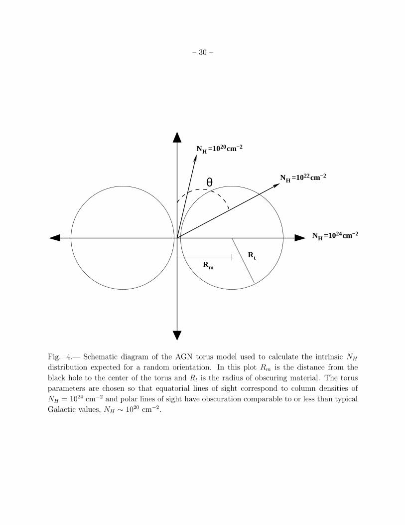
– 30 –

NH =1020cm−2

NH =1022cm−2

NH =1024cm−2

Rm

Rt

θ

Fig. 4.— Schematic diagram of the AGN torus model used to calculate the intrinsic NH

distribution expected for a random orientation. In this plot Rm is the distance from the

black hole to the center of the torus and Rt is the radius of obscuring material. The torus

parameters are chosen so that equatorial lines of sight correspond to column densities of

NH = 1024 cm−2 and polar lines of sight have obscuration comparable to or less than typical

Galactic values, NH ∼ 1020 cm−2.

– 31 –

Fig. 5.— Area covered as a function of depth reached in the GOODS North (2 Ms) and

South (1 Ms) fields with the Chandra X-ray observatory, based on the calculation presented

in A03 over only the GOODS regions. This covered area as a function of depth was used in

the subsequent calculation of expected number counts.

– 32 –

Fig. 6.— Hard X-ray flux (2-8.0 keV) distribution for the entire sample of hard X-ray

detected sources in the GOODS-North and -South fields (heavy solid line, sources with or

without spectroscopic redshifts), compared to the number counts calculated from the hard

X-ray luminosity function and models A (dot-dashed line) and B (light solid line), with the

individual contributions of unobscured (Type 1) (dashed line) and obscured (Type 2) (dotted

line) AGN shown separately. Note that Type 1 and Type 2 AGN follow similar distributions,

as expected from the unified model, since hard X-rays are not strongly affected by absorption.

– 33 –

Fig. 7.— Distribution of observed z-band magnitudes for the entire sample of GOODS-North

and GOODS-South X-ray sources (heavy solid line), compared to the summed distribution of

all the sources in model A (dot dashed line) and model B (light solid line). The distribution

of unobscured (Type 1) (dashed line) and obscured (Type 2) (dotted line) AGN calculated

using model B is also shown. The agreement is very good (K-S test gives 71% for model B

and 53% for model A), showing that in a hard X-ray luminosity function both obscured and

unobscured AGN are well represented. In the unified model (model B), the bright end of

the distribution includes both Type 1 and Type 2 AGN, while the faint end is dominated by

Type 2 AGN, as expected from the obscuration of the optical emission of the central engine.

In all cases, most of the optical emission for Type 2 AGN comes from the host galaxy.

– 34 –

0 1 2 3 4 50

20

40

60

0 1 2 3 4 50

20

40

60

Fig. 8.— Redshift distributions for AGN in the GOODS-South (left panel) and North (right

panel) fields. The observed redshift distribution (heavy solid line) includes both spectro-

scopic (hatched area) and photometric redshifts and is 100% complete in the GOODS-S field

and 75% complete in the GOODS-N region. The expected distribution (dashed line) for

the complete AGN population detected in X-rays, calculated from our models (it is indis-

tinguishable for models A and B), is similar but has more AGN at high redshift, especially

compared to the distribution of spectroscopic redshifts. The distribution for sources with

R < 24 mag (long dashed line) is very similar to the observed distribution of sources with

spectroscopic redshifts. The discrepancy is larger in the GOODS-N field because of incom-

pleteness in the redshifts. Spectroscopic redshifts are limited to AGN with R < 24 mag and

thus exclude the high-redshift obscured AGN in the model, a larger fraction of which are

included in the photometric-redshift sample. The data are therefore consistent with a signif-

icant high-redshift population of obscured AGN which are missed in spectroscopic samples

due to a selection effect.

– 35 –

Fig. 9.— Neutral hydrogen column density versus i-band magnitude for X-ray sources with red-

shifts in the GOODS-South and -North fields. The NH values were derived assuming an intrinsic

power-law spectrum with photon index Γ = 1.9 and photoelectric absorption cross sections given by

Morrison & McCammon (1983), shifted to the rest frame using spectroscopic redshifts from Szokoly

et al. (2004) and Barger et al. (2003). The horizontal line at NH = 1022 cm−2 separates Type 1

(unobscured) and Type 2 (obscured) AGN. The vertical line at i = 24.5 marks the spectroscopic

limit for most cases. Given the spread in the intrinsic luminosity of the AGN and the constant

contribution of an unreddened host galaxy, the correlation between NH and i magnitude is weak.

However, a general trend can be seen, with bright optical sources tending to be unobscured while

those with higher values of NH are fainter in the optical. Also, no Type 1 AGN is observed at

magnitudes dimmer than i ≃ 24, consistent with the predictions of our model (see Fig. 7).

– 36 –

Fig. 10.— X-ray-to-optical flux ratio distribution for sources in the GOODS-North and -

South fields (solid line) compared to the predicted distribution of model B (dashed line). The

X-ray flux is calculated in the (0.5-8 keV) band in the observed frame and is not corrected

for obscuration. Optical flux is calculated from the z-band magnitude. Both distributions

are very similar, except at the extremes. At low FX/Fopt non-AGN X-ray sources, mainly

starburst galaxies, contribute to the observed distribution, while at the high FX/Fopt, the

most obscured AGN in the model are missing from the X-ray surveys.

– 37 –

Fig. 11.— Predicted AGN number counts at 24µm for the total area and depth expected in the

GOODS Spitzer Legacy fields (0.08 deg2). (long-short dashed line:) total AGN counts; (dashed

line:) unobscured AGN; (dotted line:) obscured AGN; (solid line:) X-ray detected sources. For

total and obscured counts, the lower line correspond to the infrared dust emission model with

parameters Ri/Ro = 30 and q = 1, while the upper line was obtained using Ri/Ro = 30 and q = 2.

A third model with Ri/Ri = 100, q = 2 was also used and the results are between the other two

models. For unobscured sources, our results are independent of the model used, which reflects

the small dependence of the IR emission on the details of the torus composition and geometry for

sources in which the line of sight does not intercept it. A significant number of the total AGN in

the field, roughly 50% at the GOODS 24-µm flux limit, are not detected by Chandra in X-rays.

Most of these sources are obscured AGN with NH > 1023 cm−2.

– 38 –

Fig. 12.— Same as Figure 11, but for the 8−µm IRAC band. In this case, for the total

X-ray counts just one infrared model (Ri/Ro = 30,q = 1) was used since the difference with

other parameters was small. Again, roughly 50% of the predicted Spitzer sources at the flux

limit are not detected in the current Chandra deep fields.

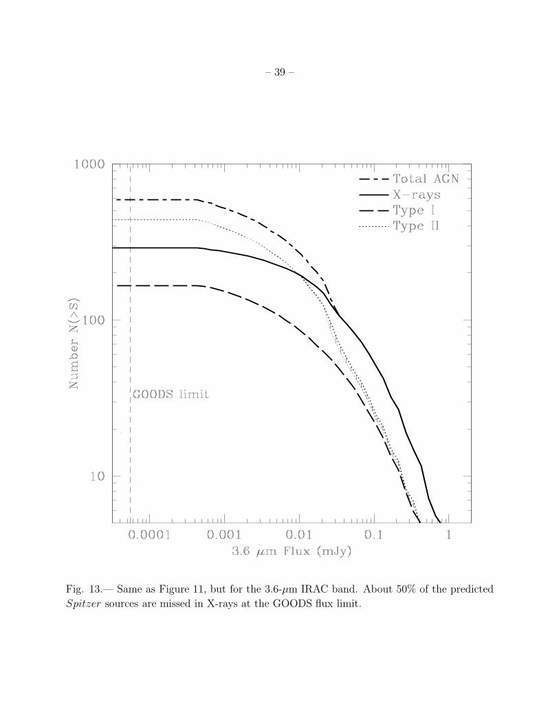
– 39 –

Fig. 13.— Same as Figure 11, but for the 3.6-µm IRAC band. About 50% of the predicted

Spitzer sources are missed in X-rays at the GOODS flux limit.