numerical study of violent impact flow using a CIP-based model

Hindawi Publishing CorporationJournal of Applied MathematicsVolume 2013, Article ID 920912, 12 pageshttp://dx.doi.org/10.1155/2013/920912

Research ArticleNumerical Study of Violent Impact Flow Usinga CIP-Based Model

Qiao-ling Ji,1 Xi-zeng Zhao,2,3 and Sheng Dong4

1 College of Natural Resources and Environmental Engineering, Shandong University of Science and Technology,Qingdao 266590, China

2Ocean College, Zhejiang University, Hangzhou 310058, China3 State Key Laboratory of Satellite Ocean Environment Dynamics, The Second Institute of Oceanography, Hangzhou 310012, China4College of Engineering, Ocean University of China, Qingdao 266100, China

Correspondence should be addressed to Xi-zeng Zhao; [email protected]

Received 10 April 2013; Revised 10 July 2013; Accepted 12 July 2013

Academic Editor: Zhihong Guan

Copyright © 2013 Qiao-ling Ji et al. This is an open access article distributed under the Creative Commons Attribution License,which permits unrestricted use, distribution, and reproduction in any medium, provided the original work is properly cited.

A two-phase flow model is developed to study violent impact flow problem. The model governed by the Navier-Stokes equationswith free surface boundary conditions is solved by a Constrained Interpolation Profile (CIP)-based high-order finite differencemethod on a fixed Cartesian grid system. The free surface is immersed in the computation domain and expressed by a one-fluiddensity function. An accurate Volume of Fluid (VOF)-type scheme, the Tangent of Hyperbola for Interface Capturing (THINC), iscombined for the free surface treatment. Results of another two free surface capturing methods, the original VOF and CIP, are alsopresented for comparison.The validity and utility of the numerical model are demonstrated by applying it to two dam-break prob-lems: a small-scale two-dimensional (2D) and three-dimensional (3D) full scale simulations and a large-scale 2D simulation. Mainattention is paid to thewater elevations and impact pressure, and the numerical results show relatively good agreementwith availableexperimental measurements. It is shown that the present numerical model can give a satisfactory prediction for violent impact flow.

1. Introduction

Violent water impact may occur in many hydrodynamicsproblems associated with important coastal and offshoreengineering applications. Wave breaking in harbors, coastalareas, and offshore platforms, liquid sloshing in tank, andgreen water on decks are the most common examples ofthis class of problems. Accurate evaluation of such impactforces and possible structure responses is important forstructure safety and disaster prevention. Water impacts areusually characterized by nonlinear phenomena, distortedfree surfaces, and large amplitude structure responses forfreely floating bodies, and their analysis is very complex.Analytical methods are only available for simple cases suchas linear problems while laboratory tests are limited by highcost and technical limitations of the experimental facilities.As a result, there is an increasing interest in numericallysimulating distorted free surfaces and their violent impactson engineering structures.

Due to the possible similarity between greenwater impactand dam-break flow, dam-break flow theory has been widelyused to study violent impact problems due to green waterincidents [1–4]. Yilmaz et al. [3] developed a semianalyticalsolution for a dam-break flow to simulate green water ona deck. Kleefsman et al. [4] studied green water impactproblem using a Navier-Stokes solver combined with a VOFmodel for free surface modeling. The studies modeled adam-break flow to mimic the water flow on a deck withoutconsidering the body-wave interaction. In order to modelviolent impact problem, analytical solutions and laboratorytests have been used. When the assumption of hydrostaticpressure ismade, analytical solutions can be obtained, knownas the shallow water equations. Among the solutions, thewidely simplest one for a frictionless dry flat bed is Ritter’ssolution [5, 6]. Laboratory experiments have been performedto study the violent impact flowproblems. Cox andOrtega [7]performed a small-scale laboratory experiment to quantifya transient wave overtopping a horizontal deck and a fixed

2 Journal of Applied Mathematics

deck. Ariyarathne et al. [8] studied the green water impactpressure due to plunging breaking waves impinging on a sim-plified, three-dimensional model structure in the laboratory.

For numerical study of violent impact flow problems, thenonlinear distorted free surface is one of its main difficulties.Among the available strategies to numerically construct aninterface, the VOF method is one of the most popularmethods in water-surface capturing, first introduced by Hirtand Nichols [9]. The advantages of the VOF method areits mass conservation and being easy to implement. Manyimproved VOF-typed schemes have been proposed, likePLIC-VOF [10], tangent of hyperbola for interface capturing(THINC) [11], THINC/WLIC [12] weighed line interfacecalculation (WLIC), and THINC/SW [13] scheme. Anotherdifficulty is the simulation of multiphase flow. Thus we needa scheme for treating both liquid and gas fluids with largedensity ratios simultaneously in one program. Fully implicitsolvers can handle this procedure, but the convergence ofiteration in a highly distorted state is still a problem.

To solve the above-mentioned difficulties, a constrainedinterpolation profile (CIP) method combined with a sur-face capturing scheme, THINC, is applied to the study.The Constrained Interpolation Profile (CIP) method wasdeveloped by Yabe et al. [14] to treat both compressible andincompressible fluids with large density ratios simultaneouslyin one program to simulate the interaction of gas with a liquidand/or solid, which is based on CIP method in Takewakiet al. [15], Takewaki and Yabe [16], Yabe and Takei [17],Yabe and Aoki [18], and Yabe et al. [19]. The CIP methodis a compact upwind scheme with subcell resolution for theadvection calculation. In the CIPmethod, both the advectionfunction and its spatial derivatives are used to construct aninterpolation approximation of high accuracy within onegrid cell. Since the spatial derivatives are also employed, theinterface profile inside the grid is retrieved, and the subcellresolution can be obtained. Furthermore, the CIP methodcan treat all the phases of matter from solid state throughliquid state and from two-phase state to gas state withoutrestriction on the time step from high-sound speed [20, 21].The CIP-based model was introduced to obtain a robustflow solver of Navier-Stokes equations for dam-break flowproblems by Hu and Kashiwagi [22]. In [22], a dam-breakand oscillation experiments were performed to validate the2D numerical model with the CIP method for the solutionof advection equation of Navier-Stokes equation and alsofor the free surface treatment. After that, Hu and Kashiwagi[23] presented an enhanced model for nonlinear wave-bodyinteractions, in which the THINC scheme was combinedwith the model to treat the violent free surface. Recently,Hu et al. [24, 25] extended the CIP model to 3D simulationof violent sloshing and conducted a 3D simulation of wave-body interactions using CIP method combined with THINCscheme. Zhao and Hu [26] presented an enhanced modelto treat body motions due to extreme waves, in which theTHINC/WLIC scheme was introduced for the free surfacecapturing. The above numerical results have shown thatthis model is able to deal with the free surface problemswith reasonable accuracy when compared to experimentaldata.

The dam-break flow is widely used to examine theperformance of various numerical techniques designed forsimulating the surface interfacial and impact problems. Thedevelopment of water flow along the floor after the suddenbreak of the damhas been a conventional target for numericalstudies, but our research interest is in the second stage ofthe flow development, that is, the flow after impact on thevertical wall. In the second stage, overturning and breakingof the free surface as well as air entrapment are observed, andthe computation of these complicated phenomena is a morechallenging subject. Many models [27, 28] show departurefrom the experiments significantly for both impact pressureand free surface elevations after the impact. Park et al. [29]proposed a VOF level-set method for simulating two-phaseflows and got satisfactory results.

The objective of the study is to examine the performanceof the model based on the CIP method and THINC schemefor simulating the violent impact and the dam-break flowproblems. We use two dam-break experiments: a small-scaleexperiment and a relatively large-scale experiment to validatethe numerical model. In the small-scale case, both a 2D-and a 3D-CIP-based models are used for analyzing the watercollapse flow and the pressure on the oppositewall to examinethe difference in simulations in different dimensions. In therelative large-scale case, we analyze the effect of air cushioncaused by the backward plunging water reentering the mainforward flow, which plays an important role in the calculationof impact pressure andwater height on the second stage of theflow.

This paper is organized as follows. In Section 2, webriefly introduce the CIP-based numerical model for twofluids (water/air). The flow solver and the treatment of freesurface are briefly introduced. After that, in Section 3, weperform two representative numerical examples, comparedwith experimental results and other numerical simulations.The paper closes with a summary of our main conclusions inSection 4.

2. A CIP-Based Model

2.1. Governing Equations. We consider an unsteady, viscous(laminar), and incompressible flow.The governing equationsare as follows:

𝜕𝑢𝑖

𝜕𝑥𝑖

= 0, (1)

𝜕𝑢𝑖

𝜕𝑡+ 𝑢𝑗

𝜕𝑢𝑖

𝜕𝑥𝑗

= −1

𝜌

𝜕𝑝

𝜕𝑥𝑖

+2𝜇

𝜌

𝜕𝑆𝑖𝑗

𝜕𝑥𝑗

+ 𝑓𝑖, (2)

where 𝑆𝑖𝑗= (1/2)((𝜕𝑢

𝑖/𝜕𝑥𝑗) + (𝜕𝑢

𝑗/𝜕𝑥𝑖)). The last term 𝑓

𝑖on

the right-hand side of (2) stands for the body pressure, suchas gravity.

2.2.TheFractional StepApproach. Thetime evolution of (2) isperformed by a fractional step method in which the equationis divided into three calculation steps: an advection step and

Journal of Applied Mathematics 3

two nonadvection steps. In the advection calculation step, theCIP method is applied to solve the hyperbolic equation.

Advection Phase:𝜕𝑢𝑖

𝜕𝑡+ 𝑢𝑗

𝜕𝑢𝑖

𝜕𝑥𝑗

= 0. (3)

The advection phase computation of (3) is conducted bythe A-type CIP scheme where the advection part can be cal-culated by a semi-Lagrangian procedure after interpolationfunction is determined. The principal of the CIP method isto use the grid point value and its spatial derivative (gradient)in two grid points to form a cubic interpolation function toapproximate the profile. In the CIP method, each grid pointhas the gradient information of the physical values, as wellas the interpolated values between a grid and the neighborgrid. Hence, the CIP has an ability to solve the advectionphase with high accuracy and stability. Details of the CIPscheme can be found in the paper by Yabe et al. [14]. Thenonadvection phase is divided into a diffusion part denotedby nonadvection phase (i), which includes a viscous term anda source term, and a state-related part to treat the velocity-pressure coupling, denoted by nonadvection phase (ii).

Nonadvection Phase (i):

𝜕𝑢𝑖

𝜕𝑡=2𝜇

𝜌

𝜕𝑆𝑖𝑗

𝜕𝑥𝑗

+ 𝑓𝑖. (4)

Nonadvection Phase (ii):𝜕𝑢𝑖

𝜕𝑡= −

1

𝜌

𝜕𝑝

𝜕𝑥𝑖

. (5)

An implicit scheme is used for the time integration of (5) as

𝑢𝑛+1

𝑖− 𝑢∗∗

𝑖

Δ𝑡= −

1

𝜌

𝜕𝑝𝑛+1

𝜕𝑥𝑖

. (6)

Taking divergence of (6) and substituting 𝜕𝑢𝑛+1𝑖

/𝜕𝑥𝑖by using

(1), we obtain the following pressure equation:

𝜕

𝜕𝑥𝑖

(1

𝜌

𝜕𝑝𝑛+1

𝜕𝑥𝑖

) =1

Δ𝑡

𝜕𝑢∗∗

𝑖

𝜕𝑥𝑖

. (7)

This is a Poisson type equation for the pressure calcula-tion. Equation (7) is assumed to be valid for liquid and gasphases. A solution of it provides the pressure distributionin the whole computation domain. In this treatment, theboundary condition for pressure at the interface betweendifferent phases is not required.

2.3. Free Surface Capturing Method. In the dam-break simu-lation, two density functions 𝜑

1and 𝜑

2are defined to denote

liquid and gas phases, respectively. One has 𝜑1+ 𝜑2= 1.

The free surface is treated as an immersed interface. The freesurface boundary is distinguished by a density function 𝜑

1,

which is solved by the equation

𝜕𝜑1

𝜕𝑡+ 𝑢𝑖

𝜕𝜑1

𝜕𝑥= 0. (8)

After all of the density functions have been determined,any physical property 𝜆, such as the density or the viscosity,can be calculated for each computation cell as follows:

𝜆 =

2

∑

𝑚=1

𝜆𝑚𝜑𝑚. (9)

The drawback of the averaging process of (9) is that thecomputational accuracy is reduced to first order in terms ofcell size at the interfaces.

The THINC scheme proposed by Xiao et al. [11] isused for free surface capturing of incompressible flow. Sometest examples indicate that the scheme has the features weneed for our computations: mass conservation, a lack ofoscillation, and smearing at the interface. Similar to the CIPscheme, the profile of 𝜑 inside an upwind computation cell isapproximated by an interpolation function. Instead of using acubic polynomial in theCIP scheme, the THINC scheme usesa hyperbolic tangent function, which is shown as follows:

𝜑𝑖 (𝑥) =

𝛼

2{1 + 𝛾 tanh [𝛽(

𝑥 − 𝑥𝑖−1/2

Δ𝑥𝑖

− 𝑥𝑖)]} , (10)

where 𝛼, 𝛽, and 𝛾 are parameters to control the quality ofthe numerical solution. Parameters 𝛼 and 𝛾 are used to avoidinterface smearing and are determined as

𝛼 = {𝜑𝑖+1

if 𝜑𝑖+1

≥ 𝜑𝑖−1,

𝜑𝑖−1

otherwise,

𝛾 = {1 if 𝜑

𝑖+1≥ 𝜑𝑖−1,

−1 otherwise.

(11)

Parameter 𝛽 determines the steepness of the jump in theinterpolation function varying from 0 to 1. Larger 𝛽 cor-responds to sharper variation of 𝜑

𝑖(𝑥). However, too large

𝛽 may result in numerical instabilities. In this paper 𝛽 =

3.5 is chosen according to many computation tests. Also anumerical flux 𝑔

𝑖±1/2= ∫𝑡𝑛+1

𝑡𝑛

(𝑢𝜑)𝑖±1/2

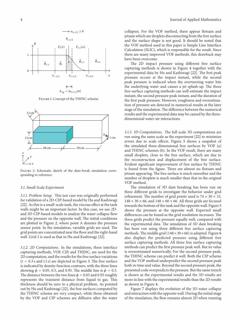
𝑑𝑡 is used in calculationof the density function; therefore, mass conservation couldbe satisfied. Figure 1 illustrates the concept of the one-dimension THINC scheme. Multidimensional computationsare performed by a dimensional splitting method.

3. Validation of Numerical Model

The dam-break flow is widely used as a benchmark test ofviolent impact flow on the deck to check the computationaccuracy for a largely distorted free surface. Its simple initialand boundary conditionsmake the validation of computationand experiment quite straightforward. In this study, wereproduce two dam-break experiments numerically: one isin a small-scale tank performed by Hu and Kashiwagi [22],in which we also conduct a 3D calculation to test the abilityof simulating complex distorted free surface flow with 3Dair-water interfaces, and the other is a relative large-scaleexperiment performed at MARIN by Zhou et al. [30] toexamine the applicability of themodel in different scale cases.


0

1

𝜙

𝜙i−1

Fi(x)

𝜙i

x

g

Fi+1(x)

𝜙i+1 𝜙i+2

x x x

i+1/2

i+1/2i−1/2 i+3/2

ui+1/2 ≥ 0

Δ up = |ui+1/2Δt|

Figure 1: Concept of the THINC scheme.

A

68 cm 50 cm

12 cm

12 cm

1 cm

zy

x

Figure 2: Schematic sketch of the dam-break simulation corre-sponding to reference.

3.1. Small-Scale Experiment

3.1.1. Problem Setup. This test case was originally performedfor validation of a 2D-CIP-basedmodel by Hu and Kashiwagi[22]. As this is a small-scale tank, the viscous effect at the tankwalls might be an important factor. In this case, we use 2D-and 3D-CIP-based models to analyze the water collapse flowand the pressure on the opposite wall. The initial conditionsare plotted in Figure 2, where point A denotes the pressuresensor point. In the simulation, variable grids are used. Thegrid points are concentrated near the floor and the right-handwall. Grid 2 is used as that in Hu and Kashiwagi [22].

3.1.2. 2D Computations. In the simulations, three interfacecapturing methods, VOF, CIP, and THINC, are used for the2D computation, and the results for the free surface variations(𝑡 = 0.3 s and 1.1 s) are depicted in Figure 3. The free surfaceis indicated by density function contours, with the three linesshowing 𝜙 = 0.05, 0.5, and 0.95. The middle line is 𝜙 = 0.5.The distance between the two lines 𝜙 = 0.05 and 0.95 roughlyrepresents the transient distance from liquid to gas. Thisthickness should be zero in a physical problem. As pointedout by Hu and Kashiwagi [22], the free surfaces computed bythe THINC scheme are very compact, while those obtainedby the VOF and CIP schemes are diffusive after the water

collapses. For the VOF method, there appear flotsam andjetsamwhich are droplets disconnecting from the free surfaceand the surface shape is not good. It should be noted thatthe VOF method used in this paper is Simple Line InterfaceCalculation (SLIC), which is responsible for the result. Sincethere are many improved VOF methods, this drawback mayhave been overcome.

The 2D impact pressure using different free surfacecapturing methods is shown in Figure 4 together with theexperimental data by Hu and Kashiwagi [22]. The first peakpressure occurs at the impact instant, while the secondpeak pressure is induced when the overturning water hitsthe underlying water and causes a jet splash-up. The threefree surface capturing methods can well estimate the impactinstant, the second pressure peak instant, and the duration ofthe first peak pressure. However, roughness and overestima-tion of pressure are detected in numerical results at the laterstage of the simulation.The difference between the numericalresults and the experimental datamay be caused by the three-dimensional water-air interactions.

3.1.3. 3D Computations. The full scale 3D computations arerun using the same scale as the experiment [22] to minimizeerrors due to scale effects. Figure 5 shows a snapshot ofthe simulated three-dimensional free surfaces by VOF (a)and THINC schemes (b). In the VOF result, there are manysmall droplets, close to the free surface, which are due tothe reconstruction and displacement of the free surface.Evident significant improvement of free surface by THINCis found from the figure. There are almost no flotsam andjetsam appearing.The free surface is much smoother and thenumber of droplets is much smaller than that in the originalVOF method.

The simulation of 3D dam breaking has been run onthree different grids to investigate the behavior under gridrefinement. The number of grid points used is 74 × 30 × 33,148 × 30 × 66, and 148 × 60 × 66. All three grids are focusedtowards the bottomof the tank and the opposite wall. Figure 5shows the pressure at the opposite wall. Expected smalldifferences can be found as the grid resolution increases. Thethree grids predict the pressure equally well, compared withthe experimental data. The simulation of 3D dam breakinghas been run using three different free surface capturingmethods.Themiddle grid (148×30×66) is adopted. Figure 6also displays the predicted pressure using different freesurface capturing methods. All three free surface capturingmethods can predict the first pressure peak well. But its valueis overestimated numerically. For the second pressure peak,the THINC scheme can predict it well. Both the CIP schemeand the VOF method underpredict the second pressure peakboth in time and value. Beyond the second pressure peak, thepresented code overpredicts the pressure. But the same trenchis shown as the experimental results and the 3D results aremore in line with the experimental results than the 2D resultsas shown in Figure 4.

Figure 7 displays the evolution of the 3D water collapseand interactionwith the oppositewall. During the initial stageof the simulation, the flow remains almost 2D when running


CIP

VOF

THINC

0

0.05

0.1

0.15

0.2y

(m)

0.2 0.4 0.6 0.8 1x (m)

0

0.05

0.1

0.15

0.2

y(m

)

0.2 0.4 0.6 0.8 1x (m)

0

0.05

0.1

0.15

0.2

y(m

)

0.2 0.4 0.6 0.8 1x (m)

(a) 𝑡 = 0.3 s

0

0.05

0.1

0.15

0.2

y(m

)

0.2 0.4 0.6 0.8 1x (m)

0

0.05

0.1

0.15

0.2

y(m

)0.2 0.4 0.6 0.8 1

x (m)

0

0.05

0.1

0.15

0.2

y(m

)

0.2 0.4 0.6 0.8 1x (m)

(b) 𝑡 = 1.1 s

Figure 3: Comparison of density function contours at 𝑡 = 0.3 s (a) and 1.1 s (b). The three lines indicate that 𝜙 = 0.05, 0.50, 0.95. Theinterface-capturing scheme is CIP (up), VOF (middle), and THINC (down).

0.4 0.6 0.8 1.0 1.2−500

0

500

1000

1500

2000

THINCVOF

CIPExperiment

Pres

sure

(Pa)

Time (s)

Figure 4: Impact pressure caused by 2D dam-break flow.

up the vertical wall and overturning back to the water tank.After 𝑡 = 0.8 s, however, the splash flow produced by theoverturning water mass quickly develops into a 3D breakingwave pattern with the presence of small water droplets andtrapped air bubbles. It is clearly seen that the CIP-basedmodel combining the THINC free surface capturing schemeis effective enough to resolve distorted free surface flow withcomplex 3D air-water interfaces.

3.2. Large-Scale Experiment

3.2.1. Problem Setup. In this section, a relative large-scaleexperimental test performed at MARIN by Zhou et al. [30] isadopted to evaluate the performance of the proposed numer-ical method. We analyse the free surface with three surfacecapturing methods and compare our numerical results of


00.20.40.60.811.2

X

0.10.05Y

0

0.1

0.2

Z

VOF

(a)

00.20.40.60.811.2

X

0.10.05Y

0

0.1

0.2

0.3

Z

THINC

(b)

Figure 5: Snapshots at 𝑡 = 1.1 s of dam-break flow: original VOF (a) and THINC (b).

0.4 0.6 0.8 1.0 1.2−500

0

500

1000

1500

2000

Fine grid 148 60 66Middle grid 148 30 66

Coarse grid 74 30 33Experiment

Pres

sure

(Pa)

Time (s)

(a)

0.4 0.6 0.8 1.0 1.2−500

0

500

1000

1500

2000

THINCVOF

CIPExperiment

Pres

sure

(Pa)

Time (s)

(b)

Figure 6: Impact pressure (3D) using different grid sizes (a) and using different free surface capturing methods (b).

water elevation and green water impact pressure with theexperimental results. A set-up overview of this problem isillustrated in Figure 8.

The experimental water tank is 3.22m in length, 1.0min width, and 2.0m in height. The initial water column isplaced behind the flap with the size of 1.2m in length, 1.0m inwidth, and 0.6m in height. For comparison, we use the waterheights measured by two standard capacitive wave gauges.The two probe points, H1 and H2, locate at 2.725m and2.228m away from the left wall of the tank, respectively. Thepressure history measured by a circular pressure transducerof 0.09m diameter at a point P2, 0.16m above the bottom onthe right wall of the tank is presented for comparison.

The effects of both the grid spacing and the time step arecarefully investigated, and the values shown in what followsare considered reasonable choices. In the computation, a vari-able grid is used, in which the grid points are concentratednear the floor and the right wall.The grid number is 334×458,and the minimum grid spacing and maximum grid spacingare 2 cm and 6 cm. The total simulation time length is 𝑡

𝑛=

2.5 s, and the time step is set to Δ𝑡 = 10−4 s.

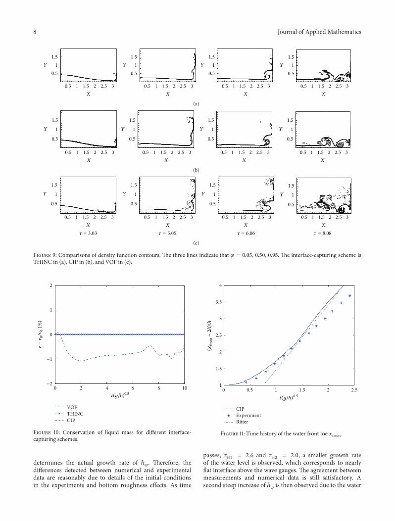
3.2.2. Free Surface Profile. Three interface capturing meth-ods, VOF, CIP, and THINC, are also used in this simulation,and the results for the free-surface variation are compared inFigure 9. Similarly, we can tell that the free surfaces computed

by the THINC scheme are very compact; the thickness of thecomputed free surface is two to three times the size of thecell. On the other hand, those obtained by the VOF and CIPschemes are diffusive after the overturning water hits the freesurface. For instance, the free surface by THINC is basicallyone line and all the time except 𝜏 = 8.08 (𝜏 = 𝑡(𝑔/ℎ)

1/2, 𝑡 andℎ are time and initial water height, resp.), while we can seenoticeably three lines from that by CIP, especially at 𝜏 = 5.05

and 𝜏 = 6.06 when there is extremely distorted deformationof the free surface. For the VOFmethod, there appear flotsamand jetsam which are droplets disconnecting from the freesurface and the surface shape is not good such as the positionof 𝑥 = 2.7m at 𝜏 = 3.03 and the tip of the overturning waveat 𝜏 = 6.06. Also the VOF method used in this paper is SLIC.

The conservation of water mass in the computations fordifferent interface-capturing schemes is checked. Figure 10shows the variation of the total water volume in the tankover the computation time, with VOF “- ⋅,” CIP “- -,” andTHINC “-∗-”. Variation of up to −1.0% is found for the CIPscheme, while the variations in total mass for the VOF andTHINC scheme are below 0.01%.The conservation is perfect.Among the three free surface capturing methods, VOF, CIP,and THINC, the VOF and THINC scheme act good in termsof mass conservation; while in terms of interface diffusion,the THINC scheme show perfect performance with verycompact surface profile and less flotsam. In the following


00.20.40.60.811.2

XY

0.1

0.2

0.3

Z

t = 0.2 s t = 0.4 s

t = 0.6 s t = 0.8 s

t = 1.0 s t = 1.2 s

00.050.1

00.20.40.60.811.2

XY

0.1

0.2

0.3

Z

Z

Z

00.050.1

00.20.40.60.811.2

XY

0.1

0.2

0.3

Z

00.050.1

00.20.40.60.811.2

XY

0.1

0.2

0.3

00.050.1

00.20.40.60.811.2

XY

0.1

0.2

0.3

Z

00.050.1

00.20.40.60.811.2

XY

0.1

0.2

0.3

00.050.1

Figure 7: Evolution of the 3D water collapse and interaction with the opposite wall.

3.22

Flap

H2 H1

2

1.2

2.2282.725

P2

0.16

0.6Water

Figure 8: Problem definition and measurement points for waterheights and pressure (in m).

sections, the THINC scheme will be applied as the freesurface capturing method.

Figure 11 shows the propagation in time of the water-front toe 𝑥front after the dam breaks. The numerical result(—) is compared with the experimental result (∗) and theanalytical shallow water solution of Ritter (- ⋅). The latteris not applicable to the initial instants of the phenomenonbecause the shallow-water conditions are not verified, so that

the water-front location would be largely overestimated withrespect to all the reported solutions. Therefore, the Rittersolution has been shifted laterally just to show the tendencyof the numerical simulations to approach the analyticalshallow-water result after a suitable time interval. We cansee the numerical result asymptotically approaches the Rittersolution as time increases. Also the numerical result showsagreement with the experiment before 𝜏 = 1.5 and areasonable deviation from the experiment after 𝜏 = 1.5.However, the experiment has a lower progressive velocitythan the numerical result. It may be due to the imperfectinitial conditions or bottom roughness in the experimentsand some physical effects not considered in the numericalmodel.

3.2.3. Water Height and Impact Pressure. In Figure 12, wecompare the water heights (ℎ

𝑤/ℎ) at H1 and H2 points,

respectively. In the experiments, standard capacitive wavegauges have been used which are sensitive to the wettedportion of the wire. Hence, the numerical values are deducedfrom the simulations by taking the water level and deductingthe height of the (possibly present) entrapped air cavity. Theinitial evolution, 𝜏H1 = 2.0 and 𝜏H2 = 1.6, is characterizedby the sudden rise of the water level due to the transitionfrom dry-deck to wet-deck conditions.Thewater-front shape


Y

0.5 1 1.5 2 2.5 3X

0.51

1.5Y

0.5 1 1.5 2 2.5 3X

0.51

1.5Y

0.5 1 1.5 2 2.5 3X

0.51

1.5Y

0.5 1 1.5 2 2.5 3X

0.51

1.5

(a)

Y

0.5 1 1.5 2 2.5 3X

0.5

1

1.5

Y

0.5 1 1.5 2 2.5 3X

0.5

1

1.5

Y

0.5 1 1.5 2 2.5 3X

0.5

1

1.5

Y

0.5 1 1.5 2 2.5 3X

0.5

1

1.5

(b)

𝜏 = 3.03 𝜏 = 5.05 𝜏 = 6.06 𝜏 = 8.08

Y

0.5 1 1.5 2 2.5 3X

0.5

1

1.5

Y

0.5 1 1.5 2 2.5 3X

0.5

1

1.5

Y

0.5 1 1.5 2 2.5 3X

0.5

1

1.5

Y

0.5 1 1.5 2 2.5 3X

0.5

1

1.5

(c)

Figure 9: Comparisons of density function contours. The three lines indicate that 𝜑 = 0.05, 0.50, 0.95. The interface-capturing scheme isTHINC in (a), CIP in (b), and VOF in (c).

0 2 4 6 8 10−2

−1

0

1

2

VOFTHINCCIP

t(g/h)0.5

�−� 0

/�0

(%)

Figure 10: Conservation of liquid mass for different interface-capturing schemes.

determines the actual growth rate of ℎ𝑤. Therefore, the

differences detected between numerical and experimentaldata are reasonably due to details of the initial conditionsin the experiments and bottom roughness effects. As time

0 0.5 1 1.5 2 2.51

1.5

2

2.5

3

3.5

4

CIPExperimentRitter

t(g/h)0.5

(xfro

nt−2h

)/h

Figure 11: Time history of the water front toe 𝑥front.

passes, 𝜏H1 = 2.6 and 𝜏H2 = 2.0, a smaller growth rateof the water level is observed, which corresponds to nearlyflat interface above the wave gauges. The agreement betweenmeasurements and numerical data is still satisfactory. Asecond steep increase of ℎ

𝑤is then observed due to the water


0 2 4 6 8 10

0

0.2

0.4

0.6

0.8

1

1.2

SimulationExperiment

t(g/h)0.5

Wat

er h

eigh

thw/h

(a)

0 2 4 6 8 10

0

0.2

0.4

0.6

0.8

1

1.2


t(g/h)0.5

Wat

er h

eigh

thw/h

(b)

Figure 12: Vertical water heights at two measurement points: (a) H1, (b) H2.

0 2 4 6 8 10

0

0.2

0.4

0.6

0.8

1

1.2

Air cushionSimulation height including air cushionExperiment

t(g/h)0.5

Wat

er h

eigh

t hw

/h

Figure 13: Effect of air on water height of H1.

overturning which gives an additional contribution to thewater height. The overturning water from the right wallreaches at location H1 at 𝜏H1 = 5.6 and later 𝜏H2 = 6.5,recorded by the gauge H2. The computed result of H2 agreeswell with the experiments, while the numerical predictionslightly overpredicts the water height of H1. Later on, theexperiment and the present simulations differ largely to someextent, especially at gauge H1. The reason for this may bethat the water is entrapped with air during overturning andbreaking. It makes the definition and measurement of waterlevel difficult. And the fact that gauge H1 locates near thefirst breaking point of the overturning wave leads to thediscrepancy between the experiment and computation. Wemake a try to analyze the effect of entrapped air on water

level at gauge H1. Figure 13 displays the evaluation of theamount of entrapped air “∗” and the water height includingthe contribution of entrapped air “-”. The calculated waterheight accords well with the experiment measurement beforethe overturning wave tip reconnects with the underlyingwater. It can be noticed that the treatment of consideringthe contribution of the entrapped air overestimates the waterheight at 𝜏H1 = 6.0–7.0. After that, the predicted water heightincluding the contribution of entrapped air agrees well withthe experimental data. We can see that (1) before 𝜏H1 =

6.0 when the contributed height of air cushion is zero, thesimulation water height agrees well with the experiment; (2)when the water begins to turn back until the wave tip hitsthe underlying water (around 𝜏H1 = 6.0–7.0), the simulationwater height including air cushion is a little higher than theexperimental measurement. This is because the definition ofwater level is complicated during this process. If we subtractthis contribution from the total water height, the water heightmay accord with the experiment result; (3) after that, theoverturned water meets with the underlying water (around𝜏H1 = 7.0), and the water height including the contributionof entrapped air corresponds well to the experimental data.Still the limited information about the experiment does notallow for a better discussion of such comparison.

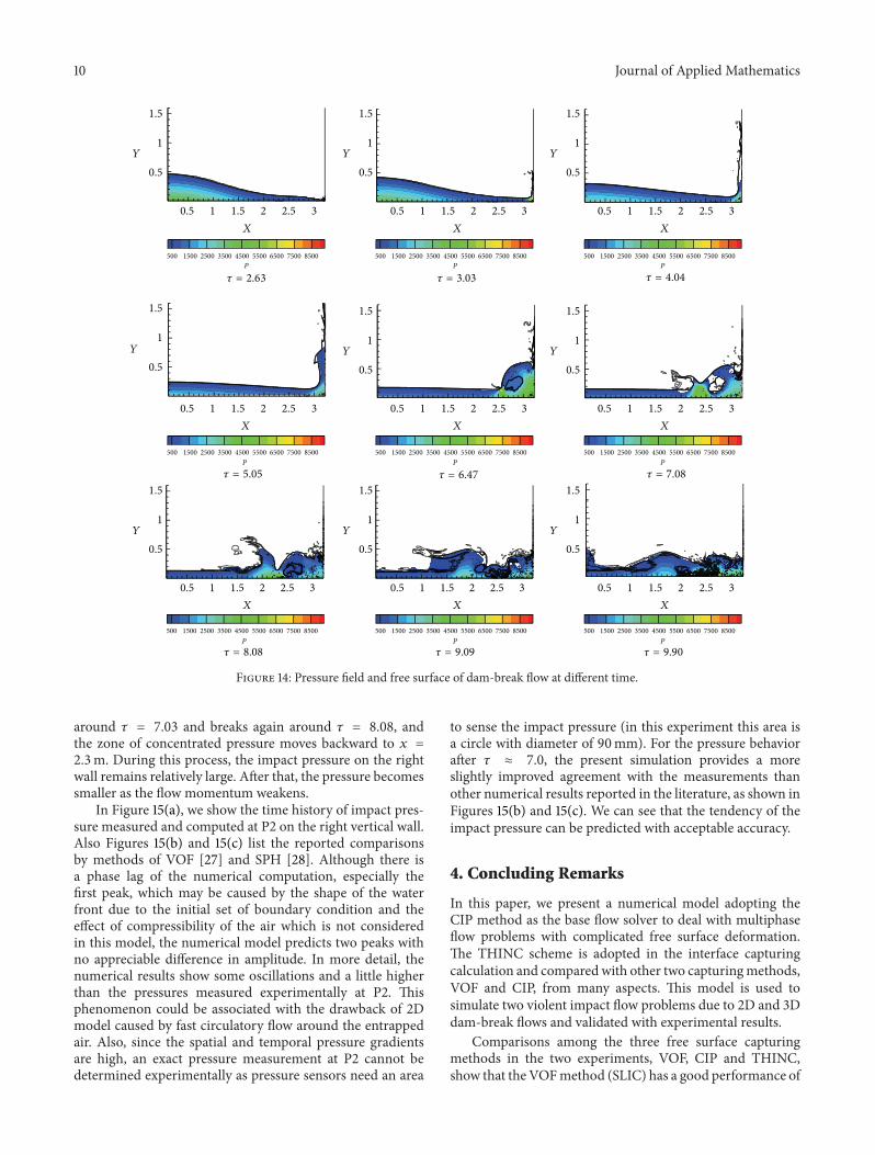
The evolution of the pressure field and free surface forthe dam-break flow is presented in Figure 14. Following thefigures of the pressure field, we can get the variation of thepressure on the vertical wall. As expected, there are two peaksof the pressure corresponding to times 𝜏 = 3.03 when thewater hits the vertical wall and 𝜏 = 6.47when the overturningwater hits the underlying water, respectively. At 𝜏 = 6.47,a plunging breaker with a large amount of air entrapped inthe water impinges on the underlying layer of water, whichgenerates great pressure against the vertical wall and at thebreaking point of the bottom (𝑥 = 2.6m). Subsequently,a second plunging breaker forms from the splashed water


X

Y

0.5 1 1.5 2 2.5 3

0.5

1

1.5

P P P

P P P

P P P

500 1500 2500 3500 4500 5500 6500 7500 8500 500 1500 2500 3500 4500 5500 6500 7500 8500 500 1500 2500 3500 4500 5500 6500 7500 8500

500 1500 2500 3500 4500 5500 6500 7500 8500 500 1500 2500 3500 4500 5500 6500 7500 8500 500 1500 2500 3500 4500 5500 6500 7500 8500

500 1500 2500 3500 4500 5500 6500 7500 8500 500 1500 2500 3500 4500 5500 6500 7500 8500 500 1500 2500 3500 4500 5500 6500 7500 8500

X

Y

0.5 1 1.5 2 2.5 3

0.5

1

1.5

X

Y

0.5 1 1.5 2 2.5 3

0.5

1

1.5

X

Y

0.5 1 1.5 2 2.5 3

0.5

1

1.5

X

Y

0.5 1 1.5 2 2.5 3

0.5

1

1.5

X

Y

0.5 1 1.5 2 2.5 3

0.5

1

1.5

X

Y

0.5 1 1.5 2 2.5 3

0.5

1

1.5

X

Y

0.5 1 1.5 2 2.5 3

0.5

1

1.5

X

Y

0.5 1 1.5 2 2.5 3

0.5

1

1.5

𝜏 = 9.90

𝜏 = 2.63 𝜏 = 3.03 𝜏 = 4.04

𝜏 = 5.05 𝜏 = 6.47 𝜏 = 7.08

𝜏 = 8.08 𝜏 = 9.09

Figure 14: Pressure field and free surface of dam-break flow at different time.

around 𝜏 = 7.03 and breaks again around 𝜏 = 8.08, andthe zone of concentrated pressure moves backward to 𝑥 =

2.3m. During this process, the impact pressure on the rightwall remains relatively large. After that, the pressure becomessmaller as the flow momentum weakens.

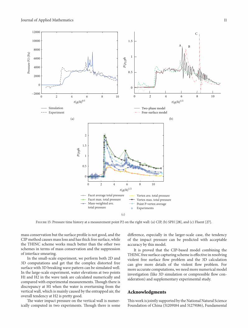
In Figure 15(a), we show the time history of impact pres-sure measured and computed at P2 on the right vertical wall.Also Figures 15(b) and 15(c) list the reported comparisonsby methods of VOF [27] and SPH [28]. Although there isa phase lag of the numerical computation, especially thefirst peak, which may be caused by the shape of the waterfront due to the initial set of boundary condition and theeffect of compressibility of the air which is not consideredin this model, the numerical model predicts two peaks withno appreciable difference in amplitude. In more detail, thenumerical results show some oscillations and a little higherthan the pressures measured experimentally at P2. Thisphenomenon could be associated with the drawback of 2Dmodel caused by fast circulatory flow around the entrappedair. Also, since the spatial and temporal pressure gradientsare high, an exact pressure measurement at P2 cannot bedetermined experimentally as pressure sensors need an area

to sense the impact pressure (in this experiment this area isa circle with diameter of 90mm). For the pressure behaviorafter 𝜏 ≈ 7.0, the present simulation provides a moreslightly improved agreement with the measurements thanother numerical results reported in the literature, as shown inFigures 15(b) and 15(c). We can see that the tendency of theimpact pressure can be predicted with acceptable accuracy.

4. Concluding Remarks

In this paper, we present a numerical model adopting theCIP method as the base flow solver to deal with multiphaseflow problems with complicated free surface deformation.The THINC scheme is adopted in the interface capturingcalculation and comparedwith other two capturingmethods,VOF and CIP, from many aspects. This model is used tosimulate two violent impact flow problems due to 2D and 3Ddam-break flows and validated with experimental results.

Comparisons among the three free surface capturingmethods in the two experiments, VOF, CIP and THINC,show that the VOFmethod (SLIC) has a good performance of


0 2 4 6 8 10−2000

0

2000

4000

6000

8000

10000

12000Pr

essu

re P

2 (P

a)


t(g/h)0.5

(a)

1

0.5

0

0 2 4 8 106

1.5A B

C

P/𝜌

Xgh

t(g/h)1/2

Two-phase modelFree-surface model

(b)

0 2 4 6 8 10

0

0.5

1

1.5

2

Facet average total pressureFacet max. total pressureMass-weighted ave. total pressure

Vertex ave. total pressureVertex max. total pressurePoint P-vertex averageExperiments

t(g/h)1/2

P/𝜌gh

(c)

Figure 15: Pressure time history at a measurement point P2 on the right wall: (a) CIP, (b) SPH [28], and (c) Fluent [27].

mass conservation but the surface profile is not good, and theCIPmethod causesmass loss and has thick free surface, whilethe THINC scheme works much better than the other twoschemes in terms of mass conservation and the suppressionof interface smearing.

In the small-scale experiment, we perform both 2D and3D computations and get that the complex distorted freesurface with 3D breaking wave pattern can be simulated well.In the large-scale experiment, water elevations at two pointsH1 and H2 in the wave tank are calculated numerically andcompared with experimental measurements.Though there isdiscrepancy at H1 when the water is overturning from thevertical wall, which is mainly caused by the entrapped air, theoverall tendency at H2 is pretty good.

The water impact pressure on the vertical wall is numer-ically computed in two experiments. Though there is some

difference, especially in the larger-scale case, the tendencyof the impact pressure can be predicted with acceptableaccuracy by this model.

It is proved that the CIP-based model combining theTHINC free surface capturing scheme is effective in resolvingviolent free surface flow problem and the 3D calculationcan give more details of the violent flow problem. Formore accurate computations, we needmore numerical modelinvestigation (like 3D simulation or compressible flow con-sideration) and supplementary experimental study.

Acknowledgments

Thiswork is jointly supported by theNationalNatural ScienceFoundation of China (51209184 and 51279186), Fundamental


Research Funds for the Central Universities (2012QNA4020),Educational Commission of Zhejiang Province of China(Y201225713), Key Laboratory of Water-Sediment SciencesandWater Disaster Prevention of Hunan Province (Grant no.2013SS03), and Scientific Research Foundation of ShandongUniversity of Science and Technology for Recruited Talents.

References

[1] Y. Ryu, K.-A. Chang, and R.Mercier, “Application of dam-breakflow to green water prediction,”Applied Ocean Research, vol. 29,no. 3, pp. 128–136, 2007.

[2] T. Schønberg and R. C. T. Rainey, “A hydrodynamic model ofGreen Water incidents,” Applied Ocean Research, vol. 24, no. 5,pp. 299–307, 2002.

[3] O. Yilmaz, A. Incecik, and J. C. Han, “Simulation of green waterflow on deck using non-linear dam breaking theory,” OceanEngineering, vol. 30, no. 5, pp. 601–610, 2003.

[4] K. M. T. Kleefsman, G. Fekken, A. E. P. Veldman, B. Iwanowski,and B. Buchner, “A volume-of-fluid based simulation methodfor wave impact problems,” Journal of Computational Physics,vol. 206, no. 1, pp. 363–393, 2005.

[5] C. Zoppou and S. Roberts, “Explicit schemes for dam-breaksimulations,” Journal of Hydraulic Engineering, vol. 129, no. 1, pp.11–34, 2003.

[6] A. Ritter, “Die Fortpflanzung der Wasserwellen,” VereineDeutscher Ingenieure Zeitswchrift, vol. 36, no. 33, pp. 947–954,1892.

[7] D. T. Cox and J. A. Ortega, “Laboratory observations of greenwater overtopping a fixed deck,” Ocean Engineering, vol. 29, no.14, pp. 1827–1840, 2002.

[8] K. Ariyarathne, K. A. Chang, and R. Mercier, “Green waterimpact pressure on a three-dimensional model structure,”Experiments in Fluids, vol. 53, no. 2, pp. 1879–1894, 2012.

[9] C. W. Hirt and B. D. Nichols, “Volume of fluid (VOF) methodfor the dynamics of free boundaries,” Journal of ComputationalPhysics, vol. 39, no. 1, pp. 201–225, 1981.

[10] D. L. Youngs, “Time-dependent multi-material flow with largefluid distortion,” in Numerical Methods for Fluid Dynamics,K. W. Morton and M. J. Baines, Eds., vol. 24, pp. 273–285,Academic Press, New York, NY, USA, 1982.

[11] F. Xiao, Y. Honma, and T. Kono, “A simple algebraic interfacecapturing scheme using hyperbolic tangent function,” Interna-tional Journal for Numerical Methods in Fluids, vol. 48, no. 9, pp.1023–1040, 2005.

[12] K. Yokoi, “Efficient implementation of THINC scheme: asimple and practical smoothed VOF algorithm,” Journal ofComputational Physics, vol. 226, no. 2, pp. 1985–2002, 2007.

[13] F. Xiao, S. Ii, and C. Chen, “Revisit to the THINC scheme:a simple algebraic VOF algorithm,” Journal of ComputationalPhysics, vol. 230, no. 19, pp. 7086–7092, 2011.

[14] T. Yabe, F. Xiao, and T. Utsumi, “The constrained interpolationprofile method for multiphase analysis,” Journal of Computa-tional Physics, vol. 169, no. 2, pp. 556–593, 2001.

[15] H. Takewaki, A. Nishiguchi, and T. Yabe, “Cubic interpo-lated pseudo-particlemethod (CIP) for solving hyperbolic-typeequations,” Journal of Computational Physics, vol. 61, no. 2, pp.261–268, 1985.

[16] H. Takewaki and T. Yabe, “The cubic-interpolated pseudoparticle (CIP) method: application to nonlinear and multi-dimensional hyperbolic equations,” Journal of ComputationalPhysics, vol. 70, no. 2, pp. 355–372, 1987.

[17] T. Yabe and E. Takei, “A new higher-order Godunovmethod forgeneral hyperbolic equations,” Journal of the Physical Society ofJapan, vol. 57, no. 8, pp. 2598–2601, 1988.

[18] T. Yabe and T. Aoki, “A universal solver for hyperbolic equationsby cubic-polynomial interpolation I. One-dimensional solver,”Computer Physics Communications, vol. 66, no. 2-3, pp. 219–232,1991.

[19] T. Yabe, T. Ishikawa, P. Y. Wang, T. Aoki, Y. Kadota, andF. Ikeda, “A universal solver for hyperbolic equations bycubic-polynomial interpolation II. Two- and three-dimensionalsolvers,”Computer Physics Communications, vol. 66, no. 2-3, pp.233–242, 1991.

[20] T. Yabe and P.-Y. Wang, “Unified numerical procedure forcompressible and incompressible fluid,” Journal of the PhysicalSociety of Japan, vol. 60, no. 7, pp. 2105–2108, 1991.

[21] Y.Ogata andT.Yabe, “Multi-dimensional semi-lagrangian char-acteristic approach to the shallow water equations by the CIPmethod,” International Journal of Computational EngineeringScience, vol. 5, no. 3, pp. 699–730, 2004.

[22] C. Hu and M. Kashiwagi, “A CIP-based method for numericalsimulations of violent free-surface flows,” Journal of MarineScience and Technology, vol. 9, no. 4, pp. 143–157, 2004.

[23] C. Hu andM. Kashiwagi, “Two-dimensional numerical simula-tion and experiment on strongly nonlinear wave-body interac-tions,” Journal of Marine Science and Technology, vol. 14, no. 2,pp. 200–213, 2009.

[24] C.H.Hu, “3-Dnumericalwave tank byCIP-based cartesian gridmethod,” in Proceedings of the 25th International Workshop onWater Waves and Floating Bodies, pp. 61–64, 2010.

[25] C.-H. Hu, K.-K. Yang, and Y.-H. Kim, “3-D numerical sim-ulations of violent sloshing by CIP-based method,” Journal ofHydrodynamics, vol. 22, no. 5, pp. 253–258, 2010.

[26] X. Z. Zhao and C. H. Hu, “Numerical and experimental studyon a 2-D floating body under extremewave conditions,”AppliedOcean Research, vol. 35, pp. 1–13, 2012.

[27] K. Abdolmaleki, K. P. Thiagarajan, and M. T. Morris-Thomas,“Simulation of the dam break problem and impact flows usinga Navier-Stokes Solver,” in Proceedings of the 15th AustralasianFluid Mechanics Conference, Sydney, Australia, 2004.

[28] A. Colagrossi and M. Landrini, “Numerical simulation ofinterfacial flows by smoothed particle hydrodynamics,” Journalof Computational Physics, vol. 191, no. 2, pp. 448–475, 2003.

[29] I. R. Park, K. S. Kim, J. Kim, and S. H. Van, “A volume-of-fluidmethod for incompressible free surface flows,” InternationalJournal for Numerical Methods in Fluids, vol. 61, no. 12, pp. 1331–1362, 2009.

[30] Z. Q. Zhou, J. O. D. Kat, and B. Buchner, “A nonlinear 3-D approach to simulate green water dynamics on deck,” inProceedings of the 7th International Conference Numerical ShipHydrodynamics, Nantes, France, 1999.

Submit your manuscripts athttp://www.hindawi.com

OperationsResearch

Advances in

Hindawi Publishing Corporationhttp://www.hindawi.com Volume 2013


Mathematical Problems in Engineering

Abstract and Applied AnalysisHindawi Publishing Corporationhttp://www.hindawi.com Volume 2013

ISRN Applied Mathematics


Hindawi Publishing Corporationhttp://www.hindawi.com

Volume 2013

International Journal of

Combinatorics


Journal of Function Spaces and Applications

International Journal of Mathematics and Mathematical Sciences


ISRN Geometry


Discrete Dynamics in Nature and Society



Volume 2013

Advances in

Mathematical Physics

ISRN Algebra


ProbabilityandStatistics

Journal of


ISRN Mathematical Analysis


Journal ofApplied Mathematics


Advances in

DecisionSciences



Stochastic AnalysisInternational Journal of

Hindawi Publishing Corporation http://www.hindawi.com Volume 2013Hindawi Publishing Corporation http://www.hindawi.com Volume 2013

The Scientific World Journal


ISRN Discrete Mathematics


Differential EquationsInternational Journal of

Volume 2013

numerical study of violent impact flow using a CIP-based model

Documents

Transcript of numerical study of violent impact flow using a CIP-based model