-i-

Thomas Tsirakoglou SID: 3302100012

SCHOOL OF SCIENCE & TECHNOLOGY A thesis submitted for the degree of

Master of Science (MSc) in Energy Systems

SEPTEMBER 2011 THESSALONIKI – GREECE

Numerical Simulation of a flat plate collector

-ii-

Thomas Tsirakoglou SID: 3302100012 Supervisor:

SCHOOL OF SCIENCE & TECHNOLOGY A thesis submitted for the degree of

Master of Science (MSc) in Energy Systems

SEPTEMBER 2011

THESSALONIKI – GREECE

Numerical Simulation of a flat plate collector

-iii-

DISCLAIMER This dissertation is submitted in part candidacy for the degree of Master of Science in Energy Systems, from the School of Science and Technology of the International Hellenic University, Thessaloniki, Greece. The views expressed in the dissertation are those of the author entirely and no endorsement of these views is implied by the said University or its staff.

This work has not been submitted either in whole or in part, for any other degree at this or any other university.

Signed: ...... ........................................

Name: Thomas Tsirakoglou................................................

Date: 26/9/2011...................................................

-iv-

Abstract

This dissertation was written as a part of the MSc in Energy Systems at the

International Hellenic University. It deals with the analysis of the operation of flat plate

solar collectors which leads to the numerical simulation of their performance.

Solar collectors are a widespread means of exploiting solar energy. They are special

kinds of heat exchangers that transform solar radiation energy to internal energy of

the transport medium. There are different kinds of solar collectors which can be

distinguished by their concentration or not, the type of heat transfer liquid used, the

temperature range of the working fluid, their and whether they are covered or

uncovered.

The evaluation of collector performance requires the calculation of the absorbed

solar radiation and the heat loss to the surroundings. The equations describing these

variables are developed in detail in this dissertation and they constitute the model for

the collector numerical simulation.

I would like to thank Dr. Georgios Martinopoulos for his concern and advice which

helped me accomplish this dissertation.

Thomas Tsirakoglou 26/9/2011

-1-

Contents

ABSTRACT .............................................................................................................. IV

CONTENTS ............................................................................................................... 1

1 INTRODUCTION .................................................................................................. 3

1.1 GENERAL AIM OF DISSERTATION ................................................................................. 3

1.2 SOLAR ENERGY ....................................................................................................... 3

2 SOLAR THERMAL SYSTEMS ................................................................................. 5

2.1 HISTORY OF EXPLOITATION OF SOLAR ENERGY ............................................................... 5

2.2 MEASUREMENT OF SOLAR RADIATION ......................................................................... 5

2.3 SOLAR THERMAL CAPACITY IN OPERATION WORLDWIDE .................................................. 7

3 TYPES OF SOLAR ENERGY COLLECTORS.............................................................. 10

3.1 FLAT PLATE COLLECTORS ......................................................................................... 12

3.2 EVACUATED TUBE COLLECTORS ...................................................................................... 15

3.3 MATERIALS USED ..................................................................................................... 17

4 SIMULATION OF FLAT PLATE COLLECTOR ................................................................ 21

4.1 SOLAR RADIATION .................................................................................................... 21

4.2 PHYSICAL MODEL FOR FLAT PLATE SOLAR COLLECTORS ............................................................. 23

4.3 ENERGY BALANCE EQUATION ........................................................................................ 24

4.4 ABSORBED SOLAR RADIATION ........................................................................................ 26

4.4.1 Reflection of radiation ......................................................................... 26

4.4.2 Absorption by glazing .......................................................................... 27

4.4.3 Optical properties of cover systems .................................................... 28

4.4.4 Equivalent angles of incidence for diffuse and ground-reflected

radiation .......................................................................................................... 29

4.4.5 Transmittance-absorptance product................................................... 29

-2-

4.5 HEAT LOSS FROM COLLECTOR ....................................................................................... 30

4.5.1 Collector overall heat loss ................................................................... 30

4.5.2 Top heat loss through the cover system.............................................. 31

4.5.3 Sky temperature .................................................................................. 33

4.5.4 Wind convection coefficient ................................................................ 33

4.5.5 Natural convection between parallel plates ....................................... 34

4.5.6 Back and edge heat loss ...................................................................... 34

4.5.7 Overall heat loss coefficient ................................................................ 35

4.6 MEAN ABSORBER PLATE TEMPERATURE ............................................................................. 35

4.6.1 Collector efficiency factor .................................................................... 36

4.6.2 Temperature distribution in flow direction ......................................... 38

4.6.3 Collector heat removal factor and flow factor .................................... 39

4.6.4 Mean fluid and plate temperatures .................................................... 40

4.6.5 Forced convection inside of tubes ....................................................... 40

4.7 THERMAL PERFORMANCE OF COLLECTORS .......................................................................... 41

4.8 ALGORITHM OF THE SIMULATION MODEL ........................................................................... 42

5 RESULTS ..................................................................................................................... 44

6 CONCLUSIONS ............................................................................................................ 47

Nomenclature................................................................................................................. 48

Appendix ........................................................................................................................ 52

Bibliography ................................................................................................................... 61

-3-

1 Introduction

1.1 General aim of dissertation

The general aim of this dissertation is to model the performance of a flat plate solar

collector using MATLAB which is a numerical computing environment and a fourth-

generation programming language.

In order to achieve this goal, the operation and performance of the flat plate

collector will be numerically simulated via several equations. The equations are an

expression of the energy equilibrium of the collector, equating the solar gains minus

losses with the thermal energy gained by the working fluid of the collector.

1.2 Solar energy

Energy from the sun in the form of solar radiation supports almost all life on earth

via photosynthesis and drives the earth’s climate and weather. Sunlight is the main

source of energy to the surface of the earth that can be harnessed via a variety of

natural and synthetic processes. Because solar energy is available as long as the sun

is available, it is considered a renewable source of energy. It is a clean source of

energy as well due to the fact that it does not produce any pollutants that could

harm the environment.

There are a few types of ways in which solar energy can be harnessed like solar

photovoltaic conversion, solar thermal energy and passive solar energy. Solar

photovoltaic conversion is what is used to convert the sun’s rays into electricity

through the use of solar panels. The amount of solar energy generated depends on

the amount of radiation the panels or solar cells receive. This is the most common of

all solar energy utilisations. Solar thermal energy uses the sun’s rays to heat

dwellings and water instead of using oil or gas.

Solar thermal collectors collect heat energy which is then transferred to the

working fluid in the heating or plumbing systems. This form of solar power use is

relatively cheap and environmental-friendly. Passive solar energy is the heating of a

-4-

home or building through architectural design. Structures or buildings are

constructed in a way to capture the sun’s power through the use of windows or

tanks. These systems heat dwellings or water without any need for a collector of any

kind [1].

-5-

2 Solar thermal systems

2.1 History of exploitation of solar energy

The principles of solar heat have been known for thousands of years. A black surface

gets hot in the sun, while a lighter coloured surface remains cooler. This principle is

used by solar water collectors which are one of the best known applications for the

direct use of the sun’s energy. They were developed some two hundred years ago

and the first known flat plate collector was made by Swiss scientist Horace de

Saussure in 1767. Solar technology advanced to roughly its present design in 1908

when William J. Bailey of the Carnegie Steel Company invented a collector with an

insulated box and copper coils. This collector was very similar to the thermosiphon

system which is used nowadays [2].

Little interest was shown in such devices until the world-wide oil crisis of 1973. This

crisis promoted new interest in alternative energy sources. As a result, solar energy

has received increased attention and many countries have taken a keen interest in

new developments of solar energy systems. The efficiency of solar heating systems

and collectors has improved since the early 1970s mainly due to the use of low-iron,

tempered glass for glazing, improved insulation and the development of durable

selective coatings [3].

2.2 Measurement of solar radiation

In solar system design it is essential to know the amount of sunlight available at a

particular location at a given time. The two most common methods which

characterize solar radiation are solar radiance (or radiation) and solar insolation.

Solar radiance is an instantaneous power density in units of kW/m² which is strongly

dependent on location and local weather. Solar radiance measurements consist of

global and direct radiation measurements taken periodically throughout the day. The

measurements are taken using either a pyranometer (Figure 1), which measures

-6-

global radiation, or a pyrheliometer (Figure 2), which measures direct radiation. In

well established locations, this data has been collected for more than twenty years.

An alternative method of measuring solar radiation, which is less accurate but also

less expensive, is using a sunshine recorder. These sunshine recorders measure the

number of hours in the day during which the sunshine is above a certain level

(typically 200mW/cm²). Data collected in this way can be used to determine the

solar insolation by comparing the measured number of sunshine hours to those

based on calculations and including several correction factors.

A method to estimate solar insolation is cloud-cover data taken from existing

satellite images.

While solar radiance is most commonly measured, another form of radiation data

used in system design is solar insolation. Solar insolation is the total amount of solar

energy received at a particular location during a specified time period, often in units

of kWh/(m² day). While the units of solar insolation and solar radiance are both a

power density, solar insolation is quite different than solar radiance as solar

insolation is the instantaneous solar radiance averaged over a given time period.

Solar radiation for a particular location can be given in several ways including:

• Typical mean year data for a particular location

• Average daily, monthly or yearly solar insolation for a given location

• Sunshine hours data

• Solar insolation based on satellite cloud cover data

• Calculations of solar radiation [4]

-7-

Figure 1: Pyranometer [5]

Figure 2: Pyrheliometer [6]

2.3 Solar thermal capacity in operation worldwide

The International Energy Agency’s Solar Heating and Cooling Programme and major

solar thermal trade associations have published new statistics on the use of solar

thermal energy (Table 1). The solar thermal collector capacity in operation

worldwide equalled 172.4 GWth corresponding to 246.2 million square meters by the

end of the year 2009. Of this, 151.5 GWth were accounted for by flat plate and

evacuated tube collectors and 19.7 GWth for unglazed water collectors. Air collector

capacity was installed to an extent of 1.2 GWth. The vast majority of glazed and

unglazed water and air collectors in operation are installed in China (101.5 GWth),

-8-

Europe (32.5 GWth), the United States and Canada (15.0 GWth), which together

account for 86.4% of total installed capacity [7].

In the year 2009, a capacity of 36.5 GWth, corresponding to 52.1 million square

meters of solar collectors, was newly installed worldwide. This means an increase in

collector installations of 25.3% compared to the year 2008. The main driver for the

above average market growth in 2009 was China whereas in key European markets

as well as in the United States and other important economic regions, such as in

Japan, the solar thermal sector suffered from the economic downturn, resulting in

stagnating or decreasing local markets [7].

The worldwide contribution of solar thermal installations to meeting the thermal

energy demand for applications such as hot water or space heating has been greatly

underestimated in the past. The underestimation of the capacity of solar thermal

was due largely to the fact that solar thermal installations have traditionally been

counted in square meters of collector area, a unit not comparable with other energy

sources. Solar thermal experts agreed on a methodology to convert installed

collector area into solar thermal capacity by using a factor of 0.7kWth/m2 to derive

the nominal capacity from the area of installed collectors [8].

The long-term technical potential for solar thermal energy, in terms of collector

area in operation per capita, is higher in northern countries than in southern

countries. The main reason is that in colder climates the demand for space heating is

substantially higher and to produce the same amount of heat a larger collector area

is needed.

In southern Europe there is a higher economical potential to use solar collectors

for industrial process heat due to the higher radiation. The potential for solar cooling

is also higher in southern Europe. However, these two factors cannot

counterbalance the higher demand for space heating in cold climates. Table 2 shows

the technical-economical potential for solar thermal energy in European Union,

based on the average heat demand, solar radiation and on the population of each

country.

-9-

Country Water Collectors

TOTAL (MWth) unglazed glazed evacuated tube

Australia 3,304 1,710.5 51.7 5,066.2 Austria 431.9 2,543.8 38.4 3,014.3 Brazil 890.3 2,799.7 - 3,690.0 China - 7,105 94,395 101,500.0 Cyprus - 598.2 2.7 601 France 74 1,279.1 23.4 1,376.4 Germany 504 7,508.7 844.5 8,880.7 Greece - 2,852.2 1.8 2,853.9 India - 1,987.3 169.6 2,168.3 Israel 20.6 2,827.5 - 2,848.5 Italy 30.6 1,263.2 177.1 1,470.9 Japan - 3,936.1 68.1 4,334.8 Korea, South - 1,047.6 - 1,047.6 Mexico 400.5 433.6 49.3 887.2 Spain 77.7 1,319.5 81.2 1,478.4 Switzerland 148.3 435.2 26.8 1,211.6 Taiwan 1.4 1,299.7 44.9 1,345.9 Turkey - 8,424.5 - 8,424.5 United Kingdom - 254.9 66.8 321.7 United States 12,455.5 1,787.8 61.4 14,373.2 TOTAL 19,703.9 54,915.5 96,539.1 172,368.6

Table 1: Total installed capacity in operation by the end of 2009 [7]

Country

Potential (per 1,000

Capita)

Potential (asolute)

Annual Energy Output

m2 m2 GWh Mtoe Austria 3,900 31,671,900 11,193 1 Belgium 3,900 40,021,800 16,827 1.4 Denmark 6,300 33,698,700 13,483 1.2 Finland 6,300 32,640,300 9,810 0.8 France 3,900 232,131,900 139,279 12 Germany 3,900 320,552,700 130,607 11.2 Greece 2,700 28,525,500 11,068 1 Ireland 3,900 14,898,000 6,704 0.6 Italy 3,300 190,885,200 116,543 10 Luxembourg 3,900 1,719,900 723 0.1 Netherlands 3,900 62,333,700 26,180 2.3 Portugal 2,700 27,062,100 16,237 1.4 Spain 2,700 106,623,000 64,448 5.5 Sweden 6,300 55,962,900 16,849 1.4 United Kingdom 3,900 233,309,700 102,196 8.8 TOTAL 3,740 1,412,037,300 682,149 58.7

Table 2: Technical-economical potential for solar thermal in EU [9]

-10-

3 Types of solar energy collectors Solar energy collectors are special kinds of heat exchangers that transform solar

radiation energy to internal energy of the transport medium. Solar collectors are the

heart of most solar energy systems and can be used for nearly any process that

requires heat. Specifically, they are used to warm buildings, heat water, generate

electricity, dry crops or cook food. The solar collector is a device that absorbs part of

the incoming solar radiation, converts it into heat and transfers the heat to a fluid

(usually air, water or oil) flowing through the collector. The solar energy collected is

carried from the circulating fluid either directly to the hot water or space

conditioning equipment or to a thermal energy storage tank from which it can be

drawn for use at night or on cloudy days.

There are basically two types of solar collectors: non-concentrating or stationary

and concentrating. A non-concentrating collector has the same area for intercepting

and absorbing solar radiation, whereas a sun-tracking concentrating solar collector

(Figure 3) usually has concave reflecting surfaces to intercept and focus the sun’s

beam radiation to a smaller receiving area. Concentrating collectors are more

suitable for high-temperature applications. Solar collectors can also be distinguished

by the type of heat transfer fluid used (water, non-freezing liquid, air or heat transfer

oil), the temperature range of the working fluid, their motion (stationary, single-axis

tracking and two-axis tracking) and whether they are covered or uncovered (Figure

4). Stationary collectors are permanently fixed in position and do not track the sun.

The main characteristics and operation of the non-concentrating stationary solar

collectors are described below.

There are two main types of collectors in this category: flat plate collectors (FPCs)

and evacuated tube collectors (ETCs) [10].

-11-

Figure 3: Concentrating sun-tracking solar collector [11]

Figure 4: Unglazed solar collector [12]

-12-

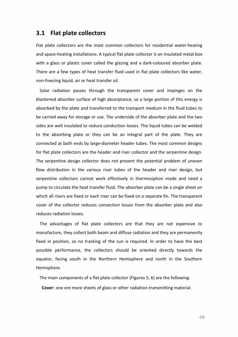
3.1 Flat plate collectors

Flat plate collectors are the most common collectors for residential water-heating

and space-heating installations. A typical flat plate collector is an insulated metal box

with a glass or plastic cover called the glazing and a dark-coloured absorber plate.

There are a few types of heat transfer fluid used in flat plate collectors like water,

non-freezing liquid, air or heat transfer oil.

Solar radiation passes through the transparent cover and impinges on the

blackened absorber surface of high absorptance, so a large portion of this energy is

absorbed by the plate and transferred to the transport medium in the fluid tubes to

be carried away for storage or use. The underside of the absorber plate and the two

sides are well insulated to reduce conduction losses. The liquid tubes can be welded

to the absorbing plate or they can be an integral part of the plate. They are

connected at both ends by large-diameter header tubes. The most common designs

for flat plate collectors are the header and riser collector and the serpentine design.

The serpentine design collector does not present the potential problem of uneven

flow distribution in the various riser tubes of the header and riser design, but

serpentine collectors cannot work effectively in thermosiphon mode and need a

pump to circulate the heat transfer fluid. The absorber plate can be a single sheet on

which all risers are fixed or each riser can be fixed on a separate fin. The transparent

cover of the collector reduces convection losses from the absorber plate and also

reduces radiation losses.

The advantages of flat plate collectors are that they are not expensive to

manufacture, they collect both beam and diffuse radiation and they are permanently

fixed in position, so no tracking of the sun is required. In order to have the best

possible performance, the collectors should be oriented directly towards the

equator, facing south in the Northern Hemisphere and north in the Southern

Hemisphere.

The main components of a flat plate collector (Figures 5, 6) are the following:

Cover: one ore more sheets of glass or other radiation-transmitting material.

-13-

Heat removal fluid passageways: tubes, fins or passages that conduct or direct

the heat transfer fluid from the inlet tot the outlet.

Absorber plate: flat, corrugated or grooved plates to which the tubes, fins or

passages are attached. The plate is usually coated with a high-absorptance,

low-emittance layer.

Headers or manifolds: pipes and ducts to admit and discharge the fluid.

Insulation: used to minimize heat loss from the back and sides of the collector.

Container: the casing surrounds the aforementioned components and protects

them from dust, moisture and any other material [10].

Figure 5: Flat plate collector [13]

Figure 6: Flat plate collector [14]

-14-

Liquid Collectors

In a liquid collector, solar energy heats a liquid as it flows through tubes in the

absorber plate. For this type of collector, the flow tubes are attached to the absorber

plate so the heat absorbed by the absorber plate is readily conducted to the liquid.

The flow tubes can be routed in parallel or in a serpentine pattern. A serpentine

pattern eliminates the possibility of header leaks and ensures uniform flow.

The simplest liquid systems use potable household water, which is heated as it

passes directly through the collector and then flows to the house to be used for

bathing, laundry, etc. This design is known as an open-loop or direct system. In areas

where freezing temperatures are common, however, liquid collectors must either

drain the water when the temperature drops or use an antifreeze type of heat-

transfer fluid.

In systems with heat-transfer fluids, the transfer fluid absorbs heat from the

collector and then passes through a heat exchanger. The heat exchanger, which

generally is in the water storage tank inside the house, transfers heat to the water.

Such designs are called closed-loop or indirect systems.

Air Collectors

Air collectors (Figure 7) have the advantage of eliminating the freezing and boiling

problems associated with liquid systems. Although leaks are harder to detect and

plug in an air system, they are also less troublesome than leaks in a liquid system. Air

systems can often use less expensive materials, such as plastic glazing, because their

operating temperatures are usually lower than those of liquid collectors.

Air collectors are simple, flat plate collectors used primarily for space heating and

drying crops. The absorber plates in air collectors can be metal sheets, layers of

screen, or non-metallic materials. The air flows through the absorber by natural

convection or when forced by a fan. Because air conducts heat much less readily

than liquid does, less heat is transferred between the air and the absorber than in a

liquid collector. In some solar air-heating systems, fans on the absorber are used to

increase air turbulence and improve heat transfer. The disadvantage of this strategy

is that it can also increase the amount of power needed for fans and, thus, increase

-15-

the costs of operating the system. In colder climates, the air is routed between the

absorber plate and the back insulation to reduce heat loss through the glazing [15].

Figure 7: Hot air solar collector [16]

3.2 Evacuated tube collectors

Evacuated tube solar collectors (Figure 8) operate differently than the other

collectors available on the market. These solar collectors consist of a heat pipe inside

a vacuum-sealed tube. In an actual installation many tubes are connected to the

same manifold.

Evacuated tube collectors combine a selective surface and an effective convection

suppressor and this combination leads to good performance at high temperatures.

The vacuum envelope reduces convection and conduction losses, so the collectors

can operate at higher temperatures than flat plate collectors. Like flat plate

collectors, they collect both direct and diffuse radiation. However, their efficiency is

higher at low incidence angles.

Evacuated tube collectors use liquid-vapor phase change materials to transfer heat

at high efficiency (Figure 9). These collectors consist of a heat pipe placed inside a

vacuum-sealed tube. The pipe is then attached to a black copper fin that fills the

-16-

tube and acts as the absorber plate. At the top of each tube there is a metal tip

attached to a sealed pipe.

The heat pipe contains a small amount of fluid that undergoes an evaporating-

condensing cycle. In this cycle, solar heat evaporates the liquid and the vapor ends

up to the heat sink region where it condenses and releases its latent heat. The

condensed fluid returns to the solar collector and the process is repeated. The

released heat is picked up from the tubes by a liquid which flows through a heat

exchanger. The heated liquid circulates through another heat exchanger and gives

off its heat to a process or water stored in a solar storage tank. Another possibility is

to use the evacuated tube collector connected directly to a hot water storage tank.

Because no evaporation or condensation above the phase-change temperature is

possible, the heat pipe offers inherent protection from freezing and overheating.

Evacuated tube collectors are produced in a variety of sizes, with outer diameters

ranging from 30mm to about 100mm. The usual length of these collectors is about

2m [22, 23].

Figure 8: Evacuated tube collector [17]

-17-

Figure 9: Evacuated tube cross section [18]

3.3 Materials used in flat plate collectors

Glazing materials

The most commonly used glazing material (Figure 10) in solar collectors is glass

because it can transmit 90% of the incoming shortwave solar irradiation while

transmitting none of the longwave radiation emitted outward by the absorber plate.

Window glass usually has high iron content and is not suitable for use in solar

collectors. Glass with low iron content has a relatively high transmittance for solar

radiation but its transmittance is essentially zero for the longwave thermal radiation

emitted by sun-heated surfaces.

Plastic films and sheets also possess high shortwave transmittance but they also

have relatively high longwave transmittances as well. Additionally, plastics are

generally limited in the temperatures they can sustain without deteriorating or

undergoing dimensional changes. Only a few types of plastics can withstand the

sun’s ultraviolet radiation for long periods. However they are not broken by hail or

stones and in the form of thin films they are completely flexible and have low mass.

Antireflective coatings and surface texture can improve transmission significantly.

The effect of dirt and dust on collector glazing may be quite small and the cleansing

effect of an occasional rainfall is usually adequate to maintain the transmittance

within 2-4% of its maximum value. Dust is collected mostly during summertime

-18-

when rainfall is less frequent, but due to the high magnitude of solar irradiation

during this period the dust protects the collector from overheating [22, 23].

Figure 10: Glazing material [19]

Collector absorbing plates

The collector plate (Figure 11) absorbs as much of the irradiation as possible through

the glazing while losing as little heat as possible upward to the atmosphere and

downward through the back of the casing. The collector plates transfer the retained

heat to the transport fluid. To maximize the energy collection, the absorber of a

collector should have a coating that has high absorptance for solar radiation (short

wavelength) and a low emittance for re-radiation (long wavelength). Such a surface

is referred as a selective surface. The absorptance of the collector surface for

shortwave solar radiation depends on the nature and colour of the coating and on

the incident angle. Usually black colour is used.

Typical selective surfaces consist of a thin upper layer which is highly absorbent to

shortwave solar radiation but relatively transparent to longwave thermal radiation,

deposited on a surface that has a high reflectance and low emittance for longwave

radiation. Selective surfaces are particularly important when the collector surface

temperature is much higher than the ambient air temperature. The cheapest

absorber coating is matte black paint. However, it is not selective and the

performance of a collector produced in this way is low, especially for operating

-19-

temperatures of more than 40°C above ambient. The most widely used type of

selective coating is black chrome.

The materials most frequently used for collector plates are copper, aluminum and

stainless steel. UV-resistant plastic extrusions are used for low-temperature

applications. The back insulation of a flat plate collector is made from fiberglass or a

mineral fiber mat that will not outgas at elevated temperatures.

The uncovered or unglazed solar collectors, usually called panel collectors, consist

of a wide absorber sheet which is made of plastic and contains closed-space fluid

passages. Materials used for plastic panel collectors include polypropylene,

polyethylene, acrylic and polycarbonate [22].

Table 3 summarizes the materials used in each part of a solar thermal collector.

Figure 11: Absorber plate [20]

-20-

Part Material Absorber materials Stainless steel or steel Aluminium or copper fins with stainless steel pipes Copper tubes extended to copper fins Copper tubes extended to aluminium fins Absorber coating Black paint Selective paint Insulation Rock wool or glass wool Polyurethane (non-CFC) Glazing Low iron tempered solar glass 3-5 mm Polymer Casing Aluminium Steel Storage tank Steel Stainless/galvanized steel Copper Storage tank cover Aluminium Galvanized steel

Table 3: Materials used for solar thermal collectors [21]

-21-

4 Simulation of flat plate collector There are two different ways to evaluate the performance of a solar collector. The

first one is to construct the collector and test it in actual conditions using the

appropriate equipment. The second way is to develop a general model which would

describe how all types of flat plate collector work. The simulation of collector

performance through a model is much more cost-efficient than the construction and

experimental testing of a collector. Consequently, the simulation model for plat

collectors is a very useful tool for designing solar collectors.

A solar collector is a special kind of heat exchanger that uses solar radiation to heat

the working fluid. Thus, the evaluation of collector performance requires the

calculation of absorbed solar radiation and heat loss via certain equations. The

equations describing the solar collector performance are developed in detail in this

dissertation. Finally, these equations are used to develop the simulation model for

flat plate collectors.

4.1 Solar radiation

First, some definitions concerning solar radiation are given. These definitions are

useful in the process of the collector simulation [10, 22].

Beam radiation is the solar radiation received from the sun without having been

scattered by the atmosphere. Beam radiation is often referred to as direct solar

radiation.

Diffuse radiation is the solar radiation received from the sun after its direction has

been changed by scattering by the atmosphere.

Total solar radiation is the sum of the beam and the diffuse solar radiation on a

surface. The most common measurements of solar radiation are total radiation on a

horizontal surface, often referred to as global radiation on the surface.

Solar time is the time based on the apparent angular motion of the sun across the

sky, with solar noon the time the sun crosses the meridian of the observer. Solar

-22-

time does not coincide with local clock time. The difference in minutes between

solar time and standard time is:

solar time = standard time + 4 × (Lst – Lloc) + E (1)

where Lst is the standard meridian for the local time zone and Lloc is the longitude of

the location in question. The equation of time E (in minutes) is determined from:

E = 229.2 (0.000075 + 0.001868 cosB – 0.032077 sinB – (2)

– 0.014615 cos2B – 0.04089 sin2B)

where

365360)1( −= nB (3)

and n is the day of the year.

The angles used in calculating solar radiation on the collector are also defined

here.

Latitude φ is the angular location north or south of the equator, north positive;

-90° ≤ φ ≤ 90°

Declination δ is the angular position of the sun at solar noon (when the sun is on

the local meridian) with respect to the plane of the equator, north positive;

-23.45° ≤ δ ≤ 23.45°

Slope β is the angle between the plane of the surface in question and the

horizontal; 0° ≤ β ≤ 180° (β > 90° means that the surface has a downward facing

component)

Surface azimuth angle γ is the deviation of the projection on a horizontal plane of

the normal to the surface from the local meridian, with zero due south, east negative

and west positive; -180° ≤ γ ≤ 180°

Hour angle ω is the angular displacement of the sun east or west of the local

meridian due to rotation of the earth on its axis at 15° per hour, morning negative,

afternoon positive.

Angle of incidence θ is the angle between the beam radiation on a surface and the

normal to that surface.

Additional angles are defined that describe the position of the sun in the sky.

-23-

Zenith angle θz is the angle between the vertical and the line to the sun, in other

words, the angle of incidence of beam radiation on a horizontal surface.

Solar altitude angle αs is the angle between the horizontal and the line to the sun,

i.e. the complement of the zenith angle.

Solar azimuth angle γs is the angular displacement from south of the projection of

beam radiation on the horizontal plane. Displacements east of south are negative

and west of south are positive.

The declination angle can be found from:

+=

365284

360sin45.23nδ (4)

The angle of incidence of beam radiation on a surface is related to the other angles

by:

ωγβδωγβφδωβφδγβφδβφδθ

sinsinsincoscoscossinsincoscoscoscoscoscossincossincossinsincos

+++−=

(5)

or:

( ) ( ) δβφωδβφθ sinsincoscoscoscos −+−= (6)

For horizontal surfaces:

δφωδφθ sinsincoscoscoscos +=z (7)

4.2 Physical model for flat plate solar collectors

The important parts of a liquid heating flat plate solar collector are the cover system

with one or more glass or plastic covers, a plate for absorbing incident solar energy,

parallel tubes attached to the plates and edge and back insulation. The detailed

configuration may be different from one collector to the other; however, the basic

geometry is similar for almost all flat plate collectors. The analysis of the flat plate

solar collector in this chapter is performed based on the configuration shown in

Figure 12.

Some assumptions made to model the flat plate solar collectors are the following

[10, 22]:

-24-

1. The collector operates in steady state.

2. Construction is of sheet and parallel tube type.

3. The headers cover a small area of the collector and can be neglected.

4. The headers provide uniform flow to tubes.

5. There is one-dimensional heat flow through the back and side insulation and

through the cover system.

6. There is a negligible temperature drop through a cover.

7. The covers are opaque to infrared radiation.

8. The sky can be considered as a blackbody for long-wavelength radiation at an

equivalent sky temperature.

9. Temperature gradients around tubes can be neglected.

10. Temperature gradients in the direction of flow and between the tubes can be

treated independently.

11. Loss through front and back are to the same ambient temperature.

12. Dust and dirt on the collector are negligible.

13. Shading of the collector absorber plate is negligible.

Figure 12: Cross section of a basic flat plate solar collector [10]

4.3 Energy balance equation

In steady state, the performance of a flat plate solar collector can be described by an

energy balance equation that indicates the distribution of incident solar energy into

-25-

useful energy gain, thermal losses and optical losses. The solar radiation absorbed by

a collector per unit area of absorber S is equal to the difference between the

incident solar radiation and the optical losses. The thermal energy loss from the

collector to the surroundings can be represented as the product of a heat transfer

coefficient UL times the difference between the mean absorber plate temperature

Tpm and the ambient temperature Tα. In steady state, the useful energy output of a

collector is the difference between the absorbed solar radiation and the thermal loss

[10, 22]:

( )[ ]+−−= αTTUASAQ pmLcpu (8)

where Ac and Ap are the gross and aperture area of the collector, respectively. The

gross collector area Ac is defined as the total area occupied by a collector and the

aperture collector area Ap is the transparent frontal area. The + superscript indicates

that only positive values of the terms in the square brackets are to be used. Thus, to

produce useful gain greater than zero the absorbed radiation must be greater than

the thermal losses. The useful gain from the collector based on the gross collector

area is:

( )[ ]+−−= αTTUSAQ pmLccu (9)

where Sc is the absorbed solar radiation per unit area based on the gross collector

area, defined as:

c

pc A

ASS = (10)

Since the radiation absorption and heat loss at the absorber plate is considered

based on the aperture area in this analysis, it is convenient to make the aperture

collector area the reference collector area of the useful gain. Then Equation 9

becomes:

( )[ ]+−−= αTTUSAQ pmLpu ' (11)

where UL’ is the overall heat loss coefficient based on the aperture area given by:

p

cLL AA

UU =' (12)

-26-

4.4 Absorbed solar radiation

The prediction of collector performance requires information on the solar energy

absorbed by the collector absorber plate. The incident radiation has three different

spatial distributions: beam radiation, diffuse radiation and ground-reflected

radiation. Using the isotropic diffuse concept on an hourly basis, the absorbed

radiation S is given by [10, 22]:

( ) ( ) ( )( )

−++

++=

2cos1

2cos1 βταρβτατα gdbgddbbb IIIRIS )13(

where (1 + cos β)/2 and (1 - cos β)/2 are the view factors from the collector to the

sky and from the collector to the ground, respectively. The subscripts b, d and g

represent beam, diffuse and ground. I is the intensity of radiation on a horizontal

surface, (τα) the transmittance-absorptance product that represents the effective

absorptance of the cover-plate system and β the collector slope. ρg is the diffuse

reflectance of ground and the geometric factor Rb is the ratio of beam radiation on

the tilted surface to that on a horizontal surface. Rb is given by:

zbR θ

θcoscos

= (14)

4.4.1 Reflection of radiation

For smooth surfaces the Fresnel expressions calculate the reflection of unpolarized

radiation on passing from medium 1 with a refractive index n1 to medium 2 with a

refractive index n2 [10, 22]:

( )( )12

212

2

sinsin

θθθθ

+−

=⊥r

)15(

( )( )12

212

2

|| tantan

θθθθ

+−

=r )16(

( )||21

rrr += ⊥ (17)

where θ1 and θ2 are the angles of incidence and refraction, as shown in Figure 13.

Equation 15 represents the perpendicular component of unpolarized radiation ⊥r

and Equation 16 represents the parallel component of unpolarized radiation ||r .

-27-

Parallel and perpendicular refer to the plane defined by the incident beam and the

surface normal. Equation 17 then gives the reflection of unpolarized radiation as the

average of the two components. The angles θ1 and θ2 are related to the indices of

refraction by Snell’s law:

1

2

2

1

sinsin

θθ

=nn

)18(

Thus if the angle of incidence and refractive indices are known, Equations 15 through

18 are sufficient to calculate the radiation of the single interface.

Figure 13: Angles of incidence and refraction [10]

4.4.2 Absorption by glazing

The absorption of radiation in a partially transparent medium is described by

Bouguer’s law, which is based on the assumption that the absorbed radiation is

proportional to the local intensity in the medium and the distance the radiation has

traveled in the medium. The transmittance of the medium is then [10, 22]:

−=

2cosexp

θτα

KL

)19(

where K is the extinction coefficient which is assumed to be a constant in the solar

spectrum and L is the thickness of the medium. The subscript α is a reminder that

only absorption losses have been considered.

-28-

4.4.3 Optical properties of cover systems

The transmittance, reflectance and absorptance of a single cover, allowing for both

reflection and absorption losses, can be determined by ray-tracing techniques. For

the perpendicular and parallel components of polarization, the transmittance τ,

reflectance ρ and absorptance α of the cover are [10, 22]:

( )22

1

111

αα τττ

⊥

⊥

⊥

⊥⊥

−

−+−

=r

rrr

)20(

( )( )

−

−+=

⊥

⊥⊥⊥ 2

22

1

11

α

α

ττ

ρr

rr )21(

( )( )α

α

ττ

α⊥

⊥⊥ −

−−=

rr

111

)22(

( )2||

2||

||

||||

1

1

1

1

αα τττ

r

r

r

r

−

−

+

−= )23(

( )( )

−

−+=

2||

22||

||||1

11

α

α

τ

τρ

r

rr )24(

( )( )α

α

ττ

α||

|||| 1

11

r

r

−

−−= )25(

For incident unpolarized radiation, the optical properties are found by the average of

the two components:

( )||21 τττ += ⊥

)26(

( )||21 ρρρ += ⊥ )27(

( )||21 ααα += ⊥ )28(

For a two-cover system, ray-tracing yields the following equations for transmittance

and reflectance:

( )

−+

−=+=

⊥

⊥

||12

12

12

12|| 112

121

ρρττ

ρρττ

τττ )29(

-29-

++

+=

⊥ ||1

212

1

2122

1τττρ

ρτττρ

ρρ )30(

where subscripts 1 and 2 refer to inner and outer cover, respectively. It should be

noted that the reflectance of the cover system depends upon which cover first

intercepts solar radiation.

4.4.4 Equivalent angles of incidence for diffuse and ground-reflected

radiation

The preceding analysis applies only to the beam component of solar radiation.

Radiation incident on a collector also consists of scattered solar radiation from the

sky and reflected solar radiation from the ground. The calculation can be simplified

by defining an equivalent angle for beam radiation that gives the same transmittance

as for diffuse and ground-reflected radiation.

If the diffuse radiation from the sky and the radiation reflected from the ground

are both isotropic, then the transmittance of the glazing systems can be found by

integrating the beam transmittance over the appropriate incidence angles. The

effective incidence angle for diffuse radiation is [10, 22]:

2, 001497.01388.07.59 ββθ +−=ed

)31(

while the effective incidence angle for ground-reflected radiation is:

2, 002693.05788.090 ββθ +−=eg )32(

where β is the solar collector slope.

4.4.5 Transmittance-absorptance product

Some of the radiation passing through the cover system is reflected back to the

cover system while the remainder is absorbed at the plate. In turn, the reflected

radiation from the plate will be partially reflected at the cover system and back to

the plate. It is assumed that the reflection from the absorber plate is diffuse and

unpolarized. The multiple reflection of diffuse radiation continues so that the

fraction of the incident energy ultimately absorbed becomes [10, 22]:

( ) ( ) dρατατα−−

=11

)33(

-30-

where τ is the transmittance of the cover system at the desired angle, α is the

angular absorptance of the absorber plate and ρd refers to the reflectance of the

cover system for diffuse radiation incident from the bottom side.

Selective surfaces may exhibit similar behaviour concerning the angular dependence

of solar absorptance. A polynomial expression for the angular dependence of

transmittance-absorptance product for angles of incidence between 0 and 80° is

given by:

7136105847

35243

10*9937.610*7734.110*8.110*0244.9

10*3026.210*7314.210*5879.11

θθθθ

θθθαα

−−−−

−−−

−+−+

+−+−=n )34(

where the subscript n refers to the normal incidence and θ is in °C.

4.5 Heat loss from collector

In solar collectors, the solar energy absorbed by the absorber plate is distributed to

useful gain and to thermal losses through the top, bottom, and edges. In this section,

the equations for each loss coefficient are derived for a general configuration of the

collector. In this analysis, the semi-gray model is employed for radiation heat

transfer.

4.5.1 Collector overall heat loss

Heat loss from a solar collector consists of top heat loss through cover system and

back and edge heat loss through back and edge insulation of the collector. With the

assumption that all the losses are based on a common mean plate temperature Tpm,

the overall heat loss from the collector can be represented as [10, 22]:

( )αTTAUQ pmcLloss −= (35)

where UL is the collector overall loss coefficient. The overall heat loss is the sum of

the top, back, and edge losses:

ebtloss QQQQ ++= (36)

where the subscripts t, b and e represent for top, back and edge, respectively.

-31-

4.5.2 Top heat loss through the cover system

To evaluate the heat loss through the cover system, all of the convection and

radiation heat transfer mechanisms between parallel plates and between the plate

and the sky must be considered.

The collector model may have up to two covers which are made of either glass or

plastic. In case of plastic covers that are partially transparent to infrared radiation,

the direct radiation exchange between the plate and sky through the cover system

must be considered while it is neglected for the glass covers since glass is opaque to

infrared radiation. The net radiation method is applied to obtain the expression for

the heat loss for the general cover system of flat plate solar collectors.

As shown in Figure 14, the net radiation method for a flat plate solar collector with

two covers is used to derive the expression for the top heat loss from the collector

plate to the ambient. The outgoing radiation flux from the covers can be written in

terms of incoming fluxes as [10, 22, 23]:

411,11,21,1 ccicico Tqqq σερτ ++= (37)

411,21,11,2 ccicico Tqqq σερτ ++= (38)

422,32,42,3 ccicico Tqqq σερτ ++= (39)

422,42,32,4 ccicico Tqqq σερτ ++= (40)

where subscripts c1 and c2 represent cover 1 (inner cover) and cover 2 (outer cover)

while τ, ρ and ε are the transmittance, reflectance and emittance of the covers and σ

is the Stefan-Boltzmann constant. The incoming fluxes are related to outgoing fluxes

by:

4,1,1 pmpopi Tqq σερ += (41)

oi qq ,3,2 = (42)

oi qq ,2,3 = (43)

4,4 si Tq σ= (44)

Applying the energy balance to two covers yields:

-32-

( ) ( )2121,,2,211,,1,1 ccccciocpmpccoi TThqqTThqq −+−=−+− (45)

( ) ( )αTThqqTThqq cwiocccccoi −+−=−+− 2,4,42121,,3,3 (46)

where hc,pc1 and hc,c1c2 are natural convection heat transfer coefficients between the

plate and cover 1 and between cover 1 and cover 2, respectively. By solving the

system of Equations 37 to 46, all the radiation fluxes and cover temperatures can be

obtained for the given values of plate and sky temperatures. The top loss from the

plate to the ambient can be calculated from:

( )[ ]11,,1,1,1,1 cpmpccocicpt TThqqAQ −+−= (47)

An empirical equation for top loss coefficient from the collector to the ambient, Ut,

that can be used for both hand and computer calculations is [22]:

( )( )( ) N

fNNh

TTTT

h

fN

TT

TC

NU

g

pwp

pmpm

we

pm

pm

t

−+−+

++

+++

+

+

−=

−

−

ε

εε

σ αα

α133.012

00591.0

1

1

22

1

(48)

where σ is the Stefan-Boltzmann constant, N is the number of glass covers, β is the

collector tilt in °C, εg is the emittance of glass, εp is the emittance of plate, Tα is the

ambient temperature, Tpm is the mean plate temperature and hw is the wind heat

transfer coefficient. f, C and e are given by the following equations:

( )( )Nhhf pww 07866.011166.0089.01 +−+= ε (49)

( )2000051.01520 β−=C for °° << 700 β (50)

(for °° << 9070 β °= 70β is used)

( )pmTe /100143.0 −= (51)

Both methods lead to nearly identical results.

-33-

Figure 14: Net radiation method for two-cover collector [23]

4.5.3 Sky temperature

The radiation heat transfer from the plate to the sky is derived using the sky

temperature Ts rather than the ambient temperature Ta. The sky can be considered

as a blackbody at some equivalent sky temperature Ts to account for the facts that

the atmosphere does not have a uniform temperature and that the atmosphere

radiates only in certain wavelength band. Ts can be calculated using the equation as

follows [10, 22, 24]:

( )[ ] 4/12 15cos013.0000073.00056.0711.0 tTT dpdps +Τ+Τ+= α (52)

where t is the hour from midnight. Ts and Ta are in K and Tdp is the dew point

temperature in °C.

4.5.4 Wind convection coefficient

Wind convection coefficient hw represents the convection heat loss from a flat plate

exposed to outside winds. It is related to three dimensionless parameters, the

Nusselt number Nu, the Reynolds number Re and the Prandtl number Pr, that are

given by [10, 22, 23]:

-34-

,kLh

Nu ew= ,RevVLe=

αv

=Pr (53)

where the characteristic length Le is four times the plate area divided by the plate

perimeter, V is the wind speed, k is the thermal conductivity, v is the kinematic

viscosity and α is the thermal diffusivity of air. The wind convection coefficient can

be calculated by [22]:

3/12/1 PrRe86.0=Nu )10Re102( 64 <<× (54)

From this equation, an approximate equation, that is widely used, is derived for hw:

Vhw 38.2 += (55)

4.5.5 Natural convection between parallel plates

For the prediction of the top loss coefficient, it is important to evaluate natural

convection heat transfer between two parallel plates tilted at some angle to the

horizon. The natural convection heat transfer coefficient hc is related to three

dimensionless parameters, the Nusselt number Nu, the Rayleigh number Ra, and the

Prandtl number Pr, that are given by [10, 22]:

,kLh

Nu c= ,3

αβvTLg

Ra v∆= αv

=Pr (56)

where L is the plate spacing, g is the gravitational constant, ΔT is the temperature

difference between plates and βv is the volumetric coefficient of expansion of air.

The relationship between the Nusselt and the Rayleigh numbers for tilt angles from 0

to 75° is [23]:

++

−

+

−

−+= 1

5830cos

cos1708

1cos

)]8.1[sin(1708144.11

3/16.1 βββ

β RaRaRa

Nu (57)

4.5.6 Back and edge heat loss

The energy loss through the back of the collector is the result of the conduction

through the back insulation and the convection and radiation heat transfer from the

back of the collector to the ambient. Since the magnitudes of the thermal resistance

of convection and radiation heat transfer are much smaller than that of conduction,

it can be assumed that all thermal resistance from the back is due to the insulation.

The back heat loss Qb can be obtained from [10, 22]:

-35-

( )αTTALk

Q pmcb

bb −= (58)

where kb and Lb are the back insulation thermal conductivity and thickness,

respectively.

Assuming that there is one-dimensional sideways heat flow around the perimeter

of the collector, the edge losses can be estimated by:

( )αTTALk

Q pmee

ee −= (59)

where ke and Le are the edge insulation thermal conductivity and thickness,

respectively while Ae is the edge area of the collector.

4.5.7 Overall heat loss coefficient

The overall loss coefficient UL based on the gross collector area can be calculated

from Equation 35 with the known values of the overall heat loss and the plate

temperature. To derive an expression for the mean temperature of the absorber

plate, it is necessary to know the overall heat loss coefficient based on the absorber

area. Since the product of heat transfer coefficient and area is constant, it can be

calculated from [10, 22]:

cLpL AUAU =' (60)

where UL’ is the modified overall heat loss coefficient based on the aperture area of

the collector.

4.6 Mean absorber plate temperature

To calculate the collector useful gain, it is necessary to know the mean temperature

of the absorber plate that is a complicated function of temperature distribution on

the absorber plate, bond conductivity, heat transfer inside of tubes and geometric

configuration. To consider these factors along with the energy collected at the

absorber plate and the heat loss, the collector efficiency factor and the collector

heat removal factor are introduced.

-36-

4.6.1 Collector Efficiency Factor

The collector efficiency factor F’ represents the temperature distribution along the

absorber plate between tubes. Figure 15 illustrates the absorber plate-tube

configuration of the collector model considered. With the assumption of negligible

temperature gradient in the fin in the flow direction, the collector efficiency factor

can be obtained by solving the classical fin problem. The distance between the tubes

is W, the tube diameter is D and the sheet is thin with a thickness δ. The plate just

above the tube is assumed to be at some local base temperature Tb. and the fin is

(W-D)/2 long. By applying energy balance on an elemental region of width dx and

unit length in the flow direction the equation for the fin can be obtained as [10, 22]:

−−=

''

2

2

L

L

US

TTkU

dxTd

αδ (61)

where UL’ is the overall loss coefficient based on the aperture area. The two

boundary conditions necessary to solve this second-order differential equation are

symmetry at the centerline and the known base temperature:

,00

==xdx

dT ( ) bDWx TT =−= 2/ (62)

The energy conducted to the region of the tube per unit of length in the flow

direction can be found by applying Fourier’s law at the fin base:

( ) ( )[ ]αTTUSFDWq bLfin −−−= '' (63)

where F is the standard fin efficiency for straight fins with rectangular profile and

defined as:

( )[ ]( ) 2/

2/tanhDWmDWm

F−−

= (64)

and m is a parameter of the fin-air arrangement defined as:

δkU

m L'

= (65)

The useful gain of the collector also includes the energy collected above the tube

region. The energy gain for this region is:

( )[ ]αTTUSDq bLtube −−= '' (66)

-37-

and the useful gain for the tube and fin per unit of depth in the flow direction is the

sum of qfin’ and qtube’:

( )[ ] ( )[ ]αTTUSDFDWq bLu −−+−= '' (67)

Ultimately, the useful gain must be transferred to the fluid. The resistance to heat

flow to the fluid results from the bond and the tube-to-fluid resistance. The useful

gain per unit of length in the flow direction can be expressed as:

bifi

fbu

CDh

TTq

11'

+

−=

π

(68)

where Di is the inner diameter of a tube, hfi is the forced-convection heat transfer

coefficient inside of tubes, Tf is the local fluid temperature and Cb is the bond

conductance. By eliminating Tb from Equations 67 and 68 and by introducing the

collector efficiency factor F’, an expression for the useful gain is obtained:

( )[ ]αTTUSWFq fLu −−= '' ' (69)

where the collector efficiency factor F’ is defined as:

( )[ ]

++

−+

=

fiibL

L

hDCFDWDUW

UF

π11

'1

'/1' (70)

A physical interpretation for F’ results from examining Equation 70. At a particular

location, the collector efficiency factor represents the ratio of the actual useful

energy gain to the useful gain that would result if the collector absorbing surface had

been at the local fluid temperature.

-38-

Figure 15: Geometric configuration of the absorber plate-tube [23]

4.6.2 Temperature distribution in flow direction

The useful gain per unit flow length is ultimately transferred to the fluid. The fluid

enters the collector at temperature Tfi and increases in temperature until at the exit

it is Tfo. An expression of the energy balance on the fluid flowing through a single

tube of length dy is [10, 22]:

( )[ ] 0'' =−−−•

αTTUSnWFdy

dTCm fL

fp (71)

where •

m is the total collector flow rate, Cp is the specific heat capacity of the fluid at

constant pressure, n is the number of parallel tubes and Tf is the temperature of the

fluid at any location y. If we assume that F’ and UL are independent of position, then

the solution for Tf is:

−=

−−

−−•

p

L

Lfi

Lf

Cm

ynWFUUSTT

USTT ''exp

/

/

α

α (72)

If the collector length is L in the flow direction, then the outlet fluid temperature Tfo

is found by substituting L for y in Equation 72. The quantity nWL is the collector area:

−=

−−

−−•

p

Lp

Lfi

Lfo

Cm

FUA

USTT

USTT 'exp

'/

'/

α

α (73)

-39-

4.6.3 Collector heat removal factor and flow factor

The collector heat removal factor FR is a quantity that relates the actual useful

energy gain of a collector to the maximum possible useful gain if the whole collector

surface were at the fluid inlet temperature. In equation form it is [10, 22]:

( )( )[ ]αTTUSA

TTCmF

fiLp

fifopR −−

−=

∗

' (74)

By using Equation 73 to substitute Tfo, the collector heat removal factor can be

expressed as:

−−=

•

•

p

Lp

Lp

pR

Cm

FUA

UA

CmF

''exp1

' (75)

It is also convenient to define the collector flow factor F’’ as the ratio of the collector

heat removal factor to the collector efficiency factor. Thus:

−−== •

•

p

Lc

Lc

pR

Cm

FUAFUA

Cm

FF

F'

exp1''

'' (76)

This collector flow factor is a function of a single variable, the dimensionless collector

capacitance rate pCm•

/ 'FUA Lc .

The quantity FR is equivalent to the effectiveness of a conventional heat exchanger,

which is defined as the ratio of the actual heat transfer to the maximum possible

heat transfer. The maximum possible useful energy gain in a solar collector occurs

when the whole collector is at the inlet fluid temperature; heat losses to the

surroundings are then at a minimum. The collector heat removal factor times this

maximum possible useful energy gain is equal to the actual useful energy gain Qu:

( )[ ]+−−= αTTUSFAQ fiLRpU ' (77)

With it, the useful energy gain is calculated as a function of the inlet fluid

temperature. This is a convenient representation when analyzing solar energy

systems since the inlet fluid temperature is usually known.

-40-

4.6.4 Mean fluid and plate temperatures

To evaluate collector performance, it is necessary to know the overall loss coefficient

and the internal fluid heat transfer coefficients. However, both UL and hfi are to some

degree functions of temperature. The mean fluid temperature can be found by [10,

22]:

( )''1'

/F

UF

AQTT

LR

pUfifm −+= (78)

This is the proper temperature for evaluating fluid properties. The mean plate

temperature will always be greater than the mean fluid temperature due to the heat

transfer resistance between the absorbing surface and the fluid. If we equate

Equations 11 and 77 and solve for the mean plate temperature, it is defined as:

( )RLR

pUfipm F

UF

AQTT −+= 1

'

/ (79)

Equation 79 can be solved in an iterative manner with Equation 48. First an estimate

of the mean plate temperature is made from which UL is calculated. With

approximate values of FR, F’’ and Qu, a new mean plate temperature is obtained from

Equation 79 and used to find a new value for the loss coefficient. The new value of

UL is used to refine FR and F’’ and the process is repeated until the mean plate

temperature is found.

4.6.5 Forced convection inside of tubes

For fully developed turbulent flow inside of tubes (Re>2300), the Nusselt number

can be obtained from Gnielinsky correlation [10, 22, 23]:

( )( )( )1Pr8/7.121

Pr1000Re8/3/2 −+

−=

f

fNu tube

long (80)

where Darcy friction factor f for smooth surface is calculated from Petukhov relation

given by:

( ) 264.1Reln79.0 −−=f (81)

For short tubes with a sharp-edged entry, the McAdams relation can be used:

-41-

+=7.0

1LD

NuNu long (82)

where D and L is inner diameter and length of a tube.

For laminar flow inside of tubes, the local Nusselt number for the case of short

tubes and constant heat flux is given by:

( )( )n

m

longLDb

LDaNuNu

/PrRe1

/PrRe

++= (83)

With the assumption that the flow inside of tubes is fully developed, the values of

Nulong, a, b, m, and n are 4.4, 0.00172, 0.00281, 1.66 and 1.29, respectively, for the

constant heat flux boundary condition. The friction factor f for fully developed

laminar flow inside of a circular tube can be calculated from:

Re64

=f (84)

4.7 Thermal performance of collectors

The thermal performance of a flat plate collector can be represented by the

instantaneous efficiency. The instantaneous collector efficiency n is a measure of

collector performance and is defined as the ratio of the useful gain over some

specified time period to the incident solar energy over the same time period [10, 22]:

∫∫=

dtIA

dtQ

Tc

uη (85)

where ΙΤ is the intensity of incident solar radiation. By introducing the Equation 77

based on the gross collector area, the instantaneous efficiency becomes:

( )( ) +

−−==

T

afiLRR

Tc

u

I

TTUFF

IAQ

ταη (86)

where the absorbed energy Sc based on the gross collector area has been replaced

by:

( )ταTc IS = (87)

-42-

(τα) is the effective transmittance-absorptance product based on the gross collector

area defined as:

( ) ( )c

pavg

cT

p

A

A

AI

SAτατα == (88)

where (τα)avg is the transmittance-absorptance product averaged for beam, diffuse

and ground-reflected radiation. SAp is the solar energy absorbed at absorber surface

and ITAc is the total solar energy incident on the gross area of the collector. In

Equation 81, two important parameters, FR(τα) and FRUL, describe the collector

performance. FR(τα) indicates how energy is absorbed by the collector while FRUL is

an indication of how energy is lost from the collector.

4.8 Algorithm of the simulation model

Programming language MATLAB was used to develop the algorithm of the simulation

model for flat plate solar collectors.

First, the algorithm calculates the optical losses of the incident solar radiation on

the absorber plate and consequently the absorbed radiation by the plate (Equation

13). The next step is the use of Equations 36, 48, 58 and 59 to find the top heat loss

through the cover system, the back and edge heat loss through back and edge

insulation and the overall heat loss of the collector. The calculation of heat loss is

made with an estimated value of the mean plate temperature. By calculating optical

and thermal losses, the useful energy gain of the collector (Equation 8), the collector

heat removal and flow factors (Equations 75, 76) are also found. Simultaneously, a

new value of mean plate temperature is obtained from Equation 79 and compared

to the estimated one. The process is repeated until desired accuracy is reached.

Finally, the instantaneous efficiency of the collector is found using Equation 86. The

flowchart of the algorithm is shown in Figure 16.

-43-

Figure 16: Flowchart of algorithm

-44-

5 Results In this chapter, the simulation of a flat plate collector is performed. Given the

technical attributes of the specific flat plate collector under test, data about the

location where it will be installed and the weather data of the location, the

simulation program provides the collector efficiency as a function of the ratio of the

temperature difference between the fluid and the ambient to the incident solar

radiation.

Test conditions and collector configurations are summarized in Table 4. The

collector under test is a flat plate solar collector which uses water as the working

fluid and its cover is made of glass. The performance of the collector was simulated

using local and climatic conditions of Thessaloniki, Greece during summer period.

The simulation program is run in MATLAB. A plot of the instantaneous efficiency of

the collector with the above technical attributes at the defined weather and local

conditions is shown in Figure 17 as a function of (Tin-Tα)/IT.

The maximum efficiency of the collector is 65.87% while the slope of the efficiency

curve is 5.19. Thus, the equation describing the collector efficiency curve is:

T

ain

ITT −

−= 32.56587.0η

As shown from the above analysis, the MATLAB-based simulation program is very

useful since it can predict the average performance of the collector very well and

consequently minimize time for new, optimum collector design.

-45-

Location and

weather conditions

Day of the year (starting from January 1st) 190 Standard meridian for local time zone 330 ° Longitude of location 337.1 ° Local standard time (in hours) 12 Latitude of location 40.65 °

Test conditions

Intensity of beam radiation 1000 W/m2 Intensity of diffuse radiation 0 W/m2 Slope of collector 45 ° Ambient temperature 20 °C Wind speed 2 m/s Ground reflectance 0.4

Collector

dimensions

Collector length 2.491 m Collector width 1.221 m Collector thickness 0.079 m Absorber plate length 2.4 m Absorber plate width 1.137 m

Cover Number of covers 1 Material Glass Index of refraction 1.526

Plate

Emittance 0.88 Extinction coefficient of cover 5 m-1 Thickness of cover 0.005 m Emittance 0.1 Thermal conductivity 380 W/(m*K) Thickness 0.0002 m Absorptance at normal incidence 0.953

Back & edge

insulation

Back insulation thermal conductivity 0.03 W/(m*K) Back insulation thickness 0.03 m Edge insulation thermal conductivity 0.03 W/(m*K) Edge insulation thickness 0.03 m

Tubes & fluid

Tube diameter 0.02 m Inner diameter of tube 0.016 m Bond conductance 400 W/(m*K) Working fluid Water Total collector flow rate 0.07877 kg/s Distance between tubes 0.1 m Length of tube 2 m

Table 4: Test conditions and specification of flat plate solar collector under test

-46-

Figure 17: Calculated efficiency of collector under test

-47-

6 Conclusions An analytical study has been conducted to develop a simulation model for flat plate

solar collectors. The model is based on established theory about solar radiation

absorption and optical losses, heat loss, thermodynamics and surface temperature

distribution.

The predicted collector performance by the simulation model is very close to the

real collector performance, given a specific collector. The slight differences between

the predicted and the actual performance may come from the deviation between

the actual environmental conditions and the assumed ones in the model process or

from lack of information about the optical properties of the absorber plate. Even if

the meteorological data used in the simulation are very accurate, the constant

weather changes cannot be taken into account. However, the average instantaneous

efficiency of the collector can be calculated with great accuracy.

-48-

Nomenclature Ac Gross collector area

Ae Edge area of collector

Ap Aperture area of collector

Cb Tube-plate bond conductance

Cp Specific heat capacity of the fluid at constant pressure

D Tube diameter

Di Inner tube diameter

E Equation of time

F Standard fin efficiency

F’ Collector efficiency factor

F’’ Collector flow factor

FR Collector heat removal factor

f Darcy friction factor

g Gravitational constant

hc Natural convection heat transfer coefficient

hfi Forced-convection heat transfer coefficient inside of tubes

hw Wind heat transfer coefficient

Ib Intensity of beam radiation

Id Intensity of diffuse radiation

IT Intensity of incident solar radiation

K Extinction coefficient

k Thermal conductivity

kb Back insulation thermal conductivity

ke Edge insulation thermal conductivity

L Characteristic length

Lb Back insulation thickness

-49-

Le Edge insulation thickness

Lloc Longitude of the location in question

Lst Standard meridian for the local time zone

m Parameter of the fin-air arrangement

•

m Total collector flow rate

N Number of covers

Nu Nusselt number

n Day of the year

n1 Refractive index of medium 1

n2 Refractive index of medium 2

r Reflection of radiation

Pr Prandtl number

Qb Back heat loss from the collector

Qe Edge heat loss from the collector

Qloss Overall heat loss from the collector

Qt Top heat loss from the collector

Qu Useful energy gain of the collector

q Radiation flux

Rb Geometric factor

Ra Rayleigh number

Re Reynolds number

S Solar radiation absorbed by the collector per unit area of absorber

Sc Solar radiation absorbed by the collector per unit area based on the gross

collector area

Tα Αmbient temperature

Tb Fin base temperature

Tc Temperature of the cover

Tdp Dew point temperature

-50-

Tfm Mean fluid temperature

Tpm Mean absorber plate temperature

Ts Sky temperature

t Hour from midnight

UL Overall loss coefficient of the collector based on gross collector area

UL’ Overall loss coefficient of the collector based on aperture area

Ut Top loss coefficient from the collector

V Wind speed

v Kinematic viscosity

W Distance between the tubes

α Absorptance

αn Absorptance at normal incidence

αs Solar altitude angle

β Slope of the collector

βv Volumetric coefficient of expansion of air

γ Surface azimuth angle

γs Solar azimuth angle

δ Declination

ε Emittance

εg Emittance of glass

εp Emittance of the plate

η Instantaneous efficiency of the collector

θ Angle of incidence

θ2 Angle of refraction

θd,e Effective incidence angle for diffuse radiation

θg,e Effective incidence angle for ground-reflected radiation

θz Zenith angle

ρ Reflectance

-51-

ρd Reflectance for diffuse radiation

ρg Reflectance of ground

σ Stefan-Boltzmann constant

τ Transmittance

τα Transmittance due to absorption of radiation

(τα) Transmittance-absorptance product

φ Latitude of the location in question

ω Hour angle

-52-

Appendix The flat plate collector simulation program is a program that can help solar

engineers design and test flat plate solar collectors. It has been developed so that

most details of the collector configuration can be specified. The program has been

developed using MATLAB. The test conditions and collector configurations are

inserted into the program by a Microsoft Office Excel file (Inputs.xls). The program is

then run in MATLAB using the command solarcollector and provides the graphical

presentation of the instantaneous collector efficiency as a function of (Tin-Tα)/IT. The

MATLAB code of the program is the following.

MATLAB code

inputs=xlsread('Inputs.xls','B:B'); %inputs from Excel file

n=inputs(1); %day of the year

Lst=inputs(2); %standard meridian for local time zone

Lloc=inputs(3); %longitude of location

standardtime=inputs(4); %local standard time

f=inputs(5)*pi/180; %latitude of location

b=inputs(6)*pi/180; %slope of collector

n1=inputs(7); %index of refraction of medium 1

n2=inputs(8); %index of refraction of medium 2

K=inputs(9); %extinction coefficient of cover

L=inputs(10); %thickness of cover

Ib=inputs(11); %intensity of beam radiation

Id=inputs(12); %intensity of diffuse radiation

V=inputs(13); %wind speed

N=inputs(14); %number of covers

ep=inputs(15); %emittance of plate

eg=inputs(16); %emittance of glass

-53-

T=inputs(17)+273.15; %ambient temperature

lcoll=inputs(18); %collector length

wcoll=inputs(19); %collector width

tcoll=inputs(20); %collector thickness

labs=inputs(21); %absorber plate length

wabs=inputs(22); %absorber plate width

kb=inputs(23); %back insulation thermal conductivity

Lb=inputs(24); %back insulation thickness

ke=inputs(25); %edge insulation thermal conductivity

Le=inputs(26); %edge insulation thickness

kapa=inputs(27); %plate thermal conductivity

delta=inputs(28); %plate thickness

W=inputs(29); %distance between tubes

D=inputs(30); %tube diameter

Di=inputs(31); %inner diameter of tube

Cb=inputs(32); %bond conductance

ltube=inputs(33); %length of tube

alfa=inputs(34); %thermal diffusivity of air

m=inputs(35); %total collector flow rate

an=inputs(36); %absorptance of plate at normal incidence

pg=inputs(37); %ground reflectance

Ac=lcoll*wcoll; %gross collector area

Ap=labs*wabs; %aperture collector area

Ae=(lcoll+wcoll)*tcoll; %edge collector area

d=23.45*pi/180*sin(360*(284+n)*pi/(365*180)); %declination angle

g=0; %surface azimuth angle

B=(n-1)*pi*360/(365*180); %angle B

E=229.2*(0.000075+0.001868*cos(B)-0.032077*sin(B)-0.014615*cos(2*B)-

-54-

0.04089*sin(2*B)); %equation of time

solartime=standardtime+(4*(Lst-Lloc)+E)/60; %solar time

w=15*(solartime-12)*pi/180; %hour angle

as=asin(cos(w)*cos(d)*cos(f)+sin(d)*sin(f)); %solar altitude angle

if (cos(w)>tan(d)/tan(f))

gs=asin(cos(d)*sin(w)/cos(as)); %solar azimuth angle

else

if (solartime<12)

gs=-pi+abs(asin(cos(d)*sin(w)/cos(as)));

else

gs=pi-asin(cos(d)*sin(w)/cos(as));

end

end

thz=acos(cos(f)*cos(d)*cos(w)+sin(f)*sin(d)); %solar zenith angle

th1=acos(sin(d)*sin(f)*cos(b)-sin(d)*cos(f)*sin(b)*cos(g)+

cos(d)*cos(f)*cos(b)*cos(w)+cos(d)*sin(f)*sin(b)*cos(g)*cos(w)+

cos(d)*sin(b) *sin(g)*sin(w)); %angle of incidence

Rb=cos(th1)/cos(thz); %geometric factor

th2=asin(n1/n2*sin(th1)); %angle of refraction

ta=exp(-K*L/cos(th2)); %transmittance, only absorption losses considered

rpe=(sin(th2-th1))^2/(sin(th2+th1))^2; %reflection, perpendicular component of

polarization

rpa=(tan(th2-th1))^2/(tan(th2+th1))^2; %reflection, parallel component of

polarization

tpe=ta*(1-rpe)/(1+rpe)*(1-rpe^2)/(1-(rpe*ta)^2); %transmittance, perpendicular

component of polarization

tpa=ta*(1-rpa)/(1+rpa)*(1-rpa^2)/(1-(rpa*ta)^2); %transmittance, parallel

component of polarization

-55-

t=(tpe+tpa)/2; %transmittance

thd1=(59.7-0.1388*b*180/pi+0.001497*(b*180/pi)^2)*pi/180; %effective incidence

angle for diffuse radiation

thg1=(90-0.5788*b*180/pi+0.002693*(b*180/pi)^2)*pi/180; %effective incidence

angle for ground-reflected radiation

thd2=asin(n1/n2*sin(thd1)); %effective angle of refraction for diffuse radiation

thg2=asin(n1/n2*sin(thg1)); %effective angle of refraction for ground-reflected

radiation

tad=exp(-K*L/cos(thd2)); %transmittance, only absorption losses considered for

diffuse radiation

tag=exp(-K*L/cos(thg2)); %transmittance, only absorption losses considered for

ground-reflected radiation

rped=(sin(thd2-thd1))^2/(sin(thd2+thd1))^2; %reflection, perpendicular component

of polarization for diffuse radiation

rpad=(tan(thd2-thd1))^2/(tan(thd2+thd1))^2; %reflection, parallel component of

polarization for diffuse radiation

rpeg=(sin(thg2-thg1))^2/(sin(thg2+thg1))^2; %reflection, perpendicular component

of polarization for ground-reflected radiation

rpag=(tan(thg2-thg1))^2/(tan(thg2+thg1))^2; %reflection, parallel component of

polarization for ground-reflected radiation

tped=tad*(1-rped)/(1+rped)*(1-rped^2)/(1-(rped*tad)^2); %transmittance,

perpendicular component of polarization for diffuse radiation

tpad=tad*(1-rpad)/(1+rpad)*(1-rpad^2)/(1-(rpad*tad)^2); %transmittance, parallel

component of polarization for diffuse radiation

pped=rped*(1+((1-rped)^2*tad^2)/(1-(rped*tad)^2)); %reflectance, perpendicular

component of polarization for diffuse radiation

ppad=rpad*(1+((1-rpad)^2*tad^2)/(1-(rpad*tad)^2)); %reflectance, parallel

component of polarization for diffuse radiation

-56-

tpeg=tag*(1-rpeg)/(1+rpeg)*(1-rpeg^2)/(1-(rpeg*tag)^2); %transmittance,

perpendicular component of polarization for ground-reflected radiation

tpag=tag*(1-rpag)/(1+rpag)*(1-rpag^2)/(1-(rpag*tag)^2); %transmittance, parallel

component of polarization for ground-reflected radiation

td=(tped+tpad)/2; %transmittance for diffuse radiation

pd=(pped+ppad)/2; %reflectance for diffuse radiation

tg=(tpeg+tpag)/2; %transmittance for ground-reflected radiation

a=(1+0.0020345*(th1*180/pi)-0.000199*(th1*180/pi)^2+0.000005324*

(th1*180/pi)^3-0.00000004799*(th1*180/pi)^4)*an; %absorptance

ad=(1+0.0020345*(thd1*180/pi)-0.000199*(thd1*180/pi)^2+0.000005324*

(thd1*180/pi)^3-0.00000004799*(thd1*180/pi)^4)*an; %absorptance for

diffuse radiation

ag=(1+0.0020345*(thg1*180/pi)-0.000199*(thg1*180/pi)^2+0.000005324*

(thg1*180/pi)^3-0.00000004799*(thg1*180/pi)^4)*an; %absorptance for

ground-reflected radiation

tab=t*a/(1-(1-a)*pd); %transmittance-absorptance product for beam radiation

tadd=td*ad/(1-(1-ad)*pd); %transmittance-absorptance product for diffuse

radiation

tagg=tg*ag/(1-(1-ag)*pd); %transmittance-absorptance product for ground-

reflected radiation

taavg=(tab+tadd+tagg)/3; %average transmittance-absorptance product

S=Ib*Rb*tab+Id*tadd*(1+cos(b))/2+pg*(Ib+Id)*tagg*(1-cos(b))/2; %solar radiation

absorbed

hw=2.8+3*V; %wind heat transfer coefficient

sb=5.6704*10^-8; %Stefan-Boltzmann constant

ef=(1+0.089*hw-0.1166*hw*ep)*(1+0.07866*N); %f

if (b*180/pi<70)

C=520*(1-0.000051*(b*180/pi)^2); %C

-57-

else

C=520*(1-0.000051*70^2);

end

Tpm=zeros(700,1); %mean plate temperature

Tfm=zeros(700,1); %mean fluid temperature

eff=zeros(700,1); %collector efficiency

x=zeros(700,1); %temperature difference between inlet fluid and ambient to

incident solar radiation

for i=1:700,

Tpm1=Tin+10; %initial guess of mean plate temperature

Cp=-0.0000854235*Tpm1^3+0.09488036*Tpm1^2-34.2228*Tpm1+8212.82;

%specific heat capacity of water

visc=(0.0000001406*Tpm1^2-0.0001024062*Tpm1+0.01895682)/(-0.003284948*

Tpm1^2+1.687644*Tpm1+785.6677); %kinematic viscosity

Re=2*m*Di/(1000*pi*Di^2*visc); %Reynolds number Pr=visc/alfa; %Prandtl number

if (Re>2300)

friction=(0.79*log(Re)-1.64)^-2; %Darcy friction factor

Nulong=(friction/8)*(Re-1000)*Pr/(1+12.7*sqrt(friction/8)*(Pr^(2/3)-1));

Nu=Nulong*(1+(Di/ltube)^0.7); %Nusselt number

else

Nu=4.4+0.00172*(Re*Pr*Di/ltube)^1.66/(1+0.00281*(Re*Pr*Di/ltube)^1.29);

end

thcond=-0.00000981358*Tpm1^2+0.007536807*Tpm1-0.7674181; %thermal

conductivity of water

hfi=Nu*thcond/Di; %forced-convection heat transfer coefficient inside of tubes

e=0.43*(1-100/Tpm1); %e

Ut=(N/((C/Tpm1*((Tpm1-T)/(N+ef))^e)+1/hw))^-1+

-58-

(sb*(Tpm1+T)*(Tpm1^2+T^2))/((ep+0.00591*N*hw)^-1+(2*N+ef-1+

0.133*ep)/eg-N); %top loss coefficient from the collector plate to the

ambient

Qt=Ac*Ut*(Tpm1-T); %top heat loss

Qb=kb/Lb*Ac*(Tpm1-T); %back heat loss

Qe=ke/Le*Ae*(Tpm1-T); %edge heat loss

QL=Qt+Qb+Qe; %overall heat loss

UL=QL/(Ac*(Tpm1-T)); %overall heat loss coefficient

UL2=UL*Ac/Ap; %modified overall heat loss coefficient

mi=(UL2/(kapa*delta))^0.5; %parameter of the fin-air arrangement

F=tanh(mi*(W-D)/2)/(mi*(W-D)/2); %standard fin efficiency

F1=(1/UL2)/(W*(1/(UL2*(D+(W-D)*F))+1/Cb+1/(pi*Di*hfi))); %collector

efficiencty factor F'

FR=m*Cp/(Ap*UL2)*(1-exp(-Ap*UL2*F1/(m*Cp))); %collector heat removal

factor

Qu=Ap*(S-UL2*(Tpm1-T)); %useful gain from the collector

Tpm2=Tin+Qu/(Ap*FR*UL2)*(1-FR); %mean plate temperature

while(abs(Tpm1-Tpm2)>0.1)

Tpm1=Tpm2;

Cp=-0.0000854235*Tpm1^3+0.09488036*Tpm1^2-34.2228*Tpm1+8212.82;

visc=(0.0000001406*Tpm1^2-0.0001024062*Tpm1+0.01895682)/

(-0.003284948*Tpm1^2+1.687644*Tpm1+785.6677);

Re=2*m*Di/(1000*pi*Di^2*visc);

Pr=visc/alfa;

if (Re>2300)

friction=(0.79*log(Re)-1.64)^-2;

Nulong=(friction/8)*(Re-1000)*Pr/(1+12.7*sqrt(friction/8)*(Pr^(2/3)-1));

Nu=Nulong*(1+(Di/ltube)^0.7);

-59-

else

Nu=4.4+0.00172*(Re*Pr*Di/ltube)^1.66/(1+0.00281*(Re*Pr*Di/ltube)^1.29);

end

thcond=-0.00000981358*Tpm1^2+0.007536807*Tpm1-0.7674181;

hfi=Nu*thcond/Di;

e=0.43*(1-100/Tpm1);

Ut=(N/(C/Tpm1*((Tpm1-T)/(N+ef))^e+1/hw)^-1+(sb*(Tpm1+T)*

(Tpm1^2+T^2))/((ep+0.00591*N*hw)^-1+(2*N+ef-1+0.133*ep)/eg-N));

Qt=Ac*Ut*(Tpm1-T);

Qb=kb/Lb*Ac*(Tpm1-T);

Qe=ke/Le*Ae*(Tpm1-T);

QL=Qt+Qb+Qe;

UL=QL/(Ac*(Tpm1-T));

UL2=UL*Ac/Ap;

mi=(UL2/(kapa*delta))^0.5;

F=tanh(mi*(W-D)/2)/(mi*(W-D)/2);

F1=(1/UL2)/(W*(1/(UL2*(D+(W-D)*F))+1/Cb+1/(pi*Di*hfi)));

FR=m*Cp/(Ap*UL2)*(1-exp(-Ap*UL2*F1/(m*Cp)));

Qu=Ap*(S-UL2*(Tpm1-T));

Tpm2=Tin+Qu/(Ap*FR*UL2)*(1-FR);

end

Tpm(i)=Tpm(i)+Tpm2;

Quse=Ap*FR*(S-UL2*(Tin-T));

F2=FR/F1; %collector flow factor F''

eff(i)=Quse/(Ac*(Ib+Id));

x(i)=(Tin-T)/(Ib+Id);

Tfm(i)=Tin+Quse/(Ap*FR*UL2)*(1-F2);

Tin=Tin+0.1;

-60-

end

alpha2=(eff(1)-eff(700))/x(700); %parameter α of collector equation

beta2=eff(1); %parameter β of collector equation

plot(x,eff);

-61-

Bibliography 1. Philibert C. The present and future use of solar thermal energy as a primary

source of energy; International Energy Agency; 2008.

2. Butti K., Perlin J. A Golden Thread: 2500 Years of Solar Architecture and

Technology; Chesire Books; 2004.

3. http://www.ises.org (International Solar Energy Society)

4. Honsberg C., Bowden S. PVCDROM; pveducation.org.

5. http://commons.wikimedia.org/wiki/File:Hukseflux_Pyranometer_SR03.jpg#fil

e

6. http://www.soldata.dk/products.htm

7. Weiss W., Mauthner F. Solar Heat Worldwide: Markets and Contribution to the

Energy Supply 2009; IEA Solar Heating & Cooling Programme; 2011.

8. Brechlin U. Worldwide capacity of solar thermal energy greatly

underestimated; European Solar Thermal Industry Federation; 2004.

9. http://www.ebhe.gr/library/Sun_In_Action2_Vol1.pdf

10. Kalogirou S. Solar energy engineering: processes and systems; London: Elsevier;

2009.

11. http://www.indiamart.com/ssae-ltd/services.html

12. http://solarsmartliving.com/hot_water/how_it_works.asp

13. http://www.longislandsolarenergysystems.com/longislandsolarhotwatertechn

ol ogy.htm

14. http://www.jgheating.co.uk/gasshop/index.php?target=pages&page_id=solar_

panels_installations

15. Bedi E., CANCEE, Falk H. Solar Collectors; energysavingnow.com; 2000.

16. http://solar-collector.net/?p=257

17. http://en.wikipedia.org/wiki/Solar_thermal_collector

18. http://www.hitemp.co.za/solargeyser.htm

19. http://www.builditsolar.com/Projects/SpaceHeating/Glazing.htm

-62-

20. http://wn.com/jcanivan

21. Tsilingiridis G., Martinopoulos G. Thirty years of domestic solar hot water

systems use in Greece – energy and environmental benefits – future

perspectives; Elsevier; 2009.

22. Duffie J. A., Beckman W. A. Solar Engineering of Thermal Processes, 2nd Edition;

New York: John Wiley & Sons; 1991.

23. Twidell J., Weir T. Renewable Energy Resources, 2nd Edition; Taylor & Francis;

2006.

24. Koo J. M., Development of a flat plate solar collector design program;

University of Wisconsin-Madison; 1999.