W&M ScholarWorks W&M ScholarWorks

Dissertations, Theses, and Masters Projects Theses, Dissertations, & Master Projects

1978

Numerical experiments with the multi-grid method Numerical experiments with the multi-grid method

Theodore Craig Poling College of William & Mary - Arts & Sciences

Follow this and additional works at: https://scholarworks.wm.edu/etd

Part of the Mathematics Commons

Recommended Citation Recommended Citation Poling, Theodore Craig, "Numerical experiments with the multi-grid method" (1978). Dissertations, Theses, and Masters Projects. Paper 1539625040. https://dx.doi.org/doi:10.21220/s2-svh0-5j49

This Thesis is brought to you for free and open access by the Theses, Dissertations, & Master Projects at W&M ScholarWorks. It has been accepted for inclusion in Dissertations, Theses, and Masters Projects by an authorized administrator of W&M ScholarWorks. For more information, please contact scholarworks@wm.edu.

NUMERICAL EXPERIMENTS

WITH THE MULTI-GRID METHOD

A Thesis

Presented to

The Faculty o f the Department of Mathematics and Computer Science

The College of William and Mary in Virg in ia

In P a r t i a l F u lf i l lm en t

Of the Requirements fo r the Degree of

Master of Arts

by

Theodore Craig Poling

1978

APPROVAL SHEET

This thesis is submitted in partial fulfillment of the requirements for the degree of

Master of Arts

Theodore Craig Poling

Approved, August 1978

£Sidney h . Lawrence

William G. Poole, Jr

David P. Stanfor

) IftA/L- / \J - _______Robert G. Voigt, Institute f#r Computer Applications in Science and Engineering

_______ [( .A H cto l ^ S___________________Roy A. Nicolaides, Institute for Computer Applications in Science and Engineering

8 9 6 0 8 3

ACKNOWLEDGEMENTS

I want to express my g r a t i tu d e to the following people fo r

t h e i r c o n t r ib u t io n to my mathematical education and m a s te r ' s t h e s i s :

To Dr. Achi Brandt fo r our long and thought provoking d iscuss ions

on the m u l t i - g r id method, f o r h is complete openness in shar ing h is

ideas and research r e s u l t s and f o r h is cons tan t encouragement and

a s s i s t a n c e in my own research e f f o r t ; to Dr. Roy A. Nicolaides f o r

helping me sep a ra te the wheat from the c h a f t in t h i s t h e s i s , and

f o r providing c r i t i c i s m which forced me to r e - e v a lu a te and hopeful ly

deepen my unders tanding o f the method; to Dr. Robert G. Voigt f o r

h is c r i t i c a l review o f t h i s r e p o r t , f o r h is continuous a s s i s t a n c e

and guidance in the use of p a r a l l e l p ro cesso rs , and f o r helping me

through some d i f f i c u l t times in the course of t h i s research e f f o r t ;

to Dr. John C. Knight and Mr. Douglas D. Dunlop fo r t h e i r specia l

a s s i s t a n c e with SL1 and fo r providing a cheerful rep r ieve when

progress was slow; to Dr. James M. Ortega f o r encouraging me to w r i te

a m a s te r ' s t h e s i s and f o r providing me with time in which to do i t ;

to Dr. Sidney H. Lawrence f o r the invaluab le t r a i n in g he gave me in

the ca lcu lus o f v a r i a t i o n s and in p a r t i a l d i f f e r e n t i a l eq ua t ion s , and

f o r h is encouragement and concern over my completion of t h i s t h e s i s ;

to Dr. William G. Poole f o r in troducing me to ICASE and fo r

coord ina t ing my t h e s i s committee; to Dr. David P. Stanford f o r an

e x c e l l e n t course in l i n e a r a lgebra and f o r rounding out the William

and Mary contingency. F in a l ly , I would l ik e to thank my wife , Cheryl,

f o r her perseverance throughout t h i s e f f o r t , and fo r the hours of time

t h a t she spent p u t t ing t h i s t h e s i s in to a p resen tab le form.

TABLE OF CONTENTS

Page

Acknowledgements ........................................... 1

L is t o f T a b l e s .................................................. . ........................

L i s t o f D ia g ra m s .................................................................................................... v

Abs trac t .......................................................................................... V1

I n t r o d u c t i o n ..................... 2

Chapter 1: General Descr ip t ion of the Method .................................... 4

Chapter 2: Construction of the Difference Equations ................... 11

Object ives . ......................................................................... 11

Statement of the P r o b l e m .................................................... 11

System Construction ................................................................. 14

Local S t i f f n e s s Matrix Construction

Using B i l in e a r T r ia l Functions . . . .............................. 16

Assembly.............................. 22

Linear Tr ia l Functions . . . ........................................... 26

Chapter 3: A Closer Look a t M ul t i -g r id Processes ........................ 29

Coarse Grid E q u a t i o n s ............................................................. 29

R e l a x a t i o n .................................................................................. 33

Mode Analysis Applied to a Relaxat ion Scheme . . . 34

A Simple Model of M ul t i -g r id Convergence . . . . . 39

Chapter 4: A M u l t i -g r id Implementation on the CDC STAR 100 . . 50

Chapter 5: M ul t i -g r id Experiments Using F in i t e Element

D is c r e t i z a t i o n s .................................. 71

Poisson Experiments .......................................... . 73

Ramifications of D i f fe re n t In te rp o la t io n

and Residual T ransfe r Techniques ................................... 80

i i

Page

Mixed Boundary Conditions ................................................ 92

Variable C o e f f ic ie n t s . . . . . . ................................... 99

Discontinuous and Singular C o e f f ic ien ts . .................. 99

I n d e f i n i t e Problems . . . . ............................................... 110

Appendix I ............................................................ 115

Appendix II ......................................................................... . . . . . . . . 141

Appendix I I I ...................................... 164

Appendix I V ....................................................... 177

R e f e r e n c e s ......................... 178

V i t a ...................... . . . . . . . . . .......................................... 179

i i i

L IS T OF TABLES

Table Page

1 ......................... 46 2 .................................. 47 3 ................................................ 55 4 .............................. 625 ...................................... . 63 6 ............................................... 65 7 .................................. 67 8 ................................................ 74 9 ................................................ 77

10 . . ....................................... 781 1 ................................................ 831 2 ................................................ 8413 . . . . .............................. 8514 . . . . .......................... 861 5 . 8716 . . . . . . 881 7 ................................................ 891 8 ................................................ 901 9 ................................................ 942 0 ......................... 952 1 .............................. 982 2 1002 3 .....................................................1052 4 ..................................................... 1082 5 .....................................................1092 6 112

i v

L IS T OF DIAGRAMS

Diagram Page

1 Simple M ul t i -g r id C y c l e ................................... . ....................... 51

2 Full M ul t i -g r id Cycle .................................................... 52

3 Full M ul t i -g r id Cycle Using a (P>Q) S tra tegy . . . . 60

4 Simple M ul t i -g r id Cycle Using a (P,Q) S tra tegy . . . 61

v

ABSTRACT

The work here r e p o r t s on the r e s u l t s from m u l t i - g r id implemen­

ta t i o n s on both vec to r and s c a l a r p rocessors .^ F in i t e d if ference ,

d i s c r e t i z a t i o n s were used in a vec to r m u l t i - g r id a lgori thm and

f i n i t e element d i s c r e t i z a t i o n s in s c a l a r a lgor i thm s. The vec to r

a lgori thm was designed as a f a s t Poisson equation so lv e r on a

r e c tan g le . The e f f i c i e n c y of the vec to r a lgori thm i s compared to

the e f f i c i e n c y o f a typ ica l f a s t Poisson equation so lv e r employing

a vec to r Fas t F o u r ie r Transform in the so lu t io n process . The s c a l a r

algori thms ( e . g . , f i n i t e element d i s c r e t i z a t i o n s ) were used to

study m u l t i -g r id e f f i c i e n c y on a model second order v a r ia b le

c o e f f i c i e n t e l l i p t i c p a r t i a l d i f f e r e n t i a l equat ion . Among the cases

s tud ied were i n d e f i n i t e equations and equations in which the

c o e f f i c i e n t s were e i t h e r s in g u la r or d iscontinuous. The numerical

data c o l l e c t e d e s t a b l i s h e s f u r t h e r the e f f i c i e n c y o f the m u l t i -g r id

method.

] The CDC S ta r TOO and the CDC 6400.

v i

INTRODUCTION

The m u l t i - g r id method i s a general numerical technique fo r

approximately so lv ing continuous problems. Although i t i s p o ten t ­

i a l l y a p p l icab le to a wide c la s s o f problems, a t t e n t i o n wil l be

focused on the numerical so lu t io n of e l l i p t i c p a r t i a l d i f f e r e n t i a l

boundary-value problems.

The d i s t in g u i s h in g f e a tu re o f the method i s the use o f a sequence

o f nested g r ids in the so lu t io n process . The problem is d i s c r e t i z e d

( e . g . , using f i n i t e element or f i n i t e d i f f e re n c e approximations) on

a sequence of g r id s G°, G^, . . . , Gm where G° i s the c o a r se s t gr id

and subsequent g r id s G t y p i c a l l y have mesh s i z e r a t i o s h^:h^+^ = 2 : l .

The system of d i s c r e t e equations corresponding to the f i n e s t g r id

Gm i s solved i t e r a t i v e l y by in t e r a c t i n g with sm al le r systems of

d i s c r e t e equat ions a ssoc ia ted with c oa rse r g r id d i s c r e t i z a t i o n s of

s im i l a r problems. Information t r a n s f e r r e d from the coarse r g r id

systems i s used to a c c e le ra te convergence to the so lu t ion of the Gm

system.

In theory [ 3 ] , [ 8] , n d i s c r e t e equat ions r e s u l t i n g from the

d i s c r e t i z a t i o n of an e l l i p t i c p a r t i a l d i f f e r e n t i a l equation can be

solved in 0 (n) opera t ions using the m u l t i - g r id method. In a d d i t io n ,

the method has a small s to rage requirement, and i s amenable to

p a r a l l e l computation [ 2] .

The p resen t au thor implemented a m u l t i -g r id a lgori thm on a

vec to r computer and a s s i s t e d in the implementation of m u l t i -g r id

a lgori thms which were used in the so lu t io n of f i n i t e element systems.

Chapters 4 and 5 conta in a d iscuss ion of the numerical experiments.

2

3

In Chapter 3 se lec ted m u l t i -g r id processes a re examined in terms of

the m u l t i -g r id t h e o r i e s of Brandt and Nicol a id es . The th e o re t i c a l

a n a ly s is o f the m u l t i -g r id processes presented in [3] was used in

p red ic t in g the convergence r a t e of the method on a model problem.

The p red ic t io n s were found to be in agreement with the experimental

evidence. Chapters 1 and 2 a re an in t roduc t ion to the method and

to the f i n i t e element d i s c r e t i z a t i o n procedures.

CHAPTER 1

GENERAL DESCRIPTION OF THE METHOD

Following the development in [1] we consider the m u l t i -g r id

method as applied to l i n e a r equa t ions . Suppose we wish to solve the

e l l i p t i c problem:

LU = F on ft (1)

BU = G on 3ft

n mWe begin by co n s t ru c t in g a sequence o f nested g r id s G , G , . . . G

over the region ft ( e . g . , t y p i c a l l y with mesh s iz e r a t i o s h^:h^+^=2 : 1)

Associated with each g r id we have a d i s c r e t e system of equat ions :

Lkuk = f k on Gk (2)

BkGk = gk on 3Gk

i.L

corresponding to the d i s c r e t i z a t i o n of problem 1 a t the k level of

ref inement. We a re i n t e r e s t e d in the so lu t io n to the system o f

equat ions a sso c ia ted with the f i n e s t g r id Gm. We wil l r e s t r i c t our

a t t e n t i o n to the so lu t io n process a t i n t e r i o r nodes.

LkGk = ?k on Gk (3)

On the f i n e s t g r id the r i g h t hand s id e of equat ion 3 corresponds to

the value of F in equation 1 evaluated a t i n t e r i o r nodal poin ts ofm l 1/

G . On c oa rse r g r id s f in equation 3 i s a q u an t i ty known as the

r e s id u a l . More p r e c i s e ly , i f u i s an approximation to the so lu t io n

^or poss ib ly a weighted average of F in the neighborhood of a gr id po in t .

4

5

o f equation 3 on gr id Gm, then:

Fm on (41

where r m is the res idua l a s so c ia ted with the approximation u™. When

L i s l i n e a r the so lu t io n um to equation 3 on g r id Gm may be expressed

Qm = ^ + vm (5)

where vm s a t i s f i e s :

• m - m _ - m « m t c \L v = r on G (6 )

Observe vm is the e r r o r between the so lu t io n um to equat ion 3 on gr id

Gm and our approximation u™.

The res idua l r m assumes d i s t i n c t values a t nodal po in ts o f Gm.

I f these values do not change ' s i g n i f i c a n t l y ' from one nodal po in t to

i t s neighbor we say t h a t the res idua l ?m i s smooth. The s ig n i f ic a n c e

of the f l u c tu a t io n s of r ”1 over the nodes of Gm is r e l a t e d to the mesh

s i z e of g r id Gm~^. T y p ica l ly , Gm” w i l l c o n s i s t of every o th e r g r id

po in t o f Gm, The res idua l r m on gr id Gm is considered to be smoothm 1

i f i t s f l u c tu a t io n s a re seen on gr id G “ .

With a mesh s i z e r a t i o of 2:1 between Gm~ and Gm9 a res idua l

on g r id Gm with a wavelength of 4hm or smaller may be completely

m isrepresented on g r id Gm~^. For in s tan c e , i f r m assumed the values

0 , 1 , 0 , - 1 , 0 along a row of neighboring mesh poin ts on Gm t h i s res idua lm 1would appear as 0 ,0 ,0 on g r id G ~ .

In the m u l t i -g r id process we would l ik e to obtain an approximaterUTI <\rnso lu t io n v to equation 6 and use i t to improve our approximation u

r\jmby adding the two. The i n t e r e s t i n g s tep i s the means by which v i s

6

obtainedo Rather than so lving equat ion 6 , a coarse g r id analogue

of 6 i s cons t ruc ted :

. m-1 -m-1 Tm-1 -m r m-l /-,vL v = I r on G (7)m

Lm~ and Lm are d i s c r e t e r e p re se n ta t io n s of the same d i f f e r e n t i a l

ope ra to r L. They a re cons t ruc ted in th e same way except t h a t a

co a r se r d i s c r e t i z a t i o n i s used when co ns t ruc t ing Lm~^. rep re se n ts

an i n t e r p o la t io n o pe ra to r which i n te r p o la t e s r e s id u a l s from level

m to level m-1. The in te r p o la t io n procedure may weight r e s id u a l s

or may simply t r a n s f e r r e s id u a l s a t f in e gr id po in ts which coincide

with coarse g r id p o in ts .

One of the primary to p ic s addressed by m u l t i - g r id t h e o r i s t s i s

the s e t of condit ions under which the so lu t io n of equation 7 i s a

good approximation to the so lu t io n of equation 6 . That i s , under

what condi t ions wil l an i n te rp o la te d approximation to the so lu t io n

of equation 7, I™_i v01-^, provide a meaningful c o r re c t io n to u111.

For the so lu t io n of equation 7 to approximate the so lu t io n of

equation 6 , r m and must in some sense , approximate ?m

and Lm. As we have seen, high frequency f l u c tu a t io n s (wavelengthm 1£ 4hm) in the res idua l a re not adequate ly approximated on g r id G ~ .

Before the approximation rm i s con s t ru c ted , high frequency

f l u c t u a t i o n s in r m should be reduced. In the m u l t i -g r id process

t h i s i s accomplished^ by i n i t i a t i n g a r e l a x a t io n procedure on:

Lmum- - - f m on Gm 18)

The i n i t i a l approximation u wil l be improved by t h i s process but

Hie assume t h a t L111 and i t s c o a rse r g r id r ep re se n ta t io n s a re constructed using p r im ar i ly uniform t r i a n g u la t i o n s of the domain so as to f a c i l i t a t e the design of e f f i c i e n t r e l a x a t io n procedures .

7

more important ly the res idua l rm wil l r a p id ly lose i t s high frequency

f l u c t u a t i o n s . Within a very few re l a x a t io n sweeps, r m wil l be

smooth and hence wil l change only s l i g h l y between neighboring mesh

po in ts on g r id Gm. When the res id ua l on g r id Gm i s smooth i t canm 1be approximated on the co a rse r g r id G “ .

M ul t i -g r id theory must a lso e s t a b l i s h how to c o n s t ru c t a p p ro p r ia tem 1

coarse gr id opera to rs L ” . I f the d i f f e r e n t i a l o pe ra to r L has

cons tan t or smoothly varying continuous c o e f f i c i e n t s , and i f the mesh

s i z e of g r id Gm” i s c lose to t h a t o f gr id Gm, and i f these mesh s izes

a re small compared to the f l u c t u a t i o n s in the c o e f f i c i e n t s of L,m i

then co n s t ru c t in g an adequate L ~ appears f e a s i b l e . However, i f

the c o e f f i c i e n t s o f L are d iscontinuous or f l u c t u a t e r ap id ly ^ , or i f

the d i f f e r e n c e in mesh s i z e s on g r id s Gm and G i s l a r g e , then

c o n s t ruc t ing s u i t a b l e coarse gr id ope ra to rs may req u i re specia l 2

techn iques .

Pu t t ing a s ide these t h e o r e t i c a l q u e s t io n s , we assume t h a t i t i s

p o ss ib le to c o n s t ru c t a coarse gr id analogue o f equat ion 6 , namely

equation 7, and t h a t the so lu t io n of equation 7 approximates t h a t of

equat ion 6 and hence can be used to improve the approximation u on

gr id Gm. Moreover, we assume t h a t the d i s c r e t i z a t i o n of the domain

i s l a rg e ly uniform, thereby f a c i l i t a t i n g the design of e f f i c i e n t

re l a x a t io n procedures. We now have a two level m u l t i -g r id scheme:

Perform r e l a x a t io n sweeps on equation 8 u n t i l the res idua l i s smooth, then c o n s t ru c t system 7. Solve system 7 by some means, poss ib ly r e l a x a t i o n , and add

^With re s p e c t to the mesh s izes on coa rse r g r id s .2

For in s tan c e , weighting the c o e f f i c i e n t s in the d i f f e r e n t i a l ope ra to r . This weighting i s convenient ly performed in the f i n i t e element con tex t .

8

the in te r p o la t e d so lu t io n of 7 onto the c u r re n t approximate so lu t io n jun of 8 .

In the m u l t i - g r id process the same log ic which was applied

to 8 i s applied to 7 s ince they are equat ions of the same form.

Associa ted with equat ion 7 we have i t s res idua l equation defined on

g r id Gm-1. An analogue of t h i s res idua l equat ion is constructed on

g r id Gm’ ^ and i s used in solving equation 7. The log ic o f coupling

an equation on a f i n e r g r id with an analogue o f i t s r e s i d u a l . equation

on a coarse r g r id proceeds from the f i n e s t g r id Gm to the c o a rse s t

g r id G°.

A typ ica l m u l t i - g r id cycle begins by performing re l a x a t io n sweeps

on g r id Gm. When the r e s id u a l s a re smooth we c o n s t ru c t the analogue

of the Gm res idua l equation on g r id Gm“ (equation 7) and proceed to

re lax on t h i s equat ion . When the re s id u a l s o f equation 7 a re smooth,2co n s t ru c t on g r id G ~ the analogue of the res idua l equat ion a ssoc­

i a t e d with equation 7. This procedure i s continued u n t i l we a r r i v e

a t the c o a r s e s t g r id G°. On G°, th e re a re u su a l ly only a few unknowns,

poss ib ly only one. With very few re la x a t io n sweeps on G° we obtain

an accu ra te approximation to the so lu t io n of the G° problem which

i s then in te r p o la te d and added to the c u r r e n t approximate so lu t ion of

the G system. This new approximation to the G system i s then2

i n te rp o la t e d and added to the c u r r e n t approximate so lu t io n of the G

system and so on u n t i l the Gm system receives an in te rp o la t e dm i lc o r re c t io n from g r id G “ . One repea ts the e n t i r e procedure u n t i l

the des i red accuracy i s obta ined .

The m u l t i -g r id cycle j u s t o u t l ined i s only one of a number of

p o s s i b i l i t i e s and i s probably one of the l e a s t d e s i r a b le techniques.

^ I t may be necessary to perform a re l a x a t io n a f t e r an i n t e r p o la t i o n .

9

The f i r s t approximation to the so lu t io n of the Gm problem using the

method descr ibed is an a r b i t r a r y guess on the f i n e s t g r i d J The

i n i t i a l e r r o r may th e re fo re be f a i r l y large and may possess Fourier

e r r o r components which a re expensive to l i q u i d a t e . A considerab ly

b e t t e r technique known as the 'Fu l l M ul t i -g r id Cycle' [1] obta ins th e

f i r s t approximation on gr id Gm by so lving the problem a t very l i t t l e

expense on G° and then in t e r p o la t i n g (using higher order i n te r p o la t io n )

t h i s so lu t io n down to g r id Gm during a downward m u l t i - g r id cycl ing

process . Once the i n i t i a l approximation i s obtained on the f i n e s t

g r id using the downward c y c l in g , the procedure i s id e n t i c a l to the

one p rev ious ly descr ibed . Both schemes were implemented and w i l l be

d iscu ssed . We mention t h a t in every case in which the 'Fu l l M ul t i -g r id

Cycle’ was used, the so lu t io n was obtained to within the t ru n ca t io n

e r r o r of the d i f f e r e n c e equat ions by the end of the downward cycl ing

process and no f u r t h e r m u l t i - g r id cycl ing was needed.

The m u l t i - g r id implementations which we undertook use a m u l t i -

g r id procedure known as the 'C orrec t ion Scheme.' The Correction

Scheme, although adequate fo r many problems, s u f f e r s some se r ious

drawbacks and has l a rg e ly been superseded by a technique known as the

'Fu l l Approximation Scheme' [1 ] . Correct ion Schemes a re r e s t r i c t e d

to l i n e a r problems and are not su i ted f o r adap t ive so lu t io n processes .

Full Approximation Schemes, on the o th e r hand, solve n o n - l inea r

equat ions without l i n e a r i z a t i o n and provide local t ru n ca t io n e r r o r

information during the so lu t io n process which can be used in adaptive

^Typical ly the f i r s t approximation i s an extension of the boundary da ta in to the i n t e r i o r of the domain.

10

s o lu t io n processes . For l i n e a r problems the two schemes a re id e n t i c a l

and, f o r t u n a t e l y , a lgori thms w r i t t e n in the Correction Scheme s t y l e ,

a re e a s i l y converted to Full Approximation a lgori thms.

CHAPTER 2

CONSTRUCTION OF THE DIFFERENCE EQUATIONS

This chapter addresses the problem of c ons t ruc t ing the equations

a r i s in g from two simple f i n i t e element d i s c r e t i z a t i o n s . The r e l a t i o n s

which a re derived wil l be helpful in unders tanding the fundamental

m u l t i -g r id processes of the next chap ter .

Objectives

The purpose of the f i n i t e element experiments i s to e s t a b l i s h

m u l t i - g r id performance on a model e l l i p t i c equat ion . Although a

s t r e n g th of the f i n i t e element approach i s u sua l ly considered to be

i t s a p p l i c a b i l i t y to i r r e g u l a r r eg io n s , the mechanism o f implementing

an e f f i c i e n t f i n i t e element scheme in the m u l t i - g r id contex t over

i r r e g u l a r regions remains unresolved. F in i t e element d i s c r e t i z a t i o n s

were chosen in these experiments as a means of studying a v a r i e ty of

d i f f e r e n t ope ra to rs and boundary cond i t io n s . In a l l cases the domain

was a r e c ta n g le .

Statement o f the Problem

The model problem i s :

Where A, B, C, and F are func t ions of two v a r ia b le s (x ,y ) , the regioni

i s the square 0<x<l, 0<y<l and the so lu t io n U s a t i s f i e s e i t h e r

D i r i c h l e t or mixed boundary c o n d i t ion s . The mixed boundary condit ions

s tud ied in these experiments cons is ted of Neumann data on th ree s ide s

(9)

11

12

of a rec tan g le and D i r i c h l e t da ta on the four th s ide .

The problem i s reformulated in to the equ iva len t problem of

f ind ing the extremals o f the func t iona l :^

J(U) = f f All2 + BU2 - CU2 - 2FU - f 2G(Y( t ) )U(y(t) )d t D x y to

(10)

where y ( t ) i s a pa ram etr iza t ion of the boundary enclosing the domain

D, and G i s a funct ion defined along the sec t ion of the boundary

y ( t ) between t = t and t = t- j . A necessary condi t ion fo r an extremal

i s t h a t the v a r i a t io n a l d e r iv a t iv e vanish.

lim J(U + hV) - J(U) _ 0 ( u )h+0 h “ U 1

The mechanics of taking t h i s d e r iv a t iv e are b r i e f l y ou t l ined to

in d ic a te more p re c i s e ly the boundary condi t ions t h a t may be s tudied

with t h i s formula t ion .

J(U + hV) = f f A(U + h V )2 + B(U + hVu) 2 (12)p X A jr y

- C(U + hV)2 - 2F(U + hV)t l

- f t Q 2G(y(t))[U(.Y(t)) + hV(Y(t))]dt

= 0(U) + / / 2AU V h + AV2h2 + 2BU V h + BV2h2 q x x x y y y

-2CUVh - CV2h2 - 2FVh - 2hG(Y( t ) )V (Y( t ) ) d t

So t h a t :

^This is a standard fo rm ula t ion , see [5 ,1 0 ] .

13

n _ 11m J(U + hV) - J(,U) (13)u ~ h-K) h

= / / AUx Vx + B U y V y - CUV - FV - G ( Y ( t } ) V C r C t ) ) d t

= " (AUxV)x ' V(AUx )x + (BUyV)y ' V(BUy )y ' CUV " FV

- G(.y(t))V(Y( t ) ) d t to

Applying the divergence theorem to the f i r s t and t h i r d terms:

t i (14>o = / t0 (A(Y(t))Ux (Y( t ) )V C y ( t ) ) , B(YCt))Uy (Y( t ) )V (Y{ t ) ) )

* N(Y( t ) ) - G(YCt))V(Y( t ) ) d t

- f f [(AUX)X + (BUy )y + CU + F]V

I f U s a t i s f i e s D i r i c h l e t boundary co nd i t io n s , V must vanish on the

boundary and hence the f i r s t i n te g ra l in equat ion 11 vanishes leaving

the cond i t ion :

f f t(AUx )x + (BUy )y + CU + F]V = 0 (15)

The condit ion fo r t h i s in te g ra l to vanish fo r a l l admiss ible funct ions

V i s :

(AUX>x + (BUy)y + CU = -F (16)

Hence extremals of equation 10 s a t i s f y equat ion 9. Therefore , to solve

equation 9 given D i r i c h l e t boundary condi t ions simply impose the

boundary cond i t ions and f ind the extremum of equat ion 10.

In the event t h a t D i r i c h l e t da ta i s not sp e c i f i e d along the

p or t ion of the boundary y ( t ) , t = [ t Q, t - j ] , we can re tu rn to equation

14

11 to determine the na tu ra l boundary condit ion along t h i s s e c t io n .

The key d i f f e r e n c e along those s e c t io n s o f the boundary where the

so lu t io n i s no longer sp e c i f i e d i s t h a t we cannot assume t h a t V

vanishes th e re . However, equat ion 11 must hold f o r a l l admiss ible

V. In p a r t i c u l a r , i t must s t i l l hold in the event t h a t V vanishes

on the e n t i r e boundary and hence equat ions 14 and 15 remain v a l id .

We a r e , however, l e f t with the ad d i t ion a l cond i t ion :

t l (17)0 = / (A(Y(t))U (Y( t ) )V (Y( t ) ) , B(Y(t))U (Y( t ) )V(Y( t ) ))

to x y

• N ( y ( t ) ) - G(y( t ) )V(y( t ) )dt

where V no longer vanishes along y(.t) from t = t to t - t - j . For

r e l a t i o n 14 to be v a l id over t h i s sec t io n of y ( t ) the following

r e l a t i o n must hold.(18)

[A(Y(t))Ux ( y ( t ) ) , B(y(t))Uy (yCt))] • N(y(t ) ) = G(y(t) )

Observe, i f A=B=1, we are solv ing a Poisson equation and i f we l e t

G=0, condit ion 18 simply says t h a t the normal d e r iv a t iv e vanishes

on those se c t io n s of the boundary where D i r i c h l e t data has not been

s p e c i f i e d .

System Construction

To c o n s t ru c t the system of equat ions a ssoc ia ted with the

minimization of a f u n c t io n a l , e s s e n t i a l l y two p ieces of information

about each element a re re q u i re d , the coord ina tes of i t s v e r t i c e s and

a knowledge of which elements ad jo in i t . By consider ing re c ta n g u la r

regions and using equal ly s ized squares and t r i a n g le s as elements

15

an a p r i o r i knowledge of the coo rd ina te s of the v e r t i c e s arid

r e l a t i v e p o s i t io n s of the elements i s assumed.

When attempting to implement f i n i t e element d i s c r e t i z a t i o n s in ;

the m u l t i - g r id con tex t over i r r e g u l a r reg ions one encounters^

d i f f i c u l t i e s . In a s tandard f i n i t e element a lgori thm one has

cons iderab le f l e x i b i l i t y in the choice o f t r i a n g u la t i o n fo r the

reg ion . However, with an a r b i t r a r y t r i a n g u la t i o n i t i s not a t a l l

c l e a r how to c o n s t ru c t r e l a x a t io n procedures with the smoothing

p ro p e r t i e s requ ired by the m u l t i - g r id process . Furthermore, fo r

m u l t i - g r id process ing one would l i k e to have a sys tematic procedure

f o r producing e i t h e r a more re f in e d or a coarse r t r i a n g u la t i o n from

a given t r i a n g u la t io n . I f a r b i t r a r y t r i a n g u la t io n s a re allowed

then during the process of r e f in in g a given region of the domain,

the number of elements c o n t r ib u t in g to the d i f f e r e n c e equation a t a

given node may change. Hence, the number o f non-zero c o e f f i c i e n t s

in the global s t i f f n e s s matr ix a s so c ia ted with t h i s node would vary.

One then encounters the d i f f i c u l t y of determining when and how to

dynamically a l l o c a t e more s to rage f o r the non-zero c o e f f i c i e n t s

a s so c ia ted with such a node.

Other severe d i f f i c u l t i e s can be envis ioned. For in s tan c e , in

f i n i t e element d i s c r e t i z a t i o n s the angles in a given element wil l

a f f e c t the accuracy o f the r e s u l t i n g d i f f e r e n c e equations [10] . A

sys tem at ic procedure fo r r e f in in g a given t r i a n g u la t io n would have

to ensure t h a t the angles in the re f in e d elements did not v i o l a t e

s p e c i f i e d angular r e s t r i c t i o n s J

H h i s observat ion i s c re d i te d to R. A. Nicola ides .

16

A l te rn a t iv e s to general t r i a n g u la t i o n s a re under i n v e s t i g a t i o n .

Some pre l iminary ideas which begin to address the p r in c ip a l i s sues are

d iscussed in [ 6] ,

Using the f l e x i b i l i t y of the f i n i t e element d i s c r e t i z a t i o n

only near boundaries appears promising as an approach toward implementing

f i n i t e element m u l t i -g r id algori thms over general geometr ies. The

remainder o f the region could be uniformly t r i a n g u la t e d . Uniform

t r i a n g u la t io n s would r e s t o r e the c a p a b i l i t y o f designing e f f e c t i v e

r e l a x a t io n procedures and would g re a t ly reduce the complexity of

designing s to rage a l l o c a t i o n , i n t e r p o la t i o n , and gr id ref inement

techniques . Most im por tan t ly , the convergence p ro p e r t i e s of m u l t i -g r id

a lgori thms which use uniform meshes could be p red ic ted by mode

a n a ly s i s .

Local S t i f f n e s s Matrix Construction

Using B i l in e a r T r ia l Functions

Consider the f u n c t io n a l :

J(U) = f ! aU* + bU* - 2fU (19)D y

defined over the square region D 0<x<1, 0<y<l with boundary y ( t ) .

An extremal o f J w i l l s a t i s f y :

(a , b cons tan t ) (20)

t lU(x,y) = R(x,y) along y ( t ) - y ( t )

t=t ot l

(aUx , bUy ) • N = 0 along y ( t )t = t o

17

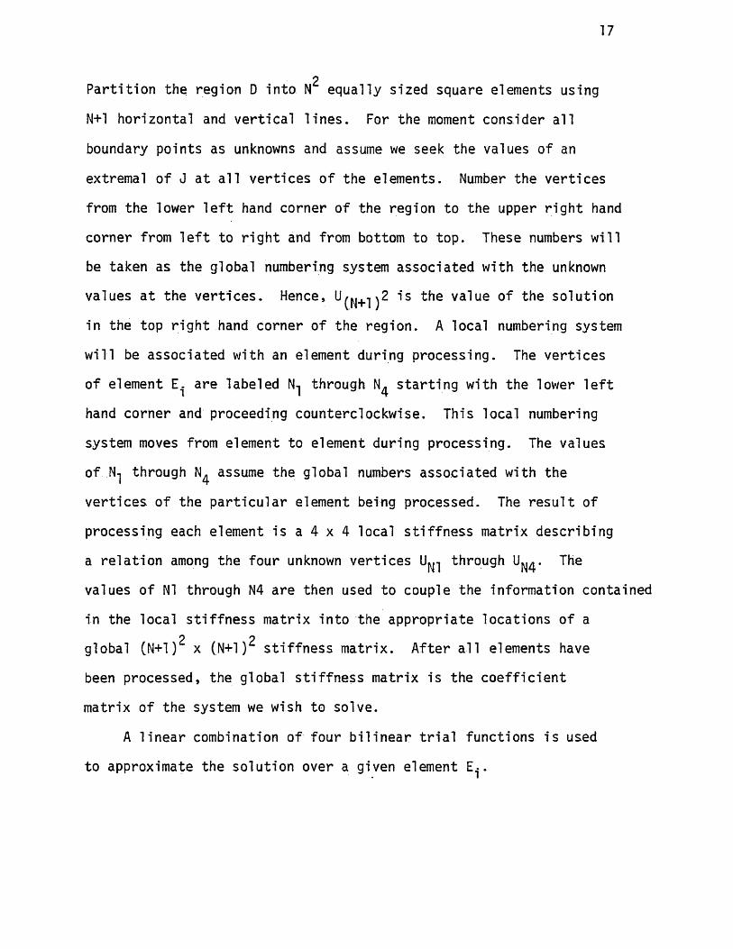
2P a r t i t i o n the region D i n to N equal ly s ized square elements using

N+l hor izon ta l and v e r t i c a l l i n e s . For the moment consider a l l

boundary po in ts as unknowns and assume we seek the values of an

extremal of J a t a l l v e r t i c e s o f the elements. Number the v e r t i c e s

from the lower l e f t hand corner of the region to the upper r i g h t hand

corner from l e f t to r i g h t and from bottom to top. These numbers w i l l

be taken as the global numbering system a sso c ia ted with the unknown

values a t the v e r t i c e s . Hence, U ^ +^ 2 i s the value of the so lu t io n

in the top r i g h t hand corner o f the region . A local numbering system

wil l be a sso c ia ted with an element during process ing . The v e r t i c e s

of element E. a re labe led N-j through N s t a r t i n g with the lower l e f t

hand corner and proceeding counterclockwise. This local numbering

system moves from element to element during process ing . The values

of N-j through N assume the global numbers a sso c ia ted with the

v e r t i c e s o f the p a r t i c u l a r element being processed. The r e s u l t of

process ing each element i s a 4 x 4 local s t i f f n e s s matr ix desc r ib ing

a r e l a t i o n among the four unknown v e r t i c e s U -j through U ^ . The

values of N1 through N4 a re then used to couple the information conta ined

in the local s t i f f n e s s matr ix in to the a p p ro p r ia te lo ca t io ns o f a 2 2global (N+l) x (N+l) s t i f f n e s s m atr ix . A f te r a l l elements have

been processed , the global s t i f f n e s s matrix i s the c o e f f i c i e n t

matr ix of the system we wish to solve .

A l i n e a r combination o f four b i l i n e a r t r i a l func t ions i s used

to approximate the so lu t io n over a given element E-.

18

UEi

j= l

a j+ jO c j r ) C211

where cj>. = a .x + b.xy + c .y + d.J J J J J

We re p re se n t the x and y coord ina tes of ver tex Ml by (x1 ,y ^ ) and

s i m i l a r ly fo r N2 through N4. The c o e f f i c i e n t s in the expression

f o r the t r i a l func t ions <j>. a re chosen so t h a t :J

j , k = 1,4 C22)

More p r e c i s e ly , the c o e f f i c i e n t s of <j> may be obtained by solving the

4 x 4 system:

xl xlyl yi

x2 x2y 2 y 2

x3 x3y3 y3

x4 x4y4 y4

al 1

bl 0

cl 0

dl 0

(23)

One ob ta ins the c o e f f i c i e n t s o f ^ through <j> analogously. The t r i a l

func t ions <j>. a re now f u l l y sp e c i f i e d over element E . . The values ofJ ■the so lu t io n U a t the v e r t i c e s N1 through N4 s a t i s f y :

N1 a,-*j ( x l . y l ) = uN1 (24)

19

4UN2 “ X ! “ / j x 2 ’y 2 = UN2

j=l

4

UN3 21 ^ (x 3 ’y 3 ) = UN3

j=l

4

UN4 “ ° j * J (X4,y4) =j=l

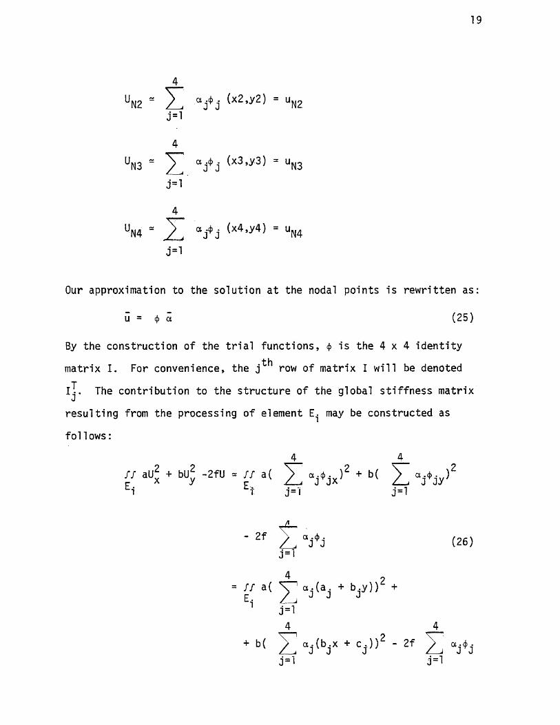
Our approximation to the so lu t io n a t the nodal po in ts i s r e w r i t t e n as

u = <j> a (25)

By the c o n s t ru c t io n of the t r i a l fu n c t io n s , <f> i s the 4 x 4 i d e n t i t yj. L

matrix I . For convenience, the j row of matrix I wil l be denotedT

I' .. The c o n t r ib u t io n to the s t r u c t u r e of the global s t i f f n e s s matr ixv

r e s u l t i n g from the process ing of element E.. may be cons t ruc ted as

fo l lo w s :

4 4f f aU2 + bll2 -2fU - a( ^ a .* .x )2 + b( ] T

i 4 j=l

2

" 2f “j * j (26)j=l

= { { a( 2 ] ° j (aj + v ))2 +1 j=i

4 4

+ b( / ] ° J (bj x + CJ'))2 ' 2f 2 °J*j j= l j=l

20

With the replacements:

'1 + V ’ “2 ' lJ2J ’ °3 ' U3J ’ "4 ' “4-y T = (a, + b .y , a , + b„y, a , + b ,y , a . + b.y) (27)

TY ” (b^x ^ C-J , ^2* Cr> 3 b^x 9 b^x

_ T _a = u hence a .. = I . u

J J

The r i g h t s ide of 26 may be expressed as:

4/ / a (yT u )2 + b(YT u )2 - 2 f f f > iT u 41. (28)e i 1 2 e i U J J

which in turn equals :

4f f aGTYlyju + bu^^YgO " 2 / / f iT u . (29)Ei Ei j=1

T TObserving t h a t the two 4 x 4 m atr ices y^y-j and Y2Y2 a re symmetric and

equating the d e r iv a t iv e Of 29 with re s p e c t to u to zero , we obta in the

r e l a t i o n :4

[ f f ay-jyj + by2Y2]u = f f f Ij4>j (30)Ei Ei j=l

The bracketed express ion in equat ion 30 i s the 4 x 4 local s t i f f n e s s

matr ix which must be proper ly coupled in to the global m atr ix . The

c o e f f i c i e n t s of the t r i a l func t ions depend so le ly on the coordina tes

o f the elements v e r t i c e s (see equation 23). I f the elements a re

squares , c a lc u l a t io n of the c o e f f i c i e n t s becomes p a r t i c u l a r l y simple

r eq u i r in g knowledge of the coord ina tes of a s in g le ve r tex of the

element and the length of i t s s id e . Thus, the co n s t ru c t io n of a

21

local s t i f f n e s s matr ix i s accomplished by a subrout ine whose input

parameters a re the coord ina tes o f an elements, v e r t i c e s . With, t h i s

in fo rm ation , y-j and y^ are cons t ruc ted and the in te g r a t i o n s performed.^

The 4 x 1 r i g h t hand s id e vec to r in equation 30 i s cons t ruc ted and

assembled analogously.

In the event t h a t a and b in r e l a t i o n 30 are co ns tan t and the

elements E| a re equa l ly s ized squares , the process ing o f each element

w i l l r e s u l t in the same local s t i f f n e s s m atr ix . I f y-j and y2 a re

evaluated and the i n t e g r a t i o n s performed, one ob ta ins the fol lowing:

/ / a y-jy-j +Ei

h T - 1 bY2Y2 - 6

2 (a+b) - 2a+b -(a+b) a - 2b

-2 a+b 2 (a+b) a - 2b -(a+b)

-ta+b) a - 2b 2 (a+b) - 2a+b

a - 2b -(a+b) - 2a+b 2 (a+b)

(31)

As a consequence of symmetry, eva lua t ion of the local s t i f f n e s s

matr ix r e q u i re s only seven i n t e g r a t i o n s . Evaluating the corresponding

r i g h t hand s ide involves four i n t e g r a t i o n s . A moderate s ized problem

may involve 64 elements on a s id e and hence a t o t a l of approximately

f o r t y - f i v e thousand i n t e g r a t i o n s . I f the problem were time dependent

t h i s number o f in t e g r a t i o n s would be performed a t each time s te p .

With f i n i t e d i f f e r e n c e d i s c r e t i z a t i o n s , on the o the r hand, a t each

time s tep one eva lua tes the c o e f f i c i e n t s and source func t ions a t the

nodal p o in ts . With e i t h e r choice of d i s c r e t i z a t i o n , as the problems become

1 For a p p rop r ia te i n te g r a t i o n formulas, see [11].

l a r g e , time dependent or n o n - l in e a r , i t appears t h a t one should

allow more in te r p la y between the d i s c r e t i z a t i o n and so lu t io n p rocesses .

In p a r t i c u l a r , we would l i k e to know when a so lu t io n i s changing

s u f f i c i e n t l y slowly in time so t h a t a co a r se r time s tep may be

taken , or when a so lu t io n i s s u f f i c i e n t l y smooth in space so t h a t a

co a r se r s p a t i a l d i s c r e t i z a t i o n may be used. The Full Approximation

Scheme or FAS produces information during the m u l t i - g r id cycle

which has been su c c e s s fu l ly used in determining when c o a rse r or

more re f in e d d i s c r e t i z a t i o n s should be used. Some s i g n i f i c a n t s teps

in adapt ive d i s c r e t i z a t i o n s as applied to the time dependent Heat

Equation have been repor ted in [ 6] .

Assembly

The f i n a l s tep in the system c o n s t ru c t io n i s the assembly o f the

loca l s t i f f n e s s m atr ices to form the global s t i f f n e s s m atr ix . The

r e l a t i o n s in the global s t i f f n e s s matr ix w i l l i n d ic a t e the d i f fe ren c in g

scheme to which our p a r t i c u l a r f i n i t e element d i s c r e t i z a t i o n corresponds

This d i f f e r e n c e equat ion w i l l be va luab le in analyzing th e convergence

p r o p e r t i e s of the method on c e r t a i n model problems.

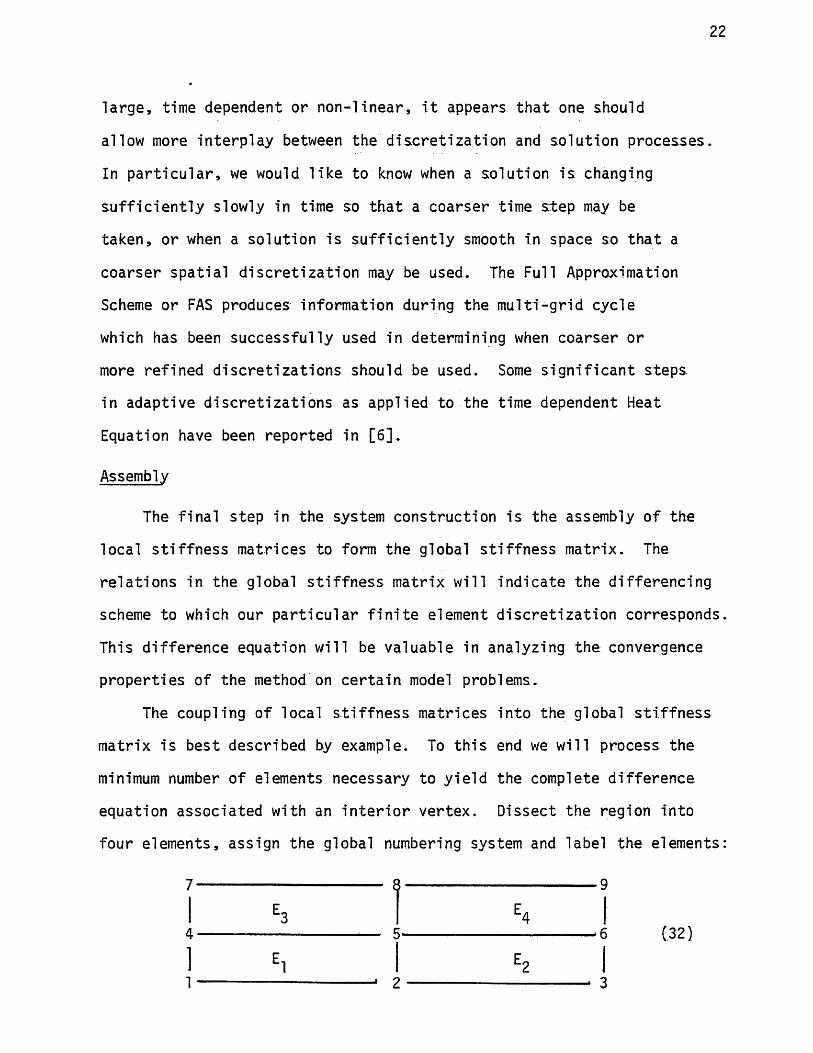
The coupling of local s t i f f n e s s m atr ices in to the global s t i f f n e s s

m atr ix i s be s t descr ibed by example. To t h i s end we wi l l process the

minimum number o f elements necessary to y i e ld the complete d i f f e r e n c e

equat ion a sso c ia ted with an i n t e r i o r v e r tex . Dissect the region in to

four e lements , a ss ign the global numbering system and label the elements

23

The key to assembly i s the sequence o f global numbers r e s id in g in

the local v a r ia b le s (N1, N2, N3, N4) = N. For in s ta n c e , as element

E-j i s processed, N = (1, 2, 5, 4) and s im i l a r ly fo r the remaining

elements. A f te r process ing an element, the a ssoc ia ted N i s used

to e x t r a c t information from the local s t i f f n e s s matr ix and to i n s e r t

t h i s information in to the global s t i f f n e s s matr ix . The information

i s refe renced as fo l lows:

N1 N2 N3 N4

Nl

N2

N3

N4

LSM (33)

More s p e c i f i c a l l y , the information contained in the local s t i f f n e s s

matr ix LSM a t lo ca t io n (4 ,1) f o r example w i l l be added to loca t io n

(N4,N1) in the global s t i f f n e s s matrix* A f te r the information is

t r a n s f e r r e d from a given local s t i f f n e s s matr ix to the app ropr ia te

l o c a t io n s in the global system, a new element i s processed r e s u l t i n g

in another local s t i f f n e s s matr ix and a new number sequence N. Upon

the conclusion o f processing the f i f t h row of the global s t i f f n e s s

matr ix w i l l , in t h i s case , give the r e l a t i o n which an i n t e r i o r nodal

po in t s a t i s f i e s . For the model problem with cons tan t c o e f f i c i e n t s ,

the d i f f e r e n c e equation r e s u l t i n g from our p a r t i c u l a r f i n i t e

element d i s c r e t i z a t i o n i s :

24

(34)

+

+

+

where RHS. . i s the sum o f i n t e g r a l s o f the r i g h t hand s ide of the ' s J

d i f f e r e n t i a l equation weighted a g a in s t the a p p ro p r ia te t r i a l fu n c t io n s .

I f a=b=l, we have a Poisson equat ion . From equation 34 we determine

t h a t the Laplacian o p e ra to r i s approximated by:

To a r r i v e a t the same approximation to the Laplacian a t po in t ( i , j ) ,

one can take T ay lo r ' s s e r i e s expansions centered a t the e ig h t

surrounding p o in ts . By manipulat ing the r e s u l t i n g eq ua t io n s , a

v a r i e ty of nine po in t approximations to the Laplacian a re obtained.

One of these i s approximation 35. In a d d i t io n , t h i s procedure y ie ld s

3 (35)

+ 3

25

the t ru n ca t io n e r r o r s o f the approximations.

Observe t h a t the express ion in the second s e t o f parentheses

i s the usual f i v e p o in t approximation to the Laplacian o p e r a t o r

and t h a t the express ion in the f i r s t s e t o f parentheses i s two v

ro t a t e d Laplac ians . Hence the nine p o in t Laplacian o p e ra to r a r i s in g -

from our p a r t i c u l a r f i n i t e element d i s c r e t i z a t i o n may be viewed as

the sum of two r o ta t e d Laplacians with one s tandard Laplacian, divided-

by th r e e . The t ru n c a t io n e r r o r s a s so c ia ted with the ro t a t e d -

approximation to the Laplacian and the standard approximation a re : -

2

12 ^Uxxxx + 6Uxxyy + Uyyyy^ +

TT <Uxxxx + V > + 0(h4)

r e s p e c t iv e ly . The t ru n ca t io n e r r o r a sso c ia ted with approximation 35

i s :

(U + 4U + u ) + 0 (h4 ) (37)12 v xxxx xxyy yyyy v '

An i n t e r e s t i n g phenomenon occurs i f the Laplacian i s approximated

by the combination o f two s tandard and one r o ta t e d Laplacian r a t h e r

than v ice versa . In t h i s case , the t ru n ca t io n e r r o r reduces to :

2Y2 A2U + 0(h4 ) (38)

For Laplaces Equation, t h i s scheme has an 0(h4 ) t ru n ca t io n e r r o r

and thus might be considered a b e t t e r d i f f e r e n c in g scheme than t h a t

which the f i n i t e element d i s c r e t i z a t i o n produced. The po in t to bear

in mind i s t h a t in t h i s simple example, the f i n i t e d i f f e r e n c e

26

equat ions which arose n a tu r a l l y from the f i n i t e element procedure •

a re not as accura te as those which a re e a s i l y derived using a

f i n i t e d i f f e r e n c e approach.

Linear Tr ia l Functions

When l i n e a r t r i a l fu n c t io ns defined over t r i a n g u l a r elements:

a re used to approximate solut ions . , the procedure i s analogous to

t h a t d iscussed in the preceding s e c t io n . The t r i a l func t ions a . are^ vJ

of the form:

(v \/ ic fho rftnv'riina+o n-F a wov'+nv The analog of equation

are t r i a n g l e s . To t h i s s t a g e , the d e r iv a t io n i s the same f o r

v a r i a b le or cons tan t c o e f f i c i e n t s . For the case of cons tan t

c o e f f i c i e n t s we de r ive the local s t i f f n e s s matr ix which r e s u l t s from

the process ing of an element. There a re b a s i c a l l y two d i f f e r e n t '

types o f t r i a n g u l a r elements:

(39)

and the c o e f f i c i e n t s a re chosen so t h a t :

j , k 1, — , 3

wnere y-jy-j ana Y2Y2 a re ma‘cr ices 0T o rae r -criree and the elements

(40)

27

which i f refe renced as ind ica ted wil l y i e ld id e n t i c a l local

s t i f f n e s s m a t r ice s . The region i s uniformly d i s c r e t i z e d as

in d ic a te d .

I-

4' (42)

Equation 40 reduces to

—a a 0 / / f * ,

Ei 1

-a a+b -b u =: f f f f i

Ei

0 -b b / m ,

- Ei

(43)

After coupling the local s t i f f n e s s m atr ices in to the global

s t i f f n e s s m a t r ix , we observe t h a t the use of l i n e a r t r i a l func t ions

over the ind ica ted region r e s u l t s in the following d i f fe ren c in g scheme

bUj ,.T-1 + > + b>Ui „ j - bUi , j +1 ,2 (44)

- a l l . , . + ( a + b ) U . . - a U . , , . + i - U j t »J. i + U J

u2

= RHS. .

which i s the s tandard f iv e po in t approximation to the negat ive

28

Laplacian when a=b=l.

In the next c h ap te r , c e r t a i n m u l t i - g r id processes a re

considered more c lo s e ly . At times' the m u l t i -g r id processes w i l l be

designed by using v a r i a t i o n a l arguments. In my exper ience , 1

v a r i a t i o n a l p r in c ip le s have provided va luab le in s ig h t s in to multi -

g r id p rocesses . However, once the m u l t i - g r id processes which

a r i s e from the v a r i a t i o n a l formulation a re s tud ied more c lo s e ly ,

one begins to see ways of improving on t h e i r e f f i c i e n c y .

CHAPTER 3

A CLOSER LOOK AT MULTI-GRID PROCESSES

This chap ter i s devoted to a c lo s e r examination of th ree t o p i c s ,

coarse g r id equa t ions , r e l a x a t i o n , and local mode a n a ly s i s . The

f i r s t to p ic i s d iscussed in terms o f th e methodology developed by

R. A. Nicolaides in [7 ] . The main r e s u l t o f sec t io n I i s the

d e r iv a t io n of the equation which coarse g r id c o r re c t io n s are required

to s a t i s f y . In s e c t io n s I I , I I I , and IV the process of r e l a x a t io n

and i t s r am i f ic a t io n s on the convergence p ro p e r t i e s o f the method

a re analyzed by Four ie r expansions .

Coarse Grid Equations

Represent the fu n c t io n a l :

J(U) = S S AU2 + BU2 - CU2 - 2FU (45)D x y

(A, B, C, and F a re func t ions of the two v a r ia b le s (x ,y ) ) in the

d i s c r e t e form:

J(u ) = uTLu - 2uTf (46)

where L i s the symmetric global s t i f f n e s s matrix r e s u l t i n g from

equation 45, f i s the r i g h t hand s ide vec to r and u r e p re se n ts an

approximation to U a t mesh po in ts of the d i s c r e t i z e d region D.

In c e r t a i n a p p l i c a t io n s , u i s an approximation to the d i s p la c e ­

ments a t various po in ts of a s t r u c tu r e and J (u ) i s an approximation

to the p o te n t ia l energy a sso c ia ted with the displacement s t a t e u.

29

30

For an equi l ib r ium p o s i t io n to be s t a b l e and hence ph y s ic a l ly

ach ievab le , i t must correspond to a r e l a t i v e minimum of J ( u ) .

Equating the d e r i v a t i v e of 2 with re s p e c t to u to zero , we obtain

the f i n i t e d i f f e r e n c e system:

LG = f (471

Equation 47 i s the r e l a t i o n to be s a t i s f i e d on the f i n e s t g r id G™.

Recall t h a t in the m u l t i - g r id con tex t an approximate so lu t io n u of

equat ion 47 i s improved by a c o r r e c t io n v e c to r , v, which i s i n t e r ­

po la ted from the c o a rse r g r id Gm"^ onto g r id Gm. Our purpose i s

to determine v a r i a t i o n a l l y the equat ion which the c o r r e c t io n termm 1v s a t i s f i e s on gr id G “ . Represent the co rrec ted so lu t io n on the

f in e g r id Gm by:

u + Ev (48).

where E i s an i n t e r p o la t i o n ope ra to r used to extend the co rre c t io n

v from g r id Gm“ onto the f i n e r g r id Gm. I f the c o r re c t io n Ev i s

to a id in reducing the energy, then:

J(u + Ev) £ J (u ) (49)

This motivates the v a r i a t i o n a l p r in c ip le used to de f ine them 1

equation s a t i s f i e d by v on g r id G ” :

Min 0(u + Ev) (50)

S € v " - ’

31

By equat ion 46:

J (u + Ev) = (uT + vTET)L(u + Ev) - 2(uT + vTET) f (51)

= uTLu + uTLEv + vTETLu + vTETLEv - 2(uT + vTET) f

Equating the d e r i v a t i v e with r e s p e c t to v to ze ro , one ob ta in s :

2ETLu + 2ETLEv - 2ETf = 0 (52)

Which may be r e w r i t t e n as:

ETLEv = ET( f - Lu) (53)

Equation 53 i s the coarse g r id r e l a t i o n which the c o r r e c t io n v i s

requ ired to s a t i s f y . Observe t h a t the vec to r :

r = f - Lu (54)

i s the r e s id u a l o f equation 47 corresponding to the approximate

so lu t io n u. The i n t e r p o la t io n matr ix E i s , in g e n e ra l , of o rder

(nf x nc) where nf i s the number of mesh po in ts on the f i n e g r id Gmm 1and nc the number of mesh po in ts on the co a rse r g r id G ’ . Hence,

TE in equation 53 maps the f i n e g r id re s idu a l vec to r r i n to a vec to r

which i s used as the r i g h t hand s ide o f the coa r se r g r id equat ions .

The in t e r p o la t i o n scheme E i s chosen so t h a t the ope ra t ion E^LE i s

the coarse g r id analog of L. By t h i s we mean t h a t i f the func t iona l

were being minimized over g r id Gm“ r a t h e r than gr id Gm, e\ e would

be the a sso c ia ted global s t i f f n e s s m atr ix . I t i s simply the ope ra to r

L defined over a c oa rse r d i s c r e t i z a t i o n .

32

Equation 53 provides a l in k between coarse and f in e g r id

systems, and a lso l in k s the processes o f i n t e r p o la t io n E and

r e s id u a l weighting E ". R eca l l , in the m u l t i -g r id p rocess , the

c o r r e c t io n procedure i s applied r e c u r s iv e ly . An approximate

s o lu t io n v of equation 53 which i s defined on gr id G ~ i s used

to c o r r e c t the approximate so lu t io n u of equat ion 47 defined on

g r id G111. S im i la r ly , an approximate so lu t io n of an equation defined

on a s t i l l co a r se r g r id Gm_^ and der ived in a manner analogous

to the d e r iv a t io n o f equation 53 i s used to c o r r e c t the c o r r e c t io n

v. This i n te r lo c k in g of c o r r e c t io n equat ions proceeds up to the

c o a r s e s t g r id G°.

Observe t h a t equation 53:

ETLEv = ET(? - Lu) on Gm_1, v e vm_1 (55)

i s the v a r i a t i o n a l equ iva len t of equation 7.

Lm-1 -m-1 = jm-1 -m Gm-1 (5 6 )m

In a f i n i t e element fo rm ula t ion , the t r i a l func t ions over a given

element may be used to c o n s t ru c t an in t e r p o la t io n scheme E. Equation

55 suggests t h a t the r e s i d u a l , f - Lu, on gr id Gm may be weighted by T TE and t h a t E LE i s a s u i t a b l e coarse g r id approximation to the f in e

g r id ope ra to r .

The arguments presented do not e s t a b l i s h equation 55 as the

only 'co a rse g r id analogue' to the res idua l equat ion on g r id Gm.o

The so lu t io n to equation 55 possesses an inheren t 0(h ) e r r o r as a

consequence of using l i n e a r elements in the Ritz approximation.^

1 Where the e r r o r i s measured in the energy norm a sso c ia ted with 45 and h i s the mesh s i z e of g r id Gm-1 .

33

Furthermore, i t i s l i k e l y t h a t we can rep lace e"^(? - Lu) by a

s u i t a b l y chosen approximation which- w i l l in troduce an e r r o r in v

which i s o f h igher o rder than the e r r o r r e s u l t i n g from the Ritz

approximation i t s e l f , see [10 ] . Hence, we can conceive of res idua l

weighting techniques involving fewer ope ra t io ns than e"*" which, when

used in equat ion 55 produce c o r r e c t io n terms as accu ra te as v.^

Relaxation

Relaxation i s an i t e r a t i v e procedure f o r improving an

approximate so lu t io n o f a system of equa t ions . In th e m u l t i - g r id

a lg o r i th m s , t h i s procedure i s used p r im ar i ly to smooth the r e s i d u a l s

and to solve fo r the c o r re c t io n terms on the coa rse r g r id s .

There a re a number o f conventional r e l a x a t io n procedures from

which to choose and one can c o n s t ru c t a v a r i e ty o f new procedures.

The e x i s t i n g a n a ly s i s fo r the conventional methods of ten does not

provide the information about the r e l a x a t io n procedure which i s most

r e l e v a n t to the m u l t i - g r id p rocess . More s p e c i f i c a l l y , i f the e r r o r

between the exac t so lu t io n of a system of d i f f e r e n c e equat ions and

an approximate so lu t io n is expanded l o c a l l y in a d i s c r e t e F o u r ie r

s e r i e s , then the information of p a r t i c u l a r i n t e r e s t in the m u l t i - g r id

con tex t i s the manner in which a given r e l a x a t io n technique l i q u i d a t e s

e r r o r components of ' h i g h 1 frequency. Low frequency e r r o r components

are l iq u id a te d inexpensively by coarse g r id c o r re c t io n s .

In [1] and [ 3 ] , Brandt developes techniques fo r analyzing the

e f f e c t s of d i f f e r e n t r e l a x a t i o n , r e s id u a l weighting , and in t e r p o la t i o n

^We have in mind a res id ua l t r a n s f e r technique known as i n j e c t i o n which i s d iscussed in l a t e r ch ap te r s .

34

procedures on the m u l t i - g r id process . These techniques have been used

r ep ea ted ly to su c c e s s fu l ly p r e d i c t accu ra te convergence r a t e e s t im ates

f o r va r ious m u l t i - g r id implementations.

In the next sec t io n we use these methods to analyze a nine poin t

success ive over r e l a x a t io n procedure. The p re d ic t io n s of the a n a ly s i s ,

a re compared with experimental evidence.

Mode Analysi s Applied to a Relaxat ion Scheme

The design of an e f f i c i e n t smoothing procedure i s the fundamental

s tep in the con s t ruc t ion of a successfu l m u l t i - g r id process . E f f i c i e n t

and p re d ic ta b le r e l a x a t io n techniques a re g e n e ra l ly d i f f i c u l t to

c o n s t r u c t . They depend not only on the d i f f e r e n t i a l opera tors in the

e qua t ions , but a lso on the t r i a n g u la t io n of the domain. The choice of

uniform meshes a ids enormously in the design process .^

Equation 34 suggests t h a t we look a t the following d i f fe ren c e

e q u a t io n :

ui , j = t 1- “ )ui . j . + 5 l l f B T C 6h2RHSi . j - <-(a+b>ui - i , j - i

-(.a+b)U.+i ^ +i -Ca+b)Ui+ i ^_1 -(a+b)Ui _1 >j+1

+2(-2a+b)U.+1)j +2(a-2b)Ui ^

+2(a-2b)Ui J + 1 )] (57)

Observe t h a t equation 57 has the same so lu t io n as equation 34. In

the following d iscuss ion U. - i s the exac t so lu t io n of equation 57• 9 J

a t mesh po in t ( i , j ) . Represent an old approximation to U. . by u. •«• * sJ

^Near boundaries we may cons ider applying specia l procedures and using non-uniform meshes.

35

and l e t u. . s tand f o r a new approximation to U. .. Consider an SOR1 sJ • sj

r e l a x a t io n sweep which improves the approximate so lu t io n a t the

mesh po in ts by modifying the values over the d i s c r e t i z e d region in

the o rder l e f t to r i g h t and bottom to top. During the SOR sweep the

old approximation u. i s rep laced by the new approximation u. . where1 jJ 1- 9 J

u. . i s obtained as fo l lows:19J

V j = + STi+ET C6h2RHSi,j-(' (a+b)Gi-i,j-i

- ( a + b )u .+1 tj+1 -Ca+b )G .+1 j . T C a + b ) ^ . , J + 1

+2 ( - 2a+b)u._i j j+ 2 ( . 2a+b)u1+ l> j+2 ( a - 2b)ui ^

+2(a -2b)u . sj +1)l C58)

Observe t h a t the barred u ' s on the r i g h t hand s ide of equation 58

correspond to values which were modified during the process of the

r e l a x a t io n sweep before mesh p o in t ( i , j ) was reached. Subtrac t ing

equat ion 58 from 57 one o b ta in s :

= j - s i i w c' {a+b)ii - i j - r (a+b)ei + i , j + i

- (a+b) ei+ j J._1 - (a+b )e 1_1 , j + l +2( ' 2a+b) £i -1 , j

+2(-2a+b)e .+ l j j + 2 . (a -2 b ) i . j j _l +2(a-2b)e1>j+1] (59)

where £. = U. . - u. . i s the e r r o r between the exact so lu t io n of1 jJ 1 ,J »9J

the d i f f e r e n c e equat ion U. . a t po in t ( i , j ) and the new approximation'9 0

u. .. S im i la r ly , e. . = U. . - u. . i s the e r r o r between the exact i , J i , J i , j

so lu t io n and the o lde r approximation u .. Represent the e= (e-j,©2 )

F o u r ie r component in the e r r o r expansions of e. • and e i . by:* 9 J * * J

36

/L e 1^ 8! + V (60 )

Aae I ( i 9 1 + ^0

r e s p e c t iv e ly . The q u a n t i ty |AQ| / jA 0 | i s the amplitude reduction^— T f t 0 -jb T A ^

f a c t o r of the (0-,,©2 ) e r r o r component. S u b s t i tu t in g AQe v 1 J 2 ;“ ' I f 1 0 + 1 0 * ) 'f o r e. . and AQe v 1 J 2 J f o r e- . in equation 59, so lv ing f o r the1sJ o i »j

r a t i o and tak ing the magnitude, we o b ta in :

. A.y (0“j,0rt) ~ A, ( 61 )

8a-j (1 “co)+coot-| (z Z£ + Z-j Z2 )8a-j-aia-j (z-j Z2 + Z-j Z2 J+c^wZ-j+agO^

z i = eISl z2 = e Ie 2

where: a-j = (a+b)

a 2 = 2(-2a+b)

= 2(a-2b) a) given

Equation 61 allows us to examine the e f f e c t s o f the 9 po in t SOR

r e la x a t io n scheme on the amplitudes of F ou r ie r components of the e r r o r .

The e f f e c t iv e n e s s o f a r e l a x a t io n scheme on a given problem can vary

d ram a t ic a l ly over d i f f e r e n t e r r o r components. I t i s p r e c i s e ly t h i s

v a r i a t i o n in e f f e c t iv e n e s s over the d i f f e r e n t components which makes

a problem d i f f i c u l t f o r conventional i t e r a t i v e methods. The d i f f i c u l t y

i s t h a t s in g le g r id techniques fo rce a compromise. I f a r e l a x a t io n

scheme i s chosen which enables one to e f f e c t i v e l y reduce the amplitudes2of the high frequency e r r o r components, then the slowly varying

^or poss ib ly a m p l i f i c a t io n f a c t o r .2 K-l KGiven a mesh r a t i o G :G =2:1, we d e f ine high frequency components on

gr id K to be those modes with wavelengths

37

components a re gene ra l ly not e f f i c i e n t l y reduced. The m u l t i - g r id

method sep a ra te s the two processes . Slowly varying components are

reduced e f f i c i e n t l y by co a r se r g r id c o r r e c t io n s and high frequency

e r r o r s a re reduced by a r e l a x a t io n scheme s p e c i f i c a l l y designed to

l i q u i d a t e them e f f e c t i v e l y . We wil l see t h a t the overa l l e f f e c t i v e ­

ness of the m u l t i - g r id technique i s p r i n c i p a l l y governed by the speed

with which f in e g r id high frequency e r r o r components are reduced.t

Before proceeding to the next sec t io n we consider a useful

proper ty of c e r t a in r e l a x a t io n schemes, see [3 ] . This p roperty r e l a t e s

to the d i r e c t i o n of the r e l a x a t io n sweep. In the d e r iv a t io n of

equat ion 61, we assumed t h a t the mesh po in ts were swept a row a t

a time from l e f t to r i g h t and from bottom to, top . The symbol

a t tempts to i l l u s t r a t e t h i s g ra p h ic a l ly . I f the po in ts are re laxed a>

column a t a time from the bottom of the region to the top and from

l e f t to r i g h t , one ob ta ins a d i f f e r e n t amplitude reduct ion f a c t o r .

y8a-j (1 -a))+coa-j (z-j Z£ + Z-j Z2)~<^2<z ' \~a 2 li}Z2

8a-j -aja-j (z-j Z2 + Z-j Z2 )+ct2£uZ'j+a3(Jl)Z2(62)

Genera l ly , y fep Q g) f s ince the qu an t i ty z-j Z2 in the numerator

o f y(0-j, 02) and the q u a n t i ty z-j z ^ in i t s denominator a re rep laced by

z-| Z2 and z 1 Z2 r e s p e c t iv e ly to ob ta in ^ 0 - j ^ 2) • ^ the q u a n t i t i e s

y(0.) and y (0 ) a t a p a r t i c u l a r mode 0 = (0, , Q0 ) d i f f e r s i g n i f i c a n t l y ,L_ 'fc 1 Cthen a l t e r n a t e r e l a x a t io n sweeps in the two d i f f e r e n t d i r e c t i o n s may

be used to improve the l iq u id a t io n r a t e o f t h i s component.^

uniform t r i a n g u la t io n of the region g r e a t ly f a c i l i t a t e s the co n s t ru c t io n of a l t e r n a t i n g d i r e c t i o n r e l a x a t io n processes .

38

To demonstrate the po in t more c l e a r l y , l e t of! and assume we a re

so lving a Poisson equat ion , e .g . a=b=l. Consider the e f f e c t o f the

two smoothing techniques l_*a n d o n the amplitude of the component

of the e r r o r corresponding to 0=(|-,O). Conducting the c a l c u l a t i o n s

one o b ta in s :

vCf.O) = .2 (63)

v(S-.O) = .4152

Hence, a 10"^ reduct ion in the amplitude of the e r r o r component

a sso c ia ted with0=(|-,O) requ i re s approximately 1.43 re l a x a t io n sweeps

i f we use technique L_>whereas 2.62 sweeps would be required fo r the

same reduct ion using technique 'l l . . . A method which a l t e r n a t e l y app l ie s

both r e l a x a t io n techniques has a smoothing r a t e equ iva len t to the

geometric average of u (e) and y (e ) :i 't-.

ur (0 ) = fu (e ) y (e) (64)c i— _

This composite method y i e ld s on average a 10 reduc t ion in the

amplitude a s so c ia ted with the 0=(|-,O) e r r o r component every 1.85

r e l a x a t io n sweeps.

The r e l a t i v e s izes of the amplitudes a sso c ia ted with d i f f e r e n t

Four ie r components of the i n i t i a l e r r o r are not known in advance.

Hence, r e l i a b l e r e l a x a t io n schemes should l iq u i d a t e any high frequency

component e f f e c t i v e l y . I f the v a r i a t i o n in the l iq u id a t io n r a t e s

over high frequency components i s severe , i t may des troy the

e f f e c t iv e n e s s of the a lgori thm. To i l l u s t r a t e the p o in t , assume a

r e l a x a t io n scheme has been devised with an average smoothing r a t e

39

u(e) of .5 over high frequency components. However, suppose t h a t the

value o f u(e) a t any given high, frequency component was e i t h e r .1

or .9 . Assume t h a t the i n i t i a l e r r o r had amplitudes a sso c ia ted w i th

each Four ie r component which were roughly equal in magnitude. Observe

t h a t a f t e r s ix r e l a x a t io n sweeps, those amplitudes which were reduced-6a t a r a t e o f y (e )= . l per sweep a re sm aller by a f a c t o r of 10" .

However, the amplitudes l iq u id a te d a t the r a t e o f y (e)= .9 are only

reduced to one -ha l f t h e i r o r ig in a l s i z e by the end of s ix sweeps.

Hence the e r r o r i s r ap id ly dominated by components which are not

e f f i c i e n t l y reduced and the r e l a x a t io n scheme looses i t s e f f e c t iv e n e s s .

I f the i n i t i a l e r r o r i s dominated a t the o u t se t by a component which,

i s inadequately l i q u id a te d , the r e l a x a t io n scheme wil l be i n e f f e c t iv e

from the beginning.

A l te rn a t ing d i r e c t i o n re l a x a t io n schemes a re designed so t h a t

e r r o r modes which are not l iq u id a te d e f f e c t i v e l y by r e la x a t io n sweeps

in one d i r e c t i o n a re l iq u id a te d e f f e c t i v e l y by sweeps in subsequent

d i r e c t i o n s . The goal of a r e l a x a t io n procedure i s to l iq u id a te

e f f e c t i v e l y a l l high frequency e r r o r components. Hence any i n i t i a l

e r r o r , reg a rd less o f i t s composition, can be l iq u id a te d .

A Simple Model of M ul t i -g r id Convergence

The m u l t i - g r id algori thms r a t e of convergence i s p r in c i p a l l y

governed by the r a t e a t which high frequency e r r o r components on the

f i n e s t gr id a re l iq u id a te d . High frequency components a re those modes

on a given gr id which cannot be adequately represen ted on c o a rse r g r id s .

Define Gm over the region - tt<x<j , Tr<y<Tr. Let Gm c o n s i s t o f ( J + l ) x

(J + l ) equal ly spaced mesh poin ts and re p re se n t th e mesh s izes

40

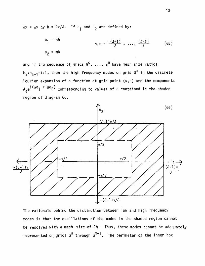
Ax = Ay by h = 2tt/ J . I f 9 and a re defined by:

9-j = nh

02 = mh

- ( J - l ) n,m = v -a- - - 9 • • • 9(j-n

2 (65)

and i f the sequence of g r id s G°, Gm have mesh s i z e r a t i o s

h|c: hj<+i = 2 : l , then the high frequency modes on g r id Gm in the d i s c r e t e

F o u r ie r expansion of a func t ion a t g r id po in t (a ,$ ) a re the components

A0e U a0l + 362) c o r r e sponding to values of 0 conta ined in the shaded

region of diagram 66.

( 6 6 )

t t / 2

t t / 2

The r a t i o n a l e behind the d i s t i n c t i o n between low and high frequency

modes i s t h a t the o s c i l l a t i o n s of the modes in the shaded region cannot

be resolved with a mesh s i z e of 2h. Thus, these modes cannot be adequately

represen ted on g r id s G° through Gm” ^ . The per im eter of the inner box

41

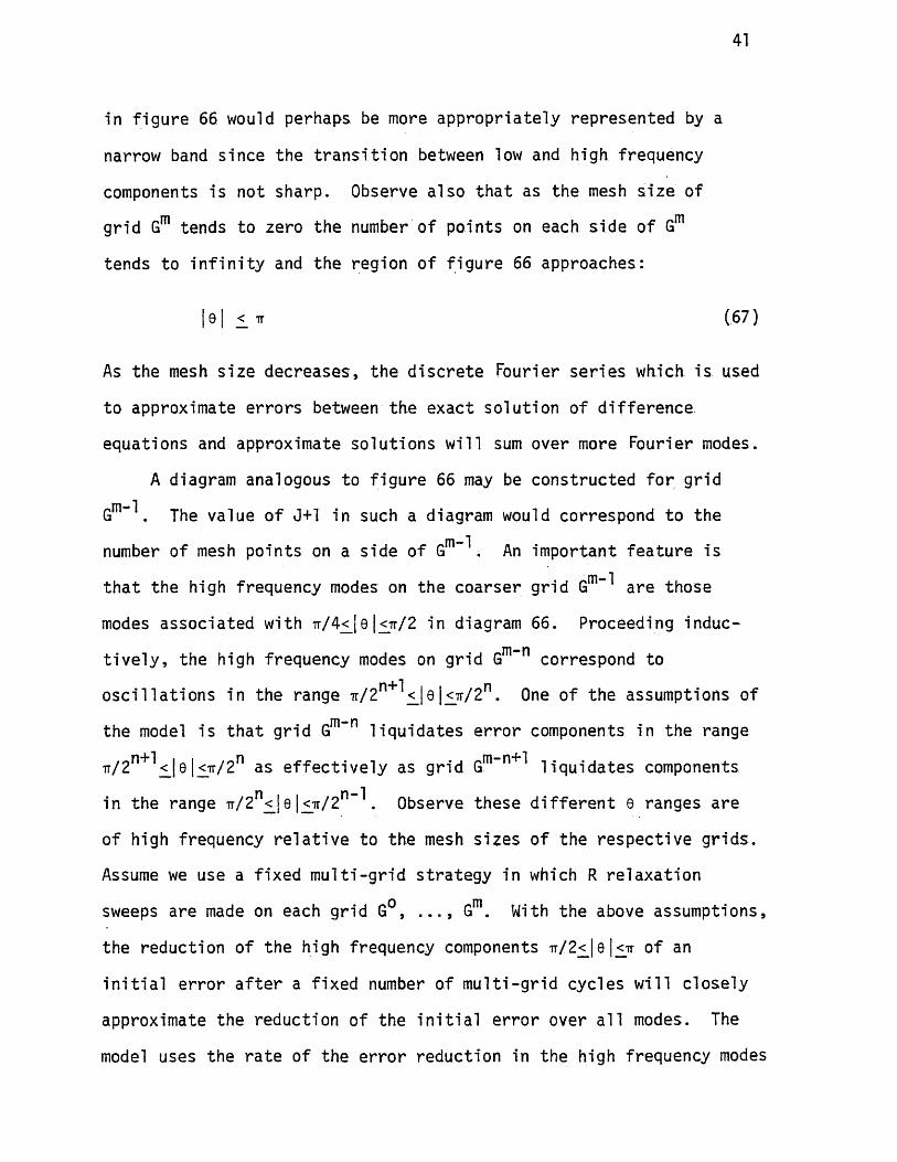
in f ig u re 66 would perhaps be more a p p ro p r ia te ly rep resen ted by a

narrow band s ince the t r a n s i t i o n between low and high frequency

components i s not sharp . Observe a lso t h a t as the mesh s i z e of

g r id Gm tends to zero the number of po in ts on each s id e of Gm

tends to i n f i n i t y and the region of f ig u re 66 approaches:

Ie| <_ ir (67)

As the mesh s i z e d e c reases , the d i s c r e t e Fourier s e r i e s which i s used

to approximate e r r o r s between the exac t so lu t io n of d if ference ,

equat ions and approximate so lu t io n s w i l l sum over more Fourier modes.

A diagram analogous to f ig u re 66 may be cons t ruc ted f o r g r idm 1

G . The value of J+l in such a diagram would correspond to them 1

number of mesh po in ts on a s id e of G . An important f e a tu r e i sm 1

t h a t the high frequency modes on the co a r se r g r id G are those

modes a sso c ia ted with tt/4<_|0 \ < * / 2 in diagram 66. Proceeding induc­

t i v e l y , the high frequency modes on g r id Gm“n correspond to

o s c i l l a t i o n s in the range iT/2n+^<J0 1<7r/2n . One of the assumptions of

the model i s t h a t g r id Gm~n l iq u i d a t e s e r r o r components in the range

TT/2n+^<_|© |<ir/2n as e f f e c t i v e l y as g r id Gm_n+ l i q u i d a t e s components

in the range 7r/2n<J e | <jr/2n~^. Observe these d i f f e r e n t e ranges a re

of high frequency r e l a t i v e to the mesh s i z e s o f the r e s p e c t iv e g r id s .

Assume we use a f ixed m u l t i - g r id s t r a t e g y in which R r e la x a t io n

sweeps are made on each gr id G°, . . . , Gm. With the above assumptions,

the reduct ion of the high frequency components Tr/2<Je|<ir of an

i n i t i a l e r r o r a f t e r a f ixed number of m u l t i -g r id cycles w i l l c lo se ly

approximate the reduct ion of the i n i t i a l e r r o r over a l l modes. The

model uses the r a t e of the e r r o r reduc t ion in the high frequency modes

42

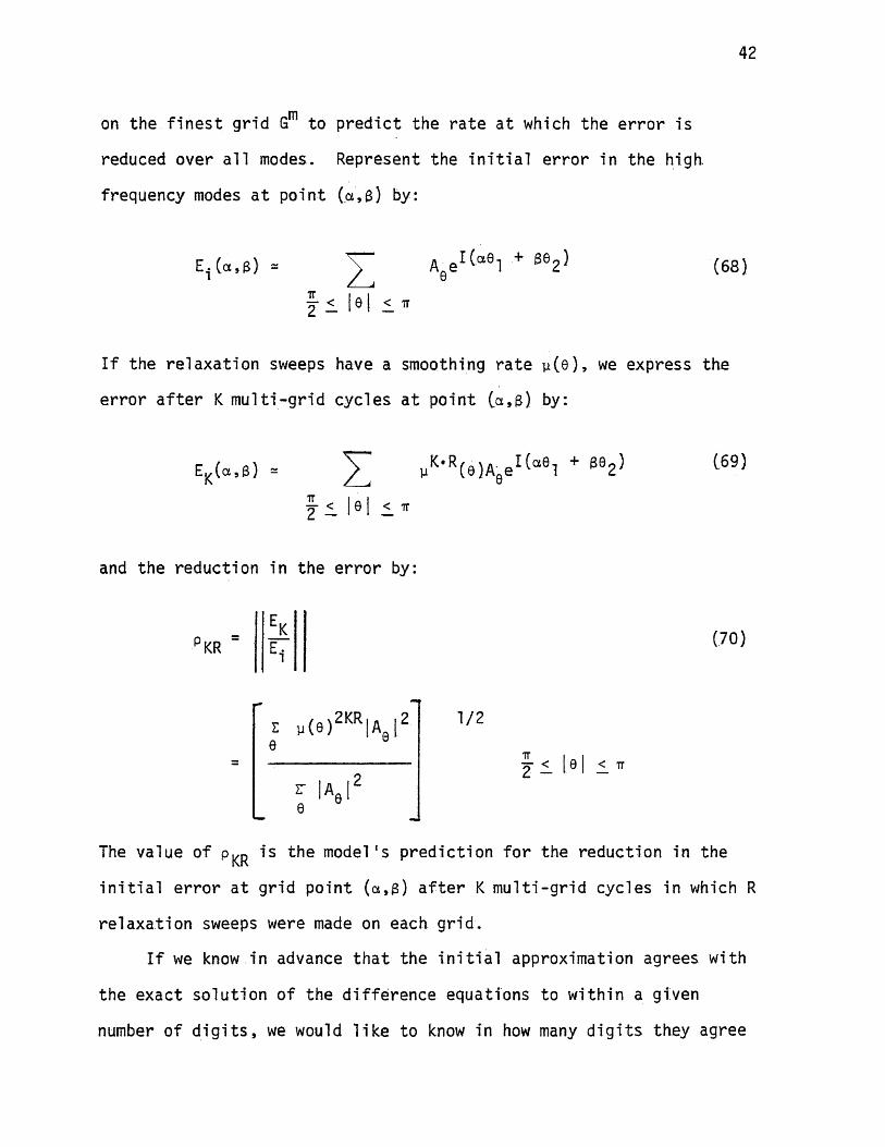
,mon the f i n e s t g r id G to p r e d i c t the r a t e a t which the e r r o r i s

reduced over a l l modes. Represent the i n i t i a l e r r o r in the high,

frequency modes a t po in t ( a , 6) by:

E . j ( a , $ ) - A0e lC“e l +8) (68 )

I f the r e l a x a t io n sweeps have a smoothing r a t e u ( e ) , we express the

e r r o r a f t e r K m u l t i - g r id cy c le s a t po in t ( a , 6) by:

K' R(9 )AQe I(aSl + ®e2>TT2 — 10 I — 7r

(69)

and the reduct ion in the e r r o r by

KRK

i v ( s ) 2KR|A | 2

z lAJ

1/2

T < | 9 | < _ TT

(70)

The value of i s the model 's p red ic t io n f o r the reduct ion in the

i n i t i a l e r r o r a t g r id po in t ( a , 3 ) a f t e r K m u l t i -g r id cycles in which R

r e l a x a t io n sweeps were made on each g r id .

I f we know in advance t h a t the i n i t i a l approximation agrees with

the exac t so lu t io n of the d i f f e r e n c e equat ions to with in a given

number of d i g i t s , we would l ik e to know in how many d i g i t s they agree

43

a f t e r K m u l t i - g r id cy c les . Hence, the q u a n t i ty of p a r t i c u l a r i n t e r e s t

i s the order of magnitude of the e r r o r reduc t ion .

A measure which we f re q u e n t ly use i s the number of m u l t i - g r id

cycles needed to obta in a ICT^ reduct ion in the i n i t i a l e r r o r . I f

the r e l a x a t io n technique i s a p p ro p r ia te to the problem being so lved ,

then the reduct ion in the e r r o r per m u l t i - g r id cycle should remain

f a i r l y co ns tan t and hence t h i s measure i s meaningful . However, i f a

r e l a x a t io n technique i s f a i l i n g on a problem, the reduc t ion in the

e r r o r per m u l t i - g r id cycle decreases as the number of m u l t i - g r id

cyc les i n c re a s e s . Under these c ircumstances , the measures defined

below must be i n te r p r e t e d more c a u t io u s ly . In p a r t i c u l a r , when

d i sc uss in g the measures, re fe ren ce must always be made to the number

of cycles over which they a re based.

A fter K m u l t i - g r id c y c l e s , the measure of the reduc t ion in the

i n i t i a l e r r o r per m u l t i - g r id cycle i s defined by:

a KR = (pKR^/K t-71^

A second measure i s defined by:

t KR = ^‘ L° 910^aKR^ 1

In the event t h a t the i n i t i a l e r r o r i s reduced by a cons tan t f a c t o r

per m u l t i - g r id c y c le , x ^ , w i l l r ep re se n t the number of m u l t i -g r id

cyc les needed to ob ta in a 10"^ reduct ion in the e r r o r . Observe t h a t

from a given problems' x ^ va lues , we can r e c o n s t ru c t the model 's

p re d ic t io n f o r the reduc t ion in the i n i t i a l e r r o r a f t e r K m u l t i - g r id

cy c les .

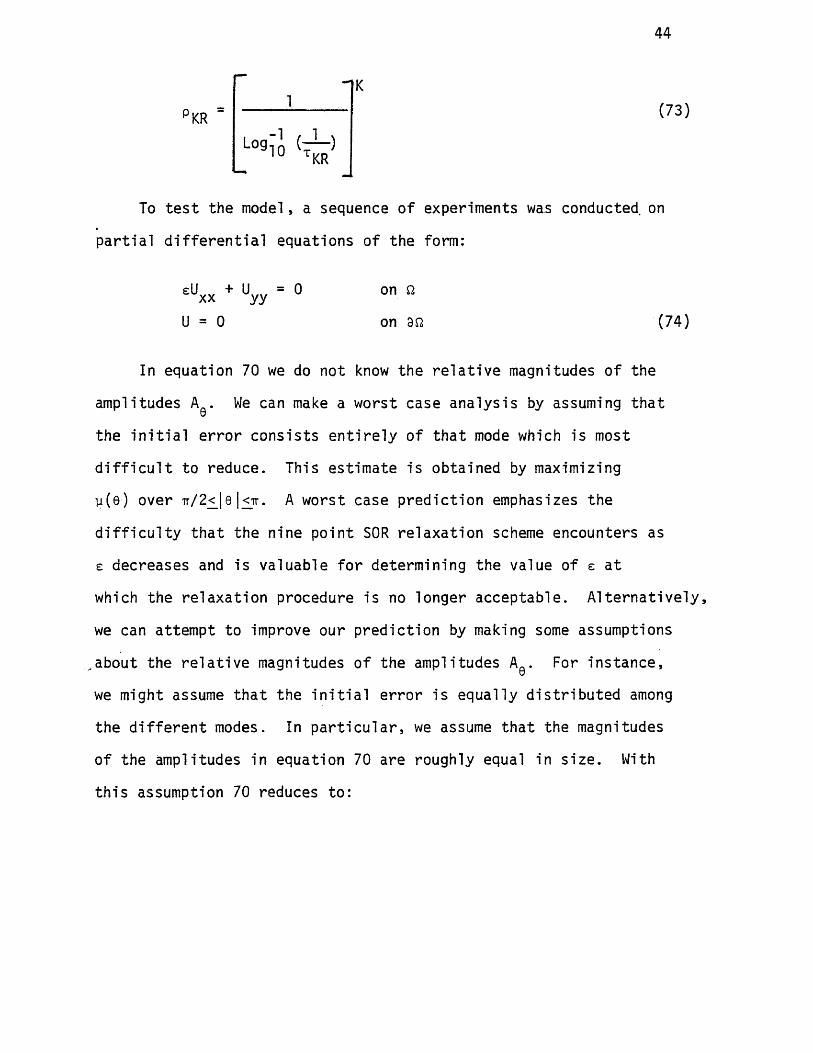
44

K1 ( 7 3 )P KR =

To t e s t the model, a sequence of experiments was conducted, on

p a r t i a l d i f f e r e n t i a l equations of the form:

on Q

on ZQ (74)

In equation 70 we do not know the r e l a t i v e magnitudes of the

ampli tudes A.. We can make a worst case a n a ly s i s by assuming t h a t9

the i n i t i a l e r r o r c o n s i s t s e n t i r e l y of t h a t mode which is most

d i f f i c u l t to reduce. This e s t im ate i s obtained by maximizing

y (e) over tt/ 2<_|0 |<jr. A worst case p re d ic t io n emphasizes the

d i f f i c u l t y t h a t the nine po in t SOR r e la x a t io n scheme encounters as

e decreases and i s va luable fo r determining the value of s a t

which the r e l a x a t io n procedure i s no longer accep tab le . A l t e r n a t i v e ly ,

we can a t tempt to improve our p re d ic t io n by making some assumptions

about the r e l a t i v e magnitudes of the amplitudes A0 . For in s ta n c e ,

we might assume t h a t the i n i t i a l e r r o r i s equal ly d i s t r i b u t e d among

the d i f f e r e n t modes. In p a r t i c u l a r , we assume t h a t the magnitudes

of the amplitudes in equation 70 are roughly equal in s i z e . With

t h i s assumption 70 reduces to :

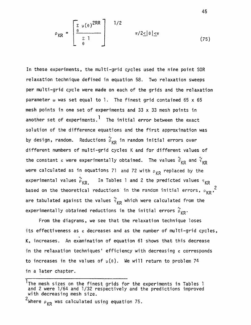
45

KR

i y ( e )2RR

z 1 e

1/2

Tt/2<_| 0 | < T T

(75)

In these experiments , the m u l t i - g r id cycles used the nine po in t SOR

re l a x a t io n technique defined in equat ion 58. Two r e l a x a t io n sweeps

per m u l t i - g r id cycle were made on each, of the g r id s and the r e l a x a t io n

parameter co was s e t equal to 1. The f i n e s t g r id contained 65 x 65

mesh p o in ts in one s e t of experiments and 33 x 33 mesh po in ts in

another s e t of experiments.^ The i n i t i a l e r r o r between the exact

s o lu t io n of the d i f f e r e n c e equat ions and the f i r s t approximation was

by d es ign , random. Reductions p ^ in random i n i t i a l e r r o r s over

d i f f e r e n t numbers of m u l t i -g r id cycles K and f o r d i f f e r e n t values o f

the cons tan t e were exper imenta l ly obta ined . The values o^R and

were c a lc u la t e d as in equat ions 71 and 72 with pKR replaced by the

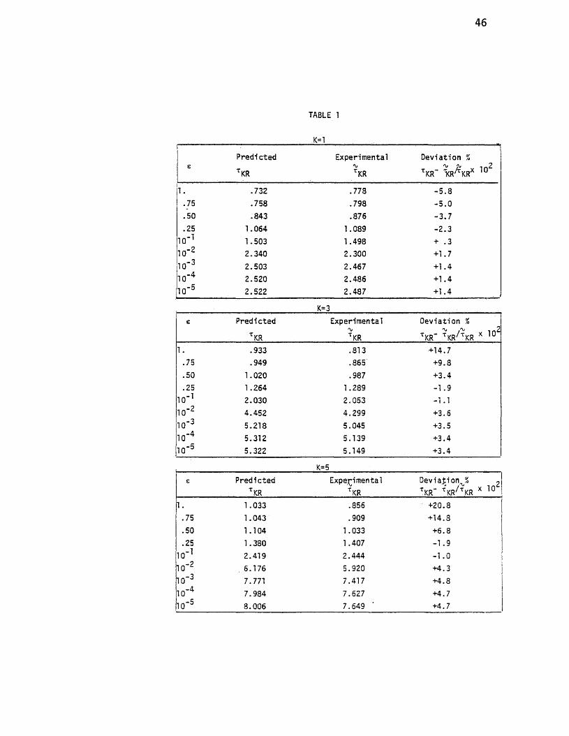
experimental values p^R In Tables 1 and 2 the p red ic ted values2

based on the t h e o r e t i c a l r educ t ions m the random i n i t i a l e r r o r s , pKR,

a re t ab u la te d a g a in s t the values which were c a lc u la t e d from the

exper im enta l ly obtained reduc t ions in the i n i t i a l e r ro r s

From the diagrams, we see t h a t the re l a x a t io n technique loses

i t s e f f e c t iv e n e s s as e decreases and as the number of m u l t i - g r id c y c le s ,

K, in c re a s e s . An examination of equation 61 shows t h a t t h i s decrease

in the r e l a x a t io n techn iques ' e f f i c i e n c y with decreas ing e corresponds

to inc reases in the values of y ( e ) . We wil l r e tu rn to problem 74

in a l a t e r chap te r .

The mesh s iz e s on the f i n e s t g r id s fo r the experiments in Tables 1 and 2 were 1/64 and 1/32 r e s p e c t iv e ly and the p re d ic t io n s improved with decreasing mesh s i z e .

2Where p ,R was c a lc u la te d using equation 75.

46

TABLE 1

K=1

ePredi cted

TKR

Experimental

t KR

Deviation %

t KR" TcR KR3* 1()2

1. .732 .778 -5 .8

in r> c .758 .798 -5 .0

.50 .843 .876 -3 .7

.25 1.064 1.089 -2 .310"1 1.503 1.498 + .310"2 2.340 2.300 +1.7TO"3 2.503 2.467 +1.410*4 2.520 2.486 +1.410"5 2.522 2.487 +1.4

K=3e Predicted

TKR

Experimental'VTKR

Deviation %

tkr- tkr/ tkr x 1q21. .933 .813 +14.7

inrs .949 .865 +9.8.50 1.020 .987 +3.4.25 1.264 1.289 -1 .9

10"1 2.030 2.053 -1 .110~2 4.452 4.299 +3.6io-3 5.218 5.045 +3.510"4 5.312 5.139 +3.410~5 5.322 5.149 +3.4

K=5£ Predicted

tkr

Experimentalt KR

Devia£ionJS 2 tKR" tKR/ t KR X 10

1. 1.033 .856 +20.8.75 1.043 .909 +14.8.50 1.104 1.033 +6.8.25 1.380 1.407 -1 .9

1 0 '1 2.419 2.444 -1 .010"2 , 6.176 5.920 +4.310 '3 7.771 7.417 +4.810"4 7.984 7.627 +4.710‘ 5 8.006 7.649 ' +4.7

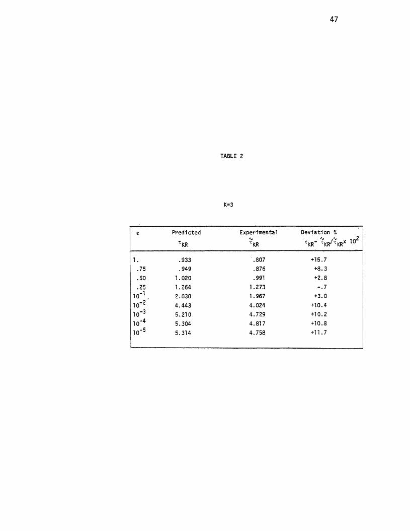
47

TABLE 2

K=3

s Predicted

t KR

Experimental

t KR

Deviation %'v* /'v . n2

tKR" tKR/ tKRx 10

1. .933 .807 +15.7.75 .949 .876 +8.3.50 1.020 .991 +2.8.25 1.264 1.273 - .7

TO"1 . 2.030 1.967 +3.0TO’ 2 4.443 4.024 +10.4TO'3 5.210 4.729 +10.2TO"4 5.304 4.817 +10.8

oI cn 5.314 4.758 +11.7

48

At t h i s j u n c tu r e , the model may be used to make an observat ion

p e r ta in in g to the so lu t io n of equations involving i n d e f i n i t e

o p e ra to rs .^ I f the value of y (e j a s so c ia ted with a p a r t i c u l a r .

F o u r ie r e r r o r component exceeds 1, then a r e l a x a t io n sweep w i l l

magnify r a t h e r than reduce the ampli tude of t h i s e r r o r component.

However, i f the components fo r which y(0)>l c l u s t e r about the

o r ig in 0=CO>O) then the m u l t i - g r id process can proceed once a minor

change has been made. A re la x a t io n sweep over any g r id w i l l amplify

the e r r o r components fo r which Reca l l , in the m u l t i - g r id

contex t each gr id has the primary r e s p o n s i b i l i t y o f reducing e r r o r

components with in a sp e c i f i e d frequency band. The f i n e g r id reduces

components of the e r r o r in the range ir/2<j0|<jr and while i t i s

doing t h i s i t w i l l amplify components with y ( e ) > l . S im i la r ly g r idm 1

G ” reduces e r r o r components in the range tt/4<J0 \ < j / 2 and while

i t i s performing i t s fu n c t io n , those e r r o r components with y(0)>l

w i l l continue to be am pl i f ied . I f the components f o r which y(0)>l

c l u s t e r about 0=(O,O), then they a re p r im ar i ly the r e s p o n s i b i l i t y

o f the c o a r s e s t g r id p rocess . On the c o a r se s t g r id a d i r e c t

s o lu t io n procedure i s used to solve the res idua l equat ion . The

s o lu t io n of the G° system obtained by th e d i r e c t so lu t io n technique

can provide a meaningful c o r r e c t io n to the G system in the low

frequency modes.

The s i t u a t i o n j u s t descr ibed i s encountered in s l i g h t l y i n d e f i n i t e

o pe ra to r s . As the o pe ra to rs in the equat ions become more i n d e f i n i t e

^In [1] th e re i s a d iscuss ion of procedures f o r deciding on the mesh s i z e of the c o a r se s t g r id based on the e igenvalues of the i n d e f i n i t e o p e ra to r s .

49

the modes f o r which yC©)>1 a re no longer as lo c a l i z e d about the

o r i g i n . They begin to appear more deeply w ith in the e reg ion . One.

method of approaching these problems i s to reduce the mesh s i z e on

the c o a r s e s t g r id G° and to apply a d i r e c t so lu t io n procedure on the

G° system. Unfor tuna te ly , as. the mesh s i z e o f the sm a l le s t g r id

i s reduced, the m u l t i - g r id procedure w i l l g e n e ra l ly become l e s s

e f f i c i e n t . The design o f m u l t i - g r id procedures fo r severe ly i n d e f i n i t e

problems which a re comparable in e f f i c i e n c y to the method as

app l ied to d e f i n i t e problems is. an area o f c u r r e n t r esea rch .

The model presented in t h i s s e c t io n i s f a i r l y crude. I t

p r e d i c t s convergence r a t e s on the b a s i s o f how a given r e l a x a t io n

technique l i q u i d a t e s high frequency e r r o r components on the f i n e s t

g r id . In the model we neg lec ted boundary e f f e c t s and assumed’

t h a t the coa rse r g r id c o r r e c t io n s l iq u id a te d the more slowly

varying e r r o r components a t a r a t e comparable to the r a t e a t which

the h ig h es t frequency components were reduced. A more re f in e d model

should analyze the e f f e c t s r e s u l t i n g from the use of d i f f e r e n t

re s id u a l weighting and in t e r p o la t i o n procedures . In [3] Four ie r

techniques are descr ibed which in theory permit one to study these r

p rocesses . The e x te n t to which the p r e d ic t io n s of the model can be

improved and genera l ized by including an a n a ly s i s of these processes,

should be explored.

CHAPTER 4

A MULTI-GRID IMPLEMENTATION ON THE CDC STAR TOO

The m u l t i - g r id implementation in the vec to r a lgori thm uses a

Correct ion Scheme and a Full M u l t i -g r id Cycle. A ty p ic a l Full3

M u lt i -g r id Cycle and a Simple Cyclev a re diagrammed on the fol lowing

page. HI and LI s tand f o r High- and low o rde r i n t e r p o la t io n s 2re s p e c t iv e ly , the symbol R r e p re s e n ts a r e l a x a t io n sweep and.

CR in d ic a t e s when r e s i d u a l s are c a l c u l a t e d . I f the computational

c o s t o f a r e l a x a t io n sweep on the f i n e s t g r id i s represen ted

by u n i ty then the numbers on the f a r l e f t s ide of the diagrams

correspond to the computational c o s t s o f r e l a x a t io n sweeps on the

c o a rse r g r id s^ .

The computational e f f o r t WRS expended on re la x a t io n in our 4Simple Cycle i s e q u iv a len t to 5.3 r e l a x a t io n sweeps on the f i n e s t

g r id .

1 K K+lWe have assumed a mesh s i z e r a t i o o f G :G =2:1.

2For g u id e l ines on choosing an a p p ro p r ia te o rder of i n t e r p o l a t i o n , seec u .

3A modified Simple Cycle was used in the f i n i t e element implementations.

4 In the f i n i t e element experiments r e l a x a t io n sweeps were not performed a f t e r the i n te r p o la t io n from G3 to G^. A subsequent cycle would begin with two r e l a x a t io n sweeps on the f i n e s t g r id . Hence, two r a t h e r than four r e l a x a t io n sweeps were performed on the f i n e s t g r id when ending

•one cycle and beginning another . On the l a s t Simple Cycle the number o f r e l a x a t io n sweeps on the f i n e s t g r id a f t e r the f in a l i n t e r p o la t io n was an opt ional parameter in the f i n i t e element implementations. The value of t h i s parameter i s zero in the r e s u l t s we r e p o r t .

50

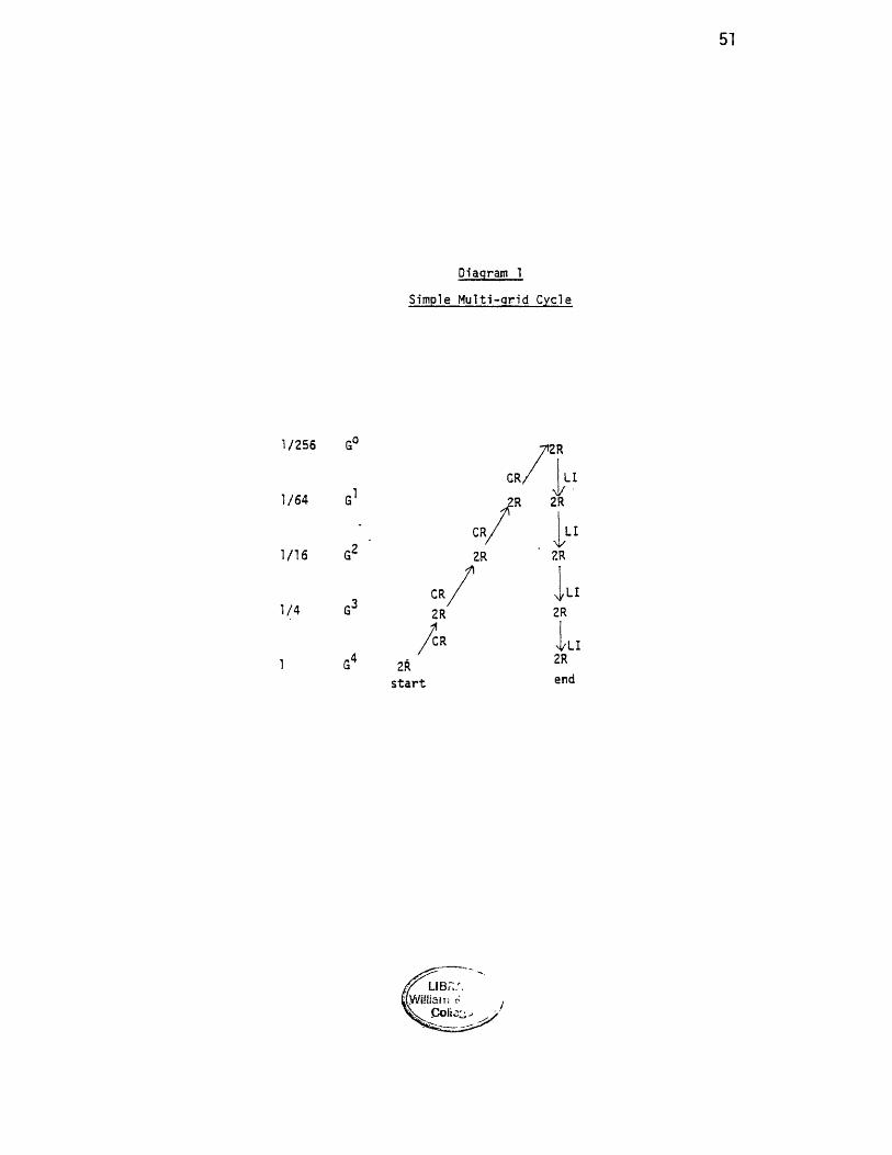
51

Diagram 1

Simple Multi-grid Cycle

1/256 G

1/64 G1

1/16 G2

12RGR:r

2R

C R /1/4 G 2R 2R

4/ l i2Rend

CR

G4 ' 2Rsta r t

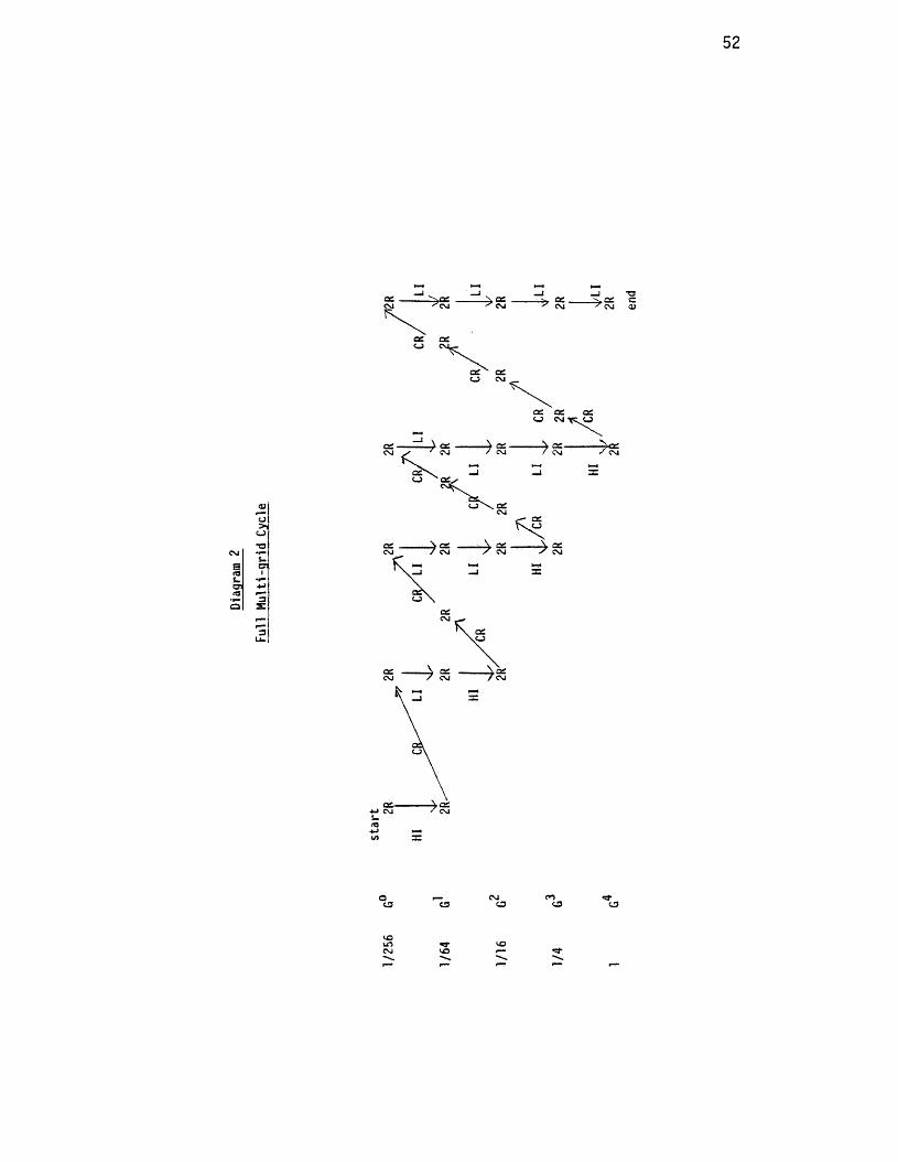
52

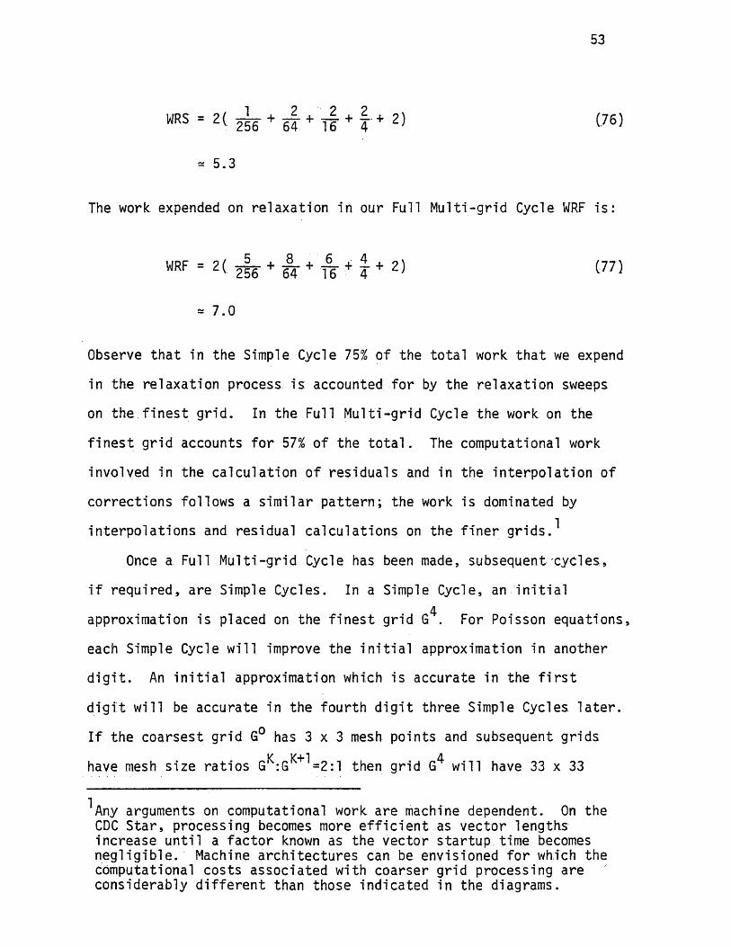
53

(76)

5.3

The work expended on r e l a x a t io n in our Full M ul t i -g r id Cycle WRF i s :

Observe t h a t in the Simple Cycle 75% of the t o t a l work t h a t we expend

in the r e l a x a t io n process i s accounted f o r by the r e l a x a t io n sweeps

on the f i n e s t g r id . In the Full M u l t i -g r id Cycle the work on the

f i n e s t g r id accounts f o r 57% of the t o t a l . The computational work

involved in the c a l c u l a t i o n of r e s id u a l s and in the i n t e r p o la t i o n of

c o r r e c t io n s follows a s im i l a r p a t t e r n ; the work is dominated by

i n t e r p o la t io n s and res idua l c a l c u l a t io n s on the f i n e r g r id s .^

Once a Full M u l t i -g r id Cycle has been made, subsequent c y c le s ,

i f r e q u i r e d , a re Simple Cycles. In a Simple Cycle, an i n i t i a l4

approximation i s placed on the f i n e s t g r id G . For Poisson equat ions ,

each Simple Cycle w i l l improve the i n i t i a l approximation in another

d i g i t . An i n i t i a l approximation which i s accura te in the f i r s t

d i g i t w i l l be accu ra te in the fo u r th d i g i t th ree Simple Cycles, l a t e r .

I f the c o a r se s t g r id G° has 3 x 3 mesh po in ts and subsequent g r id s1/ I / J .1 A

have mesh s iz e r a t i o s G :G =2:1 then gr id G wil l have 33 x 33

^Any arguments on computational work a re machine dependent. On the CDC S t a r , process ing becomes more e f f i c i e n t as vec to r lengths inc rease u n t i l a f a c t o r known as the vec to r s t a r tu p time becomes n e g l ig ib le . Machine a r c h i t e c t u r e s can be envis ioned f o r which the computational cos ts a s so c ia ted with coa rse r gr id process ing a re cons iderab ly d i f f e r e n t than those in d ic a te d in the diagrams.

WRF 2 ( 256 + 64 + 16 + 4 + (77)

* 7.0

54

2mesh p o in t s . Our d i f f e r e n c e approximation is 0 ( h ) and we a re

so lv ing over a u n i t square. The t ru n c a t io n e r r o r suggests t h a t we

solve the d i f f e re n c e equat ions to an accuracy of roughly th ree

decimal d i g i t s .4

In Simple Cycles, the i n i t i a l approximation on G i s u sua l ly

obtained by extending the boundary da ta in to the i n t e r i o r o f the

domain. Genera l ly , the accuracy of the i n i t i a l approximation i s

not known. Hence, we may need a t e s t f o r deciding when the

d i f f e r e n c e equat ions have been solved to within the s p e c i f i e d

accuracy.

Our experience with the Full M ul t i -g r id Cycle was very

encouraging. In every problem t h a t was t e s t e d , a s in g le Full

M u l t i -g r id Cycle solved the d i f f e r e n c e equations to w i th in t h e i r

t ru n ca t io n e r r o r . Subsequent Simple M u l t i -g r id Cycles were never

requ i red .

In the experiments the d i f f e r e n c e equat ions r e s u l t i n g from

Poisson equations were solved ex ac t ly . The maximum d i f f e r e n c e ,

TE, over the mesh po in ts between the exac t so lu t io n of the

d i f f e r e n c e equations and the exac t so lu t io n of the d i f f e r e n t i a l

equat ion was t a b u la te d . This q u a n t i ty was taken as a measure

of the t ru n ca t io n e r r o r . An approximate so lu t io n to the d i f f e r e n c e

equat ions was then obtained by using one Full M ul t i -g r id Cycle. The

maximum d i f f e r e n c e over the mesh p o in t s , EFMC, between t h i s

approximation and the exact so lu t io n to the d i f f e r e n c e equat ions

was then ta b u la t e d . In Table 3 we l i s t the r e s u l t s from four

ty p ic a l experiments in which the Full M ul t i -g r id Cycle descr ibed

in diagram 1 was used.

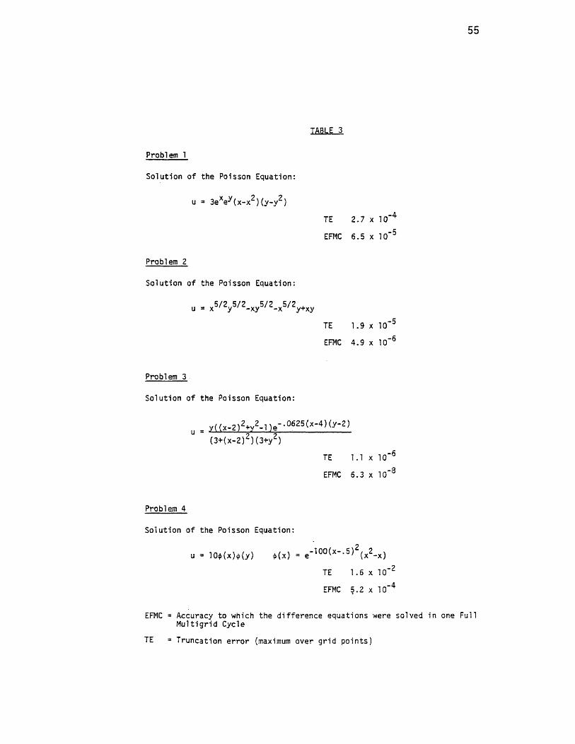
55

TABLE 3

Problem 1

Solution of the Poisson Equation:

u = 3exe,y(x-x^) (y-y2 )

TE 2.7 x 10"4

EFMC 6.5 x ICf5

Problem 2

Solution of the Poisson Equation:

u - x ^ y ^ - x y ^ - x ^ V x y

TE 1.9 x 10 '5

EFMC 4.9 x ICf6

Problem 3

Solution of the Poisson Equation:

y((x-2)^y2- l ) e - 0625^ - 4> ^ - ^(3+(x-2)2 )(3+y2 )

TE 1.1 x 10“6

EFMC 6.3 x 10"8

Problem 4

Solution of the Poisson Equation:

2u = 10*(x)*(y) *(x) = e - lq0(x- - 5) (x2-x)

TE 1.6 x 10“2

EFMC 5.2 x 10"4

EFMC = Accuracy to which the d ifference equations were solved in one Full Multigrid Cycle

TE = Truncation error (maximum over grid points)

56

A number of c o n s id e ra t io n s e n te r in to the design of m u l t i - g r id

a lgori thms which a re s u i t a b l e fo r p a ra l l e l p rocess ing . The f in a l

algori thm g e n era l ly r e f l e c t s the a r c h i t e c t u r e o f the machine on

which i t w i l l be used. We sha l l d iscuss the problems t h a t were

encountered in the design of the Full M u l t i -g r id vec to r a lgori thm .

f o r th e CDC S ta r 100.

The vec to r a lgori thm was intended to be a f a s t m u l t i - g r id

Poisson equat ion so lv e r f o r re c ta n g u la r reg ions . The Poisson

equat ions were d i s c r e t i z e d using the standard 5 p o in t approximation

to the Laplac ian. Diagram 2 i l l u s t r a t e s the i n i t i a l cycle in the

a lgori thm and diagram 1 the subsequent cycl ing p rocess .

In a m u l t i - g r id cycle a la rge p roport ion of the computational

e f f o r t i s expended in the r e l a x a t io n sweeps. The f i r s t o b jec t iv e

was to decide on an a p p ro p r ia te r e l a x a t io n procedure. The

r e l a x a t io n method should be amenable to p a r a l l e l computation and

should have e f f i c i e n t smoothing p r o p e r t i e s . Two d i f f e r e n t

r e l a x a t io n processes were considered: Weighted Simultaneous

Displacement, WSD, and Successive Over Relaxation with Red-Black

order ing [2 ,1 2 ] . Both WSD and SOR with Red-Black o rder ing are

s u i t a b l e fo r p a r a l l e l p rocess ing . During a r e l a x a t io n sweep these

schemes do not use information t h a t i s c a l c u la te d during the

sweep i t s e l f . They opera te on vec to rs o f e x i s t i n g d a ta . With2WSD i t i s p o ss ib le to r e lax over vec to rs of length N where N

i s the number of mesh po in ts on the s ide of the g r id we are p rocess ing .^

^Boundary po in ts a re processed j u s t l i k e i n t e r i o r p o in t s . However, the r e s u l t s from boundary po in t c a l c u l a t i o n s a re not s to re d .

57

Using SOR with Red-Black o rder ing the re l a x a t io n process op e ra te s2 2on vec to rs of length N /2 .

During a WSD re l a x a t io n sweep, one f i r s t c a lc u l a t e s the

r e s id u a l s R1« jJ

Ri , j ~ 4“ Fi ., j + Ui , j “ 4^Ui + l , j + Ui - l , j

+ Ui #j + T + Ui J - l ) f o r 1 n t e r i o r

R". • = 0 f o r boundary ( i , j ) (78)* »J

New approximations a t the po in t (i , j ) a re then c a lc u la t e d according

to :

. 0) ,

Ui J ~ Ui sJ “ a}0Ri , j " “4~^Ri + l , j + Ri - l , j

+ r i j + i + ( 7 9 )

f o r i n t e r i o r ( i , j ) , ajg=48/41, co-j =32/41

U. . unchanged f o r boundary ( i , j )• jJ

The weights odq and oj-j a re derived through mode a n a ly s i s . A WSD

r e l a x a t io n sweep may be performed using a t o t a l of 12 opera t ions

per g r id po in t whereas an SOR sweep with 03=1 r eq u i re s 5 opera t ions

per g r id p o i n t J Hence, in terms of opera t ion count , WSD is 2 .4

times as expensive as SOR.

At the time of the i n i t i a l experiments , we assumed t h a t the

smoothing r a t e of SOR with Red-Black order ing would, a t b e s t , be

A WSD sweep uses th re e m u l t ip l i c a t io n s and nine a d d i t io n s per g r id poin t whereas Gauss Seidel ( i . e . SOR with co=l) req u i re s one m u l t i p l i c a t io n and four ad d i t io ns per g r id po in t .

?On the S t a r , l a r g e r vec to r leng ths a re gene ra l ly an advantage s ince they a re processed more e f f i c i e n t l y . As the vectors grow beyond a c e r t a in p o in t , the inc reases in e f f i c i e n c y level o f f .

58

comparable to the smoothing r a t e o f SOR with the usual lex icog raph ica l

o rder ing .^ The smoothing r a t e s of WSD and SOR with the usual

o rder ing a re :

y = max vi (e)

t t / 2 < _ j 0 [ < _ ir ( 8 ° )

.50 SOR with u)=l

.22 WSD

These f ig u re s imply t h a t we w i l l obta in a 10"^ reduct ion in the high

frequency e r r o r components every 3 .3 r e l a x a t io n sweeps i f Gauss

Seidel i s used and every 1.5 r e l a x a t io n sweeps i f we choose WSD as

our r e l a x a t io n procedure. WSD i s th e re fo re 2.2 times as e f f e c t i v e

as Gauss Seidel with the s tandard o rder ing . At t h i s po in t i t appears

t h a t a t b e s t SOR with Red-Black o rder ing wil l be roughly comparable

to WSD, perhaps s l i g h t l y b e t t e r . Test runs were conducted using

SOR with Red-Black o rder ing . The m u l t i - g r id method diverged. In

the m u l t i - g r id cycle the r e s id u a l s had been in je c te d r a t h e r than

weighted. With WSD as the r e l a x a t io n process i n j e c t i n g the r e s id u a l s?had presented no d i f f i c u l t y . Through mode an a ly s i s i t was e s t a b l i s h e d

t h a t SOR with Red-Black order ing introduced high frequency components

i n to the r e s i d u a l s . A simple t r a n s f e r of r e s id u a l s from every o th e r3

g r id p o in t on a f in e g r id to the next coarse r level had not represen ted

A simple experiment a t a l a t e r da te e s t a b l i s h e d t h a t Red-Black o rder ing had worse smoothing p ro p e r t i e s and in f a c t in troduced high frequency components in to the r e s id u a l s .

2Conducted by Brandt.

3This technique of t r a n s f e r r i n g r e s id u a l s i s c a l l e d i n j e c t i o n .

59

the behavior o f the f i n e g r i d r e s i d u a l s adequate ly . Hence, the

r i g h t hand s ides o f the coarse g r id c o r re c t io n equations (see

equat ion 7) were in e r r o r and the c o r r e c t io n s which these equat ions

provided were meaningless. To remedy t h i s s i t u a t i o n , the r e s id u a l s

were weighted when SOR with Red-Black order ing was used. With

t h i s m od if ica t ion the m u l t i - g r id process converged. In our opin ion^ ,

the d isadvantages of SOR with Red-Black o rd e r in g , namely e x t ra

computational c o s t r e s u l t i n g from weighting the r e s i d u a l s , the use

o f s h o r t e r vec to r l e n g th s , and SOR's l e s s e f f i c i e n t smoothing

p r o p e r t i e s , outweighed the higher opera t ion count o f WSD. Hence,

we used WSD r e la x a t io n sweeps in the v e c to r a lgori thm.

In diagrams 3 and 4 we de f in e a (P,Q) s t r a t e g y fo r the Full and •

Simple M u l t i -g r id Cycles. Observe t h a t the (2 ,2) s t r a t e g y

corresponds to the. cycles descr ibed in diagrams 1 and 2.

In Table 4 computation times f o r d i f f e r e n t (P,Q) m u l t i - g r id

s t r a t e g i e s a re c a l c u l a t e d . The f i n e s t g r id had 33 x 33 mesh po in ts

in these experiments and hence we were solv ing f o r 961 unknowns.

For each Simple Cycle using the (1 ,1) s t r a t e g y , the approximate

so lu t io n to the d i f f e r e n c e equat ions was improved by another d i g i t .

For the s t r a t e g i e s ( 1 ,2 ) , ( 2 ,1 ) , and (2,2) the approximation was

improved a t a s l i g h t l y b e t t e r r a t e than a 10""* reduct ion in t h e

e r r o r per cyc le .

In Table 5, times fo r Simple M ul t i -g r id Cycles which use a

(1,1) s t r a t e g y a re t a b u la te d . Observe t h a t the system of 16,129

^This work was performed in c o l l a b o r a t io n with Voigt and Brandt.

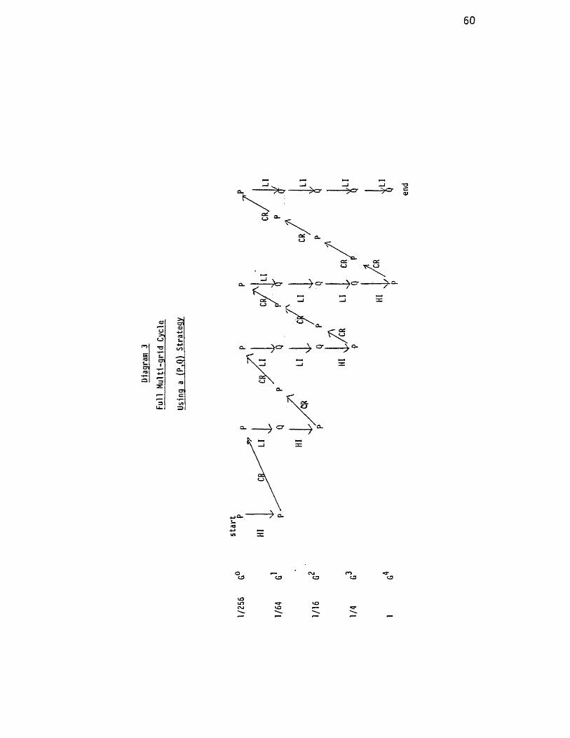
60

61

Diagram 4 Simple Multi-grid Cycle

Using a (P,Q) Strategy

1/256 Gc

1/64 G

1/16 G‘

CR

1/4CRP

/CR

start

LI

4/LlQ

end

62

TABLE 4

961 UNKNOWNS

(P,Q) STRATEGY Time per Simple M u l t i -g r id Cycle ______________________________ (seconds) ______

(1 .1) .0046

(1 ,2) .0058

(2 .1) .0058

(2.2) .0071

63

d i f f e r e n c e equat ions w i l l be solved to w i th in t h e i r t ru n c a t io n

e r r o r in approximately .138 s e c o n d s u s in g t h i s Simple Cycle

m u l t i - g r id s t r a te g y .^ One might expect to see a f a c t o r o f 4

inc rease in time between th e various cases s ince the number of

unknowns N i s inc reas ing by t h i s f a c t o r . However, the times

only inc rease by f a c t o r s of 2 .4 and 3 .2 r e s p e c t i v e l y . This i s a

consequence of the f a c t t h a t vec to rs w ith l a r g e r lengths a re

processed more e f f i c i e n t l y by the CDC S ta r 100. However, when

the average vegtor leng ths become s u f f i c i e n t l y l a r g e , vec to r

s t a r tu p time becomes n e g l ig ib le with r e s p e c t to computation time.

We wi l l then see the f a c t o r o f 4 inc rease between systems with

N and 4N unknowns.

Table 6 compares the times o f Full M u l t i -g r id Cycles using the

(1 ,1) s t r a t e g y with the times f o r Simple M ul t i -g r id Cycles which

use the (1 ,1) s t r a t e g y . In Table 6 we have l i s t e d some ty p ica l

so lu t io n times f o r the same s i z e problems when a Vector Fas t Four ie r2

Transform was used as the s o lu t io n procedure. Recall t h a t by the

end of one Full M u l t i -g r id Cycle the d i f f e r e n c e equat ions a re

solved to w ith in t h e i r t ru n c a t io n e r r o r whereas each Simple

M u l t i -g r id Cycle improves a so lu t io n by another d i g i t . The Fast

Four ie r Transform solves the d i f f e r e n c e equat ions e x ac t ly .

^This presupposes t h a t the s t a r t i n g approximation on the f i n e s t gr id was 0 (1 ) . The t ru n c a t io n e r r o r i s 0(128~2)-0(.0QQ1).

2The FFT f ig u re s were provided by Jay Lambiotte. These times are su b je c t to improvement with l a t e r v e rs io ns of the FFT.

65

TABLE 6

33 x 33 (961 Unknowns)

Time for 1 SimpleMulti-grid Cycle(seconds) .0046 .0109 .0347

Time for 1 FullMulti-grid Cycle(seconds) .0253 .0530 .1261

65 x 65 129 x 129(3,969 Unknowns) (16,129 Unknowns)

Vector Fast Fourier Transform Times .018 .052

66

The times f o r the Full M u l t i -g r id Cycles a re unexpectedly

high and need to be examined more c lo s e l y . Turning to diagrams

1 and 2 we can ob ta in a rough es t im a te of the e x t r a computational

e f f o r t involved in Full as opposed to Simple M ul t i -g r id Cycles.

Roughly 32% more e f f o r t i s expended by a Full M u l t i -g r id Cycle

on the r e l a x a t io n process and 32% more e f f o r t on re s id ua l .

c a l c u l a t i o n s . ^ The r e l a t i v e c o s t s o f the i n t e r p o la t i o n p rocesses

a re more d i f f i c u l t to a s se s s . During Full M u l t i -g r id Cycles

higher o rder i n t e r p o la t i o n s a re used. I f we assume t h a t the

higher o rde r i n t e r p o l a t i o n s a re roughly twice as expensive as

lower o rder i n t e r p o l a t i o n s , then Full M u l t i -g r id Cycles expend2roughly 232% more computational e f f o r t on i n t e r p o la t i o n .

Furthermore, assume t h a t an i n t e r p o la t i o n to the f i n e s t g r id or

a r e s id ua l c a l c u l a t i o n on th e f i n e s t g r id i s comparable in3

computational c o s t to a r e l a x a t io n sweep on the f i n e s t g r id .

With these assumptions one can e s t im a te t h a t a Full M ul t i -g r id

Cycle involves approximately 40% more computational e f f o r t than

a Simple Cycle.

Taking the f i r s t time in Table 6 f o r one Simple M ul t i -g r id

Cycle and m ult ip ly ing i t by 4 and 16 r e s p e c t iv e ly we ob ta in e s t im ates

fo r the computation times of the o th e r two cases . I f each of

these times i s increased by 40%, we ob ta in the ' e x p e c te d 1 times

f o r one Full M u l t i -g r id Cycle. In Table 7 these expected times

^We base these f i g u r e s on the (2 ,2) Full M u l t i -g r id S t ra tegy i l l u s t r a t e d In diagram 1.

2Higher order i n t e r p o la t i o n s fo rce one in to using more expensive vec to r o p e ra t io n s . For in s t a n c e , merge and compress o p e ra t io ns and c a l l s to expensive b i t p a t t e r n g e n e ra to r s .

3This overes t im ates the co s ts of these p rocesses .

67

TABLE 7

33 x 33 65 x 65 129 x 129(961 Unknowns) (3,969 Unknowns) (16,129 Unknowns)

Expected Times for one Full Multi-gridCycle (seconds) .0064 .0258 .1030

Computed Times for one Ful1 Multi-gridCycle (seconds) .0253 .0530 .1261

Vector FFT .018 .052

68

a re compared with the observed times t h a t were presented in Table 6.

We l i s t the Vector Fast Four ie r Transform times fo r purposes of

comparison. The expected t imes f o r the sm aller s ized problems are

s t i l l in s u b s ta n t ia l disagreement with the times t h a t we observed.

The probable explanat ion fo r t h i s anomally has s ince been discovered.

In the Full M ul t i -g r id Cycle the boundary da ta o f the p a r t i a l

d i f f e r e n t i a l equation and the source funct ion must be placed on

each gr id during the downward cycl ing process . The vec to r algori thm

is w r i t t e n in the SL1 language. At the time of these experiments

SL1 was an experimental language in i t s e a r ly s tages of development.

The s tandard t r igonom etr ic and exponential func t ions were not

a v a i la b le . To use these fu n c t ion s one had to i n t e r f a c e with STAR

Fort ran . The boundary da ta and source funct ions were placed on the

g r id s a po in t a t a time through a c a l l to a STAR Fortran subrout ine .

This process o f p lac ing da ta on a g r id was a s c a l a r procedure but

a f a c t o r o f equal importance was t h a t i t involved a subrout ine ca l l

a t each gr id po in t .^ Consider the so lu t io n s of problems one and

th ree in Table 3. Observe t h a t the so lu t ion to problem 1 vanishes

on the boundary of the u n i t square whereas the so lu t io n to problem2

3 s a t i s f i e s a complicated boundary cond i t ion . Furthermore,

c a lc u l a t i n g the source func t ion a sso c ia ted with problem 1 involves

fewer opera t ions than the corresponding c a lc u la t io n fo r problem 3.

The revea l ing information was t h a t the times f o r one Full M ul t i -g r id

^The i n te r f a c e techniques had not been f u l l y developed a t the. time of the experiments.

2The region was the u n i t square 0_<x<1, 0<y<l.

69

Cycle on problem 1 d i f f e r e d s i g n i f i c a n t l y from the times f o r a Full

M u l t i -g r id Cycle on problem 3 J For the 33 x 33, 65 x 65, and

129 x 129 c a se s , problem 3 requ ired 0 .11 , 0 .21 , and 0.42 more

computer time fo r a Full M u l t i -g r id Cycle than did problem 1. The

im p l ica t ion of t h i s observat ion i s t h a t the expected and observed2t imes f o r one Full M u l t i -g r id Cycle can be brought in to agreement.

I t i s d i f f i c u l t to make a se n s ib le comparison between the

Fast Four ie r Transform d i r e c t s o lu t io n technique and the i t e r a t i v e3

m u l t i - g r id method. The con tex t in which these a lgori thms are

used i s important . I f our purpose i s to solve a s in g le Poisson

equation on a r ec tan g le then we would most l i k e l y no t -use e i t h e r

o f these techniques s ince i t would not be worth the programming

e f f o r t . Poisson equat ions u su a l ly a r i s e as one of the equat ions

in a system of p a r t i a l d i f f e r e n t i a l equa t ions . While so lv ing fo r

the so lu t io n of the system of equat ions we may need to ob ta in

many approximate so lu t io n s to d i f f e r e n t Poisson equat ions . In 4t h i s con tex t a m u l t i - g r id Fas t Poisson equation so lv e r would be

extremely e f f e c t i v e . The c u r r e n t approximation to the so lu t io n

The times f o r subsequent Simple Cycles agreed.2

SL1 now has the necessary func t ions a v a i l a b l e . The source data during the downward cycl ing procedure can be placed on the g r id s in a v ec to r opera t ion and the boundary data can be placed on the g r id s with a s in g le subrou t ine c a l l .

3The m u l t i - g r id procedure, un l ike the FFT, i s not r e s t r i c t e d to c on s tan t c o e f f i c i e n t P.D.E. over r ec tan g u la r domains.

^This i s the con tex t f o r which Fast Poisson Equation so lv e rs a re designed.

70

of the system of equa t ions would be placed on the f i n e s t g r id Gm

and improved by a few Simple M u l t i -g r id C y c le s J This improved

approximation would then be used as the i n i t i a l approximation in

some i t e r a t i v e process f o r the next equation in the system. I f

the M ul t i -g r id Fast Poisson equation so lv e r i s used in t h i s

con tex t then we should compare the FFT so lu t io n times with, the

times to make one or two Simple M u l t i -g r id Cycles. From Table 6

we see t h a t in t h i s con tex t the M u l t i -g r id method o f f e r s a

s i g n i f i c a n t improvement over the FFT. This inc rease in e f f i c i e n c y

wil l continue to grow as the problem s iz e s become l a r g e r s ince

the computational e f f o r t grows l i k e 0 ( N) in the m u l t i - g r id

method and l i k e OfNLoggN) fo r the FFT so lu t io n technique .

I t would be sen se le s s to make more than a few Simple Cycles because the approximation must s a t i s f y the o th e r equat ions in the system as w e l l .

2Where N i s the number of unknowns.

CHAPTER 5

MULTI-GRID EXPERIMENTS USING

FINITE ELEMENT DISCRETIZATIONS

The numerical r e s u l t s which a re repo r ted here were obtained

through a j o i n t e f f o r t between R. A. Nicolaides and the p resen t

a u tho r . For h i s a n a ly s i s o f these r e s u l t s , see [9 ] .

Several m u l t i - g r id a lgo r i thm s , which used the Simple Cycle

Correct ion Scheme descr ibed in Chapter 4, were programmed by the

p resen t a u t h o r J These a lgori thms use the f i n i t e element d i s c r e t i z ­

a t io n s d iscussed in Chapter 2. In the experiments we proceeded

from well behaved e l l i p t i c equa t ions to equat ions which were

guaranteed to p re s e n t d i f f i c u l t i e s to the method.

The f i r s t s e t o f experiments were used to s e t s tandards by

which the performance o f the method could be judged when solving

more d i f f i c u l t equa t ions . In these experiments a v a r i e ty of

d i f f e r e n t (P,Q) s t r a t e g i e s were t e s t e d on Poisson equat ions . The

second group of experiments were used in studying the behav io r o f

the method on equat ions which had smoothly varying c o e f f i c i e n t s .

Those s t r a t e g i e s which had been most success fu l in the Poisson

experiments were employed. In the t h i r d s e t of experiments the

^The sec t io n of the code which c o n s t ru c t s the c o e f f i c i e n t m atr ices and the a sso c ia ted r i g h t hand s id e s o f the f i n i t e element systems was designed by R. A. N ico la ides . In a d d i t i o n , Nicola ides programmed sub rou t ines STIGEN and RHS in the appendices. . The data s t r u c t u r e and the m u l t i - g r id procedure i t s e l f a re pa t te rned a f t e r the codes of Brandt.

71

72

c o e f f i c i e n t s were e i t h e r d iscontinuous or ex h ib i ted some type of

s i n g u l a r i t y . The l a s t experiments marked the beginning of a study

o f equat ions with i n d e f i n i t e o p e ra to rs .^

In Chapter 3 we def ined which in the event of a s u i t a b l e

r e l a x a t io n process r e p r e s e n t s thenum ber of m u l t i - g r id cycles

r eq u i red to achieve a 10~^ reduc t ion in the e r r o r between the exact

and approximate so lu t io n of a system of d i f f e r e n c e equa t ions . The

computat ional e f f o r t per m u l t i - g r id cycle i s a func t ion of the

m u l t i - g r id s t r a t e g y t h a t i s used. To assess th e e f f e c t iv e n e s s of

a p a r t i c u l a r s t r a t e g y , we must cons ider the computational cos t of

the s t r a t e g y per cyc le as well as the number o f cy c les t h i s s t r a t e g y

r e q u i r e s to achieve a given reduc t ion in the e r r o r . For purposes

o f comparison, the computational e f f o r t involved in a given m u l t i -

g r id cycle i s measured in work u n i t s , WU. A work u n i t - i s the amount

o f GDC 6400 computer time expended on a s in g le SOR r e la x a t io n

sweep on the f i n e s t g r id during the so lu t io n of a Poisson equat ion

with D i r i c h l e t boundary c o n d i t io n s .

There a re a v a r i e ty o f m u l t i - g r id techniques which may be

t e s t e d . Cycles may d i f f e r from one another in any or a l l of the

bas ic m u l t i - g r id p rocesses : r e l a x a t i o n , res idua l t r a n s f e r , and

i n t e r p o l a t i o n . In conjunc tion with our s tu d i e s o f d i f f e r e n t (P,Q)2s t r a t e g i e s , we examined the e f f e c t s on m u l t i - g r id c y c le s when

c e r t a i n bas ic processes were a l t e r e d .

^In th ese experiments the G° system of equat ions were solved d i r e c t l y with a Gaussian e l im in a t io n subrout ine provided by Max Gunzburger.

2See fo o tno te 4 on page 50 of Chapter 4.

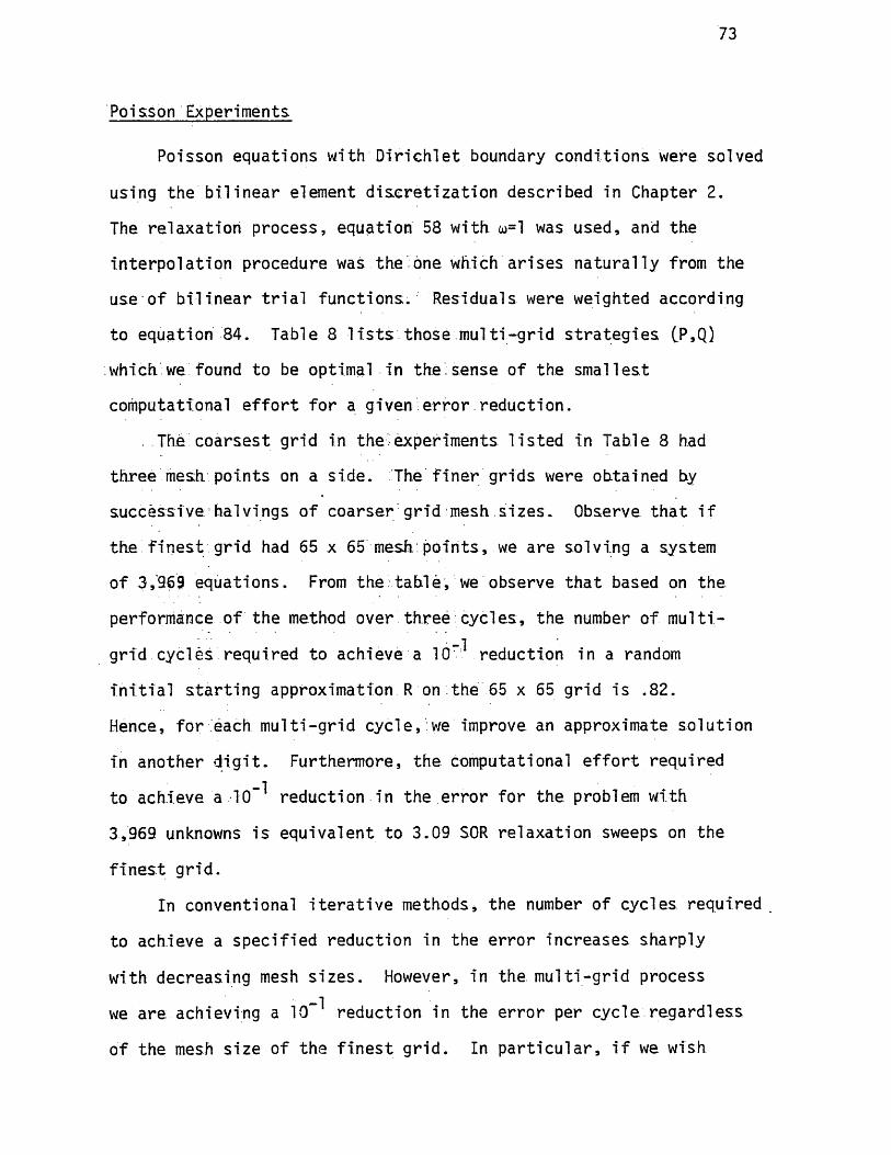
73

Poisson Experiments

Poisson equat ions with D i r i c h i e t boundary con d i t io n s were solved

using the b i l i n e a r element d i s c r e t i z a t i o n descr ibed in Chapter 2.

The r e l a x a t io n p rocess , equation 58 with u=l was used, and the

in t e r p o la t i o n procedure was the one which a r i s e s n a tu r a l l y from the

use o f b i l i n e a r t r i a l fu n c t io n s . Residuals were weighted according

to equation 84. Table 8 l i s t s those m u l t i - g r id s t r a t e g i e s (P,Q)

which we found to be optimal in t h e . s e n s e of the sm a l le s t

computational e f f o r t f o r a given e r r o r reduc t ion .

. The c o a r s e s t g r id in the 'exp er im en ts l i s t e d in Table 8 had

th ree mesh po in ts on a s id e . The f i n e r g r id s were ohtained by

success ive halvings of co a r se r g r id mesh s i z e s . Observe t h a t i f

th e f i n e s t g r id had 65 x 65 mesh, p o in t s , we a re solv ing a system

of 3,969 equat ions . From t h e . t a h l e , we observe t h a t based on the

performance o f the method over th ree cycles., the number o f m u l t i -

g r id cyc les requ ired to achieve a 10” reduc t ion in a random

i n i t i a l s t a r t i n g approximation R on the 65 x 65 gr id i s .82.

Hence, fo r each m u l t i - g r id cyc le , we improve an approximate so lu t io n

in another d i g i t . Furthermore, the computational e f f o r t requ ired

to achieve a 10"^ reduc t ion in the e r r o r fo r the problem with

3,969 unknowns i s eq u iv a le n t to 3.09 SOR r e la x a t io n sweeps on the

f i n e s t g r id .

In conventional i t e r a t i v e methods, the number of cycles required

to achieve a s p e c i f i e d reduc t ion in the e r r o r in c reases sharp ly

with decreasing mesh s i z e s . However, in the m u l t i - g r id process

we a re achieving a 10“* reduc t ion in the e r r o r per cyc le r e g a rd le s s

o f the mesh s iz e of the f i n e s t g r id . In p a r t i c u l a r , i f we wish

74

I/) OlLU £=_l<_J JP>• J=O cro <u

3ccCO

1 <T3=1

1— -o—J3 </lS L 01oc

CO LU__1

UJ Q- </i__1 2: cCO o<c CO1— +Jcc uo o

Lu 3u_iy>LU r—

CO •T—LU s_t— 1—

cc S_H— <aCO <u

co *r“o r—oco CO

Oc.s_ a ; o c c o a c CJ ao CJLU

-P»CJ £

+J >“ 3 CT» GF\ VO o VO <Ti VO oc/i s_ i -a o> CM 00 00 o> O p^ cn c. 3O C D J J O «J

cocu *+- O

c_) •*- 3 a .i— as CM CM CM CM CM CO CM £•p- - o 4->

ia;>

<oX

D1 O +1 O f - ra(U r— CJ

COo ^

r— DJ o r-* CM CO * zr <v "aJU i- *3 r*** o r-* o oo a> 00 o> VO “O S->« <U <U • ■ • • • • *

</> CJ O.QC r*—

<u

u cn cn

S ’

c o Co

sl

in WU

y p

er

Cy

cl

4.2

3.2

co *

oo

CM 3.6

<T\

CM 3.8

3.0

se

co

nd

se

co

nd

r— Ol CO CO 1 1i <a a)

S_ ■+-> -Ma> c -»-» <a O o o O o o0 9 ) Ul L CM CM CM r—> CM r—x e o> •+-> X XLU f - CO CO

LO OCO ^ r— COS-

oc*s- CC gj QC CJ a c CJ a c CJLU CO CO

-*P CO voO CO VO 00 r*N»- CO fmm VO

+J r— 3 CM ^r a* a o CO o CO X X cMl S- 1 "O oO C D 9 ) 0 O) CO CO CM CM CM CM CO CM CO LO

cj **“ 3 cl»— ac s-CT>

CO* vo uJ<a

J B■ 4J

ui O -P cn X01 r— o Oi o

r— 3 CM o cr> cn O cU C 3 a% GO 00 r+> GO CO a .

</> >» a> a) v+- C-<u CJ O.OC <c

OJa JO * i—*>> aj -M cn cn noCJ +J r—’ T3 -O

c/l &. CJ VO r^ CO vo 00 00 C c s -+jCM O C D 41 O o o

CJ i - 3 Q.CJ ro CO CM CO CM CO CM CJ o 3a<u

a a>cn cn

i—.

>1 <u 4->.— Ol CO CO 31 ra O) </) 1 1

O O<a

S_ +J +J /* ■*» -Mo c p ia o o P>— o o p— ao cna . a> c/i s_ * * • O cx £ a> -m CM r— CM I— . CM r— CM r— oo X X oLU i — CO CO

vo *—CJ

co IIs_

l_ o <Jo 4-s_ a c CJ a c CJ a c CJ QC CJs_ o

UJ ^ o o> 00 a> VO VO

s

-MP i“ 3 ol 1- 1 -O a* CO CM GO CM

11

•MO C D 9 ) 0 O

CJ i - 3 0.1— QC CO CM CM CM CM CM CM CMcr»p—

•"J" C X X

ai u iO PttJ r— CJ o o vo CO 00 on P LO r— 3

u>i

C_3CJ S- TO>1 aj a>CJ O.OC

o> CO rs* r>* r-* S-o3

O

4->ra

r— r— £<u

-u>. <— ol S- CJ O C D 9) >1 LO oo VO GO VO p^ O cn

4-J

cn

c

XouC LCJ -r— 3! Q- CJ «^r co CO CM CO CM co CO

c3

3 CL<c

S-r— O* o <a1 <a o S-. XL<P •+-> 40mmmK pM*. oD C -M (T3 a a > vi s. CM o o o 3 &-

o 3X E 0J CM i— CM fmm CM * CM C u-UJ *1— CQ CO g

cn a O4J cn “OP-* co LO cn 3 3

CO VO O ra<y\ •<—«» CT» u cn a :

-p—«*. X m . X r— X VO aX a* CM VO cr» E ii

CM CO o> LO CO0*1 r— — CO VO < c H- ao

75

to ob ta in a so lu t io n on a g r id with N x N mesh p o i n t s , then each

reduc t ion of the e r r o r by a f a c t o r of ten w i l l r e q u i r e the

computational e f f o r t expended in approximately th ree SOR re l a x a t io n

sweeps on the N x N g r id .

From equation 61 we saw t h a t d i f f e r e n t Four ie r e r r o r components

were l iq u id a te d a t d i f f e r e n t r a t e s . Hence, the i n i t i a l d i s t r i b u t i o n

of the e r r o r plays a r o l e in the i n i t i a l e r r o r l i q u i d a t i o n r a t e :

However, once those components which a re e a s i l y l iq u id a te d are reduced

to the p o in t where they comprise a n e g l ig ib le por t ion o f the t o t a l

e r r o r , the components which a re reduced a t a more modest r a t e

dominate the convergence. One can observe t h i s phenomena in Table 8

by n o t ic in g t h a t the values in column th re e inc rease s l i g h t l y during

the f i r s t few m u l t i - g r id c y c le s . I f the r e l a x a t io n procedure i s

s u i t a b l e f o r the equat ions being so lved , the values in column th ree

level o f f a t an accep tab le r a t e as the i t e r a t i o n s in c re a se .

Observe t h a t the behavior o f d i f f e r e n t (P,Q) s t r a t e g i e s was

s tu d ied on both random and c o n s tan t i n i t i a l s t a r t i n g approximations.

These experiments were designed so t h a t the so lu t io n of the

Poisson equat ion was. 0 J Hence, the s t a r t i n g approximation on the

f i n e s t g r id was the i n i t i a l e r r o r . We assumed t h a t an i n i t i a l e r r o r

t h a t was c ons t ruc ted using a random number genera to r would be

r e p r e s e n ta t iv e o f the types of i n i t i a l e r r o r s t h a t one might

encounter in p r a c t i c e . The c o n s tan t i n i t i a l approximation

corresponds to an i n i t i a l e r r o r which i s dominated by low frequency

^We used homogeneous da ta .2

Random e r r o r s should possess a r e p r e s e n t a t i v e sample of e r r o r modes.

76

modes (modes c lose to e=(.0 ,0 ) ) . From mode a n a ly s i s i t i s known

t h a t we should be so lv ing on c o a r se r g r id s when the e r r o r does not

possess high frequency components. Hence, the Simple M ul t i -g r id

Cycle does not take advantage o f smoothness in i n i t i a l e r r o r s .^

In the next experiments , we use the l i n e a r element

d i s c r e t i z a t i o n descr ibed in Chapter 2. The r e l a x a t io n process

in the m u l t i - g r id cyc le was f i v e p o in t SOR with to=l. The

i n t e r p o l a t i o n process i s the one which a r i s e s n a tu r a l l y from the

use of l i n e a r t r i a l fun c t io n s to approximate the so lu t io n . Residuals

were weighted according to the v a r i a t i o n a l p r e s c r i p t i o n discussed2

in Chapter 3.

Table 9 con ta ins information analogous to t h a t presented f o r

the case o f b i l i n e a r t r i a l fun c t io n s in Table 8. Observe t h a t the

b es t s t r a t e g i e s in the sense o f computational c o s t fo r a given

reduc t ion in the e r r o r a re not as c o n s i s t e n t l y the same as they

were f o r the case when b i l i n e a r t r i a l func t ions were used. In

Table 10 the s t r a t e g i e s are s tandard ized in the sense t h a t we

always use s t r a t e g y (3 ,0) f o r random i n i t i a l s t a r t i n g approximations

and s t r a t e g y (2 ,2) f o r c o n s tan t i n i t i a l approximations. Note t h a t

the computational cos ts per ICf^ reduc t ion in the e r r o r a sso c ia ted

with the suboptima! s tandard ized s t r a t e g i e s a re not s i g n i f i c a n t l y

d i f f e r e n t from those in the b e s t s t r a t e g i e s . In g e n e ra l , when the

r e s id u a l s were weighted, s t r a y in g s l i g h t l y from the optimal (P,Q)

s t r a t e g y did not s e r i o u s l y decrease the e f f i c i e n c y of the m u l t i - g r id

^ I t begins with r e l a x a t io n sweeps on the f i n e s t g r id . For g r e a t e r e f f i c i e n c y we should begin the r e l a x a t io n sweeps on co a r se r g r id s i f we know t h a t the e r r o r i s smooth. However, in p r a c t i c e we do not know what the i n i t i a l e r r o r looks l i k e .

2See equat ion 55.

TABL

E 9

77

o>-C_3

ea

aaoo

i . i -a aj o a> Q .r— OS

U S . T 3>» <u <v«_> O -C C

O C =3 <U >» tj -r- 3? Q.CJ

<U C -M ra a a j in s . x g a» -m

LU n— o a o o

s-os-w

uj+JU

r—• 3</l i . t -oO C D aj o a>U f - 3 ac

u to +J a» r— o 3CJ S- T3 > 0 1 9) <_> a . a :

u» S_ CJO C 3 (I) > 1

0 - ^ 3 Q -L J

a a in l X S 0J -M

U J 1— 0 3 CO

«CJ>i

os.s.U4 +->

<J4-> r— 301 S- i -oO £ 3 a) o a)O -r- 3 Q-r— ac

i—

<n o +->OJr— u

3CJ i- “O>1 <u <u CJ o*oc

o C 3 ai >iCJ -T- 3 Ol CJ

11- ra a> c u u9) C J IQ Ol 4J co S- x = aj -m LU_- - CQ LO

ac CJ ac o ac CJ ac O

oo r*K LO rK 04 <n <nLO f—» GO vo 00

3- CO CO

VO 00 LO 04 cn Ok o ovo o Ol LO 04 <n a <n

~ ~

CO oa LO 04 o r— COCO CO vo Ok o vo CO

VO or 04 ro * r O'

© CO c? r—■ o 04 *© CO

04 ro 04 04 CO 04

ac CJ o ac CJ ac O

-a

i-cn

Ok Ok r** CO LO CO 00VO cn o VO CO 44

<Si«3“ CO CO CO O)

£

4“

CUvo ^t- 04 CO vo -Co r-* cn 04 <n 44

1- i-» r- ca

C L© O rs. LO vo CO o 00 <U04 VO fK* « r OO vo <n <1)

• « • • 3< t CO 04 CM CM vn

ac. oGOp- .

><■■p—• p— o i— o CM o CM 1m

o04 04 04 «— CO r— CO *— 4-

a

4->ac CJ ac CJ ac O ac O

II

44co VO o OO o CO CO co •r—

04 <n VO P*K 04 00 CM a3

•sr CO CO CO CO CO CO-XS-o

*0 04 cn CO Ok LO CO <nLO LO r . 04 vo O 00 cn

V)4->

* £3© a vo o O CO LOGO GO cn o LO O vo CM

• • • • • • S.f*K 04 o- CO LO CO CO o

£

r-m r— r> 04 o CO o CO CUm * * u

lO p— CO r— *3" r— co r— 19

LO44

r*K CO LO (/»CO vo ocn *-“K <n o

X LO X fW X VOX <n 04 LO cn

Ok CM CO <n LO CO<n *— • CO VO ■—* <

oo«3-CO

c c c cr-. 0 0 . 0 0<a <J cj c j c j

aj cu <u <u</)(/!(/>(/)

C CO fO CO CO I—I I I I Io o o o

+-> 1— r— I— I—Cra X X X X

X X X X

■ocracc

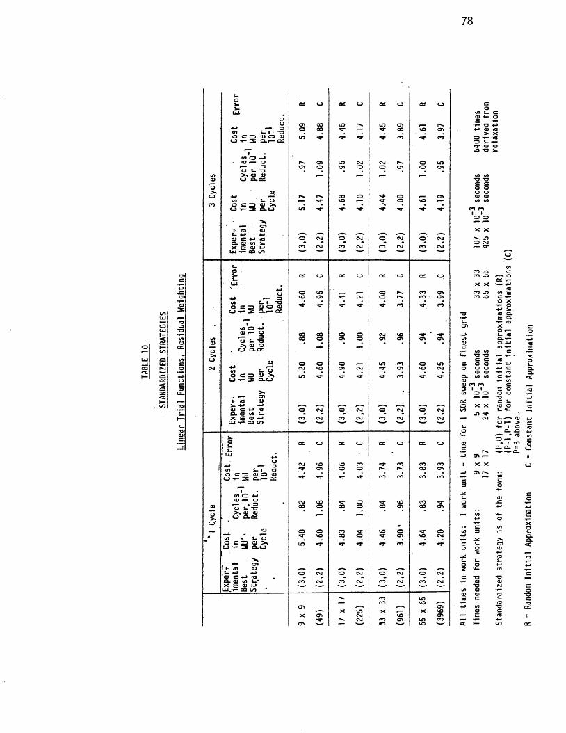
78

CTC

-M-CCT<U

3tnUJ

■acu 3LU -a1—< c </>ac <u

o I— a cr— to

LU Q u tLU e z

ca ru o«ch- a 4->

ac o■s ca 32= LU«C

r—. to (O

U1—

S-<a<uc

_ i

u t >« ai <u<u o o . ac

o +-»(/I s_ *3

CO a C 35 ai > i<_>-T- 3 O.CJ

■po»— 3s_ i -a a) a aia . r - a c

>»i— o»I ra <u S_ -M +Jai c p « a ai ut t .X S <U -M

s_oi-s_LU ,

-MCJ

-U> <— 3U t L_ 1 -Oa C 35 aj o ai

C_5 -r- 3 a.#— ac

1tn O -u><U o

3U L U

<u+Ju t £- CJO S= =3 ai >»

CJ •*- 3 CLCJ

cnI- <T3 aiS_ -M -u>4J C P <aOl 05 co L.X S <UPJ

lu *r— aa to

uci_s-

LU 4->- u

4-J 3cn S- 1 -30 3 35 <u o <U

U * f 3 a ./— a :

u i - - o >» <u <v

<J O.OC

•

I I- /a ati- -M -Miu c p ia a . <u </> l.*X g (U Pjj .i- ca tn

Q£ o a c o QC o a c CJ £o

05 S. 30) 4-JS O

05 00 LO p** LO 05 p^GS

•r- T3 4-1O co *—> CO VO 05 -m qj <Q

• > XLO CO CO o (Q

o s-^P CJ aVO “O c.

05 LO CM CM p^ o LO05 O 05 o O 05 o 05

cn cn*0 T3C 3O OO U

CO o o PB 05 <V CJVO r-> o vo i— tn cn

LO *3° CO CO

o o*— r—

X X

o CM O CM o CM o CM P . LOO CM

CO CM CO CM CO CM CO CM r— 3

CJ

inco in 3

QC CJ a c CJ QC CJ c c CJ co vo ^ Oo: -r-

X X -----rt3

o LO fmm CO p*l CO 05 co m cn SVO 05 CM o p*. CO 05 co vo 3 t-

O X<3- CO co t- O

4-> C.“O ra c .

S CLc. 1— ra05 X 3

o •— oCO CO o o CM vo +-> S- raCO o 05 o 05 05 05 05 vt Q.-»- 4->

• • • • • « o Q.-M rac ra 1— ' E

in in 3-a -o r—> • . XCZ 3 ra o

o o o LO CO O LO o o o • f -M L-CSJ VO 05 CM <5T 05 vo CM o o a 4J 3 a .

• • • • • • <u <u •»- ra Q.LO co <3* a . cn m 3 +-> c

<u •p- inCJ co co 33C i i s o racn o o o a

"OCC 3 £-o X X <a O c

o CM O CM O CM O CM OO S_ M-in

CO CM CO CM co CM CO CM r» CM aJ 4->O r - >

C. I o rao r \ o<*- » ra tn

O r— 3a c CJ CC CJ a c CJ CC CJ <v * 1 CO O

B a . a . u CJ+j 05 *— 11

CM VO VO CO co CO CO ii X X ■cj05 o o p . CO 05

4J 05 P^co CO CO CO i

c s-3 o

4—3

C* <D oCM 00 *3* o vo co o -3CO o CO o co 05 CO 05 4J 4-4

rain 4- BO

X3 in o

o o CO vo o o cn 3 c.vo CO o <r 05 vo CM OL

30 Q»LO <r CO <r C C. 05

3 o ai3 4-> p—

«a <at- c. s-O o 4-Js v»- in

o CM o CM O CM o CM 3c T3 “O

CO CM co CM CO CM CO CM •»—• OJ a>-a ISi £

</> aj *r Oai aj “O -a

p^ CO LO S s z C. 3CO vo ra «a

o» 05 4-> cn -o c cX LO X X VO a 3

X 05 CM vO 05 S ra itCM CO 05 LO CO p— 4-)

o» CO '' VO <c *— C/5 QC

79

cy c le . As a ru le of thumb, s t r a t e g i e s t h a t were g en e ra l ly very

good fo r random i n i t i a l approximations were o f the form (P,0) where

P - 2 in the case of b i l i n e a r t r i a l func t ions and P=3 in the case of

l i n e a r t r i a l fu n c t io n s . S t r a t e g ie s of the form (P-1,P-1) were

e f f e c t i v e on smooth s t a r t i n g e r r o r s . These ru le s of thumb fo r

good s t r a t e g i e s a re dependent upon the type of M u l t i -g r id Cycle

( e . g . , Simple Cycle) and the types of r e l a x a t i o n , res idua l w e igh ting ,

and i n t e r p o la t i o n ro u t in e s t h a t a re used.

For the problems t h a t were solved in our experiments , f ixed

(P,Q) s t r a t e g i e s worked e f f e c t i v e l y . An a l t e r n a t i v e to f ixed

s t r a t e g i e s a re the adap t ive techniques d iscussed in Brand t 's

paper on M u l t i -g r id Methods [1 ] , With these methods in te rn a l

c r i t e r i a a re used to decide the o rder in which g r id s a re v i s i t e d .

They take advantage o f how the s o lu t io n i s evolving. When the

so lu t io n i s smooth they au to m a t ica l ly proceed to coa r se r g r i d s .

One p r a c t i c a l d i f f i c u l t y o f adap t ive methods, when applied to

simple problems, i s t h a t th e information requ ired by the switching

mechanism may be r e l a t i v e l y expensive to c a l c u l a t e . However,

when the problems become more complicated^ then the information

requ ired by the switching mechanism becomes small r e l a t i v e to the cos t

o f a m u l t i - g r id cyc le . Our model problem involved r e l a t i v e l y

few o pera t ions per g r id p o in t so we opted f o r a f ixed s t r a t e g y .

^When they involve more ope ra t ions per g r id p o in t .

80

Ramifica tions of D i f fe re n t In t e r p o la t i o n

and Residual T ransfe r Techniques

A p o ss ib le i n t e r p o la t i o n procedure^ between g r id s i s the one

determined by the c l a s s o f p iecewise polynomials used in approx­

imating the s o lu t io n s o f the coarse and f i n e g r id systems.

Consider the s t e n c i l o f p o in t s :

O o

1 G O (81 )

where dots correspond to f i n e g r id p o in t s , c i r c l e s to coarse g r id

p o in t s , and v-j through to known values a t coarse gr id p o in t s .

I f so lu t io n s a re approximated with b i l i n e a r t r i a l func t ions then

the i n t e r p o la t i o n op e ra to r E corresponding to the s t e n c i l above i s :

'nf x nc

1 0 0 01/2 1/2 0 00 1 0 01/2 0 1/2 01/4 1/4 1/4 1/40 1/2 0 1/20 0 1 00 0 1/2 1/20 0 0 1

(82)

9 x 4

I n t e r p o la t i o n procedures cannot be s tud ied independently of the m u l t i - g r i d p ro c e s s . In p a r t i c u l a r , one should t r y to ensure t h a t the i n t e r p o la t io n process does not in troduce high frequency e r r o r components on f i n e r g r id s .

81

where nf re p re se n ts the number of f i n e g r id po in ts and nc the

number of coarse g r id p o in t s . Observe t h a t the values a t

coarse gr id po in ts

(83)

a re in t e r p o la t e d to f in e g r id po in ts by the ope ra t ion Ev. Using

the v a r i a t i o n a l p r e s c r i p t io n in Chapter 3 we weight and t r a n s f e rT-

the r e s id u a l s r through the opera t ion E r . By c o n s t ru c t in g the

i n t e r p o la t i o n ope ra to r E f o r a l a r g e r s t e n c i l of po in ts and taking

i t s t r an sp ose , one can v e r i f y t h a t the f i n e g r id res id ua l a t mesh

po in t ( i , j ) i s weighted with i t s neighbors according to:

r i »j + + r i+l , j -1 + r i -1 »j+l + r i+ l , j+ 1 )

+ + Vl.j + ri+1 + rT,j+l) (84)

before i t i s t r a n s f e r r e d to a coarse r l e v e l . The v a r i a t i o n a l

formula tion has thus in d ica ted t h a t the information requ ired in the

r i g h t hand s ide of the coarse g r id equation corresponding to po in t

( i , j ) i s a weighted average of f in e g r id r e s id u a l s about t h i s po in t .

Observe t h a t the weights in express ion 84 sum to 4. This

res idu a l sca l in g f a c t o r i s a consequence of the r a t i o of the mesh

s i z e s between consecu t ive g r id s h^ : h^+^=2:1.

82

When 4r . • i s t r a n s f e r r e d to a c o a r se r g r id system, the »

r e s id u a l s are sa id to be i n j e c t e d . I f q u a n t i t i e s of the form.

84 a re t r a n s f e r r e d , the r e s id u a l s a re sa id to be weighted. The

computational cos t s to achieve a 10""1 reduct ion in i n i t i a l e r r o r s

were computed f o r both techniques over a range of d i f f e r e n t m u l t i -

g r id s t r a t e g i e s (P,Q) and over various numbers o f m u l t i - g r id cyc les .

Tables 11 and 12 compare the computational c o s t s o f using in je c te d

as opposed to weighted r e s i d u a l s fo r cons tan t and random i n i t i a l

approximations o f the s o lu t io n s . The m u l t i - g r id cycles used in

the computations contained the i n te r p o la t io n and re l a x a t io n

processes which a r i s e n a tu r a l l y from the use of b i l i n e a r t r i a l

fu n c t io n s . 'In Table 13 and 14 s i m i l a r r e s u l t s a re tab u la te d f o r

the case when l i n e a r t r i a l func t ions and t h e i r a s so c ia te d i n t e r p o l ­

a t io n and r e l a x a t io n processes a re used in the m u l t i - g r id cyc les .

In Tables 15 through 18 we have tab u la ted the number of Simple

M u l t i -g r id Cycles req u i red to reduce the i n i t i a l e r r o r by a f a c t o r

o f 10 fo r the var ious (P,Q) s t r a t e g i e s presented in Tables 11 through

14.

I f the lowest c o s t s a t t a i n a b l e by the i n j e c t i o n procedure are

compared to the lowest cos ts a t t a i n a b l e by the weighting procedure,

one observes t h a t in terms of computational c o s t per IQ-1 e r r o r

r e d u c t io n , the optimal i n j e c t i o n s t r a t e g i e s a re v i r t u a l l y i d e n t i c a l

in e f f i c i e n c y with the optimal weighting s t r a t e g i e s . 1

H h ese observa t ions a re based on the performance o f a Simple Cycle on random i n i t i a l s t a r t i n g e r r o r s which i s the case t h a t we should be prepared to encounter in p r a c t i c e . With our Simple M ul t i -g r id Cycle, the h igher c o s t s fo r cons tan t s t a r t i n g e r r o r s near the optimal s t r a t e g i e s i s a consequence of the wasted e f f o r t on the f i n e r g r id s .

83

TABLE 11

BILINEAR ELEMENTS

Figures based on 3 Simple Cycles on a 33 x 33 grid.

Constant In i t ia l Approximation

Injected Residuals Weighted ResidualsWU/10” ' Error Reduction WU/1CT' Error Reduction

Q5 11.22 3.85 5.08 3.75 4.54 4.23 4.19 4.55 4.15 4.82

4 - 11.05 3.63 4.85 3.57 4.38 4.08 4.05 4.27 4.01 4.65 -

3 • 11.07 3.40 4.41 3.39 4.19 3.87 3.95 4.17 3.84 4.57

2 - 11.90 3.03 4.05 3.34 3.98 3.75 3.81 3.98 3.74 4.43

1 - 12.53 ( 2 7 7 4 ) 3.72 3.14 3.80 3.51 3.73 3.88 3.58 4.48

0 ★1

3.32 ( 3 7 3 2 ) 3.60.

3.71 3.82i

3.67 4.20i

3.51 4.70t

1 2 3 4 5

*Indicates divergence.

1 WU = .135 seconds

84

TABLE 12

BILINEAR ELEMENTS

Figures based on 3 Simple Cycles on a 33 x 33 grid.

Random In i t ia l Approximation

Injected Residuals Weighted ResidualsWU/10"‘ Error Reduction WU/10- ' Error Reduction

Q5 14.68 5.32 5.83 3.95 4.39 4.42 3.85 4.23 3.66 4.38

4 71.52 5.12 5.47 3.67 4.71 4.03 3.66 4.20 3.48 4.38

3 51.53 4.59 5.83 3.52 4.32 3.93 3.40 4.04 3.42 4.30

2 27.38 4.44 6.05 3.36 4.00 3.71 3.41 3.81 3.31 4.22

1 13.19 4.00 5.02 3.13 3.93 3.57 3.46 3.72 3.10 3.99

0★

13.72 5.94 3.63 3.401 3.07 3.66

...3.93

1 2 3 4 5 P

*Indicates divergence.

1 WU = .135 seconds

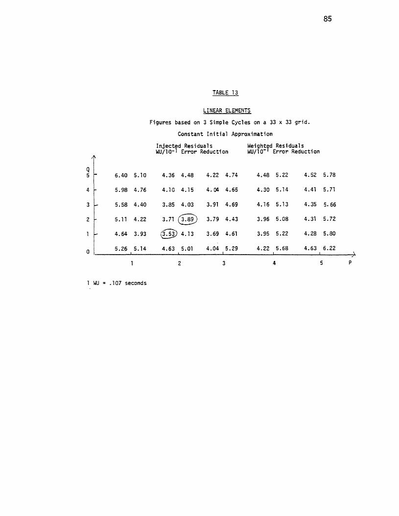
85

/fk

TABLE 13

LINEAR ELEMENTS

Figures based on 3 Simple Cycles on a 33 x 33 grid.

Constant In it ia l Approximation

Injected Residuals Weighted ResidualsWU/1CH Error Reduction WU/10"' Error Reduction

Q5 - 6.40 5.10 4.36 4.48 4.22 4.74 4.48 5.22 4.52 5,78

4 - 5.98 4.76 4.10 4.15 4.04 4.65 4.30 5.14 4.41 5.71

3 - 5.58 4.40 3.85 4 .03 3.91 4.69 4.16 5.13 4.35 5.66

2 5.11 4.22 3.71 ( j T a s ) 3.79 4.43 3.96 5.08 4.31 5.72

1 4.64 3.93 (£ 5 3 ) 4.13 3.69 4.61 3.95 5.22 4.28 5.80

0 5.26 5.14•

4.63 5.011 4.04 5.29t

4.22 5.681

4.63 6.221

1 2 3 4 5

1 WU = .107 seconds

86

TABLE 14

LINEAR ELEMENTS

Figures based on 3 Simple Cycles on a 33 x 33 grid.

Random I n i t ia l Approximation

Injected Residuals Weighted ResidualsW U / I C H Error Reduction WU/10"' Error Reduction

Q5 ★ 7.57 8.96 6.02 7.46

4 - ★ 7.05 8.11 5.54 6.44

3 - ★ 6.48 9.41 5.33 6.65

2 - * 6.14 7.28 4.95 5.81

1 - 142.73 5.50 6.11 4.60 5.79

0*

i 5.40 6.93 5.35

1 2

*Indicates divergence.

1 WU = .107 seconds

5.67 5.64 5.54 5.21 5.86

5.48 5.36 5.69 5.12 5.69

5.16 5.53 5.28 4.88 5.53

4.96 4.71 5.04 4.59 5.41

4.58 4.72 4.83 5.13

4.57 4.63 4.85 4.96 4.88

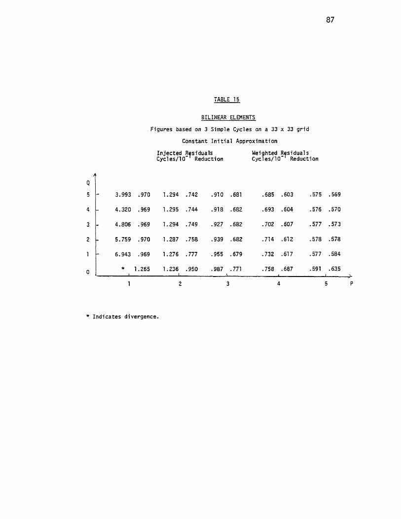
87

TABLE 15

BILINEAR ELEMENTS

Figures based on 3 Simple Cycles on a 33 x 33 grid

Constant In i t ia l Approximation

Injected Residuals Weighted ResidualsCycles/10 Reduction Cycles/10~ Reduction

AQ

5 - 3.993 .970 1.294 .742 .910 .681 .685 .603 .575 .569

4 - 4.320 .969 1.295 .744 .918 .682 .693 .604 .576 .570

3 - 4.806 .969 1.294 .749 .927 .682 .702 .607 .577 .573

2 - 5.759 .970 1.287 .758 .939 .682 .714 .612 .578 .578

1 - 6.943 .969 1.276 .777 .955 .679 .732 617 .577 .584

0*

t1.265 1.236

i.950 .987 .771

\.758

.i687 .591 .635

»1 2 3 4 5

* Indicates divergence.

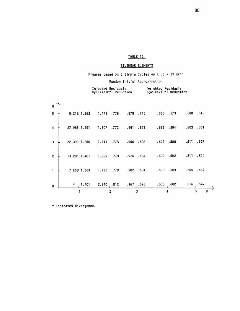
88

TABLE 16

BILINEAR ELEMENTS

■''KQ

Figures based on 3 Simple Cycles on a 33 x 33 grid

Random In i t ia l Approximation

Injected Residuals Weighted ResidualsCycles/10"' Reduction Cycles/10"! Reduction

5.218 1.363 1.479 .778 .878 .713 .635 .573 .508 .518

27.985 1.391 1.507 .772 .991 .675 .629 .594 .503 .531

22.392 1.350 1.711 .778 .956 .698 .607 .588 .511 .537

13.281 1.401 1.929 .778 .936 .684 .639 .582 .511 .544

7.258 1.369 1.720 .779 .982 .684 .680 .589 .505 .537

* 1.401 2.240 .812 .967 .693 .635 .602 .516 .547 !______________________ I___ '_____________________ ■ < __________________ !________

5 P

* Indicates divergence.

89

2.251

2.294

2.352

2.432

2.495

3.323

TABLE 17

LINEAR ELEMENTS

Figures based on 3 Simple Cycles on a 33 x 33 grid.

Constant I n it ia l Approximation

Injected Residuals Weighted ResidualsCycles/10- Reduction Cycles/ 10” ' Reduction

1.361 1.113 .909 .848 .804 .740 .754 .635 .721

1.361 1.117 .918 .854 .817 .744 .771 .643 .737

i .363 1.124 .935 .864 .840 .750 .794 .654 .759

.372 1.144 .972 .881 .878 .757 .828 .672 .789

.438 1.218 1.066 .918 .947 .776 .881 .701 .832

!.039 1.740 1.403 1.090 1.139 .877 1.003 .791 .920 1 ! : 1 ^

2 3 4 5 P

90

TABLE 18

LINEAR ELEMENTS

Figures based on 3 Simple Cycles on a 33 x 33 grid

Random I n it ia l Approximation

Injected Residuals Weighted ResidualsCycles/IO’ T Reduction Cycles/10- Reduction

A

Q

5 (- * 2.123 2.281 1 .293 1.505 1 .015 .937 .834 .735

* 2.106 2.228 1.265 1.371 1.003 .925 .882 .749

* 2.092 2.750 1.246 1.502 .987 1.003 .837 .742

* 2.104 2.299 1.272 1.384 .992 .892 .835 .719

77.134 2.078 2.115 1.253 1.439 .985 .934 .850 .719

* 2.196 2.579 1.274 1.447 1.001 .968 .884 .840 ____;________ 1 .. ■ ■______ < ■ t ■ ______

.761

.764

.760

.771

.762

.756 J____

*Indicates divergence.

91

An important c o n s id e ra t ion in decid ing whether or not to use

i n j e c t i o n f o r Simple M u l t i -g r id Cycles i s the pena l ty paid i f

adequate p recau t ions a re not made to ensure t h a t the r e s id u a l s

a re s u f f i c i e n t l y smooth. From Tables 12 and 14 we observe t h a t

the e f f i c i e n c y of s t r a t e g i e s which conta in i n j e c t i o n range from

those t h a t do not work a t a l 1 to those t h a t a re as e f f i c i e n t

as the corresponding (P,Q) s t r a t e g i e s which c o n ta in r es idua l

weighting.

For m u l t i^g r id cyc les using re s id ua l weighting , the r e l a t i v e

e f f i c i e n c y o f the method over the var ious (P,Q) s t r a t e g i e s i s ,

s i g n i f i c a n t l y l e s s pronounced. Furthermore, no s t r a t e g y con ta in ing

re s id u a l weighting d iverged . In g e n e r a l , f o r the Simple Cycle

a lgor i thm used in these experiments the r e l a t i v e l y small inc reases

in e f f i c i e n c y which could r e s u l t from the use of i n j e c t io n were

outweighed by i t s reduced r e l i a b i l i t y . We cannot conclude from

these experiments t h a t r e s id ua l weighting i s p re fe ra b le to i n j e c t i o n

f o r Poisson e qua t ions . For i n s t a n c e , the Full M u l t i -g r id Cycle2l i m i t s the high frequency e r r o r s on f i n e r g r i d s . In j e c t io n was

used in the Full M u l t i -g r id Cycles and no d i f f i c u l t i e s were3

encountered. We conclude from these experiments t h a t fo r Simple

H h i s i s a consequence of the f i n e g r id r e s id u a l s not having been smoothed enough before they were t r a n s f e r r e d .

2Obtaining the i n i t i a l approximation from the c o a r se r g r id s and using h igher o rder i n t e r p o la t io n on the way down a re the precau t ions which do t h i s [1 ] .

3S t r i c t l y speaking t h i s i s not a f a i r comparison s ince d i f f e r e n t r e l a x a t io n processes were used in the Full and Simple M ul t i -g r id Cycles. Full M u l t i -g r id Cycle experiments using a Gauss Seidel r e l a x a t io n process should be used in the comparison.

92

M u lt i -g r id Cycles i t i s gene ra l ly adv isab le to weight the

r e s id u a l s .^

From these experiments one i s tempted to make a judgement

concerning the r e l a t i v e e f f e c t i v e n e s s o f the b i l i n e a r as opposed

to l i n e a r d i s c r e t i z a t i o n s . Once again our obse rva t ions w i l l p e r ta in

only to Simple M u l t i -g r id Cycles. Our comparison should take

in to account the r e l a t i v e co s ts of the d i f f e r e n t r e l a x a t io n

processes t h a t we used. I f we compare the optimal (P,Q) s t r a t e g i e s

f o r b i l i n e a r and l i n e a r d i s c r e t i z a t i o n s , Tables 12 and 14 r e s p e c t iv e ly ,

and take in to account the r e l a t i v e cos ts o f a work u n i t , WU, then

the b i l i n e a r element d i s c r e t i z a t i o n required .41 seconds per ICT^

e r r o r reduc t ion whereas the l i n e a r element d i s c r e t i z a t i o n requ ired

.47 seconds fo r the same red u c t io n . The advantage of the b i l i n e a r

d i s c r e t i z a t i o n over the l i n e a r d i s c r e t i z a t i o n in Simple M ul t i -g r id

Cycles does not l i e in t h i s marginal improvement in e f f i c i e n c y

in the event t h a t bes t s t r a t e g i e s a re compared. I t s s t r e n g th was

cons is tency of performance when we s t rayed s l i g h t l y from the bes t

s t r a t e g y .

Mixed Boundary Conditions

In the previous s e c t io n we saw t h a t the b i l i n e a r element

m u l t i - g r id method achieved a 10” reduct ion in an i n i t i a l e r r o r

on Poisson equat ions with D i r i c h l e t boundary cond i t ions a t a

computat ional expendi ture eq u iva len t to roughly 3 nine po in t SOR

^We have been r e s t r i c t i n g our a t t e n t i o n to Poisson equat ions . For P.D.E. with v a r i a b le c o e f f i c i e n t s , weighting i s u su a l ly adv isab le .

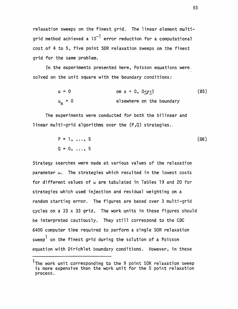
93

r e l a x a t io n sweeps on the f i n e s t g r id . The l i n e a r element mult i -

g r id method achieved a 10’ e r r o r reduc t ion f o r a computational

c o s t o f 4 to 5, f i v e po in t SOR r e la x a t io n sweeps on the f i n e s t

gr id f o r the same problem.

In the experiments p resented here , Poisson equat ions were,

solved on the u n i t square with the boundary co n d i t io n s :

u = 0 on x = 0, 0<y<l (85)

un = 0 elsewhere on the boundary

The experiments were conducted f o r both the b i l i n e a r and

l i n e a r m u l t i - g r id a lgor i thm s over the (P,Q) s t r a t e g i e s . .

P = 1, . . . , 5 (86)

Q * 0, . . . , 5

S tra tegy searches were made a t var ious values o f the r e l a x a t io n

parameter to. The s t r a t e g i e s which r e s u l t e d in the lowest cos ts

fo r d i f f e r e n t values o f to a re t ab u la te d in Tables 19 and 20 fo r

s t r a t e g i e s which used in j e c t i o n and res id ua l weighting on a

random s t a r t i n g e r r o r . The f ig u re s a re based over 3 m u l t i -g r id

cyc les on a 33 x 33 g r id . The work u n i t s in these f ig u re s should

be i n t e r p r e t e d c a u t io u s ly . They s t i l l correspond to the CDC

6400 computer time requ ired to perform a s in g le SOR r e la x a t io n

sweeps on the f i n e s t g r id during the s o lu t io n of a Poisson

equat ion with D i r i c h l e t boundary co n d i t io n s . However, in these

^The work u n i t corresponding to the 9 po in t SOR re l a x a t io n sweep i s more expensive than the work, u n i t fo r the 5 po in t r e l a x a t io n process .

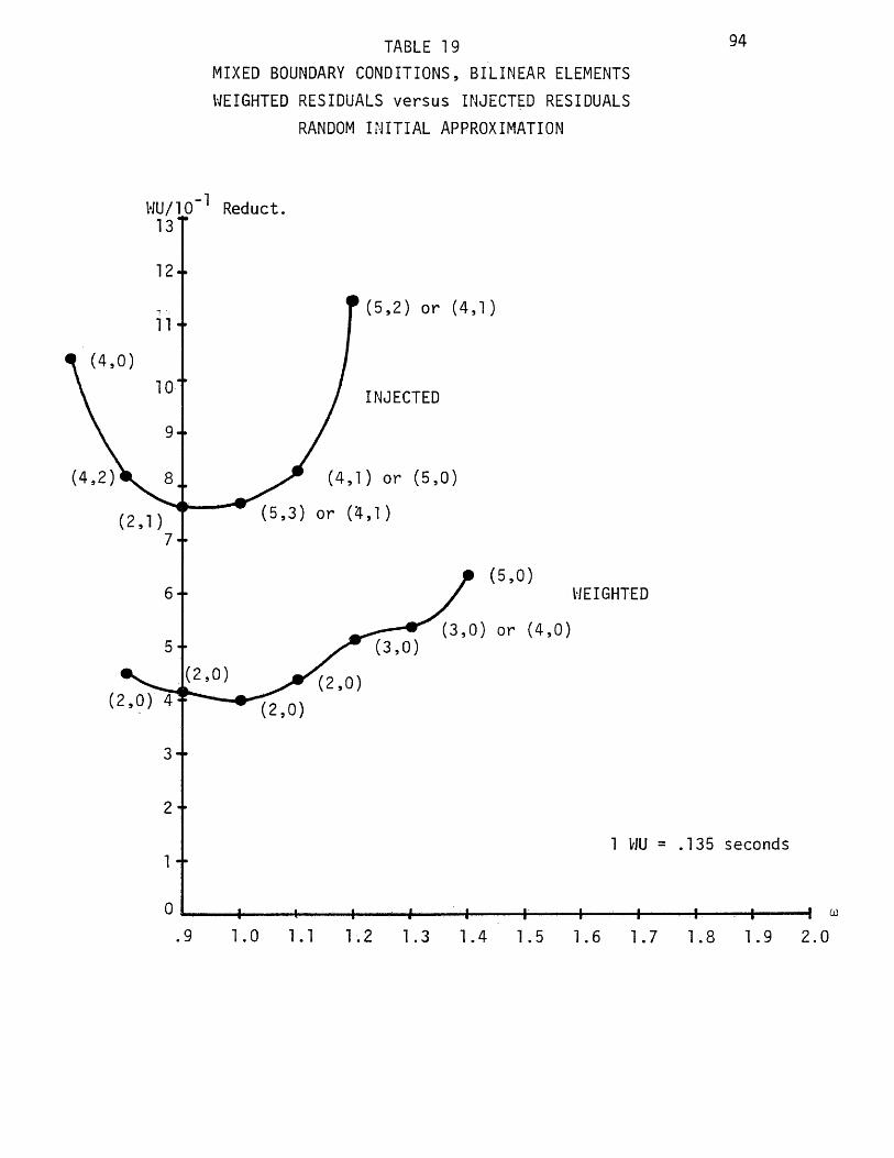
13

12

11

10

9

8

)7

6

5

3

2

1

0

TABLE 19MIXED BOUNDARY CONDITIONS, BILINEAR ELEMENTS WEIGHTED RESIDUALS versus INJECTED RESIDUALS

RANDOM INITIAL APPROXIMATION

94

Reduct.

(5 ,2) or (4 ,1)

INJECTED

(4,1) or (5,0)

(5 ,3) or (4 ,1)

(5,0)WEIGHTED

0 , 0)(3 ,0) or (4,0)

:2,0) ( 2 , 0 )

( 2 , 0 )

1 WU = .135 seconds

^ ----- — 4 I *--- -— H— ---1---------1-------------- 1 031.0 1.1 1.2 1.3 1.4 1.5 1.6 1.7 1.8 1.9 2.0

18

17,

16.

15.

14,

13

1 2 ,

11,

10

9

8

7.

6 .

5,

4.

3

2

1

0

TABLE 20MIXED BOUNDARY CONDITIONS,- LINEAR ELEMENTS

WEIGHTED RESIDUALS versus INJECTED RESIDUALS RANDOM INITIAL APPROXIMATION

95

MU/10'1 Red.* (5,2)

INJECTED

WEIGHTED

(5,0) or (4 ,0) or (3,0)

(5,0) or (3 ,0) or (4,0)

(3 ,0) or (4 ,0) or (5 ,0)

(2 , 0 )( 2 , 0 )

1 WU = .107 seconds

+-.7

+-.8

-I -4--------- 1--------- 1----------1-------- +---------1--------- 1-------—I------- - f— oj;9 1.0 1.1 1.2 1.3 1.4 1.5 1.6 1.7 1.8

96

experiments we a re performing e x t ra work a t the boundary po in ts

where Neumann condi t ions hold. Hence, f o r a Neumann problem on

the same s i z e gr id as a D i r i c h l e t problem, we expect the c o s t

in work u n i t s fo r a 10""* reduct ion in the e r r o r to be s l i g h t l y

g r e a t e r simply as a consequence of the e x t ra boundary work. When

we compare the e f f i c i e n c y o f the m u l t i - g r id cycle on Neumann

problems with i t s e f f i c i e n c y on D i r i c h l e t problems, we w i l l not

use the work u n i t as our u n i t of measure. Ins tead we use the

number of m u l t i - g r id cycles requ ired to achieve a sp e c i f i e d

reduc t ion in the i n i t i a l e r r o r as our c r i t e r i a f o r comparing

the r e l a t i v e e f f i c i e n c y o f the method in dea l ing with D i r i c h l e t

and mixed boundary co n d i t io n s . Observe t h a t with a m u l t i -g r id

cycle which uses weighted r e s i d u a l s , a good (P,Q) s t r a t e g y ,

and the proper choice of the r e l a x a t io n parameter w, the costs

of reducing a random i n i t i a l e r r o r i s roughly equ iva len t to

four work u n i t s f o r the b i l i n e a r element m u l t i - g r id procedure.

This i s comparable^ to the th re e work u n i t f i g u r e in the case

of D i r i c h l e t boundary co n d i t io n s . For the l i n e a r element

m u l t i - g r id implementation with re s id u a l weigh ting , the cos ts

can be reduced to four to s ix work u n i t s f o r problem 85. Again,

t h i s i s comparable to the four to f i v e work u n i t s expended by

the l i n e a r element m u l t i - g r id technique when app l ied to Poisson

equat ions with D i r i c h l e t boundary co n d i t io n s . Observe t h a t th e

cos ts to obta in a 10”"* reduc t ion in the e r r o r when in je c t io n

^To make the comparison more p rec i se we wil l examine the e r r o r reduc t ion r a t e in a moment.

97

i s used in the m u l t i - g r id cycles a re considerably g r e a t e r than

the c o s t s o f cycles using res id ua l weighting. Through mode an a ly s i s

i t can be e s t a b l i s h e d t h a t high frequency f l u c t u a t i o n s are i n t r o ­

duced in to the r e s id u a l s near Neumann cond i t ion boundary po in ts .

Hence, r e s id u a l s should a t l e a s t be weighted near such p o in ts .

I f the convergence process i s slower near boundaries even though

the r e s id u a l s near boundary po in ts have been weighted, ex t ra

r e l a x a t io n sweeps can be made over the boundary po in ts a t a

n e g l ig ib le a d d i t io na l computational c o s t .

In Table 21 we t a b u la t e the number of Simple M ul t i -g r id

Cycles required to ob ta in a 10"^ reduct ion in a random i n i t i a l

e r r o r . The f ig u re s a re based over 3 cycles on a 33 x 33 g r id .

We used b i l i n e a r e lements , the r e s id u a l s were weighted and oj=T.

The values in t h i s t a b l e should be compared with the corresponding

weighted res idua l performance on problems with D i r i c h l e t boundary

c ond i t ions .^

As a general ob se rva t ion , i t appears t h a t in the event of

mixed boundary cond i t ions and Simple M ul t i -g r id Cycles, specia l

p recau t ions need to be used to ensure the smoothness of the r e s id u a l s

These precau t ions may include res idua l weighting procedures , a

carefu l s e l e c t io n of i n t e r p o la t io n procedures and poss ib ly ex tra

r e l a x a t io n sweeps near the boundary po in ts .

On the average the method performs only s l i g h t l y l e s s

e f f i c i e n t l y on problems with mixed boundary condit ions than on

^See Table 16.

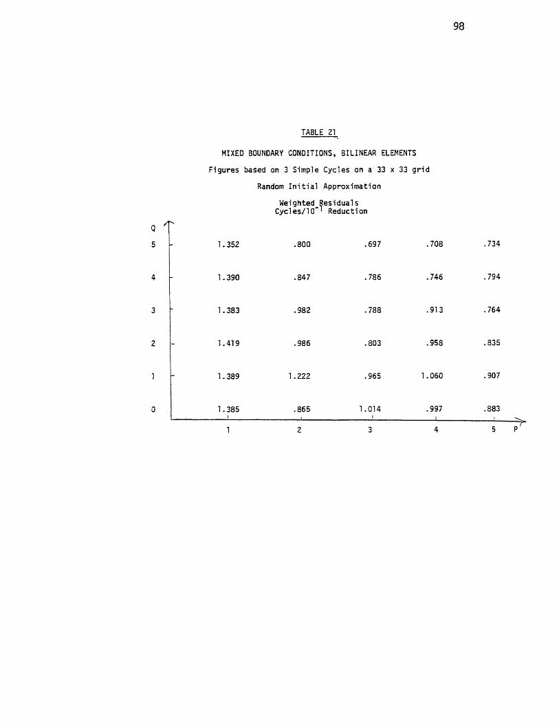
98

TABLE 21

MIXED BOUNDARY CONDITIONS, BILINEAR ELEMENTS

Figures based on 3 Simple Cycles on a 33 x 33 grid

Random In it ia l Approximation

Weighted Residuals C ycles /10"' Reduction

Q.734.708.6971.352 .8005

.746 .794.7861.390 .8474

.913 .7641.383 .982 .7883

.835.9581.419 .803.9862

.9071.0601.222 .9651.3891

.997 .8831.0141.385 .8650

99

problems with D i r i c h l e t c o n d i t io n s . However, with a proper

(P,Q) s t r a t e g y we can achieve a t l e a s t a 10” reduc t ion in the

e r r o r per Simple M u l t i -g r id Cycle in e i t h e r case .

Variable C o e f f ic ie n t s

In t h i s sec t io n we examine the so lu t io n c o s ts in work u n i t s

o f equat ions with v a r i a b le but smooth c o e f f i c i e n t s . The r e s u l t s

a re obtained using the b i l i n e a r f i n i t e element Simple Cycle

M u l t i -g r id a lgori thm with re s id u a l weighting.^ All o f the equat ions

had homogeneous D i r i c h l e t boundary da ta and source fu n c t io n s . The

i n i t i a l e r r o r s in the experiments were random and a (2 ,0 )

s t r a t e g y with u)=l was used in the m u l t i - g r id cyc les . The c o s t s

l i s t e d in Table 22 a re based on the behavior over th re e c y c le s .

The c o a r s e s t g r id c o n s is ted o f 3 x 3 mesh po in ts over the u n i t

square and subsequent g r id s were obtained by halving mesh s i z e s .

The f i r s t four examples were taken from [4 ] . Observe t h a t the

so lu t io n c o s t s f o r so lv ing these v a r i a b le c o e f f i c i e n t problems

are comparable to the th re e work u n i t f i g u r e requ ired to achieve

a 10"^ e r r o r reduc t ion in Poisson equat ions with D i r i c h l e t

boundary co nd i t io n s . These c o s ts did not inc rease with decreas ing

mesh s i z e .

Discontinuous and S ingu lar C o e f f i c ie n t s

The purpose of the experiments in t h i s s e c t io n was to examine

m u l t i - g r id convergence p r o p e r t i e s on problems which a re known to

^See Appendix I .

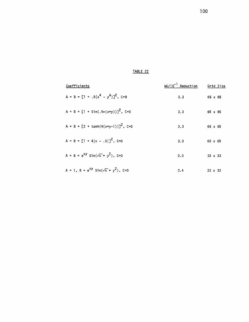
1 0 0

TABLE 22

Coeffic ients WU/1Q"1 Reduction Grid Size

A = B = [1 + .5{x4 - y4 ) ] 2 , C*0 3.3 65 x 65

A = B = [1 + Sin(.5ir(x+y))]2 , C=0 3.3 65 x 65

A = B = [2 + ta n h (4 (x + y - l) ) ]2 , C=0 3.3 65 x 65

A = B = [1 + 4 |x - . 5 1] , C=0 3.3 65 x 65

A = B » exy Sin(fx- + y2 ) , C=0 3.0 33 x 33

A = 1, B = exy Sin(/GT + y c ) , C=0 3.4 33 x 33

101

p re sen t d i f f i c u l t i e s f o r o the r numerical so lu t io n techniques .^ All

the experiments o f t h i s s e c t io n use homogeneous D i r i c h l e t and source

funct ion da ta . The b i l i n e a r f i n i t e element m u l t i - g r id procedure with

res idua l weighting i s used with a (2,0) s t r a t e g y , 01= 1, and a •

random i n i t i a l s t a r t i n g e r r o r . The f ig u re s a re based on the ’ p e r f o r ­

mance of the method over th ree m u l t i - g r id cyc les .

Example:

A = B = 1 x<.5 (87)

9 .5<x<l

0 0 .

This f i r s t problem is one s tud ied by Concus and Golub. For a

d e s c r ip t io n of the d i f f i c u l t i e s i t presented t h e i r techn iques , see

[4 ] . The m u l t i - g r id a lgori thm in Appendix I solves t h i s problem

on a 65 x 65 g r id a t a c o s t of 3 .4 work u n i t s per 10” red uc t io n .

Hence, t h i s equat ion with d iscontinuous c o e f f i c i e n t s i s solved

with the same e f f i c i e n c y as a Poisson equation with D i r i c h l e t

boundary condit ions and the costs did not inc rease with decreasing

mesh s i z e .

Example 2:

In the problem s tud ied he re , C=0 and the c o e f f i c i e n t s A=B

are defined in a checkerboard fashion over the reg ion . More p r e c i s e ly ,k kour reg io n , the u n i t square , i s divided in to 2 x 2 sm al le r but

equal squares by l i n e s p a r a l l e l to the x and y a x i s . The c o e f f i c i e n t s

A and B are then s e t equal to e or 1 in a l t e r n a t e squares . For k = l ,

The problems which are examined in t h i s sec t io n were suggested by R. A. Nico la ides . They are of p r a c t i c a l importance s ince equations with discontinuous c o e f f i c i e n t s o f ten a r i s e in physical models o f composite m a te r i a l s .

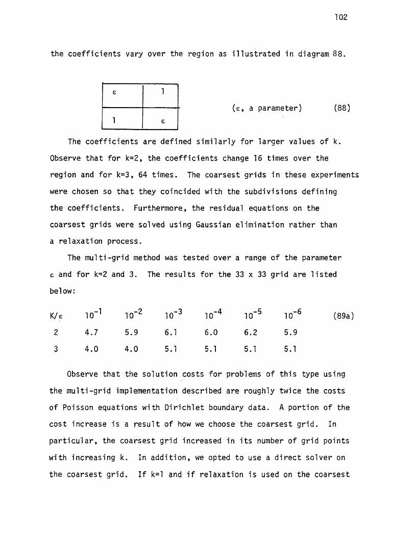
1 02

the c o e f f i c i e n t s vary over the region as i l l u s t r a t e d in diagram 88.

£ 1

1 £( e , a parameter) (88)

The c o e f f i c i e n t s a re defined s im i l a r ly fo r l a r g e r values of k.

Observe t h a t f o r k~2, the c o e f f i c i e n t s change 16 times over the

region and f o r k=3, 64 t im es. The c o a r s e s t g r id s in these experiments

were chosen so t h a t they coincided with the subd iv is ion s def in ing

the c o e f f i c i e n t s . Furthermore, the res idua l equat ions on the

c o a r s e s t g r id s were solved using Gaussian e l im in a t io n r a t h e r than

a r e l a x a t io n process .

The m u l t i - g r id method was t e s t e d over a range o f the parameter

e and f o r k=2 and 3. The r e s u l t s f o r the 33 x 33 g r id a re l i s t e d

below:

K/e 10“1 __j oi ro

1 0 “ 3 10“4 _i oi cn 10“

2 4.7 5.9 6.1 6.0 6.2 5.9

3 4.0 4.0 5.1 5.1 5.1 5.1

Observe t h a t the so lu t io n c o s ts f o r problems of t h i s type using

the m u l t i - g r id implementation descr ibed a re roughly twice the c o s ts

of Poisson equations with D i r i c h l e t boundary d a ta . A por t ion of the

c o s t in c rease i s a r e s u l t of how we choose the c o a r s e s t g r id . In

p a r t i c u l a r , the c o a r s e s t g r id increased in i t s number o f g r id po in ts

with inc reas ing k. In a d d i t i o n , we opted to use a d i r e c t so lv e r on

the c o a r s e s t g r id . I f k=l and i f r e l a x a t io n i s used on the c o a r se s t

103

g r i d , then the cos ts per ICT^ reduc t ion in a random i n i t i a l e r r o r

are as l i s t e d below:

K/e 10”1 10"2 10"3 10~4 1 0 '5 10"6 (89b)

1 3 .6 4.2 4.1 4.1 4.1 4.2

In r e t r o s p e c t th e re was probably no need fo r r e f in in g the c o a r se s t

g r id and using Gaussian e l im in a t io n as the so lu t io n process f o r the

G° system. D i f fe re n t experiments would have been cons iderab ly more

i n t e r e s t i n g and in fo rm at ive . In p a r t i c u l a r , the information w.htch.

would be most i n t e r e s t i n g to know i s how well the coarse g r id

analogue of a re s id u a l equat ion is approximating the ac tua l res idua l

equat ion on the next f i n e r g r id . The f i n i t e element formulation

a u to m at ica l ly provides a c o e f f i c i e n t weighting procedure as a

consequence of the way in which i t performs the i n t e g r a t i o n s over the

e lements. I t would be i n t e r e s t i n g to i n v e s t i g a t e the cond i t ions

under which the weighting technique t h a t a r i s e s n a tu r a l l y from the

f i n i t e element formula tion w i l l succeed.

Example 3:

Here we consider equat ions with c o e f f i c i e n t s : ^

A = B = Sin(kx)Sin(ky) , C = 0 (k, a parameter) (90)

These equat ions l i k e the o thers o f t h i s sec t ion are solved over the

u n i t square . Homogeneous da ta was used. Observe t h a t as the

parameter , k, i s in c reased , k>ir, the c o e f f i c i e n t s A and B vanish

^This problem is un l ike any o th e r problem t h a t was s tu d ied . We mention i t only to in d ic a t e t h a t the method appears to be a p p l icab le to problems where c e r t a i n m u l t i - g r id th e o r i e s c u r r e n t ly do not apply,

1 04

a t po in ts w i th in the domain. The choice of homogeneous boundary

da ta p revents the p o ss ib le overde term ina t ion of the equat ions .^

In Table 23 some ty p ic a l c o s t s in work u n i t s necessary to achieve

a 10”"* e r r o r reduc t ion a re l i s t e d f o r problems of t h i s type f o r

va r ious values o f the parameter k.

For the experiments l i s t e d , the c o a r s e s t g r id contained 3 x 3

mesh po in ts and r e l a x a t io n was used to so lve the res id ua l equat ions

on t h i s g r i d . Observe t h a t the c o s t s a re on the average l e s s than

twice those requ ired to so lve Poisson equat ions with D i r i c h l e t

boundary condi t i o n s .

Example 4:

Here we re tu rn to the p a r t i a l d i f f e r e n t i a l e q u a t io n :

g U x x + Uyy = 0 a Pa ra m e te r ) (-91)U = 0 (on the boundary)

In Chapter 3 we c ons t ruc ted a s im p l i f i e d local mode a n a ly s i s conver­

gence model o f the m u l t i - g r id method. This model was used to

p r e d i c t the number o f m u l t i - g r id c y c l e s , t , requ ired to achieveKKa 10”"* reduc t ion in a random i n i t i a l e r r o r over a range of the

parameter e in equat ion 91. The p red ic ted e r r o r reduc t ion r a t e s

were c a lc u la te d fo r one, th r e e and f iv e m u l t i - g r id c y c le s , k = l , 3,

5 and compared to the exper im enta l ly obta ined r a t e s , t ^ , based

on the same number of cycles and values o f e . In Table 1 o f Chapter

3, the p red ic ted and experimental r e s u l t s were t ab u la te d f o r

We had overlooked the p o s s i b i l i t y t h a t t h i s problem can be over ­determined a t the time o f the experiment. By sheer luck a p p ro p r i a te boundary da ta had been used.

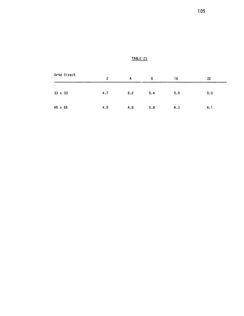
105

TABLE 23

Grid Size/K2 4 8 16 32

33 x 33 4.7 5.2 5.4 5 .9 5.0

65 x 65 4.5 4 .8 5 .8 6.3 6.1

106

problems whose f i n e s t g r id had 65 x 65 mesh p o in ts . In Table 2,

the experimenta l ly obtained are t ab u la ted a g a in s t the p red ic ted

values f o r problems in which the f i n e s t g i rd had 33 x 33 gr id

p o in t s . The f ig u re s were based o n . th re e m u l t i - g r id c y c le s , k=3.

Comparing the p red ic t io n s of the model fo r the 33 x 33 g r id to

the corresponding p re d ic t io n s f o r the 65 x 65 g r i d , we saw t h a t on

the average , the accuracy o f the models p re d ic t io n s increased

s i g n i f i c a n t l y with decreasing mesh s i z e .

In Chapter 3 we observed t h a t the 9 po in t r e l a x a t io n scheme

descr ibed by u(e) l o s t i t s e f f e c t iv e n e s s on equat ion 91 as ei—>

decreased . The e f f e c t iv e n e s s i s measured by how ra p id ly the

norm of the d i f f e r e n c e between the exact so lu t io n and the c u r r e n t approximation

to the so lu t io n of the d i f f e r e n c e equations i s reduced. In [1]

Brandt analyzes the consequences of rep lac ing the r e l a x a t io n procedure

corresponding to y(e) by l i n e r e l a x a t io n and demonstrates t h a t l in e

r e l a x a t io n wil l r e s t o r e the e f f e c t iv e n e s s o f the m u l t i - g r id cycle .

Through mode a n a ly s i s one can a lso show t h a t ano ther remedy i s to

continue to use the r e l a x a t io n process y(e) but to l e t the mesh s iz e

in the x d i r e c t i o n decrease with decreasing s .

The d i f f i c u l t y with equation 91 i s t h a t as e becomes very small ,

the approximate so lu t io n a t a po in t ( i , j ) depends very heav i ly on the

values of the so lu t io n above and below i t , ( i , j + l ) and ( _ i , j - l ) , but

only very weakly on the values o f the so lu t io n a t mesh po in ts to i t s

l e f t and r i g h t . By decreas ing the mesh s i z e in the x d i r e c t io n we

in c rease the in f luence of the information a t the p o in ts to the r i g h t

and l e f t of ( i , j ) by br inging them c lo s e r to p o in t ( i , j ) .

107

An experiment was made to demonstrate the e x te n t to which th e

e f f e c t i v e n e s s of a m u l t i - g r id cycle can be d is ru p ted when the

r e l a x a t io n procedure corresponding to \1(0) i s used in the m u l t i -g r id

cycles on equat ions of type 91. From the amplitude reduct ion

f a c t o r , u ( e ) , one can observe t h a t c e r t a in high frequency Four ie r

e r r o r modes are not smoothed s a t i s f a c t o r i l y by the r e l a x a t io n

procedure, equat ion 58, as e decreases . - For example, the ampli tude

of the Four ie r component corresponding to 0=(tt/2,O) w i l l be

smoothed a t the r a t e :

v C f , 0 ) = >—> L

0 1 / 25e - 8e + 5

29e2 + 16e + 5( fo r u)=1) (92)

Observe t h a t y( |- ,0) approaches 1 as e decreases and hence the C^O)

mode i s l iq u id a te d a t an in c re a s in g ly slower r a t e . Furthermore,

no m at te r what the choice o f u in p ( e ) , as e decreases th e re wil l be—

modes which e x h ib i t t h i s behavior . In the experiments presented in

Table 24, the i n i t i a l e r r o r was cons t ruc ted so t h a t th e amplitude

corresponding to the ( |-,0) e r r o r component was dominant. The c o s ts

to achieve a 10’ e r r o r reduc t ion a re l i s t e d in Table 24 fo r various

values of the parameter e. The f ig u re s are based over th ree cycles

on a 33 x 33 g r id . The analogous c o s ts fo r the case o f a random

i n i t i a l e r r o r are l i s t e d in Table 25.

Before leaving t h i s problem, we mention t h a t the p r e d ic t io n s of

XKR ^ ^he s im p l i f i e d loca l mode a n a ly s i s model were d i s tu rb in g in

the case o f Poisson eq ua t ion s , s = 1. In p a r t i c u l a r , as the number

of m u l t i - g r id cycles in c reased , the model p red ic ted s i g n i f i c a n t l y

worse convergence r a t e s than were exper imenta l ly observed. From

108

TABLE 24

._______ WU/IQ"^ Reduction

1.0 2.5

.75 2.9

.50 4.0

.25 7.1

1 0 '1 16.3

10“2 103.8

10"3 213.0

*3-io

237.5

i o - 5 250.5

1 09

TABLE 25

WU/10~^ Reduction

1.0 3.2

.75 3.4

.50 4.0

.25 5.3

10”1 8.2

1 0 '2 16.8

10‘ 3 18.4

10‘ 4 18.9

10"5 19.9

1 1 0

Table 1 we observe t h a t over a period of f i v e m u l t i - g r id cycles-5during which the e r r o r i s reduced by a f a c t o r o f 10 , the model

-5wil l recommend 20.8% more work to achieve the 10 e r r o r reduc t ion

than i s req u i re d . A more ca re fu l exp lanat ion of t h i s behavior f o r

e=l r eq u i re s the use of f u l l loca l mode a n a ly s i s .

When f u l l mode a n a ly s i s i s applied to the case e=l one observes

t h a t c e r t a i n Four ie r e r r o r components, which the s im p l i f i e d local

mode a n a ly s i s p r e d ic t s cannot be rep resen ted on coa rse r g r i d s , a re

converted during the m u l t i - g r id process in to modes which can be

rep resen ted and hence l iq u id a te d on co a rse r g r id s . Thus, the coarse r

g r id s help in l i q u i d a t i n g e r r o r components which the s im p l i f i ed

model assumes they cannot reduce. The ne t r e s u l t i s t h a t the

s im p l i f i e d model underest imates the e f f i c i e n c y of the m u l t i - g r id

process f o r e=l as the number o f cycles in c re ase s .

I n d e f i n i t e Problems

In Chapter 3 we b r i e f l y considered the d i f f i c u l t i e s which a r i s e

when so lv ing i n d e f i n i t e problems with i t e r a t i v e techn iques . The basic

problem i s t h a t s tandard i t e r a t i v e methods may not converge when the

d i f f e r e n c e op e ra to r has both p o s i t iv e and nega t ive e igenvalues .

In t h i s sec t ion we cons ider the performance of Simple M ul t i -g r id

Cycles on the Helmholtz equat ion:^

AU + 4U = 0

U = cos (iry)

Un = 0_______________________^Early experiments with the m u l t i - g r id method on the Helmholtz equat ion with D i r i c h l e t and mixed boundary cond i t ions were begun with Brandt but were u n fo r tu n a te ly d i s ru p ted by h is depar tu re to I s r a e l . The experience and ideas from these experiments were used in the p resen t s tudy.

0<y<l, X=0 (93)

(elsewhere on the bondary)

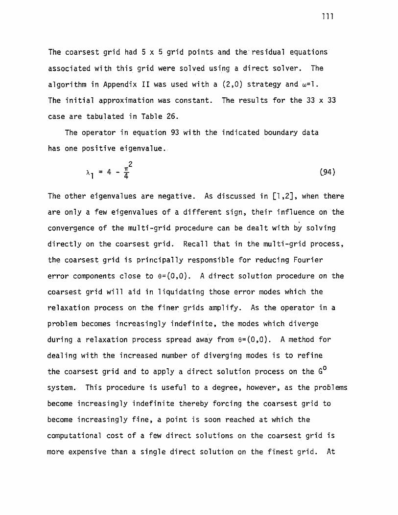
i n

The c o a r s e s t g r id had 5 x 5 g r id po in ts and the r es idua l equat ions

a s so c ia ted with t h i s g r id were solved using a d i r e c t s o lv e r . The

a lgori thm in Appendix II was used with a (2 ,0) s t r a t e g y and to=l.

The i n i t i a l approximation was c o n s ta n t . The r e s u l t s f o r the 33 x 33

case a re tab u la te d in Table 26.

The ope ra to r in equat ion 93 with the in d ica ted boundary data

has one p o s i t iv e e igenvalue .

At - 4 - \ (94)

The o th e r eigenvalues a re n ega t ive . As d iscussed in [ 1 , 2 ] , when the re

a re only a few e igenvalues of a d i f f e r e n t s ign , t h e i r in f luence on the

convergence of the m u l t i - g r id procedure can be d e a l t wi th by so lving

d i r e c t l y on the c o a r s e s t g r id . Recall t h a t in the m u l t i - g r id p rocess ,

the c o a r s e s t g r id i s p r i n c i p a l l y r e spo n s ib le fo r reducing Fourier

e r r o r components c lose to e= (0 ,0 ) . A d i r e c t so lu t io n procedure on the

c o a r s e s t g r id wil l a id in l i q u i d a t i n g those e r r o r modes which the

r e l a x a t io n process on the f i n e r g r id s amplify. As the ope ra to r in a

problem becomes in c re a s in g ly i n d e f i n i t e , the modes which d iverge

during a r e l a x a t io n process spread away from e=(0 ,0 ) . A method fo r

deal ing with the increased number of d iverg ing modes i s to r e f in e

the c o a r s e s t g r id and to apply a d i r e c t so lu t io n process on the 6°

system. This procedure i s useful to a degree, however, as the problems

become in c re a s in g ly i n d e f i n i t e thereby forc ing the c o a r s e s t g r id to

become in c re a s in g ly f i n e , a p o in t i s soon reached a t which the

computational c o s t of a few d i r e c t so lu t io n s on the c o a r s e s t g r id is

more expensive than a s in g le d i r e c t so lu t io n on the f i n e s t g r id . At

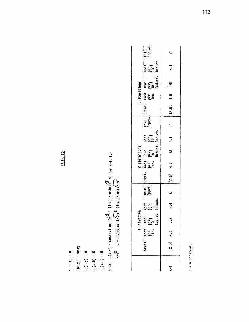
112

3“II

\C S i '

n :

Q

e=A5*

0 0)0

o

<u o <u

CO

con

stan

t.

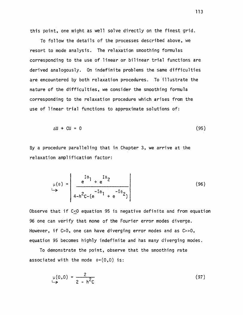
113

t h i s p o in t , one might as well so lve d i r e c t l y on the f i n e s t g r id .

To fo l low the d e t a i l s o f the processes descr ibed above, we

r e s o r t to mode a n a ly s i s . The r e l a x a t io n smoothing formulas

corresponding to the use o f l i n e a r or b i l i n e a r t r i a l fu n c t io n s are

der ived analogously . On i n d e f i n i t e problems th e same d i f f i c u l t i e s

a re encountered by both r e l a x a t i o n procedures. To i l l u s t r a t e the

na tu re o f the d i f f i c u l t i e s , we cons ider the smoothing formula

corresponding to the r e l a x a t io n procedure which a r i s e s from the

use o f l i n e a r t r i a l func t ions to approximate so lu t io n s of :

By a procedure p a r a l l e l i n g t h a t in Chapter 3, we a r r i v e a t the

r e l a x a t io n a m p l i f i c a t io n f a c t o r :

Observe t h a t i f C<0 equation 95 i s negat ive d e f i n i t e and from equation

96 one can v e r i f y t h a t none of the Fourier e r r o r modes d iverge .

However, i f C>0, one can have d iverg ing e r r o r modes and as C » 0 ,

equat ion 95 becomes highly i n d e f i n i t e and has many d iverg ing modes.

To demonstrate the p o in t , observe t h a t the smoothing r a t e

a s so c ia te d with the mode e=(0,0) i s :

AU + CU = 0 (95)

101 Ie 2e + e (96)“ I.0t “ I 0 «

4-h C-(e + e

(-97)

114

2I f we take C=(2-e)/h , (e , a pa ram eter ) , we can make u (0 ,0 )

a r b i t r a r i l y la rge by l e t t i n g e -»0. Hence, fo r a g r id with mesh s i z e

h, we can choose C such t h a t the r e l a x a t io n procedure corresponding

to y (e) d r a s t i c a l l y magnifies the ampli tude o f the e=(0,0) e r r o r

component.

Although the f i n e r g r id sweeps a lso magnify the e=(0,0) e r r o r

component, they a re e f f e c t i v e l y reducing o th e r e r r o r components*

On the c o a r s e s t g r i d , a d i r e c t so lu t io n technique i s used to a id in

l i q u i d a t i n g those e r r o r components which the r e l a x a t io n process

a m p l i f i e s . The s in g le experimental r e s u l t presented in Table 26 i s

only the beginning o f a study. With the a lgori thms l i s t e d in the

Appendices, i t should be a f a i r l y r o u t in e mat ter to pursue t h i s

s tudy o f i n d e f i n i t e problems f u r t h e r i f one has the i n c l i n a t i o n .

This concludes the numerical experiments t h a t were conducted in

c o l l a b o r a t io n with R. A. Nicola ides o f ICASE.

As an ending note we mention t h a t with the a lg o r i th m s ,1i s t e d i n '

the Appendices, a number of i n t e r e s t i n g d i r e c t i o n s can be taken. As

a s t a r t , more thorough i n v e s t i g a t i o n s should be made fo r equa t ions in

which the c o e f f i c i e n t s a re d iscon t inuous . Another i n t e r e s t i n g

d i r e c t i o n l i e s in the so lu t io n of e igenvalue problems with the

m u l t i - g r id a lgor i thm . With minor m od if ica t ions to e x i s t i n g codes,

one can begin to study e igenvalue problems through the v a r i a t i o n a l_ _ i

formulation descr ibed in [10] . Other more ambit ious d i r e c t io n s

would be to convert these codes to the Full Approximation Scheme and

to begin studying n o n - l in e a r e qua t ions .

^Not from a programming s ta n d po in t .

APPENDIX I

A f i n i t e element M ul t i -g r id Algorithm f o r the so lu t io n of (-Au ) . +X X

(-BUy)y-Cu-F on a r e c ta n g le . This code uses b i l i n e a r t r i a l func t ions

(nine po in t d i f f e r e n c e approximation) and accepts D i r i c h l e t boundary

d a ta . The add i t ion of a Gaussian e l im ina t io n subrout ine wil l enable

t h i s code to solve 'm odera te ly ' i n d e f i n i t e problems.

Comments

EXTERNAL G

EXTERNAL F

EXTERNAL EXACT

EXTERNAL A EXTERNAL B EXTERNAL C

U(11436)

AK(57180)

Boundary da ta .

Source func t ion .

Exact so lu t io n to P.D.E. (used in determining speed of convergence on t e s t problems.)

C o e f f ic ien ts of the P.D.E.t “Aux ) x + ( ’ ®uy )y " Cu = FNote: to solve u + u = 4,xx yyl e t A=B=-1 , C=0, and F=4.

i s s to rage f o r the so lu t io n on each g r id as well as space f o r r e s id u a l s .The res idua l s to rage space i s not needed but i s convenient when studying d i f f e r e n t re s id u a l weighting techniques In U a l o t 2 lo ca t io ns per g r id po in t fo r each g r id . For example i f G1 3 x 3, G2 5 x 5, G%9 x 9, G4 17 x 17, G5 33 x 33, G6 65 x 65, a l o t 2(9 + 25 + 81 + 289 + 1 0 8 9 + 4 2 2 5 ) = 11436 s to rage spaces.

is s to rage fo r the f i n i t e element c o e f f i c i e n t m atr ices a t each level and s to rage f o r the r i g h t hand s id e s of the equations a t each l e v e l . In AK a l o t 10 lo ca t io n s per g r id po in t on each g r id ( i . e . 9 fo r the non-zero

115

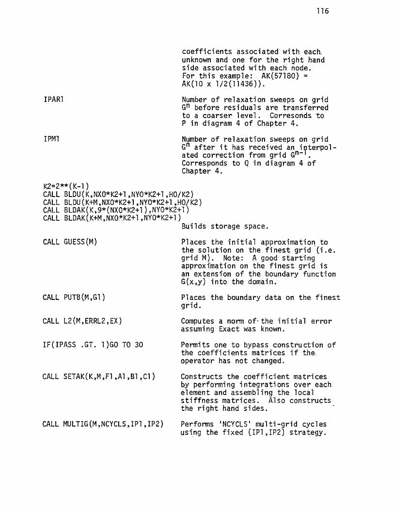
116

I PARI

I PM!

K2=2**(K-1)CALL BLDU(K,NX0*K2+1,NY0*K2+1,H0/K2)CALL BLDU( K+M,NX0*K2+1,NY0*K2+1,H0/K2)CALL BLDAK(K,9*(NX0*K2+1) ,NY0*K2+1)CALL BLDAK(K+M,NX0*K2+1,NY0*K2+1)

Builds s to rage space.

Places the i n i t i a l approximation to the so lu t io n on the f i n e s t g r id ( i . e . g r id M). Note: A good s t a r t i n gapproximation on the f i n e s t g r id is an extension o f the boundary funct ion G(x,y) in to the domain.

Places the boundary da ta on the f i n e s t g r id .

Computes a norm of*the i n i t i a l e r r o r assuming Exact was known.

Permits one to bypass c o n s t ru c t io n of the c o e f f i c i e n t s m atr ices i f t h e ope ra to r has not changed.

CALL SETAK(K,MsFl,A1,B1,C1) Constructs the c o e f f i c i e n t m atr icesby performing in t e g r a t i o n s over each, element and assembling the local s t i f f n e s s m a t r ice s . Also c o n s t ruc ts the r i g h t hand s id e s .

CALL MULTIG(M,NCYCLS,IP1,IP2) Performs rNCYCLS' m u l t i - g r id cyclesusing the f ixed CIP1»IP2) s t r a t e g y .

CALL GUESS(M)

CALL PUTB(M»G1)

CALL L2(M,ERRL2,EX)

IF(IPASS .GT. 1 )G0 TO 30

c o e f f i c i e n t s a s so c ia te d w i th each- unknown and one f o r the r i g h t hand s ide a s so c ia te d with each node.For t h i s example: AK(57180) =AK(10 x 1/2(11436)) .

Number o f r e l a x a t io n sweeps on g r id Gn before r e s id u a l s a re t r a n s f e r r e d to a c o a r se r l e v e l . Corresonds to P in diagram 4 of Chapter 4.

Number o f r e l a x a t io n sweeps on g r id Gn a f t e r i t has rece ived an i n t e r p o l ­ated c o r re c t io n from g r id Gn . Corresponds to Q in diagram 4 of Chapter 4.

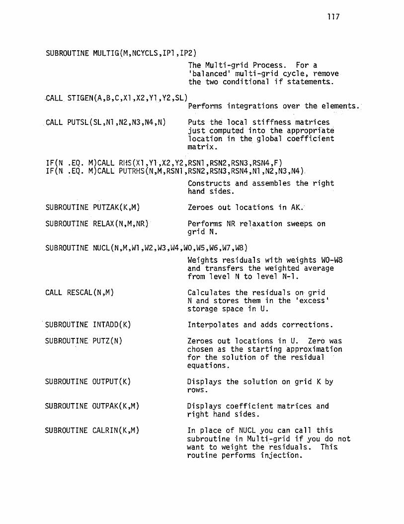
117

SUBROUTINE MULTIG(M,NCYCLS,IP1,IP2)The M u l t i -g r id Process . For a 'ba lanced ' m u l t i - g r id c y c le , remove the two cond i t iona l i f s ta tem en ts .

-CALL STIGEN(A,B,C,X1,X2,Y1,Y2,SL)

CALL PUTSL(SL,N1,N2,N3,N4,N)

Performs i n t e g r a t i o n s over the elements.

Puts the local s t i f f n e s s m atr ices j u s t computed in to th e a p p ro p r ia te lo c a t io n in the global c o e f f i c i e n t m a t r ix .

IF(N .EQ. M)CALL RHS(X1,Y1,X2,Y2,RSN1,RSN2,RSN3,RSN4,F)TF(N .EQ. M)CALL PUTRHS(.N,M,RSN1 ,RSN2,RSN3,RSN4,N1 ,N2,N3,N4)

SUBROUTINE PUTZAK(K,M]

SUBROUTINE RELAX(N,M,NR)

Constructs and assembles the r i g h t hand s id e s .

Zeroes out lo c a t io n s in AK.

Performs NR r e l a x a t io n sweeps on g r id N.

SUBROUTINE NUCL(N,M,W1,W2,W3,W4,W0,W5,W6,W7,W8)

CALL RESCAL(N,M)

SUBROUTINE INTADD(K)

SUBROUTINE PUTZ(N)

SUBROUTINE OUTPUT(K)

SUBROUTINE 0UTPAK(.K,M)

SUBROUTINE CALRIN(K,M)

Weights r e s id u a l s with weights W0-W8 and t r a n s f e r s the weighted average from level N to level N-l.

C a lcu la tes the r e s id u a l s on g r id N and s t o r e s them in the ' e x c e s s ' s to rage space in U.

In t e r p o la t e s and adds c o r r e c t i o n s .

Zeroes out lo c a t io n s in U. Zero was chosen as th e s t a r t i n g approximation f o r the so lu t io n o f the res idua l equa t ions .

Displays the so lu t io n on g r id K by rows.

Displays c o e f f i c i e n t m at r ices and r i g h t hand s id e s .

In p lace of NUCL you can c a l l t h i s subrou t ine in M u l t i -g r id i f you do not want to weight the r e s i d u a l s . This ro u t in e performs i n j e c t i o n .

1 1 8

D escr ip t ion of the Assembly Procedure (Subroutine PUTSL)

For each unknown on a given g r i d , t h e r e a re 9 s to rage lo c a t io n s in AK.

These l o c a t io n s correspond to th e 9 non-zero c o e f f i c i e n t s in the row

of the global s t i f f n e s s m atr ix a s so c ia te d with the given unknown. To

i l l u s t r a t e the assembly process we sh a l l assemble the d i f f e r e n c e equat ions

a s so c ia te d with equat ion 20 when a=b=l. D i sc re t i z e the u n i t square, as

i n d ic a te d in f ig u r e 32. For t h i s problem, the local s t i f f n e s s matr ix

LSM^, which i s re tu rned from subrout ine STIGEN, wil l be t h e same f o r

each of the fou r elements E - , i = l , . . . 4 .

LSM = 1

4 -1 -2 -1

-1 4 -1 -2

-2 -1 4 -1

-1 -2 -1 4 (98)

In the assembly p rocess , boundary po in ts a re considered as unknowns.

The d i f f e r e n c e equat ions which a re generated f o r boundary p o in ts

correspond to the na tu ra l boundary cond i t ions of the f u n c t io n a l . I f

the s o lu t io n a t a boundary p o in t i s known, the corresponding d i f f e r e n c e2equat ion w i l l not be used.

\ s M on page 23 i s e q u iv a le n t to SL in the codes.

2The row in the global s t i f f n e s s matr ix corresponding to the boundary p o in t i s no t used in a r e l a x a t io n sweep, r e s id u a l s are not c a lc u la te d a t t h i s p o in t , and i n t e r p o la t e d c o r r e c t io n terms a re not added to the so lu t io n a t t h i s p o in t .

119

The d i s c r e t e system of equa t ions corresponding to the d i s c r e t i z a t i o n :

8

4E3

IE4

6

E1/?

CM

LU

— 3

wi 11 have the form:

1 2 3 4 7 8 91 ~U12 u23 U34 U45 u5 = RHS6 u67 U78 u89 U9 0 00)

In the event o f D i r i c h l e t boundary c o n d i t io n s , only row 5 w i l l be used

in a r e l a x a t io n sweep. The o th e r values of u w i l l be known. For

purposes o f e x p o s i t io n , we w i l l , a t t im es , use a double index f o r the

9 nodal values u. _• in diagram 99:i , j

13 '23 33

12

I T

'22

2 1 ’

32

‘31001)

120

The non-zero c o e f f i c i e n t s in a row o f system 100 a re s to red in a block

o f 9 s to rag e spaces in AK. Consider the block of s to ra g e a sso c ia ted

( 102)with the unknown u. .=1 5 J

Ui,j Ui+T,j Vl,j+1 Ui,0+1 ui+l ,j+l

The middle s to rag e loca t ion^ in t h i s block con ta ins the c o e f f i c i e n t

which m u l t i p l i e s the unknown u. _• and s i m i l a r ly f o r the o th e r s to rage* sJlo c a t io n s in the block.

To i l l u s t r a t e how a block i s f i l l e d in by subrou t ine PUTSL, we

sh a l l process the four elements in f i g u r e 101. We r e s t r i c t our2

a t t e n t i o n to the d i f f e r e n c e equat ion a s so c ia te d with unknown U22»

Subroutine STIGEN rece ives the coord ina tes o f two v e r t i c e s of

element E-j as well as the c o e f f i c i e n t s o f the p a r t i a l d i f f e r e n t i a l

equat ion . This subrou t ine c o n s t ru c t s and r e tu r n s the 4 x 4 local3s t i f f n e s s matr ix SL corresponding to E-j. The number sequence

N = (N1,N2,N3,N4) in subrou t ine SETAK wil l assume th e values R— Cl,2 ,5 ,4 )

f o r element E-j:

N1 N2 N3N4 \ - l -2 -1 4 / (103)

N1 N2 N3 N4f 4 -1 -2 -1-1 4 -1 -2-2 -1 4 -1

r l -2 -1 4

1The v a r i a b le MIDPT in subrout ine PUTSL po in ts to the c e n te r lo c a t io n in a given block.

>'We a re working with row 5 in equat ion 100. The r i g h t hand s ide RHS i s co ns t ru c ted s e p a ra te ly but in an analogous fashion by sub rou t ines RHS and PUTRHS.

*The 1 s in equation 22 a re p a r t i c u l a r l y simple to c o n s t ru c t over square e lem en ts .

121

Row 3 of t h i s local s t i f f n e s s m atr ix w i l l con ta in information p e r t a in in g

to row N3 in the global s t i f f n e s s m a t r ix . This information w i l l be

s to re d in the block of 9 s to ra g e lo c a t io n s in AK t h a t has been s e t

a s id e f o r the unknown un3=u5=u22* A f te r t r a n s f e r r i n g the information

from row 3 of the local s t i f f n e s s matr ix in to AK, the block of 9

s to ra g e lo c a t io n s a s so c ia ted with u^2 w i l l look l i k e :

-26

- i6 0 -1

6

«_ ..

0 0 -0 0

un U21 U31 U12 U22 U32 U13 U23 U33 0 0 4 )

Observe t h a t the q u a n t i ty -1 /6 loca ted in lo ca t io n (3 ,4) in the local

s t i f f n e s s matr ix c o n t r ib u te s to lo c a t io n (N3,N4)=(5,4) in the global

c o e f f i c i e n t matr ix in diagram 100. Moreover, t h i s q u a n t i ty w i l l

c o n t r ib u te to the c o e f f i c i e n t t h a t w i l l m u l t ip ly u^=u^=u^2 an^

hence, by the p r e s c r ip t io n in diagram 102, w i l l be en te red in to the

s to ra g e lo ca t io n to the immediate l e f t o f the MIDPT lo c a t io n . The

o th e r e n t r i e s in the t h i r d row o f the local s t i f f n e s s matr ix a re

en te red analogously .

The second element ^ i s now processed. Subroutine STIGEN w i l l

r e tu r n the same local s t i f f n e s s matr ix SL f o r t h i s element as i t

did fo r the f i r s t element.^ However, the nufaber sequence N wil l

be d i f f e r e n t . In p a r t i c u l a r , N = ( 2 , 3 , 6 , 5 ) . The information in

diagram 103 wi l l be t r a n s f e r r e d in to AK according to t h i s new number

sequence. The fou r th row in the loca l s t i f f n e s s m atr ix w i l l con ta in

the information p e r t a in in g to the unknown un4=u5=u22* A f te r t h i s

^Reca l l , t h a t in t h i s example we a re solv ing a cons tan t c o e f f i c i e n t P.D.E. over a uniform t r i a n g u l a t i o n .

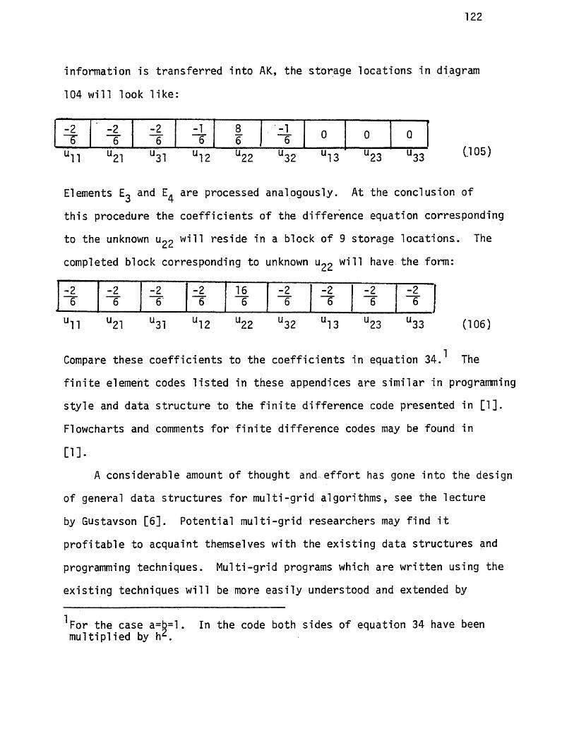
122

information i s t r a n s f e r r e d in to AK, the s to ra g e lo c a t io n s in diagram

104 w i l l look l i k e :

-26

-26

-26

-16

86 ,

-16 0 0 Q

U11 U21 U31 U12 U22 U32 U13 u23 u33 0 0 5 )

Elements and E a re processed analogously . At the conclusion of

t h i s procedure the c o e f f i c i e n t s of the d i f f e r e n c e equation corresponding

to the unknown U22 W1*H r e s id e in a block of 9 s to rage lo c a t io n s . The

completed block corresponding to unknown U22 W1’H have the form:

-2 -2 -2 -2 16 -2 -2 -2 -26 6 6 6 6 6 6 6 6

un U21 U31 U12 U22 u32 U13 U23 U33 (106)

1Compare these c o e f f i c i e n t s to the c o e f f i c i e n t s in equation 34. The

f i n i t e element codes l i s t e d in these appendices a re s im i l a r in programming

s t y l e and da ta s t r u c t u r e to the f i n i t e d i f f e r e n c e code presented in [1 ] ,

Flowcharts and comments f o r f i n i t e d i f f e r e n c e codes may be found in

[1].A cons iderab le amount of thought and e f f o r t has gone in to the design

of general da ta s t r u c tu r e s f o r m u l t i - g r id a lg o r i th m s , see the l e c tu r e

by Gustavson [6 ] . P o te n t ia l m u l t i - g r id re sea rche rs may f ind i t

p r o f i t a b l e to acqua in t themselves with the e x i s t i n g da ta s t r u c tu r e s and

programming techn iques . M u l t i -g r id programs which are w r i t t e n using the

e x i s t i n g techniques w i l l be more e a s i l y understood and extended by

For the case a=b=l. In the code both s ides of equat ion 34 have been m u l t ip l i e d by h2 .

1 2 3

o th e r m u l t i - g r id r e s e a r c h e r s . Although the codes in th e se appendices

a re not f u l l y commented, i t i s hoped t h a t they w i l l be i n t e l l i g i b l e

to i n d iv id u a l s who have had some p rev ious experience with m u l t i - g r id

a lgor i thm s .

124

E X T E R N A L G E X T E R N A L FE X T E R N A L E X A C TE X T E R N A L AE X T E R N A L 3E X T E R N A L C

j COMMON U C U 4 3 6 ) , A K ( 5 7 1 8 0 )R E A L C O N E C T , H OI N T E G E R N X Q , NYO , M

O P F NCU M I T = 6 , D E V I C E = # T T Y # )I P A S S = 1

; DO 4 0 MC YC L S = 5 , 5 .; DO 3 0 M = 5 , 5i DO 2 0 I P A R 1 = 2 0 2

DO 1 0 I P A R 2 = 1 , 1I P M 1 = I P A R 2 - 1

C A L L E L ( 2 , 2 , . 5 , M, N C Y C L S , G , F , E X A C T , A , B , C , I P A R 1 , I P M 1 ,1 I P A S S )

W R I T E C 6 , 1 0 0 } M , I P A R 1 , I P M 11 0 C O N T I N U E2 0 C O N T I N U E3 0 C O N T I N U E4 0 C O N T I N U E

C A L L O U T P U T ( 5 )1 0 0 FORMATC * M= # , I 5 , # > P A R 1 = ' , 15,' P A R 2 = ' , 1 5 )

S T O PEMC

125

♦

S U B R O U T I N E E L ( N X O / N X Q * H O , M , N C Y C L S , G 1 , F 1 , £ X , A 1 , B 1 , C 1 , I P 1 *1 1 P 2 / I P A S S )

E X T E R N AL G 1E XTERNAL F tEXTE RNAL EXE XTE RNAL A 1

i EXTERNAL 8 1EXTERNAL C lC O M M O N / B L D / I U , I A K

, C O M M O N / G R O I F l / N S T C 2 0 ) , I M X C 2 0 ) , J M X C 2 0 )C O M M O N / G R D I F 2 / H Y C 2 0 )C O M M G N / A K I N F O / N A K ( 2 0 ) # I M A K ( 2 0 ) # J M A K C 2 0 )

; COMMON U ( 1 1 4 3 6 ) # A K ( 5 7 1 8 0 )i I N- TEGER N X O , N Y O , M , N C Y C L S , I P 1 , I P 2i I N T E G E R I P A S Sl P E AL HO

I U = l■ I AKs s l

DO 1 0 K = l / MK 2 = 2 * * ( K - 1 )CALL 8 L D U C K , N X 0 * K 2 + 1 , N Y 0 * K 2 + 1 * H0 / K 2 )CALL BLDU CK + M t NX0 * K 2 + 1 1 NY0 * K 2 + 1 * H0 / K 2 )CALL B L D A K C K , 9 * C N X 0 * K 2 + 1 ) . NY0 * K 2 + 1 )CALL B L O A X ( K + M f N X O * K 2 + l # N Y O * K 2 + l )

. . 1 0 C O N T I N U ECAL L GU E S S CM )CALL P U T B ( M , G 1 )

/ C ALL L 2 ( M, E R R L 2 # E X )W R I T E ( 6 # 5 0 0 ) E R R L 2E R P A S T = E P R L 2-I F C I P ASS , G T , 1 ) GO TO 3 0DO 2 0 K= 1 f M

CAL L P U T Z A K ( K * M)

C A L L S E T A K C K , M , F 1 , A 1 , 8 1 , C 1 ) -

2 0 C O N T I N U E3 0 C O N T I N U E

CALL M U L T I G ( M , N C Y C L S # I P 1 • I P 21CALL L 2 ( M , E R R L 2 , E X )E S P = C E R R L 2 / E R P A S T ) * * ( 1 . / F L O A T CN C Y C L S ) )N = C I M X C M ) - 2 ) * C J M X ( M ) - 2 )

_ P = - A L 0 G 1 0 C E S R )C Y 1 0 M l = l . / PW R I T E C 6 # 9 0 0 1 C Y 1 0 M1W R I T E C 6 , 6 0 0 ) N C Y C L S , E R R L 2W R I T E f 6 . 7 0 0 1 F S R

5 0 0 ' F Q F MAT C ' I N I T I A L E R ROR = # , E 1 4 . 7 )6 0 0 F 0 p M A T C 0 ERROR A F T E R # , I 3 , # M U L T I G T Y r L E S = # , E 1 4 . 7 )7 0 0 F 0 R M A T ( 0 E F F E C T I V E S P E C T R A L R A D I U S s * , E 1 4 . 7 )

9 0 0 F O R M A T S C Y 1 0 M l = ' , £ 1 4 . 7 )RETURNEND

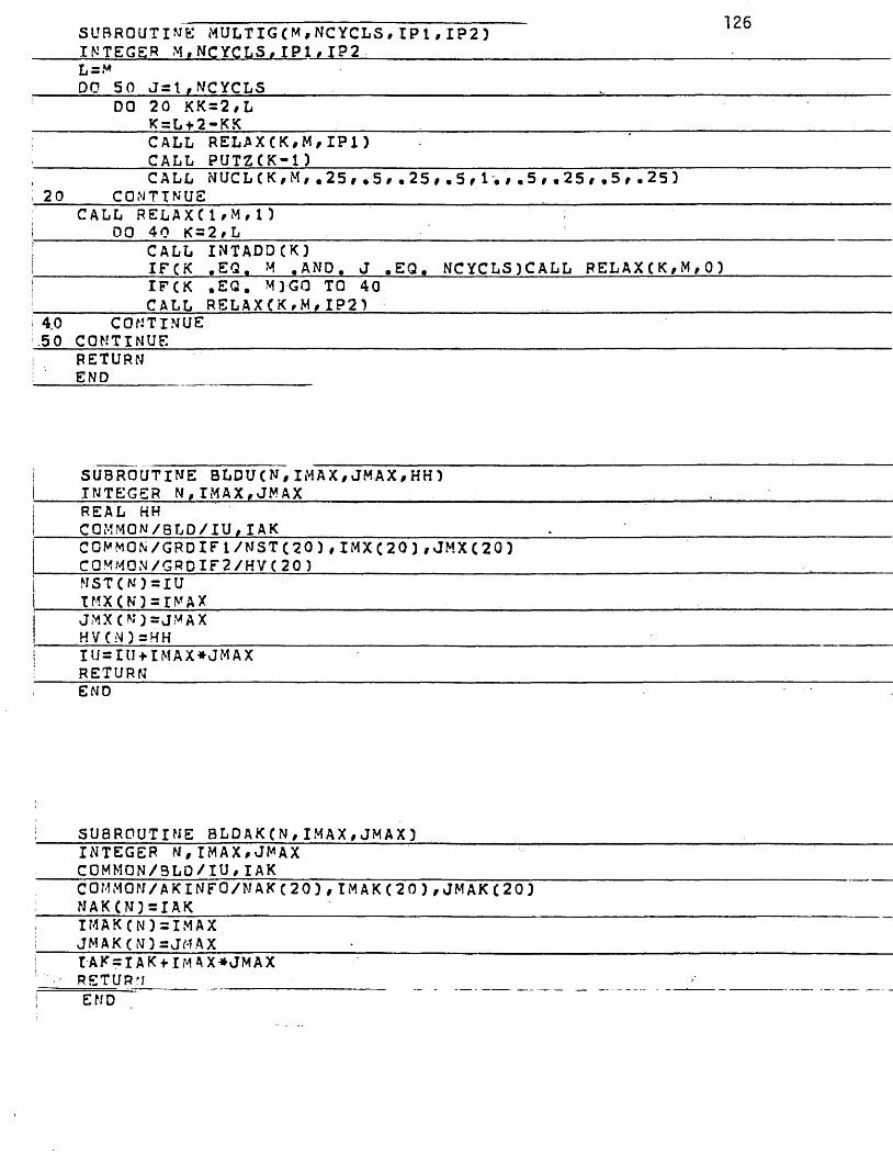
SUBROUTINE MULTIG ( M , N C Y C L S , I P 1 ,IP2) INTEGER M »NCYCLS•IP 1»IP2 _____________

126

DO 50 Jst , NCYCLSDO 20 KK=2#L

K=L+2-KKCALL RELAXCK,M,IP1)

.________ CALL PUTZ ( K~ 1 ) __________________________________CALL NUCLCK,M, .25,.5#.25,.5,1•#.5,.25#• 5r.25)

20 CONTINUECALL R E L A X C 1rM,1)

00 40 K = 2,LCALL I N T A D D (K )IF C K .EQ. M .AND, J .EQ. N C Y C L S )CALL R E L A X ( K , M , 0 )IF (K .E Q . M1G0 TO 40 CALL R E L A X ( K » M ,IP21

4„0 CONTINUE .50 CONTINUE

RETURNEND

S U B R O U T I N E B L D U C N , I M A X , J M A X , H H )I N T E G E R N , I M A X , J M A X __________________ _ _ _ _ _ _R E A L HHC Q M M Q N / B L D / I U , I A K ___________________________C O M M O N / G R D I F 1 / N S T C 2 0 ) , I M X C 2 0 ) ,J M X C 2 0 )C O M M O N / G R Q I F 2 / H V ( 2 0 ) ________________________M 5 T ( N ) = I UIMX(N) = IMAX_______ _________________ _JMX(N)=JMAXH V ( N ) s K H _________________________________________________I U = I U + 1M A X * J MAXR E T U R N _____________________________________________________END

SUBROUTINE BLDAK(N,IMAX,JMAX)INTEGER N,IMAX,JMAXCOMMON/BLD/IU,IAKCOMMON/AKINFO/NAKC20),IM A K (20),J M A K (20)NAK(N)=IAKIMAKCN)=IMAXJM A K (M }=JM A XTAK = IAK<HMAX*JMAX RETURNEND

127

Su b r o u t i n e s e t a k c n ,m ,f ,a , 8 , 0E X T E R N A L F E X T E R N A L AE X T E R N A L 8E X T E R N A L C \

j I N T E G E R M, M; R E A L S L ( 4 , 4 )j C O M M O N / G R D I F 1 / N S T C 2 0 ) / I M X C 2 0 ) , J M X C 2 0 )j C O M M O N / G R D I F 2 / H V C 2 0 )j K = H V C N )!i M 1 = 0i N2 = li N 3 = I M X ( N ) + li N 4 = N 3 - 1i

J E = J M X C N } - 1. f I E = N 3 - 2I DO 2 0 J s l f J E

DO 1 0 1 = 1 , I EM 1 = N 1 + 1N 2 — M 2 +1M 3 = N 3 + 1N 4 = N 4 + 1X 1 = ( I - 1 ) * H

: Y 1 = ( J - 1 ) * H! X 2 = I * H

Y 2 = J * HC A L L S T I G E N ( A , B , C , X 1 , X 2 , Y 1 , Y 2 , S L )

: C A L L P U T S L C S L , N 1 , N 2 , N 3 , N 4 , N )I I F CN . E Q . M ) C A L L R H S ( X 1 , Y 1 , X 2 , Y 2 , R S N 1 , R S N 2 , R S N 3., R S N 4 , F )' I F CN . E Q . M) C A L L P U T R H S C N ,M, R S N 1 , R S N 2 , R S N 3 , R S N 4 , N 1 , N 2 , N 3 , N 4 ); 1 0 c o n t i n u e

N 1 s M 1 + 1. N 2 = N 2 + 1

: N 3 =N 3 + 1j >| 4 =N 4 + 1! 2 0 C O N T I N U E

R E T U R NEND

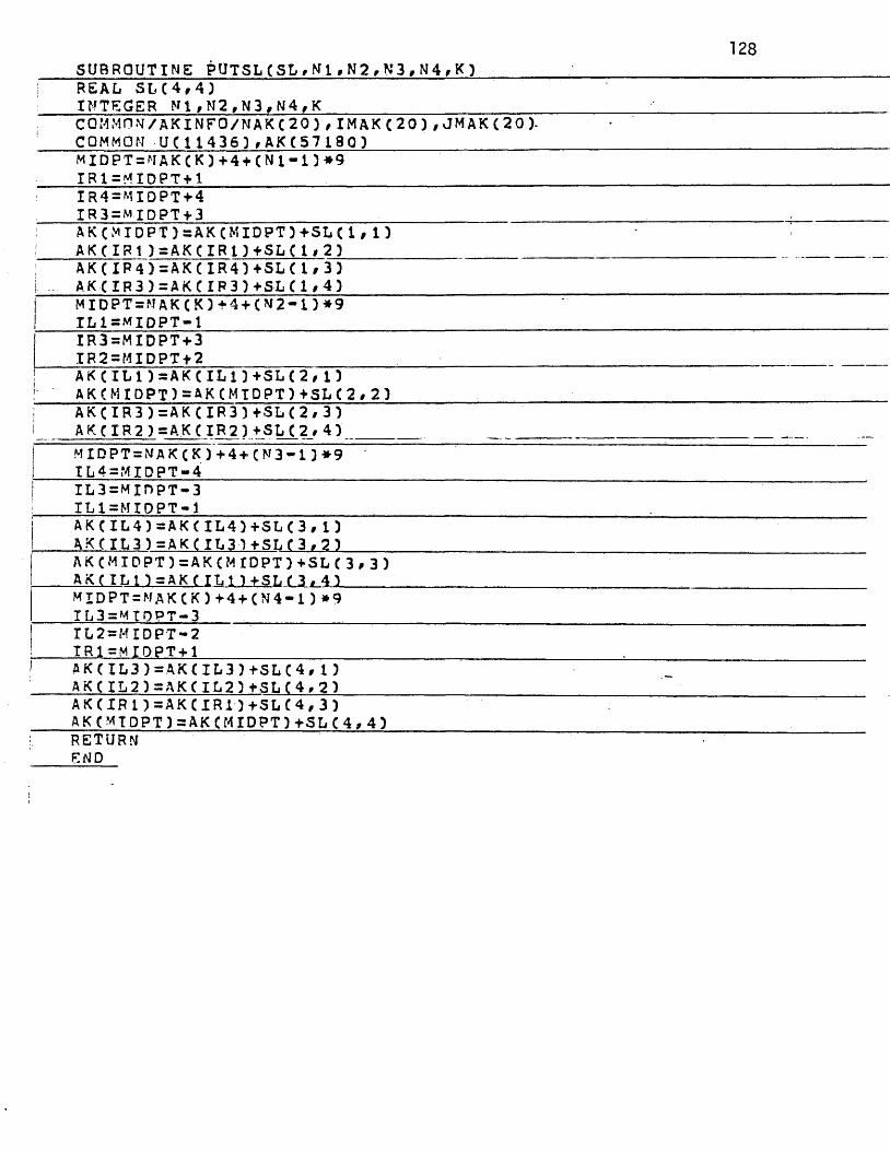
128S U B R O U T I N E P U T S L ( S L , N 1 , N 2 , N 3 , N 4 , K 3a u o r u u i i n c i r v* i o u l o u # i*.x u r w 7R E A L S L ( 4 * 4 )I N T E G E R N 1 , N 2 , N 3 , N 4 , KC Q M M O N / A K I N F O / N A K C 2 0 ) , I M A K ( 2 0 ) , J M A K ( 2 0 ) .COMMON UC 1 1 4 3 6 3 # A K C 5 7 1 8 < 3 3M I D P T = N A K C K ) + 4 + ( N l - i 3 * 9I R 1 = M I D P T + 1I R 4 = M I D P T + 4I R 3 = M I D P T + 3A K C M I D P T ) s s A K C M I D P T ) + S L ( 1 , 1 ) A K C I R t ) = A K C I R l ) + S I i ( l # 2 3A K ( I P 4 ) = A K C I R 4 ) + S L ( 1 , 3 )

! A K ( I R 3 3 = AK C I P 3 ) + S L ( 1 * 4 3j M I D P T = M A K ( K ) * 4 + ( N 2 - 1 ) * 9! i l i = m i d p t - i

I R 3 = M I D P T + 3I R 2 = M I D P T + 2A K C I L 1 ) - A K ( I L 1 3 + S L ( 2 * 1 )A K C M I D P T ) = A K C M I D P T ) + S L C 2 # 2 )A K C I R 3 ) = A K ( I R 3 ) + S L C 2 / 3 )

i A K ( XR 2 3 - A K C I R 2 1 + S L ( 2 * 4 3

M I D P T = N A K ( K ) + 4 + C N 3 - l } * 9 I L 4 = MI D P T - 4I L 3 = M i n p T - 3I L 1 = M I D P T - 1A K ( I L 4 3 = A K ( I L 4 3 + S L ( 3 # 1 )A K C I L 3 3 = A K ( I L 3 3 + S L f 3 , 2 3A K ( M I D P T 3 = A K ( M I D P T 3 + S L ( 3 * 3 3

_ A K ( I L 1 3 = A K ( I L 1 3 + S L ( 3 # 4 )M I D P T = N A K C K ) + 4 + C N 4 - 1 ) * 9I L 3 = M I O P T - 3I L 2 = M I D P T - 2TR1 - M I D P T + 1A K ( I L 3 ) = A K C I L 3 3 + S L ( 4 , 1 3 A K ( I L 2 3 = A K ( I L 2 3 + S L C 4 , 2 )

-

A K C I P 1 ) = A K C I R I ) + S L C 4 , 3 ) A K ( M . T D P T ) = A K C M I D P T 3 + S L C 4 # 4 )R E T U R NEND

129

S U B R O U T I N E P U T P H S ( K , M, R S N 1 , R S N 2 ,R S N 3 , R S N 4 , N 1 , N 2 ,N 3 ,N 4 )I N T E G E R K » M » N 1 # M 2 > N 3 » N 4 _____________________________________________________R E A L R S N 1 / F S N 2 / R S N 3 / R S N 4C O M M Q N / A y i N F O / N A K ( 2 Q ) / I M A K C 2 0 ) / J M A K ( 2 0 ) __________ ___COMMON U C 1 1 4 3 6 ) . A K C 5 7 1 8 0 )I T = N A K ( K + M ) - 1 !___________________________ •________________ _I U N 1 = I T * N 1I U N 2 = I T + N 2 _________________‘__________________________ _______________________________I U N 3 = I T + N 3T U M 4 = I T + N 4 ___________ _ ____________A K ( I U N 1 ) = AK C I U N 1 ) + R S M 1A K C I UN 2 ) = AK C I U N 2 ) + R S N 2 ________________________________________________A K ( I U N 3 ) = A K ( I U N 3 ) + R S N 3A K ( I UN 4 ) = AK C I UN 4 ) + R S N 4__________________ ____________________________________R E T U R NEND________ ________________________ ______________________ _ ____

S U B R O U T I N E ? U T Z A K ( K , M } I N T E G E R K , M __________________

j C O M M O N / A K I N F O / N A K ( 2 0 ) f I M A K C 2 0 } f J M A K C 2 0 ) COMMON U C 1 1 4 3 6 ) / A K C 5 7 1 9 0 )N p T S K s I M A K C K ) * J M A K C K )N P T S K M = I M A K ( K + M ) * J M A K ( K + M )I S T = N A K C K ) - 1DO 1 0 I = 1 / N P T S K

1 0 A K C I S T + I ) = 0 , 0I S T = N A K C K + M ) - 1DO 2 0 1 = 1 / NP T S K MA K ( I S T + I ) = 0 . 0

2 0 C O N T I N U ER E T U R NEND

1 3 0

S U B R O U T I N E R E L A X ( N , M , NR )_______________ ___________________________________ _____________C O M M Q N / G R D I F 1 / N S T C 2 0 ) , I M X C 2 0 3 , J M X C 2 0 )C Q M M Q N / A K I N F Q / N A K C 2 0 ) , I MA K ( 2 0 ) , J MA K C 2 0 3 ______________________________________COMMON U C 1 1 4 3 6 ) , A K ( 5 7 1 8 0 3

________ I N T E G E R M/ M » N R __________________________________________________________W = 1 . 0

I________Q N E M W s l . - W__________________________________________________________ ____________I M A X = I M X CM)

j________J M A X s J M X C N ) __________________________ ;________________ _ _ ______________________ _i J E = J M A X - 1!_______ I E s I M A X - l ____________________ ___________________________________________ _______________________ _! ' T < = t

5 I F ( K t G T . N R 3 GO TO 3 0 _________ _____________________________________________________________j I P T U = M S T ( N 3 +-I.M A X +1i_______ I P T A = N A K C N 1 + 4 + 9 » C I M A X + l 3_______________________________________________________________ _

I P T R S A = iN A K ( N + M ) + 1M A X + 11 DO 2 0 J = 2 »■ J E _________ _______________________________________________________________ ____________

DO 1 0 1 = 2 9 I E!_________________ C N S T s l . / A K C I P T A 3 _____________________________________________________! I T 1 = I P T U - 1M A XI __________ I T 2 = I P T U + I MAX___________________________ ____________ ________________________ _j T E M P = U ( I P T U )!_________________ U C I P T U 3 = A K C I P T A - 4 3 » U C I T 1 - 1 3 + A K C I P T A - 3 3 » U C I T 1 3

U ( I P T U ) s U C I P T U ) ■ f A K ( I P T A - 2 3 * U C I T l + l 3 + A K C I P T A - 1 3 * U C I P T U - 1 3__________________U ( I P T U 3 = T J C I P T U 3 + A K C I P T A M 3 » U f I P T U + 1 3 + A K f I P T A + 2 3 » U C I T 2 - l 3'

U ( I P T U 3 = U C I P T U 3 + A K C I P T A + 3 3 * U ( I T 2 3 + AK ( I P T A + 4 3 * U C I T 2 + 1 3U C I P T U 3 = C N S T » ( A K C I P T R S A 3 » U C I P T U 3 3______________________________________ _

| • U C I P T U 3 = t f * t ; C I P T U 3 + a N E M W * T E M Pj____________ I P T U = I P T U + 1________________________________________

I P T A = I P T A + 9j_________________ I P T R S A = I P T R 5 A + 1 _________ _____________________ ______________________________, 1 0 C O N T I N U E,_______ I P T U = T P T U + 2 ___________ _ ___________________

I P T A = I P T A + 9 * 2■ I P T R S A = I P T R S A + 2 _____________________________________________________________ _______________ _

2 0 C O N T I N U EK = K + 1__________GO TO 5

33 R E T U R N __________________________ ' __________________ ____ ____________END

131

i SUBROUTINE N U C L C N , M , W 1 , W 2 , W 3 , W 4 / W 0 , W 5 / W 6 / W 7 / W 8 ) ______________ •CQ M M ON/GRDXF1/MSTC20)/IMXC 2 0 ) /JMXC20)

!_____ COMMON/AK1NFO /NAK (20 ) , IMAK (20 D , JMAK ( 20)__________________ ____* COMMON U C H 4 3 6 5 |AK(57180)

INTEGER N , M _______,___________ ;_______________ __________PEAL W1,W2,W3,W4#W 0 , W 5 , W 6 #W7,W8

!_____ CALL RESCALCKjM)____________________________________________________IMXNPM=IMXCN+M)

!______ IMXNM1 = IMX(N-1 )____________________________ _____________________________j JMXN=JMX(N)|______ I P R E S = N S T ( N + M ) + 2 » I M X N P M + 2 __________ ;_________ ___ _______ ___

IftSAMlsNAK'CN-l+M) +IMXNM1 + 1______J E = J M X N - 2 _____________________

IE=lMXMPM-2 * ' ■______00 20 J = 3 , JE / 2 '

DO 10 1=3/IE,2______________ITt=IPRE5-IMXNPM _______________ _______ _____________

IT2=IPRSS+IMXNPM____________ AKCIRSAMt )=Wl»(U(ITt-t ) t U (I T U l )+ U (IT2-1)+ U (IT2+1 ))| AK(IRSAM1D=AKCIRSAM15 + W 2 * (U ( I T l l + U C I P R E S - l l + U d P R E S + i)j I________-MJCIT2) 3________________________________________________________

A K C I R S A M H s A K C I R S A M l )+U( IPRES)1____ _________I P R E S = I P R E S + 2 _____________________________________________ _

IRSAM1=IRSAMI+1j 10 CONTINUE____________________________________________________j IPRES=IPRES+IMXNPM+3! IRSAMl=sIRSAMl. + 2______________________________________________________| 20 CONTINUE| RETURN

ENO

132

S U B R O U T I N E _ RESC AL (

1 I N T E G E R K, Mi C U M M Q N / G R D I F 1 / N 5 T C 2 0 ) # I M X C 2 0 1 # J M X C 2 0 )

C O M M O N / A K I N F O / N A K ( 2 0 ) , I M A K C 2 0 ) , J M A K C 2 0 )■ COMMON U C 1 1 4 3 6 ) # A K C 5 7 1 8 0 )

I MA X = I?-1XCK)! J M A X = J M X C K D

I P U K P M = N S T C K + M ) + I M X C K + M ) + 1! . I P U s N S T f K l + I M A X + 1j I P A - N A K ( K D + 4 + 9 * ( I M A X + n! I P R S A = M A K ( K + M ) + I M A X M| i J E = J M A X - l

T E s I M A X - 11 DO 2 0 J = 2 # J E1i DO 1 0 1 = 2 # I Ei I T 1 = I P U - I M A X

I T 2 = I P U + I M A XU C I P U K P M ) = A K ( I P A - 4 ) * U ( I T 1 - 1 ) + A X ( I P A - 3 ) * U ( I T 1 )U C I P U K P M 1 = U C I P U K P M 1 + A K C I P A - 2 ) * U C I T 1 + 1 3 + A K C T P A - l ) * U C I P U - 1 )

1i U C I P U K P M } = U C I P U K P M } + A K ( I P A ) * U C I P U ) + A K C I P A + 1 ) * U C I P U * U11 U C I P U K P M ) : = U C I P U K P M ) + A K C I P A + 2 ) * U ( I T 2 - 1 ) t A K C I P A + 3 ) * U ( I T 2 )

U C I P U K P M ) = : U C I P U K P M ) f A K C I P A + 4 ) * U ( I T 2 + 1 )U C I P U K P M ) = A K C I P R S A ) - U ( I P U K P M )I P U K P M = I P U K P M + 1I P U = I P U + 1I P A = I P A + 9I P R S A = I P R S A + l

1 0 C O N T I N U EI P U K P M = I P U K P M + 2I P U = I P U + 2I P A = I P A + 9 * 2I P R S A = I P R S A + 2

2 0 C O N T I N U ER E T U R NEND

S U B R O U T I N E I N T A D D ( K ) I N T E G E R K ________________ 13aC O M M O N / G R D I F l / N S T C 2 0 ) , I M X C 2 0 ) , J M X C 2 0 )COMMON U ( 1 1 4 3 6 ) / A K C 5 7 1 8 0 ) ________ ;___________________ _____

! I MX K C = I M X ( K - 1 ) ; : 'J M X K C = J M X C K - 1 )___________________________ _____________ ___ ____________ _I M X K F s I M X C K )J M X K F s J M X C K ) _________ ]______________________I V J l K C = N S T C K - n

; I V t 2 K C = I V 1 1 K C + I M X K C ___________________________________________________I I V 1 2 S = I V 1 2 K C; I V 2 1 K C = . I V V 1 K C + 1______ _______________ _________________________________ ___

I V 2 2 K C = I V 1 2 K C + 1I T V 2 2 S = I V 2 2 K C ___________ ____________________________________________________| I V 2 2 K F = N S T C K ) + I M X K F + 1I I V 3 2 K F = I V 2 2 K F + 1_______________ ._________________ _ _ _ _ _| J E - J M X K F - 1I I E = I M X K F - 3 _________________________f DO 2 0 J = 2 , J E / 2|_____________DO 1 0 1-2 r I E / 2 _______________________________________ _______________I T 1 = . 5 * C U ( I V 1 1 K C ) + U C I V 1 2 K C ) )|_________________ T 2 = . 5 » C U ( I V 2 2 K C ) + U C I V 2 1 K C ) )_____________I U C I V 2 2 K F ) = . 5 * ( T 1 + T 2 ) + U ( I V 2 2 K F )!____________ U C I V 3 2 K F ) = T 2 + U C I V 3 2 K F ) _______________________________| I V 1 1 K C = I V 1 1 K C + 1‘_________________ I V 1 2 K C S I V 1 2 KC + t ___________ ,

I V 2 1 K C = I V 2 1 K C - H_________________ I V 2 2 K C = I V 2 2 K C + 1 _____________| I V 2 2 K F = I V 2 2 K F + 2I_______________ I V 3 2 K F = I V 3 2 K F + 2 _______________________________________________j 1 0 C O N T I N U E____________ T 1 = T 2 _____________________________I T 2 = . S * C U ( t V 2 2 K C ) + U ( I V 2 1 K C ) )I U C I V 2 2 K F ) = . 5 » C T H - T 2 ) + U C I V 2 2 K F ) _____________ ______________

I V I 1 K C = I V I 1 K C + 2___________ I V 1 2 K C = I V 1 2 K C + 2 _______________________________________________________

I V 2 1 KC = I V 2 1 KC + 2_________ I V 2 2 K C = I V 2 2 K C + 2 ______________________________________________________

I V 2 2 K F = I V 2 2 K F + I M X K F + 3____________ I V 3 2 K F = I V 3 2 K F + I t MXKF + 3____________________________________________; 2 0 C O N T I N U E: I V 1 2 K C = I V 1 2 S __________ ________________________ ______________ _______________j I V 2 2 K C = I V 2 2 S

T V 1 3 K F = N 5 T C K ) + 2 » I M X K F __________ ___ ______________________________| I V 2 3 K F = I V 1 3 K F + l; I V 3 3 K F = I V 2 3 K F - H ________________________________________________________

J E = J E - 1DO 4 0 J = 3 * J E » 2__________________________________________________ ___________

; DO 3 0 1 = 2 / I E , 2:________________ U C I V 2 3 K F ) ~ U ( I V 2 3 K F ) + . 5 » C U ( I V 1 2 K C ) + U ( I V 2 2 K C ) )

U C I V 3 3 K F ) - U ( I V 3 3 K F ) + U ( I V 2 2 K C )i_________________ I V 1 2 K C = I V 1 2 K C > 1 __________________

I V 2 2 K C = I V 2 2 K C + 1 -I________________ I V 2 3 K F = I V 2 3 K F + 2_______________________________ __________________

I V 3 3 K F = I V 3 3 K F + 2i 3 0 C O N T I N U E ______________________________________________________ ____________i U C I V 2 3 K F ) = U ( I V 2 3 K F ) + . 5 * ( U C I V 1 2 K C ) + U ( I V 2 2 K C ) )

I V 1 2 K C = I V 1 2 KC + 2 I V 2 2 KC = I V 2 2 K C + 2

[___________ I V 2 3 K F = I V 2 3 K F + I M X K F + 3 _____________________________________________I V 3 3 K F = I V 3 J K F + I M X K F + 3

4 0 C O N T I N U E _ _ _ ______________________________________________________________R E T U R N " .......... .

134

S U B R O U T I N E P U T Z ( N )I N T E G E R N _____________________________C O M M O N / G R D I F 1 / N S T ( 2 G ) , I M X C 2 0 ) , J M X C 2 0 )COMMON U ( 1 1 4 3 6 ) 9 A K C 5 7 1 8 0 )____________________N P T S = I M X C N ) * J M X C W )I S = N S T ( N ) - 1 . _________________________________________DO 1 0 I = 1 , N P T S

U ( I S + I ) = 0 . 0 _________________________________1 0 C O N T I N U E

R E T U R N ____________________________________________________END

S U B R O U T I N E P U T B C N f G l )__________ :___I N T E G E R NC O M M O N / G R D I F 1 / N S T C 2 0 ) , I M X C 2 0 ) , J M X ( 2 0 l C 0 M M 0 N / G R D T F 2 / H V C 2 0 )COMMON U C 1 1 4 3 6 ) » A K ( 5 7 1 8 0 3_____________________I I = I M X C N )J J s J M X C N ) ________________ __________________________I S l = N S T ( N ) - tI S 2 = I S 1 + C J J - 1 ) » I I ____________ '______________H = H V C N )n o i o k = i , n _ _ _ _ _ _ _ _ _ _ _ _ _ _ _ _ _ _

U ( I 5 1 + K ) = G 1 C C K - 1 ) * H # 0 . 0 ) ’________ _ U l I S , 2 + K ) g C - l C ( K - 1 ) » H 9 C J J * 1 ) » H ")1 0 C O N T I N U E

K E = C J J - M » I I _______________________________ _I S 1 = N S T C N )

I 5 2 ~ I 5 1 + I I - 1 ___________ ______________________ _________L = 1DO 2 0 K = I I , K E . T T __________________________________

U ( I S I + K ) = G 1 C 0 . 0 , L * H ) ; U - I I S 2 + K 3 = G 1 C C I T - . l T » H , L » H 3 ________________

L = L + 12 0 C O N T I N U E _________________________________________________

R E T U R NE N D ________________ ___

135

F U N C T I O N F C X , Y )

! R E T U R N END

F U N C T I O N G C X , Y ) G = X * X + Y * Y

--------------

R E T U R NEND

j F U N C T I O N E X A C T C X , Y ) E X A C T = X * X + Y * YR E T U R NEND

-

Ii

ji S U B R O U T I N E O U T P U T ( K )

I N T E G E R K .C Q M M O N / G R D I F 1 / N S T C 2 0 ) , I M X ( 2 0 ) , J M X C 2 0 )COMMON U C 1 1 4 3 6 ) # A K C 5 7 1 8 0 )R E A L P C 6 5 )

f I S T = M S T ( K ) - 1 ........................i I I = I M X ( K )! J J = J M X C K )i N P T S = I I * J J1 I 8 = 1 S T - ............

I £ = I B + C J J " 1 ) * 1 1j DO 2 0 I S T = I 8 , I E , I I; DO 1 0 1 = 1 , 1 1! P C I ) = U ( I S T + I )

1 0 C O N T I N U EW R I T E C 6 , 1 0 0 ) ( P C I ) , 1 = 1 , I I )

2 0 c o n t i n u e; t o o f o r m a t c i h , a n 5 . 1 2 )

R E T U R Ni » - END.

136S U B R O U T I N E O U T P A K ( K , M )i n t e g e r k , m ♦C O M M O N / A K I N F O / N A K C 2 0 ) , I M A K ( 2 0 ) , J M A K ( 2 0 ) C O M M O N / G P D I F 1 / N S T ( 2 0 ) , I M X ( 2 0 ) / J M X ( 2 0 )

c

COMMON U ( 1 1 4 3 6 ) / A K ( 5 7 1 8 0 )R E A L P ( 5 8 5 )I I = I M X ( K )J J = J M X ( K )I B = N A K ( K ) - 11 1 9 = 1 1 * 9I E = I 3 + ( J J - 1 ) » I I 9DO 2 0 I S = I B , I E , I I 9DO 1 0 1 = 1 / 1 1 9

j P C D a s A K C I S + ni 1 01

C O N T I N U EW R I T E ' ( 6 , 1 0 0 ) ( P ( I ) , 1 = 1 / 1 1 9 )

i 2 0 C O N T I N U E I B = N A K ( X + M ) - 1I E = I 8 + ( J J M ) * I IDO 4 0 I S = I B / I E # I IDO 3 0 1 = 1 / 1 1

P ( I ) = A K ( I S + I }3 0 C O N T I N U E

W R I T E ( 6 / 1 0 0 ) ( P ( I ) , 1 = 1 , I I )4 0 C O N T I N U E1 0 0 F 0 R M A T C 1 H , 1 0 F t 0 . 5 )

P E T U R NEND

S U B R O U T I N E G U E S S ( N )I N T E G E R N_____________________ ________________________ _C O M M O N / C R D I F 1 / N S T ( 2 0 3 , I M X ( 2 0 ) , J M X ( 2 0 )COMMON U ( 1 1 4 3 6 ) , A K f 5 7 1 9 0 I ____________ ________N P T S = I M X ( N ) * J M X ( N )I S = N S T ( N ) - 1 ______________________________ _DO 1 0 I = 1 , N P T S

_____________ U C I S * 1 1 = 1 ,______________________________________1 0 C O N T I N U E

R E T U R NEND

S U B R O U T I N E L 2 C N , E R R L 2 , E X A C T )137

' E X T E R N A L E X A C T C O M M O N / G R D I F 2 / H V C 2 Q )C Q M M Q N / G R D I F 1 / N S T ( 2 0 ) # I M X ( 2 0 ) , J M X C 2 0 ) COMMON U C 1 1 4 3 6 ) r A K C 5 7 1 8 0 )J E = J M X ( N 3 - lI E = I M X C N 3 - 1

| I P U 2 2 = N S T C N ) + I E + 2E R R L 2 = 0 . 0

: H= H V C N )DO 2 0 J = 2 * J E .

DO 1 0 1 = 2 # I E* X = C I - 1 ) * H

Y“ C J - 1 ) * H! E R R L 2 = £ R R L 2 + ( E X A C T ( X , Y ) - U ( I P U 2 2 ) ) * * 2! I P U 2 2 = I P U 2 2 + l

1 0 C O N T I N U EI P U 2 2 = I P U 2 2 + 2

2 0 C O N T I N U EE R R L 2 = E R R L 2 * * . 5r e t u r n

END

o u n n u u L X U £•E X T E R N A L AE X T E R N A L BE X T E R N A L CC O M M O N / G R D I F 2 / H V C 2 0 )D I M E N S I O N S ( 4 , 4 ) # P ( 4 , 4 ) ,W C 4 )F I 1 ( X # Y ) = C X - X 2 ) * C Y - Y 2 )F I 2 C X , Y J = - ( X - X 1 ) * C Y - Y 2 )F I 3 ( X * Y } = C X - X 1 ) * C Y - Y 1 )F I 4 C X , Y ) = - C X - X 2 ) * C Y - Y 1 )F I 1 X ( Y ) = Y - Y 2F I 2 X ( Y ) = - C Y - Y 2 ) F I 3 X ( Y ) = C Y ~ Y 1 )

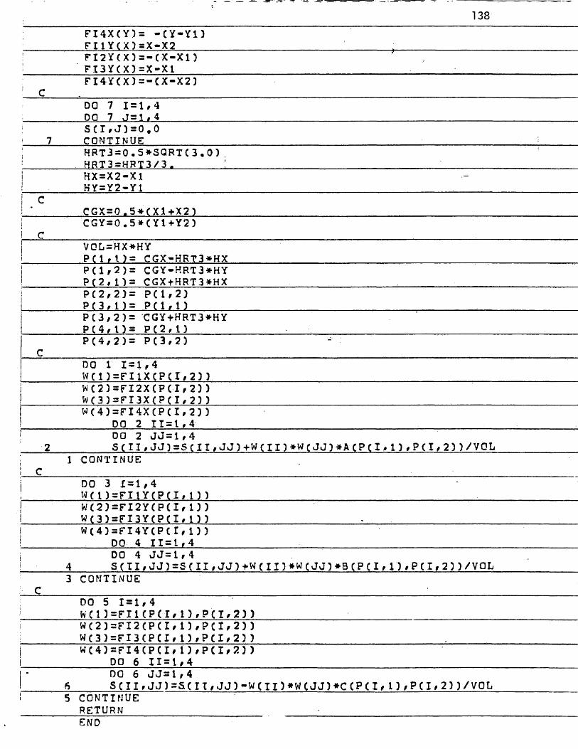
1 3 8F I 4 X C Y ) = - C Y - Y 1 )

________ F I 1 Y C X ) = X - X 2 ___________F I 2 Y ( X D = - ( X - X 1 )F I 3 Y ( X ) = X - X 1___________F I 4 Y C X ) = - C X - X 2 )_ _____

________ DO 7 J s l . 4 _______________S C I , J ) = 0 . 0

7 C O N T I N U E ___________________H R T 3 = 0 . 5 * S Q R T C 3 . 0 ) , H R T 3 - H R T 3 / 3 . !H X = X 2 - X 1H Y = Y 2 - Y 1 __________________

________ C G X = 0 . 5 » C X l + X 2 1C G Y = 0 . 5 * C Y 1 + Y 2 Y

V G L = H X * H YP C I , 1 ) = C G X - H R T 3 » H X P C 1 # 2 ) = C G Y - H R T 3 * H Y P C 2 , 1 ) = C G X * H R T 3 » H X PC 2 # 2 ) = PC I f 2 ) P C 3 , 1 ) = P C 1 , 1 ) P C 3 / 2 ) = C G Y + H R T 3 * H YP C 4 , 1 ) = PC 2 , 1 ) _________P C 4 , 2 ) = P C 3 , 2 )

DO 1 1 = 1 , 4_____________ W C l ) = F I l X C P C I / 2 n __________________________________________________________

W C 2 ) = F I 2 X C P C I # 2 ) )W C 3 ) = F I 3 X ( P C I / 2 ) )______________________________________ ______________ __________W ( ' 4 ) = F I 4 X ( P C I , 2 ) )

____________________ DO 2 1 1 = 1 , 4 ____________________________________________ ______________ _! DO 2 J J = 1 , 4

2____________ s e l l , J J ) = S C I I , J J ) + W C I I ) » W C J J ) » A C P C l , 1 ) , P C I , 2 ) ) / V O L: l c o n t i n u e

I C_________________________________________________________ ;____________________ ;________j DO 3 1 = 1 , 4i_____________ W ( 1 ) = F I 1 Y C P C I , 1 ) ) ____________________________________ ■! W ( 2 ) = F I 2 Y C P ( I , 1 ) )L ___________ W C 3 3 = F I 3 Y C P C I , 1 ) )__________________________________> ________________| W C 4 ) = F I 4 Y C P C I , 1 ) )I______________ DO 4 1 1 = 1 , 4 _______________________ ___________________________________________

DO 4 J J = 1 , 4! ■ 4________S ( 1 1 , J J ) = S C I I , J J ) *W C 1 1 ) » W C J J ) » B CP C I y 1 ) * P C I * 2 ) ) / VOL1 3 C O N T I N U E!- C________________________________________________________________________________

DO 5 1 = 1 , 4|_____________ W C 1 ) = F I 1 C P C I / l ) , P C I / 2 ) )____________________ ;________________________________i W ( 2 ) = F I 2 ( P ( I , i ) , P ( I , 2 ) )I____________ W C 3 ) = F I 3 C P C I > 1 ) , P C I # 2 ) )___________________________________________ .___________i W ( 4 ) = F I 4 ( P ( I # 1 ) , P ( 1 , 2 ) )j___________________ DO 6 1 1 = 1 , 4 ____________________________________________________________________| • DO 6 J J = 1 , 4!_________6_________s e n , j j ) = s c i i , j j i " w c m » w c j j ) » c c p c i / n # p c i » 2 ) ) / v o li 5 C O N T I N U E___________ R E T U R N

END

139

F U N C T I O N A ( X * Y V

A = - l .R E T U R NENDF U N C T I O N B ( X * Y )B = - l .R E T U R N

| ENDF U N C T I O N C C X , Y )

! c = o .I R E T U R Nj END| S U B R O U T I N E R H S C X 1 , Y 1 , X 2 , Y 2 , S 1 , S 2 , S 3 , S 4 , F )! E X T E R N A L F! D I M E N S I O N S ( 4 ) , P C 4 , 4 )j F I 1 C X , Y ) = C X - X 2 ) * C Y - Y 2 ) ' ..

! F I 2 C X / Y ) = - C X - X 1 ) * C Y - Y 2 )j F I 3 C X # Y ) s C X - X 1 ) * C Y - Y 1 )i F I 4 C X , Y ) = - C X - X 2 ) * C Y - Y 1 )! DO 2 1 = 1 , 4

■ ! 2 S C I ) = 0 . 0! C G X = 0 . 5 * C X 1 + X 2 } 1 C G Y = 0 . 5 * C Y 1 + Y 2 )

H X = X 2 - X 1H Y = Y 2 - Y 1H R T 3 = 1 , 0 / ( 2 . 0 * S Q R T C 3 . 0 ) )P C I , n = C G X - H R T 3 * H XP C 1 / 2 ) = C G Y - H R T 3 * H YP C 2 , 1 ) = C G X + H R T 3 * H XP C 2 f 2 ) = P C1# 2 )P C 3 r l ) = P C l » l ) : 'P ( 3 / 2 ) = C G Y + H R T 3 * H YP C 4 , l ) = p ( 2 , 1 )P C 4 , 2 ) s P C 3 , 2 )DO 1 1 = 1 , 4S C l ) = S C n + F C P C T # l ) # P C I # 2 ) ) * F I l C P ( I r l ) # P C I # 2 ) )S ( 2 . ) = S C 2 ) + F C P C r , 1 ) , P ( I , 2 ) ) * F I 2 ( P C I , 1 ) # P C I # 2 ) )

■ 5 C 3 ) =.S C 3 ) + F ( P C I # 1 ) / P C I / 2 ) ) * F I 3 ( P ( I # l ) / P ( I / 2 ) ) 1 i 5 C 4 ) = S C 4 ) + F C P C I / l ) / P C I / 2 ) ) * F I 4 C P ( I / l ) / P C I / 2 ) )

S 1 = S C 1 )S 2 = S C 2 )S 3 = S C 3 )S 4 = S C 4 )R E T U R NEND

140

S U B R O U T I N E C A L R I N ( K , M )C 0 M M Q N / G R D I F 1 / N 5 T ( 2 0 ) , I M X ( 2 0 1 , J M X C 2 0 )C 0 M MO N / A K I N F O / N A K ( 2 0 ) , I M A K C 2 0 ] , J M A K ( 2 0 )COMMON U C 1 1 4 3 6 1 , A K ( 5 7 1 8 0 } _______________________I N T E G E R K , MI M A X = I M X ( K 1J M A X = J M X C K )I M X K M 1 = I M X ( K ~ 1 )I T E M P = 2 * I M A X + 2I P U = N S T ( K 1 + I T E M PI P A = N A K ( K 1 + 4 + 9 * I T E M P I P R 5 A = N A K ( K + M 1 + I T E M PI R S A M 1 = N A K C K - 1 + M 1 + I M X K M 1 + 1J E = J M A X - 2I E = I M A X - 2DO 2 0 J s 3 , J E , 2

DO 1 0 1 = 3 , I E , 2I T 1 = I P U - I M A XI T 2 = I P U + I M A XA K C I R S A M 1 l = A K C I P A - 4 1 * U r T T 1 - 1 1 + A K C I P A - 3 1 * U ( I T 11A K C I R S A M 1 ) = A K C I R S A M 1 ) + A K C I P A - 2 ) * U ( I T 1 + 1 ) + A K ( I P A - 1 J * U ( I P U - 1

1 1A K C I R S A M 1 ) = A K ( I R S A M 1 3 + A K ( I P A ) * U ( I P U ) + A K ( I P A + 1 } * U C I P U + 11A K C I R S A M 1 1 = A K C I B S A M 1 l + A K ( I P A + 2 1 * U C I T 2 - l l + A K ( I P A + 3 1 * U ( I T 2 1A K C I R S A M 1 ) = A K ( I R S A M 1 1 + A K ( I P A + 4 1 * U C I T 2 + 1 }A K f I R S A M 1 1 = A K ( I P R S A 1 - A K f T R S A M 1 ^A K C I R S A M 1 ) = 4 . * A K C I R S A M UI R S A M l s I R S A M l + tI P U = I P U + 2I P A = I P A + 9 * 2I P R S A = I P R S A + 2

1 0 C O N T I N U EI R S A M l = I R S A M l + 2I P U = l P U + I M A X + 3I P A = I P A + 9 * C I M A X * 3 lI P R S A = I P R S A + I M A X + 3

2 0 C O N T I N U ER E T U R N

- END

APPENDIX I I

A f i n i t e element m u l t i - g r id a lgori thm f o r the so lu t io n of :

(-AUX)X + (_BUy)y - Cu = F

on a r e c t a n g le . This code uses b i l i n e a r t r i a l fu n c t io n s , and accep ts

mixed boundary con d i t io ns c o n s i s t in g of D i r i c h l e t da ta on one s ide of

a r ec tan g le and Neumann cond i t ions on the remaining th re e s id e s .

The code includes a Gaussian e l im ina t io n subrout ine which, is: used to

solve the G° system when i n d e f i n i t e problems a re being solved.

Comments

SUBROUTINE EL(NX0,NY0,H0,M,NCYCLS,G1,EX,A1,B1,C1,IP1,IP2,IPASS)

NX0,NY0 Number o f mesh i n t e r v a l s in the X and Y d i r e c t i o n s on g r id G°.

HO Mesh s i z e on G°.

NCYCLS Number o f m u l t i - g r id cycles to bemade.

Note: In c o n s t ru c t in g s to rage space f o r t h i s a lgor i thm , an ou te r

per im ete r of dummy p o in ts a re placed next to boundary po in ts where

Neumann cond i t ions hold. Hence, the c o a r s e s t g r id (dots) i s

embedded in the fol lowing s t r u c t u r e :

to o p o o o

D i r i c h l e t -7data

O O O O o OI

o oare in d ica ted by

O arrows.r \

v Neumann co n d i t ion s O 7

141

142

CALL MULTIG(M,10,IP1,IP2) CALL SETSOL(M)

CALL L2SOL(.M,ERRL2)

SUBROUTINE DIFF(K,EXACT)

SUBROUTINE L2(N,ERRL29EXACT)

SUBROUTINE SETGAU

These two steps: a re performed when we wish to ob ta in the so lu t io n to the d i f f e r e n c e e q u a t io n s . This so lu t io n i s in th e s to rage space SOL(’1190).

Computes a norm of the e r r o r between th e exac t so lu t io n of the d i f fe rence , equa t ions and our c u r r e n t approximate so lu t io n o f the d i f f e r e n c e equat ions .

Outputs the d i f f e r e n c e between the exac t so lu t io n of the d i f f e r e n t i a l equat ion and our approximate so lu t io n o f the d i f f e r e n c e equa t ions .

Computes a norm of the d i f f e r e n c e between an approximate so lu t io n of the d i f f e r e n c e equat ions and the exac t s o lu t io n o f the d i f f e r e n t i a l equat ion .

Accepts the c o e f f i c i e n t s o f the G° system and performs an LDU decomposition (procedure f a c t o r ) .

143

E X T E R N A L G E X T E R N A L FE X T E R N A L E X A C TE X T E R N A L A

I E X T E R N A L B!i E X T E R N A L C' COMMON U C 3 4 0 8 ) * A K ( 1 7 0 4 0 )| R E A L C O N E C T # HO

I N T E G E R N X O , N Y O , MI P A S S s l

1 ' O P E N C U N I T = 6 f D E V I C E S # T T Y # )l‘ DO 4 0 N C Y C L S = 5 . 5

DO 3 0 M = 3 * 3DO 2 0 I P A R 1 = 2 / 2j DO 1 0 I P A R 2 = 1 t 1

i I P M 1 = I P A R 2 - 1C A L L E L ( 4 # 4 / , 2 5 , M, N C Y C L S , G , F , E X A C T / A , B , C , I P A R 1 , I P M 1 , I P A S S

; 1 )

. I P A S S = 2W R I T E C 6 # 1 0 0 ) M f I P A R l # I P M l

1 0 C O N T I N U E2 0 C O N T I N U E3 0 C O N T I N U E4 0 C O N T I N U E

C A L L O U T P U T ( 3 )

. - C A L L D I F F ( 3 # E X A C T )1 0 0 F O R MA T C 9 M= # , I 5 P A R 1 = # , I 5 , # P A R 2 * ' # 1 5 )

S T O PEND

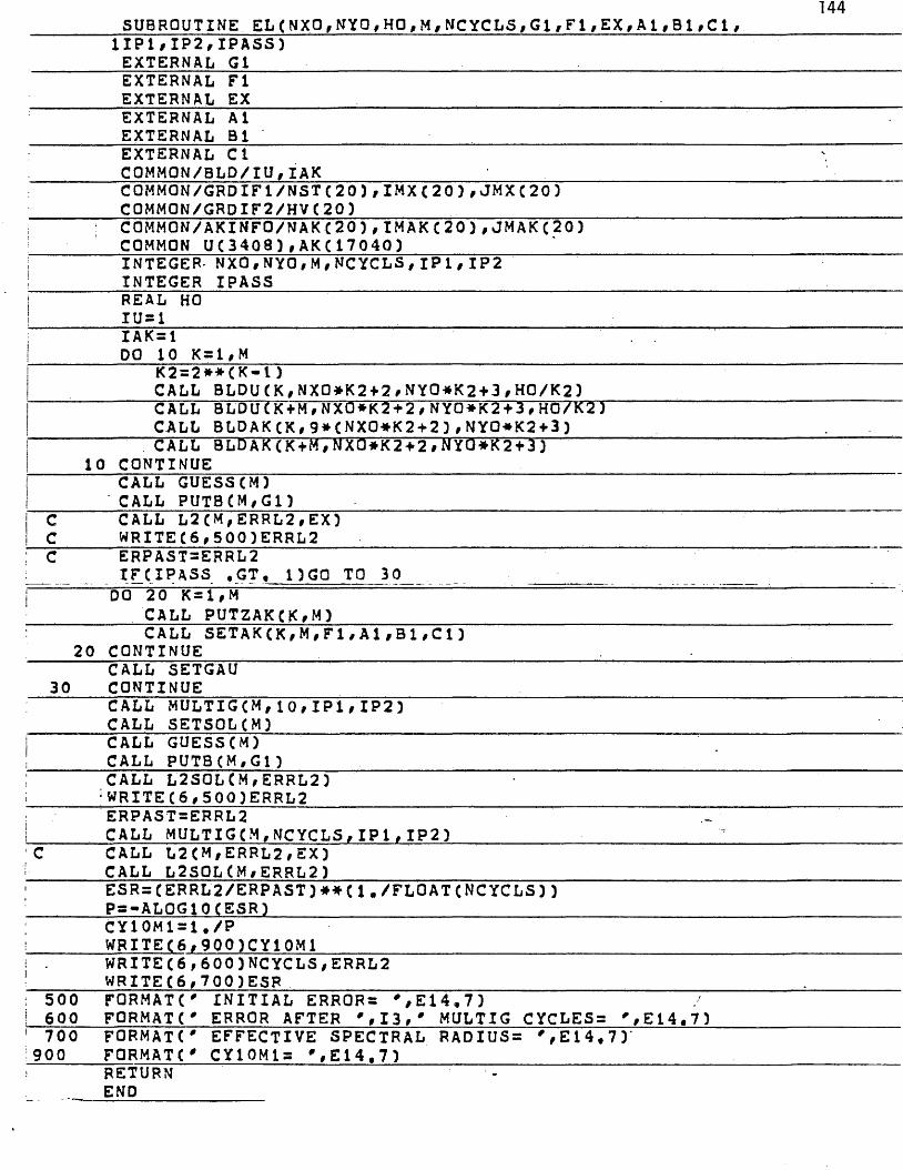
144SUBROUTINE EL(NX0yNY0yH0,MyNCYCL5yGlyFlyEXyAlyBlyCly

lIPlyIP2yIPASS)E X T E R N A L G1________ ■E X T E R N A L F IE X T E R N A L EX___________________________________________ _E X T E R N A L A1E X T E R N A L B 1 _______________________ _________________________E X T E R N A L C lC O M M Q N / B L D / I U y I A K _______________________ ' ________C Q M M O N / G R D I F 1 / N S T C 2 0 ) , I M X ( 2 0 ) yJ M X C 2 0 )C O M M O N / G R P I F 2 / H V ( 2 0 )______________ _____________________C Q M M O N / A K I N F O / N A K ( 2 0 ) , I M A K C 2 0 ) y J M A K ( 2 0 )COMMON U C 3 4 Q 8 ) , A K ( 1 7 0 4 0 ) _____________________ ~I N T E G E R - N X O y N Y O y M y N C Y C L S y i P l y I P 2 I N T E G E R I P A S S R E A L HOI U = 1 __________________________________________________________I A K = 1DO 1 0 K = l y M

K2 = 2 * * C K - 1 )C A L L B L D U ( K y N X O * K 2 + 2 ^ N Y O * K 2 + 3 y H O / K 2 ) C A L L B L D U C K + M y N X O * K 2 + 2 y N Y O * K 2 + 3 y H O / K 2 )CALL BLPAK(Ky 9*(NXO*K2 + 2)yNYO*K2 + 3)CALL BLDAK(K+MyNXO#K2+2yNYa*K2+3)

10 CONTINUECALL GUESS CM)CALL PUTBCMyGl)

c CALL L2(MyERRL2yEX}C WRITEC6y500)ERRL2C ERPAST-ERRL2

IFCIPASS ,GT, 1)GO TO 30DO 20 K = 1 y M

CALL PUTZAKCKyM)CALL S E T A K C K y M y F l y A l y B l y C n

20 CONTINUECALL SETGAU

30 CONTINUECALL MULTIGCMy10yIPlyIP23CALL SETSOL(M)CALL GUESS CM)CALL PUTB(MyGl)CALL L2S0LCMyERRL2D:WRITEC6y500)ERRL2ERPAST=ERRL2CALL MULTIGC M , N C Y C L S y I P 1 ,IP20

C CALL L2 C M y ERRL2 y EX )CALL L2SOLCMyERRL2)ESR=(ERRL2/ERPA5T) #■# ( 1 ./ F L O A T ( N C Y C L S ))Ps-ALOGIOCESR)CY10M1=1./PWRITE(6y900)CY10MlWRITEC6,600)NCYCLSyERRL2WRITECSy700)ESR

500 F O R M A T ( 0 INITIAL ERROR= #yE14,7)600 FORMAT C * ERROR AFTER M 3 i # MULTIG CYCLESs #yE14.7)700 F O R M A T C # EFFECTIVE SPECTRAL RADIUS= #,E14.7)'

900 F O R M A T (0 CYlOMls *,E14.7)RETURN -END

145

S U B R O U T I N E M U L T I G C M , N C Y C L S , I P 1 , I P 2 )I N T E G E R M 9 N C Y C L S » I P 1 » I P 2L=MDO 5 0 J = 1 # N C Y C L S

DO 2 0 KK = 2 § LK = L + 2 - K KC A L L R E L A X ( K , M , I P 1 1

i C A L L P U T Z C K - 1 )i C A L L N U C L C K , M , . 2 5 , . 5 , . 2 5 , . 5 , 1 . , . 5 , . 2 5 , . 5 , . 2 5 )

2 0 C O N T I N U EC A L L S L V G A U ( M )DO 4 0 K = 2 # L

C A L L I N T A D D ( K )i I F C K . E Q . M . A N D . J . E Q . N C Y C L S j C A L L R E L A X C K , M , 0 )f I F ( K . E Q . Ml GO TO 4 0i C A L L R E L A X ( K # M t I P 2 )

4 0 C O N T I N U E5 0 C O N T I N U E

R E T U R N_____ _ _ END

S U B R O U T I N E B L D U C N , I M A X # J M A X , H H ) I N T E G E R N 9 I M A X t J MA XR E A L HH •

C O M M O N / B L D / I U f l A K. C O M M O N / G R D I F 1 / N S T C 2 0 ) , I M X C 2 0 ) , J M X C 2 0 )

C O M M O N / G R D I F 2 / H V ( 2 0 )N S T ( N ) = I UI M X C N ) = I M A XJ M X ( N ) = J MAX

! . H V C N ) = H Hi u = i u + i m a x * j m a x

R E T U R N

_ END

146

w w w w u A X U t l U H I X U 1 » i n H A / U H M A JI N T E G E R N 9 I M A X # J M A X C O M M O N / B L D / I U , I A K

------ T 1-- -------------- ' ■' ... ........ . ............

C O M M O N / A K I N F O / N A K C 2 0 ) , I M A K ( 2 0 ) , J M A K C 2 0 ) N A K C N l s I A KI MAK C N ) = I M A X J M A K C N l s J M A Xi a k = i a k + i m a x * j m a xR E T U R NEND

SUBROUTINE SETAKCN,M ,F ,A ,B #C 1 ______________________________!EXTERNAL FEXTERNAL A _______________ ___________________EXTERNAL BEXTERNAL C__________ ;_________ .INTEGER N,MREAL S L ( 4 y 4 )_________________________________ _ _ _ _ _____________________ _COMMON/GRDIF1/NSTC20),I M X (20),J M X C 20)COMMON/GRPIF2/HV (20 3________________________________________ ______ ___________H=HVCN)NjsIMXCN)_______________ ___________________ ._________ ________________________ ___M2=N1+1N3=2»IMX(N)+1____________ ____________________________________________________ _N4=N 3-1JE=JMX(N)-3______________________IE=IMX(N)-2 -DO 20 J = 1 ,JE______________ _______________________ _________ ___________ __________

DO 10 1=1#IE___________ N 1= N 1 + 1______________________________________

N 2 = N 2 +1_________ N3=N3+1_________________________________ ___________________ __________ __

N4=N4+1___________ X1=CI-1)»H___________________________________________________ _____________

YI=(J-1D*H___________ X2=I»H______________

Y2=J*H___________ CALL STIGEN(A»B»CyXl/X2yYl » Y2 y S L )_____________________________ __

CALL PUTSLCSL,N1,N2,N3,N4,N)___________ IF C N ,EQ. M3CALL R H S C X 1,Y 1,X 2 ,Y 2 ,R S N 1,R S N 2 ,RS N 3 ,R S N 4 ,F )______

IF (N ,EQ. M)CALL PUTRHS (N , M , RSN 1, RSN2 , R'SN3 / R S N 4 , N 1, N 2 , N 3 , N 4 )10 CONTINUE_________________ _____________ -_________ _________________________

N 1= N 1+2_______ N2=N2+2 ■ ____________________________________

N3=N3+2_______ N4=N4+2______________________________ _______________________20 CONTINUE

RETURNEND

147

SUBROUTINE PUTSL(SL#N1»N2yN3yN4#K)R E A L S L ( 4 * 4 )I N T E G E R N 1 , N 2 , N 3 , N 4 , K

! C O M M O N / A K I N F O / N A K C 2 0 ) # I M A K C 2 0 ) , J M A K C 2 0 )COMMON U C 3 4 0 8 ) , A K C 1 7 0 4 0 )

| M I D P T = N A K ( K ) + 4 + ( N t - l ) * 91 I R l s M I . D P T + 1

I R 4 = M I D P T + 4i I R 3 s M I D P T + 3| A K C M I D P T ) = A K C M I D P T D + S L ( 1 , t )I A K C I R 1 ) = A K C I R l ) t S L ( 1 ,2) ___ _____ _ _ ___ ___ _____ ___. .

A K C I R 4 ) = A K C I R 4 ) + S L C 1 # 3 )A K C I R 3 ) = A K C I R 3 ) + S L C 1 # 4 )M I D P T = N A K ( K ) + 4 + C N 2 - l > * 9

! I L i = M I D P T - l! I R 3 = M I D P T + 3! I R 2 = M I D P T + 2! A K ( I L 1 ) = A K C I L 1 D + S L ( 2 # 1 )

A K ( M I D P T ) = A K ( M I D P T ) + S L (2*2)! A K C I R 3 ) = A K C I R 3 ) + S L ( 2 , 3 )1 A K ( I R 2 ) = A K C I R 2 ) + S L C 2 , 4 VI M I D P T = N A K C K ) + 4 + ( N 3 - l ) * 91 I L 4 - M I D P T - 41 I L 3 = M I D P T - 3i I L 1 = M I D P T - 1

A K ( I L 4 ) = A K C I L 4 ) + S L ( 3 , 1 )A K ( I L 3 D = A K C I L 3 ) + S L ( 3 , 2 )A K C M I D P T ) = A K C M I D P T 3 + S L C 3 , 3 )A K C I L D s A K C I L l ) + S L ( 3 / 4 )M I D P T = N A K C K ) + 4 > ( N 4 - 1 ) * 9I L 3 = M I D P T - 3I L 2 = M I D P T - 2I R 1 = M I D P T + 1AK C I L 3 ) = A K ( I L 3 ) + S L C 4 # 1 >A K C I L 2 ) = A K ( I L 2 ) + S L C 4 # 2 )A K C I R 1 ) = A K ( I R 1 ) + S L C 4 ^ 3 )A K C M I D P T ) = A K ( M I D P T ) + S L C 4 , 4 )R E T U R NEND

1 4 8

SUBROUTINE PUT R H S ( K #M , R S N 1#R S N 2 #R S N 3 #R S N 4 #N 1#N 2 #N 3 #N 4 3 INTEGER K#M#N1#N2#N3#N4

: REAL RSN1,RSN2,RSN3,RSN4CO M M O N / A K I N F O / N A K (20)#I M A K (2 0),J M A K (20)COMMON U ( 3 4 0 8 ) # A K ( 17040)

i IT=NAK(K+M)-1! I U N 1 = IT + N 1IUN2=IT+N2

! IUN3=IT+N3j IUN4=IT+N4

AKCIUN1)=AKCIUN1)+RSN1AK (IUN2)= A K (IUN2)+RSN2

i1 A K (IUN 3 ) = A K (IUN 3)+RSN3| AK(I U N 4 ) = A K ( I U N 4 )+RSN4

R E T U R NEND

S U B R O U T I N E P U T Z A K ( K > M ) I N T E G E R K# MC O M M Q N / A K I N F O / N A K C 2 0 ) # I M A K C 2 0 ) # J M A K C 2 0 )COMMON U C 3 4 0 8 ) , A K ( 1 7 0 4 0 )

I N P T S K = I M A K C K ) * J M A K ( K )N P T K P M = I M A K ( K + M ) * J M A K ( K + M )I S T = N A K ( K ) - 1DO 1 0 1 = 1 # N P T S K

1 0 A K ( I S T + 1 3 = 0 . 0I S T = N A K ( K + M ) - 1DO 2 0 1 = 1 # N P T K P MA K ( I S T + I ) = 0 • 0

2 0 C O N T I N U ER E T U R NEND

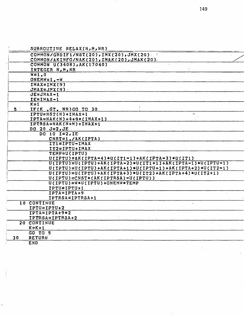
1 49

S U B R QUT I ME RELAX_( N/_M# NR )| COMMON/GRDI F 1 / N S T C 2 0 ) , I M X C 2 0 ) ,JMXC20) ^ I COMMON/AKINFO/NAK (20) #IMAKC20) #JMAKC20)-

COMMON UC340 8 ) <» AK( 17040)INTEGER N,M,NRw = i # oONEMWsl.-WIMAX=IMXCN)JMAX=JMX f N ) fJ E - J M A X - 1

I IE=IMAX-1I K = 1I 5 ' IFCK .GT. NR)GO TO 301 IPTU=NSTCN)«HMAX+1! IPTA=NAKCN)+4+9*CIMAX+l)

I P T R S A = N A K (N + M ) +IMAX+1DO 20 J=2,JE

DO 10 1 = 2 fIECNST=1./AKCIPTA)IT1=IPTU-IMAXIT2=IPTU+IMAXTEMP=U CIPTU)

i U(IPTU)=AK(IPTA-4)*UCIT1- 1)+ A K C I P T A - 3 )* U C I T 1 )1 U ( I PTU)=UCIPTU)+ A K ( IPT A - 2 )* U C I T 1 + 1 ) + A K ( IPTA-1)* U (IPTU-1 )i U (IPTU)=UCIPTU)+AKCIPTA+l)*U(IPTU+l)+AKCIPTA+2)*UCIT2-l)r UCIPTU)=UCIPTU)+AKCIPTA + 3)*UCIT2)+AKCIPTA + 4)*UCIT2-H )

U ( IPTU )=CNST*(AKCIPTRSA)-UC IPTXJ) )i U ( I P T U )=W*U CIPTU)+ONEMW*TEMPIPTU=IPTU+1IPTA = IPT.A + 9IPTRSA=IPTRSA+1

10 CONTINUEIPTU=IPTU+2IPTA=IPTAt9*2IP TR S A = IP T R S A + 2

20 CONTINUEK = K + 1GO TO 5

3 0 RETURNEN D

1 5 0S U B R O U T I N E N U C L ( N , M, W1 , W 2 , W 3 , W 4 , WQ, W 5 , W 6 , W 7 , W 8 ) C Q M M O N / G R D I F 1 / N S T C 2 0 ) # I M X C 2 0 ) # J M X C 2 0 ) TC O M M O N / A K I N F O / N A K ( 2 0 ) r I M A K C 2 0 ) * J M A K C 2 0 )COMMON U C 3 40 8 )#AK(17040) INTEGER N , M ________ __REAL W1,W2#W3,W4,W0,W5,W6,W7,W8 CALL RESCAL(N,M)I M X N P M s l M X C N + M )IMXNM1=IMXCN-1)JMXNsJMXCN)IPRES=NST(N+M)+IMXNPM+2 IPRAM1=NAKCN-1+M) -HMXNM1 + 1 JE=JMXN-1 ________ _IE=IMXNPM-1 DO 20 J=2,JE,2

DO 10 1= 3 , IE,2IT1=IPRES-IMXNPMI T 2 = I P R E S + I M X N P MA K C I P R A M 1 ) s W 1 * ( U ( I T 1 * 1 ) +U (I T 1 » 1 }+U ( I T 2 - 1 ) +U ( I T 2 + 1 ) ) A K U P R A M i r = A K C I P R A M n + W 2 * C U C I T l ) + U C I P R E S - l ) + U C I P R E S * l ) + U C I T 2 ) ) _ ______ ;_____________

JMXKC=JMX(K-1)IMXKFsIMXCK)J M X K F = J M X C K )IVI 1KC=N5T(K-1)+IMXKCIV12KC=IV11KC+IMXKC IV11S=IV11KCIV21KC=IV11KC + 1 IV22KC=IV12KC+1IV22KF = NSTCK)+2*IMXKF +1 IV32KF=IV22KF+1JE=JMXKF-3IE=IMXKF-2DO 20 J=2,JE,2

DO 10 1=2,IE,2T 1 = . 5 * C U ( I V 1 1 K C ) +U ( I V I 2 K C ) ) T 2 = . 5 * ( U ( I V 2 2 K C ) + U C I V 2 1 K C ) )U C I V22KF)=.5*(T1+T2)+U CXV22KF) U CIV3 2 K F )=T2 + U CIV32KF)I V 11KC = IV 11KC +1 IV12KC=IV12KC+1IV2lKC=IV21KC+lIV22KC=IV22KC+1IV22KF=IV2 2KF + 2 IV3 2KF = IV3 2KF + 2

10 CONTINUEIV!1KC=IV11KC+2IV12KC=IV12KC+2IV21KC=IV2lKC+2I V22KC=»I V22KC + 2 IV22KF-IV22KF+IMXKF+2IV3 2KF=IV32KF+IMXKF+2

20 CONTINUE

I V U K C - I V 1 1 S 151I V 2 1 K C = I V 1 1 K C + 1IV21KF=NSTCK)+IMXKF+1IV31KF=IV21KF+1JE=JE+1DO 40 J=i,JE,2

DO 30 I=2#IE,2U (IV 2 1 K F ) sU C IV21KF.) + • 5* (U (.1V 11 KC ) + U ( IV21KC 5 )U(IV31KF)=U(IV31KFD+UCIV21KC)IVI1KC= I V 11KC+1

: IV21KCS IV21KC + 1IV21KF=IV21KF*2I V 3 1KF=IV31KF+2

30 CONTINUE; IV11KC=IV11KC+2

IV21KC=IV21KC+2i IV21KF-IV21KF + IMXKF + 2

IV3 lKFa.I V’3 1KF+IMXKF+240 CONTINUE

RETURNEND

S U B R O U T I N E P U T Z C N ) ________________________________I N T E G E R NC Q M M Q N / G R D I F 1 / N S T ( 2 0 ) , I M X C 2 0 ) / J M X C 2 0 ) COMMON U ( 3 4 0 8 ) # AK ( 1 7 0 4 0 )N P T S a I M X C N D » J M X ( N ) _________________________I S = N S T ( N ) - 1DO 1 0 I s l i N P T S _________________ ________________

U C I S + I ) = 0 . 0 1 0 C O N T I N U E

R E T U R NEND

152

SUBROUTINE PUTB(N#G1) EXTERNAL G 1INTEGER NCQM M O N / G R D I F 1/ N S T (20)#I M X (20)# J M X (20)C0MM0N/GRDIF2/HV C 20)COMMON U (3 40 8),A K C 17040)II=IMX(N)JJ=JMXCN)H=HV(N)KE=CJJ-2)*II -

I51=NST(N)L=0DO- 20 K=II,KE,II

U CIS 1+ K )= G l (0,0, L * H )L=L+1

20 CONTINUERETURNEND

FUNCTION F(X,Y) REAL X# YF=0.0 , #RETURNENDFUNCTION G(X,Y)REAL X# YPI=AC0SC-1.)G=COSCPI*T)RETURN

I END

I FUNCTION EXACT ( X # Y ).PI=ACOSC-l,) C = -4._________CQNsSQRT(PI*PI+C)EXACT=CQS(PI»y)»COSHCGON» (l-X))/COSH(CON)R E T U R NEND

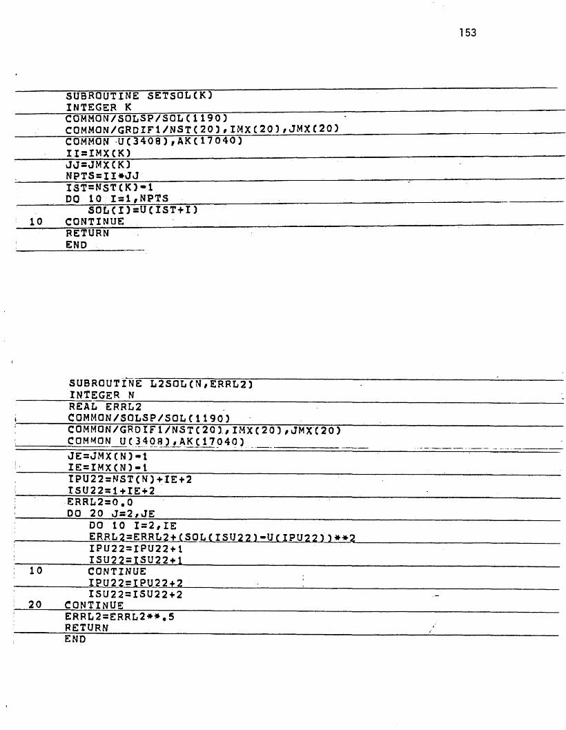
153

S U B R O U T I N E S E T S O L C K ) I N T E G E R KC O M M O N / S O L S P / S O L C 1 1 9 0 )C O M M O N / G R D I F 1 / N S T C 2 0 ) , I M X C 2 0 ) , J M X C 2 0 )COMMON U C 3 4 0 8 ) , A K ( 1 7 0 4 0 )I I = I M X C K )J J = J M X CK)N P T S = I I * J JI S T = N S T ( K ) - 1DO 1 0 1 = 1 , N P T S

S O L C I ) = U ( I S T + I )1 0 C O N T I N U E

R E T U R NEND

SUBROUTINE L 2 S O L C N ,E R R L 2 )INTEGER NREAL” ERRL2 ! : ~~

_______COMMON/SOLSP/SOL ( 1 1 9 0 ) ________C O M M O N / G R O I F 1 / N S T C 2 Q ) I M X C 2 0 ) ,JMXC20)

______ COMMON U ( 3 4 0 fl ) ,AKC170 4 0 ) ______________JE=JMX(N)-1

______ IE=IMX(N)-1____________________________________IPU22-NST(N)+IE+2I 5 U 2 2 = l + I E + 2 ________________________ _E R R L 2=0.0

______ DO 20 J=2 $ JE_______ __________________________DO 10 1=2,IE

__________ ERRL2=ERRL2+( S O L (ISU2 2 )- U ( IPU2 2 V ’)»»2IPU22=IPU22+1

_________ I S U 2 2 = I S U 2 2 + 1 ____________________________10 CONTINUE__________ IP U 2 2 = IPU 2 2 + 2 ___________ !_________

ISU22=1SU22+220 CONTINUE_______________________________________ _

ERRL2=ERRL2**.5 ______ RETURN

E N D

1 5 4S U B R O U T I N E D I F F C K , E X A C T )INTEGER K EXTERNAL EXACTC0 M M 0 N / G R D I F 1 / N S T C 2 0 ) , I M X ( 2 0 ) ,JMXC20)C 0 M M 0 N / G R D I F 2 / H V (20)

- COMMON U C 3 4 0 8 ) ,AKC17040)REAL PC65)

! IST=NSTCK)-1| II=IMX(K)| JJ=JMXCK) -

J HsHVCK)I I'M 1 = 11*1JJM1=JJ-1DO 20 J s 2 f J J M 1j DO 10 I=l,IIMl

| X=CI-1)*Hl Y=CJ-2)*H1 P (I )=U CIST+T + CJ-l) * I I )-EXACT(X# Y)! 10 CONTINUEI W R I T E (6,100)(PCI),1=1#IIM1)! 20 CONTINUE1 t o o F O R M A T (1H ,8F15.12)

RETURNEND

_________S U B R O U T I N E O U T P U T ( K ) ____________________ ■I N T E G E R K

_________C Q M M O N / G R D I F 1 / N S T C 2 Q ) # I M X C 2 0 ) , J M X ( 2 0 )COMMON U C 3 4 0 8 ) , A K ( 1 7 0 4 0 )R E A L P ( 6 5 )I I = I M X ( K )J J = J M X ( K )I S T = N S T C K ) + I I - 1 I I M 1 = I I - 1 N P T S = I I * J J

* I B = I S TI E = I B + ( J J - 3 ) * I I :DO 2 0 I S T = I B , I E # I I DO 1 0 I a 1 f I I

P ( I ) s t j ( I 5 T + I )1 0 C O N T I N U E

W R I T E ( 6 i 1 0 0 ) ( P C I ) # 1 = 1 r H M D 2 0 C O N T I N U E

1 0 0 F O R M A T C 1 H , 8 F 1 5 . 1 2 )R E T U R NEND

155

SUBROUTINE OUTPAK(K,M) INTEGER K,M

C!OMMON/AKINFO/NAK (20) # IMAK (20) , JMAK ( 20 ) COMMON/GRDIF1/NST ( 20 ) ,IMXC20),J M X C 20) COMMON U C 3 4 0 8 ) ,AKC17040)

. REAL P (306)II=IMX(K)JJsJMXCK)

, IB=NAKCK}-1 ■______ II9=II»9________________________________________

IE=IB + C J J - n * i r 9DO 20 IS = IB ,I E ,II9 __________

i DO 10 1=1,119j P (I 3 = A K (I S + I )____________ _______________ _10 CONTINUE! WRITEC6,100)CPCI),I = l , I I 9 y _________ ________20 CONTINUEI______IB = NAK ( K+M ) »1__________ ______________

IE=IB+<JJ-1)*IIj______DO 40 IS=IB,IE,II_______________________ _____

DO 30 1=1,II;__________ P ( I ) = A K (I S + I ) _____________________30 CONTINUEj, WR I T E C 6 , 1003 CP CI)/I »1#II3 ___________140 CONTINUE,100 F O R M A T d H ,10F10.5)______________ ~

RETURN I END

S U B R O U T I N E G U E S S C N ) I N T E G E R NC 0 M M O N / G R D I F 1 / N S T C 2 0 ) , I M X C 2 0 ) , J M X C 2 0 )

i COMMON U ( 3 4 0 8 D , A K C 1 7 0 4 0 )N P T S = I M X C N ) * J M X ( N )I S = N S T ( N ) - 1 _DO 1 0 1 = 1 , N P T S

U C I S + I 3 = 1 . 01 0 C O N T I N U E

R E T U R N ■END

156

1

1

uvjcjimjvj i jEXTERNAL EXACT

! COMMON/GRDIF2/HV C 20); CQMM0N/GRDIF1/NSTC20)#I M X C 2 0 ) #JMXC20)i * COMMON UC3408)#AK(17040)1 JE=JMX C N ) » 1

IE=IMXCN)-1IPU22=NST(N)+IE+2ERRL2=0.0HaHVCN)DO 2.0 J=2#JE

DO 10 1=2#IE ----X=CI-1)*HY=(J-2)*HERRL2=£RRL2+{EXACTCX#Y)-UCIPU22))**2IPU22=IPU22+1

10 CONTINUEIPU22=IPU22+2

20 c o n t i n u e .

ERRL2=ERRL2**.5r e t u r nEND

V « # « # v - # AX # A ^ # i 4. # 1 ^ # 0 JE X T E R N A L A E X T E R N A L BE X T E R N A L CC Q M M 0 N / G R D I F 2 / H V f 2 0 VD I M E N S I O N S C 4 # 4 ) # P ( 4 # 4 ) # W C 4 )F I 1 ( X # Y ) = C X - X 2 1 * C Y - Y 2 )F I 2 ( X # Y ) = - ( X - X l ) * ( Y - Y 2 )

! F I 3 C X # Y ) = C X - x n * C Y - Y l )F I 4 C X # Y ) = - C X - X 2 ) * C Y - Y 1 )F I 1 X C Y ) = Y - Y 2F I 2 X C Y ) = - ( Y - Y 2 )F I 3 X ( Y ) = ( Y - Y l )F I 4 X C Y ) = - C Y - Y l )F I 1 Y C X ) = X - X 2F I 2 Y C X ) = - C X - X 1 )F I 3 Y ( X ) s X - X 1F I 4 Y C X ) = - ( X - X 2 )

c' DO 7 1 = 1# 4

DO 7 J = 1# 4S C I # J ) = 0 . 0

7 C O N T I N U E

157H R T 3 = 0 . 5 * S Q R T C 3 . 0 )

H R T 3 = H R T 3 / 3 .

H X = X 2 - X 1H Y = Y 2 - Y 1

cC G X = 0 . 5 * C X 1 + X 2 3

cC G Y = 0 . 5 * C Y 1 + Y 2 3

V O L = H X * H YP C 1 # 1 3 = C G X - H R T 3 * H X

i P C 1 # 2 3 = C G Y - H R T 3 * H Yi P C 2 # 1 ) = C G X + H R T 3 * H Xi PC 2 , 2 ) = ' P < 1 # 2 3j

P C 3 # 1 3 = P C 1 # 1 3I P C 3 # 2 3 = C G Y + H R T 3 * H Yi P C 4 , 1 ) = PC 2 , 1 )i P C 4 # 2 3 = PC 3 , 2 )! Ci D O 1 1 = 1 , 4

W C 1 3 = F I I X CP C1 , 2 ) ); W C 2 ) = F I 2 X C P C I # 2 3 )

W C 3 0 = F I 3 X CP C I #233W C 4 3 = F I 4 X C P C I # 2 3 3

D O 2 1 1 = 1 , 4i

i 2D O 2 J J = 1 , 4S C H # J J ) = S ( I I , J J 3 + W C I I 3 * W C J J ' 3 * A < P C I # 1 ) # P C I # 2 3 3 / V O L .

i 1 C O N T I N U E: C

DO 3 1 = 1 , 4W ( j ) = F 1 1 Y C P C I # 1 ) 3

W C 2 3 = F I 2 Y C P C I # 1 ) )

W ( 3 ) = F I 3 Y C P ( I # 1 ) 3

W C 4 ) = F 1 4 Y C P C I # 1 ) ) DO 4 1 1 = 1 , 4

4DO 4 J J = i , 4s e n # J J 3 = S C I I # J J ) + W C I I ) * W C J J ) * B C P C I # 1 3 # P C I # 2 3 3 / V O L

i c

3 C O N T I N U E

DO 5 1 = 1 , 4W C l ) = F I l C P C I # n # P C I # 2 D )

; W C 2 ) = F I 2 CP C I # 1 3 # P C I # 2 3 3 W C 3 3 = F 1 3 C P C I # 1 3 , P C I # 2 3 3W C 4 ) = F 1 4 C P C I # !■) # P C I # 2 3 )

DO 6 1 1 = 1 , 4

6DO 6 J J = 1 , 4

S C I I , J J 3 = S C I I , J J 3 - W C I I 3 * W C J J 3 * C C P C I # 1 3 , P C I # 2 3 3 / V O L5 C O N T I N U E

R E T U R N -END

F U N C T I O N A ( X , Y ) asaA s - 1 ,

R E T U R N

i E N D

F U N C T I O N B ( X , Y )

. . . . . . . . - 1 " ! " "

B = - l .| R E T U R N

\ E N Dj F U N C T I O N C ( X , Y )

P I = A C O S C - 1 , )

C = — 4 ,

R E T U R N

E N D _ _ _ _ _ _

S U B R O U T I N E R H S ( X 1 , Y 1 , X 2 , Y 2 , S l , S 2 , S 3 , S 4 , F )

E X T E R N A L F| D I M E N S I O N S C 4 ) , P ( 4 , 4 )

! F I l C X , Y ) = C X - X 2 ) * ( Y - Y 2 )

F I 2 C X , Y ) = - ( X - X 1 ) * C Y - Y 2 )

! F I 3 ( X , Y ) = ( X - X 1 ) * ( Y - Y 1 )

j F I 4 C X , Y ) = - ( X - X 2 ) * ( Y - Y 1 )1 D O 2 1 = 1 , 4

| 2 S C I J s O . O! C G X = 0 . 5 * C X 1 + X 2 )

j C G Y = 0 , 5 * ( Y 1 + Y 2 }i H X = X 2 - X 1

i H Y = Y 2 - Y 1

H R T 3 = 1 . 0 / ( 2 . 0 * S Q R T C 3 , 0 ) ) '| P ( 1 # 1 ) = C G X - H R T 3 * H X

j P ( 1 , 2 ) = C G Y - H R T 3 # H Y

P ( 2 , 1 ) = C G X + H R T 3 * H X

P ( 2 , 2 ) = P ( 1 , 2 D

P C 3 , l ) = P ( l , n

! P ( 3 , 2 ) = C G Y + H R T 3 * H Y

P C 4 , 1 ) = P C 2 , 1 )

P ( 4 # 2 )=P( 3 , 2 )D O 1 1 = 1 , 4

S C l ) = S ( n + F ( P C l , 1 ) , P ( I , 2 ) ) * F I l ( P ( I , l ) , P ( I , 2 ) )

S ( 2 ) = S ( 2 ) + F ( P C I , 1 ) , P ( I , 2 ) ) * F I 2 ( P ( 1 , 1 ) " # P ( 1 , 2 ) )

S ( 3 ) = S ( 3 ) + F ( P ( I , 1 ) , P C I # 2 3 ) * F I 3 ( P ( I , 1 ) , P C I , 2 ) )

1 S ( 4 } = S C 4 ) + F ( P C 1 , 1 ) , P C I , 2 ) ) * F I 4 ( P C 1 , 1 ) , P C 1 , 2 ) )

si=scnS 2 = S ( 2 )

S 3 = S C 3 )

S 4 = S ( 4 )

r e t u r n

END

1 59

I___________ S U B R O U T I N E C A L R I N ( K , M ) ___________ _________________ _____________ _____________________________I C O M M O N / G R D I F l / N S T C 2 0 ) r I M X ( 2 0 ) » J M X ( 2 0 )I C Q M M Q N / A K I N F 0 / N A K C 2 0 0 » I MA K C 2 0 ) » J M A K C 2 0 ) _______________;_______________

COMMON U C 3 4 0 8 ) , A K C 1 7 0 4 0 )1 I N T E G E R K i M ______________ .______________ ____________________________

I M A X a l M X C K )J M A X s J M X f K } ___________ ___ ____________________________ ______________ _________________ _I M X K M 1 = I M X ( K - 1 )

___________ T T E M P = I M A X + 2 __________ _________________________________________________I P U = N S T ( K ) + I T E M PI P A = N A K C K ) + 4 + 9 » I T E M P ______________________________ II P R S A s N A K ( K + M ) > I T E M P -

___________ I PRAM 1 s N A K ( K - 1 +M ) + I M X K M 1 ♦ 1___________________________ __________________ ___I J E = J M A X - 2L _________ I E s I M A X - 1 ____________________________________________________________ .____________________ _

DO 2 0 J = l , J E , 2________________ DO 1 0 1 = 3 # I E / 2_______ __________________________ ______________________

I T l s I P U - I M A X I T 2 = I P U ^ I M A X ___________________________________________________________________________ __

A K C l P R A M n = A K C I P A - 4 D * U C I T l - l ) + A K C l P A - 3 ) * U C I T l )_____________________ A K C I P R A M 1 y a A K C I P R AMl ) + A K C I P A - 2 ) » U C I T 1 * 1 ) + A K ( I P A - 1 ) » U C I P U - 1

1 ) _______________ A K ( I P R A M l ) = A K ( I PRAM 1 ) + A K C I P A ) » U C I P U ) + AK ( I P A + 1 ) » U ( I P U + 1 3

A K C I P R A M 1 ) = A K C I P R A M 1 ) + A K C I P A + 2 ) * U ( I T 2 - 1 ) + A K ( I P A + 3 ) * U C I T 2 ) A K C I P R A M 1 ) = A K ( I P R A M 1 ) + A K C I P A + 4 ) * U ( I T 2 + 1 )A K ( I P R A M 1 ) = A K ( I P R S A ) - A K C I P R A M 1 )

!_____________ AK C I P R AMI ) = 4 t » A K C l P R AM 1 )__________________________________________________________I P R A M 1 = I P R A M 1 + 1

:_____________________ I P U = I P U + 2 ____________ ______________________ _______________________________I I P A = I P A + 9 * 2|__________________ I P R S A = I P R S A + 2 _______________ ____________________________ _______________________________; 1 0 C O N T I N U E!______________ I P R A M l . s i P R AM 1 + 2 ______________________________ ______________________________

I P U = I P U + I M A X + 2I________ I P A = I P A + 9 » C I M A X + 2 3 ________________________________________________________ .____________

I P R S A = I P R S A + I M A X + 2 ! 2 0 C O N T I N U E

R E T U R NE N D

S U B R O U T I N E S E T G A U___________COMMON U C 3 4 0 8 ) , A K C 1 7 0 4 Q ) _________________________ .

C O M M G N / A K I N F O / N A K ( 2 0 ) 9 I M A K ( 2 0 ) # J M A K C 2 0 ) __________ C 0 M M 0 N / G R P I F 1 / N S T C 2 0 ) , I MX ( 2 0 ) » J M X C 2 0 )

C O M M O N / M A T A / A G ( 5 4 9 1 ) # F C 2 8 9 ) , J T C 2 8 9 )________I R O W a Q ___________________________

I I = I M X ( 1 ) - 1J J s J M X C 1 ) - 1 ______________________I B = I I

__________ N = ( I I - 1 ) » ( J J - 1 ) _______________C J T ARRAY__________ I B A l a l B - H ______________________

J T C1 ) = 1__________ I F ( I B t E Q . 1 ) GO TO 2 7

DO 2 8 1 = 2 , I B _____________ J T C l ) = J T C I - 1 ) » I2 8 C O N T I N U E2 7 C O N T I N U E ___________________________

DO 2 9 I = 1 BA 1 , NJ T ( I ) a J T ( I ~ 1 ) + I B A 1

2 9 C O N T I N U E__________ N T O T a J T ( N ) ________________________;

DO 5 l a 1 # N T O T5________ A G ( I ) a Q , ______________ _____________

DO 1 0 J s 2 , J J__________ DO 1 0 1 = 2 f l l ____________________

I P a ( J - l ) * I M X C l ) + I - l’ I P a N A K C l ) + 9 » I P ________ •

I R O W s I R O W + 1__________ I J P a J T CI ROW )____________________

AG ( U P ) a A K ( I P + 4 )__________ I F g l R Q W , E Q , 1 ) G O TO 1 0

I F CI ROW . L E . I B ) GO TO 2 0__________ A G C I J P - I B + l ) = s A K C i P + n

I F C I . E Q , 2 ) GO TO 1 5__________ A G ( I J P - l ) = A K C I P + 3 )

A G C I J P - I B ) = A K C I P )I F C I . E Q . I I ) G O TO 1 0

1 5 A G C I J P - I B + 2 ) = A K ( I P + 2 )__________ GO TO 1 0 _________ _ ___

2 0 I F ( I , E Q . 2 ) GO TO 2 5A G C I J P - l ) = A K C I P + 3 ) ___________GO TO 1 0

2 5 A G ( I J P - I B + 2 ) a A K C I P + 2 )AG C I J P - I B * 1 ) = AK ( I P + 1 )

1 0 C O N T I N U E ___________________________C A L L F A C T O R ( N , I B )R E T U R N ‘________________E N D

161

S U B R O U T I N E S L V G A U ( M )COMMON U C 3 4 0 8 ) , A K C 1 7 0 4 0 )C O M M O N / A K I N F O / N A K C 2 0 ) , I M A K ( 2 0 ) , J M A K C 2 0 )C O M M O N / G R D I F 1 / N 5 T ( 2 0 ) # I M X ( 2 0 ) , J M X ( 2 0 )C O M M O N / M A T A / A G ( 5 4 9 1 ) , F C 2 8 9 ) , J T C 2 8 9 )I R 0 W = 0I I = I M X C 1 ) - 1J J = J M X C 1 ) - 1I Bs# 1 1DO 1 0 J » 2 * J JDO 1 0 I » 2 # 1 1I P P = C J - 1 ) * I M X C 1 ) + I - 1I P R s N A K ( M + 1 ) + I P PI R 0 W = I R 0 W + 1F ( I R O W ) =AK ( I P P )

1 0 C O N T I N U EN = I R O WC A L L B C K S L V ( N # I B )I R O W s ODO 2 0 J = 2 gJJDO 2 0 I = 2 # I II R O W = I R O W + 1I P P = N S T ( 1 ) + C J - 1 ) * I M X C 1 ) + I - lU ( I P P ) = F ( I R O W )

2 0 C O N T I N U ER E T U R NEND

162

S U B R O U T I N E F A C T O R ( N F , I B )__________ C O M M O N / M A T A / A ( 5 4 9 1 ) , F C 2 8 9 ) , J T C 2 8 9 )C F A C T O R I Z A T I O N OF A - B A N D M A T R I X O R D I N G__________ C R I T s l « E - Q 9 -- _________________________________ DO 1 0 1 = 1 » NF __________________________________________

I I = J T ( I )I F C I . E Q . l ) GO TO 3 0 _________________________I M 1 = 1 - 1S U M s Q .____________________________ .________________KO = MA X O ( 1 # I - I B )

__________ I K = I I __________________________________________________I D G = I

__________ DO 2 0 K s K O , I M l ____________ ' __________________I D G = I D G - 1

__________ I K s I K - 1_________________________________ __________ ___KK a J T ( I D G )

2 0 _____________ S U M s S U M + A C K K ) » A C I K ) » A C I K ) ______________3 0 A C I I ) 3 A C I I ) - S U M __________________________Z R = A B S C A C 1 1 ) )_________ ___________

I F C Z R . G T . C R I T ) GO TO 3 5W R I T E C 6 # 2 0 1 ) I _____________________________________

2 0 1 F O R M A T C 1 9 H A I S S I N G U L A R AT = , 1 3 )__________ DO 3 6 J J 3 1 f I I __________________ _________________3 6 W R I T E C 6 # 2 0 2 ) J J , A C J J )2 0 2 F O R M A T C 1 6 f 2 X y 2 S 1 5 . 4 ) ______________________________

S T O P3 5 P I V 3 l . Q / A C I I ) _______________________________________

I F C l * E Q « N F ) GO TO 6 0__________I A 1 3 1________________________ '___________ ___________

J O s MI N O C N F 9 I + I B ) • -DO 4 0 J 3 I A 1 » J 0 _______________________________________J I s J T C J ) + I - JSUM = Q , __________________________________________ ___________I F C I . E Q . l ) GO TO 4 0

__________I D G s I _______________________________ ________________ ____I K 3 I I

_________ J K 3 j i ____________________________________________________KO 3 M A X 0 C D I - I B , J - I B )

__________I F CKO * G T * I M l ) GO TO 4 0 _____ __________________DO 5 0 K s K O ^ I M l

__________I D G s I D G - 1 _____________________________________________KK. 3 J T C I D G )

1 J K 3 J K - 1

' 5 0I K 3 I K - 1

S U M = S U M + A C K K ) » A C J K ) * A C I K )i 4 0 A C J D = C A C J I ) - SUM ) * P I V! 1 0 C O N T I N U E

6 01

R E T U R NEND

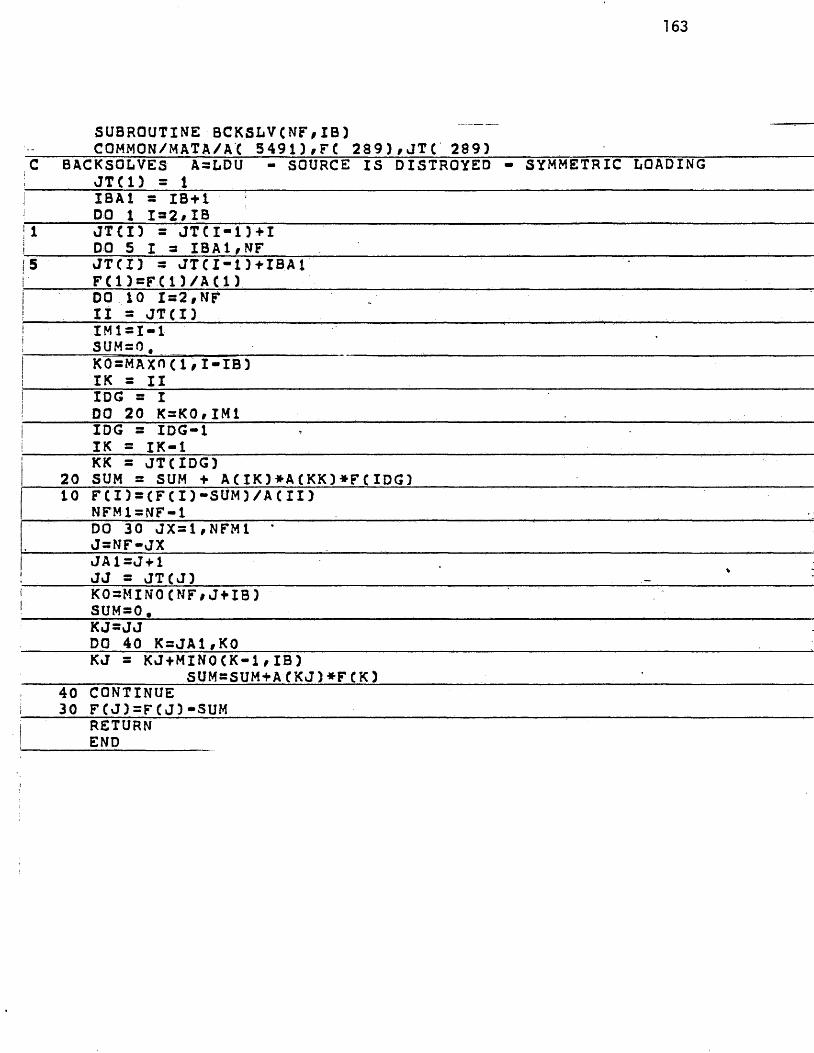
163

S U B R O U T I N E B C K S L V ( N F # I B )C O M M O N / M A T A / A C 5 4 9 1 ) , FC 2 8 9 ) , J T C 2 8 9 )

c B A C K S O L V E S A s L D U - S O U R C E I S D I S T R O Y E D - S Y M M E T R I C L O A D I N GJ J T C l ) = 1i I S A 1 = I B + 1

DO 1 I s * 2 , I Bj 1!

J T C I ) = J T C I - D + I DO 5 1 = I B A 1 , NF

! 5 J T ( I ) s J T C I - D + I B A i F C 1 ) * F ( 1 ) / A ( 1 )

! DO 1 0 I s 2 , N FI I * J T ( I )

i I M 1 = I - 1S U M 3 0 .

| K O s M A X O ( 1 , I - I B )ii I K s 1 1! I D G s II DO 2 0 K 3 K 0 , I M 1iI I D G s I D G - 1

I K = I K - 1i ■ KK 3 J T ( I D G )

2 0 SUM s SUM + A C I K ) * A ( K K ) * F ( I D G )1 0 F C I ) = ( F C I ) - S U M ) / A C I I )

N F M l s N F - lDO 3 0 J X s 1 f N F M 1 *J s N F - J XJ A l s j ^ iJ J = J T C J ) -K O s M I N O C N F , J + I B )S U M s O .K J - J JDO 4 0 K s J A l , KOK J = K J + M I N O ( K - 1 , I B )

S U M 3 S U M + A C K J ) * F C K )4 0 C O N T I N U E3 0 F ( J ) = F C J ) - S U M

R E T U R NEND

APPENDIX I I I

This a lgori thm is the Vector M ul t i -g r id Fast Poisson Equation

so lv e r . I t accep ts D i r i c h l e t boundary da ta . Procedure ALG4Q

co n ta in s the Full M u l t i -g r id Cycle descr ibed in diagram 3 of Chapter

4.

This code was w r i t t e n during the time when SL1 was s t i l l an

experimental language. Some of the s ta tem ents may appear u n u s u a l J2

These s ta tements were needed due to minor quirks in the system.

Without an SL1 Reference Manual and thorough commenting, th e d e t a i l s

of t h i s code w i l l , most l i k e l y , be incomprehensible. I t i s l i s t e d

so t h a t readers who a re i n t e r e s t e d can ge t a fee l f o r the general

s t r u c t u r e o f the Vector a lgor i thm . The basic m u l t i - g r id p rocesses

were c a r e f u l l y s e l e c te d on th e b a s is o f how amenable they were, fo r

vec to r p rocess ing .^

V o r in s tance the s ta tem en ts M+0 in Call ALG40 or the For Loop needed to c a l c u l a t e the powers of 2 in Procedure ALG4Q.

2SL1 i s a computer language designed s p e c i f i c a l l y f o r th e STAR 100 by John Knight and Douglas Dunlop of the College o f William and Mary.

3See Chapter 4.

1 6 4

_________ MODULE VECF B E G I N C Y C L E ; _____________________________________ T65—S N O C H E C K : .

REAL VEC TORI 4-5 0 0 0 1 Q ;_____RE AL V E C T O R C 1 7 0 0 0 ] V I M P ;REAL VECTOR[17000] T 1»T2,T3»T4,T5tT6 : BIT VECTORC17000) B l ; ______I N T E G E R V E C T O R [ 2 0 0 ] P T l y P T 2 y P T 3 ;REAL VECTOR C 2 0 3HV ;____________________I N T E G E R VECTORC 2 0 I NS T y I MXy JMX~;I N T E G E R I Q ;EXTERNAL P R O C E D U R E ( R E A L t R E A L ) Q 3 C L O C K SEXTERNAL P R O C E D U R E ( REAL y R E A L y R E A L ) E X A C T ;EXTERNAL P R O C E D U R E ( REAL * R E A L y R E A L ) G ;EXTERNAL P R O C E D U R E ( R E A L , R E A L *R E A L ) F

P R OCE DUR E CYCLEREAL 0 1FMX * TX y T Y ;RE AL H;REAL D I F I M PI N T E G E R LM;I N T E G E R I MP yM ;I N T E G E R P A R 1 y P A R 2 ;I N T E G E R KH : = . 5 ;P A R I r = l ;P A R 2 : = IFOR M FROM 5 TO 5 DO

CALL ALG4-0 ( 2 y 2 y H , M + 0 y 5 O y P A R H - 0 y P A R 2 + 0 )CALL D I F M A X ( M + O y D I F M X , T X y T Y ) ;PR I N T ( D I F M X y TXYT Y )"# 1 MAX DI *FF= , F 1 5 ‘.‘ 1 2 y ' I T OCCURS AT X=

Y= ' , F I 5 . 1 2 # ; ~ ‘ ...................CALL F DVAL UF S ( M-t-0 ) :CALL T V A L U E S ( M + 0 ) :LM ; = 1 ;FOR I FROM 1 TO M DO

LM : = 2 * L M ;E N D F ;LM : = ( L M + L ) * ( L M + L )VI MP C1 ! LM 1 : = QCNS T CM ] ! LM ]FOR I MP FROM 1 TO 5 DO

P R I N T ( P A R j y P A R 2 ) # 1 P A R 1 = » , 1 . 3 , ' P AR2 = M 3 #PR I NT ( M » I MP ) # * M= M 3 , ' I MP = * , 1 3 #CALL A L G 4 - 0 ( 2 y 2 yHyM-t-Oy I M P + 0 y P A R 1 + 0 yPA R 2 + 0 )CALL D I F M A X ( M + O f D I F M X y T X y T Y )P R I N T ( P I F M X y T X y T Y ) # * MAX DI F F = » y F 1 5 . 1 2 I T OCCURS AT X= « yF 1 5 . I 2 , • Y = 1 , F 1 5 . 1 2 # ;CALL D F l M P ( M + O yQ I F I M P y T X y T Y )PR I N T ( D I F I M P ) # 1 MAX D I F F FROM D I F F E R E N C E S O L . = • * F 1 5 . 1 2 # ;

_______ P R I N T ( T X y T Y ) # 1 I T OC C U R S AT X= ^ 1 5 - 1 2 ^ Y= » y F 1 5 . 1 2 # ;________ CALL FOVALUES ( M+ 0 ) ;_______________________________________________________ ___

CALL T V A L U E S ( M + Q ) j ___________________ _________________________________________E N D F ;

E N D F ;ENDP ;

166P ROCEDURE A L G 4 0 ( NXCU N Y O * HCUM , IM P , PAR 1 , P Aft 2 )'; I N T E G E R NXO » NY 0 ♦ M • I M P » K » K 2.» I »L »N IM » T IM »KK :I NT E G E R P AR 1» P AR2 ;_________________REAL HO>ERR ;______________________ _ _ _______B I T CTRUE-» C F A L S E ; __________ .___RE AL CP Uy WAL L ; . ___________________________CTRUE : = T R U E : ________ _____________________________C F A L S E : = F A L S E : ___________________________I Q : = 1 ; __________ ;______________CALL Q 3 C L 0 C K S ( C P I N W A L L ) ?_________________ :FOR K FROM 1 TO M DO _________________________ _

K 2 ; = I ;__________ ;________FOR I FROM 1 TO K - l DO_______________ ______________ _

K2 : = 2**K2 ; ■E N D F ; _CALL G R Q F N ( K + O , N X O * K 2 + l , N Y Q * K 2 + 1 , H Q / K 2 ) ? CALL G R D F N ( K + M » N X O * K 2 + l , N Y O * K 2 + l , H O / K 2 ) ;CALL PUTZ ( K+Q ) ;CALL P U T F ( K + M , C T R U E » 2 ) ;

E N D F ; . . - —

CALL 0 3 C L 0 C K S ( CPU * WALL ) ;P R I N T ( C P U ) # ' SCALAR S E T U P T I M E = * , E 1 4 . 7 # ;CALL Q 3 C L O C K S ( C P U * W A L L ) ;CALL P U T B ( I ) ;Q [ 5 3 : = . 2 5 * ( Q [ 2 3 + Q C 4 3 + Q f 6 3 + O r 8 3 ) ; •

Q C 5 } : =Q C 5 3 - Q C1 4 3 ;FOR L FROM 2 TO M DO____________

CALL I NT ADD ( L —1 » L + O » M-t-OO : CALL P U T B I L + O ) ;NI M ; = 1 : __________ _______________I F L=M T H E N _______________

NI M : = I MP ; 'END I ;FOR I IM FROM 1 TO NI M DO

FOR KK FROM 2 TO L 0 0K : = L + 2 - K K ;FOR I FROM 1 TO P A R I DO

CALL R E L A X ( K , K + M TE RR ) ; ENDF;_________ ;__________________________

________________CALL P 1 J T Z C K - 1 ) ; ______ __:______________ CALL C A L R I N ( K , K + M , K - 1 + M ) ;1 . _____E N D F ; ___________ ___________________________ ___I Q [ 5 1 : = . 2 5 * ( Q C 2 3 + Q f 4 3 + O C 6 3 + 0 [ 8 3 ) ;i__________Q C 5 3 : =QC 5 3—Q C1 4 3 ;_______________ __________'__________FOR K FROM 2 TO L DO ________________ _|_______ CALL L I N T A D Q ( K —1 1 K + 0 ) ; ________i______________ FOR I FROM 1 TO PAR 2 DO____________j - •,__________CALL RELAX ( K + 0 » K+M t E R R ) :__________j . .____________ E N D F ; __________ _____________________ _______i E N D F ; ______________________________________________ ‘I ENDF ; ____________________________1 E N D F ; ___ _______________________________________1 CALL Q 3 C L 0 C K S ( C P U t WA L L ) ;______ ’________________I PR I NT ( C P U ) # 1H , E 1 4 . 7 # ; ___________________________i ENOP;

167P ROCEDURE G R P F N I N , I M A X , J M A X »H H ) ;I NT E G E R Ny-IMAX y JMAX ; _______ __R E A L - H H ;NS-TCN3 : — I Q ; _________ __________ ___________f MX C N 3 ; = IMAX ; _________ _____________JMXCN-3 ; = J M A X : ____________________ ______HV [ N 3 : = HH ; _ _ ' ________ _____IQ : = I Q + I M A X * J M A X ; ____ENDPJ

j P R OCE DUR E K E Y ( K , P T 1 , I M A X , J M A X y H H ) ;I I N T E G E R V E C T O R C 2 Q O 3 P T 1 :I I N T E G E R K , I M A X r J M A X , I S ;I- REAL HH; __________________________________________

IMAX : = I MX[ K } ;JMAX ; = JMX [ K 3 ;_____________ _________________ _I S : = N S T [ K ] —J MAX—I ;FOR I FROM 1 TO IMAX DO

I S : = I S - KJ MAX;P T 1 C I 3 ; = 1 S ; _____________

E N D F ; ____________ .HH : ==H V [ K 3 ; ______________________ -E N P P ;

P R OC E DUR E P U T Z ( K ) ; _________[ I N T E GE R K r 1 1 , J J r I S T K , M N P T S ;1 1 : = I MX C K 3 ;________ ___ ____________J J - : = J M X [ K 3; __________________I S T K ; = N S T C K 3 ;MNPTS : = I I * J J ; ______________Q C I S T K I M N P T S 3 : = 0 . ;E N D P ;

1 6 8PROCEDURE PUTF(K,FL AG *NH ) ;REAL H tH2»XTYtZltZ; f ......-

! INTEGER NHrKtII*JJ ,11 j; 4.! BIT FLAG;! CALL KEY(KtPTltI IrJJtH);H 2 : = 1 • ;; FOR I FROM I TO NH 00

H2 :=H*H2; •! ENDF;1 FOR I FROM 1 TO II DO

FOR J FROM 1 TO JJ DOX :=(I— 1 )*H:Y :=(J-1)*H;IF FLAG

TH E N ; C A L L F( X'.Y.Z ) :0CPT1C T 1+J1 :=Z*H2/4.:

ELSE:CAL1 G ( X . Y * Z I ) ;Q C P T 1 C I ]-t-J ] : = Z l » H 2 / 4 , :

e n d i :E N D F ;

E N D F ; _______E NP P ;________ _

i

i!

P-ROCEDURE PUTB(K);_______________I N T E G E R K t l l t J J » I I M , J J M , I » J » I O :REAL XtYtHtZl; ______ 'CALL KEY(K»PT1,II.»JJ»H) :_____ __I I M : = I I - l : _______________________________J J M : = J J - 1 ;

i FOR I FROM I BY I I M TO I I DO! 10 : = P T 1 CI 1 ;: X : = ( I - l ) * H ;1 FOR J FROM I TO J J DO

Y ; = ( J - l ) »H :CALL G ( X , Y , Z 1 ) ? Q C 1 0 + J ] : =Z 1 ;

E N O F ;• E N O F ;! FOR J FROM 1 BY J J M TO J J DO! Y : = ( J - I ) * H ;

FOR I FROM I TO I I DO1 0 : = P T I [ I ] ;

! X : = ( I - I ) - H ;! CALL G ( X * Y , Z 1 ) ;

Q T I O + J ] : = Z 1 ; 'j ENDF ;

EN DF ;E N D P ;

P ROCE DURE R E L A X ( K t K R H S , E R R ) :I N T E G E R 11 » J J » I O N E S , L P A T , I L N : REAL H ; _ _ _ _ _ _____I N T E G E R L G R I D » I V 1 1 » I V 1 2 » I V 2 1 » I V 2 2 » I V 2 3 » I V 3 2 ;____________I N T E G E R I F 1 1 , I F 2 2 » I R 2 1 , I R 2 2 » I R 2 3 y I R 3 2 , I R 1 2 : __________I N T E G E R I V R l l ; ___________________ L _ ______ _________REAL W O , W l ; _ _______ ___________________ _________ ______________

________ I N T E G E R K t K R H S ; _ _ ______ .___. REAL E R R ; .

___________I N T E G E R I P T 1 » J J P 1 ; ________________________________/ * I N I T I A L I Z E * / _______________ ___________ _________________________ __________ ___

_______ I I ; = . I . MXt K. 1 ; - ______________ _________ J J : = J MX £ K 3 ; .___________________I ONES : = J J - 2 ;________________________ _________ ____________ ____________■

L P A T ; = J J ;________________________________ __ _______________ ______________I L N : = J J * ( I I - 2 ) - 2 :

B 1 C 1 I I L N 3 ; = P T R N 1 Q ( I O N E S y L P A T » I L N ) ; ________________ ________ _ ________ LGR I D ; s . I I # J J ; _______ _____________ I V R l l : = NSTC KRHS 3 ; _______ _______________________________ __

I V 1 1 : = N S T [ K 3 ?________ _I R 2 2 : = J J + 2 : _________ __ ___________________________________________

__________ I F 2 2 s = I V R l l + J J + l ; _____________ __________ ■I V 2 2 ? - I v i l + J J + 1 ; ________ •I V 2 i • = r V 2 2 — l ;________ ___________ ______________ ____________________

__________ I V 2 3 : = I V 2 2 + 1 ; • ______ ___________ I V I 2 : = I V l i + 1 ; ___________ __________ _____________ _________________ , I V 3 2 : = I V 2 2 - H J J ; • ______________________ J J P 1 : = J J - t - 1 ;_____________ ___________________ _________________ •

I P T 1 : = ( I I - l ) » J J ; _____________________ T 1 C 1 I J J P 1 3 : = 0 , 0 ; ___________ _________________ _ T I C I P T 1 ! J J P 1 3 : = 0 - 0 ; _______ FOR I FROM 2 * J J BY J J TO I P T 1 - J J DO

T I C I 3 ; = 0 . 0 ; - ___________ . __________________ T 1 C I - H 3 : = 0 , 0 ; ____ ________ __________ ________ ._____ ______________ E N D F ; _________ ______________________________ ■ _______________/ * C A L C U L A T E R E S I D U A L S OVER ALL P T S - E X C E P T THE 1 S T * // * AND L A S T COLUMNS AND T H E 1 S T P T , * / ________________________________

_/*_ OF COLUMN 2 AND LAST P T > OF COLUMN N - l _________( T I C I R 2 2 ! I L N 3 , B 1 C 1 I I L N 3) : =QC I V 2 1 !. I L N 3 + 0 C I .V23 I I LN 3;

__________ ( T I C I R 2 2 I I L N 3 t B I C 1 1 I L N 3) : = T 1 C I R 2 2 I I L N 3 + Q C I V 3 2 I I LN 3;_______ ( T I C I R 2 2 I I L N 3» B 1 C I I I LN 3 ? : = T 1 C I R 2 2 ! I L N 3 + 0 C IV. 1 2 I I LN 3 ;

- ( T 1 C I R 2 2 I I L N 3 , B 1 C I I I L N 3 ) : = - . 2 5 * T 1 C I R 2 2 I I L N 3 :___________ ( T I C I R 2 2 I I L N ) t B 1 C 1 1 1 LN 3) : = T 1 C I R 2 2 ! I L N 3 + 0 C I V 2 2 I I LN 3 ;__________( T 1 C I R 2 2 ! I L N 3 t B l C 1 I I L N 3 ) : = T 1 C I R 2 2 ! I L N 3 + 0 C I F 2 2 I I L N 3;/ * C A L CUL AT E NEW VALUES BY W E I G H T I N G THE R E S E D U A L S * // * AND R E S T O R E THE BOUND ARY P T S . * / ________________ ___ _________________

WO : = - 1 . 0 6 9 5 ;______ _____________ ___________ _ _________ _ ________W1 - : = - . 1 5 5 ; _____________ ^ _________ ________ _

I R 3 2 : = 2 * J J + 2 ; - ______________________ _________________________ ______________ I R 2 3 : = J J + 3 ;____________________________ _______________________ I R 2 1 : = J J + 1 ; ______________________ ___________________________________

I R 1 2 : = 2 ;_________________________________________ ' _____T? C I R 2 2 I I LN3 : =T 1 C I R 2 1 ! I LN 3 + T 1 C I R 2 3 I I LN 3 T2C I R 2 2 ! I L N 3 : = T 2 C I R 2 2 ! I L N 1+ T 1 C I R 1 2 ! I LN 3 ;

-________ T 2C. I R 2 2 _IXLN_3 _ : = T 2 C I R 2 2 ! I L N 3 + T 1 C I R 3 2 ! TI N I : ~_________ T 2 C I R 2 2 I I L N 3 ; = W 1 * T 2 C I R 2 2 ! I LN 3 : ____________________________________________ (Q-C I V 2 2 I I L N 3 » B 1 C 1 I I L N 3 ? ; = T 2 C I R 2 2 I I L N 3 + 0 C I V 2 2 ! I LN 3 ;

. ... T2C I R 2 2 I I L N 3 : = W0 * T 1 T I R 2 2 ? I f . N 3 ;_______________ : ( Q.C-I-V22-! I L N 3 t B 1 C 1 I I L N 3 ) : = T 2 I I R 2 2 ! I LN 1 + 0 C I V2 2 ! I L M 3 ;

E N P P :

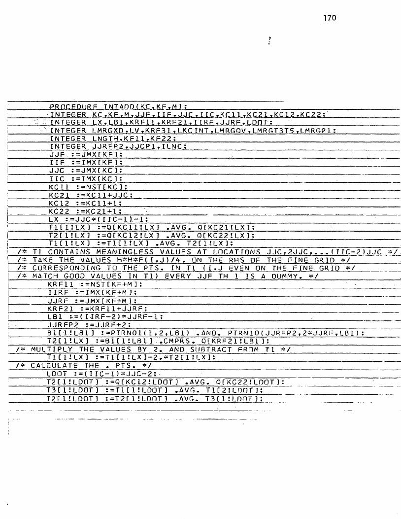
1 7 0

:___________ P R O C EPUR E I NTAPP.IKC-* KF_*M±1_____________________ . __________________________ I N T E G E R K C . « K F t H , J J F » I I F » J J C , 11 C „ KC 1 1 t K C 2 1 » KC 1 2 »KC2 2 ;______________________________I N T E G E R L X y L B I » K R F l i r K R F 2 1 y I I R F t J J R F T LOOT :_________________________ __________________!_________ I N T E G E R L MR G X D , L V , K R F 3 1 » L K C I M T , LMRGQV , L M R G T 3 T 5 , L M R G P 1 ____________ ___I___________ I N T E G E R L NGT t-U K F l l , K F 2 2 ; ___________ _________________________________________________ ___1 _________I N T E G E R J J R E P 2 t J J C P I r I L N C : '__________ J J F : = J M X [ K F ] ; . _______i I I F ; = IMX C KF 3 ; ________ ._________I J J C ; = J M X C K C 3 ; .____________ '__ ___L _ _________I I C : = I MXt KC ] : _______________ ._______ ~____________________ KC 11 : = N 5 T C K C 1 ; ___________________________________________ ___________ __________ ______;___________ K C 2 1 ; =KC 1 1 + J J C ; __________________ ___ ________________________________ ___L _ ________ KC 1 2 : = K C l l + l ; ___________ ______________________ _____ __________ _____ ___________ ___|____________ K C 2 2 ; = K C 2 H - l ; , ________ ____ __________ ______ ______!___________ l x : = j j c » ( i i c - i ).—i : ________________ ' . .. . ' ' . ' . 'I____________ T 1 I 1 I L X 3 : = Q [ K C 1 1 I L X 3 , A V G . Q C K C 2 1 I L X 3 ; __________ _I__________ T 2 C 1 I L X 3 : =Q C KC 1 2 I LX ] . A V G . QC K C 2 2 ! LX 3 ___j T I C l i . L X ] : = T 1 C 3. ! LX 3 . A V G . T 2 C 1 I L X ] ; _____________ .1 / * T 1 C O N T A I N S M E A N I N G L E S S VALUE S AT L O C A T I O N S J J C , 2 J J C , ( I I C - 2 ) J J C|___ t ± TAKE THE VALUES H * H * F t I , J ) / A . ON THE RHS OF THE F I N E G R I D * / ______________ j

/ * C O R R E S P O N D I N G TO THE P T S « I N T l ( I , J EVEN ON THE F I N E G R I D * / _________ _ _/ * MATCH GOOD VALUE S I N T l ) EVERY J J F TH 1 I S A DUMMY, * / _________________________ ,

____________K R F 1 1 ; = N S T C K F + M ] ; _____________ - ! ________ I I R F ; = I M X C K F + M 3 : ;_______ _______ ___________________ J J R F : = JMX C KF+M ] :_____________ ,_______________ ______________________________________________________________ K R F 2 1 : = K R F I 1 + J J R F ; _____________ _____________________________________________________________I LB I ( I I R F - 2 ) * J J R F —1 : ._______ __________________! _ _________J J R F P 2 s = J J R F + 2 :___ I__________i___________ 8 1 C 1 I L B 1 3 ; = P T R N 0 1 ( 1 , 2 , L B I ) . A N D . P T R N 1 0 ( J J R F P 2 , 2 * J J R F y LB 1 ? ;I, T 2 C 1 1 L X 1 : = B 1 £ 1 I L 8 1 3 . . C M P R S , 0 C K R F 2 1 I L B 1 3 ; ____________________________

/ * M U L T I P L Y THE VALUES BY 2 . AND S U B T R AC T FROM T l * / ________________T l ' t I I LX 3' : = T 1 C I I LX 3 - 2 . » T 2 C 1 I LX 3 ; ________________________________ __________________

/ * CAL C U L AT E THE . P T S . * /_ _ _______ LOOT ; = ( I I C - I ) * J J C ~ 2 ; ■ '___________ _______ ~______

T 2 C 1 I L P O T 3 : = Q C K C 1 2 ! LOOT 3 . A V G . 0 C K C 2 2 I LOOT 3 : ____________ ______ ______T 3 { I I L D O T 3 : = T 1 C 1 ! LOOT 3 . A V G . T I C 21 LOOT 3;T 2 C 1 I L D O T 3 : = T 2 C 1 ! LOOT 3 . AVG« T 3 C1 ! L O O T 3 ;

171

/ * O B T A I N THE VALUES H * H * F ( I ♦ J ) / A . ON' THE RHS OF THE F I N E G R I P * // * C O R R E S P O N D I N G TO THE . P T S . # / ___________________ ___ ____________________________ _

B 1 C 1 I L B 1 ] : = P T R N I 0 ( 1 t 2» L B 1 ) , AND. P T R N I O C J J R F , . 2 * i J J R F W . B l ) : ___________/ » R E P L A C E T H E L E A D I N G 1 WI TH A 0 # / |______ _____________________

___________ B i l l ] : = F A L S E : ___________________________________ • ________________T 3 C 1 ! LOOT 1 : = 8 1 C I ! L B 1 ] . C M P R S - Q C K R F 2 1 ! LB 1 1 ; ________________________ ;_______

T 2 C 1 ! L P 0 T 1 : = T 2 f 1 I L D O T 1 - T 3 I I I LOOT 1 ; ' '/ * MERGE X UIITH O P T ( T l WI TH T 2 ) . S T ORE IN T 3 * / ' ________ .

LMRGXD : = L X + L D O T ; __________ ______ ________ ___ _____________ ________ B i l l ! LMRGXD 3 : = P T R N 1 0 ( 1 » 2 » LMRGXD ) ;________________________ __________ __

: .________ T 3 C 1 ! LMRGXD ] : = M E R G E ( T 1 C 1 I L X 1 , T 2 C 1 I LOOT 3 , B 1 C 1 I LMRGXD 3 ) ; __________/ * C A L C U L A T E V P T S . * / ________ , ' ____________ ____ _____________

____________ LV : = ( I I C - 2 ) * J J C ; ________ J J C P 1 : = J J C - M ;____________________________________________________________________ __________________________ T 4 C 1 I L V ] ; = T 1 C I ! LV 1 . A V G . T I C J J C P 1 I LV 1; ________ __ __________________________________ T 5 C 1 I L V ] S - 0 C K C 2 1 I L V 1 . A V G , Q C K C 2 2 I L V 1 : ________________ ________

; T 4 C 1 I L V 3 : = T 4 C 1 ! L V ] . A V G . T 5 C 1 I L V 1 ; ________ _____ ______________________ ____________/ * O B T A I N THE VALUES H * H * F ( I , J ) ' / 4 . ON THE RHS OF THE F I N E GR I D * // * C O R R E S P O N D I N G TO THE V P T S . * / ___________________________________________________ ___

!___________ K R F 3 1 : = K R F 2 1 + J J R F ; ___________ _________________________________________________ _LB1 ; = ( I I R F - 4 ) * J J R F - H ; .

________ B i l l ! L B 1 ] : = P T R N O I ( 1 , 2 , L B 1 ) » A N D . P T R N 1 0 ( J J R F P 2 » 2 * J J R F y LB 1 ) : "; T 5 I 1 I L V 1 : = B 1 [ 1 ! L B 1 ] . C M P R S . O f K R F 3 1 ! LB 1 ] : ___________ .___________________I T 4 C 1 I L V 3 : = T 4 C 1 ! LV 1 - T 5 [ 1 ! LV 1 ?______________________ ___ _________________________________| / * MERGE 0 WI TH V ( Q WI TH T 4 ) *=/ ______________ _ j| L K C I N T : = ( I I C - 2 ) * J J C ; • -| _______ LMRGQV : = L V + L K C I N T ; ___________________________________________________________________________j __________ B 1 [ I I LMRGQV 3 : - P T R N 1 0 ( 1 , 2 t LMRGQV ) : ________ ___ __________ __________ _| _______ T 5 C 1 I L M R G Q V ] : = MERGE( Q C K C 2 1 ! L K C I N T U T 4 C 1 ! LV 1 » B I C I ? LMRGQ V ] ) ; ________ ;

MERGE X , . WI TH Q t V < T 3 WI T H T 5 ) > / ___________________ ’______ - ___________ L M R G T 3 T 5 : = LMRGXD+LMRGOV : __________________________________________ ___________________ :

1_____________LMRGP I : = L M R G T 3 T 5 - H :___________________________________ ' :_ _ _: B 1 C 1 I LMRGP 1 1 : = - P T R N 1 0 ' ( J . J F + l » 2 * J J F + 2 t L M R G P l ) :___________ ______________________

T 6 C 1 I L MR G T 3 T 5 3 : = M E R G E ( T 3 [ I I LMRGXD ] y T5 C1 I LMRGQV ] , B 1 C 2 1 L MR G T 3 T 5 ] ) : ~/ * C O M P R E S S T6 TO AN A P P R O P R I A T E LENGTH ~ ___________________

_________ LNGTH ,: = < I I F - 2 ) * J J F - 2 ; _____________ _________ _ __ __________________________________ B 1 1 1 ! L MRGP I 3 ; = P T R N 1 0 ( J J F , J J F - M y L M R G P I ) ; ____________________________ ’____________ T 6 [ I I L N G T H 3 ; = B I C 2 I LM R G T 3 T 5 ] . C M P R S . T 6 C 1 I L M R G T 3 T 5 ) ; __________________

/ * ADD THE VALUE S I N T6C l ! L N G T H 3 TO Q C K F 2 2 ! LNGTH ] UNDER CONTROL OF 6 1 B i l l ! LNGTH ] s = P T R N LO ( J J F - 2 » J J F , LNGTH ) : ___________ ___________________________ K F 1 1 ; = N S T [ K F 1 : _________________________________ ,____________

K F 2 2 : =KF 1 1 + J J F + 1 ;____________________ _________________________________________ ____________ __ __________ (_0C K F 2 2 ! L N G T H } , 8 1 C 1 I LNGT H 1 ) : =Q C KF 2 ? ! L NGTH 1 + T6C 1 I LN GTH 1 : " ______ ^

ENP P ; ____________________ _____________________ _____________________________

1 7 2

P R OC E DUR E L I N T A D D ( K C , K F ) : _________________ ___________________________________________I N T E G E R K C . K F . J J F » I I F » J J C » I I C . K C 1 1 . K C 2 3 . . KC 2 2 . K F 2 2 » L X . L D O T : ____

__________ I N T E G E R MXn J V . l KCT .1 MKC V . LM XDKCV . LGR I 0 I . LG T M I : ________ ________________________I N T E G E R K C 1 2 : ____________ :___________________________________ J J F ; = JMX C K F 3 : ________________ ____ _______________ ____________________ ___ _______________

I I F ; = I MX C K F 1 ;____________.___________ _____________________________ ___ __________J J C : = J M X C K C 3 : ________ ;_______ _____________ ________

; __________ I I C : = I MXCKC1 : ______ - • __________________1 KC 11 ; = N S T C KC ] : ' ' ■ . ’ ' . ' . _____________i___________ KC 1 2 : = K C 1 1 + 1 ; __________________________________________ ___________________________ __________j ________ K C 2 1 ; = K C 1 1 + J J C ; _____________ _________________________ ________________

K C 2 2 : = K C 2 1 - H ; ________ ______________________________ ___________________________________ K F 2 2 ; = N S T C K F 3 + J J F + I ;

1 LX : = ( I I C - 1 ) * J J C ; ~ ____________ ■:___________ LOOT : = L X - 1 : ____________________ . .

/ * C A L C U L A T E THE H O R I Z O N T A L V A L U E S * / __________________________________________ _________i___________T I E 1 ! LX 3 • : =Q{ KC I I ! LX 3 ,. AVG. Q C K C 2 1 I LX 3 ; ______! / » C A L C U L AT E THE DI AGONAL VA L UE S * / ________________________ ~

T 4 C 1 I L P Q T 3 : =Q C K C 2 1 ! LDQT 3 . A V G , 0 C K C 2 2 I L D O T 3 : _____________T 2 C 1 I L P O T 3 : = ( Q [ K C 1 1 ! LOOT 3 . AV G . QC KC 3. 2 i LOOT 3 ) . AVG . T 4 C 1 I L P O T 3;

| / * - MERGE THE H O R I Z O N T A L AND D I A G O N A L V A L U E S * / __________ ____LMXD : = l x + l p o t ;L « I A U , « - L A r l ^ y u 1 1

B i l l ! LMX 0 3 : = P T R N I O ( 3 . , 2 , LMXD) ;T 3 [ 1 ! LMXD 3 : = M E R G E { T 1 C 1 I LX 3 r T 2 [ 1 ! LOOT 3 , 8 1 [ 1 ! LMXD } ) ;

/ * C A L C U L A T E THE V E R T I C A L VALUE S * /LV : = L X - J J C ;

/ * MERGE THE I N T E R I O R KC V A L UE S WI TH THE V F R T I C A L VALUES * /LKCI : = L V ;

_________ LMKCV : = L V + L K C I :____ __________________ _______________________________ _____________ __B i n ; LMKCV 3 : = PTRN I 0 ( I , 2 r LMKCV ) :____________________________________ _ _ _ ^ _ ____________________ T 2 C 1 ! LMKCV 3 : = M E R G E ( 0 C K C 2 1 I L K C I 3 , T 4 C 1 I L V 3 » B 1 C 1 I LMKCV3) : ___

/ * MERGE T 3 WI TH T2 » / _______ _______________________________________________________________LMXDKCV ; = L M X P + L M K C V : ________B i l l ! LMXDKCV 3 ; = P t R N 1 0 ( J J F + 1 , 2 » ( J J F - H ) , L MXDKC V) :T I C 1 I LMXDKCV3 : = M E R G E ( T 3 C 1 1 L M X Q 3 , T 2 ( I I L M K C V 3 , B I C I ! LMXDKCV1) ;

1 / * COMP RES S OUT THE M E A N I N G L E S S VALUE S * / . ~ ________B1 1 1 I LMXDKCV 3 : - P T R N 3 . Q ( J J F , J J F + l y LMXDKCV ) : _________________

LGR I DI ; = ( I I F —2 ) * J J F ; ________________ _______________________________________________T2 C 1 I L G R I P I 3 : = B 1 C 1 ! LMXDKCV3 . C M P R S . T l C 1 I L M X D K C V 3;______________

/ * ADD THE VALUES I N T 2 TO Q C K F 2 2 1 L G I M 1 3 * / ______________________ ______________PO NOT AL T E R THE BOUNDARY P T S . - /

L G I M 1 : = L G R f 0 I - l ;B 1 C 1 I L G I Ml 3 : = P T R N 1 0 ( J J F - 2 , J J F , L G I M 1 ) ;I Q E K F 2 2 I L G I M 1 3‘, B 1 C 1 I L G I M 1 3 ) s = 0 C K F 2 2 ! LG IM'l 3 + T 2 C 2 ! L G I M I 3 :

___________E N P P ; " " '..................................... .......................

P R OCE DUR E C A L R I N ( K F , K R F , K R C ) : 173___________I N T E G E R K F , K R F , K R C , K F l l , K R F 1 1 , I I F , J J F , K F 3 1 , K R F 3 1 : _______

I N T E G E R I L N t K F 2 1 » K F 2 J J F » K F 3 2 yK F 4 - l t J J R C y l l R C » K R C l l » K R C 2 1 y I L N C :K F 1 1 : = NST C KF 3 ;_________ .____________

__________ K R F 1 I ; = N S T C K R F 3 ; ___________ _ J _________________ ~I T F : = I MX C KF ] ;______________________________________ ____ ____________________________ ____

__________ J J F : =J MX C K F ] ;________________________ __________ ____________________ _________ _____________________ K F 3 1 : = K F l l + 2 * J J F ; ______________________________________________________________ _____

K R F 3 1 : = K R F 1 1 + 2 ^ J J F ; ___________ ____________________________________________________I L N : = J J F * ( I I F - 4 ) ; ;________K F 2 1 ; = K F 1 H - J J F ; ________ ;

________ K F 2 J J F : - K F 3 1 - 1 ;________ ._________ _________________ __________________> K F 3 2 : = K F 3 1 - H : __

K F 4 1 : = K F 3 1 + J J F ; ___________ _________■ / * C A L C U L A T E THE R E S I D U A L S T O R E I T I N T l * / ______________ 'i ' T I C 1 ! I L N 3 : =Q C K F 2 1 1 I L N ] « AV G. Q C K F 2 J J F I I L N J :! T 2 C 1 I I L N 3 : = Q C K F 3 2 I I L N ] . A V G ,» QC KF4-1 ! I LN 3 ? __________ _I T i c I I I L N 3 s = T I I 1 ; I LN 3 . AVG. T 2 C 1 I I LN ] ;__________________ ___________________!_________ T I C 1 ! I L N ] : = Q C K F 3 1 I I L N 1 - T I C 1 1 I L N 1 ; _______________ ___________ ______ __________1 T l C 1 ! I L N ] : = T l C i ; i L N ] + Q [ K R F 3 i ; i L N 1 ; I T 1 C 1 I I L N ] : = 4 . * T 1 C 1 I I L N 3 ; .I / * C O MP R E S S T l AND I N J E C T THE R E S U L T ONTO * /i / * KRC FROM KR C 2 1 FOR A LENGTH OF J J R C * ( I I R C - 2 ) » / ________________I_______ J J R C : = JMX C KRC ] ; ___________________ . __________I I I R C : = IMX CKRC 3 : ______________ __________________ __j KRC 1 1 : = N S T C KRC ] :______ _____ _____________________________________________________ '! K R C 2 1 r = K R C I l + j j R C ; ____________ ______________________________ _!_______ I L N C : = J J R C * ( I I R C - 2 ) : ___________ ___________!__________B 1 [ 1 I I LN ] : = PTRN 1 0 ( U 2 t I L N ) . A M D . P T R N 1 0 ( J J F , 2 * J J F , I L N ) : ___ _ _1 Q C K R C 2 1 I I L N C 3 : = 6 1 C I I I L N 3 - C M P R S . T 1 C 1 I I L N 3 : ___________________ _ _1 E N P P ;

P ROCE DURE D l F M A X ( K r D I F M X r T X t T Y ) : REAL P I F M X J X f T Y t H t X t Y » Z 2 , C O I F :I N T E G E R K t l l t J J ; _________________C ALL K E Y ( K y P f l t I I t J J t H ) ;___________ _DI FMX : = Q t ; ________ _________________________FOR I FROM I TO I I DO _________F OR J FROM 1 TO J J DO________________ _

.X : = ( 1 - 1 ) * H : _______________________Y : = ( J - 1 ) * H ;

CALL E X A C T ( X »Y tZ2) ;___________C D I F ; = A B S ( Z 2 ~ Q C P T 1 f I 3 + J 3 ) :I F C P I F > D I F M X THEN________________

________ TX ; =X : __________________________TY : = Y ;_____________________________ __

________DI FMX : =CD I F j _____________________END I ;_______________________ |______________

E N DF : ___________________________________________ENDF ;______________ _______ ______ENPP :

1 7 4

P R OCE DUR E O U T P U T ( K ) ;___________________REAL V E C T O R ! 2 0 0 1 P ;________________REAL H ; _______________ :_______________________I N T E G E R K r l l t J J t J l y J 2 y I » J ;CALL K E Y ( K y P T l » I I » J J »H ? ;

.________J I : = 1 : __________ . ;____________L I ; I F J 1 + 7 < = J J _____ _ _ _____________

THEN J 2 ; = J I + 7 ; ________ E L S E : J 2 : = J J ;______________________

ENDI ; ________ ________________________________FOR I FROM 1 TO I I DO

FOR J FROM J I TO J 2 DO PC J 1 : ~ Q C P T 1 C I 3 + J 3 :

E N D F ; ____________________ ___________ ___________________ PR I N T ( P C J I : J 2 ] ) # 1 H , 8 F I 5 . 1 2 # ;

E N D F ; _____________________________J I : = J 2 + l ;

________I F J 1 < = J J ___________________ ____________ ____T H E N ; G O t o L l ;

E N O I ; __ _ E N D P ;

P R O C E D U R E D F I ' M P ( K , D I F I M P , T X , T Y > ; R E A L PI FIMP y T X y T Y y H y C D I F y X y Y ;I N T E G E R K T I I , J J y L L ; ______________________C ALL K E Y ( K y P T l ,1 I ,J J y H ) ; __________P I F I M P : ~ 0 « ; ___________________________LL : = 1; _________________FOR I F R O M 1 TO I I D O ___________FOR J F R OM 1 TO JJ D O _______ ____________

X : = ( 1-1 )*H:_________________" _Y : = (J - l ) * H ; ___________________C D I F ; = A B S ( V I M P C L L J - Q C P T 1 C I 1 + J 1 ) ;IF C D I F > D I F I M P T H E N _______

TX ;=X ;_____________________________ ___________ TY :=Y ;__________________________________

P I F I M P := C D I F ; ________ __________ENDI :•_______________________________________LL :=LL + l;_________________________________

ENDF;______________ _____________________________E N D F ; _______________________ _____________ENDP ;

175

P R OC E DUR E F D V A L U E S ( K ) ; ________________________________ ________________ ____________REAL H ; ____________________________;_________ ;___________________ ___________________________________I N T E G E R K , I I . , J J » M P T : ________ ___________________________________________ ______________________CALL K E Y ( K t P T l * I I ♦ J J t H ) :_______________________________________________ ____________________P R I N T ( Q C P T 1 T 2 1 + 2 1 »QC P T l f 2 1 + J J - l l . QT P T l f I 1 - 1 1 + J J - l 1 . Of P T l T I 1 - 1 1 + 2 1 )#» CORNER F D V A L UES C L O C K W I S E FROM O R I G I N » . 4 F 1 5 . 1 2 3 ; ______________________MPT : = ( ( I I — 1 ) . 0 1 V , 2 ) +•! ; __________________________________________________P R I N T ( Q [ P T 1 C M P T 1 + M P T 3 ) # 1 C E NT E R F P V A L U E = « » F I 5 . 1 ' 2 # ; _______________.______E N D P ;

PROCEDURE TVALUE5 ( K ) ;________ -REAL HyUl tU2 yU3 yUA-yXyY.Z2;_______ ,INTEGER K , I I , J J ; ______________________________. __________CALL KEY(K y PT1 »II»JJyH) ; ______ _____________________CALL EXACT ( H.H.Z2 ) ;_______________________________________________ui :=Z2 ;___________ __________________ ;__________ ;_______ _Y ; = ( J J — 2 ) ; ______________ __________________ ______________CALL EXACT ( H » Y y Z2 ) ;_______________ _______ _____ ___________ ______U2 : = Z 2 ; • __X : = ( I I -2 ) »H ; ___________________________"______ _______________c a l l e x a c t (x ,y ,z 2 ) ; _______ ____ ______________ ________________U3 ;=Z2;___________ . :______________________________c a l l EXACT( X,Hr Z2 ); ________ __________________U4 := 22; ______ ;______ __ ______ __________________PRINT(UitU2*U3,U4)#' CORNER TVALUES CLOCKWISF FROM OR IG TN » .. 4F15.12#;__________:____________________ _______ _______________ ____CALL EXACT( .5i » 5 ♦ Z 2 ) .«___________:______________ ________ ___________PR I NT ( Z 2 ) # 1 C E NT £R_ TVALUE = 1 »F 15 .12#;________________________FMop;________ _____ ____________________________________________FND M; _ ___

176

iiSTORE 919095 100876 ONE 8ONE » T30Q « ______________________________ _DELI VER ( BIN 01 POL ING 1_______ ;______ ___DESTROY(FILE) _______________ _______________

; FORTRAN!B = FILE) *________________ ___■ LOAD(SLOBX,FILE«LI=SL1LIB»CN=GO«#200,GRLPALL= ) i GO._____________ _ _ _ _ _ _ _

i i * • ' '

SUBROUTINE EXACT(X ,Y ,Z2)i_________Z2=X#X+Y*Y_____ ______ _____ . . - . _______ _________ REAL X„Y,Z2 ___________ _____ _______ _

i_____________RETURN_________ ,________________ ___________ ___________ . .| END _____ ___________________________ _!__ ______SUBROUTINE F( X ,Y ,Z )______ _ _ _ _______REAL X » Y , Z _______ ,____________ _________

Z = 4 ._________ ;_______________________ _________________________ RETURN____________ _______ ______________ END ___________________________ __ _____________________________ _

SUBROUTINE G(X,Y,Z1)_______ . __________S REAL XyYtZl_________ __________________________I Z1=X*X+Y*Y ______ . _______________ ______I. RETURN

END

APPENDIX IV

Two o th e r f i n i t e element codes were w r i t t e n . They so lve the same

problems as Appendices I and I I . However, the d i s c r e t i z a t i o n used

l i n e a r as opposed to b i l i n e a r t r i a l fu n c t io n s . L i s t in g s of these codes

w i l l be fu rn ished upon r e q u e s t .

177

REFERENCES

1. Brandt, A., "M ul t i - leve l Adaptive Solu t ions to Boundary Value Problems," Mathematics o f Computation, 31, April 1977, pages 333-391.

2. Brandt, A. , "M ul t i - leve l Adaptive Techniques (MLAT): Ideasand Software," Proceedings o f Conference on Mathematical Software, MRC, Wisconsin, 1977.

3. Brandt, A., "M ul t i - leve l Adaptive Techniques (MLAT): I . TheM u l t i -g r id Method," IBM Research Report, RC 6026, IBM T. J .Watson Research Center , Yorktown Heights , New York, 1976.

4. Concus, P. and G. Golub, "Use o f Fast D irec t Methods f o r the E f f i c i e n t Numerical Solu t ion of Nonseparable E l l i p t i c Equations ," SIAM Journal o f Numerical A na lys is , XQ.» 6 , pp. 1103-1120, 1973.

5. Gelfand, I.M. and S.V. Fomin, Calculus of V a r ia t io n s , P re n t ic e - H a l l , 1963.

6 . Proceedings of the ICASE Workshop on M ul t i -g r id Methods,June 19-23, 1978.

7. N ico la ides , R.A., "On Mult ip le Grid and Related Techniques fo rSolving D isc re te E l l i p t i c Systems," Journal of ComputationalPhysics , 1_9, pp. 418-431 , 1975.

28 . N ico la ides , R.A., "On the 1 Convergence of an Algorithm f o r

Solving F in i t e Element Equat ions ," Mathematics of Computation,31, 1977, p. 892-906.

9. Nicolades, R.A., "On Some Theore t ica l and P r a c t i c a l Aspects of M u l t i -g r id Methods," To appear, Mathematics of Computation, January 1979.

10. S t rang , G i lb e r t S. and George J . Fix , An Analysis of the F in i t e Element Method, P ren t ice -H al l Se r ies in Automatic Computation, 1973.

11. S troud, A.H., Approximate C a lcu la t ion of Mult ip le I n t e g r a l s , P ren t ice -H al l Se r ies in Automatic Computation, 1971.

12. Ortega, J.M. and R.G. Voigt , "Solu t ion of P a r t i a l D i f f e r e n t i a l Equations on Vector Computers," Proceedings of the 1977 Army Numerical Analysis and Computers Conference, ARO Report 77-3, 1977, pp. 507-519.

178

VITA

Name:

Date of B i r th :

Place of B ir th :

Theodore Craig Poling

October 2, 1953

Vienna, Aus tr ia

C i t i z en sh ip :

Education:

Symposia:

Awards:6/76 - 8/76

8/76 - 12/77

1/78 - p resen t

Courses Taught:Carnegie-Mel Ion Univers i ty

U.S.A.

B.S. Mathematics, The College o f William and Mary in V i rg in ia , 1976.

M.A., Mathematics, The College of William and Mary in V i rg in ia , 1978 (Course work and q u a l i f i e r s were completed and th e t h e s i s su c c e s s fu l ly defended, August 18, 1978.)

Workshop on M ul t i -g r id Methods held a t the I n s t i t u t e fo r Computer Applica t ions in Science and Engineering, NASA Langley Research Center. In v i t a t i o n a l Lecture: "M ult i-g r id Experimentson E l l i p t i c Problems with a F i n i t e Element Formulation," June 19-23, 1978.

S ta te Graduate Fellowship, The College of William and Mary in V irg in ia

U n iv e rs i t i e s Space Research Associa t ionA ss is tancesh ip a t the I n s t i t u t e fo r Computer Appl ica t ions in Science and Engineering*

Ph.D. Fel lowship, Carnegie-Mellon Univers i ty

Teaching A s s i s t a n t , Spring 1978, Calculus II (2 s e c t io n s )

Teaching A s s i s t a n t , Fall 1978, Ordinary D i f f e r e n t i a l Equat ions, Calculus II

Other:

7/76 C e r t i f i c a t e of Train ing: STAR-100 ComputerProgramming Training (40 hours) given by NASA Langley Research Center

*The research repor ted in t h i s t h e s i s was conducted while the author was a t the I n s t i t u t e fo r Computer Applica t ions in Science and Engineering, NASA Langley Research Center in Hampton, V i rg in ia . During t h i s time he was a s tu d en t a t the College of William and Mary in V i rg in ia . The f in a l d r a f t i n g of t h i s t h e s i s was performed while a t Carnegie-Mel Ion U nivers i ty .

1 79