Numerical Analysis and Spanwise Shape Optimization for ...

Utah State University Utah State University

DigitalCommons@USU DigitalCommons@USU

All Graduate Theses and Dissertations Graduate Studies

8-2019

Numerical Analysis and Spanwise Shape Optimization for Finite Numerical Analysis and Spanwise Shape Optimization for Finite

Wings of Arbitrary Aspect Ratio Wings of Arbitrary Aspect Ratio

Joshua D. Hodson Utah State University

Follow this and additional works at: https://digitalcommons.usu.edu/etd

Recommended Citation Recommended Citation Hodson, Joshua D., "Numerical Analysis and Spanwise Shape Optimization for Finite Wings of Arbitrary Aspect Ratio" (2019). All Graduate Theses and Dissertations. 7574. https://digitalcommons.usu.edu/etd/7574

This Dissertation is brought to you for free and open access by the Graduate Studies at DigitalCommons@USU. It has been accepted for inclusion in All Graduate Theses and Dissertations by an authorized administrator of DigitalCommons@USU. For more information, please contact [email protected].

https://digitalcommons.usu.edu/

https://digitalcommons.usu.edu/etd

https://digitalcommons.usu.edu/gradstudies

https://digitalcommons.usu.edu/etd?utm_source=digitalcommons.usu.edu%2Fetd%2F7574&utm_medium=PDF&utm_campaign=PDFCoverPages

https://digitalcommons.usu.edu/etd/7574?utm_source=digitalcommons.usu.edu%2Fetd%2F7574&utm_medium=PDF&utm_campaign=PDFCoverPages

mailto:[email protected]

http://library.usu.edu/

http://library.usu.edu/

NUMERICAL ANALYSIS AND SPANWISE SHAPE OPTIMIZATION

FOR FINITE WINGS OF ARBITRARY ASPECT RATIO

By

Joshua D. Hodson

A dissertation submitted in partial fulfillment

of the requirements for the degree

of

DOCTOR OF PHILOSOPHY

In

Mechanical Engineering

Approved:

______________________ ____________________

Douglas F. Hunsaker, Ph.D. Geordie Richards, Ph.D.

Major Professor Committee Member

______________________ ____________________

Robert E. Spall, Ph.D. James J. Joo, Ph.D.

Major Professor Committee Member

______________________ ____________________

Barton L. Smith, Ph.D. Richard S. Inouye, Ph.D.

Committee Member Vice Provost for Graduate Studies

UTAH STATE UNIVERSITY

Logan, Utah

2019

ii

Copyright © 2019 by Joshua D. Hodson

All Rights Reserved

iii

Dedicated to my father

Lee James Hodson

1939-2018

iv

ABSTRACT

Numerical Analysis and Spanwise Shape Optimization

for Finite Wings of Arbitrary Aspect Ratio

by

Joshua D. Hodson, Doctor of Philosophy

Utah State University, 2019

Major Professors: Dr. Douglas Hunsaker and Dr. Robert Spall

Department: Mechanical and Aerospace Engineering

Improvements to the current state of the art in wing shape optimization for morphing wing applications

are presented, with a focus on low-fidelity analysis methods for preliminary design. An existing aerodynamic

analysis tool based on lifting line theory is the foundation upon which this work builds, and several software

development efforts are presented that enhance the capabilities of this tool relative to wing shape

optimization. An automatic differentiation tool is integrated with the aerodynamic analysis tool to facilitate

accurate and efficient derivative calculations for gradient-based optimization. A light-weight optimization

framework written in Python is presented that is capable of efficiently searching the design space using

popular gradient-based optimization techniques and parallelization of independent objective function

evaluations. Several example optimization problems are presented using this toolset, and a method for

visualizing the design space of morphing wings using this toolset is also presented and discussed.

The morphing wing application of primary interest to the current work, the Variable Camber Compliant

Wing developed at the United States Air Force Research Laboratory, has an aspect ratio that falls below the

acceptable range of aspect ratios for lifting line theory analysis. This has led to the development of a new

method for applying lifting line theory to low-aspect-ratio lifting surfaces. A thorough review of Prandtl’s

classical lifting line theory is first presented, followed by several low-aspect-ratio proposals from the slender

wing theory of Jones to the lifting surface theories of Birnbaum, Blenk, and others. A new formulation for

slender wing theory is presented that provides new insights into the appropriate limits for a formulation

capable of spanning the entire range of aspect ratios from slender to infinite. A new empirical relation is

v

proposed that satisfies the limits at both extremes and agrees well with high-order inviscid panel code results.

A method is then presented for implementing this empirical relation in both analytical and numerical lifting

line algorithms. A comparison of results computed using this method to experimental results for the Variable

Camber Compliant Wing is also given.

(327 pages)

vi

PUBLIC ABSTRACT

Numerical Analysis and Spanwise Shape Optimization

for Finite Wings of Arbitrary Aspect Ratio

by

Joshua D. Hodson, Doctor of Philosophy

Utah State University, 2019

Major Professors: Dr. Douglas Hunsaker and Dr. Robert Spall

Department: Mechanical and Aerospace Engineering

This work focuses on the development of efficient methods for wing shape optimization for morphing

wing technologies. Existing wing shape optimization processes typically rely on computational fluid

dynamics tools for aerodynamic analysis, but the computational cost of these tools makes optimization of all

but the most basic problems intractable. In this work, we present a set of tools that can be used to efficiently

explore the design spaces of morphing wings without reducing the fidelity of the results significantly.

Specifically, this work discusses automatic differentiation of an aerodynamic analysis tool based on lifting

line theory, a light-weight gradient-based optimization framework that provides a parallel function evaluation

capability not found in similar frameworks, and a modification to the lifting line equations that makes the

analysis method and optimization process suitable to wings of arbitrary aspect ratio. The toolset discussed is

applied to several wing shape optimization problems. Additionally, a method for visualizing the design space

of a morphing wing using this toolset is presented. As a result of this work, a light-weight wing shape

optimization method is available for analysis of morphing wing designs that reduces the computational cost

by several orders of magnitude over traditional methods without significantly reducing the accuracy of the

results.

vii

ACKNOWLEDGMENTS

I have had several mentors throughout the course of this research, and I would like to express my gratitude

to each for helping me along in this journey: to Dr. Hope Forsmann at the Idaho National Laboratory for her

guidance and expertise in nuclear reactor thermal hydraulics and the Fortran programming language, to Dr.

James Joo at the U.S. Air Force Research Laboratory for his help in understanding morphing wing systems

and their role in the future of aerospace systems, and to Drs. Stephen Whitmore and Warren Phillips at Utah

State University for helping me realize my passion for aerospace. Also to Dalon Work and Tyson Etherington

for their advice, encouragement, and friendship.

Three professors in particular have had an exceptional impact on my education. First, Dr. Robert Spall,

who has been guide and mentor to me from my first day as a freshman undergraduate student to my last day

as a PhD candidate 20 years later, and who first introduced me to the worlds of computational fluid dynamics,

aerodynamics, and high performance computing. I wish him all the best as he sets sail this summer. Second,

Dr. Barton Smith, who has been a mentor for nearly as long and who reminds me that there is a real world

outside my numerical simulations, without which my numerical simulations would have no meaning. I also

want to thank Dr. Smith for connecting me with the RELAP5-3D team at Idaho National Laboratory. Finally,

Dr. Douglas Hunsaker, who among all his other responsibilities as a new faculty member at USU gave me a

majority share of his time and resources. I am forever indebted to these three men for their mentorship and

commitment to my success.

I would like to thank my wife Megan and my kids Wesley, Abigail, Preston, and Aliya, for supporting

me on a daily basis as I furthered my education. They have each made sacrifices so that I could pursue my

goal of earning a doctoral degree, and I thank them for sticking by me throughout it all. I also want to thank

my mother for her continual words of encouragement, which on a few occasions came at times when I was

ready to quit but gave me the boost I needed to forge ahead; and my father for his examples of hard work and

perseverance that have motivated me to test the limits of my abilities and always strive to do my best.

I would also like to thank those organizations that provided financial support for this work. Portions of

this research have been funded under a grant from the Office of Naval Research Sea-Based Aviation Program

(grant no. N00014-16-1-2074) and fellowships from the Department of Energy Nuclear Energy University

viii

Program, the U.S. Air Force Research Laboratory’s Summer Faculty Fellowship Program, and the USU

School of Graduate Studies Dissertation Fellowship Program.

Finally, I thank my Heavenly Father for His guidance and sustainment throughout the course of this work.

I acknowledge His hand in this and all things.

Joshua D. Hodson

ix

CONTENTS

Page

ABSTRACT ...................................................................................................................................................iv

PUBLIC ABSTRACT ....................................................................................................................................vi

ACKNOWLEDGMENTS ............................................................................................................................ vii

LIST OF TABLES ...................................................................................................................................... xiii

LIST OF FIGURES ...................................................................................................................................... xiv

LIST OF ACRONYMS .............................................................................................................................. xvii

NOMENCLATURE .................................................................................................................................. xviii

1 INTRODUCTION.................................................................................................................................... 1

2 DUAL NUMBER AUTOMATIC DIFFERENTIATION FOR WING SHAPE OPTIMIZATION ........ 4

2.1 Introduction ..................................................................................................................................... 4

2.2 Derivative Calculation Methods ...................................................................................................... 5

2.2.1 Symbolic Differentiation ......................................................................................................... 5

2.2.2 Finite Differencing .................................................................................................................. 9

2.2.3 Automatic Differentiation...................................................................................................... 11

2.2.4 Discussion ............................................................................................................................. 14

2.3 Methods and Tools for Forward-Mode Automatic Differentiation ............................................... 15

2.4 Dual Number Automatic Differentiation ....................................................................................... 17

2.4.1 Dual Number Theory ............................................................................................................. 18

2.4.2 The Dual Number Data Type ................................................................................................ 19

2.4.3 Integration with Fortran Algorithms ...................................................................................... 20

2.4.4 Special Considerations when Integrating DNAD with Existing Fortran Algorithms ............ 23

2.5 Automatic Differentiation of a 1D Scalar Transport Equation Solver ........................................... 26

2.5.1 Mathematical Model .............................................................................................................. 26

2.5.2 Numerical Model ................................................................................................................... 28

2.5.3 Automatic Differentiation of the 1D Scalar Transport Problem using DNAD ...................... 29

2.5.4 Results and Discussion .......................................................................................................... 30

x

2.6 Automatic Differentiation of MachUp .......................................................................................... 36

2.6.1 The MachUp Numerical Lifting Line Solver ........................................................................ 37

2.6.2 Modifications to the MachUp Source Code .......................................................................... 39

2.6.3 Results and Discussion .......................................................................................................... 41

3 WING SHAPE OPTIMIZATION USING A NUMERICAL LIFTING LINE ALGORITHM AND

DUAL NUMBER AUTOMATIC DIFFERENTIATION ...................................................................... 46

3.1 Introduction ................................................................................................................................... 46

3.2 Optix .............................................................................................................................................. 47

3.2.1 Optimization Method ............................................................................................................. 47

3.2.2 Code Structure ....................................................................................................................... 48

3.2.3 Parallel Execution of Independent Function Evaluations ...................................................... 49

3.2.4 Linear and Quadratic Line Searching .................................................................................... 49

3.2.5 Limitations ............................................................................................................................. 50

3.3 Wing Shape Optimization in Inviscid Flow .................................................................................. 51

3.3.1 Optimized Planform Shapes for Minimum Induced Drag ..................................................... 52

3.3.2 Optimized Geometric Twist Distributions for Minimum Induced Drag ............................... 54

3.3.3 Optimized Aerodynamic Twist Distributions for Minimum Induced Drag ........................... 56

3.4 Wing Shape Optimization for Viscous Flow ................................................................................. 58

3.4.1 Optimized Planform Shapes for Minimum Total Drag ......................................................... 60

3.4.2 Optimized Geometric Twist Distributions for Minimum Total Drag .................................... 61

3.4.3 Optimized Aerodynamic Twist Distributions for Minimum Total Drag ............................... 63

3.5 Visualization of the Design Space for Wing Shape Optimization ................................................. 64

4 ANALYTICAL LIFTING LINE METHOD FOR WINGS OF ARBITRARY ASPECT RATIO ........ 68

4.1 Introduction ................................................................................................................................... 68

4.2 Lift Generated by a Finite Wing .................................................................................................... 69

4.3 Classical Lifting Line Theory ........................................................................................................ 70

4.4 Slender Wing Theory .................................................................................................................... 77

4.5 Lifting Surface Theory .................................................................................................................. 81

xi

4.6 A Unifying Formulation of Lifting Line, Slender Wing, and Lifting Surface Methods ................ 82

4.7 Results and Discussion .................................................................................................................. 92

5 NUMERICAL LIFTING LINE METHOD FOR WINGS OF ARBITRARY ASPECT RATIO ........ 103

5.1 Introduction ................................................................................................................................. 103

5.2 The Phillips and Snyder Numerical Lifting Line Method ........................................................... 104

5.3 Modifications to the Numerical Lifting Line Method for Wings of Arbitrary Aspect Ratio ....... 108

5.4 Results and Discussion ................................................................................................................ 110

6 SUMMARY AND CONCLUSIONS ................................................................................................... 124

REFERENCES ............................................................................................................................................ 127

APPENDICES ............................................................................................................................................. 137

A MODIFIED DNAD SOURCE CODE ................................................................................................. 138

B ONE-DIMENSIONAL SCALAR TRANSPORT SOLVER IN FORTRAN ....................................... 168

B.1 User Interface .............................................................................................................................. 168

B.2 Physics Module ........................................................................................................................... 169

B.3 I/O Module .................................................................................................................................. 172

C SUMMARY OF CODE CHANGES TO APPENDIX B FOR DNAD INTEGRATION .................... 181

C.1 Changes to adpsolver Module ................................................................................................... 181

C.2 Changes to adpio Module ........................................................................................................... 181

D SUMMARY OF CODE CHANGES TO MACHUP FOR DNAD INTEGRATION .......................... 185

D.1 Changes to loads_m Module ....................................................................................................... 185

D.2 Changes to plane_m Module ....................................................................................................... 185

D.3 Changes to special_functions_m Module ............................................................................... 191

D.4 Changes to view_m Module ......................................................................................................... 195

D.5 Changes to wing_m Module ......................................................................................................... 196

D.6 Changes to airfoil_m Module ................................................................................................... 198

D.7 Changes to atmosphere_m Module ............................................................................................. 198

D.8 Changes to dataset_m Module ................................................................................................... 199

D.9 Changes to math_m Module ......................................................................................................... 199

xii

D.10 Changes to section_m Module ............................................................................................... 200

D.11 Changes to myjson_m Module ................................................................................................. 201

E EXAMPLE MACHUP INPUT FILES ................................................................................................. 209

E.1 Example JSON-Formatted Input File .......................................................................................... 209

E.2 Example Parameter File for a NACA 2412 Airfoil in Inviscid Incompressible Flow ................. 209

E.3 Example Profile File for a NACA 2412 Airfoil .......................................................................... 210

F OPTIX SOURCE CODE ..................................................................................................................... 211

G INPUT FILES AND PYTHON SCRIPTS FOR WING SHAPE OPTIMIZATION ........................... 225

G.1 Main Optimization Execution Script ........................................................................................... 225

G.2 Objective Function (obj_fcn.evaluate) ................................................................................... 226

G.3 Objective Function with Gradient Calculations (obj_fcn.evaluate_with_gradient) ............ 228

G.4 Helper Function for Extracting Variable Names (get_list_of_vars) ...................................... 230

G.5 Main MachUp Input File ............................................................................................................. 230

H AERODYNAMIC CALCULATIONS USING PANAIR ................................................................... 233

I MACHUP FUNCTIONS FOR WRITING PANAIR INPUT FILES .................................................. 239

J EXAMPLE PANAIR INPUT FILE ..................................................................................................... 245

K PRALINES SOURCE CODE .............................................................................................................. 250

K.1 Pralines Main Program (main.f90) ............................................................................................. 250

K.2 Interface Module (liftinglineinterface.f90) ....................................................................... 250

K.3 Planform Class Module (class_Planform.f90) ........................................................................ 262

K.4 Module of Setter Functions (liftinglinesetters.f90) .......................................................... 268

K.5 Solver Module (liftinglinesolver.f90) ................................................................................ 276

K.6 Output Module (liftinglineoutput.f90) ................................................................................ 284

K.7 Matrix Solver Module (matrix.f90) .......................................................................................... 292

K.8 Utilities Module (utilities.f90).............................................................................................. 293

L PROOF OF EQUATION (5.2.5) .......................................................................................................... 300

M TABULATED PROPERTIES OF THE NACA X410 FAMILY OF AIRFOILS ............................... 302

CURRICULUM VITAE ............................................................................................................................. 306

xiii

LIST OF TABLES

Table Page

2.1 Methods for Declaring Floating-Point Variables in Fortran ........................................................... 26

3.1 Aerodynamic coefficients for the NACA X412 family of airfoils in inviscid flow ........................ 52

3.2 Minimum induced drag results for untwisted wings with optimized planforms ............................. 53

3.3 Minimum induced drag results for geometric-twist-optimized rectangular wings.......................... 55

3.4 Minimum induced drag results for aerodynamic-twist-optimized rectangular wings ..................... 58

3.5 Aerodynamic coefficients for the NACA X412 family of airfoils in

viscous, incompressible flow at a Reynolds number of 610Re = ................................................. 59

3.6 Drag coefficients for initial rectangular wing and baseline elliptic wing in viscous flow. ............. 60

3.7 Minimum total drag results for untwisted wings with optimized planforms. .................................. 60

3.8 Minimum total drag results for geometric-twist-optimized rectangular wings. .............................. 62

3.9 Drag components for geometric-twist-optimized rectangular wing with 11 control points. ........... 62

3.10 Minimum total drag results for aerodynamic-twist-optimized rectangular wings. ......................... 63

3.11 Drag components for aerodynamic-twist-optimized

rectangular wing with 11 control points. ......................................................................................... 63

4.1 Summary of limits for 1R and

2R .................................................................................................. 92

4.2 Comparison of methods for calculating the wing lift slope of a finite elliptic wing ....................... 93

4.3 Comparison of resistance values 1R from methods for

calculating the wing lift slope of a finite elliptic wing .................................................................... 94

4.4 Comparison of resistance values 2R from methods for

calculating the wing lift slope of a finite elliptic wing .................................................................... 95

M.1 Airfoil Coefficient Data for the NACA 2410 Airfoil .................................................................... 302




file:///C:/Users/a00305185/OneDrive/Josh/School/PhD/Final%20Dissertation/hodson_dissertation_submission3_rev2.docx%23_Toc14356239





xiv

LIST OF FIGURES

Figure Page

2.1 An example of forward-mode AD using the function 1 2 1 2( , sin) )(xf x x x= . ................................. 12

2.2 An example of reverse-mode AD using the function 1 2 1 2( , sin) )(xf x x x= . .................................. 13

2.3 Header lines added to a Fortran module to include DNAD capabilities. ........................................ 21

2.4 Example source code, compiler commands, and code execution (a) before

and (b) after DNAD integration. Differences are highlighted in bold. ............................................ 22

2.5 Example source code for customizing output of dual number objects. ........................................... 23

2.6 Example of inconsistent data types used in a common block in different program units. .............. 25

2.7 Example input file for the Fortran program given in Appendix B. ................................................. 29

2.8 Closed-form and numerical solutions to the 1D transport equation. ............................................... 31

2.9 Percent error in numerical solution at x = 0.75 for various grid resolutions. .................................. 31

2.10 Comparison of / u computed using DNAD and Eq. (2.5.8). ................................................... 32

2.11 Comparison of / computed using DNAD and Eq. (2.5.9). ................................................... 32

2.12 Comparison of / C computed using DNAD and Eq. (2.5.10). ................................................ 33

2.13 Comparison of errors in / u computed using DNAD and finite differencing. ......................... 34

2.14 Comparison of errors in / computed using DNAD and finite differencing.......................... 34

2.15 Comparison of errors in / C computed using DNAD and finite differencing. ........................ 35

2.16 Run-time benchmarks for the adpsolver code using DNAD and finite differencing. ..................... 36

2.17 Percent error in lift and drag coefficients for various grid densities

relative to the solution computed using 1280n = nodes per semispan. ......................................... 41

2.18 Comparison of errors in /LC using DNAD and finite differencing

relative to the DNAD solution computed using 1280 nodes per semispan. .................................... 42

2.19 Comparison of errors in /iDC using DNAD and finite differencing

relative to the DNAD solution computed using 1280 nodes per semispan. .................................... 42

2.20 Run-time benchmarks for MachUp using DNAD and finite differencing. ..................................... 44

3.1 Optimized planforms for minimum induced drag. .......................................................................... 54

3.2 Optimized geometric twist distributions for minimum induced drag. ............................................. 56

xv

3.3 Optimized aerodynamic twist distributions for minimum induced drag. ........................................ 58

3.4 Optimized planforms for minimum total drag. ............................................................................... 61

3.5 Optimized geometric twist distributions for minimum total drag. .................................................. 62

3.6 Optimized aerodynamic twist distributions for minimum total drag. ............................................. 64

3.7 Contours of (a) induced and (b) parasitic drag for finite wing sections. Results are included for

rectangular wings with 8A = , 0.5LC = , and optimized aerodynamic twist for variable N. ......... 65

4.1 Discrete system of overlapping horseshoe vortices on a finite wing............................................... 71

4.2 Velocity induced at point P by a semi-infinite vortex filament. ..................................................... 72

4.3 Comparison of lift slope calculation methods applied to a finite elliptic wing ............................... 96

4.4 Comparison of lift slope calculation methods applied to a finite rectangular wing ........................ 97

4.5 Comparison of lift slope calculation methods applied to a tapered wing with 0.75TR = .............. 97

4.6 Comparison of spanwise lift coefficient distributions for elliptic wings. ........................................ 99

4.7 Comparison of spanwise lift distributions for elliptic wings. .......................................................... 99

4.8 Comparison of spanwise lift distributions for rectangular wings. ................................................. 100

4.9 Comparison of spanwise lift distributions for tapered wings with 0.75TR = . ............................. 100

4.10 Sample calculations of the aspect ratio efficiency factor using Pralines and Panair. .................... 101

5.1 Discrete system of side-by-side horseshoe vortices on a finite wing. ........................................... 104

5.2 Velocity induced at point P by an arbitrary vortex segment OR . ................................................ 105

5.3 Comparison of wing lift slope calculations for finite elliptic wings. ............................................ 108

5.4 Comparison of analytical and numerical calculations for wing lift slope of elliptic wings. ......... 110

5.5 Comparison of spanwise lift distributions for elliptic wings. ........................................................ 111

5.6 Comparison of spanwise lift distributions for rectangular wings. ................................................. 112

5.7 Comparison of spanwise lift distributions for tapered wings with 0.75TR = . ............................. 112

5.8 Sample calculations of the aspect ratio efficiency factor using MachUp and Panair. ................... 113

5.9 Comparison of numerical and experimental lift coefficients for the CAD-0 test. ......................... 114



xvi

5.12 Comparison of numerical and experimental lift coefficients for the VCCW-2 test. ..................... 117

5.13 Comparison of numerical and experimental lift coefficients for the VCCW-8 test. ..................... 117

5.14 Comparison of numerical and experimental lift coefficients for the VCCW-CU test. .................. 118

5.15 Comparison of numerical and experimental lift coefficients for the VCCW-CD test. .................. 118

5.16 Comparison of numerical and experimental lift coefficients for the VCCW-LW test. ................. 119

5.17 Comparison of numerical and experimental drag coefficients for the CAD-0 test. ...................... 119



5.20 Comparison of numerical and experimental drag coefficients for the VCCW-2 test. ................... 121

5.21 Comparison of numerical and experimental drag coefficients for the VCCW-8 test. ................... 122

5.22 Comparison of numerical and experimental drag coefficients for the VCCW-CU test. ............... 122

5.23 Comparison of numerical and experimental drag coefficients for the VCCW-CD test. ............... 123

5.24 Comparison of numerical and experimental drag coefficients for the VCCW-LW test................ 123

H.1 Lift distribution with a 20 20 mesh for an elliptic wing with 4A = and max 4%t = . ............... 234

H.2 Lift distributions as a function of average chord length with an

80 80 mesh for an elliptic wing with 4A = and max 4%t = . ..................................................... 235

H.3 Mesh refinement and extrapolated results computed

for an elliptic wing with 4A = and max 4%t = . ........................................................................... 237

H.4 Lift coefficient results computed for elliptic wings of different airfoil

thicknesses with 4A = and extrapolated results for max 0%t = .. ................................................. 237

H.5 Comparison of wing lift coefficients for wings with

straight quarter-chord and straight mid-chord. .............................................................................. 238

H.6 Comparison of spanwise lift coefficients for wings

with straight quarter-chord and straight mid-chord. ...................................................................... 238

xvii

LIST OF ACRONYMS

AD Automatic Differentiation

AFRL Air Force Research Laboratory

AVX Advanced Vector Extensions

BFGS Quasi-Newton optimization method of Broyden, Fletcher, Goldfarb, and Shanno

CCSA Conservative Convex Separable Approximation

CFD Computational Fluid Dynamics

DNAD Dual Number Automatic Differentiation

DOE Design of Experiments

JSON JavaScript Object Notation

NACA National Advisory Committee for Aeronautics

OO Operator Overloading

RMS Root-Mean-Square

SCT Source Code Transformation

SIMD Single Instruction, Multiple Data

SSE Streaming SIMD Extensions

STL Stereolithography file format

VCCW Variable Camber Compliant Wing

VWT Vertical Wind Tunnel

xviii

NOMENCLATURE

A Aspect ratio of a finite wing

a Wing lift slope

0a Section lift slope

b Wingspan

C Source term proportionality constant

c Chord length

c Average chord length

DC Total wing drag coefficient (i pD DC C+ )

dc Total section drag coefficient (i pd dc c+ )

0dc , 1dc ,

2dc Constant, linear, and quadratic terms in section parasitic drag equation

iDC Wing induced drag coefficient

idc Section induced drag coefficient

pDC Wing parasitic drag coefficient

pdc Section parasitic drag coefficient

LC Wing lift coefficient

lc Section lift coefficient

rc Section resultant aerodynamic force coefficient

Ae Aspect ratio efficiency factor

se Span efficiency factor

f, g Arbitrary functions

f Vector function response of a fluid system in a coupled multiphysics problem

H Hessian matrix

h Infinitesimal perturbation parameter

I Identity matrix

J Jacobian of a subsystem in a couple multiphysics problem

xix

J Global Jacobian of a coupled multiphysics problem

L Wing lift force

l Section lift force

m' Additional apparent mass

n Number of iterations in an iterative solution process; also the grid size in a discretized model

N Number of independent variables in an arbitrary function; also the length of a gradient vector

O Order of accuracy operator

p Arbitrary performance function

1R , 2R ,

totR Resistance values in a parallel circuit

eR Effective downwash resistance value

iR Induced downwash resistance value

TR Taper ratio

cRe Reynolds number based on chord length

wS Planform area

s Vector function response of a structural system in a coupled multiphysics problem

u, v, w Cartesian velocity components

nu , au Unit vectors in the normal and axial directions, respectively

V Freestream velocity

w Downwash; also intermediate variable used in automatic differentiation

ew Effective downwash

iw Induced downwash

x, y, z Cartesian coordinates; also chordwise, spanwise, and normal coordinates, respectively

x Arbitrary independent variable

maxcz Percent maximum camber

Section angle of attack

e Effective angle of attack

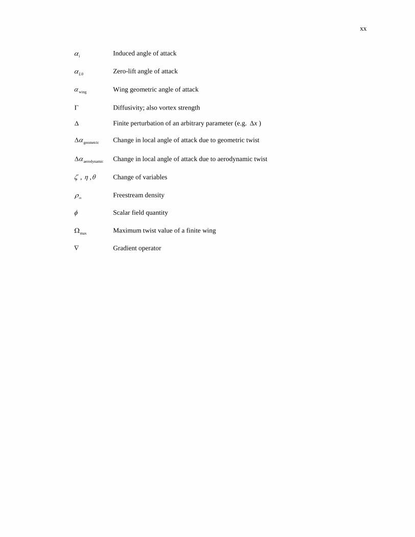
xx

i Induced angle of attack

0L Zero-lift angle of attack

wing Wing geometric angle of attack

Diffusivity; also vortex strength

Finite perturbation of an arbitrary parameter (e.g. x )

geometric Change in local angle of attack due to geometric twist

aerodynamic Change in local angle of attack due to aerodynamic twist

, , Change of variables

Freestream density

Scalar field quantity

max Maximum twist value of a finite wing

Gradient operator

1 INTRODUCTION

Aerodynamic shape optimization is an important step in the design process of modern aircraft. This step

allows designers to tailor the aerodynamic features of an aircraft to meet a specific set of mission

requirements in the most effective way possible. Optimization can be performed early in the design process

to identify what features of a design are most important and toward the end of the design process to refine

certain aspects of the design based on mission requirements. In many cases, high-fidelity Computational

Fluid Dynamics (CFD) analyses are used as the objective functions in these optimization analyses (for

example, see Refs. [1–4]). While CFD analyses provide significant insight into the specific flow

characteristics of a design, they come at a relatively high cost due to the complex computational meshes and

substantial computing resources required. This is especially true for optimization studies in which many cases

must be run to evaluate performance changes with respect to design variables. As a result, CFD is not always

the best solution for early-stage optimization when insights into trends and interactions between design

parameters are more important than highly-accurate performance characteristics.

The computational challenge of using full CFD simulations for aerodynamic optimization are

compounded when the application is a morphing wing. In an effort to improve aircraft efficiency through all

phases of flight, several morphing-wing technologies are currently in development (for example, see Refs.

[5–8]). In order to take full advantage of the benefits provided by morphing-wing technologies, performance

characteristics and control derivatives for the wing in multiple morphed configurations must be readily

available. Due to the large number of possible configurations for a morphing wing with even just a few

degrees of freedom, the efficiency of aerodynamic and structural computations is a prodigious concern.

Several alternatives to full CFD simulations are available for wing optimization. The first practical

method dates back to the early 20th century when Lanchester [9] and Prandtl [10,11] developed what is

known today as classical lifting line theory. While this was the first mathematical model able to predict lift

distributions over a 3D wing with reasonable accuracy, the original formulation is restricted to analyses of a

single finite wing with a straight quarter-chord and moderate-to-high aspect ratio in an incompressible,

inviscid flow. This method has been used to minimize induced drag [12,13] and maximize lift [14] of various

wing planforms.

2

Low-fidelity methods such as the vortex lattice method and vortex panel method represent another

alternative. These potential flow methods are widely used in industry and academia, and their development

can be found in common aerodynamic textbooks. For a well-cited overview of these methods, see Katz and

Plotkin [15]. These methods can be used to predict lift, induced drag, and pressure distributions over complex

geometries but are generally unable to account for viscous effects and airfoil thickness.

A more recent development in aerodynamic analysis is a modern numerical lifting line method presented

by Phillips and Snyder [16]. This method is similar to classical lifting line theory but uses the more general

3D vortex lifting law. The numerical formulation allows for the analysis of a system of interacting lifting

surfaces with arbitrary camber, twist, sweep, and dihedral. It can also account for viscous effects through the

use of 2D airfoil section coefficients. This model should not be confused with the vortex lattice method when

a single element is used in the chordwise direction. Although the placement of the horseshoe vortices is

similar in both methods, the fundamental equations are significantly different. For example, the vortex lattice

method with a single chordwise element places a control point at the three-quarter-chord position and closes

the formulation by requiring the normal velocity relative to the local camber line at the control point to be

zero. On the other hand, the numerical lifting line method of Phillips and Snyder [16] uses the 2D section lift

produced by the local airfoil section to calculate the 3D vortex lift of the finite wing. The latter approach is

the numerical equivalent to the analytical approach taken by Prandtl [10,11].

It is worth noting that numerical methods for solving the lifting line equation from classical lifting line

theory have been presented by McCormick [17] and Anderson et al. [18]. These methods show accurate

results for wings below stall, but they neglect the downwash produced by the bound vorticity and are

therefore limited in application to isolated straight wings without sweep or dihedral.

In this work, the numerical lifting line method of Phillips and Snyder [16] has been used as a foundation

upon which a system is built for analyzing and optimizing morphing wings. We begin in Chapter 2 with a

presentation of methods for computing derivatives and a demonstration of the process of automatic

differentiation (AD) in a numerical lifting line algorithm. In Chapter 3 we discuss the development of an

optimization framework for aerodynamic analysis and apply the derivative calculations from Chapter 2 to

several wing shape optimization problems. We also demonstrate a method for using lifting line calculations

to visualize the design space of morphing wings, which can assist in understanding and improving the wing

3

shape optimization process and results. Chapter 4 presents a detailed overview of classical lifting line theory

along with a discussion of its limitations relative to aspect ratio. We discuss the works of several researchers

directed at improving predictions for low-aspect-ratio wings and present several new analytical developments

that extend the validity of classical lifting line theory to wings of arbitrary aspect ratio. Chapter 5 presents a

method for implementing the results of Chapter 4 in the numerical lifting line method of Phillips and Snyder

[16], and concludes with a comparison of numerical results to experimental data for a low-aspect-ratio

morphing wing.

4

2 DUAL NUMBER AUTOMATIC DIFFERENTIATION FOR WING SHAPE OPTIMIZATION

2.1 Introduction

The focus of this chapter is to present an implementation for accurately and efficiently computing

derivatives within an aerodynamic analysis tool for the purpose of facilitating gradient-based wing shape

optimization. Derivative calculations are an important consideration in any gradient-based optimization

study. The gradient of the objective – a vector of partial derivatives of the objective with respect to the design

variables – is used to determine the appropriate direction and magnitude for changes in the design variables

in order to find a minimum (or maximum) in the objective. Constrained optimization algorithms usually

require the calculation of the gradient for each constrained variable as well. The ability of gradient-based

optimization algorithms to accurately and efficiently converge upon a local extremum is strongly influenced

by the accuracy and efficiency of the derivative calculations upon which they rely. For many gradient-based

optimization problems, the calculation of derivatives is often the costliest step in the optimization cycle (see

Martins [19]), thus special care must be taken in obtaining these derivatives.

Fortunately, derivatives are important to many fields of application beyond optimization and therefore

have a long history of research which can be drawn upon. The first formal presentations of derivatives are

traditionally credited to Isaac Newton and Gottfried Leibniz in the late 17th century, though the fundamental

concept of a derivative appeared much earlier (see Simmons [20]). Numerical analysis methods such as the

finite difference (see Courant et al. [21]) and finite element (see Hrennikoff [22] and Courant [23]) methods

arose from the need to solve sophisticated problems for which solutions could not be obtained through the

methods of analytical calculus. The elliptic and hyperbolic partial differential equations used to describe

boundary value and initial value problems are examples of these. For an examination of the history of the

finite difference and finite element methods, see Thomée [24].

With the advent of modern computers came a new method for computing derivatives. Wengert [25]

presented a technique for the “computation of numerical values of derivatives without developing analytical

expressions for the derivatives.” Wengert’s method formed the foundation for what is now known as

automatic (or algorithmic) differentiation (AD). Numerous publications exist on the subject, covering topics

that range from theoretical research to software development to implementation in practical analysis

applications. See, for example, Griewank and Walthers [26], Rall [27], and Corliss et al. [28]. A wide variety

5

of open-source software tools for implementing AD methods in analysis software have been published, and

numerous engineering software packages include AD capabilities. For a recent review of theoretical AD

methods, see Martins and Hwang [29]. For a recent comparison of AD software tools for various languages,

see Šrajer et al. [30].

In this chapter we apply a specific implementation of AD to MachUp, an open-source aerodynamics

analysis tool based on the numerical lifting line method of Phillips and Snyder [16]. We do this to better

facilitate accurate and efficient gradient calculations for wing shape optimization and other gradient-based

optimization problems in which MachUp is used as the objective function. We begin with a general overview

of the gradient calculation methods described above – namely, symbolic differentiation, finite differencing,

and AD. We then proceed with a description of Dual Number Automatic Differentiation (DNAD), an open-

source implementation of forward-mode AD in Fortran (see Yu and Blair [31] and Spall and Yu [32]). We

discuss modifications to DNAD that were made to improve the flexibility and ease of integrating the tool

with Fortran codes. A simple example is given illustrating the implementation process, and important

considerations when implementing DNAD in existing Fortran codes are discussed. Finally, we present the

process used to implement DNAD in MachUp.

2.2 Derivative Calculation Methods

Methods used for computing derivatives can be divided into three general categories as discussed in Sec.

2.1 – namely, symbolic differentiation, finite differencing, and AD. The three categories are presented here,

and considerations for their use are discussed.

2.2.1 Symbolic Differentiation

Given our understanding of differential calculus, the most obvious method for computing derivatives is

direct symbolic differentiation of the objective function. This involves application of the definition of the

derivative as given in any elementary calculus textbook, namely

0

( ) ( )limh

f f x h f x

x h→

+ −=

(2.2.1)

where f is the objective function, x is the independent variable, and h is a perturbation parameter. Through

symbolic differentiation, we obtain an explicit analytical equation for the derivative of a function which can

be evaluated independent of the original function and is accurate to infinite precision. Algebraic manipulation

6

of the derivative formula can be performed to express the formula in its simplest form. From a computational

perspective, the “simplest form” is that which requires the fewest mathematical operations to evaluate. Thus,

symbolic differentiation represents the most accurate and the most efficient method available for derivative

computations.

For simple functions such as those found in elementary calculus textbooks, there are no disadvantages to

using symbolic differentiation for derivative computations. On the other extreme, direct symbolic

differentiation of practical engineering problems is rarely feasible. For example, consider a coupled

multiphysics model in which fluid and structural analyses are performed iteratively to determine the response

of a system. Results from one analysis are used to update the boundary conditions of the other analysis

between iterations, and the number of iterations performed is controlled through the evaluation of residuals

in the fluid and structural responses of the system. Expressing this function as a single formula that can be

differentiated symbolically would require accumulating each mathematical operation in the process into a

single expression. Since the number of iterations – and therefore the number of mathematical operations to

be evaluated – is variable, the exact expression cannot be known a priori.

Even in the situation described above, it may still be possible to obtain symbolic derivatives of the

objective function if the problem can be broken into smaller sub-functions for which symbolic derivatives

are available. This approach uses the chain rule of differentiation to propagate derivative information through

each sub-function evaluation. For each sub-function evaluation, the Jacobian matrix – which contains the

partial derivatives of all function outputs with respect to each variable input – must be evaluated and stored.

These Jacobian matrices can then be chained together to compute the gradient of the final objective function

with respect to each original input.

To continue the coupled multiphysics example described above, let p be a single-value function that

represents the performance of the coupled multiphysics system. Also, let ( ),f s=x x x be the complete set of

inputs required for the coupled multiphysics model, where ( )1 2, , ,

lf f f fx x x=x is the set of l inputs required

for the fluid analysis and ( )1 2, , ,

ms s s sx x x=x is the set of m inputs required for the structural analysis. Then

( ) ( ),f sp p p= =x x x . The problem at hand is then to determine p , where

7

1 2 1 2

, , , , , , , ,

l mf f f s s s

p p p p p p p p pp

x x x x x x

= = = f s

x x x (2.2.2)

Now, let f and s be vector functions that represent the responses of the fluid and structural models,

respectively. Then ( ),f=f f x s and ( ),s=s s x f . If f is symbolically differentiable with respect to the input

vectors fx and s, then the Jacobian of f

f

=

fJ

f f

x s (2.2.3)

can be determined analytically. Likewise, if s is symbolically differentiable with respect to the input vectors

sx and f, then the Jacobian of s

s

=

s

s s

x fJ (2.2.4)

can also be determined analytically. Equations (2.2.3) and (2.2.4) can be used to assemble a global Jacobian

J , which contains a row and column for each element in the fx , sx , f , and s vectors. In general, this

global Jacobian has the form

f f f f

s

f s

s

f

s

f

s

s

s

f s

x x s

x x

x x

x x x x

f

x x x x

f s

f f f f

f

s s s s

f s

s

x x

J = (2.2.5)

where each term in Eq. (2.2.5) is a submatrix itself.

If we evaluate the fluid model first, we must provide an initial guess for the structural response, namely

0s . Then 1 0( , )f=f f x s and the global Jacobian for this step is

1 1 1

0f

f

I 0 0 0

0 I 0

0

0

0 0

0 I

f f

x s

0

J = (2.2.6)

8

More generally, the global Jacobian for the ith evaluation of the fluid model can be written as

1

1

i

f

i

i−

ff f

x s

I 0 0 0

0 I 0 0

0 0

0 I0 0

J = (2.2.7)

Note that the third diagonal entry in Eqs. (2.2.6) and (2.2.7) is 0 as opposed to the identity matrix. This is

because f is the dependent variable in the fluid model, so that the f in the numerators is one iteration ahead

of the f in the denominators and we have 1/i i− = 0f f for the third diagonal entry.

The structural model is evaluated using results from the fluid model as input, so that the global Jacobian

for the structural evaluation is

1

s

i

i

i

s

f

I 0 0 0

0 I 0 0

0 0 I 0

0 0s s

x

J = (2.2.8)

Similar to the global Jacobian for the fluid model, the fourth diagonal entry in Eq. (2.2.8) is 0 because s is

the dependent variable here. Then the s in the numerator is one iteration ahead of the s in the denominator

and we have 1/i i− = 0s s for the fourth diagonal entry.

The global Jacobian for the entire coupled solution is found by chaining the global Jacobians, Eqs. (2.2.7)

and (2.2.8), over each iteration. A coupled solution evaluated for n iterations will have a global Jacobian

given by

1

i in

n

i=

= s fJ J J (2.2.9)

Equation (2.2.2) can now be written as

n

n

f s n

p p p pp

=

x x f sJ (2.2.10)

While it would be tedious to symbolically evaluate Eq. (2.2.9) by hand, computer algebra systems can readily

perform the evaluations and produce a symbolic formula for the evaluation of p over n iterations. However,

this symbolic formula may be of little use in practice as it is dependent on the number of iterations performed.

9

A more practical use of the methodology presented here is to evaluate the global Jacobians numerically

during each step in the solution process and propagate a single aggregate Jacobian through each iteration.

This approach results in numerical derivatives as opposed to symbolic expressions for the derivatives, but no

additional assumptions or approximations are made in their evaluation.

An important distinction must here be made regarding the symbolic derivatives produced using this

method compared to the derivatives that would be obtained from symbolically differentiating the governing

mathematical model. While the derivatives discussed here are computed using symbolic derivatives of the

individual analysis components, they are exact in terms of the numerical model and not the underlying

mathematical model upon which the numerical algorithm is based. For further discussion on the implications

of numerical modeling error in regard to derivative calculations, see Pakalapati et al. [33] and Sec. 2.4.4.

One potential benefit of using this method is that it can provide a measurement for the level of

convergence in an iterative process such as the one described above. In our example, the last column of

submatrices in the ith global Jacobian contains the derivatives of fluid and structural responses if and

is

with respect to the initial guess 0s . As the solution approaches convergence, the responses should become

independent of the initial guess, so that these derivatives should tend toward zero. Examining the magnitudes

of these derivatives may offer insight into the level of convergence achieved at each iteration.

In summary, symbolic differentiation provides the most accurate and computationally efficient method

of calculating derivatives. Unfortunately, symbolic derivatives are not readily available for most practical

engineering problems. In some cases, the problem can be broken into smaller, symbolically differentiable

components and the partial derivatives of the complete problem can be found through application of the chain

rule of differentiation, either numerically or symbolically, without any loss in accuracy.

2.2.2 Finite Differencing

In 1928, Courant et al. [21] proposed a method for converting partial differential equations into simple

algebraic functions by replacing the partial differentials with quotient approximations. Of particular interest

to the authors were the boundary value and eigenvalue problems for elliptic differential equations and the

initial value problem for hyperbolic and parabolic differential equations, for which there are few known

analytical solutions and none of practical interest. Their development is general enough that it can readily be

10

applied to other problems requiring the calculation of derivatives, and different formulations for the quotient

approximations allow for variable levels of accuracy and complexity.

The simplest example of a finite difference approximation can be taken directly from the definition of the

derivative given in Eq. (2.2.1). Removing the limit and replacing the infinitesimal perturbation parameter h

with a finite step size x gives

( )( ) ( )f f x x f x

xx x

+ −= +

O (2.2.11)

which is the first-order-accurate forward difference formula. The first-order-accurate backward difference

formula is similar but perturbed by x− , specifically

( )( ) ( )f f x f x x

xx x

− − = +

O (2.2.12)

The second-order-accurate central difference formula is found by perturbing the functions in both positive

and negative directions, which gives

( )2( ) ( )

2

f f x x f x xx

x x

+ − − = +

O (2.2.13)

This approach can be applied iteratively to obtain derivatives of higher order as well. For example, an

approximation to the second derivative of f can be found by first finding approximations for / xf from

Eq. (2.2.13) centered at / 2x x+ and / 2x x− using a perturbation of / 2x , and then using these

derivative approximations as the perturbed function values in Eq. (2.2.13). This gives

2

2 2

2 2

() )

2) ( ) ( )2 2( ) ( (

f x f xx x

x f x f x xx xx x x

xx x

f f x

+ − −

− + − = + +=

+

O O (2.2.14)

Many other finite difference approximations are available. Other methods for deriving these formulas

also exist. For example, Taylor series expansions of the function f can be used to obtain Eqs. (2.2.11)-(2.2.14)

and many other finite difference formulas. In fact, the orders of accuracy listed in these equations were

determined using Taylor series expansion. For more finite difference formulas and the methods used to derive

them, see LeVeque [34].

While the finite difference method was originally developed specifically as a tool for solving partial

differential equations, it can be used anytime the derivative of a function is needed and an approximation is

11

acceptable. In general, the finite difference method can readily be applied to any numerical algorithm without

the need to make internal modifications to the algorithm. This is done simply by running the algorithm

multiple times at perturbed states and then applying the appropriate finite difference equation to the results.

Because of this, the finite difference method is the most versatile derivative-approximation method available.

It is also the least accurate and least efficient method, however. All of the methods discussed here are

limited in accuracy by machine precision and numerical modeling error; but the finite difference method is

subject to truncation error as well. The finite difference method is also less efficient than other methods

because full evaluations of the objective function are required for each perturbed function value in the finite

difference formula. A function with N input variables would need to be evaluated 1N + times to obtain a

first-order-accurate approximation of its gradient vector using Eqs. (2.2.11) or (2.2.12), or 2N times for a

second-order-accurate approximation using Eq. (2.2.13).

2.2.3 Automatic Differentiation

As mentioned previously, AD is a method of numerically computing partial derivatives of an algorithm,

accurate to machine precision, without the need to express the partial derivative symbolically. There are

several different approaches to AD, but all stem from the same basic idea that every numerical algorithm can

be broken down into a series of fundamental mathematical operations. If each mathematical operation in an

algorithm is differentiable, then the entire algorithm can be differentiated through sequential applications of

the chain rule of differentiation. This concept is quite similar to the example discussed in Sec. 2.2.1, but

applied at a much finer level.

The different approaches to AD can be classified into two main groups. The first group, called forward-

mode AD, performs derivative calculations in concert with the primary function evaluation. The chain rule

of differentiation is used to propagate derivative calculations from one mathematical operation to the next,

so that the derivatives of intermediate variables with respect to the independent variables are computed

alongside the calculation of the intermediate variables themselves. This is the form of AD that was first

developed by Wengert [25].

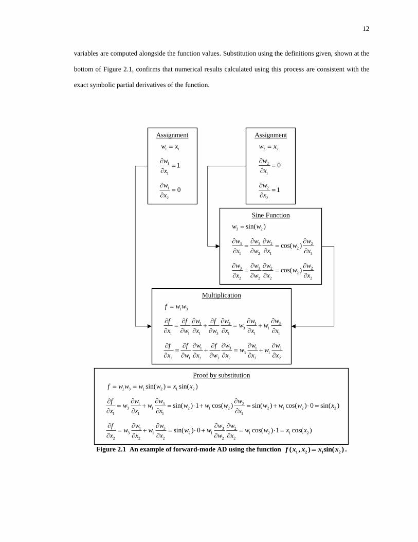
An example of forward-mode AD is given in Figure 2.1. The primary function 1 2 1 2( , ) sin( )f x x x x= is

evaluated as shown, moving from top to bottom. An intermediate variable iw is produced by each

mathematical operation, and the derivatives of each intermediate variable with respect to the two independent

12

variables are computed alongside the function values. Substitution using the definitions given, shown at the

bottom of Figure 2.1, confirms that numerical results calculated using this process are consistent with the

exact symbolic partial derivatives of the function.

Figure 2.1 An example of forward-mode AD using the function

1 2 1 2( , ) sin( )f x x x x= .

Assignment

1 1w x=

1

1

1w

x

=

1

2

0w

x

=

Assignment

22w x=

1

2 0w

x

=

2

2

1w

x

=

Sine Function

23 sin( )w w=

2

2

1 1 1

3 3 2 2cos( )w w w w

wx w x x

= =

2

2 2 2 2

3 3 2 2cos( )w w w w

wx w x x

= =

Multiplication

1 3f w w=

1

3 1

1 1 1 1 1

3 31 1

3

w ww wf f fw w

x w x w x x x

= + = +

1

3 1

2 1 2 3 2 2

3 3

2

1w ww w

wx

f fw

x w w x x x

f = + = +

1 3 1 2 1 2sin( ) sin( )f w w w w x x= = =

3

3 1 2 1 2 2 1 2 2

1 1 1 1

1 2sin( ) 1 cos )(( si) ) cos ) 0 sin n((ww wf

w w w w w wx x x x

w w x

= + = + =

+ =

3 1 2 1 1 2 1 2

2 2 2

3 31

2 2

2) 0 cos( ) 1 cos( )sin(w ww w

w w w wx x

fw w x x

x w x

= + = =

=

+

Proof by substitution

13

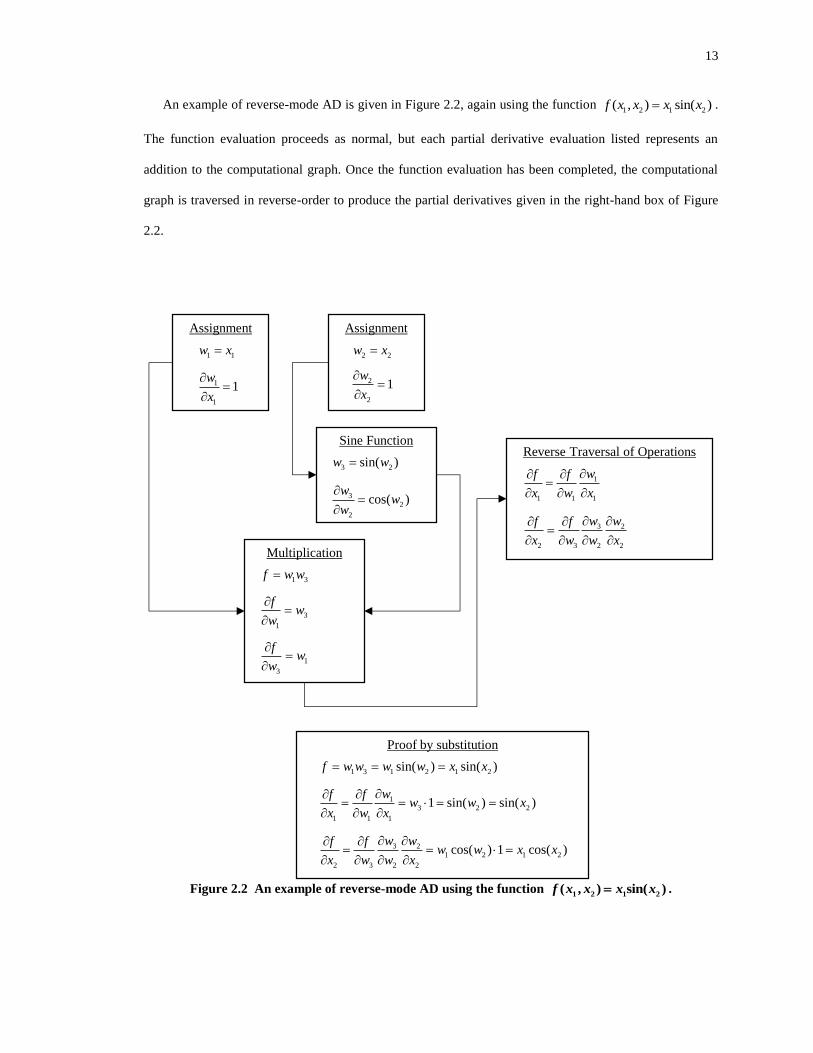
An example of reverse-mode AD is given in Figure 2.2, again using the function 1 2 1 2( , ) sin( )f x x x x= .

The function evaluation proceeds as normal, but each partial derivative evaluation listed represents an

addition to the computational graph. Once the function evaluation has been completed, the computational

graph is traversed in reverse-order to produce the partial derivatives given in the right-hand box of Figure

2.2.

Figure 2.2 An example of reverse-mode AD using the function

1 2 1 2( , ) sin( )f x x x x= .

1 3 1 2 1 2sin( ) sin( )f w w w w x x= = =

1

3 2 2

1 1 1

)1 sin( ) sin(wf f

wx

w xw x

= =

=

=

2

3 2 2

3 2

1 1 2

2

cos( ) 1 )cos(w wf

w w xx w w

fx

x

= = =

Proof by substitution

Reverse Traversal of Operations

1 1 1

1wf f

x w x

=

3 2

2 3 2 2

w wf f

x w w x

=

Multiplication

1 3f w w=

3

1

fw

w

=

1

3

fw

w

=

Assignment

1 1w x=

1

1

1w

x

=

Assignment

22w x=

2

2

1w

x

=

Sine Function

23 sin( )w w=

2

2

3 )cos(w

ww

=

14

Figures 2.1 and 2.2 were given to illustrate the overall processes of the respective methods, but many

details are hidden so that a comprehensive comparison of the two methods cannot be made based on these

examples alone. Fewer computations are required to arrive at the partial derivative solutions given in Figure

2.2 than were required to arrive at the same solution in Figure 2.1. This is only true, however, because the

number of design variables (2) is larger than the number of output variables (1). In general, the complexity

of the derivative calculations using forward-mode AD scales according to the number of design variables in

the problem, while the complexity of the derivative calculations using reverse-mode AD scales according to

the number of output variables for which gradients are needed.

Also not apparent from the examples illustrated in Figures 2.1 and 2.2 are the memory requirements for

each method. Forward-mode AD algorithms must store the intermediate partial derivatives at each step in the

solution process, so they require more memory than either symbolic differentiation or the finite difference

method. Reverse-mode AD algorithms must store the entire computational graph, however, so that their

memory requirements are considerably larger.

The effort required to implement the different modes in code is also not illustrated. In general, forward-

mode AD is considered easier to implement and less intrusive to the original source code than reverse-mode

AD. This is because, in reverse-mode AD, additional coding is required to build, manage, and traverse the

computational graph. Additionally, each output variable for which derivatives are needed must be handled

individually with existing reverse-mode AD methods, while forward-mode AD methods can be applied in

such a way that a single version of the source code can compute derivatives of any output variable with

respect to any input variable. This will be demonstrated later in this chapter. The reader is referred to the

literature (see, for example, Refs. [26–28]) for more detailed discussions on the two AD methods.

2.2.4 Discussion

The purpose of the present chapter is to facilitate accurate and efficient derivative calculations within

MachUp, as discussed in the introduction. Symbolic differentiation of the algorithm is infeasible due to the

complexity of the nonlinear system of equations which form the basis of the numerical lifting line algorithm

implemented by MachUp. Finite differencing introduces truncation error into the derivative calculations and

is less efficient than AD methods. For these reasons, the author has selected AD for implementation in

MachUp.

15

Of the available AD methods, reverse-mode AD is considered more efficient than forward-mode AD

when the number of design variables is larger than the number of dependent variables. This is likely to be

the case for any wing shape optimization problem in which MachUp is used to evaluate the objective

function, but this advantage is expected to be small because of the limited number of inputs required to define

even complex wing geometries in MachUp. The memory advantages of forward-mode AD are also not

important to this effort because the memory requirements for most typical MachUp simulations are several

orders of magnitude less than the available memory on most modern machines. The primary concerns in

deciding between forward-mode and reverse-mode AD for the current work, then, are the amount of effort

required for implementation in the existing source code and the flexibility of the resulting code in computing

derivatives of various output variables with respect to various input variables. As discussed in Sec. 2.2.3,

forward-mode AD holds advantages over reverse-mode AD in both respects.

2.3 Methods and Tools for Forward-Mode Automatic Differentiation

Two methods exist for implementing forward-mode AD in source code, namely source code

transformation (SCT) and operator-overloading (OO). SCT is done by scanning the existing source code,

identifying all floating-point variables and mathematical operations, adding additional variable declarations

for the storage of partial derivative values, and adding additional lines of code for the computation of partial

derivative values anytime a mathematical operation is performed. While to perform this process manually

would be tedious at best, several algorithms have been developed to perform SCT automatically for a variety

of programming languages. See, for example, Refs. [35–39]. SCT is possible in all programming languages,

but tools for performing SCT are quite complex. Because the derivative computations appear explicitly in

the differentiated source code, the resulting source code can be quite large when compared to the original

undifferentiated code, and different source code is obtained depending on which input variables are made

available for differentiation. As a result, several versions of the source code must be maintained in order to

allow for any flexibility in the derivative calculations, which has negative implications regarding version

control.

OO methods rely on the use of a custom data type with specifically-defined behavior for mathematical

operations. The custom data type contains storage for a single floating-point variable and its derivative with

respect to one or more independent variables. Any time a mathematical operator is applied to an instance of

16

this custom data type, code is executed to evaluate both the mathematical operation and its analytical partial

derivative(s) automatically. Not all programming languages support the polymorphic features required for

implementing AD through OO, but most common languages used for scientific and engineering applications

do (e.g. Fortran, Matlab, C++, Python, R, and Java).

As with SCT, several tools are available for implementing OO in existing source code, but

implementations are quite varied in both functionality and ease-of-use. One common method for

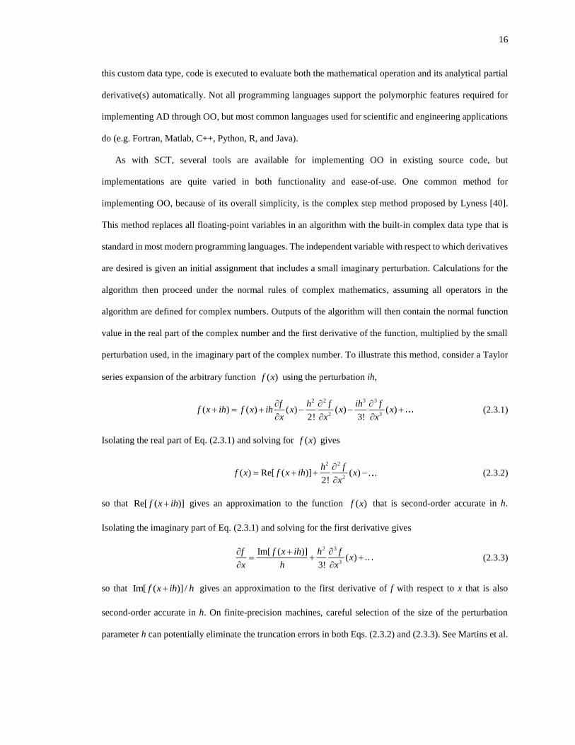
implementing OO, because of its overall simplicity, is the complex step method proposed by Lyness [40].

This method replaces all floating-point variables in an algorithm with the built-in complex data type that is

standard in most modern programming languages. The independent variable with respect to which derivatives

are desired is given an initial assignment that includes a small imaginary perturbation. Calculations for the

algorithm then proceed under the normal rules of complex mathematics, assuming all operators in the

algorithm are defined for complex numbers. Outputs of the algorithm will then contain the normal function

value in the real part of the complex number and the first derivative of the function, multiplied by the small

perturbation used, in the imaginary part of the complex number. To illustrate this method, consider a Taylor

series expansion of the arbitrary function ( )f x using the perturbation ih,

3 32

2 3

2

( ) ( ) ( ) ( ) ( )2! 3!

f h f ih ff x ih f x ih x x x

x x x

+ = + − − +

(2.3.1)

Isolating the real part of Eq. (2.3.1) and solving for ( )f x gives

2

2

2

( ) Re[ ( )] ( )2!

h ff x f x ih x

x

= + + −

(2.3.2)

so that Re[ ( )]f x ih+ gives an approximation to the function ( )f x that is second-order accurate in h.

Isolating the imaginary part of Eq. (2.3.1) and solving for the first derivative gives

2 3

3

Im[ ( )]( )

3!

f f x ih h fx

x h x

+ = + +

(2.3.3)

so that Im[ ( )] /f x ih h+ gives an approximation to the first derivative of f with respect to x that is also

second-order accurate in h. On finite-precision machines, careful selection of the size of the perturbation

parameter h can potentially eliminate the truncation errors in both Eqs. (2.3.2) and (2.3.3). See Martins et al.

17

[41] for a more detailed discussion on the complex step method and considerations for eliminating the

truncation errors when using this method.

While the complex step method is relatively simple to implement and does not require the construction

of a custom data type, it has several drawbacks that discourage its use over other OO methods. Martins et al.

[41] showed a Fortran implementation of the complex step method to be significantly less efficient than even

finite difference methods with only marginal improvement in accuracy. Also, the requirement for a

perturbation step size introduces the potential for additional truncation error in the results that would not be

incurred with a full OO implementation. Finally, the restriction to a complex number data type limits the

number of independent variables with respect to which partial derivatives can be obtained to one per

simulation.

Several full OO implementations of forward-mode AD have been developed for a variety of programming

languages. Fortran implementations include ADF95 (see Straka [42]), AUTO_DERIV (see Stamatiadis et al.

[43]), COSY INFINITY (see Berz et al. [44]), AD01 (see Pryce and Reid [45]), and DNAD (see Yu and Blair

[31]). Of these, DNAD has been selected for use in this work. Several considerations were weighed in

comparing these tools, including licensing, extensibility, level of complexity in the interface, and runtime

performance. A thorough discussion of DNAD is given in the remainder of this chapter, including a

presentation of dual number theory upon which DNAD is based, an examination of the algorithm, and the

process of integrating DNAD with MachUp. For details on the other software packages listed, the reader is

referred to Refs. [42–45].

2.4 Dual Number Automatic Differentiation

DNAD is essentially a derived data type that implements the rules of dual number theory

programmatically, which can then be used in computational software to perform dual number calculations.

In this section, we shall first present an overview of what dual number theory is. We shall then describe how

this theory is implemented as a data type in DNAD. Finally, we shall discuss the process of integrating this

derived data type into Fortran source code for automatic differentiation of an algorithm.

18

2.4.1 Dual Number Theory

The theory of dual numbers was first introduced by Clifford [46] for the purpose of describing

biquaternions. It has since found application in several areas including the calculation of derivatives. Dual

numbers extend the real number space by adjoining a nilpotent unit , which has the property

1, 1

0, 1

nn

n

==

(2.4.1)

This is similar to how complex numbers extend the real number space using the imaginary unit i, but the

differences in properties between the nilpotent unit and the imaginary unit result in distinct behavior between

the two number sets. A dual number d can be written as

d a b= + (2.4.2)

where a is the real component and b is the dual component of the dual number. A Taylor series expansion of

the dual number perturbed about the real component by the dual unit gives

2

( ) ( ) ( ) ( )2!

f a f a f a f a

+ = + + + (2.4.3)

or, applying the definition of the nilpotent unit given in Eq. (2.4.1),

( ) ( ) ( )f a f a f a + = + (2.4.4)

From Eq. (2.4.4) we see that the real component of ( )f a + gives the function value ( )f a and the dual

component gives the first derivative of the function, ( )f a . Note that Eq. (2.4.4) is not a truncation of Eq.

(2.4.3), so that the function value and its derivative obtained in this manner are exact.

Now consider two functions f and g represented as dual numbers 1d f f = + and

2d g g = + . The

product of these two dual numbers is

2

1 2 ( )( ) ( ) ( )d d f f g g fg fg gf f g fg fg gf = + + = + + + = + + (2.4.5)

which gives the correct values for the function and its derivative as the real and dual components,

respectively. Similarly, the quotient of these two dual numbers is

1

2

fd f

g gd

+ =

+ (2.4.6)

Multiplying top and bottom by the dual conjugate of the denominator, g g − , gives

19

2

1

2 2 2

2

( )fg f g f

g

gd f g f f g

d

fg

gg g

+ − − − = +

−=

(2.4.7)

which again gives the correct values for the function and its derivative as the real and dual components,

respectively.

The dual number of a trigonometric function can be determined using another Taylor series expansion.

For example, the function sin( )f x= can be expressed as a dual number as

2

3 ) sin( ) cos( ) sin( )2

(!

d xx

x xf x x = +

= + − − (2.4.8)

so that the real part – sin( )x – gives the original function and the dual part – cos( )x x – gives the correct

derivative. All other terms are zero by definition of the nilpotent unit.

This exercise can be repeated for all other continuously differentiable mathematical operations with

consistent results. Additionally, the chain rule of differentiation allows multiple operations to be chained

together to produce accurate expressions for the function and its derivative for functions of arbitrary

complexity.

Retention of higher-order terms in allows for higher-order derivatives to be calculated in like manner

to the first-order derivatives illustrated above. For an example of how dual numbers can be applied to

compute second-order derivatives, see Fike and Alonso [47]. Only first-order derivatives will be treated in

this work. However, future effort may extend DNAD to facilitate higher-order derivatives. This would

facilitate accurate and efficient calculations of Hessian matrices, which can then be used to improve the

performance of some gradient-based optimization algorithms.

2.4.2 The Dual Number Data Type

The dual number theory described in Sec. 2.4.1 has been implemented in Fortran by Yu and Blair [31]

using a derived data type with operator overloading. The derived data type consists of a single floating-point

variable that stores the primary function value, an array of floating-point values of arbitrary length containing

any number of partial derivative values, and a series of overloaded operator functions defining the mechanics

of dual number algebra. The DNAD source code is provided in Appendix A.

The source code given in Appendix A contains several modifications from the original version published

by Yu and Blair. These modifications have been made in an effort to make the software more flexible and

20

easier to use. In the original version, variables for precision and the length of the derivative vectors were

defined explicitly in the source code. These definitions have been removed. Floating-point precision is now

controlled through options specified at compile-time. For example, the DNAD module can be compiled for

double-precision floating-point algebra using the –fdefault-real-8 flag in the gfortran compiler or the –

r8 flag in the Intel Fortran compiler. Similarly, the length of the derivative vector can be specified using

preprocessor directives. For example, a derivative vector length of 3 is defined by specifying –Dndv=3 when

invoking the preprocessor. By making these modifications, the floating-point precision and derivative vector

length are now contained in the DNAD programming interface as opposed to being explicitly contained in

the DNAD source code. Additionally, the source code has been reorganized and is now contained within a

single source file. This is simply for convenience when compiling the module and linking it with Fortran

algorithms. Note that the use of preprocessor directives requires that the preprocessor be invoked before the

source code can be compiled. This is usually done when invoking the compiler by specifying a preprocessor

flag (e.g. –cpp when using gfortran or –fpp when using the Intel Fortran compiler) or by capitalizing the file

extension (e.g. *.F or *.F90 as opposed to *.f or *.f90).

Several additional operators have been added to the programming interface, including the intrinsic Fortran

tan, dtan, atan, atan2, and maxloc functions. The abs operator overload has been modified to prevent

excessive not-a-number (NaN) occurrences in the derivative values when the primary value is constant with

respect to any of the independent variables. These changes make the DNAD module more versatile in its

application to existing Fortran algorithms.

2.4.3 Integration with Fortran Algorithms

A streamlined process for integrating DNAD with Fortran algorithms has been developed. Most source

files can be modified simply by adding the lines of code shown in Figure 2.3 to the beginning of the file.

When other modifications to the source file are necessary, e.g. when logic must be added to handle input

and/or output of the additional data contained in the dual number type, these modifications can also be

contained inside compiler directives so that the normal behavior of the code can be retained when the DNAD

module is not included in the compiling process.

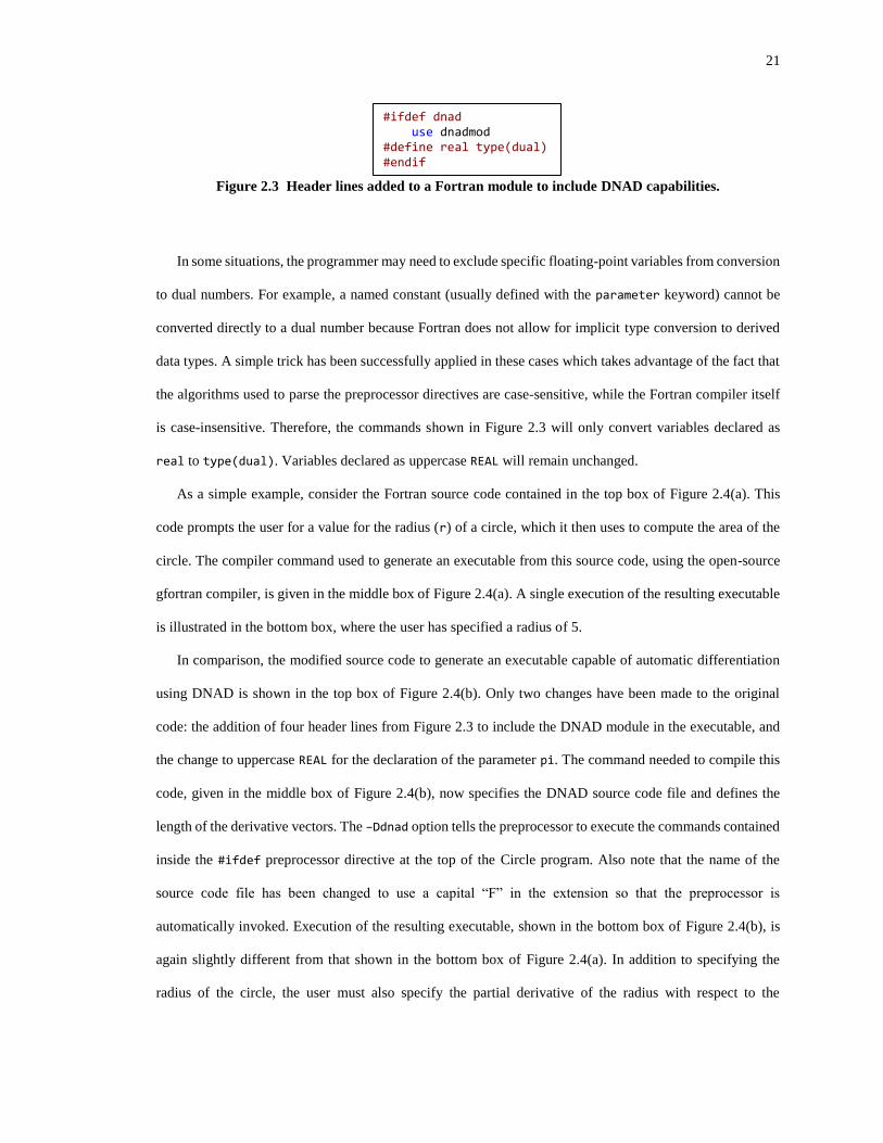
21

Figure 2.3 Header lines added to a Fortran module to include DNAD capabilities.

In some situations, the programmer may need to exclude specific floating-point variables from conversion

to dual numbers. For example, a named constant (usually defined with the parameter keyword) cannot be

converted directly to a dual number because Fortran does not allow for implicit type conversion to derived

data types. A simple trick has been successfully applied in these cases which takes advantage of the fact that

the algorithms used to parse the preprocessor directives are case-sensitive, while the Fortran compiler itself

is case-insensitive. Therefore, the commands shown in Figure 2.3 will only convert variables declared as

real to type(dual). Variables declared as uppercase REAL will remain unchanged.

As a simple example, consider the Fortran source code contained in the top box of Figure 2.4(a). This

code prompts the user for a value for the radius (r) of a circle, which it then uses to compute the area of the

circle. The compiler command used to generate an executable from this source code, using the open-source

gfortran compiler, is given in the middle box of Figure 2.4(a). A single execution of the resulting executable

is illustrated in the bottom box, where the user has specified a radius of 5.

In comparison, the modified source code to generate an executable capable of automatic differentiation

using DNAD is shown in the top box of Figure 2.4(b). Only two changes have been made to the original

code: the addition of four header lines from Figure 2.3 to include the DNAD module in the executable, and

the change to uppercase REAL for the declaration of the parameter pi. The command needed to compile this

code, given in the middle box of Figure 2.4(b), now specifies the DNAD source code file and defines the

length of the derivative vectors. The –Ddnad option tells the preprocessor to execute the commands contained

inside the #ifdef preprocessor directive at the top of the Circle program. Also note that the name of the

source code file has been changed to use a capital “F” in the extension so that the preprocessor is

automatically invoked. Execution of the resulting executable, shown in the bottom box of Figure 2.4(b), is

again slightly different from that shown in the bottom box of Figure 2.4(a). In addition to specifying the

radius of the circle, the user must also specify the partial derivative of the radius with respect to the

#ifdef dnad use dnadmod #define real type(dual) #endif

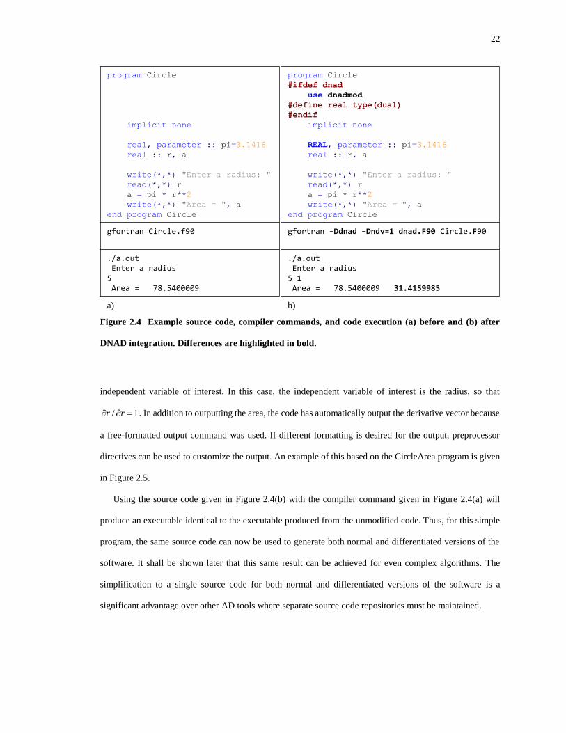
22

Figure 2.4 Example source code, compiler commands, and code execution (a) before and (b) after

DNAD integration. Differences are highlighted in bold.

independent variable of interest. In this case, the independent variable of interest is the radius, so that

/ 1r r = . In addition to outputting the area, the code has automatically output the derivative vector because

a free-formatted output command was used. If different formatting is desired for the output, preprocessor

directives can be used to customize the output. An example of this based on the CircleArea program is given

in Figure 2.5.

Using the source code given in Figure 2.4(b) with the compiler command given in Figure 2.4(a) will

produce an executable identical to the executable produced from the unmodified code. Thus, for this simple

program, the same source code can now be used to generate both normal and differentiated versions of the

software. It shall be shown later that this same result can be achieved for even complex algorithms. The

simplification to a single source code for both normal and differentiated versions of the software is a

significant advantage over other AD tools where separate source code repositories must be maintained.

program Circle

implicit none

real, parameter :: pi=3.1416

real :: r, a

write(*,*) "Enter a radius: "

read(*,*) r

a = pi * r**2

write(*,*) "Area = ", a

end program Circle

program Circle

#ifdef dnad

use dnadmod

#define real type(dual)

#endif

implicit none

REAL, parameter :: pi=3.1416

real :: r, a

write(*,*) "Enter a radius: "

read(*,*) r

a = pi * r**2

write(*,*) "Area = ", a

end program Circle

gfortran Circle.f90 gfortran –Ddnad –Dndv=1 dnad.F90 Circle.F90

./a.outEnter a radius5Area = 78.5400009

./a.outEnter a radius5 1Area = 78.5400009 31.4159985

a) b)

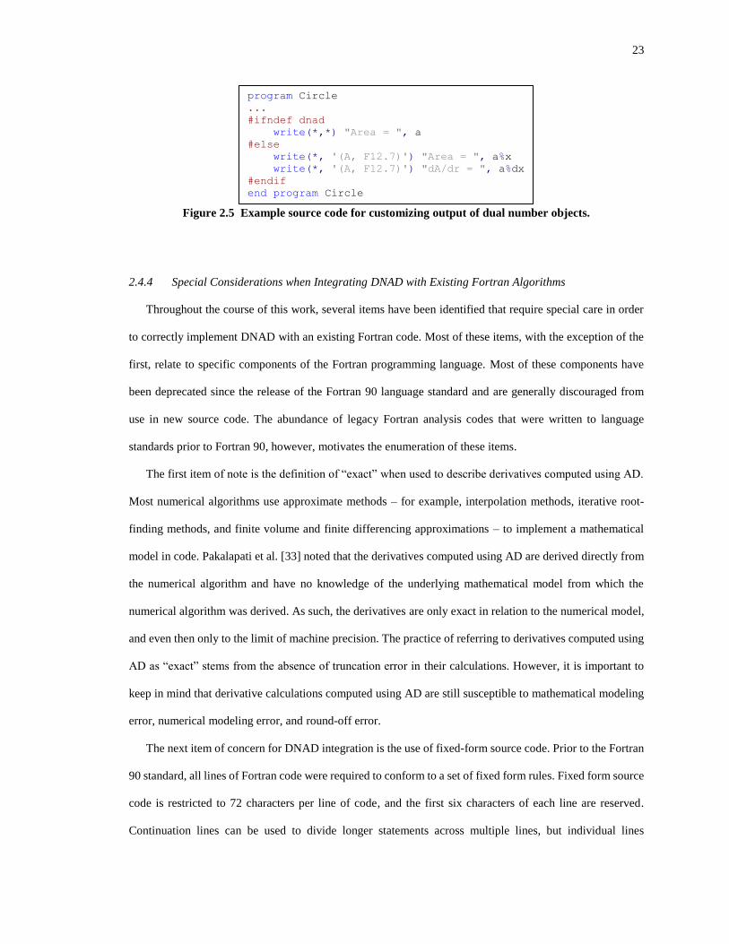
23

Figure 2.5 Example source code for customizing output of dual number objects.

2.4.4 Special Considerations when Integrating DNAD with Existing Fortran Algorithms

Throughout the course of this work, several items have been identified that require special care in order

to correctly implement DNAD with an existing Fortran code. Most of these items, with the exception of the

first, relate to specific components of the Fortran programming language. Most of these components have

been deprecated since the release of the Fortran 90 language standard and are generally discouraged from

use in new source code. The abundance of legacy Fortran analysis codes that were written to language

standards prior to Fortran 90, however, motivates the enumeration of these items.

The first item of note is the definition of “exact” when used to describe derivatives computed using AD.

Most numerical algorithms use approximate methods – for example, interpolation methods, iterative root-

finding methods, and finite volume and finite differencing approximations – to implement a mathematical

model in code. Pakalapati et al. [33] noted that the derivatives computed using AD are derived directly from

the numerical algorithm and have no knowledge of the underlying mathematical model from which the

numerical algorithm was derived. As such, the derivatives are only exact in relation to the numerical model,

and even then only to the limit of machine precision. The practice of referring to derivatives computed using

AD as “exact” stems from the absence of truncation error in their calculations. However, it is important to

keep in mind that derivative calculations computed using AD are still susceptible to mathematical modeling

error, numerical modeling error, and round-off error.

The next item of concern for DNAD integration is the use of fixed-form source code. Prior to the Fortran

90 standard, all lines of Fortran code were required to conform to a set of fixed form rules. Fixed form source

code is restricted to 72 characters per line of code, and the first six characters of each line are reserved.

Continuation lines can be used to divide longer statements across multiple lines, but individual lines

program Circle ... #ifndef dnad write(*,*) "Area = ", a #else write(*, '(A, F12.7)') "Area = ", a%x write(*, '(A, F12.7)') "dA/dr = ", a%dx #endif end program Circle

24

exceeding 72 characters in length are automatically truncated by the compiler. When preprocessor directives

are used to modify fixed form source code (such as when real variable declarations are replaced with

type(dual) – an increase of six characters – using the preprocessor directives listed in Figure 2.3), the

resulting lines of code must conform to this same limit or be truncated.

With the publication of the Fortran 90 language standard, free form source code formatting was

introduced which allows for up to 132 characters per line of code and removes the special reservation of the

first six characters on each line. This added flexibility reduces the likelihood that modifying the source code

through the preprocessor directives given in Figure 2.3 will cause inadvertent truncation of the source code.

However, the possibility still exists. For fixed form source code, the code must be checked for any lines

containing floating-point variable declarations that exceed 65 characters in width. For free form source code,

these declaration lines cannot exceed 125 characters in width. Any lines exceeding these limits must be

shortened or divided into multiple lines.

Another hurdle to the implementation of DNAD in Fortran codes is the use of the common statement to

share information between program units. When data types of variables in a common statement are consistent

between program units, the conversion of floating-point variables from real to type(dual) should work

seamlessly. However, it is possible for the memory space assigned to a common statement to be declared as

one data type in one program unit and a different data type in another program unit. This can lead to data

misalignment when the data types of variables in the common block are changed. The code given in Figure

2.6 illustrates this problem. The same common block is declared in two separate subroutines but with

inconsistent data types. The common block cb, when the two subroutines are compiled using a double-

precision compiler flag (e.g. -fdefault-real-8 for the gfortran compiler or -r8 for the Intel Fortran compiler),

will have a size of 8 bytes. However, if the DNAD header from Figure 2.3 is included and the subroutines

are recompiled, the size of the common block cb in subroutine sub1 will be 8( 1)N + , where N is the length

of the derivative vector. This is incompatible with the size of the common block in subroutine sub2 and will

generate a compiler error. Even worse, if the name is omitted from the common block declarations so that

the blank common block is used, the code will compile successfully but the character string c in subroutine

sub2 will only align with the first eight bytes of the dual number x in subroutine sub1. Any additional

variables included in the common block will then be misaligned in the executable.

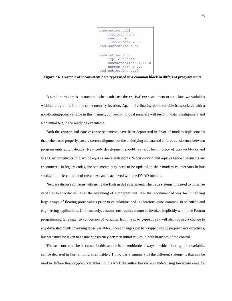
25

Figure 2.6 Example of inconsistent data types used in a common block in different program units.

A similar problem is encountered when codes use the equivalence statement to associate two variables

within a program unit to the same memory location. Again, if a floating-point variable is associated with a

non-floating-point variable in this manner, conversion to dual numbers will result in data misalignment and

a potential bug in the resulting executable.

Both the common and equivalence statements have been deprecated in favor of modern replacements

that, when used properly, ensure correct alignment of the underlying bit data and enforce consistency between

program units automatically. New code development should use modules in place of common blocks and

transfer statements in place of equivalence statements. When common and equivalence statements are

encountered in legacy codes, the statements may need to be updated to their modern counterparts before

successful differentiation of the codes can be achieved with the DNAD module.

Next we discuss concerns with using the Fortran data statement. The data statement is used to initialize

variables to specific values at the beginning of a program unit. It is the recommended way for initializing

large arrays of floating-point values prior to calculations and is therefore quite common in scientific and

engineering applications. Unfortunately, custom constructors cannot be invoked implicitly within the Fortran

programming language, so conversion of variables from real to type(dual) will also require a change to

any data statements involving those variables. These changes can be wrapped inside preprocessor directives,

but care must be taken to ensure consistency between initial values in both branches of the control.

The last concern to be discussed in this section is the multitude of ways in which floating-point variables

can be declared in Fortran programs. Table 2.1 provides a summary of the different statements that can be

used to declare floating-point variables. In this work the author has recommended using lowercase real for

subroutine sub1 implicit none real :: x common /cb/ x ... end subroutine sub1

subroutine sub2 implicit none character(len=8) :: c common /cb/ c ... end subroutine sub2

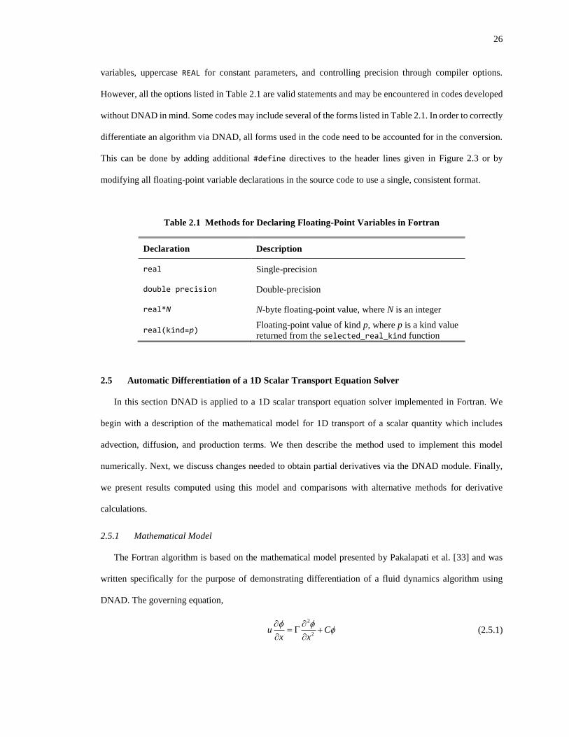
26

variables, uppercase REAL for constant parameters, and controlling precision through compiler options.

However, all the options listed in Table 2.1 are valid statements and may be encountered in codes developed

without DNAD in mind. Some codes may include several of the forms listed in Table 2.1. In order to correctly

differentiate an algorithm via DNAD, all forms used in the code need to be accounted for in the conversion.

This can be done by adding additional #define directives to the header lines given in Figure 2.3 or by

modifying all floating-point variable declarations in the source code to use a single, consistent format.

Table 2.1 Methods for Declaring Floating-Point Variables in Fortran

Declaration Description

real Single-precision

double precision Double-precision

real*N N-byte floating-point value, where N is an integer

real(kind=p) Floating-point value of kind p, where p is a kind value

returned from the selected_real_kind function

2.5 Automatic Differentiation of a 1D Scalar Transport Equation Solver

In this section DNAD is applied to a 1D scalar transport equation solver implemented in Fortran. We

begin with a description of the mathematical model for 1D transport of a scalar quantity which includes

advection, diffusion, and production terms. We then describe the method used to implement this model

numerically. Next, we discuss changes needed to obtain partial derivatives via the DNAD module. Finally,

we present results computed using this model and comparisons with alternative methods for derivative

calculations.

2.5.1 Mathematical Model

The Fortran algorithm is based on the mathematical model presented by Pakalapati et al. [33] and was

written specifically for the purpose of demonstrating differentiation of a fluid dynamics algorithm using

DNAD. The governing equation,

2

2u C

x x

= +

(2.5.1)

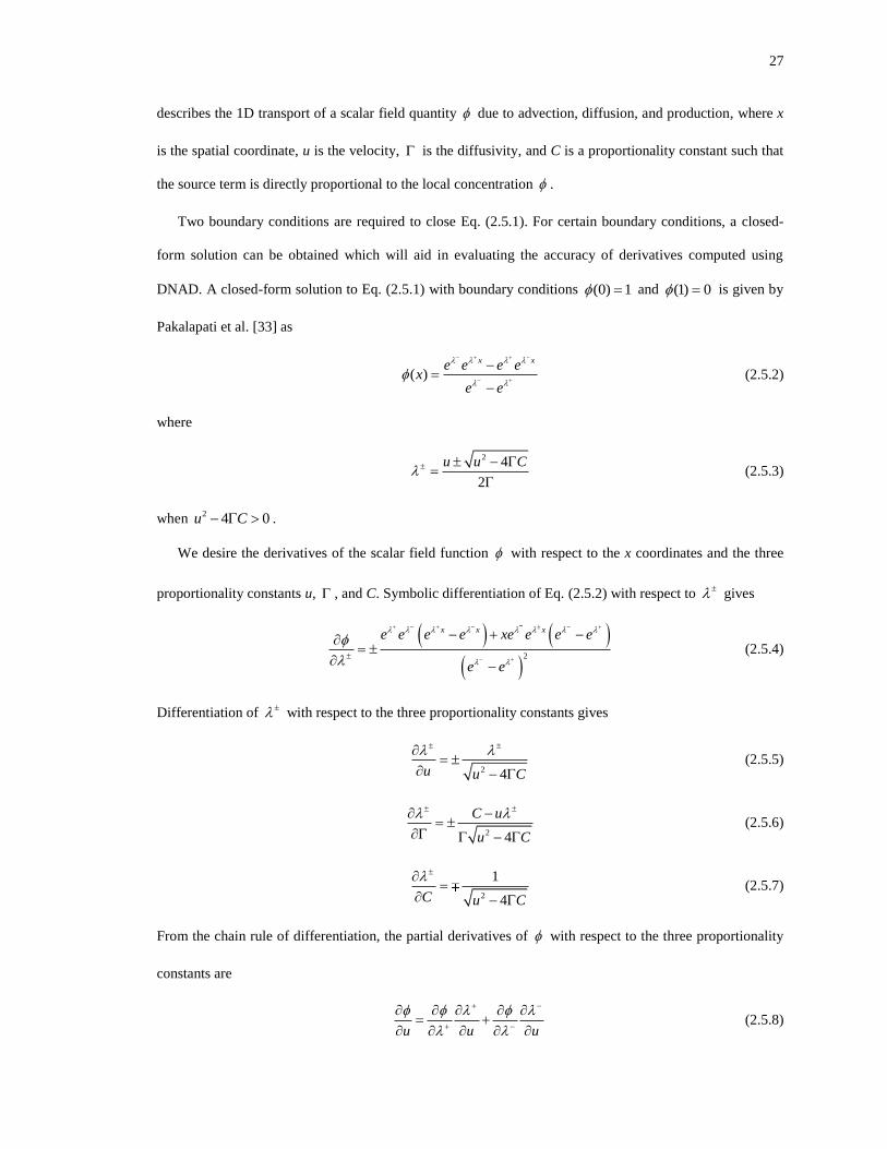
27

describes the 1D transport of a scalar field quantity due to advection, diffusion, and production, where x

is the spatial coordinate, u is the velocity, is the diffusivity, and C is a proportionality constant such that

the source term is directly proportional to the local concentration .

Two boundary conditions are required to close Eq. (2.5.1). For certain boundary conditions, a closed-

form solution can be obtained which will aid in evaluating the accuracy of derivatives computed using

DNAD. A closed-form solution to Eq. (2.5.1) with boundary conditions (0) 1 = and (1) 0 = is given by

Pakalapati et al. [33] as

( )x xe e e e

ex

e

− + + −

− +

−

−= (2.5.2)

where

2

2

4 Cu u −

=

(2.5.3)

when 2 4 0u C− .

We desire the derivatives of the scalar field function with respect to the x coordinates and the three

proportionality constants u, , and C. Symbolic differentiation of Eq. (2.5.2) with respect to gives

( ) ( )

( )2

x x xe e e e xe e e e

e e

+ +− −

+

− +

−

=

− −

−

+

(2.5.4)

Differentiation of with respect to the three proportionality constants gives

2 4u u C

=

− (2.5.5)

2 4 C

C u

u

=

−

− (2.5.6)

2

1

4C u C

=

− (2.5.7)

From the chain rule of differentiation, the partial derivatives of with respect to the three proportionality

constants are

u uu

+ −

+ − = +

(2.5.8)

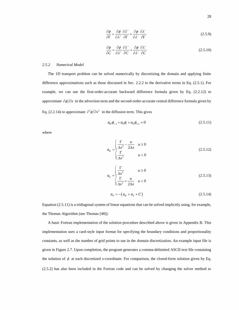
28

−+

+ −

= +

(2.5.9)

C C C

+

+

−

−

= +

(2.5.10)

2.5.2 Numerical Model

The 1D transport problem can be solved numerically by discretizing the domain and applying finite

difference approximations such as those discussed in Sec. 2.2.2 to the derivative terms in Eq. (2.5.1). For

example, we can use the first-order-accurate backward difference formula given by Eq. (2.2.12) to

approximate x in the advection term and the second-order-accurate central difference formula given by

Eq. (2.2.14) to approximate 2 2x in the diffusion term. This gives

1 1 0i P i EW ia a a − ++ + = (2.5.11)

where

2

2

0

0

2W

u

a

u

xx

xu

=

−

(2.5.12)

2

2

0

02

E

u

ax

uu

xx

=

+

(2.5.13)

( )P W Ea a a C= − + + (2.5.14)

Equation (2.5.11) is a tridiagonal system of linear equations that can be solved implicitly using, for example,

the Thomas Algorithm (see Thomas [48]).

A basic Fortran implementation of the solution procedure described above is given in Appendix B. This

implementation uses a card-style input format for specifying the boundary conditions and proportionality

constants, as well as the number of grid points to use in the domain discretization. An example input file is

given in Figure 2.7. Upon completion, the program generates a comma-delimited ASCII text file containing

the solution of at each discretized x-coordinate. For comparison, the closed-form solution given by Eq.

(2.5.2) has also been included in the Fortran code and can be solved by changing the solver method to

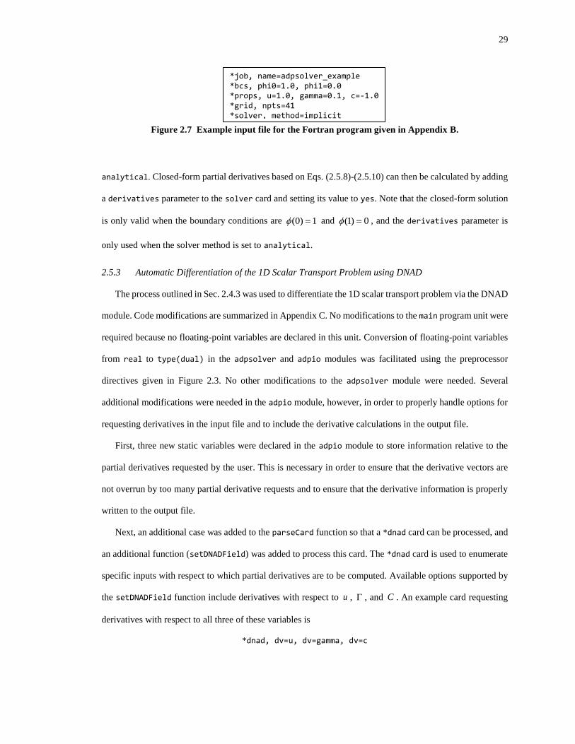
29

Figure 2.7 Example input file for the Fortran program given in Appendix B.

analytical. Closed-form partial derivatives based on Eqs. (2.5.8)-(2.5.10) can then be calculated by adding

a derivatives parameter to the solver card and setting its value to yes. Note that the closed-form solution

is only valid when the boundary conditions are (0) 1 = and (1) 0 = , and the derivatives parameter is

only used when the solver method is set to analytical.

2.5.3 Automatic Differentiation of the 1D Scalar Transport Problem using DNAD

The process outlined in Sec. 2.4.3 was used to differentiate the 1D scalar transport problem via the DNAD

module. Code modifications are summarized in Appendix C. No modifications to the main program unit were

required because no floating-point variables are declared in this unit. Conversion of floating-point variables

from real to type(dual) in the adpsolver and adpio modules was facilitated using the preprocessor

directives given in Figure 2.3. No other modifications to the adpsolver module were needed. Several

additional modifications were needed in the adpio module, however, in order to properly handle options for

requesting derivatives in the input file and to include the derivative calculations in the output file.

First, three new static variables were declared in the adpio module to store information relative to the

partial derivatives requested by the user. This is necessary in order to ensure that the derivative vectors are

not overrun by too many partial derivative requests and to ensure that the derivative information is properly

written to the output file.

Next, an additional case was added to the parseCard function so that a *dnad card can be processed, and

an additional function (setDNADField) was added to process this card. The *dnad card is used to enumerate

specific inputs with respect to which partial derivatives are to be computed. Available options supported by

the setDNADField function include derivatives with respect to u , , and C . An example card requesting

derivatives with respect to all three of these variables is

*dnad, dv=u, dv=gamma, dv=c

*job, name=adpsolver_example *bcs, phi0=1.0, phi1=0.0 *props, u=1.0, gamma=0.1, c=-1.0 *grid, npts=41 *solver, method=implicit

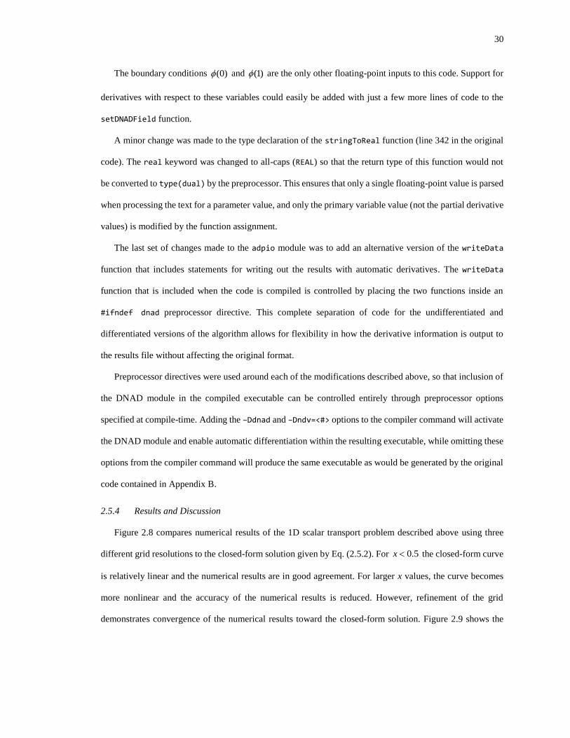
30

The boundary conditions (0) and (1) are the only other floating-point inputs to this code. Support for

derivatives with respect to these variables could easily be added with just a few more lines of code to the

setDNADField function.

A minor change was made to the type declaration of the stringToReal function (line 342 in the original

code). The real keyword was changed to all-caps (REAL) so that the return type of this function would not

be converted to type(dual) by the preprocessor. This ensures that only a single floating-point value is parsed

when processing the text for a parameter value, and only the primary variable value (not the partial derivative

values) is modified by the function assignment.

The last set of changes made to the adpio module was to add an alternative version of the writeData

function that includes statements for writing out the results with automatic derivatives. The writeData

function that is included when the code is compiled is controlled by placing the two functions inside an

#ifndef dnad preprocessor directive. This complete separation of code for the undifferentiated and

differentiated versions of the algorithm allows for flexibility in how the derivative information is output to

the results file without affecting the original format.

Preprocessor directives were used around each of the modifications described above, so that inclusion of

the DNAD module in the compiled executable can be controlled entirely through preprocessor options

specified at compile-time. Adding the –Ddnad and –Dndv=<#> options to the compiler command will activate

the DNAD module and enable automatic differentiation within the resulting executable, while omitting these

options from the compiler command will produce the same executable as would be generated by the original

code contained in Appendix B.

2.5.4 Results and Discussion

Figure 2.8 compares numerical results of the 1D scalar transport problem described above using three

different grid resolutions to the closed-form solution given by Eq. (2.5.2). For 0.5x the closed-form curve

is relatively linear and the numerical results are in good agreement. For larger x values, the curve becomes

more nonlinear and the accuracy of the numerical results is reduced. However, refinement of the grid

demonstrates convergence of the numerical results toward the closed-form solution. Figure 2.9 shows the

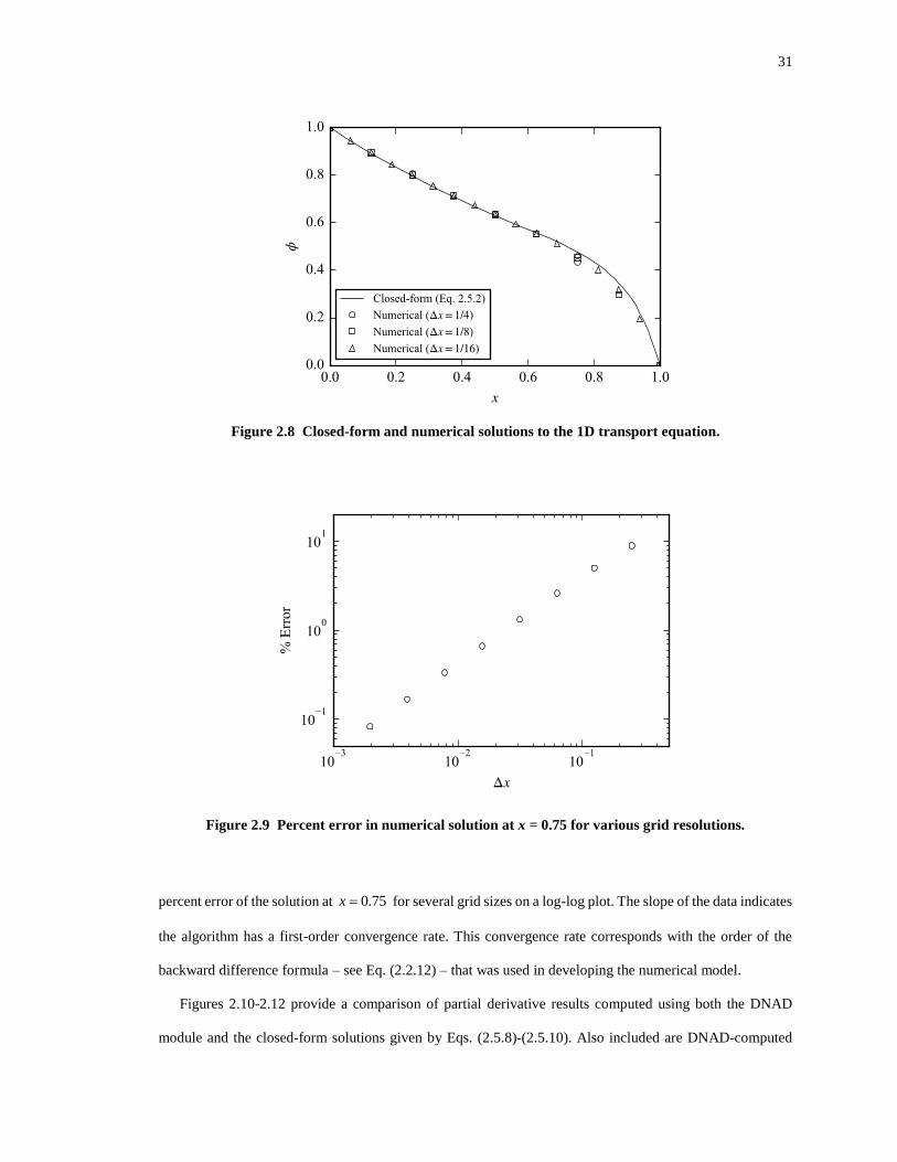
31

Figure 2.8 Closed-form and numerical solutions to the 1D transport equation.

Figure 2.9 Percent error in numerical solution at x = 0.75 for various grid resolutions.

percent error of the solution at 0.75x = for several grid sizes on a log-log plot. The slope of the data indicates

the algorithm has a first-order convergence rate. This convergence rate corresponds with the order of the

backward difference formula – see Eq. (2.2.12) – that was used in developing the numerical model.

Figures 2.10-2.12 provide a comparison of partial derivative results computed using both the DNAD

module and the closed-form solutions given by Eqs. (2.5.8)-(2.5.10). Also included are DNAD-computed

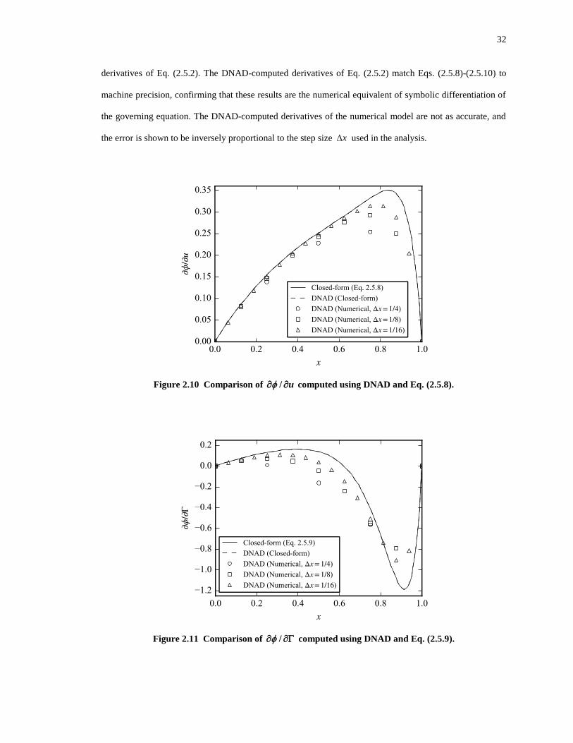
32

derivatives of Eq. (2.5.2). The DNAD-computed derivatives of Eq. (2.5.2) match Eqs. (2.5.8)-(2.5.10) to

machine precision, confirming that these results are the numerical equivalent of symbolic differentiation of

the governing equation. The DNAD-computed derivatives of the numerical model are not as accurate, and

the error is shown to be inversely proportional to the step size x used in the analysis.

Figure 2.10 Comparison of / u computed using DNAD and Eq. (2.5.8).

Figure 2.11 Comparison of / computed using DNAD and Eq. (2.5.9).

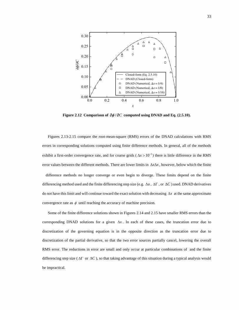
33

Figure 2.12 Comparison of C/ computed using DNAD and Eq. (2.5.10).

Figures 2.13-2.15 compare the root-mean-square (RMS) errors of the DNAD calculations with RMS

errors in corresponding solutions computed using finite difference methods. In general, all of the methods

exhibit a first-order convergence rate, and for coarse grids (210x − ) there is little difference in the RMS

error values between the different methods. There are lower limits in x x , however, below which the finite

difference methods no longer converge or even begin to diverge. These limits depend on the finite

differencing method used and the finite differencing step size (e.g. u , , or C ) used. DNAD derivatives

do not have this limit and will continue toward the exact solution with decreasing x at the same approximate

convergence rate as until reaching the accuracy of machine precision.

Some of the finite difference solutions shown in Figures 2.14 and 2.15 have smaller RMS errors than the

corresponding DNAD solutions for a given x . In each of these cases, the truncation error due to

discretization of the governing equation is in the opposite direction as the truncation error due to

discretization of the partial derivative, so that the two error sources partially cancel, lowering the overall

RMS error. The reductions in error are small and only occur at particular combinations of and the finite

differencing step size ( or C ), so that taking advantage of this situation during a typical analysis would

be impractical.

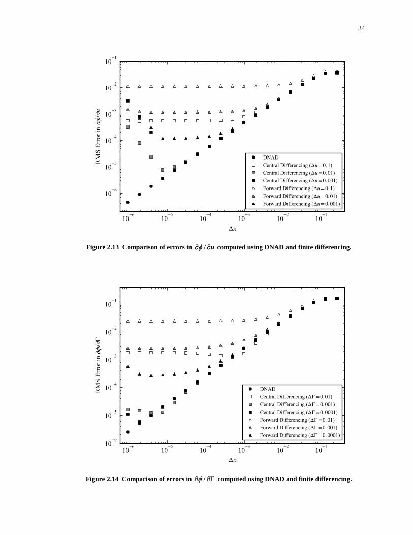
34

Figure 2.13 Comparison of errors in / u computed using DNAD and finite differencing.

Figure 2.14 Comparison of errors in / computed using DNAD and finite differencing.

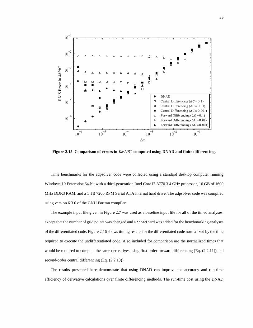
35

Figure 2.15 Comparison of errors in / C computed using DNAD and finite differencing.

Time benchmarks for the adpsolver code were collected using a standard desktop computer running

Windows 10 Enterprise 64-bit with a third-generation Intel Core i7-3770 3.4 GHz processor, 16 GB of 1600

MHz DDR3 RAM, and a 1 TB 7200 RPM Serial ATA internal hard drive. The adpsolver code was compiled

using version 6.3.0 of the GNU Fortran compiler.

The example input file given in Figure 2.7 was used as a baseline input file for all of the timed analyses,

except that the number of grid points was changed and a *dnad card was added for the benchmarking analyses

of the differentiated code. Figure 2.16 shows timing results for the differentiated code normalized by the time

required to execute the undifferentiated code. Also included for comparison are the normalized times that

would be required to compute the same derivatives using first-order forward differencing (Eq. (2.2.11)) and

second-order central differencing (Eq. (2.2.13)).

The results presented here demonstrate that using DNAD can improve the accuracy and run-time

efficiency of derivative calculations over finite differencing methods. The run-time cost using the DNAD

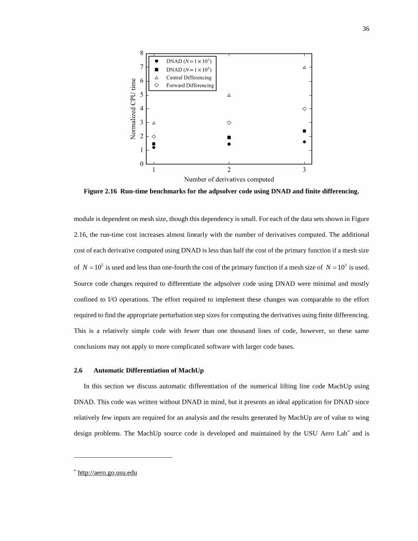
36

Figure 2.16 Run-time benchmarks for the adpsolver code using DNAD and finite differencing.

module is dependent on mesh size, though this dependency is small. For each of the data sets shown in Figure

2.16, the run-time cost increases almost linearly with the number of derivatives computed. The additional

cost of each derivative computed using DNAD is less than half the cost of the primary function if a mesh size

of 510N = is used and less than one-fourth the cost of the primary function if a mesh size of

310N = is used.

Source code changes required to differentiate the adpsolver code using DNAD were minimal and mostly

confined to I/O operations. The effort required to implement these changes was comparable to the effort

required to find the appropriate perturbation step sizes for computing the derivatives using finite differencing.

This is a relatively simple code with fewer than one thousand lines of code, however, so these same

conclusions may not apply to more complicated software with larger code bases.

2.6 Automatic Differentiation of MachUp

In this section we discuss automatic differentiation of the numerical lifting line code MachUp using

DNAD. This code was written without DNAD in mind, but it presents an ideal application for DNAD since

relatively few inputs are required for an analysis and the results generated by MachUp are of value to wing

design problems. The MachUp source code is developed and maintained by the USU Aero Lab* and is

* http://aero.go.usu.edu

http://aero.go.usu.edu/

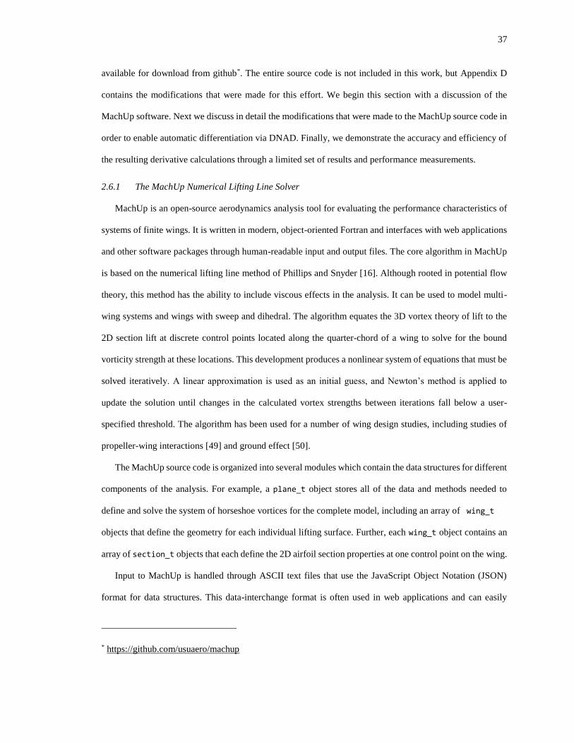
37

available for download from github*. The entire source code is not included in this work, but Appendix D

contains the modifications that were made for this effort. We begin this section with a discussion of the

MachUp software. Next we discuss in detail the modifications that were made to the MachUp source code in

order to enable automatic differentiation via DNAD. Finally, we demonstrate the accuracy and efficiency of

the resulting derivative calculations through a limited set of results and performance measurements.

2.6.1 The MachUp Numerical Lifting Line Solver

MachUp is an open-source aerodynamics analysis tool for evaluating the performance characteristics of

systems of finite wings. It is written in modern, object-oriented Fortran and interfaces with web applications

and other software packages through human-readable input and output files. The core algorithm in MachUp

is based on the numerical lifting line method of Phillips and Snyder [16]. Although rooted in potential flow

theory, this method has the ability to include viscous effects in the analysis. It can be used to model multi-

wing systems and wings with sweep and dihedral. The algorithm equates the 3D vortex theory of lift to the

2D section lift at discrete control points located along the quarter-chord of a wing to solve for the bound

vorticity strength at these locations. This development produces a nonlinear system of equations that must be

solved iteratively. A linear approximation is used as an initial guess, and Newton’s method is applied to

update the solution until changes in the calculated vortex strengths between iterations fall below a user-

specified threshold. The algorithm has been used for a number of wing design studies, including studies of

propeller-wing interactions [49] and ground effect [50].

The MachUp source code is organized into several modules which contain the data structures for different

components of the analysis. For example, a plane_t object stores all of the data and methods needed to

define and solve the system of horseshoe vortices for the complete model, including an array of wing_t

objects that define the geometry for each individual lifting surface. Further, each wing_t object contains an

array of section_t objects that each define the 2D airfoil section properties at one control point on the wing.

Input to MachUp is handled through ASCII text files that use the JavaScript Object Notation (JSON)

format for data structures. This data-interchange format is often used in web applications and can easily

* https://github.com/usuaero/machup

https://github.com/usuaero/machup

38

interface with other common engineering tools such as Matlab and Python. In addition, these input files are

human-readable and can be created and edited in any standard text editor. The JSON data structures are

handled within MachUp through an open-source JSON parsing tool available on Github* and also included

within the MachUp source code. A sample MachUp input file is shown in Appendix E. The input file defines

a single wing with an aspect ratio of 8; an elliptic chord distribution; no sweep, dihedral, or geometric twist;

and a uniform cross-section with properties corresponding approximately to those of a NACA 2412 airfoil

in inviscid, incompressible flow. The airfoil properties and profile are defined in separate files that reside

within the specified airfoil database folder. An example of these property and profile files for the NACA

2412 airfoil is given in Appendix E.

Commands to be executed are specified under the “run” record in the JSON input file. The example file

in Appendix E lists multiple commands, all of which can be performed with a single execution of the

software. The first command, “targetcl”, solves the complete lifting line algorithm multiple times using

Newton’s method to adjust the angle of attack until the specified lift coefficient is achieved. The “forces”

command generates a JSON output file that contains the aerodynamic performance coefficients calculated

by the lifting line algorithm. The “distributions” command generates a comma-separated values (CSV)

file that contains aerodynamic results for each wing section in the model. Finally, the “stl” command

generates a stereolithography (STL) file that contains a geometric representation of the model for

visualization. Note that any of the “run” commands listed can be temporarily disabled by setting the “run”

parameter for that command to 0.

Viscous effects can be included in a MachUp analysis by specifying viscous properties for the 2D airfoils

used in the analysis. For example, a 2D potential flow solution for flow around a NACA 2412 airfoil gives a

zero-lift angle of attack of approximately 0 0.0380 radL = − and a section lift slope of approximately

0 6.86 / rada = , but 2D viscous flow solutions give somewhat different values. XFOIL (see Refs. [51,52])

predicts a zero-lift angle of attack of approximately 0 0.0372 radL = − and a section lift slope of

approximately 0 6.26 / rada = for a NACA 2412 airfoil in viscous flow at a Reynolds number of Re 1E6= .

* https://github.com/jacobwilliams/json-fortran

39

Similarly, the zero-lift moment coefficient and moment slope of an airfoil will also be different between

inviscid and viscous flows and, for viscous flows, will depend on Reynolds number. Section parasitic drag

is estimated in MachUp using the relation

0 1 2

2

pd d d l d lc c c c c c= + + (2.6.1)

where the coefficients 0dc ,

1dc , and 2dc must be determined using a viscous analysis tool such as XFOIL or

from experimental data. These coefficients are identically zero by definition for inviscid flows. MachUp

sums the individual section parasitic drag components computed from Eq. (2.6.1) about the aircraft center of

gravity to evaluate global viscous forces and moments as described by Phillips [53].

The example input file in Appendix E contains other parameters not discussed here, and still other

parameters are supported by MachUp that have not been included in the example. A comprehensive

description of each available parameter is beyond the scope of this work. The reader is instead referred to the

MachUp documentation and source code available on Github.

2.6.2 Modifications to the MachUp Source Code

The original and modified lines of code required for DNAD integration in MachUp have been listed in

Appendix D. Two of the MachUp source files – main.f90 and json.f90 – were left unmodified. A few other

files – airfoil.f90, dataset.f90, and section.f90 – required only the addition of the preprocessor

directives from Figure 2.3.

After adding the preprocessor directives from Figure 2.3, several compiler errors were encountered due

to improper handling of data type conversions between real and type(dual). These compiler errors were

resolved by manually inspecting the source code and ensuring that floating point variables were properly

declared as either real or REAL as discussed in Sec. 2.4.3.

All of the remaining code changes dealt directly with I/O functions of the program. An intermediate layer

between the third-party JSON interface and the computational portion of the MachUp source code already

existed prior to DNAD integration (see myjson.f90), but was not fully implemented. Several lines of code

still called directly into the json_m module, so that variables declared as type(dual) were not properly

processed. These errors were resolved by completing the implementation of the myjson_m module and adding

some additional functions specifically for handling variables of type(dual). The preprocessor directive for

40

converting all real variable declarations to type(dual) was not added to the myjson_m module (as was done

with the other modules) so that functions for handling input and output of both data types are included in the

compiled executable. Fortran interfaces were defined at the beginning of the myjson_m module so that the

appropriate I/O function is called based on the type declarations of the arguments passed to the function. As

with other DNAD-specific changes, the functions and interfaces for handling variables of type(dual) were

enclosed in preprocessor directives so that they are only included in the compiled executable when the DNAD

module is activated.

DNAD implementation in the manner described here affords some very significant advantages over other

automatic differentiation methods. Because all JSON-specific I/O operations are processed through the

myjson_m module, no variable-specific code is needed to make a floating-point variable available for

derivative calculations. Instead, derivatives with respect to any floating-point variable contained in the JSON

input file can be computed simply by converting the single value in the JSON input file to a two-value array.

For example, consider again the example JSON input file given in Appendix E. The angle of attack and

sideslip angle are specified under the “condition” keyword:

"condition": { "alpha": 0, "beta": 0 }

Derivatives with respect to angle of attack can be computed simply by replacing the above line with the

following:

"condition": { "alpha": [0, 1], "beta": 0 }

Note, however, that angle of attack is specified in the input file in units of degrees, so that partial derivatives

of output quantities will have units of deg-1. Partial derivatives of lift coefficient, pitching moment coefficient,

and other aerodynamic performance coefficients with respect to angle of attack are typically reported in units

of rad-1. This conversion can be performed after the analysis, but it can be handled more conveniently by

specifying the operating conditions as:

"condition": { "alpha": [0, 57.2957795131], "beta": 0 }

so that, by nature of the chain rule of differentiation, all partial derivatives output by the code will have units

of rad-1.

The JSON output file, written upon successful execution of the MachUp “forces” command, also takes

advantage of the myjson_m module so that partial derivative information is automatically written for all

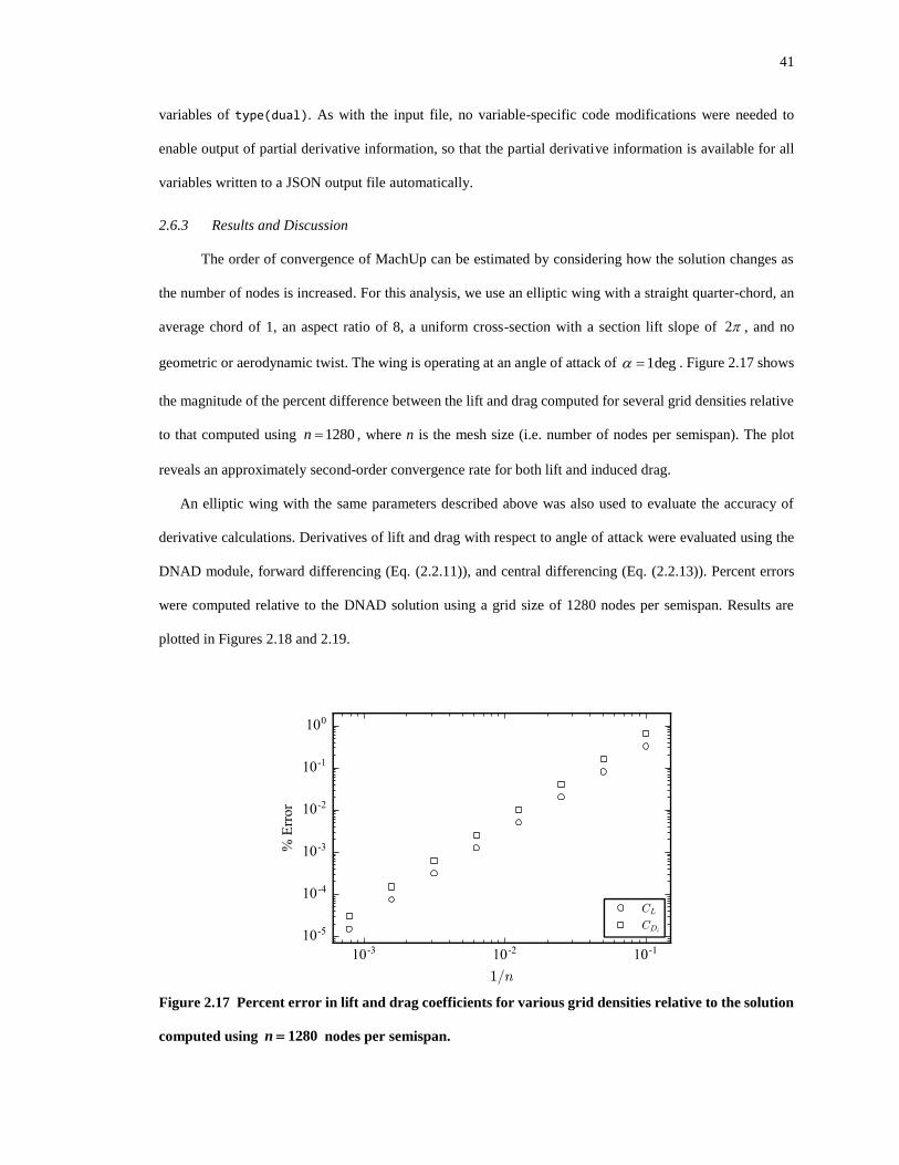
41

variables of type(dual). As with the input file, no variable-specific code modifications were needed to

enable output of partial derivative information, so that the partial derivative information is available for all

variables written to a JSON output file automatically.

2.6.3 Results and Discussion

The order of convergence of MachUp can be estimated by considering how the solution changes as

the number of nodes is increased. For this analysis, we use an elliptic wing with a straight quarter-chord, an

average chord of 1, an aspect ratio of 8, a uniform cross-section with a section lift slope of 2 , and no

geometric or aerodynamic twist. The wing is operating at an angle of attack of 1deg = . Figure 2.17 shows

the magnitude of the percent difference between the lift and drag computed for several grid densities relative

to that computed using 1280n = , where n is the mesh size (i.e. number of nodes per semispan). The plot

reveals an approximately second-order convergence rate for both lift and induced drag.

An elliptic wing with the same parameters described above was also used to evaluate the accuracy of

derivative calculations. Derivatives of lift and drag with respect to angle of attack were evaluated using the

DNAD module, forward differencing (Eq. (2.2.11)), and central differencing (Eq. (2.2.13)). Percent errors

were computed relative to the DNAD solution using a grid size of 1280 nodes per semispan. Results are

plotted in Figures 2.18 and 2.19.

Figure 2.17 Percent error in lift and drag coefficients for various grid densities relative to the solution

computed using 1280n = nodes per semispan.

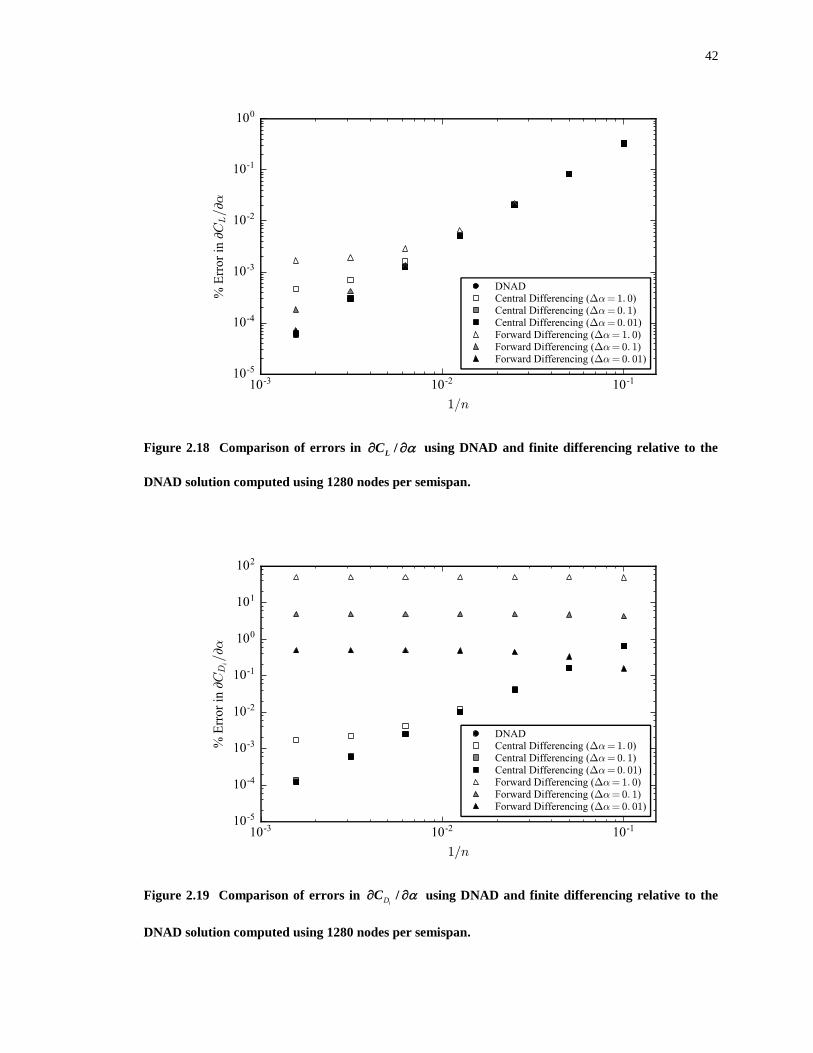
42

Figure 2.18 Comparison of errors in /

LC using DNAD and finite differencing relative to the

DNAD solution computed using 1280 nodes per semispan.

Figure 2.19 Comparison of errors in

iD /C using DNAD and finite differencing relative to the

DNAD solution computed using 1280 nodes per semispan.

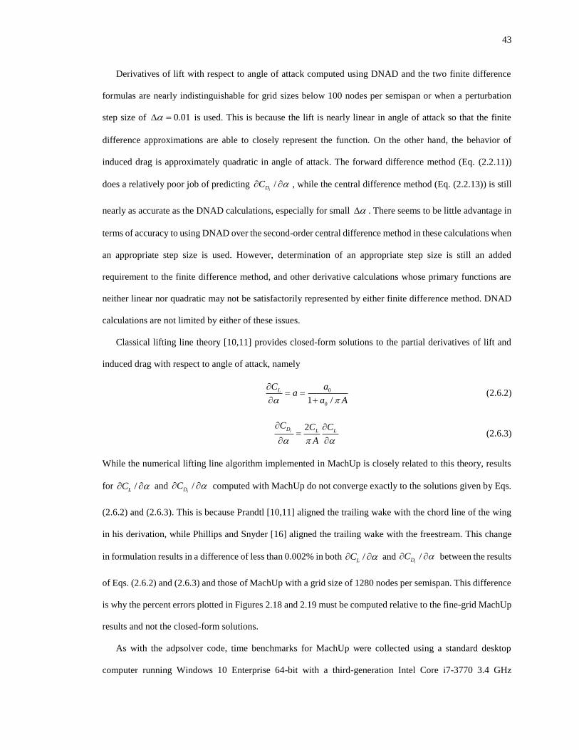
43

Derivatives of lift with respect to angle of attack computed using DNAD and the two finite difference

formulas are nearly indistinguishable for grid sizes below 100 nodes per semispan or when a perturbation

step size of 0.01 = is used. This is because the lift is nearly linear in angle of attack so that the finite

difference approximations are able to closely represent the function. On the other hand, the behavior of

induced drag is approximately quadratic in angle of attack. The forward difference method (Eq. (2.2.11))

does a relatively poor job of predicting /iDC , while the central difference method (Eq. (2.2.13)) is still

nearly as accurate as the DNAD calculations, especially for small . There seems to be little advantage in

terms of accuracy to using DNAD over the second-order central difference method in these calculations when

an appropriate step size is used. However, determination of an appropriate step size is still an added

requirement to the finite difference method, and other derivative calculations whose primary functions are

neither linear nor quadratic may not be satisfactorily represented by either finite difference method. DNAD

calculations are not limited by either of these issues.

Classical lifting line theory [10,11] provides closed-form solutions to the partial derivatives of lift and

induced drag with respect to angle of attack, namely

0

01 /

LaC

aa A

= =

+ (2.6.2)

2

iD L LC C C

A

=

(2.6.3)

While the numerical lifting line algorithm implemented in MachUp is closely related to this theory, results

for /LC and /iDC computed with MachUp do not converge exactly to the solutions given by Eqs.

(2.6.2) and (2.6.3). This is because Prandtl [10,11] aligned the trailing wake with the chord line of the wing

in his derivation, while Phillips and Snyder [16] aligned the trailing wake with the freestream. This change

in formulation results in a difference of less than 0.002% in both /LC and /iDC between the results

of Eqs. (2.6.2) and (2.6.3) and those of MachUp with a grid size of 1280 nodes per semispan. This difference

is why the percent errors plotted in Figures 2.18 and 2.19 must be computed relative to the fine-grid MachUp

results and not the closed-form solutions.

As with the adpsolver code, time benchmarks for MachUp were collected using a standard desktop

computer running Windows 10 Enterprise 64-bit with a third-generation Intel Core i7-3770 3.4 GHz

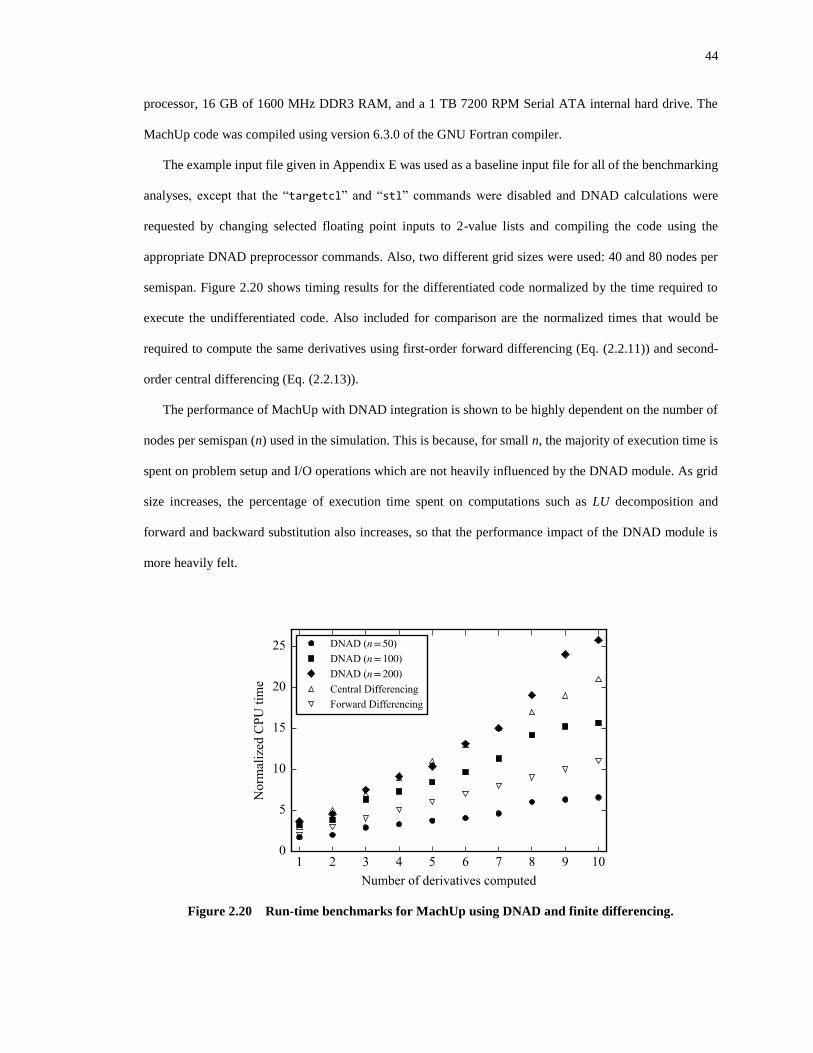
44

processor, 16 GB of 1600 MHz DDR3 RAM, and a 1 TB 7200 RPM Serial ATA internal hard drive. The

MachUp code was compiled using version 6.3.0 of the GNU Fortran compiler.

The example input file given in Appendix E was used as a baseline input file for all of the benchmarking

analyses, except that the “targetcl” and “stl” commands were disabled and DNAD calculations were

requested by changing selected floating point inputs to 2-value lists and compiling the code using the

appropriate DNAD preprocessor commands. Also, two different grid sizes were used: 40 and 80 nodes per

semispan. Figure 2.20 shows timing results for the differentiated code normalized by the time required to

execute the undifferentiated code. Also included for comparison are the normalized times that would be

required to compute the same derivatives using first-order forward differencing (Eq. (2.2.11)) and second-

order central differencing (Eq. (2.2.13)).

The performance of MachUp with DNAD integration is shown to be highly dependent on the number of

nodes per semispan (n) used in the simulation. This is because, for small n, the majority of execution time is

spent on problem setup and I/O operations which are not heavily influenced by the DNAD module. As grid

size increases, the percentage of execution time spent on computations such as LU decomposition and

forward and backward substitution also increases, so that the performance impact of the DNAD module is

more heavily felt.

Figure 2.20 Run-time benchmarks for MachUp using DNAD and finite differencing.

45

We note disproportionately large increases in the DNAD execution times shown in Figure 2.20 when

going from 2 derivatives to 3 and from 7 to 8. This has been attributed to single instruction, multiple data

(SIMD) vectorization capabilities of the hardware. Vectorization extensions such as Streaming SIMD

Extensions (SSE) and Advanced Vector Extensions (AVX) use SIMD registers to process a single instruction

on multiple data more efficiently than if the instruction was processed on each piece of data individually. The

size of the SIMD registers sets limitations on how many pieces of data can be processed with a single

vectorized instruction, so that behavior such as that seen in Figure 2.20 when going from 2 derivatives to 3

and from 7 to 8 is expected.

As a result of the above observations, the answer to whether DNAD calculations are more advantageous

than finite difference methods depends on the size of the model and the purpose of the analysis. If the entire

model has fewer than 400 nodes and fewer than 8 design variables for which derivatives are required, DNAD

presents an appealing solution in terms of both runtime efficiency and accuracy. For larger models and

problem setups with 8 or more design variables, the finite differencing approach may be satisfactory. For

problems with less than 400 nodes and 8 or more design variables, a reverse-mode AD method may be the

most efficient option, but integration of a reverse-mode AD tool and verification of this is beyond the scope

of the current work.

46

3 WING SHAPE OPTIMIZATION USING A NUMERICAL LIFTING LINE ALGORITHM AND

DUAL NUMBER AUTOMATIC DIFFERENTIATION

3.1 Introduction

Aerodynamic shape optimization is the process of designing the outer mold line (OML) of an

aerodynamic structure such that specific aerodynamic performance requirements are met in the most efficient

manner possible. As mentioned in Chapter 1, CFD analyses can be used to generate high-fidelity aerodynamic

performance predictions, but the computational cost of CFD makes it ill-suited for use as the objective

function in aerodynamic shape optimization problems. Lyu et al. [4] states that visualization of design spaces

for these types of problems is not possible with current CFD capabilities and hardware limitations. This leads

aerodynamicists to consider lower-fidelity aerodynamic tools that trade accuracy for runtime efficiency. This

approach can be especially useful early in the design process when insights into trends and interactions

between design parameters are more important than highly-accurate performance characteristics.

One such tool is MachUp, an implementation of the numerical lifting line method of Phillips and Snyder

[16]. This tool was discussed in Sec. 2.6, where a method for automatic differentiation of the software was

presented. In this chapter, we discuss the use of MachUp as the objective function in an aerodynamic shape

optimization problem. Note that the modified version of MachUp discussed in Sec. 2.6, which uses DNAD

for derivative calculations, is used here. We first present Optix, an open-source optimization framework

being developed in the Utah State University AeroLab and available through the groups Github page*. The

version of the code considered in this work is included in Appendix F. We then present solutions to several

inviscid wing shape optimization problems that were computed using MachUp and Optix, and compare the

results to known analytical solutions developed using classical lifting line theory [10,11]. Similar wing shape

optimization problems using viscous airfoil properties are then presented. Finally, we present and discuss a

wing design contour plot that was generated using MachUp and serves to visualize the complete design space

for the viscous wing shape optimization problems discussed previously.

* https://github.com/usuaero/optix

https://github.com/usuaero/optix

47

3.2 Optix

Optix is an open-source, gradient-based optimization framework written in Python. It has the capability

of solving a wide range of nonlinear optimization problems and offers some unique features that set it apart

from similar optimization frameworks. Because Optix is written entirely in Python, it is easy to interface with

and can readily be extended and customized to fit a particular problem. Optix is also cross-platform and

highly portable. It can be run on any machine where Python is available, and NumPy (see Oliphant [54]) is

the only package dependency outside of the Python Standard Library. Any combination of software available

on the host machine can be executed within the objective function, so that the objective function – typically

the most computationally expensive part of an optimization analysis – can be written in a high-performance

computing language such as Fortran or C++. The following subsections highlight the key features of Optix.

3.2.1 Optimization Method

Optix implements the BFGS method of Broyden [55], Fletcher [56], Goldfarb [57], and Shanno [58]. This

is a quasi-Newton method that uses historical calculations of the objective function and its gradient to

approximate a Hessian matrix, which in turn is used to estimate a search direction. According to Nocedal and

Wright [59] the BFGS method is among the most popular quasi-Newton methods. It has been implemented

in several scientific computing packages that offer gradient-based optimization utilities, including the GNU

Scientific Library, MATLAB, R, and SciPy.

At the beginning of the BFGS algorithm, the objective function and its gradient at the initial design point

are calculated and the Hessian matrix is initialized to the identity matrix (i.e. 0[ ] [ ]=H I ) so that the first

search direction corresponds to the direction of steepest descent. A line search is then performed to find the

local minimum in the search direction. The design point is then updated to this location, and a new gradient

vector is calculated. The BFGS algorithm then determines an updated Hessian matrix 1[ ]k+H from the

previous Hessian matrix [ ]kH according to

( )

1}

1 { { { [ ]{ }[ ] } } }[ ][

} }} }

{ }{ } { }{ { }{

{ {{ {]

}] [

TT TT

kk k

k k T T T+

+ += −

+

γ H γ δx γ H γ δxδx δx

δx γ δx γ δxH

γ

HH (3.2.1)

where

1{ { }} { }k k+= −x x xδ (3.2.2)

48

1{ } }{{ }k k+= −γ f f (3.2.3)

are the changes in the design point and gradient vector, respectively, between the current and previous

iterations. The direction of the next line search is then given by

1 1 }{ } [ ] {k k+ += −s H f (3.2.4)

This algorithm is repeated until either of two exit criteria are met: 1) the curvature condition proposed by

Wolfe [60,61] is no longer satisfied, or 2) the change in the objective function between iterations falls below

a user-specified threshold. Once one of these conditions is satisfied, the Hessian matrix is reset to the identity

matrix, and the entire process begins again using the last minimum as the initial design point. The

optimization process is complete when one of the two exit criteria are met on an iteration where the Hessian

matrix is equal to the identity matrix. The current value of the objective function and the corresponding

design point are then returned to the calling function as the final results of the optimization process.

3.2.2 Code Structure

Optix is composed of two object classes and several utility functions. The source code for these classes

and functions are listed in Appendix F. The first object class handles execution of the user-specified objective

function. The objective function is a Python function provided by the user that must accept as arguments the

current design point and a case identifier, and it must return the value of the objective function evaluated at

the current design point. A second function can be provided to evaluate gradients of the objective function,

but this is not required. If specified, the gradient function must accept the same arguments as the objective

function. It must return both the value of the objective function and the gradient vector at the specified design

point. If this function is not specified, Optix evaluates the primary objective function multiple times with

perturbed design points and uses a second-order central differencing algorithm – see Eq. (2.2.13) – to

approximate the gradient of the objective function.

The second object class contained in the Optix source code is used for controlling the optimization

algorithm. The number of design variables, their names, and their initial values are specified through an

instance of this class. In addition, line search settings, parameters for the exit criteria, and whether to use the

linear or quadratic line search algorithms (explained later in Sec. 3.2.4) are set here. A helper function is also

provided through which the user can specify a JSON file from which to load these optimizer settings.

49

The optimize function orchestrates the entire optimization process. It accepts one instance each of the

two object classes described above and returns the optimized objective function value and corresponding

design point upon completion. The optimize function relies on the Python NumPy package for efficient

matrix computations.

3.2.3 Parallel Execution of Independent Function Evaluations

Optix uses the multiprocessing module (part of the Standard Python Library) to execute independent

evaluations of the objective function simultaneously. For example, each function evaluation within the line

search is independent of all other line search evaluations, so the separate function evaluations can be divided

among available processors and run simultaneously. In addition, if finite differencing is used to approximate

the gradient vector, these function evaluations can also be executed in parallel. One gradient evaluation using

the second-order central differencing formula given in Eq. (2.2.13) requires 2 1N + function evaluations,

where N is the number of active design variables in the optimization analysis. Running these evaluations in

parallel can significantly reduce the total optimization time when even just a few design variables are active.

3.2.4 Linear and Quadratic Line Searching

As mentioned previously, Optix relies on line searching methods to locate the local minimum in a given

search direction. Two types of line searching algorithms exist in the literature, namely exact and inexact

methods. Exact methods typically require some a priori knowledge of the design space to be searched and

are restricted in application to only specific problem types. For example, the conjugate gradient method of

Hestenes and Stiefel [62] requires the design space to be composed of a system of linear equations whose

matrix is symmetric and positive-definite. While exact line searching algorithms are typically quite efficient

when applied to the correct types of problems, restrictions to specific problem types make them ill-suited for

a general optimization framework such as Optix.

Inexact line searching algorithms use approximation methods to estimate the minimum in a given search

direction, and then rely on the optimization algorithm to narrow in on the design space minimum through

successive updates to the gradient vector and Hessian matrix. Two popular inexact algorithms are the

backtracking algorithms of Goldstein [63] and Armijo [64], which attempt to overshoot the minimum of the

objective function and then successively reduce the step size until the minimum is sufficiently bounded.

50

Optix provides two backtracking algorithms of relative simplicity: a linear and a quadratic algorithm. The

linear algorithm evaluates the objective function at multiple design points in the search direction. Evaluations

continue at increasingly larger distances from the initial design point until an increase in the objective

function is obtained, at which point the algorithm fits a parabola through the last three design points

evaluated. The next design point is placed at the parabola’s vertex.

The quadratic algorithm evaluates the objective function at a user-specified number of equally-spaced

design points along the search direction and fits a parabola to the results. If the minimum of the parabola is

within a user-specified threshold of any one of the design points evaluated, or if a minimum does not exist

(i.e. the parabola reduces to a straight line or is concave), the design point corresponding to the minimum

objective function value is returned to the BFGS algorithm. If neither of these conditions are met, a new set

of design points is selected with one of them located at the parabola’s vertex, and the objective function is

reevaluated at these new locations. For convex problems, the quadratic line searching algorithm can

significantly reduce the total optimization time from that required for the linear algorithm.

3.2.5 Limitations

One limitation of Optix over other similar optimization frameworks is the lack of built-in methods for

applying bounds and constraints. Constraints can still be enforced using penalty function methods (for

example, see Smith and Coit [65]), but more efficient and robust methods exist. Some example methods

include the method of Lagrange multipliers for problems having only equality constraints, the simplex

method for linear programming problems, and the ellipsoid method for quadratic programming problems.

Explanations of these methods can be found in any introductory textbook on gradient-based optimization (for

example, see Griva et al. [66]). However, it should be noted that each method is only suited to a specific

subset of constrained optimization problems, whereas the penalty function method can be applied universally

to all constrained optimization problems.

Another limitation of Optix is its inability to distinguish between local minima and the global minimum

of a design space. For optimization problems that involve complex design spaces with multiple local minima,

results returned by Optix may depend on the initial design point provided to the optimizer. This is a common

shortfall of gradient-based optimization methods, but there are some algorithms – e.g. the conservative

convex separable approximation (CCSA) methods presented by Svanberg [67] – that have overcome this

51

limitation. Locatelli and Schoen [68] present a thorough overview of globally-convergent optimization

methods. The BFGS method implemented in Optix is not globally convergent. However, a simple design of

experiments (DOE) approach can be used to improve the likelihood of finding the global minimum of a

design space. The DOE approach systematically selects multiple design points distributed throughout the

design space and uses each point to initiate a complete gradient-based optimization analysis. The collective

results from this set of analyses does not guarantee discovery of the global minimum within the design space

but simply improves the likelihood of finding it. The level of complexity of the design space will determine

the number of simulations needed to provide adequate coverage of the design space. The computational cost

of this approach can be significant since each analysis is a full optimization analysis, but the separate analyses

are completely independent and can be run simultaneously given adequate computational resources. In the

sample analyses that follow, the objective functions are convex so the locally-convergent BFGS method is

satisfactory for this work.

3.3 Wing Shape Optimization in Inviscid Flow

Optix and MachUp have been used to solve several wing shape optimization problems for which closed-

form solutions are available. Results from these simulations are presented and discussed here. Each

simulation began with the same initial wing model – namely a spanwise-symmetric, untwisted, rectangular

wing with an aspect ratio of 8A = and a section lift slope of 1

0 6.8806rada −= – operating at a wing lift

coefficient of 0.5LC = . Control points (locations where the optimizer is allowed to vary geometric and

aerodynamic properties of the wing) were spaced uniformly along one semispan of the wing. The other

semispan was automatically updated so that the wing remained symmetric. All simulations used a grid density

of 100 nodes per semispan. The main MachUp input file and Python code used for these simulations are

given in Appendix G.

The aerodynamic properties of the airfoils used in these analyses are shown in Table 3.1 and correspond

to the NACA 4-digit X412 family of airfoils with percent maximum cambers, maxcz , ranging from 0% to 8%.

The data were generated using an inviscid panel code. The induced drag for the initial rectangular model at

a lift coefficient of 0.5LC = was calculated to be 21.05 4 105

iDC −= .

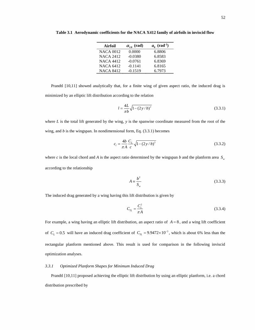
52

Table 3.1 Aerodynamic coefficients for the NACA X412 family of airfoils in inviscid flow

Airfoil 0L (rad)

0a (rad-1)

NACA 0012 0.0000 6.8806

NACA 2412 -0.0380 6.8583

NACA 4412 -0.0761 6.8369

NACA 6412 -0.1141 6.8165

NACA 8412 -0.1519 6.7973

Prandtl [10,11] showed analytically that, for a finite wing of given aspect ratio, the induced drag is

minimized by an elliptic lift distribution according to the relation

241 (2 / )l

Ly b

b= − (3.3.1)

where L is the total lift generated by the wing, y is the spanwise coordinate measured from the root of the

wing, and b is the wingspan. In nondimensional form, Eq. (3.3.1) becomes

241 (2 / )L

l

Cby b

A cc

−= (3.3.2)

where c is the local chord and A is the aspect ratio determined by the wingspan b and the planform area wS

according to the relationship

2

w

Ab

S (3.3.3)

The induced drag generated by a wing having this lift distribution is given by

2

i

L

D

C

AC

= (3.3.4)

For example, a wing having an elliptic lift distribution, an aspect ratio of 8A = , and a wing lift coefficient

of 0.5LC = will have an induced drag coefficient of 39.9472 10

iDC −= , which is about 6% less than the

rectangular planform mentioned above. This result is used for comparison in the following inviscid

optimization analyses.

3.3.1 Optimized Planform Shapes for Minimum Induced Drag

Prandtl [10,11] proposed achieving the elliptic lift distribution by using an elliptic planform, i.e. a chord

distribution prescribed by

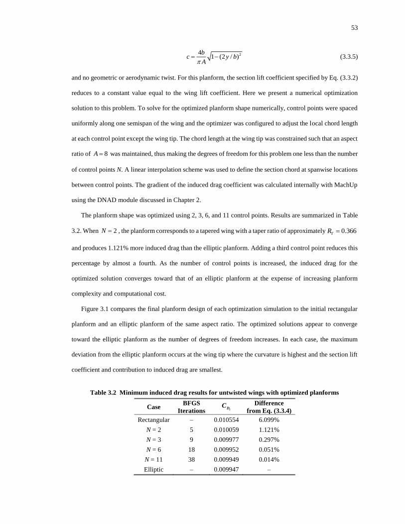
53

241 (2 / )c

by b

A= − (3.3.5)

and no geometric or aerodynamic twist. For this planform, the section lift coefficient specified by Eq. (3.3.2)

reduces to a constant value equal to the wing lift coefficient. Here we present a numerical optimization

solution to this problem. To solve for the optimized planform shape numerically, control points were spaced

uniformly along one semispan of the wing and the optimizer was configured to adjust the local chord length

at each control point except the wing tip. The chord length at the wing tip was constrained such that an aspect

ratio of 8A = was maintained, thus making the degrees of freedom for this problem one less than the number

of control points N. A linear interpolation scheme was used to define the section chord at spanwise locations

between control points. The gradient of the induced drag coefficient was calculated internally with MachUp

using the DNAD module discussed in Chapter 2.

The planform shape was optimized using 2, 3, 6, and 11 control points. Results are summarized in Table

3.2. When 2N = , the planform corresponds to a tapered wing with a taper ratio of approximately 0.366TR =

and produces 1.121% more induced drag than the elliptic planform. Adding a third control point reduces this

percentage by almost a fourth. As the number of control points is increased, the induced drag for the

optimized solution converges toward that of an elliptic planform at the expense of increasing planform

complexity and computational cost.

Figure 3.1 compares the final planform design of each optimization simulation to the initial rectangular

planform and an elliptic planform of the same aspect ratio. The optimized solutions appear to converge

toward the elliptic planform as the number of degrees of freedom increases. In each case, the maximum

deviation from the elliptic planform occurs at the wing tip where the curvature is highest and the section lift

coefficient and contribution to induced drag are smallest.

Table 3.2 Minimum induced drag results for untwisted wings with optimized planforms

Case BFGS

Iterations iDC Difference

from Eq. (3.3.4)

Rectangular – 0.010554 6.099%

N = 2 5 0.010059 1.121%

N = 3 9 0.009977 0.297%

N = 6 18 0.009952 0.051%

N = 11 38 0.009949 0.014%

Elliptic – 0.009947 –

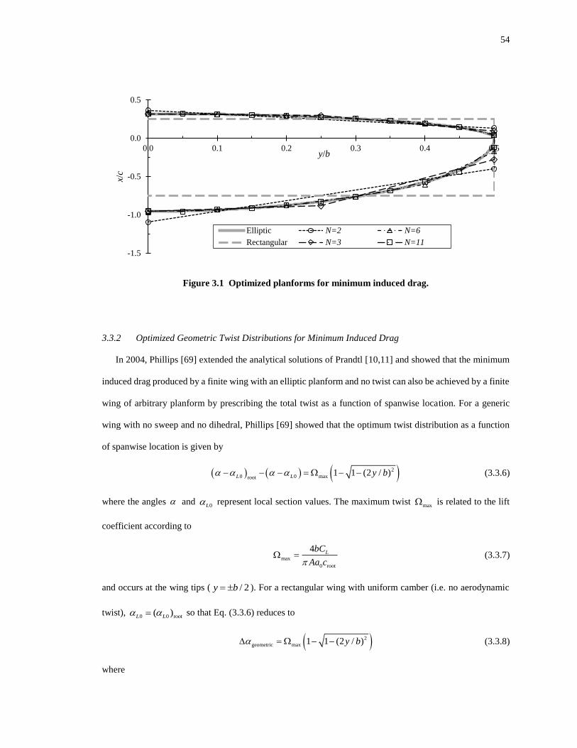
54

Figure 3.1 Optimized planforms for minimum induced drag.

3.3.2 Optimized Geometric Twist Distributions for Minimum Induced Drag

In 2004, Phillips [69] extended the analytical solutions of Prandtl [10,11] and showed that the minimum

induced drag produced by a finite wing with an elliptic planform and no twist can also be achieved by a finite

wing of arbitrary planform by prescribing the total twist as a function of spanwise location. For a generic

wing with no sweep and no dihedral, Phillips [69] showed that the optimum twist distribution as a function

of spanwise location is given by

( ) ( ) ( )2

0 0 maxroot1 1 (2 / )L L y b − =− − −− (3.3.6)

where the angles and 0L represent local section values. The maximum twist

max is related to the lift

coefficient according to

max

0 root

4 LbC

Aa c= (3.3.7)

and occurs at the wing tips ( / 2y b= ). For a rectangular wing with uniform camber (i.e. no aerodynamic

twist), 0 0 root( )L L = so that Eq. (3.3.6) reduces to

( )2

geometric max (1 1 2 / )y b −= − (3.3.8)

where

-1.5

-1.0

-0.5

0.0

0.5

0.0 0.1 0.2 0.3 0.4 0.5

x/c

y/b

Elliptic N=2 N=6

Rectangular N=3 N=11

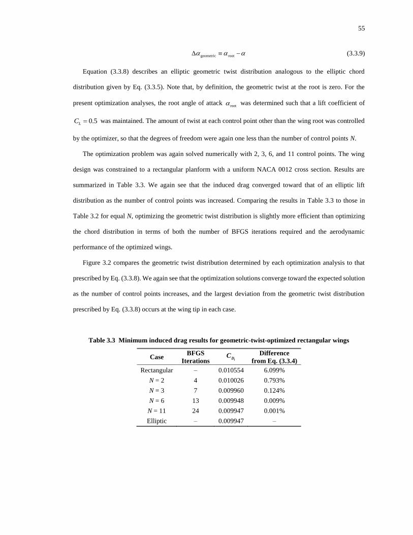
55

geometric root − (3.3.9)

Equation (3.3.8) describes an elliptic geometric twist distribution analogous to the elliptic chord

distribution given by Eq. (3.3.5). Note that, by definition, the geometric twist at the root is zero. For the

present optimization analyses, the root angle of attack root was determined such that a lift coefficient of

0.5LC = was maintained. The amount of twist at each control point other than the wing root was controlled

by the optimizer, so that the degrees of freedom were again one less than the number of control points N.

The optimization problem was again solved numerically with 2, 3, 6, and 11 control points. The wing

design was constrained to a rectangular planform with a uniform NACA 0012 cross section. Results are

summarized in Table 3.3. We again see that the induced drag converged toward that of an elliptic lift

distribution as the number of control points was increased. Comparing the results in Table 3.3 to those in

Table 3.2 for equal N, optimizing the geometric twist distribution is slightly more efficient than optimizing

the chord distribution in terms of both the number of BFGS iterations required and the aerodynamic

performance of the optimized wings.

Figure 3.2 compares the geometric twist distribution determined by each optimization analysis to that

prescribed by Eq. (3.3.8). We again see that the optimization solutions converge toward the expected solution

as the number of control points increases, and the largest deviation from the geometric twist distribution

prescribed by Eq. (3.3.8) occurs at the wing tip in each case.

Table 3.3 Minimum induced drag results for geometric-twist-optimized rectangular wings

Case BFGS

Iterations iDC Difference

from Eq. (3.3.4)

Rectangular – 0.010554 6.099%

N = 2 4 0.010026 0.793%

N = 3 7 0.009960 0.124%

N = 6 13 0.009948 0.009%

N = 11 24 0.009947 0.001%

Elliptic – 0.009947 –

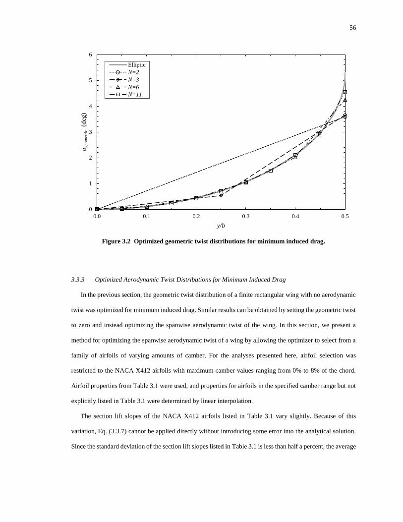
56

Figure 3.2 Optimized geometric twist distributions for minimum induced drag.

3.3.3 Optimized Aerodynamic Twist Distributions for Minimum Induced Drag

In the previous section, the geometric twist distribution of a finite rectangular wing with no aerodynamic

twist was optimized for minimum induced drag. Similar results can be obtained by setting the geometric twist

to zero and instead optimizing the spanwise aerodynamic twist of the wing. In this section, we present a

method for optimizing the spanwise aerodynamic twist of a wing by allowing the optimizer to select from a

family of airfoils of varying amounts of camber. For the analyses presented here, airfoil selection was

restricted to the NACA X412 airfoils with maximum camber values ranging from 0% to 8% of the chord.

Airfoil properties from Table 3.1 were used, and properties for airfoils in the specified camber range but not

explicitly listed in Table 3.1 were determined by linear interpolation.

The section lift slopes of the NACA X412 airfoils listed in Table 3.1 vary slightly. Because of this

variation, Eq. (3.3.7) cannot be applied directly without introducing some error into the analytical solution.

Since the standard deviation of the section lift slopes listed in Table 3.1 is less than half a percent, the average

0

1

2

3

4

5

6

0.0 0.1 0.2 0.3 0.4 0.5

αgeo

met

ric

(deg

)

y/b

Elliptic

N=2

N=3

N=6

N=11

57

section lift slope from this family of airfoils can be used in Eq. (3.3.7) with negligible effect on the results,

and we can use the approximation root in Eq. (3.3.6) such that

( )' 2

aerodynamic max 1 1 (2 / )y b − − (3.3.10)

where

aerodynamic 0 0 root( )L L − (3.3.11)

'

max

0 avg root

4

( )

LbC

A a c = (3.3.12)

and the prime indicates an approximation due to the use of the average section lift slope. Optimization

analyses with families of airfoils having a large standard deviation in section lift slope will not produce an

aerodynamic twist distribution consistent with Eq. (3.3.10). However, the section lift distribution of the final

optimized solution should still be consistent with Eqs. (3.3.1) and (3.3.2).

Because Eq. (3.3.10) specifies only a difference between the section zero-lift angles of attack and does

not specify their absolute magnitude, an additional constraint is needed to isolate a single optimal solution.

In the results that follow, the airfoil section at the wing tip was set to a NACA 2412 airfoil. The optimizer

was configured to control the airfoil definition at all other control points by specifying the percent maximum

camber maxcz , which MachUp then used to determine the airfoil properties at each control point via linear

interpolation of the data in Table 3.1.

The resulting optimal designs for 2, 3, 6, and 11 control points are summarized in Table 3.4. The

corresponding aerodynamic twist distributions are shown in Figure 3.3. Induced drag results are almost

identical to those obtained for optimized geometric twist. The number of BFGS iterations required to obtain

the optimized solutions were also comparable between the two sets of analyses in all cases except N = 11.

For N = 11, about 2.5 times fewer iterations were required to find the optimal geometric twist distribution as

were required to find the optimal aerodynamic twist distribution. This is because the percent maximum

camber value of the third control point from the root was almost exactly 4% in the latter case. Since linear

interpolation is used to determine the airfoil properties, derivatives are discontinuous at the interpolation

nodes. This led to some confusion in the optimization algorithm regarding the appropriate search direction.

58

Table 3.4 Minimum induced drag results for aerodynamic-twist-optimized rectangular wings

Case BFGS

Iterations iDC

Difference

from Eq.

(3.3.4)

Rectangular – 0.010554 6.099%

N = 2 5 0.010026 0.792%

N = 3 7 0.009960 0.124%

N = 6 15 0.009948 0.009%

N = 11 61 0.009947 0.001%

Elliptic – 0.009947 –

Figure 3.3 Optimized aerodynamic twist distributions for minimum induced drag.

3.4 Wing Shape Optimization for Viscous Flow

While the optimization analyses presented in Sec. 3.3 are beneficial from an academic perspective due to

the existence of known closed-form solutions, they have limited practical application due to their neglect of

viscous effects. As described in Sec. 2.6.1, viscous effects can be included within a MachUp analysis by

using viscous airfoil data that includes estimates of the section parasitic drag coefficients 0dc ,

1dc , and 2dc

from Eq. (2.6.1). Estimates of these parasitic drag coefficients, the zero-lift angle of attack, and the section

0

1

2

3

4

5

6

0.0 0.1 0.2 0.3 0.4 0.5

αae

rodynam

ic(d

eg)

y/b

Elliptic

N=2

N=3

N=6

N=11

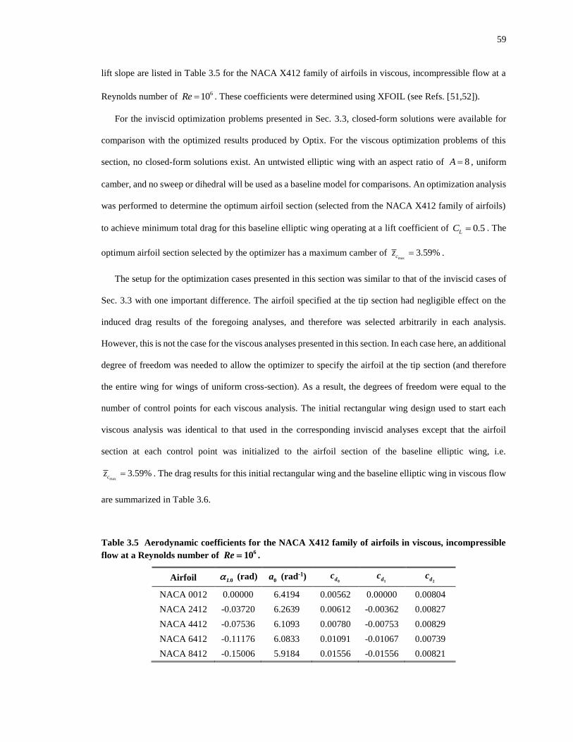
59

lift slope are listed in Table 3.5 for the NACA X412 family of airfoils in viscous, incompressible flow at a

Reynolds number of 610Re = . These coefficients were determined using XFOIL (see Refs. [51,52]).

For the inviscid optimization problems presented in Sec. 3.3, closed-form solutions were available for

comparison with the optimized results produced by Optix. For the viscous optimization problems of this

section, no closed-form solutions exist. An untwisted elliptic wing with an aspect ratio of 8A = , uniform

camber, and no sweep or dihedral will be used as a baseline model for comparisons. An optimization analysis

was performed to determine the optimum airfoil section (selected from the NACA X412 family of airfoils)

to achieve minimum total drag for this baseline elliptic wing operating at a lift coefficient of 0.5LC = . The

optimum airfoil section selected by the optimizer has a maximum camber of max

3.59%cz = .

The setup for the optimization cases presented in this section was similar to that of the inviscid cases of

Sec. 3.3 with one important difference. The airfoil specified at the tip section had negligible effect on the

induced drag results of the foregoing analyses, and therefore was selected arbitrarily in each analysis.

However, this is not the case for the viscous analyses presented in this section. In each case here, an additional

degree of freedom was needed to allow the optimizer to specify the airfoil at the tip section (and therefore

the entire wing for wings of uniform cross-section). As a result, the degrees of freedom were equal to the

number of control points for each viscous analysis. The initial rectangular wing design used to start each

viscous analysis was identical to that used in the corresponding inviscid analyses except that the airfoil

section at each control point was initialized to the airfoil section of the baseline elliptic wing, i.e.

max3.59%cz = . The drag results for this initial rectangular wing and the baseline elliptic wing in viscous flow

are summarized in Table 3.6.

Table 3.5 Aerodynamic coefficients for the NACA X412 family of airfoils in viscous, incompressible

flow at a Reynolds number of 6

10Re = .

Airfoil 0L (rad)

0a (rad-1)

0dc

1dc

2dc

NACA 0012 0.00000 6.4194 0.00562 0.00000 0.00804

NACA 2412 -0.03720 6.2639 0.00612 -0.00362 0.00827

NACA 4412 -0.07536 6.1093 0.00780 -0.00753 0.00829

NACA 6412 -0.11176 6.0833 0.01091 -0.01067 0.00739

NACA 8412 -0.15006 5.9184 0.01556 -0.01556 0.00821

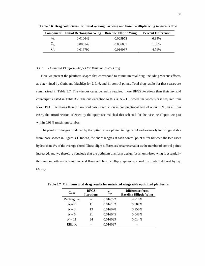
60

Table 3.6 Drag coefficients for initial rectangular wing and baseline elliptic wing in viscous flow.

Component Initial Rectangular Wing Baseline Elliptic Wing Percent Difference

iDC 0.010643 0.009952 6.94%

pDC 0.006149 0.006085 1.06%

DC 0.016792 0.016037 4.71%

3.4.1 Optimized Planform Shapes for Minimum Total Drag

Here we present the planform shapes that correspond to minimum total drag, including viscous effects,

as determined by Optix and MachUp for 2, 3, 6, and 11 control points. Total drag results for these cases are

summarized in Table 3.7. The viscous cases generally required more BFGS iterations than their inviscid

counterparts listed in Table 3.2. The one exception to this is 11N = , where the viscous case required four

fewer BFGS iterations than the inviscid case, a reduction in computational cost of about 10%. In all four

cases, the airfoil section selected by the optimizer matched that selected for the baseline elliptic wing to

within 0.01% maximum camber.

The planform designs produced by the optimizer are plotted in Figure 3.4 and are nearly indistinguishable

from those shown in Figure 3.1. Indeed, the chord lengths at each control point differ between the two cases

by less than 1% of the average chord. These slight differences became smaller as the number of control points

increased, and we therefore conclude that the optimum planform design for an untwisted wing is essentially

the same in both viscous and inviscid flows and has the elliptic spanwise chord distribution defined by Eq.

(3.3.5).

Table 3.7 Minimum total drag results for untwisted wings with optimized planforms.

Case BFGS

Iterations DC

Difference from

Baseline Elliptic Wing

Rectangular – 0.016792 4.710%

N = 2 11 0.016182 0.907%

N = 3 13 0.016078 0.256%

N = 6 21 0.016045 0.048%

N = 11 34 0.016039 0.014%

Elliptic – 0.016037 –

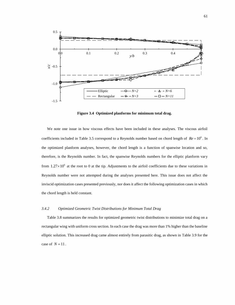
61

Figure 3.4 Optimized planforms for minimum total drag.

We note one issue in how viscous effects have been included in these analyses. The viscous airfoil

coefficients included in Table 3.5 correspond to a Reynolds number based on chord length of 610Re = . In

the optimized planform analyses, however, the chord length is a function of spanwise location and so,

therefore, is the Reynolds number. In fact, the spanwise Reynolds numbers for the elliptic planform vary

from 61.27 10 at the root to 0 at the tip. Adjustments to the airfoil coefficients due to these variations in

Reynolds number were not attempted during the analyses presented here. This issue does not affect the

inviscid optimization cases presented previously, nor does it affect the following optimization cases in which

the chord length is held constant.

3.4.2 Optimized Geometric Twist Distributions for Minimum Total Drag

Table 3.8 summarizes the results for optimized geometric twist distributions to minimize total drag on a

rectangular wing with uniform cross section. In each case the drag was more than 1% higher than the baseline

elliptic solution. This increased drag came almost entirely from parasitic drag, as shown in Table 3.9 for the

case of 11N = .

-1.5

-1.0

-0.5

0.0

0.5

0.0 0.1 0.2 0.3 0.4 0.5

x/c

y/b

Elliptic N=2 N=6

Rectangular N=3 N=11

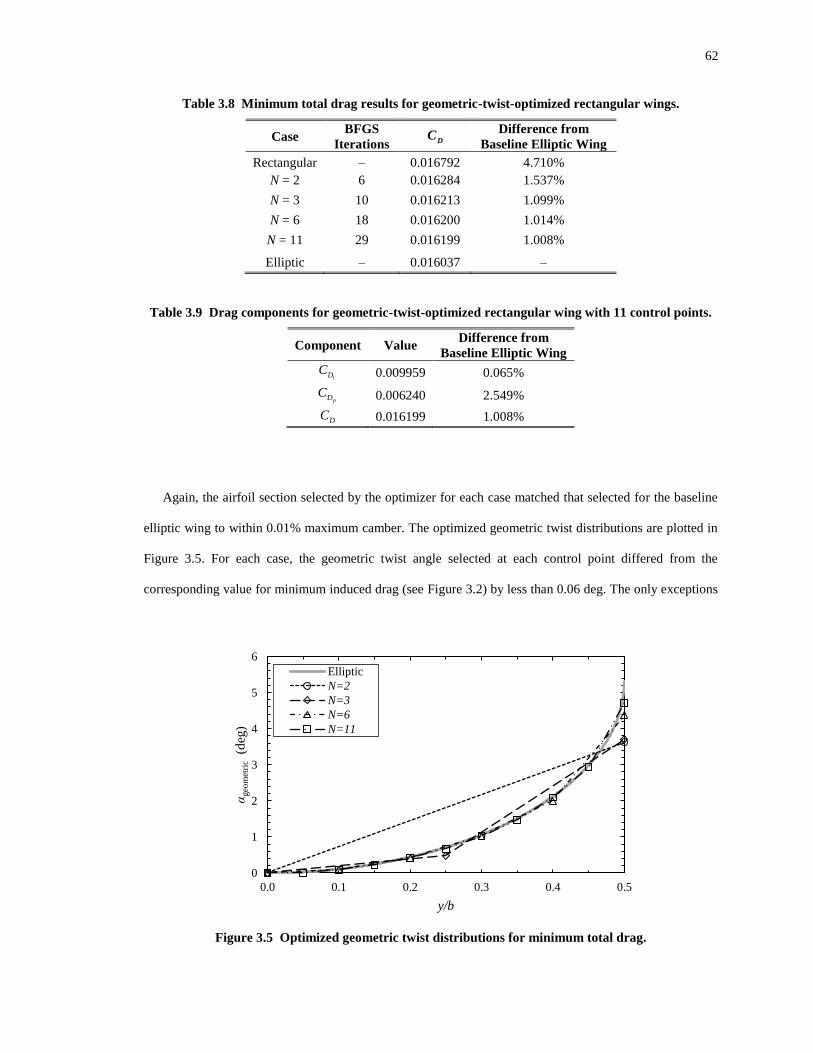
62

Table 3.8 Minimum total drag results for geometric-twist-optimized rectangular wings.

Case BFGS

Iterations DC

Difference from


Rectangular – 0.016792 4.710%

N = 2 6 0.016284 1.537%

N = 3 10 0.016213 1.099%

N = 6 18 0.016200 1.014%

N = 11 29 0.016199 1.008%

Elliptic – 0.016037 –

Table 3.9 Drag components for geometric-twist-optimized rectangular wing with 11 control points.

Component Value Difference from


iDC 0.009959 0.065%

pDC 0.006240 2.549%

DC 0.016199 1.008%

Again, the airfoil section selected by the optimizer for each case matched that selected for the baseline

elliptic wing to within 0.01% maximum camber. The optimized geometric twist distributions are plotted in

Figure 3.5. For each case, the geometric twist angle selected at each control point differed from the

corresponding value for minimum induced drag (see Figure 3.2) by less than 0.06 deg. The only exceptions

Figure 3.5 Optimized geometric twist distributions for minimum total drag.

0

1

2

3

4

5

6

0.0 0.1 0.2 0.3 0.4 0.5

αgeo

met

ric

(deg

)

y/b

Elliptic

N=2

N=3

N=6

N=11

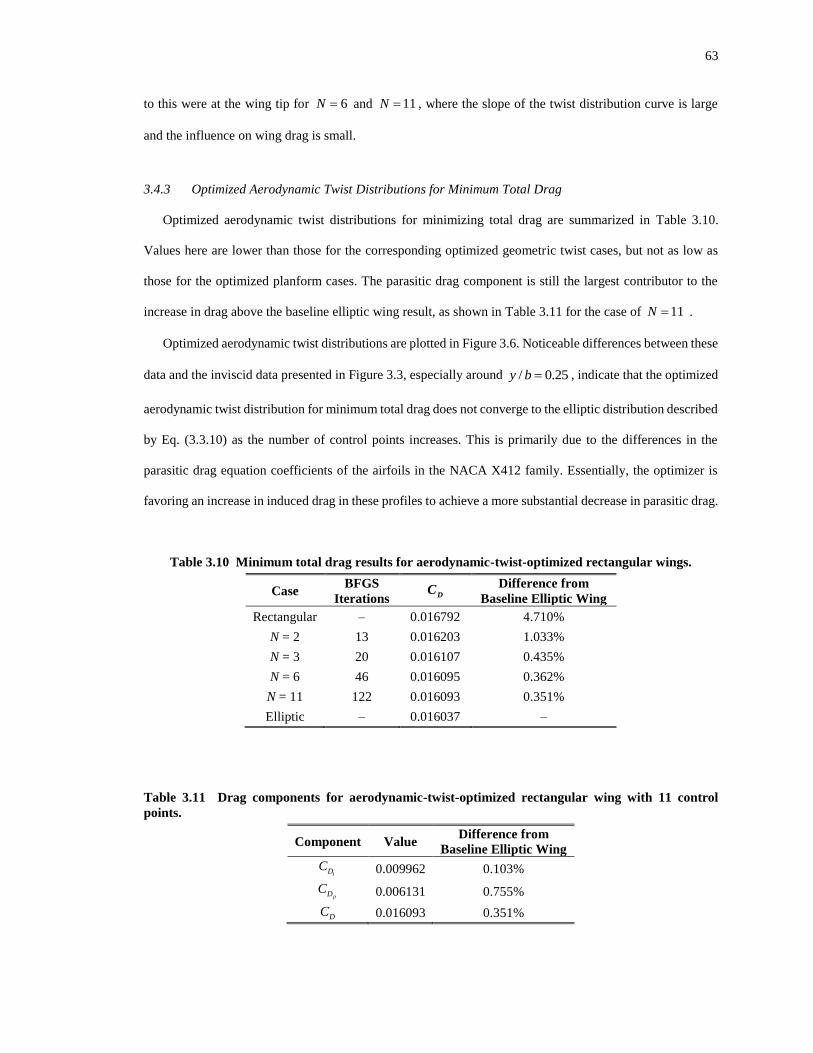
63

to this were at the wing tip for 6N = and 11N = , where the slope of the twist distribution curve is large

and the influence on wing drag is small.

3.4.3 Optimized Aerodynamic Twist Distributions for Minimum Total Drag

Optimized aerodynamic twist distributions for minimizing total drag are summarized in Table 3.10.

Values here are lower than those for the corresponding optimized geometric twist cases, but not as low as

those for the optimized planform cases. The parasitic drag component is still the largest contributor to the

increase in drag above the baseline elliptic wing result, as shown in Table 3.11 for the case of 11N = .

Optimized aerodynamic twist distributions are plotted in Figure 3.6. Noticeable differences between these

data and the inviscid data presented in Figure 3.3, especially around / 0.25y b = , indicate that the optimized

aerodynamic twist distribution for minimum total drag does not converge to the elliptic distribution described

by Eq. (3.3.10) as the number of control points increases. This is primarily due to the differences in the

parasitic drag equation coefficients of the airfoils in the NACA X412 family. Essentially, the optimizer is

favoring an increase in induced drag in these profiles to achieve a more substantial decrease in parasitic drag.

Table 3.10 Minimum total drag results for aerodynamic-twist-optimized rectangular wings.

Case BFGS

Iterations DC

Difference from


Rectangular – 0.016792 4.710%

N = 2 13 0.016203 1.033%

N = 3 20 0.016107 0.435%

N = 6 46 0.016095 0.362%

N = 11 122 0.016093 0.351%

Elliptic – 0.016037 –

Table 3.11 Drag components for aerodynamic-twist-optimized rectangular wing with 11 control

points.

Component Value Difference from


iDC 0.009962 0.103%

pDC 0.006131 0.755%

DC 0.016093 0.351%

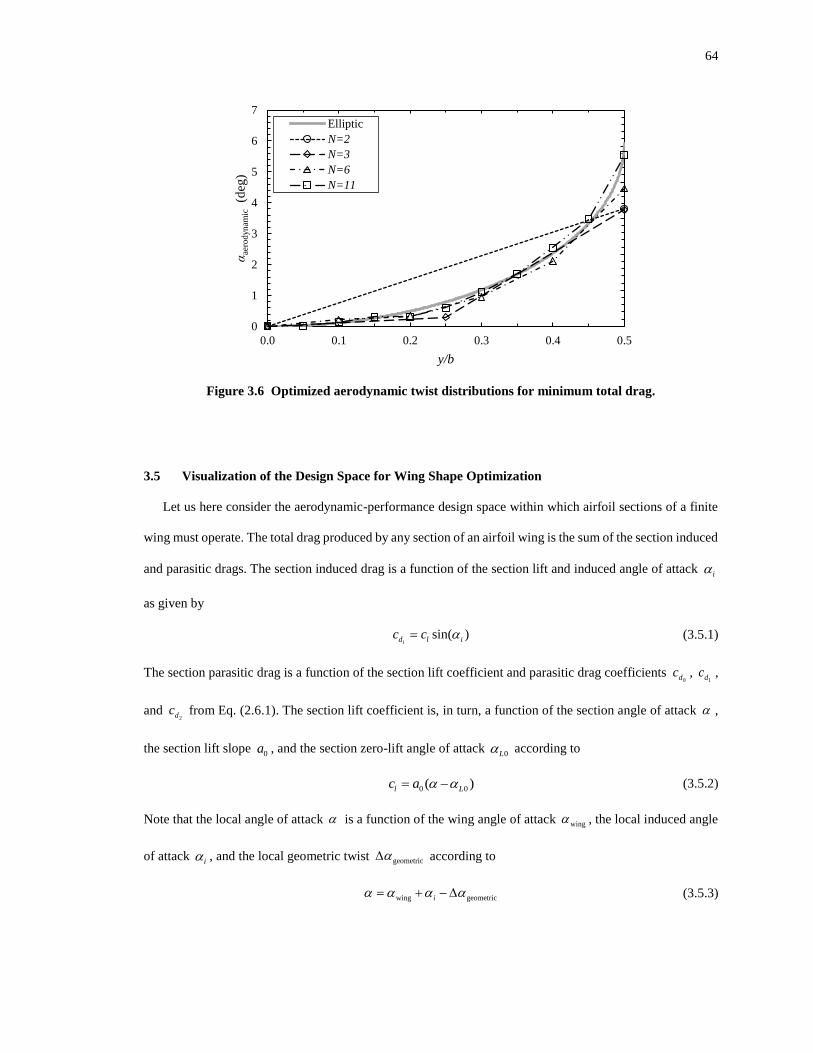
64

Figure 3.6 Optimized aerodynamic twist distributions for minimum total drag.

3.5 Visualization of the Design Space for Wing Shape Optimization

Let us here consider the aerodynamic-performance design space within which airfoil sections of a finite

wing must operate. The total drag produced by any section of an airfoil wing is the sum of the section induced

and parasitic drags. The section induced drag is a function of the section lift and induced angle of attack i

as given by

sin( )id l ic c = (3.5.1)

The section parasitic drag is a function of the section lift coefficient and parasitic drag coefficients 0dc ,

1dc ,

and 2dc from Eq. (2.6.1). The section lift coefficient is, in turn, a function of the section angle of attack ,

the section lift slope 0a , and the section zero-lift angle of attack

0L according to

0 0( )l Lc a −= (3.5.2)

Note that the local angle of attack is a function of the wing angle of attack wing , the local induced angle

of attack i , and the local geometric twist geometric according to

wing geometrici + −= (3.5.3)

0

1

2

3

4

5

6

7

0.0 0.1 0.2 0.3 0.4 0.5

αae

rodynam

ic(d

eg)

y/b

Elliptic

N=2

N=3

N=6

N=11

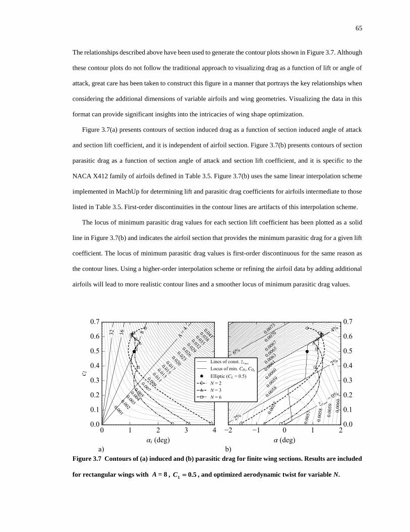
65

The relationships described above have been used to generate the contour plots shown in Figure 3.7. Although

these contour plots do not follow the traditional approach to visualizing drag as a function of lift or angle of

attack, great care has been taken to construct this figure in a manner that portrays the key relationships when

considering the additional dimensions of variable airfoils and wing geometries. Visualizing the data in this

format can provide significant insights into the intricacies of wing shape optimization.

Figure 3.7(a) presents contours of section induced drag as a function of section induced angle of attack

and section lift coefficient, and it is independent of airfoil section. Figure 3.7(b) presents contours of section

parasitic drag as a function of section angle of attack and section lift coefficient, and it is specific to the

NACA X412 family of airfoils defined in Table 3.5. Figure 3.7(b) uses the same linear interpolation scheme

implemented in MachUp for determining lift and parasitic drag coefficients for airfoils intermediate to those

listed in Table 3.5. First-order discontinuities in the contour lines are artifacts of this interpolation scheme.

The locus of minimum parasitic drag values for each section lift coefficient has been plotted as a solid

line in Figure 3.7(b) and indicates the airfoil section that provides the minimum parasitic drag for a given lift

coefficient. The locus of minimum parasitic drag values is first-order discontinuous for the same reason as

the contour lines. Using a higher-order interpolation scheme or refining the airfoil data by adding additional

airfoils will lead to more realistic contour lines and a smoother locus of minimum parasitic drag values.

Figure 3.7 Contours of (a) induced and (b) parasitic drag for finite wing sections. Results are included

for rectangular wings with = 8A , 0.5L

C = , and optimized aerodynamic twist for variable N.

66

Unlike the locus of minimum parasitic drag values, the corresponding locus of minimum induced drag

values is a function of aspect ratio. For an untwisted elliptic wing, downwash is uniform and all sections of

the wing experience the same induced angle of attack and, therefore, the same section lift coefficient. Thus

l Lc C= and i id Dc C= along the entire wingspan. Using these substitutions in Eq. (3.3.4), we can then

combine Eqs. (3.3.4) and (3.5.1) to yield

sin( )l iAc = (3.5.4)

Equation (3.5.4) has been plotted in Figure 3.7(a) for a selection of aspect ratios.

Now consider again the untwisted elliptic wing. Downwash is uniform for this wing, and therefore every

section along the wingspan operates at the same angle of attack, induced angle of attack, and lift coefficient.

The data for every section along the wingspan therefore collapses to a single point on each of the contour

plots in Figure 3.7. This point is shown for an untwisted elliptic wing with an aspect ratio of 8A = and

uniform camber of max

3.59%cz = , operating at a lift coefficient of 0.5LC = .

Prandtl [10,11] showed analytically that an untwisted elliptic wing produces the least amount of induced

drag possible for a given aspect ratio and lift coefficient, and Phillips [69] extended this work to show that

the same minimum in induced drag can be achieved by a rectangular wing having an elliptic twist distribution.

This can be seen visually in Figure 3.7(a). Because the relationship between lift and induced drag is

approximately linear for small angles (see Eq. (3.5.1)), any two wings whose sections all lie along the same

line of constant i and integrate to the same lift coefficient will also integrate to the same induced drag

coefficient.

The relationship between lift and parasitic drag is nonlinear and strongly dependent on the characteristics

of the airfoils selected, so that designs which produce minimum induced drag may not necessarily produce

minimum parasitic drag. It is the job of an optimizer, then, to balance these two competing objectives in order

to find a design that represents the minimum total drag for a given design space and given constraints.

The patterned lines with symbols in Figure 3.7 represent data from the optimization cases of Sec. 3.4.3 –

that is, optimized aerodynamic twist distributions for minimum total drag produced by a rectangular wing of

aspect ratio 8A = with no geometric twist and operating at a lift coefficient of 0.5LC = . The symbols

indicate the aerodynamic state at each control point. The connecting lines represent the distribution of

67

aerodynamic states at spanwise locations between control points. Note that, for a given wing, changing the

camber at one control point will affect the downwash along the entire wingspan, adjusting the location of all

other control points for that wing and the shape of the lines connecting them. This is also true of changes in

geometric twist and chord in designs where those parameters are allowed to vary. There is no mechanism

whereby the optimizer can adjust the aerodynamic state of one control point without affecting the

aerodynamic state of every section along the wingspan.

The data for a rectangular wing with no geometric twist and an elliptic aerodynamic twist distribution –

see Eq. (3.3.10) – would form a vertical line on both contour plots in Figure 3.7. This would minimize induced

drag but not parasitic drag. A rectangular wing with a twist and camber distribution such that the data for

each section of the wing lie somewhere along the locus of minimum parasitic drag would minimize parasitic

drag but not induced drag. In an optimization analysis, the optimizer must find a solution that represents the

best possible balance between these two competing objectives, with the added restriction of a limited number

of control points.

The ability to visualize this design space and understand the balancing act between the two components

of drag is significant. Several rudimentary implications of the data portrayed in Figure 3.7 have been

discussed here. More detailed studies of this plot and similar plots based on other families of airfoils may

provide additional insights that can aid in our understanding of the design space of finite wings. This level of

insight is impossible to gain from traditional approaches to aerodynamic shape optimization that rely on high-

fidelity CFD simulations to evaluate the objective function (see Lyu et al. [4]). By limiting the section profiles

of the wing to a family of airfoils with known aerodynamic properties, the optimization method presented

here reduces the number of design variables and the complexity of the numerical solution by several orders

of magnitude. Additionally, this approach allows us to generate drag contours of the design space in order to

more fully understand the optimized distributions arrived at through numerical optimization. For applications

that lie within the assumptions of lifting line theory, the benefits are realized without a significant reduction

in accuracy. For applications that lie outside the limits of these assumptions, this method should be applied

with caution but may still be useful in providing qualitative insights to the design space and optimization

problem of the specific application.

68

4 ANALYTICAL LIFTING LINE METHOD FOR WINGS OF ARBITRARY ASPECT RATIO

4.1 Introduction

In 1918, Prandtl [10,11] published his landmark paper on what is known today as classical lifting line

theory. This groundbreaking innovation was the first practical method for analyzing flow over a finite three-

dimensional wing. From this theory, Prandtl was able to show that the most efficient wing design in terms of

minimizing induced drag is one which produces an elliptic spanwise lift distribution. This finding led to the

distinctive elliptic planform design of the famous British Supermarine Spitfire, which is considered one of

the most strategically important fighter aircraft of World War II. Many other valuable insights to aircraft

design and performance have been gleaned from this theory in the one hundred years since its publication.

Despite its successes, classical lifting line theory is not without limitations. For example, it was originally

formulated for wings with no sweep or dihedral, and it quickly became clear that Prandtl’s theory did not

adequately account for the effects of aspect ratio for aspect ratios below about 4 (for example, see Birnbaum

[70] and Blenk [71]). However, by building upon the solid foundation laid by Prandtl, researchers have been

able to produce methods for overcoming one or more of the early limitations of classical lifting line theory.

One method, published in 2000 by Phillips and Snyder [16], accounts for sweep and dihedral in the wing and

provides a method for integrating viscous effects into the solution. Another method, known as lifting surface

theory (see Multhopp (1938) [72]), extends the applicable range of aspect ratios to less than 1. Küchemann

[73] provides an elegant formulation of lifting surface theory which recasts it in such a way that the concepts

of lifting surface theory can be readily applied to classical lifting line theory. The current work seeks to

combine the efforts of Phillips and Snyder [16] and Küchemann [73] into a single method that incorporates

the advantages of both methods. In essence, we seek to use Küchemann’s development to modify the

numerical lifting line algorithm of Phillips and Snyder so that its range of validity extends to slender wings

as well as high-aspect ratio wings.

In this chapter, a rigorous development of classical lifting line theory is presented, along with some

important observations regarding elliptic wings that arose from direct application of classical lifting line

theory. The equations for slender wing theory and lifting surface theory are also developed. Several

observations are made in comparing these theories with classical lifting line theory, and a modified equation

for slender wing theory is proposed. Several empirical equations are discussed and compared for modifying

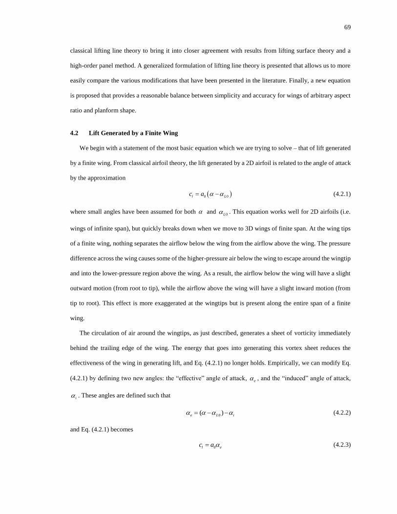
69

classical lifting line theory to bring it into closer agreement with results from lifting surface theory and a

high-order panel method. A generalized formulation of lifting line theory is presented that allows us to more

easily compare the various modifications that have been presented in the literature. Finally, a new equation

is proposed that provides a reasonable balance between simplicity and accuracy for wings of arbitrary aspect

ratio and planform shape.

4.2 Lift Generated by a Finite Wing

We begin with a statement of the most basic equation which we are trying to solve – that of lift generated

by a finite wing. From classical airfoil theory, the lift generated by a 2D airfoil is related to the angle of attack

by the approximation

( )0 0l Lc a = − (4.2.1)

where small angles have been assumed for both and 0L . This equation works well for 2D airfoils (i.e.

wings of infinite span), but quickly breaks down when we move to 3D wings of finite span. At the wing tips

of a finite wing, nothing separates the airflow below the wing from the airflow above the wing. The pressure

difference across the wing causes some of the higher-pressure air below the wing to escape around the wingtip

and into the lower-pressure region above the wing. As a result, the airflow below the wing will have a slight

outward motion (from root to tip), while the airflow above the wing will have a slight inward motion (from

tip to root). This effect is more exaggerated at the wingtips but is present along the entire span of a finite

wing.

The circulation of air around the wingtips, as just described, generates a sheet of vorticity immediately

behind the trailing edge of the wing. The energy that goes into generating this vortex sheet reduces the

effectiveness of the wing in generating lift, and Eq. (4.2.1) no longer holds. Empirically, we can modify Eq.

(4.2.1) by defining two new angles: the “effective” angle of attack, e , and the “induced” angle of attack,

i . These angles are defined such that

0( )e iL = − − (4.2.2)

and Eq. (4.2.1) becomes

0l ec a = (4.2.3)

70

To determine the total lift generated by a finite wing, we take the area-weighted average of the lift

coefficients at each spanwise location by integrating Eq. (4.2.3) over the wingspan,

2 2

0

2 2

1 1b b

L l e

w wy b y b

C c cdy a cdyS S

=− =−

= = (4.2.4)

In doing so, we have relied upon an assumption that was first made by Prandtl [10,11] in his original

development of classical lifting line theory – that is, that the spanwise sections of a finite wing behave the

same as a 2D airfoil section operating at the same angle of attack. While Prandtl offered no mathematical

justification for this assumption, it has proven to be quite reliable through a century of application.

The trick now, and the focus of this chapter, is to determine an expression for e such that Eq. (4.2.4) is

accurate for finite wings ranging in aspect ratio from slender to infinite. Several researchers, beginning with

Prandtl [10,11], have presented methods for determining an appropriate expression for e under various

assumptions. Those of greatest interest to the present work are classical lifting line theory, slender wing

theory, and lifting surface theory. Each, in turn, shall here be presented and discussed.

4.3 Classical Lifting Line Theory

Consider a flat or uniformly cambered wing of finite span in an infinite potential flow field. The boundary

condition for this flow field requires that the flow is everywhere tangent to the wing surface such that

0L

w dz

V dx

= − = − (4.3.1)

where we have applied the small angle approximation 0 0t )an( L L − − . Note that we have defined the

downwash w to be positive for positive angle of attack, so that positive downwash acts in the direction of the

–z axis.

Prandtl proposed satisfying this boundary condition by representing the wing as a series of horseshoe

vortices, each horseshoe vortex consisting of a single spanwise vortex segment aligned with the quarter-chord

of the wing and two semi-infinite vortex segments extending chordwise downstream, as shown in Figure 4.1.

In the limit as the number of horseshoe vortices goes to infinity, the streamwise vortex segments form a

continuous vortex sheet trailing behind the wing. It is this vortex sheet that is responsible for the reduced

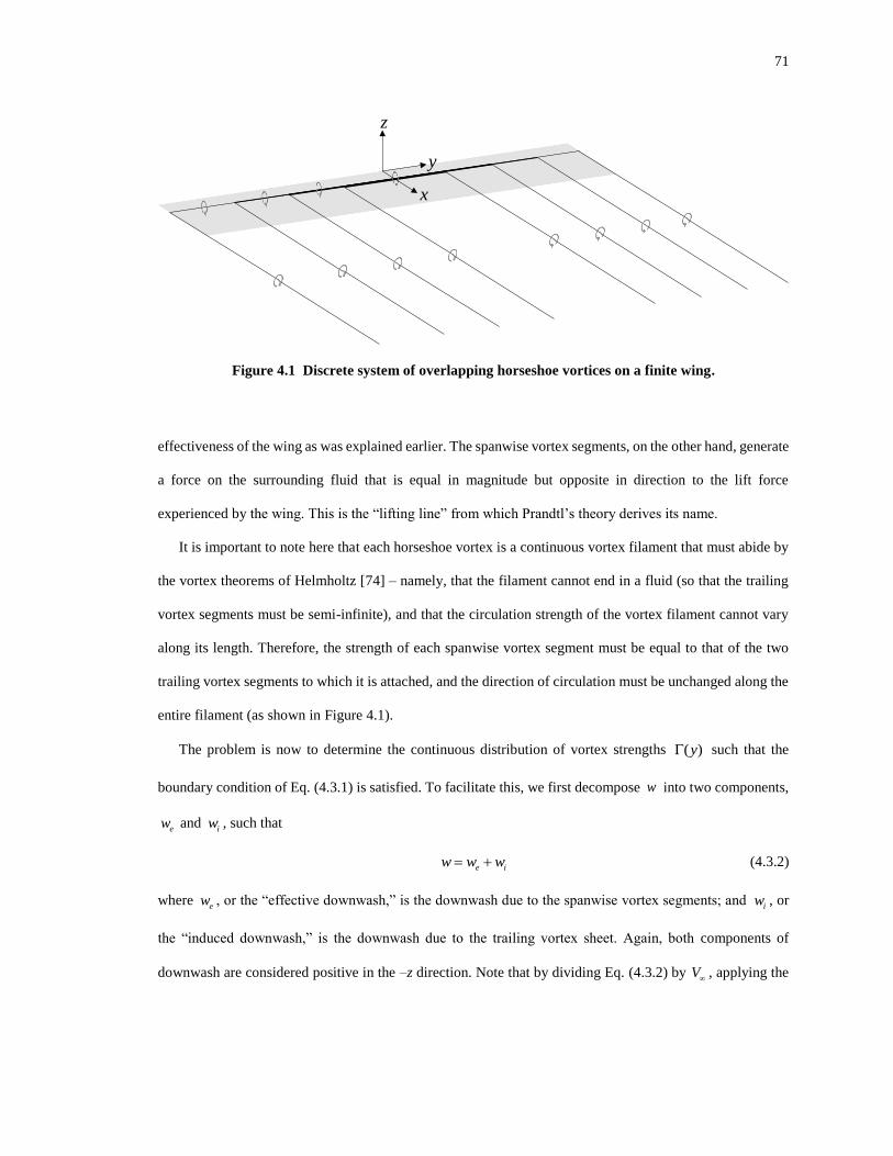
71

Figure 4.1 Discrete system of overlapping horseshoe vortices on a finite wing.

effectiveness of the wing as was explained earlier. The spanwise vortex segments, on the other hand, generate

a force on the surrounding fluid that is equal in magnitude but opposite in direction to the lift force

experienced by the wing. This is the “lifting line” from which Prandtl’s theory derives its name.

It is important to note here that each horseshoe vortex is a continuous vortex filament that must abide by

the vortex theorems of Helmholtz [74] – namely, that the filament cannot end in a fluid (so that the trailing

vortex segments must be semi-infinite), and that the circulation strength of the vortex filament cannot vary

along its length. Therefore, the strength of each spanwise vortex segment must be equal to that of the two

trailing vortex segments to which it is attached, and the direction of circulation must be unchanged along the

entire filament (as shown in Figure 4.1).

The problem is now to determine the continuous distribution of vortex strengths ( )y such that the

boundary condition of Eq. (4.3.1) is satisfied. To facilitate this, we first decompose w into two components,

ew and iw , such that

e iw w w= + (4.3.2)

where ew , or the “effective downwash,” is the downwash due to the spanwise vortex segments; and

iw , or

the “induced downwash,” is the downwash due to the trailing vortex sheet. Again, both components of

downwash are considered positive in the –z direction. Note that by dividing Eq. (4.3.2) by V, applying the

x

y

z

72

small angle approximation, and rearranging, we arrive at Eq. (4.2.2), so that both are equivalent statements

of the boundary condition.

Consider the semi-infinite vortex filament shown in Figure 4.2. The origin O and the arbitrary point P lie

on the same plane perpendicular to the vortex filament, with the vector h pointing from O to P. From the

Biot-Savart law (see Sec. 5.2 of Anderson [75]), the differential velocity vector dV induced at point P due to

the differential vortex element of length dl located at point Q is given by

34 r

= dl r

dV (4.3.3)

where r is the vector pointing from Q to P. The total velocity induced at point P by the entire vortex filament

is then

0

34 r

= =

dl r

V dV (4.3.4)

By inspection, the length from O to Q is )tan(h so that

2 ( )n

dh

dsi

l

= − (4.3.5)

and the magnitudes of the vectors r and h are related by

sinr h = (4.3.6)

Using Eqs. (4.3.5) and (4.3.6) in Eq. (4.3.4) and taking the magnitude, we get

2

sin

4 4 hV d

h

=

= (4.3.7)

Figure 4.2 Velocity induced at point P by a semi-infinite vortex filament.

73

The direction of V is given by the cross product of the vectors OQ and OP .

Now consider the trailing vortex sheet proposed by Prandtl, consisting of an infinite number of differential

semi-infinite vortex filaments originating at the quarter chord line and extending in the direction of the chord.

By analogy to Eq. (4.3.7), the differential induced downwash at a point y along the quarter chord by a

differential slice of this vortex sheet located at y = is

( )

( )4 ( )

i

ddw y

y

=

− (4.3.8)

The total induced downwash due to the trailing vortex sheet is then the integral of Eq. (4.3.8) over the

wingspan

/2

/2

1 ( )( )

4

b

i

b

d dw y d

y

=−

=

− (4.3.9)

The effective downwash ( )ew y cannot be determined in the same manner, i.e. using the potential flow

equations of a vortex filament, because the locations at which we are interested in determining the velocity

lie along the axis of the spanwise vortex segments where the velocity is singular. Prandtl therefore turned to

an alternative means for computing the effective downwash – namely, the two-dimensional Kutta-Joukowski

theorem. At this point, Prandtl injects his hypothesis that each spanwise section of a finite wing could be

modeled as a two-dimensional airfoil subject to the same circulation. The spanwise section lift is then, by the

Kutta-Joukowski theorem,

( ) ( )l y V y = (4.3.10)

and from classical airfoil theory we have

1 102

2

2

2( ) ( ) ( ) ( ) ( )l el y V c y c y V c y a y = = (4.3.11)

Equating the right-hand sides of Eqs. (4.3.10) and (4.3.11) and solving for e gives

0

2 ( )( )

( )e

yy

V a c y

= (4.3.12)

so that the effective downwash becomes

0

2 ( )( ) ( )

( )e e

yw y V y

a c y

= = (4.3.13)

74

Substituting the right-hand sides of Eqs. (4.3.9) and (4.3.13) into Eq. (4.3.2) and substituting that result in for

the total downwash in Eq. (4.3.1) gives

0

/2

/20

2 ( ) 1 ( )

( ) 4L

b

b

y d dd

V a c y V y

=−

+ = −

− (4.3.14)

which is the fundamental equation of Prandtl’s classical lifting line theory. The only unknown in Eq. (4.3.14)

is the circulation distribution ( )y , all other variables being parameters of either the wing geometry or the

operating conditions. Solution methods to this equation are not directly relevant to the current discussion; the

reader is instead referred to Anderson [75] and Phillips [53].

One important solution to Eq. (4.3.14) is the elliptic circulation distribution given by

2

0

2( ) 1

yy

b

= −

(4.3.15)

Besides being the most efficient circulation distribution in terms of minimizing induced drag, it conveniently

results in uniform induced downwash across the entire wingspan. We can see this by inserting the derivative

of Eq. (4.3.15) with respect to y into Eq. (4.3.9) and evaluating. The substitution gives

( )

122/2

0

2elliptic

/2

21

b

i

b

w dy bb

−

=−

= − −

− (4.3.16)

A convenient method for solving this integral is to use the change of variables 02cos( )by = − and

2cos( )b = − , which gives

( )i

0

0

ellipt c

0

cos( )

2 cos( ) cos( )iw d

b

=

=

− (4.3.17)

Eq. (4.3.17) can be evaluated from (see Karamcheti [76])

00

0

0

sin( )cos( )

( ) ( ) sin( )

nn

cos cosd

=− (4.3.18)

By inspection we see that 1n = so that

( ) 0

elliptic 2iw

b

= (4.3.19)

Consider a flat or uniformly-cambered wing with the elliptic circulation distribution given by Eq.

(4.3.15). Eq. (4.3.19) states that the induced downwash is uniform along the wingspan, and therefore by Eq.

75

(4.3.2) the effective downwash must also be uniform. Substituting the circulation distribution, Eq. (4.3.15),

into Eq. (4.3.13) gives

( )2

0elliptic

0

2 21

( )e

yw

a c y b

= −

(4.3.20)

which (assuming 0a to be constant over the wingspan) can only be constant if the chord distribution is also

elliptic, i.e.

2 2

elliptic 0

2 4 21 1

y c yc c

b b

= − = −

(4.3.21)

so that Eq. (4.3.20) becomes

( ) 0

elliptic

02ew

a c

= (4.3.22)

Substituting the right-hand sides of Eqs. (4.3.19) and (4.3.22) into Eq. (4.3.2) and solving for 0 , we get

0

0

0

2a

wba A

=

+ (4.3.23)

where 2

wA b S b c= = is the aspect ratio of the wing. Using this result in Eqs. (4.3.19) and (4.3.22) gives

( ) 01

i

ww

A a=

+ (4.3.24)

( )01

e

ww

a A=

+ (4.3.25)

respectively; or, by Eq. (4.3.1),

( ) 0

0

1i

L

A a

−=

+ (4.3.26)

( )

0

01e

L

a A

−=

+ (4.3.27)

We can now use Eq. (4.3.27) in Eq. (4.2.4) to solve for the total lift coefficient of the wing. The chord is the

only variable that is a function of y, and the integral of the chord over the wingspan gives the planform area

wS . Then Eq. (4.2.4) evaluates to

( )

( )0

0 0

01L e L

aC a

a A

= = −

+ (4.3.28)

76

and the effective wing lift slope becomes

0

01 / ( )

a

a Aa

+= (4.3.29)

Equation (4.3.28) gives the lift coefficient of a finite elliptic wing according to Prandtl’s classical lifting

line theory. Note that in developing this equation we have assumed 0a , , and

0L are all constant along

the wingspan. This led to the requirement that the chord distribution be elliptic according to Eq. (4.3.21). In

reality, the same circulation distribution specified in Eq. (4.3.15) can be achieved through an unlimited

number of wing configurations in which the twist ( ), camber (0L ), thickness (

0a ), and chord are all

potential functions of y . In any case, Eq. (4.3.10) still holds so that an elliptic circulation distribution will

always produce an elliptic lift distribution. The implications these alternative wing designs have on drag were

considered in detail in Chapter 3.

We can now also compute the induced drag generated on the wing by the trailing vortex sheet. This drag

is not due to viscous effects (recall that everything we have considered so far is based on inviscid potential

flow), but instead is due to the change in local angle of attack resulting from the induced downwash iw . By

definition, lift is the component of the aerodynamic force that is normal to the freestream, and drag is the

component tangent to the freestream. The section lift coefficient given by Eq. (4.2.3) is therefore not actually

lift relative to the wing but the total resultant aerodynamic force coefficient, rc , generated by the wing section

and acting at an angle i to the direction of lift. However, applying the small angle approximation we get

cos( )l r i rc c c= (4.3.30)

so that Eq. (4.2.3) still holds to a good approximation. The induced drag coefficient is given by

sin( )id r i r ic c c = (4.3.31)

and the total induced drag is then the area-weighted average of Eq. (4.3.31) similar to Eq. (4.2.4). Evaluating

this integral with the definitions for the induced and effective angles of attack from Eqs. (4.3.26) and (4.3.27)

gives

L

i

C

A

= (4.3.32)

2

i

L

D

CC

A= (4.3.33)

77

which is the well-known solution first given by Prandtl [10,11].

Equation (4.3.33) was developed under the assumption that the wing has an elliptic lift distribution, which

Prandtl [10,11] showed produces the minimum induced drag for a wing of given aspect ratio and lift. A span

efficiency factor (se ) can be used to adjust Eq. (4.3.33) for other lift distributions. See Phillips [53]. Equation

(4.3.33) is then

2

i

L

s

D

CC

Ae= (4.3.34)

where 1se = for any wing with an elliptic lift distribution and 1se for all other lift distributions.

4.4 Slender Wing Theory

The limitations of classical lifting line theory with respect to aspect ratio were recognized shortly after its

publication. Prandtl’s model was based on the assumption that the chordwise vorticity distribution at every

section of a finite wing is the same as that predicted by classical airfoil theory for a two-dimensional wing.

This assumption is only strictly true for wings of infinite aspect ratio. For finite wings, the chordwise vorticity

distribution is a function of spanwise location. Deviations from the predictions of classical airfoil theory

become more pronounced as aspect ratio is reduced, especially at spanwise sections near the wing tips.

In considering the lower limit of aspect ratio, the works of Munk [77], Bollay [78], and Jones [79] provide

analytical relationships for the aerodynamic characteristics of finite wings in the limit as 0A→ . Their results

form the basis of slender wing theory. Here we present a modified formulation of classical lifting line theory

based on their results, which is only valid for small aspect ratios ( 1A ).

In order to develop a formulation for slender wing theory similar to Eq. (4.3.14), we must first consider

several important results obtained through the development of slender wing theory. Munk [77] demonstrated

that flow in planes perpendicular to the x-axis of a slender body can be viewed as two-dimensional, and he

introduced the concept of an “additional apparent mass,” 'm , that represents the mass of fluid displaced by

each chordwise section of the wing as the wing moves into the flow. Jones [79] extended this concept to

develop relations for the lift generated by an uncambered slender delta wing. He used Munk’s relation for

the additional apparent mass,

2

4'

bdxm

= (4.4.1)

78

which is equivalent to the mass of fluid within a cylindrical volume of diameter b and length dx. The

momentum imparted to the wing at each chordwise section must balance the momentum imparted to the

additional apparent mass of fluid at that chordwise section, so that the lift force on the wing becomes

( )t

ld

x Vdm

= (4.4.2)

The time derivative of the additional apparent mass is given by

2

dm dm dx b dbdx V

dt dx dt dx

= =

(4.4.3)

so that the lift becomes

21

2( )

dbV b dxx

dxl = (4.4.4)

and the lift coefficient becomes

( )lx

cb

xd

d= (4.4.5)

The total lift coefficient generated by the delta wing is then given by integration, as in Eq. (4.2.4), but this

time we are integrating over the chord. We get

2

max

0

1(

2 2)

c

L l

w w

C c x bdxS

b A

S

== = (4.4.6)

since, for any delta wing, 0b = at 0x = and maxb b= at x c= . This gives for the lift slope of a slender delta

wing

2

aA

= (4.4.7)

which is the well-known result from Jones [79].

Jones then made three observations critical to our current development. The first is that, in order to satisfy

the Kutta condition, only sections of increasing span (i.e. 0db dx ) can generate lift, so that the use of maxb

in Eq. (4.4.6) is general for any planform regardless of the chordwise location at which maxb actually occurs.

The second, which Jones demonstrated through a development of the surface potential, is that the spanwise

lift distribution of a slender wing is elliptical and independent of chord distribution. The third observation,

which also came about through Jones’ development of the surface potential, is that the vorticity distribution

79

of a slender wing is concentrated at the leading edge of the wing, so that the aerodynamic center is also

located at the leading edge. We expect these observations to be true for any viable formulation of the slender

wing problem.

We now proceed to cast Eq. (4.3.14) in terms of these findings. First we consider the system of horseshoe

vortices that must be used to represent a slender wing. In Figure 4.1, the system of horseshoe vortices from

classical lifting line theory is shown with the lifting line located at the quarter-chord of the wing, which

corresponds to the aerodynamic center for wings of infinite span. Jones [79] demonstrated that the

aerodynamic center of a slender wing is located at the leading edge of the wing. Küchemann [73] therefore

proposed moving the lifting line from the quarter-chord to the leading edge when evaluating slender wings,

and – to represent the infinite chord-to-span ratio of slender wings – placing the leading edge of the wing at

x = − .

With this modified system of horseshoe vortices, the only change needed to Eqs. (4.3.4) and (4.3.7) is the

lower limit of integration, so that Eq. (4.3.8) becomes

( )

( )2 ( )

i

ddw y

y

=

− (4.4.8)

and the induced downwash becomes

/2

/2

1 ( )( )

2

b

i

b

d dw y d

y

=−

=

− (4.4.9)

Next we consider the effective downwash generated by slender wings. Küchemann [73] states – and it is

obvious from Eq. (4.4.6) that he is correct – that 0LC → as 0A→ , so that the effective downwash must

also go to zero. Thus e iw w by Eq. (4.3.2) and we can write, to a good approximation,

0

/2

/2

1 ( )

2b

L

bd d

dV y

=−

= −

− (4.4.10)

There is only one possible solution to Eq. (4.4.10), namely

22

( ) 1y

y bwb

= −

(4.4.11)

which is both elliptic and independent of chord distribution in agreement with the observations of Jones [79]

stated earlier. Note that Eq. (4.4.11) differs by a factor of 2 from the elliptic circulation distribution given by

80

Eqs. (4.3.15) and (4.3.23) in the limit as 0A→ . The lift can now be found by integrating Eq. (4.3.10) over

the span. In nondimensional form we get

( )/ 2

0

/2

2( )

2

b

L L

w b

CA

V y dyV S

−

= −= (4.4.12)

which agrees exactly with the lift slope predicted by Jones [79], Eq. (4.4.7).

Previous works on slender wing theory have ended at this point, and we are left with Eq. (4.4.10) as our

lifting line theory equivalent of slender wing theory. However, there is one additional step we can take due

to the knowledge that our circulation distribution is elliptic according to Eq. (4.4.11). Recall that the induced

and effective downwashes produced by a high-aspect-ratio wing with elliptic circulation, Eqs. (4.3.24) and

(4.3.25) respectively, are constant over the span. Since our slender wing solution is forced to an elliptic

circulation distribution, we conjecture that the two components of downwash are constant in this case as well.

Then from Eq. (4.2.4) and (4.4.12) we have

( )0 02

L e LCA

a

−= = (4.4.13)

Solving for e and multiplying by V

, we get

02

e

Aww

a

= (4.4.14)

Solving Eq. (4.4.11) for w and substituting, we get

2

0

4 2

2

1

ew

c

ba

y

−

=

(4.4.15)

which is identical to Eq. (4.3.13) except that the actual spanwise chord distribution has been replaced by the

elliptic chord distribution of Eq. (4.3.21). Thus for elliptic wings, Eqs. (4.3.13) and (4.4.15) are equivalent.

This again agrees with the observations of Jones [79] stated earlier, specifically that the results for a slender

wing are independent of chord distribution.

By Eqs. (4.4.9) and (4.4.15) we now have for our slender wing lifting line equation

02

0

/2

/2

1 ( )

2

2

4 21

L

b

b

d dd

V yV

c y

ba

=−

= −

−

+

−

(4.4.16)

81

Eq. (4.4.16) is a more complete statement of slender wing theory than has been presented previously. Results

computed using Eq. (4.4.16) are nearly identical to those computed using the slender wing theory of Jones

[79] for aspect ratios less than about 1, which is typically considered the upper limit for slender wing theory.

Inclusion of the effective downwash term, however, offers important insights as we look to combine slender

wing theory and classical lifting line theory into a single theory applicable for all aspect ratios. We shall refer

to this formulation hereinafter as the “modified slender wing equation.”

4.5 Lifting Surface Theory

Early efforts to extend the concepts of lifting line theory to wings of low aspect ratio began with the works

of Birnbaum [70] and Blenk [71] and developed into what is known today as lifting surface theory. Blenk

[71] was able to show good results for aspect ratios down to about 1 by replacing the single lifting line in

Prandtl’s formulation with a chordwise distribution of lifting lines, thus forming a lifting surface. His overall

formulation, however, was limited to a single finite wing of rectangular planform in inviscid, incompressible

flow. He attributed the error for aspect ratios less than one to nonlinear effects that could not be accounted

for in his linear formulation.

Zimmerman [80,81] and Winter [82] performed experimental studies on low-aspect-ratio wings. They

attributed the divergence between their results and lifting surface theory to stalling phenomena that could not

be treated with inviscid theoretical methods. Bollay [78] later developed analytical solutions for a flat

rectangular plate in which he attributed the phenomena seen by the aforementioned experimenters to the

finite angle at which the trailing vortices leave the plate.

The only purely analytical solution of lifting surface theory currently available in the literature is that of

Hauptman and Miloh [83]. By assuming an elliptic planform with a straight midchord, they derived the

acceleration potential (see Prandtl [84]) in terms of ellipsoidal harmonics and applied this to a linearized

formulation of lifting surface theory. The result was a set of closed-form equations for spanwise lift as a

function of aspect ratio. While Hauptman and Miloh [83] state that these equations “are exact within the

realm of the linear theory,” the equations are too cumbersome to apply practically as they involve evaluation

of the complete elliptic integral of the second kind (see Hauptman and Miloh [85], Smith [86], and Laitone

[87]) and, for spanwise distributions, evaluation of infinite summations that do not readily converge.

82

Using numerical calculations from lifting surface theory, several authors have proposed empirical and

semi-empirical expressions for the lift slope of low-aspect-ratio wings. Some of the more interesting

proposals come from Jones [88], Helmbold [89], Van Dyke [90], Germain [91], Kida and Miyai [92], and

Laitone [87]; but there are many others. Unfortunately, none of these provide spanwise lift distributions in

their developments, but only provide equations for the total lift coefficient produced by a wing as a function

of aspect ratio. Küchemann [73], on the other hand, presents a very elegant method for correcting the two

components of downwash in classical lifting line theory, Eq. (4.3.14), which does allow for the calculation

of spanwise lift distributions. He facilitates this by assuming that the effects of aspect ratio are uniform over

the span, which is obviously not true near the wing tips, but Küchemann [73] observes that “the error cannot

be serious, however, as the lift falls to zero there.”

4.6 A Unifying Formulation of Lifting Line, Slender Wing, and Lifting Surface Methods

Without considering spanwise lift distributions (since most of the methods mentioned above lack

sufficient development to facilitate consideration of such), we shall here present a unifying formulation of

the three theories described above for calculating the wing lift coefficients. All the methods presented here

consider only an elliptic planform in their development. Most consider a straight quarter-chord line while

some – namely Hauptman and Miloh [83] and Küchemann [73] – consider a straight mid-chord. Panair results

given in Figure H.6 of Appendix H show little difference between the two, so we shall not attempt any

correction to the methods based on where the straight chord line is located.

In general, the lift coefficient of a finite wing has already been given as

2 2

0

2 2

1 1( ) ( )

b b

L l e

w wy b y b

C c c y dy a c y dyS S

=− =−

= = (4.2.4)

where

0( )e iL = − − (4.2.2)

For an elliptic wing, the effective and induced angles of attack predicted by classical lifting line theory are

constant over the wingspan and Eq. (4.2.4) becomes

( )0 00 L iL eC a a = = − − (4.6.1)

The induced angle of attack is related to the lift coefficient according to Eq. (4.3.32),

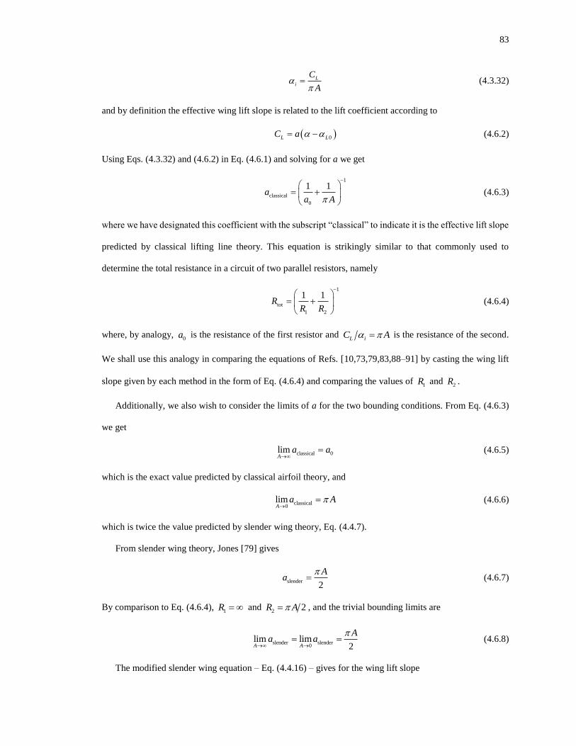
83

L

i

C

A

= (4.3.32)

and by definition the effective wing lift slope is related to the lift coefficient according to

( )0L LC a −= (4.6.2)

Using Eqs. (4.3.32) and (4.6.2) in Eq. (4.6.1) and solving for a we get

1

0

classical

1 1a

a A

−

+

=

(4.6.3)

where we have designated this coefficient with the subscript “classical” to indicate it is the effective lift slope

predicted by classical lifting line theory. This equation is strikingly similar to that commonly used to

determine the total resistance in a circuit of two parallel resistors, namely

1

tot

1 2

1 1R

R R

−

= +

(4.6.4)

where, by analogy, 0a is the resistance of the first resistor and

L iC A = is the resistance of the second.

We shall use this analogy in comparing the equations of Refs. [10,73,79,83,88–91] by casting the wing lift

slope given by each method in the form of Eq. (4.6.4) and comparing the values of 1R and

2R .

Additionally, we also wish to consider the limits of a for the two bounding conditions. From Eq. (4.6.3)

we get

classical 0limA

a a→

= (4.6.5)

which is the exact value predicted by classical airfoil theory, and

classical0

limA

a A→

= (4.6.6)

which is twice the value predicted by slender wing theory, Eq. (4.4.7).

From slender wing theory, Jones [79] gives

slender2

aA

= (4.6.7)

By comparison to Eq. (4.6.4), 1R = and

2 2R A= , and the trivial bounding limits are

slender slender0 2

lim limA A

aA

a

→ →= = (4.6.8)

The modified slender wing equation – Eq. (4.4.16) – gives for the wing lift slope

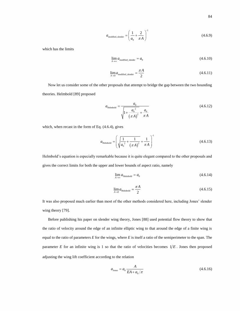
84

1

modified_slender

0

1 2a

a A

−

= +

(4.6.9)

which has the limits

0modifie _sle ded n rlimA

a a→

= (4.6.10)

lmodifie _s ended r

0 2limA

Aa

→= (4.6.11)

Now let us consider some of the other proposals that attempt to bridge the gap between the two bounding

theories. Helmbold [89] proposed

( )

0

Helmbold2

0 0

21

a

A

aa

a

A

=

+ +

(4.6.12)

which, when recast in the form of Eq. (4.6.4), gives

( )

d

1

Helmbol 2 2

0

11 1a

Aa A

−

= +

+

(4.6.13)

Helmbold’s equation is especially remarkable because it is quite elegant compared to the other proposals and

gives the correct limits for both the upper and lower bounds of aspect ratio, namely

Helmbold 0limA

a a→

= (4.6.14)

Helmbold

0lim

2A

Aa

→= (4.6.15)

It was also proposed much earlier than most of the other methods considered here, including Jones’ slender

wing theory [79].

Before publishing his paper on slender wing theory, Jones [88] used potential flow theory to show that

the ratio of velocity around the edge of an infinite elliptic wing to that around the edge of a finite wing is

equal to the ratio of parameters E for the wings, where E is itself a ratio of the semiperimeter to the span. The

parameter E for an infinite wing is 1 so that the ratio of velocities becomes 1 E . Jones then proposed

adjusting the wing lift coefficient according to the relation

Jones 0

0

a aA

EA a += (4.6.16)

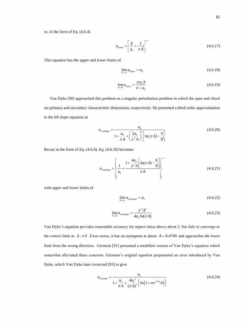
85

or, in the form of Eq. (4.6.4)

1

Jones

0

1a

a

E

A

−

=

+ (4.6.17)

This equation has the upper and lower limits of

Jones 0limA

a a→

= (4.6.18)

0

Jones0

0

limA

a A

aa

→=

+ (4.6.19)

Van Dyke [90] approached this problem as a singular perturbation problem in which the span and chord

are primary and secondary characteristic dimensions, respectively. He presented a third-order approximation

to the lift slope equation as

( )

0

VanDyke 2

0 0

2

2 9ln

81

aa

a aA

A A

+

=

+

−

(4.6.20)

Recast in the form of Eq. (4.6.4), Eq. (4.6.20) becomes

1

0

3

VanDyke

0

4 91 ln( )

1 8

aA

Aa

a A

−

+ −

= +

(4.6.21)

with upper and lower limits of

VanDyke 0limA

a a→

= (4.6.22)

4 2

VanDyke0

0

l)

iml4 n(A

aa

A

A

→= (4.6.23)

Van Dyke’s equation provides reasonable accuracy for aspect ratios above about 2, but fails to converge to

the correct limit as 0A→ . Even worse, it has an asymptote at about 0.4749A = and approaches the lower

limit from the wrong direction. Germain [91] presented a modified version of Van Dyke’s equation which

somewhat alleviated these concerns. Germain’s original equation perpetuated an error introduced by Van

Dyke, which Van Dyke later corrected [93] to give

( )

0

Germain 29/80 0

2

4ln 1

( )1

aa

a ae A

A A

−+

=

+ +

(4.6.24)

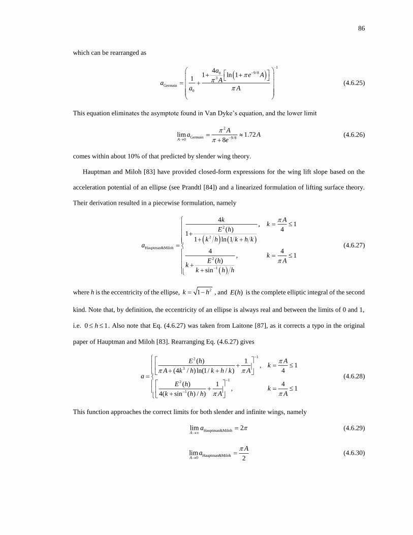
86

which can be rearranged as

( )

0

1

9/80

3

Germain

41 ln 1

1

ae

a A

a A

A

−

−

+

=

+

+

(4.6.25)

This equation eliminates the asymptote found in Van Dyke’s equation, and the lower limit

2

Germain 9/80l 1.72m

8i

A

Aa A

e

−→

+= (4.6.26)

comes within about 10% of that predicted by slender wing theory.

Hauptman and Miloh [83] have provided closed-form expressions for the wing lift slope based on the

acceleration potential of an ellipse (see Prandtl [84]) and a linearized formulation of lifting surface theory.

Their derivation resulted in a piecewise formulation, namely

( ) ( )

( )

2

2

Hauptman&Miloh

2

1

14

,( )

11 ln 1

4,

( )

sin

4

41

kk

E h

k h k h ka

kE h

kk h h

A

A

−

=

++ +

= =

++

(4.6.27)

where h is the eccentricity of the ellipse, 21k h= − , and ( )E h is the complete elliptic integral of the second

kind. Note that, by definition, the eccentricity of an ellipse is always real and between the limits of 0 and 1,

i.e. 0 1h . Also note that Eq. (4.6.27) was taken from Laitone [87], as it corrects a typo in the original

paper of Hauptman and Miloh [83]. Rearranging Eq. (4.6.27) gives

12

3

12

1

( ) 1, 1

4(4 / ) ln(1/ / )

( ) 1 4, 1

4( sin ( ) / )

E h Ak

AA k h k h ka

E hk

A Ak h h

−

−

−

+ =

+ + =

+ =

+

(4.6.28)

This function approaches the correct limits for both slender and infinite wings, namely

Hauptman&Milohlim 2A

a →

= (4.6.29)

Hauptman&Miloh0

lim2A

Aa

→= (4.6.30)

87

However, the section lift slope 0a does not appear explicitly in Eq. (4.6.27) due to the method by which it

was derived, and it is unclear how to correct this equation for section lift slopes other than 2 .

The last equation that we shall consider from the literature is that of Küchemann [73]. Küchemann uses

the flat plate distribution of Birnbaum [70] to demonstrate that classical lifting line theory can actually be

considered a lifting surface theory. Birnbaum [70] showed that the pressure distribution over a flat infinite

plate at angle of attack is given by

1/2

2 1( )p

x cx

x c

CC

V

−

= −

(4.6.31)

which can similarly be expressed as a continuous sheet of vorticity ( )x x through the Kutta-Joukowski law,

where the coefficient C must be determined. The section lift is given by

0

1l p

c

Cc xc

d= − (4.6.32)

Inserting Eq. (4.6.31) into Eq. (4.6.32) and performing the integration gives

lc CV

= (4.6.33)

or, rearranging,

lCV

c= (4.6.34)

The effective downwash can now be determined by applying the Biot-Savart Law,

0 0

)1

4 2(

c c

e p

xw

cx

d CC dx

x x

=

−= −

(4.6.35)

Combining Eqs. (4.6.34) and (4.6.35), we get

2l ec = (4.6.36)

which gives the section lift slope of a thin airfoil. This demonstrates that using a section lift slope of 0 2a =

in classical lifting line theory is equivalent to a lifting surface theory with the chordwise pressure distribution

of Eq. (4.6.31). Other pressure distributions will result in a different section lift slope, so that the chordwise

pressure distribution of any section can be incorporated into classical lifting line theory through the use of an

appropriate section lift slope.

88

Küchemann [73] then showed that a slightly modified pressure distribution,

1

)2

(p

CC

V

x cx

x c

= −

−

(4.6.37)

can be used to obtain the slender wing results of Jones [79] in a similar manner. The obvious parallels between

Eqs. (4.6.31) and (4.6.37) led Küchemann [73] to propose a more general distribution, namely

2 1

( )

n

p

cCC x

cV

x

x

− = −

(4.6.38)

where the parameter n can be defined such that a smooth transition occurs between the chordwise

distributions of Eqs. (4.6.31) and (4.6.37). Using Eq. (4.6.38) in Eq. (4.6.32) and performing the integration

gives

sin

2lC

V nc

n

= (4.6.39)

Applying the Biot-Savart Law, Eq. (4.6.35), gives

4

1 cotl ec

n

n n

=

− (4.6.40)

The coefficient in front of e can be interpreted as the “effective” section lift slope. Note that, for added

generality, 2 in the numerator can be replaced with 0a .

The only known requirements on n are that it must go to 1 in the limit 0A→ and it must go to 1/ 2 in

the limit A→ . On this basis Küchemann [73] proposed, somewhat arbitrarily, to use

1/42

0111

2n

a

A

−

+

= −

(4.6.41)

Noting the similarities between Eqs. (4.3.9) and (4.4.9), Küchemann [73] then proposed multiplying the

induced downwash term by the same parameter n. The result was an expression similar to Eqs. (4.3.14) and

(4.4.16), from classical lifting line theory and slender wing theory respectively, but general enough to be

applied over the whole range of aspect ratio,

0

/2

/20

2 )cot( ) 1 (

( ) 2 2

( )L

b

by n d d

dV a c y n V

n n

y

=−

− + = −

− (4.6.42)

By assuming an elliptic lift distribution and following the same methodology as was used to arrive at Eq.

(4.3.29), the wing lift slope resulting from this equation can be determined. It is

89

0

Kuchemann 2

0

2

4c ( )1 ot

a

A

na

n an n

=

− +

(4.6.43)

or, recast in the form of Eq. (4.6.4),

1

Kuchemann

0

cot( 2)1

2

na

na

n n

A

−

−=

+

(4.6.44)

The limits of this equation are

Kuchemann 0limA

a a→

= (4.6.45)

Kuchemann

0lim

2A

Aa

→= (4.6.46)

What is significant here is that Küchemann [73] has provided us with a mechanism whereby any

formulation cast in the form of Eq. (4.6.4), with definitions for 1R and

2R , can be directly implemented in

the more general lifting line equation

0

0

/2

/20 1 2

2 ( ) 1 ( )

( ) 4b

L

bAay d d

dV a c y RR V y

=−

+ = −

− (4.6.47)

This equation can be solved in the same manner as Eq. (4.3.14).

Let us consider again the elliptic circulation distribution given by Eq. (4.3.15), namely

2

0

2( ) 1

yy

b

= −

(4.3.15)

but this time applied to the general lifting line equation, Eq. (4.6.47). The induced downwash is given by

( )

122/2 /2

0

2elliptic

/22 2 /2

1 ( ) 21

4

b b

i

b b

d dw d d

y R y bb

A A

R

−

=− =−

= = − −

− − (4.6.48)

which, following the same solution procedure as before (see Eqs. (4.3.17) and (4.3.18)), reduces to

( )p

0

elli t

2

ic 2iw

b R

A

=

(4.6.49)

The effective downwash, following the same reasoning as was given with Eqs. (4.3.20)-(4.3.22), is then

( ) 0

elliptic

0

0

12e

aw

a c R

=

(4.6.50)

90

In applying the elliptic chord distribution from Eq. (4.3.21) here, we have relied on the assumptions that both

0a and 1R are constant over the wingspan. Substituting the right hand sides of Eqs. (4.6.49) and (4.6.50)

into Eq. (4.3.2) and solving for 0 , we get

1 2

0

2 1 1wb

A R R

= +

(4.6.51)

Substitution of Eq. (4.6.51) into Eqs. (4.6.49) and (4.6.50) now gives

2 11

iww

R R=

+ (4.6.52)

1 21

e

ww

R R=

+ (4.6.53)

respectively; or, by Eq. (4.3.1),

1

0

21

L

iR R

+

−= (4.6.54)

2

0

11

L

eR R

+

−= (4.6.55)

The total lift coefficient of the wing is found by integrating Eq. (4.2.4) over the wingspan with the effective

angle of attack given by Eq. (4.6.55). This gives

( )0

1 2

0

01

L e L

aC a

R R = = −

+ (4.6.56)

and the effective wing lift slope becomes

0

1 21a

a

R R=

+ (4.6.57)

Equation (4.6.56) can be rewritten in terms of induced angle of attack as

2

0

1

L iCR

Ra

=

(4.6.58)

so that the drag coefficient is now

2

1

0 2i

L

DCRC

a R

=

(4.6.59)

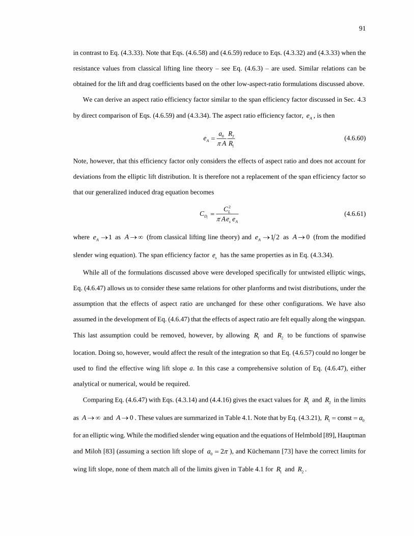
91

in contrast to Eq. (4.3.33). Note that Eqs. (4.6.58) and (4.6.59) reduce to Eqs. (4.3.32) and (4.3.33) when the

resistance values from classical lifting line theory – see Eq. (4.6.3) – are used. Similar relations can be

obtained for the lift and drag coefficients based on the other low-aspect-ratio formulations discussed above.

We can derive an aspect ratio efficiency factor similar to the span efficiency factor discussed in Sec. 4.3

by direct comparison of Eqs. (4.6.59) and (4.3.34). The aspect ratio efficiency factor, Ae , is then

0 2

1

Aea R

A R= (4.6.60)

Note, however, that this efficiency factor only considers the effects of aspect ratio and does not account for

deviations from the elliptic lift distribution. It is therefore not a replacement of the span efficiency factor so

that our generalized induced drag equation becomes

2

i

L

D

s A

C

Ae eC

= (4.6.61)

where 1Ae → as A→ (from classical lifting line theory) and 1 2Ae → as 0A→ (from the modified

slender wing equation). The span efficiency factor se has the same properties as in Eq. (4.3.34).

While all of the formulations discussed above were developed specifically for untwisted elliptic wings,

Eq. (4.6.47) allows us to consider these same relations for other planforms and twist distributions, under the

assumption that the effects of aspect ratio are unchanged for these other configurations. We have also

assumed in the development of Eq. (4.6.47) that the effects of aspect ratio are felt equally along the wingspan.

This last assumption could be removed, however, by allowing 1R and

2R to be functions of spanwise

location. Doing so, however, would affect the result of the integration so that Eq. (4.6.57) could no longer be

used to find the effective wing lift slope a. In this case a comprehensive solution of Eq. (4.6.47), either

analytical or numerical, would be required.

Comparing Eq. (4.6.47) with Eqs. (4.3.14) and (4.4.16) gives the exact values for 1R and

2R in the limits

as A→ and 0A→ . These values are summarized in Table 4.1. Note that by Eq. (4.3.21), 1 0constR a= =

for an elliptic wing. While the modified slender wing equation and the equations of Helmbold [89], Hauptman

and Miloh [83] (assuming a section lift slope of 0 2a = ), and Küchemann [73] have the correct limits for

wing lift slope, none of them match all of the limits given in Table 4.1 for 1R and

2R .

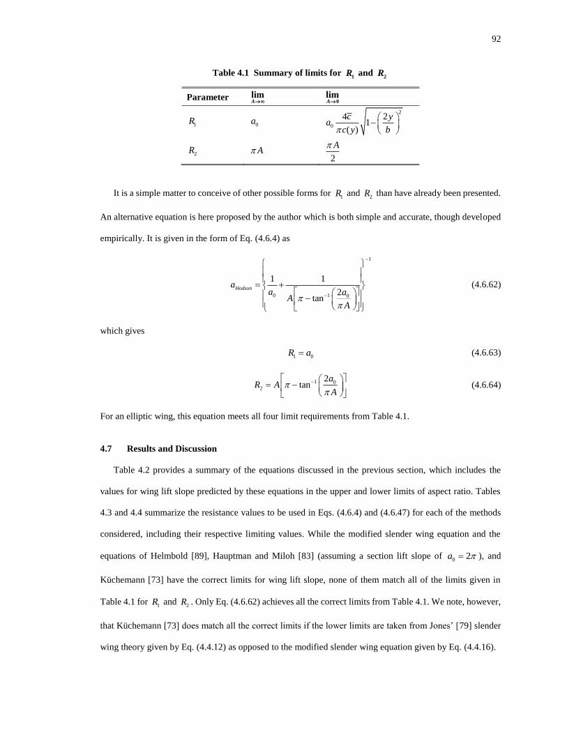
92

Table 4.1 Summary of limits for 1

R and 2

R

Parameter limA→

0

limA→

1R 0a

2

0

4 21

( )

c ya

c y b

−

2R A 2

A

It is a simple matter to conceive of other possible forms for 1R and

2R than have already been presented.

An alternative equation is here proposed by the author which is both simple and accurate, though developed

empirically. It is given in the form of Eq. (4.6.4) as

1

10 0

1 1

2tan

Hodsonaa a

AA

−

−

+

−

=

(4.6.62)

which gives

1 0R a= (4.6.63)

1 0

2

2tan

aR

AA

− =

−

(4.6.64)

For an elliptic wing, this equation meets all four limit requirements from Table 4.1.

4.7 Results and Discussion

Table 4.2 provides a summary of the equations discussed in the previous section, which includes the

values for wing lift slope predicted by these equations in the upper and lower limits of aspect ratio. Tables

4.3 and 4.4 summarize the resistance values to be used in Eqs. (4.6.4) and (4.6.47) for each of the methods

considered, including their respective limiting values. While the modified slender wing equation and the

equations of Helmbold [89], Hauptman and Miloh [83] (assuming a section lift slope of 0 2a = ), and

Küchemann [73] have the correct limits for wing lift slope, none of them match all of the limits given in

Table 4.1 for 1R and

2R . Only Eq. (4.6.62) achieves all the correct limits from Table 4.1. We note, however,

that Küchemann [73] does match all the correct limits if the lower limits are taken from Jones’ [79] slender

wing theory given by Eq. (4.4.12) as opposed to the modified slender wing equation given by Eq. (4.4.16).

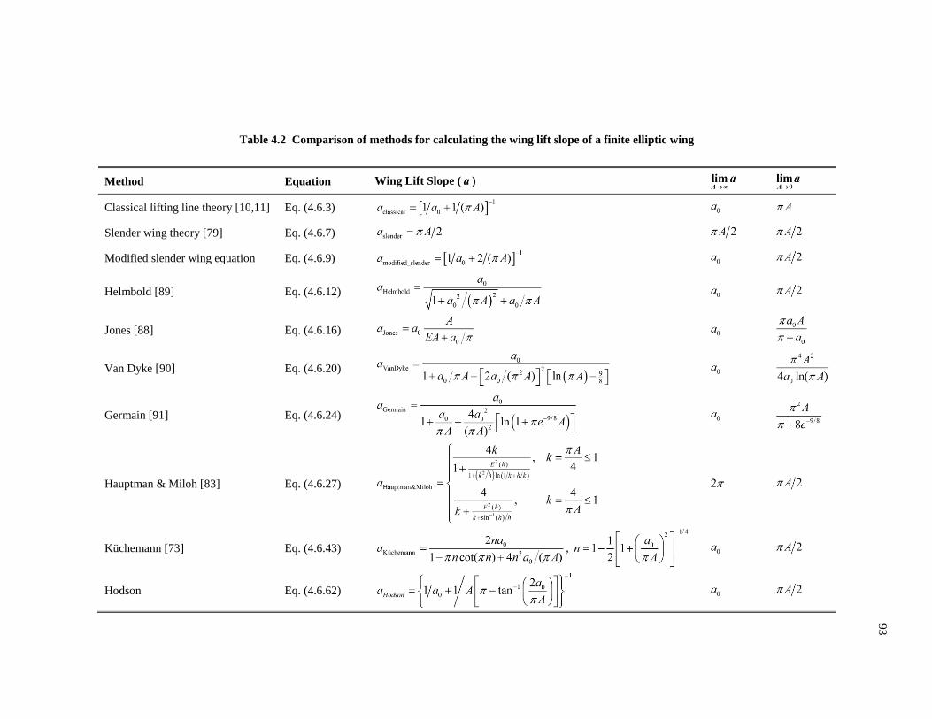
93

Table 4.2 Comparison of methods for calculating the wing lift slope of a finite elliptic wing

Method Equation Wing Lift Slope ( )

Classical lifting line theory [10,11] Eq. (4.6.3)

Slender wing theory [79] Eq. (4.6.7)

Modified slender wing equation Eq. (4.6.9)

Helmbold [89] Eq. (4.6.12)

Jones [88] Eq. (4.6.16)

Van Dyke [90] Eq. (4.6.20)

Germain [91] Eq. (4.6.24)

Hauptman & Miloh [83] Eq. (4.6.27)

Küchemann [73] Eq. (4.6.43) ,

Hodson Eq. (4.6.62)

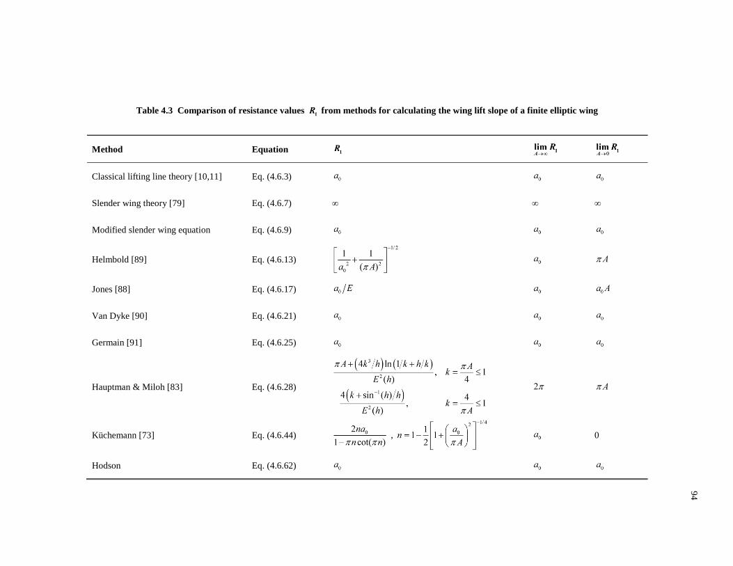
94

Table 4.3 Comparison of resistance values from methods for calculating the wing lift slope of a finite elliptic wing

Method Equation


Slender wing theory [79] Eq. (4.6.7) ∞ ∞ ∞


Helmbold [89] Eq. (4.6.13)

Jones [88] Eq. (4.6.17)

Van Dyke [90] Eq. (4.6.21)

Germain [91] Eq. (4.6.25)


Küchemann [73] Eq. (4.6.44) , 0

Hodson Eq. (4.6.62)

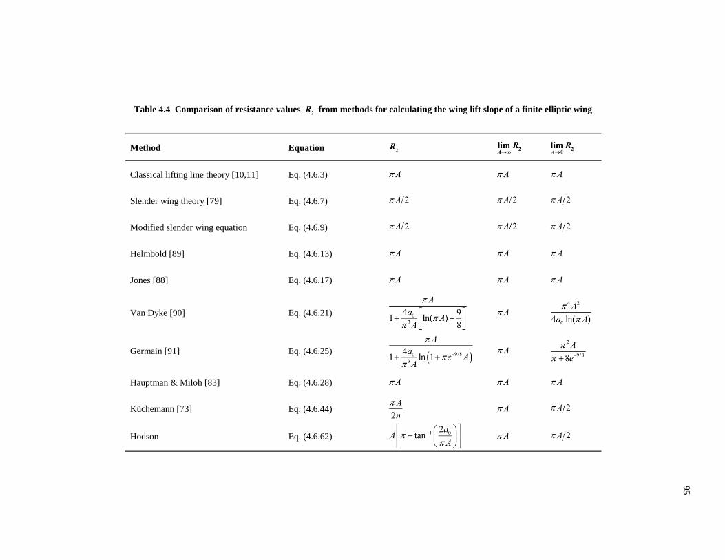
95

Table 4.4 Comparison of resistance values from methods for calculating the wing lift slope of a finite elliptic wing

Method Equation


Slender wing theory [79] Eq. (4.6.7)


Helmbold [89] Eq. (4.6.13)

Jones [88] Eq. (4.6.17)

Van Dyke [90] Eq. (4.6.21)

Germain [91] Eq. (4.6.25)


Küchemann [73] Eq. (4.6.44)

Hodson Eq. (4.6.62)

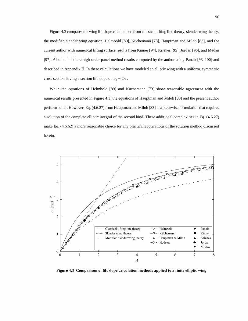
96

Figure 4.3 compares the wing lift slope calculations from classical lifting line theory, slender wing theory,

the modified slender wing equation, Helmbold [89], Küchemann [73], Hauptman and Miloh [83], and the

current author with numerical lifting surface results from Kinner [94], Krienes [95], Jordan [96], and Medan

[97]. Also included are high-order panel method results computed by the author using Panair [98–100] and

described in Appendix H. In these calculations we have modeled an elliptic wing with a uniform, symmetric

cross section having a section lift slope of 0 2a = .

While the equations of Helmbold [89] and Küchemann [73] show reasonable agreement with the

numerical results presented in Figure 4.3, the equations of Hauptman and Miloh [83] and the present author

perform better. However, Eq. (4.6.27) from Hauptman and Miloh [83] is a piecewise formulation that requires

a solution of the complete elliptic integral of the second kind. These additional complexities in Eq. (4.6.27)

make Eq. (4.6.62) a more reasonable choice for any practical applications of the solution method discussed

herein.

Figure 4.3 Comparison of lift slope calculation methods applied to a finite elliptic wing

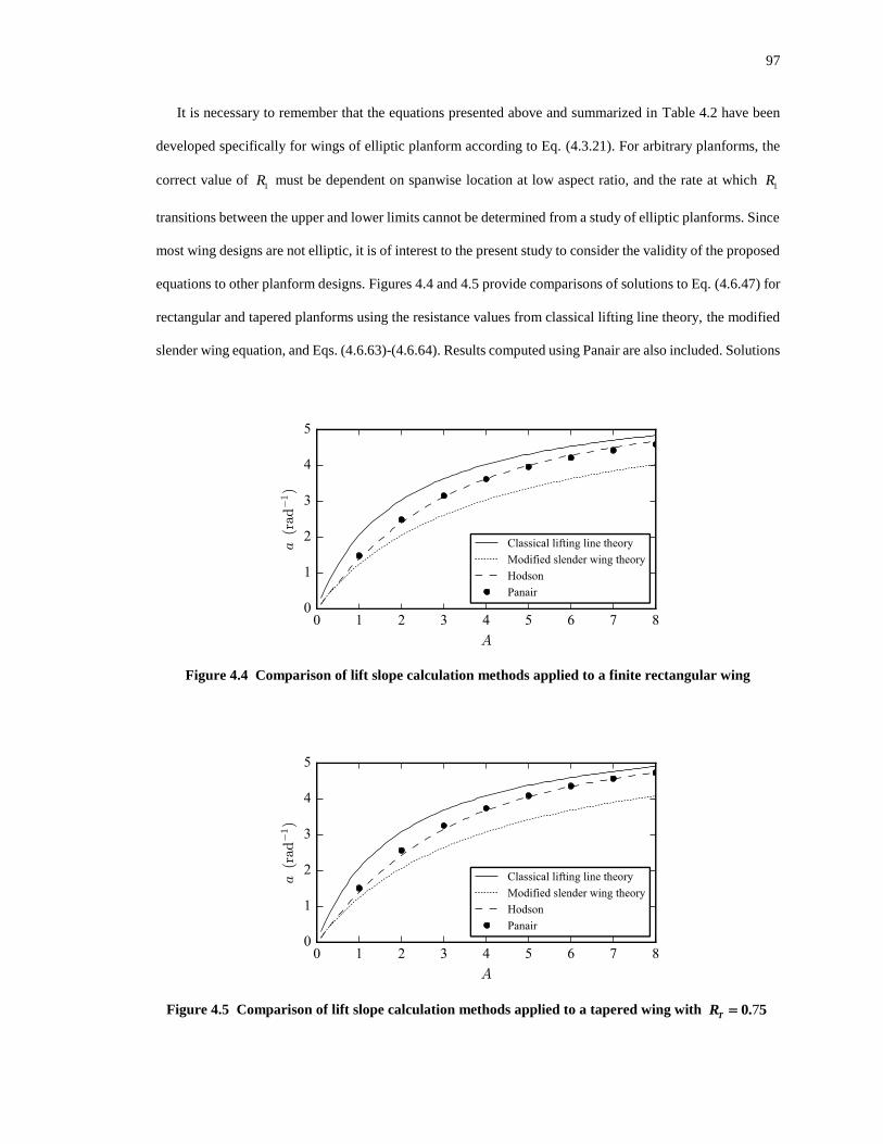
97

It is necessary to remember that the equations presented above and summarized in Table 4.2 have been

developed specifically for wings of elliptic planform according to Eq. (4.3.21). For arbitrary planforms, the

correct value of 1R must be dependent on spanwise location at low aspect ratio, and the rate at which

1R

transitions between the upper and lower limits cannot be determined from a study of elliptic planforms. Since

most wing designs are not elliptic, it is of interest to the present study to consider the validity of the proposed

equations to other planform designs. Figures 4.4 and 4.5 provide comparisons of solutions to Eq. (4.6.47) for

rectangular and tapered planforms using the resistance values from classical lifting line theory, the modified

slender wing equation, and Eqs. (4.6.63)-(4.6.64). Results computed using Panair are also included. Solutions

Figure 4.4 Comparison of lift slope calculation methods applied to a finite rectangular wing

Figure 4.5 Comparison of lift slope calculation methods applied to a tapered wing with 70. 5

TR =

98

to Eq. (4.6.47) were obtained using Pralines,* an open-source Fortran code developed by the author. This

code is based on the solution procedure presented by Phillips [53], in which Eq. (4.6.47) is approximated as

a truncated Fourier sine series. The source code is given in Appendix K.

Despite having been developed specifically for elliptic planforms, the proposed equation shows excellent

agreement with the Panair results for the rectangular and tapered planforms considered. It outperforms

classical lifting line theory over the full range of aspect ratios for both rectangular and tapered cases.

At this point we have only considered predictions of the total wing lift slope of a finite wing without

regard to the spanwise lift distribution. In fact the development presented here has assumed that the influence

of aspect ratio beyond that already captured in classical lifting line theory is felt uniformly along the

wingspan. Pralines can be used to scrutinize this assumption. For an elliptic wing, Eq. (4.6.47) predicts an

elliptic lift distribution (i.e. a constant section lift coefficient), regardless of the resistance values used. This

is shown and compared to Panair results in Figure 4.6 for a selection of aspect ratios. The results computed

using Eqs. (4.6.63) and (4.6.64) in Eq. (4.6.47) show good agreement with Panair results for / 0.4y b

regardless of aspect ratio. As expected, larger discrepancies are seen at the wing tips. However, the

magnitudes of the discrepancies shown in Figure 4.6 can be misleading since they are scaled

by the inverse of the chord length and the chord length goes to zero at the wing tip. Figure 4.7 shows the

same data but with the spanwise lift coefficients multiplied by the local chord ratio /c c , which more

accurately reflects the relative influence of each spanwise value on the overall wing lift coefficient. From

Figure 4.7 we see that the results computed using Eqs. (4.6.63) and (4.6.64) provide excellent agreement with

the Panair results over the entire wingspan. There is a slight outward shift of lift when compared to the Panair

results, but overall this shift is small – less than half a percent of the total lift generated by the wing.

Figures 4.8 and 4.9 compare lifting line theory and Panair results for rectangular and tapered planforms.

The lift coefficients have again been scaled by the local chord ratio /c c , as in Figure 4.7, to better visualize

the influence of the spanwise values on the overall lift generated by the wing. The lifting line results based

on the resistance values given by Eqs. (4.6.63) and (4.6.64) again do an excellent job of matching the Panair

results, though the discrepancies are slightly larger for rectangular and tapered wings than for elliptic wings.

* https://github.com/joddlehod/pralines

https://github.com/joddlehod/pralines

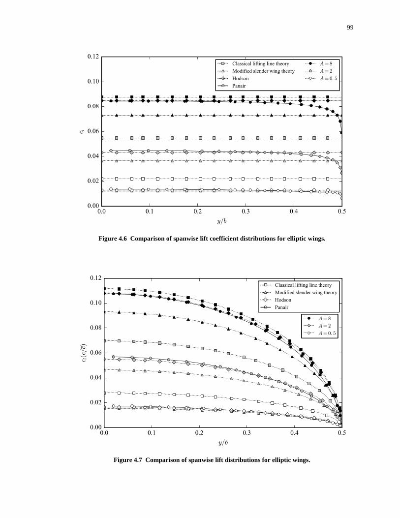
99

Figure 4.6 Comparison of spanwise lift coefficient distributions for elliptic wings.

Figure 4.7 Comparison of spanwise lift distributions for elliptic wings.

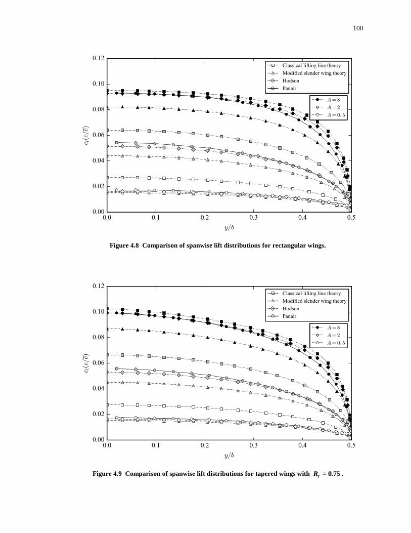
100

Figure 4.8 Comparison of spanwise lift distributions for rectangular wings.

Figure 4.9 Comparison of spanwise lift distributions for tapered wings with = 0.75

TR .

101

Finally, we wish to consider how the proposed lifting line formulation affects induced drag calculations.

Here we used the same codes, namely Pralines and Panair, to evaluate the lift and drag coefficients of several

wings of varying aspect ratios, and then apply Eq. (4.6.61) to compute the aspect ratio efficiency factor for

each analysis. These results, along with direct calculations of the aspect ratio efficiency factor using Eq.

(4.6.60), are presented in Figure 4.10.

Some difficulty was encountered in obtaining accurate drag results from Panair. In computing lift results,

we computed the solution on three different grid sizes and applied Richardson Extrapolation to improve the

accuracy of the results. This method could not be applied to the drag results, however, because the results

from successively refined grid sizes did not exhibit asymptotic convergence. Instead, each Panair data point

presented in Figure 4.10 was computed from a single Panair analysis using a 4%-thick symmetric Joukowski

Figure 4.10 Sample calculations of the aspect ratio efficiency factor using Pralines and Panair.

102

airfoil for the cross section and an 80 80 grid size. This, however, still did not yield satisfactory results.

The Panair data show an inverse trend in Ae to what is expected, indicating that as aspect ratio increases,

both e and

i increase. This would seem to violate the boundary condition given by Eq. (4.3.2), bringing

into question the validity of the drag calculations produced by Panair.

In contrast, the lifting line results shown in Figure 4.10 agree well with the theory presented in this

chapter. The results using classical lifting line theory give an aspect ratio efficiency factor of 1Ae =

regardless of aspect ratio, while the modified slender wing equation gives an aspect ratio efficiency factor of

1/ 2Ae = . These represent the theoretical upper and lower limits, respectively, of the aspect ratio efficiency

factor. The equation proposed by the present author – see Eqs. (4.6.62)-(4.6.64) – shows a smooth transition

between the two limits. While the shape of this transition cannot be confirmed due to the unreliability of the

Panair drag results, it can be assumed that the shape is reasonable as it satisfies the boundary condition given

by Eq. (4.3.2) and the corresponding lift values have already been shown to be satisfactory. Any alternative

would require the influence of an aerodynamic phenomenon that has not been considered here or in the other

works reviewed.

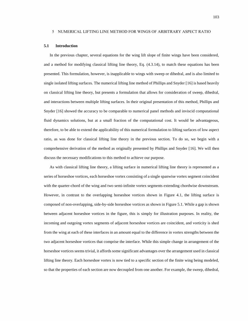
103

5 NUMERICAL LIFTING LINE METHOD FOR WINGS OF ARBITRARY ASPECT RATIO

5.1 Introduction

In the previous chapter, several equations for the wing lift slope of finite wings have been considered,

and a method for modifying classical lifting line theory, Eq. (4.3.14), to match these equations has been

presented. This formulation, however, is inapplicable to wings with sweep or dihedral, and is also limited to

single isolated lifting surfaces. The numerical lifting line method of Phillips and Snyder [16] is based heavily

on classical lifting line theory, but presents a formulation that allows for consideration of sweep, dihedral,

and interactions between multiple lifting surfaces. In their original presentation of this method, Phillips and

Snyder [16] showed the accuracy to be comparable to numerical panel methods and inviscid computational

fluid dynamics solutions, but at a small fraction of the computational cost. It would be advantageous,

therefore, to be able to extend the applicability of this numerical formulation to lifting surfaces of low aspect

ratio, as was done for classical lifting line theory in the previous section. To do so, we begin with a

comprehensive derivation of the method as originally presented by Phillips and Snyder [16]. We will then

discuss the necessary modifications to this method to achieve our purpose.

As with classical lifting line theory, a lifting surface in numerical lifting line theory is represented as a

series of horseshoe vortices, each horseshoe vortex consisting of a single spanwise vortex segment coincident

with the quarter-chord of the wing and two semi-infinite vortex segments extending chordwise downstream.

However, in contrast to the overlapping horseshoe vortices shown in Figure 4.1, the lifting surface is

composed of non-overlapping, side-by-side horseshoe vortices as shown in Figure 5.1. While a gap is shown

between adjacent horseshoe vortices in the figure, this is simply for illustration purposes. In reality, the

incoming and outgoing vortex segments of adjacent horseshoe vortices are coincident, and vorticity is shed

from the wing at each of these interfaces in an amount equal to the difference in vortex strengths between the

two adjacent horseshoe vortices that comprise the interface. While this simple change in arrangement of the

horseshoe vortices seems trivial, it affords some significant advantages over the arrangement used in classical

lifting line theory. Each horseshoe vortex is now tied to a specific section of the finite wing being modeled,

so that the properties of each section are now decoupled from one another. For example, the sweep, dihedral,

104

Figure 5.1 Discrete system of side-by-side horseshoe vortices on a finite wing.

and section lift slope (0a ) can all be specified individually for each section of the wing. In classical lifting

line theory, where the largest horseshoe vortex spans from wing tip to wing tip, each of these values is

required to be constant over the entire wing.

The fundamental problem we must solve with this new arrangement is the same as that of classical lifting

line theory – namely, to determine the vortex strengths ( )y such that the boundary condition of Eq. (4.3.1)

is satisfied. We shall follow the same general development as was done for classical lifting line theory, but

using a more general three-dimensional formulation due to the new arrangement of horseshoe vortices. This

complete development can be found in its original form in Phillips and Snyder [16]. We shall then consider

how the low aspect ratio modifications presented in the previous chapter can be applied to this numerical

method. Finally, we shall compare results from the modified method with those of other approaches.

5.2 The Phillips and Snyder Numerical Lifting Line Method

Consider the arbitrary vortex segment OR shown in Figure 5.2. Let l be the vector from point O to point

R, and consider the vortex element dl located at point Q. The velocity induced at point P by this differential

vortex element is given by the Biot-Savart law,

34 r

= dl r

dV (5.2.1)

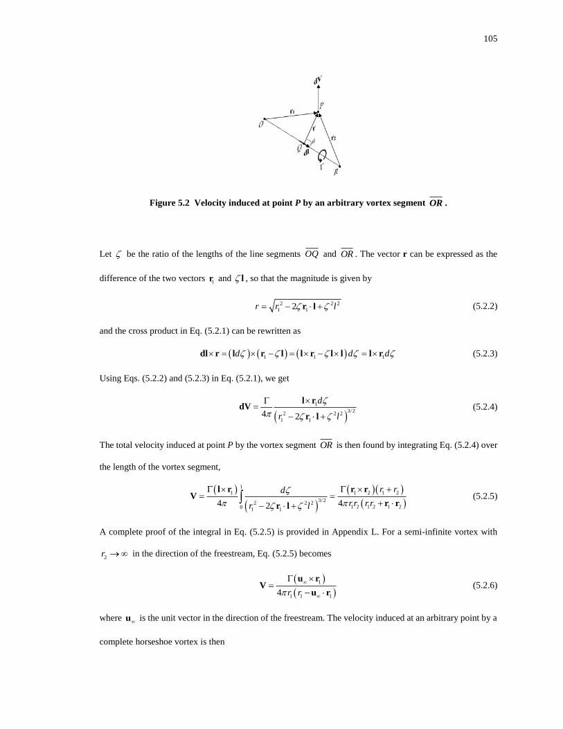
105

Figure 5.2 Velocity induced at point P by an arbitrary vortex segment OR .

Let be the ratio of the lengths of the line segments OQ and OR . The vector r can be expressed as the

difference of the two vectors r and l , so that the magnitude is given by

2 2 2

1 12r r l = − +lr (5.2.2)

and the cross product in Eq. (5.2.1) can be rewritten as

( ) ( ) ( )1 1 1d d d = − = − = dl r l r l l r l l l r (5.2.3)

Using Eqs. (5.2.2) and (5.2.3) in Eq. (5.2.1), we get

( )1

3/22 2 2

1 14 2

d

r l

=

−

+

l rd

rV

l (5.2.4)

The total velocity induced at point P by the vortex segment OR is then found by integrating Eq. (5.2.4) over

the length of the vortex segment,

( )

( )

( )( )

( )2

1

1 1 2 1 2

3/22 2 2

1 2 1 2 10 1 14 42

rd

r r

r

rr l r

+= =

+− +

r

Vl

l r r

r r r (5.2.5)

A complete proof of the integral in Eq. (5.2.5) is provided in Appendix L. For a semi-infinite vortex with

2r → in the direction of the freestream, Eq. (5.2.5) becomes

( )

( )1

1 1 14 r r

=

− V

u

u

r

r (5.2.6)

where u is the unit vector in the direction of the freestream. The velocity induced at an arbitrary point by a

complete horseshoe vortex is then

106

( )

( )

( )( )

( )

( )

( )2 1 2 1 2 1

2 2 2 1 2 1 2 1 2 1 1 14

r r

r r r r r r r r

+ = + −

− + −

u r r r u rV

u r r r u r (5.2.7)

where 1r and

2r are now the vectors from the two corner points of the horseshoe vortex to the arbitrary point.

Now consider the discrete system of horseshoe vortices used to represent a finite wing as shown in Figure

5.1. A control point placed anywhere along the quarter-chord of the wing (i.e. the lifting line) will experience

an induced velocity due to each horseshoe vortex according to Eq. (5.2.7). The induced downwash vector at

the control point by a system of n horseshoe vortices is then given by

( )( )

( )( )( )

( )( )

2 1 2 1 2 1

2 2 2 1 2 1 2 1 2 1 1 11 4

j j j j j jj

j j

n

j j j j j j j j j j

i

j

r r

r r r r r r r r

=

+ = + −

− +

−

u r r r u rw

u r r r u r (5.2.8)

where 1jr and 2jr are the vectors from the two corner points of the jth horseshoe vortex to the control point.

The velocity vector at the control point can now be expressed as the sum of the freestream velocity and the

induced downwash, namely

i= +V V w (5.2.9)

Note that the middle term within the square brackets of Eq. (5.2.8) is indeterminate when the angle

between 1jr and 2jr is g180de . However, this condition is only satisfied when the control point lies exactly

on the axis of the vortex. Since the velocity induced by a straight vortex segment along its axis is zero, the

appropriate value for this term is zero anytime 1jr and 2jr are coaxial.

In the development of classical lifting line theory, Prandtl [10,11] used the Kutta-Joukowski theorem

given by Eq. (4.3.10) to relate the lift force to the circulation for any spanwise section of the wing. Phillips

and Snyder [16] take a similar approach, but use the more general three-dimensional vortex lifting law (see

Saffman [101]). This can be written for a differential segment dl of the lifting line as

= V dldF (5.2.10)

Following Prandtl’s development of classical lifting line theory, we can equate the magnitude of this

spanwise differential force to the lift predicted by 2D airfoil theory, namely

2

0

1

2eV a dS =dF (5.2.11)

where

107

1tan n

e

a

− =

V u

V u (5.2.12)

is the effective angle of attack, nu is the unit vector normal to the local airfoil chord, and

au is the unit

vector aligned axially with the local airfoil chord. Both vectors nu and

au lie within the section plane.

Equating the right hand sides of Eqs. (5.2.10) and (5.2.11) gives

2

0

1

2eV a dS =V dl (5.2.13)

Expressed in this form, Eq. (5.2.13) is a single equation with n unknowns, namely the vorticities 1,2,...,n

for each horseshoe vortex. The control point, since it has been constrained to lie along the lifting line, also

lies along the axis of one of the n horseshoe vortices. The values of the parameters , V , dl , e , and dS

in Eq. (5.2.13) are associated with the wing section and corresponding horseshoe vortex along which the

control point lies. By placing a control point on each of the n horseshoe vortices and writing Eq. (5.2.13) for

each control point, we generate a system of n nonlinear equations in n unknowns that can be solved using an

iterative root-finding algorithm such as the Newton-Raphson method.

In Secs. 4.3 and 4.6, we were able to develop closed-form relations for the lift and drag coefficients of

wings with elliptic lift distributions. Development of similar equations using the numerical formulation of

Phillips and Snyder [16] is not straightforward due to the discrete summation and the vector notation used in

the formulation. Instead, a solver that implements this method can compute the resultant force vector at each

control point and then compute a vector sum the forces over the wing. Lift and drag components relative to

the freestream can then be computed using the vector dot product.

In the original paper by Phillips and Snyder [16], results using this method are shown to be equivalent to

those of classical lifting line theory for straight elliptic wings of various aspect ratios. Additionally, results

are shown to be in good agreement with experimental and high-order numerical results for straight wings,

wings with sweep, and wings with dihedral. However, in all comparisons the aspect ratios are greater than 4.

Figure 5.3 compares wing lift slope results computed using the numerical lifting line method of Phillips and

Snyder with results from classical lifting line theory and a vortex panel method. Solutions to the numerical

lifting line method were computed using MachUp (see Sec. 2.6.1) with 100 nodes per semispan and a section

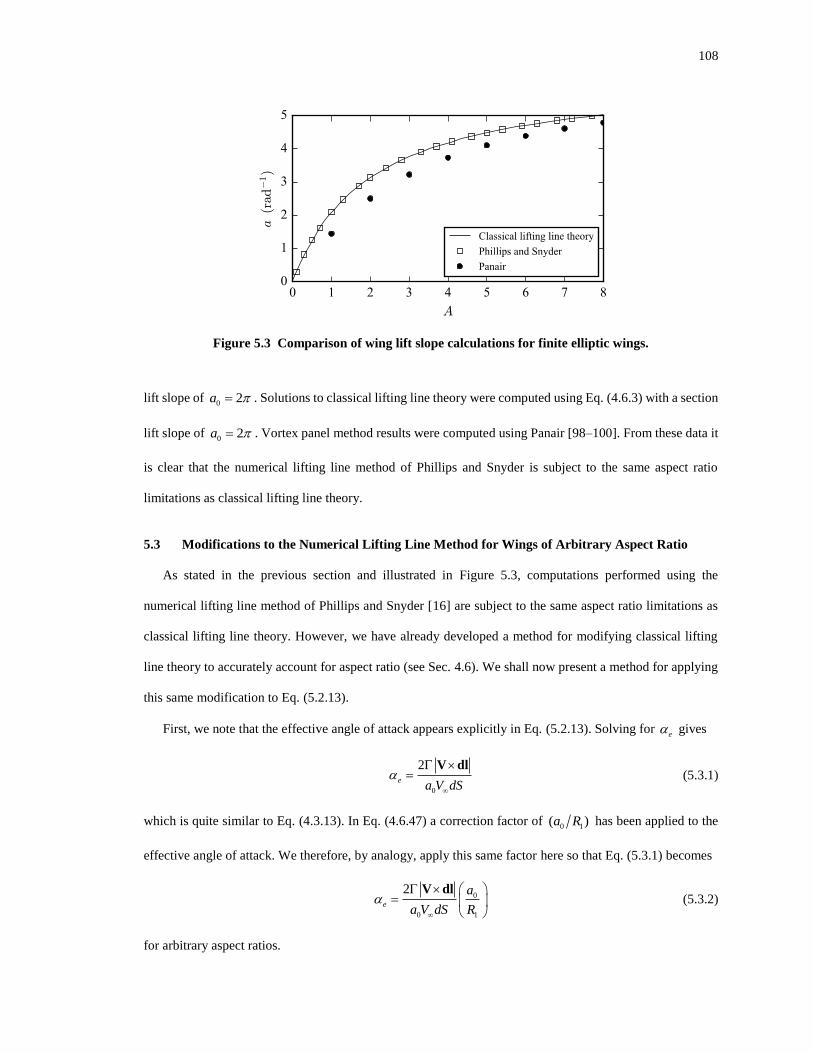
108

Figure 5.3 Comparison of wing lift slope calculations for finite elliptic wings.

lift slope of 0 2a = . Solutions to classical lifting line theory were computed using Eq. (4.6.3) with a section

lift slope of 0 2a = . Vortex panel method results were computed using Panair [98–100]. From these data it

is clear that the numerical lifting line method of Phillips and Snyder is subject to the same aspect ratio

limitations as classical lifting line theory.

5.3 Modifications to the Numerical Lifting Line Method for Wings of Arbitrary Aspect Ratio

As stated in the previous section and illustrated in Figure 5.3, computations performed using the

numerical lifting line method of Phillips and Snyder [16] are subject to the same aspect ratio limitations as

classical lifting line theory. However, we have already developed a method for modifying classical lifting

line theory to accurately account for aspect ratio (see Sec. 4.6). We shall now present a method for applying

this same modification to Eq. (5.2.13).

First, we note that the effective angle of attack appears explicitly in Eq. (5.2.13). Solving for e gives

0

2e

a V dS

=

lV d (5.3.1)

which is quite similar to Eq. (4.3.13). In Eq. (4.6.47) a correction factor of 0 1( )a R has been applied to the

effective angle of attack. We therefore, by analogy, apply this same factor here so that Eq. (5.3.1) becomes

0

0 1

2e

a

a V dS R

=

V dl (5.3.2)

for arbitrary aspect ratios.

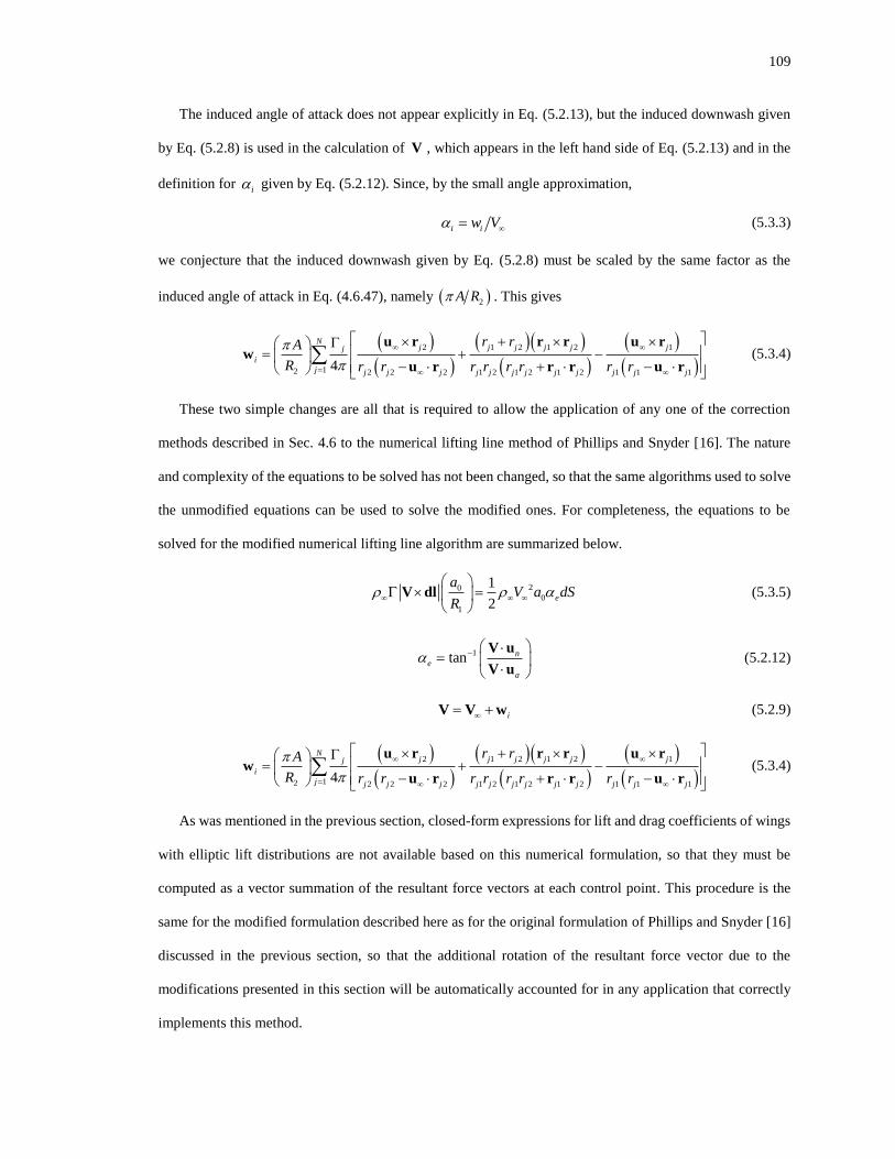
109

The induced angle of attack does not appear explicitly in Eq. (5.2.13), but the induced downwash given

by Eq. (5.2.8) is used in the calculation of V , which appears in the left hand side of Eq. (5.2.13) and in the

definition for i given by Eq. (5.2.12). Since, by the small angle approximation,

i iw V = (5.3.3)

we conjecture that the induced downwash given by Eq. (5.2.8) must be scaled by the same factor as the

induced angle of attack in Eq. (4.6.47), namely ( )2A R . This gives

( )( )

( )( )( )

( )( )

2 1 2 1 2 1

2 2 2 2 1 2 1 2 1 2 1 1 11 4

j j j j j jj

j j j j j j j

i

j j j j j

N

j

r r

R r r r r r r r r

A

=

+ = + −

− + −

u r r r u rw

u r r r u r (5.3.4)

These two simple changes are all that is required to allow the application of any one of the correction

methods described in Sec. 4.6 to the numerical lifting line method of Phillips and Snyder [16]. The nature

and complexity of the equations to be solved has not been changed, so that the same algorithms used to solve

the unmodified equations can be used to solve the modified ones. For completeness, the equations to be

solved for the modified numerical lifting line algorithm are summarized below.

20

0

1

1

2eV

a

Ra dS

=

V dl (5.3.5)

1tan n

e

a

− =

V u

V u (5.2.12)

i= +V V w (5.2.9)

( )( )

( )( )( )

( )( )

2 1 2 1 2 1

2 2 2 2 1 2 1 2 1 2 1 1 11 4

j j j j j jj

j j j j j j j

i

j j j j j

N

j

r r

R r r r r r r r r

A

=

+ = + −

− + −

u r r r u rw

u r r r u r (5.3.4)

As was mentioned in the previous section, closed-form expressions for lift and drag coefficients of wings

with elliptic lift distributions are not available based on this numerical formulation, so that they must be

computed as a vector summation of the resultant force vectors at each control point. This procedure is the

same for the modified formulation described here as for the original formulation of Phillips and Snyder [16]

discussed in the previous section, so that the additional rotation of the resultant force vector due to the

modifications presented in this section will be automatically accounted for in any application that correctly

implements this method.

110

5.4 Results and Discussion

In order to evaluate the effectiveness of the modifications described above, the MachUp source code has

been modified to include these changes, and an additional parameter has been added to the input file format

to allow selection of the resistance values to be used in an analysis. Figure 5.4 shows a comparison of wing

lift slopes computed using this modified version of MachUp with the analytical solutions from Chapter 4 for

classical lifting line theory, the modified slender wing equation, and Eqs. (4.6.63)-(4.6.64). Results computed

using Panair are also included.

The numerical model for these calculations was composed of 100 spanwise sections for one semispan

with a symmetry boundary condition at the wing root. The uniform cross section was modeled as a thin

symmetric airfoil with 0 2a = . The iterative nonlinear solver was used with a convergence tolerance of

1010−. With these settings, the numerical results agree with the analytical results to at least four digits of

precision. Additionally, the differences between the Panair results and the numerical results based on the

formulation proposed by the present author are less than 1% for A ≥ 1.

Figure 5.4 Comparison of analytical and numerical calculations for wing lift slope of elliptic wings.

111

Figures 5.5-5.7 compare the lift distributions for elliptic, rectangular, and tapered planforms predicted by

the modified MachUp code to those predicted by Panair. The results are essentially identical to the analytical

results shown in Figures 4.7-4.9. From these data we conclude that the modified equations described in Sec.

5.3 are the numerical equivalent to the analytical lifting line formulation given in Eq. (4.6.47).

This work has considered only isolated wings with no sweep; no geometric or aerodynamic twist; no

dihedral; and only elliptic, rectangular, and tapered planforms. The formulation given in Sec. 5.3, however,

is not limited to any of these constraints. Previous publications (see Refs. [12–14]) have applied the numerical

lifting line algorithm described in Sec.5.2 to a variety of other wing designs with reasonable success. While

beyond the scope of the present work, it is expected that the proposed method can produce useful results for

arbitrary wing designs.

Figure 5.8 shows aspect ratio efficiency factors computed using MachUp and Panair. The Panair results

were discussed in Sec. 4.7. The MachUp results are equivalent to the Pralines results shown in Figure 4.10.

This provides added confidence in the derivations leading to Eq. (4.6.59) since that equation is used directly

to calculate drag in Pralines but not in MachUp.

Figure 5.5 Comparison of spanwise lift distributions for elliptic wings.

112

Figure 5.6 Comparison of spanwise lift distributions for rectangular wings.

Figure 5.7 Comparison of spanwise lift distributions for tapered wings with = 0.75

TR .

113

Figure 5.8 Sample calculations of the aspect ratio efficiency factor using MachUp and Panair.

In 2017, Hodson et al. [102] presented wind tunnel data for several subscale test articles of the variable-

camber compliant wing (VCCW) developed at the U.S. Air Force Research Laboratory (AFRL). For a

description of the VCCW, see Refs. [5,6]. Of particular interest here is the aspect ratio of the VCCW – 3A =

– which falls below the generally accepted range of validity for classical lifting line theory. The data

presented by Hodson et al. [102] includes lift, drag, and pitching moment coefficients as functions of angle

of attack for five subscale test articles generated from 3D scans of the VCCW in various morphed

configurations, as well as three test articles generated from 3D CAD models with uniform NACA 0010,

2410, and 8410 airfoil cross-sections. For a description of each test article, see Ref. [102].

In order to compare numerical results generated with MachUp to the Hodson et al. [102] experimental

data, an airfoil database needed to be created containing airfoil coefficients for the different cross sections in

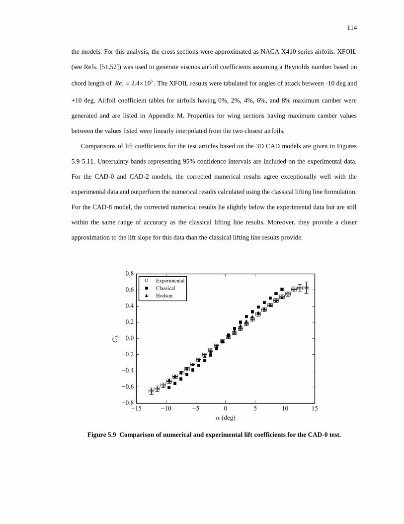
114

the models. For this analysis, the cross sections were approximated as NACA X410 series airfoils. XFOIL

(see Refs. [51,52]) was used to generate viscous airfoil coefficients assuming a Reynolds number based on

chord length of 52. 04 1cRe = . The XFOIL results were tabulated for angles of attack between -10 deg and

+10 deg. Airfoil coefficient tables for airfoils having 0%, 2%, 4%, 6%, and 8% maximum camber were

generated and are listed in Appendix M. Properties for wing sections having maximum camber values

between the values listed were linearly interpolated from the two closest airfoils.

Comparisons of lift coefficients for the test articles based on the 3D CAD models are given in Figures

5.9-5.11. Uncertainty bands representing 95% confidence intervals are included on the experimental data.

For the CAD-0 and CAD-2 models, the corrected numerical results agree exceptionally well with the

experimental data and outperform the numerical results calculated using the classical lifting line formulation.

For the CAD-8 model, the corrected numerical results lie slightly below the experimental data but are still

within the same range of accuracy as the classical lifting line results. Moreover, they provide a closer

approximation to the lift slope for this data than the classical lifting line results provide.

Figure 5.9 Comparison of numerical and experimental lift coefficients for the CAD-0 test.

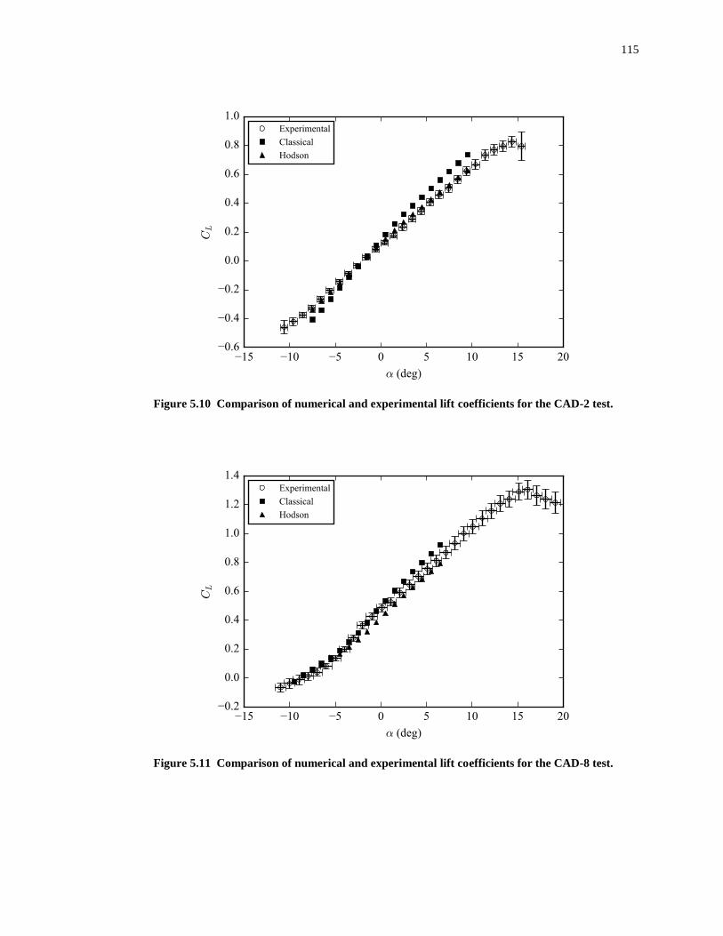
115



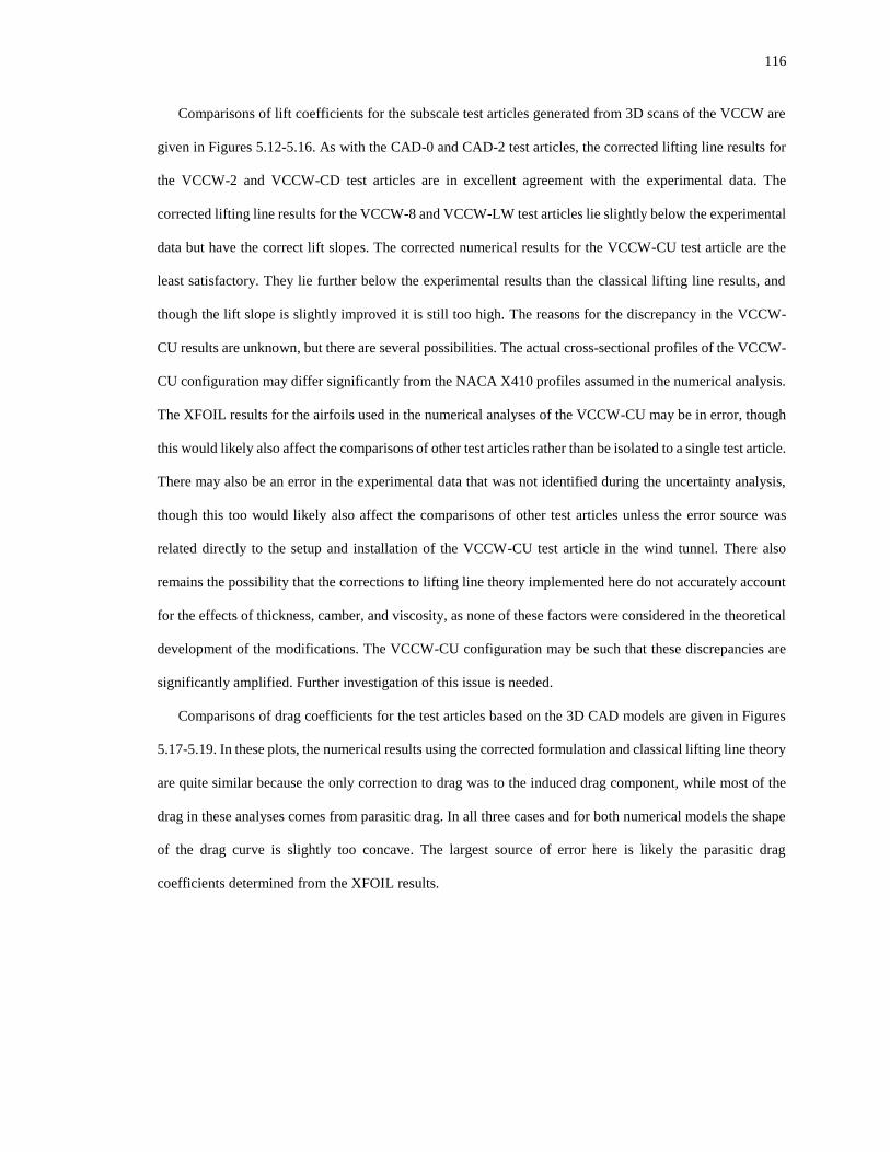
116

Comparisons of lift coefficients for the subscale test articles generated from 3D scans of the VCCW are

given in Figures 5.12-5.16. As with the CAD-0 and CAD-2 test articles, the corrected lifting line results for

the VCCW-2 and VCCW-CD test articles are in excellent agreement with the experimental data. The

corrected lifting line results for the VCCW-8 and VCCW-LW test articles lie slightly below the experimental

data but have the correct lift slopes. The corrected numerical results for the VCCW-CU test article are the

least satisfactory. They lie further below the experimental results than the classical lifting line results, and

though the lift slope is slightly improved it is still too high. The reasons for the discrepancy in the VCCW-

CU results are unknown, but there are several possibilities. The actual cross-sectional profiles of the VCCW-

CU configuration may differ significantly from the NACA X410 profiles assumed in the numerical analysis.

The XFOIL results for the airfoils used in the numerical analyses of the VCCW-CU may be in error, though

this would likely also affect the comparisons of other test articles rather than be isolated to a single test article.

There may also be an error in the experimental data that was not identified during the uncertainty analysis,

though this too would likely also affect the comparisons of other test articles unless the error source was

related directly to the setup and installation of the VCCW-CU test article in the wind tunnel. There also

remains the possibility that the corrections to lifting line theory implemented here do not accurately account

for the effects of thickness, camber, and viscosity, as none of these factors were considered in the theoretical

development of the modifications. The VCCW-CU configuration may be such that these discrepancies are

significantly amplified. Further investigation of this issue is needed.

Comparisons of drag coefficients for the test articles based on the 3D CAD models are given in Figures

5.17-5.19. In these plots, the numerical results using the corrected formulation and classical lifting line theory

are quite similar because the only correction to drag was to the induced drag component, while most of the

drag in these analyses comes from parasitic drag. In all three cases and for both numerical models the shape

of the drag curve is slightly too concave. The largest source of error here is likely the parasitic drag

coefficients determined from the XFOIL results.

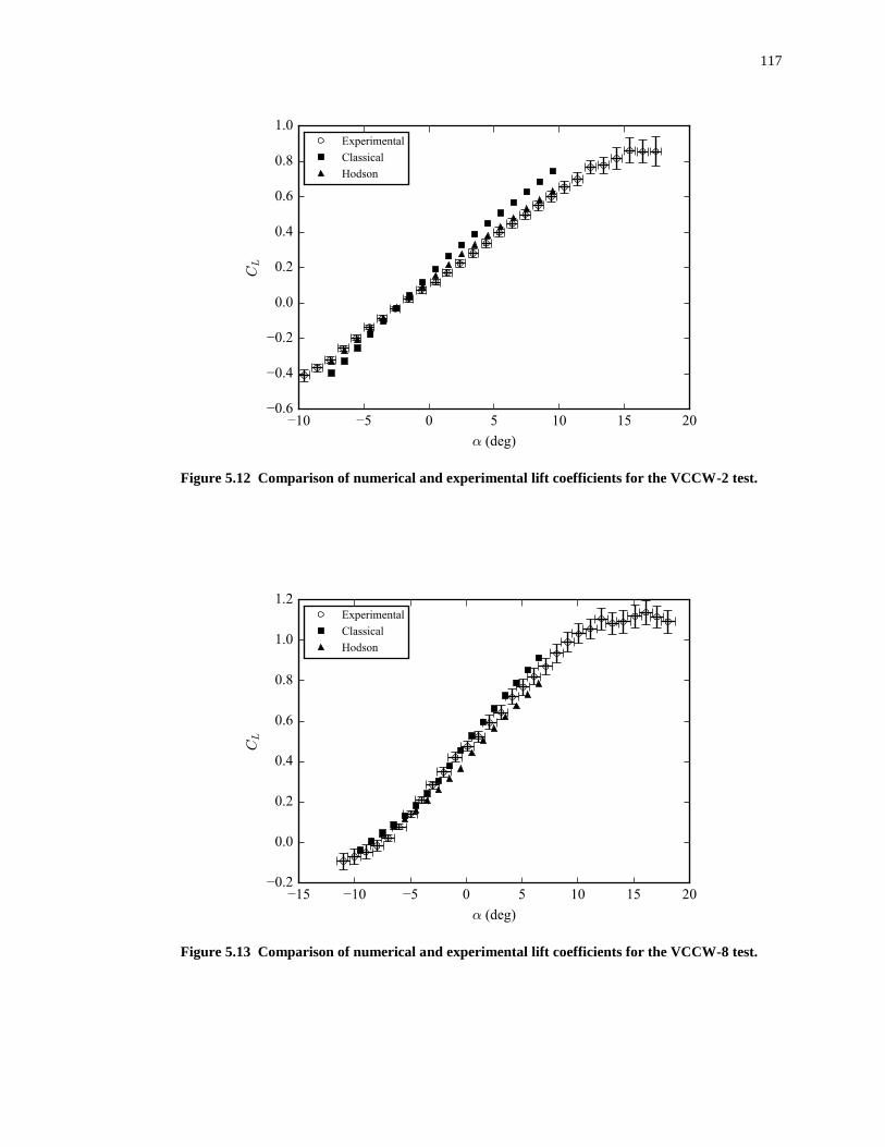
117

Figure 5.12 Comparison of numerical and experimental lift coefficients for the VCCW-2 test.

Figure 5.13 Comparison of numerical and experimental lift coefficients for the VCCW-8 test.

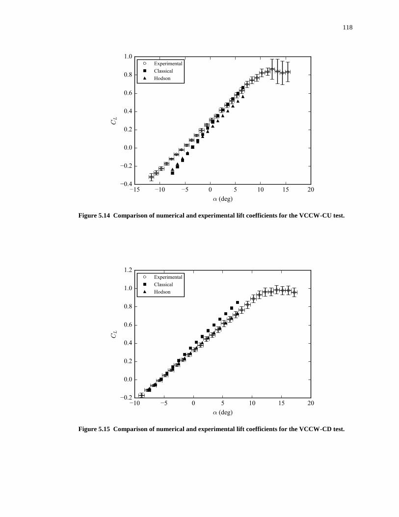
118

Figure 5.14 Comparison of numerical and experimental lift coefficients for the VCCW-CU test.

Figure 5.15 Comparison of numerical and experimental lift coefficients for the VCCW-CD test.

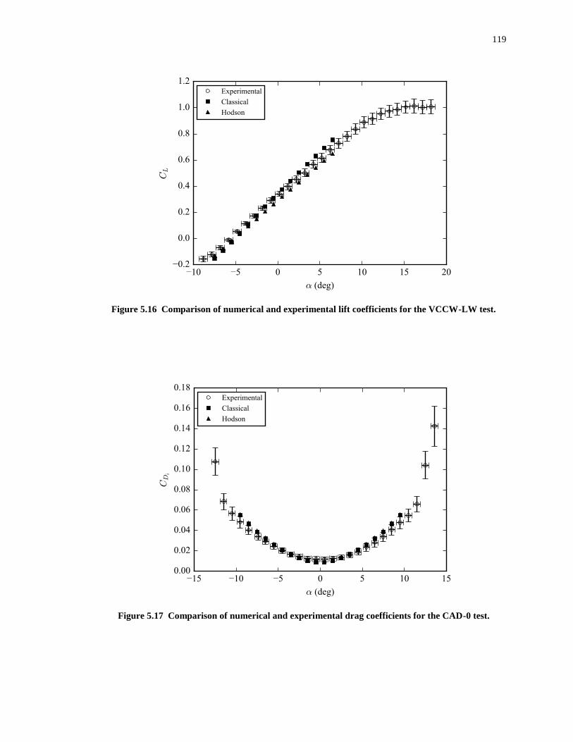
119

Figure 5.16 Comparison of numerical and experimental lift coefficients for the VCCW-LW test.

Figure 5.17 Comparison of numerical and experimental drag coefficients for the CAD-0 test.

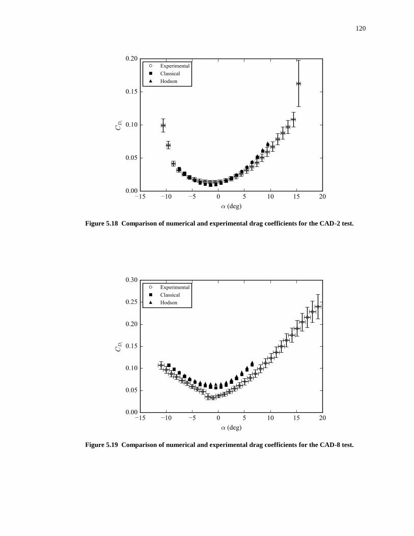
120



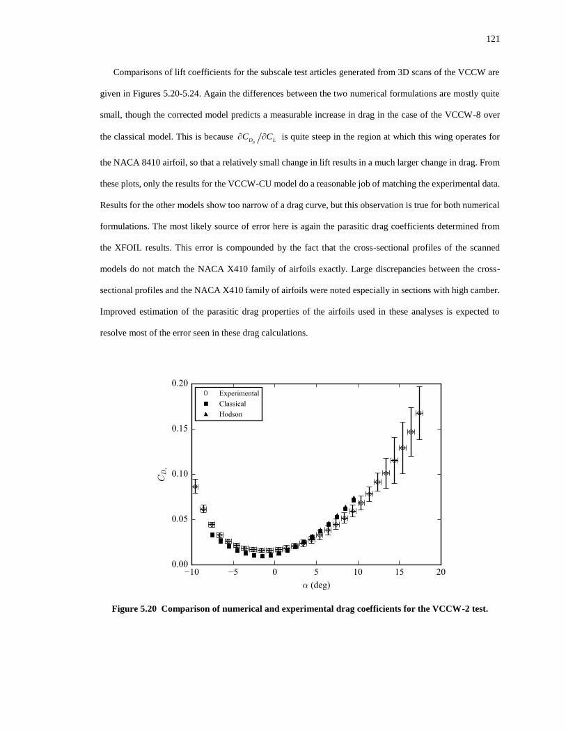
121

Comparisons of lift coefficients for the subscale test articles generated from 3D scans of the VCCW are

given in Figures 5.20-5.24. Again the differences between the two numerical formulations are mostly quite

small, though the corrected model predicts a measurable increase in drag in the case of the VCCW-8 over

the classical model. This is because pD LC C is quite steep in the region at which this wing operates for

the NACA 8410 airfoil, so that a relatively small change in lift results in a much larger change in drag. From

these plots, only the results for the VCCW-CU model do a reasonable job of matching the experimental data.

Results for the other models show too narrow of a drag curve, but this observation is true for both numerical

formulations. The most likely source of error here is again the parasitic drag coefficients determined from

the XFOIL results. This error is compounded by the fact that the cross-sectional profiles of the scanned

models do not match the NACA X410 family of airfoils exactly. Large discrepancies between the cross-

sectional profiles and the NACA X410 family of airfoils were noted especially in sections with high camber.

Improved estimation of the parasitic drag properties of the airfoils used in these analyses is expected to

resolve most of the error seen in these drag calculations.

Figure 5.20 Comparison of numerical and experimental drag coefficients for the VCCW-2 test.

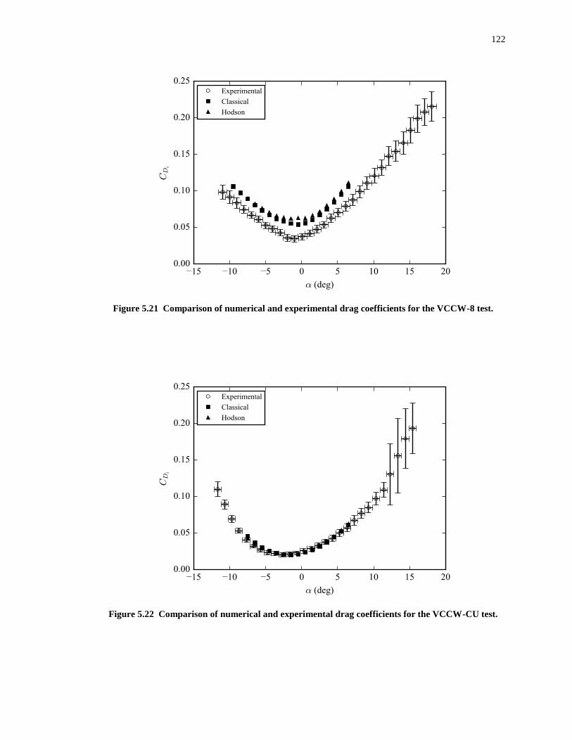
122

Figure 5.21 Comparison of numerical and experimental drag coefficients for the VCCW-8 test.

Figure 5.22 Comparison of numerical and experimental drag coefficients for the VCCW-CU test.

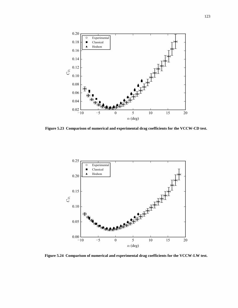
123

Figure 5.23 Comparison of numerical and experimental drag coefficients for the VCCW-CD test.

Figure 5.24 Comparison of numerical and experimental drag coefficients for the VCCW-LW test.

124

6 SUMMARY AND CONCLUSIONS

In this work, several limitations on analysis relative to wing shape optimization have been addressed.

First, an efficient method for computing gradients with respect to design parameters in an aerodynamic

analysis has been presented and integrated into MachUp, an open-source aerodynamic analysis tool based on

a numerical lifting line method. The gradients are computed automatically using DNAD, a forward-mode

automatic differentiation package that allows derivatives with respect to multiple input parameters to be

computed in a single run. The DNAD module was integrated into the MachUp source code in such a way

that inclusion or exclusion of the DNAD module can be controlled entirely at compile-time. In this way, the

integration of the DNAD module does not affect the performance of MachUp when derivatives are not

needed, and source code modifications are not required to convert between gradient-capable and non-

gradient-capable versions of the code. To the author’s knowledge, this is the first time this type of integration

has been achieved with a practical engineering analysis tool.

Second, a process and suite of tools for performing efficient wing shape optimization has been presented

and demonstrated. Optix, an open-source optimization framework that allows objective function evaluations

to be run in parallel across available resources, was described in Sec. 3.2 and the source code is listed in

Appendix F. Optix is written entirely in Python and is therefore cross-platform, easy to interface with, and

easily customizable to a wide range of optimization problems. Its most significant features include the ability

to execute independent function evaluations in parallel and to perform quadratic line-searching, both of which

have the potential to significantly reduce the time required for complex optimization problems. It can also

leverage automatic differentiation capabilities within objective functions to expedite efficient gradient

calculations. Currently, constraints must be enforced through use of the penalty function method, and global

minimization of non-convex design spaces cannot be guaranteed without the use of an outer wrapper

implementing a globally convergent optimization method. These two limitations represent the primary areas

of focus for future work in improving and expanding the capabilities of Optix.

Optix and MachUp were used together to solve several inviscid wing shape optimization problems with

known solutions, and the solutions were shown to converge toward the correct solution as the number of

degrees of freedom was increased. Solutions to several viscous wing shape optimization problems were also

solved using this method.

125

The most significant source of error in the viscous results lies in the aerodynamic properties of the airfoils

and the interpolation scheme used for determining aerodynamic properties of intermediate airfoils. Note that

this is a problem with the data input to the analysis, however, and not a problem with the analysis tools

themselves or the underlying methodology. Improving the accuracy of the airfoil aerodynamic properties and

improving the interpolation scheme used for intermediate airfoils should provide the greatest improvement

to the accuracy of these results.

Perhaps the most useful product of the optimization work presented in Chapter 3 is the contour plot shown

in Figure 3.7. Using high-fidelity analysis tools such as CFD for wing shape optimization is not only

computationally prohibitive but also precludes the ability to visualize the design and configuration space of

a morphing wing. In this work, we have demonstrated a method for rapidly visualizing the design and

configuration space of a finite morphing wing using MachUp. Figure 3.7 illustrates important relationships

between lift, induced drag, and parasitic drag and demonstrates how changes in a finite wing design can

impact these performance characteristics. The ability demonstrated here to quickly visualize and explore the

design and configuration space of a morphing wing is a significant enabler in the push to develop advanced

morphing wing technologies.

Although Chapter 3 only considered optimization of planform, geometric twist, and aerodynamic twist

on a straight wing, the tools presented can be used to evaluate and optimize geometries of multiple interacting

lifting surfaces as well as wings with more complex geometries. Examples of interacting lifting surfaces

include the interaction of main wings and stabilizers, wings in formation, wings with winglets, and wings in

ground effect. Due to modern composite manufacturing methods, very complex wing shapes can be designed

and manufactured. The tools presented in this work can be used to optimize these complex wing designs in

both single- and multi-wing systems.

Finally, development of new analytical and numerical formulations of lifting line theory have been

presented. These formulations are based heavily on the classical lifting line theory of Prandtl [10,11] and the

numerical lifting line method of Phillips and Snyder [16], but also draw on the works of several others (see

Refs. [73,79,83,85,88–91,93]) to form a lifting line model accurate over the entire range of aspect ratios,

from the slender wing to the infinite wing. The new formulations have been implemented in code and

demonstrated to outperform classical lifting line theory in matching the lift results of an inviscid panel code

126

for elliptic, rectangular, and tapered wings of arbitrary aspect ratio. They were also shown to outperform

classical lifting line theory in matching the lift results of a viscous experimental investigation of the VCCW,

a low-aspect-ratio rectangular wing with morphable cross-sections.

Drag predictions using the modified analytical and numerical formulations have been shown to agree

with the theory presented, but results from Panair were contrary to the theory and no way to reconcile the

discrepancies has yet been found. Additionally, drag predictions using the corrected numerical formulation

compared to the VCCW experimental data set showed no improvement over classical lifting line theory

predictions. Further research on the mechanisms that influence drag for low-aspect-ratio wings is needed to

reconcile these data.

127

REFERENCES

[1] Baysal, O., and Eleshaky, M., “Aerodynamic Design Optimization Using Sensitivity Analysis and

Computational Fluid Dynamics,” AIAA Journal, vol. 30, no. 3, Mar. 1992, pp. 718–725.

doi:10.2514/3.10977.

[2] Samareh, J., “Aerodynamic Shape Optimization Based on Free-Form Deformation,” Albany, NY:

AIAA, 2004.

doi:10.2514/6.2004-4630.

[3] Reuther, J., Jameson, A., Alonso, J., Rimlinger, M., and Saunders, D., “Constrained Multipoint

Aerodynamic Shape Optimization Using an Adjoint Formulation and Parallel Computers, Part 2,”

Journal of Aircraft, vol. 36, no. 1, 1999, pp. 61–74.

doi:10.2514/2.2414.

[4] Lyu, Z., Kenway, G., and Martins, J., “Aerodynamic Shape Optimization Investigations of the

Common Research Model Wing Benchmark,” AIAA Journal, vol. 53, no. 4, Apr. 2015, pp. 968–985.

doi:10.2514/1.J053318.

[5] Joo, J., Marks, C., Zientarski, L., and Culler, A., “Variable Camber Compliant Wing – Design,” 23rd

AIAA/AHS Adaptive Structures Conference, Kissimmee, FL: AIAA, 2015.

doi:10.2514/6.2015-1050.

[6] Marks, C., Zientarski, L., Culler, A., Hagen, B., Smyers, B., and Joo, J., “Variable Camber Compliant

Wing – Wind Tunnel Testing,” 23rd AIAA/AHS Adaptive Structures Conference, Kissimmee, FL:

AIAA, 2015.

doi:10.2514/6.2015-1051.

[7] Su, W., Swei, S. S.-M., and Zhu, G., “Optimum Wing Shape of Highly Flexible Morphing Aircraft

for Improved Flight Performance,” Journal of Aircraft, vol. 53, no. 5, Sep. 2016, pp. 1305–13016.

doi:10.2514/1.C033490.

[8] Barbarino, S., Bilgen, O., and Ajaj, R., “A Review of Morphing Aircraft,” Journal of Intelligent

Material Systems and Structures, vol. 22, Jun. 2011, pp. 823–877. doi:10.1177/1045389X11414084.

[9] Lanchester, F., Aerodynamics: Constituting the First Volume of a Complete Work on Aerial Flight,

London: A. Constable, 1907.

128

[10] Prandtl, L., “Tragflügel Theorie,” Nachrichten von der Gesellschaft der Wissenschaften zu

Göttingen, 1918, pp. 451–477.

[11] Prandtl, L., Applications of Modern Hydrodynamics to Aeronautics, NACA, 1921.

[12] Phillips, W., “Lifting-Line Analysis for Twisted Wings and Washout-Optimized Wings,” Journal of

Aircraft, vol. 41, no. 1, Jan. 2004, pp. 128–136.

doi:10.2514/1.262.

[13] Phillips, W., Alley, N., and Goodrich, W., “Lifting-Line Analysis of Roll Control and Variable

Twist,” Journal of Aircraft, vol. 41, no. 5, Sep. 2004, pp. 1169–1176.

doi:10.2514/1.3846.

[14] Phillips, W. F., and Alley, N. R., “Predicting Maximum Lift Coefficient for Twisted Wings Using

Lifting-Line Theory,” Journal of Aircraft, vol. 44, no. 3, May 2007, pp. 898–910.

doi:10.2514/1.25640.

[15] Katz, J., and Plotkin, A., Low-Speed Aerodynamics: From Wing Theory to Panel Methods, McGraw-

Hill, 1991.

[16] Phillips, W., and Snyder, D., “Modern Adaptation of Prandtl’s Classic Lifting-Line Theory,” Journal

of Aircraft, vol. 37, no. 4, Jul. 2000, pp. 662–670.

doi:10.2514/2.2649.

[17] McCormick, B., “The Lifting Line Model,” Aerodynamics, Aeronautics, and Flight Mechanics, New

York: Wiley, 1994, p. 672.

[18] Anderson, J., Corda, S., and Van Wie, D., “Numerical Lifting-Line Theory Applied to Drooped

Leading-Edge Wings Below and Above Stall,” Journal of Aircraft, vol. 17, no. 12, Dec. 1980, pp.

898–904.

doi:10.2514/3.44690.

[19] Martins, J., “A Coupled-Adjoint Method for High-Fidelity Aero-Structural Optimization,” Doctoral

dissertation, Stanford, 2002.

http://aero-comlab.stanford.edu/Papers/martins.thesis.pdf.

[20] Simmons, G., Calculus Gems: Brief Lives and Memorable Mathematics, Washington, D.C.: The

Mathematical Association of America, 2007.

129

[21] Courant, R., Friedrichs, K., and Lewy, H., “On the Partial Difference Equations of Mathematical

Physics,” IBM Journal of Research and Development, vol. 11, Mar. 1967, pp. 215–234.

doi:10.1147/rd.112.0215.

[22] Hrennikoff, A., “Solution of Problems of Elasticity by the Framework Method,” Journal of Applied

Mechanics, vol. 8, no. 4, 1941, pp. A169–A175.

[23] Courant, R., “Variational Methods for the Solution of Problems of Equilibrium and Vibrations,”

Bulletin of the American Mathematical Society, vol. 49, pp. 1–23.

doi:10.1090/s0002-9904-1943-07818-4.

[24] Thomée, V., “From Finite Differences to Finite Elements: A Short History of Numerical Analysis of

Partial Differential Equations,” Journal of Computational and Applied Mathematics, vol. 128, no. 1–

2, Mar. 2001, pp. 1–54.

doi:10.1016/S0377-0427(00)00507-0.

[25] Wengert, R., “A Simple Automatic Derivative Evaluation Program,” Communications of the ACM,

vol. 7, no. 8, Aug. 1964, pp. 463–464.

doi:10.1145/355586.364791.

[26] Griewank, A., and Walther, A., Evaluating Derivatives: Principles and Techniques of Algorithmic

Differentiation, Philadelphia, PA: Society of Industrial and Applied Mathematics, 2008.

doi:10.1137/1.9780898717761.

[27] Rall, L., Automatic Differentiation: Techniques and Applications, New York, NY: Springer-Verlag,

1981.

[28] Corliss, G., Faure, C., Griewank, A., Hascoët, L., and Naumann, U., Automatic Differentiation of

Algorithms: From Simulation to Optimization, New York, NY: Springer-Verlag New York, Inc.,

2002.

[29] Martins, J., and Hwang, J., “Review and Unification of Methods for Computing Derivatives of

Multidisciplinary Computational Models,” AIAA Journal, vol. 51, no. 11, Sep. 2013, pp. 2582–2599.

doi:10.2514/1.J052184.

130

[30] Šrajer, F., Kukelova, Z., and Fitzgibbon, A., “A Benchmark of Selected Algorithmic Differentiation

Tools on Some Problems in Computer Vision and Machine Learning,” Optimization Methods and

Software, vol. 33, no. 4–6, Feb. 2018, pp. 889–906.

doi:10.1080/10556788.2018.1435651.

[31] Yu, W., and Blair, M., “DNAD, A Simple Tool for Automatic Differentiation of Fortran Codes Using

Dual Numbers,” Computer Physics Communications, vol. 184, no. 5, May 2013, pp. 1446–1452.

doi:10.1016/j.cpc.2012.12.025.

[32] Spall, R., and Yu, W., “Imbedded Dual-Number Automatic Differentiation for Computational Fluid

Dynamics Sensitivity Analysis,” Journal of Fluids Engineering, vol. 135, no. 1, Dec. 2012.

doi:10.1115/1.4023074.

[33] Pakalapati, S., Sezer, H., and Celik, I., “Implications of using Dual Number Derivatives with a

Numerical Solution,” Proceedings of the ASME 2013 FLuids Engineering Division Summer Meeting,

Jul. 2013.

[34] LeVeque, R., Finite Difference Methods for Ordinary and Partial Differential Equations,

Philadelphia, PA: Society of Industrial and Applied Mathematics, 2007.

[35] Hascoët, L., and Pascual, V., “The Tapenade Automatic Differentiation Tool: Principles, Model, and

Specifications,” ACM Transactions on Mathematical Software, vol. 39, no. 3, Apr. 2013, pp. 1–20.

doi:10.1145/2450153.2450158.

[36] Naumann, U., Utke, J., Heimbach, P., Hill, C., Ozyurt, D., Wunsch, C., Fagan, M., Tallent, N., and

Strout, M., “Adjoint Code by Source Transformation with OpenAD/F,” Proceedings of the European

Conference on Computational Fluid Dynamics, 2006.

[37] Abdel-Khalik, H., Hovland, P., Lyons, A., Stover, T., and Utke, J., “A Low Rank Approach to

Automatic Differentiation,” Advances in Automatic Differentiation, vol. 64, 2008, pp. 55–65.

doi:10.1007/978-3-540-68942-3_6.

[38] Qiang, C., Linbo, Z., and Bin, W., “Model Adjointization and its Cost,” Science in China, vol. 47,

no. 5, Oct. 2004, pp. 587–611.

doi:10.1360/02yf0440.

131

[39] Bischof, C., Carle, A., Khademi, P., and Mauer, A., “ADIFOR 2.0: Automatic Differentiation of

Fortran 77 Programs,” IEEE Computational Science and Engineering, vol. 3, no. 3, 1996, pp. 18–32.

doi:10.1109/99.537089.

[40] Lyness, J., “Numerical Algorithms Based on the Theory of Complex Variable,” Proceedings of the

1967 22nd ACM National Conference, 1967, pp. 125–133.

doi:10.1145/800196.805983.

[41] Martins, J., Sturdza, P., and Alonso, J., “The Complex-Step Derivative Approximation,” ACM

Transactions on Mathematical Software, vol. 29, no. 3, Sep. 2003, pp. 245–262.

doi:10.1145/838250.838251.

[42] Straka, C., “ADF95: Tool for Automatic Differentiation of a Fortran Code Designed for Large

Numbers of Independent Variables,” Computer Physics Communications, vol. 168, no. 2, Jun. 2005,

pp. 123–139.

doi:10.1016/j.cpc.2005.01.011.

[43] Stamatiadis, S., Prosmiti, R., and Farantos, S., “AUTO_DERIV: Tool for Automatic Differentiation

of a Fortran Code,” Computer Physics Communications, vol. 127, no. 2–3, May 2000, pp. 3443–355.

doi:10.1016/S0010-4655(99)00513-5.

[44] Berz, M., Makino, K., Shamseddine, K., Hoffstӓtter, G., and Weishi, W., “COSY INFINITY and Its

Applications in Nonlinear Dynamics,” Computational Differentiation: Techniques, Applications, and

Tools, M. Berz, C. Bischof, G. Corliss, and A. Griewank, eds., Philadelphia, PA: Society of Industrial

and Applied Mathematics, 1996, pp. 363–367.

[45] Pryce, J., and Reid, J., AD01, A Fortran 90 Code for Automatic Differentiation, Oxfordshire,

England: Rutherford Appleton Laboratory, 1998.

ftp://ftp.numerical.rl.ac.uk/pub/reports/prRAL98057.pdf. Accessed January 21, 2019.

[46] Clifford, W., “Preliminary Sketch of Biquaternions,” Proceedings of the London Mathematical

Society, vol. 4, no. 64, 1973, pp. 381–395.

doi:10.1112/plms/s1-4.1.381.

132

[47] Fike, J., and Alonso, J., “The Development of Hyper-Dual Numbers for Exact Second-Derivative

Calculations,” 49th AIAA Aerospace Sciences Meeting Including the New Horizons Forum and

Aerospace Exposition, Jan. 2011.

[48] Thomas, L., Elliptic Problems in Linear Differential Equations over a Network, New York: Columbia

University, 1949.

[49] Hunsaker, D., and Snyder, D., “A Lifting-Line Approach to Estimating Propeller/Wing Interactions,”

24th Applied Aerodynamics Conference, Jun. 2006.

[50] Phillips, W., and Hunsaker, D., “Lifting-Line Predictions for Induced Drag and Lift in Ground

Effect,” Journal of Aircraft, vol. 50, no. 4, Aug. 2013, pp. 1226–1233.

doi:10.2514/1.C032152.

[51] Drela, M., “XFOIL: An Analysis and Design System for Low Reynolds Number Airfoils,” Low

Reynolds Number Aerodynamics, T.J. Mueller, ed., Berlin, Heidelberg: Springer-Verlag, 1989, pp.

1–12.

[52] Drela, M., and Giles, M., “Viscous-Inviscid Analysis of Transonic and Low Reynolds Number

Airfoils,” AIAA Journal, vol. 25, no. 10, 1987, pp. 1347–1355.

doi:10.2514/3.9789.

[53] Phillips, W., Mechanics of Flight, Hoboken, NJ: John Wiley and Sons, Inc., 2010.

[54] Oliphant, T., Guide to NumPy, USA: Trelgol Publishing, 2006.

[55] Broyden, C., “The Convergence of a Class of Double-Rank Minimization Algorithms,” Journal of

the Institute of Mathematics and Its Applications, vol. 6, 1970, pp. 76–90.

doi:10.1093/imamat/6.1.76.

[56] Fletcher, R., “A New Approach to Variable Metric Algorithms,” Computer Journal, vol. 13, no. 3,

1970, pp. 317–322.

doi:10.12691/ajams-4-5-1.

[57] Goldfarb, D., “A Family of Variable Metric Updates Derived by Variational Means,” Mathematics

of Computation, vol. 24, no. 109, 1970, pp. 23–26.

doi:10.2307/2004873.

133

[58] Shanno, D., “Conditioning of Quasi-Newton Methods for Function Minimization,” Mathematics of

Computation, vol. 24, no. 111, 1970, pp. 647–656.

doi:10.2307/2004840.

[59] Nocedal, J., and Wright, S., Numerical Optimization, Berlin, New York: Springer-Verlag, 2006.

[60] Wolfe, P., “Convergence Conditions for Ascent Methods,” SIAM Review, vol. 11, no. 2, 1969, pp.

226–235.

doi:10.1137/1011036.

[61] Wolfe, P., “Convergence Conditions for Ascent Methods. II: Some Corrections,” SIAM Review, vol.

13, no. 2, 1971, pp. 185–188.

doi:10.1137/1013035.

[62] Hestenes, M., and Stiefel, E., “Methods of Conjugate Gradients for Solving Linear Systems,” Journal

of Research of the National Bureau of Standards, vol. 49, no. 6, Dec. 1952, pp. 409–436.

doi:10.6028/jres.049.044.

[63] Goldstein, A., “Cauchy’s Method of Minimization,” Numerische Mathematik, vol. 4, no. 1, Dec.

1962, pp. 146–150.

doi:10.1007/BF01386306.

[64] Armijo, L., “Minimization of Functions Having Lipschitz Continuous First Partial Derivatives,”

Pacific Journal of Mathematics, vol. 16, no. 1, 1966, pp. 1–3.

doi:10.2140/pjm.1966.16.1.

[65] Smith, A., and Coit, D., “Constraint-Handling Techniques – Penalty Functions,” Handbook of

Evolutionary Computation, Bristol, United Kingdom: Institute of Physics Publishing and Oxford

University Press, 1997, p. C5.2:1-6.

[66] Griva, I., Nash, S., and Sofer, A., Linear and Nonlinear Optimization, Society of Industrial and

Applied Mathematics, 2009.

[67] Svanberg, K., “A Class of Globally Convergent Optimization Methods Based on Conservative

Convex Separable Approximations,” SIAM Journal on Optimization, vol. 12, no. 2, 2002, pp. 555–

573.

doi:10.1137/S1052623499362822.

134

[68] Locatelli, M., and Schoen, F., Global Optimization, Philadelphia, PA: Society of Industrial and

Applied Mathematics, 2013.

[69] Phillips, W. F., “Lifting-Line Analysis for Twisted Wings and Washout-Optimized Wings,” Journal

of Aircraft, vol. 41, no. 1, Jan. 2004, pp. 128–136.

doi:10.2514/1.262.

[70] Birnbaum, W., “Die tragende Wirbelfläche als Hilfsmittel zur Behandlung des ebenen Problems der

Tragflügeltheorie,” Zeitschrift für angewandte Mathematik und Mechanik, vol. 3, no. 4, 1923, pp.

290–297.

doi:10.1002/zamm.19230030408.

[71] Blenk, H., “Der Eindecker als tragende Wirbelfläche,” Zeitschrift für angewandte Mathematik und

Mechanik, vol. 5, no. 1, 1925, pp. 36–47.

doi:10.1002/zamm.19250050104.

[72] Multhopp, H., Methods for Calculating the Lift Distribution of Wings (Subsonic Lifting-Surface

Theory), London: Aeronautical Research Council, 1955.

[73] Kuchemann, D., A Simple Method for Calculating the Span and Chordwise Loading on Straight and

Swept Wings of any Given Aspect Ratio at Subsonic Speeds., Aeronautical Research Council, London,

1952.

http://www.dtic.mil/docs/citations/ADA951920. Accessed November 6, 2018.

[74] Helmholtz, H., “Theorie der Luftschwingungen in Röhren mit offenen Enden,” Journal für die Reine

und Angewandte Mathematik, vol. 57, no. 1, 1860, pp. 1–72.

[75] Anderson, J. D., Fundamentals of Aerodynamics, McGraw-Hill, .

[76] Karamcheti, K., Principles of Ideal-Fluid Aerodynamics, New York: Wiley, 1966.

[77] Munk, M., The Aerodynamic Forces on Airship Hulls, NACA, 1924.

[78] Bollay, W., “A Non-linear Wing Theory and its Application to Rectangular Wings of Small Aspect

Ratio,” Zeitschrift für angewandte Mathematik und Mechanik, vol. 19, no. 1, Feb. 1939, pp. 21–35.

doi:10.1002/zamm.19390190103.

[79] Jones, R., Properties of Low-Aspect-Ratio Pointed Wings at Speeds Below and Above the Speed of

Sound, Langley Field, VA: NACA Langley Aeronautical Lab., 1946.

135

[80] Zimmerman, C., Characteristics of CLark Y Airfoils of Small Aspect Ratios, Langley Field, VA:

NACA Langley Aeronautical Lab., 1933.

[81] Zimmerman, C., Aerodynamic Characteristics of Several Airfoils of Low Aspect Ratio, Langley Field,

VA: NACA Langley Aeronautical Lab., 1935.

[82] Winter, H., Flow Phenomena on Plates and Airfoils of Short Span, Washington, D.C.: NACA, 1936.

[83] Hauptman, A., and Miloh, T., “On the Exact Solution of the Linearized Lifting-Surface Problem of

an Elliptic Wing,” The Quarterly Journal of Mechanics and Applied Mathematics, vol. 39, no. 1, Feb.

1986, pp. 41–66.

doi:10.1093/qjmam/39.4.580.

[84] Prandtl, L., Recent Work on Airfoil Theory, Washington, D.C.: NACA, 1940.

[85] Hauptman, A., and Miloh, T., “Aerodynamic Coefficients of a Thin Elliptic Wing in Unsteady

Motion,” AIAA Journal, vol. 25, no. 6, Jun. 1987, pp. 769–774.

[86] Smith, J., “Comment on ‘Exact and Asymptotic Expressions of the Lift Slope Coefficient of an

Elliptic Wing,’” AIAA Journal, vol. 28, no. 6, Jun. 1990, p. 1146.

doi:10.2514/3.48881.

[87] Laitone, E., “Lift-Curve Slope for Finite-Aspect-Ratio Wings,” Journal of Aircraft, vol. 26, no. 8,

Aug. 1989, pp. 789–790.

doi:10.2514/3.45841.

[88] Jones, R., Correction of the Lifting-Line Theory for the Effect of the Chord, Washington, D.C.:

NACA, 1941.

[89] Helmbold, H., “Der Unverwundene Ellipsenflügel als Tragende Fläche,” Jahrbuch 1942 der

Deutschen Luftfahrtforschung, 1942, pp. 2–4.

[90] Van Dyke, M., “Some Inviscid Singular Perturbation Problems,” Perturbation Methods in Fluid

Mechanics, Stanford, CA: The Parabolic Press, 1975, pp. 167-193. Also see Note 13, pp. 239–241.

[91] Germain, P., “Recent Evolution in Problems and Methods in Aerodynamics,” Journal of the Royal

Aeronautical Society, vol. 71, no. 682, Oct. 1967, pp. 673–691.

doi:10.1017/S0001924000054324.

136

[92] Kida, T., and Miyai, Y., “An Alternative Treatment of Lifting-Line Theory as a Perturbation

Problem,” Journal of Applied Mathematics and Physics, vol. 29, no. 4, Jul. 1978, pp. 591–607.

doi:10.1007/BF01601487.

[93] Van Dyke, M., Perturbation Methods in Fluid Mechanics, Stanford, CA: Parabolic Press, 1975.

[94] Kinner, W., “Über Tragflügel mit kreisförmigem Grundriss,” Zeitschrift für Angewandte Mathematik

und Mechanik, vol. 16, no. 6, Dec. 1936, pp. 349–352.

[95] Krienes, K., The Elliptic Wing Based on the Potential Theory, Washington, D.C.: NACA, 1941.

[96] Jordan, P., “On Lifting Wings with Parabolic Tips,” Zeitschrift für Angewandte Mathematik und

Mechanik, vol. 54, no. 7, 1974, pp. 463–477.

[97] Medan, R., Improvements to the Kernel Function Method of Steady, Subsonic Lifting Surface Theory,

Moffett Field, CA: NASA Ames Research Center, 1974.

[98] Derbyshire, T., and Sidwell, K. W., PAN AIR Summary Document (version 1.0), Moffett Field, CA:

NASA Ames Research Center, 1982.

https://ntrs.nasa.gov/search.jsp?R=19840020672. Accessed August 24, 2018.

[99] Epton, M. A., and Magnus, A. E., PAN AIR: A computer program for predicting subsonic or

supersonic linear potential flows about arbitrary configurations using a higher order panel method.

Volume 2: User’s Manual (version 1.0), Moffett Field, CA: NASA Ames Research Center, 1981.


[100] Epton, M. A., and Magnus, A. E., PAN AIR: A computer program for predicting subsonic or

supersonic linear potential flows about arbitrary configurations using a higher order panel method.

Volume 1: Theory document (version 1.1), Moffett Field, CA: NASA Ames Research Center, 1981.


[101] Saffman, P., Vortex Dynamics, Cambridge: Cambridge University Press, 1993.

[102] Hodson, J., Hunsaker, D., Andrews, B., and Joo, J., “Experimental Results for a Variable Camber

Compliant Wing,” Denver, CO: AIAA, 2017, pp. 1–21.

doi:10.2514/6.2017-4222.

137

APPENDICES

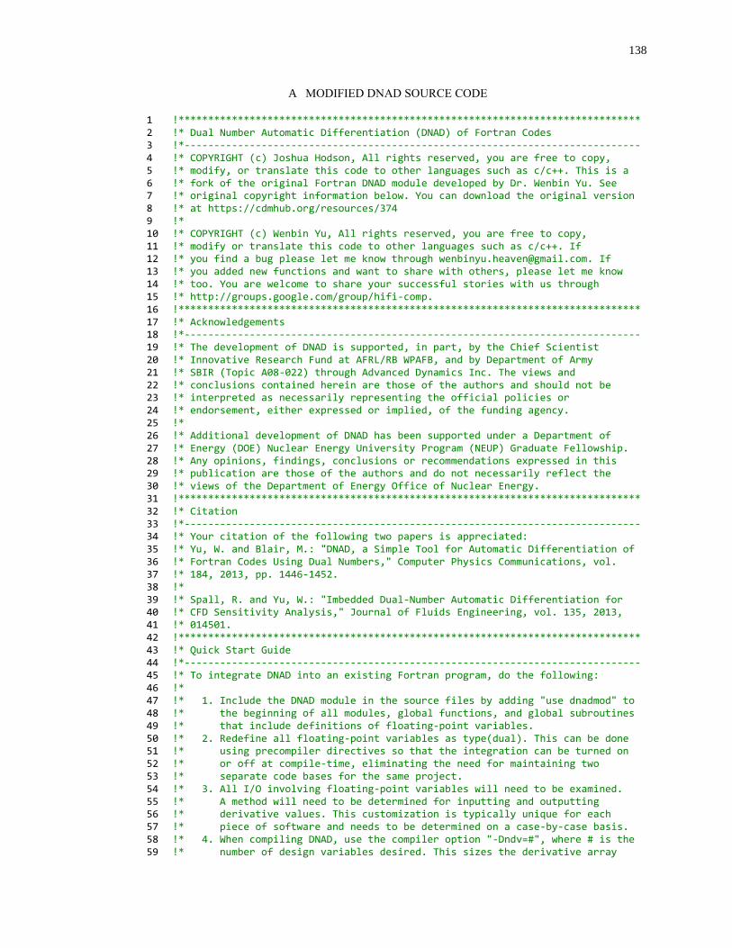
138

A MODIFIED DNAD SOURCE CODE

1 !****************************************************************************** 2 !* Dual Number Automatic Differentiation (DNAD) of Fortran Codes 3 !*----------------------------------------------------------------------------- 4 !* COPYRIGHT (c) Joshua Hodson, All rights reserved, you are free to copy, 5 !* modify, or translate this code to other languages such as c/c++. This is a 6 !* fork of the original Fortran DNAD module developed by Dr. Wenbin Yu. See 7 !* original copyright information below. You can download the original version 8 !* at https://cdmhub.org/resources/374 9 !* 10 !* COPYRIGHT (c) Wenbin Yu, All rights reserved, you are free to copy, 11 !* modify or translate this code to other languages such as c/c++. If 12 !* you find a bug please let me know through [email protected]. If 13 !* you added new functions and want to share with others, please let me know 14 !* too. You are welcome to share your successful stories with us through 15 !* http://groups.google.com/group/hifi-comp. 16 !****************************************************************************** 17 !* Acknowledgements 18 !*----------------------------------------------------------------------------- 19 !* The development of DNAD is supported, in part, by the Chief Scientist 20 !* Innovative Research Fund at AFRL/RB WPAFB, and by Department of Army 21 !* SBIR (Topic A08-022) through Advanced Dynamics Inc. The views and 22 !* conclusions contained herein are those of the authors and should not be 23 !* interpreted as necessarily representing the official policies or 24 !* endorsement, either expressed or implied, of the funding agency. 25 !* 26 !* Additional development of DNAD has been supported under a Department of 27 !* Energy (DOE) Nuclear Energy University Program (NEUP) Graduate Fellowship. 28 !* Any opinions, findings, conclusions or recommendations expressed in this 29 !* publication are those of the authors and do not necessarily reflect the 30 !* views of the Department of Energy Office of Nuclear Energy. 31 !****************************************************************************** 32 !* Citation 33 !*----------------------------------------------------------------------------- 34 !* Your citation of the following two papers is appreciated: 35 !* Yu, W. and Blair, M.: "DNAD, a Simple Tool for Automatic Differentiation of 36 !* Fortran Codes Using Dual Numbers," Computer Physics Communications, vol. 37 !* 184, 2013, pp. 1446-1452. 38 !* 39 !* Spall, R. and Yu, W.: "Imbedded Dual-Number Automatic Differentiation for 40 !* CFD Sensitivity Analysis," Journal of Fluids Engineering, vol. 135, 2013, 41 !* 014501. 42 !****************************************************************************** 43 !* Quick Start Guide 44 !*----------------------------------------------------------------------------- 45 !* To integrate DNAD into an existing Fortran program, do the following: 46 !* 47 !* 1. Include the DNAD module in the source files by adding "use dnadmod" to 48 !* the beginning of all modules, global functions, and global subroutines 49 !* that include definitions of floating-point variables. 50 !* 2. Redefine all floating-point variables as type(dual). This can be done 51 !* using precompiler directives so that the integration can be turned on 52 !* or off at compile-time, eliminating the need for maintaining two 53 !* separate code bases for the same project. 54 !* 3. All I/O involving floating-point variables will need to be examined. 55 !* A method will need to be determined for inputting and outputting 56 !* derivative values. This customization is typically unique for each 57 !* piece of software and needs to be determined on a case-by-case basis. 58 !* 4. When compiling DNAD, use the compiler option "-Dndv=#", where # is the 59 !* number of design variables desired. This sizes the derivative array

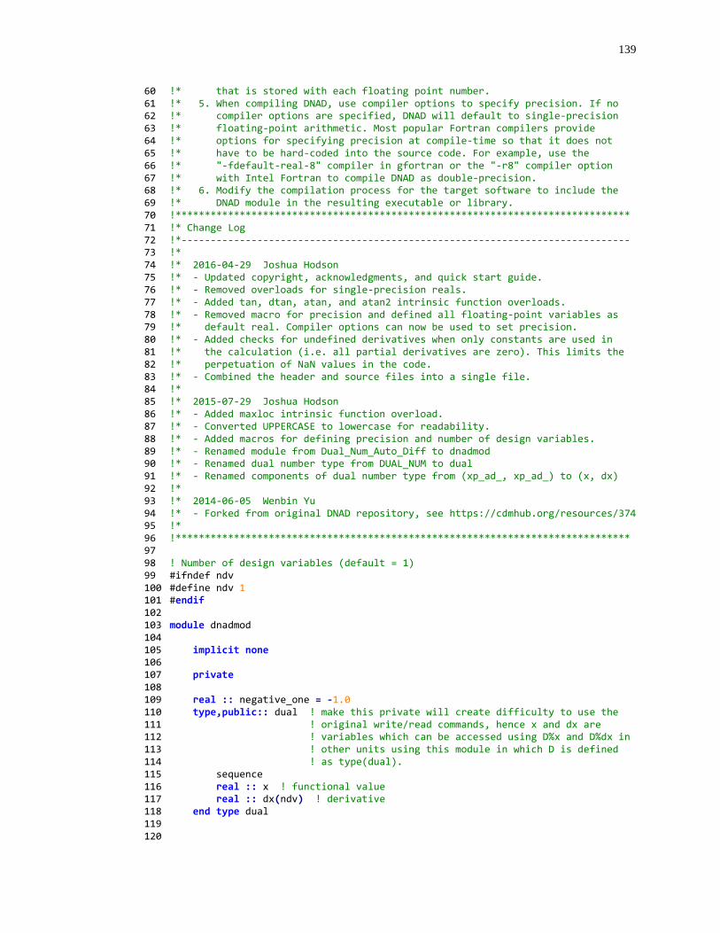
139

60 !* that is stored with each floating point number. 61 !* 5. When compiling DNAD, use compiler options to specify precision. If no 62 !* compiler options are specified, DNAD will default to single-precision 63 !* floating-point arithmetic. Most popular Fortran compilers provide 64 !* options for specifying precision at compile-time so that it does not 65 !* have to be hard-coded into the source code. For example, use the 66 !* "-fdefault-real-8" compiler in gfortran or the "-r8" compiler option 67 !* with Intel Fortran to compile DNAD as double-precision. 68 !* 6. Modify the compilation process for the target software to include the 69 !* DNAD module in the resulting executable or library. 70 !****************************************************************************** 71 !* Change Log 72 !*----------------------------------------------------------------------------- 73 !* 74 !* 2016-04-29 Joshua Hodson 75 !* - Updated copyright, acknowledgments, and quick start guide. 76 !* - Removed overloads for single-precision reals. 77 !* - Added tan, dtan, atan, and atan2 intrinsic function overloads. 78 !* - Removed macro for precision and defined all floating-point variables as 79 !* default real. Compiler options can now be used to set precision. 80 !* - Added checks for undefined derivatives when only constants are used in 81 !* the calculation (i.e. all partial derivatives are zero). This limits the 82 !* perpetuation of NaN values in the code. 83 !* - Combined the header and source files into a single file. 84 !* 85 !* 2015-07-29 Joshua Hodson 86 !* - Added maxloc intrinsic function overload. 87 !* - Converted UPPERCASE to lowercase for readability. 88 !* - Added macros for defining precision and number of design variables. 89 !* - Renamed module from Dual_Num_Auto_Diff to dnadmod 90 !* - Renamed dual number type from DUAL_NUM to dual 91 !* - Renamed components of dual number type from (xp_ad_, xp_ad_) to (x, dx) 92 !* 93 !* 2014-06-05 Wenbin Yu 94 !* - Forked from original DNAD repository, see https://cdmhub.org/resources/374 95 !* 96 !****************************************************************************** 97 98 ! Number of design variables (default = 1) 99 #ifndef ndv 100 #define ndv 1 101 #endif 102 103 module dnadmod 104 105 implicit none 106 107 private 108 109 real :: negative_one = -1.0 110 type,public:: dual ! make this private will create difficulty to use the 111 ! original write/read commands, hence x and dx are 112 ! variables which can be accessed using D%x and D%dx in 113 ! other units using this module in which D is defined 114 ! as type(dual). 115 sequence 116 real :: x ! functional value 117 real :: dx(ndv) ! derivative 118 end type dual 119 120

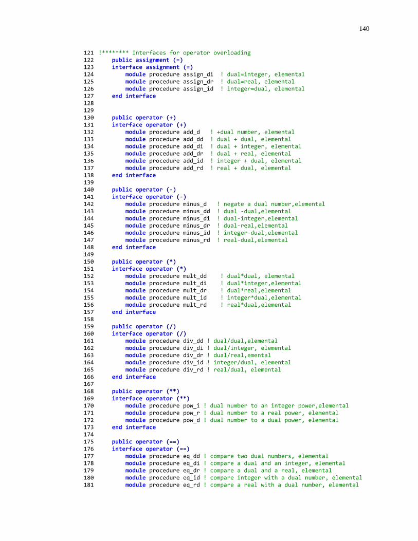
140

121 !******** Interfaces for operator overloading 122 public assignment (=) 123 interface assignment (=) 124 module procedure assign_di ! dual=integer, elemental 125 module procedure assign_dr ! dual=real, elemental 126 module procedure assign_id ! integer=dual, elemental 127 end interface 128 129 130 public operator (+) 131 interface operator (+) 132 module procedure add_d ! +dual number, elemental 133 module procedure add_dd ! dual + dual, elemental 134 module procedure add_di ! dual + integer, elemental 135 module procedure add_dr ! dual + real, elemental 136 module procedure add_id ! integer + dual, elemental 137 module procedure add_rd ! real + dual, elemental 138 end interface 139 140 public operator (-) 141 interface operator (-) 142 module procedure minus_d ! negate a dual number,elemental 143 module procedure minus_dd ! dual -dual,elemental 144 module procedure minus_di ! dual-integer,elemental 145 module procedure minus_dr ! dual-real,elemental 146 module procedure minus_id ! integer-dual,elemental 147 module procedure minus_rd ! real-dual,elemental 148 end interface 149 150 public operator (*) 151 interface operator (*) 152 module procedure mult_dd ! dual*dual, elemental 153 module procedure mult_di ! dual*integer,elemental 154 module procedure mult_dr ! dual*real,elemental 155 module procedure mult_id ! integer*dual,elemental 156 module procedure mult_rd ! real*dual,elemental 157 end interface 158 159 public operator (/) 160 interface operator (/) 161 module procedure div_dd ! dual/dual,elemental 162 module procedure div_di ! dual/integer, elemental 163 module procedure div_dr ! dual/real,emental 164 module procedure div_id ! integer/dual, elemental 165 module procedure div_rd ! real/dual, elemental 166 end interface 167 168 public operator (**) 169 interface operator (**) 170 module procedure pow_i ! dual number to an integer power,elemental 171 module procedure pow_r ! dual number to a real power, elemental 172 module procedure pow_d ! dual number to a dual power, elemental 173 end interface 174 175 public operator (==) 176 interface operator (==) 177 module procedure eq_dd ! compare two dual numbers, elemental 178 module procedure eq_di ! compare a dual and an integer, elemental 179 module procedure eq_dr ! compare a dual and a real, elemental 180 module procedure eq_id ! compare integer with a dual number, elemental 181 module procedure eq_rd ! compare a real with a dual number, elemental

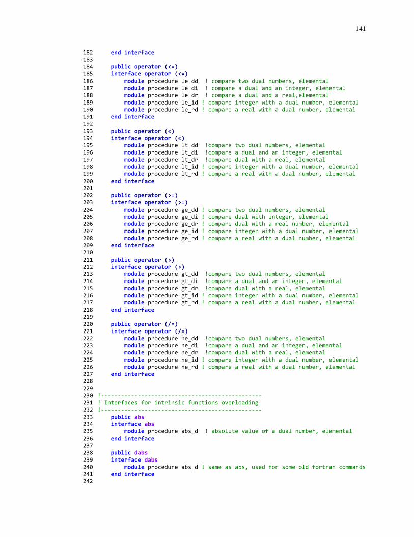
141

182 end interface 183 184 public operator (<=) 185 interface operator (<=) 186 module procedure le_dd ! compare two dual numbers, elemental 187 module procedure le_di ! compare a dual and an integer, elemental 188 module procedure le_dr ! compare a dual and a real,elemental 189 module procedure le_id ! compare integer with a dual number, elemental 190 module procedure le_rd ! compare a real with a dual number, elemental 191 end interface 192 193 public operator (<) 194 interface operator (<) 195 module procedure lt_dd !compare two dual numbers, elemental 196 module procedure lt_di !compare a dual and an integer, elemental 197 module procedure lt_dr !compare dual with a real, elemental 198 module procedure lt_id ! compare integer with a dual number, elemental 199 module procedure lt_rd ! compare a real with a dual number, elemental 200 end interface 201 202 public operator (>=) 203 interface operator (>=) 204 module procedure ge_dd ! compare two dual numbers, elemental 205 module procedure ge_di ! compare dual with integer, elemental 206 module procedure ge_dr ! compare dual with a real number, elemental 207 module procedure ge_id ! compare integer with a dual number, elemental 208 module procedure ge_rd ! compare a real with a dual number, elemental 209 end interface 210 211 public operator (>) 212 interface operator (>) 213 module procedure gt_dd !compare two dual numbers, elemental 214 module procedure gt_di !compare a dual and an integer, elemental 215 module procedure gt_dr !compare dual with a real, elemental 216 module procedure gt_id ! compare integer with a dual number, elemental 217 module procedure gt_rd ! compare a real with a dual number, elemental 218 end interface 219 220 public operator (/=) 221 interface operator (/=) 222 module procedure ne_dd !compare two dual numbers, elemental 223 module procedure ne_di !compare a dual and an integer, elemental 224 module procedure ne_dr !compare dual with a real, elemental 225 module procedure ne_id ! compare integer with a dual number, elemental 226 module procedure ne_rd ! compare a real with a dual number, elemental 227 end interface 228 229 230 !------------------------------------------------ 231 ! Interfaces for intrinsic functions overloading 232 !------------------------------------------------ 233 public abs 234 interface abs 235 module procedure abs_d ! absolute value of a dual number, elemental 236 end interface 237 238 public dabs 239 interface dabs 240 module procedure abs_d ! same as abs, used for some old fortran commands 241 end interface 242

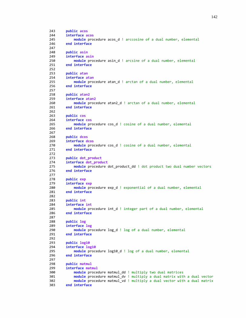
142

243 public acos 244 interface acos 245 module procedure acos_d ! arccosine of a dual number, elemental 246 end interface 247 248 public asin 249 interface asin 250 module procedure asin_d ! arcsine of a dual number, elemental 251 end interface 252 253 public atan 254 interface atan 255 module procedure atan_d ! arctan of a dual number, elemental 256 end interface 257 258 public atan2 259 interface atan2 260 module procedure atan2_d ! arctan of a dual number, elemental 261 end interface 262 263 public cos 264 interface cos 265 module procedure cos_d ! cosine of a dual number, elemental 266 end interface 267 268 public dcos 269 interface dcos 270 module procedure cos_d ! cosine of a dual number, elemental 271 end interface 272 273 public dot_product 274 interface dot_product 275 module procedure dot_product_dd ! dot product two dual number vectors 276 end interface 277 278 public exp 279 interface exp 280 module procedure exp_d ! exponential of a dual number, elemental 281 end interface 282 283 public int 284 interface int 285 module procedure int_d ! integer part of a dual number, elemental 286 end interface 287 288 public log 289 interface log 290 module procedure log_d ! log of a dual number, elemental 291 end interface 292 293 public log10 294 interface log10 295 module procedure log10_d ! log of a dual number, elemental 296 end interface 297 298 public matmul 299 interface matmul 300 module procedure matmul_dd ! multiply two dual matrices 301 module procedure matmul_dv ! multiply a dual matrix with a dual vector 302 module procedure matmul_vd ! multiply a dual vector with a dual matrix 303 end interface

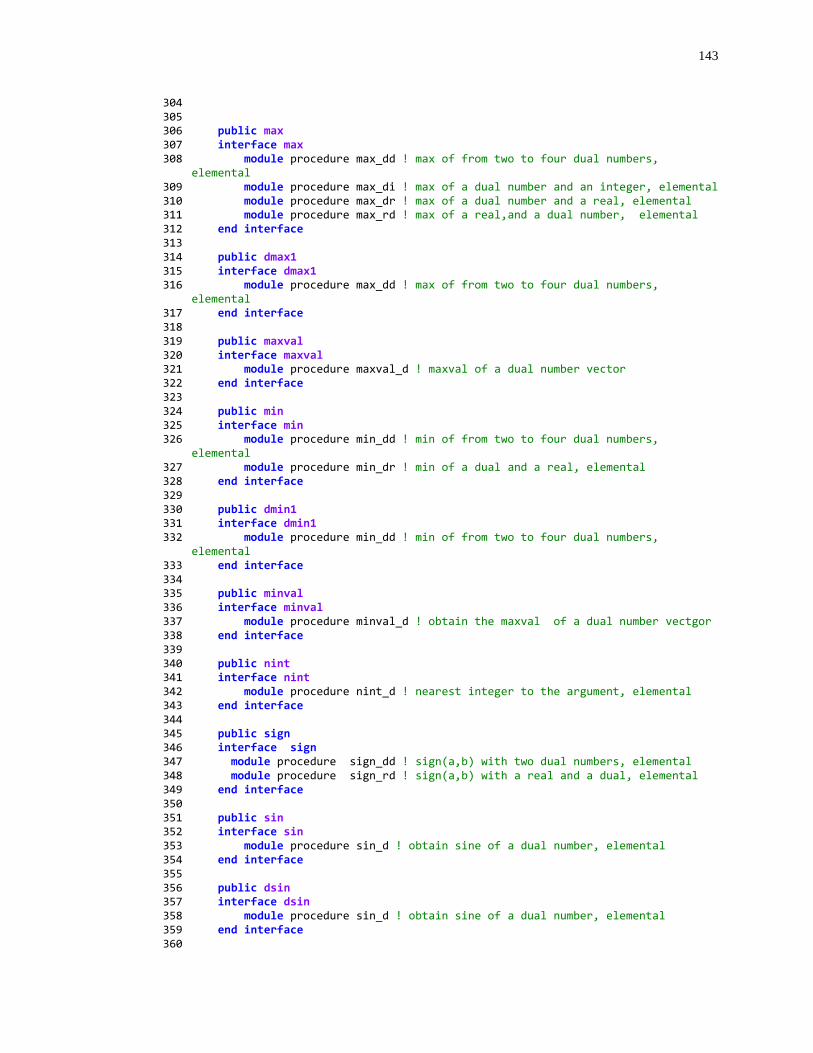
143

304 305 306 public max 307 interface max 308 module procedure max_dd ! max of from two to four dual numbers,

elemental 309 module procedure max_di ! max of a dual number and an integer, elemental 310 module procedure max_dr ! max of a dual number and a real, elemental 311 module procedure max_rd ! max of a real,and a dual number, elemental 312 end interface 313 314 public dmax1 315 interface dmax1 316 module procedure max_dd ! max of from two to four dual numbers,

elemental 317 end interface 318 319 public maxval 320 interface maxval 321 module procedure maxval_d ! maxval of a dual number vector 322 end interface 323 324 public min 325 interface min 326 module procedure min_dd ! min of from two to four dual numbers,

elemental 327 module procedure min_dr ! min of a dual and a real, elemental 328 end interface 329 330 public dmin1 331 interface dmin1 332 module procedure min_dd ! min of from two to four dual numbers,

elemental 333 end interface 334 335 public minval 336 interface minval 337 module procedure minval_d ! obtain the maxval of a dual number vectgor 338 end interface 339 340 public nint 341 interface nint 342 module procedure nint_d ! nearest integer to the argument, elemental 343 end interface 344 345 public sign 346 interface sign 347 module procedure sign_dd ! sign(a,b) with two dual numbers, elemental 348 module procedure sign_rd ! sign(a,b) with a real and a dual, elemental 349 end interface 350 351 public sin 352 interface sin 353 module procedure sin_d ! obtain sine of a dual number, elemental 354 end interface 355 356 public dsin 357 interface dsin 358 module procedure sin_d ! obtain sine of a dual number, elemental 359 end interface 360

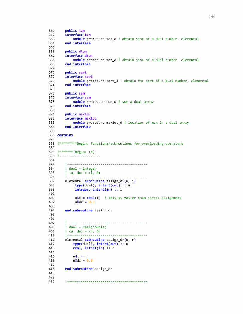
144

361 public tan 362 interface tan 363 module procedure tan_d ! obtain sine of a dual number, elemental 364 end interface 365 366 public dtan 367 interface dtan 368 module procedure tan_d ! obtain sine of a dual number, elemental 369 end interface 370 371 public sqrt 372 interface sqrt 373 module procedure sqrt_d ! obtain the sqrt of a dual number, elemental 374 end interface 375 376 public sum 377 interface sum 378 module procedure sum_d ! sum a dual array 379 end interface 380 381 public maxloc 382 interface maxloc 383 module procedure maxloc_d ! location of max in a dual array 384 end interface 385 386 contains 387 388 !*********Begin: functions/subroutines for overloading operators 389 390 !******* Begin: (=) 391 !--------------------- 392 393 !----------------------------------------- 394 ! dual = integer 395 ! <u, du> = <i, 0> 396 !----------------------------------------- 397 elemental subroutine assign_di(u, i) 398 type(dual), intent(out) :: u 399 integer, intent(in) :: i 400 401 u%x = real(i) ! This is faster than direct assignment 402 u%dx = 0.0 403 404 end subroutine assign_di 405 406 407 !----------------------------------------- 408 ! dual = real(double) 409 ! <u, du> = <r, 0> 410 !----------------------------------------- 411 elemental subroutine assign_dr(u, r) 412 type(dual), intent(out) :: u 413 real, intent(in) :: r 414 415 u%x = r 416 u%dx = 0.0 417 418 end subroutine assign_dr 419 420 421 !-----------------------------------------

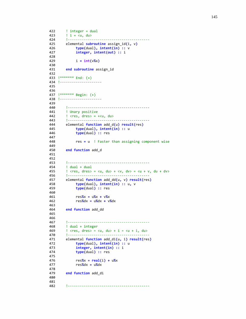
145

422 ! integer = dual 423 ! i = <u, du> 424 !----------------------------------------- 425 elemental subroutine assign_id(i, v) 426 type(dual), intent(in) :: v 427 integer, intent(out) :: i 428 429 i = int(v%x) 430 431 end subroutine assign_id 432 433 !******* End: (=) 434 !--------------------- 435 436 437 !******* Begin: (+) 438 !--------------------- 439 440 !----------------------------------------- 441 ! Unary positive 442 ! <res, dres> = +<u, du> 443 !----------------------------------------- 444 elemental function add_d(u) result(res) 445 type(dual), intent(in) :: u 446 type(dual) :: res 447 448 res = u ! Faster than assigning component wise 449 450 end function add_d 451 452 453 !----------------------------------------- 454 ! dual + dual 455 ! <res, dres> = <u, du> + <v, dv> = 456 !----------------------------------------- 457 elemental function add_dd(u, v) result(res) 458 type(dual), intent(in) :: u, v 459 type(dual) :: res 460 461 res%x = u%x + v%x 462 res%dx = u%dx + v%dx 463 464 end function add_dd 465 466 467 !----------------------------------------- 468 ! dual + integer 469 ! <res, dres> = <u, du> + i = 470 !----------------------------------------- 471 elemental function add_di(u, i) result(res) 472 type(dual), intent(in) :: u 473 integer, intent(in) :: i 474 type(dual) :: res 475 476 res%x = real(i) + u%x 477 res%dx = u%dx 478 479 end function add_di 480 481 482 !-----------------------------------------

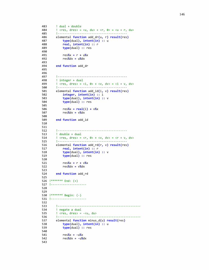
146

483 ! dual + double 484 ! <res, dres> = <u, du> + <r, 0> = 485 !----------------------------------------- 486 elemental function add_dr(u, r) result(res) 487 type(dual), intent(in) :: u 488 real, intent(in) :: r 489 type(dual) :: res 490 491 res%x = r + u%x 492 res%dx = u%dx 493 494 end function add_dr 495 496 497 !----------------------------------------- 498 ! integer + dual 499 ! <res, dres> = <i, 0> + <v, dv> = 500 !----------------------------------------- 501 elemental function add_id(i, v) result(res) 502 integer, intent(in) :: i 503 type(dual), intent(in) :: v 504 type(dual) :: res 505 506 res%x = real(i) + v%x 507 res%dx = v%dx 508 509 end function add_id 510 511 512 !----------------------------------------- 513 ! double + dual 514 ! <res, dres> = <r, 0> + <v, dv> = <r + v, dv> 515 !----------------------------------------- 516 elemental function add_rd(r, v) result(res) 517 real, intent(in) :: r 518 type(dual), intent(in) :: v 519 type(dual) :: res 520 521 res%x = r + v%x 522 res%dx = v%dx 523 524 end function add_rd 525 526 !******* End: (+) 527 !--------------------- 528 529 530 !******* Begin: (-) 531 !--------------------- 532 533 !------------------------------------------------- 534 ! negate a dual 535 ! <res, dres> = -<u, du> 536 !------------------------------------------------- 537 elemental function minus_d(u) result(res) 538 type(dual), intent(in) :: u 539 type(dual) :: res 540 541 res%x = -u%x 542 res%dx = -u%dx 543

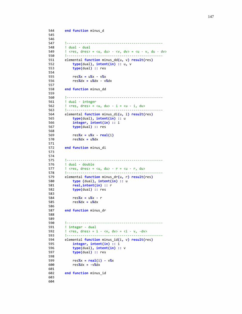
147

544 end function minus_d 545 546 547 !------------------------------------------------- 548 ! dual - dual 549 ! <res, dres> = <u, du> - <v, dv> = 550 !------------------------------------------------- 551 elemental function minus_dd(u, v) result(res) 552 type(dual), intent(in) :: u, v 553 type(dual) :: res 554 555 res%x = u%x - v%x 556 res%dx = u%dx - v%dx 557 558 end function minus_dd 559 560 !------------------------------------------------- 561 ! dual - integer 562 ! <res, dres> = <u, du> - i = 563 !------------------------------------------------- 564 elemental function minus_di(u, i) result(res) 565 type(dual), intent(in) :: u 566 integer, intent(in) :: i 567 type(dual) :: res 568 569 res%x = u%x - real(i) 570 res%dx = u%dx 571 572 end function minus_di 573 574 575 !------------------------------------------------- 576 ! dual - double 577 ! <res, dres> = <u, du> - r = 578 !------------------------------------------------- 579 elemental function minus_dr(u, r) result(res) 580 type (dual), intent(in) :: u 581 real,intent(in) :: r 582 type(dual) :: res 583 584 res%x = u%x - r 585 res%dx = u%dx 586 587 end function minus_dr 588 589 590 !------------------------------------------------- 591 ! integer - dual 592 ! <res, dres> = i - <v, dv> = 593 !------------------------------------------------- 594 elemental function minus_id(i, v) result(res) 595 integer, intent(in) :: i 596 type(dual), intent(in) :: v 597 type(dual) :: res 598 599 res%x = real(i) - v%x 600 res%dx = -v%dx 601 602 end function minus_id 603 604

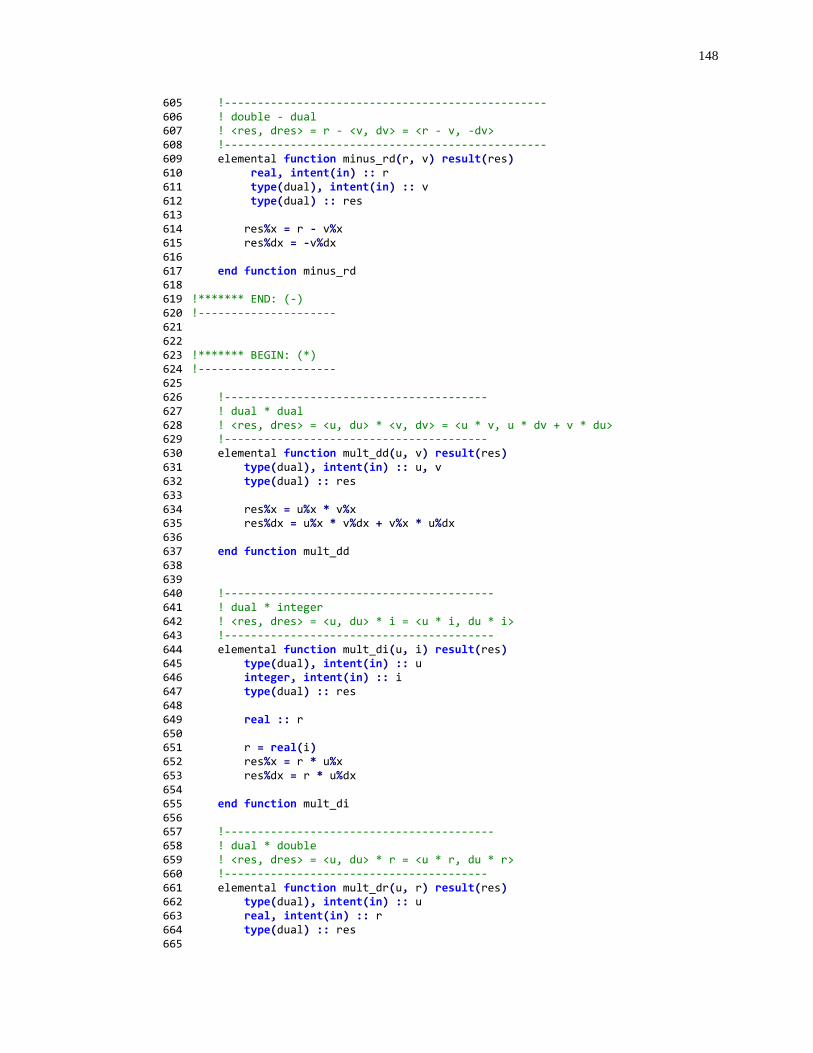
148

605 !------------------------------------------------- 606 ! double - dual 607 ! <res, dres> = r - <v, dv> = <r - v, -dv> 608 !------------------------------------------------- 609 elemental function minus_rd(r, v) result(res) 610 real, intent(in) :: r 611 type(dual), intent(in) :: v 612 type(dual) :: res 613 614 res%x = r - v%x 615 res%dx = -v%dx 616 617 end function minus_rd 618 619 !******* END: (-) 620 !--------------------- 621 622 623 !******* BEGIN: (*) 624 !--------------------- 625 626 !---------------------------------------- 627 ! dual * dual 628 ! <res, dres> = <u, du> * <v, dv> = 629 !---------------------------------------- 630 elemental function mult_dd(u, v) result(res) 631 type(dual), intent(in) :: u, v 632 type(dual) :: res 633 634 res%x = u%x * v%x 635 res%dx = u%x * v%dx + v%x * u%dx 636 637 end function mult_dd 638 639 640 !----------------------------------------- 641 ! dual * integer 642 ! <res, dres> = <u, du> * i = 643 !----------------------------------------- 644 elemental function mult_di(u, i) result(res) 645 type(dual), intent(in) :: u 646 integer, intent(in) :: i 647 type(dual) :: res 648 649 real :: r 650 651 r = real(i) 652 res%x = r * u%x 653 res%dx = r * u%dx 654 655 end function mult_di 656 657 !----------------------------------------- 658 ! dual * double 659 ! <res, dres> = <u, du> * r = 660 !---------------------------------------- 661 elemental function mult_dr(u, r) result(res) 662 type(dual), intent(in) :: u 663 real, intent(in) :: r 664 type(dual) :: res 665

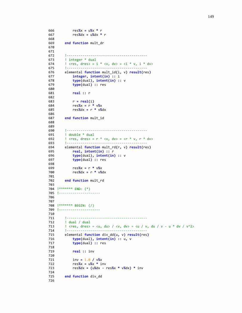
149

666 res%x = u%x * r 667 res%dx = u%dx * r 668 669 end function mult_dr 670 671 672 !----------------------------------------- 673 ! integer * dual 674 ! <res, dres> = i * <v, dv> = 675 !----------------------------------------- 676 elemental function mult_id(i, v) result(res) 677 integer, intent(in) :: i 678 type(dual), intent(in) :: v 679 type(dual) :: res 680 681 real :: r 682 683 r = real(i) 684 res%x = r * v%x 685 res%dx = r * v%dx 686 687 end function mult_id 688 689 690 !----------------------------------------- 691 ! double * dual 692 ! <res, dres> = r * <v, dv> = <r * v, r * dv> 693 !----------------------------------------- 694 elemental function mult_rd(r, v) result(res) 695 real, intent(in) :: r 696 type(dual), intent(in) :: v 697 type(dual) :: res 698 699 res%x = r * v%x 700 res%dx = r * v%dx 701 702 end function mult_rd 703 704 !******* END: (*) 705 !--------------------- 706 707 708 !******* BEGIN: (/) 709 !--------------------- 710 711 !----------------------------------------- 712 ! dual / dual 713 ! <res, dres> = <u, du> / <v, dv> = 714 !----------------------------------------- 715 elemental function div_dd(u, v) result(res) 716 type(dual), intent(in) :: u, v 717 type(dual) :: res 718 719 real :: inv 720 721 inv = 1.0 / v%x 722 res%x = u%x * inv 723 res%dx = (u%dx - res%x * v%dx) * inv 724 725 end function div_dd 726

150

727 728 !----------------------------------------- 729 ! dual / integer 730 ! <res, dres> = <u, du> / i = 731 !----------------------------------------- 732 elemental function div_di(u, i) result(res) 733 type(dual), intent(in) :: u 734 integer, intent(in) :: i 735 type(dual) :: res 736 737 real :: inv 738 739 inv = 1.0 / real(i) 740 res%x = u%x * inv 741 res%dx = u%dx * inv 742 743 end function div_di 744 745 746 !----------------------------------------- 747 ! dual / double 748 ! <res, dres> = <u, du> / r = 749 !---------------------------------------- 750 elemental function div_dr(u, r) result(res) 751 type(dual), intent(in) :: u 752 real, intent(in) :: r 753 type(dual):: res 754 755 real :: inv 756 757 inv = 1.0 / r 758 res%x = u%x * inv 759 res%dx = u%dx * inv 760 761 end function div_dr 762 763 764 !----------------------------------------- 765 ! integer / dual 766 ! <res, dres> = i / <v, dv> = 767 !----------------------------------------- 768 elemental function div_id(i, v) result(res) 769 integer, intent(in) :: i 770 type(dual), intent(in) :: v 771 type(dual) :: res 772 773 real :: inv 774 775 inv = 1.0 / v%x 776 res%x = real(i) * inv 777 res%dx = -res%x * inv * v%dx 778 779 end function div_id 780 781 782 !----------------------------------------- 783 ! double / dual 784 ! <res, dres> = r / <u, du> = <r / u, -r / u^2 * du> 785 !----------------------------------------- 786 elemental function div_rd(r, v) result(res) 787 real, intent(in) :: r

151

788 type(dual), intent(in) :: v 789 type(dual) :: res 790 791 real :: inv 792 793 inv = 1.0 / v%x 794 res%x = r * inv 795 res%dx = -res%x * inv * v%dx 796 797 end function div_rd 798 799 !******* END: (/) 800 !--------------------- 801 802 !******* BEGIN: (**) 803 !--------------------- 804 805 !----------------------------------------- 806 ! power(dual, integer) 807 ! <res, dres> = <u, du> ^ i = 808 !----------------------------------------- 809 elemental function pow_i(u, i) result(res) 810 type(dual), intent(in) :: u 811 integer, intent(in) :: i 812 type(dual) :: res 813 814 real :: pow_x 815 816 pow_x = u%x ** (i - 1) 817 res%x = u%x * pow_x 818 res%dx = real(i) * pow_x * u%dx 819 820 end function pow_i 821 822 !----------------------------------------- 823 ! power(dual, double) 824 ! <res, dres> = <u, du> ^ r = 825 !----------------------------------------- 826 elemental function pow_r(u, r) result(res) 827 type(dual), intent(in) :: u 828 real, intent(in) :: r 829 type(dual) :: res 830 831 real :: pow_x 832 833 pow_x = u%x ** (r - 1.0) 834 res%x = u%x * pow_x 835 res%dx = r * pow_x * u%dx 836 837 end function pow_r 838 839 !----------------------------------------- 840 ! POWER dual numbers to a dual power 841 ! <res, dres> = <u, du> ^ <v, dv> 842 ! = 843 !----------------------------------------- 844 elemental function pow_d(u, v) result(res) 845 type(dual), intent(in)::u, v 846 type(dual) :: res 847 848 res%x = u%x ** v%x

152

849 res%dx = res%x * (v%x / u%x * u%dx + log(u%x) * v%dx) 850 851 end function pow_d 852 853 !******* END: (**) 854 !--------------------- 855 856 857 !******* BEGIN: (==) 858 !--------------------- 859 !----------------------------------------- 860 ! compare two dual numbers, 861 ! simply compare the functional value. 862 !----------------------------------------- 863 elemental function eq_dd(lhs, rhs) result(res) 864 type(dual), intent(in) :: lhs, rhs 865 logical :: res 866 867 res = (lhs%x == rhs%x) 868 869 end function eq_dd 870 871 872 !----------------------------------------- 873 ! compare a dual with an integer, 874 ! simply compare the functional value. 875 !----------------------------------------- 876 elemental function eq_di(lhs, rhs) result(res) 877 type(dual), intent(in) :: lhs 878 integer, intent(in) :: rhs 879 logical :: res 880 881 res = (lhs%x == real(rhs)) 882 883 end function eq_di 884 885 886 !----------------------------------------- 887 ! compare a dual number with a real number, 888 ! simply compare the functional value. 889 !----------------------------------------- 890 elemental function eq_dr(lhs, rhs) result(res) 891 type(dual), intent(in) :: lhs 892 real, intent(in) :: rhs 893 logical::res 894 895 res = (lhs%x == rhs) 896 897 end function eq_dr 898 899 900 !----------------------------------------- 901 ! compare an integer with a dual, 902 ! simply compare the functional value. 903 !---------------------------------------- 904 elemental function eq_id(lhs, rhs) result(res) 905 integer, intent(in) :: lhs 906 type(dual), intent(in) :: rhs 907 logical :: res 908 909 res = (lhs == rhs%x)

153

910 911 end function eq_id 912 913 914 !----------------------------------------- 915 ! compare a real with a dual, 916 ! simply compare the functional value. 917 !----------------------------------------- 918 elemental function eq_rd(lhs, rhs) result(res) 919 real, intent(in) :: lhs 920 type(dual), intent(in) :: rhs 921 logical :: res 922 923 res = (lhs == rhs%x) 924 925 end function eq_rd 926 927 !******* END: (==) 928 !--------------------- 929 930 931 !******* BEGIN: (<=) 932 !--------------------- 933 !----------------------------------------- 934 ! compare two dual numbers, simply compare 935 ! the functional value. 936 !----------------------------------------- 937 elemental function le_dd(lhs, rhs) result(res) 938 type(dual), intent(in) :: lhs, rhs 939 logical :: res 940 941 res = (lhs%x <= rhs%x) 942 943 end function le_dd 944 945 946 !----------------------------------------- 947 ! compare a dual with an integer, 948 ! simply compare the functional value. 949 !----------------------------------------- 950 elemental function le_di(lhs, rhs) result(res) 951 type(dual), intent(in) :: lhs 952 integer, intent(in) :: rhs 953 logical :: res 954 955 res = (lhs%x <= rhs) 956 957 end function le_di 958 959 960 !----------------------------------------- 961 ! compare a dual number with a real number, 962 ! simply compare the functional value. 963 !----------------------------------------- 964 elemental function le_dr(lhs, rhs) result(res) 965 type(dual), intent(in) :: lhs 966 real, intent(in) :: rhs 967 logical :: res 968 969 res = (lhs%x <= rhs) 970

154

971 end function le_dr 972 973 974 !----------------------------------------- 975 ! compare a dual number with an integer, 976 ! simply compare the functional value. 977 !----------------------------------------- 978 elemental function le_id(i, rhs) result(res) 979 integer, intent(in) :: i 980 type(dual), intent(in) :: rhs 981 logical :: res 982 983 res = (i <= rhs%x) 984 985 end function le_id 986 987 988 !----------------------------------------- 989 ! compare a real with a dual, 990 ! simply compare the functional value. 991 !----------------------------------------- 992 elemental function le_rd(lhs, rhs) result(res) 993 real, intent(in) :: lhs 994 type(dual), intent(in) :: rhs 995 logical :: res 996 997 res = (lhs <= rhs%x) 998 999 end function le_rd 1000 1001 !******* END: (<=) 1002 !--------------------- 1003 1004 !******* BEGIN: (<) 1005 !--------------------- 1006 !----------------------------------------- 1007 ! compare two dual numbers, simply compare 1008 ! the functional value. 1009 !----------------------------------------- 1010 elemental function lt_dd(lhs, rhs) result(res) 1011 type(dual), intent(in) :: lhs, rhs 1012 logical :: res 1013 1014 res = (lhs%x < rhs%x) 1015 1016 end function lt_dd 1017 1018 !----------------------------------------- 1019 ! compare a dual with an integer, 1020 ! simply compare the functional value. 1021 !----------------------------------------- 1022 elemental function lt_di(lhs, rhs) result(res) 1023 type(dual), intent(in) :: lhs 1024 integer, intent(in) :: rhs 1025 logical :: res 1026 1027 res = (lhs%x < rhs) 1028 1029 end function lt_di 1030 1031

155

1032 !----------------------------------------- 1033 ! compare a dual number with a real number, simply compare 1034 ! the functional value. 1035 !---------------------------------------- 1036 elemental function lt_dr(lhs, rhs) result(res) 1037 type(dual), intent(in) :: lhs 1038 real, intent(in) :: rhs 1039 logical :: res 1040 1041 res = (lhs%x < rhs) 1042 1043 end function lt_dr 1044 1045 1046 !----------------------------------------- 1047 ! compare a dual number with an integer 1048 !----------------------------------------- 1049 elemental function lt_id(i, rhs) result(res) 1050 integer, intent(in) :: i 1051 type(dual), intent(in) :: rhs 1052 logical :: res 1053 1054 res = (i < rhs%x) 1055 1056 end function lt_id 1057 1058 1059 !----------------------------------------- 1060 ! compare a real with a dual 1061 !---------------------------------------- 1062 elemental function lt_rd(lhs, rhs) result(res) 1063 real, intent(in) :: lhs 1064 type(dual), intent(in) :: rhs 1065 logical :: res 1066 1067 res = (lhs < rhs%x) 1068 1069 end function lt_rd 1070 1071 !******* END: (<) 1072 !--------------------- 1073 1074 !******* BEGIN: (>=) 1075 !--------------------- 1076 !----------------------------------------- 1077 ! compare two dual numbers, simply compare 1078 ! the functional value. 1079 !---------------------------------------- 1080 elemental function ge_dd(lhs, rhs) result(res) 1081 type(dual), intent(in) :: lhs, rhs 1082 logical :: res 1083 1084 res = (lhs%x >= rhs%x) 1085 1086 end function ge_dd 1087 1088 1089 !----------------------------------------- 1090 ! compare a dual with an integer 1091 !----------------------------------------- 1092 elemental function ge_di(lhs, rhs) result(res)

156

1093 type(dual), intent(in) :: lhs 1094 integer, intent(in) :: rhs 1095 logical :: res 1096 1097 res = (lhs%x >= rhs) 1098 1099 end function ge_di 1100 1101 1102 !----------------------------------------- 1103 ! compare a dual number with a real number, simply compare 1104 ! the functional value. 1105 !----------------------------------------- 1106 elemental function ge_dr(lhs, rhs) result(res) 1107 type(dual), intent(in) :: lhs 1108 real, intent(in) :: rhs 1109 logical :: res 1110 1111 res = (lhs%x >= rhs) 1112 1113 end function ge_dr 1114 1115 1116 !----------------------------------------- 1117 ! compare a dual number with an integer 1118 !----------------------------------------- 1119 elemental function ge_id(i, rhs) result(res) 1120 integer, intent(in) :: i 1121 type(dual), intent(in) :: rhs 1122 logical :: res 1123 1124 res = (i >= rhs%x) 1125 1126 end function ge_id 1127 1128 1129 !----------------------------------------- 1130 ! compare a real with a dual 1131 !----------------------------------------- 1132 elemental function ge_rd(lhs, rhs) result(res) 1133 real, intent(in) :: lhs 1134 type(dual), intent(in) :: rhs 1135 logical :: res 1136 1137 res = (lhs >= rhs%x) 1138 1139 end function ge_rd 1140 1141 !******* END: (>=) 1142 !--------------------- 1143 1144 !******* BEGIN: (>) 1145 !--------------------- 1146 !----------------------------------------- 1147 ! compare two dual numbers, simply compare 1148 ! the functional value. 1149 !----------------------------------------- 1150 elemental function gt_dd(lhs, rhs) result(res) 1151 type(dual), intent(in) :: lhs, rhs 1152 logical :: res 1153

157

1154 res = (lhs%x > rhs%x) 1155 1156 end function gt_dd 1157 1158 1159 !----------------------------------------- 1160 ! compare a dual with an integer 1161 !----------------------------------------- 1162 elemental function gt_di(lhs, rhs) result(res) 1163 type(dual), intent(in) :: lhs 1164 integer, intent(in) :: rhs 1165 logical :: res 1166 1167 res = (lhs%x > rhs) 1168 1169 end function gt_di 1170 1171 1172 !----------------------------------------- 1173 ! compare a dual number with a real number, simply compare 1174 ! the functional value. 1175 !----------------------------------------- 1176 elemental function gt_dr(lhs, rhs) result(res) 1177 type(dual), intent(in) :: lhs 1178 real, intent(in) :: rhs 1179 logical :: res 1180 1181 res = (lhs%x > rhs) 1182 1183 end function gt_dr 1184 1185 1186 !----------------------------------------- 1187 ! compare a dual number with an integer 1188 !----------------------------------------- 1189 elemental function gt_id(i, rhs) result(res) 1190 integer, intent(in) :: i 1191 type(dual), intent(in) :: rhs 1192 logical :: res 1193 1194 res = (i > rhs%x) 1195 1196 end function gt_id 1197 1198 1199 !----------------------------------------- 1200 ! compare a real with a dual 1201 !----------------------------------------- 1202 elemental function gt_rd(lhs, rhs) result(res) 1203 real, intent(in) :: lhs 1204 type(dual), intent(in) :: rhs 1205 logical :: res 1206 1207 res = (lhs > rhs%x) 1208 1209 end function gt_rd 1210 1211 !******* END: (>) 1212 !--------------------- 1213 1214 !******* BEGIN: (/=)

158

1215 !--------------------- 1216 !----------------------------------------- 1217 ! compare two dual numbers, simply compare 1218 ! the functional value. 1219 !----------------------------------------- 1220 elemental function ne_dd(lhs, rhs) result(res) 1221 type(dual), intent(in) :: lhs, rhs 1222 logical :: res 1223 1224 res = (lhs%x /= rhs%x) 1225 1226 end function ne_dd 1227 1228 1229 !----------------------------------------- 1230 ! compare a dual with an integer 1231 !----------------------------------------- 1232 elemental function ne_di(lhs, rhs) result(res) 1233 type(dual), intent(in) :: lhs 1234 integer, intent(in) :: rhs 1235 logical :: res 1236 1237 res = (lhs%x /= rhs) 1238 1239 end function ne_di 1240 1241 1242 !----------------------------------------- 1243 ! compare a dual number with a real number, simply compare 1244 ! the functional value. 1245 !----------------------------------------- 1246 elemental function ne_dr(lhs, rhs) result(res) 1247 type(dual), intent(in) :: lhs 1248 real, intent(in) :: rhs 1249 logical :: res 1250 1251 res = (lhs%x /= rhs) 1252 1253 end function ne_dr 1254 1255 1256 !----------------------------------------- 1257 ! compare a dual number with an integer 1258 !----------------------------------------- 1259 elemental function ne_id(i, rhs) result(res) 1260 integer, intent(in) :: i 1261 type(dual), intent(in) :: rhs 1262 logical :: res 1263 1264 res = (i /= rhs%x) 1265 1266 end function ne_id 1267 1268 1269 !----------------------------------------- 1270 ! compare a real with a dual 1271 !----------------------------------------- 1272 elemental function ne_rd(lhs, rhs) result(res) 1273 real, intent(in) :: lhs 1274 type(dual), intent(in) :: rhs 1275 logical :: res

159

1276 1277 res = (lhs /= rhs%x) 1278 1279 end function ne_rd 1280 1281 !******* END: (/=) 1282 !--------------------- 1283 1284 !--------------------------------------------------- 1285 ! Absolute value of dual numbers 1286 ! <res, dres> = abs(<u, du>) = <abs(u), du * sign(u)> 1287 !--------------------------------------------------- 1288 elemental function abs_d(u) result(res) 1289 type(dual), intent(in) :: u 1290 type(dual) :: res 1291 integer :: i 1292 1293 if(u%x > 0) then 1294 res%x = u%x 1295 res%dx = u%dx 1296 else if (u%x < 0) then 1297 res%x = -u%x 1298 res%dx = -u%dx 1299 else 1300 res%x = 0.0 1301 do i = 1, ndv 1302 if (u%dx(i) .eq. 0.0) then 1303 res%dx(i) = 0.0 1304 else 1305 res%dx(i) = set_NaN() 1306 end if 1307 end do 1308 endif 1309 1310 end function abs_d 1311 1312 1313 !----------------------------------------- 1314 ! ACOS of dual numbers 1315 ! <res, dres> = acos(<u, du>) = <acos(u), -du / sqrt(1 - u^2)> 1316 !---------------------------------------- 1317 elemental function acos_d(u) result(res) 1318 type(dual), intent(in) :: u 1319 type(dual) :: res 1320 1321 res%x = acos(u%x) 1322 if (u%x == 1.0 .or. u%x == -1.0) then 1323 res%dx = set_Nan() ! Undefined derivative 1324 else 1325 res%dx = -u%dx / sqrt(1.0 - u%x**2) 1326 end if 1327 1328 end function acos_d 1329 1330 1331 !----------------------------------------- 1332 ! ASIN of dual numbers 1333 ! <res, dres> = asin(<u, du>) = <asin(u), du / sqrt(1 - u^2)> 1334 !---------------------------------------- 1335 elemental function asin_d(u) result(res) 1336 type(dual), intent(in) :: u

160

1337 type(dual) :: res 1338 1339 res%x = asin(u%x) 1340 if (u%x == 1.0 .or. u%x == -1.0) then 1341 res%dx = set_NaN() ! Undefined derivative 1342 else 1343 res%dx = u%dx / sqrt(1.0 - u%x**2) 1344 end if 1345 1346 end function asin_d 1347 1348 1349 !----------------------------------------- 1350 ! ATAN of dual numbers 1351 ! <res, dres> = atan(<u, du>) = <atan(u), du / (1 + u^2)> 1352 !---------------------------------------- 1353 elemental function atan_d(u) result(res) 1354 type(dual), intent(in) :: u 1355 type(dual) :: res 1356 1357 res%x = atan(u%x) 1358 res%dx = u%dx / (1.0 + u%x**2) 1359 1360 end function atan_d 1361 1362 1363 !----------------------------------------- 1364 ! ATAN2 of dual numbers 1365 ! <res, dres> = atan2(<u, du>, <v, dv>) 1366 ! = <atan2(u, v), v / (u^2 + v^2) * du - u / (u^2 + v^2) * dv> 1367 !---------------------------------------- 1368 elemental function atan2_d(u, v) result(res) 1369 type(dual), intent(in) :: u, v 1370 type(dual) :: res 1371 1372 real :: usq_plus_vsq 1373 1374 res%x = atan2(u%x, v%x) 1375 1376 usq_plus_vsq = u%x**2 + v%x**2 1377 res%dx = v%x / usq_plus_vsq * u%dx - u%x / usq_plus_vsq * v%dx 1378 1379 end function atan2_d 1380 1381 1382 !----------------------------------------- 1383 ! COS of dual numbers 1384 ! <res, dres> = cos(<u, du>) = <cos(u), -sin(u) * du> 1385 !---------------------------------------- 1386 elemental function cos_d(u) result(res) 1387 type(dual), intent(in) :: u 1388 type(dual) :: res 1389 1390 res%x = cos(u%x) 1391 res%dx = -sin(u%x) * u%dx 1392 1393 end function cos_d 1394 1395 1396 !----------------------------------------- 1397 ! DOT PRODUCT two dual number vectors

161

1398 ! <res, dres> = <u, du> . <v, dv> = 1399 !----------------------------------------- 1400 function dot_product_dd(u, v) result(res) 1401 type(dual), intent(in) :: u(:), v(:) 1402 type(dual) :: res 1403 1404 integer :: i 1405 1406 res%x = dot_product(u%x, v%x) 1407 do i = 1, ndv 1408 res%dx(i) = dot_product(u%x, v%dx(i)) + dot_product(v%x, u%dx(i)) 1409 end do 1410 1411 end function dot_product_dd 1412 1413 1414 !----------------------------------------- 1415 ! EXPONENTIAL OF dual numbers 1416 ! <res, dres> = exp(<u, du>) = <exp(u), exp(u) * du> 1417 !----------------------------------------- 1418 elemental function exp_d(u) result(res) 1419 type(dual), intent(in) :: u 1420 type(dual) :: res 1421 1422 real :: exp_x 1423 1424 exp_x = exp(u%x) 1425 res%x = exp_x 1426 res%dx = u%dx * exp_x 1427 1428 end function exp_d 1429 1430 1431 !----------------------------------------- 1432 ! Convert dual to integer 1433 ! i = int(<u, du>) = int(u) 1434 !---------------------------------------- 1435 elemental function int_d(u) result(res) 1436 type(dual), intent(in) :: u 1437 integer :: res 1438 1439 res = int(u%x) 1440 1441 end function int_d 1442 1443 1444 !----------------------------------------- 1445 ! LOG OF dual numbers,defined for u%x>0 only 1446 ! the error control should be done in the original code 1447 ! in other words, if u%x<=0, it is not possible to obtain LOG. 1448 ! <res, dres> = log(<u, du>) = <log(u), du / u> 1449 !---------------------------------------- 1450 elemental function log_d(u) result(res) 1451 type(dual), intent(in) :: u 1452 type(dual) :: res 1453 1454 real :: inv 1455 1456 inv = 1.0 / u%x 1457 res%x = log(u%x) 1458 res%dx = u%dx * inv

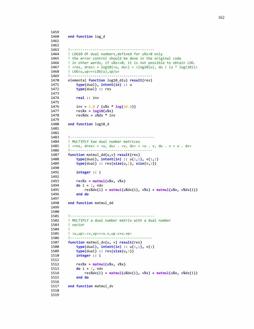
162

1459 1460 end function log_d 1461 1462 1463 !----------------------------------------- 1464 ! LOG10 OF dual numbers,defined for u%x>0 only 1465 ! the error control should be done in the original code 1466 ! in other words, if u%x<=0, it is not possible to obtain LOG. 1467 ! <res, dres> = log10(<u, du>) = <log10(u), du / (u * log(10))> 1468 ! LOG<u,up>=<LOG(u),up/u> 1469 !---------------------------------------- 1470 elemental function log10_d(u) result(res) 1471 type(dual), intent(in) :: u 1472 type(dual) :: res 1473 1474 real :: inv 1475 1476 inv = 1.0 / (u%x * log(10.0)) 1477 res%x = log10(u%x) 1478 res%dx = u%dx * inv 1479 1480 end function log10_d 1481 1482 1483 !----------------------------------------- 1484 ! MULTIPLY two dual number matrices 1485 ! <res, dres> = <u, du> . <v, dv> = 1486 !---------------------------------------- 1487 function matmul_dd(u,v) result(res) 1488 type(dual), intent(in) :: u(:,:), v(:,:) 1489 type(dual) :: res(size(u,1), size(v,2)) 1490 1491 integer :: i 1492 1493 res%x = matmul(u%x, v%x) 1494 do i = 1, ndv 1495 res%dx(i) = matmul(u%dx(i), v%x) + matmul(u%x, v%dx(i)) 1496 end do 1497 1498 end function matmul_dd 1499 1500 1501 !----------------------------------------- 1502 ! MULTIPLY a dual number matrix with a dual number 1503 ! vector 1504 ! 1505 ! <u,up>.<v,vp>=<u.v,up.v+u.vp> 1506 !---------------------------------------- 1507 function matmul_dv(u, v) result(res) 1508 type(dual), intent(in) :: u(:,:), v(:) 1509 type(dual) :: res(size(u,1)) 1510 integer :: i 1511 1512 res%x = matmul(u%x, v%x) 1513 do i = 1, ndv 1514 res%dx(i) = matmul(u%dx(i), v%x) + matmul(u%x, v%dx(i)) 1515 end do 1516 1517 end function matmul_dv 1518 1519

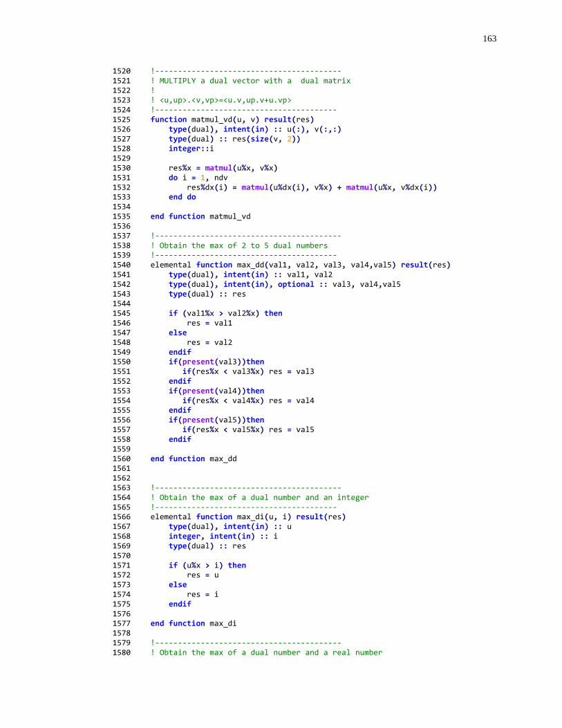
163

1520 !----------------------------------------- 1521 ! MULTIPLY a dual vector with a dual matrix 1522 ! 1523 ! <u,up>.<v,vp>=<u.v,up.v+u.vp> 1524 !---------------------------------------- 1525 function matmul_vd(u, v) result(res) 1526 type(dual), intent(in) :: u(:), v(:,:) 1527 type(dual) :: res(size(v, 2)) 1528 integer::i 1529 1530 res%x = matmul(u%x, v%x) 1531 do i = 1, ndv 1532 res%dx(i) = matmul(u%dx(i), v%x) + matmul(u%x, v%dx(i)) 1533 end do 1534 1535 end function matmul_vd 1536 1537 !----------------------------------------- 1538 ! Obtain the max of 2 to 5 dual numbers 1539 !---------------------------------------- 1540 elemental function max_dd(val1, val2, val3, val4,val5) result(res) 1541 type(dual), intent(in) :: val1, val2 1542 type(dual), intent(in), optional :: val3, val4,val5 1543 type(dual) :: res 1544 1545 if (val1%x > val2%x) then 1546 res = val1 1547 else 1548 res = val2 1549 endif 1550 if(present(val3))then 1551 if(res%x < val3%x) res = val3 1552 endif 1553 if(present(val4))then 1554 if(res%x < val4%x) res = val4 1555 endif 1556 if(present(val5))then 1557 if(res%x < val5%x) res = val5 1558 endif 1559 1560 end function max_dd 1561 1562 1563 !----------------------------------------- 1564 ! Obtain the max of a dual number and an integer 1565 !---------------------------------------- 1566 elemental function max_di(u, i) result(res) 1567 type(dual), intent(in) :: u 1568 integer, intent(in) :: i 1569 type(dual) :: res 1570 1571 if (u%x > i) then 1572 res = u 1573 else 1574 res = i 1575 endif 1576 1577 end function max_di 1578 1579 !----------------------------------------- 1580 ! Obtain the max of a dual number and a real number

164

1581 !---------------------------------------- 1582 elemental function max_dr(u, r) result(res) 1583 type(dual), intent(in) :: u 1584 real, intent(in) :: r 1585 type(dual) :: res 1586 1587 if (u%x > r) then 1588 res = u 1589 else 1590 res = r 1591 endif 1592 1593 end function max_dr 1594 1595 1596 !--------------------------------------------------- 1597 ! Obtain the max of a real and a dual 1598 !--------------------------------------------------- 1599 elemental function max_rd(n, u) result(res) 1600 real, intent(in) :: n 1601 type(dual), intent(in) :: u 1602 type(dual) :: res 1603 1604 if (u%x > n) then 1605 res = u 1606 else 1607 res = n 1608 endif 1609 1610 end function max_rd 1611 1612 1613 !----------------------------------------- 1614 ! Obtain the max value of vector u 1615 !---------------------------------------- 1616 function maxval_d(u) result(res) 1617 type(dual), intent(in) :: u(:) 1618 integer :: iloc(1) 1619 type(dual) :: res 1620 1621 iloc=maxloc(u%x) 1622 res=u(iloc(1)) 1623 1624 end function maxval_d 1625 1626 1627 !----------------------------------------- 1628 ! Obtain the min of 2 to 4 dual numbers 1629 !---------------------------------------- 1630 elemental function min_dd(val1, val2, val3, val4) result(res) 1631 type(dual), intent(in) :: val1, val2 1632 type(dual), intent(in), optional :: val3, val4 1633 type(dual) :: res 1634 1635 if (val1%x < val2%x) then 1636 res = val1 1637 else 1638 res = val2 1639 endif 1640 if(present(val3))then 1641 if(res%x > val3%x) res = val3

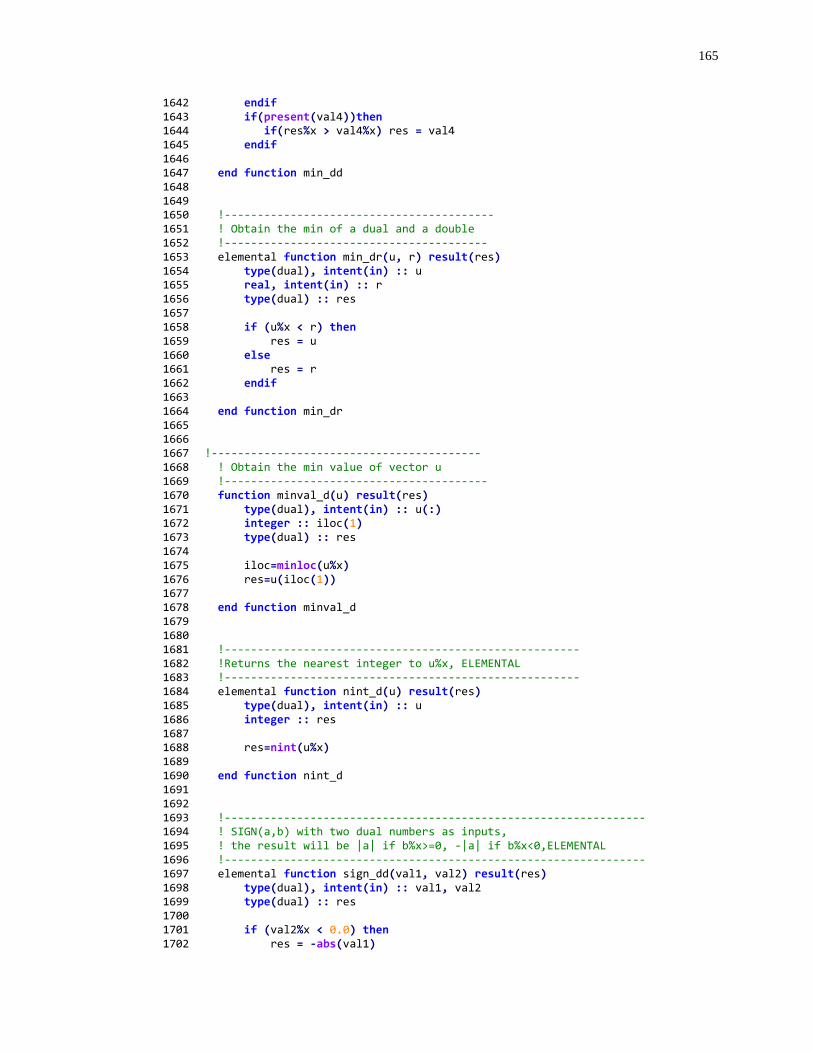
165

1642 endif 1643 if(present(val4))then 1644 if(res%x > val4%x) res = val4 1645 endif 1646 1647 end function min_dd 1648 1649 1650 !----------------------------------------- 1651 ! Obtain the min of a dual and a double 1652 !---------------------------------------- 1653 elemental function min_dr(u, r) result(res) 1654 type(dual), intent(in) :: u 1655 real, intent(in) :: r 1656 type(dual) :: res 1657 1658 if (u%x < r) then 1659 res = u 1660 else 1661 res = r 1662 endif 1663 1664 end function min_dr 1665 1666 1667 !----------------------------------------- 1668 ! Obtain the min value of vector u 1669 !---------------------------------------- 1670 function minval_d(u) result(res) 1671 type(dual), intent(in) :: u(:) 1672 integer :: iloc(1) 1673 type(dual) :: res 1674 1675 iloc=minloc(u%x) 1676 res=u(iloc(1)) 1677 1678 end function minval_d 1679 1680 1681 !------------------------------------------------------ 1682 !Returns the nearest integer to u%x, ELEMENTAL 1683 !------------------------------------------------------ 1684 elemental function nint_d(u) result(res) 1685 type(dual), intent(in) :: u 1686 integer :: res 1687 1688 res=nint(u%x) 1689 1690 end function nint_d 1691 1692 1693 !---------------------------------------------------------------- 1694 ! SIGN(a,b) with two dual numbers as inputs, 1695 ! the result will be |a| if b%x>=0, -|a| if b%x<0,ELEMENTAL 1696 !---------------------------------------------------------------- 1697 elemental function sign_dd(val1, val2) result(res) 1698 type(dual), intent(in) :: val1, val2 1699 type(dual) :: res 1700 1701 if (val2%x < 0.0) then 1702 res = -abs(val1)

166

1703 else 1704 res = abs(val1) 1705 endif 1706 1707 end function sign_dd 1708 1709 1710 !---------------------------------------------------------------- 1711 ! SIGN(a,b) with one real and one dual number as inputs, 1712 ! the result will be |a| if b%x>=0, -|a| if b%x<0,ELEMENTAL 1713 !---------------------------------------------------------------- 1714 elemental function sign_rd(val1, val2) result(res) 1715 real, intent(in) :: val1 1716 type(dual), intent(in) :: val2 1717 type(dual) :: res 1718 1719 if (val2%x < 0.0) then 1720 res = -abs(val1) 1721 else 1722 res = abs(val1) 1723 endif 1724 1725 end function sign_rd 1726 1727 1728 !----------------------------------------- 1729 ! SIN of dual numbers 1730 ! <res, dres> = sin(<u, du>) = <sin(u), cos(u) * du> 1731 !---------------------------------------- 1732 elemental function sin_d(u) result(res) 1733 type(dual), intent(in) :: u 1734 type(dual) :: res 1735 1736 res%x = sin(u%x) 1737 res%dx = cos(u%x) * u%dx 1738 1739 end function sin_d 1740 1741 1742 !----------------------------------------- 1743 ! TAN of dual numbers 1744 ! <res, dres> = tan(<u, du>) = <tan(u), du / cos(u)^2> 1745 !---------------------------------------- 1746 elemental function tan_d(u) result(res) 1747 type(dual), intent(in) :: u 1748 type(dual) :: res 1749 1750 res%x = tan(u%x) 1751 res%dx = u%dx / cos(u%x)**2 1752 1753 end function tan_d 1754 1755 1756 !----------------------------------------- 1757 ! SQRT of dual numbers 1758 ! <res, dres> = sqrt(<u, du>) = <sqrt(u), du / (2 * sqrt(u))> 1759 !---------------------------------------- 1760 elemental function sqrt_d(u) result(res) 1761 type(dual), intent(in) :: u 1762 type(dual) :: res 1763 integer :: i

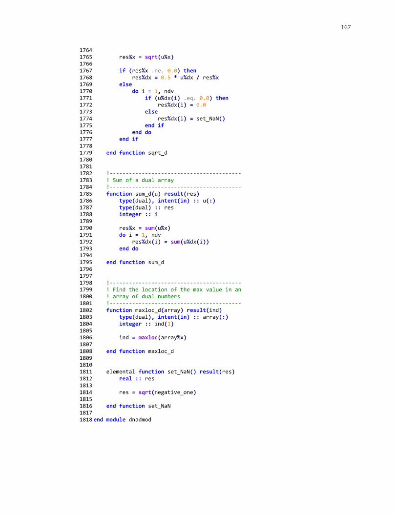
167

1764 1765 res%x = sqrt(u%x) 1766 1767 if (res%x .ne. 0.0) then 1768 res%dx = 0.5 * u%dx / res%x 1769 else 1770 do i = 1, ndv 1771 if (u%dx(i) .eq. 0.0) then 1772 res%dx(i) = 0.0 1773 else 1774 res%dx(i) = set_NaN() 1775 end if 1776 end do 1777 end if 1778 1779 end function sqrt_d 1780 1781 1782 !----------------------------------------- 1783 ! Sum of a dual array 1784 !----------------------------------------- 1785 function sum_d(u) result(res) 1786 type(dual), intent(in) :: u(:) 1787 type(dual) :: res 1788 integer :: i 1789 1790 res%x = sum(u%x) 1791 do i = 1, ndv 1792 res%dx(i) = sum(u%dx(i)) 1793 end do 1794 1795 end function sum_d 1796 1797 1798 !----------------------------------------- 1799 ! Find the location of the max value in an 1800 ! array of dual numbers 1801 !----------------------------------------- 1802 function maxloc_d(array) result(ind) 1803 type(dual), intent(in) :: array(:) 1804 integer :: ind(1) 1805 1806 ind = maxloc(array%x) 1807 1808 end function maxloc_d 1809 1810 1811 elemental function set_NaN() result(res) 1812 real :: res 1813 1814 res = sqrt(negative_one) 1815 1816 end function set_NaN 1817 1818 end module dnadmod

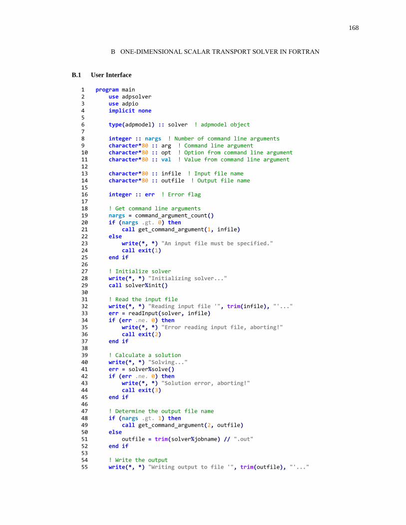
168

B ONE-DIMENSIONAL SCALAR TRANSPORT SOLVER IN FORTRAN

B.1 User Interface

1 program main 2 use adpsolver 3 use adpio 4 implicit none 5 6 type(adpmodel) :: solver ! adpmodel object 7 8 integer :: nargs ! Number of command line arguments 9 character*80 :: arg ! Command line argument 10 character*80 :: opt ! Option from command line argument 11 character*80 :: val ! Value from command line argument 12 13 character*80 :: infile ! Input file name 14 character*80 :: outfile ! Output file name 15 16 integer :: err ! Error flag 17 18 ! Get command line arguments 19 nargs = command_argument_count() 20 if (nargs .gt. 0) then 21 call get_command_argument(1, infile) 22 else 23 write(*, *) "An input file must be specified." 24 call exit(1) 25 end if 26 27 ! Initialize solver 28 write(*, *) "Initializing solver..." 29 call solver%init() 30 31 ! Read the input file 32 write(*, *) "Reading input file '", trim(infile), "'..." 33 err = readInput(solver, infile) 34 if (err .ne. 0) then 35 write(*, *) "Error reading input file, aborting!" 36 call exit(2) 37 end if 38 39 ! Calculate a solution 40 write(*, *) "Solving..." 41 err = solver%solve() 42 if (err .ne. 0) then 43 write(*, *) "Solution error, aborting!" 44 call exit(3) 45 end if 46 47 ! Determine the output file name 48 if (nargs .gt. 1) then 49 call get_command_argument(2, outfile) 50 else 51 outfile = trim(solver%jobname) // ".out" 52 end if 53 54 ! Write the output 55 write(*, *) "Writing output to file '", trim(outfile), "'..."

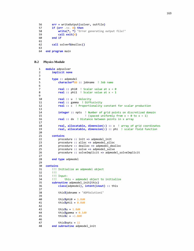
169

56 err = writeOutput(solver, outfile) 57 if (err .ne. 0) then 58 write(*, *) "Error generating output file!" 59 call exit(4) 60 end if 61 62 call solver%dealloc() 63 64 end program main

B.2 Physics Module

1 module adpsolver 2 implicit none 3 4 type :: adpmodel 5 character*80 :: jobname ! Job name 6 7 real :: phi0 ! Scalar value at x = 0 8 real :: phi1 ! Scalar value at x = 1 9 10 real :: u ! Velocity 11 real :: gamma ! Diffusivity 12 real :: c ! Proportionality constant for scalar production 13 14 integer :: npts ! Number of grid points on discretized domain 15 ! (spaced uniformly from x = 0 to x = 1) 16 real :: dx ! Distance between points in x array 17 18 real, allocatable, dimension(:) :: x ! array of grid coordinates 19 real, allocatable, dimension(:) :: phi ! scalar field function 20 21 contains 22 procedure :: init => adpmodel_init 23 procedure :: alloc => adpmodel_alloc 24 procedure :: dealloc => adpmodel_dealloc 25 procedure :: solve => adpmodel_solve 26 procedure :: solveImplicit => adpmodel_solveImplicit 27 28 end type adpmodel 29 30 contains 31 !!! Initialize an adpmodel object 32 !!! 33 !!! Input: 34 !!! this = adpmodel object to initialize 35 subroutine adpmodel_init(this) 36 class(adpmodel), intent(inout) :: this 37 38 this%jobname = "ADPSolution1" 39 40 this%phi0 = 1.0d0 41 this%phi1 = 0.0d0 42 43 this%u = 1.0d0 44 this%gamma = 0.1d0 45 this%c = -1.0d0 46 47 this%npts = 11 48 end subroutine adpmodel_init

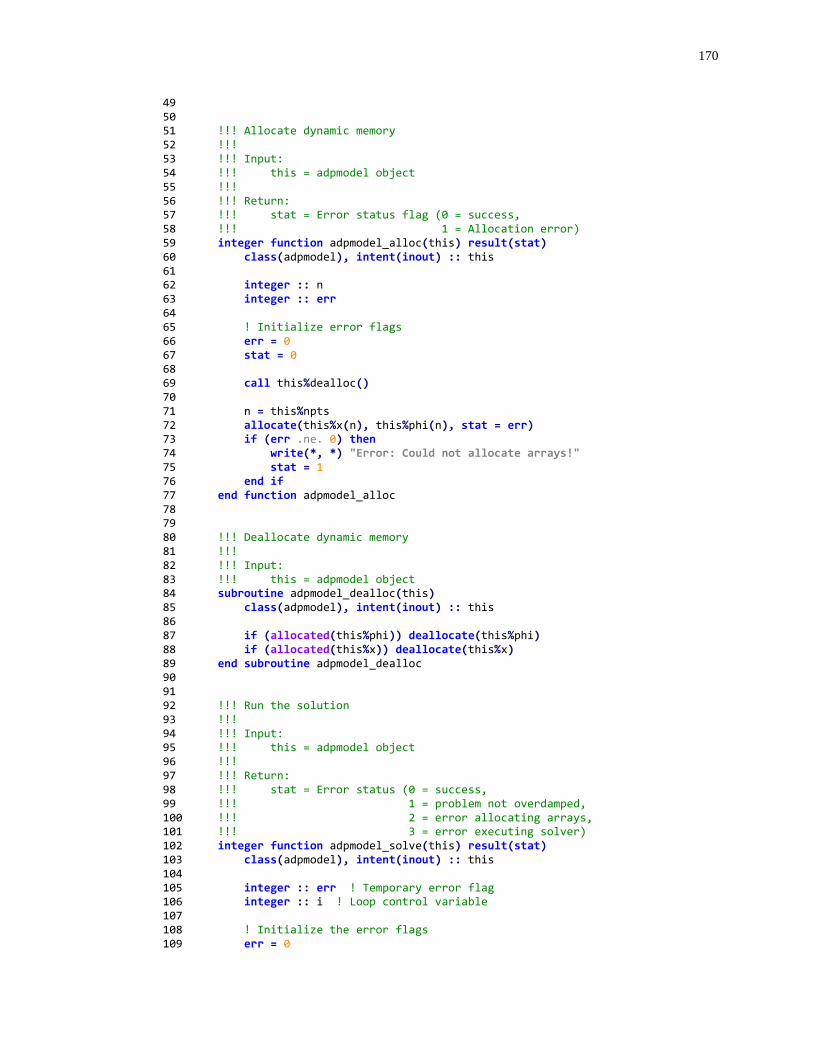
170

49 50 51 !!! Allocate dynamic memory 52 !!! 53 !!! Input: 54 !!! this = adpmodel object 55 !!! 56 !!! Return: 57 !!! stat = Error status flag (0 = success, 58 !!! 1 = Allocation error) 59 integer function adpmodel_alloc(this) result(stat) 60 class(adpmodel), intent(inout) :: this 61 62 integer :: n 63 integer :: err 64 65 ! Initialize error flags 66 err = 0 67 stat = 0 68 69 call this%dealloc() 70 71 n = this%npts 72 allocate(this%x(n), this%phi(n), stat = err) 73 if (err .ne. 0) then 74 write(*, *) "Error: Could not allocate arrays!" 75 stat = 1 76 end if 77 end function adpmodel_alloc 78 79 80 !!! Deallocate dynamic memory 81 !!! 82 !!! Input: 83 !!! this = adpmodel object 84 subroutine adpmodel_dealloc(this) 85 class(adpmodel), intent(inout) :: this 86 87 if (allocated(this%phi)) deallocate(this%phi) 88 if (allocated(this%x)) deallocate(this%x) 89 end subroutine adpmodel_dealloc 90 91 92 !!! Run the solution 93 !!! 94 !!! Input: 95 !!! this = adpmodel object 96 !!! 97 !!! Return: 98 !!! stat = Error status (0 = success, 99 !!! 1 = problem not overdamped, 100 !!! 2 = error allocating arrays, 101 !!! 3 = error executing solver) 102 integer function adpmodel_solve(this) result(stat) 103 class(adpmodel), intent(inout) :: this 104 105 integer :: err ! Temporary error flag 106 integer :: i ! Loop control variable 107 108 ! Initialize the error flags 109 err = 0

171

110 stat = 0 111 112 ! Make sure we are in the overdamped regime 113 if (this%u**2 .le. 4.0d0 * this%c * this%gamma) then 114 write(*, *) "Error: The specified properties do not meet ", & 115 "the overdamping requirement for this analysis." 116 stat = 1 117 return 118 end if 119 120 ! Allocate solution arrays 121 err = this%alloc() 122 if (err .ne. 0) then 123 stat = 2 124 return 125 end if 126 127 ! Populate x array for npts 128 this%dx = 1.0d0 / (this%nPts - 1) 129 do i = 1, this%npts 130 this%x(i) = (i - 1) * this%dx 131 end do 132 133 ! Solve the problem 134 err = this%solveImplicit() 135 136 ! Check solution status 137 if (err .ne. 0) then 138 stat = 3 139 return 140 end if 141 142 end function adpmodel_solve 143 144 145 !!! Solve the problem implicitly 146 !!! 147 !!! Inputs: 148 !!! this = AdvectionSolver object 149 !!! 150 !!! Return: 151 !!! stat = Error status (0 = success) 152 integer function adpmodel_solveImplicit(this) result(stat) 153 class(adpmodel), intent(inout) :: this 154 155 integer :: i, j ! Loop control variables 156 integer :: n ! Shortcut to npts 157 real, dimension(:), allocatable :: ld ! Lower diagonal vector 158 real, dimension(:), allocatable :: md ! Middle diagonal vector 159 real, dimension(:), allocatable :: ud ! Uppder diagonal vector 160 real, dimension(:), allocatable :: bc ! BC vector 161 162 real :: aE, aW, aP ! Matrix coefficients 163 real :: w ! temporary variable 164 165 ! Initialize error flag 166 stat = 0 167 168 ! Allocate the solution matrix and BC vector 169 n = this%npts 170 allocate(bc(n), ld(n), md(n), ud(n))

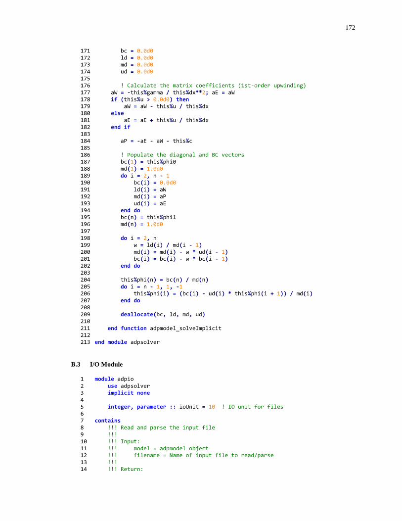
172

171 bc = 0.0d0 172 ld = 0.0d0 173 md = 0.0d0 174 ud = 0.0d0 175 176 ! Calculate the matrix coefficients (1st-order upwinding) 177 aW = -this%gamma / this%dx**2; aE = aW 178 if (this%u > 0.0d0) then 179 aW = aW - this%u / this%dx 180 else 181 aE = aE + this%u / this%dx 182 end if 183 184 aP = -aE - aW - this%c 185 186 ! Populate the diagonal and BC vectors 187 bc(1) = this%phi0 188 md(1) = 1.0d0 189 do i = 2, n - 1 190 bc(i) = 0.0d0 191 ld(i) = aW 192 md(i) = aP 193 ud(i) = aE 194 end do 195 bc(n) = this%phi1 196 md(n) = 1.0d0 197 198 do i = 2, n 199 w = ld(i) / md(i - 1) 200 md(i) = md(i) - w * ud(i - 1) 201 bc(i) = bc(i) - w * bc(i - 1) 202 end do 203 204 this%phi(n) = bc(n) / md(n) 205 do i = n - 1, 1, -1 206 this%phi(i) = (bc(i) - ud(i) * this%phi(i + 1)) / md(i) 207 end do 208 209 deallocate(bc, ld, md, ud) 210 211 end function adpmodel_solveImplicit 212 213 end module adpsolver

B.3 I/O Module

1 module adpio 2 use adpsolver 3 implicit none 4 5 integer, parameter :: ioUnit = 10 ! IO unit for files 6 7 contains 8 !!! Read and parse the input file 9 !!! 10 !!! Input: 11 !!! model = adpmodel object 12 !!! filename = Name of input file to read/parse 13 !!! 14 !!! Return:

173

15 !!! stat = Error status (0 = success, 16 !!! 1 = error opening input file, 17 !!! 2 = error parsing card(s)) 18 integer function readInput(model, filename) result(stat) 19 class(adpmodel), intent(inout) :: model 20 character*80, intent(in) :: filename ! Name of input file 21 22 character*80 :: card 23 character*80 :: id 24 25 integer :: err ! I/O error flag 26 27 ! Initialize the error flags 28 err = 0 29 stat = 0 30 31 ! Open the file for reading 32 open(unit = ioUnit, file = filename, status = 'old', & 33 & action = 'read', iostat = err) 34 if (err .ne. 0) then 35 write(*, '(A)') "ERROR: The input file could not be read." 36 write(*, '(A, A)') " Filename = ", trim(filename) 37 write(*, '(A, I3)') " I/O Error = ", err 38 close(ioUnit) 39 stat = 1 40 return 41 end if 42 43 ! Begin processing input cards 44 read(ioUnit, '(A)', iostat = err) card 45 do while (.not. is_iostat_end(err)) 46 ! Remove all whitespace from card 47 card = removeWhitespace(card) 48 49 if (card(1:1) .eq. '*') then 50 write(*, '(A, 1X, A)') "Found card:", trim(card) 51 err = parseCard(model, card) 52 if (err .ne. 0) then 53 stat = 2 54 end if 55 else if (len(trim(card)) .gt. 1) then 56 write(*, '(A, 1X, A)') "Found comment:", trim(card) 57 end if 58 59 ! Read the next card 60 read(ioUnit, '(A)', iostat = err) card 61 end do 62 63 if (stat .eq. 2) then 64 write(*, *) "Error: Some input cards were not processed." 65 end if 66 67 close(unit = ioUnit) 68 69 end function readInput 70 71 72 !!! Parse an input card and extract all parameter data 73 !!! 74 !!! Input: 75 !!! model = adpmodel object

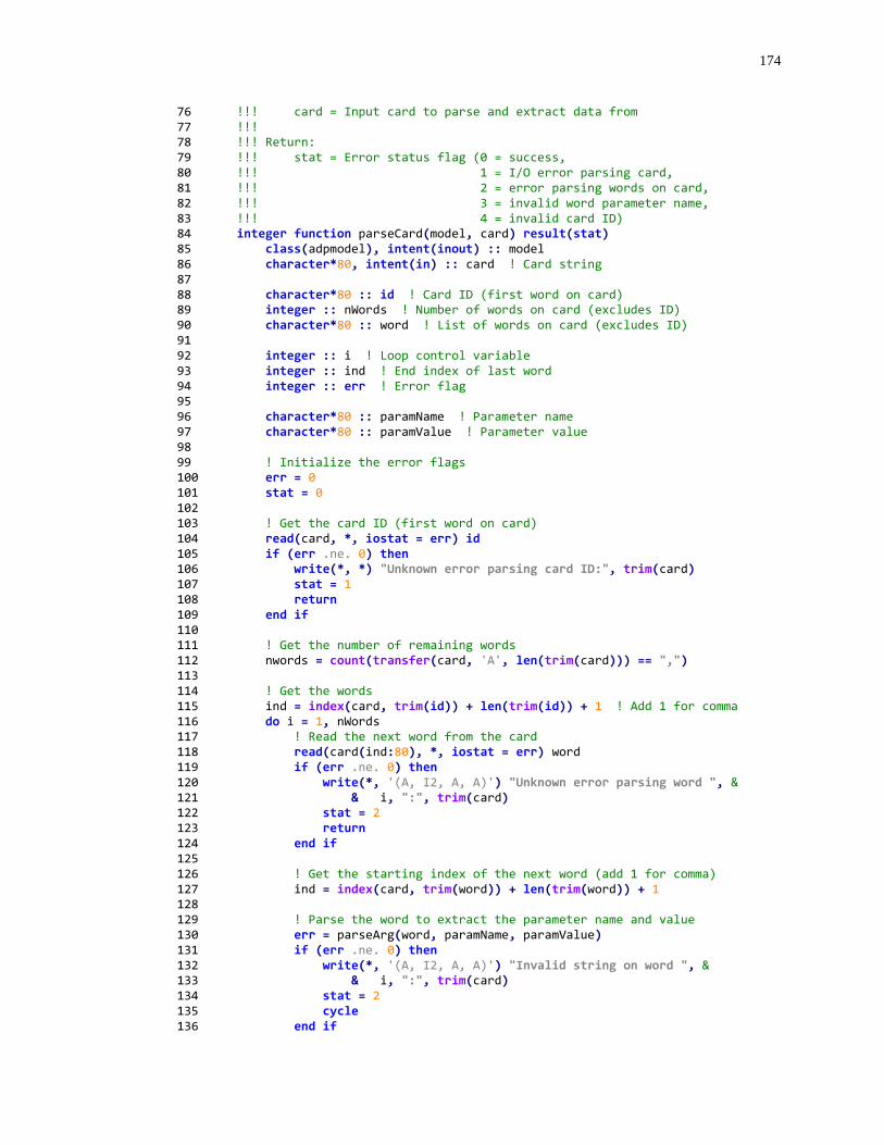
174

76 !!! card = Input card to parse and extract data from 77 !!! 78 !!! Return: 79 !!! stat = Error status flag (0 = success, 80 !!! 1 = I/O error parsing card, 81 !!! 2 = error parsing words on card, 82 !!! 3 = invalid word parameter name, 83 !!! 4 = invalid card ID) 84 integer function parseCard(model, card) result(stat) 85 class(adpmodel), intent(inout) :: model 86 character*80, intent(in) :: card ! Card string 87 88 character*80 :: id ! Card ID (first word on card) 89 integer :: nWords ! Number of words on card (excludes ID) 90 character*80 :: word ! List of words on card (excludes ID) 91 92 integer :: i ! Loop control variable 93 integer :: ind ! End index of last word 94 integer :: err ! Error flag 95 96 character*80 :: paramName ! Parameter name 97 character*80 :: paramValue ! Parameter value 98 99 ! Initialize the error flags 100 err = 0 101 stat = 0 102 103 ! Get the card ID (first word on card) 104 read(card, *, iostat = err) id 105 if (err .ne. 0) then 106 write(*, *) "Unknown error parsing card ID:", trim(card) 107 stat = 1 108 return 109 end if 110 111 ! Get the number of remaining words 112 nwords = count(transfer(card, 'A', len(trim(card))) == ",") 113 114 ! Get the words 115 ind = index(card, trim(id)) + len(trim(id)) + 1 ! Add 1 for comma 116 do i = 1, nWords 117 ! Read the next word from the card 118 read(card(ind:80), *, iostat = err) word 119 if (err .ne. 0) then 120 write(*, '(A, I2, A, A)') "Unknown error parsing word ", & 121 & i, ":", trim(card) 122 stat = 2 123 return 124 end if 125 126 ! Get the starting index of the next word (add 1 for comma) 127 ind = index(card, trim(word)) + len(trim(word)) + 1 128 129 ! Parse the word to extract the parameter name and value 130 err = parseArg(word, paramName, paramValue) 131 if (err .ne. 0) then 132 write(*, '(A, I2, A, A)') "Invalid string on word ", & 133 & i, ":", trim(card) 134 stat = 2 135 cycle 136 end if

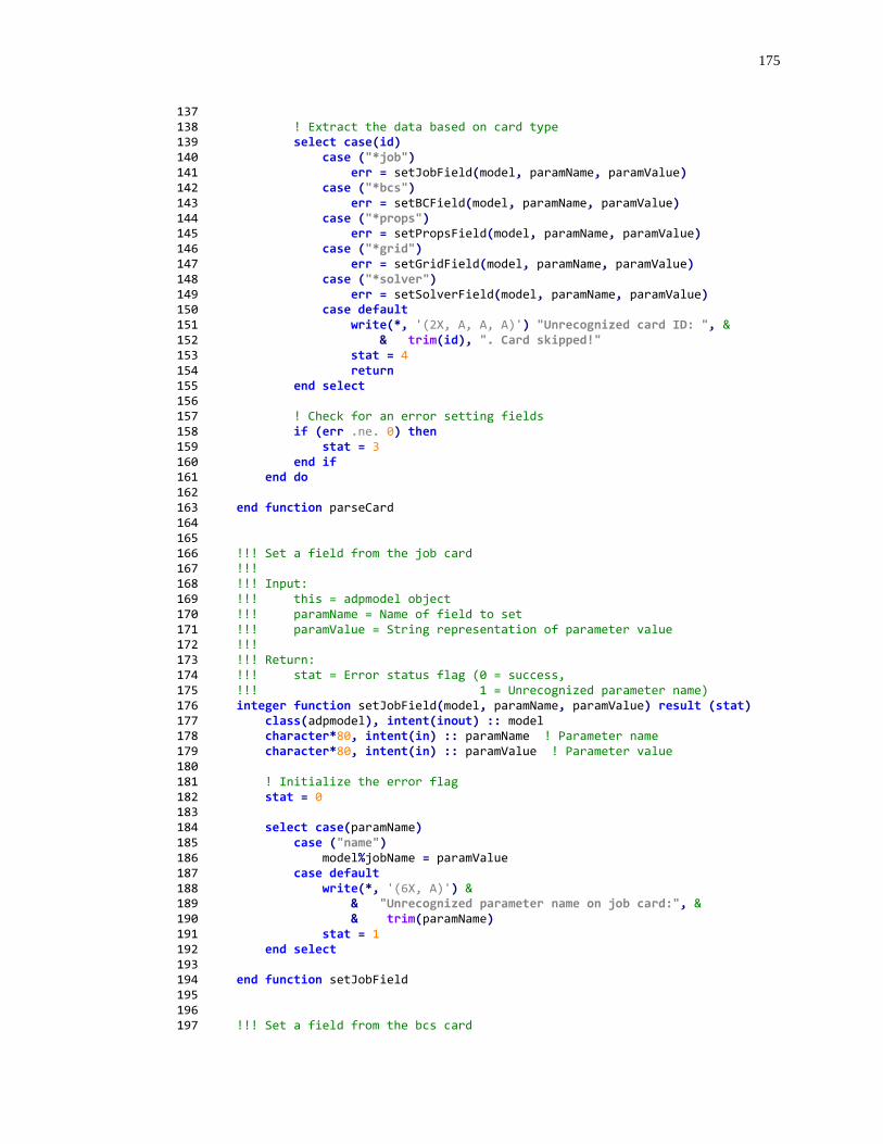
175

137 138 ! Extract the data based on card type 139 select case(id) 140 case ("*job") 141 err = setJobField(model, paramName, paramValue) 142 case ("*bcs") 143 err = setBCField(model, paramName, paramValue) 144 case ("*props") 145 err = setPropsField(model, paramName, paramValue) 146 case ("*grid") 147 err = setGridField(model, paramName, paramValue) 148 case ("*solver") 149 err = setSolverField(model, paramName, paramValue) 150 case default 151 write(*, '(2X, A, A, A)') "Unrecognized card ID: ", & 152 & trim(id), ". Card skipped!" 153 stat = 4 154 return 155 end select 156 157 ! Check for an error setting fields 158 if (err .ne. 0) then 159 stat = 3 160 end if 161 end do 162 163 end function parseCard 164 165 166 !!! Set a field from the job card 167 !!! 168 !!! Input: 169 !!! this = adpmodel object 170 !!! paramName = Name of field to set 171 !!! paramValue = String representation of parameter value 172 !!! 173 !!! Return: 174 !!! stat = Error status flag (0 = success, 175 !!! 1 = Unrecognized parameter name) 176 integer function setJobField(model, paramName, paramValue) result (stat) 177 class(adpmodel), intent(inout) :: model 178 character*80, intent(in) :: paramName ! Parameter name 179 character*80, intent(in) :: paramValue ! Parameter value 180 181 ! Initialize the error flag 182 stat = 0 183 184 select case(paramName) 185 case ("name") 186 model%jobName = paramValue 187 case default 188 write(*, '(6X, A)') & 189 & "Unrecognized parameter name on job card:", & 190 & trim(paramName) 191 stat = 1 192 end select 193 194 end function setJobField 195 196 197 !!! Set a field from the bcs card

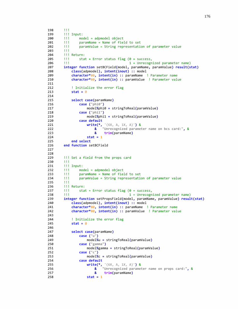
176

198 !!! 199 !!! Input: 200 !!! model = adpmodel object 201 !!! paramName = Name of field to set 202 !!! paramValue = String representation of parameter value 203 !!! 204 !!! Return: 205 !!! stat = Error status flag (0 = success, 206 !!! 1 = Unrecognized parameter name) 207 integer function setBCField(model, paramName, paramValue) result(stat) 208 class(adpmodel), intent(inout) :: model 209 character*80, intent(in) :: paramName ! Parameter name 210 character*80, intent(in) :: paramValue ! Parameter value 211 212 ! Initialize the error flag 213 stat = 0 214 215 select case(paramName) 216 case ("phi0") 217 model%phi0 = stringToReal(paramValue) 218 case ("phi1") 219 model%phi1 = stringToReal(paramValue) 220 case default 221 write(*, '(6X, A, 1X, A)') & 222 & "Unrecognized parameter name on bcs card:", & 223 & trim(paramName) 224 stat = 1 225 end select 226 end function setBCField 227 228 229 !!! Set a field from the props card 230 !!! 231 !!! Input: 232 !!! model = adpmodel object 233 !!! paramName = Name of field to set 234 !!! paramValue = String representation of parameter value 235 !!! 236 !!! Return: 237 !!! stat = Error status flag (0 = success, 238 !!! 1 = Unrecognized parameter name) 239 integer function setPropsField(model, paramName, paramValue) result(stat) 240 class(adpmodel), intent(inout) :: model 241 character*80, intent(in) :: paramName ! Parameter name 242 character*80, intent(in) :: paramValue ! Parameter value 243 244 ! Initialize the error flag 245 stat = 0 246 247 select case(paramName) 248 case ("u") 249 model%u = stringToReal(paramValue) 250 case ("gamma") 251 model%gamma = stringToReal(paramValue) 252 case ("c") 253 model%c = stringToReal(paramValue) 254 case default 255 write(*, '(6X, A, 1X, A)') & 256 & "Unrecognized parameter name on props card:", & 257 & trim(paramName) 258 stat = 1

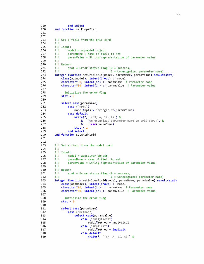
177

259 end select 260 end function setPropsField 261 262 263 !!! Set a field from the grid card 264 !!! 265 !!! Input: 266 !!! model = adpmodel object 267 !!! paramName = Name of field to set 268 !!! paramValue = String representation of parameter value 269 !!! 270 !!! Return: 271 !!! stat = Error status flag (0 = success, 272 !!! 1 = Unrecognized parameter name) 273 integer function setGridField(model, paramName, paramValue) result(stat) 274 class(adpmodel), intent(inout) :: model 275 character*80, intent(in) :: paramName ! Parameter name 276 character*80, intent(in) :: paramValue ! Parameter value 277 278 ! Initialize the error flag 279 stat = 0 280 281 select case(paramName) 282 case ("npts") 283 model%npts = stringToInt(paramValue) 284 case default 285 write(*, '(6X, A, 1X, A)') & 286 & "Unrecognized parameter name on grid card:", & 287 & trim(paramName) 288 stat = 1 289 end select 290 end function setGridField 291 292 293 !!! Set a field from the model card 294 !!! 295 !!! Input: 296 !!! model = adpsolver object 297 !!! paramName = Name of field to set 298 !!! paramValue = String representation of parameter value 299 !!! 300 !!! Return: 301 !!! stat = Error status flag (0 = success, 302 !!! 1 = Unrecognized parameter name) 303 integer function setSolverField(model, paramName, paramValue) result(stat) 304 class(adpmodel), intent(inout) :: model 305 character*80, intent(in) :: paramName ! Parameter name 306 character*80, intent(in) :: paramValue ! Parameter value 307 308 ! Initialize the error flag 309 stat = 0 310 311 select case(paramName) 312 case ("method") 313 select case(paramValue) 314 case ("analytical") 315 model%method = analytical 316 case ("implicit") 317 model%method = implicit 318 case default 319 write(*, '(6X, A, 1X, A)') &

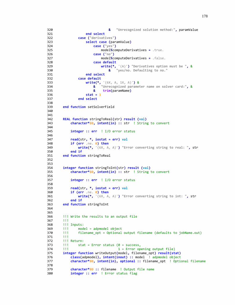
178

320 & "Unrecognized solution method:", paramValue 321 end select 322 case ("derivatives") 323 select case (paramValue) 324 case ("yes") 325 model%computeDerivatives = .true. 326 case ("no") 327 model%computeDerivatives = .false. 328 case default 329 write(*, '(A)') "Derivatives option must be ", & 330 & "yes/no. Defaulting to no." 331 end select 332 case default 333 write(*, '(6X, A, 1X, A)') & 334 & "Unrecognized parameter name on solver card:", & 335 & trim(paramName) 336 stat = 1 337 end select 338 339 end function setSolverField 340 341 342 REAL function stringToReal(str) result (val) 343 character*80, intent(in) :: str ! String to convert 344 345 integer :: err ! I/O error status 346 347 read(str, *, iostat = err) val 348 if (err .ne. 0) then 349 write(*, '(6X, A, A)') "Error converting string to real: ", str 350 end if 351 end function stringToReal 352 353 354 integer function stringToInt(str) result (val) 355 character*80, intent(in) :: str ! String to convert 356 357 integer :: err ! I/O error status 358 359 read(str, *, iostat = err) val 360 if (err .ne. 0) then 361 write(*, '(6X, A, A)') "Error converting string to int: ", str 362 end if 363 end function stringToInt 364 365 366 !!! Write the results to an output file 367 !!! 368 !!! Inputs: 369 !!! model = adpmodel object 370 !!! filename_opt = Optional output filename (defaults to jobName.out) 371 !!! 372 !!! Return: 373 !!! stat = Error status (0 = success, 374 !!! 1 = Error opening output file) 375 integer function writeOutput(model, filename_opt) result(stat) 376 class(adpmodel), intent(inout) :: model ! adpmodel object 377 character*80, intent(in), optional :: filename_opt ! Optional filename 378 379 character*80 :: filename ! Output file name 380 integer :: err ! Error status flag

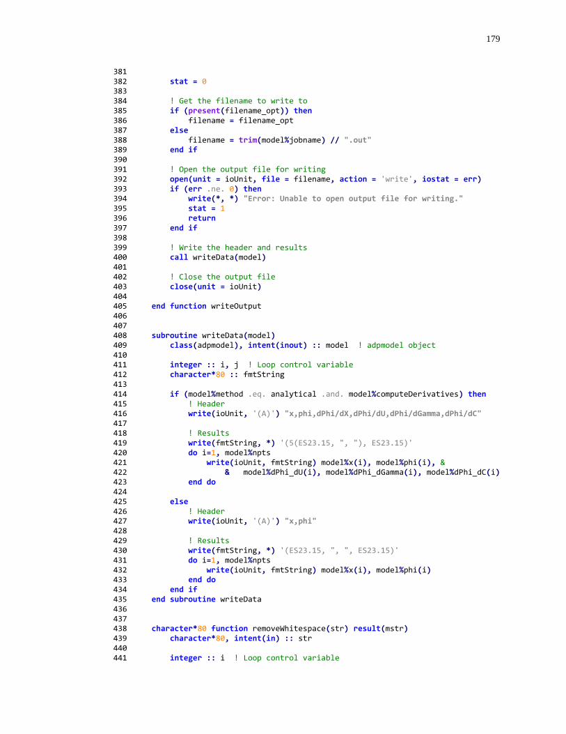
179

381 382 stat = 0 383 384 ! Get the filename to write to 385 if (present(filename_opt)) then 386 filename = filename_opt 387 else 388 filename = trim(model%jobname) // ".out" 389 end if 390 391 ! Open the output file for writing 392 open(unit = ioUnit, file = filename, action = 'write', iostat = err) 393 if (err .ne. 0) then 394 write(*, *) "Error: Unable to open output file for writing." 395 stat = 1 396 return 397 end if 398 399 ! Write the header and results 400 call writeData(model) 401 402 ! Close the output file 403 close(unit = ioUnit) 404 405 end function writeOutput 406 407 408 subroutine writeData(model) 409 class(adpmodel), intent(inout) :: model ! adpmodel object 410 411 integer :: i, j ! Loop control variable 412 character*80 :: fmtString 413 414 if (model%method .eq. analytical .and. model%computeDerivatives) then 415 ! Header 416 write(ioUnit, '(A)') "x,phi,dPhi/dX,dPhi/dU,dPhi/dGamma,dPhi/dC" 417 418 ! Results 419 write(fmtString, *) '(5(ES23.15, ", "), ES23.15)' 420 do i=1, model%npts 421 write(ioUnit, fmtString) model%x(i), model%phi(i), & 422 & model%dPhi_dU(i), model%dPhi_dGamma(i), model%dPhi_dC(i) 423 end do 424 425 else 426 ! Header 427 write(ioUnit, '(A)') "x,phi" 428 429 ! Results 430 write(fmtString, *) '(ES23.15, ", ", ES23.15)' 431 do i=1, model%npts 432 write(ioUnit, fmtString) model%x(i), model%phi(i) 433 end do 434 end if 435 end subroutine writeData 436 437 438 character*80 function removeWhitespace(str) result(mstr) 439 character*80, intent(in) :: str 440 441 integer :: i ! Loop control variable

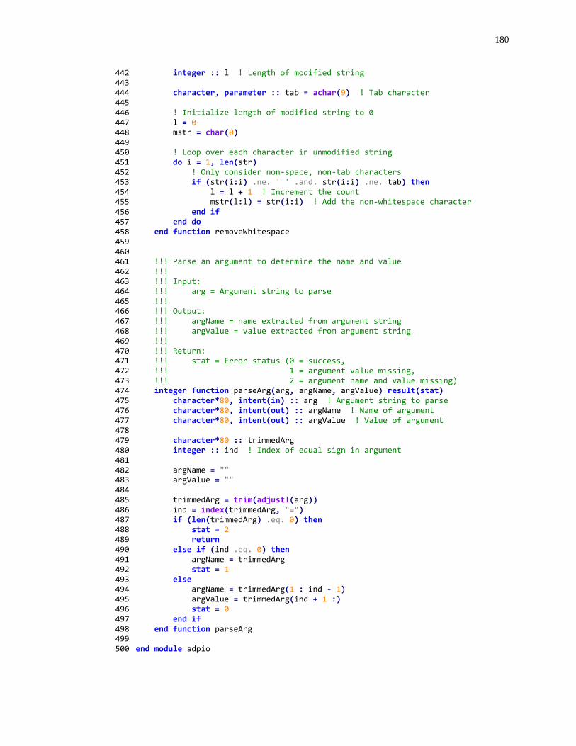
180

442 integer :: l ! Length of modified string 443 444 character, parameter :: tab = achar(9) ! Tab character 445 446 ! Initialize length of modified string to 0 447 l = 0 448 mstr = char(0) 449 450 ! Loop over each character in unmodified string 451 do i = 1, len(str) 452 ! Only consider non-space, non-tab characters 453 if (str(i:i) .ne. ' ' .and. str(i:i) .ne. tab) then 454 l = l + 1 ! Increment the count 455 mstr(l:l) = str(i:i) ! Add the non-whitespace character 456 end if 457 end do 458 end function removeWhitespace 459 460 461 !!! Parse an argument to determine the name and value 462 !!! 463 !!! Input: 464 !!! arg = Argument string to parse 465 !!! 466 !!! Output: 467 !!! argName = name extracted from argument string 468 !!! argValue = value extracted from argument string 469 !!! 470 !!! Return: 471 !!! stat = Error status (0 = success, 472 !!! 1 = argument value missing, 473 !!! 2 = argument name and value missing) 474 integer function parseArg(arg, argName, argValue) result(stat) 475 character*80, intent(in) :: arg ! Argument string to parse 476 character*80, intent(out) :: argName ! Name of argument 477 character*80, intent(out) :: argValue ! Value of argument 478 479 character*80 :: trimmedArg 480 integer :: ind ! Index of equal sign in argument 481 482 argName = "" 483 argValue = "" 484 485 trimmedArg = trim(adjustl(arg)) 486 ind = index(trimmedArg, "=") 487 if (len(trimmedArg) .eq. 0) then 488 stat = 2 489 return 490 else if (ind .eq. 0) then 491 argName = trimmedArg 492 stat = 1 493 else 494 argName = trimmedArg(1 : ind - 1) 495 argValue = trimmedArg(ind + 1 :) 496 stat = 0 497 end if 498 end function parseArg 499 500 end module adpio

181

C SUMMARY OF CODE CHANGES TO APPENDIX B FOR DNAD INTEGRATION

C.1 Changes to adpsolver Module

Original: lines 1-2

1 module adpsolver 2 implicit none

Modified: lines 1-6

1 module adpsolver 2 #ifdef dnad 3 use dnadmod 4 #define real type(dual) 5 #endif 6 implicit none

C.2 Changes to adpio Module

Original: lines 1-2

1 module adpio 2 implicit none

Modified: lines 1-6

1 module adpio 2 #ifdef dnad 3 use dnadmod 4 #define real type(dual) 5 #endif 6 use adpsolver

Original: lines 5-7

5 integer, parameter :: ioUnit = 10 ! IO unit for files 6 7 contains

Modified: lines 9-16

9 integer, parameter :: ioUnit = 10 ! IO unit for files 10 #ifdef dnad 11 integer, parameter :: maxdvs = 3 ! Maximum number of derivatives supported 12 integer :: dvcount = 0 ! Count of partial derivatives requested 13 character*80, dimension(maxdvs) :: dvnames = "" ! List of derivative names 14 #endif 15 16 Contains

Original: lines 149-150

149 err = setSolverField(model, paramName, paramValue) 150 case default

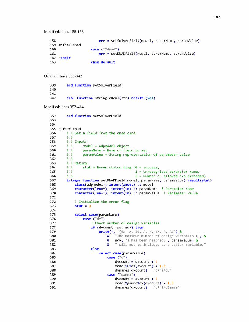
182


158 err = setSolverField(model, paramName, paramValue) 159 #ifdef dnad 160 case ("*dnad") 161 err = setDNADField(model, paramName, paramValue) 162 #endif 163 case default


339 end function setSolverField 340 341 342 real function stringToReal(str) result (val)


352 end function setSolverField 353 354 355 #ifdef dnad 356 !!! Set a field from the dnad card 357 !!! 358 !!! Input: 359 !!! model = adpmodel object 360 !!! paramName = Name of field to set 361 !!! paramValue = String representation of parameter value 362 !!! 363 !!! Return: 364 !!! stat = Error status flag (0 = success, 365 !!! 1 = Unrecognized parameter name, 366 !!! 2 = Number of allowed dvs exceeded) 367 integer function setDNADField(model, paramName, paramValue) result(stat) 368 class(adpmodel), intent(inout) :: model 369 character(len=*), intent(in) :: paramName ! Parameter name 370 character(len=*), intent(in) :: paramValue ! Parameter value 371 372 ! Initialize the error flag 373 stat = 0 374 375 select case(paramName) 376 case ("dv") 377 ! Check number of design variables 378 if (dvcount .ge. ndv) then 379 write(*, '(6X, A, I0, A, /, 6X, A, A)') & 380 & "The maximum number of design variables (", & 381 & ndv, ") has been reached.", paramValue, & 382 & " will not be included as a design variable." 383 else 384 select case(paramValue) 385 case ("u") 386 dvcount = dvcount + 1 387 model%u%dx(dvcount) = 1.0 388 dvnames(dvcount) = "dPhi/dU" 389 case ("gamma") 390 dvcount = dvcount + 1 391 model%gamma%dx(dvcount) = 1.0 392 dvnames(dvcount) = "dPhi/dGamma"

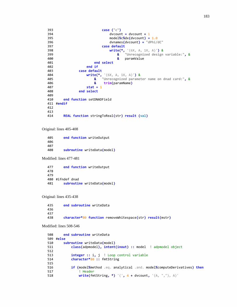
183

393 case ("c") 394 dvcount = dvcount + 1 395 model%c%dx(dvcount) = 1.0 396 dvnames(dvcount) = "dPhi/dC" 397 case default 398 write(*, '(6X, A, 1X, A)') & 399 & "Unrecognized design variable:", & 400 & paramValue 401 end select 402 end if 403 case default 404 write(*, '(6X, A, 1X, A)') & 405 & "Unrecognized parameter name on dnad card:", & 406 & trim(paramName) 407 stat = 1 408 end select 409 410 end function setDNADField 411 #endif 412 413 414 REAL function stringToReal(str) result (val)


405 end function writeOutput 406 407 408 subroutine writeData(model)


477 end function writeOutput 478 479 480 #ifndef dnad 481 subroutine writeData(model)


435 end subroutine writeData 436 437 438 character*80 function removeWhitespace(str) result(mstr)


508 end subroutine writeData 509 #else 510 subroutine writeData(model) 511 class(adpmodel), intent(inout) :: model ! adpmodel object 512 513 integer :: i, j ! Loop control variable 514 character*80 :: fmtString 515 516 if (model%method .eq. analytical .and. model%computeDerivatives) then 517 ! Header 518 write(fmtString, *) '(', 4 + dvcount, '(A, ","), A)'

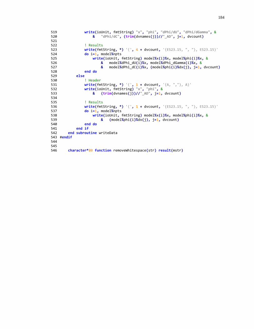
184

519 write(ioUnit, fmtString) "x", "phi", "dPhi/dU", "dPhi/dGamma", & 520 & "dPhi/dC", (trim(dvnames(j))//"_AD", j=1, dvcount) 521 522 ! Results 523 write(fmtString, *) '(', 4 + dvcount, '(ES23.15, ", "), ES23.15)' 524 do i=1, model%npts 525 write(ioUnit, fmtString) model%x(i)%x, model%phi(i)%x, & 526 & model%dPhi_dU(i)%x, model%dPhi_dGamma(i)%x, & 527 & model%dPhi_dC(i)%x, (model%phi(i)%dx(j), j=1, dvcount) 528 end do 529 else 530 ! Header 531 write(fmtString, *) '(', 1 + dvcount, '(A, ","), A)' 532 write(ioUnit, fmtString) "x", "phi", & 533 & (trim(dvnames(j))//"_AD", j=1, dvcount) 534 535 ! Results 536 write(fmtString, *) '(', 1 + dvcount, '(ES23.15, ", "), ES23.15)' 537 do i=1, model%npts 538 write(ioUnit, fmtString) model%x(i)%x, model%phi(i)%x, & 539 & (model%phi(i)%dx(j), j=1, dvcount) 540 end do 541 end if 542 end subroutine writeData 543 #endif 544 545 546 character*80 function removeWhitespace(str) result(mstr)

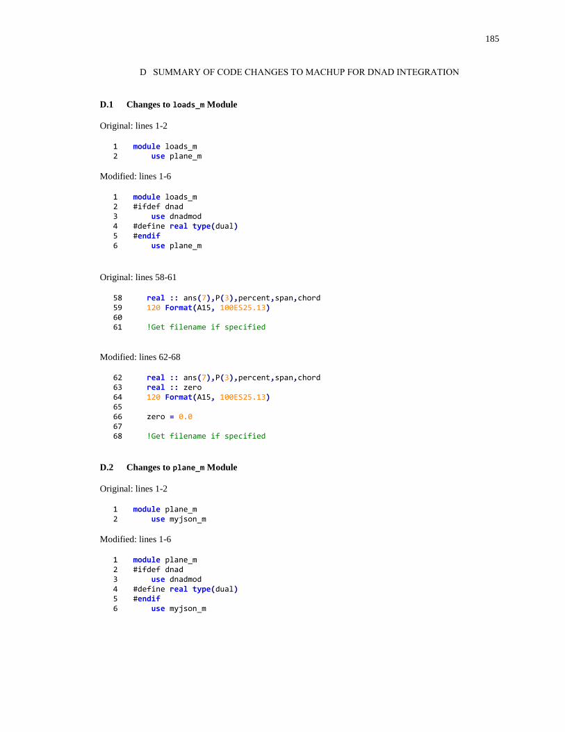
185

D SUMMARY OF CODE CHANGES TO MACHUP FOR DNAD INTEGRATION

D.1 Changes to loads_m Module

Original: lines 1-2

1 module loads_m 2 use plane_m

Modified: lines 1-6

1 module loads_m 2 #ifdef dnad 3 use dnadmod 4 #define real type(dual) 5 #endif 6 use plane_m


58 real :: ans(7),P(3),percent,span,chord 59 120 Format(A15, 100ES25.13) 60 61 !Get filename if specified


62 real :: ans(7),P(3),percent,span,chord 63 real :: zero 64 120 Format(A15, 100ES25.13) 65 66 zero = 0.0 67 68 !Get filename if specified

D.2 Changes to plane_m Module

Original: lines 1-2

1 module plane_m 2 use myjson_m

Modified: lines 1-6

1 module plane_m 2 #ifdef dnad 3 use dnadmod 4 #define real type(dual) 5 #endif 6 use myjson_m

186


150 call t%json%get('plane.name', cval); call json_check(); t%name = trim(cval) 151 t%CG(1) = json_file_required_real(t%json,'plane.CGx') 152 t%CG(2) = json_file_required_real(t%json,'plane.CGy') 153 t%CG(3) = json_file_required_real(t%json,'plane.CGz') 154 155 t%Sr = json_file_required_real(t%json,'reference.area') 156 t%long_r = json_file_required_real(t%json,'reference.longitudinal_length') 157 t%lat_r = json_file_required_real(t%json,'reference.lateral_length') 158 159 t%alpha = json_file_required_real(t%json,'condition.alpha'); t%alpha =

t%alpha*pi/180.0 160 t%beta = json_file_optional_real(t%json,'condition.beta',0.0); t%beta =

t%beta*pi/180.0 161 162 t%omega(1) = json_file_optional_real(t%json,'condition.omega.roll',0.0) 163 t%omega(2) = json_file_optional_real(t%json,'condition.omega.pitch',0.0) 164 t%omega(3) = json_file_optional_real(t%json,'condition.omega.yaw',0.0) 165 166 t%hag = json_file_optional_real(t%json,'condition.ground',0.0) 167 if(t%hag.gt.0.0) t%groundplane = 1 168 169 call t%json%get('solver.type', cval); call json_check(); solver = trim(cval) 170 jacobian_converged = json_file_optional_real(t%json,'solver.convergence',

1.0e-6) 171 jacobian_omega = json_file_optional_real(t%json,'solver.relaxation',0.9) 172 nonlinear_maxiter = json_file_optional_integer(t%json,'solver.maxiter',100) 173 174 call t%json%get('airfoil_DB', cval); call json_check(); DB_Airfoil =

trim(cval)


154 call t%json%get('plane.name', cval); call json_check(); t%name = trim(cval) 155 call myjson_get(t%json,'plane.CGx', t%CG(1)) 156 call myjson_get(t%json,'plane.CGy', t%CG(2)) 157 call myjson_get(t%json,'plane.CGz', t%CG(3)) 158 159 call myjson_get(t%json,'reference.area', t%Sr) 160 call myjson_get(t%json,'reference.longitudinal_length', t%long_r) 161 call myjson_get(t%json,'reference.lateral_length', t%lat_r) 162 163 call myjson_get(t%json,'condition.alpha',t%alpha); t%alpha=t%alpha*pi/180.0 164 call myjson_get(t%json,'condition.beta',t%beta,0.0); t%beta=t%beta*pi/180.0 165 166 call myjson_get(t%json,'condition.omega.roll', t%omega(1), 0.0) 167 call myjson_get(t%json,'condition.omega.pitch', t%omega(2), 0.0) 168 call myjson_get(t%json,'condition.omega.yaw', t%omega(3), 0.0) 169 170 call myjson_get(t%json,'condition.ground', t%hag, 0.0) 171 if(t%hag.gt.0.0) t%groundplane = 1 172 173 call t%json%get('solver.type', cval); call json_check(); solver = trim(cval) 174 call myjson_get(t%json,'solver.convergence', jacobian_converged, 1.0e-6) 175 call myjson_get(t%json,'solver.relaxation', jacobian_omega, 0.9) 176 call myjson_get(t%json,'solver.maxiter', nonlinear_maxiter, 100) 177 178 call t%json%get('airfoil_DB', cval); call json_check(); DB_Airfoil =

trim(cval)

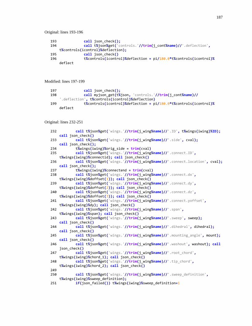
187


193 call json_check(); 194 call t%json%get('controls.'//trim(j_cont%name)//'.deflection',

t%controls(icontrol)%deflection); 195 call json_check() 196 t%controls(icontrol)%deflection = pi/180.0*t%controls(icontrol)%

deflect


197 call json_check(); 198 call myjson_get(t%json, 'controls.'//trim(j_cont%name)//

'.deflection', t%controls(icontrol)%deflection) 199 t%controls(icontrol)%deflection = pi/180.0*t%controls(icontrol)%

deflect


232 call t%json%get('wings.'//trim(j_wing%name)//'.ID', t%wings(iwing)%ID); call json_check()

233 call t%json%get('wings.'//trim(j_wing%name)//'.side', cval); call json_check();

234 t%wings(iwing)%orig_side = trim(cval) 235 call t%json%get('wings.'//trim(j_wing%name)//'.connect.ID',

t%wings(iwing)%connectid); call json_check() 236 call t%json%get('wings.'//trim(j_wing%name)//'.connect.location', cval);

call json_check(); 237 t%wings(iwing)%connectend = trim(cval) 238 call t%json%get('wings.'//trim(j_wing%name)//'.connect.dx',

t%wings(iwing)%doffset(1)); call json_check() 239 call t%json%get('wings.'//trim(j_wing%name)//'.connect.dy',

t%wings(iwing)%doffset(2)); call json_check() 240 call t%json%get('wings.'//trim(j_wing%name)//'.connect.dz',

t%wings(iwing)%doffset(3)); call json_check() 241 call t%json%get('wings.'//trim(j_wing%name)//'.connect.yoffset',

t%wings(iwing)%dy); call json_check() 242 call t%json%get('wings.'//trim(j_wing%name)//'.span',

t%wings(iwing)%span); call json_check() 243 call t%json%get('wings.'//trim(j_wing%name)//'.sweep', sweep);

call json_check() 244 call t%json%get('wings.'//trim(j_wing%name)//'.dihedral', dihedral);

call json_check() 245 call t%json%get('wings.'//trim(j_wing%name)//'.mounting_angle', mount);

call json_check() 246 call t%json%get('wings.'//trim(j_wing%name)//'.washout', washout); call

json_check() 247 call t%json%get('wings.'//trim(j_wing%name)//'.root_chord',

t%wings(iwing)%chord_1); call json_check() 248 call t%json%get('wings.'//trim(j_wing%name)//'.tip_chord',

t%wings(iwing)%chord_2); call json_check() 249 250 call t%json%get('wings.'//trim(j_wing%name)//'.sweep_definition',

t%wings(iwing)%sweep_definition); 251 if(json_failed()) t%wings(iwing)%sweep_definition=1

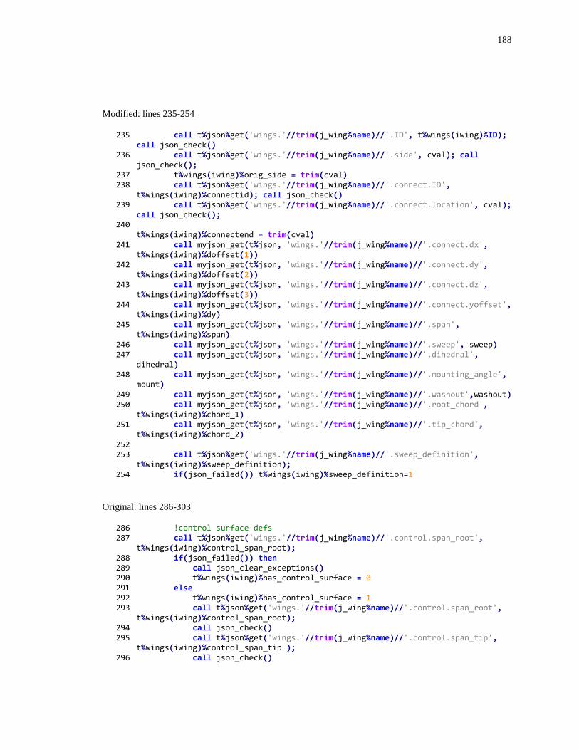
188


235 call t%json%get('wings.'//trim(j_wing%name)//'.ID', t%wings(iwing)%ID); call json_check()

236 call t%json%get('wings.'//trim(j_wing%name)//'.side', cval); call json_check();

237 t%wings(iwing)%orig_side = trim(cval) 238 call t%json%get('wings.'//trim(j_wing%name)//'.connect.ID',

t%wings(iwing)%connectid); call json_check() 239 call t%json%get('wings.'//trim(j_wing%name)//'.connect.location', cval);

call json_check(); 240

t%wings(iwing)%connectend = trim(cval) 241 call myjson_get(t%json, 'wings.'//trim(j_wing%name)//'.connect.dx',

t%wings(iwing)%doffset(1)) 242 call myjson_get(t%json, 'wings.'//trim(j_wing%name)//'.connect.dy',

t%wings(iwing)%doffset(2)) 243 call myjson_get(t%json, 'wings.'//trim(j_wing%name)//'.connect.dz',

t%wings(iwing)%doffset(3)) 244 call myjson_get(t%json, 'wings.'//trim(j_wing%name)//'.connect.yoffset',

t%wings(iwing)%dy) 245 call myjson_get(t%json, 'wings.'//trim(j_wing%name)//'.span',

t%wings(iwing)%span) 246 call myjson_get(t%json, 'wings.'//trim(j_wing%name)//'.sweep', sweep) 247 call myjson_get(t%json, 'wings.'//trim(j_wing%name)//'.dihedral',

dihedral) 248 call myjson_get(t%json, 'wings.'//trim(j_wing%name)//'.mounting_angle',

mount) 249 call myjson_get(t%json, 'wings.'//trim(j_wing%name)//'.washout',washout) 250 call myjson_get(t%json, 'wings.'//trim(j_wing%name)//'.root_chord',

t%wings(iwing)%chord_1) 251 call myjson_get(t%json, 'wings.'//trim(j_wing%name)//'.tip_chord',

t%wings(iwing)%chord_2) 252 253 call t%json%get('wings.'//trim(j_wing%name)//'.sweep_definition',

t%wings(iwing)%sweep_definition); 254 if(json_failed()) t%wings(iwing)%sweep_definition=1


286 !control surface defs 287 call t%json%get('wings.'//trim(j_wing%name)//'.control.span_root',

t%wings(iwing)%control_span_root); 288 if(json_failed()) then 289 call json_clear_exceptions() 290 t%wings(iwing)%has_control_surface = 0 291 else 292 t%wings(iwing)%has_control_surface = 1 293 call t%json%get('wings.'//trim(j_wing%name)//'.control.span_root',

t%wings(iwing)%control_span_root); 294 call json_check() 295 call t%json%get('wings.'//trim(j_wing%name)//'.control.span_tip',

t%wings(iwing)%control_span_tip ); 296 call json_check()

189

297 call t%json%get('wings.'//trim(j_wing%name)//'.control.chord_root', t%wings(iwing)%control_chord_root);

298 call json_check() 299 call t%json%get('wings.'//trim(j_wing%name)//'.control.chord_tip',

t%wings(iwing)%control_chord_tip ); 300 call json_check() 301 call t%json%get('wings.'//trim(j_wing%name)//'.control.is_sealed',

t%wings(iwing)%control_is_sealed); 302 call json_check() 303 end if


289 !control surface defs 290 call myjson_get(t%json, 'wings.'//trim(j_wing%name)//

'.control.span_root', t%wings(iwing)%control_span_root, -1.0) 291 292 if(t%wings(iwing)%control_span_root < 0.0) then 293 call json_clear_exceptions() 294 t%wings(iwing)%has_control_surface = 0 295 else 296 t%wings(iwing)%has_control_surface = 1 297 call myjson_get(t%json, 'wings.'//trim(j_wing%name)//

'.control.span_tip', t%wings(iwing)%control_span_tip) 298 call myjson_get(t%json, 'wings.'//trim(j_wing%name)//

'.control.chord_root', t%wings(iwing)%control_chord_root) 299 call myjson_get(t%json, 'wings.'//trim(j_wing%name)//

'.control.chord_tip', t%wings(iwing)%control_chord_tip) 300 call t%json%get('wings.'//trim(j_wing%name)//'.control.is_sealed',

t%wings(iwing)%control_is_sealed); 301 call json_check() 302 end if


377 case ('linear') 378 airfoils(i)%aL0 = json_file_required_real(f_json,trim(prefix)//

'properties.alpha_L0'); 379 airfoils(i)%CLa = json_file_required_real(f_json,trim(prefix)//

'properties.CL_alpha'); 380 airfoils(i)%CmL0 = json_file_required_real(f_json,trim(prefix)//

'properties.Cm_L0'); 381 airfoils(i)%Cma = json_file_required_real(f_json,trim(prefix)//

'properties.Cm_alpha'); 382 airfoils(i)%CD0 = json_file_required_real(f_json,trim(prefix)//

'properties.CD_min'); 383 airfoils(i)%CLmax = json_file_optional_real(f_json,trim(prefix)//

'properties.CL_max',-1.0); 384 airfoils(i)%has_data_file = 0


376 case ('linear') 377 call myjson_get(f_json, trim(prefix)//'properties.alpha_L0',

airfoils(i)%aL0); 378 call myjson_get(f_json, trim(prefix)//'properties.CL_alpha',

airfoils(i)%CLa); 379 call myjson_get(f_json, trim(prefix)//'properties.Cm_L0',

airfoils(i)%CmL0);

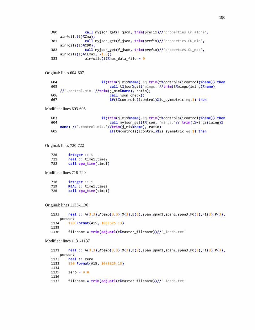
190

380 call myjson_get(f_json, trim(prefix)//'properties.Cm_alpha', airfoils(i)%Cma);

381 call myjson_get(f_json, trim(prefix)//'properties.CD_min', airfoils(i)%CD0);

382 call myjson_get(f_json, trim(prefix)//'properties.CL_max', airfoils(i)%CLmax, -1.0);

383 airfoils(i)%has_data_file = 0


604 if(trim(j_mix%name).eq.trim(t%controls(icontrol)%name)) then 605 call t%json%get('wings.'//trim(t%wings(iwing)%name)

//'.control.mix.'//trim(j_mix%name), ratio); 606 call json_check() 607 if(t%controls(icontrol)%is_symmetric.eq.1) then


603 if(trim(j_mix%name).eq.trim(t%controls(icontrol)%name)) then 604 call myjson_get(t%json, 'wings.'// trim(t%wings(iwing)%

name) //'.control.mix.'//trim(j_mix%name), ratio) 605 if(t%controls(icontrol)%is_symmetric.eq.1) then


720 integer :: i 721 real :: time1,time2 722 call cpu_time(time1)


718 integer :: i 719 REAL :: time1,time2 720 call cpu_time(time1)


1133 real :: A(3,3),Atemp(3,3),X(3),B(3),span,span1,span2,span3,F0(3),F1(3),P(3), percent

1134 120 Format(A15, 100ES25.13) 1135 1136 filename = trim(adjustl(t%master_filename))//'_loads.txt'


1131 real :: A(3,3),Atemp(3,3),X(3),B(3),span,span1,span2,span3,F0(3),F1(3),P(3), percent

1132 real :: zero 1133 120 Format(A15, 100ES25.13) 1134 1135 zero = 0.0 1136 1137 filename = trim(adjustl(t%master_filename))//'_loads.txt'

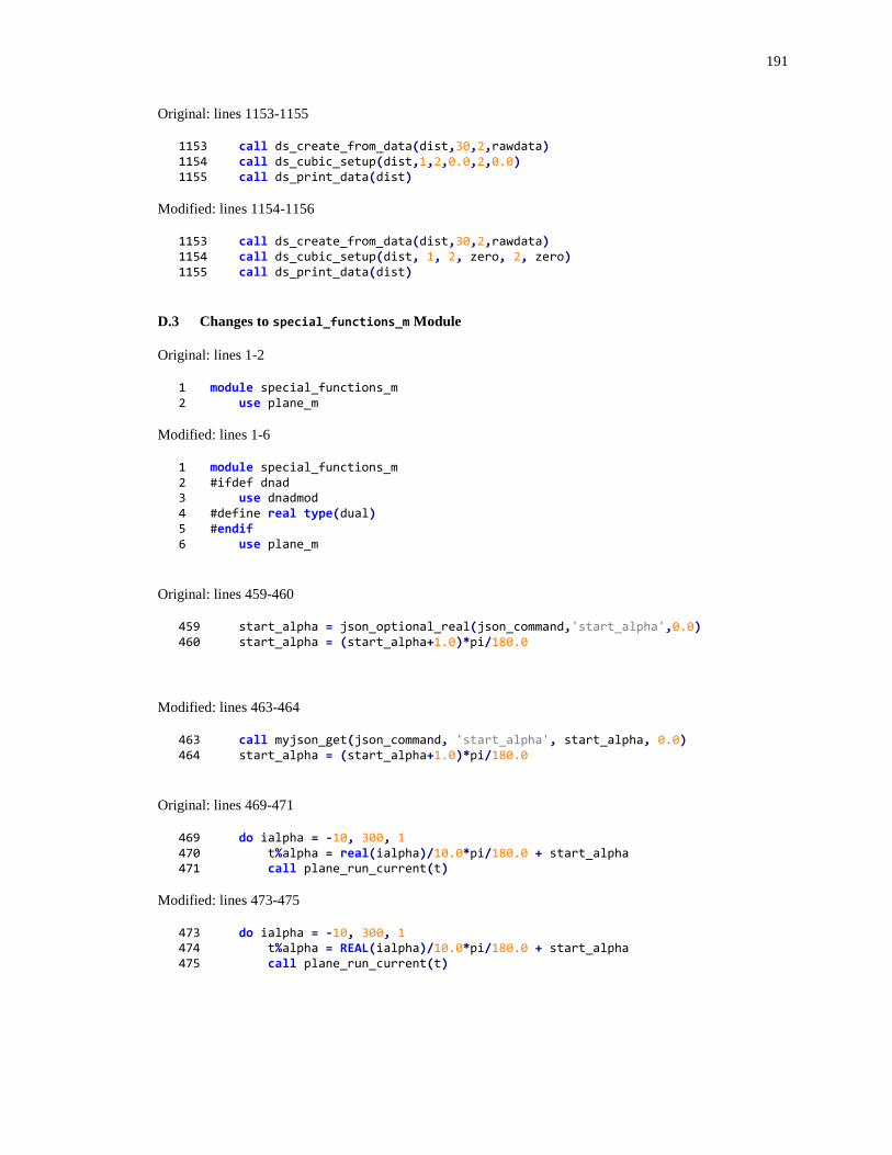
191


1153 call ds_create_from_data(dist,30,2,rawdata) 1154 call ds_cubic_setup(dist,1,2,0.0,2,0.0) 1155 call ds_print_data(dist)


1153 call ds_create_from_data(dist,30,2,rawdata) 1154 call ds_cubic_setup(dist, 1, 2, zero, 2, zero) 1155 call ds_print_data(dist)

D.3 Changes to special_functions_m Module

Original: lines 1-2

1 module special_functions_m 2 use plane_m

Modified: lines 1-6

1 module special_functions_m 2 #ifdef dnad 3 use dnadmod 4 #define real type(dual) 5 #endif 6 use plane_m


459 start_alpha = json_optional_real(json_command,'start_alpha',0.0) 460 start_alpha = (start_alpha+1.0)*pi/180.0


463 call myjson_get(json_command, 'start_alpha', start_alpha, 0.0) 464 start_alpha = (start_alpha+1.0)*pi/180.0


469 do ialpha = -10, 300, 1 470 t%alpha = real(ialpha)/10.0*pi/180.0 + start_alpha 471 call plane_run_current(t)


473 do ialpha = -10, 300, 1 474 t%alpha = REAL(ialpha)/10.0*pi/180.0 + start_alpha 475 call plane_run_current(t)

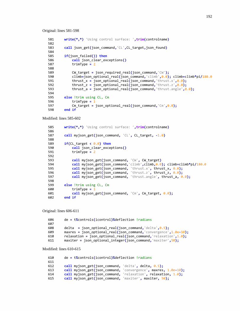
192


581 write(*,*) 'Using control surface: ',trim(controlname) 582 583 call json_get(json_command,'CL',CL_target,json_found) 584 585 if(json_failed()) then 586 call json_clear_exceptions() 587 trimType = 2 588 589 CW_target = json_required_real(json_command,'CW'); 590 climb=json_optional_real(json_command,'climb',0.0); climb=climb*pi/180.0 591 thrust_x = json_optional_real(json_command,'thrust.x',0.0); 592 thrust_z = json_optional_real(json_command,'thrust.z',0.0); 593 thrust_a = json_optional_real(json_command,'thrust.angle',0.0); 594 595 else !trim using CL, Cm 596 trimType = 1 597 Cm_target = json_optional_real(json_command,'Cm',0.0); 598 end if


585 write(*,*) 'Using control surface: ',trim(controlname) 586 587 call myjson_get(json_command, 'CL', CL_target, -1.0) 588 589 if(CL_target < 0.0) then 590 call json_clear_exceptions() 591 trimType = 2 592 593 call myjson_get(json_command, 'CW', CW_target) 594 call myjson_get(json_command,'climb',climb,0.0); climb=climb*pi/180.0 595 call myjson_get(json_command, 'thrust.x', thrust_x, 0.0); 596 call myjson_get(json_command, 'thrust.z', thrust_z, 0.0); 597 call myjson_get(json_command, 'thrust.angle', thrust_a, 0.0); 598 599 else !trim using CL, Cm 600 trimType = 1 601 call myjson_get(json_command, 'Cm', Cm_target, 0.0); 602 end if


606 de = t%controls(icontrol)%deflection !radians 607 608 delta = json_optional_real(json_command,'delta',0.5); 609 maxres = json_optional_real(json_command,'convergence',1.0e-10); 610 relaxation = json_optional_real(json_command,'relaxation',1.0); 611 maxiter = json_optional_integer(json_command,'maxiter',50);


610 de = t%controls(icontrol)%deflection !radians 611 612 call myjson_get(json_command, 'delta', delta, 0.5); 613 call myjson_get(json_command, 'convergence', maxres, 1.0e-10); 614 call myjson_get(json_command, 'relaxation', relaxation, 1.0); 615 call myjson_get(json_command, 'maxiter', maxiter, 50);

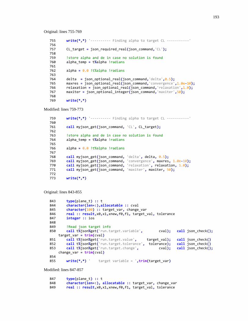
193


755 write(*,*) '---------- Finding alpha to target CL -----------' 756 757 CL_target = json_required_real(json_command,'CL'); 758 759 !store alpha and de in case no solution is found 760 alpha_temp = t%alpha !radians 761 762 alpha = 0.0 !t%alpha !radians 763 764 delta = json_optional_real(json_command,'delta',0.5); 765 maxres = json_optional_real(json_command,'convergence',1.0e-10); 766 relaxation = json_optional_real(json_command,'relaxation',1.0); 767 maxiter = json_optional_integer(json_command,'maxiter',50); 768 769 write(*,*)


759 write(*,*) '---------- Finding alpha to target CL -----------' 760 761 call myjson_get(json_command, 'CL', CL_target); 762 763 !store alpha and de in case no solution is found 764 alpha_temp = t%alpha !radians 765 766 alpha = 0.0 !t%alpha !radians 767 768 call myjson_get(json_command, 'delta', delta, 0.5); 769 call myjson_get(json_command, 'convergence', maxres, 1.0e-10); 770 call myjson_get(json_command, 'relaxation', relaxation, 1.0); 771 call myjson_get(json_command, 'maxiter', maxiter, 50); 772 773 write(*,*)


843 type(plane_t) :: t 844 character(len=:),allocatable :: cval 845 character(100) :: target_var, change_var 846 real :: result,x0,x1,xnew,f0,f1, target_val, tolerance 847 integer :: ios 848 849 !Read json target info 850 call t%json%get('run.target.variable', cval); call json_check();

target_var = trim(cval) 851 call t%json%get('run.target.value', target_val); call json_check() 852 call t%json%get('run.target.tolerance', tolerance); call json_check() 853 call t%json%get('run.target.change', cval); call json_check();

change_var = trim(cval) 854 855 write(*,*) ' target variable = ',trim(target_var)


847 type(plane_t) :: t 848 character(len=:), allocatable :: target_var, change_var 849 real :: result,x0,x1,xnew,f0,f1, target_val, tolerance

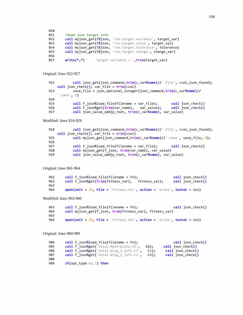
194

850 851 !Read json target info 852 call myjson_get(t%json, 'run.target.variable', target_var) 853 call myjson_get(t%json, 'run.target.value', target_val) 854 call myjson_get(t%json, 'run.target.tolerance', tolerance) 855 call myjson_get(t%json, 'run.target.change', change_var) 856 857 write(*,*) ' target variable = ',trim(target_var)


922 call json_get(json_command,trim(c_var%name)//'.file', cval,json_found); call json_check(); var_file = trim(cval)

923 save_file = json_optional_integer(json_command,trim(c_var%name)// '.save', 0)

924 925 call f_json%load_file(filename = var_file); call json_check() 926 call f_json%get(trim(var_name), var_value); call json_check() 927 call json_value_add(p_root, trim(c_var%name), var_value)


924 call json_get(json_command,trim(c_var%name)//'.file', cval,json_found); call json_check(); var_file = trim(cval)

925 call myjson_get(json_command,trim(c_var%name)//'.save', save_file, 0); 926 927 call f_json%load_file(filename = var_file); call json_check() 928 call myjson_get(f_json, trim(var_name), var_value) 929 call json_value_add(p_root, trim(c_var%name), var_value)


961 call f_json%load_file(filename = fn); call json_check() 962 call f_json%get(trim(fitness_var), fitness_val); call json_check() 963 964 open(unit = 10, File = 'fitness.txt', action = 'write', iostat = ios)


963 call f_json%load_file(filename = fn); call json_check() 964 call myjson_get(f_json, trim(fitness_var), fitness_val) 965 966 open(unit = 10, File = 'fitness.txt', action = 'write', iostat = ios)


984 call f_json%load_file(filename = fn); call json_check() 985 call f_json%get('total.MyAirplane.CD', CD); call json_check() 986 call f_json%get('total.Wing_1_left.Cl', Cl); call json_check() 987 call f_json%get('total.Wing_1_left.Cn', Cn); call json_check() 988 989 if(opt_type.eq.1) then

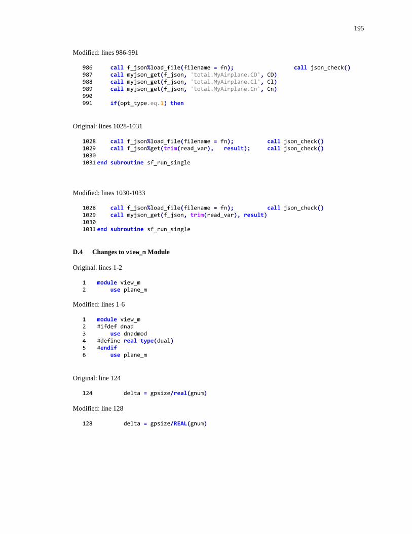
195


986 call f_json%load_file(filename = fn); call json_check() 987 call myjson_get(f_json, 'total.MyAirplane.CD', CD) 988 call myjson_get(f_json, 'total.MyAirplane.Cl', Cl) 989 call myjson_get(f_json, 'total.MyAirplane.Cn', Cn) 990 991 if(opt_type.eq.1) then


1028 call f_json%load_file(filename = fn); call json_check() 1029 call f_json%get(trim(read_var), result); call json_check() 1030 1031 end subroutine sf_run_single


1028 call f_json%load_file(filename = fn); call json_check() 1029 call myjson_get(f_json, trim(read_var), result) 1030 1031 end subroutine sf_run_single

D.4 Changes to view_m Module

Original: lines 1-2

1 module view_m 2 use plane_m

Modified: lines 1-6

1 module view_m 2 #ifdef dnad 3 use dnadmod 4 #define real type(dual) 5 #endif 6 use plane_m

Original: line 124

124 delta = gpsize/real(gnum)

Modified: line 128

128 delta = gpsize/REAL(gnum)

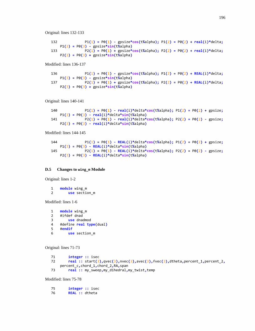
196


132 P1(1) = P0(1) - gpsize*cos(t%alpha); P1(2) = P0(2) + real(i)*delta; P1(3) = P0(3) - gpsize*sin(t%alpha)

133 P2(1) = P0(1) + gpsize*cos(t%alpha); P2(2) = P0(2) + real(i)*delta; P2(3) = P0(3) + gpsize*sin(t%alpha)


136 P1(1) = P0(1) - gpsize*cos(t%alpha); P1(2) = P0(2) + REAL(i)*delta; P1(3) = P0(3) - gpsize*sin(t%alpha)

137 P2(1) = P0(1) + gpsize*cos(t%alpha); P2(2) = P0(2) + REAL(i)*delta; P2(3) = P0(3) + gpsize*sin(t%alpha)


140 P1(1) = P0(1) - real(i)*delta*cos(t%alpha); P1(2) = P0(2) + gpsize; P1(3) = P0(3) - real(i)*delta*sin(t%alpha)

141 P2(1) = P0(1) - real(i)*delta*cos(t%alpha); P2(2) = P0(2) - gpsize; P2(3) = P0(3) - real(i)*delta*sin(t%alpha)


144 P1(1) = P0(1) - REAL(i)*delta*cos(t%alpha); P1(2) = P0(2) + gpsize; P1(3) = P0(3) - REAL(i)*delta*sin(t%alpha)

145 P2(1) = P0(1) - REAL(i)*delta*cos(t%alpha); P2(2) = P0(2) - gpsize; P2(3) = P0(3) - REAL(i)*delta*sin(t%alpha)

D.5 Changes to wing_m Module

Original: lines 1-2

1 module wing_m 2 use section_m

Modified: lines 1-6

1 module wing_m 2 #ifdef dnad 3 use dnadmod 4 #define real type(dual) 5 #endif 6 use section_m


71 integer :: isec 72 real :: start(3),qvec(3),nvec(3),avec(3),fvec(3),dtheta,percent_1,percent_2,

percent_c,chord_1,chord_2,RA,span 73 real :: my_sweep,my_dihedral,my_twist,temp


75 integer :: isec 76 REAL :: dtheta

197

77 real :: start(3), qvec(3), nvec(3), avec(3), fvec(3), percent_1, percent_2, percent_c, chord_1, chord_2, RA, span

78 real :: my_sweep, my_dihedral, my_twist, temp


104 call wing_allocate(t) 105 dtheta = pi/real(t%nSec) 106 t%area = 0.0 107 span = 0.0 108 do isec=1,t%nSec 109 percent_1 = 0.5*(1.0-cos(dtheta*real(isec-1))) 110 percent_2 = 0.5*(1.0-cos(dtheta*real(isec))) 111 percent_c = 0.5*(1.0-cos(dtheta*(real(isec)-0.5))) 112 if(t%side.eq.'left') then !must handle differently for left wing


109 call wing_allocate(t) 110 dtheta = pi/REAL(t%nSec) 111 t%area = 0.0 112 span = 0.0 113 do isec=1,t%nSec 114 percent_1 = 0.5*(1.0-cos(dtheta*REAL(isec-1))) 115 percent_2 = 0.5*(1.0-cos(dtheta*REAL(isec))) 116 percent_c = 0.5*(1.0-cos(dtheta*(REAL(isec)-0.5))) 117 if(t%side.eq.'left') then !must handle differently for left wing


274 integer :: isec 275 real :: A,B,C,D,P1(3),P2(3),P3(3),tempv(3),tempr,temp_percent 276 P1(1) = CG(1) - hag*sin(alpha) !offset from CG


279 integer :: isec 280 real :: A,B,C,D,P1(3),P2(3),P3(3),tempv(3),tempr,temp_percent,zero 281 zero = 0.0 282 P1(1) = CG(1) - hag*sin(alpha) !offset from CG


295 t%sec(isec)%chord_2 = tempr 296 297 call math_reflect_point(A,B,C,0.0,t%sec(isec)%un,tempv) 298 t%sec(isec)%un = tempv 299 call math_reflect_point(A,B,C,0.0,t%sec(isec)%ua,tempv) 300 t%sec(isec)%ua = tempv 301 call math_reflect_point(A,B,C,0.0,t%sec(isec)%uf,tempv) 302 t%sec(isec)%uf = tempv

198


301 t%sec(isec)%chord_2 = tempr 302 303 call math_reflect_point(A,B,C,zero,t%sec(isec)%un,tempv) 304 t%sec(isec)%un = tempv 305 call math_reflect_point(A,B,C,zero,t%sec(isec)%ua,tempv) 306 t%sec(isec)%ua = tempv 307 call math_reflect_point(A,B,C,zero,t%sec(isec)%uf,tempv) 308 t%sec(isec)%uf = tempv

D.6 Changes to airfoil_m Module

Original: lines 1-2

1 module airfoil_m 2 use dataset_m

Modified: lines 1-6

1 module airfoil_m 2 #ifdef dnad 3 use dnadmod 4 #define real type(dual) 5 #endif 6 use dataset_m

D.7 Changes to atmosphere_m Module

Original: lines 1-2

1 module atmosphere_m 2 use dataset_m

Modified: lines 1-6

1 module atmosphere_m 2 #ifdef dnad 3 use dnadmod 4 #define real type(dual) 5 #endif 6 use dataset_m

Original: line 12

12 real :: temp(36,7)


17 real :: temp(36,7) 18 real :: zero 19 20 zero = 0.0

199


52 call ds_create_from_data(t%properties,36,7,temp(:,:)) 53 call ds_cubic_setup(t%properties,1,2,0.0,2,0.0) 54 55 end subroutine atm_create


60 call ds_create_from_data(t%properties,36,7,temp(:,:)) 61 call ds_cubic_setup(t%properties,1,2,zero,2,zero) 62 63 end subroutine atm_create

D.8 Changes to dataset_m Module

Original: lines 1-2

1 module dataset_m 2 use math_m

Modified: lines 1-6

1 module dataset_m 2 #ifdef dnad 3 use dnadmod 4 #define real type(dual) 5 #endif 6 use math_m

D.9 Changes to math_m Module

Original: lines 1-4

1 module math_m 2 implicit none 3 real, parameter :: pi = 3.1415926535897932 4 contains

Modified: lines 1-9

1 module math_m 2 #ifdef dnad 3 use dnadmod 4 #define real type(dual) 5 #endif 6 7 implicit none 8 REAL, parameter :: pi = 3.1415926535897932 9 contains


225 INTEGER::n,D,info 226 REAL,DIMENSION(n)::B,X 227 REAL,DIMENSION(n,n)::A

200

228 229 INTEGER,allocatable,DIMENSION(:) :: INDX


230 INTEGER::n,D,info 231 real,DIMENSION(n)::B,X 232 real,DIMENSION(n,n)::A 233 234 INTEGER,allocatable,DIMENSION(:) :: INDX


274 REAL, PARAMETER :: TINY=1.5D-16 275 REAL AMAX,DUM, SUM, A(N,N) 276 REAL,ALLOCATABLE,DIMENSION(:) :: VV 277 INTEGER N, CODE, D, INDX(N)


279 REAL, PARAMETER :: TINY=1.5D-16 280 real AMAX,DUM, SUM, A(N,N) 281 real,ALLOCATABLE,DIMENSION(:) :: VV 282 INTEGER N, CODE, D, INDX(N)


356 integer :: N 357 REAL SUM, A(N,N),B(N) 358 INTEGER INDX(N)


361 integer :: N 362 real SUM, A(N,N),B(N) 363 INTEGER INDX(N)

D.10 Changes to section_m Module

Original: lines 1-2

1 module section_m 2 use airfoil_m

Modified: lines 1-6

1 module section_m 2 #ifdef dnad 3 use dnadmod 4 #define real type(dual) 5 #endif 6 use airfoil_m

201

D.11 Changes to myjson_m Module


1 module myjson_m 2 use json_m 3 implicit none 4 5 logical :: json_found 6 7 contains 8 9 !-------------------------------------------------------------------------------

- 10 real function json_required_real(json,name) 11 implicit none 12 type(json_value),intent(in),pointer :: json 13 character(len=*) :: name 14 real :: value 15 16 call json_get(json, name, value, json_found) 17 if(json_failed()) then 18 write(*,*) 'Error: Unable to read required value: ',name 19 STOP 20 end if 21 22 json_required_real = value 23 end function json_required_real 24 25 !-------------------------------------------------------------------------------

- 26 real function json_optional_real(json,name,default_value) 27 implicit none 28 type(json_value),intent(in),pointer :: json 29 character(len=*) :: name 30 real :: value, default_value 31 32 call json_get(json, name, value, json_found) 33 if((.not.json_found) .or. json_failed()) then 34 write(*,*) trim(name),' set to ',default_value 35 value = default_value 36 call json_clear_exceptions() 37 end if 38 39 json_optional_real = value 40 end function json_optional_real 41 42 !-------------------------------------------------------------------------------

- 43 integer function json_optional_integer(json,name,default_value) 44 implicit none 45 type(json_value),intent(in),pointer :: json 46 character(len=*) :: name 47 integer :: value, default_value 48 49 call json_get(json, name, value, json_found) 50 if((.not.json_found) .or. json_failed()) then 51 write(*,*) trim(name),' set to ',default_value 52 value = default_value 53 call json_clear_exceptions() 54 end if

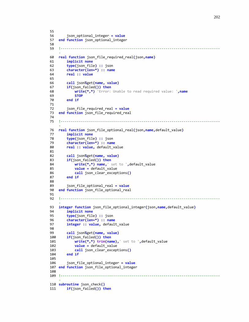
202

55 56 json_optional_integer = value 57 end function json_optional_integer 58 59 !-------------------------------------------------------------------------------

- 60 real function json_file_required_real(json,name) 61 implicit none 62 type(json_file) :: json 63 character(len=*) :: name 64 real :: value 65 66 call json%get(name, value) 67 if(json_failed()) then 68 write(*,*) 'Error: Unable to read required value: ',name 69 STOP 70 end if 71 72 json_file_required_real = value 73 end function json_file_required_real 74 75 !-------------------------------------------------------------------------------

- 76 real function json_file_optional_real(json,name,default_value) 77 implicit none 78 type(json_file) :: json 79 character(len=*) :: name 80 real :: value, default_value 81 82 call json%get(name, value) 83 if(json_failed()) then 84 write(*,*) name,' set to ',default_value 85 value = default_value 86 call json_clear_exceptions() 87 end if 88 89 json_file_optional_real = value 90 end function json_file_optional_real 91 92 !-------------------------------------------------------------------------------

- 93 integer function json_file_optional_integer(json,name,default_value) 94 implicit none 95 type(json_file) :: json 96 character(len=*) :: name 97 integer :: value, default_value 98 99 call json%get(name, value) 100 if(json_failed()) then 101 write(*,*) trim(name),' set to ',default_value 102 value = default_value 103 call json_clear_exceptions() 104 end if 105 106 json_file_optional_integer = value 107 end function json_file_optional_integer 108 109 !-------------------------------------------------------------------------------

- 110 subroutine json_check() 111 if(json_failed()) then

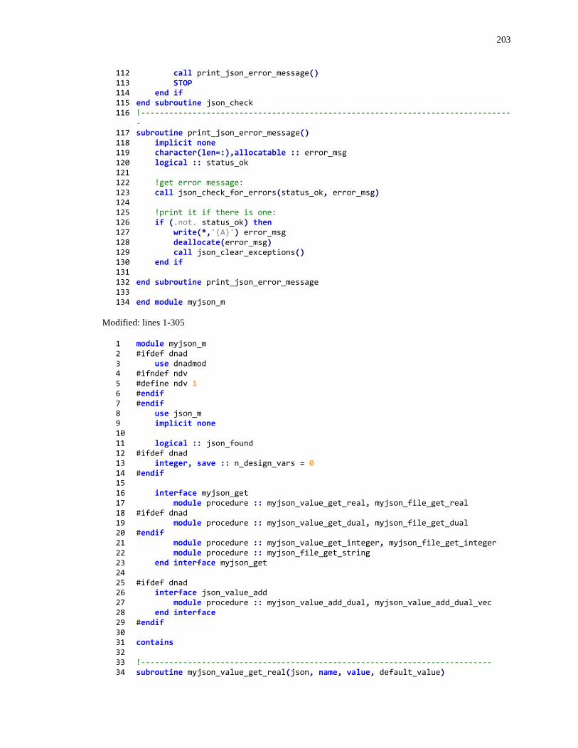
203

112 call print_json_error_message() 113 STOP 114 end if 115 end subroutine json_check 116 !-------------------------------------------------------------------------------

- 117 subroutine print_json_error_message() 118 implicit none 119 character(len=:),allocatable :: error_msg 120 logical :: status_ok 121 122 !get error message: 123 call json_check_for_errors(status_ok, error_msg) 124 125 !print it if there is one: 126 if (.not. status_ok) then 127 write(*,'(A)') error_msg 128 deallocate(error_msg) 129 call json_clear_exceptions() 130 end if 131 132 end subroutine print_json_error_message 133 134 end module myjson_m


1 module myjson_m 2 #ifdef dnad 3 use dnadmod 4 #ifndef ndv 5 #define ndv 1 6 #endif 7 #endif 8 use json_m 9 implicit none 10 11 logical :: json_found 12 #ifdef dnad 13 integer, save :: n_design_vars = 0 14 #endif 15 16 interface myjson_get 17 module procedure :: myjson_value_get_real, myjson_file_get_real 18 #ifdef dnad 19 module procedure :: myjson_value_get_dual, myjson_file_get_dual 20 #endif 21 module procedure :: myjson_value_get_integer, myjson_file_get_integer 22 module procedure :: myjson_file_get_string 23 end interface myjson_get 24 25 #ifdef dnad 26 interface json_value_add 27 module procedure :: myjson_value_add_dual, myjson_value_add_dual_vec 28 end interface 29 #endif 30 31 contains 32 33 !--------------------------------------------------------------------------- 34 subroutine myjson_value_get_real(json, name, value, default_value)

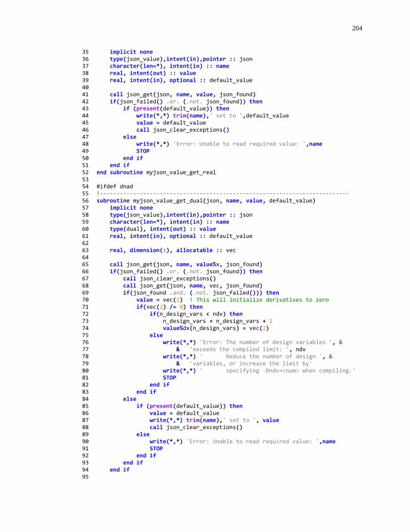
204

35 implicit none 36 type(json_value),intent(in),pointer :: json 37 character(len=*), intent(in) :: name 38 real, intent(out) :: value 39 real, intent(in), optional :: default_value 40 41 call json_get(json, name, value, json_found) 42 if(json_failed() .or. (.not. json_found)) then 43 if (present(default_value)) then 44 write(*,*) trim(name),' set to ',default_value 45 value = default_value 46 call json_clear_exceptions() 47 else 48 write(*,*) 'Error: Unable to read required value: ',name 49 STOP 50 end if 51 end if 52 end subroutine myjson_value_get_real 53 54 #ifdef dnad 55 !--------------------------------------------------------------------------- 56 subroutine myjson_value_get_dual(json, name, value, default_value) 57 implicit none 58 type(json_value),intent(in),pointer :: json 59 character(len=*), intent(in) :: name 60 type(dual), intent(out) :: value 61 real, intent(in), optional :: default_value 62 63 real, dimension(:), allocatable :: vec 64 65 call json_get(json, name, value%x, json_found) 66 if(json_failed() .or. (.not. json_found)) then 67 call json_clear_exceptions() 68 call json_get(json, name, vec, json_found) 69 if(json_found .and. (.not. json_failed())) then 70 value = vec(1) ! This will initialize derivatives to zero 71 if(vec(2) /= 0) then 72 if(n_design_vars < ndv) then 73 n_design_vars = n_design_vars + 1 74 value%dx(n_design_vars) = vec(2) 75 else 76 write(*,*) 'Error: The number of design variables ', & 77 & 'exceeds the compiled limit: ', ndv 78 write(*,*) ' Reduce the number of design ', & 79 & 'variables, or increase the limit by' 80 write(*,*) ' specifying -Dndv=<num> when compiling.' 81 STOP 82 end if 83 end if 84 else 85 if (present(default_value)) then 86 value = default_value 87 write(*,*) trim(name),' set to ', value 88 call json_clear_exceptions() 89 else 90 write(*,*) 'Error: Unable to read required value: ',name 91 STOP 92 end if 93 end if 94 end if 95

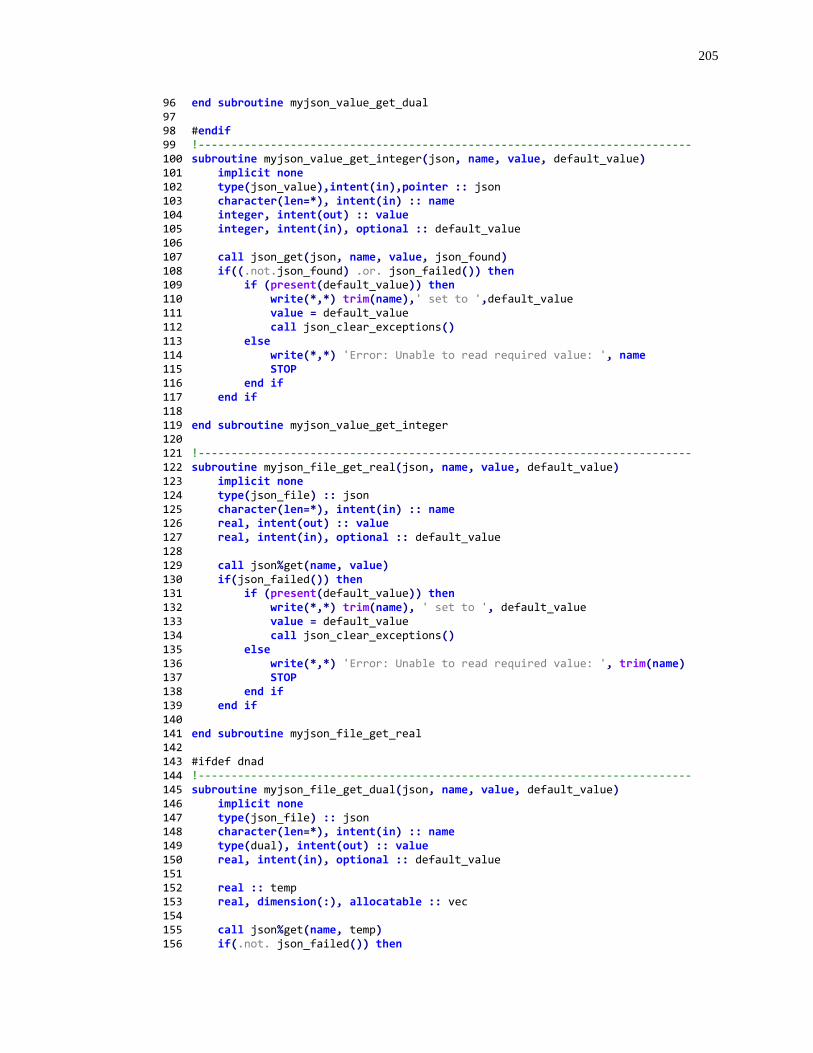
205

96 end subroutine myjson_value_get_dual 97 98 #endif 99 !--------------------------------------------------------------------------- 100 subroutine myjson_value_get_integer(json, name, value, default_value) 101 implicit none 102 type(json_value),intent(in),pointer :: json 103 character(len=*), intent(in) :: name 104 integer, intent(out) :: value 105 integer, intent(in), optional :: default_value 106 107 call json_get(json, name, value, json_found) 108 if((.not.json_found) .or. json_failed()) then 109 if (present(default_value)) then 110 write(*,*) trim(name),' set to ',default_value 111 value = default_value 112 call json_clear_exceptions() 113 else 114 write(*,*) 'Error: Unable to read required value: ', name 115 STOP 116 end if 117 end if 118 119 end subroutine myjson_value_get_integer 120 121 !--------------------------------------------------------------------------- 122 subroutine myjson_file_get_real(json, name, value, default_value) 123 implicit none 124 type(json_file) :: json 125 character(len=*), intent(in) :: name 126 real, intent(out) :: value 127 real, intent(in), optional :: default_value 128 129 call json%get(name, value) 130 if(json_failed()) then 131 if (present(default_value)) then 132 write(*,*) trim(name), ' set to ', default_value 133 value = default_value 134 call json_clear_exceptions() 135 else 136 write(*,*) 'Error: Unable to read required value: ', trim(name) 137 STOP 138 end if 139 end if 140 141 end subroutine myjson_file_get_real 142 143 #ifdef dnad 144 !--------------------------------------------------------------------------- 145 subroutine myjson_file_get_dual(json, name, value, default_value) 146 implicit none 147 type(json_file) :: json 148 character(len=*), intent(in) :: name 149 type(dual), intent(out) :: value 150 real, intent(in), optional :: default_value 151 152 real :: temp 153 real, dimension(:), allocatable :: vec 154 155 call json%get(name, temp) 156 if(.not. json_failed()) then

206

157 value = temp ! Derivatives not specified, initialize to zero 158 else 159 call json_clear_exceptions() 160 call json%get(name, vec) 161 if(.not. json_failed()) then 162 value = vec(1) ! This will initialize derivatives to zero 163 if(vec(2) /= 0) then 164 if(n_design_vars < ndv) then 165 n_design_vars = n_design_vars + 1 166 value%dx(n_design_vars) = vec(2) 167 else 168 write(*,*) 'Error: The number of design variables ', & 169 & 'exceeds the compiled limit: ', ndv 170 write(*,*) ' Reduce the number of design ', & 171 & 'variables, or increase the limit by' 172 write(*,*) ' specifying -Dndv=<num> when compiling.' 173 STOP 174 end if 175 end if 176 else 177 if (present(default_value)) then 178 value = default_value 179 write(*,*) trim(name),' set to ', value 180 call json_clear_exceptions() 181 else 182 write(*,*) 'Error: Unable to read required value: ', trim(name) 183 STOP 184 end if 185 end if 186 end if 187 188 end subroutine myjson_file_get_dual 189 190 #endif 191 !--------------------------------------------------------------------------- 192 subroutine myjson_file_get_integer(json, name, value, default_value) 193 implicit none 194 type(json_file) :: json 195 character(len=*), intent(in) :: name 196 integer, intent(out) :: value 197 integer, intent(in), optional :: default_value 198 199 call json%get(name, value) 200 if(json_failed()) then 201 if (present(default_value)) then 202 write(*,*) trim(name),' set to ',default_value 203 value = default_value 204 call json_clear_exceptions() 205 else 206 write(*,*) 'Error: Unable to read required value: ',name 207 STOP 208 end if 209 end if 210 end subroutine myjson_file_get_integer 211 212 !--------------------------------------------------------------------------- 213 subroutine myjson_file_get_string(json, name, value) 214 implicit none 215 type(json_file) :: json 216 character(len=*), intent(in) :: name 217 character(:), allocatable, intent(out) :: value

207

218 219 call json%get(name, value) 220 if(json_failed()) then 221 write(*,*) 'Error: Unable to read required value: ',name 222 STOP 223 end if 224 225 value = trim(value) 226 end subroutine myjson_file_get_string 227 228 !--------------------------------------------------------------------------- 229 subroutine json_check() 230 if(json_failed()) then 231 call print_json_error_message() 232 STOP 233 end if 234 end subroutine json_check 235 !--------------------------------------------------------------------------- 236 subroutine print_json_error_message() 237 implicit none 238 character(len=:),allocatable :: error_msg 239 logical :: status_ok 240 241 !get error message: 242 call json_check_for_errors(status_ok, error_msg) 243 244 !print it if there is one: 245 if (.not. status_ok) then 246 write(*,'(A)') error_msg 247 deallocate(error_msg) 248 call json_clear_exceptions() 249 end if 250 251 end subroutine print_json_error_message 252 253 #ifdef dnad 254 subroutine myjson_value_add_dual(me, name, val) 255 256 implicit none 257 258 type(json_value), pointer :: me 259 character(len=*),intent(in) :: name 260 type(dual),intent(in) :: val 261 262 real,allocatable,dimension(:) :: vec 263 integer :: vec_length 264 265 ! Dual numbers are written to json as a vector: [u, du/dx, du/dy, ...] 266 vec_length = size(val%dx) + 1 267 allocate(vec(vec_length)) 268 vec(1) = val%x 269 vec(2:) = val%dx 270 271 call json_value_add(me, name, vec) 272 273 end subroutine myjson_value_add_dual 274 275 subroutine myjson_value_add_dual_vec(me, name, val) 276 277 implicit none 278

208

279 type(json_value), pointer :: me 280 character(len=*),intent(in) :: name 281 type(dual),dimension(:),intent(in) :: val 282 283 type(json_value),pointer :: var 284 integer :: i 285 286 !create the variable as an array: 287 call json_value_create(var) 288 call to_array(var,name) 289 290 !populate the array: 291 do i=1,size(val) 292 call json_value_add(var, '', val(i)) 293 end do 294 295 !add it: 296 call json_value_add(me, var) 297 298 !cleanup: 299 nullify(var) 300 301 end subroutine myjson_value_add_dual_vec 302 !*************************************************************************** 303 304 #endif 305 end module myjson_m

209

E EXAMPLE MACHUP INPUT FILES

E.1 Example JSON-Formatted Input File

{ "run": { "targetcl": { "CL": 0.5, "delta": 0.1, "relaxation": 1.0, "maxiter": 100, "convergence": 1.0E-12, "run": 1 }, "forces": {"run": 1}, "distributions": {"run": 1}, "stl": {"run": 1} }, "solver": { "type": "nonlinear", "convergence": 1.0E-12, "relaxation": 0.9 }, "plane": { "name": "MyAirplane", "CGx": 0, "CGy": 0, "CGz": 0 }, "reference": { "area": 8.0, "longitudinal_length": 1.0, "lateral_length": 8.0 }, "condition": { "alpha": 5.0, "beta": 0.0 }, "airfoil_DB": "./AirfoilDB", "wings": { "wing_main": { "name": "wing_main", "ID": 1, "is_main": 1, "side": "both", "connect": { "ID": 0, "location": "tip", "dx": 0, "dy": 0, "dz": 0, "yoffset": 0 }, "span": 4, "mounting_angle": 0, "sweep": 0.0, "dihedral": 0.0, "washout": 0, "root_chord": 1.27323954473516, "tip_chord": -1, "airfoils": { "NACA_2412": "" }, "grid": 100, "control": {} } } }

E.2 Example Parameter File for a NACA 2412 Airfoil in Inviscid Incompressible Flow

{ "NACA_2412": { "properties": { "type": "linear", "alpha_L0": -0.0380, "CL_alpha": 6.8583, "Cm_L0": 0.0, "Cm_alpha": 0.0, "CD0": 0.0, "CD0_L": 0.0, "CD0_L2": 0.0, "CL_max": 1.4, "Comments": "All angles in radians and slopes in 1/radians" } } }

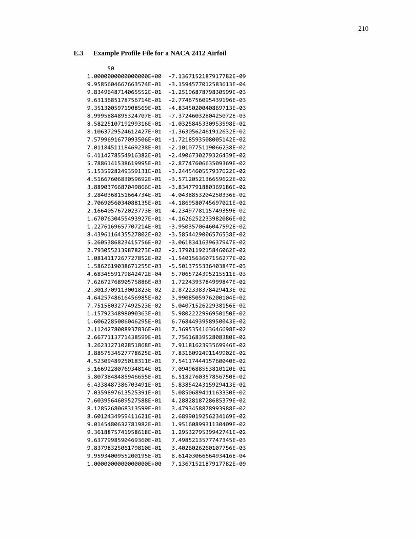
210

E.3 Example Profile File for a NACA 2412 Airfoil

50

1.0000000000000000E+00 -7.1367152187917782E-09

9.9585604667663574E-01 -3.1594577012583613E-04

9.8349648714065552E-01 -1.2519687879830599E-03

9.6313685178756714E-01 -2.7746756095439196E-03

9.3513005971908569E-01 -4.8345020040869713E-03

8.9995884895324707E-01 -7.3724603280425072E-03

8.5822510719299316E-01 -1.0325845330953598E-02

8.1063729524612427E-01 -1.3630562461912632E-02

7.5799691677093506E-01 -1.7218593508005142E-02

7.0118451118469238E-01 -2.1010775119066238E-02

6.4114278554916382E-01 -2.4906730279326439E-02

5.7886141538619995E-01 -2.8774760663509369E-02

5.1535928249359131E-01 -3.2445460557937622E-02

4.5166760683059692E-01 -3.5712052136659622E-02

3.8890376687049866E-01 -3.8347791880369186E-02

3.2840368151664734E-01 -4.0438853204250336E-02

2.7069056034088135E-01 -4.1869580745697021E-02

2.1664057672023773E-01 -4.2349778115749359E-02

1.6707630455493927E-01 -4.1626252233982086E-02

1.2276169657707214E-01 -3.9503570646047592E-02

8.4396116435527802E-02 -3.5854429006576538E-02

5.2605386823415756E-02 -3.0618341639637947E-02

2.7930552139878273E-02 -2.3790119215846062E-02

1.0814117267727852E-02 -1.5401563607156277E-02

1.5862619038671255E-03 -5.5013755336403847E-03

4.6834559179842472E-04 5.7065724395215511E-03

7.6267276890575886E-03 1.7224393784999847E-02

2.3013709113001823E-02 2.8722338378429413E-02

4.6425748616456985E-02 3.9908505976200104E-02

7.7515803277492523E-02 5.0407152622938156E-02

1.1579234898090363E-01 5.9802222996950150E-02

1.6062285006046295E-01 6.7684493958950043E-02

2.1124278008937836E-01 7.3695354163646698E-02

2.6677113771438599E-01 7.7561683952808380E-02

3.2623127102851868E-01 7.9118162393569946E-02

3.8857534527778625E-01 7.8316092491149902E-02

4.5230948925018311E-01 7.5411744415760040E-02

5.1669228076934814E-01 7.0949688553810120E-02

5.8073848485946655E-01 6.5182760357856750E-02

6.4338487386703491E-01 5.8385424315929413E-02

7.0359897613525391E-01 5.0850689411163330E-02

7.6039564609527588E-01 4.2882818728685379E-02

8.1285268068313599E-01 3.4793458878993988E-02

8.6012434959411621E-01 2.6899019256234169E-02

9.0145480632781982E-01 1.9516089931130409E-02

9.3618875741958618E-01 1.2953279539942741E-02

9.6377998590469360E-01 7.4985213577747345E-03

9.8379832506179810E-01 3.4026026260107756E-03

9.9593400955200195E-01 8.6140306666493416E-04

1.0000000000000000E+00 7.1367152187917782E-09

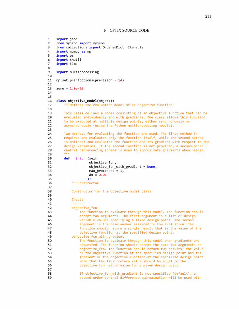
211

F OPTIX SOURCE CODE

1 import json 2 from myjson import myjson 3 from collections import OrderedDict, Iterable 4 import numpy as np 5 import os 6 import shutil 7 import time 8 9 import multiprocessing 10 11 np.set_printoptions(precision = 14) 12 13 zero = 1.0e-20 14 15 16 class objective_model(object): 17 """Defines the evaluation model of an objective function 18 19 This class defines a model consisting of an objective function that can be 20 evaluated individually and with gradients. The class allows this function 21 to be executed at multiple design points, either synchronously or 22 asynchronously (using the Python multiprocessing module). 23 24 Two methods for evaluating the function are used. The first method is 25 required and evaluates only the function itself, while the second method 26 is optional and evaluates the function and its gradient with respect to the 27 design variables. If the second function is not provided, a second-order 28 central differencing scheme is used to approximate gradients when needed. 29 """ 30 def __init__(self, 31 objective_fcn, 32 objective_fcn_with_gradient = None, 33 max_processes = 1, 34 dx = 0.01 35 ): 36 """Constructor 37 38 Constructor for the objective_model class 39 40 Inputs 41 ------ 42 objective_fcn: 43 The function to evaluate through this model. The function should 44 accept two arguments. The first argument is a list of design 45 variable values specifying a fixed design point. The second 46 argument is the case number assigned to the evaluation. The 47 function should return a single result that is the value of the 48 objective function at the specified design point. 49 objective_fcn_with_gradient: 50 The function to evaluate through this model when gradients are 51 requested. The function should accept the same two arguments as 52 objective_fcn. The function should return two results: the value 53 of the objective function at the specified design point and the 54 gradient of the objective function at the specified design point. 55 Note that the first return value should be equal to the 56 objective_fcn return value for a given design point. 57 58 If objective_fcn_with_gradient is not specified (default), a 59 second-order central difference approximation will be used with

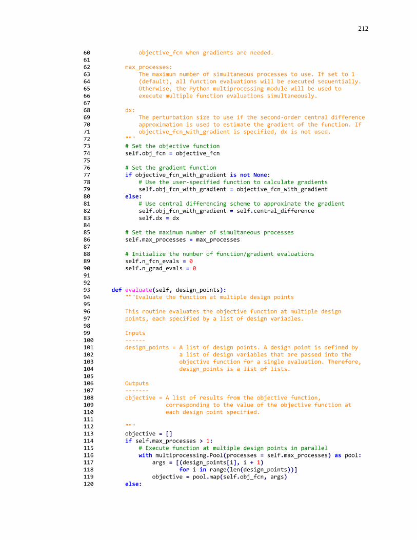
212

60 objective_fcn when gradients are needed. 61 62 max_processes: 63 The maximum number of simultaneous processes to use. If set to 1 64 (default), all function evaluations will be executed sequentially. 65 Otherwise, the Python multiprocessing module will be used to 66 execute multiple function evaluations simultaneously. 67 68 dx: 69 The perturbation size to use if the second-order central difference 70 approximation is used to estimate the gradient of the function. If 71 objective_fcn_with_gradient is specified, dx is not used. 72 """ 73 # Set the objective function 74 self.obj_fcn = objective_fcn 75 76 # Set the gradient function 77 if objective_fcn_with_gradient is not None: 78 # Use the user-specified function to calculate gradients 79 self.obj_fcn_with_gradient = objective_fcn_with_gradient 80 else: 81 # Use central differencing scheme to approximate the gradient 82 self.obj_fcn_with_gradient = self.central_difference 83 self.dx = dx 84 85 # Set the maximum number of simultaneous processes 86 self.max_processes = max_processes 87 88 # Initialize the number of function/gradient evaluations 89 self.n_fcn_evals = 0 90 self.n_grad_evals = 0 91 92 93 def evaluate(self, design_points): 94 """Evaluate the function at multiple design points 95 96 This routine evaluates the objective function at multiple design 97 points, each specified by a list of design variables. 98 99 Inputs 100 ------ 101 design_points = A list of design points. A design point is defined by 102 a list of design variables that are passed into the 103 objective function for a single evaluation. Therefore, 104 design_points is a list of lists. 105 106 Outputs 107 ------- 108 objective = A list of results from the objective function, 109 corresponding to the value of the objective function at 110 each design point specified. 111 112 """ 113 objective = [] 114 if self.max_processes > 1: 115 # Execute function at multiple design points in parallel 116 with multiprocessing.Pool(processes = self.max_processes) as pool: 117 args = [(design_points[i], i + 1) 118 for i in range(len(design_points))] 119 objective = pool.map(self.obj_fcn, args) 120 else:

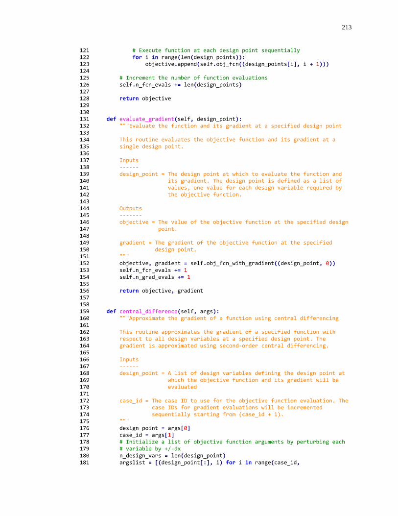
213

121 # Execute function at each design point sequentially 122 for i in range(len(design_points)): 123 objective.append(self.obj_fcn((design_points[i], i + 1))) 124 125 # Increment the number of function evaluations 126 self.n_fcn_evals += len(design_points) 127 128 return objective 129 130 131 def evaluate_gradient(self, design_point): 132 """Evaluate the function and its gradient at a specified design point 133 134 This routine evaluates the objective function and its gradient at a 135 single design point. 136 137 Inputs 138 ------ 139 design_point = The design point at which to evaluate the function and 140 its gradient. The design point is defined as a list of 141 values, one value for each design variable required by 142 the objective function. 143 144 Outputs 145 ------- 146 objective = The value of the objective function at the specified design 147 point. 148 149 gradient = The gradient of the objective function at the specified 150 design point. 151 """ 152 objective, gradient = self.obj_fcn_with_gradient((design_point, 0)) 153 self.n_fcn_evals += 1 154 self.n_grad_evals += 1 155 156 return objective, gradient 157 158 159 def central_difference(self, args): 160 """Approximate the gradient of a function using central differencing 161 162 This routine approximates the gradient of a specified function with 163 respect to all design variables at a specified design point. The 164 gradient is approximated using second-order central differencing. 165 166 Inputs 167 ------ 168 design_point = A list of design variables defining the design point at 169 which the objective function and its gradient will be 170 evaluated 171 172 case_id = The case ID to use for the objective function evaluation. The 173 case IDs for gradient evaluations will be incremented 174 sequentially starting from (case_id + 1). 175 """ 176 design_point = args[0] 177 case_id = args[1] 178 # Initialize a list of objective function arguments by perturbing each 179 # variable by +/-dx 180 n_design_vars = len(design_point) 181 argslist = [(design_point[:], i) for i in range(case_id,

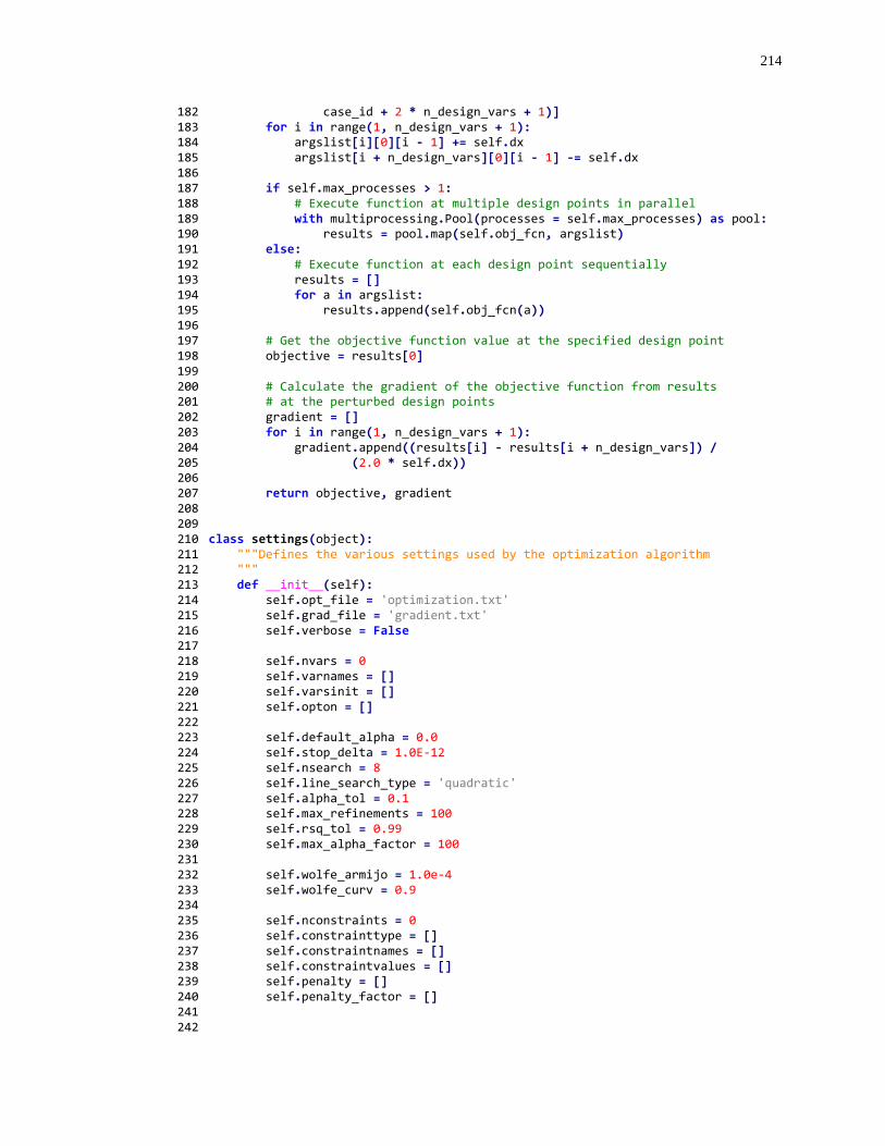
214

182 case_id + 2 * n_design_vars + 1)] 183 for i in range(1, n_design_vars + 1): 184 argslist[i][0][i - 1] += self.dx 185 argslist[i + n_design_vars][0][i - 1] -= self.dx 186 187 if self.max_processes > 1: 188 # Execute function at multiple design points in parallel 189 with multiprocessing.Pool(processes = self.max_processes) as pool: 190 results = pool.map(self.obj_fcn, argslist) 191 else: 192 # Execute function at each design point sequentially 193 results = [] 194 for a in argslist: 195 results.append(self.obj_fcn(a)) 196 197 # Get the objective function value at the specified design point 198 objective = results[0] 199 200 # Calculate the gradient of the objective function from results 201 # at the perturbed design points 202 gradient = [] 203 for i in range(1, n_design_vars + 1): 204 gradient.append((results[i] - results[i + n_design_vars]) / 205 (2.0 * self.dx)) 206 207 return objective, gradient 208 209 210 class settings(object): 211 """Defines the various settings used by the optimization algorithm 212 """ 213 def __init__(self): 214 self.opt_file = 'optimization.txt' 215 self.grad_file = 'gradient.txt' 216 self.verbose = False 217 218 self.nvars = 0 219 self.varnames = [] 220 self.varsinit = [] 221 self.opton = [] 222 223 self.default_alpha = 0.0 224 self.stop_delta = 1.0E-12 225 self.nsearch = 8 226 self.line_search_type = 'quadratic' 227 self.alpha_tol = 0.1 228 self.max_refinements = 100 229 self.rsq_tol = 0.99 230 self.max_alpha_factor = 100 231 232 self.wolfe_armijo = 1.0e-4 233 self.wolfe_curv = 0.9 234 235 self.nconstraints = 0 236 self.constrainttype = [] 237 self.constraintnames = [] 238 self.constraintvalues = [] 239 self.penalty = [] 240 self.penalty_factor = [] 241 242

215

243 def load(settings_file): 244 self = settings() 245 input = myjson(settings_file) 246 247 # Read settings from JSON file 248 json_settings = input.get('settings', OrderedDict) 249 self.default_alpha = json_settings.get('default_alpha', float) 250 self.stop_delta = json_settings.get('stop_delta', float) 251 self.nsearch = json_settings.get('n_search', int) 252 self.line_search_type = json_settings.get('line_search_type', str, 253 'quadratic') 254 self.verbose = json_settings.get('verbose', bool, False) # optional 255 256 self.alpha_tol = json_settings.get('alpha_tol', float, self.alpha_tol) 257 self.max_refinements = json_settings.get('max_refinements', int, 258 self.max_refinements) 259 self.rsq_tol = json_settings.get('rsq_tol', float, self.rsq_tol) 260 self.max_alpha_factor = json_settings.get('max_alpha_factor', int, 261 self.max_alpha_factor) 262 263 self.wolfe_armijo = json_settings.get('wolfe_armijo', float, 264 self.wolfe_armijo) 265 self.wolfe_curv = json_settings.get('wolfe_curvature', float, 266 self.wolfe_curv) 267 268 # Read variables 269 json_variables = input.get('variables', OrderedDict, OrderedDict()) 270 self.nvars = 0 271 self.varnames = [] 272 self.varsinit = [] 273 self.opton = [] 274 for var_name in json_variables.data: 275 self.add_variable(var_name, 276 json_variables.get(var_name +'.init', float), 277 json_variables.get(var_name + '.opt', str) == 'on') 278 279 # Read constraints 280 json_constraints = input.get('constraints', OrderedDict, OrderedDict()) 281 self.nconstraints = len(json_constraints.data) 282 self.nconstraints = 0 283 self.contrainttype = [] 284 self.constraintnames = [] 285 self.constraintvalues = [] 286 self.penalty = [] 287 self.penalty_factor = [] 288 valid_constraint_types = ['=', '<', '>'] 289 for const_name in json_constraints.data: 290 json_constraint_data = json_constraints.get(const_name, 291 OrderedDict) 292 const_type = json_constraint_data.get('type', str) 293 if const_type not in valid_constraint_types: 294 print('Unknown constraint type: {0}. Constraint {1} skipped.' 295 .format(const_type, const_name)) 296 print('Valid constraint types are {0}.' 297 .format(valid_constraint_types)) 298 continue 299 300 self.constrainttype.append(const_type) 301 self.constraintnames.append(const_name) 302 self.constraintvalues.append( 303 json_constraint_data.get('value', float))

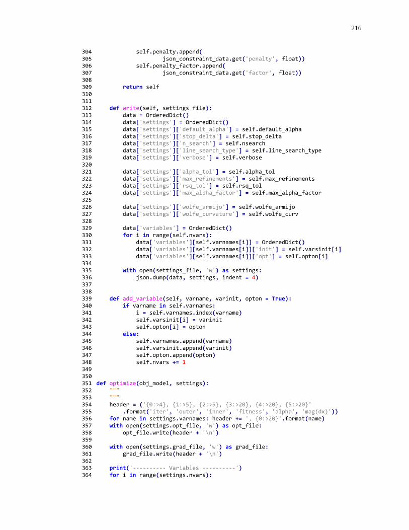
216

304 self.penalty.append( 305 json_constraint_data.get('penalty', float)) 306 self.penalty_factor.append( 307 json_constraint_data.get('factor', float)) 308 309 return self 310 311 312 def write(self, settings_file): 313 data = OrderedDict() 314 data['settings'] = OrderedDict() 315 data['settings']['default_alpha'] = self.default_alpha 316 data['settings']['stop_delta'] = self.stop_delta 317 data['settings']['n_search'] = self.nsearch 318 data['settings']['line_search_type'] = self.line_search_type 319 data['settings']['verbose'] = self.verbose 320 321 data['settings']['alpha_tol'] = self.alpha_tol 322 data['settings']['max_refinements'] = self.max_refinements 323 data['settings']['rsq_tol'] = self.rsq_tol 324 data['settings']['max_alpha_factor'] = self.max_alpha_factor 325 326 data['settings']['wolfe_armijo'] = self.wolfe_armijo 327 data['settings']['wolfe_curvature'] = self.wolfe_curv 328 329 data['variables'] = OrderedDict() 330 for i in range(self.nvars): 331 data['variables'][self.varnames[i]] = OrderedDict() 332 data['variables'][self.varnames[i]]['init'] = self.varsinit[i] 333 data['variables'][self.varnames[i]]['opt'] = self.opton[i] 334 335 with open(settings_file, 'w') as settings: 336 json.dump(data, settings, indent = 4) 337 338 339 def add_variable(self, varname, varinit, opton = True): 340 if varname in self.varnames: 341 i = self.varnames.index(varname) 342 self.varsinit[i] = varinit 343 self.opton[i] = opton 344 else: 345 self.varnames.append(varname) 346 self.varsinit.append(varinit) 347 self.opton.append(opton) 348 self.nvars += 1 349 350 351 def optimize(obj_model, settings): 352 """ 353 """ 354 header = ('{0:>4}, {1:>5}, {2:>5}, {3:>20}, {4:>20}, {5:>20}' 355 .format('iter', 'outer', 'inner', 'fitness', 'alpha', 'mag(dx)')) 356 for name in settings.varnames: header += ', {0:>20}'.format(name) 357 with open(settings.opt_file, 'w') as opt_file: 358 opt_file.write(header + '\n') 359 360 with open(settings.grad_file, 'w') as grad_file: 361 grad_file.write(header + '\n') 362 363 print('---------- Variables ----------') 364 for i in range(settings.nvars):

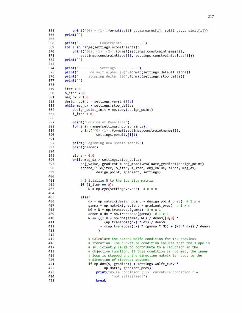
217

365 print('{0} = {1}'.format(settings.varnames[i], settings.varsinit[i])) 366 print('') 367 368 print('---------- Constraints ----------') 369 for i in range(settings.nconstraints): 370 print('{0}, {1}, {2}'.format(settings.constraintnames[i], 371 settings.constrainttype[i], settings.constraintvalues[i])) 372 print('') 373 374 print('---------- Settings ----------') 375 print(' default alpha: {0}'.format(settings.default_alpha)) 376 print(' stopping delta: {0}'.format(settings.stop_delta)) 377 print('') 378 379 iter = 0 380 o_iter = 0 381 mag_dx = 1.0 382 design_point = settings.varsinit[:] 383 while mag_dx > settings.stop_delta: 384 design_point_init = np.copy(design_point) 385 i_iter = 0 386 387 print('Constraint Penalties') 388 for i in range(settings.nconstraints): 389 print('{0} {1}'.format(settings.constraintnames[i], 390 settings.penalty[i])) 391 392 print('Beginning new update matrix') 393 print(header) 394 395 alpha = 0.0 396 while mag_dx > settings.stop_delta: 397 obj_value, gradient = obj_model.evaluate_gradient(design_point) 398 append_file(iter, o_iter, i_iter, obj_value, alpha, mag_dx, 399 design_point, gradient, settings) 400 401 # Initialize N to the identity matrix 402 if (i_iter == 0): 403 N = np.eye(settings.nvars) # n x n 404 405 else: 406 dx = np.matrix(design_point - design_point_prev) # 1 x n 407 gamma = np.matrix(gradient - gradient_prev) # 1 x n 408 NG = N * np.transpose(gamma) # n x 1 409 denom = dx * np.transpose(gamma) # 1 x 1 410 N += ((1.0 + np.dot(gamma, NG) / denom)[0,0] * 411 (np.transpose(dx) * dx) / denom 412 - ((np.transpose(dx) * (gamma * N)) + (NG * dx)) / denom 413 ) 414 415 # Calculate the second Wolfe condition for the previous 416 # iteration. The curvature condition ensures that the slope is 417 # sufficiently large to contribute to a reduction in the 418 # objective function. If this condition is not met, the inner 419 # loop is stopped and the direction matrix is reset to the 420 # direction of steepest descent. 421 if np.dot(s, gradient) < settings.wolfe_curv * 422 np.dot(s, gradient_prev): 423 print("Wolfe condition (ii): curvature condition " + 424 "not satisified!") 425 break

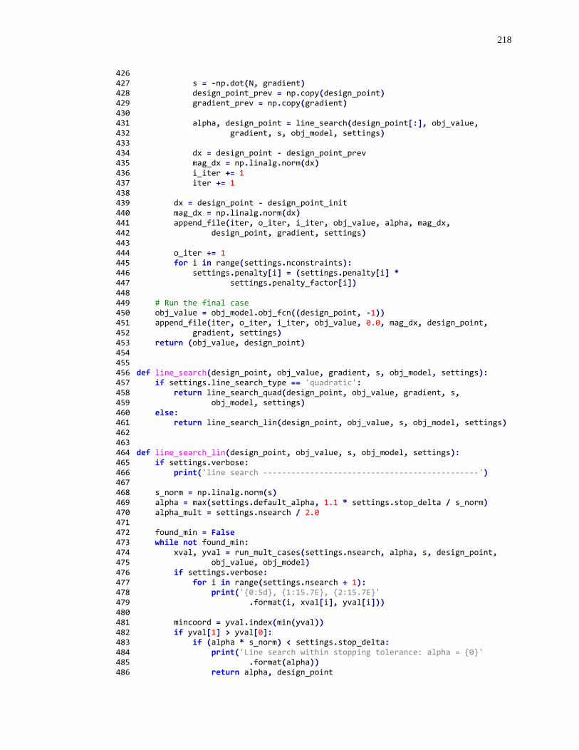
218

426 427 s = -np.dot(N, gradient) 428 design_point_prev = np.copy(design_point) 429 gradient_prev = np.copy(gradient) 430 431 alpha, design_point = line_search(design_point[:], obj_value, 432 gradient, s, obj_model, settings) 433 434 dx = design_point - design_point_prev 435 mag_dx = np.linalg.norm(dx) 436 i_iter += 1 437 iter += 1 438 439 dx = design_point - design_point_init 440 mag_dx = np.linalg.norm(dx) 441 append_file(iter, o_iter, i_iter, obj_value, alpha, mag_dx, 442 design_point, gradient, settings) 443 444 o_iter += 1 445 for i in range(settings.nconstraints): 446 settings.penalty[i] = (settings.penalty[i] * 447 settings.penalty_factor[i]) 448 449 # Run the final case 450 obj_value = obj_model.obj_fcn((design_point, -1)) 451 append_file(iter, o_iter, i_iter, obj_value, 0.0, mag_dx, design_point, 452 gradient, settings) 453 return (obj_value, design_point) 454 455 456 def line_search(design_point, obj_value, gradient, s, obj_model, settings): 457 if settings.line_search_type == 'quadratic': 458 return line_search_quad(design_point, obj_value, gradient, s, 459 obj_model, settings) 460 else: 461 return line_search_lin(design_point, obj_value, s, obj_model, settings) 462 463 464 def line_search_lin(design_point, obj_value, s, obj_model, settings): 465 if settings.verbose: 466 print('line search ----------------------------------------------') 467 468 s_norm = np.linalg.norm(s) 469 alpha = max(settings.default_alpha, 1.1 * settings.stop_delta / s_norm) 470 alpha_mult = settings.nsearch / 2.0 471 472 found_min = False 473 while not found_min: 474 xval, yval = run_mult_cases(settings.nsearch, alpha, s, design_point, 475 obj_value, obj_model) 476 if settings.verbose: 477 for i in range(settings.nsearch + 1): 478 print('{0:5d}, {1:15.7E}, {2:15.7E}' 479 .format(i, xval[i], yval[i])) 480 481 mincoord = yval.index(min(yval)) 482 if yval[1] > yval[0]: 483 if (alpha * s_norm) < settings.stop_delta: 484 print('Line search within stopping tolerance: alpha = {0}' 485 .format(alpha)) 486 return alpha, design_point

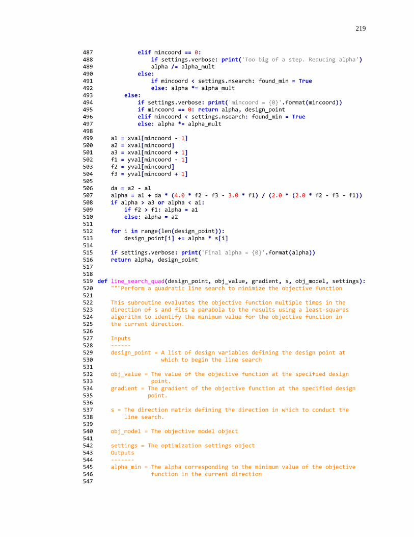
219

487 elif mincoord == 0: 488 if settings.verbose: print('Too big of a step. Reducing alpha') 489 alpha /= alpha_mult 490 else: 491 if mincoord < settings.nsearch: found_min = True 492 else: alpha *= alpha_mult 493 else: 494 if settings.verbose: print('mincoord = {0}'.format(mincoord)) 495 if mincoord == 0: return alpha, design_point 496 elif mincoord < settings.nsearch: found_min = True 497 else: alpha *= alpha_mult 498 499 a1 = xval[mincoord - 1] 500 a2 = xval[mincoord] 501 a3 = xval[mincoord + 1] 502 f1 = yval[mincoord - 1] 503 f2 = yval[mincoord] 504 f3 = yval[mincoord + 1] 505 506 da = a2 - a1 507 alpha = a1 + da * (4.0 * f2 - f3 - 3.0 * f1) / (2.0 * (2.0 * f2 - f3 - f1)) 508 if alpha > a3 or alpha < a1: 509 if f2 > f1: alpha = a1 510 else: alpha = a2 511 512 for i in range(len(design_point)): 513 design_point[i] += alpha * s[i] 514 515 if settings.verbose: print('Final alpha = {0}'.format(alpha)) 516 return alpha, design_point 517 518 519 def line_search_quad(design_point, obj_value, gradient, s, obj_model, settings): 520 """Perform a quadratic line search to minimize the objective function 521 522 This subroutine evaluates the objective function multiple times in the 523 direction of s and fits a parabola to the results using a least-squares 524 algorithm to identify the minimum value for the objective function in 525 the current direction. 526 527 Inputs 528 ------ 529 design_point = A list of design variables defining the design point at 530 which to begin the line search 531 532 obj_value = The value of the objective function at the specified design 533 point. 534 gradient = The gradient of the objective function at the specified design 535 point. 536 537 s = The direction matrix defining the direction in which to conduct the 538 line search. 539 540 obj_model = The objective model object 541 542 settings = The optimization settings object 543 Outputs 544 ------- 545 alpha_min = The alpha corresponding to the minimum value of the objective 546 function in the current direction 547

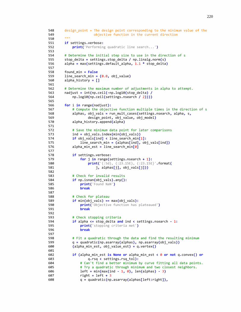
220

548 design_point = The design point corresponding to the minimum value of the 549 objective function in the current direction 550 """ 551 if settings.verbose: 552 print('Performing quadratic line search...') 553 554 # Determine the initial step size to use in the direction of s 555 stop_delta = settings.stop_delta / np.linalg.norm(s) 556 alpha = max(settings.default_alpha, 1.1 * stop_delta) 557 558 found_min = False 559 line_search_min = (0.0, obj_value) 560 alpha_history = [] 561 562 # Determine the maximum number of adjustments in alpha to attempt. 563 nadjust = int(np.ceil(-np.log10(stop_delta) / 564 np.log10(np.ceil(settings.nsearch / 2)))) 565 566 for i in range(nadjust): 567 # Compute the objective function multiple times in the direction of s 568 alphas, obj_vals = run_mult_cases(settings.nsearch, alpha, s, 569 design_point, obj_value, obj_model) 570 alpha_history.append(alpha) 571 572 # Save the minimum data point for later comparisons 573 ind = obj_vals.index(min(obj_vals)) 574 if obj_vals[ind] < line_search_min[1]: 575 line_search_min = (alphas[ind], obj_vals[ind]) 576 alpha_min_est = line_search_min[0] 577 578 if settings.verbose: 579 for j in range(settings.nsearch + 1): 580 print('{:5d}, {:23.15E}, {:23.15E}'.format( 581 j, alphas[j], obj_vals[j])) 582 583 # Check for invalid results 584 if np.isnan(obj_vals).any(): 585 print('Found NaN') 586 break 587 588 # Check for plateau 589 if min(obj_vals) == max(obj_vals): 590 print('Objective function has plateaued') 591 break 592 593 # Check stopping criteria 594 if alpha <= stop_delta and ind < settings.nsearch - 1: 595 print('stopping criteria met') 596 break 597 598 # Fit a quadratic through the data and find the resulting minimum 599 q = quadratic(np.asarray(alphas), np.asarray(obj_vals)) 600 (alpha_min_est, obj_value_est) = q.vertex() 601 602 if (alpha_min_est is None or alpha_min_est < 0 or not q.convex() or 603 q.rsq < settings.rsq_tol): 604 # Can't find a better minimum by curve fitting all data points. 605 # Try a quadratic through minimum and two closest neighbors. 606 left = min(max(ind - 1, 0), len(alphas) - 3) 607 right = left + 3 608 q = quadratic(np.asarray(alphas[left:right]),

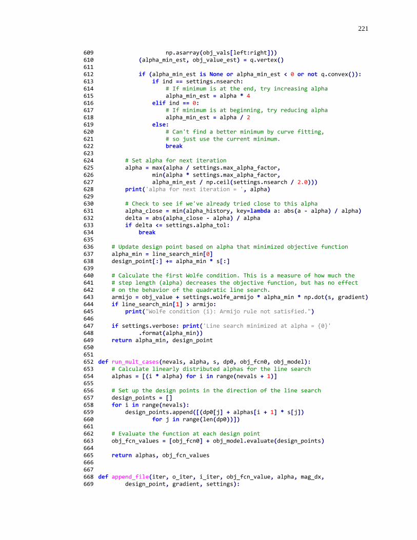
221

609 np.asarray(obj_vals[left:right])) 610 (alpha_min_est, obj_value_est) = q.vertex() 611 612 if (alpha_min_est is None or alpha_min_est < 0 or not q.convex()): 613 if ind == settings.nsearch: 614 # If minimum is at the end, try increasing alpha 615 alpha_min_est = alpha * 4 616 elif ind == 0: 617 # If minimum is at beginning, try reducing alpha 618 alpha_min_est = alpha / 2 619 else: 620 # Can't find a better minimum by curve fitting, 621 # so just use the current minimum. 622 break 623 624 # Set alpha for next iteration 625 alpha = max(alpha / settings.max_alpha_factor, 626 min(alpha * settings.max_alpha_factor, 627 alpha_min_est / np.ceil(settings.nsearch / 2.0))) 628 print('alpha for next iteration = ', alpha) 629 630 # Check to see if we've already tried close to this alpha 631 alpha_close = min(alpha_history, key=lambda a: abs(a - alpha) / alpha) 632 delta = abs(alpha_close - alpha) / alpha 633 if delta <= settings.alpha_tol: 634 break 635 636 # Update design point based on alpha that minimized objective function 637 alpha_min = line_search_min[0] 638 design_point[:] += alpha_min * s[:] 639 640 # Calculate the first Wolfe condition. This is a measure of how much the 641 # step length (alpha) decreases the objective function, but has no effect 642 # on the behavior of the quadratic line search. 643 armijo = obj_value + settings.wolfe_armijo * alpha_min * np.dot(s, gradient) 644 if line_search_min[1] > armijo: 645 print("Wolfe condition (i): Armijo rule not satisfied.") 646 647 if settings.verbose: print('Line search minimized at alpha = {0}' 648 .format(alpha_min)) 649 return alpha_min, design_point 650 651 652 def run_mult_cases(nevals, alpha, s, dp0, obj_fcn0, obj_model): 653 # Calculate linearly distributed alphas for the line search 654 alphas = [(i * alpha) for i in range(nevals + 1)] 655 656 # Set up the design points in the direction of the line search 657 design_points = [] 658 for i in range(nevals): 659 design_points.append([(dp0[j] + alphas[i + 1] * s[j]) 660 for j in range(len(dp0))]) 661 662 # Evaluate the function at each design point 663 obj_fcn_values = [obj_fcn0] + obj_model.evaluate(design_points) 664 665 return alphas, obj_fcn_values 666 667 668 def append_file(iter, o_iter, i_iter, obj_fcn_value, alpha, mag_dx, 669 design_point, gradient, settings):

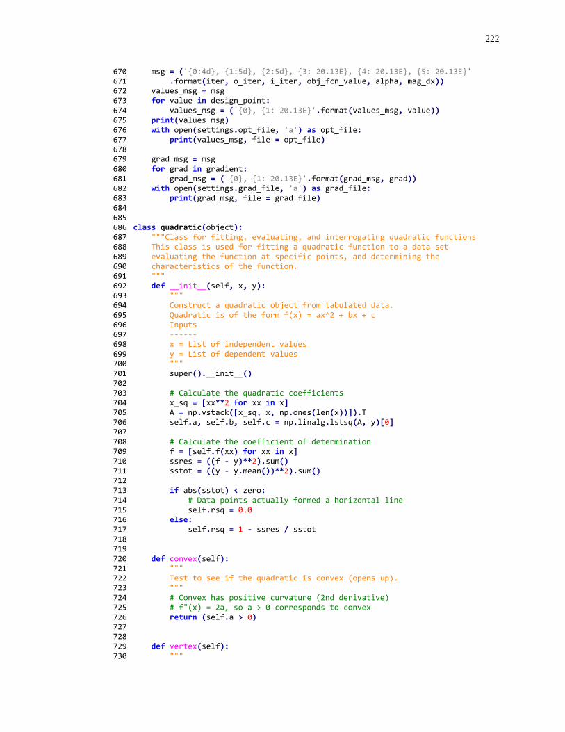
222

670 msg = ('{0:4d}, {1:5d}, {2:5d}, {3: 20.13E}, {4: 20.13E}, {5: 20.13E}' 671 .format(iter, o_iter, i_iter, obj_fcn_value, alpha, mag_dx)) 672 values_msg = msg 673 for value in design_point: 674 values_msg = ('{0}, {1: 20.13E}'.format(values_msg, value)) 675 print(values_msg) 676 with open(settings.opt_file, 'a') as opt_file: 677 print(values_msg, file = opt_file) 678 679 grad_msg = msg 680 for grad in gradient: 681 grad_msg = ('{0}, {1: 20.13E}'.format(grad_msg, grad)) 682 with open(settings.grad_file, 'a') as grad_file: 683 print(grad_msg, file = grad_file) 684 685 686 class quadratic(object): 687 """Class for fitting, evaluating, and interrogating quadratic functions 688 This class is used for fitting a quadratic function to a data set 689 evaluating the function at specific points, and determining the 690 characteristics of the function. 691 """ 692 def __init__(self, x, y): 693 """ 694 Construct a quadratic object from tabulated data. 695 Quadratic is of the form f(x) = ax^2 + bx + c 696 Inputs 697 ------ 698 x = List of independent values 699 y = List of dependent values 700 """ 701 super().__init__() 702 703 # Calculate the quadratic coefficients 704 x_sq = [xx**2 for xx in x] 705 A = np.vstack([x_sq, x, np.ones(len(x))]).T 706 self.a, self.b, self.c = np.linalg.lstsq(A, y)[0] 707 708 # Calculate the coefficient of determination 709 f = [self.f(xx) for xx in x] 710 ssres = ((f - y)**2).sum() 711 sstot = ((y - y.mean())**2).sum() 712 713 if abs(sstot) < zero: 714 # Data points actually formed a horizontal line 715 self.rsq = 0.0 716 else: 717 self.rsq = 1 - ssres / sstot 718 719 720 def convex(self): 721 """ 722 Test to see if the quadratic is convex (opens up). 723 """ 724 # Convex has positive curvature (2nd derivative) 725 # f"(x) = 2a, so a > 0 corresponds to convex 726 return (self.a > 0) 727 728 729 def vertex(self): 730 """

223

731 Find the coordinates of the vertex 732 """ 733 if self.a != 0.0: 734 # Find x where f'(x) = 2ax + b = 0 735 x = -0.5 * self.b / self.a 736 return (x, self.f(x)) 737 else: 738 # Quadratic is actually a line, no minimum! 739 return (None, None) 740 741 742 def f(self, x): 743 """ 744 Evaluate the quadratic function at x 745 """ 746 if x is not None: return self.a * x**2 + self.b * x + self.c 747 else: return None 748 749 750 class myjson: 751 def __init__(self, filename=None, parent=None, data=None, path=None): 752 self.file = '' 753 self.data = OrderedDict() 754 self.path = '' 755 756 if filename is not None: self.load(filename) 757 elif parent is not None: 758 self.file = parent.file 759 self.data = data 760 self.path = parent.path + path 761 762 763 def load(self, filename): 764 if not os.path.isfile(filename): 765 print('Error: Cannot find file "{0}". Make sure'.format(filename)) 766 print(' the path is correct and the file is accessible.') 767 raise IOError(filename) 768 769 self.file = filename 770 with open(self.file) as file: 771 self.data = json.load(file, object_pairs_hook = OrderedDict) 772 773 774 def get(self, value_path, value_type, default_value = None): 775 abs_path = self.path + '.' + value_path 776 777 json_data = self.data 778 for path in value_path.split('.'): 779 try: 780 json_data = json_data[path] 781 except KeyError as exc: 782 if default_value is None: 783 print('Error: required JSON path not found. Op aborted.') 784 print(' Missing path is "{0}"'.format(abs_path)) 785 raise 786 else: 787 json_data = default_value 788 789 if not isinstance(value_type, Iterable): value_type = [value_type] 790 if type(json_data) not in value_type: 791 print('Error: JSON value is of an incorrect type.')

224

792 print(' Expected {0} but found {1}' 793 .format(value_type, type(json_data))) 794 print(' Invalid path is "{0}"'.format(abs_path)) 795 raise KeyError(value_path) 796 797 if type(json_data) is OrderedDict: 798 return myjson(parent = self, data = json_data, path = value_path) 799 else: 800 return json_data 801 802 803 def load(filename): 804 return myjson(filename)

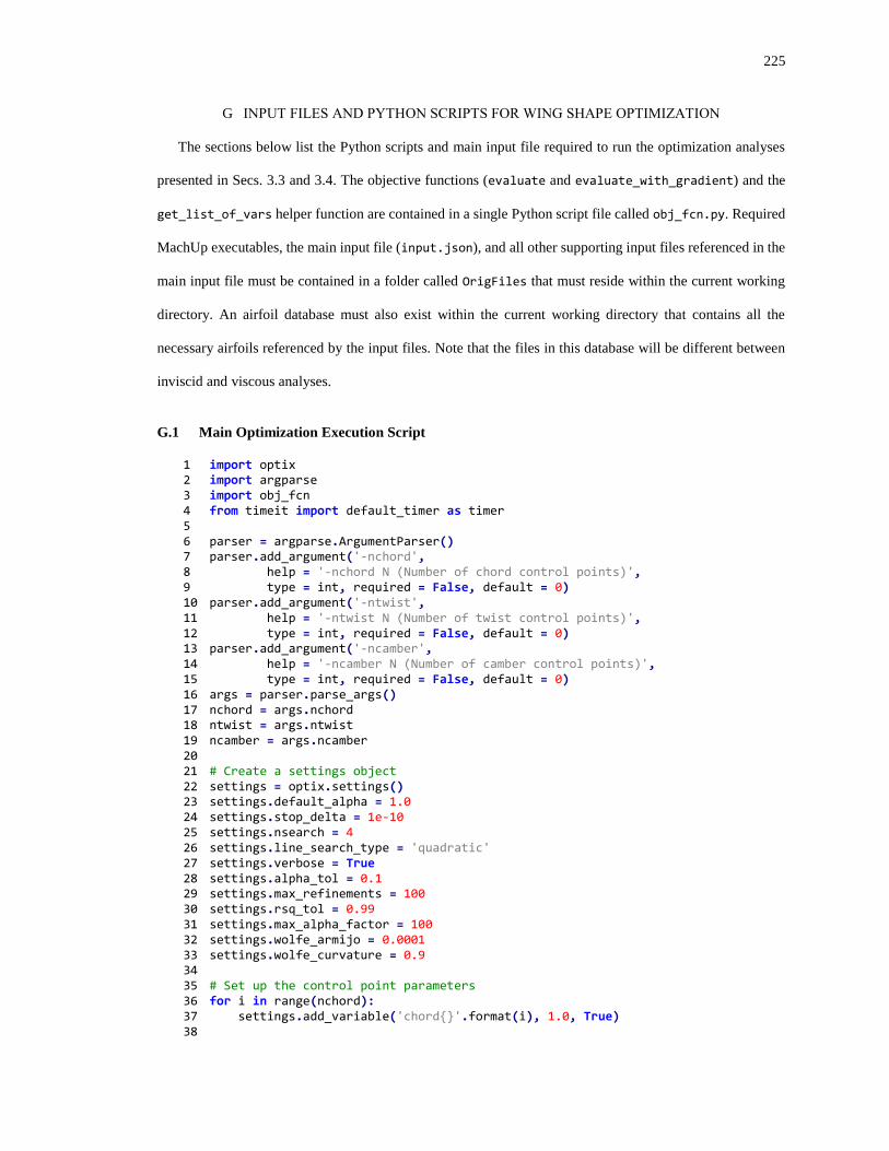
225

G INPUT FILES AND PYTHON SCRIPTS FOR WING SHAPE OPTIMIZATION

The sections below list the Python scripts and main input file required to run the optimization analyses

presented in Secs. 3.3 and 3.4. The objective functions (evaluate and evaluate_with_gradient) and the

get_list_of_vars helper function are contained in a single Python script file called obj_fcn.py. Required

MachUp executables, the main input file (input.json), and all other supporting input files referenced in the

main input file must be contained in a folder called OrigFiles that must reside within the current working

directory. An airfoil database must also exist within the current working directory that contains all the

necessary airfoils referenced by the input files. Note that the files in this database will be different between

inviscid and viscous analyses.

G.1 Main Optimization Execution Script

1 import optix 2 import argparse 3 import obj_fcn 4 from timeit import default_timer as timer 5 6 parser = argparse.ArgumentParser() 7 parser.add_argument('-nchord', 8 help = '-nchord N (Number of chord control points)', 9 type = int, required = False, default = 0) 10 parser.add_argument('-ntwist', 11 help = '-ntwist N (Number of twist control points)', 12 type = int, required = False, default = 0) 13 parser.add_argument('-ncamber', 14 help = '-ncamber N (Number of camber control points)', 15 type = int, required = False, default = 0) 16 args = parser.parse_args() 17 nchord = args.nchord 18 ntwist = args.ntwist 19 ncamber = args.ncamber 20 21 # Create a settings object 22 settings = optix.settings() 23 settings.default_alpha = 1.0 24 settings.stop_delta = 1e-10 25 settings.nsearch = 4 26 settings.line_search_type = 'quadratic' 27 settings.verbose = True 28 settings.alpha_tol = 0.1 29 settings.max_refinements = 100 30 settings.rsq_tol = 0.99 31 settings.max_alpha_factor = 100 32 settings.wolfe_armijo = 0.0001 33 settings.wolfe_curvature = 0.9 34 35 # Set up the control point parameters 36 for i in range(nchord): 37 settings.add_variable('chord{}'.format(i), 1.0, True) 38

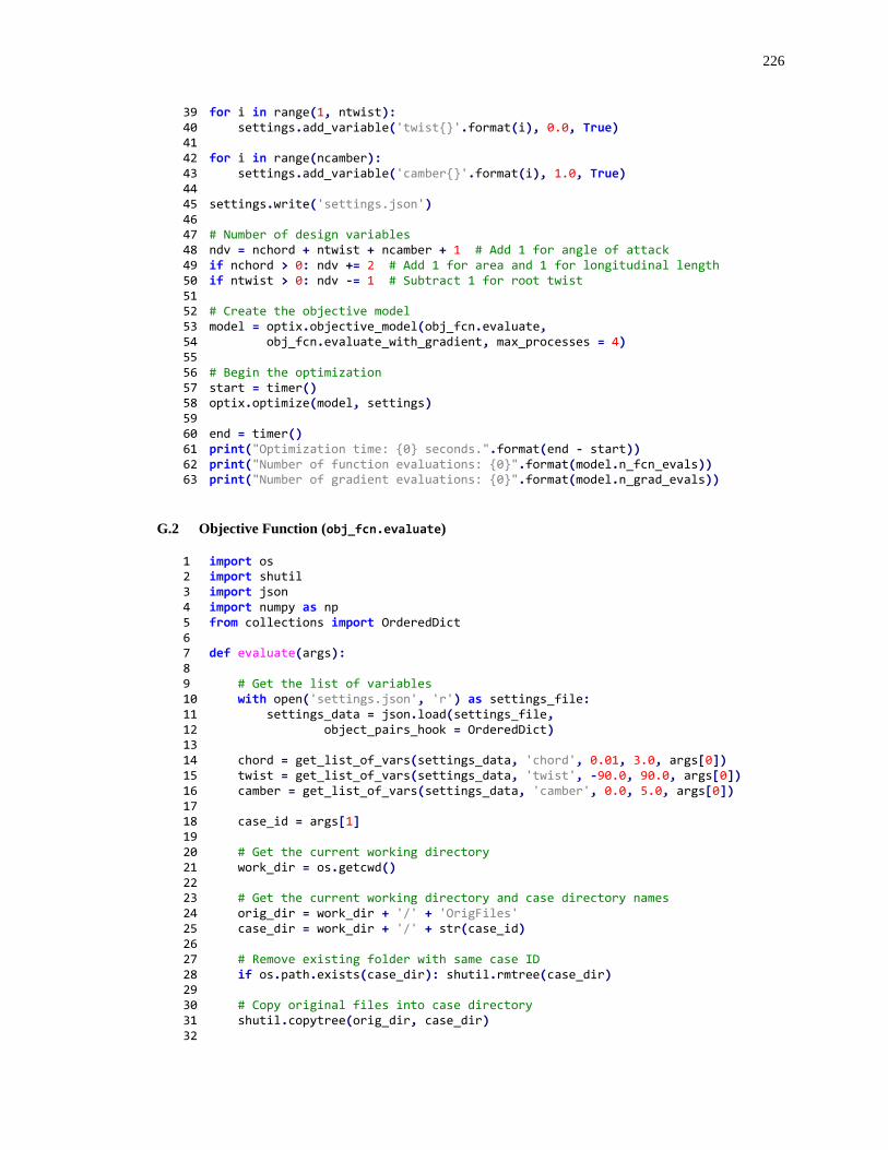
226

39 for i in range(1, ntwist): 40 settings.add_variable('twist{}'.format(i), 0.0, True) 41 42 for i in range(ncamber): 43 settings.add_variable('camber{}'.format(i), 1.0, True) 44 45 settings.write('settings.json') 46 47 # Number of design variables 48 ndv = nchord + ntwist + ncamber + 1 # Add 1 for angle of attack 49 if nchord > 0: ndv += 2 # Add 1 for area and 1 for longitudinal length 50 if ntwist > 0: ndv -= 1 # Subtract 1 for root twist 51 52 # Create the objective model 53 model = optix.objective_model(obj_fcn.evaluate, 54 obj_fcn.evaluate_with_gradient, max_processes = 4) 55 56 # Begin the optimization 57 start = timer() 58 optix.optimize(model, settings) 59 60 end = timer() 61 print("Optimization time: {0} seconds.".format(end - start)) 62 print("Number of function evaluations: {0}".format(model.n_fcn_evals)) 63 print("Number of gradient evaluations: {0}".format(model.n_grad_evals))

G.2 Objective Function (obj_fcn.evaluate)

1 import os 2 import shutil 3 import json 4 import numpy as np 5 from collections import OrderedDict 6 7 def evaluate(args): 8 9 # Get the list of variables 10 with open('settings.json', 'r') as settings_file: 11 settings_data = json.load(settings_file, 12 object_pairs_hook = OrderedDict) 13 14 chord = get_list_of_vars(settings_data, 'chord', 0.01, 3.0, args[0]) 15 twist = get_list_of_vars(settings_data, 'twist', -90.0, 90.0, args[0]) 16 camber = get_list_of_vars(settings_data, 'camber', 0.0, 5.0, args[0]) 17 18 case_id = args[1] 19 20 # Get the current working directory 21 work_dir = os.getcwd() 22 23 # Get the current working directory and case directory names 24 orig_dir = work_dir + '/' + 'OrigFiles' 25 case_dir = work_dir + '/' + str(case_id) 26 27 # Remove existing folder with same case ID 28 if os.path.exists(case_dir): shutil.rmtree(case_dir) 29 30 # Copy original files into case directory 31 shutil.copytree(orig_dir, case_dir) 32

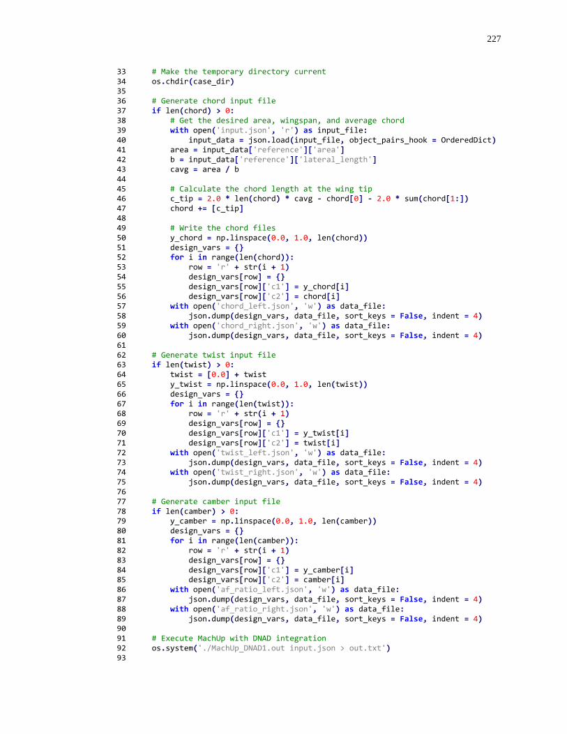
227

33 # Make the temporary directory current 34 os.chdir(case_dir) 35 36 # Generate chord input file 37 if len(chord) > 0: 38 # Get the desired area, wingspan, and average chord 39 with open('input.json', 'r') as input_file: 40 input_data = json.load(input_file, object_pairs_hook = OrderedDict) 41 area = input_data['reference']['area'] 42 b = input_data['reference']['lateral_length'] 43 cavg = area / b 44 45 # Calculate the chord length at the wing tip 46 c_tip = 2.0 * len(chord) * cavg - chord[0] - 2.0 * sum(chord[1:]) 47 chord += [c_tip] 48 49 # Write the chord files 50 y_chord = np.linspace(0.0, 1.0, len(chord)) 51 design_vars = {} 52 for i in range(len(chord)): 53 row = 'r' + str(i + 1) 54 design_vars[row] = {} 55 design_vars[row]['c1'] = y_chord[i] 56 design_vars[row]['c2'] = chord[i] 57 with open('chord_left.json', 'w') as data_file: 58 json.dump(design_vars, data_file, sort_keys = False, indent = 4) 59 with open('chord_right.json', 'w') as data_file: 60 json.dump(design_vars, data_file, sort_keys = False, indent = 4) 61 62 # Generate twist input file 63 if len(twist) > 0: 64 twist = [0.0] + twist 65 y_twist = np.linspace(0.0, 1.0, len(twist)) 66 design_vars = {} 67 for i in range(len(twist)): 68 row = 'r' + str(i + 1) 69 design_vars[row] = {} 70 design_vars[row]['c1'] = y_twist[i] 71 design_vars[row]['c2'] = twist[i] 72 with open('twist_left.json', 'w') as data_file: 73 json.dump(design_vars, data_file, sort_keys = False, indent = 4) 74 with open('twist_right.json', 'w') as data_file: 75 json.dump(design_vars, data_file, sort_keys = False, indent = 4) 76 77 # Generate camber input file 78 if len(camber) > 0: 79 y_camber = np.linspace(0.0, 1.0, len(camber)) 80 design_vars = {} 81 for i in range(len(camber)): 82 row = 'r' + str(i + 1) 83 design_vars[row] = {} 84 design_vars[row]['c1'] = y_camber[i] 85 design_vars[row]['c2'] = camber[i] 86 with open('af_ratio_left.json', 'w') as data_file: 87 json.dump(design_vars, data_file, sort_keys = False, indent = 4) 88 with open('af_ratio_right.json', 'w') as data_file: 89 json.dump(design_vars, data_file, sort_keys = False, indent = 4) 90 91 # Execute MachUp with DNAD integration 92 os.system('./MachUp_DNAD1.out input.json > out.txt') 93

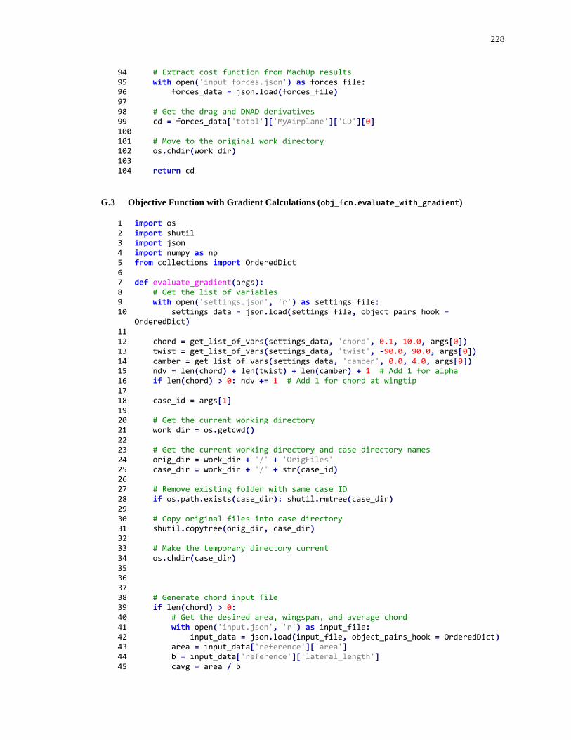
228

94 # Extract cost function from MachUp results 95 with open('input_forces.json') as forces_file: 96 forces_data = json.load(forces_file) 97 98 # Get the drag and DNAD derivatives 99 cd = forces_data['total']['MyAirplane']['CD'][0] 100 101 # Move to the original work directory 102 os.chdir(work_dir) 103 104 return cd

G.3 Objective Function with Gradient Calculations (obj_fcn.evaluate_with_gradient)

1 import os 2 import shutil 3 import json 4 import numpy as np 5 from collections import OrderedDict 6 7 def evaluate_gradient(args): 8 # Get the list of variables 9 with open('settings.json', 'r') as settings_file: 10 settings_data = json.load(settings_file, object_pairs_hook =

OrderedDict) 11 12 chord = get_list_of_vars(settings_data, 'chord', 0.1, 10.0, args[0]) 13 twist = get_list_of_vars(settings_data, 'twist', -90.0, 90.0, args[0]) 14 camber = get_list_of_vars(settings_data, 'camber', 0.0, 4.0, args[0]) 15 ndv = len(chord) + len(twist) + len(camber) + 1 # Add 1 for alpha 16 if len(chord) > 0: ndv += 1 # Add 1 for chord at wingtip 17 18 case_id = args[1] 19 20 # Get the current working directory 21 work_dir = os.getcwd() 22 23 # Get the current working directory and case directory names 24 orig_dir = work_dir + '/' + 'OrigFiles' 25 case_dir = work_dir + '/' + str(case_id) 26 27 # Remove existing folder with same case ID 28 if os.path.exists(case_dir): shutil.rmtree(case_dir) 29 30 # Copy original files into case directory 31 shutil.copytree(orig_dir, case_dir) 32 33 # Make the temporary directory current 34 os.chdir(case_dir) 35 36 37 38 # Generate chord input file 39 if len(chord) > 0: 40 # Get the desired area, wingspan, and average chord 41 with open('input.json', 'r') as input_file: 42 input_data = json.load(input_file, object_pairs_hook = OrderedDict) 43 area = input_data['reference']['area'] 44 b = input_data['reference']['lateral_length'] 45 cavg = area / b

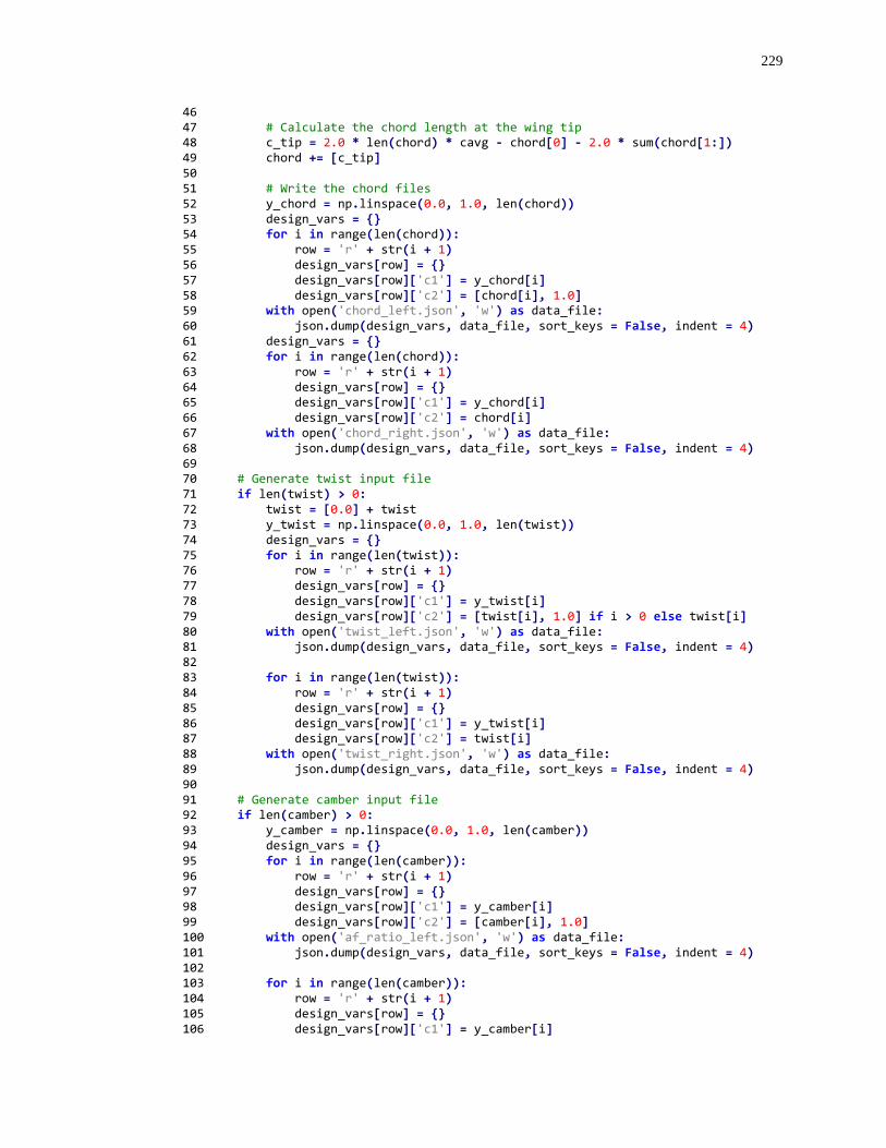
229

46 47 # Calculate the chord length at the wing tip 48 c_tip = 2.0 * len(chord) * cavg - chord[0] - 2.0 * sum(chord[1:]) 49 chord += [c_tip] 50 51 # Write the chord files 52 y_chord = np.linspace(0.0, 1.0, len(chord)) 53 design_vars = {} 54 for i in range(len(chord)): 55 row = 'r' + str(i + 1) 56 design_vars[row] = {} 57 design_vars[row]['c1'] = y_chord[i] 58 design_vars[row]['c2'] = [chord[i], 1.0] 59 with open('chord_left.json', 'w') as data_file: 60 json.dump(design_vars, data_file, sort_keys = False, indent = 4) 61 design_vars = {} 62 for i in range(len(chord)): 63 row = 'r' + str(i + 1) 64 design_vars[row] = {} 65 design_vars[row]['c1'] = y_chord[i] 66 design_vars[row]['c2'] = chord[i] 67 with open('chord_right.json', 'w') as data_file: 68 json.dump(design_vars, data_file, sort_keys = False, indent = 4) 69 70 # Generate twist input file 71 if len(twist) > 0: 72 twist = [0.0] + twist 73 y_twist = np.linspace(0.0, 1.0, len(twist)) 74 design_vars = {} 75 for i in range(len(twist)): 76 row = 'r' + str(i + 1) 77 design_vars[row] = {} 78 design_vars[row]['c1'] = y_twist[i] 79 design_vars[row]['c2'] = [twist[i], 1.0] if i > 0 else twist[i] 80 with open('twist_left.json', 'w') as data_file: 81 json.dump(design_vars, data_file, sort_keys = False, indent = 4) 82 83 for i in range(len(twist)): 84 row = 'r' + str(i + 1) 85 design_vars[row] = {} 86 design_vars[row]['c1'] = y_twist[i] 87 design_vars[row]['c2'] = twist[i] 88 with open('twist_right.json', 'w') as data_file: 89 json.dump(design_vars, data_file, sort_keys = False, indent = 4) 90 91 # Generate camber input file 92 if len(camber) > 0: 93 y_camber = np.linspace(0.0, 1.0, len(camber)) 94 design_vars = {} 95 for i in range(len(camber)): 96 row = 'r' + str(i + 1) 97 design_vars[row] = {} 98 design_vars[row]['c1'] = y_camber[i] 99 design_vars[row]['c2'] = [camber[i], 1.0] 100 with open('af_ratio_left.json', 'w') as data_file: 101 json.dump(design_vars, data_file, sort_keys = False, indent = 4) 102 103 for i in range(len(camber)): 104 row = 'r' + str(i + 1) 105 design_vars[row] = {} 106 design_vars[row]['c1'] = y_camber[i]

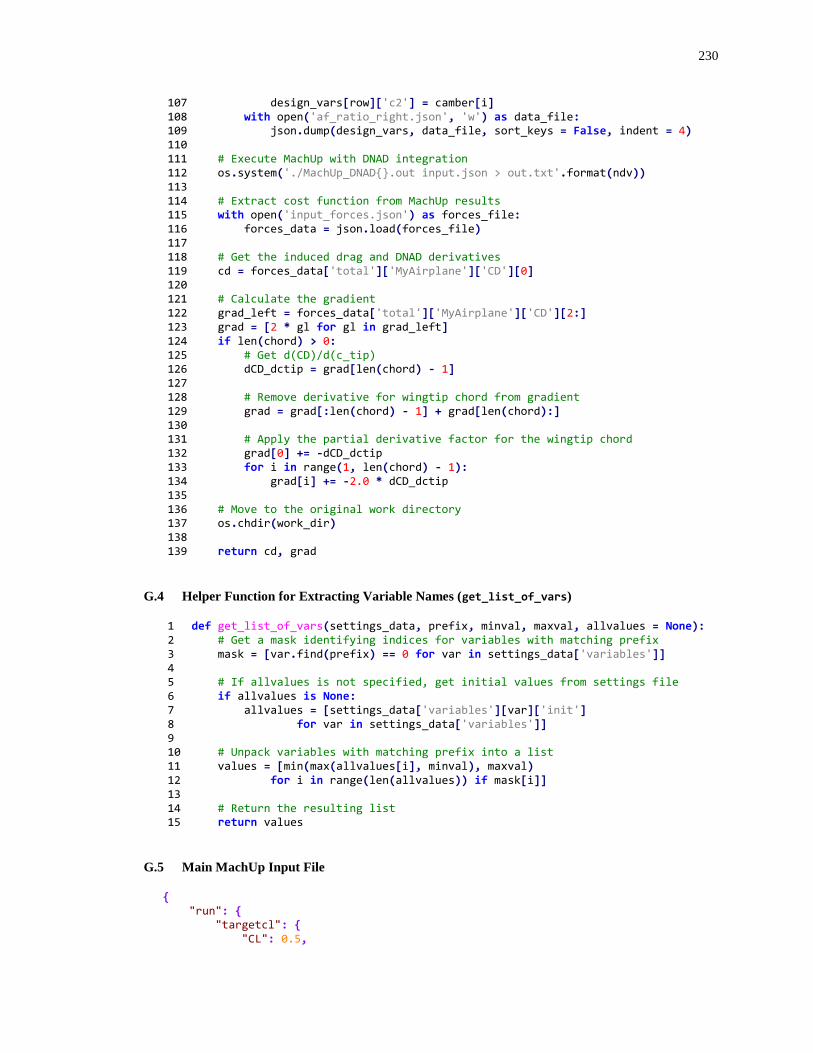
230

107 design_vars[row]['c2'] = camber[i] 108 with open('af_ratio_right.json', 'w') as data_file: 109 json.dump(design_vars, data_file, sort_keys = False, indent = 4) 110 111 # Execute MachUp with DNAD integration 112 os.system('./MachUp_DNAD{}.out input.json > out.txt'.format(ndv)) 113 114 # Extract cost function from MachUp results 115 with open('input_forces.json') as forces_file: 116 forces_data = json.load(forces_file) 117 118 # Get the induced drag and DNAD derivatives 119 cd = forces_data['total']['MyAirplane']['CD'][0] 120 121 # Calculate the gradient 122 grad_left = forces_data['total']['MyAirplane']['CD'][2:] 123 grad = [2 * gl for gl in grad_left] 124 if len(chord) > 0: 125 # Get d(CD)/d(c_tip) 126 dCD_dctip = grad[len(chord) - 1] 127 128 # Remove derivative for wingtip chord from gradient 129 grad = grad[:len(chord) - 1] + grad[len(chord):] 130 131 # Apply the partial derivative factor for the wingtip chord 132 grad[0] += -dCD_dctip 133 for i in range(1, len(chord) - 1): 134 grad[i] += -2.0 * dCD_dctip 135 136 # Move to the original work directory 137 os.chdir(work_dir) 138 139 return cd, grad

G.4 Helper Function for Extracting Variable Names (get_list_of_vars)

1 def get_list_of_vars(settings_data, prefix, minval, maxval, allvalues = None): 2 # Get a mask identifying indices for variables with matching prefix 3 mask = [var.find(prefix) == 0 for var in settings_data['variables']] 4 5 # If allvalues is not specified, get initial values from settings file 6 if allvalues is None: 7 allvalues = [settings_data['variables'][var]['init'] 8 for var in settings_data['variables']] 9 10 # Unpack variables with matching prefix into a list 11 values = [min(max(allvalues[i], minval), maxval) 12 for i in range(len(allvalues)) if mask[i]] 13 14 # Return the resulting list 15 return values

G.5 Main MachUp Input File

{ "run": { "targetcl": { "CL": 0.5,

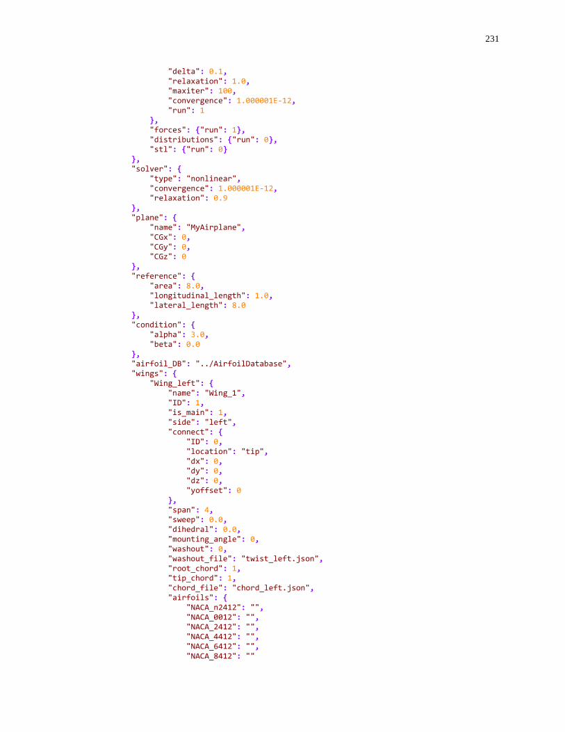
231

"delta": 0.1, "relaxation": 1.0, "maxiter": 100, "convergence": 1.000001E-12, "run": 1 }, "forces": {"run": 1}, "distributions": {"run": 0}, "stl": {"run": 0} }, "solver": { "type": "nonlinear", "convergence": 1.000001E-12, "relaxation": 0.9 }, "plane": { "name": "MyAirplane", "CGx": 0, "CGy": 0, "CGz": 0 }, "reference": { "area": 8.0, "longitudinal_length": 1.0, "lateral_length": 8.0 }, "condition": { "alpha": 3.0, "beta": 0.0 }, "airfoil_DB": "../AirfoilDatabase", "wings": { "Wing_left": { "name": "Wing_1", "ID": 1, "is_main": 1, "side": "left", "connect": { "ID": 0, "location": "tip", "dx": 0, "dy": 0, "dz": 0, "yoffset": 0 }, "span": 4, "sweep": 0.0, "dihedral": 0.0, "mounting_angle": 0, "washout": 0, "washout_file": "twist_left.json", "root_chord": 1, "tip_chord": 1, "chord_file": "chord_left.json", "airfoils": { "NACA_n2412": "", "NACA_0012": "", "NACA_2412": "", "NACA_4412": "", "NACA_6412": "", "NACA_8412": ""

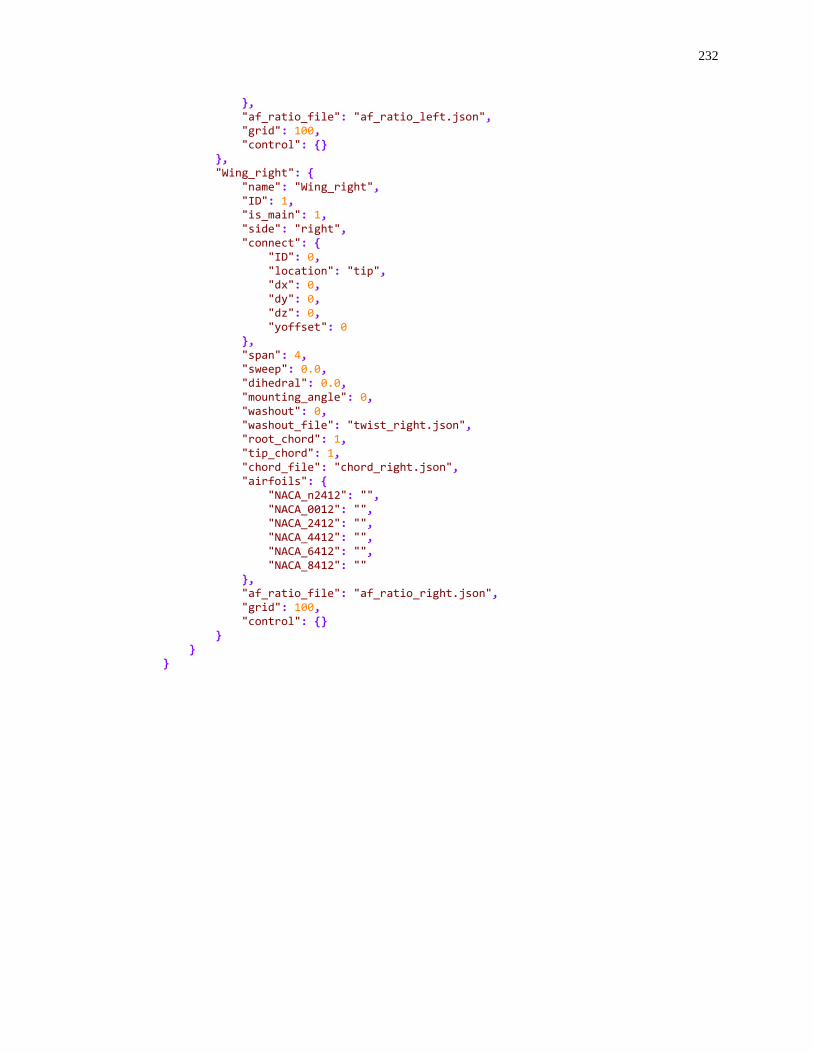
232

}, "af_ratio_file": "af_ratio_left.json", "grid": 100, "control": {} }, "Wing_right": { "name": "Wing_right", "ID": 1, "is_main": 1, "side": "right", "connect": { "ID": 0, "location": "tip", "dx": 0, "dy": 0, "dz": 0, "yoffset": 0 }, "span": 4, "sweep": 0.0, "dihedral": 0.0, "mounting_angle": 0, "washout": 0, "washout_file": "twist_right.json", "root_chord": 1, "tip_chord": 1, "chord_file": "chord_right.json", "airfoils": { "NACA_n2412": "", "NACA_0012": "", "NACA_2412": "", "NACA_4412": "", "NACA_6412": "", "NACA_8412": "" }, "af_ratio_file": "af_ratio_right.json", "grid": 100, "control": {} } } }

233

H AERODYNAMIC CALCULATIONS USING PANAIR

Panair is an open-source Fortran code that implements a high-order panel method for performing potential

flow analysis of arbitrary geometries. It was originally developed by Boeing Military Airplane Development

under contract to NASA in the latter part of the twentieth century, and has seen wide use in industry and

academia since that time. Source code,* documentation,†,‡,§ and a list of research publications** related to

Panair can be found online. Because of its established reliability in performing aerodynamic calculations,

Panair has been used in the present research to perform baseline calculations against which the accuracy of

various formulations of lifting line theory can be measured.

In order to rapidly process finite wing models of different configurations with Panair, several functions

were added to the MachUp source code for converting wing geometry data into properly-formatted Panair

input files. These functions are listed in Appendix I. For each wing configuration analyzed, a MachUp input

file was generated with the planform shape, airfoil geometry, and number of spanwise sections defined.

MachUp was then executed to generate a Panair input file for this geometry. The Panair input file was then

processed by Panair to calculate pressure distributions over the wing surface. Upon successful execution,

Panair produces an output file that defines the predicted pressure coefficient at each node specified in the

input file. A suite of Python scripts were used to integrate the pressures calculated by Panair to determine the

spanwise section lift distribution and the total lift generated by the wing.

A wing representation in the Panair input file is divided into two panel networks – one representing the

upper surface of the wing and another representing the lower surface. For rectangular and tapered wings,

where the tip chord is nonzero, a third panel network is needed to define an endcap to close the volume of

the wing. This endcap network is automatically added to the Panair input file by MachUp. Since all wings

considered in the present work are symmetric about the root plane, a symmetry boundary condition is defined

at the root so that only one semispan of the wing is modeled. A representative Panair input file is included in

Appendix J. This model represents an elliptic wing with an aspect ratio of 4A = , an average chord length of

* http://www.pdas.com/panairdownload.html † https://ntrs.nasa.gov/archive/nasa/casi.ntrs.nasa.gov/19840020672.pdf ‡ https://ntrs.nasa.gov/archive/nasa/casi.ntrs.nasa.gov/19920013405.pdf § https://ntrs.nasa.gov/archive/nasa/casi.ntrs.nasa.gov/19920013622.pdf ** http://www.pdas.com/panairrefs.html

http://www.pdas.com/panairdownload.html

https://ntrs.nasa.gov/archive/nasa/casi.ntrs.nasa.gov/19840020672.pdf



http://www.pdas.com/panairrefs.html

234

avg 1mc = , and a symmetric Joukowski airfoil with maximum thickness max 4%t = . The wing is operating at

a geometric angle of attack of 1deg = in incompressible flow with freestream density 31kg / m = and

velocity 1m / sV = . There are 11 chordwise nodes and 21 spanwise nodes each for the upper and lower

wing surface networks, defining a combined 20 20 mesh of panels for a total of 400 panels in the model.

The spanwise lift distribution computed using this input file is shown in Figure H.1.

The physical scale of the model was found to have a noticeable effect on the pressure results, especially

near the wing tip and for fine panel meshes. The source of this variation in the results based on physical scale

is unknown since the pressure coefficients written to the Panair output file are nondimensional. It is theorized

that data written to and read from intermediate solution files on disk during the solution process may be of

limited precision so that, when read in, rounding error is introduced into the solution. If true, this rounding

error could then be reduced by increasing the physical scale of the model so that more digits of precision are

written to disk. This theory has not been tested, however, and a different source of error may be present in

the code. In order to alleviate this problem, multiple Panair solutions were evaluated with increasing scales

until a reasonably converged solution was achieved. An example of this using a mesh size of 80 80 panels

for the elliptic wing described previously is shown in Figure H.2. For the wing configurations considered in

this work, the results become independent of scale for 5mc .

Figure H.1 Lift distribution with a 20×20 mesh for an elliptic wing with = 4A and

max4%t = .

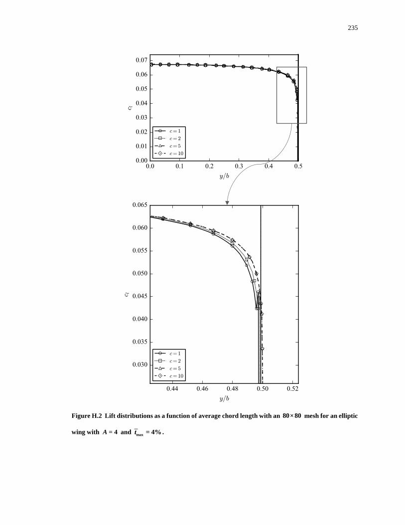
235

Figure H.2 Lift distributions as a function of average chord length with an 80×80 mesh for an elliptic

wing with = 4A and max

= 4%t .

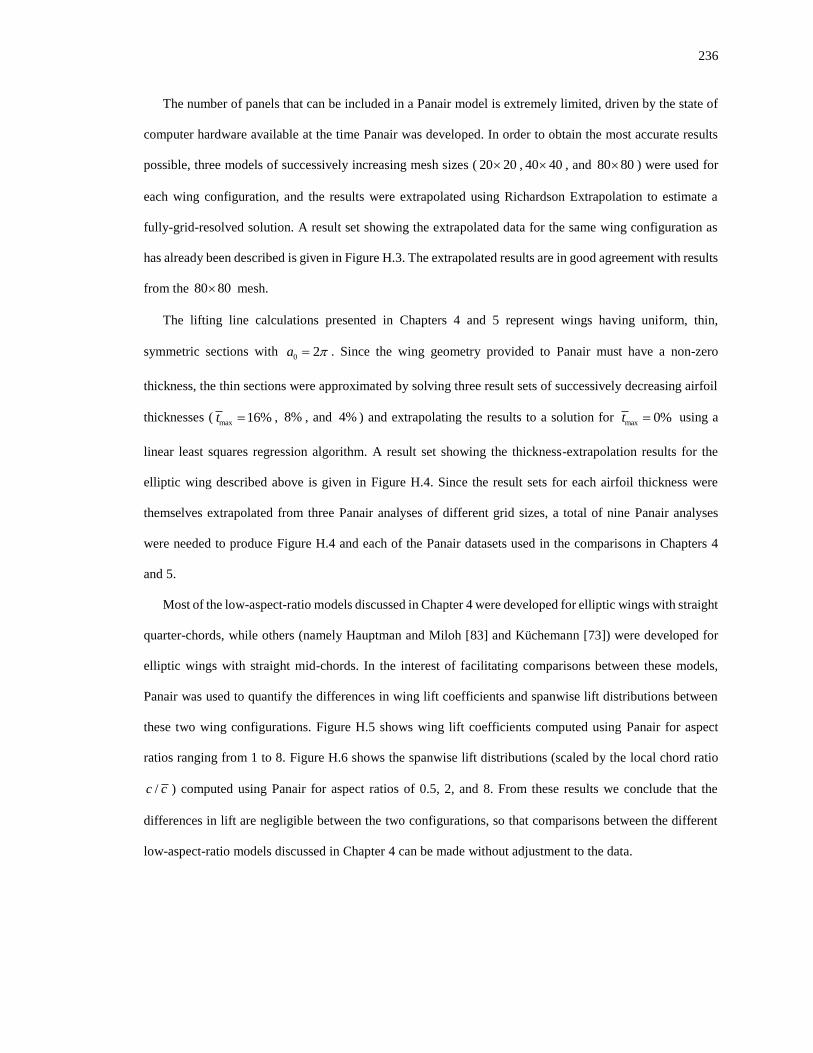
236

The number of panels that can be included in a Panair model is extremely limited, driven by the state of

computer hardware available at the time Panair was developed. In order to obtain the most accurate results

possible, three models of successively increasing mesh sizes ( 20 20 , 40 40 , and 80 80 ) were used for

each wing configuration, and the results were extrapolated using Richardson Extrapolation to estimate a

fully-grid-resolved solution. A result set showing the extrapolated data for the same wing configuration as

has already been described is given in Figure H.3. The extrapolated results are in good agreement with results

from the 80 80 mesh.

The lifting line calculations presented in Chapters 4 and 5 represent wings having uniform, thin,

symmetric sections with 0 2a = . Since the wing geometry provided to Panair must have a non-zero

thickness, the thin sections were approximated by solving three result sets of successively decreasing airfoil

thicknesses (max 16%t = , 8% , and 4% ) and extrapolating the results to a solution for

max 0%t = using a

linear least squares regression algorithm. A result set showing the thickness-extrapolation results for the

elliptic wing described above is given in Figure H.4. Since the result sets for each airfoil thickness were

themselves extrapolated from three Panair analyses of different grid sizes, a total of nine Panair analyses

were needed to produce Figure H.4 and each of the Panair datasets used in the comparisons in Chapters 4

and 5.

Most of the low-aspect-ratio models discussed in Chapter 4 were developed for elliptic wings with straight

quarter-chords, while others (namely Hauptman and Miloh [83] and Küchemann [73]) were developed for

elliptic wings with straight mid-chords. In the interest of facilitating comparisons between these models,

Panair was used to quantify the differences in wing lift coefficients and spanwise lift distributions between

these two wing configurations. Figure H.5 shows wing lift coefficients computed using Panair for aspect

ratios ranging from 1 to 8. Figure H.6 shows the spanwise lift distributions (scaled by the local chord ratio

/c c ) computed using Panair for aspect ratios of 0.5, 2, and 8. From these results we conclude that the

differences in lift are negligible between the two configurations, so that comparisons between the different

low-aspect-ratio models discussed in Chapter 4 can be made without adjustment to the data.

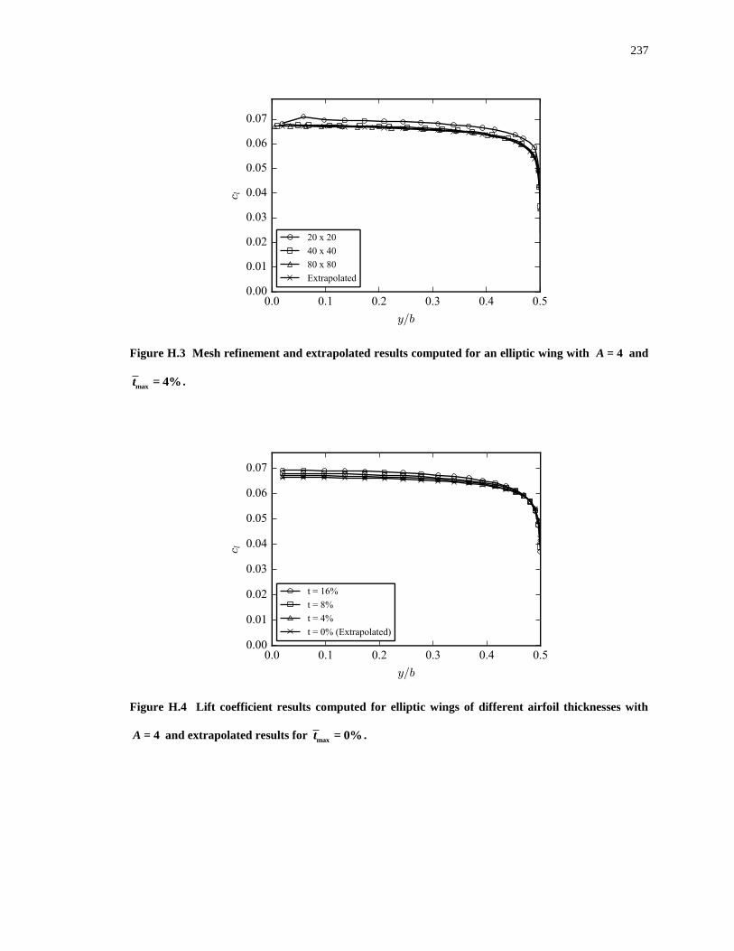
237

Figure H.3 Mesh refinement and extrapolated results computed for an elliptic wing with = 4A and

max= 4%t .

Figure H.4 Lift coefficient results computed for elliptic wings of different airfoil thicknesses with

= 4A and extrapolated results for max

= 0%t .

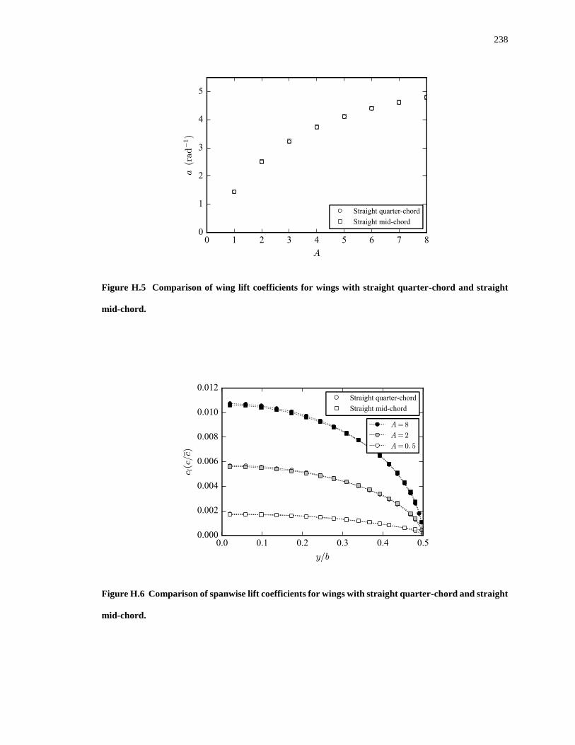
238

Figure H.5 Comparison of wing lift coefficients for wings with straight quarter-chord and straight

mid-chord.

Figure H.6 Comparison of spanwise lift coefficients for wings with straight quarter-chord and straight

mid-chord.

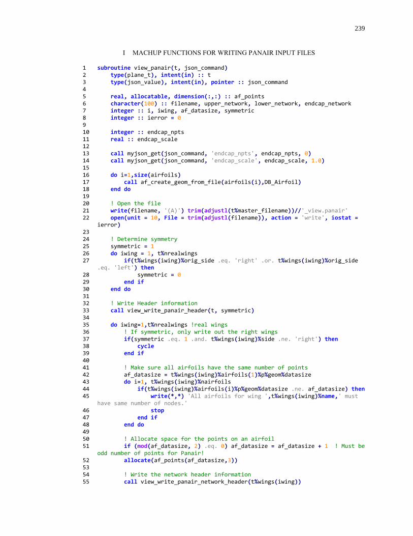
239

I MACHUP FUNCTIONS FOR WRITING PANAIR INPUT FILES

1 subroutine view_panair(t, json_command) 2 type(plane_t), intent(in) :: t 3 type(json_value), intent(in), pointer :: json_command 4 5 real, allocatable, dimension(:,:) :: af_points 6 character(100) :: filename, upper_network, lower_network, endcap_network 7 integer :: i, iwing, af_datasize, symmetric 8 integer :: ierror = 0 9 10 integer :: endcap_npts 11 real :: endcap_scale 12 13 call myjson_get(json_command, 'endcap_npts', endcap_npts, 0) 14 call myjson_get(json_command, 'endcap_scale', endcap_scale, 1.0) 15 16 do i=1,size(airfoils) 17 call af_create_geom_from_file(airfoils(i),DB_Airfoil) 18 end do 19 20 ! Open the file 21 write(filename, '(A)') trim(adjustl(t%master_filename))//'_view.panair' 22 open(unit = 10, File = trim(adjustl(filename)), action = 'write', iostat =

ierror) 23 24 ! Determine symmetry 25 symmetric = 1 26 do iwing = 1, t%nrealwings 27 if(t%wings(iwing)%orig_side .eq. 'right' .or. t%wings(iwing)%orig_side

.eq. 'left') then 28 symmetric = 0 29 end if 30 end do 31 32 ! Write Header information 33 call view_write_panair_header(t, symmetric) 34 35 do iwing=1,t%nrealwings !real wings 36 ! If symmetric, only write out the right wings 37 if(symmetric .eq. 1 .and. t%wings(iwing)%side .ne. 'right') then 38 cycle 39 end if 40 41 ! Make sure all airfoils have the same number of points 42 af_datasize = t%wings(iwing)%airfoils(1)%p%geom%datasize 43 do i=1, t%wings(iwing)%nairfoils 44 if(t%wings(iwing)%airfoils(i)%p%geom%datasize .ne. af_datasize) then 45 write(*,*) 'All airfoils for wing ',t%wings(iwing)%name,' must

have same number of nodes.' 46 stop 47 end if 48 end do 49 50 ! Allocate space for the points on an airfoil 51 if (mod(af_datasize, 2) .eq. 0) af_datasize = af_datasize + 1 ! Must be

odd number of points for Panair! 52 allocate(af_points(af_datasize,3)) 53 54 ! Write the network header information 55 call view_write_panair_network_header(t%wings(iwing))

240

56 57 ! Write the upper network 58 write(upper_network, '(A, I0)') 'upper_', t%wings(iwing)%ID 59 call view_write_panair_network(t%wings(iwing), af_points,

trim(adjustl(upper_network)), af_datasize, af_datasize / 2 + 1) 60 61 ! Write the lower network 62 write(lower_network, '(A, I0)') 'lower_', t%wings(iwing)%ID 63 call view_write_panair_network(t%wings(iwing), af_points,

trim(adjustl(lower_network)), af_datasize / 2 + 1, 1) 64 65 ! Write the endcap network 66 if(t%wings(iwing)%chord_2 >= 0.0) then 67 write(endcap_network, '(A, I0)') 'endcap_', t%wings(iwing)%ID 68 call view_write_panair_endcap(t%wings(iwing), af_points,

trim(adjustl(endcap_network)), endcap_npts, endcap_scale) 69 end if 70 71 ! Attach a wake to the trailing edge of the upper network 72 call view_write_panair_wake(trim(adjustl(upper_network))) 73 deallocate(af_points) 74 end do 75 76 write(10, "(A)") "$END" 77 close(10) 78 79 end subroutine view_panair 80 81 82 subroutine view_write_panair_header(plane, symmetric) 83 type(plane_t), intent(in) :: plane 84 integer, intent(in) :: symmetric 85 86 write(10, '(A)') '$TITLE' 87 write(10, '(A)') plane%name 88 write(10, '(A)') 'Generated by MachUp' 89 write(10, '(A)') '$DATACHECK' 90 write(10, '(A)') '=ndtchk' 91 write(10, '(A)') '0.0' 92 write(10, '(A)') '$SYMMETRIC' 93 write(10, '(A, T11, A)') '=xzpln', 'xypln' 94 write(10, '(I0, A, T11, A)') symmetric, '.0', '0.0' 95 write(10, '(A)') '$MACH NUMBER' 96 write(10, '(A)') '=amach' 97 write(10, '(F10.6)') 0.0 98 write(10, '(A)') '$CASES' 99 write(10, '(A)') '=nacase' 100 write(10, '(A)') '1.0' 101 write(10, '(A)') '$ANGLES OF ATTACK' 102 write(10, '(A)') '=alpc' 103 write(10, '(F10.6)') 0.0 104 write(10, '(A)') '=alpha(0)' 105 write(10, '(F10.6)') plane%alpha * 180.0 / pi 106 write(10, '(A)') '$YAW ANGLE' 107 write(10, '(A)') '=betc' 108 write(10, '(F10.6)') 0.0 109 write(10, '(A)') '=beta(0)' 110 write(10, '(F10.6)') plane%beta * 180.0 / pi 111 write(10, '(A)') '$REFERENCE DATA' 112 write(10, '(A, T11, A, T21, A)') '=xref', 'yref', 'zref' 113 write(10, '(3F10.6)') 0.0, 0.0, 0.0

241

114 write(10, '(A, T11, A, T21, A, T31, A)') '=sref', 'bref', 'cref', 'dref' 115 write(10, '(4F10.6)') plane%Sr, plane%lat_r, plane%long_r, plane%lat_r 116 write(10, '(A)') '$PRINTOUT CONTROL' 117 write(10, '(A, T11, A, T21, A, T31, A, T41, A, T51, A)') '=isings',

'igeomp', 'isingp', 'icontp', 'ibconp', 'iedgep' 118 write(10, '(A, T11, A, T21, A, T31, A, T41, A, T51, A)') '0.0', '0.0',

'0.0', '0.0', '0.0', '0.0' 119 write(10, '(A, T11, A, T21, A, T31, A, T41, A)') '=ipraic', 'nexdgn',

'ioutpr', 'ifmcpr', 'icostp' 120 write(10, '(A, T11, A, T21, A, T31, A, T41, A)') '0.0', '0.0', '1.0', '0.0',

'0.0' 121 end subroutine view_write_panair_header 122 123 124 subroutine view_write_panair_network_header(wi) 125 type(wing_t), intent(in) :: wi 126 127 integer :: nnetworks 128 129 if(wi%chord_2 >= 0.0) then 130 nnetworks = 3 131 else 132 nnetworks = 2 133 end if 134 135 ! Write header info 136 write(10, "(A, I0)") "$POINTS for wing ", wi%ID 137 write(10, "(A)") "=kn" ! Number of networks in $POINTS block 138 write(10, "(I0, T2, A)") nnetworks, ".0" 139 write(10, "(A)") "=kt" ! Boundary condition (1 = solid surface) 140 write(10, "(A)") "1.0" 141 142 end subroutine view_write_panair_network_header 143 144 145 subroutine view_write_panair_network(wi, af_points, network, istart, iend) 146 type(wing_t), intent(in) :: wi 147 real, allocatable, dimension(:,:), intent(inout) :: af_points 148 character(len=*), intent(in) :: network 149 integer, intent(in) :: istart, iend 150 151 integer :: isec, isec_start, isec_end, isec_inc 152 type(section_t), pointer :: si 153 154 write(10, "(A, T11, A)") "=nm", "nn" 155 write(10, "(I0, T11, I0, T71, A)") istart - iend + 1, wi%nSec + 1, network 156 157 if(wi%side .eq. "left") then 158 isec_start = wi%nSec 159 isec_end = 1 160 isec_inc = -1 161 else 162 isec_start = 1 163 isec_end = wi%nSec 164 isec_inc = 1 165 end if 166 167 do isec = isec_start, isec_end, isec_inc 168 si => wi%sec(isec) 169 call view_create_local_airfoil_panair(wi, si, 1, af_points) 170 call view_write_panair_points(istart, iend, af_points)

242

171 end do 172 173 call view_create_local_airfoil_panair(wi, si, 2, af_points) 174 call view_write_panair_points(istart, iend, af_points) 175 176 end subroutine view_write_panair_network 177 178 179 subroutine view_create_local_airfoil_panair(wi, si, sec_side, af_points) 180 type(wing_t), intent(in) :: wi 181 type(section_t), pointer, intent(in) :: si 182 integer, intent(in) :: sec_side 183 real, allocatable, dimension(:,:), intent(inout) :: af_points 184 185 real :: percent, chord, RA 186 integer :: i, mid 187 integer :: af_datasize 188 189 real :: a, b, c 190 real, dimension(3) :: midpoint 191 192 af_datasize = size(af_points, 1) 193 if (mod(af_datasize, 2) .eq. 0) then 194 write(*,*) "Allocated size of af_points must always be odd for Panair

interface!" 195 write(*,*) "If the number of points on an airfoil is even, allocate

af_points to" 196 write(*,*) "one more than this." 197 stop 198 end if 199 200 if(sec_side .eq. 1) then 201 percent = si%percent_1 202 else if(sec_side .eq. 2) then 203 percent = si%percent_2 204 else 205 percent = si%percent_c 206 end if 207 208 if(wi%chord_2 >= 0.0) then 209 chord = wi%chord_1 + percent*(wi%chord_2 - wi%chord_1) 210 else 211 RA = 8.0 * wi%span / pi / wi%chord_1 212 chord = 8.0 * wi%span / pi / RA * sqrt(1.0 - percent**2) 213 end if 214 215 if(sec_side .eq. 1) then 216 call view_create_local_airfoil(si%af1_a, si%af1_b, wi%side,

si%af_weight_1, chord, & 217 & si%twist1, si%dihedral1, si%P1, af_points) 218 else if(sec_side .eq. 2) then 219 call view_create_local_airfoil(si%af2_a, si%af2_b, wi%side,

si%af_weight_2, chord, & 220 & si%twist2, si%dihedral2, si%P2, af_points) 221 else 222 call view_create_local_airfoil(si%afc_a, si%afc_b, wi%side,

si%af_weight_c, chord, & 223 & si%twist, si%dihedral, si%PC, af_points) 224 end if 225

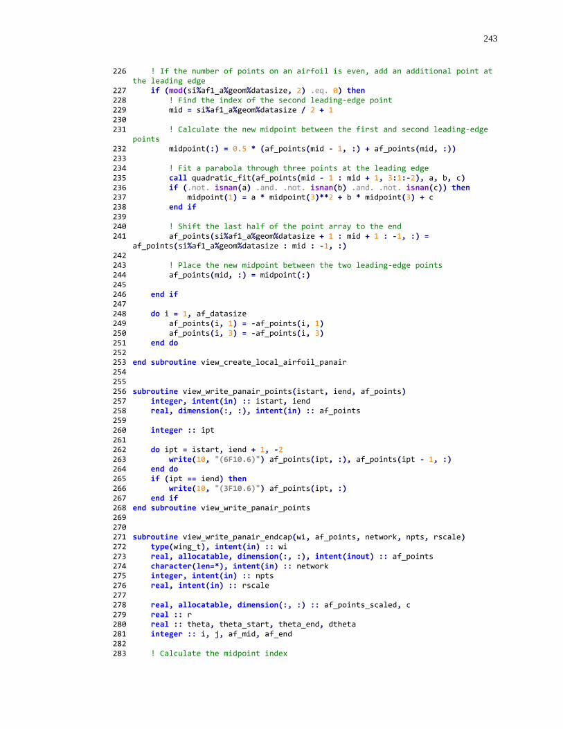
243

226 ! If the number of points on an airfoil is even, add an additional point at the leading edge

227 if (mod(si%af1_a%geom%datasize, 2) .eq. 0) then 228 ! Find the index of the second leading-edge point 229 mid = si%af1_a%geom%datasize / 2 + 1 230 231 ! Calculate the new midpoint between the first and second leading-edge

points 232 midpoint(:) = 0.5 * (af_points(mid - 1, :) + af_points(mid, :)) 233 234 ! Fit a parabola through three points at the leading edge 235 call quadratic_fit(af_points(mid - 1 : mid + 1, 3:1:-2), a, b, c) 236 if (.not. isnan(a) .and. .not. isnan(b) .and. .not. isnan(c)) then 237 midpoint(1) = a * midpoint(3)**2 + b * midpoint(3) + c 238 end if 239 240 ! Shift the last half of the point array to the end 241 af_points(si%af1_a%geom%datasize + 1 : mid + 1 : -1, :) =

af_points(si%af1_a%geom%datasize : mid : -1, :) 242 243 ! Place the new midpoint between the two leading-edge points 244 af_points(mid, :) = midpoint(:) 245 246 end if 247 248 do i = 1, af_datasize 249 af_points(i, 1) = -af_points(i, 1) 250 af_points(i, 3) = -af_points(i, 3) 251 end do 252 253 end subroutine view_create_local_airfoil_panair 254 255 256 subroutine view_write_panair_points(istart, iend, af_points) 257 integer, intent(in) :: istart, iend 258 real, dimension(:, :), intent(in) :: af_points 259 260 integer :: ipt 261 262 do ipt = istart, iend + 1, -2 263 write(10, "(6F10.6)") af_points(ipt, :), af_points(ipt - 1, :) 264 end do 265 if (ipt == iend) then 266 write(10, "(3F10.6)") af_points(ipt, :) 267 end if 268 end subroutine view_write_panair_points 269 270 271 subroutine view_write_panair_endcap(wi, af_points, network, npts, rscale) 272 type(wing_t), intent(in) :: wi 273 real, allocatable, dimension(:, :), intent(inout) :: af_points 274 character(len=*), intent(in) :: network 275 integer, intent(in) :: npts 276 real, intent(in) :: rscale 277 278 real, allocatable, dimension(:, :) :: af_points_scaled, c 279 real :: r 280 real :: theta, theta_start, theta_end, dtheta 281 integer :: i, j, af_mid, af_end 282 283 ! Calculate the midpoint index

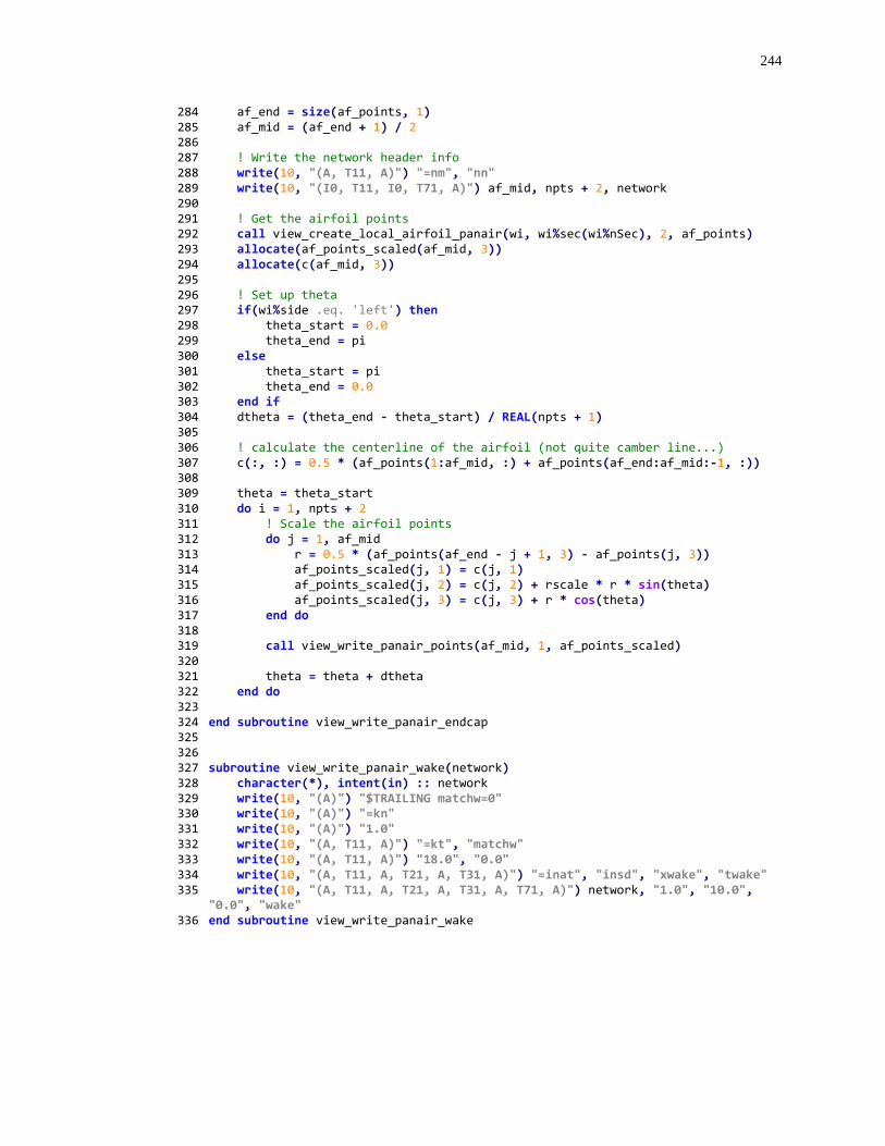
244

284 af_end = size(af_points, 1) 285 af_mid = (af_end + 1) / 2 286 287 ! Write the network header info 288 write(10, "(A, T11, A)") "=nm", "nn" 289 write(10, "(I0, T11, I0, T71, A)") af_mid, npts + 2, network 290 291 ! Get the airfoil points 292 call view_create_local_airfoil_panair(wi, wi%sec(wi%nSec), 2, af_points) 293 allocate(af_points_scaled(af_mid, 3)) 294 allocate(c(af_mid, 3)) 295 296 ! Set up theta 297 if(wi%side .eq. 'left') then 298 theta_start = 0.0 299 theta_end = pi 300 else 301 theta_start = pi 302 theta_end = 0.0 303 end if 304 dtheta = (theta_end - theta_start) / REAL(npts + 1) 305 306 ! calculate the centerline of the airfoil (not quite camber line...) 307 c(:, :) = 0.5 * (af_points(1:af_mid, :) + af_points(af_end:af_mid:-1, :)) 308 309 theta = theta_start 310 do i = 1, npts + 2 311 ! Scale the airfoil points 312 do j = 1, af_mid 313 r = 0.5 * (af_points(af_end - j + 1, 3) - af_points(j, 3)) 314 af_points_scaled(j, 1) = c(j, 1) 315 af_points_scaled(j, 2) = c(j, 2) + rscale * r * sin(theta) 316 af_points_scaled(j, 3) = c(j, 3) + r * cos(theta) 317 end do 318 319 call view_write_panair_points(af_mid, 1, af_points_scaled) 320 321 theta = theta + dtheta 322 end do 323 324 end subroutine view_write_panair_endcap 325 326 327 subroutine view_write_panair_wake(network) 328 character(*), intent(in) :: network 329 write(10, "(A)") "$TRAILING matchw=0" 330 write(10, "(A)") "=kn" 331 write(10, "(A)") "1.0" 332 write(10, "(A, T11, A)") "=kt", "matchw" 333 write(10, "(A, T11, A)") "18.0", "0.0" 334 write(10, "(A, T11, A, T21, A, T31, A)") "=inat", "insd", "xwake", "twake" 335 write(10, "(A, T11, A, T21, A, T31, A, T71, A)") network, "1.0", "10.0",

"0.0", "wake" 336 end subroutine view_write_panair_wake

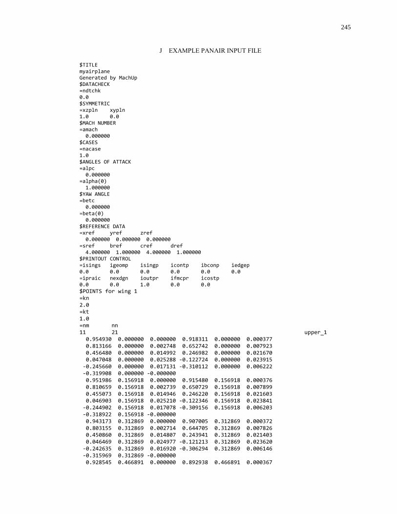
245

J EXAMPLE PANAIR INPUT FILE

$TITLE myairplane Generated by MachUp $DATACHECK =ndtchk 0.0 $SYMMETRIC =xzpln xypln 1.0 0.0 $MACH NUMBER =amach 0.000000 $CASES =nacase 1.0 $ANGLES OF ATTACK =alpc 0.000000 =alpha(0) 1.000000 $YAW ANGLE =betc 0.000000 =beta(0) 0.000000 $REFERENCE DATA =xref yref zref 0.000000 0.000000 0.000000 =sref bref cref dref 4.000000 1.000000 4.000000 1.000000 $PRINTOUT CONTROL =isings igeomp isingp icontp ibconp iedgep 0.0 0.0 0.0 0.0 0.0 0.0 =ipraic nexdgn ioutpr ifmcpr icostp 0.0 0.0 1.0 0.0 0.0 $POINTS for wing 1 =kn 2.0 =kt 1.0 =nm nn 11 21 upper_1 0.954930 0.000000 0.000000 0.918311 0.000000 0.000377 0.813166 0.000000 0.002748 0.652742 0.000000 0.007923 0.456480 0.000000 0.014992 0.246982 0.000000 0.021670 0.047048 0.000000 0.025288 -0.122724 0.000000 0.023915 -0.245660 0.000000 0.017131 -0.310112 0.000000 0.006222 -0.319908 0.000000 -0.000000 0.951986 0.156918 0.000000 0.915480 0.156918 0.000376 0.810659 0.156918 0.002739 0.650729 0.156918 0.007899 0.455073 0.156918 0.014946 0.246220 0.156918 0.021603 0.046903 0.156918 0.025210 -0.122346 0.156918 0.023841 -0.244902 0.156918 0.017078 -0.309156 0.156918 0.006203 -0.318922 0.156918 -0.000000 0.943173 0.312869 0.000000 0.907005 0.312869 0.000372 0.803155 0.312869 0.002714 0.644705 0.312869 0.007826 0.450860 0.312869 0.014807 0.243941 0.312869 0.021403 0.046469 0.312869 0.024977 -0.121213 0.312869 0.023620 -0.242635 0.312869 0.016920 -0.306294 0.312869 0.006146 -0.315969 0.312869 -0.000000 0.928545 0.466891 0.000000 0.892938 0.466891 0.000367

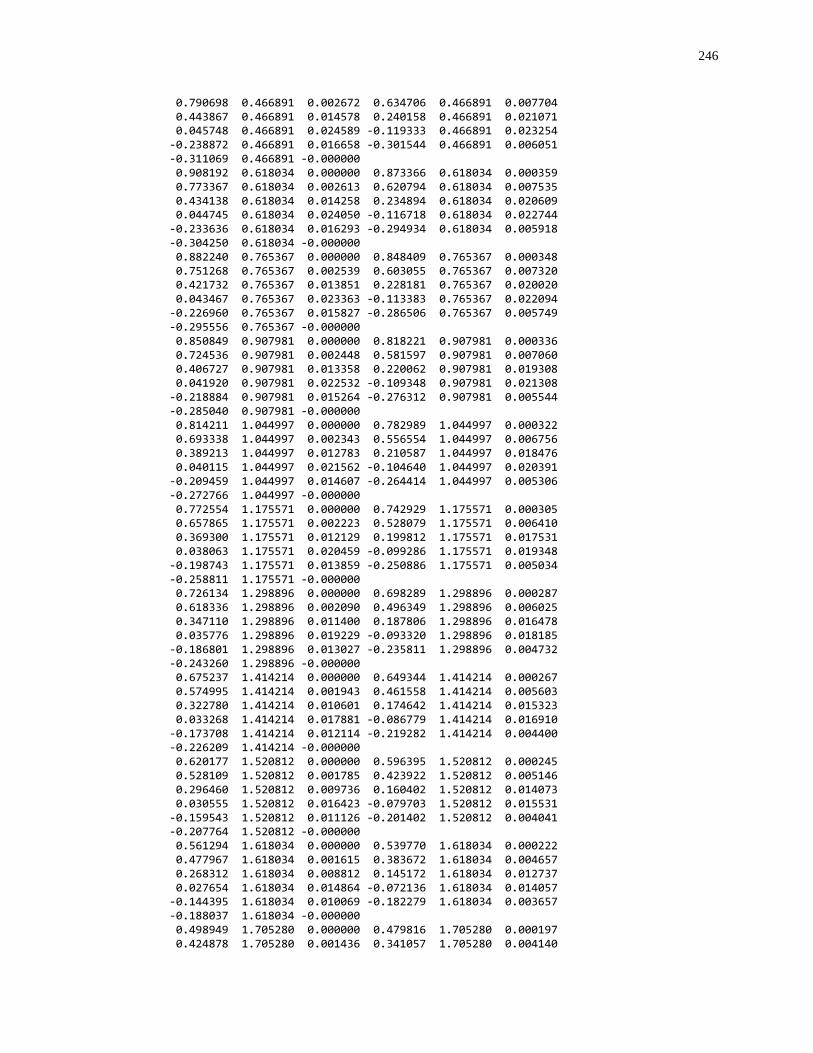
246

0.790698 0.466891 0.002672 0.634706 0.466891 0.007704 0.443867 0.466891 0.014578 0.240158 0.466891 0.021071 0.045748 0.466891 0.024589 -0.119333 0.466891 0.023254 -0.238872 0.466891 0.016658 -0.301544 0.466891 0.006051 -0.311069 0.466891 -0.000000 0.908192 0.618034 0.000000 0.873366 0.618034 0.000359 0.773367 0.618034 0.002613 0.620794 0.618034 0.007535 0.434138 0.618034 0.014258 0.234894 0.618034 0.020609 0.044745 0.618034 0.024050 -0.116718 0.618034 0.022744 -0.233636 0.618034 0.016293 -0.294934 0.618034 0.005918 -0.304250 0.618034 -0.000000 0.882240 0.765367 0.000000 0.848409 0.765367 0.000348 0.751268 0.765367 0.002539 0.603055 0.765367 0.007320 0.421732 0.765367 0.013851 0.228181 0.765367 0.020020 0.043467 0.765367 0.023363 -0.113383 0.765367 0.022094 -0.226960 0.765367 0.015827 -0.286506 0.765367 0.005749 -0.295556 0.765367 -0.000000 0.850849 0.907981 0.000000 0.818221 0.907981 0.000336 0.724536 0.907981 0.002448 0.581597 0.907981 0.007060 0.406727 0.907981 0.013358 0.220062 0.907981 0.019308 0.041920 0.907981 0.022532 -0.109348 0.907981 0.021308 -0.218884 0.907981 0.015264 -0.276312 0.907981 0.005544 -0.285040 0.907981 -0.000000 0.814211 1.044997 0.000000 0.782989 1.044997 0.000322 0.693338 1.044997 0.002343 0.556554 1.044997 0.006756 0.389213 1.044997 0.012783 0.210587 1.044997 0.018476 0.040115 1.044997 0.021562 -0.104640 1.044997 0.020391 -0.209459 1.044997 0.014607 -0.264414 1.044997 0.005306 -0.272766 1.044997 -0.000000 0.772554 1.175571 0.000000 0.742929 1.175571 0.000305 0.657865 1.175571 0.002223 0.528079 1.175571 0.006410 0.369300 1.175571 0.012129 0.199812 1.175571 0.017531 0.038063 1.175571 0.020459 -0.099286 1.175571 0.019348 -0.198743 1.175571 0.013859 -0.250886 1.175571 0.005034 -0.258811 1.175571 -0.000000 0.726134 1.298896 0.000000 0.698289 1.298896 0.000287 0.618336 1.298896 0.002090 0.496349 1.298896 0.006025 0.347110 1.298896 0.011400 0.187806 1.298896 0.016478 0.035776 1.298896 0.019229 -0.093320 1.298896 0.018185 -0.186801 1.298896 0.013027 -0.235811 1.298896 0.004732 -0.243260 1.298896 -0.000000 0.675237 1.414214 0.000000 0.649344 1.414214 0.000267 0.574995 1.414214 0.001943 0.461558 1.414214 0.005603 0.322780 1.414214 0.010601 0.174642 1.414214 0.015323 0.033268 1.414214 0.017881 -0.086779 1.414214 0.016910 -0.173708 1.414214 0.012114 -0.219282 1.414214 0.004400 -0.226209 1.414214 -0.000000 0.620177 1.520812 0.000000 0.596395 1.520812 0.000245 0.528109 1.520812 0.001785 0.423922 1.520812 0.005146 0.296460 1.520812 0.009736 0.160402 1.520812 0.014073 0.030555 1.520812 0.016423 -0.079703 1.520812 0.015531 -0.159543 1.520812 0.011126 -0.201402 1.520812 0.004041 -0.207764 1.520812 -0.000000 0.561294 1.618034 0.000000 0.539770 1.618034 0.000222 0.477967 1.618034 0.001615 0.383672 1.618034 0.004657 0.268312 1.618034 0.008812 0.145172 1.618034 0.012737 0.027654 1.618034 0.014864 -0.072136 1.618034 0.014057 -0.144395 1.618034 0.010069 -0.182279 1.618034 0.003657 -0.188037 1.618034 -0.000000 0.498949 1.705280 0.000000 0.479816 1.705280 0.000197 0.424878 1.705280 0.001436 0.341057 1.705280 0.004140

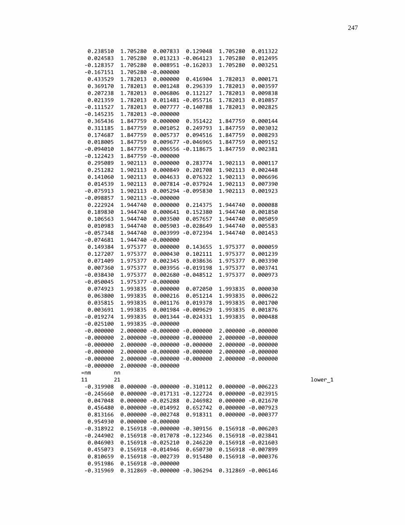
247

0.238510 1.705280 0.007833 0.129048 1.705280 0.011322 0.024583 1.705280 0.013213 -0.064123 1.705280 0.012495 -0.128357 1.705280 0.008951 -0.162033 1.705280 0.003251 -0.167151 1.705280 -0.000000 0.433529 1.782013 0.000000 0.416904 1.782013 0.000171 0.369170 1.782013 0.001248 0.296339 1.782013 0.003597 0.207238 1.782013 0.006806 0.112127 1.782013 0.009838 0.021359 1.782013 0.011481 -0.055716 1.782013 0.010857 -0.111527 1.782013 0.007777 -0.140788 1.782013 0.002825 -0.145235 1.782013 -0.000000 0.365436 1.847759 0.000000 0.351422 1.847759 0.000144 0.311185 1.847759 0.001052 0.249793 1.847759 0.003032 0.174687 1.847759 0.005737 0.094516 1.847759 0.008293 0.018005 1.847759 0.009677 -0.046965 1.847759 0.009152 -0.094010 1.847759 0.006556 -0.118675 1.847759 0.002381 -0.122423 1.847759 -0.000000 0.295089 1.902113 0.000000 0.283774 1.902113 0.000117 0.251282 1.902113 0.000849 0.201708 1.902113 0.002448 0.141060 1.902113 0.004633 0.076322 1.902113 0.006696 0.014539 1.902113 0.007814 -0.037924 1.902113 0.007390 -0.075913 1.902113 0.005294 -0.095830 1.902113 0.001923 -0.098857 1.902113 -0.000000 0.222924 1.944740 0.000000 0.214375 1.944740 0.000088 0.189830 1.944740 0.000641 0.152380 1.944740 0.001850 0.106563 1.944740 0.003500 0.057657 1.944740 0.005059 0.010983 1.944740 0.005903 -0.028649 1.944740 0.005583 -0.057348 1.944740 0.003999 -0.072394 1.944740 0.001453 -0.074681 1.944740 -0.000000 0.149384 1.975377 0.000000 0.143655 1.975377 0.000059 0.127207 1.975377 0.000430 0.102111 1.975377 0.001239 0.071409 1.975377 0.002345 0.038636 1.975377 0.003390 0.007360 1.975377 0.003956 -0.019198 1.975377 0.003741 -0.038430 1.975377 0.002680 -0.048512 1.975377 0.000973 -0.050045 1.975377 -0.000000 0.074923 1.993835 0.000000 0.072050 1.993835 0.000030 0.063800 1.993835 0.000216 0.051214 1.993835 0.000622 0.035815 1.993835 0.001176 0.019378 1.993835 0.001700 0.003691 1.993835 0.001984 -0.009629 1.993835 0.001876 -0.019274 1.993835 0.001344 -0.024331 1.993835 0.000488 -0.025100 1.993835 -0.000000 -0.000000 2.000000 -0.000000 -0.000000 2.000000 -0.000000 -0.000000 2.000000 -0.000000 -0.000000 2.000000 -0.000000 -0.000000 2.000000 -0.000000 -0.000000 2.000000 -0.000000 -0.000000 2.000000 -0.000000 -0.000000 2.000000 -0.000000 -0.000000 2.000000 -0.000000 -0.000000 2.000000 -0.000000 -0.000000 2.000000 -0.000000 =nm nn 11 21 lower_1 -0.319908 0.000000 -0.000000 -0.310112 0.000000 -0.006223 -0.245660 0.000000 -0.017131 -0.122724 0.000000 -0.023915 0.047048 0.000000 -0.025288 0.246982 0.000000 -0.021670 0.456480 0.000000 -0.014992 0.652742 0.000000 -0.007923 0.813166 0.000000 -0.002748 0.918311 0.000000 -0.000377 0.954930 0.000000 -0.000000 -0.318922 0.156918 -0.000000 -0.309156 0.156918 -0.006203 -0.244902 0.156918 -0.017078 -0.122346 0.156918 -0.023841 0.046903 0.156918 -0.025210 0.246220 0.156918 -0.021603 0.455073 0.156918 -0.014946 0.650730 0.156918 -0.007899 0.810659 0.156918 -0.002739 0.915480 0.156918 -0.000376 0.951986 0.156918 -0.000000 -0.315969 0.312869 -0.000000 -0.306294 0.312869 -0.006146

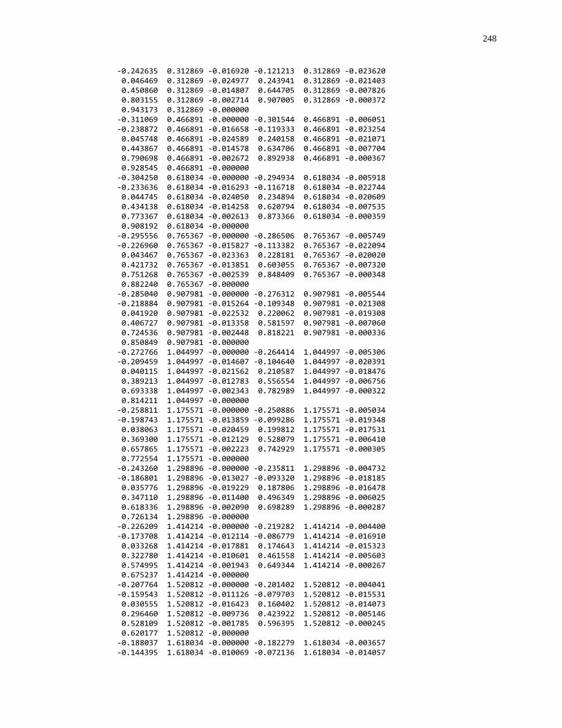
248

-0.242635 0.312869 -0.016920 -0.121213 0.312869 -0.023620 0.046469 0.312869 -0.024977 0.243941 0.312869 -0.021403 0.450860 0.312869 -0.014807 0.644705 0.312869 -0.007826 0.803155 0.312869 -0.002714 0.907005 0.312869 -0.000372 0.943173 0.312869 -0.000000 -0.311069 0.466891 -0.000000 -0.301544 0.466891 -0.006051 -0.238872 0.466891 -0.016658 -0.119333 0.466891 -0.023254 0.045748 0.466891 -0.024589 0.240158 0.466891 -0.021071 0.443867 0.466891 -0.014578 0.634706 0.466891 -0.007704 0.790698 0.466891 -0.002672 0.892938 0.466891 -0.000367 0.928545 0.466891 -0.000000 -0.304250 0.618034 -0.000000 -0.294934 0.618034 -0.005918 -0.233636 0.618034 -0.016293 -0.116718 0.618034 -0.022744 0.044745 0.618034 -0.024050 0.234894 0.618034 -0.020609 0.434138 0.618034 -0.014258 0.620794 0.618034 -0.007535 0.773367 0.618034 -0.002613 0.873366 0.618034 -0.000359 0.908192 0.618034 -0.000000 -0.295556 0.765367 -0.000000 -0.286506 0.765367 -0.005749 -0.226960 0.765367 -0.015827 -0.113382 0.765367 -0.022094 0.043467 0.765367 -0.023363 0.228181 0.765367 -0.020020 0.421732 0.765367 -0.013851 0.603055 0.765367 -0.007320 0.751268 0.765367 -0.002539 0.848409 0.765367 -0.000348 0.882240 0.765367 -0.000000 -0.285040 0.907981 -0.000000 -0.276312 0.907981 -0.005544 -0.218884 0.907981 -0.015264 -0.109348 0.907981 -0.021308 0.041920 0.907981 -0.022532 0.220062 0.907981 -0.019308 0.406727 0.907981 -0.013358 0.581597 0.907981 -0.007060 0.724536 0.907981 -0.002448 0.818221 0.907981 -0.000336 0.850849 0.907981 -0.000000 -0.272766 1.044997 -0.000000 -0.264414 1.044997 -0.005306 -0.209459 1.044997 -0.014607 -0.104640 1.044997 -0.020391 0.040115 1.044997 -0.021562 0.210587 1.044997 -0.018476 0.389213 1.044997 -0.012783 0.556554 1.044997 -0.006756 0.693338 1.044997 -0.002343 0.782989 1.044997 -0.000322 0.814211 1.044997 -0.000000 -0.258811 1.175571 -0.000000 -0.250886 1.175571 -0.005034 -0.198743 1.175571 -0.013859 -0.099286 1.175571 -0.019348 0.038063 1.175571 -0.020459 0.199812 1.175571 -0.017531 0.369300 1.175571 -0.012129 0.528079 1.175571 -0.006410 0.657865 1.175571 -0.002223 0.742929 1.175571 -0.000305 0.772554 1.175571 -0.000000 -0.243260 1.298896 -0.000000 -0.235811 1.298896 -0.004732 -0.186801 1.298896 -0.013027 -0.093320 1.298896 -0.018185 0.035776 1.298896 -0.019229 0.187806 1.298896 -0.016478 0.347110 1.298896 -0.011400 0.496349 1.298896 -0.006025 0.618336 1.298896 -0.002090 0.698289 1.298896 -0.000287 0.726134 1.298896 -0.000000 -0.226209 1.414214 -0.000000 -0.219282 1.414214 -0.004400 -0.173708 1.414214 -0.012114 -0.086779 1.414214 -0.016910 0.033268 1.414214 -0.017881 0.174643 1.414214 -0.015323 0.322780 1.414214 -0.010601 0.461558 1.414214 -0.005603 0.574995 1.414214 -0.001943 0.649344 1.414214 -0.000267 0.675237 1.414214 -0.000000 -0.207764 1.520812 -0.000000 -0.201402 1.520812 -0.004041 -0.159543 1.520812 -0.011126 -0.079703 1.520812 -0.015531 0.030555 1.520812 -0.016423 0.160402 1.520812 -0.014073 0.296460 1.520812 -0.009736 0.423922 1.520812 -0.005146 0.528109 1.520812 -0.001785 0.596395 1.520812 -0.000245 0.620177 1.520812 -0.000000 -0.188037 1.618034 -0.000000 -0.182279 1.618034 -0.003657 -0.144395 1.618034 -0.010069 -0.072136 1.618034 -0.014057

249

0.027654 1.618034 -0.014864 0.145172 1.618034 -0.012737 0.268312 1.618034 -0.008812 0.383672 1.618034 -0.004657 0.477967 1.618034 -0.001615 0.539770 1.618034 -0.000222 0.561294 1.618034 -0.000000 -0.167151 1.705280 -0.000000 -0.162033 1.705280 -0.003251 -0.128357 1.705280 -0.008951 -0.064123 1.705280 -0.012495 0.024583 1.705280 -0.013213 0.129048 1.705280 -0.011322 0.238510 1.705280 -0.007833 0.341057 1.705280 -0.004140 0.424878 1.705280 -0.001436 0.479816 1.705280 -0.000197 0.498949 1.705280 -0.000000 -0.145235 1.782013 -0.000000 -0.140788 1.782013 -0.002825 -0.111527 1.782013 -0.007777 -0.055716 1.782013 -0.010857 0.021359 1.782013 -0.011481 0.112127 1.782013 -0.009838 0.207238 1.782013 -0.006806 0.296339 1.782013 -0.003597 0.369170 1.782013 -0.001248 0.416904 1.782013 -0.000171 0.433529 1.782013 -0.000000 -0.122423 1.847759 -0.000000 -0.118675 1.847759 -0.002381 -0.094010 1.847759 -0.006556 -0.046965 1.847759 -0.009152 0.018005 1.847759 -0.009677 0.094516 1.847759 -0.008293 0.174687 1.847759 -0.005737 0.249793 1.847759 -0.003032 0.311185 1.847759 -0.001052 0.351422 1.847759 -0.000144 0.365436 1.847759 -0.000000 -0.098857 1.902113 -0.000000 -0.095830 1.902113 -0.001923 -0.075913 1.902113 -0.005294 -0.037924 1.902113 -0.007390 0.014539 1.902113 -0.007814 0.076322 1.902113 -0.006696 0.141060 1.902113 -0.004633 0.201708 1.902113 -0.002448 0.251282 1.902113 -0.000849 0.283774 1.902113 -0.000117 0.295089 1.902113 -0.000000 -0.074681 1.944740 -0.000000 -0.072394 1.944740 -0.001453 -0.057348 1.944740 -0.003999 -0.028649 1.944740 -0.005583 0.010983 1.944740 -0.005903 0.057657 1.944740 -0.005059 0.106563 1.944740 -0.003500 0.152380 1.944740 -0.001850 0.189830 1.944740 -0.000641 0.214375 1.944740 -0.000088 0.222924 1.944740 -0.000000 -0.050045 1.975377 -0.000000 -0.048512 1.975377 -0.000973 -0.038430 1.975377 -0.002680 -0.019198 1.975377 -0.003741 0.007360 1.975377 -0.003956 0.038636 1.975377 -0.003390 0.071409 1.975377 -0.002345 0.102111 1.975377 -0.001239 0.127207 1.975377 -0.000430 0.143655 1.975377 -0.000059 0.149384 1.975377 -0.000000 -0.025100 1.993835 -0.000000 -0.024331 1.993835 -0.000488 -0.019274 1.993835 -0.001344 -0.009629 1.993835 -0.001876 0.003691 1.993835 -0.001984 0.019378 1.993835 -0.001700 0.035815 1.993835 -0.001176 0.051214 1.993835 -0.000622 0.063800 1.993835 -0.000216 0.072050 1.993835 -0.000030 0.074923 1.993835 -0.000000 -0.000000 2.000000 -0.000000 -0.000000 2.000000 -0.000000 -0.000000 2.000000 -0.000000 -0.000000 2.000000 -0.000000 -0.000000 2.000000 -0.000000 -0.000000 2.000000 -0.000000 -0.000000 2.000000 -0.000000 -0.000000 2.000000 -0.000000 -0.000000 2.000000 -0.000000 -0.000000 2.000000 -0.000000 -0.000000 2.000000 -0.000000 $TRAILING matchw=0 =kn 1.0 =kt matchw 18.0 0.0 =inat insd xwake twake upper_1 1.0 10.0 0.0 wake_1

$END

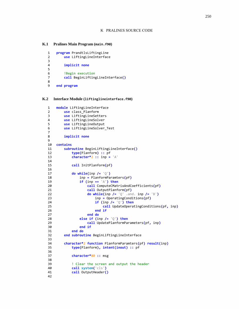
250

K PRALINES SOURCE CODE

K.1 Pralines Main Program (main.f90)

1 program PrandtlsLiftingLine 2 use LiftingLineInterface 3 4 implicit none 5 6 !Begin execution 7 call BeginLiftingLineInterface() 8 9 end program

K.2 Interface Module (liftinglineinterface.f90)

1 module LiftingLineInterface 2 use class_Planform 3 use LiftingLineSetters 4 use LiftingLineSolver 5 use LiftingLineOutput 6 use LiftingLineSolver_Test 7 8 implicit none 9 10 contains 11 subroutine BeginLiftingLineInterface() 12 type(Planform) :: pf 13 character*2 :: inp = 'A' 14 15 call InitPlanform(pf) 16 17 do while(inp /= 'Q') 18 inp = PlanformParamters(pf) 19 if (inp == 'A') then 20 call ComputeCMatrixAndCoefficients(pf) 21 call OutputPlanform(pf) 22 do while(inp /= 'Q' .and. inp /= 'B') 23 inp = OperatingConditions(pf) 24 if (inp /= 'Q') then 25 call UpdateOperatingConditions(pf, inp) 26 end if 27 end do 28 else if (inp /= 'Q') then 29 call UpdatePlanformParameters(pf, inp) 30 end if 31 end do 32 end subroutine BeginLiftingLineInterface 33 34 character*2 function PlanformParamters(pf) result(inp) 35 type(Planform), intent(inout) :: pf 36 37 character*80 :: msg 38 39 ! Clear the screen and output the header 40 call system('cls') 41 call OutputHeader() 42

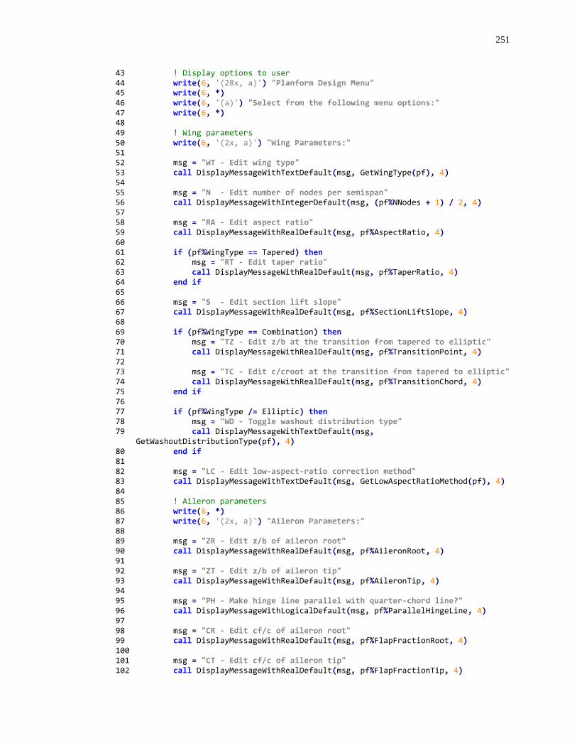
251

43 ! Display options to user 44 write(6, '(28x, a)') "Planform Design Menu" 45 write(6, *) 46 write(6, '(a)') "Select from the following menu options:" 47 write(6, *) 48 49 ! Wing parameters 50 write(6, '(2x, a)') "Wing Parameters:" 51 52 msg = "WT - Edit wing type" 53 call DisplayMessageWithTextDefault(msg, GetWingType(pf), 4) 54 55 msg = "N - Edit number of nodes per semispan" 56 call DisplayMessageWithIntegerDefault(msg, (pf%NNodes + 1) / 2, 4) 57 58 msg = "RA - Edit aspect ratio" 59 call DisplayMessageWithRealDefault(msg, pf%AspectRatio, 4) 60 61 if (pf%WingType == Tapered) then 62 msg = "RT - Edit taper ratio" 63 call DisplayMessageWithRealDefault(msg, pf%TaperRatio, 4) 64 end if 65 66 msg = "S - Edit section lift slope" 67 call DisplayMessageWithRealDefault(msg, pf%SectionLiftSlope, 4) 68 69 if (pf%WingType == Combination) then 70 msg = "TZ - Edit z/b at the transition from tapered to elliptic" 71 call DisplayMessageWithRealDefault(msg, pf%TransitionPoint, 4) 72 73 msg = "TC - Edit c/croot at the transition from tapered to elliptic" 74 call DisplayMessageWithRealDefault(msg, pf%TransitionChord, 4) 75 end if 76 77 if (pf%WingType /= Elliptic) then 78 msg = "WD - Toggle washout distribution type" 79 call DisplayMessageWithTextDefault(msg,

GetWashoutDistributionType(pf), 4) 80 end if 81 82 msg = "LC - Edit low-aspect-ratio correction method" 83 call DisplayMessageWithTextDefault(msg, GetLowAspectRatioMethod(pf), 4) 84 85 ! Aileron parameters 86 write(6, *) 87 write(6, '(2x, a)') "Aileron Parameters:" 88 89 msg = "ZR - Edit z/b of aileron root" 90 call DisplayMessageWithRealDefault(msg, pf%AileronRoot, 4) 91 92 msg = "ZT - Edit z/b of aileron tip" 93 call DisplayMessageWithRealDefault(msg, pf%AileronTip, 4) 94 95 msg = "PH - Make hinge line parallel with quarter-chord line?" 96 call DisplayMessageWithLogicalDefault(msg, pf%ParallelHingeLine, 4) 97 98 msg = "CR - Edit cf/c of aileron root" 99 call DisplayMessageWithRealDefault(msg, pf%FlapFractionRoot, 4) 100 101 msg = "CT - Edit cf/c of aileron tip" 102 call DisplayMessageWithRealDefault(msg, pf%FlapFractionTip, 4)

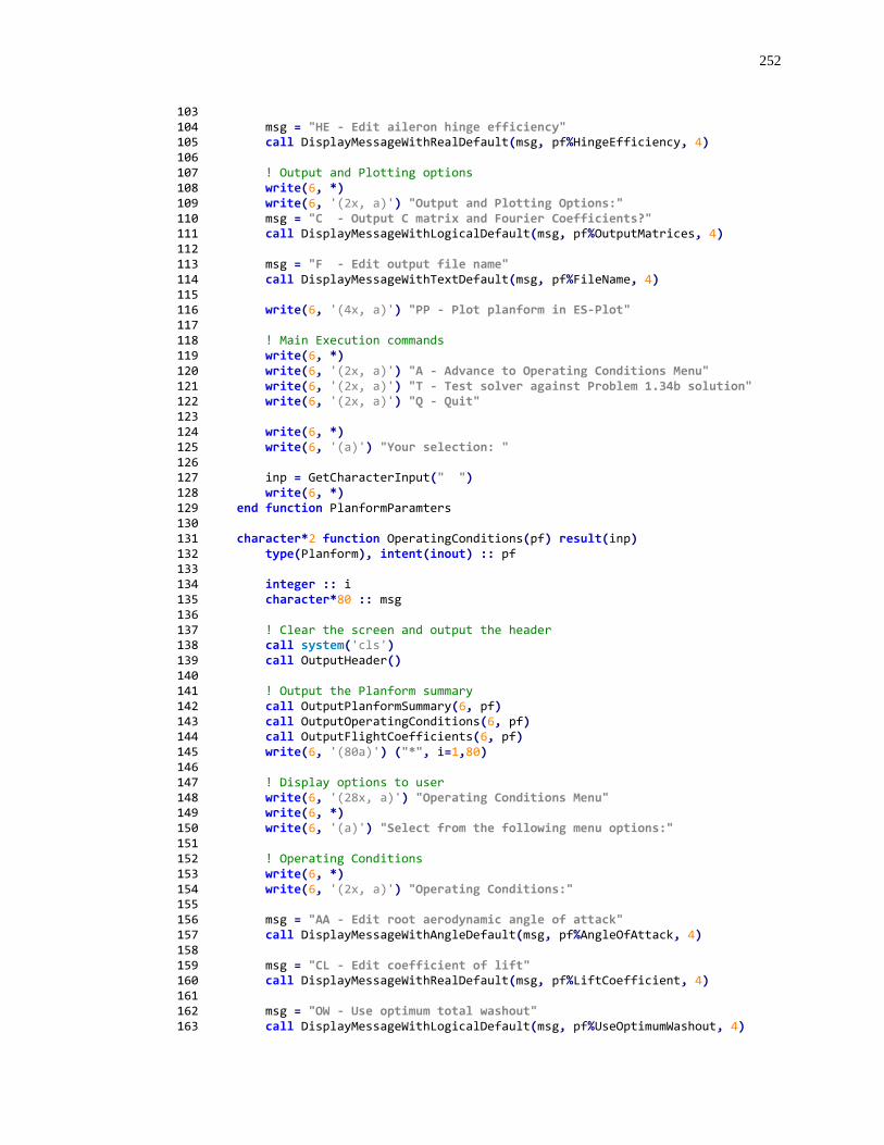
252

103 104 msg = "HE - Edit aileron hinge efficiency" 105 call DisplayMessageWithRealDefault(msg, pf%HingeEfficiency, 4) 106 107 ! Output and Plotting options 108 write(6, *) 109 write(6, '(2x, a)') "Output and Plotting Options:" 110 msg = "C - Output C matrix and Fourier Coefficients?" 111 call DisplayMessageWithLogicalDefault(msg, pf%OutputMatrices, 4) 112 113 msg = "F - Edit output file name" 114 call DisplayMessageWithTextDefault(msg, pf%FileName, 4) 115 116 write(6, '(4x, a)') "PP - Plot planform in ES-Plot" 117 118 ! Main Execution commands 119 write(6, *) 120 write(6, '(2x, a)') "A - Advance to Operating Conditions Menu" 121 write(6, '(2x, a)') "T - Test solver against Problem 1.34b solution" 122 write(6, '(2x, a)') "Q - Quit" 123 124 write(6, *) 125 write(6, '(a)') "Your selection: " 126 127 inp = GetCharacterInput(" ") 128 write(6, *) 129 end function PlanformParamters 130 131 character*2 function OperatingConditions(pf) result(inp) 132 type(Planform), intent(inout) :: pf 133 134 integer :: i 135 character*80 :: msg 136 137 ! Clear the screen and output the header 138 call system('cls') 139 call OutputHeader() 140 141 ! Output the Planform summary 142 call OutputPlanformSummary(6, pf) 143 call OutputOperatingConditions(6, pf) 144 call OutputFlightCoefficients(6, pf) 145 write(6, '(80a)') ("*", i=1,80) 146 147 ! Display options to user 148 write(6, '(28x, a)') "Operating Conditions Menu" 149 write(6, *) 150 write(6, '(a)') "Select from the following menu options:" 151 152 ! Operating Conditions 153 write(6, *) 154 write(6, '(2x, a)') "Operating Conditions:" 155 156 msg = "AA - Edit root aerodynamic angle of attack" 157 call DisplayMessageWithAngleDefault(msg, pf%AngleOfAttack, 4) 158 159 msg = "CL - Edit coefficient of lift" 160 call DisplayMessageWithRealDefault(msg, pf%LiftCoefficient, 4) 161 162 msg = "OW - Use optimum total washout" 163 call DisplayMessageWithLogicalDefault(msg, pf%UseOptimumWashout, 4)

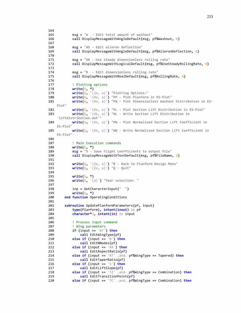
253

164 165 msg = "W - Edit total amount of washout" 166 call DisplayMessageWithAngleDefault(msg, pf%Washout, 4) 167 168 msg = "AD - Edit aileron deflection" 169 call DisplayMessageWithAngleDefault(msg, pf%AileronDeflection, 4) 170 171 msg = "SR - Use steady dimensionless rolling rate" 172 call DisplayMessageWithLogicalDefault(msg, pf%UseSteadyRollingRate, 4) 173 174 msg = "R - Edit dimensionless rolling rate" 175 call DisplayMessageWithRealDefault(msg, pf%RollingRate, 4) 176 177 ! Plotting options 178 write(6, *) 179 write(6, '(2x, a)') "Plotting Options:" 180 write(6, '(4x, a)') "PP - Plot Planform in ES-Plot" 181 write(6, '(4x, a)') "PW - Plot Dimensionless Washout Distribution in ES-

Plot" 182 write(6, '(4x, a)') "PL - Plot Section Lift Distribution in ES-Plot" 183 write(6, '(4x, a)') "WL - Write Section Lift Distribution to

'liftdistribution.dat'" 184 write(6, '(4x, a)') "PN - Plot Normalized Section Lift Coefficient in

ES-Plot" 185 write(6, '(4x, a)') "WN - Write Normalized Section Lift Coefficient in

ES-Plot" 186 187 ! Main Execution commands 188 write(6, *) 189 msg = "S - Save Flight coefficients to output file" 190 call DisplayMessageWithTextDefault(msg, pf%FileName, 2) 191 192 write(6, '(2x, a)') "B - Back to Planform Design Menu" 193 write(6, '(2x, a)') "Q - Quit" 194 195 write(6, *) 196 write(6, '(a)') "Your selection: " 197 198 inp = GetCharacterInput(" ") 199 write(6, *) 200 end function OperatingConditions 201 202 subroutine UpdatePlanformParameters(pf, input) 203 type(Planform), intent(inout) :: pf 204 character*2, intent(in) :: input 205 206 ! Process input command 207 ! Wing parameters 208 if (input == 'WT') then 209 call EditWingType(pf) 210 else if (input == 'N') then 211 call EditNNodes(pf) 212 else if (input == 'RA') then 213 call EditAspectRatio(pf) 214 else if (input == 'RT' .and. pf%WingType == Tapered) then 215 call EditTaperRatio(pf) 216 else if (input == 'S') then 217 call EditLiftSlope(pf) 218 else if (input == 'TZ' .and. pf%WingType == Combination) then 219 call EditTransitionPoint(pf) 220 else if (input == 'TC' .and. pf%WingType == Combination) then

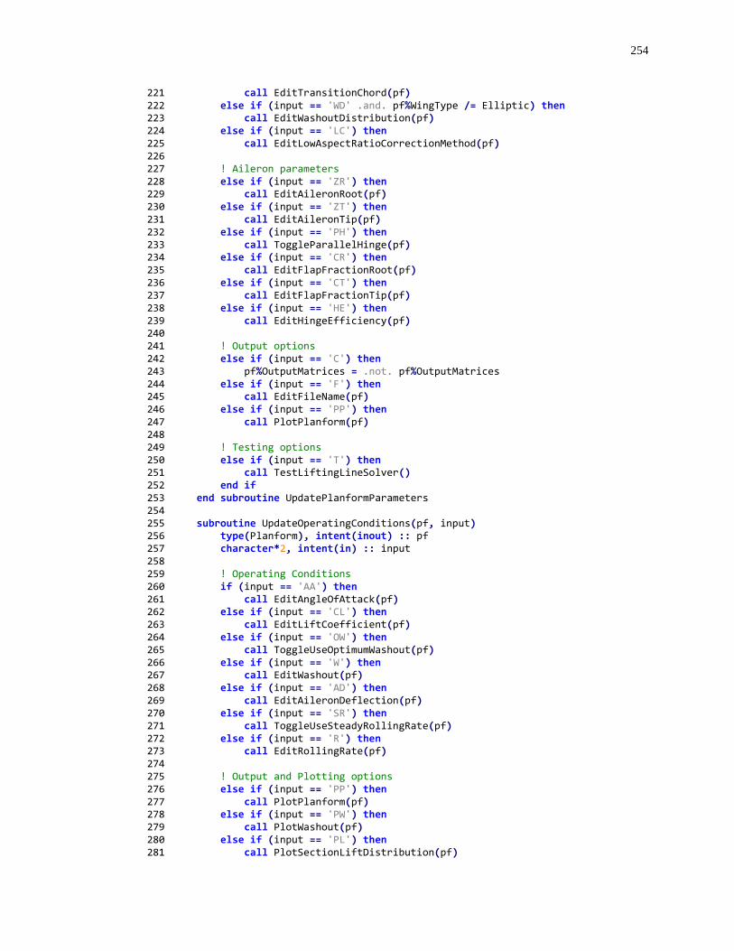
254

221 call EditTransitionChord(pf) 222 else if (input == 'WD' .and. pf%WingType /= Elliptic) then 223 call EditWashoutDistribution(pf) 224 else if (input == 'LC') then 225 call EditLowAspectRatioCorrectionMethod(pf) 226 227 ! Aileron parameters 228 else if (input == 'ZR') then 229 call EditAileronRoot(pf) 230 else if (input == 'ZT') then 231 call EditAileronTip(pf) 232 else if (input == 'PH') then 233 call ToggleParallelHinge(pf) 234 else if (input == 'CR') then 235 call EditFlapFractionRoot(pf) 236 else if (input == 'CT') then 237 call EditFlapFractionTip(pf) 238 else if (input == 'HE') then 239 call EditHingeEfficiency(pf) 240 241 ! Output options 242 else if (input == 'C') then 243 pf%OutputMatrices = .not. pf%OutputMatrices 244 else if (input == 'F') then 245 call EditFileName(pf) 246 else if (input == 'PP') then 247 call PlotPlanform(pf) 248 249 ! Testing options 250 else if (input == 'T') then 251 call TestLiftingLineSolver() 252 end if 253 end subroutine UpdatePlanformParameters 254 255 subroutine UpdateOperatingConditions(pf, input) 256 type(Planform), intent(inout) :: pf 257 character*2, intent(in) :: input 258 259 ! Operating Conditions 260 if (input == 'AA') then 261 call EditAngleOfAttack(pf) 262 else if (input == 'CL') then 263 call EditLiftCoefficient(pf) 264 else if (input == 'OW') then 265 call ToggleUseOptimumWashout(pf) 266 else if (input == 'W') then 267 call EditWashout(pf) 268 else if (input == 'AD') then 269 call EditAileronDeflection(pf) 270 else if (input == 'SR') then 271 call ToggleUseSteadyRollingRate(pf) 272 else if (input == 'R') then 273 call EditRollingRate(pf) 274 275 ! Output and Plotting options 276 else if (input == 'PP') then 277 call PlotPlanform(pf) 278 else if (input == 'PW') then 279 call PlotWashout(pf) 280 else if (input == 'PL') then 281 call PlotSectionLiftDistribution(pf)

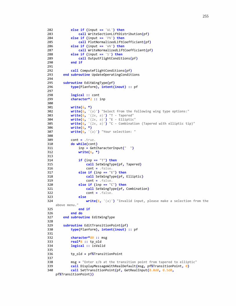
255

282 else if (input == 'WL') then 283 call WriteSectionLiftDistribution(pf) 284 else if (input == 'PN') then 285 call PlotNormalizedLiftCoefficient(pf) 286 else if (input == 'WN') then 287 call WriteNormalizedLiftCoefficient(pf) 288 else if (input == 'S') then 289 call OutputFlightConditions(pf) 290 end if 291 292 call ComputeFlightConditions(pf) 293 end subroutine UpdateOperatingConditions 294 295 subroutine EditWingType(pf) 296 type(Planform), intent(inout) :: pf 297 298 logical :: cont 299 character*2 :: inp 300 301 write(6, *) 302 write(6, '(a)') "Select from the following wing type options:" 303 write(6, '(2x, a)') "T - Tapered" 304 write(6, '(2x, a)') "E - Elliptic" 305 write(6, '(2x, a)') "C - Combination (Tapered with elliptic tip)" 306 write(6, *) 307 write(6, '(a)') "Your selection: " 308 309 cont = .true. 310 do while(cont) 311 inp = GetCharacterInput(" ") 312 write(6, *) 313 314 if (inp == "T") then 315 call SetWingType(pf, Tapered) 316 cont = .false. 317 else if (inp == "E") then 318 call SetWingType(pf, Elliptic) 319 cont = .false. 320 else if (inp == "C") then 321 call SetWingType(pf, Combination) 322 cont = .false. 323 else 324 write(6, '(a)') "Invalid input, please make a selection from the

above menu." 325 end if 326 end do 327 end subroutine EditWingType 328 329 subroutine EditTransitionPoint(pf) 330 type(Planform), intent(inout) :: pf 331 332 character*80 :: msg 333 real*8 :: tp_old 334 logical :: isValid 335 336 tp_old = pf%TransitionPoint 337 338 msg = "Enter z/b at the transition point from tapered to elliptic" 339 call DisplayMessageWithRealDefault(msg, pf%TransitionPoint, 0) 340 call SetTransitionPoint(pf, GetRealInput(0.0d0, 0.5d0,

pf%TransitionPoint))

256

341 342 isValid = AreCombinationWingCoefficientsValid(pf) 343 do while(.not. isValid) 344 call SetTransitionPoint(pf, tp_old) 345 write(6, *) 346 write(6, '(a)') "The input provided results in invalid ellipse

coefficients." 347 write(6, '(a)') "Try a new value or press <ENTER> to accept

default." 348 349 call SetTransitionPoint(pf, GetRealInput(0.0d0, 0.5d0,

pf%TransitionPoint)) 350 isValid = AreCombinationWingCoefficientsValid(pf) 351 end do 352 end subroutine EditTransitionPoint 353 354 subroutine EditTransitionChord(pf) 355 type(Planform), intent(inout) :: pf 356 357 character*80 :: msg 358 real*8 :: tc_old 359 logical :: isValid 360 361 tc_old = pf%TransitionChord 362 363 msg = "Enter c/croot at the transition point from tapered to elliptic" 364 call DisplayMessageWithRealDefault(msg, pf%TransitionChord, 0) 365 call SetTransitionChord(pf, GetRealInput(0.0d0, 10.0d0,

pf%TransitionChord)) 366 367 isValid = AreCombinationWingCoefficientsValid(pf) 368 do while(.not. isValid) 369 call SetTransitionChord(pf, tc_old) 370 write(6, *) 371 write(6, '(a)') "The input provided results in invalid ellipse

coefficients." 372 write(6, '(a)') "Try a new value or press <ENTER> to accept

default." 373 374 call SetTransitionChord(pf, GetRealInput(0.0d0, 2.0d0,

pf%TransitionChord)) 375 isValid = AreCombinationWingCoefficientsValid(pf) 376 end do 377 end subroutine EditTransitionChord 378 379 subroutine EditWashoutDistribution(pf) 380 type(Planform), intent(inout) :: pf 381 382 if (pf%WashoutDistribution == Linear) then 383 call SetWashoutDistribution(pf, Optimum) 384 else 385 call SetWashoutDistribution(pf, Linear) 386 end if 387 end subroutine EditWashoutDistribution 388 389 subroutine EditLowAspectRatioCorrectionMethod(pf) 390 type(Planform), intent(inout) :: pf 391 392 logical :: cont 393 character*2 :: inp 394

257

395 write(6, *) 396 write(6, '(a)') "Select from the following low-aspect-ratio correction

methods:" 397 write(6, '(2x, a)') "C - Classical Lifting Line Theory (no correction)" 398 write(6, '(2x, a)') "H - Hodson" 399 write(6, '(2x, a)') "M - Modified Slender Wing" 400 write(6, '(2x, a)') "K - Kuchemann" 401 write(6, *) 402 write(6, '(a)') "Your selection: " 403 404 cont = .true. 405 do while(cont) 406 inp = GetCharacterInput(" ") 407 write(6, *) 408 409 if (inp == "C") then 410 call SetLowAspectRatioMethod(pf, Classical) 411 cont = .false. 412 else if (inp == "H") then 413 call SetLowAspectRatioMethod(pf, Hodson) 414 cont = .false. 415 else if (inp == "M") then 416 call SetLowAspectRatioMethod(pf, ModifiedSlender) 417 cont = .false. 418 else if (inp == "K") then 419 call SetLowAspectRatioMethod(pf, Kuchemann) 420 cont = .false. 421 else 422 write(6, '(a)') "Invalid input, please make a selection from the

above menu." 423 end if 424 end do 425 end subroutine 426 427 subroutine EditNNodes(pf) 428 type(Planform), intent(inout) :: pf 429 430 character*80 :: msg 431 integer :: npss 432 character*80 :: int_str 433 434 npss = (pf%NNodes + 1) / 2 435 436 msg = "Enter number of nodes per semispan or press <ENTER> to accept

default" 437 call DisplayMessageWithIntegerDefault(msg, npss, 0) 438 call SetNNodes(pf, GetIntInput(4, 1000, npss)) 439 end subroutine EditNNodes 440 441 subroutine EditAspectRatio(pf) 442 type(Planform), intent(inout) :: pf 443 444 character*80 :: msg 445 446 write(6, *) 447 msg = "Enter new aspect ratio or press <ENTER> to accept default" 448 call DisplayMessageWithRealDefault(msg, pf%AspectRatio, 0) 449 call SetAspectRatio(pf, GetRealInput(1.0d-12, 100.0d0, pf%AspectRatio)) 450 end subroutine EditAspectRatio 451 452 subroutine EditTaperRatio(pf)

258

453 type(Planform), intent(inout) :: pf 454 455 character*80 :: msg 456 457 write(6, *) 458 msg = "Enter new taper ratio or press <ENTER> to accept default" 459 call DisplayMessageWithRealDefault(msg, pf%TaperRatio, 0) 460 call SetTaperRatio(pf, GetRealInput(0.0d0, 100.0d0, pf%TaperRatio)) 461 end subroutine EditTaperRatio 462 463 subroutine EditLiftSlope(pf) 464 type(Planform), intent(inout) :: pf 465 466 character*80 :: msg 467 468 write(6, *) 469 msg = "Enter new section lift slope or press <ENTER> to accept default" 470 call DisplayMessageWithRealDefault(msg, pf%SectionLiftSlope, 0) 471 call SetSectionLiftSlope(pf, GetRealInput(-100.0d0 * pi, 100.0d0 * pi, & 472 & pf%SectionLiftSlope)) 473 end subroutine EditLiftSlope 474 475 subroutine EditAileronRoot(pf) 476 type(Planform), intent(inout) :: pf 477 478 character*80 :: msg 479 480 write(6, *) 481 msg = "Enter new z/b for aileron root or press <ENTER> to accept

default" 482 call DisplayMessageWithRealDefault(msg, pf%AileronRoot, 0) 483 call SetAileronRoot(pf, GetRealInput(0.0d0, pf%AileronTip,

pf%AileronRoot)) 484 end subroutine EditAileronRoot 485 486 subroutine EditAileronTip(pf) 487 type(Planform), intent(inout) :: pf 488 489 character*80 :: msg 490 491 write(6, *) 492 msg = "Enter new z/b for aileron tip or press <ENTER> to accept default" 493 call DisplayMessageWithRealDefault(msg, pf%AileronTip, 0) 494 call SetAileronTip(pf, GetRealInput(pf%AileronRoot, 0.5d0,

pf%AileronTip)) 495 end subroutine EditAileronTip 496 497 subroutine EditFlapFractionRoot(pf) 498 type(Planform), intent(inout) :: pf 499 500 character*80 :: msg 501 502 write(6, *) 503 if (pf%ParallelHingeLine) then 504 write(6, '(a)') "NOTE: Hinge is no longer constrained to be parallel

with quarter-chord line." 505 end if 506 507 msg = "Enter new cf/c at aileron root or press <ENTER> to accept

default" 508 call DisplayMessageWithRealDefault(msg, pf%DesiredFlapFractionRoot, 0)

259

509 call SetFlapFractionRoot(pf, GetRealInput(0.0d0, 1.0d0, pf%DesiredFlapFractionRoot))

510 end subroutine EditFlapFractionRoot 511 512 subroutine EditFlapFractionTip(pf) 513 type(Planform), intent(inout) :: pf 514 515 character*80 :: msg 516 517 write(6, *) 518 msg = "Enter new cf/c at aileron tip or press <ENTER> to accept default" 519 call DisplayMessageWithRealDefault(msg, pf%FlapFractionTip, 0) 520 call SetFlapFractionTip(pf, GetRealInput(0.0d0, 1.0d0,

pf%FlapFractionTip)) 521 end subroutine EditFlapFractionTip 522 523 subroutine ToggleParallelHinge(pf) 524 type(Planform), intent(inout) :: pf 525 526 if (pf%ParallelHingeLine) then 527 call SetFlapFractionRoot(pf, pf%DesiredFlapFractionRoot) 528 else 529 call SetParallelHingeLine(pf) 530 end if 531 end subroutine ToggleParallelHinge 532 533 subroutine EditHingeEfficiency(pf) 534 type(Planform), intent(inout) :: pf 535 536 character*80 :: msg 537 538 write(6, *) 539 msg = "Enter aileron hinge efficiency or press <ENTER> to accept

default" 540 call DisplayMessageWithRealDefault(msg, pf%HingeEfficiency, 0) 541 call SetHingeEfficiency(pf, GetRealInput(0.0d0, 1.0d0,

pf%HingeEfficiency)) 542 end subroutine EditHingeEfficiency 543 544 subroutine EditDeflectionEfficiency(pf) 545 type(Planform), intent(inout) :: pf 546 547 character*80 :: msg 548 549 write(6, *) 550 msg = "Enter deflection efficiency or press <ENTER> to accept default" 551 call DisplayMessageWithRealDefault(msg, pf%DeflectionEfficiency, 0) 552 call SetDeflectionEfficiency(pf, GetRealInput(0.0d0, 1.0d0, & 553 & pf%DeflectionEfficiency)) 554 end subroutine EditDeflectionEfficiency 555 556 subroutine EditFileName(pf) 557 type(Planform), intent(inout) :: pf 558 559 character*80 :: msg 560 561 write(6, *) 562 msg = "Enter output file name or press <ENTER> to accept default" 563 call DisplayMessageWithTextDefault(msg, pf%FileName, 0) 564 call SetFileName(pf, GetStringInput(pf%FileName)) 565 end subroutine EditFileName

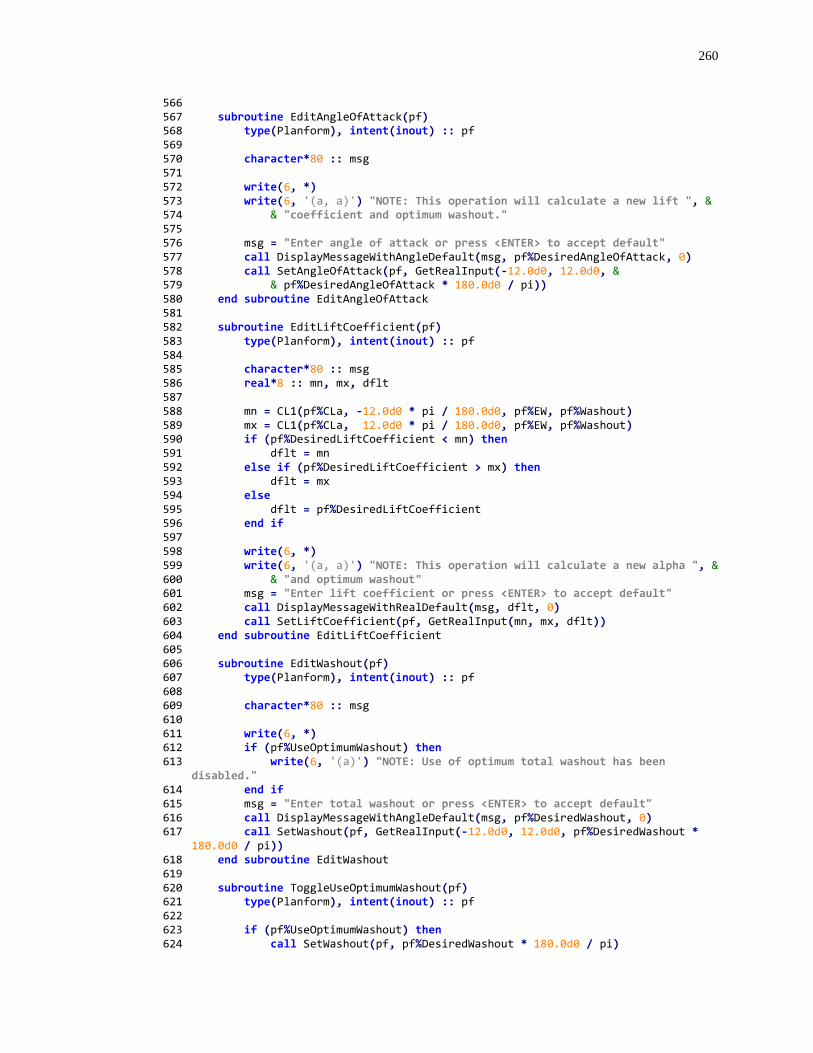
260

566 567 subroutine EditAngleOfAttack(pf) 568 type(Planform), intent(inout) :: pf 569 570 character*80 :: msg 571 572 write(6, *) 573 write(6, '(a, a)') "NOTE: This operation will calculate a new lift ", & 574 & "coefficient and optimum washout." 575 576 msg = "Enter angle of attack or press <ENTER> to accept default" 577 call DisplayMessageWithAngleDefault(msg, pf%DesiredAngleOfAttack, 0) 578 call SetAngleOfAttack(pf, GetRealInput(-12.0d0, 12.0d0, & 579 & pf%DesiredAngleOfAttack * 180.0d0 / pi)) 580 end subroutine EditAngleOfAttack 581 582 subroutine EditLiftCoefficient(pf) 583 type(Planform), intent(inout) :: pf 584 585 character*80 :: msg 586 real*8 :: mn, mx, dflt 587 588 mn = CL1(pf%CLa, -12.0d0 * pi / 180.0d0, pf%EW, pf%Washout) 589 mx = CL1(pf%CLa, 12.0d0 * pi / 180.0d0, pf%EW, pf%Washout) 590 if (pf%DesiredLiftCoefficient < mn) then 591 dflt = mn 592 else if (pf%DesiredLiftCoefficient > mx) then 593 dflt = mx 594 else 595 dflt = pf%DesiredLiftCoefficient 596 end if 597 598 write(6, *) 599 write(6, '(a, a)') "NOTE: This operation will calculate a new alpha ", & 600 & "and optimum washout" 601 msg = "Enter lift coefficient or press <ENTER> to accept default" 602 call DisplayMessageWithRealDefault(msg, dflt, 0) 603 call SetLiftCoefficient(pf, GetRealInput(mn, mx, dflt)) 604 end subroutine EditLiftCoefficient 605 606 subroutine EditWashout(pf) 607 type(Planform), intent(inout) :: pf 608 609 character*80 :: msg 610 611 write(6, *) 612 if (pf%UseOptimumWashout) then 613 write(6, '(a)') "NOTE: Use of optimum total washout has been

disabled." 614 end if 615 msg = "Enter total washout or press <ENTER> to accept default" 616 call DisplayMessageWithAngleDefault(msg, pf%DesiredWashout, 0) 617 call SetWashout(pf, GetRealInput(-12.0d0, 12.0d0, pf%DesiredWashout *

180.0d0 / pi)) 618 end subroutine EditWashout 619 620 subroutine ToggleUseOptimumWashout(pf) 621 type(Planform), intent(inout) :: pf 622 623 if (pf%UseOptimumWashout) then 624 call SetWashout(pf, pf%DesiredWashout * 180.0d0 / pi)

261

625 else 626 call SetOptimumWashout(pf) 627 end if 628 end subroutine ToggleUseOptimumWashout 629 630 subroutine EditAileronDeflection(pf) 631 type(Planform), intent(inout) :: pf 632 633 character*80 :: msg 634 635 write(6, *) 636 msg = "Enter aileron deflection or press <ENTER> to accept default" 637 call DisplayMessageWithAngleDefault(msg, pf%AileronDeflection, 0) 638 call SetAileronDeflection(pf, GetRealInput(-12.0d0, 12.0d0, & 639 & pf%AileronDeflection * 180.0d0 / pi)) 640 end subroutine EditAileronDeflection 641 642 subroutine ToggleUseSteadyRollingRate(pf) 643 type(Planform), intent(inout) :: pf 644 645 pf%UseSteadyRollingRate = .not. pf%UseSteadyRollingRate 646 if (pf%UseSteadyRollingRate) then 647 call SetSteadyRollingRate(pf) 648 else 649 call SetRollingRate(pf, pf%DesiredRollingRate) 650 end if 651 end subroutine ToggleUseSteadyRollingRate 652 653 subroutine EditRollingRate(pf) 654 type(Planform), intent(inout) :: pf 655 656 character*80 :: msg 657 658 write(6, *) 659 660 if (pf%UseSteadyRollingRate) then 661 write(6, '(a)') "NOTE: Use of steady rolling rate has been

disabled." 662 end if 663 664 msg = "Enter dimensionless rolling rate or press <ENTER> to accept

default" 665 call DisplayMessageWithRealDefault(msg, pf%DesiredRollingRate, 0) 666 call SetRollingRate(pf, GetRealInput(-100.0d0, 100.0d0,

pf%DesiredRollingRate)) 667 end subroutine EditRollingRate 668 669 subroutine DisplayMessageWithRealDefault(msg, dflt, tab) 670 character*80, intent(in) :: msg ! Message to be displayed 671 real*8, intent(in) :: dflt ! Default value to show in parenthesis 672 integer, intent(in) :: tab ! Size of indentation to use 673 674 call DisplayMessageWithTextDefault(msg, FormatReal(dflt, 5), tab) 675 end subroutine DisplayMessageWithRealDefault 676 677 subroutine DisplayMessageWithAngleDefault(msg, dflt, tab) 678 character*80, intent(in) :: msg ! Message to be displayed 679 real*8, intent(in) :: dflt ! Default value to show in parenthesis 680 integer, intent(in) :: tab ! Size of indentation to use 681 682 character*80 :: dflt_deg

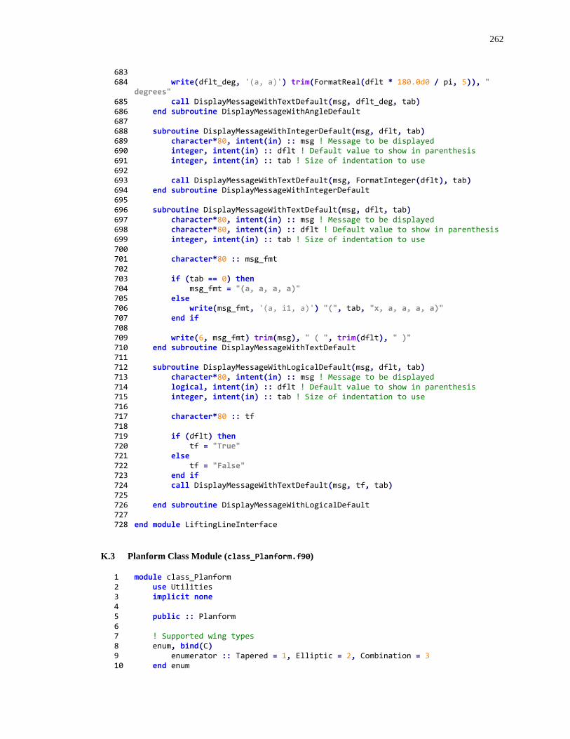
262

683 684 write(dflt_deg, '(a, a)') trim(FormatReal(dflt * 180.0d0 / pi, 5)), "

degrees" 685 call DisplayMessageWithTextDefault(msg, dflt_deg, tab) 686 end subroutine DisplayMessageWithAngleDefault 687 688 subroutine DisplayMessageWithIntegerDefault(msg, dflt, tab) 689 character*80, intent(in) :: msg ! Message to be displayed 690 integer, intent(in) :: dflt ! Default value to show in parenthesis 691 integer, intent(in) :: tab ! Size of indentation to use 692 693 call DisplayMessageWithTextDefault(msg, FormatInteger(dflt), tab) 694 end subroutine DisplayMessageWithIntegerDefault 695 696 subroutine DisplayMessageWithTextDefault(msg, dflt, tab) 697 character*80, intent(in) :: msg ! Message to be displayed 698 character*80, intent(in) :: dflt ! Default value to show in parenthesis 699 integer, intent(in) :: tab ! Size of indentation to use 700 701 character*80 :: msg_fmt 702 703 if (tab == 0) then 704 msg_fmt = "(a, a, a, a)" 705 else 706 write(msg_fmt, '(a, i1, a)') "(", tab, "x, a, a, a, a)" 707 end if 708 709 write(6, msg_fmt) trim(msg), " ( ", trim(dflt), " )" 710 end subroutine DisplayMessageWithTextDefault 711 712 subroutine DisplayMessageWithLogicalDefault(msg, dflt, tab) 713 character*80, intent(in) :: msg ! Message to be displayed 714 logical, intent(in) :: dflt ! Default value to show in parenthesis 715 integer, intent(in) :: tab ! Size of indentation to use 716 717 character*80 :: tf 718 719 if (dflt) then 720 tf = "True" 721 else 722 tf = "False" 723 end if 724 call DisplayMessageWithTextDefault(msg, tf, tab) 725 726 end subroutine DisplayMessageWithLogicalDefault 727 728 end module LiftingLineInterface

K.3 Planform Class Module (class_Planform.f90)

1 module class_Planform 2 use Utilities 3 implicit none 4 5 public :: Planform 6 7 ! Supported wing types 8 enum, bind(C) 9 enumerator :: Tapered = 1, Elliptic = 2, Combination = 3 10 end enum

263

11 12 ! Supported washout distribution types 13 enum, bind(C) 14 enumerator :: Linear = 1, Optimum = 2 15 end enum 16 17 ! Supported low-aspect-ratio methods 18 enum, bind(C) 19 enumerator :: Classical=1, Hodson=2, ModifiedSlender=3, Kuchemann=4 20 end enum 21 22 type Planform 23 ! Wing Parameters 24 integer :: WingType = Tapered ! Wing type 25 integer :: WashoutDistribution = Linear ! Washout distribution type 26 integer :: NNodes = 99 ! Total number of nodes 27 real*8 :: AspectRatio = 5.56d0 ! Aspect ratio 28 real*8 :: TaperRatio = 1.0d0 ! Taper ratio (tapered wing only) 29 real*8 :: TransitionPoint = 0.25d0 ! Transition point (Combination wing

only) 30 real*8 :: TransitionChord = 1.0d0 ! c/croot at transtion point

(Combination wing only) 31 real*8 :: SectionLiftSlope = 2.0d0 * pi ! Section lift slope 32 real*8 :: AileronRoot = 0.253d0 ! Location of aileron root (z/b) 33 real*8 :: AileronTip = 0.438d0 ! Location of aileron tip (z/b) 34 logical :: ParallelHingeLine = .true. ! Is the hinge line parallel to

the 35 ! quarter-chord line? When true, 36 ! FlapFractionTip will be

calculated 37 real*8 :: DesiredFlapFractionRoot = 0.28d0 ! Desired flap fraction at

aileron root (cf/c) 38 real*8 :: FlapFractionRoot = 0.28d0 ! Flap fraction at aileron root

(cf/c) 39 real*8 :: FlapFractionTip = 0.25d0 ! Flap fraction at aileron tip (cf/c) 40 real*8 :: HingeEfficiency = 0.85d0 ! Aileron hinge efficiency 41 real*8 :: DeflectionEfficiency = 1.0d0 ! Aileron deflection efficiency 42 integer :: LowAspectRatioMethod = Classical ! Low-Aspect-Ratio

correction method 43 44 ! Coefficients for Tapered wing with elliptic tip 45 real*8 :: C1 = 0.0d0 ! Represents transition point 46 real*8 :: C2 = 0.0d0 ! Represents slope of tapered section 47 real*8 :: C3 = 0.0d0 ! Represents secondary axis of ellipse 48 real*8 :: C4 = 0.0d0 ! Represents ellipse center offset 49 real*8 :: C5 = 0.0d0 ! Represents croot/b 50 51 ! Output Options 52 logical :: OutputMatrices = .true. ! Write C Matrix and Fourier

coefficients to output file? 53 character*80 :: FileName = "planform.out" ! Name of output file 54 55 ! Operating Conditions 56 real*8 :: DesiredAngleOfAttack = pi / 36.0d0 ! Desired root aerodynamic

angle of Attack 57 ! (alpha - alpha_L0), in

radians 58 ! When specified, a new

LiftCoefficient is calculated 59 real*8 :: AngleOfAttack = pi / 36.0d0 ! Root Aerodynamic Angle of Attack 60 ! (alpha - alpha_L0), in radians

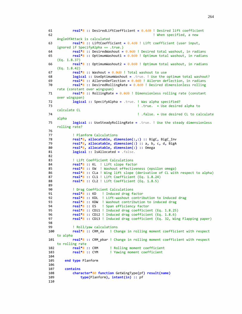
264

61 real*8 :: DesiredLiftCoefficient = 0.4d0 ! Desired lift coefficient 62 ! When specified, a new

AngleOfAttack is calculated 63 real*8 :: LiftCoefficient = 0.4d0 ! Lift coefficient (user input,

ignored if SpecifyAlpha == .true.) 64 real*8 :: DesiredWashout = 0.0d0 ! Desired total washout, in radians 65 real*8 :: OptimumWashout1 = 0.0d0 ! Optimum total washout, in radians

(Eq. 1.8.37) 66 real*8 :: OptimumWashout2 = 0.0d0 ! Optimum total washout, in radians

(Eq. 1.8.42) 67 real*8 :: Washout = 0.0d0 ! Total washout to use 68 logical :: UseOptimumWashout = .true. ! Use the optimum total washout? 69 real*8 :: AileronDeflection = 0.0d0 ! Aileron deflection, in radians 70 real*8 :: DesiredRollingRate = 0.0d0 ! Desired dimensionless rolling

rate (constant over wingspan) 71 real*8 :: RollingRate = 0.0d0 ! Dimensionless rolling rate (constant

over wingspan) 72 logical :: SpecifyAlpha = .true. ! Was alpha specified? 73 ! .true. = Use desired alpha to

calculate CL 74 ! .false. = Use desired CL to calculate

alpha 75 logical :: UseSteadyRollingRate = .true. ! Use the steady dimensionless

rolling rate? 76 77 ! Planform Calculations 78 real*8, allocatable, dimension(:,:) :: BigC, BigC_Inv 79 real*8, allocatable, dimension(:) :: a, b, c, d, BigA 80 real*8, allocatable, dimension(:) :: Omega 81 logical :: IsAllocated = .false. 82 83 ! Lift Coefficient Calculations 84 real*8 :: KL ! Lift slope factor 85 real*8 :: EW ! Washout effectiveness (epsilon omega) 86 real*8 :: CLa ! Wing lift slope (derivative of CL with respect to alpha) 87 real*8 :: CL1 ! Lift Coefficient (Eq. 1.8.24) 88 real*8 :: CL2 ! Lift Coefficient (Eq. 1.8.5) 89 90 ! Drag Coefficient Calculations 91 real*8 :: KD ! Induced drag factor 92 real*8 :: KDL ! Lift-washout contribution to induced drag 93 real*8 :: KDW ! Washout contribution to induced drag 94 real*8 :: ES ! Span efficiency factor 95 real*8 :: CDi1 ! Induced drag coefficient (Eq. 1.8.25) 96 real*8 :: CDi2 ! Induced drag coefficient (Eq. 1.8.6) 97 real*8 :: CDi3 ! Induced drag coefficient (Eq. 32, Wing Flapping paper) 98 99 ! Roll/yaw calculations 100 real*8 :: CRM_da ! Change in rolling moment coefficient with respect

to alpha 101 real*8 :: CRM_pbar ! Change in rolling moment coefficient with respect

to rolling rate 102 real*8 :: CRM ! Rolling moment coefficient 103 real*8 :: CYM ! Yawing moment coefficient 104 105 end type Planform 106 107 contains 108 character*80 function GetWingType(pf) result(name) 109 type(Planform), intent(in) :: pf 110

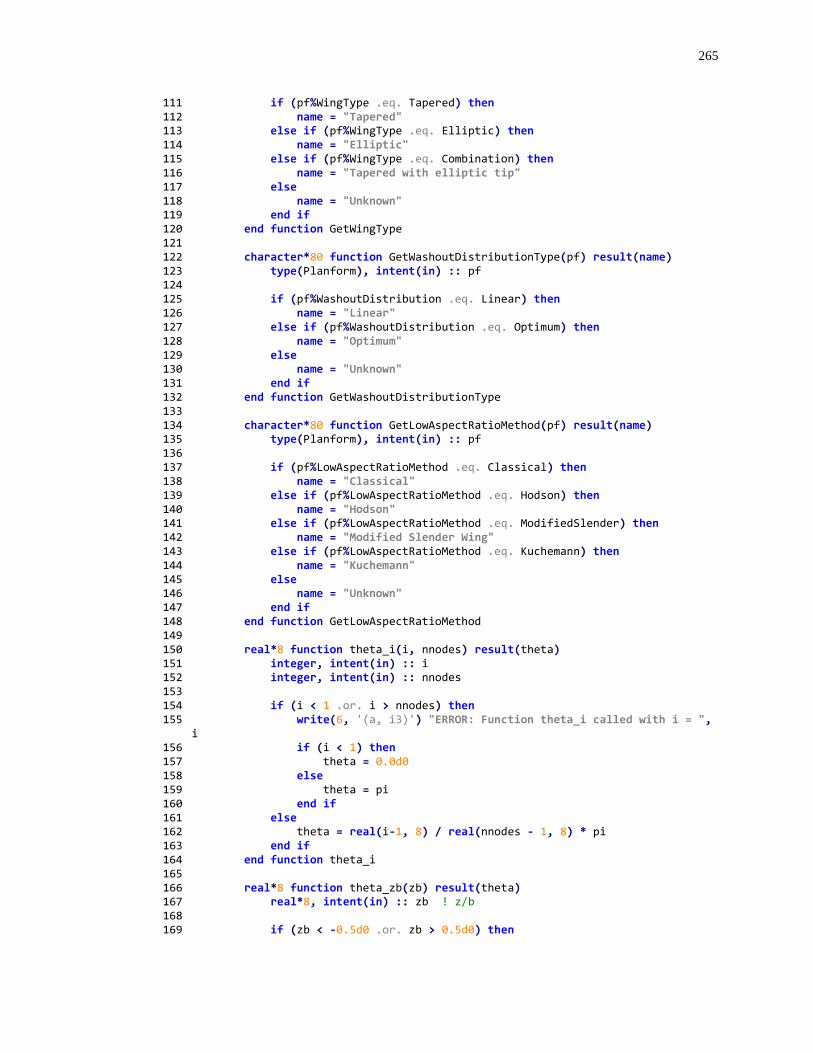
265

111 if (pf%WingType .eq. Tapered) then 112 name = "Tapered" 113 else if (pf%WingType .eq. Elliptic) then 114 name = "Elliptic" 115 else if (pf%WingType .eq. Combination) then 116 name = "Tapered with elliptic tip" 117 else 118 name = "Unknown" 119 end if 120 end function GetWingType 121 122 character*80 function GetWashoutDistributionType(pf) result(name) 123 type(Planform), intent(in) :: pf 124 125 if (pf%WashoutDistribution .eq. Linear) then 126 name = "Linear" 127 else if (pf%WashoutDistribution .eq. Optimum) then 128 name = "Optimum" 129 else 130 name = "Unknown" 131 end if 132 end function GetWashoutDistributionType 133 134 character*80 function GetLowAspectRatioMethod(pf) result(name) 135 type(Planform), intent(in) :: pf 136 137 if (pf%LowAspectRatioMethod .eq. Classical) then 138 name = "Classical" 139 else if (pf%LowAspectRatioMethod .eq. Hodson) then 140 name = "Hodson" 141 else if (pf%LowAspectRatioMethod .eq. ModifiedSlender) then 142 name = "Modified Slender Wing" 143 else if (pf%LowAspectRatioMethod .eq. Kuchemann) then 144 name = "Kuchemann" 145 else 146 name = "Unknown" 147 end if 148 end function GetLowAspectRatioMethod 149 150 real*8 function theta_i(i, nnodes) result(theta) 151 integer, intent(in) :: i 152 integer, intent(in) :: nnodes 153 154 if (i < 1 .or. i > nnodes) then 155 write(6, '(a, i3)') "ERROR: Function theta_i called with i = ",

i 156 if (i < 1) then 157 theta = 0.0d0 158 else 159 theta = pi 160 end if 161 else 162 theta = real(i-1, 8) / real(nnodes - 1, 8) * pi 163 end if 164 end function theta_i 165 166 real*8 function theta_zb(zb) result(theta) 167 real*8, intent(in) :: zb ! z/b 168 169 if (zb < -0.5d0 .or. zb > 0.5d0) then

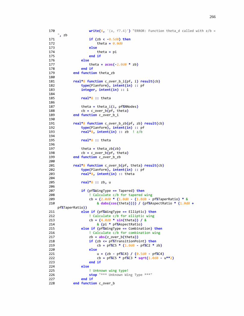
266

170 write(6, '(a, f7.4)') "ERROR: Function theta_d called with z/b = ", zb

171 if (zb < -0.5d0) then 172 theta = 0.0d0 173 else 174 theta = pi 175 end if 176 else 177 theta = acos(-2.0d0 * zb) 178 end if 179 end function theta_zb 180 181 real*8 function c_over_b_i(pf, i) result(cb) 182 type(Planform), intent(in) :: pf 183 integer, intent(in) :: i 184 185 real*8 :: theta 186 187 theta = theta_i(i, pf%NNodes) 188 cb = c_over_b(pf, theta) 189 end function c_over_b_i 190 191 real*8 function c_over_b_zb(pf, zb) result(cb) 192 type(Planform), intent(in) :: pf 193 real*8, intent(in) :: zb ! z/b 194 195 real*8 :: theta 196 197 theta = theta_zb(zb) 198 cb = c_over_b(pf, theta) 199 end function c_over_b_zb 200 201 real*8 function c_over_b(pf, theta) result(cb) 202 type(Planform), intent(in) :: pf 203 real*8, intent(in) :: theta 204 205 real*8 :: zb, u 206 207 if (pf%WingType == Tapered) then 208 ! Calculate c/b for tapered wing 209 cb = (2.0d0 * (1.0d0 - (1.0d0 - pf%TaperRatio) * & 210 & dabs(cos(theta)))) / (pf%AspectRatio * (1.0d0 +

pf%TaperRatio)) 211 else if (pf%WingType == Elliptic) then 212 ! Calculate c/b for elliptic wing 213 cb = (4.0d0 * sin(theta)) / & 214 & (pi * pf%AspectRatio) 215 else if (pf%WingType == Combination) then 216 ! Calculate c/b for combination wing 217 zb = abs(z_over_b(theta)) 218 if (zb <= pf%TransitionPoint) then 219 cb = pf%C5 * (1.0d0 - pf%C2 * zb) 220 else 221 u = (zb - pf%C4) / (0.5d0 - pf%C4) 222 cb = pf%C5 * pf%C3 * sqrt(1.0d0 - u**2) 223 end if 224 else 225 ! Unknown wing type! 226 stop "*** Unknown Wing Type ***" 227 end if 228 end function c_over_b

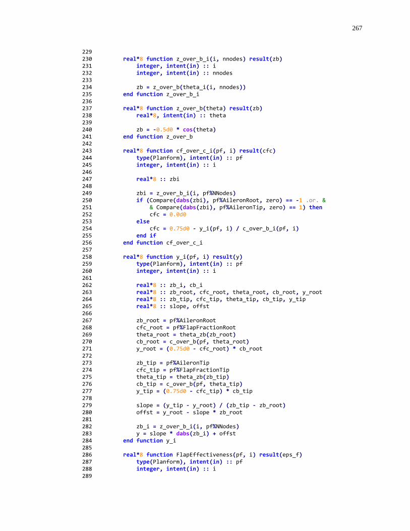
267

229 230 real*8 function z_over_b_i(i, nnodes) result(zb) 231 integer, intent(in) :: i 232 integer, intent(in) :: nnodes 233 234 zb = z_over_b(theta_i(i, nnodes)) 235 end function z_over_b_i 236 237 real*8 function z_over_b(theta) result(zb) 238 real*8, intent(in) :: theta 239 240 zb = -0.5d0 * cos(theta) 241 end function z_over_b 242 243 real*8 function cf_over_c_i(pf, i) result(cfc) 244 type(Planform), intent(in) :: pf 245 integer, intent(in) :: i 246 247 real*8 :: zbi 248 249 zbi = z_over_b_i(i, pf%NNodes) 250 if (Compare(dabs(zbi), pf%AileronRoot, zero) == -1 .or. & 251 & Compare(dabs(zbi), pf%AileronTip, zero) == 1) then 252 cfc = 0.0d0 253 else 254 cfc = 0.75d0 - y_i(pf, i) / c_over_b_i(pf, i) 255 end if 256 end function cf_over_c_i 257 258 real*8 function y_i(pf, i) result(y) 259 type(Planform), intent(in) :: pf 260 integer, intent(in) :: i 261 262 real*8 :: zb_i, cb_i 263 real*8 :: zb_root, cfc_root, theta_root, cb_root, y_root 264 real*8 :: zb_tip, cfc_tip, theta_tip, cb_tip, y_tip 265 real*8 :: slope, offst 266 267 zb_root = pf%AileronRoot 268 cfc_root = pf%FlapFractionRoot 269 theta_root = theta_zb(zb_root) 270 cb_root = c_over_b(pf, theta_root) 271 y_root = (0.75d0 - cfc_root) * cb_root 272 273 zb_tip = pf%AileronTip 274 cfc_tip = pf%FlapFractionTip 275 theta_tip = theta_zb(zb_tip) 276 cb_tip = c_over_b(pf, theta_tip) 277 y_tip = (0.75d0 - cfc_tip) * cb_tip 278 279 slope = (y_tip - y_root) / (zb_tip - zb_root) 280 offst = y_root - slope * zb_root 281 282 zb_i = z_over_b_i(i, pf%NNodes) 283 y = slope * dabs(zb_i) + offst 284 end function y_i 285 286 real*8 function FlapEffectiveness(pf, i) result(eps_f) 287 type(Planform), intent(in) :: pf 288 integer, intent(in) :: i 289

268

290 real*8 :: theta_f, eps_fi 291 292 theta_f = acos(2.0d0 * cf_over_c_i(pf, i) - 1.0d0) 293 eps_fi = 1.0d0 - (theta_f - sin(theta_f)) / pi 294 eps_f = eps_fi * pf%HingeEfficiency * pf%DeflectionEfficiency 295 end function FlapEffectiveness 296 297 subroutine DeallocateArrays(pf) 298 type(Planform), intent(inout) :: pf 299 300 if (pf%IsAllocated) then 301 deallocate(pf%BigC) 302 deallocate(pf%BigC_Inv) 303 deallocate(pf%a) 304 deallocate(pf%b) 305 deallocate(pf%c) 306 deallocate(pf%d) 307 deallocate(pf%BigA) 308 deallocate(pf%Omega) 309 310 pf%IsAllocated = .false. 311 end if 312 end subroutine DeallocateArrays 313 314 subroutine AllocateArrays(pf) 315 type(Planform), intent(inout) :: pf 316 317 if (pf%IsAllocated) call DeallocateArrays(pf) 318 319 allocate(pf%BigC(pf%NNodes, pf%NNodes)) 320 allocate(pf%BigC_Inv(pf%NNodes, pf%NNodes)) 321 allocate(pf%a(pf%NNodes)) 322 allocate(pf%b(pf%NNodes)) 323 allocate(pf%c(pf%NNodes)) 324 allocate(pf%d(pf%NNodes)) 325 allocate(pf%BigA(pf%NNodes)) 326 allocate(pf%Omega(pf%NNodes)) 327 pf%IsAllocated = .true. 328 end subroutine AllocateArrays 329 330 end module class_Planform

K.4 Module of Setter Functions (liftinglinesetters.f90)

1 module LiftingLineSetters 2 use class_Planform 3 implicit none 4 5 contains 6 subroutine InitPlanform(pf) 7 type(Planform), intent(inout) :: pf 8 9 call SetParallelHingeLine(pf) 10 end subroutine InitPlanform 11 12 ! Planform Parameters 13 subroutine SetWingType(pf, wingType) 14 type(Planform), intent(inout) :: pf 15 integer, intent(in) :: wingType 16

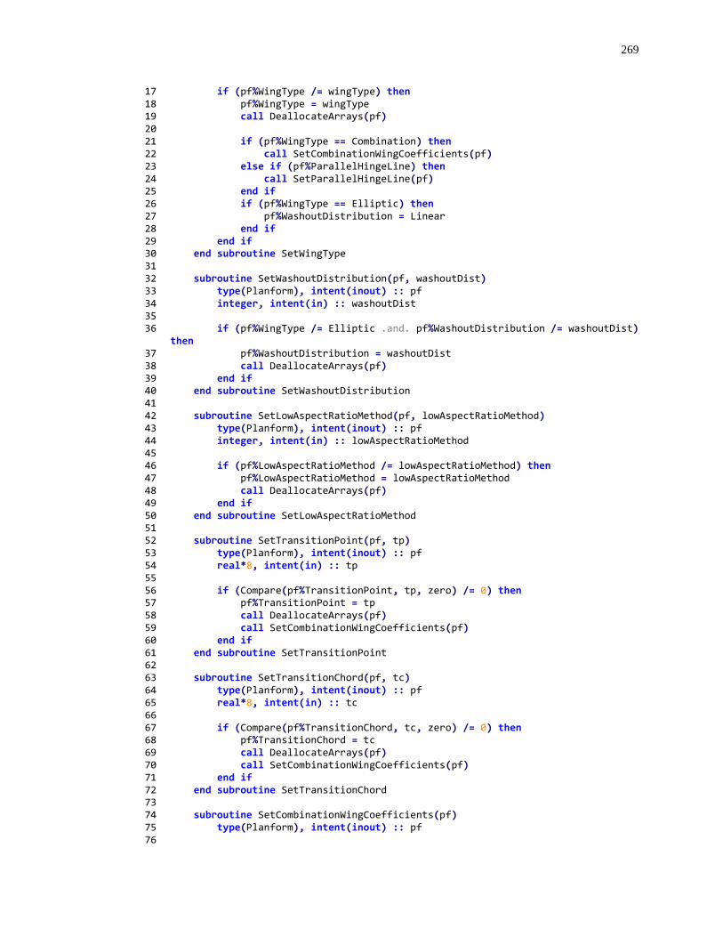
269

17 if (pf%WingType /= wingType) then 18 pf%WingType = wingType 19 call DeallocateArrays(pf) 20 21 if (pf%WingType == Combination) then 22 call SetCombinationWingCoefficients(pf) 23 else if (pf%ParallelHingeLine) then 24 call SetParallelHingeLine(pf) 25 end if 26 if (pf%WingType == Elliptic) then 27 pf%WashoutDistribution = Linear 28 end if 29 end if 30 end subroutine SetWingType 31 32 subroutine SetWashoutDistribution(pf, washoutDist) 33 type(Planform), intent(inout) :: pf 34 integer, intent(in) :: washoutDist 35 36 if (pf%WingType /= Elliptic .and. pf%WashoutDistribution /= washoutDist)

then 37 pf%WashoutDistribution = washoutDist 38 call DeallocateArrays(pf) 39 end if 40 end subroutine SetWashoutDistribution 41 42 subroutine SetLowAspectRatioMethod(pf, lowAspectRatioMethod) 43 type(Planform), intent(inout) :: pf 44 integer, intent(in) :: lowAspectRatioMethod 45 46 if (pf%LowAspectRatioMethod /= lowAspectRatioMethod) then 47 pf%LowAspectRatioMethod = lowAspectRatioMethod 48 call DeallocateArrays(pf) 49 end if 50 end subroutine SetLowAspectRatioMethod 51 52 subroutine SetTransitionPoint(pf, tp) 53 type(Planform), intent(inout) :: pf 54 real*8, intent(in) :: tp 55 56 if (Compare(pf%TransitionPoint, tp, zero) /= 0) then 57 pf%TransitionPoint = tp 58 call DeallocateArrays(pf) 59 call SetCombinationWingCoefficients(pf) 60 end if 61 end subroutine SetTransitionPoint 62 63 subroutine SetTransitionChord(pf, tc) 64 type(Planform), intent(inout) :: pf 65 real*8, intent(in) :: tc 66 67 if (Compare(pf%TransitionChord, tc, zero) /= 0) then 68 pf%TransitionChord = tc 69 call DeallocateArrays(pf) 70 call SetCombinationWingCoefficients(pf) 71 end if 72 end subroutine SetTransitionChord 73 74 subroutine SetCombinationWingCoefficients(pf) 75 type(Planform), intent(inout) :: pf 76

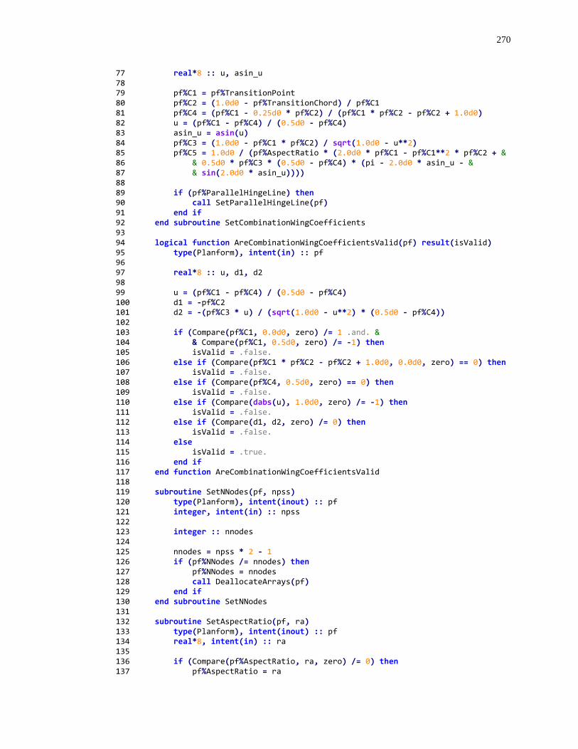
270

77 real*8 :: u, asin_u 78 79 pf%C1 = pf%TransitionPoint 80 pf%C2 = (1.0d0 - pf%TransitionChord) / pf%C1 81 pf%C4 = (pf%C1 - 0.25d0 * pf%C2) / (pf%C1 * pf%C2 - pf%C2 + 1.0d0) 82 u = (pf%C1 - pf%C4) / (0.5d0 - pf%C4) 83 asin_u = asin(u) 84 pf%C3 = (1.0d0 - pf%C1 * pf%C2) / sqrt(1.0d0 - u**2) 85 pf%C5 = 1.0d0 / (pf%AspectRatio * (2.0d0 * pf%C1 - pf%C1**2 * pf%C2 + & 86 & 0.5d0 * pf%C3 * (0.5d0 - pf%C4) * (pi - 2.0d0 * asin_u - & 87 & sin(2.0d0 * asin_u)))) 88 89 if (pf%ParallelHingeLine) then 90 call SetParallelHingeLine(pf) 91 end if 92 end subroutine SetCombinationWingCoefficients 93 94 logical function AreCombinationWingCoefficientsValid(pf) result(isValid) 95 type(Planform), intent(in) :: pf 96 97 real*8 :: u, d1, d2 98 99 u = (pf%C1 - pf%C4) / (0.5d0 - pf%C4) 100 d1 = -pf%C2 101 d2 = -(pf%C3 * u) / (sqrt(1.0d0 - u**2) * (0.5d0 - pf%C4)) 102 103 if (Compare(pf%C1, 0.0d0, zero) /= 1 .and. & 104 & Compare(pf%C1, 0.5d0, zero) /= -1) then 105 isValid = .false. 106 else if (Compare(pf%C1 * pf%C2 - pf%C2 + 1.0d0, 0.0d0, zero) == 0) then 107 isValid = .false. 108 else if (Compare(pf%C4, 0.5d0, zero) == 0) then 109 isValid = .false. 110 else if (Compare(dabs(u), 1.0d0, zero) /= -1) then 111 isValid = .false. 112 else if (Compare(d1, d2, zero) /= 0) then 113 isValid = .false. 114 else 115 isValid = .true. 116 end if 117 end function AreCombinationWingCoefficientsValid 118 119 subroutine SetNNodes(pf, npss) 120 type(Planform), intent(inout) :: pf 121 integer, intent(in) :: npss 122 123 integer :: nnodes 124 125 nnodes = npss * 2 - 1 126 if (pf%NNodes /= nnodes) then 127 pf%NNodes = nnodes 128 call DeallocateArrays(pf) 129 end if 130 end subroutine SetNNodes 131 132 subroutine SetAspectRatio(pf, ra) 133 type(Planform), intent(inout) :: pf 134 real*8, intent(in) :: ra 135 136 if (Compare(pf%AspectRatio, ra, zero) /= 0) then 137 pf%AspectRatio = ra

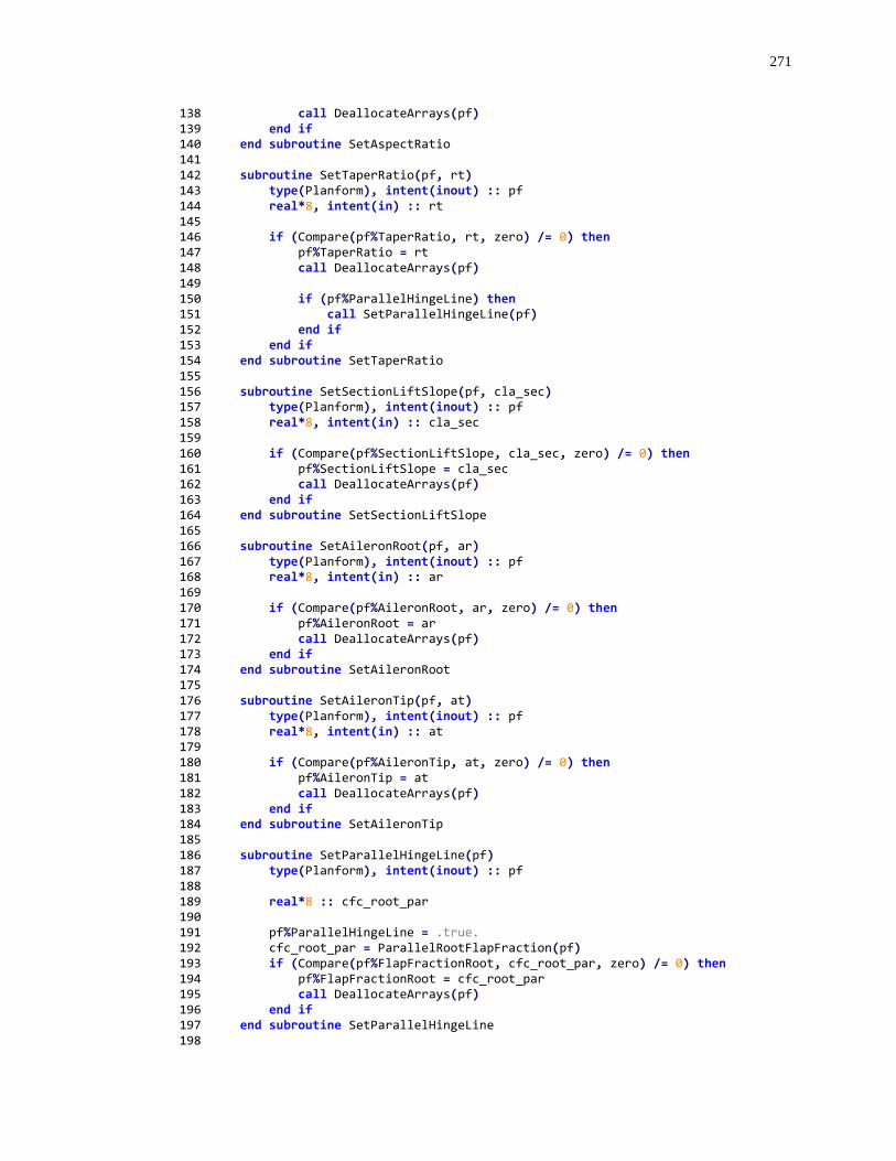
271

138 call DeallocateArrays(pf) 139 end if 140 end subroutine SetAspectRatio 141 142 subroutine SetTaperRatio(pf, rt) 143 type(Planform), intent(inout) :: pf 144 real*8, intent(in) :: rt 145 146 if (Compare(pf%TaperRatio, rt, zero) /= 0) then 147 pf%TaperRatio = rt 148 call DeallocateArrays(pf) 149 150 if (pf%ParallelHingeLine) then 151 call SetParallelHingeLine(pf) 152 end if 153 end if 154 end subroutine SetTaperRatio 155 156 subroutine SetSectionLiftSlope(pf, cla_sec) 157 type(Planform), intent(inout) :: pf 158 real*8, intent(in) :: cla_sec 159 160 if (Compare(pf%SectionLiftSlope, cla_sec, zero) /= 0) then 161 pf%SectionLiftSlope = cla_sec 162 call DeallocateArrays(pf) 163 end if 164 end subroutine SetSectionLiftSlope 165 166 subroutine SetAileronRoot(pf, ar) 167 type(Planform), intent(inout) :: pf 168 real*8, intent(in) :: ar 169 170 if (Compare(pf%AileronRoot, ar, zero) /= 0) then 171 pf%AileronRoot = ar 172 call DeallocateArrays(pf) 173 end if 174 end subroutine SetAileronRoot 175 176 subroutine SetAileronTip(pf, at) 177 type(Planform), intent(inout) :: pf 178 real*8, intent(in) :: at 179 180 if (Compare(pf%AileronTip, at, zero) /= 0) then 181 pf%AileronTip = at 182 call DeallocateArrays(pf) 183 end if 184 end subroutine SetAileronTip 185 186 subroutine SetParallelHingeLine(pf) 187 type(Planform), intent(inout) :: pf 188 189 real*8 :: cfc_root_par 190 191 pf%ParallelHingeLine = .true. 192 cfc_root_par = ParallelRootFlapFraction(pf) 193 if (Compare(pf%FlapFractionRoot, cfc_root_par, zero) /= 0) then 194 pf%FlapFractionRoot = cfc_root_par 195 call DeallocateArrays(pf) 196 end if 197 end subroutine SetParallelHingeLine 198

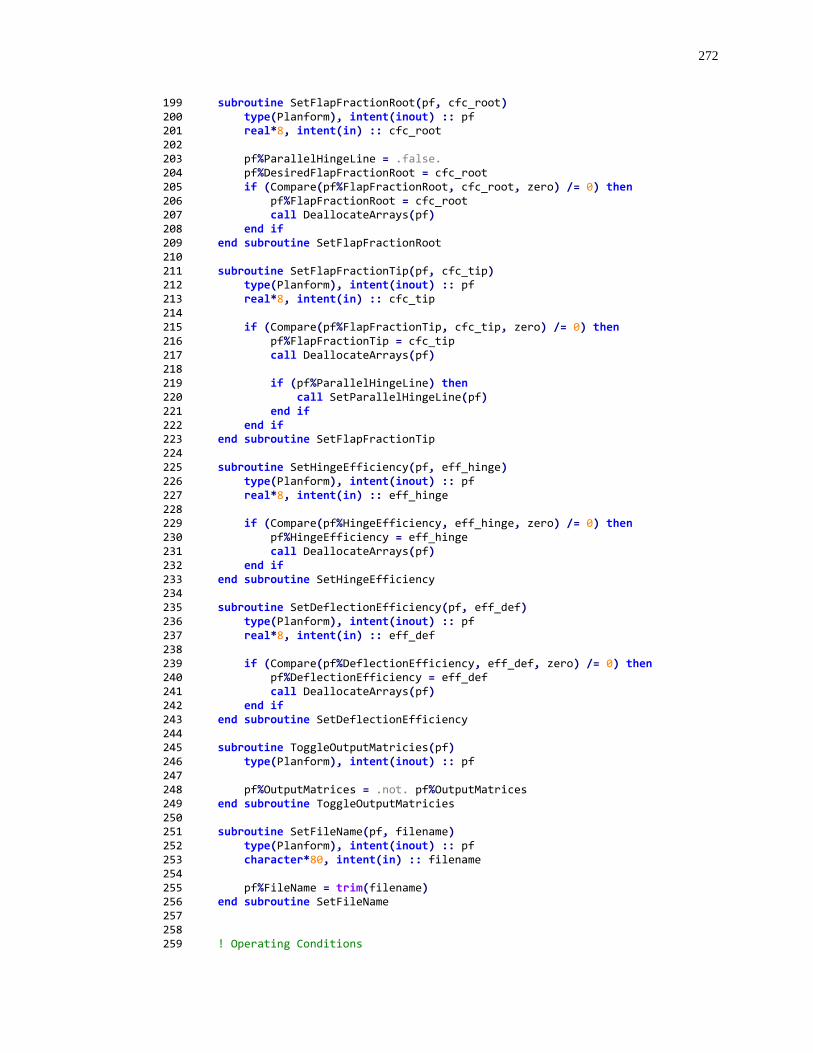
272

199 subroutine SetFlapFractionRoot(pf, cfc_root) 200 type(Planform), intent(inout) :: pf 201 real*8, intent(in) :: cfc_root 202 203 pf%ParallelHingeLine = .false. 204 pf%DesiredFlapFractionRoot = cfc_root 205 if (Compare(pf%FlapFractionRoot, cfc_root, zero) /= 0) then 206 pf%FlapFractionRoot = cfc_root 207 call DeallocateArrays(pf) 208 end if 209 end subroutine SetFlapFractionRoot 210 211 subroutine SetFlapFractionTip(pf, cfc_tip) 212 type(Planform), intent(inout) :: pf 213 real*8, intent(in) :: cfc_tip 214 215 if (Compare(pf%FlapFractionTip, cfc_tip, zero) /= 0) then 216 pf%FlapFractionTip = cfc_tip 217 call DeallocateArrays(pf) 218 219 if (pf%ParallelHingeLine) then 220 call SetParallelHingeLine(pf) 221 end if 222 end if 223 end subroutine SetFlapFractionTip 224 225 subroutine SetHingeEfficiency(pf, eff_hinge) 226 type(Planform), intent(inout) :: pf 227 real*8, intent(in) :: eff_hinge 228 229 if (Compare(pf%HingeEfficiency, eff_hinge, zero) /= 0) then 230 pf%HingeEfficiency = eff_hinge 231 call DeallocateArrays(pf) 232 end if 233 end subroutine SetHingeEfficiency 234 235 subroutine SetDeflectionEfficiency(pf, eff_def) 236 type(Planform), intent(inout) :: pf 237 real*8, intent(in) :: eff_def 238 239 if (Compare(pf%DeflectionEfficiency, eff_def, zero) /= 0) then 240 pf%DeflectionEfficiency = eff_def 241 call DeallocateArrays(pf) 242 end if 243 end subroutine SetDeflectionEfficiency 244 245 subroutine ToggleOutputMatricies(pf) 246 type(Planform), intent(inout) :: pf 247 248 pf%OutputMatrices = .not. pf%OutputMatrices 249 end subroutine ToggleOutputMatricies 250 251 subroutine SetFileName(pf, filename) 252 type(Planform), intent(inout) :: pf 253 character*80, intent(in) :: filename 254 255 pf%FileName = trim(filename) 256 end subroutine SetFileName 257 258 259 ! Operating Conditions

273

260 subroutine SetAngleOfAttack(pf, alpha) 261 type(Planform), intent(inout) :: pf 262 real*8, intent(in) :: alpha 263 264 pf%SpecifyAlpha = .true. 265 pf%DesiredAngleOfAttack = alpha * pi / 180.0d0 266 pf%AngleOfAttack = pf%DesiredAngleOfAttack 267 if (pf%UseOptimumWashout) then 268 call SetOptimumWashout(pf) 269 end if 270 pf%LiftCoefficient = CL1(pf%CLa, pf%AngleOfAttack, pf%EW, pf%Washout) 271 end subroutine SetAngleOfAttack 272 273 subroutine SetLiftCoefficient(pf, cl) 274 type(Planform), intent(inout) :: pf 275 real*8, intent(in) :: cl 276 277 pf%SpecifyAlpha = .false. 278 pf%DesiredLiftCoefficient = cl 279 pf%LiftCoefficient = pf%DesiredLiftCoefficient 280 if (pf%UseOptimumWashout) then 281 call SetOptimumWashout(pf) 282 end if 283 pf%AngleOfAttack = RootAlpha(pf%CLa, pf%LiftCoefficient, pf%EW,

pf%Washout) 284 end subroutine SetLiftCoefficient 285 286 subroutine SetAileronDeflection(pf, da) 287 type(Planform), intent(inout) :: pf 288 real*8, intent(in) :: da 289 290 pf%AileronDeflection = da * pi / 180.0d0 291 end subroutine SetAileronDeflection 292 293 subroutine SetWashout(pf, washout) 294 type(Planform), intent(inout) :: pf 295 real*8, intent(in) :: washout 296 297 pf%DesiredWashout = washout * pi / 180.0d0 298 pf%Washout = pf%DesiredWashout 299 pf%UseOptimumWashout = .false. 300 if (pf%SpecifyAlpha) then 301 pf%LiftCoefficient = CL1(pf%CLa, pf%AngleOfAttack, pf%EW,

pf%Washout) 302 else 303 pf%AngleOfAttack = RootAlpha(pf%CLa, pf%LiftCoefficient, pf%EW,

pf%Washout) 304 end if 305 end subroutine SetWashout 306 307 subroutine SetOptimumWashout(pf) 308 type(Planform), intent(inout) :: pf 309 310 logical :: cont 311 integer :: i 312 real*8 :: oldCL, newCL, resCL 313 real*8 :: oldOmega, newOmega, resOmega 314 315 if (pf%SpecifyAlpha) then 316 oldCL = pf%LiftCoefficient 317 oldOmega = pf%Washout

274

318 cont = .true. 319 i = 0 320 do while (i < 100 .or. (cont .and. i < 1000)) 321 i = i + 1 322 newOmega = OptimumWashout1(pf%KDL, oldCL, pf%KDW, pf%CLa) 323 newCL = CL1(pf%CLa, pf%AngleOfAttack, pf%EW, newOmega) 324 325 resCL = Residual(oldCL, newCL) 326 resOmega = Residual(oldOmega, newOmega) 327 328 cont = (Compare(resCL, 0.0d0, zero) /= 0 .or. Compare(resOmega,

0.0d0, zero) /= 0) 329 oldOmega = newOmega 330 oldCL = newCL 331 end do 332 333 if (i >= 1000) then 334 stop "*** Max number of convergence iterations reached! ***" 335 else 336 pf%LiftCoefficient = newCL 337 pf%OptimumWashout1 = newOmega 338 end if 339 end if 340 341 pf%OptimumWashout1 = OptimumWashout1(pf%KDL, pf%LiftCoefficient, & 342 & pf%KDW, pf%CLa) 343 if (pf%WashoutDistribution == Optimum) then 344 pf%OptimumWashout2 = OptimumWashout2(pf, pf%LiftCoefficient, & 345 pf%AspectRatio, pf%SectionLiftSlope) 346 end if 347 pf%Washout = pf%OptimumWashout1 348 pf%UseOptimumWashout = .true. 349 350 if (.not. pf%SpecifyAlpha) then 351 pf%AngleOfAttack = RootAlpha(pf%CLa, pf%LiftCoefficient, pf%EW,

pf%Washout) 352 end if 353 end subroutine SetOptimumWashout 354 355 subroutine SetRollingRate(pf, rollingrate) 356 type(Planform), intent(inout) :: pf 357 real*8, intent(in) :: rollingrate 358 359 pf%DesiredRollingRate = rollingrate 360 pf%RollingRate = rollingrate 361 pf%UseSteadyRollingRate = .false. 362 end subroutine 363 364 subroutine SetSteadyRollingRate(pf) 365 type(Planform), intent(inout) :: pf 366 367 real*8 :: steady_pbar 368 369 pf%RollingRate = SteadyRollingRate(pf) 370 pf%UseSteadyRollingRate = .true. 371 end subroutine SetSteadyRollingRate 372 373 real*8 function ParallelRootFlapFraction(pf) result(cfc_root_par) 374 type(Planform), intent(in) :: pf 375 376 real*8 :: cb_root, cfc_root

275

377 real*8 :: cb_tip, cfc_tip 378 379 cb_tip = c_over_b_zb(pf, pf%AileronTip) 380 cfc_tip = pf%FlapFractionTip 381 cb_root = c_over_b_zb(pf, pf%AileronRoot) 382 cfc_root_par = 0.75d0 - cb_tip / cb_root * (0.75d0 - cfc_tip) 383 end function ParallelRootFlapFraction 384 385 real*8 function RootAlpha(cla, cl, ew, omega) result(alpha) 386 real*8, intent(in) :: cla 387 real*8, intent(in) :: cl 388 real*8, intent(in) :: ew 389 real*8, intent(in) :: omega 390 391 alpha = cl / cla + ew * omega 392 end function RootAlpha 393 394 real*8 function SteadyRollingRate(pf) result(pbar_steady) 395 type(Planform), intent(in) :: pf 396 397 ! Calculate steady dimensionless rolling rate (Eq. 1.8.59) 398 pbar_steady = -pf%CRM_da / pf%CRM_pbar * pf%AileronDeflection 399 end function SteadyRollingRate 400 401 real*8 function OptimumWashout1(kdl, cl, kdw, cla) result(ow1) 402 real*8, intent(in) :: kdl 403 real*8, intent(in) :: cl 404 real*8, intent(in) :: kdw 405 real*8, intent(in) :: cla 406 407 ow1 = (kdl * cl) / (2.0d0 * kdw * cla) 408 end function OptimumWashout1 409 410 real*8 function OptimumWashout2(pf, cl, ra, ls) result(ow2) 411 type(Planform), intent(in) :: pf 412 real*8, intent(in) :: cl 413 real*8, intent(in) :: ra 414 real*8, intent(in) :: ls 415 416 ow2 = (4.0d0 * cl) / (pi * ra * ls * c_over_b(pf, pi / 2.0d0)) 417 end function OptimumWashout2 418 419 real*8 function CL1(cla, alpha, ew, w) result(cl) 420 real*8, intent(in) :: cla 421 real*8, intent(in) :: alpha 422 real*8, intent(in) :: ew 423 real*8, intent(in) :: w 424 425 cl = cla * (alpha - ew * w) ! Eq. 1.8.24 426 end function CL1 427 428 real*8 function CL2(ra, bigA1) result(cl) 429 real*8, intent(in) :: ra 430 real*8, intent(in) :: bigA1 431 432 cl = pi * ra * bigA1 ! Eq. 1.8.5 433 end function CL2 434 435 real*8 function CDi1(pf) result(cdi) 436 type(Planform), intent(in) :: pf 437

276

438 real*8 :: n, a0, A, r1, r2 439 440 a0 = pf%SectionLiftSlope 441 A = pf%AspectRatio 442 443 ! Set the low aspect ratio method parameters 444 if (pf%LowAspectRatioMethod == Hodson) then 445 r1 = a0 446 r2 = A * (pi - atan((2.0 * a0) / (pi * A))) 447 else if (pf%LowAspectRatioMethod == ModifiedSlender) then 448 r1 = a0 449 r2 = 0.5 * pi * A 450 else if (pf%LowAspectRatioMethod == Kuchemann) then 451 n = 1.0 - 0.5 * (1.0 + (a0 / (pi * A))**2)**(-0.25) 452 r1 = 2 * n * a0 / (1.0 - pi * n / tan(pi * n)) 453 r2 = pi * A / (2.0 * n) 454 else ! Assume Classical 455 r1 = a0 456 r2 = pi * A 457 end if 458 459 cdi = (pf%CL1**2 * (1.0d0 + pf%KD) - pf%KDL * pf%CL1 * pf%CLa * & 460 & pf%Washout + pf%KDW * (pf%CLa * pf%Washout)**2) / (pi * A) & 461 & * (r1 / r2) * (pi * A) / a0 ! Low-RA correction 462 end function CDi1 463 464 real*8 function CDi2(pf) result(cdi) 465 type(Planform), intent(in) :: pf 466 467 integer :: i 468 469 cdi = 0.0d0 470 do i = 1, pf%NNodes 471 cdi = cdi + real(i, 8) * pf%BigA(i)**2 472 end do 473 cdi = cdi * pi * pf%AspectRatio 474 end function CDi2 475 476 real*8 function CDi3(pf) result(cdi) 477 type(Planform), intent(in) :: pf 478 479 integer :: i 480 real*8 :: ri 481 482 cdi = 0.0d0 483 do i = 1, pf%NNodes 484 ri = real(i, 8) 485 cdi = cdi + ri * pf%BigA(i)**2 486 end do 487 cdi = (cdi - 0.5d0 * pf%RollingRate * pf%BigA(2)) * pi * pf%AspectRatio 488 end function CDi3 489 490 end module LiftingLineSetters

K.5 Solver Module (liftinglinesolver.f90)

1 module LiftingLineSolver 2 use class_Planform 3 use LiftingLineSetters 4 use LiftingLineOutput

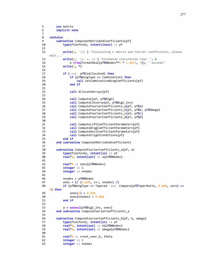
277

5 use matrix 6 implicit none 7 8 contains 9 subroutine ComputeCMatrixAndCoefficients(pf) 10 type(Planform), intent(inout) :: pf 11 12 write(6, '(a)') "Calculating C matrix and Fourier coefficients, please

wait..." 13 write(6, '(a, a, a)') "Estimated calculation time: ", & 14 & trim(FormatReal(pf%NNodes**2 * 1.0d-5, 3)), " seconds" 15 write(6, *) 16 17 if (.not. pf%IsAllocated) then 18 if (pf%WingType == Combination) then 19 call SetCombinationWingCoefficients(pf) 20 end if 21 22 call AllocateArrays(pf) 23 24 call ComputeC(pf, pf%BigC) 25 call ComputeCInverse(pf, pf%BigC_Inv) 26 call ComputeFourierCoefficients_a(pf, pf%a) 27 call ComputeFourierCoefficients_b(pf, pf%b, pf%Omega) 28 call ComputeFourierCoefficients_c(pf, pf%c) 29 call ComputeFourierCoefficients_d(pf, pf%d) 30 31 call ComputeLiftCoefficientParameters(pf) 32 call ComputeDragCoefficientParameters(pf) 33 call ComputeRollCoefficientParameters(pf) 34 call ComputeFlightConditions(pf) 35 end if 36 end subroutine ComputeCMatrixAndCoefficients 37 38 subroutine ComputeFourierCoefficients_a(pf, a) 39 type(Planform), intent(in) :: pf 40 real*8, intent(out) :: a(pf%NNodes) 41 42 real*8 :: ones(pf%NNodes) 43 integer :: i 44 integer :: nnodes 45 46 nnodes = pf%NNodes 47 ones = (/ (1.0d0, i=1, nnodes) /) 48 if (pf%WingType == Tapered .and. Compare(pf%TaperRatio, 0.0d0, zero) ==

0) then 49 ones(1) = 0.0d0 50 ones(nnodes) = 0.0d0 51 end if 52 53 a = matmul(pf%BigC_Inv, ones) 54 end subroutine ComputeFourierCoefficients_a 55 56 subroutine ComputeFourierCoefficients_b(pf, b, omega) 57 type(Planform), intent(in) :: pf 58 real*8, intent(out) :: b(pf%NNodes) 59 real*8, intent(out) :: omega(pf%NNodes) 60 61 real*8 :: croot_over_b, theta 62 integer :: i 63 integer :: nnodes

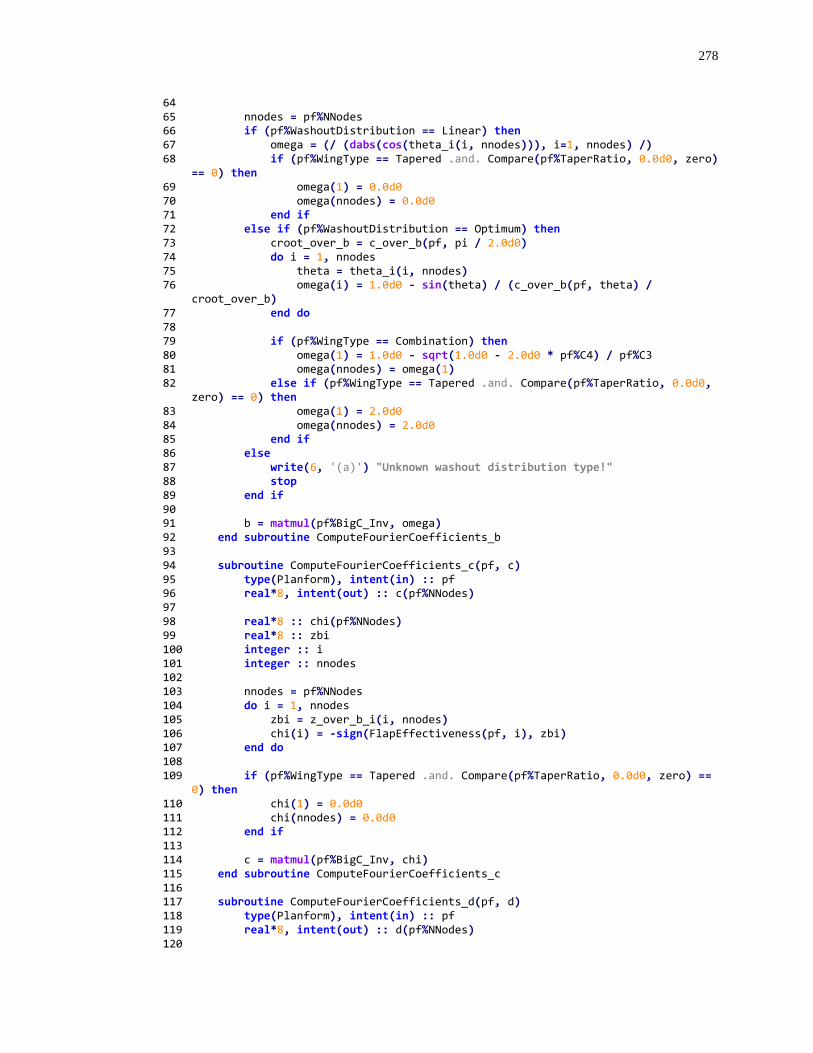
278

64 65 nnodes = pf%NNodes 66 if (pf%WashoutDistribution == Linear) then 67 omega = (/ (dabs(cos(theta_i(i, nnodes))), i=1, nnodes) /) 68 if (pf%WingType == Tapered .and. Compare(pf%TaperRatio, 0.0d0, zero)

== 0) then 69 omega(1) = 0.0d0 70 omega(nnodes) = 0.0d0 71 end if 72 else if (pf%WashoutDistribution == Optimum) then 73 croot_over_b = c_over_b(pf, pi / 2.0d0) 74 do i = 1, nnodes 75 theta = theta_i(i, nnodes) 76 omega(i) = 1.0d0 - sin(theta) / (c_over_b(pf, theta) /

croot_over_b) 77 end do 78 79 if (pf%WingType == Combination) then 80 omega(1) = 1.0d0 - sqrt(1.0d0 - 2.0d0 * pf%C4) / pf%C3 81 omega(nnodes) = omega(1) 82 else if (pf%WingType == Tapered .and. Compare(pf%TaperRatio, 0.0d0,

zero) == 0) then 83 omega(1) = 2.0d0 84 omega(nnodes) = 2.0d0 85 end if 86 else 87 write(6, '(a)') "Unknown washout distribution type!" 88 stop 89 end if 90 91 b = matmul(pf%BigC_Inv, omega) 92 end subroutine ComputeFourierCoefficients_b 93 94 subroutine ComputeFourierCoefficients_c(pf, c) 95 type(Planform), intent(in) :: pf 96 real*8, intent(out) :: c(pf%NNodes) 97 98 real*8 :: chi(pf%NNodes) 99 real*8 :: zbi 100 integer :: i 101 integer :: nnodes 102 103 nnodes = pf%NNodes 104 do i = 1, nnodes 105 zbi = z_over_b_i(i, nnodes) 106 chi(i) = -sign(FlapEffectiveness(pf, i), zbi) 107 end do 108 109 if (pf%WingType == Tapered .and. Compare(pf%TaperRatio, 0.0d0, zero) ==

0) then 110 chi(1) = 0.0d0 111 chi(nnodes) = 0.0d0 112 end if 113 114 c = matmul(pf%BigC_Inv, chi) 115 end subroutine ComputeFourierCoefficients_c 116 117 subroutine ComputeFourierCoefficients_d(pf, d) 118 type(Planform), intent(in) :: pf 119 real*8, intent(out) :: d(pf%NNodes) 120

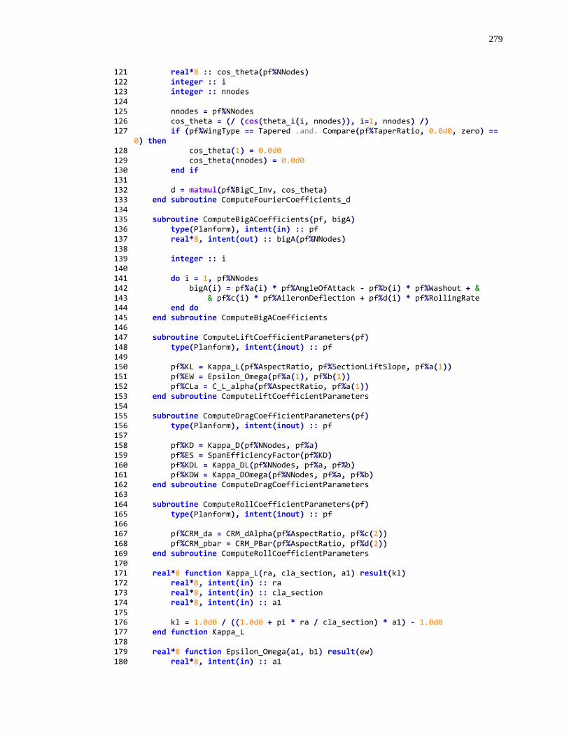
279

121 real*8 :: cos_theta(pf%NNodes) 122 integer :: i 123 integer :: nnodes 124 125 nnodes = pf%NNodes 126 cos_theta = (/ (cos(theta_i(i, nnodes)), i=1, nnodes) /) 127 if (pf%WingType == Tapered .and. Compare(pf%TaperRatio, 0.0d0, zero) ==

0) then 128 cos_theta(1) = 0.0d0 129 cos_theta(nnodes) = 0.0d0 130 end if 131 132 d = matmul(pf%BigC_Inv, cos_theta) 133 end subroutine ComputeFourierCoefficients_d 134 135 subroutine ComputeBigACoefficients(pf, bigA) 136 type(Planform), intent(in) :: pf 137 real*8, intent(out) :: bigA(pf%NNodes) 138 139 integer :: i 140 141 do i = 1, pf%NNodes 142 bigA(i) = pf%a(i) * pf%AngleOfAttack - pf%b(i) * pf%Washout + & 143 & pf%c(i) * pf%AileronDeflection + pf%d(i) * pf%RollingRate 144 end do 145 end subroutine ComputeBigACoefficients 146 147 subroutine ComputeLiftCoefficientParameters(pf) 148 type(Planform), intent(inout) :: pf 149 150 pf%KL = Kappa_L(pf%AspectRatio, pf%SectionLiftSlope, pf%a(1)) 151 pf%EW = Epsilon_Omega(pf%a(1), pf%b(1)) 152 pf%CLa = C_L_alpha(pf%AspectRatio, pf%a(1)) 153 end subroutine ComputeLiftCoefficientParameters 154 155 subroutine ComputeDragCoefficientParameters(pf) 156 type(Planform), intent(inout) :: pf 157 158 pf%KD = Kappa_D(pf%NNodes, pf%a) 159 pf%ES = SpanEfficiencyFactor(pf%KD) 160 pf%KDL = Kappa_DL(pf%NNodes, pf%a, pf%b) 161 pf%KDW = Kappa_DOmega(pf%NNodes, pf%a, pf%b) 162 end subroutine ComputeDragCoefficientParameters 163 164 subroutine ComputeRollCoefficientParameters(pf) 165 type(Planform), intent(inout) :: pf 166 167 pf%CRM_da = CRM_dAlpha(pf%AspectRatio, pf%c(2)) 168 pf%CRM_pbar = CRM_PBar(pf%AspectRatio, pf%d(2)) 169 end subroutine ComputeRollCoefficientParameters 170 171 real*8 function Kappa_L(ra, cla_section, a1) result(kl) 172 real*8, intent(in) :: ra 173 real*8, intent(in) :: cla_section 174 real*8, intent(in) :: a1 175 176 kl = 1.0d0 / ((1.0d0 + pi * ra / cla_section) * a1) - 1.0d0 177 end function Kappa_L 178 179 real*8 function Epsilon_Omega(a1, b1) result(ew) 180 real*8, intent(in) :: a1

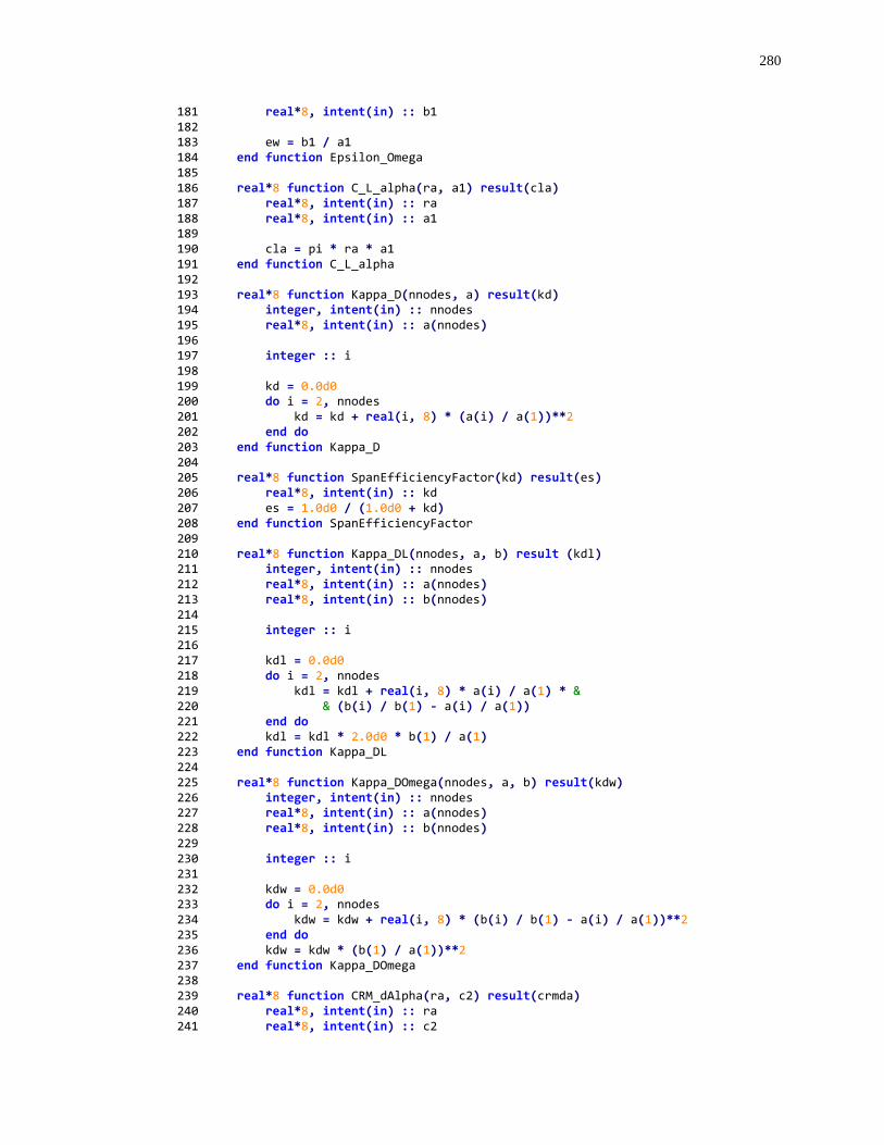
280

181 real*8, intent(in) :: b1 182 183 ew = b1 / a1 184 end function Epsilon_Omega 185 186 real*8 function C_L_alpha(ra, a1) result(cla) 187 real*8, intent(in) :: ra 188 real*8, intent(in) :: a1 189 190 cla = pi * ra * a1 191 end function C_L_alpha 192 193 real*8 function Kappa_D(nnodes, a) result(kd) 194 integer, intent(in) :: nnodes 195 real*8, intent(in) :: a(nnodes) 196 197 integer :: i 198 199 kd = 0.0d0 200 do i = 2, nnodes 201 kd = kd + real(i, 8) * (a(i) / a(1))**2 202 end do 203 end function Kappa_D 204 205 real*8 function SpanEfficiencyFactor(kd) result(es) 206 real*8, intent(in) :: kd 207 es = 1.0d0 / (1.0d0 + kd) 208 end function SpanEfficiencyFactor 209 210 real*8 function Kappa_DL(nnodes, a, b) result (kdl) 211 integer, intent(in) :: nnodes 212 real*8, intent(in) :: a(nnodes) 213 real*8, intent(in) :: b(nnodes) 214 215 integer :: i 216 217 kdl = 0.0d0 218 do i = 2, nnodes 219 kdl = kdl + real(i, 8) * a(i) / a(1) * & 220 & (b(i) / b(1) - a(i) / a(1)) 221 end do 222 kdl = kdl * 2.0d0 * b(1) / a(1) 223 end function Kappa_DL 224 225 real*8 function Kappa_DOmega(nnodes, a, b) result(kdw) 226 integer, intent(in) :: nnodes 227 real*8, intent(in) :: a(nnodes) 228 real*8, intent(in) :: b(nnodes) 229 230 integer :: i 231 232 kdw = 0.0d0 233 do i = 2, nnodes 234 kdw = kdw + real(i, 8) * (b(i) / b(1) - a(i) / a(1))**2 235 end do 236 kdw = kdw * (b(1) / a(1))**2 237 end function Kappa_DOmega 238 239 real*8 function CRM_dAlpha(ra, c2) result(crmda) 240 real*8, intent(in) :: ra 241 real*8, intent(in) :: c2

281

242 243 crmda = -pi * ra / 4.0d0 * c2 244 end function CRM_dAlpha 245 246 real*8 function CRM_PBar(ra, d2) result(crmpbar) 247 real*8, intent(in) :: ra 248 real*8, intent(in) :: d2 249 250 crmpbar = -pi * ra / 4.0d0 * d2 251 end function CRM_PBar 252 253 subroutine ComputeFlightConditions(pf) 254 type(Planform), intent(inout) :: pf 255 256 ! Make sure planform characteristics have been computed 257 if (.not. pf%IsAllocated) then 258 call ComputeCMatrixAndCoefficients(pf) 259 end if 260 261 ! Compute root aerodynamic angle of attack, if necessary 262 if (.not. pf%SpecifyAlpha) then 263 pf%AngleOfAttack = RootAlpha(pf%CLa, pf%LiftCoefficient, pf%EW,

pf%Washout) 264 else 265 pf%LiftCoefficient = CL1(pf%CLa, pf%AngleOfAttack, pf%EW,

pf%Washout) 266 end if 267 268 ! Compute optimum total washout, if necessary 269 if (pf%UseOptimumWashout) then 270 call SetOptimumWashout(pf) 271 else 272 call SetWashout(pf, pf%DesiredWashout * 180.0d0 / pi) 273 end if 274 275 ! Compute steady rolling rate, if necessary 276 if (pf%UseSteadyRollingRate) then 277 call SetSteadyRollingRate(pf) 278 end if 279 280 ! Compute BigA Fourier Coefficients 281 call ComputeBigACoefficients(pf, pf%BigA) 282 283 ! Compute lift coefficients 284 call ComputeLiftCoefficients(pf) 285 286 ! Compute drag coefficient 287 call ComputeDragCoefficients(pf) 288 289 ! Compute roll coefficient 290 pf%CRM = CRoll(pf%CRM_da, pf%CRM_pbar, pf%AileronDeflection,

pf%RollingRate) 291 292 ! Compute yaw coefficient 293 pf%CYM = CYaw(pf, pf%CL1, pf%BigA) 294 end subroutine ComputeFlightConditions 295 296 subroutine ComputeLiftCoefficients(pf) 297 type(Planform), intent(inout) :: pf 298 299 pf%CL1 = CL1(pf%CLa, pf%AngleOfAttack, pf%EW, pf%Washout)

282

300 pf%CL2 = CL2(pf%AspectRatio, pf%BigA(1)) 301 end subroutine ComputeLiftCoefficients 302 303 subroutine ComputeDragCoefficients(pf) 304 type(Planform), intent(inout) :: pf 305 306 pf%CDi1 = CDi1(pf) 307 pf%CDi2 = CDi2(pf) 308 pf%CDi3 = CDi3(pf) 309 end subroutine ComputeDragCoefficients 310 311 real*8 function CRoll(crmda, crmpbar, da, pbar) result(crm) 312 real*8, intent(in) :: crmda 313 real*8, intent(in) :: crmpbar 314 real*8, intent(in) :: da 315 real*8, intent(in) :: pbar 316 317 crm = crmda * da + crmpbar * pbar 318 end function CRoll 319 320 real*8 function CYaw(pf, cl, bigA) result(cym) 321 type(Planform), intent(in) :: pf 322 real*8, intent(in) :: cl 323 real*8, intent(in) :: bigA(pf%NNodes) 324 325 integer :: i 326 integer :: nnodes 327 nnodes = pf%NNodes 328 329 cym = cl / 8.0d0 * (6.0d0 * bigA(2) - pf%RollingRate) + & 330 & pi * pf%AspectRatio / 8.0d0 * (10.0d0 * bigA(2) - & 331 & pf%RollingRate) * bigA(3) 332 do i = 4, nnodes 333 cym = cym + 0.25d0 * pi * pf%AspectRatio * & 334 & (2.0d0 * real(i, 8) - 1.0d0) * bigA(i-1) * bigA(i) 335 end do 336 end function CYaw 337 338 subroutine ComputeC(pf, c) 339 type(Planform), intent(in) :: pf 340 real*8, intent(inout) :: c(pf%NNodes, pf%NNodes) 341 342 integer :: i 343 integer :: nnodes 344 345 nnodes = pf%NNodes 346 347 ! Compute values for i=1, i=N 348 call C1j_Nj(c, pf) 349 350 ! Compute values for i=2 to i=N-1 351 do i = 2, nnodes-1 352 call Cij(c, i, pf) 353 end do 354 end subroutine ComputeC 355 356 subroutine ComputeCInverse(pf, c_inv) 357 type(Planform), intent(in) :: pf 358 real*8, intent(inout) :: c_inv(pf%NNodes, pf%NNodes) 359 360 call matinv_gauss(pf%NNodes, pf%BigC, c_inv)

283

361 end subroutine ComputeCInverse 362 363 subroutine C1j_Nj(c, pf) 364 real*8, dimension(:,:), intent(inout) :: c 365 type(Planform), intent(in) :: pf 366 367 integer :: j 368 integer :: jsq 369 integer :: nnode 370 real*8 :: cb0 371 372 nnode = pf%NNodes 373 do j = 1, nnode 374 jsq = j**2 375 c(1, j) = real(jsq, 8) 376 c(nnode, j) = real((-1)**(j + 1) * jsq, 8) 377 end do 378 379 cb0 = c_over_b(pf, pi) 380 if (dabs(cb0) < 1.0d-10) then 381 call C1j_Nj_zero_chord(c, pf) 382 end if 383 384 end subroutine C1j_Nj 385 386 subroutine Cij(c, i, pf) 387 real*8, dimension(:,:), intent(inout) :: c 388 integer, intent(in) :: i 389 type(Planform), intent(in) :: pf 390 391 integer :: j 392 integer :: nnode 393 real*8 :: theta 394 real*8 :: cb 395 real*8 :: sin_theta 396 real*8 :: a0, A, r1, r2, r1y 397 real*8 :: n 398 399 nnode = pf%NNodes 400 theta = theta_i(i, nnode) 401 cb = c_over_b_i(pf, i) 402 sin_theta = sin(theta) 403 404 a0 = pf%SectionLiftSlope 405 A = pf%AspectRatio 406 407 ! Set the low aspect ratio method parameters 408 if (pf%LowAspectRatioMethod == Hodson) then 409 r1 = a0 * (A / cb * sin_theta)**exp(-8.0 * A) 410 r2 = A * (pi - atan((2.0 * a0) / (pi * A))) 411 else if (pf%LowAspectRatioMethod == ModifiedSlender) then 412 r1 = a0 413 r2 = 0.5 * pi * A 414 else if (pf%LowAspectRatioMethod == Kuchemann) then 415 n = 1.0 - 0.5 * (1.0 + (a0 / (pi * A))**2)**(-0.25) 416 r1 = 2 * n * a0 / (1.0 - pi * n / tan(pi * n)) 417 r2 = pi * A / (2.0 * n) 418 else ! Assume Classical 419 r1 = a0 420 r2 = pi * A 421 end if

284

422 423 do j = 1, nnode 424 c(i, j) = (4.0d0 / (pf%SectionLiftSlope * cb) * (a0 / r1) + & 425 & real(j, 8) / sin_theta * ((pi * A) / r2)) * sin(real(j, 8) *

theta) 426 end do 427 end subroutine Cij 428 429 subroutine C1j_Nj_zero_chord(c, pf) 430 real*8, dimension(:,:), intent(inout) :: c 431 type(Planform), intent(in) :: pf 432 433 integer :: j, n 434 435 n = pf%NNodes 436 437 if (pf%WingType == Tapered) then 438 do j = 1, n 439 c(1, j) = 2.0d0 * pf%AspectRatio * (1.0d0 + real(j, 8)) 440 c(n, j) = real((-1)**(j + 1), 8) * c(1, j) 441 end do 442 else if (pf%WingType == Elliptic) then 443 do j = 1, n 444 c(1, j) = c(1, j) + real(j, 8) * pi * & 445 & pf%AspectRatio / pf%SectionLiftSlope 446 c(n, j) = c(n, j) + real((-1)**(j + 1) * j, 8) * pi * & 447 & pf%AspectRatio / pf%SectionLiftSlope 448 end do 449 else if (pf%WingType == Combination) then 450 ! TODO: Add code for combination wing type 451 do j = 1, n 452 c(1, j) = c(1, j) + 4.0d0 * real(j, 8) * & 453 & sqrt(1.0d0 - 2.0d0 * pf%C4) / & 454 & (pf%C3 * pf%C5 * pf%SectionLiftSlope) 455 c(n, j) = c(n, j) + 4.0d0 * real((-1)**(j + 1) * j, 8) * & 456 & sqrt(1.0d0 - 2.0d0 * pf%C4) / & 457 & (pf%C3 * pf%C5 * pf%SectionLiftSlope) 458 end do 459 else 460 stop "*** Unknown Wing Type ***" 461 end if 462 463 end subroutine C1j_Nj_zero_chord 464 465 end module LiftingLineSolver

K.6 Output Module (liftinglineoutput.f90)

1 module LiftingLineOutput 2 use Utilities 3 use class_Planform 4 use LiftingLineSetters 5 use matrix 6 implicit none 7 8 contains 9 subroutine OutputHeader() 10 integer :: i 11 12 write(6, ('(80a)')) ("*", i=1, 80)

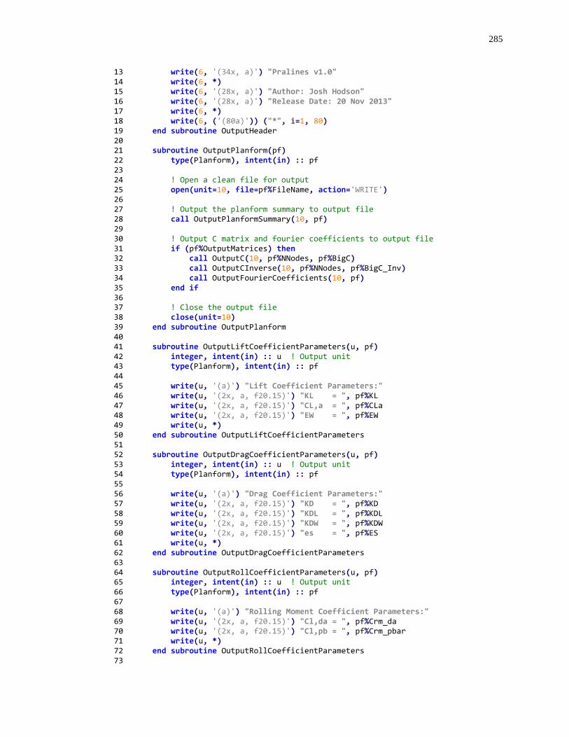
285

13 write(6, '(34x, a)') "Pralines v1.0" 14 write(6, *) 15 write(6, '(28x, a)') "Author: Josh Hodson" 16 write(6, '(28x, a)') "Release Date: 20 Nov 2013" 17 write(6, *) 18 write(6, ('(80a)')) ("*", i=1, 80) 19 end subroutine OutputHeader 20 21 subroutine OutputPlanform(pf) 22 type(Planform), intent(in) :: pf 23 24 ! Open a clean file for output 25 open(unit=10, file=pf%FileName, action='WRITE') 26 27 ! Output the planform summary to output file 28 call OutputPlanformSummary(10, pf) 29 30 ! Output C matrix and fourier coefficients to output file 31 if (pf%OutputMatrices) then 32 call OutputC(10, pf%NNodes, pf%BigC) 33 call OutputCInverse(10, pf%NNodes, pf%BigC_Inv) 34 call OutputFourierCoefficients(10, pf) 35 end if 36 37 ! Close the output file 38 close(unit=10) 39 end subroutine OutputPlanform 40 41 subroutine OutputLiftCoefficientParameters(u, pf) 42 integer, intent(in) :: u ! Output unit 43 type(Planform), intent(in) :: pf 44 45 write(u, '(a)') "Lift Coefficient Parameters:" 46 write(u, '(2x, a, f20.15)') "KL = ", pf%KL 47 write(u, '(2x, a, f20.15)') "CL,a = ", pf%CLa 48 write(u, '(2x, a, f20.15)') "EW = ", pf%EW 49 write(u, *) 50 end subroutine OutputLiftCoefficientParameters 51 52 subroutine OutputDragCoefficientParameters(u, pf) 53 integer, intent(in) :: u ! Output unit 54 type(Planform), intent(in) :: pf 55 56 write(u, '(a)') "Drag Coefficient Parameters:" 57 write(u, '(2x, a, f20.15)') "KD = ", pf%KD 58 write(u, '(2x, a, f20.15)') "KDL = ", pf%KDL 59 write(u, '(2x, a, f20.15)') "KDW = ", pf%KDW 60 write(u, '(2x, a, f20.15)') "es = ", pf%ES 61 write(u, *) 62 end subroutine OutputDragCoefficientParameters 63 64 subroutine OutputRollCoefficientParameters(u, pf) 65 integer, intent(in) :: u ! Output unit 66 type(Planform), intent(in) :: pf 67 68 write(u, '(a)') "Rolling Moment Coefficient Parameters:" 69 write(u, '(2x, a, f20.15)') "Cl,da = ", pf%Crm_da 70 write(u, '(2x, a, f20.15)') "Cl,pb = ", pf%Crm_pbar 71 write(u, *) 72 end subroutine OutputRollCoefficientParameters 73

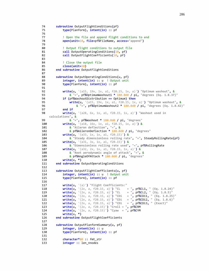
286

74 subroutine OutputFlightConditions(pf) 75 type(Planform), intent(in) :: pf 76 77 ! Open the file and append flight conditions to end 78 open(unit=10, file=pf%FileName, access="append") 79 80 ! Output flight conditions to output file 81 call OutputOperatingConditions(10, pf) 82 call OutputFlightCoefficients(10, pf) 83 84 ! Close the output file 85 close(unit=10) 86 end subroutine OutputFlightConditions 87 88 subroutine OutputOperatingConditions(u, pf) 89 integer, intent(in) :: u ! Output unit 90 type(Planform), intent(in) :: pf 91 92 write(u, '(a15, 19x, 1x, a1, f20.15, 1x, a)') "Optimum washout", & 93 & "=", pf%OptimumWashout1 * 180.0d0 / pi, "degrees (Eq. 1.8.37)" 94 if (pf%WashoutDistribution == Optimum) then 95 write(u, '(a15, 19x, 1x, a1, f20.15, 1x, a)') "Optimum washout", & 96 & "=", pf%OptimumWashout2 * 180.0d0 / pi, "degrees (Eq. 1.8.42)" 97 end if 98 write(u, '(a28, 6x, 1x, a1, f20.15, 1x, a)') "Washout used in

calculations", & 99 & "=", pf%Washout * 180.0d0 / pi, "degrees" 100 write(u, '(a18, 16x, 1x, a1, f20.15, 1x, a)') & 101 & "Aileron deflection", "=", & 102 & pf%AileronDeflection * 180.0d0 / pi, "degrees" 103 write(u, '(a33, 1x, 1x, a1, f20.15)') & 104 & "Steady dimensionless rolling rate", "=", SteadyRollingRate(pf) 105 write(u, '(a31, 3x, 1x, a1, f20.15)') & 106 & "Dimensionless rolling rate used", "=", pf%RollingRate 107 write(u, '(a32, 2x, 1x, a1, f20.15, 1x, a)') & 108 & "Root aerodynamic angle of attack", "=", & 109 & pf%AngleOfAttack * 180.0d0 / pi, "degrees" 110 write(u, *) 111 end subroutine OutputOperatingConditions 112 113 subroutine OutputFlightCoefficients(u, pf) 114 integer, intent(in) :: u ! Output unit 115 type(Planform), intent(in) :: pf 116 117 write(u, '(a)') "Flight Coefficients:" 118 write(u, '(2x, a, f20.15, a)') "CL = ", pf%CL1, " (Eq. 1.8.24)" 119 write(u, '(2x, a, f20.15, a)') "CL = ", pf%CL2, " (Eq. 1.8.5)" 120 write(u, '(2x, a, f20.15, a)') "CDi = ", pf%CDi1, " (Eq. 1.8.25)" 121 write(u, '(2x, a, f20.15, a)') "CDi = ", pf%CDi2, " (Eq. 1.8.6)" 122 write(u, '(2x, a, f20.15, a)') "CDi = ", pf%CDi3, " (Exact)" 123 write(u, '(2x, a, f20.15)') "Croll = ", pf%CRM 124 write(u, '(2x, a, f20.15)') "Cyaw = ", pf%CYM 125 write(u, *) 126 end subroutine OutputFlightCoefficients 127 128 subroutine OutputPlanformSummary(u, pf) 129 integer, intent(in) :: u 130 type(Planform), intent(in) :: pf 131 132 character*80 :: fmt_str 133 integer :: len_nnodes

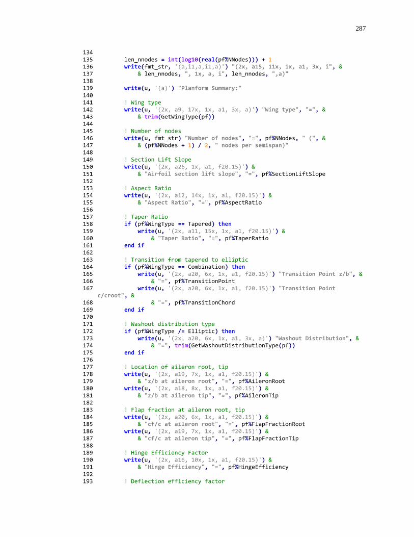
287

134 135 len_nnodes = int(log10(real(pf%NNodes))) + 1 136 write(fmt_str, '(a,i1,a,i1,a)') "(2x, a15, 11x, 1x, a1, 3x, i", & 137 & len_nnodes, ", 1x, a, i", len_nnodes, ",a)" 138 139 write(u, '(a)') "Planform Summary:" 140 141 ! Wing type 142 write(u, '(2x, a9, 17x, 1x, a1, 3x, a)') "Wing type", "=", & 143 & trim(GetWingType(pf)) 144 145 ! Number of nodes 146 write(u, fmt_str) "Number of nodes", "=", pf%NNodes, " (", & 147 & (pf%NNodes + 1) / 2, " nodes per semispan)" 148 149 ! Section Lift Slope 150 write(u, '(2x, a26, 1x, a1, f20.15)') & 151 & "Airfoil section lift slope", "=", pf%SectionLiftSlope 152 153 ! Aspect Ratio 154 write(u, '(2x, a12, 14x, 1x, a1, f20.15)') & 155 & "Aspect Ratio", "=", pf%AspectRatio 156 157 ! Taper Ratio 158 if (pf%WingType == Tapered) then 159 write(u, '(2x, a11, 15x, 1x, a1, f20.15)') & 160 & "Taper Ratio", "=", pf%TaperRatio 161 end if 162 163 ! Transition from tapered to elliptic 164 if (pf%WingType == Combination) then 165 write(u, '(2x, a20, 6x, 1x, a1, f20.15)') "Transition Point z/b", & 166 & "=", pf%TransitionPoint 167 write(u, '(2x, a20, 6x, 1x, a1, f20.15)') "Transition Point

c/croot", & 168 & "=", pf%TransitionChord 169 end if 170 171 ! Washout distribution type 172 if (pf%WingType /= Elliptic) then 173 write(u, '(2x, a20, 6x, 1x, a1, 3x, a)') "Washout Distribution", & 174 & "=", trim(GetWashoutDistributionType(pf)) 175 end if 176 177 ! Location of aileron root, tip 178 write(u, '(2x, a19, 7x, 1x, a1, f20.15)') & 179 & "z/b at aileron root", "=", pf%AileronRoot 180 write(u, '(2x, a18, 8x, 1x, a1, f20.15)') & 181 & "z/b at aileron tip", "=", pf%AileronTip 182 183 ! Flap fraction at aileron root, tip 184 write(u, '(2x, a20, 6x, 1x, a1, f20.15)') & 185 & "cf/c at aileron root", "=", pf%FlapFractionRoot 186 write(u, '(2x, a19, 7x, 1x, a1, f20.15)') & 187 & "cf/c at aileron tip", "=", pf%FlapFractionTip 188 189 ! Hinge Efficiency Factor 190 write(u, '(2x, a16, 10x, 1x, a1, f20.15)') & 191 & "Hinge Efficiency", "=", pf%HingeEfficiency 192 193 ! Deflection efficiency factor

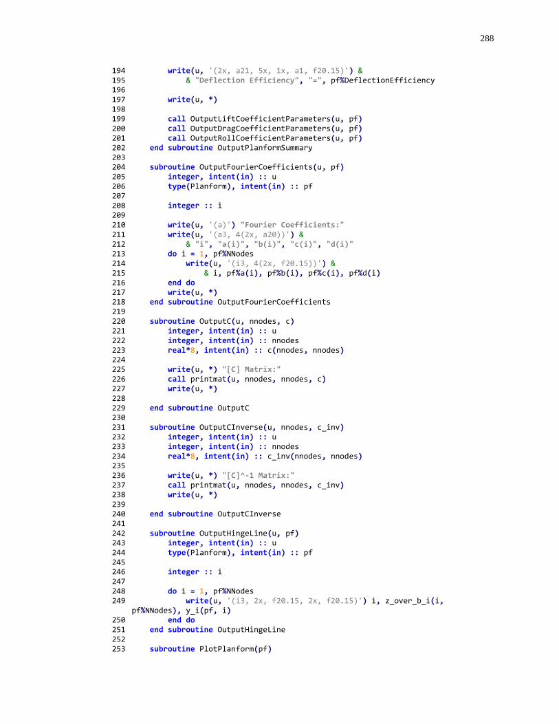
288

194 write(u, '(2x, a21, 5x, 1x, a1, f20.15)') & 195 & "Deflection Efficiency", "=", pf%DeflectionEfficiency 196 197 write(u, *) 198 199 call OutputLiftCoefficientParameters(u, pf) 200 call OutputDragCoefficientParameters(u, pf) 201 call OutputRollCoefficientParameters(u, pf) 202 end subroutine OutputPlanformSummary 203 204 subroutine OutputFourierCoefficients(u, pf) 205 integer, intent(in) :: u 206 type(Planform), intent(in) :: pf 207 208 integer :: i 209 210 write(u, '(a)') "Fourier Coefficients:" 211 write(u, '(a3, 4(2x, a20))') & 212 & "i", "a(i)", "b(i)", "c(i)", "d(i)" 213 do i = 1, pf%NNodes 214 write(u, '(i3, 4(2x, f20.15))') & 215 & i, pf%a(i), pf%b(i), pf%c(i), pf%d(i) 216 end do 217 write(u, *) 218 end subroutine OutputFourierCoefficients 219 220 subroutine OutputC(u, nnodes, c) 221 integer, intent(in) :: u 222 integer, intent(in) :: nnodes 223 real*8, intent(in) :: c(nnodes, nnodes) 224 225 write(u, *) "[C] Matrix:" 226 call printmat(u, nnodes, nnodes, c) 227 write(u, *) 228 229 end subroutine OutputC 230 231 subroutine OutputCInverse(u, nnodes, c_inv) 232 integer, intent(in) :: u 233 integer, intent(in) :: nnodes 234 real*8, intent(in) :: c_inv(nnodes, nnodes) 235 236 write(u, *) "[C]^-1 Matrix:" 237 call printmat(u, nnodes, nnodes, c_inv) 238 write(u, *) 239 240 end subroutine OutputCInverse 241 242 subroutine OutputHingeLine(u, pf) 243 integer, intent(in) :: u 244 type(Planform), intent(in) :: pf 245 246 integer :: i 247 248 do i = 1, pf%NNodes 249 write(u, '(i3, 2x, f20.15, 2x, f20.15)') i, z_over_b_i(i,

pf%NNodes), y_i(pf, i) 250 end do 251 end subroutine OutputHingeLine 252 253 subroutine PlotPlanform(pf)

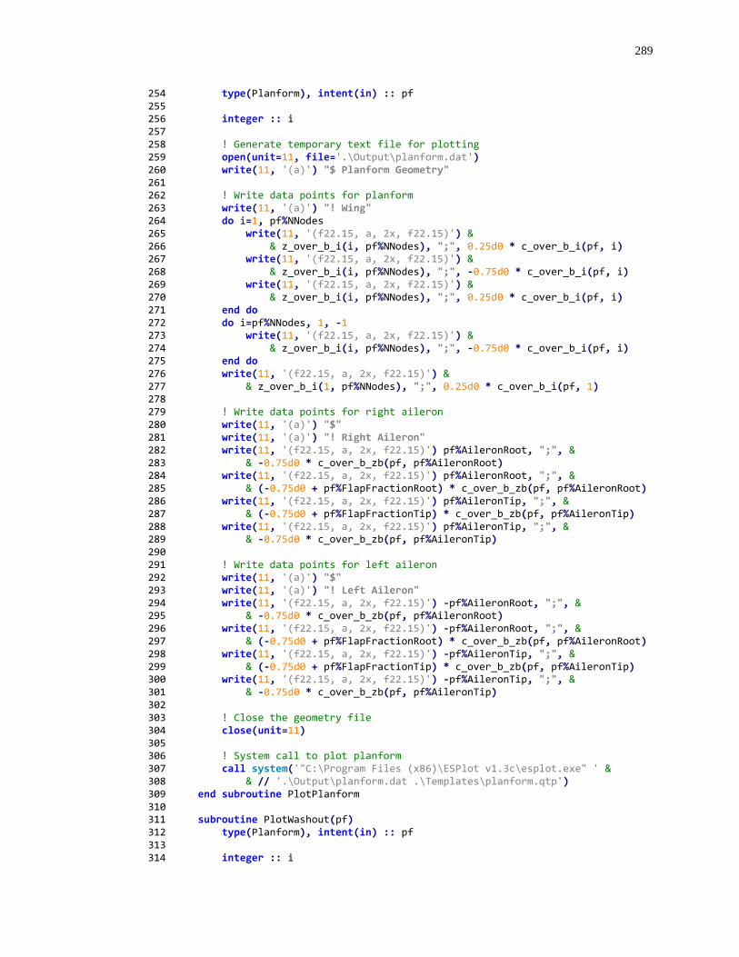
289

254 type(Planform), intent(in) :: pf 255 256 integer :: i 257 258 ! Generate temporary text file for plotting 259 open(unit=11, file='.\Output\planform.dat') 260 write(11, '(a)') "$ Planform Geometry" 261 262 ! Write data points for planform 263 write(11, '(a)') "! Wing" 264 do i=1, pf%NNodes 265 write(11, '(f22.15, a, 2x, f22.15)') & 266 & z_over_b_i(i, pf%NNodes), ";", 0.25d0 * c_over_b_i(pf, i) 267 write(11, '(f22.15, a, 2x, f22.15)') & 268 & z_over_b_i(i, pf%NNodes), ";", -0.75d0 * c_over_b_i(pf, i) 269 write(11, '(f22.15, a, 2x, f22.15)') & 270 & z_over_b_i(i, pf%NNodes), ";", 0.25d0 * c_over_b_i(pf, i) 271 end do 272 do i=pf%NNodes, 1, -1 273 write(11, '(f22.15, a, 2x, f22.15)') & 274 & z_over_b_i(i, pf%NNodes), ";", -0.75d0 * c_over_b_i(pf, i) 275 end do 276 write(11, '(f22.15, a, 2x, f22.15)') & 277 & z_over_b_i(1, pf%NNodes), ";", 0.25d0 * c_over_b_i(pf, 1) 278 279 ! Write data points for right aileron 280 write(11, '(a)') "$" 281 write(11, '(a)') "! Right Aileron" 282 write(11, '(f22.15, a, 2x, f22.15)') pf%AileronRoot, ";", & 283 & -0.75d0 * c_over_b_zb(pf, pf%AileronRoot) 284 write(11, '(f22.15, a, 2x, f22.15)') pf%AileronRoot, ";", & 285 & (-0.75d0 + pf%FlapFractionRoot) * c_over_b_zb(pf, pf%AileronRoot) 286 write(11, '(f22.15, a, 2x, f22.15)') pf%AileronTip, ";", & 287 & (-0.75d0 + pf%FlapFractionTip) * c_over_b_zb(pf, pf%AileronTip) 288 write(11, '(f22.15, a, 2x, f22.15)') pf%AileronTip, ";", & 289 & -0.75d0 * c_over_b_zb(pf, pf%AileronTip) 290 291 ! Write data points for left aileron 292 write(11, '(a)') "$" 293 write(11, '(a)') "! Left Aileron" 294 write(11, '(f22.15, a, 2x, f22.15)') -pf%AileronRoot, ";", & 295 & -0.75d0 * c_over_b_zb(pf, pf%AileronRoot) 296 write(11, '(f22.15, a, 2x, f22.15)') -pf%AileronRoot, ";", & 297 & (-0.75d0 + pf%FlapFractionRoot) * c_over_b_zb(pf, pf%AileronRoot) 298 write(11, '(f22.15, a, 2x, f22.15)') -pf%AileronTip, ";", & 299 & (-0.75d0 + pf%FlapFractionTip) * c_over_b_zb(pf, pf%AileronTip) 300 write(11, '(f22.15, a, 2x, f22.15)') -pf%AileronTip, ";", & 301 & -0.75d0 * c_over_b_zb(pf, pf%AileronTip) 302 303 ! Close the geometry file 304 close(unit=11) 305 306 ! System call to plot planform 307 call system('"C:\Program Files (x86)\ESPlot v1.3c\esplot.exe" ' & 308 & // '.\Output\planform.dat .\Templates\planform.qtp') 309 end subroutine PlotPlanform 310 311 subroutine PlotWashout(pf) 312 type(Planform), intent(in) :: pf 313 314 integer :: i

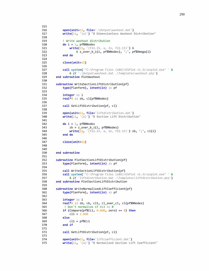
290

315 316 open(unit=11, file='.\Output\washout.dat') 317 write(11, '(a)') "$ Dimensionless Washout Distribution" 318 319 ! Write washout distribution 320 do i = 1, pf%NNodes 321 write(11, '(f22.15, a, 2x, f22.15)') & 322 & z_over_b_i(i, pf%NNodes), ";", pf%Omega(i) 323 end do 324 325 close(unit=11) 326 327 call system('"C:\Program Files (x86)\ESPlot v1.3c\esplot.exe" ' & 328 & // '.\Output\washout.dat .\Templates\washout.qtp') 329 end subroutine PlotWashout 330 331 subroutine WriteSectionLiftDistribution(pf) 332 type(Planform), intent(in) :: pf 333 334 integer :: i 335 real*8 :: zb, cl(pf%NNodes) 336 337 call GetLiftDistribution(pf, cl) 338 339 open(unit=11, file='liftdistribution.dat') 340 write(11, '(a)') "$ Section Lift Distribution" 341 342 do i = 1, pf%NNodes 343 zb = z_over_b_i(i, pf%NNodes) 344 write(11, '(f22.15, a, 2x, f22.15)') zb, ";", cl(i) 345 end do 346 347 close(unit=11) 348 349 350 end subroutine 351 352 subroutine PlotSectionLiftDistribution(pf) 353 type(Planform), intent(in) :: pf 354 355 call WriteSectionLiftDistribution(pf) 356 call system('"C:\Program Files (x86)\ESPlot v1.3c\esplot.exe" ' & 357 & // 'liftdistribution.dat .\Templates\liftdistribution.qtp') 358 end subroutine PlotSectionLiftDistribution 359 360 subroutine WriteNormalizedLiftCoefficient(pf) 361 type(Planform), intent(in) :: pf 362 363 integer :: i 364 real*8 :: zb, cb, cl1, cl_over_cl, cl(pf%NNodes) 365 ! Don't normalize if CL1 == 0 366 if (Compare(pf%CL1, 0.0d0, zero) == 0) then 367 cl1 = 1.0d0 368 else 369 cl1 = pf%CL1 370 end if 371 372 call GetLiftDistribution(pf, cl) 373 374 open(unit=11, file='liftcoefficient.dat') 375 write(11, '(a)') "$ Normalized Section Lift Coefficient"

291

376 377 do i = 1, pf%NNodes 378 zb = z_over_b_i(i, pf%NNodes) 379 cb = c_over_b_zb(pf, zb) 380 if (Compare(cb, 0.0d0, zero) == 0) then 381 if (Compare(cl(i), 0.0d0, zero) == 0) then 382 if (pf%WingType == Elliptic) then 383 cl_over_cl = NLC_ZeroChord_Elliptic(pf, zb, cb, cl1) 384 else if (pf%WingType == Tapered) then 385 cl_over_cl = NLC_ZeroChord_Tapered(pf, zb, cb, cl1) 386 else if (pf%WingType == Combination) then 387 cl_over_cl = NLC_ZeroChord_Tapered(pf, zb, cb, cl1) 388 else 389 stop "***Unknown Wing Type***" 390 end if 391 else 392 ! Finite lift from zero-chord section, should never happen 393 cl_over_cl = 1.0d0 / zero 394 end if 395 else 396 cl_over_cl = cl(i) / cb / cl1 397 end if 398 write(11, '(f22.15, a, 2x, f22.15)') zb, ";", cl_over_cl 399 end do 400 401 close(unit=11) 402 end subroutine 403 404 subroutine PlotNormalizedLiftCoefficient(pf) 405 type(Planform), intent(in) :: pf 406 407 call WriteNormalizedLiftCoefficient(pf) 408 call system('"C:\Program Files (x86)\ESPlot v1.3c\esplot.exe" ' & 409 & // 'liftcoefficient.dat .\Templates\liftcoefficient.qtp') 410 end subroutine PlotNormalizedLiftCoefficient 411 412 subroutine GetLiftDistribution(pf, cl) 413 type(Planform), intent(in) :: pf 414 real*8, intent(out) :: cl(pf%NNodes) 415 416 integer :: i, j 417 real*8 :: zb, theta 418 419 do i = 1, pf%NNodes 420 zb = z_over_b_i(i, pf%NNodes) 421 theta = theta_zb(zb) 422 cl(i) = 0.0d0 423 do j = 1, pf%NNodes 424 cl(i) = cl(i) + pf%BigA(j) * sin(real(j, 8) * theta) 425 end do 426 cl(i) = cl(i) * 4.0d0 427 end do 428 end subroutine GetLiftDistribution 429 430 real*8 function NLC_ZeroChord_Elliptic(pf, zb, cb, cl) result(cl_over_cl) 431 type(Planform), intent(in) :: pf 432 real*8, intent(in) :: zb 433 real*8, intent(in) :: cb 434 real*8, intent(in) :: cl 435 436 integer :: i

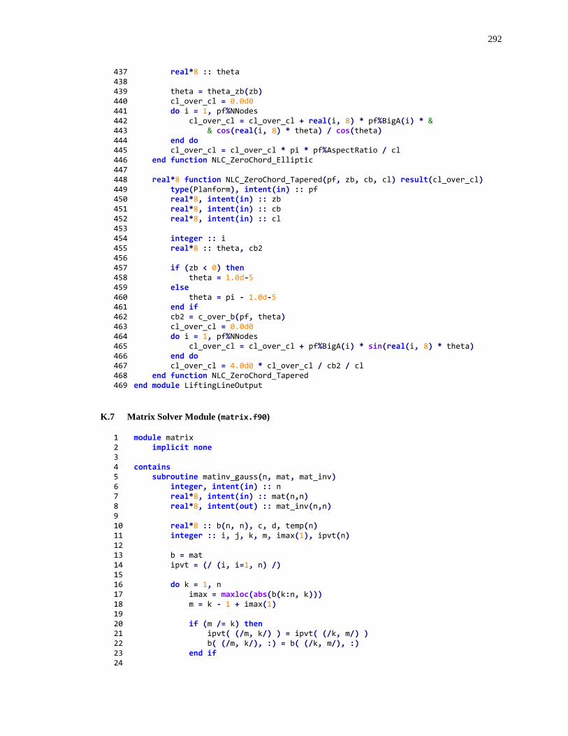
292

437 real*8 :: theta 438 439 theta = theta_zb(zb) 440 cl_over_cl = 0.0d0 441 do i = 1, pf%NNodes 442 cl_over_cl = cl_over_cl + real(i, 8) * pf%BigA(i) * & 443 & cos(real(i, 8) * theta) / cos(theta) 444 end do 445 cl_over_cl = cl_over_cl * pi * pf%AspectRatio / cl 446 end function NLC_ZeroChord_Elliptic 447 448 real*8 function NLC_ZeroChord_Tapered(pf, zb, cb, cl) result(cl_over_cl) 449 type(Planform), intent(in) :: pf 450 real*8, intent(in) :: zb 451 real*8, intent(in) :: cb 452 real*8, intent(in) :: cl 453 454 integer :: i 455 real*8 :: theta, cb2 456 457 if (zb < 0) then 458 theta = 1.0d-5 459 else 460 theta = pi - 1.0d-5 461 end if 462 cb2 = c_over_b(pf, theta) 463 cl_over_cl = 0.0d0 464 do i = 1, pf%NNodes 465 cl_over_cl = cl_over_cl + pf%BigA(i) * sin(real(i, 8) * theta) 466 end do 467 cl_over_cl = 4.0d0 * cl_over_cl / cb2 / cl 468 end function NLC_ZeroChord_Tapered 469 end module LiftingLineOutput

K.7 Matrix Solver Module (matrix.f90)

1 module matrix 2 implicit none 3 4 contains 5 subroutine matinv_gauss(n, mat, mat_inv) 6 integer, intent(in) :: n 7 real*8, intent(in) :: mat(n,n) 8 real*8, intent(out) :: mat_inv(n,n) 9 10 real*8 :: b(n, n), c, d, temp(n) 11 integer :: i, j, k, m, imax(1), ipvt(n) 12 13 b = mat 14 ipvt = (/ (i, i=1, n) /) 15 16 do k = 1, n 17 imax = maxloc(abs(b(k:n, k))) 18 m = k - 1 + imax(1) 19 20 if (m /= k) then 21 ipvt( (/m, k/) ) = ipvt( (/k, m/) ) 22 b( (/m, k/), :) = b( (/k, m/), :) 23 end if 24

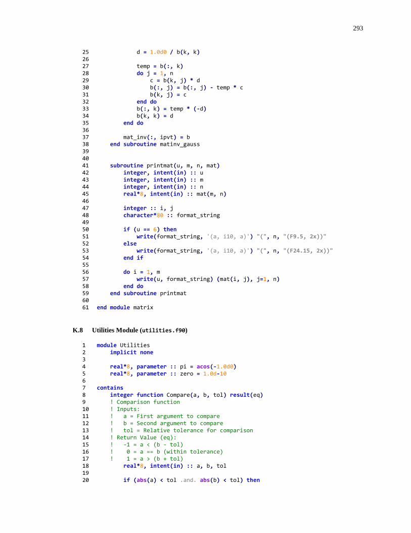
293

25 d = 1.0d0 / b(k, k) 26 27 temp = b(:, k) 28 do j = 1, n 29 c = b(k, j) * d 30 b(:, j) = b(:, j) - temp * c 31 b(k, j) = c 32 end do 33 b(:, k) = temp * (-d) 34 b(k, k) = d 35 end do 36 37 mat_inv(:, ipvt) = b 38 end subroutine matinv_gauss 39 40 41 subroutine printmat(u, m, n, mat) 42 integer, intent(in) :: u 43 integer, intent(in) :: m 44 integer, intent(in) :: n 45 real*8, intent(in) :: mat(m, n) 46 47 integer :: i, j 48 character*80 :: format_string 49 50 if (u == 6) then 51 write(format_string, '(a, i10, a)') "(", n, "(F9.5, 2x))" 52 else 53 write(format_string, '(a, i10, a)') "(", n, "(F24.15, 2x))" 54 end if 55 56 do i = 1, m 57 write(u, format_string) (mat(i, j), j=1, n) 58 end do 59 end subroutine printmat 60 61 end module matrix

K.8 Utilities Module (utilities.f90)

1 module Utilities 2 implicit none 3 4 real*8, parameter :: pi = acos(-1.0d0) 5 real*8, parameter :: zero = 1.0d-10 6 7 contains 8 integer function Compare(a, b, tol) result(eq) 9 ! Comparison function 10 ! Inputs: 11 ! a = First argument to compare 12 ! b = Second argument to compare 13 ! tol = Relative tolerance for comparison 14 ! Return Value (eq): 15 ! -1 = a < (b - tol) 16 ! 0 = a == b (within tolerance) 17 ! 1 = a > (b + tol) 18 real*8, intent(in) :: a, b, tol 19 20 if (abs(a) < tol .and. abs(b) < tol) then

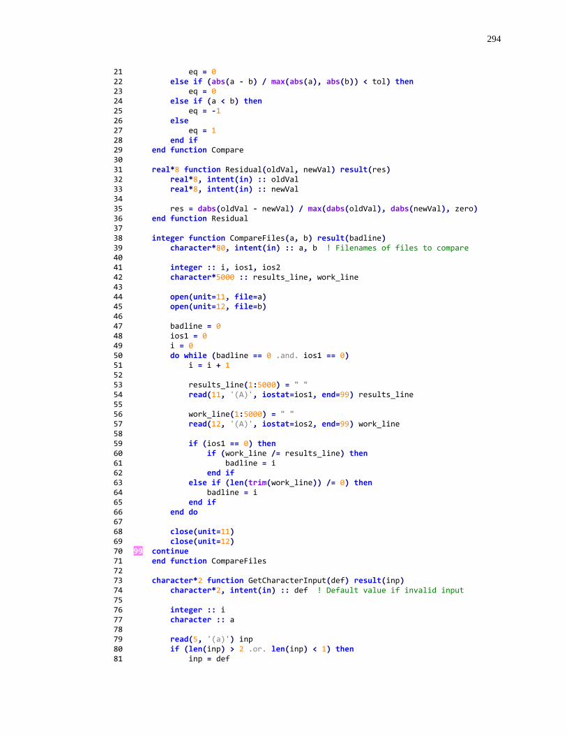
294

21 eq = 0 22 else if (abs(a - b) / max(abs(a), abs(b)) < tol) then 23 eq = 0 24 else if (a < b) then 25 eq = -1 26 else 27 eq = 1 28 end if 29 end function Compare 30 31 real*8 function Residual(oldVal, newVal) result(res) 32 real*8, intent(in) :: oldVal 33 real*8, intent(in) :: newVal 34 35 res = dabs(oldVal - newVal) / max(dabs(oldVal), dabs(newVal), zero) 36 end function Residual 37 38 integer function CompareFiles(a, b) result(badline) 39 character*80, intent(in) :: a, b ! Filenames of files to compare 40 41 integer :: i, ios1, ios2 42 character*5000 :: results_line, work_line 43 44 open(unit=11, file=a) 45 open(unit=12, file=b) 46 47 badline = 0 48 ios1 = 0 49 i = 0 50 do while (badline == 0 .and. ios1 == 0) 51 i = i + 1 52 53 results_line(1:5000) = " " 54 read(11, '(A)', iostat=ios1, end=99) results_line 55 56 work_line(1:5000) = " " 57 read(12, '(A)', iostat=ios2, end=99) work_line 58 59 if (ios1 == 0) then 60 if (work_line /= results_line) then 61 badline = i 62 end if 63 else if (len(trim(work_line)) /= 0) then 64 badline = i 65 end if 66 end do 67 68 close(unit=11) 69 close(unit=12) 70 99 continue 71 end function CompareFiles 72 73 character*2 function GetCharacterInput(def) result(inp) 74 character*2, intent(in) :: def ! Default value if invalid input 75 76 integer :: i 77 character :: a 78 79 read(5, '(a)') inp 80 if (len(inp) > 2 .or. len(inp) < 1) then 81 inp = def

295

82 else 83 do i = 1, 2 84 a = inp(i:i) 85 if(iachar(a) >= iachar('a') .and. iachar(a) <= iachar('z')) then 86 inp(i:i) = char(iachar(a) - 32) 87 end if 88 end do 89 end if 90 end function GetCharacterInput 91 92 character*80 function GetStringInput(def) result(inp) 93 character*80, intent(in) :: def ! Default value if invalid input 94 95 integer :: i, ios 96 character :: a 97 98 read(5, '(a)', iostat=ios) inp 99 if (len(trim(inp)) < 1 .or. ios /= 0) then 100 inp = def 101 end if 102 end function GetStringInput 103 104 integer function GetIntInput(mn, mx, def) result(inp) 105 integer, intent(in) :: mn ! Minimum accepted value 106 integer, intent(in) :: mx ! Maximum accepted value 107 integer, intent(in) :: def ! Default value if invalid input 108 109 logical :: cont 110 character*80 :: inp_str 111 integer :: ios 112 integer :: len_mn, len_mx 113 character*80 :: msg_fmt 114 115 cont = .true. 116 do while (cont) 117 read(5, '(a)', iostat=ios) inp_str 118 if (ios == 0 .and. trim(inp_str) /= "") then 119 read(inp_str, *, iostat=ios) inp 120 if (ios /= 0 .or. inp < mn .or. inp > mx) then 121 len_mn = int(log10(real(abs(mn)))) + 1 122 if (mn < 0) len_mn = len_mn + 1 123 124 len_mx = int(log10(real(abs(mx)))) + 1 125 if (mx < 0) len_mx = len_mx + 1 126 127 write(msg_fmt, '(a, i1, a, i1, a)') "(a, a, i", len_mn, & 128 & ", a, i", len_mx, ", a)" 129 130 write(6, *) 131 write(6, msg_fmt) "Invalid input. Please ", & 132 & "specify an integer between ", mn, " and ", mx, "," 133 write(6, '(a)') "or press <ENTER> to accept the default

value." 134 else 135 cont = .false. 136 end if 137 else 138 inp = def 139 cont = .false. 140 end if 141 end do

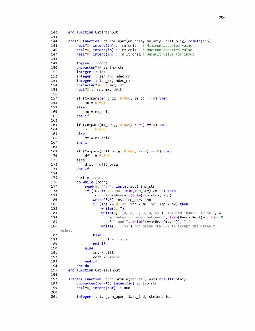
296

142 end function GetIntInput 143 144 real*8 function GetRealInput(mn_orig, mx_orig, dflt_orig) result(inp) 145 real*8, intent(in) :: mn_orig ! Minimum accepted value 146 real*8, intent(in) :: mx_orig ! Maximum accepted value 147 real*8, intent(in) :: dflt_orig ! Default value for input 148 149 logical :: cont 150 character*80 :: inp_str 151 integer :: ios 152 integer :: len_mn, ndec_mn 153 integer :: len_mx, ndec_mx 154 character*80 :: msg_fmt 155 real*8 :: mn, mx, dflt 156 157 if (Compare(mn_orig, 0.0d0, zero) == 0) then 158 mn = 0.0d0 159 else 160 mn = mn_orig 161 end if 162 163 if (Compare(mx_orig, 0.0d0, zero) == 0) then 164 mx = 0.0d0 165 else 166 mx = mx_orig 167 end if 168 169 if (Compare(dflt_orig, 0.0d0, zero) == 0) then 170 dflt = 0.0d0 171 else 172 dflt = dflt_orig 173 end if 174 175 cont = .true. 176 do while (cont) 177 read(5, '(a)', iostat=ios) inp_str 178 if (ios == 0 .and. trim(inp_str) /= "") then 179 ios = ParseFormula(trim(inp_str), inp) 180 write(*,*) ios, inp_str, inp 181 if (ios /= 0 .or. inp < mn .or. inp > mx) then 182 write(6, *) 183 write(6, '(a, a, a, a, a, a)') "Invalid input. Please ", & 184 & "enter a number between ", trim(FormatReal(mn, 5)), & 185 & " and ", trim(FormatReal(mx, 5)), "," 186 write(6, '(a)') "or press <ENTER> to accept the default

value." 187 else 188 cont = .false. 189 end if 190 else 191 inp = dflt 192 cont = .false. 193 end if 194 end do 195 end function GetRealInput 196 197 integer function ParseFormula(inp_str, num) result(estat) 198 character(len=*), intent(in) :: inp_str 199 real*8, intent(out) :: num 200 201 integer :: i, j, n_oper, last_ind, strlen, ios

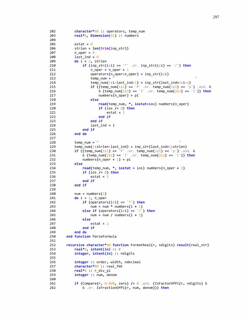
297

202 character*40 :: operators, temp_num 203 real*8, Dimension(41) :: numbers 204 205 estat = 0 206 strlen = len(trim(inp_str)) 207 n_oper = 0 208 last_ind = 0 209 do i = 2, strlen 210 if (inp_str(i:i) == '*' .or. inp_str(i:i) == '/') then 211 n_oper = n_oper + 1 212 operators(n_oper:n_oper) = inp_str(i:i) 213 temp_num = " " 214 temp_num(1:i-last_ind-1) = inp_str(last_ind+1:i-1) 215 if ((temp_num(1:1) == 'P' .or. temp_num(1:1) == 'p') .and. & 216 & (temp_num(2:2) == 'I' .or. temp_num(2:2) == 'i')) then 217 numbers(n_oper) = pi 218 else 219 read(temp_num, *, iostat=ios) numbers(n_oper) 220 if (ios /= 0) then 221 estat = 1 222 end if 223 end if 224 last_ind = i 225 end if 226 end do 227 228 temp_num = " " 229 temp_num(1:strlen-last_ind) = inp_str(last_ind+1:strlen) 230 if ((temp_num(1:1) == 'P' .or. temp_num(1:1) == 'p') .and. & 231 & (temp_num(2:2) == 'I' .or. temp_num(2:2) == 'i')) then 232 numbers(n_oper + 1) = pi 233 else 234 read(temp_num, *, iostat = ios) numbers(n_oper + 1) 235 if (ios /= 0) then 236 estat = 1 237 end if 238 end if 239 240 num = numbers(1) 241 do i = 1, n_oper 242 if (operators(i:i) == '*') then 243 num = num * numbers(i + 1) 244 else if (operators(i:i) == '/') then 245 num = num / numbers(i + 1) 246 else 247 estat = 2 248 end if 249 end do 250 end function ParseFormula 251 252 recursive character*80 function FormatReal(r, ndigits) result(real_str) 253 real*8, intent(in) :: r 254 integer, intent(in) :: ndigits 255 256 integer :: order, width, ndecimal 257 character*80 :: real_fmt 258 real*8 :: r_div_pi 259 integer :: num, denom 260 261 if (Compare(r, 0.0d0, zero) /= 0 .and. (IsFactorOfPi(r, ndigits) & 262 & .or. IsFractionOfPi(r, num, denom))) then

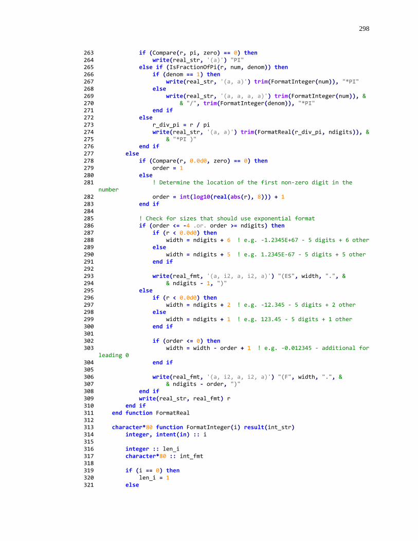
298

263 if (Compare(r, pi, zero) == 0) then 264 write(real_str, '(a)') "PI" 265 else if (IsFractionOfPi(r, num, denom)) then 266 if (denom == 1) then 267 write(real_str, '(a, a)') trim(FormatInteger(num)), "*PI" 268 else 269 write(real_str, '(a, a, a, a)') trim(FormatInteger(num)), & 270 & "/", trim(FormatInteger(denom)), "*PI" 271 end if 272 else 273 r_div_pi = r / pi 274 write(real_str, '(a, a)') trim(FormatReal(r_div_pi, ndigits)), & 275 & "*PI )" 276 end if 277 else 278 if (Compare(r, 0.0d0, zero) == 0) then 279 order = 1 280 else 281 ! Determine the location of the first non-zero digit in the

number 282 order = int(log10(real(abs(r), 8))) + 1 283 end if 284 285 ! Check for sizes that should use exponential format 286 if (order <= -4 .or. order >= ndigits) then 287 if (r < 0.0d0) then 288 width = ndigits + 6 ! e.g. -1.2345E+67 - 5 digits + 6 other 289 else 290 width = ndigits + 5 ! e.g. 1.2345E-67 - 5 digits + 5 other 291 end if 292 293 write(real_fmt, '(a, i2, a, i2, a)') "(ES", width, ".", & 294 & ndigits - 1, ")" 295 else 296 if (r < 0.0d0) then 297 width = ndigits + 2 ! e.g. -12.345 - 5 digits + 2 other 298 else 299 width = ndigits + 1 ! e.g. 123.45 - 5 digits + 1 other 300 end if 301 302 if (order <= 0) then 303 width = width - order + 1 ! e.g. -0.012345 - additional for

leading 0 304 end if 305 306 write(real_fmt, '(a, i2, a, i2, a)') "(F", width, ".", & 307 & ndigits - order, ")" 308 end if 309 write(real_str, real_fmt) r 310 end if 311 end function FormatReal 312 313 character*80 function FormatInteger(i) result(int_str) 314 integer, intent(in) :: i 315 316 integer :: len_i 317 character*80 :: int_fmt 318 319 if (i == 0) then 320 len_i = 1 321 else

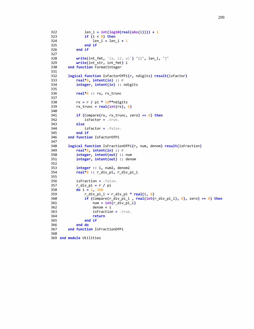
299

322 len_i = int(log10(real(abs(i)))) + 1 323 if (i < 0) then 324 len_i = len_i + 1 325 end if 326 end if 327 328 write(int_fmt, '(a, i2, a)') "(i", len_i, ")" 329 write(int_str, int_fmt) i 330 end function FormatInteger 331 332 logical function IsFactorOfPi(r, ndigits) result(isFactor) 333 real*8, intent(in) :: r 334 integer, intent(in) :: ndigits 335 336 real*8 :: rx, rx_trunc 337 338 rx = r / pi * 10**ndigits 339 rx_trunc = real(int(rx), 8) 340 341 if (Compare(rx, rx_trunc, zero) == 0) then 342 isFactor = .true. 343 else 344 isFactor = .false. 345 end if 346 end function IsFactorOfPi 347 348 logical function IsFractionOfPi(r, num, denom) result(isFraction) 349 real*8, intent(in) :: r 350 integer, intent(out) :: num 351 integer, intent(out) :: denom 352 353 integer :: i, num2, denom2 354 real*8 :: r_div_pi, r_div_pi_i 355 356 isFraction = .false. 357 r_div_pi = r / pi 358 do i = 1, 360 359 r_div_pi_i = r_div_pi * real(i, 8) 360 if (Compare(r_div_pi_i , real(int(r_div_pi_i), 8), zero) == 0) then 361 num = int(r_div_pi_i) 362 denom = i 363 isFraction = .true. 364 return 365 end if 366 end do 367 end function IsFractionOfPi 368 369 end module Utilities

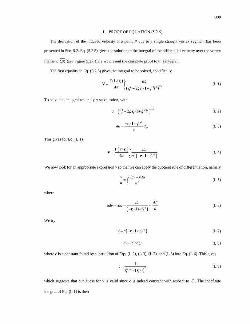
300

L PROOF OF EQUATION (5.2.5)

The derivation of the induced velocity at a point P due to a single straight vortex segment has been

presented in Sec. 5.2. Eq. (5.2.5) gives the solution to the integral of the differential velocity over the vortex

filament OR (see Figure 5.2). Here we present the complete proof to this integral.

The first equality in Eq. (5.2.5) gives the integral to be solved, specifically

( )

( )1

3/22 2 2

0 1 1

1

4 2

d

r l

=

− +

l

l r

rV (L.1)

To solve this integral we apply u-substitution, with

( )1/2

2 2 2

1 12u r l = − +lr (L.2)

2

1 ld

uu d

+=−r l

(L.3)

This gives for Eq. (L.1)

( )

( )2 2

1

1

1

04

du

u l −

=

+

l

l r

rV (L.4)

We now look for an appropriate expression v so that we can apply the quotient rule of differentiation, namely

2

v udv vdu

u u

−= (L.5)

where

( )2

1

du dudv vdu

ul

− = =

− +lr (L.6)

We try

( )2

1v c l= − +r l (L.7)

2dv cl d= (L.8)

where c is a constant found by substitution of Eqs. (L.2), (L.3), (L.7), and (L.8) into Eq. (L.6). This gives

( )

22 2

1 1

1c

r l=

− r l (L.9)

which suggests that our guess for v is valid since c is indeed constant with respect to . The indefinite

integral of Eq. (L.1) is then

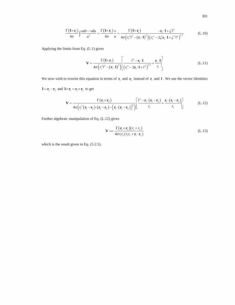
301

( ) ( ) ( )

( )( ) ( )

21 1 1 1

2 1/222 2 2 2 2

1 1 1 14 4 4 2

ludv vdu v

uu r l r l

− +−= =

−

+−

l

l r l r l r

r l

r l

r (L.10)

Applying the limits from Eq. (L.1) gives

( )

( )( ) ( )

21 1 1

1/222 2 2 211 1 1 1

4 2

l

rr l r l

− = +

− +−

l r lV

r

r l

l

l

r

r (L.11)

We now wish to rewrite this equation in terms of 1r and

2r instead of 1r and l . We use the vector identities

1 2= −l r r and 1 1 2 =l r rr to get

( )

( ) ( ) ( )( )( ) ( )2

1 2 1 1 2 1 1 2

222 1

1 1 2 1 2 1 1 24

l

r rr

− − −= +

− − −

−

r r r r rV

r r

r rr r r r

r

r (L.12)

Further algebraic manipulation of Eq. (L.12) gives

( )( )

( )1 2 1 2

1 2 1 2 1 24

r

r r r

r

r

+==

+

r rV

r r (L.13)

which is the result given in Eq. (5.2.5).

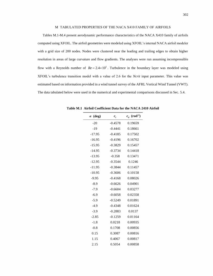
302

M TABULATED PROPERTIES OF THE NACA X410 FAMILY OF AIRFOILS

Tables M.1-M.4 present aerodynamic performance characteristics of the NACA X410 family of airfoils

computed using XFOIL. The airfoil geometries were modeled using XFOIL’s internal NACA airfoil modeler

with a grid size of 200 nodes. Nodes were clustered near the leading and trailing edges to obtain higher

resolution in areas of large curvature and flow gradients. The analyses were run assuming incompressible

flow with a Reynolds number of 52.4 10Re = . Turbulence in the boundary layer was modeled using

XFOIL’s turbulence transition model with a value of 2.6 for the Ncrit input parameter. This value was

estimated based on information provided in a wind tunnel survey of the AFRL Vertical Wind Tunnel (VWT).

The data tabulated below were used in the numerical and experimental comparisons discussed in Sec. 5.4.

Table M.1 Airfoil Coefficient Data for the NACA 2410 Airfoil

α (deg) lc

dc (rad-1)

-20 -0.4578 0.19659

-19 -0.4441 0.18661

-17.95 -0.4185 0.17502

-16.95 -0.4196 0.16702

-15.95 -0.3829 0.15457

-14.95 -0.3734 0.14418

-13.95 -0.358 0.13471

-12.95 -0.3544 0.1246

-11.95 -0.3844 0.11457

-10.95 -0.3606 0.10158

-9.95 -0.4168 0.08026

-8.9 -0.6626 0.04901

-7.9 -0.6604 0.03277

-6.9 -0.6058 0.02358

-5.9 -0.5249 0.01891

-4.9 -0.4348 0.01624

-3.9 -0.2883 0.0137

-2.85 -0.1259 0.01164

-1.8 0.0218 0.00935

-0.8 0.1708 0.00856

0.15 0.3087 0.00816

1.15 0.4067 0.00817

2.15 0.5054 0.00858

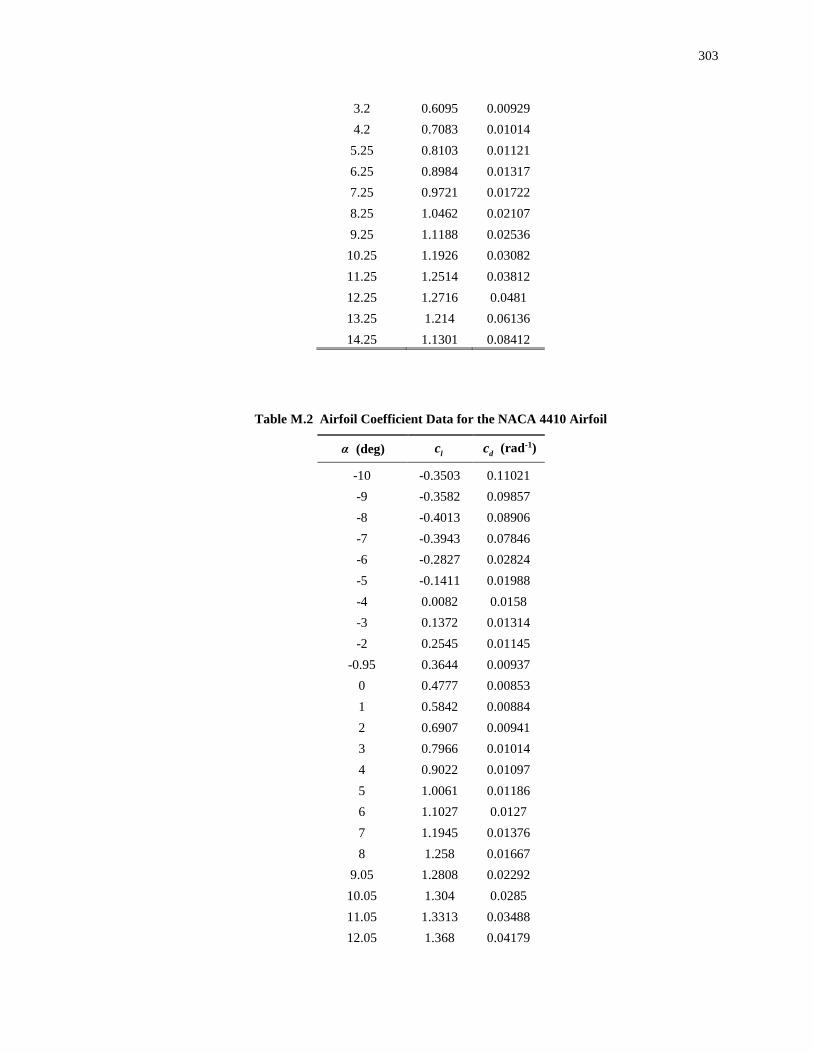
303

3.2 0.6095 0.00929

4.2 0.7083 0.01014

5.25 0.8103 0.01121

6.25 0.8984 0.01317

7.25 0.9721 0.01722

8.25 1.0462 0.02107

9.25 1.1188 0.02536

10.25 1.1926 0.03082

11.25 1.2514 0.03812

12.25 1.2716 0.0481

13.25 1.214 0.06136

14.25 1.1301 0.08412


α (deg) lc

dc (rad-1)

-10 -0.3503 0.11021

-9 -0.3582 0.09857

-8 -0.4013 0.08906

-7 -0.3943 0.07846

-6 -0.2827 0.02824

-5 -0.1411 0.01988

-4 0.0082 0.0158

-3 0.1372 0.01314

-2 0.2545 0.01145

-0.95 0.3644 0.00937

0 0.4777 0.00853

1 0.5842 0.00884

2 0.6907 0.00941

3 0.7966 0.01014

4 0.9022 0.01097

5 1.0061 0.01186

6 1.1027 0.0127

7 1.1945 0.01376

8 1.258 0.01667

9.05 1.2808 0.02292

10.05 1.304 0.0285

11.05 1.3313 0.03488

12.05 1.368 0.04179

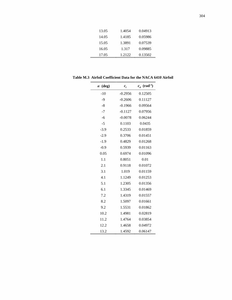
304

13.05 1.4054 0.04913

14.05 1.4185 0.05986

15.05 1.3891 0.07539

16.05 1.317 0.09885

17.05 1.2122 0.13502


α (deg) lc

dc (rad-1)

-10 -0.2956 0.12505

-9 -0.2606 0.11127

-8 -0.1966 0.09564

-7 -0.1127 0.07956

-6 -0.0078 0.06244

-5 0.1103 0.0435

-3.9 0.2533 0.01859

-2.9 0.3706 0.01451

-1.9 0.4829 0.01268

-0.9 0.5939 0.01163

0.05 0.6974 0.01096

1.1 0.8051 0.01

2.1 0.9118 0.01072

3.1 1.019 0.01159

4.1 1.1249 0.01253

5.1 1.2305 0.01356

6.1 1.3345 0.01469

7.2 1.4319 0.01557

8.2 1.5097 0.01661

9.2 1.5531 0.01862

10.2 1.4981 0.02819

11.2 1.4764 0.03854

12.2 1.4658 0.04972

13.2 1.4592 0.06147

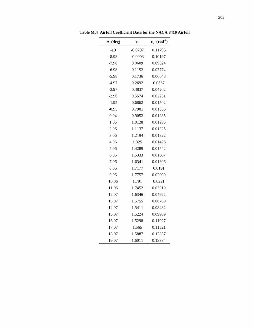
305


α (deg) lc

dc (rad-1)

-10 -0.0797 0.11796

-8.98 -0.0003 0.10197

-7.98 0.0609 0.09024

-6.98 0.1152 0.07774

-5.98 0.1736 0.06648

-4.97 0.2692 0.0537

-3.97 0.3837 0.04202

-2.96 0.5574 0.02251

-1.95 0.6862 0.01502

-0.95 0.7981 0.01335

0.04 0.9052 0.01285

1.05 1.0128 0.01285

2.06 1.1137 0.01225

3.06 1.2194 0.01322

4.06 1.325 0.01428

5.06 1.4289 0.01542

6.06 1.5333 0.01667

7.06 1.6341 0.01806

8.06 1.7177 0.0191

9.06 1.7757 0.02009

10.06 1.791 0.0221

11.06 1.7452 0.03019

12.07 1.6346 0.04922

13.07 1.5755 0.06769

14.07 1.5411 0.08482

15.07 1.5224 0.09989

16.07 1.5298 0.11027

17.07 1.565 0.11521

18.07 1.5887 0.12357

19.07 1.6011 0.13384

306

CURRICULUM VITAE

Joshua D. Hodson

July 2019

EDUCATION

Ph.D. Mechanical Engineering, Utah State University, Jun. 2019 (3.96 GPA)

Numerical Analysis and Spanwise Shape Optimization for Finite Wings of Arbitrary Aspect Ratio

M.S. Mechanical Engineering, Utah State University, Aug. 2007 (3.96 GPA)

RANS Modeling of Nuclear Reactor Lower Plenum Geometries

B.S. Mechanical Engineering, Utah State University, Aug. 2007 (3.77 GPA, Cum Laude)

TEACHING AND PROFESSIONAL EXPERIENCE

03/18 – present Aerospace Research Engineer, Air Force Research Laboratory

12/06 – 02/18 Sr. Principle Mechanical Engineer (Analysis), Orbital ATK Flight Systems

05/17 – 08/17 Graduate Research Assistant, Air Force Research Laboratory

01/17 – 05/17 Teaching Assistant (Computational Fluid Dynamics), Utah State University

08/16 – 12/16 Instructor (Aerodynamics), Utah State University

08/13 – 12/13 Teaching Assistant (Thermodynamics II), Utah State University

05/05 – 12/06 Graduate Research Assistant, Utah State University

05/04 – 04/05 Mechanical Engineer Intern (Design), Space Dynamics Laboratory

01/04 – 05/04 Math Tutor, Utah State University

JOURNAL PUBLICATIONS

[1] D. Hunsaker, J. Taylor, J. Hodson, and O. Pope, “Aerodynamic Centers of Arbitrary Airfoils below

Stall,” J. Aircraft, accepted for publication.

[2] B. Limb, D. Work, J. Hodson, and B. Smith, “The Inefficacy of Chauvenet’s Criterion for

Elimination of Data Points,” J. Fluids Eng., Vol. 139, No. 5, Jun. 2016.

[3] J. Hodson, R. Spall, and B. Smith, “Turbulence Model Assessment for Flow across a Row of

Confined Cylinders,” Nuclear Technology, Vol. 161, pp. 268-276, 2008.

CONFERENCE PRESENTATIONS AND PAPERS

[1] J. Hodson, G. Reich, J. Deaton, A. Pankonien, P. Beran, “Aerostructure Design of a 2D Morphing

Airfoil in Unsteady Supersonic Flow using Bio-Inspired Evolutionary Design Processes and Low-

Fidelity Physics Models,” ASME SMASIS, Louisville, KY, Sep. 2019, accepted for presentation,

SMASIS2019-5598.

[2] B. Bielefeldt, D. Hartl, J. Hodson, G. Reich, P. Beran, A. Pankonien, J. Deaton, “Graph-Based

Interpretation of L-System Encodings Toward Aeroelastic Topology Optimization of a Morphing

Airfoil in Supersonic Flow,” Proceedings of the ASME Conference on Smart Materials, Adaptive

Structures and Intelligent Systems, Louisville, KY, Sep. 2019, accepted for publication,

SMASIS2019-5609.

[3] J. Hodson, A. Christopherson, J. Deaton, A. Pankonien, G. Reich, and P. Beran, “Aeroelastic

Topology Optimization of a Morphing Airfoil in Supersonic Flow using Evolutionary Design,”

Multidisciplinary Design Optimization, AIAA SciTech Forum, San Diego, CA, Jan. 2019, AIAA-

2019-1466.

307

[4] D. Hunsaker, O. Pope, J. Hodson, and J. Rosqvist, “Aerodynamic Centers of Arbitrary Airfoils,”

AIAA Aerospace Sciences Meeting, AIAA SciTech Forum, Kissimmee, FL, Jan. 2018.

[5] R. Spall and J. Hodson, “Educational Results obtained using an Improved Two-Dimensional Panel

Method Code in Undergraduate Fluid Dynamics and Aerodynamics Courses,” ASME Fluids

Engineering Division Summer Meeting, Waikoloa, HI, Jul. 2017, FEDSM2017-69031.

[6] J. Hodson, D. Hunsaker, B. Andrews, and J. Joo, “Experimental Results for a Variable Camber

Compliant Wing,” 35th AIAA Applied Aerodynamics Conference, AIAA Aviation Forum, Denver,

CO, Jun. 2017, AIAA-2017-4222.

[7] J. Hodson, D. Hunsaker, and R. Spall, “Wing Optimization using Dual Number Automatic

Differentiation in MachUp,” 55th AIAA Aerospace Sciences Meeting, AIAA SciTech Forum,

Grapevine, TX, Jan. 2017, AIAA-2017-0033.

[8] H. Dewey, J. Hodson, and K. Illum, “Asset Monitoring with the Internet of Things,” Orbital ATK

Internal Conference, Apr. 2016.

[9] J. Hodson, H. Dewey, and D. DeVries, “Individual Motor Monitoring and Data Management

Solutions to Solid Rocket Prognostic Health Management,” JANNAF 43rd Structures and

Mechanical Behavior Subcommittee Meeting, Salt Lake City, UT, Dec. 2015.

[10] J. Hodson, J. Forsmann, and R. Spall, “Dual Number Automatic Differentiation in RELAP5-3D”,

International RELAP5 User Group Meeting, Idaho Falls, ID, Aug. 2015.

[11] J. Hodson and H. Dewey, “IMLM DAAS Software Design and Implementation,” Orbital ATK

Internal Conference, Apr. 2015.

[12] J. Hodson and R. Spall, “Dual Number Automatic Differentiation for CFD Optimization,” Utah

Fluids Meeting, Aug. 2014.

[13] R. Monson and J. Hodson, “Real-Time Model Updates using Sensor Data in IMLM DAAS,”

JANNAF 9th Modeling and Simulation Subcommittee Meeting, Colorado Springs, CO, Apr. 2013.

[14] J. Hodson, R. Spall, and B. Smith, “RANS Predictions in an Idealized Lower-Plenum Model,” 14th

International Conference on Nuclear Engineering, Jul. 2006. ICONE14-89222.

[15] J. Hodson, E. Thorston, R. Spall, and B. Smith, “CFD Validation of Flow Regimes in an Idealized

Lower-Plenum Model,” ANS Winter Meeting and Technology Expo., Washington, D.C., Nov. 2005.

Numerical Analysis and Spanwise Shape Optimization for ...

Documents

Transcript of Numerical Analysis and Spanwise Shape Optimization for ...