Novel Auto-Reclosing Blocking Method for Combined ... - MDPI

energies

Article

Novel Auto-Reclosing Blocking Method forCombined Overhead-Cable Lines in Power NetworksRicardo Granizo Arrabé 1,*, Carlos Antonio Platero Gaona 1, Fernando Álvarez Gómez 2

and Emilio Rebollo López 1

1 Department of Electrical Engineering, ETS Ingenieros Industriales, Technical University of Madrid,C/José Gutierrez Abascal, 2, 28006 Madrid, Spain; [email protected] (C.A.P.G.);[email protected] (E.R.L.)

2 Department of Electrical Engineering, ETS Ingeniería y Diseño Industrial, Technical University of Madrid,C/Ronda de Valencia, 3, 28012 Madrid, Spain; [email protected]

* Correspondence: [email protected]; Tel.: +34-91-336-6842

Academic Editor: Miguel CastillaReceived: 25 June 2016; Accepted: 15 November 2016; Published: 17 November 2016

Abstract: This paper presents a novel auto-reclosing blocking method for combined overhead-cablelines in power distribution networks that are solidly or impedance grounded, with distributiontransformers in a delta connection in their high-voltage sides. The main contribution of this newtechnique is that it can detect whether a ground fault has been produced at the overhead lineside or at the cable line side, thus improving the performance of the auto-reclosing functionality.This localization technique is based on the measurements and analysis of the argument differencesbetween the load currents in the active conductors of the cable and the currents in the shields atthe cable end where the transformers in delta connection are installed, including a wavelet analysis.This technique has been verified through computer simulations and experimental laboratory tests.

Keywords: ground faults; protection; distribution protections; electrical distribution networks

1. Introduction

Power systems use protection devices to detect and clear different types of short circuits, overloadsand, in general, abnormal working conditions or fault situations that might be dangerous to the facilitiesand the stability of the electrical power system. Most faults in power distribution networks are locatedin the lines those that take place in the machinery, switchgear and measurement devices installed at themain substations. Some distribution lines have two different parts: the cable line side and the overheadline side [1]. Protection relays have the responsibility to clear faults that happen in their protectionzones and for that purpose, a close and quite approximate location of the ground fault in electricalpower systems is required for protection systems [2]. Overhead protection systems have differentworking principles to cable protection systems [3]. At any distribution line, the protection system mustguarantee the power supply in the most reliable way. For that purpose, there are many protectionfunctions implemented to clear up all types of possible faults and keep the grid as stable as possible.Power distribution networks normally have voltage levels up to 45 kV although in some countries inEurope their voltage levels can reach up to 150 kV [4]. If there is a ground fault, a three-phase trippingorder will be given to clear it, and a loss of power demand results [5]. It is extremely important to knowthe maximum reclosing time [6,7] to recover power supply and keep the system as stable as possible.

When a distribution line is formed by cable and overhead sections (Figure 1), faults in the cableline side cause irreparable damage because the insulation of the cable has been partially or totallydeteriorated: this is the reason why reclosing attempts are not allowed. Faults at the overhead lineside are normally produced by lightning strikes [8]. On the other hand, faults in the overhead line side

Energies 2016, 9, 964; doi:10.3390/en9110964 www.mdpi.com/journal/energies

http://www.mdpi.com/journal/energies

http://www.mdpi.com

http://www.mdpi.com/journal/energies

Energies 2016, 9, 964 2 of 20

permit reclosing without risk, because the air insulation is normally recovered in a few millisecondsand almost one second if there is mutual capacitive coupling to other lines.

Energies 2016, 9, 964 2 of 21

side are normally produced by lightning strikes [8]. On the other hand, faults in the overhead line

side permit reclosing without risk, because the air insulation is normally recovered in a few

milliseconds and almost one second if there is mutual capacitive coupling to other lines.

(Rsa)

(Zta)Transition

Station

(Rt)(Rsb)

(Rt)

(Rt)

(Rt)

(1)

(2)

Distribution

Substation - A

Overhead

Line - 1

Overhead

Line - 2

Overhead

Line - n

(2)

End

Substation - B

Figure 1. Power distribution network with transition cable-overhead line. (1) Active conductor of

power cables; (2) Shields of the power cable; (Rt) Tower ground resistance; (Rsa) Ground resistance of

distribution substation-A; (Rsb) Ground resistance of end substation-B; (Zta) Grounding impedance.

In Figure 1, the earthing of the cable shields at the transition station is connected to of the

corresponding tower, whose earthing resistance value is represented as Rt. Substations A and B have

their respective grounding resistances Rsa and Rsb. The earthing resistances Rt at every tower have

normally slightly different values.

If a fault occurs at the cable line side and is cleared up, a post-reclosing order on the fault

condition will be an unsuccessful reclosing maneuver. Also, the grid will have to withstand a new

fault condition and be able to clear it up again. Beside these two disadvantages of unsuccessful

reclosing maneuvers, another is the fact of creating significant and extensive damage in the cable,

being the most probable consequence to have to replace it entirely. This circumstance will keep the

distribution line out of order for a long time while the cable is replaced. Therefore, the

discrimination of the fault in the overhead side or in the line side is essential to allow to protection

and the control system to send a reclosing order [9]. Currently, there are different protection criteria

to remove from service a line with a ground fault.

This presents a technique that determines where the ground fault has taken place in an

overhead-cable line considering a grounding method mostly used in power distribution networks

with the overhead side substations solidly grounded, or through grounding impedance with low

ohmic value. At the cable end side, the system is ungrounded with power transformers in a delta

connection in their primary side. The models used follow the impedance calculation described in the

standard EN60909-3 [10].

We first present a brief overview of line protection techniques. Section 2 describes the

formulation used for modeling the cables. Section 3 includes the impedances of cables and general

equations for shield connections. Then, Section 4 details the principles of the proposed

auto-reclosing blocking method technique. Section 5 analyzes the software simulations of the

operation of the proposed method, and Section 6 presents the results of experimental fault tests

carried out in the laboratory. Finally, Section 7 concludes with the main contributions of the

proposed technique.

Figure 1. Power distribution network with transition cable-overhead line. (1) Active conductor ofpower cables; (2) Shields of the power cable; (Rt) Tower ground resistance; (Rsa) Ground resistance ofdistribution substation-A; (Rsb) Ground resistance of end substation-B; (Zta) Grounding impedance.

In Figure 1, the earthing of the cable shields at the transition station is connected to of thecorresponding tower, whose earthing resistance value is represented as Rt. Substations A and B havetheir respective grounding resistances Rsa and Rsb. The earthing resistances Rt at every tower havenormally slightly different values.

If a fault occurs at the cable line side and is cleared up, a post-reclosing order on the fault conditionwill be an unsuccessful reclosing maneuver. Also, the grid will have to withstand a new fault conditionand be able to clear it up again. Beside these two disadvantages of unsuccessful reclosing maneuvers,another is the fact of creating significant and extensive damage in the cable, being the most probableconsequence to have to replace it entirely. This circumstance will keep the distribution line out oforder for a long time while the cable is replaced. Therefore, the discrimination of the fault in theoverhead side or in the line side is essential to allow to protection and the control system to senda reclosing order [9]. Currently, there are different protection criteria to remove from service a linewith a ground fault.

This presents a technique that determines where the ground fault has taken place inan overhead-cable line considering a grounding method mostly used in power distribution networkswith the overhead side substations solidly grounded, or through grounding impedance with lowohmic value. At the cable end side, the system is ungrounded with power transformers in a deltaconnection in their primary side. The models used follow the impedance calculation described in thestandard EN60909-3 [10].

We first present a brief overview of line protection techniques. Section 2 describes the formulationused for modeling the cables. Section 3 includes the impedances of cables and general equations forshield connections. Then, Section 4 details the principles of the proposed auto-reclosing blockingmethod technique. Section 5 analyzes the software simulations of the operation of the proposedmethod, and Section 6 presents the results of experimental fault tests carried out in the laboratory.Finally, Section 7 concludes with the main contributions of the proposed technique.

Energies 2016, 9, 964 3 of 20

2. State-of-the-Art

There are two main protection relays that incorporate the auto-reclosing facility in powerdistribution networks: distance and ground fault directional overcurrent protection relays. In thissection, both techniques are presented.

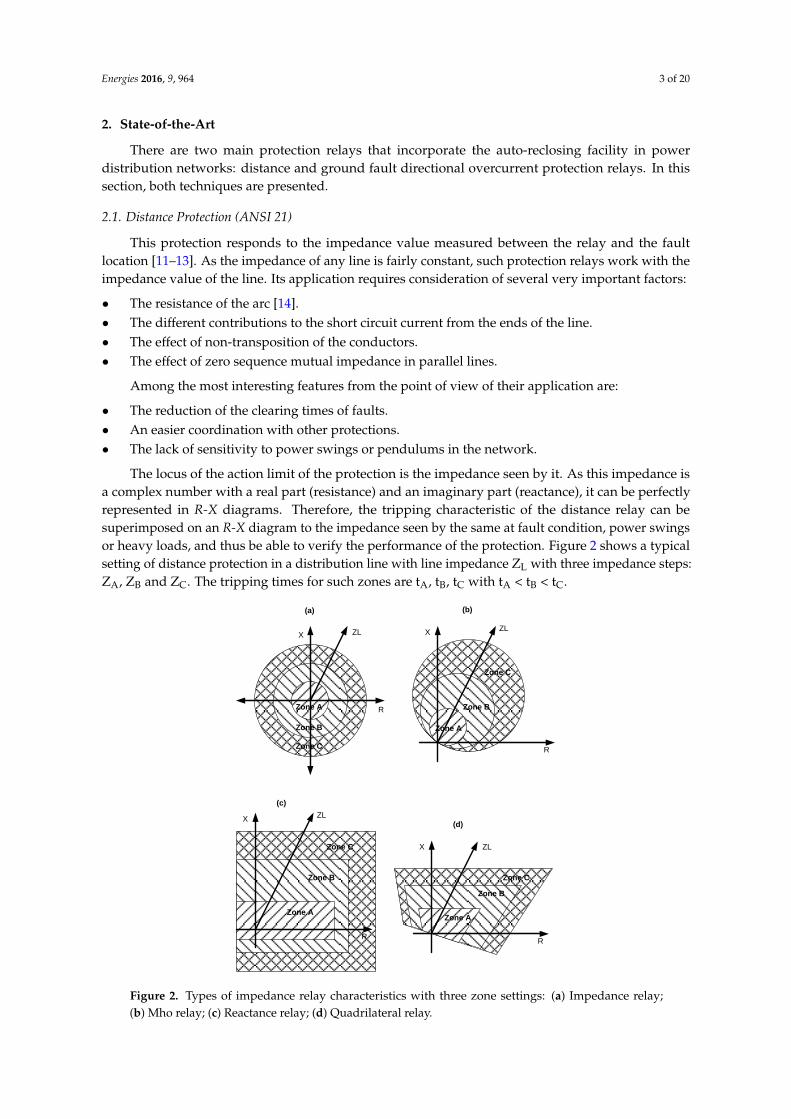
2.1. Distance Protection (ANSI 21)

This protection responds to the impedance value measured between the relay and the faultlocation [11–13]. As the impedance of any line is fairly constant, such protection relays work with theimpedance value of the line. Its application requires consideration of several very important factors:

• The resistance of the arc [14].• The different contributions to the short circuit current from the ends of the line.• The effect of non-transposition of the conductors.• The effect of zero sequence mutual impedance in parallel lines.

Among the most interesting features from the point of view of their application are:

• The reduction of the clearing times of faults.• An easier coordination with other protections.• The lack of sensitivity to power swings or pendulums in the network.

The locus of the action limit of the protection is the impedance seen by it. As this impedance isa complex number with a real part (resistance) and an imaginary part (reactance), it can be perfectlyrepresented in R-X diagrams. Therefore, the tripping characteristic of the distance relay can besuperimposed on an R-X diagram to the impedance seen by the same at fault condition, power swingsor heavy loads, and thus be able to verify the performance of the protection. Figure 2 shows a typicalsetting of distance protection in a distribution line with line impedance ZL with three impedance steps:ZA, ZB and ZC. The tripping times for such zones are tA, tB, tC with tA < tB < tC.

Energies 2016, 9, 964 3 of 21

2. State-of-the-Art

There are two main protection relays that incorporate the auto-reclosing facility in power

distribution networks: distance and ground fault directional overcurrent protection relays. In this

section, both techniques are presented.

2.1. Distance Protection (ANSI 21)

This protection responds to the impedance value measured between the relay and the fault

location [11–13]. As the impedance of any line is fairly constant, such protection relays work with the

impedance value of the line. Its application requires consideration of several very important factors:

The resistance of the arc [14].

The different contributions to the short circuit current from the ends of the line.

The effect of non-transposition of the conductors.

The effect of zero sequence mutual impedance in parallel lines.

Among the most interesting features from the point of view of their application are:

The reduction of the clearing times of faults.

An easier coordination with other protections.

The lack of sensitivity to power swings or pendulums in the network.

The locus of the action limit of the protection is the impedance seen by it. As this impedance is a

complex number with a real part (resistance) and an imaginary part (reactance), it can be perfectly

represented in R-X diagrams. Therefore, the tripping characteristic of the distance relay can be

superimposed on an R-X diagram to the impedance seen by the same at fault condition, power

swings or heavy loads, and thus be able to verify the performance of the protection. Figure 2 shows a

typical setting of distance protection in a distribution line with line impedance ZL with three

impedance steps: ZA, ZB and ZC. The tripping times for such zones are tA, tB, tC with tA < tB < tC.

R

X ZL

Zone C

Zone B

Zone A

R

XZL

Zone A

Zone B

Zone C

R

XZL

Zone A

Zone B

Zone C

Zone A

R

X ZL

Zone C

Zone B

Zone A

(a) (b)

(c)

(d)

Figure 2. Types of impedance relay characteristics with three zone settings: (a) Impedance relay;

(b) Mho relay; (c) Reactance relay; (d) Quadrilateral relay.

Figure 2. Types of impedance relay characteristics with three zone settings: (a) Impedance relay;(b) Mho relay; (c) Reactance relay; (d) Quadrilateral relay.

Energies 2016, 9, 964 4 of 20

Any small current or voltage transformer error could represent an important increase or decreasein the measured impedance. Consequently, if the fault was produced very close to the transitionoverhead-cable line, it is not known in which side it has happened. Therefore, impedance protectionis not fully selective to discriminate whether the ground fault has happened in the cable or in theoverhead side. In power distribution networks rated 45 or 66 kV, distance protection is mainly usedwhen the system is solidly grounded.

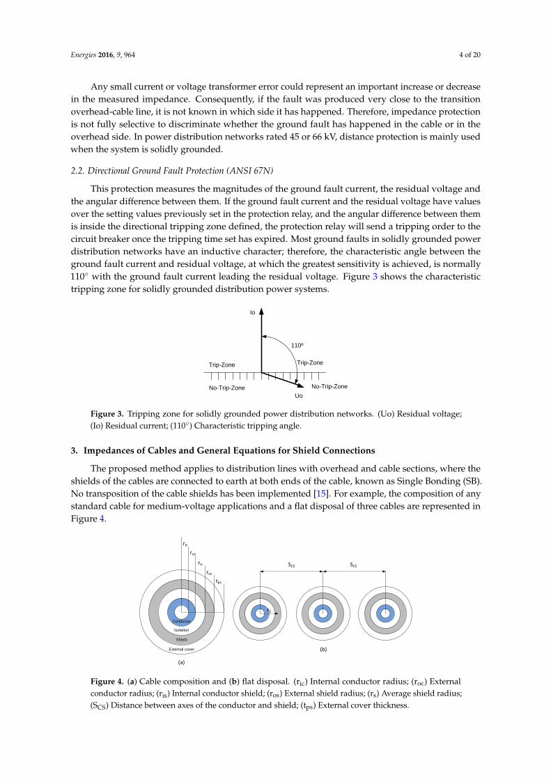
2.2. Directional Ground Fault Protection (ANSI 67N)

This protection measures the magnitudes of the ground fault current, the residual voltage andthe angular difference between them. If the ground fault current and the residual voltage have valuesover the setting values previously set in the protection relay, and the angular difference between themis inside the directional tripping zone defined, the protection relay will send a tripping order to thecircuit breaker once the tripping time set has expired. Most ground faults in solidly grounded powerdistribution networks have an inductive character; therefore, the characteristic angle between theground fault current and residual voltage, at which the greatest sensitivity is achieved, is normally110 with the ground fault current leading the residual voltage. Figure 3 shows the characteristictripping zone for solidly grounded distribution power systems.

Energies 2016, 9, 964 4 of 21

Any small current or voltage transformer error could represent an important increase or

decrease in the measured impedance. Consequently, if the fault was produced very close to the

transition overhead-cable line, it is not known in which side it has happened. Therefore, impedance

protection is not fully selective to discriminate whether the ground fault has happened in the cable

or in the overhead side. In power distribution networks rated 45 or 66 kV, distance protection is

mainly used when the system is solidly grounded.


This protection measures the magnitudes of the ground fault current, the residual voltage and

the angular difference between them. If the ground fault current and the residual voltage have

values over the setting values previously set in the protection relay, and the angular difference

between them is inside the directional tripping zone defined, the protection relay will send a

tripping order to the circuit breaker once the tripping time set has expired. Most ground faults in

solidly grounded power distribution networks have an inductive character; therefore, the

characteristic angle between the ground fault current and residual voltage, at which the greatest

sensitivity is achieved, is normally 110° with the ground fault current leading the residual voltage.

Figure 3 shows the characteristic tripping zone for solidly grounded distribution power systems.

Uo

Io

110º

No-Trip-Zone

Trip-Zone Trip-Zone

No-Trip-Zone

Figure 3. Tripping zone for solidly grounded power distribution networks. (Uo) Residual voltage;

(Io) Residual current; (110°) Characteristic tripping angle.

3. Impedances of Cables and General Equations for Shield Connections

The proposed method applies to distribution lines with overhead and cable sections, where the

shields of the cables are connected to earth at both ends of the cable, known as Single Bonding (SB).

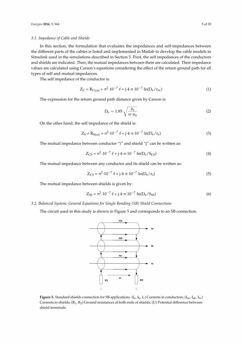
No transposition of the cable shields has been implemented [15]. For example, the composition of

any standard cable for medium-voltage applications and a flat disposal of three cables are

represented in Figure 4.

ric

roc

ris

ros

tps

Isolation

Shield

External cover

Conductor

SCS SCS

rS

(a)

(b)

Figure 4. (a) Cable composition and (b) flat disposal. (ric) Internal conductor radius; (roc) External

conductor radius; (ris) Internal conductor shield; (ros) External shield radius; (rs) Average shield

radius; (SCS) Distance between axes of the conductor and shield; (tps) External cover thickness.

Figure 3. Tripping zone for solidly grounded power distribution networks. (Uo) Residual voltage;(Io) Residual current; (110) Characteristic tripping angle.


The proposed method applies to distribution lines with overhead and cable sections, where theshields of the cables are connected to earth at both ends of the cable, known as Single Bonding (SB).No transposition of the cable shields has been implemented [15]. For example, the composition of anystandard cable for medium-voltage applications and a flat disposal of three cables are represented inFigure 4.

Energies 2016, 9, 964 4 of 21

Any small current or voltage transformer error could represent an important increase or

decrease in the measured impedance. Consequently, if the fault was produced very close to the

transition overhead-cable line, it is not known in which side it has happened. Therefore, impedance

protection is not fully selective to discriminate whether the ground fault has happened in the cable

or in the overhead side. In power distribution networks rated 45 or 66 kV, distance protection is

mainly used when the system is solidly grounded.


This protection measures the magnitudes of the ground fault current, the residual voltage and

the angular difference between them. If the ground fault current and the residual voltage have

values over the setting values previously set in the protection relay, and the angular difference

between them is inside the directional tripping zone defined, the protection relay will send a

tripping order to the circuit breaker once the tripping time set has expired. Most ground faults in

solidly grounded power distribution networks have an inductive character; therefore, the

characteristic angle between the ground fault current and residual voltage, at which the greatest

sensitivity is achieved, is normally 110° with the ground fault current leading the residual voltage.

Figure 3 shows the characteristic tripping zone for solidly grounded distribution power systems.

Uo

Io

110º

No-Trip-Zone

Trip-Zone Trip-Zone

No-Trip-Zone

Figure 3. Tripping zone for solidly grounded power distribution networks. (Uo) Residual voltage;

(Io) Residual current; (110°) Characteristic tripping angle.


The proposed method applies to distribution lines with overhead and cable sections, where the

shields of the cables are connected to earth at both ends of the cable, known as Single Bonding (SB).

No transposition of the cable shields has been implemented [15]. For example, the composition of

any standard cable for medium-voltage applications and a flat disposal of three cables are

represented in Figure 4.

ric

roc

ris

ros

tps

Isolation

Shield

External cover

Conductor

SCS SCS

rS

(a)

(b)

Figure 4. (a) Cable composition and (b) flat disposal. (ric) Internal conductor radius; (roc) External

conductor radius; (ris) Internal conductor shield; (ros) External shield radius; (rs) Average shield

radius; (SCS) Distance between axes of the conductor and shield; (tps) External cover thickness.

Figure 4. (a) Cable composition and (b) flat disposal. (ric) Internal conductor radius; (roc) Externalconductor radius; (ris) Internal conductor shield; (ros) External shield radius; (rs) Average shield radius;(SCS) Distance between axes of the conductor and shield; (tps) External cover thickness.

Energies 2016, 9, 964 5 of 20

3.1. Impedance of Cable and Shields

In this section, the formulation that evaluates the impedances and self-impedances betweenthe different parts of the cables is listed and implemented in Matlab to develop the cable models inSimulink used in the simulations described in Section 5. First, the self impedances of the conductorsand shields are indicated. Then, the mutual impedances between them are calculated. Their impedancevalues are calculated using Carson’s equations considering the effect of the return ground path for alltypes of self and mutual impedances.

The self impedance of the conductor is:

ZC = RC(ca) + π2·10−7·f + j·4·π·10−7·ln(De/roc) (1)

The expression for the return ground path distance given by Carson is:

De = 1.85·√

ρeω·µo

(2)

On the other hand, the self impedance of the shield is:

ZS = RS(ca) + π2·10−7·f + j·4·π·10−7·ln(De/rs) (3)

The mutual impedance between conductor “i” and shield “j” can be written as:

ZCS = π2·10−7·f + j·4·π·10−7·ln(De/SCS) (4)

The mutual impedance between any conductor and its shield can be written as:

ZCS = π2·10−7·f + j·4·π·10−7·ln(De/rs) (5)

The mutual impedance between shields is given by:

ZSS = π2·10−7·f + j·4·π·10−7·ln(De/SSS) (6)

3.2. Balanced System: General Equations for Single Bonding (SB) Shield Connections

The circuit used in this study is shown in Figure 5 and corresponds to an SB connection.

Energies 2016, 9, 964 5 of 21

3.1. Impedance of Cable and Shields

In this section, the formulation that evaluates the impedances and self-impedances between the

different parts of the cables is listed and implemented in Matlab to develop the cable models in

Simulink used in the simulations described in Section 5. First, the self impedances of the conductors

and shields are indicated. Then, the mutual impedances between them are calculated. Their

impedance values are calculated using Carson s equations considering the effect of the return

ground path for all types of self and mutual impedances.

The self impedance of the conductor is:

ZC = RC(ca) + π2·10−7·f + j·4·π·10−7·ln(De/roc) (1)

The expression for the return ground path distance given by Carson is:

De = 1.85·√ρe

ω·μo (2)

On the other hand, the self impedance of the shield is:

ZS = RS(ca) + π2·10−7·f + j·4·π·10−7·ln(De/rs) (3)

The mutual impedance between conductor “i” and shield “j” can be written as:

ZCS = π2·10−7·f + j·4·π·10−7·ln(De/SCS) (4)

The mutual impedance between any conductor and its shield can be written as:

ZCS = π2·10−7·f + j·4·π·10−7·ln(De/rs) (5)

The mutual impedance between shields is given by:

ZSS = π2·10−7·f + j·4·π·10−7·ln(De/SSS) (6)

3.2. Balanced System: General Equations for Single Bonding (SB) Shield Connections

The circuit used in this study is shown in Figure 5 and corresponds to an SB connection.

R1 R2U

Ia

Ib

Ic

Isa

Isb

Isc

Figure 5. Standard shields connection for SB applications. (Ia, Ib, Ic) Currents in conductors;

(Isa, Isb, Isc) Currents in shields; (R1, R2) Ground resistances at both ends of shields; (U) Potential

difference between shield terminals.

When the load currents form a three-phase balanced system and only a positive sequence

component exists, the vector sum of the line currents flowing in the conductors is zero. The voltages

induced in the shields have a component due to the flow of current through conductor, and another

due to the currents circulating in the shields. As shown in Figure 5, the shields are grounded at both

ends and the voltages between the two grounding connections are equal to the three shields as:

Figure 5. Standard shields connection for SB applications. (Ia, Ib, Ic) Currents in conductors; (Isa, Isb, Isc)Currents in shields; (R1, R2) Ground resistances at both ends of shields; (U) Potential difference betweenshield terminals.

Energies 2016, 9, 964 6 of 20

When the load currents form a three-phase balanced system and only a positive sequencecomponent exists, the vector sum of the line currents flowing in the conductors is zero. The voltagesinduced in the shields have a component due to the flow of current through conductor, and anotherdue to the currents circulating in the shields. As shown in Figure 5, the shields are grounded at bothends and the voltages between the two grounding connections are equal to the three shields as:

U = U1C + U1S = U2C + U2S = U3C + U3S (7)

The mathematical models for such induced voltages are listed below:

• Induced voltages in shields due to circulating currents in conductors:

U1C = L·(ZC1S1·I1 + ZC2S1·I2 + ZC3S1·I3) (8)



• Induced voltages in shields due to circulating currents in shields:

U1S = L·(ZS1S1·IS1 + ZS2S1·IS2 + ZS3S1·IS3) (11)



All the previous equations can be expressed as a matrix system: U1

U2

U3

=

U1C

U2C

U3C

+

U1S

U2S

U3S

(14)

where: U1

U2

U3

= L ·

ZC1S1 ZC2S1 ZC3S1

ZC1S2 ZC2S2 ZC3S2

ZC1S3 ZC2S3 ZC3S3

·

I1

I2

I3

+L ·

ZS1S1 ZS2S1 ZS3S1

ZS1S2 ZS2S2 ZS3S2

ZS1S3 ZS2S3 ZS3S3

·

IS1

IS2

IS3

(15)

4. Principles of Novel Auto-Reclosing Blocking Method for Power Distribution Networks

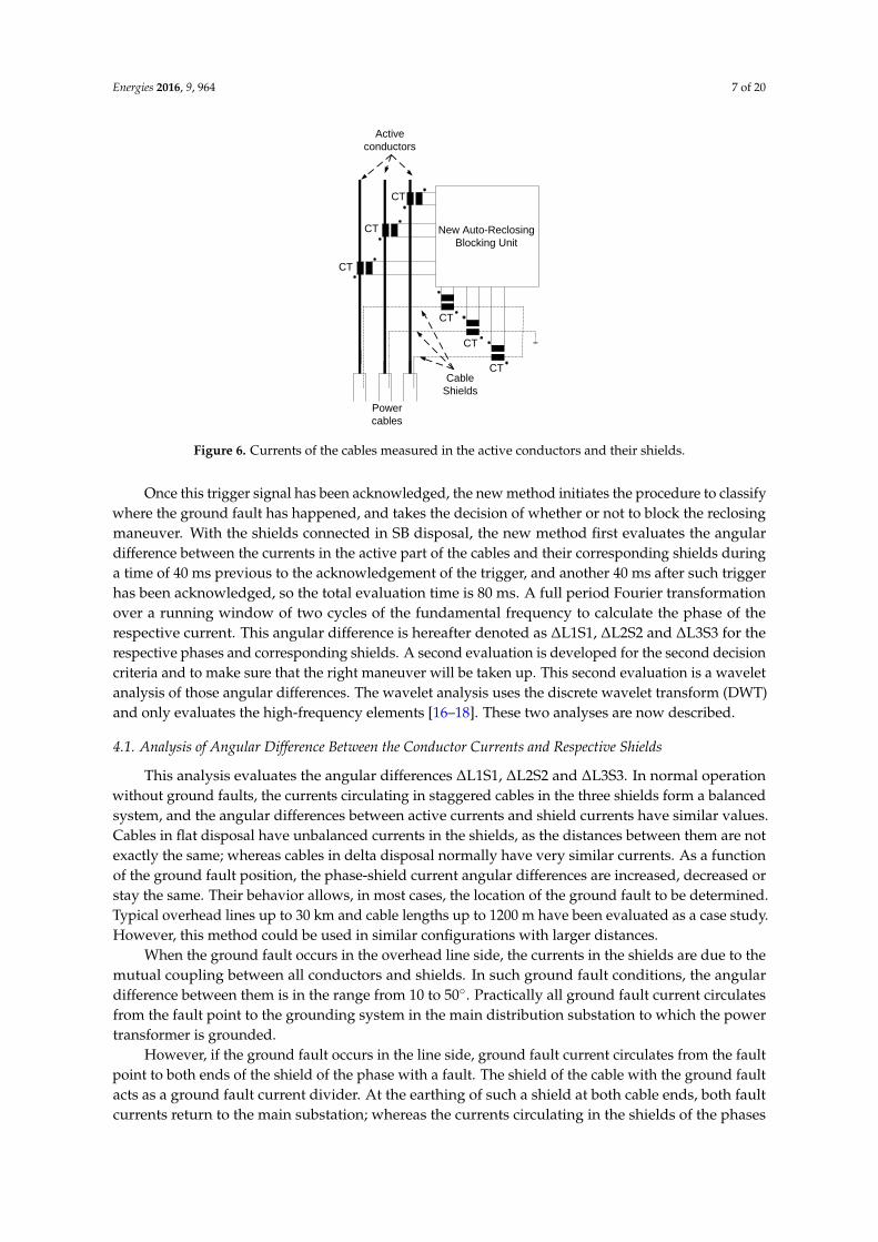
The new method presented measures the currents at the three shields of the cables at their endslocated at the substation side, and the currents in the active part of the three phases of the cableas indicated in Figure 6. This was studied for solidly or low-value impedance grounded powerdistribution networks with distribution transformers in a delta connection at their high-voltage sides.This method is valid when the transition overhead-cable is not very far away from the substation wherethe measurements of currents in shields and conductors are done. We employ a trigger signal to startthe analysis and consider a total time signal length of 40 ms as a pre-trigger time and 40 ms active faulttime. The trigger signal is provided by any protection relay when a ground fault has been detected.The time set 40 ms for the active fault time is acceptable, as the ground faults at power distributionnetworks are active for longer times and the minimum tripping time for standard overcurrent orvoltage relays is 30 ms. Apart from this time, the medium-voltage circuit breaker opening times are notless than 40–50 ms. This means that 40 ms as an active fault time is good enough, as will be verified inthe simulation and real test results.

Energies 2016, 9, 964 7 of 20

Energies 2016, 9, 964 7 of 21

ΔL3S3 for the respective phases and corresponding shields. A second evaluation is developed for the

second decision criteria and to make sure that the right maneuver will be taken up. This second

evaluation is a wavelet analysis of those angular differences. The wavelet analysis uses the discrete

wavelet transform (DWT) and only evaluates the high-frequency elements [16–18]. These two

analyses are now described.

Cable

Shields

Active

conductors

New Auto-Reclosing

Blocking Unit

Power

cables

CT

CT

CT

CT

CT

CT

Figure 6. Currents of the cables measured in the active conductors and their shields.

4.1. Analysis of Angular Difference Between the Conductor Currents and Respective Shields

This analysis evaluates the angular differences ΔL1S1, ΔL2S2 and ΔL3S3. In normal operation

without ground faults, the currents circulating in staggered cables in the three shields form a

balanced system, and the angular differences between active currents and shield currents have

similar values. Cables in flat disposal have unbalanced currents in the shields, as the distances

between them are not exactly the same; whereas cables in delta disposal normally have very similar

currents. As a function of the ground fault position, the phase-shield current angular differences are

increased, decreased or stay the same. Their behavior allows, in most cases, the location of the

ground fault to be determined. Typical overhead lines up to 30 km and cable lengths up to 1200 m

have been evaluated as a case study. However, this method could be used in similar configurations

with larger distances.

When the ground fault occurs in the overhead line side, the currents in the shields are due to the

mutual coupling between all conductors and shields. In such ground fault conditions, the angular

difference between them is in the range from 10 to 50°. Practically all ground fault current circulates

from the fault point to the grounding system in the main distribution substation to which the power

transformer is grounded.

However, if the ground fault occurs in the line side, ground fault current circulates from the

fault point to both ends of the shield of the phase with a fault. The shield of the cable with the

ground fault acts as a ground fault current divider. At the earthing of such a shield at both cable

ends, both fault currents return to the main substation; whereas the currents circulating in the

shields of the phases without any fault keep circulating from one end to the other of the cable. This

circulation process makes ΔL1S1, ΔL2S2 and ΔL3S3 greatly increase and have values well above 50°

The threshold to decide whether the auto-reclosing maneuver is blocked has been selected as 50°,

which appears in the algorithm developed for this new application.

Figure 6. Currents of the cables measured in the active conductors and their shields.

Once this trigger signal has been acknowledged, the new method initiates the procedure to classifywhere the ground fault has happened, and takes the decision of whether or not to block the reclosingmaneuver. With the shields connected in SB disposal, the new method first evaluates the angulardifference between the currents in the active part of the cables and their corresponding shields duringa time of 40 ms previous to the acknowledgement of the trigger, and another 40 ms after such triggerhas been acknowledged, so the total evaluation time is 80 ms. A full period Fourier transformationover a running window of two cycles of the fundamental frequency to calculate the phase of therespective current. This angular difference is hereafter denoted as ∆L1S1, ∆L2S2 and ∆L3S3 for therespective phases and corresponding shields. A second evaluation is developed for the second decisioncriteria and to make sure that the right maneuver will be taken up. This second evaluation is a waveletanalysis of those angular differences. The wavelet analysis uses the discrete wavelet transform (DWT)and only evaluates the high-frequency elements [16–18]. These two analyses are now described.

4.1. Analysis of Angular Difference Between the Conductor Currents and Respective Shields

This analysis evaluates the angular differences ∆L1S1, ∆L2S2 and ∆L3S3. In normal operationwithout ground faults, the currents circulating in staggered cables in the three shields form a balancedsystem, and the angular differences between active currents and shield currents have similar values.Cables in flat disposal have unbalanced currents in the shields, as the distances between them are notexactly the same; whereas cables in delta disposal normally have very similar currents. As a functionof the ground fault position, the phase-shield current angular differences are increased, decreased orstay the same. Their behavior allows, in most cases, the location of the ground fault to be determined.Typical overhead lines up to 30 km and cable lengths up to 1200 m have been evaluated as a case study.However, this method could be used in similar configurations with larger distances.

When the ground fault occurs in the overhead line side, the currents in the shields are due to themutual coupling between all conductors and shields. In such ground fault conditions, the angulardifference between them is in the range from 10 to 50. Practically all ground fault current circulatesfrom the fault point to the grounding system in the main distribution substation to which the powertransformer is grounded.

However, if the ground fault occurs in the line side, ground fault current circulates from the faultpoint to both ends of the shield of the phase with a fault. The shield of the cable with the ground faultacts as a ground fault current divider. At the earthing of such a shield at both cable ends, both faultcurrents return to the main substation; whereas the currents circulating in the shields of the phases

Energies 2016, 9, 964 8 of 20

without any fault keep circulating from one end to the other of the cable. This circulation processmakes ∆L1S1, ∆L2S2 and ∆L3S3 greatly increase and have values well above 50 The threshold todecide whether the auto-reclosing maneuver is blocked has been selected as 50, which appears in thealgorithm developed for this new application.

4.2. Wavelet Analysis of the Angular Difference Between the Conductor Currents and Respective Shields

The use of wavelet analysis allows information in the time domain. The signal to be studied isdecomposed into different short scales of windows for the higher frequencies, and long window scalesfor the low frequencies. Electrical signals such as currents and voltages are not free from harmonics;the Discrete Wavelet Transform is very effective. Its formulation can be written as follows:

ΨS,τ(t) = S−1/2·Ψ(t − τ/S); S > 0; S ε R (16)

where the mother wavelet Ψ is expanded or contracted by the scale factor S (S−1/2·Ψ(t/S)).Such a mother wavelet is inversely proportional to the frequency and is shifted by the shift factorτ(Ψ(t − τ)) [19]. The mother wavelet chosen to develop the DWT analysis must have good featuresto remove harmonics as well as high performance when extracting the main characteristics of thestudied signal. There are several mother wavelets such as Harr, Daubechies, Biorthogonal, Coiflets, etc.The number of decomposition steps is chosen function of the sampling frequency of the original signal.The first decomposition has two elements: a high-frequency element D1 and a low-frequency elementA1. As a function of the sampling frequency fs, the frequency band of D1 element is fs/2–fs/4 Hz,whereas the frequency band of A1 element is fs/4–0 Hz. In the second decomposition, the A1 elementis decomposed into D2 element for the high-frequency band (fs/4–fs/8 Hz) and A2 element for thelow-frequency band (fs/8–0 Hz). This process is repeated until the desired frequency band reachedallows the right information of the evaluated signal to be extracted. In Figure 7, the decompositiondeveloped by the wavelet transform can be seen.

Energies 2016, 9, 964 8 of 21

4.2. Wavelet Analysis of the Angular Difference Between the Conductor Currents and Respective Shields

The use of wavelet analysis allows information in the time domain. The signal to be studied is

decomposed into different short scales of windows for the higher frequencies, and long window

scales for the low frequencies. Electrical signals such as currents and voltages are not free from

harmonics; the Discrete Wavelet Transform is very effective. Its formulation can be written

as follows:

ΨS,τ(t) = S−1/2·Ψ(t − τ/S); S > 0; S ϵ R (16)

where the mother wavelet Ψ is expanded or contracted by the scale factor S (S−1/2·Ψ(t/S). Such a

mother wavelet is inversely proportional to the frequency and is shifted by the shift factor

τ(Ψ(t − τ) [19]. The mother wavelet chosen to develop the DWT analysis must have good features to

remove harmonics as well as high performance when extracting the main characteristics of the

studied signal. There are several mother wavelets such as Harr, Daubechies, Biorthogonal, Coiflets,

etc. The number of decomposition steps is chosen function of the sampling frequency of the original

signal. The first decomposition has two elements: a high-frequency element D1 and a low-frequency

element A1. As a function of the sampling frequency fs, the frequency band of D1 element is

fs/2–fs/4 Hz, whereas the frequency band of A1 element is fs/4–0 Hz. In the second decomposition, the

A1 element is decomposed into D2 element for the high-frequency band (fs/4–fs/8 Hz) and A2 element

for the low-frequency band (fs/8–0 Hz). This process is repeated until the desired frequency band

reached allows the right information of the evaluated signal to be extracted. In Figure 7, the

decomposition developed by the wavelet transform can be seen.

y(x)

HF

LF

A1

HF

LF

A2

HF

LF

Hzf

D is

i

2

Hzf

D s

22 2

Hzf

D s

11 2

Hzf

A is

i

12

Figure 7. Wavelet transform. Frequency bands related to decomposition steps.

The Daubechies 2 mother wavelet, dB2, has been selected, as it has good characteristics to

classify the magnitude of the D1 component [20] when the ground fault is located at the overhead or

cable side of the line. The threshold for D1 value components has been selected to 50 to block the

auto-reclosing order when its value is higher. The variable W represents its value in the algorithm

(Figure 8).

4.3. Algorithm of New Auto-Reclosing Blocking Method

Figure 8 shows the algorithm used to determine the location of the ground fault is. The analysis

of ΔL1S1, ΔL2S2 and ΔL3S3 is developed in parallel with a wavelet analysis that evaluates the

maximum values of the dB2-cD1 coefficients for such ΔL1S1, ΔL2S2 and ΔL3S3. The values of the

dB2-cD1 coefficients are analyzed, and the variable W is obtained.

Figure 7. Wavelet transform. Frequency bands related to decomposition steps.

The Daubechies 2 mother wavelet, dB2, has been selected, as it has good characteristics to classifythe magnitude of the D1 component [20] when the ground fault is located at the overhead or cable sideof the line. The threshold for D1 value components has been selected to 50 to block the auto-reclosingorder when its value is higher. The variable W represents its value in the algorithm (Figure 8).

4.3. Algorithm of New Auto-Reclosing Blocking Method

Figure 8 shows the algorithm used to determine the location of the ground fault is. The analysis of∆L1S1, ∆L2S2 and ∆L3S3 is developed in parallel with a wavelet analysis that evaluates the maximumvalues of the dB2-cD1 coefficients for such ∆L1S1, ∆L2S2 and ∆L3S3. The values of the dB2-cD1coefficients are analyzed, and the variable W is obtained.

Energies 2016, 9, 964 9 of 20Energies 2016, 9, 964 9 of 21

Analysis

+/-40 ms

from the

trigger input

Angle

Differences

Phase/Shield

<60º Reclosing

Blocked.

Fault at

Cable

Side

Wavelet

analysis.

Coefficients

dB2-cD1

evaluation

AND

W

>50º

<60ºW>50

Input

Trigger.

Trip – L1

Input

Trigger.

Trip – L2

Input

Trigger.

Trip – L3

Figure 8. Algorithm of the new auto-reclosing blocking method.

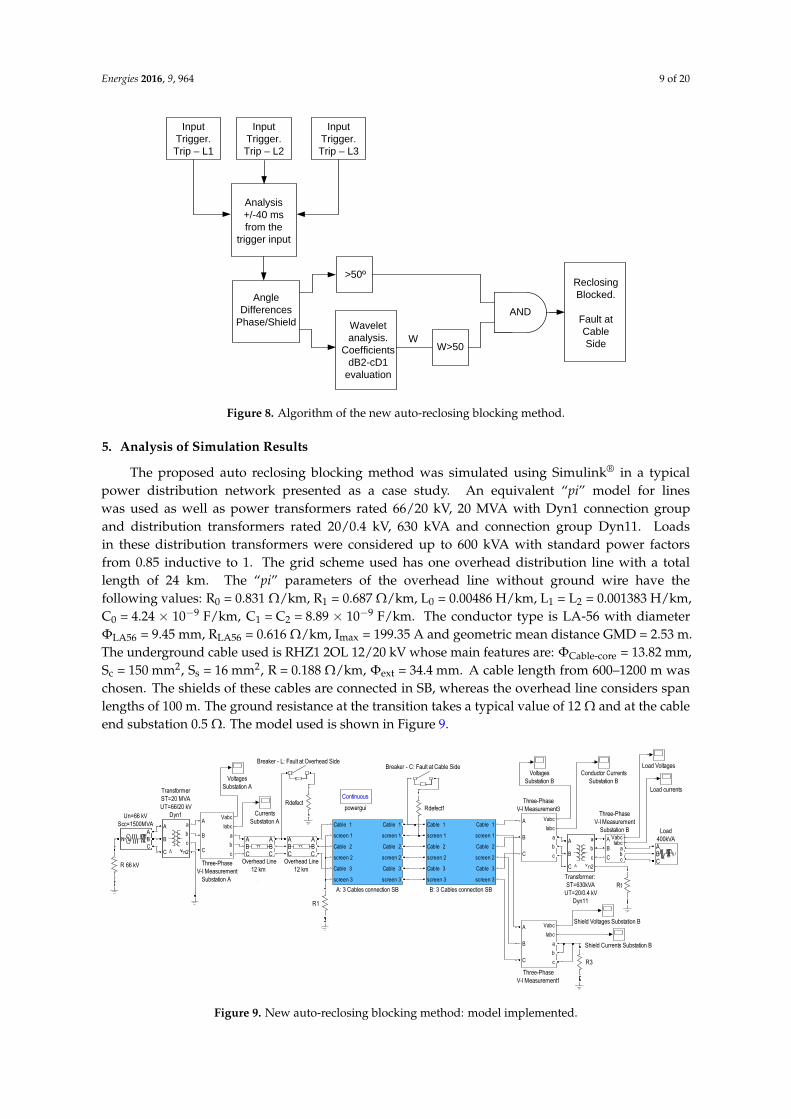
5. Analysis of Simulation Results

The proposed auto reclosing blocking method was simulated using Simulink® in a typical

power distribution network presented as a case study. An equivalent “pi” model for lines was used

as well as power transformers rated 66/20 kV, 20 MVA with Dyn1 connection group and distribution

transformers rated 20/0.4 kV, 630 kVA and connection group Dyn11. Loads in these distribution

transformers were considered up to 600 kVA with standard power factors from 0.85 inductive to 1.

The grid scheme used has one overhead distribution line with a total length of 24 km. The “pi”

parameters of the overhead line without ground wire have the following values: R0 = 0.831 Ω/km,

R1 = 0.687 Ω/km, L0 = 0.00486 H/km, L1 = L2 = 0.001383 H/km, C0 = 4.24 × 10−9 F/km,

C1 = C2 = 8.89 × 10−9 F/km. The conductor type is LA-56 with diameter ΦLA56 = 9.45 mm,

RLA56 = 0.616 Ω/km, Imax = 199.35 A and geometric mean distance GMD = 2.53 m. The underground

cable used is RHZ1 2OL 12/20 kV whose main features are: ΦCable-core = 13.82 mm, Sc = 150 mm2,

Ss = 16 mm2, R = 0.188 Ω/km, Φext = 34.4 mm. A cable length from 600–1200 m was chosen. The shields

of these cables are connected in SB, whereas the overhead line considers span lengths of 100 m. The

ground resistance at the transition takes a typical value of 12 Ω and at the cable end substation 0.5 Ω.

The model used is shown in Figure 9.

Figure 9. New auto-reclosing blocking method: model implemented.

Continuous

powergui

Voltages

Substation BVoltages

Substation A

N

A

B

C

Un=66 kV

Scc=1500MVA

A

B

C

a

b

c

n2

Transformer:

ST=630kVA

UT=20/0.4 kV

Dyn11

A

B

C

a

b

c

n2

Transformer

ST=20 MVA

UT=66/20 kV

Dyn1Vabc

Iabc

A

B

C

a

b

c

Three-Phase

V-I Measurement3

Vabc

Iabc

A

B

C

a

b

c

Three-Phase

V-I Measurement1

VabcIabc

A

B

C

abc

Three-Phase

V-I Measurement

Substation B

Vabc

IabcA

B

C

a

b

c

Three-Phase

V-I Measurement

Substation A

Shield Voltages Substation B

Shield Currents Substation B

Rt

Rdefect1Rdefect

R3

R1

R 66 kV

ABC

ABC

Overhead Line

12 km

ABC

ABC

Overhead Line

12 km

Load currents

Load Voltages

ABC

Load

400kVA

Currents

Substation A

Conductor Currents

Substation B

Breaker - L: Fault at Overhead SideBreaker - C: Fault at Cable Side

Cable 1

screen 1

Cable 2

screen 2

Cable 3

screen 3

Cable 1

screen 1

Cable 2

screen 2

Cable 3

screen 3

B: 3 Cables connection SB

Cable 1

screen 1

Cable 2

screen 2

Cable 3

screen 3

Cable 1

screen 1

Cable 2

screen 2

Cable 3

screen 3

A: 3 Cables connection SB



The proposed auto reclosing blocking method was simulated using Simulink® in a typicalpower distribution network presented as a case study. An equivalent “pi” model for lineswas used as well as power transformers rated 66/20 kV, 20 MVA with Dyn1 connection groupand distribution transformers rated 20/0.4 kV, 630 kVA and connection group Dyn11. Loadsin these distribution transformers were considered up to 600 kVA with standard power factorsfrom 0.85 inductive to 1. The grid scheme used has one overhead distribution line with a totallength of 24 km. The “pi” parameters of the overhead line without ground wire have thefollowing values: R0 = 0.831 Ω/km, R1 = 0.687 Ω/km, L0 = 0.00486 H/km, L1 = L2 = 0.001383 H/km,C0 = 4.24 × 10−9 F/km, C1 = C2 = 8.89 × 10−9 F/km. The conductor type is LA-56 with diameterΦLA56 = 9.45 mm, RLA56 = 0.616 Ω/km, Imax = 199.35 A and geometric mean distance GMD = 2.53 m.The underground cable used is RHZ1 2OL 12/20 kV whose main features are: ΦCable-core = 13.82 mm,Sc = 150 mm2, Ss = 16 mm2, R = 0.188 Ω/km, Φext = 34.4 mm. A cable length from 600–1200 m waschosen. The shields of these cables are connected in SB, whereas the overhead line considers spanlengths of 100 m. The ground resistance at the transition takes a typical value of 12 Ω and at the cableend substation 0.5 Ω. The model used is shown in Figure 9.

Energies 2016, 9, 964 9 of 21

Analysis

+/-40 ms

from the

trigger input

Angle

Differences

Phase/Shield

<60º Reclosing

Blocked.

Fault at

Cable

Side

Wavelet

analysis.

Coefficients

dB2-cD1

evaluation

AND

W

>50º

<60ºW>50

Input

Trigger.

Trip – L1

Input

Trigger.

Trip – L2

Input

Trigger.

Trip – L3



The proposed auto reclosing blocking method was simulated using Simulink® in a typical

power distribution network presented as a case study. An equivalent “pi” model for lines was used

as well as power transformers rated 66/20 kV, 20 MVA with Dyn1 connection group and distribution

transformers rated 20/0.4 kV, 630 kVA and connection group Dyn11. Loads in these distribution

transformers were considered up to 600 kVA with standard power factors from 0.85 inductive to 1.

The grid scheme used has one overhead distribution line with a total length of 24 km. The “pi”

parameters of the overhead line without ground wire have the following values: R0 = 0.831 Ω/km,

R1 = 0.687 Ω/km, L0 = 0.00486 H/km, L1 = L2 = 0.001383 H/km, C0 = 4.24 × 10−9 F/km,

C1 = C2 = 8.89 × 10−9 F/km. The conductor type is LA-56 with diameter ΦLA56 = 9.45 mm,

RLA56 = 0.616 Ω/km, Imax = 199.35 A and geometric mean distance GMD = 2.53 m. The underground

cable used is RHZ1 2OL 12/20 kV whose main features are: ΦCable-core = 13.82 mm, Sc = 150 mm2,

Ss = 16 mm2, R = 0.188 Ω/km, Φext = 34.4 mm. A cable length from 600–1200 m was chosen. The shields

of these cables are connected in SB, whereas the overhead line considers span lengths of 100 m. The

ground resistance at the transition takes a typical value of 12 Ω and at the cable end substation 0.5 Ω.

The model used is shown in Figure 9.


Continuous

powergui

Voltages

Substation BVoltages

Substation A

N

A

B

C

Un=66 kV

Scc=1500MVA

A

B

C

a

b

c

n2

Transformer:

ST=630kVA

UT=20/0.4 kV

Dyn11

A

B

C

a

b

c

n2

Transformer

ST=20 MVA

UT=66/20 kV

Dyn1Vabc

Iabc

A

B

C

a

b

c

Three-Phase

V-I Measurement3

Vabc

Iabc

A

B

C

a

b

c

Three-Phase

V-I Measurement1

VabcIabc

A

B

C

abc

Three-Phase

V-I Measurement

Substation B

Vabc

IabcA

B

C

a

b

c

Three-Phase

V-I Measurement

Substation A

Shield Voltages Substation B

Shield Currents Substation B

Rt

Rdefect1Rdefect

R3

R1

R 66 kV

ABC

ABC

Overhead Line

12 km

ABC

ABC

Overhead Line

12 km

Load currents

Load Voltages

ABC

Load

400kVA

Currents

Substation A

Conductor Currents

Substation B

Breaker - L: Fault at Overhead SideBreaker - C: Fault at Cable Side

Cable 1

screen 1

Cable 2

screen 2

Cable 3

screen 3

Cable 1

screen 1

Cable 2

screen 2

Cable 3

screen 3

B: 3 Cables connection SB

Cable 1

screen 1

Cable 2

screen 2

Cable 3

screen 3

Cable 1

screen 1

Cable 2

screen 2

Cable 3

screen 3

A: 3 Cables connection SB


Energies 2016, 9, 964 10 of 20

5.1. Angular Difference Analysis in Power Distribution Networks Solidly Grounded at the Overhead Side andIsolated at the Cable End Side

The angular differences ∆L1S1, ∆L2S2 and ∆L3S3 between currents in the shields and in theactive part of the cables in a system ungrounded at the cable side (typical power transformer indelta connection) and solidly grounded at the overhead side have been all simulated during normaloperation of the power distribution network without ground fault and with it along different positionat the overhead side and at the cable side. Multiple simulations show that the classification of theground faults turns out to be:

• Ground fault in the overhead side: if ∆L1S1, ∆L2S2 and ∆L3S3 are less than 50, normally inall phases.

• Ground fault in the cable line side: if at least one of ∆L1S1, ∆L2S2 or ∆L3S3 is clearly over 50.

Figures 10 and 11 show how the variations of ∆L1S1, ∆L2S2 and ∆L3S3 are when the powerdistribution network suffers a ground fault in phase L1 at the overhead line side 12 km from thetransition, and at the cable line side in its central position in t = 200 ms. The overhead line has a totallength of 24 km and the cable 600 m.

Energies 2016, 9, 964 10 of 21

5.1. Angular Difference Analysis in Power Distribution Networks Solidly Grounded at the Overhead Side and

Isolated at the Cable End Side

The angular differences ΔL1S1, ΔL2S2 and ΔL3S3 between currents in the shields and in the

active part of the cables in a system ungrounded at the cable side (typical power transformer in delta

connection) and solidly grounded at the overhead side have been all simulated during normal

operation of the power distribution network without ground fault and with it along different

position at the overhead side and at the cable side. Multiple simulations show that the classification

of the ground faults turns out to be:

Ground fault in the overhead side: if ΔL1S1, ΔL2S2 and ΔL3S3 are less than 50°, normally in

all phases.

Ground fault in the cable line side: if at least one of ΔL1S1, ΔL2S2 or ΔL3S3 is clearly over 50°.

Figures 10 and 11 show how the variations of ΔL1S1, ΔL2S2 and ΔL3S3 are when the power

distribution network suffers a ground fault in phase L1 at the overhead line side 12 km from the

transition, and at the cable line side in its central position in t = 200 ms. The overhead line has a total

length of 24 km and the cable 600 m.

Figure 10. Angular differences with ground fault at the overhead side in phase L1.

Figure 11. Angular differences with ground fault at the cable line side in phase L1.

Considering distances from the transition, Table 1 shows the results of the variation in ΔL1S1,

ΔL2S2 and ΔL3S3 from only 1 m to more than 10 km in the overhead line side, and from 1 to 599 m in

the cable line side. It can be seen how the variations of ΔL1S1, ΔL2S2 and ΔL3S3 are reduced when

the ground fault occurs at the overhead line side and are very high when the ground fault happens t

the cable line side.

0.15 0.2 0.25 0.3-100

-95

-90

-85

-80

-75

-70

-65

-60

Time (s)

An

gle

Diffe

ren

ce

Co

nd

ucto

r-S

hie

ld (

de

gre

es)

Ground fault in t=200 ms at the overhead side in phase L1

Angle difference L1-S1

Angle Difference L2-S2

Angle Difference S3-L3 15,64º

12,20º 15,44º

0.15 0.2 0.25 0.3-400

-300

-200

-100

0

100

Time (s)

An

gle

Diffe

ren

ce

Ph

ase

-Sh

ield

(d

eg

ree

s)

Ground fault in t=200 ms at the cable side in phase L1




167,95º

73,35º23,15º


Energies 2016, 9, 964 10 of 21

5.1. Angular Difference Analysis in Power Distribution Networks Solidly Grounded at the Overhead Side and


The angular differences ΔL1S1, ΔL2S2 and ΔL3S3 between currents in the shields and in the

active part of the cables in a system ungrounded at the cable side (typical power transformer in delta

connection) and solidly grounded at the overhead side have been all simulated during normal

operation of the power distribution network without ground fault and with it along different

position at the overhead side and at the cable side. Multiple simulations show that the classification

of the ground faults turns out to be:

Ground fault in the overhead side: if ΔL1S1, ΔL2S2 and ΔL3S3 are less than 50°, normally in

all phases.

Ground fault in the cable line side: if at least one of ΔL1S1, ΔL2S2 or ΔL3S3 is clearly over 50°.

Figures 10 and 11 show how the variations of ΔL1S1, ΔL2S2 and ΔL3S3 are when the power

distribution network suffers a ground fault in phase L1 at the overhead line side 12 km from the

transition, and at the cable line side in its central position in t = 200 ms. The overhead line has a total

length of 24 km and the cable 600 m.



Considering distances from the transition, Table 1 shows the results of the variation in ΔL1S1,

ΔL2S2 and ΔL3S3 from only 1 m to more than 10 km in the overhead line side, and from 1 to 599 m in

the cable line side. It can be seen how the variations of ΔL1S1, ΔL2S2 and ΔL3S3 are reduced when

the ground fault occurs at the overhead line side and are very high when the ground fault happens t

the cable line side.

0.15 0.2 0.25 0.3-100

-95

-90

-85

-80

-75

-70

-65

-60

Time (s)

An

gle

Diffe

ren

ce

Co

nd

ucto

r-S

hie

ld (

de

gre

es)

Ground fault in t=200 ms at the overhead side in phase L1

Angle difference L1-S1


Angle Difference S3-L3 15,64º

12,20º 15,44º

0.15 0.2 0.25 0.3-400

-300

-200

-100

0

100

Time (s)

An

gle

Diffe

ren

ce

Ph

ase

-Sh

ield

(d

eg

ree

s)

Ground fault in t=200 ms at the cable side in phase L1




167,95º

73,35º23,15º


Considering distances from the transition, Table 1 shows the results of the variation in ∆L1S1,∆L2S2 and ∆L3S3 from only 1 m to more than 10 km in the overhead line side, and from 1 to 599 m inthe cable line side. It can be seen how the variations of ∆L1S1, ∆L2S2 and ∆L3S3 are reduced when theground fault occurs at the overhead line side and are very high when the ground fault happens t thecable line side.

Energies 2016, 9, 964 11 of 20

Table 1. Phase angle variation with ground faults at the overhead and cable line sides.

Fault at Overhead Line Side Fault at Cable Line Side

Distance from Transition

Fault in Phase L1


Fault in Phase L1

Variation in Phase Angles Variation in Phase Angles

∆L1S1 ∆L2S2 ∆L3S3 ∆L1S1 ∆L2S2 ∆L3S3

1 m 15.18 10.98 15.26 1 m 73.69 168.62 24.03

10 m 15.16 10.99 15.24 10 m 73.72 168.65 24.05

100 m 15.17 11.01 15.26 50 m 73.75 168.61 24.12

1000 m 15.18 11.05 14.27 100 m 73.71 168.52 23.73

5000 m 15.25 11.33 15.37 300 m 73.35 167.95 23.15

>10,000 m 15.44 12.20 15.64 599 m 67.32 157.11 27.67



Fault in Phase L2


Fault in Phase L2


∆L1S1 ∆L2S2 ∆L3S3 ∆L1S1 ∆L2S2 ∆L3S3

1 m 15.34 15.33 10.81 1 m 24.02 73.72 168.58

10 m 15.35 15.34 10.88 10 m 24.10 73.70 168.59

100 m 15.34 15.33 10.87 50 m 23.92 73.71 168.47

1000 m 15.37 15.36 10.85 100 m 23.85 73.79 168.42

5000 m 15.48 15.45 11.20 300 m 22.99 73.55 167.65

>10,000 m 15.67 15.56 11.72 599 m 27.87 67.51 157.52



Fault in Phase L3

Distance from transition

Fault in Phase L3


∆L1S1 ∆L2S2 ∆L3S3 ∆L1S1 ∆L2S2 ∆L3S3

1 m 11.78 15.41 15.25 1 m 168.61 24.01 73.31

10 m 11.79 15.42 15.22 10 m 168.62 24.02 73.70

100 m 11.77 15.43 15.23 50 m 168.51 23.92 73.72

1000 m 11.82 15.45 15.25 100 m 168.40 23.75 73.31

5000 m 12.13 15.55 15.33 300 m 168.12 23.11 73.55

>10,000 m 12.66 15.73 15.45 599 m 157.36 67.78 68.01

5.2. Wavelet Analysis in a Power Distribution Network Solidly Grounded at the Overhead Line Side andIsolated at the Cable End Side

The simulation results of this configuration included in Table 2 show that the angular differencewhen the ground fault has happened in the overhead side has dB2-cD1 coefficients lower than 0.1,and over 100 when the fault is in the e line side. Figures 12 and 13 show the results obtained for groundfaults in phase L1 at the overhead line side and cable lines side respectively.

Energies 2016, 9, 964 11 of 21

Table 1. Phase angle variation with ground faults at the overhead and cable line sides.


Distance from

Transition

Fault in Phase L1 Distance from

Transition

Fault in Phase L1


ΔL1S1 ΔL2S2 ΔL3S3 ΔL1S1 ΔL2S2 ΔL3S3

1 m 15.18° 10.98° 15.26° 1 m 73.69° 168.62° 24.03°

10 m 15.16° 10.99° 15.24° 10 m 73.72° 168.65° 24.05°

100 m 15.17° 11.01° 15.26° 50 m 73.75° 168.61° 24.12°

1000 m 15.18° 11.05° 14.27° 100 m 73.71° 168.52° 23.73°

5000 m 15.25° 11.33° 15.37° 300 m 73.35° 167.95° 23.15°

>10,000 m 15.44° 12.20° 15.64° 599 m 67.32° 157.11° 27.67°


Distance from

Transition


Transition

Fault in Phase L2



1 m 15.34° 15.33° 10.81° 1 m 24.02° 73.72° 168.58°

10 m 15.35° 15.34° 10.88° 10 m 24.10° 73.70° 168.59°

100 m 15.34° 15.33° 10.87° 50 m 23.92° 73.71° 168.47°

1000 m 15.37° 15.36° 10.85° 100 m 23.85° 73.79° 168.42°

5000 m 15.48° 15.45° 11.20° 300 m 22.99° 73.55° 167.65°

>10,000 m 15.67° 15.56° 11.72° 599 m 27.87° 67.51° 157.52°


Distance from

Transition


transition

Fault in Phase L3



1 m 11.78° 15.41° 15.25° 1 m 168.61° 24.01° 73.31°

10 m 11.79° 15.42° 15.22° 10 m 168.62° 24.02° 73.70°

100 m 11.77° 15.43° 15.23° 50 m 168.51° 23.92 73.72°

1000 m 11.82° 15.45° 15.25° 100 m 168.40° 23.75° 73.31°

5000 m 12.13° 15.55° 15.33° 300 m 168.12° 23.11° 73.55°

>10,000 m 12.66° 15.73° 15.45° 599 m 157.36° 67.78° 68.01°

5.2. Wavelet Analysis in a Power Distribution Network Solidly Grounded at the Overhead Line Side and


The simulation results of this configuration included in Table 2 show that the angular difference

when the ground fault has happened in the overhead side has dB2-cD1 coefficients lower than 0.1,

and over 100 when the fault is in the e line side. Figures 12 and 13 show the results obtained for

ground faults in phase L1 at the overhead line side and cable lines side respectively.

Figure 12. Wavelet dB2-1-cD1 coefficients of the angular difference signals with ground fault in

phase L1 at the overhead side 12 km from the transition.

0.1995 0.2 0.2005 0.201 0.2015-0.2

-0.15

-0.1

-0.05

0

0.05

0.1

0.15

0.2

Time (s)

dB

2-c

D1

Co

eff

icie

nts

Ground fault in t=0.2 s at the overhead side in phase L1

dB2-cD1 Angle difference Conductor L2/Shield S2



Figure 12. Wavelet dB2-1-cD1 coefficients of the angular difference signals with ground fault in phaseL1 at the overhead side 12 km from the transition.


Figure 13. Wavelet dB2-1-cD1 coefficients of the angular difference signals with ground fault in

phase L1 at the cable line side 300 m from the transition.

Table 2. Wavelet analysis: simulation results. Ground faults at the overhead and cable line sides.

Overhead line side solidly grounded and cable line side isolated. Phase currents measured in the

conductors (L1, L2, L3) and in their shields (S1, S2, S3).


Distance from

Transition


Transition

Fault in Phase L1

W (dB2-cD1 Coefficients) W (dB2-cD1 Coefficients)


1 m 0.0068 0.0067 0.0065 1 m 173.88 0.0134 0.0096

10 m 0.0039 0.0041 0.0041 10 m 173.89 0.0123 0.0097

100 m 0.0033 0.0038 0.0039 50 m 127.32 0.0113 0.0094

1000 m 0.0027 0.0029 0.0025 100 m 127.32 0.0119 0.0097

5000 m 0.0019 0.0024 0.0019 300 m 127.31 0.0128 0.0089

>10,000 m 0.0014 0.0016 0.0013 599 m 123.67 0.02784 0.0332


Distance from

Transition


Transition

Fault in Phase L2



1 m 0.0067 0.0064 0.0069 1 m 0.0095 173.90 0.0136

10 m 0.0044 0.0039 0.0042 10 m 0.0098 173.90 0.0122

100 m 0.0037 0.0031 0.0039 50 m 0.0095 127.30 0.0114

1000 m 0.0029 0.0022 0.0028 100 m 0.0098 127.30 0.0120

5000 m 0.0021 0.0017 0.0022 300 m 0.0088 127.31 0.0130

>10,000 m 0.0016 0.0011 0.0015 599 m 0.0333 123.70 0.02782


Distance from

Transition


Transition

Fault in Phase L3



1 m 0.0066 0.0064 0.0065 1 m 0.0135 0.0094 173.91

10 m 0.0044 0.0045 0.0037 10 m 0.0121 0.0097 173.91

100 m 0.0037 0.0039 0.0030 50 m 0.0113 0.0097 127.29

1000 m 0.0029 0.0031 0.0024 100 m 0.0121 0.0099 127.29

5000 m 0.0023 0.0023 0.0018 300 m 0.0131 0.0087 127.30

>10,000 m 0.0016 0.0015 0.0013 599 m 0.02783 0.0334 127.71

6. Experimental Results

Different laboratory tests were developed in order to test the validity of the new auto-reclosing

blocking method, and to check the computer simulation results obtained.

0.18 0.185 0.19 0.195 0.2 0.205

0

50

100

150

Time (s)

dB

2-c

D1

Co

eff

icie

nts

db2-cD1 Coefficients for ground fault in the the cable side in t=0.2 s in phase L1

dB2-cD1-Angle Difference Conductor L2/Shield S2



127.3

Figure 13. Wavelet dB2-1-cD1 coefficients of the angular difference signals with ground fault in phaseL1 at the cable line side 300 m from the transition.

Table 2. Wavelet analysis: simulation results. Ground faults at the overhead and cable line sides.Overhead line side solidly grounded and cable line side isolated. Phase currents measured in theconductors (L1, L2, L3) and in their shields (S1, S2, S3).



Fault in Phase L1


Fault in Phase L1


∆L1S1 ∆L2S2 ∆L3S3 ∆L1S1 ∆L2S2 ∆L3S3

1 m 0.0068 0.0067 0.0065 1 m 173.88 0.0134 0.009610 m 0.0039 0.0041 0.0041 10 m 173.89 0.0123 0.0097

100 m 0.0033 0.0038 0.0039 50 m 127.32 0.0113 0.00941000 m 0.0027 0.0029 0.0025 100 m 127.32 0.0119 0.00975000 m 0.0019 0.0024 0.0019 300 m 127.31 0.0128 0.0089

>10,000 m 0.0014 0.0016 0.0013 599 m 123.67 0.02784 0.0332



Fault in Phase L2


Fault in Phase L2


∆L1S1 ∆L2S2 ∆L3S3 ∆L1S1 ∆L2S2 ∆L3S3

1 m 0.0067 0.0064 0.0069 1 m 0.0095 173.90 0.013610 m 0.0044 0.0039 0.0042 10 m 0.0098 173.90 0.0122

100 m 0.0037 0.0031 0.0039 50 m 0.0095 127.30 0.01141000 m 0.0029 0.0022 0.0028 100 m 0.0098 127.30 0.01205000 m 0.0021 0.0017 0.0022 300 m 0.0088 127.31 0.0130

>10,000 m 0.0016 0.0011 0.0015 599 m 0.0333 123.70 0.02782



Fault in Phase L3


Fault in Phase L3


∆L1S1 ∆L2S2 ∆L3S3 ∆L1S1 ∆L2S2 ∆L3S3

1 m 0.0066 0.0064 0.0065 1 m 0.0135 0.0094 173.9110 m 0.0044 0.0045 0.0037 10 m 0.0121 0.0097 173.91

100 m 0.0037 0.0039 0.0030 50 m 0.0113 0.0097 127.291000 m 0.0029 0.0031 0.0024 100 m 0.0121 0.0099 127.295000 m 0.0023 0.0023 0.0018 300 m 0.0131 0.0087 127.30

>10,000 m 0.0016 0.0015 0.0013 599 m 0.02783 0.0334 127.71

6. Experimental Results

Different laboratory tests were developed in order to test the validity of the new auto-reclosingblocking method, and to check the computer simulation results obtained.

Energies 2016, 9, 964 13 of 20

6.1. Experimental Setup

The tests were carried out on a solidly earthed source supplied by a power transformer rated800 VA, 400/100 Vac and Dyn1 connection group. Two line module emulators with equivalent circuit“pi” were used with the following features: R = 88.48 mΩ, L = 4 mH and C = 4 µF each capacitor.The real cable used has the following characteristics: R = 1.8 Ω, L = 22 mH and C = 4.9 nF with a totalcable length of 300 m. Two overcurrent protection relays of type MRI4 by Woodward-Seg are usedas disturbance recorders to store the values of the currents flowing in the active conductors and theshields of the cables. A second transformer rated 800 VA, 400/100 Vac and Dyn11 is used to supplydifferent loads in delta connection. Figure 14 shows the experimental setup and the RLC features ofthe line module emulators used.

Energies 2016, 9, 964 13 of 21

6.1. Experimental Setup

The tests were carried out on a solidly earthed source supplied by a power transformer rated

800 VA, 400/100 Vac and Dyn1 connection group. Two line module emulators with equivalent

circuit “pi” were used with the following features: R = 88.48 mΩ, L = 4 mH and C = 4 μF each

capacitor. The real cable used has the following characteristics: R = 1.8 Ω, L = 22 mH and C = 4.9 nF

with a total cable length of 300 m. Two overcurrent protection relays of type MRI4 by

Woodward-Seg are used as disturbance recorders to store the values of the currents flowing in the

active conductors and the shields of the cables. A second transformer rated 800 VA, 400/100 Vac and

Dyn11 is used to supply different loads in delta connection. Figure 14 shows the experimental setup

and the RLC features of the line module emulators used.

Figure 14. Experimental setup. 1: Protection relays; 2: Auxiliary power supply; 3: Power supply; 4:

Loads; 5: Ground fault switch; 6: Transformer; 7: PC; 8: Cables; 9: Line modules; 10: RLC parameters

of the line modules (9) used.

Several single ground faults at all phases in lines and cables were carried out in the network

erected in the laboratory. Tests were developed at 100 V phase-to-phase voltage and load currents of

less than 1 A with different cosφ values. The positions where the ground faults were developed

(indicated in Figure 15) are represented schematically in Figure 16.

Figure 14. Experimental setup. 1: Protection relays; 2: Auxiliary power supply; 3: Power supply;4: Loads; 5: Ground fault switch; 6: Transformer; 7: PC; 8: Cables; 9: Line modules; 10: RLC parametersof the line modules (9) used.

Several single ground faults at all phases in lines and cables were carried out in the networkerected in the laboratory. Tests were developed at 100 V phase-to-phase voltage and load currentsof less than 1 A with different cosφ values. The positions where the ground faults were developed(indicated in Figure 15) are represented schematically in Figure 16.


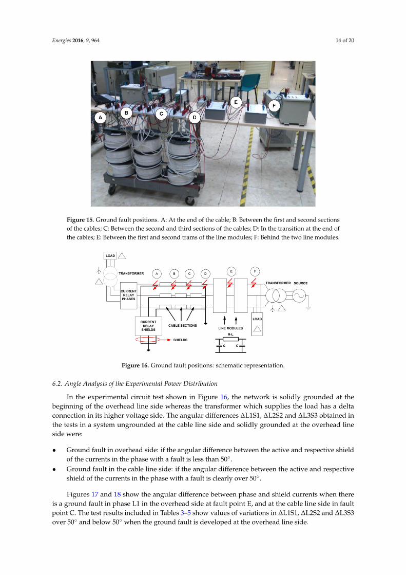
Figure 15. Ground fault positions. A: At the end of the cable; B: Between the first and second sections

of the cables; C: Between the second and third sections of the cables; D: In the transition at the end of

the cables; E: Between the first and second trams of the line modules; F: Behind the two line modules.

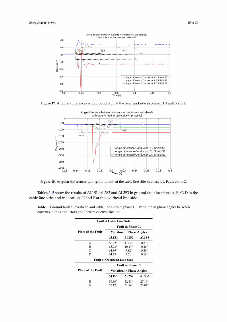
Figure 16. Ground fault positions: schematic representation.

6.2. Angle Analysis of the Experimental Power Distribution.

In the experimental circuit test shown in Figure 16, the network is solidly grounded at the

beginning of the overhead line side whereas the transformer which supplies the load has a delta

connection in its higher voltage side. The angular differences ΔL1S1, ΔL2S2 and ΔL3S3 obtained in

the tests in a system ungrounded at the cable line side and solidly grounded at the overhead line

side were:

Ground fault in overhead side: if the angular difference between the active and respective

shield of the currents in the phase with a fault is less than 50°.

Ground fault in the cable line side: if the angular difference between the active and respective

shield of the currents in the phase with a fault is clearly over 50°.

Figures 17 and 18 show the angular difference between phase and shield currents when there is

a ground fault in phase L1 in the overhead side at fault point E, and at the cable line side in fault

point C. The test results included in Tables 3–5 show values of variations in ΔL1S1, ΔL2S2 and

ΔL3S3 over 50° and below 50° when the ground fault is developed at the overhead line side.

Figure 15. Ground fault positions. A: At the end of the cable; B: Between the first and second sectionsof the cables; C: Between the second and third sections of the cables; D: In the transition at the end ofthe cables; E: Between the first and second trams of the line modules; F: Behind the two line modules.

Energies 2016, 9, 964 14 of 21

Figure 15. Ground fault positions. A: At the end of the cable; B: Between the first and second sections

of the cables; C: Between the second and third sections of the cables; D: In the transition at the end of

the cables; E: Between the first and second trams of the line modules; F: Behind the two line modules.


6.2. Angle Analysis of the Experimental Power Distribution.

In the experimental circuit test shown in Figure 16, the network is solidly grounded at the

beginning of the overhead line side whereas the transformer which supplies the load has a delta

connection in its higher voltage side. The angular differences ΔL1S1, ΔL2S2 and ΔL3S3 obtained in

the tests in a system ungrounded at the cable line side and solidly grounded at the overhead line

side were:

Ground fault in overhead side: if the angular difference between the active and respective

shield of the currents in the phase with a fault is less than 50°.

Ground fault in the cable line side: if the angular difference between the active and respective

shield of the currents in the phase with a fault is clearly over 50°.

Figures 17 and 18 show the angular difference between phase and shield currents when there is

a ground fault in phase L1 in the overhead side at fault point E, and at the cable line side in fault

point C. The test results included in Tables 3–5 show values of variations in ΔL1S1, ΔL2S2 and

ΔL3S3 over 50° and below 50° when the ground fault is developed at the overhead line side.


6.2. Angle Analysis of the Experimental Power Distribution

In the experimental circuit test shown in Figure 16, the network is solidly grounded at thebeginning of the overhead line side whereas the transformer which supplies the load has a deltaconnection in its higher voltage side. The angular differences ∆L1S1, ∆L2S2 and ∆L3S3 obtained inthe tests in a system ungrounded at the cable line side and solidly grounded at the overhead lineside were:

• Ground fault in overhead side: if the angular difference between the active and respective shieldof the currents in the phase with a fault is less than 50.

• Ground fault in the cable line side: if the angular difference between the active and respectiveshield of the currents in the phase with a fault is clearly over 50.

Figures 17 and 18 show the angular difference between phase and shield currents when thereis a ground fault in phase L1 in the overhead side at fault point E, and at the cable line side in faultpoint C. The test results included in Tables 3–5 show values of variations in ∆L1S1, ∆L2S2 and ∆L3S3over 50 and below 50 when the ground fault is developed at the overhead line side.


Figure 17. Angular differences with ground fault at the overhead side in phase L1. Fault point E.

Figure 18. Angular differences with ground fault at the cable line side in phase L1. Fault point C.

Tables 3–5 show the results of ΔL1S1, ΔL2S2 and ΔL3S3 in ground fault locations A, B, C, D in

the cable line side, and in locations E and F at the overhead line side.

Table 3. Ground fault at overhead and cable line sides in phase L1. Variation in phase angles

between currents in the conductors and their respective shields.

Fault at Cable Line Side

Place of the Fault

Fault in Phase L1

Variation in Phase Angles

ΔL1S1 ΔL2S2 ΔL3S3

A 66.32° 11.02° 0.33°

B 65.93° 10.24° 0.26°

C 64.89° 9.82° 0.20°

D 64.25° 9.31° 0.18°

Fault at Overhead Line Side

Place of the Fault

Fault in Phase L1



E 30.80° 32.31° 27.16°

F 29.12° 31.86° 26.02°

0.2 0.25 0.3 0.35 0.4 0.45 0.5-160

-140

-120

-100

-80

-60

-40

-20

Time (s)

De

gre

es (

º)

Angle change between currents in conductors and shields.

Ground fault at the overhead side in E.

Angle difference Conductor L1/Shield S1



32.3º

27.2º30.8º

0.12 0.14 0.16 0.18 0.2 0.22 0.24 0.26 0.28 0.3-400

-350

-300

-250

-200

-150

-100

-50

Time (s)

De

gre

es (

º)

Angle difference between currents in conductors and shieldswith ground fault in cable side in phase L1

Angle difference Conductor L1 / Shield S1



9.82º

64.89º

0.2º


Energies 2016, 9, 964 15 of 21



Tables 3–5 show the results of ΔL1S1, ΔL2S2 and ΔL3S3 in ground fault locations A, B, C, D in

the cable line side, and in locations E and F at the overhead line side.

Table 3. Ground fault at overhead and cable line sides in phase L1. Variation in phase angles

between currents in the conductors and their respective shields.


Place of the Fault

Fault in Phase L1



A 66.32° 11.02° 0.33°

B 65.93° 10.24° 0.26°

C 64.89° 9.82° 0.20°

D 64.25° 9.31° 0.18°


Place of the Fault

Fault in Phase L1



E 30.80° 32.31° 27.16°

F 29.12° 31.86° 26.02°

0.2 0.25 0.3 0.35 0.4 0.45 0.5-160

-140

-120

-100

-80

-60

-40

-20

Time (s)

De

gre

es (

º)

Angle change between currents in conductors and shields.

Ground fault at the overhead side in E.




32.3º

27.2º30.8º

0.12 0.14 0.16 0.18 0.2 0.22 0.24 0.26 0.28 0.3-400

-350

-300

-250

-200

-150

-100

-50

Time (s)

De

gre

es (

º)

Angle difference between currents in conductors and shieldswith ground fault in cable side in phase L1




9.82º

64.89º

0.2º


Tables 3–5 show the results of ∆L1S1, ∆L2S2 and ∆L3S3 in ground fault locations A, B, C, D in thecable line side, and in locations E and F at the overhead line side.

Table 3. Ground fault at overhead and cable line sides in phase L1. Variation in phase angles betweencurrents in the conductors and their respective shields.


Place of the Fault

Fault in Phase L1


∆L1S1 ∆L2S2 ∆L3S3

A 66.32 11.02 0.33

B 65.93 10.24 0.26

C 64.89 9.82 0.20

D 64.25 9.31 0.18


Place of the Fault

Fault in Phase L1


∆L1S1 ∆L2S2 ∆L3S3

E 30.80 32.31 27.16

F 29.12 31.86 26.02

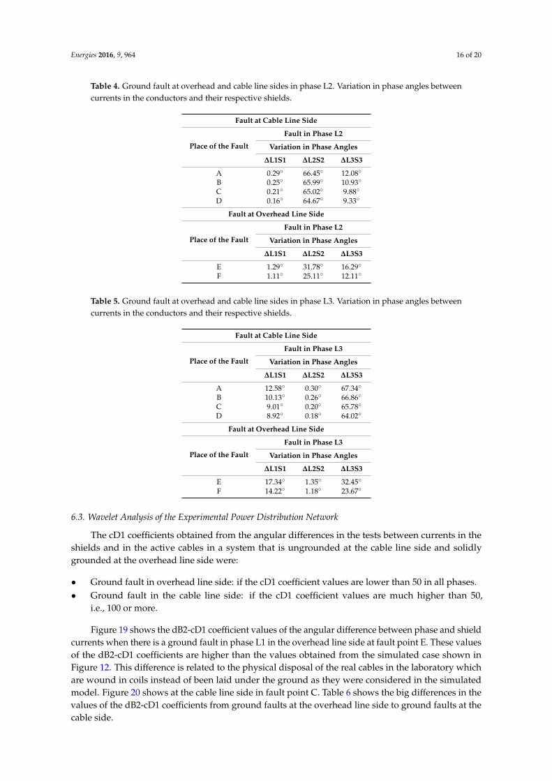
Energies 2016, 9, 964 16 of 20



Place of the Fault

Fault in Phase L2


∆L1S1 ∆L2S2 ∆L3S3

A 0.29 66.45 12.08

B 0.25 65.99 10.93

C 0.21 65.02 9.88

D 0.16 64.67 9.33


Place of the Fault

Fault in Phase L2


∆L1S1 ∆L2S2 ∆L3S3

E 1.29 31.78 16.29

F 1.11 25.11 12.11



Place of the Fault

Fault in Phase L3


∆L1S1 ∆L2S2 ∆L3S3

A 12.58 0.30 67.34

B 10.13 0.26 66.86

C 9.01 0.20 65.78

D 8.92 0.18 64.02


Place of the Fault

Fault in Phase L3


∆L1S1 ∆L2S2 ∆L3S3

E 17.34 1.35 32.45

F 14.22 1.18 23.67

6.3. Wavelet Analysis of the Experimental Power Distribution Network

The cD1 coefficients obtained from the angular differences in the tests between currents in theshields and in the active cables in a system that is ungrounded at the cable line side and solidlygrounded at the overhead line side were:

• Ground fault in overhead line side: if the cD1 coefficient values are lower than 50 in all phases.• Ground fault in the cable line side: if the cD1 coefficient values are much higher than 50,

i.e., 100 or more.

Figure 19 shows the dB2-cD1 coefficient values of the angular difference between phase and shieldcurrents when there is a ground fault in phase L1 in the overhead line side at fault point E. These valuesof the dB2-cD1 coefficients are higher than the values obtained from the simulated case shown inFigure 12. This difference is related to the physical disposal of the real cables in the laboratory whichare wound in coils instead of been laid under the ground as they were considered in the simulatedmodel. Figure 20 shows at the cable line side in fault point C. Table 6 shows the big differences in thevalues of the dB2-cD1 coefficients from ground faults at the overhead line side to ground faults at thecable side.


Figure 19. Wavelet analysis of the angular differences with a ground fault at the overhead line side in

phase L1. Fault point E.

Figure 20. Wavelet analysis of the angular differences with a ground fault at the cable line side in

phase L1. Fault point C.

Table 6. Ground fault at overhead and cable line sides. Wavelet analysis: experimental results.

Overhead line side solidly grounded and cable line side isolated.

Fault at Cable Line Side Fault at Overhead Line Side

Location of the Fault

Fault in Phase L1


Fault in Phase L1



A 152.24 2.45 18.29 E 4.80 0.03 0.50

B 145.88 1.96 14.12

C 142.01 0.80 7.21 F 4.66 0.02 0.42

D 136.54 0.69 4.75



Fault in Phase L2


Fault in Phase L2



A 20.04 154.31 3.01 E 0.04 4.88 0.59

B 16.59 148.22 2.42

C 9.92 143.67 0.89 F 0.03 4.72 0.48

D 6.82 138.08 0.82



Fault in Phase L3


Fault in Phase L3



A 2.66 19.44 153.01 E 0.47 0.04 4.34

B 1.49 15.18 144.78

C 0.81 6.96 140.12 F 0.51 0.02 4.11

D 0.52 3.97 134.96

0.08 0.085 0.09 0.095 0.1 0.105 0.11

-6

-4

-2

0

2

4

Time (s)

dB

2-c

D1

Co

eff

icie

nts

dB2-cD1 Coefficients for ground fault in phase L1 at the overhead side in position E

dB2-cD1 coefficients Conductor L1 / Shield S1



0.030.5

4.8

0.15 0.16 0.17 0.18 0.19 0.2 0.21 0.22-160

-140

-120

-100

-80

-60

-40

-20

0

20

Time (s)

dB

b2

-cD

1 C

oe

ffic

ien

t V

alu

es

dB2-cD1 Coefficient values for ground fault in phase L1 at the cable side in location C

dB2-cD1 Coeffientes Conductor L1 / Shield S1



142

0.8 7.2

Figure 19. Wavelet analysis of the angular differences with a ground fault at the overhead line side inphase L1. Fault point E.

Energies 2016, 9, 964 17 of 21

Figure 19. Wavelet analysis of the angular differences with a ground fault at the overhead line side in

phase L1. Fault point E.

Figure 20. Wavelet analysis of the angular differences with a ground fault at the cable line side in

phase L1. Fault point C.

Table 6. Ground fault at overhead and cable line sides. Wavelet analysis: experimental results.

Overhead line side solidly grounded and cable line side isolated.



Fault in Phase L1


Fault in Phase L1



A 152.24 2.45 18.29 E 4.80 0.03 0.50

B 145.88 1.96 14.12

C 142.01 0.80 7.21 F 4.66 0.02 0.42

D 136.54 0.69 4.75



Fault in Phase L2


Fault in Phase L2



A 20.04 154.31 3.01 E 0.04 4.88 0.59

B 16.59 148.22 2.42

C 9.92 143.67 0.89 F 0.03 4.72 0.48

D 6.82 138.08 0.82



Fault in Phase L3


Fault in Phase L3



A 2.66 19.44 153.01 E 0.47 0.04 4.34

B 1.49 15.18 144.78

C 0.81 6.96 140.12 F 0.51 0.02 4.11

D 0.52 3.97 134.96

0.08 0.085 0.09 0.095 0.1 0.105 0.11

-6

-4

-2

0

2

4

Time (s)

dB

2-c

D1

Co

eff

icie

nts

dB2-cD1 Coefficients for ground fault in phase L1 at the overhead side in position E




0.030.5

4.8

0.15 0.16 0.17 0.18 0.19 0.2 0.21 0.22-160

-140

-120

-100

-80

-60

-40

-20

0

20

Time (s)

dB

b2

-cD

1 C

oe

ffic

ien

t V

alu

es

dB2-cD1 Coefficient values for ground fault in phase L1 at the cable side in location C




142

0.8 7.2

Figure 20. Wavelet analysis of the angular differences with a ground fault at the cable line side in phaseL1. Fault point C.

Table 6. Ground fault at overhead and cable line sides. Wavelet analysis: experimental results.Overhead line side solidly grounded and cable line side isolated.



Fault in Phase L1


Fault in Phase L1


∆L1S1 ∆L2S2 ∆L3S3 ∆L1S1 ∆L2S2 ∆L3S3

A 152.24 2.45 18.29E 4.80 0.03 0.50B 145.88 1.96 14.12

C 142.01 0.80 7.21F 4.66 0.02 0.42D 136.54 0.69 4.75



Fault in Phase L2


Fault in Phase L2


∆L1S1 ∆L2S2 ∆L3S3 ∆L1S1 ∆L2S2 ∆L3S3

A 20.04 154.31 3.01E 0.04 4.88 0.59B 16.59 148.22 2.42

C 9.92 143.67 0.89F 0.03 4.72 0.48D 6.82 138.08 0.82



Fault in Phase L3


Fault in Phase L3


∆L1S1 ∆L2S2 ∆L3S3 ∆L1S1 ∆L2S2 ∆L3S3

A 2.66 19.44 153.01E 0.47 0.04 4.34B 1.49 15.18 144.78

C 0.81 6.96 140.12F 0.51 0.02 4.11D 0.52 3.97 134.96

Energies 2016, 9, 964 18 of 20

7. Conclusions and Future Work

A new auto-reclosing blocking method for combined overhead-cable lines in power distributionnetworks has been presented in this article. This method is applicable when the transitionoverhead-cable is close to the substation where the measurements of currents in shields and conductorsare done. The shields of the cables are grounded at both ends. The proposed ground fault auto-reclosingmethod is based on two analyses. The first evaluates the difference between the currents in the activepart of the cable and those in the shields, whereas the second analysis uses the wavelet Daubechies dB2and extracts the coefficients cD1 from the same differences used in the first analysis. If the argumentdifferences between the currents in the conductors of the cable and those in the shields have a phasevariation just after a ground fault occurs with higher values than a reference difference and, at thesame time, the Daubechies-cD1 coefficients of such differences have values over a reference threshold,then a ground fault has occurred in the cable line side and the reclosing is blocked. On the otherhand, if the phase variation just after a ground fault takes place between the currents in the conductorof the cable and those in the shields has lower values than a reference argument difference, and theDaubechies-cD1 coefficients of such a variation have very small values, the ground fault has occurredat the overhead line side, and the reclosing is released.

The simulations turned out to be totally satisfactory and the experimental results of the laboratorytests showed that the localization of the ground fault is correct. This novel technique has importantadvantages compared to up-and-running ground fault detection systems:

• It discriminates whether a ground fault happens at the overhead line side or cable line side;• It does not use any voltage measurement;• It does not use any directional criterion;• It does not use the residual ground fault current to localize the ground fault;• It does not consider any distance calculation to localize the ground fault;• It does not consider any differential tripping criterion to localize the ground fault.

The aforementioned advantages of the proposed technique make it easier to determine wherethe ground fault is and, consequently, to allow the protection relay to make the best possible use ofthe auto-reclosing functionality. The stability of the grid is also improved because wrong reclosingcommands are not sent while ground fault conditions are active.

Acknowledgments: The authors wish to thank the reviewers for their helpful and constructive comments.

Author Contributions: Ricardo Granizo Arrabé developed the study and included all the mathematicalformulations of the cables in the simulated models. Carlos Antonio Platero Gaona and Fernando ÁlvarezGómez performed the laboratory tests and checked the validity of the new auto-reclosing blocking method. EmilioRebollo López revised and improved the Matlab-Simulink® model. All the authors contributed to writing thisarticle, including their conceptual approaches to the solution obtained.

Conflicts of Interest: The authors declare no conflicts of interest.

Abbreviations

The following abbreviations are used throughout the article:

AC Alternating CurrentAND Logical FunctionCT Current TransformercD Detail CoefficientDWT Discrete Wavelet TransformationDyn1 Delta-Star with Ground Connection of Power TransformerDyn11 Delta-Star with Ground Connection of Distribution TransformerdB2 Daubechies 2 Mother WaveletGMD Geometric Mean DistanceHF High FrequencyLF Low FrequencySB Single Bonding∆LiSj variation of the argument difference between the current in phase i and that in shield j

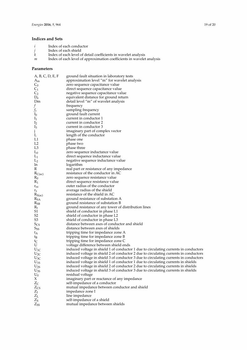
Energies 2016, 9, 964 19 of 20

Indices and Sets

i Index of each conductorj Index of each shieldk Index of each level of detail coefficients in wavelet analysism Index of each level of approximation coefficients in wavelet analysis

Parameters

A, B, C, D, E, F ground fault situation in laboratory testsAm approximation level “m” for wavelet analysisC0 zero sequence capacitance valueC1 direct sequence capacitance valueC2 negative sequence capacitance valueDe equivalent distance for ground returnDm detail level “m” of wavelet analysisf frequencyfs sampling frequencyI0 ground fault currentI1 current in conductor 1I2 current in conductor 2I3 current in conductor 3j imaginary part of complex vectorL length of the conductorL1 phase oneL2 phase twoL3 phase threeL0 zero sequence inductance valueL1 direct sequence inductance valueL2 negative sequence inductance valueln logarithmR real part or resistance of any impedanceRC(ac) resistance of the conductor in ACR0 zero sequence resistance valueR1 direct sequence resistance valueroc outer radius of the conductorrs average radius of the shieldRS(ac) resistance of the shield in ACRSA ground resistance of substation ARSB ground resistance of substation BRt ground resistance of any tower of distribution linesS1 shield of conductor in phase L1S2 shield of conductor in phase L2S3 shield of conductor in phase L3SCS distance between axes of conductor and shieldSSS distance between axes of shieldstA tripping time for impedance zone AtB tripping time for impedance zone BtC tripping time for impedance zone CU voltage difference between shield endsU1C induced voltage in shield 1 of conductor 1 due to circulating currents in conductorsU2C induced voltage in shield 2 of conductor 2 due to circulating currents in conductorsU3C induced voltage in shield 3 of conductor 3 due to circulating currents in conductorsU1S induced voltage in shield 1 of conductor 1 due to circulating currents in shieldsU2S induced voltage in shield 2 of conductor 2 due to circulating currents in shieldsU3S induced voltage in shield 3 of conductor 3 due to circulating currents in shieldsU0 residual voltageX imaginary part or reactance of any impedanceZC self-impedance of a conductorZCS mutual impedance between conductor and shieldZI impedance zone IZL line impedanceZS self-impedance of a shieldZSS mutual impedance between shields

Energies 2016, 9, 964 20 of 20

References

1. Tleis, N. Power Systems Modelling and Fault Analysis, 1st ed.; Newnes: Oxford, UK, 2008.2. Saha, M.M.; Izykowsky, J.; Rosolowsky, E. Fault Location on Power Networks; Springer: Berlin, Germany, 2009.3. Horowitz, S.H.; Phadke, A.G. Power System Relaying, 3rd ed.; Wiley: New York, NY, USA, 2008.4. L’Abbate, A.; Fulli, G.; Starr, F.; Peteves, S. Distributed Power Generation in Europe: Technical Issues for Further

Integration; JRC European Commission Scientific and Technical Report, EUR 23234 EN; Office for OfficialPublications of the European Communities: Luxembourg, 2007.

5. Tamo, T.; Voufo, J. Fault diagnosis on medium voltage (MV) electric power distribution networks: The caseof the downstream network of the AES-SONEL Ngousso sub-station. Energies 2009, 2, 243–257.

6. Li, P.; Zhang, B.H.; Hao, Z.G.; Rao, Y.F.; Wang, Y.T.; Bo, Z.Q.; Klimek, A.; Zhao, Q.; He, W. Optimal ReclosingTime of Transmission Lines and its Application in Real Power System. In Proceedings of the 9th InternationalConference on Developments in Power System Protection, Glasgow, UK, 17–20 March 2008.

7. He, R.W. A New Approach to the Calculation of Reclosing Time for Adaptive Auto-reclosure. In Proceedingsof the 2010 Asia-Pacific Power and Energy Engineering Conference, Chengdu, China, 28–31 March 2010.

8. Zoro, R.; Mefiardhi, R. Lightning performance on overhead distribution lines: Field observation at WestJava—Indonesia. In Proceedings of the 7th International Power Engineering Conference, Singapore,29 November–2 December 2005.

9. Yu, Y.Z.; Qin, J.; Li, G.X.; Chen, S.Y.; Li, J.; Chen, Y.Y. A Survey on Fault Location Methods for HybridTransmission Lines Consisting of Power Cables and Overhead Lines. Power Syst. Technol. 2006, 30, 64–69.

10. Standard CEI_60909-3. Short-Circuit Current Calculation in Three-Phase a.c. Systems. Part 3. Currentsduring Two Separate Simultaneous Single Phase Line-to-Earth Short Circuits and Partial Short-CircuitCurrents Flowing through Earth. Available online: https://webstore.iec.ch/publication/3890 (accessed on17 November 2016).

11. Radojevic, Z.; Terzija, V. Two Terminals Numerical Algorithm for Fault Distance Calculation and FaultAnalysis. In Proceedings of the 2006 IEEE PES Power Systems Conference and Exposition, Atlanta, GA,USA, 29 October–1 November 2006.

12. Zhou, Y.; Xu, G.; Chen, Y. Fault Location in Power Electrical Traction Line System. Energies 2012, 5, 5002–5018.[CrossRef]

13. Terzija, V.V.; Dobrijevic, D.M. Short Circuit Studies in Transmission Networks Using Improved Fault Model.In Proceedings of the IEEE Lausanne Power Tech, Lausanne, Switzerland, 1–5 July 2007.

14. Simón, P.; Garnacho, F.; Moreno, J.; González, A. Cálculo y Diseño de Líneas Eléctricas de Alta Tensión; IbergarcetaPublicaciones, S.L.: Madrid, Spain, 2011.

15. Magnago, F.H.; Abur, A. Fault location using wavelets. IEEE Trans. Power Deliv. 1998, 13, 1475–1480.[CrossRef]

16. Costa, F.B.; Souza, B.A.; Brito, N.S.D. Real-time classification of transmission line faults based on maximaloverlap discrete wavelet transform. In Proceedings of the 2012 IEEE/PES Transmission and DistributionConference and Exposition, Orlando, FL, USA, 7–10 May 2012.

17. Han, J.; Crossley, P.A. Fault location on a mixed overhead and underground transmission feederusing a multiple-zone quadrilateral impedance relay and a double-ended travelling wave fault locator.In Proceedings of the 2014 12th International Conference on Developments in Power System Protection,Copenhagen, Denmark, 31 March–3 April 2014.

18. Huang, J.G.; Hu, X.Y.; Li, X.S.; Hu, H.M.; Lv, Y.P. A Novel Single-Phase Earth Fault Feeder Detectionby Traveling Wave and Wavelets. In Proceedings of the 2006 International Conference on Power SystemTechnology, Chongqing, China, 22–26 October 2006.

19. Martínez, F.; Peris, A.; Rodenas, F. Tratamiento de Señales Digitales Mediante Wavelets y su uso con Matlab;Editorial Club Universitario: Alicante, Spain, 2004.

20. Hong, Y.Y.; Wei, Y.H.; Chang, Y.R.; Lee, Y.D.; Liu, P.W. Fault Detection and Location by Static Switches inMicrogrids Using Wavelet Transform and Adaptive Network-Based Fuzzy Inference System. Energies 2014,7, 2658–2675. [CrossRef]

© 2016 by the authors; licensee MDPI, Basel, Switzerland. This article is an open accessarticle distributed under the terms and conditions of the Creative Commons Attribution(CC-BY) license (http://creativecommons.org/licenses/by/4.0/).

https://webstore.iec.ch/publication/3890

http://dx.doi.org/10.3390/en5125002

http://dx.doi.org/10.1109/61.714808

http://dx.doi.org/10.3390/en7042658

http://creativecommons.org/

http://creativecommons.org/licenses/by/4.0/.

Novel Auto-Reclosing Blocking Method for Combined ... - MDPI

Documents

Transcript of Novel Auto-Reclosing Blocking Method for Combined ... - MDPI