The Tail-Fatness of FX Returns Reconsidered

Ronald Huisman Kees Koedijk Clemens Kool

Franz Palm

March 21, 2002

Correspondence: Franz C. Palm, Faculty of Economics and Business Administration, Maastricht University, P.O. Box 616, 6200 MD Maastricht, The Netherlands. Telephone: +31-43-3883833; Fax: +31-43-3884874; e-mail: F.Palm @KE.unimaas.nl. Ronald Huisman is affiliated with Erasmus University, Rotterdam; Kees Koedijk is at Erasmus University, Rotterdam, and at Maastricht University; Clemens Kool and Franz Palm are both at Maastricht University. The authors would like to thank seminar participants at Maastricht University for their helpful comments. All remaining errors pertain to the authors.

2

1 Introduction

It is a well-known stylized fact that foreign exchange returns are non-normal and tend to have fat-tailed distributions. Although information about the precise magnitude of the tail-fatness is crucial for applications such as risk analysis, little consensus exists in this respect, due to estimation problems. Typically, empirical estimation of tail-fatness is conditional on the specific (fat-tailed) distribution � such as the Student-t or stable � chosen.1 Since these alternative distributions are non-nested, an incorrect choice of distribution of returns may lead to significant estimation errors and flawed inference.

In recent years, extreme value analysis has been proposed to overcome this potential difficulty. It investigates the distribution of the maximum (minimum) in large samples, thereby determining the shape of the tails of a distribution. The limit law for the maximum is characterized by the so-called tail-index α, which corresponds one-to-one with the number of existing moments of the underlying distribution. Note that alternative distributions like the stable and Student-t now are nested within the limit law for extremes; for the stable distribution, it is the characteristic exponent β (< 2) which equals the tail-index α, while for the Student-t distribution it is the number of degrees of freedom v. The gain in applying extreme value analysis is that one can nest and test for different tail sizes. However, information about the center characteristics of the distribution is disregarded. Since it is information about the outlier observations that is crucial for studying issues like exchange rate volatility, exchange rate risk and value at risk, the use of extreme value analysis offers a positive net gain in our view.

The best-known and most often applied extreme value estimator for the tail-index was proposed by Hill (1975). Although asymptotically unbiased, this maximum likelihood estimator suffers severely from small sample bias. In fact, this holds for most alternative estimators, see Pictet et.al. (1996). Consequently, the empirical applicability of tail-index estimation is limited to cases of extremely large samples, either in the form of high frequency data or a very long sample period.2 In real life, often neither of these two conditions is fulfilled and only a small sample analysis is feasible.

In this contribution, we re-examine the tail-fatness of exchange rate returns using the tail-index estimator proposed by Huisman, Koedijk, Kool and Palm (2001) � henceforth HKKP �, which is unbiased in small samples. We show that previous tail-estimates in the literature overestimate the amount of fat-tailedness in exchange rate returns. Additionally, goodness-of-fit statistics provide supportive evidence of the appropriateness of assuming that a Student-t distribution underlies the data-generating 1 See Westerfield (1977), Rogalski and Vinso (1978) and Boothe and Glassman (1987), McCulloch (1997). 2 Recently, efficient nonparametric estimators have been proposed, see Beirlant et.al. (1996), for example. However, their implementation is complex and small-sample properties are as yet unknown.

3

process of exchange rate returns. The evidence is more convincing for floating than for exchange rates which have been subject to the exchange rate mechanism (ERM) within the European Monetary System (EMS).

The paper is set up as follows. In section 2, we briefly discuss extreme value theory and introduce the HKKP estimator to obtain unbiased tail-index estimates in small samples. In section 3, we describe data on sixteen exchange rates between January 1979 and April 1996. In section 4, we apply the HKKP tail index estimator and explicitly compare the HKKP tail index estimates with results from the existing literature. Also, we successfully examine the goodness-of-fit of a Student-t distribution with the degree of freedom equalling the HKKP tail estimates. Conclusions are given in section 5.

2 The Tail-Index

The tail-index α measures the speed with which the tail of a fat-tailed distribution F(.) approaches zero, when F(.) fulfills the following regular variation condition at infinity3:

(1) x=F(t)-1F(tx)-1 -

tαlim ∞→ ,

which implies that the higher α, the less fat-tailed the distribution is. Because the tail-index α equals the maximum number of finite moments in the sample, the tail-index can directly be used to test for the number of existing moments.

The HKKP-estimator is a simple and appropriate tool to obtain unbiased tail-index estimates in small samples.4 The methodology starts from the observation that the bias of the conventional Hill (1975)-estimator is a function of sample size n. Then, the bias-function is used to correct for the small sample bias. In this respect, the HKKP-estimator may be seen as a modified Hill estimator.5Suppose a sample of n observations is drawn from some unknown fat-tailed distribution. Let the parameter γ be the tail-index of this distribution (per definition, γ equals 1/α, where α refers to the maximum number of existing finite moments), while xi is the ith increasing order statistic (i = 1,2..n). Hill (1975) proposes the following estimator for the tail-index:

(2) ),x(-)x(k1=(k) k-n1+j-n

k

j=1

lnln∑γ

3 Many studies have shown that many financial series, including exchange rate returns fulfill this condition. 4 This estimator is discussed and tested in a more elaborate way in Huisman, Koedijk, Kool and Palm (2001). 5 In the literature, the tail-index is referred to as either α or γ, where γ equals 1/α; we use both interchangeably.

4

where k is the pre-specified number of tail observations to include (k = 1 .. n-1). The choice of k is crucial to obtain an unbiased estimate of the tail-index.6 In this respect, an asymptotic approximation of the bias in the Hill estimator can be derived for the following class of distribution functions: (3) ),bx+(1ax-1=F(x) -- βα

where α,β > 0 and a and b are real numbers. It has been shown that for a wide range of fat-tailed distribution equation (3) provides the second order asymptotic expansion of the cumulative distribution function (c.d.f.). For this class of distribution functions, the expected value and the variance of the Hill estimator in large samples for a given k can be approximated by

(4) )nk(a)+(

b-1(k))E( - αβ

αβ

βααβ

αγ ≈ ,

and

(5) αγ

2k1(k))var( ≈ ,

respectively. According to equations (4) and (5), the bias increases with k, while the variance decreases. A trade-off results between unbiasedness and accuracy. Most empirical studies suffer from this trade-off problem. Generally, a single "optimal" k is selected. However, equation (3) clearly shows that a bias exists for any k exceeding zero. One way out of the dilemma is to increase the number of observations (n), which decreases the importance of the bias for any given k decreases. The HKKP-estimator overcomes the problem of the need to select an optimal k in small samples, by exploiting an important characteristic of the bias function. For values of k smaller than some threshold value κ (for example for k < n/2), the bias of the conventional Hill-estimate of γ increases almost linearly in k (Note that if α = β, the relationship (4) is linear in k) .and can be approximated by: (6) .1...=k(k),+k+=(k) 10 κεββγ

An error term ε(k) has been included. Instead of selecting a single value of k to estimate the tail-index of the distribution under consideration, we propose to compute γ(k) for a 6 Various studies select k to minimize the MSE of the Hill-estimates conditional on a known distribution, see for instance Koedijk and Kool (1994). See Loretan and Phillips (1994) for an alternative approach.

5

range of values of k from 1 to κ. Subsequently, the vector of computed γ(k)'s is used in equation (6). We already argued that an unbiased estimate of γ can be obtained only for k → 0. Evaluation of equation (6) for k approaching zero yields the bias-corrected estimator of γ proposed by HKKP, which is equal to the estimated intercept β0. Although the coefficients in (6) can be estimated by Ordinary Least Squares (OLS), two issues have to be considered. First, equation (5) indicates that the variance of Hill estimates γ(k) varies with k, so that the error term, ε(k) in equation (6) is heteroskedastic. As an alternative, we suggest a Weighted Least Squares (WLS) approach. Dividing the right- and left hand sides of equation (6) by √k and applying OLS to the transformed equation yields the WLS estimator which accounts for heteroskedasticity. The estimated tail-index γ equals the first element of the vector bwls

Second, an overlapping data problem exists due to the construction of γ(k). The variables γ(k) are correlated, in terms of k, since estimates γ(k) for the values s and m for k are based on 1+min(s,m) common observations, see equation (2). Consequently, the usual formulae for the standard errors are inappropriate for the OLS and WLS estimators, but the well-known formulae for the standard errors of these estimators when applied to the generalized regression model are consistent will be used (for the details, see HKKP, 2001). HKKP (2001) have found the WLS estimator to be more accurate than the OLS estimator and to be hardly less accurate than the generalized least squares estimator which also accounts for the correlation between elements of the disturbance term in (7). Therefore, in the empirical part, we report weighted least squares estimates and appropriate standard errors accounting for the disturbance correlation resulting from the use of order statistics as mentioned above.

3 Data

The data consist of London closing mid-prices against the Pound Sterling for the period January 2, 1979 and April 4, 1996 obtained from DATASTREAM. The currencies of sixteen countries are considered: Austria, Belgium, Canada, Denmark, France, Germany, Ireland, Italy, Japan, the Netherlands, Norway, Spain, Sweden, Switzerland, the United Kingdom and the United States. We sample the data at the weekly frequency7 (using end-of-period data) to reduce the influences of ARCH effects and other types of dependency between subsequent observations that are present in many financial data,

7 Kearns and Pagan (1997) argue that the dependency between the observations results in serious biases for GARCH and IGARCH type models, especially when those estimates are obtained from small samples. Lucas (1997) shows that the tail-index estimator that we use in this study produces rather unbiased tail-index estimates for a GARCH(1,1) process in a sample of 250 observations. This, combined with the fact that we use weekly data to eliminate as much dependency as possible, supports that the results presented here are accurate.

6

since the tail-index estimates are produced assuming independent observations8. We have preferred not to use more recent data as the probability distribution of EMS exchange rates in more recent years is likely to have been affected by the expected start of the common currency euro as of January 1, 1999 and the decisions taken in the years preceding this date to make that start possible. All data are expressed as the number of foreign currencies to pay for one unit of the numeraire currency.

Table 1 contains summary statistics of the weekly data. With respect to skewness and kurtosis the following observations can be made from the table. First, the EMS currencies denoted in German Marks are skewed to the right, whereas the amount of skewness is much smaller and hovers around zero for the floating exchange rates denoted in US Dollars. Second, all exchange rate returns exhibit excess kurtosis9, reflecting apparent fat-tailedness. The excess kurtosis is most apparent for the EMS exchange rates in general, and for the Spanish Peseta and Swedish Krone in particular. [Insert Table 1 approximately here]

4 Results

In this section, we present tail-index estimates for the 16 currencies described in the previous section with the US dollar and the DM alternating as benchmark currency. We compare the tail-index estimates obtained from the HKKP estimator with results from the literature that are mostly obtained using maximum likelihood techniques. Subsequently, goodness-of-fit tests are done to investigate whether a hypothesized Student-t distribution with degrees of freedom equal to the obtained HKKP tail-index estimates is able to adequately reproduce the actual distribution of exchange rate returns.

4.1 Tail-index estimates

The observed excess kurtosis in table 1 already supports the finding of many other studies that the distribution of foreign exchange rate returns is fat-tailed. Note though that the kurtosis estimate is conditional on existence of the fourth moment of the underlying distribution. Especially for cases where quite large excess kurtosis values are obtained, such as, for example, the Spanish Peseta and the Swedish Krone against the DM, this assumption might be unwarranted. A direct way to test for the existence of the fourth moments is to evaluate the tail-index estimates for each exchange rate. For this purpose, HKKP-tail estimates with appropriate standard errors are reported in table 2. 8 Note that the true tail-index of the underlying return distribution is unaffected by time-aggregation; thus, the choice of sampling frequency should only affect the estimation results through the change in number of observations. 9 Excess with respect to the normal distribution which has a kurtosis equal to 3.

7

Estimates are shown for left-tail and right-tail observations separately and for the combination of both tails.10 [Insert Table 2 approximately here] According to table 2, the fourth moments are likely to exist for all exchange rates vis-à-vis the US dollar. Considering both tails simultaneously, tail-index estimates are found to vary between 4.0 for the Spanish Peseta and 8.1 for the British Pound. The tail-index estimates for currencies vis-à-vis the German Mark are smaller, indicating a higher amount of fat-tailedness. The estimates vary between 2.2 for the French Franc and 5.4 for the Canadian Dollar. For many of these exchange rates, the standard errors are such that the finiteness of the fourth moments can be rejected.

From table 2 we also conclude that the tail-index of the left and the right tail often differ considerably. For example, we obtain a tail-index estimate equal to 4.3 for the left tail of Canadian vis-à-vis the German Mark and an estimate equal to 7.3 for the right tail. If these tails differ significantly, one should use tail-specific estimates when inference is drawn from the tails. The columns headed �t� contain the t-statistics from testing the hypothesis that the tail-index estimate of the left tail equals the tail-index estimate of the right tail (accounting appropriately for the dependence between left and right tail index estimates resulting from the fact that tail index estimates are functions of order statistics; see HKKP, 2001, for details) . The results show that the difference between the left tail-index and the right tail-index is insignificant for the majority of exchange rates. It is significant at the 5% level for the Canadian Dollar, the Danish Krone, the Norwegian Krone, the Spanish Peseta and the Swedish Krone all vis-à-vis the German Mark and for the Japanese Yen, the Spanish Peseta, and the Swiss Franc vis-à-vis the US Dollar.

4.2 The tail-index of EMS rates versus floating rates

Koedijk, Stork and de Vries (1992) and Koedijk and Kool (1994) show that EMS exchange rate returns exhibit fatter tails than floating rate returns. The information in in table 2 provides clear evidence in support of this conclusion. For all EMS currencies, tail-estimates are lower when measured vis-à-vis the German Mark than vis-à-vis the US dollar, regardless of whether the left-tail, right-tail or both are considered. Table 3 contains the results of formally testing the null hypothesis that the tail-index of a currency vis-à-vis the German Mark equals the tail-index of the same currency but now against the US Dollar. The test statistic is asymptotically normally distributed. For 10 All observations are taken in deviation of their sample mean. The left tail is examined using the absolute value of all negative returns, the right tail is examined using all positive returns and to examine both tails simultaneously we use the absolute values of all returns.

8

negative values the tail fatness against the German Mark exceeds that against the US Dollar.

For most of the countries that have floated against both the US dollar and the DM, the equality of tail-fatness across numeraire currencies can not be rejected. This is the case for Canada, Japan, Spain, and Switzerland. Note that Spain has participated in the ERM only from 1989 onward, and has devalued a few times against the DM in 1992 and 1993. For all ERM countries equality of tail-estimates across numeraire currencies is firmly rejected with the tails against the DM showing significantly more fatness than the tail-estimates against the US dollar. The same holds (marginally) for Norway and Sweden, even though they did not formally participate in the EMS over the sample period. Consequently, the HKKP estimates support earlier conclusions that the return distribution of non-floating exchange rates has substantially fatter tails than does the distribution under floating.

4.3 A comparison: HKKP estimates versus the literature

The HKKP tail-index estimates reported in table 2 are much higher than values that were found in previous studies for floating rates. For example, Loretan and Phillips (1994) report α's for the German Mark / US Dollar around 3.4 where we find 5.3 for both tails instead. Boothe and Glassman (1987) report a tail-index estimate equal to 3.2 for the German Mark / US Dollar.

These differences can be explained in two ways. Firstly, they might be due to the different sample periods. Loretan and Phillips examine the period 1978 through 1991 and Boothe and Glassman examine the period 1973 through 1984. Our sample is partly overlapping with theirs as it covers the period 1979 through 1996. However, HKKP present tail-index estimates obtained over roughly the same sample as Loretan and Phillips and find systematically higher tail-index estimates for all currencies examined than Loretan and Phillips.

Second, the use of different estimation procedures might lead to different results. Loretan and Phillips (1994) obtain their estimates from the conventional Hill estimator (2). This estimator is biased in small samples, as we already discussed, while the HKKP-estimates in table 2 are approximately unbiased. Boothe and Glassman (1987) obtain tail-index estimates use a maximum likelihood procedure to estimate the tail index conditional on the true distribution being Student-t. As argued before, this distributional assumption may be incorrect in general and lead to estimation errors. In this respect, the inequality of left and right tails for many currencies, as illustrated in table 2, is of concern. The assumption of a symmetric distribution like a Student-t distribution, a sum-stable distribution and a mixture of normals definitely leads to misspecification. Finally, the conventional Hill-estimator is a maximum likelihood estimator as is the Boothe and Glassman method, raising the issue of small sample bias again. Overall, we conclude that

9

exchange rate returns have fatter than the normal distribution, but that they exhibit considerably less fatness than has been argued in the literature before. This holds especially true for floating exchange rate returns.

4.4 Distributional characteristics

The fact that the tail-fatness of exchange rate returns has been considerably over-estimated in the literature, has important implications for the issue of which statistical distribution captures the observed distribution of exchange rate returns best. Our results, for instance, indicate that the stable distribution with 2≥α is likely to be inappropriate for exchange rate returns. The characteristic exponent of the stable distribution which equals the tail-index is by definition below 2, while we find tail-index values around 5 for most floating exchange rate returns.

Westerfield (1977), Rogalski and Vinso (1978), and Boothe and Glassman (1987) examined several distributions to capture fat-tailedness. The Student-t distribution, a mixture of normals, and the sum-stable distribution are shown to provide the best fit among various alternative candidates, although goodness-of-fit tests only provide statistically weak evidence. This may be due to the poor quality of previous tail-estimates.

Here, we investigate whether a (potentially asymmetric) Student-t distribution with the number of degrees of freedom equal to the estimated tail-indices, is able to adequately fit the observed frequencies in the tails of the exchange rate return distribution.

Let xi be the exchange rate returns under consideration. To fit the Student-t distribution, we assume that yi = θ(xi - m) is Student-t distributed with α degrees of freedom. Here m is a location parameter that equals the sample mean. The scale parameter θ is a function of the variance and can be derived as follows. For a student-t distribution with α degrees of freedom, the variance of yi equals α / (α-2) where α > 2. Consequently, the scale parameter θ can be expressed in terms of the variance of the exchange rate and the number of degrees of freedom α:

(10) )x2)var(-(=

iααθ .

Now, we set the number of degrees of freedom equal to the (unbiased) HKKP tail-index estimate for each currency instead of estimating this number using the maximum likelihood procedure as in Boothe and Glassman. In this way, we circumvent the usual small sample bias in other methods. Because the tail-index estimates for the left and right tail differ significantly for some exchange rates, we model and reproduce each tail

10

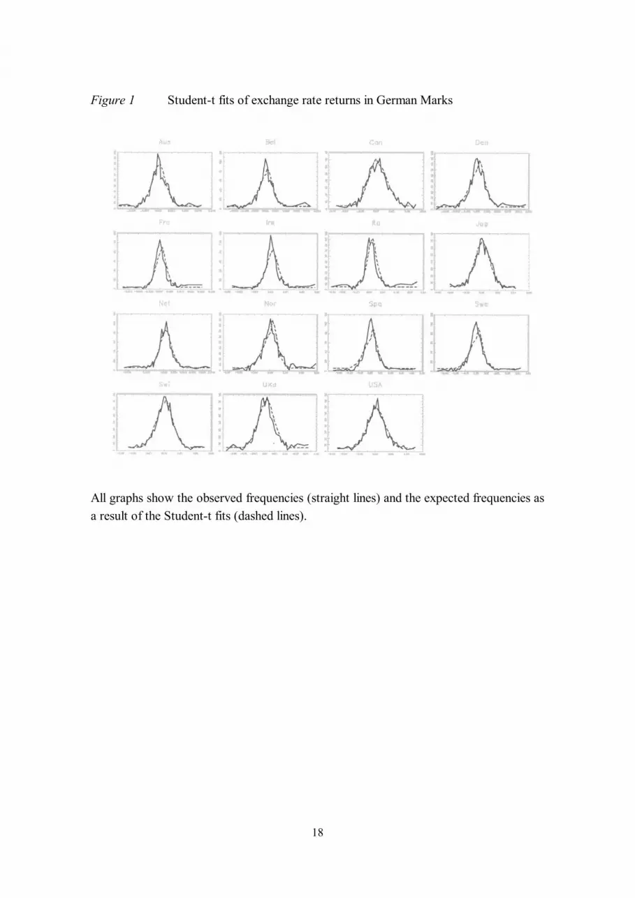
separately. The above procedure allows for the reproduction of data-generating distribution for exchange rate returns conditional on the HKKP- tail estimate and the observed sample variance. In figures 1 and 2 both these fitted (hypothetical) Student-t distribution and the observed empirical distribution of each exchange rate return series are given in the form of histograms. Note that the whole distribution is fitted by separately using the estimated tail-index for each tail. For an example, consider the US Dollar vis-à-vis the German Mark. We fit the left tail with a Student-t distribution with α equal to 5.2 and the right tail with a Student-t distribution with α equal to 5.9. Figure 1 shows the fitted distribution for the exchange rates in terms of the German Mark, whereas the US Dollar is taken as the numeraire currency in Figure 2. [Insert Figures 1 and 2 approximately here] At first glance, the Student-t distribution seems to fit the complete empirical distribution of exchange rate returns surprisingly well for many exchange rates. Some important deviations from the symmetric Student-t exist for the French Franc, the Italian Lira, the Spanish Peseta and the Swedish Krone against the German Mark due to non-zero skewness in EMS rates as is reflected in table 1. In figure 2, skewness problems appear less severe. Substantial differences between actual and fitted distributions only seem present for the Japanese Yen and the Spanish Peseta. To test the hypothesis that the fitted Student-t distribution is a good approximation for the unconditional empirical distribution of exchange rate returns, we apply a Pearson goodness-of-fit tests similar to the one used by Boothe and Glassman (1987). The goodness-of-fit test compares the observed and expected number of observations in c intervals. The test statistics is aymptotically chi-squared distributed with (c-1) degrees of freedom. We set the number of intervals c equal to 20.11 The intervals (except the first in the left tail and the last in the right tail which are open to the left and the right respectively) are chosen such that they are of equal length and that the tails intervals have 5 expected observations, which is the minimum for the test statistic to be chi-squared distributed.

The Student-t distribution for returns is rejected for the British Pound, the Canadian Dollar, the German Mark and the Japanese Yen vis-à-vis the US Dollar. It is not rejected for the Canadian Dollar only. Table 4 contains the results both for the whole distribution and for the tails. With respect to the latter, we distinguish between fitting the 5% largest and 5% smallest observations and fitting the 10% largest and 10% smallest observations. 11 As Boothe and Glassman (1987), who use 14 intervals, we find that our results are very robust with respect to the number of intervals chosen. See Bain and Engelhardt (1987) for more details on goodness-of-fit tests.

11

[Insert Table 4 approximately here] From table 4, we observe that the Student-t is a good approximation for the complete distribution of returns for many of the floating exchange rates (see the �all� column). For the tails, the fit is even better. For all currencies against the US dollar, the test fails to reject the Student-t fit both for the 5% and 10% categories. Note that this result also holds for the exchange rates for which the Student-t distribution was rejected for all observations: the Japanese Yen, the Spanish Peseta, the Swedish Krone and the Swiss Franc. This result implies that one could safely use the Student-t distribution to obtain tail information for these floating rates.

Especially the fit of the tails is relevant here. Although the Student-t fits the overall distribution rather well too, if the goal is to fit the complete distribution, empirical distribution kernel estimates and splines are likely to produce even better fits. But the Student-t distribution has the advantage of providing a good local fit in the tails and accurate exceedence probabilities or quantiles for the tails. Especially for events that occur with a probability smaller than 1/n, a good fit of the tails through a Student-t distribution is potentially valuable. Extrapolation out-of-sample using the functional form of the Student-t can be done with great ease and could be very useful for risk management.

The results are not that strong for the exchange rates vis-à-vis the German Mark. The Student-t is rejected to fit the tails for the Belgian Franc, the Danish Krone, the French Franc, the Irish Punt, the Italian Lira, the Norwegian Krone, the Spanish Peseta, the Swedish Krone and the British Pound. One reason why the Student-t distribution is rejected in the tails for the exchange rates mentioned above may be the realignments that took place in the EMS. To test for the impact of these realignments we computed HKKP tail-index estimates from a sample where all realignment observations were excluded. Fitting a Student-t with the new tail-estimate for the 5% smallest and 5% largest observations, leads to goodness-of-fit statistics in the 5% (R) column. The results improve somewhat and show that we cannot reject the Student-t distribution for the Danish Krone and the Irish Punt. Note that the Student-t is rejected to fit the whole distribution but accepted to fit the tails for the Belgian Franc, the Danish Krone and the Irish Punt due to the fact that all of these exhibit highly skewed distributions. Clearly, realignments do not provide the complete story about the difference between ERM and floating exchange rate return distributions.

5 Conclusions and practical implications

In this contribution, we focus on the tail characteristics of the unconditional distribution of exchange rate returns. It is a stylized fact that exchange rate returns are fat-tailed.

12

However, methods used to compute the degree of fat-tailedness generally suffer from small sample bias. We apply the unbiased HKKP tail-index estimate, which essentially is a modified Hill-estimate corrected for small sample bias. The correction exploits the fact that the bias is an approximately linear function of the number of tail observations used.

We apply this method to currencies of 16 countries, measured against both US dollar and DM for the period 1979-1996. We conclude first, that the magnitude of tail fatness in exchange rate returns has been seriously over-estimated in the past, especially for many floating rates. Second, the tail-indexes for the left tail (negative returns) differ significantly from those of the right tail for many exchange rates; the assumption of an underlying symmetric distribution is inappropriate, therefore. Third, the tails of EMS exchange rate returns are significantly fatter than the tails of floating rate returns. Fourth, the Student-t distribution is found to fit the tails of all floating exchange when the degrees of freedom parameter is set equal to the HKKP tail estimate. For some of the exchange rate returns in terms of the German Mark, apparent skewness and realignments in the EMS result in somewhat poorer fits, even when realignments are excluded. More research is needed to better understand the difference between exchange rates that are subject to an exchange rate mechanism and floating exchange rates in this respect. Nevertheless, the Student-t fits the tails well for almost all exchange rates under consideration.

The results put forward in this contribution have important implications for managing exchange rate risk. Risk on extreme events on floating exchange rate positions has seriously been over-estimated in the past. Furthermore, one needs to analyze positive and negative returns separately and one cannot directly assume that the probability of extreme events is the same for short and long foreign exchange positions. Also, the probability on extreme events is much higher for EMS rates.

Finally, the Student-t distribution can be used as an accurate approximation for tails of the unconditional distribution of foreign exchange rate returns if one sets the number of degrees of freedom equal to the unbiased HKKP tail-index estimate. This holds for all floating rates and for most of the non-freely floating (EMS) exchange rates that are expressed against the German Mark. Exceedence probabilities and quantile estimates used as inputs for Value at Risk formulae can be easily obtained by extrapolation of the fitted Student-t distribution. This is especially attractive for the analysis of the risk on out-of-sample events which occur with probability smaller than 1/n.

13

6 References

Bain, L.J. and M. Engelhardt, 1987, Introduction to Probability Theory and Mathematical Statistics, Duxbury, Press Boston.

Beirlant, J., Vynckier, P. and J. Teugels, 1996, Tail-index Estimation, Pareto Quantile Plots and Regression Diagnostics, Journal of the American Statistical Association, 91, 1659-1667.

Boothe, P. and D. Glassmann, 1987, The Statistical Distribution of Exchange Rates: Empirical Evidence and Economic Implications, Journal of International Economics, 22, 297-320.

Hill, B., 1975, A Simple General Approach to Inference about the Tail of a Distribution, Annals of Mathematical Statistics, 3, 1163-1174.

Huisman, R., K.G. Koedijk, C.J.M. Kool and F. Palm, 2001, Tail-index Estimator in Small Sample, Journal of Business and Economic Statistics, 19, 208-216.

Kearns, P. and A. Pagan, 1997, Estimating the Density Tail Index for Financial Time Series, The Review of Economics and Statistics, 79, 171-175.

Koedijk, K.G. and C.J.M. Kool, 1994, Tail Estimates and the EMS Target Zone, Review of International Economics, 2, 153-165.

Koedijk, K.G., P.A. Stork and C.G. de Vries, 1992, Differences between Foreign Exchange Rate Regimes: the View from Tails, Journal of International Money and Finance, 462-473.

Loretan, M. and P.C.B. Phillips, 1994, Testing the Covariance Stationarity of Heavy-Tailed Time Series: An Overview of the Theory with Applications to Several Financial Data Series, Journal of Empirical Finance, 211-248.

Lucas, A. (1997), Discussion on Fat Tails in Small Samples, presented at the 5th workshop on Finance and Econometrics in Brussels.

McCulloch, J.H., 1997, Measuring Tail Thickness to Estimate the Stable Index α: A Critique, Journal of Business Economics and Statistics, 15, 11, 74-81.

Pictet, O., Dacarogna, M. and U. Müller, 1996, Hill, Bootstrap and Jackknife Estimators for Heavy Tails, working paper, Olsen & Associates, Zürich.

Rogalski, R.J. and J.D. Vinso, 1978, Empirical Properties of Foreign Exchange Rates, Journal of International Business Studies, 9, 69-79.

Westerfield, J.M., 1977, An Examination of Foreign Exchange Risk under Fixed and Floating Rate Regimes, Journal of International Economics, 7, 181-20

14

1. Summary statistics These summary statistics cover the sample period from January 2, 1979 through April 4, 1996. The data is sampled at the weekly frequency. The mean and standard deviations of the (std.) returns are in annualized percentages. In the other columns, the skewness and excess kurtosis are provided. Currency

numeraire: German Mark

numeraire: US Dollar

mean std. skew kurt. mean std. skew kurt.

Austria

-0.005

1.172

-0.116

3.551

-0.634

5.219

-0.101

1.469

Belgium 0.350 1.542 1.661 20.718 -0.279 5.173 -0.093 1.518 Canada 0.957 5.454 0.020 1.500 0.328 2.177 0.092 2.669 Denmark 0.561 1.666 1.534 11.758 -0.068 5.093 -0.099 1.150 France 0.780 1.848 2.864 28.210 0.151 5.139 0.059 1.857 Germany �- �- �- �- -0.629 5.248 -0.065 1.457 Ireland 0.925 2.518 1.760 16.855 0.296 5.171 0.207 2.656 Italy 1.574 3.250 2.284 18.090 0.945 5.044 0.676 5.855 Japan -0.542 4.471 -0.252 1.307 -1.171 4.993 -0.537 2.774 Netherlands 0.098 0.869 0.255 13.376 -0.531 5.166 -0.094 1.269 Norway 0.803 2.669 2.089 15.334 0.174 4.475 0.454 3.218 Spain 1.472 3.919 8.687 148.89 0.843 5.573 2.958 33.490 Sweden 1.109 3.936 6.319 84.030 0.480 4.948 3.145 34.096 Switzerland -0.234 2.501 0.149 3.111 -0.863 6.002 -0.123 1.305 U. Kingdom 0.961 3.960 0.592 3.026 0.332 5.158 0.235 3.379 U. States 0.629 5.248 0.065 3.457 �- �- �- �-

15

2. Tail-index α estimates This table provides tail-index estimates for the weekly returns on the sixteen currencies over the sample period from January 2, 1979 through April 4, 1996. The estimates presented are for both tails simultaneously, the left, and the right tail respectively. We present t-statistics for the two-sided test of the hypothesis that the tail-index for the left tail equals that for the right tail. In the last column, we present t-statistics for the hypothesis that the tail-index for the currency vis-à-vis the German Mark equals that of the same currency vis-à-vis the US Dollar. The standard errors given in parentheses account for the correlation resulting from overlapping observations.

both Left right t Both left right t

Austria

3.419 (0.333)

3.461 (0.476)

3.185 (0.452)

0.421

5.753 (0.561)

5.621 (0.798)

5.986 (0.822)

-0.318

Belgium 3.248 (0.317)

3.953 (0.541)

2.718 (0.388)

1.856 5.382 (0.524)

5.120 (0.721)

5.701 (0.789)

-0.544

Canada 5.454 (0.531)

4.371 (0.605)

7.259 (1.024)

-2.428 4.609 (0.449)

4.006 (0.551)

5.660 (0.803)

-1.698

Denmark 3.290 (0.321)

4.157 (0.562)

2.695 (0.389)

2.139 5.280 (0.515)

4.844 (0.679)

5.724 (0.795)

-0.842

France 2.205 (0.215)

2.707 (0.344)

2.489 (0.389)

0.421 5.236 (0.510)

5.520 (0.762)

4.772 (0.673)

0.736

Germany

�- �- �- �- 5.323 (0.519)

5.937 (0.834)

4.828 (0.670)

1.037

Ireland 2.616 (0.255)

2.890 (0.376)

2.761 (0.418)

0.230 5.757 (0.561)

5.441 (0.744)

6.010 (0.858)

-0.501

Italy 2.281 (0.222)

2.364 (0.304)

2.426 (0.373)

-0.129 4.714 (0.459)

5.283 (0.720)

4.228 (0.605)

1.122

Japan 5.250 (0.512)

5.546 (0.782)

5.303 (0.732)

0.217 6.099 (0.594)

9.037 (1.318)

5.801 (0.777)

2.115

Netherlands 2.790 (0.272)

2.707 (0.376)

2.857 (0.401)

-0.271 5.365 (0.523)

6.278 (0.880)

4.705 (0.653)

1.436

Norway 3.314 (0.323)

4.945 (0.664)

2.512 (0.366)

3.209 4.442 (0.433)

4.886 (0.672)

4.035 (0.571)

0.965

Spain 3.187 (0.311)

4.596 (0.610)

2.525 (0.372)

2.897 4.034 (0.393)

5.084 (0.690)

3.283 (0.472)

2.155

Sweden 3.034 (0.296)

4.072 (0.546)

2.434 (0.356)

2.515 4.264 (0.416)

5.079 (0.696)

3.594 (0.512)

1.719

Switzerland 4.786 (0.466)

5.613 (0.793)

4.179 (0.577)

1.462 5.734 (0.599)

8.314 (1.157)

4.552 (0.637)

2.849

U. Kingdom 3.847 (0.375)

4.162 (0.555)

4.019 (0.590)

0.177 8.111 (0.790)

8.027 (1.092)

7.787 (1.117)

0.154

U. States

5.232 (0.519)

4.828 (0.670)

5.937 (0.834)

-1.037 �- �- �- �-

16

3. EMS versus floating We report t-statistics for the two-sided test of the hypothesis that the tail of a currency rate vis-à-vis the German Mark equals the tail of the same currency vis-à-vis the US Dollar. For the EMS currencies, this is a test on tail equality of EMS and floating rates. Both refers to the test on both tails simultaneously. Left and right refer to the left and the right tail respectively. currency

both

Left

right

Austria

-3.578

-2.325

-2.986

Belgium -3.485 -1.295 -3.393 Canada 1.215 0.446 1.229 Denmark -3.279 -0.779 -3.422 France -5.476 -3.365 -2.935 Germany �- �- �- Ireland -5.097 -3.065 -3.404 Italy -4.772 -3.735 -2.535 Japan -1.083 -2.278 -0.467 Netherlands -4.368 -3.732 -2.412 Norway -2.088 0.065 -2.246 Spain -1.690 -0.530 -1.261 Sweden -2.409 -1.138 -1.860 Switzerland -1.249 -1.926 -0.434 U. Kingdom -4.876 -3.155 -2.983 U. States

�- �- �-

17

4. Goodness-of-fit statistics for Student-t This table provides chi-squared goodness-of-fit statistics to test the null hypothesis that the Student-t distribution with the number of degrees of freedom equal to the tail-index estimate α provides a good fit of the exchange rate returns. The tests are performed on all observations (all), on the 10% largest and the 10% smallest observations (10%), on the 5% largest and the 5% smallest observations (5%) and on the 5% largest and smallest obtained from the sample from which data for all realignment periods are excluded 5% (R). The expected and observed frequencies are calculated over 20 intervals for all and 10%; they are calculated over 10 intervals in case of 5%. Currency

numeraire:

German Mark

numeraire: US Dollar

5%

5% (R)

10%

all

5%

10%

all

Austria

9.487

10.822

18.567

22.952

4.869

22.874

20.815

Belgium 18.132 19.385 31.061 44.003 5.485 13.455 13.879 Canada 12.655 14.963 24.293 23.268 6.363 12.058 18.200 Denmark 18.292 11.170 24.936 46.153 7.753 15.144 12.390 France 21.792 18.474 37.924 100.795 5.302 16.572 20.582 Germany �- �- �- �- 11.350 16.812 21.391 Ireland 17.892 16.011 25.640 77.832 4.888 15.027 16.169 Italy 36.178 44.268 48.642 92.668 9.811 7.750 14.866 Japan 10.591 10.383 13.166 18.843 13.291 20.651 45.325 Netherlands 12.263 15.799 26.580 28.459 7.573 16.317 12.752 Norway 46.615 23.638 59.060 80.006 10.280 19.000 26.829 Spain 46.507 47.795 51.876 118.308 10.573 12.285 48.066 Sweden 21.269 22.692 40.355 74.582 15.816 16.925 32.819 Switzerland 3.462 5.651 13.990 10.741 16.277 23.588 33.518 U. Kingdom 27.569 32.558 33.325 41.453 7.566 14.793 27.681 U. States

11.207 13.093 17.279 21.502 �- �- �-

Chi-squared critical value for 19 degrees of freedom at the 5% level is 30.140; for 9 degrees of freedom it equals 16.920. Reject the null that the Student-t is a good approximation for the exchange rate returns if the reported goodness-of-fit statistic exceeds the corresponding critical value. The fitted Student-t distributions are not tail -symmetric; i.e. we used the separate tail-index estimates for the left and right tail.

18

Figure 1 Student-t fits of exchange rate returns in German Marks

All graphs show the observed frequencies (straight lines) and the expected frequencies as a result of the Student-t fits (dashed lines).

19

Figure 2 Student-t fits of exchange rate returns in US Dollars

All graphs show the observed frequencies (straight lines) and the expected frequencies as a result of the Student-t fits (dashed lines).