Austral. J. Statist., 30(1), 1988, 67-77

NONPARAMETRIC RELIABILITY ESTIMATION BASED ON A FEW ORDERED OBSERVATIONS

H. ARSHAM

Information and Quantitative Sciences Department, University of Baltimore.

Summary

The usual one-sided Kolmogorov-Smirnov distance is generalized to obtain an improved lower confidence region for the extreme left tail of the reliability function based on k observations in a “k out of n censored” plan. Finite sample and asymptotic critical values necessary for implemen- tation are given. The two numerical comparisons with existing parametric procedures for the case of complete or censored samples demonstrate the applicability of the proposed nonparametric procedure.

Key Words. One-sided confidence regions; empirical reliability function; censored data; Poisson process; generalized K-S statistics.

1. Introduction

Let z1,22,. . . , z,, be n independent random observations with a com- mon continuous cumulative distribution function (cdf) F(-), and let F,,(.) denote the empirical cdf. If the sample is censored in a “k out of n cen- sored” plan then only the k, k fixed (1 5 k 5 n) order statistics will be observed taking values q j ) , (1 5 j 2 k). In analysis of a pro-rated war- ranty such as setting a warranty assurance (I - a) or warranty period (20) it is desirable to have an accurate estimate of the reliability function a(.) = 1 - F(.) for the left tail of R(.) based on a censored (or com- plete) sample. Since the nature of the life distribution is not generally known, the problem is to construct a distribution-free confidence region for it. The most widely used nonparametric confidence region based on Rn(.) = 1 - Fn(-) is the usual one-sided Kolmogorov-Smirnov (K-S) simul- taneous confidence region:

P [ R ( z ) 2 Rn(z) - A ( n , k , a ) for all z : (n - k ) / n 5 R(z) 5 11 = 1 - a (1)

68 H. ARSHAM

where A(.) is the critical value of the usual one-sided (K-S) distance for a given ( n , k , a ) . One problem in applying the region (1) to, for example, the pro-rated warranty analysis is that the constructed region has a constant bandwidth for a given (n, k , a ) which does not permit us to emphasize on the left tail of R(z ) where we want to have more precise information about the reliability R(z).

It is well known that a lower confidence interval on R(zo), for any fixed 20, zo 5 z ( k ) , at level 1 - a can be obtained from the Beta distribution with parameters n - k 4- 1 and k. This confidence interval is valid at the point 20, and not for all z simultaneously.

The goal of this paper is to give a compromise between these two extremes. For the point zo in the left tail one can construct a confidence region with a narrower band in the neighbourhood of 20 than is afforded by the usual K-S confidence region. We consider a confidence region of the following desirable form: for 7 > 1,s > 0,

Note that region (2) is narrower in the left and wider in the right. For 7 = 1 this generalized K-S confidence region has a constant bandwidth similar to the region given by (1).

The first two sections to follow will develop such a confidence region for the censored and complete observations respectively. For the user the construction of the confidence region is described in section 4 and illus- trated in section 5 .

2. Confidence Regions Using Censored Sample

Let Un(.) be the empirical cdf of n independent Uniform [0,1] random variables. By using the usual distribution-free argument (2) reduces to

2.1. Exact Confidence Regions When a confidence region is constructed using the censored data, the

actual band would be a fixed width over the right tail, since in this case it is not required to remain within the band beyond the kth failure in an "k

NONPARAMETRIC RELIABILITY ESTIMATION 69

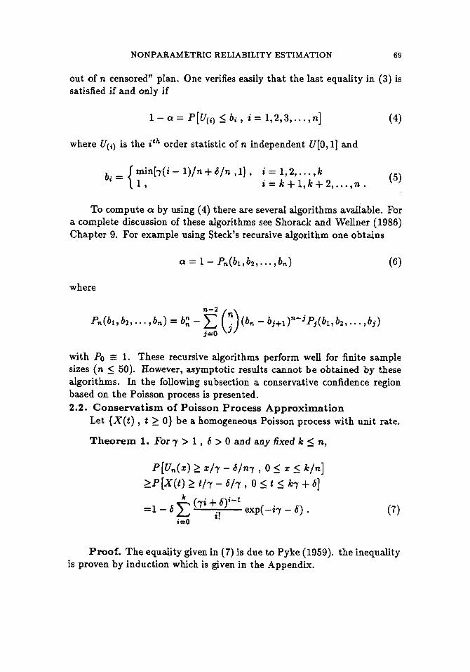
out of n censored” plan. One verifies easily that the last equality in (3) is satisfied if and only if

where U(i, is the i*h order statistic of n independent U[O, 11 and

(5) min[7 ( i - l ) /n+S/n ,1 ] , i = 1,2 ,..., k

i = k + l , k + 2 ,..., n . bj =

To compute cy: by using (4) there are several algorithms available. For a complete discussion of these algorithms see Shorack and Wellner (1986) Chapter 9. For example using Steck’s recursive algorithm one obtains

where

with Po i 1. These recursive algorithms perform well for finite sample sizes (n 5 50). However, asymptotic results cannot be obtained by these algorithms. In the following subsection a conservative confidence region based on the Poisson process is presented. 2.2. Conservatism of Poisson Process Approximation

Let { X ( t ) , t 2 0) be a homogeneous Poisson process with unit rate.

Theorem 1. For 7 > 1 , 6 > 0 and any fixed E 5 n,

exp(-ir - 6) . k (7i + 6)i-1

i ! i = O

(7)

Proof. The equality given in (7) is due to Pyke (1959). the inequality is proven by induction which is given in the Appendix.

70 H. ARSHAM

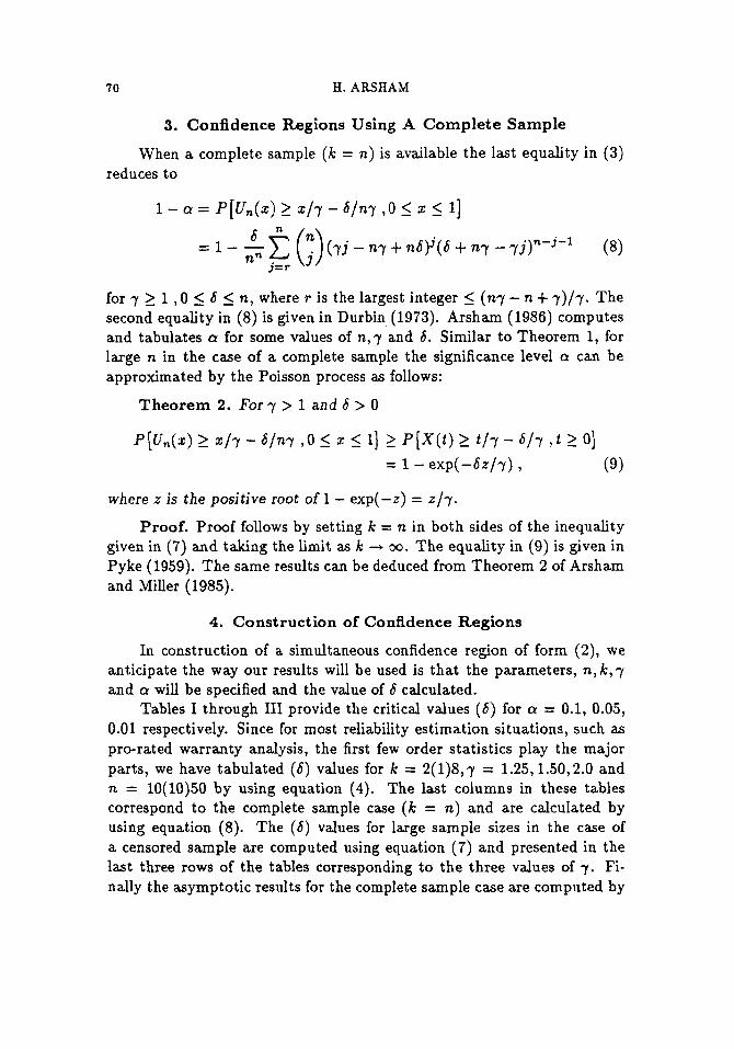
3. Confidence Regions Using A Complete Sample

When a complete sample (k = n) is available the last equality in (3) reduces to

6 " nn j=r

= 1 - - (I) ( y j - ny + n6)j(6 + n7 - 7j )"- j - ' (8)

for y 2 1 , O 5 6 I n, where T is the largest integer 5 (n7 - n + y)/y. The second equality in (8) is given in Durbin (1973). Arsham (1986) computes and tabulates a for some values of n,y and 6. Similar to Theorem 1, for large n in the case of a complete sample the significance level a can be approximated by the Poisson process as follows:

Theorem 2. Fory > 1 and 6 > 0

where I is the positive root of 1 - exp(-z) = 1/7.

Proof. Proof follows by setting k = n in both sides of the inequality given in (7) and taking the limit as k --+ 00. The equality in (9) is given in Pyke (1959). The same results can be deduced from Theorem 2 of Arsham and Miller (1985).

4. Construction of Confidence Regions

In construction of a simultaneous confidence region of form (2), we anticipate the way our results will be used is that the parameters, n, k, y and a will be specified and the value of 6 calculated.

Tables I through 111 provide the critical values (6) for Q = 0.1, 0.05, 0.01 respectively. Since for most reliability estimation situations, such as pro-rated warranty analysis, the first few order statistics play the major parts, we have tabulated (6) values for k = 2(1)8,y = 1.25,1.50,2.0 and n = 10(10)50 by using equation (4). The last columns in these tables correspond to the complete sample case (k = n) and are calculated by using equation (8). The (6) values for large sample sizes in the case of a censored sample are computed using equation (7) and presented in the last three rows of the tables corresponding to the three values of y. Fi- nally the asymptotic results for the complete sample case are computed by

NONPARAMETRIC RELIABILITY ESTIMATION 71

TABLE I The Critical Values (6) for the Simultaneous Confidence Regions J?(z)>R-(z)-(-pl+ 6/n) with Significance Level a=0.1 in a “k out of n censored” Plan for ~ = 1 . 2 5 , 1.5 and 2.0.

k n 2 3 4 5 6 7 8 n

10

20

30

40

50

00

2.437

2.335

2.198

2.662

2.550

2.390

2.742

2.626

2.459

2.783

2.665

2.494

2.808

2.689

2.516

3.310

3.067

2.733

2.615

2.432

2.219

2.944

2.731

2.456

3.062

2.838

2.544

3.122

2.894

2.589

3.159

2.927

2.617

3.614

3.257

2.799

2.697

2.460

2.219

3.129

2.828

2.476

3.284

2.966

2.577

3.364

3.035

2.630

3.413

3.078

2.662

3.859

3.395

2.835

2.727

2.464

2.219

3.255

2.882

2.482

3.448

2.043

2.590

3.547

3.127

2.648

3.608

3.179

2.683

4.064

3.498

2.856

2.731

2.464

2.219

3.341

2.910

2.483

3.571

3.093

2.595

3.690

3.189

2.655

3.763

3.249

2.693

4.240

3.579

2.868

2.731

2.464

2.219

3.399

2.924

2.483

3.665

3.124

2.596

3.803

3.231

2.659

3.888

3.298

2.698

4.393

3.643

2.876

2.731

2.464

2.219

3.436

2.929

2.483

3.737

3.143

2.597

3.894

3.260

2.660

3.990

3.333

2.700

4.527

3.694

2.881

2.731

2.464

2.219

3.477

2.931

2.483

3.921

3.167

2.597

4.228

3.312

2.661

4.456

3.412

2.702

6.200

3.951

2.890

using equation (9) and presented in the lower right corner of the tables. The numbers for the critical values given in these tables are accurate to at least three digits. Note that the factor 7 influences the shape of the confidence region. Larger values of 7 imply a narrower left tail confidence region. In practice the narrowing factor is selected in such a way that the corresponding confidence region has the desirable shape. This can be

72 H. ARSHAM

TABLE I1 The Critical Values ( 6 ) for the Simultaneous Confidence Regions R(s)>R,,(s)-(r-I+ 6/n) with Significance Level u=0.05 in a "k out of n censored" Plan for r=1.25, 1.5 and 2.0.

k n 2 3 4 5 6 7 8 n

10

20

30

40

50

00

2.983 2.874 2.727

3.330 3.206 3.025

3.455 3.326 3.135

3.520 3.388 3.192

3.559 3.426 3.227

4.209 3.935 3.540

3.151 2.961 2.743

3.642 3.407 3.098

3.822 3.574 3.236

3.916 3.660 3.308

3.973 3.713 3.353

4.584 4.178 3.629

3.218 2.980 2.743

3.842 3.513 3.120

4.076 3.720 3.275

4.198 3.829 3.358

4.273 3.896 3.409

4.889 4.358 3.679

3.234 2.981 2.743

3.974 3.568 3.125

4.261 3.810 3.289

4.411 3.939 3.379

4.503 4.019 3.435

5.147 4.496 3.709

3.234 2.981 2.743

4.065 3.595 3.126

4.398 3.866 3.295

4.576 4.013 3.388

4.686 4.105 3.448

5.369 4.604 3.727

3.234 2.981 2.743

4.115 3.607 3.126

4.501 3.901 3.296

4.706 4.063 3.392

4.833 4.164 3.454

5.564 4.691 3.739

3.234 2.981 2.743

4.148 3.611 3.126

4.577 3.921 3.297

4.809 4.096 3.394

4.953 4.207 3.456

5.737 4.762 3.746

3.234 2.981 2.743

4.176 3.612 3.126

4.573 3.944 3.297

5.161 4.153 3.394

5.469 4.298 3.458

8.067 5.140 3.760

achieved after repeatedly trying several different values for 7.

lowing are also routine problems: In constructing confidence regions for the reliability function the fol-

i) For a given (n, y, 6,a) what is the minimum level of censorship? ii) Given (k, n,7,6) what is the confidence coefficient (1 - a)?

iii) Given (k, n, 6, a) find the narrowing factor 7.

NONPARAMETRIC RELIABILITY ESTIMATION 73

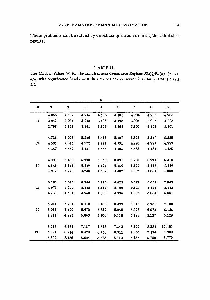
These problems can be solved by direct computation or using the tabulated results.

TABLE I11 The Critical Values (6) for the Simultaneous Confidence Regions R(z)>Rm(z)-(y-l+ S/n) with Significance Level ci=O.Ol in a k out of n censored" Plan for y=1.25, 1.5 and 2.0.

k n 2 3 4 5 6 7 8 n

4.056 10 3.942

3.796

4.177 3.994 3.801

4.205 3.998 3.801

4.205 3.998 3.801

4.205 3.998 3.801

4.205 3.998 3.801

4.205 4.205 3.998 3.998 3.801 3.801

4.736 20 4.595

4.38 7

5.078 4.815 4.462

5.286 4.922 4.481

5.413 4.971 4.484

5.487 4.991 4.485

5.528 4.998 4.485

5.547 5.555 4.999 4.999 4.485 4.485

4.993 30 4.845

4.617

5.430 5.145 4.740

5.728 5.320 4.786

5.939 5.424 4.802

6.091 5.486 4.807

6.200 5.521 4.808

6.278 6.416 5.540 5.556 4.809 4.809

5.118 40 4.976

4.739

5.616 5.320 4.891

5.964 5.535 4.956

6.223 5.675 4.983

6.422 5.766 4.995

6.576 5.827 4.999

6.695 7.042 5.865 5.923 5.000 5.001

5 . m 50 5.056

4.814

5.731 5.429 4.985

6.110 5.670 5.063

6.400 5.832 5.100

6.629 5.945 5.116

6.813 6.023 5.124

6.961 7.100 6.078 6.186 5.127 5.129

6.215 00 5.891

5.390

6.731 6.248 5.536

7.157 6.520 5.624

7.523 6.736 5.678

7.843 6.911 5.713

8.127 7.055 5.735

8.382 12.400 7.174 7.902 5.750 5.779

74 H. ARSHAM

6. Numerical Comparison and Conclusions

In this section we present two examples to illustrate the construction of the generalized K-S confidence region discussed in the preceding section. In doing reliability studies, one is concerned with the probability of survival until a specified time.

A widely used method of obtaining confidence bounds on a reliability function is a parametric procedure requiring a very strong assumption on the form of the underlying distribution of the population sampled. This assumption (possibly correct) is made to overcome the weakness of K-S confidence regions and hence it is likely that one could obtain improved bounds on the reliability. In the following two examples we contrast the nonparametric construction developed here with the parametric procedures reported in the literature to see if there are wide discrepancies. Example 1. Johns and Lieberman (1966) assume an item has a life time which is distributed as a Weibull distribution with two unknown param- eters. A sample of size n = 10 is placed on test and the test terminated after the 5th failure; i.e. k = 5. The ordered failure times in hours are as follows: ql) = 5 0 , ~ ( 2 ) = 75,239) = 125,q4) = 250, and 2 ( 5 ) = 300. A lower confidence bound for the reliability at 20 = 40 hours is desired, with confidence coefficient 1 - a = 0.90. Based on knowing that the ob- servations are from Weibull distribution with two unknown parameters, the lower confidence bound on the reliability at 40 hours is reported to be 0.796.

We now contrast this result with nonparametric constructions. Using the usual K-S confidence region (1) the critical value is calculated as A = 0.3160 not 0.3226 for a complete sample of 10 observations nor 0.4470 for a full sample of 5. The constructed region evaluted a t 20 = 40 is

P[R(zo ) 2 1 - 0.31601 = 0.90

That is, the lower confidence bound on the reliability at 40 hours is 0.684. For constructing a generalized K-S confidence bound we note that since xo = 40 is even smaller than z(1), larger values for 7 produce sharper . , bounds. Let 7 = 2.

substitution in (2) and the evaluation at zo = 40 we obtain Using Table I with n = 10, k = 5 the critical value is 6 = 2.219. By

PIR(zo) 2 2(1) - (2 - 1 + 5 3 1 = 0.90

NONPARAMETRIC RELIABILITY ESTIMATION 75

That is, based on the generalized K-S procedure the lower confidence bound on the reliability a t 40 hours is 0.778. Comparing with the usual K-S confidence bound some improvement is achieved without assuming any knowledge about the underlying distribution of the population. In fact, more improvement can be made by choosing y = 4. By direct computation using equation (4) we obtain 6 = 2.060. The resulting confidence bound on the reliability at 40 hours is 0.794. Example 2. As a second example, consider the results of tests on en- durance of deep-groove ball bearings. The data are given in Thoman, Bain and Antle (1970) for a complete sample of k = n = 23 ball bearing; the results of the test, in millions of revolutions before failure, are: 17.88, 28.92, 33.00, 41.52, 42.12, 45.60, 48.48, 51.84, 51.96, 54.12, 55.56, 67.80, 68.64, 68.64, 68.88, 84.12, 93.12, 98.64, 105.12, 105.83, 127.92, 128.04, 173.40. It is assumed that the underlying distribution is Weibull with two unknown parameters. Based on this a 90% lower confidence bound for the reliability at 20 = 40 is computed to be 0.694.

Using the usual K-S confidence region, the critical value for n = Ic = 23 is calculated as A = 0.2165. By substitution in (1) and evaluating Rn(z) at 20 = 40 we obtain

20 J"R(z0) 2 - 23 - 0.21651 = 0.90

that is, the lower confidence bound on the reliability at 40 millions revo- lution based on the usual K-S confidence region is 0.653.

To construct a lower confidence bound for the reliability at 20 = 40, by comparing xo with the first few order statistics reveals that a small value 7 is a good choice. Let 7 = 1.25 then the 6 value can be obtained either by interpolating for n = 23 using the last column in Table I or by direct computation using equation (8). The exact value for 6 is 3.631. By substitution in (2) we obtain:

P[R(zo) 2 1.25(20/23) - (1.25 - 1 + 3.631/23)] = 0.9

that is, the lower confidence bound on the reliability at zo = 40 is 0.679. Although for the above two examples the parametric procedures pro-

vide confidence bounds having a slight edge over the bound constructed by using the generalized K-S confidence region, we have deleted the re- quirement that the life distributions must be specified in advance. I t is typical to assume that the life distribution are exponential, Weibull, log- normal, gamma or extreme value. Whereas the above assumption may

76 H. ARSHAM

be reasonable in some situations, the possibility does remain that under certain circumstances an analyst may be hesitant or unwilling to entertain any one of these distributions.

As mentioned earlier the narrowing factor 7 is selected in such a way that the corresponding confidence region has the desirable shape. This suggests that the procedure is adaptive, i.e. the value of y can legitimately depend upon the data. Actually the confidence region is only valid for a y which is chosen u pn’on‘. Recognizing that statisticians are concerned with the risk implication of their decision alternatives this problem may be con- sidered from a decision theoric approach. In the treatment, a loss function (usually the widely used quadratic loss function) is considered and then “the best” (having minimum risk) invariant (1 - a) level confidence region is obtained by the solution of a 2-dimensional constrained minimization problem. For a discussion on this approach see Phadia (1974) and the references therein.

Acknowledgement

I thank Dr Marilyn Oblak for her comments. This work is sponsored by the Educational Foundation of the University of Baltimore (Summer 1987).

References ARSHAM, H. (1986). Generalized K-S confidence regions: some exact results. J . Statist.

Comput. Simulation 25, 9-23. ARSHAM, H. and MILLER, D.R. (1985). A Poisson process approximation for generd-

ized K-S confidence regions. Statistics Neerlandica 39, 291-302. DURBIN, J. (1973). Distribution theory for tests based on the sample distribution func-

tions. Regiond Conferencedl Series in Applied Mathematics Vol. 9, SIAM, Philadel- phia.

JOHNS Jr., M.V. and LIEBERMAN, G.J. (1966). An exact asymptotically efficient con- fidence bound for reliability in the case of the Weibull distribution. Technometria 8, 135-175.

PHADIA, E.G. (1974), Best invariant confidence bands for a continuous cumulative distribution function: Austral. J. Statist. 16, 148-152.

PYKE, R. (1959). The supremum and infimum of the Poisson process. Ann. of Math. Statist. 30, 568-576.

SHORACK, G.R. and WELLNER, J.A. (1986). Empirical Processes m’th Applications to Statistics. New York: John Wiley and Sons Inc.

THOMAN, D.R., BAIN, L.J. and ANTLE, C.E. (1970). Maximum likehood estimation, exact confidence intervals for reliability, and tolerance limits in the Weibull distri- bution. Technometria 12, 363-371.

Received November 1986

NONPARAMETRIC RELIABILITY ESTIMATION 77

Appendix

Define Vn(t) = nUn(t/n>,O 5 t I n and let c = l/r and d = S/y. In

P [Vn(t) 2 ct - d $ 0 I t 5 k] 2 P [Vn( t ) 2 ct - d , 0 5 t 5 min( n77 k + a)] for any fixed k 5 I?.. Let P n ( c , d ) = P[Vn(t) 2 ct - d , 0 I t 5 min(n,yk + S ) ] and Pm(c7d) = P [ X ( t ) 2 ct - d 0 I t I 7k + 61. It suffices to show that Pn(c ,d ) 2 Pm(c,d). Note that P l ( c , d ) 2 P,(c,d) follows from the fact that a Uniform [0,1] random variable is stochastically less than an exponential random variable with mean 1. Next, make the inductive hypothesis that Pn(c ,d ) 2 P,(c,d),n < m. Consider the Process V,, letting D, = min(t > 0 : V,(t) = t ) and define the process VA(t) = Vm(t) for 0 5 t 5 D, )= 00 for D, 5 t I m. Note that the transition function of VA is greater than the transition function of the Poisson process X; thus, it is possible to construct dependent versions of Vh and X such that P(VA(t) 2 X ( t ) 0 5 t _< m) = 1 and from this we get a construction of V, and X such that

terms of crossing probabilities note that

P[V,(t) 2 X ( t ) 7 0 5 t 5 D,] = 1.

For such a construction see the proof of Theorem 2 in Arsham and Miller. From the construction on [O,D,) we obtain

P[V,(t) 2 ct - d 0 5 t < s ~ D , = S] 2 P [ X ( t ) 2 d - d 0 5 t < s ~ D , = S] .

It suffices to demonstrate

P[V,(t) 1 ct - d 8 5 t 5 min(m,ky + S)lDm = s] 2 P [ X ( t ) 2 d - d s 5 t I ky + SID, = s] (Al)

to complete the proof. The rhs of (Al) is less than or equal to

P [ X ( t ) 2 ct - d s 5 t 5 k7 + ~ I s ( s ) = j - 11 = P [ X ( t ) 1 d t ) = ct + c.9 - d - j + 1 , o I t 5 Icy +s] (A21

where j = min(L : L integer,L 2 s). The left hand side of (Al) equals

L P[Vm-j(t) 2 YI(~) 7 0 L t I m - j ] (A3) equations (A2) and (A3) combined with the inductive hypothesis verify (Al) completing the proof.