Rochester Institute of Technology Rochester Institute of Technology

RIT Scholar Works RIT Scholar Works

Theses

1994

Nonlinear system identification Nonlinear system identification

Edward H. Ziegler

Follow this and additional works at: https://scholarworks.rit.edu/theses

Recommended Citation Recommended Citation Ziegler, Edward H., "Nonlinear system identification" (1994). Thesis. Rochester Institute of Technology. Accessed from

This Thesis is brought to you for free and open access by RIT Scholar Works. It has been accepted for inclusion in Theses by an authorized administrator of RIT Scholar Works. For more information, please contact ritscholarworks@rit.edu.

Approved by:

Nonlinear SystemIdentification

by:

Edward H. Ziegler IV

A Thesis Submitted

in Partial Fulfillment

of the Requirements

for the Degree of

MASTER OF SCIENCE

10

Mechanical Engineering

Prof. _

Dr. Joseph Torok (Thesis Advisor)

Prof._---------------Dr. P. Venkataraman

Prof~ _

Dr. Michael Kotlarchyk

Prof _Dr. Charles Haines (Department Head)

Department ofMechanical Engineering

College ofEngineering

Rochester Institute of Technology

February 1994

Permission Grant

I, Edward H. Ziegler IV, hereby grant permission to the Wallace Memorial Library of the

Rochester Institute ofTechnology to reproduce my thesis in whole or in part. This

permission is extended as long as no reproduction will be used for commercial use or profit.

Author's Signature: _

Date: 6 - g - 73

Abstract

The prediction of a single observable time series has been achieved with reasonable

accuracy and duration for the nonlinear systems developed by Rossler and Lorenz. Based

onTakens'

Delay-vector Space, an artificial system has been generated using a polynomial

least squares technique that includes all possible fifth order combinations of the vectors in

the delay space. Furthermore, an optimum shift value has been shown to exist, such that

any deviation decreases the accuracy and stability of the prediction. Additionally, an

augmented form of the autocorrelation function, similar to the delay vector expansion, has

been investigated. The first inflection of this correlation, typically in the dimension of the

system, tends to coincide with the optimum shift value required for the best prediction.

This method has also been utilized in conjunction with the Grassberger-Procaccia Distance

correlation function to accurately determine the fractal dimension of the systems being

investigated.

Acknowledgments

I would like to thank everyone who made this thesis possible, especially:

Dr. Joseph Torok for his inspiration and enthusiasm in the area of

nonlinear system dynamics.

Dr. Venkataraman and Dr. Kotlarchyk for their time and knowledge

contributed to this thesis.

Dr. Charles Haines and Dr. Paul Petersen for their guidance and

leadership which make this engineering program so successful.

Manu Mathew, William Robertson, and Paul Danckaert for their

assitance and friendship thoughout this endeavor.

My parents, and the rest ofmy family, for making it possible for me to

achieve my aspirations.

Most ofall, MollyMcAllister for her patience, assistance, and kindness.

May the rest ofour lives be happily chaotic.

List of Symbols

a,b,c,F,G Parameters for state equations.

aQ-ap, A Polynomial coeficients and array.

\ Autocorrelation value.

Dc Distance correlation function.

e; Local error between actual vlaues and fitted approximations.

i,j,k Array and vector indecies.

kj - k4 Temporary variable for Runge-Kutta Method.

1, m Length ofPendulum, Mass ofpendulum.

Mc Multicorrelation value.

N Total number ofpoints in a vector.

O Order ofmagnitude function.

p Arbitrary maximum order of a polynomial.

qi, Q Generic state variable vector and vector space.

r Radii increments.

S Squared error summation function.

t Time variable.

T,T Time Period for periodic functions, Matrix transpose.

x(t), X State variable vector and space. Sampled data vector.

x Independent variable or vector. Henon mapping variable.

Xt Delayed vector space, containing shifted values ofx(t).

x_ Polynomial expansion matrix ofx vector.

X-, Polynomial expansion matrix ofX vector space.

y Dependent variable or vector. Henon mapping variable.

At Sampling rate.

a Magnitude of the forcing function for the pendulum.

C, The damping factor.

y Fractal dimension of the system.

r\ Degree ofFreedom for a system.

0 Heavyside function.

p. One less than the degree of freedom, r|- 1 . .

v Index delay, shift value.

T Time delay, shift value.

n Natural frequency.

9, 0, 6 Angular position, velocity, and acceleration for the pendulum.

in

Table ofContents

Abstract i

Acknowledgments ii

List of Symbols iii

1.0 Introduction 1

1.1 Phase Space and Autonomous Systems 4

1.2 Strange Attractors 10

1.2.1 HenonMapping 13

1.2.2 Rossler Attractor 14

1.2.3 Lorenz Attractor 17

1.2.4 Lorenz-2 Attractor 20

1.3 Runge-Kutta Integration 23

1.4 Central DifferenceMethod 24

2.0 Determination of an Optimum Shift, T 25

2.1 Autocorrelation Function 27

2.2 Multicorrelation Function 35

2.3 Conclusions and Recommendations for the Optimum Time Shift 40

3.0 Determining Dimensionality 41

3.1 Fractal Dimension 43

3.2 Dimensional Results 46

3.3 Conclusions and Recommendations for Dimension 52

4.0 Prediction 53

4.1 Least Square Approximation 55

4.2 Multiple Variables Least Squares 57

4.3 Prediction Results 61

4 . 4 Conclusions and Recommendations for Prediction ofNonlinear Systems 71

Appendix I : Matlab Programs 72

References 104

IV

** 10

5

1 1 i

>_v \ ^w \ *

\

0 ~

-5

-10

__^**yy

-15

8 -6 -4 -2 0 2 4 6 8 10

1.0 Introduction

Ifthe doors ofperception were cleansed,

everythingwould appear as it really is,

infinite.

- William Blake

The purpose of this investigation is to serve as a basis for the study ofnonlinear

system dynamics. More specifically, it investigates the possibility ofdeveloping an artificial

system ofequations, similar to state equations, that can be used to predict the original data,

with reasonable accuracy andduration111

Since the complexity ofa system is frequently greater than the amount ofknown

information, it becomes necessary to extract the maximum amount of information from the

data available121. The most general and useful case arises when only a single time-series data

set is available, requiring all other information to be derived from this vector and time

increment. Due to the interrelation inherent in nonlinear equations, the trajectory of each

** The evaluation of the delayed vector coordinates of the Rossler Attractor,

based on the first complete run of the fitting procedure.

variable is dependent on all the other variables; consequently, all the information required to

reconstruct a given variable is contained within itself*31. The most accepted method to extract

this information is based on FlorisTakens'

theory ofdelay-vector space, Xx, which is

generated by the following transpose:

'

x(t)|T

vx(t + x)

Xx = <.

>,for simplicity, jj.

=t|-1

x(t + nt)

where x is the time shift, or delay value, and rj is the degree of freedom of thesystem'41

Takens proved that the delayed-vector space is topologically equivalent to the phase portrait

of the system'51. Based on this theory, an artificial system of equations may be developed,

such that:

Xx = /(Xx)

which resembles an ordinary system of state equations, except that the additional state

variables are substituted by shifted values of the one data set[6].

The development of this vector space into a set of equations will be broken down into

three main parts. First a shifting value that provides the maximum amount of information

about the time series must be established. The standard method ofdetermining this value,

based on the autocorrelation function, and a modification of this technique, mutlicorrelation,

are examined in Section 2, whch also includes examples of the topologicalequivalence'71

Once an appropriate shifting value has been evaluated, the degrees of freedom for the system,

equivalent to the number of equations required, can then be determined. Based on the

topological properties of the delayed-vector space, the fractal dimension, y, of the system can

be calculated as the delay-vector space is expanded'71. The evaluation of this dimension is

based on the distance correlation function introduced by Grassberger-Procaccia and is

investigated in Section 3[8]. Finally, the delayed-vector space can be constructed and then

fitted against its numerically calculated derivative to generate an artificial system of equations

which may be used to predict the system. The generalized least-squares algorithm used for

this procedure is developed and evaluated in Section 4, focusing on the possible dependence

on an optimum shifting value'11. Conclusions and recommendations for future studies are

included at the end ofeach section.

This procedure is useful when only limited information about a system is known or

available, which is a frequent occurrence when investigating natural phenomena'91. It may also

be used to render additional insight into existing nonlinear mechanical and electrical systems.

An example of this may be inferred from the pendulum, which is used to introduce common

terminology and properties ofnonlinear systems in Sections 1.1 and 1.2, such as: phase space,

autonomous systems, and nonlinearity'101. Also in Section 1.2, the systems being investigated

throughout this study are introduced, including: the Henon Mapping, and the Rossler, Lorenz,

and Lorenz-2 Attractors. Additionally, the numerical technique required to integrate these

equations and calculate necessary derivatives are included in Sections 1.3 and 1.4,

respectively'111 All programs are listed sequentially, with respect to the text in which they are

referred, in AppendixI'121

1.1 Phase Space and Autonomous Systems

To begin our explanation of autonomous systems and phase space, consider the

pendulum, often thought to be one of the simplest dynamical systems'101. Depicted below is

the standard representation of a simple pendulum, with center ofmass, m, located at a fixed

length, 1, from its pivot point,

where 0,0, and 0 are the angular displacement, velocity, and acceleration, respectively. The

other external forces include: gravity, mg, acting downward; a constant damping parameter, c;

and an external force of amplitude, a, and forcing frequency, cof. Based on this model, the

following equation ofmotion can be developed:

ml0 + c0 + mg sin 0=

occos(coft)

Reducing to nondimensional form, the equation becomes:

0 + 2co n0+ co I sin 0 = Acos( ft)

where, C, is the damping factor and c_n is the natural frequency'131. This system closely

resembles a generic, second order system, which is easily achieved using the small angle

approximation, sin0 0. Substituting variables x for 0, results in the familiar equation for a

simple harmonic oscillator:

x + 2Cfo nx + co*x = Acos(

f t)

This linearization is generally assumed so that standard analytical techniques may be used.

The simplest case of this system is its free response with no damping, so that A= 0

and C, = 0, reducing the EOM to:

x +2x = 0

For the typical initial conditions ofzero displacement and unitary velocity, x(0)=

x0= 0 and

x(0)=

x0= 1, the time series solution is readily shown to be:

x = sin(nt)

x=

ncos(nt)

The familiar sine and cosine time histories are shown in Figure 1 . 1 . 1A. In comparison, the

phase space representation is shown in Figure 1.1. IB, which is simply the velocity verses the

Figure 1.1.1:

A) Time history

of the free

response of a

second order,

undamped system,

position (top)

and

velocity (bottom).

B) The

corresponding

phase plane

representation,

n=l.

1

0.5 / \e

/ \

rV /

-0.5 V J-1

1 1 1 1_

-1.5 -0.5 0_5 1.5

Portion, 8

position, or more generally the derivatives plotted against the state variable. In this case and

throughout the text, a two dimensional phase space, or phase plane, will be used. One benefit

ofusing phase space is that, as long as the solution is bounded, an infinite time history may be

easily represented. Furthermore, all information is contained geometrically.

The next simplest case is the free response of an underdamped system,A- 0 and

0<C<\. Using the same initial conditions, x^= 0 and Xq

=

1, results in the following time

series solutions:

x =e'""9

sin(dt), where d=n>/l-C2

a

x = e-m"[dcos(dt)-nCsin(dt)],

wa

whered is the resulting damped frequency of the system. Figure 1 . 1 .2A and 1 . 1 .2B depict

the time history and phase portrait of the exponentially decaying oscillations, respectively.

Note that for any reasonable initial condition, within the basin of attraction, this system will

spiral to its steady state. Basins of attraction include all initial conditions whose trajectories

will eventually converge to the attractor. In this case the steady state corresponds to the

origin of the phase plane, which is accordingly called a pointattractor'101

This system may be alternatively expressed by the use of state equations, which is

achieved by the simple substitution ofvariables y = x, and appropriate changes in the initial

conditions, x0=

x0 and y0= x0. The equation ofmotion becomes:

y +2ny + ;;x =Acos(ft)

After an additional substition for the forcing term, <j> = ft, the following three state

equations can be generated:

x = y

y=-^x-2Cny

+Acos(|)

<}> =f

This representation of the system is now considered to be autonomous, since there is no

longer a dependence on time. Solutions to these equations are easily iterated from the initial

0.5

-0.5

'~_

0 5 10 15 20 25 30 35 40 45 50

Time; t

Figure 1.1.2:

A) Time history

of the free

response ofan

underdamped,

second order

system,

C= 0.25 and n=l,

position (top)

and

velocity (bottom).

B) Equivalent

phase space

representation,

additional initial

condition to

demonstrate point

attraction.

Position, 0

values using numericalintegration techniques, such as the fourth-order Runge-Kutte method,

which is the topic of section 1.3fnl. Based on these equations, consider the harmonic

response of a significantly underdampedsecond order system. The brief, initial transient

portion and steady state responseare depicted as a time history and phase portrait in Figures

1.1.3A and B, respectively. In the phase plane,the initial conditions interior and exterior are

attracted to the elliptical steady state, known as alimit cycle or orbital attractor1101.

Figure 1.1.3:

A) Time history

of the harmonic

response of an

underdamped,

second order

system,

C = 0.25,n=l,

f= 2/3 rad./sec,

and A = 0.9.

B) The equivalent

phase plane

system depicting a

limit cycle and/or

orbital attractor.

-OJ 0 0.5 1

Position, 6

Compare the phase portraits of linearized model of the pendulum to the original,

nondimendional EOM which may be rewritten as the following autonomous state equations:

0 =

= sin0-2n +Acos<|)

4 =f

Due to the retention ofthe nonlinear sine term, the true dynamics ofthe system are more

accurately described'101. An example ofa point attractor and limit cycle, equivalent to figures

1 . 1 .2B and 1 . 1.3B,

are shown in figures 1 . 1 .4 and 1 . 1.5,

respectively1101. While the behavior

is similar, the trajectories are slightly irregular, reflecting the nonlinearity of the system. The

next section, Strange Attractors, further examines several properties and behaviors related to

nonlinear systems.

e*

'i

l

" 1 i 1r

-

0.5

/ *_ \

-

0

V x /\ /

i

-OJ

\..

*

-1

-1.5 -0.5 OJ 1.5

Figure 1.1.4:

The actual free

response of an

underdamped

pendulum.

Depiction of

point attraction,

for parameters:

n=l, C = 0.25,

f=2/3, and

A = 0.

Position, 6

Figure 1.1.5:

The actual

harmonic

response ofa

pendulum.

Depiction of a

limit cycle and/or

orbital attractor,

for parameters:

n=l, C = 0.25,

f=2/3, and

A = 0.9.

1.2 Strange Attractors

"Strangeattractor"

is a descriptive term for the patterns generated in phase space by

nonlinear dynamic equations, which can not be simply described using standard geometric

terms, such as point, orbit, as discussed in the previous section'91. There is, however, a

definite structure or pattern that a trajectory is attracted to and will stay within, given initial

conditions within the basin of attraction'14,15]. The purpose of this section is to acquaint those

who are unfamiliar with several characteristics of chaotic systems, such as, non-linearity,

parameter dependence, and sensitivity to initial conditions'14,151. Sub-sections 1 .2. 1 - 4

introduce the attractors used throughout this study, including: the Henon Mapping, Rossler's

Attractor, Lorenz's Attractor, and a second variation of a Lorenz Attractor, respectively'14'161.

Nonlinearity refers to the coupling ofvariables in a system of equations that can not be

expressed as a proportionalrelationship'101 Examples ofnonlinear terms include: non-unitary

and non-zero exponents, trigonometric functions, logarithmic functions, and especially the

product of two or more variables. Additionally, unlike steady state solutions of linear

differential equations, the solutions ofnonlinear systems can not always be expressed by the

linear superposition ofperiodic functions'101 However, it is the parameters of the equations

which determine whether or not the system is periodic, quasi-periodic, or chaotic'10'141. Recall

from the previous section the state equations for the pendulum:

0 =

=- I sin 0 - 2 _+A cos<j>

<t =f

As shown in Figure 1.1.5, and based on common experience, the pendulum is usually

considered to behave periodically. However, if the parameters are set to specific values,

quasi-periodic and even chaotic behavior can theoretically be generated. One such chaotic

interval occurs for values of the parameters of n=

1, C=

0.25, f=

2/3, and 0.5 < A < 1.5,

in which the behavior ranges through all varieties ofbehavior'101 Figures 1.2.1 and 1.2.2

show the quasi-period 2, for A=

1.07, and chaotic behavior, for A=

1.15, respectively'101.

10

Figure 1.2.1:

Double periodic

behavior for a

forced pendulum

with parameters:

co.-U-0.25,

f=2/3, and

A =1.07

0 1

Position, 6

Figure 1.2.2:

Chaotic behavior

for a forced

pendulum

with parameters:

n=U= 0.25,

f=2/3, and

A=1.15

Originally noticed by Lorenz in 1961, sensitivity to initial conditions is one of the most

important characteristics ofchaotic systems'151. It is the tendency for two trajectories that

have almost identical initial conditions, to become radically different with the progressionof

time, as to have no relation. Consequently, the prediction ofa nonlinear system is difficult and

may only be achieved, withreasonable accuracy, for a limited number of iterations. To further

emphasize the sensitivity ofchaotic systems,Figure 1.2.3A shows two time histories of the

11

first position vector of identical Lorenz equations, with the exact same initial conditions, see

section 1.2.3 for the equations used. The divergence here is caused by slightly different time

steps used in the integration, causing small errors to be propagated in each iteration, until the

results no longer have any correlation. Figure 1.2.3B shows the subsequent error between the

two position vectors. This is similar to the error plots used in section 4 to demonstrate the

differences between the actual velocities and the predicted ones.

Figure 1.2.3:

A) Two time

portraits for the

Lorenz Attractor,

with identical

initial conditions,

using two

different time

increments for

integration.

At = 0.002

and

At= 0.005.

B) The

subsequent

error between

the two

position vectors,

similar to the

error plots

used in

section 4.

Time, t

12

1.2.1 The Henon Mapping

Developed byMichel Henon as a simplified model for the dynamics of the Lorenz

system, the Henon mapping is one of the simplest sets ofequations that depicts nonlinear

behavior'91. The original difference equations used by Henon are as follows:

xi+1=l-1.4x2+yi

yi+i= 0.3x;

Alternative parameters may be chosen that will also generate chaotic behavior. One of the key

characteristics of this mapping is that it covers the entire attractor in relatively few, simple

iterations, which is important when working with slower computers. Figure 1.2.4 shows a

Henon mapping containing 10,000 points. This was generated using theMatlab program

henon.nt, which runs independently given an initial condition [xq, y0] and the number of

additional points desired. The origin makes a good initial condition, although the first several

points are obviously not on the attractor and are consequently considered transient. Common

practice is to discard the first hundred or so points.

Figure 1.2.4:

Henon

Mapping,

10,000

points.

?. 0-

13

1.2.2 The RosslerAttractor

Another simplification ofLorenz's equations is Otto E. Rossler's attractor. It is an

artificial system created specifically to represent the stretch-and-fold characteristic ofchaotic

systems, reducing the nonlinearity to its most fundamental, a single coupling between the first

and third variables'91. It may be represented by the following equations:

<_i =-q2-<b

q2=qi+a-q2

q3=b +q1q3-cq3

where a=0.2, b=0.2, and c=4.6 are the values used in our investigations.

The stretch-and-fold characteristic is clearly demonstrated in the plot of the first and

second state variables shown in Figure 1.2.5. The three position vectors, with equal time

steps, may be generated using the Matlab program rossler.m in conjunction with rk4.m, from

which the corresponding velocities may be calculated using rosvel.m. Figure 1 .2.6 depicts

the time history of the three position vectors, with the corresponding phase planes shown in

Figures 1.2.7-9.

Figure 1.2.5:

Typical trajectory

for the first and

second position

vectors of the

Rossler Attractor.

0 2

Position, q,

6 8 10

14

15

"ioh

i

I 5

J 11 LL

i

" ""__J

20 40 60 80 100 120 140 160 180 200

Time,!

-2 0 2

Position, q,

Figure 1.2.6:

Time portrait of

Rossler Attractor,

time step, At= 0.02,

and initial conditions,

q0 = [ -5.7168,

-2.8577,

0.0190 ]T.

10

Figure 1.2.7: Phase portrait of the first position and velocity vectors of the Rossler

Attractor. Base Vector used for analysis.

15

10 -11-

I I

Figure 1.2.8: Phase portrait of the second position and velocity vectors of the Rossler

Attractor.

12 14 162 4 6 8 10

Position, q,

Figure 1.2.9: Phase portrait of the third position and velocity vectors of the Rossler

Attractor.

16

1.2.3 LorenzAttractor

Running a simplified computerweather simulation in 1961, Edward Lorenz first

noticed the property of sensitive dependence on initial conditions, better known as the

butterfly effect'151. Based on these results, Lorenz looked for a .Implersystem which would

still produce this complex behavior. This was achieved in the following equations, intended to

model convection:

<_i=-a-qi+a-q2

q2 =c-qi-q2-qrq3

<J3=

<_r<_2_b-c_3

where a=10, b=8/3, c=28 are the parameters originally chosen by Lorenz and used throughout

this study'91.

Like the Rossler Attractor, the position vectors and corresponding velocities may be

generated using theMatlab programs lorenz.m, rk4.m, and lorvel.m. The well known first

and third position trajectory, resembling butterfly wings, is shown in Figure 1.2.10. The time

histories of the three position vectors are depicted in Figure 1 .2. 1 1, with the corresponding

phase planes shown in Figures 1.2.12 - 1.2.14.

45

Figure 1.2.10:

Lorenz's

butterfly,

typical trajectory

for the first $

and third

position

vectors,

10,000 points.

-20 -15 -10 -5 0 5

Position, q,

10 15 20

17

Figure 1.2.11:

Time portraits of

Lorenz Attractor,

time step, At= 0.005,

and initial conditions,

q0__r 5.0441,

-2.2363,

31.6983 ]T.

150

100

50

i

>

-50

-100-

-150

-20 -15 -10 -5 0 5

Position, q,

10 15 20

Figure 1.2.12: Phase portrait of the first position and velocity vectors of the Lorenz

Attractor. Base vector used for analysis.

18

300

-25 -20 -15 -10 -5 0 5

Position, q,

10 15 20 25

Figure 1.2.13: Phase portrait of the second position and velocity vectors of the Lorenz

Attractor.

10 15 20 25 30

Position, q,

35 40 45

Figure 1.2.14: Phase portrait of the third position and velocity vectors of the Lorenz

Attractor.

19

1.2.4 Lorenz-2

In order to verify the methods developed using the Rossler and the first Lorenz

Attractors, a third dynamic system was sought. This lead to the following equations based on

Lorenz's 1963 article inAtmospheric Sciencell6].

qi=-a(q1-F)-q2-q2

q2= qrq2-bqrq3-q2+G

q3=bq1-q2+q1-q3-q3

where a=0.25, b=4, F=8, and G=l are the parameters used in this study.

Although this system is likely to pre-date the attractor described in the previous section, it

will be referred to as the Lorenz-2 Attractor, while the more familiar set ofequations will be

addressed as just the Lorenz Attractor. The position vectors and velocities may be generated

using theMatlab programs lorenz2.m in conjunction with rk4.m, and lorveH.m, respectively.

Figure 1.2.15 shows the clearest two dimensional representation of the attractor, the second and

third position trajectory. Figure 1 .2. 16 depicts the time histories of the three position vectors,

with the corresponding phase planes shown in Figures 1.2.17- 19.

2.5

Figure 1.2.15:

Typical trajectory2

of the second andIJ

third position 1

vectors of thej OJ

Lorenz-2 e

0

Attractor,*S8pft-

-0.5

10,000 points.-II-

-u

-2-

-2.51

-2.5 -2 -IJ -1 -0.5 0 0.5

Position, q,

1.5 2 Z5

20

20 25 30

Timet

Figure 1.2.16:

Time portrait of

Lorenz-2 Attractor,

time step, At= 0.005,

and initial conditions,

q0= [ 0.8489

-0.8378

-1.6962]T.

^-1 -0.5 0 0.5 1 1-5

Position, q,

2 1 1 1 1 1 1

1 /^^~-Z/^^y^^^^v^^^^V^^^v

0 ( tt 1 I O ti 1 )-

ff

>

-1 \ \ \ V\ v\ V^ ^*~Pf II1III I 1 IIw

e

V

>

-2 \ ^^^ ^N-^N^ ^*^~/^f /"1^^

/

-3

.__

.1 ! 1 . 1 .

2.5

Figure 1.2.17: Phase portrait of the first postion and velocity vectorsof the Lorenz-2

Attractor.

21

-2.5 -2 -1.5 -1 -0.5 0 0.5 1 1.5

Position, q,

Figure 1.2.18: Phase portrait of the second position and velocity vectors of theLorenz-2

Attractor.

Figure 1.2.19: Phase portrait of the third positionand velocity vectors of the

Lorenz-2

Attractor. Base vector used for analysis.

22

1.3 Runge-Kutta IntegrationMethod

In order to generate solutions for the nonlinear state equations of the pendulum, the

Rossler Attractor and the two Lorenz Attractors, see the previous section, a numerical

integration method is required. TheMatlab package includes two variable step integration

methods: ODE23, which uses second and third order Runge-Kutta methods; and ODE45,

which uses fourth and fifth order methods'121. Although the optimization increases the speed

and accuracy of the integration, it also results in varying time increments, which does not

typically reflect sampled data. Additionally, the vector can not be differentiated using ordinary

fixed interval methods. Consequently, a simpler algorithm, using the ordinary fourth-order

Runge-Kutta method, has been created, rk4.m, which implements the following equations:

Xi+1=Xi+-6-(k1+2k2+2k3+k4),

k1=At-/(Xi,ti),

k2 =At-/(Xi+jk1,ti+|At),

k^At-yXXi+^ti+iAt),

k4=At-/(Xi+k3,ti+At),

where X represents the state vectors, and t represents the correspondingtime vector with

increments ofAt'111. The function,/, represents the state equations involving X and t, as in the

pendulum example in section 1.1. The integration programs all require the input function to be

written as a separateM-file, which may then be called using single quotesaround the name, for

example 'rossler'. Additional input arguments include: initial time, t;; time step, At; final time,

^ and the initial state variable, q0. In contrast to the intrinsicfunctions ODE23 and ODE45,

rk4.m outputs the state vectors first and time vector second. The state equation programs may

be easily modified ifdesired.Another application of this Runge-Kutta method is rkpoly.m,

which is used in conjunctionwith nlpoly.m to solve the coefficient matrix generated to fit the

data, using nlfit.m. This application is discussed in further detail in section 4.3.

23

1.4 Central DifferenceMethod for Differentiation

The opposite ofnumerical integration, numerical differentiation, is equally important

to this investigation. Since Matlab does not have a specific differentiation procedure, centl.m,

cent4.m, and cent6.m have been created using the following central difference methods,

respectively:

Second-order central difference method

^ xi+1-Xi_1+ 2

2Atv '

Fourth-order central difference method

y- ~X+2 +^Xi+l ~^xi-l +xi-2 , c>( At4 _

12AtU{ }

Sixth-order central difference method

^ _ Xi+3~

^Xi+2 + ^5x j+1~

45xM + 9x,_2-

X,_3 6i_

60At( '

where xt is the derivative at point Xj, and At is the sampling increment'111. The order of the

central difference refers to both its accuracy and the number ofunusable points. For example,

in a sixth-order central difference, the error due to truncation is on the order ofmagnitude, O,

of the time step raised to the sixth power. Additionally, the derivatives for the first and last

three points are not available using this technique, and consequently lost.

In its present form, this study uses the central difference method for two applications.

The second-order central difference is used to find the first inflection point of the correlation

function, see section 2.2, where the value ofthe derivative is less important than the number

of discarded points. The more accurate, sixth-order method has been formulated to calculate

the derivatives that will be used to fit the delayed space equations. This is necessary to

minimize the accumulation of error resulting from the series ofnumerical approximations

being performed, see section 4.3 for the actual procedure.

24

**

2.0 Determinaion of an optimal shift, X.

We do whatwe can,

and then make a theory toprove

ourperformance the best.

- Emerson

The shifting time, t, is fundamental to theevaluation of the system dynamics based

onTakens'

theory, described in the introduction, Section 1.0W. This value is essential to

evaluation of the fractal dimension of the system, covered in Section 3, and ultimately

determines the stability of the curve fitting procedurediscussed in Section 4. Consequently,

it is ofprimary importance toestablish an accurate method ofdetermining this value. There

are a considerable number ofarticlesdevoted to the evaluation of this quantity; however, a

definitive method for finding the optimum value, x^, has yet to be established'171. The most

common practice is based on the discrete, non-periodicautocorrelation function, which is

** TheMuuicorrelations of the Rossler Attractor for dimensions twothrough five,

used to evaluate an approximate optimum shifting value.

25

examined in Section 2.1. A variation of this method, multicorrelation, is introduced in

Section 2.2[7].

Since only discrete systems are being evaluated, the optimum time shift, x^, must be

approximated as an index shift, v where:

x = v At

The values considered to be optimum in this study have been established through a trial and

error procedure, bracketing the index which resulted in the best curve fit. This process is

investigated in detail in Section 4. The approximate optimum values for the systems being

investigated are listed in the Table 1 .0. 1, below. These values are averaged from several

curve fittings and are recommended as bench marks, not absolutes, for the local optimum

shift. Optimum values tend to vary slightly due to the local dependence of the section of the

attractor being investigated.

Rossler Lorenz Lorenz-2

Estimated Optimum

Time Shift, T

0.46 sec. 0.16 sec. 0.17 sec.

Approximate Index

shifts, v

At = 0.02, v= 23

At = 0.005, v= 92

At = 0.005, v= 32

At = 0.002, v= 80

At = 0.005, v= 34

At = 0.002, v= 85

Table 1.0.1: General optimum shifting values for the Rossler, Lorenz and Lorenz-2

Attractors.

26

2.1 Autocorrelation

The autocorrelation function is typically used to provide information about random

functions'131. Specifically, it evaluates the dependence of the function value at one time, t, on

the function value at another time, t+x. In its most familiar form, for continuous, periodic

functions, the autocorrelation is expressed as:

1T

Ac(x) = -Jx(t)-x(t + x)dt, 0<x<T

where T represents the period of the function and x is the time shift'131. Qualitatively, this

correlation gives a maximum value when x(t) and x(t+x) are identical, which occurs when the

shifting value is equal to zero and at multiples of the period, nT. Another point of interest is

when the autocorrelation goes to zero. At this value the two functions are theoretically

orthogonal, which was originally expected to be the shift that would yield the maximum

amount of information about the system.

When only numerical data is available, the discrete, periodic form of the equation may

be used, which is written:

Ac(J)=4l>x1+J> J= 0,1.2,.-,N/2

Nfi=l

whereN is the number ofpoints in one period and j is the index shift. Only the first halfof the

correlation needs to be performed, since the second half is simply its mirror image and does

27

not increase the amount of information about the system. To keep the total number of

multiplications equal to N, use either additional points after the first period or roll over the

original data set.

This equation may be generalized for discrete, non-periodic data sets, by considering

the period to be infinitely long, consequently makingN the total number ofpoints. Since the

data is now finite, appropriate adjustments must be made in the normalization, resulting in the

following equation:

Ac(i) =^Zvxi+j. rO,l,2,...,N/2

^ J i=l

Due to the decreasing amount of information contained in the N-j length vectors, only the first

halfof the shifted values, N/2, are generally considered, and typically less may be of interest.

This function is implemented by the Matlab program autocor.m, which also evaluates the first

local minimum of the autocorrelation, denoted as the index shift v^. It is this point which will

be shown to be a possible property of the attractor, as opposed to the previously mentioned

index shift causing the autocorrelation to go to zero, denoted asv0'71

Our investigation into time shifts begins with the Henon Mapping, due to its speedy

generation and the relatively few points required to describe the attractor. The autocor

relations for the x and y vectors are shown in Figure 2.1.1. Aside from the difference in

magnitudes, the correlations are identical. For both, the first shift, v=

1, causes the

autocorrelation to cross zero and to be at its first local minimum; consequently, the difference

between these two points can not yet be distinguished. However, several important properties

may still be noted from this example. The delayed coordinate representation may be created

by plotting the shifted values, Xj+V, against the original vector. The results resemble a flipped

version of the original mapping, adjusted by some constant, see Figure 2. 1.2. This is expected

since the y value is simply scaled from the previous x value'71. See Section 1 .2. 1 for the

equations generating this mapping. More importantly, this property holds true for dynamic

systems as well, which will be demonstrated for the Rossler and Lorenz systems. Lastly,

28

Figure 2.1.3 depicts the effect ofchoosing a larger shifting value that's autocorrelation is

closer to zero, V= 5 . The points begin to scatter and no longer maintain the form of the

original attractor, demonstrating the affect ofover-shifting and the dependency recent

values'171. This condition worsens as the shifting value is increased.

~0.6

Figure 2.1.1:

Autocorrelation

ofHenon

Mapping,

x (top) &

y (bottom).

The first index

crosses the zero

axis and is also

the first local

minimum,

V0=Vmin=1-

>

<

ee

0.4

0.2a

1e

a_

s

-0.2

10 15 20 25 30 35 40

Shirting Value, v

10 15 20 25 30 35

Shifting Value, v

40

45

45

50

50

-IJ -0.5 0 0J

Original Vectors, x, & y,

IJ

Figure 2.1.2:

Delayed

coordinate

representations of

the Henon

Mapping,

x (larger) and

y (smaller),

v=l.

29

Figure 2.1.3:

Delayed

coordinate

representation of

the -Henon

Mapping, with

an index shift of

v =5. The loss of

the attractor form

is the result over-

shifting.

-0.5 o 0.5

Original Vector, x,

Next, consider the autocorrelation for the Rossler Attractor, which tends to be

extremely consistent, regardless of the starting point or the number ofpoints being evaluated.

This may be demonstrated by running two correlations with differing initial conditions, one of

twenty thousand points and the other for just two thousand. An example of this may be seen

in Figure 2. 1.4,

which depicts almost identical values for v0 and v,,^. This consistancy is

likely due to the almost periodic behavior of the attractor, indicative of its simplicity, and is

Figure 2.1.4:

Autocorrelation

for two Rossler

Attractors, with

different initial

conditions and

At = 0.02.

20,000 pts, ICj

vo=74,vmin=145

--- 2,000 pts, IC2

vo=74,vmin=146

100 200 300 400 500 600

Shifting Value, v

700 800 900 1000

30

not apt to apply to more complicated ones. As with the HenonMapping, the Rossler

Attractor may be depicted using delay coordinates. The orthogonal vectors created by using

the shift v0 are shown in Figure 2.1.5. While the construction is possibly recognizable as

Rossler's, there is a slight folding which is indicative ofover-shifting'171. In contrast, Figure

2.1.6 depicts the delay coordinate representation of the optimal shifting value, v^.

10

Figure 2.1.5:

Delay coordinate8-

construction ofa 6-

Rossler Attractor

with At = 0.02i4'

and v = v0= 74.

*

*

Folding indicates

over-shifting.\% -2-

-4-

-6-

-8-

-2024

Original Vector, q1(

Figure 2.1.6:

Delay coordinate

construction of the

Rossler Attractor,

with At = 0.02,

using optimal

shifting value,

v^= 23.

-2024

Original Vector, q1(

10

31

In contrast to the Rossler Attractor, the autocorrelation for the Lorenz Attractor is

extremely inconsistent when the initial conditions or the length of the section being evaluated

are varied. This is demonstrated in Figure 2.1.7, where the correlations for four position

vectors are compared, starting with two initial conditions and continuing for either ten or

twenty thousand points. From this figure it is apparent that the four correlations do not cross

the zero axis at the same point, clearly proving that v0 is not a consistent characteristic of the

system. Although the values of the first local minimums are not identical, they are much

closer to being coincident, increasing the likelihood of this being a property of the attractor.

Furthermore, the 20,000 point correlation, for the second initial condition, just misses having

a minimum closer to that of the 10,000 point correlation. Figure 2.1.8 shows the over-shifting

of the Lorenz Attractor using the smallest ofthe values obtained from these autocorrelations.

This should be compared to the delayed coordinate representation of the optimum shift,

depicted in Figure 2. 1.9, which is considerably less than the first local minimum.

igure 2.1.7:70

Autocorelations

for four Lorenz60

Attractors of50

varying initialV

conditions and< 40

E

lengths, with 1 30

e

3 200

<

At = 0.005.

20,000 pts, IC,

v0=124,vmin=157 10

10,000 pts, IC,ft

v0=117,vmin=156

u

- 20,000 pts, IC2 -10

(

v0=523,vBin=195

10,000 pts, IC2

v0=569,vmin=127

100 200 300 400 500 600 700 800 900 1000

ShiftingValue, v

32

xu

15

i i

10'_C^^^a</>^NKM 1 /#/ Js S%4cs*jQb&.

? 5

C

2

0>

u

"8

COfes^\/^0^5c^_&

-10

WS^nx^^vTx/A V^^^^^^e^^^^lM,

-15

Figure 2.1.8:

Delay coordinate

construction of a

Lorenz Attractor

withAt= 0.005

and v= v0= 117.

Folding indicates

over-shifting.

-20 -15 -10 -5 0 5

Original Vector, q,,

10 15 20

Figure 2.1.9:

Delay coordinate

construction of the

Lorenz Attractor,

with At = 0.005,

using optimal

shifting value,

vopt=32.

-20 -15 -10 -5 0 5

Original Vector, qM

10 15 20

In their article Prediction in ChaoticNonlinear Systems, Henry Abarbanel, et. al.,

suggest using 1/10 to 1/20 ofthe local minimum as the optimum shift, which they admit is a

somewhat arbitrary method'71. Furthermore, thistechnique does not adequately approximate

the optimum values obtained from the curve fitting for either Rossler or Lorenz systems.

Consequently, a more definitive method for determining theoptimum shift has been deemed

necessary. Although seemingly trivial, it is important tonote that the most pertinent

33

information about a point is contained locally, as the shift approaches zero, v => 0. The loss

of this quality is represented by the over-shifting depicted in the previous examples for Henon,

Rossler, and Lorenz. The transition from this dependency on the most recent values, to the

first local minimum of the autocorrelation, is the first inflection point. For the Lorenz

Attractor, this inflection point occurs almost exactly at the optimum shifting value required by

the curve fitting. Regretfully, the corresponding point for the Rossler Attractor is still over

three times the optimum value. This discrepancy has led to the investigation of the inflection

point for higher-order correlations, orMulticorrelation, which is the topic of the next section.

34

2.2 Multicorrelation

Multicorrelation generalizes the autocorrelation function by adding multipli-shifted

vectors into the correlation, to some higher dimension, tj, similar to the dimensional expansion

ofTakens'

theory. This may be expressed by the following equation:

M,i(T1'^=^~Trxi"x^:'xj"-'xi+w' J=(U>2,...,N/2

W W i=l

for simplicity |i=T|-l, one less then the dimension. The autocorrelation is equivalent to a two

dimensional multicorrelation. This is the algorithm implemented by theMatlab programs

multicor.m, which calculates the correlation for an individual dimension, and mdimcor.m,

which calculates the correlations for two through some final dimension. These programs use a

second-order central difference method to calculate the derivative and then find the first local

maximum or minimum, corresponding to the first inflection point of the correlation, v^.

Additionally, the correlations are normalized by dividing by the first value, so that the graphical

results may be more easily compared.

Typical 2-5 dimensional multicorrelations for the Rossler, Lorenz, and Lorenz-2

Attractors are depicted in Figures 2.2. 1 - 3, respectively. As with the autocorrelation, the

u

Figure 2.2.1:

2-5 dimensional

multicorrelation

_^

for the Rossler

Attractor.

2,^=70

3,^-22

4,v__f=17

-- 5, vM- 10

100 200 300 400 500 600

Shifting Value, v

700 800 900 1000

35

1

0.8

0.6

0.4

* 0_2

B

o

g-0.2

|-0.4

-0.6

-0.8

-1

- ^

\ /v/ -

I II f

I

w

Figure 2.2.2:

2-5 dimensional

multicorrelation

for the Lorenz

Attractor.

2,^-33

- 3,Vfaf=22

- 4^=10

-- 5, v^= 12

50 100 150 200 250

ShiftingValue, v

300 350 400

Figure 2.2.3:

2-5 dimensional

multicorrelation

for the Lorenz-2

Attractor.

2^=53

--- 3,^-34

4,^=16

-- 5, Vinf= 13

200 400 600 800 1000 1200 1400 1600 1800 2000

Shifting Value, v

multicorrelations for the RosslerAttractor are extremely regular and do not alter significantly,

by changing either the length or initial condition. Onthe other hand, the correlations for

Lorenz vary substantiallywith thesection ofthe attractor being investigated. The Lorenz-2 is

somewhere in between, not as orderly as Rossler, and not as irregular as theother Lorenz

system. Due to the additional terms in the correlations, each consecutivelyhigher dimension

contains an increased number ofmaximums and minimums. Additionally, the Lorenz

36

Attractor shows an obvious odd and even bias. This is due to the structure of the system,

having two basins of attraction. Although not as influential, this odd/even property of the

multicorrelation is common to all attractors.

The first inflections, for these correlations and additional initial conditions and time

steps, are listed in Table 2.2.1. For comparison, at the end of each row is the equivalent local

Table 2.2.1: First inflection points for dimensions 2-5 for various initial conditions and

time steps, for the Rossler, Lorenz, and Lorenz-2 Attractors, including optimal

shifting time resulting in the best curve fit for the beginning of that section.

Attractor Init.

Cond.

No. of

Points

Time

Shift

Multicorrelation Dimension Optimum

Shift2 3 4 5

Rossler IC, 5000 0.020 70 22 17 10 -23

IC2 5000 0.020 69 22 17 10 -23

IC2 20000 0.005 277 84 69 40 -92

IC3 20000 0.005 276 84 69 40 -91

Lorenz ic, 20000 0.005 l:33 22 10 12 -32

IC2 20000 0.005 33 23 10 12 -32

IC2 25000 0.002 82 52 24 27 -77

IC3 25000 0.002 82 28 24 13 -80

Lorenz-2 ic, 20000 0.005 53 34 II 16 13 -34

IC2 20000 0.005 51 35 15 13 -35

ic2 25000 0.002 123 85 37 31 -85

IC3 25000 0.002 134 86 40 32 -85

37

optimum time shift, based on the best curve fit for the first 20% ofpoints from the section

being evaluated. The curve fitting process is covered in detail in section 4, with the results for

selected sections shown in section 4.3. As mentioned in the previous section, the optimum

shifting value for the Lorenz Attractor is approximately equal to the first inflection point for a

two dimensional correlation, equivalent to the autocorrelation. For the Rossler and Lorenz-2

systems, the optimums are very close to the first inflection for a three dimensional correlation.

This discrepancy is most likely due to the strong odd/even bias noted for the Lorenz

Attractor, possibly causing the optimum shift to have a stronger affiliation for the even

correlation. The possibility of fitting the Lorenz Attractors with only two delayed vectors was

attempted and proved unobtainable using the current curve fitting procedure.

The deviation between the first inflection points and the optimum values is in part due

to local affects, resulting from curve fitting a smaller segment of the attractor than was used in

the correlation. Furthermore, the inflection points seems to be closer to the optimum shift

when there is only limited information available for the fitting procedure. This may be inferred

from the Rossler Attractor, which is the easiest to fit, yet the inflection point diverges from the

optimum shift as the time step is decreased, effectively increasing the amount of information.

The fit for the Lorenz system is not as stable as Rossler's and the inflection point remains fairly

consistent with respect to the optimum. A completely stable fit for the Lorenz-2 was not

obtained using the current fitting procedure. The values listed resulted in the longest and most

stable fit. As the data becomes increasingly difficult to fit, owing to the nonlinearity or lack of

information of the system, the inflection point becomes more crucial to the stability of the

prediction. Consequently the importance of the inflection is directly related to the degree of

nonlinearity of the system.

Another possible cause for the discrepancy of the inflection points, also based on the

degree ofnonlinearity, is that the exact inflection point would occur at the appropriate fractal

dimension of the system. Since a fractal dimension is not achievable using this procedure, the

inflection must consequently be inferred from the most applicable whole dimension. Since the

38

Rossler and Lorenz systems have fractal dimensions slightly over two, their inflection points

are not as binding to the third dimensional correlation. Where as the more nonlinear Lorenz-2

Attractor is much more dependent on three equations. Again, it is the degree ofnonlinearity

that dictates the dependence of the optimum value on the inflection point.

39

2.3 Conclusion and Recommendations for the Optimum Time Shift

The standard method ofestimating the shifting value based on the autocorrelation

function has been expanded to include multipli-shifted vectors, similar toTakens'

delay-vector

expansion. The first inflection point of this correlation has been shown to be a fairly

consistent method ofdetermining the optimum shift required by the curve fitting procedure

used in Section 4, based on a polynomial least-squares technique. For most cases the proper

inflection occurs at the dimension equivalent to the degrees of freedom for the system.

However, for the Lorenz system this point is found at the preceding dimension, possibly due

to an odd/even bias caused by the multiple basins ofattraction. Furthermore, this method has

been shown to be more critical as the prediction becomes more difficult, which occurs when

the sampling rate is decreased or as degree ofnon-linearity is increased.

Although this procedure works well for the low dimensional systems investigated here,

its applicability to higher order systems, with varying degrees ofnonlinearity, must still be

established. Of equal or greater importance, the influence ofnoise on this method must also

be determined, including its applicability to real data. Furthermore, a mathematical basis is

still required to prove the validity ofusing the first inflection point of the multicorrelation as

the optimum shift. It is also recommended that the procedure for finding the first inflection

point be updated, to use a forward differencing method or equivalent process, so the first

points are not discarded. Additionally, the effect of this method on the evaluation of the

fractal dimension is investigated in the next section, Determining Dimensionality.

40

*? 0

-1

-2

-3

-4

-5

6

-7

-8

-9

-10

3.0 Determining Dimensionality

"The classification ofthe constituents ofa chaos,

nothing less here is essayed"

-Herman Melville,Moby Dick

Once a suitable time shift has been determined, it is then necessary to establish the

number of independent variables and corresponding state equations that are required to fully

describe the system, known as the degree of freedom, r\. While this quantity is not directly

measurable, the complexity of the system may be gleaned in the form of its equivalent fractal

dimension, y, which describes the interrelation of thesevariables'91 Since equations can only

exist in integer quantities, it can be shown that the degree of freedom may be obtained by

rounding the dimensionality to the next higher whole value. For example, the Lorenz

Attractor has a fractal dimension ofapproximately 2.06, and consequently requires three

independent variables and state equations to generate this motion.

** The dimensional evalution of the delayed vector coordinates of the Rossler Attractor,

based on the first complete run of the fitting procedure.

41

Although there are numerous methods being investigated to establish this dimension,

this study has chosen to use the most accepted method, the Grassberger-Procaccia distance

correlation function'81. The basis of this theory is explained in section 3.1, and then applied to

the systems being investigated in section 3.2. Table 3.2.1 lists the best obtained published

values for the fractal dimensions that will be used as bench marks for ourstudy'2'8'16,18]. The

approximation symbols denote that no exact numerical value has been specified by the

publications.

Henon Rossler Lorenz Lorenz-2

Dimension 1.26 -2.02 2.06 -2.51

Table 3.2.1: Published system dimensions.

42

3.1 Fractal Dimensions

The numerical determination ofdimension is most easily understood topologically,

by considering the points of a system contained within a hypersphere of radius, r, and some

dimension, rj.

tl-1

When the dimension of the hypersphere is smaller than the systems fractal dimension, r) < y, the

distances between the points are compressed, represented above by the spacer*1'1

This is

illustrated by the two points connected by the dashed lines forwhich the distance is compressed

as the space is reduced from r\ to ri-l'8]. Oppositely, the distances will remain constant when

the dimension of the hypersphere is equal to or greater than the system's, r\> y'81. For example,

the points on a plane are equally representedin two or three dimensional space. Hence, the

dimension of a system converges as the embedding dimension of thehypersphere is increased

above the dimension of the system.

To evaluate the fractal dimension, it can be shown that for sufficientlysmall radii, the

number ofpoints contained within a hypersphere of a given radius, Dc(r),increases

43

proportionally to the radius, which can be expressed by the relationship:

Dc(r)ocr'

or equivalently represented as the ratios:

___-

Taking the log ofboth sides and solving for the dimension results in the following equation:

AlnD /1/ c/r~

/Alnr

Consequently, the dimension may be extrapolated from the slope of the double logarithmic

plot of the number ofpoints contained within a range of radii'81. The use ofdimensional

embedding to determine the fractal dimension is readily applied toTakens'

delayed-vector

space, Xx. As previously stated, the system's dimension will converge as the number of

additionally shifted vector terms is increased.

One of the most accepted methods to perform this embedding is the distance

correlation function, Dc(r), proposed by Grassberger and Procaccia, which calculates the

distance between the i* and j* rows of a vector space, of length N, and relates it to a given

radius, r, as follows:

Dc(r,N,r|) = YY0(r-|Xx1-Xx,||),N(N -_)&,

' J"

where Xx; and XXj are rows of the delayed vector spaceexpanded to dimension rj, see

Section 1 .0[19]. The heavyside function, 0, is used to determine whether the distance is

within the radius and depending on its argument, equals either one or zero, as follows:

0(y>O) = l

0(y < 0) = 0

The EuclideanNorm, represented by the double vertical bars, is used to calculate the

distances, and may be expressed as:

|Xx, -XxJ^Xx,,, +(Xxi>2 + -+(Xx1>M-XxJ,,)2

where p. is one less than the embedding dimension for notationalconvenience'71.

44

Figure 3.1.1:0

Typical -2 -

dimensional -.

embedding,V

4showing the

m

log-log plot*

of the distance

correlation

function vs.

a range of radii.

C

3

-

-16

-1R

/ *

IO

7 1-6 -5 -4 -3 -2 -1 0 1

Hypersphere Radius, Kn(r)

_'

Once this process has been repeated for a range of radii, a double logarithmic plot of

the distance correlation values verses the radii may be generated. This is depicted in Figure

3.1.1 for the entire range of radii. Above a certain value, R, the slope tapers offuntil its

asymptotic to zero, when all the points are contained in the hypersphere. At the opposite

extreme, below R, , there are not a sufficient number ofpoints being evaluated to give an

accurate correlation. Consequently, the almost linear portion between these values, the

scaling region, is used to calculate the slope representing the system's dimension'201.

The process ofdetermining the dimension is implemented using theMatlab program

dimembedm. For each dimension, it performs the Grassberger-Procaccia distance correlation

function and evaluates the number ofpoints that fall within a specified scaling region. From this

it then calculates the slope corresponding to the fractal dimension ofthe system and then plots

the results. The procedure stops when embedding dimension is some preset value above the

systems dimension, to allow for convergence. Each iteration also updates the maximum and

minimum radii, which are then used for the next dimension. The application of this program is

investigated in the next section, Dimensional Results.

45

3.2 Dimensional Results

The Grassberger-Procaccia distance correlation function is used exclusively throughout

this study to determine the fractal dimensions of the systems. In an effort to obtain the most

accurate results, various sections ofthe correlation have been investigated for use as the scaling

region. Additionally, the affect ofa constant shifting value is compared to the implementation

of individual shifting values for each embedding dimension, evaluated by the multicorrelation

function. Finally the influence of the sampling rate and size of the attractor section are

evaluated generating the most reliable results. The convergence of the fractaldimension will be

considered to be either the constant increase toward the known dimensional value, or

subsequent oscillation about it, as the embedding space is expanded.

Our investigation into fractal dimensions begins again with the HenonMapping, due to

the relatively few number ofpoints required to fully describe the system'21. Figure 3.2.1

shows the dimension slowly converging to the desired value of 1.26. These results were

obtained from a four thousand point HenonMapping, embedded into dimensions three

through nine. However, for another section of four thousand points, the results were just as

-3

Figure 3.2.1:

Dimensional-4

Embedding of a_T

-5

4,000 point

HenonMapping,

slowly converging 1-7

toward a fractal E

dimension of 1.26.O -8

u

c

-9

a

-10

-11

Dim. Slope

3 1.2189

4 1.2322

5 1.2407

6 1.2443

7 1.2428

8 1.2457

9 1.2472

-7 -5 -4 -3

Hypersphere Radius, ln(r)

46

likely to diverge. Smaller sections were originally processed resulting in a dimension of 1.21,

which is a common value. Using DEC5000-125 series workstations, operating at six million

instructions per second, these results required approximately four hours to obtain only

inconclusive results. Due to the exponential nature of the distance correlation function, the

anticipated twenty thousand points typically used to evaluate the other attractors would take

approximately52

times as long, or approximately four days'211. Higher dimensional

embeddings also require additional time due to the increased number computations in the

distance computations resulting from the extra columns.

In an effort to achieve adequate results with minimum computation time, the distance

correlations were run for only ten thousand points for the Rossler and Lorenz systems,

requiring only about twenty-six hours each. Using moderate time steps and the optimum

shifting values, the embedding dimension was significantly increased, by steps of three, up to

twenty-one, in hopes that the fractal dimension would converge at higher dimensions. The

results of these embeddings are shown in Figures 3.2.2 and 3.2.3, respectively. Regretfully,

the Rossler Attractor only reached a dimension of 1.94 and the Lorenz Attractor completely

diverged after the second embedding into six dimensions. In comparison to previous runs for

-4

-5

-6

-If

-8b

XPW?.4

-1.5 -1 -0.5 0.5

12 1.86

15 1.89

18 1.92

21 1.94

1 13

Hypersphere Radius, ln(r)

2.5

Figure 3.2.2:

Dimensional

Embedding ofa

10,000 point

Rossler Attractor,

failing to converge

to a desired fractal

dimension of2.02,

with At = 0.02

and a constant

delay value,

v= 23.

47

Figure 3.2.3:-l

Dimensional -2

Embedding ofa 1*10,000 point tt

a

Lorenz Attractor, T -*

diverging fromB

-5

a desired fractal !dimension of2.06,

with At = 0.005w

B

S -7

and a constant a

delay value,8

v = 31.-9

Dim. Slope

3 1.78

6 1.93

9 1.84

12 1.80

15 1.71

18 1.61

21 1.51

-0.5 0 0.5 1 1.5 2

Hypersphere Radius, ln(r)

23 3_5

smaller sections of the attractors, the fractal dimension does not appear to be greatly effected

by embedding spaces much greater than the dimension of the system. In these examples and

the HenonMapping, the distances between the embedding curves decreases relatively

uniformly with increasing embedding dimension. This is due to the constant shifting values

used for all the embeddings, which also seems to cause the fractal dimensions to increase or

decrease relatively uniformly. In these examples the scaling region was based solely on

approximately the middle third ofthe correlation, known as the Golden Section'201.

Based on these results and several other embeddings implementing a variety of ranges,

it was decided that a section between 25% and 50% of the correlation tended to be the most

consistent'201. Additionally, due to the nature ofexponentials, the upper radius has been

limited to be less than the log ofone. Using this criteria, Figure 3.2.4 depicts one of the

attempts to embed twenty thousand points ofa Lorenz Attractor. In an effort of improve the

accuracy ofthe points generated using the Runge-Kutta method,this run used a relatively

small time step, At= 0.001. Although, the fractal dimensions did not reach the desired value,

the results ended up fairly consistent, not rapidly diverging which frequently occurs for the

Lorenz Attractor. This is in part due to the use of the multicorrelation function, implemented

48

-5

tr

-6

m

B

s

.g

n

1 -8

-9-

-10-

iu

E

S

Dim. Slope

3 1.693

5 1.688

7 1.682

9 1.680

11 1.675

13 1.673

'

-n

-3 -2.5 -2 -13 -1

Hypersphere Radius, ln(r)

-0.5

Figure 3.2.4:

Dimensional

Embedding ofa

20,000 point

Lorenz Attractor,

diverging from a

desired fractal

dimension of2.06,

with At = 0.001

calculating the

delay value at

each iteration.

by theMatlab program multicor.m, which calculates a shifting value for each embedding

dimension, see Section 2.2. This resulted in a decrease in the distances between the

correlations, until the correlations almost overlap. This is due to the infection of the

multicorrelation becoming increasingly small as the dimension is increased, until it is no longer

recognizable. The shifting value then increases to the next higher inflection, which is

represented by the subsequent large shift between the slopes of the distance correlation.

This property is more readily visible in Figures 3.2.5- 7, which show the distance

correlations converging to the proper fractal dimensions for the Rossler, Lorenz, and Lorenz-2

systems, respectively. The correlations used the same scaling region criteria and shifting

values, determined by the multicorrelation function, as the previous example. However, the

twenty thousand points were based on sampling every fourth point from the original eighty

thousand point attractors, generated with reasonable time steps'161. This effectively increased

the quantity of information about the systems dynamics, without losing accuracy during the

integration process. The fractal dimension is intended to embody the system's dynamics and

can not be determined by simple dynamical closeness. Due to the composite time-step being

49

Figure 3.2.5:

Dimensional

Embedding ofa

20,000 point

Rossler Attractor,

converging to the

desired fractal

dimension of

2.027 {+0.034,-0.045},

with At = 0.08

calculating the

delay value at

each iteration.

-7

.g

a

1<5

wB

3

5

-10

u

Dim. Slope

3 2.053

4 2.027

5 2.045

6 2.074

7 2.076

8 2.074

-5

1-6a

^ -7

B

2

-8

a-io

a

-n

-12

Dim. Slope

3 1.982

4 2.009

5 1.988

6 2.054

7 2.035

.*

-:-

_r y

8 2.051

9 2.026

10 2.061

11 2.035

-3.5 -3 -2.5 -2 -1.5 -1

Hypersphere Radius, ln(r)

-0.5

-12L

A.

','

.r y'

.,'

*"

9 2.078

10 2.094

11 2.079

-3 -2.5 -2 -1.5 -1

Hypersphere Radius, ln(r)

-0.5

Figure 3.2.6:

Dimensional

Embedding of a

20,000 point

Lorenz Attractor,

converging to the

desired fractal

dimension of

2.067 {+0.027,-0.040},

with At = 0.02

calculating the

delay value at

each iteration.

relatively large, the inflection point ofthe multicorrelation decreases very quickly, causing the

convergence and subsequent jumps in the distance correlations to become more apparent. In

conjunction with this shift change, the dimensional values also oscillate about the true fractal

dimension.

50

Figure 3.2.7:

Dimensional

Embedding ofa

20,000 point

Lorenz-2 Attractor,

converging to the

desired fractal

dimension of

2.510 {+0.033, -0.082},

with At = 0.04,

calculating the

delay value at

each iteration.

-2

F

_

a,B

5 -8-

Uiu

B

a

10-

-12-

-14

Dim. Slope

3 2.428

4 2.448

5 2.537

6 2.540

7 2.535

8 2.517

9 2.529

10 2.493

11 2.563

-5.5 -5 -4.5 -4 -3.5 -3 -2.5 -2

Hypersphere Radius, ln(r)

-1.5 -1 -0.5

51

3.3 Conclusion and Recommendations for Dimension

The fractal dimension for the HenonMapping, and the Rossler, Lorenz, and Lorenz-2

Attractors have been accurately determined to within 3.3% error, by implementing the

Grassberger-Procaccia distance correlation function. The best results were achieved using the

scaling region within the second quarter of the of the correlation, with the additional condition

of the radius being less than one. Furthermore, it has been established that the fractal

dimension is dependent on the nearby distances generated by the system dynamics, as opposed

to just dynamic closeness due to small time increments. Consequently, calculations for the

dimension are more favorably affected by lengthening the sampling period than by increasing

the sampling rate. The application of the multicorrelation function to determine a new shift

for each embedding tends to normalize the dimension value obtained, so that the calculated

values vacillates about the actual value. Another property of the multicorrelation function is

that the value of the first inflection decreases as the dimension is increased, until it becomes

inapplicable and the next inflection point is selected. This property may be used as an limiting

feature for when the embedding dimension has been exceeded.

Although this method has proven to be adequate for the low dimensional system

investigated in this study, there is still doubt as to its applicability and reliability for higher

dimensional systems'91. Another convergence criteria, suggested by Peitgen et. al., is to

embed up to twice the dimension of the system plus one, 2y+l, which becomes extensive for

high dimensional systems. Due to the extensive numerical computations required by this

algorithm and the limited application ofmatrix manipulation, another language, such as C, is

highly recommended for this procedure. Reducing the number of computations may also be

achieved by limiting the scaling region to only one logarithmic interval above the smallest

stable radius'201. Lastly, since it is only necessary to extract the degrees of freedom of the

system, not the exact dimension, an alternative method which does not require as extensive

computations should be developed'22'231.

52

** on

15

10

5

0

-5

-10

-15

-20

-25

-30

f/

f \

t %

# %

"^v. Vaz_^:3~~AjP

^^^^rf 1 ft

2 -1.5 -1 -0.5 0 0.5 1 1.5 2 2.5

4.0 Prediction ofNonlinear Systems

"Prediction is difficult, especially of thefuture."

- Niels Bohr

Having determined the degree of freedom, T|, for the system and a corresponding

initial shifting value, v, an artificial set of equations may now be developed, such that:

Xv = /(Xv)

where Xv is the numerical derivative of the discrete form ofTakens'

delayed-vector space,

Xv, which may be expressed as:

Xj xI+v

Xv=4

X2 X2+v

X; X1+|1V

XN XN+v

... X1+HV

... X2+nv

..

... V.i+HV

".

...

XN+Jiv

for notational simplicity, p=

T|- 1, one less than the dimension'11. The continuous form of

** Prediction of the third position vector of the Lorenz-2 Attractor.

53

this equation, Xx, is introduced in Section 1 .0. The remaining problem for this section is how

to develop a set ofdynamic equations capable ofpredicting the future values of the system,

based solely on the numerical derivative as a function of the delayed-vector space.

This study has chosen to use a least-squares approach to fit a set of coefficients to a

nonlinear polynomial containing all combinations of the delayed-vector terms, up to some final

power. For completeness, a review of the development of least-squares approximation for a

single variable is covered in Section 4.l'n'24]. This method is then expanded in Section 4.2 to

account for multiple variables, which also demonstrates the effectiveness of the algorithm for

fitting typical multivariable cases. Finally the application to the delayed-vector space is

investigated in section 4.3, which evaluates the affect of shifting values on the predictability of

the fitting process.

54

4.1 Review ofLeast-Squares Approximation

One of the most common procedures for predicting data is the method of least-

squares. In order to understand its application toTakens'

delay-vector space, it is first

necessary to have a general understanding of this fitting process. The objective is to find

the optimum polynomial coefficient matrix, a=

{ ao a, % a,, }T, that predicts the

dependent variable, y, for each independent value, x, such that:

Y,= /OO =

a0 + a.X; + a2x2+...+apxf

where p is the order of thepolynomial'111 The local error, e;, depicted below, is calculated by

subtracting the polynomial results from the actual values.

y

X; X

The squares function, S, is defined as the sum of these local errors, squared, which is

dependent on the coefficients of the polynomial as follows'111:

S(AT) =Xe'=Z(y.-ao-a,x1-a2xf-

i=l i=l

Minimization of the error is achieved by setting the partial derivatives of this function equal to

zero, for each polynomial coefficient, resulting in the following equations'111:

-=o N

=2>2-(yi-a0-a,xi-a2x2-...-apx;>)= o,

3a0 tf

dSN

t- = Z"2xi "to "ao "a>xi -a2xf-...-apxf )= 0,

5a, tf

as

aa.

= -2xP-Cy, -a0 -a,Xi

-a2xf-. apxj')= 0

i=l

55

Expansion of the summations and rearrangement of terms result in the following system of

equations:

N N N N N

aol +a1xi+a2x2

+...+ apJiX= Yi,

1=1 >=1 i=l i=l i=l

o2>i+ai2>? + a2x? +...+ apXx,p+1=Exi-yi.i=l

o2>f +a,Zxr+a22xr2+-+ap2x2p

= 5>P .y.

>=1 i=l i=l i=l i=i

From this, the following matrix expression is readily developed'111:

N N

N 5>_2>2

i=l i=lN N N

Z 2>? I*?=i. >=i. i=i.

N

"

N N

2>,p Zx.p+1 Zxf+2

i=l i=l i=l

N N

2>rr i

a0 Iv*i=l i=l

N ai N

i=l

<

a2 = Zxi-yii=l

N

:

N

2>2>V Zxf-y,

i=i -i=l

These matrices are easily generated by the following expression'241:

XIXaP P

=

x>

XP=

"l

1

xl

x2

x,

x_xp

x2s

a = >

a0

i

a2 -, and y= <

Yi

y2

1 xN XNxp

N.

.V

Yn.

where,

The coefficient array can now be solved by multiplying each side by the inverse ofx^Tx,. The

key feature is that each column of the matrix Xp is generated by raising the independent

variable to the desired power. This property may also be applied for any function of interest,

such as logarithmic or exponential. A number of such simple manipulations can be found in

theMatlab programy?/./w, which was a cursory study of least-squares approximation for

nonlinear regressions. More importantly, it lead to the concept ofa generalized fitting

algorithm described in the next section.

56

4.2 Multiple Dependent Variable Least-Squares

The purpose of this section is to establish a method for predicting the results, y, from a

number of independent variables, X, such that:

Yi =/(Xi) = /(xu,xi2,...,xin)

where r\ represents the degrees of freedom for the system. In order to simplify the algorithm,

it is first necessary to include a column ofones before the independent vector space, X, to

generate the matrix x, as follows:

*F =

1 xi,i x12

1 x21 x22

1 XN1 xN2

c2,n

LN,T1

whereN is the number ofpoints in the data set. The multivariable polynomial matrix, Xp, is

then generated by multiplying all possible p-order combinations of these columns. Due to the

additional ones column, this is easily achieved using the following expression:

Xp.. = %,ki%Xi:.,%Mf, for k^Tl + l,

k2 =ki,t| + l,

kP =kp_i,r| + l.

where the value ofj is incremented with each change of the k indices. The resulting matrix,

Xp, contains all combinations of the columns up to p^-order. This matrix is comparable to

the single variable polynomial matrix, Xp, developed in the previous section. This is easily

shown by considering a one dimensional system, r\=\; Xp reduces simply to Xp. Amore

complex example, for 3 degrees of freedom, {x, x2 x3 }, and 3rd-order combinations, results

in the following twenty columns:

l3

l2x, l2x2 l2x3lx2

lx,x2 lx,x3lx2

lx2x3lx2

xf x2x2 x?x3x,x2

x,x2x3 xtx3 x2 x2x3x2x2

x3

57

The least-squares technique may then be applied, as shown in the preceding section:

XjXpa = Xjy

The coefficient array may then be solved using ordinary methods and will correspond to the

columns generated in the polynomial matrix, like the previous example. Additional nonlinear

regressions may also be added in a similar fashion, if desired. In its present form, theMatlab

program nlfit.m calculates the coefficients for a fifth order expansion, given any dependent

vector, y, and its vector space argument, X.

The application of this method to system dynamics is a straight forward substitution of

variables:

X = Q = {q, q2.

qj, and Y = Q = {q, q2 qj

After appropriate expansion to polynomial matrix, Q each state equation,

<_j =//(<_i><_2>"->clTi)>is solved for individually, resulting in r| coefficient vectors,

A = {a1 a2 aj

The final form of the equation can then be expressed as:

q;qpa= q;q

Since the derivatives are frequently unknown, a central difference procedure can be used to

estimate these values, see Section 1 .4. For improved accuracy, the sixth order method is

recommended, which is implemented by the Matlab program cent6.m, the first and last three

points will be discarded due to this procedure. To test the accuracy of this procedure, the

system may be reiterated, given an initial condition, usingtheMatlab program rkpoly.m,

which also requires nlpoly.m. The corresponding velocities are generated using nlpvel.m.

During the development of this procedure, variousaspects were tested, including the

order of the polynomial expansion and the accuracy of the central difference applied.When

the actual velocities are used in the fitting process, the resulting polynomial coefficients are

exact, for all orders ofpolynomialequal to or above those employed in the system's equations.

For numerically approximated derivatives, the accuracy of thecentral differencing procedure

58

Figure 4.2.1:

Prediction of the

first position

vector ofthe

Rossler Attractor,

using the actual

position vectors

and derivatives

estimated by a

sixth order central

difference method,

Original

Predicted.-4-20246

Actual and Predicted Position Vectors, q, & q',

-20 -15 -10 -5 0 5 10 15

Actual and Predicted Position Vectors, q, & q\

20

Figure 4.2.2:

Prediction of the

first position

vector of the

Lorenz Attractor,

using the actual

position vectors

and derivatives

estimated by a

sixth order central

difference method,

Original

Predicted.

dictates the predictability. Figures 4.2. 1 and 4.2.2 depict the results of a typical prediction of

the first position vectors for the Rossler and Lorenz Attractors, respectively. For these two

cases, third order coefficient combinationshave been implemented, in conjunction with a sixth

order central difference method to approximate the derivatives. The resulting coefficients

59

come within a ten-thousandth of the actual values. However, this small difference causes the

eventual divergence from the original values, due to the cumulative error propagation in the

integration process.

The application toTakens'

theory is similarly a straight forward substitution of

variables. However, in this case only one set ofvalues is required, x(t). From this data, the

delayed-vector space, Xx, is generated based on the predetermined values for the shift, x, and

dimension, r\. This array is then used in place ofX, while the derivatives are solved

numerically and substituted for Y, as follows:

X = Xx =

x(t)

x(t + x)

x(t + px)

,and Y = Xx =

x(t)

x(t + x)

x(t + px)

where p=

t|-l, one less than the dimension. Again, after expansion to the desired order

polynomial, Xxp, the least squares technique can be applied:

Xt'XtA = Xt;XtP p P

The resulting coefficient matrix, A, contains r\ coefficient vectors corresponding to the

artificial state equations. This entire process is implemented by theMatlab program recon.m,

which also integrates the coefficients, using rkpoly.m and nlpoly.m, as well as, calculates the

corresponding derivatives, using nlpvel.m. The integration process may be bypassed using

initcondm, which effectively predicts the initial velocities for each existing delayed-vector

coordinate. An example of this procedure is shown as the introductory figure ofSection 1,

which was the first attempt to predict the Rossler Attractor. The application of these methods

to the Rossler, Lorenz, and Lorenz-2 systems is covered in the next section, Prediction

Results.

60

4.3 Prediction Results

The polynomial Least Squares method developed in the previous section forTakens'

Delay-vector Space will now be applied to the prediction of a single position vector for each of

the three attractors evaluated in this study. The predicted systems are integrated from a single

set of initial conditions using a fourth order Runge-Kutta method which implements the

polynomial coefficient matrix. The predictability of the artificial system will be evaluated

qualitatively based on graphical results. The primary assessment will be based on a plot of the

error between the predicted velocities and the actual velocities, with additional comparisons

between the predicted values and the actual system. Based on these methods, the possibility of

an optimum shifting value will be shown to exist, such that increasing or decreasing the delay

value detrimentally effects the predicted values, by increasing the local deviation and being less

stable. Table 2.2. 1 lists the local optimum shifting values resulting from the prediction of a

variety of sections for each attractor. The systems will be investigated in order of increasing

nonlinearity, Rossler, Lorenz and Lorenz-2, which will also be demonstrated to be the

predominant criteria for predictability.

The first attempt to predict the Rossler Attractor is shown as the lead-in picture for

Section 1, on page one. However, this is not an actual prediction, only the evaluation of the

velocities resulting from the coefficient matrix applied to the original points, equivalent to

calculating the initial condition for each point.Based on only third order polynomial

combinations, this original prediction was not very exact,which is apparent in the oscillation of

the predicted initial conditions about the real values. Consequently, the polynomial expansion

has been increased to include fifth order terms, which proves adequate. Figure 4.3.1 depicts

the prediction of a well distributed section of the Rossler Attractor, with an optimum shift of

v= 92. The corresponding error plot between the

actual and predicted velocities is shown in

Figure 4.3.2. The error due to optimum shift value is clearly bracketed by the errors from the

next higher and lower shift values. Being the least nonlinear of the systems investigated, with a

61

Actual

... v= 92

...v= 91

... v= 84

-6-4 -2 02468 10

Actual and Predicted Position Vectors, q, & Xx,

Figure 4.3.1: Phase portrait of the first position and velocity vectors of the actual and

predicted Rossler Attractor, At= 0.005.

... v= 91

v= 92

v= 93

"1-40 500 1000 1500 2000 2500 3000 3500 4000 4500 5000

Velocity Index, i

Figure 4.3.2: Error between the actual and predicted velocityfor the first velocity

vectors of the Rossler Attractor, At= 0.005.

62

X

<8

15

10-

Cs

I 5

M_

we

1-5

O

"eJ-lOs

-15

1 1

s&pggis^

''**....

"

""""*-i"*r<

V z^^na

//<*< '//":

'v^

/ ff*/ ;7/7: V

II >' !: II ::'* 1

11 J1 1 -ill

. u'i< > -.V \\t / /

\\WaV**' *

* * fl\ V >y

**"*. fT

'"'''%'*-^5&s^. *^\* '

**.."

^^^T^ jV i

\.'

'*'*>A.**

^.**i'"-- *'<

_

\\ *xv^

..-*

. 1 . i

\v v ->

PaActual

... v = 90

... v= 91

v= 92

-10 -5 0 5 10 15

Actual and Predicted Position Vectors, q, & Xt,

Figure 4.3.3: Phase portrait of the first position and velocity vectors of the actual and

predicted Rossler Attractor, At = 0.005, depicting unstable coefficient matrix.

... v = 90

v= 91

... v= 92

500 1000 1500 3500 4000 4500 50002000 2500 3000

Velocity Index, i

Figure 4.3.4: Error between the actual and predicted velocity for the first velocity

vectors of the Rossler Attractor, At= 0.005.

63

fractal dimension of approximately 2.02, the Rossler Attractor is the most easily and best

predicted. This is demonstrated by the fact that the shifting value determined using the

multicorrelation, v^=

84, almost ten percent less than the optimum, remains stable, but is

clearly not the best prediction.

The section of the attractor being fit does not always .esult in a stable coefficient

matrix, as shown in Figures 4.2.3 and 4.3.4. Still, the error from the optimum shift is

bracketed by the error due to next higher and lower shift values. In this case, the optimum

shift is the only prediction that remains stable, although it does not accurately reflect the

original data. This is likely due to the small range of the attractor that has been used in the

fitting process. Consequently the segment chosen plays an important role in the eventual

predictability of the system. Generally, a better and more stable prediction will result when

more information is contained in the fitted section. Based on numerous predictions ofvarious

sections of the attractor, the optimum shift has been determined to typically occur at a delay of

approximately, Topt= 0.46 seconds. Due to the relatively regular behavior of the Rossler

system, there are only insignificant local effects to cause deviation from this value.

Only slightly more nonlinear, with a fractal dimension of2.06, the prediction of the

Lorenz Attractor is significantly more effected by the shift value. In the search for a stable

coefficient matrix for this system, the possibility of an optimum shifting value was first realized.

Figure 4.3.5 shows the error plots for a range of shift values, in which the error values seem to

inflect periodically about some minimum error. The corresponding shift value should generate

the best prediction. After approximately 300 points, there is a clear separation between the

errors with shift values above 32 and those below 29. A shift of 3 1 resulted in the best

prediction. Figures 4.3.6 and 4.3.7 depict the prediction for each of these three shifting values.

A simplified error plot for these values is shown in Figure 4.3.8, which clearly depicts the

bracketing of the optimum value, as well as a significantreduction in error.

64

100 150 200 250 300

Velocity Index, i

350 400 450 500

V = 21

V= 24

v= 27

... v= 29

v= 32

... v= 36

Figure 4.3.5: Error between the actual and predicted velocity for the first velocity

vectors of the Lorenz Attractor, At= 0.005.

4 6 8 10 12

Actual and Predicted Position Vectors, q, & Xx,

14

Actual

-- v= 29

... v= 31

v= 32

16

Figure 4.3.6: Phase portrait of the first position and velocity vectors of the actual and

predicted Lorenz Attractor, At= 0.005. Depicts spiraling too tightly, 29 <Topt-

65

Actual

... v = 29

... v = 31

v= 32

15 20-15 -10 -5 0 5 10

Actual and Predicted Position Vectors, q, & Xx,

Figure 4.3.7: Phase portrait of the first position and velocity vectors of the actual and

predicted Lorenz Attractor, At = 0.005. Depicts spiraling too loosely, 32 > x,opf

1UU 1 1

ii*

i

I

t i

i

i i

i

*u 1 t t'

J i . i50 -

1

i i

i

1. ; 1

.1

"S /',t ' '

1

1 t 1,I : i i .

'' i** / 1 i : \ i

'

I'v.fu'

1

' .

4s

r

*'7*

1 / *...--. 1(

'

'''':

.

** /

' * !i

'. _.;

'1 t1 1* 1

<t o * 'v.V-' *>**'-*-% *'*

*'i---AT-;?- i .

1 i i _ / . 1 ,

. '. '* h

.:

' ' * -

1 ,1

,

o**

;

V-- f *- /

' i :

',e p

V' ' '. .'5V- 1

t

i ; i (i.\j

: *-. i i I !i ; !'.'/ ' ' "

S i* " '

\ ' ! '

w -50; $7 V si! -

< : ? V'

s ; ;

s | ;i j

'. . ! i

ti"

i*

*-100 ;!

-

E

100 800

v= 29

... v = 31

v= 32

900200 300 400 500 600 700

Velocity Index, i

Figure 4.3.8: Error between the actual and predicted velocity for the first velocity

vectors of the Lorenz Attractor, At= 0.005.

66

1JU

X

1

8 100

tf

50

1

iff

o

"S -50

^ -100

-150-

<

-2001

-20

Actual

~v= 31

v = 32

v= 33

15 20-15 -10 -5 0 5 10

Actual and Predicted Position Vectors, q, & Xx,

Figure 4.3.9: Phase portrait of the first position and velocity vectors of the actual and

predicted Lorenz Attractor, At = 0.005, depicting unstable coefficient matrix.

300

v= 31

v= 32

-v= 33

400 500 600

Velocity Index, i

1000

Figure 4.3.10: Error between the actual and predicted velocity for the first velocity

vectors ofthe Lorenz Attractor, At = 0.005.

67

Another visible property of the optimum shift value is its tendency to expand or

contract in accordance to the actual system. This is evident in the equivalent trajectories of

500 points shown in Figure 4.3.5. For values less than the optimum, the prediction spirals too

tightly. Conversely, shift values greater than the optimum spiral out too loosely. This can also

be seen in the full picture, Figure 4.3.6. Stated more generally, value* greater than the

optimum move too quickly to the next values, while values less then the optimum adhere to

previous points. A more dramatic case is shown in figures 4.3.9 and 4.3. 10 where only the

optimum shift remains stable, while the bracketing values quickly go off to infinity. This is not

uncommon for the prediction the Lorenz, for which even the optimum shift does not always

remain stable. This is most likely due to its slightly greater nonlinearity than Rossler's, which

may also account for the variation of its optimum shift.

The effect ofnonlinearity on predictability is further emphasized by the unobtainability

of a completely stable coefficient matrix for the Lorenz-2 Attractor, which has a fractal

dimension of 2.51. Consequently, the optimum shift value is based solely on the longest,

relatively stable, prediction. Two examples are shown in Figures 4.3. 1 1 and 4.3.13, with the

corresponding plots of the error between the actual and predicted velocities shown in Figures

4.3. 12 and 4.3.14, respectively. As with the previous attractors, the error due to the optimum

shift is bracketed by the errors of their next higher and lower shift values. For the first case

these values offer virtual identical results, although the next higher and lower values broke off

to infinity much sooner. The second case stays stable significantly longer than its bracketing

values, much like the previous examples for Rossler and Lorenz. Predictions using larger

sampling rates were not quite as successful. Various attemptswere made to improve the

results, including increasing the order of the polynomial terms, increasing the length of the

section being evaluated, and increasing the dimension space. Regretfully these all require

extensive computational time and no conclusive results have been obtained at this time.

68

30

X

ce

I*se

2

20-

10-

"8

l-io

5 "20

Su

<

-30

-I 1 T 1 1 1 1 1

/f>\\ \ i

__. ', \

^-^^^^-A^/^^rW i

f /^^

to PA^TtA+^__ ,

-******. /

:\j^~

AJ

-2

Actual

... v= 84

-- v= 85

... v= 86

2.5-1.5 -1 -0.5 0 0.5 1 1.5 2

Actual and Predicted Position Vectors, q, & Xx,

Figure 4.3.11: Phase portrait of the third position and velocity vectors of the actual and

predicted Lorenz-2 Attractor, At = 0.002, depicting unstable coefficient matrix.

V.J i ! 1 1 1

CO

04u

e

w

> / 1

1 0.3 /*1 1

o

1 / ' ;l

Q. 0.2 / '-J

"OI '']

B / ' :f

j"*""""*^. / f ;|

_MM

--5^vA-X / '

:f

S 0.1 /P Pf >;;\//.7"

*\"

'\ 1 '

u e

< /''''^S \S\ / '-'1

B /^^ '

\A / *-a

t 0 W 1 * in

1x_ / ' 7\ X

*If

e -0.1

U

^^1

V ^P-':\'

1 1

50 100 150 200

Velocity Index, i

250 300

v= 83

... v= 84

v= 85

v= 86

v= 87

Figure 4.3.12: Error between the actual and predicted velocity for the third velocity

vectors of the Lorenz-2 Attractor, At= 0.002.

69

-2

Actual

--- v= 85

-1.5 -1 -0.5 0 0.5 1 1.5

Actual and Predicted Position Vectors, q, & Xx,

Figure 4.3.13: Phase portrait of the third position and velocity vectors of the actual and

predicted Lorenz-2 Attractor, At= 0.002, depicting unstable coefficient matrix.

... v= 84

v= 85

... v= 86

100 200 300 400

Velocity Index, i

500 600 700

Figure 4.3.14: Error between the actual and predicted velocityfor the third velocity

vectors of the Lorenz-2 Attractor, At= 0.002.

70

4.4 Conclusions and Recommendations for Prediction ofNonlinear Systems

The predictions of the first position vectors for Rossler and Lorenz systems have been

achieved with moderate success, using a Least-Squares approximation, implementing fifth

order polynomial combinations. Furthermore, it has been demonstrated that an optimum

shifting value is likely to exist, such that any deviation from this value reduces the

effectiveness of the prediction. This is visible in the bracketing of the prediction error of

optimum shift value by the errors ofnext higher and lower shifting values. Additionally, shift

values greater than the optimum tend to drift toward future values, while values less then the

optimum adhere to previous points. Based on the best predictions for numerous sections,

optimum shift values of0.46 and 0. 16 seconds have been estimated for the Rossler and

Lorenz Attractors, respectively. Deviation from the optimum shift for individual sections is

most likely caused by local effects. Additionally, sections that cover a wide range of the

attractor tend to increase the stability of the prediction. Although, a stable prediction of the

Lorenz-2 system was not adequately achieved, the possibility ofoptimum shifting value still

seems probable, resulting in a value of0.17 seconds. Furthermore the predictability of a

system clearly decreased with increasing nonlinearity.

Further research into the application ofhigher order polynomial terms will hopefully

lead to a successful prediction of the Lorenz-2 Attractor. Other aspects of the fitting process

that need additional investigation are the influence of segment length and role of the sampling

rate. An improved forth-fifth order Runge-Kutta integration is also likely to increase the

predictability of the systems. Most importantly, a quantitative method for evaluating the best

prediction needs to be developed. This could then be used to evaluate the predictability of

other initial conditions, the influence ofnoise, and experimentalsystems. Due to the rapidly

expanding nature of the polynomialcoefficient matrix, this method becomes computationally

intensive for larger systems and stronger nonlinearity. Consequently, investigations into

alternative methods are strongly recommendedfl]

71

Appendix I - Matlab Programs

Pend.m 73

Pendlim.m 73

Henon.m 74

Rossler.m 75

Rosvel.m 75

Lorenz.m 76

Lorvel.m 76

Lorenz2.m 77

Lorvel2.m 77

Cent2.m 78

Cent4.m 78

Cent6.m 79

Rk4.m 80

Rkpoly.m 81

Autocor.m 82

Multicor.m 83

Mdimcor.m 84

Dimembed.m 86

Nlfit.m 89

Nlpol.m 90

Nlpvel.m 91

Recon.m 92

Continue.m, 93

Initcond.m 94

Delayed.m 95

Fit.m 96

Expand.m 102

Printhpg.m 103

Printps.m 103

72

PEND.M

% This is aMATLAB program to be called by RK4.M, ODE23, or ODE45

% to evaluate the position vectors ofa driven pendulum. Must

% be surrounded by single quotes, 'pend'. Use PENDLEVI.M to limit

% the position vector between negative and positive PI.

% Use q(:, 1) for the angular Position vector

% and q(:,2) for the angular Velocity vector.

%

% [qdot]=pend(q,t)

o,% Created by: Edward H. Ziegler, 11/93

function [qdot]=pend(q,t)

% PARAMETERS

% zeta=damping factor

% A=magnitude ofnondimensional force

% wf=driving frequency

zeta=0.25;A=l.07;wf=2/3;

% FUNCTIONS

qdot=[q(2),(-sin(q(l))-2*zeta*q(2)+A*cos(q(3))),wf];

PENDLEVI.M

% This is aMATLAB program to limit the angular position values,

% generated using PEND.M and RK4.M to negative and positive PI.

% Use q(:,2) for the angular Position vector

% and q(:, 1) for the angular Velocity vector.

%

% [q]=pendlim(q)

% Created by: Edward H. Ziegler, 11/93

73

PENDLEV1.M (cont.)

function [q]=pendlim(q)

[m,n]=size(q);

for i=l:m

ifq(i,l)>pi

q(i,l)=q(i,l)-2*pi;

elseifq(i,l) < -pi

q(i,l)=q(i,l)+2*pi;

end

end

HENON.M

% This is aMATLAB progam to determine the values of the HENON

% attractor. Two vectors of length"m"

are generated given the

% initial conditions "x 1"

and "y 1"

.

%

% [x,y]=henon(xl,yl,m)

% Created by: Edward H. Ziegler, 1 1/93

function [x,y]=henon(xl,yl,m);

% INITIALIZATION AND SIZING OF VECTORS

x=zeros(m,l);

y=zeros(m,l);

x(l)=xl;y(l)=yl;

% ITERATIVEMAPPING PROCEDURE

fork=l:m-l

x(k+l)=y(k)+l-1.4*x(k)A2;

y(k+l)=0.3*x(k);

end;

74

ROSSLER.M

% This is aMATLAB program to be called by RK4.M, ODE23, or ODE45

% to evaluate the position vectors of a ROSSLER attractor. Must

% be surrounded by single quotes, 'rossler'.

%

% [qprime]=rossler(q,t)

% Created by: Edward H. Ziegler, 11/93

function [qprime]=rossler(q,t)

% PARAMETERS

a=0.2;b=0.2;c=4.6;

% FUNCTIONS

qprime=[-q(3)-q(2),q(l)+a*q(2),b+q(3).*(q(l)-c)];

ROSVEL.M

% This is aMATLAB program to evaluate the velocities of a

% ROSSLER attractor after the position vector is generated

% using the RK4.M and ROSSLER.M programs.

%

% [qdot]=rosvel(q)

% Created by: Edward H. Ziegler, 11/93

function [qdot]=rosvel(q)

% PARAMETERS

a=0.2;b=0.2;c=4.6;

% FUNCTIONS

qdot(

qdot(

qdot(

,l)=-q(:,3)-q(:,2);

,2)=q(:,l)+a*q(:,2);

,3)=b+q(:,3).*(q(:,l)-c);

75

LORENZ.M

% This is aMATLAB program to be called by RK4.M ODE23, or Ode45

% to evaluate the position vectors of a LORENZ attractor. Must

% be surrounded by single quotes, 'lorenz'.

%

% [qdot]=lorenz(q,t)

% Created by: Edward H. Ziegler, 1 1/93

function [qdot]=lorenz(q,t)

% PARAMETERS

a=10;b=8/3;c=28;

% FUNCTION

qdot=[-a*q(l)+a*q(2),c*q(l)-q(2)-q(l)*q(3),-b*q(3)+q(l)*q(2)];

LORVEL.M

% This is aMATLAB program to evaluate the velocities of a

% LORENZ attractor after the position vector is generated

% using the RK4.M and LORENZ.M programs.

%

% [qdot]=lorvel(q)

% Created by: Edward H. Ziegler, 11/93

function [qdot]=lorvel(q)

% PARAMETERS

a=10;b=8/3;c=28;

% FUNCTIONS

qdot(

qdot(

qdot(

,l)=-a*q(:,l)+a*q(:,2);

,2)=c*q(:,l)-q(:,2)-q(:,l).*q(:,3);

,3)=-b*q(:,3)+q(:,l).*q(:,2);

76

L0RENZ2.M

0.% This is aMATLAB program to be called by RK4.M, ODE23, or Ode45

% to evaluate the position vectors of a LORENZ2 attractor. Must

% be surrounded by single quotes, 'lorenz2'.

%

0.% [qdot]=lorenz2(q,t)

% Created by: Edward H. Ziegler, 11/93

function [qdot]=lorenz2(q,t)

% PARAMETERS

a=0.25;b=4;F=8.0;G=l;

% FUNCTION

qdot-[-q(2)-2-q(3)-2-a*(q(l)-F),q(l)*q(2)-b*q(l)*q(3)-q(2)+G,.

b*q(l)*q(2)+q(l)*q(3)-q(3)];

LORVEL2.M

% This is a MATLAB program to evaluate the velocities of a

% L0RENZ2 attractor after the position vector is generated

% using the RK4.M and L0RENZ2.M programs.

%

% [qdot]=lorvel2(q)

% Created by: Edward H. Ziegler, 11/93

function [qdot]=lorvel2(q)

% PARAMETERS

a=0.25;b=4;F=8.0;G=l;

% FUNCTION

qdot(:,l)=-q(:,2)A2-q(:,3)A2-a*(q(:,l)-F*ones(q(:,l)));

qdot(:,2)=q(:,l).*q(:,2)-b*q(:,l).*q(:,3)-q(:,2)+G*ones(q(:,2));

qdot(:,3)=b*q(:,l).*q(:,2)+q(:,l).*q(:,3)-q(:,3);

77

CENT2.M

% This is aMatlab program to calculate the first derivative,

% "xdot", using a second order central difference method, where

%"x"

is the input vector with a time step of "dt".

% Derivatives at the endpoints are not estimated,"xshort"

is

% the appropriatly shortened version of the original vector.

%

% [xshort,xdot]=cent2(x,dt)

% Created by: Edward H. Ziegler, 11/93

function [xshort,xdot]=cent2(x,dt);

[NP,MP]=size(x);

%disp(['Calculating the derivative to second order accuracy.'])

xdot=zeros(NP-2,MP);

xdot(l :NP-2,:)=(x(3 :NP,:)-x(l :NP-2,:)) 7(2*dt);

xshort=x(2:NP-l,:);

CENT4.M

% This is aMatlab program to calculate the first derivative,

% "xdot", using a fourth order central difference method, where

%"x"

is the input vector with a time step of"dt"

% Derivatives at the endpoints are not estimated,"xshort"

is

% the appropriatly shortened versionof the original vector.

%

% [xshort,xdot]=cent4(x,dt)

% Created by: Edward H. Ziegler, 11/93

function [xshort,xdot]=cent4(x,dt);

[NP,MP]=size(x);

78

CENT4.M (cont.)

disp(['Calculating the derivative to fourth order accuracy.'])

xdot=zeros(NP-4,MP);

xdot(l :NP-4,:)=(-x(5:NP,:)+8*x(4:NP-l,:)-8*x(2:NP-3,:)+x(l :NP-4,:)) ./(12*dt);

xshort=x(3:NP-2,:);

CENT6.M

% This is aMatlab program to calculate the first derivative,

% "xdot", using a sixth order central difference method, where

%"x"

is the input vector with a time step of "dt".

% Derivatives at the endpoints are not estimated,"xshort"

is

% the appropriatly shortened version of the original vector.

%

% [xshort,xdot]=cent6(x,dt)

% Created by: Edward H. Ziegler, 11/93

function [xshort,xdot]=cent6(x,dt);

[NP,MP]=size(x);

disp('Calculating the derivative to sixth order accuracy.')

xdot=zeros(NP-6,MP);

xdot(l:NP-6,:Hx(7:NP,:)-9*x(6:NP-l,:)+45*x(5:NP-2,:)-45*x(3:NP-4,:)+.

9*x(2:NP-5,:)-x(l :NP-6,:)) ./(60*dt);

xshort=x(4:NP-3,:);

79

RK4.M

% This is aMATLAB program that uses a forth order Runge-Kutta

% technique to integrate a given function "f'

at constant time

% increments "dt", from initial time"ti"

to final time "tf',

% and initial condition "qO". The function must be surounded by

% single quotes and may be called from a separate "M file".

%

% [q,t]=rk4('f,ti,dt,tf,q0);

% Created by: Edward H. Ziegler, 11/93

function [q,t]=rk4(f,ti,dt,tf,q0);

t=0:dt:tf;

nf^(tf-ti)/dt;

wd=length(qO);

q=NaN*

ones(nf,wd);

q(l,0=qO;

for n=l:l:nf

kl = dt*feval(f, q(n,:), t(n));

k2 = dt*feval(f, q(n,:) + 0.5*kl , t(n) + 0.5*dt);

k3 = dt*feval(f, q(n,:) + 0.5*k2 , t(n) + 0.5*dt);

k4 = dt*feval(f, q(n,:) + k3, t(n) + dt);

q(n+l,:)=q(n,:)+(l/6)*(kl + 2*k2 + 2*k3 + k4);

end;

80

0.

RKPOLY.M

% This is aMATLAB program that uses a forth order Runge-Kutta

% technique to integrate multivariable polynomial coeficient matrix "a",

% as generated byNLFIT.M, at constant time increments "dt", given

% an initial condition "qO", and the desired number of iterations"m"

% Equivalent expansion algorithms must be used in

% NLFIT.M, NLPOLY.M and NLPVEL.M.

%

% [q,t]=rkpoly(a,dt,qO,m);

% Created by: Edward H. Ziegler, 11/93

function [q,t]=rkpoly(a,dt,qO,m);

disp('Integrating using a forth order Runge-Kutta method.')

f='nlpoly';

n=length(qO);

t=(0:dt:m*dt)';

q=NaN*ones(m,n);

q(l,0=qO;

diff=0;

for n=l:l:m-l

kl=dt*feval(f, q(n,:), a);

k2 = dt*feval(f, q(n,:) + 0.5*kl , a);

k3 = dt*feval(f, q(n,:) + 0.5*k2 , a);

k4 = dt*feval(f, q(n,:) + k3, a);

q(n+l,:)=q(n,:)+(l/6)*(kl + 2*k2 + 2*k3 + k4);

end;

81

AUTOCOR.M

% This is MATLAB program to calculate the first tenth of the

% auto-correlation values, "ac", for a vector"x"

and evaluate

% the first local minimum, "Nu".

%

% [ac,Nu]=autocor(x)

% Created by: Edward H. Ziegler, 11/93

function [ac,Nu]=autocor(x)

disp('Calculating the Delay Step')

% Initialize constants

n=length(x);

n2=fix(n/10);

% Calculate auto-correlation for first tenth ofvalues

ac=ones(l,n2);

fork=l:n2;

ac(k)=sum(x( 1 :n-k+ 1 ).*x(k:n))/(n-k+ 1 );

end;

plot(ac),grid,title('

Auto-Correlation ofFirst 10% ofvalues');

pause(7);

%lprint

% Find first local minimum

len=length(ac);

acl=ac(l:len-l);

ac2=ac(2:len);

i=find(acl-ac2<0);

Nu=ceil(i(l)-1);

disp(['The first local minimum occurs at ', num2str(Nu)])

82

MULTICOR.M

% This isMATLAB program to calculate the first tenth of the

% multi-correlation values "mc",and evaluate the first inflection

% point "Nu", given a vector "x", time step "dt", and a single

% dimension "ndim". Called by DIMEMBED.M.

%

% [mc,Nu]=multicor(x,dt,ndim)

% Created by: Edward H. Ziegler, 1 1/93

function [mc,Nu]=multicor(x,dt,ndim)

disp(['Calculating the delay step for ',num2str(ndim),'

dimensions.'])

% Initialize constants

len=length(x);

n2=fix(len/10);

mc=zeros(n2,l);

% Calculate multi-correlation values

forj=l:n2;

n=len-(ndim-l)*j;

X=x(l:n+1);

for k=l :ndim-l % Generate delayed vector space.

X=X.*x(k*j:n+k*j);

end

mc(j)=sum(X)/(n+l);

end;

mc=mc./mc( 1 ); % Normalize multi-correlation values.

% Find the first inflection point.

[mcshort,mcdot]=cent2(mc,dt);

L2=length(mcdot);

i=zeros(L2,l);

ifmcdot(l)>=

mcdot(2)

i=find(mcdot(l:L2-l)<=

mcdot(2:L2);

else

83

MULTICOR.M (cont.)

i=find(mcdot(l:L2-l)>=

mcdot(2:L2));

end

Nu=i(l)+ 1;

disp(['The first inflection occurs at ', num2str(Nu),.

'

for ',num2str(ndim),'

dimensions. '])

MDIMCOR.M

% This isMATLAB program to calculate the first tenth of the

% multi-correlation values "Mc",and evaluate the first inflection

% point "Nu", given a vector "x", time step "dt", and for

% dimensions two through "enddim".

%

% [Mc,Nu]=mdimcor(x,dt,enddim)

% Created by: Edward H. Ziegler, 11/93

function [Mc,Nu]=mdimcor(x,dt,enddim)

% Initialize constants

len=length(x);

n2=fix(len/10);

Mc=zeros(n2,enddim- 1 );

Nu=zeros(enddim-1,1);

% Increment dimension

for ndim=2:enddim

disp(['Calculating the optimum delay step for',num2str(ndim),'

dimensions.'])

% CalculateMulti-correlation values

mc=zeros(n2,l);

forj=l:n2;

n=len-(ndim-l)*j;

84

MDEMCOR.M (cont.)

X=x(l:n+1);

for k=l :ndim-l % Generate delayed vector space.

X=X.*x(k*j:n+k*j);

end

mc(j)=sumPQ/(n+l);

end;

Mc(:,ndim-l)=mc./mc(l); % Normalize multi-correlation values.

% Find the first inflection point.

[mcshort,mcdot]=cent2(mc,dt);

L2=length(mcdot);

i=zeros(L2,l);

ifmcdot(l)>=

mcdot(2)

i=find(mcdot(l:L2-l)<=

mcdot(2:L2));

else

i=find(mcdot(l:L2-l)>=

mcdot(2:L2));

end

Nu(ndim-l)=i(l)+l;

disp(['The first inflection occurs at ', num2str(Nu(ndim-l)),...

'

for ',num2str(ndim),'

dimensions. '])

end

85

0.

DEMEMBED.M

% This is aMATLAB program to evaluate the dimensional embedding of

% a time series data set"x"

measured at time step "dt". The

% Multicorrelation function is used to determine the delay shift

% value "Nu". The distance correlation"N"

is calculated using the

% Grassberger-Procaccia technique at given distances"D"

(logarithmic

% values are actually calculated). These values are plotted against

% their linear, least-squared fitted values "Ns", for which the slopes

% are stored in "a".

%

% [D,N,Ns,a,Nu]=dimembed(x,dt)

function [D,N,Ns,a,Nu]=dimembed(x,dt)

% Reshape"x"

into a column vector and initialize variables .

clock l=clock;

x=x(:);

pmax= 1 3 ;maxdim=13; %"ndim"

is the current dimension.

ndim=3; skip=2; sl=l; s2=0; c=0; %"skip"

increases the dimension.

Rmin=log(le-13);Rmax=log(le+13); %"Rmin"

and"Rmax"

are the range

clg; % ofdistances being considered.

while si > (ndim-maxdim)

ifc~=l

% Find shifting value"Nu"

for each dimension and plotMulticorrelation.

[Mc,nu]=multicor(x,ndim,dt);

Nu=[Nu ; nu];

subplot(211),plot(Mc);

% Create delayed coordinate vector space "xd".

len=length(x)-(ndim-l)*Nu;

N2=len*(len-l)/2;

xd=ones(len,ndim);

for p=l :ndim;

xd(l :len,p)=x((p-l)*Nu+l :(p-l)*Nu+len);

end;

end

86

DEMEMBED.M (cont.)

% Generate radius increment and allocate Vector sizes.

Rl=0.75*Rmin+0.25*Rmax; % Only the center section of

Ru=0 . 5*Rmin+0 . 5*Rmax; % Rmin and Rmax is being used .

ifRu > 0

Ru=0;

end

dr=(Ru-Rl) /(pmax-1);

Rl=(Rl:dr:Ru)';

N 1=zeros(pmax, 1 );n=zeros(pmax, 1 );

% Reset rmin and rmax, check counter.

Rmax=log(le- 13);Rmin=log( 1e+ 13);

ifc<=0

disp(['Calculating initial maximum and minimum radii for '...

dimensions.'])

ndim=ndim-skip;

else

disp(['Calculating Slope for a',num2str(ndim),...'

'

dimensional embeding.'])

end

% Calculate distances between k and k+j rows.

for k=l:len-l;

kl=len-k;

p=(k)*ones(l,kl);

xn=xd(p,:)-xd(k+l :len,:);

r=0.5*log(sum((xnA2)'));

% Search for minimum and maximum radii to be used in next iteration.

rmax=max(r);

ifrmax>Rmax

Rmax=rmax;

end;

rmin=min(r);

if rmin < Rmin

87

DIMEMBED.M (cont.)

Rmin=rmin;

end;

ifc>0

% Count number ofpoints in each distance increment.

for p=l:pmax

n(p)=sum(r<=Rl(p));

Nl(p)=Nl(p) + n(p);

end;

end;

end;

ifc>0

D(:,c)=Rl;

N(:,c)=log(Nl./N2);

Nu(c,l:2)=[ndim,Nu];

clg;

% Calculate slope, construct lines, and Plot with distance correlation.

a(c,:H[D(:,c),ones(D(:,c))]\N(:,c))';

Ns(:,c)=[D(:,c),ones(D(:,c))]*a(c,:)';

subplot(212),plot(D(:,c),N(:,c),'or',D(:,c),Ns(:,c),'-b'),...

pause(l);

s2=sl;sl=a(c,l);

disp(['The Slope for a',num2str(ndim),...'

'

dimensional embedding is ',num2str(a(c,l))])disp([num2str(etime(clock,clockl)/60),'

minutes have elapsed'])

disp(['

'])

end

c=c+l;

ndim=ndim+skip;

end

% Plot lines depicting all distance correlations and slopes.

clg;

plot(D,N,'or',D,Ns,'-b'),grid;

88

NLFIT.M

% This is aMATLAB program to calculate the multivariable polynomial

% coeficient matrix "a", based on least-squared regression technique

% for multivariables, with fifth order combinations ofvariables.

% The algorithm generates a best fit for the state equation based on

% the vector space"x"

and its derivative "xd", which may be calculated

% using CENT6.M, CENT4.M or CENT2.M. The equation may be integrated

% using RKPOLY.M in conjunction with NLPOLY.M with corresponding

% velocities calculated with NLPVEL.M. INITCOND.M may also be used to

% evaluate the how well the coeficient fits the original data.

% Equivalent expansion algorithms must be used in

% NLFIT.M NLPOLY.M and NLPVEL.M.

%

% [a]=nlfit(x,xd);

% Created by: Edward H. Ziegler, 11/93

function [a]=nlfit(x,xd)

disp('Calculating least square fit with fifth order combinations')

[m,n]=size(x); [p,q]=size(xd);

c=0; xl=ones(m,l);

x=[xl x];

forkl=l:n+l

fork2=kl:n+l

for k3=k2:n+l

fork4=k3:n+l

for k5=k4:n+l

c=c+l;

X(:,c)=x(:,kl).*x(:,k2).*x(:>k3).*x(:,k4).*x(:,k5);

end

end

end

end

end

fork=l:n

a(k,:)=(X\xd(:,k)).';

end

89

NLPOLY.M

% This is aMATLAB program expands the vector space"q"

so it may be

% multiplied times the multivariable polynomial coeficient matrix "a",

% as generated byNLFIT.M. It is the equivalent of the multivariable

% polynomial state equation with parameters "a". Use NLPVEL.M to

% calculate the derivatives of the resulting vector space.

% Equivalent expansion algorithms must be used in

% NLFIT.M, NLPOLY.M, and NLPVEL.M.

%

% [qd]=nlpoly(q,a);

% Created by: Edward H. Ziegler, 1 1/93

function [qd]=nlpoly(q,a)

n=length(q);

c=0;

ql=[l q];

forkl=l:n+l

fork2=kl:n+l

for k3=k2:n+l

fork4=k3:n+l

for k5=k4:n+l

c=c+l;

Q(l,c)=ql(:,kl).*ql(:,k2).*ql(:,k3).*ql(:,k4)...

*ql(:,k5);

end

end

end

end

end

qd=a*Q';

qd=qd';

90

NLPVEL.M

% This is aMATLAB program to calculate the derivative vectors"qd"

% generated by the multivariable polynomial expansion technique, given

% the vector space"q"

generated byNLPOLY.M in conjuction with

% RKPOLY.Mand coeficient matrix "a", as generated byNLFIT.M.

% Equivalent expansion algorithms must be used in

% NLFIT.M NLPOLY.M, and NLPVEL.M.

%

% [qd]=nlpvel(q,a);

% Created by: Edward H. Ziegler, 11/93

function [qd]=nlpvel(q,a)

[m,n]=size(q);

c=0;

uno=ones(m,l);

ql=[uno q];

forkl=l:n+l

fork2=kl:n+l

for k3=k2:n+l

fork4=k3:n+l

for k5=k4:n+l

c=c+l;

Q(:,c)=ql(:,kl).*ql(:,k2).*ql(:,k3).*ql(:,k4)...

*ql(:,k5);

end

end

end

end

end

qd=a*Q';

qd=qd';

91

RECON.M

% This is aMATLAB program to reconstruct a time series data set using

% the "delayedvector"

space theory and multivariable least squared

% reduction method. First the coeficient matrix "coef is determined,

% given a column vector "X", the time step "dt", a delay value "delay",

% and a dimension "dim". This coeficent matrix is then used to

% integrate the first delayed values to obtain a new set ofvectors "q",

% for the desired number of iterations "points". The derivative"qd"

% is then calculated from these values.

% This program DOES INTEGRATE the values of the delayed coordinates.

% Requires additional programs CENT6.M, NLFIT.M, and NLPVEL.M.

%

% [coef,q,qd]=recon(X,dt,delay,dim,points)

% Created by: Edward H. Ziegler, 1 1/93

function [coef,q,qd]=recon(X,dt,delay,dim,points)

len=length(X);

% Generate delayed vector space

fork=l:dim

Xd(:,k)=X(l+(k-l)*delay:len+(k-dim)*delay);

end

% Generate multivariable coeficient matrix.

[xs,xd]=cent6(Xd,dt);

[coef]=nlfit(xs,xd);

% Integrate values of the new system.

[q,t]=rkpoly(coef,dt,Xd(4,:),points);

% Calculate derivatives of the new system.

qd=nlpvel(q,coef);

92

CONTINUE.M

0.% This is aMATLAB program to continue the iteration of a non-linear

% system based on the multivariable polynomial expansion, RKPOLY.M

% given the coeficient matrix "coef, the existing iterations of the

% multivariable array "x", the equivalent derivate array "xd", the

% time step "dt", and the number of additional iterations "points".

% The new multivariable array"q"

and its derviative"qd"

contain

% the original values.

% Requires additional programs RKPOLY.M, NLPOLY.M, and NLPVEL.M.

%

% [q,qd]=continue(coef,x,xd,dt,points)

% Created by: Edward H. Ziegler, 11/93

function [q,qd]=continue(coef,x,xd,dt,points)

[m,n]=size(x);

% Generate nonlinear equations to describe motion

[q,t]=rkpoly(coef,dt,x(m,:),points+l);

qd=nlpvel(q,coef);

q=[x;q(2:points+l,:)];

qd=[xd;qd(2 :points+ 1,: )] ;

93

INITCOND.M

% This is aMATLAB program to evaluate the initial conditions generated

% by the "delayedvector"

space theory and multivariable least squared

% reduction method. This determines the coeficient matrix "coef,

% given a column vector "x", the time step "dt", a delay value "delay",

% and a dimension "dim". Based on this coeficent matrix, the values of

% the derivative"Xd"

is calculated for each delayed coordinate "X".

% This DOES NOT INTEGRATE the values of the delayed coordinates.

% Requires additional programs CENT6.M NLFIT.M, and NLPVEL.M.

%

% [coef,X,Xd]=initcond(x,dt,delay,dim)

% Created by: Edward H. Ziegler, 1 1/93

function [coef,X,Xd]=initcond(x,dt,delay,dim)

len=length(x);

% Generate delayed vector space.

for k=l:dim

X(:,k)=x(l+(k-l)*delay:len+(k-dim)*delay);

end

% Generate multivariable coeficient array.

[xs,xd]=cent6(X,dt);

[coef]=nlfit(xs,xd);

% Calculate values of resulting derivatives.

Xd=nlpvel(X,coef);

94

DELAYED.M

% This is aMatlab program to create a "delayedvector"

coordinate

% system, "xTau",given a vector, "x", the delay value, "delay", and

% the desired dimension, "dim".

%

% [xTau]=delayed(x,delay,dim)

% Created by: Edward H. Ziegler, 11/93

function [xTau]=delayed(x,delay,dim)

len=length(x)-dim*delay;

xTau=zeros(len,dim);

for k=l:dim

xTau(:,k)=x((k-l)*delay+l:(k-l)*delay+len);

end

95

FIT.M

% This is aMATLAB program to find the best fitting coeficients"A"

for

% the 28 equations listed below. These fits are based on variations

% of least-squared regression method of the vectors"x"

and "y". The

% goodness of fit is also evaluated by the value "R", which is ideally

% equal to 1 .

%

% l.y=aO + alx 15. y

=

abA(l/x)

% 2. y=aO + alx + a2xA2 16. y

=axAbx

o.

% 3.y=aO + alx + a2xA2 + a3xA3 17. y

= axAb/x

% 4. y =l/( aO + alx) 18. y=

a*exp(bx)

% 5.y=l/(aO + alx + a2xA2) 19. y=

a*exp(b/x)

% 6. y =l/( aO + alx + a2xA2 + a3xA3) 20. y=a + b*ln(x)

% 7. y=aO + al/x 2 1 . y

= l/(a + b*ln(x) )

% 8. y= aO + al/x + a2xA2 22. y

= abAx xAc

% 9. y=aO + al/x + a2xA2 + a3xA3 23. y

= abA(l/x)xAc

% 10. y=

l/( aO + al/x + a2xA2 + a3xA3) 24. y= a*exp((x - b)A2/c)

% 1 1 . y=

l/( aO + al/x + a2xA2 + a3xA3) 25. y=

a*exp((ln(x)-b).A2/c)

% 12. y=

l/( aO + al/x + a2xA2 + a3xA3) 26. y= axAb (l-x)Ac

% 1 3 . y=axAb 27. y= a(x/b)Ac exp(x/b)

% 14. y=abAx 28. y= l/(a(x + b)A2 + c)

%

% [AR]=fit(x,y)

% Created by: Edward H. Ziegler, 11/93

function [A,R]=fit(x,y)

N=length(x);

y=y(:); x=x(:);

A=zeros(28,4);

R=zeros(28,l);

X=ones(N,4);

for m=1:4

X(:,m+l)=x.A(m);

end

96

FTT.M (cont.)

% 1-3. y=aO + alx + a2xA2 + a3xA3

forn=l:3

A(n,l:n+l)=(X(:,l:n+l)\y).';

yl=X(:,l:n+l)*A(n,l:n+l)';

r=corrcoef(y,yl);

R(n)=r(l,2);

end

% 4-6. y =l/( aO + alx + a2xA2 + a3xA3)

yt=l./y;

forn=l:3

A(n+3,l:n+l)=(X(:,l:n+l)\yt).';

yl=l./(X(:,l:n+l)*A(n+3,l:n+l)');

r=corrcoef(y,yl);

R(n+3)=r(l,2);

end

% 7-9. y= aO + al/x + a2xA2 + a3xA3

X=l.IX;

for n=l:3

A(n+6,l:n+l)=(X(:,l:n+l)\y).';

yl=X(:,l:n+l)*A(n+6,l:n+l)';

r=corrcoefKy,yl);

R(n+6)=r(l,2);

end

% 10-12. y=

l/( aO + al/x + a2xA2 + a3xA3)

yt=l Vy;

for n=l:3

A(n+9,l:n+l)= (X(:,l:n+l)\yt).';

yl=l ./(X(:,l:n+l)*A(n+9,l:n+l)');

r=corrcoef(y,yl);

R(n+9)=r(l,2);

end

% 13.y= axAb

97

FIT.M (cont.)

yt=log(y);xt=log(x);

p=polyfit(xt,yt,l);

A(13,l)=exp(p(2));A(13,2)=p(l);

yl=A(13,l).*x.AA(13,2);

r=corrcoef(y,yl);

R(13)=r(l,2);

% 14. y=abAx

yt=log(y);

p=polyfit(x,yt,l);

A(14,l)=exp(p(2));A(14,2)=exp(p(l));

yl=A(14,l).*A(14,2)Ax;

r=corrcoef(y,yl);

R(14)=r(l,2);

%15. y=

abA(l/x)

yt=log(y);xt=l./x;

p=polyfit(xt,yt,l);

A(15,l)=exp(p(2));A(15,2)=exp(p(l));

yl=A(15,l).*A(15,2)A(l A);

r=corrcoef(y,yl);

R(15)=r(l,2);

% 16. y= axAbx

yt=log(y);xt=x.*log(x);

p=polyfit(xt,yt,l);

A(16,l)=exp(p(2));A(16,2)=p(l);

yl=A(16,l).*xA(A(16,2).*x);

r=corrcoefTy,yl);

R(16)=r(l,2);

% 17. y= axAb/x

yt=log(y); xt=log(x) .lx;

p=polyfit(xt,yt,l);

A(17,l)=exp(p(2));A(17,2)=p(l);

yl=A(17,l).*x.A(A(17,2)./x);

98

FIT.M (cont.)

r=corrcoef(y,yl);

R(17)=r(l,2);

%18. y=

a*exp(bx)

yt=log(y);

p=polyfit(x,yt,l);

A(18,l)=exp(p(2));A(18,2)=p(l);

yl=A(18,l).*exp(A(18,2).*x);

r=corrcoef(y,yl);

R(18)=r(l,2);

%19. y=

a*exp(b/x)

yt=log(y); xt=l .lx;

p=polyfit(xt,yt,l);

A(19,l)=exp(p(2));A(19,2)=p(l);

yl=A(19,l).*exp(A(19,2) A);

r=corrcoef(y,yl);

R(19)=r(l,2);

% 20. y=a + b*ln(x)

xt=log(x);

p=polyfit(xt,y,l);

A(20,l)=p(2);A(20,2)=p(l);

yl=A(20,l)+A(20,2).*log(x);

r=corrcoef(y,yl);

R(20)=r(l,2);

%21.y=l/(a + b*ln(x))

yt=l Jy; xt=log(x);

p=polyfit(xt,yt,l);

A(21,l)=p(2);A(21,2)=p(l);

yl=l./(A(21,l)+A(21,2).*log(x));

r=corrcoef(y,yl);

R(21)=r(l,2);

% 22. y= abAx xAc

99

FIT.M (cont.)

Y=log(y);

X3=ones(N,3);

X3(:,2)=x;X3(:,3)=log(x);

p=(X3\Y).';

A(22,l)=exp(p(l));A(22,2)=exp(p(2)); A(22,3)=p(3);

yl=A(22,l)*A(18,2)Ax.*xAA(22,3);

r=corrcoef(y,yl);

R(22)=r(l,2);

%23. y= abA(l/x)xAc

Y=log(y);

X3(:,l)=ones(N,l); X3(:,2)=l ./x;X3(:,3)= log(x);

p=(X3\Y).';

A(23,l)=exp(p(l)); A(23,2)=exp(p(2)); A(23,3)=p(3);

yl=A(23,l)*A(23,2)A(l./x).*xAA(23,3);

r=corrcoef(y,yl);

R(23)=r(l,2);

% 24. y= a*exp((x

-

b)A2/c)

yt=log(y);

p=polyfit(x,yt,2);

A(24,3)= 1./p(l);

A(24,2)=-p(2).*A(24,3)./2;

A(24,l)=exp(p(3)-A(24,2) A2 ./A(24,3));

yl=A(24,l).*exp(((x-A(24,2))A2)./A(24,3));

r=corrcoef(y,yl);

R(24)=r(l,2);

% 25. y=a*exp((ln(x)-b)A2/c)

yt=log(y); xt=log(x);

p=polyfit(xt,yt,2);

A(25,3)= 1./p(l);

A(25,2)=-p(2).*A(25,3)./2;

A(25,l)= exp(p(3)-A(25,2)A2 ./A(25,3));

yl=A(25,l).*exp(((log(x)-A(25,2))A2)./A(25,3));

r=corrcoefl[y,yl);

100

FIT.M (cont.)

R(25)=r(l,2);

% 26. y= axAb (l-x)Ac

yt=log(y);

X3(:,l)=ones(N,l);X3(:,2)= log(x);

X3(:,3)= log(l-x);

p=(X3\Y).';

A(26,l)=exp(p(l)); A(26,2)=p(2); A(26,3)=p(3);

yl=A(26,l).*xAA(26,2).*(ones(N,l)-x)AA(26,3);

while yl~= NaN

r=corrcoefty,yl);

R(26)=r(l,2);

end

% 27. y= a(x/b)Ac exp(x/b)

Y=log(y);

X3(:,l)=ones(N,l);X3(:,2)=

x;X3(:,3)= log(x);

p=(X3\Y).';

A(27,2)= l/p(2);A(27,3)=

exp(p(3));

A(27,l)=p(l)+p(3)*log(l/p(2));

while yl~= NaN

r=corrcoefty,yl);

R(27)=r(l,2);

end

%28.y=l/(a(x + b)A2 + c)

yt= 1./y;

p=polyfit(x,yt,2);

A(28,l)=p(l);

A(28,2)= p(2)/(2*p(l));

A(28,3)=p(3)-A(28,1)*A(28,2)A2;

yl=l

+ A(28,3));

r=corrcoef(y,yl);

R(28)=r(l,2);

101

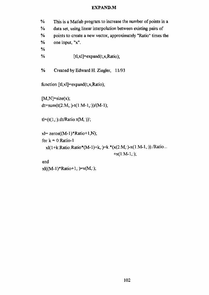
EXPAND.M

% This is aMatlab program to increase the number ofpoints in a

% data set, using linear interpolation between existing pairs of

% points to create a new vector, approximately"Ratio"

times the

% one input, "x".

%

% [tl,xl]=expand(t,x,Ratio);

% Created by Edward H. Ziegler, 1 1/93

function [tl,xl]=expand(t,x,Ratio);

[M,N]=size(x);

dt=sum(t(2:M, :)-t( 1 :M- 1,

:))/(M- 1 );

tl=(t(l,:):dt/Ratio:t(M:))';

xl=

zeros((M-l)*Ratio+l,N);

fork = 0:Ratio-l

xl(l+k:Ratio:Ratio*(M-l)+k,:)=k.*(x(2:M,:)-x(l:M-l,:))./Ratio...

+x(l:M-l,:);

end

xl((M- l)*Ratio+l, :)=x(M, :);

102

PRINTHPG.M

o.% This is aMATLAB program to send aMATLAB plot to a standard

% XEROX laser plotter in a UNIX based system.

function printhpg

meta metatmp % Put current plot into temporary metafile

% Invoke GPP, creating device specific output

! gpp metatmp -dhpgl

% Delete the temporary metafile

! lpr -Pxerox8810 metatmp.hpgl

! rm metatmp.met

! rm metatmp.hpgl

% This is aMATLAB program to create a post script file from a

% MATLAB plot and send it to a storage directory"POST"

in a

% VAX/VMS system.

PRINTPS.M

function printps

meta metatmp % Put current plot into temporary metafile

% Invoke GPP, creating device specific output

! gpp metatmp /dps

% Delete the temporary metafile

! deletemetatmp.met;*

! renamemetatmp.ps;*

! rename *.ps [.post]*.ps

return

end

103

References

1. M. Giona, F. Lentini, and V. Cimagalli, Functional Reconconstruction andLocalPrediction ofChaotic Time Series. Physical Review A 44, 3496-502, 1991.

2. G. Rowlands and J.C. Sprott, Extraction ofDynamicalEquationsfrom ChaoticData.

Physica D 58, 251-59, 1992.

3. JM. Martinerie, AM. Albano, A.I. Mees, and PE. Raw,Mutual Information, Strange

Attractors, and the OptimalEstimation ofDimension. Physical Review A 45, 7058-

64, 1992.

4. Th. Buzug and G Pfister, Comparison ofAlgorithms Calculating OptimalEmbeddingParametersfor the Delay Time Coordinates. Physica D 58, 127-37, 1992.

5. J.F. Gibson, J.D. Farmer, M. Castagli, and S. Eubank, AnAnalyticApproach to Practical

State Space Reconstruction. Physica D 57, 1-30, 1992.

6. LA. Smith, Identification andPrediction ofLowDimensionalDynamics. Physica D 58,

50-76, 1992.

7. H. D. I. Abaranel, R. Brown, J. B. Kadtke, Prediction in ChaoticNonlinear Systems:

Methodsfor Time Serieswith BroadbandFourier Spectra. Physical Review A 41,

1782-807, 1990.

8. P. Grassberger and I. Procaccia, Characterization ofStrange Attractors. Physical Review

Letters 50, 346-349, 1983.

9. H. Peitgen, H. Jurgens, and D. Saupe, Chaos andFractals: New Frontiers ofScience.

Springer-Verlag, NewYork NY, 1992.

10. G.L. Baker and J.P. Gollub, Chaotic Dynamics: An Introduction. Cambridge University

Press, New York NY, 1990.

11. CF. Gerald and P.O. Wheatley,AppliedNumericalAnalysis. Addison-Wesley

Publishing Co., New York NY, 1989.

12. The MathWorks, Inc., The Student Edition ofMatlab. Prentice-Hall, Inc., Englewood

Cliffs NJ, 1992.

13. L. Meirovitch, Elements of VibrationAnalysis. McGraw-Hill Inc., New York NY, 1986.

14. I. Stewart, Does GodPlayDice? TheMathematics ofChaos. Blackwell, Cambridge

MA 1990.

104

15. J. Gleick, Chaos:Making ofa New Science. Penguin Books, New York NY, 1987.

16. M. B. Kennel, R. Brown, H. D. I. Abaranel, DeterminingEmbeddingDimensionforPhase Space Reconstruction using Geometrical Construction. Physical Review A 45

3403-11, 1992.

17. Th. Buzug and G. Pfister, OptimalDelay Time andEmbeddingDimensionforDelaytime Coordinates byAnalysis of the Global static and local dynamical behavior ofStrange Attractors. Physical Review A 45, 7073-84, 1992.

18. HS. Greenside, A. Wolf, J. Swift, and T. Pignataro, Impracticality ofa Box CountingAlgorithmfor Calculating the Dimensionality ofStrange Attractors. Physical Review

A 25, 3453-3456, 1982.

19. R.L.Smith, EstimatingDimension inNoisy Chaotic Time Series. Journal of the Royal

Statistical Society B 54, 329-51, 1992.

20. J. Theiler, EfficientAlgorithmforEstimating the Correlation Dimensionfrom a Set of

Discrete Points. Physical Review A 36, 4456-62, 1987.

21. P Grassberger, An OptimizedBox-AssistedAlgorithmforFractalDimension. Physics

Letters A 148, 63-8, 1990.

22. M. Palus and Ivan Dvorak, Singular-ValueDecomposition inAttractor Reconstruction.

Physica D 55, 221-34, 1992.

23. K. Judd, An ImprovedEstimator ofDimension and Some Comments on ProvidingConfidence Intervals. Physica D 56, 216-28, 1992.

24. B. Noble and J.W. Daniel, AppliedLinearAlgebra. Prentice-Hall, Inc., Englewood

Cliffs NJ, 1988.

105