Non-passive transport of volatile organic compounds in the unsaturated zone
55
Non-Passive Transport of Volatile Organic Compounds in the Unsaturated Zone Orlando Silva and Jordi Grifoll* Departament d’Enginyeria Quimica, Escola Tecnica Superior d’Enginyeria Quimica (ETSEQ), Universitat Rovira i Virgili, Av. dels Països Catalans 26, 43007 Tarragona, Spain. * Corresponding author. Tel.: +34 977 55 96 39; fax +34 977 55 96 21 E-mail addresses: [email protected] (O. Silva), [email protected] (J. Grifoll) Manuscript Click here to download Manuscript: Silva_and_Grifoll_revised.doc
-
Upload
independent -
Category
Documents
-
view
1 -
download
0
Transcript of Non-passive transport of volatile organic compounds in the unsaturated zone
Non-Passive Transport of Volatile Organic Compounds in the Unsaturated Zone
Orlando Silva and Jordi Grifoll*
Departament d’Enginyeria Quimica, Escola Tecnica Superior d’Enginyeria Quimica (ETSEQ),
Universitat Rovira i Virgili, Av. dels Països Catalans 26,
43007 Tarragona, Spain.
*Corresponding author. Tel.: +34 977 55 96 39; fax +34 977 55 96 21 E-mail addresses:
[email protected] (O. Silva), [email protected] (J. Grifoll)
ManuscriptClick here to download Manuscript: Silva_and_Grifoll_revised.doc
1
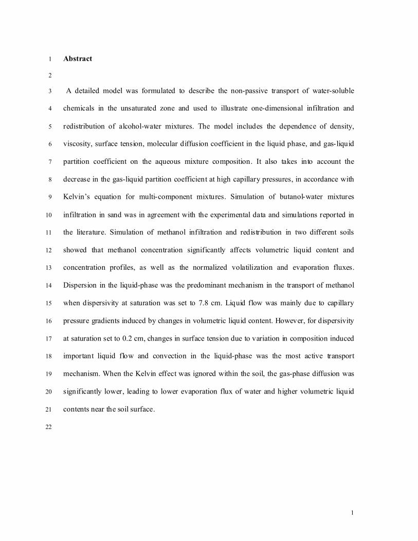
Abstract 1
2
A detailed model was formulated to describe the non-passive transport of water-soluble 3
chemicals in the unsaturated zone and used to illustrate one-dimensional infiltration and 4
redistribution of alcohol-water mixtures. The model includes the dependence of density, 5
viscosity, surface tension, molecular diffusion coefficient in the liquid phase, and gas-liquid 6
partition coefficient on the aqueous mixture composition. It also takes into account the 7
decrease in the gas-liquid partition coefficient at high capillary pressures, in accordance with 8
Kelvin’s equation for multi-component mixtures. Simulation of butanol-water mixtures 9
infiltration in sand was in agreement with the experimental data and simulations reported in 10
the literature. Simulation of methanol infiltration and redistribution in two different soils 11
showed that methanol concentration significantly affects volumetric liquid content and 12
concentration profiles, as well as the normalized volatilization and evaporation fluxes. 13
Dispersion in the liquid-phase was the predominant mechanism in the transport of methanol 14
when dispersivity at saturation was set to 7.8 cm. Liquid flow was mainly due to capillary 15
pressure gradients induced by changes in volumetric liquid content. However, for dispersivity 16
at saturation set to 0.2 cm, changes in surface tension due to variation in composition induced 17
important liquid flow and convection in the liquid-phase was the most active transport 18
mechanism. When the Kelvin effect was ignored within the soil, the gas-phase diffusion was 19
significantly lower, leading to lower evaporation flux of water and higher volumetric liquid 20
contents near the soil surface. 21
22
2
1. Introduction 23
24
Most numerical models of flow and transport through the vadose zone assume that flow is 25
independent of solute concentration. However, the presence of some chemicals in water can 26
affect the physical properties of the fluid phases, and the resulting transport processes are 27
known as non-passive. Thus, modeling of infiltration, redistribution and 28
volatilization/evaporation of these aqueous mixtures should take into account their non-29
passive transport behavior. 30
Various authors have already considered the dependence of some properties on 31
concentration. For example, Boufadel et al. [6] developed a one-dimensional model to 32
simulate the density-dependent flow of salt water in variably saturated media. They found that 33
the concentration at the front and the flux front position and magnitude propagate faster in the 34
case of density-dependent solutions than in the case of passive transport. In a later study, 35
Boufadel et al. [7] expanded their model to take into account density-and-viscosity-dependent 36
flow in two-dimensional variably saturated porous media and used it to investigate beach 37
hydraulics at seawater concentration in the context of nutrient delivery for bioremediation of 38
oil spills on beaches. Numerical simulations applied to a rectangular section of a hypothetical 39
beach showed that buoyancy in the unsaturated zone is significant in anisotropic fine-textured 40
soils with low dispersivities. In all the cases considered, the effects of concentration-41
dependent viscosity were negligible compared to the effects of concentration-dependent 42
density. Ouyang and Zheng [33] used the model FEMWATER to simulate the transport of 43
two chemicals, one with relatively low water solubility (aldicarb) and the other with relatively 44
high water solubility (acephate), through an unsaturated sandy soil. Comparison of 45
simulations showed that the effects of solution density on the transport of aldicarb were 46
negligible, whereas acephate, with density-driven transport, migrated 22 % deeper into the 47
3
soil in a period of 90 days than without considering density-driven transport. They also 48
performed a numerical experiment including a viscosity-concentration relationship, but the 49
results indicated that the effect of the viscosity was negligible compared with the effect of 50
density for the simulation conditions used in their study. The study of Ouyang and Zheng [33] 51
suggested that under certain circumstances, e.g. high chemical concentration, high water 52
solubility, and high pure chemical density, exclusion of the density-induced mechanism could 53
result in inaccurate predictions of water movement and chemical leaching through the vadose 54
zone. These usual simplifications could also lead to inadequate interaction between the 55
different mass transfer mechanisms when they are included in modeling of transport through 56
reactive soils. As Zhang et al. [48] pointed out, concentrated aqueous solutions are 57
significantly different from dilute solutions in transport and geochemical processes because of 58
their large density, viscosity, and complicated ionic interactions. 59
A number of studies of the effects induced on the flow by surfactants have emphasized their 60
non-passive transport behavior in the vadose zone. Smith and Gillham [43] developed an 61
isothermal saturated-unsaturated flow and transport model with solute concentration-62
dependent surface tension. They applied the model to simulate the infiltration of aqueous 63
solutions of butanol and methanol into two soils with different silt contents. Their numerical 64
simulations indicated that solutes that depress surface tension cause a local increase in the 65
hydraulic head gradients, which increases the liquid fluxes and the solute transport. Smith and 66
Gillham [44] complemented their previous work with laboratory experiments conducted in 67
saturated-unsaturated column sand. In this second work, they also incorporated the effect of 68
concentration-dependent viscosity into their earlier model [43] to scale the unsaturated 69
hydraulic conductivity. From their experimental data and numerical simulations, they 70
distinguished two flow effects associated with concentration-dependent surface tension in the 71
vadose zone: (i) the transient unsaturated flow caused by changes in pressure head, and (ii) a 72
4
decrease in the height of the capillary fringe. Both effects were proportional to the changes in 73
the relative surface tension with solute concentration. They also observed that higher water 74
contents were obtained in steady state for the butanol solution than for water and attributed 75
this difference to the relatively higher viscosity of the butanol solution. Henry et al. [19] 76
studied the effect of solute solubility on unsaturated flow and concluded that the surfactants 77
can significantly affect the flow in unsaturated porous media. Through a series of closed, 78
horizontal sand column experiments, they demonstrated that the surfactant-induced flow 79
caused by a highly soluble compound such as butanol was very different from the flow caused 80
by a relatively insoluble surfactant such as myristyl alcohol, though both induced a similar 81
reduction in the surface tension of water. This difference was attributed to the fact that, unlike 82
butanol, myristyl alcohol is virtually insoluble and primarily resides at the air-water interface 83
rather than in the bulk solution. Thus, flow only occurs at surfactant concentrations that are 84
greater than or equal to those needed to completely cover the air-water interface, which leads 85
to an ineffective transport of myristyl alcohol to previously clean regions [23]. In another 86
study of surfactant-induced flow phenomena, Henry et al. [20] found that hysteresis was an 87
important factor in horizontal flow. They conducted experiments in closed, horizontal 88
columns filled with silica sand and with butanol as the surfactant. They also modified a one-89
dimensional hysteretic unsaturated flow and transport numerical model to include the 90
dependence of surface tension and viscosity on concentration. Under hysteretic conditions and 91
at final steady state, the model predicted uniform concentration and pressure profiles, but a 92
non-uniform liquid content profile unlike the situation expected if the system was non-93
hysteretic. Also, flow simulations were sensitive to dispersivity. As Henry et al. [20] noted, 94
lower dispersivity caused sharper surfactant concentration gradients, which led to larger 95
capillary pressure gradients and higher fluxes near a solute front. In the same context, these 96
authors [22] modified a two-dimensional model for flow and transport in unsaturated soils to 97
5
include the dependence of surface tension and viscosity on the surfactant concentration. They 98
directly compared the simulations to the sand box infiltration experiments with butanol-water 99
mixtures presented by Henry and Smith [21]. A longitudinal dispersivity value of 1 cm was 100
used in the simulations and shown to cause too much dispersion relative to the experimental 101
data at larger travel distances. In a recent review of the surfactant-induced flow phenomena in 102
the vadose zone, Henry and Smith [23] presented experimental evidence that surfactant-103
induced flow effects can be significant when considered on the laboratory scale. These effects 104
may be due to surfactant modifications of moisture retention characteristics and unsaturated 105
hydraulic conductivity, which affect unsaturated flow and chemical transport. They also 106
recognized that more work is needed to better understand the potential impact of surfactant-107
induced flow effects on field-scale transport in the vadose zone and suggest that models 108
should include a better description of processes and phenomena such as hysteresis in the 109
hydraulic functions, vapor-phase transport of surfactant or partitioning of surfactant to the 110
different phases. 111
Despite all of these studies, the effects of several common simplifications for modeling non-112
passive transport of solutes have still not been evaluated. Although several numerical models 113
can be adapted to simulate some situations of non-passive transport through the vadose zone 114
in multiphase systems, e.g., STOMP [46] and VST2D [13], in most of them it is considered 115
that several properties are independent of the mixture composition. 116
In this paper, we present a model for non-passive infiltration-redistribution and transport of 117
water-soluble solutes in the vadose zone. This model incorporates the dependence of density, 118
viscosity, surface tension, molecular diffusion coefficient in the liquid phase, and the gas-119
liquid and solid-liquid partition coefficients, on the solute concentration. We also include the 120
reduction in the gas-liquid partition coefficient due to high capillary pressures in accordance 121
with Kelvin’s equation for multicomponent mixtures. The effects of these dependencies were 122
6
illustrated using a one-dimensional numerical implementation of the transport model to 123
simulate the infiltration, redistribution and volatilization of alcohol-water mixtures into 124
different soils. 125
126
127
2. Basic equations and numerical resolution 128
129
2.1. Balance equations 130
131
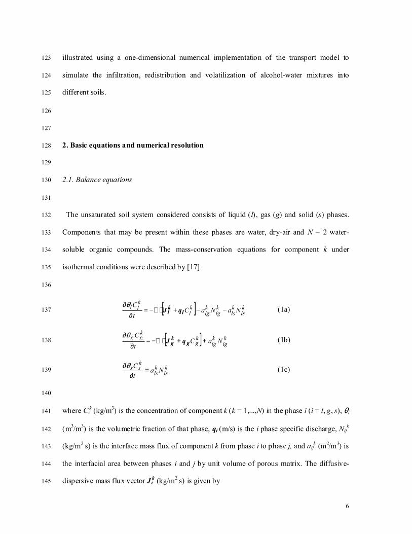
The unsaturated soil system considered consists of liquid (l), gas (g) and solid (s) phases. 132
Components that may be present within these phases are water, dry-air and N – 2 water-133
soluble organic compounds. The mass-conservation equations for component k under 134
isothermal conditions were described by [17] 135
136
[ ] kls
kls
klg
klg
kl
kll NaNaC
tC
−−+⋅−∇=∂
∂l
kl qJ
θ (1a) 137
[ ] klg
klg
kg
kgg NaC
tC
++⋅−∇=∂
∂g
kg qJ
θ (1b) 138
kls
kls
kss Na
tC =
∂∂θ (1c) 139
140
where Cik (kg/m3) is the concentration of component k (k = 1,...,N) in the phase i (i = l, g, s), θi 141
(m3/m3) is the volumetric fraction of that phase, qi (m/s) is the i phase specific discharge, Nijk 142
(kg/m2 s) is the interface mass flux of component k from phase i to phase j, and aijk (m2/m3) is 143
the interfacial area between phases i and j by unit volume of porous matrix. The diffusive-144
dispersive mass flux vector Jik (kg/m2 s) is given by 145
7
146
ki
kii
ki CDJ ∇−= θ (2) 147
148
where Dik (m2/s) is the diffusion-dispersion tensor for component k [4]. Under the assumption 149
of local phase equilibrium [17], the three component equations (1) can be combined to give 150
151
( )kl
klk C
tC
kkg
kl JJ ββββ++⋅−∇=
∂∂ϕ
(3a) 152
ksls
kglglk HH θθθϕ ++= (3b) 153
kglHglk qq +=β (3c) 154
155
Assuming that dry-air is present neither in the liquid-phase nor in the solid-phase, only the 156
gas-phase transport (equation (1b)) was considered for the dry-air mass conservation equation 157
158
[ ]ag
agg C
tC
gag qJ +⋅−∇=
∂∂θ
(4) 159
160
where Cga is the dry-air concentration in the gas-phase. 161
The specific discharge of phase i, qi (m/s), is given by the generalized Darcy’s law [4] 162
163
( )zk
qi gPk
iii
ri ρµ
+∇−= (5) 164
165
8
In equation (5), k is the intrinsic permeability tensor of the soil (m2), gz (m/s2) is the gravity 166
vector, kri is the relative permeability (dimensionless), ρi (kg/m3) is the density, µi (kg/m s) is 167
the dynamic viscosity, and Pi (Pa) is the pressure of phase i. 168
The diffusive-dispersive mass flux vector of air Jga (kg/m2 s) was calculated from the 169
condition 170
171
01
=∑=
N
k
kgJ (6) 172
173
The partition coefficient, Hijk , between phases i and j is defined by 174
175
slgjiCCH k
j
kik
ij ,,, == (7) 176
177
Use of constant partition coefficients is a common assumption when modeling solute 178
transport in variably-saturated soils. However, in this work the gas-liquid partition coefficient, 179
Hglk , was assumed to be dependent on solute concentration and soil-liquid content [10, 11, 12] 180
as given by 181
182
= ∗RT
VPHH kMkgl
kgl
ˆexp (8) 183
184
where the exponential term accounts for the Kelvin’s effect in multicomponent liquid 185
mixtures [39, 42]. In (8), kV̂ (m3/mol) is the partial molar volume of component k in the 186
liquid-phase, R is the universal gas constant, PM = Pl - Pg (Pa), is the matric pressure of the 187
9
liquid and T (K) is the temperature. The gas-liquid partition coefficient for plane interfacial 188
surfaces corresponds to the dimensionless Henry’s law constant, Hgl*k , and its dependence on 189
component concentration was calculated from the liquid-vapor equilibrium condition [45] 190
191
RTVp
H mkvap
kk
glˆ
γ=∗ (9) 192
193
in which pvapk (Pa) is the vapor pressure of component k, mV̂ (m3/mol) is the partial molar 194
volume of the liquid mixture, and γk (dimensionless) is the activity coefficient of component 195
k. In very dry soil conditions, the small quantity of liquid in the medium is no longer under 196
the influence of capillary forces so, strictly speaking, the original matric pressure definition is 197
not applicable. Nevertheless, as Baggio et al. [3] suggested, the matric pressure definition can 198
be expanded as 199
200
mM V
hP ˆ∆−= (10) 201
202
where ∆h (J/mol) refers to the enthalpy difference between the vapor in the gas-phase and the 203
condensed and/or adsorbed liquid-phase, excluding the latent enthalpy of vaporization. 204
Taking this definition, matric pressure and Kelvin’s equation can be applied throughout all the 205
range from wet to dry conditions [15, 41]. 206
207
2.2. Boundary conditions, dispersivities and numerical procedure 208
209
10
In this work, the one-dimensional version of the non-passive transport model described 210
previously was implemented to simulate the infiltration, redistribution and 211
volatilization/evaporation of alcohol-water mixtures in soils. A dynamic boundary condition 212
at the surface was set to accommodate either a given infiltration or an 213
evaporation/volatilization flux. In case of infiltration, the top boundary condition for the 214
transport of each component (equation (3)) was the component mass flux at the surface, No(k ) 215
(kg/m2 s), calculated as 216
217
kinllo
ko CqN ,= (11) 218
219
where qlo (m/s) is the given infiltration liquid specific discharge and Cl,ink (kg/m3) is the 220
concentration of component k in the infiltrating liquid. In the absence of infiltration, the 221
evaporation/volatilization mass flux for component k at the surface was calculated by 222
considering a mass transfer limitation from the soil surface to the bulk atmosphere 223
224
( )kgo
kbk
ko
ko CCkN −= (12) 225
226
In equation (12), kok (m/s) is the atmosphere-side mass transfer coefficient for component k, 227
Cbkk (kg/m3) is the background concentration of component k in the atmosphere, and Cgo
k 228
(kg/m3) is the concentration of component k in the gas-phase at the soil surface. For given 229
values of wind velocity, soil roughness and Schmidt number of the chemical volatilized, the 230
mass transfer coefficients, kok, were estimated with the semi-empirical correlation proposed 231
by Brutsaert [8]. This correlation is only applicable under neutral atmospheric conditions and 232
was developed from available experimental data. In case of non-neutral conditions a different 233
11
approach using the Obukhow length should be used as suggested by Brutsaert [8]. In all cases, 234
the boundary condition at the bottom was set as zero diffusive and dispersive fluxes and zero 235
matric pressure gradient. The lower gas-phase boundary condition was set as a no-flow 236
boundary, while the upper gas-phase boundary condition was a constant atmospheric pressure. 237
The longitudinal diffusion-dispersion coefficient for component k, Dik (m2/s), was calculated 238
as 239
240
Lii
koik
i DDD +=τ
(13) 241
242
where the molecular diffusion and the longitudinal dispersion coefficients in phase i are 243
denoted by Doik (m2/s) and DLi (m2/s), and τi (dimensionless) is the tortuosity of phase i. 244
Tortuosities, τg and τl, were evaluated according to the first model of Millington and Quirk 245
[26], i.e. τi =ε2/3/θi. Longitudinal dispersion coefficients for each phase were calculated as 246
DLi = αLiqi/θi, where αLi (m) is the longitudinal dispersivity for phase i given as a function of 247
the volumetric phase content, in accordance with the correlation proposed by Grifoll et al. 248
[18]. 249
250
( )5o 4316613 iiLiLi S.S. +−=αα (14) 251
252
in which Si = θi/ε is the actual saturation of phase i and oLiα is the dispersivity at saturation. 253
Grifoll and Cohen [17] used a similar approach to equation (14). As they pointed out, the 254
adoption of an empirical longitudinal dispersivity model, like described by equation (14), is 255
12
not meant to suggest its general applicability, but can be used to illustrate a general trend in 256
dispersivity behavior. 257
The governing partial differential equations, equations (3) and (4), were discretized spatially 258
and temporally in algebraic form using the finite volumes method [34] with a fully implicit 259
scheme (backward Euler) for time integration. The non-linear discretized governing equations 260
were solved using the multivariable Newton-Raphson iteration technique [26]. Volumetric 261
liquid content, dry-air concentration in the gas-phase and alcohol concentration in the liquid-262
phase were selected as primary variables. The Jacobian coefficient matrix was calculated 263
using a finite difference approximation [26]. The linear system of equations formulated in the 264
Newton-Raphson method was solved for the correction to the primary variables by the 265
iterative Preconditioned Biconjugate Gradient Method [26, 35]. The preconditioner matrix 266
was the diagonal part of the Jacobian coefficient matrix [35]. Values for the convergence limit 267
and maximum number of Newton-Raphson iterations have been defined conveniently as input 268
parameters. Convergence limits were defined with respect to the maximum residual of each 269
mass balance equation, normalized by the sum of the mass fluxes absolute values. The 270
tolerance employed in all simulations was 10-7 while the maximum number of Newton-271
Raphson iterations was set to 10. If the convergence limit was not satisfied after 10 iterations, 272
the time step was reduced to 50% and the calculation was restarted from the end of the 273
previous time step. Otherwise, if the convergence was attained within the maximum number 274
of iterations, the time step was doubled without exceeding a maximum ∆tmax = 60 s, and a 275
new time step was initiated. 276
The one-dimensional grid was generated by distinguishing two regions. First, from the 277
surface to a depth of z = 0.135 m and starting with ∆z1 = 0.2 mm, the grid spacing increases 278
with a progression factor of 1.008. Second, from z = 0.135 m to the bottom of the system 279
(z = 0.5 m) the grid was set uniform with a grid spacing of ∆z = 1.33 mm. 280
13
The sensitivity of the numerical solution to grid spacing and time step was analyzed for Test 281
Case I as it is described in section 3.2.1 below. For the standard grid and maximum time step 282
given above, maximum discrepancies between the numerical results and the exact values are 283
expected to be less than 1%. 284
To check the numerical algorithm, we compared the solution of the passive transport of 285
water-methanol mixtures into a loam-type soil with the solution reported by Grifoll and 286
Cohen [17]. The maximum discrepancy between these two solutions was also less than 1%. 287
288
289
3. Results and discussion 290
291
The present numerical model has been used to simulate several test cases in order to 292
investigate the non-passive transport behavior of volatile organic compounds. The first test 293
presented is the infiltration of water-butanol mixtures into sand as reported by Smith and 294
Gillham [44]. Their experimental and simulation results were compared to the present 295
numerical results in order to check our model, the numerical algorithm and the computational 296
code. The next two test cases were for the infiltration of methanol-water mixtures into a 297
Sandy Clay Loam and Silty Clay soils. These test cases illustrated how the dependency of 298
physical properties on concentration affects a system in which the solute is soluble in water at 299
any proportion. Initial test simulations showed that the convective gas-phase component did 300
not contribute effectively to the transport of methanol and water. In the present test cases of 301
soils with relatively low permeabilities, the inclusion of gas-phase convection did not change 302
the evolution of the volumetric liquid content and methanol concentration profiles by more 303
than 0.5% and very high CPU times were required. Note that the differences in gas-phase 304
densities due to the saturation or absence of methanol were not high enough to induce density-305
14
dependent advection [28]. In addition, as stated by Lenhard et al. [28], effects of density-306
driven vapor flow are more evident in porous media with permeabilities grater than 10-11 m2. 307
On the contrary, the permeabilities of the soils studied in this work are less than 4x10-13 m2. 308
Most of the results presented in the next sections were therefore obtained by neglecting gas-309
phase convection when solving the numerical model. 310
311
3.1. Dissolved butanol infiltration 312
313
Smith and Gillham [44] studied the infiltration of a butanol-water mixture into a 2 meters 314
column-sand. Their experimental procedure consisted of infiltrating distilled water until the 315
steady state was reached and then changing the infiltration liquid to an aqueous solution of 316
butanol with 7% w/w at the same infiltration rate. Their experimental results were compared 317
with their earlier numerical transport model [43], which was modified to include the 318
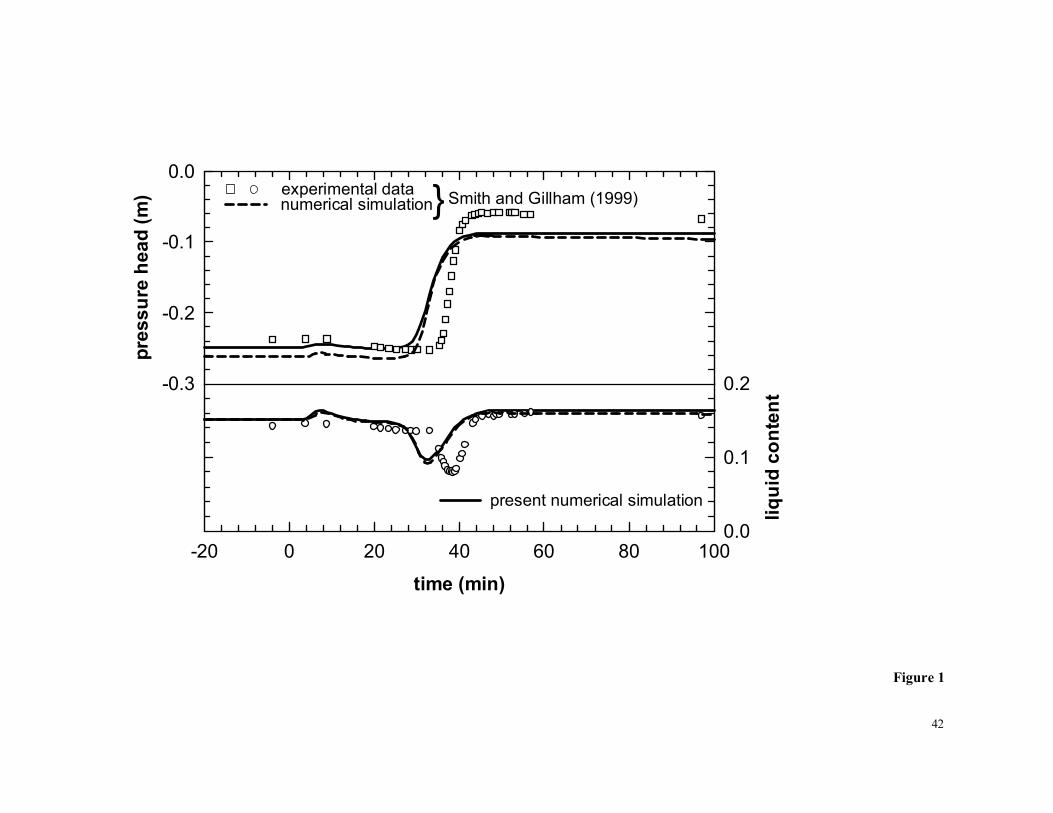
dependencies of surface tension and viscosity on butanol concentration. Figure 1 shows the 319
evolution of the pressure head and liquid content measured at a depth of 38 cm in the column, 320
the simulation results of Smith and Gillham [44], and the present numerical calculations. For 321
the present simulation, the dependency of surface tension and viscosity on solute 322
concentration, as well as the soil water retention curve, were taken from Smith and Gillham 323
[44]. A measured constant dispersivity αLi = 0.00177 m [44] was also used in this case. 324
Deviations from steady state in pressure head and liquid content after the application of 325
butanol solution were observed. These variations were due to the dependency of surface 326
tension and viscosity on butanol concentration. 327
As the solute front passed, the water content significantly decreased to a minimum before 328
increasing to a slightly higher value than that of the previous steady state. The highly 329
15
localized drainage and rewetting were caused by hydraulic gradients induced by the surface 330
tension variations associated with the solute front. 331
Both the model of Smith and Gillham [44] and the present model describe the main 332
characteristics of the experiment. It should be noted that the model parameters used by Smith 333
and Gillham [44] were estimated independently of the experimental results that appear in 334
Figure 1. They suggested that some experimental uncertainty could be introduced in the 335
measurement of dispersivity because it was determined using a concentrated solution of NaCl 336
that could be subject to density effects. Moreover, the differences in the pressure head and 337
volumetric liquid content between the two simulation results were less than 4.8%, which 338
gives an indication of the ability of the present model to simulate non-passive transport of 339
solutes. 340
341
3.2. Methanol infiltration 342
343
The impact of the non-passive behavior on the infiltration and redistribution of methanol-344
water mixtures is illustrated in two cases in which different soils were used. In both of these 345
test cases we simulated a hypothetical scenario composed by an initial period of infiltration 346
followed by a period of volatilization/evaporation. Therefore, at least close to the soil surface 347
where volatilization and evaporation occur, the soil was expected to reach conditions of very 348
low liquid content (θl < 0.10). To simulate these situations realistically, we used an extended 349
version of the Brooks-Corey soil water retention curve proposed by Rossi and Nimmo [38], 350
which is given as 351
352
( )
≤≤<≤
= −
−
10
1 SSSPSSeP
SPjeb
jS
dwM
RN
λ
α
, (15) 353
16
354
In equation (15) S = θl/ε and Se = (S - Sr)/(1 - Sr) are the actual and effective liquid 355
saturation, respectively, PM,w (Pa) is the matric water pressure, while Pb (Pa) (bubble pressure 356
or air entry pressure), λ (pore size distribution index), and θr (residual volumetric water 357
content) are the classical Brooks-Corey parameters. The oven dry matric water pressure, Pd, 358
was taken as 980 MPa, as suggested by Rossi and Nimmo [38]. The parameters αRN and θj 359
(Sj = θj/ε), introduced by these authors, were calculated as functions of the classical Brooks-360
Corey parameters, as suggested by Morel-Seytoux and Nimmo [31]. Liquid-phase relative 361
permeability was computed as a function of liquid saturation from the soil-moisture retention 362
function according to the model of Burdine [9] 363
364
( )( )1
2
ISISkrl = (16) 365
where 366
( )( )( ) ( ) ( )
≤≤−−
++−
<≤−=
++ 112
12
012
21212
22
22
SSSSP
SeP
SSePSI
jejeb
rS
d
jS
d
RNj
RN
λλα
α
λλα
α
(17) 367
368
Given a volumetric liquid content, the matric pressure for pure water as given by equation 369
(15) has been scaled for mixtures with the methanol concentration Cl as [29] 370
371
( )w,M
w
lM PCP
σσ
= (18) 372
373
17
where σw is the surface tension of water and σ(Cl) (N/m) is the surface tension of the liquid 374
mixture. 375
The physical properties of methanol-water mixtures depend on methanol concentration. In 376
this work, each of these dependencies has been described by a polynomial function, as 377
378
( ) ( )∑=j
jljl CaCp (19) 379
380
where p stands for any of the properties allowed to vary with methanol concentration (surface 381
tension, density, viscosity and diffusion coefficient of methanol in the liquid-phase) and Cl is 382
the methanol concentration in the liquid-phase. The polynomial coefficients aj , obtained by 383
fitting equation (19) to available experimental data [14], are given in Table 1. Diffusion 384
coefficients of methanol and water in the gas-phase were taken as constants, with values 385
Dogm = 1.6×10⁻⁵ m2/s [17] and Dog
w = 2.6×10⁻⁵ m2/s [37], respectively. 386
To calculate the gas-liquid partition coefficients for methanol and water, the partial molar 387
volumes and the activity coefficients according to equations (8) and (9) are required. Activity 388
coefficients for water and methanol were calculated using Wilson’s equation [27] with the 389
parameters fitted by Gmehling et al. [16] to available experimental data. Molar volumes were 390
calculated following the procedure described by Lide and Kihiaian [30], who suggested the 391
Redlich-Kister equation to calculate molar excess volumes. The gas-liquid partition 392
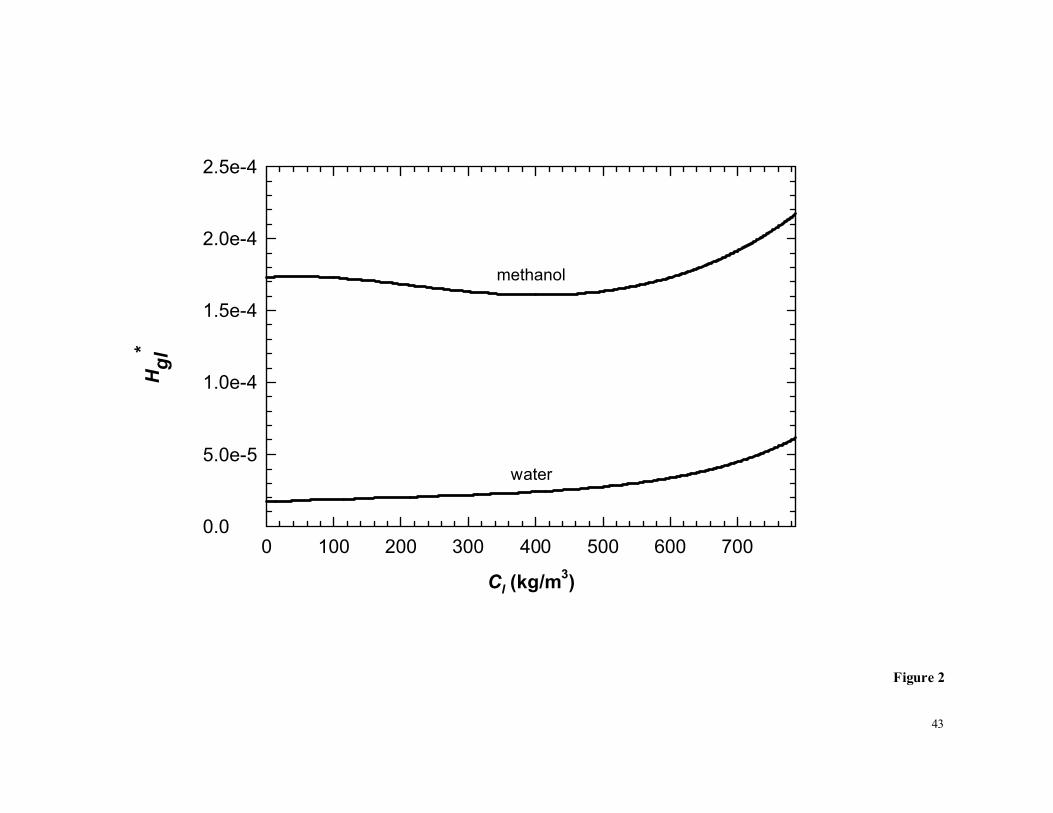
coefficients Hgl* for water and methanol calculated by this procedure are shown in Figure 2. 393
For water, this partition coefficient increases monotonically from 1.73x10⁻⁵, in absence of 394
methanol, to the limiting value 6.14x10⁻⁵ as the pure methanol condition is approached. The 395
partition coefficient for methanol reaches a minimum value of 1.61x10⁻⁴ when Cl = 405 kg/m3 396
and then increases progressively to 2.17x10⁻⁴, which is the value for pure methanol. Sorption 397
18
of methanol onto the soil solid was assumed to be described by a constant partition coefficient 398
Hslm = 3.7x10⁻³, estimated for a soil with 2% of organic matter [17]. In their experimental 399
work, Smith and Gillham [44] used homogeneous sand and therefore found low values of 400
dispersivity. In heterogeneous natural soils higher dispersivities are expected. Jaynes [24], for 401
instance, obtained values of dispersivity between 0.0453 and 0.25 m for a depth of 0.3 m. 402
Also, Abbasi et al. [1] estimated soil hydraulic and solute transport parameters from several 403
two-dimensional furrow irrigation experiments and obtained values of longitudinal 404
dispersivity between 0.026 and 0.328 m for a depth of 1 m. In this paper, dispersivity at 405
saturation for both the liquid and the gas phases was set to oLiα = 0.078 m, the value suggested 406
by Biggar and Nielsen [5] for saturated soil conditions in an agricultural field [32]. In their 407
work, Biggar and Nielsen measured dispersivities in ponded soils (of a broad textural class: 408
loam, clay loam, silty clay, silty clay loam) under steady state infiltration conditions at depths 409
between 30.5 and 182.9 cm, infiltration pore velocities between 1.3 and 105.4 cm/day, while 410
hydraulic conductivities at saturation ranged from 0.3 to 70 cm/day. In the test cases of the 411
present work, the selected soils and process conditions were, most of the time, within the 412
range of values above described. 413
414
3.2.1. Test case I 415
The first case study involved five simulations of the infiltration of methanol-water mixtures 416
into a homogeneous Sandy Clay Loam soil, each with different methanol concentration of the 417
infiltrating liquid, Cl,in. These concentrations ranged from Cl,in = 0.001 kg/m3, in which the 418
methanol behaves as a passive scalar, to Cl,in = 786.6 kg/m3, which corresponds to pure 419
methanol. The upper boundary condition was set at an infiltration rate of 0.25 cm/hr for 15 420
hours, followed by 57 hours in which the methanol and water were allowed to volatilize at the 421
surface according to equation (12). The background concentration of methanol in the 422
19
atmosphere was assumed to be zero, while the background concentration of water in the 423
atmosphere was calculated assuming a relative humidity of 40%. The initial condition was a 424
uniform volumetric water content of 0.128 m3/m3, which corresponds to a matric potential of 425
–100 m. The hydraulic parameters of equations (15), (16) and (17), taken from Rawls and 426
Brakensiek [36] as typical values for a Sandy Clay Loam soil, are given in Table 2. 427
When comparing the results of the simulations for different grid spacing and time steps, it is 428
observed that methanol concentration and volumetric liquid content values at the surface are 429
the most sensitive to these variations. Five simulations with different grid spacing were run 430
for a maximum time step of ∆tmax = 60 s and Cl,in = 400 kg/m3. A coarse grid with N = 125 431
control volumes was used in the first simulation. In the following ones, the number of control 432
volumes N was successively doubled by halving the grid spacing. The methanol concentration 433
and the volumetric liquid content at the surface at the end of the simulations were extrapolated 434
to an infinite number of volumes, ∞0lC and ∞
0lθ . Figure 3(a) shows the ratio of 0lC and 0lθ to 435
their extrapolated value ∞0lC and ∞
0lθ as a function of the inverse of the number of control 436
volumes. Deviations from the extrapolated value were higher in the case of methanol 437
concentration. However, for both concentration and volumetric liquid content, and for all 438
grids tested, the relative deviations were less than 0.6%. The sensitivity of simulations to time 439
step was tested using the grid described at the end of section 2.2 (500 volumes) and 440
Cl,in = 400 kg/m3. Five simulations were run with ∆tmax = 240, 120, 60, 30 and 15 s and the 441
values at the surface extrapolated to zero time step. Figure 3(b) shows that methanol 442
concentration at the surface was sensitive to time step, although for ∆tmax < 240 s, the 443
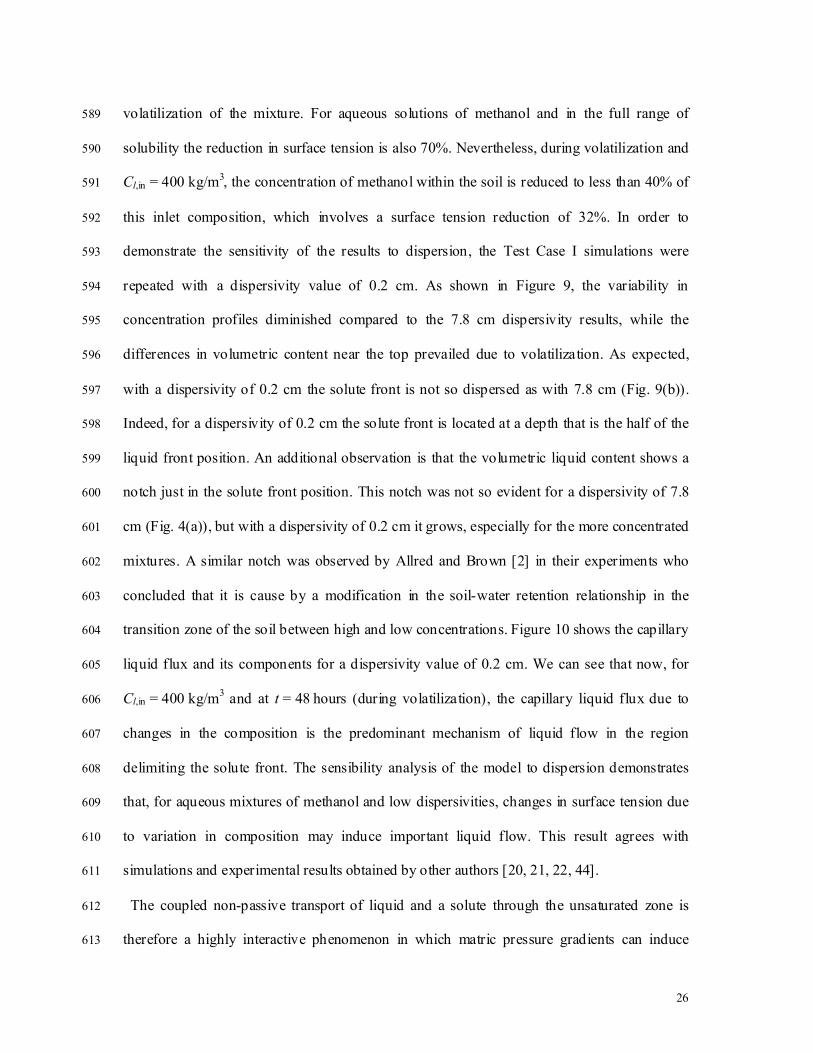
concentration differences respect the extrapolated value were less than 5%. For the standard 444
simulation conditions (N = 500, ∆tmax = 60 s), the maximum deviations expected are less than 445
1%. 446
20
Figure 4 shows the volumetric liquid content and normalized concentration profiles 48 hours 447
after the beginning of the experiment for five methanol concentrations in the infiltrating 448
liquid. Normalization has been carried out with respect Cl,in in order to emphasize the 449
non-passive behavior because, in the case of passive transport, the normalized concentration 450
profiles in Fig. 4 should be independent of concentration since the solute transport equation 451
(3) is linear when the coefficients do not depend on the solute concentration. 452
The differences in volumetric liquid content profiles for different Cl,in, shown in Fig. 4(a), 453
are due to three factors: i) the dilution effect on the incoming mixture caused by the initial 454
pure water in the soil, ii) differences in the liquid-phase flow caused by changes in viscosity, 455
density and surface tension, and iii) the volatilization of the mixture. Note that the relative 456
densities of the mixture change from 1 for pure water to 0.786 for pure methanol. Then, when 457
methanol dilutes in water, the volume of the mixture should shrink due to the non-ideal 458
mixing effects as described by the dependence of density on concentrations (Eq. (19) and 459
Table 1). This effect is more pronounced when the infiltrating mixture is more concentrated in 460
methanol. During infiltration the causes of the differences in volumetric liquid content are this 461
non-ideal mixing effect and the changes in liquid flow caused by variations in viscosity and 462
surface tension. In the case of pure methanol and after 48 hours of simulation (i.e. 33 hours of 463
volatilization), by balancing the volumes of initial water, infiltrated liquid, final liquid in the 464
soil and volatilized liquid, it was calculated that the non-ideal mixing effect is about 3.6% of 465
the initial water plus infiltrated liquid volume, whereas the percentage of volatilized liquid is 466
about 9.6%. The relative influence of changes in liquid flow due to variations in viscosity and 467
surface tension cannot be deduced from this balance, but the percentage of volatilized liquid 468
increases from 5% of the initial plus infiltrated volume for pure water, to a maximum of 10% 469
at a concentration of Cl,in = 400 kg/m3, and then decreases to 9.6% for pure methanol. Note 470
that the viscosity of the liquid is a concave function of the methanol concentration, reaching a 471
21
maximum at about 392 kg/m3. This shows that more viscous infiltrating mixtures move more 472
slowly and consequently, by remaining close to the surface for a longer period, undergo a 473
higher volatilization. Because of the combined effect of volatilization, viscosity and surface 474
tension dependent flow, and non-ideal mixing, the front position for passive transport 475
(Cl,in = 0.001 kg/m3) is 29.4% deeper than for pure methanol (z = 0.34 m). Moreover, the 476
liquid content near the surface also depends on Cl,in because, as is explained below, the 477
volatilization rate at the surface is low for low concentrations of methanol. 478
The gas-liquid partition coefficient for methanol is between 6 and 10 times higher than for 479
water (see Fig. 2). Higher overall volatilization rates are therefore observed for more 480
concentrated mixtures. The differences in the normalized methanol concentration profiles 481
developed at the soil top (Fig. 4(b)) are largely due to methanol transfer limitations from 482
inside the soil to the surface, which are higher for more dilute mixtures. This is shown in 483
Figure 4(b), where we find progressively larger differences between the concentration profiles 484
established in the first 10 cm adjacent to the soil surface, especially for Cl,in > 400 kg/m3. 485
The volatilization flux of methanol moN , normalized by the corresponding flux at the 486
beginning of volatilization moN ini, , is shown in Figure 5(a) for the five numerical experiments. 487
Volatilization decreases as the methanol concentration and liquid content at surface decrease. 488
These volatilization fluxes suffer a sudden decrease due to the development of high capillary 489
pressures near the surface, which reduce the gas-liquid partition coefficient according to the 490
exponential term in equation (8) (Kelvin effect). This behavior is similar to the decrease in 491
soil water evaporation rates from stage-one to stage-two evaporation [40]. At high infiltration 492
methanol concentrations, volatilization rates are higher. This leads sooner to these high 493
capillary pressures and, therefore, to the observed decrease in the volatilization flux. 494
22
The evaporation flux of water woN undergoes a similar sudden regime change. However, as 495
shown in Figure 5(b), after the infiltration has ceased the water evaporation rate increases due 496
to the loss of methanol to the atmosphere, which increases the concentration of water at the 497
soil surface. This initial period of increasing evaporation lasts until Kelvin’s effect begins to 498
be noticeable. During this first stage, normalized evaporation is higher at higher infiltrating 499
methanol concentrations. Similar behavior in the time variation of the evaporation flux of 500
water was experimentally and numerically observed by Chen et al. [11]. It is worth noting that 501
when the Kelvin equation and the water vapor diffusion were not included in their water 502
transport model, the simulation results deviated from the experimental measurements. 503
The role of the various contributions to total liquid movement can be illustrated by 504
inspecting the individual partial fluxes due to capillary component and gravitational 505
component. The partial fluxes can be defined, according to equation (5), as given below 506
507
zPkkq l
l
rlcapl ∂
∂−=µ, (20a) 508
gkkq ll
rlgrav,l ρ
µ= (20b) 509
510
where caplq , and vgra,lq are the capillary and gravitational components of the flux, respectively. 511
The contribution made by each of these components to the specific discharge after 48 hours 512
of simulation and for each infiltration concentration is shown in Figure 6. For all cases, the 513
contribution from the gravity flux was negligible and the main contribution was from 514
capillary flux. There were significant differences in the capillary liquid flux due to the relative 515
differences in dryness at the surface and the different viscosity profiles from different 516
compositions of the infiltrating methanol-water mixture. Note that, for Cl,in ≥ 400 kg/m3 and 517
23
close to the surface, the liquid flux drops to almost zero because of the low liquid content in 518
this zone (see Fig. 4(a)), which makes the relative permeability negligible. On the other hand, 519
the matric pressure depends on both the liquid content and the solute concentration. We can 520
therefore divide the capillary flux into two components—one that is due to changes in 521
volumetric liquid content and one to changes in the composition of the liquid mixture. These 522
components are defined as 523
524
zC
CPkkq l
l
l
l
rlCcap,l ∂
∂∂∂−=
µ (21a) 525
zPkkq l
l
l
l
rlcap,l ∂
∂∂∂−= θθµ
θ (21b) 526
527
where Ccaplq , is the capillary liquid flux due to changes in methanol concentration and θ
caplq , is 528
the corresponding flux due to variations in the liquid content. Figure 7 shows the 529
contributions of these components for Cl,in = 400 kg/m3 after 48 hours of simulation. We can 530
see that θcaplq , is the main component of the capillary flux and that there is a small contribution 531
of Ccaplq , from z = 0.15 m to the front position. Similar contribution profiles were obtained for 532
the other Cl,in cases, which indicates that, in the cases we studied, the main flow mechanism 533
for the infiltration of methanol was the capillary component due to variations in liquid 534
content. 535
The relative magnitude of the various mechanisms involved in the component transport 536
through the soil can be illustrated by inspecting the individual partial fluxes due to diffusion, 537
dispersion and convection. These partial fluxes are defined for each phase i = l, g and each 538
component k as 539
540
24
zCD
Jki
i
koi
ik
idif ∂∂
−=τ
θ, (22a) 541
zCDJ
ki
Liik
idisp ∂∂
−= θ, (22b) 542
kii
kiconv CqJ =, (22c) 543
544
Methanol and water transport by diffusion in the liquid-phase was negligible in all cases. 545
Figure 8 shows the partial fluxes profiles for methanol and all the relevant mechanisms after 546
48 hours of simulation since the start of the numerical experiment. These mechanisms are 547
diffusion in the gas-phase, Jdif,gm, and dispersion, Jdisp ,l
m, and convection, Jconv,lm, in the liquid-548
phase. All the fluxes were normalized with respect to the volatilization flux at that time, moN . 549
Diffusion in the gas-phase is not an active mechanism for methanol transport, as we can see in 550
Fig. 8(a), except very close to the surface and when Cl,in ≥ 400 kg/m3. In these circumstances 551
the soil close to the surface is very dry (see Fig. 4(a)) and in this region no mechanism in the 552
liquid-phase is able to transport the methanol. Diffusion in the gas-phase is therefore the only 553
active mechanism in this thin region. The methanol concentration gradient that drives the gas-554
phase diffusion is magnified by the Kelvin effect that decreases the concentration of methanol 555
close to the surface, as the soil becomes drier. Numerical experiments with higher Cl,in causes 556
a decrease in the liquid saturation which induce higher gas-phase diffusive fluxes. For 557
Cl,in < 400 kg/m3, the top soil is not so dry because volatilization is lower for lower 558
concentrations of methanol. For these low input concentrations, therefore, dispersion in the 559
liquid-phase (see Fig. 8(b)) is the most active mechanism, and accounts for 90% of the 560
transport at the surface. 561
It is important to note the close relationship between the volumetric liquid content and 562
concentration profiles in Fig. 4, the liquid-phase velocities in Fig. 6 and the partial mass 563
25
fluxes in Fig. 8. For example, at the depth corresponding to the liquid front position for the 564
various cases viscosity increases as the infiltrating mixture becomes more concentrated. As 565
the viscosity is higher, the velocities are lower and a decrease in dispersion in the liquid-phase 566
could be expected. However, the higher the infiltrating concentration, the lower the liquid 567
volumetric content and the higher the methanol concentration gradients. This leads to higher 568
partial dispersive fluxes (equation (22b)) in this zone for more concentrated infiltrating 569
mixtures (see Fig. 8(b)). A similar analysis explains the interaction between the liquid-phase 570
velocity, the different transport mechanisms and the liquid content and concentration profiles 571
in the upper part of the soil (z ≤ 0.15 m). 572
Results of the simulations previously described appear to be inconsistent with experimental 573
and modeling observations of Smith and Gillham [44]. Unlike our simulations that predict a 574
main flow mechanism driven by the capillary component due to variations in liquid content 575
(see Fig. 7), Smith and Gillham [44] observed a significant impact of the solute concentration 576
on unsaturated flow. This discrepancy in principle may be due to our use of a large 577
dispersivity value that reduces the concentration gradient and thereby reduces the magnitude 578
of the effect of the solute on unsaturated liquid fluxes. However, it should be noted that the 579
increase in the matric pressure due to the reduction of the surface tension in accordance with 580
the scaling proposed by Leverett [29] is more pronounced in case of butanol aqueous solution 581
than with aqueous mixtures of methanol. As explained by Smith and Gillham [43] “butanol, 582
0-7% by weight at 25 ºC, causes a nonlinear and relatively large change in surface tension 583
with concentration. Methanol, 0-7% by weight at 25 ºC, causes a near linear and relatively 584
small change in surface tension”. A simple calculus shows that in the case of butanol the 585
reduction is about 70% in the range of 0-7% by weight. Here it is noteworthy that 586
experiments and simulations carried out by Smith and Gillham [43, 44] involve scenarios of 587
pure infiltration, unlike our simulations, which include infiltration followed by the 588
26
volatilization of the mixture. For aqueous solutions of methanol and in the full range of 589
solubility the reduction in surface tension is also 70%. Nevertheless, during volatilization and 590
Cl,in = 400 kg/m3, the concentration of methanol within the soil is reduced to less than 40% of 591
this inlet composition, which involves a surface tension reduction of 32%. In order to 592
demonstrate the sensitivity of the results to dispersion, the Test Case I simulations were 593
repeated with a dispersivity value of 0.2 cm. As shown in Figure 9, the variability in 594
concentration profiles diminished compared to the 7.8 cm dispersivity results, while the 595
differences in volumetric content near the top prevailed due to volatilization. As expected, 596
with a dispersivity of 0.2 cm the solute front is not so dispersed as with 7.8 cm (Fig. 9(b)). 597
Indeed, for a dispersivity of 0.2 cm the solute front is located at a depth that is the half of the 598
liquid front position. An additional observation is that the volumetric liquid content shows a 599
notch just in the solute front position. This notch was not so evident for a dispersivity of 7.8 600
cm (Fig. 4(a)), but with a dispersivity of 0.2 cm it grows, especially for the more concentrated 601
mixtures. A similar notch was observed by Allred and Brown [2] in their experiments who 602
concluded that it is cause by a modification in the soil-water retention relationship in the 603
transition zone of the soil between high and low concentrations. Figure 10 shows the capillary 604
liquid flux and its components for a dispersivity value of 0.2 cm. We can see that now, for 605
Cl,in = 400 kg/m3 and at t = 48 hours (during volatilization), the capillary liquid flux due to 606
changes in the composition is the predominant mechanism of liquid flow in the region 607
delimiting the solute front. The sensibility analysis of the model to dispersion demonstrates 608
that, for aqueous mixtures of methanol and low dispersivities, changes in surface tension due 609
to variation in composition may induce important liquid flow. This result agrees with 610
simulations and experimental results obtained by other authors [20, 21, 22, 44]. 611
The coupled non-passive transport of liquid and a solute through the unsaturated zone is 612
therefore a highly interactive phenomenon in which matric pressure gradients can induce 613
27
solute transport and, reciprocally, mixture composition may change the transport properties 614
and induce a flow pattern. 615
616
3.2.2. Test case II 617
A second case study was carried out to illustrate the potential impact of the Kelvin effect on 618
non-passive transport of solute in the vadose zone and its impact on the volatilization of 619
methanol and the evaporation of water. In some simulations in this case study, the Kelvin 620
exponential factor of equation (8) was not considered except at the surface, and the results 621
were compared to simulations in which full consideration of this factor along the system was 622
taken into account. Note that, if the methanol-water mixture is allowed to volatilize/evaporate 623
at a rate that is independent of the liquid content at surface, i.e. ignoring the Kelvin factor, no 624
decrease in volatilization/evaporation fluxes would be observed and a regime like stage-two 625
evaporation [40] would not be attained. With a stage-one like volatilization/evaporation 626
remaining indefinitely, the system would progress to a non-feasible physical situation in 627
which there would be no mechanism for the transport of components from the inside to the 628
soil surface able to maintain these relatively high volatilization/evaporation fluxes dictated by 629
the atmosphere-side mass transfer limitations. In all present simulations, therefore, the Kelvin 630
effect at the surface was considered in order to attain feasible physical situations. 631
The simulations for this second case were the infiltration and redistribution of a methanol-632
water mixture into a Silty Clay soil. The infiltrating methanol concentration was Cl,in = 400 633
kg/m3 and the infiltration rate was set at 0.075 cm/hr for 20 hours, followed by 148 hours in 634
which the methanol and water were allowed to redistribute and volatilize. Like in the Test 635
Case I we assumed the background concentration of methanol to be zero, and calculated the 636
background concentration of water in the atmosphere assuming a relative humidity of 40%. 637
The hydraulic parameters of a typical Silty Clay soil were selected as given by Rawls and 638
28
Brakensiek [36] and listed in Table 2. The hydraulic characteristic of this soil allows high 639
capillary pressures to develop at a relatively high liquid content, a condition for which we 640
expect the Kelvin effect to have a greater impact. The initial condition for the simulation was 641
a constant volumetric water content of 0.169 m3/m3, which corresponds to a matric head of 642
-500 m. 643
Figure 11 shows the liquid content and normalized concentration profiles 48 and 168 hours 644
after the start of the simulation (28 and 148 hours of volatilization/evaporation, respectively). 645
The dotted line represents the results obtained when the Kelvin effect within the soil is 646
ignored. At both 48 and 168 hours, and along the first 5 cm, the volumetric liquid content is 647
lower when the Kelvin factor is allowed to act within the soil. As Fig. 11(a) shows, this 648
difference increases with time as the soil dries. The maximum difference in the volumetric 649
liquid content is located within the first 5 cm adjacent to the soil surface, increasing from 650
122.4% after 48 hours to 129.8% after 168 hours. For the normalized methanol concentration 651
this difference increases from 32.8% after 48 hours to 42.8% after 168 hours. 652
To evaluate the impact of including the Kelvin effect in simulations, it is important to note 653
that the main transport mechanism affected is diffusion in the gas-phase. This can easily be 654
deduced from the definition of gas-liquid partition coefficient and equation (22). At this point 655
it is helpful to analyze the case of the transport of pure water. In that case, the vapor 656
concentration gradients within the soil are only those developed due to the reduction of the 657
vapor pressure according to the Kelvin equation. Consequently, the diffusion of water in the 658
gas-phase disappears if the Kelvin reduction factor is ignored within the soil and, therefore, 659
the soil dries slower than when Kelvin effect is considered within the soil. In fact, ignoring or 660
including the Kelvin effect within the soil is equivalent to consider or neglect the transport of 661
water by gas-phase diffusion. This problem was studied by Chen et al. [11], who found that 662
including the contribution of water vapor diffusion in water transport is important for 663
29
improving the accuracy of water content and water flux prediction. It is noteworthy that these 664
authors obtained differences in water content profile near the soil surface predicted when 665
water vapor diffusion was and was not included in the water transport simulations, which are 666
similar to the differences in volumetric liquid content shown in Fig.11(a) caused by including 667
or ignoring the Kelvin effect within the soil. The impact of Kelvin effect on the gas-phase 668
diffusion fluxes of methanol and water are shown in Figure 12. These fluxes have been 669
normalized by the respective fluxes of volatilization and evaporation at the beginning of the 670
volatilization period (20 h). As we can see in Fig. 12, gas-phase diffusion is significantly 671
reduced when Kelvin effect is ignored in the model. If the Kelvin effect is considered over the 672
entire soil, the drying process near the surface significantly reduces the liquid-phase flux and, 673
therefore, the liquid-phase convection and dispersion. This reduction in dispersion in the 674
liquid-phase along the first 2 cm is compensated by an increase in gas-phase diffusion in this 675
region. When the Kelvin effect is allowed to act only at the surface, the concentration in the 676
gas-phase within the soil is not affected by matric pressure variations and the changes in 677
concentration in the liquid-phase are insufficient to increase the gas-phase diffusion. As in 678
this situation the liquid content is higher under relatively steep liquid concentration gradients, 679
there are relatively high liquid-phase dispersive fluxes that at least partially compensate for 680
the incapability of the gas-phase diffusion transport. The Kelvin effect also affected, in a 681
similar way, the transport of water by dispersion in the liquid-phase and gas-phase diffusion. 682
Due to the low gas-phase diffusion of both methanol and water when the Kelvin effect is 683
ignored within the soil, volatilization and evaporation rates are lower than the respective 684
fluxes obtained when the Kelvin factor is considered within the soil. This situation is 685
illustrated in Fig. 13, which shows the evolution of the methanol volatilization and water 686
evaporation at the surface. We can see that there is a small difference in the volatilization flux 687
of methanol but a significant one in the evaporation flux of water. Under certain conditions 688
30
(clay and dry soil), therefore, there may be a great difference between considering the Kelvin 689
effect within the soil and ignoring it. This difference is reflected in the fluxes for transport to 690
the surface and mainly affects the less volatile compound (water, in this case). 691
We can conclude from this case study that the Kelvin effect plays an important role in 692
properly representing the dynamic behavior of solute volatilization and water evaporation 693
under high capillary pressures. 694
695
696
4. Conclusions 697
698
A model for the non-passive infiltration, redistribution and volatilization of liquid mixtures 699
has been developed. It has been used to illustrate the transport of butanol and methanol 700
aqueous solutions in the vadose zone. The coupled non-passive transport of liquid and solute 701
through the unsaturated zone is a highly interactive phenomenon. Matric pressure gradients 702
can induce solute transport. Reciprocally, the mixture composition may change the transport 703
properties and induce a given pattern of flow. 704
Simulations for completely miscible methanol-water mixtures and two different soils (Sandy 705
Clay Loam and Silty Clay) showed significant differences in volatilization fluxes, front 706
position, liquid content and concentration profiles that depend on the composition of the 707
infiltrating liquid. For the cases we studied and a dispersivity value of 7.8 cm, the 708
predominant mechanism in the transport of methanol through the soil was dispersion in the 709
liquid-phase, with a major contribution from gas-phase diffusion near the surface during 710
volatilization. By decomposing the liquid flux into capillary and gravity components, we 711
found that the liquid flow is mainly due to pressure gradients induced by changes in the 712
volumetric liquid content. However, simulations with a lower dispersivity (0.2 cm) showed 713
31
that, in this case, convection was more active for methanol transport than dispersion. Also in 714
this case, the capillary liquid flux due to changes in the composition is the predominant 715
mechanism of liquid flow in the solute-front region. 716
Including or ignoring in the model the reduction of gas-liquid partition coefficients 717
according to the Kelvin equation has an important impact on the global transport behavior. 718
When the Kelvin effect was ignored within the soil, the gas-phase diffusion was significantly 719
lower. The corresponding evaporation flux of water was also lower and, therefore, the 720
volumetric liquid contents were greater. The maximum differences in the volumetric liquid 721
content and normalized methanol concentration profiles were developed in the first 5 cm 722
adjacent to the soil surface. These differences were increasing with time, reaching the values 723
of 130 % and 43 % respectively at the end of the simulation. It was found that, under dry 724
conditions on a Silty Clay soil, mass fluxes that transport the solute to the surface can be 725
significantly different when the Kelvin factor is considered within the soil from when it is 726
ignored. This directly affects the dynamic of solute volatilization and water evaporation rates. 727
This phenomenon may play an important role under conditions of severe dryness, which 728
could be crucial to accurately model the fluid flow and contaminant transport in arid regions 729
or in clay soils, where liquid retention properties favor the development of high capillary 730
pressures. 731
732
733
Acknowledgments 734
735
We gratefully acknowledge the financial assistance received from the DGICYT of Spain, 736
under project FIS2005-07194 and from the Generalitat de Catalunya (2005SGR-00735). We 737
also acknowledge the support received from the DURSI and the European Social Fund.738
32
References 739
740
[1] Abbasi F, Simunek J, Feyen J, van Genuchten MTh, Shouse PJ. Simultaneous inverse 741
estimation of soil hydraulic and solute transport parameters from transient field 742
experiments: homogeneous soil. T ASAE 2003;46(4):1085-95. 743
[2] Allred B, Brown GO. Boundary condition and soil attribute impacts on anionic 744
surfactant mobility in unsaturated soil. Ground Water 1996;34(6):964-71. 745
[3] Baggio P, Bonacina C, Schrefler BA. Some considerations on modeling heat and mass 746
transfer in porous media. Transport Porous Med. 1997;28:233-51. 747
[4] Bear J., Bachmat Y. Introduction to modeling of transport phenomena in porous media. 748
Dordrecht : Kluwer; 1991. 749
[5] Biggar JW, Nielsen DR. Spatial variability of the leaching characteristics of a field soil. 750
Water Resour Res 1976;1:78-84. 751
[6] Boufadel MC, Suidan MT, Venosa AD. Density-dependent flow in one-dimensional 752
variably-saturated media. J Contam Hydrol 1997;202:280-301. 753
[7] Boufadel MC, Suidan MT, Venosa AD. A numerical model for density-and-viscosity-754
dependent flows in two-dimensional variably saturated porous media. J Contam Hydrol 755
1999;37:1-20. 756
[8] Brutsaert W. A theory for local evaporation (or heat transfer) from rough and smooth 757
surfaces at ground level. Water Resour Res 1975;11(4):543-50. 758
[9] Burdine NT. Relative permeability calculations from pore-size distribution data. 759
Petroleum Trans 1953;198:71-77. 760
[10] Chen D, Rolston DE, Yamaguchi T. Calculating partition coefficients of organic vapors 761
in unsaturated soil and clays. Soil Science 2000;165(3) 217-25. 762
33
[11] Chen D, Rolston DE, Moldrup P. Coupling diazinon volatilization and water evaporation 763
in unsaturated soils: I. Water transport. Soil Science 2000;165(9);681-89. 764
[12] Chen D, Rolston DE. Coupling diazinon volatilization and water evaporation in 765
unsaturated soils: II. Diazinon transport. Soil Science 2000;165(9):690-98. 766
[13] Friedel MJ. Documentation and verification of VST2D. A model for simulating transient, 767
variably saturated, coupled water-heat-solute transport in heterogeneous, anisotropic, 2-768
dimensional, ground-water systems with variable fluid density. U.S. Geol. Surv. Water-769
Resour. Invest.Rep. 00-4105, 2000.124 pp. 770
[14] Gammon BE, Marsh KN, Dewan AKR. Transport properties and related 771
thermodynamics data of binary mixtures. Part 1. New York: American Institute of 772
Chemical Engineers; 1993. 773
[15] Gawin D, Pesavento F, Schrefler BA. Modelling of hygro-thermal behaviour and damage 774
of concrete at temperature above the critical point of water. Int J Numer Anal Meth 775
Geomech 2002;26:537-62. 776
[16] Gmehling J, Onken U, Rarey-Nies JR., 1988. Vapor-liquid equilibrium data collection. 777
Aqueous systems. Vol. I, part 1b (Supplement 2). Frankfurt: DECHEMA; 1988. 778
[17] Grifoll J, Cohen Y. Contaminant migration in the unsaturated soil zone: the effect of 779
rainfall and evapotranspiration. J Contam Hydrol 1996;23:185-211. 780
[18] Grifoll J, Gastó JM, Cohen Y., Non-isothermal soil water transport and evaporation. Adv 781
Water Resour 2005;28(11):1254-66. 782
[19] Henry EJ, Smith JE, Warrick AW. Solubility effects on surfactant-induced unsaturated 783
flow through porous media. J Hydrol 1999;223:164-74. 784
[20] Henry EJ, Smith JE, Warrick AW. Surfactant effects on unsaturated flow in porous 785
media with hysteresis: horizontal column experiments and numerical modeling. J Hydrol 786
2001;245:73-88. 787
34
[21] Henry EJ, Smith, JE. The effect of surface-active solutes on water flow and contaminant 788
transport in variably saturated porous media with capillary fringe effects. J Contam 789
Hydrol 2002;56:247-70. 790
[22] Henry EJ, Smith JE, Warrick AW. Two-dimensional modeling of flow and transport in 791
the vadose zone with surfactant-induced flow. Water Resour Res 2002;38(11):33-1 – 33-792
16. 793
[23] Henry EJ, Smith JE. Surfactant-induced flow phenomena in the vadose zone: a review of 794
data and numerical modeling. Vadose Zone J 2003;2:154-67. 795
[24] Jaynes DB. Field study of bromacil transport under continuous-flood irrigation. Soil Sci 796
Soc Am J 1991;55:658-64. 797
[25] Jin Y, Jury A. Characterizing the dependence of gas diffusion coefficient on soil 798
properties. Soil Sci Soc Am J 1996;60:66-71. 799
[26] Kelley CT. Iterative methods for linear and nonlinear equations. Philadelphia: SIAM; 800
1995. 801
[27] Kyle BG. Chemical and process thermodynamics. New Jersey: Prentice Hall; 1999. 802
[28] Lenhard RJ, Oostrom M, Simmons CS, White MD. Investigation of density-dependent 803
gas advection of trichloroethylene: experiment and a model validation exercise. J Contam 804
Hydrol 1995;19:47-67. 805
[29] Leverett MC, Capillary behavior in porous solids. Trans AIME 1941;142:152-69. 806
[30] Lide DR; Kehiaian HV. CRC Handbook of thermophysical and thermochemical data. 807
CRC Press; 1994. 808
[31] Morel-Seytoux HJ, Nimmo JR. Soil water retention and maximum capillary drive from 809
saturation to oven dryness. Water Resour Res 1999;35(7):2031-41. 810
[32] Nielsen DR, Biggar JW. Spatial variability of field-measured soil-water properties. 811
Hilgardia 1973;42(7):215-59. 812
35
[33] Ouyang Y, Zheng Ch. Density-driven transport of dissolved chemicals through 813
unsaturated soil. Soil Science 1999;164(6):376-90. 814
[34] Patankar SV. Numerical heat transfer and fluid flow. New York: McGraw-Hill; 1980. 815
[35] Press WH, Teukolsky SA, Vetterling WT, Flannery BP. Numerical recipes in fortran 77: 816
the art of scientific computing. New York: Cambridge University Press; 1986-1992. 817
[36] Rawls WJ, Brakensiek DL. Estimation of soil water retention and hydraulic properties. 818
Unsaturated flow in hydrology modeling, theory and practice. Kluwer Academic 819
Publishers; 1989. 820
[37] Reid RC, Prausnitz JM, Poling BE. The properties of gases and liquids. New York: 821
McGraw-Hill Inc.; 1987. 822
[38] Rossi C, Nimmo JR. Modeling of soil water retention from saturation to oven dryness. 823
Water Resour Res 1994;30(3):701-8. 824
[39] Rowlinson JS, Widom B. Molecular theory of capillarity. Oxford: Clarendon Press; 825
1984. 826
[40] Salvucci GD. Soil and moisture independent estimation of stage-two evaporation from 827
potential evaporation and albedo or surface temperature. Water Resour Res 828
1997;33(1):111-22. 829
[41] Schrefler BA. Multiphase flow in deforming porous material. Int J Numer Anal Meth 830
Geomech 2004;60:27-50. 831
[42] Shapiro AA, Stenby EH. Kelvin equation for non-ideal multicomponent mixture. Fluid 832
Phase Equilibria 1997;134:87-101. 833
[43] Smith JE, Gillham RW. The effect of concentration-dependent surface tension on the 834
flow of water and transport of dissolved organic compounds: a pressure head-based 835
formulation and numerical model. Water Resour Res 1994;30(2):343-54. 836
36
[44] Smith JE, Gillham RW. Effects of solute concentration-dependent surface tension on 837
unsaturated flow: laboratory sand column experiments. Water Resour Res 838
1999;35(4):973-82. 839
[45] Valsaraj KT. Elements of environmental engineering. Thermodynamics and kinetics. 840
Boca Raton: CRC Press Inc.; 1995. 841
[46] White MD, Oostrom M, Lenhard RJ. Modeling fluid flow and transport in variably 842
saturated porous media with the STOMP simulator. 1. Nonvolatile three-phase model 843
description. Adv Water Resour 1995;18(6):353-64. 844
[47] White MD, Oostrom M. STOMP: Subsurface transport over multiple phases. Theory 845
guide. PNNL-12030. Pac. Northw. Natl. Lab., Richland, WA; 2000. 846
[48] Zhang G, Zheng Z, Wan J. Modeling reactive geochemical transport of concentrated 847
aqueous solutions. Water Resour Res 2005;41(W02018):1-14. 848
37
Table captions 849
850
Table 1. Polynomial coefficients obtained by fit of experimental data at 20 ºC to Eq. (19). 851
852
Table 2. Simulation conditions and hydraulic soil properties. 853
854
38
Table 1. Polynomial coefficients obtained by fit of experimental data† at 20 ºC to Eq. (19)
Property a0 a1 a2 a3 a4 R2 σl, (N m-1) 7.275 x 10⁻² -2.134 x 10⁻⁴ 5.352 x 10⁻⁷ -6.831 x 10⁻¹⁰ 3.105 x 10⁻¹³ 0.996 ρl, (kg m-3) 9.9701 x 10² -1.917 x 10⁻¹ 1.665 x 10⁻⁴ -3.340 x 10⁻⁷ - 0.99994 µl, (kg m-1 s-1) 1.003 x 10⁻³ 3.134 x 10⁻⁶ 3.710 x 10⁻⁹ -2.082 x 10⁻¹¹ 1.298 x 10⁻¹⁴ 0.998 Dol
m, (m2 s-1) 1.350 x 10⁻⁹ -7.419 x 10⁻¹³ -4.789 x 10⁻¹⁵ 8.486 x 10⁻¹⁸ - 0.983 † Experimental data extracted from Gammon et al. [14].
39
Table 2. Simulation conditions and hydraulic soil properties Test case I Test case II
Simulation conditions Soil type Sandy Clay Loam Silty Clay Soil depth (m) 0.5 0.5 Initial pressure head (m), Pini -100 -500 Infiltration rate (cm/h), qlo 0.25 0.075 Total time of simulation (h) 72 168 Initial period of infiltration (h) 15 20 Dispersivity at saturation (cm), αLi
o 0.2; 7.8 7.8 aAtmosphere-side mass transfer coefficient for methanol (kg/m2 s), ko
m 3.5x10⁻³ 3.5x10⁻³ aAtmosphere-side mass transfer coefficient for water (kg/m2 s), ko
w 4.0x10⁻³ 4.0x10⁻³
Hydraulic soil properties bSoil porosity, ε 0.33 0.423 bResidual water content, θr 0.068 0.056 bBrooks-Corey parameter, λ 0.25 0.127 bBubble pressure, Pbw (Pa) 2754 3352 bHydraulic saturated conductivity, Ks (cm/h) 0.43 0.09 cVolumetric liquid content at junction, θj 0.1415 0.3079 cRossi-Nimmo parameter, α 0.0557 0.0756
aCalculated according to Brutsaert [8] assuming a wind velocity of 2 m/s and a surface roughness length of 1 cm. bFrom Rawls and Brakensiek [36]. cCalculated according to Morel-Seytoux and Nimmo [31].
40
Figure captions
Figure 1. Evolution in time of pressure head and liquid content at 38 cm depth for the
infiltration in sand of a water-butanol solution at 7% w/w. Comparison of experimental and
numerical simulation data of Smith and Gillham [44] with present numerical simulation.
Figure 2. Gas-liquid partition coefficients for methanol-water system.
Figure 3. Dependency of the concentration and liquid content at surface on (a) the grid
spacing and (b) the maximum time step.
Figure 4. Infiltration and redistribution of methanol-water mixtures of different compositions
into a Sandy Clay Loam soil. Simulation results after 48 hours and a dispersivity of 7.8 cm.
(a) Volumetric liquid content. (b) Methanol concentration in the liquid-phase.
Figure 5 . Evolution of normalized methanol volatilization and water evaporation fluxes for
several infiltration methanol concentrations. (a) Volatilization of methanol. (b) Evaporation
of water.
Figure 6. Liquid flux as function of methanol concentration decomposed into capillary and
gravity components, after 48 hours of simulation. (a) Capillary liquid flux component. (b)
Gravity liquid flux component.
Figure 7. Capillary liquid flux and its components after 48 hours of simulation,
Cl,in = 400 kg/m3 and a dispersivity of 7.8 cm.
41
Figure 8. Normalized partial fluxes in a Sandy Clay Loam soil after 48 hours. (a) Diffusive
partial flux of methanol in the gas-phase. (b) Dispersive partial flux of methanol in the
liquid-phase. (c) Convective partial flux of methanol in the liquid-phase.
Figure 9. Infiltration and redistribution of methanol-water mixtures of different compositions
into a Sandy Clay Loam soil. Simulation results after 48 hours and a dispersivity of 0.2 cm.
(a) Volumetric liquid content. (b) Methanol concentration in the liquid-phase.
Figure 10. Capillary liquid flux and its components after 48 hours of simulation,
Cl,in = 400 kg/m3 and a dispersivity of 0.2 cm.
Figure 11. Profiles after infiltration, redistribution and volatilization of a methanol-water
mixture into a Silty Clay soil (dotted line for results ignoring Kelvin effect within the soil).
(a) Volumetric liquid content. (b) Methanol concentration in the liquid-phase.
Figure 12. Kelvin effect on normalized partial fluxes in a Silty Clay soil after 168 hours and
Cl,in = 400 kg/m3 (dotted line for results ignoring Kelvin effect within the soil). (a) Diffusive
partial flux of methanol in the gas-phase. (b) Diffusive partial flux of water in the gas-phase.
Figure 13. Kelvin effect on methanol volatilization and water evaporation from a Silty Clay
soil (dotted line for results ignoring Kelvin effect within the soil). (a) Volatilization of
methanol. (b) Evaporation of water.
42
Figure 1
time (min)-20 0 20 40 60 80 100
liqui
d co
nten
t
0.0
0.1
0.2
pres
sure
hea
d (m
)
-0.3
-0.2
-0.1
0.0Smith and Gillham (1999)
present numerical simulation
}numerical simulationexperimental data
43
Cl (kg/m3)
0 100 200 300 400 500 600 700
Hgl
*
0.0
5.0e-5
1.0e-4
1.5e-4
2.0e-4
2.5e-4
Figure 2
methanol
water
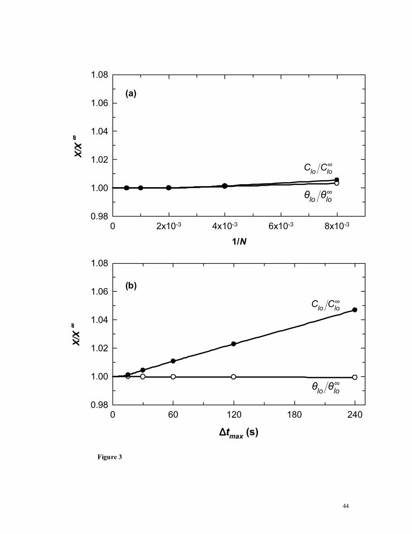
44
∆∆∆∆tmax (s)0 60 120 180 240
X/X
∞∞ ∞∞
0.98
1.00
1.02
1.04
1.06
1.08
1/N0 2x10⁻³ 4x10⁻³ 6x10⁻³ 8x10⁻³
X/X
∞∞ ∞∞
0.98
1.00
1.02
1.04
1.06
1.08
∞lolo CC
∞lolo θθ
(a)
(b)
Figure 3
∞lolo CC
∞lolo θθ
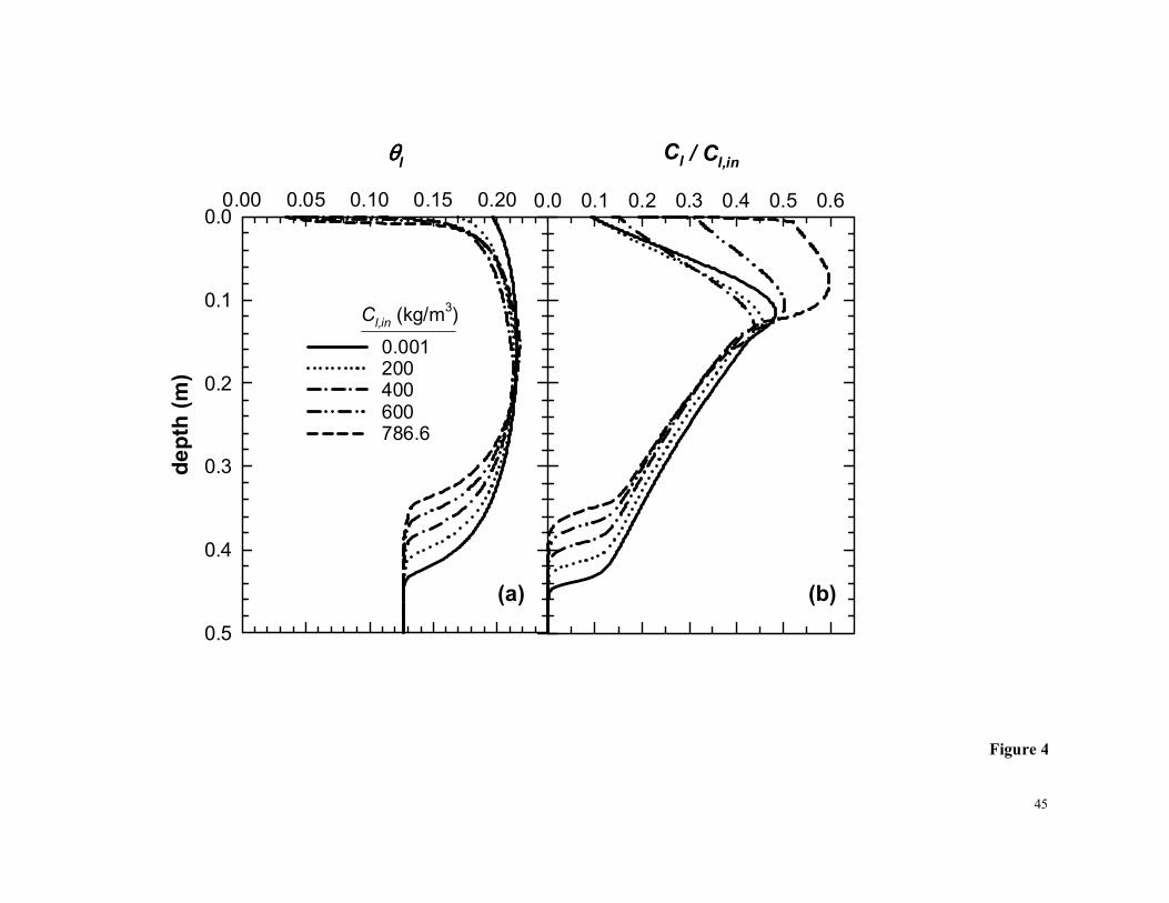
45
Figure 4
θθθθl
0.00 0.05 0.10 0.15 0.20de
pth
(m)
0.0
0.1
0.2
0.3
0.4
0.5
(a)
Cl / Cl,in
0.0 0.1 0.2 0.3 0.4 0.5 0.6
(b)
Cl,in (kg/m3)
0.001200400600786.6
46
Figure 5
(a) METHANOL
N0m
/N0,
inim
0.0
0.2
0.4
0.6
0.8
1.0
(b) WATER
time (hours)20 30 40 50 60 70
N0w
/N0,
iniw
0.0
0.5
1.0
1.5
0.001200400600786.6
Cl,in (kg/m3)
47
Figure 6
Capillary liquid fluxql,cap (m/s)
-6e-8 -4e-8 -2e-8 0 2e-8
dept
h (m
)
0.0
0.1
0.2
0.3
0.4
0.5
Gravity liquid fluxql,grav (m/s)
(a)
-4e-8 -2e-8 0 2e-8 4e-8
(b)
0.001200400600786.6
Cl,in (kg/m3)
48
Capillay flux components (m/s)-3e-8 -2e-8 -1e-8 0 1e-8 2e-8 3e-8
dept
h (m
)0.0
0.1
0.2
0.3
0.4
0.5
Figure 7
ql,cap ql,capθ ql,cap
C
49
Figure 8
Jdif,gm/N0
m
-0.5 0.0 0.5 1.0de
pth
(m)
0.0
0.1
0.2
0.3
0.4
0.5
Jdisp,lm/N0
m
0.0 0.5 1.0
(a) (b)
Jconv,lm/N0
m
0.0 0.5 1.0
(c)
0.001200400600786.6
Cl,in (kg/m3)
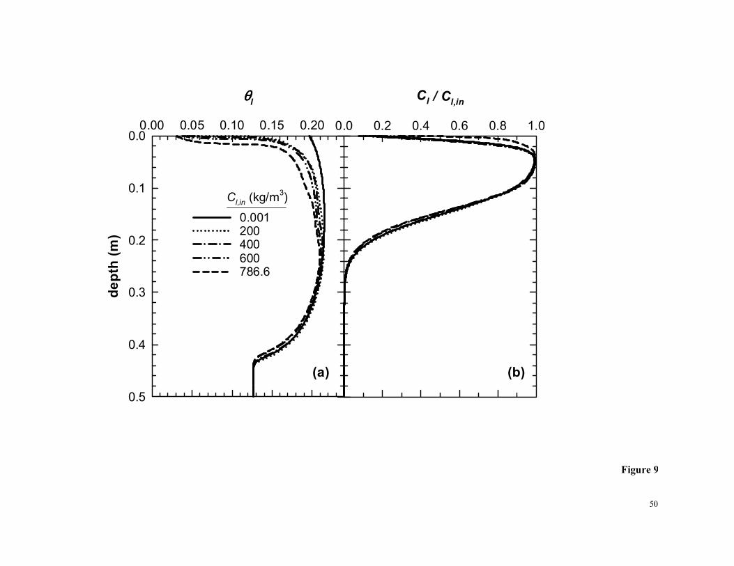
50
Figure 9
θθθθl
0.00 0.05 0.10 0.15 0.20de
pth
(m)
0.0
0.1
0.2
0.3
0.4
0.5
(a)
Cl / Cl,in
0.0 0.2 0.4 0.6 0.8 1.0
(b)
Cl,in (kg/m3)
0.001200400600786.6
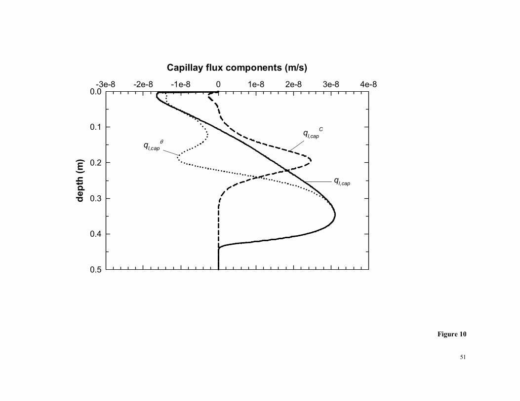
51
Capillay flux components (m/s)-3e-8 -2e-8 -1e-8 0 1e-8 2e-8 3e-8 4e-8
dept
h (m
)0.0
0.1
0.2
0.3
0.4
0.5
Figure 10
ql,cap
ql,capθ
ql,capC
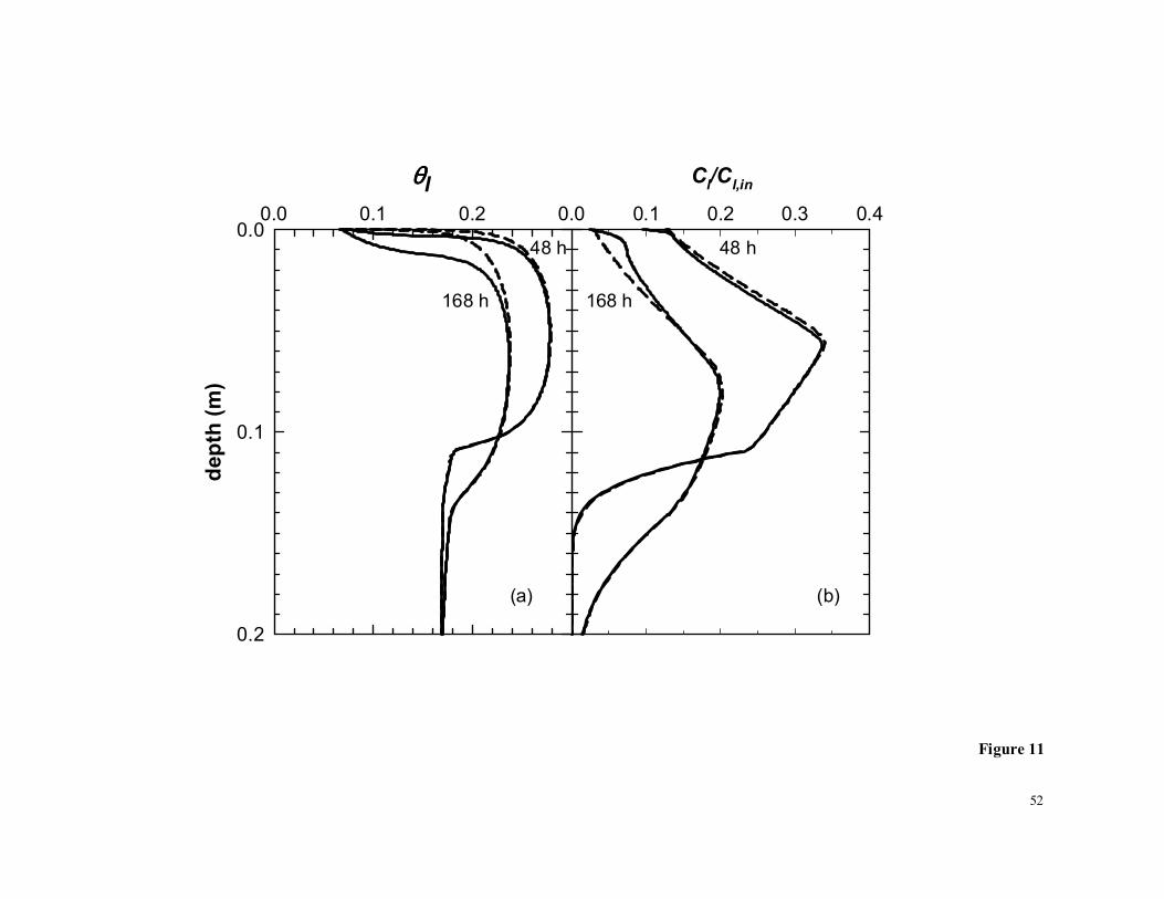
52
Figure 11
Cl/Cl,in
0.0 0.1 0.2 0.3 0.4
θθθθl 0.0 0.1 0.2
dept
h (m
)0.0
0.1
0.2
48 h
(a) (b)
168 h
48 h
168 h
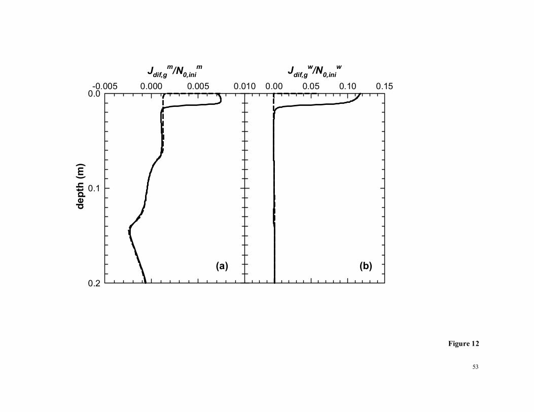
53
Figure 12
Jdif,gw/N0,ini
w
0.00 0.05 0.10 0.15
Jdif,gm/N0,ini
m
-0.005 0.000 0.005 0.010de
pth
(m)
0.0
0.1
0.2
(a) (b)
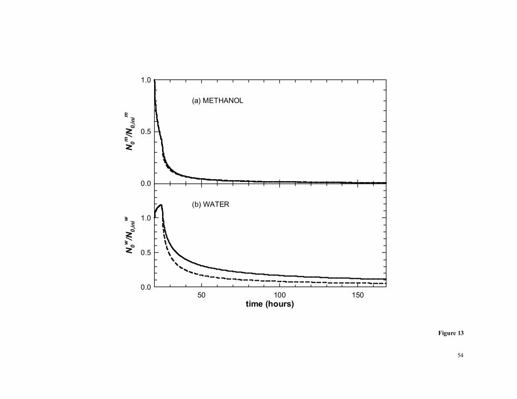
54
N0m
/N0,
inim
0.0
0.5
1.0
time (hours)50 100 150
N0w
/N0,
iniw
0.0
0.5
1.0
Figure 13
(a) METHANOL
(b) WATER


![Passive design[1]](https://static.fdokumen.com/doc/165x107/63215c9580403fa2920cb59b/passive-design1.jpg)