Non-linear real exchange rate effects in the UK labour market

Gabriella Legrenzi

University of Cambridge, UK e-mail: GDL22@cam.ac.uk

and

Costas Milas*

City University, UK

e-mail: c.milas@city.ac.uk

August 2004

Abstract

Using data over the 1973q1-2004q1 period, this paper identifies an important role for the real exchange rate in affecting UK labour market conditions. When the real exchange rate is undervalued, short-run unemployment falls as firms respond to an improvement in domestic competitiveness by increasing their demand for labour. The unemployment response to the real exchange rate deviations occurs outside a narrow interval band. To the extent that the real exchange rate equation reflects monetary policy considerations, our results imply that unemployment can be targeted by economic policy. Our results also suggest that when the real exchange rate is undervalued, workers respond to an improvement in domestic competitiveness by demanding and getting higher wages. Again, this effect is non-linear. Keywords: Real exchange rate; unemployment; monetary policy; Smooth Transition Vector Error Correction Model. JEL classification: C32; C51; C52; F30; F41 *Address for correspondence: Dr Costas Milas, Department of Economics, City University, Northampton Square, London EC1V OHB, UK. Tel: +44 (0) 2070404129, Fax: +44 (0) 2070408580 e-mail: c.milas@city.ac.uk

Non-linear real exchange rate effects in the UK labour market

Abstract

Using data over the 1973q1-2004q1 period, this paper identifies an important role for the real exchange rate in affecting UK labour market conditions. When the real exchange rate is undervalued, short-run unemployment falls as firms respond to an improvement in domestic competitiveness by increasing their demand for labour. The unemployment response to the real exchange rate deviations occurs outside a narrow interval band. To the extent that the real exchange rate equation reflects monetary policy considerations, our results imply that unemployment can be targeted by economic policy. Our results also suggest that when the real exchange rate is undervalued, workers respond to an improvement in domestic competitiveness by demanding and getting higher wages. Again, this effect is non-linear. Keywords: Real exchange rate; unemployment; monetary policy; Smooth Transition Vector Error Correction Model. JEL classification: C32; C51; C52; F30; F41

1

1. Introduction

The use of non-linear models in explaining economic phenomena is motivated by the idea that

the behaviour of economic variables depends on different states of the world or regimes that

prevail at any point in time. Regime switching behaviour in real exchange rates can be explained

by the existence of a band in terms of the costs of trading goods; to the extent that deviations of

the real exchange rate from its long-run level are small relative to the costs of trading, these

deviations are left uncorrected (Dumas, 1992). Over the last few years, the Smooth Transition

Autoregressive (thereafter STAR) methodology has been a popular way of introducing regime-

switching behaviour in real exchange rate models, where the transition from one regime to the

other occurs in a smooth way. 1 For instance, Baum et al. (2001) and Michael et al. (1997) model

the real exchange rate (for a number of countries including the UK) as a stationary variable and

estimate its dynamics based on Exponential STAR (ESTAR) models. Paya and Peel (2003)

estimate an ESTAR model of the dollar–yen real exchange rate which incorporates a

deterministic trend as a proxy for the equilibrium level. On the other hand, Sarantis (1999) finds

that real exchange rates (including the UK one) are non-stationary and proceeds by estimating

real exchange ESTAR and Logistic STAR (LSTAR) models in first differences. 2 A common

feature of these papers is that they all estimate univariate real exchange rate models.

This marks a significant point of departure for our paper: while we follow Sarantis (1999) in

treating the real exchange rate as a non-stationary variable, we find that the latter cointegrates

with real wages and the real price of oil. Acknowledging, however, the ongoing debate about the

unit root properties of the real exchange rate, we also check the robustness of our main results by

looking at the possibility that the real exchange rate is stationary.

Our main empirical model builds upon the theoretical work of Alogoskoufis (1990) who

derived a linear real exchange rate equation based on the production sector of the economy (see

also Chaudhuri and Daniel, 1998, who estimate a more restrictive model involving only the real

1 STAR models were introduced by Teräsvirta and Anderson (1992) in order to examine non-linearities over the business cycle, whereas their statistical properties were discussed in Granger and Teräsvirta (1993) and Teräsvirta (1994), among others. 2 Empirical results in support of a stationary real exchange rate are quite mixed and depend e.g. upon the sample size selected or the definition of the price series used (for a recent survey see e.g. Baum et al., 2001). Studies using long data series (e.g. Taylor, 1996, Lothian and Taylor, 1996, and Michael et al., 1997) find that the real exchange rate is

2

exchange rate and the real price of oil). Noting that cointegration tests perform reasonably well

when the adjustment process is non-linear (van Dijk and Franses 2000), we then proceed by

employing a multivariate STAR framework to model the non-linear dynamics of the real

exchange rate equation as part of a small system involving real wages, the unemployment rate

and the real price of oil. 3 Inclusion of the unemployment rate in our system could be justified in

terms of an Okun’s law channel; for instance, Nakagawa (2002) who looks at the relationship

between real exchange rates and interest rate differentials, discusses non-linear effects in a model

where an undervalued real exchange rate raises aggregate demand for output relative to its full

employment level.

Modelling our system in a smooth transition framework contrasts with the Threshold

Autoregressive (TAR; see e.g. Tong, 1990) and the Hamilton (1989) Markov regime-switching

models, which assume that the transition between regimes occurs abruptly rather than smoothly.

On economic grounds, STAR models seem to be more appropriate than TAR or Markov regime-

switching models. Modelling the real exchange rate as a function of real wages and the real price

of oil implies that real exchange rate movements are affected by conditions prevailing in the

production sector of the economy. In this case, a smooth transition rather than a sharp switch

between regimes could be justified in terms of frictions in the product market due to product

heterogeneity, government imposed barriers to trade, or labour market inflexibility distorting the

rapid adjustment of wages.

According to our results, the short-run real exchange rate adjusts quickly to disequilibrium

deviations of the real exchange rate from its long-run level outside an interval band, which is

estimated to be rather wide. This is not surprising as our sample period coincides with floating

exchange rates being in operation. We also find that when the real exchange rate is above its long-

run equilibrium level (i.e. it is undervalued), short-run unemployment falls as firms respond to an

improvement in domestic competitiveness by increasing their demand for labour. Further, there is a

strong response of short-run unemployment to the disequilibrium error outside an interval band,

which is estimated to be rather narrow. To the extent that the real exchange rate equation reflects

monetary and more generally economic policy considerations, our results imply that

unemployment can be targeted by economic policy. Furthermore, if economic authorities want to

stationary but Engel (2000) argues that these tests may have reached the wrong conclusion. 3 Multivariate STAR models were recently discussed in Granger and Swanson (1996), Weise (1999), Rothman et al. (2001) and van Dijk et al. (2002) among others.

3

avoid large swings in unemployment then they should be prepared to intervene in exchange

markets with the aim of keeping real exchange rate movements within a narrow interval band.

Our results also suggest that when the real exchange rate is undervalued, workers respond to an

improvement in domestic competitiveness by demanding and getting higher wages. Again, this

effect is non-linear. Therefore, our findings recognise an important role for the real exchange rate

in affecting labour market conditions in the UK.

The structure of the paper is as follows. The next section discusses briefly the theory of

linearity testing within a multivariate STAR framework. Section 3 of the paper discusses the

econometric specification of a real exchange rate model, whereas Section 4 estimates the model.

Section 5 presents a discussion of our findings and provides a robustness check by also looking at

the possibility that the real exchange rate is a stationary rather than a non-stationary variable.

Finally, section 6 provides some concluding remarks.

2. Specification of multivariate smooth transition models

Following Rothman et al. (2001), we write a k-dimensional Smooth Transition Vector Error

Correction Model (STVECM) as:

∆ Φ ∆ Φ ∆

Φ ∆ Φ ∆

y z y x G

z y x G s

t t jj

p

t j jj

p

t j t

t jj

p

t j jj

p

t j t t

= + + +⎛

⎝⎜

⎞

⎠⎟ −

+ + + +⎛

⎝⎜

⎞

⎠⎟ +

−=

−

−=

−

−

−=

−

−=

−

−

∑ ∑

∑ ∑

µ α

µ α ε

1 1 1 11

1

20

1

2 2 1 31

1

40

1

1, ,

, ,

( (

( ) ,

s ))

(1)

where yt is a (k x 1) vector of I(1) endogenous variables, xt is an (m x 1) vector of I(1) exogenous

variables, , α),0(~ Σε iidt i, , are (k x r) matrices, and z2 ,1=i t = β′[yt′, xt′]′ for some (q x r)

matrix β denote the error correction terms, with q = k + m. Φ1,j and Φ3,j, , are (k x k)

matrices. Φ

1,...,1 −= pj

2,j and Φ4,j, , are (k x m) matrices and µ1,...,0 −= pj i, 2 ,1=i , are ( ) vectors.

G(s

1×k

t) is the transition function, assumed to be continuous and bounded between zero and one. The

STVECM framework can be considered as a regime-switching model which allows for two

regimes, G(st) = 0 and G(st) = 1, respectively, where the transition from one to the other regime

occurs in a smooth way. We focus our attention on the ‘quadratic logistic’ function (Jansen and

Teräsvirta, 1996):

4

(2) ,0,)](/))((exp[1),,;( 122121 >γσ−−γ−+=γ −

tttt scscsccsG

where σ2(st) is the sample variance of st. This model assumes asymmetric adjustment to

deviations of st from an interval band (c1, c2). The parameter γ determines the speed of the

transition from one regime to the other. If γ → 0, the model becomes linear, whereas if γ → + ∞,

G(st) is equal to 1 for 1cst < and , and equal to 0 when c2cst > 1 < st < c2.

In this paper we assume that the possible candidates for the transition variable st are the r

cointegrating relationships in zt-1 = β′[yt−1′, xt−1′]′. More specifically, the next section estimates

one cointegrating vector, which is identified as a long-run real exchange rate equation. Therefore,

model (2) above is particularly attractive from an economic point of view as it implies the

existence of an interval band (c1, c2) outside which there is a strong tendency for the real

exchange rate to revert to its equilibrium value.

A test of linearity in model (1) using the transition function (2), is a test of the null

hypothesis H0: γ = 0 against the alternative H1: γ > 0. By taking a first-order Taylor

approximation of G(st) around γ = 0, the test can be done within the reparameterised model (see

e.g. the discussion in Saikkonen and Luukkonen, 1988):

,21

0,5

21

1,4

212

1

0,3

1

1,211

1

0,1

1

1,0100

ttjt

p

jjtjt

p

jjtttjt

p

jj

tjt

p

jjttjt

p

jjjt

p

jjtt

esxsyszsx

syszxyzy

+∆Β+∆Β+Α+∆Β

+∆Β+Α+∆Β+∆Β+Α+Μ=∆

−

−

=−

−

=−−

−

=

−

−

=−−

−

=−

−

=−

∑∑∑

∑∑∑

(3)

where et are the original errors εt plus the error arising form the Taylor approximation. Model (3)

is a linear VECM augmented by additional cross-product regressors due to the Taylor expansion.

Here, the null hypothesis of linearity is H0′ : A1 = A2 = B2,j = B3,j = B4,j = B5,j = 0, where

for the B1,...,1 −= pj 2,j and B4,j matrices and 1,...,0 −= pj for the B3,j and B5,j matrices. For

each equation in the VECM, this is a standard variable addition Lagrange Multiplier (LM) which

follows asymptotically the χ2 distribution with 2r + 2k(p – 1) +2mp degrees of freedom. In small

samples, the χ2 test may be heavily oversized. Therefore, it may be preferable to use an F version

5

of the test. Both the χ2 and F versions of the LM statistic are equation specific tests for linearity

which are computed from an auxiliary regression of the residuals from each equation in the linear

VECM on all variables entering model (3). To test the null hypothesis of linearity in all equations

simultaneously, we need a system-wide test. Following Weise (1999), define Ω0 and Ω1 as the

estimated variance-covariance residual matrices from the linear VECM and the augmented model

(3), respectively. The appropriate log-likelihood system-wide test statistic is given by

10 loglog Ω−Ω=TLR , where T is the size of the sample. Under the null hypothesis of

linearity, the test follows asymptotically the χ2 distribution with 2rk + 2k2(p – 1) +2kmp degrees

of freedom. The equation specific LM tests and the system wide LR test are run for all possible st

candidates, that is, all cointegrating relationships. The decision rule is to select as the appropriate

transition variable the cointegrating relationship for which the p-value of the test statistic is the

smallest one. 4

3. Econometric specification of a real exchange rate model

The theoretical framework discussed above will now be tested on a small model of the UK

real exchange rate. In an earlier paper, Alogoskoufis (1990) introduces a model with traded (T)

and non-traded (NT) goods. 5 The model assumes perfect competition in the T sector with firms

producing according to a two-level CES production function which is separable into capital,

labour and imported oil. For the NT sector, the model assumes profit maximising monopolistic

competitive firms. The relative price of tradeables to the price of domestic output, pT − p is

derived in log-linear form as:

)(1))(1(1

1TOTT pppwpp −⎟⎟

⎠

⎞⎜⎜⎝

⎛ππ−

τ+−τ−−=− , (4)

where π1 (0 <π1< 1) is the share of value added in gross output, τ is the share of tradables in total

output, (w – pT) refers to real product wages in the tradables sector and (pO – pT) is the relative

price of imported oil. The price of domestic tradeables, pT, is proxied by the price of UK imports

in domestic currency and p refers to the GDP deflator. In this case, equation (4) is a measure of

4 An extension of the Saikkonen and Luukkonen (1988) linearity tests involves a second-order Taylor approximation of the transition function as suggested by Escribano and Jordá (1999). This involves adding cubic and fourth power terms in model (3), which is hardly practical to implement since we are faced with a small sample size. Further, as van Dijk et al. (2002) point out, neither one of the tests in Saikkonen and Luukkonen (1988) or Escribano and Jordá (1999) dominates in terms of power. Given that the tests are not exact but approximations, some caution is needed when using the rule of the minimum probability value in order to determine the appropriate transition variable. 5 For other versions of price models with traded and non-traded goods see Martin (1997).

6

the real exchange rate as a negative function of w – pT and a positive function of pO – pT. An

increase in pT − p is equivalent to a real depreciation or an improvement in the real

competitiveness of the domestic economy.

Following the notation in Section 2 of the paper, our model uses a set of k = 3 endogenous

variables:

yt = [pT − p, w – pT, u]′, (5)

conditioning on xt = pO – pT, that is, m = 1 exogenous variable. We use quarterly seasonally

adjusted UK data over the period 1973q1-2004q1. The price of UK imports, pT, the GDP deflator,

p, the wage rate in the manufacturing sector (as a proxy for tradeables), w, the price of raw

materials and fuels purchased by the UK manufacturers (as a measure of imported energy), pO

and the unemployment rate, u, are all taken from the Office for National Statistics (ONS; all

variables are in logs). Within our multivariate system, labour market arguments suggest that real

wages interact with the unemployment rate. Further, Nakagawa (2002) discusses non-linear

effects in a model where an undervalued real exchange rate raises aggregate demand for output

relative to its full employment level. Hence there should be a negative correlation between the

real exchange rate misalignment and unemployment through an Okun’s law channel; when the

real exchange rate is undervalued, firms respond to an improvement in domestic competitiveness

which induces shifts in aggregate demand by increasing their demand for labour. As a result,

unemployment falls. In addition, firms are assumed to take the real price of oil, p – p , as given

and therefore we impose exogeneity of this variable, which may improve the statistical properties

of the system (see the discussion in Hansen and Juselius, 1994).

O T

6

4. Empirical results

4.1 Long-run behaviour

Figure 1 plots the logs of the levels and the first differences of the pT − p, w – pT, u and pO – pT

6 Obviously, some other variables like productivity or tax rates can affect wages or unemployment. Extending the information set to this direction is not pursued here, as we are primarily interested in discussing the non-linear behaviour of the real exchange rate equation. Furthermore, use of a larger information set is impractical because the number of estimated coefficients in the linearity tests and the STVECM rises considerably relative to the number of estimated coefficients in the linear VECM. For these reasons we settle for a relatively small baseline system.

7

series. Preliminary analysis using the ADF unit root tests suggested that at least for the sample

period examined here, all series are I(1) in levels and I(0) in first differences. To test for

cointegration, we estimate the linear VECM in levels using a lag length of p = 4 (based on the

Akaike Information Criterion) and allowing for a drift parameter to enter the VECM

unrestrictedly. Table 1 reports the eigenvalues, λi, and the λ-max and trace statistic tests for

cointegration (see Johansen, 1988). The 95 percent critical values are taken from Mackinnon et

al. (1999) in the context of the Pesaran et al. (2000) linear system with both endogenous and

exogenous I(1) variables. Both the λ-max and trace statistics indicate the existence of r = 1

cointegrating vector. For exact identification, we normalise the estimated vector on the real

exchange rate, pT − p. Then we test one over-identifying restriction, that is, long-run exclusion of

the unemployment rate, u. The restriction is accepted as it calculates χ2(1) = 2.34 (p-value = 0.13)

and the resulting cointegrating vector is:

pT − p = −0.460 (w – pT) +0.190 (pO – pT)

(0.050) (0.090)

where standard errors are given in parentheses below the estimated coefficients. The estimated

cointegrating relationship looks like the theoretical real exchange rate equation (4) with the share

of traded goods in total output (i.e. τ) estimated at 54 percent and the share of value added in

gross output (i.e. π1) estimated at 74 percent (the latter is derived from τ(1 −π1) /π1 = 0.190). 7 8

4.2 Linearity testing and short-run estimates

Having estimated the long-run real exchange rate equation, we test for linearity in model (3)

using the estimated cointegrating vector CVt-1 as the possible transition variable st. Linearity tests

are run for a different number of lags of the transition variable st-d = CVt-d (namely d = 1, 2, 3, and

7 Using annual data over the 1952-1985 period, Alogoskoufis (1990) estimates τ between 31 percent and 39 percent, and π1 at 92 percent. However, he points out that his estimates for τ are implausibly low. Our estimate for π1 at 74 percent is much closer to π1 at 71.7 percent in Bruno and Sachs (1982). Their estimate is based on a system of factor-price frontier, output supply, and labour demand equations using annual data over the 1956-1978 period. 8 Chaudhuri and Daniel (1998) adopt the Engle-Granger two-step procedure to test for cointegration in a bivariate model involving real exchange rates and real oil prices for sixteen OECD countries. Using monthly data over the 1973(1)-1996(2) period, they find that the UK real exchange rate cointegrates with the real price of oil. The coefficient on the real price of oil is estimated at 0.389.

8

4 lags). Then the appropriate lag is selected as the one for which the linearity test is most strongly

rejected. We report bootstrapped p-values instead of asymptotic p-values although our results are

not sensitive to the above choice. To compute the bootstrapped p-values of the equation specific

F tests and the system wide LR test reported in Table 2, we followed closely Weise (1999). First,

we estimated the linear VECM equations, where there was evidence of heteroscedasticity. To

control for this, the VECM residuals were regressed on all RHS variables entering the linear

VECM as well as their squares, and the original residuals were transformed using the estimated

coefficients from this auxiliary regression. Draws were taken from the transformed residuals and

one thousand artificial data series were constructed. For each of these artificial series, F and LR

statistics were constructed and then compared to the corresponding statistics from the actual data.

The bootstrapped p-values were derived as the number of times the F and LR statistics from the

artificial data exceeded the corresponding statistics from the actual data, divided by one thousand.

According to the results in Table 2, linearity is mostly rejected for CVt-1. Using the

disequilibrium error CVt-1 in the ‘quadratic logistic’ function (2), we therefore proceed by

estimating the non-linear short-run ∆(pT − p)t, ∆(w – pT)t and ∆ut equations. Before estimating the

non-linear models, it is worth mentioning that Granger and Teräsvirta (1993) and Teräsvirta

(1994) stress particular problems like slow convergence or overestimation associated with

estimates of the γ parameter. For this reason, we follow their suggestion in scaling the ‘quadratic

logistic’ function (2) by dividing it by the variance of the transition variable σ2(CVt-1) (which

equals 0.003), so that γ becomes a scale-free parameter. Based on this scaling, we use γ = 1 as a

starting value and values of CVt-1 close to its minimum (which equals −0.093) and maximum

(which equals 0.093) as starting values for the parameters c1 and c2, respectively. The estimates

of the linear equations for ∆(pT − p)t, ∆(w – pT)t and ∆ut are used as starting values for the

remaining parameters in the STVECM equations (1). 9 Tables 3 to 5 report the non-linear least

squares (NLS) estimates for the parsimonious STVECM equations (1).10

The main parameters of interest in the non-linear models are the estimated values of the

threshold parameters c1 and c2, and the speed of adjustment, γ. The c1 and c2 estimates reported in

9 To save space, the estimates of the linear models are not reported but are available by the authors on request. 10 One could also argue in favour of a structural rather than a reduced form model by testing the significance of current ∆(pT − p)t, ∆(w − pT)t and ∆ut effects in the estimated equations. However, these effects were insignificant.

9

Tables 3 to 5 are statistically significant in all models. The c1 and c2 estimates indicate the

existence of two regimes for the ∆(pT − p)t, ∆(w − pT)t and ∆ut equations; one characterised by

large deviations of the real exchange rate from its long-run equilibrium and an alternative one

which is characterised by small real exchange rate deviations from its equilibrium level. The

economic implications of these results will be discussed in the following section. The estimates

of the γ parameter are rather high for all models indicating that the speed of the transition from

( ) 0,,; 21 =γ ccsG t to ( ) 1,,; 21 =γ ccsG t is rapid at the estimated thresholds c1 and c2. Notice,

however, the rather high standard error of the γ estimates. Teräsvirta (1994) and van Dijk et al.

(2002) point out that this should not be interpreted as evidence of weak non-linearity. Accurate

estimation of γ is not always feasible, as it requires many observations in the immediate

neighborhood of the threshold parameters c1 and c2. Further, large changes in γ have only a small

effect on the shape of the transition function implying that high accuracy in estimating γ is not

necessary (see the discussion in van Dijk et al., 2002).

From Tables 3 to 5 one can notice a large improvement in the diagnostic tests of the non-linear

relative to the linear models. The error variance ratio of the non-linear relative to the linear

models (i.e. s2NL/s2

L) is less than one, indicating that the non-linear models have a better fit. In

particular, the s2NL/s2

L ratio shows a reduction in the residual variances of the non-linear

compared to the linear models which ranges from around 26 percent for the ∆(pT − p)t equation to

around 28 percent for the ∆ut equation and to some 32 percent for the ∆(w – pT)t equation.

5. Discussion of the results

Real exchange rate equation

Consider first the ∆(pT − p)t equation in Table 3. The estimate of the disequilibrium error (i.e.

CVt-1) in the second regime (i.e. coefficient α2 is equal to –0.161 when ( ) 1,,; 21 =γ ccsG t ) implies

that when the real exchange rate exceeds an estimated interval band of (c1, c2) = (–0.051, 0.065),

the short-run real exchange rate adjusts back to equilibrium, whereas there is no adjustment

within the estimated interval band. The effect is rather small suggesting a slow adjustment to

disequilibrium deviations of the real exchange rate from its long-run relationship. Bearing in mind

that the real exchange rate equation captures aspects of the real competitiveness of the domestic

economy that depend on conditions prevailing in the production sector, this sluggishness could

10

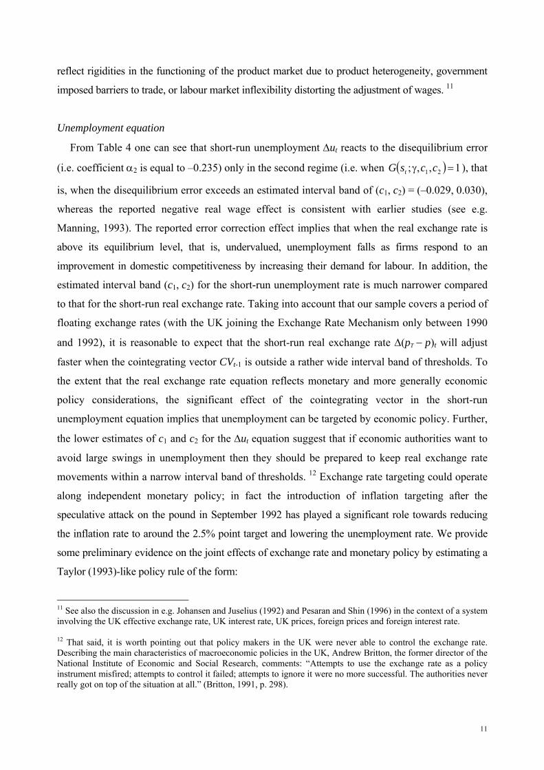
reflect rigidities in the functioning of the product market due to product heterogeneity, government

imposed barriers to trade, or labour market inflexibility distorting the adjustment of wages. 11

Unemployment equation

From Table 4 one can see that short-run unemployment ∆ut reacts to the disequilibrium error

(i.e. coefficient α2 is equal to –0.235) only in the second regime (i.e. when ( 1,,; 21 =)γ ccsG t ), that

is, when the disequilibrium error exceeds an estimated interval band of (c1, c2) = (–0.029, 0.030),

whereas the reported negative real wage effect is consistent with earlier studies (see e.g.

Manning, 1993). The reported error correction effect implies that when the real exchange rate is

above its equilibrium level, that is, undervalued, unemployment falls as firms respond to an

improvement in domestic competitiveness by increasing their demand for labour. In addition, the

estimated interval band (c1, c2) for the short-run unemployment rate is much narrower compared

to that for the short-run real exchange rate. Taking into account that our sample covers a period of

floating exchange rates (with the UK joining the Exchange Rate Mechanism only between 1990

and 1992), it is reasonable to expect that the short-run real exchange rate ∆(pT − p)t will adjust

faster when the cointegrating vector CVt-1 is outside a rather wide interval band of thresholds. To

the extent that the real exchange rate equation reflects monetary and more generally economic

policy considerations, the significant effect of the cointegrating vector in the short-run

unemployment equation implies that unemployment can be targeted by economic policy. Further,

the lower estimates of c1 and c2 for the ∆ut equation suggest that if economic authorities want to

avoid large swings in unemployment then they should be prepared to keep real exchange rate

movements within a narrow interval band of thresholds. 12 Exchange rate targeting could operate

along independent monetary policy; in fact the introduction of inflation targeting after the

speculative attack on the pound in September 1992 has played a significant role towards reducing

the inflation rate to around the 2.5% point target and lowering the unemployment rate. We provide

some preliminary evidence on the joint effects of exchange rate and monetary policy by estimating a

Taylor (1993)-like policy rule of the form:

11 See also the discussion in e.g. Johansen and Juselius (1992) and Pesaran and Shin (1996) in the context of a system involving the UK effective exchange rate, UK interest rate, UK prices, foreign prices and foreign interest rate. 12 That said, it is worth pointing out that policy makers in the UK were never able to control the exchange rate. Describing the main characteristics of macroeconomic policies in the UK, Andrew Britton, the former director of the National Institute of Economic and Social Research, comments: “Attempts to use the exchange rate as a policy instrument misfired; attempts to control it failed; attempts to ignore it were no more successful. The authorities never really got on top of the situation at all.” (Britton, 1991, p. 298).

11

[ ][ 92))5.2()(1(

)921())(1(

4132111

4132111

dgapEidgapEii

tttt

ttttt

γ+−πγ+γγ−+γ+ ]−β+πβ+ββ−+β=

+−

+− (6)

Here, it is the 3-month treasury bill rate. Etπt+1 is the inflation rate (i.e. the annual change in the

retail price index) that at time t is expected for time (t+1), gapt is the difference between real

output and a Hodrick and Prescott (1997) trend and d 92 is a dummy variable taking the value of 1

from 1992q4 onwards and zero otherwise. This captures the time varying effects before and after

October 1992 when an inflation point target of 2.5 percent was introduced. 13 We treat inflation and

the output gap as endogenous, replacing expected future inflation with actual future inflation and

use lagged variables as instruments for inflation and the output gap. The deviation from the Taylor

rule interest rate (that, is, the residual term from (6)) is then inserted as an additive regressor in the

non-linear unemployment rate model. The estimate on the Taylor rule residuals is equal to 0.004

(standard error = 0.002); therefore, a 1 percentage point increase in the interest rate relative to the

Taylor rule interest rate (which is equivalent to an unanticipated tightening in monetary policy)

has the effect of increasing the short-run unemployment rate by about 0.4%. At the same time,

the estimate on the real exchange rate disequilibrium error (i.e. coefficient α2) drops to –0.130 but

it is still significant (i.e. standard error = 0.054). This finding provides some evidence on the joint

effects of exchange rate and monetary policy (in the form of inflation targeting) on unemployment.

Real wage equation

Our results in Table 5 suggest that short-run wages ∆(w − pT)t are strongly affected by real

exchange rate fluctuations outside an estimated interval band of (c1, c2) = (–0.090, 0.042) (i.e.

coefficient α2 on CVt-1 is equal to 0.356 in the second regime ( ( ) 1,,; 21 =γ ccsG t ). Hence, there is

strong evidence that when the real exchange rate is undervalued, workers respond to an

improvement in domestic competitiveness by demanding and getting higher wages.

Figure 2 plots the mean-corrected deviations from the estimated long-run relationship.

Movements of the disequilibrium error above (below) the zero line are associated with an

undervalued (overvalued) real exchange rate. One can notice from Figure 2 (where the estimated

threshold parameters c1 = –0.051, and c2 = 0.065 for the real exchange rate equation have been

13 The estimates of (6) are comparable with the range of estimates reported by Nelson (2000). The estimate on Etπt+1 rises from 0.13 before 1992 to 1.49 afterwards whereas the estimate on gapt drops from 1.04 before 1992 to 0.64 afterwards. The lagged interest rate smoothing effect is estimated at 0.78 for both periods.

12

super-imposed), that during the 1980-1982 period, the real exchange rate is highly overvalued.

Supported by the great appreciation of the dollar vis a vis the currencies of most of the

industrialised countries during the first half of the 1980s (see e.g. Engel and Hamilton, 1990), the

real exchange rate consequently reverts to its long-run equilibrium. In fact, it becomes highly

undervalued in early 1985 after which the dollar witnesses a persistent depreciation against most

foreign currencies. The real exchange rate is also highly undervalued during 1994-1996. It is

notable that early 1980s, which captures the 1980-1981 economic recession, follows the second

OPEC oil price hike (an increase in oil prices of around 15 percent in June 1979) and coincides

with important changes in economic policies following the election of the Thatcher government

in May 1979. In particular, 1979 saw the abolition of exchange rate controls, which was not

aimed at any particular effect on the exchange rate, as well as public spending cuts and an

increase in indirect taxation. The new government encouraged the use of cheaper labour,

especially female labour, which led to more part-time employment. At the same time, a very tight

monetary policy aiming at a rapid decrease in the rate of inflation, led to a more overvalued real

exchange rate (see Figure 2), a rapid increase in unemployment (see Figure 1) and a severe

recession (see e.g. Britton, 1991; Mizon, 1995). Taking into account the slow adjustment of the

real exchange rate reported in the previous section of the paper, it is not surprising that after the

UK's exit from the ERM in September 1992, the real exchange rate experienced a path of

persistent depreciation, which peaked between 1994 and 1996 (see Figure 2). The persistent

appreciation in the recent years is consistent with the common belief (and concern) that the

exchange rate is currently too high for the UK to join the European Monetary Union.

What if the real exchange rate is stationary?

This paper has treated the real exchange rate as a non-stationary variable. Given the ongoing

debate on its stationary properties, we checked the robustness of our results by estimating non-

linear models where the demeaned real exchange rate (pT − p)t is assumed to be stationary. In this

case, up to 4 lags of (pT − p)t are used as potential transition variables. 14 To save space, we only

report a summary of our results. In brief, linearity tests favour (pT − p)t-1 as the most suitable

transition variable. However, we do not find any significant feedback from (pT − p)t-1 in the non-

14 Demeaning the real exchange rate results in (pT − p)t fluctuating between a minimum of –0.406 and a maximum of 0.336.

13

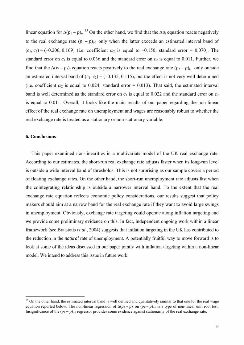
linear equation for ∆(pT − p)t. 15 On the other hand, we find that the ∆ut equation reacts negatively

to the real exchange rate (pT − p)t-1 only when the latter exceeds an estimated interval band of

(c1, c2) = (–0.206, 0.169) (i.e. coefficient α2 is equal to –0.150; standard error = 0.070). The

standard error on c1 is equal to 0.036 and the standard error on c2 is equal to 0.011. Further, we

find that the ∆(w – pT)t equation reacts positively to the real exchange rate (pT − p)t-1 only outside

an estimated interval band of (c1, c2) = (–0.135, 0.115), but the effect is not very well determined

(i.e. coefficient α2 is equal to 0.024; standard error = 0.013). That said, the estimated interval

band is well determined as the standard error on c1 is equal to 0.022 and the standard error on c2

is equal to 0.011. Overall, it looks like the main results of our paper regarding the non-linear

effect of the real exchange rate on unemployment and wages are reasonably robust to whether the

real exchange rate is treated as a stationary or non-stationary variable.

6. Conclusions

This paper examined non-linearities in a multivariate model of the UK real exchange rate.

According to our estimates, the short-run real exchange rate adjusts faster when its long-run level

is outside a wide interval band of thresholds. This is not surprising as our sample covers a period

of floating exchange rates. On the other hand, the short-run unemployment rate adjusts fast when

the cointegrating relationship is outside a narrower interval band. To the extent that the real

exchange rate equation reflects economic policy considerations, our results suggest that policy

makers should aim at a narrow band for the real exchange rate if they want to avoid large swings

in unemployment. Obviously, exchange rate targeting could operate along inflation targeting and

we provide some preliminary evidence on this. In fact, independent ongoing work within a linear

framework (see Bratsiotis et al., 2004) suggests that inflation targeting in the UK has contributed to

the reduction in the natural rate of unemployment. A potentially fruitful way to move forward is to

look at some of the ideas discussed in our paper jointly with inflation targeting within a non-linear

model. We intend to address this issue in future work.

15 On the other hand, the estimated interval band is well defined and qualitatively similar to that one for the real wage equation reported below. The non-linear regression of ∆(pT − p)t on (pT − p)t-1 is a type of non-linear unit root test. Insignificance of the (pT − p)t-1 regressor provides some evidence against stationarity of the real exchange rate.

14

References

Alogoskoufis, G., 1990. Traded goods, competitiveness and aggregate fluctuations in the United

Kingdom, Economic Journal 100, 141-163.

Baum, C.F., J.T. Barkoulas and M. Caglayan, 2001. Nonlinear adjustment to purchasing power

parity in the post-Bretton Woods era, Journal of International Money and Finance 20, 379-399.

Bratsiotis, G., C. Martin and T. Panagiotidis, 2004. Monetary policy and the natural rate of

unemployment. To be presented at the 2004 MMF conference at Cass Business School. Available

from: http://www.cass.city.ac.uk/conferences/mmf2004/

Britton, A.J.C., 1991. Macroeconomic Policy in Britain 1974-1987. National Institute of

Economic and Social Research, Economic and Social Studies 36. Cambridge University Press,

Cambridge.

Bruno, M. and J.D. Sachs, 1982. Input price shocks and the slowdown in economic growth: the

case of UK manufacturing, Review of Economic Studies 49, 679-705.

Chaudhuri, K. and B.C. Daniel, 1998. Long-run equilibrium real exchange rates and oil prices,

Economics Letters 58, 231-238.

Dumas, B., 1992. Dynamic equilibrium and the real exchange rate in a spatially separated world,

Review of Financial Studies 5, 153-180.

Engel, C., 2000. Long-run PPP may not hold after all, Journal of International Economics 57,

243-273.

Engel, C. and J.D. Hamilton, 1990. Long swings in the dollar: are they in the data and do markets

know it? American Economic Review 80, 689-713.

Escribano, A. and O. Jordá, 1999. Improved testing and specification of smooth transition

regression models’, in Rothman, P. (Ed.), Nonlinear Time Series Analysis of Economic and

Financial Data, Boston, Kluwer, pp. 289-319.

Granger, C.W.J. and N.R. Swanson, 1996. Future developments in the study of cointegrated

variables, Oxford Bulletin of Economic and Statistics 58, 537-553.

Granger, C.W.J. and T. Teräsvirta, 1993. Modelling nonlinear economic relationships. Oxford

University Press, Oxford.

Hamilton, J.D., 1989. A new approach to the economic analysis of nonstationary time series and

the business cycle, Econometrica 57, 357-384.

Hansen, H. and K. Juselius, 1994. Manual to cointegration analysis of time series: CATS in

RATS. Mimeo, University of Copenhagen.

15

Hodrick, R.J. and E.C. Prescott, 1997. Postwar U.S. business cycles: An empirical investigation,

Journal of Money, Credit, and Banking, 29, 1–16.

Jansen, E.S. and T. Teräsvirta, 1996. Testing parameter constancy and super exogeneity in

econometric equations, Oxford Bulletin of Economics and Statistics 58, 735-768.

Johansen, S., 1988. Statistical analysis of cointegration vectors, Journal of Economic Dynamics

and Control 12, 231-254.

Johansen, S. and K. Juselius, 1992. Testing structural hypotheses in a multivariate cointegration

analysis of the PPP and UIP for UK, Journal of Econometrics 53, 211-244.

Lothian, J.R. and M.P. Taylor, 1996. Real exchange rate behavior: The recent float from the

perspective of the past two centuries, Journal of Political Economy 104, 488-509.

Mackinnon, J.G., A.A. Haug and L. Michelis, 1999. Numerical distribution functions of

likelihood ratio tests for cointegration, Journal of Applied Econometrics 14, 563-577.

Manning, A., 1993. Wage bargaining and the Phillips curve: the identification and specification

of aggregate wage equations, Economic Journal 103, 98-118.

Martin, C., 1997. Price formation in an open economy: theory and evidence for the United

Kingdom, 1951-1991, Economic Journal 107, 1391-1404.

Michael, P., A.R. Nobay, and D.A. Peel, 1997. Transactions costs and nonlinear adjustment in

real exchange rates: an empirical investigation, Journal of Political Economy 105, 862-879.

Mizon, G.E., 1995. Progressive modeling of macroeconomic time series. The LSE methodology,

in Hoover, K.D. (Ed.), Macroeconometrics: Developments, tensions and prospects. Kluwer

Academic Press, Dordrecht, 107-180.

Nakagawa, H., 2002. Real exchange rates and real interest differentials: implications of nonlinear

adjustment in real exchange rates, Journal of Monetary Economics 49, 629-649.

Nelson, E., 2000. UK monetary policy 1972–1997: a guide using Taylor rules. Bank of England

Working Paper no. 120.

Paya, I., and D.A. Peel, 2003. Purchasing power parity adjustment speeds in high frequency data

when the equilibrium real exchange rate is proxied by a deterministic trend, The Manchester

School 71, 39-53 (Supplement).

Pesaran, M.H. and Y. Shin, 1996. Cointegration and speed of convergence to equilibrium, Journal

of Econometrics 71, 117-143.

Pesaran, M.H., Y. Shin, and R.J. Smith, 2000. Structural analysis of vector error correction

models with exogenous I(1) variables, Journal of Econometrics 97, 293-343.

Rothman, P., D. van Dijk, and P.H. Franses, 2001. A multivariate STAR analysis of the

16

relationship between money and output, Macroeconomic Dynamics 5, 506-532.

Saikkonen, P. and R. Luukkonen, 1988. Lagrange Multiplier tests for testing non-linearities in

time series models, Scandinavian Journal of Statistics 15, 55-68.

Sarantis, N., 1999. Modeling non-linearities in real effective exchange rates, Journal of

International Money and Finance 18, 27-45.

Taylor, A.M., 1996. International capital mobility in history: purchasing-power parity in the long

run, National Bureau of Economic Research Working Paper No. 5472, Cambridge, MA.

Taylor, J., 1993. Discretion versus policy rules in practice, Carnegie-Rochester Conference Series

on Public Policy, 39, 195-214.

Teräsvirta, T, 1994. Specification, estimation, and evaluation of smooth transition autoregressive

models, Journal of the American Statistical Association 89, 208-218.

Teräsvirta, T., and H.M. Anderson, 1992. Characterizing nonlinearities in business cycles using

smooth transition autoregressive models, Journal of Applied Econometrics 7, S119-S136.

Tong, H., 1990. Non-linear time series: a dynamical system approach. Oxford University Press,

Oxford.

van Dijk, D., Franses, P.H., 2000. Nonlinear error-correction models for interest rates in the

Netherlands, in: Barnett, W.A., Hendry, D.F., Hylleberg, S., Teräsvirta, T., Tjostheim, D.,

Würtz, A., (Eds.), Nonlinear Econometric Modelling in Time Series Analysis, Cambridge

University Press, Cambridge, pp. 203-227.

van Dijk, D., T. Teräsvirta, and P.H. Franses, 2002. Smooth transition autoregressive models – a

survey of recent developments, Econometric Reviews 21, 1-47.

Weise, C.L., 1999. The asymmetric effects of monetary policy: a nonlinear vector autoregression

approach, Journal of Money, Credit, and Banking 31, 85-108.

17

Table 1

Eigenvalues, test statistics and critical values

λi λ-max Trace

0.24 H0 H1 Stat. 95% H0 H1 Stat. 95%

0.15 r = 0 r = 1 27.52 24.87 r = 0 r ≥ 1 46.55 39.56

0.03 r ≤ 1 r = 2 13.21 18.36 r ≤ 1 r ≥ 2 19.23 23.62

0.00 r ≤ 2 r = 3 2.34 11.42 r ≤ 2 r = 3 2.34 11.42

Notes: r denotes the number of cointegration vectors. Critical values are from Mackinnon et al., (1999).

Table 2

Linearity tests

Lagrange Multiplier F statistics for: Transition variable

∆(pT − p) model

∆(w − pT) model

∆u model

System wide test

LR CVt-1 2.212

(0.003) 2.624

(0.001) 3.100

(0.000) 152.075 (0.000)

CVt-2 1.259 (0.232)

1.921 (0.025)

1.681 (0.050)

108.684 (0.003)

CVt-3 2.230 (0.010)

2.649 (0.001)

2.845 (0.001)

147.851 (0.000)

CVt-4 1.049 (0.409)

1.505 (0.087)

1.576 (0.094)

93.298 (0.068)

Notes: Bootstrapped p-values in parentheses. The p-values for the equation specific Lagrange Multiplier F statistics and the system wide LR test statistic are derived from bootstrapping with one thousand replications. CV is the transition variable: CV = pT − p + 0.460 (w – pT) − 0.190 (pO – pT), in mean-corrected form. The null hypothesis is linearity. The alternative hypothesis is the STVECM representation.

18

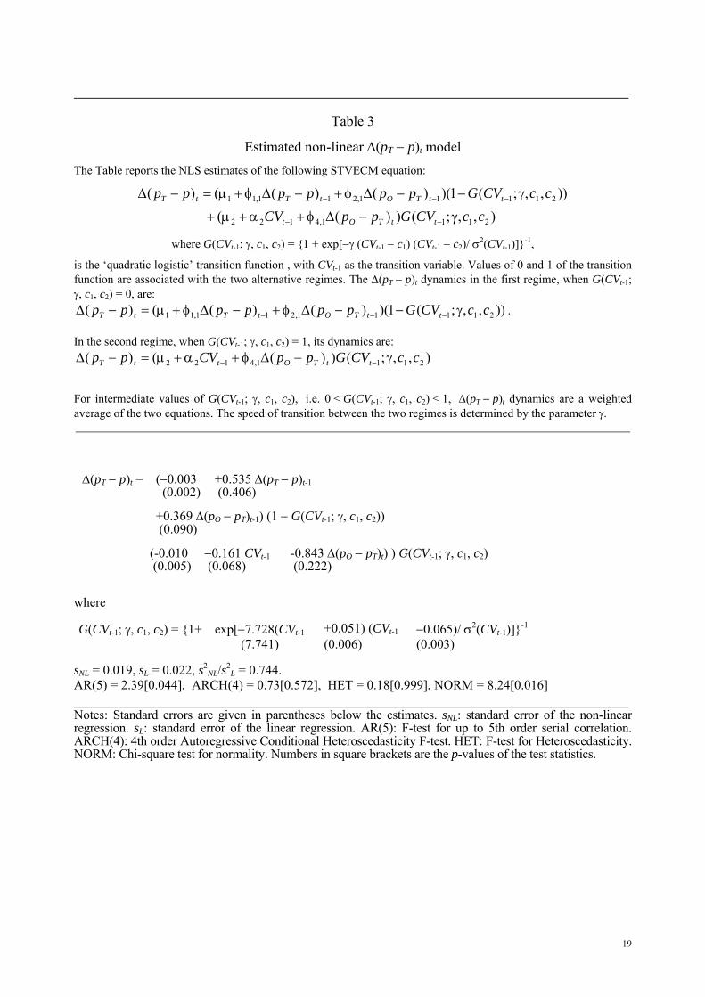
Table 3

Estimated non-linear ∆(pT − p)t modelThe Table reports the NLS estimates of the following STVECM equation:

),,;())(()),,;(1)()()(()(

2111,4122

21111,211,11

ccCVGppCVccCVGpppppp

ttTOt

ttTOtTtT

γ−∆φ+α+µ+

γ−−∆φ+−∆φ+µ=−∆

−−

−−−

where G(CVt-1; γ, c1, c2) = 1 + exp[−γ (CVt-1 − c1) (CVt-1 − c2)/ σ2(CVt-1)]-1,

is the ‘quadratic logistic’ transition function , with CVt-1 as the transition variable. Values of 0 and 1 of the transition function are associated with the two alternative regimes. The ∆(pT − p)t dynamics in the first regime, when G(CVt-1; γ, c1, c2) = 0, are:

)),,;(1)()()(()( 21111,211,11 ccCVGpppppp ttTOtTtT γ−−∆φ+−∆φ+µ=−∆ −−− . In the second regime, when G(CVt-1; γ, c1, c2) = 1, its dynamics are:

),,;())(()( 2111,4122 ccCVGppCVpp ttTOttT γ−∆φ+α+µ=−∆ −−

For intermediate values of G(CVt-1; γ, c1, c2), i.e. 0 < G(CVt-1; γ, c1, c2) < 1, ∆(pT − p)t dynamics are a weighted average of the two equations. The speed of transition between the two regimes is determined by the parameter γ. ∆(pT − p)t = (−0.003 +0.535 ∆(pT − p)t-1

(0.002) (0.406) +0.369 ∆(pO − pT)t-1) (1 − G(CVt-1; γ, c1, c2)) (0.090) (-0.010 −0.161 CVt-1 -0.843 ∆(pO − pT)t) ) G(CVt-1; γ, c1, c2) (0.005) (0.068) (0.222) where G(CVt-1; γ, c1, c2) = 1+ exp[−7.728(CVt-1 +0.051) (CVt-1 −0.065)/ σ2(CVt-1)]-1

(7.741) (0.006) (0.003) sNL = 0.019, sL = 0.022, s2

NL/s2L = 0.744.

AR(5) = 2.39[0.044], ARCH(4) = 0.73[0.572], HET = 0.18[0.999], NORM = 8.24[0.016] Notes: Standard errors are given in parentheses below the estimates. sNL: standard error of the non-linear regression. sL: standard error of the linear regression. AR(5): F-test for up to 5th order serial correlation. ARCH(4): 4th order Autoregressive Conditional Heteroscedasticity F-test. HET: F-test for Heteroscedasticity. NORM: Chi-square test for normality. Numbers in square brackets are the p-values of the test statistics.

19

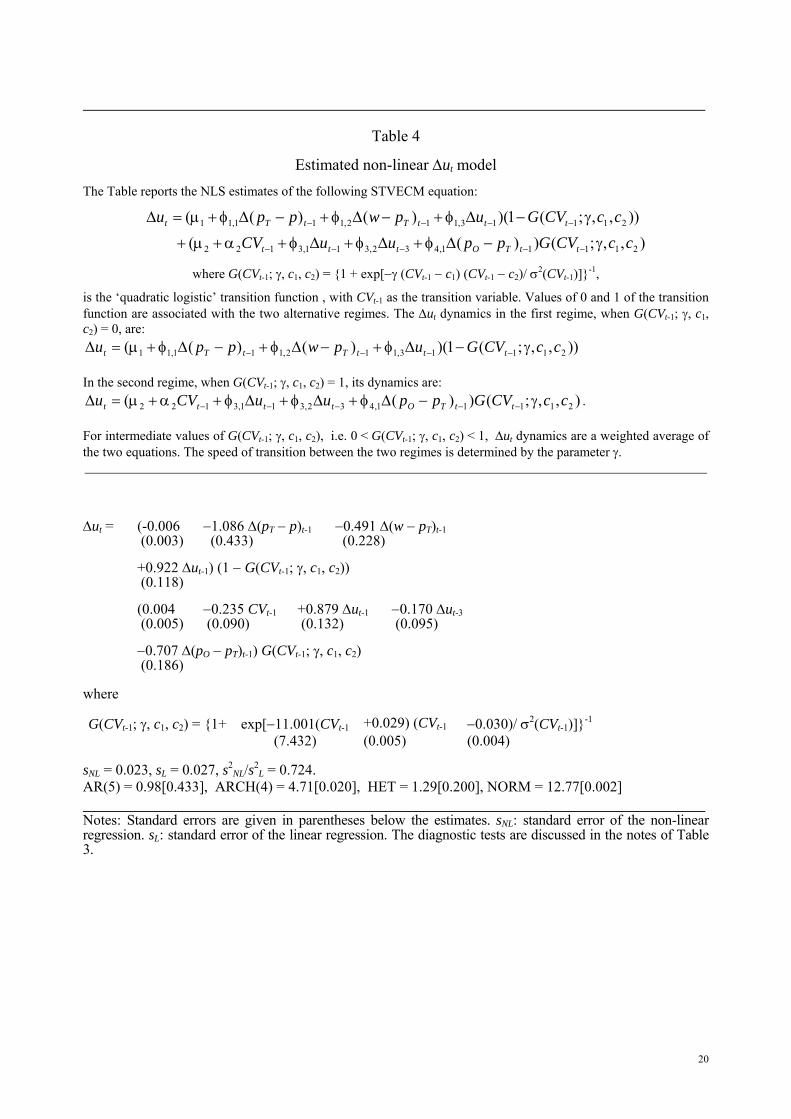
Table 4

Estimated non-linear ∆ut modelThe Table reports the NLS estimates of the following STVECM equation:

),,;())(()),,;(1)()()((

21111,432,311,3122

21113,112,111,11

ccCVGppuuCVccCVGupwppu

ttTOttt

tttTtTt

γ−∆φ+∆φ+∆φ+α+µ+

γ−∆φ+−∆φ+−∆φ+µ=∆

−−−−−

−−−−

where G(CVt-1; γ, c1, c2) = 1 + exp[−γ (CVt-1 − c1) (CVt-1 − c2)/ σ2(CVt-1)]-1,

is the ‘quadratic logistic’ transition function , with CVt-1 as the transition variable. Values of 0 and 1 of the transition function are associated with the two alternative regimes. The ∆ut dynamics in the first regime, when G(CVt-1; γ, c1, c2) = 0, are:

)),,;(1)()()(( 21113,112,111,11 ccCVGupwppu tttTtTt γ−∆φ+−∆φ+−∆φ+µ=∆ −−−− In the second regime, when G(CVt-1; γ, c1, c2) = 1, its dynamics are:

),,;())(( 21111,432,311,3122 ccCVGppuuCVu ttTOtttt γ−∆φ+∆φ+∆φ+α+µ=∆ −−−−− . For intermediate values of G(CVt-1; γ, c1, c2), i.e. 0 < G(CVt-1; γ, c1, c2) < 1, ∆ut dynamics are a weighted average of the two equations. The speed of transition between the two regimes is determined by the parameter γ. ∆ut = (-0.006 −1.086 ∆(pT − p)t-1 −0.491 ∆(w − pT)t-1 (0.003) (0.433) (0.228) +0.922 ∆ut-1) (1 − G(CVt-1; γ, c1, c2)) (0.118) (0.004 −0.235 CVt-1 +0.879 ∆ut-1 −0.170 ∆ut-3 (0.005) (0.090) (0.132) (0.095) −0.707 ∆(pO − pT)t-1) G(CVt-1; γ, c1, c2) (0.186) where G(CVt-1; γ, c1, c2) = 1+ exp[−11.001(CVt-1 +0.029) (CVt-1 −0.030)/ σ2(CVt-1)]-1

(7.432) (0.005) (0.004) sNL = 0.023, sL = 0.027, s2

NL/s2L = 0.724.

AR(5) = 0.98[0.433], ARCH(4) = 4.71[0.020], HET = 1.29[0.200], NORM = 12.77[0.002] Notes: Standard errors are given in parentheses below the estimates. sNL: standard error of the non-linear regression. sL: standard error of the linear regression. The diagnostic tests are discussed in the notes of Table 3.

20

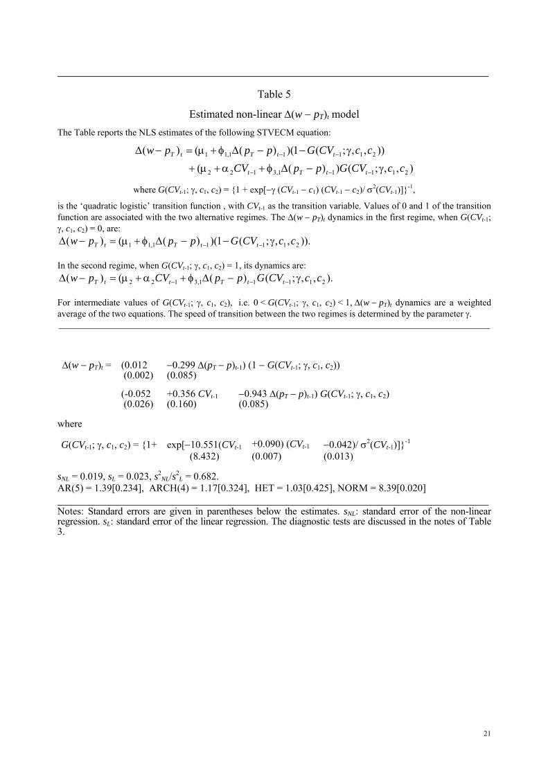
Table 5

Estimated non-linear ∆(w − pT)t modelThe Table reports the NLS estimates of the following STVECM equation:

),,;())(()),,;(1)()(()(

21111,3122

21111,11

ccCVGppCVccCVGpppw

ttTt

ttTtT

γ−∆φ+α+µ+

γ−−∆φ+µ=−∆

−−−

−−

where G(CVt-1; γ, c1, c2) = 1 + exp[−γ (CVt-1 − c1) (CVt-1 − c2)/ σ2(CVt-1)]-1,

is the ‘quadratic logistic’ transition function , with CVt-1 as the transition variable. Values of 0 and 1 of the transition function are associated with the two alternative regimes. The ∆(w − pT)t dynamics in the first regime, when G(CVt-1; γ, c1, c2) = 0, are:

)).,,;(1)()(()( 21111,11 ccCVGpppw ttTtT γ−−∆φ+µ=−∆ −−

In the second regime, when G(CVt-1; γ, c1, c2) = 1, its dynamics are:

).,,;()(()( 21111,3122 ccCVGppCVpw ttTttT γ−∆φ+α+µ=−∆ −−− For intermediate values of G(CVt-1; γ, c1, c2), i.e. 0 < G(CVt-1; γ, c1, c2) < 1, ∆(w − pT)t dynamics are a weighted average of the two equations. The speed of transition between the two regimes is determined by the parameter γ. ∆(w − pT)t = (0.012 −0.299 ∆(pT − p)t-1) (1 − G(CVt-1; γ, c1, c2))

(0.002) (0.085) (-0.052 +0.356 CVt-1 −0.943 ∆(pT − p)t-1) G(CVt-1; γ, c1, c2) (0.026) (0.160) (0.085) where G(CVt-1; γ, c1, c2) = 1+ exp[−10.551(CVt-1 +0.090) (CVt-1 −0.042)/ σ2(CVt-1)]-1

(8.432) (0.007) (0.013) sNL = 0.019, sL = 0.023, s2

NL/s2L = 0.682.

AR(5) = 1.39[0.234], ARCH(4) = 1.17[0.324], HET = 1.03[0.425], NORM = 8.39[0.020] Notes: Standard errors are given in parentheses below the estimates. sNL: standard error of the non-linear regression. sL: standard error of the linear regression. The diagnostic tests are discussed in the notes of Table 3.

21

Figure 1: Plots of the levels and the first differences of the series

Levels of the series

1980 1990 2000

0

.25

.5

real exchange rate

1980 1990 2000

-.75

-.5

-.25

0

.25 real wages

1980 1990 2000.5

1

1.5

2

unemployment

1980 1990 2000

0

.1

.2

.3 real price of oil

First differences of the series

1980 1990 2000-.05

0

.05

.1

real wages

real exchange rate

1980 1990 2000

-.15

-.1

-.05

0

.05

real wages

1980 1990 2000

-.1

0

.1

.2 unemployment

1980 1990 2000

-.05

0

.05

.1 real price of oil

22

Figure 2: Deviations from the estimated long-run real exchange rate relationship

1975 1980 1985 1990 1995 2000 2005

-.075

-.05

-.025

0

.025

.05

.075

23